Embed Size (px)
Citation preview

DRDC Toronto CR 2005-121
Development of a Dynamic Biomechanical Model for Load Carriage: Phase III Part C1:
Pressure and Force Distribution Measurement for the Design of Waist Belts in
Personal Load Carriage Systems
By L.J. Hadcock
Ergonomics Research Group
Queen’s University Kingston, Ontario, Canada
K7L 3N6
Project Manager: J. M. Stevenson (613) 533-6288
PWGSC Contract No. W7711-0-7632-06
on behalf of DEPARTMENT OF NATIONAL DEFENCE
as represented by
Defence Research and Development Canada -Toronto 1133 Sheppard Avenue West North York, Ontario, Canada
M3M 3B9
DRDC Scientific Authority: Maj Linda Bossi (416) 635-2197
August 2005
The scientific or technical validity of this Contract Report is entirely the responsibility of the contractor and the contents do not necessarily have the approval or endorsement of Defence
R&D Canada
© Her Majesty the Queen as represented by the Minister of National Defence, 2005
© Sa Majesté la Reine, représentée par le ministre de la Défense nationale, 2005

Pressure and Force Distribution Measurement i
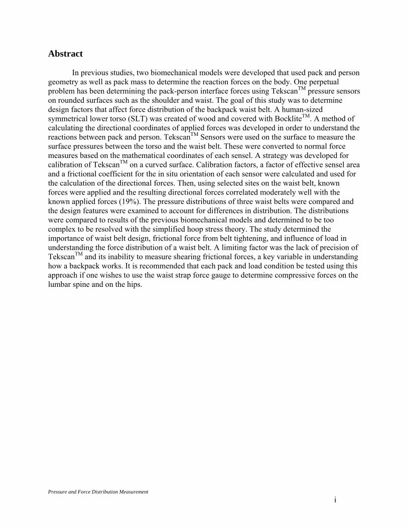
Abstract In previous studies, two biomechanical models were developed that used pack and person geometry as well as pack mass to determine the reaction forces on the body. One perpetual problem has been determining the pack-person interface forces using TekscanTM pressure sensors on rounded surfaces such as the shoulder and waist. The goal of this study was to determine design factors that affect force distribution of the backpack waist belt. A human-sized symmetrical lower torso (SLT) was created of wood and covered with BockliteTM. A method of calculating the directional coordinates of applied forces was developed in order to understand the reactions between pack and person. TekscanTM Sensors were used on the surface to measure the surface pressures between the torso and the waist belt. These were converted to normal force measures based on the mathematical coordinates of each sensel. A strategy was developed for calibration of TekscanTM on a curved surface. Calibration factors, a factor of effective sensel area and a frictional coefficient for the in situ orientation of each sensor were calculated and used for the calculation of the directional forces. Then, using selected sites on the waist belt, known forces were applied and the resulting directional forces correlated moderately well with the known applied forces (19%). The pressure distributions of three waist belts were compared and the design features were examined to account for differences in distribution. The distributions were compared to results of the previous biomechanical models and determined to be too complex to be resolved with the simplified hoop stress theory. The study determined the importance of waist belt design, frictional force from belt tightening, and influence of load in understanding the force distribution of a waist belt. A limiting factor was the lack of precision of TekscanTM and its inability to measure shearing frictional forces, a key variable in understanding how a backpack works. It is recommended that each pack and load condition be tested using this approach if one wishes to use the waist strap force gauge to determine compressive forces on the lumbar spine and on the hips.
Pressure and Force Distribution Measurement ii
Résumé
Dans les études antérieures, deux modèles biomécaniques fondés sur la géométrie du sac à dos et de la personne ainsi que sur la masse du sac avaient été élaborés pour déterminer les forces de réaction corporelles. Un problème perpétuel est la détermination, à l’aide des capteurs de pression TekscanMC, des forces exercées à l’interface sac-personne sur des surfaces arrondies, comme les épaules et la taille. La présente étude a pour but de déterminer les facteurs de conception de la ceinture du sac à dos qui ont un effet sur la répartition des forces. À cette fin, on a fabriqué un torse inférieur symétrique (SLT) de taille humaine avec du bois et on l’a recouvert de BockliteMC. Afin de comprendre les interactions entre le sac et la personne, une méthode a été élaborée pour calculer les coordonnées directionnelles des forces appliquées. Des capteurs TekscanMC ont été posés à la surface pour mesurer les pressions exercées à la surface entre le torse et la ceinture. Les coordonnées mathématiques de chacun des capteurs à cellules ont servi à convertir les mesures de pression en mesures de force normale. Une stratégie a été élaborée pour l’étalonnage du TekscanMC sur une surface arrondie. Les facteurs d’étalonnage, qui dépendent de la surface efficace de la cellule et du coefficient de frottement utilisés pour l’orientation de chaque capteur sur place, ont été calculés et ont servi à calculer les forces directionnelles. Ensuite, des forces connues ont été appliquées à des emplacements donnés de la ceinture; la corrélation entre les forces directionnelles obtenues et les forces connues appliquées était relativement bonne (19 %). Une comparaison de la répartition des pressions a été effectuée entre trois ceintures, et leurs caractéristiques de conception ont été examinées pour expliquer les différences de répartition. La répartition a ensuite été comparée avec les résultats obtenus au moyen des modèles biomécaniques précédents; on a déterminé qu’elle était trop complexe pour être déterminée à l’aide de la théorie simplifiée de tension de charge. L’étude a démontré l’importance de la conception de la ceinture, la force de frottement résultant du serrage et l’incidence de la charge sur la compréhension de la répartition des forces d’une ceinture. Le manque de précision du TekscanMC et son incapacité à mesurer les forces de cisaillement, qui est un facteur important pour la compréhension du fonctionnement d’un sac à dos, ont limité l’étude. Nous recommandons de recourir à cette méthode pour mettre à l’essai chaque sac à dos et chaque condition de charge afin de permettre l’utilisation du dynamomètre de ceinture pour déterminer les forces de compression sur la colonne lombaire et les hanches.
Pressure and Force Distribution Measurement iii
Executive Summary Introduction This study was completed under contract PWSGC #W7711-0-7632-03 Sections 6 B and C for DRDC Toronto. Section 6B was to construct a standardized lower torso (SLT) model in order to be used in Section 6C for the validation of a waist belt model. Two previous static biomechanical models have been developed under previous DCIEM contracts (Stevenson et al, 1995 and Pelot et al, 1998). The first was a shoulder-based model that was used to help establish recommended shoulder and lumbar reaction forces and the second model added a waist belt but no load lifter or hip stabilizer straps. When Rigby (1999) attempted to add these components, results were poorer than previous models because of indeterminacy in the system. The goal of this research was to develop a valid waist belt model for future dynamic biomechanical modeling analysis. Previous biomechanical models have made several assumptions of the waist belt, most notably a constant tension throughout the belt and frictional forces acting in a direction resisting movement of the waist belt. Section 6C used the SLT to validate these earlier models as well as determining the relationship between strap force tension and the measured pressure distribution. Specific Objectives The primary objectives of this research were: 1. To develop a simplified model of the human lower torso as an addition to the current suite of tools used by the Ergonomics Research Group. 2. To develop a valid waist belt model for a backpack. 3. To determine the factors affecting force distribution on a load carriage system waist belt. To accomplish these objectives, several specific milestones were also identified: • Determination of the frictional components of the waist belt. • Development of a novel calibration procedure for contact pressure sensors in this application. • Determination of the effects of the direction of strap tightening on measured pressures on the body. • Determination of the relationship of the strap force tension in the waist belt to the measured pressures on the body. Major Findings A Symmetrical Lower Torso (SLT) was designed and constructed. The SLT allowed measured forces, for any point on the surface, to be resolved into directional vectors in three dimensions with the known coordinates of the point. A strategy was developed using the TekscanTM 9600 sensors to determine waist belt compressive force distribution within an RMS error of <10N.
A calibration procedure using an effective TekscanTM sensel area and a longitudinal frictional coefficient has been demonstrated. This is limited in application to vertical loading and was more successful in cases where the loads exceeded 50N.
Within the limitations of TekscanTM technology, it was possible to calibrate the sensors on a curved surface. However, the need for a minimum of three repetitions to reduce random error has been demonstrated. This calibration procedure has also demonstrated the need to calibrate all

Pressure and Force Distribution Measurement iv
sensors, in situ, that are used in curved positions, or disregard the magnitudes of the measured forces.
It was possible to derive a coefficient of friction for the isolated waist belt model and to determine how factors such as the direction of belt tightening affected magnitude of the measured normal forces on the torso.
The effects of tightening direction were shown to be significant in no-load tests of waist belts. The measured forces on the hips were significantly lower on the side of the strap force transducer and these effects are reduced with an increase in load. The apparent effects due to the tightening direction of the waist belt were consistent and predictable but their relationship to the forces acting on more compliant surfaces, such as the human body cannot be extrapolated from this observation.
Previous models involving a waist belt have oversimplified the role of friction with the assumption of a constant belt tension. The complexity of the measured forces in the waist belt indicated that a direct relationship between strap force tension, measured in one location, and the forces acting on the body, was not possible. However, by testing the pack under realistic conditions (i.e. load, tension) it is possible to express hips, lumbar and abdominal tension as a multiple of waist strap tension for individual waist belts.
The application of the frictional distributions appear to depend on the materials used in the construction of the belt. In this preliminary study, the padding orientation and conical shape of the waist belt determined the severity of localized compressive forces at the base of the belt. A less conical shape created lines of pressure about the bottom of the waist belt as the effects of the belt tension were concentrated in this area due to the geometry of the SLT.
At this time, a model for an individual waist belt is limited by an inability to predict frictional force distributions. TekscanTM instrumentation is also limited in this regard since it cannot directly evaluate the effect of shear forces on the torso.
Pressure and Force Distribution Measurement v
Recommendations The backpack must be tested under the load conditions anticipated in the field in order to determine the pressures in relation to the belt tension.
The directions of frictional forces need to be more closely examined as the impending pack motion may not be downwards as originally considered, depending on the mass of the pack and the tension in the belt. If the effective tension were higher than the effective mass on the belt, the pack would have a tendency to move upwards because of the hoop shape rather than downwards with the force of gravity. The apparent consistent effect of loading the pack and the increase in waist belt tension should be explored further. Incremental loading would better provide an understanding of this relationship.
The unbalanced forces resulting from the compressive force of belt tensioning need to be examined further. The variation in the three waist belts in this study was too great to determine with any certainty how waist belt design relates to the force and frictional distribution in the waist belt. In order to determine the actions of the waist belt padding, the properties of the material, such as compliance of the foam, and the frictional properties of the covering materials should be determined. Identical belts with different materials or different designs with the same materials would facilitate this understanding.
The effect of different lean angles of the torso on the distribution of forces should be examined. A forward lean angle of 8° would vertically orient the abdominal area of the model, more closely resembling the human body.
The padding surface of each belt may be experiencing relatively large shear forces due to circumferential pressure. These forces and their distribution are not easily modeled and would likely differ greatly when the belt interacts with the compliance of the human body. As a way of subjectively testing different materials on humans, correlations could be made through user trials and questionnaires to determine the relationship between user preferences and compliance of the padding. Belt designs could also be compared with the correlation to subjective testing.
Shear force measurement systems should be evaluated as to their applicability to quantify the frictional forces observed on the SLT.
The SLT has a number of potential uses such as: comparison of different materials used for waist belts, further improvements to the waist belt model, and comparison of novel designs in waist belt technology. A simplified shoulder can be combined with the SLT to allow for the loading of a complete pack. TekscanTM sensors on the shoulder would allow for a more complete measurement of the forces of the upper pack and allow for complete resolution of the forces on the body. Strap force transducers on the shoulder straps would determine the relationship of the measured strap forces and the measured forces on the shoulder.
The design of different waist belt attachment points to the pack should be explored. Specifically, the ability to transmit a moment, and therefore this connection should be considered. While padding design did not show differences in the total distribution of force on the hips, the reduction of the line of pressure about the bottom was apparent in the more conical belts. The testing of a belt with an adjustable angle would help investigate this effect.
Pressure and Force Distribution Measurement vi
Sommaire Introduction
La présente étude a été réalisée en vertu du contrat TPSGC no W7711-0-7632-03, sections 6 B et C, pour le compte de RDDC Toronto. La section 6B consiste en la construction d’un torse inférieur normalisé (SLT) qui sera utilisé à la section 6C pour la validation du modèle de ceinture. Deux modèles biomécaniques statiques ont été élaborés dans le cadre de contrats IMED (Stevenson et al, 1995 et Pelot et al, 1998). Le premier modélisait les épaules et a servi à établir les forces de réaction recommandées pour les épaules et la région lombaire, et une ceinture a été ajoutée au second modèle, mais sans sangle de levage de charge, ni sangle de stabilisation aux hanches. Lorsque Rigby (1999) a essayé d’ajouter ces éléments, les résultats ont été moins bons que ceux des modèles précédents en raison de l’indétermination du système. La présente étude a pour but d’élaborer un modèle valide de ceinture qui servira à une future analyse du modèle biomécanique dynamique.
Dans les modèles biomécaniques précédents, on avait fixé plusieurs hypothèses concernant la ceinture, plus particulièrement que la traction était constante dans toute la ceinture et que les forces de frottement agissaient dans la direction inverse du mouvement de la ceinture. Dans la section 6C, on a utilisé le SLT pour valider les modèles antérieurs ainsi que pour déterminer les relations entre la traction de la sangle et la répartition des pressions mesurées. Objectifs précis
Voici les principaux objectifs de la recherche : 4. Élaborer un modèle simplifié d’un torse inférieur humain, afin de l’ajouter à l’ensemble
d’outils utilisés actuellement par le groupe de recherche en ergonomie. 5. Élaborer un modèle de ceinture de sac à dos valide. 6. Déterminer les facteurs ayant un effet sur la répartition des forces dans une ceinture
destinée à un système de transport de charge.
Pour atteindre ces objectifs, on a défini plusieurs étapes particulières : • Déterminer les éléments de frottement de la ceinture. • Mettre au point une nouvelle procédure d’étalonnage des capteurs de pression de contact
pour cette application. • Déterminer les effets de la direction de serrage de la ceinture sur les pressions corporelles
mesurées. • Déterminer la relation entre la traction de la ceinture et les pressions corporelles mesurées.

Pressure and Force Distribution Measurement vii
Principaux résultats
On a conçu et fabriqué un torse inférieur symétrique (SLT). Le SLT a permis de décomposer, pour tout point de la surface, les forces mesurées en vecteurs directionnels tridimensionnels à l’aide des coordonnées connues d’un point. Une stratégie a été élaborée pour déterminer, à l’aide des capteurs du TekscanMC 9600, la répartition des forces de compression de la ceinture, avec une erreur type de <10 N.
Une procédure d’étalonnage utilisant la surface utile des capteurs à cellules du TekscanMC et le coefficient de frottement longitudinal a été démontrée. Son application est limitée aux charges verticales et convient mieux aux charges supérieures à 50 N.
En dépit des limites de la technologie du TekscanMC, on a pu étalonner les capteurs sur une surface arrondie. Toutefois, pour réduire l’erreur aléatoire, il a fallu faire au moins trois tentatives. La procédure d’étalonnage indique également que tous les capteurs utilisés à des emplacements arrondis doivent être étalonnés sur place, sinon on ne doit pas tenir compte de la valeur des forces mesurées.
On a pu dériver un coefficient de friction pour le modèle de ceinture isolé et déterminer l’incidence de facteurs, comme la direction du serrage de la ceinture, sur la valeur des forces normales mesurées sur le torse.
Les effets de la direction de serrage constatés étaient considérables dans les essais des ceintures sans charge. Les forces mesurées aux hanches étaient considérablement plus faibles du côté du transducteur de restitution des efforts; les effets étaient moindres avec une charge plus lourde. Les effets apparents de la direction de serrage de la ceinture sont uniformes et prévisibles, mais les relations avec les forces agissant sur des surfaces plus flexibles, comme le corps humain, ne peuvent être extrapolées à partir de ces observations.
Dans les modèles précédents où une ceinture était utilisée, on avait trop simplifié le rôle du frottement en faisant l’hypothèse que la traction de la ceinture soit constante. La complexité des forces mesurées dans la ceinture indique qu’il n’est pas possible d’établir une relation directe entre la traction de la ceinture, mesurée à un emplacement, et les forces exercées sur le corps. Toutefois, lors d’essais menées avec le sac à dos dans des conditions réalistes (c.-à-d. de charge et de tension), il a été possible d’exprimer la traction aux hanches et dans les régions lombaire et abdominale comme un multiple de la traction de la ceinture pour des ceintures individuelles.
La répartition du frottement semble dépendre des matériaux utilisés dans la fabrication de la ceinture. Dans cette étude préliminaire, l’orientation du matelassage et la forme conique de la ceinture déterminaient l’importance des forces de compression localisées à la base de la ceinture. L’utilisation d’une forme moins conique a engendré des lignes de pression dans la partie inférieure de la ceinture, car les effets de la traction de la ceinture étaient concentrés à cet endroit en raison de la géométrie du SLT.
À l’heure actuelle, l’élaboration d’un modèle sur une ceinture individuelle est limitée par l’incapacité de prédire la répartition des forces de frottement. Les instruments TekscanMC sont
Pressure and Force Distribution Measurement viii
également limités à cet égard, car ils ne permettent pas d’évaluer directement l’effet des forces de cisaillement sur le torse. Recommandations
Le sac à dos doit être mis à l’essai avec des charges en conditions réelles afin de déterminer les pressions par rapport à la traction de la ceinture.
Un examen plus approfondi des directions des forces de frottement doit être effectué, car, contrairement à l’hypothèse d’origine, le sac à dos pourrait ne pas se déplacer vers le bas, selon la masse du sac et la traction de la ceinture. Si la traction effective est supérieure à la masse effective de la ceinture, le sac devrait avoir tendance à se déplacer vers le haut en raison de sa forme arrondie, plutôt que vers le bas, attiré par la gravité. L’effet apparent du chargement du sac et l’augmentation de la traction de la ceinture devraient être étudiés plus en détail. Un chargement graduel devrait permettre de mieux comprendre cette relation.
Les forces non équilibrées résultant de la force de compression produite par le serrage de la ceinture doivent faire l’objet d’un examen plus approfondi. Les trois ceintures utilisées dans l’étude comportaient des différences trop importantes pour permettre de déterminer avec certitude la relation entre la conception des ceintures et la répartition des forces et du frottement dans la ceinture. Afin de déterminer les effets du matelassage de la ceinture, il faut identifier les propriétés des matériaux, comme l’élasticité de la mousse, et les propriétés de frottement des matériaux de recouvrement. Des essais effectués avec des ceintures identiques fabriqués avec des matériaux différents, ou avec des ceintures fabriquées différemment, mais avec les mêmes matériaux, faciliteraient la compréhension.
L’effet de différents angles d’inclinaison du torse sur la répartition des forces devrait être étudiée. L’application d’un angle d’inclinaison de 8° vers l’avant orienterait verticalement la région abdominale du mannequin, de manière à mieux simuler celle d’un humain.
La surface du matelassage de chacune des ceintures peut subir de grandes forces de cisaillement en raison de la pression circonférentielle. La modélisation de ces forces et de leur répartition n’est pas facile, car celles-ci peuvent différer grandement lors de l’interaction entre la ceinture et la surface souple du corps humain. Pour évaluer les réactions subjectives des humains à différents matériaux, on pourrait établir des corrélations en réalisant des essais avec des utilisateurs et en leur faisant remplir un questionnaire, afin de déterminer la relation entre les préférences des utilisateurs et l’élasticité du matelassage. Les différents types de ceintures seraient ensuite comparés aux résultats de la corrélation effectuée suite aux essais subjectifs.
L’applicabilité des systèmes de mesure des forces devraient être évaluée pour la quantification des forces de frottement observées sur le SLT.
Le SLT peut servir à différentes fins, notamment comparer les différents matériaux utilisés dans la fabrication des ceintures, améliorer le modèle de ceinture et comparer les nouvelles technologies de fabrication de ceinture. Une épaule simplifiée pourrait être ajoutée au SLT pour permettre le port d’un sac à dos complet. L’installation de capteurs TekscanMC sur
Pressure and Force Distribution Measurement ix
l’épaule permettrait de prendre des mesures complètes des forces exercées dans la partie supérieure du sac et de résoudre complètement les forces corporelles. En plaçant des transducteurs de restitution des efforts sur les sangles d’épaule, on pourrait établir une relation entre les forces mesurées sur la sangle et les forces mesurées sur l’épaule.
On devrait examiner l’effet de différents points de fixation de la ceinture au sac à dos. Plus précisément, la capacité de transmettre un moment; par conséquent, cet élément devrait être pris en compte. Même si la conception du matelassage n’a pas permis de constater des écarts dans la répartition totale des forces sur les hanches, la réduction de la ligne de pression dans la partie inférieure était apparente avec les ceintures plus coniques. La réalisation d’essais avec une ceinture dont l’angle est réglable permettrait d’examiner cet effet.
Pressure and Force Distribution Measurement x
Table of Contents Project Manager:.............................................................................................................................. i
Abstract ............................................................................................................................................ i
Résumé............................................................................................................................................ ii
Executive Summary ....................................................................................................................... iii
Sommaire ....................................................................................................................................... vi
Table of Contents.............................................................................................................................x
List of Tables and Figures............................................................................................................ xiii
Glossary of Terms..........................................................................................................................xv
1.0 Introduction..........................................................................................................................1
1.1 Anatomy of a Modern Pack ............................................................................................ 1
1.2 Role and Design of Waist belts....................................................................................... 3
1.3 Introduction to Backpack Modeling ............................................................................... 4
2.0 Applications of Modeling and Pressure Measurements to Load Carriage Research...........6
2.1 Models of Load Carriage Systems.................................................................................. 7
2.2 Waist belt Models ......................................................................................................... 10
2.3 Experimental Methods for Waist belt Contact Mechanics ........................................... 12
2.4 Contact Pressure Measurement..................................................................................... 13
3.0 Methodology......................................................................................................................16
3.1 Design of the Symmetrical Lower Torso...................................................................... 16
3.2 The Development of the Mathematical Model ............................................................. 19
3.2.1 Determination of SLT Coordinates....................................................................... 19 3.2.2 Estimation of the Coefficient of Friction .............................................................. 22
3.3 Tools Used for Calibration and Validation Experiments.............................................. 24
3.3.1 TekscanTM Calibration .......................................................................................... 24 3.3.2 Force Plate ............................................................................................................ 24 3.3.3 Strap Force Transducer ......................................................................................... 25 3.3.4 Force Gauge .......................................................................................................... 26
3.4 Analysis Methods.......................................................................................................... 26
3.4.1 Robustness of the Mathematical Model: Internal Verification of the Calculations..... 27
4.0 Validation and Calibration of Testing Apparatus ..............................................................28
4.1 Loading Validation ....................................................................................................... 28
4.2 In-Situ Calibration ........................................................................................................ 31
4.2.1 Calibration Procedure ........................................................................................... 31

Pressure and Force Distribution Measurement xi
4.2.2 Optimization Method............................................................................................ 32 4.2.3 Calibration Results................................................................................................ 34
4.3 Reproducibility in Waist belt Testing........................................................................... 37
4.3.1 Method .................................................................................................................. 37 4.3.2 Results................................................................................................................... 37
5.0 Effect of Strap Tension Contact Force Distribution in Waist belts ...................................39
5.1 General Analysis Method ............................................................................................. 39
5.1.1 Method and Results............................................................................................... 41 5.1.2 Secondary Force Distributions.............................................................................. 42
5.2 Effect of Design on Contact Force Distribution ........................................................... 45
5.2.1 Methods................................................................................................................. 45 5.2.2 Results................................................................................................................... 47
5.3 Force Distribution of the Waist belt: Unloaded vs. Loaded Pack................................. 51
5.3.1 Expected Loading ................................................................................................. 52 5.3.2 Results................................................................................................................... 52
6.0 Discussion..........................................................................................................................58
6.1 Measurement Error ....................................................................................................... 58
6.2 Waist belt Design Effects.............................................................................................. 59
7.0 Conclusions and Future Work ...........................................................................................62
7.1 Future Work .................................................................................................................. 62
8.0 References..........................................................................................................................64
Appendix A - Symmetrical Lower Torso Design ....................................................................... A-1
Anthropometric Data .............................................................................................................. A-1
Appendix B - Mathematical Model Spreadsheets .......................................................................B-1
Main Spreadsheet.................................................................................................................... B-2
Normal Planes....................................................................................................................... B-10
Sample data set – Normal plane calculation ......................................................................... B-11
Appendix C - Data Acquisition Procedures.................................................................................C-1
A) Force Plate ......................................................................................................................... C-1
A2) Centre of Pressure Calculations................................................................................... C-2 A3) Force Plate Calibration ................................................................................................ C-4
B) Force Gauge ....................................................................................................................... C-5
C) TekscanTM Data Acquisition .............................................................................................. C-6
D) Strap Force Transducers .................................................................................................... C-6
Pressure and Force Distribution Measurement xii
Appendix D - System Calibration............................................................................................... D-1
System Calibration.................................................................................................................. D-1
Calibration of Flat Lumbar and Abdominal Sensors .............................................................. D-2
Results of Initial Calibration................................................................................................... D-3
Appendix E - Determination of Static Coefficient of Friction ....................................................E-1
Appendix F - Strap Force Transducer and Tekscan Sensor Testing............................................F-1
Appendix G - Pack-On Testing Procedure ................................................................................. G-1

Pressure and Force Distribution Measurement xiii
List of Tables and Figures Figure 1.1 Typical Commercial Internal Frame Backpack (Stevenson, 1995)......................................... 2 Figure 2.1 Shoulder Model for a Backpack.............................................................................................. 8 Figure 2.2 Waist belt Model with Lumbar Forces.................................................................................... 9 Figure 2.3 Hoop stress in the waist belt.................................................................................................. 10 Figure 2.4 Assumed pressure distribution on the torso from the belt in the x-y plane. .......................... 11 Figure 2.5 Tension in the Waist belt....................................................................................................... 11 Figure 2.6 Compressive Forces on the Hips........................................................................................... 12 Figure 2.7 Tekscan Sensor and Cuff....................................................................................................... 13 Figure 2.8 Reaction Forces on the Body Under the a) Current System and b) Proposed System. ......... 15 Figure 3.1 Symmetrical Lower Torso - Physical Model in three views ................................................. 17 Figure 3.2 Symmetrical Lower Torso – View of SLT on in-floor force plate with TekscanTM Sensors.17 Figure 3.3 Sensor Placement on the SLT ............................................................................................... 18 Figure 3.4 Coordinate Systems on Base of SLT..................................................................................... 19 Figure 3.5 Tangent to the Circle ............................................................................................................. 20 Figure 3.6 Z-Intercept............................................................................................................................. 21 Figure 3.7 Normal Plane to a line of points on the surface of the SLT. ................................................. 21 Figure 3.8 Normal Plane - Lumbar and Abdomen ................................................................................. 22 Figure 3.9 Strap Force Transducer ......................................................................................................... 25 Figure 3.10 TekscanTM Sensor ............................................................................................................. 26 Figure 4.1 Calibration Set-up. Where Fx=Pcosθ, Fz=-Psinθ, and My=Pd............................................... 28 Figure 4.2 Calibration Block .................................................................................................................. 29 Table 4.1a Tekscan Expected and Measured Forces............................................................................... 30 Table 4.1b Force Plate Expected and Measured Forces.......................................................................... 30 Table 4.1c Force Place Expected and Measured Moments..................................................................... 30 Figure 4.3. Flow chart of optimization procedure....................................................................................... 33 Table 4.2 RMS Values (N).................................................................................................................... 34 Table 4.3 Effective Sensel Area ............................................................................................................ 34 Figure 4.4 Location of Sensors on the Hip Sections .............................................................................. 35 Table 4.4 Optimized Coefficient of Friction ......................................................................................... 36 Figure 4.5 Simple Waist belt .................................................................................................................. 37 Table 4.5 Measured and Expected Values for Isolated Mass................................................................ 38 Figure 4.6 Standard Error of the Mean of summed forces in the x, y, and z directions over nine trials 38 Figure 5.1 Summation of Forces measured on the SLT by the waist belt on the a) abdominal area b)
lumbar area and c) right and left hips................................................................................................. 40 Figure 5.2 Estimated forces on the lumbar area due to belt tension....................................................... 40 Figure 5.3 Estimated forces on the hip due to belt tension..................................................................... 41 Table 5.1 Ratio of Measured Force to Belt Tension, Belt #1................................................................ 42 Table 5.1b Ratio of Measured Force to Belt Tension, Belt #1, Opposite Orientation ............................ 42 Figure 5.4 Summation of Forces on the Isolated Lumbar and Abdominal Areas .................................. 43
Pressure and Force Distribution Measurement xiv
Table 5.2 Ratio of Measured force to Belt Tension Secondary Calculation – Belt #1 ......................... 43 Figure 5.5 Deformation of the padding on the ends of the waist belt..................................................... 44 Figure 5.6a. Tekscan pressure profile on hip ........................................................................................ 44 Figure 5.6b Tekscan pressure profile on lumbar area .......................................................................... 45 Figure 5.7 Testing Belt #2 ...................................................................................................................... 46 Figure 5.8 Testing Belt #3 ...................................................................................................................... 46 Table 5.3 Ratio of Measured Force to Belt Tension: Belt #2................................................................ 48 Table 5.4 Ratio of Measured Force to Belt Tension Secondary Calculation: Belt #2 .......................... 48 Table 5.5 Ratio of Measured Force to Belt Tension: Belt #3................................................................ 48 Table 5.6 Ratio of Measured Force to Belt Tension: Secondary Calculation: Belt #3 ......................... 49 Figure 5.9 Division of quadrants for summation.................................................................................... 49 Table 5.7 Comparison of Belt Styles in X and Y Directions ................................................................ 49 Figure 5.10 Forces in the Z-direction (Newtons) ................................................................................. 50 Figure 5.11 Placement of the backpack with waist belt on the SLT with an external force, FA,
balancing the pack in the Y-direction................................................................................................. 51 Figure 5.12 Forces on the waist belt with loaded pack ........................................................................ 52 Figure 5.14 Vertical Z forces on the SLT with Unloaded and Loaded Backpack: Measured in
Newtons 56 Figure 5.15 Friction on a pulley. T1 and T2 are the lower and upper straps respectively and Υ is the
wrap angle. ......................................................................................................................................... 57 Table C.1 Centre of Pressure – Expected vs. Calculated Results ........................................................ C-3 Figure C.1 Plot of Expected vs. Calculated Results.............................................................................. C-3 Table C.2 Standard Deviation and Standard Error for Centre of Pressure .......................................... C-4 Figure C.2 Applied Mass vs. VoltageTable C.3 Regression Analysis for Logarithmic Loading ......... C-4 Table C.3 Regression Analysis for Logarithmic Loading ................................................................... C-5 Table C.4 Push-Pull Gauge Calibration Results ..................................................................................C-6 Figure C.3 Strap Force Transducer Calibration .................................................................................... C-7 Figure D.1 Calibration Set-up ...............................................................................................................D-1 Figure D.2 Free body diagram of calibration set-up..............................................................................D-1 Figure D.3 Calibration set-up for lumbar and abdominal areas ............................................................D-2 Table D.1 Force Gauge (Expected) vs. Tekscan (Measured)...............................................................D-3 Table D.2 Force Gauge vs. Force Plate................................................................................................D-3 Table D.3 Results of the Initial Sum of Squared Error Calculations ...................................................D-4 Table D.4 Results of Sum of Squared Error using Constant coefficient of Friction............................D-4 Figure E.1 Friction on an inclined plane............................................................................................... E-1 Table F.1 Tekscan Data for Strap Tension Comparison...................................................................... F-1 Table F.2 Averaged (Absolute) Values with Factor for Strap Tension – X Values ............................ F-1 Table F.3 Averaged (Absolute) Values with Factor for Strap Tension – Y Values ............................ F-1

Pressure and Force Distribution Measurement xv
Glossary of Terms
APLCS – Advanced personal load carriage system.
BockliteTM – A material that acts as a skin analog. Generally for use in prosthetics, a 3mm thick, skin-coloured material that is resistant to creep as well as providing slight skin compliance.
Load Carriage System – A means of carrying loads on the human body. Designs vary greatly but for the purposes of this study the system will refer to a backpack with shoulder straps and a waist belt for connection to the trunk.
Normal Unit Vector – The surface normal converted to ratios of the vector in order to reflect only the direction and not the magnitude.
Surface Normal Vector – The direction of a vector expressed in three-dimensions that is perpendicular and tangential to a point on a body.
Suspension System – The means by which a pack is connected to the user’s body. Generally consists of a waist belt and two shoulder straps held together by a cloth (internal) or metal (external) back frame. It may also have additional connection point such as load-lifter straps and hip stabilizers.
Tekscan Sensor – A flexible Mylar sheet with dimensions approximately 7.6cm x 20cm, with a thickness of 0.4mm. It is connected by a cuff to an A/D board which is read by the Tekscan software. The sensor contains resistive ink that responds to applied force with a change in resistance. This voltage is converted to pressure by knowing the applied force and the area over which it is applied.
Tekscan Sensel – An individual sensing element on a Tekscan Sensor. There are 96 sensels per sensor, each having an individual effective area of 161mm2.
Tekscan Calibration – Procedure outlined by the manufacturer to calculate a correction factor for the individual sensors. The calibration factor is then applied to the individual sensor prior to data collection.
Tekscan Equilibration – A procedure to ensure equal loading of the Tekscan sensors. A uniform force is applied to each sensel. The software calculates an offset for each sensel and applies it to data acquired.
Waist Belt – Generally a padded strap that encircles the user’s waist and connects to the pack bag to transfer some of the load onto the hips.

Pressure and Force Distribution Measurement 1
1.0 Introduction Personal load carriage is performed on a daily basis throughout the world. Cultural and regional differences impact the methods, from head carriage in African and Asian countries, to pulks and sleds in Scandinavia and other northern climates. The type of loads carried and terrain covered greatly effect methods of load carriage, as does the economic status in the region. While methods of personal load carriage vary throughout the world, first world countries tend to use the ‘backpack’ as the conventional method. Early aboriginal load carriage on the back started with tumplines around the forehead to support a box or basket on the back. The tumpline method allows the user to maintain a relatively upright posture although there is significant compression on the spine (Raffan, 1994). The tumpline design gradually evolved with the addition of shoulder straps. These simple packs are still in wide use for canoe travel. Frameless backpacks developed as a simple sack with two shoulder straps. These packs evolved with the addition of a wooden frame lashed together with canvas, to which the packbag, and anything else, was attached. The true ‘external frame’ was an improvement as it allowed the load to be carried closer to the body with a contoured aluminum frame. The packbag was held slightly away from the body by canvas or nylon cross-straps to allow for increased ventilation. The shoulder straps were part of a crude suspension system that included the first waist belt. The load was carried higher on these frames and often interfered with head movement. They tended to be less stable over rough terrain as the centre of mass was higher due to the geometry of the pack. Modern day heavy users of personal load carriage systems are militaries and recreational hikers. Military load carriage is more specialized than conventional recreational requirements. Compartmentalization is important for the soldier, as is complete hands-free use, ease of adjustment for different users and quick jettison of the system in emergency situations. The foot soldier’s pack must be extremely versatile for different terrain, climate, and capacity. The pack must meet certain specifications for noise, visibility, and durability. Recreational hikers tend to have less specialized needs. Average hikers choose a pack by personal comfort and volume (Jenkins, 1992). Internal frame packs are most popular with hikers as they tend to reduce awkwardness, improve mobility, and allow the position of the centre of gravity of the pack to be manipulated easily. Internal dividers are common to achieve this versatility. Innovations in commercial and military designs to features such as suspension systems and load distribution are applicable across both applications. 1.1 Anatomy of a Modern Pack The modern commercial backpack consists of a bag component with numerous pockets and attachment points and a suspension system comprised of shoulder straps, a hip belt and a frame connecting these two components. An internal frame, as seen in Figure 1.1,
Pressure and Force Distribution Measurement 2
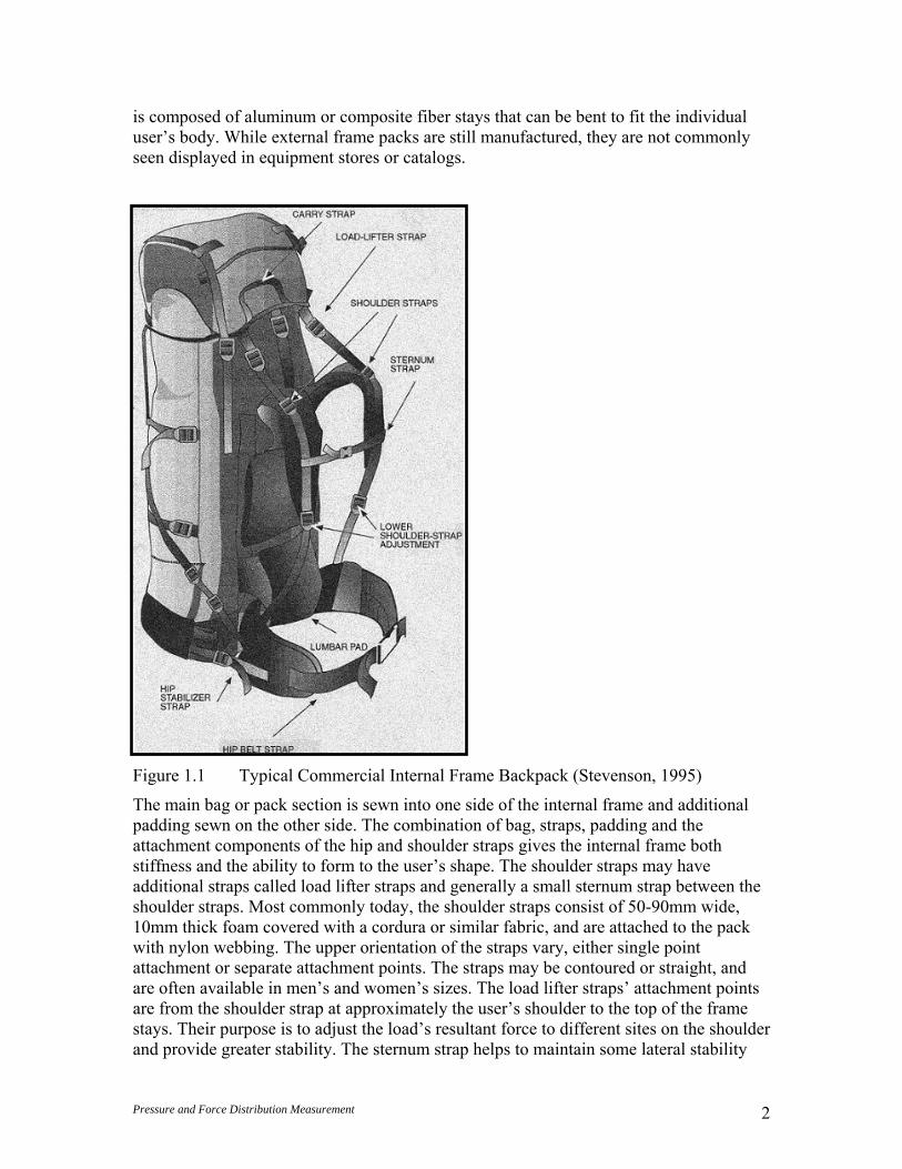
is composed of aluminum or composite fiber stays that can be bent to fit the individual user’s body. While external frame packs are still manufactured, they are not commonly seen displayed in equipment stores or catalogs.
Figure 1.1 Typical Commercial Internal Frame Backpack (Stevenson, 1995)
The main bag or pack section is sewn into one side of the internal frame and additional padding sewn on the other side. The combination of bag, straps, padding and the attachment components of the hip and shoulder straps gives the internal frame both stiffness and the ability to form to the user’s shape. The shoulder straps may have additional straps called load lifter straps and generally a small sternum strap between the shoulder straps. Most commonly today, the shoulder straps consist of 50-90mm wide, 10mm thick foam covered with a cordura or similar fabric, and are attached to the pack with nylon webbing. The upper orientation of the straps vary, either single point attachment or separate attachment points. The straps may be contoured or straight, and are often available in men’s and women’s sizes. The load lifter straps’ attachment points are from the shoulder strap at approximately the user’s shoulder to the top of the frame stays. Their purpose is to adjust the load’s resultant force to different sites on the shoulder and provide greater stability. The sternum strap helps to maintain some lateral stability

Pressure and Force Distribution Measurement 3
and take some load but is needed primarily to prevent the shoulder straps from drifting into the axilla. 1.2 Role and Design of Waist belts There is great variation in waist belt design between manufacturers. In general, the waist belt is attached to the pack at the lumbar pad area and fastens in the front over the user’s abdomen. The material used for padding varies, as does the thickness and shape. Many belts are reinforced with a plastic frame sheet on the outside of the belt. Hip stabilizer straps connect the side of the waist belt with the lower edges of the pack. The waist belt should carry the majority of the load to prevent fatigue of the upper body (Jenkins, 1992). The load can be transferred between the shoulders and hips to minimize discomfort over long periods. The waist belt is used as a support to inhibit the front-to-back and side-to-side movement of the pack, independent of the user’s body. It should rest over the iliac crests of the user to transmit the load onto the hips. With the load on the hips, the weight of the pack is being carried by the relatively large musculature of the legs instead of the smaller muscles of the upper body. The waist belt should be tight enough to minimize slipping and rubbing, while loose enough to not inhibit respiration or cause discomfort or compression of the abdomen. The waist belt can be attached to the pack in many different configurations, from static single-point or multiple-point sewn attachments, to plastic pivots or dynamic attachments. The use of a packframe with a well-padded waist belt reduces loads on the shoulders, reduces incidences of some injuries and results in less perceived pain (Knapik, et al., 1996). The commercial backpack market is constantly changing waist belt designs and materials and marketing it as the latest ‘technology’. These biomechanical effects are not generally quantified with measurable results. Dana DesignTM attaches the waist belt behind the frame for ‘positive load transfer, not sag’ and their belts have ‘contour molded’ foam (Dana Design, www.danadesign.com). The North FaceTM offers ‘dual-density’ foam padding of their waist belts as well as separate men’s and women’s designs (www.thenorthface.com). SerratusTM offers ‘thermo-molded’ foam, men’s and women’s styles and special sewing techniques that eliminate wrinkling of the belt covering material (Serratus, www.serratus.com). MountainsmithTM has designed an auto-centering waist belt buckle (www.mountainsmith.com). Lowe AlpineTM uses two-position belt tensioners and has a bi-laminate construction (www.lowealpine.com). Arc’TeryxTM uses four layer, thermo-molded foam construction, an articulating or floating attachment point, an adjustable waist belt angle, and lateral load transfer rods (Arc’Teryx, www.arcteryx.com). Although each of these companies markets their products based on design features, there are no scientific data available to support the design shape or materials used. Only two studies were found that examined the lumbar reaction forces at the level of the L3-l4 vertebrae. Reid (1999) examined the effects of lateral rods in a commercial design by measuring the forces and moments at the level of L3-L4 vertebra. The addition of the

Pressure and Force Distribution Measurement 4
lateral rods reduced the vertical load applied to the shoulders by 10% without increasing the shear load on the lumbar spine. This experiment was performed under static conditions. In another study, Reid et al (1998) examined the effects of various locations of attachment points for the lower shoulder strap. Based on comparing the shoulder and lumbar reaction forces across 12 different attachment points, a location was identified that optimized the shoulder and lumbar reaction forces. As can be seen from the lack of scientific evidence, design in the area of backpacks lacks vigor. Most of the design features have evolved historically or have been developed through experience. Only recently has instrumentation been developed to undertake a more scientific approach to pack design, specifically the waist belt. 1.3 Introduction to Backpack Modeling Two ways to determine the reaction forces on the shoulders and lumbar pad during load carriage are by direct measurement of forces or pressures on these areas and by modeling these forces through a biomechanical model of the backpack. If a biomechanical model is being developed, it must be evaluated though comparison to an independent measure, such as a direct measure. This concept is easy to understand but often difficult to perform. It is problematic to validate a biomechanical model of a backpack, as there are concerns with finding a reliable direct measurement device and concerns with the complexity of the biomechanical model. If an accurate biomechanical model of a backpack can be developed and validated, then there are several important uses for such a model. Firstly, the model can be very helpful for the design and comparison of novel concepts and materials. Secondly, the model can be used to understand the importance of change in load location and load mass. Each of these factors may have implications on the amount of shoulder and lumbar reaction force needed to carry a backpack. Finally, a biomechanical model can be used to recommend tissue tolerance limits based on subjective discomfort scores. Although direct measures can also be used to interpret subjective discomfort, it is often more convenient and cost effective to make these interpretations with a biomechanical model. To develop a valid biomechanical model for a backpack, it is reasonable to separate the components and develop a model for shoulder straps separately from the waist belt. MacNeil (1996) developed and validated a shoulder strap biomechanical model where no waist belt was considered. Pelot (1998) developed and improved a model that included a waist belt with moderate success. However, when Rigby (1999) attempted to add additional features such as load lifter straps and hip stabilizer straps, the model failed to predict shoulder and waist belt forces. Some of the concerns that Rigby (1999) identified were that the strap force sensors did not truly reflect the waist belt’s responses, that friction might play a larger role than he anticipated and that the waist belt connection point to the suspension system should not be modeled as a pin joint nor should the anterior-posterior force by the waist belt be considered zero.
Pressure and Force Distribution Measurement 5
Based on Rigby’s recommendations, the primary objectives of this thesis were to develop a valid waist belt model for a backpack and to determine the factors affecting force distribution on a load carriage system waist belt. To accomplish these objectives, several specific objectives were also identified:
1. Determination of the frictional components of the waist belt. 2. Development of a novel calibration procedure for contact pressure sensors in
this application. 3. Determination of the effects of the direction of strap tightening on measured
pressures on the body. 4. Determination of the relationship of the strap force tension in the waist belt to
the measured pressures on the body.
Pressure and Force Distribution Measurement 6
2.0 Applications of Modeling and Pressure Measurements to Load Carriage Research While many different load carriage systems have been designed and used for both military and civilian purposes, objective measurements for evaluation of designs is a relatively new area of research. Weight limits for load carriage have been recommended based on various measures: heart rate scores, blood pressure (Sagiv, 1994), perceived exertion (Goslin, 1986), and VO2 maximal tests (Epstein et al., 1988). While the largest area of research is simply the amount of load carried, load placement has been examined by comparing physiological measures (Legg et al., 1992) and loss of performance with load position (Holewijn and Lotens, 1992). Inverse dynamic biomechanical modeling to determine joint forces with varying loads has been used (Goh, 1998). Subjective measures have been observed with the use of questionnaires (Jenkins, 1992). The primary measures have been subjective and relating to performance, such as obtaining feedback from user groups (e.g. expert trekkers and military personnel). As individual opinion varies greatly, subjective measures do not provide clearly defined advantages and disadvantages between designs. No studies have examined psycho-social factors that may contribute to an individual’s perception of pack comfort and design properties, such as: physical anthropometry of the individual, pack colour and appearance, preconceived opinions of a pack design based upon the manufacturer’s reputation, peer pressure, or mood during testing. It is especially difficult to determine optimal design features through subjective opinions alone. One solution to design problems is to construct a means of objectively testing packs that minimize human variability when analyzing design features for load carriage. In this way, the comparison of features can be quantified objectively under controlled conditions. The approach has been to compare a number of packs and subjects’ opinions of load control and load transfer features with specific measured outputs from standardized measurement tools (Stevenson, 1996). By correlating subjects’ opinions with objective measurements, it was possible to validate the objective measures. One main tool has been a Load Carriage (LC) Simulator that is pneumatically operated by computer controls and programmed to simulate gait cadence at various speeds (Stevenson, 1995). The mannequin of the LC Simulator is used to determine the forces, moments, pressures and relative motion of the body because of the pack design, load and method of wearing the pack. Secondly, a pack compliance testing mannequin is capable of bending at the level of the third and fourth lumbar vertebrae (L3/L4) about the principal axis of rotation for torsion, lateral bending or forward bending. For this device force-displacement profiles show the resistance to motion of the pack suspension system. Finally, a load distribution mannequin has force and moment measurement capabilities both at L3 and at the base of the mannequin. This device allows researchers to partition the upper and lower body reaction forces that support a backpack.
Pressure and Force Distribution Measurement 7
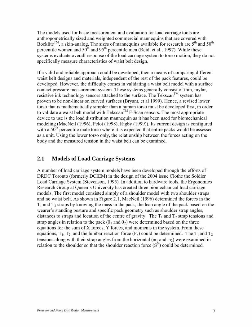
The models used for basic measurement and evaluation for load carriage tools are anthropometrically sized and weighted commercial mannequins that are covered with BockliteTM, a skin-analog. The sizes of mannequins available for research are 5th and 50th percentile women and 50th and 95th percentile men (Reid, et al., 1997). While these systems evaluate overall response of the load carriage system to torso motion, they do not specifically measure characteristics of waist belt design. If a valid and reliable approach could be developed, then a means of comparing different waist belt designs and materials, independent of the rest of the pack features, could be developed. However, the difficulty comes in validating a waist belt model with a surface contact pressure measurement system. These systems generally consist of thin, mylar, resistive ink technology sensors attached to the surface. The TekscanTM system has proven to be non-linear on curved surfaces (Bryant, et al 1999). Hence, a revised lower torso that is mathematically simpler than a human torso must be developed first, in order to validate a waist belt model with TekscanTM F-Scan sensors. The most appropriate device to use is the load distribution mannequin as it has been used for biomechanical modeling (MacNeil (1996), Pelot (1998), Rigby (1999)). Its current design is configured with a 50th percentile male torso where it is expected that entire packs would be assessed as a unit. Using the lower torso only, the relationship between the forces acting on the body and the measured tension in the waist belt can be examined. 2.1 Models of Load Carriage Systems A number of load carriage system models have been developed through the efforts of DRDC Toronto (formerly DCIEM) in the design of the 2004 issue Clothe the Soldier Load Carriage System (Stevenson, 1995). In addition to hardware tools, the Ergonomics Research Group at Queen’s University has created three biomechanical load carriage models. The first model consisted simply of a shoulder model with two shoulder straps and no waist belt. As shown in Figure 2.1, MacNeil (1996) determined the forces in the T1 and T2 straps by knowing the mass in the pack, the lean angle of the pack based on the wearer’s standing posture and specific pack geometry such as shoulder strap angles, distances to straps and location of the centre of gravity. The T1 and T2 strap tensions and strap angles in relation to the pack (θ1 and θ2) were determined based on the three equations for the sum of X forces, Y forces, and moments in the system. From these equations, T1, T2, and the lumbar reaction force (Fx) could be determined. The T1 and T2 tensions along with their strap angles from the horizontal (ω1 and ω2) were examined in relation to the shoulder so that the shoulder reaction force (SN) could be determined.

Pressure and Force Distribution Measurement 8
Figure 2.1 Shoulder Model for a Backpack. T1=Upper shoulder strap, T2=Lower shoulder strap, υ1=Upper strap angle in relation to the pack, υ2=Lower strap angle in relation to the pack, Fx=Lumbar reaction force, W=Weight of the pack, γ=Lean angle of the pack, SN=Shoulder reaction force, Sf=Frictional force on the shoulder, ϖ1=Upper shoulder strap angle from the horizontal, ϖ2=Lower shoulder strap angle from the horizontal. MacNeil (1996) determined a frictional force, Sf, using a coefficient of static friction measured with an inclined plane. The differences between T1 and T2 were considered to be due to the effects of this frictional force. This model was successful (r2=0.95) in estimating the reaction force on the shoulder but was rather simple with the exclusion of the waist belt. Despite this limitation it was quite successful at predicting subjects’ opinions based on backpack design data. However, for most modern commercial and military load carriage systems that employ a waist belt, this model was limited primarily to daypacks or children’s backpacks. The second model that was created by Rigby (1997) and Pelot (1998) expanded the MacNeil model to include a waist belt. This model kept the same features for modeling the shoulder reaction force but incorporated a waist belt that was treated as a pin joint with no horizontal transmission of force to the waist belt. The waist belt itself was treated as a hoop and modeled as a thin-walled cylinder with hoop stress. No contact or friction was assumed to be present on the back.
ω
ω1
S Sf
T1
T2
T2
T1
Fx
θ2
θ1
W
γ
Pressure and Force Distribution Measurement 9
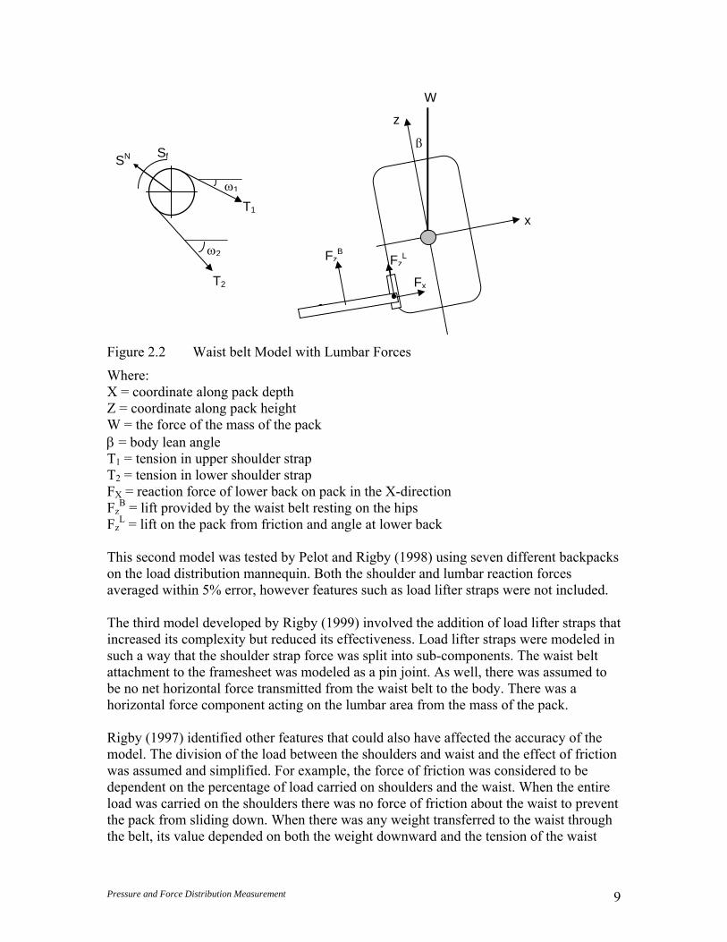
Figure 2.2 Waist belt Model with Lumbar Forces
Where: X = coordinate along pack depth Z = coordinate along pack height W = the force of the mass of the pack β = body lean angle T1 = tension in upper shoulder strap T2 = tension in lower shoulder strap FX = reaction force of lower back on pack in the X-direction Fz
B = lift provided by the waist belt resting on the hips Fz
L = lift on the pack from friction and angle at lower back This second model was tested by Pelot and Rigby (1998) using seven different backpacks on the load distribution mannequin. Both the shoulder and lumbar reaction forces averaged within 5% error, however features such as load lifter straps were not included. The third model developed by Rigby (1999) involved the addition of load lifter straps that increased its complexity but reduced its effectiveness. Load lifter straps were modeled in such a way that the shoulder strap force was split into sub-components. The waist belt attachment to the framesheet was modeled as a pin joint. As well, there was assumed to be no net horizontal force transmitted from the waist belt to the body. There was a horizontal force component acting on the lumbar area from the mass of the pack. Rigby (1997) identified other features that could also have affected the accuracy of the model. The division of the load between the shoulders and waist and the effect of friction was assumed and simplified. For example, the force of friction was considered to be dependent on the percentage of load carried on shoulders and the waist. When the entire load was carried on the shoulders there was no force of friction about the waist to prevent the pack from sliding down. When there was any weight transferred to the waist through the belt, its value depended on both the weight downward and the tension of the waist
FzL
x
z
W
β
FzB
Fx
ω2
ω1
SN Sf
T1
T2
Pressure and Force Distribution Measurement 10
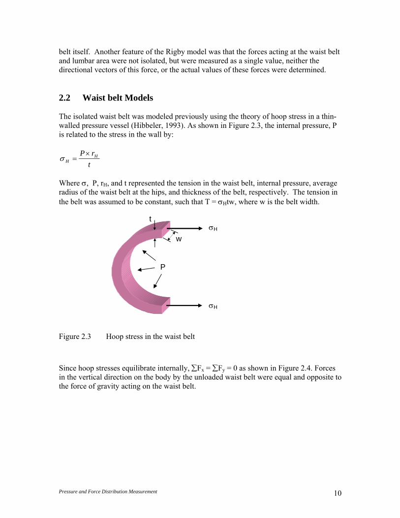
belt itself. Another feature of the Rigby model was that the forces acting at the waist belt and lumbar area were not isolated, but were measured as a single value, neither the directional vectors of this force, or the actual values of these forces were determined. 2.2 Waist belt Models The isolated waist belt was modeled previously using the theory of hoop stress in a thin-walled pressure vessel (Hibbeler, 1993). As shown in Figure 2.3, the internal pressure, P is related to the stress in the wall by:
trP H
H×
=σ
Where σ, P, rH, and t represented the tension in the waist belt, internal pressure, average radius of the waist belt at the hips, and thickness of the belt, respectively. The tension in the belt was assumed to be constant, such that T = σHtw, where w is the belt width.
Figure 2.3 Hoop stress in the waist belt
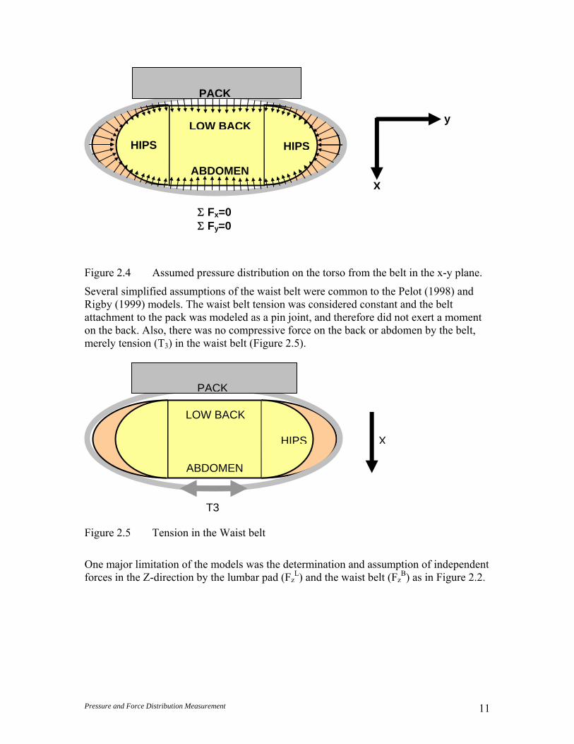
Since hoop stresses equilibrate internally, ∑Fx = ∑Fy = 0 as shown in Figure 2.4. Forces in the vertical direction on the body by the unloaded waist belt were equal and opposite to the force of gravity acting on the waist belt.
σH
σH
w
t
P
Pressure and Force Distribution Measurement 11
Figure 2.4 Assumed pressure distribution on the torso from the belt in the x-y plane.
Several simplified assumptions of the waist belt were common to the Pelot (1998) and Rigby (1999) models. The waist belt tension was considered constant and the belt attachment to the pack was modeled as a pin joint, and therefore did not exert a moment on the back. Also, there was no compressive force on the back or abdomen by the belt, merely tension (T3) in the waist belt (Figure 2.5).
Figure 2.5 Tension in the Waist belt
One major limitation of the models was the determination and assumption of independent forces in the Z-direction by the lumbar pad (Fz
L) and the waist belt (FzB) as in Figure 2.2.
X
y
ABDOMEN
LOW BACK
PACK
HIPSHIPS
Σ Fx=0 Σ Fy=0
ABDOMEN
LOW BACK
PACK
HIPS X
T3
Pressure and Force Distribution Measurement 12
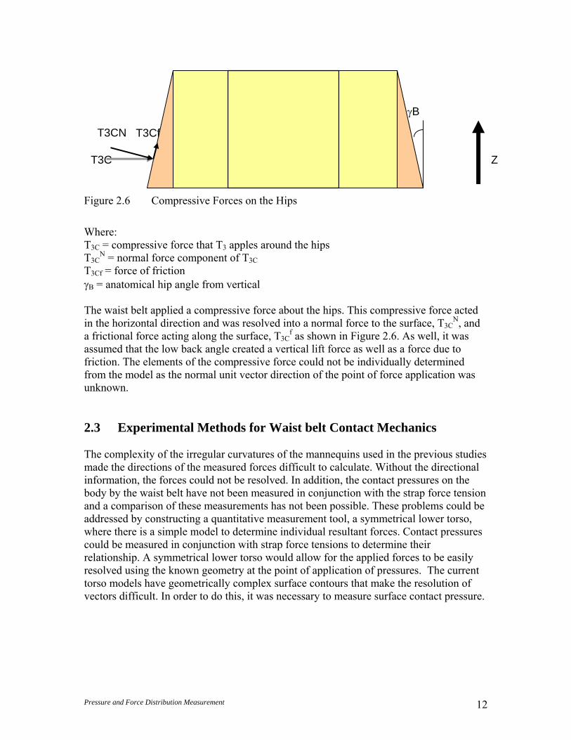
Figure 2.6 Compressive Forces on the Hips
Where: T3C = compressive force that T3 apples around the hips T3C
N = normal force component of T3C T3Cf = force of friction γB = anatomical hip angle from vertical The waist belt applied a compressive force about the hips. This compressive force acted in the horizontal direction and was resolved into a normal force to the surface, T3C
N, and a frictional force acting along the surface, T3C
f as shown in Figure 2.6. As well, it was assumed that the low back angle created a vertical lift force as well as a force due to friction. The elements of the compressive force could not be individually determined from the model as the normal unit vector direction of the point of force application was unknown.
2.3 Experimental Methods for Waist belt Contact Mechanics The complexity of the irregular curvatures of the mannequins used in the previous studies made the directions of the measured forces difficult to calculate. Without the directional information, the forces could not be resolved. In addition, the contact pressures on the body by the waist belt have not been measured in conjunction with the strap force tension and a comparison of these measurements has not been possible. These problems could be addressed by constructing a quantitative measurement tool, a symmetrical lower torso, where there is a simple model to determine individual resultant forces. Contact pressures could be measured in conjunction with strap force tensions to determine their relationship. A symmetrical lower torso would allow for the applied forces to be easily resolved using the known geometry at the point of application of pressures. The current torso models have geometrically complex surface contours that make the resolution of vectors difficult. In order to do this, it was necessary to measure surface contact pressure.
Z
γB
T3Cf T3CN
T3C

Pressure and Force Distribution Measurement 13
2.4 Contact Pressure Measurement Various methods of surface pressure measurement are available commercially. The two most common systems are the TekscanTM F-scan system and NovelTM Electronics PEDAR system. Rash, et al (1997) compared the two systems and found no significant difference in the systems’ abilities to measure uniform average pressure, although more sensor-to-sensor variation was found in the TekscanTM system. The size and relatively low cost of the TekscanTM sensors, as well as their reported favorable comparison to the PEDAR system facilitated their use. Therefore, the surface pressure measurement tools used for research on load carriage in the Biomechanics laboratory at Queen’s University were the TekscanTM F-Scan sensors, Figure 2.7.
Figure 2.7 Tekscan Sensor and Cuff
Each sensor consists of a flexible Mylar sheet with dimensions approximately 7.6cm x 20cm, with a thickness of 0.4mm. The sensor contains resistive ink that responds to applied force with a change in resistance. They are connected by a cuff and cable to an A/D board in the computer that is read by the TekscanTM software. This voltage is converted to pressure by an algorithm, stated by the manufacturer, using the effective area of the individual sensel and the voltage converted to a force with a regression line calculated during calibration. These sensors are affixed to the surface of the mannequins, a difficult task since they have a tendency to wrinkle over various protruding landmarks. Symmetrical placement of these sensors over a region of the mannequin’s anatomy is also difficult due to the slight dissimilarities and curvatures of the body surfaces. The normal directions of points on the surface are generally unknown and therefore the measured forces are difficult to resolve. This resistive ink technology has achieved varying success. These sensors have been shown to have an average calibration error of 4%, creep of 19%, and hysteresis of 12% (Woodburn and Helliwell, 1997). As well, the measurements between sensors have significant variability and the calibration protocol determined by the manufacturer is inaccurate (Woodburn and Helliwell, 1997). Average pressure results on flat surfaces have an accuracy of 4% and precision of 9.6%, while peak pressure measurements have both an accuracy and precision of 14% (Bryant, et al., 1999).
Pressure and Force Distribution Measurement 14
In addition to the surface compliance effects and time dependency, various additional factors affecting sensor accuracy have been determined. For example, a temperature range from 24° to 37°C resulted in a 50% increase in sensor output (Luo, 1998). For the current study however, the temperature for calibration and experimentation was held a constant at 21ºC. When the sensors were used on a curved surface, there was inherent change of the surface geometry with the nature of the contact surfaces. This resulted in an increased gain for radii of curvature greater than 50mm (MacNeil, 1996). This response had also been shown by Buis and Convery (1997) to attenuate with a radius of curvature of less than 50mm. The sensitivity has been shown to decrease with the addition of pliable material (Sumiya, 1998) yet is not suitable for use on hard surfaces such as plexiglas (Luo, 1998). An additional limitation with the TekscanTM system is that the F-ScanTM sensors are not calibrated for use on curved surfaces. Equilibration is possible, but difficult and inconsistent on the surface of the mannequins. The manufacturer makes no claims to their accuracy or precision when used on curved surfaces. Bryant, et al (1999) attempted to overcome some of these concerns by constructing a hand-held pressure calibrator that would apply a constant force regardless of the surface shape. As a result of calibration difficulties, TekscanTM sensors have been used in a limited manner only. They have proven to be a useful comparison tool for peak pressure areas and the relative magnitude, but not the actual values of the forces (Stevenson, et al., 1996). Developing a calibration method to cope with rounded surfaces on human mannequins to enhance the TekscanTM F-Scan accuracy form one of the objectives of this study. Pelot and Rigby (1998) endeavored to use pressure sensors in his biomechanical model to measure body forces, however, he confined his analysis to peak pressure points and a comparison of peak pressures between packs. Although he also measured strap tensions in the waist belt and lower shoulder strap, he did not correlate these two measures. To develop a scientific approach to waist belt design, it is important to understand how they work. Stevenson et al. (1995) have used a waist belt strap sensor in all of their research on the LC Simulator and LC Compliance tester to standardize the tension for all pack testing. However, the impact of this standard tension due to different waist belt designs is unknown. Neither Pelot (1998) nor Rigby (1999) used the waist belt strap tension gauge in their hoop stress modeling of waist belt design. Rigby (1999) was particularly sensitive to the need to examine the waist belt by itself as his model could not resolve the lumbar forces. A lower torso model with a method of measuring applied forces and resolving those forces into their respective resultants in the X, Y, Z directions is necessary to further the biomechanical model as shown in Figure 2.8, the current models use the sum of the measurements from the sensor to determine the average force acting on the area as well as peak pressure locations on the body. The lack of directional information for the measured forces limits the ability to resolve the measured force vectors. This is necessary
Pressure and Force Distribution Measurement 15
to gain an understanding of the applied pressures at the waist and to determine the effects at the lumbar area independent of the rest of the system.
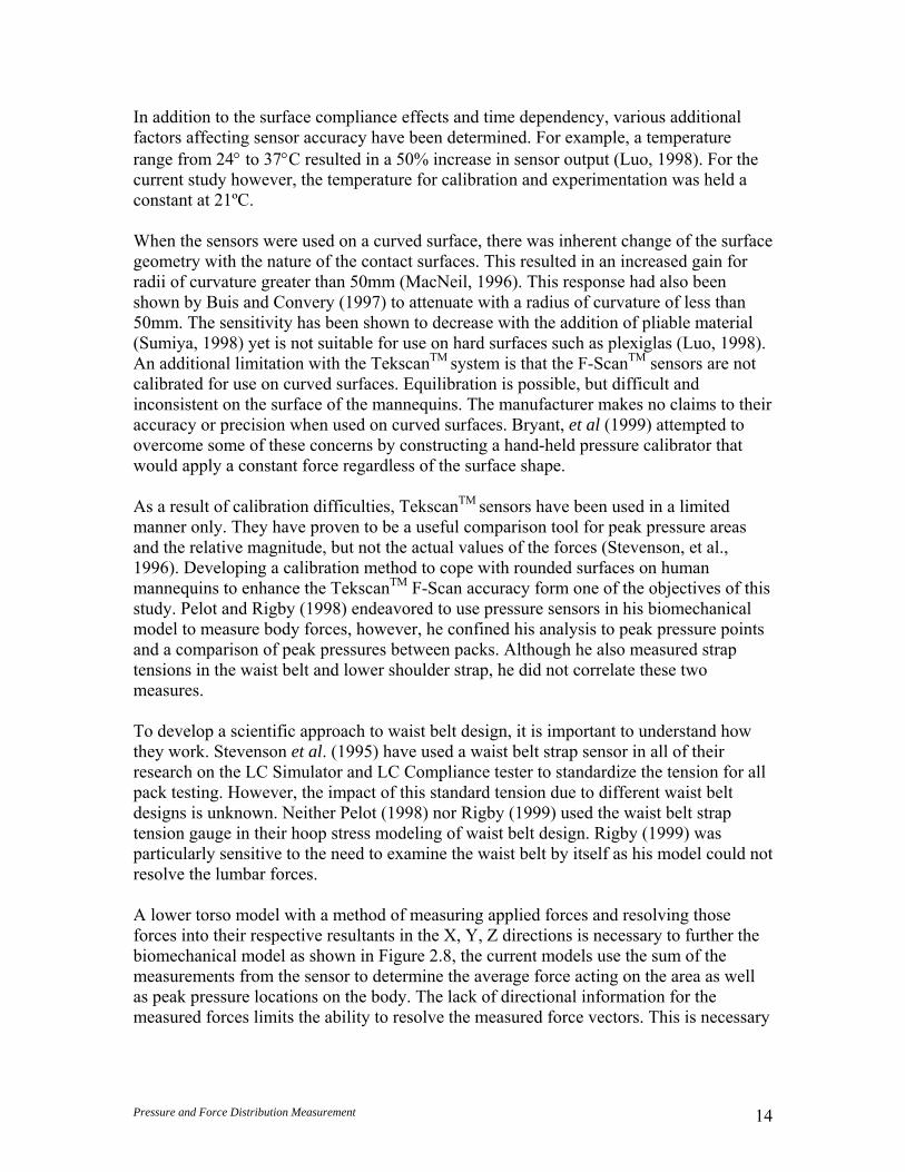
Figure 2.8 Reaction Forces on the Body Under the a) Current System and b) Proposed System.
Fx and Fz cannot be determined from the current system as the coordinate of the point of pressure measurement and the normal direction of the applied force is not known. With the proposed system, the measured force can be resolved into directional components as the direction of the normal force is known. A direct comparison of pressure and force distribution of different belt designs and materials has not been performed, nor has the relationship between belt tension and the force distribution been examined. The ability to quantify the differences between designs and measure the effects of proposed changes would be of great importance to backpack manufacturers.
Fz
a) Current System b) Proposed System
Known: Σ FR, Σ Fx, Σ Fy, Σ Fz Known: Σ FR
FR
FR
FR
FR
Fz
Fx Fz
Fz
Fz
Fx
Fx
FR Fx
Fx

Pressure and Force Distribution Measurement 16
3.0 Methodology 3.1 Design of the Symmetrical Lower Torso The Symmetrical Lower Torso Model (SLT) was designed to provide a simple method of determining the surface normals of applied forces. The previous torsos were commercial mannequins with non-symmetrical curves and irregular bony landmarks. As well, it was difficult to place the TekscanTM sensors on the surface of the previous models without creating bubbles and wrinkles (Bryant, et al., 1999). A simple cylinder was considered for the torso model similar to the simplified shoulder representation of MacNeil (1996). However, due to the vertical orientation of the torso compared to the horizontal orientation of the shoulder, a conical model was considered more representative of the human body. It was hypothesized that there would be lower tensions in the waist belt than on the shoulder and that friction would play a greater part to prevent slippage of the belt. The waist size of the SLT corresponded with the waist dimensions of the 50th percentile male upper torso. The waist-to-hip ratio was determined as the average of the 5th and 50th percentile female and 50th and 95th percentile male mannequins currently in use. A waist-to-hip ratio of 0.85 was chosen, as it was also consistent with ratios for healthy males or females as reported by McArdle (1996). The SLT was designed to fit on the base platform of the load distribution mannequin and had a similar appearance to the previous model. The distance from waist-to-hip was measured from the existing load carriage mannequins as well as from 10 human subjects (5M, 5F) of average fitness level, with mean age 29 years +/-11yrs. The distance from the narrowest part of the waist to the height of the largest circumference about the buttocks was measured. As a result the SLT was designed to be unisex. The height of the SLT was 318mm and corresponded to the previous model (Appendix A). The centre rectangular section was added to signify the relative flatness of the lower back and abdomen. The SLT had symmetrical quadrants, consisting of a hip-shaped cone with an 8° angle that was vertically split into two halves and glued to the sides of the three-dimensional trapezoid of the back and abdomen (Figure 3.1).
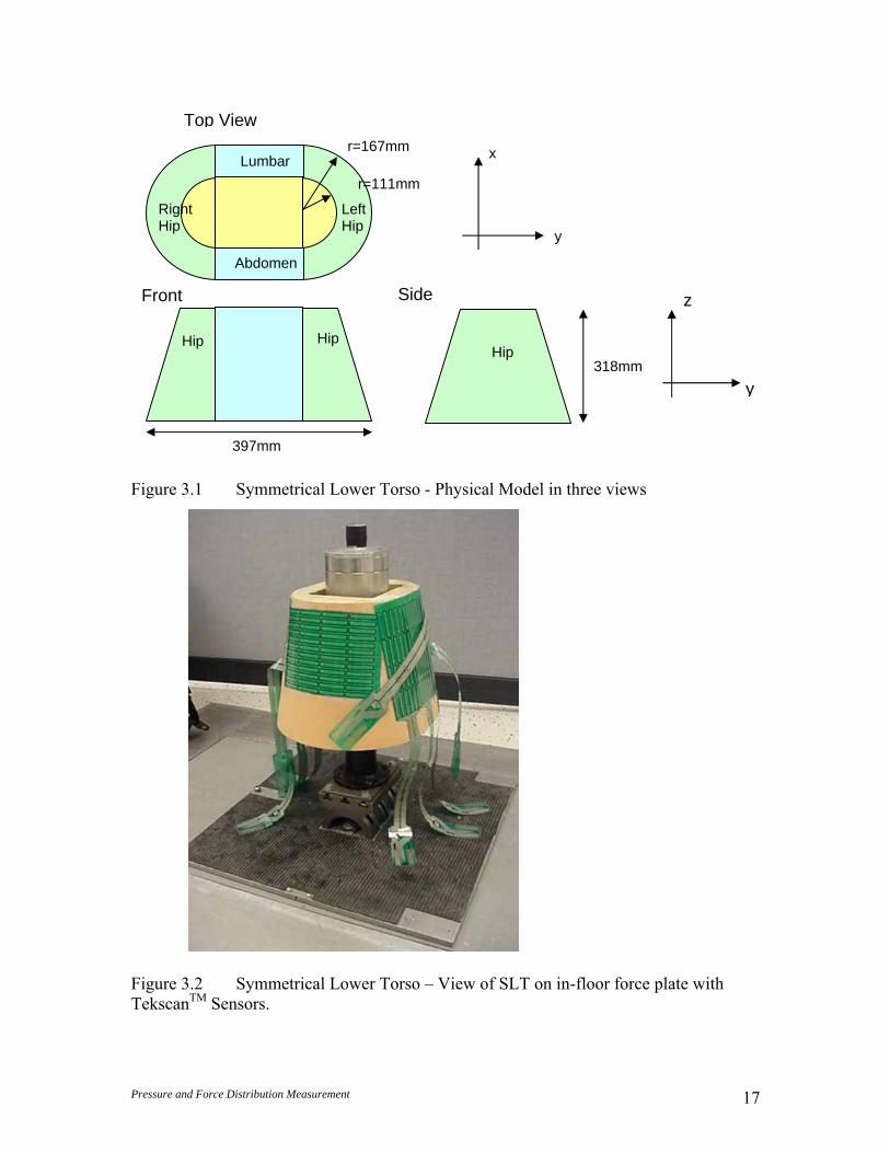
Pressure and Force Distribution Measurement 17
Figure 3.1 Symmetrical Lower Torso - Physical Model in three views
Figure 3.2 Symmetrical Lower Torso – View of SLT on in-floor force plate with TekscanTM Sensors.
Top View
Side Front
Lumbar
Abdomen
Right Hip
Left Hip
Hip Hip Hip
r=167mm
r=111mm
x
y
318mm
397mm
z
y
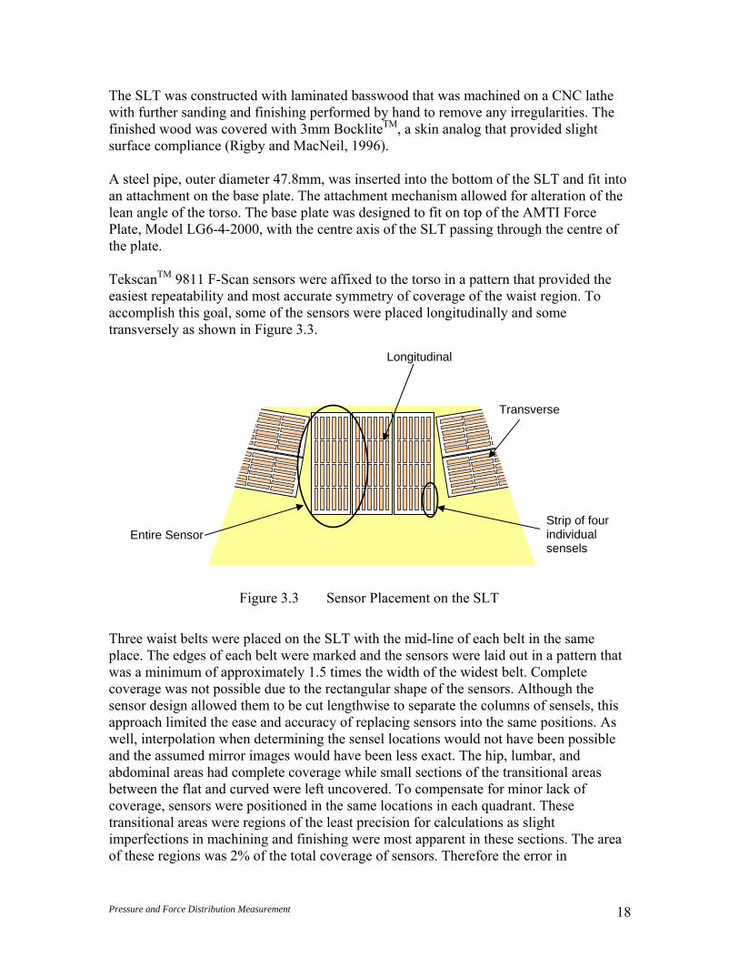
Pressure and Force Distribution Measurement 18
The SLT was constructed with laminated basswood that was machined on a CNC lathe with further sanding and finishing performed by hand to remove any irregularities. The finished wood was covered with 3mm BockliteTM, a skin analog that provided slight surface compliance (Rigby and MacNeil, 1996). A steel pipe, outer diameter 47.8mm, was inserted into the bottom of the SLT and fit into an attachment on the base plate. The attachment mechanism allowed for alteration of the lean angle of the torso. The base plate was designed to fit on top of the AMTI Force Plate, Model LG6-4-2000, with the centre axis of the SLT passing through the centre of the plate. TekscanTM 9811 F-Scan sensors were affixed to the torso in a pattern that provided the easiest repeatability and most accurate symmetry of coverage of the waist region. To accomplish this goal, some of the sensors were placed longitudinally and some transversely as shown in Figure 3.3.
Figure 3.3 Sensor Placement on the SLT
Three waist belts were placed on the SLT with the mid-line of each belt in the same place. The edges of each belt were marked and the sensors were laid out in a pattern that was a minimum of approximately 1.5 times the width of the widest belt. Complete coverage was not possible due to the rectangular shape of the sensors. Although the sensor design allowed them to be cut lengthwise to separate the columns of sensels, this approach limited the ease and accuracy of replacing sensors into the same positions. As well, interpolation when determining the sensel locations would not have been possible and the assumed mirror images would have been less exact. The hip, lumbar, and abdominal areas had complete coverage while small sections of the transitional areas between the flat and curved were left uncovered. To compensate for minor lack of coverage, sensors were positioned in the same locations in each quadrant. These transitional areas were regions of the least precision for calculations as slight imperfections in machining and finishing were most apparent in these sections. The area of these regions was 2% of the total coverage of sensors. Therefore the error in
Longitudinal
Transverse
Entire Sensor Strip of four individual sensels
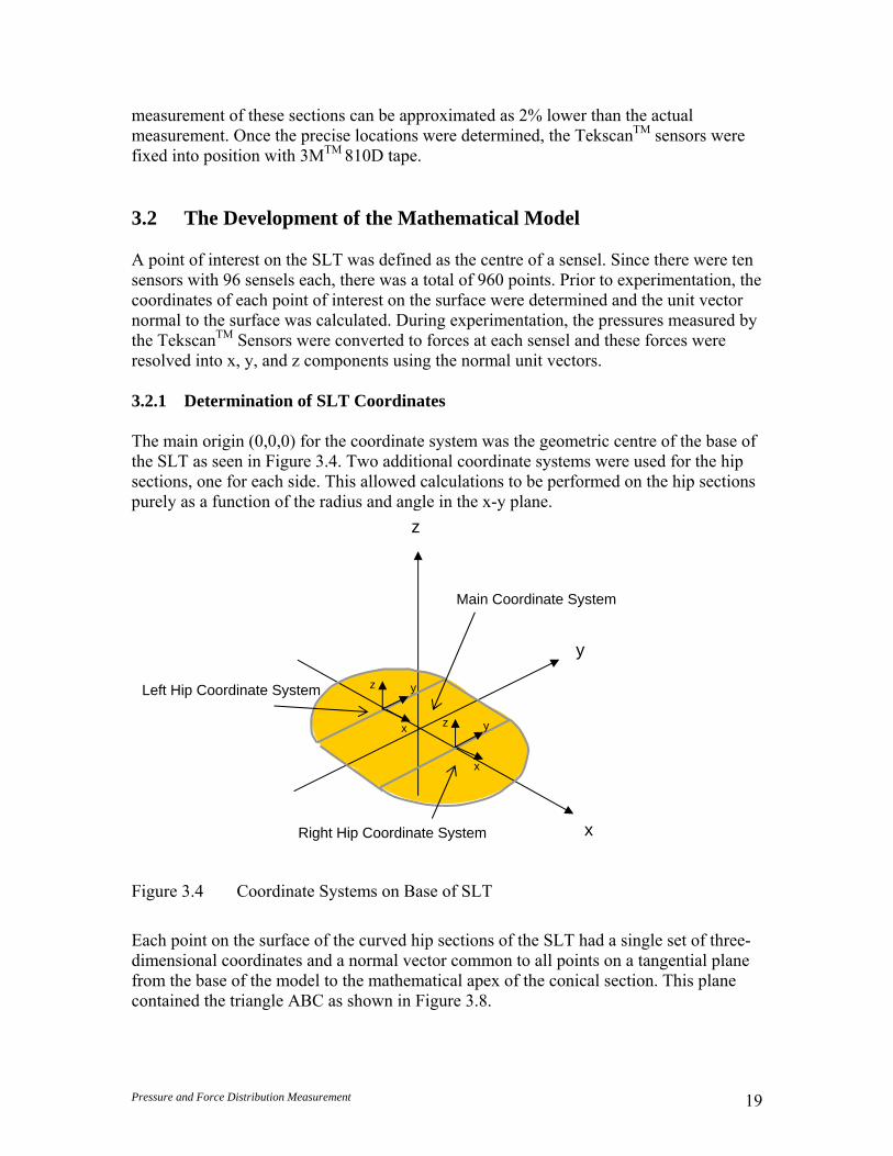
Pressure and Force Distribution Measurement 19
measurement of these sections can be approximated as 2% lower than the actual measurement. Once the precise locations were determined, the TekscanTM sensors were fixed into position with 3MTM 810D tape. 3.2 The Development of the Mathematical Model A point of interest on the SLT was defined as the centre of a sensel. Since there were ten sensors with 96 sensels each, there was a total of 960 points. Prior to experimentation, the coordinates of each point of interest on the surface were determined and the unit vector normal to the surface was calculated. During experimentation, the pressures measured by the TekscanTM Sensors were converted to forces at each sensel and these forces were resolved into x, y, and z components using the normal unit vectors. 3.2.1 Determination of SLT Coordinates The main origin (0,0,0) for the coordinate system was the geometric centre of the base of the SLT as seen in Figure 3.4. Two additional coordinate systems were used for the hip sections, one for each side. This allowed calculations to be performed on the hip sections purely as a function of the radius and angle in the x-y plane.
Figure 3.4 Coordinate Systems on Base of SLT
Each point on the surface of the curved hip sections of the SLT had a single set of three-dimensional coordinates and a normal vector common to all points on a tangential plane from the base of the model to the mathematical apex of the conical section. This plane contained the triangle ABC as shown in Figure 3.8.
z
y
x
z y
x z y
x
Right Hip Coordinate System
Left Hip Coordinate System
Main Coordinate System

Pressure and Force Distribution Measurement 20
A point was defined on the circumference of the hip according to the polar coordinates z, θ, where z is the height above the base plane and θ is the angle from the y-axis. θ was measured on the top of the SLT with a protractor for each point. The distance from the base of the SLT on the surface of the cone was measured. Using the right-angle triangle rule, the distance in the vertical z-direction was calculated. This z-value allowed for the calculation of the radius of the cone at the point of interest. This radius was resolved using the right-angle triangle rule, resulting in the coordinates of the point of interest (x0, y0). For the right hip, the base plane is shown in Figure 3.5. The equation of the tangent to the circle at the given point is given in point-slope form:
Figure 3.5 Tangent to the Circle
For the x intercept of the tangent: For the y intercept of the tangent:
))(()( 00
00 xx
yx
yy tt −−=−
00
00
00
00
))((
))(()0(
0
xxy
yx
xxyx
y
y
t
t
t
+−−=
−−=−
=
))((
)0)(()(
0
00
00
00
00
xyx
yy
xyx
yy
x
t
t
t
−−+=
−−=−
=
(0,yt)
(x0,y0)
(xt,0)θ
y
x
B
A
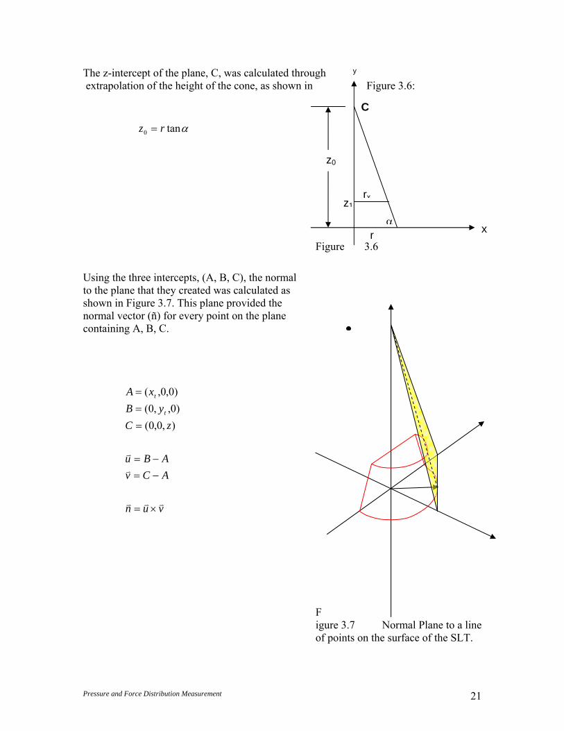
Pressure and Force Distribution Measurement 21
z0
α
rxz1
y
x
C
r
The z-intercept of the plane, C, was calculated through extrapolation of the height of the cone, as shown in Figure 3.6:
Figure 3.6
Using the three intercepts, (A, B, C), the normal to the plane that they created was calculated as shown in Figure 3.7. This plane provided the normal vector (ñ) for every point on the plane containing A, B, C.
Figure 3.7 Normal Plane to a line of points on the surface of the SLT.
αtan0 rz =
vun
ACvABu
zCyB
xA
t
t
vvv
v
v
×=
−=−=
===
),0,0()0,,0()0,0,(
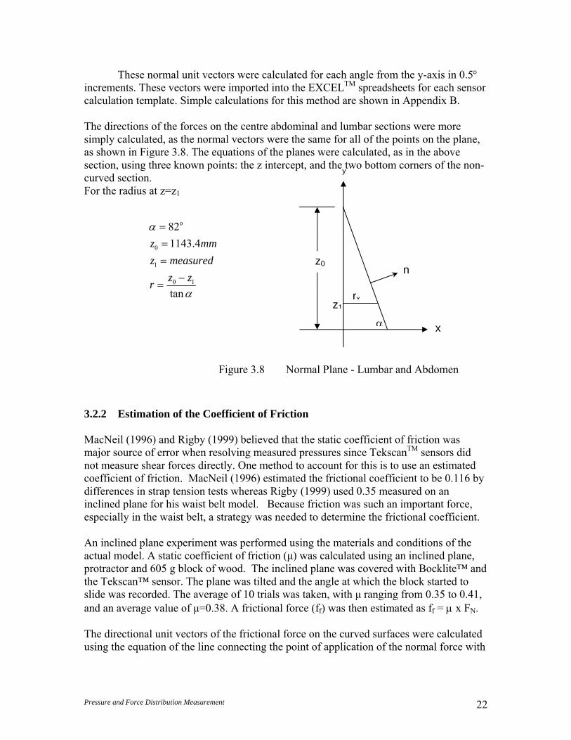
Pressure and Force Distribution Measurement 22
These normal unit vectors were calculated for each angle from the y-axis in 0.5° increments. These vectors were imported into the EXCELTM spreadsheets for each sensor calculation template. Simple calculations for this method are shown in Appendix B. The directions of the forces on the centre abdominal and lumbar sections were more simply calculated, as the normal vectors were the same for all of the points on the plane, as shown in Figure 3.8. The equations of the planes were calculated, as in the above section, using three known points: the z intercept, and the two bottom corners of the non-curved section. For the radius at z=z1
Figure 3.8 Normal Plane - Lumbar and Abdomen
3.2.2 Estimation of the Coefficient of Friction MacNeil (1996) and Rigby (1999) believed that the static coefficient of friction was major source of error when resolving measured pressures since TekscanTM sensors did not measure shear forces directly. One method to account for this is to use an estimated coefficient of friction. MacNeil (1996) estimated the frictional coefficient to be 0.116 by differences in strap tension tests whereas Rigby (1999) used 0.35 measured on an inclined plane for his waist belt model. Because friction was such an important force, especially in the waist belt, a strategy was needed to determine the frictional coefficient. An inclined plane experiment was performed using the materials and conditions of the actual model. A static coefficient of friction (μ) was calculated using an inclined plane, protractor and 605 g block of wood. The inclined plane was covered with Bocklite™ and the Tekscan™ sensor. The plane was tilted and the angle at which the block started to slide was recorded. The average of 10 trials was taken, with μ ranging from 0.35 to 0.41, and an average value of μ=0.38. A frictional force (ff) was then estimated as ff = μ x FN. The directional unit vectors of the frictional force on the curved surfaces were calculated using the equation of the line connecting the point of application of the normal force with
α
α
tan
4.114382
10
1
0
zzr
measuredzmmz
o
−=
===
z0
α
rxz1
y
x
n

Pressure and Force Distribution Measurement 23
the z-coordinate of the theoretical top of the cone. This assumed that any impending motion is in the longitudinal direction. As such,
In dimensionless form: Where:
Each of these unit vectors was multiplied to the frictional force to generate the friction component in the x, y, and z directions respectively. The normal vectors on the non-curved surfaces of the abdomen and back were the same for the entire plane. The vectors were calculated using the z coordinate of the theoretical top of the cone and the centre of the base of the plane, the y coordinate of the plane (Figure 3.7). The frictional force was given by:
In dimensionless form:
Where:
Fx, Fy, Fz, fx, fy, and fz were each summed for the entire sensel. These values were automatically copied to the EXCELTM summary sheet to be combined with the rest of the sensors to provide an entire data set.
))(,,0(),0,0()0,,0(
0zyfzyf
Ndir
odirN
−=
−=
0=i
20
2 )( zy
yj−+
=
20
2
0
)( zy
zk
−+
−=
))(,,(),0,0(),,(
0zzyxfzzyxf
dirN
odirN
−=
−=
20
22 )( zzyxxi
−++=
20
22 )( zzyxyj
−++=
20
220
)()(
zzyxzzk
−++
−=
),,( kjif N =
),,( kjif N =
Pressure and Force Distribution Measurement 24
3.3 Tools Used for Calibration and Validation Experiments 3.3.1 TekscanTM Calibration To measure pressures on the body created by the waist belt, TekscanTM F-Scan 9811 Pressure Sensors were used. These sensors consisted of an array of 96 individual sensels, 16 rows by six columns. The array was on a thin, flexible Mylar sheet, each sensel measuring 6mm by 7mm. Each sensel contained a homogenous layer of resistive ink, sandwiched between two conductive sheets. When a force was applied, the resulting resistance between the two sheets was measured as a voltage. The software took this voltage value, determined it to be acting across the entire sensel area of 161.29 mm2, and subsequently calculated the pressure acting on the sensel. A calibration jig (Bryant, et al., 1999) was developed to calibrate each TekscanTM F-Scan sensor. The jig consisted of a rectangular bladder sandwiched between two metal plates with the corners of the plates kept in place with four bolts. Each sensor was placed on top of the lower plate, with the bladder and upper plate placed on top. The sensor was taped in place to inhibit movement. The bladder was then inflated to 10psi and the data input to a calibration algorithm (Bryant, et al., 1999). The data sets were converted to a calibration line with linear regression. Each calibration line consisted of a constant and a slope, representing the offset and gain respectively for each sensel. 3.3.2 Force Plate The model LG6-4-2000 (AMTI Incorporated, Boston, USA) force platform was built into the floor of the testing facility. The force platform measured forces and moments simultaneously in the X, Y and Z directions using four measurement gauges, one at each corner. The output voltages were proportional to the force applied to the system. The voltage signal was amplified with a Model SGA6-4 (AMTI Incorporated) and input to a National Instruments BNC-2090 connection box and sent througha 25-pin connector to an A/D board in the CPU of the computer. This signal was then captured using Labview Software (National Instruments Inc.). Potter (1998) showed that the force plate had an average percent error in the vertical direction of 0.078% and a standard deviation of 0.34%. He also showed a resolution of 0.002kg and r2=0.999. Finally, the precision of standard deviation in the z-direction was shown to be equal to 0.374 mV. The output voltages were converted to Newtons using a linear procedure defined by the manufacturer. The force plate instrumentation was zeroed across all six channels. One data set was recorded for 5 seconds at 50Hz with the plate unloaded. The force plate was then loaded with weight in the following increments: 2.27kg, 4.55kg, 9.09kg, 22.73kg, 45.45kg, 90.91kg. The voltages were recorded for each trial. The raw voltages were plotted against the applied forces in the Z-direction. As the masses were not of uniform size or material, the comparison of any of the other forces could not easily be calculated as the exact centre of pressure for each mass is unknown. Regression
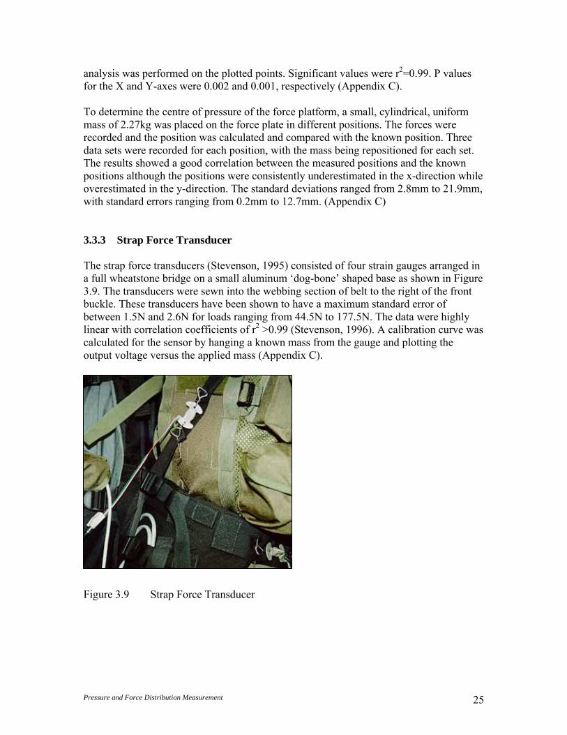
Pressure and Force Distribution Measurement 25
analysis was performed on the plotted points. Significant values were r2=0.99. P values for the X and Y-axes were 0.002 and 0.001, respectively (Appendix C).
To determine the centre of pressure of the force platform, a small, cylindrical, uniform mass of 2.27kg was placed on the force plate in different positions. The forces were recorded and the position was calculated and compared with the known position. Three data sets were recorded for each position, with the mass being repositioned for each set. The results showed a good correlation between the measured positions and the known positions although the positions were consistently underestimated in the x-direction while overestimated in the y-direction. The standard deviations ranged from 2.8mm to 21.9mm, with standard errors ranging from 0.2mm to 12.7mm. (Appendix C) 3.3.3 Strap Force Transducer The strap force transducers (Stevenson, 1995) consisted of four strain gauges arranged in a full wheatstone bridge on a small aluminum ‘dog-bone’ shaped base as shown in Figure 3.9. The transducers were sewn into the webbing section of belt to the right of the front buckle. These transducers have been shown to have a maximum standard error of between 1.5N and 2.6N for loads ranging from 44.5N to 177.5N. The data were highly linear with correlation coefficients of r2 >0.99 (Stevenson, 1996). A calibration curve was calculated for the sensor by hanging a known mass from the gauge and plotting the output voltage versus the applied mass (Appendix C).
Figure 3.9 Strap Force Transducer

Pressure and Force Distribution Measurement 26
3.3.4 Force Gauge The ShimpoTM MF-100 push-pull gauge was a handheld force-measuring instrument. A bracket was designed to allow it to be linked in series with a 50.8 mm (2”) webbing strap to measure the tension in a strap. The gauge has a capacity of 445.9N (100lb) and had an analog dial measured in increments of 2.2N (0.5lb). The accuracy, specified by the manufacturer, was 0.2% full scale, or 0.9N (0.2lb) (www.shimpoinst.com). A simple calibration performed by suspending known masses from the gauge produced standard errors between 0.04N and 0.2N (0.01 and 0.05 lbs.). The errors for this gage were higher than the manufacturer specifications, perhaps due to reading of the gauge or setting the baseline load (Appendix C). 3.4 Analysis Methods Using Microsoft Excel as the analysis program, each sensor resulted in two worksheets in the calculation template (Appendix B). The first sheet was an input page for the measured TekscanTM force data. The input data consisted of the averaged sensel measurements for 40 data sets measured at 50 Hz. The frequency and number of data sets were chosen as representative of the measurements after being compared with higher and lower frequencies and numbers of data sets. The averaged data were converted to Newtons prior to being pasted onto the input worksheet. The second sheet consisted of the coordinates and calculations of each sensel on the sensor. Each sensor consisted of six columns and sixteen rows of individual sensels.
Figure 3.10 TekscanTM Sensor
The columns were numbered one through six while the rows were lettered A through P. Sensel designations were consistent regardless of the placement orientation of the sensor. Each sensor was on a separate worksheet with the name of the worksheet indicating the sensor number. The sensors were numbered with the year purchased and the order of calibration (e.g. 01-12). This numbering system corresponded to the file names of the calibration matrix. The layout of columns for all sensors followed the same format whereby the first column of data was the label for the rows. The second column was the x-coordinates for the first column of sensels on the
1 2 3 4 5 6
A B C D E F G H I J K L M N O P
8mm
7mm
Pressure and Force Distribution Measurement 27
sensor; the second was the y-coordinate and the third, the z-coordinate. Two columns for the radius and angle from the y-axis followed this, respectively. The angle from the y-axis was input as a constant for each sensel, as measured from the torso. The z-coordinate was also input as a constant for the sensel as it was measured from the torso. These two values were used to compute the radius of the cone at the point and subsequently the x and y coordinates. Once the x,y,z locations were entered, the normal unit vector with the corresponding angle from y was input from the normal calculation spreadsheet. The vector was broken down into l, m, and n directions corresponding to the X, Y and Z directions respectively. To match the x,y,z location with the TekscanTM force, each sensor’s input was pasted into a separate worksheet that was linked to the main calculation page for each sensor. The force measured by TekscanTM was input into the corresponding sensel location on the calculation page. This scalar value was multiplied by each directional vector of the normal unit vector. The resulting normal TekscanTM force vectors in each of the x, y, and z directions were placed in the next three columns respectively. The directional vectors for friction, fx, fy and fz, were calculated in the next three columns by multiplication with the coefficient of friction. 3.4.1 Robustness of the Mathematical Model: Internal Verification of the
Calculations Several tests were conducted to ensure that the spreadsheet manipulations were correct. The precision of the mathematical model was tested with the input of uniform forces for each sensel. A force value of 1N was input for each sensel in the system. The forces in the X and Y directions summed to zero. As the z values were not expected to equilibrate to zero, a comparison calculation was made by summing the resultant vertical component of each 1N force. These results showed the model was correct in the calculation of the coordinates and normal vectors for each point. As a secondary test, values of zero for each of the measured forces were input to the model. This acted as a troubleshooting measure to verify that cell references were correct.

Pressure and Force Distribution Measurement 28
4.0 Validation and Calibration of Testing Apparatus 4.1 Loading Validation TekscanTM sensor output was directly compared to that of the force plate and force gauge measurements in a simulation of waist belt loading. The loading system is shown in Figure 4.1. A zero lean angle was used to maximize symmetry for initial testing. A length of 50.8mm (2”) wide webbing was wrapped around the left side of the SLT and connected to the force gauge. The angle of the webbing corresponded to the slope of the SLT in order to maximize contact with the sensor and provide a normal force to the surface. A spreader bar was inserted between the SLT and the gauge to hold the strap out from the sides of the SLT as contact on only one sensor on a hip was being tested. Mathematical proof that the spreader bar did not change the external forces acting on the system is shown in Appendix D. The belt was constrained vertically to support the weight of the spreader bar.
Figure 4.1 Calibration Set-up. Where Fx=Pcosθ, Fz=-Psinθ, and My=Pd.
Small blocks covering 16 Sensels were designed to concentrate the forces, as shown in Figure 4.2. These blocks were constructed of a square of high density styrofoam contoured with the shape of the curve of the hip region. One side was covered with closed-cell foam to maximize the surface area contact of the block. One to four of these blocks were used with the resulting measured forces resolved into a single point application of force in the centre of the block.
θ θ z
x
Spreader BarWebbing Strap
Force Plate
Force Gauge
Spreader Bar
Force Gauge Contoured Pressure Blocks
SLT
Webbing Strap
A) Top View
B) Side View
d
P
P

Pressure and Force Distribution Measurement 29
Figure 4.2 Calibration Block
Loads ranging from 25 to 110N were randomly applied to the waist belt and maintained. Readings were taken simultaneously with the Force Plate and the TekscanTM sensors. The force gauge was read at the start and finish of data collection to ensure the consistency of the applied force. Expected moments and forces on the load cell were calculated from the equilibrium expressions shown in Figure 4.1. The values measured by the TekscanTM sensors were also input to the mathematical model to determine the resultant forces. The loading validation results are shown in Table 4.1. The force plate and force gauge measurements had good correlation with an average percentage difference of 2.5%, averaged over forces and moments The results showed that the applied force using the strap was consistent with the Force Plate. In contrast, these results indicated discrepancies between the measurements of the three systems. The percentage difference between the TekscanTM sensors and the applied force were largely unacceptable, ranging from 43.4% to 73.8% below the expected values.
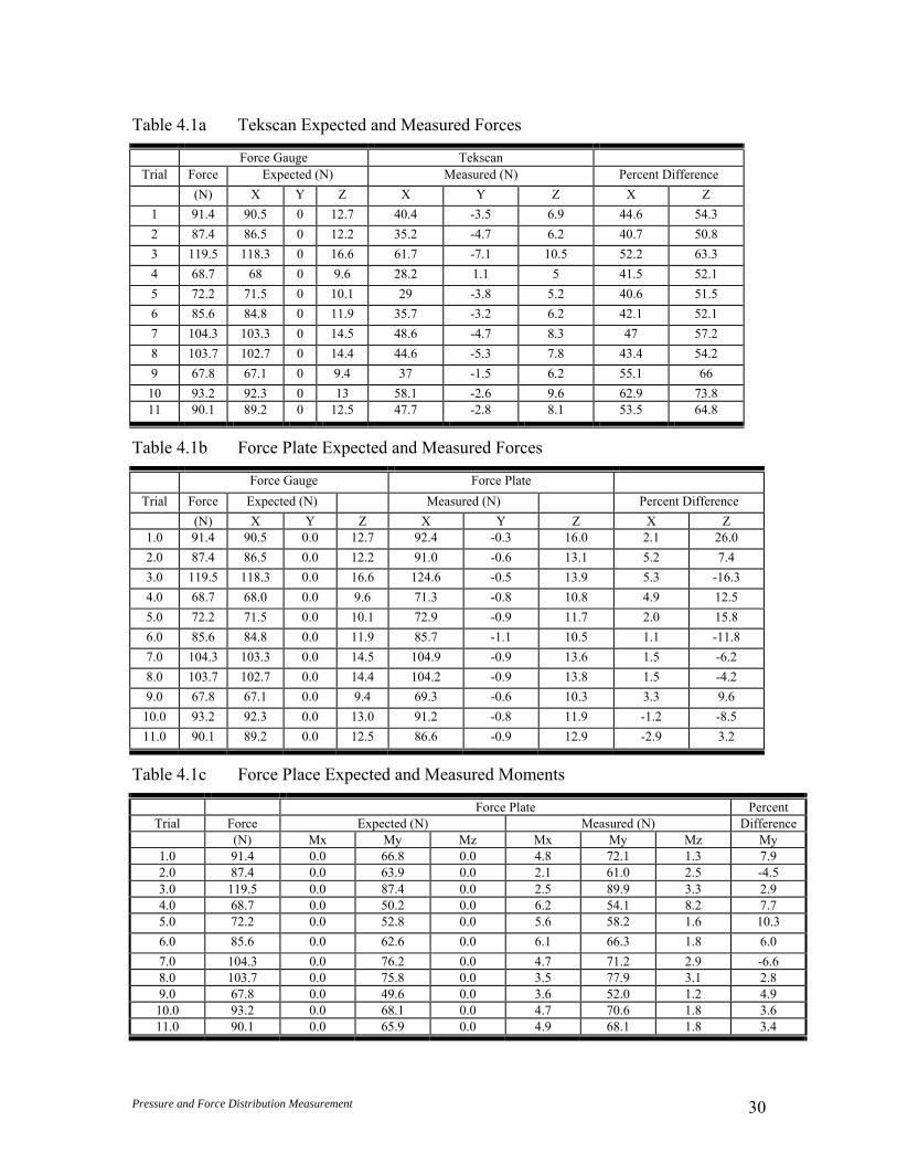
Pressure and Force Distribution Measurement 30
Table 4.1a Tekscan Expected and Measured Forces
Force Gauge Tekscan Trial Force Expected (N) Measured (N) Percent Difference
(N) X Y Z X Y Z X Z 1 91.4 90.5 0 12.7 40.4 -3.5 6.9 44.6 54.3 2 87.4 86.5 0 12.2 35.2 -4.7 6.2 40.7 50.8 3 119.5 118.3 0 16.6 61.7 -7.1 10.5 52.2 63.3 4 68.7 68 0 9.6 28.2 1.1 5 41.5 52.1 5 72.2 71.5 0 10.1 29 -3.8 5.2 40.6 51.5 6 85.6 84.8 0 11.9 35.7 -3.2 6.2 42.1 52.1 7 104.3 103.3 0 14.5 48.6 -4.7 8.3 47 57.2 8 103.7 102.7 0 14.4 44.6 -5.3 7.8 43.4 54.2 9 67.8 67.1 0 9.4 37 -1.5 6.2 55.1 66 10 93.2 92.3 0 13 58.1 -2.6 9.6 62.9 73.8 11 90.1 89.2 0 12.5 47.7 -2.8 8.1 53.5 64.8
Table 4.1b Force Plate Expected and Measured Forces
Force Gauge Force Plate Trial Force Expected (N) Measured (N) Percent Difference
(N) X Y Z X Y Z X Z 1.0 91.4 90.5 0.0 12.7 92.4 -0.3 16.0 2.1 26.0 2.0 87.4 86.5 0.0 12.2 91.0 -0.6 13.1 5.2 7.4 3.0 119.5 118.3 0.0 16.6 124.6 -0.5 13.9 5.3 -16.3 4.0 68.7 68.0 0.0 9.6 71.3 -0.8 10.8 4.9 12.5 5.0 72.2 71.5 0.0 10.1 72.9 -0.9 11.7 2.0 15.8 6.0 85.6 84.8 0.0 11.9 85.7 -1.1 10.5 1.1 -11.8 7.0 104.3 103.3 0.0 14.5 104.9 -0.9 13.6 1.5 -6.2 8.0 103.7 102.7 0.0 14.4 104.2 -0.9 13.8 1.5 -4.2 9.0 67.8 67.1 0.0 9.4 69.3 -0.6 10.3 3.3 9.6
10.0 93.2 92.3 0.0 13.0 91.2 -0.8 11.9 -1.2 -8.5 11.0 90.1 89.2 0.0 12.5 86.6 -0.9 12.9 -2.9 3.2
Table 4.1c Force Place Expected and Measured Moments
Force Plate Percent Trial Force Expected (N) Measured (N) Difference
(N) Mx My Mz Mx My Mz My 1.0 91.4 0.0 66.8 0.0 4.8 72.1 1.3 7.9 2.0 87.4 0.0 63.9 0.0 2.1 61.0 2.5 -4.5 3.0 119.5 0.0 87.4 0.0 2.5 89.9 3.3 2.9 4.0 68.7 0.0 50.2 0.0 6.2 54.1 8.2 7.7 5.0 72.2 0.0 52.8 0.0 5.6 58.2 1.6 10.3 6.0 85.6 0.0 62.6 0.0 6.1 66.3 1.8 6.0 7.0 104.3 0.0 76.2 0.0 4.7 71.2 2.9 -6.6 8.0 103.7 0.0 75.8 0.0 3.5 77.9 3.1 2.8 9.0 67.8 0.0 49.6 0.0 3.6 52.0 1.2 4.9 10.0 93.2 0.0 68.1 0.0 4.7 70.6 1.8 3.6 11.0 90.1 0.0 65.9 0.0 4.9 68.1 1.8 3.4
Pressure and Force Distribution Measurement 31
4.2 In-Situ Calibration Initial data collection of TekscanTM pressure sensors mounted on the SLT produced results that varied greatly from the applied force values. To improve the calibration, a modified procedure was developed that incorporated compensation for sensor curvature. The manufacturer stated that the effective sensel area was 161mm2 when the sensor was used on a flat surface (TekscanTM, 2000). However, it was hypothesized that curvature effects would introduce a scale factor to the relationship between sensor output and applied force. As such, this factor could be treated as a change in effective area of the sensor. By treating the sensor area as a variable, the effective sensel area for each sensor in its curved position could be determined through optimization. As the exact coefficient of friction was also unknown, these two inputs were optimized to minimize the difference between the predicted loads from the TekscanTM system and the expected loading from the external force gauge.
4.2.1 Calibration Procedure The initial calibration procedure was the same for that of the initial calibration of the SLT (Appendix D). The sensors on the hip areas were loaded independently and the applied force was distributed through the 50.8mm (2”) wide webbing belt over four blocks of rigid Styrofoam with 10mm thick closed cell foam padding on each. The belt position in the vertical direction was varied to minimize the effects, if any, of different belt shapes in the z-direction. The sensors on the outer edges of both the abdomen and lumbar area were loaded in pairs to ensure symmetrical load application. The sensors were each loaded with one of the blocks of foam with padding underneath the 50.8mm (2”) wide webbing belt. The centre sensors on the abdomen and lumbar sections were loaded using a different procedure as their geometry made it impossible to use the same calibration procedure (Appendix D). The SLT was tilted to an angle from the horizontal between 10° and 13° and a mass, acting as an applied force, was placed on the SLT solely on the sensor being calibrated. This experimental design allowed for the sensors on the lumbar and abdominal areas to be isolated for calibration. The sensor measurements were taken and the results compared with the resultant forces of the applied mass. To test repeatability of sensel measures, nine trials of data were collected for each sensor. These data sets of applied force ranging from 36N to 154N were collected in random order and over three days. Initial testing indicated that the sensor values measured for applied forces of less than 48N were below the capability of the sensors. Therefore, the applied forces used for calibration were always above this value. These trials were input into the spreadsheets for each sensor where the values for the effective sensel area and the friction coefficient were input as variables. Any trials that had greater than 10% of the
Pressure and Force Distribution Measurement 32
total applied force in the y-direction, before optimization, were discarded as this indicated that the testing apparatus was not symmetrical in the loading of the applied force. 4.2.2 Optimization Method The sum of the squared errors between the TekscanTM forces and applied forces were calculated and minimized using the effective sensel area and coefficient of friction variables. This is illustrated in Figure 4.3. The initial calibration procedure was applied to the raw TekscanTM data and the calibrated sensel data were input to the waist belt model. The sensel forces were calculated, summed, and compared to the applied forces. The root mean square error (RMS) for each sensor was calculated as a measure of precision. For this calculation, the sum of squared errors for each sensor was divided by the number of trials. If this value was not a minimum, the coefficient of friction and the effective area values were adjusted and the waist belt model calculations were performed again.
nSSERMS =
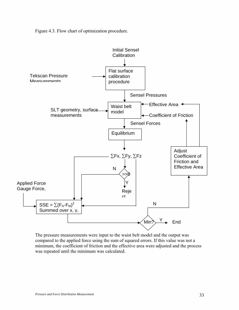
Pressure and Force Distribution Measurement 33
Figure 4.3. Flow chart of optimization procedure.
The pressure measurements were input to the waist belt model and the output was compared to the applied force using the sum of squared errors. If this value was not a minimum, the coefficient of friction and the effective area were adjusted and the process was repeated until the minimum was calculated.
Y
Initial Sensel Calibration
Tekscan Pressure Measurements
SLT geometry, surface measurements
Flat surface calibration procedure
Waist belt model
Equilibrium
Effective Area Coefficient of Friction
Sensel Pressures
Sensel Forces
∑Fx, ∑Fy, ∑Fz
SSE = ∑(FA-FM)2
Summed over x, y,
Applied Force Gauge Force,
Min?
Adjust Coefficient of Friction and Effective Area
End Y
N
Reject
>>0 N

Pressure and Force Distribution Measurement 34
4.2.3 Calibration Results The root mean square error values in Newtons are seen in Table 4.2. Every sensor had an RMS error of less than 8 Newtons, indicating good precision. Sensors 01 and 05 were located on flat surfaces and were not considered to have an effect of curvature.
Table 4.2 RMS Values (N)
Sensor SSE RMS 01 ----- ----- 03 289.39 7.61 05 ----- ----- 06 122.33 6.39 07 227.29 7.54 09 66.47 4.71 10 122.33 6.39 12 103.49 5.87 13 289.39 7.61 15 245.71 6.40
Table 4.3 shows the effective sensel area for each sensor after optimization. Excellent correlation occurred between sensors located in opposite positions, sensors 01-12 and 01-09 had a difference of 5.4%, sensors 01-07 and 01-15 had a difference of 2%. While sensors 01-12 and 01-15, located on the same side, had a difference of 27%, and sensors 01-09 and 01-07, also located on the same side, had a difference 24%.
Table 4.3 Effective Sensel Area
Sensor Effective Area (mm^2)
01 ----- 03 205.3 05 ----- 06 207.5 07 167.8 09 221.7 10 207.5 12 234.7 13 205.3 15 171.2

Pressure and Force Distribution Measurement 35
Figure 4.4 Location of Sensors on the Hip Sections
The results indicated a difference in curvature affected the effective sensel area as the radius of curvature changed with position in the z-direction. The optimized values for the effective sensel area of each sensor were considered to be constant for each sensor, providing the locations of the sensors were not changed. As expected, the optimized coefficients of friction were below the previously determined experimental coefficient of static friction (μ=0.38), shown in Table 4.4. Generally, the sliding coefficient of friction is 25% lower than the static coefficient (Hibbeler, 1995). The standard error between all of the measured values was small enough to consider the average of the values to be a constant to two decimal places, μ=0.26. This assumption resulted in a change in RMS errors of less than 0.05N.
Sensor 01-09 Sensor 01-12
Sensor 01-15Sensor 01-07
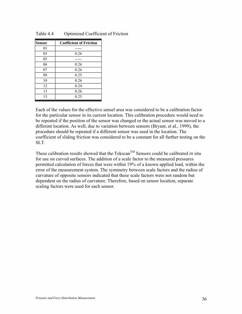
Pressure and Force Distribution Measurement 36
Table 4.4 Optimized Coefficient of Friction
Sensor Coefficient of Friction 01 ----- 03 0.26 05 ----- 06 0.26 07 0.26 09 0.25 10 0.26 12 0.24 13 0.26 15 0.25
Each of the values for the effective sensel area was considered to be a calibration factor for the particular sensor in its current location. This calibration procedure would need to be repeated if the position of the sensor was changed or the actual sensor was moved to a different location. As well, due to variation between sensors (Bryant, et al., 1999), the procedure should be repeated if a different sensor was used in the location. The coefficient of sliding friction was considered to be a constant for all further testing on the SLT. These calibration results showed that the TekscanTM Sensors could be calibrated in situ for use on curved surfaces. The addition of a scale factor to the measured pressures permitted calculation of forces that were within 19% of a known applied load, within the error of the measurement system. The symmetry between scale factors and the radius of curvature of opposite sensors indicated that these scale factors were not random but dependent on the radius of curvature. Therefore, based on sensor location, separate scaling factors were used for each sensor.
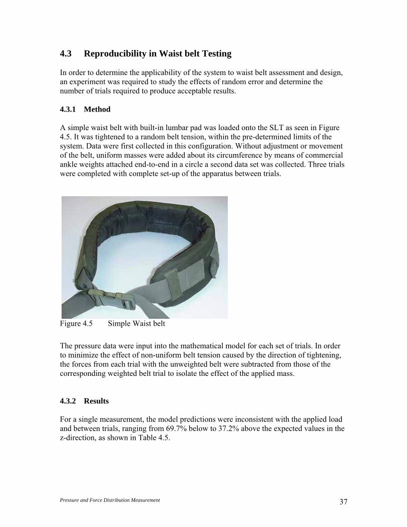
Pressure and Force Distribution Measurement 37
4.3 Reproducibility in Waist belt Testing In order to determine the applicability of the system to waist belt assessment and design, an experiment was required to study the effects of random error and determine the number of trials required to produce acceptable results.
4.3.1 Method A simple waist belt with built-in lumbar pad was loaded onto the SLT as seen in Figure 4.5. It was tightened to a random belt tension, within the pre-determined limits of the system. Data were first collected in this configuration. Without adjustment or movement of the belt, uniform masses were added about its circumference by means of commercial ankle weights attached end-to-end in a circle a second data set was collected. Three trials were completed with complete set-up of the apparatus between trials.
Figure 4.5 Simple Waist belt
The pressure data were input into the mathematical model for each set of trials. In order to minimize the effect of non-uniform belt tension caused by the direction of tightening, the forces from each trial with the unweighted belt were subtracted from those of the corresponding weighted belt trial to isolate the effect of the applied mass. 4.3.2 Results For a single measurement, the model predictions were inconsistent with the applied load and between trials, ranging from 69.7% below to 37.2% above the expected values in the z-direction, as shown in Table 4.5.

Pressure and Force Distribution Measurement 38
Table 4.5 Measured and Expected Values for Isolated Mass
Expected Measured Trial Fz (N) Fz (N) Percent Difference
1 44.6 32.5 -27.0 2 44.6 60.9 36.5 3 44.6 22.5 -49.6 4 44.6 59.2 32.8 5 44.6 13.5 -69.7 6 44.6 61.2 37.2 7 44.6 14.0 -68.6 8 44.6 32.9 -26.3 9 44.6 30.7 -31.2
Average 34.4 -18.4
This indicated the possibility of excessive random error in the system. Further trials were performed to determine the number of trials needed to reduce these random errors to obtain acceptable results. A plot of the standard errors of the means for the x, y, and z values of nine trials are seen in Figure 4.6.
Standard Error of the Mean
05
101520253035
0 2 4 6 8 10
Number of Trials
Stan
dard
Err
or (N
)
xyz
Figure 4.6 Standard Error of the Mean of summed forces in the x, y, and z directions over nine trials
A distinct break point was seen at three trials although the errors decreased minimally until the ninth trial. These results indicated that three trials were sufficient to reduce random error. In subsequent testing as many as ten trials and as few as three trials were used in each set-up, depending on the level of concern over precision.

Pressure and Force Distribution Measurement 39
5.0 Effect of Strap Tension Contact Force Distribution in Waist belts In previous studies of load carriage performance, TekscanTM sensors have been used in conjunction with strap force transducers (Stevenson, 1995). The values measured by the transducers were input into earlier biomechanical models as variables in the calculation of the forces in the system, however this has proven inconclusive. Since the system is statically indeterminate, the purpose of this experiment was to determine the correlation between the measured strap tension and resultant pressure measurements.
5.1 General Analysis Method In order to examine the relationship between tension and pressure, a simple equilibrium expression was first developed. The pressure data were divided into halves, medially and laterally, and the forces in the X and Y-directions were calculated for each half as shown in Figure 5.1. The tension was considered to be constant throughout the belt and was expected to correspond to the measured forces as in the theorized relationship of the strap force tension to the measured forces in Figures 5.2 and 5.3. This assumed that any frictional forces, if present, are in equilibrium along the length of the belt. As the measured tension differed slightly between trials, the resulting forces were normalized by expressing them as a factor of the applied tension, as read by the strap force sensor.
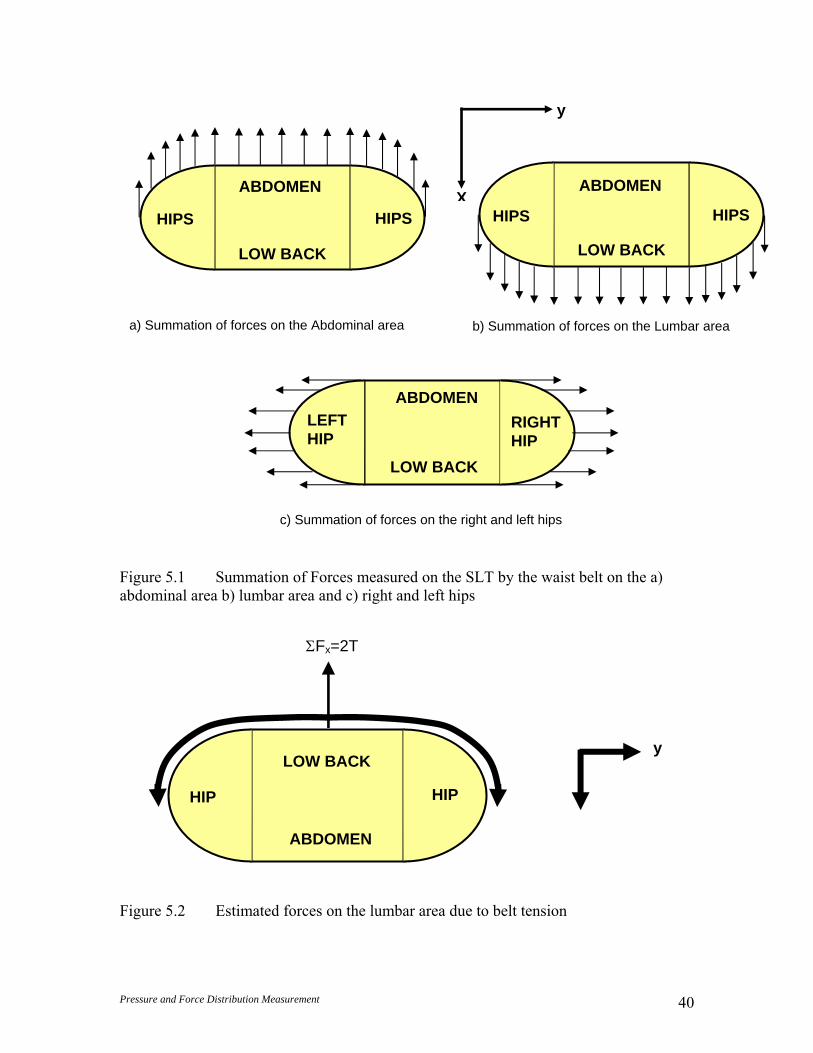
Pressure and Force Distribution Measurement 40
Figure 5.1 Summation of Forces measured on the SLT by the waist belt on the a) abdominal area b) lumbar area and c) right and left hips
Figure 5.2 Estimated forces on the lumbar area due to belt tension
X
y
ABDOMEN
LOW BACK
HIPSHIPS
ABDOMEN
LOW BACK
HIPS HIPS
ABDOMEN
LOW BACK
LEFT HIP
RIGHT HIP
a) Summation of forces on the Abdominal area b) Summation of forces on the Lumbar area
c) Summation of forces on the right and left hips
y
ABDOMEN
LOW BACK
HIP HIP
ΣFx=2T

Pressure and Force Distribution Measurement 41
Figure 5.3 Estimated forces on the hip due to belt tension
5.1.1 Method and Results A strap force transducer was mounted on the simple waist belt. The waist belt was then placed on the SLT and tightened to approximately 50N. The strap tension and pressure measurements were recorded. Ten trials were completed with resetting of the apparatus between each trial.
The results are shown in Table 5.1. The column labeled “front’ refers to the ratio of measured force to belt tension in the x-direction across the entire anterior half of the SLT. ‘Rear’ refers to the ratio of measured force to the belt tension in the x-direction across the entire posterior half of the SLT. The left and right hips referred to the ratio in the y-direction across the entire left and right sides of the SLT, respectively. In order to insure that the SLT was symmetrical in the anterior and posterior directions, three trials were completed with the waist belt on in the opposite orientation. The results were not significantly different than those in the first orientation and are shown in Table 5.1b.
T
T
∑ = TF y 2 HIP
y
x
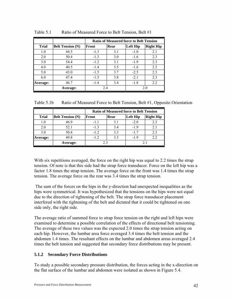
Pressure and Force Distribution Measurement 42
Table 5.1 Ratio of Measured Force to Belt Tension, Belt #1
Ratio of Measured force to Belt Tension Trial Belt Tension (N) Front Rear Left Hip Right Hip 1.0 44.5 -1.3 3.1 -1.0 2.1 2.0 50.4 -1.3 3.0 -1.6 2.3 3.0 54.4 -1.2 3.1 -1.9 2.3 4.0 40.5 -1.4 3.5 -1.6 2.2 5.0 43.0 -1.5 3.7 -2.5 2.3 6.0 47.4 -1.5 3.8 -2.1 2.3
Average: 46.7 -1.4 3.4 -1.8 2.2 Average: 2.4 2.0
Table 5.1b Ratio of Measured Force to Belt Tension, Belt #1, Opposite Orientation
Ratio of Measured force to Belt Tension Trial Belt Tension (N) Front Rear Left Hip Right Hip 1.0 46.9 -1.1 3.1 -2.0 2.3 2.0 52.1 -1.3 3.4 -1.9 2.1 3.0 50.4 -1.2 3.3 -1.7 2.3
Average: 49.8 -1.2 3.3 -1.9 2.2 Average: 2.3 2.1
With six repetitions averaged, the force on the right hip was equal to 2.2 times the strap tension. Of note is that this side had the strap force transducer. Force on the left hip was a factor 1.8 times the strap tension. The average force on the front was 1.4 times the strap tension. The average force on the rear was 3.4 times the strap tension. The sum of the forces on the hips in the y-direction had unexpected inequalities as the hips were symmetrical. It was hypothesized that the tensions on the hips were not equal due to the direction of tightening of the belt. The strap force transducer placement interfered with the tightening of the belt and dictated that it could be tightened on one side only, the right side. The average ratio of summed force to strap force tension on the right and left hips were examined to determine a possible correlation of the effects of directional belt tensioning. The average of these two values was the expected 2.0 times the strap tension acting on each hip. However, the lumbar area force averaged 3.4 times the belt tension and the abdomen 1.4 times. The resultant effects on the lumbar and abdomen areas averaged 2.4 times the belt tension and suggested that secondary force distributions may be present. 5.1.2 Secondary Force Distributions To study a possible secondary pressure distribution, the forces acting in the x-direction on the flat surface of the lumbar and abdomen were isolated as shown in Figure 5.4.
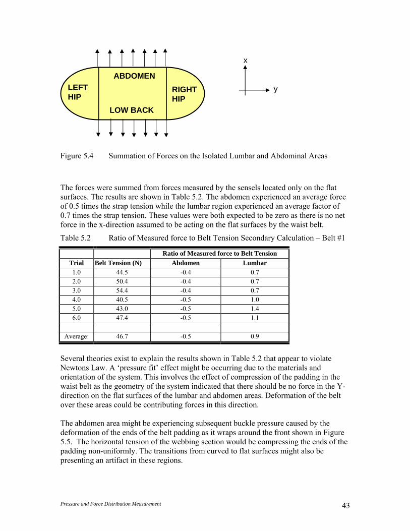
Pressure and Force Distribution Measurement 43
Figure 5.4 Summation of Forces on the Isolated Lumbar and Abdominal Areas
The forces were summed from forces measured by the sensels located only on the flat surfaces. The results are shown in Table 5.2. The abdomen experienced an average force of 0.5 times the strap tension while the lumbar region experienced an average factor of 0.7 times the strap tension. These values were both expected to be zero as there is no net force in the x-direction assumed to be acting on the flat surfaces by the waist belt.
Table 5.2 Ratio of Measured force to Belt Tension Secondary Calculation – Belt #1
Ratio of Measured force to Belt Tension Trial Belt Tension (N) Abdomen Lumbar 1.0 44.5 -0.4 0.7 2.0 50.4 -0.4 0.7 3.0 54.4 -0.4 0.7 4.0 40.5 -0.5 1.0 5.0 43.0 -0.5 1.4 6.0 47.4 -0.5 1.1
Average: 46.7 -0.5 0.9
Several theories exist to explain the results shown in Table 5.2 that appear to violate Newtons Law. A ‘pressure fit’ effect might be occurring due to the materials and orientation of the system. This involves the effect of compression of the padding in the waist belt as the geometry of the system indicated that there should be no force in the Y-direction on the flat surfaces of the lumbar and abdomen areas. Deformation of the belt over these areas could be contributing forces in this direction. The abdomen area might be experiencing subsequent buckle pressure caused by the deformation of the ends of the belt padding as it wraps around the front shown in Figure 5.5. The horizontal tension of the webbing section would be compressing the ends of the padding non-uniformly. The transitions from curved to flat surfaces might also be presenting an artifact in these regions.
ABDOMEN
LOW BACK
RIGHT HIP
LEFT HIP
y
x
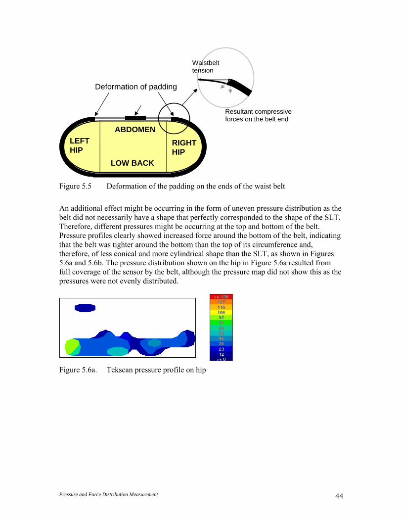
Pressure and Force Distribution Measurement 44
Figure 5.5 Deformation of the padding on the ends of the waist belt
An additional effect might be occurring in the form of uneven pressure distribution as the belt did not necessarily have a shape that perfectly corresponded to the shape of the SLT. Therefore, different pressures might be occurring at the top and bottom of the belt. Pressure profiles clearly showed increased force around the bottom of the belt, indicating that the belt was tighter around the bottom than the top of its circumference and, therefore, of less conical and more cylindrical shape than the SLT, as shown in Figures 5.6a and 5.6b. The pressure distribution shown on the hip in Figure 5.6a resulted from full coverage of the sensor by the belt, although the pressure map did not show this as the pressures were not evenly distributed.
Figure 5.6a. Tekscan pressure profile on hip
ABDOMEN
Deformation of padding
LOW BACK
RIGHT HIP
LEFT HIP
Waistbelt tension
Resultant compressive forces on the belt end
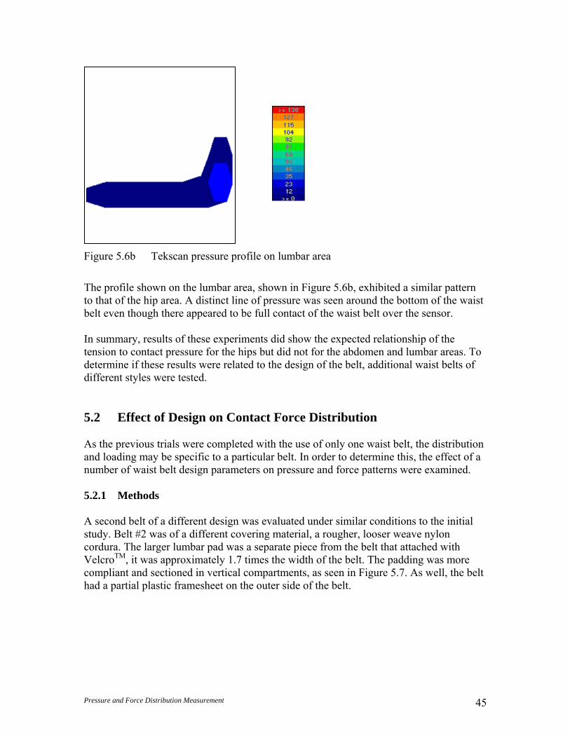
Pressure and Force Distribution Measurement 45
Figure 5.6b Tekscan pressure profile on lumbar area
The profile shown on the lumbar area, shown in Figure 5.6b, exhibited a similar pattern to that of the hip area. A distinct line of pressure was seen around the bottom of the waist belt even though there appeared to be full contact of the waist belt over the sensor. In summary, results of these experiments did show the expected relationship of the tension to contact pressure for the hips but did not for the abdomen and lumbar areas. To determine if these results were related to the design of the belt, additional waist belts of different styles were tested. 5.2 Effect of Design on Contact Force Distribution As the previous trials were completed with the use of only one waist belt, the distribution and loading may be specific to a particular belt. In order to determine this, the effect of a number of waist belt design parameters on pressure and force patterns were examined. 5.2.1 Methods A second belt of a different design was evaluated under similar conditions to the initial study. Belt #2 was of a different covering material, a rougher, looser weave nylon cordura. The larger lumbar pad was a separate piece from the belt that attached with VelcroTM, it was approximately 1.7 times the width of the belt. The padding was more compliant and sectioned in vertical compartments, as seen in Figure 5.7. As well, the belt had a partial plastic framesheet on the outer side of the belt.
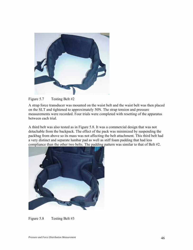
Pressure and Force Distribution Measurement 46
Figure 5.7 Testing Belt #2
A strap force transducer was mounted on the waist belt and the waist belt was then placed on the SLT and tightened to approximately 50N. The strap tension and pressure measurements were recorded. Four trials were completed with resetting of the apparatus between each trial. A third belt was also tested as in Figure 5.8. It was a commercial design that was not detachable from the backpack. The effect of the pack was minimized by suspending the packbag from above so its mass was not affecting the belt attachment. This third belt had a very distinct and separate lumbar pad as well as stiff foam padding that had less compliance than the other two belts. The padding pattern was similar to that of Belt #2.
Figure 5.8 Testing Belt #3
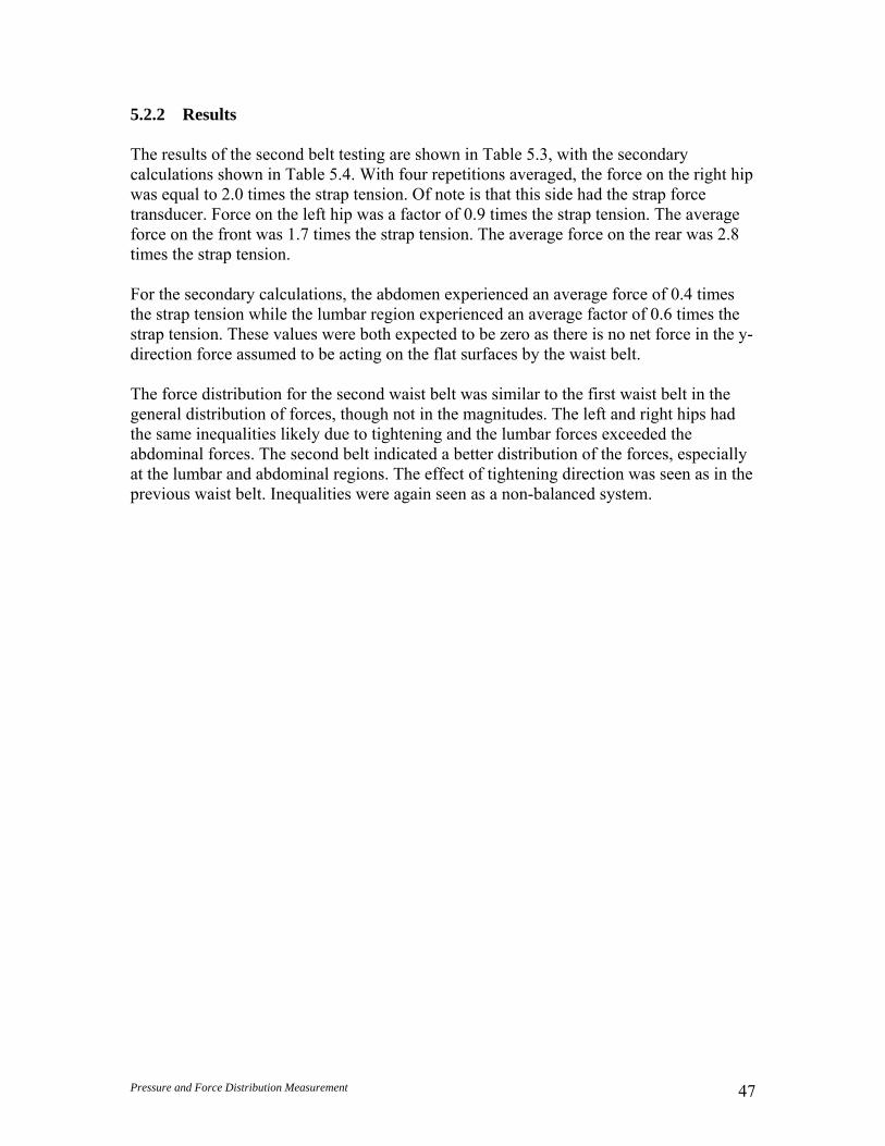
Pressure and Force Distribution Measurement 47
5.2.2 Results The results of the second belt testing are shown in Table 5.3, with the secondary calculations shown in Table 5.4. With four repetitions averaged, the force on the right hip was equal to 2.0 times the strap tension. Of note is that this side had the strap force transducer. Force on the left hip was a factor of 0.9 times the strap tension. The average force on the front was 1.7 times the strap tension. The average force on the rear was 2.8 times the strap tension. For the secondary calculations, the abdomen experienced an average force of 0.4 times the strap tension while the lumbar region experienced an average factor of 0.6 times the strap tension. These values were both expected to be zero as there is no net force in the y-direction force assumed to be acting on the flat surfaces by the waist belt. The force distribution for the second waist belt was similar to the first waist belt in the general distribution of forces, though not in the magnitudes. The left and right hips had the same inequalities likely due to tightening and the lumbar forces exceeded the abdominal forces. The second belt indicated a better distribution of the forces, especially at the lumbar and abdominal regions. The effect of tightening direction was seen as in the previous waist belt. Inequalities were again seen as a non-balanced system.
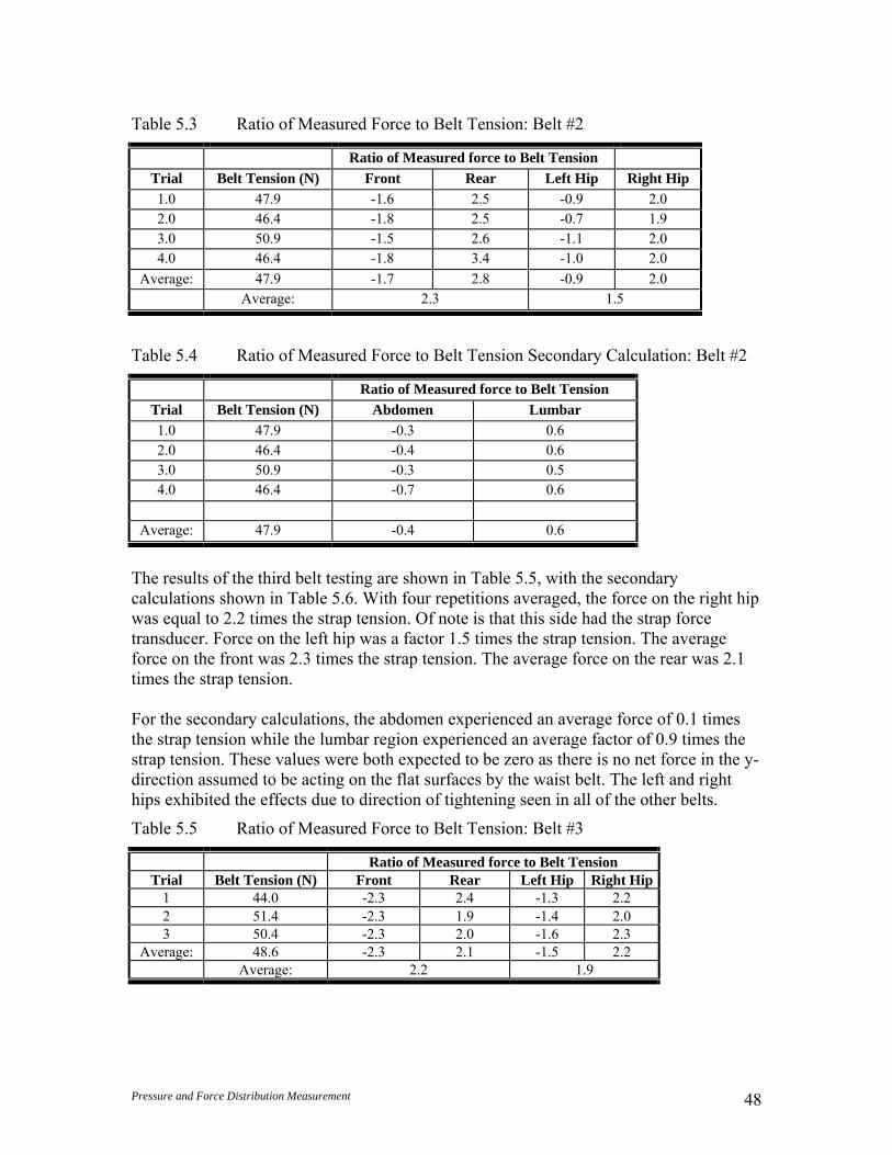
Pressure and Force Distribution Measurement 48
Table 5.3 Ratio of Measured Force to Belt Tension: Belt #2
Ratio of Measured force to Belt Tension Trial Belt Tension (N) Front Rear Left Hip Right Hip 1.0 47.9 -1.6 2.5 -0.9 2.0 2.0 46.4 -1.8 2.5 -0.7 1.9 3.0 50.9 -1.5 2.6 -1.1 2.0 4.0 46.4 -1.8 3.4 -1.0 2.0
Average: 47.9 -1.7 2.8 -0.9 2.0 Average: 2.3 1.5
Table 5.4 Ratio of Measured Force to Belt Tension Secondary Calculation: Belt #2
Ratio of Measured force to Belt Tension Trial Belt Tension (N) Abdomen Lumbar 1.0 47.9 -0.3 0.6 2.0 46.4 -0.4 0.6 3.0 50.9 -0.3 0.5 4.0 46.4 -0.7 0.6
Average: 47.9 -0.4 0.6
The results of the third belt testing are shown in Table 5.5, with the secondary calculations shown in Table 5.6. With four repetitions averaged, the force on the right hip was equal to 2.2 times the strap tension. Of note is that this side had the strap force transducer. Force on the left hip was a factor 1.5 times the strap tension. The average force on the front was 2.3 times the strap tension. The average force on the rear was 2.1 times the strap tension. For the secondary calculations, the abdomen experienced an average force of 0.1 times the strap tension while the lumbar region experienced an average factor of 0.9 times the strap tension. These values were both expected to be zero as there is no net force in the y-direction assumed to be acting on the flat surfaces by the waist belt. The left and right hips exhibited the effects due to direction of tightening seen in all of the other belts.
Table 5.5 Ratio of Measured Force to Belt Tension: Belt #3
Ratio of Measured force to Belt Tension Trial Belt Tension (N) Front Rear Left Hip Right Hip
1 44.0 -2.3 2.4 -1.3 2.2 2 51.4 -2.3 1.9 -1.4 2.0 3 50.4 -2.3 2.0 -1.6 2.3
Average: 48.6 -2.3 2.1 -1.5 2.2 Average: 2.2 1.9
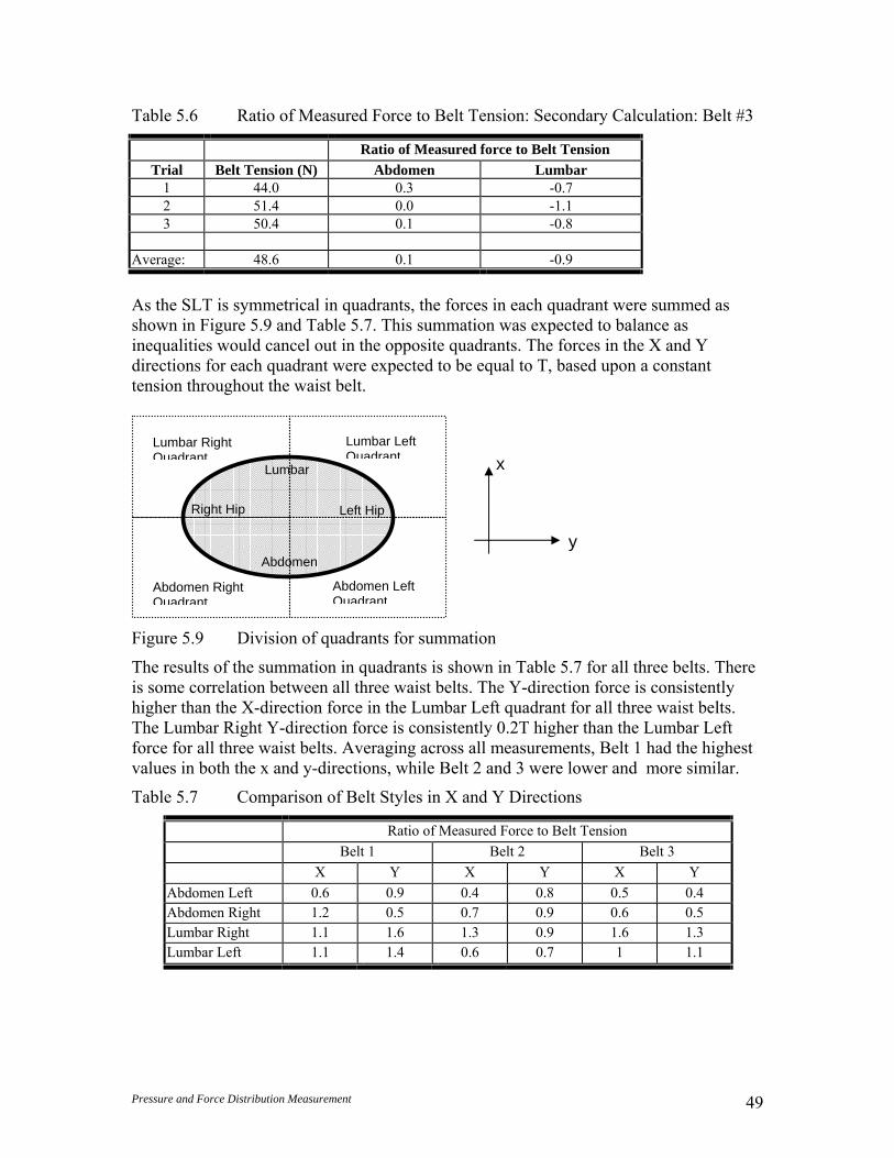
Pressure and Force Distribution Measurement 49
Table 5.6 Ratio of Measured Force to Belt Tension: Secondary Calculation: Belt #3
Ratio of Measured force to Belt Tension Trial Belt Tension (N) Abdomen Lumbar
1 44.0 0.3 -0.7 2 51.4 0.0 -1.1 3 50.4 0.1 -0.8
Average: 48.6 0.1 -0.9
As the SLT is symmetrical in quadrants, the forces in each quadrant were summed as shown in Figure 5.9 and Table 5.7. This summation was expected to balance as inequalities would cancel out in the opposite quadrants. The forces in the X and Y directions for each quadrant were expected to be equal to T, based upon a constant tension throughout the waist belt.
Figure 5.9 Division of quadrants for summation
The results of the summation in quadrants is shown in Table 5.7 for all three belts. There is some correlation between all three waist belts. The Y-direction force is consistently higher than the X-direction force in the Lumbar Left quadrant for all three waist belts. The Lumbar Right Y-direction force is consistently 0.2T higher than the Lumbar Left force for all three waist belts. Averaging across all measurements, Belt 1 had the highest values in both the x and y-directions, while Belt 2 and 3 were lower and more similar.
Table 5.7 Comparison of Belt Styles in X and Y Directions
Ratio of Measured Force to Belt Tension Belt 1 Belt 2 Belt 3 X Y X Y X Y
Abdomen Left 0.6 0.9 0.4 0.8 0.5 0.4 Abdomen Right 1.2 0.5 0.7 0.9 0.6 0.5 Lumbar Right 1.1 1.6 1.3 0.9 1.6 1.3 Lumbar Left 1.1 1.4 0.6 0.7 1 1.1
Lumbar Left Quadrant
Abdomen Left Quadrant
Abdomen Right Quadrant
Lumbar Right Quadrant
Lumbar
Abdomen
Left Hip Right Hip
y
x
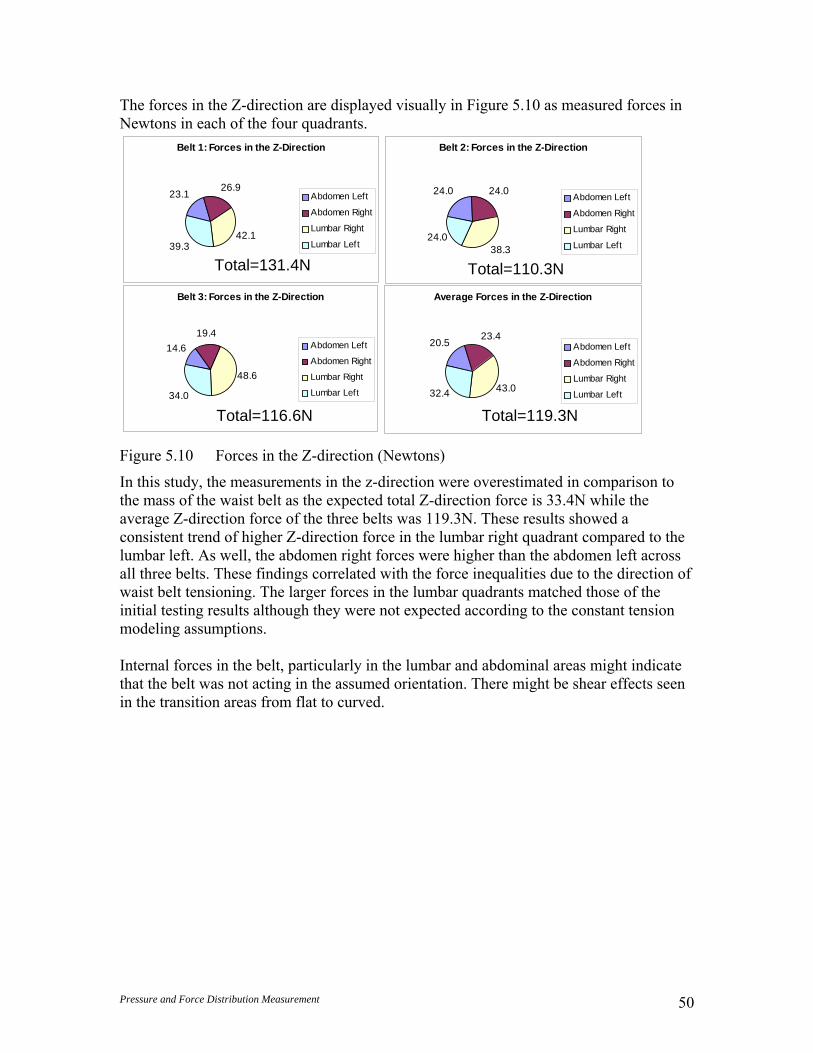
Pressure and Force Distribution Measurement 50
The forces in the Z-direction are displayed visually in Figure 5.10 as measured forces in Newtons in each of the four quadrants.
Figure 5.10 Forces in the Z-direction (Newtons)
In this study, the measurements in the z-direction were overestimated in comparison to the mass of the waist belt as the expected total Z-direction force is 33.4N while the average Z-direction force of the three belts was 119.3N. These results showed a consistent trend of higher Z-direction force in the lumbar right quadrant compared to the lumbar left. As well, the abdomen right forces were higher than the abdomen left across all three belts. These findings correlated with the force inequalities due to the direction of waist belt tensioning. The larger forces in the lumbar quadrants matched those of the initial testing results although they were not expected according to the constant tension modeling assumptions. Internal forces in the belt, particularly in the lumbar and abdominal areas might indicate that the belt was not acting in the assumed orientation. There might be shear effects seen in the transition areas from flat to curved.
Belt 2: Forces in the Z-Direction
24.0 24.0
38.324.0
Abdomen Left
Abdomen Right
Lumbar Right
Lumbar Left
Average Forces in the Z-Direction
20.5 23.4
43.032.4
Abdomen Left
Abdomen Right
Lumbar Right
Lumbar Left
Belt 1: Forces in the Z-Direction
23.126.9
42.139.3
Abdomen Left
Abdomen Right
Lumbar Right
Lumbar Left
Belt 3: Forces in the Z-Direction
14.619.4
48.6
34.0
Abdomen Left
Abdomen Right
Lumbar Right
Lumbar Left
Total=131.4N Total=110.3N
Total=116.6N Total=119.3N
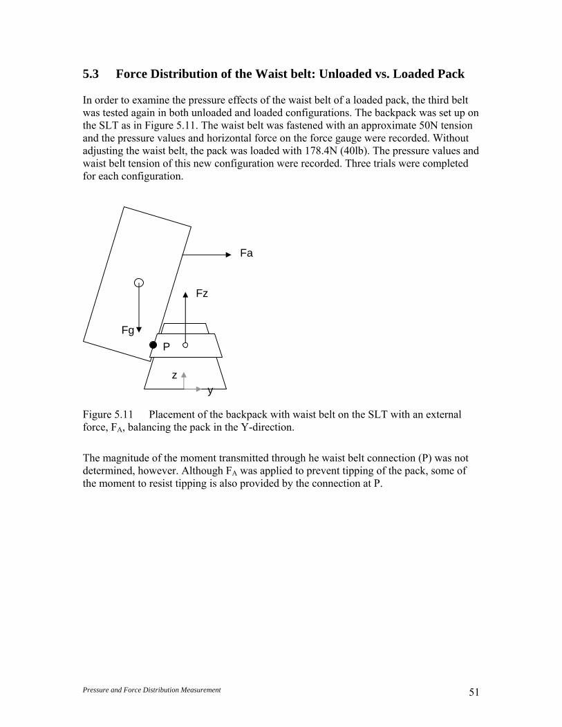
Pressure and Force Distribution Measurement 51
5.3 Force Distribution of the Waist belt: Unloaded vs. Loaded Pack In order to examine the pressure effects of the waist belt of a loaded pack, the third belt was tested again in both unloaded and loaded configurations. The backpack was set up on the SLT as in Figure 5.11. The waist belt was fastened with an approximate 50N tension and the pressure values and horizontal force on the force gauge were recorded. Without adjusting the waist belt, the pack was loaded with 178.4N (40lb). The pressure values and waist belt tension of this new configuration were recorded. Three trials were completed for each configuration.
Figure 5.11 Placement of the backpack with waist belt on the SLT with an external force, FA, balancing the pack in the Y-direction.
The magnitude of the moment transmitted through he waist belt connection (P) was not determined, however. Although FA was applied to prevent tipping of the pack, some of the moment to resist tipping is also provided by the connection at P.
Fa
z y
Fg
Fz
P
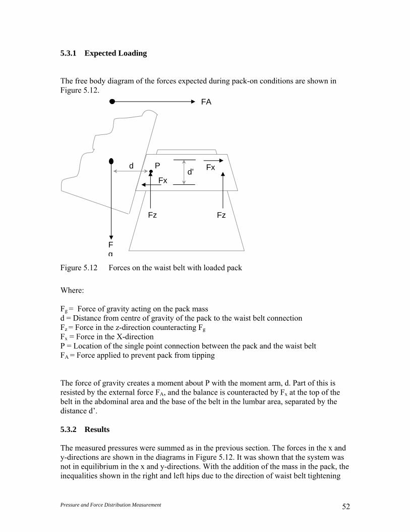
Pressure and Force Distribution Measurement 52
5.3.1 Expected Loading The free body diagram of the forces expected during pack-on conditions are shown in Figure 5.12.
Figure 5.12 Forces on the waist belt with loaded pack
Where: Fg = Force of gravity acting on the pack mass d = Distance from centre of gravity of the pack to the waist belt connection Fz = Force in the z-direction counteracting Fg Fx = Force in the X-direction P = Location of the single point connection between the pack and the waist belt FA = Force applied to prevent pack from tipping The force of gravity creates a moment about P with the moment arm, d. Part of this is resisted by the external force FA, and the balance is counteracted by Fx at the top of the belt in the abdominal area and the base of the belt in the lumbar area, separated by the distance d’. 5.3.2 Results The measured pressures were summed as in the previous section. The forces in the x and y-directions are shown in the diagrams in Figure 5.12. It was shown that the system was not in equilibrium in the x and y-directions. With the addition of the mass in the pack, the inequalities shown in the right and left hips due to the direction of waist belt tightening
d’
Fz
d
Fz
Fg
Fx Fx
P
FA
Pressure and Force Distribution Measurement 53
were reduced and nearly equilibrated. The forces on the lumbar and abdominal areas remained non-balanced. The tension in the waist belt consistently increased with the addition of mass, to a factor of 2 times the unloaded tension. The external forces were minimized and used only to prevent the pack from tipping backwards. These forces ranged from 13N to 34N. The higher forces were observed in the loaded condition. The direction of application was along the x-axis. Expected measurement errors were the same as those measured in the calibration procedure. The RMS errors ranged from 4.7N to 7.6N for the optimization.
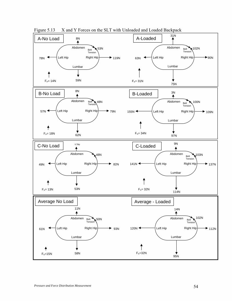
Pressure and Force Distribution Measurement 54
Figure 5.13 X and Y Forces on the SLT with Unloaded and Loaded Backpack
Belt Tension
A-No Load
53NAbdomen
Lumbar
Left Hip Right Hip 78N
8N
119N
59N
Belt Tension
FA= 14N
A-Loaded
102N Abdomen
Lumbar
Left Hip Right Hip 63N
31N
90N
75N
Belt Tension
FA= 31N
100NAbdomen
Lumbar
Left Hip Right Hip 155N
3N
109N
97N
Belt Tension
B-Loaded
FA= 34N
48N Abdomen
Lumbar
Left Hip Right Hip 57N
8N
79N
62N
B-No Load Belt Tension
FA= 18N
Lumbar
48N Abdomen
Left Hip Right Hip 49N
17N
82N
53N
C-No Load
FA= 13N
103N Abdomen
Lumbar
Left Hip Right Hip 141N
9N
137N
114N
C-Loaded
Belt Tension
FA= 32N
50N Abdomen
Lumbar
Left Hip Right Hip 61N
11N
93N
58N
Average No Load
Belt Tension
FA=15N
102N Abdomen
Lumbar
Left Hip Right Hip 120N
14N
112N
95N
Average - Loaded
Belt Tension
FA=32N

Pressure and Force Distribution Measurement 55
The z-values were also summed in Figure 5.14. The z-direction forces in the unloaded condition were not as expected as the mass of the empty pack was a constant known value of 33N (7.5lb). The averaged measured force was 105.4N. The measured z-values under loaded pack conditions showed that there was equilibrium as the z-force exerted directly by the pack was known. The expected z-direction force was 212N (47.5lb). The average measured force in the z-direction for the loaded pack was 205N. The average measured force in the z-direction when the pack was loaded was within 4% of the expected value (r2=0.964).

Pressure and Force Distribution Measurement 56
Figure 5.14 Vertical Z forces on the SLT with Unloaded and Loaded Backpack: Measured in Newtons
With load in the pack, the measured force in the z-direction was within 4% of the expected value. When the belt was isolated with no load in the pack, the forces in the z-direction had major discrepancies, with an average measurement error of 315%. This result indicated that the forces of friction and belt geometry were misrepresented by the mathematical model at low loads. As balance was not shown in the x and y directions during unloaded and loaded conditions, there appeared to be more complex frictional and tension factors than originally modeled. The tension in the belt may not be a constant as was assumed for calculations and previous biomechanical models. This created an indeterminate problem as these forces cannot be measured with one strap force
Trial A
24.2
45.7
3.3
40.7
LUMBAR
L HIP
ABDOMEN
R HIP
Trial A- Loaded
30.9
59.2
13.0
79.4LUMBARL HIPABDOMEN
R HIP
Trial B
25.6
33.7
3.242.9
LUMBARL HIPABDOMENR HIP
Trial B- Loaded
40.1
95.0
1.4
73.1
LUMBARL HIPABDOMENR HIP
Trial C
21.7
24.6
7.043.6 LUMBAR
L HIPABDOMENR HIP
Trial C- Loaded
47.0
83.5
3.8
88.8LUMBARL HIPABDOMENR HIP
Average - Loaded
39.3
79.2
6.1
80.4LUMBAR
L HIP
ABDOMEN
R HIP
Average - No Load
23.8
34.7
4.5
42.4LUMBAR
L HIPABDOMEN
R HIP
Total: Total:
Total: Total: 96.9N
Total: Total:
Total: 205NTotal:
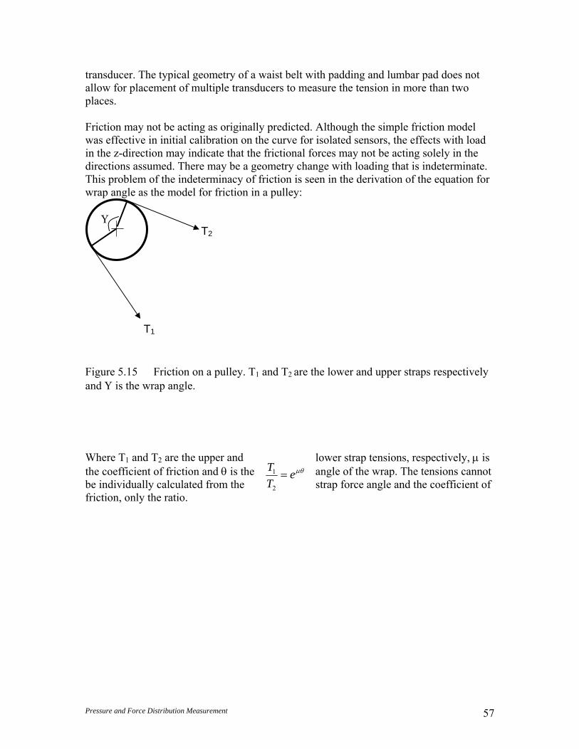
Pressure and Force Distribution Measurement 57
transducer. The typical geometry of a waist belt with padding and lumbar pad does not allow for placement of multiple transducers to measure the tension in more than two places. Friction may not be acting as originally predicted. Although the simple friction model was effective in initial calibration on the curve for isolated sensors, the effects with load in the z-direction may indicate that the frictional forces may not be acting solely in the directions assumed. There may be a geometry change with loading that is indeterminate. This problem of the indeterminacy of friction is seen in the derivation of the equation for wrap angle as the model for friction in a pulley:
Figure 5.15 Friction on a pulley. T1 and T2 are the lower and upper straps respectively and Υ is the wrap angle.
Where T1 and T2 are the upper and lower strap tensions, respectively, μ is the coefficient of friction and θ is the angle of the wrap. The tensions cannot be individually calculated from the strap force angle and the coefficient of friction, only the ratio.
T2
T1
Υ
μθeTT
=2
1
Pressure and Force Distribution Measurement 58
6.0 Discussion A model torso was developed that allowed the normal directions of each point of interest on the surface to be calculated. The measured force vectors were resolved into directional components to further understand the forces acting on the body by a backpack waist belt. A calibration procedure was developed for use of the TekscanTM sensors on a curved surface. The procedure also determined a coefficient of sliding friction for TekscanTM over BockliteTM. The discussion has been broken down into two sections. The first section deals with the potential of measurement errors which could have affected the results. The second section deals with interpretation of results from the biomechanical testing of waist belt designs. 6.1 Measurement Error Push-pull gauge. The display of the push-pull gauge was in increments of 0.23kg (0.5 lb) on an analog dial. Measurement reading error was present, accounting to an accuracy of +/- 0.23kg (0.5lb). This error would have contributed to discrepancies during calibration of the SLT set-up. Depending on the force applied, this attributed to range 2.2N of error. The z-axis angle of the applied force was measured with inclinometers. Error in the reading of the inclinometer could account for error in the resolution and comparison of the applied force vector. Sensitivity analysis was performed by changing the measured angle in the calculations by +/- three degrees. The result had an average standard error of 0.36. The applied force was assumed to be in the x-direction but discrepancies may have occurred. Force Plate. The centre of the force plate was not marked by the manufacturer but was measured from the edges after installation. Placement of the SLT apparatus was assumed to be at the origin of the force plate although experimental centre of pressure measurements taken showed the force plate to be off-centre by an average of 4.5mm (Appendix C). Noise and cross-talk present in the system was assumed to be negligible after subtraction of an averaged baseline value. Vibration of the floor in which the force plate was installed was considered a source of error but assumed to be negligible. Strap force transducer. The strap force transducers are not calibrated in situ and therefore may introduce some error when used in different applications. The transducer was sewn into the webbing of the belt by hand, while great care was taken to ensure the sensor was in line with the hoop force of the belt, some error can be expected. In some cases there was contact on the underside of the transducer by the excess webbing. This may have induced some bending of the transducer. TekscanTM. The TekscanTM sensors were initially calibrated on a flat surface but used on a curved surface. The sensors were not equilibrated as each sensel was being summed individually so the inequalities should cancel out. No forces were shown to be present

Pressure and Force Distribution Measurement 59
when the sensors were affixed to the curved surface and unloaded. When calibrated in situ, the sensors exhibited favorable results although the large experimental error of 28% (Helliwell, 1992) could be accounting for a great deal of the unbalanced measured forces. Wear of the sensors in this study was a concern as they were used over 12 months although no apparent degradation was seen in the data. As well, the pressures applied in this study were in the lower range of the sensor capabilities and therefore may have been less accurate than higher forces. The inability of the sensors to measure shear forces limited their usefulness. Limitations of the mathematical model. The locations of the sensels were measured on the SLT. There was error involved with the exact location as several assumptions were made. The active sensel areas were assumed to be of the identical size as well as the sensor being placed on the SLT in a symmetrical arrangement. The sensels in each quadrant corresponded to those in opposite locations. Each normal vector calculation was dependent upon the measured sensel location. Surface irregularities on the model may have caused slight variations on the actual location and angle of the sensel. The sensors did not provide complete coverage due to the shape of the sensor. The uncovered area was the same in each quadrant so it was assumed to provide consistent error. These gaps would result in a slight under-measurement (2%) of the Tekscan TM forces compared to the applied force. The RMS errors calculated in the calibration optimization procedure showed the accuracy expected from the model. The RMS values were below 8N. In summary, the most significant source of error in the equipment is the random measurement error of the TekscanTM system. With repeated testing, the effects of random error are reduced with a minimum of three trials. In relation to the errors observed with the unbalanced measured forces during waist belt testing, the equipment errors were less significant, as the sensors were calibrated in situ with an accuracy of >8N RMS. The unbalanced effects, due to unknown frictional forces were more significant than those inherent in the equipment. 6.2 Waist belt Design Effects The three waist belts tested varied significantly in design, as did the force distributions on the lower torso. The padding pattern of the first belt was the simplest with the division of padding into two sections along the transverse plane. The covering material was stiff and wrinkles were present in it. The second and third belts were more similar in their padding pattern of multiple longitudinal sections of padding. The covering materials were less stiff and there were fewer wrinkles than in the first belt. The second belt appeared to have slightly more compliant padding than the third. The lumbar area of the first belt was the same as the rest of the padding with no distinct area. The second belt had a large lumbar pad, approximately 1.3 times the width of the waist belt. The lumbar pad had square corners and was not contoured. The third lumbar pad was highly rounded and approximately 1.7 times the width of the waist belt.
Pressure and Force Distribution Measurement 60
The results of the force distribution measurement for the first belt indicated a correlation to the hoop stress as modeled on the hips, but the forces on the lumbar and abdominal areas were not explained by this theory. The large load on the lumbar area indicated that there were forces acting on the torso that were not accounted for by the hoop stresses. Distinct differences between the top and bottom of the waist belt were shown on the pressure maps. The belt did not perfectly match the shape of the SLT and was tighter around the bottom than the top as it was less conical. The lack of contours and sections in the padding of the first belt was expected to result in symmetrical coverage of the torso and a subsequent even pressure distribution; this was not the case. The second and third belts were expected to have more similar distributions compared to that of the first belt due to the similarity in padding style. There was no consistency between the belts although there was less of a distinct line of pressure around the bottom of the belt. The vertical sections of foam may have allowed for more compression of the padding and distribution of the pressure internally in the foam. The space in between the vertical padding sections would have allowed for spreading of the foam more than in the first belt that would not have allowed spreading in the lateral direction. The three belt designs were of different lengths which meant that the padding did not always end at the same location on the abdomen. The ends of the waist belt appeared be compressed by the angle of the webbing strap dependent on their location. The shorter the waist belt, the further the ends of the padding would be from the flat abdominal section and therefore the webbing attachment would be at an angle, instead of straight across the abdomen. This created subsequent compression of the ends of the belt. The length of the belt also determined the amount of contact of the buckle on the abdomen. The higher pressure points on the abdomen were due to the buckle when the waist belt length was shorter. One visible pattern in the force distribution data for each waist belt was the consistency of higher forces on the right hand side of the torso. The left abdominal side was consistently lower than the right while the left lumbar was lower or equal to the right side. The consistency of these results suggested that the direction of belt tightening had a distinct effect on the force distribution. The strap force transducer was located on the left hand side in a constrained position that did not facilitate the tightening of the belt in both directions. This inequality in the system rendered the theory of constant belt tension oversimplified. Large discrepancies of measured forces in the Z-direction in the unloaded condition, regardless of belt design, indicated large measurement errors. The TekscanTM sensors for this condition were measuring in the lower range of their capabilities. Alternatively, these discrepancies may represent frictional forces that were not accounted for. The calibration of the sensors in the curved position accounted for friction with the calculation of a constant coefficient of sliding friction when a force was applied. The measurement accuracy determined during calibration of the sensors was >8N RMS for the system. The unbalanced forces observed in subsequent waist belt testing indicated frictional forces caused by the waist belt that were not accounted for in the analysis of friction during calibration. The addition of forces in the circumferential direction by the waist belt
Pressure and Force Distribution Measurement 61
changed the frictional distributions. This distribution was not consistent between the belts, suggesting a design dependency for the friction distribution. This distribution and the relationship to strap force tension was not determined. The discrepancies of measured to applied forces and the degree to which they were unbalanced during waist belt testing indicated that unknown frictional components were a significant source of error. The addition of mass in the pack increased the belt tension by a factor of two consistently over the three trials. The force in the z-direction was not consistent with the unloaded belt but became consistent with the addition of mass. This indicated that the significance of the frictional forces acting on the body in the z-direction as a result of the circumferential pressures was reduced relative to the force in the z-direction. Therefore, it appears that the higher the mass and tension in the belt, the lower the effect of internal shear forces of the padding.

Pressure and Force Distribution Measurement 62
7.0 Conclusions and Future Work
1. A strategy was developed to determine waist belt compressive force distribution within an RMS error of <10N. A calibration procedure using an effective sensel area and a longitudinal frictional coefficient has been demonstrated. This is limited in application to vertical loading and was more successful in cases where the loads exceeded 50N.
2. Within the limitations of TekscanTM technology, it was possible to calibrate the sensors on a curved surface. However, the need for a minimum of three repetitions to reduce random error has been demonstrated. This calibration procedure has also demonstrated the need to calibrate all sensors, in situ, that are used in curved positions, or disregard the magnitudes of the measured forces.
3. It was possible to derive a coefficient of friction for the isolated waist belt model and to determine how factors such as the direction of belt tightening affected magnitude of the measured normal forces on the torso. The effects of tightening direction were shown to be significant in no-load tests of waist belts. The measured forces on the hips were significantly lower on the side that the strap force transducer was on and these effects are reduced with an increase in load. The apparent effects due to the tightening direction of the waist belt were consistent and predictable but their relationship to the forces acting on a more compliant surfaces, such as the human body cannot be extrapolated from this observation.
4. Previous models involving a waist belt have oversimplified the role of friction with the assumption of a constant belt tension. The complexity of the measured forces in the waist belt indicated that a direct relationship between strap force tension, measured in one location, and the forces acting on the body, was not possible.
5. The application of the frictional distributions appear to depend on the materials used in the construction of the belt. In this preliminary study, the padding orientation and conical shape of the waist belt appeared to determine the severity of localized compressive forces at the base of the belt. A less conical shape created lines of pressure about the bottom of the waist belt as the effects of the belt tension were concentrated in this area due to the geometry of the SLT.
6. At this time, a model for an individual waist belt is limited by an inability to predict frictional force distributions. TekscanTM instrumentation is also limited in this regard since it cannot directly evaluate the effect of shear forces on the torso.
7.1 Future Work
1. The directions of frictional forces need to be more closely examined as the impending pack motion may not be downwards as originally considered, depending on the mass of the pack and the tension in the belt. If the effective tension were higher than the effective mass on the belt, the pack would have a tendency to move upwards rather than downwards with the force of gravity. The apparent consistent effect of loading the pack and the increase in waist belt

Pressure and Force Distribution Measurement 63
tension should be explored further. Incremental loading would better provide an understanding of this relationship.
2. The unbalanced forces resulting from the compressive force of belt tensioning need to be examined further. The variation in the three waist belts in this study was too great to determine with any certainty how waist belt design relates to the force and frictional distribution in the waist belt. In order to determine the actions of the waist belt padding, the properties of the material, such as compliance of the foam, and the frictional properties of the covering materials should be determined. Identical belts with different materials or different designs with the same materials would facilitate this.
3. The effect of different lean angles of the torso on the distribution of forces should be examined. A forward lean angle of 8° would vertically orient the abdominal area of the model, more closely resembling the human body.
4. The padding surface of each belt may be experiencing relatively large shear forces due to circumferential pressure. These forces and their distribution are not easily modelled and would likely differ greatly when the belt interacts with the compliance of the human body. As a way of subjectively testing different materials on humans, correlations could be made through user trials and questionnaires to determine the relationship between user preferences and compliance of the padding. Belt designs could also be compared with the correlation to subjective testing.
5. The TekscanTM pressure measurement system was limited in its ability to measure shear. Future testing should be performed when shear measurement technology becomes more widely available.
6. The SLT has a number of potential uses such as: comparison of different materials used for waist belts, furthering of the waist belt models, and comparison of novel designs in waist belt technology. A simplified shoulder can be combined with the SLT to allow for the loading of a complete pack. TekscanTM sensors on the shoulder would allow for a more complete measurement of the forces of the upper pack and allow for complete resolution of the forces on the body. Strap force transducers on the shoulder straps would determine the relationship of the measured strap forces and the measured forces on the shoulder. The inconsistencies measured during tightening needs to be examined.
7. The design of different waist belt attachment points to the pack should be explored. Specifically, the ability to transmit a moment, and therefore this connection should be considered. While padding design did not show differences in the total distribution of force on the hips, the reduction of the line of pressure about the bottom was apparent in the more conical belts. The testing of a belt with an adjustable angle would help investigate this effect.
Pressure and Force Distribution Measurement 64
8.0 References AMTI (1989). Biomechanics Platform Set Instructions Manual. Boston, Mass. Bryant, J.T., Reid, S.A., Morin, E., Stevenson, J.M., Pelot, R.P. (1999). Development of a Calibration Jig for the F-Scan Pressure measurement system. PWGSC Contract # W7711-7-7405/SRV, (58 pages). Buis, A.W.P. and P. Convery (1997). Calibration problems encountered while monitoring stump/socket interface pressures with force sensing resistors: Techniques adopted to minimize inaccuracies, Prosthetics and Orthotics International 21:179-182. Epstein, Y., Rosenblum, J., Burstein, R., Sawka, M. (1988). External load can alter the energy cost of prolonged exercise, European Journal of Applied Physiology, 57:243-7. Goh, J-H, Thambyah A, Bose K. (1998). Effects of varying backpack loads on peak forces in the lumbosacral spine during walking, Clinical Biomechanics, 13(1):26-31. Goslin, B.R., Rorke, S. (1986). The perception of exertion during load carriage, Ergonomics, 29(5):677-86. Hibbeler, R.C. (1993). Statics and Mechanics of Materials, Macmillan Publishing Company, NY. Holewijn, M. (1990). Physiological strain due to load carrying. European Journal of Applied Physiology, 59:237-45. Holewijn, M., Lotens, W.A. (1992). The influence of backpack design on physical performance, Ergonomics, 35(1):149-157. Jenkins, M. (1992). The Weekend Pack Test, Backpacker, October, pg 53-57. Knapik, J., Harman, E., Reynolds, K. (1996). Load carriage using packs: A review of physiological, biomechanical and medical aspects, Applied Ergonomics, 27:207-16. Legg, S.J., Ramsey, T, Knowles, D.J. (1992). The metabolic cost of backpack and shoulder load carriage, Ergonomics, 35(9):1063-8. Legg, S.J., Mahanty, A. (1985). Comparison of five modes of carrying load close to the trunk, Ergonomics, 28(12):1653-60. Luo, Z.P., L.J. Berglund and K.N An (1998). Validation of F-Scan Pressure Sensor System: A Technical Note, Journal of Rehabilitation Research and Development, 35:186-191.

Pressure and Force Distribution Measurement 65
MacNeil, S.K. (1996). Validation and Development of a Mathematical Model of the Shoulder for load Carriage, Master’s Thesis, Queen’s University, Kingston, ON. MacNeil, S.K. Rigby, W.A. (1996). Determination of an appropriate substitute skin. Queen’s University, Kingston, On. (unpublished). McArdle, W.D., F. Katch, V. Katch (1996). Exercise Physiology: Energy, nutrition, and human performance, 4th, Ed., Williams & Wilkins, Maryland, USA. McPoil, T.G.P.P.A., et al (1995). A Comparison of Two in-shoe plantar pressure measurement systems, The Lower Extremity, 2:95-103. Morin, E, Reid, S.A, Bryant (1998). Research and Development of an Advanced Personal Load Carriage Measurement System, Phase IV: Section E Applicability of the F-Scan System for Humane Pressure Assessment, PWGSC Contract No. W7711-7-7420/A Report to the Defense and Civil Institute of Environmental Medicine. Pelot, R.P., Pinter, J., Rigby, A., Bryant, J.T., Stevenson, J.M. (1998) Section F: Phase II of Parametric Analysis of Advanced Personal Load Carriage Systems. PWGSC Contract # W7711-7-7420/A (45 pgs). Pelot, R.P., Rigby, A., Bryant, J.T., Stevenson, J.M. (1998) Section C: Phase II of a Biomechanical Model for Load Carriage Assessment. PWGSC Contract # W7711-7-7420/A (45 pgs). Potter, D.W. (1998) AMTI (Boston, Mass.) Force Platform: a technical note. School of Physical and Health Education. Queen’s University, Kingston, Ontario. (unpublished). Raffan, J. (1995). Load Carriage Backgrounder. Report for Ergonomics Research Group, Queen’s University. (unpublished). Reid, S.A., Bryant, J.T., Morin E., Stevenson, J.M., Doan, J.E. (1999). Clothe the Soldier: Phase IIID: Effect of Back Pack Shoulder Strap Lower Attachment Point on the Load Distribution to the Torso, PWGSC Contract # W7711-7-7412/001/SRV, (29 pages).
Reid, S.A., Bryant, J.T., Morin E., Stevenson, J.M., Doan, J.E. (1999). Clothe the Soldier: Phase IIID: Effect of Lateral Rods and No Rods in the Suspension System of the Pack, PWGSC Contract # W7711-7-7412/001/SRV, (39 pages). Reid, S.A., Doan, J, Bryant, J.T., Morin, E., Sui, D. (1997) Research and Development of an Advanced Personal Load Carriage System (Phases II and III) Section A: Futher Developemtn of Comprehensive Measurement Systems, PWGSC Contract #WW7711-5-7273/001/TOS, (42 pages).
Pressure and Force Distribution Measurement 66
Rigby, W.A. (1999). Development of a Biomechanical Model and Validation of Assessment Tools for Personal Load Carriage Systems, Master’s Thesis, Queen’s University, Kingston, ON. Rigby, W.A., McNeil, S.K. (1996) Determination of an Appropriate Substitute Skin, Queen’s University, Kingston, ON. (unpublished). Sagiv, M, et al. (1994). Left Ventricular responses during prolonged treadmill walking with heavy load carriage, Medicine and Science in Sports and Exercise, 26:285-8. Shimpo Instruments Inc. Website, www.shimpoinst.com Stevenson, J.M., Bryant, J.T., Reid, S.A. and Pelot, R.P. (1996). Research and Development of an Advanced Personal Load Carriage System: Section D, Validation of the Load Carriage Simulator, PWGSC Contract No. W7711-7-7225/01-XSE Report to the Defence and Civil Institute of Environmental Medicine. Stevenson, J.M., Bryant, J.T., Morin, E.L., Pelot, R.P., Reid, S.A., Doan, J.B. (1998). Research and Development of an Advanced Personal Load Carriage Measurement System, Phase IV, PWGSC Contract No. W7711-7-7420/A Report to the Defense and Civil Institute of Environmental Medicine. Stevenson, J.M., Bryant, J.T., dePencier, R.D., Pelot, R.P., and Reid, J.G. (1995). Research and Development of an Advanced Personal Load Carriage System (Phase I-D). DSS Contract # W7711-4-7225/01-XSE (350 pgs). Stewart, J, Ed.(1991). Calculus, Second Edition, Brooks/Cole Publishing Company, California. Sumiya, T, Suzuki, Y., Kashahara, T., Ogata, H. (1998). Sensing Stability and Dynamic Response of the F-Scan in-shoe sensing system: a technical note, J Rehabil Res Dev, 35(2):186-91. Tekscan F-Scan Pressure Assessment System, User’s Manual. Tekscan, Inc, Boston, MA, 2000. Wilke, H-J, Neef, P., Hinz, B., Seidel, H., Claes, L (1992). Intradiscal Pressure together with anthropometric data – a data set for the validation of models. Clinical Biomechanics, 16(1): S111-S126. Woodburn, J. and P.S. Helliwell (1996). Observations on the F-Scan in-shoe pressure measuring system, Clinical Biomechanics 11:301-304.

Pressure and Force Distribution Measurement A-1
Appendix A - Symmetrical Lower Torso Design
Anthropometric Data Listed below are the anthropometric data necessary to construct the SLT physical model. Dimensions from the 50th percentile male mannequin at the waist: Circumference, Cm = 0.84 m Width (Transverse plane) = 0.292m Depth (Midsagittal plane) = 0.229m Using the depth as the diameter for the ends: Cends = πd Cends = 0.719 m For the lumbar and abdomen: Cm – Cends = CLA CLA/2 = Width of lumbar section CLA = 0.121 m CL = CA = 0.0605 m The width with these dimensions does not quite correspond with the current torso model, so 0.00125m was added to the sides for a better match. Therefore, CL = CA = 0.06175 m The total circumference with these values is 0.8429 m. The desired waist to hip ratio is 0.85.
Determination of the radius and angulation at the hips:
mH
H
WH
HW
992.085.0
8429.085.0
85.0
=
=
=
=
mrr
sidernceCircumfere
1382.0)1235.0(2992.0
)(22
=+=
+=π
π
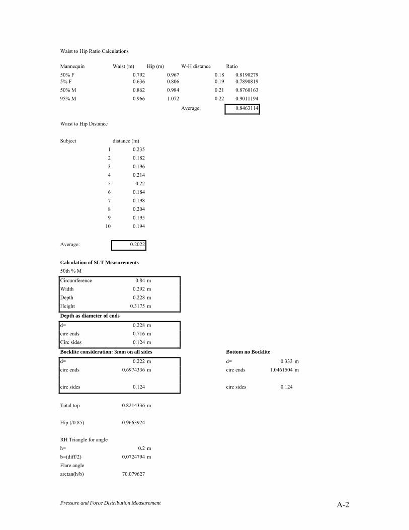
Pressure and Force Distribution Measurement A-2
Waist to Hip Ratio Calculations
Mannequin Waist (m) Hip (m) W-H distance Ratio 50% F 0.792 0.967 0.18 0.8190279 5% F 0.636 0.806 0.19 0.7890819 50% M 0.862 0.984 0.21 0.8760163 95% M 0.966 1.072 0.22 0.9011194
Average: 0.8463114
Waist to Hip Distance
Subject distance (m)
1 0.235 2 0.182 3 0.196 4 0.214 5 0.22 6 0.184 7 0.198 8 0.204 9 0.195
10 0.194
Average: 0.2022
Calculation of SLT Measurements 50th % M
Circumference 0.84 m Width 0.292 m Depth 0.228 m Height 0.3175 m
Depth as diameter of ends
d= 0.228 m circ ends 0.716 m Circ sides 0.124 m
Bocklite consideration: 3mm on all sides Bottom no Bocklite
d= 0.222 m d= 0.333 m circ ends 0.6974336 m circ ends 1.0461504 m
circ sides 0.124 circ sides 0.124
Total top 0.8214336 m
Hip (/0.85) 0.9663924
RH Triangle for angle h= 0.2 m b=(diff/2) 0.0724794 m Flare angle arctan(h/b) 70.079627
Pressure and Force Distribution Measurement B-1
Appendix B - Mathematical Model Spreadsheets Summary Sheet for Single Trial
Date: 10-May Load: cdn belt N Tension: N/A
Force Friction
Sensor Friction Eff Area X Y Z fx fy fz
3 0.257 4.87056 -0.0338 28.9847 4.0760 0.0012 -1.0475 7.4536 5 0.257 4.5413 0.0000 -16.1095 2.2640 0.0000 0.5819 4.1401 6 0.257 4.821583 10.7179 -62.8996 9.0741 -0.3871 2.2734 16.5934 7 0.257 5.959539 -50.7786 -10.4442 8.1912 1.8341 -0.3772 14.9788 9 0.257 4.5066 -72.7495 -13.8913 12.6065 2.6276 -0.7351 23.0529
10 0.257 4.821583 -7.0958 -63.0574 9.0253 0.2560 2.2785 16.5041 12 0.257 4.262788 78.1762 -49.3790 14.0966 -2.8236 1.7835 25.7777 13 0.257 4.87056 3.3321 8.3025 1.2590 -0.1203 -0.2999 2.3023
14 (01) 0.257 4.4604 0.0000 39.6413 5.5712 0.0000 -1.4318 10.1878 15 0.257 5.843816 62.7379 -4.7702 9.7143 -2.2660 0.1723 17.7640
Sum 24.3063 -143.6227 75.8783 -0.8782 3.1980 138.7548
Total 23.4281 -140.4246 214.6331
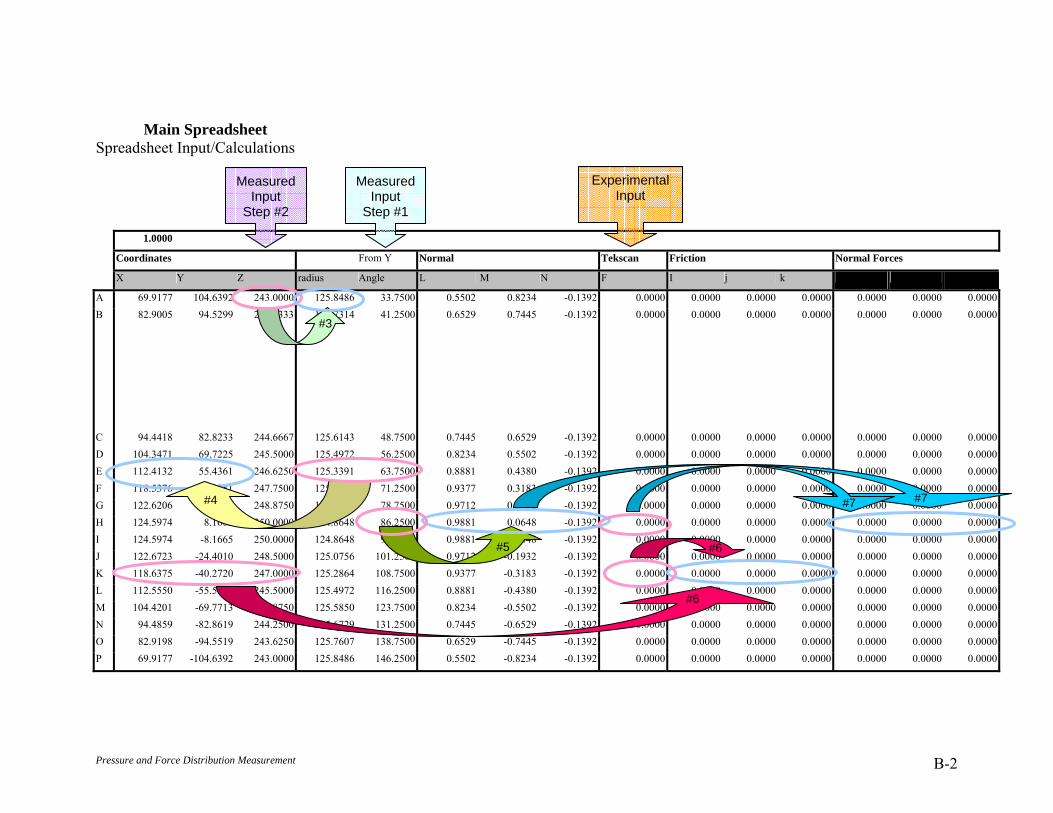
Pressure and Force Distribution Measurement B-2
Main Spreadsheet Spreadsheet Input/Calculations
1.0000
Coordinates From Y Normal Tekscan Friction Normal Forces
X Y Z radius Angle L M N F I j k I j k
A 69.9177 104.6392 243.0000 125.8486 33.7500 0.5502 0.8234 -0.1392 0.0000 0.0000 0.0000 0.0000 0.0000 0.0000 0.0000 B 82.9005 94.5299 243.8333 125.7314 41.2500 0.6529 0.7445 -0.1392 0.0000 0.0000 0.0000 0.0000 0.0000 0.0000 0.0000
C 94.4418 82.8233 244.6667 125.6143 48.7500 0.7445 0.6529 -0.1392 0.0000 0.0000 0.0000 0.0000 0.0000 0.0000 0.0000 D 104.3471 69.7225 245.5000 125.4972 56.2500 0.8234 0.5502 -0.1392 0.0000 0.0000 0.0000 0.0000 0.0000 0.0000 0.0000 E 112.4132 55.4361 246.6250 125.3391 63.7500 0.8881 0.4380 -0.1392 0.0000 0.0000 0.0000 0.0000 0.0000 0.0000 0.0000 F 118.5376 40.2381 247.7500 125.1810 71.2500 0.9377 0.3183 -0.1392 0.0000 0.0000 0.0000 0.0000 0.0000 0.0000 0.0000 G 122.6206 24.3908 248.8750 125.0229 78.7500 0.9712 0.1932 -0.1392 0.0000 0.0000 0.0000 0.0000 0.0000 0.0000 0.0000 H 124.5974 8.1665 250.0000 124.8648 86.2500 0.9881 0.0648 -0.1392 0.0000 0.0000 0.0000 0.0000 0.0000 0.0000 0.0000 I 124.5974 -8.1665 250.0000 124.8648 93.7500 0.9881 -0.0648 -0.1392 0.0000 0.0000 0.0000 0.0000 0.0000 0.0000 0.0000 J 122.6723 -24.4010 248.5000 125.0756 101.2500 0.9712 -0.1932 -0.1392 0.0000 0.0000 0.0000 0.0000 0.0000 0.0000 0.0000 K 118.6375 -40.2720 247.0000 125.2864 108.7500 0.9377 -0.3183 -0.1392 0.0000 0.0000 0.0000 0.0000 0.0000 0.0000 0.0000 L 112.5550 -55.5060 245.5000 125.4972 116.2500 0.8881 -0.4380 -0.1392 0.0000 0.0000 0.0000 0.0000 0.0000 0.0000 0.0000 M 104.4201 -69.7713 244.8750 125.5850 123.7500 0.8234 -0.5502 -0.1392 0.0000 0.0000 0.0000 0.0000 0.0000 0.0000 0.0000 N 94.4859 -82.8619 244.2500 125.6729 131.2500 0.7445 -0.6529 -0.1392 0.0000 0.0000 0.0000 0.0000 0.0000 0.0000 0.0000 O 82.9198 -94.5519 243.6250 125.7607 138.7500 0.6529 -0.7445 -0.1392 0.0000 0.0000 0.0000 0.0000 0.0000 0.0000 0.0000 P 69.9177 -104.6392 243.0000 125.8486 146.2500 0.5502 -0.8234 -0.1392 0.0000 0.0000 0.0000 0.0000 0.0000 0.0000 0.0000
Measured Input
Step #1
Measured Input
Step #2
#3
#4
#5
#6
Experimental Input
#6
#7 #7
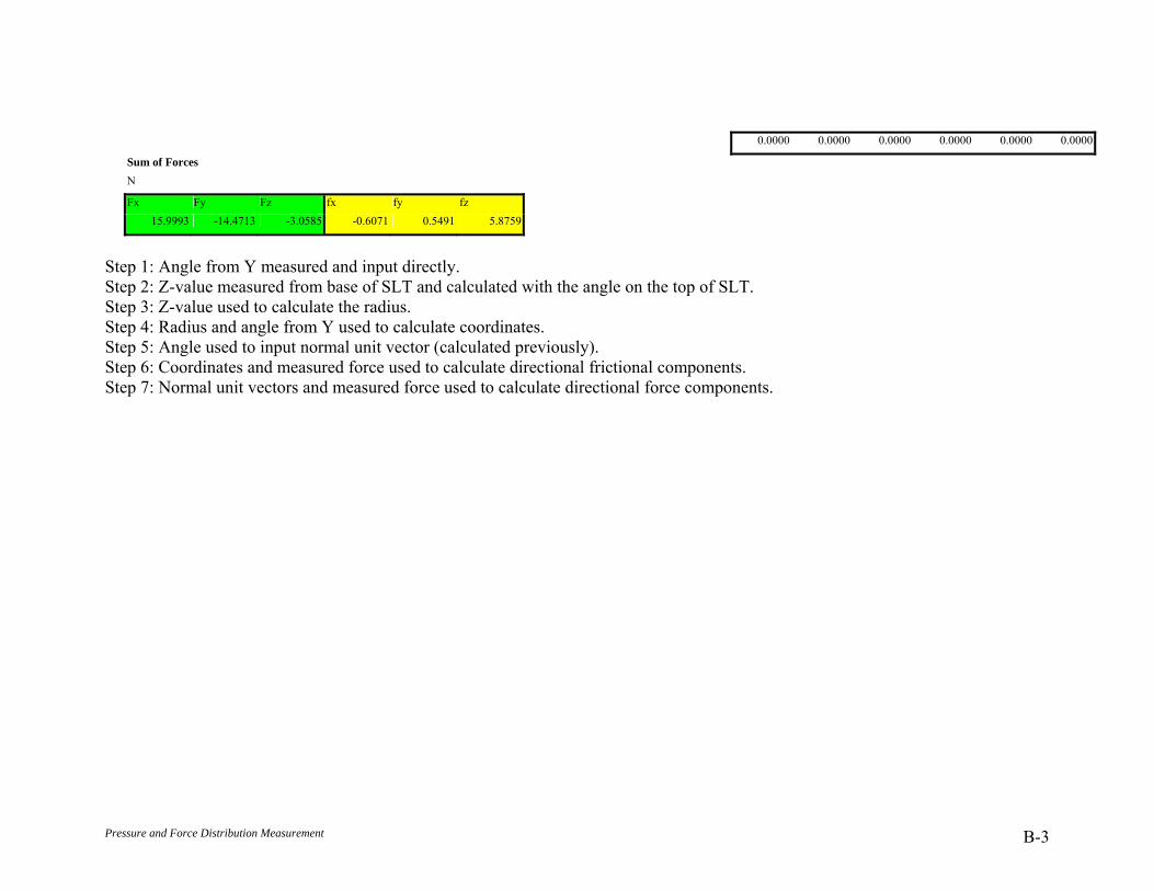
Pressure and Force Distribution Measurement B-3
0.0000 0.0000 0.0000 0.0000 0.0000 0.0000
Sum of Forces N
Fx Fy Fz fx fy fz 15.9993 -14.4713 -3.0585 -0.6071 0.5491 5.8759
Step 1: Angle from Y measured and input directly. Step 2: Z-value measured from base of SLT and calculated with the angle on the top of SLT. Step 3: Z-value used to calculate the radius. Step 4: Radius and angle from Y used to calculate coordinates. Step 5: Angle used to input normal unit vector (calculated previously). Step 6: Coordinates and measured force used to calculate directional frictional components. Step 7: Normal unit vectors and measured force used to calculate directional force components.
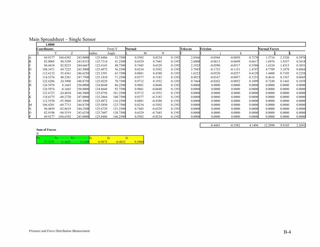
Pressure and Force Distribution Measurement B-4
Main Spreadsheet – Single Sensor 1.0000 Coordinates From Y Normal Tekscan Friction Normal Forces X Y Z radius Angle L M N F I j k I j k A 69.9177 104.6392 243.0000 125.8486 33.7500 0.5502 0.8234 0.1392 2.8566 -0.0568 -0.0850 0.7270 1.5716 2.3520 0.3976B 82.9005 94.5299 243.8333 125.7314 41.2500 0.6529 0.7445 0.1392 2.6000 -0.0613 -0.0699 0.6617 1.6976 1.9357 0.3618C 94.4418 82.8233 244.6667 125.6143 48.7500 0.7445 0.6529 0.1392 2.1925 -0.0590 -0.0517 0.5580 1.6324 1.4315 0.3051D 104.3471 69.7225 245.5000 125.4972 56.2500 0.8234 0.5502 0.1392 5.7943 -0.1723 -0.1151 1.4747 4.7709 3.1878 0.8064E 112.4132 55.4361 246.6250 125.3391 63.7500 0.8881 0.4380 0.1392 1.6223 -0.0520 -0.0257 0.4129 1.4408 0.7105 0.2258F 118.5376 40.2381 247.7500 125.1810 71.2500 0.9377 0.3183 0.1392 0.4923 -0.0167 -0.0057 0.1253 0.4616 0.1567 0.0685G 122.6206 24.3908 248.8750 125.0229 78.7500 0.9712 0.1932 0.1392 0.7464 -0.0262 -0.0052 0.1899 0.7249 0.1442 0.1039H 124.5974 8.1665 250.0000 124.8648 86.2500 0.9881 0.0648 0.1392 0.0000 0.0000 0.0000 0.0000 0.0000 0.0000 0.0000I 124.5974 -8.1665 250.0000 124.8648 93.7500 0.9881 -0.0648 0.1392 0.0000 0.0000 0.0000 0.0000 0.0000 0.0000 0.0000J 122.6723 -24.4010 248.5000 125.0756 101.2500 0.9712 -0.1932 0.1392 0.0000 0.0000 0.0000 0.0000 0.0000 0.0000 0.0000K 118.6375 -40.2720 247.0000 125.2864 108.7500 0.9377 -0.3183 0.1392 0.0000 0.0000 0.0000 0.0000 0.0000 0.0000 0.0000L 112.5550 -55.5060 245.5000 125.4972 116.2500 0.8881 -0.4380 0.1392 0.0000 0.0000 0.0000 0.0000 0.0000 0.0000 0.0000M 104.4201 -69.7713 244.8750 125.5850 123.7500 0.8234 -0.5502 0.1392 0.0000 0.0000 0.0000 0.0000 0.0000 0.0000 0.0000N 94.4859 -82.8619 244.2500 125.6729 131.2500 0.7445 -0.6529 0.1392 0.0000 0.0000 0.0000 0.0000 0.0000 0.0000 0.0000O 82.9198 -94.5519 243.6250 125.7607 138.7500 0.6529 -0.7445 0.1392 0.0000 0.0000 0.0000 0.0000 0.0000 0.0000 0.0000P 69.9177 -104.6392 243.0000 125.8486 146.2500 0.5502 -0.8234 0.1392 0.0000 0.0000 0.0000 0.0000 0.0000 0.0000 0.0000 -0.4443 -0.3582 4.1494 12.2998 9.9185 2.2691 Sum of Forces N Fx Fy Fz fx fy fz 27.3370 11.1622 5.1349 -0.9874 -0.4032 9.3900
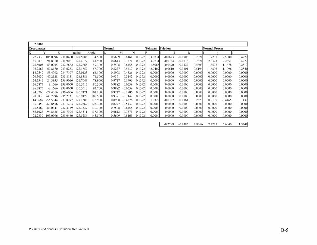
Pressure and Force Distribution Measurement B-5
2.0000
Coordinates Normal Tekscan Friction Normal Forces X Y Z radius Angle L M N F I j k I j k
72.2330 105.0996 231.0460 127.5286 34.5000 0.5609 0.8161 0.1392 3.0731 -0.0623 -0.0906 0.7821 1.7237 2.5080 0.427785.0870 94.8310 231.9061 127.4077 41.9000 0.6613 0.7371 0.1392 3.0731 -0.0734 -0.0818 0.7821 2.0323 2.2651 0.427796.5005 83.0035 232.7662 127.2868 49.3000 0.7508 0.6458 0.1392 1.8085 -0.0490 -0.0422 0.4603 1.3577 1.1678 0.2517
106.2862 69.8170 233.6263 127.1659 56.7000 0.8277 0.5437 0.1392 2.0409 -0.0610 -0.0401 0.5194 1.6892 1.1096 0.2840114.2549 55.4792 234.7197 127.0123 64.1000 0.8908 0.4326 0.1392 0.0000 0.0000 0.0000 0.0000 0.0000 0.0000 0.0000120.3030 40.2528 235.8131 126.8586 71.5000 0.9391 0.3142 0.1392 0.0000 0.0000 0.0000 0.0000 0.0000 0.0000 0.0000124.3346 24.3935 236.9066 126.7049 78.9000 0.9717 0.1906 0.1392 0.0000 0.0000 0.0000 0.0000 0.0000 0.0000 0.0000126.2875 8.1666 238.0000 126.5513 86.3000 0.9882 0.0639 0.1392 0.0000 0.0000 0.0000 0.0000 0.0000 0.0000 0.0000126.2875 -8.1666 238.0000 126.5513 93.7000 0.9882 -0.0639 0.1392 0.0000 0.0000 0.0000 0.0000 0.0000 0.0000 0.0000124.3760 -24.4016 236.6066 126.7471 101.1000 0.9717 -0.1906 0.1392 0.0000 0.0000 0.0000 0.0000 0.0000 0.0000 0.0000120.3830 -40.2796 235.2131 126.9429 108.5000 0.9391 -0.3142 0.1392 0.0000 0.0000 0.0000 0.0000 0.0000 0.0000 0.0000114.3687 -55.5344 233.8197 127.1388 115.9000 0.8908 -0.4326 0.1392 1.0322 -0.0332 0.0161 0.2627 0.9195 -0.4465 0.1437106.3450 -69.8556 233.1263 127.2362 123.3000 0.8277 -0.5437 0.1392 0.0000 0.0000 0.0000 0.0000 0.0000 0.0000 0.0000
96.5360 -83.0341 232.4329 127.3337 130.7000 0.7508 -0.6458 0.1392 0.0000 0.0000 0.0000 0.0000 0.0000 0.0000 0.000085.1027 -94.8485 231.7394 127.4311 138.1000 0.6613 -0.7371 0.1392 0.0000 0.0000 0.0000 0.0000 0.0000 0.0000 0.000072.2330 -105.0996 231.0460 127.5286 145.5000 0.5609 -0.8161 0.1392 0.0000 0.0000 0.0000 0.0000 0.0000 0.0000 0.0000
-0.2789 -0.2385 2.8066 7.7225 6.6040 1.5348
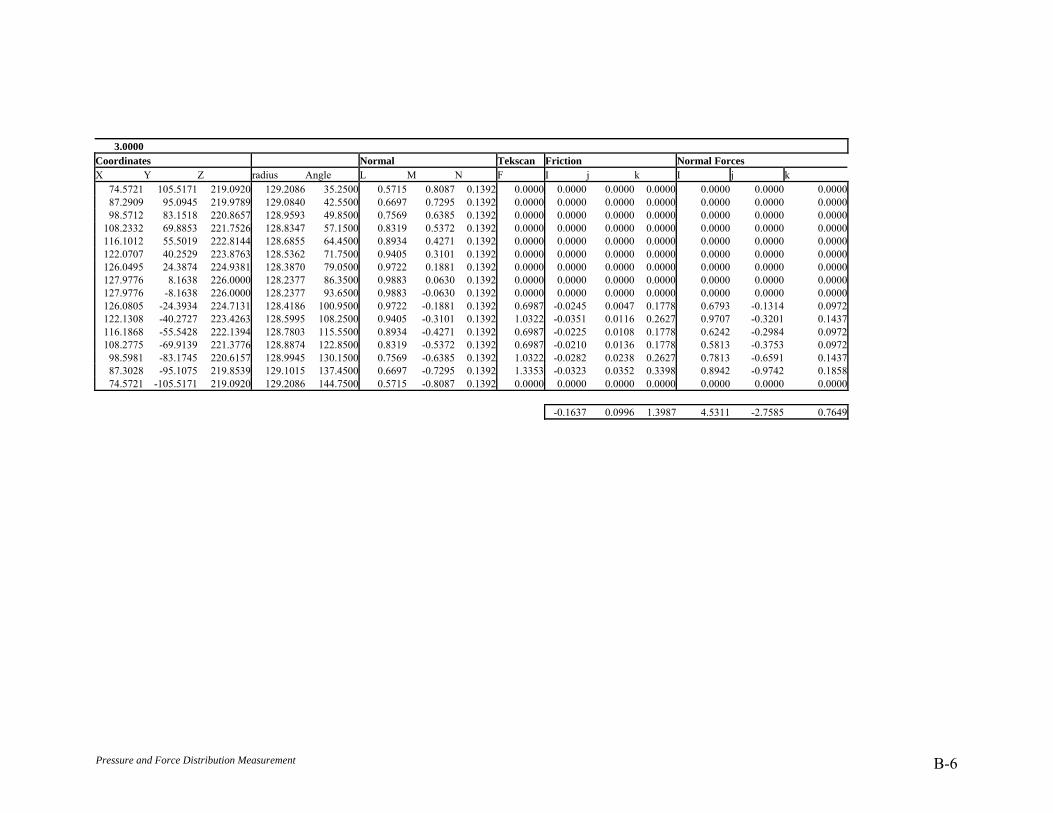
Pressure and Force Distribution Measurement B-6
3.0000
Coordinates Normal Tekscan Friction Normal Forces X Y Z radius Angle L M N F I j k I j k
74.5721 105.5171 219.0920 129.2086 35.2500 0.5715 0.8087 0.1392 0.0000 0.0000 0.0000 0.0000 0.0000 0.0000 0.000087.2909 95.0945 219.9789 129.0840 42.5500 0.6697 0.7295 0.1392 0.0000 0.0000 0.0000 0.0000 0.0000 0.0000 0.000098.5712 83.1518 220.8657 128.9593 49.8500 0.7569 0.6385 0.1392 0.0000 0.0000 0.0000 0.0000 0.0000 0.0000 0.0000
108.2332 69.8853 221.7526 128.8347 57.1500 0.8319 0.5372 0.1392 0.0000 0.0000 0.0000 0.0000 0.0000 0.0000 0.0000116.1012 55.5019 222.8144 128.6855 64.4500 0.8934 0.4271 0.1392 0.0000 0.0000 0.0000 0.0000 0.0000 0.0000 0.0000122.0707 40.2529 223.8763 128.5362 71.7500 0.9405 0.3101 0.1392 0.0000 0.0000 0.0000 0.0000 0.0000 0.0000 0.0000126.0495 24.3874 224.9381 128.3870 79.0500 0.9722 0.1881 0.1392 0.0000 0.0000 0.0000 0.0000 0.0000 0.0000 0.0000127.9776 8.1638 226.0000 128.2377 86.3500 0.9883 0.0630 0.1392 0.0000 0.0000 0.0000 0.0000 0.0000 0.0000 0.0000127.9776 -8.1638 226.0000 128.2377 93.6500 0.9883 -0.0630 0.1392 0.0000 0.0000 0.0000 0.0000 0.0000 0.0000 0.0000126.0805 -24.3934 224.7131 128.4186 100.9500 0.9722 -0.1881 0.1392 0.6987 -0.0245 0.0047 0.1778 0.6793 -0.1314 0.0972122.1308 -40.2727 223.4263 128.5995 108.2500 0.9405 -0.3101 0.1392 1.0322 -0.0351 0.0116 0.2627 0.9707 -0.3201 0.1437116.1868 -55.5428 222.1394 128.7803 115.5500 0.8934 -0.4271 0.1392 0.6987 -0.0225 0.0108 0.1778 0.6242 -0.2984 0.0972108.2775 -69.9139 221.3776 128.8874 122.8500 0.8319 -0.5372 0.1392 0.6987 -0.0210 0.0136 0.1778 0.5813 -0.3753 0.0972
98.5981 -83.1745 220.6157 128.9945 130.1500 0.7569 -0.6385 0.1392 1.0322 -0.0282 0.0238 0.2627 0.7813 -0.6591 0.143787.3028 -95.1075 219.8539 129.1015 137.4500 0.6697 -0.7295 0.1392 1.3353 -0.0323 0.0352 0.3398 0.8942 -0.9742 0.185874.5721 -105.5171 219.0920 129.2086 144.7500 0.5715 -0.8087 0.1392 0.0000 0.0000 0.0000 0.0000 0.0000 0.0000 0.0000
-0.1637 0.0996 1.3987 4.5311 -2.7585 0.7649
Pressure and Force Distribution Measurement B-7
4.0000
Coordinates Normal Tekscan Friction Normal Forces X Y Z radius Angle L M N F I j k I j k
76.9344 105.8911 207.1380 130.8886 36.0000 0.5821 0.8011 0.1392 0.0000 0.0000 0.0000 0.0000 0.0000 0.0000 0.000089.5115 95.3201 208.0516 130.7602 43.2000 0.6779 0.7219 0.1392 0.0000 0.0000 0.0000 0.0000 0.0000 0.0000 0.0000
100.6536 83.2679 208.9652 130.6318 50.4000 0.7630 0.6312 0.1392 0.0000 0.0000 0.0000 0.0000 0.0000 0.0000 0.0000110.1877 69.9272 209.8789 130.5034 57.6000 0.8361 0.5306 0.1392 0.0000 0.0000 0.0000 0.0000 0.0000 0.0000 0.0000117.9520 55.5040 210.9091 130.3586 64.8000 0.8960 0.4216 0.1392 0.0000 0.0000 0.0000 0.0000 0.0000 0.0000 0.0000123.8407 40.2383 211.9394 130.2138 72.0000 0.9418 0.3060 0.1392 0.0000 0.0000 0.0000 0.0000 0.0000 0.0000 0.0000127.7652 24.3725 212.9697 130.0690 79.2000 0.9727 0.1856 0.1392 0.0000 0.0000 0.0000 0.0000 0.0000 0.0000 0.0000129.6679 8.1580 214.0000 129.9242 86.4000 0.9883 0.0622 0.1392 0.0000 0.0000 0.0000 0.0000 0.0000 0.0000 0.0000129.6679 -8.1580 214.0000 129.9242 93.6000 0.9883 -0.0622 0.1392 0.0000 0.0000 0.0000 0.0000 0.0000 0.0000 0.0000127.7859 -24.3765 212.8197 130.0901 100.8000 0.9727 -0.1856 0.1392 0.0000 0.0000 0.0000 0.0000 0.0000 0.0000 0.0000123.8808 -40.2513 211.6394 130.2560 108.0000 0.9418 -0.3060 0.1392 0.0000 0.0000 0.0000 0.0000 0.0000 0.0000 0.0000118.0092 -55.5309 210.4591 130.4219 115.2000 0.8960 -0.4216 0.1392 0.0000 0.0000 0.0000 0.0000 0.0000 0.0000 0.0000110.2174 -69.9461 209.6289 130.5386 122.4000 0.8361 -0.5306 0.1392 0.0000 0.0000 0.0000 0.0000 0.0000 0.0000 0.0000100.6716 -83.2828 208.7986 130.6553 129.6000 0.7630 -0.6312 0.1392 0.0000 0.0000 0.0000 0.0000 0.0000 0.0000 0.0000
89.5196 -95.3286 207.9683 130.7719 136.8000 0.6779 -0.7219 0.1392 2.3928 -0.0586 0.0624 0.6090 1.6220 -1.7273 0.333076.9344 -105.8911 207.1380 130.8886 144.0000 0.5821 -0.8011 0.1392 1.1989 -0.0252 0.0347 0.3051 0.6979 -0.9605 0.1669
-0.0838 0.0971 0.9141 2.3199 -2.6878 0.4999
Pressure and Force Distribution Measurement B-8
5.0000
Coordinates Normal Tekscan Friction Normal Forces X Y Z radius Angle L M N F I j k I j k
79.3191 106.2211 195.1840 132.5687 36.7500 0.5925 0.7935 0.1392 0.0000 0.0000 0.0000 0.0000 0.0000 0.0000 0.000091.7484 95.5074 196.1244 132.4365 43.8500 0.6860 0.7141 0.1392 0.0000 0.0000 0.0000 0.0000 0.0000 0.0000 0.0000
102.7471 83.3515 197.0648 132.3043 50.9500 0.7690 0.6239 0.1392 0.0000 0.0000 0.0000 0.0000 0.0000 0.0000 0.0000112.1494 69.9427 198.0051 132.1722 58.0500 0.8403 0.5240 0.1392 0.0000 0.0000 0.0000 0.0000 0.0000 0.0000 0.0000119.8071 55.4856 199.0039 132.0318 65.1500 0.8986 0.4162 0.1392 0.0000 0.0000 0.0000 0.0000 0.0000 0.0000 0.0000125.6129 40.2090 200.0026 131.8914 72.2500 0.9431 0.3019 0.1392 0.0000 0.0000 0.0000 0.0000 0.0000 0.0000 0.0000129.4816 24.3488 201.0013 131.7511 79.3500 0.9732 0.1830 0.1392 0.0000 0.0000 0.0000 0.0000 0.0000 0.0000 0.0000131.3582 8.1493 202.0000 131.6107 86.4500 0.9884 0.0613 0.1392 0.0000 0.0000 0.0000 0.0000 0.0000 0.0000 0.0000131.3582 -8.1493 202.0000 131.6107 93.5500 0.9884 -0.0613 0.1392 0.0000 0.0000 0.0000 0.0000 0.0000 0.0000 0.0000129.4920 -24.3507 200.9263 131.7616 100.6500 0.9732 -0.1830 0.1392 0.0000 0.0000 0.0000 0.0000 0.0000 0.0000 0.0000125.6329 -40.2154 199.8526 131.9125 107.7500 0.9431 -0.3019 0.1392 0.0000 0.0000 0.0000 0.0000 0.0000 0.0000 0.0000119.8358 -55.4989 198.7789 132.0634 114.8500 0.8986 -0.4162 0.1392 0.0000 0.0000 0.0000 0.0000 0.0000 0.0000 0.0000112.1643 -69.9520 197.8801 132.1897 121.9500 0.8403 -0.5240 0.1392 0.0000 0.0000 0.0000 0.0000 0.0000 0.0000 0.0000102.7562 -83.3589 196.9814 132.3160 129.0500 0.7690 -0.6239 0.1392 0.0000 0.0000 0.0000 0.0000 0.0000 0.0000 0.0000
91.7525 -95.5116 196.0827 132.4423 136.1500 0.6860 -0.7141 0.1392 0.0000 0.0000 0.0000 0.0000 0.0000 0.0000 0.000079.3191 -106.2211 195.1840 132.5687 143.2500 0.5925 -0.7935 0.1392 0.0000 0.0000 0.0000 0.0000 0.0000 0.0000 0.0000
0.0000 0.0000 0.0000 0.0000 0.0000 0.0000
Pressure and Force Distribution Measurement B-9
6.0000
Coordinates Normal Tekscan Friction Normal Forces X Y Z radius Angle L M N F I j k I j k
81.7254 106.5066 183.2300 134.2487 37.5000 0.6028 0.7856 0.1392 0.0000 0.0000 0.0000 0.0000 0.0000 0.0000 0.000094.0009 95.6560 184.1971 134.1128 44.5000 0.6941 0.7063 0.1392 0.0000 0.0000 0.0000 0.0000 0.0000 0.0000 0.0000
104.8514 83.4025 185.1643 133.9768 51.5000 0.7750 0.6165 0.1392 0.0000 0.0000 0.0000 0.0000 0.0000 0.0000 0.0000114.1181 69.9317 186.1314 133.8409 58.5000 0.8443 0.5174 0.1392 0.0000 0.0000 0.0000 0.0000 0.0000 0.0000 0.0000121.6664 55.4466 187.0986 133.7050 65.5000 0.9011 0.4107 0.1392 0.0000 0.0000 0.0000 0.0000 0.0000 0.0000 0.0000127.3871 40.1650 188.0657 133.5691 72.5000 0.9444 0.2978 0.1392 0.0000 0.0000 0.0000 0.0000 0.0000 0.0000 0.0000131.1988 24.3163 189.0329 133.4331 79.5000 0.9737 0.1805 0.1392 0.4764 -0.0168 -0.0031 0.1212 0.4639 0.0860 0.0663133.0486 8.1376 190.0000 133.2972 86.5000 0.9884 0.0605 0.1392 0.0000 0.0000 0.0000 0.0000 0.0000 0.0000 0.0000133.0486 -8.1376 190.0000 133.2972 93.5000 0.9884 -0.0605 0.1392 0.0000 0.0000 0.0000 0.0000 0.0000 0.0000 0.0000131.1988 -24.3163 189.0329 133.4331 100.5000 0.9737 -0.1805 0.1392 0.0000 0.0000 0.0000 0.0000 0.0000 0.0000 0.0000127.3871 -40.1650 188.0657 133.5691 107.5000 0.9444 -0.2978 0.1392 0.0000 0.0000 0.0000 0.0000 0.0000 0.0000 0.0000121.6664 -55.4466 187.0986 133.7050 114.5000 0.9011 -0.4107 0.1392 0.0000 0.0000 0.0000 0.0000 0.0000 0.0000 0.0000114.1181 -69.9317 186.1314 133.8409 121.5000 0.8443 -0.5174 0.1392 0.0000 0.0000 0.0000 0.0000 0.0000 0.0000 0.0000104.8514 -83.4025 185.1643 133.9768 128.5000 0.7750 -0.6165 0.1392 0.0000 0.0000 0.0000 0.0000 0.0000 0.0000 0.0000
94.0009 -95.6560 184.1971 134.1128 135.5000 0.6941 -0.7063 0.1392 0.0000 0.0000 0.0000 0.0000 0.0000 0.0000 0.000081.7254 -106.5066 183.2300 134.2487 142.5000 0.6028 -0.7856 0.1392 0.0000 0.0000 0.0000 0.0000 0.0000 0.0000 0.0000
-0.0168 -0.0031 0.1212 0.4639 0.0860 0.0663

Pressure and Force Distribution Measurement B-10
Normal Planes
Lumbar and Abdomen Area
Normal Plane - Lumbar
Intercepts
For Friction:
X Y Z X Y Z
A1 30 122.4053 267.5 0 0 1138.459
H3 6 134.70263 180 0 -122.4053 267.5000
M5 -18 143.48643 117.5
(H3-A1)U -24 12.297323 -87.5 0 122.4053 870.959
(M5-A1)V -48 21.081125 -150
0 0.1391731 0.9902681
U X V 1.819E-12 600 84.324501
Normal Unit 3.002E-15 0.9902681 0.1391731
Normal Plane - Abdomen
Intercepts
X Y Z
A1 -30.0000 -122.4053 267.5000
H3 -6 -134.70263 180
M5 18 -143.48643 117.5
(H3-A1)U 24 -12.297323 -87.5
(M5-A1)V 48 -21.081125 -150
U X V -1.819E-12 -600 84.324501
Normal Unit -3.002E-15 -0.9902681 0.1391731

Pressure and Force Distribution Measurement B-11
Sample data set – Normal plane calculation Sample Data Set: For:
Coordinates of the point: The coordinates of point ‘P’ are (157.5, 33.47) Tangent line at point P:
Using implicit differentiation: Using the point-slope form:
mmr
o
16112
==θ
mmyy
ry
mmxx
rx
47.33)12sin()161(
sin
5.157)12cos()161(
cos
===
===
θ
θ
)161(22
222
=+
=+
yxryx
7.4
)47.335.157(
'
'0'22
−=
−=
=−=
−==+
m
m
myxy
xyyyyx
)5.157)(7.4()5.33())(()( 00
−−=−−=−
xyxxmyy

Pressure and Force Distribution Measurement B-12
For the x-intercept, set y=0 For the y-intercept, set x=0 Therefore the three intercepts of the resulting plane where θ=12o are:
6.164)5.157)(7.4()5.330()5.157)(7.4()5.33(
=−−=−−−=−
xxxy
8.773)5.1570)(7.4()5.33()5.157)(7.4()5.33(
=−−=−−−=−
yy
xy
)14.0,21.0,97.0(:
)5.127367,8.188565,3.886465())))6.164(*8.773(0*6.164()),6.1145*6.164(0*0(),0*06.1145*8.773((
)6.1145,0,6.164())06.1145(),00(),6.1640((
)0,8.773,6.164()00(),08.773(),6.1640((
)6.1145,0,0()0,8.773,0()0,0,6.164(
=
=−−−−−−=
×=
−=−−−=
−=
−=−−−=
−=
===
nUnitvectornn
vun
vv
ACv
uu
ABu
CBA
v
v
v
vvv
v
v
v
v
v
v
Pressure and Force Distribution Measurement B-13
For z=0
A U V
r= 160 mm
Tangent intercepts Vector cross product unit vector
Coordinates X Y Z XY XZ
Angle (from y)
radians
X Y Z X Y Z X Y Z X Y Z x y z
0 0 0 160 0 #DIV/0! 0 0 0 160 0 0 0 1138.5 #DIV/0!
160 0 #DIV/0!
0 1138.46
182153 #DIV/0!
#### #DIV/0!
#DIV/0! #DIV/0!
1 0.017453
2.7924
159.98 0 9167.8 0 0 0 160 0 0 0 1138.5 -9167.8 160.02 0 -9167.79
0 1138.46
182181 -1E+0
7
1E+06
0.0173
-0.99 0.1392
2 0.034907
5.5839
159.9 0 4584.6 0 0 0 160.1 0 0 0 1138.5 -4584.6 160.1 0 -4584.59
0 1138.46
182264 -5E+0
6
7E+05
0.0346
-0.99 0.1392
3 0.05236
8.3738
159.78 0 3057.2 0 0 0 160.2 0 0 0 1138.5 -3057.2 160.22 0 -3057.17
0 1138.46
182403 -3E+0
6
5E+05
0.0518
-0.989 0.1392
4 0.069813
11.161
159.61 0 2293.7 0 0 0 160.4 0 0 0 1138.5 -2293.7 160.39 0 -2293.69
0 1138.46
182598 -3E+0
6
4E+05
0.0691
-0.988 0.1392
39.75 0.693768
102.31
123.01 0 250.22 0 0 0 208.1 0 0 0 1138.5 -250.22 208.11 0 -250.219
0 1138.46
236919 -28486
4
52072 0.6332
-0.761 0.1392
46.45 0.810705
115.96
110.24 0 220.76 0 0 0 232.2 0 0 0 1138.5 -220.76 232.22 0 -220.759
0 1138.46
264379 -25132
5
51266 0.7177
-0.682 0.1392
53.15 0.927642
128.03
95.956 0 199.95 0 0 0 266.8 0 0 0 1138.5 -199.95 266.79 0 -199.948
0 1138.46
303730 -22763
3
53344 0.7924
-0.594 0.1392
59.85 1.04458
138.35
80.362 0 185.03 0 0 0 318.6 0 0 0 1138.5 -185.03 318.56 0 -185.032
0 1138.46
362664 -21065
2
58943 0.8563
-0.497 0.1392
66.55 1.161517
146.79
63.672 0 174.4 0 0 0 402.1 0 0 0 1138.5 -174.4 402.06 0 -174.404
0 1138.46
457731 -19855
2
70121 0.9085
-0.394 0.1392
73.25 1.278454
153.21
46.111 0 167.09 0 0 0 555.2 0 0 0 1138.5 -167.09 555.18 0 -167.089
0 1138.46
632047 -19022
4
92764 0.9483
-0.285 0.1392
79.95 1.395391
157.54
27.921 0 162.49 0 0 0 916.9 0 0 0 1138.5 -162.49 916.87 0 -162.493
0 1138.46
1043814
-18499
2
1E+05
0.9751
-0.173 0.1392
86.65 1.512328
159.73
9.3496 0 160.27 0 0 0 2738 0 0 0 1138.5 -160.27 2738.1 0 -160.274
0 1138.46
3117186
-18246
5
4E+05
0.9886
-0.058 0.1392
93.35 1.629265
159.73
-9.35 0 160.27 0 0 0 -2738 0 0 0 1138.5 -160.27 -2738 0 -160.274
0 1138.46
-3E+06 -18246
5
-4E+0
5
-0.989
-0.058 -0.1392
100.05 1.746202
157.54
-27.92 0 162.49 0 0 0 -917 0 0 0 1138.5 -162.49 -916.9 0 -162.493
0 1138.46
-1E+06 -18499
2
-1E+0
5
-0.975
-0.173 -0.1392
106.75 1.863139
153.21
-46.11 0 167.09 0 0 0 -555 0 0 0 1138.5 -167.09 -555.2 0 -167.089
0 1138.46
-632047
-19022
4
-92764
-0.948
-0.285 -0.1392
113.45 1.980076
146.79
-63.67 0 174.4 0 0 0 -402 0 0 0 1138.5 -174.4 -402.1 0 -174.404
0 1138.46
-457731
-19855
2
-70121
-0.908
-0.394 -0.1392
120.15 2.097013
138.35
-80.36 0 185.03 0 0 0 -319 0 0 0 1138.5 -185.03 -318.6 0 -185.032
0 1138.46
-362664
-21065
2
-58943
-0.856
-0.497 -0.1392
126.85 2.21395
128.03
-95.96 0 199.95 0 0 0 -267 0 0 0 1138.5 -199.95 -266.8 0 -199.948
0 1138.46
-303730
-22763
3
-53344
-0.792
-0.594 -0.1392
133.55 2.330887
115.96
-110.2 0 220.76 0 0 0 -232 0 0 0 1138.5 -220.76 -232.2 0 -220.759
0 1138.46
-264379
-25132
5
-51266
-0.718
-0.682 -0.1392
140.25 2.447824
102.31
-123 0 250.22 0 0 0 -208 0 0 0 1138.5 -250.22 -208.1 0 -250.219
0 1138.46
-236919
-28486
4
-52072
-0.633
-0.761 -0.1392
146.95 2.564761
87.259
-134.1 0 293.38 0 0 0 -191 0 0 0 1138.5 -293.38 -190.9 0 -293.378
0 1138.46
-217316
-33399
9
-56002
-0.54 -0.83 -0.1392
153.65 2.681698
71.017
-143.4 0 360.48 0 0 0 -179 0 0 0 1138.5 -360.48 -178.6 0 -360.479
0 1138.46
-203274
-41039
1
-64364
-0.44 -0.887 -0.1392
160.35 2.798635
53.804
-150.7 0 475.8 0 0 0 -170 0 0 0 1138.5 -475.8 -169.9 0 -475.803
0 1138.46
-193417
-54168
2
-80836
-0.333
-0.933 -0.1392
167.05 2.915573
35.856
-155.9 0 713.96 0 0 0 -164 0 0 0 1138.5 -713.96 -164.2 0 -713.965
0 1138.46
-186907
-81282
0
-1E+0
5
-0.222
-0.965 -0.1392
173.75 3.03251
17.419
-159 0 1469.7 0 0 0 -161 0 0 0 1138.5 -1469.7 -161 0 -1469.68
0 1138.46
-183243
-2E+0
6
-2E+0
5
-0.108
-0.984 -0.1392
180.45 3.149447
-1.256
6
-160 0 -20372 0 0 0 -160 0 0 0 1138.5 20372 -160 0 20372.04
0 1138.46
-182159
2.3E+07
3E+06
-0.008
0.9902 0.1392
187.15 3.266384
-19.91
5
-158.8 0 -1285.5 0 0 0 -161 0 0 0 1138.5 1285.48 -161.3 0 1285.477
0 1138.46
-183581
1463463
2E+05
-0.123
0.9826 0.1392
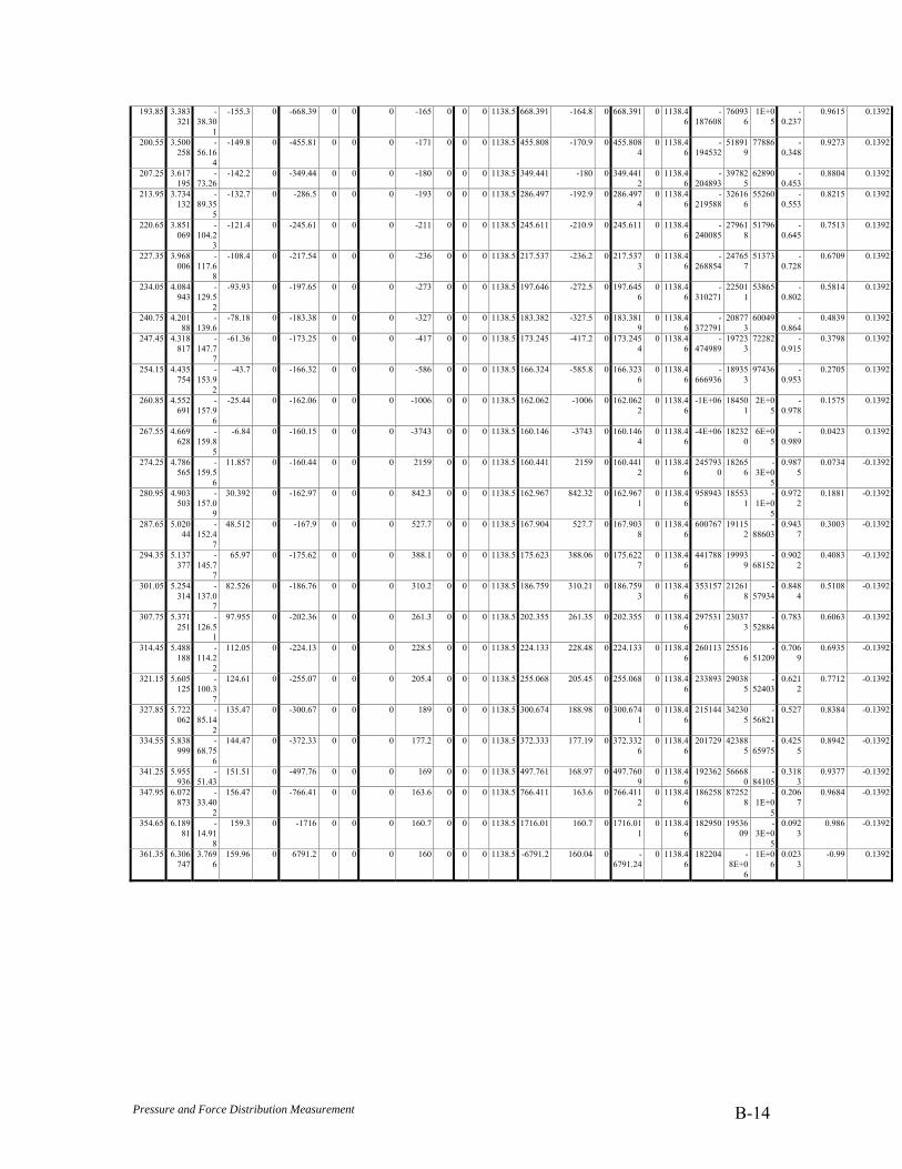
Pressure and Force Distribution Measurement B-14
193.85 3.383321
-38.30
1
-155.3 0 -668.39 0 0 0 -165 0 0 0 1138.5 668.391 -164.8 0 668.391 0 1138.46
-187608
760936
1E+05
-0.237
0.9615 0.1392
200.55 3.500258
-56.16
4
-149.8 0 -455.81 0 0 0 -171 0 0 0 1138.5 455.808 -170.9 0 455.8084
0 1138.46
-194532
518919
77886 -0.348
0.9273 0.1392
207.25 3.617195
-73.26
-142.2 0 -349.44 0 0 0 -180 0 0 0 1138.5 349.441 -180 0 349.4412
0 1138.46
-204893
397825
62890 -0.453
0.8804 0.1392
213.95 3.734132
-89.35
5
-132.7 0 -286.5 0 0 0 -193 0 0 0 1138.5 286.497 -192.9 0 286.4974
0 1138.46
-219588
326166
55260 -0.553
0.8215 0.1392
220.65 3.851069
-104.2
3
-121.4 0 -245.61 0 0 0 -211 0 0 0 1138.5 245.611 -210.9 0 245.611 0 1138.46
-240085
279618
51796 -0.645
0.7513 0.1392
227.35 3.968006
-117.6
8
-108.4 0 -217.54 0 0 0 -236 0 0 0 1138.5 217.537 -236.2 0 217.5373
0 1138.46
-268854
247657
51373 -0.728
0.6709 0.1392
234.05 4.084943
-129.5
2
-93.93 0 -197.65 0 0 0 -273 0 0 0 1138.5 197.646 -272.5 0 197.6456
0 1138.46
-310271
225011
53865 -0.802
0.5814 0.1392
240.75 4.20188
-139.6
-78.18 0 -183.38 0 0 0 -327 0 0 0 1138.5 183.382 -327.5 0 183.3819
0 1138.46
-372791
208773
60049 -0.864
0.4839 0.1392
247.45 4.318817
-147.7
7
-61.36 0 -173.25 0 0 0 -417 0 0 0 1138.5 173.245 -417.2 0 173.2454
0 1138.46
-474989
197233
72282 -0.915
0.3798 0.1392
254.15 4.435754
-153.9
2
-43.7 0 -166.32 0 0 0 -586 0 0 0 1138.5 166.324 -585.8 0 166.3236
0 1138.46
-666936
189353
97436 -0.953
0.2705 0.1392
260.85 4.552691
-157.9
6
-25.44 0 -162.06 0 0 0 -1006 0 0 0 1138.5 162.062 -1006 0 162.0622
0 1138.46
-1E+06 184501
2E+05
-0.978
0.1575 0.1392
267.55 4.669628
-159.8
5
-6.84 0 -160.15 0 0 0 -3743 0 0 0 1138.5 160.146 -3743 0 160.1464
0 1138.46
-4E+06 182320
6E+05
-0.989
0.0423 0.1392
274.25 4.786565
-159.5
6
11.857 0 -160.44 0 0 0 2159 0 0 0 1138.5 160.441 2159 0 160.4412
0 1138.46
2457930
182656
-3E+0
5
0.9875
0.0734 -0.1392
280.95 4.903503
-157.0
9
30.392 0 -162.97 0 0 0 842.3 0 0 0 1138.5 162.967 842.32 0 162.9671
0 1138.46
958943 185531
-1E+0
5
0.9722
0.1881 -0.1392
287.65 5.02044
-152.4
7
48.512 0 -167.9 0 0 0 527.7 0 0 0 1138.5 167.904 527.7 0 167.9038
0 1138.46
600767 191152
-88603
0.9437
0.3003 -0.1392
294.35 5.137377
-145.7
7
65.97 0 -175.62 0 0 0 388.1 0 0 0 1138.5 175.623 388.06 0 175.6227
0 1138.46
441788 199939
-68152
0.9022
0.4083 -0.1392
301.05 5.254314
-137.0
7
82.526 0 -186.76 0 0 0 310.2 0 0 0 1138.5 186.759 310.21 0 186.7593
0 1138.46
353157 212618
-57934
0.8484
0.5108 -0.1392
307.75 5.371251
-126.5
1
97.955 0 -202.36 0 0 0 261.3 0 0 0 1138.5 202.355 261.35 0 202.355 0 1138.46
297531 230373
-52884
0.783 0.6063 -0.1392
314.45 5.488188
-114.2
2
112.05 0 -224.13 0 0 0 228.5 0 0 0 1138.5 224.133 228.48 0 224.133 0 1138.46
260113 255166
-51209
0.7069
0.6935 -0.1392
321.15 5.605125
-100.3
7
124.61 0 -255.07 0 0 0 205.4 0 0 0 1138.5 255.068 205.45 0 255.068 0 1138.46
233893 290385
-52403
0.6212
0.7712 -0.1392
327.85 5.722062
-85.14
2
135.47 0 -300.67 0 0 0 189 0 0 0 1138.5 300.674 188.98 0 300.6741
0 1138.46
215144 342305
-56821
0.527 0.8384 -0.1392
334.55 5.838999
-68.75
6
144.47 0 -372.33 0 0 0 177.2 0 0 0 1138.5 372.333 177.19 0 372.3326
0 1138.46
201729 423885
-65975
0.4255
0.8942 -0.1392
341.25 5.955936
-51.43
151.51 0 -497.76 0 0 0 169 0 0 0 1138.5 497.761 168.97 0 497.7609
0 1138.46
192362 566680
-84105
0.3183
0.9377 -0.1392
347.95 6.072873
-33.40
2
156.47 0 -766.41 0 0 0 163.6 0 0 0 1138.5 766.411 163.6 0 766.4112
0 1138.46
186258 872528
-1E+0
5
0.2067
0.9684 -0.1392
354.65 6.18981
-14.91
8
159.3 0 -1716 0 0 0 160.7 0 0 0 1138.5 1716.01 160.7 0 1716.011
0 1138.46
182950 1953609
-3E+0
5
0.0923
0.986 -0.1392
361.35 6.306747
3.7696
159.96 0 6791.2 0 0 0 160 0 0 0 1138.5 -6791.2 160.04 0 -6791.24
0 1138.46
182204 -8E+0
6
1E+06
0.0233
-0.99 0.1392

Pressure and Force Distribution Measurement C-1
Appendix C - Data Acquisition Procedures A) Force Plate The raw voltage data were obtained from the acquisition software. The output was in six columns, representing Fx, Fy, Fz, Mx, My, and Mz. The average value for 400 points, measured at 50Hz, was calculated for each of the six measurements. These values were imported into an Excel spreadsheet. The baseline data were obtained with the acquisition of a data file measuring the forces applied by the SLT and the frame on the load cell, with all instrumentation affixed, but with no external forces applied. The calibration or baseline file was subtracted from the averages to reduce the effects of noise and baseline inequalities. The calibrated voltages were then converted to forces with the application of conversion formulas and corresponding sensitivity values, designated by the manufacturer, for each measured voltage. For conversion to Newtons from the given voltage, the following equation was used:
Vo = 0.000001 x S x Vexc x G x Input Where:
Vo= the output voltage from the amplifier used 0.000001= volts/micro-volt, units for sensitivity
S= the sensitivity Vexc= the bridge excitation voltage
G= the amplifier gain Input= the input force or moment
Rearranging the equation to solve for the input force or moment:
GVSV
Inputexc ×××
=000001.0
0
Where: Excitation voltage = 10V Gain = 4000 Sensitivities:
Pound
VoltMicrovoltsFx/526.1=
Pound
VoltMicrovoltsFy/526.1=
PoundVoltMicrovoltsFz
/389.0=
PoundVoltMicrovoltsM x
/496.0=

Pressure and Force Distribution Measurement C-2
PoundVoltMicrovoltsM y
/696.0=
PoundVoltMicrovoltsM z
/134.1=
The measured forces Fx, Fy, and Fz were resolved to a single resultant force. The moments were used to calculate the coordinates of the applied force.
xFM
zFM
yFM
xz
zy
yx
×=
×=
×=
Where x,y,z are the coordinates of the applied resultant force. These coordinates were compared to the estimated point of application measured on the SLT.
A2) Centre of Pressure Calculations The calculated COP coordinates (x,y) for a force platform are as follows:
)1()(
)( −×⎥⎦
⎤⎢⎣
⎡ ×+=
z
xoffy
FFZM
xCOP
)1()(
)( −×⎥⎦
⎤⎢⎣
⎡ ×+=
z
yoffx
FFZM
yCOP
where:
COP(x) = The x coordinate of the center of pressure COP(y) = The y coordinate of the center of pressure Zoff = The vertical offset from the top plate to the origin of the force platform (a negative #) Fx = The force along the x axis Fy = The force along the y axis Fz = The force along the z axis Mx = The moment about the x axis My = The moment about the y axis Mz = The moment about the z axis

Pressure and Force Distribution Measurement C-3
Centre of Pressure Positions
-15
-10
-5
0
5
10
15
-10 -5 0 5 10
X (inches)
Y (in
ches
)
Calculated ValuesExpected Values
Centre of Pressure Results
Table C.1 Centre of Pressure – Expected vs. Calculated Results
Expected Calculated X Y X Y
0 0 -0.3017 0.07745 0 0 -0.6734 0.1237 0 0 -0.4527 0.09911 0 -12 -1.0035 -11.461 0 -12 -1.7965 -11.803 0 -12 -1.5253 -12.127 0 12 -0.8911 11.3121 0 12 -1.2318 13.0101 0 12 -1.2497 12.4381
-6 -5 -5.013 -5.4783 -6 -5 -5.5938 -5.4778 -6 -5 -5.5634 -5.4583 5 -6 4.36473 -5.7219 5 -6 4.17275 -5.6334 5 -6 4.21495 -5.5484
-5 6 -5.8456 6.34528 -5 6 -5.6531 6.41828 -5 6 -5.7082 6.30707
Figure C.1 Plot of Expected vs. Calculated Results
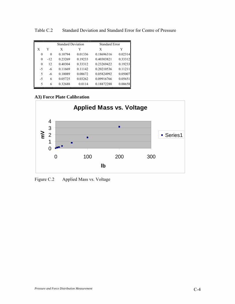
Pressure and Force Distribution Measurement C-4
Table C.2 Standard Deviation and Standard Error for Centre of Pressure
Standard Deviation Standard Error
X Y X Y X Y 0 0 0.10794 0.01336 0.18696316 0.023140 -12 0.23269 0.19233 0.40303821 0.333120 12 0.40304 0.33312 0.23269422 0.19233
-5 -6 0.11669 0.11142 0.20210536 0.112115 -6 0.10089 0.08672 0.05824992 0.05007
-5 6 0.05725 0.03262 0.09916766 0.056515 6 0.32688 0.0114 0.18872288 0.00658
A3) Force Plate Calibration
Applied Mass vs. Voltage
01234
0 100 200 300
lb
mV Series1
Figure C.2 Applied Mass vs. Voltage
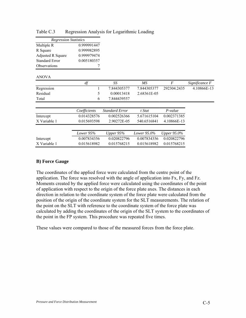
Pressure and Force Distribution Measurement C-5
Table C.3 Regression Analysis for Logarithmic Loading Regression Statistics
Multiple R 0.999991447 R Square 0.999982895 Adjusted R Square 0.999979474 Standard Error 0.005180357 Observations 7
ANOVA
df SS MS F Significance F Regression 1 7.844305377 7.844305377 292304.2435 4.10866E-13Residual 5 0.00013418 2.68361E-05 Total 6 7.844439557
Coefficients Standard Error t Stat P-value
Intercept 0.014328576 0.002526366 5.671615104 0.002371385 X Variable 1 0.015693598 2.90272E-05 540.6516841 4.10866E-13
Lower 95% Upper 95% Lower 95.0% Upper 95.0%
Intercept 0.007834356 0.020822796 0.007834356 0.020822796 X Variable 1 0.015618982 0.015768215 0.015618982 0.015768215
B) Force Gauge The coordinates of the applied force were calculated from the centre point of the application. The force was resolved with the angle of application into Fx, Fy, and Fz. Moments created by the applied force were calculated using the coordinates of the point of application with respect to the origin of the force plate axes. The distances in each direction in relation to the coordinate system of the force plate were calculated from the position of the origin of the coordinate system for the SLT measurements. The relation of the point on the SLT with reference to the coordinate system of the force plate was calculated by adding the coordinates of the origin of the SLT system to the coordinates of the point in the FP system. This procedure was repeated five times. These values were compared to those of the measured forces from the force plate.
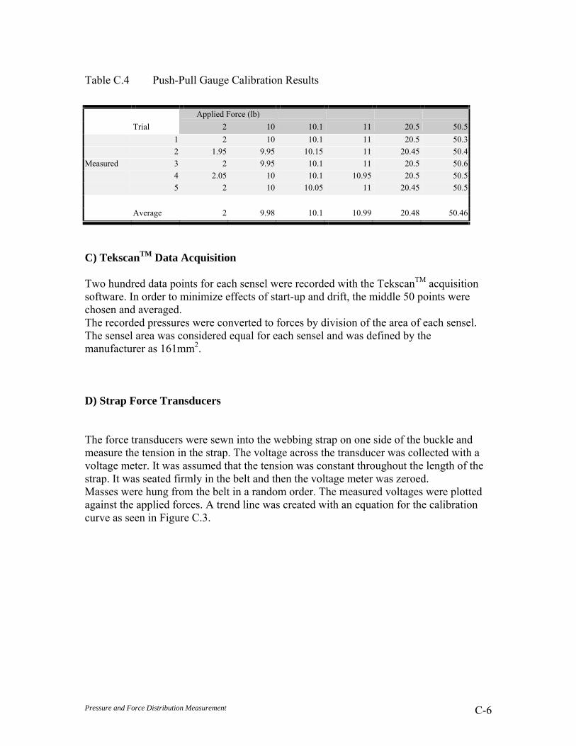
Pressure and Force Distribution Measurement C-6
Table C.4 Push-Pull Gauge Calibration Results
Applied Force (lb) Trial 2 10 10.1 11 20.5 50.5 1 2 10 10.1 11 20.5 50.3 2 1.95 9.95 10.15 11 20.45 50.4
Measured 3 2 9.95 10.1 11 20.5 50.6 4 2.05 10 10.1 10.95 20.5 50.5 5 2 10 10.05 11 20.45 50.5 Average 2 9.98 10.1 10.99 20.48 50.46
C) TekscanTM Data Acquisition Two hundred data points for each sensel were recorded with the TekscanTM acquisition software. In order to minimize effects of start-up and drift, the middle 50 points were chosen and averaged. The recorded pressures were converted to forces by division of the area of each sensel. The sensel area was considered equal for each sensel and was defined by the manufacturer as 161mm2. D) Strap Force Transducers The force transducers were sewn into the webbing strap on one side of the buckle and measure the tension in the strap. The voltage across the transducer was collected with a voltage meter. It was assumed that the tension was constant throughout the length of the strap. It was seated firmly in the belt and then the voltage meter was zeroed. Masses were hung from the belt in a random order. The measured voltages were plotted against the applied forces. A trend line was created with an equation for the calibration curve as seen in Figure C.3.

Pressure and Force Distribution Measurement C-7
Strap Force Transducer Calibration
y = -3.1352x - 46.6R2 = 0.9953
-800-700-600-500-400-300-200-100
00 50 100 150 200 250
Applied Force (N)
Volta
ge
Figure C.3 Strap Force Transducer Calibration
The equation of the trend line was used for conversion of the output voltages to forces in Newtons.

Pressure and Force Distribution Measurement D-1
Appendix D - System Calibration System Calibration The set-up can be seen below:
Figure D.1 Calibration Set-up
The free-body diagram is seen below:
Figure D.2 Free body diagram of calibration set-up
The equilibrium equations are shown below. The system is static, therefore: ΣFx=0 ΣFy=0 From the orientation of the webbing it was shown that:
Spreader BarWebbing Strap
Force Plate
Pull Gauge
Spreader Bar
Pull Gauge Contoured Pressure Blocks
SLT
Webbing Strap
Top View
Side View
FA
FW
FW
FS FB1
FB2
FBW2
FBW3
FBW1
FBW4
x
y

Pressure and Force Distribution Measurement D-2
FA= 2FW The resultant forces from this applied force are acted on the SLT. FA-ΣFSx=0 The symmetry of the SLT about the x-axis caused the forces acting on it in the y-direction to cancel out. ΣFSy=0 The spreader bar was an internal component of the system and the forces that acted on it canceled in both directions. Σ FB=0 FB1+ FBW1+FBW2=FB2+FBW3+FBW4
Calibration of Flat Lumbar and Abdominal Sensors
Figure D.3 Calibration set-up for lumbar and abdominal areas
Applied
Force Plate
Lean Angle
SL
Side View

Pressure and Force Distribution Measurement D-3
Results of Initial Calibration
Table D.1 Force Gauge (Expected) vs. Tekscan (Measured)
Trial Force Expected (N) Measured (N) Standard Deviation (N) X Y Z X Y Z X Y Z
1 91.4 90.5 0.0 12.7 40.4 -3.5 6.9 35.4 2.5 4.1 2 87.4 86.5 0.0 12.2 35.2 -4.7 6.2 36.3 3.4 4.2 3 119.5 118.3 0.0 16.6 61.7 -7.1 10.5 40.0 5.0 4.4 4 68.7 68.0 0.0 9.6 28.2 1.1 5.0 28.2 0.8 3.2 5 72.2 71.5 0.0 10.1 29.0 -3.8 5.2 30.1 2.7 3.5 6 85.6 84.8 0.0 11.9 35.7 -3.2 6.2 34.7 2.3 4.1 7 104.3 103.3 0.0 14.5 48.6 -4.7 8.3 38.7 3.4 4.4 8 103.7 102.7 0.0 14.4 44.6 -5.3 7.8 41.1 3.8 4.7 9 67.8 67.1 0.0 9.4 37.0 -1.5 6.2 21.3 1.0 2.3
10 93.2 92.3 0.0 13.0 58.1 -2.6 9.6 24.2 1.8 2.4 11 90.1 89.2 0.0 12.5 47.7 -2.8 8.1 29.3 2.0 3.1
Table D.2 Force Gauge vs. Force Plate
Force Gauge -resolved Force plate Standard Deviation X Y Z X Y Z X Y Z
136.0 0.0 18.9 136.4 -0.3 16.0 0.3 0.2 2.1 107.0 0.0 14.9 109.4 -0.6 13.1 1.7 0.4 1.3 122.2 0.0 17.0 123.6 -0.5 13.9 1.0 0.4 2.2 100.3 0.0 14.0 102.8 -0.8 12.2 1.8 0.6 1.2 91.9 0.0 12.8 94.8 -0.9 11.7 2.1 0.6 0.8 77.6 0.0 10.8 80.4 -1.1 10.5 2.0 0.8 0.2 78.5 0.0 10.9 81.8 -0.9 8.3 2.4 0.7 1.8 83.8 0.0 11.7 86.3 -0.9 8.4 1.8 0.6 2.3 99.9 0.0 13.9 103.3 -0.6 10.3 2.5 0.4 2.5 78.0 0.0 10.9 81.3 -0.8 8.7 2.3 0.6 1.6 78.5 0.0 10.9 80.9 -0.9 8.5 1.7 0.7 1.7 84.7 0.0 11.8 87.4 -1.2 8.6 2.9 0.4 2.9
Load Cell Expected Force Plate Actual
Trial Fx Fy Fz Mx My Mz X Y Z Mx My Mz 1 136 0 18.9 0 38.4 0 136.4 -0.3 16 4.8 43.2 1.3 2 107 0 14.9 0 30.2 0 109.4 -0.6 13.1 2.1 22.1 2.5 3 122.2 0 17 0 34.5 0 123.6 -0.5 13.9 2.5 29.9 3.3 4 100.3 0 14 0 28.4 0 102.8 -0.8 12.2 6.2 32.7 8.2 5 91.9 0 12.8 0 26.0 0 94.8 -0.9 11.7 5.6 23.9 1.6 6 77.6 0 10.8 0 21.9 0 80.4 -1.1 10.5 6.1 25 1.8 7 78.5 0 10.9 0 22.2 0 81.8 -0.9 8.3 4.7 11.3 2.9 8 83.8 0 11.7 0 23.7 0 86.3 -0.9 8.4 3.5 21.6 3.1 9 99.9 0 13.9 0 28.2 0 103.3 -0.6 10.3 3.6 34.8 1.2
10 78 0 10.9 0 22.1 0 81.3 -0.8 8.7 4.7 31.6 1.8 11 78.5 0 10.9 0 22.2 0 80.9 -0.9 8.5 4.9 31.2 1.8 12 84.7 0 11.8 0 23.9 0 87.4 -1.2 8.6 11 26.4 0.9
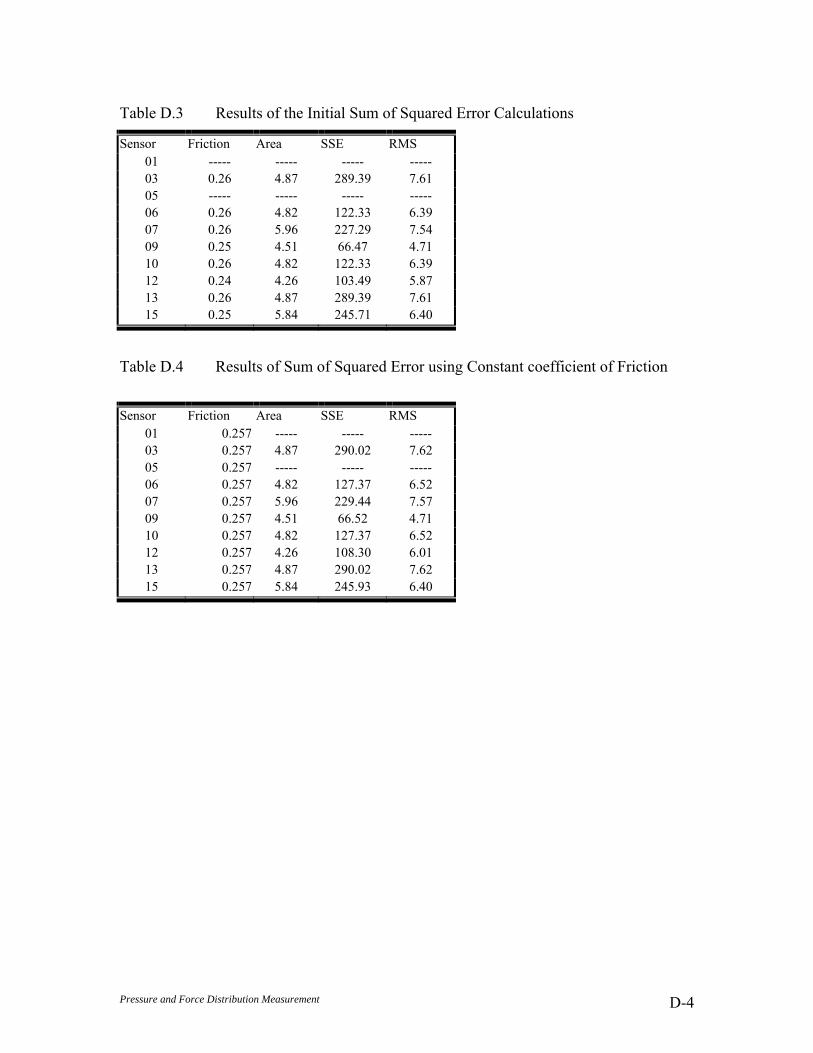
Pressure and Force Distribution Measurement D-4
Table D.3 Results of the Initial Sum of Squared Error Calculations
Sensor Friction Area SSE RMS 01 ----- ----- ----- ----- 03 0.26 4.87 289.39 7.61 05 ----- ----- ----- ----- 06 0.26 4.82 122.33 6.39 07 0.26 5.96 227.29 7.54 09 0.25 4.51 66.47 4.71 10 0.26 4.82 122.33 6.39 12 0.24 4.26 103.49 5.87 13 0.26 4.87 289.39 7.61 15 0.25 5.84 245.71 6.40
Table D.4 Results of Sum of Squared Error using Constant coefficient of Friction
Sensor Friction Area SSE RMS
01 0.257 ----- ----- ----- 03 0.257 4.87 290.02 7.62 05 0.257 ----- ----- ----- 06 0.257 4.82 127.37 6.52 07 0.257 5.96 229.44 7.57 09 0.257 4.51 66.52 4.71 10 0.257 4.82 127.37 6.52 12 0.257 4.26 108.30 6.01 13 0.257 4.87 290.02 7.62 15 0.257 5.84 245.93 6.40

Pressure and Force Distribution Measurement E-1
Appendix E - Determination of Static Coefficient of Friction
The force of friction on a flat surface is:
Where:
Figure E.1 Friction on an inclined plane
On an inclined surface:
Gravity also has an effect on the inclined surface:
The object will slide when Therefore, solving for coefficient of friction
nr FF ×= μ
ForceNormalFfrictionoftCoefficien
frictionofforceF
n
r
___
__
===
μ
WFr ××= θμ cos
WFg ×= θsin
rg FF ≥
θμθθμ
θθμ
tancossin
sincos
=
=
×=××
=
WW
FF rg
θ
Fr
FN
Fg
W
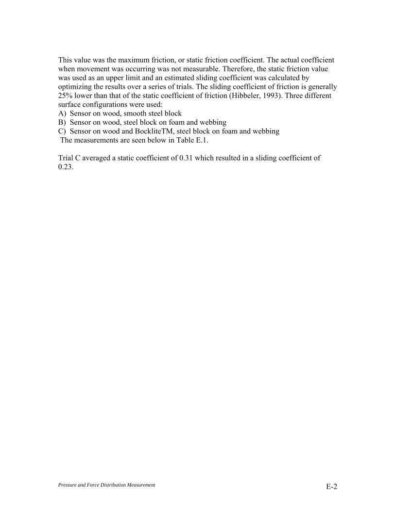
Pressure and Force Distribution Measurement E-2
This value was the maximum friction, or static friction coefficient. The actual coefficient when movement was occurring was not measurable. Therefore, the static friction value was used as an upper limit and an estimated sliding coefficient was calculated by optimizing the results over a series of trials. The sliding coefficient of friction is generally 25% lower than that of the static coefficient of friction (Hibbeler, 1993). Three different surface configurations were used: A) Sensor on wood, smooth steel block B) Sensor on wood, steel block on foam and webbing C) Sensor on wood and BockliteTM, steel block on foam and webbing The measurements are seen below in Table E.1. Trial C averaged a static coefficient of 0.31 which resulted in a sliding coefficient of 0.23.

Pressure and Force Distribution Measurement E-3
Table E.1 Inclined Plane Calculations Inclined Plane Calculations
Trial A Trial B
Mass: 2.75 Lb Mass: 2.78 lb Mass Mat'l: Steel block Mass Mat'l: Steel block on foam and webbing Surface: Sensor on wood Surface: Sensor on wood
Trial Angle (degrees) Coefficient Trial Angle (degrees) Coefficient
1 23 0.4244748 1 22 0.40402622 19 0.3443276 2 22 0.40402623 21 0.383864 3 19 0.34432764 23 0.4244748 4 19 0.34432765 21 0.383864 5 20 0.36397026 21 0.383864 6 19 0.34432767 19 0.3443276 7 18 0.32491978 21 0.383864 8 21 0.3838649 22 0.4040262 9 20 0.3639702
10 22 0.4040262 10 19 0.3443276
Average: 0.3881113 Average: 0.3622087
Trial C
Mass: 5.8 Lb Mass Mat'l: Steel block on foam and webbing Surface: Sensor on wood and Bocklite
Trial Angle (degrees) Coefficient
1 20 0.3639702 2 17 0.3057307 3 18 0.3249197 4 16 0.2867454 5 18 0.3249197 6 16 0.2867454 7 18 0.3249197 8 16 0.2867454 9 17 0.3057307
10 16 0.2867454
Average: 0.3097172
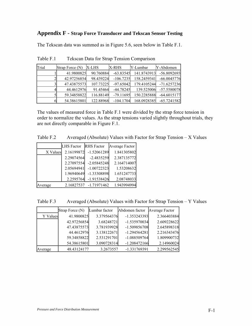
Pressure and Force Distribution Measurement F-1
Appendix F - Strap Force Transducer and Tekscan Sensor Testing The Tekscan data was summed as in Figure 5.6, seen below in Table F.1.
Table F.1 Tekscan Data for Strap Tension Comparison
Trial Strap Force (N) X-LHS X-RHS Y-Lumbar Y-Abdomen 1 41.9800825 90.760884 -63.83545 141.8743913 -56.80926932 42.97256854 98.439224 -106.7235 158.2459341 -66.00457763 47.43875573 107.73225 -97.65042 179.4105244 -71.62572364 44.4612976 91.45464 -44.78245 139.525006 -57.55800785 59.34858822 116.88149 -79.11695 150.2285888 -64.60151776 54.38615801 122.88968 -104.1704 168.0928385 -65.7241582
The values of measured force in Table F.1 were divided by the strap force tension in order to normalize the values. As the strap tensions varied slightly throughout trials, they are not directly comparable in Figure F.1.
Table F.2 Averaged (Absolute) Values with Factor for Strap Tension – X Values
LHS Factor RHS Factor Average FactorX Values 2.16199872 -1.52061289 1.841305802
2.29074564 -2.4835259 2.387135772 2.27097554 -2.05845248 2.164714007 2.05694941 -1.00722323 1.53208632 1.96940649 -1.33308898 1.651247733 2.2595764 -1.91538426 2.08748033Average 2.16827537 -1.71971462 1.943994994
Table F.3 Averaged (Absolute) Values with Factor for Strap Tension – Y Values
Strap Force (N) Lumbar factor Abdomen factor Average Factor Y Values 41.9800825 3.379564376 -1.353243393 2.366403884
42.97256854 3.68248721 -1.535970034 2.609228622 47.43875573 3.781939928 -1.509856708 2.645898318 44.4612976 3.138122671 -1.294564281 2.216343476 59.34858822 2.531291701 -1.088509764 1.809900732 54.38615801 3.090728314 -1.208472166 2.14960024 Average 48.43124177 3.2673557 -1.331769391 2.299562545
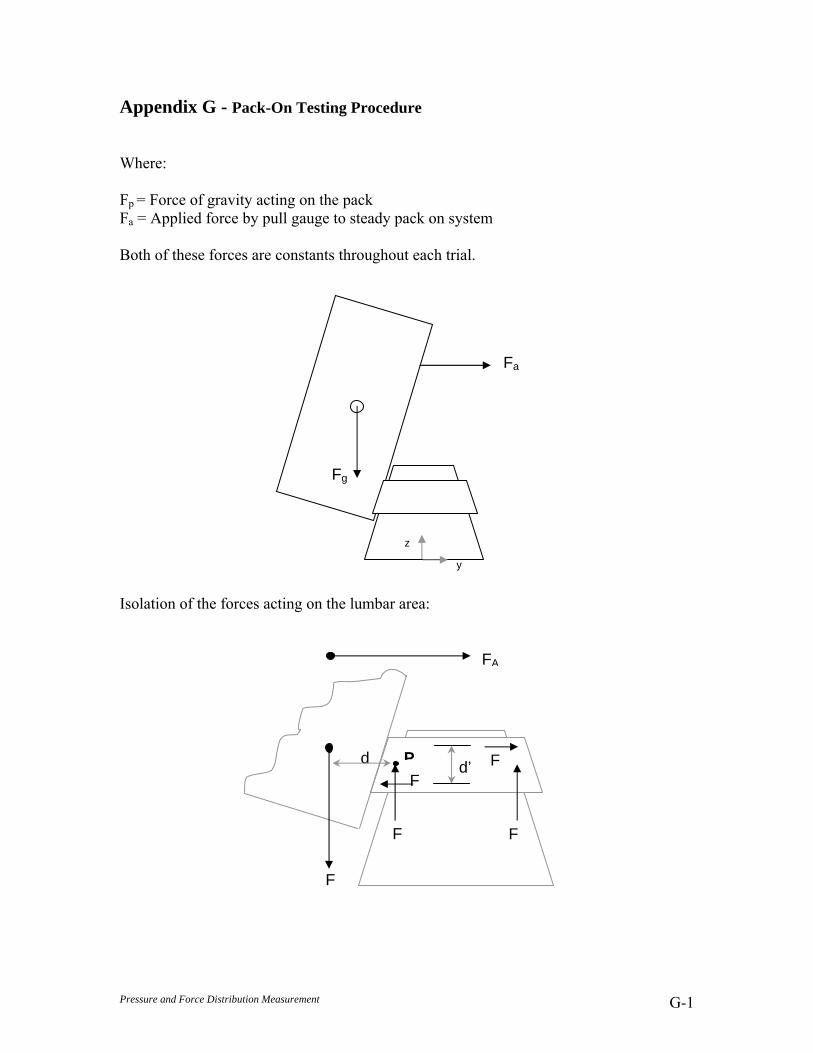
Pressure and Force Distribution Measurement G-1
Appendix G - Pack-On Testing Procedure Where: Fp = Force of gravity acting on the pack Fa = Applied force by pull gauge to steady pack on system Both of these forces are constants throughout each trial. Isolation of the forces acting on the lumbar area:
Fa
z
y
Fg
d’
F
d
F
F
FF
P
FA

UNCLASSIFIED
DOCUMENT CONTROL DATA(Security classification of the title, body of abstract and indexing annotation must be entered when the overall document is classified)
1. ORIGINATOR (The name and address of the organization preparing the document, Organizationsfor whom the document was prepared, e.g. Centre sponsoring a contractor's document, or taskingagency, are entered in section 8.)
Publishing: DRDC Toronto
Performing: Ergonomics Research Group, Queen's University,Kingston, Ontario K7L 3N6
Monitoring:
Contracting: DRDC Toronto
2. SECURITY CLASSIFICATION(Overall security classification of the documentincluding special warning terms if applicable.)
UNCLASSIFIED
3. TITLE (The complete document title as indicated on the title page. Its classification is indicated by the appropriate abbreviation (S, C, R, or U) in parenthesis atthe end of the title)
Development of a Dynamic Biomechanical Model for Load Carriage: Phase III Part C1:Pressure and Force Distribution Measurement for the Design of Waist Belts in PersonalLoad Carriage Systems (U)
4. AUTHORS (First name, middle initial and last name. If military, show rank, e.g. Maj. John E. Doe.)
L.J. Hadcock
5. DATE OF PUBLICATION(Month and year of publication of document.)
August 2005
6a NO. OF PAGES(Total containing information, includingAnnexes, Appendices, etc.)
117
6b. NO. OF REFS(Total cited in document.)
38
7. DESCRIPTIVE NOTES (The category of the document, e.g. technical report, technical note or memorandum. If appropriate, enter the type of document,e.g. interim, progress, summary, annual or final. Give the inclusive dates when a specific reporting period is covered.)
Contract Report
8. SPONSORING ACTIVITY (The names of the department project office or laboratory sponsoring the research and development − include address.)
Sponsoring:
Tasking:
9a. PROJECT OR GRANT NO. (If appropriate, the applicableresearch and development project or grant under which the document waswritten. Please specify whether project or grant.)
12CM03
9b. CONTRACT NO. (If appropriate, the applicable number under whichthe document was written.)
W7711−0−7632−06
10a. ORIGINATOR'S DOCUMENT NUMBER (The officialdocument number by which the document is identified by the originatingactivity. This number must be unique to this document)
DRDC Toronto CR 2005−121
10b. OTHER DOCUMENT NO(s). (Any other numbers under whichmay be assigned this document either by the originator or by thesponsor.)
11. DOCUMENT AVAILABILITY (Any limitations on the dissemination of the document, other than those imposed by security classification.)
Unlimited distribution
12. DOCUMENT ANNOUNCEMENT (Any limitation to the bibliographic announcement of this document. This will normally correspond to the DocumentAvailability (11), However, when further distribution (beyond the audience specified in (11) is possible, a wider announcement audience may be selected.))
Unlimited announcement
UNCLASSIFIED
UNCLASSIFIED
DOCUMENT CONTROL DATA(Security classification of the title, body of abstract and indexing annotation must be entered when the overall document is classified)
13. ABSTRACT (A brief and factual summary of the document. It may also appear elsewhere in the body of the document itself. It is highly desirable that the abstract
of classified documents be unclassified. Each paragraph of the abstract shall begin with an indication of the security classification of the information in the paragraph(unless the document itself is unclassified) represented as (S), (C), (R), or (U). It is not necessary to include here abstracts in both official languages unless the text isbilingual.)
(U) In previous studies, two biomechanical models were developed that used pack and persongeometry as well as pack mass to determine the reaction forces on the body. Oneperpetual problem has been determining the pack−person interface forces usingTekscanTM pressure sensors on rounded surfaces such as the shoulder and waist. Thegoal of this study was to determine design factors that affect force distribution of thebackpack waist belt. A human−sized symmetrical lower torso (SLT) was created of woodand covered with BockliteTM. A method of calculating the directional coordinates ofapplied forces was developed in order to understand the reactions between pack andperson. TekscanTM Sensors were used on the surface to measure the surface pressuresbetween the torso and the waist belt. These were converted to normal force measuresbased on the mathematical coordinates of each sensel. A strategy was developed forcalibration of TekscanTM on a curved surface. Calibration factors, a factor of effectivesensel area and a frictional coefficient for the in situ orientation of each sensor werecalculated and used for the calculation of the directional forces. Then, using selected siteson the waist belt, known forces were applied and the resulting directional forces correlatedmoderately well with the known applied forces (19%). The pressure distributions of threewaist belts were compared and the design features were examined to account fordifferences in distribution. The distributions were compared to results of the previousbiomechanical models and determined to be too complex to be resolved with the simplifiedhoop stress theory. The study determined the importance of waist belt design, frictionalforce from belt tightening, and influence of load in understanding the force distribution of awaist belt. A limiting factor was the lack of precision of TekscanTM and its inability tomeasure shearing frictional forces, a key variable in understanding how a backpack works.It is recommended that each pack and load condition be tested using this approach if onewishes to use the waist strap force gauge to determine compressive forces on the lumbarspine and on the hips.
14. KEYWORDS, DESCRIPTORS or IDENTIFIERS (Technically meaningful terms or short phrases that characterize a document and could be helpful in
cataloguing the document. They should be selected so that no security classification is required. Identifiers, such as equipment model designation, trade name,military project code name, geographic location may also be included. If possible keywords should be selected from a published thesaurus, e.g. Thesaurus ofEngineering and Scientific Terms (TEST) and that thesaurus identified. If it is not possible to select indexing terms which are Unclassified, the classification of eachshould be indicated as with the title.)
(U) Load carriage; Dynamic Biomechanical Model; Lower Torso Model; Waist Belt Model;Pressure and Force Distribution; Contact pressure Sensors; Strap Force Tension;Tekscan
UNCLASSIFIED