Embed Size (px)
Citation preview
DEVELOPMENT OF A METHODOLOGY FOR GEOSPATIAL IMAGE
STREAMING
A THESIS SUBMITTED TO
THE GRADUATE SCHOOL OF NATURAL AND APPLIED SCIENCES
OF
MIDDLE EAST TECHNICAL UNIVERSITY
BY
ERDEM TURKER KIVCI
IN PARTIAL FULFILLMENT OF THE REQUIREMENTS
FOR
THE DEGREE OF MASTER OF SCIENCE
IN
GEODETIC AND GEOGRAPHICAL INFORMATION TECHNOLGIES
SEPTEMBER 2010

Approval of the thesis:
DEVELOPMENT OF A METHODOLOGY FOR GEOSPATIAL IMAGE
STREAMING
submitted by ERDEM TURKER KIVCI in partial fulfillment of the requirements
for the degree of Master of Science in Geodetic and Geographical Information
Technolgies Department, Middle East Technical University by,
Prof. Dr. Canan Özgen
Dean, Graduate School of Natural and Applied Sciences
Assoc. Prof. Mahmut Onur Karslıoğlu
Head of Department, Geodetic and Geographical Inf. Tech.
Assoc. Prof. Dr. Şebnem Düzgün
Supervisor, Mining Engineering Dept., METU
Examining Committee Members:
Prof. Dr. Vedat Toprak
Geological Engineering Dept., METU
Assoc. Prof. Dr. Şebnem Düzgün
Mining Engineering Dept., METU
Asst. Prof. Dr. Refik Samet
Computer Engineering, Ankara University
Asst. Prof. Dr. Erhan Eren
Information Systems Dept., METU
Levent Ucuzal, M.Sc.
General Manager, Bilgi GIS
Date: 13.09.2010

iii
I hereby declare that all information in this document has been obtained and
presented in accordance with academic rules and ethical conduct. I also declare
that, as required by these rules and conduct, I have fully cited and referenced
all material and results that are not original to this work.
Name, Last name: ERDEM TURKER KIVCI
Signature : _________________
iv
ABSTRACT
DEVELOPMENT OF A METHODOLOGY FOR GEOSPATIAL IMAGE
STREAMING
Kıvcı, Erdem Türker
M.S., Department of Geodetic and Geographical Information Technolgies
Supervisor: Assoc. Prof. Dr. Şebnem Düzgün
September 2010, 109 pages
Serving geospatial data collected from remote sensing methods (satellite images,
areal photos, etc.) have become crutial in many geographic information system (GIS)
applications such as disaster management, municipality applications, climatology,
environmental observations, military applications, etc. Even in today’s highly
developed information systems, geospatial image data requies huge amount of
physical storage spaces and such characteristics of geospatial image data make its
usage limited in above mentioned applications. For this reason, web-based GIS
applications can benefit from geospatial image streaming through web-based
architectures. Progressive transmission of geospatial image and map data on web-
based architectures is implemented with the developed image streaming
methodology. The software developed allows user interaction in such a way that the
users will visualize the images according to their level of detail. In this way
geospatial data is served to the users in an efficient way. The main methods used to
transmit geospatial images are serving tiled image pyramids and serving wavelet
v
based compressed bitstreams. Generally, in GIS applications, tiled image pyramids
that contain copies of raster datasets at different resolutions are used rather than
differences between resolutions. Thus, redundant data is transmitted from GIS server
with different resolutions of a region while using tiled image pyramids. Wavelet
based methods decreases redundancy. On the other hand methods that use wavelet
compressed bitsreams requires to transform the whole dataset before the
transmission. A hybrid streaming methodology is developed to decrease the
redundancy of tiled image pyramids integrated with wavelets which does not require
transforming and encoding whole dataset. Tile parts’ coefficients produced with the
methodlogy are encoded with JPEG 2000, which is an efficient technology to
compress images at wavelet domain.
Keywords: Image Compression, OGC, WMS, WMTS, Geospatial Raster Data,
Wavelet Transformation, Tiled Image Pyramids, JPEG 2000
vi
ÖZ
MEKANSAL İÇERİKLİ GÖRÜNTÜ AKIŞI İÇİN BİR YÖNTEM
GELİŞTİRİLMESİ
Kıvcı, Erdem Türker
Yüksek Lisans, Jeodezi ve Coğrafi Bilgi Teknolojileri Bölümü
Tez Yöneticisi: Doç. Dr. Şebnem Düzgün
Eylül 2010, 109 sayfa
Uzaktan algılama yöntemleri (uydular, hava araçları, vb.) ile toplanmış olan
mekansal içerikli verilerin sunumu afet yönetimi, belediyecilik, iklim bilimi
uygulamaları, çevresel gözlem uygulamaları, askeri uygululamalar gibi birçok alanda
önem kazanmıştır. Mekansal içerikli görüntü veri tabanları, günümüz koşullarına
göre, fiziksel olarak çok yer kaplamaktadır ve bu verinin sunumu ve iletimi yukarıda
sözü edilen alanlarda kullanımını yavaşlatmaktadır. Bu nedenle uygulamaların,
mekansal içerikli görüntü sunum hizmetlerini merkezi veri tabanı üzerinden, web
tabanlı bir mimari ile sağlamaları gerekmektedir. Mekansal içerikli görüntünün
arttırımsal iletimi geliştirilmiş olan görüntü akışı methodunun gerçekleştirilmesi ile
sağlanmıştır. Geliştirilmiş olan bu sistem görüntü ile etkileşimleri (görütü üzerinde
gezinme, görüntüye yaklaşma, uzaklaşma vb.) de gözönüne alınarak, kullanıcıların
görüntülemek istedikleri veriyi kendileri için anlamlı seviyedeki detayda
görüntüleyip kullanmalarına imkan sağlamaktadır. Web üzerinden coğrafi görüntü
vii
iletimi için kullanılmakta olan 2 temel yöntem; bölünmüş görüntü piramitlerinin
sunuluması ve dalgacık dönüşümü kullanılarak sıkıştırılmış veri bloklarının
sunulmasıdır. Coğrafi bilgi sistemlerinde kullanılmakta olan görüntü piramitleri
genellikle veri setinin farklı çözünürlükler arasında ki farklarını değil doğrudan
kopyalarını içermektedir. Bu nedenle bölünmüş görüntü piramitlerinin
aktarılmasında tekrarlı veri aktarımı söz konusudur. Dalgacık dönüşümü tabanlı
sıkıştırma yöntemleri ise bütün veri seti üzerinde uygulanması sonrasında
kullanıldığından dolayı ancak veri setinin tamamı dönüştürüldükten sonra veri
sunulabilmektedir. Geliştirilen görüntü akışı yöntemi ile bölümüş görüntü
piramitlerinin dalgacık dönüşümleriyle bütünleştirilmesiyle tekrar eden veri aktarımı
azaltılmış ve veri setinin tamamının dönüştürülmesine gerek kalmadan görüntü
iletimi sağlanabilmektedir. Dönüştürülmüş görüntü parçaları dalgacık tabanlı
görüntüleri etkin bir biçimde sıkıştırmakta olan JPEG 2000 teknlojisi ile
kodlanmıştır.
Anahtar Kelimeler : Görüntü Sıkıştırma, OGC, WMS, WMTS, Coğrafi Rastar Veri,
Dalgacık Dönüşümü, Bölünmüş Görüntü Piramidi, JPEG 2000

viii
To my familiy

ix
ACKNOWLEDGEMENTS
I am very grateful to Assoc. Prof. Dr. Şebnem Düzgün for her guidance suggestions,
explanations and encouragement throughout my study. Without her assistance and
effort, I could not complete this thesis within the period of M.S. study
Special thanks to my father Çetin and my mother Meral and my sister Yasemin for
their endless motivation, understanding and encouragement. I also would like to
thank Meral Özkaya for her motivation and support during my study.
I would like to thak to Ministiry of Industry & Trade and Bilgi GIS for their
financial support to my study (covered in the project “İnternet Tabanli Mekansal
İçerikli Görüntü İletemi Yazılımı”, code of project “00162.STZ.2007-2”) which is
funded as a SAN-TEZ project. I also would like to thank to Bilgi GIS family for
technical and courage support. Their tolerance and support increased my desire to
overcomemy thesis.

x
TABLE OF CONTENTS
ABSTRACT ................................................................................................................. iv
ÖZ ................................................................................................................................ vi
ACKNOWLEDGEMENTS ......................................................................................... ix
TABLE OF CONTENTS .............................................................................................. x
LIST OF TABLES ...................................................................................................... xii
LIST OF FIGURES ................................................................................................... xiv
ABREVIATIONS ...................................................................................................... xvi
CHAPTERS
1 INTRODUCTION ............................................................................................... 1
1.1 REQUIREMENTS TO INCREASE THE PERFORMANCE OF
IMAGE TRANSMISSION ................................................................................... 2
1.2 METHODS USED TO INCREASE PERFORMANCE OF
GEOSPATIAL IMAGE TRANSMISSION .......................................................... 5
1.2.1 TILED IMAGE PYRAMIDS ............................................................ 5
1.2.2 TRANSFORMED AND COMPRESSED IMAGE BITSTREAMS 9
1.3 PROBLEM DEFINITION AND OBJECTIVES ....................................... 12
2 RASTER DATA MANAGEMENT .................................................................. 16
2.1 CHALLENGES OF RASTER DATA MANAGEMENT .......................... 16
2.1.1 SIZE OF GEOSPATIAL IMAGES ................................................... 16
2.1.2 ARRANGING REQUIRED METADATA ....................................... 19
2.1.3 OPERATIONS FOR GEOSPATIAL IMAGE TRANMISSION ...... 20
2.2 RASTER DATA STORAGE ..................................................................... 21
3 IMAGE TRANSFORMATIONS ...................................................................... 25
3.1 DISCRETE COSINE TRANSFORMATION ............................................ 25
3.2 KARHUNEN LOEWE TRANSFORMATION ......................................... 29
3.3 WAVELET TRANSFORMATION ........................................................... 37
4 DEVELOPED METHODOLOGY FOR PROGRESSIVE TILE
TRANSMISSION ....................................................................................................... 43
4.1 METHODOLOGY ....................................................................................... 44
4.2 IMPLEMENTATION ................................................................................ 48
4.3 RESULTS AND DISCUCCSIONS ........................................................... 52

xi
4.3.1 SCANNED MAPS ............................................................................. 58
4.3.2 HIGH RESOLUTION ORTHO IMAGES ........................................ 61
4.3.3 SHADED RELIEFS .......................................................................... 63
4.3.4 ALTERNATIVE COMPOSITIONS OF SATELLITE IMAGES .... 65
4.3.5 BLUE MARBLE NEXT GENERATION ......................................... 68
5 CONCLUSIONS AND RECOMENDATIONS ............................................... 71
REFERENCES ............................................................................................................ 74
ONLINE REFERENCES .................................................................................... 76
APPENDICES
A TEST IMAGE DATASETS ............................................................................. 77
B SOURCE CODE ............................................................................................. 88
xii
LIST OF TABLES
TABLES
Table 1.1 Requirements to increase the performance of image transmission .............. 2
Table 2.1 Storage Properties of Geographical Raster Datasets For a Region With a
Minimum Bounding Box has dimension 50Km x 60km ...................................... ….18
Table 2.2 Comparisson of different raster formats .................................................... 24
Table 3.1 Eigenvalues related with each components of Landsat TM 7 bands
transformation .......................................................................................................... ..31
Table 3.2 SNR values of each band for number of components used ....................... 32
Table 3.3 RMSE values of each band for number of components used .................... 33
Table 3.4 Eigen Values of single band KLT with row order……………………….33
Table 3.5 Eigen Values of single band KLT with resampling order ………………36
Table 3.6 SNR Values of single band KLT for number of components used ……..37
Table 3.7 File Sizes of the Wavelet Transformed Lossless Compressed Pyramid Tile
Bitsreams With JPEG 2000 and Non-hierarchical PNG Images …………………..42
Table 4.1 Lossy Compressed Image Tile Pyramid hierarchy Size ………………..54
Table 4.2 Comparision of JPEG 2000 encoded Image Tile Pyramid and Progressive
Image Tile Pyramid hierarchies SNR ……………………………………………...57
Table 4.3 Comparision of JPEG encoded Image Tile Pyramid and Progressive Image
Tile Pyramid hierarchies SNR ……………………………………………………..58
Table 4.4 Lossy compressed DRG-250K-3 image JP2 JPEG and Progressive Tile
xiii
Stream Based on W5x3 SNRs ……………………………………………………...59
Table 4.5 Lossy compressed Ortho Image-1 image JP2 JPEG and Progressive Tile
Stream Based on W5x3 SNRs……………………………………………………....62
Table 4.6 Lossy compressed Srtm-relief image JP2 JPEG and Progressive Tile
Stream Based on W5x3 SNRs ……………………………………………………...64
Table 4.7 Lossy compressed Escon-vnir image JP2 JPEG and Progressive Tile
Stream Based on W5x3 SNRs ……………………………………………………...67
Table 4.8 Lossy compressed Bmng-3 image JP2 JPEG and Progressive Tile Stream
Based on W5x3 SNRs ………………………………………………………………69
xiv
LIST OF FIGURES
FIGURES
Figure 1.1 A tile image pyramid structure with downsampling factor 2 and 3
resolution levels ........................................................................................................... 6
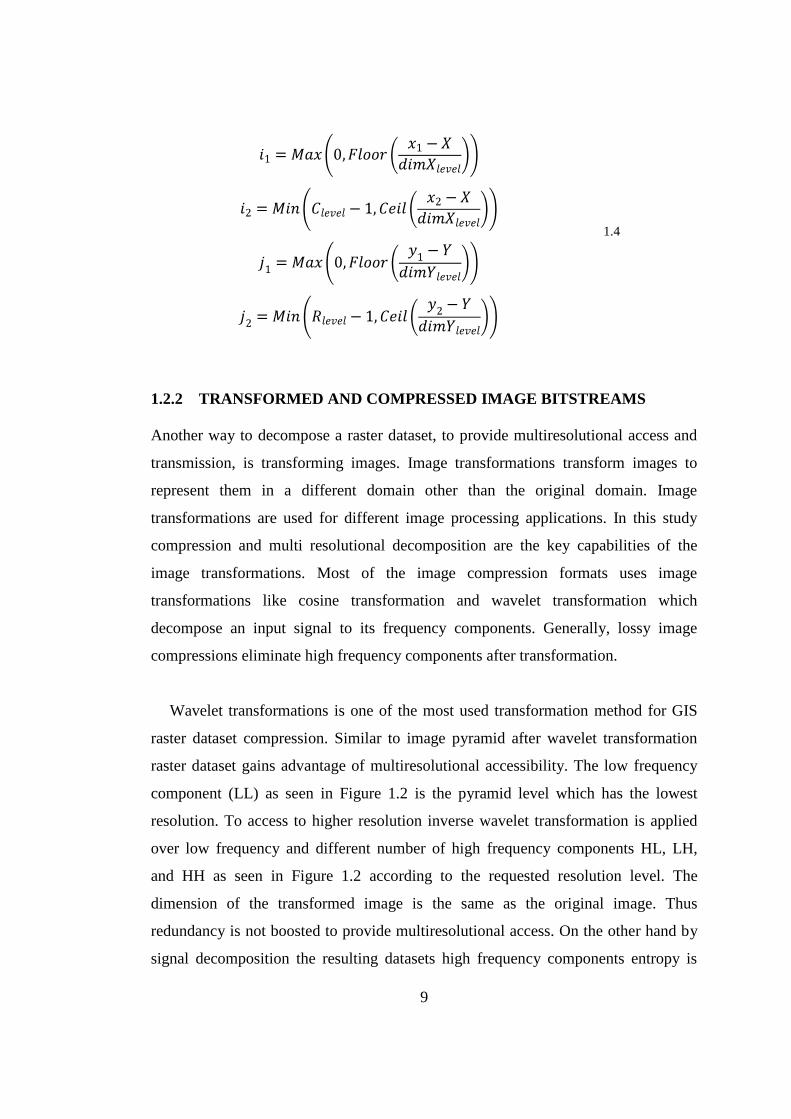
Figure 1.2 Frequency Components of a Wavelet Transformed Image with 4
resolution levels ......................................................................................................... 10
Figure 1.3 Precincts in a JPEG2000 structure with red dashed lines ......................... 12
Figure 1.4 General architecture of discussed systems ............................................... 13
Figure 1.5 Basic model of system that is developed .................................................. 15
Figure 3.1 Flow chart of JPEG progressive coding ................................................... 28
Figure 3.2 Flow chart of KLT .................................................................................... 30
Figure 3.3 Landsat TM Images 7 bands to be transformed with KLT ....................... 31
Figure 3.4 Landsat TM Images 7 components KLT transformation result................ 32
Figure 3.5 Vector determination function with resampling sample over single band 34
Figure 3.6 Landsat TM Image single component KLT transformation result ........... 35
Figure 3.7 Subband Coding………………………………………….……………...39
Figure 3.8 Wavelet Transformed Landsat TM Image from Izmir region…………...39
Figure 3.9 Single component of Landsat TM Image from Izmir region……………40
Figure 3.10 Inverse transformation with lifting scheme …………………….……...40
Figure 3.11 Inverse transformation with lifting scheme …………………….……...41
Figure 4.1 Flow chart of hybrid methodology developed for progressive image tiles
.................................................................................................................................... 46
Figure 4.2 Architecture of the Developed Geopsatial Image Transmission System.51
Figure 4.3 Lossless compressed JP2 encoded tiled image pyramids and JP2 encoded
Progressive Image Tiles……………………………………………………………..56
Figure 4.4 Number of tiles downloaded with 1Mbps of DRG-250K-3 image with
different image pyramid hierarchies .......................................................................... 59
xv
Figure 4.5 Number of tiles downloaded with 1Mbps of Ortho-Image-1 image with
different image pyramid hierarchies .......................................................................... 62
Figure 4.6 Number of tiles downloaded with 1Mbps of Srtm-Relief image with
different image pyramid hierarchies .......................................................................... 64
Figure 4.7 Number of tiles downloaded with 1Mbps of Escon-vnir image with
different image pyramid hierarchies .......................................................................... 66
Figure 4.8 Number of tiles downloaded with 1Mbps of Bmng-3 image with different
image pyramid hierarchies ....................................................................................... ..69
Figure A.1 Istanbul Landsat Image 1……………………………..…………………78
Figure A.2 Istanbul Landsat Image 2………………………………………………..79
Figure A.3 LANDSAT-N36-1 Image……………………………………………….79
Figure A.4 LANDSAT-N36-2 Image……………………………………………….80
Figure A.5 WA State LANDSAT…………………………………………………...80
Figure A.6 Escon-vnir Image……………………………………………………….81
Figure A.7 WA State Relief…………………………………………………………81
Figure A.8 SRTM Relief……………………………………………………………82
Figure A.9 Ortho Image 1……………………………………………….…………..82
Figure A.10 Ortho Image 2………………………………………………………….83
Figure A.11 Ortho Image 3………………………………………………………….83
Figure A.12 Ortho Image 4………………………………………………………….84
Figure A.13 Ortho Image 5………………………………………………………….84
Figure A.14 Blue Marble Next Generation Image……….……………….…………85
Figure A.15 DRG 250K Image1………………………………………...…………..86
Figure A.16 DRG 250K Image 2 ……………………………………..…………….86
Figure A.17 DRG 250K Image 3……………………………………...…………….87
Figure A.18 Ancient Piri Reis Map…………………………………………………87

xvi
ABREVIATIONS
GIS Geographical Information Systems
OGC Open Geospatial Consortium
WMS Web Map Service
WMTS Web Map Tile Service
ECW Enhanced Compression Wavelet
ECWP Enhanced Compression Wavelet Protocol
JPEG Joint Photographic Experts Group
JPIP JPEG 2000 Interactive Protocol
PNG Portable Network Graphics
GML Geography Markup Language
WKT Well Known Text
WKB Well Known Binary
BLOB Binary Large Object
DCT Discrete Cosine Transformation
KLT Karhunen Loewe Transformation
DWT Discrete Wavelet Transformation
SNR Signal Noise Ratio
RMSE Root Mean Square Error
STFT Short time Fourier Transformation
PIT Progressive image tiles
1
CHAPTER 1
INTRODUCTION
Geographical Information Systems (GIS) are information systems, which provide to
collect, store, query and display data with related spatial information. There are many
commercial GIS softwares that are used in the market. However, many of them are
desktop applications. GIS starts to take place in nonprofessional people’s life in
nowadays. The strong development of internet supports to development of GIS as a
new architecture, which provides geographical information from sources in different
points, covering user requirements at real time (Wu, et al., 2001).
Increasing structure of broadband communication and personal computers that
supports high performance districted graphics, professional data displaying functions
became popular with services such as Google Earth, NASA Worldwind and
Microsoft Visual Earth (Bettio, et al., 2007). With the emergence of the new
generation GIS and geospatial image transmission standards, usage of the web has
been one of the most important function of GIS. These popular softwares have many
users. In order to construct these softwares effectively, combination of certain
technologies have to be used: displaying geospatial images that have high quality at
high frame speed as adapted, transmitting spatial data from server to client
effectively.
Development of internet, mobile computing technology and wide use of web
increases the popularity of GIS on web. Thus, two basic architectures have been
developed (Hu , et al., July, 2004): Client-server based web mapping and web

2
services mapping systems. Web services use agreed common protocols. The most
common protocol for geographic data serving is Open GIS Consortiums’ (OGC)
protocols. These determined standards for web services, by OGC, provide many
advantages for using web based GIS. However rendering the results for each query
causes low performance which is the significant disadvantage (Hu, 2004). On the
other hand, OGC published a new standard web map tile service (WMTS) (Maso, et
al., 2010) which will have performance improvements over OGC web map services
(WMS) (Beaujardiere, 2004). Furthermore, JPEG 2000 standard part 9 JPEG 2000
Interactive Protocol (JPIP) is one of the most important technologies that are
discussed in OGC Community to improve the transmission of spatial data. OGC Web
Coverage Service is the center of the interest in discussions in the community to
cover the JPIP for spatial data transmission purposes. GIS raster data transmission
performance improvement is an active study field which directly affects the
commercial products enhancements and increases the frequent usage of GIS.
1.1 REQUIREMENTS TO INCREASE THE PERFORMANCE OF IMAGE
TRANSMISSION
Web based GIS generally handles large amount of data and there are several client
architecture which uses different types of connections. Due to these facts,
visualization and transmission methods and data model used by the system has to be
scalable (Komzák , et al., 2003). To provide a scalable system, required capabilities
are listed in Table 1.1;
Table 1.1 Requirements to increase the performance of image transmission
ID Requirement Type
Req-I Dataset served has to be randomly accessible. Data Structure
Req-II Different scales of dataset have to be accessible. Data Structure
Req-III Hierarchical structure of the dataset has to be
seamless.
Data Structure
3
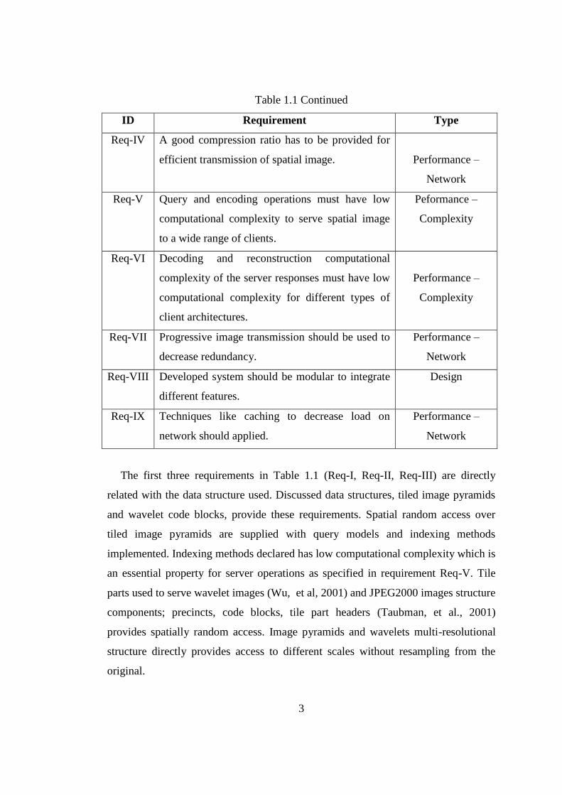
Table 1.1 Continued
ID Requirement Type
Req-IV A good compression ratio has to be provided for
efficient transmission of spatial image.
Performance –
Network
Req-V Query and encoding operations must have low
computational complexity to serve spatial image
to a wide range of clients.
Peformance –
Complexity
Req-VI Decoding and reconstruction computational
complexity of the server responses must have low
computational complexity for different types of
client architectures.
Performance –
Complexity
Req-VII Progressive image transmission should be used to
decrease redundancy.
Performance –
Network
Req-VIII Developed system should be modular to integrate
different features.
Design
Req-IX Techniques like caching to decrease load on
network should applied.
Performance –
Network
The first three requirements in Table 1.1 (Req-I, Req-II, Req-III) are directly
related with the data structure used. Discussed data structures, tiled image pyramids
and wavelet code blocks, provide these requirements. Spatial random access over
tiled image pyramids are supplied with query models and indexing methods
implemented. Indexing methods declared has low computational complexity which is
an essential property for server operations as specified in requirement Req-V. Tile
parts used to serve wavelet images (Wu, et al, 2001) and JPEG2000 images structure
components; precincts, code blocks, tile part headers (Taubman, et al., 2001)
provides spatially random access. Image pyramids and wavelets multi-resolutional
structure directly provides access to different scales without resampling from the
original.
4
Req-IV (compression requirement), Req-VII (progressive image transmission
requirement) and Req-IX (caching requirement) have to be provided to decrease the
load on network and for quick response times. JPIP and ECWP provide direct access
over compressed files which have the related file formats. Also client side caching is
applicable over systems which use these protocols. Jpeg2000 and ECW file formats
used by these protocols provides high compression ratio. A number of compressed
code blocks are served in each response with a progressive order. Thus clients could
progressively reconstruct the requested image and update the displayed image. On
the other hand tiled image pyramids do not support compression natively. However
each tile is a separate image so each tile could be compressed with standard image
file formats. Generally JPEG format is used to store and transmit each tile. Client
side caching is applied for tiles by caching the tiles requested previously (Yang, , et
al., 2005) and also caching the tiles that are prefetched (Tu, et al., 2001) for future
requests. During prefetching tiles that would probably displayed by the user are
requested from the server. By this way if the prefetching is used than the clients have
to make requests with information that declares if the request is a prefetching request
or user request. Therefore the server could order the request to give high priority to
direct user requests. Server would manage request with two different queues. One of
the queues would contain prefetch requests and the other one would contain direct
user requests. Prefetch queue would be processed only if the direct user request
queue is empty.
Low computational complexity of encoding and decoding is a critical issue that
severely affects the performance of the system, which was declared in Req-V and
Req-VI. Thus the image transformations performance is the key element which is the
most important factor encoding process. Integer lifting scheme is preferred in
wavelet transformation for fast transformation. Daubechies 9/7 is a good choice for
natural image compression (Daubechies, 1992). However Haar transformation is

5
preferred to because of the kernel length of the filters which affects the number of
operations that have to be executed to transform the image (Wu, et al., 2001).
1.2 METHODS USED TO INCREASE PERFORMANCE OF GEOSPATIAL
IMAGE TRANSMISSION
There are two main methods to increase performance of transmission of geospatial
images; Tiled image pyramids and serving transformed and compressed bitstreams of
images. Tiled image pyramids have a well structured hierarchy. Queries over such
hierarchy have low computational complexity. However, redundant data is
transmitted within different levels of tiles that cover the same region, which causes
load over the transmission network. Redundancy could be removed with wavelet
transformed compressed code streams. Compressed code blocks are served to clients
in order to response user requests. On the other hand transforming and compression
GIS datasets that would be provided by the server has to be completed before serving
them. Transformation and compression are pre-processes that have to be performed.
If the datasource which is used by the server is not a local datasource than whole data
set has to be downloaded by the server for pre-processing.
1.2.1 TILED IMAGE PYRAMIDS
Tiling image pyramids and indexing them is a popular way to increase the
performance of geospatial image transmission. However, the amount of the data is
increased, where the increase ratio depends on resampling factor declared between
image pyramid levels. Hierarchical structure of an image tile pyramid is seen in
Figure 1.1. Additionally, image pyramids that are used for geospatial images cause
redundant data transmission. This redundancy could be decreased with multi-
resolution image transformations. The amount of the redundant data without
compression could be calculated depending on the amount of the original data (G),
the downsampling facto (dfac) and the number of levels (lev) used. The extra amount
of storage need is calculated nearly 12.5 percent of the original dataset when the
downsampling factor is 3 (Tu, et al.,2001). The generalized formula that is used to
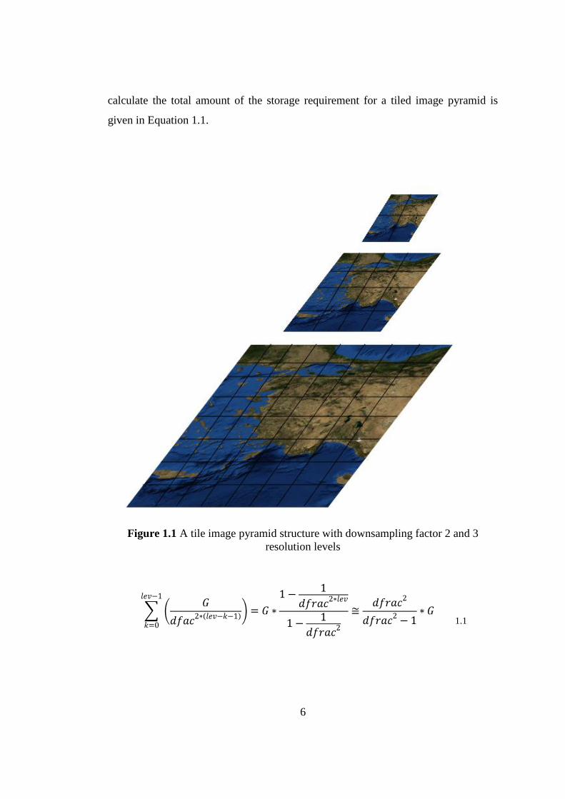
6
calculate the total amount of the storage requirement for a tiled image pyramid is
given in Equation 1.1.
Figure 1.1 A tile image pyramid structure with downsampling factor 2 and 3
resolution levels
1.1
7
Tiled image pyramids are well organized hierarchical data structure to manage
raster datasets. Different scaled regions of resultant sets could be queried over image
pyramids. Structure of image pyramids provides development of different query
models and indexing mechanisms for multiresolution random access over GIS raster
datasets. These queries are executed to reply the basic GIS functions, which are
zoom in - zoom out (this requires random access) and pan or go to declared bounding
rectangle, which also requires random access. The structure and the query
mechanism comes from tile dimensions, which are used in searching methodology
over structure, and the number of levels to build pyramid. The main strategy is to
find the appropriate resolution level from the client request and find the tiles that
have the extent which, intersects with the requested region.
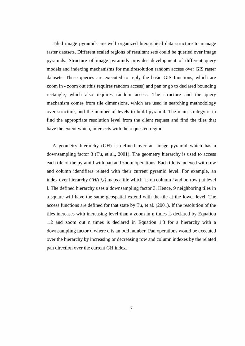
A geometry hierarchy (GH) is defined over an image pyramid which has a
downsampling factor 3 (Tu, et al., 2001). The geometry hierarchy is used to access
each tile of the pyramid with pan and zoom operations. Each tile is indexed with row
and column identifiers related with their current pyramid level. For example, an
index over hierarchy GH(i,j,l) maps a tile which is on column i and on row j at level
l. The defined hierarchy uses a downsampling factor 3. Hence, 9 neighboring tiles in
a square will have the same geospatial extend with the tile at the lower level. The
access functions are defined for that state by Tu, et al. (2001). If the resolution of the
tiles increases with increasing level than a zoom in n times is declared by Equation
1.2 and zoom out n times is declared in Equation 1.3 for a hierarchy with a
downsampling factor d where d is an odd number. Pan operations would be executed
over the hierarchy by increasing or decreasing row and column indexes by the related
pan direction over the current GH index.
8
1.2
1.3
Using this indexing method, each tile index required to display the requested
region is computed directly by the client. This method is worthwhile for clients that
generally requests static scale range between each level. But the new generation GISs
clients users scale ranges is not be defined as clear as this state. Since each user type
do not need the same pyramid levels of the datasets. Hash indexing function over
pyramids (Yang, et al.,, 2005) method is more applicable in this case. A hash
function produces tile identifiers for a bounding box of region of interest. Similar to
the previous technique a pyramid contains multi resolutional redundant images of the
original dataset. On the other hand geographical coordinates are directly used rather
than geometric hierarchy to query over the tiled pyramid structure. Each pyramid
level scale and dimension of the geographical extent of a tile (dimX,dimY) and the
number of tiles over row R and column C for each level are stored as metadata over
the structure. When a client request is made over the structure, the pyramid level
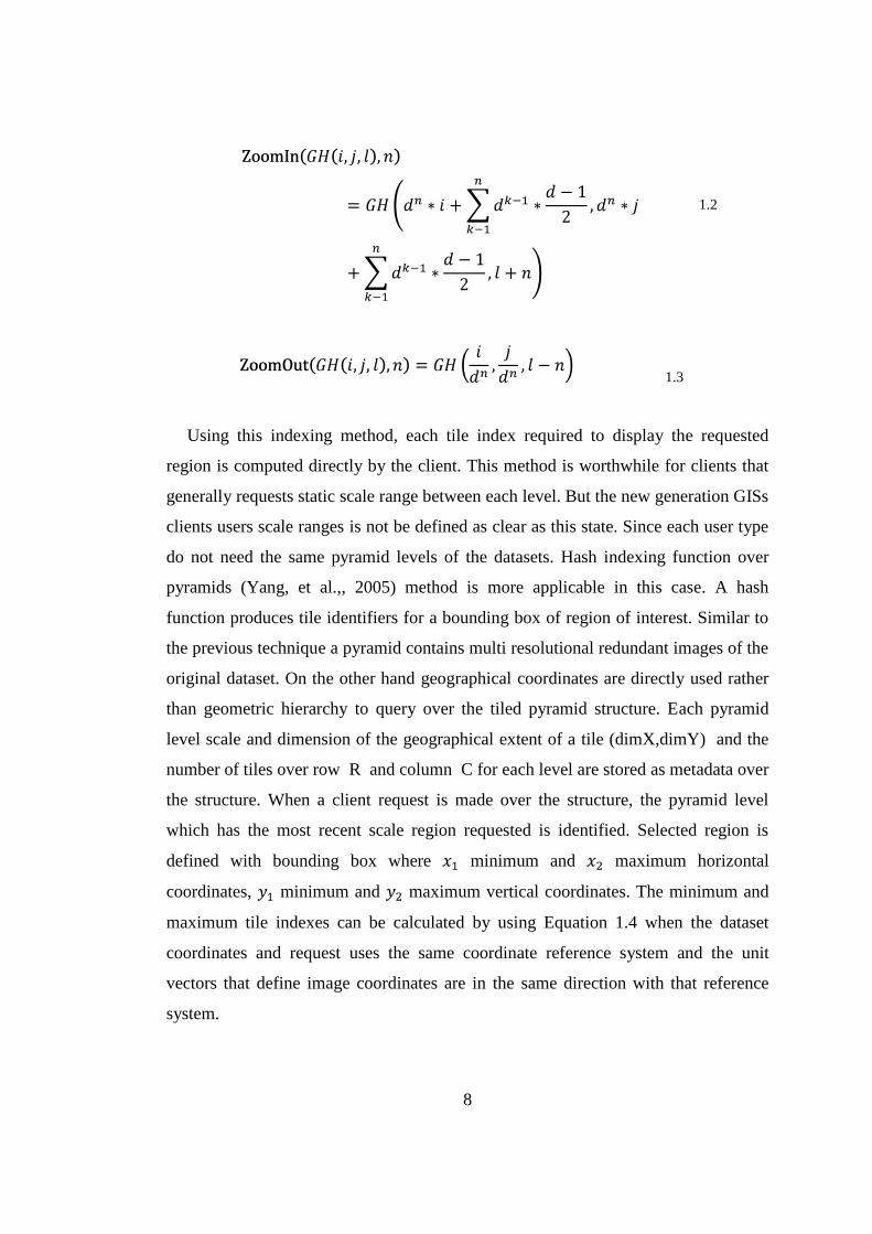
which has the most recent scale region requested is identified. Selected region is
defined with bounding box where minimum and maximum horizontal
coordinates, minimum and maximum vertical coordinates. The minimum and
maximum tile indexes can be calculated by using Equation 1.4 when the dataset
coordinates and request uses the same coordinate reference system and the unit
vectors that define image coordinates are in the same direction with that reference
system.
9
1.4
1.2.2 TRANSFORMED AND COMPRESSED IMAGE BITSTREAMS
Another way to decompose a raster dataset, to provide multiresolutional access and
transmission, is transforming images. Image transformations transform images to
represent them in a different domain other than the original domain. Image
transformations are used for different image processing applications. In this study
compression and multi resolutional decomposition are the key capabilities of the
image transformations. Most of the image compression formats uses image
transformations like cosine transformation and wavelet transformation which
decompose an input signal to its frequency components. Generally, lossy image
compressions eliminate high frequency components after transformation.
Wavelet transformations is one of the most used transformation method for GIS
raster dataset compression. Similar to image pyramid after wavelet transformation
raster dataset gains advantage of multiresolutional accessibility. The low frequency
component (LL) as seen in Figure 1.2 is the pyramid level which has the lowest
resolution. To access to higher resolution inverse wavelet transformation is applied
over low frequency and different number of high frequency components HL, LH,
and HH as seen in Figure 1.2 according to the requested resolution level. The
dimension of the transformed image is the same as the original image. Thus
redundancy is not boosted to provide multiresolutional access. On the other hand by
signal decomposition the resulting datasets high frequency components entropy is

10
decreased which causes better compression. Because of these capabilities of wavelet
transformation, it is used in different applications and studies in addition to
compressed file formats.
Figure 1.2 Frequency Components of a Wavelet Transformed Image with 4
resolution levels
Enhanced Compression Wavelet (ECW) is a proprietary image file format
developed by Earth Resource Mapping. ECW images could be transmitted
progressively. Image data blocks are served to client and compressed blocks are
decompressed and the resulting codeblocks are decomposed to build the requested
image on client. Only the data blocks requested for the map extents at requested
resolution are served to the client. The clients could cache the served data blocks
compressed or uncompressed so redundant transmission could be prevented. This
provides a significant reduction on network load (Merzhausen, 2001).
11
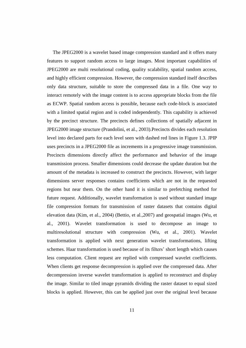
The JPEG2000 is a wavelet based image compression standard and it offers many
features to support random access to large images. Most important capabilities of
JPEG2000 are multi resolutional coding, quality scalability, spatial random access,
and highly efficient compression. However, the compression standard itself describes
only data structure, suitable to store the compressed data in a file. One way to
interact remotely with the image content is to access appropriate blocks from the file
as ECWP. Spatial random access is possible, because each code-block is associated
with a limited spatial region and is coded independently. This capability is achieved
by the precinct structure. The precincts defines collections of spatially adjacent in
JPEG2000 image structure (Prandolini, et al., 2003).Precincts divides each resolution
level into declared parts for each level seen with dashed red lines in Figure 1.3. JPIP
uses precincts in a JPEG2000 file as increments in a progressive image transmission.
Precincts dimensions directly affect the performance and behavior of the image
transmission process. Smaller dimensions could decrease the update duration but the
amount of the metadata is increased to construct the precincts. However, with larger
dimensions server responses contains coefficients which are not in the requested
regions but near them. On the other hand it is similar to prefetching method for
future request. Additionally, wavelet transformation is used without standard image
file compression formats for transmission of raster datasets that contains digital
elevation data (Kim, et al., 2004) (Bettio, et al.,2007) and geospatial images (Wu, et
al., 2001). Wavelet transformation is used to decompose an image to
multiresolutional structure with compression (Wu, et al., 2001). Wavelet
transformation is applied with next generation wavelet transformations, lifting
schemes. Haar transformation is used because of its filters’ short length which causes
less computation. Client request are replied with compressed wavelet coefficients.
When clients get response decompression is applied over the compressed data. After
decompression inverse wavelet transformation is applied to reconstruct and display
the image. Similar to tiled image pyramids dividing the raster dataset to equal sized
blocks is applied. However, this can be applied just over the original level because
12
multi resolutional structure is achieved by wavelets which are separately applied over
each block.
Figure 1.3 Precincts in a JPEG2000 structure with red dashed lines
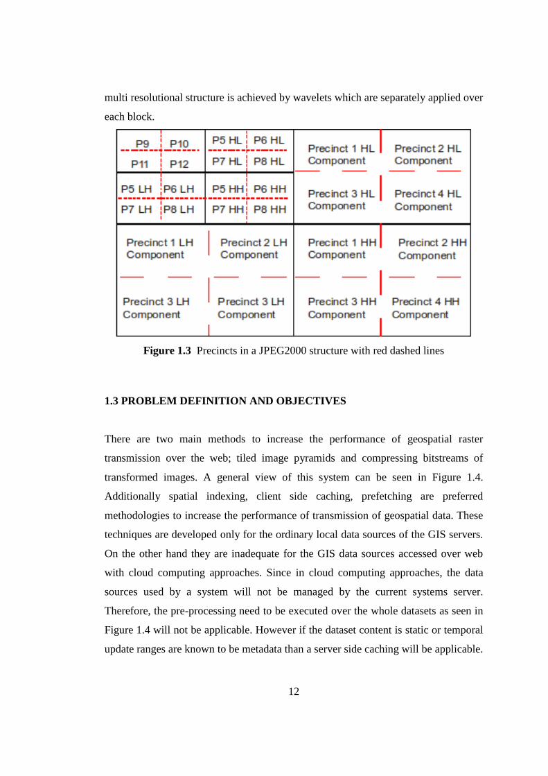
1.3 PROBLEM DEFINITION AND OBJECTIVES
There are two main methods to increase the performance of geospatial raster
transmission over the web; tiled image pyramids and compressing bitstreams of
transformed images. A general view of this system can be seen in Figure 1.4.
Additionally spatial indexing, client side caching, prefetching are preferred
methodologies to increase the performance of transmission of geospatial data. These
techniques are developed only for the ordinary local data sources of the GIS servers.
On the other hand they are inadequate for the GIS data sources accessed over web
with cloud computing approaches. Since in cloud computing approaches, the data
sources used by a system will not be managed by the current systems server.
Therefore, the pre-processing need to be executed over the whole datasets as seen in
Figure 1.4 will not be applicable. However if the dataset content is static or temporal
update ranges are known to be metadata than a server side caching will be applicable.
13
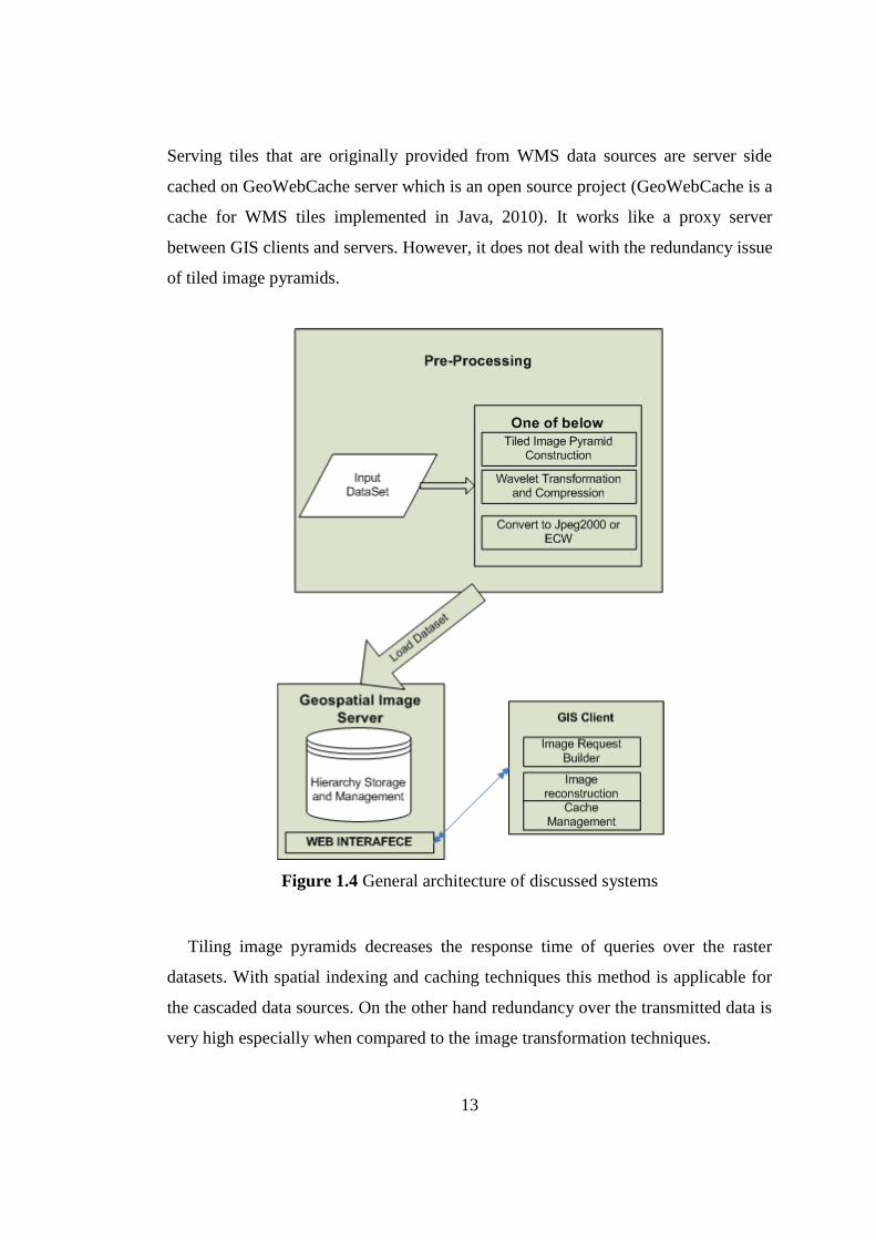
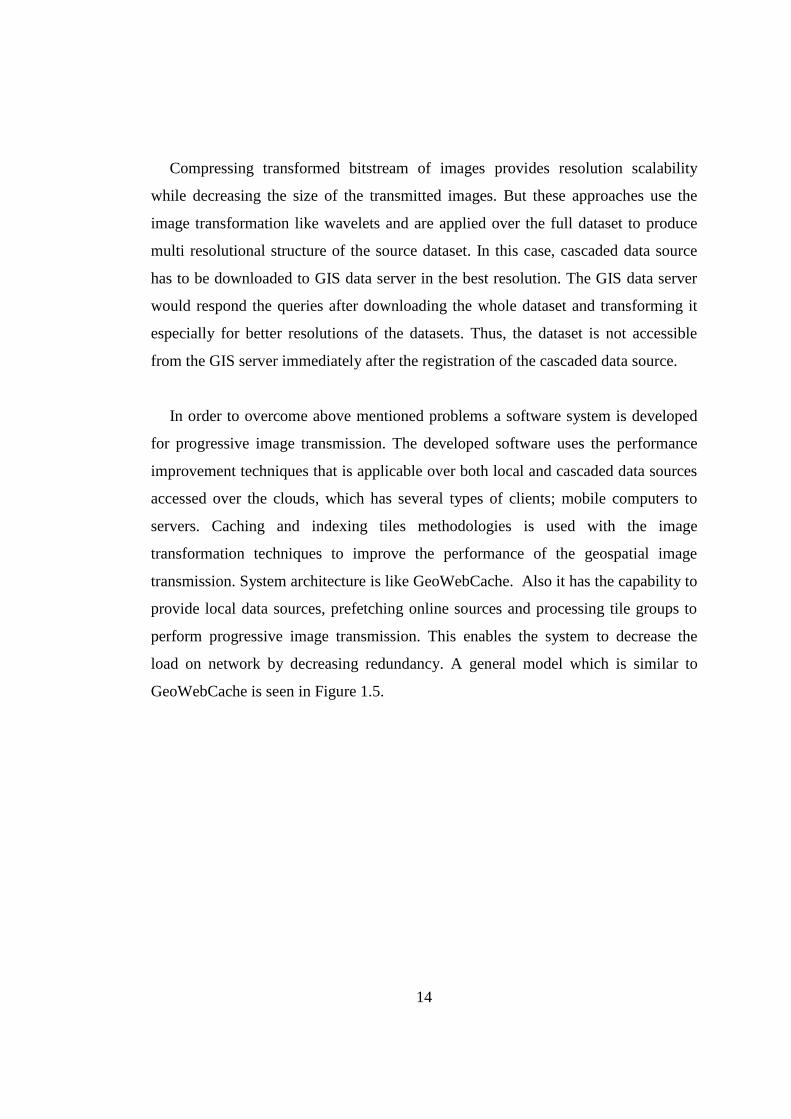
Serving tiles that are originally provided from WMS data sources are server side
cached on GeoWebCache server which is an open source project (GeoWebCache is a
cache for WMS tiles implemented in Java, 2010). It works like a proxy server
between GIS clients and servers. However, it does not deal with the redundancy issue
of tiled image pyramids.
Figure 1.4 General architecture of discussed systems
Tiling image pyramids decreases the response time of queries over the raster
datasets. With spatial indexing and caching techniques this method is applicable for
the cascaded data sources. On the other hand redundancy over the transmitted data is
very high especially when compared to the image transformation techniques.
14
Compressing transformed bitstream of images provides resolution scalability
while decreasing the size of the transmitted images. But these approaches use the
image transformation like wavelets and are applied over the full dataset to produce
multi resolutional structure of the source dataset. In this case, cascaded data source
has to be downloaded to GIS data server in the best resolution. The GIS data server
would respond the queries after downloading the whole dataset and transforming it
especially for better resolutions of the datasets. Thus, the dataset is not accessible
from the GIS server immediately after the registration of the cascaded data source.
In order to overcome above mentioned problems a software system is developed
for progressive image transmission. The developed software uses the performance
improvement techniques that is applicable over both local and cascaded data sources
accessed over the clouds, which has several types of clients; mobile computers to
servers. Caching and indexing tiles methodologies is used with the image
transformation techniques to improve the performance of the geospatial image
transmission. System architecture is like GeoWebCache. Also it has the capability to
provide local data sources, prefetching online sources and processing tile groups to
perform progressive image transmission. This enables the system to decrease the
load on network by decreasing redundancy. A general model which is similar to
GeoWebCache is seen in Figure 1.5.
15
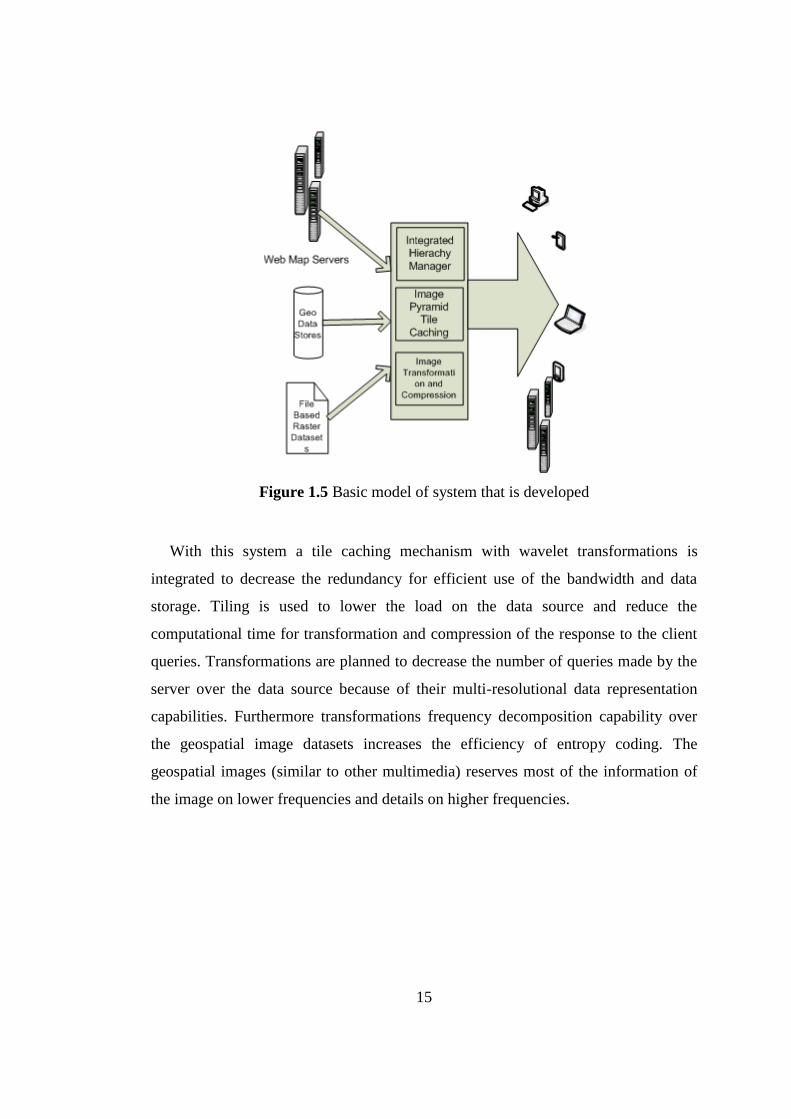
Figure 1.5 Basic model of system that is developed
With this system a tile caching mechanism with wavelet transformations is
integrated to decrease the redundancy for efficient use of the bandwidth and data
storage. Tiling is used to lower the load on the data source and reduce the
computational time for transformation and compression of the response to the client
queries. Transformations are planned to decrease the number of queries made by the
server over the data source because of their multi-resolutional data representation
capabilities. Furthermore transformations frequency decomposition capability over
the geospatial image datasets increases the efficiency of entropy coding. The
geospatial images (similar to other multimedia) reserves most of the information of
the image on lower frequencies and details on higher frequencies.
16
CHAPTER 2
RASTER DATA MANAGEMENT
Data is the one of the critical element of GIS and beyond spatial data infrastructure
(SDI). Data used by GIS is conventionally abstracted by two categories; raster and
vector. Geographic features are represented with geometric objects such as points,
lines, polygons which are binded to a coordinate reference system(CRS). The
datasets that contains a specific type of feature is called vector layer. On the other
hand raster layers cover a regions continuous data in GIS. Traditionally raster data
used in GIS is abstracted with regular grids that could be referenced with Cartesien
coordinate system. In GIS raster layers are referenced to earth by a projection and
CRS. The objective of the thesis is related with raster layers so raster data
management issues will be discussed in subsequent sections.
2.1 CHALLENGES OF RASTER DATA MANAGEMENT
2.1.1 SIZE OF GEOSPATIAL IMAGES
The objective of the thesis is to develop software that is efficient to transmit
geospatial images to the web GIS clients. A GIS server has to manage a region’s
different raster layers that have different resolution. According to the resolution of
the dataset and the regions area the uncompressed size of the layers vary between
gigabytes to terabytes.
17
For example an enterprise’s region of interest is limited with a minimum
bounding box that has a dimension 50km x 60km on earth. High resolution satellite
images with 1 meters spatial resolution, RGB composed and pan-sharpened Landsat
images with 15 meter spatial resolution, ortho-rectified aerial images with 30 cm
spatial resolution, and scanned maps with scales 1:25000 and 1:100000 are used by
the typical enterprise.
Uncompressed sizes of the datasets depend on the number of pixels in the datasets
and the number of bytes to represent a pixel. Number of pixels of a dataset with
known dimensions on earth could be calculated by using Equation 2.1.
2.1
Scanned map’s spatial resolution depends on the two key factors. First the
scanner’s (which is used for digitization process) technical specification number dots
per inch (dpi) and second the source maps scale. Hereby the scanned maps spatial
resolution in meters is given in Equation 2.2.
2.2
Let us assume that whole datasets have 3 bands with 8 bits radiometric resolution.
With this assumption a pixel is represented with 24 bits, 3 bytes. Let us assume that
actual maps are digitized by a scanner which has 600 dpi. Hereby with equations 2.1
and 2.2 datasets raw storage requirements could be calculated as seen in Table 3.1.
18
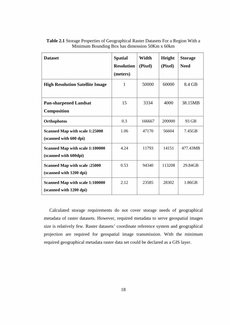
Table 2.1 Storage Properties of Geographical Raster Datasets For a Region With a
Minimum Bounding Box has dimension 50Km x 60km
Dataset Spatial
Resolution
(meters)
Width
(Pixel)
Height
(Pixel)
Storage
Need
High Resolution Satellite Image
1 50000 60000 8.4 GB
Pan-sharpened Landsat
Composition
15 3334 4000 38.15MB
Orthophotos 0.3 166667 200000 93 GB
Scanned Map with scale 1:25000
(scanned with 600 dpi)
1.06 47170 56604 7.45GB
Scanned Map with scale 1:100000
(scanned with 600dpi)
4.24 11793 14151 477.43MB
Scanned Map with scale :25000
(scanned with 1200 dpi)
0.53 94340 113208 29.84GB
Scanned Map with scale 1:100000
(scanned with 1200 dpi)
2.12 23585 28302 1.86GB
Calculated storage requirements do not cover storage needs of geographical
metadata of raster datasets. However, required metadata to serve geospatial images
size is relatively few. Raster datasets’ coordinate reference system and geographical
projection are required for geospatial image transmission. With the minimum
required geographical metadata raster data set could be declared as a GIS layer.
19
2.1.2 ARRANGING REQUIRED METADATA
GIS servers have to publish the layers’ geographical metadata. At the beginning of a
geospatial image transmission session GIS client access the metadata of the layers.
Clients resolve geographic metadata to build posterior requests over served layers by
user interactions. Geographical metadata has to be managed with the raster dataset.
The minimum geographical metadata required are spatial reference system, and
projection information on that spatial reference system with ground control points or
minimum bounding rectangle.
There are different approaches to encode and manage raster datasets’ metadata.
OGC and ISO/TC211 defined several encoding types to encode the objects that
define geographical projection and coordinate reference systems. Also schemas to
manage geographical data and related metadata are defined by these organizations.
ISO 19115 defines the schema required for describing geographic information and
services (Geographic information - Metadata, 2003). The metadata covered with
schema are information about the identification, the extent, the quality, the spatial
and temporal schema, spatial reference, and distribution of digital geographic data.
ISO 19115 metadata could be encoded and stored with different methods. ISO 19139
defines a XML encoding (Geographic Metadata XML (GMD)) on ISO 19115
metadata (Geographic information -- Metadata -- XML schema implementation,
2007). ISO 19123, which defines a schema to manage coverage data, could be used
for raster coverage's that is integrated with the related metadata specifications
(Geographic information -- Schema for coverage geometry and functions, 2005).
Geography Markup Language (GML), Well Known Text (WKT) and Well
Known Binary (WKB) are the encoding models for geographic features defined by
OGC. Spatial Reference Systems can be represented with a textual encoding by
WKTs. Spatial reference systems can be represented with a binary encoding with
WKBs (Herring, 2006). To manage and access WKTs and WKBs with different
20
systems (CORBA , OLE/COM, SQL interfaces are defined by OGC. Geographic
Markup Language defines objects to cover geographical data and metadata.
gml:AbstractCRS and gml:AbstractCoordinateReferenceSystem are the base object
types to define coordinate reference systems. And gml: RectifiedGrid object type is
defined within Grid Schema to define a grid that could be projected on the declared
spatial coordinate system for the grid (Portele, 2007). In addition OGC published
GML in JPEG 2000 for Geographic Imagery Encoding Specification to embed gml
into JPEG2000 xml boxes. Thus spatial reference system and projection could be
encoded within a JPEG2000 file. Additionally specification provides annotating
geographic features with the related gml objects on the image.
2.1.3 OPERATIONS FOR GEOSPATIAL IMAGE TRANMISSION
A GIS stake holder’s basic expectations from a map viewing system are to be able to
use zoom in, zoom out and pan operations. These operations need random access to
geospatial datasets. Moreover for zoom in and zoom out operations resampling of
datasets or multi-resolutional access to datasets is required.
Resampling operation has a high complexity. On desktop GIS applications it
would be acceptable to wait the resampling for the result a piece of data on the
dataset. But the resampling operations complexity would cause high load over o web
GIS server. It is trivial that both the responses to the clients that are requested at
original or different scale will be delayed because of resampling. Thus web GIS
server's needs to access to datasets at different scales. In other words data storage has
to provide multi-resolutional access over the geospatial raster dataset.
Other than access operations geospatial operations over datasets could be required
for specific use cases. These operations could be listed as; re-projection, rendering
vector layers, overlaying different layers, operations on temporal dimension (i.e.
change detection), spatial filtering (i.e. low-pass filtering, high-pass filtering,
21
nonlinear operations), RGB composition from declared layers etc. Performance
overhead of these operations over GIS server cannot be solved with data storage
methods.
If the processing operations over datasets are predictable for web GIS clients then
caching the results of the operations over the datasets on the GIS server could be
useful. If the operations on the datasets are designated then, if available, the
operation could be executed over the whole related datasets and the results are
stored. But if the datasets are updated frequently then these methods individually
would be overhead over the GIS server.
2.2 RASTER DATA STORAGE
There are different raster file formats and also database systems to store and manage
geospatial images. Some of the image file formats designed to contain metadata and
also some of them directly designed for geospatial images, could be used to store and
transfer geospatial images. On the other hand standard image file formats that are not
designed to contain metadata, geographical or another domains metadata could be
used with external metadata to support geospatial images. But in this case there has
to be an additional effort to manage and store metadata such as world files. World
files which are plain text files contain georeferencing information of the related files.
World files have the same name with world file except the "w" character at the end
of world file (World files for raster datasets, 2010). For example a JPEG file that
contains a part of a high resolution satellite image of Ankara "ankara1.jpeg" would
have a world file named "ankara1.jpegw" or "ankara1.jpw" which is located in the
same directory with the image file.
There are several file formats related to raster storage, which have different
encoding, access and metadata management methodologies.
22
JPEG JPEG is discrete cosine transform (DCT) and Huffman coding based
compressed image file format. JPEG supports lossy and lossless compression. With
JPEG compression images could be lossy compressed 1:10 ratio with little or no
visual image quality loss. Gray and RGB colored images could be compressed with
JPEG. While compressing RGB colored images color space transformation is
applied. Images are transformed RGB color space to YUV color space. In YUV color
space Y component represents luminance, U and V components represents color
information of each pixel. U and V color components are downsampled and their
resolution are decreased to half. After color transformation and resampling of
components DCT is applied to 8x8 on all three components. After quantizing
transformed values with applying Huffman compression process is completed.
GeoTIFF After rectification and reGIStration process geospatial images could be
stored in tagged image file format files (TIFF) with geographic reGIStration
parameters. GeoTIFF standardize how to store geographic metadata within a TIFF
file. Most of the geographic information system software packages supports
GeoTIFF. GeoTIFF could contain a JPEG file that is tagged with geographical
information. On the other hand GeoTIFF supports lossless compression with
methods like LZW and PackBits.
JPEG 2000 JPEG 2000 differentiates from JPEG with wavelet and Embedded Block
Coding with Optimal Truncation (EBCOT) techniques. The most important features
of JPEG 2000 are high compression ratio lossy and lossles compression, regional
compression with region of interest definitions, embedded metadata management
with xml boxes, scalable file format support, and different radiometric resolution
support, multi-resolutional and spatially random access. JPEG 2000 supports
transparency with alpha band. Alpha band is important for geospatial images to
represents cells that contains no data values.
23
ECW Embedded compression wavelet is an open standard that is developed by Earth
Resource Mapping Company. Especially for high resolution satellite images and
orthophotos efficient compression is achieved with ECW format. Typically ECW file
format supports 1:10 to 1:100 compression ratios. Multi-resolutional and spatially
random access to ECW files is available. Geographical projection information could
be embedded to ECW files. Also with ECW protocol (ECWP) progressive image
transmission is supported.
MRSID Multi Resolutional Seamless Image Database (MRSID) is a wavelet based
image compression file format. This format is developed from LizardTech Company
for GIS. LizardTech's product GeoExpress provides to read and write MRSID
images. ExpressView Browser Plug-in supports to view MRSID images via web
browsers. The main steps of MRSID image coding could be summarized with;
producing multi-resolutional image with wavelet transformation, all resolution levels
have 4 subbands coded with 32 bits, all subbands are divided to 64x64 sized blocks,
all blocks are divided to sub blocks over bit layers.
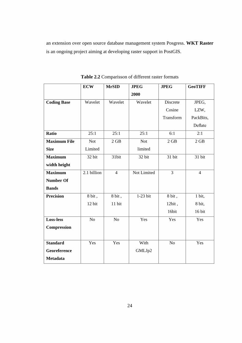
The comparison of the formats discussed above can be seen in Table 2.2 which is
modified from the technical overview made by ER Mapper at 2002 (Accelerating
WebGIS with Image Web Server, 2010).
Database Systems Above methods provides storage by file based systems. There are
database systems to manage geospatial images and its metadata. GeoRaster is a
feature of Oracle spatial. GeoRaster provides to store geospatial images and related
metadata. Moreover it provides indexing, query operations, analyzing geospatial
images. With Oracle Application Server MapViewer geospatial images could be
viewed over map. GeoRaster uses tiled image pyramid structure to provide multi-
resolutional and randomly accessible GIS raster datasets. Tile images are stored in
blocks that contain Binary Large Objects (BLOB). On the other hand PostGIS is
another database system to manage geospatial objects like Oracle Spatial. PostGIS is
24
an extension over open source database management system Posgress. WKT Raster
is an ongoing project aiming at developing raster support in PostGIS.
Table 2.2 Comparisson of different raster formats
ECW
MrSID
JPEG
2000
JPEG GeoTIFF
Coding Base
Wavelet Wavelet Wavelet Discrete
Cosine
Transform
JPEG,
LZW,
PackBits,
Deflate
Ratio 25:1 25:1 25:1 6:1 2:1
Maximum File
Size
Not
Limited
2 GB Not
limited
2 GB 2 GB
Maximum
width height
32 bit 31bit 32 bit 31 bit 31 bit
Maximum
Number Of
Bands
2.1 billion
4 Not Limited
3 4
Precision
8 bit ,
12 bit
8 bit ,
11 bit
1-23 bit
8 bit ,
12bit ,
16bit
1 bit,
8 bit,
16 bit
Loss-less
Compression
No No Yes Yes Yes
Standard
Georeference
Metadata
Yes Yes With
GMLJp2
No Yes
25
CHAPTER 3
IMAGE TRANSFORMATIONS
Transform coding is the process to transform an image from a domain to another
domain and code image in the transformed domain. Most of the image and video
compression formats uses image transformation as the basis of the encoding. Also
transformations provide different types of progression other than spatial progression
by the exchanged domain.
Transmitting an image that supports progressive access increases the response
time of the image request. Image transformations are the key elements of the
progressive image transmission. In this chapter Discrete Cosine Transform,
Karhunen Loewe Transform and Wavelet Transformations are examined in
according to their progressive coding facility.
3.1 DISCRETE COSINE TRANSFORMATION
Discrete Cosine Transform (DCT) is used as the base transformation of JPEG image
file format. After dividing images into equally sized blocks each block is transformed
with DCT. Thus the transformation coefficients of each block are not affected signal
components in neighboring blocks. This causes blocking effect at high compression
ratio while using JPEG. After transformation the resulting low frequency
components contains the main information of the image. Therefore transformation
results would be quantized with a quantization table that would decrease the
26
coefficients in direct proportion to increase of the frequency. In that case the affect of
the high frequency components on the inverse transformed image would be
eliminated.
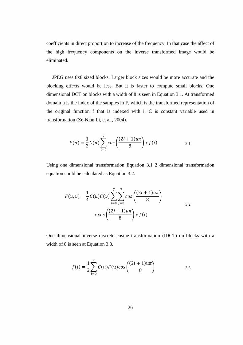
JPEG uses 8x8 sized blocks. Larger block sizes would be more accurate and the
blocking effects would be less. But it is faster to compute small blocks. One
dimensional DCT on blocks with a width of 8 is seen in Equation 3.1. At transformed
domain u is the index of the samples in F, which is the transformed representation of
the original function f that is indexed with i. C is constant variable used in
transformation (Ze-Nian Li, et al., 2004).
3.1
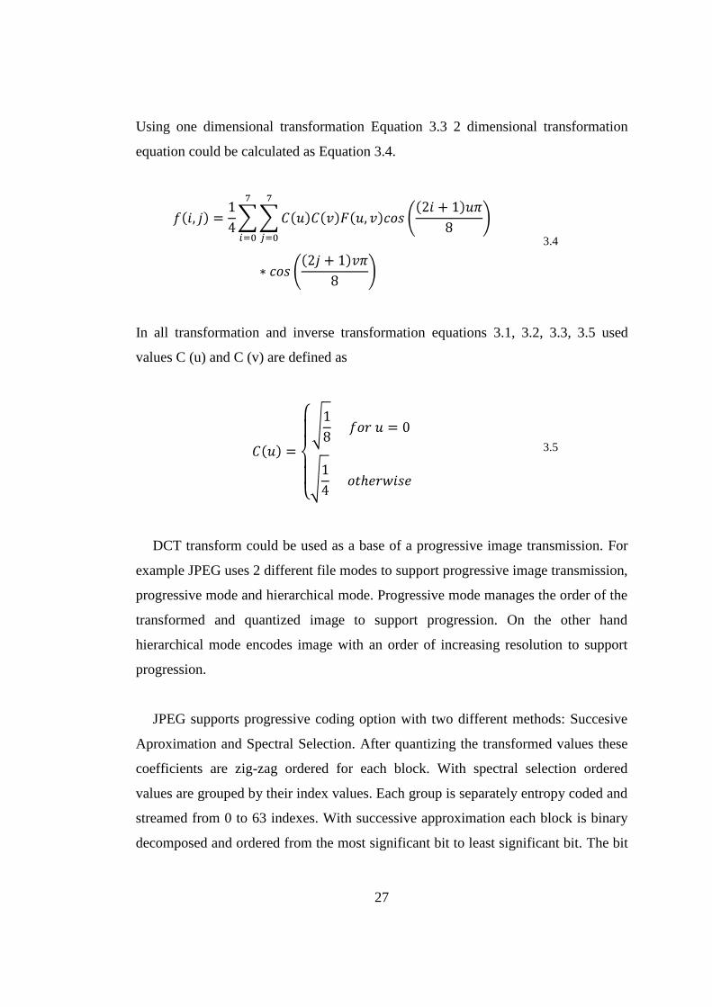
Using one dimensional transformation Equation 3.1 2 dimensional transformation
equation could be calculated as Equation 3.2.
3.2
One dimensional inverse discrete cosine transformation (IDCT) on blocks with a
width of 8 is seen at Equation 3.3.
3.3
27
Using one dimensional transformation Equation 3.3 2 dimensional transformation
equation could be calculated as Equation 3.4.
3.4
In all transformation and inverse transformation equations 3.1, 3.2, 3.3, 3.5 used
values C (u) and C (v) are defined as
3.5
DCT transform could be used as a base of a progressive image transmission. For
example JPEG uses 2 different file modes to support progressive image transmission,
progressive mode and hierarchical mode. Progressive mode manages the order of the
transformed and quantized image to support progression. On the other hand
hierarchical mode encodes image with an order of increasing resolution to support
progression.
JPEG supports progressive coding option with two different methods: Succesive
Aproximation and Spectral Selection. After quantizing the transformed values these
coefficients are zig-zag ordered for each block. With spectral selection ordered
values are grouped by their index values. Each group is separately entropy coded and
streamed from 0 to 63 indexes. With successive approximation each block is binary
decomposed and ordered from the most significant bit to least significant bit. The bit
28
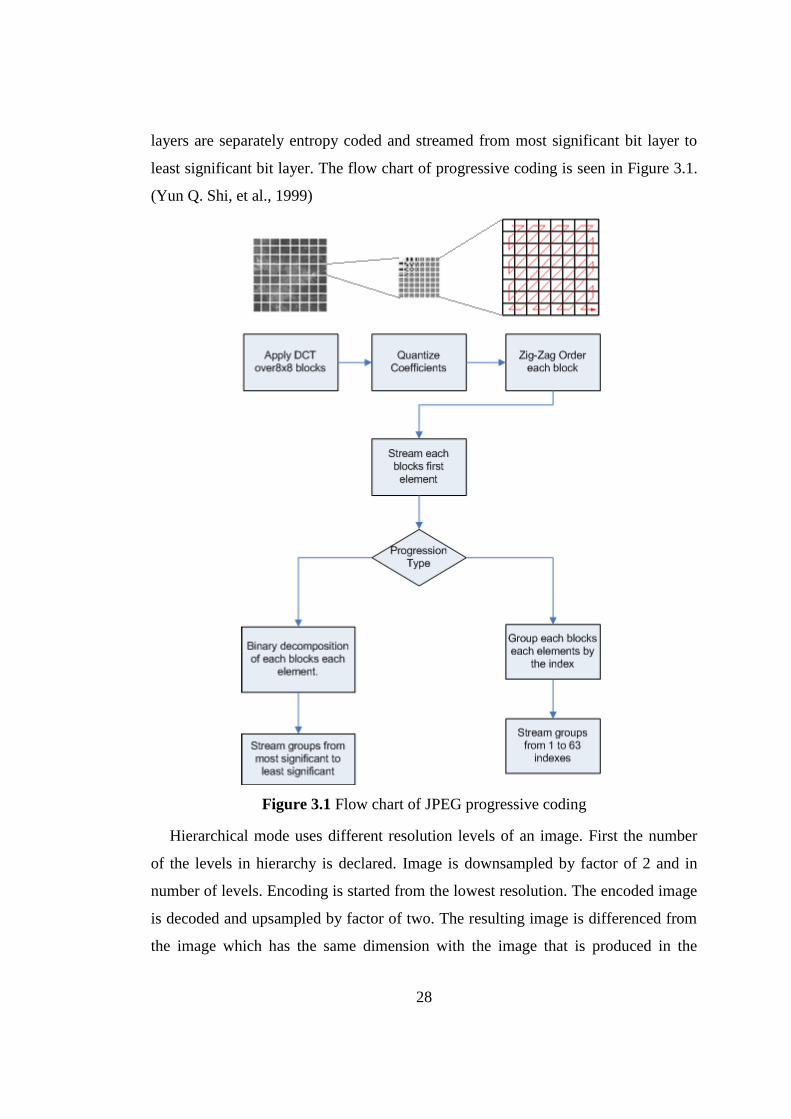
layers are separately entropy coded and streamed from most significant bit layer to
least significant bit layer. The flow chart of progressive coding is seen in Figure 3.1.
(Yun Q. Shi, et al., 1999)
Figure 3.1 Flow chart of JPEG progressive coding
Hierarchical mode uses different resolution levels of an image. First the number
of the levels in hierarchy is declared. Image is downsampled by factor of 2 and in
number of levels. Encoding is started from the lowest resolution. The encoded image
is decoded and upsampled by factor of two. The resulting image is differenced from
the image which has the same dimension with the image that is produced in the
29
downsampling process of the original image. The difference image is encoded. This
process is operated for each resolution level similar to differential pulse-code
modulation. The lowest resolutions encoded image and the differences are
transmitted in order with the related resolution level.
3.2 KARHUNEN LOEWE TRANSFORMATION
In Karhunen Loewe Transformation (KLT) image transformation which is also
known as Hotelling Transformation, Principal Component Analysis(PCA) is used in
many applications of image processing like face recognition, image compression,
and pattern recognition (Smith, 2002). When KLT is applied on a set of vectors
which composes a dataset the number of the vectors are the same in the transformed
domain with the original domain. On the other hand k number of vectors in the
transformed domain, where k is less than the number of the vectors in the original
domain, contains the high frequency components of the images as seen in Figure 3.3.
It means that these vectors has high entropy and contains high volume of
information.
Inverse transformation of the KLT transformed images does not need the all of the
transformation output vectors. In this case the input vectors for the inverse
transformation are choosed in an order with decreasing frequencies. The output
vectors of the inverse transformation process similarity to the original vectors would
be increase with higher number of input vectors and with higher correlation between
the original vectors.
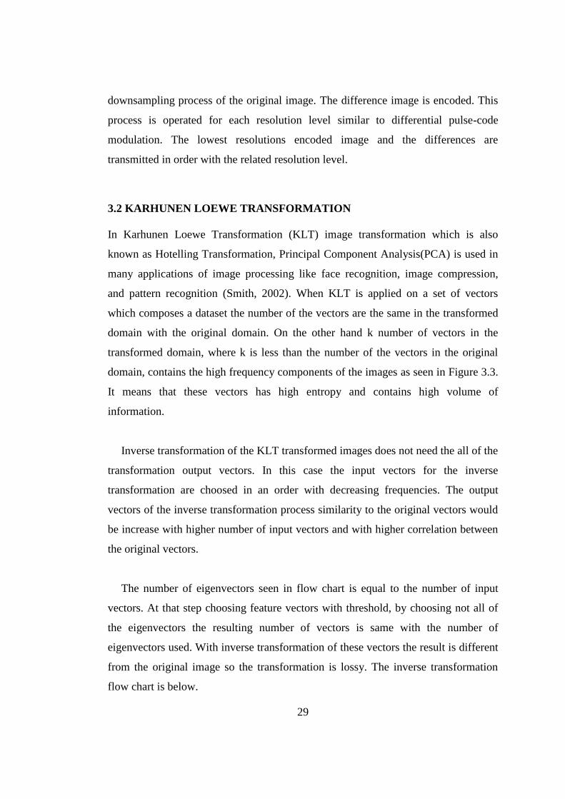
The number of eigenvectors seen in flow chart is equal to the number of input
vectors. At that step choosing feature vectors with threshold, by choosing not all of
the eigenvectors the resulting number of vectors is same with the number of
eigenvectors used. With inverse transformation of these vectors the result is different
from the original image so the transformation is lossy. The inverse transformation
flow chart is below.
30
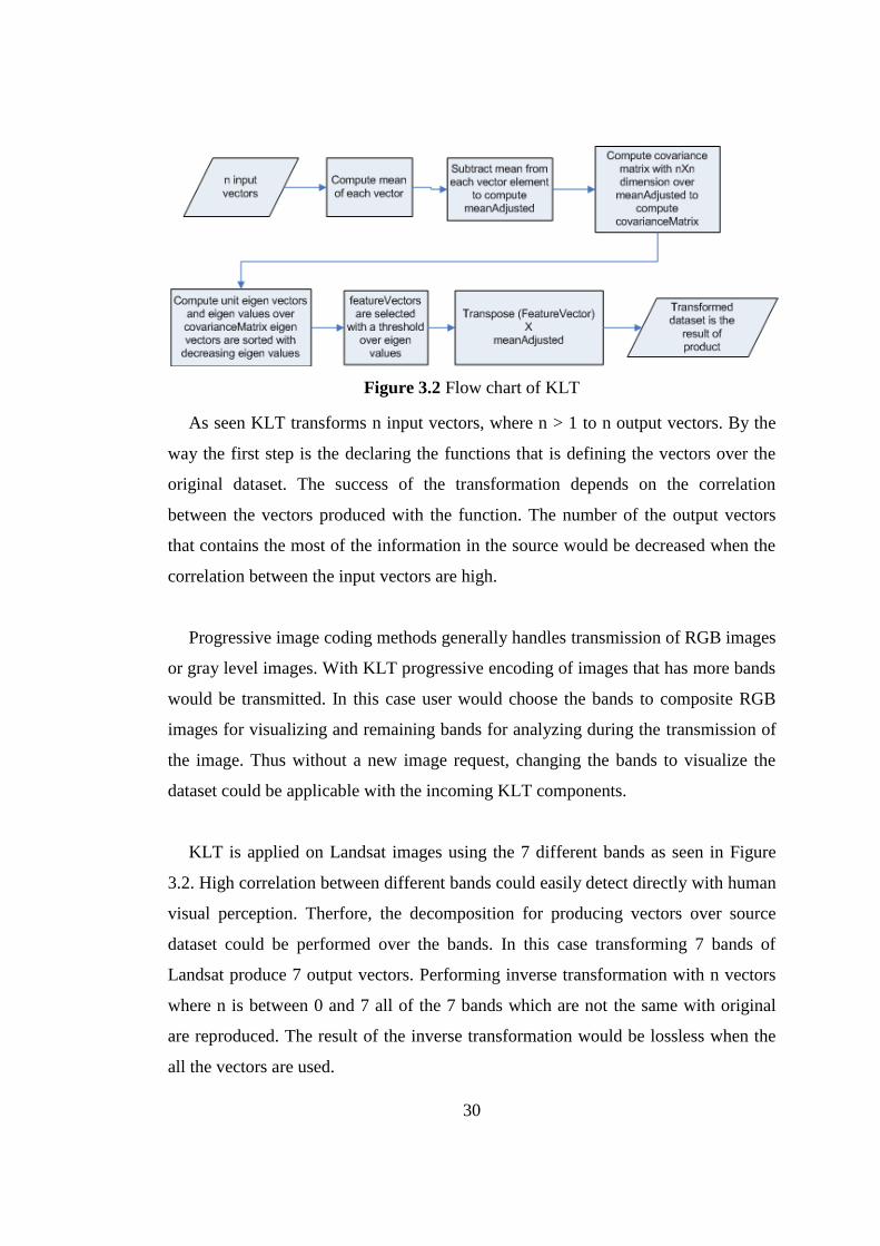
Figure 3.2 Flow chart of KLT
As seen KLT transforms n input vectors, where n > 1 to n output vectors. By the
way the first step is the declaring the functions that is defining the vectors over the
original dataset. The success of the transformation depends on the correlation
between the vectors produced with the function. The number of the output vectors
that contains the most of the information in the source would be decreased when the
correlation between the input vectors are high.
Progressive image coding methods generally handles transmission of RGB images
or gray level images. With KLT progressive encoding of images that has more bands
would be transmitted. In this case user would choose the bands to composite RGB
images for visualizing and remaining bands for analyzing during the transmission of
the image. Thus without a new image request, changing the bands to visualize the
dataset could be applicable with the incoming KLT components.
KLT is applied on Landsat images using the 7 different bands as seen in Figure
3.2. High correlation between different bands could easily detect directly with human
visual perception. Therfore, the decomposition for producing vectors over source
dataset could be performed over the bands. In this case transforming 7 bands of
Landsat produce 7 output vectors. Performing inverse transformation with n vectors
where n is between 0 and 7 all of the 7 bands which are not the same with original
are reproduced. The result of the inverse transformation would be lossless when the
all the vectors are used.
31
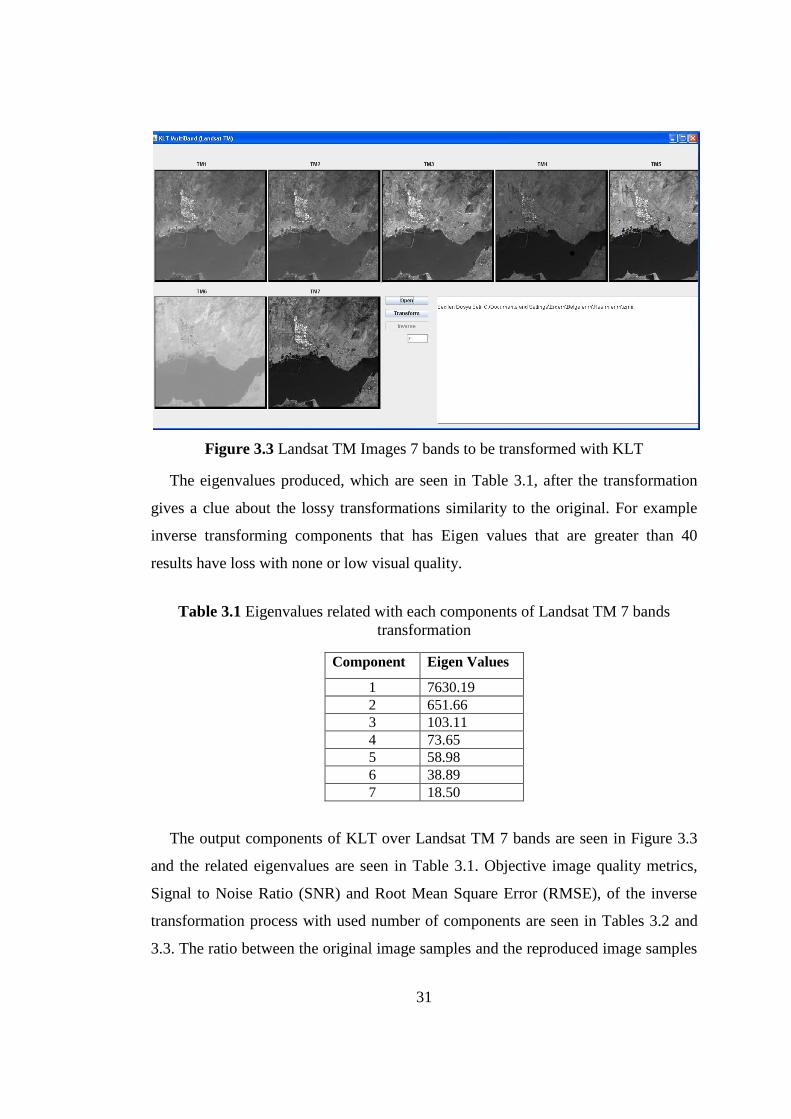
Figure 3.3 Landsat TM Images 7 bands to be transformed with KLT
The eigenvalues produced, which are seen in Table 3.1, after the transformation
gives a clue about the lossy transformations similarity to the original. For example
inverse transforming components that has Eigen values that are greater than 40
results have loss with none or low visual quality.
Table 3.1 Eigenvalues related with each components of Landsat TM 7 bands
transformation
Component Eigen Values
1 7630.19
2 651.66
3 103.11
4 73.65
5 58.98
6 38.89
7 18.50
The output components of KLT over Landsat TM 7 bands are seen in Figure 3.3
and the related eigenvalues are seen in Table 3.1. Objective image quality metrics,
Signal to Noise Ratio (SNR) and Root Mean Square Error (RMSE), of the inverse
transformation process with used number of components are seen in Tables 3.2 and
3.3. The ratio between the original image samples and the reproduced image samples
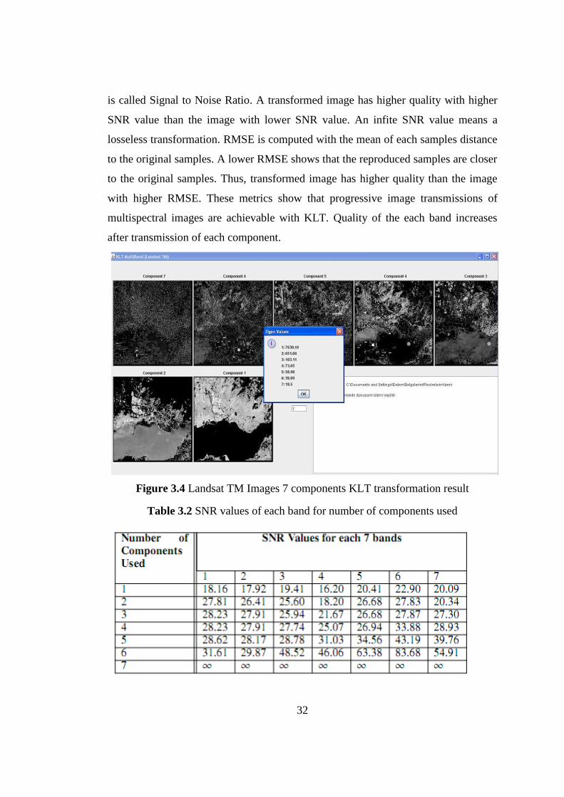
32
is called Signal to Noise Ratio. A transformed image has higher quality with higher
SNR value than the image with lower SNR value. An infite SNR value means a
losseless transformation. RMSE is computed with the mean of each samples distance
to the original samples. A lower RMSE shows that the reproduced samples are closer
to the original samples. Thus, transformed image has higher quality than the image
with higher RMSE. These metrics show that progressive image transmissions of
multispectral images are achievable with KLT. Quality of the each band increases
after transmission of each component.
Figure 3.4 Landsat TM Images 7 components KLT transformation result
Table 3.2 SNR values of each band for number of components used
33
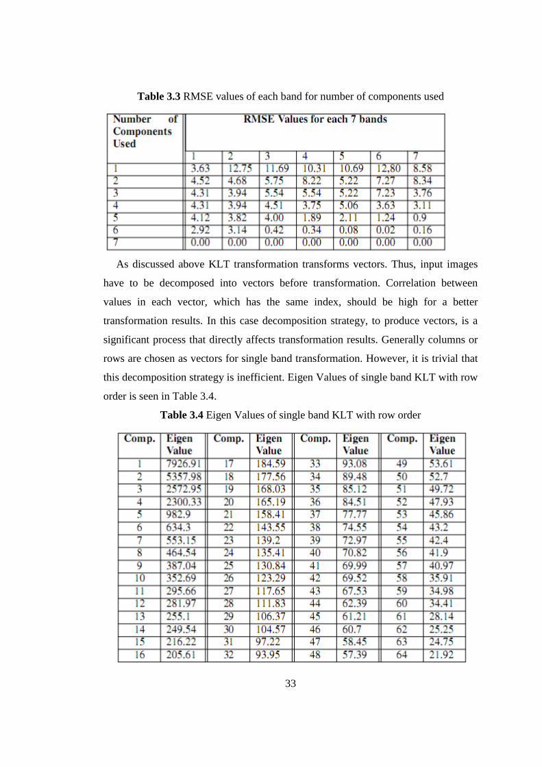
Table 3.3 RMSE values of each band for number of components used
As discussed above KLT transformation transforms vectors. Thus, input images
have to be decomposed into vectors before transformation. Correlation between
values in each vector, which has the same index, should be high for a better
transformation results. In this case decomposition strategy, to produce vectors, is a
significant process that directly affects transformation results. Generally columns or
rows are chosen as vectors for single band transformation. However, it is trivial that
this decomposition strategy is inefficient. Eigen Values of single band KLT with row
order is seen in Table 3.4.
Table 3.4 Eigen Values of single band KLT with row order
34
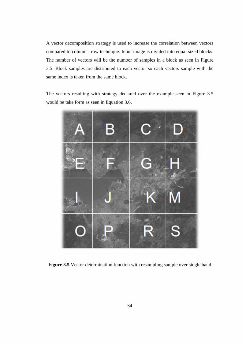
A vector decomposition strategy is used to increase the correlation between vectors
compared to column - row technique. Input image is divided into equal sized blocks.
The number of vectors will be the number of samples in a block as seen in Figure
3.5. Block samples are distributed to each vector so each vectors sample with the
same index is taken from the same block.
The vectors resulting with strategy declared over the example seen in Figure 3.5
would be take form as seen in Equation 3.6.
Figure 3.5 Vector determination function with resampling sample over single band
35
……….
……….
3.6
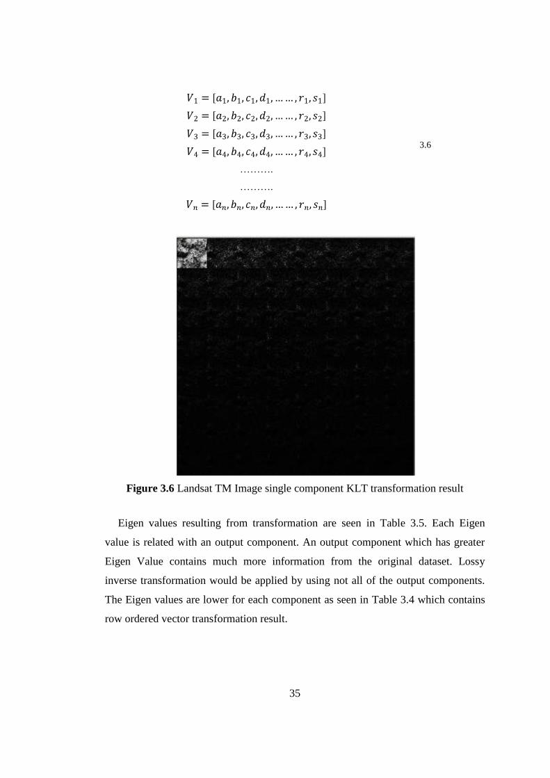
Figure 3.6 Landsat TM Image single component KLT transformation result
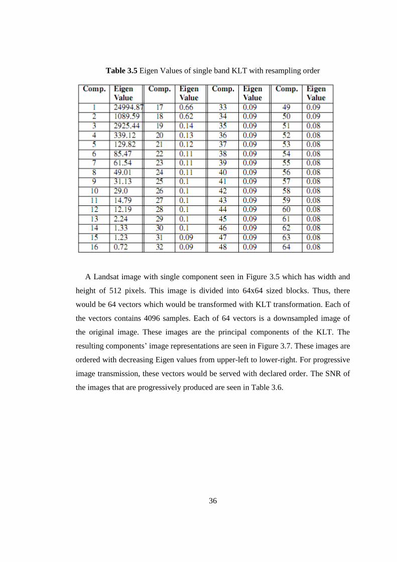
Eigen values resulting from transformation are seen in Table 3.5. Each Eigen
value is related with an output component. An output component which has greater
Eigen Value contains much more information from the original dataset. Lossy
inverse transformation would be applied by using not all of the output components.
The Eigen values are lower for each component as seen in Table 3.4 which contains
row ordered vector transformation result.
36
Table 3.5 Eigen Values of single band KLT with resampling order
A Landsat image with single component seen in Figure 3.5 which has width and
height of 512 pixels. This image is divided into 64x64 sized blocks. Thus, there
would be 64 vectors which would be transformed with KLT transformation. Each of
the vectors contains 4096 samples. Each of 64 vectors is a downsampled image of
the original image. These images are the principal components of the KLT. The
resulting components’ image representations are seen in Figure 3.7. These images are
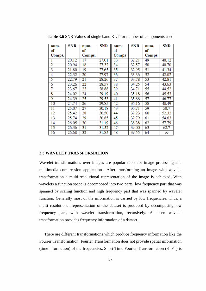
ordered with decreasing Eigen values from upper-left to lower-right. For progressive
image transmission, these vectors would be served with declared order. The SNR of
the images that are progressively produced are seen in Table 3.6.
37
Table 3.6 SNR Values of single band KLT for number of components used
3.3 WAVELET TRANSFORMATION
Wavelet transformations over images are popular tools for image processing and
multimedia compression applications. After transforming an image with wavelet
transformation a multi-resolutional representation of the image is achieved. With
wavelets a function space is decomposed into two parts; low frequency part that was
spanned by scaling function and high frequency part that was spanned by wavelet
function. Generally most of the information is carried by low frequencies. Thus, a
multi resolutional representation of the dataset is produced by decomposing low
frequency part, with wavelet transformation, recursively. As seen wavelet
transformation provides frequency information of a dataset.
There are different transformations which produce frequency information like the
Fourier Transformation. Fourier Transformation does not provide spatial information
(time information) of the frequencies. Short Time Fourier Transformation (STFT) is
38
applied to obtain spatial information of the frequencies decomposed. Windowed
blocks of the original data are transformed to apply STFT. Thus, the frequencies that
has larger bandwidth from the window size will not be decomposed with this
method. However wavelet transformation provides the time-frequency representation
natively (Polikar, 2001).
With wavelet transformations, spatial information's resolution of the frequency
components decomposed decreases with the frequency because of the higher spatial
extent of the components which have higher band widths. Thus, by transforming low
frequency components recursively dimension of the low frequency components are
decreased, which carries the most of the information. Generally high frequency
components are compressed better than low frequency components because of their
lower entropy.
Discrete wavelet transformations (DWT) are used in different computing
applications like image processing, multi-resolutional processing, and multimedia
compression. The DWT analyzes the input data at different frequency bands with
different resolutions by decomposing the data into a coarse approximation (Low
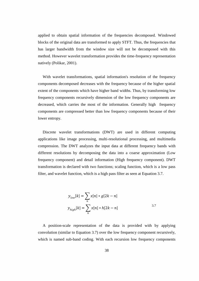
frequency component) and detail information (High frequency component). DWT
transformation is declared with two functions; scaling function, which is a low pass
filter, and wavelet function, which is a high pass filter as seen at Equation 3.7.
3.7
A position-scale representation of the data is provided with by applying
convolution (similar to Equation 3.7) over the low frequency component recursively,
which is named sub-band coding. With each recursion low frequency components
39
each dimension and also resolution are decreased to half. The recursion process is
seen in Figure 3.7. After transforming image with this process high frequency
components has low energy as seen in Figure 3.8.
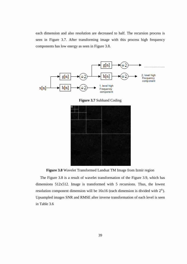
Figure 3.7 Subband Coding
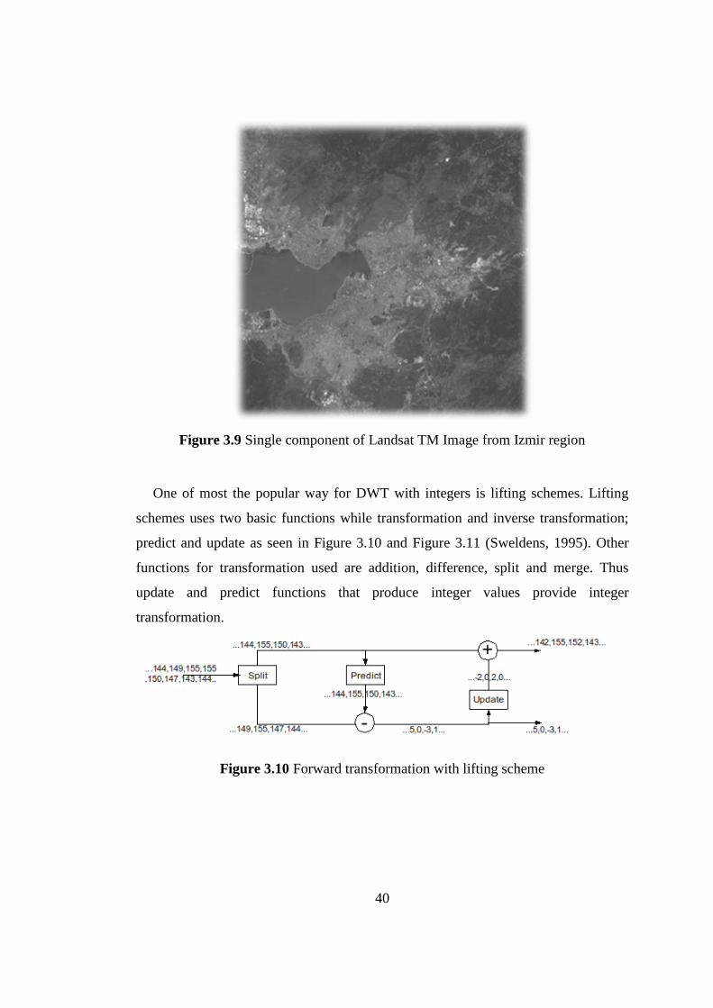
Figure 3.8 Wavelet Transformed Landsat TM Image from Izmir region
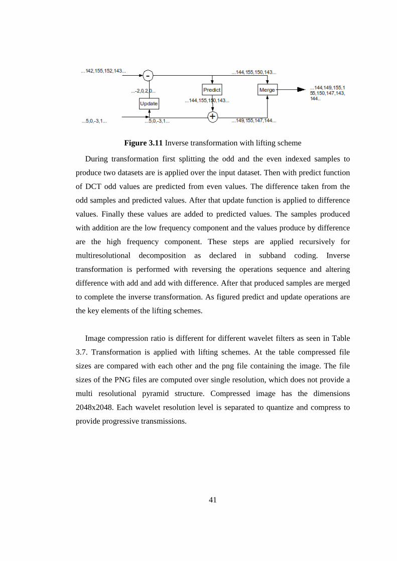
The Figure 3.8 is a result of wavelet transformation of the Figure 3.9, which has
dimensions 512x512. Image is transformed with 5 recursions. Thus, the lowest
resolution component dimension will be 16x16 (each dimension is divided with ).
Upsampled images SNR and RMSE after inverse transformation of each level is seen
in Table 3.6
40
Figure 3.9 Single component of Landsat TM Image from Izmir region
One of most the popular way for DWT with integers is lifting schemes. Lifting
schemes uses two basic functions while transformation and inverse transformation;
predict and update as seen in Figure 3.10 and Figure 3.11 (Sweldens, 1995). Other
functions for transformation used are addition, difference, split and merge. Thus
update and predict functions that produce integer values provide integer
transformation.
Figure 3.10 Forward transformation with lifting scheme
41
Figure 3.11 Inverse transformation with lifting scheme
During transformation first splitting the odd and the even indexed samples to
produce two datasets are is applied over the input dataset. Then with predict function
of DCT odd values are predicted from even values. The difference taken from the
odd samples and predicted values. After that update function is applied to difference
values. Finally these values are added to predicted values. The samples produced
with addition are the low frequency component and the values produce by difference
are the high frequency component. These steps are applied recursively for
multiresolutional decomposition as declared in subband coding. Inverse
transformation is performed with reversing the operations sequence and altering
difference with add and add with difference. After that produced samples are merged
to complete the inverse transformation. As figured predict and update operations are
the key elements of the lifting schemes.
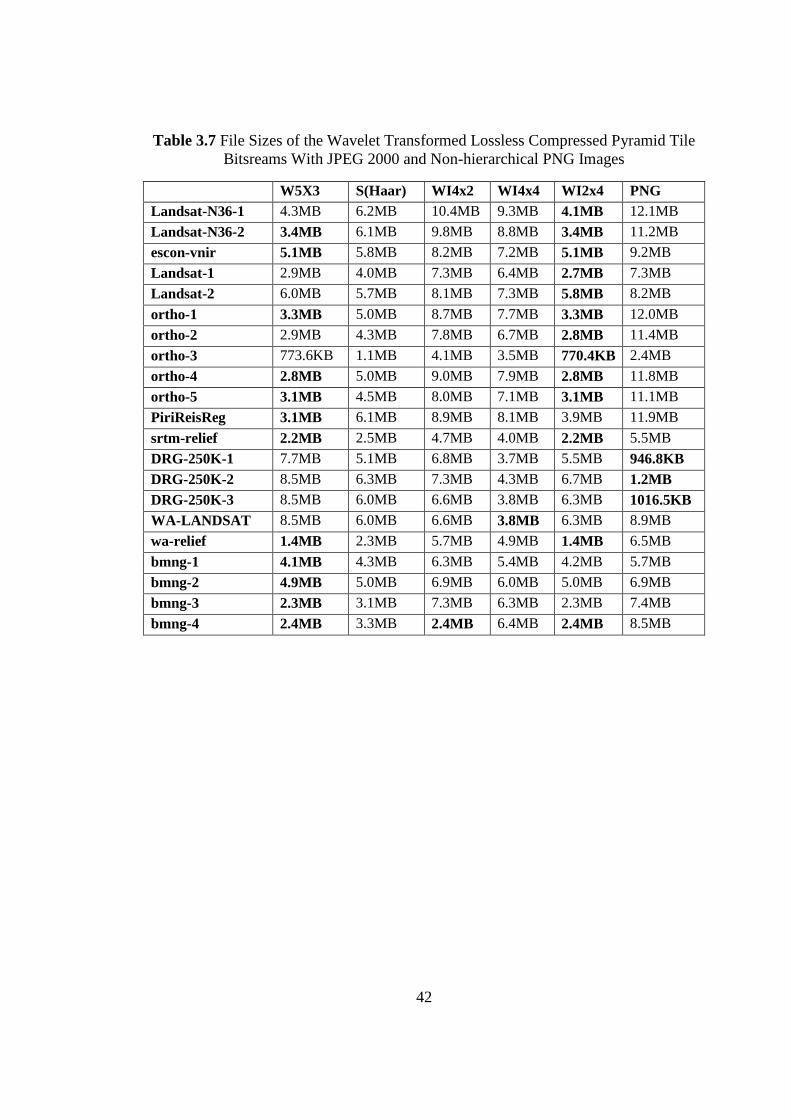
Image compression ratio is different for different wavelet filters as seen in Table
3.7. Transformation is applied with lifting schemes. At the table compressed file
sizes are compared with each other and the png file containing the image. The file
sizes of the PNG files are computed over single resolution, which does not provide a
multi resolutional pyramid structure. Compressed image has the dimensions
2048x2048. Each wavelet resolution level is separated to quantize and compress to
provide progressive transmissions.
42
Table 3.7 File Sizes of the Wavelet Transformed Lossless Compressed Pyramid Tile
Bitsreams With JPEG 2000 and Non-hierarchical PNG Images
W5X3 S(Haar) WI4x2 WI4x4 WI2x4 PNG
Landsat-N36-1 4.3MB 6.2MB 10.4MB 9.3MB 4.1MB 12.1MB
Landsat-N36-2 3.4MB 6.1MB 9.8MB 8.8MB 3.4MB 11.2MB
escon-vnir 5.1MB 5.8MB 8.2MB 7.2MB 5.1MB 9.2MB
Landsat-1 2.9MB 4.0MB 7.3MB 6.4MB 2.7MB 7.3MB
Landsat-2 6.0MB 5.7MB 8.1MB 7.3MB 5.8MB 8.2MB
ortho-1 3.3MB 5.0MB 8.7MB 7.7MB 3.3MB 12.0MB
ortho-2 2.9MB 4.3MB 7.8MB 6.7MB 2.8MB 11.4MB
ortho-3 773.6KB 1.1MB 4.1MB 3.5MB 770.4KB 2.4MB
ortho-4 2.8MB 5.0MB 9.0MB 7.9MB 2.8MB 11.8MB
ortho-5 3.1MB 4.5MB 8.0MB 7.1MB 3.1MB 11.1MB
PiriReisReg 3.1MB 6.1MB 8.9MB 8.1MB 3.9MB 11.9MB
srtm-relief 2.2MB 2.5MB 4.7MB 4.0MB 2.2MB 5.5MB
DRG-250K-1 7.7MB 5.1MB 6.8MB 3.7MB 5.5MB 946.8KB
DRG-250K-2 8.5MB 6.3MB 7.3MB 4.3MB 6.7MB 1.2MB
DRG-250K-3 8.5MB 6.0MB 6.6MB 3.8MB 6.3MB 1016.5KB
WA-LANDSAT 8.5MB 6.0MB 6.6MB 3.8MB 6.3MB 8.9MB
wa-relief 1.4MB 2.3MB 5.7MB 4.9MB 1.4MB 6.5MB
bmng-1 4.1MB 4.3MB 6.3MB 5.4MB 4.2MB 5.7MB
bmng-2 4.9MB 5.0MB 6.9MB 6.0MB 5.0MB 6.9MB
bmng-3 2.3MB 3.1MB 7.3MB 6.3MB 2.3MB 7.4MB
bmng-4 2.4MB 3.3MB 2.4MB 6.4MB 2.4MB 8.5MB
43
CHAPTER 4
DEVELOPED METHODOLOGY FOR PROGRESSIVE TILE
TRANSMISSION
Tiling image pyramids is a popular method to increase the performance of geospatial
web services that serves geospatial images. OGC published a new standard, Web
Map Tile Service (WMTS), which defines the interface between GIS server and
clients that uses image tiles. Furthermore tiling enables server side caching as applied
on GeoWebCache, which is an open source software project. Inspite of performance
improvement of tile services, redundant data transmission occurs that causes a load
over the transmission network.
On the other hand non-redundant transmission of the image datasets could be
provided with compression methods, which use wavelet transformation as the basis.
JPEG 2000 image could be served with JPIP and ECW image could be served with
ECWP protocols, which are defined in sections 1.2.2 and 2.2. These protocols
provide non-redundant image transformation. However the whole dataset has to be
transformed before any of the image transmission session. Datasets have to be
imported to JPEG 2000 before serving them by the GIS server or have to be imported
to ECW before serving them with ECWP.
In Chapter 3 it is seen that wavelet transformation provides a multi resolutional
non-redundant transformed image data structure. In this thesis a tile caching
mechanism with wavelet transformations are integrated to improve the performance
44
of geospatial image transmission. Wavelet transformation is used to decrease the
redundancy for efficient use of the bandwidth and data storage. With this method
whole dataset transformation is not required to transmit multi resolutional image
parts. On server side tiling and caching is used to lower the load on the data source
and reduce the computational time for transformation and compression of the
response to the client queries. On the other hand client side caching should be used to
decrease load on network. Also tiling provides easy to implement and high
performance caching mechanism.
4.1 METHODOLOGY
Internet based geospatial image transmission is one of the critical elements of web
GIS. The first step in a geospatial image transmission is sharing metadata.
Coordinate reference system and geographic projection are the required metadata to
request and visualize geospatial datasets. Raster datasets, especially high resolution
datasets, are large in size. Visualizing such datasets, with a web based system,
requires multi-resolutional spatial random access. Thus, indexing mechanisms have
to be used to improve the performance to access regions on datasets. Other
performance increasing methods used with tiling are ; client side caching to decrease
the load on the network, server side caching to decrease the load on the data source,
pre-fetching to decrease the time to display the subsequent regions with different or
the same resolution with current tile.
Image transformations are the bases of the most popular image compression
formats. DCT is used in JPEG, wavelet transformations are the basis of JPEG 2000,
which has a wide usage area, like ECW and MrSID which are popular formats in
GIS. KLT transformation is another image transformation that decomposes an image
into different components with different and decreasing entropies. In addition to
compression capabilities of the image transformation they could provide different
types of quality layers. Wavelets provide highly scalable data structure, which is a
45
multi-resolutional leveled structure to access to the transformed image with coarser
to detailed images. Wavelets are used to produce hierarchical and non-redundant
structures to provide tile part images and differences to extract different resolutions.
Image pyramid tile indexes provide high performance access to large sized
datasets. There are systems that use image pyramid tile images to serve datasets to
GIS clients. However redundant data is transmitted from GIS server with different
resolutions of a region. Transmitting differences between resolutions would decrease
the redundancy. Indexing the differences with tile indexes provides efficient access
to codeblocks. However, serving the differences for all levels would cause a high
overhead caused by the required number of parent levels through to the root. To
decrease the number of required parent levels code-blocks should contain differences
the root with defined level intervals. Tiles should contain the differences from the
current intervals root tile, which are covered by the parent tiles with increasing
resolution. Thus, root tiles of intervals contain images and the remaining tiles contain
differences from their parent tiles.
The flow chart of the developed methodology is seen in Figure 4.1. An abstract
tiled image pyramid is constructed to index tile parts. After that each tile is
transformed to produce sub-hierarchy.
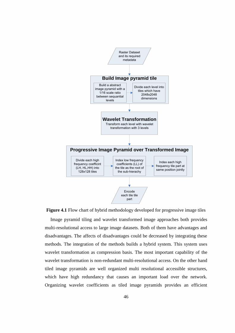
46
Progressive Image Pyramid over Transformed Image
Build Image pyramid tile
Build a abstract
image pyramid with a
1/16 scale ratio
between sequantial
levels
Divide each level into
tiles which have
2048x2048
dimensions
Raster Dataset
and its required
metadata
Wavelet TransformationTransform each level with wavelet
transformation with 3 levels
Divide each high
frequency coefficint
(LH, HL,HH) into
128x128 tiles
Index each high
frequency tile part at
same position jointly
Index low frequency
coefficients (LL) of
the tile as the root of
the sub-hierachy
Encode
each tile tile
part
Figure 4.1 Flow chart of hybrid methodology developed for progressive image tiles
Image pyramid tiling and wavelet transformed image approaches both provides
multi-resolutional access to large image datasets. Both of them have advantages and
disadvantages. The affects of disadvantages could be decreased by integrating these
methods. The integration of the methods builds a hybrid system. This system uses
wavelet transformation as compression basis. The most important capability of the
wavelet transformation is non-redundant multi-resolutional access. On the other hand
tiled image pyramids are well organized multi resolutional accessible structures,
which have high redundancy that causes an important load over the network.
Organizing wavelet coefficients as tiled image pyramids provides an efficient
47
method to compute data blocks indexes to request and reconstruct the required sub-
image.
Wavelet coefficients could be organized as image pyramid tile parts. However the
number of the required tile levels to reconstruct the image from wavelet coefficients
increases with the number of the wavelet transformation level. Therfore, wavelet
transformation could be used to produce sub-levels of an image pyramid to decrease
redundancy over the hierarchy. n number of wavelet transformations over an image
provides n+1 hierarchical levels. Using transformations would decrease the number
of image pyramid levels that has to be produced from the source dataset. Thus, the
load over data source would be decreased. Producing tiles that covers wavelet
coefficients provides easy to implement systems, which already use hierarchical map
tiles.
Build Image Pyramid Tile and Wavelet Transformation components in Figure
4.1 are developed over an image tile pyramid hierarchy which has tiles with
dimensions 256x256. Tiles with sizes 256x256 are frequently used in internet
mapping systems. 3 levels of transformation are applied over tiles. Thus, 4
sequential levels would be provided after transforming each tile part. Tile parts with
dimensions 2048x2048 are processed to provide a single tile with dimensions
256x256 at lowest frequency after transformation which has 3 levels. During
wavelet transformation it is observed that 3 levels of transformation are sufficient for
a good compression ratio. Higher levels of transformation would provide better
compression ratio however more number of transformations causes more
computation time which would suffer web GIS server.
Progressive Image Pyramid over Transformed Image in Figure 4.1 which
contains the whole wavelet coefficient at lowest frequency is providing to store and
serve as a single tile. Higher frequencies are divided into 128x128 tile parts. These
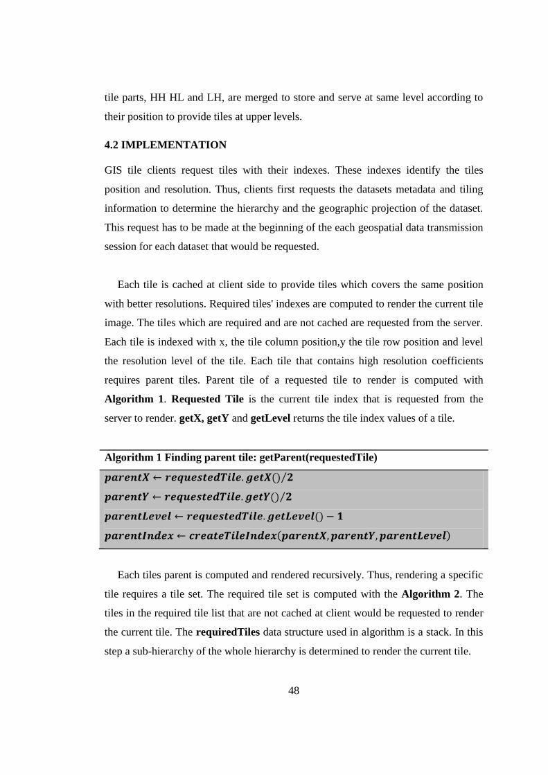
48
tile parts, HH HL and LH, are merged to store and serve at same level according to
their position to provide tiles at upper levels.
4.2 IMPLEMENTATION
GIS tile clients request tiles with their indexes. These indexes identify the tiles
position and resolution. Thus, clients first requests the datasets metadata and tiling
information to determine the hierarchy and the geographic projection of the dataset.
This request has to be made at the beginning of the each geospatial data transmission
session for each dataset that would be requested.
Each tile is cached at client side to provide tiles which covers the same position
with better resolutions. Required tiles' indexes are computed to render the current tile
image. The tiles which are required and are not cached are requested from the server.
Each tile is indexed with x, the tile column position,y the tile row position and level
the resolution level of the tile. Each tile that contains high resolution coefficients
requires parent tiles. Parent tile of a requested tile to render is computed with
Algorithm 1. Requested Tile is the current tile index that is requested from the
server to render. getX, getY and getLevel returns the tile index values of a tile.
Algorithm 1 Finding parent tile: getParent(requestedTile)
Each tiles parent is computed and rendered recursively. Thus, rendering a specific
tile requires a tile set. The required tile set is computed with the Algorithm 2. The
tiles in the required tile list that are not cached at client would be requested to render
the current tile. The requiredTiles data structure used in algorithm is a stack. In this
step a sub-hierarchy of the whole hierarchy is determined to render the current tile.
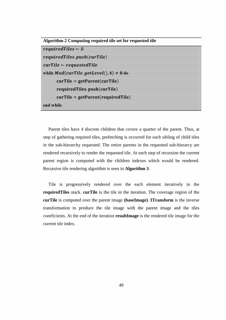
49
Algorithm 2 Computing required tile set for requested tile
Parent tiles have 4 discrete children that covers a quarter of the parent. Thus, at
step of gathering required tiles, prefetching is occurred for each sibling of child tiles
in the sub-hierarchy requested. The entire parents in the requested sub-hierarcy are
rendered recursively to render the requested tile. At each step of recursion the current
parent region is computed with the children indexes which would be rendered.
Recursive tile rendering algorithm is seen in Algorithm 3.
Tile is progressively rendered over the each element iteratively in the
requiredTiles stack. curTile is the tile in the iteration. The coverage region of the
curTile is computed over the parent image (baseImage). ITransform is the inverse
transformation to produce the tile image with the parent image and the tiles
coeeficients. At the end of the iteration resultImage is the rendered tile image for the
current tile index.
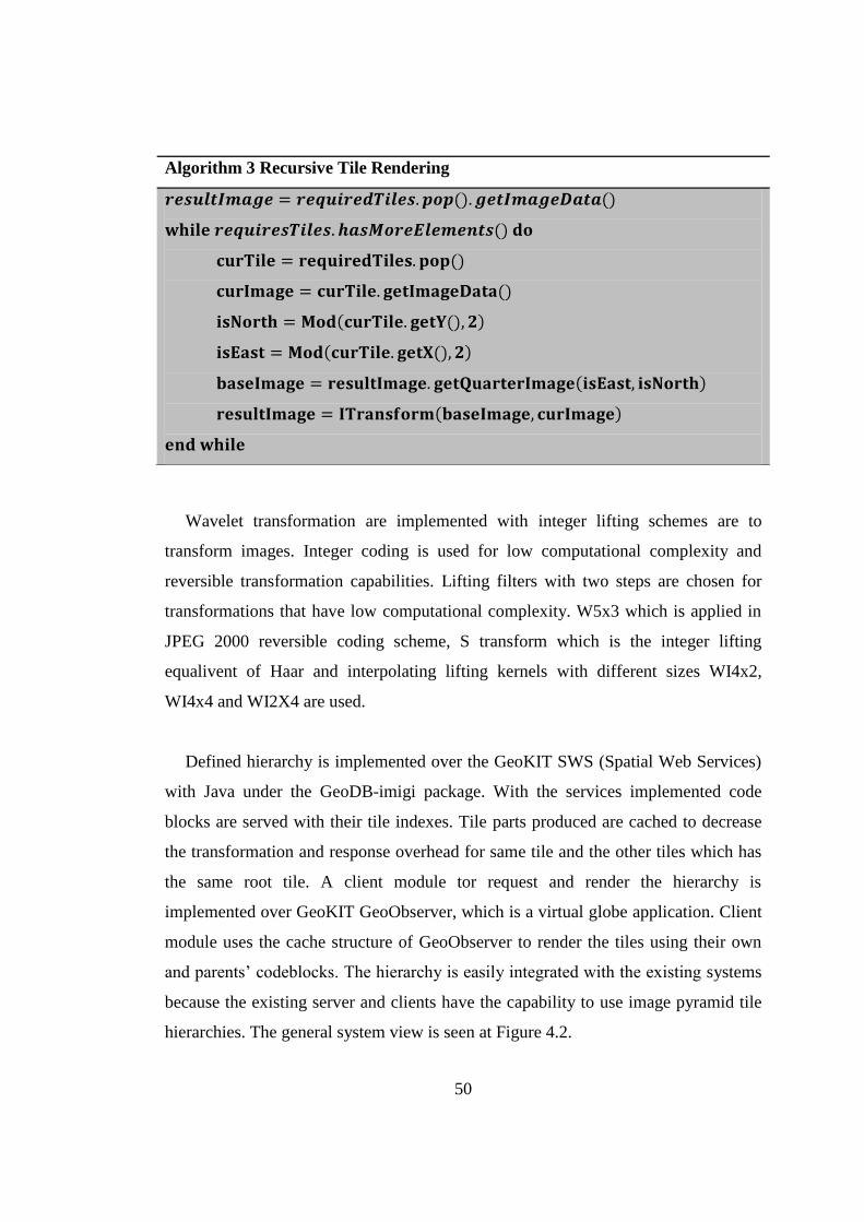
50
Wavelet transformation are implemented with integer lifting schemes are to
transform images. Integer coding is used for low computational complexity and
reversible transformation capabilities. Lifting filters with two steps are chosen for
transformations that have low computational complexity. W5x3 which is applied in
JPEG 2000 reversible coding scheme, S transform which is the integer lifting
equalivent of Haar and interpolating lifting kernels with different sizes WI4x2,
WI4x4 and WI2X4 are used.
Defined hierarchy is implemented over the GeoKIT SWS (Spatial Web Services)
with Java under the GeoDB-imigi package. With the services implemented code
blocks are served with their tile indexes. Tile parts produced are cached to decrease
the transformation and response overhead for same tile and the other tiles which has
the same root tile. A client module tor request and render the hierarchy is
implemented over GeoKIT GeoObserver, which is a virtual globe application. Client
module uses the cache structure of GeoObserver to render the tiles using their own
and parents’ codeblocks. The hierarchy is easily integrated with the existing systems
because the existing server and clients have the capability to use image pyramid tile
hierarchies. The general system view is seen at Figure 4.2.
Algorithm 3 Recursive Tile Rendering
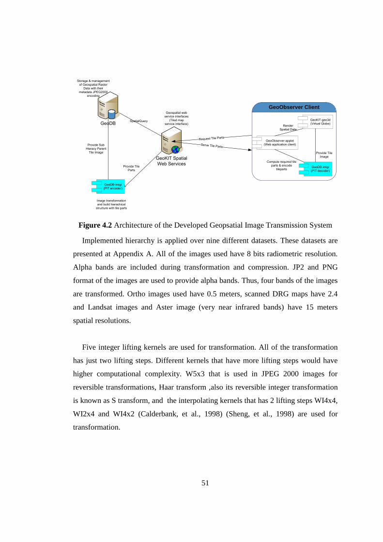
51
GeoDB
GeoKIT Spatial
Web Services
GeoDB-imigi
(PIT encoder)
SpatialQuery
Provide Sub
Hieracy Parent
Tile Image
Provide Tile
Parts
Storage & management
of Geospatial Raster
Data with their
metadata JPEG2000
encoding
Geospatial web
service interfaces
(Tiled map
service interface)
Image transformation
and build hierachical
structure with tile parts
GeoObserver Client
GeoDB-imigi
(PIT decoder)
GeoKIT-geo3d
(Virtual Globe)
GeoObserver-applet
(Web application client)
Request Tile Parts
Provide Tile
Image
Render
Spatial Data
Compute required tile
parts & encode
tileparts
Serve Tile Parts
Figure 4.2 Architecture of the Developed Geopsatial Image Transmission System
Implemented hierarchy is applied over nine different datasets. These datasets are
presented at Appendix A. All of the images used have 8 bits radiometric resolution.
Alpha bands are included during transformation and compression. JP2 and PNG
format of the images are used to provide alpha bands. Thus, four bands of the images
are transformed. Ortho images used have 0.5 meters, scanned DRG maps have 2.4
and Landsat images and Aster image (very near infrared bands) have 15 meters
spatial resolutions.
Five integer lifting kernels are used for transformation. All of the transformation
has just two lifting steps. Different kernels that have more lifting steps would have
higher computational complexity. W5x3 that is used in JPEG 2000 images for
reversible transformations, Haar transform ,also its reversible integer transformation
is known as S transform, and the interpolating kernels that has 2 lifting steps WI4x4,
WI2x4 and WI4x2 (Calderbank, et al., 1998) (Sheng, et al., 1998) are used for
transformation.
52
4.3 RESULTS AND DISCUCCSIONS
Ordinary image pyramid tiling method is applied over the test datasets to compare
with the progressive tile hierarchy. The resulting images are encoded with JPEG,
PNG and JPEG 2000 formats. JPEG 2000 and PNG encoded tiles contains alpha
band for transparency. Tile sets are compressed with 5 levels of transformation and a
compression ratio 30 with JPEG 2000 encoding, which has resulting tile images that
are visually lossles or near lossless. Total sizes of the hierarchies with different
encodings of ordinary hierarchy and with different lifting kernels used for
progressive tile hierarchies are seen in Table 4.1.
Total sizes of the hierarchies with different encodings of ordinary hierarchy and
with different lifting kernels used for progressive tile hierarchies are given in Table
4.1. The number of tiles downloaded, for 5 different type of dataset, over a network
with one megabit per second is seen in Figure 4.3. As seen in the Figure 4.3 number
of tiles downloaded with JP2 encoded Progressive Image Tiles (PIT) are downloaded
faster than the JP2 encoded tile images.
Transformed pyramid hierarchy is compressed with JPEG2000. Tiles that carry
high frequency components of the images are compressed without wavelet
transformation during compression. Thus, JPEG 2000 is used for quantization and
entropy coding, not used for multi-resolutional coding. Different compression ratios
are used for different levels in hierarchy. The compression ratios are chosen to get a
total file size for hierarchy similar to ordinary hiearcy which is encoded with
JPEG2000. After experiments compression ratio for progressive tile structure is
formulated with the Equation 4.1. Tiles at parent levels are compressed with lower
compression ratio because loss is inherited by the child tiles.
4.1
53
Implemented transformations lossless and lossy compression capabilities are
compared with each other and popular image compression formats. 5 different types
of images from 9 different data sets are used in experiments. During lossless
compression it is observed that WI2x4 transformed images are generally compressed
with better compression ratio from the other data blocks which are transformed with
other filters. The second filter that has the best compression ratio is W5x3. Some of
the W5x3 transformed images have the same compression ratio WI2x4. WI4x4 has
better performance on scanned maps during lossless compression. Lossless
compression performances compared with the resulting data blocks sizes. On the
other hand during lossy compression each filters results data blocks are compressed
with same compression ratios. Thus, lossy compression performances are compared
with objective quality metrics SNR at each tiles rendered from code blocks. It is
observed that the W5x3 filter has the best performance over the lossy compressed
geospatial images. W5x3 transformed hierarchies compressed with JPEG 2000 have
better quality then the tiles compressed separately with JPEG and JPEG 2000.
The results are compared in Table 4.1 according to their sizes. However
compression methods that are used to compress hierarchies are lossy methods.
Objective image quality metrics could be used to compare the lossy compressed
datasets. SNR is used to compare each kernel and each encodings performance.The
tiles which are gathered directly from the datasource, are used as source image to
compute SNR. SNR of progressive tile hierarchy tiles are compared with lossy
compressed JPEG and JPEG 2000 images. Comparision of each datasets progressive
tiles with JPEG images is seen in Table 4.3 and with JPEG 2000 images is seen in
Table 4.2.
During losless compression, images that are transformed with WI2x4 (and for
some cases, scanned maps, with WI4x4) are compressed with higher compression
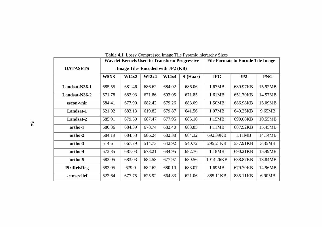
Table 4.1 Lossy Compressed Image Tile Pyramid hierarchy Sizes
DATASETS
Wavelet Kernels Used to Transform Progressive
Image Tiles Encoded with JP2 (KB)
File Formats to Encode Tile Image
W5X3 WI4x2 WI2x4 WI4x4 S-(Haar) JPG JP2 PNG
Landsat-N36-1 685.55 681.46 686.62 684.02 686.06 1.67MB 689.97KB 15.92MB
Landsat-N36-2 671.78 683.03 671.86 693.05 671.85 1.61MB 651.70KB 14.57MB
escon-vnir 684.41 677.90 682.42 679.26 683.09 1.50MB 686.98KB 15.09MB
Landsat-1 621.02 683.13 619.82 679.87 641.56 1.07MB 649.25KB 9.65MB
Landsat-2 685.91 679.50 687.47 677.95 685.16 1.15MB 690.08KB 10.55MB
ortho-1 680.36 684.39 678.74 682.40 683.85 1.11MB 687.92KB 15.45MB
ortho-2 684.19 684.53 686.24 682.38 684.32 692.39KB 1.11MB 14.14MB
ortho-3 514.61 667.79 514.73 642.92 540.72 295.21KB 537.91KB 3.35MB
ortho-4 673.35 687.03 673.21 684.95 682.76 1.18MB 690.21KB 15.49MB
ortho-5 683.05 683.03 684.58 677.97 680.56 1014.26KB 688.87KB 13.84MB
PiriReisReg 683.05 679.0 682.62 680.10 683.07 1.69MB 679.70KB 14.96MB
srtm-relief 622.64 677.75 625.92 664.83 621.06 885.11KB 885.11KB 6.90MB
54
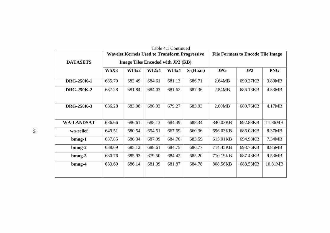
Table 4.1 Continued
DATASETS
Wavelet Kernels Used to Transform Progressive
Image Tiles Encoded with JP2 (KB)
File Formats to Encode Tile Image
W5X3 WI4x2 WI2x4 WI4x4 S-(Haar) JPG JP2 PNG
DRG-250K-1 685.70 682.49 684.61 681.13 686.71 2.64MB 690.27KB 3.80MB
DRG-250K-2 687.28
681.84 684.03 681.62 687.36 2.84MB 686.13KB 4.53MB
DRG-250K-3 686.28
683.08 686.93 679.27 683.93 2.60MB 689.76KB 4.17MB
WA-LANDSAT 686.66 686.61 688.13 684.49 688.34 840.03KB 692.88KB 11.86MB
wa-relief 649.51 680.54 654.51 667.69 660.36 696.03KB 686.02KB 8.37MB
bmng-1 687.85 686.34 687.99 684.70 683.59 615.01KB 694.98KB 7.34MB
bmng-2 688.69 685.12 688.61 684.75 686.77 714.45KB 693.76KB 8.85MB
bmng-3 680.76 685.93 679.50 684.42 685.20 710.19KB 687.48KB 9.53MB
bmng-4 683.60
686.14 681.09 681.87 684.78 808.56KB 688.53KB 10.81MB
55

Figure 4.3 Lossless compressed JP2 encoded tiled image pyramids and JP2 encoded Progressive Image Tiles
56
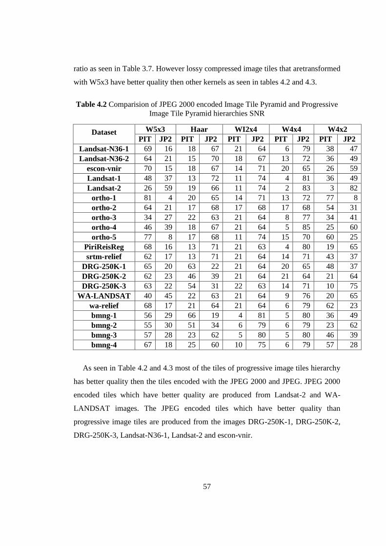
57
ratio as seen in Table 3.7. However lossy compressed image tiles that aretransformed
with W5x3 have better quality then other kernels as seen in tables 4.2 and 4.3.
Table 4.2 Comparision of JPEG 2000 encoded Image Tile Pyramid and Progressive
Image Tile Pyramid hierarchies SNR
Dataset W5x3 Haar WI2x4 W4x4 W4x2
PIT JP2 PIT JP2 PIT JP2 PIT JP2 PIT JP2
Landsat-N36-1 69 16 18 67 21 64 6 79 38 47
Landsat-N36-2 64 21 15 70 18 67 13 72 36 49
escon-vnir 70 15 18 67 14 71 20 65 26 59
Landsat-1 48 37 13 72 11 74 4 81 36 49
Landsat-2 26 59 19 66 11 74 2 83 3 82
ortho-1 81 4 20 65 14 71 13 72 77 8
ortho-2 64 21 17 68 17 68 17 68 54 31
ortho-3 34 27 22 63 21 64 8 77 34 41
ortho-4 46 39 18 67 21 64 5 85 25 60
ortho-5 77 8 17 68 11 74 15 70 60 25
PiriReisReg 68 16 13 71 21 63 4 80 19 65
srtm-relief 62 17 13 71 21 64 14 71 43 37
DRG-250K-1 65 20 63 22 21 64 20 65 48 37
DRG-250K-2 62 23 46 39 21 64 21 64 21 64
DRG-250K-3 63 22 54 31 22 63 14 71 10 75
WA-LANDSAT 40 45 22 63 21 64 9 76 20 65
wa-relief 68 17 21 64 21 64 6 79 62 23
bmng-1 56 29 66 19 4 81 5 80 36 49
bmng-2 55 30 51 34 6 79 6 79 23 62
bmng-3 57 28 23 62 5 80 5 80 46 39
bmng-4 67 18 25 60 10 75 6 79 57 28
As seen in Table 4.2 and 4.3 most of the tiles of progressive image tiles hierarchy
has better quality then the tiles encoded with the JPEG 2000 and JPEG. JPEG 2000
encoded tiles which have better quality are produced from Landsat-2 and WA-
LANDSAT images. The JPEG encoded tiles which have better quality than
progressive image tiles are produced from the images DRG-250K-1, DRG-250K-2,
DRG-250K-3, Landsat-N36-1, Landsat-2 and escon-vnir.
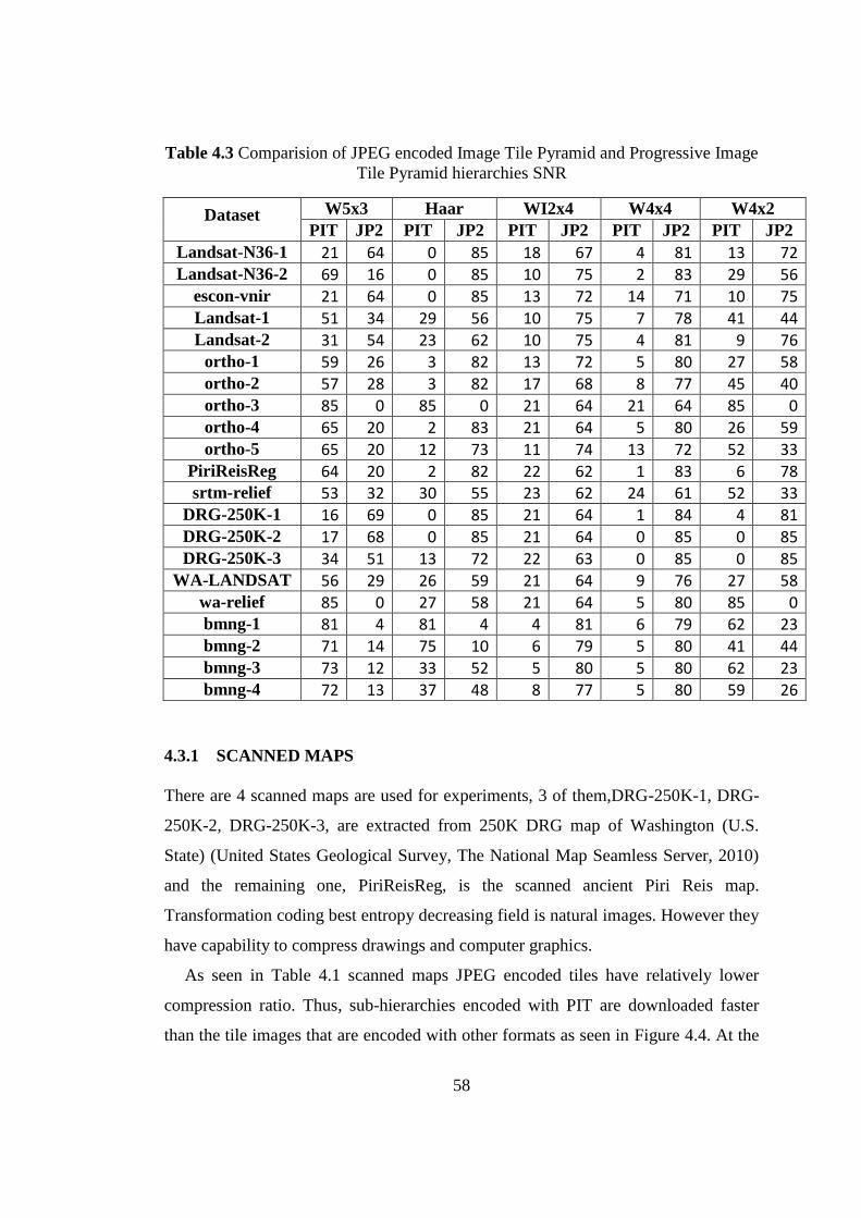
58
Table 4.3 Comparision of JPEG encoded Image Tile Pyramid and Progressive Image
Tile Pyramid hierarchies SNR
Dataset W5x3 Haar WI2x4 W4x4 W4x2
PIT JP2 PIT JP2 PIT JP2 PIT JP2 PIT JP2
Landsat-N36-1 21 64 0 85 18 67 4 81 13 72 Landsat-N36-2 69 16 0 85 10 75 2 83 29 56
escon-vnir 21 64 0 85 13 72 14 71 10 75 Landsat-1 51 34 29 56 10 75 7 78 41 44 Landsat-2 31 54 23 62 10 75 4 81 9 76
ortho-1 59 26 3 82 13 72 5 80 27 58 ortho-2 57 28 3 82 17 68 8 77 45 40 ortho-3 85 0 85 0 21 64 21 64 85 0 ortho-4 65 20 2 83 21 64 5 80 26 59 ortho-5 65 20 12 73 11 74 13 72 52 33
PiriReisReg 64 20 2 82 22 62 1 83 6 78 srtm-relief 53 32 30 55 23 62 24 61 52 33
DRG-250K-1 16 69 0 85 21 64 1 84 4 81 DRG-250K-2 17 68 0 85 21 64 0 85 0 85 DRG-250K-3 34 51 13 72 22 63 0 85 0 85
WA-LANDSAT 56 29 26 59 21 64 9 76 27 58 wa-relief 85 0 27 58 21 64 5 80 85 0 bmng-1 81 4 81 4 4 81 6 79 62 23 bmng-2 71 14 75 10 6 79 5 80 41 44 bmng-3 73 12 33 52 5 80 5 80 62 23 bmng-4 72 13 37 48 8 77 5 80 59 26
4.3.1 SCANNED MAPS
There are 4 scanned maps are used for experiments, 3 of them,DRG-250K-1, DRG-
250K-2, DRG-250K-3, are extracted from 250K DRG map of Washington (U.S.
State) (United States Geological Survey, The National Map Seamless Server, 2010)
and the remaining one, PiriReisReg, is the scanned ancient Piri Reis map.
Transformation coding best entropy decreasing field is natural images. However they
have capability to compress drawings and computer graphics.
As seen in Table 4.1 scanned maps JPEG encoded tiles have relatively lower
compression ratio. Thus, sub-hierarchies encoded with PIT are downloaded faster
than the tile images that are encoded with other formats as seen in Figure 4.4. At the
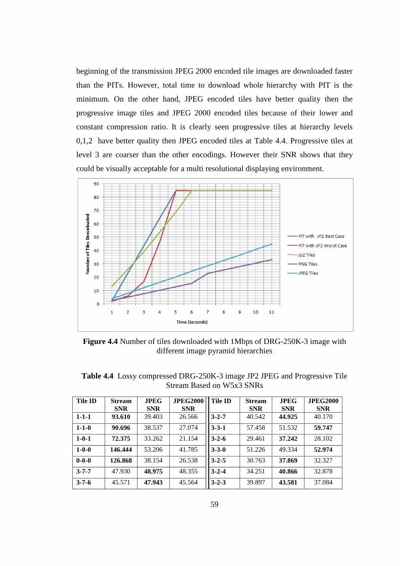
59
beginning of the transmission JPEG 2000 encoded tile images are downloaded faster
than the PITs. However, total time to download whole hierarchy with PIT is the
minimum. On the other hand, JPEG encoded tiles have better quality then the
progressive image tiles and JPEG 2000 encoded tiles because of their lower and
constant compression ratio. It is clearly seen progressive tiles at hierarchy levels
0,1,2 have better quality then JPEG encoded tiles at Table 4.4. Progressive tiles at
level 3 are coarser than the other encodings. However their SNR shows that they
could be visually acceptable for a multi resolutional displaying environment.
Figure 4.4 Number of tiles downloaded with 1Mbps of DRG-250K-3 image with
different image pyramid hierarchies
Table 4.4 Lossy compressed DRG-250K-3 image JP2 JPEG and Progressive Tile
Stream Based on W5x3 SNRs
Tile ID Stream
SNR
JPEG
SNR
JPEG2000
SNR
Tile ID Stream
SNR
JPEG
SNR
JPEG2000
SNR
1-1-1 93.610 39.403 26.566 3-2-7 40.542 44.925 40.170
1-1-0 90.696 38.537 27.074 3-3-1 57.458 51.532 59.747
1-0-1 72.375 33.262 21.154 3-2-6 29.461 37.242 28.102
1-0-0 146.444 53.206 41.785 3-3-0 51.226 49.334 52.974
0-0-0 126.868 38.154 26.538 3-2-5 30.763 37.869 32.327
3-7-7 47.930 48.975 48.355 3-2-4 34.251 40.866 32.878
3-7-6 45.571 47.943 45.564 3-2-3 39.897 43.581 37.084
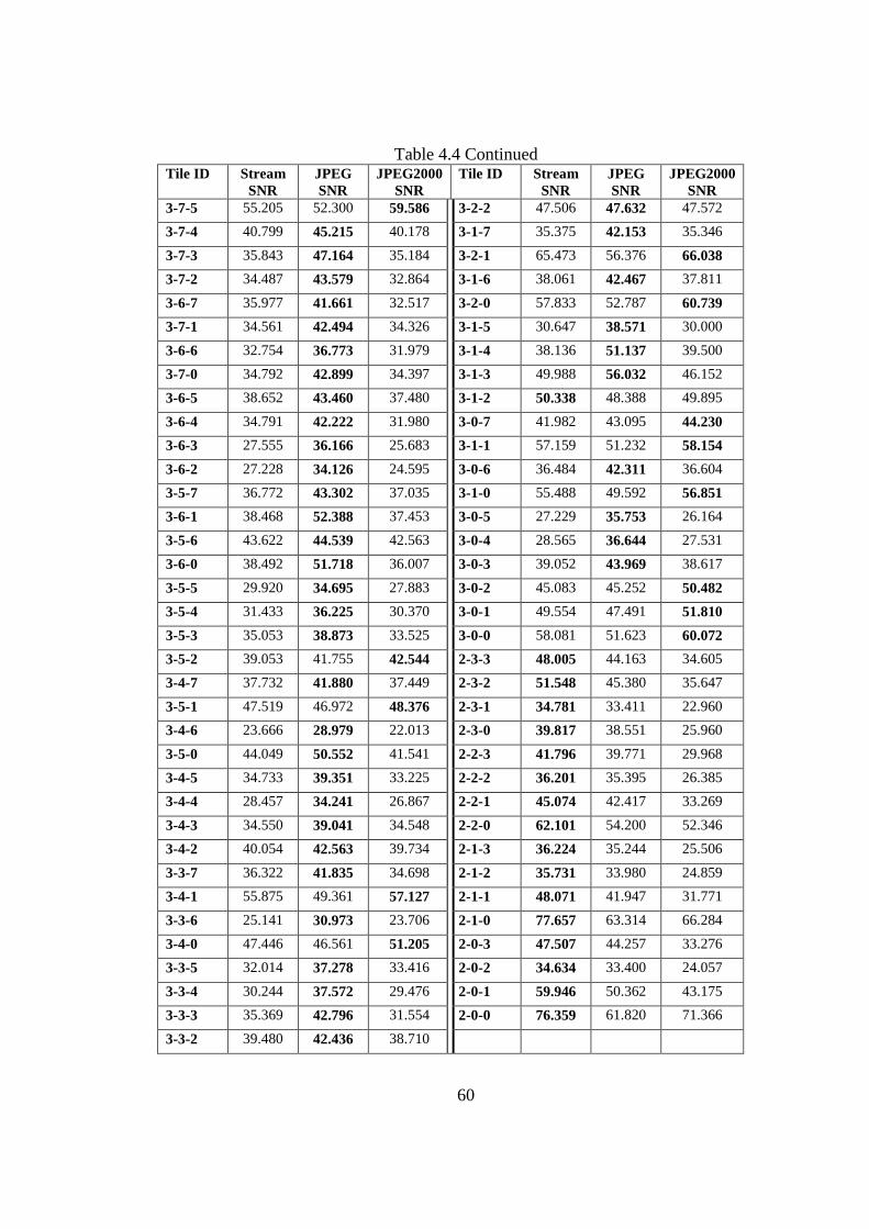
60
Table 4.4 Continued Tile ID Stream
SNR
JPEG
SNR
JPEG2000
SNR
Tile ID Stream
SNR
JPEG
SNR
JPEG2000
SNR
3-7-5 55.205 52.300 59.586 3-2-2 47.506 47.632 47.572
3-7-4 40.799 45.215 40.178 3-1-7 35.375 42.153 35.346
3-7-3 35.843 47.164 35.184 3-2-1 65.473 56.376 66.038
3-7-2 34.487 43.579 32.864 3-1-6 38.061 42.467 37.811
3-6-7 35.977 41.661 32.517 3-2-0 57.833 52.787 60.739
3-7-1 34.561 42.494 34.326 3-1-5 30.647 38.571 30.000
3-6-6 32.754 36.773 31.979 3-1-4 38.136 51.137 39.500
3-7-0 34.792 42.899 34.397 3-1-3 49.988 56.032 46.152
3-6-5 38.652 43.460 37.480 3-1-2 50.338 48.388 49.895
3-6-4 34.791 42.222 31.980 3-0-7 41.982 43.095 44.230
3-6-3 27.555 36.166 25.683 3-1-1 57.159 51.232 58.154
3-6-2 27.228 34.126 24.595 3-0-6 36.484 42.311 36.604
3-5-7 36.772 43.302 37.035 3-1-0 55.488 49.592 56.851
3-6-1 38.468 52.388 37.453 3-0-5 27.229 35.753 26.164
3-5-6 43.622 44.539 42.563 3-0-4 28.565 36.644 27.531
3-6-0 38.492 51.718 36.007 3-0-3 39.052 43.969 38.617
3-5-5 29.920 34.695 27.883 3-0-2 45.083 45.252 50.482
3-5-4 31.433 36.225 30.370 3-0-1 49.554 47.491 51.810
3-5-3 35.053 38.873 33.525 3-0-0 58.081 51.623 60.072
3-5-2 39.053 41.755 42.544 2-3-3 48.005 44.163 34.605
3-4-7 37.732 41.880 37.449 2-3-2 51.548 45.380 35.647
3-5-1 47.519 46.972 48.376 2-3-1 34.781 33.411 22.960
3-4-6 23.666 28.979 22.013 2-3-0 39.817 38.551 25.960
3-5-0 44.049 50.552 41.541 2-2-3 41.796 39.771 29.968
3-4-5 34.733 39.351 33.225 2-2-2 36.201 35.395 26.385
3-4-4 28.457 34.241 26.867 2-2-1 45.074 42.417 33.269
3-4-3 34.550 39.041 34.548 2-2-0 62.101 54.200 52.346
3-4-2 40.054 42.563 39.734 2-1-3 36.224 35.244 25.506
3-3-7 36.322 41.835 34.698 2-1-2 35.731 33.980 24.859
3-4-1 55.875 49.361 57.127 2-1-1 48.071 41.947 31.771
3-3-6 25.141 30.973 23.706 2-1-0 77.657 63.314 66.284
3-4-0 47.446 46.561 51.205 2-0-3 47.507 44.257 33.276
3-3-5 32.014 37.278 33.416 2-0-2 34.634 33.400 24.057
3-3-4 30.244 37.572 29.476 2-0-1 59.946 50.362 43.175
3-3-3 35.369 42.796 31.554 2-0-0 76.359 61.820 71.366
3-3-2 39.480 42.436 38.710
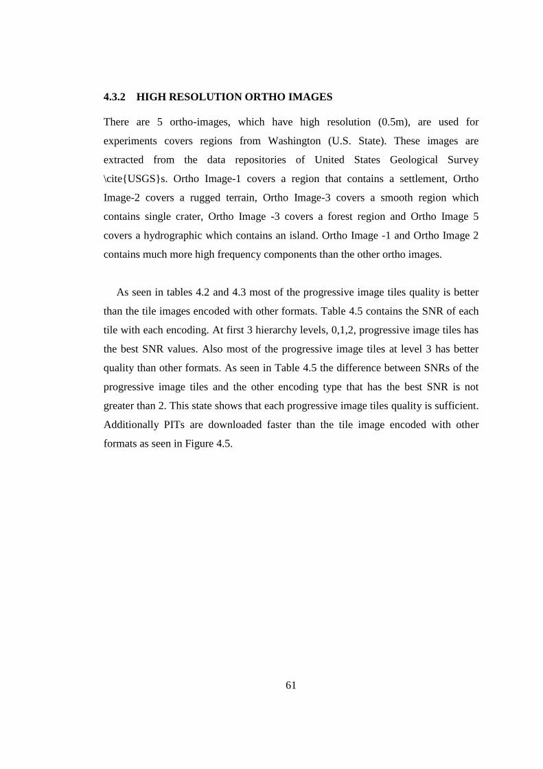
61
4.3.2 HIGH RESOLUTION ORTHO IMAGES
There are 5 ortho-images, which have high resolution (0.5m), are used for
experiments covers regions from Washington (U.S. State). These images are
extracted from the data repositories of United States Geological Survey
\cite{USGS}s. Ortho Image-1 covers a region that contains a settlement, Ortho
Image-2 covers a rugged terrain, Ortho Image-3 covers a smooth region which
contains single crater, Ortho Image -3 covers a forest region and Ortho Image 5
covers a hydrographic which contains an island. Ortho Image -1 and Ortho Image 2
contains much more high frequency components than the other ortho images.
As seen in tables 4.2 and 4.3 most of the progressive image tiles quality is better
than the tile images encoded with other formats. Table 4.5 contains the SNR of each
tile with each encoding. At first 3 hierarchy levels, 0,1,2, progressive image tiles has
the best SNR values. Also most of the progressive image tiles at level 3 has better
quality than other formats. As seen in Table 4.5 the difference between SNRs of the
progressive image tiles and the other encoding type that has the best SNR is not
greater than 2. This state shows that each progressive image tiles quality is sufficient.
Additionally PITs are downloaded faster than the tile image encoded with other
formats as seen in Figure 4.5.
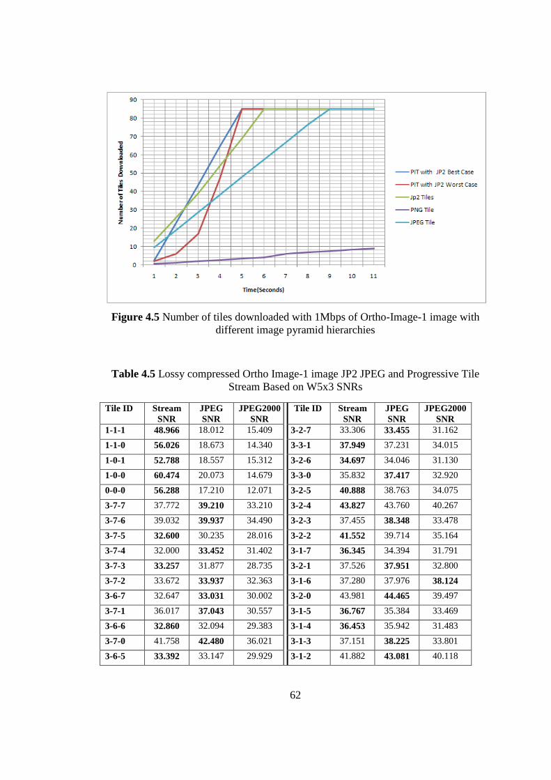
62
Figure 4.5 Number of tiles downloaded with 1Mbps of Ortho-Image-1 image with
different image pyramid hierarchies
Table 4.5 Lossy compressed Ortho Image-1 image JP2 JPEG and Progressive Tile
Stream Based on W5x3 SNRs
Tile ID Stream
SNR
JPEG
SNR
JPEG2000
SNR
Tile ID Stream
SNR
JPEG
SNR
JPEG2000
SNR
1-1-1 48.966 18.012 15.409 3-2-7 33.306 33.455 31.162
1-1-0 56.026 18.673 14.340 3-3-1 37.949 37.231 34.015
1-0-1 52.788 18.557 15.312 3-2-6 34.697 34.046 31.130
1-0-0 60.474 20.073 14.679 3-3-0 35.832 37.417 32.920
0-0-0 56.288 17.210 12.071 3-2-5 40.888 38.763 34.075
3-7-7 37.772 39.210 33.210 3-2-4 43.827 43.760 40.267
3-7-6 39.032 39.937 34.490 3-2-3 37.455 38.348 33.478
3-7-5 32.600 30.235 28.016 3-2-2 41.552 39.714 35.164
3-7-4 32.000 33.452 31.402 3-1-7 36.345 34.394 31.791
3-7-3 33.257 31.877 28.735 3-2-1 37.526 37.951 32.800
3-7-2 33.672 33.937 32.363 3-1-6 37.280 37.976 38.124
3-6-7 32.647 33.031 30.002 3-2-0 43.981 44.465 39.497
3-7-1 36.017 37.043 30.557 3-1-5 36.767 35.384 33.469
3-6-6 32.860 32.094 29.383 3-1-4 36.453 35.942 31.483
3-7-0 41.758 42.480 36.021 3-1-3 37.151 38.225 33.801
3-6-5 33.392 33.147 29.929 3-1-2 41.882 43.081 40.118
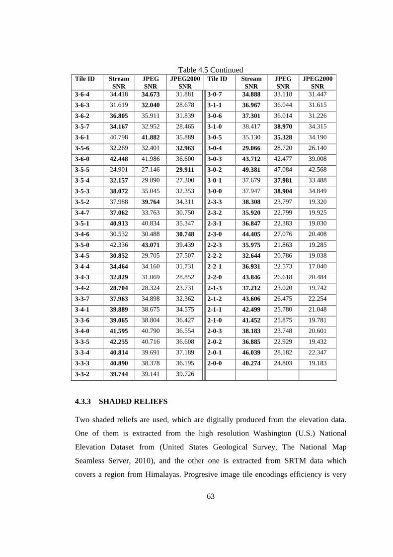
63
Table 4.5 Continued Tile ID Stream
SNR
JPEG
SNR
JPEG2000
SNR
Tile ID Stream
SNR
JPEG
SNR
JPEG2000
SNR
3-6-4 34.418 34.673 31.881 3-0-7 34.888 33.118 31.447
3-6-3 31.619 32.040 28.678 3-1-1 36.967 36.044 31.615
3-6-2 36.805 35.911 31.839 3-0-6 37.301 36.014 31.226
3-5-7 34.167 32.952 28.465 3-1-0 38.417 38.970 34.315
3-6-1 40.798 41.882 35.889 3-0-5 35.130 35.328 34.190
3-5-6 32.269 32.401 32.963 3-0-4 29.066 28.720 26.140
3-6-0 42.448 41.986 36.600 3-0-3 43.712 42.477 39.008
3-5-5 24.901 27.146 29.911 3-0-2 49.381 47.084 42.568
3-5-4 32.157 29.890 27.300 3-0-1 37.679 37.981 33.488
3-5-3 38.072 35.045 32.353 3-0-0 37.947 38.904 34.849
3-5-2 37.988 39.764 34.311 2-3-3 38.308 23.797 19.320
3-4-7 37.062 33.763 30.750 2-3-2 35.920 22.799 19.925
3-5-1 40.913 40.834 35.347 2-3-1 36.847 22.383 19.030
3-4-6 30.532 30.488 30.748 2-3-0 44.405 27.076 20.408
3-5-0 42.336 43.071 39.439 2-2-3 35.975 21.863 19.285
3-4-5 30.852 29.705 27.507 2-2-2 32.644 20.786 19.038
3-4-4 34.464 34.160 31.731 2-2-1 36.931 22.573 17.040
3-4-3 32.829 31.069 28.852 2-2-0 43.846 26.618 20.484
3-4-2 28.704 28.324 23.731 2-1-3 37.212 23.020 19.742
3-3-7 37.963 34.898 32.362 2-1-2 43.606 26.475 22.254
3-4-1 39.889 38.675 34.575 2-1-1 42.499 25.780 21.048
3-3-6 39.065 38.804 36.427 2-1-0 41.452 25.875 19.781
3-4-0 41.595 40.790 36.554 2-0-3 38.183 23.748 20.601
3-3-5 42.255 40.716 36.608 2-0-2 36.885 22.929 19.432
3-3-4 40.814 39.691 37.189 2-0-1 46.039 28.182 22.347
3-3-3 40.890 38.378 36.195 2-0-0 40.274 24.803 19.183
3-3-2 39.744 39.141 39.726
4.3.3 SHADED RELIEFS
Two shaded reliefs are used, which are digitally produced from the elevation data.
One of them is extracted from the high resolution Washington (U.S.) National
Elevation Dataset from (United States Geological Survey, The National Map
Seamless Server, 2010), and the other one is extracted from SRTM data which
covers a region from Himalayas. Progresive image tile encodings efficiency is very
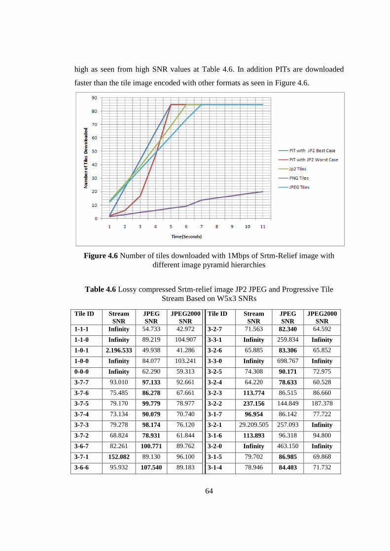
64
high as seen from high SNR values at Table 4.6. In addition PITs are downloaded
faster than the tile image encoded with other formats as seen in Figure 4.6.
Figure 4.6 Number of tiles downloaded with 1Mbps of Srtm-Relief image with
different image pyramid hierarchies
Table 4.6 Lossy compressed Srtm-relief image JP2 JPEG and Progressive Tile
Stream Based on W5x3 SNRs
Tile ID Stream
SNR
JPEG
SNR
JPEG2000
SNR
Tile ID Stream
SNR
JPEG
SNR
JPEG2000
SNR
1-1-1 Infinity 54.733 42.972 3-2-7 71.563 82.340 64.592
1-1-0 Infinity 89.219 104.907 3-3-1 Infinity 259.834 Infinity
1-0-1 2.196.533 49.938 41.286 3-2-6 65.885 83.306 65.852
1-0-0 Infinity 84.077 103.241 3-3-0 Infinity 698.767 Infinity
0-0-0 Infinity 62.290 59.313 3-2-5 74.308 90.171 72.975
3-7-7 93.010 97.133 92.661 3-2-4 64.220 78.633 60.528
3-7-6 75.485 86.278 67.661 3-2-3 113.774 86.515 86.660
3-7-5 79.170 99.779 78.977 3-2-2 237.156 144.849 187.378
3-7-4 73.134 90.079 70.740 3-1-7 96.954 86.142 77.722
3-7-3 79.278 98.174 76.120 3-2-1 29.209.505 257.093 Infinity
3-7-2 68.824 78.931 61.844 3-1-6 113.893 96.318 94.800
3-6-7 82.261 100.771 89.762 3-2-0 Infinity 463.150 Infinity
3-7-1 152.082 89.130 96.100 3-1-5 79.702 86.985 69.868
3-6-6 95.932 107.540 89.183 3-1-4 78.946 84.403 71.732
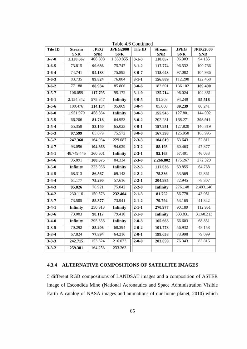
65
Table 4.6 Continued Tile ID Stream
SNR
JPEG
SNR
JPEG2000
SNR
Tile ID Stream
SNR
JPEG
SNR
JPEG2000
SNR
3-7-0 1.120.667 408.608 1.369.855 3-1-3 110.657 96.303 94.185
3-6-5 73.815 90.686 75.747 3-1-2 117.774 96.532 100.766
3-6-4 74.741 94.183 75.895 3-0-7 118.043 97.082 104.986
3-6-3 83.735 89.824 76.884 3-1-1 156.889 112.298 122.468
3-6-2 77.188 88.934 85.806 3-0-6 183.691 136.102 189.400
3-5-7 106.059 117.795 95.172 3-1-0 125.714 96.024 102.361
3-6-1 2.154.842 575.647 Infinity 3-0-5 91.308 94.249 95.518
3-5-6 100.476 114.134 95.869 3-0-4 85.000 89.239 80.241
3-6-0 1.951.970 458.664 Infinity 3-0-3 155.945 127.801 144.002
3-5-5 66.206 81.718 64.953 3-0-2 202.281 168.271 208.911
3-5-4 65.358 83.140 65.023 3-0-1 157.951 127.820 146.819
3-5-3 97.599 85.679 75.572 3-0-0 167.398 125.958 165.995
3-5-2 247.360 164.034 229.087 2-3-3 104.619 63.643 52.811
3-4-7 93.096 104.368 94.029 2-3-2 88.193 60.463 47.377
3-5-1 48.749.445 360.601 Infinity 2-3-1 92.163 57.401 46.033
3-4-6 95.891 108.675 84.324 2-3-0 2.266.802 175.267 272.329
3-5-0 Infinity 223.956 Infinity 2-2-3 117.036 69.855 64.768
3-4-5 68.313 86.567 69.143 2-2-2 75.336 53.569 42.361
3-4-4 61.177 75.290 57.616 2-2-1 204.985 72.945 78.307
3-4-3 95.826 76.921 75.042 2-2-0 Infinity 276.148 2.493.146
3-4-2 230.110 150.578 232.404 2-1-3 81.752 56.778 43.951
3-3-7 73.505 88.377 73.941 2-1-2 79.794 53.165 41.342
3-4-1 Infinity 250.913 Infinity 2-1-1 270.977 90.189 112.951
3-3-6 73.083 98.117 79.410 2-1-0 Infinity 333.831 3.168.213
3-4-0 Infinity 295.358 Infinity 2-0-3 165.663 66.603 68.851
3-3-5 70.292 85.206 68.394 2-0-2 101.778 56.932 48.158
3-3-4 67.824 77.894 64.216 2-0-1 199.058 73.998 79.099
3-3-3 242.715 153.624 216.033 2-0-0 203.059 76.343 83.816
3-3-2 259.381 164.258 233.263
4.3.4 ALTERNATIVE COMPOSITIONS OF SATELLITE IMAGES
5 different RGB compositions of LANDSAT images and a composition of ASTER
image of Escondida Mine (National Aeronautics and Space Administration Visible
Earth A catalog of NASA images and animations of our home planet, 2010) which
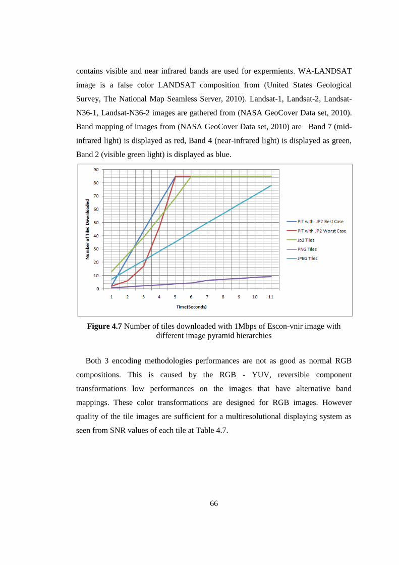
66
contains visible and near infrared bands are used for expermients. WA-LANDSAT
image is a false color LANDSAT composition from (United States Geological
Survey, The National Map Seamless Server, 2010). Landsat-1, Landsat-2, Landsat-
N36-1, Landsat-N36-2 images are gathered from (NASA GeoCover Data set, 2010).
Band mapping of images from (NASA GeoCover Data set, 2010) are Band 7 (mid-
infrared light) is displayed as red, Band 4 (near-infrared light) is displayed as green,
Band 2 (visible green light) is displayed as blue.
Figure 4.7 Number of tiles downloaded with 1Mbps of Escon-vnir image with
different image pyramid hierarchies
Both 3 encoding methodologies performances are not as good as normal RGB
compositions. This is caused by the RGB - YUV, reversible component
transformations low performances on the images that have alternative band
mappings. These color transformations are designed for RGB images. However
quality of the tile images are sufficient for a multiresolutional displaying system as
seen from SNR values of each tile at Table 4.7.
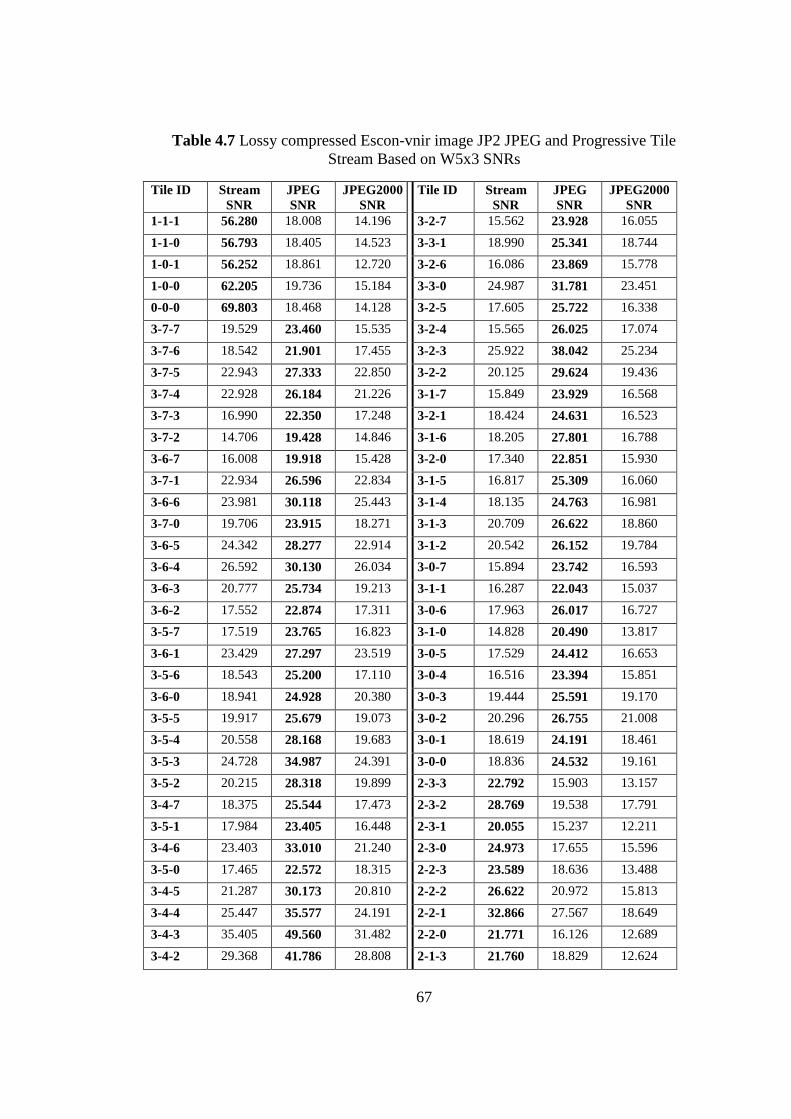
67
Table 4.7 Lossy compressed Escon-vnir image JP2 JPEG and Progressive Tile
Stream Based on W5x3 SNRs
Tile ID Stream
SNR
JPEG
SNR
JPEG2000
SNR
Tile ID Stream
SNR
JPEG
SNR
JPEG2000
SNR
1-1-1 56.280 18.008 14.196 3-2-7 15.562 23.928 16.055
1-1-0 56.793 18.405 14.523 3-3-1 18.990 25.341 18.744
1-0-1 56.252 18.861 12.720 3-2-6 16.086 23.869 15.778
1-0-0 62.205 19.736 15.184 3-3-0 24.987 31.781 23.451
0-0-0 69.803 18.468 14.128 3-2-5 17.605 25.722 16.338
3-7-7 19.529 23.460 15.535 3-2-4 15.565 26.025 17.074
3-7-6 18.542 21.901 17.455 3-2-3 25.922 38.042 25.234
3-7-5 22.943 27.333 22.850 3-2-2 20.125 29.624 19.436
3-7-4 22.928 26.184 21.226 3-1-7 15.849 23.929 16.568
3-7-3 16.990 22.350 17.248 3-2-1 18.424 24.631 16.523
3-7-2 14.706 19.428 14.846 3-1-6 18.205 27.801 16.788
3-6-7 16.008 19.918 15.428 3-2-0 17.340 22.851 15.930
3-7-1 22.934 26.596 22.834 3-1-5 16.817 25.309 16.060
3-6-6 23.981 30.118 25.443 3-1-4 18.135 24.763 16.981
3-7-0 19.706 23.915 18.271 3-1-3 20.709 26.622 18.860
3-6-5 24.342 28.277 22.914 3-1-2 20.542 26.152 19.784
3-6-4 26.592 30.130 26.034 3-0-7 15.894 23.742 16.593
3-6-3 20.777 25.734 19.213 3-1-1 16.287 22.043 15.037
3-6-2 17.552 22.874 17.311 3-0-6 17.963 26.017 16.727
3-5-7 17.519 23.765 16.823 3-1-0 14.828 20.490 13.817
3-6-1 23.429 27.297 23.519 3-0-5 17.529 24.412 16.653
3-5-6 18.543 25.200 17.110 3-0-4 16.516 23.394 15.851
3-6-0 18.941 24.928 20.380 3-0-3 19.444 25.591 19.170
3-5-5 19.917 25.679 19.073 3-0-2 20.296 26.755 21.008
3-5-4 20.558 28.168 19.683 3-0-1 18.619 24.191 18.461
3-5-3 24.728 34.987 24.391 3-0-0 18.836 24.532 19.161
3-5-2 20.215 28.318 19.899 2-3-3 22.792 15.903 13.157
3-4-7 18.375 25.544 17.473 2-3-2 28.769 19.538 17.791
3-5-1 17.984 23.405 16.448 2-3-1 20.055 15.237 12.211
3-4-6 23.403 33.010 21.240 2-3-0 24.973 17.655 15.596
3-5-0 17.465 22.572 18.315 2-2-3 23.589 18.636 13.488
3-4-5 21.287 30.173 20.810 2-2-2 26.622 20.972 15.813
3-4-4 25.447 35.577 24.191 2-2-1 32.866 27.567 18.649
3-4-3 35.405 49.560 31.482 2-2-0 21.771 16.126 12.689
3-4-2 29.368 41.786 28.808 2-1-3 21.760 18.829 12.624
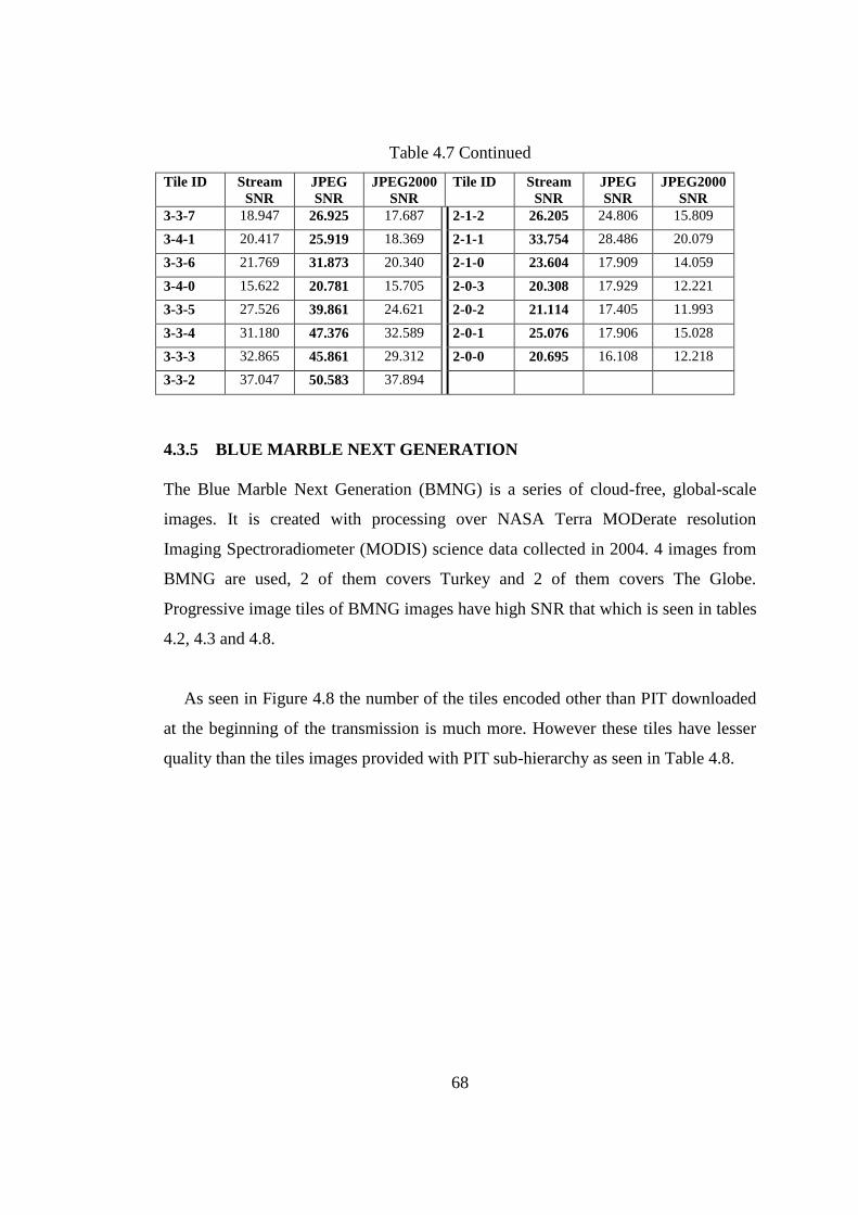
68
Table 4.7 Continued
Tile ID Stream
SNR
JPEG
SNR
JPEG2000
SNR
Tile ID Stream
SNR
JPEG
SNR
JPEG2000
SNR
3-3-7 18.947 26.925 17.687 2-1-2 26.205 24.806 15.809
3-4-1 20.417 25.919 18.369 2-1-1 33.754 28.486 20.079
3-3-6 21.769 31.873 20.340 2-1-0 23.604 17.909 14.059
3-4-0 15.622 20.781 15.705 2-0-3 20.308 17.929 12.221
3-3-5 27.526 39.861 24.621 2-0-2 21.114 17.405 11.993
3-3-4 31.180 47.376 32.589 2-0-1 25.076 17.906 15.028
3-3-3 32.865 45.861 29.312 2-0-0 20.695 16.108 12.218
3-3-2 37.047 50.583 37.894
4.3.5 BLUE MARBLE NEXT GENERATION
The Blue Marble Next Generation (BMNG) is a series of cloud-free, global-scale
images. It is created with processing over NASA Terra MODerate resolution
Imaging Spectroradiometer (MODIS) science data collected in 2004. 4 images from
BMNG are used, 2 of them covers Turkey and 2 of them covers The Globe.
Progressive image tiles of BMNG images have high SNR that which is seen in tables
4.2, 4.3 and 4.8.
As seen in Figure 4.8 the number of the tiles encoded other than PIT downloaded
at the beginning of the transmission is much more. However these tiles have lesser
quality than the tiles images provided with PIT sub-hierarchy as seen in Table 4.8.
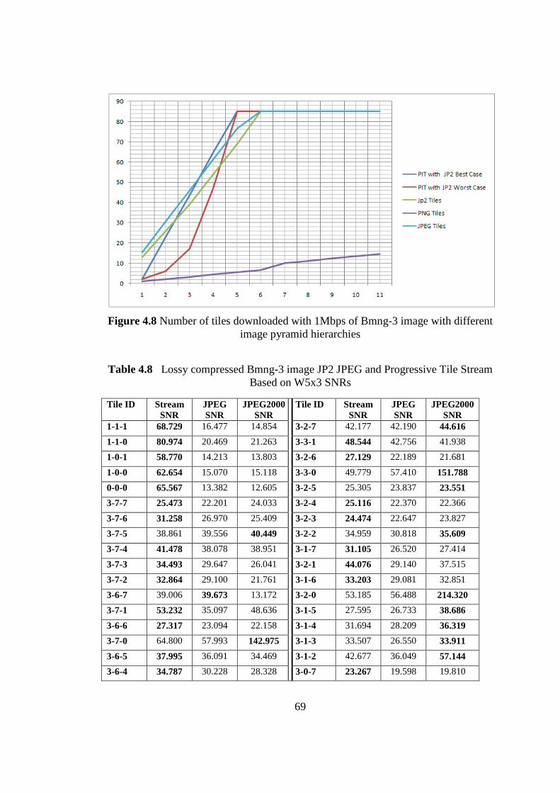
69
Figure 4.8 Number of tiles downloaded with 1Mbps of Bmng-3 image with different
image pyramid hierarchies
Table 4.8 Lossy compressed Bmng-3 image JP2 JPEG and Progressive Tile Stream
Based on W5x3 SNRs
Tile ID Stream
SNR
JPEG
SNR
JPEG2000
SNR
Tile ID Stream
SNR
JPEG
SNR
JPEG2000
SNR
1-1-1 68.729 16.477 14.854 3-2-7 42.177 42.190 44.616
1-1-0 80.974 20.469 21.263 3-3-1 48.544 42.756 41.938
1-0-1 58.770 14.213 13.803 3-2-6 27.129 22.189 21.681
1-0-0 62.654 15.070 15.118 3-3-0 49.779 57.410 151.788
0-0-0 65.567 13.382 12.605 3-2-5 25.305 23.837 23.551
3-7-7 25.473 22.201 24.033 3-2-4 25.116 22.370 22.366
3-7-6 31.258 26.970 25.409 3-2-3 24.474 22.647 23.827
3-7-5 38.861 39.556 40.449 3-2-2 34.959 30.818 35.609
3-7-4 41.478 38.078 38.951 3-1-7 31.105 26.520 27.414
3-7-3 34.493 29.647 26.041 3-2-1 44.076 29.140 37.515
3-7-2 32.864 29.100 21.761 3-1-6 33.203 29.081 32.851
3-6-7 39.006 39.673 13.172 3-2-0 53.185 56.488 214.320
3-7-1 53.232 35.097 48.636 3-1-5 27.595 26.733 38.686
3-6-6 27.317 23.094 22.158 3-1-4 31.694 28.209 36.319
3-7-0 64.800 57.993 142.975 3-1-3 33.507 26.550 33.911
3-6-5 37.995 36.091 34.469 3-1-2 42.677 36.049 57.144
3-6-4 34.787 30.228 28.328 3-0-7 23.267 19.598 19.810
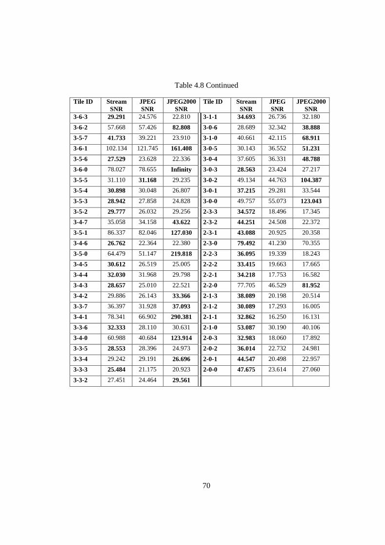
70
Table 4.8 Continued
Tile ID Stream
SNR
JPEG
SNR
JPEG2000
SNR
Tile ID Stream
SNR
JPEG
SNR
JPEG2000
SNR
3-6-3 29.291 24.576 22.810 3-1-1 34.693 26.736 32.180
3-6-2 57.668 57.426 82.808 3-0-6 28.689 32.342 38.888
3-5-7 41.733 39.221 23.910 3-1-0 40.661 42.115 68.911
3-6-1 102.134 121.745 161.408 3-0-5 30.143 36.552 51.231
3-5-6 27.529 23.628 22.336 3-0-4 37.605 36.331 48.788
3-6-0 78.027 78.655 Infinity 3-0-3 28.563 23.424 27.217
3-5-5 31.110 31.168 29.235 3-0-2 49.134 44.763 104.387
3-5-4 30.898 30.048 26.807 3-0-1 37.215 29.281 33.544
3-5-3 28.942 27.858 24.828 3-0-0 49.757 55.073 123.043
3-5-2 29.777 26.032 29.256 2-3-3 34.572 18.496 17.345
3-4-7 35.058 34.158 43.622 2-3-2 44.251 24.508 22.372
3-5-1 86.337 82.046 127.030 2-3-1 43.088 20.925 20.358
3-4-6 26.762 22.364 22.380 2-3-0 79.492 41.230 70.355
3-5-0 64.479 51.147 219.818 2-2-3 36.095 19.339 18.243
3-4-5 30.612 26.519 25.005 2-2-2 33.415 19.663 17.665
3-4-4 32.030 31.968 29.798 2-2-1 34.218 17.753 16.582
3-4-3 28.657 25.010 22.521 2-2-0 77.705 46.529 81.952
3-4-2 29.886 26.143 33.366 2-1-3 38.089 20.198 20.514
3-3-7 36.397 31.928 37.093 2-1-2 30.089 17.293 16.005
3-4-1 78.341 66.902 290.381 2-1-1 32.862 16.250 16.131
3-3-6 32.333 28.110 30.631 2-1-0 53.087 30.190 40.106
3-4-0 60.988 40.684 123.914 2-0-3 32.983 18.060 17.892
3-3-5 28.553 28.396 24.973 2-0-2 36.014 22.732 24.981
3-3-4 29.242 29.191 26.696 2-0-1 44.547 20.498 22.957
3-3-3 25.484 21.175 20.923 2-0-0 47.675 23.614 27.060
3-3-2 27.451 24.464 29.561
71
CHAPTER 5
CONCLUSIONS AND RECOMENDATIONS
A data structure developed to provide geospatial image transmission with high
performance is seen in Section 4.1. This structure provides an encoding mechanism
for multi-resolution random access. This access is provided with tile image pyramids
tile indexes. With this property developed methodology could be integrated easily
with current GIS systems that use web tile services.
Minimum requirements to develop a system that serve geospatial raster datasets
are determined. The minimum metadata that has to be managed and served by the
GIS server are coordinate reference system of the datasets, dimension of the datasets
and geographical projection information of the datasets. The storage management
which is used by GIS server has to provide multi resolutional random access
seamlessly over the GIS raster datasets, which has high volume because of their
dimensions.
Wavelets are the transformation which provides multi resolutional structure as
seen in Section 3.3. Wavelet transformations are decreasing entropy of images that is
important to increase compression ratio. Thus, wavelet transformed images have a
well defined structure which could be integrated with image pyramids to decrease
redundant data transmission.
72
Developed methodology produces wavelet coefficients. These coefficients are
compressed with JPEG 2000 with parameterized factors as seen in Section 4.2.
Parameters used in this thesis are chosen to supply file sizes. They are similar to tiled
image pyramid sizes which are compressed with JPEG 2000. With these parameters
quality of the tiles encoded with developed methodology are better than the tiled
image pyramids encoded with JPEG 2000 and other file formats as seen in Section
4.3. On the other hand compression parameter could be changed to provide image
tiles with different qualities. Additionally different entropy coding schemes or image
compression formats could be used other than JPEG 2000.
Developed structure is implemented with Java as seen in Appendix B. Five
different kernels for wavelet transformations are implemented with integer lifting
schemes to transform images. Additionally methods implemented to build the tile
hierarchy structure over the wavelet transformed image coefficients. Tiled image
pyramids are recently used structures used in web GIS. Thus, developed system
could be easily integrated with GIS software packages developed with java and
support tiled image pyramids.
JPIP protocol could be wrapped with progressive image tiles interfaces. This
would be simplifying to integrate JPIP tehnology with GIS application that already
use web map tile services. Each sub hierarchie’s parent tile image would be encoded
with JPEG 2000 to serve sub hierarchy with JPIP. Image has to be encoded as a
single tile during JPEG 2000 encoding. Priciencts are used within JPIP similar to tile
parts in PIT. Thus, priciencts dimensions should be choosed similar to tile parts
dimensions.
At the implementation of the developed methodology tile sizes of the abstract
structure are chosen with dimensions 2048x2048. Three levels of wavelet
transformation are applied over the tiles to provide 256x256 (that are frequently used
in GIS applications) with a 4 levels of sub hierarchy. Tile dimensions and number of
73
transformation level could be changed to provide different structure with different
properties.
Karhunen Loewe Transformation which is an examined transformation other than
wavelet transformation in this thesis could be used to decrease redundancy of the
multispectral images. On the other hand KLT could be applied over single bands
with different input strategies. Row based or similarly column based strategies are
inefficient methods. Different vector producing should be developed to increase the
performance as it seen in Section 3.2
74
REFERENCES
Beaujardiere, J. d. (2004, January). OGC Web Map Service Interface. Open GIS Consortium
Inc.
Bettio, F., Gobbetti, E., Marton, F., & Pintore, G. (2007). High-quality networked terrain
rendering from compressed bitstreams. In Web3D '07: Proceedings of the twelfth
international conference on 3D web technology (pp. 37-44). Perugia, Italy: ACM.
Calderbank, A. R., Daubechies, I., Sweldens, W., & Yeo, B.-L. (1998). Wavelet Transforms
That Map Integers to Integers. Applied and Computational Harmonic Analysis , 5 Number 3,
332 - 369.
Daubechies, I. (1992). Ten lectures on wavelets. Philadelphia, PA, USA: Society for
Industrial and Applied Mathematics.
Geographic information -- Metadata -- XML schema implementation. (2007). Geographic
information -- Metadata -- XML schema implementation. International Standards
Organization.
Geographic information - Metadata. (2003). Geographic information - Metadata.
International Standards Organization.
Geographic information -- Schema for coverage geometry and functions. (2005). Geographic
information -- Schema for coverage geometry and functions. International Standards
Organization.
Herring, J. R. (2006, October). OpenGIS Implementation Specification for Geographic
information - Simple feature access -Part 1: Common architecture. Open GIS Consortium
Inc.
Hu, S. Y., & Tao, V. (July, 2004). Use Image Streaming Technologies to Present High
Resolution Images on The Internet. In Geo-Imagery Bridging Continents (Vol. XXXV, p.
1138). ISPRS.
Hu, Y. (2004). A Web-based two-dimensional/three dimensional geospatial image
visualization system. Master Thesis. York University (Canada).
Kim, J. K., & Ra, J. B. (2004). A real-time terrain visualization algorithm using wavelet-
based compression. Vis. Comput. , 20 Number 2, 67-85.
75
Komzák, J., & Slavík, P. (2003). Scaleable GIS Data Transmission and Visualisation. In IV
'03: Proceedings of the Seventh International Conference on Information Visualization (p.
230). Washington, DC, USA: IEEE Computer Society.
Kyle, M., Burggraf, D., Forde, S., & Lake, R. (2006, January). GML in JPEG 2000 for
Geographic Imagery (GMLJP2) Encoding Specification. Open GIS Consortium Inc.
Maso, J., Pomakis, K., & Julias, N. (2010, April). OpenGIS Web Map Tile Service
Implementation Standard. Open GIS Consortium Inc.
Merzhausen, C. U. (2001). Wavelet based ECW image co mpression.
Portele, C. (2007, August). OpenGIS Geography Markup Language (GML) Encoding
Standard. Open GIS Consortium Inc.
Prandolini, R., & Taubman, D. S. (2003). Architecture, philosophy, and performance of
JPIP- internet protocol standard for JPEG2000. (T. Ebrahimi, & T. Sikora, Eds.) Visual
Communications and Image Processing 2003 , 5150 Number 1, 791-805.
Sheng, F., Bilgin, A., Sementilliy, P. J., & Marcellin, M. W. (1998). Lossy And Lossless
Image Compression Using Reversible Integer Wavelet Transforms. In Proc. of ICIP 1998
(pp. 876-880).
Sweldens, W. (1995). The Lifting Scheme: A New Philosophy in Biorthogonal Wavelet
Constructions. In in Wavelet Applications in Signal and Image Processing III (pp. 68-79).
Taubman, D. S., & Marcellin, M. W. (2001). JPEG 2000: Image Compression
Fundamentals, Standards and Practice. Norwell, MA, USA: Kluwer Academic Publishers.
Tu, S., He, X., Li, X., & Ratcliff, J. J. (2001). A systematic approach to reduction of user-
perceived response time for GIS web services. In GIS '01: Proceedings of the 9th ACM
international symposium on Advances in geographic information systems (pp. 47-52).
Atlanta, Georgia, USA: ACM.
Wu, J., Amaratunga, K., & Chitradon, R. (2001). Design of a Distributed Interactive Online
GIS Viewer by Wavelets. Journal of Computing in Civil Engineering .
Yang, P., Wong, C., David, Yang, R., Kafatos, M., & Li, Q. (2005). Performance-improving
techniques in web-based GIS. International Journal of Geographical Information Science ,
19 Number 3, 319-342.
Yun Q. Shi, Huifang Sun. (1999). Image and video compression for multimedia engineering
: fundamentals, algorithms, and standards. Boca Raton, Florida: CRC Press.
Ze-Nian Li, Mark S. Drew. (2004). Fundementals of Multimedia. New Jersey: Prentice Hall.

76
ONLINE REFERENCES
Accelerating WebGIS with Image Web Server. Accelerating WebGIS with Image Web
Server. Retrieved June 2010, from www.resmap.com/pdf/acceleratingwebgis.pdf
GeoWebCache is a cache for WMS tiles implemented in Java. GeoWebCache is a cache for
WMS tiles implemented in Java. Retrieved June 2010, from GeoWebCache is a cache for
WMS tiles implemented in Java: http://geowebcache.org/trac
NASA GeoCover Data set. (2010, June). NASA GeoCover Data set. Retrieved from
https://zulu.ssc.nasa.gov/mrsid/
National Aeronautics and Space Administration Visible Earth A catalog of NASA images
and animations of our home planet. National Aeronautics and Space Administration Visible
Earth A catalog of NASA images and animations of our home planet. Retrieved June 2010,
from http://visibleearth.nasa.gov/
Polikar, R. (2001, January). The Wavelet Tutorial. Retrieved June 2010, from
http://users.rowan.edu/~polikar/wavelets/wttutorial.html
Smith, L. I. (2002). A tutorial on Principal Components Analysis. Retrieved August 2010,
from http://www.cs.otago.ac.nz/cosc453/student_tutorials/principal_components.pdf
United States Geological Survey, The National Map Seamless Server. United States
Geological Survey, The National Map Seamless Server. Retrieved June 2010, from
http://seamless.usgs.gov/
World files for raster datasets. World files for raster datasets. Retrieved June 2010, from
http://webhelp.esri.com/arcgisdesktop/9.3/index.cfm?id=3046\&pid=3034
\&topicname=World\_files\_for\_raster\_datasets

77
APPENDIX A
TEST IMAGE DATASETS
Test images used are extracted from 9 datasets, which are publicly available.
Data Set-I LANDSAT image that uses bands 7 (mid-infrared light) 4 (nearinfrared
light) 2 (visible green light) (NASA GeoCover Data set, 2010)
Data Set-II False color LANDSAT image (United States Geological Survey, The
National Map Seamless Server, 2010)
Data Set-III Escondida Mine ASTER image that contains visible and near infrared
bands (National Aeronautics and Space Administration Visible Earth A catalog of
NASA images and animations of our home planet, 2010)
Data Set-IV Digital Elevation Model of Washington State (United States Geological
Survey, The National Map Seamless Server, 2010)
Data Set-V SRTM Elevation Data of World
Data Set-VI High resolution ortho images of Washington State (United States
Geological Survey, The National Map Seamless Server, 2010)
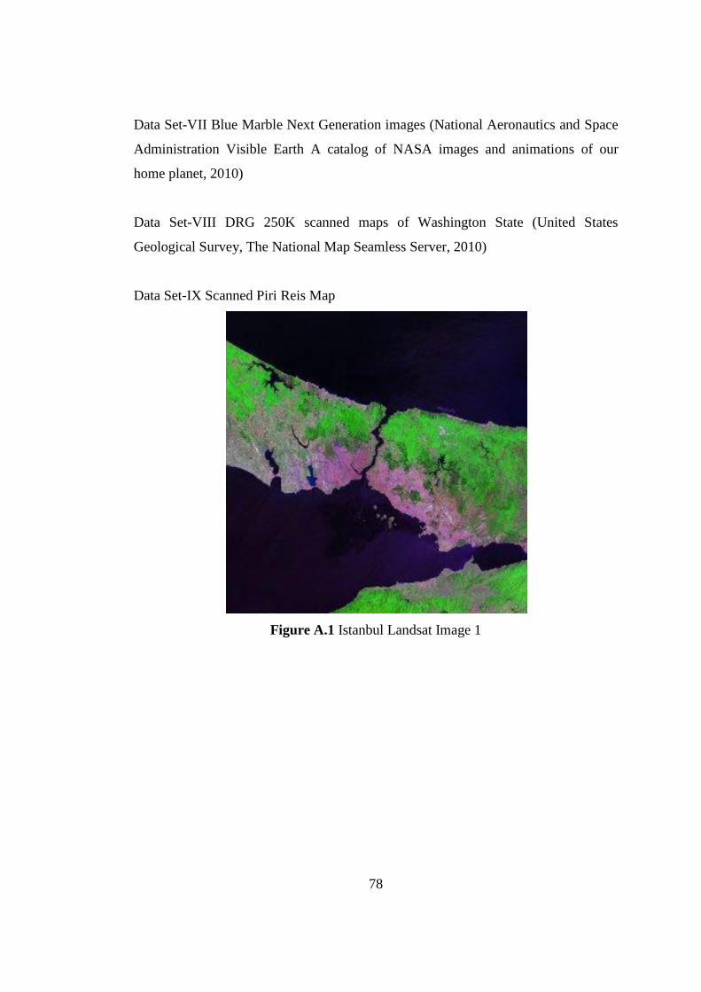
78
Data Set-VII Blue Marble Next Generation images (National Aeronautics and Space
Administration Visible Earth A catalog of NASA images and animations of our
home planet, 2010)
Data Set-VIII DRG 250K scanned maps of Washington State (United States
Geological Survey, The National Map Seamless Server, 2010)
Data Set-IX Scanned Piri Reis Map
Figure A.1 Istanbul Landsat Image 1
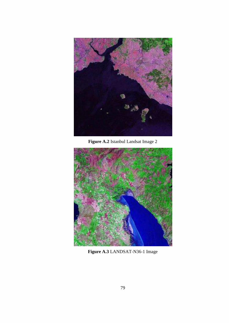
79
Figure A.2 Istanbul Landsat Image 2
Figure A.3 LANDSAT-N36-1 Image
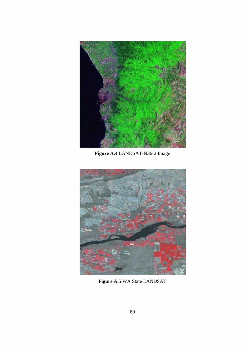
80
Figure A.4 LANDSAT-N36-2 Image
Figure A.5 WA State LANDSAT
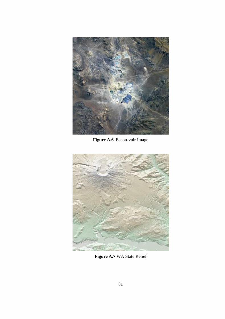
81
Figure A.6 Escon-vnir Image
Figure A.7 WA State Relief
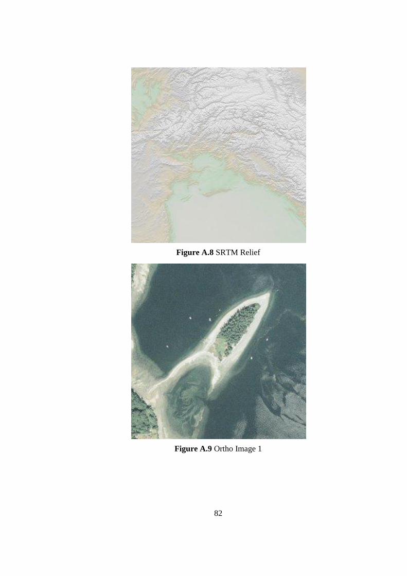
82
Figure A.8 SRTM Relief
Figure A.9 Ortho Image 1
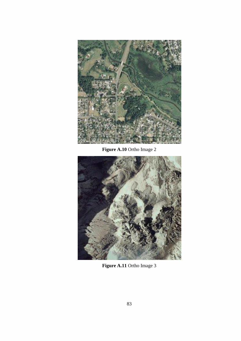
83
Figure A.10 Ortho Image 2
Figure A.11 Ortho Image 3
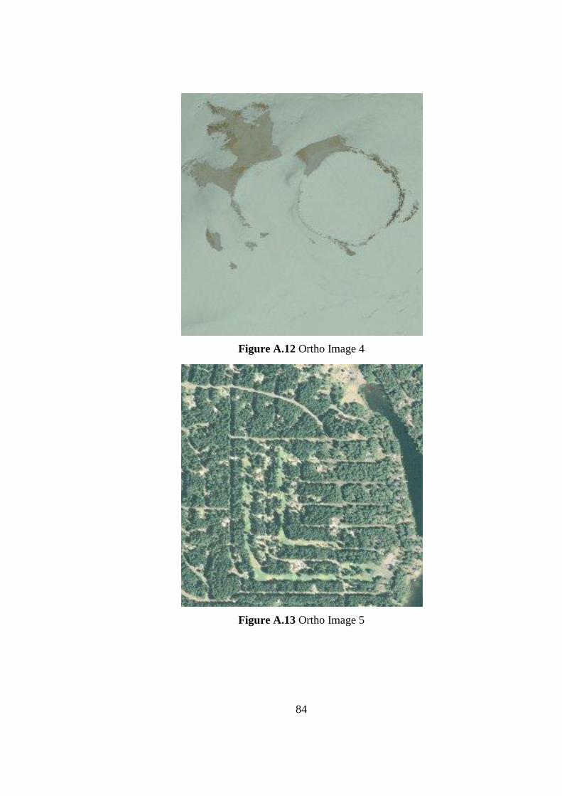
84
Figure A.12 Ortho Image 4
Figure A.13 Ortho Image 5
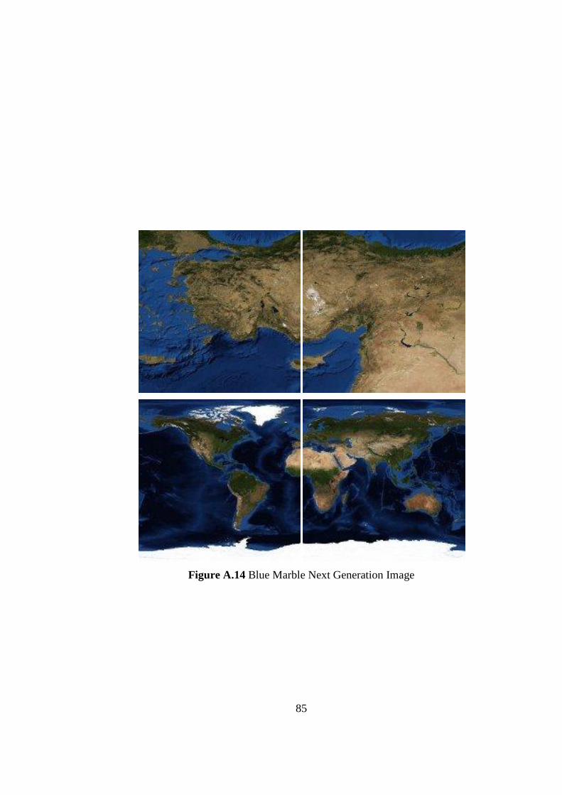
85
Figure A.14 Blue Marble Next Generation Image
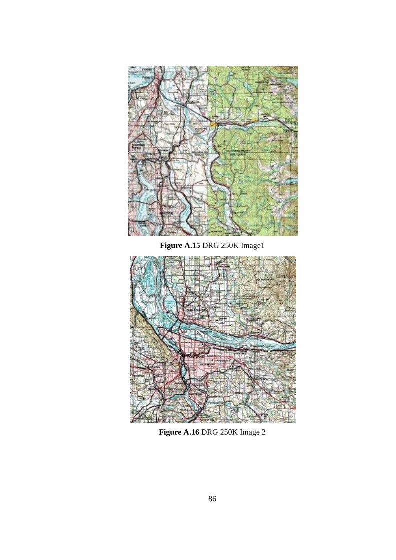
86
Figure A.15 DRG 250K Image1
Figure A.16 DRG 250K Image 2
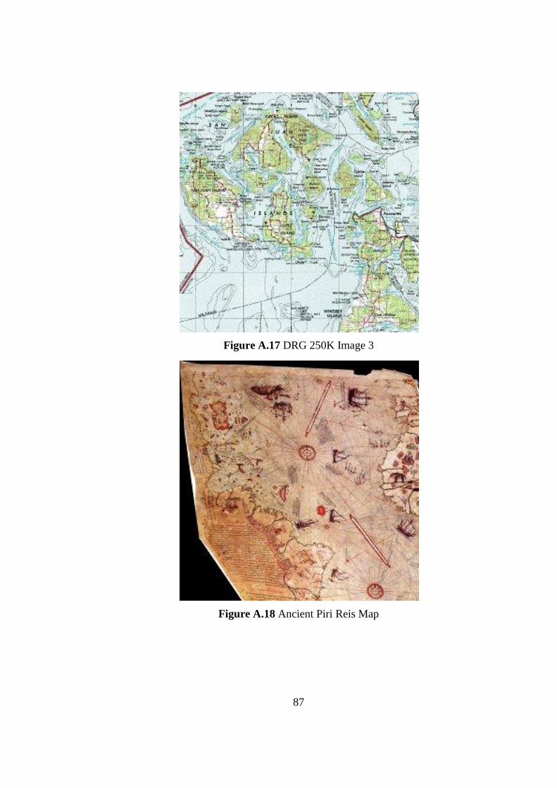
87
Figure A.17 DRG 250K Image 3
Figure A.18 Ancient Piri Reis Map
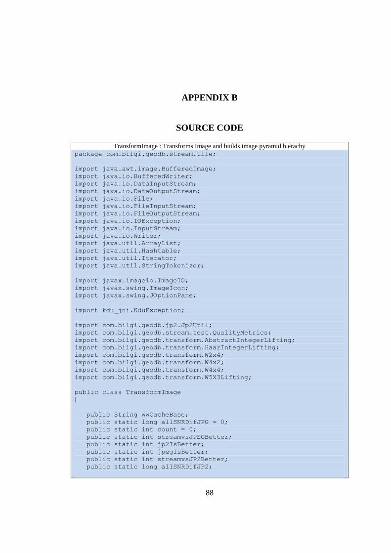
88
APPENDIX B
SOURCE CODE
TransformImage : Transforms Image and builds image pyramid hierachy
package com.bilgi.geodb.stream.tile;
import java.awt.image.BufferedImage;
import java.io.BufferedWriter;
import java.io.DataInputStream;
import java.io.DataOutputStream;
import java.io.File;
import java.io.FileInputStream;
import java.io.FileOutputStream;
import java.io.IOException;
import java.io.InputStream;
import java.io.Writer;
import java.util.ArrayList;
import java.util.Hashtable;
import java.util.Iterator;
import java.util.StringTokenizer;
import javax.imageio.ImageIO;
import javax.swing.ImageIcon;
import javax.swing.JOptionPane;
import kdu_jni.KduException;
import com.bilgi.geodb.jp2.Jp2Util;
import com.bilgi.geodb.stream.test.QualityMetrics;
import com.bilgi.geodb.transform.AbstractIntegerLifting;
import com.bilgi.geodb.transform.HaarIntegerLifting;
import com.bilgi.geodb.transform.W2x4;
import com.bilgi.geodb.transform.W4x2;
import com.bilgi.geodb.transform.W4x4;
import com.bilgi.geodb.transform.W5X3Lifting;
public class TransformImage
{
public String wwCacheBase;
public static long allSNRDifJPG = 0;
public static int count = 0;
public static int streamvsJPEGBetter;
public static int jp2IsBetter;
public static int jpegIsBetter;
public static int streamvsJP2Better;
public static long allSNRDifJP2;
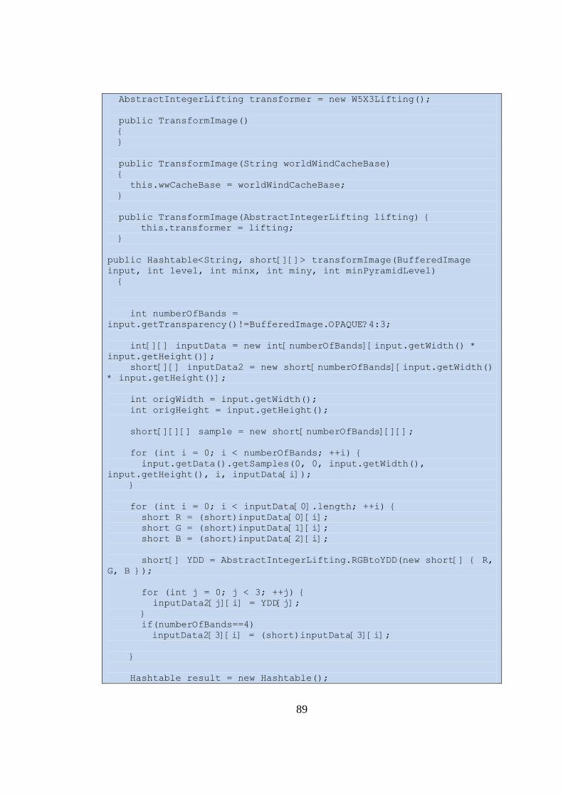
89
AbstractIntegerLifting transformer = new W5X3Lifting();
public TransformImage()
{
}
public TransformImage(String worldWindCacheBase)
{
this.wwCacheBase = worldWindCacheBase;
}
public TransformImage(AbstractIntegerLifting lifting) {
this.transformer = lifting;
}
public Hashtable<String, short[][]> transformImage(BufferedImage
input, int level, int minx, int miny, int minPyramidLevel)
{
int numberOfBands =
input.getTransparency()!=BufferedImage.OPAQUE?4:3;
int[][] inputData = new int[numberOfBands][input.getWidth() *
input.getHeight()];
short[][] inputData2 = new short[numberOfBands][input.getWidth()
* input.getHeight()];
int origWidth = input.getWidth();
int origHeight = input.getHeight();
short[][][] sample = new short[numberOfBands][][];
for (int i = 0; i < numberOfBands; ++i) {
input.getData().getSamples(0, 0, input.getWidth(),
input.getHeight(), i, inputData[i]);
}
for (int i = 0; i < inputData[0].length; ++i) {
short R = (short)inputData[0][i];
short G = (short)inputData[1][i];
short B = (short)inputData[2][i];
short[] YDD = AbstractIntegerLifting.RGBtoYDD(new short[] { R,
G, B });
for (int j = 0; j < 3; ++j) {
inputData2[j][i] = YDD[j];
}
if(numberOfBands==4)
inputData2[3][i] = (short)inputData[3][i];
}
Hashtable result = new Hashtable();
90
for (int k = level; k > 0; --k) {
short[][][][] bandHighs = new short[numberOfBands][][][];
int numOfParts = 0;
for (int i = 0; i < numberOfBands; ++i) {
short[][] temp = transformer.lift2d(inputData2[i]);
inputData2[i] = temp[0];
int tmpSize = (int)Math.sqrt(temp[0].length);
numOfParts = tmpSize / 128;
short[][][] highParts = new short[numOfParts][numOfParts][];
for (int r = 0; r < numOfParts; ++r) {
for (int c = 0; c < numOfParts; ++c)
highParts[c][r] = new short[49152];
}
for (int coef = 1; coef < 4; ++coef)
for (int r = 0; r < numOfParts; ++r)
for (int c = 0; c < numOfParts; ++c)
for (int tmpR = 0; tmpR < 128; ++tmpR)
System.arraycopy(temp[coef], c * 128 + (r * 128 +
tmpR) * tmpSize, highParts[c][r], (coef - 1) * 16384 + tmpR * 128,
128);
bandHighs[i] = highParts;
}
for (int i = 0; i < numOfParts; ++i)
for (int j = 0; j < numOfParts; ++j) {
short[][] tmp = new short[numberOfBands][];
for (int b = 0; b < numberOfBands; ++b)
tmp[b] = bandHighs[b][i][(numOfParts - 1 - j)];
result.put((minPyramidLevel + k) + "_" + ((minx << k) + i)
+ "_" + ((miny << k) + j), tmp);
}
}
short[][] tmp = new short[numberOfBands][];
for (int i = 0; i < numberOfBands; ++i) {
tmp[i] = inputData2[i];
}
result.put(minPyramidLevel + "_" + minx + "_" + miny, tmp);
return result;
}
public BufferedImage createBufferedImage(int[][] data, boolean
91
isLow)
{
int dim1 = 128;
if (isLow)
dim1 = (int)Math.sqrt(data[0].length);
int dim2 = data[0].length / dim1;
int type =data.length
==4?BufferedImage.TYPE_INT_ARGB:BufferedImage.TYPE_INT_RGB;
BufferedImage result = new BufferedImage(dim1, dim2, type);
for (int j = 0; j < dim2; ++j)
for (int i = 0; i < dim1; ++i) {
short[] rgb = AbstractIntegerLifting.YDDtoRGB(new short[] {
(short)data[0][(i + j * dim1)], (short)data[1][(i + j * dim1)],
(short)data[2][(i + j * dim1)] });
int rgbPack =rgb[0] << 16 | rgb[1] << 8 | rgb[2];
if(data.length ==4)
rgbPack = rgbPack |data[3][(i + j * dim1)]<<24;
result.setRGB(i, j, rgbPack);
}
return result;
}
public int[][] inverseTransform(int[][] low, int[][] high, int
row, int col)
{
int[][] result = new int[low.length][65536];
int[][] curLow = new int[low.length][16384];
int tcol = 1 - col;
for (int i = 0; i < low.length; ++i) {
for (int r = 0; r < 128; ++r) {
try{
System.arraycopy(low[i], 128 * row + (r + 128 * tcol) * 256,
curLow[i], r * 128, 128);
}
catch (Exception e) {
// e.printStackTrace();
}
}
}
for (int i = 0; i < low.length; ++i)
{
int[][] coefs = new int[4][16384];
coefs[0] = curLow[i];
for (int j = 0; j < 3; ++j) {
System.arraycopy(high[i], j * 128 * 128, coefs[(j + 1)], 0,
16384);

92
}
result[i] = transformer.unlift2d(coefs);
}
return result;
}
public int[] getTileStreamSamples(InputStream inStream)
throws IOException, KduException
{
DataInputStream stream2 = new DataInputStream(inStream);
int rlev = stream2.readInt();
int rx = stream2.readInt();
int ry = stream2.readInt();
int layerNameLength = stream2.readInt();
String lyrName = "";
for (int i = 0; i < layerNameLength; ++i)
lyrName = lyrName + stream2.readChar();
int[] result = new int[65536];
BufferedImage bim = getTileImage(rlev, rx, ry, lyrName);
bim.getRGB(0, 0, 256, 256, result, 0, 256);
return result;
}
public BufferedImage getTileImage(int level, int x, int y, String
layerName)
throws IOException
{
int waveletLevel = level % 4;
int baseX = x >> waveletLevel;
int baseY = y >> waveletLevel;
TileIndex index = new TileIndex(level - waveletLevel, baseX,
baseY);
FileInputStream streamBase = new FileInputStream(new File(
//
wwCacheBase+layerName+File.separatorChar+index.getGeobsCachePa
th()
"/data/imigiTest/"+index.level+"_"+index.xIndex+"_"+index.yInd
ex+".jp2"
));
int[][] low = getTileCoefs(streamBase);
streamBase.close();
for (int i = waveletLevel - 1; i >= 0; --i) {
int highLevel = level - i;
int highX = x >> i;
int highY = y >> i;
93
TileIndex tindex = new TileIndex(highLevel, highX, highY);
FileInputStream stream = new FileInputStream(new File(
//
wwCacheBase+layerName+File.separatorChar+tindex.getGeobsCacheP
ath()
"/data/imigiTest/"+tindex.level+"_"+tindex.xIndex+"_"+tindex.y
Index+".jp2"
));
int[][] high = getTileCoefs(stream);
stream.close();
int col = highX % 2;
int row = highY % 2;
low = inverseTransform(low, high, col, row);
}
return createBufferedImage(low, true);
}
public int[][] getTileCoefs(InputStream stream)
{
int[][] result;
try
{
DataInputStream stream2 = new DataInputStream(stream);
int rlev = stream2.readInt();
int rx = stream2.readInt();
int ry = stream2.readInt();
int layerNameLength = stream2.readInt();
String lyrName = "";
for (int i = 0; i < layerNameLength; ++i)
lyrName = lyrName + stream2.readChar();
result = Jp2Util.decodeShortBands(stream);
} catch (Exception e) {
return null;
}
return result;
}
}
94
TileIndex : Tile index structure for progressive image tiles
package com.bilgi.geodb.stream.tile;
import java.io.File;
import java.util.ArrayList;
public class TileIndex {
public int level;
public int xIndex;
public int yIndex;
public static final int transformLevel = 4;
public TileIndex(int level, int xIndex, int yIndex){
this.level = level;
this.xIndex = xIndex;
this.yIndex = yIndex;
}
public String getGeobsCachePath(){
return
""+level+File.separatorChar+yIndex+File.separatorChar+yIndex+"_"+xIn
dex+".jp2";
}
public ArrayList<TileIndex> getRequiredTiles(){
ArrayList<TileIndex> result = new
ArrayList<TileIndex>();
int waveletLevel = level % transformLevel;
int baseX = xIndex>>waveletLevel;
int baseY = yIndex>>waveletLevel;
result.add(new TileIndex(level - waveletLevel,baseX
,baseY));
for(int i=waveletLevel-1;i>=0;i--){
int highLevel = level-i;
int highX = xIndex>>i;
int highY = yIndex>>i;
result.add(new TileIndex(highLevel, highX,
highY));
}
return result;
}
}
95
AbstractIntegerLifting : Integer Lifting Kernels extends this class
package com.bilgi.geodb.transform;
public abstract class AbstractIntegerLifting
{
public static int EVEN = 0;
public static int ODD = 1;
public static int AVERAGE = 0;
public static int DIFFERENCE = 1;
public static int LL = 0;
public static int LH = 1;
public static int HL = 2;
public static int HH = 3;
protected short[][] split(short[] data)
{
short[][] result = new short[2][data.length / 2];
for (int i = 0; i < data.length / 2; ++i) {
result[EVEN][i] = data[(i * 2)];
result[ODD][i] = data[(i * 2 + 1)];
}
return result;
}
protected short[] merge(short[] even, short[] odd) {
short[] result = new short[even.length * 2];
for (int i = 0; i < even.length; ++i) {
result[(i * 2)] = even[i];
result[(i * 2 + 1)] = odd[i];
}
return result;
}
protected void add(short[] data1, short[] data2) {
for (int i = 0; i < data1.length; ++i) {
int tmp10_9 = i;
short[] tmp10_8 = data1; tmp10_8[tmp10_9] =
(short)(tmp10_8[tmp10_9] + data2[i]); }
}
protected void subtract(short[] data1, short[] data2) {
for (int i = 0; i < data1.length; ++i) {
int tmp10_9 = i;
short[] tmp10_8 = data1;
tmp10_8[tmp10_9] = (short)(tmp10_8[tmp10_9] - data2[i]);
}
}
protected abstract short[] predict(short[] paramArrayOfShort);
protected abstract short[] update(short[] paramArrayOfShort);
96
public short[][] lift(short[] line) {
short[][] splitted = split(line);
subtract(splitted[ODD], predict(splitted[EVEN]));
add(splitted[EVEN], update(splitted[ODD]));
return splitted;
}
public short[] unlift(short[] difference, short[] average)
{
subtract(average, update(difference));
add(difference, predict(average));
return merge(average, difference);
}
public short[][] lift2d(short[] LL)
{
short[][] result = new short[4][];
int width = (int)Math.sqrt(LL.length);
short[] low = new short[width * width / 2];
short[] high = new short[width * width / 2];
short[] tempLL = new short[(int)Math.sqrt(LL.length)];
for (int i = 0; i < width; ++i) {
System.arraycopy(LL, i * width, tempLL, 0, width);
short[][] temp = lift(tempLL);
System.arraycopy(temp[AVERAGE], 0, low, i * width / 2, width /
2);
System.arraycopy(temp[DIFFERENCE], 0, high, i * width / 2,
width / 2);
}
short[] lowlow = new short[width * width / 4];
short[] lowhigh = new short[width * width / 4];
short[] highlow = new short[width * width / 4];
short[] highhigh = new short[width * width / 4];
for (int i = 0; i < width / 2; ++i)
{
short[] tempLow = new short[width];
short[] tempHigh = new short[width];
for (int j = 0; j < width; ++j) {
tempLow[j] = low[(i + j * width / 2)];
tempHigh[j] = high[(i + j * width / 2)];
}
short[][] temp = lift(tempLow);
97
short[][] temp2 = lift(tempHigh);
for(int j=0;j<width/2;j++){
lowlow[i+j*width/2] = temp[AVERAGE][j];
lowhigh[i+j*width/2] = temp[DIFFERENCE][j];
highlow[i+j*width/2] = temp2[AVERAGE][j];
highhigh[i+j*width/2] = temp2[DIFFERENCE][j];
}
}
result[AbstractIntegerLifting.LL] = lowlow;
result[LH] = lowhigh;
result[HL] = highlow;
result[HH] = highhigh;
return result;
}
public short[] unlift2d(short[][] coeff)
{
short[] result = new short[coeff[LL].length * 4];
short preWith = (short)(int)Math.sqrt(coeff[LL].length);
short[][] low = new short[preWith * 2][preWith];
short[][] high = new short[preWith * 2][preWith];
for (int i = 0; i < preWith; ++i) {
short[] tempL = new short[preWith];
short[] tempH = new short[preWith];
for(int j=0;j<preWith;j++){
tempL[j]= coeff[LL][i+j*preWith];
tempH[j]= coeff[LH][i+j*preWith];
}
short[] templow = unlift(tempH, tempL);
for(int j=0;j<preWith;j++){
tempL[j]= coeff[HL][i+j*preWith];
tempH[j]= coeff[HH][i+j*preWith];
}
short[] tempHigh = unlift(tempH, tempL);
for (int j = 0; j < preWith * 2; ++j) {
low[j][i] = templow[j];
high[j][i] = tempHigh[j];
}
}
for (int i = 0; i < preWith * 2; ++i) {
98
short[] temp = unlift(high[i], low[i]);
System.arraycopy(temp, 0, result, preWith * i * 2, preWith *
2);
}
return result;
}
public short[][] WT2D(short[] source, int level)
{
short[][] result = new short[1 + level * 3][];
short[] LL = source;
for (int i = level; i > 0; --i) {
short[][] temp = lift2d(LL);
for (int j = 2; j >= 0; --j)
result[(i * 3 - j)] = temp[(j + 1)];
LL = temp[0];
}
result[0] = LL;
return result;
}
public short[] IWT2D(short[][] coefStack, int level) {
short[] result = new short[coefStack[0].length << level * 2];
short[][] temp = new short[4][];
temp[LL] = coefStack[0];
for (int i = 1; i <= level; ++i) {
for (int j = 3; j > 0; --j)
temp[j] = coefStack[(i * 3 - j + 1)];
temp[0] = unlift2d(temp);
}
result = temp[0];
return result;
}
////////////////////////////////////////////////////////////////////
/////////////////
protected int[][] split(int[] data)
{
int[][] result = new int[2][data.length / 2];
for (int i = 0; i < data.length / 2; ++i) {
result[EVEN][i] = data[(i * 2)];
result[ODD][i] = data[(i * 2 + 1)];
}
99
return result;
}
protected int[] merge(int[] even, int[] odd) {
int[] result = new int[even.length * 2];
for (int i = 0; i < even.length; ++i) {
result[(i * 2)] = even[i];
result[(i * 2 + 1)] = odd[i];
}
return result;
}
protected void add(int[] data1, int[] data2) {
for (int i = 0; i < data1.length; ++i) {
int tmp10_9 = i;
int[] tmp10_8 = data1; tmp10_8[tmp10_9] =
(int)(tmp10_8[tmp10_9] + data2[i]); }
}
protected void subtract(int[] data1, int[] data2) {
for (int i = 0; i < data1.length; ++i) {
int tmp10_9 = i;
int[] tmp10_8 = data1; tmp10_8[tmp10_9] =
(int)(tmp10_8[tmp10_9] - data2[i]);
}
}
protected abstract int[] predict(int[] paramArrayOfint);
protected abstract int[] update(int[] paramArrayOfint);
public int[][] lift(int[] line) {
int[][] splitted = split(line);
subtract(splitted[ODD], predict(splitted[EVEN]));
add(splitted[EVEN], update(splitted[ODD]));
return splitted;
}
public int[] unlift(int[] difference, int[] average)
{
subtract(average, update(difference));
add(difference, predict(average));
return merge(average, difference);
}
public int[][] lift2d(int[] LL)
{
int[][] result = new int[4][];
int width = (int)Math.sqrt(LL.length);
100
int[] low = new int[width * width / 2];
int[] high = new int[width * width / 2];
int[] tempLL = new int[(int)Math.sqrt(LL.length)];
for (int i = 0; i < width; ++i) {
System.arraycopy(LL, i * width, tempLL, 0, width);
int[][] temp = lift(tempLL);
System.arraycopy(temp[AVERAGE], 0, low, i * width / 2, width /
2);
System.arraycopy(temp[DIFFERENCE], 0, high, i * width / 2,
width / 2);
}
int[] lowlow = new int[width * width / 4];
int[] lowhigh = new int[width * width / 4];
int[] highlow = new int[width * width / 4];
int[] highhigh = new int[width * width / 4];
for (int i = 0; i < width / 2; ++i)
{
int[] tempLow = new int[width];
int[] tempHigh = new int[width];
for (int j = 0; j < width; ++j) {
tempLow[j] = low[(i + j * width / 2)];
tempHigh[j] = high[(i + j * width / 2)];
}
int[][] temp = lift(tempLow);
int[][] temp2 = lift(tempHigh);
for(int j=0;j<width/2;j++){
lowlow[i+j*width/2] = temp[AVERAGE][j];
lowhigh[i+j*width/2] = temp[DIFFERENCE][j];
highlow[i+j*width/2] = temp2[AVERAGE][j];
highhigh[i+j*width/2] = temp2[DIFFERENCE][j];
}
}
result[AbstractIntegerLifting.LL] = lowlow;
result[LH] = lowhigh;
result[HL] = highlow;
result[HH] = highhigh;
return result;
}
public int[] unlift2d(int[][] coeff)
{
101
int[] result = new int[coeff[LL].length * 4];
int preWith = (int)(int)Math.sqrt(coeff[LL].length);
int[][] low = new int[preWith * 2][preWith];
int[][] high = new int[preWith * 2][preWith];
for (int i = 0; i < preWith; ++i) {
int[] tempL = new int[preWith];
int[] tempH = new int[preWith];
for(int j=0;j<preWith;j++){
tempL[j]= coeff[LL][i+j*preWith];
tempH[j]= coeff[LH][i+j*preWith];
}
int[] templow = unlift(tempH, tempL);
for(int j=0;j<preWith;j++){
tempL[j]= coeff[HL][i+j*preWith];
tempH[j]= coeff[HH][i+j*preWith];
}
int[] tempHigh = unlift(tempH, tempL);
for (int j = 0; j < preWith * 2; ++j) {
low[j][i] = templow[j];
high[j][i] = tempHigh[j];
}
}
for (int i = 0; i < preWith * 2; ++i) {
int[] temp = unlift(high[i], low[i]);
System.arraycopy(temp, 0, result, preWith * i * 2, preWith *2);
}
return result;
}
public int[][] WT2D(int[] source, int level)
{
int[][] result = new int[1 + level * 3][];
int[] LL = source;
for (int i = level; i > 0; --i) {
int[][] temp = lift2d(LL);
for (int j = 2; j >= 0; --j)
result[(i * 3 - j)] = temp[(j + 1)];
LL = temp[0];
}
result[0] = LL;
102
return result;
}
public int[] IWT2D(int[][] coefStack, int level) {
int[] result = new int[coefStack[0].length << level * 2];
int[][] temp = new int[4][];
temp[LL] = coefStack[0];
for (int i = 1; i <= level; ++i) {
for (int j = 3; j > 0; --j)
temp[j] = coefStack[(i * 3 - j + 1)];
temp[0] = unlift2d(temp);
}
result = temp[0];
return result;
}
public static short[] RGBtoYDD(short[] rgb) {
short[] result = new short[3];
short r = rgb[0];
short g = rgb[1];
short b = rgb[2];
short y = g;
short db = (short)(b - g);
short dr = (short)(r - g);
result[0] = y;
result[1] = db;
result[2] = dr;
return result;
}
public static short[] YDDtoRGB(short[] YDD) {
short[] result = new short[3];
short y = YDD[0];
short db = YDD[1];
short dr = YDD[2];
short g = y;
short r = (short)(y + dr);
short b = (short)(y + db);
result[0] = (short)Math.min(Math.max(0, r),255);
result[1] = (short)Math.min(Math.max(0, g),255);
result[2] = (short)Math.min(Math.max(0, b),255);
return result;
}
}
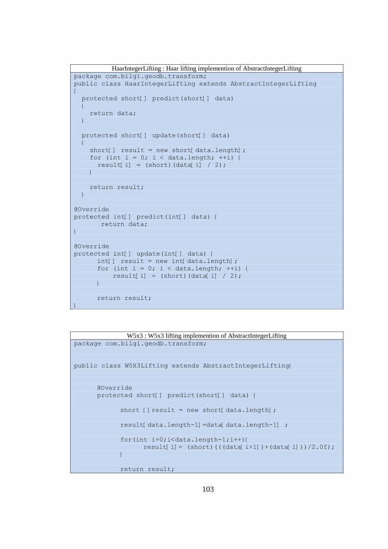
103
HaarIntegerLifting : Haar lifting implemention of AbstractIntegerLifting
package com.bilgi.geodb.transform;
public class HaarIntegerLifting extends AbstractIntegerLifting
{
protected short[] predict(short[] data)
{
return data;
}
protected short[] update(short[] data)
{
short[] result = new short[data.length];
for (int i = 0; i < data.length; ++i) {
result[i] = (short)(data[i] / 2);
}
return result;
}
@Override
protected int[] predict(int[] data) {
return data;
}
@Override
protected int[] update(int[] data) {
int[] result = new int[data.length];
for (int i = 0; i < data.length; ++i) {
result[i] = (short)(data[i] / 2);
}
return result;
}
W5x3 : W5x3 lifting implemention of AbstractIntegerLifting
package com.bilgi.geodb.transform;
public class W5X3Lifting extends AbstractIntegerLifting{
@Override
protected short[] predict(short[] data) {
short []result = new short[data.length];
result[data.length-1]=data[data.length-1] ;
for(int i=0;i<data.length-1;i++){
result[i]= (short)(((data[i+1])+(data[i]))/2.0f);
}
return result;
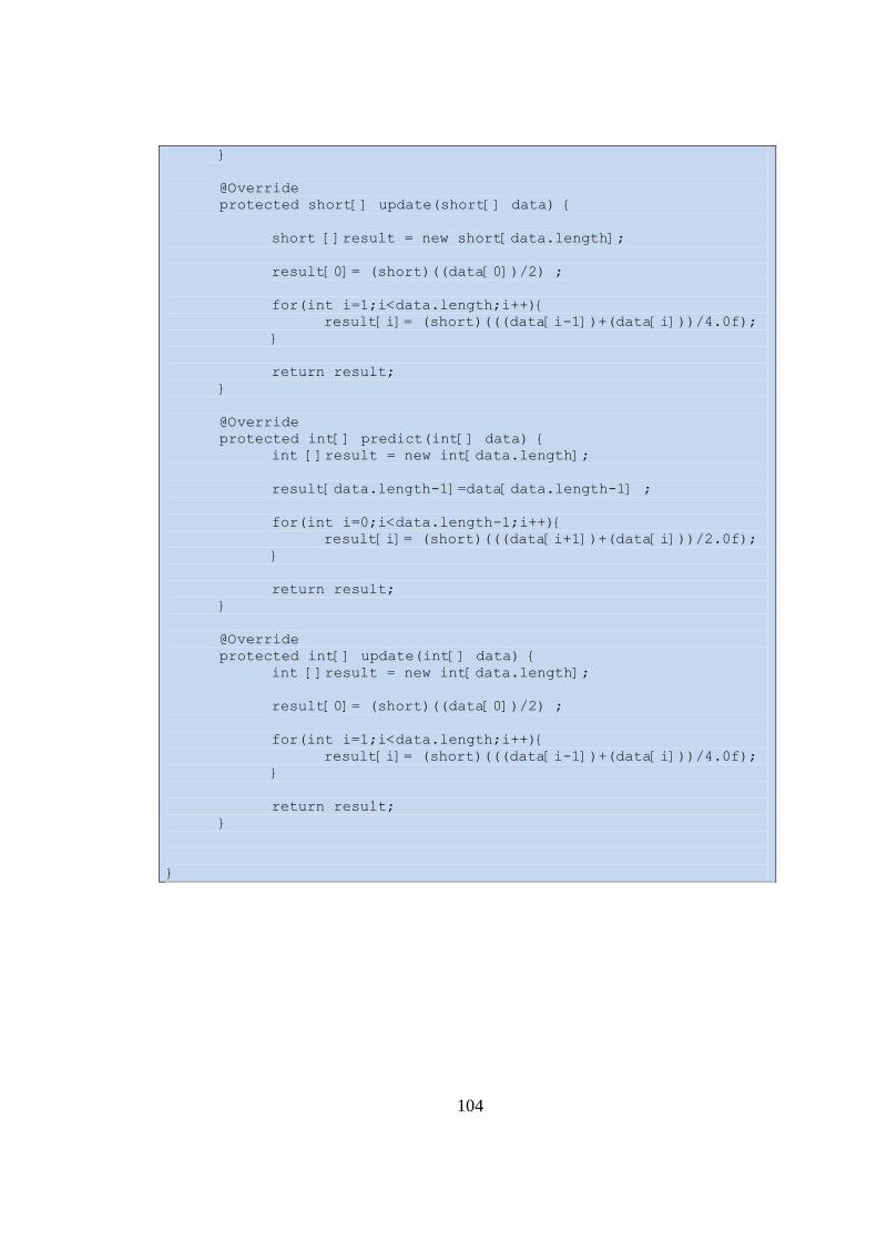
104
}
@Override
protected short[] update(short[] data) {
short []result = new short[data.length];
result[0]= (short)((data[0])/2) ;
for(int i=1;i<data.length;i++){
result[i]= (short)(((data[i-1])+(data[i]))/4.0f);
}
return result;
}
@Override
protected int[] predict(int[] data) {
int []result = new int[data.length];
result[data.length-1]=data[data.length-1] ;
for(int i=0;i<data.length-1;i++){
result[i]= (short)(((data[i+1])+(data[i]))/2.0f);
}
return result;
}
@Override
protected int[] update(int[] data) {
int []result = new int[data.length];
result[0]= (short)((data[0])/2) ;
for(int i=1;i<data.length;i++){
result[i]= (short)(((data[i-1])+(data[i]))/4.0f);
}
return result;
}
}
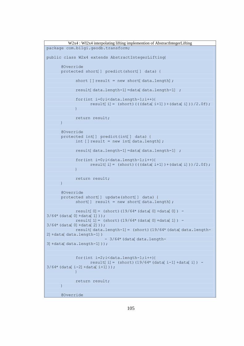
105
W2x4 : WI2x4 interpolating lifting implemention of AbstractIntegerLifting
package com.bilgi.geodb.transform;
public class W2x4 extends AbstractIntegerLifting{
@Override
protected short[] predict(short[] data) {
short []result = new short[data.length];
result[data.length-1]=data[data.length-1] ;
for(int i=0;i<data.length-1;i++){
result[i]= (short)(((data[i+1])+(data[i]))/2.0f);
}
return result;
}
@Override
protected int[] predict(int[] data) {
int []result = new int[data.length];
result[data.length-1]=data[data.length-1] ;
for(int i=0;i<data.length-1;i++){
result[i]= (short)(((data[i+1])+(data[i]))/2.0f);
}
return result;
}
@Override
protected short[] update(short[] data) {
short[] result = new short[data.length];
result[0]= (short)(19/64*(data[0]+data[0]) -
3/64*(data[0]+data[1]));
result[1]= (short)(19/64*(data[0]+data[1]) -
3/64*(data[0]+data[2]));
result[data.length-1]= (short)(19/64*(data[data.length-
2]+data[data.length-1])
- 3/64*(data[data.length-
3]+data[data.length-1]));
for(int i=2;i<data.length-1;i++){
result[i]= (short)(19/64*(data[i-1]+data[i]) -
3/64*(data[i-2]+data[i+1]));
}
return result;
}
@Override
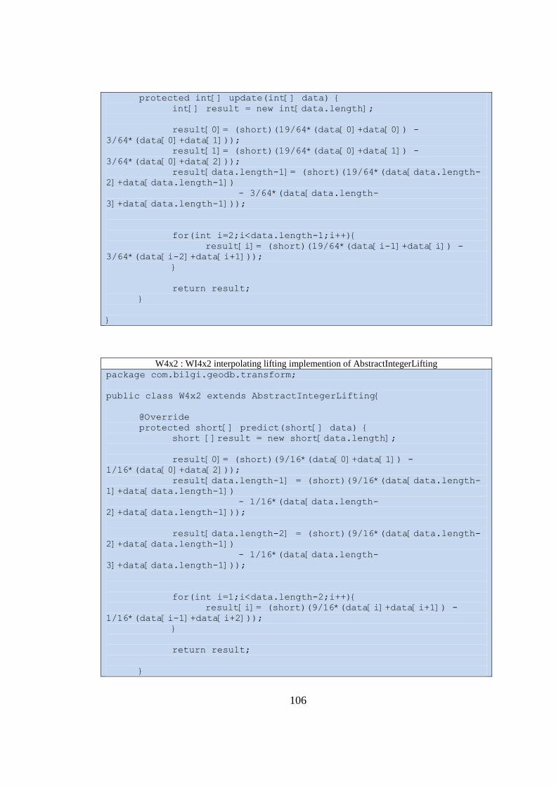
106
protected int[] update(int[] data) {
int[] result = new int[data.length];
result[0]= (short)(19/64*(data[0]+data[0]) -
3/64*(data[0]+data[1]));
result[1]= (short)(19/64*(data[0]+data[1]) -
3/64*(data[0]+data[2]));
result[data.length-1]= (short)(19/64*(data[data.length-
2]+data[data.length-1])
- 3/64*(data[data.length-
3]+data[data.length-1]));
for(int i=2;i<data.length-1;i++){
result[i]= (short)(19/64*(data[i-1]+data[i]) -
3/64*(data[i-2]+data[i+1]));
}
return result;
}
}
W4x2 : WI4x2 interpolating lifting implemention of AbstractIntegerLifting
package com.bilgi.geodb.transform;
public class W4x2 extends AbstractIntegerLifting{
@Override
protected short[] predict(short[] data) {
short []result = new short[data.length];
result[0]= (short)(9/16*(data[0]+data[1]) -
1/16*(data[0]+data[2]));
result[data.length-1] = (short)(9/16*(data[data.length-
1]+data[data.length-1])
- 1/16*(data[data.length-
2]+data[data.length-1]));
result[data.length-2] = (short)(9/16*(data[data.length-
2]+data[data.length-1])
- 1/16*(data[data.length-
3]+data[data.length-1]));
for(int i=1;i<data.length-2;i++){
result[i]= (short)(9/16*(data[i]+data[i+1]) -
1/16*(data[i-1]+data[i+2]));
}
return result;
}
107
@Override
protected int[] predict(int[] data) {
int []result = new int[data.length];
result[0]= (short)(9/16*(data[0]+data[1]) -
1/16*(data[0]+data[2]));
result[data.length-1] = (short)(9/16*(data[data.length-
1]+data[data.length-1])
- 1/16*(data[data.length-
2]+data[data.length-1]));
result[data.length-2] = (short)(9/16*(data[data.length-
2]+data[data.length-1])
- 1/16*(data[data.length-
3]+data[data.length-1]));
for(int i=1;i<data.length-2;i++){
result[i]= (short)(9/16*(data[i]+data[i+1]) -
1/16*(data[i-1]+data[i+2]));
}
return result;
}
@Override
protected short[] update(short[] data) {
short []result = new short[data.length];
result[0]= (short)(data[0]/2) ;
for(int i=1;i<data.length;i++){
result[i]= (short)(((data[i-1])+(data[i]))/4.0f);
}
return result;
}
@Override
protected int[] update(int[] data) {
int []result = new int[data.length];
result[0]= (short)(data[0]/2) ;
for(int i=1;i<data.length;i++){
result[i]= (short)(((data[i-1])+(data[i]))/4.0f);
}
return result;
}
}
108
W4x4 : WI4x4 interpolating lifting implemention of AbstractIntegerLifting
package com.bilgi.geodb.transform;
public class W4x4 extends AbstractIntegerLifting{
@Override
protected short[] predict(short[] data) {
short[] result = new short[data.length];
result[0]= (short)(19/64*(data[0]+data[0]) -
3/64*(data[0]+data[1]));
result[1]= (short)(19/64*(data[0]+data[1]) -
3/64*(data[0]+data[2]));
result[data.length-1]= (short)(19/64*(data[data.length-
2]+data[data.length-1])
- 3/64*(data[data.length-
3]+data[data.length-1]));
for(int i=2;i<data.length-1;i++){
result[i]= (short)(19/64*(data[i-1]+data[i]) -
3/64*(data[i-2]+data[i+1]));
}
return result;
}
@Override
protected int[] predict(int[] data) {
int[] result = new int[data.length];
result[0]= (short)(19/64*(data[0]+data[0]) -
3/64*(data[0]+data[1]));
result[1]= (short)(19/64*(data[0]+data[1]) -
3/64*(data[0]+data[2]));
result[data.length-1]= (short)(19/64*(data[data.length-
2]+data[data.length-1])
- 3/64*(data[data.length-
3]+data[data.length-1]));
for(int i=2;i<data.length-1;i++){
result[i]= (short)(19/64*(data[i-1]+data[i]) -
3/64*(data[i-2]+data[i+1]));
}
return result;
}
@Override
protected short[] update(short[] data) {
short[] result = new short[data.length];
result[0]= (short)(19/64*(data[0]+data[0]) -
3/64*(data[0]+data[1]));
result[1]= (short)(19/64*(data[0]+data[1]) -
109
3/64*(data[0]+data[2]));
result[data.length-1]= (short)(19/64*(data[data.length-
2]+data[data.length-1])
- 3/64*(data[data.length-
3]+data[data.length-1]));
for(int i=2;i<data.length-1;i++){
result[i]= (short)(19/64*(data[i-1]+data[i]) -
3/64*(data[i-2]+data[i+1]));
}
return result;
}
@Override
protected int[] update(int[] data) {
int[] result = new int[data.length];
result[0]= (short)(19/64*(data[0]+data[0]) -
3/64*(data[0]+data[1]));
result[1]= (short)(19/64*(data[0]+data[1]) -
3/64*(data[0]+data[2]));
result[data.length-1]= (short)(19/64*(data[data.length-
2]+data[data.length-1])
- 3/64*(data[data.length-
3]+data[data.length-1]));
for(int i=2;i<data.length-1;i++){
result[i]= (short)(19/64*(data[i-1]+data[i]) -
3/64*(data[i-2]+data[i+1]));
}
return result;
}
}