Development of a MR Hydraulic Bushing

for Automotive Applications

by

Brad B. Schubert

A thesis

presented to the University of Waterloo

in fulfillment of the

thesis requirement for the degree of

Master of Applied Science

in

Mechanical Engineering

Waterloo, Ontario, Canada, 2005

©Brad Schubert, 2005

ii

I hereby declare that I am the sole author of this thesis. This is a true copy of the thesis, including any

required final revisions, as accepted by my examiners.

I understand that my thesis may be made electronically available to the public.

iii

Abstract

The purpose of this work is to design a semi-active magnetorheological (MR) hydraulic bushing. The

semi-active bushing is intended to be used to isolate a cylinder deactivating engine. Cylinder

deactivation causes high transient torsional loading in addition to changing the magnitude and mode

of engine vibrations requiring an adaptive or controllable isolator.

Practical and simple semi-active control strategies are inspired by investigating the optimization of

linear and slightly cubic nonlinear single degree of freedom isolators. Experimental verification of

the optimization technique, which minimizes the root mean square (RMS) of engine acceleration

frequency response and RMS of the force transmitted frequency response, shows that this method can

be implemented on real linear systems to isolate the engine from harmonic inputs. This optimization

technique is also applied to tune selected model parameters of existing two degree of freedom

hydraulic bushings.

This thesis also details the development of a MR hydraulic bushing. The MR bushing design

retrofits an existing bushing with a pressure driven flow mode valve on the inertia track. A new

efficient valve design is selected and developed for the application. The MR hydraulic bushing is

designed, mathematically modeled, and numerically simulated. The simulation results show that the

MR bushing tends to increase the low frequency dynamic stiffness magnitude while simultaneously

decreasing the phase. The next stage of the project is fabrication and testing of the semi-active

bushing. The performance of the manufactured MR bushing is tested on a base excitation apparatus.

Varying the current input to the MR valve was found to have a small effect on the response of the

suspended mass. The results are in agreement with the effects demonstrated by the dynamic stiffness

numerical simulation.

iv

Acknowledgements

Firstly, I would like to acknowledge John Ulicny and Ping Lee of General Motors for their

contributions to the project in the area of magnetorheological fluids and engine isolation technology.

A great deal of this research is inspired and made possible through the teamwork of past and

present students of Dr. Farid Golnaraghi; and so, I would like to extend my thanks in no particular

order to R. Alkhatib, A. Narimani, N. Eslaminasab, T. Gillespie, S. Arzanpour, and Y. Shen for their

contributions to my experimental, theoretical and numerical work. In addition, I would like to thank

my good friends and colleagues T. Arvajeh, R. Majlesi, O. Ansari, and A. Wolff for teaching about

the graduate student lifestyle.

Special thanks to Robert Wagner for your hard work, design advice and for sharing machining

know-how.

I would like to sincerely express my gratitude to Dr. Golnaraghi for providing me the opportunity

and the freedom to apply engineering skills to explore and experiment with science, and most

importantly giving me the chance to grow as an academic and an engineer.

Finally, thank you Kathryn, my beautiful wife, for your patience, understanding, encouragement,

and your confidence in me. But most of all, thank you for your sacrifice – you know I’ll make it up

to you!

v

Dedication

For Mom and Dad, whom I can attribute all my success and happiness in life.

vi

Table of Contents Abstract .................................................................................................................................................iii Acknowledgements ............................................................................................................................... iv Dedication .............................................................................................................................................. v Table of Contents ..................................................................................................................................vi List of Figures .....................................................................................................................................viii List of Tables.......................................................................................................................................xiii Nomenclature ......................................................................................................................................xiv Chapter 1 Introduction........................................................................................................................... 1

1.1 Root Mean Square Frequency Domain Optimization .................................................................. 2 1.2 Isolating Cylinder-on-Demand Engines ....................................................................................... 3 1.3 A New Solution: Semi-Active Isolators ....................................................................................... 5 1.4 Thesis Overview........................................................................................................................... 7

Chapter 2 Literature Review ................................................................................................................. 9 2.1 Optimization of Isolators.............................................................................................................. 9

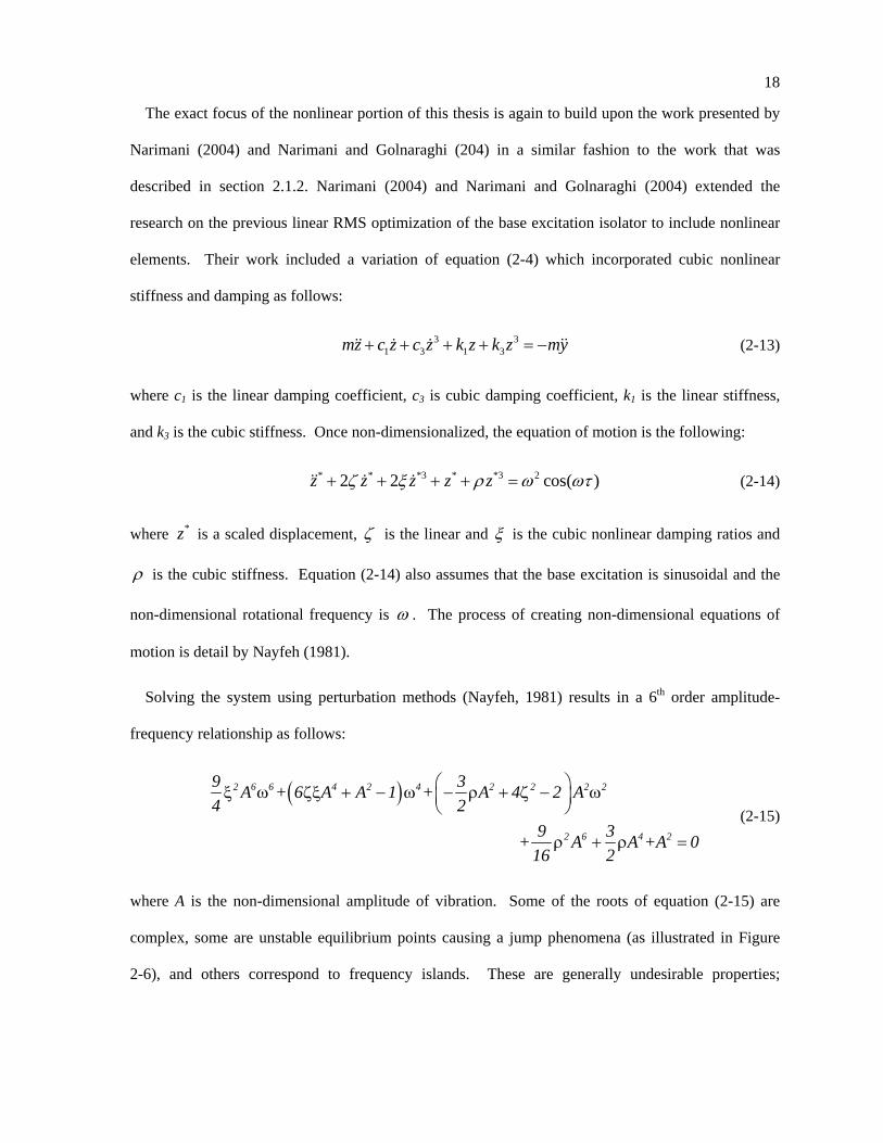
2.1.1 Linear Mount Optimization................................................................................................. 10 2.1.2 Nonlinear Optimization ....................................................................................................... 17

2.2 Engine Isolators .......................................................................................................................... 21 2.2.1 Hydraulic Mounts and Bushings ......................................................................................... 21 2.2.2 Semi-active Engine Isolators ............................................................................................... 24

2.3 Summary .................................................................................................................................... 28 Chapter 3 Model Development and Optimization............................................................................... 29

3.1 Forced Linear Isolator Optimization .......................................................................................... 29 3.1.1 Harmonic Forcing Excitation .............................................................................................. 32 3.1.2 Rotating Unbalance Excitation............................................................................................ 36 3.1.3 Linear Optimization Summary ............................................................................................ 39

3.2 Force Nonlinear Isolator Optimization....................................................................................... 41 3.2.1 Unforced Time Domain Solution of Cubic Nonlinear Isolator ........................................... 41 3.2.2 Forced Solution of Cubic Nonlinear Isolator ...................................................................... 45 3.2.3 RMS Optimization of the Cubic Nonlinear System ............................................................ 48

3.3 MR Hydraulic Bushing Modeling .............................................................................................. 52 3.3.1 MR Bushing Design ............................................................................................................ 52 3.3.2 MR Bushing Dynamic Modeling ........................................................................................ 58

vii

3.3.3 RMS Optimization of the Passive Bushing Parameters ...................................................... 62 3.3.4 MR Bushing Simulation ...................................................................................................... 68

3.4 Summary .................................................................................................................................... 75 Chapter 4 Experiment Implementation ............................................................................................... 77

4.1 Linear RMS Optimization Experiment....................................................................................... 77 4.2 Hydraulic Bushing Experiment .................................................................................................. 83

4.2.1 MR Valve Implementation .................................................................................................. 83 4.2.2 Fixture design ...................................................................................................................... 85 4.2.3 Sensors and Excitation ........................................................................................................ 87 4.2.4 Experiment Issues................................................................................................................ 89

4.3 Summary .................................................................................................................................... 93 Chapter 5 Experimental Results and Evaluation .................................................................................94

5.1 Linear RMS Optimization Experiments ..................................................................................... 94 5.1.1 RMS Optimization of the Base Excited Isolator ................................................................. 94 5.1.2 RMS Optimization of the Unbalance Excited Isolator ........................................................ 98 5.1.3 RMS Optimization of the Harmonic Force Excited Isolator ............................................... 98

5.2 MR Hydraulic Bushing Experiment ......................................................................................... 101 5.2.1 Verification of Bushing Model Parameter Values............................................................. 101 5.2.2 Dry MR Hydraulic Bushing Experiments ......................................................................... 105 5.2.3 MR Hydraulic Bushing Experiments ................................................................................ 108

5.3 Summary .................................................................................................................................. 114 Chapter 6 Conclusions and Future Work .......................................................................................... 115

6.1 RMS Optimization.................................................................................................................... 115 6.2 MR Bushing ............................................................................................................................. 117

Bibliography....................................................................................................................................... 120

viii

List of Figures Figure 1-1: Photograph of a hydraulic engine bushing .......................................................................... 5 Figure 2-1: Schematic of a linear 1 DoF isolator representing an engine mount. ................................ 10 Figure 2-2: The frequency response functions of the base excitation linear passive absorber............. 12

Figure 2-3: The R versus η map illustrating the line of optimum design for a base excited linear

passive vibration isolator (Jazar et al., 2003). .............................................................................. 14 Figure 2-4: The simulated relative displacement time response to a sine square bump input, for three

systems identified in Figure 2-3 (Jazar et al., 2003). ................................................................... 16 Figure 2-5: The simulated transmitted force time response to a sine square bump input, for three

systems shown in Figure 2-3 (Jazar et al., 2003). ........................................................................ 16 Figure 2-6: Base excitation response of non-dimensional amplitude illustrating the jump. ................ 19 Figure 2-7: RMS patch illustrating the effect of varying nonlinear cubic stiffness and damping in a

base excited system. Nominal linear system parameter values: nω = 10 Hz, ζ = 0.4. .............. 20

Figure 2-8: RMS patch illustrating the effect of varying nonlinear cubic stiffness and damping in an

base excited system relative to varying the linear system parameters (Narimani & Golnaraghi

2004). Nominal linear system parameter values: nω = 10 Hz, ζ = 0.4. .................................... 21

Figure 2-9: Typical hydraulic mount including the decoupler (Geisberger, 2000). ............................. 22 Figure 2-10: Mechanical model of a base/unbalance excited hydraulic bushing. ................................ 23 Figure 2-11: Illustration of a MR device consisting of an annular channel of pressure driven flow

passing through the perpendicular magnetic field it two locations. (green – MRF, orange –

magnetic coil) ............................................................................................................................... 26 Figure 2-12: Schematic of the valve presented in Gorodkin et al. (1998) and Kordonski et al. (1995)

illustrating the two radial channels of pressure driven flow passing through the perpendicular

magnetic field. (green – MRF, orange – magnetic coil).............................................................. 27 Figure 2-13: Mechanical model of the hydraulic bushing presented by Ahn et al. (1999) and

Ahmadian and Ahn (1999). .......................................................................................................... 27 Figure 3-1: Illustration of the various simplified forms of isolator inputs. .......................................... 30 Figure 3-2: Normalized amplitude with respect to static displacement under a harmonic force. ........ 31 Figure 3-3: The RMS force transmissibility given a harmonic force input for a linear vibration isolator

versus the damping ratio for various natural frequencies. ............................................................ 33 Figure 3-4: The RMS force transmissibility given a harmonic force input for a linear vibration isolator

versus the natural frequency for various damping ratios.............................................................. 33

ix

Figure 3-5: The RMS absolute displacement given a harmonic force input for a linear vibration

isolator versus damping ratio for various natural frequencies...................................................... 34 Figure 3-6: The RMS absolute displacement given a harmonic force input for a linear vibration

absorber versus the natural frequency for various damping ratios. .............................................. 35 Figure 3-7: The RMS force transmissibility versus the RMS absolute displacement illustrating the

line of optimum design for a harmonic forced linear passive vibration isolator. ......................... 35 Figure 3-8: The RMS force transmitted given a rotating unbalance for a linear vibration isolator

versus the damping ratio for various natural frequencies. ............................................................ 36 Figure 3-9: The RMS force transmitted given a rotating unbalance for a linear vibration isolator

versus the natural frequency for various damping ratios.............................................................. 37 Figure 3-10: The RMS absolute displacement given a rotating unbalance for a linear vibration isolator

versus damping ratio for various natural frequencies................................................................... 37 Figure 3-11: The RMS absolute displacement given a rotating unbalance for a linear vibration

absorber versus the natural frequency for various damping ratios. .............................................. 38 Figure 3-12: The RMS force transmitted versus the RMS absolute displacement illustrating the line of

optimum design for a rotating unbalance linear passive vibration isolator. ................................. 38 Figure 3-13: Illustrative summary of the various inputs and their corresponding RMS domain

optimization design curves. .......................................................................................................... 40 Figure 3-14: The line of optimum design for the base, rotating unbalance and harmonic forced excited

linear passive vibration isolator in the ζ –fn plane. ..................................................................... 40

Figure 3-15: Amplitude versus time relative to the actual numerical simulation of the nonlinear

system for various initial conditions............................................................................................. 44 Figure 3-16: Amplitude of the time domain solution of the cubic nonlinear system for various initial

conditions illustrating the unstable limit cycle of the negative cubic damping system................ 45 Figure 3-17: RMS patch illustrating the effect of varying nonlinear cubic stiffness and damping in an

unbalance forced system............................................................................................................... 49 Figure 3-18: RMS patch illustrating the effect of varying nonlinear cubic stiffness and damping in an

unbalance forced system............................................................................................................... 49 Figure 3-19: Effects of varying linear parameters on the dimensionless response to a step input. ...... 51 Figure 3-20: MR valve schematic illustrating the radial fluid channels (green) as well as the flux path

(blue), the coil (orange), core material (grey) and non-flux conducting material (brown). ......... 52 Figure 3-21: Magnetic properties of 1020 steel.................................................................................... 53 Figure 3-22: Radial channel of MR fluid through the valve. ............................................................... 54 Figure 3-23: Magnetic properties of GM Corp. formulated MRF 13MAG098. .................................. 56

x

Figure 3-24: Valve gain KMR versus input current I. ............................................................................ 58 Figure 3-25: Dynamic stiffness of hydraulic bushing P/N 90576090 for 0.1 and 2.0 mm inputs (peak

to peak). (solid – simulation, dotted – experimental) .................................................................. 60 Figure 3-26: Base excitation RMS optimization of the inertia track parameters (solid – constant dh;

dotted – constant l; circles - nominal mount and tuned inertia track, as indicated)...................... 63 Figure 3-27: Harmonic forced RMS optimization of the inertia track parameters (solid – constant dh,

dotted – constant l, circle - nominal mount)................................................................................. 64 Figure 3-28: Dynamic stiffness given a 20% decrease in inertia track length. .................................... 64 Figure 3-29: Reduction in transferred force given a 20% decrease in inertia track length. ................. 65 Figure 3-30: Increase in displacement given a 20% decrease in inertia track length........................... 65 Figure 3-31: Base excitation RMS optimization of the pumping chamber parameters (solid – constant

C1, dotted – constant Ap, circle - nominal mount). ....................................................................... 67 Figure 3-32: Harmonic forced RMS optimization of the pumping chamber parameters (solid –

constant C1, dotted – constant Ap, circle - nominal mount). ......................................................... 68 Figure 3-33: Prototype MR bushing simulation and purchased bushing filled with MRF simulation

compared to the purchase bushing experimentally measured dynamic stiffness. ........................ 70 Figure 3-34: Simulation time domain response of the chamber pressures, inertia track flow rate and

hydraulic pressure drop versus the MR effect (dotted line in the top axes) for I = 0.1 A, Z = 1

mm (2 mm peak to peak).............................................................................................................. 71 Figure 3-35: Simulation time domain response of the chamber pressures, inertia track flow rate and

hydraulic pressure drop versus the MR effect (dotted line in the top axes) for I = 0.4 A, Z = 1

mm (2 mm peak to peak).............................................................................................................. 72 Figure 3-36: MR Bushing dynamic stiffness simulation results for various current inputs and Z = 1

mm (2 mm peak to peak).............................................................................................................. 73 Figure 3-37: Effect of changing fluid inertia and compliance on the bushing dynamic stiffness. ....... 74 Figure 3-38: Effect of increasing compliance the forced response. ..................................................... 75 Figure 4-1: Single degree of freedom isolator experiment apparatus mounted on the LDS V722

shaker............................................................................................................................................ 78 Figure 4-2: An inertial force can be applied to the suspended mass by accelerating the reference frame

attached to the base of the isolator. .............................................................................................. 79 Figure 4-3: Friction causing jump phenomena during low energy frequency responses. .................... 81 Figure 4-4: Piecewise nonlinearity as the dashpot reaches maximum displacement under high

damping ratios .............................................................................................................................. 81

xi

Figure 4-5: Preliminary results illustrating nearly linear experimental base excitation frequency

responses. ..................................................................................................................................... 82 Figure 4-6: Hydraulic bushing casing to house the rubber purchased mount, with ports to allow

bypassing the inertia track and of pressure measurement (top left). Illustration of the various

ports and chamber of the bushing and casing (top right), where the red curve represents the

original inertia track. Exploded view of the bushing and casing (bottom).................................. 84 Figure 4-7: Prototype MR valve exploded view (brown – 1020 steel core material, grey – 6061

aluminum). ................................................................................................................................... 85 Figure 4-8: Illustration of the setup to measure dynamic stiffness....................................................... 86 Figure 4-9: Dynamic stiffness fixture and bushing mounted on the LDS V722 shaker....................... 86 Figure 4-10: Illustration of the setup to measure transmissibility via a base excitation experiment.... 87 Figure 4-11: Solid model of the base excitation setup mounted on the shaker. ................................... 88 Figure 4-12: The MR valve set up used to conduct base excitation experiments ................................ 88 Figure 4-13: Variation of relative displacement despite constant amplitude input during a dynamic

stiffness test. ................................................................................................................................. 90 Figure 4-14: Variation of transferred force with peaks corresponding to the peaks in relative

displacement during a dynamic stiffness test. .............................................................................. 90 Figure 4-15: Modal analysis results illustrating the first mode of vibration of the shaker frame at

approximately 19 Hz. ................................................................................................................... 91 Figure 4-16: Modal analysis results illustrating the second mode of vibration of the shaker frame at

approximately 47 Hz. ................................................................................................................... 91 Figure 4-17: Initial hydraulic bushing acceleration results given base excitation input. Two main

modes of vibration are present: linear mode (19 Hz) and a rotational mode (26 Hz) identified by

the high edge acceleration with respect to the acceleration of the centre of mass. ...................... 92 Figure 4-18: Illustration of the undesirable rotational mode of vibration. ........................................... 92 Figure 5-1: Base excitation frequency response (experiment – solid line, simulation – dotted line)... 95 Figure 5-2: Base excitation experiment RMS results compared to theoretical results. ........................ 97 Figure 5-3: Experiment base excitation results illustrated on the linear RMS optimization graph. Note

that the experiment RMS values are computed from 5 to 20 Hz.................................................. 97 Figure 5-4: Forced frequency response (experiment– solid line, simulation – dotted line). ................ 99 Figure 5-5: Experimental RMS Results compared to linear results. .................................................. 100 Figure 5-6: Experiment harmonic forced results illustrated on the linear RMS optimization graph.

Note that the experiment RMS values are computed from 5 to 20 Hz....................................... 100 Figure 5-7: Photograph of the hydraulic bushing P/N 90575028 (similar to 90576090). .................. 101

xii

Figure 5-8: Response of the rubber and hydraulic bushing P/N 90575028 (m = 19.3 kg)................. 103 Figure 5-9: Hydraulic bushing simulation illustrating the change in the response of the two degrees of

freedom as the suspended mass increases to 80 kg. ................................................................... 104 Figure 5-10: Dynamic stiffness of bushing P/N 90576090 (preload 1050 N) and bushing P/N

90575028 (preload 1175 N) measured in the University of Waterloo laboratory. ..................... 104 Figure 5-11: Dry engine mount base excitation with a 19.3 kg suspended mass. .............................. 105 Figure 5-12: Base excitation of the dry engine mount with a 31 kg suspended mass. Base amplitudes

are varied from 0.6 mm to 0.9. ................................................................................................... 106 Figure 5-13: Force transmissibility with respect to base acceleration for the dry mount with a 31 kg

suspended mass. Experiments are conducted for base amplitudes from 0.4 to 1.8 mm peak to

peak. (dashed - backward sweep, solid - forward sweep) .......................................................... 107 Figure 5-14: Original MR bushing base excitation (|Y| = 0.4 mm) results generated with the 19.3 kg

mass and using the roller bearings (top – mass acceleration, bottom – relative displacement) . 109 Figure 5-15: MR bushing base excitation relative displacement results generated with the 31.3 kg

mass and using the brass bearings (solid – forward sweep, dotted – backward sweep)............. 111 Figure 5-16: MR bushing base excitation mass acceleration results generated with the 31.3 kg mass

and using the brass bearings (solid – forward sweep, dotted – backward sweep)...................... 112 Figure 5-17: MR bushing base excitation transferred force results generated with the 31.3 kg mass

and using the brass bearings (solid – forward sweep, dotted – backward sweep)...................... 113 Figure 6-1: Increase of the off-state notch frequency to improve the bandwidth of the MR bushing 117 Figure 6-2: Potential implementation of MR valve in a production hydraulic bushing. .................... 118

xiii

List of Tables Table 3-1: Dimensionless peak step response data describing the effect of varying the nonlinear

stiffness and damping. .................................................................................................................. 50 Table 3-2: Dimensionless peak pulse response data describing the effect of varying the cubic

nonlinear stiffness and damping. .................................................................................................. 51 Table 3-3: Properties of GM Corp. formulated MRF 13MAG098. ..................................................... 57 Table 3-4: MR valve design parameters............................................................................................... 57 Table 3-5: Simulation MR valve dynamic stiffness pole and zero properties...................................... 69 Table 5-1: Base excitation test parameters and observations. .............................................................. 94 Table 5-2: Forced excitation test parameters and observations............................................................ 99

xiv

Nomenclature

a X / Y= && acceleration with respect to base excitation amplitude [1/s]

iA inertia track cross-sectional area [m2]

fA pole real area

fA′ magnetic pole effective area

pA effective pumping area [m2]

rB rubber linear damping [N-s/m] c linear damping coefficient [N-s/m]

1 21 1C C C= + lumped compliance [N/mm5]

1C , 2C lower and upper chamber compliance, respectively [mm5/N] cMR constant of magnitude 2-3 depending on the controllability dh inertia track hydraulic diameter Di inner diameter of the MR valve coil Do outer diameter of the MR valve coil e eccentricity of unbalance mass [m]

πω 2nnf = natural frequency [Hz] fo harmonic force excitation amplitude per unit mass [N/kg] F(t) engine dynamic loading [N] FT transmitted force [N] FT transmitted force per unit mass [N/kg] g height of the MR valve fluid channel

fH field intensity [At/m] I MR valve input current [A] i 1= − imaginary unit k linear stiffness coefficient [N/m] Kr rubber linear stiffness [N/m] KMR MR valve gain [Pa/A] l total length of the of the MR valve fluid path in the flux (inertia track) L inertia track fluid inductance [Pa-s2/m3] Lc the length of the coil Li inductance of the MR valve coil [H] MR magnetorheological MRF magnetorheological fluid m mass of engine [kg] mo engine unbalance mass [kg] N number of wire turns in a magnetic coil OPM magnet wire resistance per unit length [Ω /m]

1P , 2P upper and lower chamber pressures [Pa] Q inertia track flowrate Qin flow from pumping chamber to the MR valve Qout flow from MR valve to the compliance chamber

nr = ω ω excitation frequency ratio

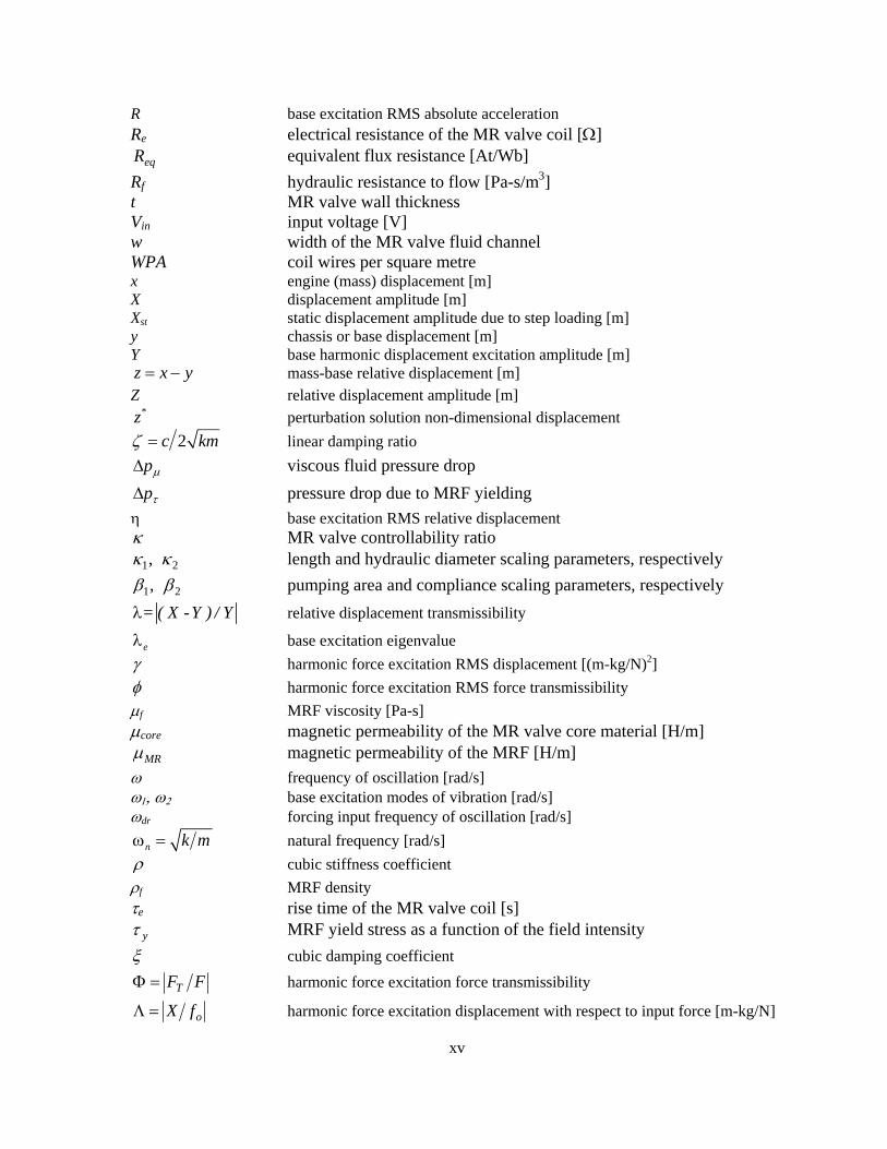
xv

R base excitation RMS absolute acceleration Re electrical resistance of the MR valve coil [Ω]

eqR equivalent flux resistance [At/Wb] Rf hydraulic resistance to flow [Pa-s/m3] t MR valve wall thickness Vin input voltage [V] w width of the MR valve fluid channel WPA coil wires per square metre x engine (mass) displacement [m] X displacement amplitude [m] Xst static displacement amplitude due to step loading [m] y chassis or base displacement [m] Y base harmonic displacement excitation amplitude [m] z x y= − mass-base relative displacement [m] Z relative displacement amplitude [m]

*z perturbation solution non-dimensional displacement 2c kmζ = linear damping ratio

µp∆ viscous fluid pressure drop

τp∆ pressure drop due to MRF yielding η base excitation RMS relative displacement κ MR valve controllability ratio

1 2,κ κ length and hydraulic diameter scaling parameters, respectively

1 2,β β pumping area and compliance scaling parameters, respectively = ( X -Y ) / Yλ relative displacement transmissibility

eλ base excitation eigenvalue γ harmonic force excitation RMS displacement [(m-kg/N)2] φ harmonic force excitation RMS force transmissibility µf MRF viscosity [Pa-s] µcore magnetic permeability of the MR valve core material [H/m]

MRµ magnetic permeability of the MRF [H/m] ω frequency of oscillation [rad/s] ω1, ω2 base excitation modes of vibration [rad/s] ωdr forcing input frequency of oscillation [rad/s]

n k mω = natural frequency [rad/s] ρ cubic stiffness coefficient ρf MRF density τe rise time of the MR valve coil [s]

yτ MRF yield stress as a function of the field intensity ξ cubic damping coefficient

FFT=Φ harmonic force excitation force transmissibility

ofX=Λ harmonic force excitation displacement with respect to input force [m-kg/N]

xvi

2noT emF ωψ = unbalance excitation non-dimensional force transmitted

emXm o=Ω unbalance excitation non-dimensional displacement χ unbalance excitation RMS non-dimensional force transmitted Γ unbalance excitation RMS non-dimensional displacement ϕ magnetic flux [Wb]

1

Chapter 1 Introduction

In the automotive industry, there is a natural demand from the customer to decrease cost of the

vehicle, while increasing comfort and fuel economy. These are usually highly conflicting design

criteria, which are generally satisfied by decreasing the amount of material used to create the system,

and thus decreasing the mass of the vehicle and replacing it with improved and sophisticated

technology as the cost of this technology decreases.

An example of this on the forefront of automotive engineering is the advent of drive-by-wire

technology. Steering-by-wire is becoming a reality in automobiles with the intent to replace the

mechanical linkage between the steering wheel and the tire as well as the power steering system with

a lightweight, efficient electromechanical system. Many decades ago, a similar fly-by-wire design

was implemented in the aerospace industry initially on fighter jets (and the NASA space shuttles)

where previously mechanical and hydro-mechanical systems were used to control aeroplanes, likely

for a price higher than what most people would pay for an entire automobile.

One of the characteristics of vehicles that define their quality is the amount of noise, vibration and

harshness (NVH) in the cabin. Muller, Weltin, Law, Roberts, and Siebler (1994) note that decreasing

the mass of vehicles represents the ability for energy sources to more easily transfer through the

structur; hence, increased NVH is the cost in comfort associated with an increase in fuel economy and

decrease in price of the automobile.

An automobile engine, body and chassis system is susceptible to undesired vibrations due two

sources of excitation: inherent unbalance and periodic combustion forces in the reciprocating engine

as well as disturbances transmitted through the vehicle’s suspension system from the road. The

frequency range of these vibrations is typically in the range of 1-200 Hz (Jazar & Golnaraghi, 2002).

2

Engine mounts are vibration isolators which are used to minimize the effect of the disturbances

described above on the system. In general, it is desirable to restrain the relative motion of the engine

to satisfy mechanical constraints while minimizing the force transmitted to and from the engine itself

(Singh, Kim, Ravindra, 1992). Minimizing the force transferred reduces the impact of the dynamics

of the engine given a base (chassis or body) excitation source, thus improving ride and minimizing

potentially damaging inertia forces on the engine. Moreover, minimizing transfer of unbalance forces

through the engine to the chassis reduces cabin noise and thus improves rider comfort.

For several decades now, NVH has benefited from the implementation of hydraulic mounts

(Flower, 1985). Hydraulic bushings, a variation of a hydraulic mount, are currently widely used in

industry; however, the development of cost effective semi-active or active isolation solutions is the

next frontier. Moreover, the introduction of cylinder-on-demand technology has intensified the

pursuit of a controllable isolator due to the affect it has on engine vibration isolation.

The goal of this thesis is to investigate the optimization of isolators to comply with the transferred

force criteria and displacement constraint with the intent to apply this optimization to the design of

semi-active isolators. The semi-active bushing is to be designed to isolate a cylinder-on-demand

engine.

1.1 Root Mean Square Frequency Domain Optimization

As mentioned above, engine isolators must be designed with the intent to minimise the force

transferred through the mount, while maintaining the amplitude of vibration within a fixed range.

The problem is: how can these criteria and constraints be met? Is there a relationship between them?

These questions have been partially answered by studying the root mean square (RMS) of the

absolute acceleration and the relative displacement frequency responses of a single degree of freedom

(DoF) isolator (Jazar, Narimani, Golnaraghi, & Swanson, 2003). It was concluded that a set of

3

optimal parameters could be found for a harmonic base excitation using a simple RMS cost function,

to be detailed in Chapter 2 of this thesis.

Furthermore, Narimani and Golnaraghi (2004) present an optimal linear system and added slight

nonlinearity to the stiffness and damping. These nonlinear parameters were again optimized in a

similar manner to that applied to the linear system by Jazar et al. (2003) for a base excitation input.

One of the goals of this thesis is to build on the frequency domain optimization work on linear

engine mounts presented by Jazar et al. (2003) as well as the nonlinear work presented by Narimani

and Golnaraghi (2004). This extension of their work will include studies for different inputs as well

as an examination of the change in the transient response when small amounts of nonlinear stiffness

and damping are present.

An experiment will be conducted to verify the RMS optimization methods on a simple spring mass

damper test bed. The purpose of this experiment is to verify that these optimization procedures can

be applied to a real system. Inevitably, any real system will exhibit some degree of nonlinearity

regardless of efforts to eliminate such complicating characteristics in the laboratory. Often, the

degree of nonlinearity is so small that it is considered negligible; which, as this thesis will show, is a

sound and practical assumption on the test bed used. It is also of interest to apply this optimization

technique to the design of hydraulic bushings.

1.2 Isolating Cylinder-on-Demand Engines

The improvement of fuel economy has led automotive manufacturers to design engines which

automatically switch between modes of operation. Each mode has a different number of cylinders

firing depending on the requirements of the driver.

For example, when accelerating all six cylinders in a V6 engine should be firing to provide the

maximum amount of power; however, once the target cruising speed is met and the load on the

engine decreases the engine management unit (EMU) may take any given 3 cylinders out of the firing

4

sequence (Hardie et al., 2002). Jackson and Jones (1976) discovered over 25 years ago that this

technique could save a quarter of the gas used in a V16 cylinder engine using 50% of the cylinders,

also noting that they experience torsional vibrations when switching to 50% mode requiring a special

torsional analysis. High energy savings are achievable largely due to the fact that steady state speed

requires such a small amount of power (less than 30 HP) with respect to the maximum power of

modern vehicles, as suggested by Ashely (2004), which can exceed 300 HP.

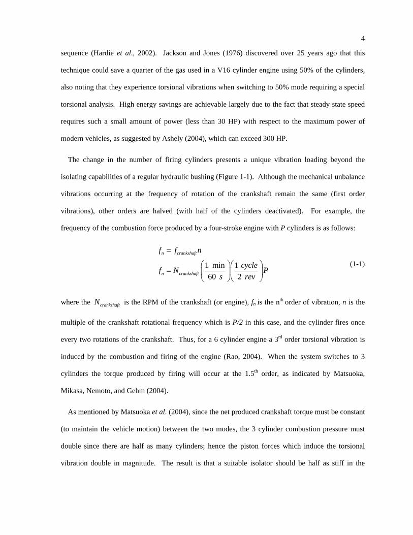
The change in the number of firing cylinders presents a unique vibration loading beyond the

isolating capabilities of a regular hydraulic bushing (Figure 1-1). Although the mechanical unbalance

vibrations occurring at the frequency of rotation of the crankshaft remain the same (first order

vibrations), other orders are halved (with half of the cylinders deactivated). For example, the

frequency of the combustion force produced by a four-stroke engine with P cylinders is as follows:

1 min 160 2

n crankshaft

n crankshaft

f f n

cyclef N Ps rev

=

⎛ ⎞⎛ ⎞= ⎜ ⎟⎜ ⎟

⎝ ⎠⎝ ⎠

(1-1)

where the crankshaftN is the RPM of the crankshaft (or engine), fn is the nth order of vibration, n is the

multiple of the crankshaft rotational frequency which is P/2 in this case, and the cylinder fires once

every two rotations of the crankshaft. Thus, for a 6 cylinder engine a 3rd order torsional vibration is

induced by the combustion and firing of the engine (Rao, 2004). When the system switches to 3

cylinders the torque produced by firing will occur at the 1.5th order, as indicated by Matsuoka,

Mikasa, Nemoto, and Gehm (2004).

As mentioned by Matsuoka et al. (2004), since the net produced crankshaft torque must be constant

(to maintain the vehicle motion) between the two modes, the 3 cylinder combustion pressure must

double since there are half as many cylinders; hence the piston forces which induce the torsional

vibration double in magnitude. The result is that a suitable isolator should be half as stiff in the

5

operating frequency range of the 3 cylinder mode of the engine. This is likely around 1000-2200

RPM ( 1.5 25 55f Hz= − ). The isolator must also maintain performance in 6 cylinder mode similar to

current products.

Figure 1-1: Photograph of a hydraulic engine bushing

1.3 A New Solution: Semi-Active Isolators

The true need for a new isolator spawns from the need to minimize fuel consumption which led to the

implementation of cylinder-on-demand engines, also known as cylinder deactivation. Cylinder-on-

demand produces changing load conditions, making it far too difficult to maintain the NVH

performance of the vehicle with the current isolator design.

There are various mechanisms to influence the force produced by an isolator, in particular a

hydraulic engine mount. For every mechanism, there are several proposed designs for active and

semi-active mounts: Muller (1994); Kim and Singh (1995); Foumani, Khajepour, and Durali (2004);

6

Vahdati and Ahmadian (2003); Lee and Lee (2002), Matsuoka et al. (2004); and Jazar and Golnaraghi

(2003). With the exception of the design proposed by Matsuoka et al. (2004), which is scheduled to

be on the 2005 Honda Odyssey, none of the previous designs have been witnessed by the author to be

implemented for the automotive market.

Producing a reliable active mounts is difficult since it requires an actuator, adequate sealing,

moving parts, and possibly large amounts of energy for the actuator among other design issues.

Similarly, semi-active isolators often require an actuator and moving parts; essentially having all the

poor traits of an active mount with limited incremental performance. By comparison,

magnetorheological (MR) semi-active systems represent a low cost, low energy consumption, and

potentially very effective isolation solution with no moving parts.

It is the goal of this work is to develop a simple model of a hydraulic bushing, assuming that the

nonlinearity in engine mounts can be attributed mostly to fluid damping, and simulate the response of

the bushing to evaluate the performance in the frequency domain. The dynamic stiffness of current

production bushings, supplied by General Motors Corporation (GMC), will be used to verify the

mathematical model. This bushing will be used as a foundation to develop a semi-active MR bushing

to isolate the cylinder deactivating engine vibrations on a GMC V6 vehicle platform. As will be

discussed in greater detail in the following chapters, the MR bushing design will implement the flow

mode (or valve mode) effect of MR fluids – a similar design which has led to the success of Lord

Corporation’s MR damper RD-1005.

The bushing design will be fabricated and tested. The industry standard for illustrating the

performance of engine isolators is a plot of dynamic stiffness in the frequency domain. This data

requires a specific test bed. From an isolation point of view, the performance of the mount is best

measured by examining the transmissibility of displacement, velocity, and acceleration for given

inputs to the isolator. For this reason, a base excitation experiment will also be conducted. This type

7

of experiment is rarely conducted and documented in the field and is considered by the author to be

an improvement on the prior art.

1.4 Thesis Overview

In the previous sections, the need for semi-active engine bushings was presented. The objective of

this thesis is to reduce the vibrations induced in a cylinder deactivating engine by using a MR

bushing. The strategy for designing this bushing is to implement RMS optimization techniques to

select appropriate parameters for the system and shed light on simple and practical control strategies

to be further developed in future work.

In Chapter 2, a review of the prior work on RMS optimization is presented. This review of the

literature covers both isolation of base excitations using a linear Voigt rubber model and isolators

with slightly nonlinear elements. The advantage of adding nonlinearity via semi-active control is

illustrated. Chapter 2 also details current engine isolator designs including a review of literature

pertaining to controllable devices and how MR technology can be applied.

The core theoretical portion of the thesis follows Chapter 2. The linear and nonlinear RMS studies

introduced in Chapter 2 are extended to various inputs in Chapter 3. This work provides the

foundation for semi-active control strategies.

The prototype MR valve design is described in Chapter 3 and the input-output relationship of the

valve is developed using numerical modeling. Dynamic equations of motion are developed for a MR

bushing, similar to typical engine mount equations. This model is used to simulate the dynamic

stiffness of the MR bushing.

Chapter 3 also applies the RMS optimization technique, which was originally used to optimize the

parameters of the linear and nonlinear isolators, to hydraulic bushings. It is shown that this method

can be used to improve the performance of hydraulic bushings.

8

Chapters 4 and 5 pertain to the experimental portion of the thesis. Chapter 4 describes the

experimental apparatus used to verify the linear RMS optimization techniques, including the test bed

used to conducts experiments on engine bushings. Chapter 5 discusses the results of the RMS and

bushing experiments.

Finally, conclusion and recommendations for future work can be found in Chapter 6.

9

Chapter 2 Literature Review

2.1 Optimization of Isolators

As alluded to in the introduction, the fundamental requirement or function of an isolator is to

minimize the force transmitted and maintain the relative displacement of the mount. This is the

nature of the rubber isolators, according to the Kelvin (Voigt) model of rubber (otherwise referred to

as a linear isolator, as illustrated in Figure 2-1), in that they can only produce force in response to

changes in relative displacement and relative velocity.

The idea of designing a passive linear isolator which could both minimize the force transmitted and

simultaneously minimize the relative displacement is unrealistic. Providing passive isolation from

force cannot be achieved without the cost of deflection (Andrews, 2002).

The art of optimization can be taken to any level. Modern computing power permits optimization

on an unimaginable computational scale. Lin, Luo, and Zhang (1990) developed an optimization

strategy for an n-degree of freedom (DoF) system. Their method uses a relatively complex cost

function and produces good response results at the cost of being computationally intensive and highly

sophisticated.

Madjlesi, Schubert, Khajepour, and Ismail (2003) present another sophisticated optimization

method whereby the optimum mount stiffness is derived by experimentally determining the frequency

response functions (FRFs) which describe the noise transfer paths through the engine mounts to

objective points in the cabin. Steady-state engine mount optimization is conducted by tweaking the

frequency response of the mount and minimizing the objective point outputs using experimentally

obtained engine loading and the FRFs. This method is very effective; however, it too is

computationally intensive, sophisticated, and most importantly the result of optimisation may not be

10

manufacturable due to the limits of the isolator material properties and mechanical design constraints.

A more detailed review of optimization literature is included in the work of Narimani (2004).

The RMS optimization method presented by Jazar et al. (2003) uses a very practical and

mechanically intuitive cost function, has a closed form solution, and is extremely simple. This

method is the basis for a large portion of the work in this thesis, and will be detailed in the following

section.

2.1.1 Linear Mount Optimization

Traditionally, the fundamental vibration isolation problem is approached by separating the system

from the source of vibration with a linear spring and damper, as illustrated in Figure 2-1.

Figure 2-1: Schematic of a linear 1 DoF isolator representing an engine mount.

Reviewing the work presented by Jazar et al. (2003), the equation of motion of the above system is

)cos()()( temyxkyxcxm drdro ωω=−+−+ &&&& (2-1)

where m is the total suspended mass [kg], c is the damping coefficient [N-s/m], k is the stiffness

[N/m], mo is an eccentric mass of eccentricity e [m] and driving frequency ωdr [rad/s]. The

displacement of the base and mass are y [m] and x [m], respectively. Equation (2-1) can be

rearranged to the following form:

k c

x

y

m

F(t)=moeωdr2cos(ωdrt)

z

11

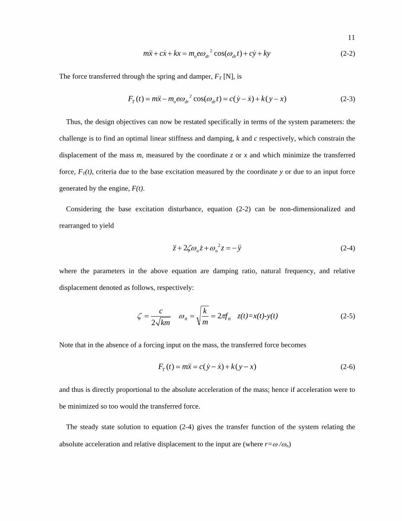
2 cos( )o dr drmx cx kx m e t cy kyω ω+ + = + +&& & & (2-2)

The force transferred through the spring and damper, FT [N], is

2( ) cos( ) ( ) ( )T o dr drF t mx m e t c y x k y xω ω= − = − + −&& & & (2-3)

Thus, the design objectives can now be restated specifically in terms of the system parameters: the

challenge is to find an optimal linear stiffness and damping, k and c respectively, which constrain the

displacement of the mass m, measured by the coordinate z or x and which minimize the transferred

force, FT(t), criteria due to the base excitation measured by the coordinate y or due to an input force

generated by the engine, F(t).

Considering the base excitation disturbance, equation (2-2) can be non-dimensionalized and

rearranged to yield

22 n nz z z yζω ω+ + = −&&&& & (2-4)

where the parameters in the above equation are damping ratio, natural frequency, and relative

displacement denoted as follows, respectively:

2

ckm

ζ = nn fmk πω 2== z(t)=x(t)-y(t) (2-5)

Note that in the absence of a forcing input on the mass, the transferred force becomes

( ) ( ) ( )TF t mx c y x k y x= = − + −&& & & (2-6)

and thus is directly proportional to the absolute acceleration of the mass; hence if acceleration were to

be minimized so too would the transferred force.

The steady state solution to equation (2-4) gives the transfer function of the system relating the

absolute acceleration and relative displacement to the input are (where r=ω /ωn)

12

2 2

2 2 2

1 (2 )

(1 ) (2 )

rXaY r r

ω ζ

ζ

+= =

− +

&& (2-7)

and

2

2 2 2(1 ) (2 )X Y r

Y r rλ

ζ−

= =− +

(2-8)

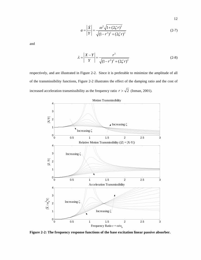
respectively, and are illustrated in Figure 2-2. Since it is preferable to minimize the amplitude of all

of the transmissibility functions, Figure 2-2 illustrates the effect of the damping ratio and the cost of

increased acceleration transmissibility as the frequency ratio 2r > (Inman, 2001).

0 0.5 1 1.5 2 2.5 30

1

2

3

4Motion Transmissibility

|X/Y

|

0 0.5 1 1.5 2 2.5 30

1

2

3

4Relative Motion Transmissibility (|Z| = |X-Y|)

|Z /Y

|

0 0.5 1 1.5 2 2.5 30

1

2

3

4Acceleration Transmissibility

|X /

ω n2 Y|

Frequency Ratio r = ω/ωn

Increasing ζ

Increasing ζ

Increasing ζ

Increasing ζ

Increasing ζ

:

Figure 2-2: The frequency response functions of the base excitation linear passive absorber.

13

Optimum stiffness and damping ratio should be found by examining the response of the system in

the frequency range of 0-20 Hz, a critical range for typical mechanical systems (Alkhatib, Jazar, &

Golnaraghi, 2004). Given a certain damping ratio and stiffness, the performance of the system can be

characterized by computing the RMS of the frequency response over a certain bandwidth. According

to Inman (2001), RMS is a common method of representing a response in the field of vibration. In

this case, it is representative of the variance of magnitude of relative motion or acceleration

transmissibility – analogous to a weighted average amplitude.

The definition of the root mean square (RMS) of a function h(ω) from ω = 0-20 Hz is as follows

40 2

0

1( ( )) ( )40

RMS h h dπ

ω ω ωπ

= ∫ (2-9)

The above formulation is the foundation for the work of Jazar et al. (2003) and Narimani and

Golnaraghi (2004). Applying equation (2-9) to the base excitation, we define

( )R RMS a= , RMS absolute acceleration (2-10)

)(λη RMS= , RMS relative displacement (2-11)

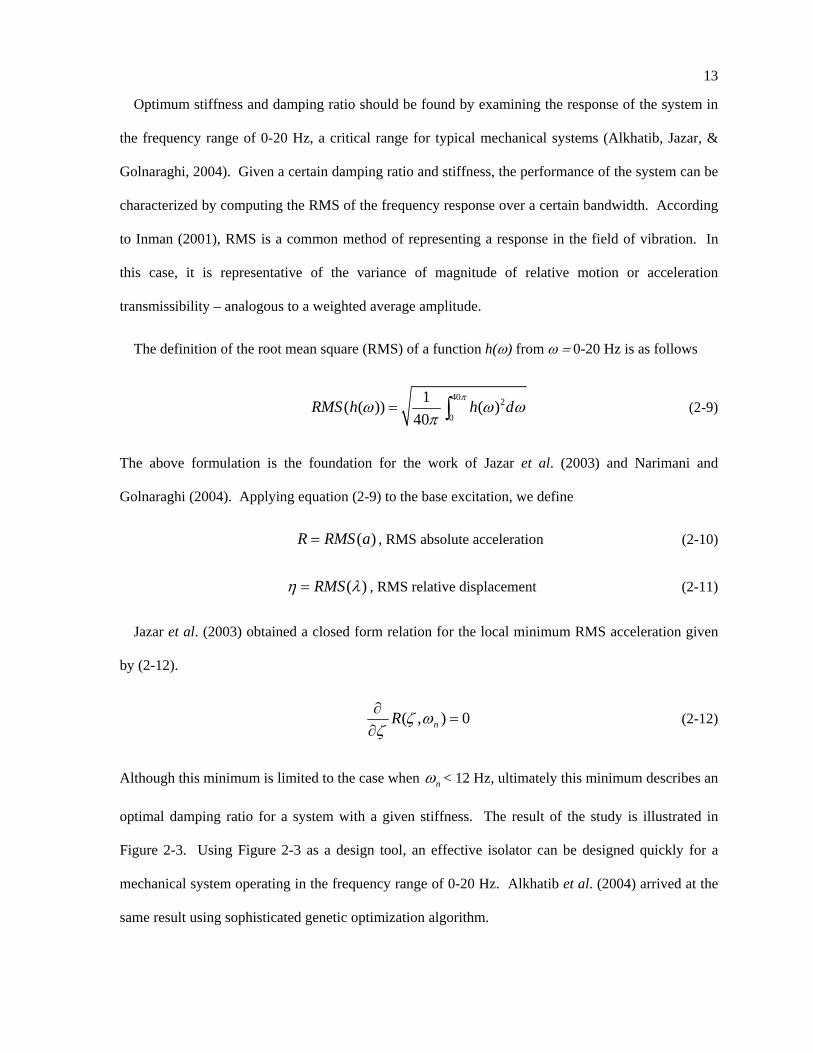
Jazar et al. (2003) obtained a closed form relation for the local minimum RMS acceleration given

by (2-12).

( , ) 0nR ζ ωζ∂

=∂

(2-12)

Although this minimum is limited to the case when nω < 12 Hz, ultimately this minimum describes an

optimal damping ratio for a system with a given stiffness. The result of the study is illustrated in

Figure 2-3. Using Figure 2-3 as a design tool, an effective isolator can be designed quickly for a

mechanical system operating in the frequency range of 0-20 Hz. Alkhatib et al. (2004) arrived at the

same result using sophisticated genetic optimization algorithm.

14

Figure 2-3: The R versus η map illustrating the line of optimum design for a base excited linear

passive vibration isolator (Jazar et al., 2003).

If the designer has the liberty of full control over the damping, the natural frequency could be

selected base on time domain criteria, then damping ratio picked off Figure 2-3 to satisfy the relative

motion constraint or to satisfy both relative motion and minimum acceleration, keeping in mind that,

for a given base excitation, the mass acceleration is proportional to the force transmitted as per

equation (2-6). However, having control over the damping is often difficult to do practically.

Therefore, if the damping ratio is fixed and selected based on time domain criteria, the natural

frequency is more practically tuneable in a mechanical system by varying the stiffness to yield the

appropriate frequency response according to Figure 2-3.

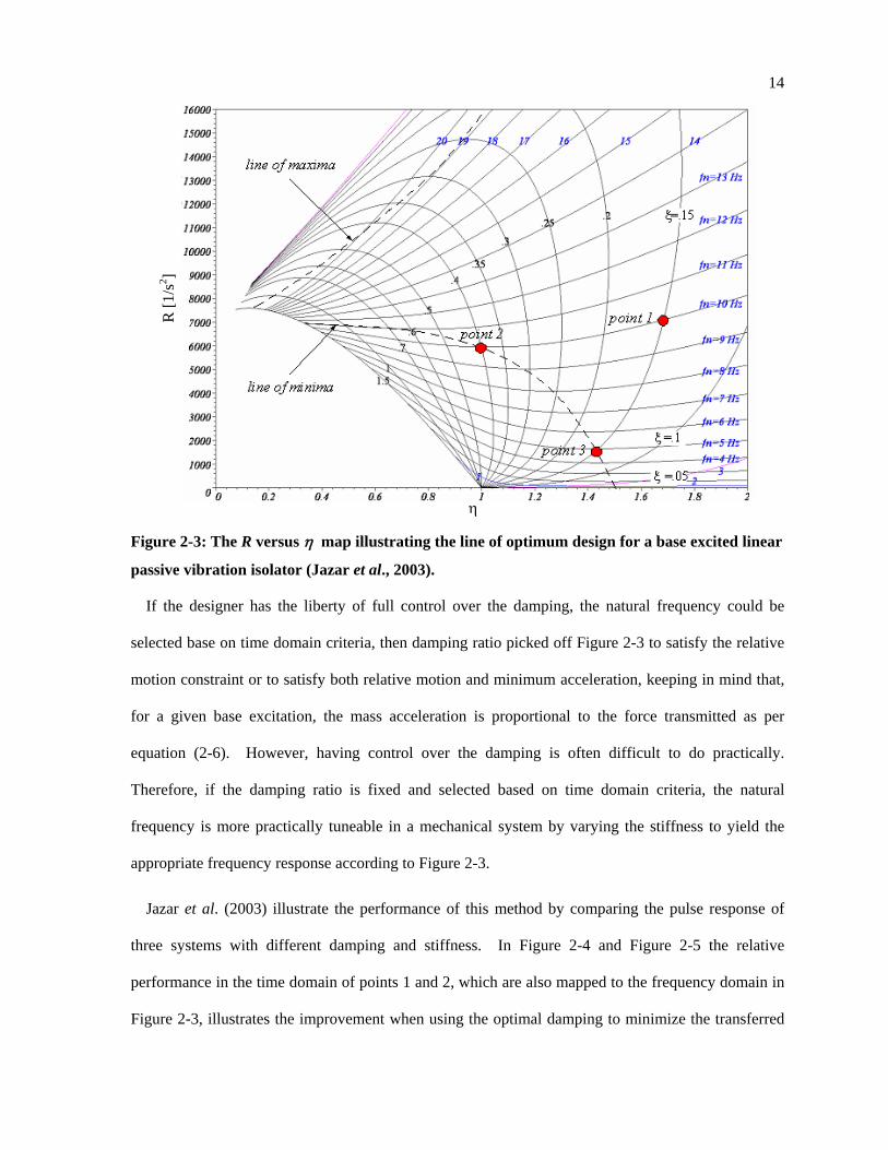
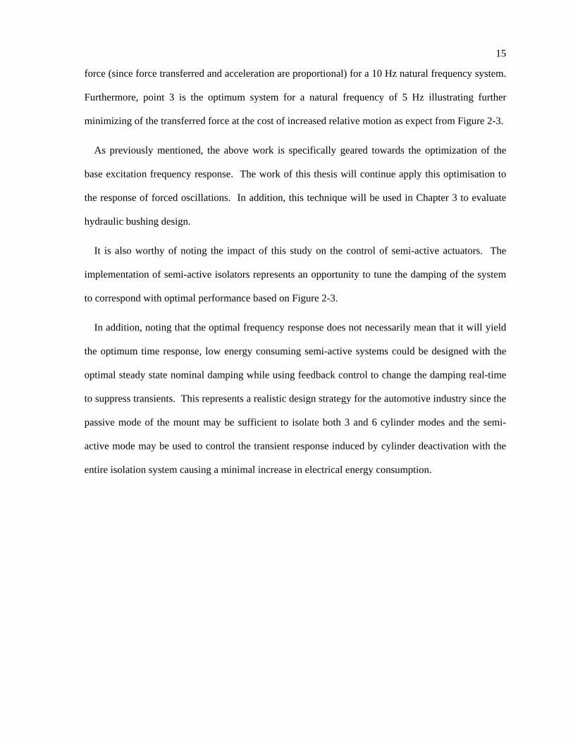
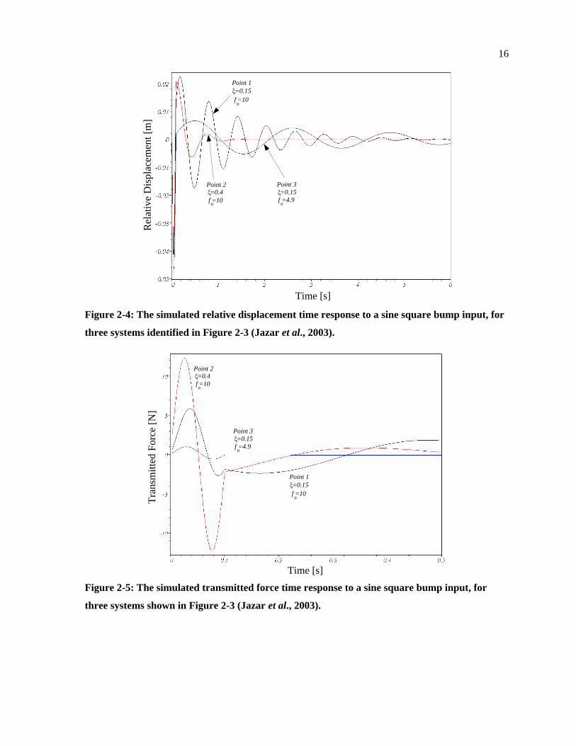
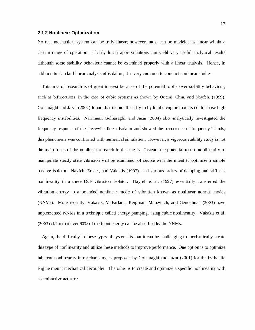
Jazar et al. (2003) illustrate the performance of this method by comparing the pulse response of

three systems with different damping and stiffness. In Figure 2-4 and Figure 2-5 the relative

performance in the time domain of points 1 and 2, which are also mapped to the frequency domain in

Figure 2-3, illustrates the improvement when using the optimal damping to minimize the transferred

η

R [1

/s2 ]

15

force (since force transferred and acceleration are proportional) for a 10 Hz natural frequency system.

Furthermore, point 3 is the optimum system for a natural frequency of 5 Hz illustrating further

minimizing of the transferred force at the cost of increased relative motion as expect from Figure 2-3.

As previously mentioned, the above work is specifically geared towards the optimization of the

base excitation frequency response. The work of this thesis will continue apply this optimisation to

the response of forced oscillations. In addition, this technique will be used in Chapter 3 to evaluate

hydraulic bushing design.

It is also worthy of noting the impact of this study on the control of semi-active actuators. The

implementation of semi-active isolators represents an opportunity to tune the damping of the system

to correspond with optimal performance based on Figure 2-3.

In addition, noting that the optimal frequency response does not necessarily mean that it will yield

the optimum time response, low energy consuming semi-active systems could be designed with the

optimal steady state nominal damping while using feedback control to change the damping real-time

to suppress transients. This represents a realistic design strategy for the automotive industry since the

passive mode of the mount may be sufficient to isolate both 3 and 6 cylinder modes and the semi-

active mode may be used to control the transient response induced by cylinder deactivation with the

entire isolation system causing a minimal increase in electrical energy consumption.

16

Point 2ξ=0.4fn=10

Point 3ξ=0.15fn=4.9

Point 1ξ=0.15fn=10

Rela

tive

Dis

plac

emen

t

Time [sec] Figure 2-4: The simulated relative displacement time response to a sine square bump input, for

three systems identified in Figure 2-3 (Jazar et al., 2003).

Tran

smitt

ed F

orce

Point 2ξ=0.4fn=10

Point 3ξ=0.15fn=4.9

Point 1ξ=0.15f

n=10

Time [sec] Figure 2-5: The simulated transmitted force time response to a sine square bump input, for

three systems shown in Figure 2-3 (Jazar et al., 2003).

Time [s]

Rel

ativ

e D

ispl

acem

ent [

m]

Time [s]

Tran

smitt

ed F

orce

[N]

17

2.1.2 Nonlinear Optimization

No real mechanical system can be truly linear; however, most can be modeled as linear within a

certain range of operation. Clearly linear approximations can yield very useful analytical results

although some stability behaviour cannot be examined properly with a linear analysis. Hence, in

addition to standard linear analysis of isolators, it is very common to conduct nonlinear studies.

This area of research is of great interest because of the potential to discover stability behaviour,

such as bifurcations, in the case of cubic systems as shown by Oueini, Chin, and Nayfeh, (1999).

Golnaraghi and Jazar (2002) found that the nonlinearity in hydraulic engine mounts could cause high

frequency instabilities. Narimani, Golnaraghi, and Jazar (2004) also analytically investigated the

frequency response of the piecewise linear isolator and showed the occurrence of frequency islands;

this phenomena was confirmed with numerical simulation. However, a vigorous stability study is not

the main focus of the nonlinear research in this thesis. Instead, the potential to use nonlinearity to

manipulate steady state vibration will be examined, of course with the intent to optimize a simple

passive isolator. Nayfeh, Emaci, and Vakakis (1997) used various orders of damping and stiffness

nonlinearity in a three DoF vibration isolator. Nayfeh et al. (1997) essentially transferred the

vibration energy to a bounded nonlinear mode of vibration known as nonlinear normal modes

(NNMs). More recently, Vakakis, McFarland, Bergman, Manevitch, and Gendelman (2003) have

implemented NNMs in a technique called energy pumping, using cubic nonlinearity. Vakakis et al.

(2003) claim that over 80% of the input energy can be absorbed by the NNMs.

Again, the difficulty in these types of systems is that it can be challenging to mechanically create

this type of nonlinearity and utilize these methods to improve performance. One option is to optimize

inherent nonlinearity in mechanisms, as proposed by Golnaraghi and Jazar (2001) for the hydraulic

engine mount mechanical decoupler. The other is to create and optimize a specific nonlinearity with

a semi-active actuator.

18

The exact focus of the nonlinear portion of this thesis is again to build upon the work presented by

Narimani (2004) and Narimani and Golnaraghi (204) in a similar fashion to the work that was

described in section 2.1.2. Narimani (2004) and Narimani and Golnaraghi (2004) extended the

research on the previous linear RMS optimization of the base excitation isolator to include nonlinear

elements. Their work included a variation of equation (2-4) which incorporated cubic nonlinear

stiffness and damping as follows:

3 31 3 1 3mz c z c z k z k z my+ + + + = − &&&& & & (2-13)

where c1 is the linear damping coefficient, c3 is cubic damping coefficient, k1 is the linear stiffness,

and k3 is the cubic stiffness. Once non-dimensionalized, the equation of motion is the following:

* * *3 * *3 22 2 cos( )z z z z zζ ξ ρ ω ωτ+ + + + =&& & & (2-14)

where *z is a scaled displacement, ζ is the linear and ξ is the cubic nonlinear damping ratios and

ρ is the cubic stiffness. Equation (2-14) also assumes that the base excitation is sinusoidal and the

non-dimensional rotational frequency is ω . The process of creating non-dimensional equations of

motion is detail by Nayfeh (1981).

Solving the system using perturbation methods (Nayfeh, 1981) results in a 6th order amplitude-

frequency relationship as follows:

( )2 6 6 4 2 4 2 2 2 2

2 6 4 2

9 3A + 6 A A 1 + A 4 2 A4 2

9 3 + A A +A 016 2

⎛ ⎞ξ ω ζξ + − ω − ρ + ζ − ω⎜ ⎟⎝ ⎠

ρ + ρ = (2-15)

where A is the non-dimensional amplitude of vibration. Some of the roots of equation (2-15) are

complex, some are unstable equilibrium points causing a jump phenomena (as illustrated in Figure

2-6), and others correspond to frequency islands. These are generally undesirable properties;

19

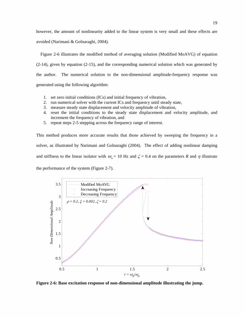
however, the amount of nonlinearity added to the linear system is very small and these effects are

avoided (Narimani & Golnaraghi, 2004).

Figure 2-6 illustrates the modified method of averaging solution (Modified MoAVG) of equation

(2-14), given by equation (2-15), and the corresponding numerical solution which was generated by

the author. The numerical solution to the non-dimensional amplitude-frequency response was

generated using the following algorithm:

1. set zero initial conditions (ICs) and initial frequency of vibration, 2. run numerical solver with the current ICs and frequency until steady state, 3. measure steady state displacement and velocity amplitude of vibration, 4. reset the initial conditions to the steady state displacement and velocity amplitude, and

increment the frequency of vibration, and 5. repeat steps 2-5 stepping across the frequency range of interest.

This method produces more accurate results that those achieved by sweeping the frequency in a

solver, as illustrated by Narimani and Golnaraghi (2004). The effect of adding nonlinear damping

and stiffness to the linear isolator with nω = 10 Hz and ζ = 0.4 on the parameters R and η illustrate

the performance of the system (Figure 2-7).

0.5 1 1.5 2 2.5

0.5

1

1.5

2

2.5

3

3.5

r = ωd/ωn

Non

-Dim

ensi

onal

Am

plitu

de ρ = 0.2, ξ = 0.002, ζ = 0.2

Modified MoAVGIncreasing FrequencyDecreasing Frequency

Figure 2-6: Base excitation response of non-dimensional amplitude illustrating the jump.

20

0.7 0.75 0.8 0.85 0.9 0.95 1 1.05 1.1 1.15 1.23000

3500

4000

4500

5000

5500

6000

6500

7000

7500

8000

ξ =

0.00

8

ξ =

-0.0

08

ρ = 0.2

ρ = -0.9

η

R [1

/s2 ] ρ = 0

ρ = -0.8

ρ = -0.6

ρ = -0.4

ρ = -0.2

ξ = 0

ρ = -1.2

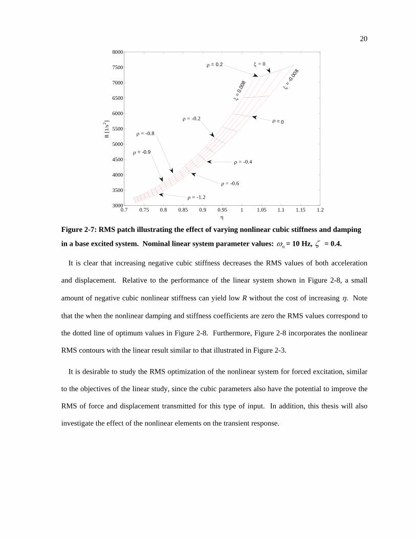
Figure 2-7: RMS patch illustrating the effect of varying nonlinear cubic stiffness and damping

in a base excited system. Nominal linear system parameter values: nω = 10 Hz, ζ = 0.4.

It is clear that increasing negative cubic stiffness decreases the RMS values of both acceleration

and displacement. Relative to the performance of the linear system shown in Figure 2-8, a small

amount of negative cubic nonlinear stiffness can yield low R without the cost of increasing η. Note

that the when the nonlinear damping and stiffness coefficients are zero the RMS values correspond to

the dotted line of optimum values in Figure 2-8. Furthermore, Figure 2-8 incorporates the nonlinear

RMS contours with the linear result similar to that illustrated in Figure 2-3.

It is desirable to study the RMS optimization of the nonlinear system for forced excitation, similar

to the objectives of the linear study, since the cubic parameters also have the potential to improve the

RMS of force and displacement transmitted for this type of input. In addition, this thesis will also

investigate the effect of the nonlinear elements on the transient response.

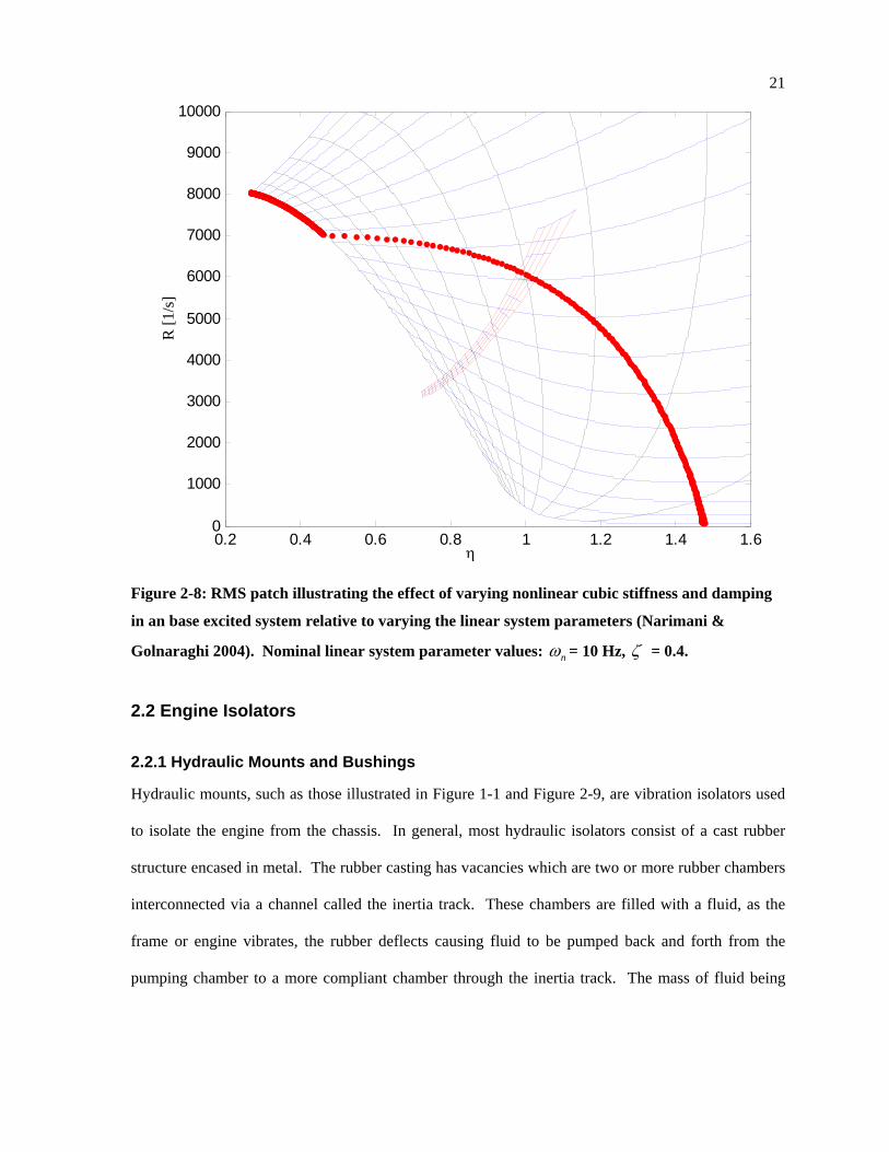
21

Figure 2-8: RMS patch illustrating the effect of varying nonlinear cubic stiffness and damping

in an base excited system relative to varying the linear system parameters (Narimani &

Golnaraghi 2004). Nominal linear system parameter values: nω = 10 Hz, ζ = 0.4.

2.2 Engine Isolators

2.2.1 Hydraulic Mounts and Bushings

Hydraulic mounts, such as those illustrated in Figure 1-1 and Figure 2-9, are vibration isolators used

to isolate the engine from the chassis. In general, most hydraulic isolators consist of a cast rubber

structure encased in metal. The rubber casting has vacancies which are two or more rubber chambers

interconnected via a channel called the inertia track. These chambers are filled with a fluid, as the

frame or engine vibrates, the rubber deflects causing fluid to be pumped back and forth from the

pumping chamber to a more compliant chamber through the inertia track. The mass of fluid being

η

R [1

/s]

0.2 0.4 0.6 0.8 1 1.2 1.4 1.60

1000

2000

3000

4000

5000

6000

7000

8000

9000

10000

22

forced through the inertia track has a liquid column resonance and dissipates energy through fluid

flow losses, causing a damping effect.

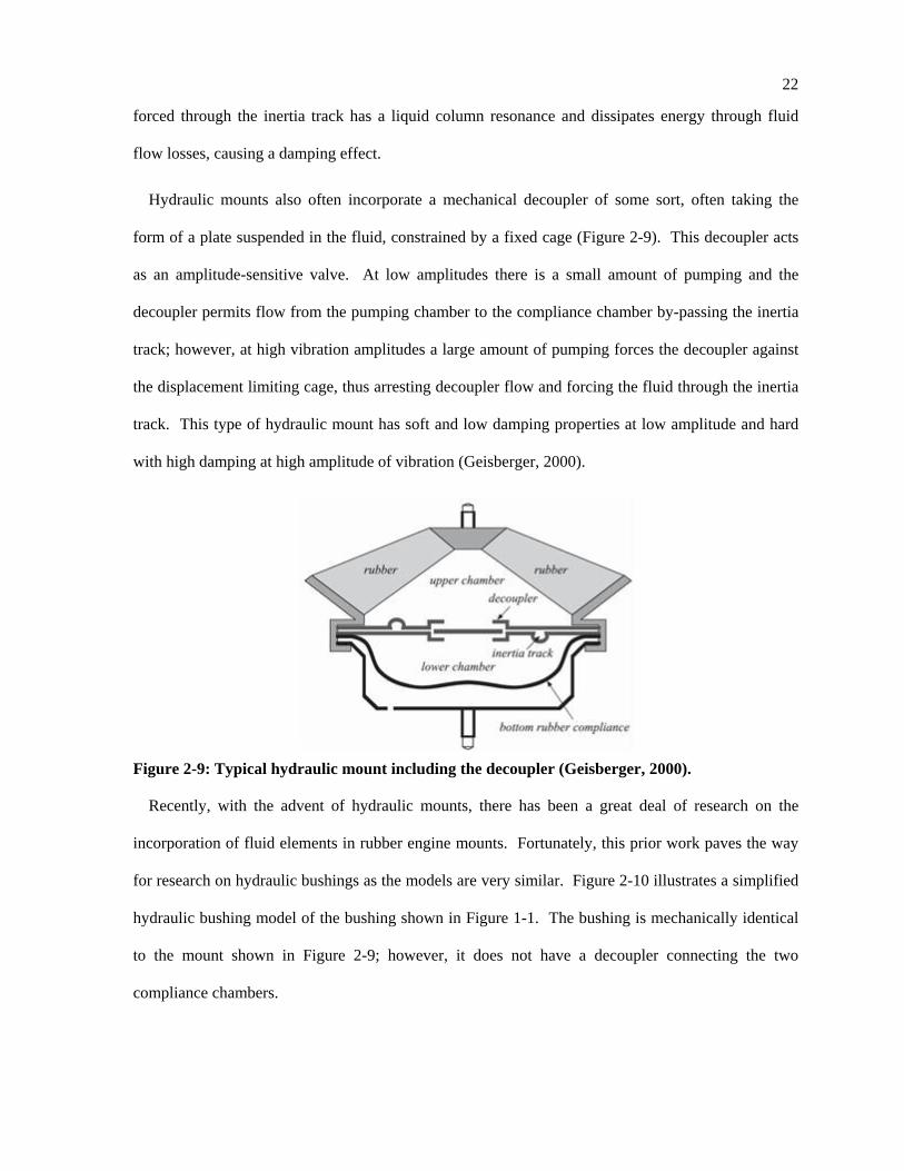
Hydraulic mounts also often incorporate a mechanical decoupler of some sort, often taking the

form of a plate suspended in the fluid, constrained by a fixed cage (Figure 2-9). This decoupler acts

as an amplitude-sensitive valve. At low amplitudes there is a small amount of pumping and the

decoupler permits flow from the pumping chamber to the compliance chamber by-passing the inertia

track; however, at high vibration amplitudes a large amount of pumping forces the decoupler against

the displacement limiting cage, thus arresting decoupler flow and forcing the fluid through the inertia

track. This type of hydraulic mount has soft and low damping properties at low amplitude and hard

with high damping at high amplitude of vibration (Geisberger, 2000).

Figure 2-9: Typical hydraulic mount including the decoupler (Geisberger, 2000).

Recently, with the advent of hydraulic mounts, there has been a great deal of research on the

incorporation of fluid elements in rubber engine mounts. Fortunately, this prior work paves the way

for research on hydraulic bushings as the models are very similar. Figure 2-10 illustrates a simplified

hydraulic bushing model of the bushing shown in Figure 1-1. The bushing is mechanically identical

to the mount shown in Figure 2-9; however, it does not have a decoupler connecting the two

compliance chambers.

23

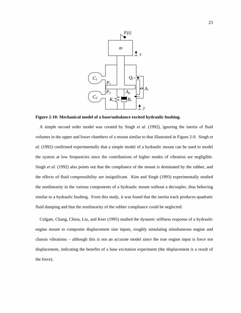
Figure 2-10: Mechanical model of a base/unbalance excited hydraulic bushing.

A simple second order model was created by Singh et al. (1992), ignoring the inertia of fluid

volumes in the upper and lower chambers of a mount similar to that illustrated in Figure 2-9. Singh et

al. (1992) confirmed experimentally that a simple model of a hydraulic mount can be used to model

the system at low frequencies since the contributions of higher modes of vibration are negligible.

Singh et al. (1992) also points out that the compliance of the mount is dominated by the rubber, and

the effects of fluid compressibility are insignificant. Kim and Singh (1993) experimentally studied

the nonlinearity in the various components of a hydraulic mount without a decoupler, thus behaving

similar to a hydraulic bushing. From this study, it was found that the inertia track produces quadratic

fluid damping and that the nonlinearity of the rubber compliance could be neglected.

Colgate, Chang, Chiou, Liu, and Keer (1995) studied the dynamic stiffness response of a hydraulic

engine mount to composite displacement sine inputs, roughly simulating simultaneous engine and

chassis vibrations – although this is not an accurate model since the true engine input is force not

displacement, indicating the benefits of a base excitation experiment (the displacement is a result of

the force).

C2

C1 Qi

Kr Br

P1

P2 Ap

x

m

F(t)

y

Ai

24

Using experimental methods pioneered by many works in the early 1990s such as that of Kim and

Singh (1993), Geisberger, Khajepour, and Golnaraghi (2002) developed an experimental apparatus

used to extract the dynamic response of all the engine mount subsystems. From this experimental

investigation, Geisberger et al. (2002) created an extensive analytical model including several

accurate models of the nonlinearities such as decoupler flow resistance to yield accurate results over a

large range of frequency and various amplitudes.

Golnaraghi and Jazar (2001, 2002) also developed a simple model of hydraulic mounts with only a

decoupler and demonstrated the validity of the model experimentally for both low and high

frequencies, as well as a nonlinear study of decoupler dynamics using perturbation methods. This

verifies that a simple model is sufficient to study the bushing dynamics.

The design of a semi-active mount will require the development of a simple model of a hydraulic

bushing. Prior research by Golnaraghi and Jazar (2001, 2002), Geisberger et al. (2002), Singh et al.

(1992) and others details the nonlinearity associated with the decoupler as well as the inertia track,

pumping area, and rubber compliance. Since the bushing in this study does not have a decoupler, it is

proposed that a simple two degree of freedom linear model can be used to model the isolator, with the

realization that the fluid damping is highly nonlinear and will require tuning for different amplitudes

of vibration.

2.2.2 Semi-active Engine Isolators

In essence, a MR hydraulic bushing is a vibration isolator which is controlled by a microchip. The

microchip, in conjunction with sensors to quantify the vibrations and provide feedback, controls an

input electric current to the hydraulic bushing. This current creates a magnetic field in the inertia

track connecting to chambers of the bushing filled with MR fluid – a solution of solid iron particles in

a typically hydrocarbon based fluid medium. As the hydraulic bushing begins to vibrate it pumps

MR fluid through the inertia track from one chamber to the other and vice versa. Thus, the magnetic

25

field induced by the microchip controller can be used to control the flow of fluid (by changing the

yield stress of the fluid via the magnetic field) through the inertia track and thus change the

characteristics of the hydraulic bushing.

Recently, there have been several applications of electrorheological (ER) fluids to mounts and

isolators and some similar applications of MR fluids (MRFs). Williams, Rigby, Sproston, and

Stanway (1993) built a simple model of an automotive engine mount using ER fluids. They were

able to mathematically simulate the steady state behaviour and experimentally generate promising

results with their scaled model. This design utilized the squeeze flow mode properties of the engine

mount. A full scale prototype of a flow mode ER engine mount was built by Hong, Choi, Jung, Ham,

and Kim (2001). They also demonstrated that using the fluid could reduce transmissibility of

acceleration and displacement using skyhook controllers.

There exists very little prior work on MR engine isolators. Of the few documented experiments,

Choi, Lee, Song, and Park (2002) and Choi, Song, Lee, Lim, and Kim (2003) designed and

manufactured a mixed mode MR engine mount and conducted base excitation experiments to

complete a hardware-in-the-loop full car model to demonstrate the effectiveness of their design, also

with a skyhook controller. Shtarkmen (1993) has patented a similar design.

However, to date, there exists little evidence that there has been a great deal of research conducted

on the application of MRF engine mounts in the operating in the flow mode or valve mode. One

patent does exist, implementing MRF in an engine mount with a decoupler (Baudendistel et al.,

2002). Many MR damper designs exist which utilize the flow mode characteristics and many of them

are patented by Carlson, Chrzan, and James (1994). It is shown by Kuzhir, Bossis, and Bashtovoi

(2003) as well as Kuzhir, Bossis, Bashtovoi, and Volkova (2003) that MR fluids perform best in

pressure driven flow when the orientation of the magnetic field is perpendicular to the direction of

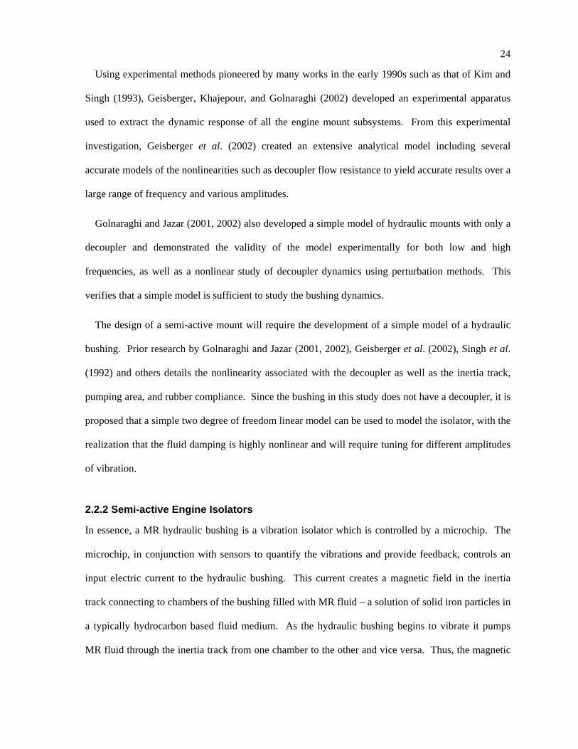
flow. Many of the designs of Carlson et al. (1994) are similar to the cross-section illustration in

Figure 2-11. Although this arrangement does work and is commonly used, it is not necessarily the

26

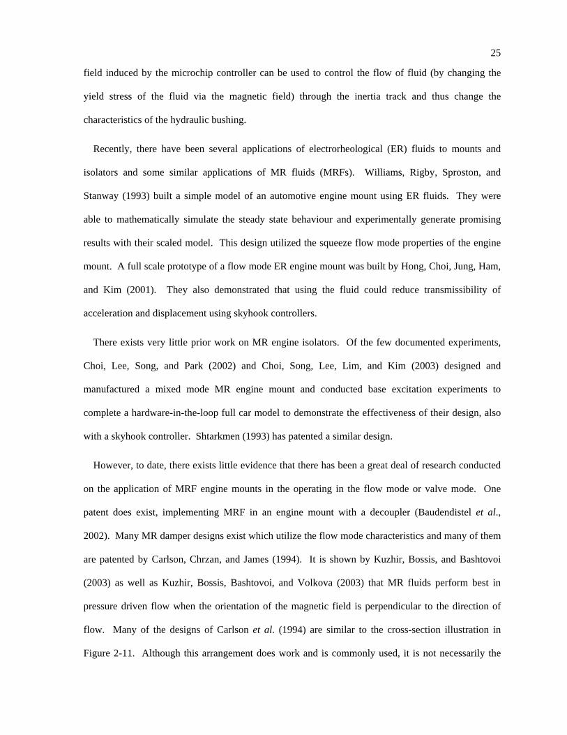
most efficient design. A more efficient design is presented by Gorodkin, Lukianovich, and Kordonski

(1998) and patented by Kordonski et al. (1995). This design is similar to that of Figure 2-11 except

that the fluid entering the device flows in a radial channel (Figure 2-12). The length of the flow path

which is in contact with the flux is much longer in this design. This is because the entire length of the

channel passes through the flux, rather than passing through only a short distance as in the previous

design. The length of the path of flow in the flux is directly proportional to the pressure drop in the

presence of a perpendicular flux, thus increasing the path length increases the performance of the

device.

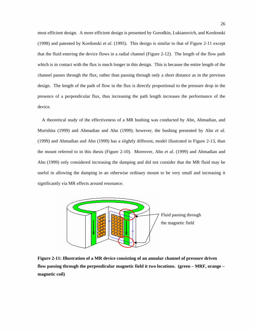
A theoretical study of the effectiveness of a MR bushing was conducted by Ahn, Ahmadian, and

Morishita (1999) and Ahmadian and Ahn (1999); however, the bushing presented by Ahn et al.

(1999) and Ahmadian and Ahn (1999) has a slightly different, model illustrated in Figure 2-13, than

the mount referred to in this thesis (Figure 2-10). Moreover, Ahn et al. (1999) and Ahmadian and

Ahn (1999) only considered increasing the damping and did not consider that the MR fluid may be

useful in allowing the damping in an otherwise ordinary mount to be very small and increasing it

significantly via MR effects around resonance.

Figure 2-11: Illustration of a MR device consisting of an annular channel of pressure driven

flow passing through the perpendicular magnetic field it two locations. (green – MRF, orange –

magnetic coil)

Fluid passing through

the magnetic field

27

Figure 2-12: Schematic of the valve presented in Gorodkin et al. (1998) and Kordonski et al.

(1995) illustrating the two radial channels of pressure driven flow passing through the

perpendicular magnetic field. (green – MRF, orange – magnetic coil)

Figure 2-13: Mechanical model of the hydraulic bushing presented by Ahn et al. (1999) and

Ahmadian and Ahn (1999).

Radial

channels of

MRF in the

magnetic field

C2

C1 Qi

Kr Br

P1

P2 Ap

x

m

F(t)

y

Ai

28

2.3 Summary

The minimization of absolute acceleration with respect to relative displacement transmissibility for a

given stiffness of a single DoF isolator is illustrated in section 2.1.1. This method will be applied in

this thesis to select parameters for the transient operation of the cylinder deactivation bushing, while

using feedback control during transients. Section 2.1.2 reviews the RMS response of a linear isolator

with small amounts cubic stiffness and cubic damping. Previous work has found that negative cubic

stiffness provides a great improvement in isolating base excitation. Cubic stiffness and damping may

be induced via feedback control of a semi-active device such as the MR bushing to be developed.

The RMS optimization techniques used in the base excitation linear and nonlinear results presented in

this chapter will be applied in Chapter 3 to determine the optimal stiffness and damping under forced

excitations.

Section 2.2.1 reviews work on the well documented hydraulic engine mount. The relationship

between prior work and the bushing which is the subject of this thesis is established to be similar.

Several semi-active and active engine isolators are discussed in section 2.2.2. This section introduces

the reader to MR fluids and the fundamental design concepts. A valve designed by Gorodkin et al.

(1998) and Kordonski et al. (1995) is illustrated. This thesis will implement this efficient flow mode

MR valve in the inertia track of a hydraulic bushing.

29

Chapter 3 Model Development and Optimization

This chapter of the thesis includes the development of RMS optimization procedures for a forced

linear and cubic nonlinear isolator. Also, the effect of the nonlinear parameters on the time response

is examined briefly via numerical simulation. The optimization results are presented and discussed.

The model of the prototype MR valve that was manufactured is presented and the optimization of

its performance described. Moreover, the hydraulic bushing dynamic equations are introduced, and

the dynamic stiffness equation is presented. It is shown how the dynamic stiffness equation can be fit

to experimental data assuming that the fluid resistance varies nonlinearly.

The RMS optimization method is applied to the hydraulic bushing model to illustrate its ability to

improve the performance of the bushing inertia track and pumping chamber design.

The hydraulic bushing model is modified to model the MR bushing. Time and frequency domain

simulation results are presented, illustrating the performance of the semi-active bushing. Finally, an

alternative approach to changing the dynamic stiffness to perhaps better accommodate the cylinder-

on-demand requirements is briefly presented.

3.1 Forced Linear Isolator Optimization

The previous work discussed in Section 2.1.1 optimized the linear isolator, shown in Figure 2-1, for

base excitation inputs (Jazar et al., 2003). This section of the thesis develops the appropriate

equations for optimizing the rotating unbalance and harmonic forcing input problems. These various

inputs, illustrated for clarity in Figure 3-1, are equally important since isolators often experience more

than one type of input loading, such as the case in the application of isolating engines from vehicle

chassis or bodies.

30

Figure 3-1: Illustration of the various simplified forms of isolator inputs.

In the previous chapter, the equation of motion of the linear isolator was presented as follows:

2 cos( )o dr drmx cx kx m e t cy kyω ω+ + = + +&& & & (3.1)

Given a forced disturbance in the form of engine unbalance ( 0y y= =& ), equation (3.1) can be non-

dimensionalized to the form

22 ( )n n ox x x f tζω ω+ + =&& & (3.2)

where the input force is

2( )( ) cos( )oo dr dr

m eF tf t tm m

ω ω= = (3.3)

Writing the mass normalized transferred force

2( )( ) 2Tn n

F tFT t x xm

ζω ω= = +& (3.4)

and assuming the magnitude of the input force is not a function of the driving frequency as in (3.3),

thus creating the harmonic forcing input, the following transfer functions can be written relating

transferred force, FT, and displacement of the mass, X, to the input magnitude, respectively:

k c

x

y

m

z k c

x

m

F(t)

Rotating Unbalance Base Excitation Harmonic Forcing

k c

x

m

F(t)

31

2

2 2 2

1 (2 )(1 ) (2 )

T

o

FFT rf F r r

ζζ

+Φ = = =

− + (3.5)

2 2 2 2

1(1 ) (2 )o n

Xf r rω ζ

Λ = =− +

(3.6)

where r=ωdr/ωn. Equation (3.6) represents the scaled absolute displacement of the mass (illustrated in

Figure 3-2). Equation (3.5) represents the transmitted force. This frequency response of the

transmitted force is similar to that of the motion transmissibility illustrated in the previous chapter

(Figure 2-2). This suggests the following relationship: oX f X Y∝ when comparing the

harmonic forcing and base excitation frequency responses.

0 0.5 1 1.5 2 2.5 30

1

2

3

4

|Xω n2 /f o|

Frequency Ratio ωdr/ω

Increasing ζ

Figure 3-2: Normalized amplitude with respect to static displacement under a harmonic force.

The response of the rotating unbalance system is different from the harmonic forcing in that the

magnitude of the force is assumed to vary with frequency such that

2o drF m eω= (3.7)

as in equation (3.3). The transfer functions Ψ and Ω represent transmitted force and absolute

displacement, respectively.

2

22 2 2 2

1 (2 )(1 ) (2 )

T

o n

F rrm e r r

ζψω ζ

+= =

− + (3.8)

32

2 2 2 2

1(1 ) (2 )o n

Xf r rω ζ

Ω = =− +

(3.9)

Similar to the derivation of R and η, the RMS of Φ , Λ , Ψ , and Ω are represented as follows:

Harmonic Forcing ( )RMSφ = Φ , RMS force transmissibility ( )RMSγ = Λ , RMS absolute displacement Rotating Unbalance ( )RMSχ ψ= , RMS force transmitted ( )RMSΓ = Ω , RMS absolute displacement

In the following sections of this chapter, the linear isolator will be optimized using the above cost

functions, in a similar manner to that done for the base excitation system.

3.1.1 Harmonic Forcing Excitation

Given a harmonic forced system, the RMS force transmitted has a minimum and maximum given a

certain stiffness and damping as illustrated in Figure 3-3 and Figure 3-4. As can be seen in Figure

3-3, a minimum transmitted force can be achieved for a given stiffness by tuning the amount of

damping such that ζ and fn, the natural frequency, would lie on the line of minima. Transmitted

force could be maximized when 0nfφ∂ ∂ = at the maximums shown in Figure 3-4.

Note that, for high stiffness, 0φ ζ∂ ∂ = becomes a boundary limited minimum. Figure 3-4

illustrates that 0nfφ∂ ∂ = yields a local maximum of transmitted force.

33

0.5 1 1.50.4

0.5

0.6

0.7

0.8

0.9

1

1.1

1.2

ζ

φ

fn=1 Hz

2 Hz

3 Hz

4 Hz

5 Hz6 Hz7 Hz

line o

f min

ima

Figure 3-3: The RMS force transmissibility given a harmonic force input for a linear vibration

isolator versus the damping ratio for various natural frequencies.

2 4 6 8 10 12 14 16 18 200.4

0.6

0.8

1

1.2

1.4

1.6

1.8

2

2.2

2.4

fn [Hz]

φ

0.1

0.2

0.30.4

ζ=1.5

Figure 3-4: The RMS force transmissibility given a harmonic force input for a linear vibration

isolator versus the natural frequency for various damping ratios.

34

Furthermore, Figure 3-5 and Figure 3-6 show that minimizing displacement is boundary limited

given that there is no solution to either 0γ ζ∂ ∂ = or 0=∂∂ nωγ .

As previously shown in the base excitation optimization, the RMS of force transmissibility (φ) and

displacement (γ) are both functions of ζ and fn; thus for a unique pair of ζ and fn we can find a

related value of φ and γ to illustrate the preceding results in the φ − γ plane (Figure 3-7). The line of

minima in Figure 3-7 represents the optimal damping ratio which will yield the minimum force

transmissibility for a given stiffness or natural frequency.

0.5 1 1.5

1

2

3

4

5

6

7

8

9

10x 10

-4

ζ

γ [m

-kg/

N]

fn =3 Hz

4 Hz

5 Hz

6 Hz7 Hz

8 Hz

Figure 3-5: The RMS absolute displacement given a harmonic force input for a linear vibration

isolator versus damping ratio for various natural frequencies.

35

2 4 6 8 10 12 14 16 18 200

0.1

0.2

0.3

0.4

0.5

0.6

0.7

0.8

0.9

1x 10

-3

fn [Hz]

γ [k

g-m

/N]

ζ = 0.1

0.20.31.5

Figure 3-6: The RMS absolute displacement given a harmonic force input for a linear vibration

absorber versus the natural frequency for various damping ratios.

0 0.2 0.4 0.6 0.8 1 1.2 1.4 1.6 1.8 2

x 10-3

0.6

0.7

0.8

0.9

1

1.1

γ [kg-m/N]

φ

3 Hz

4 Hz

5 H

z

6 H

z

7 H

z

ζ = 0.2

0.30.4

ζ = 1.5

line of minima

Figure 3-7: The RMS force transmissibility versus the RMS absolute displacement illustrating

the line of optimum design for a harmonic forced linear passive vibration isolator.

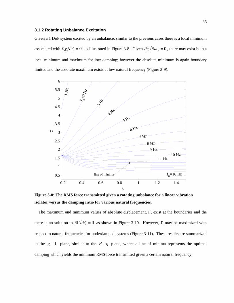
36

3.1.2 Rotating Unbalance Excitation

Given a 1 DoF system excited by an unbalance, similar to the previous cases there is a local minimum

associated with 0χ ζ∂ ∂ = , as illustrated in Figure 3-8. Given 0=∂∂ nωχ , there may exist both a

local minimum and maximum for low damping; however the absolute minimum is again boundary

limited and the absolute maximum exists at low natural frequency (Figure 3-9).

0.2 0.4 0.6 0.8 1 1.2 1.4

0.5

1

1.5

2

2.5

3

3.5

4

4.5

5

5.5

6

ζ

χ

1 H

z

f n=2

Hz

3 Hz

4 Hz

5 Hz

6 Hz

7 Hz

8 Hz9 Hz

10 Hz11 Hz

fn=16 Hzline of minima

Figure 3-8: The RMS force transmitted given a rotating unbalance for a linear vibration

isolator versus the damping ratio for various natural frequencies.

The maximum and minimum values of absolute displacement, Γ, exist at the boundaries and the

there is no solution to 0ζ∂Γ ∂ = as shown in Figure 3-10. However, Γ may be maximized with

respect to natural frequencies for underdamped systems (Figure 3-11). These results are summarized

in the Γ−χ plane, similar to the η−R plane, where a line of minima represents the optimal

damping which yields the minimum RMS force transmitted given a certain natural frequency.

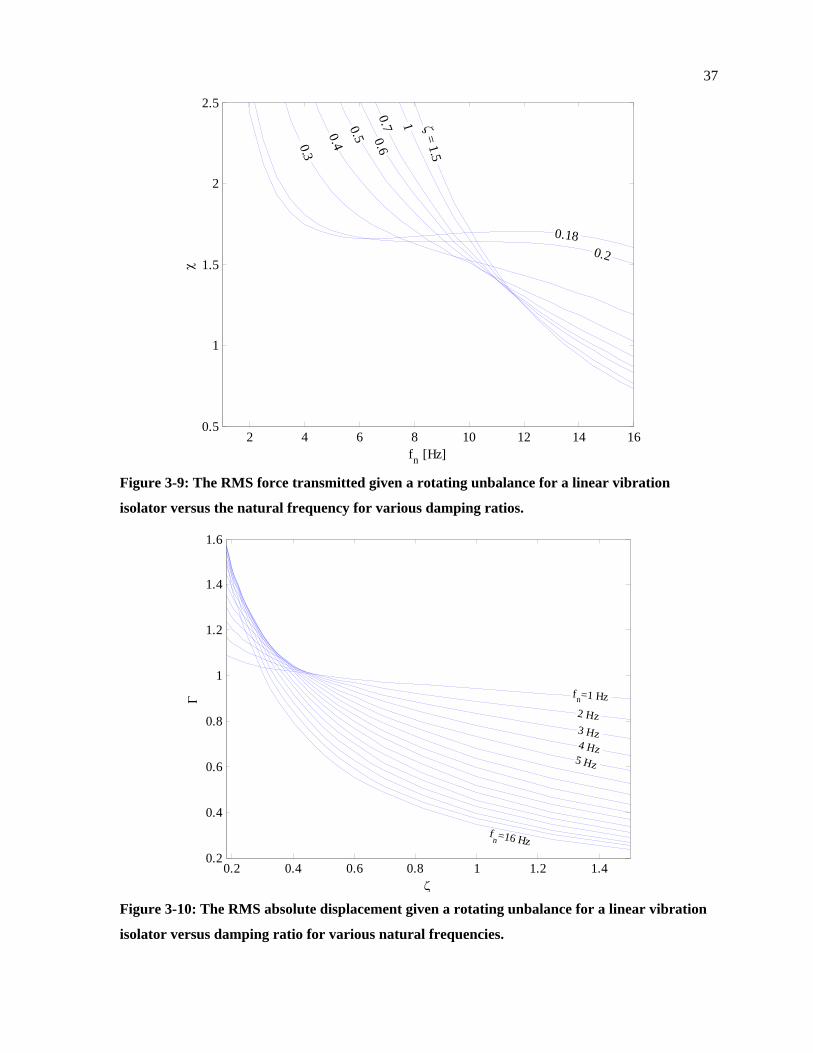
37

2 4 6 8 10 12 14 160.5

1

1.5

2

2.5

fn [Hz]

χ

0.180.2

ζ = 1.5

10.70.6

0.50.4 0.3

Figure 3-9: The RMS force transmitted given a rotating unbalance for a linear vibration

isolator versus the natural frequency for various damping ratios.

0.2 0.4 0.6 0.8 1 1.2 1.40.2

0.4

0.6

0.8

1

1.2

1.4

1.6

ζ

Γ fn=1 Hz2 Hz3 Hz4 Hz

5 Hz

fn=16 Hz

Figure 3-10: The RMS absolute displacement given a rotating unbalance for a linear vibration

isolator versus damping ratio for various natural frequencies.

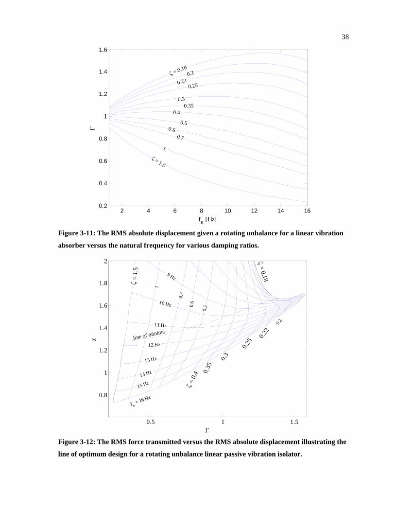
38

2 4 6 8 10 12 14 160.2

0.4

0.6

0.8

1

1.2

1.4

1.6

fn [Hz]

Γ

ζ = 0.180.2

0.220.25

0.30.35

0.4

0.50.6

0.7

1

ζ = 1.5

Figure 3-11: The RMS absolute displacement given a rotating unbalance for a linear vibration

absorber versus the natural frequency for various damping ratios.

0.5 1 1.5

0.8

1

1.2

1.4

1.6

1.8

2

Γ

χ

f n = 16 Hz

15 Hz14 Hz

13 Hz

12 Hz

9 Hz

10 Hz

ζ =

1.5

1

0.7

0.6

0.5

ζ = 0

.4 0.35

0.3

0.25 0.2

2

ζ = 0.18

0.211 Hz

line of minima

Figure 3-12: The RMS force transmitted versus the RMS absolute displacement illustrating the

line of optimum design for a rotating unbalance linear passive vibration isolator.

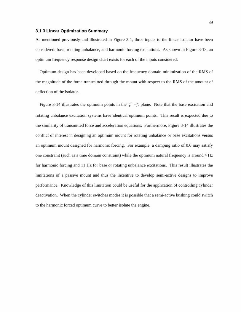
39

3.1.3 Linear Optimization Summary

As mentioned previously and illustrated in Figure 3-1, three inputs to the linear isolator have been

considered: base, rotating unbalance, and harmonic forcing excitations. As shown in Figure 3-13, an

optimum frequency response design chart exists for each of the inputs considered.

Optimum design has been developed based on the frequency domain minimization of the RMS of

the magnitude of the force transmitted through the mount with respect to the RMS of the amount of

deflection of the isolator.

Figure 3-14 illustrates the optimum points in the ζ –fn plane. Note that the base excitation and

rotating unbalance excitation systems have identical optimum points. This result is expected due to

the similarity of transmitted force and acceleration equations. Furthermore, Figure 3-14 illustrates the

conflict of interest in designing an optimum mount for rotating unbalance or base excitations versus

an optimum mount designed for harmonic forcing. For example, a damping ratio of 0.6 may satisfy

one constraint (such as a time domain constraint) while the optimum natural frequency is around 4 Hz

for harmonic forcing and 11 Hz for base or rotating unbalance excitations. This result illustrates the

limitations of a passive mount and thus the incentive to develop semi-active designs to improve

performance. Knowledge of this limitation could be useful for the application of controlling cylinder

deactivation. When the cylinder switches modes it is possible that a semi-active bushing could switch

to the harmonic forced optimum curve to better isolate the engine.

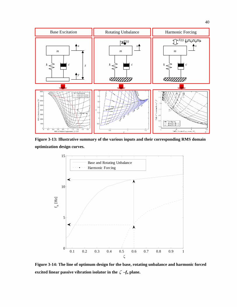
40

Figure 3-13: Illustrative summary of the various inputs and their corresponding RMS domain

optimization design curves.

0.1 0.2 0.3 0.4 0.5 0.6 0.7 0.8 0.9 10

5

10

15

ζ

f n [Hz]

Base and Rotating UnbalanceHarmonic Forcing

Figure 3-14: The line of optimum design for the base, rotating unbalance and harmonic forced

excited linear passive vibration isolator in the ζ –fn plane.

Rotating Unbalance Base Excitation Harmonic Forcing

k c

xm

k c

x

y

m

z k c

xm

F(t) F(t)

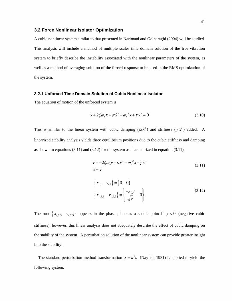
41

3.2 Force Nonlinear Isolator Optimization

A cubic nonlinear system similar to that presented in Narimani and Golnaraghi (2004) will be studied.

This analysis will include a method of multiple scales time domain solution of the free vibration

system to briefly describe the instability associated with the nonlinear parameters of the system, as

well as a method of averaging solution of the forced response to be used in the RMS optimization of

the system.

3.2.1 Unforced Time Domain Solution of Cubic Nonlinear Isolator

The equation of motion of the unforced system is

3 2 32 0n nx x x x xζω α ω γ+ + + + =&& & & (3.10)

This is similar to the linear system with cubic damping ( 3xα & ) and stiffness ( 3xγ ) added. A

linearized stability analysis yields three equilibrium positions due to the cubic stiffness and damping

as shown in equations (3.11) and (3.12) for the system as characterized in equation (3.11).

3 2 32 n nv v v x x

x vζω α ω γ= − − − −

=

&

& (3.11)

,1 ,1

,2,3 ,2,3

0 0

0

c c

nc c

x v

Ix v ωγ

=

⎧ ⎫±⎪ ⎪= ⎨ ⎬⎪ ⎪⎩ ⎭

(3.12)

The root ,2,3 ,2,3c cx v appears in the phase plane as a saddle point if 0γ < (negative cubic

stiffness); however, this linear analysis does not adequately describe the effect of cubic damping on

the stability of the system. A perturbation solution of the nonlinear system can provide greater insight

into the stability.

The standard perturbation method transformation nx uε= (Nayfeh, 1981) is applied to yield the

following system:

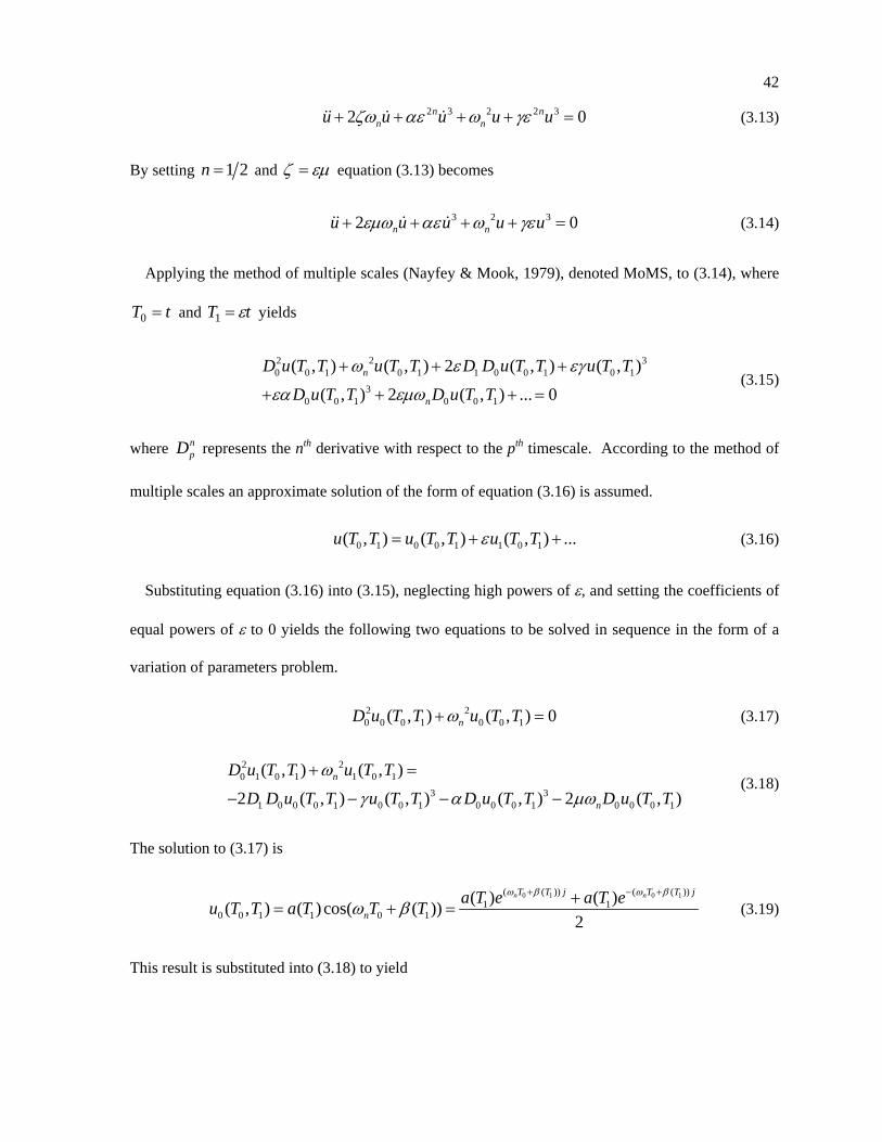
42

2 3 2 2 32 0n nn nu u u u uζω αε ω γε+ + + + =&& & & (3.13)

By setting 1 2n = and ζ εµ= equation (3.13) becomes

3 2 32 0n nu u u u uεµω αε ω γε+ + + + =&& & & (3.14)

Applying the method of multiple scales (Nayfey & Mook, 1979), denoted MoMS, to (3.14), where

tT =0 and tT ε=1 yields

2 2 30 0 1 0 1 1 0 0 1 0 1

30 0 1 0 0 1

( , ) ( , ) 2 ( , ) ( , )

( , ) 2 ( , ) ... 0n

n

D u T T u T T D D u T T u T T

D u T T D u T T

ω ε εγ

εα εµω

+ + +

+ + + = (3.15)

where npD represents the nth derivative with respect to the pth timescale. According to the method of

multiple scales an approximate solution of the form of equation (3.16) is assumed.

0 1 0 0 1 1 0 1( , ) ( , ) ( , ) ...u T T u T T u T Tε= + + (3.16)

Substituting equation (3.16) into (3.15), neglecting high powers of ε, and setting the coefficients of

equal powers of ε to 0 yields the following two equations to be solved in sequence in the form of a

variation of parameters problem.

2 20 0 0 1 0 0 1( , ) ( , ) 0nD u T T u T Tω+ = (3.17)

2 20 1 0 1 1 0 1

3 31 0 0 0 1 0 0 1 0 0 0 1 0 0 0 1

( , ) ( , )

2 ( , ) ( , ) ( , ) 2 ( , )n

n

D u T T u T T

D D u T T u T T D u T T D u T T

ω

γ α µω

+ =

− − − − (3.18)

The solution to (3.17) is

0 1 0 1( ( )) ( ( ))

1 10 0 1 1 0 1

( ) ( )( , ) ( ) cos( ( ))2

n nT T j T T j

na T e a T eu T T a T T T

ω β ω β

ω β+ − ++

= + = (3.19)

This result is substituted into (3.18) to yield

43

0 0

2 2 30 1 0 1 1 0 1 1 1 1 1

( ( ))2 3 31 1 1 1

3( , ) ( , ) ( ) ( ) ( )8

3( ) ( ) ( )8

n

n n

T T jn n n

D u T T u T T a T D T a T

a T a T D a T j e NST CCω β

ω ω β γ

µω αω ω +

⎧+ = −⎨⎩

⎫⎡ ⎤− + + + +⎬⎢ ⎥⎣ ⎦ ⎭

(3.20)

where, as denoted by Nayfeh (1981), NST are non-secular terms and CC represents the complex

conjugate of the terms appearing to the right of the equality. Since the perturbation solution does not

include secular terms (Nayfeh, 1981), the coefficient of 0 0( ( ))nT T je ω β+ in equation (3.20) must sum to

zero as shown in equation (3.21).

3 2 3 31 1 1 1 1 1 1 1

3 3( ) ( ) ( ) ( ) ( ) ( ) 08 8n n n na T D T a T a T a T D a T jω β γ µω αω ω ⎫⎧ ⎡ ⎤− − + + =⎨ ⎬⎢ ⎥⎩ ⎣ ⎦ ⎭

(3.21)

Solving equation (3.21) results in the equations for the rate of change of amplitude and phase.

2 338n na a aµω αω′ = − − ,

238 n

aγβω

′ = (3.22)

Furthermore, solving the first order differential equations in equation (3.22) yields the amplitude of

the response as a function of time.

1

1 220

20

4( )2(3 8 ) 6

nTn n

a Ta ea

µωαω µ αωµ µ

=+

−

(3.23)

The above result, equation (3.23), is illustrated and compared to the numerical solution of the

system in Figure 3-15.

44

0 0.2 0.4 0.6 0.8 1 1.2 1.4 1.6 1.8 2-0.3

-0.2

-0.1

0

0.1

0.2

0.3

0.4

0.5

Time [s]

u(t)

u'' + 2εµ wn u' + αε u'3 + wn2u + γ ε u3 = 0

ζ =0.15ωn =30.8

ε =0.5µ =0.3γ =0.1α =0.1

MoMS AmplitudeSolution

Numerical Solution (ODE 45)

Figure 3-15: Amplitude versus time relative to the actual numerical simulation of the nonlinear

system for various initial conditions.

By examining the first derivative of the steady state amplitude with respect to the initial condition

a0, we find that a critical amplitude results when α < 0 (or in the presence of negative cubic

damping). This suggests an unstable limit cycle. The diameter of the limit cycle is given by alc as

follows:

62

3n

lcn

aµαω

αω−

= ± (3.24)

This is demonstrated for the following case: 0.03µ = , 0.5α = − , and 30.8nω = . This yields the

limit cycle 0.228lca = ± . If the initial amplitude is beyond this critical amplitude the system is

unstable, as illustrated in Figure 3-16.

45

0 0.1 0.2 0.3 0.4 0.5 0.6 0.7 0.8 0.9 10

0.05

0.1

0.15

0.2

0.25

0.3

0.35

0.4

0.45

0.5

T1

A(T

1)u'' + 2εµ ωn u' + αε u'3 + ωn

2u + γ ε u3 = 0

α =-0.5ζ =0.15ωn =30.8

ε =0.5µ =0.3

alc = .228

Figure 3-16: Amplitude of the time domain solution of the cubic nonlinear system for various

initial conditions illustrating the unstable limit cycle of the negative cubic damping system.

3.2.2 Forced Solution of Cubic Nonlinear Isolator

Given the unbalance excitation of the nonlinear system under study can be expressed as

3 3 21 3 1 3 cos( )o d dmx c x c x k x k x m e tω ω+ + + + =&& & & (3.25)

This can be non-dimensionalized with the following substitutions to yield equation (3.26).

* 233 , , , ,o d

n o no n

k m e xk f u tm m f

ωω τ ω ωω

= = = = =

( ) ( ) ( ) ( )2 2

2 2 2

1 1,n nt tτ ω τ ω

∂ ∂ ∂ ∂= =

∂ ∂ ∂ ∂

2 2 3 2 * 3 21 3 32 2 cos( )o n ou u f u u f k uζ ω ζ ω ωτ′′ ′ ′+ + + + = (3.26)

46

Substituting the cubic stiffness parameter 2 *3of kρ = and cubic damping parameter 2 2

3o nfξ ω ζ=

yields the simplified equivalent system:

3 3 22 2 cos( )u u u u uζ ξ ρ ω ωτ′′ ′ ′+ + + + = (3.27)

The system can be solved using the modified averaging technique (MoAVG – discussed in Chapter

2) assuming a solution

( ) ( ) cos( ( ))u aτ τ ωτ β τ= + (3.28)

The differential equation can be solved by variation of parameters, where

)sin( βωτω +−=′ au (3.29)

)sin()sin()cos( βωτββωτωβωτ +′−+−+′=′ aaau (3.30)

φβωτ =+ (3.31)

)cos()cos()sin( 2 βωτβωβωτωβωτω +′−+−+′−=′′ aaau (3.32)

Equations (3.29) to (3.32) are used to develop the following equalities:

0)sin()cos( =′−′ φβφ aa (3.33)

2 3 3

3 3 2 3 3 2

sin( ) cos( ) cos( ) 2 sin( ) 2 sin( )2 sin( ) cos ( ) cos( ) cos ( ) cos( )

a a a a aa a a

ω φ ωβ φ ω φ ζ ω φ ξ ω φ

ξ ω φ φ φ ρ φ ω φ β

′ ′+ = − − −

+ + + − − (3.34)

Using the above relationships, the first derivatives of the amplitude and phase can be obtained:

3 2 21 1

3 3 3 3 3 3 2

3

1 1 1sin(2 ) cos(2 ) sin( ) sin( 2 )4 2 2

1 3 1cos(2 ) cos(4 ) sin(2 )4 4 2

1 1sin(2 ) sin(4 )2 8

a a a a

a a a a

a a

ω ρ φ ζ ω ζ ω φ ω β ω φ β

ξ ω φ ξ ω φ ξ ω ω φ

φ ρ φ

′ = − + − + − +

+ − − −

+ +

(3.35)

47

3 3 2 2

3 2 2

3 3 3 3

3 1 1 1 1 1cos(2 ) cos(2 ) cos(2 )8 2 2 2 2 2

1 1 1cos(4 ) sin(2 ) cos( 2 ) cos( )8 2 21 1sin(4 ) sin(2 )4 2

a a a a a a a

a a

a a

ω β ρ ρ φ ω ω φ φ

ρ φ ζ ω φ ω φ β ω β

ξ ω φ ξ ω φ

′ = + − − + +

+ − − − + −

+ − (3.36)

and averaged over a period of 2π to yield:

2 3 3 2

0

1 3 1 sin( )2 4 2

a a a aπ

ω ω ζ ω ξ ω ω βπ

⎛ ⎞′ ′≈ = − + −⎜ ⎟⎝ ⎠∫ (3.37)

)cos(

21

2)1(

83

21 2

232

0βωωρβω

πβω

π−

−+=′≈′ ∫

aaaa (3.38)

Equations (3.37) and (3.38) can be solved for the frequency and phase as follows:

2 2

2 3 3 3 23 32 (1 )2 4

a a a aω ζ ω ξ ω ρ ω⎛ ⎞ ⎛ ⎞= + + + −⎜ ⎟ ⎜ ⎟⎝ ⎠ ⎝ ⎠

(3.39)

2 3

1

2 2

322tan 3 (1 )

4

a

a

ζω ξ ωβ

ρ ω

−

⎛ ⎞+⎜ ⎟= ⎜ ⎟

⎜ ⎟+ −⎝ ⎠

(3.40)

The solution can be compared to the linear solution by neglecting the nonlinear terms:

( ) ( )222 22 (1 )a aω ζ ω ω= + − (3.41)

Solving the above for amplitude yields the linear solution for amplitude:

( ) ( )22 22 1

a ω

ζω ω=

+ − (3.42)

Similarly, (3.40) yields the linear phase:

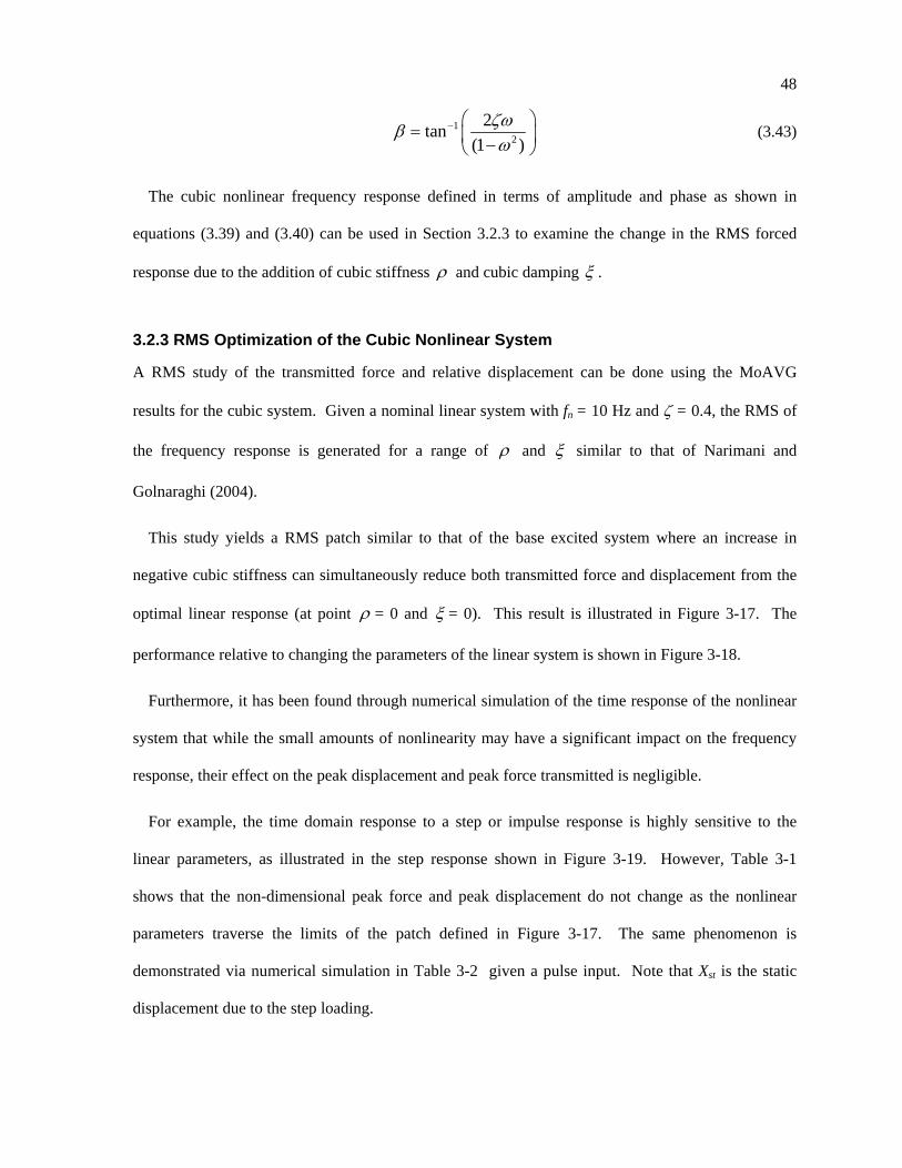
48

12

2tan(1 )

ζωβω

− ⎛ ⎞= ⎜ ⎟−⎝ ⎠

(3.43)

The cubic nonlinear frequency response defined in terms of amplitude and phase as shown in

equations (3.39) and (3.40) can be used in Section 3.2.3 to examine the change in the RMS forced

response due to the addition of cubic stiffness ρ and cubic damping ξ .

3.2.3 RMS Optimization of the Cubic Nonlinear System

A RMS study of the transmitted force and relative displacement can be done using the MoAVG

results for the cubic system. Given a nominal linear system with fn = 10 Hz and ζ = 0.4, the RMS of

the frequency response is generated for a range of ρ and ξ similar to that of Narimani and

Golnaraghi (2004).

This study yields a RMS patch similar to that of the base excited system where an increase in

negative cubic stiffness can simultaneously reduce both transmitted force and displacement from the

optimal linear response (at point ρ = 0 and ξ = 0). This result is illustrated in Figure 3-17. The

performance relative to changing the parameters of the linear system is shown in Figure 3-18.

Furthermore, it has been found through numerical simulation of the time response of the nonlinear

system that while the small amounts of nonlinearity may have a significant impact on the frequency

response, their effect on the peak displacement and peak force transmitted is negligible.

For example, the time domain response to a step or impulse response is highly sensitive to the

linear parameters, as illustrated in the step response shown in Figure 3-19. However, Table 3-1

shows that the non-dimensional peak force and peak displacement do not change as the nonlinear

parameters traverse the limits of the patch defined in Figure 3-17. The same phenomenon is

demonstrated via numerical simulation in Table 3-2 given a pulse input. Note that Xst is the static

displacement due to the step loading.

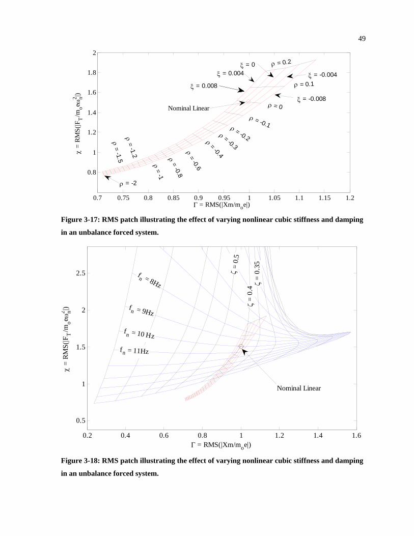
49

0.7 0.75 0.8 0.85 0.9 0.95 1 1.05 1.1 1.15 1.2

0.8

1

1.2

1.4

1.6

1.8

2

Γ = RMS(|Xm/moe|)

χ =

RMS(

|FT

/moe ω

n2 |)

ρ = 0.2

ρ = 0.1

ρ = 0

ρ = -0.1ρ = -0.2ρ = -0.3

ρ = -0.4ρ = -0.6

ρ = -0.8

ρ = -1

ρ = -1.2

ρ = -2

ρ = -1.5

ξ = 0.008

ξ = 0.004ξ = 0

ξ = -0.004

ξ = -0.008Nominal Linear

Figure 3-17: RMS patch illustrating the effect of varying nonlinear cubic stiffness and damping

in an unbalance forced system.

0.2 0.4 0.6 0.8 1 1.2 1.4 1.6

0.5

1

1.5

2

2.5

Γ = RMS(|Xm/moe|)

χ =

RMS(

|FT

/moe ω

n2 |)

fn = 10 Hz

ζ =

0.5

ζ =

0.35

ζ =

0.4

fn = 9Hz

fn = 11Hz

fn = 8Hz

Nominal Linear

Figure 3-18: RMS patch illustrating the effect of varying nonlinear cubic stiffness and damping

in an unbalance forced system.

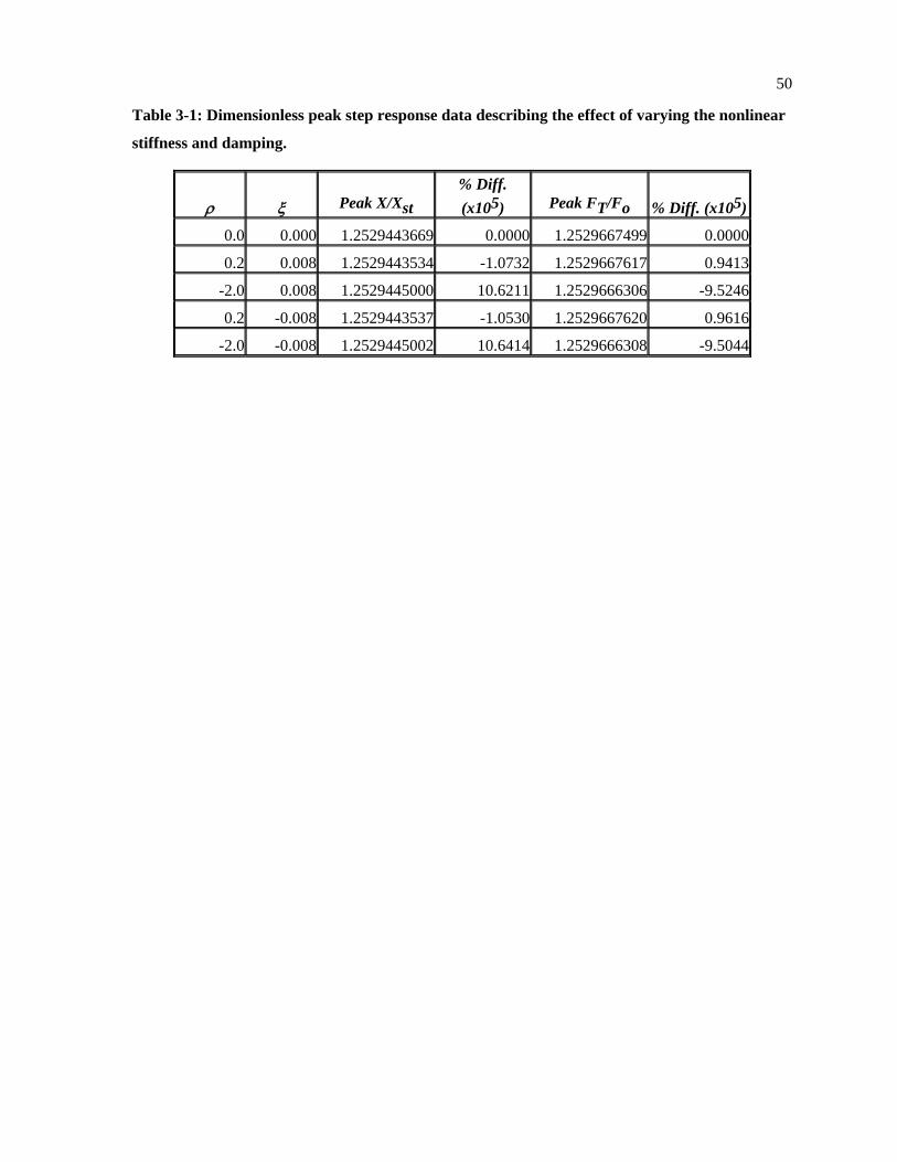
50

Table 3-1: Dimensionless peak step response data describing the effect of varying the nonlinear

stiffness and damping.

ρ ξ Peak X/Xst % Diff. (x105) Peak FT/Fo % Diff. (x105)

0.0 0.000 1.2529443669 0.0000 1.2529667499 0.0000

0.2 0.008 1.2529443534 -1.0732 1.2529667617 0.9413

-2.0 0.008 1.2529445000 10.6211 1.2529666306 -9.5246

0.2 -0.008 1.2529443537 -1.0530 1.2529667620 0.9616

-2.0 -0.008 1.2529445002 10.6414 1.2529666308 -9.5044

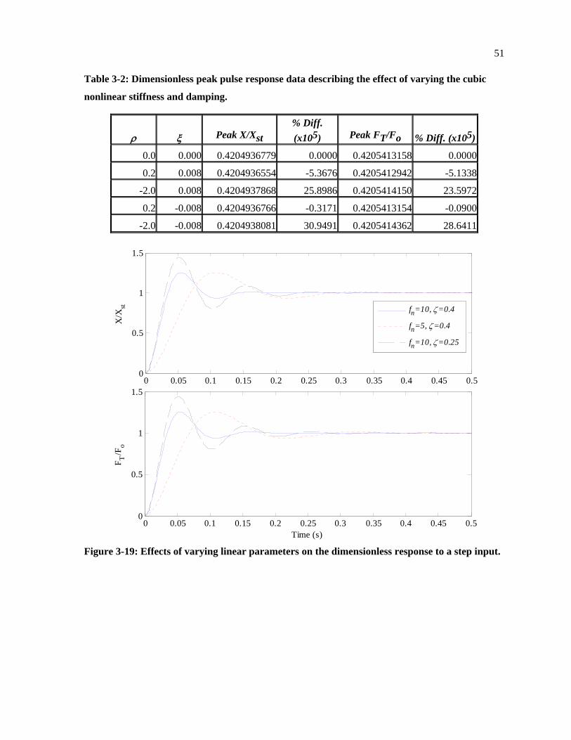
51

Table 3-2: Dimensionless peak pulse response data describing the effect of varying the cubic

nonlinear stiffness and damping.

ρ ξ Peak X/Xst % Diff. (x105) Peak FT/Fo % Diff. (x105)

0.0 0.000 0.4204936779 0.0000 0.4205413158 0.0000

0.2 0.008 0.4204936554 -5.3676 0.4205412942 -5.1338

-2.0 0.008 0.4204937868 25.8986 0.4205414150 23.5972

0.2 -0.008 0.4204936766 -0.3171 0.4205413154 -0.0900

-2.0 -0.008 0.4204938081 30.9491 0.4205414362 28.6411

0 0.05 0.1 0.15 0.2 0.25 0.3 0.35 0.4 0.45 0.50

0.5

1

1.5

X/X

st

0 0.05 0.1 0.15 0.2 0.25 0.3 0.35 0.4 0.45 0.50

0.5

1

1.5

Time (s)

F T/F

o

fn=10, ζ =0.4

fn=5, ζ =0.4

fn=10, ζ =0.25

Figure 3-19: Effects of varying linear parameters on the dimensionless response to a step input.

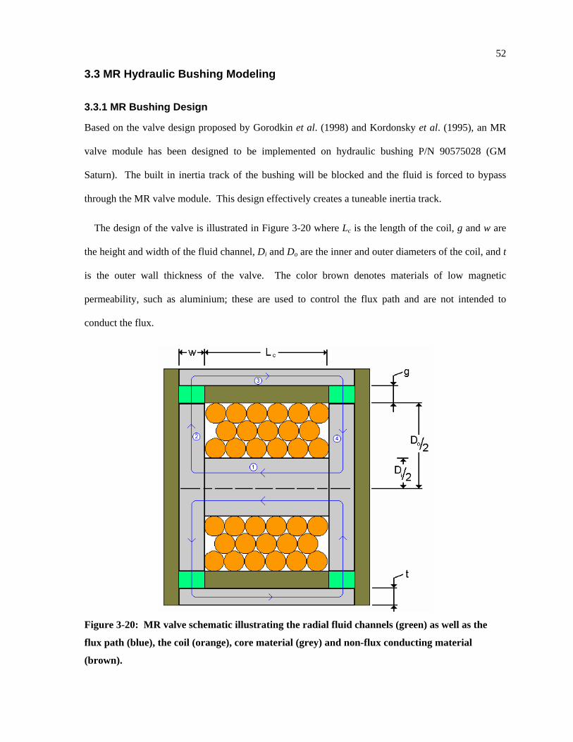
52

3.3 MR Hydraulic Bushing Modeling

3.3.1 MR Bushing Design

Based on the valve design proposed by Gorodkin et al. (1998) and Kordonsky et al. (1995), an MR

valve module has been designed to be implemented on hydraulic bushing P/N 90575028 (GM

Saturn). The built in inertia track of the bushing will be blocked and the fluid is forced to bypass

through the MR valve module. This design effectively creates a tuneable inertia track.

The design of the valve is illustrated in Figure 3-20 where Lc is the length of the coil, g and w are

the height and width of the fluid channel, Di and Do are the inner and outer diameters of the coil, and t

is the outer wall thickness of the valve. The color brown denotes materials of low magnetic

permeability, such as aluminium; these are used to control the flux path and are not intended to

conduct the flux.

Figure 3-20: MR valve schematic illustrating the radial fluid channels (green) as well as the

flux path (blue), the coil (orange), core material (grey) and non-flux conducting material

(brown).

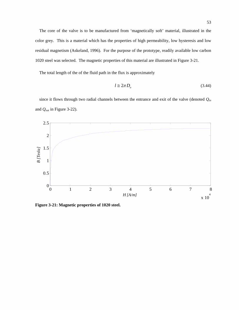
53

The core of the valve is to be manufactured from ‘magnetically soft’ material, illustrated in the

color grey. This is a material which has the properties of high permeability, low hysteresis and low

residual magnetism (Askeland, 1996). For the purpose of the prototype, readily available low carbon

1020 steel was selected. The magnetic properties of this material are illustrated in Figure 3-21.

The total length of the of the fluid path in the flux is approximately

2 ol Dπ≅ (3.44)

since it flows through two radial channels between the entrance and exit of the valve (denoted Qin

and Qout in Figure 3-22).

0 1 2 3 4 5 6 7 8

x 104

0

0.5

1

1.5

2

2.5

H [A/m]

B [T

esla

]

Figure 3-21: Magnetic properties of 1020 steel.

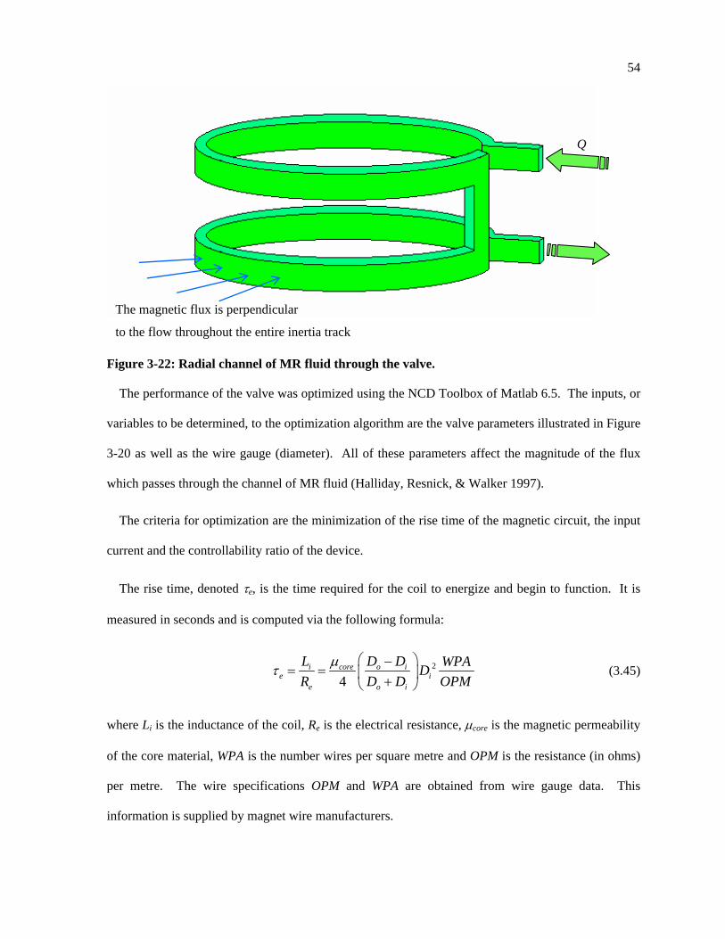
54

Figure 3-22: Radial channel of MR fluid through the valve.

The performance of the valve was optimized using the NCD Toolbox of Matlab 6.5. The inputs, or

variables to be determined, to the optimization algorithm are the valve parameters illustrated in Figure

3-20 as well as the wire gauge (diameter). All of these parameters affect the magnitude of the flux

which passes through the channel of MR fluid (Halliday, Resnick, & Walker 1997).

The criteria for optimization are the minimization of the rise time of the magnetic circuit, the input

current and the controllability ratio of the device.

The rise time, denoted τe, is the time required for the coil to energize and begin to function. It is

measured in seconds and is computed via the following formula:

2

4i core o i

e ie o i

L D D WPADR D D OPM

µτ⎛ ⎞−

= = ⎜ ⎟+⎝ ⎠ (3.45)

where Li is the inductance of the coil, Re is the electrical resistance, µcore is the magnetic permeability

of the core material, WPA is the number wires per square metre and OPM is the resistance (in ohms)

per metre. The wire specifications OPM and WPA are obtained from wire gauge data. This

information is supplied by magnet wire manufacturers.

The magnetic flux is perpendicular

to the flow throughout the entire inertia track

Q

55

The input current is derived from the resistance (Re) of the circuit and the input voltage (Vin). The

input voltage is assumed to be 24 V. Thus the current is computed from in eI V R= .

The controllability of the valve is an expression which relates the pressure drop across the valve

with and without a magnetic field. The total pressure drop as defined by Lord Corporation (1999) is

( ) ( )MRf y f MR

c lp p p R Q I R Q K I tgµ τ τ∆ = ∆ + ∆ = + = + (3.46)

where µp∆ is the viscous pressure drop, τp∆ is the pressure drop due to yielding the MR fluid, cMR

is a constant of magnitude 2-3 depending on the controllability, l is the length of the inertia track, Rf is

the hydraulic resistance to flow, and yτ is the yield stress of the fluid. A measurable property of

MRFs is the yield stress as a function of the field intensity in the fluid. Yield stress can be written

)( fyy Hττ = or since fH is a function of the input current ( )y y Iτ τ= . The controllability ratio is

defined as follows:

MRf y

p c lRgp

µ

τ

κ τ∆ ⎛ ⎞

= ∝ ⎜ ⎟∆ ⎝ ⎠ (3.47)

To determine the magnitude of the controllability, the yield stress must be computed. In order to

determine the yield stress, the magnetic circuit equations must be solved given the inputs to the

optimization algorithm as listed above. The circuit is solved via the simplified equation eqNI R ϕ= ,

which can be rearranged to yield the field intensity as shown in equations (3.48) and (3.49).

eqNI Rϕ = (3.48)

( ) ( )f MR f eq MR fH A NI R Aϕ µ µ′ ′= = (3.49)

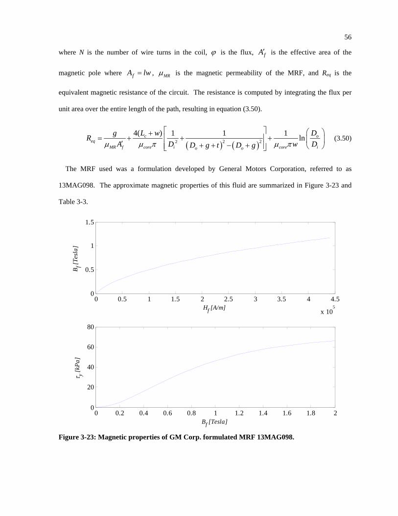
56

where N is the number of wire turns in the coil, ϕ is the flux, fA′ is the effective area of the

magnetic pole where fA lw= , MRµ is the magnetic permeability of the MRF, and Req is the

equivalent magnetic resistance of the circuit. The resistance is computed by integrating the flux per

unit area over the entire length of the path, resulting in equation (3.50).

( ) ( )2 22

4( ) 1 1 1 lnc oeq

MR f core i core io o

L w DgRA D w DD g t D gµ µ π µ π

⎡ ⎤ ⎛ ⎞+= + + +⎢ ⎥ ⎜ ⎟′ + + − +⎢ ⎥ ⎝ ⎠⎣ ⎦

(3.50)

The MRF used was a formulation developed by General Motors Corporation, referred to as

13MAG098. The approximate magnetic properties of this fluid are summarized in Figure 3-23 and

Table 3-3.

0 0.2 0.4 0.6 0.8 1 1.2 1.4 1.6 1.8 20

20

40

60

80

Bf [Tesla]

τ y [kPa

]

0 0.5 1 1.5 2 2.5 3 3.5 4 4.5

x 105

0

0.5

1

1.5

Hf [A/m]

B f [Tes

la]

Figure 3-23: Magnetic properties of GM Corp. formulated MRF 13MAG098.

57

Table 3-3: Properties of GM Corp. formulated MRF 13MAG098.

Fluid Parameter

Value

Percent Solids (by volume)

30 %

fµ 0.173 Pa s⋅

fρ 32910 kg m

It is important to note that flux saturation is also an issue when simulated magnetic circuits. Since

B Aϕ= , the maximum B for each effective area of the valve design was checked each iteration of

the optimization algorithm and the flux was reduced in accordance with the saturation limits of the

core material of about 2.25 Tesla (Figure 3-21).

The final valve design parameters are illustrated in Table 3-4. The resulting gain on current, KMR,

as shown in equation (3.46) with cMR = 2.2 is plotted versus current in Figure 3-25. Saturation of the

valve occurs at approximately 1 A. This gain assumes steady state conditions in the valve.

Table 3-4: MR valve design parameters.

Design Parameter

Value

Do 24.1 mmDi 9.7 mmg 5 mmt 15 mmw 15 mmLc 15 mm

Wire gauge 26N 579 turns

cMR 2.2

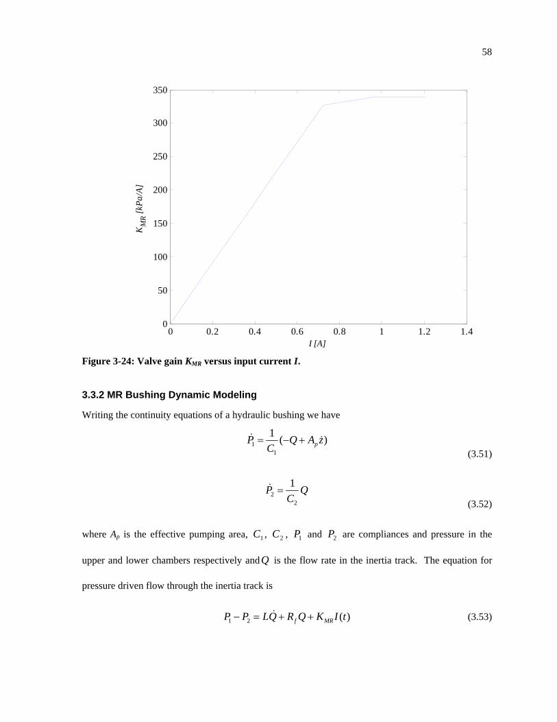
58

0 0.2 0.4 0.6 0.8 1 1.2 1.40

50

100

150

200

250

300

350

I [A]

KM

R [kPa

/A]

Figure 3-24: Valve gain KMR versus input current I.

3.3.2 MR Bushing Dynamic Modeling

Writing the continuity equations of a hydraulic bushing we have

1

1

1 ( )pP Q A zC

= − +& &

(3.51)

2

2

1P QC

=&

(3.52)

where Ap is the effective pumping area, 1C , 2C , 1P and 2P are compliances and pressure in the

upper and lower chambers respectively andQ is the flow rate in the inertia track. The equation for

pressure driven flow through the inertia track is

1 2 ( )f MRP P LQ R Q K I t− = + +& (3.53)

59

where KMR is a gain on input current I(t) producing a magnetorheological damping pressure drop.

The parameters of the above hydraulic equations are

4 2

128 4,f f

fh h

l lR L

d dπµ ρ

π= = (3.54)

where fµ is the fluid viscosity, fρ is the fluid density, and dh is the hydraulic diameter of the inertia

track. The resistance, Rf, is a linear approximation adequate for the purposes of the model.

Using equations (3.51) to (3.53), the force transmitted through the bushing in the laplace domain is

as follows:

22

2 1

2 21

1( ) ( ) ( )

f p MR

pT r r

f f

R A Ks sA L LC LCF s K B s Z s I sR RC C Cs s s sL L L L

⎡ ⎤ ⎡ ⎤+ +⎢ ⎥ ⎢ ⎥= + + +⎢ ⎥ ⎢ ⎥

⎢ ⎥ ⎢ ⎥+ + + +⎣ ⎦ ⎣ ⎦

(3.55)

where

1 2

1 1C C C= + (3.56)

Neglecting the MR effect and the rubber damping, the dynamic stiffness is found to be:

2 2 2 2

2 21

2( )( )( ) 2

p z z pTdyn r

p p p

A s sF sK s KZ s C s s

ωζ ω α ωζ ω ω

⎡ ⎤ + += = +⎢ ⎥

+ +⎢ ⎥⎣ ⎦ (3.57)

where

pC

Lω = , 2

4f

pR

LCζ = (3.58)

2

1 22

1

pr

pr

AK

C CA

KC

ωα+

+=+

(3.59)

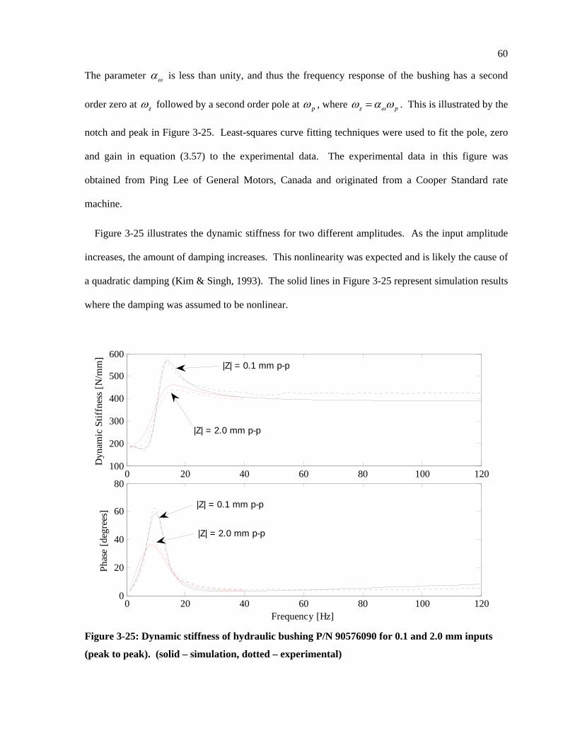
60

The parameter ωα is less than unity, and thus the frequency response of the bushing has a second

order zero at zω followed by a second order pole at pω , where z pωω α ω= . This is illustrated by the

notch and peak in Figure 3-25. Least-squares curve fitting techniques were used to fit the pole, zero

and gain in equation (3.57) to the experimental data. The experimental data in this figure was

obtained from Ping Lee of General Motors, Canada and originated from a Cooper Standard rate

machine.

Figure 3-25 illustrates the dynamic stiffness for two different amplitudes. As the input amplitude

increases, the amount of damping increases. This nonlinearity was expected and is likely the cause of

a quadratic damping (Kim & Singh, 1993). The solid lines in Figure 3-25 represent simulation results

where the damping was assumed to be nonlinear.

0 20 40 60 80 100 120100

200

300

400

500

600

Dyn

amic

Stif

fnes

s [N

/mm

]

0 20 40 60 80 100 1200

20

40

60

80

Frequency [Hz]

Phas

e [d

egre

es] |Z| = 0.1 mm p-p

|Z| = 2.0 mm p-p

|Z| = 0.1 mm p-p

|Z| = 2.0 mm p-p

Figure 3-25: Dynamic stiffness of hydraulic bushing P/N 90576090 for 0.1 and 2.0 mm inputs

(peak to peak). (solid – simulation, dotted – experimental)

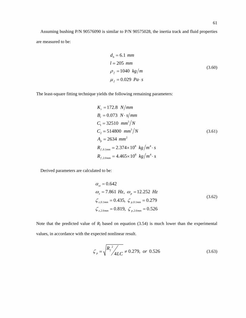
61

Assuming bushing P/N 90576090 is similar to P/N 90575028, the inertia track and fluid properties

are measured to be:

6.1

2051040

0.029

h

f

f

d mm

l mmkg m

Pa s

ρ

µ

=

=

=

= ⋅

(3.60)

The least-square fitting technique yields the following remaining parameters:

51

52

2

8 4,0.1

8 4,2.0

172.8

0.073

32510

514800

2634

2.374 10

4.465 10

r

r

p

f mm

f mm

K N mm

B N s mm

C mm N

C mm N

A mm

R kg m s

R kg m s

=

= ⋅

=

=

=

= × ⋅

= × ⋅

(3.61)

Derived parameters are calculated to be:

,0.1 ,0.1

,2.0 ,2.0

0.642

7.861 , 12.252

0.435, 0.279

0.819, 0.526

z p

z mm p mm

z mm p mm

Hz Hzωα

ω ω

ζ ζ

ζ ζ

=

= =

= =

= =

(3.62)

Note that the predicted value of Rf based on equation (3.54) is much lower than the experimental

values, in accordance with the expected nonlinear result.

2

0.279, 0.5264f

pR orLCζ = ≠ (3.63)

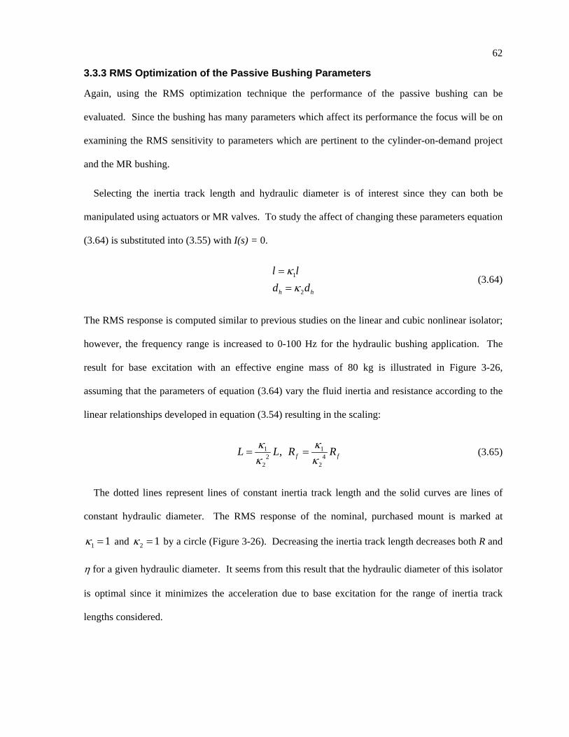
62

3.3.3 RMS Optimization of the Passive Bushing Parameters

Again, using the RMS optimization technique the performance of the passive bushing can be

evaluated. Since the bushing has many parameters which affect its performance the focus will be on

examining the RMS sensitivity to parameters which are pertinent to the cylinder-on-demand project

and the MR bushing.

Selecting the inertia track length and hydraulic diameter is of interest since they can both be

manipulated using actuators or MR valves. To study the affect of changing these parameters equation

(3.64) is substituted into (3.55) with I(s) = 0.

1

2h h

l ld d

κκ

==

(3.64)

The RMS response is computed similar to previous studies on the linear and cubic nonlinear isolator;

however, the frequency range is increased to 0-100 Hz for the hydraulic bushing application. The

result for base excitation with an effective engine mass of 80 kg is illustrated in Figure 3-26,

assuming that the parameters of equation (3.64) vary the fluid inertia and resistance according to the

linear relationships developed in equation (3.54) resulting in the scaling:

1 12 4

2 2

, f fL L R Rκ κκ κ

= = (3.65)

The dotted lines represent lines of constant inertia track length and the solid curves are lines of

constant hydraulic diameter. The RMS response of the nominal, purchased mount is marked at

1 1κ = and 2 1κ = by a circle (Figure 3-26). Decreasing the inertia track length decreases both R and

η for a given hydraulic diameter. It seems from this result that the hydraulic diameter of this isolator

is optimal since it minimizes the acceleration due to base excitation for the range of inertia track

lengths considered.

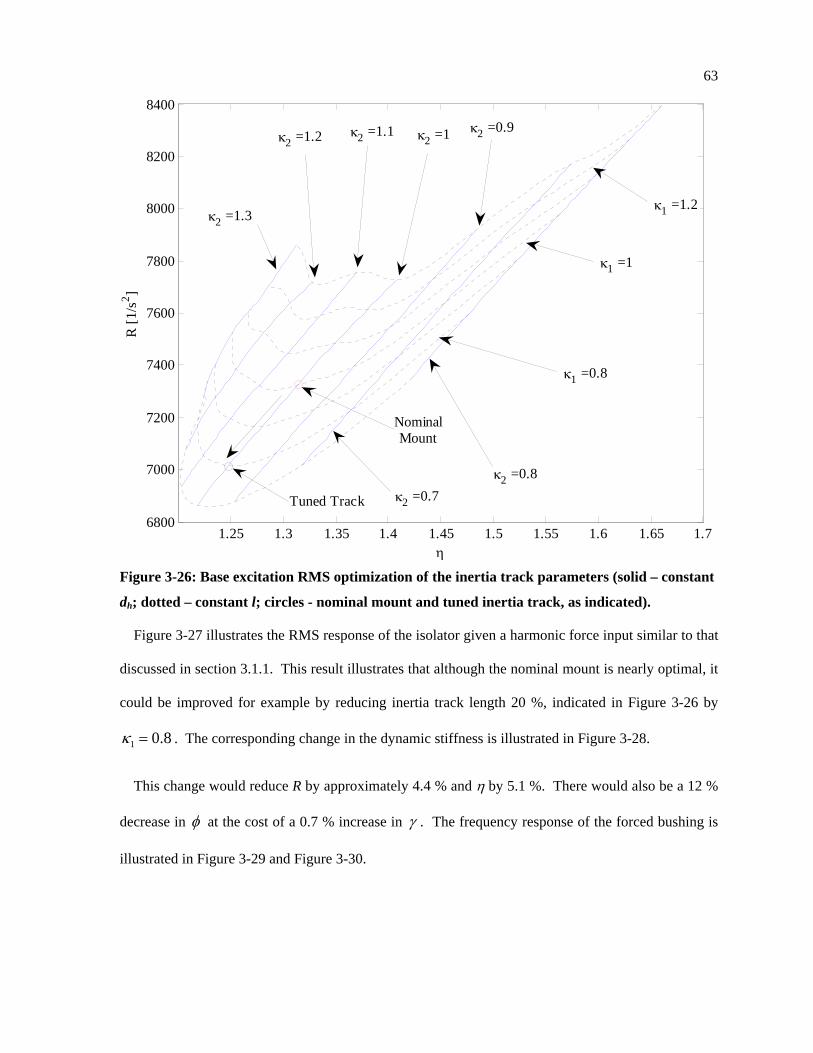
63

1.25 1.3 1.35 1.4 1.45 1.5 1.55 1.6 1.65 1.76800

7000

7200

7400

7600

7800

8000

8200

8400

R [1

/s2 ]

η

κ2 =1.1 κ2 =1 κ2 =0.9

κ2 =0.8κ2 =0.7

κ2 =1.2

κ2 =1.3

κ1 =1

κ1 =1.2

κ1 =0.8

NominalMount

Tuned Track

Figure 3-26: Base excitation RMS optimization of the inertia track parameters (solid – constant

dh; dotted – constant l; circles - nominal mount and tuned inertia track, as indicated).

Figure 3-27 illustrates the RMS response of the isolator given a harmonic force input similar to that

discussed in section 3.1.1. This result illustrates that although the nominal mount is nearly optimal, it

could be improved for example by reducing inertia track length 20 %, indicated in Figure 3-26 by

1 0.8κ = . The corresponding change in the dynamic stiffness is illustrated in Figure 3-28.

This change would reduce R by approximately 4.4 % and η by 5.1 %. There would also be a 12 %

decrease in φ at the cost of a 0.7 % increase in γ . The frequency response of the forced bushing is

illustrated in Figure 3-29 and Figure 3-30.

64

2 2.2 2.4 2.6 2.8 3 3.2 3.4 3.6 3.8 4

x 10-6

0.7

0.8

0.9

1

1.1

1.2

1.3

1.4

φ [m

-kg/

N]

γ

κ2 =1.3κ2 =1.2κ2 =1.1κ2 =1

κ2 =0.9

κ1 =1.2

κ1 =1 κ1 =0.8

Nominal Mount

Figure 3-27: Harmonic forced RMS optimization of the inertia track parameters (solid –

constant dh, dotted – constant l, circle - nominal mount).

200

400

600

Dyn

amic

St

iffne

ss [N

/mm

]

0 10 20 30 40 50 60 70 80 90 1000

50

100

Frequency [Hz]

Phas

e [d

egre

es]

κ1 = 1, κ2 = 1

κ1 = 0.8, κ2 = 1

Figure 3-28: Dynamic stiffness given a 20% decrease in inertia track length.

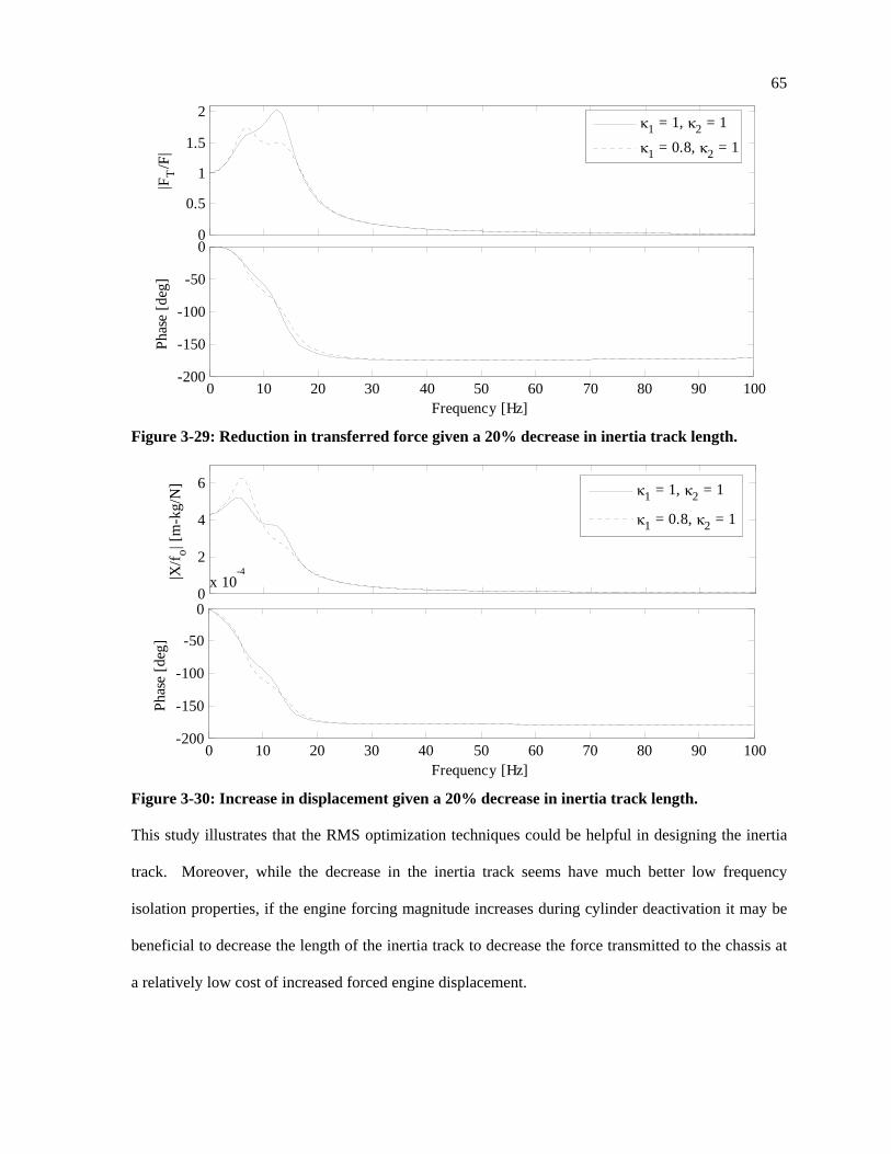
65

0

0.5

1

1.5

2

|FT

/F|

0 10 20 30 40 50 60 70 80 90 100-200

-150

-100

-50

0

Phas

e [d

eg]

Frequency [Hz]

κ1 = 1, κ2 = 1

κ1 = 0.8, κ2 = 1

Figure 3-29: Reduction in transferred force given a 20% decrease in inertia track length.

0

2

4

6

x 10-4|X

/f o| [m

-kg/

N]

0 10 20 30 40 50 60 70 80 90 100-200

-150

-100

-50

0

Phas

e [d

eg]

Frequency [Hz]

κ1 = 1, κ2 = 1

κ1 = 0.8, κ2 = 1

Figure 3-30: Increase in displacement given a 20% decrease in inertia track length.

This study illustrates that the RMS optimization techniques could be helpful in designing the inertia

track. Moreover, while the decrease in the inertia track seems have much better low frequency

isolation properties, if the engine forcing magnitude increases during cylinder deactivation it may be

beneficial to decrease the length of the inertia track to decrease the force transmitted to the chassis at

a relatively low cost of increased forced engine displacement.

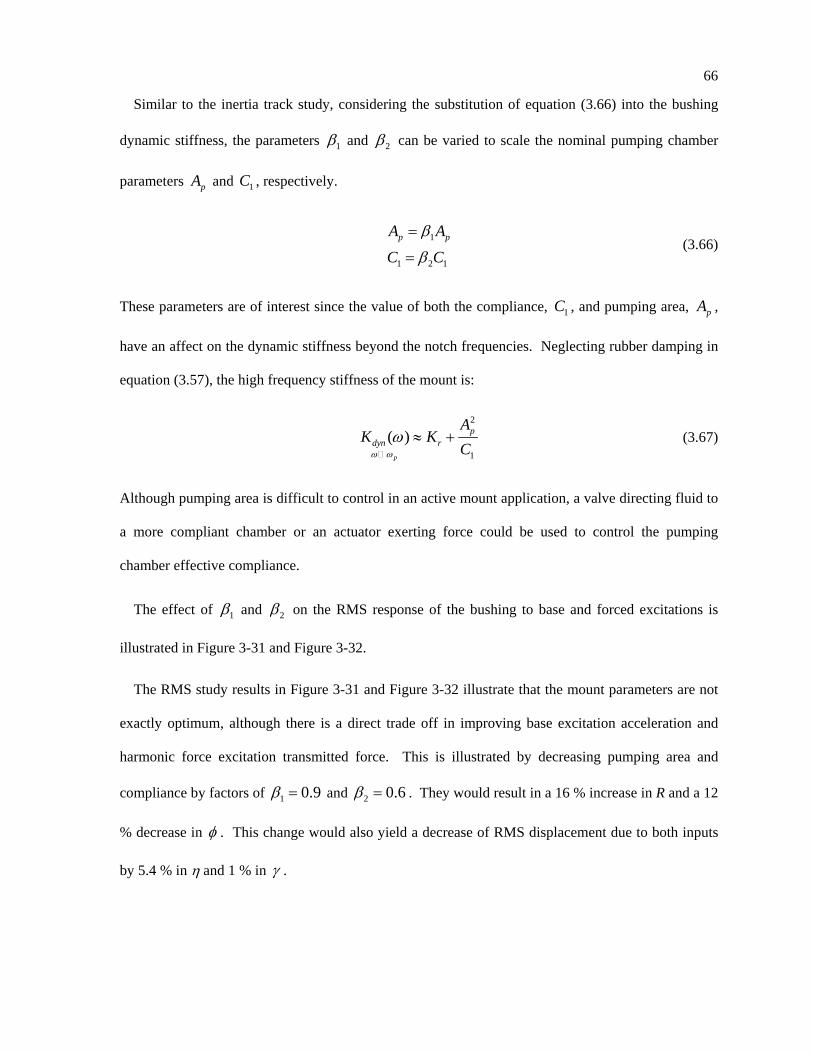
66

Similar to the inertia track study, considering the substitution of equation (3.66) into the bushing

dynamic stiffness, the parameters 1β and 2β can be varied to scale the nominal pumping chamber

parameters pA and 1C , respectively.

1

1 2 1

p pA A

C C

β

β

=

= (3.66)

These parameters are of interest since the value of both the compliance, 1C , and pumping area, pA ,

have an affect on the dynamic stiffness beyond the notch frequencies. Neglecting rubber damping in

equation (3.57), the high frequency stiffness of the mount is:

2

1

( )p

pdyn r

AK K

Cω ω

ω ≈ + (3.67)

Although pumping area is difficult to control in an active mount application, a valve directing fluid to

a more compliant chamber or an actuator exerting force could be used to control the pumping

chamber effective compliance.

The effect of 1β and 2β on the RMS response of the bushing to base and forced excitations is

illustrated in Figure 3-31 and Figure 3-32.

The RMS study results in Figure 3-31 and Figure 3-32 illustrate that the mount parameters are not

exactly optimum, although there is a direct trade off in improving base excitation acceleration and

harmonic force excitation transmitted force. This is illustrated by decreasing pumping area and

compliance by factors of 1 0.9β = and 2 0.6β = . They would result in a 16 % increase in R and a 12

% decrease in φ . This change would also yield a decrease of RMS displacement due to both inputs

by 5.4 % in η and 1 % in γ .

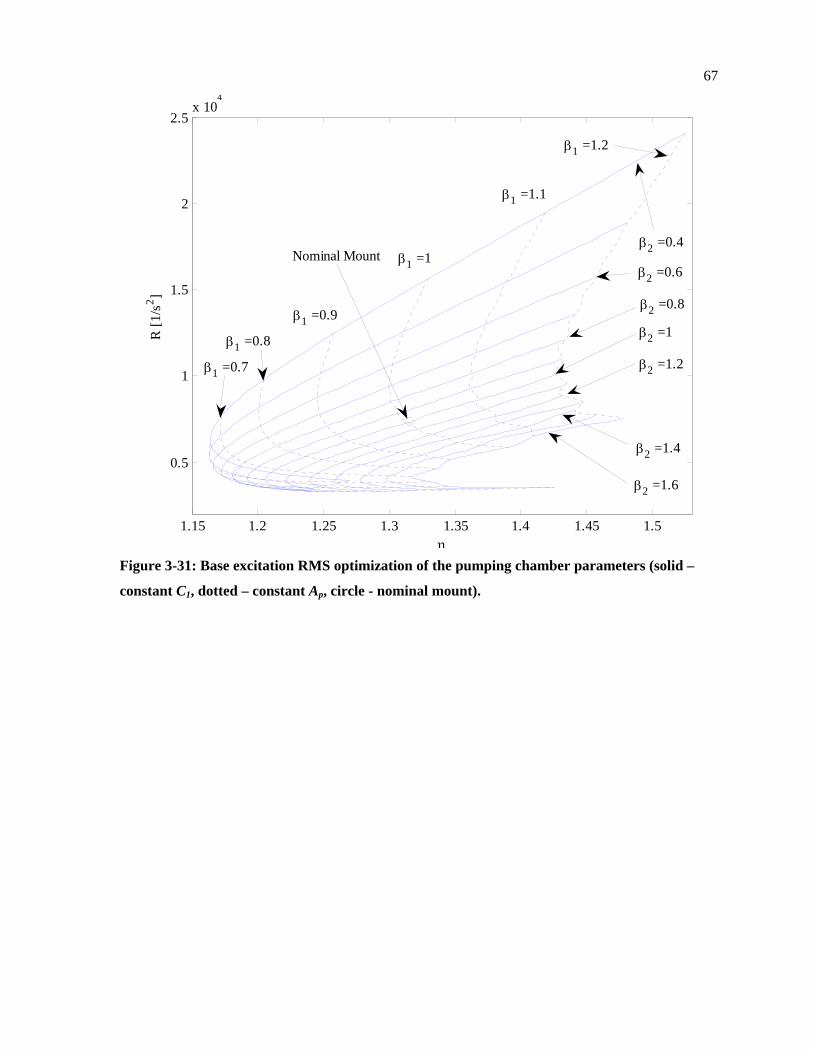
67

1.15 1.2 1.25 1.3 1.35 1.4 1.45 1.5

0.5

1

1.5

2

2.5x 10

4

R [1

/s2 ]

η

β2 =1

β2 =0.8

β2 =0.6

β2 =0.4

β2 =1.4

β2 =1.6

β2 =1.2

β1 =1

β1 =1.1

β1 =1.2

β1 =0.9

β1 =0.8

β1 =0.7

Nominal Mount

Figure 3-31: Base excitation RMS optimization of the pumping chamber parameters (solid –

constant C1, dotted – constant Ap, circle - nominal mount).

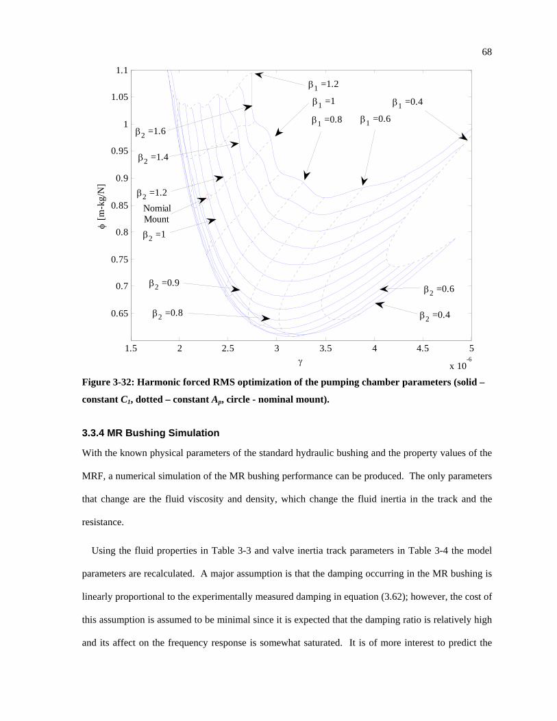
68

1.5 2 2.5 3 3.5 4 4.5 5

x 10-6

0.65

0.7

0.75

0.8

0.85

0.9

0.95

1

1.05

1.1

φ [m

-kg/

N]

γ

β1 =1.2

β1 =1

β1 =0.8 β1 =0.6

β1 =0.4

β2 =1.6

β2 =1.4

β2 =1.2

β2 =1

β2 =0.4

β2 =0.6

β2 =0.8

β2 =0.9

NomialMount

Figure 3-32: Harmonic forced RMS optimization of the pumping chamber parameters (solid –

constant C1, dotted – constant Ap, circle - nominal mount).

3.3.4 MR Bushing Simulation

With the known physical parameters of the standard hydraulic bushing and the property values of the

MRF, a numerical simulation of the MR bushing performance can be produced. The only parameters

that change are the fluid viscosity and density, which change the fluid inertia in the track and the

resistance.

Using the fluid properties in Table 3-3 and valve inertia track parameters in Table 3-4 the model

parameters are recalculated. A major assumption is that the damping occurring in the MR bushing is

linearly proportional to the experimentally measured damping in equation (3.62); however, the cost of

this assumption is assumed to be minimal since it is expected that the damping ratio is relatively high

and its affect on the frequency response is somewhat saturated. It is of more interest to predict the

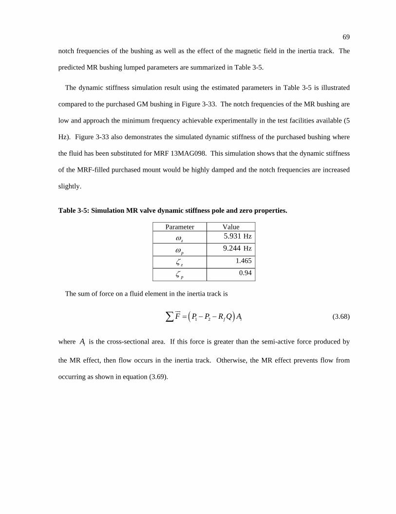
69

notch frequencies of the bushing as well as the effect of the magnetic field in the inertia track. The

predicted MR bushing lumped parameters are summarized in Table 3-5.

The dynamic stiffness simulation result using the estimated parameters in Table 3-5 is illustrated

compared to the purchased GM bushing in Figure 3-33. The notch frequencies of the MR bushing are

low and approach the minimum frequency achievable experimentally in the test facilities available (5

Hz). Figure 3-33 also demonstrates the simulated dynamic stiffness of the purchased bushing where

the fluid has been substituted for MRF 13MAG098. This simulation shows that the dynamic stiffness

of the MRF-filled purchased mount would be highly damped and the notch frequencies are increased

slightly.

Table 3-5: Simulation MR valve dynamic stiffness pole and zero properties.

Parameter Value

zω 5.931 Hz

pω 9.244 Hz

zζ 1.465

pζ 0.94

The sum of force on a fluid element in the inertia track is

( )1 2 f iF P P R Q A= − −∑ur

(3.68)

where iA is the cross-sectional area. If this force is greater than the semi-active force produced by

the MR effect, then flow occurs in the inertia track. Otherwise, the MR effect prevents flow from

occurring as shown in equation (3.69).

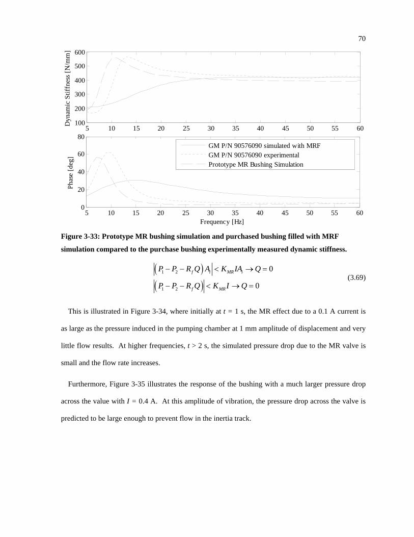
70

5 10 15 20 25 30 35 40 45 50 55 60100

200

300

400

500

600

Dyn

amic

Stif

fnes

s [N

/mm

]

5 10 15 20 25 30 35 40 45 50 55 600

20

40

60

80

Phas

e [d

eg]

Frequency [Hz]

GM P/N 90576090 simulated with MRFGM P/N 90576090 experimentalPrototype MR Bushing Simulation

Figure 3-33: Prototype MR bushing simulation and purchased bushing filled with MRF

simulation compared to the purchase bushing experimentally measured dynamic stiffness.

( )( )

1 2

1 2

0

0

f i MR i

f MR

P P R Q A K IA Q

P P R Q K I Q

− − < → =

− − < → = (3.69)

This is illustrated in Figure 3-34, where initially at t = 1 s, the MR effect due to a 0.1 A current is

as large as the pressure induced in the pumping chamber at 1 mm amplitude of displacement and very

little flow results. At higher frequencies, t > 2 s, the simulated pressure drop due to the MR valve is

small and the flow rate increases.

Furthermore, Figure 3-35 illustrates the response of the bushing with a much larger pressure drop

across the value with I = 0.4 A. At this amplitude of vibration, the pressure drop across the valve is

predicted to be large enough to prevent flow in the inertia track.

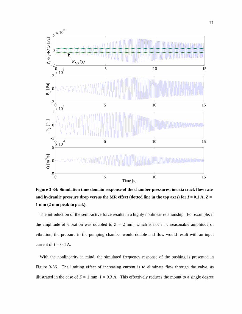
71

0 5 10 15-2

0

2x 10

5

P 1-P2-R

*Q [P

a]

0 5 10 15-2

0

2x 10

5

P 1 [Pa]

0 5 10 15-1

0

1x 10

4

P 2 [Pa]

0 5 10 15-5

0

5x 10

-4

Q [m

3 /s]

Time [s]

KMRI(t)

Figure 3-34: Simulation time domain response of the chamber pressures, inertia track flow rate

and hydraulic pressure drop versus the MR effect (dotted line in the top axes) for I = 0.1 A, Z =

1 mm (2 mm peak to peak).

The introduction of the semi-active force results in a highly nonlinear relationship. For example, if

the amplitude of vibration was doubled to Z = 2 mm, which is not an unreasonable amplitude of

vibration, the pressure in the pumping chamber would double and flow would result with an input

current of I = 0.4 A.

With the nonlinearity in mind, the simulated frequency response of the bushing is presented in

Figure 3-36. The limiting effect of increasing current is to eliminate flow through the valve, as

illustrated in the case of Z = 1 mm, I = 0.3 A. This effectively reduces the mount to a single degree

72

of freedom systems with constant stiffness. Otherwise, increasing the current increases the low

frequency stiffness by reducing flow through the inertia track; therefore, having the effect of

decreasing the notch frequency of the bushing.

0 5 10 15-2

0

2x 10

5

P 1-P2-R

*Q [P

a]

0 5 10 15-1

0

1x 10

5

P 1 [Pa]

0 5 10 15-1

0

1

P 2 [Pa]

0 5 10 15-1

0

1

Q [m

3 /s]

Time [s] Figure 3-35: Simulation time domain response of the chamber pressures, inertia track flow rate

and hydraulic pressure drop versus the MR effect (dotted line in the top axes) for I = 0.4 A, Z =

1 mm (2 mm peak to peak).

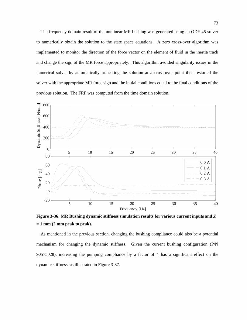
73

The frequency domain result of the nonlinear MR bushing was generated using an ODE 45 solver

to numerically obtain the solution to the state space equations. A zero cross-over algorithm was

implemented to monitor the direction of the force vector on the element of fluid in the inertia track

and change the sign of the MR force appropriately. This algorithm avoided singularity issues in the

numerical solver by automatically truncating the solution at a cross-over point then restarted the

solver with the appropriate MR force sign and the initial conditions equal to the final conditions of the

previous solution. The FRF was computed from the time domain solution.

5 10 15 20 25 30 35 400

200

400

600

800

Dyn

amic

Stif

fnes

s [N

/mm

]

5 10 15 20 25 30 35 40-20

0

20

40

60

80

Frequency [Hz]

Phas

e [d

eg]

0.0 A0.1 A0.2 A0.3 A

Figure 3-36: MR Bushing dynamic stiffness simulation results for various current inputs and Z

= 1 mm (2 mm peak to peak).

As mentioned in the previous section, changing the bushing compliance could also be a potential

mechanism for changing the dynamic stiffness. Given the current bushing configuration (P/N

90575028), increasing the pumping compliance by a factor of 4 has a significant effect on the

dynamic stiffness, as illustrated in Figure 3-37.

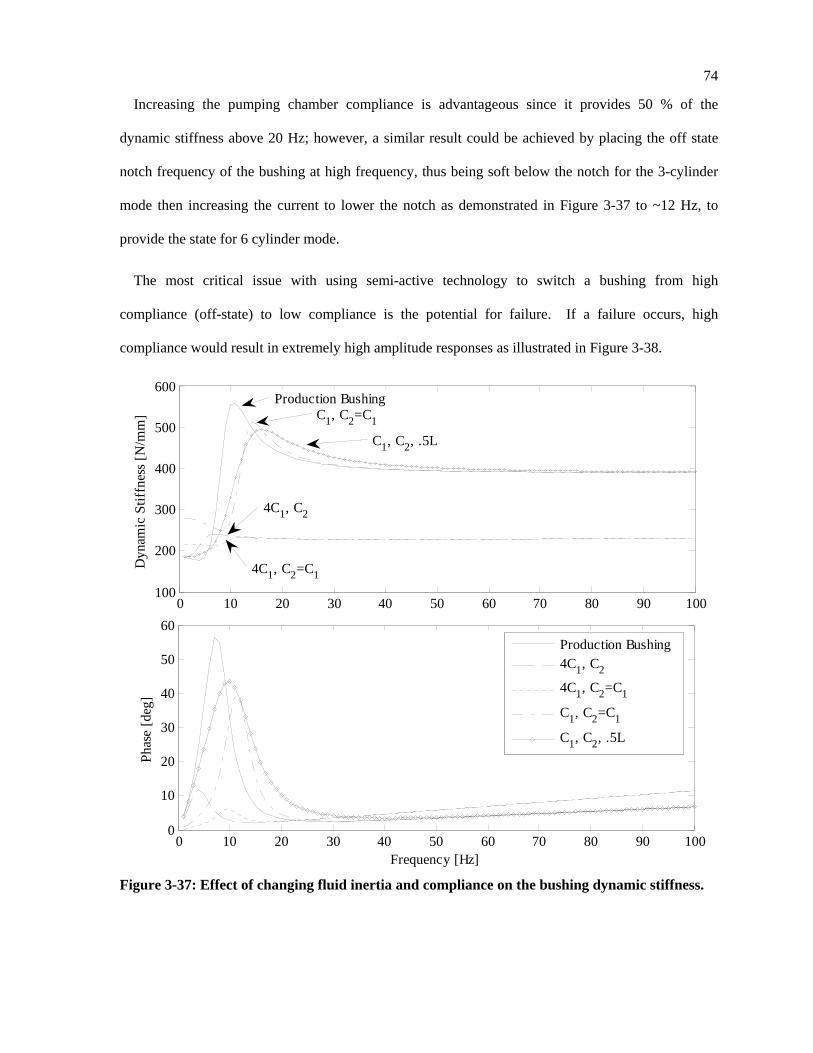
74

Increasing the pumping chamber compliance is advantageous since it provides 50 % of the

dynamic stiffness above 20 Hz; however, a similar result could be achieved by placing the off state

notch frequency of the bushing at high frequency, thus being soft below the notch for the 3-cylinder

mode then increasing the current to lower the notch as demonstrated in Figure 3-37 to ~12 Hz, to

provide the state for 6 cylinder mode.

The most critical issue with using semi-active technology to switch a bushing from high

compliance (off-state) to low compliance is the potential for failure. If a failure occurs, high

compliance would result in extremely high amplitude responses as illustrated in Figure 3-38.

0 10 20 30 40 50 60 70 80 90 100100

200

300

400

500

600

Dyn

amic

Stif

fnes

s [N

/mm

]

Production Bushing

4C1, C2=C1

4C1, C2

C1, C2, .5L

C1, C2=C1

0 10 20 30 40 50 60 70 80 90 1000

10

20

30

40

50

60

Phas

e [d

eg]

Frequency [Hz]

Production Bushing4C1, C2

4C1, C2=C1

C1, C2=C1

C1, C2, .5L

Figure 3-37: Effect of changing fluid inertia and compliance on the bushing dynamic stiffness.

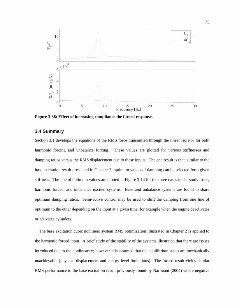
75

0

5

10

|FT

/F|

0 5 10 15 20 25 300

2

4

6x 10

-3

|X/f o| [

m-k

g/N

]

Frequency [Hz]

C14C1

Figure 3-38: Effect of increasing compliance the forced response.

3.4 Summary

Section 3.1 develops the equations of the RMS force transmitted through the linear isolator for both

harmonic forcing and unbalance forcing. These values are plotted for various stiffnesses and

damping ratios versus the RMS displacement due to these inputs. The end result is that, similar to the

base excitation result presented in Chapter 2, optimum values of damping can be selected for a given

stiffness. The line of optimum values are plotted in Figure 3-14 for the three cases under study: base,

harmonic forced, and unbalance excited systems. Base and unbalance systems are found to share

optimum damping ratios. Semi-active control may be used to shift the damping from one line of

optimum to the other depending on the input at a given time, for example when the engine deactivates

or activates cylinders.

The base excitation cubic nonlinear system RMS optimization illustrated in Chapter 2 is applied to

the harmonic forced input. A brief study of the stability of the systems illustrated that there are issues

introduced due to the nonlinearity; however it is assumed that the equilibrium states are mechanically

unachievable (physical displacement and energy level limitations). The forced result yields similar

RMS performance to the base excitation result previously found by Narimani (2004) where negative

76

stiffness significantly decreases both force and displacement transmitted. Finally, a transient

simulation analysis reveals that the negative damping has no significant impact on the step and

impulse inputs; hence the linear damping and stiffness could be selected for optimum time domain

performance and the cubic stiffness added to tune the frequency response.

A further extension of the RMS optimization technique is achieved by tuning the hydraulic bushing

inertia track length and hydraulic diameter as well as the pumping area and pumping chamber

compliance. For the given bushing and engine mass it was found that decreasing the inertia track

length by 20% would offer the best improvement in the frequency response since it would decrease

both absolute acceleration and force transmitted with negligible increase in the RMS of displacement.

The next sections of this chapter deal with MR valve design and simulation of the MR bushing

with the MR valve replacing the inertia track. The result illustrates that as the current is increased the

bushing tends to a single degree of freedom as fluid flow is decreased. At high currents, flow does

not occur and the dynamic stiffness is constant with very little damping. This mechanism could be

used by increasing the notch frequency of the bushing and using the current to change the low

frequency stiffness.

As an alternative to the MR bushing design, it is suggested that changing the pumping chamber

compliance may an effective way to produce a large variation in dynamic stiffness. The case

presented in Figure 3-37 illustrates that an increase in compliance by a factor of 4 decreases the

stiffness by roughly 50%.

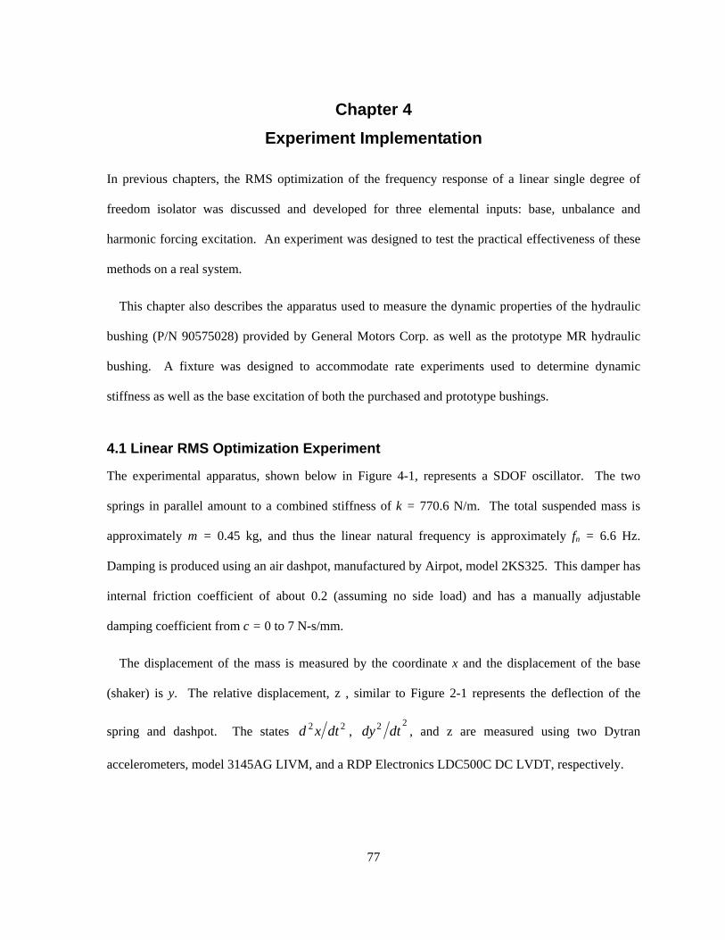
77

Chapter 4 Experiment Implementation

In previous chapters, the RMS optimization of the frequency response of a linear single degree of

freedom isolator was discussed and developed for three elemental inputs: base, unbalance and

harmonic forcing excitation. An experiment was designed to test the practical effectiveness of these

methods on a real system.

This chapter also describes the apparatus used to measure the dynamic properties of the hydraulic

bushing (P/N 90575028) provided by General Motors Corp. as well as the prototype MR hydraulic

bushing. A fixture was designed to accommodate rate experiments used to determine dynamic

stiffness as well as the base excitation of both the purchased and prototype bushings.

4.1 Linear RMS Optimization Experiment

The experimental apparatus, shown below in Figure 4-1, represents a SDOF oscillator. The two

springs in parallel amount to a combined stiffness of k = 770.6 N/m. The total suspended mass is

approximately m = 0.45 kg, and thus the linear natural frequency is approximately fn = 6.6 Hz.

Damping is produced using an air dashpot, manufactured by Airpot, model 2KS325. This damper has

internal friction coefficient of about 0.2 (assuming no side load) and has a manually adjustable

damping coefficient from c = 0 to 7 N-s/mm.

The displacement of the mass is measured by the coordinate x and the displacement of the base

(shaker) is y. The relative displacement, z , similar to Figure 2-1 represents the deflection of the

spring and dashpot. The states 22 dtxd , 22 dtdy , and z are measured using two Dytran

accelerometers, model 3145AG LIVM, and a RDP Electronics LDC500C DC LVDT, respectively.

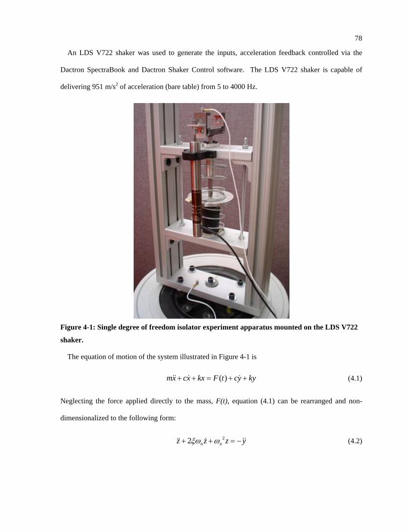
78

An LDS V722 shaker was used to generate the inputs, acceleration feedback controlled via the

Dactron SpectraBook and Dactron Shaker Control software. The LDS V722 shaker is capable of

delivering 951 m/s2 of acceleration (bare table) from 5 to 4000 Hz.

Figure 4-1: Single degree of freedom isolator experiment apparatus mounted on the LDS V722

shaker.

The equation of motion of the system illustrated in Figure 4-1 is

( )mx cx kx F t cy ky+ + = + +&& & & (4.1)

Neglecting the force applied directly to the mass, F(t), equation (4.1) can be rearranged and non-

dimensionalized to the following form:

22 n nz z z yξω ω+ + = −&&&& & (4.2)

79

Now, with respect to the inertial frame, forcing on the mass becomes the acceleration input and a

coordinate transformation yields equation (4.3).

( ) cos( )o dr

F ty f tm

ω− = =&& (4.3)

z x→ (4.4)

22 ( )n nx x x F t mξω ω+ + =&& & (4.5)

Hence, rather than directly applying a force to the mass, the frame can be accelerated to apply an

inertial force as illustrated in Figure 4-2. This is applicable to the experiment since the shaker can

only produce controlled displacement.

Figure 4-2: An inertial force can be applied to the suspended mass by accelerating the reference

frame attached to the base of the isolator.

The RMS response of the base excitation experiment is produced with a constant displacement

amplitude sweep over the frequency range. Constant displacement amplitude frequency sweep

produced an acceleration loading

2drY Yω=&& (4.6)

k c

m

x

F my= &&

, ,y y y& &&

c x

y

m

z k

globaly

z x→

80

where drω is the driving frequency. Hence, the base excitation experiment doubles as an unbalance

excitation experiment.

Similarly, the harmonic forcing excitation of the linear isolator can be produced by applying a

constant displacement amplitude sweep over the frequency range.

The system illustrated in Figure 4-1 is not perfectly linear; however, with careful selection of the

inputs the impact of nonlinearity may be minimized. The purpose of this discussion is to explain

some of the nonlinear characteristics observed in a simple qualitative way.

As mentioned previously, the dashpot has a certain amount of friction. Friction

sgn( )frictionF F z= & (4.7)

also exists in the nylon bearing supporting the suspended mass. To the human hand, it is difficult to

perceive this minute force; however, the LVDT is much more precise and detects the motion created

as a result of small forces, as demonstrated in Figure 4-3. This figure illustrates that with low input

amplitudes the inertia force applied to the mass is less than the friction until approximately 7 Hz

during the forward sweep. Beyond 7 Hz, the mass breaks free and relative motion is observed.

The opposite effect is observed on the backward sweep since the inertia of the mass is greater than

friction until approximately 6 Hz near the tail end of resonance. Experimentally, it was found that an

amplitude of 2.25 mm was sufficient to overcome friction at 5 Hz regardless of the magnitude of

damping ratio and sweep direction.

Furthermore, strong jump phenomena can be observed when the amplitude of vibration reaches the

maximum with high damping. The result is a piecewise linear system, the dynamics of which are

clearly nonlinear. This nonlinearity is avoided by reducing the input amplitude to avoid saturating

the dashpot.

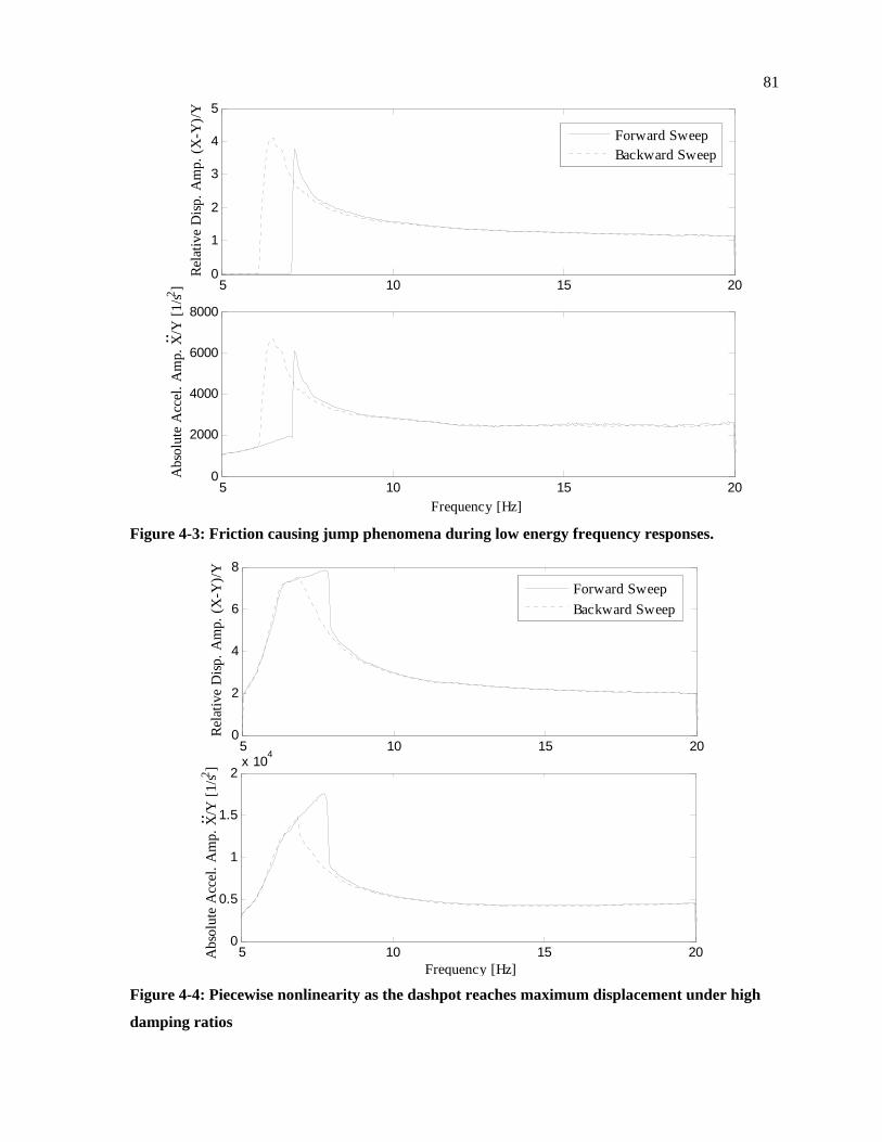
81

5 10 15 200

1

2

3

4

5

Rela

tive

Disp

. Am

p. (X

-Y)/Y

5 10 15 200

2000

4000

6000

8000

Frequency [Hz]

Abs

olut

e A

ccel

. Am

p. X

/Y [1

/s2 ]

:

Forward SweepBackward Sweep

Figure 4-3: Friction causing jump phenomena during low energy frequency responses.

5 10 15 200

2

4

6

8

Rela

tive

Disp

. Am

p. (X

-Y)/Y

5 10 15 200

0.5

1

1.5

2x 104

Frequency [Hz]

Abs

olut

e A

ccel

. Am

p. X

/Y [1

/s2 ]

:

Forward SweepBackward Sweep

Figure 4-4: Piecewise nonlinearity as the dashpot reaches maximum displacement under high

damping ratios

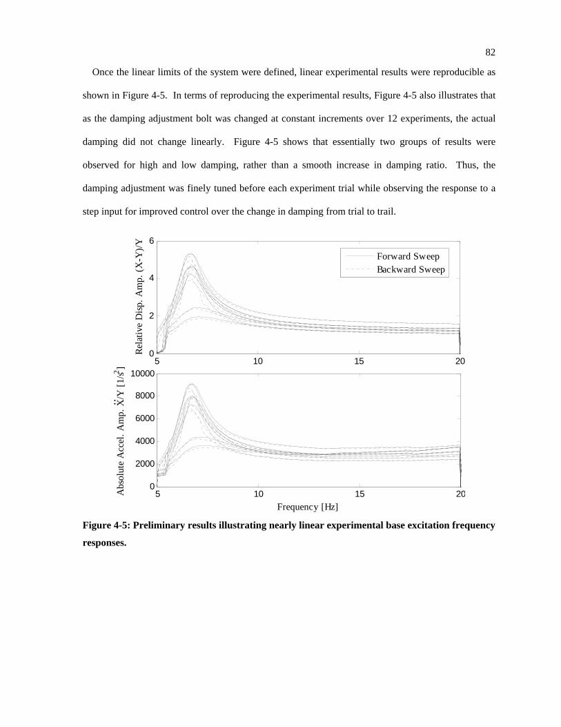
82

Once the linear limits of the system were defined, linear experimental results were reproducible as

shown in Figure 4-5. In terms of reproducing the experimental results, Figure 4-5 also illustrates that

as the damping adjustment bolt was changed at constant increments over 12 experiments, the actual

damping did not change linearly. Figure 4-5 shows that essentially two groups of results were

observed for high and low damping, rather than a smooth increase in damping ratio. Thus, the

damping adjustment was finely tuned before each experiment trial while observing the response to a

step input for improved control over the change in damping from trial to trail.

5 10 15 200

2

4

6

Rela

tive

Disp

. Am

p. (X

-Y)/Y

5 10 15 200

2000

4000

6000

8000

10000

Frequency [Hz]

Abs

olut

e A

ccel

. Am

p. X

/Y [1

/s2 ]

:

Forward SweepBackward Sweep

Figure 4-5: Preliminary results illustrating nearly linear experimental base excitation frequency

responses.

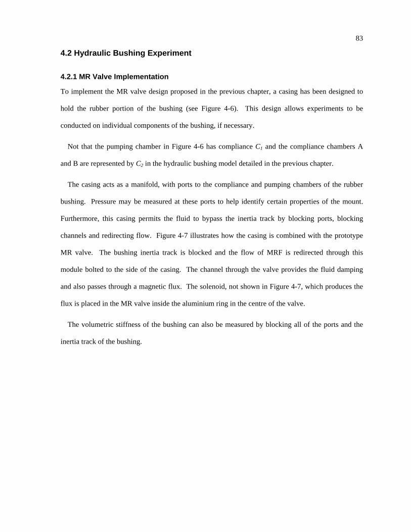
83

4.2 Hydraulic Bushing Experiment

4.2.1 MR Valve Implementation

To implement the MR valve design proposed in the previous chapter, a casing has been designed to

hold the rubber portion of the bushing (see Figure 4-6). This design allows experiments to be

conducted on individual components of the bushing, if necessary.

Not that the pumping chamber in Figure 4-6 has compliance C1 and the compliance chambers A

and B are represented by C2 in the hydraulic bushing model detailed in the previous chapter.

The casing acts as a manifold, with ports to the compliance and pumping chambers of the rubber

bushing. Pressure may be measured at these ports to help identify certain properties of the mount.

Furthermore, this casing permits the fluid to bypass the inertia track by blocking ports, blocking

channels and redirecting flow. Figure 4-7 illustrates how the casing is combined with the prototype

MR valve. The bushing inertia track is blocked and the flow of MRF is redirected through this

module bolted to the side of the casing. The channel through the valve provides the fluid damping

and also passes through a magnetic flux. The solenoid, not shown in Figure 4-7, which produces the

flux is placed in the MR valve inside the aluminium ring in the centre of the valve.

The volumetric stiffness of the bushing can also be measured by blocking all of the ports and the

inertia track of the bushing.

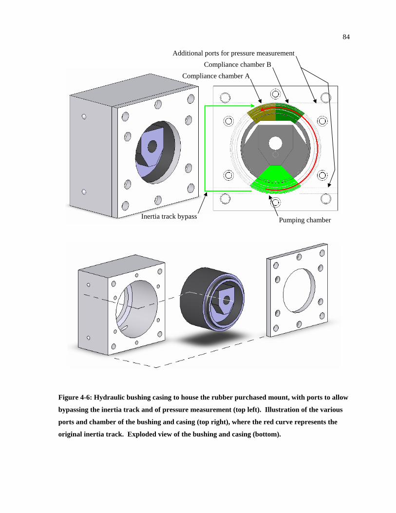
84

Figure 4-6: Hydraulic bushing casing to house the rubber purchased mount, with ports to allow

bypassing the inertia track and of pressure measurement (top left). Illustration of the various

ports and chamber of the bushing and casing (top right), where the red curve represents the

original inertia track. Exploded view of the bushing and casing (bottom).

Pumping chamber

Compliance chamber A Compliance chamber B

Inertia track bypass

Additional ports for pressure measurement

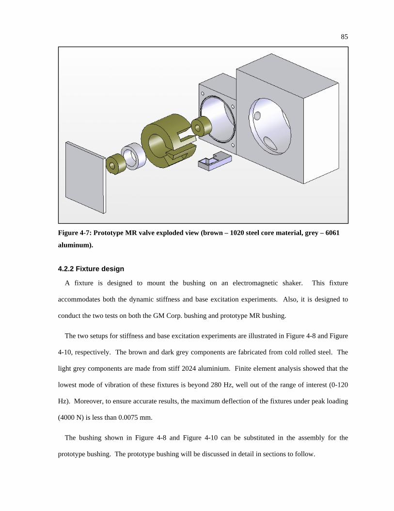
85

Figure 4-7: Prototype MR valve exploded view (brown – 1020 steel core material, grey – 6061

aluminum).

4.2.2 Fixture design

A fixture is designed to mount the bushing on an electromagnetic shaker. This fixture

accommodates both the dynamic stiffness and base excitation experiments. Also, it is designed to

conduct the two tests on both the GM Corp. bushing and prototype MR bushing.

The two setups for stiffness and base excitation experiments are illustrated in Figure 4-8 and Figure

4-10, respectively. The brown and dark grey components are fabricated from cold rolled steel. The

light grey components are made from stiff 2024 aluminium. Finite element analysis showed that the

lowest mode of vibration of these fixtures is beyond 280 Hz, well out of the range of interest (0-120

Hz). Moreover, to ensure accurate results, the maximum deflection of the fixtures under peak loading

(4000 N) is less than 0.0075 mm.

The bushing shown in Figure 4-8 and Figure 4-10 can be substituted in the assembly for the

prototype bushing. The prototype bushing will be discussed in detail in sections to follow.

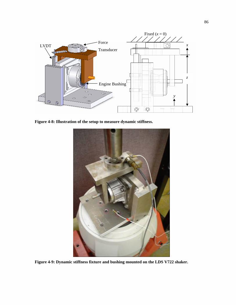
86

Figure 4-8: Illustration of the setup to measure dynamic stiffness.

Figure 4-9: Dynamic stiffness fixture and bushing mounted on the LDS V722 shaker.

Force

Transducer LVDT

Engine Bushing

y

x

z

Fixed (x = 0)

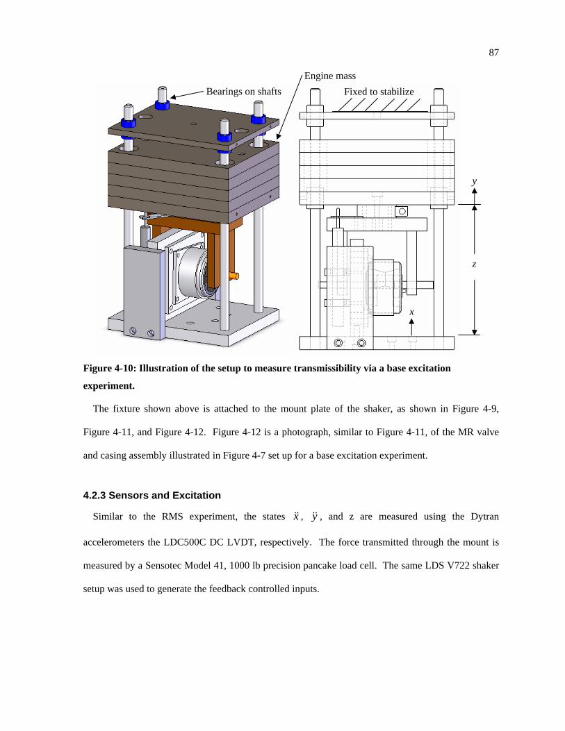
87

Figure 4-10: Illustration of the setup to measure transmissibility via a base excitation

experiment.

The fixture shown above is attached to the mount plate of the shaker, as shown in Figure 4-9,

Figure 4-11, and Figure 4-12. Figure 4-12 is a photograph, similar to Figure 4-11, of the MR valve

and casing assembly illustrated in Figure 4-7 set up for a base excitation experiment.

4.2.3 Sensors and Excitation

Similar to the RMS experiment, the states x&& , y&& , and z are measured using the Dytran

accelerometers the LDC500C DC LVDT, respectively. The force transmitted through the mount is

measured by a Sensotec Model 41, 1000 lb precision pancake load cell. The same LDS V722 shaker

setup was used to generate the feedback controlled inputs.

Bearings on shafts

x

y

z

Fixed to stabilize Engine mass

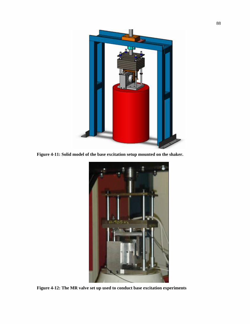
88

Figure 4-11: Solid model of the base excitation setup mounted on the shaker.

Figure 4-12: The MR valve set up used to conduct base excitation experiments

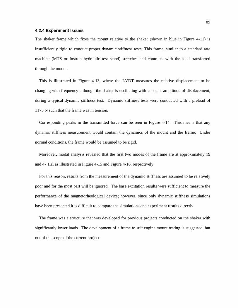
89

4.2.4 Experiment Issues

The shaker frame which fixes the mount relative to the shaker (shown in blue in Figure 4-11) is

insufficiently rigid to conduct proper dynamic stiffness tests. This frame, similar to a standard rate

machine (MTS or Instron hydraulic test stand) stretches and contracts with the load transferred

through the mount.

This is illustrated in Figure 4-13, where the LVDT measures the relative displacement to be

changing with frequency although the shaker is oscillating with constant amplitude of displacement,

during a typical dynamic stiffness test. Dynamic stiffness tests were conducted with a preload of

1175 N such that the frame was in tension.

Corresponding peaks in the transmitted force can be seen in Figure 4-14. This means that any

dynamic stiffness measurement would contain the dynamics of the mount and the frame. Under

normal conditions, the frame would be assumed to be rigid.

Moreover, modal analysis revealed that the first two modes of the frame are at approximately 19

and 47 Hz, as illustrated in Figure 4-15 and Figure 4-16, respectively.

For this reason, results from the measurement of the dynamic stiffness are assumed to be relatively

poor and for the most part will be ignored. The base excitation results were sufficient to measure the

performance of the magnetorheological device; however, since only dynamic stiffness simulations

have been presented it is difficult to compare the simulations and experiment results directly.

The frame was a structure that was developed for previous projects conducted on the shaker with

significantly lower loads. The development of a frame to suit engine mount testing is suggested, but

out of the scope of the current project.

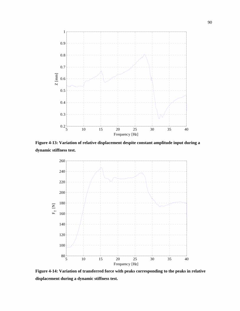
90

5 10 15 20 25 30 35 400.2

0.3

0.4

0.5

0.6

0.7

0.8

0.9

1

Z [m

m]

Frequency [Hz] Figure 4-13: Variation of relative displacement despite constant amplitude input during a

dynamic stiffness test.

5 10 15 20 25 30 35 4080

100

120

140

160

180

200

220

240

260

F T [N

]

Frequency [Hz] Figure 4-14: Variation of transferred force with peaks corresponding to the peaks in relative

displacement during a dynamic stiffness test.

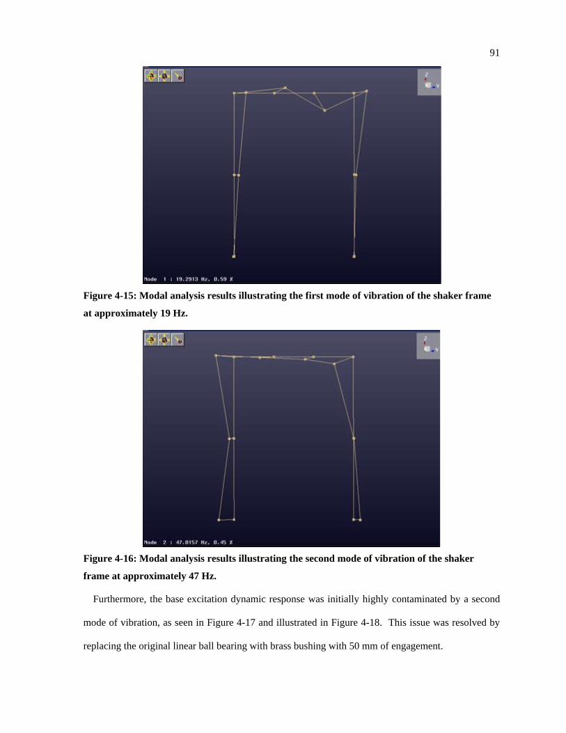
91

Figure 4-15: Modal analysis results illustrating the first mode of vibration of the shaker frame

at approximately 19 Hz.

Figure 4-16: Modal analysis results illustrating the second mode of vibration of the shaker

frame at approximately 47 Hz.

Furthermore, the base excitation dynamic response was initially highly contaminated by a second

mode of vibration, as seen in Figure 4-17 and illustrated in Figure 4-18. This issue was resolved by

replacing the original linear ball bearing with brass bushing with 50 mm of engagement.

92

5 10 15 20 25 30 35 40 45 500

5

10

15

20

25

30

35

Acc

eler

atio

n [m

/s²]

Frequency [Hz]

Centre of massacceleration(d2x/dt2)

Centre of massacceleration (d2x/dt2)

Centre of massacceleration (d2x/dt2)

linear first mode of vibration

Acceration of theedge of the mass(d2x2/dt2)illustrating the rotational mode of vibration

Visible Contaminationof d2x/dt2 by d2x2/dt2

d2y/dt2

d2x/dt2

d2x2/dt2

Figure 4-17: Initial hydraulic bushing acceleration results given base excitation input. Two

main modes of vibration are present: linear mode (19 Hz) and a rotational mode (26 Hz)

identified by the high edge acceleration with respect to the acceleration of the centre of mass.

Figure 4-18: Illustration of the undesirable rotational mode of vibration.

y

x

z

93

4.3 Summary

This chapter details the three setups used to conduct the experiments. In section 4.1 the setup used to

verify the previous base excitation frequency domain optimization work conducted by Jazar et al.

(2003). In addition, this single degree of freedom setup is used to verify the new forced response

results presented in Chapter 3.

Section 4.2 describes the components of the MR valve, and the integration of the valve with the

existing bushing using a custom made manifold. A fixture is designed to interface the purchased

engine bushing and prototype MR bushing to an electromagnetic shaker. The fixture is designed to

accommodate both dynamic stiffness experiments and base excitation; however the existing structure

is inadequate for dynamic stiffness measurement. It is also concluded that, for base excitation

experiments, very long engagement bushings or bearings are required to eliminate rotational modes of

vibration and binding.

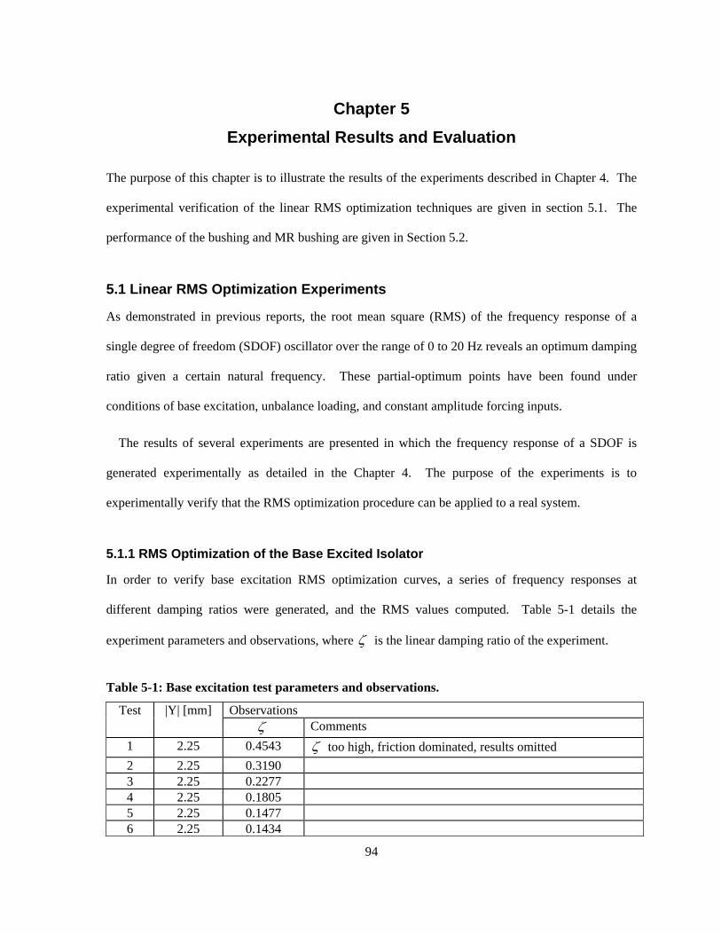
94

Chapter 5 Experimental Results and Evaluation

The purpose of this chapter is to illustrate the results of the experiments described in Chapter 4. The

experimental verification of the linear RMS optimization techniques are given in section 5.1. The

performance of the bushing and MR bushing are given in Section 5.2.

5.1 Linear RMS Optimization Experiments

As demonstrated in previous reports, the root mean square (RMS) of the frequency response of a

single degree of freedom (SDOF) oscillator over the range of 0 to 20 Hz reveals an optimum damping

ratio given a certain natural frequency. These partial-optimum points have been found under

conditions of base excitation, unbalance loading, and constant amplitude forcing inputs.

The results of several experiments are presented in which the frequency response of a SDOF is

generated experimentally as detailed in the Chapter 4. The purpose of the experiments is to

experimentally verify that the RMS optimization procedure can be applied to a real system.

5.1.1 RMS Optimization of the Base Excited Isolator

In order to verify base excitation RMS optimization curves, a series of frequency responses at

different damping ratios were generated, and the RMS values computed. Table 5-1 details the

experiment parameters and observations, where ζ is the linear damping ratio of the experiment.

Table 5-1: Base excitation test parameters and observations.

Observations Test |Y| [mm] ζ Comments

1 2.25 0.4543 ζ too high, friction dominated, results omitted 2 2.25 0.3190 3 2.25 0.2277 4 2.25 0.1805 5 2.25 0.1477 6 2.25 0.1434

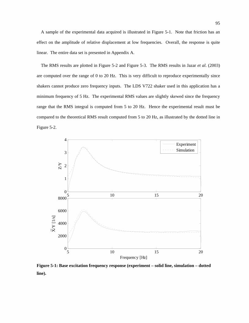
95

A sample of the experimental data acquired is illustrated in Figure 5-1. Note that friction has an

effect on the amplitude of relative displacement at low frequencies. Overall, the response is quite

linear. The entire data set is presented in Appendix A.

The RMS results are plotted in Figure 5-2 and Figure 5-3. The RMS results in Jazar et al. (2003)

are computed over the range of 0 to 20 Hz. This is very difficult to reproduce experimentally since

shakers cannot produce zero frequency inputs. The LDS V722 shaker used in this application has a

minimum frequency of 5 Hz. The experimental RMS values are slightly skewed since the frequency

range that the RMS integral is computed from 5 to 20 Hz. Hence the experimental result must be

compared to the theoretical RMS result computed from 5 to 20 Hz, as illustrated by the dotted line in

Figure 5-2.

5 10 15 200

2000

4000

6000

8000

Frequency [Hz]

X/Y

[1/s]

5 10 15 200

1

2

3

4

Z/Y

:

ExperimentSimulation

Figure 5-1: Base excitation frequency response (experiment – solid line, simulation – dotted

line).

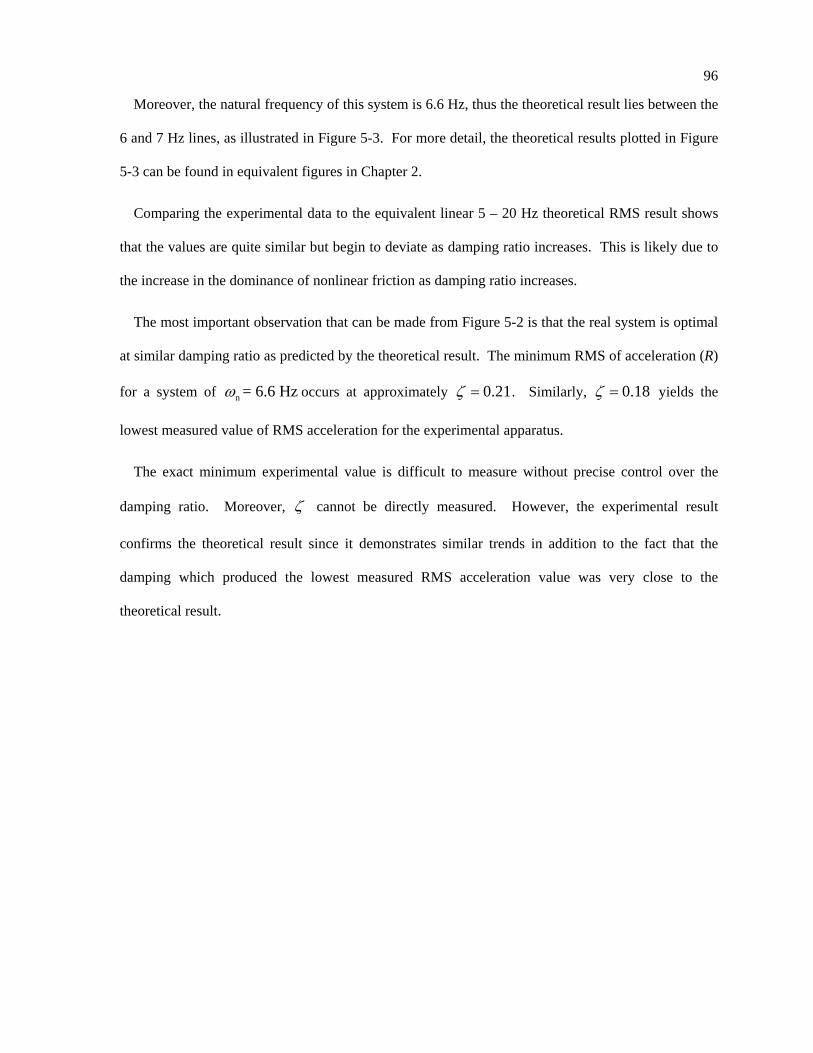
96

Moreover, the natural frequency of this system is 6.6 Hz, thus the theoretical result lies between the

6 and 7 Hz lines, as illustrated in Figure 5-3. For more detail, the theoretical results plotted in Figure

5-3 can be found in equivalent figures in Chapter 2.

Comparing the experimental data to the equivalent linear 5 – 20 Hz theoretical RMS result shows

that the values are quite similar but begin to deviate as damping ratio increases. This is likely due to

the increase in the dominance of nonlinear friction as damping ratio increases.

The most important observation that can be made from Figure 5-2 is that the real system is optimal

at similar damping ratio as predicted by the theoretical result. The minimum RMS of acceleration (R)

for a system of n = 6.6 Hzω occurs at approximately 0.21ζ = . Similarly, 0.18ζ = yields the

lowest measured value of RMS acceleration for the experimental apparatus.

The exact minimum experimental value is difficult to measure without precise control over the

damping ratio. Moreover, ζ cannot be directly measured. However, the experimental result

confirms the theoretical result since it demonstrates similar trends in addition to the fact that the

damping which produced the lowest measured RMS acceleration value was very close to the

theoretical result.

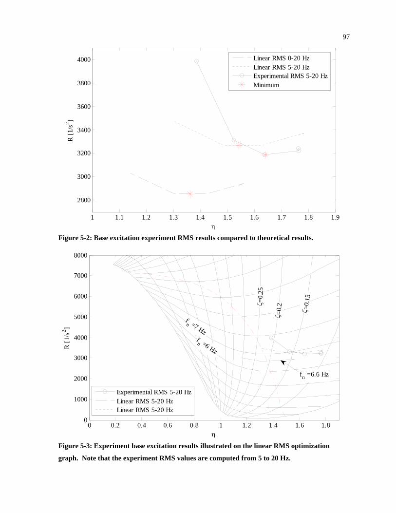
97

1 1.1 1.2 1.3 1.4 1.5 1.6 1.7 1.8 1.9

2800

3000

3200

3400

3600

3800

4000

η

R [1

/s2 ]

Linear RMS 0-20 HzLinear RMS 5-20 HzExperimental RMS 5-20 HzMinimum

Figure 5-2: Base excitation experiment RMS results compared to theoretical results.

0 0.2 0.4 0.6 0.8 1 1.2 1.4 1.6 1.80

1000

2000

3000

4000

5000

6000

7000

8000

η

R [1

/s2 ]

fn =6 Hz

fn =7 Hz

ζ =0.

2ζ =0.

25

ζ =0.

15

fn =6.6 Hz

Experimental RMS 5-20 HzLinear RMS 5-20 HzLinear RMS 5-20 Hz

Figure 5-3: Experiment base excitation results illustrated on the linear RMS optimization

graph. Note that the experiment RMS values are computed from 5 to 20 Hz.

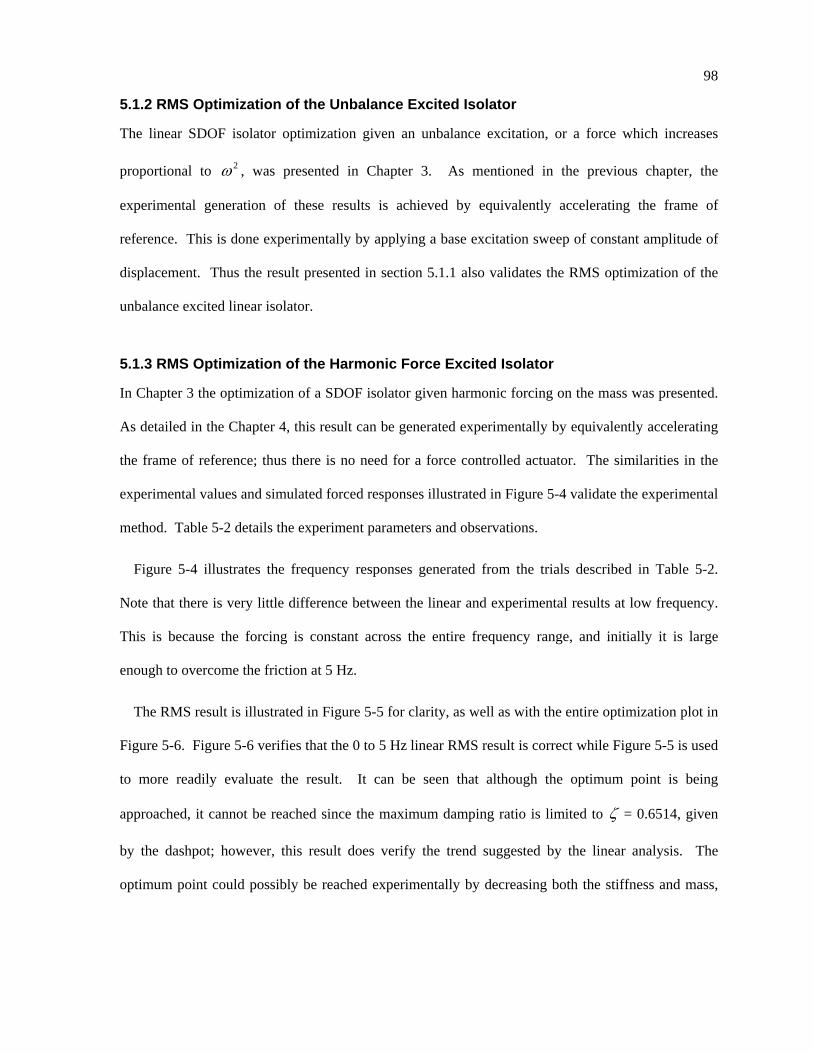
98

5.1.2 RMS Optimization of the Unbalance Excited Isolator

The linear SDOF isolator optimization given an unbalance excitation, or a force which increases

proportional to 2ω , was presented in Chapter 3. As mentioned in the previous chapter, the

experimental generation of these results is achieved by equivalently accelerating the frame of

reference. This is done experimentally by applying a base excitation sweep of constant amplitude of

displacement. Thus the result presented in section 5.1.1 also validates the RMS optimization of the

unbalance excited linear isolator.

5.1.3 RMS Optimization of the Harmonic Force Excited Isolator

In Chapter 3 the optimization of a SDOF isolator given harmonic forcing on the mass was presented.

As detailed in the Chapter 4, this result can be generated experimentally by equivalently accelerating

the frame of reference; thus there is no need for a force controlled actuator. The similarities in the

experimental values and simulated forced responses illustrated in Figure 5-4 validate the experimental

method. Table 5-2 details the experiment parameters and observations.

Figure 5-4 illustrates the frequency responses generated from the trials described in Table 5-2.

Note that there is very little difference between the linear and experimental results at low frequency.

This is because the forcing is constant across the entire frequency range, and initially it is large

enough to overcome the friction at 5 Hz.

The RMS result is illustrated in Figure 5-5 for clarity, as well as with the entire optimization plot in

Figure 5-6. Figure 5-6 verifies that the 0 to 5 Hz linear RMS result is correct while Figure 5-5 is used

to more readily evaluate the result. It can be seen that although the optimum point is being

approached, it cannot be reached since the maximum damping ratio is limited to ζ = 0.6514, given

by the dashpot; however, this result does verify the trend suggested by the linear analysis. The

optimum point could possibly be reached experimentally by decreasing both the stiffness and mass,

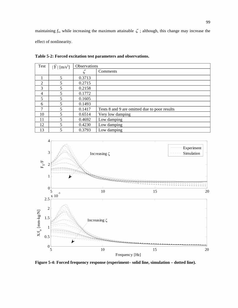
99

maintaining fn, while increasing the maximum attainable ζ ; although, this change may increase the

effect of nonlinearity.

Table 5-2: Forced excitation test parameters and observations.

Observations Test |Y&& | [m/s2] ζ Comments

1 5 0.3713 2 5 0.2715 3 5 0.2158 4 5 0.1772 5 5 0.1605 6 5 0.1493 7 5 0.1417 Tests 8 and 9 are omitted due to poor results

10 5 0.6514 Very low damping 11 5 0.4692 Low damping 12 5 0.4230 Low damping 13 5 0.3793 Low damping

5 10 15 200

1

2

3

4

FT

/F

5 10 15 200

0.5

1

1.5

2

2.5x 10

-3

Frequency [Hz]

X/f o [m

m-k

g/N

]

ExperimentSimulationIncreasing ζ

Increasing ζ

Figure 5-4: Forced frequency response (experiment– solid line, simulation – dotted line).

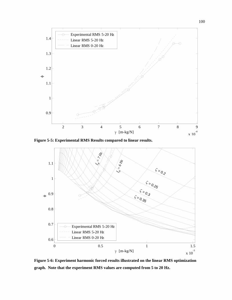
100

2 3 4 5 6 7 8 9

x 10-4

0.9

1

1.1

1.2

1.3

1.4

γ [m-kg/N]

φ

Experimental RMS 5-20 HzLinear RMS 5-20 HzLinear RMS 0-20 Hz

Figure 5-5: Experimental RMS Results compared to linear results.

0 0.5 1 1.5

x 10-3

0.6

0.7

0.8

0.9

1

1.1

γ [m-kg/N]

φ

f n =

7 Hz

f n =

6 Hz

ζ = 0.3

ζ = 0.25

ζ = 0.2

ζ = 0.35

Experimental RMS 5-20 HzLinear RMS 5-20 HzLinear RMS 0-20 Hz

Figure 5-6: Experiment harmonic forced results illustrated on the linear RMS optimization

graph. Note that the experiment RMS values are computed from 5 to 20 Hz.

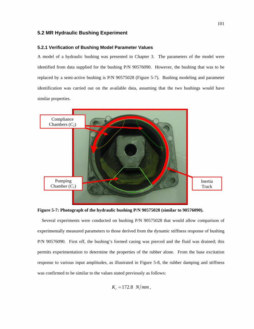
101

5.2 MR Hydraulic Bushing Experiment

5.2.1 Verification of Bushing Model Parameter Values

A model of a hydraulic bushing was presented in Chapter 3. The parameters of the model were

identified from data supplied for the bushing P/N 90576090. However, the bushing that was to be

replaced by a semi-active bushing is P/N 90575028 (Figure 5-7). Bushing modeling and parameter

identification was carried out on the available data, assuming that the two bushings would have

similar properties.

Figure 5-7: Photograph of the hydraulic bushing P/N 90575028 (similar to 90576090).

Several experiments were conducted on bushing P/N 90575028 that would allow comparison of

experimentally measured parameters to those derived from the dynamic stiffness response of bushing

P/N 90576090. First off, the bushing’s formed casing was pierced and the fluid was drained; this

permits experimentation to determine the properties of the rubber alone. From the base excitation

response to various input amplitudes, as illustrated in Figure 5-8, the rubber damping and stiffness

was confirmed to be similar to the values stated previously as follows:

172.8rK N mm= ,

Pumping Chamber (C1)

Compliance Chambers (C2)

Inertia Track

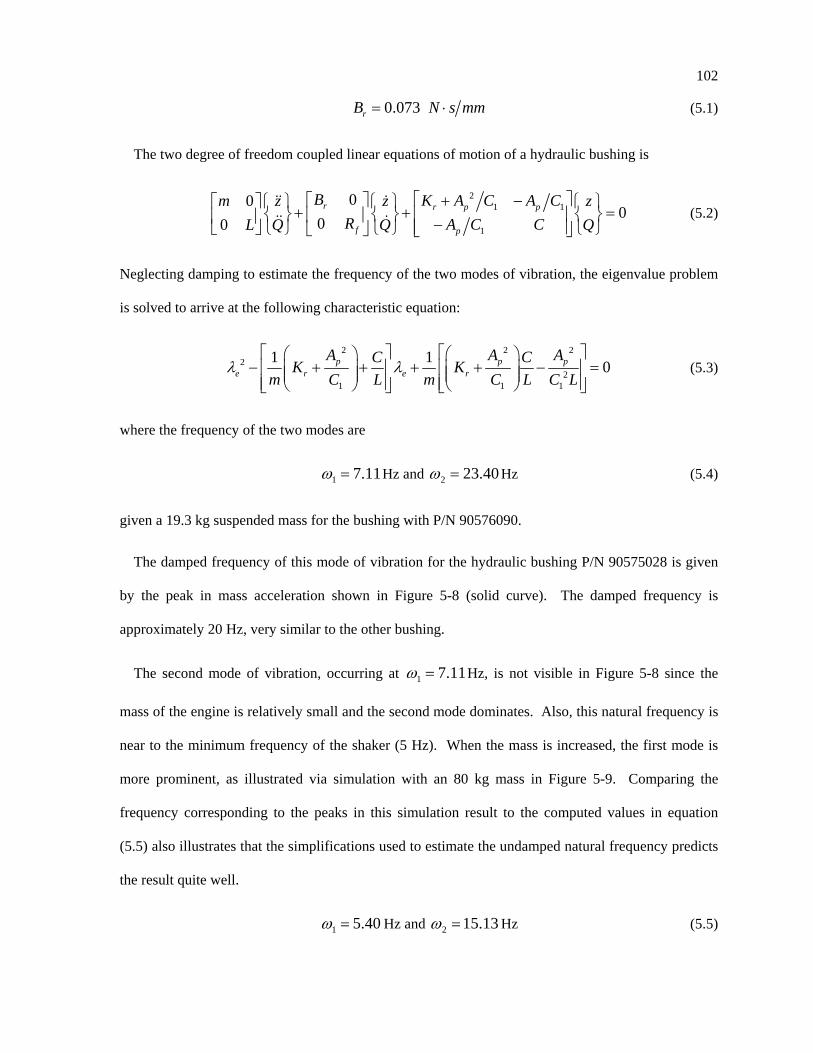
102

0.073rB N s mm= ⋅ (5.1)

The two degree of freedom coupled linear equations of motion of a hydraulic bushing is

2

1 1

1

000

00r r p p

f p

B K A C A Cm z z zR A C CL Q Q Q

⎡ ⎤+ −⎡ ⎤⎡ ⎤ ⎧ ⎫ ⎧ ⎫ ⎧ ⎫+ + =⎢ ⎥⎨ ⎬ ⎨ ⎬ ⎨ ⎬⎢ ⎥⎢ ⎥ −⎢ ⎥⎣ ⎦ ⎩ ⎭ ⎩ ⎭ ⎩ ⎭⎣ ⎦ ⎣ ⎦

&& &&& & (5.2)

Neglecting damping to estimate the frequency of the two modes of vibration, the eigenvalue problem

is solved to arrive at the following characteristic equation:

2 2 2

22

1 1 1

1 1 0p p pe r e r

A A AC CK Km C L m C L C L

λ λ⎡ ⎤ ⎡ ⎤⎛ ⎞ ⎛ ⎞

− + + + + − =⎢ ⎥ ⎢ ⎥⎜ ⎟ ⎜ ⎟⎜ ⎟ ⎜ ⎟⎢ ⎥ ⎢ ⎥⎝ ⎠ ⎝ ⎠⎣ ⎦ ⎣ ⎦ (5.3)

where the frequency of the two modes are

1 7.11ω = Hz and 2 23.40ω = Hz (5.4)

given a 19.3 kg suspended mass for the bushing with P/N 90576090.

The damped frequency of this mode of vibration for the hydraulic bushing P/N 90575028 is given

by the peak in mass acceleration shown in Figure 5-8 (solid curve). The damped frequency is

approximately 20 Hz, very similar to the other bushing.

The second mode of vibration, occurring at 1 7.11ω = Hz, is not visible in Figure 5-8 since the

mass of the engine is relatively small and the second mode dominates. Also, this natural frequency is

near to the minimum frequency of the shaker (5 Hz). When the mass is increased, the first mode is

more prominent, as illustrated via simulation with an 80 kg mass in Figure 5-9. Comparing the

frequency corresponding to the peaks in this simulation result to the computed values in equation

(5.5) also illustrates that the simplifications used to estimate the undamped natural frequency predicts

the result quite well.

1 5.40ω = Hz and 2 15.13ω = Hz (5.5)

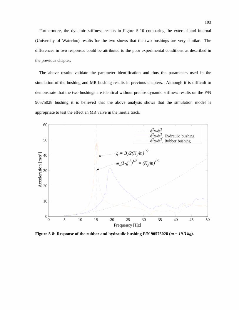
103

Furthermore, the dynamic stiffness results in Figure 5-10 comparing the external and internal

(University of Waterloo) results for the two shows that the two bushings are very similar. The

differences in two responses could be attributed to the poor experimental conditions as described in

the previous chapter.

The above results validate the parameter identification and thus the parameters used in the

simulation of the bushing and MR bushing results in previous chapters. Although it is difficult to

demonstrate that the two bushings are identical without precise dynamic stiffness results on the P/N

90575028 bushing it is believed that the above analysis shows that the simulation model is

appropriate to test the effect an MR valve in the inertia track.

0 5 10 15 20 25 30 35 40 45 500

10

20

30

40

50

60

Acc

eler

atio

n [m

/s²]

Frequency [Hz]

ωn(1-ζ 2)1/2 = (Kr/m)1/2

ζ = Br/2(Kr/m)1/2

d2y/dt2

d2x/dt2, Hydraulic bushingd2x/dt2, Rubber bushing

Figure 5-8: Response of the rubber and hydraulic bushing P/N 90575028 (m = 19.3 kg).

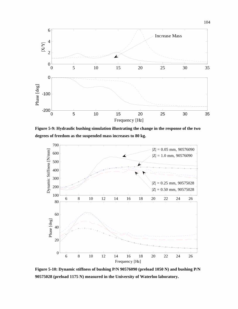
104

0 5 10 15 20 25 30 35-200

-100

0

Phas

e [d

eg]

Frequency [Hz]

0 5 10 15 20 25 30 350

2

4

6

|X/Y

| Increase Mass

Figure 5-9: Hydraulic bushing simulation illustrating the change in the response of the two

degrees of freedom as the suspended mass increases to 80 kg.

6 8 10 12 14 16 18 20 22 24 26100

200

300

400

500

600

700

Dyn

amic

Stif

fnes

s [N

/mm

] |Z| = 0.05 mm, 90576090

|Z| = 0.25 mm, 90575028|Z| = 0.50 mm, 90575028

|Z| = 1.0 mm, 90576090

6 8 10 12 14 16 18 20 22 24 260

20

40

60

80

Phas

e [d

eg]

Frequency [Hz] Figure 5-10: Dynamic stiffness of bushing P/N 90576090 (preload 1050 N) and bushing P/N

90575028 (preload 1175 N) measured in the University of Waterloo laboratory.

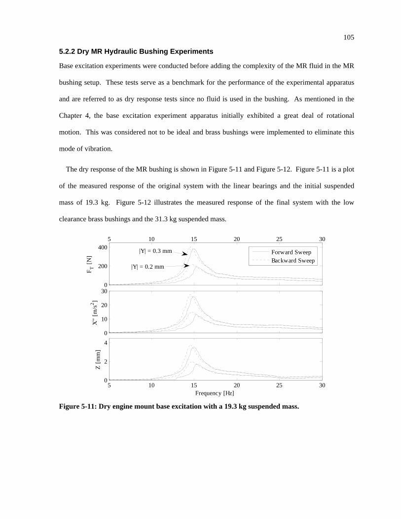
105

5.2.2 Dry MR Hydraulic Bushing Experiments

Base excitation experiments were conducted before adding the complexity of the MR fluid in the MR

bushing setup. These tests serve as a benchmark for the performance of the experimental apparatus

and are referred to as dry response tests since no fluid is used in the bushing. As mentioned in the

Chapter 4, the base excitation experiment apparatus initially exhibited a great deal of rotational

motion. This was considered not to be ideal and brass bushings were implemented to eliminate this

mode of vibration.

The dry response of the MR bushing is shown in Figure 5-11 and Figure 5-12. Figure 5-11 is a plot

of the measured response of the original system with the linear bearings and the initial suspended

mass of 19.3 kg. Figure 5-12 illustrates the measured response of the final system with the low

clearance brass bushings and the 31.3 kg suspended mass.

5 10 15 20 25 30

0

200

400

F T [N

]

|Y| = 0.3 mm

|Y| = 0.2 mm

0

10

20

30

X''

[m/s

2 ]

5 10 15 20 25 300

2

4

Z [m

m]

Frequency [Hz]

Forward SweepBackward Sweep

Figure 5-11: Dry engine mount base excitation with a 19.3 kg suspended mass.

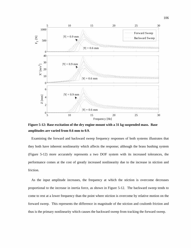
106

5 10 15 20 25 30

0

500

1000

F T [N

] |Y| = 0.9 mm

|Y| = 0.6 mm

0

10

20

30

40

X''

[m/s

2 ]

|Y| = 0.6 mm

|Y| = 0.9 mm

5 10 15 20 25 300

2

4

6

Z [m

m]

Frequency [Hz]

|Y| = 0.6 mm

|Y| = 0.9 mm

Forward Sweep

Backward Sweep

Figure 5-12: Base excitation of the dry engine mount with a 31 kg suspended mass. Base

amplitudes are varied from 0.6 mm to 0.9.

Examining the forward and backward sweep frequency responses of both systems illustrates that

they both have inherent nonlinearity which affects the response; although the brass bushing system

(Figure 5-12) more accurately represents a two DOF system with its increased tolerances, the

performance comes at the cost of greatly increased nonlinearity due to the increase in stiction and

friction.

As the input amplitude increases, the frequency at which the stiction is overcome decreases

proportional to the increase in inertia force, as shown in Figure 5-12. The backward sweep tends to

come to rest at a lower frequency than the point where stiction is overcome by relative motion on the

forward sweep. This represents the difference in magnitude of the stiction and coulomb friction and

thus is the primary nonlinearity which causes the backward sweep from tracking the forward sweep.

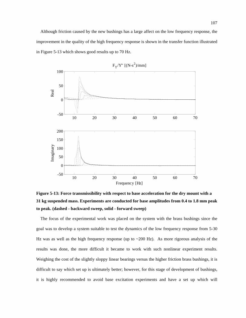
107

Although friction caused by the new bushings has a large affect on the low frequency response, the

improvement in the quality of the high frequency response is shown in the transfer function illustrated

in Figure 5-13 which shows good results up to 70 Hz.

10 20 30 40 50 60 70-50

0

50

100FT/Y'' [(N-s2)/mm]

Real

10 20 30 40 50 60 70-50

0

50

100

150

200

Imag

inar

y

Frequency [Hz]

Figure 5-13: Force transmissibility with respect to base acceleration for the dry mount with a

31 kg suspended mass. Experiments are conducted for base amplitudes from 0.4 to 1.8 mm peak

to peak. (dashed - backward sweep, solid - forward sweep)

The focus of the experimental work was placed on the system with the brass bushings since the

goal was to develop a system suitable to test the dynamics of the low frequency response from 5-30

Hz was as well as the high frequency response (up to ~200 Hz). As more rigorous analysis of the

results was done, the more difficult it became to work with such nonlinear experiment results.

Weighing the cost of the slightly sloppy linear bearings versus the higher friction brass bushings, it is

difficult to say which set up is ultimately better; however, for this stage of development of bushings,

it is highly recommended to avoid base excitation experiments and have a set up which will

108

accurately measure the dynamic stiffness thus reducing the amount of nonlinearity to a more

manageable level.

5.2.3 MR Hydraulic Bushing Experiments

Figures 5-14 to 5-17 illustrate the effect of varying current on the base acceleration and relative

motion of the MR bushing for both experiment setups and the transmitted force for the base excitation

setup with the brass bushings.

The initial result, illustrated in Figure 5-14, shows the base excitation response of the system given

the linear bearings and a 19.3 kg suspended mass. Although the solenoid was designed to yield

approximately 580 turns of 26 gauge wire only 335 turns where achieved on the initial

implementation of the actual design. The current is incremented from 0 to 2 A, and given by the

frequency response the MR valve appears to saturate between 1 and 2 A.

The result for the initial test illustrate that the impact of the MR effect on the base excitation

response is minimal. However, both the acceleration and displacement response do demonstrate the

two degrees of freedom of the MR hydraulic bushing; where the damped modal natural frequencies

are approximately:

1 17.3ω = Hz and 2 18.7ω = Hz (5.6)

for the off state (0 A) response shown in blue. Furthermore, as the amount of current increases these

frequencies appear to decrease and the peak vibration amplitude increases. This observation is in

direct agreement with the MR hydraulic bushing dynamic stiffness nonlinear simulation results

presented in Chapter 3 which shows a downward shift of the notch frequencies and increase in

dynamic stiffness as the current is increased. Moreover, as shown in the dynamic stiffness simulation

results of Chapter 3 amount of damping reduces as the valve current increases which causes the

increase in vibration amplitude.

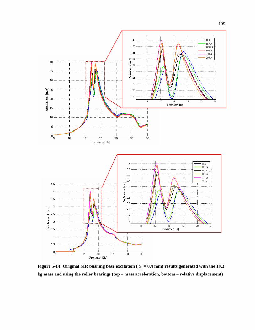
109

Figure 5-14: Original MR bushing base excitation (|Y| = 0.4 mm) results generated with the 19.3

kg mass and using the roller bearings (top – mass acceleration, bottom – relative displacement)

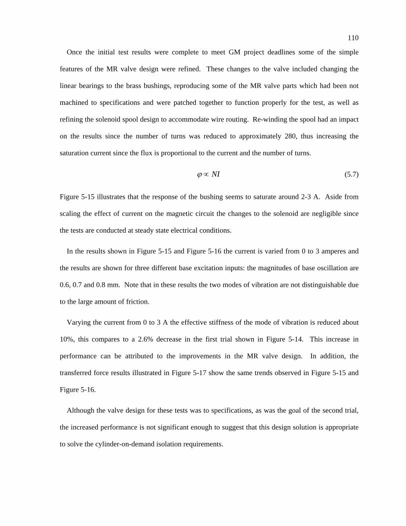
110

Once the initial test results were complete to meet GM project deadlines some of the simple

features of the MR valve design were refined. These changes to the valve included changing the

linear bearings to the brass bushings, reproducing some of the MR valve parts which had been not

machined to specifications and were patched together to function properly for the test, as well as

refining the solenoid spool design to accommodate wire routing. Re-winding the spool had an impact

on the results since the number of turns was reduced to approximately 280, thus increasing the

saturation current since the flux is proportional to the current and the number of turns.

NIϕ ∝ (5.7)

Figure 5-15 illustrates that the response of the bushing seems to saturate around 2-3 A. Aside from

scaling the effect of current on the magnetic circuit the changes to the solenoid are negligible since

the tests are conducted at steady state electrical conditions.

In the results shown in Figure 5-15 and Figure 5-16 the current is varied from 0 to 3 amperes and

the results are shown for three different base excitation inputs: the magnitudes of base oscillation are

0.6, 0.7 and 0.8 mm. Note that in these results the two modes of vibration are not distinguishable due

to the large amount of friction.

Varying the current from 0 to 3 A the effective stiffness of the mode of vibration is reduced about

10%, this compares to a 2.6% decrease in the first trial shown in Figure 5-14. This increase in

performance can be attributed to the improvements in the MR valve design. In addition, the

transferred force results illustrated in Figure 5-17 show the same trends observed in Figure 5-15 and

Figure 5-16.

Although the valve design for these tests was to specifications, as was the goal of the second trial,

the increased performance is not significant enough to suggest that this design solution is appropriate

to solve the cylinder-on-demand isolation requirements.

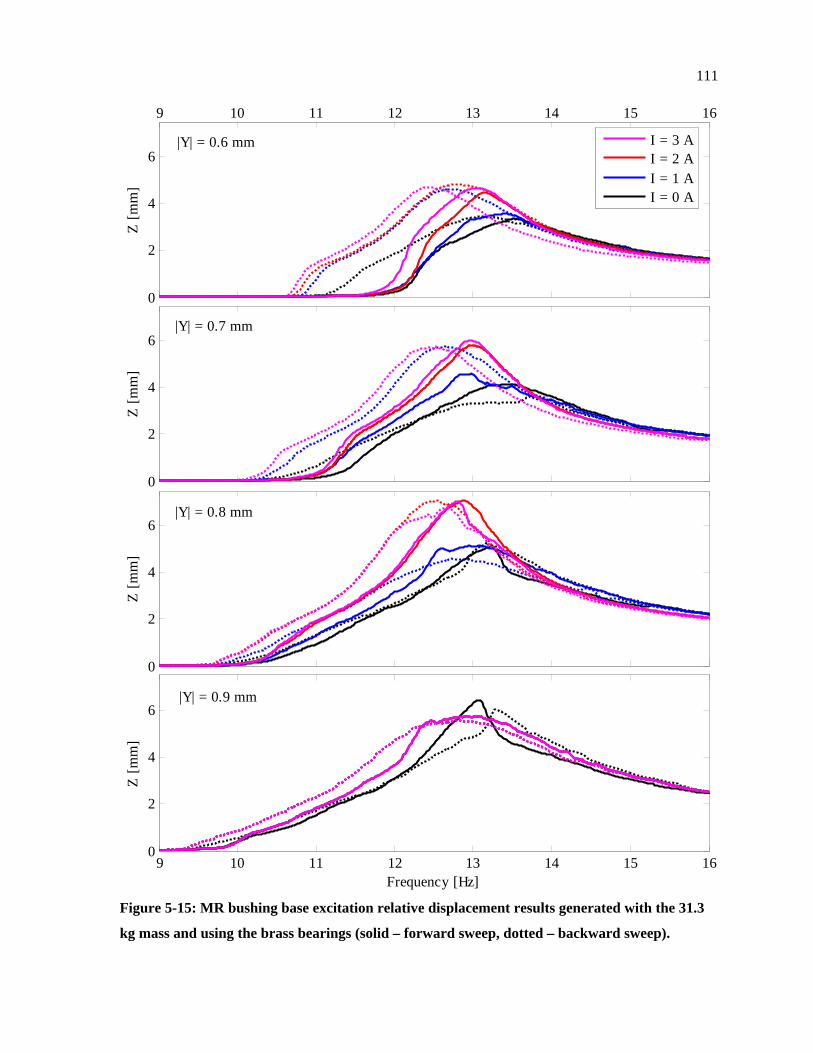
111

9 10 11 12 13 14 15 16

0

2

4

6

Z [m

m]

0

2

4

6

Z [m

m]

0

2

4

6

Z [m

m]

9 10 11 12 13 14 15 160

2

4

6

Z [m

m]

Frequency [Hz]

I = 3 AI = 2 AI = 1 AI = 0 A

|Y| = 0.9 mm

|Y| = 0.8 mm

|Y| = 0.7 mm

|Y| = 0.6 mm

Figure 5-15: MR bushing base excitation relative displacement results generated with the 31.3

kg mass and using the brass bearings (solid – forward sweep, dotted – backward sweep).

112

9 10 11 12 13 14 15 16

0

10

20

30

40d2 x/

dt2 [m

/s2 ]

0

10

20

30

40

d2 x/dt

2 [m/s

2 ]

0

10

20

30

40

d2 x/dt

2 [m/s

2 ]

9 10 11 12 13 14 15 160

10

20

30

40

d2 x/dt

2 [m/s

2 ]

Frequency [Hz]

I = 3 AI = 2 AI = 1 AI = 0 A

|Y| = 0.6 mm

|Y| = 0.7 mm

|Y| = 0.8 mm

|Y| = 0.9 mm

Figure 5-16: MR bushing base excitation mass acceleration results generated with the 31.3 kg

mass and using the brass bearings (solid – forward sweep, dotted – backward sweep).

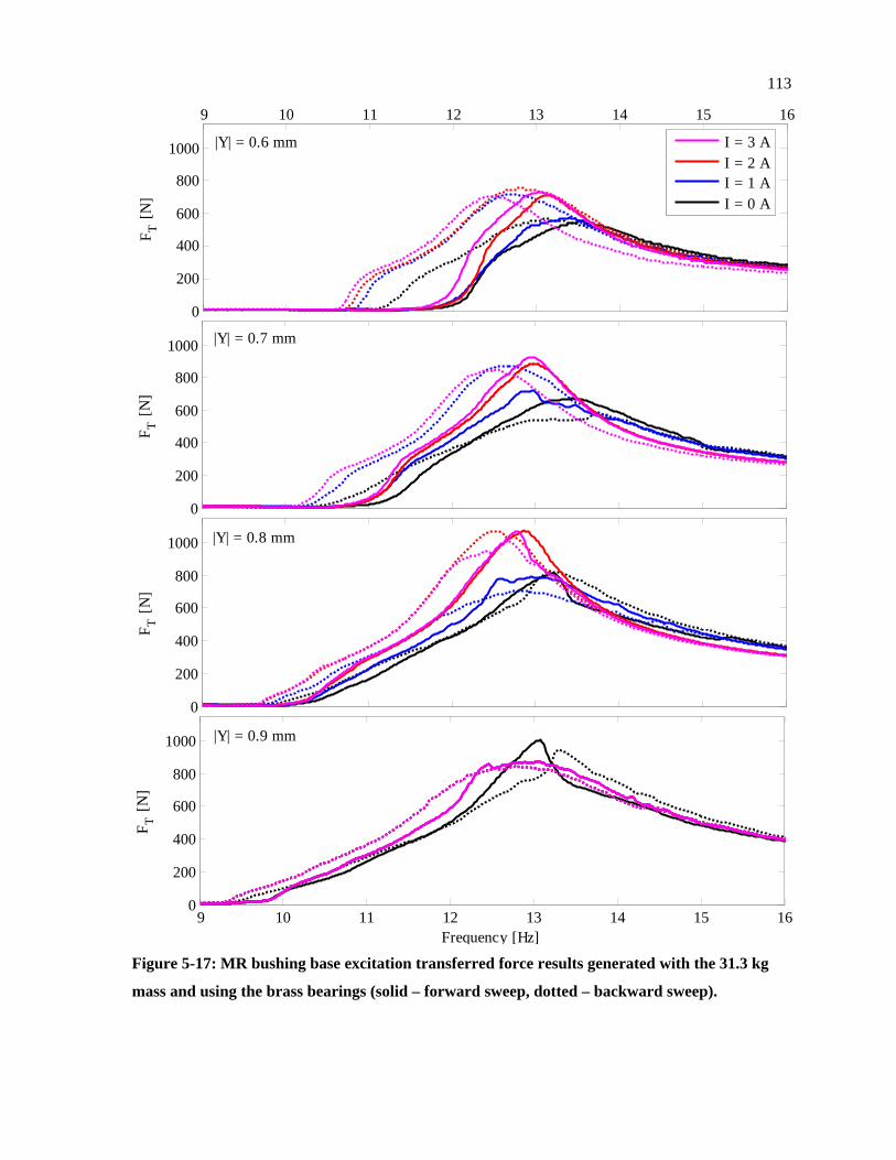
113

9 10 11 12 13 14 15 16

0

200

400

600

800

1000F T

[N]

0

200

400

600

800

1000

F T [N

]

|Y| = 0.7 mm

0

200

400

600

800

1000

F T [N

]

|Y| = 0.8 mm

9 10 11 12 13 14 15 160

200

400

600

800

1000

F T [N

]

Frequency [Hz]

|Y| = 0.9 mm

I = 3 AI = 2 AI = 1 AI = 0 A

|Y| = 0.6 mm

Figure 5-17: MR bushing base excitation transferred force results generated with the 31.3 kg

mass and using the brass bearings (solid – forward sweep, dotted – backward sweep).

114

5.3 Summary

In section 5.2, the theoretical RMS optimization results are shown to be applicable to a real system.

Base excitation and rotating unbalance input experiment results show that the minimum of the RMS

of absolute acceleration and force transmitted occur at similar damping ratios. These two theoretical

results are verified with a single experiment as described in Chapter 4. The experiment results also

verify the harmonic forcing RMS optimization curves.

Base excitation experiment results are shown for the purchased bushing, as well as the prototype

MR bushing. The performance of the two hydraulic bushings (P/N 90576090 and 90575028) are

compared by examining the static stiffness of the rubber as well as the dynamic stiffness. The static

stiffness is found to be very similar. The dynamic stiffness is also quite similar and the difference in

performance is attributed to the poor dynamic stiffness testing facilities used for bushing P/N

90575028; otherwise, the results show that the bushings are very similar.

Finally, the first and second attempts at producing MR bushing results yield the same performance

despite improvement to the MR valve in the second trial. The MR bushing has a relatively small

effect on the performance of the base excitation system. It is found that as the current input increases

the peak acceleration and displacement also increase. These frequencies of the peaks also shift down

by approximately 10% over the full variation of current. This is explained by the decrease in

damping associated with the decrease in fluid flowing through the inertia track when the valve is

functioning, as per the MR dynamic stiffness simulation results shown in Chapter 3.

115

Chapter 6 Conclusions and Future Work

The purpose of this thesis is to investigate the application of MR technology in the area of engine

isolation. Semi-active engine hydraulic bushings are required to meet new performance requirements

associated with cylinder deactivation engines. When the engine control unit (ECU) changes the

number of cylinders firing the magnitude of the forcing changes requiring different bushing

properties. Also, transient vibrations resulting from torsional loading during the process of activating

and deactivation cylinders need to be better controlled with a MR bushing.

6.1 RMS Optimization

The design of engine isolators in general has been approached by examining the frequency

response of three fundamental inputs which represent the basic inputs experienced in a vehicle: base

excitation from the body or chassis, unbalance forces from the rotating engine components, and

harmonic forcing representing the engine combustion forces. Previous researchers found that plotting

the RMS acceleration versus RMS displacement of a single DoF oscillator under base excitation for a

given stiffness reveals that there exists an optimum damping ratio which minimizes the RMS

acceleration. This result was verified experimentally in Chapter 5 of this thesis. It is also

documented previously (Section 2.1.2) that adding negative cubic stiffness to a linear oscillator

greatly improves the performance in the frequency domain. Cubic damping was found to have very

little positive effect on the frequency response relative to cubic stiffness.

Similar to the base excitation optimization study, harmonic forcing and rotating unbalance forcing

each were found to have a damping ratio for a given stiffness which would yield a minimum RMS

transmitted force. This result was also confirmed experimentally. It is important to note that the base

excitation and rotating unbalance systems have common optimum points. Furthermore, cubic

damping had little effect on the forced frequency response of the isolator whereas negative cubic

116

stiffness was found to greatly improve the isolation of harmonic forcing inputs as was found in the

base excitation case mentioned above.

The time domain response of the cubic nonlinear system also demonstrated some interesting

behavior. While the cubic damping and especially the cubic stiffness were found to have large

influence on the frequency response they seemed to have negligible effect on the response to step and

impulse inputs as illustrated by the numerical simulation results. The time domain response appears

to be dominated by the linear stiffness and damping. This property of slightly cubic nonlinear is not

confirmed experimentally; however it suggest that linear stiffness and damping coefficients can be

selected to provide optimal time domain response and small amounts of cubic stiffness could be

added to improve the frequency response (or steady state performance).

The progress made in area of linear optimization shows how optimum semi-active damping ratios

could selected based on the dominance of the input – being either predominantly base excitation,

unbalance, or harmonic forcing. Of course, semi-active control is not possible without some ability to

sense these states either using accelerometers installed on the bushing, feedback from the ECU, or

possibly even tracking the vehicle driver inputs to estimate the vibration conditions under the hood.

The cubic nonlinear RMS study shows how feedback could be used to create controlled nonlinearity

in a semi-active system and greatly improve performance.

Most importantly, the RMS optimization technique was applied to the design of hydraulic

bushings. For a specific case with assumed effective engine mass the RMS optimization of the

bushing revealed that the inertia track length of the bushing under study could be tuned (a 20 %

decrease in length) to improve the RMS acceleration by approximately 4.4 % and RMS displacement

by 5.1 % under base excitations. Also, this tuning of the inertia track would decrease RMS force

transmitted by 12 % with a marginal increase in RMS displacement of the engine of 0.7 % in the case

of harmonic forcing. Further study is needed to investigate whether this is a practical way to design

hydraulic engine bushings.

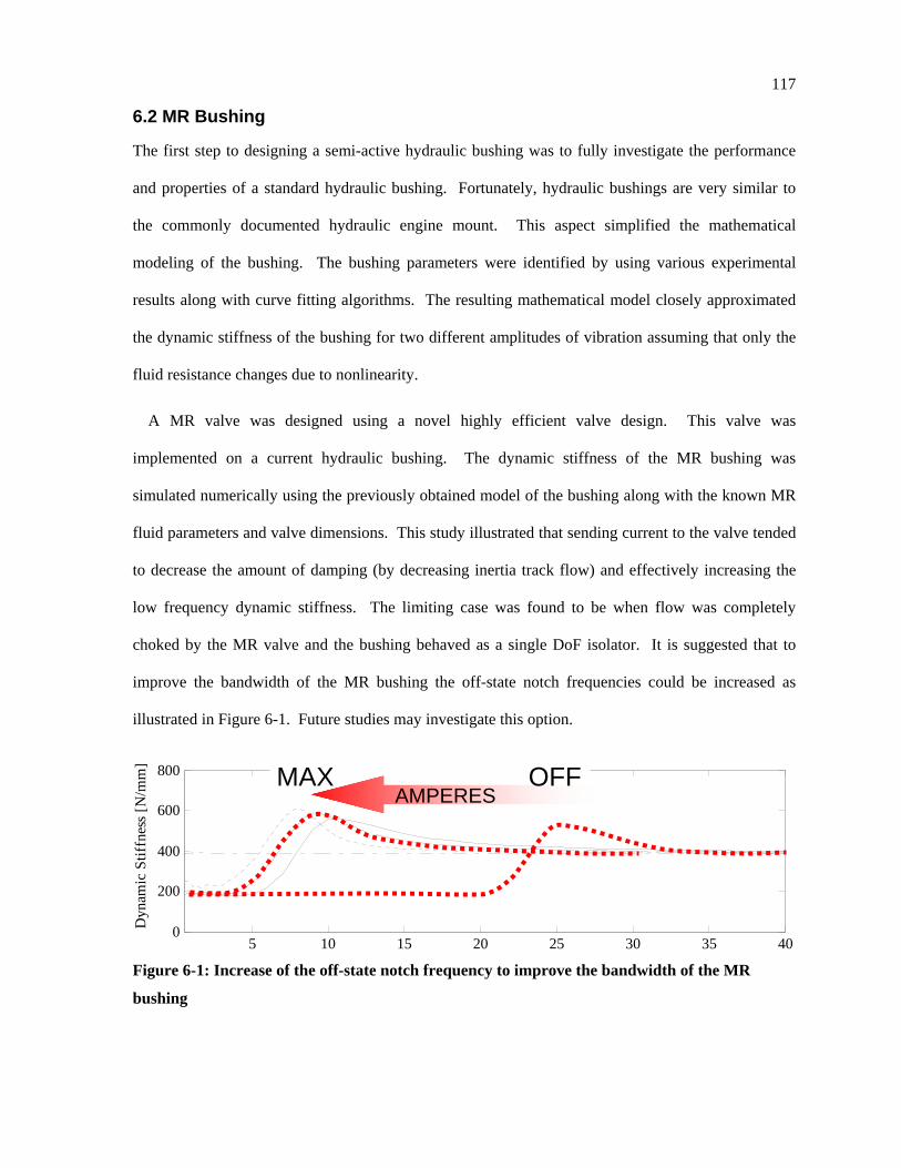
117

6.2 MR Bushing

The first step to designing a semi-active hydraulic bushing was to fully investigate the performance

and properties of a standard hydraulic bushing. Fortunately, hydraulic bushings are very similar to

the commonly documented hydraulic engine mount. This aspect simplified the mathematical

modeling of the bushing. The bushing parameters were identified by using various experimental

results along with curve fitting algorithms. The resulting mathematical model closely approximated

the dynamic stiffness of the bushing for two different amplitudes of vibration assuming that only the

fluid resistance changes due to nonlinearity.

A MR valve was designed using a novel highly efficient valve design. This valve was

implemented on a current hydraulic bushing. The dynamic stiffness of the MR bushing was

simulated numerically using the previously obtained model of the bushing along with the known MR

fluid parameters and valve dimensions. This study illustrated that sending current to the valve tended

to decrease the amount of damping (by decreasing inertia track flow) and effectively increasing the

low frequency dynamic stiffness. The limiting case was found to be when flow was completely

choked by the MR valve and the bushing behaved as a single DoF isolator. It is suggested that to

improve the bandwidth of the MR bushing the off-state notch frequencies could be increased as

illustrated in Figure 6-1. Future studies may investigate this option.

Figure 6-1: Increase of the off-state notch frequency to improve the bandwidth of the MR

bushing

5 10 15 20 25 30 35 400

200

400

600

800

Dyn

amic

Stif

fnes

s [N

/mm

] OFFMAX AMPERES

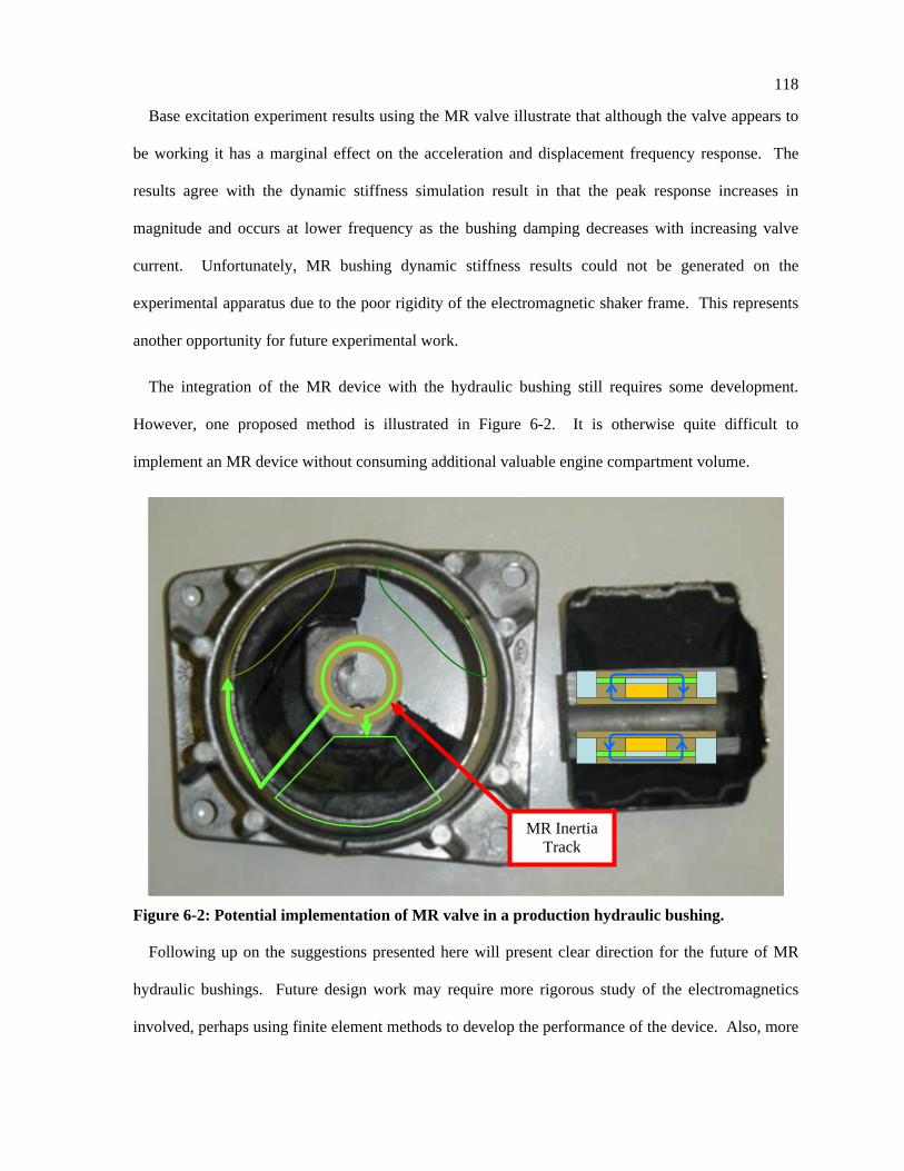
118

Base excitation experiment results using the MR valve illustrate that although the valve appears to

be working it has a marginal effect on the acceleration and displacement frequency response. The

results agree with the dynamic stiffness simulation result in that the peak response increases in

magnitude and occurs at lower frequency as the bushing damping decreases with increasing valve

current. Unfortunately, MR bushing dynamic stiffness results could not be generated on the

experimental apparatus due to the poor rigidity of the electromagnetic shaker frame. This represents

another opportunity for future experimental work.

The integration of the MR device with the hydraulic bushing still requires some development.

However, one proposed method is illustrated in Figure 6-2. It is otherwise quite difficult to

implement an MR device without consuming additional valuable engine compartment volume.

Figure 6-2: Potential implementation of MR valve in a production hydraulic bushing.

Following up on the suggestions presented here will present clear direction for the future of MR

hydraulic bushings. Future design work may require more rigorous study of the electromagnetics

involved, perhaps using finite element methods to develop the performance of the device. Also, more

MR Inertia Track

119

detailed mechanical design work is also required to move the existing MR valve design from the

prototype to production phase.

If future work finds that the MR valve does not meet the requirements of the cylinder deactivation

application it is shown that increasing the compliance of the pumping chamber of the bushing by a

factor of 4 could reduce the dynamic stiffness by approximately 50%. This could possibly be

achieved by implementing a MR valve used to connect the pumping chamber to a much more

compliant chamber. This concept is essentially an active decoupler, where the passive decoupler is

found in the common hydraulic engine mount as described in Chapter 2. Note that this application of

MR fluid would require a MR valve which is quite different from the valve presented in this work.

However, it should also be noted that since a valve would be required to be normally open (with no

current) in this alternative design the bushing would be permanently soft in the event of failure. This

is shown to result in extremely high amplitudes of vibration. This effect may also cause this bushing

design to consume relatively high amounts of power if the hard, or valve closed, state is the

predominant state.

120

Bibliography

Alkhatib, R., Jazar, G.N., & Golnaraghi, M.F. (2004, August 23). Optimal design of passive linear

suspension using genetic algorithm. Journal of Sound and Vibration, 275(3-5), 665-691.

Ahn, Y.K., Ahmadian, M., & Morishita, S. (1999). On the Design and Development of a Magneto-

Rheological Mount. Vehicle System Dynamics, 32, 199-216.

Ahmadian, M., & Ahn, Y.K. (1999, March). Performance Analysis of Magneto-Rheological Mounts,

Journal of Intelligent Material Systems and Structures, 10, 248-256.

Andrews, F. J. (2002, January). A primer on vibration isolation. Sound and Vibration, 36(1), 42-46.

Ashley, S. (2004, December). Firing on half-cylinders. Scientific American, 291(6), 20-22.

Askeland, D.R. (1996). The Science and Engineering of Materials (3rd S.I. ed.). London: Chapman

and Hall.

Baudendistel, T.A., Tewani, S.G., Shores, J.M., Long, M.W., Longhouse, R.E., Namuduri, C.S., &

Alexandridis, A.A. (2002). Hydraulic mount with magnetorheological fluid. US Patent

0171186.

Carlson, D.J., Chrzan, M.J., & James, F.O. (1994). Magnetorheological fluid devices. US Patent

5284330.

Choi, S.B., Lee, H.H., Song, H.J., & Park, J.-S. (2002). Vibration Control of a Passenger Car Using

MR Engine Mounts. Smart Structures and Material, 4701, 1-8.

Choi, S.B., Song, H.J., Lee, H.H., Lim, S.C., & Kim, H.J. (2003). Vibration control of a passenger

vehicle featuring magnetorheological engine mounts. International Journal of Vehicle Design,

33(1-3), 2-16.

121

Colgate, J.E., Chang, C.-T., Chiou, Y.-C., Liu, W.K., & Keer, L.M. (1995, July 20). Modelling of a

hydraulic engine mount focusing on response to sinusoidal and composite excitations. Journal

of Sound and Vibration, 184(3), 503-528.

Flower, W.C. (1985). Understanding Hydraulic Mounts for Improved Vehicle Noise, Vibration and

Ride Qualities. Surface Vehicle Noise and Vibration Conference Proceedings (pp. 123-132).

Traverse City, MI: Society of Automotive Engineers.

Foumani, M.S., Khajepour, A., & Durali, M. (2004). A New High-Performance Adaptive Engine

Mount. Journal of Vibration and Control, 10(1), 39-54.

Geisberger, A.A. (2000). Hydraulic Engine Mount Modeling, Parameter Identification and

Experimental Validation (MASc. Thesis). Waterloo, ON, CA: University of Waterloo.

Geisberger, A., Khajepour, A., Golnaraghi, F. (2002, January 10). Non-linear modelling of hydraulic

mounts: Theory and experiment. Journal of Sound and Vibration, 249(2), 371-397.

Golnaraghi, M.F., & Jazar, G.N. (2001, May). Development and analysis of a simplified nonlinear

model of a hydraulic engine mount. Journal of Vibration and Control, 7(4), 495-526.

Golnaraghi, M.F., & Jazar, N.G. (2002). Nonlinear modeling, experimental verification, and

theoretical analysis of a hydraulic engine mount. Journal of Vibration and Control, 8(1), 87-

116.

Gorodkin, S., Lukianovich, A., & Kordonski, W. (1998, August). Magnetorheological Throttle Valve

in Passive Damping Systems. Journal of Intelligent Material Systems and Structures, 9.

Halliday, D., Resnick, R., & Walker, J. (1997). Fundamentals of Physics: Extended (5th ed.). New

York: John Wiley and Sons Inc..

122

Hardie, C., Tait, H., Craig, S., Chase, J.G., Smith, B.W., & Harris, G. (2002). Automated tuning of

an engine management unit for an automotive engine. Journal of Automobile Engineering,

216(10), 841-849.

Hong, S.R., Choi, S.B., Jung, W.J., Ham, I.B., & Kim, D.K. (2001). Vibration of an ER Mount

Subjected to High Static Loads. Journal of Sound and Vibration, 242(4), 740-748.

Inman, D. J. (2001). Engineering vibration, (2nd ed.). Upper Saddle River, N.J.:Prentice Hall.

Jackson, M.D., & Jones, P. (1976, August 2). Deactivating Compressor-Engine Cylinders Saves

Fuel. Oil and Gas Journal, 74(31), 130-133.

Jazar, G.N., & Golnaraghi, M.F. (2002, September). Engine Mounts for Automotive Applications: A

Survey. The Shock and Vibration Digest, 34(5), 363-379.

Jazar, G.N., Narimani, A., Golnaraghi, M.F., & Swanson, D.A. (2003). Practical Frequency and Time

Optimal Design of Passive Linear Vibration Isolation Mounts. Vehicle System Dynamics,

39(6), 437-466.

Kim, G., & Singh, R. (1993, September). Nonlinear analysis of automotive hydraulic engine mount.

Journal of Dynamic Systems, Measurement and Control, Transactions of the ASME, 115(3),

482-487.

Kim, G., & Singh, R. (1995, January 19). Study of passive and adaptive hydraulic engine mount

systems with emphasis on non-linear characteristics. Journal of Sound and Vibration, 179(3),

427-453.

Kordonsky, W.I., Gorodkin, S.R., Kolomentsev, A.V., Kuzmin, V.A., Luk’ianovich, A.V.,

Protasevich, N.A., Prokhorov, I.V., & Zinovii, P.S. (1995). Magnetorheological valve and

devices incorporation magnetorheological elements. US Patent 5452745.

123

Kuzhir, P., Bossis, G., & Bashtovoi, V. (2003, November/December). Effect of the orientation of the

magnetic field on the flow of a magnetorheological fluid. I. Plane channel. Journal of

Rheology, 47(6), 1373-1384.

Kuzhir, P., Bossis, G., Bashtovoi, V., & Volkova, O. (2003, November/December). Effect of the

orientation of the magnetic field on the flow of magnetorheological fluid. II. Cylindrical

channel. Journal of Rheology, 47(6), 1385-1398

Lee, Y.-W., & Lee, C.-W. (2002). Dynamic analysis and control of an active engine mount system.

Proceedings of the Institution of Mechanical Engineers, Part D: Journal of Automobile

Engineering (pp. 921-931), 216(11). Professional Engineering Publishing.

Lin, Y., Luo, W., & Zhang, Y.M. (1990, July). New method for the optimization of a vibration

isolation system. Journal of Vibration, Acoustics, Stress, and Reliability in Design, 112,(3),

413-416.

Lord Corporation. (1999). Engineering Note: Designing with MR Fluids, Materials Division (rev.

12).

Madjlesi, R., Schubert, B., Khajepour, A., & Ismail, F. (2003). A new approach in mounting systems

optimization. American Society of Mechanical Engineers, Dynamic Systems and Control

Division (Publication) DSC, 72(2), 963-970.

Matsuoka, H., Mikasa, T., Nemoto, H., & Gehm, R. (Ed.) (2004, September). Bringing down the

noise. Automotive Engineering International, 112(9), 83-87.

Muller, M., Weltin, U., Law, D., Roberts, M.M., & Siebler, T.W. (1994, July). Engine mounts and

NVH. Automotive Engineering, 102(7), 19-23.

Narimani, A. (2004). Development of Linear and Nonlinear Isolation Techniques for passive and

Semi-Active Application (Ph.D. Dissertation). Waterloo, ON, CA: University of Waterloo.

124

Narimani, A., & Golnaraghi, M. F. (2004). Nonlinear Isolator Optimization Using RMS Cost

Function. International Mechanical Engineering Congress and R&D Expo (Paper No

IMECE2004-61314). Anaheim, California: ASME.

Narimani, A., Golnaraghi, M.F., & Jazar, G. N. (2004, February). Sensitivity analysis of the

frequency response of a piecewise linear system in a frequency island. Journal of Vibration

and Control, 10(2), 175-198.

Nayfeh, A. H. (1981). Introduction to perturbation techniques. New York: Wiley.

Nayfeh, A. H., & Mook, D.T. (1979). Nonlinear Oscillations. New York: Wiley.

Nayfeh, T.A., Emaci, E., & Vakakis, A.F. (1997, August). Application of nonlinear localization to the

optimization of a vibration isolation system. AIAA Journal, 35(8), 1378-1386.

Oueini, S.S., Chin, C.-M., & Nayfeh, A.H. (1999, November). Dynamics of a cubic nonlinear

vibration absorber. Nonlinear Dynamics, 20(3), 283-295.

Rao, S. S. (2004). Mechanical vibrations (4th ed.). Upper Saddle River, N.J.: Pearson Prentice Hall.

Singh, R., Kim, G., & Ravindra, P.V. (1992). Linear Analysis of Automotive Hydro-Mechanical

Mount with Emphasis on Decouple Characteristics. Journal of Sound and Vibrations, 158(2),

219-243.

Shtarkmen, E.M. (1993). Vehicle engine mount. US Patent 5176368.

Vahdati, N., & Ahmadian, M. (2003). Single pumper semi-active fluid mount. Proceedings of the

2003 ASME International Mechanical Engineering Congress (pp. 167-175), 72(1).

Washington, DC: American Society of Mechanical Engineers.

Vakakis, A.F., McFarland, D. M., Bergman, L., Manevitch, L., & Gendelman, O. (2003). Passive

vibration control through nonlinear energy pumping. Proceedings of the ASME Design

125

Engineering Technical Conference (pp. 1883-1888), 5. Chicago, IL: American Society of

Mechanical Engineers.

Williams, E.W., Rigby, S.G., Sproston, J.L., & Stanway, R. (1993, June). Electrorheological fluids

applied to an automotive engine mount. Journal of Non-Newtonian Fluid Mechanics, 47, 221-

238.