Embed Size (px)
Citation preview
Development of a Novel Portable Cooling Device for Inducing Mild Hypothermia
by Mayank Kalra
B.A.Sc., University of British Columbia, 2012
Thesis Submitted in Partial Fulfillment of the
Requirements for the Degree of
Master of Applied Science
in the
School of Mechatronic Engineering
Faculty of Applied Sciences
Mayank Kalra 2014
SIMON FRASER UNIVERSITY Summer 2014

ii
Approval
Name: Mayank Kalra Degree: Master of Applied Science Title: Development of a Novel Portable Cooling Device for
Inducing Mild Hypothermia Examining Committee: Chair: Kevin Oldknow
Lecturer, School of Mechatronic Systems Engineering
Majid Bahrami Co- Supervisor Associate Professor
Carolyn Sparrey Co-Supervisor Assistant Professor
Ryan D’Arcy Internal Examiner Professor School of Engineering Science, School of Computing Science
Date Defended/Approved:
August 12, 2014

iii
Partial Copyright Licence
iv
Abstract
Therapeutic hypothermia is rapidly becoming an integral part of post-resuscitative care
for post-cardiac arrest patients, with cooling increasingly being initiated in the pre-
hospital setting in order to improve patient outcome. However, commercially available
devices are not sufficiently portable or do not provide enough cooling power.
Additionally, despite the significant impact of thermoregulation on core temperature
change during rapid cooling, current mathematical models for thermoregulation have not
been validated for hypothermic conditions. In the present study, a novel portable cooling
device using adsorption cooling has been proposed, and a prototype was developed to
prove that the concept is feasible. Additionally, a geometrically accurate 3D model of an
upper leg was developed in order to further understand heat transfer in the human body
and to validate thermoregulation models from literature. There was good agreement
between simulation results and experimental data at 18°C water immersion, however,
significant discrepancy was observed at lower temperature.
Keywords: adsorption refrigeration; therapeutic hypothermia; bioheat model; portable cooling; passive cooling system
v
Acknowledgements
I would like to thank my supervisors, Drs. Majid Bahrami and Carolyn Sparrey for
giving me the chance to pursue this area of research, and for their support through my
graduate studies. Their insights and recommendations have been invaluable for getting
the desired results.
I would also like to thank all my colleagues at the Lab for Alternative Energy
Conversion and the Neurospine Biomechanics Lab for their support. In particular, I
would like to thank Marius Haiducu and Dr. Wendell Huttema for their help with setting
up the experiments, Dr. Claire McCague for her help with adsorbent material
development and characterization, Mehran Ahmadi for his help with setting up COMSOL
Multiphysics simulations, Amir Sharafian for sharing his expertise on adsorption
refrigeration, and Cecilia Berlanga for helping with experiments and data analysis.
I would like to thank Dr. Peter Tikuisis at Defence Research and Development
Canada for providing unpublished experimental data for water immersion at 18°C, and
Dr. Michael English at McGill University for providing unpublished experimental data for
cooling blanket analysis. I would like to thank the National Library of Medicine (NLM) and
the Visible Human Project for the anatomical images which were used to construct the
3D model of the upper leg.
This project was financially supported by Natural Sciences and Engineering
Research Council of Canada (NSERC).

vi
Table of Contents
Approval .............................................................................................................................ii Partial Copyright Licence .................................................................................................. iii Abstract .............................................................................................................................iv Acknowledgements ........................................................................................................... v Table of Contents ..............................................................................................................vi List of Tables ................................................................................................................... viii List of Figures....................................................................................................................ix Nomenclature ................................................................................................................... xii Executive Summary ........................................................................................................ xiv
Chapter 1. Introduction ............................................................................................... 1 1.1. Emergence of Pre-hospital Therapeutic Hypothermia ............................................. 1 1.2. Methods of Inducing Hypothermia ............................................................................ 2
1.2.1. In-hospital Methods ..................................................................................... 2 1.2.2. Pre-hospital Methods .................................................................................. 3
1.3. Adsorption-Based Cooling Device Concept ............................................................. 4 1.4. Performance Specifications for a Pre-Hospital hypothermic Cooling System .......... 8 1.5. Understanding Heat Transfer in the Human Body ................................................... 9 1.6. Objectives ................................................................................................................ 9
Chapter 2. Adsorption Cooling Device Development ............................................ 11 2.1. Review of Adsorption Cooling Technology ............................................................. 11
2.1.1. Characterization of Adsorbents ................................................................. 14 2.1.2. Review of Various Adsorbents and their Uptake ....................................... 15
2.2. Approach ................................................................................................................ 18 2.3. Method ................................................................................................................... 19
2.3.1. Small-scale Bench-top Experiment ........................................................... 19 Uptake Measurement Techniques ......................................................................... 19 Custom Thermo-gravimetric Vapour Sorption System .......................................... 21 Experimental Procedure ........................................................................................ 24 Uncertainty Estimation ........................................................................................... 26 Sample Selection and Composite Adsorbent Preparation .................................... 27
2.3.2. Adsorbent Bed Prototype Development .................................................... 28 Key Features of the Prototype Adsorbent Bed ...................................................... 29 Prototype Construction .......................................................................................... 30 Finite Element Simulations of Heat Transfer in Adsorbent bed ............................. 33 Adsorbent Bed Prototype Testing .......................................................................... 37
2.4. Results ................................................................................................................... 39 2.4.1. Custom Thermo-gravimetric System Results ............................................ 39 2.4.2. Adsorbent Bed Prototype Testing Results ................................................ 44
2.5. Discussion .............................................................................................................. 49
Chapter 3. Bioheat Transfer Simulation .................................................................. 53 3.1. Review of Bioheat Transfer Models ....................................................................... 53
vii
3.2. Model Development and Simulation Parameters ................................................... 56 3.3. Simulation Conditions............................................................................................. 62 3.4. Results ................................................................................................................... 65 3.5. Discussion .............................................................................................................. 70
Chapter 4. Discussion & Conclusion ....................................................................... 73 4.1. Discussion .............................................................................................................. 73 4.2. Conclusions & Recommendations ......................................................................... 74
References .................................................................................................................. 76 Appendix. Improving Mass Transfer With Vapor Flow Channels ............................. 85

viii
List of Tables
Table 2.1. Comparison of performance from sorption-based microclimate cooling systems in literature .................................................................... 12
Table 2.2. Characteristics of adsorbent samples tested with the TGA and the custom thermo-gravimetric setup ............................................................ 28
Table 2.3. Properties for adsorption characterization, thermo-physical properties, and dimensions used in the simulations ................................ 35
Table 2.4. Diffusivity values for C030 obtained by fitting transient uptake data from custom thermo-gravimetric system with LDF model at various temperatures ........................................................................................... 44
Table 2.5. Diffusivity values for C030 and K60 obtained by fitting transient uptake data from TGA with LDF model at various temperatures ............ 44
Table 3.1. Thermal properties of tissue implemented in current model .................... 61
Table 3.2. Specifications of experimental cooling studies which are used for validation of the current model ................................................................ 63

ix
List of Figures
Figure 1.1. a) Conceptualization of the proposed adsorption-based portable cooling device showing the adsorbent module and the blanket evaporator, b) Schematic of the adsorbent device showing the flow of water vapor from the evaporator into the adsorbent and the resulting heat flow from the tissue into the evaporator .............................. 6
Figure 1.2. Project roadmap ...................................................................................... 10
Figure 2.1. a) Illustration of backpack-type sorption-based microclimate cooling system [28] and b) cross section of a single pad in the layered-type cooling system [26] ............................................................. 12
Figure 2.2. Comparison of uptake as a function of adsorbent temperature, as experimentally measured in literature for physical and composite adsorbents at water vapor pressure of a) 2.5 kPa and b) 0.87 kPa ........ 17
Figure 2.3. Two techniques currently used to measure vapour sorption: a) thermo-gravimetric [47], and b) constant vapor volume [50] ................... 20
Figure 2.4. Schematic of the custom thermo-gravimetric vapor sorption system ..................................................................................................... 22
Figure 2.5. Components of custom thermo-gravimetric system: a) valve system and pressure transducer, b) filter flask with thermocouples and adsorbent sample, c) filter flask in oil bath with heater and insulation foam, d) Assembly of copper plates and cartridge heater, and e) evaporator assembly (only ABS shell visible) .................. 23
Figure 2.6. Schematic of the circuit used to control the cartridge heater ................... 24
Figure 2.7. Parts used in construction of the adsorbent bed prototype including a) bottom cap plate, b) top plate with gasket, c) perforated internal fin, d) internal fin with mesh attached, and e) single folded fin ........................................................................................ 31
Figure 2.8. Completed adsorbent bed prototype a) isometric view with acrylic lid, and b) top view showing internal fins and gaps for vapor flow ........... 32
Figure 2.9. Geometry of the adsorbent bed heat transfer simulation implemented in COMSOL ........................................................................ 36
Figure 2.10. Results from grid independence study showing variation in average surface heat flux from boundaries exposed to air with varying mesh size assuming a constant volumetric heat generation of 10 kW/m3 in the adsorbent bed ......................................... 36
Figure 2.11. Schematics and pictures of experimental setup for a),c) constant vapor pressure test, and b),d) water bath cooling test. ........................... 39
Figure 2.12. Transient raw data obtained from custom thermo-gravimetric system for 20 grams of C030 (Feb14) showing a) water uptake, b) adsorbent and oil bath temperatures, and c) water vapor pressure ........ 40
x
Figure 2.13. Comparison of equilibrium uptake at water vapor pressure of 1200 Pa and various temperatures for 20 g of B150 with the custom thermo-gravimetric system and 14 mg of B150 with the TGA ................. 41
Figure 2.14. Equilibrium uptake measured with the custom thermo-gravimetric system at 1200 Pa water vapor pressure for different layer thicknesses of a) C024 and b) C030 ....................................................... 42
Figure 2.15. Equilibrium uptake for 20 g sample of C030 measured with custom thermo-gravimetric system compared to measurements with TGA and from literature, as well as comparison with commercial grade silica gel (BLUE) ........................................................ 43
Figure 2.16. Pressure at the inlet of the adsorbent bed during uptake by 950 grams of C030 in prototype adsorbent bed with inlet vapor pressure varying between 1320 and 1820 Pa, and polynomial fit for the pressure trend. ............................................................................. 45
Figure 2.17. Total water uptake by 950 grams of C030 in prototype adsorbent bed with inlet vapor pressure varying between 1320 and 1820 Pa, and 950 grams of BLUE (commercial silica gel) with inlet vapor pressure varying between 1230 and 1870 Pa ......................................... 46
Figure 2.18. Temperature measured on the side of the adsorbent bed with thermocouples spaced vertically by 5 cm during uptake by 950 grams of C030 in prototype adsorbent bed with inlet vapor pressure varying between 1320 and 1820 Pa ......................................... 46
Figure 2.19. Cooling power per kilogram of adsorbent, calculated based on water uptake by 950 grams of C030 in prototype adsorbent bed with inlet vapor pressure varying between 1320 and 1820 Pa ................ 47
Figure 2.20. Results for cooling of a 650 mL bath of water with 950 grams C030 in the adsorbent bed prototype showing a) bath temperature, b) inlet pressure, and c) total water uptake ........................ 48
Figure 3.1. Details of upper leg 3D model showing a) an example of creating a boundary for the muscle in Solidworks by tracing over the Visible Human Dataset figure, b) the solid model including cavities for blood vessels, c) the bone loft surface, and d) the muscle loft surface, and e) segments of the model ................................................... 58
Figure 3.2. Grid independence study for 3D upper leg model showing the variation in average surface heat flux as a function of mesh size for hsurface = 100 W/m2K, and Tambient = 9°C .............................................. 62
Figure 3.3. a) Surface heat flux from the medial and lateral sides of the leg at water immersion temperatures of 18°C and hsurface = 110 W/m2K, and b) surface heat flux from the medial side of the leg of subject 4 compared with simulation results for current model, model with no central vasoconstriction (no CV), model with no local and central vasoconstriction (no CV, no LV) and model with no shivering (no SH). .................................................................................... 66
xi
Figure 3.4. Comparison of medial and lateral heat flux between simulation results and experimental data (Mitchell et al., 1970) at hsurface = 140 W/m2K and a) Tcoolant = 9°C, b) Tcoolant = 4°C, c) Tcoolant = -2°C. Simulations were also run assuming no local vasoconstriction (no LV). .......................................................................................................... 68
Figure 3.5. Contribution of various heat sources to the cumulative heat generation with Tcoolant = 9°C and hsurface = 140 W/m2K in a) current model (including local vasoconstriction), and b) no local vasoconstriction ....................................................................................... 69
Figure 3.6. Comparison of temperature profiles below surface of skin as measured experimentally and from simulation results at immersion temperature of 8°C and hsurface = 110 W/m2K. The last simulation is run assuming ωmuscle is held constant at half the initial value (ω = const). ...................................................................................................... 70
xii
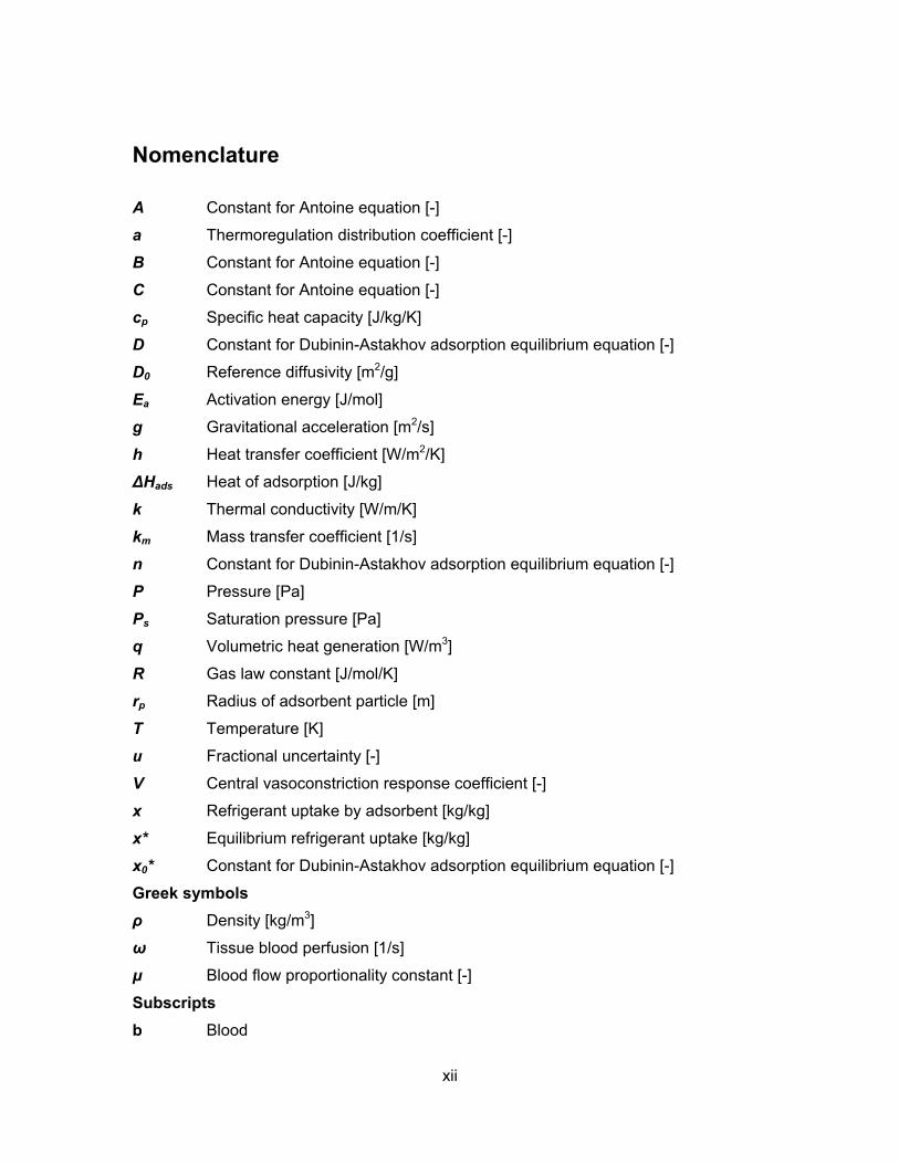
Nomenclature
A Constant for Antoine equation [-]
a Thermoregulation distribution coefficient [-]
B Constant for Antoine equation [-]
C Constant for Antoine equation [-]
cp Specific heat capacity [J/kg/K]
D Constant for Dubinin-Astakhov adsorption equilibrium equation [-]
D0 Reference diffusivity [m2/g]
Ea Activation energy [J/mol]
g Gravitational acceleration [m2/s]
h Heat transfer coefficient [W/m2/K]
ΔHads Heat of adsorption [J/kg]
k Thermal conductivity [W/m/K]
km Mass transfer coefficient [1/s]
n Constant for Dubinin-Astakhov adsorption equilibrium equation [-]
P Pressure [Pa]
Ps Saturation pressure [Pa]
q Volumetric heat generation [W/m3]
R Gas law constant [J/mol/K]
rp Radius of adsorbent particle [m]
T Temperature [K]
u Fractional uncertainty [-]
V Central vasoconstriction response coefficient [-]
x Refrigerant uptake by adsorbent [kg/kg]
x* Equilibrium refrigerant uptake [kg/kg]
x0* Constant for Dubinin-Astakhov adsorption equilibrium equation [-]
Greek symbols ρ Density [kg/m3]
ω Tissue blood perfusion [1/s]
μ Blood flow proportionality constant [-]
Subscripts b Blood

xiii
met Metabolic
sh Shivering
t Tissue

xiv
Executive Summary
Background
Therapeutic Hypothermia is the practice of inducing mild hypothermia after
resuscitation from a cardiac arrest. A multicentre clinical trial in 2002 found that reducing
a patient’s core temperature to 32-34°C for 24 hours after resuscitation increased their
chances of survival by 14%, and improved their neurological outcomes (as measured 6
months after the event). Although the optimal time for inducing hypothermia has not
been clearly established, several preclinical trials have shown that cooling as soon as
possible after the cardiac arrest improves outcomes, leading to increasing adoption of
policies for inducing hypothermia in the pre-hospital setting.
Motivation
The practice of inducing pre-hospital hypothermia has so far mostly relied on
simple methods such as rapid infusion of saline solution at 4°C and surface cooling with
ice packs, but the coolers needed in the ambulance to keep the saline solution or ice
packs cold can weigh between 10-30 kg and take up significant amount of space, which
is a very limited and valuable resource in the ambulance. Medical devices for pre-
hospital cooling such as RhinoChill® Intranasal Cooling System (Benechill, San Diego,
CA), and EMCOOLS cooling pads (EMCOOLS Inc, Vienna, Austria) also weight 10-20
kg, and are too bulky to implement in some ambulances. Consequently, further
improvement in compactness and simplicity of the cooling device can lead to significant
gains in adoption of pre-hospital hypothermia.
Surface cooling is widely considered to be the most non-invasive and clinically
simple method for inducing hypothermia, but surface cooling devices can perform
unpredictably when tested on humans, mainly due to the lack of knowledge about the
thermal response of the human body under hypothermic conditions. Therefore,
validation of a numerical bioheat model which includes thermoregulation parameters
would be a major step towards advancing the ability to predict the performance of a
cooling device for inducing hypothermia.
xv
Goal and Objectives
The goal for the present study is to develop a portable cooling device that can
rapidly cool the patient in the pre-hospital setting. Due to the extensive scope of this
project, the focus of the present study was divided into two main objectives:
development of a 1st generation proof-of-concept prototype for the cooling device, and
validation of a numerical model of transient surface heat loss from a human in
hypothermic conditions by conducting 3D finite element simulations of localized cooling
and comparing results with experimental studies.
The feasibility of the cooling technology for the device was judged based on the
portability, ability to operate without electrical power, and ability to deliver sufficient
cooling power to cool the patient.
Approach
Commercially available cooling technologies are not very suitable for use in the
pre-hospital setting. For example, the vapor-compression refrigeration system is
considerably heavy and requires continuous electrical power, and cold phase-change
materials need to be kept in bulky freezers or replaced daily to keep them cold.
However, a novel technology called adsorption cooling has the potential to be very
lightweight and operate without electrical power or any supporting refrigeration.
The concept that was explored in this project involves the use of a mass of dry
adsorbent (in an adsorbent module) to adsorb water vapor and provide cooling in an
evaporator which can be in the form of a cooling blanket or can be used to cool 1.5-2 L
of saline solution which can be subsequently administered intravenously. A prototype
adsorbent bed containing 1kg of adsorbent was constructed and cooling power over 30
minutes of operation was measured.
In order to validate a numerical model of heat loss from a human, a geometrically
accurate 3D model of the upper leg was developed by manually segmenting transverse
anatomical images of the upper leg from the Visible Human Dataset. Heat transfer in the
geometry was numerically simulated using COMSOL Multiphysics, including
xvi
mathematical models from literature for thermoregulatory mechanisms such as
vasoconstriction and shivering. The boundary conditions replicated conditions from
experimental studies from literature.
Results
Results from testing of the proof-of-concept prototype showed that a cooling
power of 100 W can be achieved for the first 30 minutes from adsorption with 1 kg
adsorbent in the prototype adsorbent bed, so only 2.5 kg of adsorbent would be needed
to provide the 250 W required for hypothermia treatment. Additionally, results show that
2.5 kg of adsorbent would also be sufficient to cool 1.5 L of saline solution from room
temperature to 6°C for intravenous infusion. Effective thermal management and vapor
diffusion in the adsorbent bed were found to be essential to achieve high cooling power.
The bioheat transfer simulation results showed that the current thermoregulatory
models do not accurately predict thermoregulation in hypothermic conditions because
they do not include cold-induced vasodilation and reduction in leg muscle perfusion.
Additionally, model simulations showed that an insignificant amount of cooling was
directly delivered to the blood vessels, indicating that emphasis on uniform cooling over
a large surface area will yield higher cooling rates than targeted cooling of areas with
superficial blood vessels.
Conclusions
Results from the present study indicate that adsorption cooling would be well
suited to provide cooling in a pre-hospital setting. An adsorption-based cooling device
would be very lightweight (6kg or less), and not require any electrical power,
refrigeration, or regular replacement. The device would also be simple to operate by the
EMS, given that only one valve between the adsorbent and the evaporator needs to be
opened to initiate cooling.

1
Chapter 1. Introduction
1.1. Emergence of Pre-hospital Therapeutic Hypothermia
Therapeutic Hypothermia is the practice of inducing mild hypothermia after
resuscitation from a cardiac arrest. A multicentre clinical trial in 2002 found that reducing
a patient’s core temperature to 32-34°C for 24 hours after resuscitation increased their
chances of survival by 14%, and improved their neurological outcomes (as measured 6
months after the event) [1]. Other studies have found similar results [2], and this therapy
has been recommended by the International Liaison Committee on Resuscitation [3].
Some studies have shown that mild systemic hypothermia can also improve outcomes in
stroke, traumatic brain injury, and spinal cord injury [4]–[9].
Therapeutic hypothermia benefits the patient by reducing reperfusion injury,
which is known to act by two separate mechanisms:
• First, during a cardiac arrest, the cessation of blood flow to the brain (known
as ischemia) causes ionic imbalances which leads to cells swelling and
subsequent death a few hours later, irrespective of the state of blood flow [2].
• Second, cerebral blood flow remains abnormally low for a few hours after the
events, which causes prolonged ischemia and significant reduction in oxygen
supply to the brain, causing cell death [10].
Despite strong clinical evidence of the efficacy of therapeutic hypothermia, the
mechanisms by which it reduces the impact of reperfusion injury is not yet clearly known
[2]. The main hypothesis is that hypothermia may reduce the metabolic requirements
(and oxygen consumption) of the brain, since it is clearly established that all types of
tissue have a reduced metabolism when cooled [11].
2
A consequence of the insufficient knowledge about the fundamental mechanisms
of therapeutic hypothermia is the continuing debate about the optimal target temperature
and the effectiveness of cooling earlier. A recent clinical trial compared cooling to 33°C
versus 36°C, and found no significant difference in the outcomes [12]. However, several
aspects of the study have been called into question, including the relatively long time
window of 4 hours between cardiac arrest and initiation of cooling, and the relatively high
rewarming rate [13].
Although the optimal time for inducing hypothermia has not been clearly
established, several animal trials have shown that cooling as soon as possible after the
cardiac arrest improves outcomes [14]. Some human trials for pre-hospital cooling have
reported improvement in patient outcome with faster or earlier cooling, but they were too
small and underpowered to demonstrate statistical significance [14]–[16]. Nonetheless, a
survey of EMS Directors in the US in 2008 revealed that 6.2% of the regions already
induce hypothermia in the pre-hospital setting [17]. Therefore, there is a need to develop
an effective technology for inducing hypothermia during transport to the hospital.
1.2. Methods of Inducing Hypothermia
1.2.1. In-hospital Methods
A 2006 survey of Emergency Physicians in the US showed that the most
prevalent method to induce hypothermia is by surface cooling, with 84% having
previously used commercially available cooling blanket devices, and 60% having used
ice packs applied to the skin [18]. The cooling blanket devices currently available in the
market rely on a vapor-compression refrigeration system which continuously cools the
water that is circulating through the blanket. Examples include: Arctic Sun® Temperature
Management System (Medivance, Louisevill, CO), Medi-therm Hyper/Hypothermia
System (Gaymar, Orchard Park, NY), and Blanketrol (Cincinnati Sub-Zero, Cincinnati,
OH). Other methods for surface cooling include forced air cooling, and packing ice
around the neck, axillae, and groin in order to cool areas with superficial blood vessels
[19], [20].
3
Though surface cooling is simple to implement and non-invasive, the body’s
thermoregulatory responses such as vasoconstriction and shivering frequently prevent
rapid induction of hypothermia. More direct methods of cooling such as endovascular
cooling by administering ice cold intravenous solution or heat exchange catheters can
bypass some or most of the thermoregulatory defences by directly cooling the blood
which is circulated through the core region. Examples of heat exchange catheter
systems include ThermoguardXP (Zoll, San Jose, CA), and the Cool Gard system
(Alsius, Irving, CA). Despite the advantage in cooling rate, administration of ice cold
intravenous solutions is not suitable for the 24-28 hours of continuous cooling required
for therapeutic hypothermia, mainly due to the restriction of maximum volume of fluid
that can be added to the circulatory system without significantly increasing blood
pressure or risking pulmonary edema. Heat exchange catheter systems can provide
rapid and continuous cooling, but the main disadvantage is the significant invasiveness
of the procedure, which limits usage to Intensive Care Units or the OR [20].
The invasiveness of the catheter-based systems makes them unsuitable for the
pre-hospital setting. In addition, the bulkiness and high power consumption of both
catheter-based and blanket-based system renders then unusable in an ambulance.
Therefore, a portable and non-invasive cooling system is required.
1.2.2. Pre-hospital Methods
The practice of inducing pre-hospital hypothermia has so far mostly relied on
simple methods such as rapid infusion of saline solution at 4°C and surface cooling with
ice packs [16], [21]. However, the freezers or large coolers needed in the ambulance to
keep the saline solution or ice packs cold can weigh between 10-30 kg and take up
significant amount of space, which is a very limited and valuable resource in the
ambulance. Additionally, some coolers have an active cooling system which requires
continuous electrical power. Alternatively, insulation-based coolers do not require
electrical power, but they gain heat from the environment over time and the ice packs or
saline solution bags need to be replaced every few hours regardless of usage, which
can be a significant burden for the EMS personnel.
4
Consequently, more innovative and portable devices for rapid cooling have
recently entered the market. The RhinoChill® Intranasal Cooling System (Benechill, San
Diego, CA) is a portable device that injects an evaporative cooling directly into the nasal
cavity via a nasal catheter. Due to the proximity of the nasal cavity to the brain, the
majority of the cooling power is delivered directly to the brain. However, the fully-loaded
RhinoChill system weighs about 10kg, and additional bottles of coolant and carrier
compressed gas are required every 20 minutes to maintain cooling (each coolant and
gas combination weighs an additional 5kg).
The EMCOOLS cooling pads (EMCOOLS Inc, Vienna, Austria) are composed of
phase change material which changes phase at a temperature around -5°C, and can be
applied to the patient’s skin. The direct contact between the phase change material and
the skin causes a rapid cooling, and has shown to not cause any permanent cold injury
to the skin [22]. Besides the weight of the pads themselves (8kg for cooling an adult),
the pads need to be kept in special insulation box in order to maintain the phase change
material at or below -5°C in the ambulance. The insulating box and supporting
infrastructure can weigh up to 15 kg.
Despite the recent improvements in the portability of cooling devices, the size,
weight and complexity of these devices is still the main roadblock for the adoption of pre-
hospital cooling. A survey of US EMS Directors in 2008 showed that the main barriers to
implementation were: lack of refrigeration equipment (60% of respondents), overburden
with other tasks (62%), and the lack of space for cooling equipment (29%) [17]. This
proves that further improvement in compactness and simplicity of the cooling device can
lead to significant gains in adoption of pre-hospital hypothermia.
1.3. Adsorption-Based Cooling Device Concept
Physical adsorption is a process wherein molecules of a vaporized refrigerant
(adsorbate) adhere to the surface of a microporous material (adsorbent) due to weak
surface attraction. Chemical adsorption is similar to physical adsorption except that a
chemical reaction occurs between the adsorbate and adsorbent, i.e. chemical bonds are
broken and formed in the process. The adsorption processes can be used to provide
5
cooling by adsorbing refrigerant from an evaporator, where the evaporation of the
refrigerant (an endothermic process) creates cooling in the evaporator. The total amount
of refrigerant that can be adsorbed by an adsorbent (known as adsorption capacity or
equilibrium uptake) decreases as adsorbent temperature increases, thus adsorbents can
be “dried out” at high temperatures, making the adsorbate and adsorbent reusable..
The concept that was explored in this project involves the use of a mass of dry
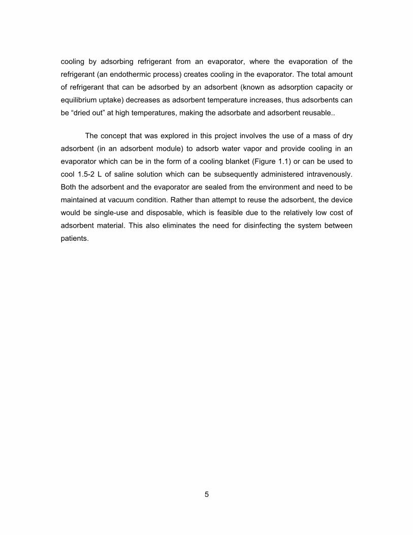
adsorbent (in an adsorbent module) to adsorb water vapor and provide cooling in an
evaporator which can be in the form of a cooling blanket (Figure 1.1) or can be used to
cool 1.5-2 L of saline solution which can be subsequently administered intravenously.
Both the adsorbent and the evaporator are sealed from the environment and need to be
maintained at vacuum condition. Rather than attempt to reuse the adsorbent, the device
would be single-use and disposable, which is feasible due to the relatively low cost of
adsorbent material. This also eliminates the need for disinfecting the system between
patients.
6
a)
b)
Figure 1.1. a) Conceptualization of the proposed adsorption-based portable cooling device showing the adsorbent module and the blanket evaporator, b) Schematic of the adsorbent device showing the flow of water vapor from the evaporator into the adsorbent and the resulting heat flow from the tissue into the evaporator
This concept has several advantages over the other cooling technologies that are
currently used in the pre-hospital setting:
• The adsorbent material and the adsorbate (water) are expected to be the most
significant contributions to the final weight and size of the device because no
moving parts are required, allowing for a compact and lightweight device
7
• The proposed single-use adsorption-based device does not require any
electrical power during operation or storage in the ambulance
• Unlike devices which need to be kept cold in an insulated box and need to be
replaced every few hours, the adsorption-based device can be stored at room
temperature and will not need to be replaced until it is used
• The device is easy to use, given that a single valve between the adsorbent
and the evaporator needs to be opened to begin cooling
• Cooling can be extended for as long as necessary by simply replacing the
used adsorbent module with a new one, as long as the gas-tight seal from the
environment can be maintained, and sufficient water is in the evaporator to
continue cooling.
However, there are several technical challenges that need to be overcome before the
advantages mentioned above can be realised:
• Commercially available adsorbents such as silica gel and zeolite themselves
do not uptake sufficient water to provide a significant cooling effect from a few
kilograms of material (more details about the comparative performance of
adsorbents are provided in section 2.1).
• Due to the phase change of the adsorbate at the surface of the adsorbent
from gas to liquid, adsorption is an exothermic process and the adsorbent can
significantly heat up during operation. Since equilibrium water uptake
decreases with increasing adsorbent temperature, effective heat dissipation
from the adsorbent module is critical for good performance.
• As is the case with any other porous materials, adsorbents can frequently
have issues with effective mass flow. The two sources of mass flow resistance
in adsorption are inter-particular resistance (i.e. restriction of vapor flow to a
particle caused by the presence of other particles around it) and intra-
particular resistance (i.e. restriction of vapor flow within a particle). As

8
explained further in section 2.1, mass flow resistance can reduce the uptake
rate and subsequently the cooling power.
• Adsorption is a transient process. The instantaneous uptake rate (and thus the
cooling power) depends on the uptake at that instant, the adsorbent
temperature, and the evaporator pressure, all of which vary over time.
Consequently, accurate modeling of adsorption and transient surface heat
loss from the human body is required in order to validate that the device can
provide enough cooling power to reduce the core temperature.
1.4. Performance Specifications for a Pre-Hospital hypothermic Cooling System
A set of performance requirements is necessary in the development of any novel
product in order to evaluate the value of the new technology or product over the current
alternatives. As such, the final prototype was judged based on the following critical
requirements:
• The device must provide at least 250 Watts of cooling for a period of 30 minutes at an evaporator temperature between 10-15°C. The cooling
power was determined based on the cooling power that is provided by
commercially available surface cooling devices, and the evaporator
temperature range was determined based on a surface contact heat transfer
coefficient of 100 W/m2K and a skin temperature of 15-20°C which was
measured during hypothermia treatment. The cooling power, heat transfer
coefficient, and skin temperature during surface cooling were measured by Dr.
Michael English [23], [24]. The duration of 30 minutes was selected based on
average time of 23 minutes between return of spontaneous circulation and
arrival at hospital [25].
• The total mass of adsorbent required for providing the specified cooling power must be 4kg or less. Assuming the adsorbent module and blanket
weigh 2kg, the final device weight should be 6kg or less in order to
9
significantly improve the portability compared to commercially available
devices which weigh in the range of 10-20kg.
1.5. Understanding Heat Transfer in the Human Body
Surface cooling devices can frequently perform unpredictably when tested on
humans, mainly due to the lack of knowledge about the thermal response of the human
body under hypothermic conditions. The core cooling rate varies significantly between
different individuals based on several factors, including the body weight, fat percentage,
age, and the unique variations in thermoregulation that naturally exist between different
individuals.
Since medical device development is still a rather linear process (development
bench-top tests animal trials clinical trials), the inability to accurately predict the
expected performance of the device can cause delays in commercialization and increase
the financial resources needed to reach the market. Consequently, acquiring in-depth
knowledge of the dynamic heat loss from the human body under hypothermic conditions
and numerically simulating this scenario would be a worthwhile endeavour. Although a
variety of bioheat models and mathematical thermoregulation models currently exist in
literature, they have not been validated with experimental data in hypothermic
conditions. Therefore, validation of a numerical bioheat model which includes
thermoregulation parameters would be a major step towards advancing the ability to
predict the performance of a cooling device for inducing hypothermia..
1.6. Objectives
The goal for the current work is to develop a portable cooling device that can
rapidly cool the patient in the pre-hospital setting. Due to the extensive scope of this
project, the focus of the present study was divided into two main objectives:
development of a 1st generation proof-of-concept prototype for the adsorption-based
cooling device, and validation of a numerical model of transient surface heat loss from a
human in hypothermic conditions by conducting 3D finite element simulations of
10
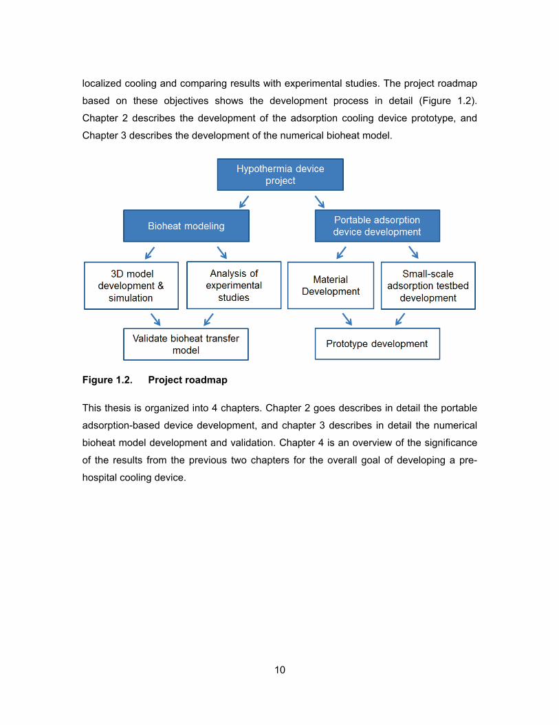
localized cooling and comparing results with experimental studies. The project roadmap
based on these objectives shows the development process in detail (Figure 1.2).
Chapter 2 describes the development of the adsorption cooling device prototype, and
Chapter 3 describes the development of the numerical bioheat model.
Figure 1.2. Project roadmap
This thesis is organized into 4 chapters. Chapter 2 goes describes in detail the portable
adsorption-based device development, and chapter 3 describes in detail the numerical
bioheat model development and validation. Chapter 4 is an overview of the significance
of the results from the previous two chapters for the overall goal of developing a pre-
hospital cooling device.

11
Chapter 2. Adsorption Cooling Device Development
2.1. Review of Adsorption Cooling Technology
The simplicity, portability, and independence from input power makes sorption
cooling technology an ideal candidate for portable cooling applications. It has previously
been investigated for microclimate cooling [26]–[29], which is aimed at preventing heat
stress in people that exercise or work in hot environments. Those studies aimed to
develop effective surface cooling technology for temperature of 25-35°C to effectively
prevent heat stress. However, to induce hypothermia, the evaporator surface cannot be
higher than 15°C. The lower water temperature means that the water vapor pressure
must be 3-4 times lower and that the water uptake will be respectively lower. Moreover,
a sorbent material that is optimal for high pressure is not necessarily optimal for low
pressure. Therefore, a systematic study of the cooling capacity of adsorbent materials is
required to determine suitable materials for hypothermic applications.
The sorption-based microclimate cooling devices were either backpack-type [28],
[29] where the sorbent is in a separate chamber carried like a backpack and the water is
in a jacket (Figure 2.1a), or layered-type where the sorbent is layered above the water
uniformly through the jacket and the two are separated by a rigid spacer [26], [27]
(Figure 2.1b).

12
a)
b)
Figure 2.1. a) Illustration of backpack-type sorption-based microclimate cooling system [28] and b) cross section of a single pad in the layered-type cooling system [26]
Table 2.1. Comparison of performance from sorption-based microclimate cooling systems in literature
Study Sorbent Evaporator Temperature [°C]
Cooling per kg of sorbent [Watts]
[28] Calcium Oxide 21 28 W for 4 hours
[29] Magnesium Chloride +
12.5% Molecular Sieve 4A
35 71 W for 30 minutes
[26] Lithium Chloride 16-20 105 W for 1 hour
[27] Lithium Chloride 23-27 127 W for 1 hour
A comparison of the cooling performance from the different studies shows that
the layer-type cooling pad combined with lithium chloride as the sorbent holds the
highest cooling capacity (Table 2.1). However, one of the studies using lithium chloride
evaluated cooling power based on mass change of the sorbent over the 60 minutes [26],
13
which is not necessarily equivalent to the cooling power delivered on the surface of the
cold side. The proximity of the sorbent to the water allows for heat transfer from the hot
sorbent to the water, which lowers actual cooling power delivered on the surface of the
cold side. The other study using lithium chloride delivered a constant heat flux on the
cold surface of the cooling pad using a film heater [27], but the calculated cooling power
does not take into account the fact that the water heats up almost linearly over the last
40 minutes of the experiment, indicating that perhaps the heat flux delivered by the film
heater significantly overpowers the cooling effect.
Heat transfer in the cooling pad from the hot sorbent to the water remains one of
the main issues with the layered-type concept. Although radiation heat transfer can be
minimized by putting a perforated aluminum sheet between the sorbent and the water
[26], conduction through the spacer and convection through the refrigerant vapor cannot
be minimized without significantly increasing the thickness of the pad. Moreover, it is
difficult to implement a method to prevent transfer of water vapor before the cooling is
needed. Therefore a single-component device is not practical for a high temperature
gradient application like hypothermic cooling.
Lithium chloride and other salts, which are chemical adsorbents, can have a
large equilibrium uptake compared to physical adsorbents such as silica gel. However,
these salts can only be used in thin layers because they agglomerate and then liquefy
upon uptake of sufficient water; and since adsorption first happens on the outermost
layer, the agglomeration and liquefaction can prevent vapor flow to the deeper layers
[30]. In order to prevent clumping, previous designs of microclimate cooling systems
which used lithium chloride immersed cotton towels in the salt solution and then dried
the towels. As explained further in section 2.1.2, a more efficient method of preventing
clumping is to use a physical adsorbent as the host matrix. The following sections
provide an introduction to characterization of various adsorbents and selection of the
optimal adsorbent for this application.
14
2.1.1. Characterization of Adsorbents
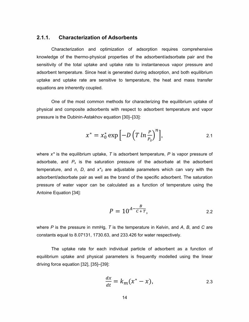
Characterization and optimization of adsorption requires comprehensive
knowledge of the thermo-physical properties of the adsorbent/adsorbate pair and the
sensitivity of the total uptake and uptake rate to instantaneous vapor pressure and
adsorbent temperature. Since heat is generated during adsorption, and both equilibrium
uptake and uptake rate are sensitive to temperature, the heat and mass transfer
equations are inherently coupled.
One of the most common methods for characterizing the equilibrium uptake of
physical and composite adsorbents with respect to adsorbent temperature and vapor
pressure is the Dubinin-Astakhov equation [30]–[33]:
𝑥∗ = 𝑥0∗ exp �−𝐷 �𝑇 𝑙𝑛 𝑃𝑃𝑠�𝑛�, 2.1
where x* is the equilibrium uptake, T is adsorbent temperature, P is vapor pressure of
adsorbate, and Ps is the saturation pressure of the adsorbate at the adsorbent
temperature, and n, D, and x*0 are adjustable parameters which can vary with the
adsorbent/adsorbate pair as well as the brand of the specific adsorbent. The saturation
pressure of water vapor can be calculated as a function of temperature using the
Antoine Equation [34]:
𝑃 = 10𝐴−𝐵
𝐶 + 𝑇, 2.2
where P is the pressure in mmHg, T is the temperature in Kelvin, and A, B, and C are
constants equal to 8.07131, 1730.63, and 233.426 for water respectively.
The uptake rate for each individual particle of adsorbent as a function of
equilibrium uptake and physical parameters is frequently modelled using the linear
driving force equation [32], [35]–[39]:
𝑑𝑥𝑑𝑡
= 𝑘𝑚(𝑥∗ − 𝑥), 2.3
15
where km is the mass transfer coefficient within the particles, and is defined by:
𝑘𝑚 = 15 𝐷0𝑒−𝐸𝑎𝑅𝑇
𝑟𝑝2, 2.4
where D0 is the reference diffusivity, Ea is the activation energy, R is the universal gas
law constant, T is the temperature of the adsorbent, and rp is the radius of the spherical
particle. Even though this model is specifically for mass transfer resistance in a spherical
particle, it was shown that deviations for cylindrical and cubic particles would be less
than 10%, so it can also be used for irregular-shape particles, as long as the size of the
particle is known [40].
2.1.2. Review of Various Adsorbents and their Uptake
Common adsorbates used in adsorption systems include water, methanol,
ethanol, and ammonia. Water was selected as the most appropriate for this application,
mainly because methanol and ammonia can have negative consequences for the patient
if the evaporator leaks onto the skin. Ethanol is also relatively safe, but its latent heat of
vaporization is less than half that of water, 841 kJ/kg and 2260 kJ/kg respectively,
indicating that more than the double the mass of ethanol will need to be evaporated to
provide the same cooling power. Moreover, water is ideal for this application because
the temperature will not go below 0°C so there is no chance of causing cold injury to the
skin.
Water is compatible with several adsorbents including silica gels, zeolites, and
salts such as calcium chloride and lithium chloride. Silica gels are a highly porous and
solid form of silicon dioxide, and their pore sizes can vary from 0.5 to 15nm, and total
surface area of 100-1000 m2/gram. Zeolites are a crystal form of aluminasilicate, where
the crystal structure forms the pores required for adsorption. Synthetic zeolite molecular
sieve 4A and 13X are frequently used in adsorption cooling systems.
As previously mentioned, bulk powder salts will easily agglomerate and clump
together, preventing vapor flow and further adsorption after the outer layer is saturated.
16
However, their uptake per unit mass of desiccant is significantly greater than physical
adsorbents. Consequently, recent research has focused on loading the physical
adsorbents with salts in order to exploit the large uptake of the salts and the good mass
transfer characteristics of physical sorbents [41]. These composite adsorbents
(collectively called Selective Water Sorbents or SWS) have shown to significantly
improve performance over both the physical and chemical adsorbents individually [30],
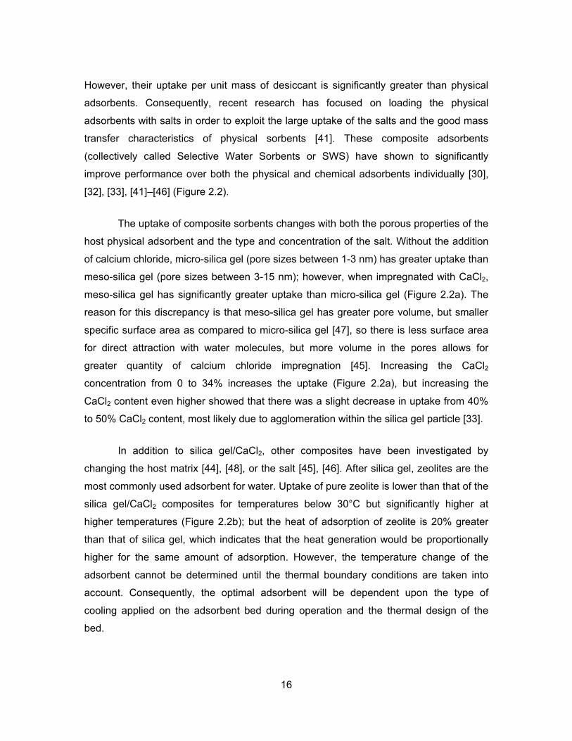
[32], [33], [41]–[46] (Figure 2.2).
The uptake of composite sorbents changes with both the porous properties of the
host physical adsorbent and the type and concentration of the salt. Without the addition
of calcium chloride, micro-silica gel (pore sizes between 1-3 nm) has greater uptake than
meso-silica gel (pore sizes between 3-15 nm); however, when impregnated with CaCl2,
meso-silica gel has significantly greater uptake than micro-silica gel (Figure 2.2a). The
reason for this discrepancy is that meso-silica gel has greater pore volume, but smaller
specific surface area as compared to micro-silica gel [47], so there is less surface area
for direct attraction with water molecules, but more volume in the pores allows for
greater quantity of calcium chloride impregnation [45]. Increasing the CaCl2
concentration from 0 to 34% increases the uptake (Figure 2.2a), but increasing the
CaCl2 content even higher showed that there was a slight decrease in uptake from 40%
to 50% CaCl2 content, most likely due to agglomeration within the silica gel particle [33].
In addition to silica gel/CaCl2, other composites have been investigated by
changing the host matrix [44], [48], or the salt [45], [46]. After silica gel, zeolites are the
most commonly used adsorbent for water. Uptake of pure zeolite is lower than that of the
silica gel/CaCl2 composites for temperatures below 30°C but significantly higher at
higher temperatures (Figure 2.2b); but the heat of adsorption of zeolite is 20% greater
than that of silica gel, which indicates that the heat generation would be proportionally
higher for the same amount of adsorption. However, the temperature change of the
adsorbent cannot be determined until the thermal boundary conditions are taken into
account. Consequently, the optimal adsorbent will be dependent upon the type of
cooling applied on the adsorbent bed during operation and the thermal design of the
bed.

17
a)
b)
Figure 2.2. Comparison of uptake as a function of adsorbent temperature, as
experimentally measured in literature for physical and composite adsorbents at water vapor pressure of a) 2.5 kPa and b) 0.87 kPa
0
0.1
0.2
0.3
0.4
0.5
0.6
0.7
0.8
0.9
20 30 40 50 60 70 80
Upt
ake
[g w
ater
/ g
adso
rben
t]
Temperature [°C]
Meso-Silica GelMicro-Silica GelMicro-Silica gel + 22% CaCl2Meso-Silica Gel + 34% CaCl2Meso-Silica Gel + 32% LiBrMeso-Silica Gel + 13.5% MgSO4MCM-41 + 37.7% CaCl2
0
0.1
0.2
0.3
0.4
0.5
0.6
0.7
0.8
0.9
20 30 40 50 60 70 80
Upt
ake
[g w
ater
/ g
adso
rben
t]
Temperature [°C]
Zeolite 13XZeolite 13X + 30% CaCl2Zeolite 13X + 46% CaCl2Silica Gelmeso-silica gel + 34% CaCl2
meso-silica gel [45] micro-silica gel [45] micro-silica gel + 22% CaCl2 [45] meso-silica gel + 34% CaCl2 [45] meso-silica gel + 32% LiBr [45] meso-silica gel + 13.5% MgSO4 [46] MCM-41 + 37.7% CaCl2 [44]
zeolite 13X [48] zeolite 13X + 30% CaCl2 [48] zeolite 13X + 46% CaCl2 [48] meso-silical gel [48] meso-silica gel + 34% CaCl2 [45]

18
Few studies have investigated the kinetics of water vapor adsorption on SWS
[42], [49]–[52]. Initial studies based on a pressure jump showed that the increased mass
resistance caused by salt impregnation and larger grain size slowed down the
adsorption rate [42], [49]. Further work investigated the diffusivity of silica gel-CaCl2
adsorbent based on a temperature jump methodology [50], [51]. A study aimed at
modeling an adsorption refrigeration system using silica gel-CaCl2 used kinetic data from
ref. [49] for implementation in the LDF model.
None of the studies in literature have analyzed the adsorption characteristics of
multiple layers of silica gel-CaCl2 adsorbent; all experimental work has been done on a
single layer. However, vapor diffusion in silica gel-CaCl2 composites can be significantly
influenced by the presence of liquid salt solution within the pores or even around entire
particle, which can block vapor diffusion similar to pure chemical adsorbents [52].
Consequently, a study of the adsorption characteristics in a multi-layer sample of silica
gel-CaCl2 is critical to ensure that water vapor diffusion is uniform throughout the
adsorbent module.
The next section describes the different techniques used for measuring uptake
and the development of bench-top custom thermo-gravimetric system that was designed
to measure the uptake and adsorption rate for a multi-layered adsorbent sample at
various adsorbent temperatures and water vapor pressure.
2.2. Approach
Development of the 1st generation prototype of the adsorption-based cooling
device was divided into two main objectives. Our first objective was to load standard
silica gel with calcium chloride and develop a custom experimental test-bed to determine
the adsorption characteristics of each sample of the composite adsorbent. In this study,
silica gel-CaCl2 was chosen as the most appropriate adsorbent, since both ingredients
are readily available, inexpensive, and non-toxic; and there is a wealth of data already
available for validating the adsorption characteristics. Section 2.3.1 provides rationale for
development of the custom test-bed.
19
Our second objective was to optimize the design of the adsorbent module to
ensure that heat and mass transfer can be maximized while minimizing the mass of the
adsorbent bed. Finite element modeling was used to design the adsorbent module and
simulation results were subsequently compared with experimental results.
2.3. Method
2.3.1. Small-scale Bench-top Experiment
Uptake Measurement Techniques
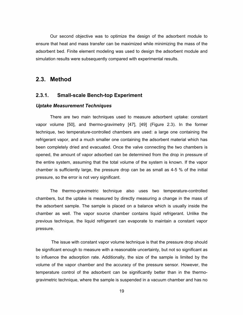
There are two main techniques used to measure adsorbent uptake: constant
vapor volume [50], and thermo-gravimetry [47], [49] (Figure 2.3). In the former
technique, two temperature-controlled chambers are used: a large one containing the
refrigerant vapor, and a much smaller one containing the adsorbent material which has
been completely dried and evacuated. Once the valve connecting the two chambers is
opened, the amount of vapor adsorbed can be determined from the drop in pressure of
the entire system, assuming that the total volume of the system is known. If the vapor
chamber is sufficiently large, the pressure drop can be as small as 4-5 % of the initial
pressure, so the error is not very significant.
The thermo-gravimetric technique also uses two temperature-controlled
chambers, but the uptake is measured by directly measuring a change in the mass of
the adsorbent sample. The sample is placed on a balance which is usually inside the
chamber as well. The vapor source chamber contains liquid refrigerant. Unlike the
previous technique, the liquid refrigerant can evaporate to maintain a constant vapor
pressure.
The issue with constant vapor volume technique is that the pressure drop should
be significant enough to measure with a reasonable uncertainty, but not so significant as
to influence the adsorption rate. Additionally, the size of the sample is limited by the
volume of the vapor chamber and the accuracy of the pressure sensor. However, the
temperature control of the adsorbent can be significantly better than in the thermo-
gravimetric technique, where the sample is suspended in a vacuum chamber and has no
20
contact with the temperature-controlled walls [52]. The thermo-gravimetric technique can
be modified such that the sample is in direct contact with a temperature-controlled wall
[38], but the addition of heater wires or coolant flow circuit can influence the
measurement of the balance.
a)
b)
Figure 2.3. Two techniques currently used to measure vapour sorption: a) thermo-gravimetric [47], and b) constant vapor volume [50]
21
Custom Thermo-gravimetric Vapour Sorption System
The thermo-gravimetric system developed for the present study was custom-
designed to handle larger samples than the TGA available at the Lab for Alternative
Energy Conversion (LAEC) at SFU (IGA-002, Hiden Isochema, Warrington, UK), with
the target adsorbent sample size of about 10-50 grams.
The system had an evaporator which contains the water, a filtering flask which
contained the adsorbent, and a series of valves which separated the vacuum pump,
water, and adsorbent, as schematically shown in Figure 2.4. The uptake was measured
by reading the change in mass of the sample with the balance. The system was capable
of controlling the vapor pressure by controlling the water temperature, and the adsorbent
temperature.
The chamber containing water was constructed from a rectangular 1/8” thick
aluminium tube (1.5” X 1.5” X 12”) which was capped on both ends with 1/8” thick
aluminium plates. In order to create a vacuum seal, the caps were attached to the
rectangular tube with an epoxy (Stycast 2850F) which had been previously degassed.
One of the caps has a 1/4” NPT threaded hole. The shell structure which allows coolant
to circulate around the aluminium chamber was constructed from an 18” segment of 3”
ID ABS pipe which was capped on both ends. A through-wall pipe coupling connected
the aluminum water chamber to the valve V1 through a hole in one of the ABS shell
caps. The ABS cap also had an inlet and an outlet for the coolant, which was circulated
through a PolyStat 3C15 chiller (Cole Parmer) in order to regulate the temperature
(Figure 2.5e).

22
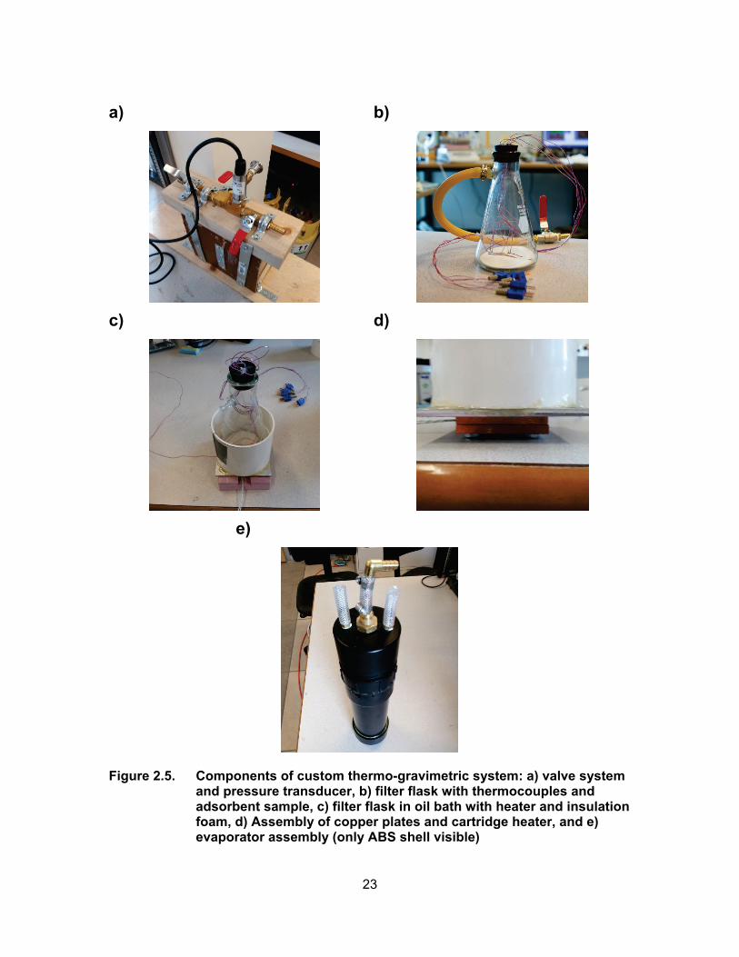
Figure 2.4. Schematic of the custom thermo-gravimetric vapor sorption system
The adsorbent sample was placed inside a 500mL filter flask (Kimble-Chase
Kimax). The adsorbent temperature was measured with five thermocouples, which were
inserted through holes in the rubber stopper and the holes were subsequently sealed
with super glue. In order to ensure that the thermocouples were directly in contact with
the adsorbent, the ends of the thermocouples were inserted through a 1/4” X 1/4” heat-
resistant rubber strip which adheres to the bottom surface of the flask (Figure 2.5b). The
heater and oil bath assembly consisted of a 35W cartridge heater (HDC19101, 120V
input, Omega) which was encased in two copper plates which acted as heat spreaders.
The top copper plate was attached to a 1/4” aluminum plate with fasteners (Figure 2.5d).
The aluminum plate formed the bottom surface of the oil bath, and plastic tube epoxied
on the aluminum plate formed the walls (Figure 2.5c). Oil was used as the coolant
because it does not evaporate when heater to around 60°C, whereas water would
evaporate, and the decrease in water mass would interfere with the measurement of the
adsorbent mass change.
The adsorbent flask and the heater assembly weere placed on a lab balance
(Mettler Toledo NewClassic MS Toploading Balance 4200g X 0.01g, Cole Parmer) with
a layer of 1” thick insulating foam between the lower copper plate and the surface of the
heater such that the balance measurement was not influenced by the temperature of the
heater. A soft latex tube (5/16” ID, 1/8” wall thickness) was used to connect the valve
system and the filter flask so that the balance measurement was minimally affected by
the rigidity and tension within the tube.
23
a)
b)
c)
d)
e)
Figure 2.5. Components of custom thermo-gravimetric system: a) valve system and pressure transducer, b) filter flask with thermocouples and adsorbent sample, c) filter flask in oil bath with heater and insulation foam, d) Assembly of copper plates and cartridge heater, and e) evaporator assembly (only ABS shell visible)

24
The valve system consisted of two 1/4” NPT Tee connections and three 1/4” NPT
ball valves. The evaporator and filter flask were connected with 1/4” NPT to 3/8” hose
barb connection, and the vacuum pump was connected with a KF fitting. The vacuum
pump used for evacuating the system was TriScroll 600 DryScroll series (Agilent
Technologies). The pressure transducer used for this experiment was PX309-005AI
(Omega).
Pressure transducer and thermocouple readings were collected using NI 9207
and NI 9213 DAQ modules (respectively) connected to a NI DAQ chassis. The balance
was connected directly to the data collection computer using a serial port.
All data collection and display was performed in LABVIEW with a reading period
of 1 second. In order to maintain a constant temperature of the oil bath, a feedback loop
was created in LABVIEW wherein the program switched the heater on and off based on
the average temperature of the adsorbent (T1-5). The heater was controlled through
LABVIEW with the NI 9485 digital output module. Since the NI 9485 module cannot
handle 120V AC, it was used to control a relay which controlled the connection between
a 120V AC power supply and the heater (Figure 2.6). The chiller temperature was also
controlled with the LABVIEW program.
Figure 2.6. Schematic of the circuit used to control the cartridge heater
Experimental Procedure
The experiments began by first completely drying out the adsorbent. The
adsorbent sample was heated in an oven for 2 hours at 200°C and then the mass was
measured and recorded (assumed to be the dry mass). The sample was subsequently
placed in the filtering flask, which was connected to the valve system and then

25
evacuated by turning on the vacuum pump and opening valves V2 and V3. Once the
flask was sufficiently evacuated, valve V2 was closed. The flask was then placed on a
hot plate with the temperature set at 200°C. The adsorbent temperature and pressure
were monitored, and if a pressure rise accompanies the rise in adsorbent sample
temperature, it indicated that the sample is not completely dry. With the flask still placed
on the hot plate, the flask was periodically evacuated for approximately 5 minutes to
remove all moisture from the system (by turning on the vacuum pump and opening valve
V2). If the pressure did not rise more than 50 Pa above the base pressure
(approximately 20-30 Pa) during 30 minutes, the sample was considered to be
completely dry. The hot plate was then switched off and the flask was allowed to cool to
approximately 70°C before placing in the oil bath (which was placed on the balance).
Once the flask was in the oil bath, the adsorbent temperature was maintained at 50°C. A
drift in the balance reading was indicative of tension in the rubber hose or the heater
wire. Once the balance reading was observed to vary by only ±0.01 g for a period of 30
minutes, the reading was considered to be stable.
In order to prepare the evaporator, 100mL of water was placed in the refrigerant
chamber, and the outlet of the chamber was then connected to the valve system with a
plastic hose (3/8” ID). The inlet and outlet for the evaporator shell were connected to the
chiller, which was switched on and the temperature was maintained at a temperature
between 7 and 15°C. Valve V3 was then closed and valve V1 was opened so that
evacuation of the evaporator can commence. Fully opening valve V2 and turning on the
vacuum pump would result in a large amount of water vapor flowing into the vacuum
pump, which would cause pump degradation. Instead, the pump was switched on and
valve V2 was cracked open, until the pressure reading was close to the 1230 Pa (vapor
pressure of water at 10°C). Valve V2 was subsequently closed. It was necessary to
repeat the evacuation of the evaporator several times before all the air was completely
removed.
Once the adsorbent temperature was stable at 50°C and the evaporator pressure
was stable at 1230 Pa, the experiment was started by opening valve V3. Due to
adsorption, the temperature of the adsorbent rose by 5-10°C. Once the temperature was
stable again at 50°C and the balance reading stabilized, the temperature of the

26
adsorbent was reduced to 40°C. Similarly, once the balance reading stabilized, the
temperature of the adsorbent was again reduced to 30°C. The balance reading,
adsorbent temperatures, chiller temperature, and pressure are all saved in an MS Excel
file.
Uncertainty Estimation
The main source of uncertainty in the experiments were from the mass
measurement. The balance had a linearity error and repeatability error of ±0.02 g and
±0.01 g respectively, as specified by the manufacturer. Additionally, switching on of the
cartridge heater was observed to influence the balance reading by up to 0.05 g, most
likely due to electromagnetic interference. An addition uncertainty of ±0.06 g was
attributed to the possible error caused by tension in the heater wire and latex tube. The
root sum of squares was used to estimate the final mass uncertainty:
𝑢𝑚𝑎𝑠𝑠 =
��𝑢𝑙𝑖𝑛𝑒𝑎𝑟𝑖𝑡𝑦�2 + �𝑢𝑟𝑒𝑝𝑒𝑎𝑡𝑎𝑏𝑖𝑙𝑖𝑡𝑦�
2 + (𝑢𝐸𝑀𝐼)2 + (𝑢𝑡𝑒𝑛𝑠𝑖𝑜𝑛)2 2.5
where the final value of umass was ±0.08 g.
Uncertainty in temperature measurement of the adsorbent at each time step was
calculated based on the formula:
𝑢𝑇 =𝑇𝑚𝑎𝑥𝑖𝑚𝑢𝑚 − 𝑇𝑚𝑖𝑛𝑖𝑚𝑖𝑚 + 2℃
2√𝑁
Where Tmaximum and Tminimum are the maximum and minimum measurements from the
thermocouples respectively, 2°C represents the inherent uncertainty of the T-type
thermocouples, and N is the number of thermocouples used (five in this case). For the
time-averaged temperature (required for calculating the diffusivity and equilibrium
uptake), uncertainty was calculated using the formula:

27
𝑢𝑇,𝑡𝑖𝑚𝑒_𝑎𝑣𝑒𝑟𝑎𝑔𝑒 =�𝑇𝑎𝑣𝑒𝑟𝑎𝑔𝑒,𝑚𝑎𝑥𝑖𝑚𝑢𝑚 − 𝑇𝑎𝑣𝑒𝑟𝑎𝑔𝑒,𝑚𝑖𝑛𝑖𝑚𝑢𝑚� + 2𝑢𝑇
2
Where Taverage,maximum, and Taverage,minimum are the maximum and minimum of the average
of the five thermocouple readings over the selected time range respectively.
The pressure sensor had an accuracy of ±92 Pa, and a maximum zero offset uncertainty
of ±740 Pa. The zero-offset was calibrated with measurement of pressure inside a
vacuum chamber which was vacuumed for 30 minutes this reading was assumed to be 0
Pa.
Sample Selection and Composite Adsorbent Preparation
The irregular-grain silica gels used for preparing the composite adsorbents were
obtained from Silicycle Inc. (Quebec, Canada), and the anhydrous (powder) calcium
chloride was obtained from Fisher Scientific (Fair Lawn, New Jersey). The uptake results
were compared with commercially available desiccant silica gel (Silica Gel Indicating
Type, Desican, Toronto).
Composite adsorbent were prepared by wetting the dry silica gel with ethanol
then soaking with concentrated aqueous CaCl2 solution. The silica gel-salt mixture was
placed on open trays in a fume hood and left to dry for 24 hrs, and heater on a hot plate
set at 80°C if the sample was large. The sample was subsequently heated in an oven at
200°C until the weight of the sample stabilized [47].
The samples were selected such that the combined results from the custom
thermo-gravimetric system and the TGA would show the influence of CaCl2 presence,
pore size, and grain size on the uptake of the adsorbent (Table 2.2). The range of grain
sizes for each sample was provided by the manufacturer. Given that the main purpose of
the custom thermo-gravimetric system was to determine the impact of layer thickness of
composite adsorbents on the uptake, the main parameter of interest was the grain size.
Consequently, extensive tests were only performed on samples C024 and C030.
Additionally, some tests were done on B150 in order to ensure that the custom setup
28
results were similar to the TGA results. The effect of pore size was investigated in-depth
with the TGA.
The influence of layer thickness was observed in the custom thermo-gravimetric
system by testing samples weighing approximately 20 g and 35-40 g. The thickness of
the samples varied between approximately 3.5 and 7.5 mm, depending on the density
and mass of the sample.
Table 2.2. Characteristics of adsorbent samples tested with the TGA and the custom thermo-gravimetric setup
Sample Name
CaCl2 concentration (by weight) [%]
Virgin silica gel pore size (μm)
Grain size range (mm)
B60 - 6 0.25 - 0.5
B150 - 15 0.25 - 0.5
K60 - 6 0.50 - 1.0
BLUE - unknown 2-4 (spherical)
C020 27.7 6 0.25-0.5
C024 33.0 15 0.25-0.5
C030 33.0 6 0.50-0.1
2.3.2. Adsorbent Bed Prototype Development
The prototype was developed in order to prove that the uptake performance
observed in the small samples of 20-40 g could be replicated on a larger scale, and to
demonstrate that the goal of a 6kg device to deliver 250 Watts was achievable. As
previously mentioned, there are two main issues which become influential when the
adsorbent size is increased from a few grams to the order of kilograms: heat dissipation
and vapor transport.
The thermal conductivity of adsorbents is low (in the order of 0.1 to 1 W/mK),
mainly due to their porous nature. When a relatively large sample is used, effective

29
dissipation of heat of adsorption becomes a significant design challenge. A significant
amount of research effort in the area of adsorption refrigeration cycles is focused on
embedding adsorbent into various heat exchangers such as finned tube [53], plate [54],
and shell and tube heat exchangers [55]. However, heat dissipation elements such as
fins and tubes add mass to the system and reduce overall portability. Consequently, in
addition to measuring the cooling power per unit mass of adsorbent material (specific
cooling power), the metric of adsorbent bed to adsorbent mass ratio has been
recommended for evaluating the performance of the bed [56].
Additionally, transport of water vapor through the adsorbent was found to be an
issue in cases where the adsorbent particles are very small or the adsorbent bed
dimensions are very large [37]. In the case of composite adsorbents, studies have also
suggested that the vapor transport issue may be compounded by the presence of salt
solution in the flow paths [52]. Our preliminary measurements have also shown that
enforcing channels for water vapor flow through the adsorbent bed can significantly
increase the adsorption rate (Appendix A).
Key Features of the Prototype Adsorbent Bed
Given that the proposed device should not require any electrical power during
operation, active cooling by circulation of heat transfer fluid or usage of fans would
require a battery pack to be attached to the device. Batteries and active cooling
components such as fans and pumps would significantly increase the mass and
complexity of the device. Therefore, for the purpose of this project, active cooling
methods were considered to be out of scope.
Passive cooling methods include the dissipation of heat to phase change
material which can store the energy, and dissipation of heat to the environment with the
aid of natural convection. Preliminary estimates showed approximately 55,000 J of heat
would be generated with 250 Watts for cooling for 30 minutes (heat of adsorption is
greater than the heat of evaporation of water by a factor of approximately 1.1 [32]), and
that commercially available phase change materials have a latent heat of fusion of
approximately 350,000 J/kg [57], therefore, the mass of phase change material required

30
would be in the order of 1.5 to 2 kg. Since dissipation of heat to the environment requires
no additional mass except the fins, it was determined to be the more lightweight solution.
In addition to external fins for maximizing heat dissipation by natural convection,
a method for effective heat transfer inside the adsorbent bed was necessary.
Furthermore, a structure for allowing vapor to flow uniformly through the adsorbent
material was required. A single solution for both these issues was to place thermally
conductive perforated plates inside the adsorbent bed such that they would define
narrow channels of empty space between layers of adsorbent. The plates would act as
internal fins and enhance the heat transfer rate from the centre of the adsorbent bed to
the outside, and also allow for vapor to flow unrestricted through the channel and
penetrate the adsorbent through the perforations.
The next two sections describe the development of the prototype and a
description of the finite element heat transfer simulations conducted for the adsorbent
bed. The simulations were developed in order to demonstrate that heat transfer during
the adsorption process can be accurately modeled, and simulations can be used in the
future for optimizing the design of the adsorbent bed and selection of the optimal
adsorbent.
Prototype Construction
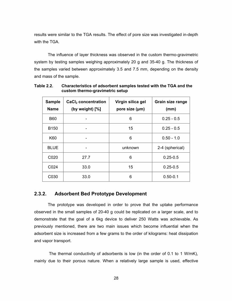
A prototype for the targeted adsorption-based cooling device was constructed
mainly from aluminum due to its high thermal conductivity, high weight-to-strength ratio,
and corrosion-resistance in the presence of water vapor and salt. A rectangular 1/8”
aluminum tube (4” X 4” X 12”) was capped with a 1/8” aluminum plate on one side and a
1/8” plate (5” X 5”) with a 4” X 4” square milled out from the centre on the other side
(Figure 2.7a,b). Both plates were epoxied to the rectangular tube with Stycast 2850F,
and the latter plate formed the bottom surface on which a Viton gasket (McMaster Carr,
Cleveland, OH) was placed. The shell was closed by placing an acrylic lid on the gasket.

31
a)
b)
c)
d)
e)
Figure 2.7. Parts used in construction of the adsorbent bed prototype including
a) bottom cap plate, b) top plate with gasket, c) perforated internal fin, d) internal fin with mesh attached, and e) single folded fin
32
The internal fins were constructed from perforated 0.032” aluminum sheets
(0.0625” hole diameter, 23% open area) (Figure 2.7c). Since the sheet hole diameter
(1.5 mm) was larger than the size of the silica gel particles (0.5 -1 mm), a stainless steel
wire cloth mesh (0.125 mm opening, 0.1 mm wire diameter) was attached to each of the
fins using staples to prevent particles falling into the vapor flow channels (Figure 2.7d).
The edges of the fins were bent at 90° to create a lip so that a large surface contact
could be made between the rectangular tube inner wall and the fin and contact
resistance could be minimized. The fins were bonded to the walls of the tube by adding
thermally conductive epoxy (Stycast 2850F) to the bent surface before sliding into place.
The external heat sinks were folded fins constructed by bending 0.02” aluminum
sheets into the required shape (Figure 2.7e). The fins were manually bent using a
custom jig which could accommodate small bend radius and fin pitch (width of each
individual fin); however, the jig could not maintain a small bend radius if the fins were
over 10 cm in height. In order to cover the surface area of the shell wall with a height of
30 cm, 3 fins with a height of 7.3 were used with 2 cm high gap between each fin
assembly, forming an interrupted fin heat sink. The folded fins were bonded to the outer
rectangular tube wall with thermally conductive epoxy (Stycast 2850F). The completed
prototype (Figure 2.8) weighed 2.3 kg and had an adsorbent capacity of 1.3 kg.
a)
b)
Figure 2.8. Completed adsorbent bed prototype a) isometric view with acrylic lid, and b) top view showing internal fins and gaps for vapor flow
33
Finite Element Simulations of Heat Transfer in Adsorbent bed
A 2D transient numerical simulation of heat transfer horizontally from the
adsorbent to the shell and the ambient air was conducted and the results were
compared with experimental results from the prototype. The purpose of this study was to
develop a simplified numerical model and investigate its validity, such that the model can
be used in the future for conducting an analysis of sensitivity of the performance of the
adsorbent bed to various design and adsorbent parameters. Meshing and simulations
were conducted in COMSOL Multiphysics v4.3a (COMSOL Inc., Burlington).
The main simplifying assumption of the model was that vapor pressure is uniform
throughout the adsorbent bed. In other words vapor flow was assumed to be perfect
through the bed and there was no mass transfer resistance. This assumption was
considered valid because the kinetic results from the custom thermo-gravimetric system
showed no difference in reference diffusivity in the 40 g sample compared to the 20 g
sample, indicating that the layer thickness had no noticeable impact on horizontal mass
transfer through the layer (Table 2.4). Additionally, results indicated that there was no
noticeable vapor pressure drop vertically through the prototype adsorbent bed (see
section 2.4.2).
The governing equation for heat transfer is a modified version of the energy
balance equation [58]:
�𝜌𝑎𝑑𝑠,𝑏𝑢𝑙𝑘𝑐𝑝,𝑎𝑑𝑠,𝑏𝑢𝑙𝑘 + 𝑥𝜌𝑎𝑑𝑠,𝑏𝑢𝑙𝑘𝑐𝑝,𝑟𝑒𝑓�𝜕𝑇𝜕𝑡
=
𝑘𝑏𝑢𝑙𝑘 �𝜕2𝑇𝜕𝑥2
+ 𝜕2𝑇𝜕𝑦2
� + 𝜌𝑎𝑑𝑠,𝑏𝑢𝑙𝑘Δ𝐻𝑎𝑑𝑠𝜕𝑥𝜕𝑡
2.6
where ρads,bulk is the bulk density of the adsorbent (including the spaces between
particles) cp,ads,bulk is the specific heat capacity of the bulk adsorbent, cp,ref is the specific
heat capacity of the liquid refrigerant (water in this case), T is the temperature, kbulk is the
bulk thermal conductivity, and ΔHads is the specific heat of adsorption, and x is the
uptake. The term on the LHS is the change in temperature of the adsorbent and the
adsorbed water over time, the first term on the RHS is the thermal conduction in the bed,
and the second term on the RHS is the volumetric heat generation due to adsorption.
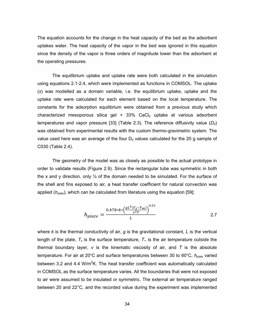
34
The equation accounts for the change in the heat capacity of the bed as the adsorbent
uptakes water. The heat capacity of the vapor in the bed was ignored in this equation
since the density of the vapor is three orders of magnitude lower than the adsorbent at
the operating pressures.
The equilibrium uptake and uptake rate were both calculated in the simulation
using equations 2.1-2.4, which were implemented as functions in COMSOL. The uptake
(x) was modelled as a domain variable, i.e. the equilibrium uptake, uptake and the
uptake rate were calculated for each element based on the local temperature. The
constants for the adsorption equilibrium were obtained from a previous study which
characterized mesoporous silica gel + 33% CaCl2 uptake at various adsorbent
temperatures and vapor pressure [33] (Table 2.3). The reference diffusivity value (D0)
was obtained from experimental results with the custom thermo-gravimetric system. The
value used here was an average of the four D0 values calculated for the 20 g sample of
C030 (Table 2.4).
The geometry of the model was as closely as possible to the actual prototype in
order to validate results (Figure 2.9). Since the rectangular tube was symmetric in both
the x and y direction, only ¼ of the domain needed to be simulated. For the surface of
the shell and fins exposed to air, a heat transfer coefficient for natural convection was
applied (hplate), which can be calculated from literature using the equation [59]:
ℎ𝑝𝑙𝑎𝑡𝑒 =0.478∗𝑘∗�𝑔𝐿
3(𝑇𝑠−𝑇∞)𝜈2𝑇
�0.25
𝐿 2.7
where k is the thermal conductivity of air, g is the gravitational constant, L is the vertical
length of the plate, Ts is the surface temperature, T∞ is the air temperature outside the
thermal boundary layer, ν is the kinematic viscosity of air, and T is the absolute
temperature. For air at 20°C and surface temperatures between 30 to 60°C, hplate varied
between 3.2 and 4.4 W/m2K. The heat transfer coefficient was automatically calculated
in COMSOL as the surface temperature varies. All the boundaries that were not exposed
to air were assumed to be insulated or symmetric. The external air temperature ranged
between 20 and 22°C, and the recorded value during the experiment was implemented

35
in the model. The initial temperature measured with the thermocouples at the side of the
wall was used in the model as the overall initial temperature.
The mesh used for simulations was a free-triangular mesh with 8418 elements,
generated in COMSOL. A steady-state grid independence study assuming a constant
volumetric heat generation of 10 kW/m3 in the adsorbent domain showed that the
average surface heat flux from the boundaries exposed to air only varied by 0.01% in the
mesh size range of 4405 to 54949 (Figure 2.10).
The total water uptake in the adsorbent bed was calculated from the simulation
results by averaging the uptake in the simulation and multiplying by the mass of the
adsorbent in the experiment (950g), and the cooling power per kilogram of adsorbent
was calculated by averaging the derivative of the uptake and multiplying the value by
1kg. The temperature was measured in the centre of the un-finned face of the adsorbent
bed (point P1 in Figure 2.9). All simulation results were then compared with experimental
results.
Table 2.3. Properties for adsorption characterization, thermo-physical properties, and dimensions used in the simulations
variable value source variable value source Adsorption characterization Thermo-physical properties
n 0.162 [33] ρads 693 [kg/m3] exp. D 1.963 [33] cp,ads 924 [J/kg/K] [32] x0 34.1 [33] kal 0.12 [W/m/K] [60] D0 4.40E-05 [m2/g] exp. ΔHads 2330E3 [J/kg] [41] Ea 4.20E+04 [J/mol] [32] ρal 2700 [kg/m3] COMSOL R 8.314 [J/mol/K] [32] cp,al 900 [J/kg/K] COMSOL rp 0.375 [mm] manuf. kal 160 [W/m/K] COMSOL ρwater 1000 [kg/m3] COMSOL cp,water 4200 [J/kg/K] COMSOL
Dimensions tspace 1 [mm] exp. tshell 3.175 [mm] manuf. tplate 0.625 [mm] manuf. tfin 0.5 [mm] manuf. tads exp. lfin 5 [cm] exp.
wshell 5.08 [cm] exp. s 1 [cm] exp. L 26 [cm] exp.

36
Figure 2.9. Geometry of the adsorbent bed heat transfer simulation implemented in COMSOL
Figure 2.10. Results from grid independence study showing variation in average surface heat flux from boundaries exposed to air with varying mesh size assuming a constant volumetric heat generation of 10 kW/m3 in the adsorbent bed
54949 28018
8418
5305
4405 308.89
308.895
308.9
308.905
308.91
308.915
308.92
308.925
0 10000 20000 30000 40000 50000 60000
aver
age
surfa
ce h
eat f
lux
[W/m
2 ]
mesh size

37
Adsorbent Bed Prototype Testing
The transient uptake of the prototype was measured as the final proof-of-concept
experiment. As mentioned in section 1.3, there are two ways that the cooling effect of
adsorption can be used to induce hypothermia: cooling with a blanket, and cooling saline
solution which is subsequently administered intravenously. Therefore, two separate tests
were undertaken: measurement of the cooling capacity with the water vapor pressure
relatively constant at 1,230 to 1,700 Pa, corresponding to water temperature 10-15°C
(blanket cooling), and ability to cool a certain mass of water from room temperature to 4-
6°C (intravenous cooling).
For these tests, a 1 kg sample of C030 was made using the same procedure as
described in section 0. C030 was selected because results from the custom thermo-
gravimetric system showed that it had the highest uptake out of all the samples tested
(see section 2.4.1). Before conducting tests, the sample was dried by heating to 200°C
in an oven for 4-5 hours, until the mass of the sample remained constant over a 15
minute drying period. After the sample was placed in the prototype, evacuation of the
system proceeded as previously described in section 2.3.1.
The experimental setup for large scale-tests was similar to the small-scale testing
setup (Figure 2.11). However, vapor pressure drop in the tubing was found to be a
significant issue due to the high mass flow rates. To minimize the pressure drop, a short
tube directly connecting the adsorbent to the evaporator with a valve in the middle (V4)
was added (Figure 2.11a,b). Additionally, the temperature of the adsorbent material is
not controlled with a heater as in the small-scale tests. During the test, valve V4 was
open to allow vapor flow, valves V1 and V2 were closed and V3 was open so that the
vapor pressure could be measured as close to the inlet of the adsorbent as possible.
Temperature of the adsorbent bed was measured with four thermocouples (T1-T4)
placed at the middle of the un-finned face of the shell and spaced 5 cm vertically. The
thermocouples were held in place by electrical tape.
For testing the uptake at relatively constant vapor pressure, the temperature of
the water was controlled with a chiller as best as possible (Figure 2.11a). However, due
to the high cooling rate, the water temperature inevitably dropped during the experiment,

38
reducing the vapor pressure. Additionally, as the uptake rate decreased in the later
stages of the experiments, the pressure drop through the tubing also decreased.
Consequently, the pressure measured at the inlet tended to vary significantly, and the
chiller temperature had to be adjusted manually throughout the experiment to keep the
pressure in the desired range.
For testing the ability to cool a mass of water, the temperature-controlled
evaporator was replaced with a bath of water (600-800 grams) in a vacuum desiccator
(F4201, Bel Art, NJ). A thermocouple was fed through the lid of the desiccator (T5) to
measure the water temperature (Figure 2.11b). Heat transfer with the environment was
assumed to be negligible.
a)
b)
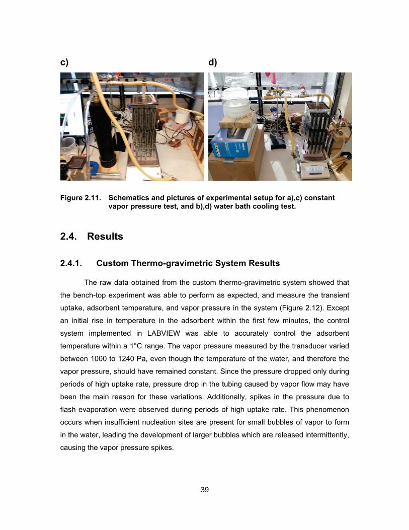
39
c)
d)
Figure 2.11. Schematics and pictures of experimental setup for a),c) constant vapor pressure test, and b),d) water bath cooling test.
2.4. Results
2.4.1. Custom Thermo-gravimetric System Results
The raw data obtained from the custom thermo-gravimetric system showed that
the bench-top experiment was able to perform as expected, and measure the transient
uptake, adsorbent temperature, and vapor pressure in the system (Figure 2.12). Except
an initial rise in temperature in the adsorbent within the first few minutes, the control
system implemented in LABVIEW was able to accurately control the adsorbent
temperature within a 1°C range. The vapor pressure measured by the transducer varied
between 1000 to 1240 Pa, even though the temperature of the water, and therefore the
vapor pressure, should have remained constant. Since the pressure dropped only during
periods of high uptake rate, pressure drop in the tubing caused by vapor flow may have
been the main reason for these variations. Additionally, spikes in the pressure due to
flash evaporation were observed during periods of high uptake rate. This phenomenon
occurs when insufficient nucleation sites are present for small bubbles of vapor to form
in the water, leading the development of larger bubbles which are released intermittently,
causing the vapor pressure spikes.
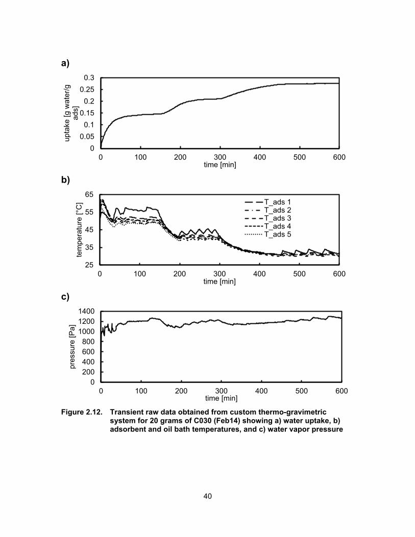
40
a)
b)
c)
Figure 2.12. Transient raw data obtained from custom thermo-gravimetric
system for 20 grams of C030 (Feb14) showing a) water uptake, b) adsorbent and oil bath temperatures, and c) water vapor pressure
00.05
0.10.15
0.20.25
0.3
0 100 200 300 400 500 600
upta
ke [g
wat
er/g
ad
s]
time [min]
25
35
45
55
65
0 100 200 300 400 500 600
tem
pera
ture
[°C
]
time [min]
T_ads 1T_ads 2T_ads 3T_ads 4T_ads 5
0200400600800
100012001400
0 100 200 300 400 500 600
pres
sure
[Pa]
time [min]
41
Figure 2.13. Comparison of equilibrium uptake at water vapor pressure of 1200 Pa and various temperatures for 20 g of B150 with the custom thermo-gravimetric system and 14 mg of B150 with the TGA
Comparison of equilibrium uptake measured for 20 grams of B150 samples and
data from the TGA for the same vapor pressure and temperatures showed that the
results from the custom thermo-gravimetric system were indeed valid (Figure 2.13). Any
differences with results from the TGA were within the range of the experimental
uncertainty, as reported in section 2.3.1.
The influence of adsorbent layer thickness was observed to be significant for
sample C024, and also noticeable for sample C030 (Figure 2.14). The 10, 20, and 40 g
samples of C024 had a layer thickness of approximately 2.3, 4.6, and 9.2 mm
respectively; and the 20, and 40 g samples of C030 had a layer thickness of
approximately 3.7, and 7.4 mm respectively. For both adsorbents, the difference in
uptake between the 40 and 20 g samples increased as the overall uptake increased.
However, there was no noticeable difference in uptake between the 10 and 20 g
samples for C024. The uptake for C030 was observed to be greater than that of the
C024 sample for the entire temperature range.
0
0.01
0.02
0.03
0.04
0.05
30 35 40 45 50 55
upta
ke [g
wat
er/ g
ads
orbe
nt]
adsorbent temperature [°C]
B150 - Feb7
B150 - Feb12
B150 TGA
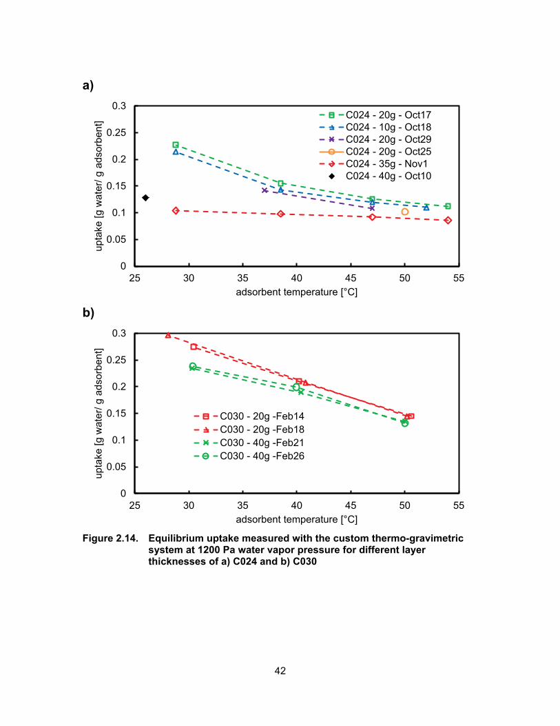
42
a)
b)
Figure 2.14. Equilibrium uptake measured with the custom thermo-gravimetric
system at 1200 Pa water vapor pressure for different layer thicknesses of a) C024 and b) C030
0
0.05
0.1
0.15
0.2
0.25
0.3
25 30 35 40 45 50 55
upta
ke [g
wat
er/ g
ads
orbe
nt]
adsorbent temperature [°C]
C024 - 20g - Oct17C024 - 10g - Oct18C024 - 20g - Oct29C024 - 20g - Oct25C024 - 35g - Nov1C024 - 40g - Oct10
0
0.05
0.1
0.15
0.2
0.25
0.3
25 30 35 40 45 50 55
upta
ke [g
wat
er/ g
ads
orbe
nt]
adsorbent temperature [°C]
C030 - 20g -Feb14C030 - 20g -Feb18C030 - 40g -Feb21C030 - 40g -Feb26
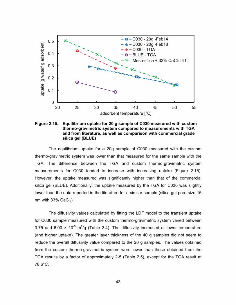
43
Figure 2.15. Equilibrium uptake for 20 g sample of C030 measured with custom thermo-gravimetric system compared to measurements with TGA and from literature, as well as comparison with commercial grade silica gel (BLUE)
The equilibrium uptake for a 20g sample of C030 measured with the custom
thermo-gravimetric system was lower than that measured for the same sample with the
TGA. The difference between the TGA and custom thermo-gravimetric system
measurements for C030 tended to increase with increasing uptake (Figure 2.15).
However, the uptake measured was significantly higher than that of the commercial
silica gel (BLUE). Additionally, the uptake measured by the TGA for C030 was slightly
lower than the data reported in the literature for a similar sample (silica gel pore size 15
nm with 33% CaCl2).
The diffusivity values calculated by fitting the LDF model to the transient uptake
for C030 sample measured with the custom thermo-gravimetric system varied between
3.75 and 6.00 × 10⁻⁵ m2/g (Table 2.4). The diffusivity increased at lower temperature
(and higher uptake). The greater layer thickness of the 40 g samples did not seem to
reduce the overall diffusivity value compared to the 20 g samples. The values obtained
from the custom thermo-gravimetric system were lower than those obtained from the
TGA results by a factor of approximately 2-5 (Table 2.5), except for the TGA result at
78.6°C.
0
0.1
0.2
0.3
0.4
0.5
20 25 30 35 40 45 50 55
upta
ke [g
wat
er/ g
ads
orbe
nt]
adsorbent temperature [°C]
C030 - 20g -Feb14C030 - 20g -Feb18C030 - TGABLUE - TGAAristov (2002)Meso-silica + 33% CaCl2 [41]

44
Table 2.4. Diffusivity values for C030 obtained by fitting transient uptake data from custom thermo-gravimetric system with LDF model at various temperatures
20g – Feb14 20g – Feb19
T [°C] xfinal [-] D0 [1/s2] X105 T [°C] xfinal [-] D0 [1/s2] X105
50.0 ± 2.9 0.145 3.80 49.9 ± 2.4 0.145 3.75
40.6 ± 1.8 0.209 5.60 40.4 ± 1.8 0.208 4.44
40g – Feb21 40g – Feb26
50.1 ± 2.5 0.135 4.07 49.9 ± 2.2 0.132 3.75
40.5 ± 2.1 0.189 4.05 38.9 ± 3.2 0.199 4.52
30.9 ± 1.9 0.234 5.08 30.8 ± 1.7 0.238 6.00
Table 2.5. Diffusivity values for C030 and K60 obtained by fitting transient uptake data from TGA with LDF model at various temperatures
C030
T [°C] xfinal [-] D0 [1/s2] X105
78.6 0.067 2.67
34.8 0.278 11.2
25.0 0.417 14.9
2.4.2. Adsorbent Bed Prototype Testing Results
As mentioned in the experiment description (section 2.3), the vapor pressure was
maintained as close to a constant value as possible by varying the chiller temperature,
but it varied depending on the pressure drop in the tubing and the temperature of the
water (Figure 2.16). The pressure spikes observable in the last 10 minutes were due to
flash evaporation. The vapor pressure over the entire test varied between 1320 and

45
1820 Pa, corresponding to a saturated water temperature between 11-16°C. The
pressure trend was curve fitted to a 5th degree polynomial so that it could be used as an
analytical function input in COMSOL for the adsorption simulation.
Figure 2.16. Pressure at the inlet of the adsorbent bed during uptake by 950 grams of C030 in prototype adsorbent bed with inlet vapor pressure varying between 1320 and 1820 Pa, and polynomial fit for the pressure trend.
The total water uptake by 950 grams of C030 during the 32 minute experiment
was 78 grams, corresponding to an average adsorbent uptake of 0.082 (Figure 2.17).
The average cooling power over the duration was 99 Watts, given that the latent heat of
vaporization for water at 15°C is 2440 kJ/kg. The uptake rate was relatively constant for
the first 15 minutes and then dropped noticeably. Commercial grade silica gel (BLUE) in
similar conditions only had an average uptake of 0.051, approximately 60% of uptake by
C030.
The drop in uptake rate at 15 minutes for C030 was accompanied by the
plateauing of the temperature on the outer surface of the shell at approximately 55°C.
There was no significant difference in the measurements of the four thermocouples after
15 minutes, but a maximum temperature difference of 7°C was observed in the first half
of the test, with the thermocouples closer to the outlet indicating a higher temperature.
0200400600800
100012001400160018002000
0 5 10 15 20 25 30 35
pres
sure
[Pa]
time [min]
experimental polynomial fit
P(t) = -7.25×10⁻¹³
(t5) + 4.46×10
-9(t
4) - 9.36×10
-6(t
3) + 7.68×10
-3(t
2)
- 1.92(t) + 1.54×10³
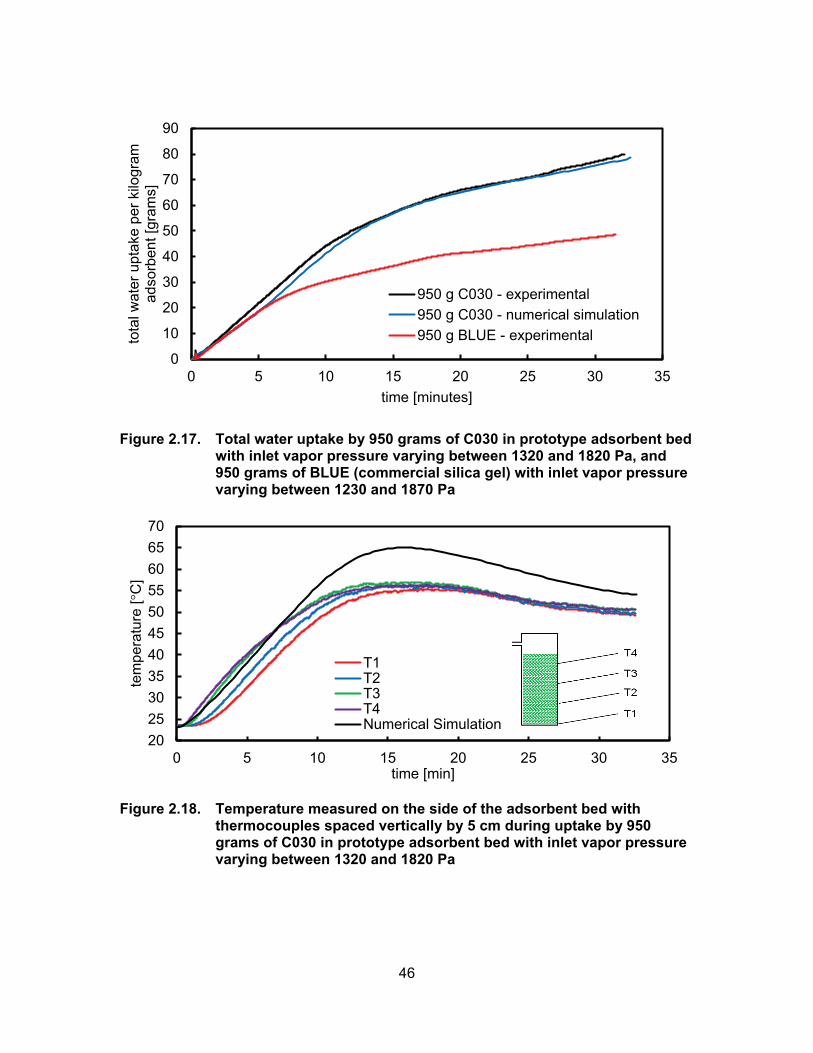
46
Figure 2.17. Total water uptake by 950 grams of C030 in prototype adsorbent bed with inlet vapor pressure varying between 1320 and 1820 Pa, and 950 grams of BLUE (commercial silica gel) with inlet vapor pressure varying between 1230 and 1870 Pa
Figure 2.18. Temperature measured on the side of the adsorbent bed with thermocouples spaced vertically by 5 cm during uptake by 950 grams of C030 in prototype adsorbent bed with inlet vapor pressure varying between 1320 and 1820 Pa
0
10
20
30
40
50
60
70
80
90
0 5 10 15 20 25 30 35
tota
l wat
er u
ptak
e pe
r kilo
gram
ad
sorb
ent [
gram
s]
time [minutes]
950 g C030 - experimental950 g C030 - numerical simulation950 g BLUE - experimental
2025303540455055606570
0 5 10 15 20 25 30 35
tem
pera
ture
[°C
]
time [min]
T1T2T3T4Numerical Simulation
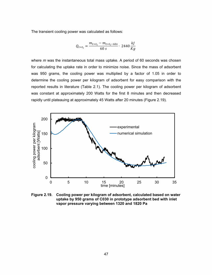
47
The transient cooling power was calculated as follows:
𝑄𝑡=𝑡𝑖 =𝑚𝑡=𝑡𝑖 − 𝑚𝑡=𝑡𝑖−60𝑠
60 𝑠∙ 2440
𝑘𝐽𝐾𝑔
where m was the instantaneous total mass uptake. A period of 60 seconds was chosen
for calculating the uptake rate in order to minimize noise. Since the mass of adsorbent
was 950 grams, the cooling power was multiplied by a factor of 1.05 in order to
determine the cooling power per kilogram of adsorbent for easy comparison with the
reported results in literature (Table 2.1). The cooling power per kilogram of adsorbent
was constant at approximately 200 Watts for the first 8 minutes and then decreased
rapidly until plateauing at approximately 45 Watts after 20 minutes (Figure 2.19).
Figure 2.19. Cooling power per kilogram of adsorbent, calculated based on water uptake by 950 grams of C030 in prototype adsorbent bed with inlet vapor pressure varying between 1320 and 1820 Pa
0
50
100
150
200
0 5 10 15 20 25 30 35
cool
ing
pow
er p
er k
ilogr
am
adso
rben
t [W
atts
]
time [minutes]
experimentalnumerical simulation

48
a)
b)
c)
Figure 2.20. Results for cooling of a 650 mL bath of water with 950 grams C030 in
the adsorbent bed prototype showing a) bath temperature, b) inlet pressure, and c) total water uptake
The present numerical simulation was able to accurately predict the transient
total uptake, with a maximum difference of 4 grams between simulation and
experimental data (Figure 2.17). However, the predicted temperature at point P1 (Figure
0
5
10
15
20
25
0 5 10 15 20 25 30 35
bath
tem
pera
ture
[°C
]
time [min]
0500
10001500200025003000
0 5 10 15 20 25 30 35
pres
sure
[Pa]
time [min]
05
1015202530
0 5 10 15 20 25 30 35
tota
l wat
er u
ptak
e [g
ram
s]
time [min]
49
2.9) differed from the experimental results measured at the same location significantly
after 10 minutes, reaching a maximum of 10°C higher than the experimental results
(Figure 2.18). The overall cooling power predicted was reasonably accurate after 7
minutes, but was lower than the experimental results by approximately 50°C in the first
few minutes (Figure 2.20).
The second experiment showed that the 950 grams of adsorbent in the prototype
adsorbent bed could uptake sufficient water to cool a bath of water weighing 650 grams
from room temperature to 6°C within 25 minutes (Figure 2.20a). As expected, the inlet
pressure dropped significantly, plateauing at 700 Pa in the later stages (Figure 2.20b).
The total water uptake was only 25 grams, corresponding to an average adsorbent
uptake of 0.026, significantly smaller than the previous experiment at higher pressure
(Figure 2.20c).
2.5. Discussion
The present study proved that an adsorption-based cooling device would be well
suited to the requirements for a pre-hospital cooling technology. A cooling power of 100
W was achieved for the first 30 minutes from adsorption with 950 g C030 in the
prototype adsorbent bed, so only 2.5 kg of adsorbent would be needed to provide the
250 W required for hypothermia treatment.
However, the empty structure (dead weight) of the prototype in the present study
weighs 2.3 kg and has an adsorbent capacity of 1.3 kg, so the structure contributes
more weight to the device than the adsorbent material. The current design is good for a
proof-of-concept, but future prototypes should be kept as lightweight as possible, e.g. by
using plastic film material for vacuum sealing (as seen in the small-scale prototype
presented in Appendix A) and possibly graphite sheets rather than aluminum sheets for
heat dissipation elements.
Although the cooling power measured in the literature using only lithium chloride
as the adsorbent claimed 100-127 W of cooling per kilogram of adsorbent for 1 hour, the
methodology for measuring the cooling power used in the two experiments is quite
50
uncertain, as discussed previously in section 2.1 [26], [27]. Additionally, lithium chloride
may be inferior to the calcium chloride-based adsorbent for a medical application
because its high toxicity would be a significant concern for patient safety, especially if
the adsorbent is embedded in the blanket component.
The present study also proved that significant gains in total uptake could be
made by using composite materials rather than standard commercial silica gel (Figure
2.15 and Figure 2.17). However, this study also showed that the uptake of composite
adsorbents can change with layer thickness (Figure 2.14), and that loading physical
adsorbents with salts also severely restricted mass transfer (Table 2.5).
The fact that increasing the layer thickness for both the C024 and the C030
samples decreases their equilibrium uptake may be explained by a restriction of vapor
diffusion into the adsorbent bed caused by calcium chloride solution present in the pores
between grains (macropores). As the anhydrous calcium chloride in the micropores of
the silica gel adsorbs water, it becomes a liquid solution and can flow to the outer
surface of the silica gel grain, completely filling the macropores. If a section of the
adsorbent is completely enclosed by a layer of saturated calcium chloride solution, it
may not reach the uptake capacity, thus reducing the overall equilibrium uptake. This
hypothesis is supported by the fact that the impact of layer thickness was more prevalent
in C024, which has smaller grains and therefore smaller macropores than C030.
The same phenomenon would also occur if calcium chloride is present not just in
the micropores of the silica gel, but also in a powder form outside the silica gel. This can
occur by testing the same sample multiple times, as calcium chloride may form a
solution and cover the surface of the grain, then dry out on the surface of the grain
during the subsequent drying period.
Although the presence of salt solution in macropores of composite adsorbents
has been previously observed [52], its impact on adsorption equilibrium of multiple-
layers has not been previously been studied. Consequently, further experimental work
on multi-layered adsorbent is required before a strong conclusion can be made on the
subject.

51
The reference diffusivity values of 3.75 to 6.00 × 10⁻⁵ m2/g obtained for C030
from the custom thermo-gravimetric system (Table 2.4) were significantly lower than the
value of 2.54 × 10⁻⁴ m2/g used in the literature for silica gel [32], [37], and the values
obtained for C030 from the TGA at low temperatures (Table 2.5). However, given that
the value obtained from the TGA at 78°C is 2.67 × 10⁻⁵ m2/g, it is not possible to state
that layer thickness had any impact of the measured diffusivity value based on the
current data.
The fact that there is no noticeable difference in the diffusivity measured from the
40 g and 20 g samples points to the possibility that layer thickness had no impact on the
measurement. However, it is important to note that uncertainty in diffusivity
measurement from the custom thermo-gravimetric system is relatively high, due to the
high deviation in the temperature and variation of the vapour pressure over time.
The increase in diffusivity with increasing uptake observable in the TGA and the
custom thermo-gravimetric data has previously been observed. A study of diffusivity of a
single layer of silica gel loaded with calcium chloride found that the presence of salt
solution forms a parallel path for diffusion of water vapor into the adsorbent and
increases the uptake rate [52]. Consequently, the vapour diffusion is slower when the
total uptake is low and there is no salt solution present in the adsorbent bed.
Results from the 950 g C030 in the prototype adsorbent bed show that there was
no significant difference in the temperature rise vertically along the bed (Figure 2.18).
Since the rate of heat generation is dependent on the adsorption rate, the uniform
temperature rise indicates that there is no significant drop in vapour pressure along the
height of the bed. Although the presence of the vapour flow channels successfully
prevented a non-uniform adsorption similar to the prototype presented in Appendix A,
the ratio of adsorbent thickness to channel thickness can be optimized to minimize the
dead volume of the adsorbent bed and increase compactness of the overall device.
The results from the prototype tests clearly indicate a significant reduction in
cooling power caused by a rise in temperature after 8 minutes (Figure 2.18 and Figure
2.19), indicating that thermal management of the adsorbent bed is of the utmost
importance. Due to the low thermal conductivity of the adsorbent material, the average

52
temperature of the adsorbent is likely significantly higher than the surface temperature
measured. The average uptake of 0.083 measured after 30 minutes in the prototype test
with C030 is only 27% of the equilibrium uptake measured at 30°C.
Consequently, significant gains in uptake can be made by improving the thermal
management of the adsorbent bed. It may be possible to implement a forced convective
cooling system, e.g. with fans powered by batteries. The additional mass of the active
cooling components may be completely offset up a reduction in the mass of adsorbent
needed to achieve the required cooling power.
Additionally, further study is required into the optimal adsorbent. Despite the
improvement of C030 sample over commercial grade silica gel, the equilibrium uptake
remains low at the high temperatures reached in the prototype tests. In contrast, zeolite
13X maintains a total uptake of 0.24 (mwater /madsorbent) even at temperatures between 60-
70°C (Figure 2.2). The issue of reduced uptake with increased layer thickness can also
be avoided by using a sorbent with no salt content.
The present numerical simulation was accurately able to predict the transient
mass uptake and the cooling power of the device (Figure 2.17 and Figure 2.19). The
deviation of cooling power in the simulation results over the first few minutes is most
likely due to the inaccurate modeling of the vapour pressure, wherein the measured
pressure is initially 1800 Pa but the curve fit predicts approximately 1500 Pa. The
simulation also accurately predicted the rate of temperature rise and the duration
required for the temperature to plateau, but the maximum temperature predicted was
higher than our experimental measurement by approximately 10°C. The reason for this
difference may be due to inaccurate modeling of the equilibrium uptake at high
temperature, or the heat of adsorption, which is modelled as a constant here but is
known to change depending on the instantaneous uptake [41]. The uniform pressure
distribution assumption did not significantly impact the results, and was effective in
reducing the computational resources required. With accurate modeling of adsorption
equilibrium, kinetics, and heat of adsorption, numerical simulations can be a powerful
tool for evaluating different thermal designs of the adsorbent bed and testing the
performance of different adsorbents in a specific design.
53
Chapter 3. Bioheat Transfer Simulation
3.1. Review of Bioheat Transfer Models
Determining the cooling rate and temperature distribution of an in vivo sample of
tissue is not as easy as doing the same for, say, a piece of metal of the same geometry;
the calculation is influenced by the level of blood flow in the network of capillaries within
the tissue, metabolic heat generation in each cell, and thermoregulatory responses.
Given that the feedback control mechanism of thermoregulation is always active and
core temperature always fluctuates to some extent, the body can never be said to be in
a thermal equilibrium or steady-state, even if the environmental conditions remain
constant. Additionally, calculation of thermal response of the human body is hindered by
the complicated geometry and the varying thermal properties of the different types of
tissue.
Due to the lack of validated comprehensive models for thermal response of
humans, animal models are frequently used to test hypotheses about optimization of
cooling methods [61]; however, physiological and anatomical difference between the
human body and the animal model can render the results unreliable [62]–[64]. For
example, some animals have shown the ability to selectively cool the brain during
hyperthermia due to the existence of the carotid rete, where the venous blood and
arterial blood are able to exchange heat, allowing for the cooling of the warm arterial
blood by the venous blood which gets cooled by the environment as it circulates through
the face. This has piqued the interest of the scientific community, because the ability to
selective cool the brain would reduce the cooling power and time required to achieve
cerebral hypothermia. However, humans do not have a carotid rete, and there is very
little scientific consensus about whether selective brain cooling is possible in humans
[62], [63].
54
As opposed to animal models, computational modeling of the body offer an ability
to accurately replicate the geometry and tissue composition of the human body; and
validated models can even help determine the underlying factors which influence core
temperature drop during surface cooling. Several whole-body and localized models are
present in the literature.
The historical development of whole-body models was described in detail in 2012
[65]. The first significant step towards human thermal modeling came in 1948 when the
Pennes bioheat equation was published [66], which is an energy balance equation for
tissue that includes a term for heat exchange caused by perfusion of blood into tissue.
Soon after came the early whole-body models which used the Pennes bioheat equation
and defined the geometry as being composed of homogeneous cylindrical elements
representing the head, trunk, arms, and legs [67]. The homogeneous cylinders were
subsequently divided into concentric cylinders of skin, fat, muscle and tissue; and
thermoregulatory mechanisms were introduced as control functions which varied the
heat generation caused by shivering, and perfusion rates based on the local and
hypothalamus temperature [68], [69]. The control functions were fitted such that the
overall model results would agree with experimental data [11]. Although this method of
defining thermoregulation parameters may blend the impact of various factors and make
it more difficult to validate each isolated thermoregulatory response, it was at the time far
more difficult to directly measure each response such as shivering and vasoconstriction.
However, modern techniques have allowed for direct measurement of
vasoconstriction and shivering levels in a controlled environment [70], [71]; and the
modern Fiala multi-node model developed in 2001 is similar to the previous models
except that it takes advantage of the recent data and correlates the thermoregulation
parameters with the directly measured data [72]–[74]. The body was assumed to consist
of 15 spherical and cylindrical elements (representing the trunk, head, neck, extremities,
etc.). A separate control function is used for each of the four major thermoregulatory
mechanisms (vasoconstriction, shivering, sweating, and vasodilation). Although the
methodology used for developing the model is not significantly novel compared to other
literature, the thermoregulation control functions and parameters are comprehensively
defined, and this aspect of the work is widely used in the literature [70], [75]–[78]. More
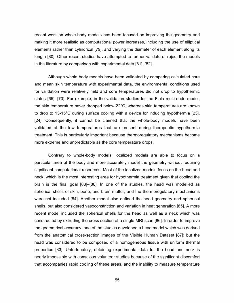
55
recent work on whole-body models has been focused on improving the geometry and
making it more realistic as computational power increases, including the use of elliptical
elements rather than cylindrical [79], and varying the diameter of each element along its
length [80]. Other recent studies have attempted to further validate or reject the models
in the literature by comparison with experimental data [81], [82].
Although whole body models have been validated by comparing calculated core
and mean skin temperature with experimental data, the environmental conditions used
for validation were relatively mild and core temperatures did not drop to hypothermic
states [65], [73]. For example, in the validation studies for the Fiala multi-node model,
the skin temperature never dropped below 22°C, whereas skin temperatures are known
to drop to 13-15°C during surface cooling with a device for inducing hypothermia [23],
[24]. Consequently, it cannot be claimed that the whole-body models have been
validated at the low temperatures that are present during therapeutic hypothermia
treatment. This is particularly important because thermoregulatory mechanisms become
more extreme and unpredictable as the core temperature drops.
Contrary to whole-body models, localized models are able to focus on a
particular area of the body and more accurately model the geometry without requiring
significant computational resources. Most of the localized models focus on the head and
neck, which is the most interesting area for hypothermia treatment given that cooling the
brain is the final goal [83]–[86]. In one of the studies, the head was modelled as
spherical shells of skin, bone, and brain matter; and the thermoregulatory mechanisms
were not included [84]. Another model also defined the head geometry and spherical
shells, but also considered vasoconstriction and variation in heat generation [85]. A more
recent model included the spherical shells for the head as well as a neck which was
constructed by extruding the cross section of a single MRI scan [86]. In order to improve
the geometrical accuracy, one of the studies developed a head model which was derived
from the anatomical cross-section images of the Visible Human Dataset [87]; but the
head was considered to be composed of a homogeneous tissue with uniform thermal
properties [83]. Unfortunately, obtaining experimental data for the head and neck is
nearly impossible with conscious volunteer studies because of the significant discomfort
that accompanies rapid cooling of these areas, and the inability to measure temperature

56
within the brain or neck without serious risk to the volunteer’s health. Consequently,
none of the models mentioned above were validated with experimental data.
The Visible Human dataset was also used in another study for development of
the geometry of a forearm model [88]. The temperature distribution within the forearm
model was validated with experimental data from the literature. Another model of the
upper limb consists of four elements (upper arm, forearm, hand and digits), with the
upper arm, forearm, and the digits shaped as concentric cylinders and the hand as a
rectangular block [89]. The study also modelled various superficial and deep blood
vessels as cylinders with a convective coefficient of heat transfer between the blood and
the interior wall of the vessel. The model was validated for mild conditions (lowest
means skin temperature for the arm was 23°C). The results indicated that there was a
3% increase in heat transfer when skin blood flow returned through superficial veins as
opposed to returning through deep vessels, implying that the impact of blood flow
through superficial blood vessels is relatively small. However, this result was in a neutral
environment, and the authors suggested that the superficial vessels could play a more
significant role at lower environmental temperatures [89].
The influence of blood vessels was also analyzed in an analytical study of heat
transfer in the neck, wherein the goal was to determine if blood in the carotid artery
could be sufficiently cooled by surface cooling of the neck so as to induce selective brain
cooling [64]. Results indicated that carotid blood temperature drop of up to 2°C is
achievable; however the model did not take into account blood perfusion in the neck
tissue, so the results may be overly optimistic. Nonetheless, these studies prove that the
contribution of superficial blood vessels to the overall heat transfer in a segment of the
body remains to be tested at low temperatures.
3.2. Model Development and Simulation Parameters
To define the required boundary conditions for a surface cooling device, a model
for predicting transient heat flux under various surface temperatures needs to be
developed. As shown in the previous section (3.1), various passive and thermoregulation
models exist in literature, but validation of simulation results with experimental data is

57
still missing at hypothermic conditions. Consequently, this study was designed to
validate the thermoregulation models presently available by comparison with
experimental data at very low surface temperatures. Furthermore, the impact of specific
thermoregulatory responses was analyzed in the context of heat transfer to surface
cooling devices and overall core cooling rate. In order to reduce the influence of
geometry on the simulation results, the model was designed to be as geometrically
realistic as possible, and the influence of geometry was analyzed by comparing the
simulation results with the results from a simplified geometry. Additionally, large and
superficial blood vessels were included in the model in the interest of making the model
as realistic as possible, and their impact on heat transfer was studied as well.
Given that the geometry of the model was to be as accurate as possible, a
whole-body model was considered out-of-scope given the significant computational
resources required; thus localized cooling in the upper leg was analyzed. There were
three main reasons for modelling the upper leg as opposed to other areas: 1) the upper
leg is more geometrically simple than other areas such as the torso and head and neck,
and also far from any major organs which can influence the simulation, 2) unlike the
arms, the upper leg has a significant thermal mass and is one of the relevant areas for
surface cooling, and 3) there are in vivo experimental results available for validation at
very cold conditions [90]–[93].
The geometrically accurate 3D model of the upper leg was developed by
manually segmenting seven transverse anatomical images of the upper leg from the
Visible Human Dataset (image # 1992 to 2292). Each image was imported into
Solidworks 2012 (Dassault Systèmes, Waltham) and a separate spline was developed
for each cross section to represent the boundaries of the skin, fat, muscle, and bones,
and blood vessels. The solid model was created by connecting the splines for the
boundaries of the skin with a loft extrude function. The solid model was discretized with
loft surfaces representing the boundaries of the fat, muscle, bone, and blood vessels.
Skin was assumed to the outer 2mm layer of the model as assumed in literature [72],
because the boundary between muscle and skin is not visibly distinguishable.
58
a)
b)
c)
d)
e)
Figure 3.1. Details of upper leg 3D model showing a) an example of creating a boundary for the muscle in Solidworks by tracing over the Visible Human Dataset figure, b) the solid model including cavities for blood vessels, c) the bone loft surface, and d) the muscle loft surface, and e) segments of the model
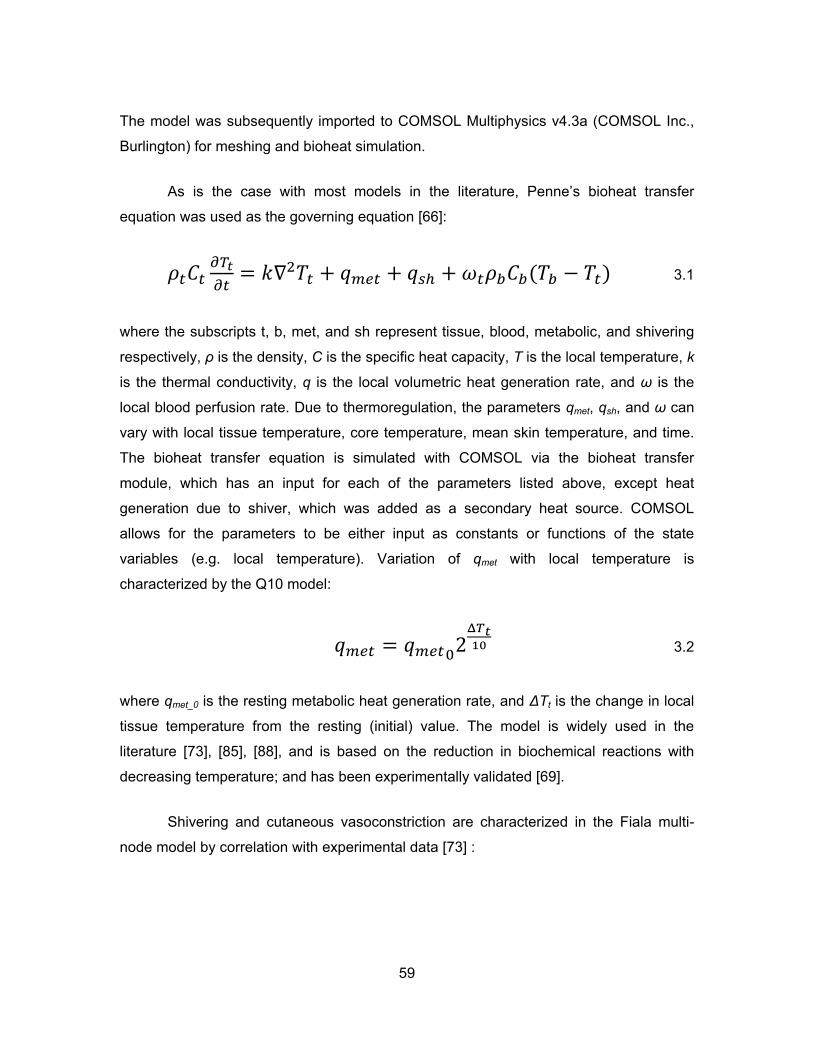
59
The model was subsequently imported to COMSOL Multiphysics v4.3a (COMSOL Inc.,
Burlington) for meshing and bioheat simulation.
As is the case with most models in the literature, Penne’s bioheat transfer
equation was used as the governing equation [66]:
𝜌𝑡𝐶𝑡𝜕𝑇𝑡𝜕𝑡
= 𝑘∇2𝑇𝑡 + 𝑞𝑚𝑒𝑡 + 𝑞𝑠ℎ + 𝜔𝑡𝜌𝑏𝐶𝑏(𝑇𝑏 − 𝑇𝑡) 3.1
where the subscripts t, b, met, and sh represent tissue, blood, metabolic, and shivering
respectively, ρ is the density, C is the specific heat capacity, T is the local temperature, k
is the thermal conductivity, q is the local volumetric heat generation rate, and ω is the
local blood perfusion rate. Due to thermoregulation, the parameters qmet, qsh, and ω can
vary with local tissue temperature, core temperature, mean skin temperature, and time.
The bioheat transfer equation is simulated with COMSOL via the bioheat transfer
module, which has an input for each of the parameters listed above, except heat
generation due to shiver, which was added as a secondary heat source. COMSOL
allows for the parameters to be either input as constants or functions of the state
variables (e.g. local temperature). Variation of qmet with local temperature is
characterized by the Q10 model:
𝑞𝑚𝑒𝑡 = 𝑞𝑚𝑒𝑡02Δ𝑇𝑡10 3.2
where qmet_0 is the resting metabolic heat generation rate, and ΔTt is the change in local
tissue temperature from the resting (initial) value. The model is widely used in the
literature [73], [85], [88], and is based on the reduction in biochemical reactions with
decreasing temperature; and has been experimentally validated [69].
Shivering and cutaneous vasoconstriction are characterized in the Fiala multi-
node model by correlation with experimental data [73] :

60
𝑞𝑠ℎ = 𝑎𝑠ℎ10[𝑡𝑎𝑛ℎ (0.48�𝛥𝑇𝑠𝑘𝑖𝑛,𝑚𝑒𝑎𝑛 + 3.62� − 1]𝛥𝑇𝑠𝑘𝑖𝑛,𝑚𝑒𝑎𝑛 −
27.9𝛥𝑇ℎ𝑦𝑝𝑜𝑡ℎ𝑎𝑙𝑎𝑚𝑢𝑠 + 1.7𝛥𝑇𝑠𝑘𝑖𝑛,𝑚𝑒𝑎𝑛𝑑𝑇𝑠𝑘𝑖𝑛,𝑚𝑒𝑎𝑛
𝑑𝑡 3.3
𝜔𝑠𝑘𝑖𝑛 = 𝜔𝑠𝑘𝑖𝑛01+𝑎𝑣𝑉
2Δ𝑇𝑡10 3.4
where V is the central vasoconstrictor response and is defined as:
𝑉 = 35[𝑡𝑎𝑛 ℎ�0.34�𝛥𝑇𝑠𝑘𝑖𝑛,𝑚𝑒𝑎𝑛 + 1.07� − 1� 𝛥𝑇𝑠𝑘𝑖𝑛,𝑚𝑒𝑎𝑛 +
3.9𝛥𝑇𝑠𝑘𝑖𝑛,𝑚𝑒𝑎𝑛𝑑𝑇𝑠𝑘𝑖𝑛,𝑚𝑒𝑎𝑛
𝑑𝑡 3.5
where ΔTskin,mean and ΔThypothalamus are the change in mean skin temperature and
hypothalamus temperature from their resting values. The terms av and ash are
experimentally derived tissue constants that represent the distribution of the
thermoregulatory response relative to the rest of the body [68], [70], [73], [94]. For the
leg, the values of av and ash are 0.1 and 0.04 respectively [73].
The thermoregulation modeling equations shows that shivering is only active
when the mean skin temperature or hypothalamus temperature changes (eq. 3.3;
however, vasoconstriction can be active even if there is only a change in the local tissue
temperature. This indicates that there are two different contributions to the
vasoconstrictor response: local cooling and systemic cooling; and the influence of both
contributing factors must be studied independently. Perfusion in fat and muscle is
modeled by assuming that changes in blood flow in these regions are determined by
changes in metabolic activity of the tissue. A proportionality constant µ defines the linear
relationship between metabolic activity and blood flow [68], [73]:
Δ𝜔𝑡 = 𝜇Δ(𝑞𝑚𝑒𝑡 + 𝑞𝑠ℎ) 3.6
where Δωt is the change in local tissue perfusion rate from the resting value and:
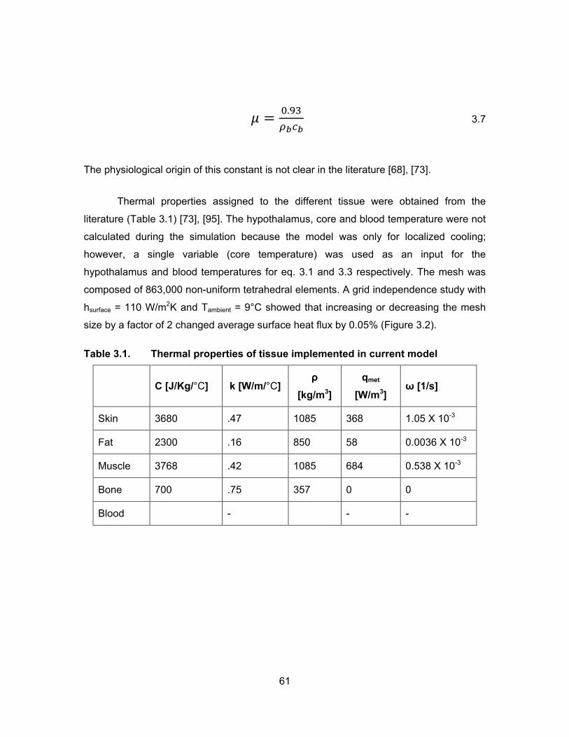
61
𝜇 = 0.93𝜌𝑏𝑐𝑏
3.7
The physiological origin of this constant is not clear in the literature [68], [73].
Thermal properties assigned to the different tissue were obtained from the
literature (Table 3.1) [73], [95]. The hypothalamus, core and blood temperature were not
calculated during the simulation because the model was only for localized cooling;
however, a single variable (core temperature) was used as an input for the
hypothalamus and blood temperatures for eq. 3.1 and 3.3 respectively. The mesh was
composed of 863,000 non-uniform tetrahedral elements. A grid independence study with
hsurface = 110 W/m2K and Tambient = 9°C showed that increasing or decreasing the mesh
size by a factor of 2 changed average surface heat flux by 0.05% (Figure 3.2).
Table 3.1. Thermal properties of tissue implemented in current model
C [J/Kg/°C] k [W/m/°C] ρ
[kg/m3] qmet
[W/m3] ω [1/s]
Skin 3680 .47 1085 368 1.05 X 10⁻³
Fat 2300 .16 850 58 0.0036 X 10⁻³
Muscle 3768 .42 1085 684 0.538 X 10⁻³
Bone 700 .75 357 0 0
Blood - - -
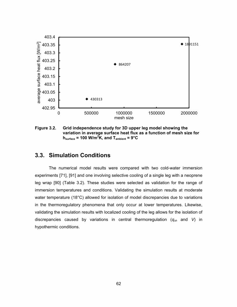
62
Figure 3.2. Grid independence study for 3D upper leg model showing the variation in average surface heat flux as a function of mesh size for hsurface = 100 W/m2K, and Tambient = 9°C
3.3. Simulation Conditions
The numerical model results were compared with two cold-water immersion
experiments [71], [91] and one involving selective cooling of a single leg with a neoprene
leg wrap [90] (Table 3.2). These studies were selected as validation for the range of
immersion temperatures and conditions. Validating the simulation results at moderate
water temperature (18°C) allowed for isolation of model discrepancies due to variations
in the thermoregulatory phenomena that only occur at lower temperatures. Likewise,
validating the simulation results with localized cooling of the leg allows for the isolation of
discrepancies caused by variations in central thermoregulation (qsh and V) in
hypothermic conditions.
430313
864207
1891151
402.95
403
403.05
403.1
403.15
403.2
403.25
403.3
403.35
403.4
0 500000 1000000 1500000 2000000
aver
age
surfa
ce h
eat f
lux
[W/m
2 ]
mesh size

63
Table 3.2. Specifications of experimental cooling studies which are used for validation of the current model
Ref. Subjects Coolant temperature
Areas Cooled
Shivering Core temperature change
Data Collected (Upper leg)
[91] 5 8°C, full body immersion
Yes Yes Skin & muscle temperature
[71] 4 18°C full body immersion
Yes No Skin temperature, heat flux
[90] 1 -2, 4, 9°C Single leg (neoprene wrap)
No No Heat flux
The simulation conditions were matched to each study. The walls of the blood
vessels were assumed to be isothermal at the core temperature in order to simplify
computation. The surface of the leg was convectively cooled with a heat transfer
coefficient of 110 W/m2/°C, to simulate the water immersion study [24]. The study
involving isolated leg cooling used a neoprene leg wrap with cold water flowing through
the wrap and calculated a surface heat transfer coefficient of 140 W/m2/°C [90]. The
initial condition for all simulations was determined by steady-state simulation of ambient
conditions (hsurface = 4 W/m2/°C, Tambient = 22°C).
Localized cooling with the neoprene wrap did not affect the mean skin
and core temperature and subjects did not shiver, so qsh and V were assumed to be 0
[90]. One cold water immersion study recorded skin temperatures at various locations
[92], allowing for calculation of mean skin temperature and its derivative with respect to
time by using the DuBois equation [96]. These values were used for the calculation of
shivering and vasoconstriction terms. The second cold water immersion study did not
provide the mean skin temperature [91], so vasoconstriction (V) was assumed to be 750,
corresponding to a mean skin temperature of approximately 11°C. The sensitivity of the
model outcomes to the assumption was verified by varying V between 400 and 1000 and
observing a 1% change in cutaneous perfusion. Unlike other experiments, core
temperature changed significantly during this experiment. To include this factor, the
blood temperature, i.e. blood perfusion and blood vessel wall temperature, was modeled
using a piecewise function to match the measured core temperature. Shivering was
64
experimentally observed to linearly increase from the start of the experiment to 200 W at
20 minutes, and was modeled as such in the simulations.
Both the localized cooling and immersion studies measured heat flux on
the medial and lateral sides of the thigh. Under localized cooling heat flux was measured
on a 5 cm2 area of the medial and lateral sides of the thigh, about 10 cm from the top of
the thigh [90]. In the immersion study the exact location of heat flux measurement was
not specified [71]. The simulation results for lateral and medial heat flux are calculated
by averaging the results over 5 cm2 on equivalent locations on the model, with the center
of the squares aligned with the cross-sectional centroid 10 cm from the top of the model.
To replicate experimental measures of muscle temperature profile in the
leg [91], the temperature profile in the model was sampled along a line that crossed the
center of mass 15 cm from the top of the model and rotated by 26° clockwise from the x-
axis. Comparing model predictions with experimental data provides good insight into the
cooling penetration as a function of time.
The validated models were then used to develop parametric studies to
determine the sensitivity of the simulation results to physiological variables (variations in
central and local vasoconstriction, shivering, and muscle blood flow). Additionally, the
simulation results were used to determine the contribution of various heat sources to the
total heat loss from the leg.
Developing a geometrically accurate model is time consuming and
computationally costly compared with one-dimensional analytical models of concentric
cylinders. Results from the current model were compared to an established 1D model
[72]. The radii of tissue layers were selected to keep the skin surface area and
volumetric tissue composition consistent with the 3D model. Radii were 1.59, 8.46, 9.79,
and 9.99 cm for bone, muscle, fat, and skin respectively.
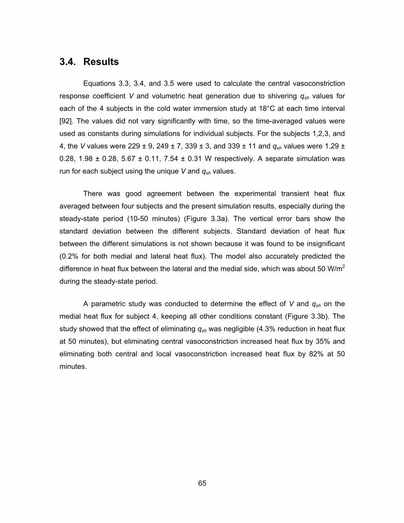
65
3.4. Results
Equations 3.3, 3.4, and 3.5 were used to calculate the central vasoconstriction
response coefficient V and volumetric heat generation due to shivering qsh values for
each of the 4 subjects in the cold water immersion study at 18°C at each time interval
[92]. The values did not vary significantly with time, so the time-averaged values were
used as constants during simulations for individual subjects. For the subjects 1,2,3, and
4, the V values were 229 ± 9, 249 ± 7, 339 ± 3, and 339 ± 11 and qsh values were 1.29 ±
0.28, 1.98 ± 0.28, 5.67 ± 0.11, 7.54 ± 0.31 W respectively. A separate simulation was
run for each subject using the unique V and qsh values.
There was good agreement between the experimental transient heat flux
averaged between four subjects and the present simulation results, especially during the
steady-state period (10-50 minutes) (Figure 3.3a). The vertical error bars show the
standard deviation between the different subjects. Standard deviation of heat flux
between the different simulations is not shown because it was found to be insignificant
(0.2% for both medial and lateral heat flux). The model also accurately predicted the
difference in heat flux between the lateral and the medial side, which was about 50 W/m2
during the steady-state period.
A parametric study was conducted to determine the effect of V and qsh on the
medial heat flux for subject 4, keeping all other conditions constant (Figure 3.3b). The
study showed that the effect of eliminating qsh was negligible (4.3% reduction in heat flux
at 50 minutes), but eliminating central vasoconstriction increased heat flux by 35% and
eliminating both central and local vasoconstriction increased heat flux by 82% at 50
minutes.
66
a)
b)
Figure 3.3. a) Surface heat flux from the medial and lateral sides of the leg at
water immersion temperatures of 18°C and hsurface = 110 W/m2K, and b) surface heat flux from the medial side of the leg of subject 4 compared with simulation results for current model, model with no central vasoconstriction (no CV), model with no local and central vasoconstriction (no CV, no LV) and model with no shivering (no SH).
Simulation results for transient heat flux were compared with experimental results
from ref. [90] for localized cooling at coolant temperatures of -2, 4, and 9°C (Figure 3.4).
Simulation results in all conditions showed significantly higher heat flux than
0
100
200
300
400
500
600
700
800
900
0 10 20 30 40 50
Hea
t flu
x [W
/m2 ]
time [min]
current model - medialcurrent model - lateralexperimental - medialexperimental - lateral
0
100
200
300
400
500
600
700
800
900
0 10 20 30 40 50
Hea
t Flu
x [W
/m2 ]
time [min]
experimentalcurrent modelcurrent model - no CVcurrent model - no LV, no CVcurrent model - no SH
experimental [92]
experimental – medial [92]
experimental – lateral [92]

67
experimental data in the transient period of 0-10 minutes, with a difference of
approximately 1000-500 W in the first few minutes. There was also noticeable
discrepancy in the steady-state period (10-40 minutes) during cooling at -2 and 4°C, but
there was good agreement at 9°C. When the simulations were run assuming no
vasoconstriction, the discrepancy was significantly smaller (time-averaged absolute error
between simulation and experimental results was on average 30.2% for all simulations
with vasoconstriction, and 13% without vasoconstriction). Irrespective of the state of
vasoconstriction, the discrepancy was observed to decrease with increasing
temperature.
Analysis of the time-dependent magnitude of individual heat sources (including
tissue metabolism, perfusion, and blood vessels) showed that a substantial amount of
heat came from metabolic generation and blood perfusion in the muscle, and heat loss
from the blood vessels only accounted for 3.7 W (Figure 3.5). As expected, the
magnitude of the heat source due to cutaneous perfusion changed drastically (factor of
4.8) when comparing the simulation results assuming local vasoconstriction and no
vasoconstriction.
Comparison of experimental muscle temperature profile from the study in ref. [91]
with simulations of similar conditions showed good agreement at a depth of 4.5 cm, but
experimental temperatures were significantly lower at 1.5 and 3 cm at 20 and 60 minutes
(Figure 3.6). The temperature profile was found to be sensitive to variations in muscle
perfusion, and decreasing the muscle perfusion to 50% of the initial value improved the
agreement between the experimental data and simulation results.
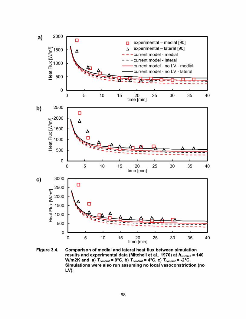
68
a)
b)
c)
Figure 3.4. Comparison of medial and lateral heat flux between simulation
results and experimental data (Mitchell et al., 1970) at hsurface = 140 W/m2K and a) Tcoolant = 9°C, b) Tcoolant = 4°C, c) Tcoolant = -2°C. Simulations were also run assuming no local vasoconstriction (no LV).
0
500
1000
1500
2000
0 5 10 15 20 25 30 35 40
Hea
t Flu
x [W
/m2 ]
time [min]
experimental - medialexperimental - lateralcurrent model - medialcurrent model - lateralcurrent model - no LV - medialcurrent model - no LV - lateral
0
500
1000
1500
2000
2500
0 5 10 15 20 25 30 35 40
Hea
t Flu
x [W
/m2 ]
time [min]
0
500
1000
1500
2000
2500
3000
0 5 10 15 20 25 30 35 40
Hea
t Flu
x [W
/m2 ]
time [min]
experimental – medial [90] experimental – lateral [90]
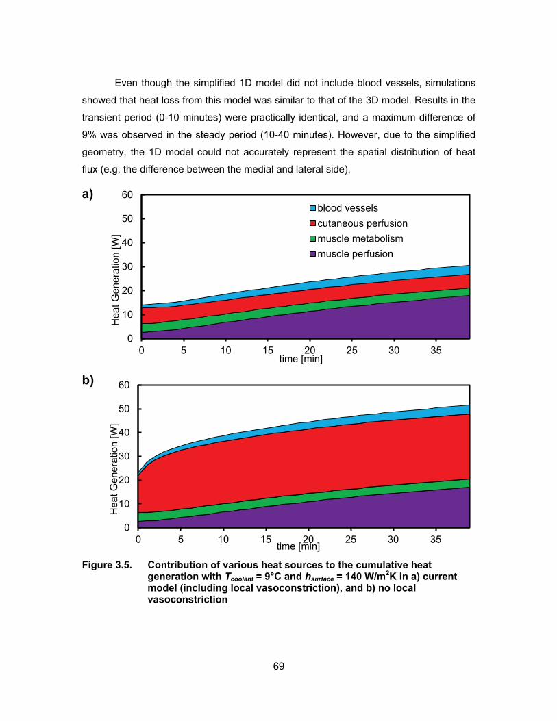
69
Even though the simplified 1D model did not include blood vessels, simulations
showed that heat loss from this model was similar to that of the 3D model. Results in the
transient period (0-10 minutes) were practically identical, and a maximum difference of
9% was observed in the steady period (10-40 minutes). However, due to the simplified
geometry, the 1D model could not accurately represent the spatial distribution of heat
flux (e.g. the difference between the medial and lateral side).
a)
b)
Figure 3.5. Contribution of various heat sources to the cumulative heat
generation with Tcoolant = 9°C and hsurface = 140 W/m2K in a) current model (including local vasoconstriction), and b) no local vasoconstriction
0
10
20
30
40
50
60
0 5 10 15 20 25 30 35
Hea
t Gen
erat
ion
[W]
time [min]
blood vesselscutaneous perfusionmuscle metabolismmuscle perfusion
0
10
20
30
40
50
60
0 5 10 15 20 25 30 35
Hea
t Gen
erat
ion
[W]
time [min]
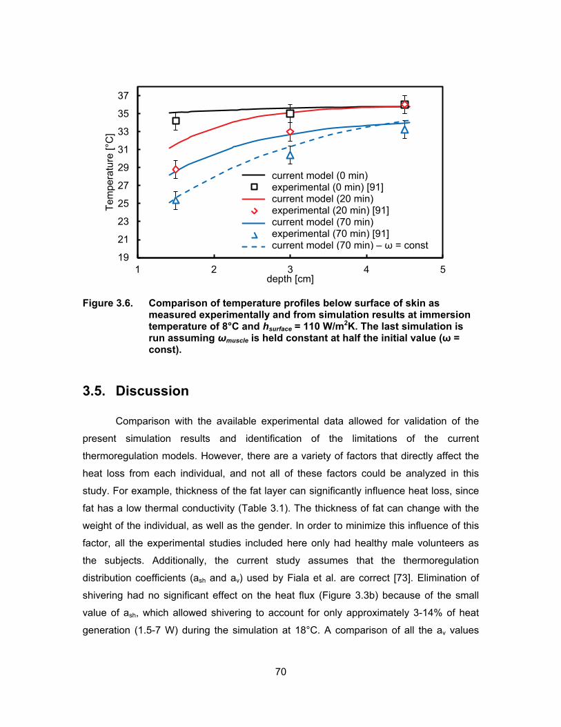
70
Figure 3.6. Comparison of temperature profiles below surface of skin as measured experimentally and from simulation results at immersion temperature of 8°C and hsurface = 110 W/m2K. The last simulation is run assuming ωmuscle is held constant at half the initial value (ω = const).
3.5. Discussion
Comparison with the available experimental data allowed for validation of the
present simulation results and identification of the limitations of the current
thermoregulation models. However, there are a variety of factors that directly affect the
heat loss from each individual, and not all of these factors could be analyzed in this
study. For example, thickness of the fat layer can significantly influence heat loss, since
fat has a low thermal conductivity (Table 3.1). The thickness of fat can change with the
weight of the individual, as well as the gender. In order to minimize this influence of this
factor, all the experimental studies included here only had healthy male volunteers as
the subjects. Additionally, the current study assumes that the thermoregulation
distribution coefficients (ash and av) used by Fiala et al. are correct [73]. Elimination of
shivering had no significant effect on the heat flux (Figure 3.3b) because of the small
value of ash, which allowed shivering to account for only approximately 3-14% of heat
generation (1.5-7 W) during the simulation at 18°C. A comparison of all the av values
19
21
23
25
27
29
31
33
35
37
1 2 3 4 5
Tem
pera
ture
[°C
]
depth [cm]
current model (0 mins)experimental (0 mins)current model (20 mins)experimental (20 mins)current model (70 mins)experimental (70 mins)current model (70 mins) - ω = const
current model (0 min) experimental (0 min) [91] current model (20 min) experimental (20 min) [91] current model (70 min) experimental (70 min) [91] current model (70 min) – ω = const

71
available in the literature showed variation by up to a factor of 10, despite all the values
being based on experimental results [70].
Vasoconstriction is a well-recognized physiological response to moderate
cooling, however the results of this study combined with previous studies demonstrates
a lack of vasoconstriction, or perhaps even vasodilation at the low temperatures required
rapid for hypothermic cooling. At moderate temperature (18°C), inclusion of central and
local vasoconstriction was necessary for the model to accurately predict heat flux for the
immersion experiments (Figure 3.3b). This observation is corroborated by a study
showing vasoconstriction had a significant impact on heat loss in the finger [97].
However, our simulation results were improved by excluding vasoconstriction when
coolant temperature was low (9, 4, or -2°C) indicating that vasoconstriction may not
occur at low temperatures. This lack of vasoconstriction has been experimentally
observed and is known as cold-induced vasodilation [98]. Similarly, a leg immersion
study showed that cutaneous perfusion in the leg was significantly reduced at immersion
temperature of 22°C, but remained at baseline levels at immersion temperature of 8°C
[93]. This result has important implications for inducing therapeutic hypothermia with
surface cooling. The presence of high skin blood flow (absence of vasoconstriction) will
result in more rapid core cooling because direct contact between a large volume of warm
blood and the cold skin tissue allows for rapid cooling of the bloodstream (Figure 3.5).
Therefore, in addition to the large heat conduction expected at low surface
temperatures, it is possible that the presence of cold-induced vasodilation will further
increase the core cooling rate. Mapping the specific temperature range for cold-induced
vasodilation combined with this new computational model of hypothermia will assist in
designing an optimally efficient surface cooling system.
The effects of hypothermia on blood flow in arteries and its effect on muscle
perfusion were highlighted when validating the computation model predictions against
experimental temperature profiles in the leg (Figure 3.6). The model results showed that
using the established linear model (eq. 3.6) to determine muscle perfusion parameters
did not accurately capture the temperature profile in deep tissues. Reducing the muscle
perfusion parameter to a constant value that was 50% less than the baseline value
provided better correlation with experimental results. This effect of hypothermia on
72
muscle perfusion was observed in immersion experiments; femoral artery blood flow
dropped to approximately 50% of the baseline value at immersion temperatures of 8°C
and 22°C over 30-40 minutes [93]. The decreased blood flow was attributed to
decreased muscle perfusion for immersion at 8°C since the cutaneous blood flow
remained constant; whereas, the decreased blood flow at 22°C could be attributed
primarily to a decrease in cutaneous blood flow. These results demonstrate the need to
redefine the muscle perfusion parameter in current thermoregulatory models to
accurately simulate hypothermia and the physiological changes in muscle perfusion that
occur at low temperatures.
Targeted cooling of areas with superficial blood vessels is thought to improve
heat transfer to the blood stream; as directly cooling the blood stream will result in the
most rapid change in core temperature [99]. In practice, ice packs are usually placed
around the neck, groin, and axillae in order to target superficial blood vessels [20], [100].
However, the current simulations show that the maximum cooling power delivered to all
the blood vessels is approximately 5 W, which is insignificant compared to the 150-300
W that is required for rapid cooling [23]. The small role of blood vessels observed in our
study compare well with analytical studies of cooling of the carotid artery in a neck model
showed similarly insignificant heat transfer, even under the assumption that the neck
surface was at 0°C [64], [101]. These results suggest that even though the heat flux on
the surface of areas such as axillae, groin, and neck may be higher than the rest of body
surface, the small surface area in these regions limits the total cooling power; instead
distributing the surface cooling over a large surface area will maximize cooling rate.
Similarly, a study involving surface cooling of pigs found that cooling the neck surface
(7% of total surface area) resulted in 15% of the core cooling rate that was achieved by
cooling 100% of the surface; indicating that cooling the neck is twice as effective as
cooling other areas, but still results in a very low core cooling rate [61].

73
Chapter 4. Discussion & Conclusion
4.1. Discussion
Therapeutic hypothermia is rapidly becoming an integral part of post-
resuscitative care for post-cardiac arrest patients [25] and a neuroprotective strategy for
brain and spinal cord injuries [1, 6, 24]. The majority of medical opinion suggests that
cooling earlier in the pre-hospital setting should improve patient outcome; but the lack of
a portable and non-invasive rapid cooling technology has influenced the effectiveness of
pre-hospital trials and the subsequent adoption of pre-hospital hypothermia [16], [17],
[21]. In the present study a prototype for a novel adsorption-based cooling device was
developed and tested under realistic conditions. Additionally, a numerical 3D model of
the upper leg was developed and simulations were able to quantify the sensitivity of
surface heat loss to factors such as geometry, blood vessels, blood perfusion and
shivering during hypothermic conditions.
Although the cooling power requirements for the adsorption cooling device were
developed based on data from literature for cooling blankets, a more accurate evaluation
of the adsorption-based cooling device can be done after the in-depth bioheat study
conducted in chapter 3. Given that the average transition time in the ambulance is 23
minutes [25], accurate bioheat modeling is noticeably important for design of a pre-
hospital surface cooling device because the surface heat flux is observed to be very
dynamic for the first 20-25 minutes (Figure 3.3 and Figure 3.4).
Nonetheless, an estimate of the performance can be made based on the steady-
state results, assuming that the heat transfer coefficient of the blanket is 110 W/m2K and
covers 0.6m2 surface area, i.e. the same as the Medivance Arctic Sun ® Temperature
Management System [24]. Knowing that the steady-state heat flux with 9°C coolant in a
neoprene wrap is approximately 400 W/m2 (Figure 3.3), the total cooling power with 9°C

74
blanket water can be calculated by multiplying the heat flux with the surface area and
accounting for the high heat transfer coefficient of the neoprene leg wrap:
400𝑊𝑚2 (ℎ𝑒𝑎𝑡 𝑓𝑙𝑢𝑥) ∗ 0.6𝑚2(𝑠𝑢𝑟𝑓𝑎𝑐𝑒 𝑎𝑟𝑒𝑎)
∗ 110 𝑊
𝑚2𝐾 (ℎ𝑒𝑎𝑡 𝑡𝑟𝑎𝑛𝑠𝑓𝑒𝑟 𝑐𝑜𝑒𝑓𝑓𝑖𝑐𝑖𝑒𝑛𝑡 𝑜𝑓 𝑏𝑙𝑎𝑛𝑘𝑒𝑡)
140 𝑊𝑚2𝐾 (ℎ𝑒𝑎𝑡 𝑡𝑟𝑎𝑛𝑠𝑓𝑒𝑟 𝑐𝑜𝑒𝑓𝑓𝑖𝑐𝑖𝑒𝑛𝑡 𝑜𝑓 𝑙𝑒𝑔 𝑤𝑟𝑎𝑝)
= 190𝑊
Since the prototype with approximately 1 kg of adsorbent has provided an average of
110 W of cooling with average water temperature of 13°C (Figure 2.19), it is realistic to
expect that 190 W of cooling power can be achieved at 9°C water temperature with 2-3
kg of adsorbent.
To put the cooling power in perspective, a full body immersion at 8°C measured
a core temperature drop of 2.5°C per hour [91]. Assuming a uniform heat flux throughout
the body, and knowing that the heat transfer coefficient of water immersion is also 110
W/m2K [24], and that the total surface area of the adult male body is approximately 2 m2
[71], the core temperature drop rate from the cooling device with 2-3 kg of adsorbent
can be calculated to be 0.75°C per hour. Of course, this cooling rate can be increased
simply by increasing the mass of adsorbent. By comparison, the RhinoChill® Intranasal
Cooling System (Benechill, San Diego, CA) which weighs 10 kg achieves 1.1°C per
hour.
4.2. Conclusions & Recommendations
Results from testing of the prototype adsorption-based cooling device indicate
that the technology can provide sufficient cooling power while maintaining a small
footprint in the ambulance. Effective thermal management and vapor diffusion in the
adsorbent bed were found to be essential to achieve high cooling power. Composite
silica gel-calcium chloride adsorbent had a higher uptake than silica gel, but the
selection of the adsorbent material would likely depend on the final thermal design of the
adsorbent bed.

75
The bioheat simulation results showed that the current thermoregulatory models
did not accurately predict thermoregulation in hypothermic conditions because they did
not include cold-induced vasodilation and reduction in leg muscle perfusion. Additionally,
model simulations showed that an insignificant amount of cooling was directly delivered
to the blood vessels, indicating that emphasis on uniform cooling over a large surface
area would yield higher cooling rates than targeted cooling of areas with superficial
blood vessels.
In order to accurately predict the performance of the cooling device, future work
should focus on combining the adsorption model and the bioheat model presented in this
study. Alternatively, the bioheat model can potentially be combined with a physical
bench-top test-bed for dynamically controlling the heat flux to a surface heater as a
function of the surface temperature and time. Future work on the surface cooling device
should focus on development of the blanket component, further optimizing the thermal
design of the adsorbent bed, and testing other adsorbents in similar conditions.
76
References
[1] G. The, “Mild therapeutic hypothermia to improve the neurologic outcome after cardiac arrest.,” N Engl J Med, vol. 346, no. 8, pp. 549–56, Feb. 2002.
[2] S. A. Bernard, T. W. Gray, M. D. Buist, B. M. Jones, W. Silvester, G. Gutteridge, and K. Smith, “Treatment of comatose survivors of out-of-hospital cardiac arrest with induced hypothermia,” N Engl J Med, vol. 346, pp. 557–563, 2002.
[3] J. P. Nolan, P. T. Morley, T. L. Vanden Hoek, R. W. Hickey, M. of the A. L. S. T. Force, W. G. J. Kloeck, J. Billi, B. W. Böttiger, K. Okada, C. Reyes, M. Shuster, P. A. Steen, M. H. Weil, V. Wenzel, M. of the P. L. S. T. Force, A. Contributors, P. Carli, and D. Atkins, “Therapeutic Hypothermia After Cardiac Arrest: An Advisory Statement by the Advanced Life Support Task Force of the International Liaison Committee on Resuscitation,” Circulation, vol. 108, no. 1, pp. 118–121, Jul. 2003.
[4] C. M. Maier, G. H. Sun, D. Kunis, M. A. Yenari, and G. K. Steinberg, “Delayed induction and long-term effects of mild hypothermia in a focal model of transient cerebral ischemia: neurological outcome and infarct size,” J Neurosurg, vol. 94, no. 1, pp. 90–96, Jan. 2001.
[5] B. K. Kwon, C. Mann, H. M. Sohn, A. S. Hilibrand, F. M. Phillips, J. C. Wang, and M. G. Fehlings, “Hypothermia for spinal cord injury,” Spine J, vol. 8, no. 6, pp. 859–874, Nov. 2008.
[6] S. A. Bernard and M. Buist, “Induced hypothermia in critical care medicine: a review,” Crit Care Med, vol. 31, no. 7, pp. 2041–2051, 2003.
[7] A. Cappuccino, L. J. Bisson, B. Carpenter, J. Marzo, W. D. Dietrich III, and H. Cappuccino, “The Use of Systemic Hypothermia for the Treatment of an Acute Cervical Spinal Cord Injury in a Professional Football Player,” Spine, vol. 35, no. 2, pp. E57–E62, Jan. 2010.
[8] M. Isaka, H. Kumagai, Y. Sugawara, K. Okada, K. Orihashi, M. Ohtaki, and T. Sueda, “Cold spinoplegia and transvertebral cooling pad reduce spinal cord injury during thoracoabdominal aortic surgery,” J Vasc Surg, vol. 43, no. 6, pp. 1257–1262, Jun. 2006.
[9] D. Yashon, W. M. Vise, R. C. Dewey, and W. E. Hunt, “Temperature of the spinal cord during local hypothermia in dogs,” J Nerosurgery, vol. 39, no. 6, pp. 742–745, 1973.
77
[10] K. Oku and K. Kuboyama, “Cerebral and systemic arteriovenous oxygen monitoring after cardiac arrest: inadequate cerebral oxygen delivery,” Resuscitation, vol. 27, no. 2, pp. 141–152, Mar. 1994.
[11] J. D. Hardy and J. A. Stolwijk, “Partitional calorimetric studies of man during exposures to thermal transients,” J Appl Physiol, vol. 21, no. 6, pp. 1799–1806, Nov. 1966.
[12] N. Nielsen, J. Wetterslev, T. Cronberg, D. Erlinge, Y. Gasche, C. Hassager, J. Horn, J. Hovdenes, J. Kjaergaard, M. Kuiper, T. Pellis, P. Stammet, M. Wanscher, M. P. Wise, A. Åneman, N. Al-Subaie, S. Boesgaard, J. Bro-Jeppesen, I. Brunetti, J. F. Bugge, C. D. Hingston, N. P. Juffermans, M. Koopmans, L. Køber, J. Langørgen, G. Lilja, J. E. Møller, M. Rundgren, C. Rylander, O. Smid, C. Werer, P. Winkel, and H. Friberg, “Targeted temperature management at 33°C versus 36°C after cardiac arrest.,” N Engl J Med, vol. 369, no. 23, pp. 2197–206, Dec. 2013.
[13] “Targeted Temperature Management after Cardiac Arrest,” N Engl J Med, vol. 370, no. 14, pp. 1356–1361, 2014.
[14] M. Diao, F. Huang, J. Guan, Z. Zhang, Y. Xiao, Y. Shan, Z. Lin, and L. Ding, “Prehospital therapeutic hypothermia after cardiac arrest: A systematic review and meta-analysis of randomized controlled trials,” Resuscitation, vol. 84, no. 8, pp. 1021–1028, Aug. 2013.
[15] C. G. Markgraf, G. L. Clifton, and M. R. Moody, “Treatment window for hypothermia in brain injury,” J Neurosurg, vol. 95, no. 6, pp. 979–983, Dec. 2001.
[16] S. A. Bernard, K. Smith, P. Cameron, K. Masci, D. M. Taylor, D. J. Cooper, A.-M. Kelly, W. Silvester, and R. I. C. H. RICH, “Induction of prehospital therapeutic hypothermia after resuscitation from nonventricular fibrillation cardiac arrest,” Crit Care Med, vol. 40, no. 3, pp. 747–753, Mar. 2012.
[17] B. P. Suffoletto, D. D. Salcido, and J. J. Menegazzi, “Use of prehospital-induced hypothermia after out-of-hospital cardiac arrest: A survey of the national association of emergency medical services physicians,” PREHOSPITAL Emerg CARE, vol. 12, no. 1, pp. 52–56, 2008.
[18] R. M. Merchant, J. Soar, M. B. Skrifvars, T. Silfvast, D. P. Edelson, F. Ahmad, K. N. Huang, M. Khan, T. L. Vanden Hoek, L. B. Becker, and B. S. Abella, “Therapeutic hypothermia utilization among physicians after resuscitation from cardiac arrest,” Crit Care Med, vol. 34, no. 7, pp. 1935–1940, Jul. 2006.
[19] O. Kimberger and A. Kurz, “Thermoregulatory management for mild therapeutic hypothermia,” Best Pract Res Clin Anaesthesiol, vol. 22, no. 4, pp. 729–744, Dec. 2008.

78
[20] M. D. Georgia and A. Deogaonkar, “Methods to induce hypothermia,” in Therapeutic hypothermia, S. A. Mayer and D. I. Sessler, Eds. New York: Marcel Dekker, 2005, pp. 293–322.
[21] F. Kim, M. Olsufka, W. T. Longstreth, C. Maynard, D. Carlbom, S. Deem, P. Kudenchuk, M. K. Copass, and L. A. Cobb, “Pilot randomized clinical trial of prehospital induction of mild hypothermia in out-of-hospital cardiac arrest patients with a rapid infusion of 4 degrees C normal saline,” Circulation, vol. 115, no. 24, pp. 3064–3070, 2007.
[22] T. Uray, R. Malzer, and V. H. C. Arrest, “Out-of-hospital surface cooling to induce mild hypothermia in human cardiac arrest: A feasibility trial,” Resuscitation, vol. 77, no. 3, pp. 331–338, Jun. 2008.
[23] M. J. English, “Heat transfer coefficient: Medivance Arctic Sun Temperature Management System vs. water immersion,” Unpublished raw data, 2008.
[24] M. J. English and T. M. Hemmerling, “Heat transfer coefficient: Medivance Arctic Sun Temperature Management System vs. water immersion.,” Eur J Anaesthesiol, vol. 25, no. 7, pp. 531–7, Jul. 2008.
[25] S. a Bernard, K. Smith, P. Cameron, K. Masci, D. M. Taylor, D. J. Cooper, A.-M. Kelly, and W. Silvester, “Induction of therapeutic hypothermia by paramedics after resuscitation from out-of-hospital ventricular fibrillation cardiac arrest: a randomized controlled trial.,” Circulation, vol. 122, no. 7, pp. 737–42, Aug. 2010.
[26] Y. Yang, J. Stapleton, B. T. Diagne, G. P. Kenny, and C. Q. Lan, “Man-portable personal cooling garment based on vacuum desiccant cooling,” Appl Therm Eng, vol. 47, pp. 18–24, Dec. 2012.
[27] D. Lee and Y. Hwang, “Subminiature Cool Pad Applying Sorption Cooling Effect,” HVAC&R Res, vol. 12, no. 3b, pp. 37–41, 2006.
[28] L. R. Gnryll and W. C. Balderson, “Development of a man-portable microclimate adsorption cooling device,” in Proceedings of the Intersociety Energy Conversion Engineering Conference, 1997, pp. 1646–1651.
[29] F. Parrish and R. P. Scarngne, “Lightweight passive microclimate cooling device,” Mainstream Eng Corp, vol. Technical, 1993.
[30] L. W. Wang, R. Z. Wang, and R. G. Oliveira, “A review on adsorption working pairs for refrigeration,” Renew Sustain Energy Rev, vol. 13, no. 3, pp. 518–534, Apr. 2009.
[31] R. E. Critoph, “Performance limitations of adsorption cycles for solar cooling,” Sol Energy, vol. 41, no. 1, pp. 21–31, 1988.

79
[32] B. B. Saha, A. Chakraborty, S. Koyama, and Y. I. Aristov, “A new generation cooling device employing CaCl2-in-silica gel–water system,” Int J Heat Mass Transf, vol. 52, no. 1–2, pp. 516–524, Jan. 2009.
[33] K. Daou, R. Z. Wang, and Z. Z. Xia, “Development of a new synthesized adsorbent for refrigeration and air conditioning applications,” Appl Therm Eng, vol. 26, no. 1, pp. 56–65, Jan. 2006.
[34] C. Antoine, “Tensions des vapeurs; nouvelle relation entre les tensions et les températures,” Comptes Rendus des Séances l’Académie des Sci, vol. 107, no. 1, pp. 681–684, 1988.
[35] E. Glueckauf, “Theroy of chromatography: formulae for diffusion into spheres and their application to chromatography,” Trans Faraday Soc, vol. 51, no. 11, pp. 1540–1551, 1955.
[36] Sakoda and Suzuki, “Fundamental study on solar powered adsorption,” J Chem Eng Japan, vol. 121, no. 1965, 1984.
[37] G. G. Ilis, M. Mobedi, and S. Ülkü, “Comparison of Uniform and Non-uniform Pressure Approaches Used to Analyze an Adsorption Process in a Closed Type Adsorbent Bed,” Transp Porous Media, vol. 98, no. 1, pp. 81–101, Feb. 2013.
[38] C. Y. Tso and C. Y. H. Chao, “Activated carbon, silica-gel and calcium chloride composite adsorbents for energy efficient solar adsorption cooling and dehumidification systems,” Int J Refrig, vol. 35, no. 6, pp. 1626–1638, Sep. 2012.
[39] H. T. Chua, K. C. Ng, W. Wang, C. Yap, and X. L. Wang, “Transient modeling of a two-bed silica gel–water adsorption chiller,” Int J Heat Mass Transf, vol. 47, no. 4, pp. 659–669, Feb. 2004.
[40] J. Karger and M. Ruthven, Diffusion in Zeolites and Other Microporous Solids. New York: John Wiley, 1992.
[41] Y. Aristov, “Selective Water Sorbents for Multiple Applications 1. CaCl2 Confined in Mesopores of Silica Gel: Sorption Properties,” React Kinet Catal Lett, vol. 59, no. 2, pp. 325–333, 1996.
[42] B. Dawoud and Y. Aristov, “Experimental study on the kinetics of water vapor sorption on selective water sorbents, silica gel and alumina under typical operating conditions of sorption heat pumps,” Int J Heat Mass Transf, vol. 46, no. 2, pp. 273–281, Jan. 2003.
[43] L. G. Gordeeva, A. D. Grekova, T. a. Krieger, and Y. I. Aristov, “Adsorption properties of composite materials (LiCl+LiBr)/silica,” Microporous Mesoporous Mater, vol. 126, no. 3, pp. 262–267, Dec. 2009.
80
[44] M. Tokarev, L. Gordeeva, V. Romannikov, and I. Glaznev, “New composite sorbent CaCl 2 in mesopores for sorption cooling / heating,” Int J Therm Sci, vol. 41, pp. 470–474, 2002.
[45] Y. . Aristov, G. Restuccia, G. Cacciola, and V. . Parmon, “A family of new working materials for solid sorption air conditioning systems,” Appl Therm Eng, vol. 22, no. 2, pp. 191–204, Feb. 2002.
[46] L. G. Gordeeva, I. S. Glaznev, and Y. I. Aristov, “Sorption of water by Sodium, Copper, and Magnesium Sulfates dispersed into mesopores of Silica Gel and Alumina,” Russ J Phys Chem, vol. 77, no. 10, pp. 1715–20, 2003.
[47] C. McCague, K. Fayazmanesh, M. Kalra, and M. Bahrami, “Water adsorption of CaCl2 confined in mesoporous silica gel with various pore sizes,” in International Sorption Heat Pump Conference, 2014.
[48] K. C. Chan, C. Y. H. Chao, G. N. Sze-To, and K. S. Hui, “Performance predictions for a new zeolite 13X/CaCl2 composite adsorbent for adsorption cooling systems,” Int J Heat Mass Transf, vol. 55, no. 11–12, pp. 3214–3224, May 2012.
[49] Y. I. Aristov, I. S. Glaznev, a. Freni, and G. Restuccia, “Kinetics of water sorption on SWS-1L (calcium chloride confined to mesoporous silica gel): Influence of grain size and temperature,” Chem Eng Sci, vol. 61, no. 5, pp. 1453–1458, Mar. 2006.
[50] Y. I. Aristov, B. Dawoud, I. S. Glaznev, and a. Elyas, “A new methodology of studying the dynamics of water sorption/desorption under real operating conditions of adsorption heat pumps: Experiment,” Int J Heat Mass Transf, vol. 51, no. 19–20, pp. 4966–4972, Sep. 2008.
[51] B. N. Okunev, a. P. Gromov, L. I. Heifets, and Y. I. Aristov, “A new methodology of studying the dynamics of water sorption/desorption under real operating conditions of adsorption heat pumps: Modelling of coupled heat and mass transfer in a single adsorbent grain,” Int J Heat Mass Transf, vol. 51, no. 1–2, pp. 246–252, Jan. 2008.
[52] D. S. Ovoshchnikov, I. S. Glaznev, and Y. I. Aristov, “Water sorption by the calcium chloride/silica gel composite: The accelerating effect of the salt solution present in the pores,” Kinet Catal, vol. 52, no. 4, pp. 620–628, Aug. 2011.
[53] A. Freni, F. Russo, S. Vasta, M. Tokarev, Y. I. Aristov, and G. Restuccia, “An advanced solid sorption chiller using SWS-1Ll,” Appl Therm Eng, vol. 27, no. 13, pp. 2200–2204, Sep. 2007.
[54] X. L. Wang, H. T. Chua, and K. C. Ng, “Experimental investigation of silica gel-water adsorption chillers with and without a passive heat recovery scheme,” Int J Refrig, vol. 28, no. 5, pp. 756–765, Aug. 2005.
81
[55] D. C. Wang and J. Y. Wu, “Influence of intermittent heat source on adsorption ice maker using waste heat,” Energy Convers Manag, vol. 46, no. 6, pp. 985–998, Apr. 2005.
[56] A. Sharafian and M. Bahrami, “Assessment of adsorber bed designs in waste-heat driven adsorption cooling systems for vehicle air conditioning and refrigeration,” Renew Sustain Energy Rev, vol. 30, pp. 440–451, Feb. 2014.
[57] M. M. Farid, A. M. Khudhair, S. A. K. Razack, and S. Al-Hallaj, “A review on phase change energy storage: materials and applications,” Energy Convers Manag, vol. 45, no. 9–10, pp. 1597–1615, Jun. 2004.
[58] H. Demir, M. Mobedi, and S. Ülkü, “Effects of porosity on heat and mass transfer in a granular adsorbent bed,” Int Commun Heat Mass Transf, vol. 36, no. 4, pp. 372–377, Apr. 2009.
[59] D. W. Incropera, Fundamentals of Heat and Mass Transfer, 3rd ed. John Wiley & Sons, 1990, p. 543.
[60] A. Freni, M. Tokarev, G. Restuccia, A. Okunev, and Y. Aristov, “Thermal conductivity of selective water sorbents under the working conditions of a sorption chiller,” Appl Therm Eng, vol. 22, no. 14, pp. 1631–1642, Oct. 2002.
[61] W. Weihs, A. Schratter, F. Sterz, A. Janata, S. Hoegler, M. Holzer, U. M. Losert, H. Herkner, and W. Behringer, “The importance of surface area for the cooling efficacy of mild therapeutic hypothermia,” Resuscitation, vol. 82, no. 1, pp. 74–78, Jan. 2011.
[62] M. Cabanac, “Selective brain cooling in humans - fancy or fact,” FASEB J, vol. 7, no. 12, pp. 1143–1146, Sep. 1993.
[63] B. A. Harris and P. J. D. Andrews, “Direct brain cooling,” in Therapeutic hypothermia, S. A. Mayer and D. I. Sessler, Eds. New York: Marcel Dekker, 2005, pp. 323–386.
[64] L. Zhu, “Theoretical evaluation of contributions of heat conduction and countercurrent heat exchange in selective brain cooling in humans.,” Ann Biomed Eng, vol. 28, no. 3, pp. 269–77, Mar. 2000.
[65] E. H. Wissler, “Whole-Body Human Thermal Modeling, an Alternative to Immersion in Cold Water and Other Unpleasant Endeavors,” J Heat Transfer, vol. 134, no. 3, p. 031019, 2012.
[66] H. H. Pennes, “Analysis of tissue and arterial blood temperatures in the resting human forearm. 1948.,” J Appl Physiol, vol. 1, no. 2, pp. 93–122, Jul. 1948.
82
[67] E. H. Wissler, “Steady-state temperature distribution in man,” J Appl Physiol, vol. 16, no. 4, p. 734–&, 1961.
[68] J. A. Stolwijk, “A mathematical model of physiological temperature regulation,” NASA Contractor Report CR-1855, no. August, 1971.
[69] J. A. Stolwijk and J. D. HARDY, “Temperature regulation in man - a theoretical study,” Pflugers Arch Gesamte Physiol Menschen Tiere, vol. 291, no. 2, p. 129–&, 1966.
[70] N. M. W. Severens, W. D. van Marken Lichtenbelt, A. J. H. Frijns, B. R. M. Kingma, B. a J. M. de Mol, and A. a van Steenhoven, “Measurement of model coefficients of skin sympathetic vasoconstriction.,” Physiol Meas, vol. 31, no. 1, pp. 77–93, Jan. 2010.
[71] P. Tikuisis, “Heat balance precedes stabilization of body temperatures during cold water immersion.,” J Appl Physiol, vol. 95, no. 1, pp. 89–96, Jul. 2003.
[72] D. Fiala, K. J. Lomas, and M. Stohrer, “A computer model of human thermoregulation for a wide range of environmental conditions: the passive system,” pp. 1957–1972, 1999.
[73] D. Fiala, K. J. Lomas, and M. Stohrer, “Computer prediction of human thermoregulatory and temperature responses to a wide range of environmental conditions.,” Int J Biometeorol, vol. 45, no. 3, pp. 143–59, Sep. 2001.
[74] D. Fiala, “Dynamic Simulation of Human Heat Transfer and Thermal Comfort,” 1998.
[75] N. Bogerd, a Psikuta, H. a M. Daanen, and R. M. Rossi, “How to measure thermal effects of personal cooling systems: human, thermal manikin and human simulator study.,” Physiol Meas, vol. 31, no. 9, pp. 1161–8, Sep. 2010.
[76] W. D. van Marken Lichtenbelt, A. J. H. Frijns, M. J. van Ooijen, D. Fiala, A. M. Kester, and A. A. van Steenhoven, “Validation of an individualised model of human thermoregulation for predicting responses to cold air,” Int J Biometeorol, vol. 51, no. 3, pp. 169–179, Jan. 2007.
[77] W. D. van Marken Lichtenbelt, A. J. H. Frijns, D. Fiala, F. E. M. Janssen, A. M. J. van Ooijen, and A. A. van Steenhoven, “Effect of individual characteristics on a mathematical model of human thermoregulation,” J Therm Biol, vol. 29, no. 7–8, pp. 577–581, 2004.
[78] C. van Treeck, J. Frisch, M. Pfaffinger, E. Rank, S. Paulke, I. Schweinfurth, R. Schwab, R. Hellwig, and A. Holm, “Integrated thermal comfort analysis using a parametric manikin model for interactive real-time simulation,” J Build Perform Simul, vol. 2, no. 4, pp. 233–250, 2009.
83
[79] M. S. Ferreira and J. I. Yanagihara, “A transient three-dimensional heat transfer model of the human body,” Int Commun Heat Mass Transf, vol. 36, no. 7, pp. 718–724, Aug. 2009.
[80] X. Sun, S. Eckels, and Z. C. Zheng, “An improved thermal model of the human body An improved thermal model of the human body,” HVAC&R Res, vol. 18, no. 3, pp. 323–338, 2012.
[81] P. Tikuisis, R. R. Gonzalez, and K. B. Pandolf, “Thermoregulatory model for immersion of humans in cold water Thermoregulatory model for immersion of humans in cold water,” J Appl Physiol, vol. 64, pp. 719–727, 2013.
[82] A. Munir, S. Takada, and T. Matsushita, “Re-evaluation of Stolwijk’s 25-node human thermal model under thermal-transient conditions: Prediction of skin temperature in low-activity conditions,” Build Environ, vol. 44, no. 9, pp. 1777–1787, Sep. 2009.
[83] B. H. Dennis, R. C. Eberhart, G. S. Dulikravich, and S. W. Radons, “Finite-element simulation of cooling of realistic 3-D human head and neck,” J Biomech Eng, vol. 125, no. 6, pp. 832–840, 2003.
[84] C. Diao, L. Zhu, and H. Wang, “Cooling and rewarming for brain ischemia or injury: theoretical analysis,” Ann Biomed Eng, vol. 31, no. 3, pp. 346–353, Mar. 2003.
[85] F. E. M. Janssen, G. M. J. Van Leeuwen, and A. A. Van Steenhoven, “Numerical simulation of scalp cooling to prevent chemotherapy-induced alopecia.,” J Mech Eng, vol. 51, pp. 386–390, 2005.
[86] E. Keller, R. Mudra, C. Gugl, M. Seule, S. Mink, and J. Fröhlich, “Theoretical evaluations of therapeutic systemic and local cerebral hypothermia.,” J Neurosci Methods, vol. 178, no. 2, pp. 345–9, Apr. 2009.
[87] M. J. Acherman, “The visible human project,” in Proceedings of IEEE 86, 1998, pp. 505–511.
[88] R. Trobec and M. Depolli, “Simulated temperature distribution of the proximal forearm.,” Comput Biol Med, vol. 41, no. 10, pp. 971–9, Oct. 2011.
[89] M. S. Ferreira and J. I. Yanagihara, “A heat transfer model of the human upper limbs,” Int Commun Heat Mass Transf, vol. 39, no. 2, pp. 196–203, Feb. 2012.
[90] J. W. Mitchell, T. L. Galvez, J. Hengle, G. E. Myers, and K. L. Siebecker, “Thermal response of human legs during cooling.,” J Appl Physiol, vol. 29, no. 6, pp. 859–65, Dec. 1970.
84
[91] G. K. Bristow, M. D. Sessler, and G. G. Giesbrecht, “Leg temperature and heat content in humans during immersion hypothermia and rewarming,” Aviat Sp Environ Med, vol. 65, no. 1, pp. 220–6, 1994.
[92] P. Tikuisis, “Heat balance precedes stabilization of body temperatures during cold water immersion,” Unpublished raw data, Jul. 2003.
[93] W. Gregson, M. a Black, H. Jones, J. Milson, J. Morton, B. Dawson, G. Atkinson, and D. J. Green, “Influence of cold water immersion on limb and cutaneous blood flow at rest.,” Am J Sports Med, vol. 39, no. 6, pp. 1316–23, Jun. 2011.
[94] R. G. Gordon, R. B. Roemer, and S. M. Horvath, “A mathematical model of the human temperature regulatory system--transient cold exposure response.,” IEEE Trans Biomed Eng, vol. 23, no. 6, pp. 434–44, Nov. 1976.
[95] E. D. Yildirim and B. Ozerdem, “A numerical simulation study for the human passive thermal system,” Energy Build, vol. 40, no. 7, pp. 1117–1123, Jan. 2008.
[96] D. Mitchell and C. H. Wyndham, “Comparison of weighting formulas for calculating mean skin temperature,” J Appl Physiol, vol. 26, no. 5, p. 616–&, 1969.
[97] M. S. Ferreira and J. I. Yanagihara, “A heat transfer model of the human upper limbs,” Int Commun Heat Mass Transf, vol. 39, no. 2, pp. 196–203, Feb. 2012.
[98] I. Sendowski, G. Savourey, Y. Besnard, and J. Bittel, “Cold induced vasodilatation and cardiovascular responses in humans during cold water immersion of various upper limb areas.,” Eur J Appl Physiol Occup Physiol, vol. 75, no. 6, pp. 471–7, Jan. 1997.
[99] D. I. Sessler, “Defeating thermoregulatory defences against hypothermia,” in Therapeutic hypothermia, A. Mayer and D. I. Sessler, Eds. Ney York: Marcel Dekker, 2005, pp. 229–264.
[100] O. Kimberger and A. Kurz, “Thermoregulatory management for mild therapeutic hypothermia,” Best Pract Res Clin Anaesthesiol, vol. 22, no. 4, pp. 729–744, 2008.
[101] E. Keller, R. Mudra, C. Gugl, M. Seule, S. Mink, and J. Fröhlich, “Theoretical evaluations of therapeutic systemic and local cerebral hypothermia.,” J Neurosci Methods, vol. 178, no. 2, pp. 345–9, Apr. 2009.
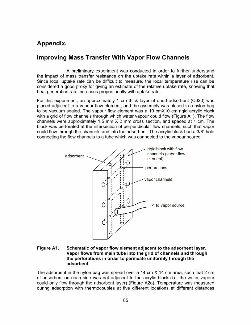
85
Appendix. Improving Mass Transfer With Vapor Flow Channels
A preliminary experiment was conducted in order to further understand the impact of mass transfer resistance on the uptake rate within a layer of adsorbent. Since local uptake rate can be difficult to measure, the local temperature rise can be considered a good proxy for giving an estimate of the relative uptake rate, knowing that heat generation rate increases proportionally with uptake rate.
For this experiment, an approximately 1 cm thick layer of dried adsorbent (C020) was placed adjacent to a vapour flow element, and the assembly was placed in a nylon bag to be vacuum sealed. The vapour flow element was a 10 cmX10 cm rigid acrylic block with a grid of flow channels through which water vapour could flow (Figure A1). The flow channels were approximately 1.5 mm X 2 mm cross section, and spaced at 1 cm. The block was perforated at the intersection of perpendicular flow channels, such that vapor could flow through the channels and into the adsorbent. The acrylic block had a 3/8” hole connecting the flow channels to a tube which was connected to the vapour source.
Figure A1. Schematic of vapor flow element adjacent to the adsorbent layer. Vapor flows from main tube into the grid of channels and through the perforations in order to permeate uniformly through the adsorbent
The adsorbent in the nylon bag was spread over a 14 cm X 14 cm area, such that 2 cm of adsorbent on each side was not adjacent to the acrylic block (i.e. the water vapour could only flow through the adsorbent layer) (Figure A2a). Temperature was measured during adsorption with thermocouples at five different locations at different distances
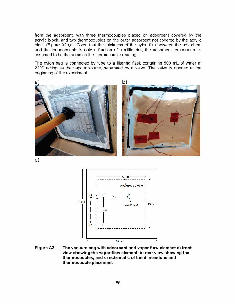
86
from the adsorbent, with three thermocouples placed on adsorbent covered by the acrylic block, and two thermocouples on the outer adsorbent not covered by the acrylic block (Figure A2b,c). Given that the thickness of the nylon film between the adsorbent and the thermocouple is only a fraction of a millimeter, the adsorbent temperature is assumed to be the same as the thermocouple reading.
The nylon bag is connected by tube to a filtering flask containing 500 mL of water at 22°C acting as the vapour source, separated by a valve. The valve is opened at the beginning of the experiment.
a)
b)
c)
Figure A2. The vacuum bag with adsorbent and vapor flow element a) front
view showing the vapor flow element, b) rear view showing the thermocouples, and c) schematic of the dimensions and thermocouple placement

87
Results show that the temperature in the adsorbent covered with the acrylic block increased to a maximum of 60-67°C (T1, T2, T3), while the outer adsorbent only reached 32-37°C (T4, T5), indicating that significantly more uptake occurred in the adsorbent covered with the acrylic block (Figure A3). The peak of T4 and T5 also occurred significantly later and the initial temperature rise was much slower, indicating a much slower uptake rate.
Although the local uptake was not directly measured, the temperature rise at each location was a good indication of the relative uptake rate. The results clearly indicate that mass transfer resistance in the adsorbent is high enough to significantly influence uptake, and vapour flow channels must be built into subsequent prototypes.
Figure A3. Transient temperature readings from the thermocouples T1-T5 showing local temperature during uptake
2025303540455055606570
0 5 10 15 20
tem
pera
ture
[°C
]
time [min]
T1 T2T3 T4T5