Embed Size (px)
Citation preview
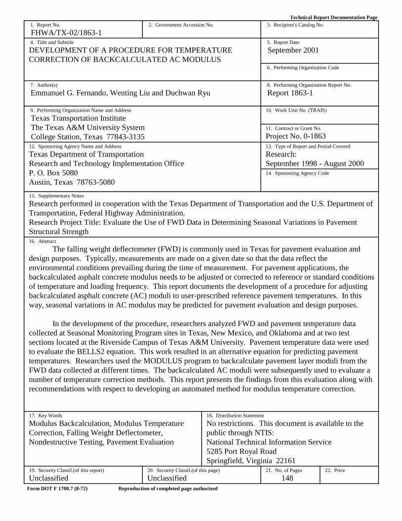
Technical Report Documentation Page 1. Report No.
FHWA/TX-02/1863-1 2. Government Accession No. 3. Recipient's Catalog No.
4. Title and Subtitle
DEVELOPMENT OF A PROCEDURE FOR TEMPERATURECORRECTION OF BACKCALCULATED AC MODULUS
5. Report Date
September 2001 6. Performing Organization Code
7. Author(s)
Emmanuel G. Fernando, Wenting Liu and Duchwan Ryu 8. Performing Organization Report No.
Report 1863-1
9. Performing Organization Name and Address
Texas Transportation Institute The Texas A&M University System College Station, Texas 77843-3135
10. Work Unit No. (TRAIS)
11. Contract or Grant No.
Project No. 0-186312. Sponsoring Agency Name and Address
Texas Department of TransportationResearch and Technology Implementation OfficeP. O. Box 5080Austin, Texas 78763-5080
13. Type of Report and Period Covered
Research:September 1998 - August 200014. Sponsoring Agency Code
15. Supplementary Notes
Research performed in cooperation with the Texas Department of Transportation and the U.S. Department ofTransportation, Federal Highway Administration.Research Project Title: Evaluate the Use of FWD Data in Determining Seasonal Variations in PavementStructural Strength16. Abstract
The falling weight deflectometer (FWD) is commonly used in Texas for pavement evaluation anddesign purposes. Typically, measurements are made on a given date so that the data reflect theenvironmental conditions prevailing during the time of measurement. For pavement applications, thebackcalculated asphalt concrete modulus needs to be adjusted or corrected to reference or standard conditionsof temperature and loading frequency. This report documents the development of a procedure for adjustingbackcalculated asphalt concrete (AC) moduli to user-prescribed reference pavement temperatures. In thisway, seasonal variations in AC modulus may be predicted for pavement evaluation and design purposes.
In the development of the procedure, researchers analyzed FWD and pavement temperature datacollected at Seasonal Monitoring Program sites in Texas, New Mexico, and Oklahoma and at two testsections located at the Riverside Campus of Texas A&M University. Pavement temperature data were usedto evaluate the BELLS2 equation. This work resulted in an alternative equation for predicting pavementtemperatures. Researchers used the MODULUS program to backcalculate pavement layer moduli from theFWD data collected at different times. The backcalculated AC moduli were subsequently used to evaluate anumber of temperature correction methods. This report presents the findings from this evaluation along withrecommendations with respect to developing an automated method for modulus temperature correction.
17. Key Words
Modulus Backcalculation, Modulus TemperatureCorrection, Falling Weight Deflectometer,Nondestructive Testing, Pavement Evaluation
18. Distribution Statement
No restrictions. This document is available to thepublic through NTIS:National Technical Information Service5285 Port Royal RoadSpringfield, Virginia 22161
19. Security Classif.(of this report)
Unclassified20. Security Classif.(of this page)
Unclassified21. No. of Pages
14822. Price
Form DOT F 1700.7 (8-72) Reproduction of completed page authorized


DEVELOPMENT OF A PROCEDURE FOR TEMPERATURECORRECTION OF BACKCALCULATED AC MODULUS
by
Emmanuel G. FernandoAssociate Research EngineerTexas Transportation Institute
Wenting LiuAssistant Research Scientist
Texas Transportation Institute
and
Duchwan RyuGraduate Research Assistant
Department of Statistics
Report 1863-1Project Number 0-1863
Research Project Title: Evaluate the Use of FWD Data in Determining Seasonal Variationsin Pavement Structural Strength
Sponsored by theTexas Department of Transportation
In Cooperation with theU.S. Department of TransportationFederal Highway Administration
September 2001
TEXAS TRANSPORTATION INSTITUTEThe Texas A&M University SystemCollege Station, Texas 77843-3135


v
DISCLAIMER
The contents of this report reflect the views of the authors, who are responsible for the
facts and the accuracy of the data presented. The contents do not necessarily reflect the
official views or policies of the Texas Department of Transportation (TxDOT) or the Federal
Highway Administration (FHWA). This report does not constitute a standard, specification,
or regulation, nor is it intended for construction, bidding, or permit purposes. The engineer
in charge of the project was Dr. Emmanuel G. Fernando, P.E. # 69614.

vi
ACKNOWLEDGMENTS
The work reported herein was conducted as part of a research project sponsored by
TxDOT and FHWA. The objective of the study was to develop an automated procedure for
temperature correction of backcalculated asphalt concrete modulus. The authors gratefully
acknowledge the support and guidance of the project director, Dr. Michael Murphy, of the
Materials and Pavements Section of TxDOT. In addition, the contributions of the following
individuals are noted and sincerely appreciated:
1. Mr. John Ragsdale of the Texas Transportation Institute (TTI) and Mr. Cy Helms
of TxDOT collected the falling weight deflectometer (FWD) and pavement
temperature data at the Riverside test sections;
2. Mr. Tom Freeman of TTI assembled the data on the seasonal monitoring program
(SMP) sites that the authors used to evaluate methods for predicting pavement
temperatures and for correcting backcalculated asphalt concrete (AC) modulus to
a given reference temperature; and
3. Mr. Seong-Wan Park prepared the literature review of temperature and moisture
correction methods.

vii
TABLE OF CONTENTS
Page
LIST OF FIGURES . . . . . . . . . . . . . . . . . . . . . . . . . . . . . . . . . . . . . . . . . . . . . . . . . . . . . . . viii
LIST OF TABLES . . . . . . . . . . . . . . . . . . . . . . . . . . . . . . . . . . . . . . . . . . . . . . . . . . . . . . . . xv
CHAPTER
I INTRODUCTION . . . . . . . . . . . . . . . . . . . . . . . . . . . . . . . . . . . . . . . . . . . . . . . . . . . . 1Background and Significance of Work . . . . . . . . . . . . . . . . . . . . . . . . . . . . . . . . . . 1Research Objective and Scope . . . . . . . . . . . . . . . . . . . . . . . . . . . . . . . . . . . . . . . . 6
II PREDICTION OF PAVEMENT TEMPERATURES . . . . . . . . . . . . . . . . . . . . . . . . 9Application of BELLS2 to Predict Pavement Temperatures . . . . . . . . . . . . . . . . 10Calibration of the BELLS2 Equation . . . . . . . . . . . . . . . . . . . . . . . . . . . . . . . . . . 11Alternative Equation for Predicting Pavement Temperature . . . . . . . . . . . . . . . . 15Seasonal Prediction of Pavement Temperature . . . . . . . . . . . . . . . . . . . . . . . . . . 17
III EVALUATION OF TEMPERATURE CORRECTION METHODS . . . . . . . . . . 31Methodology . . . . . . . . . . . . . . . . . . . . . . . . . . . . . . . . . . . . . . . . . . . . . . . . . . . . . 31Backcalculated Layer Moduli . . . . . . . . . . . . . . . . . . . . . . . . . . . . . . . . . . . . . . . . 33Temperature Correction Methods Selected for Evaluation . . . . . . . . . . . . . . . . . 39Evaluation of Binder-Viscosity Relationships . . . . . . . . . . . . . . . . . . . . . . . . . . . 46Results From Evaluation of Temperature Correction Methods . . . . . . . . . . . . . . 53Comparison of Pavement Temperatures at Different Depths . . . . . . . . . . . . . . . . 69
IV SUMMARY AND RECOMMENDATIONS . . . . . . . . . . . . . . . . . . . . . . . . . . . . . . 73The Modulus Temperature Correction Program . . . . . . . . . . . . . . . . . . . . . . . . . . 75Additional Research Needs . . . . . . . . . . . . . . . . . . . . . . . . . . . . . . . . . . . . . . . . . . 80
REFERENCES . . . . . . . . . . . . . . . . . . . . . . . . . . . . . . . . . . . . . . . . . . . . . . . . . . . . . . . . . . . 83
APPENDIX
A LITERATURE REVIEW OF METHODS FOR SEASONALCORRECTION OF FWD DATA . . . . . . . . . . . . . . . . . . . . . . . . . . . . . . . . . . . . . . . 89
Background . . . . . . . . . . . . . . . . . . . . . . . . . . . . . . . . . . . . . . . . . . . . . . . . . . . . . . 89Review of the Literature . . . . . . . . . . . . . . . . . . . . . . . . . . . . . . . . . . . . . . . . . . . . 89Climatic Data . . . . . . . . . . . . . . . . . . . . . . . . . . . . . . . . . . . . . . . . . . . . . . . . . . . 107
B PLOTS OF BACKCALCULATED AND CORRECTEDAC MODULI WITH TEST TEMPERATURES . . . . . . . . . . . . . . . . . . . . . . . . . . 109

viii
LIST OF FIGURES
Figure Page
1.1 Time-Temperature Dependency of Asphalt Concrete Mixtures . . . . . . . . . . . . . . . 2
1.2 Illustration of Stress-Dependency of an Unstabilized Soil . . . . . . . . . . . . . . . . . . . 3
1.3 Effects of Temperature and Moisture on Soil Particles(Texas Transportation Researcher, 1989) . . . . . . . . . . . . . . . . . . . . . . . . . . . . . . . . 5
2.1 Comparison of Predicted Temperatures from BELLS2with Measured Temperatures . . . . . . . . . . . . . . . . . . . . . . . . . . . . . . . . . . . . . . . . 12
2.2 Comparison of Predicted Temperatures from the CalibratedBELLS2 with the Measured Temperatures . . . . . . . . . . . . . . . . . . . . . . . . . . . . . . 14
2.3 Comparison of Predicted Temperatures from AlternativeModel with the Measured Temperatures . . . . . . . . . . . . . . . . . . . . . . . . . . . . . . . 16
2.4 Comparison of Predicted Mean Monthly Pavement Temperatureswith Measured Values for SMP Site 481122 (1 inch Depth) . . . . . . . . . . . . . . . . 19
2.5 Comparison of Predicted Mean Monthly Pavement Temperatureswith Measured Values for SMP Site 481077 (1 inch Depth) . . . . . . . . . . . . . . . . 19
2.6 Comparison of Predicted Mean Monthly Pavement Temperatureswith Measured Values for SMP Site 481068 (1 inch Depth) . . . . . . . . . . . . . . . . 20
2.7 Comparison of Predicted Mean Monthly Pavement Temperatureswith Measured Values for SMP Site 481060 (1 inch Depth) . . . . . . . . . . . . . . . . 20
2.8 Comparison of Predicted Mean Monthly Pavement Temperatureswith Measured Values for SMP Site 404165 (1 inch Depth) . . . . . . . . . . . . . . . . 21
2.9 Comparison of Predicted Mean Monthly Pavement Temperatureswith Measured Values for SMP Site 481122 (near Mid-Depth) . . . . . . . . . . . . . 21
2.10 Comparison of Predicted Mean Monthly Pavement Temperatureswith Measured Values for SMP Site 481077 (near Mid-Depth) . . . . . . . . . . . . . 22
2.11 Comparison of Predicted Mean Monthly Pavement Temperatureswith Measured Values for SMP Site 481068 (near Mid-Depth) . . . . . . . . . . . . . 22
2.12 Comparison of Predicted Mean Monthly Pavement Temperatureswith Measured Values for SMP Site 481060 (near Mid-Depth) . . . . . . . . . . . . . 23

ix
Figure Page
2.13 Comparison of Predicted Mean Monthly Pavement Temperatureswith Measured Values for SMP Site 404165 (near Mid-Depth) . . . . . . . . . . . . . 23
2.14 Comparison of Predicted Mean Monthly Pavement Temperatureswith Measured Values for SMP Site 481122 (near Bottom of AC Layer) . . . . . . 24
2.15 Comparison of Predicted Mean Monthly Pavement Temperatureswith Measured Values for SMP Site 481077 (near Bottom of AC Layer) . . . . . . 24
2.16 Comparison of Predicted Mean Monthly Pavement Temperatureswith Measured Values for SMP Site 481068 (near Bottom of AC Layer) . . . . . . 25
2.17 Comparison of Predicted Mean Monthly Pavement Temperatureswith Measured Values for SMP Site 481060 (near Bottom of AC Layer) . . . . . . 25
2.18 Comparison of Predicted Mean Monthly Pavement Temperatureswith Measured Values for SMP Site 404165 (near Bottom of AC Layer) . . . . . . 26
2.19 Comparison of Predicted Mean Monthly Pavement Temperatureswith Averages of Measured Values (1 inch Depth) . . . . . . . . . . . . . . . . . . . . . . . 27
2.20 Comparison of Predicted Mean Monthly Pavement Temperatureswith Averages of Measured Values (near Mid-Depth) . . . . . . . . . . . . . . . . . . . . . 27
2.21 Comparison of Predicted Mean Monthly Pavement Temperatureswith Averages of Measured Values (near Bottom of AC Layer) . . . . . . . . . . . . . 28
3.1 Illustration of Approach Followed to Evaluate TemperatureCorrection Methods . . . . . . . . . . . . . . . . . . . . . . . . . . . . . . . . . . . . . . . . . . . . . . . 32
3.2 Variation of Backcalculated AC Modulus withTest Temperature (351112) . . . . . . . . . . . . . . . . . . . . . . . . . . . . . . . . . . . . . . . . . 35
3.3 Variation of Backcalculated AC Modulus withTest Temperature (404165) . . . . . . . . . . . . . . . . . . . . . . . . . . . . . . . . . . . . . . . . . 35
3.4 Variation of Backcalculated AC Modulus withTest Temperature (481060) . . . . . . . . . . . . . . . . . . . . . . . . . . . . . . . . . . . . . . . . . 36
3.5 Variation of Backcalculated AC Modulus withTest Temperature (481068) . . . . . . . . . . . . . . . . . . . . . . . . . . . . . . . . . . . . . . . . . 36
3.6 Variation of Backcalculated AC Modulus withTest Temperature (481077) . . . . . . . . . . . . . . . . . . . . . . . . . . . . . . . . . . . . . . . . . 37

x
Figure Page
3.7 Variation of Backcalculated AC Modulus withTest Temperature (481122) . . . . . . . . . . . . . . . . . . . . . . . . . . . . . . . . . . . . . . . . . 37
3.8 Variation of Backcalculated AC Modulus withTest Temperature (Pad 12) . . . . . . . . . . . . . . . . . . . . . . . . . . . . . . . . . . . . . . . . . . 38
3.9 Variation of Backcalculated AC Modulus withTest Temperature (Pad 21) . . . . . . . . . . . . . . . . . . . . . . . . . . . . . . . . . . . . . . . . . . 38
3.10 Fitted Curve to Backcalculated AC Moduli (SMP Site 404165) . . . . . . . . . . . . . 49
3.11 Fitted Curve to Backcalculated AC Moduli (SMP Site 481060) . . . . . . . . . . . . . 49
3.12 Fitted Curve to Backcalculated AC Moduli (SMP Site 481068) . . . . . . . . . . . . . 50
3.13 Fitted Curve to Backcalculated AC Moduli (SMP Site 481077) . . . . . . . . . . . . . 50
3.14 Fitted Curve to Backcalculated AC Moduli (SMP Site 481122) . . . . . . . . . . . . . 51
3.15 Fitted Curve to Backcalculated AC Moduli (Pad 12) . . . . . . . . . . . . . . . . . . . . . . 51
3.16 Fitted Curve to Backcalculated AC Moduli (Pad 21) . . . . . . . . . . . . . . . . . . . . . . 52
3.17 Corrected AC Moduli Using Eq. (3.5) and tr = 24 �C(SMP Site 404165) . . . . . . . . . . . . . . . . . . . . . . . . . . . . . . . . . . . . . . . . . . . . . . . . 54
3.18 Corrected AC Moduli Using Eq. (3.5) and tr = 24 �C(SMP Site 481060) . . . . . . . . . . . . . . . . . . . . . . . . . . . . . . . . . . . . . . . . . . . . . . . . 54
3.19 Corrected AC Moduli Using Eq. (3.5) and tr = 24 �C(SMP Site 481068) . . . . . . . . . . . . . . . . . . . . . . . . . . . . . . . . . . . . . . . . . . . . . . . . 55
3.20 Corrected AC Moduli Using Eq. (3.5) and tr = 24 �C(SMP Site 481077) . . . . . . . . . . . . . . . . . . . . . . . . . . . . . . . . . . . . . . . . . . . . . . . . 55
3.21 Corrected AC Moduli Using Eq. (3.5) and tr = 24 �C(SMP Site 481122) . . . . . . . . . . . . . . . . . . . . . . . . . . . . . . . . . . . . . . . . . . . . . . . . 56
3.22 Corrected AC Moduli Using Eq. (3.5) and tr = 24 �C (Pad 12) . . . . . . . . . . . . . . 56
3.23 Corrected AC Moduli Using Eq. (3.5) and tr = 24 �C (Pad 21) . . . . . . . . . . . . . . 57
3.24 Corrected AC Moduli Using Eq. (3.4) and tr = 24 �C(SMP Site 404165) . . . . . . . . . . . . . . . . . . . . . . . . . . . . . . . . . . . . . . . . . . . . . . . . 57
xi
Figure Page
3.25 Corrected AC Moduli Using Eq. (3.4) and tr = 24 �C(SMP Site 481060) . . . . . . . . . . . . . . . . . . . . . . . . . . . . . . . . . . . . . . . . . . . . . . . . 58
3.26 Corrected AC Moduli Using Eq. (3.4) and tr = 24 �C(SMP Site 481068) . . . . . . . . . . . . . . . . . . . . . . . . . . . . . . . . . . . . . . . . . . . . . . . . 58
3.27 Corrected AC Moduli Using Eq. (3.4) and tr = 24 �C(SMP Site 481077) . . . . . . . . . . . . . . . . . . . . . . . . . . . . . . . . . . . . . . . . . . . . . . . . 59
3.28 Corrected AC Moduli Using Eq. (3.4) and tr = 24 �C(SMP Site 481122) . . . . . . . . . . . . . . . . . . . . . . . . . . . . . . . . . . . . . . . . . . . . . . . . 59
3.29 Corrected AC Moduli Using Eq. (3.4) and tr = 24 �C (Pad 12) . . . . . . . . . . . . . . 60
3.30 Corrected AC Moduli Using Eq. (3.4) and tr = 24 �C (Pad 21) . . . . . . . . . . . . . . 60
3.31 Corrected AC Moduli Using Eq. (3.1) and tr = 24 �C(SMP Site 404165) . . . . . . . . . . . . . . . . . . . . . . . . . . . . . . . . . . . . . . . . . . . . . . . . 61
3.32 Corrected AC Moduli Using Eq. (3.1) and tr = 24 �C(SMP Site 481060) . . . . . . . . . . . . . . . . . . . . . . . . . . . . . . . . . . . . . . . . . . . . . . . . 61
3.33 Corrected AC Moduli Using Eq. (3.1) and tr = 24 �C(SMP Site 481068) . . . . . . . . . . . . . . . . . . . . . . . . . . . . . . . . . . . . . . . . . . . . . . . . 62
3.34 Corrected AC Moduli Using Eq. (3.1) and tr = 24 �C(SMP Site 481077) . . . . . . . . . . . . . . . . . . . . . . . . . . . . . . . . . . . . . . . . . . . . . . . . 62
3.35 Corrected AC Moduli Using Eq. (3.1) and tr = 24 �C(SMP Site 481122) . . . . . . . . . . . . . . . . . . . . . . . . . . . . . . . . . . . . . . . . . . . . . . . . 63
3.36 Corrected AC Moduli Using Eq. (3.1) and tr = 24 �C (Pad 12) . . . . . . . . . . . . . . 63
3.37 Corrected AC Moduli Using Eq. (3.1) and tr = 24 �C (Pad 21) . . . . . . . . . . . . . . 64
3.38 Comparison of Mid-Depth with 1 inch Depth Test Temperatures . . . . . . . . . . . . 70
3.39 Comparison of Mid-Depth with 1.6 inch Depth Test Temperatures . . . . . . . . . . 70
4.1 Flowchart of the Modulus Temperature Correction Program(Fernando and Liu, 2001) . . . . . . . . . . . . . . . . . . . . . . . . . . . . . . . . . . . . . . . . . . . 76
4.2 Example Plot of Corrected and Backcalculated AC Moduli vs.Test Temperature . . . . . . . . . . . . . . . . . . . . . . . . . . . . . . . . . . . . . . . . . . . . . . . . . 79

xii
Figure Page
4.3 Example Plot of Predicted Monthly Variations in AC Modulus . . . . . . . . . . . . . 80
A1 Comparison of Predicted AC Temperatures from BELLS2with Measured Values (Stubstad et al., 1998) . . . . . . . . . . . . . . . . . . . . . . . . . . . 93
A2 FWD Deflections Normalized to a Standard Temperatureof 68 �F (Kim et al., 1995) . . . . . . . . . . . . . . . . . . . . . . . . . . . . . . . . . . . . . . . . . . 95
A3 Procedure to Determine the Equivalent Uniform ACLayer Temperature . . . . . . . . . . . . . . . . . . . . . . . . . . . . . . . . . . . . . . . . . . . . . . . 100
B1 Corrected AC Moduli Using Eq. (3.5) and tr = 7 �C(SMP Site 404165) . . . . . . . . . . . . . . . . . . . . . . . . . . . . . . . . . . . . . . . . . . . . . . . 111
B2 Corrected AC Moduli Using Eq. (3.5) and tr = 7 �C(SMP Site 481060) . . . . . . . . . . . . . . . . . . . . . . . . . . . . . . . . . . . . . . . . . . . . . . . 111
B3 Corrected AC Moduli Using Eq. (3.5) and tr = 7 �C(SMP Site 481068) . . . . . . . . . . . . . . . . . . . . . . . . . . . . . . . . . . . . . . . . . . . . . . . 112
B4 Corrected AC Moduli Using Eq. (3.5) and tr = 7 �C(SMP Site 481077) . . . . . . . . . . . . . . . . . . . . . . . . . . . . . . . . . . . . . . . . . . . . . . . 112
B5 Corrected AC Moduli Using Eq. (3.5) and tr = 7 �C(SMP Site 481122) . . . . . . . . . . . . . . . . . . . . . . . . . . . . . . . . . . . . . . . . . . . . . . . 113
B6 Corrected AC Moduli Using Eq. (3.5) and tr = 7 �C (Pad 12) . . . . . . . . . . . . . . 113
B7 Corrected AC Moduli Using Eq. (3.5) and tr = 7 �C (Pad 21) . . . . . . . . . . . . . . 114
B8 Corrected AC Moduli Using Eq. (3.4) and tr = 7 �C(SMP Site 404165) . . . . . . . . . . . . . . . . . . . . . . . . . . . . . . . . . . . . . . . . . . . . . . . 114
B9 Corrected AC Moduli Using Eq. (3.4) and tr = 7 �C(SMP Site 481060) . . . . . . . . . . . . . . . . . . . . . . . . . . . . . . . . . . . . . . . . . . . . . . . 115
B10 Corrected AC Moduli Using Eq. (3.4) and tr = 7 �C(SMP Site 481068) . . . . . . . . . . . . . . . . . . . . . . . . . . . . . . . . . . . . . . . . . . . . . . . 115
B11 Corrected AC Moduli Using Eq. (3.4) and tr = 7 �C(SMP Site 481077) . . . . . . . . . . . . . . . . . . . . . . . . . . . . . . . . . . . . . . . . . . . . . . . 116
B12 Corrected AC Moduli Using Eq. (3.4) and tr = 7 �C(SMP Site 481122) . . . . . . . . . . . . . . . . . . . . . . . . . . . . . . . . . . . . . . . . . . . . . . . 116

xiii
Figure Page
B13 Corrected AC Moduli Using Eq. (3.4) and tr = 7 �C (Pad 12) . . . . . . . . . . . . . . 117
B14 Corrected AC Moduli Using Eq. (3.4) and tr = 7 �C (Pad 21) . . . . . . . . . . . . . . 117
B15 Corrected AC Moduli Using Eq. (3.1) and tr = 7 �C(SMP Site 404165) . . . . . . . . . . . . . . . . . . . . . . . . . . . . . . . . . . . . . . . . . . . . . . . 118
B16 Corrected AC Moduli Using Eq. (3.1) and tr = 7 �C(SMP Site 481060) . . . . . . . . . . . . . . . . . . . . . . . . . . . . . . . . . . . . . . . . . . . . . . . 118
B17 Corrected AC Moduli Using Eq. (3.1) and tr = 7 �C(SMP Site 481068) . . . . . . . . . . . . . . . . . . . . . . . . . . . . . . . . . . . . . . . . . . . . . . . 119
B18 Corrected AC Moduli Using Eq. (3.1) and tr = 7 �C(SMP Site 481077) . . . . . . . . . . . . . . . . . . . . . . . . . . . . . . . . . . . . . . . . . . . . . . . 119
B19 Corrected AC Moduli Using Eq. (3.1) and tr = 7 �C(SMP Site 481122) . . . . . . . . . . . . . . . . . . . . . . . . . . . . . . . . . . . . . . . . . . . . . . . 120
B20 Corrected AC Moduli Using Eq. (3.1) and tr = 7 �C (Pad 12) . . . . . . . . . . . . . . 120
B21 Corrected AC Moduli Using Eq. (3.1) and tr = 7 �C (Pad 21) . . . . . . . . . . . . . . 121
B22 Corrected AC Moduli Using Eq. (3.5) and tr = 41 �C(SMP Site 404165) . . . . . . . . . . . . . . . . . . . . . . . . . . . . . . . . . . . . . . . . . . . . . . . 121
B23 Corrected AC Moduli Using Eq. (3.5) and tr = 41 �C(SMP Site 481060) . . . . . . . . . . . . . . . . . . . . . . . . . . . . . . . . . . . . . . . . . . . . . . . 122
B24 Corrected AC Moduli Using Eq. (3.5) and tr = 41 �C(SMP Site 481068) . . . . . . . . . . . . . . . . . . . . . . . . . . . . . . . . . . . . . . . . . . . . . . . 122
B25 Corrected AC Moduli Using Eq. (3.5) and tr = 41 �C(SMP Site 481077) . . . . . . . . . . . . . . . . . . . . . . . . . . . . . . . . . . . . . . . . . . . . . . . 123
B26 Corrected AC Moduli Using Eq. (3.5) and tr = 41 �C(SMP Site 481122) . . . . . . . . . . . . . . . . . . . . . . . . . . . . . . . . . . . . . . . . . . . . . . . 123
B27 Corrected AC Moduli Using Eq. (3.5) and tr = 41 �C (Pad 12) . . . . . . . . . . . . . 124
B28 Corrected AC Moduli Using Eq. (3.5) and tr = 41 �C (Pad 21) . . . . . . . . . . . . . 124
B29 Corrected AC Moduli Using Eq. (3.4) and tr = 41 �C(SMP Site 404165) . . . . . . . . . . . . . . . . . . . . . . . . . . . . . . . . . . . . . . . . . . . . . . . 125

xiv
Figure Page
B30 Corrected AC Moduli Using Eq. (3.4) and tr = 41 �C(SMP Site 481060) . . . . . . . . . . . . . . . . . . . . . . . . . . . . . . . . . . . . . . . . . . . . . . . 125
B31 Corrected AC Moduli Using Eq. (3.4) and tr = 41 �C(SMP Site 481068) . . . . . . . . . . . . . . . . . . . . . . . . . . . . . . . . . . . . . . . . . . . . . . . 126
B32 Corrected AC Moduli Using Eq. (3.4) and tr = 41 �C(SMP Site 481077) . . . . . . . . . . . . . . . . . . . . . . . . . . . . . . . . . . . . . . . . . . . . . . . 126
B33 Corrected AC Moduli Using Eq. (3.4) and tr = 41 �C(SMP Site 481122) . . . . . . . . . . . . . . . . . . . . . . . . . . . . . . . . . . . . . . . . . . . . . . . 127
B34 Corrected AC Moduli Using Eq. (3.4) and tr = 41 �C (Pad 12) . . . . . . . . . . . . . 127
B35 Corrected AC Moduli Using Eq. (3.4) and tr = 41 �C (Pad 21) . . . . . . . . . . . . . 128
B36 Corrected AC Moduli Using Eq. (3.1) and tr = 41 �C(SMP Site 404165) . . . . . . . . . . . . . . . . . . . . . . . . . . . . . . . . . . . . . . . . . . . . . . . 128
B37 Corrected AC Moduli Using Eq. (3.1) and tr = 41 �C(SMP Site 481060) . . . . . . . . . . . . . . . . . . . . . . . . . . . . . . . . . . . . . . . . . . . . . . . 129
B38 Corrected AC Moduli Using Eq. (3.1) and tr = 41 �C(SMP Site 481068) . . . . . . . . . . . . . . . . . . . . . . . . . . . . . . . . . . . . . . . . . . . . . . . 129
B39 Corrected AC Moduli Using Eq. (3.1) and tr = 41 �C(SMP Site 481077) . . . . . . . . . . . . . . . . . . . . . . . . . . . . . . . . . . . . . . . . . . . . . . . 130
B40 Corrected AC Moduli Using Eq. (3.1) and tr = 41 �C(SMP Site 481122) . . . . . . . . . . . . . . . . . . . . . . . . . . . . . . . . . . . . . . . . . . . . . . . 130
B41 Corrected AC Moduli Using Eq. (3.1) and tr = 41 �C (Pad 12) . . . . . . . . . . . . . 131
B42 Corrected AC Moduli Using Eq. (3.1) and tr = 41 �C (Pad 21) . . . . . . . . . . . . . 131

xv
LIST OF TABLES
Table Page
1.1 Sensitivity of Predicted Life-Cycle Costs (in $/yd2)to Changes in Pavement Layer Moduli . . . . . . . . . . . . . . . . . . . . . . . . . . . . . . . . . . 6
2.1 Adjustment of IR Temperatures to Consider Effect of Shading . . . . . . . . . . . . . . 10
2.2 Coefficients of the BELLS2 and BELLS3 Equations . . . . . . . . . . . . . . . . . . . . . . 12
2.3 Coefficients of the Calibrated BELLS2 Equation . . . . . . . . . . . . . . . . . . . . . . . . 13
2.4 Coefficients of the Calibrated BELLS2 Equation without �4 Term . . . . . . . . . . . 14
2.5 Coefficients of the Alternative Model for PredictingPavement Temperature . . . . . . . . . . . . . . . . . . . . . . . . . . . . . . . . . . . . . . . . . . . . . 16
2.6 Comparison of Predictive Accuracy of Models Evaluated . . . . . . . . . . . . . . . . . . 17
2.7 Goodness-of-Fit Statistics Indicating Correlation betweenPredicted Mean Monthly Pavement Temperatures and Averagesof Measured Values . . . . . . . . . . . . . . . . . . . . . . . . . . . . . . . . . . . . . . . . . . . . . . . 28
3.1 Pavement Layering at Test Sites and Depths of Temperature Measurements . . . . . . . . . . . . . . . . . . . . . . . . . . . . . . . . . . . . . . . . . 34
3.2 Typical A and VTS Coefficients for AC-Graded Asphalts . . . . . . . . . . . . . . . . . . 44
3.3 Typical A and VTS Coefficients for PG-Graded Asphalts . . . . . . . . . . . . . . . . . . 45
3.4 A and VTS Coefficients Determined from BackcalculatedAC Moduli . . . . . . . . . . . . . . . . . . . . . . . . . . . . . . . . . . . . . . . . . . . . . . . . . . . . . . 47
3.5 Goodness-of-Fit Statistics of Nonlinear Model Given by Eq. (3.11) . . . . . . . . . . 52
3.6 Slopes of Regression Lines Fitted to the Corrected Moduli . . . . . . . . . . . . . . . . . 66
3.7 Absolute Differences between Reference and Mean CorrectedAC Moduli . . . . . . . . . . . . . . . . . . . . . . . . . . . . . . . . . . . . . . . . . . . . . . . . . . . . . . 68
A1 Percentage of Temperature Correction Factor Applied toEach FWD Sensor . . . . . . . . . . . . . . . . . . . . . . . . . . . . . . . . . . . . . . . . . . . . . . . . 102

xvi
Table Page
A2 Regression Coefficients for Estimating Asphalt Tensile andSubgrade Compressive Strains for MODULUS RemainingLife Analysis . . . . . . . . . . . . . . . . . . . . . . . . . . . . . . . . . . . . . . . . . . . . . . . . . . . . 102
A3 Indicators of Seasonal Variation of Subgrade Response (van Gurp, 1995) . . . . . . . . . . . . . . . . . . . . . . . . . . . . . . . . . . . . . . . . 104

1
CHAPTER I
INTRODUCTION
The Texas Department of Transportation (TxDOT) uses the falling weight
deflectometer (FWD) for pavement evaluation. A common application is the backcalculation
of pavement layer moduli by deflection basin fitting. In Texas, pavement engineers use the
MODULUS program (Michalak and Scullion, 1995) to provide estimates of pavement layer
moduli from measured FWD deflections. These estimates are subsequently used in other
applications, such as the FPS-19 flexible pavement design procedure, the Program for
Analyzing Loads Superheavy (Jooste and Fernando, 1995 and Fernando, 1997), and the
Program for Load Zoning Analysis (PLZA) developed by Fernando and Liu (1999).
For pavement applications, engineers must adjust the results obtained from the FWD
or correct them to reference or standard conditions of temperature, moisture, and loading
frequency. As indicated in the research project statement for TxDOT Project 0-1863, this
problem has been studied by state, federal, and international researchers. Comprehensive
summaries of related findings are given in the National Cooperative Highway Research
Program (NCHRP) Report 327, “Determining Asphaltic Concrete Pavement Structural
Properties by Nondestructive Testing,” (Lytton et al., 1990) and in a dissertation presented by
van Gurp (1995) to the Delft University. The appendix to this report reviews existing
methods for temperature and moisture correction of FWD deflections and backcalculated
layer moduli. What is needed is to use the knowledge gained from previous studies to
develop an automated method for correcting FWD data to standard conditions. By having an
automated procedure, TxDOT pavement engineers can more effectively consider seasonal
variations in structural strength in the design of pavements, analysis of superheavy load
routes, and evaluation of axle weight restrictions.
BACKGROUND AND SIGNIFICANCE OF WORK
Asphalt concrete (AC) mixture stiffness varies with temperature, time of loading, and
load level (at temperatures above 20 �C). Figure 1.1 illustrates the time-temperature
dependency of asphalt concrete mixtures as determined from laboratory tests. Note that

2
Figure 1.1. Time-Temperature Dependency of Asphalt Concrete Mixtures.
the stiffness (or modulus) of the material decreases with increasing temperature and time of
loading. The time-temperature dependency of a given mix may be characterized directly in
the laboratory by conducting creep or frequency sweep tests on cores or molded specimens at
various test temperatures. Alternatively, the time-temperature dependency may be estimated
nondestructively by dynamic analysis of FWD data using the full-time load and deflection
histories (Magnuson and Lytton, 1997). This backcalculation requires collection of FWD
data at a given location on the pavement at different times of the day or year to get
deflections that cover a range of pavement temperatures.
In many practical situations, it may not be feasible to directly determine the time-
temperature dependency using the laboratory or field tests previously noted. For these cases,
equations for predicting AC stiffness from knowledge of the basic mixture properties may be
used. An example is the Asphalt Institute (1982) equation to predict dynamic modulus and
the more recent equation by Witczak and Fonseca (1996) that has been proposed for the 2002

3
Figure 1.2. Illustration of Stress-Dependency of an Unstabilized Soil.
American Association of State Highway Transportation Officials (AASHTO) pavement
design guide. The application of these equations for temperature correction of AC modulus
is evaluated later in this report.
For unbound materials, the stiffness and strength properties have been found to vary
with load level, moisture condition, and temperature. Figure 1.2 illustrates the influence of
stress level on the resilient modulus of soils from laboratory measurements. As shown, the
resilient modulus tends to increase with confining pressure, �3, and diminish with increasing
deviatoric stress, �d, consistent with the stress-dependent model proposed by Uzan (1985).
Correction for the effect of load level on the backcalculated modulus will require
characterization of the stress-dependency of the material. For this purpose, resilient modulus
tests may be conducted in the laboratory following AASHTO T-292-91. In many practical
applications, however, the analysis of pavement response and performance is typically made
on the basis of the standard 80 kN single axle. For these applications, corrections for load

4
level effects will not be necessary if FWD deflections are obtained at a load of 40 kN,
corresponding to the standard axle.
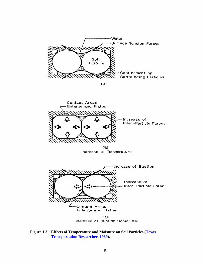
Figure 1.3 illustrates the influence of temperature and moisture on unbound materials.
If soil particles are assumed to be confined in all directions, a rise in temperature will cause
an increase in the contact forces between particles due to the inability of the particles to
expand because of confinement. Under these conditions, the material will become stiffer.
Figure 1.3 also illustrates the effect of moisture on soil particles. The change in
stiffness is related to the state of moisture tension in unsaturated soils, also known as soil
suction (Chandra et al., 1989). Soil suction is made up of two components:
1. osmotic suction due to salts dissolved in the pore water, and
2. matric suction due to the attraction of water for the surfaces of the soil particles.
The latter component is a negative pressure that exists in the soil water as a result of capillary
tension. Soil suction is a measure of the soil’s affinity for water and indicates the intensity
with which it will attract water. The drier the soil, the greater the soil suction (Chen, 1988)
and the stiffer the material owing to the greater capillary tension holding the soil particles
together. In the field, soil suction typically ranges from 2 to 6 pF (Lytton et al., 1990), where
pF is the logarithm (base 10) of the absolute value of soil suction expressed in centimeters of
head. In terms of hydrostatic pressure, this corresponds to a range of -0.42 to -14,220 psi.
Because of the effects of temperature, moisture, load level, and frequency of loading
on the modulus of pavement materials, measurements of pavement deflections will reflect the
influence of these variables. Thus, applications of FWD data for pavement design, pavement
evaluation, superheavy load analysis, load zoning, and others will require correction of
backcalculated moduli to reference or standard conditions. To illustrate the importance of
this correction, researchers evaluated a number of pavement designs using TxDOT’s FPS-19
computer program. Table 1.1 presents results from this evaluation. This table summarizes
the sensitivity of the predicted life-cycle costs to changes in the pavement layer moduli for
two different levels of surface thickness. From the results shown, the following observations
may be made:
1. The predicted life-cycle costs are significantly affected by the layer moduli values
assumed in the design. Thus, errors in the layer moduli will lead to errors in
selecting the optimal design strategy.
5
Figure 1.3. Effects of Temperature and Moisture on Soil Particles (TexasTransportation Researcher, 1989).

6
Table 1.1. Sensitivity of Predicted Life-Cycle Costs (in $/yd2) to Changes in PavementLayer Moduli.
ACThickness
(in)
ACModulus
(ksi)
Base Modulus (ksi)
20 40
Subgrade Modulus (ksi)
5 15 5 15
2400 6.97 (7.6%) 6.57 (1.4%) 6.41 (-1.1%) 5.66 (-12.7%)
600 6.70 (3.4%) 6.27 (-3.2%) 6.31 (-2.6%) 5.38 (-17.0%)
4400 7.10 (9.6%) 6.48 (0%) 6.48 (0%) 5.93 (-8.5%)
600 6.48 (0%) 5.93 (-8.5%) 5.93 (-8.5%) 5.38 (-17.0%)
2. The effect of AC modulus is more pronounced for thicker surface layers.
3. The subgrade modulus exhibits a greater effect for the thicker surface when the
base modulus is at the low level. However, at the high base modulus, the effect of
changes in the subgrade modulus is more pronounced for the thinner surface.
4. The base modulus exhibits a greater effect for the thicker surface when the
subgrade modulus is at the low level. However, at the high subgrade modulus, the
effect of changes in the base modulus is more pronounced for the thinner surface.
The above observations demonstrate the sensitivity of pavement designs to the pavement
layer moduli used in the design procedure. Thus, if the effects of temperature, moisture, load
level, and load duration are not properly considered in the analysis of FWD data, the resulting
errors in pavement layer moduli can significantly influence the selection of the optimal
design strategy.
RESEARCH OBJECTIVE AND SCOPE
Project 0-1863 aimed to develop an automated method of correcting FWD data to
standard conditions of temperature and moisture. To accomplish this objective, existing
methods for temperature and moisture correction were to be used in developing the
automated procedure required from this project. The scope of work was limited to asphalt
concrete pavements with unbound base materials.
7
To identify existing methods for temperature and moisture correction, researchers
initially conducted a literature review of previous investigations in this area. From this
review, methods were selected for evaluation in this project using available data from the
Seasonal Monitoring Program (SMP) sites in Texas, Oklahoma, and New Mexico that were
collected under the Long-Term Pavement Performance (LTPP) program.
While the original scope of the project included the correction of FWD data for
moisture effects, the project was later modified to delay this investigation to a later time and
move it to a future research study. Project funding was subsequently reduced. However, a
field test program was included in the scope of work to collect additional FWD and pavement
temperature measurements to supplement the SMP data for evaluating temperature correction
methods. These measurements were conducted on two test sections located at the Riverside
Campus of Texas A&M University.
This report documents the research efforts to develop an automated method for
temperature correction of FWD data. The report is organized into the following chapters:
1. Chapter I provides background on the effects of temperature, moisture, load level,
and frequency of loading on the modulus of asphalt concrete and unbound
pavement materials. The importance of considering the effects of these variables
in the collection and analysis of FWD data is demonstrated. In addition, this
chapter presents the objective and scope of the project.
2. Chapter II presents the evaluation of the BELLS equation (Stubstad et al., 1998)
for predicting pavement temperatures and its calibration using the SMP data for
Texas, Oklahoma, and New Mexico and the additional data collected at the Texas
A&M test sections.
3. Chapter III evaluates selected methods for temperature correction.
4. Chapter IV summarizes research findings with respect to developing the
automated procedure for temperature correction and recommendations for future
work.
Appendix A presents the literature review conducted by researchers to identify existing
methods for temperature and moisture correction of FWD deflections and backcalculated
layer moduli. Finally, Appendix B presents charts from the evaluation of selected modulus
temperature correction methods. The automated method for temperature correction is
presented in a companion report by Fernando and Liu (2001).

9
CHAPTER II
PREDICTION OF PAVEMENT TEMPERATURES
Before correction to a reference temperature may be made, the pavement temperature
one is correcting from must first be established. This pavement temperature is herein referred
to as the base temperature for the modulus correction and refers to the pavement temperature
at which FWD deflections were taken. This temperature may be obtained by direct
measurement with a temperature probe during the FWD survey or from approximate methods
based on air and surface temperatures that are more readily available or easily measured.
While direct measurement of pavement temperature may be made at each FWD station,
conducting measurements at this frequency is not always feasible in practice. As a minimum,
TxDOT recommends taking pavement temperature readings at the beginning and end of the
FWD survey. From these readings, the temperatures at the other stations may be estimated
by interpolation based on the time of the FWD measurement. Of course, the FWD operator
can measure pavement temperatures at closer intervals to get better estimates from the
interpolation. In this way, the operator can better capture pavement temperature variations
during the survey.
Alternatively, one may use approximate methods to establish the base temperature for
the modulus correction. Lukanen et al. (1998) recently developed a set of equations for
predicting pavement temperatures in a research project sponsored by the Federal Highway
Administration (FHWA). These equations, referred to in the literature as BELLS2 and
BELLS3, were developed using pavement temperature data collected on 41 SMP sites in
North America. Both equations require the infrared (IR) surface temperature at the time
FWD deflections were measured at a given station and the average of the previous day’s
minimum and maximum air temperatures in the vicinity of the project surveyed.
BELLS2 is the equation for the FWD testing protocol used in the LTPP program. On
the other hand, BELLS3 is intended for routine testing and was developed from efforts made
to consider the effects of shading on the IR temperatures measured at the SMP sites. As
noted by Stubstad et al. (1998), FWD tests on the SMP sites involve multiple drops with the

10
Table 2.1. Adjustment of IR Temperatures to Consider Effect of Shading.
Sky Cover Reported Added to IR Temperature (�C)
Sunny +4.0
Partly Cloudy +3.0
Cloudy +1.5
result that each test point is shaded by the FWD for about six minutes. For routine FWD
testing, deflection measurements on a given station will normally be completed in less than a
minute. Thus, to simulate the effect of shading, the developers of the BELLS3 equation
adjusted the IR temperatures measured on the SMP sites according to Table 2.1 (Stubstad, et
al., 1998). The adjusted IR temperatures were subsequently used to develop the BELLS3
equation. Stubstad et al. (1998) noted that the above adjustments are based on limited tests
conducted on asphalt concrete pavements in Florida and California. In fact, they
recommended fine tuning the equation at some point in time because of the small amount of
data on which the shading adjustments were based. For this reason, the evaluation reported
in this chapter was limited to the BELLS2 equation. Researchers evaluated the applicability
of this equation to Texas conditions using the measured IR and pavement temperature data
from the asphalt concrete SMP sites in Texas, New Mexico, and Oklahoma and from the
asphalt sections located at the Texas A&M Riverside Campus. This evaluation resulted in an
alternative form of the BELLS equation that is presented in this chapter.
APPLICATION OF BELLS2 TO PREDICT PAVEMENT TEMPERATURES
The BELLS2 equation was evaluated using temperature data from the following sites:
1. five SMP sites in Texas - 481060, 481068, 481077, 481122, and 483739;
2. one SMP site in New Mexico - 351112;
3. one SMP site in Oklahoma - 404165; and
4. Two test sections (12 and 21) located at the Texas A&M Riverside Campus.
In this evaluation, researchers compared the predicted temperatures from the BELLS2
equation against measured temperatures taken at different times on the above sites and at
three different depths corresponding to near the surface, middle of the asphalt, and near the

11
bottom of the asphalt layer. The measured IR temperatures taken at the time of the FWD
measurements were used in the predictions. The form of the BELLS2 (as well as the
BELLS3) equation is given by:
Td = �0 + �1 IR + [log10(d) - 1.25] [ �2 IR + �3 T(1-day) + �4 sin(hr18 - 15.5) ]
+ �5 IR sin(hr18 - 13.5) (2.1)
where,
Td = pavement temperature at depth, d, within the asphalt layer, �C;
IR = surface temperature measured with the infrared temperature gauge, �C;
d = depth at which the temperature is to be predicted, mm
T(1-day) = the average of the previous day’s high and low air temperatures, �C; and
hr18 = time of day in the 24-hour system but calculated using an 18-hour asphalt
temperature rise and fall time as explained by Stubstad et al. (1998).
The coefficients of Eq. (2.1) are given in Table 2.2 for both the BELLS2 and BELLS3
equations. Figure 2.1 compares the predicted temperatures from BELLS2 with the
corresponding measured temperatures at the test sections included in this evaluation. To
establish the accuracy of the predictions, the coefficient of determination, R2, and the root-
mean-square error (RMSE) were determined. Accounting for the number of independent
variables in the model, an adjusted R2 of 0.878 was computed for the 1575 observations
included in Figure 2.1. The RMSE associated with the predictions is 7.410 �C.
Note that there is a noticeable bias in the predictions, as the points in Figure 2.1 tend
to curve down from the line of equality with temperature increase. Since BELLS2 was
developed using a larger database that included many more sites located in the United States
and Canada, it is of interest to determine if the accuracy of the predictions may be improved
by calibrating the equation using only the temperature data from the nine sections included in
the evaluation. The next section presents this calibration.
CALIBRATION OF THE BELLS2 EQUATION
Researchers used the BELLS model given in Eq. (2.1) in the calibration. By multiple
linear regression using the temperature data from the project sites, the model coefficients
given in Table 2.3 were determined. This table also shows the t-statistic for evaluating the

12
Figure 2.1. Comparison of Predicted Temperatures from BELLS2 with MeasuredTemperatures.
Table 2.2 Coefficients of the BELLS2 and BELLS3 Equations.
Coefficient BELLS2 BELLS3
�0 +2.780 +0.950
�1 +0.912 +0.892
�2 -0.428 -0.448
�3 +0.553 +0.621
�4 +2.630 +1.830
�5 +0.027 +0.042
13
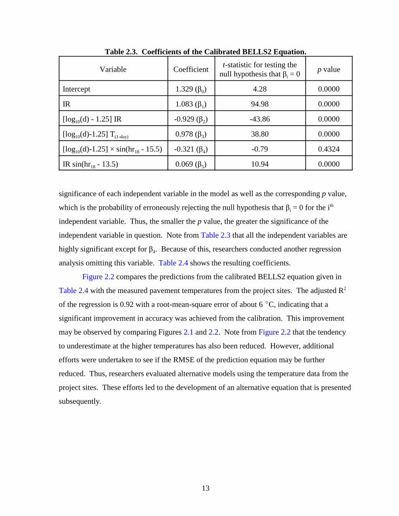
Table 2.3. Coefficients of the Calibrated BELLS2 Equation.
Variable Coefficientt-statistic for testing the
null hypothesis that �i = 0p value
Intercept 1.329 (�0) 4.28 0.0000
IR 1.083 (�1) 94.98 0.0000
[log10(d) - 1.25] IR -0.929 (�2) -43.86 0.0000
[log10(d)-1.25] T(1-day) 0.978 (�3) 38.80 0.0000
[log10(d)-1.25] × sin(hr18 - 15.5) -0.321 (�4) -0.79 0.4324
IR sin(hr18 - 13.5) 0.069 (�5) 10.94 0.0000
significance of each independent variable in the model as well as the corresponding p value,
which is the probability of erroneously rejecting the null hypothesis that �i = 0 for the ith
independent variable. Thus, the smaller the p value, the greater the significance of the
independent variable in question. Note from Table 2.3 that all the independent variables are
highly significant except for �4. Because of this, researchers conducted another regression
analysis omitting this variable. Table 2.4 shows the resulting coefficients.
Figure 2.2 compares the predictions from the calibrated BELLS2 equation given in
Table 2.4 with the measured pavement temperatures from the project sites. The adjusted R2
of the regression is 0.92 with a root-mean-square error of about 6 �C, indicating that a
significant improvement in accuracy was achieved from the calibration. This improvement
may be observed by comparing Figures 2.1 and 2.2. Note from Figure 2.2 that the tendency
to underestimate at the higher temperatures has also been reduced. However, additional
efforts were undertaken to see if the RMSE of the prediction equation may be further
reduced. Thus, researchers evaluated alternative models using the temperature data from the
project sites. These efforts led to the development of an alternative equation that is presented
subsequently.

14
Figure 2.2. Comparison of Predicted Temperatures from the Calibrated BELLS2Equation with the Measured Temperatures.
Table 2.4. Coefficients of the Calibrated BELLS2 Equation without �4 Term.
Variable Coefficientt-statistic for testing the
null hypothesis that �i = 0p value
Intercept 1.472 (�0) 5.84 0.0000
IR 1.079 (�1) 111.85 0.0000
[log10(d) - 1.25] IR -0.924 (�2) -45.52 0.0000
[log10(d)-1.25] T(1-day) 0.979 (�3) 39.01 0.0000
IR sin(hr18 - 13.5) 0.065 (�5) 14.83 0.0000

15
ALTERNATIVE EQUATION FOR PREDICTING PAVEMENT TEMPERATURE
Researchers developed the following alternative model for predicting pavement
temperatures:
Td = �0 + �1 (IR + 2)1.5 + log10(d) × { �2 (IR + 2)1.5 + �3 sin2(hr18 - 15.5)
+ �4 sin2(hr18 - 13.5) + �5 [T(1-day) + 6]1.5 } + �6 sin2(hr18 - 15.5) sin2(hr18 - 13.5) (2.2)
where the terms are as defined previously. Table 2.5 lists the coefficients of Eq. (2.2)
determined by multiple linear regression. In addition, the corresponding t-statistic and p
value for each coefficient are shown. These statistics verify that all the variables in the
equation are highly significant, with p values of less than one percent.
Figure 2.3 compares the predicted temperatures from the alternative model with the
corresponding measured temperatures from the test sites. The adjusted R2 of the alternative
equation is 0.93, which is close to the corresponding statistic of 0.92 for the calibrated
BELLS2 equation. However, the equation results in about a 7 percent reduction in the RMSE
(5.6 �C versus 6.0 �C for the calibrated BELLS2 equation).
Table 2.6 summarizes the accuracies of the predicted temperatures from the equations
investigated. From this table, it is evident that a significant improvement in predictive
accuracy was achieved by calibrating the BELLS2 equation against the temperature data
collected from the project sites. Among the three equations, the most accurate predictions
were obtained using the alternative model given by Eq. (2.2). Figure 2.3 shows that the
predictions from this model exhibit the least bias among the three equations investigated by
researchers, with the data points generally plotting closest to the line of equality. For this
reason, researchers recommend its application for predicting pavement temperatures in
Texas. As researchers developed this equation using data that are more representative of
conditions in the state, it is referred to herein as the Texas-LTPP equation. Application of the
equation will require measurements of surface temperatures with an infrared sensor. It is
noted that only a few of TxDOT’s FWDs are equipped with infrared sensors. Thus,
implementation of the Texas-LTPP equation will require that these sensors be installed in all
FWDs. It is also noted that the infrared surface temperature is a very significant variable in

16
Figure 2.3. Comparison of Predicted Temperatures from Alternative Model with theMeasured Temperatures.
Table 2.5. Coefficients of the Alternative Model for Predicting Pavement Temperature.
Coefficient Estimate t-statistic for testing the null hypothesis that �i = 0 p value
�0 6.460 21.10 0.0000
�1 0.199 60.79 0.0000
�2 -0.083 -43.08 0.0000
�3 -0.692 -3.46 0.0006
�4 1.875 7.50 0.0000
�5 0.059 50.11 0.0000
�6 -6.784 -11.50 0.0000

17
Table 2.6. Comparison of Predictive Accuracy of Models Evaluated.
Model Adjusted R2 Root-Mean-Square Error, �C
BELLS2 0.878 7.410
Calibrated BELLS2 0.920 5.998
Alternative Model, Eq. (2.2) 0.931 5.584
the equation. In practice, the operator must therefore give attention to maintaining the
infrared sensor in good operating condition and checking the sensor calibration to ensure
validity of the temperature measurements.
SEASONAL PREDICTION OF PAVEMENT TEMPERATURE
The equations investigated previously may be used, in practice, to establish the base
temperature for the modulus correction. In addition, one needs to specify the temperature to
which the backcalculated modulus should be corrected. This latter temperature is referred to
as the reference temperature, which under current TxDOT practice, is usually taken as the
average year-round pavement temperature at a given site.
In certain instances, however, it may be necessary to model the seasonal variation in
material properties. For these applications, it would be necessary to estimate the pavement
temperatures for the different seasons such that the backcalculated moduli may be corrected
to the reference temperatures representative of the seasonal variations at a project site. Thus,
a method for predicting seasonal pavement temperatures is needed. As the equations
presented previously are not practical to use for this purpose, researchers considered other
equations for predicting pavement temperature. The following equation from the Asphalt
Institute (1982) was selected for evaluation:
(2.3)M M P T M M A Tz z
= ++
−
++1
1
4
34
46
( ) ( )
where,
MMPT = mean monthly pavement temperature, �F;
MMAT = mean monthly air temperature, �F; and
z = depth at which pavement temperature is to be predicted, inches.
18
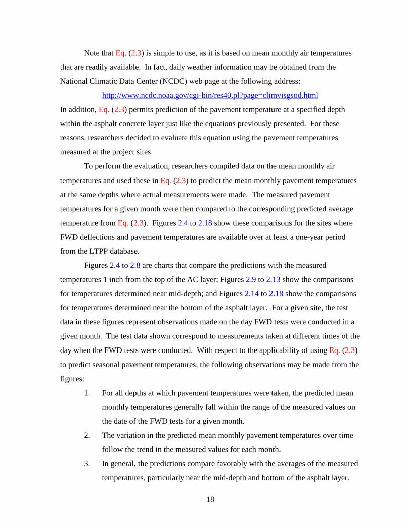
Note that Eq. (2.3) is simple to use, as it is based on mean monthly air temperatures
that are readily available. In fact, daily weather information may be obtained from the
National Climatic Data Center (NCDC) web page at the following address:
http://www.ncdc.noaa.gov/cgi-bin/res40.pl?page=climvisgsod.html
In addition, Eq. (2.3) permits prediction of the pavement temperature at a specified depth
within the asphalt concrete layer just like the equations previously presented. For these
reasons, researchers decided to evaluate this equation using the pavement temperatures
measured at the project sites.
To perform the evaluation, researchers compiled data on the mean monthly air
temperatures and used these in Eq. (2.3) to predict the mean monthly pavement temperatures
at the same depths where actual measurements were made. The measured pavement
temperatures for a given month were then compared to the corresponding predicted average
temperature from Eq. (2.3). Figures 2.4 to 2.18 show these comparisons for the sites where
FWD deflections and pavement temperatures are available over at least a one-year period
from the LTPP database.
Figures 2.4 to 2.8 are charts that compare the predictions with the measured
temperatures 1 inch from the top of the AC layer; Figures 2.9 to 2.13 show the comparisons
for temperatures determined near mid-depth; and Figures 2.14 to 2.18 show the comparisons
for temperatures determined near the bottom of the asphalt layer. For a given site, the test
data in these figures represent observations made on the day FWD tests were conducted in a
given month. The test data shown correspond to measurements taken at different times of the
day when the FWD tests were conducted. With respect to the applicability of using Eq. (2.3)
to predict seasonal pavement temperatures, the following observations may be made from the
figures:
1. For all depths at which pavement temperatures were taken, the predicted mean
monthly temperatures generally fall within the range of the measured values on
the date of the FWD tests for a given month.
2. The variation in the predicted mean monthly pavement temperatures over time
follow the trend in the measured values for each month.
3. In general, the predictions compare favorably with the averages of the measured
temperatures, particularly near the mid-depth and bottom of the asphalt layer.

19
Figure 2.5. Comparison of Predicted Mean Monthly Pavement Temperatures withMeasured Values for SMP Site 481077 (1 inch Depth).
Figure 2.4. Comparison of Predicted Mean Monthly Pavement Temperatures withMeasured Values for SMP Site 481122 (1 inch Depth).

20
Figure 2.7. Comparison of Predicted Mean Monthly Pavement Temperatures withMeasured Values for SMP Site 481060 (1 inch Depth).
Figure 2.6. Comparison of Predicted Mean Monthly Pavement Temperatures withMeasured Values for SMP Site 481068 (1 inch Depth).

21
Figure 2.9. Comparison of Predicted Mean Monthly Pavement Temperatures withMeasured Values for SMP Site 481122 (near Mid-Depth).
Figure 2.8. Comparison of Predicted Mean Monthly Pavement Temperatures withMeasured Values for SMP Site 404165 (1 inch Depth).

22
Figure 2.11. Comparison of Predicted Mean Monthly Pavement Temperatures withMeasured Values for SMP Site 481068 (near Mid-Depth).
Figure 2.10. Comparison of Predicted Mean Monthly Pavement Temperatures withMeasured Values for SMP Site 481077 (near Mid-Depth).

23
Figure 2.13. Comparison of Predicted Mean Monthly Pavement Temperatures withMeasured Values for SMP Site 404165 (near Mid-Depth).
Figure 2.12. Comparison of Predicted Mean Monthly Pavement Temperatures withMeasured Values for SMP Site 481060 (near Mid-Depth).

24
Figure 2.15. Comparison of Predicted Mean Monthly Pavement Temperatures withMeasured Values for SMP Site 481077 (near Bottom of AC Layer).
Figure 2.14. Comparison of Predicted Mean Monthly Pavement Temperatures withMeasured Values for SMP Site 481122 (near Bottom of AC Layer).

25
Figure 2.17. Comparison of Predicted Mean Monthly Pavement Temperatures withMeasured Values for SMP Site 481060 (near Bottom of AC Layer).
Figure 2.16. Comparison of Predicted Mean Monthly Pavement Temperatures withMeasured Values for SMP Site 481068 (near Bottom of AC Layer).

26
Figure 2.18. Comparison of Predicted Mean Monthly Pavement Temperatures withMeasured Values for SMP Site 404165 (near Bottom of AC Layer).
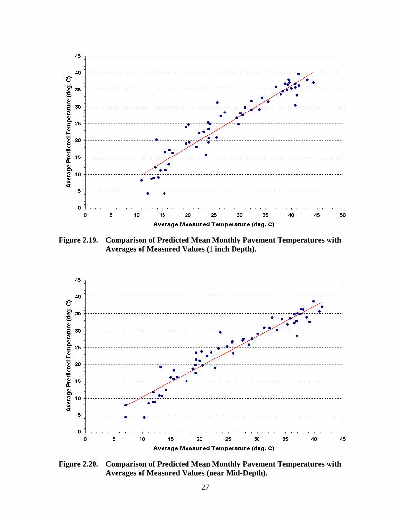
The correlation between the predictions from Eq. (2.3) and the averages of the
measured pavement temperatures is clearly evident from Figures 2.19 to 2.21,
which compare the predicted and measured values at each depth considered.
The R2 and RMSE of the fitted line in each figure are given in Table 2.7 to
establish the correlation between the averages of the measured pavement
temperatures and the predicted mean monthly values. The statistics in this table
reflect the good correlation in the data points, particularly near the middle and
bottom of the layer, where the R2 and RMSE are slightly better. This
observation probably reflects the influence of the surrounding environment, as
the effects of temperature variations due to wind, cloud cover, shading, and
other factors are expected to be greater near the surface and to diminish with
depth.
In view of the above findings, researchers are of the opinion that Eq. (2.3) produces
reasonable results and may be used to predict monthly variations in pavement temperatures to
27
Figure 2.20. Comparison of Predicted Mean Monthly Pavement Temperatures withAverages of Measured Values (near Mid-Depth).
Figure 2.19. Comparison of Predicted Mean Monthly Pavement Temperatures withAverages of Measured Values (1 inch Depth).

28
Figure 2.21. Comparison of Predicted Mean Monthly Pavement Temperatures withAverages of Measured Values (near Bottom of AC Layer).
Table 2.7. Goodness-of-Fit Statistics Indicating Correlation between Predicted MeanMonthly Pavement Temperatures and Averages of Measured Values.
Depth of Evaluation R2 RMSE (�C)
1 inch from surface 0.887 3.338
Near mid-depth of AC layer 0.921 2.641
Near bottom of AC layer 0.930 2.430

29
support evaluations of seasonal effects. For example, the monthly variations in pavement
temperatures at a given project may be estimated and used in a temperature correction
procedure to predict the expected monthly variations in asphalt concrete moduli at the project
site for pavement design, superheavy load analysis, load zoning, and other applications.
Researchers do not expect the implementation of the equation to be difficult in practice. The
equation only requires the engineer to input the mean monthly air temperatures at the vicinity
of the site, which are readily available from weather reporting services.
Researchers note that the modulus temperature correction program developed in this
project (Fernando and Liu, 2001) includes a database of mean monthly air temperatures for
all counties in the state. This database was provided by the project director and may be used
by the engineer in the absence of site-specific weather information. The next chapter
presents the evaluation of temperature correction methods.

31
CHAPTER III
EVALUATION OF TEMPERATURE CORRECTION METHODS
METHODOLOGY
To evaluate temperature correction methods, researchers used the FWD data collected
on the SMP and Riverside Campus test sites. While methods for correcting pavement
deflections have been proposed, the approach followed was to evaluate existing methods for
temperature correction of backcalculated moduli from the FWD deflections. In the opinion
of researchers, the seasonal adjustment of pavement deflections is probably best suited for
network-level applications, such as comparative evaluations of pavement response and
performance between different regions of the state. For project-level investigations,
temperature adjustment of backcalculated moduli is recommended. Note that the shape of
the deflection basin is affected by all pavement layers. Thus, adjustment for seasonal effects
should be made after the backcalculation of layer moduli (Shaat et al., 1992).
It is noted that the MODULUS program (Michalak and Scullion, 1995) incorporates
the U.S. Army Corps of Engineers’ procedure (Bush, 1987) to correct pavement deflections
to a reference temperature of 70 �F. This procedure may be used in applications where
temperature adjustment of pavement deflections is warranted. To provide an alternative
procedure for temperature correction of backcalculated moduli, researchers developed the
Modulus Temperature Correction Program (MTCP) that is documented in a companion
report by Fernando and Liu (2001). Researchers developed this program based on the
findings presented in this report.
To evaluate temperature correction methods, researchers used the MODULUS
program to backcalculate layer moduli from the measured FWD deflections collected on the
project sites at different times and pavement temperatures. Selected temperature correction
methods were then used to correct the backcalculated moduli to a standard temperature.
Theoretically, the correction to a standard temperature should yield the same corrected
modulus for different backcalculated moduli corresponding to different test temperatures.
Unfortunately, this is difficult to achieve in practice because of inaccuracies in modeling the

32
Figure 3.1. Illustration of Approach Followed to Evaluate Temperature CorrectionMethods.
response of pavements to load and environmental factors, variations in pavement layer
thickness along a given section, errors in temperature measurements, and random or
unexplained measurement errors. Nevertheless, the effectiveness of a temperature correction
procedure may be evaluated based on the reduction in the variation of the backcalculated
modulus with pavement temperature.
Figure 3.1 illustrates the approach taken by researchers to evaluate temperature
correction methods. Prior to correction, the temperature dependency of the backcalculated
asphalt concrete modulus is clearly evident from the figure. After correction, the normalized
modulus is observed to vary about a given level that corresponds to the modulus at the
assumed reference temperature. There is a clear reduction in the variation of the
backcalculated AC modulus with temperature after correction. Note that the corrected
moduli are plotted versus the pavement test temperatures corresponding to the backcalculated
moduli in Figure 3.1. By examining the variation of the corrected moduli with test

33
temperature and the difference between the reference modulus and the average of the
corrected moduli, researchers evaluated the effectiveness of selected temperature correction
methods. This chapter presents results from this evaluation.
BACKCALCULATED LAYER MODULI
FWD surveys were typically conducted at the SMP sites on a monthly basis. At each
site, FWD deflections were collected at different stations and at different times of the day on
which a survey was made. Consequently, deflections at a range of pavement temperatures are
available to establish the temperature dependency of the asphalt concrete mixture found at a
given site. Pavement temperatures were generally taken at three different depths
corresponding to 1 inch below the surface, near mid-depth, and near the bottom of the AC
layer. The temperatures were measured at a particular location on each site, at different times
of the day on which a deflection survey was made.
At the Riverside Campus test sites, researchers collected FWD deflections in March,
May, and July 2000. Four deflection surveys were conducted on each of these months, two
per site. For each survey, researchers collected FWD deflections at five stations along the
given site. These measurements were conducted over a 12-hour period (from 5 am to 5 pm
on the day of the survey).
Table 3.1 shows the layer thicknesses at the various test sites. Also shown are the
depths at which pavement temperatures were measured. Researchers used the layering
information given in Table 3.1 to backcalculate the layer moduli from the FWD deflections
using MODULUS. To minimize the effect of possible load-induced damage on the
backcalculated material properties, only FWD data collected at the middle of the test lane
were analyzed. Further, researchers conducted the backcalculations using the deflections
taken at a selected station on each site. This was done to minimize errors that may arise due
to unknown variations in the pavement structure along the site. It is noted that no evaluations
were made on SMP site 483739, as the surface layer on this site is thin. For this condition,
the deflection basin is not sensitive to the backcalculated AC modulus.
Figures 3.2 to 3.9 show the variation of the backcalculated AC moduli with test
temperature. The AC mixtures are observed to exhibit temperature-dependent behavior
except for SMP site 351112. As shown in Figure 3.2, the backcalculated AC moduli from

34
Table 3.1. Pavement Layering at Test Sites and Depths of Temperature Measurements.
Site LocationLayer Thickness (inches)
Depth of TemperatureMeasurement (inches)
Surface Base Subbase 1 2 3
351112US62, Lea County,New Mexico
6.3 6.0 1.0 3.0 5.0
404165US60, MajorCounty, Oklahoma
2.7 5.41 1.0 4.5 7.5
481060US77, RefugioCounty, Texas
7.5 12.3 6.02 1.0 4.0 7.0
481068SH19, LamarCounty, Texas
10.9 6.0 8.02 1.0 5.0 9.0
481077US287, HallCounty, Texas
5.1 10.4 1.0 2.5 4.5
481112US181, WilsonCounty, Texas
3.4 15.6 8.4 1.0 2.0 3.0
483739US77, KenedyCounty, Texas
1.8 11.4 7.42 1.0 1.5
Pad 123 Riverside Campus 5.0 12.0 12.0 0.3 2.5 4.0
Pad 213 Riverside Campus 3.0 12.0 8.0 0.3 1.5 2.71 Asphalt-stabilized base2 Lime-treated soil3 Non-trafficked test sections

35
Figure 3.2. Variation of Backcalculated AC Modulus with Test Temperature (351112).
Figure 3.3. Variation of Backcalculated AC Modulus with Test Temperature (404165).

36
Figure 3.4. Variation of Backcalculated AC Modulus with Test Temperature (481060).
Figure 3.5. Variation of Backcalculated AC Modulus with Test Temperature (481068).

37
Figure 3.6. Variation of Backcalculated AC Modulus with Test Temperature (481077).
Figure 3.7. Variation of Backcalculated AC Modulus with Test Temperature (481122).

38
Figure 3.8. Variation of Backcalculated AC Modulus with Test Temperature (Pad 12).
Figure 3.9. Variation of Backcalculated AC Modulus with Test Temperature (Pad 21).

39
this site do not appear to be influenced by the pavement temperature. Researchers conducted
additional backcalculations to verify if this behavior is also observed from the FWD data
collected at other stations on the site. It was also observed that the backcalculated AC
moduli from the other stations do not vary with pavement temperature, similar to the trend
shown in Figure 3.2. In an attempt to find reasons that might explain, or data that might
substantiate, this apparent insensitivity to temperature variations, researchers searched the
available LTPP database (DataPave 2.0). However, researchers did not find any information
to establish whether the AC mixture at the site was modified to reduce temperature
susceptibility. Also, while modulus data were supposed to be determined from laboratory
tests done on cores taken from the SMP sites, researchers did not find this information in the
database. No visual distress was also reported during the period in which FWD data
analyzed in this project were collected. In view of these results, site 351112 was not included
in the evaluation of temperature correction methods presented herein.
TEMPERATURE CORRECTION METHODS SELECTED FOR EVALUATION
From the literature review, temperature correction methods based on the following
equations were selected for evaluation in this project:
1. Chen equation developed using FWD and pavement temperature data collected
from TxDOT’s Mobile Load Simulator (MLS) investigations (Chen et al., 2000);
2. the Asphalt Institute (1982) dynamic modulus equation; and
3. the dynamic modulus equation developed by Witczak and Fonseca (1996) that is
a proposed method for predicting dynamic modulus in the AASHTO 2002
pavement design guide.
The above selections were made in consultation with the project monitoring committee.
Equations (3.1) to (3.3) show, respectively, Chen’s method for modulus temperature
correction, the Asphalt Institute dynamic modulus equation, and the more recent equation
developed by Witczak and Fonseca (1996) to predict the dynamic modulus of AC mixtures.
Chen equation (Chen et al., 2000):
(3.1)EE
T TTrT
r
=+ × + −( . ) ( . ). .1 8 3 2 1 8 3 22 446 2 2 446 2

40
where,
ETr = modulus corrected to a reference temperature of Tr (�C); and
ET = modulus determined from testing at a temperature of T (�C).
Asphalt Institute (1982):
(3.2)[ ]lo g | * | . . . .
.
. .
.
( . . log ) .
( . . log ).
. .
1020 0
0 17 033 70
1 3 0 49 825 0 5
1 3 0 49 8250 5
1 1 0 02 774
5 5 5 3 8 3 3 0 0 2 8 8 2 9 0 0 3 4 7 6 0 0 7 0 3 7 7
0 0 0 0 0 0 5
0 0 0 1 8 9 0 9 3 1 7 5 71
1 0
1 0
E p
f V
t p
t p
f f
a F
pf
ac
pf ac
= + − +
+
−
+
°
+
+
η
where,
|E*| = absolute value of complex modulus, psi;
p200 = percent passing No. 200 sieve, by total aggregate weight;
f = loading frequency, Hz;
Va = percent air voids, by volume;
�70 �F = bitumen viscosity at 70 �F, 106 poises;
pac = percent asphalt content, by weight of mix; and
tp = temperature, �F.
Witczak and Fonseca (1996):
(3.3)
[ ]
lo g . . . ( ) .
. .( )
. . . . ( ) ./ / /
( . log . log )
10 20 0 20 02
4
4 3 8 3 82
3 4
0 71 6 0 74 25
2 6 1 0 0 0 8 2 25 0 0 0 0 0 01 0 1 0 0 0 1 9 6
0 0 3 1 5 7 0 4 1 5
1 8 7 0 0 0 2 8 08 0 0 0 0 0 40 4 0 0 0 0 1 78 6 0 0 1 6 4
1 1 0 1 0
E p p p
VV
V V
p p p p
e
a
beff
be ff a
f
= − + − +
− −+
++ + − +
+ − − η

41
where,
E = asphalt mix dynamic modulus, 105 psi;
� = bitumen viscosity at given temperature and degree of aging, 106 poises;
f = loading frequency, Hz;
Va = percent air voids, by volume;
Vbeff = percent effective binder content, by volume;
p3/4 = percent retained on 3/4-inch sieve, by total aggregate weight;
p3/8 = percent retained on 3/8-inch sieve, by total aggregate weight;
p4 = percent retained on No. 4 sieve, by total aggregate weight; and
p200 = percent passing No. 200 sieve, by total aggregate weight.
Using Eq. (3.2), Lytton et al. (1990) derived the following relationship for
temperature and frequency correction of asphalt concrete modulus:
(3.4)
[ ]
lo g lo g .
.
.
.
. .
( . . log ) ( . . log )
( . . log )
.
( . . log )
.
. .
10 10 20 0 0 17 033 0 17 033
1 3 0 49 825 1 3 0 49 825
1 3 0 49 825
1 1
1 3 0 49 825
1 1
0 02 774 0 02 774
0 0 2 8 82 91 1
0 0 0 0 00 5
0 0 0 1 89
0 9 3 1 75 71 1
1 0 1 0
1 0 1 0
E E pf f
p t t
pt
f
t
f
f f
rr
ac rf f
acr
f
r
f
r
r
r
= + −
+ −
− −
+ −
+ +
+ +
where,
Er = modulus corrected to reference conditions of temperature and frequency of
loading;
E = the measured or backcalculated modulus;
p200 = percent passing No. 200 sieve, by total aggregate weight;
pac = percent asphalt content, by weight of mix;
fr = reference frequency of loading, Hz;

42
f = test frequency (Hz) corresponding to the measured or backcalculated
modulus;
tr = reference temperature, �F; and
t = test temperature ( �F) corresponding to the measured or backcalculated
modulus.
In addition, researchers derived the following relationship for temperature and
frequency correction based on the equation developed by Witczak and Fonseca (1996):
(3.5)lo g lo g ( . log ) ( . log )10 10 0 74 25 0 74 25
1
1
1
11 0 1 0E E
e eR T B BR R T T= +
+−
+
− + − +α η η
where,
� = (3.6)1 8 7 0 0 0 3 0 0 0 0 04 0 0 0 0 18 0 0 1 6 44 3 8 3 82
3 4. . . . ( ) ./ / /+ + − +p p p p
BR = (3.7)0 716 1 0. lo g f R
BT = (3.8)0 716 1 0. lo g f T
ER = AC modulus corrected for the selected reference temperature and loading
frequency;
ET = measured or backcalculated asphalt concrete modulus;
�R = binder viscosity corresponding to the reference temperature, 106 poises;
�T = binder viscosity corresponding to the test temperature, 106 poises;
p4 = cumulative percent retained on No. 4 sieve by total aggregate weight;
p3/8 = cumulative percent retained on 3/8-inch sieve by total aggregate weight;
p3/4 = cumulative percent retained on 3/4-inch sieve by total aggregate weight;
fR = reference loading frequency, Hz; and
fT = test frequency, Hz.
Note that Eqs. (3.1), and (3.4) to (3.8) permit the correction to be made for any user-
specified reference temperature. In addition, Eqs. (3.4) to (3.8) permit the correction to a
reference frequency of loading. In the opinion of researchers, all equations are simple enough
to implement in practice, a factor that was considered in selecting the modulus temperature
correction methods to evaluate in this project. Note that the Chen equation does not require

43
AC mixture properties for the correction. This equation was developed for the typical
mixtures used in the state. To support applications that involve other mixtures, Eqs. (3.4) to
(3.8) were included in the evaluation. Note that basic mixture properties (i.e., percent asphalt
and aggregate gradation) are variables that are included in these equations. In addition, the
binder viscosities corresponding to the base and reference temperatures are used in Eq. (3.5)
to adjust the measured or backcalculated modulus to the specified reference temperature. For
this purpose, the viscosity-temperature relationship for the binder used in the AC mix is
characterized using the following equation from the American Society for Testing and
Material (ASTM) specification D-2493:
(3.9)log log log1 0 1 0 1 0η = + °A V T S T R
where,
� = the binder viscosity, centipoise;
T�R = the temperature, degrees Rankine; and
A, VTS = model coefficients determined from testing.
In practice, A and VTS may be determined by conducting dynamic shear rheometer
(DSR) tests at a range of temperatures on the binder extracted from a core taken at the project
site. This extraction will also provide the gradation data needed to use Eq. (3.5) for
temperature correction.
DSR tests may be conducted at an angular frequency of 10 rad/sec and for a
temperature range of 40 to 130 �F (4 to 54 �C). From the binder complex shear modulus G*
and phase angle � determined at a given temperature, the corresponding binder viscosity may
be estimated from the equation:
(3.10)ηδ
=
G *
sin
.
1 0
14 8 6 2 8
The binder viscosities determined at the different test temperatures may be used in a
regression analysis to get the A and VTS coefficients of Eq. (3.9). Table 3.2 shows typical
values of these coefficients for AC-graded binders while Table 3.3 shows the coefficients for
performance-graded (PG) asphalts. The coefficients in Table 3.2 are from research
conducted by Mirza (1993), and are representative of asphalts that have undergone field
aging. Those in Table 3.3 are from unpublished data taken from the AASHTO 2002

44
Table 3.2. Typical A and VTS Coefficients for AC-Graded Asphalts1.
Viscosity Grade(Original
Conditions)
Viscosity Range at140 �F (poises)
A VTS
AC - 2.5 100 - 350 11.8408 -3.9974
AC - 5 350 - 700 11.4711 -3.8557
AC - 10 700 - 1400 11.0770 -3.7097
AC - 20 1400 - 2800 10.9168 -3.6469
AC - 40 2800 - 5200 10.6528 -3.5477
1 Representative of asphalts that have undergone field aging.
development work. The predicted binder viscosities from these coefficients are
representative of mix/laydown conditions.

45
Table 3.3. Typical A and VTS Coefficients for PG-Graded Asphalts1.
HighTemp.Grade
Low Temperature Grade
-10 -16 -22 -28 -34 -40 -46
A VTS A VTS A VTS A VTS A VTS A VTS A VTS
46 11.504 -3.901 10.101 -3.393 8.755 -2.905
52 13.386 -4.570 13.305 -4.541 12.755 -4.342 11.840 -4.012 10.707 -3.602 9.496 -3.164 8.310 -2.736
58 12.316 -4.172 12.248 -4.147 11.787 -3.981 11.010 -3.701 10.035 -3.350 8.976 -2.968
64 11.432 -3.842 11.375 -3.822 10.980 -3.680 10.312 -3.440 9.461 -3.134 8.524 -2.798
70 10.690 -3.566 10.641 -3.548 10.299 -3.426 9.715 -3.217 8.965 -2.948 8.129 -2.648
76 10.059 -3.331 10.015 -3.315 9.715 -3.208 9.200 -3.024 8.532 -2.785
82 9.514 -3.128 9.475 -3.114 9.209 -3.019 8.750 -2.856 8.151 -2.642
1 Coefficients representative of mix/laydown conditions (unpublished data from AASHTO 2002 development work).
46
EVALUATION OF BINDER-VISCOSITY RELATIONSHIPS
Application of Eq. (3.5) requires the binder viscosity-temperature relationships for the
test sites established in this project. However, laboratory data from measurements of binder
viscosity at a range of test temperatures were not available from the LTPP database at the
time of this study. Since the approach taken in this project is to use existing data to evaluate
temperature correction methods, researchers evaluated the binder viscosity-temperature
relationships based on the backcalculated AC moduli taken at different temperatures and the
information on volumetric mixture properties available from the LTPP database. In this way,
researchers determined the A and VTS coefficients that characterize the binder viscosity-
temperature relationship for each site included in this investigation.
To explain the procedure followed for estimating the A and VTS coefficients, note that
Eq. (3.3) can be expressed in the following form (Witczak and Fonseca, 1996):
(3.11)ye x= +
+ −δα
β γ1 ( )
where,
y = log10 E;
�, � = coefficients that are functions of the volumetric mixture properties;
� = a coefficient that is a function of the loading frequency;
� = 0.7425; and
x = log10 �.
The independent variable x in Eq. (3.11) may be expressed as a function of the test
temperature using Eq. (3.9). Thus, by nonlinear regression, researchers estimated the A and
VTS coefficients corresponding to the mix tested at each site.
Table 3.4 shows the A and VTS coefficients that were backcalculated from the AC
moduli determined from FWD data taken at different temperatures. In this evaluation, the �
and � coefficients of Eq. (3.11) were established using the volumetric mixture properties
obtained from the LTPP database. The relationship for � is given in Eq. (3.6) while that for �
is given by:

47
Table 3.4. A and VTS Coefficients Determined from Backcalculated AC Moduli.
Site A VTS
404165 14.987 -5.122
481060 8.769 -2.869
481068 9.153 -3.032
481077 11.469 -3.882
481122 14.753 -5.058
Pad 12 8.355 -2.725
Pad 21 16.067 -5.481
(3.12)
δ = − + − +
− −+
0 2 6 1 0 0 0 8 2 2 5 0 0 0 0 0 0 1 0 1 0 0 0 1 9 6
0 0 3 1 5 7 0 4 1 5
20 0 20 02
4. . . ( ) .
. .( )
p p p
VV
V Va
beff
be ff a
Note that Eq. (3.12) is readily obtained from comparison of Eqs. (3.11) and (3.3).
To determine �, researchers used a test frequency corresponding to the impulse
loading of the FWD. The frequency f may be estimated from the duration (in seconds) of the
impulse load t using the following relationship proposed by Lytton et al. (1990):
(3.13)ft
=1
2
Since the duration of the impulse load for the FWD is about 30 msec, a test frequency of 16.7
Hz is determined from Eq. (3.13). Researchers used this value to calculate the coefficient �
from the relationship:
(3.14)β = − 0 716 1 0. lo g f
Thus, only the A and VTS coefficients were backcalculated using the AC moduli
determined from FWD data taken at different temperatures. The coefficients � and � were set
to the corresponding values determined from the properties of the mix placed at a given site,
while the coefficient � is a constant determined as explained above.

48
Figures 3.10 to 3.16 show the fitted curves drawn using the A and VTS coefficients
determined following the procedure described. In the researchers’ opinion, the curves fit the
backcalculated moduli quite adequately. To evaluate the goodness-of-fit, the average of the
absolute differences between the fitted curve and the data points was evaluated for each site.
Table 3.5 gives the statistics determined. To provide a point of reference for the average
absolute difference |D|, the standard deviation � of the backcalculated moduli are also given.
Both statistics are given on an arithmetic scale in Table 3.5, in units of ksi. It is noted that
the backcalculated moduli vary over a wide range as shown in the table. In general,
researchers consider the average absolute differences to be satisfactory when compared with
the magnitudes of the backcalculated moduli.
Researchers note that the approach taken illustrates a method of temperature
correction when FWD data taken at a range of temperatures are available. To implement this
in practice, FWD and pavement temperature measurements at a single location may be taken
over time or over a day. The model given by Eq. (3.11) may then be fitted to the
backcalculated AC moduli to determine modulus temperature correction factors using Eq.
(3.5) for a specified reference temperature and loading frequency.
One may note that, while the procedure presented provides a method for
nondestructively estimating the A and VTS coefficients of the binder viscosity-temperature
relationship of the mix found on a project, volumetric mixture properties are still needed to
determine temperature correction factors using Eq. (3.5). In the opinion of researchers, there
are two options that an engineer may consider:
1. He or she may collect FWD data following routine procedures and take cores to
determine layer thickness, run extractions and mechanical sieve analyses to get
volumetric mixture properties, and conduct dynamic shear rheometer tests on the
extracted binder to evaluate the viscosity-temperature relationship of the mix.
The engineer will then have the data to use with Eq. (3.5) for temperature
correction of the AC moduli backcalculated from the FWD deflections.
2. Alternatively, the engineer may collect FWD data over a range of pavement
temperatures and use the procedure presented to determine the coefficients �, �,
A, and VTS by fitting Eq. (3.11) to the backcalculated AC moduli at different

49
Figure 3.10. Fitted Curve to Backcalculated AC Moduli (SMP Site 404165).
Figure 3.11. Fitted Curve to Backcalculated AC Moduli (SMP Site 481060).

50
Figure 3.12. Fitted Curve to Backcalculated AC Moduli (SMP Site 481068).
Figure 3.13. Fitted Curve to Backcalculated AC Moduli (SMP Site 481077).

51
Figure 3.14. Fitted Curve to Backcalculated AC Moduli (SMP Site 481122).
Figure 3.15. Fitted Curve to Backcalculated AC Moduli (Pad 12).

52
Figure 3.16. Fitted Curve to Backcalculated AC Moduli (Pad 21).
Table 3.5. Goodness-of-Fit Statistics of Nonlinear Model Given by Eq. (3.11).
Site
AverageAbsolute
Difference,|D| (ksi)
Backcalculated Modulus (ksi)| |D
σStandardDeviation, �
Minimum Maximum
404165 240 848 500 3166 0.28
481060 63 479 352 2027 0.13
481068 33 374 129 1463 0.09
481077 232 824 75 3000 0.28
481122 175 515 100 1809 0.34
Pad 12 56 175 158 820 0.32
Pad 21 287 526 214 2300 0.55
53
temperatures. Note that � and � are constants for a given mix and may be
determined from the data using nonlinear regression. In this project, researchers
did not have to backcalculate these coefficients, as volumetric mixture properties
were found from the LTPP database. However, these coefficients may also be
backcalculated from the FWD data. The engineer will then have the �, A, and
VTS coefficients to determine temperature correction factors using Eq. (3.5).
The choice of which option to take depends on what is feasible to do for the given
project and its importance. If the project is on a major highway that receives a lot of truck
traffic, it would be prudent, in the researchers’ opinion, to run tests to characterize the
properties that are needed to evaluate a given mix. The costs for these tests are generally
small compared to the costs of designing and constructing the project.
Alternatively, one may consider using a procedure that does not require any properties
of the mix but simply the test temperatures at which FWD deflections were taken. In this
instance, the applicability of such methods for the specific mix used on a given project should
be considered. The engineer should review available information to establish testing
requirements and then run tests accordingly to get the information that he or she needs for
planning, design, and construction of the given project.
RESULTS FROM EVALUATION OF TEMPERATURE CORRECTION METHODS
Researchers used each of the three temperature correction methods presented
previously to correct the backcalculated moduli from the test sites to reference temperatures
of 7, 24, and 41 �C (45, 75, and 105 �F). The results from this evaluation are presented in
Figures 3.17 to 3.37, which compare the AC moduli before and after correction for the
middle reference temperature tr = 24 �C. Appendix B gives the results from the temperature
corrections made at the low (7 �C) and high (41 �C) reference temperatures. In these figures,
the AC moduli before and after correction are plotted against the measured test temperatures
at the time of the FWD surveys. Since Chen’s equation is based on the mid-depth pavement
temperature, corrections of backcalculated AC moduli were made using the measured test
temperatures at the middle of the asphalt layer for all three methods investigated.

54
Figure 3.17. Corrected AC Moduli Using Eq. (3.5) and tr = 24 �C (SMP Site 404165).
Figure 3.18. Corrected AC Moduli Using Eq. (3.5) and tr = 24 �C (SMP Site 481060).

55
Figure 3.19. Corrected AC Moduli Using Eq. (3.5) and tr = 24 �C (SMP Site 481068).
Figure 3.20. Corrected AC Moduli Using Eq. (3.5) and tr = 24 �C (SMP Site 481077).

56
Figure 3.21. Corrected AC Moduli Using Eq. (3.5) and tr = 24 �C (SMP Site 481122).
Figure 3.22. Corrected AC Moduli Using Eq. (3.5) and tr = 24 �C (Pad 12).
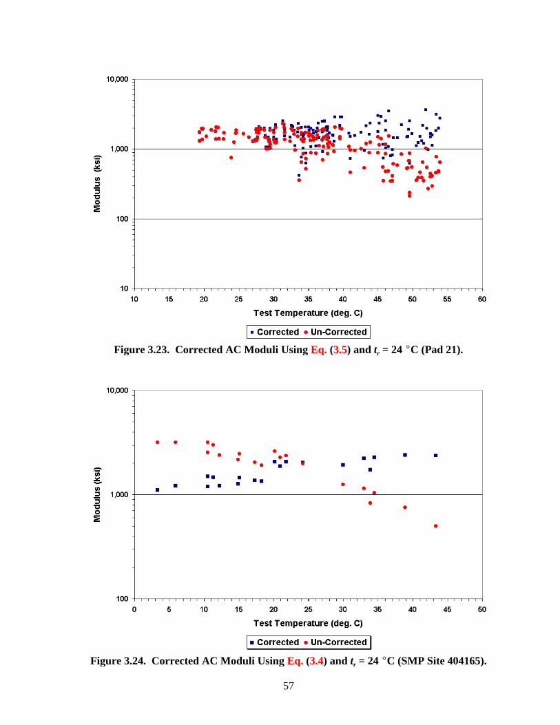
57
Figure 3.23. Corrected AC Moduli Using Eq. (3.5) and tr = 24 �C (Pad 21).
Figure 3.24. Corrected AC Moduli Using Eq. (3.4) and tr = 24 �C (SMP Site 404165).

58
Figure 3.25. Corrected AC Moduli Using Eq. (3.4) and tr = 24 �C (SMP Site 481060).
Figure 3.26. Corrected AC Moduli Using Eq. (3.4) and tr = 24 �C (SMP Site 481068).

59
Figure 3.27. Corrected AC Moduli Using Eq. (3.4) and tr = 24 �C (SMP Site 481077).
Figure 3.28. Corrected AC Moduli Using Eq. (3.4) and tr = 24 �C (SMP Site 481122).

60
Figure 3.29. Corrected AC Moduli Using Eq. (3.4) and tr = 24 �C (Pad 12).
Figure 3.30. Corrected AC Moduli Using Eq. (3.4) and tr = 24 �C (Pad 21).

61
Figure 3.31. Corrected AC Moduli Using Eq. (3.1) and tr = 24 �C (SMP Site 404165).
Figure 3.32. Corrected AC Moduli Using Eq. (3.1) and tr = 24 �C (SMP Site 481060).

62
Figure 3.33. Corrected AC Moduli Using Eq. (3.1) and tr = 24 �C (SMP Site 481068).
Figure 3.34. Corrected AC Moduli Using Eq. (3.1) and tr = 24 �C (SMP Site 481077).

63
Figure 3.35. Corrected AC Moduli Using Eq. (3.1) and tr = 24 �C (SMP Site 481122).
Figure 3.36. Corrected AC Moduli Using Eq. (3.1) and tr = 24 �C (Pad 12).

64
Figure 3.37. Corrected AC Moduli Using Eq. (3.1) and tr = 24 �C (Pad 21).
Figures 3.17 to 3.23 show the moduli corrected to the middle reference temperature of
24 �C using Eq. (3.5); Figures 3.24 to 3.30 present the results from Eq. (3.4); and Figures
3.31 to 3.37 show the corrected moduli from Chen’s equation. Researchers note the
following observations from the results shown in Figures 3.17 to 3.37 and the figures
presented in Appendix B:
1. The corrected AC moduli from Eq. (3.5) are quite satisfactory. For a given site
and reference temperature, the corrected AC moduli vary about a constant level,
indicating that the equation has performed acceptably in normalizing the
backcalculated AC moduli to the given reference temperature.
2. The results based on Eq. (3.4) show a noticeable linear variation between the
logarithm of the corrected moduli and the test temperature for several sites.
There appears to be an overcorrection at the high test temperatures, resulting in
unreasonably high values of the corrected modulus at these temperatures,
particularly when corrections are made to the low reference temperature of 7 �C
(as may be observed from Figures B8, B9, and B12 to B14 in Appendix B).

65
3. Chen’s equation gives better results compared to Eq. (3.4). The corrected moduli
from this method generally showed less variation with test temperature compared
to the results from Eq. (3.4). However, the corrected moduli appear to show a
slight curvature for some sites, and for others, there is a slight linear variation of
the logarithm of the corrected moduli with test temperature. In addition, while
there is less variation in the corrected moduli with test temperature, there appears
to be an overcorrection at the low reference temperature, similar to the results
obtained from Eq. (3.4). This may be observed in Figures B15, B16, B19, and
B21.
Theoretically, the correction method should give the same modulus for a given
reference temperature. Thus, to measure the effectiveness with which the temperature
correction is accomplished, researchers determined the slope of the trend line for a given
reference temperature and correction method. Table 3.6 shows the slopes of the regression
lines between the logarithms of the corrected moduli and test temperatures. The closer the
slope is to zero, the smaller the variation of the corrected moduli with test temperature and
the better the temperature correction. Researchers conducted t-tests to establish the statistical
significance of the slopes of the regression lines. Where the slopes are significant at the 1
percent level, the cells have been shaded in Table 3.6.
The results shown in Table 3.6 clearly indicate that the corrected moduli from
Eq. (3.5) show no significant relationship with test temperature for all sites and reference
temperatures considered. This finding is to be expected since researchers calibrated the
equation to the modulus-temperature relationship of the AC mix found at each site using the
FWD data. The calibration was accomplished by estimating the coefficients of the binder-
viscosity relationship from the backcalculated moduli determined at different pavement test
temperatures.
Table 3.6 shows that the moduli from the other two methods exhibited a linear
variation with test temperature even after correction. From statistical tests, the slopes of the
regression lines based on corrections using Chen’s equation were found to be significantly
different from zero in four of the seven sites considered in this evaluation. Looking at the
slopes based on Eq. (3.4), researchers found that the corrected moduli exhibited a significant
variation with test temperature in five of the seven sites.

66
Table 3.6. Slopes of Regression Lines Fitted to the Corrected Moduli.
Test Site Reference
Temperature ( �C)
Temperature Correction Method1
Eq. (3.1) Eq. (3.4) Eq. (3.5)
404165
7 0.007862 0.008713 -0.001732
24 0.007862 0.008713 -0.001736
41 0.007862 0.008713 -0.001736
481060
7 0.002785 0.010713 0.000327
24 0.002785 0.010713 0.000162
41 0.002785 0.010713 0.000163
481068
7 0.000975 0.004996 -0.000025
24 0.000975 0.004996 -0.000048
41 0.000975 0.004996 -0.000049
481077
7 -0.004489 0.001393 -0.000264
24 -0.004489 0.001393 -0.000260
41 -0.004489 0.001393 -0.000260
481122
7 -0.013111 0.002422 0.000177
24 -0.013111 0.002422 0.000175
41 -0.013111 0.002422 0.000175
Pad 12
7 0.000412 0.020712 0.000194
24 0.000412 0.020712 0.000220
41 0.000412 0.020712 0.000219
Pad 21
7 0.001198 0.025765 0.000300
24 0.001198 0.025765 0.000452
41 0.001198 0.025765 0.0004521 Shaded cells indicate slopes that are statistically significant at the1 percent level.

67
Researchers also evaluated the accuracy of the corrections from the three different
methods. For this purpose, the modulus at a given reference temperature was determined
from the modulus-temperature relationship of the mix found at a site. These relationships are
given by the fitted curves to the backcalculated AC moduli shown in Figures 3.10 to 3.16.
The accuracy of the corrections was assessed by comparing the average of the corrected
moduli with the corresponding reference modulus for a given mix and reference temperature.
Note that the average of the absolute differences between the corrected and reference moduli
may also be used to assess the accuracy of a given temperature correction method. However,
this statistic will also include the errors from the backcalculations that may arise due to
inaccuracies in modeling the response of pavements to load and environmental factors, errors
in measurement of deflections and pavement temperatures, and other unexplained or random
factors that introduce variability in the backcalculated AC modulus. Thus, researchers
compared the average of the corrected moduli with the corresponding reference modulus to
assess the accuracy of the corrections from a given method. Table 3.7 shows the absolute
differences between the reference and corrected AC moduli for the different sites and
reference temperatures considered. Since Eq. (3.5) has been calibrated to the modulus-
temperature relationship of the mix at a given site, the results from this method may be used
as benchmarks in evaluating the accuracy of the corrections from Eq. (3.4) and Chen’s
equation.
Based on the results given in Table 3.7, the corrections from Chen’s equation are
observed to correspond better to the corresponding reference moduli compared with the
corrections determined using Eq. (3.4). It is observed that the average of the absolute
differences between the reference and corrected AC moduli from Chen’s equation is 685 ksi,
compared to 1064 ksi for the other method. It is also observed that the large errors generally
occur when the backcalculated AC moduli are corrected to the low reference temperature,
particularly for Pad 21.
Researchers note that the AC layer is 3 inches thick on Pad 21. Under existing
TxDOT practice, no temperature corrections are made when the AC layer is less than 3
inches thick. Thus, this site is a borderline case that, perhaps, should not have been included
in the evaluation of temperature correction methods. However, Figure 3.16 does show a

68
Table 3.7. Absolute Differences between Reference and Mean Corrected AC Moduli.
Test Site Reference
Temperature ( �C)
Temperature Correction Method1
Eq. (3.1) Eq. (3.4) Eq. (3.5)
404165
7 2481 1616 108
24 471 216 81
41 39 133 25
481060
7 1891 1410 0
24 73 212 1
41 12 126 2
481068
7 320 191 0
24 53 74 0
41 8 41 1
481077
7 10 11 70
24 58 127 22
41 58 15 6
481122
7 1057 958 131
24 213 52 58
41 128 28 13
Pad 12
7 989 1905 12
24 10 437 7
41 1 43 3
Pad 21
7 5850 11,695 96
24 555 2965 99
41 100 80 59
Average at 7 �C 1800 2541 60
Average at 24 �C 205 583 38
Average at 41 �C 49 67 16
Overall Average 685 1064 381 Means of absolute differences are in ksi.

69
noticeable trend in the backcalculated AC moduli with test temperature. Thus, researchers
included this site in the evaluation.
COMPARISON OF PAVEMENT TEMPERATURES AT DIFFERENT DEPTHS
Temperature corrections of backcalculated AC moduli require the pavement
temperature at the time of the FWD survey. These temperatures are usually taken at specified
depths. In a number of methods, the AC layer thickness must be known to get the pavement
test temperature. Chen’s equation, for example, is based on the mid-depth pavement
temperature, while other methods use the average of temperatures taken at different depths.
To implement any of these procedures, the determination of layer thicknesses prior to the
FWD survey is recommended. This determination will permit technicians to measure
pavement temperatures at the prescribed depths during the deflection survey as well as
provide the thicknesses engineers need to backcalculate layer moduli from the FWD
deflections.
Still, data collection procedures are currently implemented wherein temperatures are
measured at specific depths from the surface. In Texas, for example, the current practice is to
measure pavement temperatures at a depth of 1 inch below the surface. Similarly, European
practice calls for measuring temperatures at a depth of 1.6 inches (4 cm). These procedures
are easy to implement, particularly in situations where the AC layer thickness is not known
prior to the FWD survey. However, to perform the temperature correction, one must input
the pavement test temperature prescribed by a given method. For example, if Chen’s
equation is to be used to perform the temperature correction, one must input the mid-depth
pavement temperature. If operators take temperatures at other depths during the survey,
errors in the corrected AC moduli will arise. The magnitudes of these errors will depend on
the differences between the measured temperatures and the corresponding values that would
have been obtained if measurements were made at mid-depth. Since data at different depths
are available for the test sites included in this investigation, researchers compared the
measurements at different depths to see how different the temperatures are. The comparisons
are presented in Figures 3.38 and 3.39.
Figure 3.38 compares the mid-depth temperatures with the corresponding values
taken 1 inch below the surface. It is observed that the temperatures taken at these depths are
highly correlated. However, the mid-depth temperatures are noticeably lower than the

70
Figure 3.38. Comparison of Mid-Depth with 1-inch Depth Test Temperatures.
Figure 3.39. Comparison of Mid-Depth with 1.6-inch Depth Test Temperatures.

71
temperatures taken at 1-inch depth, as might be expected. A linear regression of the test data
results in the following equation:
(3.15)T Tm id inc h= + × −0 915 0 929 1. .
where,
Tmid = mid-depth test temperature, �C; and
T1-inch = test temperature at 1-inch depth, �C.
The coefficient of determination R2 of Eq. (3.15) is 0.963 with 516 observations. The root-
mean-square-error (RMSE) is 2.16 �C, and both the intercept and slope of the equation are
statistically significant at the 1 percent level.
In the absence of mid-depth test temperatures, TxDOT engineers may use Eq. (3.15)
to estimate this variable from the 1-inch pavement temperatures that are normally collected
during an FWD survey. The resulting estimate may then be used in Chen’s equation to
correct backcalculated AC moduli to a given reference temperature. Note, however, that the
RMSE of the equation is 2.16 �C.
Researchers also compared the mid-depth temperatures with the corresponding
temperatures at 1.6-inch depth. Note that the latter temperatures were estimated by
interpolation from the measured values inasmuch as no temperatures were taken at 1.6-inch
depth at the test sites. Figure 3.39 shows this comparison. The agreement with the mid-
depth temperature is noticeably better compared with the data shown in Figure 3.38. This
observation might be expected since this depth is closer to the middle of the AC layer (near
the surface, the temperature gradients would tend to be high). A linear regression of the test
data results in the following equation:
(3.16)T Tm id inch= − + × −0 2 11 0 9 87 1 6. . .
where T1.6-inch is the temperature at 1.6-inch depth in �C. The R2 of the above equation is
0.978 and the RMSE is 1.68 �C. If the independent and dependent variables are the same,
the intercept would be zero and the slope would be one. Note that the slope of Eq. (3.16) is
close to one and the intercept is close to zero. In fact, the intercept is not statistically
significant from zero at the 10 percent level. These observations further show the close
agreement between the temperatures measured at these depths.


73
CHAPTER IV
SUMMARY AND RECOMMENDATIONS
In this chapter, researchers summarize the findings from the analyses of pavement
temperature and FWD data presented earlier in Chapters II and III. With respect to the
development of an automated procedure for temperature correction of backcalculated
modulus, researchers note the following findings based on the results of the analyses
conducted in this project:
1. The BELLS2 equation for predicting pavement temperatures was evaluated
against the recorded measurements at seven SMP sites and two test sections
located at the Riverside Campus of Texas A&M University. Researchers found
that the predicted pavement temperatures from the BELLS2 equation were highly
correlated with the corresponding measured temperatures, exhibiting an R2 of
0.878. However, the root-mean-square error of the predictions is 7.41 �C. In an
attempt to improve the accuracy of the predictions, researchers recalibrated the
BELLS2 equation and evaluated other functional forms of a model for predicting
pavement temperatures. These efforts led to the development of an alternative
equation referred to herein as the Texas-LTPP equation. This alternative model,
given by Eq. (2.2), has an R2 of 0.93 and a root-mean-square error of 5.6 �C.
Researchers recommend its application for predicting pavement temperatures in
cases where direct measurements are not available. Application of the equation
will require measurements of surface temperature with an infrared sensor and the
previous day’s high and low air temperatures. The equation may be used to
establish the base temperatures for the modulus correction.
2. Researchers also evaluated the applicability of Eq. (2.3) for predicting seasonal
variations in pavement temperature. In this evaluation, the measured pavement
temperatures at the test sites were compared to the predictions obtained from the
equation. The comparisons showed that the predicted mean monthly
temperatures generally fall within the range of the measured temperatures and
74
follow the trends in these temperatures over time. In addition, the predicted
mean monthly temperatures were found to correlate well with the averages of the
measured values at the test sites. In view of these results, researchers
recommend the application of Eq. (2.3) for predicting monthly variations in
pavement temperatures to support evaluations of seasonal effects on
backcalculated AC moduli.
3. Researchers evaluated the binder viscosity-temperature relationships for the
asphalt mixtures found at the test sites using the backcalculated AC moduli
determined at various test temperatures. The results from this evaluation indicate
that Eq. (3.11) models the modulus-temperature relationship quite adequately and
may be used to characterize the temperature dependency of bituminous mixtures
when FWD data taken at different temperatures are available. For these cases,
one may fit Eq. (3.11) to the backcalculated AC moduli determined at different
temperatures to get the �, A, and VTS coefficients for calculating temperature
correction factors using Eq. (3.5).
4. Of the three methods evaluated, the best results were achieved using the
modulus-temperature relationship established from analyses of the FWD data
collected at different pavement temperatures on the test sites. In this evaluation,
the backcalculated AC moduli were used to get the �, A, and VTS coefficients of
Eq. (3.5). The equation was then used to correct the backcalculated moduli to a
specified reference temperature. Researchers found that the corrected moduli
from this approach showed no significant variation with test temperature for all
sites and reference temperatures considered. In addition, this approach gave the
best agreement between the averages of corrected moduli and the corresponding
reference moduli.
5. The corrections from Chen’s equation are generally better than the results
obtained using Eq. (3.4). In the absence of data on volumetric mixture properties
and the binder viscosity-temperature relationship for a given mix, this equation
may be applied to perform the temperature corrections. However, while the
equation may be easy to use in practice, researchers note that the potential errors
in the corrected moduli may be quite significant, particularly at low reference

75
temperatures. Note from Table 3.7 that the average of the absolute differences
from Chen’s equation is 1800 ksi at the reference temperature of 7 �C. At 24 �C,
the average absolute difference is 205 ksi over all the sites included in the
evaluation. In the researchers’ opinion, these results indicate the importance of
collecting data to evaluate the temperature dependency of a given mix. This may
be accomplished by laboratory testing of cores or by collecting FWD data at
different pavement temperatures. The engineer should review available
information to establish testing requirements and then run tests accordingly to get
the information that he or she needs for planning, design, and construction of a
given project.
6. The mid-depth temperature is required to perform a temperature correction using
Chen’s equation. To implement this method, researchers recommend the
determination of layer thicknesses prior to the FWD survey. This will permit
technicians to measure the mid-depth pavement temperature as well as provide
the thicknesses that are needed to backcalculate layer moduli from the FWD
deflections. Still, situations arise in practice where the layer thicknesses are not
known prior to the deflection survey. In these cases, technicians measure
pavement temperatures at a certain depth below the surface. Under current
TxDOT practice, pavement temperatures are taken at a depth of 1 inch.
Comparing the temperature data from the test sites, researchers saw that the mid-
depth temperatures are highly correlated with the corresponding temperatures at
depths of 1 and 1.6 inches below the surface. However, the data show a closer
agreement between the 1.6-inch and mid-depth pavement temperatures. In view
of this finding, researchers recommend taking pavement temperatures at this
depth in cases where the AC layer thickness is not known prior to the FWD
survey.
THE MODULUS TEMPERATURE CORRECTION PROGRAM
Figure 4.1 shows the flowchart of the Modulus Temperature Correction Program
(MTCP) developed from this research project. The operation of the program is explained in
the companion report by Fernando and Liu (2001) and will not be repeated here. Its

76
Figure 4.1. Flowchart of the Modulus Temperature Correction Program (Fernando andLiu, 2001).
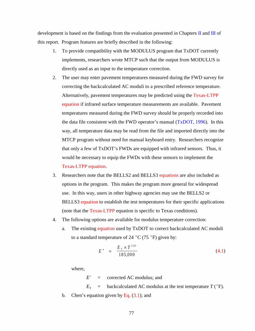
77
development is based on the findings from the evaluation presented in Chapters II and III of
this report. Program features are briefly described in the following:
1. To provide compatibility with the MODULUS program that TxDOT currently
implements, researchers wrote MTCP such that the output from MODULUS is
directly used as an input to the temperature correction.
2. The user may enter pavement temperatures measured during the FWD survey for
correcting the backcalculated AC moduli to a prescribed reference temperature.
Alternatively, pavement temperatures may be predicted using the Texas-LTPP
equation if infrared surface temperature measurements are available. Pavement
temperatures measured during the FWD survey should be properly recorded into
the data file consistent with the FWD operator’s manual (TxDOT, 1996). In this
way, all temperature data may be read from the file and imported directly into the
MTCP program without need for manual keyboard entry. Researchers recognize
that only a few of TxDOT’s FWDs are equipped with infrared sensors. Thus, it
would be necessary to equip the FWDs with these sensors to implement the
Texas-LTPP equation.
3. Researchers note that the BELLS2 and BELLS3 equations are also included as
options in the program. This makes the program more general for widespread
use. In this way, users in other highway agencies may use the BELLS2 or
BELLS3 equation to establish the test temperatures for their specific applications
(note that the Texas-LTPP equation is specific to Texas conditions).
4. The following options are available for modulus temperature correction:
a. The existing equation used by TxDOT to correct backcalculated AC moduli
to a standard temperature of 24 �C (75 �F) given by:
(4.1)′ =×
EE TT
2 8 1
18 5 00 0
.
,
where,
E� = corrected AC modulus; and
ET = backcalculated AC modulus at the test temperature T (�F).
b. Chen’s equation given by Eq. (3.1); and

78
c. The temperature correction method based on the dynamic modulus equation
developed by Witczak and Fonseca (1996). Temperature correction factors
from this method (referred to as Dynamic Modulus in Figure 4.1) are
determined using Eq. (3.5).
Note that Eq. (4.1) only permits corrections to be made for the reference
temperature of 24 �C. Researchers included this as an option to the program as
the method is currently used by TxDOT. To correct backcalculated AC moduli
to other reference temperatures and evaluate seasonal effects, Eq. (3.1) or (3.5)
may be used in the program. Researchers note that Chen’s equation does not
require AC mixture properties for temperature correction. This equation was
developed for the typical mixtures used by TxDOT. To support applications that
involve other mixtures, the user should use the Dynamic Modulus method. This
application will require characterization of the binder viscosity-temperature
relationship of the mix. For this purpose, dynamic shear rheometer tests may be
conducted on the asphalt binder over a range of test temperatures. Alternatively,
the relationship may be estimated nondestructively from FWD data collected at
different temperatures as demonstrated in this project. The binder viscosity-
temperature relationship is specified by the user by entering the applicable A and
VTS coefficients in the computer program. Typical values of these coefficients
are given in Tables 3.2 and 3.3.
5. The program permits the user to predict the monthly variation in asphalt concrete
modulus given the mean monthly temperatures for a given project. In the
program, the mean monthly pavement temperatures are estimated from the mean
monthly air temperatures using Eq. (2.3). As an aid in using this feature,
researchers included a database of mean monthly air temperatures covering all
counties of Texas. The reference modulus specified by the user is then adjusted
to the predicted mean monthly pavement temperatures.
6. MTCP includes a number of options for plotting the results of the temperature
corrections. As shown in Figure 4.1, the user may draw charts of the FWD
deflections, the backcalculated layer moduli, pavement temperature
measurements, the corrected AC moduli, and the predicted monthly variation in

79
Figure 4.2. Example Plot of Corrected and Backcalculated AC Moduli vs. TestTemperature.
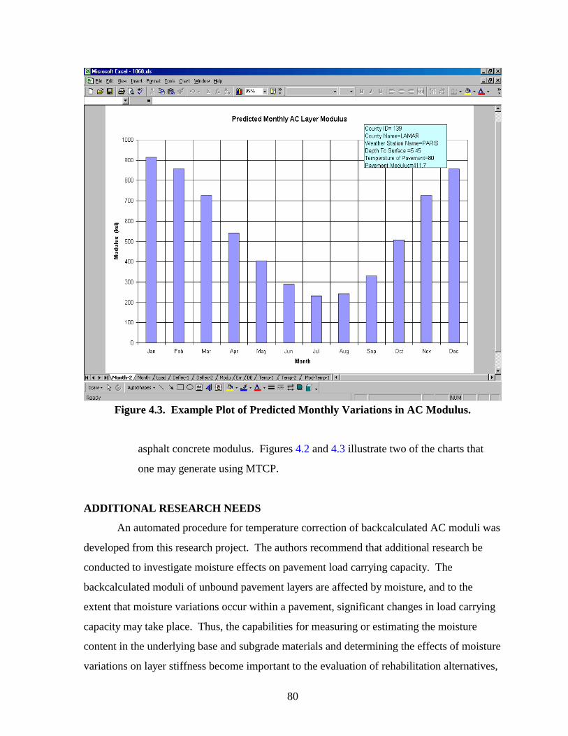
80
Figure 4.3. Example Plot of Predicted Monthly Variations in AC Modulus.
asphalt concrete modulus. Figures 4.2 and 4.3 illustrate two of the charts that
one may generate using MTCP.
ADDITIONAL RESEARCH NEEDS
An automated procedure for temperature correction of backcalculated AC moduli was
developed from this research project. The authors recommend that additional research be
conducted to investigate moisture effects on pavement load carrying capacity. The
backcalculated moduli of unbound pavement layers are affected by moisture, and to the
extent that moisture variations occur within a pavement, significant changes in load carrying
capacity may take place. Thus, the capabilities for measuring or estimating the moisture
content in the underlying base and subgrade materials and determining the effects of moisture
variations on layer stiffness become important to the evaluation of rehabilitation alternatives,

81
load carrying capacity for superheavy loads or overweight truck traffic, and the need for load
restrictions. The following additional research tasks are recommended:
1. Develop test program for field and laboratory measurements. This task shall
develop a plan for instrumenting and testing pavement sections. The plan will
include the following:
a. a test matrix that identifies the materials to be evaluated;
b. the number of pavement sections to be instrumented and the proposed
locations of the test sections;
c. the sensors that will be used to measure moisture and the pavement depths
where the sensors will be installed;
d. the tests to be made; and
e. the schedule for testing.
To support the field evaluation, researchers will also develop a plan for materials
testing in the laboratory. The plan will identify the tests to be conducted, the
moisture levels under which tests will be made, and the materials to be tested.
The laboratory tests are expected to include characterizations of resilient
modulus, permanent deformation, soil suction, and dielectric properties.
1. Conduct test program. After approval of the test program, researchers will
acquire moisture sensors and data acquisition equipment that are needed for field
instrumentation and testing. The objectives of this task are to establish the
effects of moisture on pavements, identify conditions where such effects become
important, evaluate methods for field measurement of moisture, and create a
database for developing a moisture correction procedure. Initial work will
involve sampling materials from the test sections and making preparations for
laboratory testing. Materials sampling will be conducted in conjunction with the
pavement instrumentation effort. Field monitoring will commence after
pavement instrumentation and shall be conducted for the duration proposed in
the test program. During this time, FWD, ground penetrating radar (GPR), and
soil moisture measurements shall be made on a periodic basis to track seasonal
changes and evaluate moisture effects. In addition, the performance of selected

82
methods of measuring or estimating moisture shall be evaluated. Laboratory
tests included in the work plan shall be conducted.
2. Develop procedure for moisture correction. This task covers the analysis of the
laboratory and field data conducted in Task 2. The main goal is to develop a
procedure for correcting base and subgrade moduli to reference moisture
conditions. Toward this goal, researchers will analyze the data to establish the
effects of moisture on the resilient modulus of unbound materials, evaluate
existing methods for moisture correction, and develop procedures for measuring
moisture in situ based on the findings from the evaluation of moisture sensors in
Task 2. An automated procedure for moisture correction shall be developed.
3. Develop recommendations for implementation. This task will develop
recommendations for implementing the moisture correction procedure within
TxDOT. The recommendations will cover user training, testing requirements,
and methods for measuring moisture or soil suction in situ.
4. Research documentation. Researchers shall document the work conducted in the
project, the results from field and laboratory tests, the development of the
computer program for moisture correction, and recommendations for
implementation.
83
REFERENCES
Asphalt Institute (1982). “Research and Development of the Asphalt Institute’s Thickness
Design Manual (MS-1) Ninth Edition.” Research Report No. 82-2, Asphalt Institute,
Lexington, KY.
Asphalt Institute (1982). Thickness Design - Asphalt Pavements for Highways & Streets.”
Manual Series No. 1, Asphalt Institute, Lexington, KY.
Almeida, J. R. de (1998). “Back-Calculation of Flexible Pavements with Consideration of
Temperature Gradients.” Proc. of the 5th International Conference on the Bearing Capacity of
Roads and Airfields, Trondheim, Norway, pp 487-496.
AASHTO (1993). “Guide for Design of Pavement Structures.” American Association of
State Highway and Transportation Officials, Washington, D.C.
Baltzer, S. and J. M. Jansen (1994). “Temperature Correction of Asphalt-Moduli for FWD-
Measurements.” Proc. of the 4th International Conference on the Bearing Capacity of Roads
and Airfields, Minneapolis, MN, pp 753-768.
Barker, W. R., W. N. Brabston, and Y. T. Chou (1977). “A General System for the Structural
Design of Flexible Pavements.” Proc. of the 4th International Conference on the Structural
Design of Asphalt Pavements, Ann Arbor, MI, pp 209-248.
Bush, A. J. (1987). “Development of a Pavement Evaluation Method for Low Volume
Airfield Pavements.” Ph.D. Dissertation, University of Illinois, Urbana, IL.
Cebon, D. (1993). “Interaction Between Heavy Vehicles and Roads.” Society of Automotive
Engineers, Warrendale, PA.

84
Chandra, D., K. M. Chua, and R. L. Lytton (1989). “Effects of Temperature and Moisture on
the Load Response of Granular Base Material in Thin Pavements.” Transportation Research
Record 1252, National Research Council, Washington, D.C., pp 33-41.
Chen, D., J. Bilyeu, H. H. Lin, and M. Murphy (2000). “Temperature Correction on Falling
Weight Deflectometer Measurements.” Transportation Research Record 1716,
Transportation Research Board, Washington, D. C., pp 30-39.
Chen, F. H. (1988). Foundations on Expansive Soils. Elsevier, Amsterdam, The
Netherlands.
Fernando, E. G., and W. Liu (2001). “User’s Guide for the Modulus Temperature Correction
Program (MTCP).” Research Report 1863-2, Texas Transportation Institute, Texas A&M
University, College Station, TX.
Fernando, E. G., and W. Liu (1999). “Program for Load-Zoning Analysis (PLZA): User’s
Guide.” Research Report 2123-1, Texas Transportation Institute, Texas A&M University,
College Station, TX.
Fernando, E. G. (1997). “PALS 2.0 User’s Guide.” Research Report 3923-1, Texas
Transportation Institute, Texas A&M University, College Station, TX.
Jooste, F. J., and E. G. Fernando (1995). “Development of a Procedure for the Structural
Evaluation of Superheavy Load Routes.” Research Report 1335-3F, Texas Transportation
Institute, Texas A&M University, College Station, TX.
Johnson, A. M., and R. L. Baus (1992). “Alternative Method for Temperature Correction of
Backcalculated Equivalent Pavement Moduli.” Transportation Research Record 1355,
National Research Council, Washington, D.C., pp 75-81.

85
Jung, F. W. (1990). “Interpretation of Deflection Basin for Real-World Materials in Flexible
Pavements.” Research Report RR-242, Ontario Ministry of Transportation, Research and
Development Branch, Ontario, Canada.
Kim, Y. R., B. O. Hibbs, and Y. C. Lee (1995). “Temperature Correction of Deflections and
Backcalculated Moduli.” Transportation Research Record 1473, National Research Council,
Washington, D.C., pp 55-62.
Kim, Y. R., S. W. Park, J. D. Troxler, S. R. Ranjithan, and T. Scullion (1997). “Assessment
of Pavement Layer Condition Using Deflection Data.” NCHRP 10-48 Interim Report, North
Carolina State University, Raleigh, NC.
Lukanen, E. O., R. N. Stubstad, and R. C. Briggs (1998). “Temperature Predictions and
Adjustment Factors for Asphalt Pavements.” Research Report FHWA-RD-98-085, Federal
Highway Administration, McLean, VA.
Lytton, R. L., F. P. Germann, Y. J. Chou, and S. M. Stoffels (1990). “Determining Asphaltic
Concrete Pavement Structural Properties by Nondestructive Testing.” National Cooperative
Highway Research Program (NCHRP) Report 327, Transportation Research Board,
Washington D.C.
Magnuson, A. H., and R. L. Lytton (1997). “Development of Dynamic Analysis Techniques
for Falling Weight Deflectometer Data.” Research Report 1175-2, Texas Transportation
Institute, Texas A&M University, College Station, TX.
Matter, N. S., and O. T. Farouki (1994). “Detailed Study on the Climatic and Seasonal
Variation Effects on Pavements in Northern Ireland.” Proc. of the 4th International
Conference on the Bearing Capacity of Roads and Airfields, Minneapolis, MN, pp 721-737.
Michalak, C. H., and T. Scullion (1995). “MODULUS 5.0: User’s Manual.” Research
Report 1987-1, Texas Transportation Institute, Texas A&M University, College Station, TX.

86
Mirza, M. W. (1993). “Development of a Global Aging System for Short and Long Term
Aging of Asphalt Cements.” PhD. Dissertation, University of Maryland, College Park, MD.
N. D. Lea International Ltd. (1995). Modeling Road Deterioration and Maintenance Effects
in HDM-4.” Final Report, RETA 5549-REG Highway Development and Management
Research, Asian Development Bank, Manila, Philippines.
Noureldin, A. S. (1994). “Influence of Stress Levels and Seasonal Variations on In Situ
Pavement Layer Properties.” Transportation Research Record 1448, National Research
Council, Washington, D.C., pp 16-24.
Park, S. W., and Y. R. Kim (1997). “Temperature Correction of Backcalculated Moduli and
Deflections Using Linear Viscoelasticity and Time-Temperature Superposition.”
Transportation Research Record 1570, National Research Council, Washington, D.C.,
pp 108-117.
Saxton, K. E., W. J. Rawls, J. S. Romberger, and R. I. Papendick (1986). “Estimating
Generalized Soil-Water Characteristics from Texture.” Soil Science Society of America
Journal, Vol. 50, No. 4, Madison, WI, pp 1031-1036.
Shaat, A. A., M. A. Kamal, and N. S. Matter (1992). “Relationships between Climatic
Conditions and the Structural Parameters of Flexible Pavements.” Proc. of the 7th
International Conference on Asphalt Pavements, Vol. 3, University of Nottingham, UK,
pp 326-333.
Stubstad, R. N., E. O. Lukanen, C. A. Richter, and S. Baltzer (1998). “Calculation of AC
Layer Temperatures from FWD Field Data.” Proc. of the 5th International Conference on the
Bearing Capacity of Roads and Airfields, Trondheim, Norway, pp 919-928.
Texas Department of Transportation (1996). “Falling Weight Deflectometer Operator’s
Manual.” Texas Department of Transportation, Austin, TX.

87
Texas Transportation Researcher (1989). “Models Developed to Predict Climatic Effects on
Low-Volume Roads.” Vol. 25, No. 4, Texas Transportation Institute, Texas A&M
University, College Station, TX, pp 5-6.
Thornthwaite, C. W. (1948). “An Approach Towards a Rational Classification of Climate.”
Geographical Review, Vol. 38, pp 55-94.
Ullidtz, P. (1987). Pavement Analysis. Elsevier, Amsterdam, The Netherlands.
Uzan, J. (1985). “Granular Material Characterization.” Transportation Research Record
1022, Transportation Research Board, Washington, D.C., pp 52-59.
van Gurp, C. A. P. M. (1982). “Adjustment of Subgrade Modulus and Equivalent Layer
Thickness for Climatic Influences.” Report 7-82-115-32, Road and Railway Research
Laboratory, Delft University of Technology, The Netherlands.
van Gurp, C. A. P. M. (1994). “Effect of Temperature Gradients and Season on Deflection
Data.” Proc. of the 4th International Conference on the Bearing Capacity of Roads and
Airfields, Minneapolis, MN, pp 199-214.
van Gurp, C. A. P. M. (1995). “Characterization of Seasonal Influences on Asphalt
Pavements With the Use of Falling Weight Deflectometers.” PhD. Dissertation, Delft
University of Technology, The Netherlands.
Witczak, M. W., and O. A. Fonseca (1996). “Revised Predictive Model for Dynamic
(Complex) Modulus of Asphalt Mixtures.” Transportation Research Record 1540,
Transportation Research Board, Washington, D. C., pp 15 - 23.
Wolfe, R. K., and R. J. McNichols, (1994). “Simulation of Hourly Temperature Gradients in
Asphalt Concrete Pavement Structures.” Department of Industrial Engineering, Toledo
University, Toledo, OH.

88
Wray, W. K. (1984). “The Principle of Soil Suction and Its Geotechnical Engineering
Applications.” Fifth International Conference on Expansive Soils, Adelaide, Australia,
pp 114-118.

89
APPENDIX A
LITERATURE REVIEW OF METHODS FOR SEASONAL
CORRECTION OF FWD DATA
BACKGROUND
Pavement materials and their response to wheel loads are sensitive to environmental
factors, particularly moisture and temperature (Cebon, 1993). The FWD is widely used for
nondestructive testing to assess the bearing capacity of pavements. However, previous
studies have shown that pavement deflections measured using the FWD at the same location
vary with the time of day when readings were taken. In many cases, the variations can be tied
to the influence of temperature and moisture on pavement material properties.
In general, factors influencing deflections are loading, environment, and pavement
conditions. Among the environmental factors, the most significant are temperature and
moisture distribution within and around pavement structures. Such seasonal variations due to
temperature and moisture tend to change the strength of pavement materials. Therefore, the
resistance to traffic-induced stresses are altered (Asphalt Institute, 1982; AASHTO, 1993).
Consequently, the need exists to develop a method for correcting deflections or layer moduli
to standard conditions. To correct FWD data for temperature and moisture effects that are
applicable to flexible pavements with unbound base layers, the fundamental mechanisms of
temperature and moisture effects on unbound materials must also be understood to improve
the interpretation of surface deflection data.
REVIEW OF THE LITERATURE
Variations in the structural properties of AC pavements may occur due to variations in
the moisture content of the unbound base and subgrade layers, temperature gradients,
fluctuations of the groundwater table, and freeze-thaw cycles. NCHRP Report 327 (Lytton et
al., 1990) identified the following factors as being important:
1. load level,
2. frequency of loading,

90
3. temperature,
4. moisture,
5. size of footprint, and
6. contact pressure on the pavement surface.
The moisture content of unbound base and subgrade are affected by many factors, among
which are (Shaat et al.,1992):
1. size and shape of particles,
2. pore structure,
3. groundwater table,
4. rainfall, and
5. humidity.
However, changes in the moisture content within pavement layers are less likely to occur as
compared to changes in temperature (Noureldin, 1994). Generally the fraction of incoming
solar radiation reflected by the ground is dependent on the characteristics of the surface. The
AC surface layer absorbs about 90 to 95 percent of the solar radiation (Shaat et al., 1992). As
a result, AC pavement surface deflections vary significantly with temperature. Several
approaches have been proposed to determine a standard temperature.
The Asphalt Institute (1982) proposed a relationship between mean pavement
temperature at a given depth below the surface and mean monthly air temperature:
(A1)M Mz z
p a= ++
−+
+
1
1
4
3 4
46
where,
Ma = mean monthly air temperature, �F;
Mp = mean pavement temperature, �F; and
z = depth below surface, inches.
Usually the temperature at the upper third point of each layer is used to get a weighted
average pavement temperature. For the purpose of predicting weekly variations in air
temperatures, Ullidtz (1987) proposed the following equation:
(A2)TT T T T U U O
=+
+−
×−
×
( ) ( )cos
( )1 2 1 2
2 2 2 6π
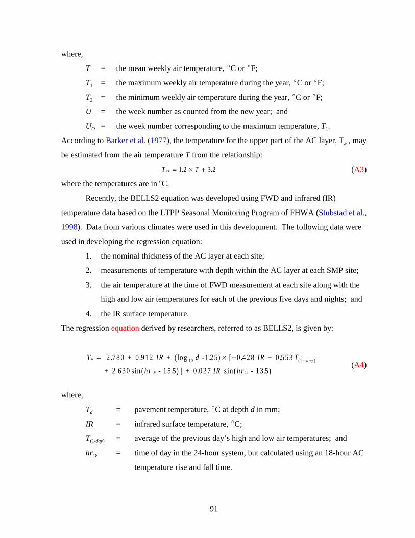
91
where,
T = the mean weekly air temperature, �C or �F;
T1 = the maximum weekly air temperature during the year, �C or �F;
T2 = the minimum weekly air temperature during the year, �C or �F;
U = the week number as counted from the new year; and
UO = the week number corresponding to the maximum temperature, T1.
According to Barker et al. (1977), the temperature for the upper part of the AC layer, Tac, may
be estimated from the air temperature T from the relationship:
(A3)T Tac = × +1 2 3 2. .
where the temperatures are in oC.
Recently, the BELLS2 equation was developed using FWD and infrared (IR)
temperature data based on the LTPP Seasonal Monitoring Program of FHWA (Stubstad et al.,
1998). Data from various climates were used in this development. The following data were
used in developing the regression equation:
1. the nominal thickness of the AC layer at each site;
2. measurements of temperature with depth within the AC layer at each SMP site;
3. the air temperature at the time of FWD measurement at each site along with the
high and low air temperatures for each of the previous five days and nights; and
4. the IR surface temperature.
The regression equation derived by researchers, referred to as BELLS2, is given by:
(A4)T . + . IR + d - . . IR + . T
+ . h r - . + . IR h r - .
d da y= × − −2 7 8 0 0 9 1 2 1 2 5 0 4 2 8 0 5 5 3
2 6 3 0 1 5 5 0 0 2 7 1 3 510 1
1 8 1 8
( log ) [
s in ( ) ] s in ( )( )
where,
Td = pavement temperature, �C at depth d in mm;
IR = infrared surface temperature, �C;
T(1-day) = average of the previous day’s high and low air temperatures; and
hr18 = time of day in the 24-hour system, but calculated using an 18-hour AC
temperature rise and fall time.

92
According to Stubstad et al. (1998), only times between 11:00 and 05:00 hr the
following morning are used in the sin(hr18 - 15.5) decimal function of the BELLS2 equation.
If the actual clock time is not within this time range, the sin function is calculated as if the
time is 11:00 hr. If the time is between midnight and 05:00 hr, add 24 to the actual decimal
time. Then calculate as indicated in the following example:
Given that the clock time is 13:15 hr; in decimal form, 13.25 � 15.50 = �2.25;
�2.25/18 = �0.125; �0.125 × 2 � = �0.785 radians; sin(�0.785) = �0.707.
When using the sin(hr18 - 13.5) decimal function, only times between 09:00 and 03:00 hr the
following morning are used. If the actual clock time is not within this time range, then the
sin function is calculated as if the time is 09:00 hr. If the time is between midnight and 03:00
hr, add 24 to the actual decimal time. Then calculate as indicated in the following example:
Given that the clock time is 15:08 hr; in decimal form, 15.13 �13.50 = 1.63; 1.63/18
= 0.091; 0.091 × 2 � = 0.569 radians; sin(0.569) = 0.539.
Figure A1 shows a comparison of the predicted temperatures using BELLS2 and the
measured pavement temperatures at the LTPP SMP sites. The R2 and standard error of the
estimate of the equation are 0.977 and 1.8 �C, respectively. It is noted that the IR reading is
the most sensitive parameter in the equation. Therefore, the accuracy and calibration of the
IR sensor on the FWD is essential. Since the IR temperatures taken on pavements that are at
or below freezing can negatively affect the accuracy of these measurements, care must be
taken in using the equation for data taken under these conditions. Also, the equation is valid
for AC thicknesses between 45 and 305 mm.
Researchers at North Carolina State University (Kim et al., 1997) developed a
prediction model for an effective AC layer temperature using the change of pavement
temperatures as a function of AC layer thickness, depth from the pavement surface, and time
of day. The proposed equation is given by:
(A5)T z t f z t T o( , ) ( , )=
where,
T(z, t) = subsurface temperature at depth z and at time of day t;
f (z, t) = temperature scaling factor; and

93
Figure A1. Comparison of Predicted AC Temperatures from BELLS2 with MeasuredValues (Stubstad et al., 1998).
To = surface temperature measured at time t.
The temperature scaling factor f(z, t) is given by the relationship:
(A6)f z t A t z B t( , ) ( ) ( )=
where A(t) and B(t) are coefficients established as functions of time. Researchers concluded
that the model proposed above is more effective and accurate than the AASHTO equation for
predicting mean pavement temperature using the measured surface temperature and the
average air temperature for the last 5 days prior to the FWD test.
For considering temperature gradients, the AC layer is partitioned into sublayers with
temperatures taken at corresponding depths. An equivalent AC temperature is then
determined using the equation (Almeida, 1998):
(A7)T
T z d z
heq
h
=∫ ( )0
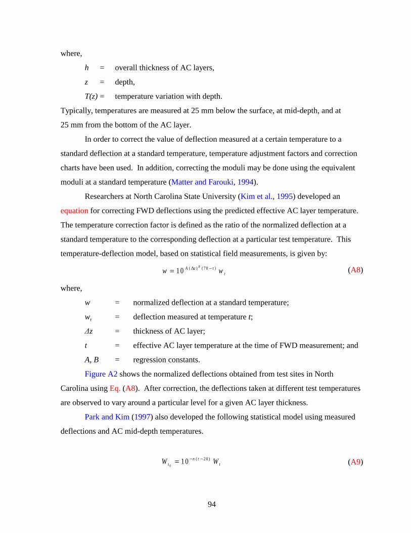
94
where,
h = overall thickness of AC layers,
z = depth,
T(z) = temperature variation with depth.
Typically, temperatures are measured at 25 mm below the surface, at mid-depth, and at
25 mm from the bottom of the AC layer.
In order to correct the value of deflection measured at a certain temperature to a
standard deflection at a standard temperature, temperature adjustment factors and correction
charts have been used. In addition, correcting the moduli may be done using the equivalent
moduli at a standard temperature (Matter and Farouki, 1994).
Researchers at North Carolina State University (Kim et al., 1995) developed an
equation for correcting FWD deflections using the predicted effective AC layer temperature.
The temperature correction factor is defined as the ratio of the normalized deflection at a
standard temperature to the corresponding deflection at a particular test temperature. This
temperature-deflection model, based on statistical field measurements, is given by:
(A8)w wA z tt
B
= −1 0 7 0( ) ( )∆
where,
w = normalized deflection at a standard temperature;
wt = deflection measured at temperature t;
�z = thickness of AC layer;
t = effective AC layer temperature at the time of FWD measurement; and
A, B = regression constants.
Figure A2 shows the normalized deflections obtained from test sites in North
Carolina using Eq. (A8). After correction, the deflections taken at different test temperatures
are observed to vary around a particular level for a given AC layer thickness.
Park and Kim (1997) also developed the following statistical model using measured
deflections and AC mid-depth temperatures.
(A9)W Wtn t
t01 0 2 0= − −( )

95
Figure A2. FWD Deflections Normalized to a Standard Temperature of 68 oF(Kim et al., 1995).
where,
n = 5.807 × 10⁻⁶ (hac)1.4635 along the wheel path; or
n = 6.560 × 10⁻⁶ (hac)1.4241 along the middle of the lane;
hac = thickness of AC layer, mm;
= the deflection corrected to temperature to, �C; andW t 0
Wt = the deflection measured at temperature t, oC.
However, the literature reviewed does not identify the sensors to which the temperature
correction is applied.
Another study conducted by N. D. Lea International Ltd. (1995) for the Asian
Development Bank recommended that the temperature adjustment of the peak deflection be
made as follows:
1. Obtain the weighted mean annual pavement temperature (WMAPT) for the
region. This is the temperature at which the damage to the pavement is the same
as the damage due to the range of temperatures the pavement actually
experiences.

96
2. Estimate the AC temperature near the surface, mid-depth, and bottom of the AC
layer from the following equation:
(A10)T T T H
T T HH S A a c
S A a c
= − + + +− +2 6 0 842 1 31
0 165
. . ( ) . (log )
. ( ) (log )
where,
TH = the AC temperature, �C, at a depth of Hac, mm;
Ts = the surface temperature during testing, �C;
TA = the mean air temperature, �C, of the month in which the
deflections were measured (average of five measurements)
The average of the temperatures at the three depths yields the estimate of the
pavement temperature (Tac) during deflection measurements.
3. Determine the temperature adjustment factor (TAF) as follows:
(A11)T A F = W M A P T
T ac
4. Determine the deflection adjustment factor (DAF) as follows:
If TAF is less than 1, then
(A12)D A F = 1 + (T A F - 1 ) [-1 .3 1 2 - 0 .0 0 04 9 8D + 1 .0 2 7 lo g (H S )
+ 0 .0 7 56 (T A F - 1 )]
9 0 0
If TAF is greater than 1, then
(A13)D A F = 1 + (T A F - 1 ) [-0 .8 9 7 - 0 .0 0 04 6 3D + 0 .8 5 log (H S )
- 0 .4 1 8 (T A F - 1 )]
9 0 0
where HS is the thickness of the AC layer, mm, and D900 is the displacement
measured at 900 mm from the FWD load plate.
5. Adjust the peak deflection Do as follows:
(A14)D (co rrected ) = D (m easu red ) D A F o o ×
Thin pavements with AC thickness less than 40 mm do not require temperature correction.
To correct the modulus determined at a temperature T to a standard temperature T0, a
correction factor given by the following model is typically applied:

97
(A15)λE =
E
E
T
T
O
where,
ETo = the modulus corrected to the standard temperature To;
ET = the backcalculated AC modulus corresponding to the test temperature T; and
�E = the temperature correction factor.
Several methods have been proposed for the correction factor (Johnson and Baus, 1992;
Ullidtz, 1987; Park and Kim, 1997). The majority of these models are primarily based on a
statistical analysis of a limited range of AC mixture types and pavements. Several models for
the temperature correction factor are given in the following.
Johnson and Baus (1992):
(A16)λE T= − −1 0 0 00 0217 5 701 .8 86 1 .8 86. ( )
where T is in �F.
Ullidtz (1987):
(A17)λET
=−
1
3 1 7 7 1 6 7 3. . ( lo g )
for T > 1 �C.
The Danish Road Institute corrects AC moduli based on the AC temperature
measured at a depth of 40 mm irrespective of the AC thickness. The backcalculated moduli
are corrected to a standard modulus, corresponding to a reference temperature of 25 �C, using
the following equation (Baltzer and Jansen, 1994):
(A18)E
ET
T
re fa c
a c
re f
=− ×1 2 log ( )

98
where,
Tref = the reference temperature, �C;
Eref = the reference AC modulus, MPa;
Tac = the AC temperature measured during the FWD test at a depth of 40 mm
below the surface; and
Eac = the AC modulus from the backcalculation, MPa.
Another model was developed using the effective AC temperature at a depth of one-third of
the AC layer. This model is given by:
(A19)λEm T= −1 0 2 0( )
where T is in �C. The constant m was determined to be 0.018 by Baltzer and Jansen (1994).
In addition, Kim et al. (1995) developed a model with a constant m equal to 0.0275 based on
the mid-depth temperature.
Jung (1990) proposed the following formula for determining the modulus of the AC
layer at a standard temperature:
(A20)[ ]E S E A k T A T S= × −ex p ( )
where,
ES = modulus of AC layer (MPa) at the standard temperature;
EA = modulus of AC layer (MPa) corresponding to the test temperature;
TA = mean pavement temperature, �C;
TS = the standard temperature, �C; and
k = equation coefficient.
Jung noted that the coefficient k is constant over a fairly wide temperature range and equal to
0.072.
The AASHTO method corrects peak displacement to a reference temperature of 20
�C. An adjustment factor is determined from the predicted average AC layer temperature.
The normalized deflection is then calculated as the product of the measured peak
displacement at the time of test and the adjustment factor (AASHTO, 1993). From the study
by Baltzer and Jansen (1994), this method was found to be sensitive to large temperature
gradients, but shows good results on pavements with smaller temperature gradients.

99
van Gurp (1994) developed asphalt strain adjustment procedures based on the concept
of equivalency with various AC thicknesses and moduli. This approach is made on the basis
of AC moduli and not on the basis of deflections. If the temperatures are measured at 25 mm
depth, at mid-depth, and at 25 mm from the bottom of AC layer, the effective thickness can
be determined using the following equation:
(A21)hh n n n n n n n n
n n neq =+ + + + +
+ +4
6 4 1 10 1 6 6 4 1
2 11 2
21 2
21 2 2
22
1 2 2
3
where,
h = actual AC layer thickness;
Ei = moduli of AC sublayer i;
n1 = E1 / E2; and
n2 = E2 / E3.
An estimate of the AC mixture moduli-temperature relationship is required to determine the
sublayer moduli of the different lifts, knowing the pavement temperatures at different depths.
Using the equivalent AC layer thickness, the thermal gradient parameter (TGP) is determined
as follows:
(A22)T G Ph
heq= −1
The maximum tensile strain is corrected using the TGP:
(A23)ε εr cor r uncor T G P, , ( )= −1
where,
�r,cor = maximum AC tensile strain corrected for thermal gradient; and
�r,uncor = maximum AC tensile strain uncorrected for thermal gradient.
van Gurp (1994) also developed a procedure to determine an equivalent uniform AC
temperature. This procedure is illustrated in Figure A3. When temperatures are measured at
the same locations as described, the equivalent temperature can be obtained by first
estimating an equivalent modulus from the equation:
(A24)( )E En n n n n n n n
n n neq =
+ + + + ++ +
3
1 22
1 22
1 2 22
2
1 2 2
6 4 1 1 0 1 6 6 4 1
6 4 2 1

100
Figure A3. Procedure to Determine the Equivalent Uniform AC Layer Temperature.
Then, the equivalent temperature is determined from the modulus-temperature relationship
for the given mix as per Figure A3. Even though some errors can be generated due to the two
conversion steps, van Gurp concluded that the effect is small enough to use the equivalent
temperature.
Wolfe and McNichols (1994) developed procedures using yearly weather data
obtained from the National Climatic Data Center to estimate the temperature profiles that
affect the relationship between the modulus and temperature. Many factors are required to
estimate temperature profiles:
1. wind velocity,
2. cloud cover,
3. solar radiation,
4. air temperature,
5. latitude,
6. longitude, and
7. location and time of day.

101
The pavement moduli are corrected by means of the hourly temperature profiles. Then, the
equivalent vertical and horizontal strains are calculated based on the corrected pavement
moduli.
The MODULUS program (Michalak and Scullion, 1995) also has a temperature
correction procedure based on the U.S. Army Corps of Engineers’ (USACE) equations
(Bush, 1987). The remaining life analysis option of the computer program uses this
procedure. Adjustments are made to the first four FWD sensors as shown in Table A1, where
the adjustments for sensors 2 to 4 are expressed as percentages of the correction factor for the
maximum deflection. If the AC thickness is less than 75 mm (2.95 in), no temperature
correction is made. After temperature correction of the deflections bowls and projection of
the monthly deflection bowls using the USACE procedure, pavement strains (in units of
microstrain) are estimated using the following regression equations:
(A25)εv A B W C W= + × + ×1 7
(A26)ε t D E W W= + × −( )1 2
where,
A, B, C, D, and E = regression coefficients shown in Table A2;
W1, W2, and W7 = normalized deflections (mils);
�v = vertical compressive strain at the top of the subgrade; and
�t = tensile strain at the bottom of the AC layer.
While methods for correcting pavement deflections have been proposed, the use of
these procedures is probably best suited for network-level applications, such as comparative
evaluations of pavement response and performance between different regions of the state.
For project-level investigations, any adjustment to the measured deflection basin is not
recommended. The shape of the deflection basin is an important feature of the pavement
response and is affected by all pavement layers. Therefore, adjustment for seasonal effects
should be made after the backcalculation of layer moduli (Shaat et al., 1992).
In general, the effect of temperature dominates the pattern of the deflections up to
600 mm while the effect of moisture dominates the pattern of the deflections, D900 mm and
D1200 mm (Matter and Farouki, 1994). There are many sources of variation in subgrade
response (van Gurp, 1994):

102
Table A1. Percentage of Temperature Correction Factor Applied to Each FWD Sensor.
FWD SensorAC Thickness
< 75 mmAC Thickness
75 mm - 125 mmAC Thickness
> 125 mm
W1 0 100 100
W2 0 45 62
W3 0 12 34
W4 0 5 10
Table A2. Regression Coefficients for Estimating Asphalt Tensile and SubgradeCompressive Strains for MODULUS Remaining Life Analysis.
ACThickness
(mm)A B C D E
0 - 13 -210 41 303.8 0 0
13 - 37 -91.2 32.6 235.2 -231.1 14.7
37 - 62 -11.0 26.92 123.7 -147.85 27.06
62 - 87 1.19 23.4 69.4 -98.7 35.15
87 - 113 -1.15 20.7 43.68 -66.6 40.28
113 - 128 -4.59 18.5 30.04 -43.5 42.75
128 - 175 -7.19 16.6 22.74 -25.1 42.72
> 175 -10.36 13.38 16.63 1.28 37.3
1. stress sensitivity of pavement materials;
2. thermal stresses in the subgrade due to soil temperature changes;
3. variation of soil moisture content and suction;
4. condition of the pavement surface; and
5. testing induced effects.

103
Significant changes of AC layer moduli lead to changes in the confining and deviatoric
stresses in the underlying layers. Therefore, this stress-dependent behavior of unbound layers
may cause changes of moduli. In addition, an increase in soil temperature will cause an
increase in the contact forces between particles due to volumetric expansion. The contact
pressure that is related to the confining pressure will affect the moduli of the soil. Moisture
condition, suction changes, and condition of the pavement surface may also cause seasonal
variations. To correct the backcalculated subgrade modulus from FWD testing, van Gurp
(1994) proposed a simple method based on data that are easy to determine and implement in
practice. An index system was developed to adjust subgrade moduli to the standard
condition corresponding to an AC temperature of 20 �C. Table A3 shows the different
factors considered in the methodology and the index assigned to each factor. The aggregate
score of the indices is called the subgrade stiffness index (SSI). The individual indices have
been arranged in such a way that an SSI of zero represents a case where negligible sensitivity
to seasonal variations is predicted. A negative SSI is typical for projects where subgrade
stiffness will be higher in winter than in summer, whereas a positive SSI is characteristic of
pavement sections that show the opposite effect. The subgrade modulus determined at any
day of testing can be adjusted using the SSI and the following equations:
(A27)S E = S S I
4 00S G
(A28)E E
1 + S E (T - 2 0 )S G , R
S G
S G A=
where,
SSI = subgrade stiffness index;
SESG = seasonal sensitivity of subgrade, MPa/MPa/�C;
ESG, R = standard subgrade modulus, MPa;
ESG = subgrade modulus at day of testing, MPa; and
TA = asphalt temperature at time of FWD testing, �C.

104
Table A3. Indicators of Seasonal Variation of Subgrade Response (van Gurp, 1995).
Factor of Influence Change of
Index
Stress sensitivity effects by changes of asphalt stiffness� Sand subgrade� Silt subgrade or thick sand subbase on cohesive subgrade� Clay subgrade or thin sand subbase on silt subgrade
+1 0�1
Thermally induced stresses in unbound layers� Loosely packed sand subgrade� Densely packed sand subgrade� Densely packed thick sand subbase on cohesive subgrade� Other
+1+2+1 0
Soil moisture content and groundwater table changes� High groundwater table level with substantial seasonal variation� Other groundwater conditions
+1 0
Suction by trees� Willows or poplars near the pavement edge� Other species of trees near the pavement edge� No trees
+4+3 0
Visual condition of pavement surface� Extent of cracking less than 10 percent; no or slight rutting� Extent of cracking less than 10 percent; moderate or severe deep-seated
rutting� Extent of cracking between 10 and 20 percent� Extent of cracking more than 20 percent
0
+1+2+4
Testing induced variation� Delft University of Technology FWD� Dynatest 8000 and 8081 models� Phønix ML10000 model� Phønix PRI model
�3�2�3 0
In addition, van Gurp (1982) developed a sine-shaped model for the seasonal fluctuations of
subgrade modulus:
(A29)E t E E t tSG SG SG s( ) s in [ ( )]= + × −∆ 2π
where,
ESG(t) = subgrade modulus at time, t (MPa);
�SG = mean annual subgrade modulus (MPa);

105
�ESG = amplitude of annual cycle of subgrade modulus (MPa);
t = time (years); and
ts = shift in phase (years).
The shift in phase is defined as that part of the year expired since January 1 on the date of the
year that the subgrade modulus equals the predicted mean annual modulus and crosses this
mean line with a positive gradient.
TTI researchers (Chandra et al., 1989) developed a formula for correcting moduli of
unbound materials to standard temperature and moisture conditions. In their study, the
granular base course moduli of thin pavements showed an increasing trend as temperature
and suction increased. Increases in temperature and suction may cause an increase of the
contact pressure between particles, as illustrated in Figure 1.3 in Chapter 1 of this report.
Basically, two main assumptions were made in developing the formula (Lytton et al., 1990):
1. the thermal coefficient of volume expansion does not change with changes in
temperature; and
2. the volumetric moisture content does not change appreciably with changes in soil
suction.
If either of the above assumptions is questionable, nonlinear representations can be used.
The first assumption should be satisfied if the temperature in unbound materials remains
above freezing. This assumption is considered to be valid for unbound materials consisting
of hard aggregates with less than five percent passing the No. 200 sieve size. Unbound
materials with appreciable amounts of fines may experience significant changes in the
thermal coefficient of volume expansion in the interval of temperature in which freezing or
thawing occurs. The second assumption requires the determination of the suction versus
volumetric moisture content relationship for the material of interest. The equation developed
to correct the moduli of unbound materials for temperature and moisture (suction) effects is:
(A30)∆∆
∆ΨE K K u x x TV=
+−
+
1 2
3
2
2
1
4 3θ
ω ωα
θν( )

106
where,
u = K2 � 1;
� = 3(1 � �2)/(4E);
x = (0.48 � nobs)/0.22;
nobs = porosity;
E = modulus associated with initial temperature and soil suction;
�E = change in modulus resulting from changes in soil suction and
temperature;
� = Poisson’s ratio associated with initial temperature and suction;
�� = thermal coefficient of volume expansion, which is appropriately three
times the linear thermal coefficient;
�T = initial temperature minus final temperature;
�� = initial suction minus final suction;
�v = volumetric moisture content;
� = the mean principal stress; and
K1, K2 = stress dependency material constants.
Soil suction is a measure of a soil’s affinity for water and indicates the intensity with which it
will attract water. The drier the soil, the greater is the soil suction (Chen, 1988; Wray, 1984).
Generally, soil suction is considered to consist of only two components, matric and
osmotic suction. The sum of the two components is called total suction (or total free energy)
as follows:
(A31)h h ht m o= +where,
ht = total suction;
hm = matric suction; and
ho = osmotic suction.
In addition, total suction is given by the Kelvin equation:
(A32)hR T
m g
P
Pt
o=
ln

107
where,
ht = total soil suction (gm-cm/gm, or simply cm), which is a negative number,
indicating that the water in the soil is in tension;
R = universal molar gas constant (8.31432 J / mole �K);
T = absolute temperature ( �K);
m = molecular mass of water vapor (18.016 g / mole);
g = acceleration due to gravity (981 cm/sec2);
P = partial pressure of pore water vapor (kPa);
Po = saturation pressure of water vapor over a flat surface of pure water at the
same temperature (kPa); and
P/Po = relative humidity of the soil water (dimensionless).
Saxton et al. (1986) developed a simple empirical equation to estimate soil suction.
This equation was derived from 55 tests on soil specimens that had less than 5 percent sand
and where the clay content varied within the range of 5 to 60 percent:
(A33)Ψ = 100 A Bθ
(A34)[ ]A C S S C= − − − × − ×− −e x p . . . .4 3 9 6 0 0 7 1 5 4 4 8 8 0 1 0 4 2 8 5 1 04 2 5 2
(A35)B C S C= − − − × −3 1 4 0 0 0 0 2 2 2 3 8 4 8 1 02 5 2. . .
where,
� = soil suction (kPa);
� = volumetric water content (m3/m3);
S = percent sand; and
C = percent clay.
The correction procedure to adjust moduli to the standard moisture condition should be
performed after the AC modulus has been corrected to standard temperature and load
frequency according to Lytton et al. (1990).
CLIMATIC DATA
In order to consider seasonal variations and their effects on the performance of
pavements, knowledge of the meteorological conditions and related seasonal cycles at a given
location is essential. These include the effects of rainfall, evaporation, and temperature in

108
the vicinity of pavement structure areas. Simply, rainfall and evaporation data can be
obtained by empirical methods or field measurements. Thornthwaite (1948) developed a
simple moisture balance equation given by:
(A36)Et
Ip
a
=
1 6
1 0
where,
Ep = estimated evapotranspiration of water, mm/day;
t = mean monthly air temperature, �C;
I = annual total of (t/5)1.514 calculated for each month; and
a = 0.000000675( I )3 - 0.0000771( I )2 + 0.01792 ( I ) + 0.49239.
The moisture balance of each month can be calculated using the above equation.
Today, daily weather information can be obtained easily using the Internet. The
National Climatic Data Center (NCDC) of the National Oceanic and Atmospheric
Administration (NOAA) provides weather information at the following address:
http://www.ncdc.noaa.gov/cgi-bin/res40pl?page=climvisgsod.html
The accessibility of weather information will help in the practical application of the seasonal
correction methods presented in this appendix.

APPENDIX B
PLOTS OF BACKCALCULATED AND CORRECTED AC MODULI
WITH TEST TEMPERATURES
109


111
Figure B1. Corrected AC Moduli Using Eq. (3.5) and tr = 7 �C (SMP Site 404165).
Figure B2. Corrected AC Moduli Using Eq. (3.5) and tr = 7 �C (SMP Site 481060).
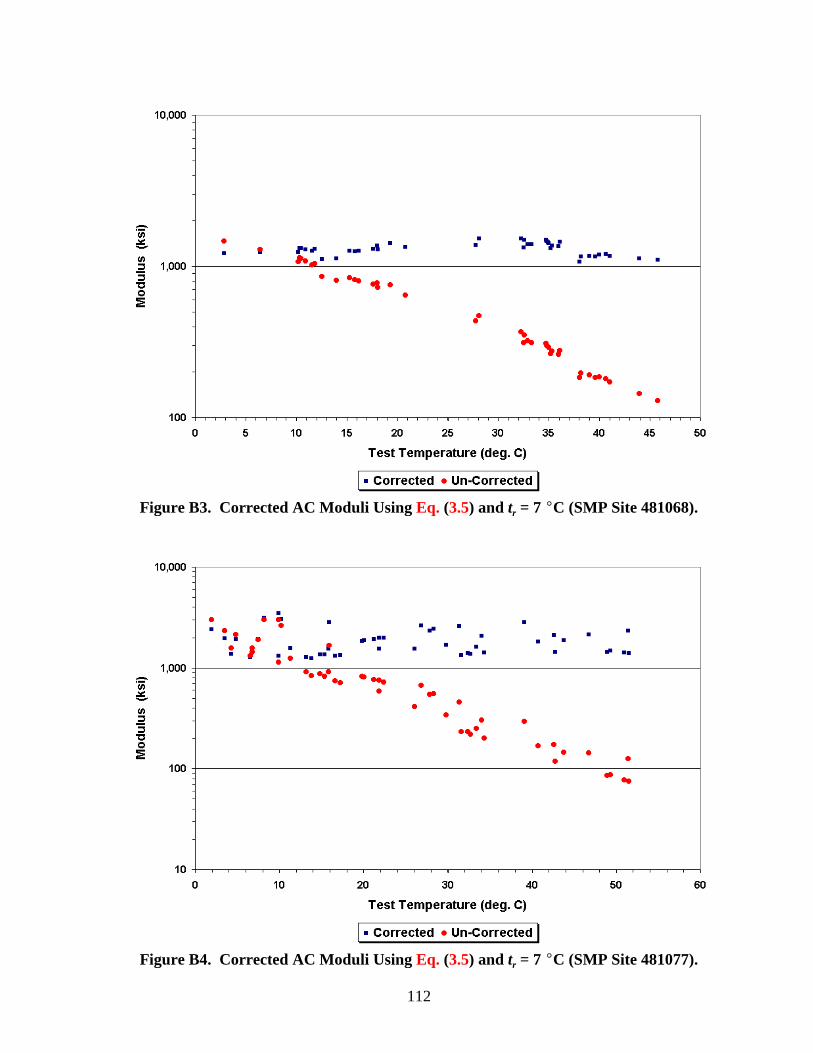
112
Figure B3. Corrected AC Moduli Using Eq. (3.5) and tr = 7 �C (SMP Site 481068).
Figure B4. Corrected AC Moduli Using Eq. (3.5) and tr = 7 �C (SMP Site 481077).
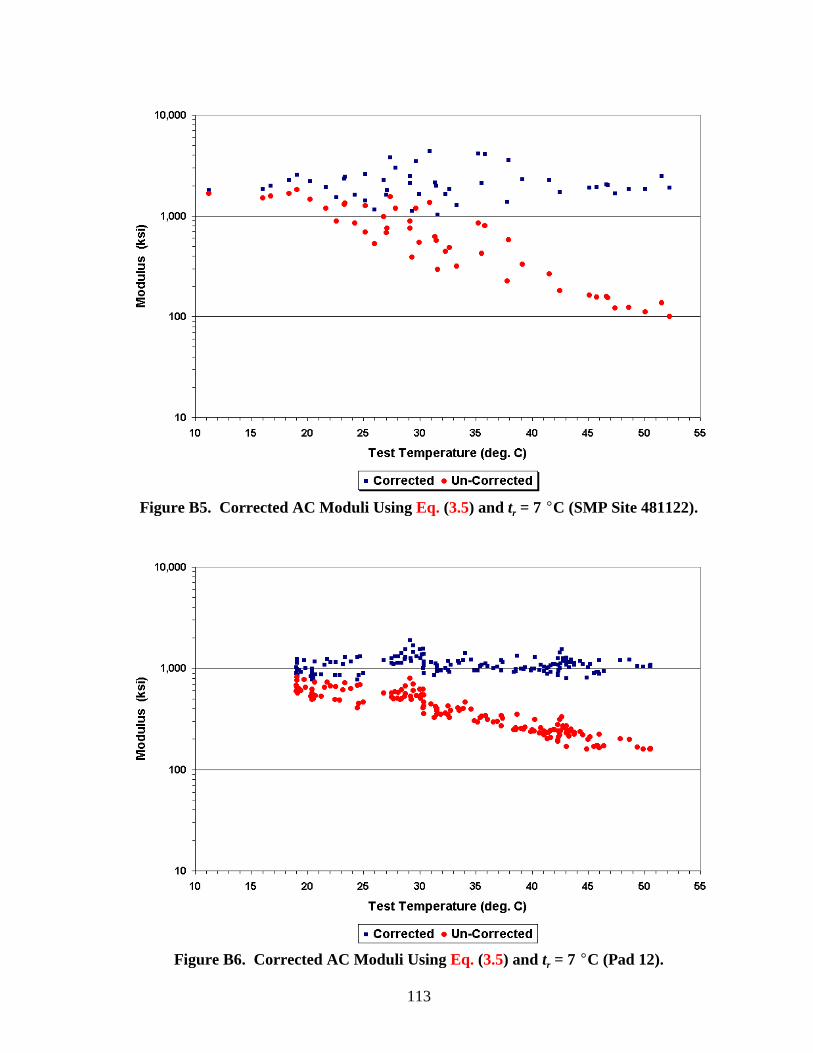
113
Figure B5. Corrected AC Moduli Using Eq. (3.5) and tr = 7 �C (SMP Site 481122).
Figure B6. Corrected AC Moduli Using Eq. (3.5) and tr = 7 �C (Pad 12).

114
Figure B7. Corrected AC Moduli Using Eq. (3.5) and tr = 7 �C (Pad 21).
Figure B8. Corrected AC Moduli Using Eq. (3.4) and tr = 7 �C (SMP Site 404165).

115
Figure B9. Corrected AC Moduli Using Eq. (3.4) and tr = 7 �C (SMP Site 481060).
Figure B10. Corrected AC Moduli Using Eq. (3.4) and tr = 7 �C (SMP Site 481068).
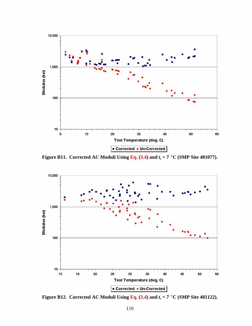
116
Figure B11. Corrected AC Moduli Using Eq. (3.4) and tr = 7 �C (SMP Site 481077).
Figure B12. Corrected AC Moduli Using Eq. (3.4) and tr = 7 �C (SMP Site 481122).

117
Figure B13. Corrected AC Moduli Using Eq. (3.4) and tr = 7 �C (Pad 12).
Figure B14. Corrected AC Moduli Using Eq. (3.4) and tr = 7 �C (Pad 21).

118
Figure B15. Corrected AC Moduli Using Eq. (3.1) and tr = 7 �C (SMP Site 404165).
Figure B16. Corrected AC Moduli Using Eq. (3.1) and tr = 7 �C (SMP Site 481060).

119
Figure B17. Corrected AC Moduli Using Eq. (3.1) and tr = 7 �C (SMP Site 481068).
Figure B18. Corrected AC Moduli Using Eq. (3.1) and tr = 7 �C (SMP Site 481077).

120
Figure B19. Corrected AC Moduli Using Eq. (3.1) and tr = 7 �C (SMP Site 481122).
Figure B20. Corrected AC Moduli Using Eq. (3.1) and tr = 7 �C (Pad 12).

121
Figure B21. Corrected AC Moduli Using Eq. (3.1) and tr = 7 �C (Pad 21).
Figure B22. Corrected AC Moduli Using Eq. (3.5) and tr = 41 �C (SMP Site 404165).

122
Figure B23. Corrected AC Moduli Using Eq. (3.5) and tr = 41 �C (SMP Site 481060).
Figure B24. Corrected AC Moduli Using Eq. (3.5) and tr = 41 �C (SMP Site 481068).
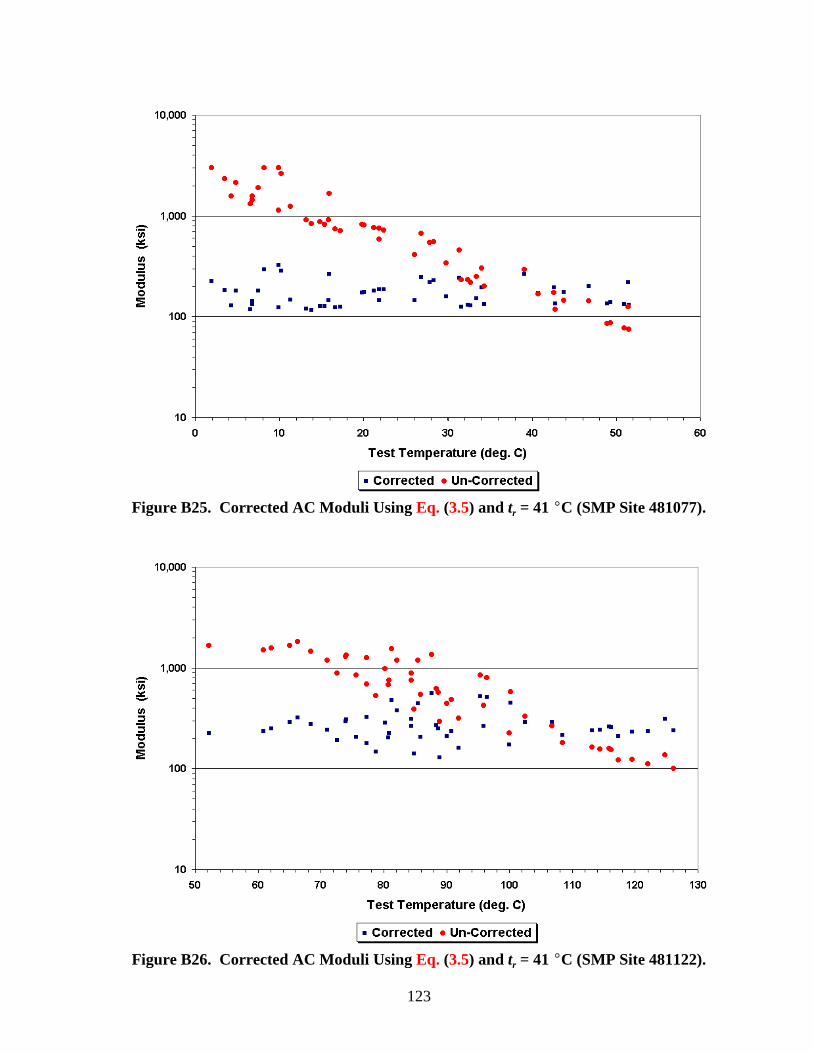
123
Figure B25. Corrected AC Moduli Using Eq. (3.5) and tr = 41 �C (SMP Site 481077).
Figure B26. Corrected AC Moduli Using Eq. (3.5) and tr = 41 �C (SMP Site 481122).
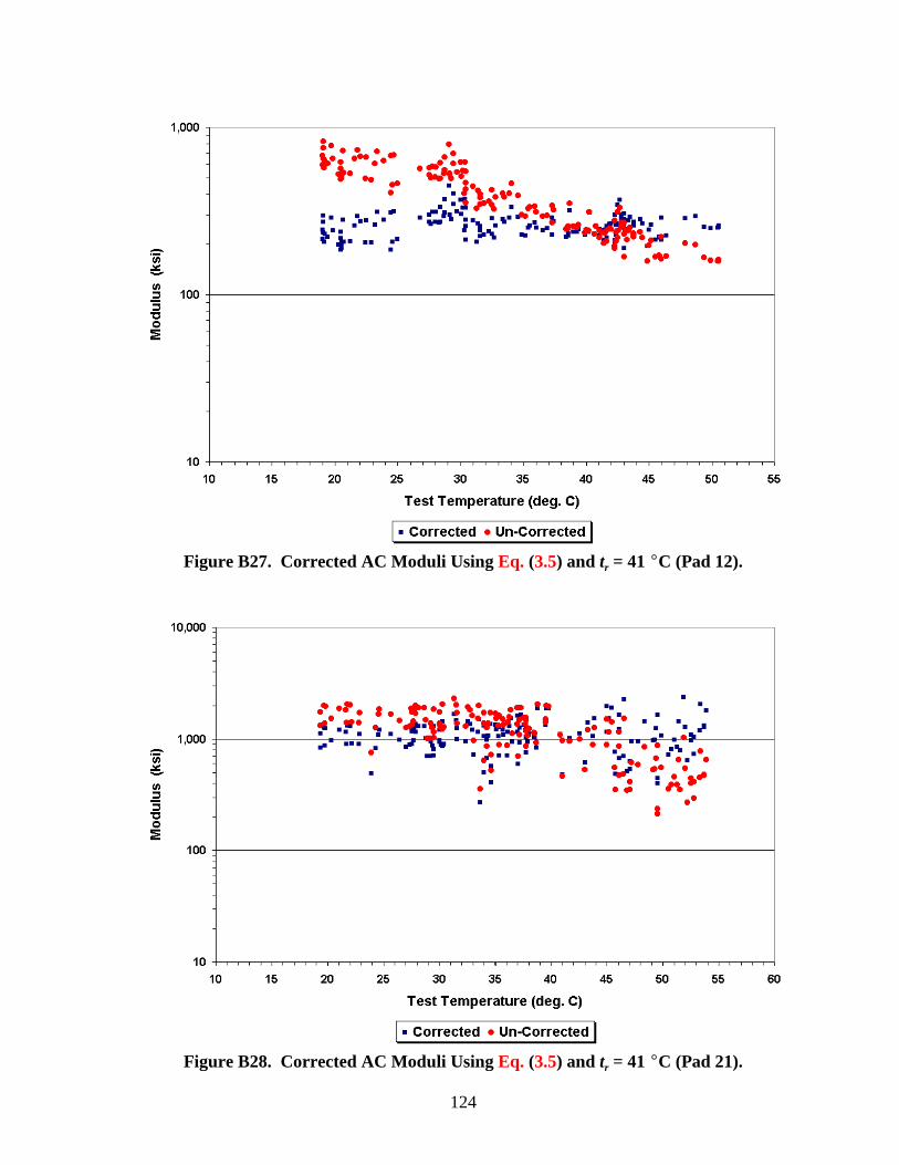
124
Figure B27. Corrected AC Moduli Using Eq. (3.5) and tr = 41 �C (Pad 12).
Figure B28. Corrected AC Moduli Using Eq. (3.5) and tr = 41 �C (Pad 21).

125
Figure B29. Corrected AC Moduli Using Eq. (3.4) and tr = 41 �C (SMP Site 404165).
Figure B30. Corrected AC Moduli Using Eq. (3.4) and tr = 41 �C (SMP Site 481060).

126
Figure B31. Corrected AC Moduli Using Eq. (3.4) and tr = 41 �C (SMP Site 481068).
Figure B32. Corrected AC Moduli Using Eq. (3.4) and tr = 41 �C (SMP Site 481077).
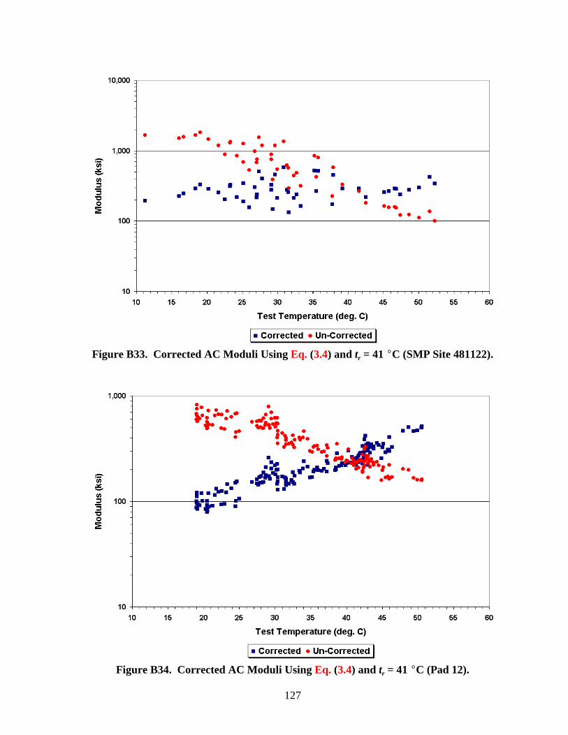
127
Figure B33. Corrected AC Moduli Using Eq. (3.4) and tr = 41 �C (SMP Site 481122).
Figure B34. Corrected AC Moduli Using Eq. (3.4) and tr = 41 �C (Pad 12).

128
Figure B35. Corrected AC Moduli Using Eq. (3.4) and tr = 41 �C (Pad 21).
Figure B36. Corrected AC Moduli Using Eq. (3.1) and tr = 41 �C (SMP Site 404165).

129
Figure B37. Corrected AC Moduli Using Eq. (3.1) and tr = 41 �C (SMP Site 481060).
Figure B38. Corrected AC Moduli Using Eq. (3.1) and tr = 41 �C (SMP Site 481068).

130
Figure B39. Corrected AC Moduli Using Eq. (3.1) and tr = 41 �C (SMP Site 481077).
Figure B40. Corrected AC Moduli Using Eq. (3.1) and tr = 41 �C (SMP Site 481122).

131
Figure B41. Corrected AC Moduli Using Eq. (3.1) and tr = 41 �C (Pad 12).
Figure B42. Corrected AC Moduli Using Eq. (3.1) and tr = 41 �C (Pad 21).