Development of a Tour-Based Truck Travel Demand Model ...docs.trb.org/prp/14-4293.pdf · 1 Development of a Tour-Based Truck Travel Demand Model using Truck GPS Data ... 5 trucks

Arun Kuppam, Jason Lemp, Dan Beagan, Vladimir Livshits, Lavanya

Vallabhaneni, Sreevatsa Nippani

Development of a Tour-Based Truck Travel Demand Model using Truck GPS Data 1

7/31/2013 2

Word Count = 4,728 (words) + 11 * 250 (tables and figures) = 7,478 3

Authors 4

Arun Kuppam (Corresponding Author) 5 Cambridge Systematics, Inc. 6 10415 Morado Circle, Building II, Suite 340 7 Austin, TX 78759 8 Phone: (512) 691-8503 9 Fax: (512) 691-3289 10 E-mail: [email protected] 11

Jason Lemp 12 Cambridge Systematics, Inc. 13 10415 Morado Circle, Building II, Suite 340 14 Austin, TX 78759 15 Phone: (512) 691-8501 16 Fax: (512) 691-3289 17 E-mail: [email protected] 18

Dan Beagan 19 Cambridge Systematics, Inc. 20 100 CambridgePark Drive, Suite 400 21 Cambridge, MA 02140 22 Phone: (617) 354-0167 23 Fax: (617) 354-1542 24 E-mail: [email protected] 25

Vladimir Livshits 26 Maricopa Association of Governments 27 302 North First Avenue, Suite 300 28 Phoenix, AZ 85003 29 Phone: (602) 254-6300 30 Fax: (602) 254-6490 31 E-mail: [email protected] 32

Lavanya Vallabhaneni 33 Maricopa Association of Governments 34 302 North First Avenue, Suite 300 35 Phoenix, AZ 85003 36 Phone: (602) 254-6300 37 Fax: (602) 254-6490 38 E-mail: [email protected] 39

Sreevatsa Nippani 40 Maricopa Association of Governments 41 302 North First Avenue, Suite 300 42 Phoenix, AZ 85003 43 Phone: (602) 254-6300 44 Fax: (602) 254-6490 45 E-mail: [email protected] 46

TRB 2014 Annual Meeting Original paper submittal - not revised by author



Prepared for presentation and possible publication 1 Transportation Research Board 2 93

rd Annual Meeting 3

Washington, D.C. 4 January 2014 5 6 7




ABSTRACT 1

The concept of truck travel demand forecasting, internal to a region, has always been built upon modeling discrete 2 truck trip ends, distributing truck trip ends to various origins and destinations using travel time impedances and some 3 land use characteristics, and allocating truck trip tables into distinct time periods using factors derived from observed 4 counts. An innovative enhancement to this approach is to apply activity-based modeling (ABM) principles to truck 5 tour characteristics and develop a tour-based truck travel demand model. 6 7 This paper focuses on two aspects – (a) processing of truck GPS data, and (b) developing a tour-based truck model. 8 The processing of truck GPS data is done for the MAG region to construct a truck tour database necessary for 9 estimating tour-based models. The tour-based models include stop generation and purpose models, and time period 10 allocation and duration models to predict the occurrence of truck stops in space and time for each industry sector. 11 This paper also discusses the calibration and validation of these discrete choice models that are linked together to 12 output trip chains or truck tours for different industry sectors. 13

14

15

16




INTRODUCTION 1

The existing truck model structure for the Maricopa Association of Governments (MAG) in the Phoenix region is a 2 trip-based hybrid model that uses trip rates and trip lengths to model internal trucks and commodity-based regression 3 models to capture external trucks. This model has been recently updated using new commodity flow data for external 4 trucks and new truck GPS data for the internal trucks. In parallel, MAG also wanted to test a tour-based modeling 5 framework with the large volume of truck GPS data. 6

In the recent past, Cambridge Systematics (CS) has successfully acquired, processed, and used truck GPS 7 data to update internal truck model parameters with statistical significance for other regions. As part of this study, CS 8 acquired and processed GPS data from American Transportation Research Institute (ATRI), which is a non-profit 9 organization that compiles data predominantly from heavy trucks, that is, FHWA classes 8-13 (1). This data had over 10 three million GPS event records for the month of April 2011 that was reported by over 20,000 trucks. About 95 11 percent of truck tours are generated by retail establishments, farms, households, wholesale trade and manufacturing 12 facilities in the region. This truck tour database formed a strong foundation to estimate robust tour-based models for 13 various industry sectors. 14

The objective of the truck tour model is to develop truck trip chains by industry sector where the first trip is 15 generated on every tour. These truck trip chains can be grouped into the major linkages based on the land uses at 16 which trucks make stops and the probability of making another stop based on the number of previous stops. For each 17 truck tour, a series of choice models are employed in order to determine the time period of tour start times, propensity 18 to make additional stops, next stop purpose, location of the stop and stop duration. 19

The basic concept that sets the framework for truck tours is the stop pattern of a truck making stops at several 20 land uses. This is equivalent to a passenger ABM’s daily activity pattern model that models the number and types of 21 stops made by each unit (person or establishment) in the population. In the truck stop pattern model, the sequence of 22 stops that is modeled, is constrained by the occurrences of land use to land use exchanges derived from the processed 23 truck tour database. Once this is modeled, the destination and time of day choice models are conditioned on the stop 24 pattern information derived from the upper level models. 25

GPS Devices in Trucks 26

The information that is used to support the development of truck trip distribution and touring models traditionally 27 comes from truck trip diaries. These truck trip diaries are difficult to deploy and collect, generally do not support 28 large volumes of data, and are very expensive (2). Therefore, MAG was determined to try other alternate methods of 29 data collection or acquisition such as the GPS data. GPS devices are widely deployed in cell phones, autos, and 30 trucks. These devices can display information about the position of the vehicle, often on a map of the area, and the 31 desired destination, based on signals received from Global Positioning Satellites. Sometimes these devices not only 32 receive the GPS satellite signals or other information, such as traffic conditions, they also may wirelessly transmit that 33 information back to a central location. 34

There are a variety of reasons why truck GPS information is collected. The information may be an 35 Automatic Vehicle Location (AVL) system to provide information to locate, for security reasons, the vehicle, driver 36 and/or cargo, or to provide navigational or dispatch information. The GPS transmitter may be tied to the engine bus 37 or other vehicle equipment as part of an Events Activated Tracking System (EATS). The event triggering a GPS 38 transmission may be a condition of the engine (e.g., a specific temperature), a vehicle event (e.g., hard braking, or 39 vehicle speed), or a request by the central office ( e.g., a ping). Deploying a GPS transmitter and a central receiver 40 may also be part of a Fleet Telematics System (FTS). Thus the purpose of GPS devices may be varied, such as : 41 operational – to track and schedule the movement of vehicle, drivers or cargo; or maintenance – to track the condition 42 and operation of the vehicle. 43

The GPS event information is collected to serve the business purposes of the truck fleet operators. Those 44 businesses are under no obligation to share this information with others. In fact this information, since it contains 45 sensitive information about the business practices of truck fleet operations, is contractually protected when it is 46 collected as a part of subscription but provided to third parties.... However, information pertaining to the GPS 47




locations (in the form of latitude and longitude) and the time stamp at which the transmission was sent is available. 1 This information can be processed to derive a truck trip or tour database that can be used for model estimation. 2

ATRI GPS DATA FOR MAG 3

CS successfully processed the ATRI data for the Los Angeles MPO as part of a regional goods movement project. CS 4 also acquired and processed data from other vendors such as Trimble and Calmar as part of the Los Angeles project 5 (3). The Trimble data was used for updating the light-heavy and medium-heavy duty trucks while Calmar and ATRI 6 were used to develop the heavy-heavy duty truck trip rates. For an NCFRP project, CS purchased Trimble data for 7 four metropolitan regions namely Phoenix, Chicago, Baltimore and Los Angeles, and examined trip chaining patterns 8 of trucks, nature of truck tours, number of stops, average impedance between stops and the nature of land use at each 9 stop on tour (4). CS, through a MAG contract, purchased the ATRI data for the MAG modeling area for the period 10 from April 1, 2011 to April 30, 2011. The raw data delivery from ATRI contained 3,429,603 GPS event records. The 11 locations of these GPS records are shown in Figure 1. There are GPS event records reported for 22,657 trucks that 12 indulge in 58,637 tours. At these GPS events, the vehicle may be stopped or moving. In principle, only certain 13 stopped records can be grouped into tours or trips, but tours or trips cannot be precisely computed without further 14 processing. 15

Figure 1 also shows GPS records for one random truck for the whole month of April 2011. There are 719 16 records for this truck, which makes 40 tours in April 2011. A “tour” is defined as a sequence of GPS events for a 17 given truck, where the event after last event is a change of date and a change in time of more than 2 hours. This time 18 check is to allow for tours that extend past midnight. This definition of a “tour’ is only intended to be used in the 19 initial filtering of the GPS records. Subsequent processing was done to determine truck tours consistent with its use in 20 the development of touring models. 21

The GPS event records for one random tour on April 1, 2011 for this truck is shown in Table 1. This table 22 shows the ‘primary anonymized data’, which is the raw data as obtained directly from ATRI, as well as the ‘processed 23 data. The processing was conducted to determine the condition that can be associated with each GPS event. For each 24 event, the time and position of the truck is computed. The Great Circle Distance (e.g., air miles) between the GPS 25 events is calculated based on a comparison of the latitudes and longitudes of the events. The time between the 26 preceding and following events is calculated based on the timestamp of those events. The “air speed” in MPH is 27 calculated based on the distance from the last (…or to the next) GPS event divided by the time from the last (…or to 28 the next) GPS event. It is from this comparison of the sequence of time, distances and speeds that a determination was 29 made as to the action of the truck at that event. It should also be noted that the imprecision of the GPS location 30 reading may erroneously give the indication that the truck has moved when the GPS location readings vary very 31 slightly. This is due to the fact that the truck is making incidental movements within the same trip end (e.g., moving 32 from a holding location to a loading dock), and those incidental movements are a continuation of the full stop that had 33 already been determined. It is for this reason that the criteria for motion with respect to the last or next events is a 34 speed of 5 MPH and not absolute zero. These events are also depicted on the left hand side in Figure 2. 35

36




1 2

3

4

5

6

7

8

9

10

11

12

13

14

FIGURE 1. All ATRI MAG GPS Truck Events During April 2011 15

16

17

18

ATRI GPS All Truck IDs

April 2011

All Trucks in April 2011

GPS Events = 3,429,603

Truck Tours = 58,637

Trucks = 22,657

ATRI GPS Truck ID 3570452

April 2011

One Truck (ID 357042) in April 2011

GPS Events = 719

Truck Tours = 40

Trucks = 1




The types of GPS events presented in Table 1 are defined as follows: 1

• First Starting –The first GPS event record in a tour whose “air speed” to the next GPS event is greater than 2 5 MPH. This indicates that the truck has just started to make a trip. This is a transitional event as the status 3 of the truck is about change from a full stop to full motion. 4

• Moving – If the speed of the preceding GPS event and the next GPS event is more than 5 MPH, it is a 5 “moving” event. That is, the truck is in full motion and is on its way to making a trip. 6

• Stopping – The “air speed” from the last event is greater than 5 MPH and the “air speed” to the next event is 7 less than 5 MPH. This indicates that the truck is slowing down to make a stop. This is also a transitional 8 event as the status of the truck is about change from full motion to a full stop. 9

• Stopped – This is not the last stop on a tour, and the “air speed” to the last event and to the next event is less 10 than 5 MPH. This indicates that the truck has stopped and will be at that location for a certain duration of 11 time. 12

• Starting – This record occurs after a ‘stopped’ event type when the “air speed” from the last event is less 13 than 5 MPH and to the next GPS event is greater than 5 MPH. This indicates that the truck is in motion 14 again and is traveling to the next stop on the tour. 15

• Last Stopped – The last GPS event record in a tour where the “air speed” from the last GPS event and to the 16 next event is less than 5 MPH. This event type is used for illustrative purposes only, and it does not 17 functionally differ from the “stopped” event type. 18

Using these criteria for the GPS events shown in Table 1, it was possible to determine that only the transitional 19 events where the truck is reported as starting (or entering) and stopping (or exiting) define truck trip ends (shown in 20 red in Table 1). Between these transitional events, the truck may either be moving or stopped. The ‘moving’ and 21 ‘stopped’ records add no information about those calculated trip ends, and were deleted from the GPS database. Only 22 the transitional events are useful in determining the trip ends and have impacts on calculating truck trips and tours. 23

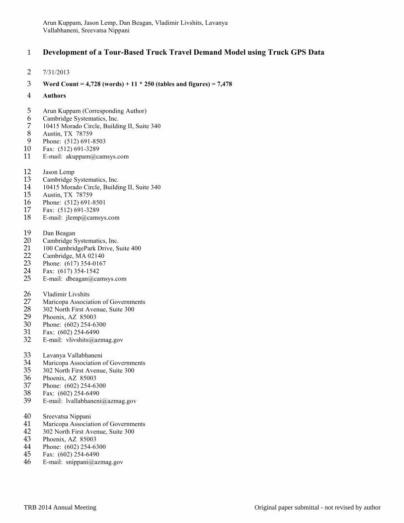
As shown in Table 1, there are four trip ends from this truck tour, which results from six GPS transitional events. 24 Since the truck is returning back to its home base, there are actually only three trip ends or three trips resulting from 25 three legitimate stops. The real truck tour for this particular truck, after the data has been processed, is shown in 26 Figure 2, on the right hand side. The GPS coordinates of these trip ends were then geographically joined to shapefiles 27 of TAZ boundaries and Land Use boundaries, and the appropriate TAZs and land uses of the three stops were 28 identified as shown in Figure 2. 29

30




TABLE 1. Attributes of ATRI GPS Truck Records for Truck ID 357042 on April 1, 2011 1

PRIMARY ANONYMIZED DATA PROCESSED DATA

Truck_ID Date Time Longitude Latitude Event

Trip Distance (miles) Time

From

Last

(min)

Time To

Next

Min)

Speed

From Last

Speed To

Next Event Type TAZ LU

Last Next (MPH) (MPH)

357042 4/1/2011 3:27:06 AM -112.1705 33.4353 1 0.00 0.00 - 3.93 0.00 0.00 stopped

357042 4/1/2011 4:02:38 A.M. -112.1704 33.4353 2 0.00 0.00 3.93 16.10 0.00 0.00 stopped

357042 4/1/2011 3:47:08 A.M. -112.1695 33.4353 3 0.06 6.39 16.1 12.87 0.21 29.79 First Starting 884 Industrial

357042 4/1/2011 4:00:00 A.M. -112.2637 33.4838 4 6.39 2.53 12.87 2.63 29.79 57.6 moving

357042 4/1/2011 4:02:38 A.M. -112.2689 33.5200 5 2.53 4.56 2.63 11.1 57.6 24.67 moving

357042 4/1/2011 4:13:44 A.M. -112.3409 33.5475 6 4.56 0.00 11.1 0.27 24.67 0.42 Stopping

357042 4/1/2011 4:14:00 A.M. -112.3408 33.5475 7 0.00 0.06 0.27 2.1 0.42 1.78 stopped 413 Industrial





357042 4/1/2011 5:02:38 A.M. -112.3381 33.5449 12 0.01 0.05 39.17 20 0.01 0.15 stopped 413 Industrial

357042 4/1/2011 5:22:38 A.M. -112.3383 33.5456 13 0.05 0.13 20 7.37 0.15 1.08 stopped 413 Industrial

357042 4/1/2011 5:30:00 A.M. -112.3385 33.5475 14 0.13 5.22 7.37 15 1.08 20.88 Starting 413 Industrial

357042 4/1/2011 5:45:00 A.M. -112.2673 33.5009 15 5.22 7.53 15 15 20.88 30.11 moving

357042 4/1/2011 6:00:00 A.M. -112.1391 33.4804 16 7.53 0.30 15 1.23 30.11 14.61 moving

357042 4/1/2011 6:01:14 A.M. -112.1345 33.4784 17 0.30 0.00 1.23 0.17 14.61 1.45 Stopping

357042 4/1/2011 6:01:24 AM -112.1346 33.4784 18 0.00 0.00 0.17 1.23 1.45 0.07 stopped 745 Landfill




357042 4/1/2011 7:34:30 A.M. -112.1344 33.4791 22 0.04 2.98 0.87 10.5 2.91 17.04 Starting 745 Landfill

357042 4/1/2011 7:45:00 AM -112.1692 33.4472 23 2.98 0.83 10.5 3.9 17.04 12.77 Moving

357042 4/1/2011 7:48:54 A.M. -112.1702 33.4352 24 0.83 0.00 3.9 13.77 12.77 0.01 Stopping 884 Industrial

357042 4/1/2011 8:02:40 AM -112.1702 33.4352 25 0.00 - 13.77 - 0.01 - Last Stopped




1

2

3

4

5

6

7

8

9

10

11

12

FIGURE 2. ATRI GPS Truck Records for Truck ID 357042 on Apri1 1, 2011 13

14

Purpose: HHs Zone: 734 Depart TOD: PM


April 1, 2011

Purpose: Industry Zone: 287 Depart TOD: Night

Industrial

Industrial

Land Fill,

Sand, Gravel


April 1, 2011

Raw GPS Events

GPS Events = 25

Truck Tours = 1

Trucks = 1

Processed GPS Records

Truck Trip Ends = 3

Truck Tours = 1

Trucks = 1




Based on all of the information that has been processed, it is possible to describe the tour for this example truck. 1 From Table 1, the following information can be derived: 2

• The truck begins its tour at GPS event 3, which is in an industrial land use located in TAZ 884. This first trip 3 in the tour begins at 3:47 am. 4

• The vehicle is moving in GPS event 4 and 5 and stopping in GPS event 6, which is in an industrial land use 5 in TAZ 413. The travel time, based on the time between the starting GPS event and the stopping GPS event 6 at 4:13 am, is 26 minutes. 7

• The truck remains at this location until GPS event 14 at 5:30 am, which means that the truck remained at this 8 trip end for 87 minutes. 9

• It continues to move in GPS events 15 and 16 until it is stopping in GPS event 17, which is located in a 10 Landfill Land Use in TAZ 745, at 6:01 am. This means that there was a 31 minute travel time between the 11 two trip ends. 12

• The truck remains at this location until GPS event 22 at 7:34 am, which means that the truck remained at this 13 trip end for 94 minutes. 14

• It continues to move in GPS event 23 until it is stopping in GPS event 24, which is located in an Industrial 15 Land Use in TAZ 884, where the tour began, at 7:48 am. This means that there was a 15 minute travel time 16 between the two trip ends. There is no duration at the stop calculated because it is the last stop of the tour. 17

This shows that GPS truck records can be processed to provide stop and tour information consistent with the 18 information which would be provided by a truck trip diary. These calculations were automated and conducted for all 19 of the GPS records.. This allows the determination of possible trip and tours. 20

QA/QC of Processed Truck Trip Database 21

In order to further test the data processing for selecting trips from the GPS records, the following tests were done: 22

• Visual Inspection of Stops – The truck stops from a small sample of truck trips will be overlaid onto a highway 23 map. The start and end times of truck stops were also displayed for these sample truck trips. The sequence of 24 stops in terms of time and position on the highway were examined to see if the truck trips have been created 25 correctly and if they follow a certain path. 26

• Aerial Imagery of Stops – The truck stops from a small sample of truck trips will be overlaid on an aerial image 27 of the region using Google Earth. The land use of stops were displayed on to the shape file. The characteristics 28 of the land uses (parking lot, warehouse, mall, etc.) were examined to see if the land uses defined for each stop 29 appear reasonable. 30

In summary, after the examination of the processed truck trip database, it was determined that the criteria and 31 thresholds used in this study were reasonable and corroborated by additional QA/QC measures. Further, random 32 checks that were performed, indicate the likelihood that the methodology employed successfully eliminates false 33 positives, that is, stops that are not true trip ends. 34

TRUCK TOUR-BASED MODEL 35

The basic concept behind truck tour-based models is consistent with activity-based passenger models. These models 36 focus on the tour characteristics of truck trips and are less concerned about what is being carried in the vehicle. One 37 example of a tour-based model was developed in Calgary, Canada, which applies tour-based micro-simulation 38 modeling concepts to urban goods movement modeling that was originally developed for passenger modeling (5). In 39 this model, a series of choice models are employed in order to determine the type of vehicle that will be used to 40 conduct the business of the tour, the purpose of each stop (goods pickup or delivery, service, return to home), and the 41 location of the next stop. 42




The tour-based components track the activity of trucks, and since these components will operate at the 1

vehicle level, they will only generate estimates of a single mode (6). Trucks are associated with establishments, and 2 truck activity is seen as a function of the type of activity that occurs at that establishment. The tour-based components 3 operate within zones, as do the trip-based truck models, and the activity estimates are aggregated for all of the 4 establishments in a zone. The tour-based model described here generates the number of stops that have to be made in 5 each zone for a particular type of truck (e.g., retail, manufacturing), and then string these trips together into tours. The 6 number of stops on a tour, the type of stops, the location and time of day of stops are all estimated from the model 7 based on the type of truck making the tour, the activities conducted by the truck, the characteristics of the stops, and 8 the traffic conditions in the network. 9

Model Estimation 10

There were several truck records that were eliminated due to inability to geocode, unable to find appropriate land uses, 11 and weekend trips. So the processed GPS data yielded a truck tour database that comprises of data from 4,443 trucks 12 that indulged in over 15,000 tours and 39,000 trips. A summary of these trips is shown below: 13

• Retail: 10,639 (26.6%) 14

• Construction: 372 (0.9%) 15

• Farming: 2,777 (6.9%) 16

• Mining: 0 (0.0%) 17

• Households: 3,242 (8.1%) 18

• Government: 1,150 (2.9%) 19

• Warehousing: 8,226 (20.6%) 20

• Transportation: 103 (0.3%) 21

• Office: 491 (1.2%) 22

• Manufacturing: 12,255 (30.7%) 23

• Service: 725 (1.8%) 24

• Total: 39,980 (100.0%) 25

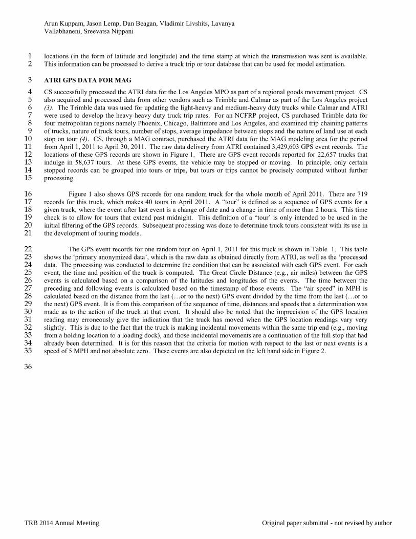
One major assumption was that “tour purpose” was defined by the land use in the truck’s starting location for 26 the tour. That is, if a tour has a “retail” land use as the starting origin, then the whole tour is classified as a “retail 27 tour”. This is the best that could be done because the GPS data does not divulge the industry type of each truck. 28 Upon further examining the data, it was found that the majority of the truck tours are incomplete, that is, the trucks do 29 not return to their home base or the starting origin. Only about eight percent of truck tours completed the tour and 30 returned to starting origin. Truck tours are modeled through a sequence of models as shown in Figure 3. These 31 models include predicting tour generation at the zonal level by tour purpose (i.e., starting land use type), the number 32 of stops for each tour, the purpose of those stops, the location of stops, and the time of day for stops. 33

34




1

FIGURE 3. Tour-Based Truck Model 2

Tour Generation – The tour generation model estimates the number of tours generated in each zone by truck tour 3 purpose. Truck tour purpose is defined as the starting land use type of the tour. Using a combination of existing 4 heavy truck trip rates, tour completion percentage and average stops per tour, the tour rates were computed by tour 5 purpose. These rates are multiplied by the appropriate employment variable for each tour purpose to produce number 6 of tours. 7

Stop Frequency Model – The stop frequency model predicts the number of stops on each truck tour. This is a 8 multinomial logit (MNL) model where the number of stops are the choices that have utilities associated with it. The 9 choices were limited to 11 stops as there were only a fraction of trucks that indulged in more than 11 stops on a single 10 tour. 11

The model estimation results are presented in Table 2. The key variables that were found to be significant in 12 explaining stop frequency were the starting land use of the tour and zonal land use variables. The zonal variables that 13 influence stop making behavior are employment by type and households at the starting zone of the tour. 14

Another key variable was the accessibility index that is expressed as a logarithmic function of travel time and 15 employment at the destination end. 16

Accessibility Index (AI) = ln (1 + Sumj [(exp (-0.05*TTij) / 10000) * EMPj]) 17

Where, 18

Tour

Generation

Heavy

truck tour

rates by

industry

type

Stop

Generation

1 stop

2 stops

……..

11 stops

Tour

Completion

Yes –

return to

home base

No – does

not return

Stop Purpose

One of 10

stop types

•Retail

•Constr.

•Farming

•Resid.

•Govt.

•Warehs.

•Transp.

•Office

•Industrial

•Service

Stop Location

One of

3,000 TAZs

Stop TOD

Choice

1st Stop

TOD (24 1-

hr periods)

Next Stop

TOD (24 1-

hr periods)




TTij is travel time between i and j; 1

EMPj is employment at the destination zone j. 2

Tour Completion Model – The tour completion model predicts whether the tour returns to its starting location or 3 ends at another location. This is a binomial logit choice model with two alternatives: tour does not complete or tour 4 completes. These results are shown in Table 3. 5

The tour purpose and the number of stops on the tour make a significant impact on the tour completion 6 probability. The greater the number of stops on the tour, the less the likelihood of a tour being completed. Industrial 7 and warehousing tours are more prone to completing the tour while farming and service trucks are less likely to 8 completing the tour. The land use variables like employment and accessibility indices do influence the completion of 9 the tour as they do the stop making behavior. 10

11




TABLE 2. Stop Frequency Model 1

Variable Coefficient t-stat

Constant - 2 stops -0.8927 -26.14

Constant - 3 stops -1.1971 -28.13

Constant - 4 stops -1.8482 -36.60

Constant - 5 stops -2.1850 -39.14

Constant - 6 stops -2.7774 -42.44

Constant - 7 stops -3.1509 -42.48

Constant - 8 stops -3.4930 -41.40

Constant - 9 stops -3.9498 -39.64

Constant - 10 stops -4.2327 -37.48

Constant - 11 stops -4.5434 -35.22

Number of Stops – Construction 0.4895 2.26

Log (No. of Stops) – Construction -3.0722 -3.21

Number of Stops – Farming 0.1302 2.97

Log (No. of Stops) - Farming -0.4224 -3.23

Number of Stops - Household 0.0186 1.13

Number of Stops - Government 0.1479 2.18

Log (No. of Stops) - Government -0.3833 -1.82

Number of Stops - Warehousing 0.1958 5.41

Log (No. of Stops) - Warehousing -0.7160 -4.01

Number of Stops – Industrial 0.2074 4.69

Log (No. of Stops) - Industrial -0.7632 -3.16

(Total Emp. Start Zone) / (No. of Stops) -0.0001 -4.24

(Total HHs Start Zone) / (No. of Stops) -0.0002 -4.34

(AI to Construction Emp.) / (No. of Stops) - Construction -2.4742 -2.54

(AI to Wholesale Emp.) / (No. of Stops) - Warehousing -0.2225 -1.17

(AI to Manufacturing Emp.) / (No. of Stops) - Industrial -0.2059 -1.07

Observations 15,428

Log Likelihood at Zero -36994.7283

Log Likelihood with Constants Only -26251.8629

Log Likelihood at Convergence -26191.4987

Rho-Squared wrt Zero 0.2920

Rho-Squared wrt Constants Only 0.0023

2 3




TABLE 3. Tour Completion Model 1

Variable Coefficient t-stat

Constant -3.9129 -25.74

Tour Purpose = Construction, Transportation, Office, or Service -1.7912 -4.48

Tour Purpose = Farming -2.7742 -4.25

Tour Purpose = Household -0.3716 -1.02

Tour Purpose = Government -0.6500 -1.63

Tour Purpose = Warehouse 0.8176 4.04

Tour Purpose = Industrial 0.7998 3.67

Number of Stops on Tour 0.1123 3.26

Number of Stops - Farming Tour 0.1433 1.90

Number of Stops - Household Tour 0.1503 2.21

Number of Stops - Government Tour 0.1725 2.18

Number of Stops - Warehouse Tour 0.1468 3.84

Number of Stops - Industrial Tour 0.1641 4.17

Total Employment in Start Zone 0.0004 7.75

Total Emp. - Farming Tour 0.0007 2.56

Total Emp. - Household Tour -0.0004 -2.48

Total Emp. - Warehouse Tour -0.0003 -4.82

Total Emp. - Industrial Tour -0.0003 -3.87

Observations 15,428






2

3




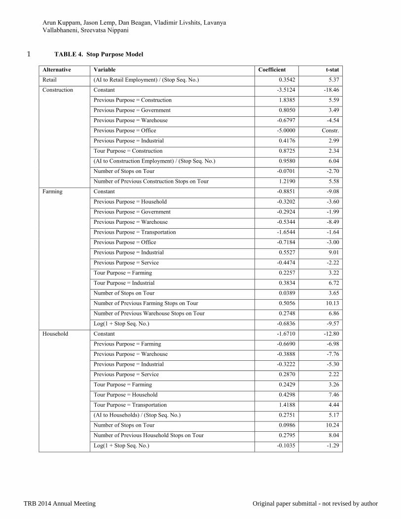
Stop Purpose Model – The stop purpose model predicts the purpose (i.e., land use type) of each stop that is predicted 1 by the stop frequency model. This is a MNL model that predicts purpose of the stops in sequence, that is, from the 2 first stop to the last stop. The alternatives or choices used in this model are the same land use types as defined in the 3 trip-based truck model. Because there are no tour observations for mining, only the following 10 alternatives were 4 used: 5

• Retail 6 • Construction 7 • Farming 8 • Households 9 • Government 10 • Warehousing 11 • Transportation 12 • Office 13 • Industrial/Manufacturing 14 • Service (or Other) 15

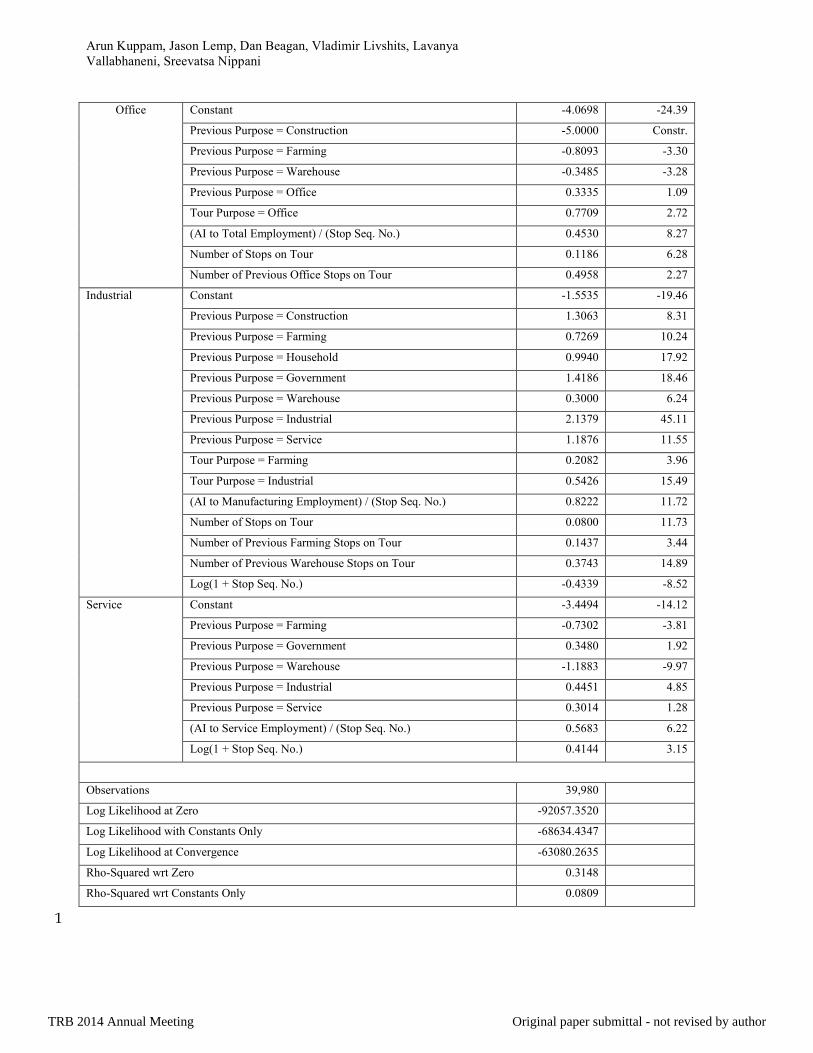
The estimated model is presented in Table 4. All the coefficients are segmented by tour purpose. This influences 16 the type of stop purpose significantly. The starting land use of the tour influences the stop purpose of subsequent 17 stops on the tour. Other key explanatory variables that were found to be significant in this model are previous stop 18 purpose, where certain purpose to purpose interchanges are much more prevalent than others, and the number of 19 previous stops by purpose, which includes the total number of stops of each type already simulated for the tour. The 20 accessibility indices that are segmented by tour purpose were also found to be significant in explaining the stop 21 purpose. The zonal land use variables including employment by type and households at the starting zone also 22 influence the stop purpose. 23

24 25 26




TABLE 4. Stop Purpose Model 1

Alternative Variable Coefficient t-stat

Retail (AI to Retail Employment) / (Stop Seq. No.) 0.3542 5.37

Construction Constant -3.5124 -18.46

Previous Purpose = Construction 1.8385 5.59

Previous Purpose = Government 0.8050 3.49

Previous Purpose = Warehouse -0.6797 -4.54

Previous Purpose = Office -5.0000 Constr.

Previous Purpose = Industrial 0.4176 2.99

Tour Purpose = Construction 0.8725 2.34

(AI to Construction Employment) / (Stop Seq. No.) 0.9580 6.04

Number of Stops on Tour -0.0701 -2.70

Number of Previous Construction Stops on Tour 1.2190 5.58

Farming Constant -0.8851 -9.08

Previous Purpose = Household -0.3202 -3.60

Previous Purpose = Government -0.2924 -1.99


Previous Purpose = Transportation -1.6544 -1.64

Previous Purpose = Office -0.7184 -3.00


Previous Purpose = Service -0.4474 -2.22

Tour Purpose = Farming 0.2257 3.22



Number of Previous Farming Stops on Tour 0.5056 10.13

Number of Previous Warehouse Stops on Tour 0.2748 6.86

Log(1 + Stop Seq. No.) -0.6836 -9.57

Household Constant -1.6710 -12.80

Previous Purpose = Farming -0.6690 -6.98


Previous Purpose = Industrial -0.3222 -5.30

Previous Purpose = Service 0.2870 2.22


Tour Purpose = Household 0.4298 7.46

Tour Purpose = Transportation 1.4188 4.44

(AI to Households) / (Stop Seq. No.) 0.2751 5.17


Number of Previous Household Stops on Tour 0.2795 8.04

Log(1 + Stop Seq. No.) -0.1035 -1.29




Government Constant -3.0937 -27.07






Tour Purpose = Government 0.7976 6.35

(AI to Total Employment) / (Stop Seq. No.) 0.3455 7.83


Number of Previous Government Stops on Tour 0.4729 5.84

Warehouse Constant 0.0800 1.13

Previous Purpose = Construction -1.6150 -5.82


Previous Purpose = Household -0.8162 -14.67

Previous Purpose = Government -1.4950 -12.55


Previous Purpose = Office -0.1851 -1.91

Previous Purpose = Industrial -1.3035 -24.01

Previous Purpose = Service -1.1516 -8.46

Tour Purpose = Warehouse 0.0758 2.20



(AI to Wholesale Employment) / (Stop Seq. No.) 0.7901 8.93



Number of Previous Industrial Stops on Tour 0.1793 9.37

Log(1 + Stop Seq. No.) -0.6628 -12.45

Transportation Constant -6.3091 -15.41

Previous Purpose = Construction -5.0000 Constr.

Previous Purpose = Household 0.8515 2.72



Previous Purpose = Transportation -1.0984 -1.81





Number of Previous Transportation Stops on Tour 1.2871 4.46




Office Constant -4.0698 -24.39

Previous Purpose = Construction -5.0000 Constr.



Previous Purpose = Office 0.3335 1.09

Tour Purpose = Office 0.7709 2.72



Number of Previous Office Stops on Tour 0.4958 2.27

Industrial Constant -1.5535 -19.46


Previous Purpose = Farming 0.7269 10.24

Previous Purpose = Household 0.9940 17.92


Previous Purpose = Warehouse 0.3000 6.24





(AI to Manufacturing Employment) / (Stop Seq. No.) 0.8222 11.72


Number of Previous Farming Stops on Tour 0.1437 3.44


Log(1 + Stop Seq. No.) -0.4339 -8.52

Service Constant -3.4494 -14.12






(AI to Service Employment) / (Stop Seq. No.) 0.5683 6.22

Log(1 + Stop Seq. No.) 0.4144 3.15

Observations 39,980






1




Stop Location Choice Model – The stop location choice model predicts the location of each stop simulated for the 1 tour, and is similar in design to a destination choice model employed for distributing passenger trips. Every zone in 2 the region is a potential choice for this model. Similar to any other destination choice model, size variables are 3 included in the model. These include employment at the stop location by type. 4

Two types of accessibility variables are included in the model: 5

• Direct zone-to-zone accessibility variables or travel time between (a) previous stop location to current stop 6 location, and (b) first stop location to current stop location. 7

• Aggregate accessibility measures – This is important to describe the accessibility of a stop zone to 8 employment types corresponding to the next stop purpose. 9

Other variables include zonal area type such as CBD, rural, and suburban. This is defined as a combination of 10 employment and population density. Most of these variables are segmented by the starting land use of the tour, 11 previous stop purpose, current stop purpose, and number of stops on tour by purpose. 12

13




TABLE 5. Stop Location Choice Model 1

Utility Variables Coefficient t-stat

Intrazonal with Previous Stop 1.9438 16.89

Intrazonal with Tour Start Zone 3.2847 25.13

Intrazonal with Previous Stop & Tour Start Zone -4.2323 -29.50

Intrazonal with Previous Stop - Stop Purpose = WHL,MNF -0.9357 -7.71

Intrazonal with Tour Start Zone - Stop Purpose = WHL, MNF 0.4606 3.41

Intrazonal with Previous Stop - Prev. Purpose = WHL, MNF -0.4074 -3.33

Intrazonal with Tour Start Zone - Prev. Purpose = WHL, MNF 0.1540 1.13

Log(1 + Pk Travel Time) -1.9154 -89.84

Log(1 + Pk Travel Time) - Total Stops on Tour >= 3 -0.2284 -7.14

Log(1 + Pk Travel Time) - First Stop on Tour, Total Stops on Tour >= 2 0.0919 3.44

Log(1 + Pk Travel Time) * Total Stops on Tour -0.0248 -4.59

Log(1 + Pk Return Travel Time) / (Stops Remaining + 1) - Total Stops on Tour >=2 -0.3907 -14.99

AI to Retail Employment - HH stop, RET next stop 0.9715 2.37

AI to Farming Employment - FRM next stop 2.2147 10.16

AI to Total Employment - HH stop, GOV next stop 2.7709 2.83

AI to Warehouse Employment + AI to Ind. Emp. - WHL stop 0.6668 16.12

AI to Warehouse Employment - Transportation Stop 2.2925 2.95

AI to Total Employment - HH stop, OFF next stop 3.3334 2.03

AI to Warehouse Employment + AI to Industrial Emp. - MNF stop 0.5931 15.48

AI to Service Employment - HH stop, SRV next stop 2.6099 2.33

Size Variables

Retail Stop, Total Emp. (Retail Emp is the base variable) -3.0102 -64.31

Construction Stop, Total Emp. (Construction Emp is the base variable) -1.2670 -4.36

Farming Stop, Total Emp. (Farming Emp is the base variable) -2.2886 -15.00

Household Stop, Households (Base variable) 0.0000 n/a

Government Stop, Total Emp. (Base variable) 0.0000 n/a

Wholesale Stop, Total Emp. (Warehouse Emp is the base variable) -4.7998 -51.12

Wholesale Stop, Industrial Emp. (Warehouse Emp is the base variable) -1.1768 -15.30

Transportation Stop, Total Emp. (Base variable) 0.0000 n/a

Office Stop, Total Emp. (Base variable) 0.0000 n/a

Manufacturing Stop, Total Emp. (Industrial Emp is the base variable) -3.8941 -43.09

Manufacturing Stop, Warehouse Emp. 0.9711 15.37

Service Stop, Service Emp. (Base variable) 0.0000 n/a

Observations 39,803




2

3




Stop Time of Day Choice Model – The stop time of day choice model predicts the time period of each stop on a tour. 1 Two separate models were estimated for time of day choice. The first is used for the departure time of a tour’s first 2 trip, and the second is used for subsequent trips. The reason for defining two separate models is that subsequent trip 3 departure times should depend, in part, on the timing of a tour’s previous trips. Thus, duration between trips is an 4 important variable in the subsequent time of day choice model. Both models are MNL models, where the alternatives 5 include each one-hour period of the day (24 alternatives in total). In application, the one-hour periods are aggregated 6 back to the four existing time periods used in the regional model – AM peak, mid-day, PM peak and night. 7

There are two main reasons for defining the alternatives as one-hour periods rather than the four existing time 8 periods used in MAG’s regional model. First, this ensures alternatives are of uniform size, and no special 9 considerations are needed to adjust variables for the size. Second, the more refined time period definitions should 10 allow travel time between stops to have important implications. In addition, it allows availability restrictions to be 11 more well-defined for the subsequent stop period model. Since truckers involved in interstate commerce are not 12 allowed to work more than 12 consecutive hours by law, availability restrictions are important. 13

The following variables were found to be significant in the time of day choice models shown in Tables 6 and 7: 14

• Starting land use for the tour; 15

• Previous and current stop purpose; 16

• Number of stops on tour by purpose; 17

• Travel distance/time from previous stop to current stop; 18

• Previous stop time of day (if not first stop). 19




TABLE 6. Time of Day Choice Model – First Trip 1

TOD Segment Variable Coefficient t-stat

AM All Constant -0.8526 -4.07

Tour Purpose = FRM, WHL, or MNF Constant 0.6694 4.29

First Stop Purpose = FRM, WHL, or MNF Constant 0.4608 5.14

All Total Stops on Tour 0.1865 4.77

Tour Purpose = FRM, WHL, or MNF Total Stops on Tour -0.2781 -5.65

All Log(1 + Pk Travel Time to First Stop) -0.2832 -5.69

MD All Constant -1.8406 -19.13

First Stop Purpose = FRM, WHL, or MNF Constant 0.1810 4.27



All Indicator for Completed Tour 0.6124 8.96

All Log(1 + Pk Travel Time to First Stop) 0.1739 6.89

All MD Shift Variable 0.4333 23.44

Tour Purpose = FRM, WHL, or MNF MD Shift Variable -0.1189 -5.72

PM All Constant 0.5981 6.23

Tour Purpose = FRM, WHL, or MNF Constant -0.4432 -5.53



All Log(1 + Pk Travel Time to First Stop) 0.0901 4.06

All PM Shift Variable -0.1309 -6.19

Tour Purpose = FRM, WHL, or MNF PM Shift Variable 0.1111 4.14

NT All NT Shift Variable Early -0.0953 -5.46

Tour Purpose = FRM, WHL, or MNF NT Shift Variable Early -0.0417 -2.00

All NT Shift Variable Late 0.1375 10.53

Tour Purpose = FRM, WHL, or MNF NT Shift Variable Late -0.0314 -2.04

Observations 15,196


Log Likelihood wrt Constants Only -46068.1240



Rho-Squared wrt Constants 0.0115

2




TABLE 7. Time of Day Choice Model – Subsequent Trips 1

Variable Coeff. t-stat

Constant - Same 1-hr Period as Previous Stop -2.881 -8.1

Constant - First 1-hr Period after Previous Stop -1.664 -5.2

Constant - Second 1-hr Period after Previous Stop -1.742 -6.1

Constant - Third 1-hr Period after Previous Stop -1.775 -7.0

Constant - Fourth 1-hr Period after Previous Stop -1.701 -7.7

Constant - Fifth or Sixth 1-hr Period after Previous Stop -1.497 -8.4

Constant - Seventh or Eighth 1-hr Period after Previous Stop -1.138 -8.9

Departure Time Shift Variable ^^ -0.946 -21.5

Departure Shift - Prev. Stop = Construction 0.150 1.7

Departure Shift - Prev. Stop = Warehouse 0.075 6.8

Departure Shift - Prev. Stop = Transportation -0.159 -1.6

Departure Shift - Prev. Stop = Manufacturing 0.102 5.7

Departure Shift * Log (1 + Peak Travel Time to Previous Stop) 0.144 28.7

Departure Shift * Total Number of Stops on Tour -0.042 -17.9

Departure Shift * Construction Stops on Tour -0.069 -2.7

Departure Shift * Households Stops on Tour -0.031 -4.8

Departure Shift * Government Stops on Tour -0.037 -3.5

Departure Shift * Service Stops on Tour -0.053 -3.4

Time / Stops Remaining ^^^ 0.037 2.0

Time / Stops Remaining - Prev. Stop = Construction 0.183 1.7

Time / Stops Remaining - Prev. Stop = Farming 0.083 3.0

Time / Stops Remaining - Prev. Stop = Manufacturing 0.047 1.9

Observations 22,648






^^ This variable is equal to the number of periods the alternative is after the departure period of the previous stop. 2 ^^^ This variable is computed as (16 - Departure Shift wrt First Trip Departure Period) / (1 + Total Number of Stops 3 Remaining) 4

5




MODEL CALIBRATION 1

All the tour model components were coded in GIS-DK and implemented in TransCAD. Each component was 2 individually assessed and calibrated. The reasonability of the explanatory variables were determined by their 3 magnitude, t-statistic and their relation to the dependent variable. Some of the key findings include: 4

• Construction tours are less prone to making more stops, while government-related tours have a higher 5 propensity to making more stops. 6

• More number of stops on a tour make the truck less likely to complete the tour. 7

• Stop purpose is often strongly influenced by the tour type or the first land use of the truck origin. 8

• Travel time has a negative effect on location choice utility, and is more pronounced as the number of stops 9 on tour increase. 10

• Previous stop purpose has a significant impact on the time period of the next stop. 11

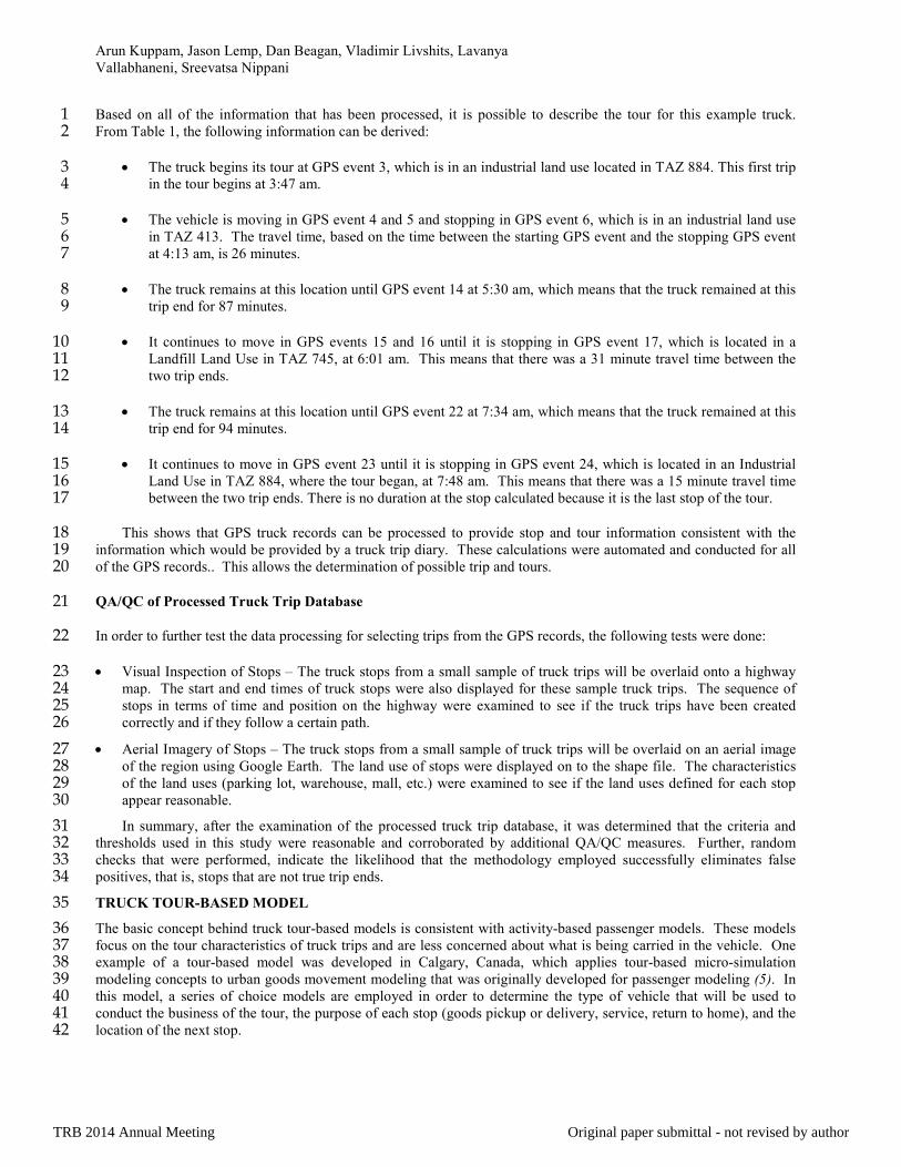
The individual model outputs were also compared against the truck GPS data to assess the model performance. 12 These results are depicted in Figure 4. These comparisons indicate that the model components are predicting very 13 closely to the observed data for the most part. There are some differences which can be further improved upon with 14 more rigorous calibration and validation of the model. 15

16




FIGURE 4. Truck Model Outputs versus Truck GPS Data 1

2

0.000.501.001.502.002.503.00

No

of

Sto

ps

Number of Stops by Tour Type

Target

Model

0.0%

5.0%

10.0%

15.0%

20.0%

25.0%

30.0%

35.0%

Ret Cns Frm Min Hhs Gov War Trn Off Ind Srv

Pe

rce

nt

of

Sto

p P

urp

ose

s

Stop Purposes

Stop Purpose Distribution

Model

Target

0%

2%

4%

6%

8%

10%

1 3 5 7 9 11 13 15 17 19 21 23

TOD of First Stop

Model Target

0%

2%

4%

6%

8%

10%

1 3 5 7 9 11 13 15 17 19 21 23

TOD of Subsequent Stops

Model Target




CONCLUSIONS 1

It is important for agencies to account for freight movements and a major part of freight is trucks. Therefore, it is 2 important to invest wisely in data collection methods and meet the desired targets in terms of sample sizes so that a 3 robust truck trip model or a tour-based model can be developed. This effort described in this paper demonstrated that 4 the purchasing and processing of truck GPS data is definitely a cost effective way to develop a tour-based truck model 5 that requires a large volume of information on truck travel. 6

REFERENCES 7

1. American Transportation Research Institute, Methods of Travel Time Measurement in Freight-Significant 8 Corridors. Paper presented at the January 2005 Annual Meeting of the Transportation Research Board, January 9 2005. 10

2. Kuppam, A., V. Livshits, L. Vallabhaneni, M. Zmud, J. Wilke, R. Elmore-Yalch, M. Fischer. An Approach for 11 Collecting Internal Truck Travel Data: Lessons Learned from Maricopa Association of Government’s Internal 12 Truck Travel Study. Paper presented at the 2008 Annual Meeting of the Transportation Research Board. January 13 2008. 14

3. Cambridge Systematics, Inc. SCAG Task 4 Data Verification and Analysis, Technical Memorandum. October 15 2010. 16

4. Cambridge Systematics, Inc. Freight-Demand Modeling to Support Public-Sector Decision Making, NCFRP 17 Report 8, 2010. 18

5. City of Calgary, 2001 Regional Transportation Model: Commercial Vehicle Model, August 2006. 19 6. Fischer, M. J., An Innovative Framework for Modeling Freight Transportation in Los Angeles County, January 20

2005. 21

22


Documents

Development of a Tour-Based Truck Travel Demand Model ...docs.trb.org/prp/14-4293.pdf · 1 Development of a Tour-Based Truck Travel Demand Model using Truck GPS Data ... 5 trucks