Embed Size (px)
Citation preview
H:\PAPERS_Conferences\EI_Conferences\EMIS08\Gerry_John\WASBAQS_EI_part1_draft_053008.doc 1
Development of an Air Emission Inventory for the Western Arizona Sonora Border Air Quality Study (WASBAQS) Part 1 – U.S. Emission Inventory
Gerard Mansell, John Grant, Amnon Bar-Ilan, Alison K. Pollack ENVIRON International Corporation, 773 San Marin Dr, Suite 2115, Novato, CA 94998
Martinus E. Wolf and Paula G. Fields Eastern Research Group, Inc. (ERG), 8950 Cal Center Dr, Suite 348, Sacramento, CA 95826-3259
[email protected] ABSTRACT
In response to concerns about high particulate matter (PM) and air toxics concentrations that have been measured along the U.S./Mexico border, the Arizona Department of Environmental Quality (ADEQ) is conducting the Western Arizona-Sonora Border Air Quality Study (WASBAQS) which is the third in a series of studies of pollution along the Arizona/Mexico border. The principal objectives of the WASBAQS are to: (1) Fully characterize the gaseous and particulate air pollutants, (2) Estimate the risk to human health for the populations of Yuma, Arizona; San Luis Río Colorado, Sonora; and rural northeastern Baja California areas, and (3) Evaluate proposed control strategies to improve air quality in the border region of southwest Arizona, southeast California, and Mexico (states of Sonora and Baja California) (WASBAQS Study Area). The WASBAQS seeks to achieve these objectives in four phases: 1) air quality monitoring, 2) development of a gridded emissions inventory, 3) air quality modeling and control strategy evaluation, and 4) risk assessment.
The emission inventory includes estimates of all criteria pollutants, ammonia, particulate matter and hazardous air pollutants (HAPs) for calendar year 2005. All relevant emission sources within the study area were considered, including point sources (those emitting 10 or more tons of a relevant pollutant per year), area sources (e.g., agricultural tillage, pesticide and fertilizer usage, and disperse sources of VOCs such as gasoline dispensing facilities, etc.), on-road mobile sources (i.e., tailpipe exhaust, tire and brake wear, road dust from vehicles traveling on paved and unpaved roadways), and nonroad mobile sources (e.g., lawn and garden equipment, agricultural equipment, etc.). The inventory also includes emissions from wildfires and windblown fugitive dust. Where practical and available, local data sources and source-specific information were incorporated into the inventory. In addition, HAP emissions estimates were developed using speciation data from the most recent version of the U.S. EPA’s SPECIATE database. The geographic extent of the inventory includes portions of Yuma County (AZ), Imperial County (CA), and the northern portions of the Mexican states of Sonora and Baja California.
This paper discusses the development of the WASBAQS emissions inventory for the U.S. portion of the study domain. In addition, for certain source categories (i.e., windblown fugitive dust and ammonia), both the U.S. and Mexican portions of the domain are estimated as a whole – the development of emission estimates from these sources are also presented and discussed in this paper. The development of the WASBAQS emission inventory for the Mexico portion of the study region is presented in a companion paper (i.e., Part 2).
H:\PAPERS_Conferences\EI_Conferences\EMIS08\Gerry_John\WASBAQS_EI_part1_draft_053008.doc 2
INTRODUCTION Background
The Western Arizona-Sonora Border Air Quality Study (WASBAQS) is being conducted by the
Arizona Department of Environmental Quality (ADEQ) in response to concerns about high particulate matter (PM) and air toxics concentrations that have been measured along the U.S./Mexico border, and is the third in a series of studies of pollution along the Arizona/Mexico border. The principal objectives of the WASBAQS are to: (1) Fully characterize the gaseous and particulate air pollutants, (2) Estimate the risk to human health for the populations of Yuma, Arizona; San Luis Río Colorado, Sonora; and rural northeastern Baja California areas, and (3) Evaluate proposed control strategies to improve air quality in the border region of southwest Arizona, southeast California, and Mexico. The WASBAQS seeks to achieve these objectives in four phases: 1) air quality monitoring, 2) development of a gridded emissions inventory, 3) air quality modeling and control strategy evaluation, and 4) risk assessment.
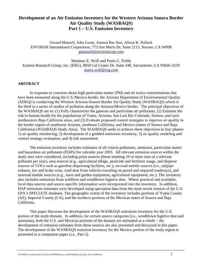
Figure 1. The WASBAQS modeling domain.
Inventory Scope
The WASBAQS study area encompasses approximately 1,275,073 acres (1,992 square miles) with Yuma, Arizona in the northern portion of the study area, and San Luis Río Colorado, Sonora, Mexico in the southern portion of the study area (See Figure 1). The study area includes the following portions of Arizona, Mexico, and California:
Southern part of Yuma County, Arizona; Northwestern part of Sonora, Mexico; Northeastern part of Baja California; and Far southeastern portion of Imperial County, California.
The study area contains two moderately sized cities – Yuma, Arizona and San Luis Río Colorado, Sonora, Mexico – as well as numerous smaller cities throughout the agricultural areas of southwestern Yuma County and Sonora, Mexico.
H:\PAPERS_Conferences\EI_Conferences\EMIS08\Gerry_John\WASBAQS_EI_part1_draft_053008.doc 3
The emission inventory source types include industrial point sources (those emitting 10 or more
tons of a relevant pollutant per year) area sources (e.g., agricultural tillage, pesticide and fertilizer usage, and disperse sources of VOCs such as gasoline dispensing facilities, etc.), on-road mobile sources (i.e., tailpipe exhaust, tire and brake wear, road dust from vehicles traveling on paved roadways), and off-road mobile sources (e.g., lawn and garden equipment, agricultural equipment). The inventory also includes emissions from wildfires and windblown fugitive dust. Pollutants inventoried for the WASBAQS project include criteria pollutants (PM2.5, PM10, SOx, NOx, VOC, CO and NH3) as well as the 189 Hazardous Air Pollutants (HAPs) listed in the 1990 Clean Air Act Amendments, under Title III. The temporal resolution of the emissions inventory is hourly for a typical weekday and typical weekend day for each season of calendar year 2005. METHODS AND DATA SOURCES
The emission estimation methodologies and data sources for the development of the US portion of the WASBAQS inventory are presented below for each source category. In addition, the development of ammonia and windblown dust emissions for both the US and Mexico portions of the domain, are also included due to the regional emissions modeling approaches used for these source categories. Detailed discussions are provided for cases where local data were available and used. In the interest of brevity, for all other sources, only brief descriptions and key references are provided; the reader is referred to the W ASBAQS project report and documentation for more detailed information regarding estimation methodologies and data sources. Speciation
Unless otherwise noted, all emissions of pollutants not directly estimated based on emission factors were estimated using EPA SPECIATE4.0 particulate and gaseous profiles. Emissions were generated based on SPECIATE4.0 profiles for species identified in the work plan for the study: 189 hazardous air pollutants, hydrogen sulfide, and identified additional PM10 and PM2.5 metal and aerosol species. For a given source category, VOC, PM2.5, or PMC emissions were multiplied by the selected SPECIATE4.0 profile weight fractions to estimate SPECIATE4.0 based emissions. EPA’s latest cross reference table was used to identify appropriate speciation profiles available in the SPECIATE4.0 database. Although several PM2.5, PM10 and PMC profiles are available in the SPECIATE4.0 database, this cross reference table only includes the simplified PM2.5 profiles that carry five major PM components: sulfate, nitrate, organic carbons, elemental carbons, and other fine PM. For this study effort, ENVIRON acquired more detailed profiles based on descriptions provided in the database. PMC profiles not available in the database were replaced by PM2.5 profiles for the same source category.
STATIONARY POINT SOURCES
The only major point sources in the modeling domain are in Yuma County: the APS Yucca Power Plant near Yuma, and Yuma Cogeneration Associates. APS operates four natural gas-fueled combustion turbine units at the Yucca Power Plant that produce nearly 150 megawatts of electricity. The plant has one other combustion turbine unit and one steam unit owned by the Imperial Irrigation District. The Yuma Cogeneration Associates facility, located at 280 North 27th Drive in Yuma, has a 55 MW (nominal) combined cycle gas turbine. The facility generates electricity for sale to San Diego Gas & Electric, and also provides low-pressure steam and intermediate-pressure steam to an industrial customer in the vicinity. Calendar year 2005 annual emissions for NOx, VOC, and CO for these two sources were provided by ADEQ staff.
H:\PAPERS_Conferences\EI_Conferences\EMIS08\Gerry_John\WASBAQS_EI_part1_draft_053008.doc 4
ADEQ staff also provided Yuma County 2005 minor point source emissions. Only those sources within the modeling domain were included. The ADEQ provided emissions data for criteria pollutants and total HAPs, SCCs and stack parameters. In addition, the specific pollutants included in the total HAP emissions were provided, although the percentage of each pollutant was not provided.
For the Yucca Power Plant, 2005 hourly continuous emissions monitoring (CEM) data was not available from the U.S. EPA’s Clean Air Markets Division (CAMD) Acid Rain Program. For the Yuma Cogeneration Associates, facility-specific operating schedule information, required for generation of temporal profiles were not available. In lieu of CEM and facility-specific data, temporal profiles developed by the Western Regional Air Partnership (WRAP), and other Regional Planning Organizations (RPOs), were applied to the two major stationary point sources in the US portion of the modeling domain. The profiles were developed based on typical throughput data for calendar year 2002 to represent a typical operating schedule based on an analysis of multiple years of facility-specific CEM data, applicable for all major point sources within the State of Arizona. For the minor point sources, the U.S. EPA default temporal profiles were applied. Spatial allocation of point source emissions were based on geographic coordinates for each of the major sources, as well as many of the minor point sources. For minor point sources were no coordinates are available (e.g., several minor point sources are movable sources such as portable soil vapor extraction units, rock crushers, portable concrete batch plants, etc.), the associated emissions were spatially distributed uniformly across the Yuma County portion of the modeling domain. AREA SOURCES
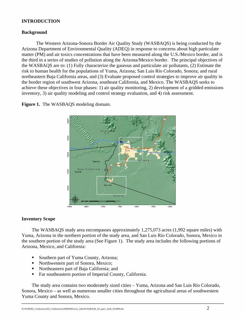
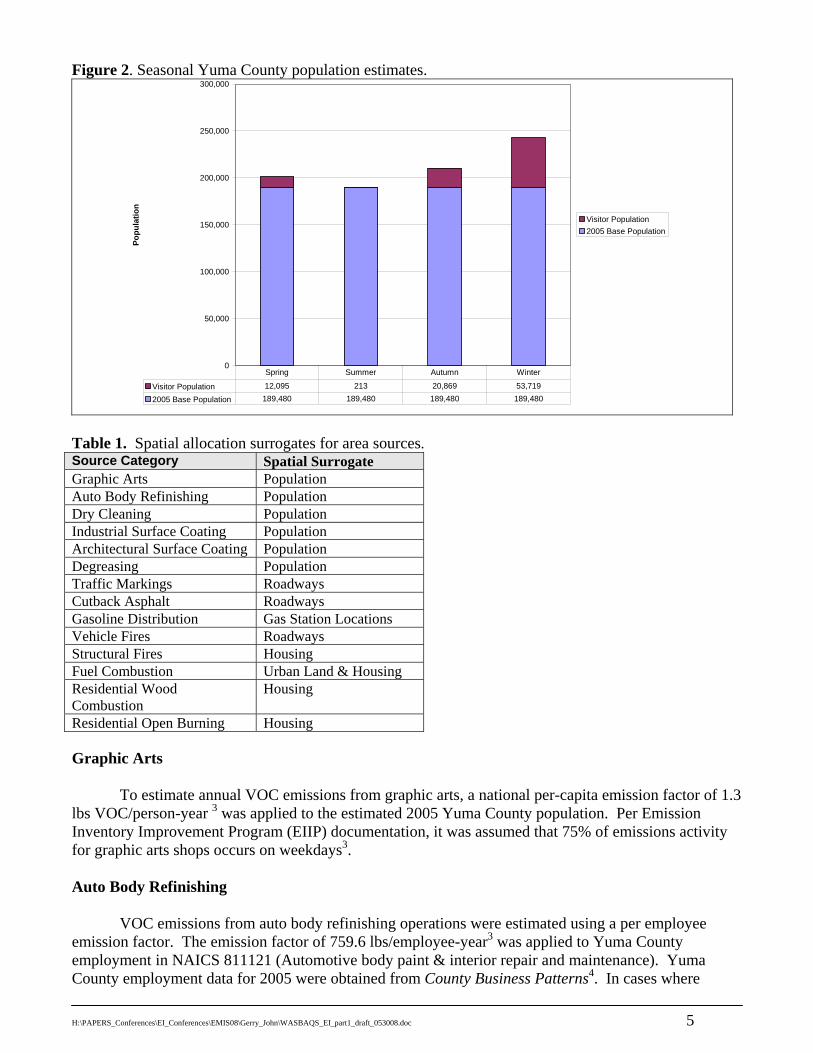
The development of the non-point stationary area sources are described in this section. For many of these sources, emission estimates are based on population using per-capita emission factors. Yuma County population was estimated as the sum of year-round population from Arizona Department of Economic Security (ADES) estimates1 and winter visitor population estimates derived from a study of winter visitor population in Yuma2. Winter visitor population by season was estimated by adding the census population and winter visitor population in each month and taking this sum to estimate seasonal population. As shown in Figure 2, winter visitor population is a significant fraction of total Yuma County population in the winter season. Seasonal emissions were calculated by multiplying annual emission estimates by the ratio of estimated seasonal population (including winter visitors) to average annual population (including winter visitors), thus incorporating temporal changes in population from season to season.
Spatial surrogates based on population, housing. Roadways and land use were developed and used to allocate stationary area sources for grid modeling. The source category-surrogate assignments are presented below in Table 1.
H:\PAPERS_Conferences\EI_Conferences\EMIS08\Gerry_John\WASBAQS_EI_part1_draft_053008.doc 5
Figure 2. Seasonal Yuma County population estimates.
0
50,000
100,000
150,000
200,000
250,000
300,000
Popu
latio
n
Visitor Population2005 Base Population
Visitor Population 12,095 213 20,869 53,719
2005 Base Population 189,480 189,480 189,480 189,480
Spring Summer Autumn Winter
Table 1. Spatial allocation surrogates for area sources. Source Category Spatial Surrogate Graphic Arts Population Auto Body Refinishing Population Dry Cleaning Population Industrial Surface Coating Population Architectural Surface Coating Population Degreasing Population Traffic Markings Roadways Cutback Asphalt Roadways Gasoline Distribution Gas Station Locations Vehicle Fires Roadways Structural Fires Housing Fuel Combustion Urban Land & Housing Residential Wood Combustion
Housing
Residential Open Burning Housing Graphic Arts
To estimate annual VOC emissions from graphic arts, a national per-capita emission factor of 1.3 lbs VOC/person-year 3 was applied to the estimated 2005 Yuma County population. Per Emission Inventory Improvement Program (EIIP) documentation, it was assumed that 75% of emissions activity for graphic arts shops occurs on weekdays3. Auto Body Refinishing
VOC emissions from auto body refinishing operations were estimated using a per employee emission factor. The emission factor of 759.6 lbs/employee-year3 was applied to Yuma County employment in NAICS 811121 (Automotive body paint & interior repair and maintenance). Yuma County employment data for 2005 were obtained from County Business Patterns4. In cases where
H:\PAPERS_Conferences\EI_Conferences\EMIS08\Gerry_John\WASBAQS_EI_part1_draft_053008.doc 6
employment data were given as a range, employment was estimated to be the average of the two extremes (e.g. given range = 0 – 19, value used = 9.5).
For VOC emissions, a 33 percent reduction was applied to reflect the promulgation of national VOC rules. This is the estimated total reduction of VOCs emanating from auto body refinishing to be achieved by the national VOC rule5. EIIP documentation suggests that auto body refinishing shops typically operate five days per week3. Dry Cleaning
VOC emissions from dry cleaning operations were estimated using a per employee emission factor. The emission factor of 1800 lbs/employee-year3 was applied to county level employment in NAICS 812320 (Dry cleaning and laundry services, except coin-operated). Coin-operated dry cleaners (NAICS 812310) were not included in the calculation for VOCs because coin-operated dry cleaners use PERC only, which contributes to HAP emissions, but is not included in VOC calculations because PERC is not considered photo-chemically reactive. Yuma County 2005 employment was obtained from County Business Patterns4. Per EIIP, five day/week operation schedule is assumed3. Industrial Surface Coating
VOC emissions from industrial surface coating operations were estimated using either per employee emission factors or per capita emission factors. There are ten distinct surface coating operations with distinct per employee emission factors and three operations with per capita emission factors, for a total of 13 categories. For each type of operation with a per employee factor, the emission factor was applied to county level employment in numerous NAICS categories. The EIIP document gives source categories with corresponding SIC codes, but given that the most recent County Business Patterns use NAICS codes, the corresponding NAICS codes were identified for use3,4. 2005 Yuma County employment by NAICS was obtained from County Business Patterns. For the three source categories with per capita emission factors, those factors were applied to the 2005 Yuma County population estimate.
There is no seasonal variation of industrial surface coating emissions, and a 5 day/week operation schedule is assumed3. Architectural Surface Coating
County usage of architectural surface coatings was estimated based on a national per-capita use factor. This factor was developed by dividing the 2005 national usage of surface coatings by the estimated 2005 national population4.
Combining usage factors with estimated 2005 Yuma County populations provides the total county usage of solvent-based and water-based coatings. Emissions for each coating type were calculated as the product of usage and the EIIP emission factors of 3.87 lb VOC/gal for solvent-based coatings and 0.74 lb VOC/gal for water-based coatings. The resulting emissions were then decreased by 20% to obtain the final VOC emissions. This reduction accounts for a national VOC rule promulgated after the development of the emission factors, for which the estimated impact on emissions was a reduction of 20%4.
Surface coating is not practicable at temperatures below 50 degrees3. Monthly average temperatures in Yuma County are in excess of 50 degrees year-round. Therefore, it was assumed that emissions will occur uniformly year-round in Yuma County. Activity is assumed to occur seven days per week per EIIP documentation3.
H:\PAPERS_Conferences\EI_Conferences\EMIS08\Gerry_John\WASBAQS_EI_part1_draft_053008.doc 7
Degreasing
In order to achieve the most detailed characterization that is possible with the resources available, emissions for solvent degreasing were estimated using two different approaches. Each of these approaches covered a different type of solvent utilization activity. Both methods used were developed by the EIIP and use employment as activity and per-employee emission factors to determine emissions. EIIP Method: Solvent Cleaning Equipment
The activity data used to calculate degreasing emissions from solvent cleaning equipment were 2005 Yuma County employment. Employment data are available from County Business Patterns, categorized by NAICS. NAICS categories were identified as corresponding to the SIC categories in question. County employment data for 2005 were collected for these NAICS categories. The product of Yuma County employment and a per-employee emission factor from the EIIP document was then used to calculate emissions. EIIP Method: Solvent Cleanup
The EIIP method for estimating emissions from solvent cleanup activities was developed from information collected for the Industrial Cleaning Solvents Act3. The Industrial Cleaning Solvents Act provides estimates of solvent amounts used at the national level for cleanup activities for 15 industries. These estimates were drawn from references that were prepared as early as 1979 and as recently as 1993. For 9 of the 15 industries, the ACT provides estimates of national VOC emissions from cleanup and for the other 6 industries solvent volume-use estimates are provided. Emissions were estimated for 8 of 9 industries for which ACT provided national VOC emissions estimates and 2 of 6 for which ACT provided national VOC usage emissions. For the two industries for which VOC emission estimates were not available, 100% volatilization was conservatively assumed for all VOC used in solvent cleanup activities. Emission factors were calculated for each industry by taking the midpoint of the range of the year VOC emissions or solvent use and dividing this number by the 1990 U.S. employment for the industry. Five industries were dropped from consideration for emissions from solvent cleanup: packaging was dropped because emissions from the packaging industry are most commonly associated with point sources; lithographic printing, retro-grave printing, and auto body refinishing were included in other area source categories; and there was no information regarding employment for FRP boats.
Emission estimates were made by multiplying the per-employee emission factor by the number of employees in Yuma County employed in that industry in 2005. Employment data are available from County Business Patterns categorized by NAICS. County employment data for 2005 were collected for these NAICS categories.
For all categories of degreasing emissions except automobile repair cold cleaning, per EIIP Guidance emissions were assumed to occur uniformly year round. Automobile repair cold cleaning operations were assumed to follow seasonal population trends. All categories of degreasing emissions were assumed to occur six days per week3. Traffic Markings
To estimate emissions from traffic markings, usage data for Yuma County were requested from the Arizona Department of Transportation (ADOT) as well as the municipalities of Yuma County. Suitable local data were only provided by two of five agencies likely to use traffic markings and therefore were not sufficient for use as activity in estimating traffic marking emissions. EIIP
H:\PAPERS_Conferences\EI_Conferences\EMIS08\Gerry_John\WASBAQS_EI_part1_draft_053008.doc 8
methodology in which nationwide traffic marking usage is allocated to the county level was used to estimate emissions for this category.
Nationwide total United States traffic coating was estimated at 30,799 thousand gallons in 20054. To estimate State of Arizona traffic marking usage, the ratio of Arizona State to nationwide maintenance spending was applied to nationwide traffic coating use estimates6. To estimate Yuma county usage, the estimated Arizona state usage was applied to the ratio of Yuma County population to Arizona state population1. Based on the above nationwide usage and surrogate data, Yuma County traffic coating usage was estimated at approximately 11,000 gallons. EIIP documentation provides an overall VOC emission factor for traffic marking usage of 3.36 pounds of VOC per gallon of coating3. It was assumed that emissions from this category occur uniformly, year round five days per week. Cutback Asphalt
Yuma County cutback asphalt usage data were requested from ADOT as well as the municipalities of Yuma County, but we’re provided only for the cities of Yuma and Somerton. The EIIP provides no alternative for estimating emissions when local data are not available; therefore, EPA 1999 NEI emissions estimates were used to estimate Yuma County cutback asphalt emissions (NEI 2002 estimates were unavailable at the time of development of the inventory). Cutback asphalt emissions were assumed to occur year round. The EIIP document states that due to the nature of cutback asphalt emissions, they should be assumed to occur seven days per week. Gasoline Distribution
Emissions from gasoline distribution are divided into three segments: Stage I, Stage II and storage tank breathing. Stage I emissions are those associated with the delivery of gasoline to gas stations (i.e., from the tanker truck into the underground storage tank). Stage II emissions are those that occur at the pump when fuel is transferred to vehicles. Emissions from these processes are estimated as the product of emission factors and activity level. Activity for this category is gasoline throughput by station for each station in the modeling domain in Yuma County as collected by ADEQ for this study7. For stations where no activity estimates were available, average throughput was assumed.
A distinct emission factor is available from EIIP guidance for each segment of gasoline distribution. The EIIP document presents several emission factors for underground tank filling based on the filling practices in the state. Per ADEQ staff8 there are no Stage I or Stage II controls required in Yuma County. The Stage I emissions factor for submerged underground tank filling was used based on input provided by ADEQ permitting staff 8.
For trucks in transit, the activity of total gasoline throughput was adjusted as suggested by the EIIP document to correct for gasoline that is transported more than once. The adjustment used was to multiply throughput by a factor of 1.253.
Stage II emission factors were derived from EPA’s MOBILE 6.2 on-road vehicles emission factor model. Yuma County seasonal MOBILE 6.2 inputs were developed as discussed below. Refueling emission factors were applied to the 2005 gasoline throughput at each station to estimate 2005 seasonal emissions at each station.
Seasonal allocation for tank breathing and Stage I emissions were based on 2005 monthly fuel sales data for Yuma County 9. Annual emissions were allocated to months based on the fraction of annual sales occurring in each month. Whereas tank breathing and Stage I emission factors do not vary by season, Stage II emission factors estimated using MOBILE6 do vary by season. Thus, by station,
H:\PAPERS_Conferences\EI_Conferences\EMIS08\Gerry_John\WASBAQS_EI_part1_draft_053008.doc 9
Stage II emissions were estimated by season by applying seasonal emission factors to seasonal throughput estimates. Annual Stage II emissions were then estimated as the sum of seasonal emissions. EPA’s default weekly temporal allocation factors were applied for fuels distribution emissions.
Gasoline throughput by station in combination with gasoline station location data allowed the treatment of gasoline distribution emissions as point sources, i.e. as emissions emanating from each gasoline station rather than allocating emissions to the modeling domain with surrogates. Vehicle Fires
This category covers emissions from accidental vehicle fires. Emissions from vehicle fires were estimated based on the number of vehicle fires in 2005 in Yuma County, EIIP reported emission factors, and the average amount of components burned per vehicle fire (500 lb/vehicle)3. No seasonal variation was assumed for these emission estimates. Structural Fires
This category covers emissions from accidental structural fires that occur in residential or commercial structures. Emissions from structural fires were estimated based on the number of structural fires in 2005 in Yuma County, EIIP reported emission factors, and the average fuel loading per structural fire (1.15 tons/fire)3. No seasonal variation was assumed for these emission estimates. Fuel Combustion
State energy use data were collected from the Energy Information Administration (EIA) for calendar years 2000 through 200410. Fuel consumption for 2005, not yet available, was then estimated by using linear regression from the 2000-2004 data. The fuel consumption data provided by the EIA were divided into five source categories and a number of fuels.
To apportion state level residential consumption to Yuma County, 2000 Census data on the number of homes heating with each fuel type and the total annual heating-degree-days (HDD) by Arizona County were used. The number of homes in each Arizona County heating with wood (HWF) was multiplied by the annual heating degree days for that county1,11. The resulting HDD*HWF were summed for a state total HDD*HWF. The fraction of fuel use to be apportioned to Yuma County was the HDD*HWF for Yuma County divided by the total HDD*HWF for the state. Multiplying that ratio by state level residential wood consumption gives Yuma County activity. For industrial and commercial activity, the ratio used for apportioning was county level employment by NAICS to state level employment by NAICS. These figures were collected from 2005 County Business Patterns offered by the US Census Bureau4. Emissions of criteria pollutants were then determined by applying emission factors from AP-42 to the activity data. Point Source Reconciliation
The area source fuel combustion emissions estimate used the estimated total fuel consumption in Yuma County as its fundamental measure of activity. A portion of that fuel was consumed by industrial and commercial facilities that are represented in the point source emission inventory. Therefore, to eliminate double counting of emissions from fuel combustion, it was necessary to subtract fuel consumed by these industrial facilities and the emissions of commercial point source facilities from the area source emissions calculation.
To determine the extent of double counting with the point source inventory, that inventory was queried to extract facilities with combustion processes. The resulting list of facilities was further
H:\PAPERS_Conferences\EI_Conferences\EMIS08\Gerry_John\WASBAQS_EI_part1_draft_053008.doc 10
reduced by eliminating electric generation facilities and facilities that combusted only a byproduct (e.g. a flare controlling VOC emissions) rather than a purchased fuel. These steps were taken to account for the fact that the area source emissions calculations did not include fuel used by electric generation facilities or such process byproducts. ADEQ provided fuel consumption data for all of these point sources. Using that data, the fuel consumed by those point sources was extracted from the area source fuel combustion emissions calculation. The result of this point and area fuel combustion reconciliation may be a conservative estimate of emissions from fuel combustion as fuel consumption from the Yuma Proving Grounds was not able to be provided. Thus, fuel combustion at the Yuma Proving Grounds may be double counted.
The calculation of seasonal emissions was performed in two ways. For residential consumption, activity occurs seven days per week. The fraction of heating degree days occurring during each season were obtained and divided by the total number of HDD in the year to estimate seasonal emission allocations. The allocation for commercial/institutional and industrial combustion was based on standard EPA temporal allocation profiles, specified by SCC12. Residential Wood Combustion
No suitable sources of local data were found to determine activity data for residential wood combustion. Therefore activity estimates were based on EIA estimates of wood used in home heating in Arizona in 200510.
To apportion state level residential wood consumption to Yuma County, 2000 Census data on the number of homes heating with wood and the total annual heating-degree-days (HDD) by Arizona County were used. The number of homes in each Arizona county heating with wood (HWF) was multiplied by the annual heating degree days for that county1,11. The resulting HDD*HWF were summed for a state total HDD*HWF. The fraction of wood use to be apportioned to Yuma County was the HDD*HWF for Yuma county divided by the total HDD*HWF for the state. Multiplying that ratio by state level residential wood consumption gives Yuma County activity. The ratio of Yuma County 2005 residential wood consumption to the residential wood consumption estimated in EPA’s 2002 NEI was then used to scale NEI 2002 emissions to 2005.
Based on Yuma County climatic data, it was assumed that all residential wood consumption activity occurred in the winter. Residential Open Burning
Residential open burning in Yuma County was estimated based on permits issued by the Yuma County Metro Fire Department allowing for the burning of yard trimmings. Only emissions from the open burning of yard trimming waste were estimated because all permitted open burning was associated with organic materials, i.e. burning of municipal waste is prohibited.
As there was no data regarding the quantity or material make-up associated with issued permits, assumptions regarding open burning activity were made. It was assumed that each open burning permit issued was associated with the amount of yard trimming waste generated by one household in one year. The national yard trimming waste generation rate utilized in EPA’s 2002 NEI of 0.54 lbs/person-day was assumed. This estimate was then multiplied by the average Yuma County household size (2.86 people, US Census, 2000) to derive an estimate of Yuma County yard trimming waste generated per permit.
H:\PAPERS_Conferences\EI_Conferences\EMIS08\Gerry_John\WASBAQS_EI_part1_draft_053008.doc 11
To estimate the types of material burned for each permit, fractions of waste generated and burning practices assumed in EPA’s 2002 NEI were used. It was assumed that 25%, 25%, and 50% of all yard trimming material was leaves, brush, and grass, respectively. Further, it was assumed that grass would not be burned13. Emissions were determined using emission factors from EPA’s 2002 NEI.
The monthly variation of residential open burning emissions was based on the fraction of residential burn permits issued in each month14. Landfills, Waste Incineration & Wastewater Treatment
All landfill, waste incineration, and wastewater related emissions in Yuma County are included in the point sources inventory. US Army Yuma Proving Grounds
Emission estimates for the US Army Yuma Proving Grounds were provided by Army representatives and included both criteria and hazardous air pollutants. Data were provided by region on a quarterly basis for those activities occurring within the WASBAQS modeling domain.
The available data included spatial information regarding the location of each of the emission sources by source category. However emissions estimates were only provided as a total across all individual source types for each calendar quarter of 2005. Therefore, spatial allocation of these emissions involved allocating the total emissions for each source category uniformly across all regions for which emissions were estimated. Rather than spreading these emissions across the entire region within the WASBAQS modeling domain covered by the Proving Grounds, the specific grid cells containing the specified locations of activity were first identified. The emissions were then distributed uniformly across these grid cells only. Given the relatively small amount of emissions from the source, spatially allocating the emissions in this manner introduces only minimal impacts with respect to the overall modeling emission inventory for the WASBAQS project. Ammonia Emissions
Ammonia emissions for the WASBAQS inventory were estimated using a GIS-based ammonia emissions modeling system developed for the Western Regional Air Partnership (WRAP). The development of the model, including data sources and estimation methodology, is documented in Chitjian and Mansell15. The model treats the source categories of primary significance in the overall emission inventory (excluding the mobile, industrial point and fire source categories). The emission source categories include livestock, fertilizer application, natural soils and domestic sources. Where possible, the model also considers environmental conditions (wind speed, temperature, soil moisture and pH) in developing the emission factors as well as the temporal allocation of the ammonia emissions. Given the lack of hourly gridded meteorological data for the project, these capabilities of the ammonia modeling system were not utilized for the project.
Livestock animal headcounts are based on the National Agricultural Statistics Service (NASS) county livestock files (NASS, 2003). For Yuma County, livestock numbers were revised and updated based on the 2005 Arizona Agricultural Statistics Bulletin. In addition, representatives from the University of Arizona Cooperative Extension indicated that no cattle are present within the modeling region; a large cattle feedlot is located just outside of the modeling domain in Wellington16 All cattle activity numbers were therefore removed from the Yuma County data. Livestock headcounts for Mexico were derived from the 1999 Mexico NEI.
H:\PAPERS_Conferences\EI_Conferences\EMIS08\Gerry_John\WASBAQS_EI_part1_draft_053008.doc 12
Ammonia emissions from fertilizer application were developed using monthly, county-level fertilizer sales data derived from the Association of American Plant Food Control Officers Association, the USDA agricultural Census and county crop files. No updated or revised data for Yuma County were available. Fertilizer application rates by crop and fertilizer type for Mexico were derived from state-level estimates and were assumed applicable to the Mexicali and San Luis Rio Colorado portions of the modeling domain. Total crop acreages were combined with the crop-specific fertilizer rates to obtain the total amount of fertilizer applied in the Mexican portion of the domain.
Activity data for domestic sources are based on the most recent US Census (2000), and assumed pet ratios. No temporal variation of domestic ammonia emissions was considered, i.e., average winter and summer day emission estimates were obtained as the annual estimate divided by the total number of days in 2005. Activity data for ammonia emissions from native soils (total land area by land cover type) is based on the landuse/landcover data developed by Shupe Geomapping for the project.
Emission factors for all ammonia emissions were based on literature reviews performed by various researchers, as used in the most recent version of the WRAP NH3 modeling.
Spatial allocation of county-level emission estimates is based on landuse/landcover and population. Landuse/landcover was derived from the Shupe databases and agricultural crop lands specified in the agricultural pesticide database. For domestic ammonia emissions, population density is used to allocate county-level emissions to the modeling grid. For the US portion of the domain, the 2000 US Census data were used, as developed by the US EPA. For Mexico, populations and population density were based on the year 2000 Mexico Census data.
Temporal allocation of livestock ammonia emissions was based on monthly allocation factors developed for the Carnegie Mellon University (CMU) NH3 model. Fertilizer ammonia emissions were distributed temporally based on the monthly activity data for Yuma County. Total annual fertilizer application rates by fertilizer type were used to develop monthly temporal profiles. No weekly or diurnal profiles were developed or used for the current inventory.
Ammonia emission from native soils and domestic sources were assumed constant throughout the year. Average daily emission estimates were obtained as the annual estimate divided by the total number of days in 2005 for these source categories. Pesticide Application
Application of pesticides for both agricultural and non-agricultural use can lead to emissions of numerous VOCs, some of which are Hazardous Air Pollutants (HAPS). Volatilization is the primary process by which pesticides are emitted. Depending on the pesticide formulation and application method, pesticide applications may result in particulate matter (PM) emissions; however, PM emissions from pesticide applications are not well-characterized and consideration is typically always limited to volatilization. As a result only VOC pesticide emissions are considered here. Pesticides include both active ingredients and inert ingredients (solvents). Both active ingredients and solvents may emit VOCs during and after application, and according to a 1987 marketing study, the ratio of mass of solvents to mass active ingredients used in pesticide production in the U.S. is approximately 0.9117. The methods described below account for total VOC emissions from both active and inert ingredients. However, when pesticides are registered in the U.S., only the identity and amount of active ingredients in each formulation must be reported. The ingredients in the inert portion are generally proprietary and therefore the identities and amounts of chemicals in the inert ingredients are not known.
H:\PAPERS_Conferences\EI_Conferences\EMIS08\Gerry_John\WASBAQS_EI_part1_draft_053008.doc 13
VOC Emissions Methods and Data Sources
Because of the large scale agricultural activity in the WASBAQS domain, agricultural pesticide use is the focus of this analysis; non-agricultural pesticide emissions are discussed at the end of this section. Pesticide use is relatively well-documented in all U.S. counties as a result of reporting and registration requirements. In Arizona, a Pesticide Use Reporting (PUR) database has been compiled from 1080 forms, which commercial applicators in Arizona are legally required to submit to the Arizona Department of Agriculture (ADA) for all pesticide applications (including aerial applications). Reporting is also required by private applicators for pesticide on Arizona’s groundwater protection list. A query of this database for all records in Yuma County in 2004 was provided to ENVIRON at the beginning of the project. A public data request for 2005 records was made by ENVIRON to the ADA. California maintains a database through their Department of Pesticide Regulation18 from which 2005 pesticide use for Imperial County were obtained. Both county databases included at a minimum information on application date, pesticide name, amount applied, crop type, and crop acreage. Imperial County has more agricultural activity compared to Yuma County; however most of this activity is outside the WASBAQS domain. The California databases also include non-agricultural commercial and industrial pesticide use. Consumer pesticide use is not included in this analysis but is expected to be insignificant compared to agricultural pesticide use in Imperial and Yuma counties.
The initial 2004 Yuma database of records included nearly 300 individual products, however did not include an indication of active ingredient identity and amount. Information on most registered pesticides in the U.S. is available from EPA’s Pesticide Product Information System (PPIS). These data were downloaded and linked to the Yuma pesticide records using unique pesticide registration numbers to identify the active ingredients; however, a large number of products in the Yuma database were not represented in the PPIS database or in EPA’s guidance document. Therefore an alternate calculation method was sought to estimate VOC emissions.
California’s DPR has established a method for calculating the VOC ‘emissions potential’ (EP) from products registered and used in California, and using this method the DPR and Air Resources Board estimate pesticide VOC emissions as part of their State Implementation Plan emission inventory and air quality modeling efforts. The VOC emission potential is defined as ‘that fraction of a product that is assumed to potentially contribute to atmospheric VOCs and is based on thermogravimetric analysis of pesticide products’18. The California DPR uses this method to update their VOC inventory each year and actively updates product EPs and evaluates the accuracy of the pesticide emissions estimates.
Once all products were assigned an EP and density, VOC emissions were calculated for each pesticide application in the 2005 Yuma PUR database. Since the Yuma PUR database included actual dates of each application, emissions could be summed by date, month, season etc. The Yuma PUR database also included township, range, and section (TRS) values for each record to indicate application location. These TRS data were used for spatial allocation of pesticide emissions. Hazardous Air Pollutants (HAPs)
The 2005 Yuma PUR database also included the identity of the active ingredient (or active ingredients) in most products, and the lbs of active ingredient for each pesticide application. Approximately 164 known active ingredients are in the Yuma PUR database; however, approximately 13% of all records did not have an active ingredient name, chemical code, or application amount. Those records did have pesticide product numbers and product application amounts, and therefore were accounted for in the VOC emission totals. For those active ingredients that were known, their 6-digit
H:\PAPERS_Conferences\EI_Conferences\EMIS08\Gerry_John\WASBAQS_EI_part1_draft_053008.doc 14
EPA ID number was matched to one or more Chemical Abstract Service (CAS) numbers using EPA PPIS data.
EPA provides a list of the official 189 HAPS on their website; however some of these HAPS are not specific chemicals but aggregate categories in which multiple unique chemicals could fall. The EPA’s National Emissions Inventory website includes an expanded list of 500 chemicals that are found in the NEI database and that are known HAPS. Using CAS numbers, this list was matched to the list of Yuma active ingredients to determine if, and what, HAPS are in Yuma pesticides. The amounts of active ingredient for each product included in the database were summed to estimate the total amount of HAPS applied in Yuma County. The emissions potential for the product associated with each HAP was multiplied by the mass of HAP to estimate HAP emissions. The inherent assumption is that the fraction of HAP emitted relative to mass HAP applied is the same as fraction of mass VOC emitted relative to mass pesticide applied. While the use of the EP to estimate HAP emissions does have some uncertainty, it is used here in absence of a well-defined method. Non-agricultural Pesticide Use
Pesticides are also applied for non-agricultural, non-household purposes. The pesticide use records downloaded from Imperial County included non-agricultural pesticide use, excluding consumer usage. It is not entirely clear what uses this non-agricultural category does and does not include; however the ratio of agricultural to non-agricultural use in Imperial County was used here to approximate the non-agricultural pesticide use in the Yuma portion of the WASBAQS domain. The mass of agricultural and non-agricultural pesticide applications in Imperial County in 2005 were 12,706,386 lbs and 826,311 lbs respectively (non-agricultural pesticide use was approximately 6.50% of agricultural pesticide use). Pesticide emissions from non-agricultural use were assumed to be approximated by this same ratio within Yuma County. Imperial County Area Sources
Imperial County area source emission estimates (excluding ammonia and pesticides) were derived from the California Air Resources Board (CARB) data available for download at http://www.arb.ca.gov/ei/emissiondata.htm. Imperial County emissions data were obtained by EIC code and re-mapped to SCC codes using the EIC to SCC cross-reference files provided by CARB. County-level emissions were allocated to the WASBAQS modeling domain using spatial allocation factors derived from the NLCD and the US Census. MOBILE SOURCES
The development of calendar year 2005 on-road and off-road mobile source emissions is described in this section. Both on-road and off-road mobile sources were considered. On-Road Mobile Sources
On-road mobile source emissions were estimated based on detailed transportation network activity data, available from the Yuma Metropolitan Planning Organization (YMPO) and Yuma county-wide HPMS VMT data available from the Arizona Department of Transportation (ADOT). As described below, transportation network activity data were used to estimate Yuma County emissions for roadways within the transportation network coverage, while HPMS data were utilized to estimate emissions outside YMPO transportation network data coverage boundaries. For spatial allocation, the YMPO transportation network-based emissions were allocated to the specific links in the transportation network, while county-level HPMS-based emissions were allocated using roadway surrogates.
H:\PAPERS_Conferences\EI_Conferences\EMIS08\Gerry_John\WASBAQS_EI_part1_draft_053008.doc 15
YMPO Transportation Network Activity Data
ENVIRON received 2004 transportation network data from the YMPO, output from the YMPO TransCAD travel demand model, in a GIS format and included link lengths, roadway classes, free-flow speeds, roadway capacities, and total daily volumes. The speeds and volumes were provided for both link directions. The available TransCAD data were representative of average annual weekday for 2004 and projected to 2005 using a 2% growth factor. The resulting activity data were then adjusted for seasonality using 2005 quarterly traffic counts obtained from the YMPO’s website, http://www.ympo.org/trafficcount.htm. HPMS Activity Data
Yuma County 2005 HPMS VMT data were obtained from the Arizona Department of Transportation (ADOT) website (http://tpd.azdot.gov/data/reports/vmt2005.php). As ADOT was only able to provide county-wide total VMT, 2005 HPMS VMT was distributed by roadway type according to VMT estimates from the WRAP Mobile Source Inventory19. The YMPO transportation network data were merged and reconciled with the county-wide HPMS VMT activity. Hourly Temporal Profiles
Temporal profiles for on-road mobile sources were developed using the results from analysis of detailed traffic counter data by vehicle class, roadway type20. The databases used in the analysis included the FHWA Traffic Volume Trends (http://www.fhwa.dot.gov/policy/ohpi/travel/index.htm) for temporal activity of vehicles, and the FHWA Vehicle Travel Information System (VTRIS) (http://www.fhwa.dot.gov/ohim/ohimvtis.htm) that identifies individual vehicle classes to estimate temporal variation in the vehicle mix. Three sets of profiles were developed: day of week profiles by vehicle class; hour of day profiles for weekdays, by vehicle class; and hour of day profiles for weekends, by vehicle class. The temporal profiles were determined for the eight vehicle classes in EPA’s MOBILE5 model and reflect the variation in vehicle activity by vehicle class across the days of the week and the hours of the day. Fleet Characterization
The age distribution of a given vehicle fleet is an important on-road emissions modeling input. For this study, 2005 Yuma County vehicle registration data were provided by ADOT21. While light duty fleets traveling in Yuma County are likely to be reflected well in Yuma County vehicle registration data received from ADOT, heavy duty fleets are likely to be better reflected by MOBILE6 defaults due to inter-county and interstate travel of heavy duty vehicles. Therefore, light duty vehicle registration utilized in on-road modeling was based on Yuma County registration data while heavy duty registration relied on MOBILE6 national defaults. As the Yuma County registration distribution exhibited extremely low one-year old vehicle fractions, these were adjusted to be equivalent to MOBILE6 defaults under the assumption that those data were inaccurate due possibly to incomplete inclusion of new vehicles in the local data.
The Yuma County light duty vehicle registration data were separated by vehicle type which overlapped multiple MOBILE6 vehicle classes. As it was not possible to distinguish even between MOBILE6 light duty vehicles and light duty trucks in the ADOT data, the MOBILE6 registration distribution for all light duty vehicles was estimated based on the aggregation of all ADOT light duty vehicle classes.
H:\PAPERS_Conferences\EI_Conferences\EMIS08\Gerry_John\WASBAQS_EI_part1_draft_053008.doc 16
Temperature and Humidity
Daily and hourly temperature data from the Yum Mesa station as obtained from ADEQ were used to estimate hourly temperatures for emissions associated with the YMPO transportation network activity data, and daily minimum and maximum temperatures were used to develop emissions associated with activity outside of the YMPO transportation network. Fuel Properties
Fuel properties were estimated by time period based on 2005 fuel sampling results received from ADEQ21. These data included eight diesel fuel samples with fuel sulfur content data, and 36 gasoline fuel samples for three grades of gasoline (regular, midgrade, premium) with the full suite of gasoline properties required for MOBILE6 modeling. Of the 36 gasoline fuel samples, 3 contained detectable quantities of ethanol. The fuel properties of samples with ethanol were significantly different from samples without ethanol. As including the gasoline samples with ethanol could potentially introduce bias in estimated seasonal fuel properties, and oxygenates are not required in Yuma County, these were dropped from consideration. To estimate seasonal gasoline properties, simple averages of all samples taken in a season, weighted by fuel grade sales data available from EIA were used. As no samples were available for the autumn season, autumn season fuel properties were assumed equivalent to summer season gasoline properties. Diesel fuel sulfur content was estimated as an annual average. Weekend/Weekday Activity
The MOBILE6 weekend vehicle activity command (WE VEH US) was utilized to estimate emissions for weekend days; MOBILE6 thus utilized weekend activity for start, hot soak duration, and trip length distributions, while MOBILE6 weekday defaults were used for weekdays. YMPO Transportation Network Emissions Processing
For the YMPO network data, hourly VMT by MOBILE5 vehicle class for each link were calculated. Hourly speeds were calculated using a Bureau of Public Roads (BPR) volume-delay function using curve calibration coefficients were based on FHWA data6.
The capacity provided in the TransCAD data was daily capacity, so it was divided by 10 per the recommendation of the YMPO transportation modeling (Lima and Associates) to be more reflective of an hourly capacity. The hourly volume to capacity ratio (V/C) was then used to adjust the free-flow speeds provided in the TransCAD data, where a maximum of 1.25 for the V/C ratio was used in the BPR curve to avoid the speeds being adjusted too aggressively low.
MOBILE6 was run for an array of speeds for each of the four roadway types with the database output. The hourly link VMT for each vehicle class was then multiplied by the emission factor for that roadway type and speed closest to the adjusted speed. HPMS Emissions Processing
Emissions in Yuma County outside the YMPO network were estimated according to the inputs described above, utilizing speed and vehicle mix assumption from the WRAP Mobile Source Emission Inventory19.
H:\PAPERS_Conferences\EI_Conferences\EMIS08\Gerry_John\WASBAQS_EI_part1_draft_053008.doc 17
Imperial County On-road Emissions
Imperial County on-road source emission estimates were taken from the California Air Resources Board (CARB) data that were available for download at http://www.arb.ca.gov/ei/emissiondata.htm. Ammonia emissions, not available in the CARB emission inventory, were estimated using CARB provided 1999 and 2014 ammonia emissions factors of 100 milligrams per mile and 24 milligrams per mile, respectively; 2005 ammonia emission factors were estimated by linearly interpolating the CARB provided emission factors. As emissions data were available by EIC code, ENVIRON used EIC to SCC cross-reference files received from CARB to derive emissions for Imperial County by SCC. Temporal profiles were implemented as described above for Yuma County. Seasonal adjustments for Imperial County were assumed to be equivalent to those applied in Yuma County. Off-Road Mobile Sources
Off-road equipment emission estimates for Yuma and Imperial counties for calendar year 2005 were developed using EPA’s NONROAD2005 model for Yuma County, while for Imperial County ARB’s OFFROAD model v2.0.1.2 was used. Corrections were made to model activity data for some types of agricultural equipment, and off highway vehicles (OHV) and all terrain vehicles (ATVs) for Imperial County and Yuma County as described below. Off-Road Equipment Emissions for Yuma County
Off-road mobile sources encompass a wide variety of equipment types that either move under their own power or are capable of being moved from site to site. More specifically, these sources, which are not licensed or certified as highway vehicles, are defined as those that move or are moved within a 12-month period and are covered under the EPA's emissions regulations as nonroad mobile sources. Where feasible and appropriate, local activity data for specific source categories were gathered and used to develop the inventory. US EPA’s NONROAD2005 model was used to estimate emissions for most off-road sources. The NONROAD model includes the following equipment categories:
• agricultural equipment, such as tractors, combines, and balers; • airport ground support, such as terminal tractors; • construction equipment, such as graders and back hoes; • industrial and commercial equipment, such as fork lifts and sweepers; • residential and commercial lawn and garden equipment, such as leaf blowers and mowers; • logging equipment, such as shredders and large chain saws; • recreational equipment, such as off-road motorbikes and ATV’s; and • recreational marine vessels, such as power boats.
The model includes more than 80 basic and 260 specific types of nonroad equipment, and further stratifies equipment types by horsepower rating and fuel type. The model also estimates emissions of non-exhaust HC for eight modes — crankcase, hot soaks, diurnal, displacement, spillage, running loss, tank permeation, and hose permeation emissions. In addition, the model incorporates the effects of all federally promulgated emission certification standards applicable to diesel engines, small gasoline engines, recreational marine gasoline engines and recreational and commercial marine diesel engines.
H:\PAPERS_Conferences\EI_Conferences\EMIS08\Gerry_John\WASBAQS_EI_part1_draft_053008.doc 18
The basic equation for estimating emissions in the NONROAD model is as follows: Emissions = (Pop)*(Power)*(LF)*(A)*(EF) where,
Pop = Engine Population Power = Average Power (hp) LF = Load Factor (fraction of available power) A = Activity (hrs/yr) EF = Emission Factor (g/hp-hr)
For national or state level emissions estimation, the corresponding engine population is
determined and then multiplied by the average power, activity, and emission factors. National average engine power, load factor, annual activity, and emission factors can be directly used to calculate the national annual total emissions. For county level estimates, equipment population by county is first be estimated in the model by geographically allocating the state engine population through the use of econometric or physical indicators, such as construction valuation or water surface area. The NONROAD model has default estimates for most variables and factors used in the calculations, included with the model input files, and can be changed by the user if data more appropriate to the local area are available.
Activity is temporally allocated with an analogous equation, but using monthly and day of week fractions of yearly activity. The NONROAD model was run for a weekday and weekend day for each season of calendar year 2005 for Yuma County to estimate seasonal weekday and weekend emissions.
The NONROAD model requires specification of Reid vapor pressure (RVP), sulfur content and average, minimum and maximum temperatures. Fuel properties were estimated by time period based on 2005 fuel sampling results received from ADEQ21. These data included eight diesel fuel samples with fuel sulfur content data, and 36 gasoline fuel samples for three grades of gasoline (regular, midgrade, and premium) with the full suite of properties required for MOBILE6 modeling. Of the 36 gasoline fuel samples, 33 contained detectable quantities of ethanol. The fuel properties of samples with ethanol were significantly different from samples without ethanol. As including the gasoline samples with ethanol could potentially introduce bias in estimated seasonal fuel properties, these were dropped from consideration.
Daily and hourly temperature data for three weather stations (Yuma Mesa, Yuma Valley and Yuma Gila) were obtained from ADEQ. Minimum, maximum and average temperatures for all seasons in Yuma County for the calendar year 2005 were calculate from the available hourly data. Seasonal RVP, fuel sulfur content and temperatures were then used in the NONROAD model runs. Revised Agricultural Equipment Populations
To make use of the best available data regarding agricultural equipment populations in Yuma County for 2005, agricultural equipment usage data available from survey information from the US Department of Agriculture’s 2002 Census of Agriculture (NASS, 2006) was utilized. This survey provides estimates of the in-use equipment populations for agriculture in Yuma County, and was used here to develop equipment population files to replace the defaults in EPA’s NONROAD2005 model.
As the NONROAD model does not estimate ammonia emissions, gasoline (non-catalyst) and diesel ammonia emission factors from EPA’s 2002 NMIM emission inventory estimates for 2002 were
H:\PAPERS_Conferences\EI_Conferences\EMIS08\Gerry_John\WASBAQS_EI_part1_draft_053008.doc 19
used. Gasoline and diesel equipment are assumed to emit ammonia at a rate of 116 mg per gallon and 83.3 mg per gallon of fuel consumed, respectively.
Yuma County-level emission estimates were allocated to the modeling domain using spatial allocation factors derived from the National Land Cover Database (NLCD). Off-Road Equipment Emission for Imperial County
California Air Resources Board’s (CARB) OFFROAD 2007 model was used to estimate Imperial County emissions for most off-road sources, which incorporates emissions factors and activity of the equipment to estimate emissions of TOG, CO, NOx, CO2, SO2 and PM., as well as emissions of non-exhaust HC for four modes: hot soak; diurnal; resting loss; and running loss emissions. In the OFFROAD model, the population module contains base equipment populations, growth factors, and scrappage curves that are used to derive an equipment-specific model year population distribution for specified calendar years from 1970 through 2040. The OFFROAD model allocates statewide population to each geographic region and reflects seasonal operating patterns. OFFROAD generates emission inventories by equipment type, according to the following equation:
Emissions= EF * Pop * AvgHp * Load * Activity where,
AvgHp = Maximum rated average horsepower Load = Load factor Activity = Annual activity in hours per year EF = Emission factor in grams per horsepower-hour Pop = Population
Emission estimates for off-road equipment for Imperial County were obtained by running the
OFFROAD model for a typical weekday (Monday- Friday) and a typical weekend day (Saturday- Sunday) for all seasons. Ammonia emissions for Imperial County were generated using the same approach as applied in Yuma County, as described above.
Imperial County-level emission estimates were allocated to the modeling domain using spatial allocation factors derived from the NLCD, analogous to the allocation of Yuma County emissions estimates. Off Highway Motorcycles and All Terrain Vehicles Adjustments
As some off highway motorcycles (OHM) and all terrain vehicles (ATV) from Yuma county visit the Imperial Sand Dunes, the emission calculation for off highway vehicles were adjusted to reflect the usage of Arizona off-road OHM and ATV within California. The Imperial Sand Dunes sheriff’s office22 indicated that 90% of Imperial County OHM and ATV activity occurs in the Imperial Sand Dunes. As 25% of Imperial Sand Dune activity is represented by OHMs and ATVs from Arizona, 90% * 25% or 22.5% of Imperial County OHM and ATV population would be represented by Arizona OHMs and ATVs operating in the Imperial Sand Dunes. Therefore, the population of OHVs and ATVs for Yuma County (as obtained from the NONROAD model) was reduced by the number estimated to travel to Imperial Sand Dunes. The number of Arizona-based OHVs and ATVs traveling to Imperial Sand Dunes were then added to the population of Imperial County-registered OHVs and ATVs (as obtained from the OFFROAD model) to obtain total emissions of these vehicles in Imperial Sand Dunes. The remaining OHV and ATVs in Yuma County were assumed to operate only within the county boundaries, and it is this remaining population which was used to generate Yuma County OHV and ATV emissions.
H:\PAPERS_Conferences\EI_Conferences\EMIS08\Gerry_John\WASBAQS_EI_part1_draft_053008.doc 20
The emissions from OHV and ATVs were assumed to be zero during the summer months as there are very few OHV and ATVs operating in summer due to the hot weather, resulting in insignificant emissions. It was assumed that all the OHV and ATVs from Yuma County that visited Imperial Sand Dunes were included entirely within the modeling domain for Imperial County. Locomotive – Switching and Line-Haul
Union Pacific operates rail lines in Imperial and Yuma Counties. Gross tonnage and fuel consumption data by rail segment for the year 2005 was provided by Union Pacific. 2005 annual emission estimates by railroad segment based on fuel consumption were provided for NOx, CO, VOC and PM. Emissions data for the Yuma and Imperial County rail segments within the modeling domain were extracted from the data sets provided. No emissions from rail yard activities were present within Yuma or Imperial Counties. No specific temporal variation was provided with the locomotive emissions data – daily emissions are assumed to be equally distributed over 365 days of the year. Emissions were spatially distributed to modeling grid cells based on length of rail line.
AGRICULTURAL, WILDFIRE AND PRESCRIBED BURNING
Wildfires, agricultural burning, and prescribed burning emissions for the 2005 WASBAQS
inventory were estimated based on activity data gathered from personal communications with the Assistant Area Extension Agent, Arizona, the Forestry Division, the Arizona State Land Department and from the Geo Spatial Multi Agency Coordination (GeoMac) website. Fire data for Imperial County were obtained from the Air Pollution District of Imperial County. Emission estimates were calculated using techniques developed by the Western Regional Air Partnership23. The general fire emission calculation used the following equation:
emission mass = fire size * fuel loading* emission factor * 0.0005
Available site-specific sources of wildfire and agricultural burning activity data collected for the 2005 in Yuma and Imperial Counties include the Arizona State Land Department, the Arizona Agricultural and Natural Resources Department and the WRAP Phase 3-4 Fire EI Report. Wildfire Emissions Estimation
The wildfire emissions were calculated by wildfire incident date and by type of land (e.g., grassland, unclassified desert, and cattails) for 2005. Data for wildfires that occurred on state land included fuel type for each fire whereas no fuel type information was available for wildfires on federal lands. To classify fuel type of each federal land fire, its minimum distance from each state fire, included in modeling domain, was estimated. For federal fires within 2 miles from the state fires, the vegetation type was assumed to be the same as for that particular state fire. For the remainder of the fires, fuel type was assumed to be unclassified desert vegetation type, with the exception of the ‘Hidden’ fire, which had the highest reported acreage burned. For this particular fire, fuel type was determined, via personal communication, to be cattails.
Non-piled prescribed fire emission factors and default NFDRS Models fuel loading for wildfires were based on data from the WRAP Fire Phase II EI report, which provided default fuel loading by vegetation type, including grassland, western grass and sage brush. The fire records on the GeoMac website show that there were no wildfires incidents that occurred on federal lands in 2005 for Imperial County. Wildfires activity data on the state land for Imperial County could not be gathered from the available resources. Federal and state fire emissions were spatially allocated to the modeling domain based on geographic locations of each fire, as provided in the state and federal activity data and from the GeoMac website.
H:\PAPERS_Conferences\EI_Conferences\EMIS08\Gerry_John\WASBAQS_EI_part1_draft_053008.doc 21
Agricultural Burning Emissions Estimation
Burning of wheat stubbles is extensive in Yuma County compared to burning of other agricultural crops. 2005 agricultural burning emissions for Yuma County were estimated from activity data for total acreage burned, obtained from personal communication with Kurt D. Nolte (Area Extension Agent, Arizona). Nolte indicated that wheat is the only major crop that is burned regularly in Yuma County and that 40% of total wheat acreage is burned throughout the year in Yuma County. Nolte also indicated that wheat stubble burning occurs only during the months of June and July. For Imperial County, agricultural burning activity data with total acreage burned by crop were obtained from the Air Pollution Control District (APCD), Imperial County. APCD indicated that only burning of wheat and Bermuda grass takes place in the areas close to Yuma County, therefore only wheat and Bermuda grass vegetation burning was considered. APCD further indicated that burning of wheat occurs in the months of May, June, July and August whereas burning of Bermuda grass takes place during the months of November, December, January and February.
The emission factors and fuel loadings of wheat durum for Yuma county and wheat and Bermuda grass for Imperial County were obtained from WRAP Phase II Fire EI report. The emissions factors and fuel loading for Bermuda grass is not specified in the WRAP report and hence, for estimation, the fuel loading and emission factors of a “rye” was used. Average emissions per day for summer, winter, fall and spring were calculated using information on the timing of burning activities for both Yuma and Imperial Counties, as noted above.
The total acreage burned for Yuma and Imperial County by crop represents the burning activity for the entire counties. To obtain total acreage burned within the modeling domain for Yuma and Imperial County spatial allocation factors were estimated based on agricultural land use data from the NLCD and applied to the county-level emission estimates. For Yuma County, the resulting agricultural burning emissions were further were spatially allocated based the location and total acreage of wheat fields throughout the domain. The pesticide application database used to estimate pesticide emissions, discussed above, was used in combination with GIS data layers for township, range, and section (TRS) of Yuma County to spatially locate wheat fields for allocation of agricultural burning emissions.
As Imperial County is mostly comprised of sand dunes and only a small fraction of wild land is
covered in the modeling domain, it was assumed that no wildfire incidents occurred in 2005 for the portion of Imperial County within the modeling domain. This was also confirmed by the GeoMac website historical wildfire records, which shows that no wildfire incident occurred on federal land within the modeling domain for the calendar year 2002, 2003, 2004 and 2005. The wildfire burning activity is assumed to be insignificant for the portion of the modeling domain for Imperial County and hence emissions from this category are assumed to be insignificant. FUGITIVE DUST SOURCES
Fugitive dust sources represent a significant source of PM emissions throughout WASBAQS study domain. 2005 fugitive dust emissions were estimated for Yuma and Imperial Counties from agricultural tilling and harvesting, paved and unpaved road dust, construction dust and windblown fugitive dust.
H:\PAPERS_Conferences\EI_Conferences\EMIS08\Gerry_John\WASBAQS_EI_part1_draft_053008.doc 22
Agricultural Tilling and Harvesting Dust Emissions
Emissions from agricultural activities are expected to contribute substantially to the PM10 and PM2.5 emission inventories in the U.S. portion of the WASBAQS domain, given the amount of agricultural activity in both Yuma and Imperial Counties. The two primary activities that produce dust emissions are harvesting and tilling (tilling is also referred to as land-preparation). Activity Data
Activity data for agricultural dust emissions are harvested acres by crop type. Harvested acres by crop were obtained separately from county crop reports for Yuma and Imperial counties 24,25. Based on preliminary discussions with ADEQ, nearly all Yuma County agricultural activity is assumed to occur in the WASBAQS domain. In contrast, only a fraction of Imperial County agricultural activity occurs in the WASBAQS domain. For Imperial County, the county total harvested acres by crop were allocated to the WASBAQS modeling domain based on the percentage of land acreage for each crop type as represented in GIS land use data obtained from the California Department of Water Resources26. Agricultural Tilling Emissions Calculation Method
Agricultural land preparation, or tilling, produces PM emissions as a result of the mechanical disturbance of the soil by the tilling equipment or tractors pulling this equipment. An EPA and a CARB calculation method were considered here for estimating emissions. In both cases, emissions factors depend on the type of tilling method applied to a certain crop, for example conventional methods vs. conservation methods. The ARB method was chosen since emissions factors are derived from recent experiments in California, which are likely more regionally representative for the WASBAQS modeling domain. The ARB method was also chosen by the Western Regional Air Partnership and included in their Fugitive Dust Handbook27. The ARB calculation method is documented as:
Ecrop = (EFtill method * P till method-crop) * Acrop
Parameter Description Approach Ecrop PM10 emissions per crop EFtill method lbs/acre-pass for different till
methods Based on factors for 5 different till methods – data collected by UC Davis researchers in San Joaquin Valley. Mapping of the 5 basic till methods to multiple other till methods are found in CARB 2003a.
Acrop Acres (harvested) Crop acreage obtained from references: The University of Arizona 2006, Imperial County 2006.
p till method-crop Number of passes or tillings per year by till method and crop
Default values from ARB inventory methods (CARB 2003a) were used for this analysis.
As discussed in CARB documentation, PM10 emissions factors in units of mass PM10 emissions
per acre-pass were measured for five common types of land preparation activities: root cutting, discing/tilling/chiseling, ripping/subsoiling, land planning/floating, and weeding. These five emissions factors were then assigned to a list of 30 other specific land preparation activities by CARB using expert input. Common methods of land preparation and the number of acre-passes per crop type were then estimated and assigned the appropriate emissions factor, also using expert input.
H:\PAPERS_Conferences\EI_Conferences\EMIS08\Gerry_John\WASBAQS_EI_part1_draft_053008.doc 23
PM10 emissions were calculated by crop type for both Imperial and Yuma counties. The fraction of PM2.5 in agricultural dust is the subject of ongoing research. Based on a study conducted by the Midwest Research Institute, a fraction of 0.15 for the ratio of PM2.5 / PM10 is applicable to agricultural dust27. This ratio of 0.15 was applied to all PM10 emissions estimates to get PM2.5 emissions. Agricultural Harvesting Emissions Calculation Method
Harvesting PM emissions are a result of mechanical disturbance of the soil and plant material during harvesting. Harvesting emissions factors also differ primarily by crop type. A method documented by the ARB to estimate PM emissions from harvesting activities was chosen for this study since it is the most recent and most thorough evaluation of harvesting emissions factors. The calculation method is given as:
Ecrop = EFcrop * Acrescrop
Parameter Description Approach Ecrop PM10 fugitive dust emissions EFcrop Variable factor by crop type
(mass/area) Factors for total fugitive dust emissions for total harvesting process measured by UC Davis for cotton, almonds, and wheat. A mapping of these 3 factors to over 200 different crop types, adjusting the numbers for different crops, is included in CARB 2003b.
Acrescrop Acres harvested for each crop. Crop acreage obtained from references: The University of Arizona 2006, Imperial County 2006.
UC Davis researchers measured PM10 emissions factors for harvesting operations for three
specific crops in California: cotton, almond and wheat. These three emissions factors were then assigned to other crops by agricultural experts, scaling the values where appropriate. Assignments were made to other crops to reflect the relative geologic PM10 generation potential of the harvest practices used for those crops. As with agricultural tilling, a factor of 0.15 is applied to the PM10 emission estimates to get PM2.5 emissions. Temporal Emissions Distribution
Agricultural land tilling and harvesting occurs during specific times each year and varies by crop type. Emissions calculations were performed separately for individual crop types and distributed by month and season according to crop calendars and input provided by Arizona Cooperative Extension staff in Yuma County28. Since the Imperial agricultural activity in the WASBAQS domain is adjacent to Yuma County, it was assumed that agricultural activities in these two areas are similar and thus the same temporal distributions were applicable across the entire US portion of the modeling domain. These temporal profiles were initially created based on crop calendars provided in the 2005 Yuma crop report produced by the University of Arizona (2006), and assuming that land preparation would occur two to three months prior to planting. These data were then adjusted based on expert input from the University of Arizona Cooperative Extension staff 28.
Based on expert input, diurnal and weekend/weekday patterns of agricultural activity is highly variable, however, in general, activities in Yuma County can be assumed to occur 6 days per week and from sunrise to sunset28. PM10 and PM2.5 emissions were calculated by crop type and month and summed by season. In each season, the number of workdays (all days except Sunday) was totaled for calendar year 2005 and the seasonal totals were divided by these numbers to estimate daily emissions. It was assumed that no harvesting and tilling activities occurred on Sundays in all seasons. The mean number of hours of daylight by season was calculated using an online sunrise/sunset hour calculator.
H:\PAPERS_Conferences\EI_Conferences\EMIS08\Gerry_John\WASBAQS_EI_part1_draft_053008.doc 24
Emissions Speciation and Hazardous Air Pollutants
The EPA routinely updates its SPECIATE database with the best available speciation profiles for almost all sources of PM and organic gas emissions. This database includes numerous chemical profiles for agricultural dust, including a composite profile for PM2.5. No profiles in SPECIATE 4.0 are specific to Yuma County, and therefore application of a default profile is a limitation since geological characteristics of the soil, and hence the PM composition, is expected to vary by region. The ARB maintains an online database of speciation profiles which includes a single profile applicable to agricultural dust sources. The profile was developed based on samples measured in California, which may be comprised of soil that is reasonably similar to that in the WASBAQS domain. Neither database distinguishes between compositions of tilling and harvesting dust. For lack of more specific data we assume here that dust from tilling and harvesting activities has the same chemical composition. The composition of the PM2.5 fraction is typically also different than the PM10 fraction, and thus different profiles are required for these two size fractions.
For consistency, ARB’s speciation profiles for agricultural dust were used for these sources. EPA’s SPECIATE 4.0 data base includes multiple profiles for PM2.5 and PM10 for agricultural PM, however these profiles may have been generated using a variety of sampling and analysis methodologies and there is no specific guidance on which one is more appropriate for the WASBAQS domain. SPECIATE 4.0 also includes a composite profile for PM2.5 only, which is assumed to be a combination of other profiles in the database. This composite profile is very similar to the PM2.5 profile found in ARB’s database. Using ARB profiles for both PM2.5 and PM10 allows consistency in the data source/methodology for speciation of these two PM fractions. Based on these speciation profiles, total WASBAQS HAPS emissions from agricultural PM10 sources were estimated to be 7,955 lbs/yr, and from PM2.5 1,324 lbs/yr in 2005. Road Dust Emissions
Fugitive dust from paved and unpaved roads is a significant source of particulate matter emissions. In general the processes that affect paved road dust emissions include the weight of the vehicles that drive on the roadway surface, the particles on the roadway surface available for entrainment, and precipitation on the roadway which decreases road dust emissions. Common among road dust inventories are a number of assumptions that must be made to estimate emissions, but for which detailed local data are typically not available: unpaved roadway VMT, unpaved roadway silt content, unpaved road surface moisture content, and paved roadway silt content. In the following text, the procedure that has been used to estimate road dust emissions and the data used to generate these emissions are described. Estimated PM10 and PM2.5 road dust emissions for 2005 are then provided. Paved Road Dust Paved road dust emissions were estimated based on recently revised AP-42 methodology:
E = ( k * (s/2)0.65 * (W/3)1.5 – C ) * (1 – P/(4*N)) where: E = particulate emission factor (g/VMT)
k = particle size multiplier for particle size range and units of interest (g/VMT) s = road surface silt loading (g/m2) W = mean vehicle weight (tons) C = emission factor for 1980's vehicle fleet exhaust, brake wear and tire wear. P = number of days with at least 0.01 inch of precipitation N = number of days in the averaging period
H:\PAPERS_Conferences\EI_Conferences\EMIS08\Gerry_John\WASBAQS_EI_part1_draft_053008.doc 25
Silt loading data on Yuma County local roadways for some roadway types were collected by
ERG, and emission factors where silt loading samples were collected were then estimated. For roadway types where silt loading data was not collected, silt loadings were taken from Yuma PM10 Maintenance Plan29. Paved road emission factors, by season and functional class (roadway type), were then developed using the above equation. Unpaved Road Dust Unpaved road dust emissions were estimated based on recently revised AP-42 methodology (EPA, 2006b):
E = [( k * (s/12)a * (S/30)d) / (M/0.5)c] - C * (N – P/N) where: E = particulate emission factor (g/VMT)
k, a, b, c = empirical constants s = road surface silt content (%) M = road surface moisture content (%) S = mean vehicle speed (mph) C = emission factor for 1980's vehicle fleet exhaust, brake wear and tire wear. P = number of days with at least 0.01 inch of precipitation N = number of days in the averaging period
ERG collected silt content and moisture content on Yuma County local unpaved roadways and
estimated emission factors where samples were collected. Unpaved road emission factors (g/VMT), by season, as used in the inventory for PM10 emissions are 524, 494, 530 and 487 for spring, summer, winter and fall, respectively. PM2.5 emission factors were assumed equal to10% of the PM10 emission factors. VMT Estimates
VMT estimates applied to estimate road dust emissions were derived from on-road HPMS VMT as described above. The fraction of on-road VMT that occurred on unpaved roadways was estimated based upon the fraction of total VMT that occurred on unpaved roads in 1999. The fraction of unpaved VMT on each roadway type was estimated based on EPA 2002 NEI estimates. Seasonal and daily temporal allocation estimates for on-road mobile sources were also used to temporally allocate road dust emission estimates. Paved road dust emissions were spatially distributed based on all roadways surrogates, while unpaved road dust emissions were spatially distributed based on rural roadway surrogates. Imperial County Road Dust Emissions
Imperial County road dust emission estimates were derived from the California Air Resources Board (CARB) that were available for download at http://www.arb.ca.gov/ei/emissiondata.htm. Emissions of pollutants not directly estimated based on emission factors were estimated utilizing EPA SPECIATE4.0 particulate and gaseous profiles as described above for Yuma County road dust emissions. Annual emissions were allocated to each season for weekday and weekends using Yuma County temporal profiles as described above. Paved road dust emissions were spatially distributed based on all roadways surrogates, while unpaved road dust emissions were spatially distributed based on rural roadway surrogates.
H:\PAPERS_Conferences\EI_Conferences\EMIS08\Gerry_John\WASBAQS_EI_part1_draft_053008.doc 26
Construction Dust Emissions
The activity indicator used for estimating emissions of dust from construction was 2005 construction acreage. Construction acreage for building construction was estimated separately for residential construction and non-residential construction. Residential construction acreage was estimated based on data for new residential housing units, single-family housing and multiple family housing, authorized for construction as shown. If only permit data was supplied, the average acreages per new single family unit (0.25 acres), per two family unit (0.33 acres), and per apartment unit (0.50 acres), as assumed in the Yuma PM10 Maintenance Plan29, were multiplied by the number of units approved to obtain residential acreage by structure type estimates.
Non-residential construction acreage estimates were available from the City of Somerton, but were not available from the County of Yuma Department of Developmental Services nor the City of Yuma Department of Public Works. For municipalities in which data were not available, 2005 acreage was estimated based on linearly interpolating between 1999 and 2013 acreage estimates in the Yuma County PM Maintenance Plan29.
Road construction activity estimates were developed based on miles of roadway constructed in 2005, and EPA default roadway construction acres disturbed per mile constructed estimates. All Municipalities in the study domain, except the City of Yuma, provided 2005 miles constructed estimates. For the City of Yuma, 2005 miles constructed was estimated based on linearly interpolating between 1999 and 2013 miles constructed estimates in the Yuma County PM Maintenance Plan29.
To calculate dust emissions from construction, the duration of construction activities were assumed, by type of construction activity. Annual emissions of PM10 for each area of construction were calculated by multiplying the activity discussed above by the duration and emission factors based on those utilized in the 2002 NEI. PM2.5 emissions were calculated as 10% of PM10 emissions, as in the 2002 NEI.
Two additional adjustments were made to improve the accuracy of the construction dust emissions estimates to account for the soil types specific to Yuma County. Following the NEI documentation guidelines, a soil silt content correction factor of 40% and a soil moisture correction factor of 6 were applied. Both adjustment factors used were based on based on Yuma County PM Maintenance Plan29.
The spatial allocation of road construction, residential construction, and non-residential construction emissions are assumed to correspond to roadway, housing, and urban land distribution, respectively. For structure and road construction, data was sought from municipalities to identify seasonal trends in activity, however, these data were not provided by either the County of Yuma or the City of Yuma, the municipalities where most construction takes place. Therefore, activity was assumed to occur uniformly, year-round. Based on the daily allocation used by EPA’s NONROAD model, 83.3 percent of weekly activity was assumed to occur Monday through Friday. Windblown Fugitive Dust Emissions
Fugitive PM dust emissions from wind erosion were estimated for the entire WASBAQS modeling domain (including portions of Mexico) using a model developed by the WRAP. The WRAP Regional Modeling Center (RMC) developed a windblown fugitive dust PM emission estimation methodology as a multi-phase project over the past several years. The current methodology is based on the WRAP RMC Phase II development effort and builds upon a review of recent literature and
H:\PAPERS_Conferences\EI_Conferences\EMIS08\Gerry_John\WASBAQS_EI_part1_draft_053008.doc 27
windblown dust studies. A summary of the literature review and methodology development can be found in Mansell, et al.30 Estimation Methodology
The methodology relies on the determination of threshold surface friction velocities, u*t, as a function of aerodynamic surface roughness length, z0. In addition to aerodynamic roughness, the degree of disturbance of the surface also plays a key role in the estimation of threshold friction velocities, although specification of disturbance levels for soils is difficult and was not considered for this application. The relationship between u*t and z0 implemented in the model was based on the work of Marticorena, et al.31.
Surface friction velocities, including the threshold friction velocity, are a function of the aerodynamic surface roughness lengths. The surface roughness lengths are in turn dependent on surface characteristics, particularly land use/land cover however, this information is not generally available in land use databases, because they were not specifically developed to quantify aerodynamic properties of surfaces. Based on the designation of land use type, the aerodynamic roughness can be assigned based on previously reported values for similar surfaces. In the current implementation of the windblown dust emission model, surface roughness lengths are assigned based on the land cover type. For agricultural fields, aerodynamic roughness will vary as a function of plant height and cover through a growing season and the tillage practices. In the model, these affects are considered only for agricultural lands, as described below. Emission Fluxes
Field and wind tunnel experiments suggest that dust emissions are proportional to wind friction speed and approximate theoretical model predictions, but the considerable scatter in the available data make it impossible to clearly define this dependence. Different surfaces appear to have different constants of proportionality for the flux versus wind friction velocity relationship, implying that the flux is predictable, but surface and soil properties affect the magnitude of the flux. A detailed discussion of wind tunnel studies, including various limitations and measured data, can be found elsewhere30. Using the Alfaro, et al.32 approach, which is based on an analysis of wind tunnel study data, emissions of dust from soils can be confined to four different emission factors, depending on the geometric mean grain size. Agricultural Land Adjustments
Unlike other types of vacant land, windblown dust emissions from agricultural land are subject to a number of non-climatic influences, including irrigation and seasonal crop growth. As a result, several non-climatic correction or adjustment factors were developed for applicability to the agricultural wind erosion emissions. These factors included:
• Long-term effects of irrigation (i.e., soil “clodiness”); • Crop canopy cover; • Post-harvest vegetative cover (i.e., residue); • Bare soil (i.e., barren areas within an agriculture field that do not develop crop canopy for
various reasons, etc.); and • Field borders (i.e., bare areas surrounding and adjacent to agricultural fields).
H:\PAPERS_Conferences\EI_Conferences\EMIS08\Gerry_John\WASBAQS_EI_part1_draft_053008.doc 28
The methodology used to develop individual non-climatic correction factors were based upon previous similar work performed by the California Air Resources Board (CARB) in their development of California-specific adjustment factors for USDA’s Wind Erosion Equation (WEQ). These correction factors were developed for specific soil textures, crop types, and geographic locations and then applied to the wind erosion estimates developed from the wind tunnel studies. Correction factors are developed only for the 17 field crops specifically identified in the BELD3.1 data set used by the WRAP during model development efforts (i.e., alfalfa, barley, corn, cotton, grass, hay, oats, pasture, peanuts, potatoes, rice, rye, sorghum, soybeans, tobacco, wheat, and miscellaneous crops). Crop types and crop-specific calendars for the Yuma County portion of the WASBAQS domain were developed from available land cover data and the 2005 Arizona Agricultural Statistics Bulletin and mapped to the BELD crop types for which adjustment factors were developed. All agricultural lands in the Mexican portion of the domain were treated as miscellaneous crops due to the lack of specific spatial information and planting and harvesting schedules. Land Cover Data
The land cover data for use in estimating windblown fugitive dust emissions were developed from GIS datasets provided for the project by Shupe Geomapping33. The crop specific data for Yuma County obtained from the pesticide databases were merged with the general Shupe land use data. The agricultural pesticide database included crop acreages by Township/Range/Section (TRS) of each crop type. Because the pesticide data included multiple records for each crop and location, only the dominant crop for each TRS location were retained in the database. Agricultural land, as coded in the Shuppe database, was then replaced with the specific crops and acreages obtained from the pesticide records.
The application of the WRAP Windblown Dust model relies on the specification of surface roughness lengths by land use category in order to estimate the threshold friction velocities necessary for the initiation of wind erosion, as discussed above. In addition, only four land cover categories are considered to have the potential for generating fugitive dust from wind erosion. These land use categories and the corresponding surface roughness lengths include agricultural lands (z0=0.015 cm), shrublands (z0=0.05 cm), grasslands (z0=0.1 cm) and barren land (z0=0.002 cm). Soil Characteristics Data
Soils characteristics data (soil texture) are used in the model to determine dust emissions rates as a function of wind speeds. The SSURGO1 soils geographic database developed by USDA Natural Resource Conservation Service was used as the primary soils database for this study. Because some of the survey areas within the modeling domain were missing from the SSURGO1 database, the State Soil Geographic Database (STATSGO) was used to fill in these regions. The SSURGO1 database was obtained from http://soildatamart.nrcs.usda.gov while the STATSGO databases were obtained from the Earth System Science Center (ESSC) at Penn State University. The classification of soil textures and soil group codes is based on the standard soil triangle that classifies soil texture in terms of percent sand, silt and clay. Combining the soil groups defined by and the standard soil triangle provides the mapping of the 12 soil textures to the 4 soil groups considered in the model. Meteorological Data
The RMC windblown dust model, as used in the present application, was developed to generate hourly gridded estimates of PM dust emissions based on land use, soils characteristics, hourly meteorological data and additional information related to agricultural practices. For the current application to the WASBAQS modeling domain, hourly observational data was provided by ADEQ. These observational data were used as the basis for interpolation to gridded, hourly-resolved wind speed
H:\PAPERS_Conferences\EI_Conferences\EMIS08\Gerry_John\WASBAQS_EI_part1_draft_053008.doc 29
fields. While precipitation rates are also used in the windblown dust model and can have a considerable impact on the overall dust emission estimates, the observation network of precipitation data was not robust enough to develop sufficient gridded datasets for the dust model. Precipitation data were therefore not incorporated into the windblown dust emission estimates. Model Application
Windblown fugitive PM dust emissions for the WASBAQS domain were developed using the WRAP RMC windblown dust emission model as described above. The model was run for every hour for calendar year 2005. Representative average day emissions for each season for 2005 were developed by summing the hourly data for each month and then dividing by the total number of hours in each season. An average annual day emission estimate was obtained by summing all hours of the year and dividing by 365. The model estimates PM10 dust emissions; it is assumed that PM2.5 is equal to 0.1*PM10.30
EMISSIONS MODELING
The emissions modeling for the WASBAQS project is to be conducted using version 3 of the Emission Processing System, EPS3. We provide here a brief description of emissions modeling and, in particular, the application of EPS3 for the development of the WASBAQS emissions inventory. Emissions Modeling Systems
Emissions models are necessary for the development of air quality model-ready inventory data files. The emissions modeling system develops the necessary data files through chemical speciation of criteria and toxic pollutants, temporal allocation of annual emission estimates to hourly emission estimates for the modeling period and the spatial allocation of county-level emissions to the gridded modeling domain. Commonly used emission processing systems include EPS, SMOKE, EMS and the recently developed CONCEPT modeling system.
The preparation of emission inventory data for air quality modeling generally involves the application of an emission modeling system to the basic functions of spatial and temporal allocation and chemical speciation. The inputs to the emission model vary for each major emission source category (area, point, mobile, biogenic). For the area and point source categories considered for this project, the inputs include annual emission estimates of criteria and hazardous air pollutants on a county- or regional-level. In addition to these inputs, various cross-reference data relating emission source categories, specified by SCC codes, to speciation and temporal profiles and spatial surrogates, are required. Emissions Processing System – Version 3 (EPS3)
The Emissions Processing System, version 3, consists of a suite of FORTRAN program modules to perform each of the necessary processing steps to generate air quality model-ready emissions data files. These include:
• Chemical speciation: Emission estimates of criteria pollutants must be speciated for the particular chemical mechanism employed in the air quality model.
• Temporal allocation: Annual, or seasonal, emission estimates are resolved hourly for air quality modeling. These allocations are generally determined from the particular source category, specified by SCC codes. Monthly, weekly and diurnal profiles are cross-references to SCC codes to provide the appropriate temporal resolution.
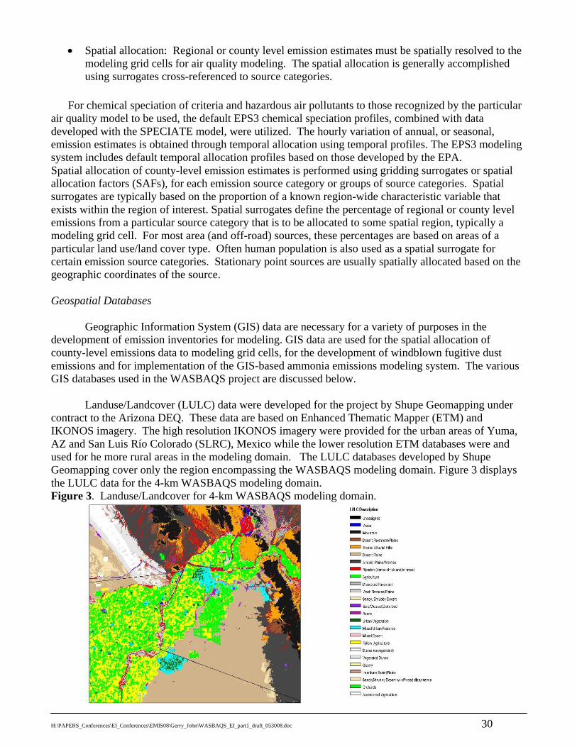
H:\PAPERS_Conferences\EI_Conferences\EMIS08\Gerry_John\WASBAQS_EI_part1_draft_053008.doc 30
• Spatial allocation: Regional or county level emission estimates must be spatially resolved to the modeling grid cells for air quality modeling. The spatial allocation is generally accomplished using surrogates cross-referenced to source categories.
For chemical speciation of criteria and hazardous air pollutants to those recognized by the particular
air quality model to be used, the default EPS3 chemical speciation profiles, combined with data developed with the SPECIATE model, were utilized. The hourly variation of annual, or seasonal, emission estimates is obtained through temporal allocation using temporal profiles. The EPS3 modeling system includes default temporal allocation profiles based on those developed by the EPA. Spatial allocation of county-level emission estimates is performed using gridding surrogates or spatial allocation factors (SAFs), for each emission source category or groups of source categories. Spatial surrogates are typically based on the proportion of a known region-wide characteristic variable that exists within the region of interest. Spatial surrogates define the percentage of regional or county level emissions from a particular source category that is to be allocated to some spatial region, typically a modeling grid cell. For most area (and off-road) sources, these percentages are based on areas of a particular land use/land cover type. Often human population is also used as a spatial surrogate for certain emission source categories. Stationary point sources are usually spatially allocated based on the geographic coordinates of the source. Geospatial Databases
Geographic Information System (GIS) data are necessary for a variety of purposes in the development of emission inventories for modeling. GIS data are used for the spatial allocation of county-level emissions data to modeling grid cells, for the development of windblown fugitive dust emissions and for implementation of the GIS-based ammonia emissions modeling system. The various GIS databases used in the WASBAQS project are discussed below.
Landuse/Landcover (LULC) data were developed for the project by Shupe Geomapping under contract to the Arizona DEQ. These data are based on Enhanced Thematic Mapper (ETM) and IKONOS imagery. The high resolution IKONOS imagery were provided for the urban areas of Yuma, AZ and San Luis Río Colorado (SLRC), Mexico while the lower resolution ETM databases were and used for he more rural areas in the modeling domain. The LULC databases developed by Shupe Geomapping cover only the region encompassing the WASBAQS modeling domain. Figure 3 displays the LULC data for the 4-km WASBAQS modeling domain. Figure 3. Landuse/Landcover for 4-km WASBAQS modeling domain.
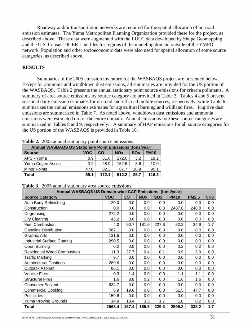
H:\PAPERS_Conferences\EI_Conferences\EMIS08\Gerry_John\WASBAQS_EI_part1_draft_053008.doc 31
Roadway and/or transportation networks are required for the spatial allocation of on-road
emission estimates. The Yuma Metropolitan Planning Organization provided these for the project, as described above. These data were augmented with the LULC data developed by Shupe Geomapping and the U.S. Census TIGER Line files for regions of the modeling domain outside of the YMPO network. Population and other socioeconomic data were also used for spatial allocation of some source categories, as described above. RESULTS
Summaries of the 2005 emission inventory for the WASBAQS project are presented below. Except for ammonia and windblown dust emissions, all summaries are provided for the US portion of the WASBAQS. Table 2 presents the annual stationary point source emissions for criteria pollutants. A summary of area source emissions by source category are provided in Table 3. Tables 4 and 5 present seasonal daily emission estimates for on-road and off-road mobile sources, respectively, while Table 6 summarizes the annual emissions estimates for agricultural burning and wildland fires. Fugitive dust emissions are summarized in Table 7. As noted above, windblown dust emissions and ammonia emissions were estimated on for the entire domain. Annual emissions for these source categories are summarized in Tables 8 and 9, respectively. A summary of HAP emissions for all source categories for the US portion of the WASBAQS is provided in Table 10. Table 2. 2005 annual stationary point source emissions.
Annual WASBAQS US Stationary Point Emissions (tons/year) Source VOC CO NOx SOx PM10 APS - Yuma 8.9 61.0 272.0 3.2 18.2Yuma Cogen Assoc. 3.2 28.9 152.5 3.6 10.0Minor Points 47.0 82.3 87.7 18.9 90.1Total 59.1 172.1 512.2 25.7 118.3
Table 3. 2005 annual stationary area source emissions.
Annual WASBAQS US Domain-wide CAP Emissions (tons/year) Source Category VOC CO NOx SOx PM10 PM2.5 NH3Auto Body Refinishing 20.0 0.0 0.0 0.0 0.0 0.0 0.0Construction 0.0 0.0 0.0 0.0 2487.6 248.8 0.0Degreasing 272.2 0.0 0.0 0.0 0.0 0.0 0.0Dry Cleaning 43.2 0.0 0.0 0.0 0.0 0.0 0.0Fuel Combustion 4.0 90.7 181.6 227.6 52.3 34.9 1.7Gasoline Distribution 587.1 0.0 0.0 0.0 0.0 0.0 0.0Graphic Arts 131.6 0.0 0.0 0.0 0.0 0.0 0.0Industrial Surface Coating 290.5 0.0 0.0 0.0 0.0 0.0 0.0Open Burning 0.2 0.8 0.0 0.0 0.2 0.2 0.0Residential Wood Combustion 11.3 27.7 0.4 0.1 3.9 3.9 0.0Traffic Marking 9.7 0.0 0.0 0.0 0.0 0.0 0.0Architectural Coatings 289.6 0.0 0.0 0.0 0.0 0.0 0.0Cutback Asphalt 86.1 0.0 0.0 0.0 0.0 0.0 0.0Vehicle Fires 0.3 1.4 0.0 0.0 1.1 1.1 0.0Structural Fires 1.6 8.8 0.2 0.0 1.6 1.6 0.0Consumer Solvent 634.7 0.0 0.0 0.0 0.0 0.0 0.0Commercial Cooking 6.9 19.6 0.0 0.0 51.5 47.7 0.0Pesticides 159.6 0.0 0.0 0.0 0.0 0.0 0.0Yuma Proving Grounds 14.9 18.4 3.3 1.7 1.0 0.2 0.0Total 2563.4 167.4 185.5 229.3 2599.2 338.2 1.7
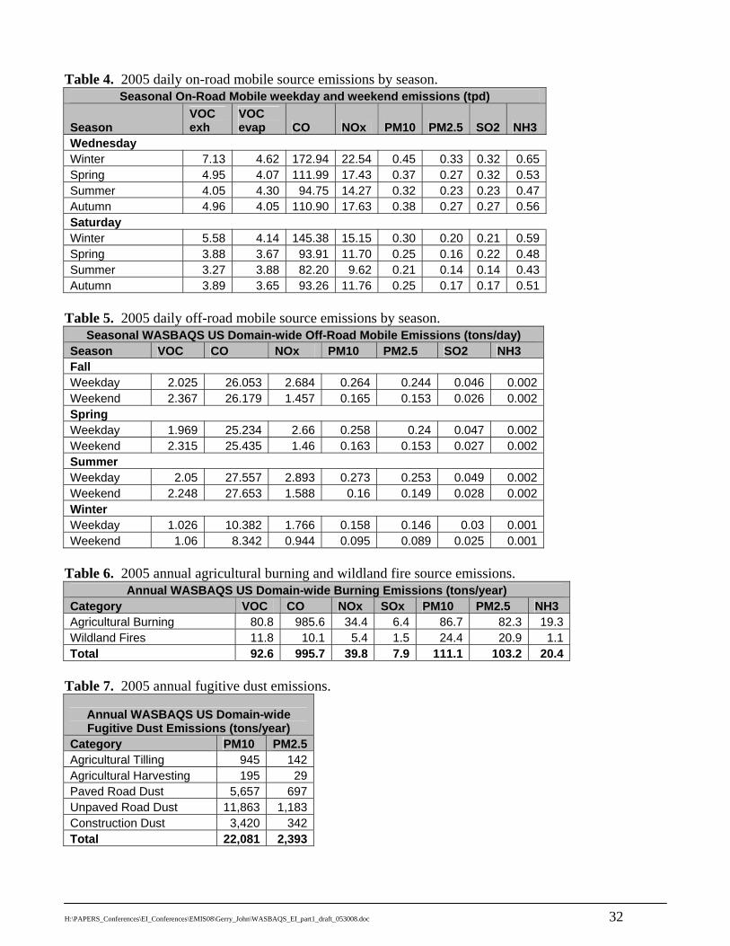
H:\PAPERS_Conferences\EI_Conferences\EMIS08\Gerry_John\WASBAQS_EI_part1_draft_053008.doc 32
Table 4. 2005 daily on-road mobile source emissions by season.
Seasonal On-Road Mobile weekday and weekend emissions (tpd)
Season VOC exh
VOC evap CO NOx PM10 PM2.5 SO2 NH3
Wednesday Winter 7.13 4.62 172.94 22.54 0.45 0.33 0.32 0.65 Spring 4.95 4.07 111.99 17.43 0.37 0.27 0.32 0.53 Summer 4.05 4.30 94.75 14.27 0.32 0.23 0.23 0.47 Autumn 4.96 4.05 110.90 17.63 0.38 0.27 0.27 0.56 Saturday Winter 5.58 4.14 145.38 15.15 0.30 0.20 0.21 0.59 Spring 3.88 3.67 93.91 11.70 0.25 0.16 0.22 0.48 Summer 3.27 3.88 82.20 9.62 0.21 0.14 0.14 0.43 Autumn 3.89 3.65 93.26 11.76 0.25 0.17 0.17 0.51
Table 5. 2005 daily off-road mobile source emissions by season.
Seasonal WASBAQS US Domain-wide Off-Road Mobile Emissions (tons/day) Season VOC CO NOx PM10 PM2.5 SO2 NH3 Fall Weekday 2.025 26.053 2.684 0.264 0.244 0.046 0.002 Weekend 2.367 26.179 1.457 0.165 0.153 0.026 0.002 Spring Weekday 1.969 25.234 2.66 0.258 0.24 0.047 0.002 Weekend 2.315 25.435 1.46 0.163 0.153 0.027 0.002 Summer Weekday 2.05 27.557 2.893 0.273 0.253 0.049 0.002 Weekend 2.248 27.653 1.588 0.16 0.149 0.028 0.002 Winter Weekday 1.026 10.382 1.766 0.158 0.146 0.03 0.001 Weekend 1.06 8.342 0.944 0.095 0.089 0.025 0.001
Table 6. 2005 annual agricultural burning and wildland fire source emissions.
Annual WASBAQS US Domain-wide Burning Emissions (tons/year) Category VOC CO NOx SOx PM10 PM2.5 NH3 Agricultural Burning 80.8 985.6 34.4 6.4 86.7 82.3 19.3 Wildland Fires 11.8 10.1 5.4 1.5 24.4 20.9 1.1 Total 92.6 995.7 39.8 7.9 111.1 103.2 20.4
Table 7. 2005 annual fugitive dust emissions.
Annual WASBAQS US Domain-wide Fugitive Dust Emissions (tons/year)
Category PM10 PM2.5Agricultural Tilling 945 142Agricultural Harvesting 195 29Paved Road Dust 5,657 697Unpaved Road Dust 11,863 1,183Construction Dust 3,420 342Total 22,081 2,393
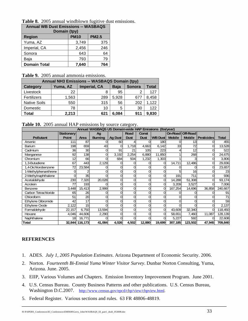
H:\PAPERS_Conferences\EI_Conferences\EMIS08\Gerry_John\WASBAQS_EI_part1_draft_053008.doc 33
Table 8. 2005 annual windblown fugitive dust emissions. Annual WB Dust Emissions -- WASBAQS
Domain (tpy) Region PM10 PM2.5 Yuma, AZ 3,749 375Imperial, CA 2,456 246Sonora 643 64Baja 793 79Domain Total 7,640 764
Table 9. 2005 annual ammonia emissions.
Annual NH3 Emissions -- WASBAQS Domain (tpy) Category Yuma, AZ Imperial, CA Baja Sonora Total Livestock 22 8 95 2 127Fertilizers 1,563 289 5,928 677 8,458Native Soils 550 315 56 202 1,122Domestic 78 10 5 30 122Total 2,213 621 6,084 911 9,830
Table 10. 2005 annual HAP emissions by source category.
PollutantStationary
Point AreaAg
Burning Ag DustRoad Dust
Const Dust WB Dust
On-Road Mobile
Off-Road Mobile Pesticides Total
Arsenic 111 87 0 60 4 0 180 0 13 0 455 Barium 198 659 43 0 1,718 4,663 6,142 33 72 0 13,528 Cadmium 36 30 0 91 21 105 223 4 12 0 522 Manganese 92 138 0 3,192 2,254 6,880 11,850 1 268 0 24,675 Chromium 12 66 0 684 504 1,232 1,303 1 3 0 3,806 1,3-Butadiene 67 443 2,129 0 0 0 0 14,711 12,486 0 29,836 1,4-Dichlorobenzene 72 23,584 0 0 0 0 0 0 0 0 23,657 1-Methylphenanthrene 0 2 0 0 0 0 0 5 16 0 23 2-Methylnaphthalene 0 35 0 0 0 0 0 191 711 0 936 Acetaldehyde 230 7,320 20,028 0 0 0 0 14,288 51,308 0 93,174 Acrolein 77 193 0 0 0 0 0 3,209 3,527 0 7,006 Benzene 3,448 15,413 2,999 0 0 0 0 167,254 14,696 36,858 240,667 Carbon Tetrachloride 65 26 0 0 0 0 0 0 0 0 91 Chloroform 51 20 0 0 0 0 0 0 0 0 71 Ethylene Dibromide 42 17 0 0 0 0 0 0 0 0 59 Ethylene Oxide 2,122 15 0 0 0 0 0 0 0 0 2,137 Formaldehyde 22,157 6,750 13,594 0 0 0 0 43,609 32,340 0 118,450 Hexane 4,046 44,606 2,290 0 0 0 0 58,651 7,460 11,087 128,139 Naphthalene 18 16,771 0 0 0 0 0 5,227 592 0 22,608Total 32,844 116,173 41,084 4,026 4,502 12,880 19,699 307,185 123,502 47,945 709,840
Annual WASBAQS US Domain-wide HAP Emissions (lbs/year)
REFERENCES
1. ADES. July 1, 2005 Population Estimates. Arizona Department of Economic Security. 2006.
2. Norton. Fourteenth Bi-Ennial Yuma Winter Visitor Survey. Dunbar Norton Consulting, Yuma, Arizona. June. 2005.
3. EIIP, Various Volumes and Chapters. Emission Inventory Improvement Program. June 2001.
4. U.S. Census Bureau. County Business Patterns and other publications. U.S. Census Bureau, Washington D.C.2007. http://www.census.gov/epcd/cbp/view/cbpview.html.
5. Federal Register. Various sections and rules. 63 FR 48806-48819.
H:\PAPERS_Conferences\EI_Conferences\EMIS08\Gerry_John\WASBAQS_EI_part1_draft_053008.doc 34
6. FHWA. Highway Statistics, 2004: Total Disbursements for Highways. Federal Highway Administration. 2007. http://www.fhwa.dot.gov/policy/ohim/hs04/index.htm.
7. ADEQ. 2007b. Results of WASBAQS Domain, Yuma County Gasoline Station Survey. Arizona Department of Environmental Quality, Air Assessment Section. June. Personal Communication.
8. Baggiore, 2007. S. Baggiore. New Source Unit, Permits Section, Air Quality Division, Arizona Department of Environmental Quality. September. Personal Communication.
9. ADEQ. Arizona Gasoline Stations by County - Year 2005. New Source Unit, Permits Section, Air Quality Division, Arizona Department of Environmental Quality. 2006a.
10. EIA. State Energy Consumption Estimates, 1960-2004, Arizona. Energy Information Administration, Washington D.C. January 2007. http://www.eia.doe.gov/emeu/states/_seds.html.
11. WRCC. Arizona Climate Summaries: Period of Record General Climate Summaries – Heating Degree Days. Western Regional Climate Center, Desert Research Institute. 2007. http://www.wrcc.dri.edu/summary/climsmaz.html.
12. EPA. Documentation for the Draft 2002 Nonpoint Source National Emission Inventory for Criteria and Hazardous Air Pollutants (February 2006 Version). Prepared by E.H. Pechan & Associates, Inc. EPA Contract No. 68-D-02-063. 2006. http://www.epa.gov/ttn/chief/net/2002inventory.html.
13. EPA. Compilation of Air Pollution Emission Factors (AP-42) – Volume 13: Miscellaneous Sources, Section 2.1 Paved Roads, Fifth Edition. U.S. Environmental Protection Agency, Office of Air Quality Planning and Standards, Research Triangle Park, North Carolina. January 2006a. http://www.epa.gov/ttn/chief/ap42.
14. ADEQ. Personal Communication: Yuma County Vehicle Fire, Structural Fire, and Burn Permit Data Arizona Department of Environmental Quality, Air Assessment Section. April 2007.
15. Chitjian, M. and G. Mansell. “An Improved Ammonia Inventory for the WRAP Domain – Technical Description of the Modeling System.” Prepared for the WRAP Emissions Forum. November 2003.
16. Nolte. Personal communication with K. Nolte, University of Arizona Cooperative Extension, Yuma County Office, regarding agricultural burning. January 2007.
17. ERG. Emissions Inventory Improvement Program. Volume III Chapter 9. Pesticides - Agricultural and Non-agricultural. 2001. http://www.epa.gov/ttn/chief/eiip/techreport/volume03/iii09_jun2001.pdf (accessed January 16th, 2007).
18. California DPR. Department of Pesticide Regulation website http://www.cdpr.ca.gov/ 2007.
19. Pollack, A, L. Chan, P. Chandraker, J. Grant, C. Lindhjem, S. Rao, J. Russell, C. Tran. WRAP Mobile Source Emission Inventories Update. Prepared for the Western Governors’ Association. May 2006., http://www.wrapair.org/forums/ef/UMSI/0606_WRAP_Mobile_Source_EI_Final_Report.pdf
20. Lindhjem, C. “Development Work for Improved Heavy-Duty Vehicle Modeling Capability Data Mining FHWA Datasets Phase II: Final Report”, EPA Contract No. 68-C-02-022, Work Assignment No. 2-6, Prepared for: Evelyn Sue Kimbrough, Atmospheric Protection Branch Office of Research and Development U.S. Environmental Protection Agency, September 2004.
21. Sedlacek, R.F. Personal Communications with R.F. Sedlacek, Arizona Department of Environmental Quality. 2007.
22. Hammad, 2007. N. Imperial Sand Dune’s Sheriff’s Office, November Personal Communication.
23. WRAP. “Development of 2000-04 Baseline Period and 2018 year Emission Inventories,” Western Regional Air Partnership, January 2007. http://www.airsci.com/wrap/phase3-4/Workplan_Ph3and4_Final.pdf
H:\PAPERS_Conferences\EI_Conferences\EMIS08\Gerry_John\WASBAQS_EI_part1_draft_053008.doc 35
24. Imperial County. “2005 Agricultural Crop and Livestock Report: Imperial County,” 2006. http://www.imperialcounty.net/ag/clreports.htm (accessed February 2007).
25. UA. Yuma County Agricultural Statistics 2005. Prepared by the Arizona Cooperative Extension at the University of Arizona. 2006.
26. CDWR. Land Use GIS data, California Department of Water Resources. 2007. http://www.landwateruse.water.ca.gov/basicdata/landuse/landusesurvey.cfm. (accessed January 16th, 2007).
27. WRAP. Fugitive Dust Handbook Chapter 2. Western Regional Air Partnership, 2006. 2006. http://www.wrapair.org/forums/dejf/fdh/ch2-agtill.html. (accessed January 16th, 2007).
28. UA. 2007. K. Nolte, Ph.D., Arizona Cooperative Extension, University of Arizona, June. Personal communication.
29. ADEQ. Yuma PM10 Maintenance Plan. Arizona Department of Environmental Quality. 2006. http://www.azdeq.gov/environ/air/plan/notmeet.html.
30. Mansell, G.E., R. Morris and M. Omary. Recommendations and Model Performance Evaluation for the Phase II Windblown Fugitive Dust Emission Project. Technical Memorandum prepared for the WRAP Dust Emission Joint Forum. July 2004.
31. Marticorena, B., Bergametti, G., Gillette, D., and Belnap, J. Factors controlling threshold friction velocity in semiarid and arid areas of the United States. J. Geophysics Research 102 (D19): 23277-23287. 1997.
32. Alfaro, S.C. and Gomes, L. Modeling mineral aerosol production by wind erosion: emission intensities and aerosol size distributions in source areas. J. Geophys. Res. 106 (16): 18075-18084. 2001.
33. Shupe, S.M. Land Use/Land Cover Classification in the WASBAQS Study Area - Work Plan. Prepared for Randy Sedlacek, Arizona Department of Environmental Quality. Prepared by Scott M. Shupe, PhD, Shupe Geomapping, Maple Ridge, BC, Canada. 2006.

H:\PAPERS_Conferences\EI_Conferences\EMIS08\Gerry_John\WASBAQS_EI_part1_draft_053008.doc 36
KEYWORDS Emissions inventories HAPs Emissions modeling