Embed Size (px)
Citation preview
Louisiana State UniversityLSU Digital Commons
LSU Historical Dissertations and Theses Graduate School
1997
Development of an Analysis System forDiscontinuities in Rigid Airfield Pavements.Michael Ivan HammonsLouisiana State University and Agricultural & Mechanical College
Follow this and additional works at: https://digitalcommons.lsu.edu/gradschool_disstheses
This Dissertation is brought to you for free and open access by the Graduate School at LSU Digital Commons. It has been accepted for inclusion inLSU Historical Dissertations and Theses by an authorized administrator of LSU Digital Commons. For more information, please [email protected].
Recommended CitationHammons, Michael Ivan, "Development of an Analysis System for Discontinuities in Rigid Airfield Pavements." (1997). LSU HistoricalDissertations and Theses. 6424.https://digitalcommons.lsu.edu/gradschool_disstheses/6424

INFORMATION TO USERS
This manuscript has been reproduced from the microfilm master. UMI
films the tmct directly from the original or copy submitted. Thus, some
thesis and dissertation copies are in typewriter face, while others may be
from any type of computer printer.
The quality of this reproduction is dependent upon the quality of the
copy submitted. Broken or indistinct print, colored or poor quali^
illustrations and photographs, print bleedthrough, substandard margins,
and improper alignment can adversely affect reproduction.
In the unlikely event that the author did not send UMI a complete
manuscript and there are missing pages, these will be noted. Also, if
unauthorized copyright material had to be removed, a note will indicate
the deletion.
Oversize materials (e.g., maps, drawings, charts) are reproduced by
sectioning the original, beginning at the upper left-hand comer and
continuing from left to right in equal sections with small overlaps. Each
original is also photographed in one exposure and is included in reduced
form at the back o f the book.
Photographs included in the original manuscript have been reproduced
xerographically in this copy. Higher quality 6” x 9” black and white
photographic prints are available for any photographs or illustrations
appearing in this copy for an additional charge. Contact UMI directly to
order.
UMIA Bell & Howell Infonnation Company
300 North Zed) Road, Ann Arbor MI 48106-1346 USA 313/761-4700 800/521-0600
Reproduced with permission of the copyright owner. Further reproduction prohibited without permission.

Reproduced with permission of the copyright owner. Further reproduction prohibited without permission.
DEVELOPMENT OF AN ANALYSIS SYSTEM FOR DISCONTINUITIES IN RIGID AIRFIELD PAVEMENTS
A Dissertation
Submitted to the Graduate Faculty of the Louisiana State University and
Agricultural and Mechanical College in partial fulfillment of the
requirements for the degree of Doctor of Philosophy
m
The Department of Civil and Environmental Engineering
byMichael Ivan Hammons
B.S., Louisiana Tech University, 1980 M.S., Mississippi State University, 1985
May 1997
Reproduced with permission of the copyright owner. Further reproduction prohibited without permission.

UNI Number: 9736019
UMI Microform 9736019 Copyright 1997, by UMI Company. All rights reserved.
This microform edition is protected against unauthorized copying under Title 17, United States Code.
UMI300 North Zeeb Road Ann Arbor, MI 48103
Reproduced with permission of the copyright owner. Further reproduction prohibited without permission.

DEDICATION
This dissertation is dedicated to the memory of the most brilliant lady I have ever known,
my mother, Dorothy Vercher Hammons, who departed this life on March 2, 1996. As my
greatest encourager, she never doubted my ability to achieve.
Reproduced with permission of the copyright owner. Further reproduction prohibited without permission.

ACKNOWLEDGMENTS
The research reported herein was sponsored by the U.S. Department of Transportation,
Federal Aviation Administration (FAA), Airport Technology Branch, under Interagency
Agreement DTFA03-94-X-00010 with the Airfields and Pavements Division (APD), Geotech-
nical Laboratory (GL), U.S. Army Engineer Waterways Experiment Station (WES),
Vicksburg, Mississippi. Dr. Xiaogong Lee, Airport Technology Branch, FAA, was technical
monitor. Dr. Satish Agrawal is Manager, Airport Technology Branch, FAA.
I would like to acknowledge the support of the Airfields and Pavements Division, Geo-
technical Laboratory, Waterways Experiment Station, for making it possible for me to
achieve my goal of advanced studies leading to the Doctor of Philosophy degree. I would
like to especially express my gratitude to Drs. Raymond S. Rollings and Don C. Banks,
WES, for their interest and helpful comments during the course of this research. The helpful
contributions of Messrs. Bill Grogan, Dennis Mathews, Billy Neeley, Dan Wilson, and Cliff
Gill as well as Ms. Donna Day to the experimental program are gratefully acknowledged.
Many thanks should also be extended to Dr. Anastasios M. loannides, a consultant to
WES, of the University of Cincinnati. Dr. loannides provided invaluable suggestions during
our numerous informal discussions concerning analytical modeling of pavements. His keen
intellect and insight contributed greatly to the educational value of this experience.
Of course, none of this would be possible without the help, encouragement, and coopera
tion of my advisor. Dr. John B. Metcalf. Dr. Metcalf is a true scholar and a gentleman, and
I am honored to be his student. I also owe well-deserved thanks to the members of my grad
uate committee: Dr. R. Richard Avent, Dr. George M. Hammitt, U, Dr. George Z.
Voyiadjis, and Dr. Freddy Roberts.
Ill
Reproduced with permission of the copyright owner. Further reproduction prohibited without permission.

Most importantly, I wish to express my gratitude to my wife, Janet, and my children,
Aaron, Amy, and James, for supporting me unfailingly throughout this effort. Their love,
encouragement, and prayers gave me the stamina to persevere to the end.
IV
Reproduced with permission of the copyright owner. Further reproduction prohibited without permission.
TABLE OF CONTENTS
DEDICATION....................................................................................................................... ii
ACKNOWLEDGMENTS..................................................................................................... iü
LIST OF TABLES.................................................................................................................. viii
LIST OF FIG U RES............................................................................................................... ix
ABSTRACT ......................................................................................................................... xvi
CHAPTER1 INTRODUCTION................................................................................................ 1
Background ....................................................................................................... 1Objectives .......................................................................................................... 3Scope .................................................................................................................. 3
2 PROBLEM STATEMENT.................................................................................... 5Rigid Pavement System...................................................................................... 5Load Transfer Definitions................................................................................. 8Load Transfer Mechanisms............................................................................... 9Rigid Pavement Foundations ............................................................................ 10
3 HISTORICAL DEVELOPMENTS ..................................................................... 12Response Model ................................................................................................ 14Critical Design Stresses...................................................................................... 14Accelerated Trafficking Tests............................................................................ 15Subgrade Characterization................................................................................. 17Rigid Pavement Joints........................................................................................ 19Sum m ary............................................................................................................ 25
4 CLASSICAL RESPONSE M ODELS.................................................................. 27Westergaard T heory........................................................................................... 27
Response charts ............................................................................................. 28Computerized solutions ................................................................................. 29Westergaard theory limitations....................................................................... 30
Elastic Layer M o d e ls ........................................................................................ 31Models for Dowel Stresses ............................................................................... 33Westergaard-Type Solution for Load T ran sfe r................................................ 38
5 FINITE ELEMENT RESPONSE MODELS ..................................................... 432D Finite Element Models................................................................................. 43
ILLI-SLAB m o d e ls ........................................................................................ 453D Finite Element Models................................................................................. 58
GEOSYS m o d e l............................................................................................. 58ABAQUS models ........................................................................................... 60
Reproduced with permission of the copyright owner. Further reproduction prohibited without permission.
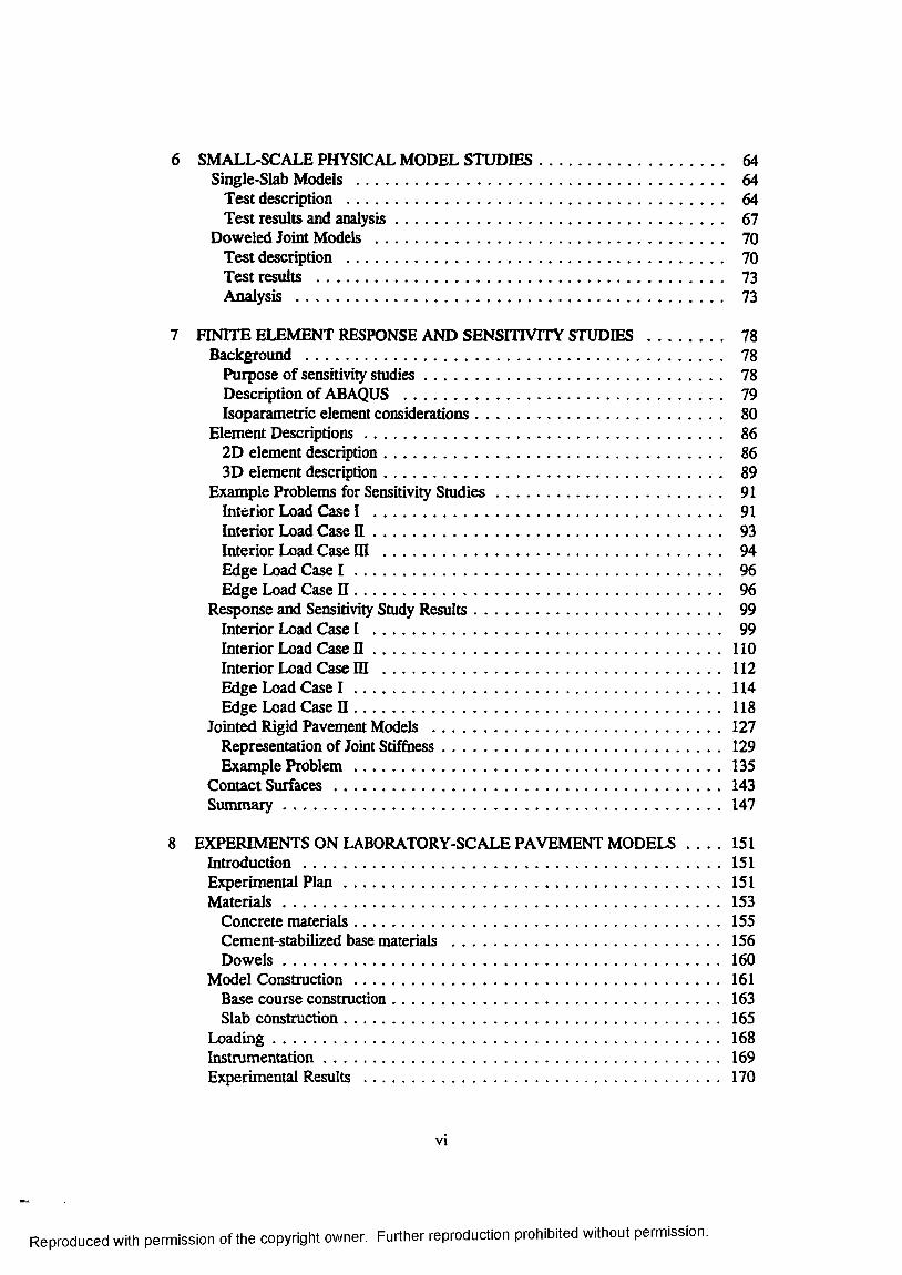
SMALL-SCALE PHYSICAL MODEL STUDIES............................................. 64Single-Slab Models .......................................................................................... 64
Test description ............................................................................................. 64Test results and analysis................................................................................. 67
Doweled Joint Models ...................................................................................... 70Test description ............................................................................................. 70Test results .................................................................................................... 73Analysis ......................................................................................................... 73
FINITE ELEMENT RESPONSE AND SENSITIVITY STUDIES .................. 78Background ....................................................................................................... 78
Purpose of sensitivity studies......................................................................... 78Description of ABAQUS .............................................................................. 79Isoparametric element considerations............................................................ 80
Element Descriptions........................................................................................ 862D element description................................................................................... 863D element description................................................................................... 89
Example Problems for Sensitivity S m d ies ....................................................... 91Interior Load Case I ...................................................................................... 91Interior Load Case I I ..................................................................................... 93Interior Load Case III ................................................................................... 94Edge Load Case I .......................................................................................... 96Edge Load Case I I .......................................................................................... 96
Response and Sensitivity Study Results............................................................. 99Interior Load Case I ..................................................................................... 99Interior Load Case I I ........................................................................................ 110Interior Load Case m ......................................................................................112Edge Load Case I ..........................................................................................114Edge Load Case I I .............................................................................................118
Jointed Rigid Pavement Models ..........................................................................127Representation of Joint Stiffness....................................................................... 129Example P rob lem .............................................................................................135
Contact Surfaces..................................................................................................143Sum m ary.............................................................................................................. 147
EXPERIMENTS ON LABORATORY-SCALE PAVEMENT M OD ELS 151Introduction......................................................................................................... 151Experimental P la n ............................................................................................... 151M ateria ls .............................................................................................................. 153
Concrete materials.............................................................................................155Cement-stabilized base materials .....................................................................156D ow els.............................................................................................................. 160
Model Construction.......................................................................................... 161Base course construction................................................................................... 163Slab construction............................................................................................ 165
Loading.................................................................................................................168Instrumentation................................................................................................. 169Experimental Results .......................................................................................... 170
VI
Reproduced with permission of the copyright owner. Further reproduction prohibited without permission.
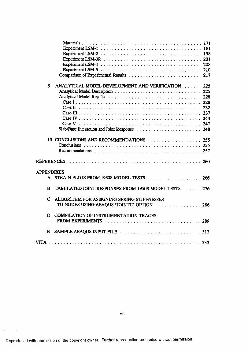
Materials............................................................................................................ 171Experiment L S M -1 ........................................................................................... 181Experiment L S M -2 ........................................................................................... 198Experiment LSM -3R........................................................................................ 201E}^riment L S M -4 ...........................................................................................208Experiment L S M -5...........................................................................................210
Comparison of Experimental R esu lts ..................................................................217
9 ANALYTICAL MODEL DEVELOPMENT AND VERIFICATION .................... 225Analytical Model Description.............................................................................. 225Analytical Model Results......................................................................................228
Case I .................................................................................................................228Case n .............................................................................................................. 232Case m .............................................................................................................. 237Case IV .............................................................................................................. 243Case V .............................................................................................................. 247
Slab/Base Interaction and Joint Response ..........................................................248
10 CONCLUSIONS AND RECOMMENDATIONS............................................255Conclusions..........................................................................................................255Recommendations ................................................................................................257
REFERENCES........................................................................................................................ 260
APPENDDŒSA STRAIN PLOTS FROM 1950S MODEL T E S T S ............................................266
B TABULATED JOINT RESPONSES FROM 1950S MODEL TESTS ....................276
C ALGORITHM FOR ASSIGNING SPRING STIFFNESSESTO NODES USING ABAQUS "JOINTC OPTION ........................................ 286
D COMPILATION OF INSTRUMENTATION TRACESFROM EXPERIMENTS ...................................................................................... 289
E SAMPLE ABAQUS INPUT F IL E ........................................................ 313
V IT A ........................................................................................................................................ 333
vu
Reproduced with permission of the copyright owner. Further reproduction prohibited without permission.
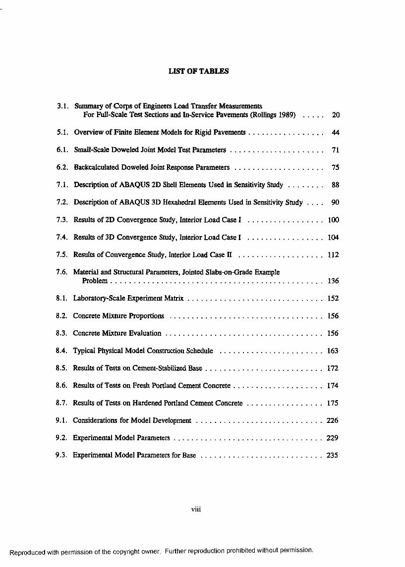
LIST OF TABLES
3.1. Summary of Corps of Engineers Load Transfer MeasurementsFor Full-Scale Test Sections and In-Service Pavements (Rollings 1989) ........... 20
5.1. Overview of Finite Element Models for Rigid Pavements......................................... 44
6.1. Small-Scale Doweled Joint Model Test Param eters.................................................. 71
6.2. Backcalculated Doweled Joint Response Param eters................................................ 75
7.1. Description of ABAQUS 2D Shell Elements Used in Sensitivity S tu d y .................... 88
7.2. Description of ABAQUS 3D Hexahedral Elements Used in Sensitivity Study . . . . 90
7.3. Results of 2D Convergence Study, Interior Load Case I ........................................ 100
7.4. Results of 3D Convergence Study, Interior Load Case I ........................................... 104
7.5. Results of Convergence Study, Interior Load Case II ............................................. 112
7.6. Material and Structural Parameters, Jointed Slabs-on-Grade ExampleProblem.................................................................................................................... 136
8.1. Laboratory-Scale Experiment M atrix......................................................................... 152
8.2. Concrete Mixture Proportions .................................................................................. 156
8.3. Concrete Mixture Evaluation........................................................................................156
8.4. Typical Physical Model Construction Schedule ..........................................................163
8.5. Results of Tests on Cement-Stabilized B ase ..................................................................172
8.6. Results of Tests on Fresh Portland Cement Concrete.................................................. 174
8.7. Results of Tests on Hardened Portland Cement C oncrete ...........................................175
9.1. Considerations for Model Development.......................................................................226
9.2. Experimental Model Parameters...................................................................................229
9.3. Experimental Model Parameters for B a se .................................................................... 235
vui
Reproduced with permission of the copyright owner. Further reproduction prohibited without permission.
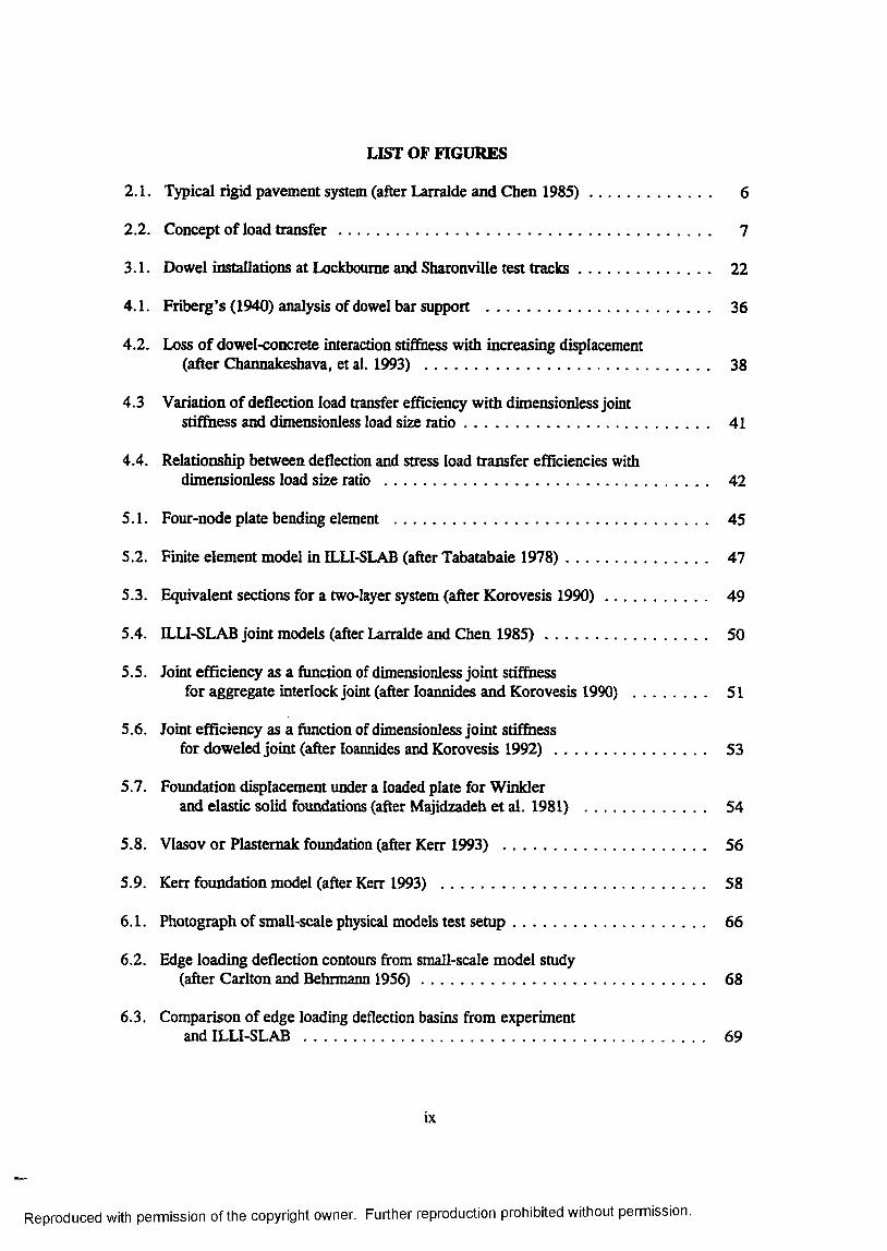
LIST OF FIGURES
2.1. Typical rigid pavement system (after Larralde and Chen 1 9 8 5 ).............................. 6
2.2. Concept of load tra n s fe r ............................................................................................ 7
3.1. Dowel installations at Lockboume and Sharonville test tra c k s ................................. 22
4.1. Friberg’s (1940) analysis of dowel bar support ....................................................... 36
4.2. Loss of dowel-concrete interaction stiffiiess with increasing displacement(after Channakeshava, et al. 1993) ....................................................................... 38
4.3 Variation of deflection load transfer efficiency with dimensionless jointstiffiiess and dimensionless load size ra tio ............................................................. 41
4.4. Relationship between deflection and stress load transfer efficiencies withdimensionless load size ratio ................................................................................. 42
5.1. Four-node plate bending element .............................................................................. 45
5.2. Finite element model in ILLI-SLAB (after Tabatabaie 1978).................................. 47
5.3. Equivalent sections for a two-layer system (after Korovesis 1 9 9 0 ).......................... 49
5.4. ILLI-SLAB joint models (after Larralde and Chen 1 9 8 5 )....................................... 50
5.5. Joint efficiency as a function of dimensionless joint stiffiiessfor aggregate interlock joint (after loannides and Korovesis 1990) .................... 51
5.6. Joint efficiency as a function of dimensionless joint stiffiiessfor doweled joint (after loannides and Korovesis 1 9 9 2 ) ...................................... 53
5.7. Foundation displacement under a loaded plate for Winklerand elastic solid foundations (after Majidzadeh et al. 1981) .......................... 54
5.8. Vlasov or Plastemak foundation (after Kerr 1993) ................................................. 56
5.9. Kerr foundation model (after Kerr 1993) ................................................................. 58
6.1. Photograph of small-scale physical models test se tu p ............................................... 66
6.2. Edge loading deflection contours fiom small-scale model study(after Carlton and Behrmann 1956)....................................................................... 68
6.3. Comparison of edge loading deflection basins from experimentand ILLI-SLAB .................................................................................................... 69
IX
Reproduced with permission of the copyright owner. Further reproduction prohibited without permission.
6.4. Typical small-scale dowel joint test slab showing approximate straingage positions......................................................................................................... 72
6.5. Backcalculated dimensionless joint stiffiiess from small-scale model tests ............ 76
6.6. Backcalculated modulus of dowel reaction from small-scale model tests .............. 77
7.1. Interpolation functions, 2D Lagrangian isoparametric element.............................. 83
7.2. Interpolation functions, 2D serendipity isoparametric elem ent.............................. 84
7.3. System configuration. Interior Load Case I .............................................................. 92
7.4. System configuration. Interior Load Case 0 ............................................................ 94
7.5. System configuration. Interior Load Case H I ............................................................ 95
7.6. System configuration. Edge Load Case I .............................................................. 97
7.7. System configuration, Edge Load Case ü .............................................................. 98
7.8. Definition of element dimensions for determining mesh f ineness.......................... 101
7.9. Finite element meshes in plane of slab surface. Interior Load Case I .................... 102
7.10. Finite element meshes in plane of slab thickness, Interior Load Case I .................. 105
7.11. Dimensionless bending stress. Interior Load Case I .................................................. 106
7.12. Dimensionless deflection. Interior Load Case I ....................................................... 107
7.13. CPU time, selected 3D runs. Interior Load Case I .................................................. 108
7.14. Dimensionless bending stress summary, Interior Load Case I ................................ 109
7.15. Dimensionless deflection summary. Interior Load Case I ........................................ 110
7.16. Finite element meshes in plane of slab surface. Interior Load Case H ....................... I l l
7.17. Finite element meshes in plane of slab surface. Interior Load Case HI .................. 113
7.18. Stress ratio. Interior Load Case ED .......................................................................... 114
7.19. Deflection ratio. Interior Load Case El ................................................................... 115
7.20. Finite element meshes in plane of slab surface. Edge Load Case 1 ......................... 116
7.21. Dimensionless bending stress, Edge Load Case I .....................................................118
Reproduced with permission of the copyright owner. Further reproduction prohibited without permission.
7.22. Summary of 2D and 3D runs, dimensionless bending stress, EdgeLoad Case I .......................................................................................................... 119
7.23. Finite element meshes in plane of slab surface, Edge Load Case n ........................... 120
7.24. Dimensionless bending stress, default transverse shear stiffness. EdgeLoad Case I I .......................................................................................................... 121
7.25. Dimensionless bending stress, 100 times default transverse shear stifihess.Edge Load Case n ............................................................................................. 122
7.26. Dimensionless deflection, default transverse shear stifbess, EdgeLoad Case I I ....................................................................................................... 123
7.27. Dimensionless deflection, 100 times default transverse shear stifBiess,Edge Load Case n ............................................................................................. 124
7.28. Effect of slab width to depth ratio on edge stresses......................................................125
7.29. Finite element distribution of through slab thickness ...................................... 126
7.30. Theoretical and experimental dimensionless bending stress fromsmall-scale model studies................................................................................... 128
7.31. Ratio of theoretical to experimental bending stress fromsmall-scale model studies......................................................................................129
7.32. Simply-supported beam problem to test JOINTC elem ent........................................... 134
7.33. Results from simply-supported beam with JOINTC elements ....................................135
7.34. Finite element mesh for 2D jointed rigid pavement model .........................................138
7.35. Bending stresses predicted by 2D finite element model of a jointedpavement .......................................................................................................... 139
7.36. Comparison of joint response parameters, 2D finite element model ..........................140
7.37. Conq>arison of bending stresses predicted by 2D and 3D finite elementmodels of a jointed pavement ............................................................................142
7.38. Comparison of 3D finite element model with closed-form solution,dimensionless joint stiffness versus deflection load transfer efficiency 143
7.39. Comparison of 3D finite element model with closed-form solution, stress loadtransfer efficiency versus deflection load transfer efficiency............................ 144
7.40. Example of over constraint for contact problem ...........................................................147
XI
Reproduced with permission of the copyright owner. Further reproduction prohibited without permission.
7.41. Simply-supported beam problem to test contact interaction featuresof ABAQUS....................................................................................................... 148
7.42. Results from simply-supported beam with contact and friction.................................149
8.1. Test configurations for laboratory scale m odels ........................................................154
8.2. Grain size distribution of sand/silica flour blend........................................................158
8.3. Moisture-densiQr curves for cement-stabilized sand/silica flour b le n d .................... 159
8.4. Compressive strength test results on cement-stabilized sand/silicaflour blend compacted to maximum density..................................................... 160
8.5. Dowel locations............................................................................................................ 161
8.6. Photograph of completed reaction b o x ...................................................................... 162
8.7. Photograph of adjustable screed/compaction device ................................................ 164
8.8. Installation of polyethylene film in reaction b o x ....................................................... 166
8.9. Placement of thin sand layer ......................................................................................166
8.10. Bond breaker and doweled joint just prior to concrete placem ent............................167
8.11. Test setup for plate bearing test on rubber p a d .......................................................... 178
8.12. Bearing stress-displacement data from plate bearing test on rubberblock in load control...........................................................................................179
8.13. Corrected plate bearing stress..................................................................................... 181
8.14. Bearing stress-displacement data from plate bearing test on rubberblock in displacement co n tro l........................................................................... 182
8.15. Instrumentation plan, Experiment L SM -IA ...............................................................183
8.16. Loading history. Experiment LSM-1 A ...................................................................... 184
8.17. Posttest photograph. Experiments LSM-1 A and LSM -IB ........................................ 185
8.18. Raw and corrected displacement data from LVDTs positionedperpendicular to edge. Experiment L S M -IA .................................................. 187
8.19. Raw and corrected displacement data from LVDTs positionedparallel to edge. Experiment L S M -IA ............................................................ 188
XU
Reproduced with permission of the copyright owner. Further reproduction prohibited without permission.
8.20. Analytical relationship between modulus of subgrade reaction and deflectionfrom ABAQUS models. Experiment LSM -IA ....................................................189
8.21. Comparison of experimental and analytical deflection basin profilesperpendicular to edge. Experiment LSM -IA ......................................................190
8.22. Comparison of experimental and analytical deflection basin profilesparallel to edge. Experiment L S M -IA ................................................................191
8.23. Instrumentation plan. Experiment LSM -IB .................................................................. 192
8.24. Loading history. Experiment L S M -IB ......................................................................... 193
8.25. Raw and corrected displacement data from LVDTs, Experiment L S M -IB ............... 195
8.26. Analytical relationship between modulus of subgrade reaction and deflectionfrom ABAQUS models. Experiment L S M -IB ....................................................196
8.27. Comparison of experimental and analytical deflection basin profiles.Experiment LSM-IB ...........................................................................................197
8.28. Loading history. Experiment L S M -2 ............................................................................198
8.29. Instrumentation plan. Experiments LSM-2, -3R, -4, and -5 .......................................200
8.30. Posttest photograph of slab top surface. Experiment L S M -2 ...................................... 201
8.31. Series of photographs in vicinity of joint. Experiment L SM -2.................................... 202
8.32. Selected deflection basin profiles. Experiment LSM -2.................................................203
8.33. Loading history. Experiment LSM -3R .........................................................................204
8.34. Posttest photograph of top surface of slabs. Experiment LSM-3R ............................ 205
8.35. Selected photographs o f Joint region during testing. Experiment L S M -3 R 206
8.36. Selected deflection basin profiles. Experiment LSM-3R.............................................. 207
8.37. Loading history. Experiment L S M -4 ............................................................................209
8.38. Posttest photograph of top surface of slabs, Experiment LSM -4..................................210
8.39. Selected photographs of joint region during testing. Experiment L S M -4 .................. 211
8.40. Selected deflection basin profiles. Experiment LSM -4.................................................212
8.41. Loading history. Experiment L S M -5 ........................................................................... 213
XIll
Reproduced with permission of the copyright owner. Further reproduction prohibited without permission.
8.42. Posttest photograph of top surface of slabs. Experiment LSM -5.................................214
8.43. Selected photographs of joint region during testing. Experiment LSM-5 ................ 215
8.44. Selected deflection basin profiles. Experiment LSM -5................................................ 216
8.45. Load-deflection curves from experiments, loaded side of joint .............................. 217
8.46. Load-deflection curves from experiments, unloaded side of jo in t .............................. 218
8.47. Deflection load transfer efficiencies from experiments................................................219
8.48. Effectiveness of slab end restraint.................................................................................222
9.1. Analytical model case descriptions .............................................................................. 227
9.2. Finite element model. Case I .........................................................................................230
9.3. Raw and corrected displacements, Experiment LSM-2 ..............................................232
9.4. Experimental and analytical deflection basin profiles. Experiment L S M -2 233
9.5. Comparison of experimental deflection load transfer efficiency withanalytical value, Experiment LSM-2 ..................................................................233
9.6. Finite element model. Cases H, HI, IV, and V .............................................................234
9.7. Comparison of experimental deflection load transfer efficiency withanalytical value. Experiment L S M -3R ............................................................... 236
9.8. Experimental and analytical deflection basin profiles. Experiment LSM -3R 237
9.9. Variation of analytical deflection load transfer efficiency with jointstiffness. Case U .................................................................................................. 238
9.10. Variation of analytical deflection load transfer efficiency with changesin aggregate interlock in cracked base. Case H I ................................................ 239
9.11. Postulated shift in analytical curve due to direct bearing in joint.Case m .................................................................................................................241
9.12. Experimental and analytical deflection basin profiles. Experiment L S M -4 242
9.13. Variation of analytical deflection load transfer efficiency with frictionbetween base course and slab. Case I V ............................................................... 243
9.14. Vertical deflection profiles along edge illustrating gap between slab andbase. Case I V .......................................................................................................244
xiv
Reproduced with permission of the copyright owner. Further reproduction prohibited without permission.
9.15. Gap opening between slab and base. Case IV .............................................................245
9.16. Horizontal deflection profiles along edge illustrating slip between slaband base, Case I V ................................................................................................246
9.17. Relative slip between slab and base. Case I V ...............................................................247
9.18. Experimental and analytical deflection basin profiles. Experiment L S M -5 248
9.19. Variation of analytical deflection load transfer efficiency with frictionbetween base course and slab and aggregate interlock across crack.Case V .................................................................................................................249
9.20. Comparison of joint responses from Cases m and V ...................................................250
9.21. Comparison of joint responses from Cases HI, IV, and V ............................................251
9.22. Comparison of joint responses from finite element models and experiments 252
9.23. Possible implications of slab/base interaction on joint performance ..........................253
XV
Reproduced with permission of the copyright owner. Further reproduction prohibited without permission.

ABSTRACT
The response of the rigid pavement slab-joint-base structural system is complex, and accu
rately predicting the response of such a system requires a significant degree of analytical
sophistication. The research reported in this dissertation has defined some essential features
required to adequately model the system and has demonstrated a technique to develop a com
prehensive three-dimensional (3D) finite element model of the rigid pavement slab-joint-
foundation structural system. Analysis of experimental data from the 1950s confirms that
explicit modeling of dowels is not required to model the structural response of the system.
Additional experimental data gathered as a part of this research indicates that joint response
depends upon the presence and condition of a stabilized base. The presence of cracking in
the base and the degree of bonding between the slabs and stabilized base course influences the
structural capacity and load transfer capability of the rigid pavement structure. The finite ele
ment models developed in this research indicate that a comprehensive 3D finite element mod
eling technique provides a rational approach to modeling the structural response of the jointed
rigid airport pavement system. Modeling features which are required include explicit 3D
modeling of the slab continua, load transfer capability at the joint (modeled by springs
between the slabs), explicit 3D modeling of the base course continua, aggregate interlock
capability across the cracks in the base course (again, modeled by springs across the crack),
and contact interaction between the slabs and base course. The contact interaction model
feature should allow gaps to open between the slab and base, and, where the slabs and base
are in contact, transfer of shear stresses across the interface via friction should be modeled.
XVI
Reproduced with permission of the copyright owner. Further reproduction prohibited without permission.

Some keywords for this document include rigid pavement, joints, load transfer, dowels,
aggregate interlock, joint efficiency, stabilized bases, finite element analysis, contact inter
action, and friction.
XVII
Reproduced with permission of the copyright owner. Further reproduction prohibited without permission.
CHAPTER 1: INTRODUCTION
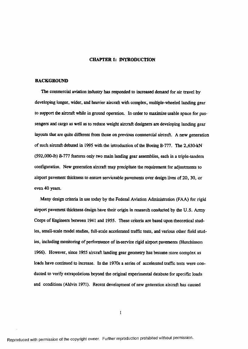
BACKGROUND
The commercial aviation industry has responded to increased demand for air travel by
developing longer, wider, and heavier aircraft with complex, multiple-wheeled landing gear
to support the aircraft while in ground operation. In order to maximize usable space for pas
sengers and cargo as well as to reduce weight aircraft designers are developing landing gear
layouts that are quite different from those on previous commercial aircraft. A new generation
of such aircraft debuted in 1995 with the introduction of the Boeing B-777. The 2,630-kN
(592,000-lb) B-777 features only two main landing gear assemblies, each in a triple-tandem
configuration. New generation aircraft may precipitate the requirement for adjustments to
airport pavement thickness to ensure serviceable pavements over design lives of 20, 30, or
even 40 years.
Many design criteria in use today by the Federal Aviation Administration (FAA) for rigid
airport pavement thickness design have their origin in research conducted by the U.S. Army
Corps of Engineers between 1941 and 1955. These criteria are based upon theoretical stud
ies, small-scale model studies, full-scale accelerated traffic tests, and various other field stud
ies, including monitoring of performance of in-service rigid airport pavements (Hutchinson
1966). However, since 1955 aircraft landing gear geometry has become more complex as
loads have continued to increase. In the 1970s a series of accelerated traffic tests were con
ducted to verify extrapolations beyond the original experimental database for specific loads
and conditions (Ahlvin 1971). Recent development of new generation aircraft has caused
Reproduced with permission of the copyright owner. Further reproduction prohibited without permission.
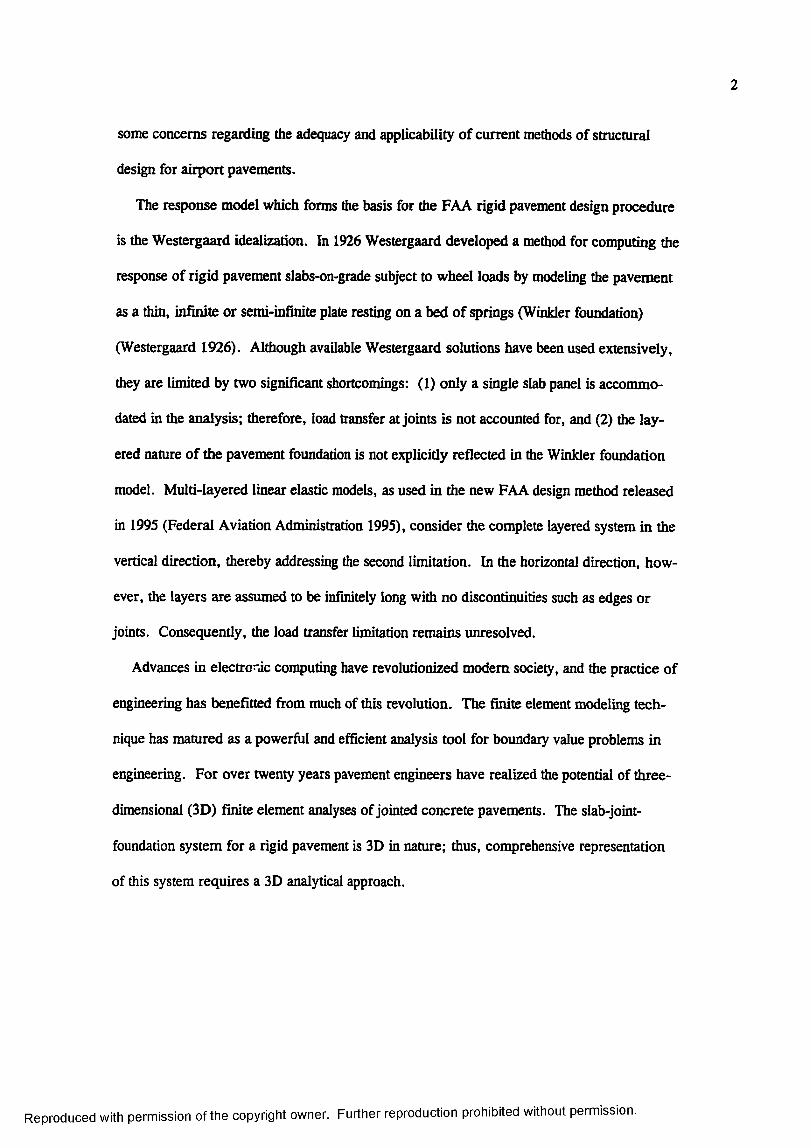
some concerns regarding the adequacy and applicability of current methods of structural
design for airport pavements.
The response model which forms the basis for the FAA rigid pavement design procedure
is the Westergaard idealization. In 1926 Westergaard developed a method for computing the
response of rigid pavement slabs-on-grade subject to wheel loads by modeling the pavement
as a thin, infinite or semi-infinite plate resting on a bed of springs (Winkler foundadon)
(Westergaard 1926). Although available Westergaard solutions have been used extensively,
they are limited by two significant shortcomings: (1) only a single slab panel is accommo
dated in the analysis; therefore, load transfer at joints is not accounted for, and (2) the lay
ered nature of the pavement foundation is not explicitly reflected in the Winkler foundation
model. Multi-layered linear elastic models, as used in the new FAA design method released
in 1995 (Federal Aviation Administration 1995), consider the complete layered system in the
vertical direction, thereby addressing the second limitation. In the horizontal direction, how
ever, the layers are assumed to be infinitely long with no discontinuities such as edges or
joints. Consequently, the load transfer limitation remains unresolved.
Advances in electronic computing have revolutionized modem society, and the practice of
engineering has benefitted from much of this revolution. The finite element modeling tech
nique has matured as a powerful and efficient analysis tool for boundary value problems in
engineering. For over twenty years pavement engineers have realized the potential of three-
dimensional (3D) finite element analyses of jointed concrete pavements. The slab-joint-
foundation system for a rigid pavement is 3D in nature; thus, comprehensive representation
of this system requires a 3D analytical approach.
Reproduced with permission of the copyright owner. Further reproduction prohibited without permission.

OBJECTIVES
The prünaiy research objectives of this study were the following;
• Review currently-available rigid pavement models with particular emphasis on their
joint and foundation modeling capabilities.
• Using modem analytical methods, analyze the yet lu^ublished scale-model studies on
two-slab panel models with doweled joints performed by the U. S. Army Corps of
Engineers Rigid Pavement Laboratory in the 1950s.
• Obtain data on the behavior of the rigid pavement slab-joint-foundation system by con
ducting scale-model studies of jointed rigid pavement slabs on cement-stabilized bases.
• Develop a comprehensive 3D finite element model of the rigid pavement slab-joint-
foundation system that can be implemented in the advanced pavement design concepts
currently under development by FAA.
SCOPE
This study offers a significant advancement in the state of the art for rigid pavement analy
sis by moving in the direction of a more comprehensive 3D finite element response model for
rigid pavements. However, it is inçortant that our perspective include the historical develop
ments that have given rise to the current technology. Therefore, a survey of the problem
addressed by this research along with the definitions o f the fundamental joint response metrics
for rigid airfield pavements are presented in Chapter 2 followed in Chapter 3 by a synopsis of
the historical background for the current FAA rigid pavement design criteria. In Chapters 4
and 5 classical and finite element response models germane to this research are reviewed.
Chapter 6 contains an analysis of doweled joint response data fi-om small-scale model tests
conducted in the 1950s by the Corps of Engineers. Chapter 7 describes in detail a compre
hensive two-dimensional (2D) and 3D finite element response and sensitivity study for the
Reproduced with permission of the copyright owner. Further reproduction prohibited without permission.

jointed rigid pavement problem. Experiments on laboratory-scale jointed rigid pavement
models are described and their results presented in Chapter 8. These experimental results are
used in Chapter 9 to verify the development of a conçrehensive 3D finite element analysis
procedure for discontinuities in rigid airfield pavements. Finally, conclusions and
recommendations from this research are found in C luster 10.
The Westergaard idealization layered elastic analysis, and finite element programs based
on two-dimensional (2D) elements have proven to be use Ail tools in the design and analysis of
rigid pavements. It is not likely that 3D finite element models will summarily replace these
techniques in the near future. However, several very important physical processes cannot be
adequately modeled without the 3D approach; furthermore, recent developments in engineer
ing mechanics are best suited for 3D applications. Conq>rehensive 3D modeling provides a
more fundamental understanding of certain aspects of pavement response that can be incorpo
rated into the design process.
Although very important in understanding the overall response and performance of rigid
pavement systems, environmental loadings were not considered as a part of this study. How
ever, future studies including such effects could use the results of this study as a basis for
research.
Reproduced with permission of the copyright owner. Further reproduction prohibited without permission.

CHAPTER 2: PROBLEM STATEMENT
RIGID PAVEMENT SYSTEM
A rigid pavement system consists of a number of portland cement concrete slabs, finite in
length and width, over one or more foundation layers. Figure 2.1 shows a representation of
a typical rigid pavement system subjected to a static loading. When a slab-on-grade is sub
jected to a wheel load, it develops bending stresses and distributes the load over the founda
tion. The response o f these finite slabs is controlled by joint or edge discontinuities. By their
nature joints weaken the structural system. Thus, the response and effectiveness of joints are
primary concerns in rigid pavement analysis and design.
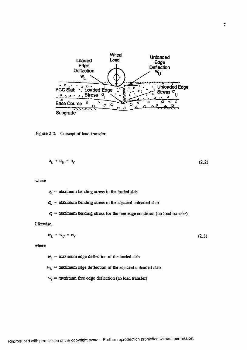
Figure 2.2 presents a conceptual view of the mechanism of load transfer at a joint. The
concept of load transfer is very simple; stresses and deflections in a loaded slab are reduced
if a portion of the load is transferred to an adjacent slab. Load transfer is very important and
fundamental to the FAA rigid pavement design procedure. A complex mechanism, load
transfer varies with concrete pavement temperature, age, moisture content, construction qual-
i^ , magnitude and repetition of load, and Qrpe of joint.
When a joint is capable of transferring load, statics dictates that the total load (P) must be
equal to the sum of that portion of the load supported by the loaded slab (PJ and the portion
of the load supported by the unloaded slab (Py), i.e.,
= P (2 .1 )
Load may be transferred across a joint by shear or bending moments. However, it has
been commonly argued that load transfer is primarily caused by vertical shear and that
moment transfer is negligible. In either case, the following relationship applies:
Reproduced with permission of the copyright owner. Further reproduction prohibited without permission.
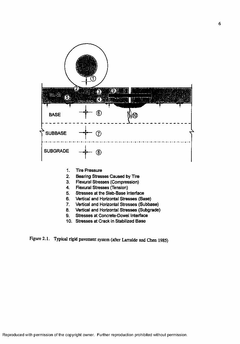
SUBGRADE (D
1. Tire Pressure2. Bearing Stresses Caused by Tire3. Flexural Stresses (Compression)4. Flexural Stresses (Tension)5. Stresses at the Slab-Base Interface6. Vertical and Horizontal Stresses (Base)7. Vertical and Horizontal Stresses (Subbase)8. Vertical and Horizontal Stresses (Subgrade)9. Stresses at Concrete-Dowel Interface10. Stresses at Crack in Stabilized Base
Figure 2.1. Typical rigid pavement system (after Larralde and Chen 1985)
Reproduced with permission of the copyright owner. Further reproduction prohibited without permission.
Loaded Edge
Deflection w,
WheelLoad
* o fl o •PCCSlab % Loaded
0 a Û • Ù . S tress c
Base Course ^ q ^ o
UnloadedEdge
Deflection
. o " * Unloaded" Edge■ o o s tre ss <7
Subgrade
Figure 2.2. Concept of load transfer
<V (2 .2)
where
^ = maximum bending stress in the loaded slab
% = maximum bending stress in the adjacent unloaded slab
Of = maximum bending stress for the free edge condition (no load transfer)
Likewise,
where
= maximum edge deflection of the loaded slab
Wy = maximum edge deflection of the adjacent unloaded slab
Wf = maximum free edge deflection (no load transfer)
(2.3)
Reproduced with permission of the copyright owner. Further reproduction prohibited without permission.

LOAD TRANSFER DEFINIHONS
Deflection load transfer efficiency {LTE^ is defined as the ratio of the deflection of the
unloaded slab to the deflection o f the loaded slab as follows:
LTE, (2.4)
Similarly, stress load transfer efficiency (JLTE is defined as the ratio of the edge bending
stress in the unloaded slab to edge stress in the loaded slab as follows:
LTE. (2.5)
Load transfer (LT) in the FAA rigid pavement design procedure is defined as that portion of
the edge stress that is carried by the adjacent unloaded slab:
LT =V ^ f)
(2.6)
LT is commonly expressed as a percentage. It should be noted from the above equations that
the ranges of LTEg and LTE„ are from zero to one, while the range of LT is from zero to one
half. Equation 2.6 can be related to Equation 2.5 as follows:
L T -I + LTE_ (2.7)
The FAA design criteria prescribe LT = 0.25, effectively reducing the design stress and
allowing a reduced slab thickness. This accepted value is primarily based upon observations
from experimental pavements trafficked from the mid-1940s to the mid-1950s. If the load
Reproduced with permission of the copyright owner. Further reproduction prohibited without permission.
transfer requirement is violated through a degradation of the joint system, the pavement life
can be significantly reduced.
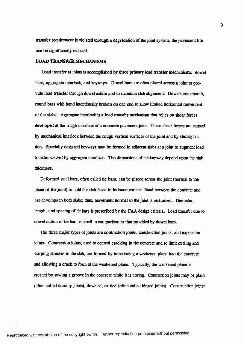
LOAD TRANSFER MECHANISMS
Load transfer at joints is accon^lished by three primary load transfer mechanisms: dowel
bars, aggregate interlock, and keyways. Dowel bars are often placed across a joint to pro
vide load transfer through dowel action and to maintain slab alignment. Dowels are smooth,
round bars with bond intentionally broken on one end to allow limited horizontal movement
of the slabs. Aggregate interlock is a load transfer mechanism that relies on shear forces
developed at the rough interface of a concrete pavement joint. These shear forces are caused
by mechanical interlock between the rough vertical surfaces of the joint and by sliding fric
tion. Specially designed keyways may be formed in adjacent slabs at a joint to augment load
transfer caused by aggregate interlock. The dimensions of the keyway depend upon the slab
thickness.
Deformed steel bars, often called tie bars, can be placed across the joint (normal to the
plane o f the joint) to hold the slab faces in intimate contact. Bond between the concrete and
bar develops in both slabs; thus, movement normal to the joint is restrained. Diameter,
length, and spacing of tie bars is prescribed by the FAA design criteria. Load transfer due to
dowel action of tie bars is small in conq>arison to that provided by dowel bars.
The three major types of joints are contraction joints, construction joints, and expansion
joints. Contraction joints, used to control cracking in the concrete and to limit curling and
warping stresses in the slab, are formed by introducing a weakened plane into the concrete
and allowing a crack to form at the weakened plane. Typically, the weakened plane is
created by sawing a groove in the concrete while it is curing. Contraction joints may be plain
(often called dummy joints), doweled, or tied (often called hinged joints). Construction joints
Reproduced with permission of the copyright owner. Further reproduction prohibited without permission.

10
are required between lanes of paving or where it is necessary to stop construction within a
paving lane. The two most common types of load transfer devices in construction joints are
dowels and keyways. Expansion joints are used at the intersections of pavements with struc
tures, and in some cases, within pavements. Their primary purpose is to relieve compressive
stresses induced by e?q>ansion of the concrete caused by temperature and moisture changes.
Expansion joints may be doweled or thickened edge. To obtain load transfer at an expansion
joint, a load transfer device is required (usually a dowel bar).
RIGID PAVEMENT FOUNDATIONS
The slabs may be placed directly on the subgrade; however, most current practice has
slabs placed on an unbound or a bound base course. Such base course layers in airport
pavements may be constructed to (a) provide uniform bearing support for the pavement slab;
(b) replace soft, highly compressible or expansive soils; (c) protect the subgrade from frost
effects; (d) produce a suitable surface for operating construction equipment; (e) improve
foundation strength; (f) prevent subgrade pumping; and (g) provide drainage of water from
under the pavement. An unbound base course may be a densely graded granular material or
an open-graded or free-draining granular material. The base may be bound with portland
cement, a lime-fly ash blend, bitumen, or other agent.
One or more subbases may be present in the pavement system. These subbases may be a
lesser qualiQr granular material and may be chemically stabilized. The subbase provides
additional strength to the pavement system, provides more uniform support over variable soil
conditions, and may provide protection against frost damage and swelling.
The subgrade is the namrally occurring soil, compacted naturally occurring soil, or com
pacted fill. It may be subject to pumping, frost damage, or swelling. Subgrade soils will
Reproduced with permission of the copyright owner. Further reproduction prohibited without permission.

11
have very different values of strength depending on the soil classification, moisture condi
tions, and connection.
Reproduced with permission of the copyright owner. Further reproduction prohibited without permission.

CHAPTER 3: HISTORICAL DEVELOPMENTS
Many of the design criteria in use by the FAA for rigid airport pavements have their origin
in research conducted by the U.S. Army Corps of Engineers between 1941 and 1955
(Hutchinson 1966). When the Corps was assigned responsibility for design and construction
of military airfields in November, 1940, two major problems became immediately apparent.
First, new heavy bomber aircraft, such as the B-17 Flying Fortress and B-24 Liberator, had
maximum gross weights of 333 kN (75,000 lb) and produced single-wheel main gear loadings
of 156 kN (35,000 lb), three to five times greater than any highway or airfield loadings previ
ously encountered. The second problem was a lack of rational and valid design procedures
by which rigid pavements could be designed to carry loads of these magnitudes (Sale and
Hutchinson 1959). These problems were exacerbated during and after World W ar n as the
demands upon rigid pavements continued to increase due to the development o f ever heavier
bomber aircraft including the propeller-driven B-29 and B-36 was well as the B-47 and B-52
jet bomber aircraft.
The technical issues faced by the early Corps’ researchers were formidable. Many of the
basic principles of airport pavement design accepted today concerning pavement response,
design loadings, critical stresses, materials characterization, and others were not yet estab
lished in 1940. Among these technical questions were the following:
• What is an appropriate response model for rigid airfield pavements?
• What are the critical stresses that the pavement must be designed to resist?
• How should the subgrade be characterized for design? What type of tests should be
conducted to characterize the support provided by the subgrade?
12
Reproduced with permission of the copyright owner. Further reproduction prohibited without permission.

13
• Which loading is more severe: static loadings generated by fully loaded aircraft at rest
or dynamic loadings which occur at the point of touchdown during landing operations?
• What effects do joints have on rigid pavement response and how should these be
accommodated in design criteria?
• How can pavements be designed to resist repeated heavy loads over a given design
Ufe?
• What is an appropriate failure criteria?
• What is the effect of aircraft wander?
To provide answers for these questions, the Corps embarked on an investigational pro
gram in 1941 with a four-tiered approach involving theoretical studies, small-scale model
studies, full-scale accelerated test track and miscellaneous field studies, and condition surveys
of existing rigid airfield pavements.
A review of the available design methodologies revealed that substantial variations existed
in design criteria from agency to agency. Design methodologies commonly used by state
agencies or foreign governments relied heavily on local experience, materials, and empiri
cisms developed from performance records within the agency’s purview. It was apparent that
research was required to develop criteria that could be universally applied for all conditions
that might be encountered, whether in the United States or abroad. The criteria needed to be
sinq)le, practical, and uniform. The objectives of the investigational program, as stated by
Sale and Hutchinson (1959), were as follows: (a) eliminate the use of untried methods;
(b) insure adequately designed pavements; (c) provide methods not subject to variation occa
sioned by arbitrary cost differences of local competitive materials; (d) avoid reductions in
pavement thickness in order to balance costs; and (e) establish procedures that would readily
lend themselves to further development though tests, investigations, and study of actual
Reproduced with permission of the copyright owner. Further reproduction prohibited without permission.
14
pavement behavior. From these studies criteria were developed for plain and reinforced con
crete pavements as well as rigid and flexible overlays.
RESPONSE MODEL
One of the first requirements in developing design criteria was to adopt an appropriate
response model for rigid pavements. The theory of Professor Harald Malcolm Westergaard
(1926) proved to ^proximate the observed response of rigid pavements. Westergaard
assumed the slab to be a thin plate, the load to be circular, and the subgrade to be a bed of
springs. By 1941 Westergaard’s method of calculating stresses was considered to be the most
advanced method for predicting critical stresses and deflections in rigid pavements and was
adopted by the Corps as the response model for design (Sale 1977). Although Westergaard
considered the interior, comer, and edge loading cases in his early works, he concentrated on
interior loadings. It was not until 1948 that he published relationships that were valid for
computation of stresses caused by large wheel loads on large contact areas at the edge of
slabs (Westergaard 1948).
CRITICAL DESIGN STRESSES
In 1941 the Corps began a series of static and dynamic load tests on concrete slabs at
Wright Field, Dayton, Ohio, in part to verify Westergaard’s theory for airfield rigid pave
ment design (Sale and Hutchinson 1959). A set of 6 m (20 ft) square slabs was constructed
on a number of subgrades of different strengths and tested to failure under static circular plate
loadings. Also, dynamic loadings were generated by dropping loaded aircraft tires onto the
pavement. The test slabs were instrumented with strain and deflection gages. The basic con
clusions from these tests were that the Westergaard formula accurately predicted the critical
stresses at structural failure, and dynamic loadings produced no greater stresses than
equivalent static loadings.
Reproduced with permission of the copyright owner. Further reproduction prohibited without permission.
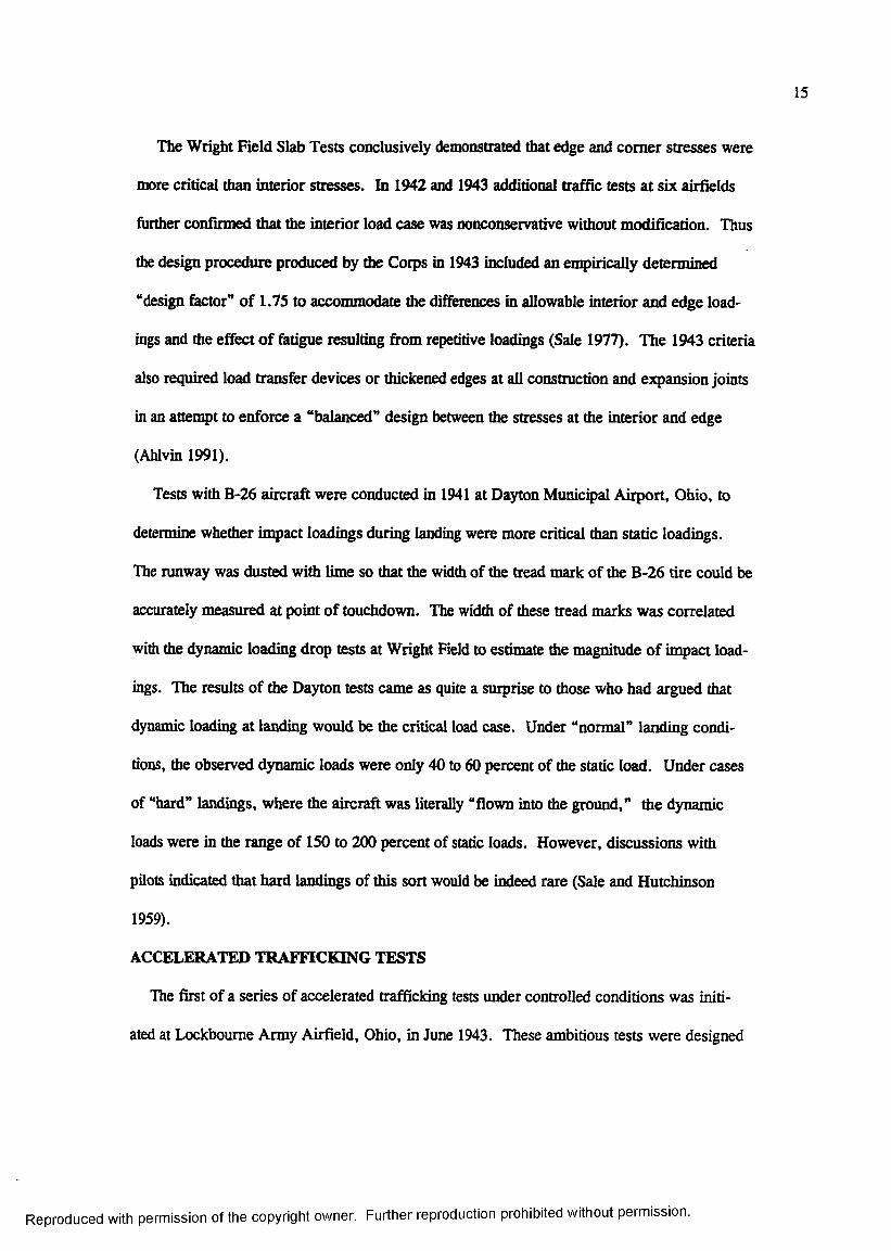
15
The Wright Field Slab Tests conclusively demonstrated that edge and comer stresses were
more critical than interior stresses. In 1942 and 1943 additional traffic tests at six airfields
further confirmed that the interior load case was nonconservative without modification. Thus
the design procedure produced by the Corps in 1943 included an empirically determined
"design factor” of 1.75 to accommodate the differences in allowable interior and edge load
ings and the effect o f fatigue resulting from repetitive loadings (Sale 1977). The 1943 criteria
also required load transfer devices or thickened edges at all construction and expansion joints
in an attenq)t to enforce a "balanced” design between the stresses at the interior and edge
(Ahlvin 1991).
Tests with B-26 aircraft were conducted in 1941 at Dayton Municipal Airport, Ohio, to
determine whether in tac t loadings during landing were more critical than static loadings.
The runway was dusted with lime so that the width of the tread mark of the B-26 tire could be
accurately measured at point of touchdown. The width of these tread marks was correlated
with the dynamic loading drop tests at Wright Field to estimate the magnitude of inq^act load
ings. The results of the Dayton tests came as quite a surprise to those who had argued that
dynamic loading at landing would be the critical load case. Under "normal” landing condi
tions, the observed dynamic loads were only 40 to 60 percent of the static load. Under cases
of “hard” landings, where the aircraft was literally "flown into the ground,” the dynamic
loads were in the range of 150 to 200 percent of static loads. However, discussions with
pilots indicated that hard landings of this sort would be indeed rare (Sale and Hutchinson
1959).
ACCELERATED TRAFFICKING TESTS
The first of a series of accelerated trafficking tests under controlled conditions was initi
ated at Lockboume Army Airfield, Ohio, in June 1943. These ambitious tests were designed
Reproduced with permission of the copyright owner. Further reproduction prohibited without permission.

16
to pennit a comprehensive evaluation of many of the factors influencing rigid pavement
design. Extensive strain and deflection measurements were made at slab interiors, edges, and
comers.
The concept of coverages was introduced to account for distribution of traffic over the
width of the pavement. Based upon probabilistic concepts, one coverage was said to occur
when each point in the wander width of the pavement feature had been subjected to one
maximum stress repetition by the operating aircraft. At the time of the Lockboume tests,
5.000 coverages was considered to be representative of a design life of 10 years.
Among the conclusions of the Lockboume accelerated trafficking tests as summarized by
Sale and Hutchinson (1959) were the following;
• Stresses produced in a pavement slab by either traffic loadings or static loadings are
more severe when the loading is applied at the comers and edges of a slab than when
applied at the center.
• The Westergaard edge load equations (developed in 1943 and published in final form
by Westergaard in 1948) were valid for a single loading condition, but an additional
“design factor” must applied to account properly for stress repetitions (fatigue), tem
perature gradients, and other unknown variables.
Measurements from the Lockboume tests showed that responses calculated by Wester
gaard’s theory were conservative and followed the shape and form of the test track measure
ments. Therefore, the Corps revised its design criteria to edge stresses, adopting a 25 percent
load transfer at the joints. A “design factor” of 1.3 was used for stress repetitions up to
5.000 coverages and to accommodate environmental stresses. The design factor (DF) was
defined as the ratio of the design flexural strength of the concrete (R) to the maximum free
edge stress. In its most general form, the DF is given by
Reproduced with permission of the copyright owner. Further reproduction prohibited without permission.
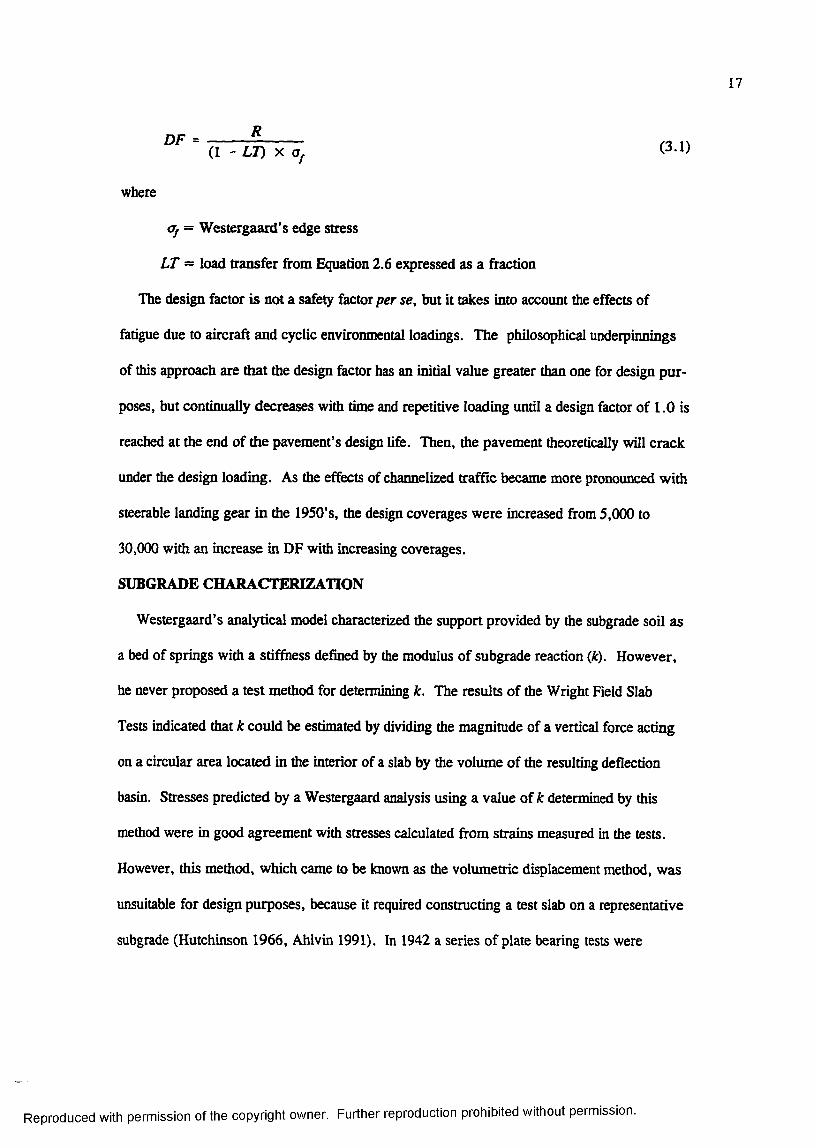
17
DF = --------- n(1 ' L7) X oy
where
Of = Westergaard’s edge stress
LT = load transfer from Equation 2.6 expressed as a fraction
The design factor is not a safety factor per se, but it takes into account the effects of
fatigue due to aircraft and cyclic environmental loadings. The philosophical underpinnings
of this approach are that the design factor has an initial value greater than one for design pur
poses, but continually decreases with time and repetitive loading until a design factor of 1.0 is
reached at the end of the pavement’s design life. Then, the pavement theoretically will crack
under the design loading. As the efrects of channelized traffic became more pronounced with
steerable landing gear in the 1950's, the design coverages were increased from 5,000 to
30,000 with an increase in DF with increasing coverages.
SUBGRADE CHARACTERIZATION
Westergaard’s analytical model characterized the support provided by the subgrade soil as
a bed of springs with a stiffness defined by the modulus of subgrade reaction {k). However,
be never proposed a test method for determining k. The results of the Wright Field Slab
Tests indicated that k could be estimated by dividing the magnitude of a vertical force acting
on a circular area located in the interior of a slab by the volume of the resulting deflection
basin. Stresses predicted by a Westergaard analysis using a value of k determined by this
method were in good agreement with stresses calculated from strains measured in the tests.
However, this method, which came to be known as the volumetric displacement method, was
unsuitable for design purposes, because it required constructing a test slab on a representative
subgrade (Hutchinson 1966, Ahlvin 1991). In 1942 a series of plate bearing tests were
Reproduced with permission of the copyright owner. Further reproduction prohibited without permission.

18
conducted on each subgrade for the Wright Field Slab Tests with plates varying in diameter
from 305 mm (12 in.) to 1828 mm (72 in.). Almost without exception, tests made with a
762-mm (30-in.) diameter plate were in close agreement with k values determined from the
volumetric displacement method (Sale and Hutchinson 1959). This plate bearing test, with
minor variations, is still in use today to characterize the modulus of subgrade reaction for
rigid pavement design.
The adequacy of the plate bearing test method has been questioned repeatedly in the past.
One of the primary shortcomings of the test is that it requires a representative subgrade to be
prepared before an accurate subgrade modulus can be obtained. The use of thick base
courses and stabilized layers presents an obvious problem. However, one of the advantages
of the plate bearing test is that it is a measure of the elastic (and plastic) properties of the soil
at a unit loading which is approximately equal to the unit load to which the soil will be sub
jected (Hutchinson 1966). It can also be shown that the design pavement thickness is not par
ticularly sensitive to typical variations in k\ therefore, the plate bearing value is considered
adequate for design purposes.
In the 1950s the Corps began to require that the modulus of subgrade reaction for design
of rigid pavements over base course be determined from plate bearing tests conducted on top
of the base course. As these data accumulated, the Corps began to develop curves relating
the k value on top o f the base to the k value of the subgrade. In the 1970s these curves were
approved by the Corps for design supplanting the requirement to conduct tests directly on the
base (Ahlvin 1991). Later the FAA adopted this approach into its design doctrine. However,
recent studies by Darter et al. (1995) have shown that the concept of the top-of-the-base k is
not valid and that stabilized layers should be considered as a structural layer in analysis and
design.
Reproduced with permission of the copyright owner. Further reproduction prohibited without permission.

19
RIGID PAVEMENT JOINTS
Early experiences with highways revealed the importance of tying rigid pavement slabs
together to prevent separation at the joints. Typically, deformed steel reinforcing bars were
used in highway construction. However, an additional benefit was discovered; some load
transfer was provided at the joint. Because highway slabs were being designed for interior
loads, this advantage was not immediately appreciated. Later, as it became apparent that
edge loadings were more critical than interior loadings, highway engineers began to construct
rigid pavements with thickened edges. This practice was carried over into the first Corps’
rigid pavement design procedure in 1943 (Hutchinson 1966).
Early work of the Corps of Engineers showed that the design thickness of rigid pavements
was controlled by the tensile stress that occurred at the edge of the pavement slabs. This
work also indicated that the edge stresses were reduced by properly designed load transfer
devices at the joints. Thus, thinner, more economical pavement designs could be produced
that would have satisfactory performance. A second benefit was increased surface smooth
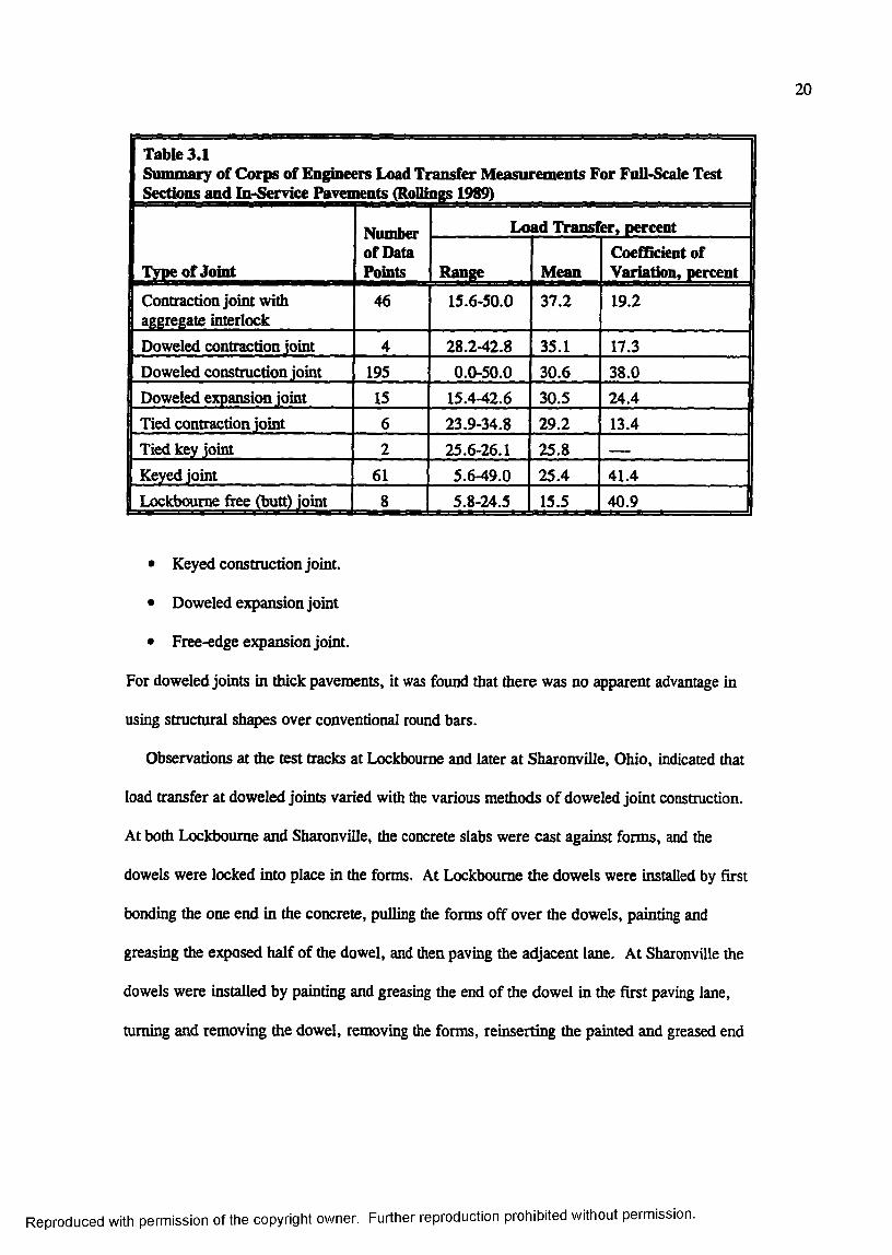
ness as load transfer devices reduced differential vertical movements at the joints. Table 3.1
summarizes some of the values of load transfer from full-scale accelerated trafficking tests
and in-service pavements.
Based upon the performance of the test items in the Lockboume No. 2 Test Track and
upon measured deflections and strains, the following ranking of joint types from the most
effective to the least (in terms of load transfer) was made (Sale and Hutchinson 1939):
• Doweled contraction joint.
• Doweled construction joint.
• Keyed construction joint with tie bars.
• Contraction joint.
Reproduced with permission of the copyright owner. Further reproduction prohibited without permission.
20
Table 3.1Summary of Corps of Engineers Load Transfer Measurements For Full-Scale Test Sections and In-Service Pavements (Rollings 1989)
Type of Joint
Number of Data Points
Load Transfer, percent
Range MeanCoefficient of Variation, percent
Contraction joint with aggregate interlock
46 15.6-50.0 37.2 19.2
Doweled contraction joint 4 28.2-42.8 35.1 17.3Doweled construction joint 195 0.0-50.0 30.6 38.0Doweled expansion joint 15 15.4-42.6 30.5 24.4Tied contraction joint 6 23.9-34.8 29.2 13.4
1 Tied key joint 2 25.6-26.1 25.8 ----
Keyed joint 61 5.6-49.0 25.4 41.41 Lockboume free (butt) joint 8 5.8-24.5 15.5 40.9
• Keyed construction joint.
• Doweled expansion joint
• Free-edge expansion joint.
For doweled joints in thick pavements, it was found that there was no apparent advantage in
using structural shapes over conventional round bars.
Observations at the test tracks at Lockboume and later at SharonvUle, Ohio, indicated that
load transfer at doweled joints varied with the various methods of doweled joint construction.
At both Lockboume and SharonvUle, the concrete slabs were cast against forms, and the
dowels were locked into place in the forms. At Lockboume the dowels were installed by first
bonding the one end in the concrete, pulling the forms off over the dowels, painting and
greasing the exposed half of the dowel, and then paving the adjacent lane. At SharonvUle the
dowels were instaUed by painting and greasing the end of the dowel in the first paving lane,
turning and removing the dowel, removing the forms, reinserting the painted and greased end
Reproduced with permission of the copyright owner. Further reproduction prohibited without permission.
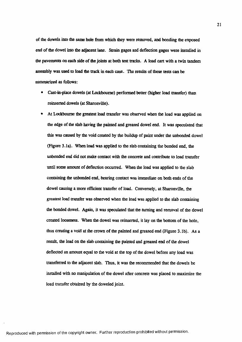
21
of the dowels into the same hole from which they were removed, and bonding the exposed
end of the dowel into the adjacent lane. Strain gages and deflection gages were installed in
the pavements on each side of the joints at both test tracks. A load cart with a twin tandem
assembly was used to load the track in each case. The results of these tests can be
summarized as follows:
• Cast-in-place dowels (at Lockboume) performed better (higher load transfer) than
reinserted dowels (at SharonvUle).
• At Lockboume die greatest load transfer was observed when the load was applied on
the edge of the slab having the painted and greased dowel end. It was speculated that
this was caused by the void created by the buUdup of paint under the unbonded dowel
(Figure 3.1a). When load was applied to the slab containing the bonded end, the
unbonded end did not make contact with the concrete and contribute to load transfer
untU some amount of deflection occurred. When the load was applied to the slab
containing the unbonded end, bearing contact was immediate on both ends of the
dowel causing a more efficient transfer of load. Conversely, at SharonvUle, the
greatest load transfer was observed when the load was applied to the slab containing
the bonded dowel. Again, it was speculated that the turning and removal of the dowel
created looseness. When the dowel was reinserted, it lay on the bottom of the hole,
thus creating a void at the crown of the painted and greased end (Figure 3. lb). As a
resiUt, the load on the slab containing the painted and greased end of the dowel
deflected an amount equal to the void at the top of the dowel before any load was
transferred to the adjacent slab. Thus, it was the recommended that the dowels be
installed with no manipulation of the dowel after concrete was placed to maximize the
load transfer obtained by the doweled joint.
Reproduced with permission of the copyright owner. Further reproduction prohibited without permission.
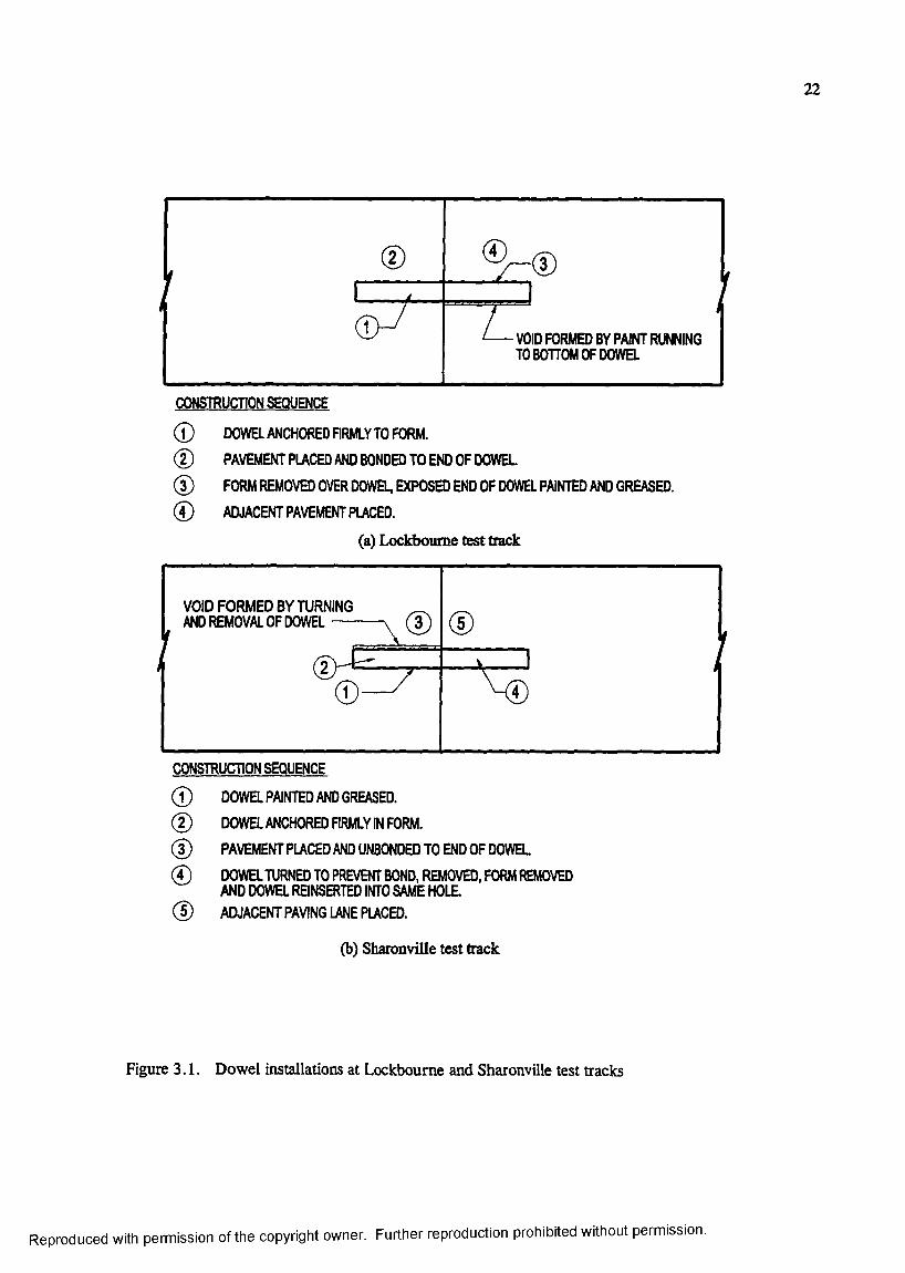
22
VOID FORMED BY PAINT RUNNING TO BOTTOM OF DOWEL
CONSTRUCTION SEQUENCE
0 DOWEL ANCHORED FIRMLYTO FORM.0 PAVEMENT PLACED AND BONDED TO END OF DOWEL0 FORM REMOVED OVER DOWEL EXPOSED END OF DOWEL PAINTED AND GREASED.0 ADJACENT PAVEMENT PLACED.
(a) Lockboume test track
VOID FORMED BY TURNING AND REMOVAL OF DOWEL —
CONSTRUCTION SEQUENCE
0 DOWEL PAINTED AND GREASED.0 DOWEL ANCHORED FIRMLY IN FORM.0 PAVEMENT PLACED AND UNBONDED TO END OF DOWEL0 DOWEL TURNED TO PREVENT BOND. REMOVED, FORM REMOVED
AND DOWEL REINSERTED INTO SAME HOLE.0 ADJACENT PAVING LANE PLACED.
(b) Sharonville test track
Figure 3.1. Dowel installations at Lockboume and Sharonville test tracks
Reproduced with permission of the copyright owner. Further reproduction prohibited without permission.
23
• Load transfer across doweled joints resulted in an edge stress reduction in excess of
25 percent.
• Load transfer efficiencies computed from deflections were greater than load transfer
efficiencies conq>uted from stresses.
• The load transfer across joints in multi-layer pavements is about the same as load
transfer in single layer construction.
A review of the ui^ublished minutes of the All-Division Meeting on Doweled Joints held
at the Ohio River Division Laboratories, September 1958, revealed that it was the opinion of
the Corps’ rigid pavement e?q)erts that doweled joints provided the best performance of the
commonly used joint types. The available performance data up to that point revealed that the
25 percent load transfer value used in design was conservative for doweled joints. Indeed, it
was a topic of discussion that the load transfer assumption should perhaps be increased for
doweled joints allowing a thinner pavement to be constructed. It was the opinion of these
experts that load transfer values of 35 to 40 percent might be appropriate for doweled joints.
However, it is important to note that these same experts were cognizant of the importance of
careful construction procedures in obtaining load transfer. The minutes of the meeting con
tain this statement:
We must realize that we do not, as yet, have sufficient information to accurately evaluate the amount of load transfer that is obtained from the various methods of construction [of doweled joints], therefore, for the time being, we must be conservative and continue to use the asstuned 25 percent. This does not mean, however, that we can relax our construction requirements. We must insist on good dowel installations, and we must keep the dowel looseness to a minimum if we are to ever realize the benefits of the doweled joint, because performance of the joints now being constructed will pay an inq)ortant role in any friture work we may do along this line. Otherwise, if through looseness, we fail to obtain the better load transfer, we may as well not use the more expensive doweled joint.
After World War II aircraft loadings continued to increase. To accommodate these
increasing demands on the pavement, aircraft manufacturers added more wheels to the
Reproduced with permission of the copyright owner. Further reproduction prohibited without permission.
24
landing gear to achieve wheel loadings sufficient to permit usage on existing pavements.
These multipie-wheel gear loadings over an entire slab raised doubts about the adequacy of
the assumptions concerning interior and edge loadings on slabs assumed to extend to infinity.
The advent of the C5-A military transport and the Boeing B-747 commercial aircraft with
loads twice as heavy as their predecessors lead to Multiple-Wheel Heavy Gear Load
(MWHGL) Pavement Tests conducted at the Waterways E?q)eriment Station in the late 1960s
and early 1970s (Ahlvin 1971; Bums 1971; Ledbetter 1971a, 1971b). A rigid pavement test
track was trafficked as a part of the MWHGL tests. The track was constructed in two 7.6-m
(25-ft) wide lanes separated by a longitudinal keyed construction joint. The keyway was
formed using metal strips. All transverse joints were weakened plane contraction joints.
Four test items were constructed so that failures would occur at times varying from a few
weeks to a few years under normal operating conditions and traffic volumes as follows:
Item Thickness
1 254 mm (10 in.)
2 305 mm (12 in.)
3 356 mm (14 in.)
4 203 mm (8 in.)
The subgrade was a lean clay soil compacted to 95 percent of the modified density at opti
mum water content. The modulus of subgrade reaction was approximately 27.1 MPa/m
(1(X) psi/in.).
A 12-wheel load cart, each wheel loaded to 133 kN (30,000 lb) for a total load of
1,600 kN (360,000 lb), was used to traffic the test section in such a way as to obtain edge
loading along the longitudinal keyed joint.
Reproduced with permission of the copyright owner. Further reproduction prohibited without permission.

25
The results of these tests raised questions about the practice of using keyed construction
joints for heavy loads on low-strength subgrades. Observations made from test pits excavated
after trafficking indicated that the keyed joint had failed either by shearing the key or by
spalling of the bottom portion of the keyway. It was not possible to determine exactly when
the keyed joint failed, but it was likely in the first 1,650 coverages, as evidenced by faulting
along the joint. The failure of both the male and female portions of the keyed joints were
taken as evidence of optimum geometry of the keyed joint. No inferences concerning the
performance of keyed joints on a stiffi subgrade could be made.
The performance of the transverse weakened-plane contraction joints was considered ade
quate. Little, if any, faulting was observed. An examination of the e;q>osed faces of the
joints in the test pits did not reveal excessive deterioration of the aggregate interlock.
SUMMARY
The FAA Westergaard rigid pavement structural design criteria has its origins in research
conducted by the U.S. Army Corps o f Engineers from 1940 to 1970. The following state
ments summarize the development of these criteria;
• The response model that forms the basis for the FAA structural design criteria for
rigid pavements is Westergaard’s 1948 edge loading model. The applicability of this
model was verified by a series of full-scale and small scale experiments conducted by
the Corps during the years during and just after World War U.
• The FAA structural design criteria for rigid pavements allows a reduction of Wester
gaard’s edge load stresses by 25 percent to account for load transfer at joints. This
reduction is based upon experimental evidence from full-scale and small-scale experi
ments as well as measurements of in-service pavements. However, it is recognized
Reproduced with permission of the copyright owner. Further reproduction prohibited without permission.

26
that in reality load transfer is not a constant value but varies with a number of factors,
among which are type of joint and qualiQr of joint construction.
The FAA structural design criteria for rigid pavements features a fatigue relationship
which relates aircraft traffic, measured in coverages, to the ratio o f concrete flexural
strength to design stress. A series of full-scale e>q)erimental test tracks was used to
develop a database of performance data for this purpose.
Reproduced with permission of the copyright owner. Further reproduction prohibited without permission.
CHAPTER 4: CLASSICAL RESPONSE MODELS
WESTERGAARD THEORY
Professor Harald Malcolm Westergaard published a series of papers containing relation
ships for calculating stresses in rigid pavements based upon the theory of elasticity. His pio
neering work was first published in Danish in 1923 (Westergaard 1923). However, this work
was not widely read, and in 1926, he published a method in English for calculating the
stresses in a rigid pavements (Westergaard 1926). He developed relationships for stresses
...by assuming the slab to act as a homogeneous, isotropic, elastic solid in equilibrium, and by assuming that the reactions of the subgrade to be vertical only and to be proportional to the deflections of the slab (Westergaard 1926).
Westergaard characterized the subgrade by the modulus of subgrade reaction (k), which is
a measure of the stifhiess of the subgrade and has units of force per area per unit deflection or
force/leogth\ An important term in the Westergaard theory which quantifies the stif&ess of
the slab relative to that of the subgrade, called the radius of relative stiffness, is expressed by
the following relationship;
(4.1)12(1-v^)k
where
E = modulus of elasticity of concrete
h = thickness of slab
V = Poisson’s ratio of concrete
Assuming the response of the slab to be that of a plate on a Winkler foundation, Wester
gaard developed a closed form relationship for the dimensionless ratio afi^/P as a function of
27
Reproduced with permission of the copyright owner. Further reproduction prohibited without permission.

28
dimensionless ratio a / / where o is the maximum bending stress, f is the magnitude of the
applied load, and a is the radius of the circular area over which the applied load acts for the
following three cases:
• Wheel load close to the comer of a semi-infinite slab.
• Wheel load at the interior of an infinite slab.
• Wheel load at the edge of a semi-infinite slab.
In 1932 the Bureau of Public Roads conducted the Arlington Road Tests at Arlington, Vir
ginia, using Westergaard’s theory as a basis for planning the tests. Following these tests
Westergaard modified his 1926 formulas to reflect the conditions and results of the tests
(Westergaard 1933). Westergaard extended his procedures to airfield pavements in 1939.
Again, Westergaard revised his formulas, this time to account for the larger contact area of
aircraft tires (Westergaard 1939). Although Westergaard considered the interior, comer, and
edge loading cases in his early works, he concentrated on interior loadings. loannides,
Thompson, and Barenberg (1985) found that several of the equations ascribed to Westergaard
in the literature are incorrect due to typographical errors or misapplication. They also
reported that the 1926 equation for edge loading was incorrect.
It was not until 1948 that Westergaard published relationships that were valid for computa
tion of stresses caused by edge loading of large wheel loads on large contact areas (Wester
gaard 1948). His revised formulas allowed the load to be characterized as an ellipse rather
than being limited to a circular tire print. loannides, Thonq)son, and Barenberg (1985) rec
ommended the use o f these equations as being more accurate than the 1926 equations.
Response charts
Pickett and Ray (1951) developed a graphical solution of the Westergaard theory in the
form of influence charts. These graphical solutions greatly simplified the determination of
Reproduced with permission of the copyright owner. Further reproduction prohibited without permission.

29
theoretical deflections and moments caused by wheel loads on slabs. Influence charts were
presented for four different load cases; interior loading assuming a bed of springs subgrade,
interior loading assuming an elastic solid subgrade, edge loading assuming a bed of springs
subgrade, and load placed at (/2 from an edge assuming a bed of springs subgrade. Stresses
can be calculated from the moment read from the chart by dividing by the section modulus,
defined as A /6. In a separate p ^ r , Pickett et al. (1951) presented 16 additional influence
charts for deflection, moment, and reactive pressures under interior, near edge, and near cen
ter loadings on slabs for springs, elastic solid, and elastic layer subgrades.
The first step in ^plying the influence chart involves solving for the radius of relative
stiffiiess of the pavement section. The scale for the chart is then set according to the value of
the radius of relative sti%iess, and the tire print to be analyzed is subsequently drawn to this
scale. The number o f blocks (including partial blocks) covered by the tire print are counted
and multiplied by the appropriate relationship to obtain either moment, deflection, or reactive
pressure.
Because of their simplicity, the FAA, U.S. Army, and U.S. Air Force adopted the influ
ence charts for the computation of maximum tensile stress for edge loading (Hutchinson
1966). Multiple-wheel gear assemblies can be analyzed with the charts simply by drawing
them to the appropriate scale and counting the blocks covered by the tire print. However, it
should be noted that the orientation of the gear must be positioned such that the maximum
number of blocks is covered to calculate the maximum stress or deflection.
Computerized solutions
A few computerized solutions to the Westergaard theory have been developed, most nota
bly the programs H-51, H51-ES, and PDILB (commonly referred to as the PGA AIRPORT
program.) The H-51 program, originally developed by General Dynamics Corporation and
Reproduced with permission of the copyright owner. Further reproduction prohibited without permission.

30
modified by WES, calculates the edge stress under multiple-wheel loads on a slab supported
by a dense liquid foundation. The solution is essentially a conq>uterized version of Pickett
and Ray’s response charts. The program allows the user to place the gear at any number of
different orientations and positions to calculate the maximum stress condition. H-Sl was
modified by loannides (1984) by incorporating an elastic solid foundation in the program
H51-ES. The PCA AIRPORT program is based upon Westergaard’s theory for loads at the
interior of an infinite slab supported by a dense liquid foundation (Packard, no date). This
program also allows multiple-wheel assemblies and allows the user to orient the gear to maxi
mize the response. loannides (1984) developed WESTER, a collection of Westergaard solu
tions in a single, user-fiiendly personal computer program.
Westergaard theory limitations
For nearly three quarters of a century, Westergaard’s theory has been used to calculate the
response of rigid pavements to wheel loads. His theory is relatively simple to apply and has
been accepted as accurate. However, there are several limitations as discussed in the follow
ing paragraphs.
• All pavement layers below the slab must be represented by a single parameter, the
modulus of subgrade reaction. A Qpical pavement may have several layers of materi
als including unbound or bound subbases and base courses with each overlying layer
having an increase in quality and stiffness. In a typical application o f Westergaard’s
theory to such a system, these layers are modeled by an increased modulus of sub
grade reaction intended to give an equivalent response.
• The foundation is assumed to respond linear-elastically. Few subgrade, subbase, or
base materials are truly linear-elastic. In fact most are nonlinear, stress-dependent.
Reproduced with permission of the copyright owner. Further reproduction prohibited without permission.

31
and change with time and environment. The effect of nonlinear, stress-dependent
material behavior on rigid pavement foundations is obscure.
• Westergaard assumed the slab to be in full contact with the subgrade at all points.
Thus the boundary conditions are violated if a void develops due to pumping or if the
slab and subgrade separate due to curling and warping.
• Westergaard assumed that the slabs were infinite (for the interior load case) or semi-
infinite (for the edge and comer load case); that is, the slabs extend far enough from
the loaded area that boundaries (discontinuities such as cracks or joints) have no effect
on the solution. In actual practice this may not be the case, because rigid pavement
slabs tend to be relatively narrow and have many cracks and joints.
• Load transfer cannot be directly modeled. For airport pavement design, load transfer
is set at a constant 25 percent; thus edge stresses are reduced by that amount in calcu
lating the design factor. These values have been related to performance in field test
sections to formulate design criteria.
• The thickness of the slab must be uniform. This assumption makes it impossible to
analyze slabs with thickened edges or other slabs of nonuniform thickness.
ELASTIC LAYER MODELS
The elastic layer theory was first formulated for a concentrated load and one layer by
Boussinesq and later generalized by others for a uniformly distributed load acting over a cir
cular area and to two or more layers. Manual solutions of one- or two-layer elastic systems
subjected to a singular circular load are cumbersome at best. Computerized solutions have
made it possible to analyze a system of many layers subjected to multiple loads. Among
these programs are the BISAR, CHEVRON, and JULEA programs (Barker and Gonzalez
1991).
Reproduced with permission of the copyright owner. Further reproduction prohibited without permission.

32
The basic assumptions of the elastic layer theory (Crawford and Katona 1975) are as
follows:
• All materials in the system are assumed to be homogeneous, isotropic, and linear elas
tic; thus, each pavement layer can be represented by three parameters; thickness,
modulus of elasdci^, and Poisson’s ratio. Each layer may have different elastic
properties.
• Each layer is indnite in horizontal extent, and the bottom layer extends vertically to
indniQr.
• The load is static and is uniformly distributed over one or more circular areas. Most
programs assume the load to be entirely vertical, although some can accommodate
horizontal components.
• The layers are continuously in contact. Also, the degree of restraint between adjacent
layers must be assumed. Common assumptions are that adjacent layers are fully
bonded or that they are fnctionless. Some programs can allow any degree of restraint
between these two extremes.
In the past several years layered elastic design models for rigid pavements have been
developed. The U.S. Army and Air Force have developed design guidance for elastic lay
ered design methodologies for both rigid and flexible pavements (Departments of Army and
Air Force 1988, 1989). The FAA (1995) has adopted an alternative design procedure
(known as LEDFAA) based on a layered elastic theory. For rigid pavements the basic design
principle is to limit the tensile stresses in the slab to a level sufficiently below the concrete
flexural strength so that failure (cracking) occurs only after some significant number of load
repetitions. Rigid and flexible overlays of rigid pavements can be accommodated in the
design model.
Reproduced with permission of the copyright owner. Further reproduction prohibited without permission.
33
Because of the assumptions of the layered elastic model, certain limitations are intrinsic;
• The model assumes each layer to be infinite in horizontal extent; therefore, joints and
cracks in rigid pavements are ignored. Even the base and subbase layers in a pave
ment are not infinite in horizontal extent. Stabilized layers may also develop cracks
which caimot be directly modeled.
• The model assumes each material to be linear elastic. This assumption may lead to
inconsistencies in stress calculations in the foundation layers. For example, it is not
possible for an unbotmd granular layer to carry significant tensile stresses; yet the lay
ered elastic model may predict such stresses.
MODELS FOR DOWEL STRESSES
Dowels have been used as load transfer devices in jointed concrete pavements for over
three-quarters of a century. Dowel bars are thought to prevent faulting, reduce pumping, and
reduce comer breaks. However, the design of dowels is based mostly on experience. Most
design criteria prescribe the diameter, length, and spacing of dowel bars based upon
pavement thickness.
Dowels located at some distance away from the point of application of the load are not as
effective in transferring load as those that are closer. The number o f dowels effective in dis
tributing the load has been debated since the early developments of rigid pavement modeling.
Westergaard (1928) concluded that only the first couple of dowels on either side of the load
are effective in transferring load. Based upon Westergaard's theory, Friberg (1940) noted
that for loadings a considerable distance fiom any edge, the maximum positive moment
occurs beneath the load, and the maximum negative moment occurs a distance of 1.8( from
the point of loading. Beyond 1.8Î, sometimes referred to as the effective length (e), the
Reproduced with permission of the copyright owner. Further reproduction prohibited without permission.
34
moment changes very little. Friberg concluded, therefore, that the influence of dowel shear
beyond that point is negligible, stating:
The effective dowel shear decreases inversely as the distance of the dowel from the point of loading, to zero at a distance of 1.8(. No dowels beyond that point influence the moment at the load point.
Friberg’s assumption of linear decrease of transferred shear force with distance appears
realistic and has been widely accepted (loannides and Korovesis 1992). Kushing and Fre
mont (1940) accepted Friberg’s linear assumption, but postulated that e could be as great as
7t?. Finite element studies led Tabatabaie (1978) to conclude that the linear assumption of
Friberg was appropriate, but that the effective length was l.OW. The above arguments are
appropriate for a single-wheel loading only; multiple wheel gear configurations will lead to
different values of the effective length. In fact, loannides and Korovesis (1992) have shown
that e is not a constant and is not function of g alone.
It is thought that bearing stresses under the dowel are responsible for spalling and loose
ness of the dowels. Analytical models for determining the bearing stresses in dowel bars
have been in existence since the late 1930s. Several investigators have presented formulas
for calculating the concrete bearing stresses (Friberg 1940; Tabatabaie 1978; loannides, Lee,
and Darter 1990). According to loannides et al. (1990), all of these formulations for bearing
stress ((^) may be represented by the following relationship:
o^ = A {structural) x B {load) (4 2)
The first term. A, is determined from the structural characteristics of the pavement system,
while the second term, B, quantifies the transferred load.
Friberg (1940) presented an analysis of stresses in doweled joints based upon the work of
Timoshenko and Lessels (1925). His analysis was based upon considering the dowel as a
semi-infinite beam on a Winkler foundation. His basic relationship for dowel stresses was
Reproduced with permission of the copyright owner. Further reproduction prohibited without permission.

35
(4 .3)
where
K = modulus of dowel support
yo = deflection of the dowel with respect to the concrete at the face of the joint
Friberg’s analysis of dowel bar support is shown in Figure 4.1.
Friberg’s relationship for the maximum deformation of concrete under a dowel bar with a
shear force P, is
where
CO = joint opening
Ea = modulus of elasticity of the dowel
li = moment of inertia o f dowel bar
P = relative stiffoess of the dowel-concrete system.
Friberg adopted Timoshenko’s definition of the relative stiffness of a bar embedded in
concrete as
Kd(4.5)
4 %
The bearing stress on the concrete at the joint face then becomes
E l 4 P %
°b - (4.6)
Reproduced with permission of the copyright owner. Further reproduction prohibited without permission.
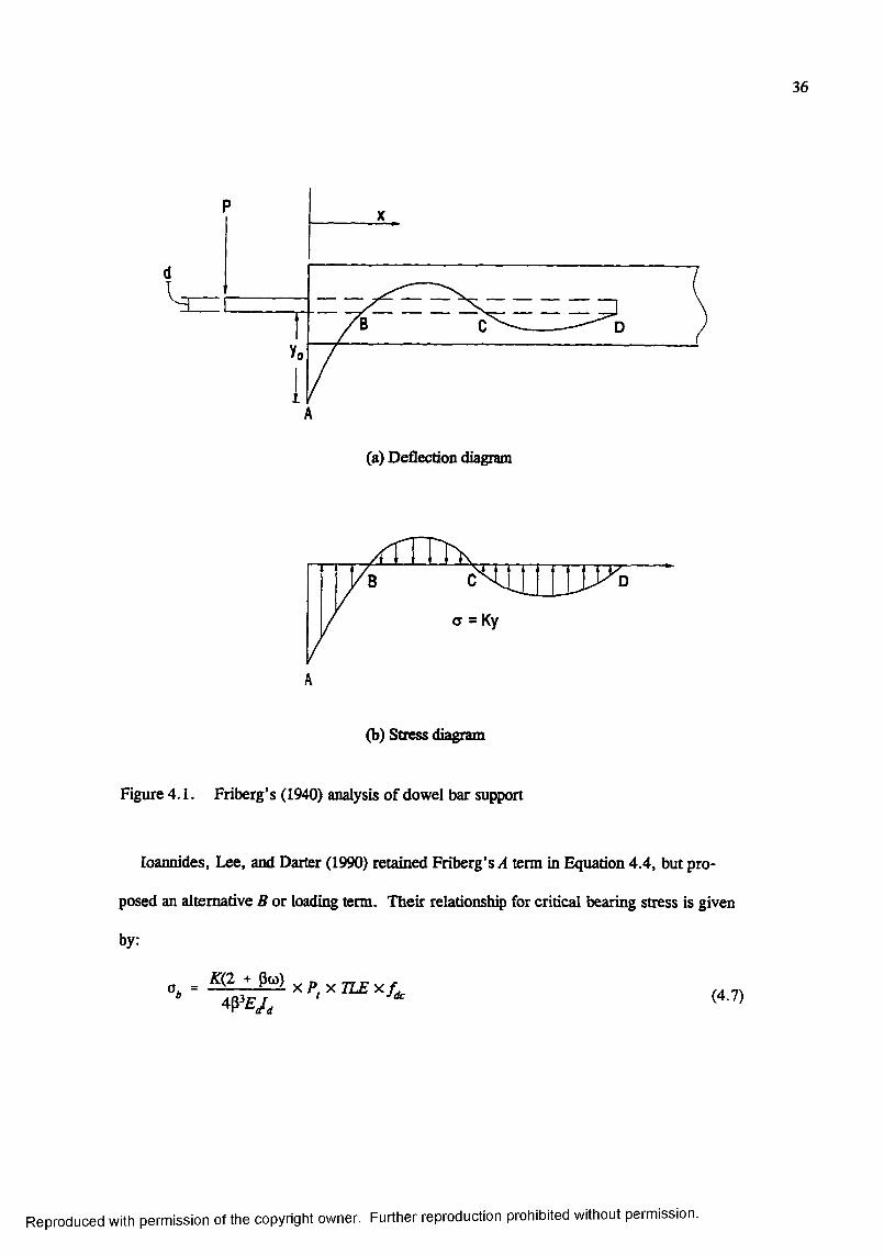
36
A
(a) Deflection diagram
a = Ky
(b) Stress diagram
Figure 4.1. Friberg’s (1940) analysis of dowel bar support
loannides, Lee, and Darter (1990) retained Friberg’s A term in Equation 4.4, but pro
posed an alternative B or loading term. Their relationship for critical bearing stress is given
by:
(4.7)
Reproduced with permission of the copyright owner. Further reproduction prohibited without permission.
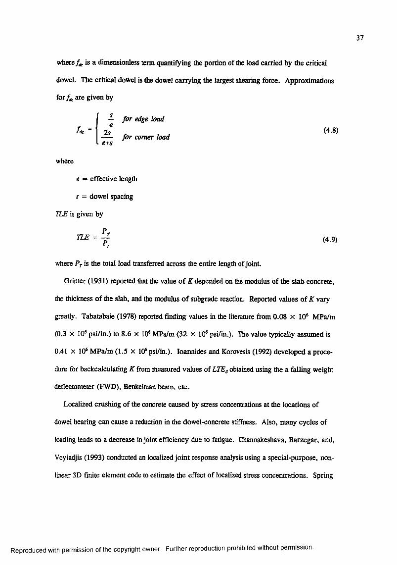
37
where is a dimensiooless term quantifying the portion of the load carried by the critical
dowel. The critical dowel is the dowel carrying the largest shearing force. Approximations
fox fic are given by
fd c = '
— for edge load
k ^ (4 8) for comer loade+s
where
e = effective length
s = dowel spacing
TLE is given by
TTj r -^ (4.9)t
where Pj- is the total load transferred across the entire length of joint.
Grinter (1931) reported that the value o f K depended on the modulus of the slab concrete,
the thickness o f the slab, and the modulus o f subgrade reaction. Reported values of K vary
greatly. Tabatabaie (1978) reported finding values in the literature from 0.08 x 10* MPa/m
(0.3 X 10® psi/in.) to 8.6 x 10® MPa/m (32 x 10® psi/in.). The value typically assumed is
0.41 X 10® MPa/m (1.5 x 10® psi/in.). loannides and Korovesis (1992) developed a proce
dure for backcalculating K fi-om measured values of LTEg obtained using the a falling weight
deflectometer (FWD), Benkelman beam, etc.
Localized crushing of the concrete caused by stress concentrations at the locations of
dowel bearing can cause a reduction in the dowel-concrete stiffness. Also, many cycles of
loading leads to a decrease in joint efficiency due to fatigue. Chaimakeshava, Barzegar, and,
Voyiadjis (1993) conducted an localized joint response analysis using a special-purpose, non
linear 3D finite element code to estimate the effect of localized stress concentrations. Spring
Reproduced with permission of the copyright owner. Further reproduction prohibited without permission.
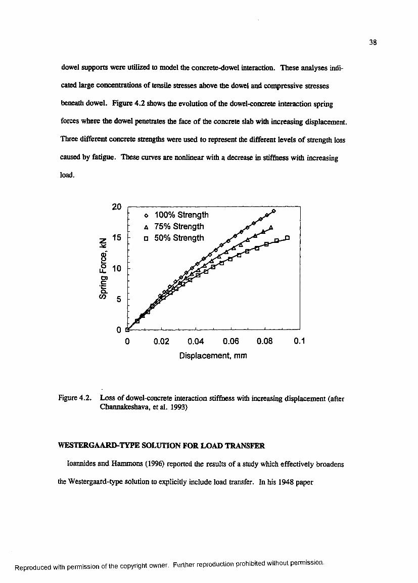
38
dowel supports were utilized to model the coocrete-dowel interaction. These analyses indi
cated large concentrations of tensile stresses above the dowel and compressive stresses
beneath dowel. Figure 4.2 shows the evolution of the dowel-concrete interaction spring
forces where the dowel penetrates die face o f the concrete slab widi increasing displacement.
Three different concrete strengths were used to represent the different levels o f strength loss
caused by fatigue. These curves are nonlinear with a decrease in stiffoess with increasing
load.
g£E"CQ.
CO
20o 100% Strength A 75% Strength □ 50% Strength15
10
5
00.08 0.10.060.020 0.04
Displacement, mm
Figure 4.2. Loss of dowel-concrete interaction stiffoess with increasing displacement (after Channakeshava, et al. 1993)
WESTERGAARD-TYPE SOLUTION FOR LOAD TRANSFER
loannides and Hammons (1996) reported the results of a study which effectively broadens
the Westergaard-type solution to explicitly include load transfer. In his 1948 paper
Reproduced with permission of the copyright owner. Further reproduction prohibited without permission.
39
Westergaard briefly described a solution for the edge load transfer problem. However, this
work was limited by his implicit assumption that deflection load transfer and stress load trans
fer were identical. Model studies and full-scale tests in the 1940s and 1950s conducted by the
Corps of Engineers, and more recently by finite element investigations (loannides and
Korovesis 1990, 1992), disproved this assumption.
In 1949 Mikhail S. Skarlatos described his analytical investigations (Skarlatos 1949). He
defined a dimensionless joint stiffness (/) in terms of the radius of relative stiffness, modulus
of subgrade reaction, and a parameter iq) which represents the force transferred across a unit
length of joint per unit differential deflection across the joint as foUows;
f " (4.10)
Using this approach, Skarlatos developed relationships involving integral equations for maxi
mum stress and deflection on the unloaded side of the joint. loannides and Hammons (1996),
using modem personal computers and powerful mathematical software, were able to perform
these integrations for square loaded areas of various sizes, 2e by 2e. Following the same
approach as Westergaard, closed-form equations for the maximum deflection and maximum
bending stress on the unloaded side of a joint capable of load transfer were developed. When
used together with Westergaard’s edge loading equations, the relationships developed by
loannides and Hammons (1996) can be used to investigate the load transfer problem.
The results of the analytical development work were consolidated into two graphs as sug
gested by the loannides and Korovesis (1990). Figures 4.3 and 4.4 illustrate the variation of
the deflection load transfer efficiencies, LTEs, and stress load transfer efficiencies, LTEg,
with respect to the dimensionless joint stiffness,/, and the dimensionless loaded area size.
Reproduced with permission of the copyright owner. Further reproduction prohibited without permission.
40
e/l. Nonlinear regression was used to develop an expression for LTEg as a function/and eJê
as follows:
1/ \
(4.11)
LTEj -
0.214 - 0.183 f - - lo g /1 + log'* V IJ
1.180
Likewise, nonlinear regression was used to develop an egression for LTEg as a function
of LTEg and e/f. The following regression formula was obtained:
LTE, =1206 - + 377
1 + 689 (f)
LTE„ - 693 il LTEt
LTE^ + 370 - 154( f )
(4.12)LTEt
Nonlinear regression was used to develop an expression for LTEg as a function of eli and
LTEg. The resulting algorithm was obtained:
LTEg =10.14 + 4.00 LTEg - 4.3 ( 1 ) .3 .9 8 LTEl
21.03 + - 20.98 L7E,(4.13)
The functional forms of these regression algorithms were arbitrary from an engineering view
point and were selected from among a large number of choices investigated. These relation
ships, based upon sound analytical principles, provide a complete solution for the load
transfer problem in jointed rigid pavements in a form that is convenient for routine engineer
ing calculations.
Reproduced with permission of the copyright owner. Further reproduction prohibited without permission.
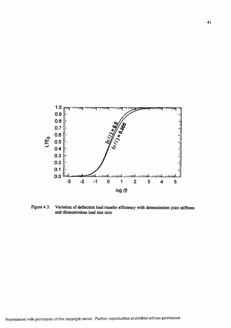
41
1.0 proi]-0.9 ^0.8 p0.7 ^0 .6 Ê-0.5 0.4 Ê- 0.3 ^0 .2 É-0.1 'r 0.0
-3
Tiniij
UJ
2 1 0 1 2 3 4 5
log (Ü
Figure 4.3. Variation of deflection load transfer efficiency with dimensionless joint stiffoess and dimensionless load size ratio
Reproduced with permission of the copyright owner. Further reproduction prohibited without permission.
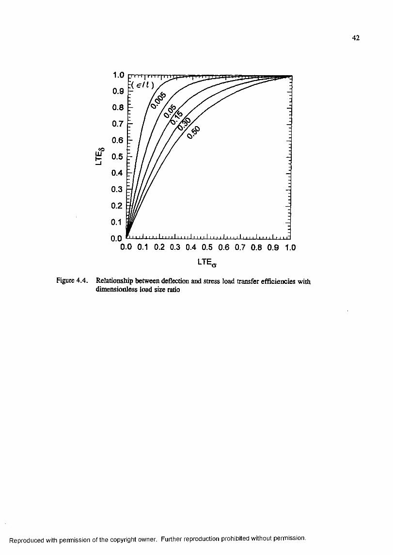
42
1.0
0.9
0.8
0.7
0.6to
^ 0.6b
0.4
0.3
0.2
0.1
0.0 -U .
0.0 0.1 0.2 0.3 0.4 0.5 0.6 0.7 0.8 0.9 1.0
LTE,
Figure 4.4. Relationship between deflection and stress load transfer efficiencies with dimensionless load size ratio
Reproduced with permission of the copyright owner. Further reproduction prohibited without permission.
CE[APTER5: FINITE ELEMENT RESPONSE MODELS
The finite element method is a powerful approximation technique that has been used to
analyze a broad class of boundary value problems in engineering. With the development of
the high-speed digital computer, finite element techniques have been applied to a varieQr of
problems in pavement analysis. The finite element method’s ability to model joint and edge
discontinuities has led to its emergence as the analysis method of choice for rigid pavement
research (Chatti 1992).
Table 5.1 presents an overview of certain key attributes of the more common finite ele
ment programs applied to rigid pavements as reported in the literature. These finite element
programs can be characterized in two general categories by their representation of the slab
model as either (a) 2D thin plate elements or (b) 3D continuum elements.
2D FINITE ELEMENT MODELS
A number of finite element programs featuring the use of a 2D thin plate model for the
concrete slab have been developed and reported in the literature in recent years. These
include ILU-SLAB, JSLAB, BCENSLABS, WESUQID, FEACONS m , KENLAYER,
WESLAYER, and RIGMUL. Each of the programs has similarities, yet certain key features
(such as mechanics of the joint and available foimdation models) vary. Some of the programs
allow the user to choose the foundation model fi-om a library of available models. Each of
the programs incorporates load transfer capabilities with some differences in the philosophy
and mechanics of the load transfer model. Because it is perhaps the most widely used and
verified of these programs, only ILLI-SLAB will be described in detail in this dissertation.
43
Reproduced with permission of the copyright owner. Further reproduction prohibited without permission.
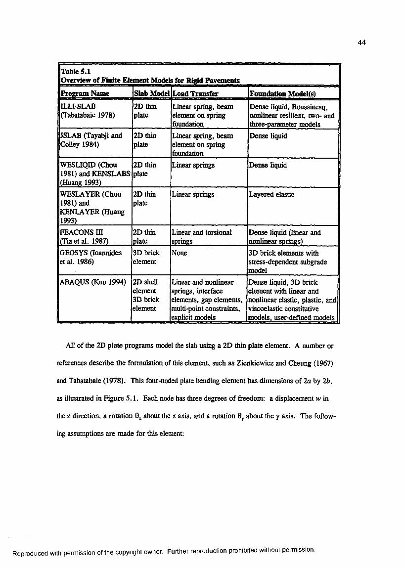
44
Ixable 5.11 Overview of Finite Element Models for Rigid Pavements8 Program Name Slab Model Load Transfer Foundation Model(s)ILLI-SLAB (Tabatabaie 1978)
2D thin plate
Linear spring, beam element on spring foundation
Dense liquid, Boussinesq, nonlinear resilient, two- and three-parameter models
JSLAB (Tayabji and CoUey 1984)
2D thin plate
Linear spring, beam element on spring foundation
Dense liquid
WESLIQID (Chou 1981) and KENSLABS (Huang 1993)
2D thin plate
Linear springs Dense liquid
WESLAYER (Chou 1981) andKENLAYER (Huang 1993)
2D thin plate
Linear springs Layered elastic
FEACONS m (Tia et al. 1987)
2D thin plate
Linear and torsional springs
Dense liquid (linear and nonlinear springs)
GEOSYS (loannides et al. 1986)
3D brick element
None 3D brick elements with stress-dependent subgrade model
ABAQUS (Kuo 1994) 2D shell element 3D brick element
Linear and nonlinear springs, interface elements, gap elements, multi-point constraints, explicit models
Dense liquid, 3D brick element with linear and nonlinear elastic, plastic, and viscoelastic constitutive models, user-defined models
All of the 2D plate programs model the slab using a 2D thin plate element. A number or
references describe the formulation of this element, such as Zienkiewicz and Cheung (1967)
and Tabatabaie (1978). This four-noded plate bending element has dimensions of 2a by 2b,
as illustrated in Figure 5.1. Each node has three degrees of freedom: a displacement w in
the z direction, a rotation 0 about the x axis, and a rotation 8y about the y axis. The follow
ing assumptions are made for this element:
Reproduced with permission of the copyright owner. Further reproduction prohibited without permission.
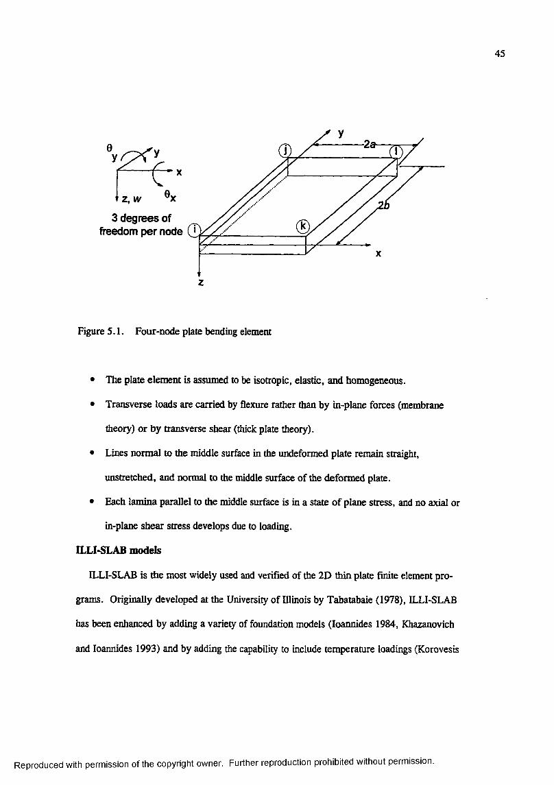
45
t Z , IV ' 'X
3 degrees of freedom per node
z
Figure 5.1. Four-node plate bending element
• The plate element is assumed to be isotropic, elastic, and homogeneous.
• Transverse loads are carried by flexure rather than by in-plane forces (membrane
theory) or by transverse shear (thick plate theory).
• Lines normal to the middle surface in the undeformed plate remain straight,
unstretched, and normal to the middle surface of the deformed plate.
• Each lamina parallel to the middle surface is in a state of plane stress, and no axial or
in-plane shear stress develops due to loading.
ILLI-SLAB models
ILLI-SLAB is the most widely used and verified of the 2D thin plate finite element pro
grams. Originally developed at the University of Illinois by Tabatabaie (1978), ILLI-SLAB
has been enhanced by adding a variety of foundation models (loannides 1984, Khazanovich
and loannides 1993) and by adding the capability to include temperature loadings (Korovesis
Reproduced with permission of the copyright owner. Further reproduction prohibited without permission.

46
1990). It was extended by Chatti (1992) at the University o f California at Berkeley to a new
dynamic conq>uter program called DYNA-SLAB for the analysis of jointed concrete pave
ments with load transfer systems at joints subjected to moving transient loads. Larralde and
Chen (1985) presented a method of analysis including fatigue based on ILLI-SLAB.
Majidzadeh, lives, and McComb (1981) coupled the slab and load transfer models in ILLI-
SLAB with a three-layer elastic foundation model to formulate the finite element program
RIGMUL.
The basic assumptions made by Tabatabaie (1978) in the initial development of ILLI-
SLAB are as follows:
• Thin plate theory (as previously described) can be used to model the slab, overlay, or
stabilized base.
• The subgrade behaves as a bed of springs.
• In case of a bonded stabilized base or overlay, there is full strain compatibility at the
interface. In the case o f an unbonded base or overlay, the shear stresses at the
interface are neglected.
• The dowel bars at joints behave like a linear-elastic material and are located at the
neutral axis of the slab.
• When an aggregate interlock or a keyway is used as the load-transfer system, the load
is transferred from one slab to an adjacent one by means o f shear. However, when
dowel bars are used as the load transfer system, moment as well as shear may be
transferred across the joints.
Figure 5.2 shows the finite element model used by Tabatabaie. The rectangular plate
element was employed to model the two-layer slab system (Figure 5.2a). For the case in
Reproduced with permission of the copyright owner. Further reproduction prohibited without permission.
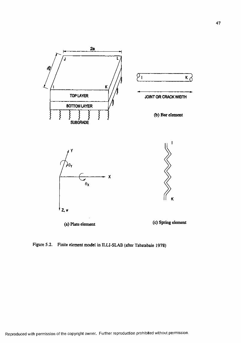
47
TOP LAYER
BOTTOM LAYER
SUBGRADE
F
JOINT OR CRACK WIDTH
(b) Bar element
Z,w
(a) Plate element (c) Spring element
Figure 5.2. Finite element model in ILLI-SLAB (after Tabatabaie 1978)
Reproduced with permission of the copyright owner. Further reproduction prohibited without permission.

48
which the two layers are bonded, the transformed section technique was used to develop an
equivalent layer (Figure 5.3). The subgrade is modeled as a bed of springs characterized by
the modulus o f subgrade reaction (A;). The value of k can be varied spatially from node to
node by the user.
Load transfer model
Figure 5.4 shows the concept of how ILLI-SLAB models joint load transfer. A pure shear
(aggregate interlock) load transfer mechanism is modeled by a linear spring element at each
node along the joint face (Figure 5.2c). The spring element features one degree of freedom
per node: w, the displacement in the z direction. The spring constant (called an “aggregate
interlock factor,” AGG) is input by the user and is indicative of the stiffness of the joint. The
value of the aggregate interlock factor can be estimated by backcalculating it from field tests.
Using ILLI-SLAB, loannides and Korovesis (1990) developed an s-shaped curve defining a
relationship between joint efficiency and a dimensionless joint stifftiess {AGG/kS) shown in
Figure 5.5. The points plotted in Figure 5.5 represent individual ILLI-SLAB runs used to
develop the curve. This curve shows that any value of joint efficiency from zero to 100 per
cent can be calculated with an appropriate choice of aggregate interlock factor or vice versa.
Comparison of Figure 5.5 with Figure 4.2 and Equation 4.10 reveals that the dimensionless
joint stiffness proposed by loannides and Korovesis (1990) is identical to that employed by
Skarlatos (1949) when AGG = q.
Dowel bars are modeled by a two-node bar element (Figure 5.2b) having three degrees of
freedom per node: a displacement w in the z direction and a rotation 0 about the y axis, and
a rotation 0, about x a ^ . A vertical spring element (Figure 5.2b) is employed to model the
relative deformation of the dowel bar and the surrounding concrete. The spring element
extends between the dowel bar and the surrounding concrete at the joint face. The dowel
Reproduced with permission of the copyright owner. Further reproduction prohibited without permission.
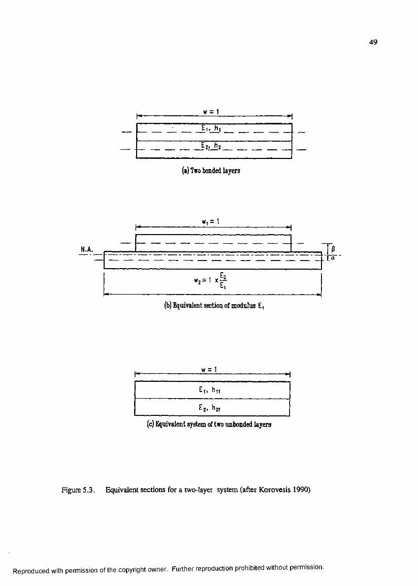
w = 1
(a) Two bonded layers
Wi = 1
(b) Equivalent section of modulus E,
w = 1
49
h -------------------------- :---- :----------------------------- M
E„ h,
Ez, hz
E„ h,f
Ez. hzf
(c) Equivalent system of two unbonded layers
Figure 5.3. Equivalent sections for a two-layer system (after Korovesis 1990)
Reproduced with permission of the copyright owner. Further reproduction prohibited without permission.
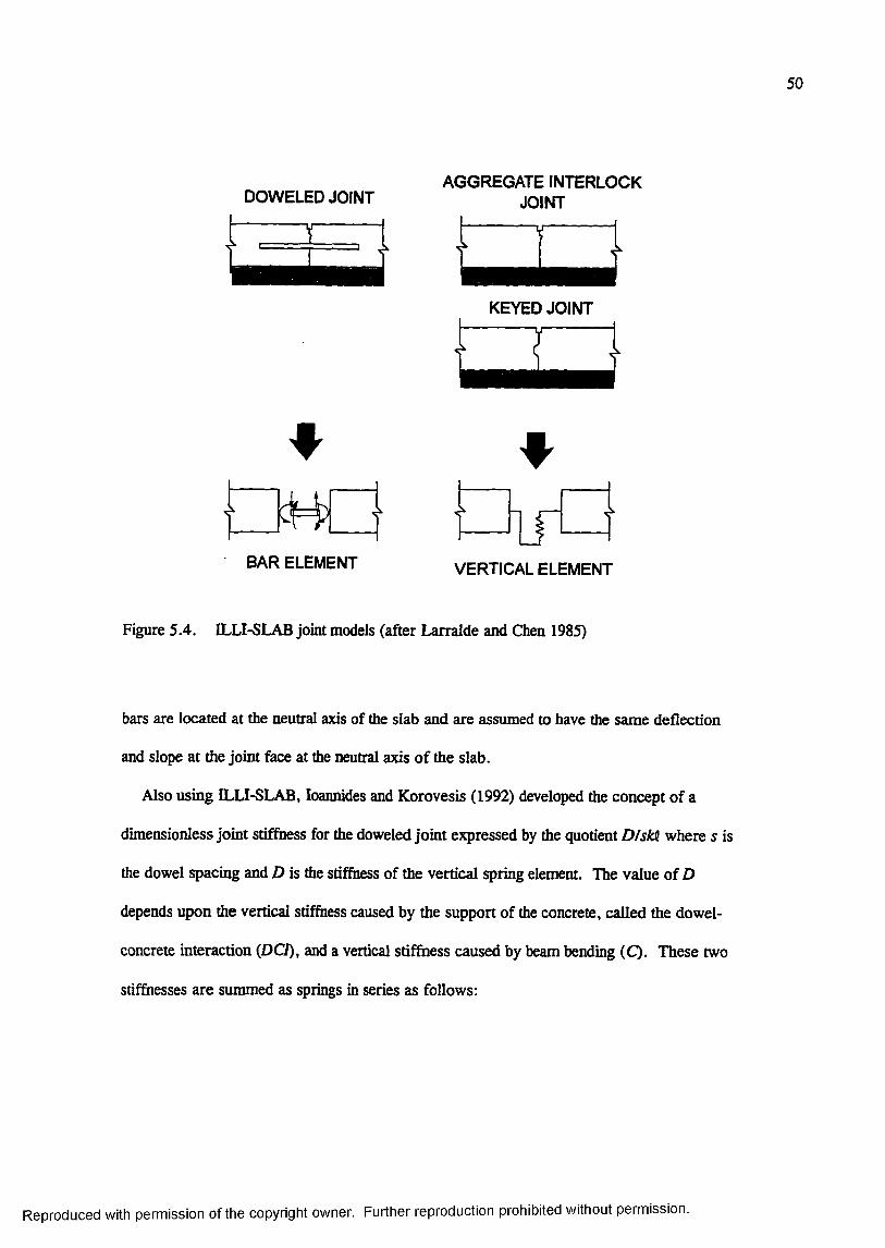
50
DOWELED JOINT
BAR ELEMENT
AGGREGATE INTERLOCK JOINT
KEYED JOINT
VERTICAL ELEMENT
Figure 5.4. ILLI-SLAB joint models (after Larralde and Chen 1985)
bars are located at the neutral axis of the slab and are assumed to have the same deflection
and slope at the joint face at the neutral axis of the slab.
Also using ILLI-SLAB, loannides and Korovesis (1992) developed the concept of a
dimensionless joint stiffoess for the doweled joint expressed by the quotient DfskS. where s is
the dowel spacing and D is the stiffness of the vertical spring element. The value of D
depends upon the vertical stiffness caused by the support of the concrete, called the dowel-
concrete interaction (DCi), and a vertical stiffoess caused by beam bending (Q . These two
stiffnesses are summed as springs in series as follows:
Reproduced with permission of the copyright owner. Further reproduction prohibited without permission.
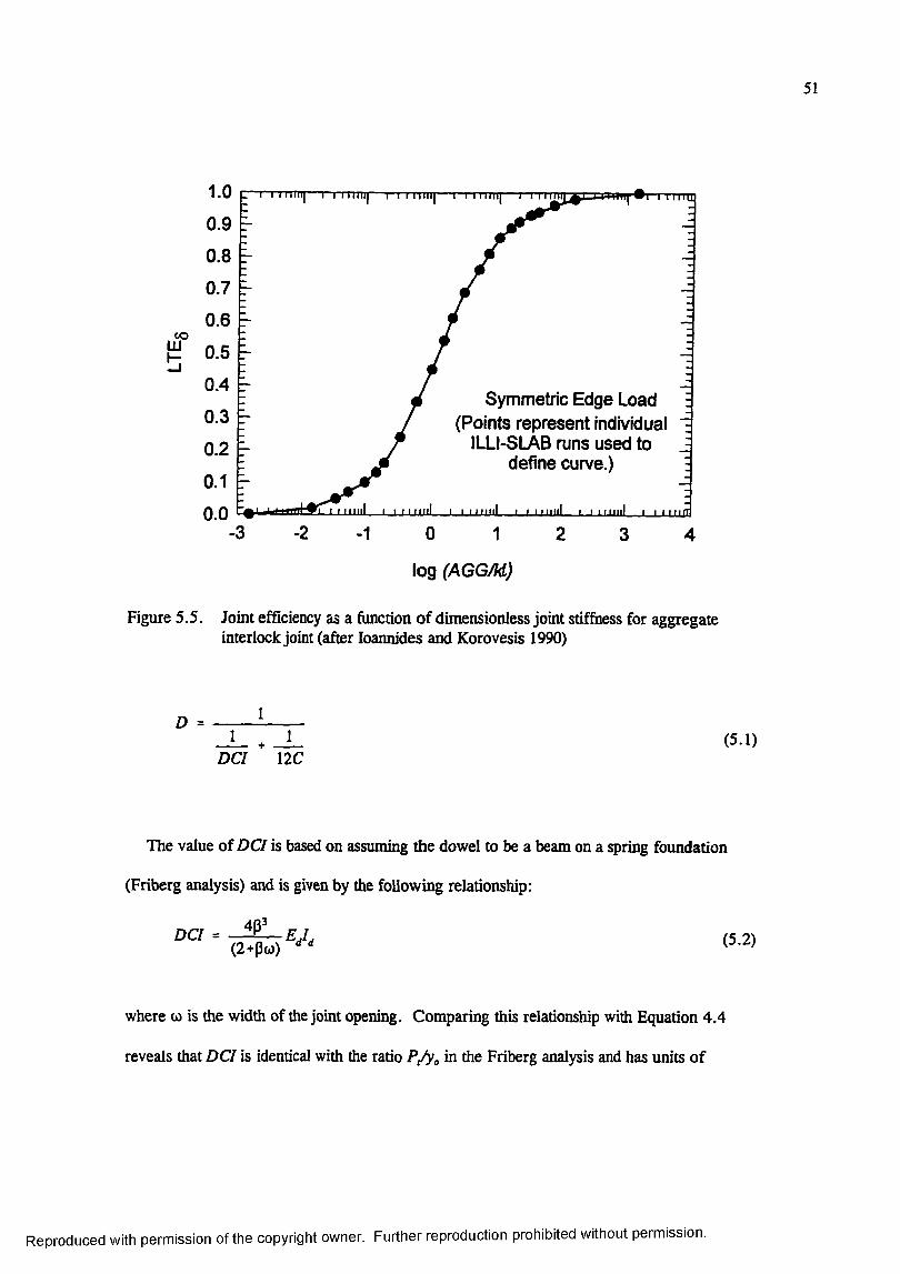
51
0.9
0.80.7
0.6
0.5CO
0.40.3
0.2
0.1
Symmetric Edge Load (Points represent Individual
ILLI-SLAB runs used to define curve.)
0.03 •2 01 21 3 4
log (AGGM)
Figure 5.5. Joint efficiency as a function of dimensionless joint stiffness for aggregate interlock joint (after loannides and Korovesis 1990)
D =J _ + _ L (5.1)
DCI 12C
The value of DCI is based on assuming the dowel to be a beam on a spring foundation
(Friberg analysis) and is given by the following relationship:
(2+Pw) (5.2)
where o> is the width of the joint opening. Comparing this relationship with Equation 4.4
reveals that DCI is identical with the ratio P/yg in the Friberg analysis and has units of
Reproduced with permission of the copyright owner. Further reproduction prohibited without permission.

52
force/length. The term fi is identical to that used by Friberg (Equation 4.5). The term C in
Equation 5.1 is defined by the relationship
where
* ' SGi is the shear modulus of the dowel bar as defined by
2 ( 1 +v^)
The term Aj is the effective cross-sectional area in shear and is assumed to be 0.9 times
the circular area as follows;
A , = 0.9‘ 4
(5.6)
A plot of joint efficiency as a function of dimensionless joint stiffness is presented in
Figure 5.6. As with the aggregate interlock factor, any value of joint efficiency from zero to
100 percent can be obtained by appropriate choice of the joint stiffness. loannides and
Korovesis’ formulation of the dimensionless joint stiffness for the doweled joint is identical to
that proposed by Skarlatos (1949) when q = D/s (Equation 4.10).
Foundation models
The original subgrade model used by Tabatabaie was the dense liquid or Winkler founda
tion. Later enhancements to ILLI-SLAB have included the addition of a library of foundation
models. Currently available models are discussed below.
Reproduced with permission of the copyright owner. Further reproduction prohibited without permission.
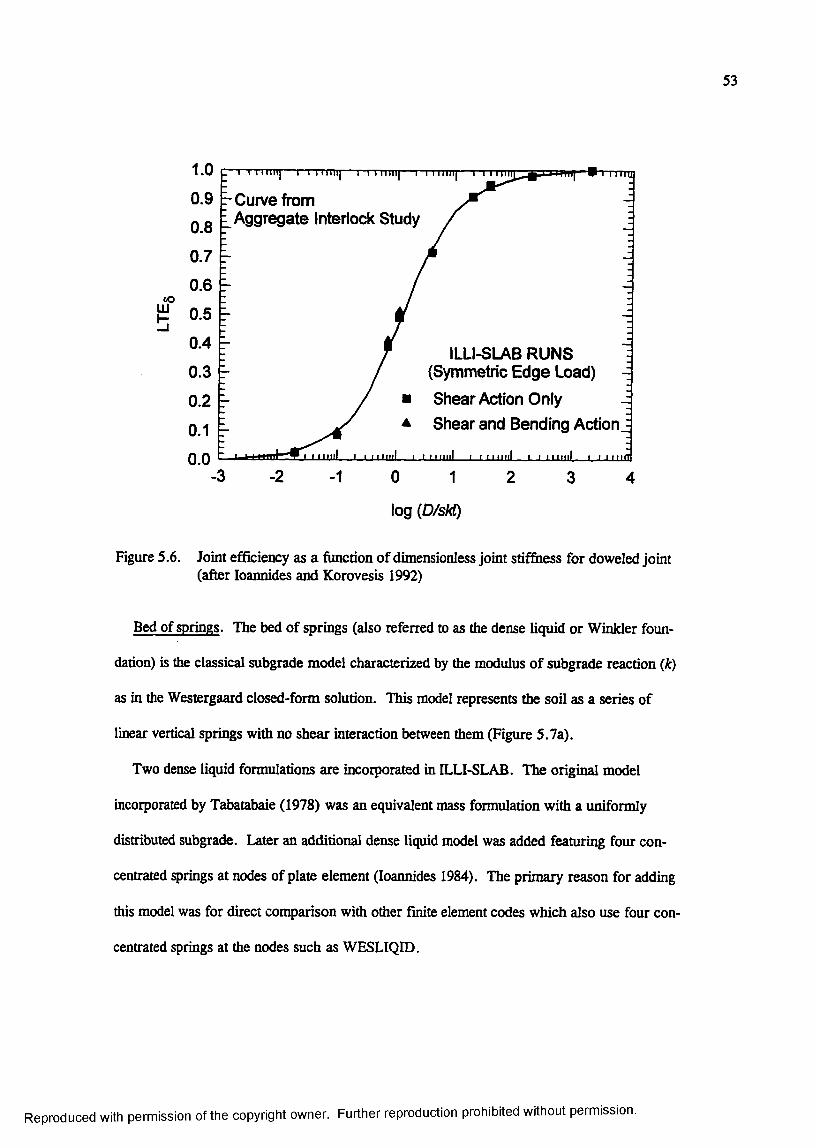
53
1.0
0.90.8
0.70.6
0.5
0.4
0.3
0.2
0.1
r i rniit]— i i'iuiii|— r r-n iiii|— i i i iiiii|— r m
Curve fromAggregate Interlock Study
T TT Tni
ILLI-SLAB RUNS (Symmetric Edge Load)
■ Shear Action Only A Shear and Bending Action J
-3 -1 0 1
log (0/sAO
Figure 5.6. Joint efficiency as a function of dimensionless joint stiffness for doweled joint (after loannides and Korovesis 1992)
Bed of springs. The bed of springs (also referred to as the dense liquid or Winkler foun
dation) is the classical subgrade model characterized by the modulus of subgrade reaction (k)
as in the Westergaard closed-form solution. This model represents the soil as a series of
linear vertical springs with no shear interaction between them (Figure 5.7a).
Two dense liquid formulations are incorporated in ILLI-SLAB. The original model
incorporated by Tabatabaie (1978) was an equivalent mass formulation with a uniformly
distributed subgrade. Later an additional dense liquid model was added featuring four con
centrated springs at nodes of plate element (loannides 1984). The primary reason for adding
this model was for direct comparison with other finite element codes which also use four con
centrated springs at the nodes such as WESLIQID.
Reproduced with permission of the copyright owner. Further reproduction prohibited without permission.
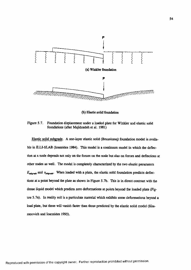
54
(a) Winkler foundation
(b) Elastic solid foundation
Figure 5.7. Foundation displacement under a loaded plate for Winkler and elastic solid foundations (after Majidzadeh et al. 1981}
Elastic solid subgrade. A one-layer elastic solid (Boussinesq) foundation model is availa
ble in ILLI-SLAB (loannides 1984). This model is a continuum model in which the deflec
tion at a node depends not only on the forces on the node but also on forces and deflections at
other nodes as well. The model is completely characterized by the two elastic parameters
oibgnde and When loaded with a plate, the elastic solid foundation predicts deflec
tions at a point beyond the plate as shown in Figure 5.7b. This is in direct contrast with the
dense liquid model which predicts zero deformations at points beyond the loaded plate (Fig
ure 5.7a). In reality soil is a particulate material which exhibits some deformations beyond a
load plate, but these will vanish faster than those predicted by the elastic solid model (Kha
zanovich and loannides 1993).
Reproduced with permission of the copyright owner. Further reproduction prohibited without permission.
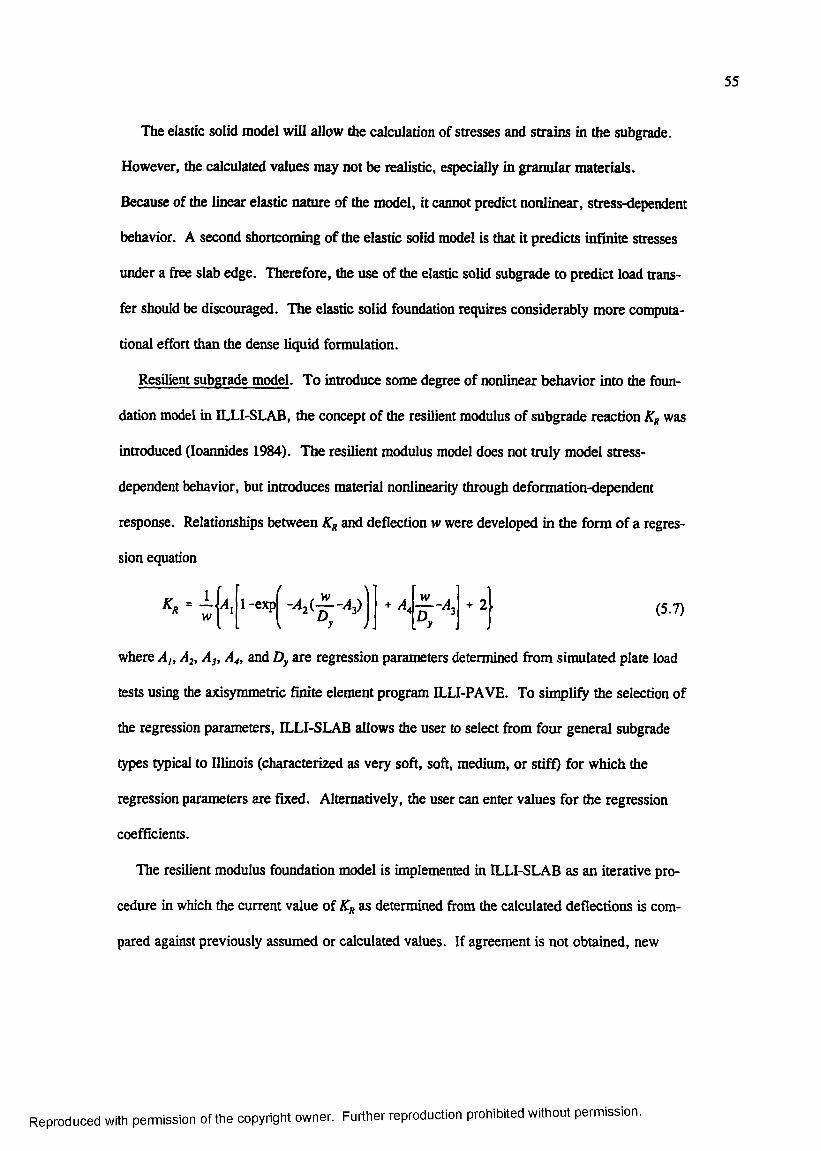
55
The elastic solid model will allow the calculation of stresses and strains in the subgrade.
However, the calculated values may not be realistic, especially in granular materials.
Because of the linear elastic nature of the model, it caimot predict nonlinear, stress-dependent
behavior. A second shortcoming of the elastic solid model is that it predicts infinite stresses
under a free slab edge. Therefore, the use of the elastic solid subgrade to predict load trans
fer should be discouraged. The elastic solid foundation requires considerably more computa
tional effort than the dense liquid formulation.
Resilient subgrade model. To introduce some degree of nonlinear behavior into the foun
dation model in ILLI-SLAB, the concept of the resilient modulus of subgrade reaction Kg was
introduced (loannides 1984). The resilient modulus model does not truly model stress-
dependent behavior, but introduces material nonlineariQr through deformation-dependent
response. Relationships between Kg and deflection w were developed in the form of a regres
sion equation
l-expy t
(5.7)
where A,, A4 , and Dy are regression parameters determined from simulated plate load
tests using the axisymmetric finite element program ILLI-PAVE. To simplify the selection of
the regression parameters, ILLI-SLAB allows the user to select from four general subgrade
types typical to Illinois (characterized as very soft, soft, medium, or stiff) for which the
regression parameters are fixed. Alternatively, the user can enter values for the regression
coefficients.
The resilient modulus foundation model is implemented in ILLI-SLAB as an iterative pro
cedure in which the current value of Kg as determined from the calculated deflections is com
pared against previously assumed or calculated values. If agreement is not obtained, new
Reproduced with permission of the copyright owner. Further reproduction prohibited without permission.
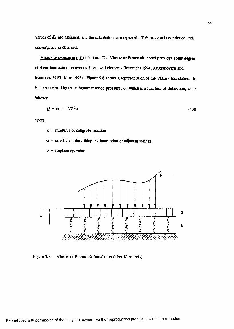
56
values of Kg are assigned, and the calculations are repeated. This process is continued until
convergence is obtained.
Vlasov two-parameter foundation. The Vlasov or Pasternak model provides some degree
of shear interaction between adjacent soil elements (loannides 1994, Khazanovich and
loannides 1993, Kerr 1993). Figure 5.8 shows a representation of the Vlasov foundadon. It
is characterized by the subgrade reaction pressure, Q, which is a function of deflection, w, as
follows:
where
Q = kw - GVSv
k = modulus of subgrade reaction
G = coefficient describing the interaction of adjacent springs
V = Laplace operator
(5.8)
wG
k
Figure 5.8. Vlasov or Plastemak foundation (after Kerr 1993)
Reproduced with permission of the copyright owner. Further reproduction prohibited without permission.
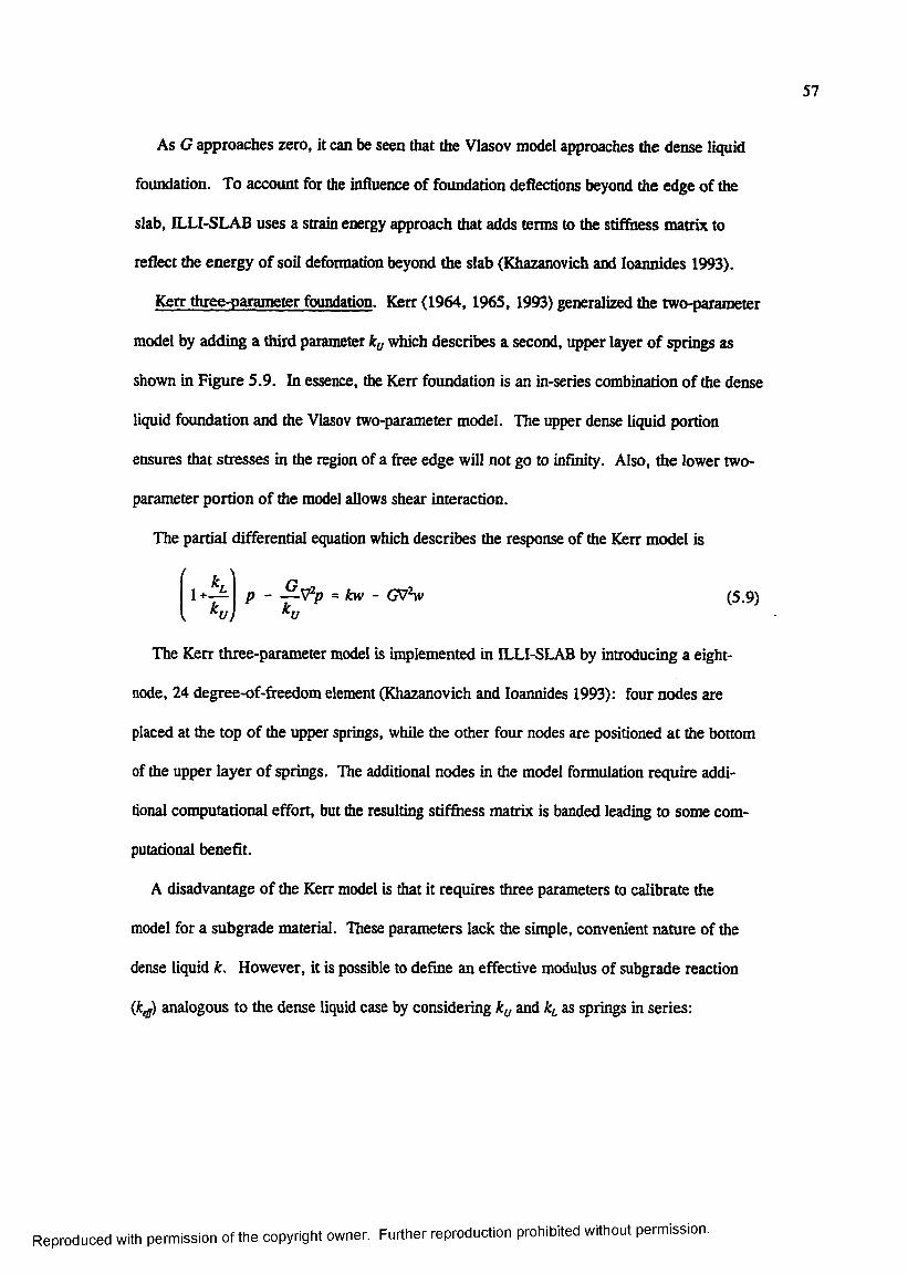
57
As G approaches zero, it can be seen that the Vlasov model approaches the dense liquid
foundation. To account for the influence of foundation deflections beyond the edge of the
slab, ILLI-SLAB uses a strain energy approach that adds terms to the stiffness matrix to
reflect the energy of soil deformation beyond the slab (Khazanovich and loannides 1993).
Kerr three-parameter foundation. Kerr (1964, 1965, 1993) generalized the two-parameter
model by adding a third parameter ky which describes a second, upper layer of springs as
shown in Figure 5.9. In essence, the Kerr foundation is an in-series combination of the dense
liquid foundation and the Vlasov two-parameter model. The upper dense liquid portion
ensures that stresses in the region of a free edge will not go to infinity. Also, the lower two-
parameter portion of the model allows shear interaction.
The partial differential equation which describes the response of the Kerr model is
h
kr1+ -^ p - — V p = kw - G7hv (5 .9 )
ky
The Kerr three-parameter model is implemented in ILLI-SLAB by introducing a eight-
node, 24 degree-of-ffeedom element (Khazanovich and loannides 1993): four nodes are
placed at the top of the upper springs, while the other four nodes are positioned at the bottom
of the upper layer of springs. The additional nodes in the model formulation require addi
tional computational effort, but the resulting stifûiess matrix is banded leading to some com
putational benefit.
A disadvantage of the Kerr model is that it requires three parameters to calibrate the
model for a subgrade material. These parameters lack the simple, convenient nature of the
dense liquid k. However, it is possible to define an effective modulus of subgrade reaction
(it^) analogous to the dense liquid case by considering ky and as springs in series:
Reproduced with permission of the copyright owner. Further reproduction prohibited without permission.
58
w ku
G
k,
Figure 5.9. Kerr foundation model (after Kerr 1993)
± . ± (5.10)
Zhemochkin-Sinitsyn-Shtaerman foundation. The Zhemochkin-Sinitsyn-Shtaerman model
is an in-series combination of the dense liquid and elastic solid models (Khazanovich and
loannides 1993). Like the Kerr model, it overcomes the elastic solid model’s shortcoming of
predicting infinite stresses at a free edge. The computational effort required for the
Zhemochkin-Sinitsyn-Shtaerman model is conçarable to that of the elastic solid foundation.
3D FINITE ELEMENT MODELS
GEOSYS model
loannides et al. (1986) developed user guidelines for a 3D finite element pavement model.
GEOSYS, an existing 3D finite element program, was adopted for this study. The authors
stated that their purpose was to “provide an essential guide of the effective utilization o f the
Reproduced with permission of the copyright owner. Further reproduction prohibited without permission.

59
three-dimensional finite element approach ... and perhaps eliminate the need for conducting
such preliminary and time consuming studies again.”
GEOSYS is a multipurpose, 3D, finite element program developed for geotechnical appli
cations. It has a library of several element Qrpes including beams, rods, 2D quadrilaterals;
and 3D brick and shell elements. Also, it is capable of time-dependent loading, gravier load
ing, and incremental excavation or construction.
For the pavement studies a 3D isoparametric brick element was used to model both the
slab and foundation. The element had eight nodes with three translational degrees of freedom
per node. The pavement layers were assumed to be linear elastic, isotropic, homogeneous
materials.
Over 100 GEOSYS runs were executed. The effects of the finite element mesh fineness,
vertical and lateral subgrade extent, boundary conditions, number of slab layers, vertical divi
sion of the subgrade were investigated. No attenq>t was made to model joints in this study.
The primary findings of the study were;
• A subgrade depth of about lOî should be used to ensure convergence of subgrade
deflections and strains.
• A lateral subgrade extent of about 76 to 10? should be used ensure convergence of sub
grade deflections.
• The horizontal lower subgrade boundary should be on rollers to allow the subgrade
elements to distribute loads by deforming. Similarly the lateral boundary conditions
should also be rollers.
• Maximum responses of the slab can be modeled adequately by representing the slab as
two layers o f 3D brick elements. Very little increase in accuracy can be gained by
increasing the number of layers in the slab to five or even six layers.
Reproduced with permission of the copyright owner. Further reproduction prohibited without permission.

60
• The subgrade may be divided into three regions in the vertical direction. The upper
region should extend to a depth of K. The thickness of the finite element layers
should not be greater than 0.25f to 0.5*. The middle region should extend from a
depth of id to 4d and should be divided into at least two layers of elements. The lower
region may be divided into one or more layers of elements.
• Smaller subgrade elements are required near the slab with the element size increasing
near the lateral boundaries.
• The slab mesh fineness ratio, defined as the ratio o f the shortest plan view length of
the element to the element thickness should be less than 0.8. The element aspect ratio,
defined as the ratio of the long plan view side of the element divided by the short plan
view side of the element, should be less than 4.
ABAQUS models
ABAQUS is a general-purpose, nonlinear, 3D, dynamic finite element code developed by
Hibbitt, Karlsson, and Sorensen, Inc. (ABAQUS 1993). ABAQUS incorporates a compre
hensive library of element types and material models.
Zaghloul and White (1993) used ABAQUS to perform nonlinear, dynamic analysis of
rigid highway pavements. Their 3D model was very general and included such aspects as
vertical friction between the pavement edge and the adjacent soil and the lateral passive pres
sure of the adjacent soil. The slab, subbase, and subgrade were modeled with 3D, eight-node
continuum elements. The subgrade was modeled with up to five different layers. Coulomb
type friction was imposed between layers with full contact between the slab and subbase
assumed as an initial condition.
Joints were modeled using gap elements with an initial opening in the range of 9 to 19 mm
(0.35 to 0.75 in.). Gap elements were placed between the nodes on each side of the joint to
Reproduced with permission of the copyright owner. Further reproduction prohibited without permission.
61
allow for the nodes to be in contact or separated, depending upon the deformed shape of the
slabs. When the nodes were in contact, friction forces were developed. Dowel bars were
modeled as reinforcing bars at the mid-depth of the slabs. Bond stress on one side was
assumed to be zero to allow for relative horizontal movements between slabs.
Subbase and base courses were modeled using nonlinear, stress-dependent constitutive
models. The subbase and granular subgrade materials were modeled with the Drucker-Prager
incremental plasticity model. This model predicted elastic material behavior at stress levels
below a yield criteria and plastic behavior beyond the yield criteria. All unloading was linear
elastic.
Clay subgrades were modeled with a critical state plasticity model, often referred to as the
modified Cam-Clay model. This model is based upon the concept of a critical state defined
as that stress state for which, upon yielding, perfectly plastic flow occurs. The loci of all
critical state points forms a critical state line which effectively separates stress states for
which softening behavior and hardening behavior occurs.
The load was applied in such a fashion to simulate a truck tire traveling at various veloci
ties across the pavement. Parametric studies were conducted to investigate the effects of the
load velocity, load position, load magnitude, base course, dowel bars, joint width, and slab
thickness. The pavement modeled for these studies consisted of a 200 mm (7.9 in.) thick
concrete slab resting directly on a sandy subgrade. The model was loaded with an 80 kN
(18,000 lb) single axle load moving at a speed of 2.8 km/h (4.5 mi/hr). The results of the
parameter studies were consistent with the current state of knowledge of joint behavior. The
analyses indicated that dowel bars increased the joint efficiency and decreased the maximum
vertical deflections. The model also predicted an increase in joint efficiency with closer
Reproduced with permission of the copyright owner. Further reproduction prohibited without permission.
62
dowel spacing. The effect of a stiff subbase on joint efficiency increased the joint efficiency
for both doweled and undoweled joints.
Kuo (1994) attempted to realistically model some of the more complex aspects of rigid
pavement behavior with a three-dimensional model developed using ABAQUS. He used this
model to smdy the effects of various foundation supports, base thicknesses and stiffness,
interface conditions between layers, temperature and moisture gradients, and load transfer at
joints. One of the major objectives of his research was to investigate factors influencing the
value of the modulus of subgrade reaction, particularly for pavements with stabilized layers.
The second major objective was to determine the effects of base layers on slab response.
As a part of his research Kuo conducted an investigation into the proper element Qrpes to
model the slab on grade using the ABAQUS “FOUNDATION” model. The “FOUNDA
TION” option in ABAQUS is equivalent to the dense liquid or Winkler foundation of classi
cal analysis. In applying the “FOUNDATION” option, the user simply applies a spring
coefficient (with units force/length^) to the face of an element. Kuo found that the twenty-
node isoparametric brick element with reduced integration (C3D20R) adequately approxi
mated the theoretical Westergaard solution. This element formulation was subsequently used
in more sophisticated analyses involving the modeling of the base and subgrade layers.
Kuo employed a simplistic yet effective model for aggregate interlock and doweled joints.
Aggregate interlock was modeled using the ABAQUS “JOINTC” element type. The
“JOINTC” element, which can be applied in both 2D and 3D analyses, is placed between
nodes on either side of the joint. Translational and rotational spring constants can be used to
define the joint stiffness in both translational and rotational degrees of freedom. The spring
constants are specified as piecewise linear functions of the displacement in the active degree
of freedom. Damping can also be specified in a dynamic analysis. Kuo compared the results
Reproduced with permission of the copyright owner. Further reproduction prohibited without permission.

63
of this ABAQUS “JOINTC” model with those from an ILLI- SLAB run with the same shear
interlock stiffriess and found that the results conpared very closely for both load transfer effr-
ciency and maximum slab stresses.
Kuo modeled doweled bars with beam elements. To account for slip of one end of the
dowel bars, he invoked the “SLIDER” option, one of the multipoint constraints available in
ABAQUS. A multipoint constraint is a restriction in^osed between degrees of freedom of a
model. The “SLIDER” multipoint constraint allows the possibili^ of a node moving along a
straight line defined by two other nodes and the line length of change. By invoking this
restraint, Kuo was allowed one end of the dowel bar to move relative to the slab. However,
Kuo did not model dowel-concrete interaction. He found that his model compared favorably
with ILLI-SLAB when a very high dowel concrete interaction was assumed in ILLI-SLAB.
Reproduced with permission of the copyright owner. Further reproduction prohibited without permission.
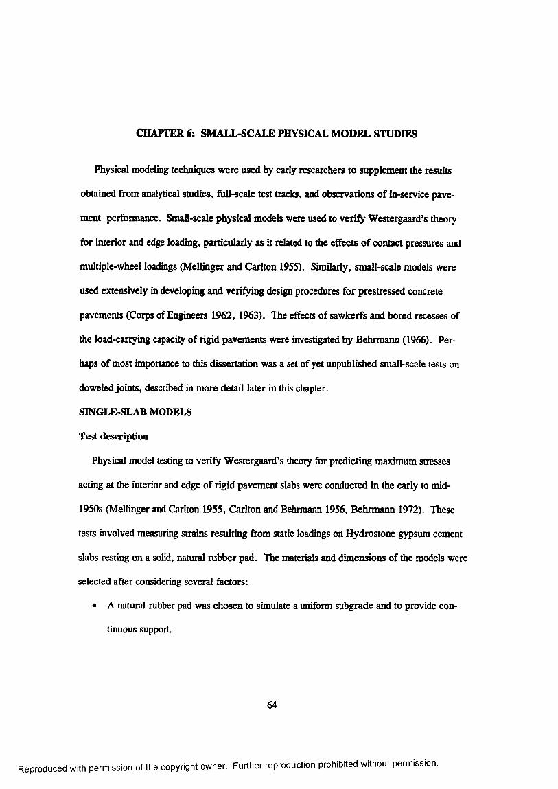
CHAPTER 6: SMALL-SCALE PHYSICAL MODEL STUDIES
Physical modeling techniques were used by early researchers to supplement the results
obtained from analytical studies, full-scale test tracks, and observations of in-service pave
ment performance. Small-scale physical models were used to verify Westergaard’s theory
for interior and edge loading, particularly as it related to the effects of contact pressures and
multiple-wheel loadings (Mellinger and Carlton 1955). Similarly, small-scale models were
used extensively in developing and verifying design procedures for prestressed concrete
pavements (Corps of Engineers 1962, 1963). The effects of sawkerfs and bored recesses of
the load-carrying capacity of rigid pavements were investigated by Behrmann (1966). Per
haps of most importance to this dissertation was a set of yet unpublished small-scale tests on
doweled joints, described in more detail later in this chapter.
SINGLE-SLAB MODELS
Test description
Physical model testing to verify Westergaard’s theory for predicting maximum stresses
acting at the interior and edge of rigid pavement slabs were conducted in the early to mid-
1950s (Mellinger and Carlton 1955, Carlton and Behrmann 1956, Behrmann 1972). These
tests involved measuring strains resulting from static loadings on Hydrostone gypsum cement
slabs resting on a solid, natural rubber pad. The materials and dimensions of the models were
selected after considering several factors:
• A natural rubber pad was chosen to simulate a uniform subgrade and to provide con
tinuous support.
64
Reproduced with permission of the copyright owner. Further reproduction prohibited without permission.

65
• Hydrostone gypsum cement was chosen to provide a homogeneous and isotropic
material to model a slab of constant thickness.
• The horizontal dimensions of the slab were chosen so that distant edge effects were
minimal.
• The thickness of the rubber pad was chosen so that the bottom effects were minimal.
• The size of the loaded area and the thickness of the slab were of such relative dimen
sions that the ordinary theory of bending of thin plates is applicable.
• Applied loads in the tests were small to ensure that stresses in the model did not
exceed the elastic limit of the slab and subgrade.
The material properties that were of concern were;
slab modulus of elasticity,
slab Poisson"s ratio, v , and
modulus of subgrade reaction, k.
The basic similitude relationship between the model and prototype was
^model _ ^prototypeJ — - 1---------- (6 . 1)
model prototype
where ^ is the radius of relative stiffîiess as defined by Equation 4.1 and a is the radius of the
circular loaded area.
The slab dimensions were approximately 380 mm (15 in.) by 380 mm (15 in.) by 3 mm
(0.125 in.) thick. The slabs were constructed by placing gypsum cement mortar in a steel
form between two plates of glass to insure a uniform thickness. The rubber pad had dimen
sions of 610 ram (24 in.) by 610 mm (24 in.) by 305 mm (12 in.) thick, and was supported
by a rigid concrete table and confined on its sides by a rigid box.
Reproduced with permission of the copyright owner. Further reproduction prohibited without permission.

66
After a 7-day curing period, 6.3-mm- (0.25-in.)-long resistance wire strain gages were
bonded to the slab. Up to 17 gages were installed on a single slab. E^^rience with corre
sponding gages bonded opposite each other on the top and bottom o f the slab had shown that
strain measurements were identical within the precision of the gages. Thus the strain gages
were ^ ic a l ly placed on the top of the slab for convenience. The slab was subsequently
placed directly on the rubber subgrade. A layer of 19-mm (0.75-in.) lead cubes was uni
formly distributed over the top surface o f the slab to insure intimate contact between the slab
and subgrade. Static loads were applied through a circular rubber pad cemented to a rigid
die. The static load was applied by means of a reaction beam as shown in Figure 6.1.
Figure 6.1 Photograph of small-scale physical models test setup
Reproduced with permission of the copyright owner. Further reproduction prohibited without permission.

67
The measured elastic properties of the cured gypsum cement were = 20,700 MPa
(3,000,000 psi) and — 0.25. The flexural strength was 17 MPa (2,5(X) psi). The modulus
of subgrade reaction of the natural rubber subgrade was determined by measuring the volu
metric displacement o f the subgrade within the limits of the slab as 9.6 MPa/m (35 psi/in.)
for interior loading and 17.8 MPa/m (65 psi/in.) for edge loading. Based upon the physical
constants of the model, the model had a radius of relative stifhiess of approximately 43 mm
(1.7 in.).
Test results and analysis
Figure 6.2 shows a contour plot of deflections for a typical test under edge loading condi
tions (Carlton and Behrmann 1956). Figure 6.3 shows the deflection basin profile from the
test shown in Figure 6.2 along with profiles obtained from finite element solutions from ILLI-
SLAB. The experimental basin was obtained by carefully scaling the deflections along the
edge from Figure 6.2. The lower ILLI-SLAB deflection basin was obtained using the
reported values of = 20,700 MPa (3,000,0(X) psi), = 0.25, and k - 17.8 MPa/m
(65 psi/in.). Obviously, the calculated response using these values does not approximate that
of the experiment. Therefore, an iterative backcalculation procedure was used to determine
the combination of E, and k (holding = 0.25) which would produce a deflection basin pro
file matching that of the experiment. The best match curve is shown as the upper ILLI-SLAB
curve in Figure 6.3. These backcalculated material characterization values were as follows:
E, = 24,340 MPa (3,530,000 psi)
H = 0.25
it = 44.11 MPa/m (162.5 psi/in.)
These values will be used in analyses of data from scaled dowel joint models.
Reproduced with permission of the copyright owner. Further reproduction prohibited without permission.
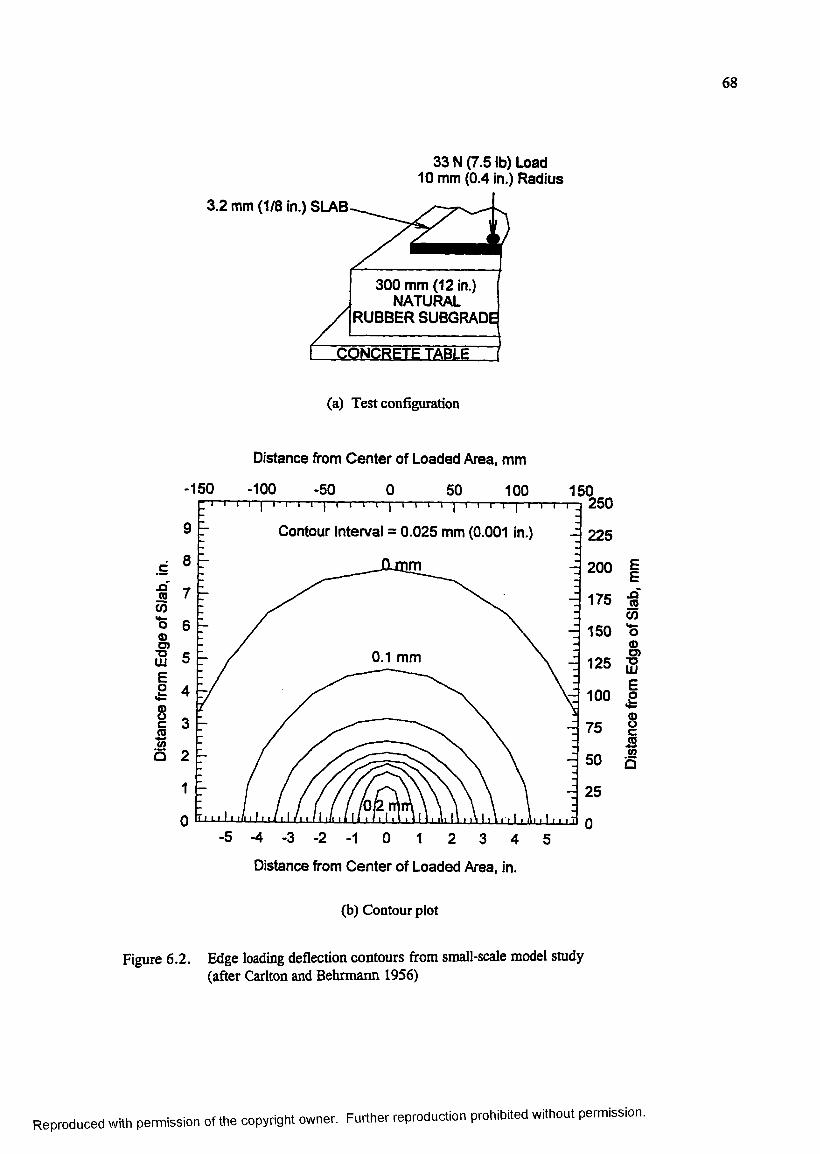
68
33 N (7.5 lb) Load 10 mm (0.4 in.) Radius
3.2 mm (1/8 in.) SLAB
300 mm (12 in.) NATURAL
I RUBBER SUBGRADg
C_QNCRETE_TABLi~
(a) Test configuration
Distance from Center of Loaded Area, mm
jaisCO
"o(DO)•oUJE
8Ia
-150 -100 -50 0 50 100 150250
9 Contour Interval = 0.025 mm (0.001 in.) 225
6 2007 175
6 150
0.1 mm5 125
4 100
3
2
1Ü/2
0-5 -4 -3 -2 -1 0 1 2 3 4 5
Distance from Center of Loaded Area, in.
(b) Contour plot
Figure 6.2. Edge loading deflection contours from small-scale model study (after Carlton and Behrmarm 1956)
EExTCO
CO
0d)
s
1 8
Reproduced with permission o f the copyright owner. Further reproduction prohibited without permission.
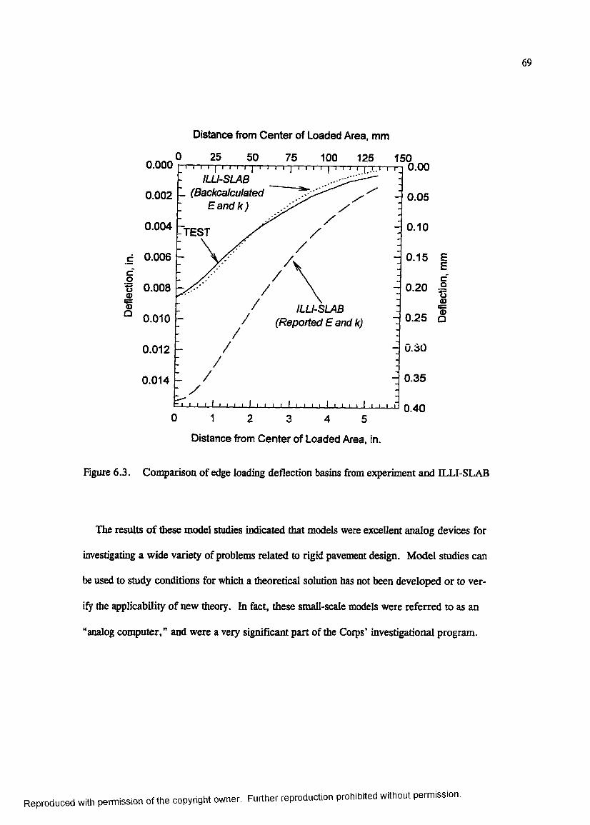
69
Distance from Center of Loaded Area, mm
75 100 125 1500.000 0.00I L L I - S L A B
- ( B a c k c a l c u l a t e d
I E a n d k )
0.002 0.05
0.004 0.10FTEST
0.006 0.15Çci 0.008<D 0.20
I I L L I - S L A B
( R e p o r t e d E a n d k )0.250.010
0.300.012
0.350.014
0.400 1 2 3 4 5
i1
Distance from Center of Loaded Area, in.
Figure 6.3. Comparison of edge loading deflection basins from experiment and ILLI-SLAB
The results o f these model studies indicated that models were excellent analog devices for
investigating a wide variety of problems related to rigid pavement design. Model studies can
be used to study conditions for which a theoretical solution has not been developed or to ver
ify the applicability of new theory. In fact, these small-scale models were referred to as an
“analog conçuter,” and were a very significant part of the Corps’ investigational program.
Reproduced with permission o f the copyright owner. Further reproduction prohibited without permission.
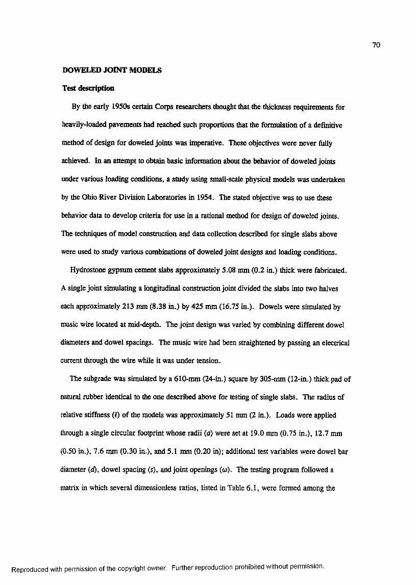
70
DOWELED JOINT MODELS
Test description
By the early 1950$ certain Corps researchers thought that the thickness requirements for
heavily-loaded pavements had reached such proportions that the formulation of a definitive
method of design for doweled joints was imperative. These objectives were never fully
achieved. In an attempt to obtain basic information about the behavior of doweled joints
under various loading conditions, a study using small-scale physical models was undertaken
by the Ohio River Division Laboratories in 1954. The stated objective was to use these
behavior data to develop criteria for use in a rational method for design of doweled joints.
The techniques of model construction and data collection described for single slabs above
were used to study various combinations of doweled joint designs and loading conditions.
Hydrostone gypsum cement slabs approximately 5.08 mm (0.2 in.) thick were fabricated.
A single joint simulating a longitudinal construction joint divided the slabs into two halves
each approximately 213 mm (8.38 in.) by 425 mm (16.75 in.). Dowels were simulated by
music wire located at mid-depth. The joint design was varied by combining different dowel
diameters and dowel spacings. The music wire had been straightened by passing an electrical
current through the wire while it was under tension.
The subgrade was simulated by a 610-mm (24-in.) square by 305-mm (12-in.) thick pad of
natural rubber identical to the one described above for testing of single slabs. The radius of
relative stiffness (?) of the models was approximately 51 mm (2 in.). Loads were applied
through a single circular fooçrint whose radii (a) were set at 19.0 mm (0.75 in.), 12.7 mm
(0.50 in.), 7.6 mm (0.30 in.), and 5.1 mm (0.20 in); additional test variables were dowel bar
diameter (d), dowel spacing (f), and joint openings (w). The testing program followed a
matrix in which several dimensionless ratios, listed in Table 6.1, were formed among the
Reproduced with permission of the copyright owner. Further reproduction prohibited without permission.
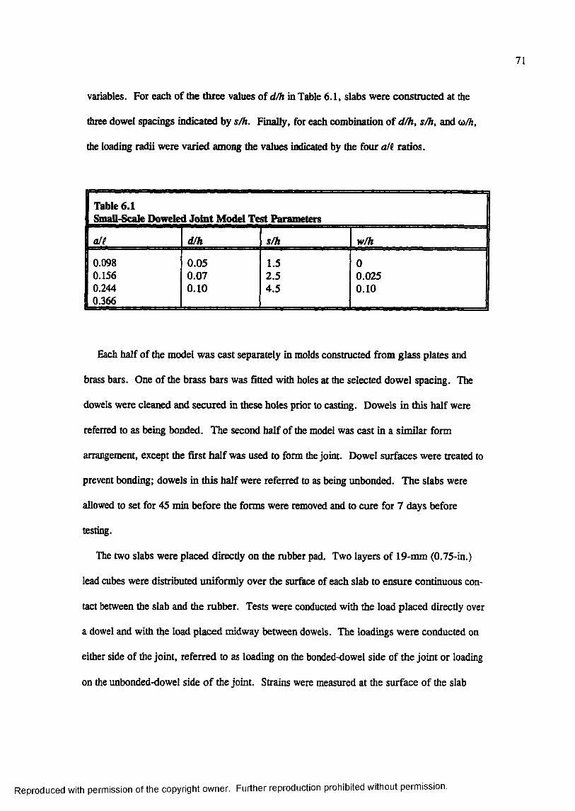
71
variables. For each of the three values of d/h in Table 6.1, slabs were constructed at the
three dowel spacings indicated by s/h. Finally, for each combination of d/h, s/h, and a>/h,
the loading radii were varied among the values indicated by the four alt. ratios.
1 Table 6.1 1 Small-Scale Doweled Joint Model Test Parameters
d/h s/h w/h
0.098 0.05 1.5 00.156 0.07 2.5 0.0250.244 0 .1 0 4.5 0 .1 00.366
Each half of the model was cast separately in molds constructed from glass plates and
brass bars. One of the brass bars was fitted with holes at the selected dowel spacing. The
dowels were cleaned and secured in these holes prior to casting. Dowels in this half were
referred to as being bonded. The second half of the model was cast in a similar form
arrangement, except the first half was used to form the joint. Dowel surfaces were treated to
prevent bonding; dowels in this half were referred to as being unbonded. The slabs were
allowed to set for 45 min before the forms were removed and to cure for 7 days before
testing.
The two slabs were placed directly on the rubber pad. Two layers of 19-mm (0.75-in.)
lead cubes were distributed uniformly over the surface of each slab to ensure continuous con
tact between the slab and the rubber. Tests were conducted with the load placed directly over
a dowel and with the load placed midway between dowels. The loadings were conducted on
either side of the joint, referred to as loading on the bonded-dowel side of the joint or loading
on the unbonded-dowel side o f the joint. Strains were measured at the surface of the slab
Reproduced with permission of the copyright owner. Further reproduction prohibited without permission.
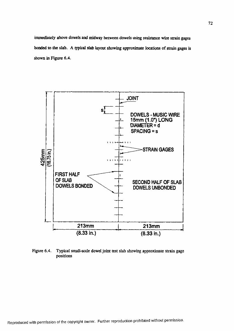
72
immediately above dowels and midway between dowels using resistance wire strain gages
bonded to the slab. A typical slab layout showing approximate locations of strain gages is
shown in Figure 6.4.
JOINT
DOWELS-MUSIC WIRE 15mm (1.0") LONG DIAMETER = d SPACING = s
STRAIN GAGESLOlOCO
FIRST HALF ^ OF SLAB ^ DOWELS BONDED
SECOND HALF OF SLAB DOWELS UNBONDED
213mm 213mm(8.33 in.) (8.33 in.)
Figure 6.4. Typical small-scale dowel joint test slab showing approximate strain gage positions
Reproduced with permission of the copyright owner. Further reproduction prohibited without permission.
73
Test results
Experimental strain curves are presented in Appendix A. The values of strain measured
on either side of the joint were used to estimate load transfer using the following
approximation:
LT (%)= —— X 100 (6.2)
where and Ef are the e?q)erimentally obtained edge strains on the unloaded slab and a slab
loaded at a free edge, respectively. This approximation differs from an exact measurement of
LT, because it neglects Poisson's effects; however, the error in the approximation is small.
The estimates of L T are tabulated in Appendix B. These values confirm that load transfer
depends on the size of the dowel, spacing of the dowel, joint opening, and radius of the
loaded area. For the various combinations of joint parameters tested, the load transfer values
obtained in the experiments were mostly greater than 25 percent, supporting data obtained
from full-scale experimental slabs.
Analysis
The data were analyzed to backcalculate the joint response parameters necessary to esti
mate the dimensionless doweled joint stifkess D/skH and the modulus o f dowel reaction K.
First, the basic material characterizations were assumed to be the same as those backcalcu
lated from the experiments of Carlton and Behrmann (1956); that is,
E, = 24,340 MPa (3,530,000 psi)
V, = 0.25
^ = 44.11 MPa/m (162.5 psi/in.)
Reproduced with permission of the copyright owner. Further reproduction prohibited without permission.
74
The modulus of elasticity of the dowels were set at Ej = 207,000 MPa (30,000,000 psi) and
a Poission’s ratio of = 0.25, values typical of steel. For each combination of test param
eters, LTEf, was estimated from LTE„ using Equation 4.13.
Table 6.2 summarizes the backcalculated values of the modulus of dowel reaction and
doweled joint stifhiesses. These data are plotted in Figures 6.5 and 6 .6 . In Figure 6.5 val
ues of K have been normalized by forming the dimensionless ratio o f KQi - d)/E suggested by
Nishizawa et al. (1989). Backcalculated values of dimensionless joint stiffness ranged from a
low of 3.7 to a high of 996.2, a range of three orders of magnitude. In almost every case,
the backcalculated values of dimensionless joint stfHhess decrease as the joint opening
increases and increase as the dowel diameter increases, which follows with intuition. How
ever, modulus of dowel reaction does not appear to be as well behaved as the dimensionless
joint stiffiiess. Backcalculated values of K varied from 0.3 X 10® MPa/m (1.0 x 10® psi/in.)
to 598 X 10® MPa/m (2,220 x 10® psi/in.). These values range from approximately equal to
those values commonly reported in the literature to some two orders of magnitude greater
than those commonly reported. The reasons for these discrepancies are not immediately
apparent. However, it is possible that there exists a significant size effect, similar to that
observed as the size of the circular plate is varied in the plate bearing test method for
determining the modulus of subgrade reaction. It should be noted that K is not an intrinsic
material property, but rather a system parameter. Thus, K, like the modulus of subgrade
reaction, is a useful tool for calculating system response, but can be difficult to measure even
in carefully controlled experiments, and even more difficult to estimate a priori for design
purposes. Despite the limitations exhibited by the modulus of dowel reaction, the experimen
tal data confirm the usefulness of the dimensionless joint stiffness as a means of characteriz
ing the response of the doweled joint.
Reproduced with permission of the copyright owner. Further reproduction prohibited without permission.
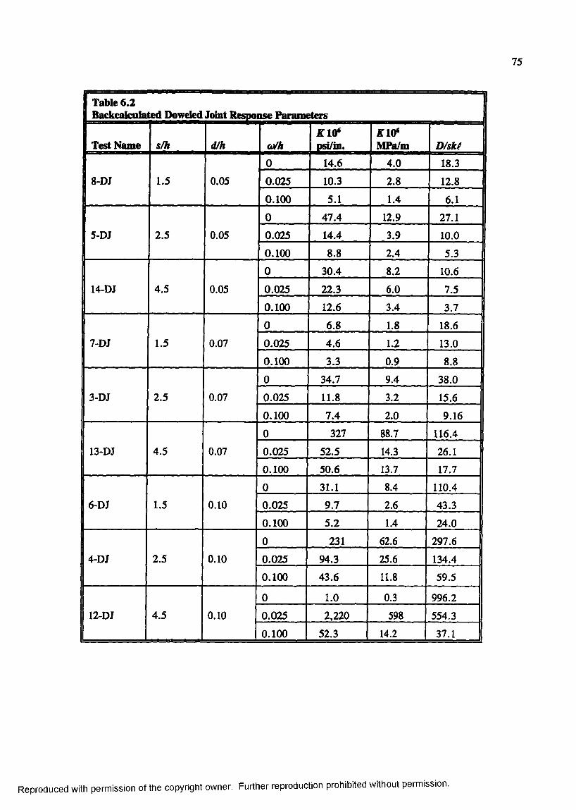
75
1 Table 6.2 1 Backcalculatted Doweled Joint Response Parameters
Test Name s/h d/h a /hK IC /psi/in.
f 10* MPa/m D/sk(
8 -DJ 1.5 0.05
0 14.6 4.0 18.3
0.025 10.3 2 .8 12 .8
0 .1 0 0 5.1 1.4 6 .1
5-DJ 2.5 0.05
0 47.4 12.9 27.1
0.025 14.4 3.9 10.0
0 .1 0 0 8 .8 2.4 5.3
14-DJ 4.5 0.05
0 30.4 8 .2 10 .6
0.025 22.3 6 .0 7.5
0 .1 0 0 12.6 3.4 3.7
7-DJ 1.5 0.07
0 6 .8 1.8 18.6
0.025 4.6 1.2 13.0
0 .1 0 0 3.3 0.9 8 .8
3-DJ 2.5 0.07
0 34.7 9.4 38.0
0.025 11.8 3.2 15.6
0 .1 0 0 7.4 2 .0 9.16
13-DJ 4.5 0.07
0 327 88.7 116.4
0.025 52.5 14.3 26.1
0 .1 0 0 50.6 13.7 17.7
6-DJ 1.5 0 .10
0 31.1 8.4 110.4
0.025 9.7 2 .6 43.3
0 .1 0 0 5.2 1.4 24.0
4-DJ 2.5
0 231 62.6 297.6
0 .10 0.025 94.3 25.6 134.4
0 .1 0 0 43.6 11.8 59.5
12-DJ 4.5
0 1.0 0.3 996.2
0 .10 0.025 2 ,2 2 0 598 554.3
0 .1 0 0 52.3 14.2 37.1
Reproduced with permission of the copyright owner. Further reproduction prohibited without permission.
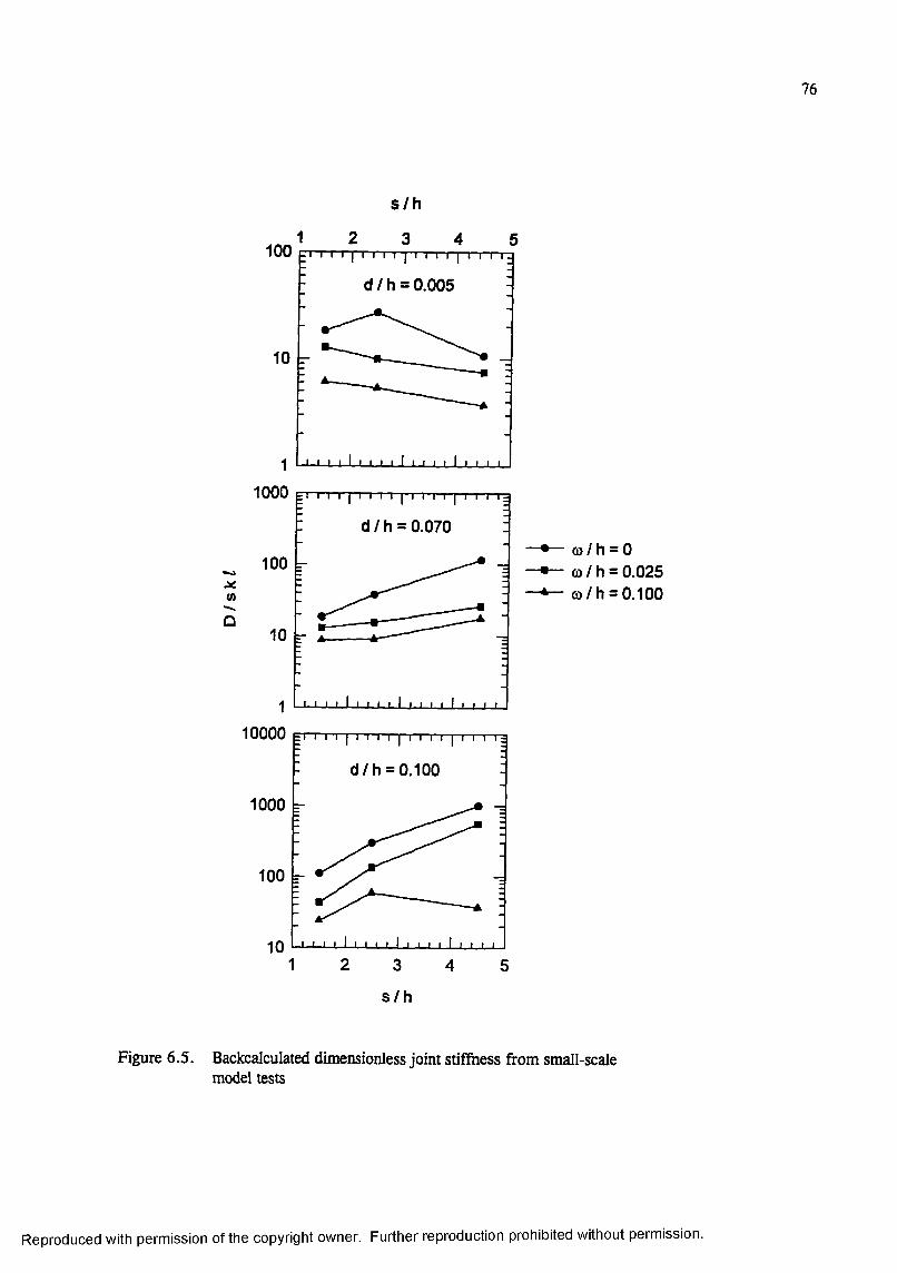
76
s / h
100
d / h = 0.006
10
“j i- i- i I I I I I I I I I I I I I I I I I
1000 h i I I I f T I I I I I I I T ] " T T 7 T
: d /h = 0.070
100
(0
Û
10000 r I I I |T I 'I I
d /h = 0.100
1000
100
1 2 3 4 5
— co/h = 0 o)/h = 0.025
— m /h = 0.100
s / h
Figure 6.5. Backcalculated dimensionless joint stiffiiess from small-scale model tests
Reproduced with permission of the copyright owner. Further reproduction prohibited without permission.
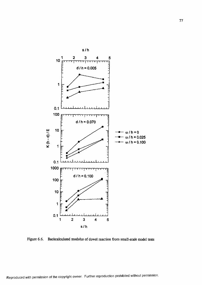
77
n I ' I I I I T I I I r f T I I 1 t I I
d / h = 0.005
1 k-
UJ 10
T3I
^ I I 1 I I I I I T I I I T"I j I— I I 'I
d /h = 0.070
0 1 1 1 - l . L l l J . L l l l i l i i l r i i i
1000
d /h = 0.100100
10
1
0.11 2 3 54
"•— <0 / h = 0 “■— G) / h = 0.025
— co/h = 0.100
s / h
Figure 6 ,6 . Backcalculated modulus of dowel reaction from small-scale model tests
Reproduced with permission of the copyright owner. Further reproduction prohibited without permission.
CHAPTER?: FINITE ELEMENT RESPONSE AND SENSITIVITY STUDIES
BACKGROUND
This chapter contains a discussion of response and sensitiviQr studies conducted with the
finite element code ABAQUS. The finite element method is a numerical procedure for
obtaining approximate solutions to many types of problems in structural analysis and mechan
ics, heat transfer, fluid flow, and other disciplines of engineering. It makes use of an
approach referred to as “going from part to whole," i.e., instead of solving the problem for an
entire body in one operation, the solution is approximated for discrete elements and then
combined to obtained the solution for the whole (Desai and Abel 1972). As such, the solution
for the whole is, at best, no better than the approximations used for the discrete elements.
Purpose of sensitivity studies
The purpose of these sensitivity studies was primarily to select the refinement of the dis
cretization (referred to as the mesh fineness) and the approximations within the elements
(choice of element type) for the 3D rigid pavement problem. This process involved produc
ing a number of finite element models with varying mesh fineness and element types, execut
ing those models to obtain approximate solutions, and observing the convergence trends for
key response parameters such as bending stress, shear stress, and deflection. Where possi
ble, these responses were compared to analytical solutions and e;q)erimental results. All dis
cussions presented in this chapter are relevant to ABAQUS, but would likely hold for any
finite element code with identical element types and solution schemes.
78
Reproduced with permission of the copyright owner. Further reproduction prohibited without permission.

79
First, a well-accepted analytical solution was chosen to check the accuracy of the approxi
mations made by the various finite element models produced during the sensitivity studies.
Because of the widespread acceptance and verification of Westergaard’s theory, it was chosen
for this study. For the sensitivity studies to be valid, the finite element models generated
must be conq)atible with Westergaard’s assun^tions. Thus, all sensitivity studies for this
research were conducted for the general problem o f an elastic plate resting on a bed of
springs foundation considering interior or edge loading conditions. Solutions to Wester
gaard’s theory include Westergaard’s equations, Pickett and Ray response charts, and com
puterized solutions such as WESTER, a computerized compendium of Westergaard solutions
developed by loannides (1984). ILLI-SLAB is pe rh ^s the most widely used and verified
2D plate theory finite element solution for the rigid pavement problem. Thus, where
possible, all finite element solutions were compared against a Westergaard theory solution
obtained from WESTER. Also, an ILLI-SLAB solution, developed considering the user
guidance given by loannides (1984), was used as a benchmark.
Description of ABAQUS
ABAQUS is a general-purpose finite element program developed and marketed by Hibbitt,
Karlsson, and Sorensen, Inc. of Pawtucket, Rhode Island. ABAQUS is written in transporta
ble FORTRAN, although the ii^ut/output routines are optimized for specific computer sys
tems. The source code for ABAQUS, not available to the user, contains about 300,(XX)
executable statements.
One of the salient features of ABAQUS is its use o f the library concept to create different
models by combining different solution procedures, element types, and material models. The
analysis module consists of an element library, a material library, a procedure library, and a
loading library. Selections from each of these libraries can be mixed and matched in any
Reproduced with permission of the copyright owner. Further reproduction prohibited without permission.

80
reasonable way to create a finite element model. Among the element families in the element
library are the following which are of specific interest for this research:
• First- and second-order continuum elements in one, two, and three dimensions.
• First- and second-order axisymmetric and general shell elements.
• Contact elements and surfaces for determining normal and shear stresses transmitted at
the point of contact between two bodies.
• Special purpose stress elements such as springs, dashpots, and flexible joints.
The material library includes linear and nonlinear elasticity models as well as plasticity and
viscoplasticity formulations. The analysis procedure library includes static stress analysis,
steady-state and transient dynamic analysis, and a number of other specialized procedures.
All ABAQUS computations were conducted on Cray Y-MP or Cray C-90 supercomputers.
Finite element model development for ABAQUS was accomplished interactively on engineer
ing workstations using The MacNeal-Schwendler Corporation’s PATRAN software incorpo
rating an ABAQUS application interface. PATRAN was also utilized to post-process many of
the results from ABAQUS.
Isoparametric element considerations
All of the ABAQUS continuum finite elements considered for this study were modem,
isoparametric element formulations. Isoparametric elements are elements for which the
geometry and displacement formulations are of the same order. Stated more precisely, the
interpolation of the element coordinates and element displacements use the same interpolation
functions, which are defined in a natural coordinate system (Bathe 1982). A natural coordi
nate system is a local coordinate system which specifies the location of any point within the
element by a set of dimensionless numbers whose magnitudes never exceed unity (Desai and
Reproduced with permission of the copyright owner. Further reproduction prohibited without permission.

81
Able 1972). An interpolation function must be formulated such that its value in the natural
coordinate system is unity at node i and zero at all other nodes. The full development of
isoparametric elements is documented in many finite element texts and will not be discussed
here.
Isoparametric elements satisfy the following necessary and sufficient conditions for com
pleteness and compatibility (Desai and Abel 1972):
• The displacement models must be continuous within the elements, and the displace
ments must be compatible between adjacent nodes.
• The displacement modes must include the rigid body displacements of the elements.
• The displacement models must include the constant strain states of the element.
The isoparametric concept is a powerful generalized technique for constructing complete
and conforming elements of any order (Desai and Abel 1972). In the first-order or linear
element, the interpolation functions of the elements are linear with respect to the natural coor
dinates. Similarly, for a quadratic or second-order element, the interpolation functions are
quadratic with respect to the natural coordinates.
A second-order element which has interpolation fimction based solely upon nodes at the
comers and mid-sides of the element is commonly referred to as a serendipity element, while
those elements that feature an internal node and use full product forms of the LaGrange poly
nomials are referred to as Lagrangian elements. In one dimension (ID), an nth-order
Lagrange polynomial is defined as
X-X:n * l
v ( t c } ) = n,=1 (x^-x) (7.1)i*k
where the element has n + 1 nodes defined by the nodal coordinate vector
Reproduced with permission of the copyright owner. Further reproduction prohibited without permission.
82
be} (7.2)
In 2D and 3D the Lagrange polynomials are made up of products o f the ID Lagrange
polynomials.
Figures 7.1 and 7.2 illustrate the Lagrangian and serendipity element interpolation func
tions, respectively, in 2D for quadrilateral elements. Each of these elements is a second
order (quadratic) element. The interpolation functions for the nine-noded element in Fig
ure 7,1 are made up of exclusively of products of Lagrangian polynomials. However, the
eight-noded or serendipity element in Figure 7.2 requires additional terms other than products
of Lagrangian polynomials to force the value of Nf to be unity at node i and zero at the other
seven nodes.
These concepts can be readily extended to 3D continuum elements. The Lagrangian hexa-
hedral element has 27 nodes and 27 interpolation functions which are quadratic products of
the Lagrangian polynomials of the three natural coordinates shown here as g, h, and r. The
serendipity hexahedral element is characterized by 20 nodes (one at each of the eight comers
of the element and one located along each of the twelve lines forming the edges of the ele
ment) with twenty corresponding quadratic interpolation functions.
All of the isoparametric elements are integrated numerically. For many element types, the
user has the option of selecting elements with full integration or reduced integration. The
choice of order of integration is inqjortant, because it can have a significant affect on cost of
the analysis and on the accuracy of the solution (Bathe 1982). Full integration means that the
Reproduced with permission of the copyright owner. Further reproduction prohibited without permission.
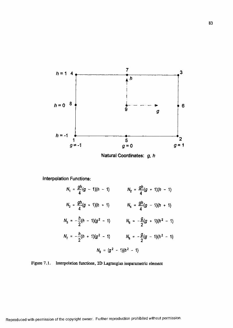
83
1
h = 0
h = -1
g = oNatural Coordinates: g, h
interpolation Functions:
N, = % - 1)(/i - 1) 4
Wj . ^ ( g * 1)((i - 1) 4
«5 = - f h - 1)(3“ - 1)
«2 = ^ ( g ^ 1 ) 0 - 1)4
N, = % - 1 ) 0 + 1)4
% = - & + 1)0 ' - 1)
N. = - | ( f f - 1)0 ' - 1)
«5 = 0 ' - 1)0 ' - 1)
Figure 7.1. Interpolation functions, 2D Lagrangian isoparametric element
Reproduced with permission of the copyright owner. Further reproduction prohibited without permission.
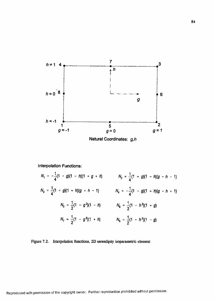
84
A? = 0 ®
Natural Coordinates: g,h
Interpolation Functions:
1= ' 7 (1 - g){1 - h ) { ^ + g + h )
4
^3 " + 9)(1 + /i)(g + h - 1)4
«S = | ( 1 - ff^(1 - h)
«7 = - |(1 - 9^(1 + h)
^2 ~ 9)(1 - A)(g - h - 1)4
N4 = - - j (1 - g)(1 + A)(g - ft + 1) 4
% = i(1 - ft“)(1 7. g)
We = j ( ' - - g)
Figure 7.2. Interpolation functions, 2D serendipity isoparametric element
Reproduced with permission of the copyright owner. Further reproduction prohibited without permission.

85
Gaussian integration employed will integrate the element stiftiiess matrix exactly if the deter
minant of the Jacobian matrix is constant over the element, i.e., if opposing sides for 2D ele
ments or opposing faces for 3D elements are parallel. For reduced integration the integration
scheme is one order less than that required to fully integrate the element stiffiiess matrix.
Solution times may be significantly less with reduced integration resulting in considerable
savings for large 3D models.
In problems where the predominant response mode is bending, fully integrated first-order
elements may “lock”; i.e., the stifhess may be several orders o f magnitude too great. Spuri
ous shear stresses known as parasitic shear stresses are present. In these cases a reduction in
order of the niunerical integration can lead to improved results. The finite element displace
ment formulation overestimates the stiffness of the system; thus, by not evaluating the ele
ment stiffness matrices exactly, better results may be obtained if the error in the numerical
integration compensates for the overestimation of the system stiffness. However, a possibil
ity with reduced integration is a type of mesh instability known as hourglassing. For 2D and
3D reduced integration elements, the element stifkess matrix is rank deficient, causing prob
lems with the solution if the element is not provided with sufficient stiffness restraint in the
global assemblage of elements. When this occurs, the global stifhiess matrix becomes ill-
conditioned and, in some cases, singular. An hourglass mode does not result in strain (and
therefore does not contribute to the energy integral) leading to spurious zero-energy displace
ment modes which behave like a rigid-body mode.
Hourglass modes for the first-order reduced integration quadrilateral and hexahedral ele
ments can propagate through the mesh, and hourglassing can become be a serious problem.
ABAQUS employs hourglass control for these elements in an attempt to suppress hourglass
ing. In effect, additional stiffness is artificially added to the system to restrain the
Reproduced with permission of the copyright owner. Further reproduction prohibited without permission.
86
hourglassing modes. Default hourglass stifhiess values are based upon the elastic properties
of the system. Values for these stiffnesses other than the default values may be specified by
the user. The artificial energy associated with the hourglass control stiffiiesses must be much
less than the total strain energy of the system. First-order reduced integration elements with
hourglass control may perform satisfactorily for very fine meshes, but can be inaccurate for
coarse meshes.
ELEMENT DESCRIPTIONS
The ABAQUS element library contains a vast selection of element types and formulations.
A basic understanding of the type of element and assun^tions made in the formulation of the
element is required before selecting a element for use in a finite element model. The follow
ing paragraphs contain brief descriptions of the 2D and 3D elements considered in this
response and sensitivity study.
2D element description
Even though the purpose of this research was to develop a 3D finite element model for the
rigid pavement system, it was instructive to conduct certain sensitivity studies in 2D. These
2D sensitivity studies were conducted using elements from the ABAQUS element library.
The ABAQUS element library contains a large library of general shell elements for analysis
of curved shell, plate bending, and membrane problems. For a flat plate subjected to both
in-plane and transverse loads, the bending and membrane effects are uncoupled; thus the total
response can be obtained by superimposing the bending and membrane responses. In general
this is not true of the shell element. The shell element is similar to a plate element, except
that the mid-surface of a general shell element can be curved. In this case the bending and
membrane stresses are coupled, and it is no longer possible to superimpose the two conditions
(Fagan 1992).
Reproduced with permission of the copyright owner. Further reproduction prohibited without permission.
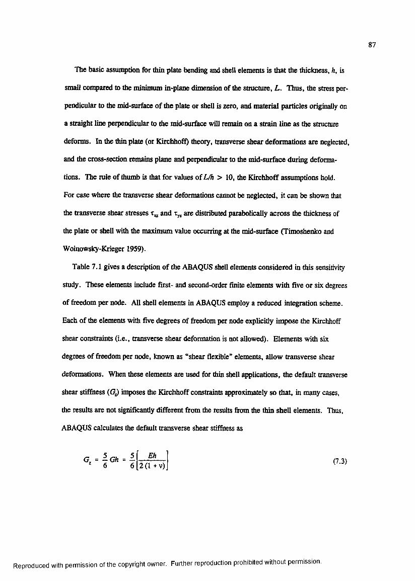
87
The basic assumption for thin plate bending and shell elements is that the thickness, h, is
small conq)ared to the minimum in-plane dimension of the structure, L . Thus, the stress per
pendicular to the mid-surface of the plate or shell is zero, and material particles originally on
a straight line perpendicular to the mid-surface will remain on a strain line as the structure
deforms. In the thin plate (or Kircbho% theory, transverse shear deformations are neglected,
and the cross-section remains plane and perpendicular to the mid-surface during deforma
tions. The rule of thumb is that for values of L/h > 10, the Kirchhoff assumptions hold.
For case where the transverse shear deformations cannot be neglected, it can be shown that
the transverse shear stresses and Ty, are distributed parabolically across the thickness of
the plate or shell with the maximum value occurring at the mid-surface (Timoshenko and
Woinowsky-Krieger 1959).
Table 7.1 gives a description of the ABAQUS shell elements considered in this sensitivity
study. These elements include first- and second-order finite elements with five or six degrees
of freedom per node. All shell elements in ABAQUS en^loy a reduced integration scheme.
Each of the elements with five degrees of freedom per node explicitly impose the Kirchhoff
shear constraints (i.e., transverse shear deformation is not allowed). Elements with six
degrees of freedom per node, known as “shear flexible” elements, allow transverse shear
deformations. When these elements are used for thin shell applications, the default transverse
shear stiffiiess (GJ imposes the Kirchhoff constraints approximately so that, in many cases,
the results are not significantly different from the results from the thin shell elements. Thus,
ABAQUS calculates the default transverse shear stifihess as
Eh2 (1 +v) (7.3)
Reproduced with permission of the copyright owner. Further reproduction prohibited without permission.
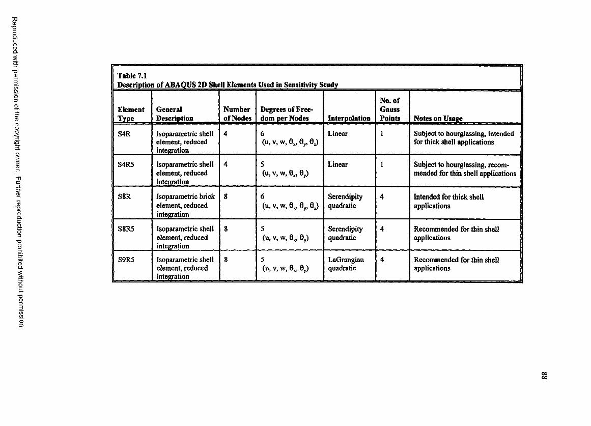
CD■DOQ.C
gQ.
■oCD
C /)
o'Z5
CD
8cS'
3CD
Cp.
CD■oIcao3■oo
CDQ.
Oc■o
CD
</>(/)
Table 7.1Description of ABAQUS 2D Shell Elements Used in Sensitivity Study
ElementType
GeneralDescription
Number of Nodes
Degrees of Freedom per Nodes Interpolation
No. of Gauss Points Notes on Usage
S4R Isoparametric shell element, reduced intégration
4 6(u, V, w, 8 ,, 0y, 8 J
Linear 1 Subject to hourglassing, intended for thick shell applications
S4R5 Isoparametric shell element, reduced integration
4 5(u, V, w, 0 , By)
Linear 1 Subject to hourglassing, recom- 1 mended for thin shell applications I
S8R Isoparametric brick element, reduced integration
8 6(u, V, w, 8 „ By, B j
Serendipityquadratic
4 Intended for thick shell applications
S8R5 Isoparametric shell element, reduced integration
8 5(u, V , w, B„, By)
Serendipityquadratic
4 Recommended for thin shell applications
S9R5 Isoparametric shell element, reduced integration
8 5(u, V, w, B„ By)
LaGrangianquadratic
4 Recommended for thin shell applications
gg
89
where
G = shear modulus of shell
h = thickness of shell
E = modulus o f elastici^ of shell
V = Poisson’s ratio of shell.
Elements S4R and S8 R are especially susceptible to hourglass displacement modes in the
displacement components perpendicular to the shell surface. In general, the 8-node serendip
ity element is considered a good basic element for most shell problems. When reduced inte
gration is employed (as is the case for all of the ABAQUS shell elements used in this study),
shear locking is of no consequence. Although the reduced integration element can exhibit
hourglassing, it, too, is nonconsequential because hourglass modes cannot propagate
throughout the mesh (Schnobrich 1990).
3D element description
Table 7.2 contains a listing of the 3D hexahedral elements from the ABAQUS library con
sidered in this study. Element types considered included both linear and quadratic elements,
employing both full integration and reduced integration. Furthermore, both Lagranian and
serendipity formulations were considered for the quadratic elements. Each element type fea
tures three translational degrees of freedom per node. The C3D27 and C3D27R elements are
variable node elements; that is, the number of nodes can be reduced from 27 nodes per ele
ment down to 21 nodes per element (or any number between) by removing the interior node
from each of the faces of the element as desired.
As is the case with 2D shell elements, fully-integrated elements can exhibit locking where
bending is the primary response mode. This is particularly true of the linear element.
Reduced integration provides relief from locking but may lead to problems with hourglassing.
Reproduced with permission of the copyright owner. Further reproduction prohibited without permission.
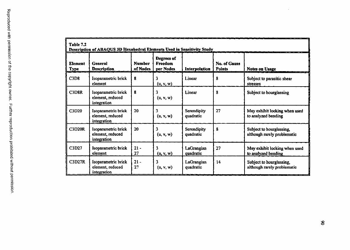
73CD■DOQ.C
8Û.
■DCD
C /î(go"3O
8cq'
3CD
C3.3"CD
5■OICao3
■OO
&
oc■o
CD
Table 7.2Description of ABAQUS 3D Hexahedral Elements Used in Sensitivity Study
ElementType
GeneralDescription
Number of Nodes
Degrees of Freedom per Nodes Interpolation
No. of Gauss Points Notes on Usage
C3D8 Isoparametric brick element
8 3_(u. V , w)
Linear 8 Subject to parasitic shear stresses
C3D8R Isoparametric brick element, reduced integration
8 3( U , V, w )
Linear 8 Subject to hourglassing
C3D20 Isoparametric brick element, reduced integration
20 3(u, V , w)
Serendipityquadratic
27 May exhibit locking when used to analyzed bending
C3D20R Isoparametric brick element, reduced integration
20 3(u, V , w)
Serendipityquadratic
8 Subject to hourglassing, although rarely problematic
C3D27 Isoparametric brick element
2 1 -27
3(u, v,w)
LaGrangianquadratic
27 May exhibit locking when used to analyzed bending
C3D27R Isoparametric brick element, reduced integation
2 1 -27
3(u, V, w)
LaGrangianquadratic
14 Subject to hourglassing, although rarely problematic
C /)
o'3
8
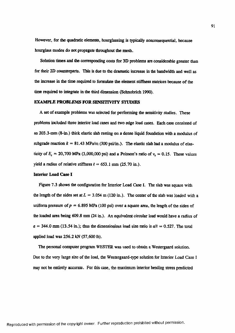
91
However, for the quadratic elements, hourglassing is Qq)ically nonconsequential, because
hourglass modes do not propagate throughout the mesh.
Solution times and the corresponding costs for 3D problems are considerable greater fhan
for their 2D counterparts. This is due to the dramatic increase in the bandwidth and well as
the increase in the time required to formulate the element stifhiess matrices because o f the
time required to integrate in the third dimension (Schnobrich 1990).
EXAMPLE PROBLEMS FOR SENSITIVITY STUDIES
A set of example problems was selected for performing the sensitivity studies. These
problems included three interior load cases and two edge load cases. Each case consisted of
an 203.3-mm (8-in.) thick elastic slab resting on a dense liquid foundation with a modulus of
subgrade reaction k = 81.43 MPa/m (300 psi/in.). The elastic slab had a modulus of elas
ticity of E; = 20,700 MPa (3,000,000 psi) and a Poisson’s ratio of v, = 0.15. These values
yield a radius of relative stiffness I = 653.1 mm (25.70 in.).
Interior Load Case I
Figure 7.3 shows the configuration for Interior Load Case I. The slab was square with
the length of the sides set at L = 3.054 m (120 in.). The center of the slab was loaded with a
uniform pressure o f p = 6.895 MPa (100 psi) over a square area, the length of the sides of
the loaded area being 609.8 mm (24 in.). An equivalent circular load would have a radius of
a = 344.0 mm (13.54 in.); thus the dimensionless load size ratio is a/H = 0.527. The total
applied load was 256.2 kN (57,600 lb).
The personal computer program WESTER was used to obtain a Westergaard solution.
Due to the very large size of the load, the Westergaard-type solution for Interior Load Case I
may not be entirely accurate. For this case, the maximum interior bending stress predicted
Reproduced with permission of the copyright owner. Further reproduction prohibited without permission.
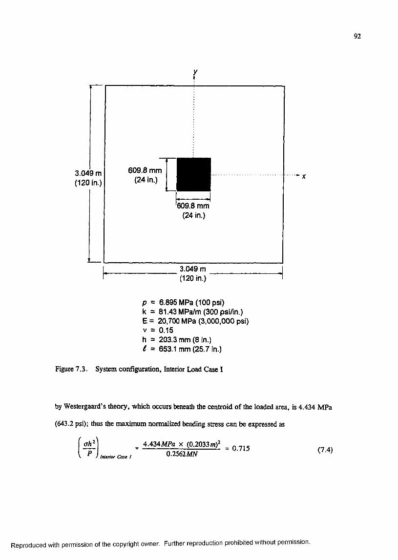
92
3.049 m (120 in.)
609.8 mm (24 in.)
609.8 mm (24 in.)
3.049 m (120 in.)
p = 6.895 MPa (100 psi) k = 81.43 MPa/m (300 psi/in.)E = 20,700 MPa (3,000,000 psi) V = 0.15h = 203.3 mm (8 in.) l = 653.1 mm (25.7 in.)
Figure 7.3. System configuration. Interior Load Case I
by Westergaard's theory, which occurs beneath the centroid of the loaded area, is 4.434 MPa
(643.2 psi); thus the maximum normalized bending stress can be expressed as
P Inttrior Case I
^ 4.434AfPg X (0.2033m) ^ q 0.2562MJV (7.4)
Reproduced with permission of the copyright owner. Further reproduction prohibited without permission.
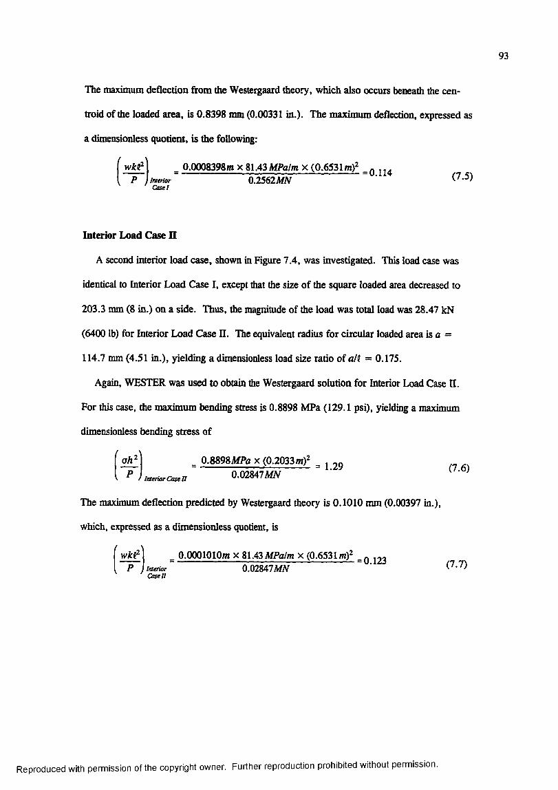
93
The maximum deflection from the Westergaard theory, which also occurs beneath the cen
troid of the loaded area, is 0.8398 mm (0,00331 in.). The maximum deflection, expressed as
a dimensionless quotient, is the following;
_ 0.0008398m x 81.43MPo/m x (0.6531 m) _q P ) Interior 0.2562M/V
Case!(7.5)
Interior Load Case H
A second interior load case, shown in Figure 7.4, was investigated. This load case was
identical to Interior Load Case I, except that the size of the square loaded area decreased to
203.3 mm (8 in.) on a side. Thus, the magnitude of the load was total load was 28.47 kN
(6400 lb) for Interior Load Case U. The equivalent radius for circular loaded area is a =
114.7 mm (4.51 in.), yielding a dimensionless load size ratio of ali = 0.175.
Again, WESTER was used to obtain the Westergaard solution for Interior Load Case II.
For this case, the maximum bending stress is 0.8898 MPa (129.1 psi), yielding a maximum
dimensionless bending stress of
ah _ 0.8898MPUX (0.2033m): _ ^ ^ 9 n 6 ^interiorcosea 0.02847MV ' ^p )
The maximum deflection predicted by Westergaard theory is 0.1010 mm (0.00397 in.),
which, expressed as a dimensionless quotient, is
v t ^ ] _ 0.0001010m X 81.43 MPu/m x (0.6531m): _q , P I Interior' 0.02847 MN ~ ■
Casell
Reproduced with permission of the copyright owner. Further reproduction prohibited without permission.
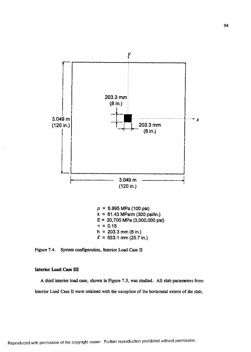
94
203.3 mm (8 in.)
3.049 m (120 in.) 203.3 mm
(Bin.)
3.049 m (120 in.)
p = 6.895 MPa (100 psi) k = 81.43 MPa/m (300 psi/in.)E = 20,700 MPa (3,000,000 psi) V = 0.15h = 203.3 mm (8 in.)6 = 653.1 mm (25.7 in.)
Figure 7.4. System configuration. Interior Load Case II
Interior Load Case m
A third interior load case, shown in Figure 7.5, was studied. All slab parameters from
Interior Load Case II were retained with the exception of the horizontal extent of the slab.
Reproduced with permission of the copyright owner. Further reproduction prohibited without permission.
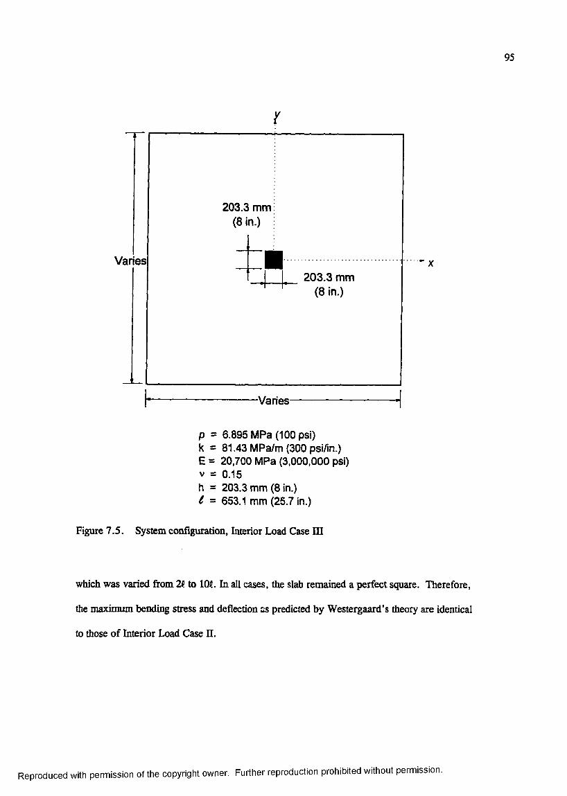
95
203.3 mm (8 in.)
Varies - X
203.3 mm (8 In.)
Varies
p = 6.895 MPa (100 psi) k = 81.43 MPa/m (300 psi/in.)E = 20,700 MPa (3,000,000 psi) V = 0.15h = 203.3 mm (8 in.) l = 653.1 mm (25.7 in.)
Figure 7.5. System configuration, Interior Load Case XU
which was varied from 2H to IOC. In all cases, the slab remained a perfect square. Therefore,
the maximum bending stress and deflection as predicted by Westergaard’s theory are identical
to those of Interior Load Case U.
Reproduced with permission of the copyright owner. Further reproduction prohibited without permission.
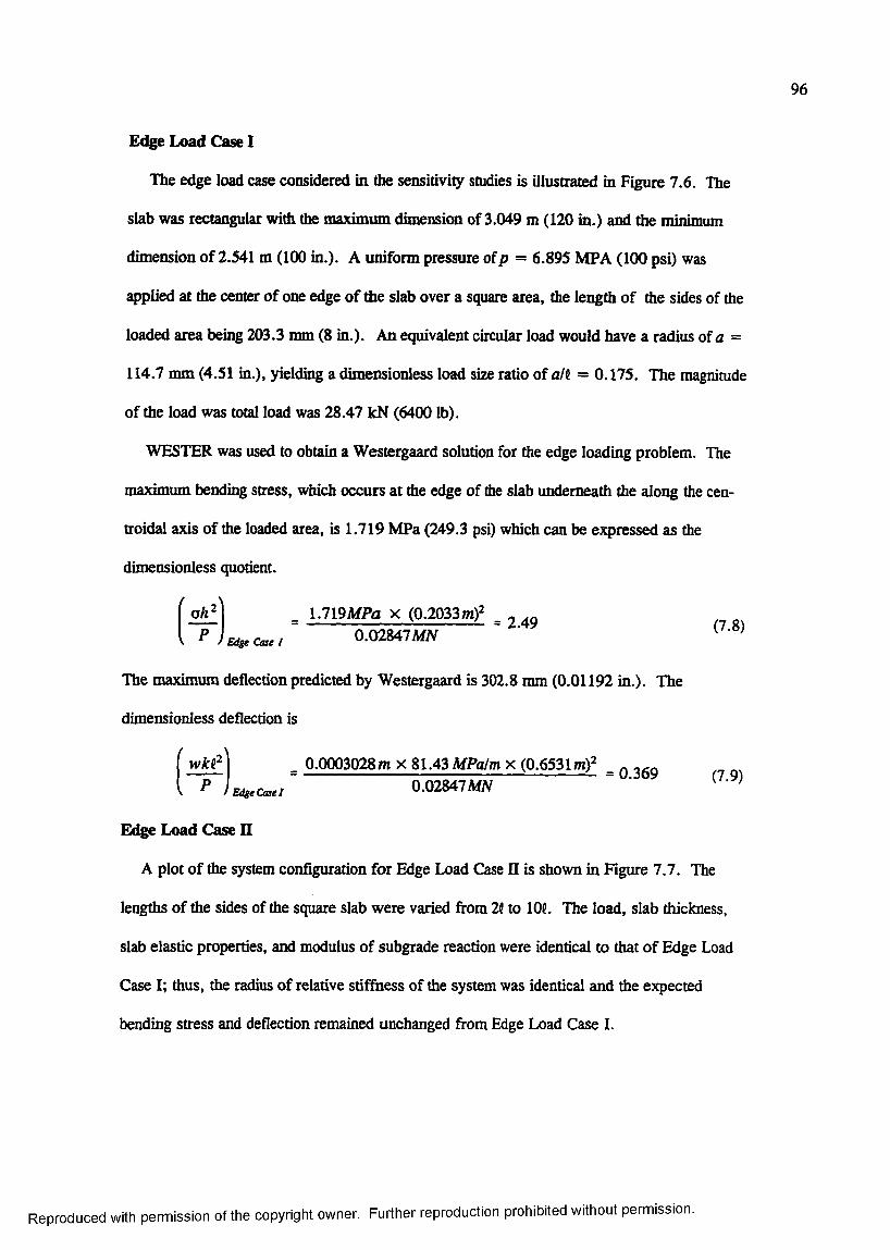
96
Edge Load Case I
The edge load case considered in the sensitivity studies is illustrated in Figure 7.6. The
slab was rectangular with the maximum dimension of 3.049 m (120 in.) and the minimum
dimension of 2.541 m (100 in.). A uniform pressure of p = 6.895 MPA (100 psi) was
applied at the center of one edge of the slab over a square area, the length of the sides of the
loaded area being 203.3 mm (8 in.). An equivalent circular load would have a radius of a =
114.7 mm (4.51 in.), yielding a dimensionless load size ratio of alt. = 0.175. The magnitude
of the load was total load was 28.47 kN (6400 lb).
WESTER was used to obtain a Westergaard solution for the edge loading problem. The
maximum bending stress, which occurs at the edge of the slab underneath the along the cen-
troidal axis of the loaded area, is 1.719 MPa (249.3 psi) which can be expressed as the
dimensionless quotient.
= 1.719MPa X (0.2033m): _n r k T i Q A m i x T I'0.02847MVV f I
The maximum deflection predicted by Westergaard is 302.8 mm (0.01192 in.). The
dimensionless deflection is
0.0003028m x 81.43 MPaim x (0.6531 m)^ . _ _= — = 0.369 (7.9)
wkt^E^eC asel 0.02847MNP
Edge Load Case II
A plot of the system configuration for Edge Load Case U is shown in Figure 7.7. The
lengths of the sides of the square slab were varied from 2t to 106. The load, slab thickness,
slab elastic properties, and modulus of subgrade reaction were identical to that of Edge Load
Case I; thus, the radius of relative stiffness of the system was identical and the expected
bending stress and deflection remained unchanged from Edge Load Case I.
Reproduced with permission of the copyright owner. Further reproduction prohibited without permission.
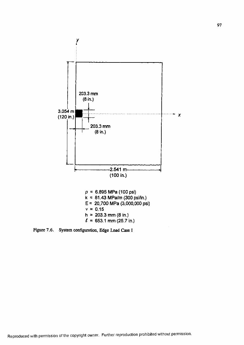
97
203.3 mm (8 In.)
3.054 m (120 In.)
203.3 mm (Bln.)
■2.541 m (100 In.)
p = 6.895 MPa (100 psi) k = 81.43 MPa/m (300 psi/in.)E = 20.700 MPa (3,000,000 psi) V = 0.15h = 203.3 mm (8 in.)6 = 653.1 mm (25.7 in.)
Figure 7.6. System configuration, Edge Load Case I
Reproduced with permission of the copyright owner. Further reproduction prohibited without permission.
98
203.3 mm (8 in.)
Varies
203.3 mm (8 in.)
Varies
p = 6.895 MPa (100 psi) k = 81.43 MPa/m (300 psi/in.)E = 20,700 MPa (3,000,000 psi) V = 0.15h = 203.3 mm (8 in.) l - 653.1 mm (25.7 in.)
Figure 7.7. System configuration, Edge Load Case II
Reproduced with permission of the copyright owner. Further reproduction prohibited without permission.

99
RESPONSE AND SENSITTVITY STUDY RESULTS
Some of the questions to be answered by the response and sensitivity study include the fol
lowing:
• What 3D hexahedron element is appropriate for the slab-on-grade problem?
• What mesh fineness is required in the plane of the slab surface?
• What mesh fineness is required in the plane of the slab thickness?
• Should the analyst be concerned about transverse shear deformations for interior and
edge load cases for rigid pavements?
• What is the minimum slab dimension in the plane of the slab surface required to meet
Westergaard’s assumption of a semi-infinite or infinite slab? How significant is this
boundary effect for finite element modeling?
These issues are addressed in the remainder of this chapter.
Interior Load Case I
Interior Load Case I was the most general load case studied and was primarily intended to
study mesh fineness and element selection issues. Studies were conducted in both 2D and
3D. These studies are described and summarized below.
2D convergence studies
Four finite element meshes representing different degrees of mesh refinement were gener
ated. Table 7.3 is a summary of the results of these calculations. The degree of mesh refine
ment is characterized by the dimensionless ratio hlla were h is the thickness of the slab and
2a is the minimum length of the side of an element. Figure 7.8(a) shows a diagram of the
lengths of the sides of the 2D shell elements. Each of the finite element meshes are shown in
Figure 7.9.
Reproduced with permission of the copyright owner. Further reproduction prohibited without permission.
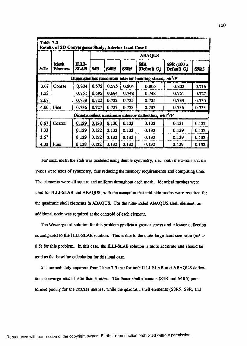
100
1 Table 7.3Results of 2D Convergence Study, Interior Load Case I
h/2a
0.67
MeshFineness
ILLI-SLAB
ABAQUS
S4R S4R5 S8R5S8R(Default
S8 R (100 X Default Gj) S9R5
Dimensionless ma^imimi Ulterior bending stress ah^/P
Coarse
Fine
0.804 0.575 0.575 0.804 0.805 0.802 0.7161.33 0.751 0.695 0.694 0.748 0.748 0.751 0.7272.67 0.739 0.722 0.722 0.735 0.735 0.739 0.7304.00 0.736 0.727 0.727 0.733 0.733 0.736 0.733
Dimens oniess maximum interior deflection, wl
0.67 Coarse
Fine
0.129 0.130 0.130 0.132 0.132 0.131 0.1321.33 0.129 0.132 0.132 0.132 0.132 0.139 0.1322.67 0.129 0.132 0.132 0.132 0.132 0.129 0.1324.00 0.128 0.132 0.132 0.132 0.132 0.129 0.132
For each mesh the slab was modeled using double symmetry, i.e., both the x-axis and the
y-axis were axes of symmetry, thus reducing the memory requirements and computing time.
The elements were all square and uniform throughout each mesh. Identical meshes were
used for ILLI-SLAB and ABAQUS, with the exception that mid-side nodes were required for
the quadratic shell elements in ABAQUS. For the nine-noded ABAQUS shell element, an
additional node was required at the centroid of each element.
The Westergaard solution for this problem predicts a greater stress and a lessor deflection
as compared to the ILLI-SLAB solution. This is due to the quite large load size ratio (u/( >
0.5) for this problem. In this case, the ILLI-SLAB solution is more accurate and should be
used as the baseline calculation for this load case.
It is immediately apparent from Table 7.3 that for both ILLI-SLAB and ABAQUS deflec
tions converge much faster than stresses. The linear shell elements (S4R and S4R5) per
formed poorly for the coarser meshes, while the quadratic shell elements (S8R5, S8 R, and
Reproduced with permission of the copyright owner. Further reproduction prohibited without permission.
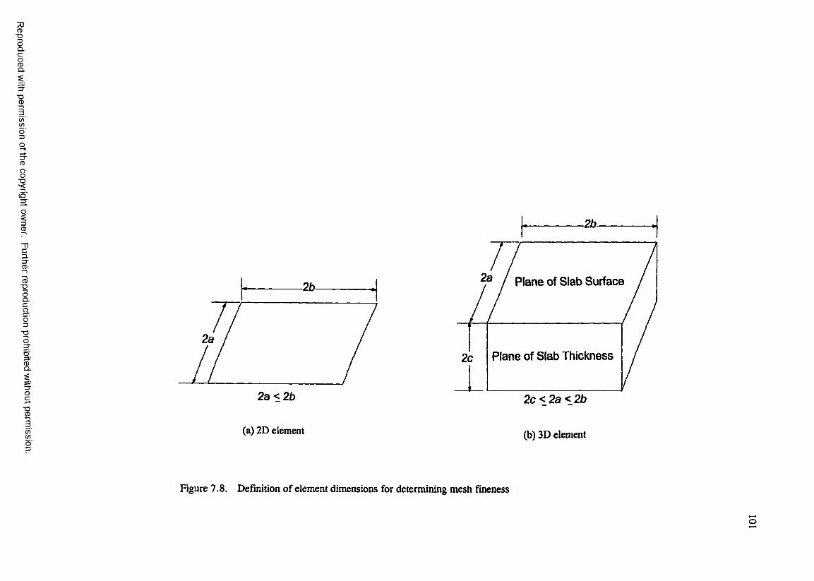
7)CD
"DOQ .C
gQ .
■DCD
C /)C /)
CD
8
CD -2b-
CD■OOQ .Cg.o=3
■OO
&
oc
-g
c /)(go"3
2a <26
Plane of Slab Surface
Plane of Slab Thickness
2c < 2a < 2b
(a) 2D element (b) 3D element
Figure 7.8. Definition of element dimensions for determining mesh fineness
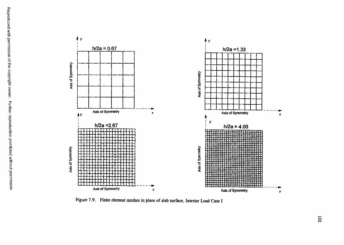
7DCD■DOQ .C
gQ .
■DCD
C/)C /)
CD
85
3.3"CD
CD"OOQ .CaO3■OO
CDQ .
"OCD
C/)C /)
II
h/2a = 0. 67 h/2a=1.33
AyA x is o f S y m m e t r y
h/2a =2.67
I*5CO
îco
A x is o f S y m m e t r y
h/2a = 4.00
îI*3(0
A x is o f S y m m e t r yA x is o f S y m m e t r y
Figure 7.9. Finite element meshes in plane of slab surface, Interior Load Case I

103
S9R5) performed much better. The differences observed between the ABAQUS shell ele
ments with six degrees of freedom per node (S4R and S8 R) and their conjugate element with
five degrees of freedom per node (S4R5 and S8RS, respectively) were small.
3D convergence studies
A partial matrix o f convergence studies was conducted in 3D for Interior Load Case I.
The results of these studies are summarized in Table 7.4. This load case was used to study
the choice of element types for 3D modeling, the mesh fineness in the plane of the pavement
surface, and the mesh fineness across the depth o f the slab. As in the case of the 2D shell
elements, the fineness of the mesh in the plane of the slab is characterized by the element
aspect ratio in that plane defined by h/2 a were 2a is the length of the smallest side of the ele
ment in the horizontal plane. Likewise, in the plane of the slab thickness, the fineness of the
mesh is characterized by the aspect ratio h/2 c, where 2 c is the length of the smallest side of
the element in the vertical plane. These dimensions are indicated in Figure 7.8(b). In plan
view the meshes were composed of square elements whose aspect ratios were identical to
those shown in Figure 7.9. Figure 7.10 shows a diagram of selected 3D meshes through the
thickness of the slab.
The results tabulated in Table 7.4 indicate that the linear hexahedral elements, both fully-
integrated (C3D8) and under-integrated (C3D8R) are much too stiff for the rigid pavement
problem. This is due to locking of the element. However, the responses of the quadratic
elements (C3D20, C3D20R, C3D27, and C3D27R) are much better than those of the linear
elements. Each of the serendipity formulation elements (C3D20 and C3D20R) and the
Lagrangian elements (C3D27 and C3D27R) performed quite well. The convergence trends
for dimensionless bending stress and dimensionless deflection are shown in Figures 7.11 and
7.12, respectively. One of the primary distinctions between the serendipity and Lagrangian
Reproduced with permission of the copyright owner. Further reproduction prohibited without permission.
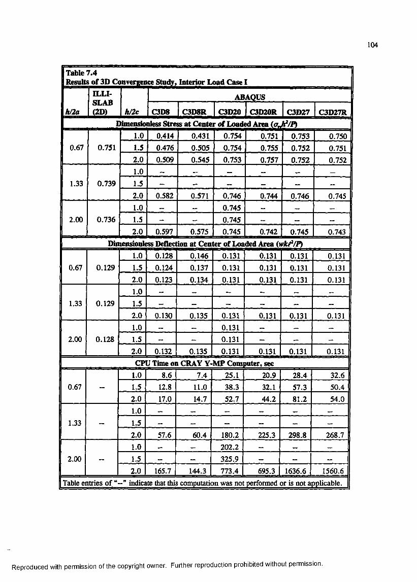
104
TableResult
7.4s of 3D O mvergence Study, Interior Load Case I
ELLI-SLAB(2D)
ABAQUS
h/2 a h/2 c C3D8 C3D8R C3D20 C3D20R C3D27 C3D27R1Hmensioniess Stress at Center of Loaded Area (aJ^/P)
1 .0 0.414 0.431 0.754 0.751 0.753 0.7500.67 0.751 1.5 0.476 0.505 0.754 0.755 0.752 0.751
2 .0 0.509 0.545 0.753 0.757 0.752 0.7521.0 — — — — — _
1.33 0.739 1.5 — — — — __
2 .0 0.582 0.571 0.746 0.744 0.746 0.7451.0 — 0.745 —
2 .0 0 0.736 1.5 — 0.745 — _ —
2 .0 1 0.597 0.575 0.745 0.742 0.745 0.743Dinlensionless Deflectdon at Center of Loaded Area {wkP/Pi
1.0 0.128 0.146 0.131 0.131 0.131 0.1310.67 0.129 1.5 0.124 0.137 0.131 0.131 0.131 0.131
2 .0 0.123 0.134 0.131 0.131 0.131 0.1311 .0 — — — ——
1.33 0.129 1.5 — — — — — —
2 .0 0.130 0.135 0.131 0.131 0.131 0.1311.0 — — 0.131 — — ——
2 .00 0.128 1.5 — 0.131 — — —
2 .0 0.132 0.135 0.131 0.131 0.131 0.131CPU Time on CRAY Y-MP Com 3uter, sec
1.0 8 .6 7.4 25.1 20.9 28.4 32.60.67 1.5 12.8 11.0 38.3 32.1 57.3 50.4
2 .0 17.0 14.7 52.7 44.2 81.2 54.01.0 — — _
1.33 — 1.5 — ^— — — _
2 .0 57.6 60.4 180.2 225.3 298.8 268.71.0 — — 2 0 2 .2 — — —
2 .0 0 — 1.5 — 325.9 — — —
2 .0 165.7 144.3 773.4 695.3 1636.6 1560.6Table entries of indicate that this computation was not performed or is not applicable.
Reproduced with permission of the copyright owner. Further reproduction prohibited without permission.

105
h/2a = 0.67, h/2c= 1.0
h/2a = 0.67, h/2c = 1.5
h/2a = 0.67, h/2c = 2.0
h/2a =2 .0 , h/2c = 2.0
h/2a =2 .0 , h/2c = 2.0
Figure 7.10 Finite element meshes in plane of slab thickness, Interior Load Case I
elements is in the amount of CPU time required to perform the calculations as illustrated in
Figure 7.13. The solution time for the C3D27 element is over two times that required for the
C3D20 element. For both the C3D20R and C3D27R, use o f reduced integration results in a
reduction of CPU time by about 10 percent over its fully-integrated counterpart.
The results in Table 7.4 show that increasing the mesh fineness in the plane of the slab
thickness from h/2c = 0.67 (in this case, two elements through the slab thickness) to
Reproduced with permission of the copyright owner. Further reproduction prohibited without permission.
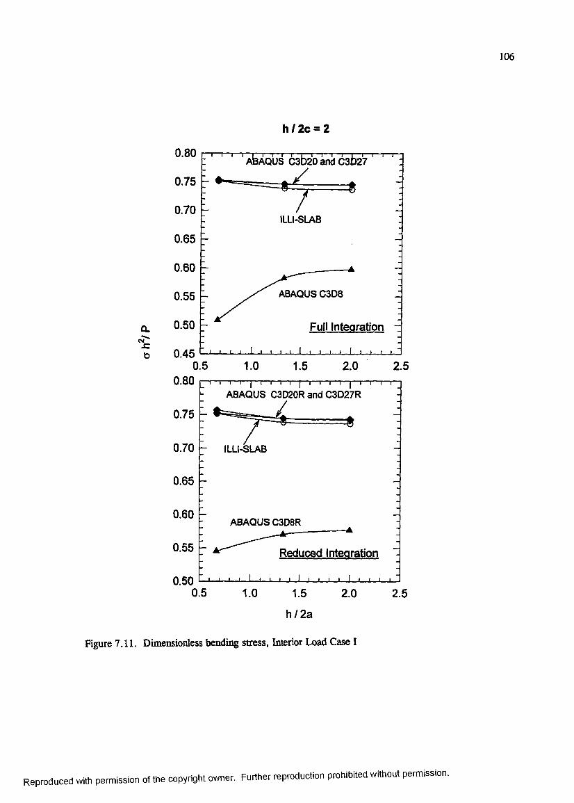
106
Q.
t)
h /2c = 2
0.80AÈÀQUS C3b20 and CSbzV
0.75
0.70ILLl-SLAB
0.65
0.60
ABAQUS C3D80.55
0.50 Full Integration
0.450.5 1.0 1.5 2.0 2.5
0.80ABAQUS C3D20R and C3D27R
0.75
0.70 ILLl-SLAB
0.65
0.60ABAQUS C3D8R
0.55 Reduced Integration
0.500.5 1.0 1.5 2.0 2.5
h / 2 a
Figure 7.11. Dimensionless bending stress. Interior Load Case I
Reproduced with permission of the copyright owner. Further reproduction prohibited without permission.
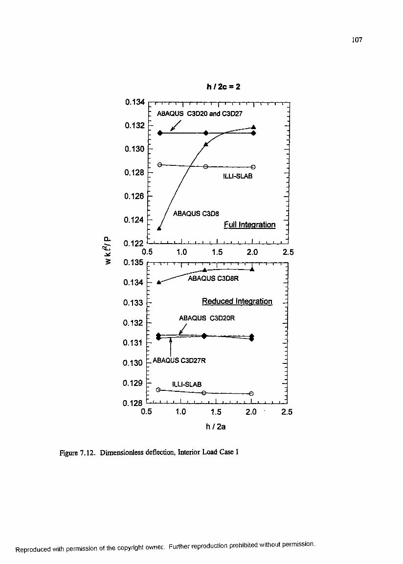
107
Q .
g
h /2 c = 2
0.134ABAQUS C3D20 and C3D27
0.132
0.130
0.128 ILLI-SLAB
0.126
ABAQUS C3D80.124 Full Integration
0.122 L L I t.
0.5 1.0 1.5 2.0 2.50.135
ABAQUS C3D8R0.134
Reduced Integration0.133
ABAQUS C3D20R0.132
0.131
ABAQUS C3D27R0.130
0.129 ILLI-SLAB
0.1280.5 1.0 2.0 2.51.5
h / 2 a
Figure 7.12. Dimensionless deflection, Interior Load Case I
Reproduced with permission of the copyright owner. Further reproduction prohibited without permission.
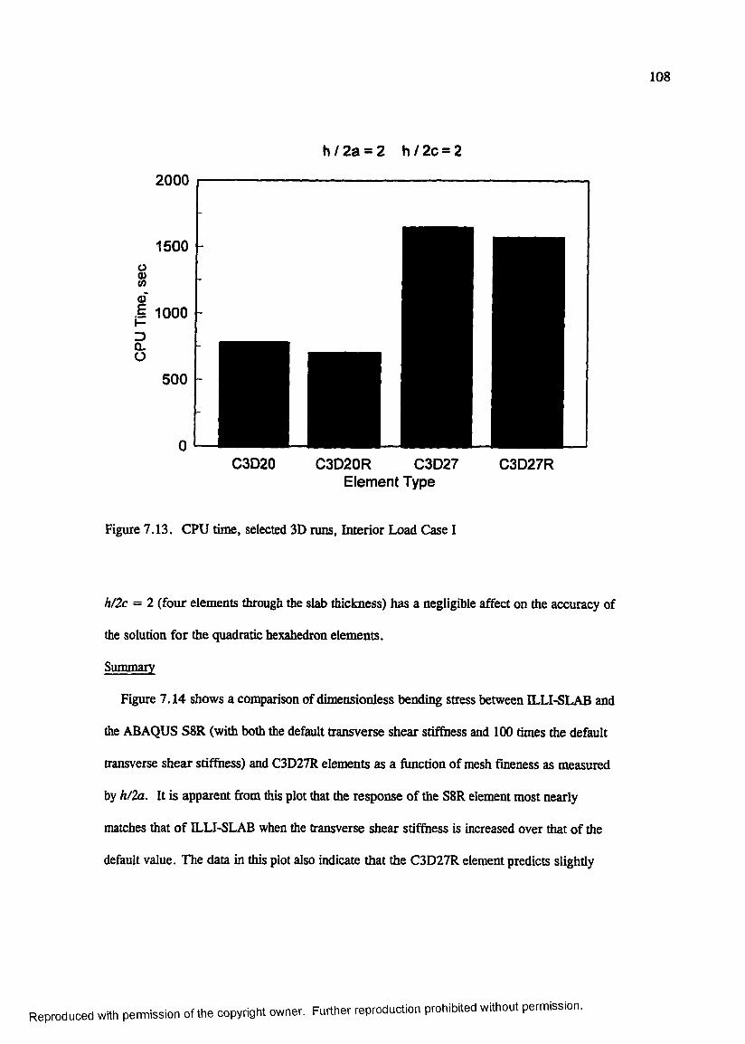
108
h / 2a = 2 h / 2c = 2
2000
i 1000
C3D20 C3D20R C3D27 Elem ent Type
C3D27R
Figure 7.13. CPU time, selected 3D runs, Interior Load Case I
h/2 c = 2 (four elements through the slab thickness) has a negligible affect on the accuracy of
the solution for the quadratic hexahedron elements.
Summary
Figure 7.14 shows a comparison of dimensionless bending stress between ILLI-SLAB and
the ABAQUS S8R (with both the default transverse shear stiffness and 100 times the default
transverse shear stiffness) and C3D27R elements as a function of mesh fineness as measured
by h/2a. It is apparent from this plot that the response of the S8R element most nearly
matches that of ILLI-SLAB when the transverse shear stiffness is increased over that of the
default value. The data in this plot also indicate that the C3D27R element predicts slightly
Reproduced with permission o f the copyright owner. Further reproduction prohibited without permission.
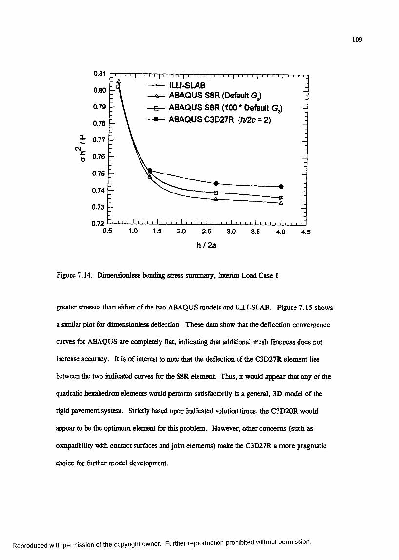
109
Q.
ILLI-SLABABAQUS S8R (Default G^)
B - ABAQUS S8R (100 * Defeult G,) # - ABAQUS C3D27R { h / 2 c - 2 )
h / 2 a
Figure 7.14. Dimensionless bending stress summary, Interior Load Case I
greater stresses than either o f the two ABAQUS models and ILLI-SLAB, Figure 7.15 shows
a similar plot for dimensionless deflection. These data show that the deflection convergence
curves for ABAQUS are conqiletely flat, indicating that additional mesh fineness does not
increase accuracy. It is of interest to note that the deflection of the C3D27R element lies
between the two indicated curves for the S8R element. Thus, it would appear that any of the
quadratic hexahedron elements would perform satisfactorily in a general, 3D model of the
rigid pavement system. Strictly based upon indicated solution times, the C3D20R would
appear to be the optimum element for this problem. However, other concerns (such as
compatibility with contact surfaces and joint elements) make the C3D27R a more pragmatic
choice for further model development.
Reproduced with permission of the copyright owner. Further reproduction prohibited without permission.
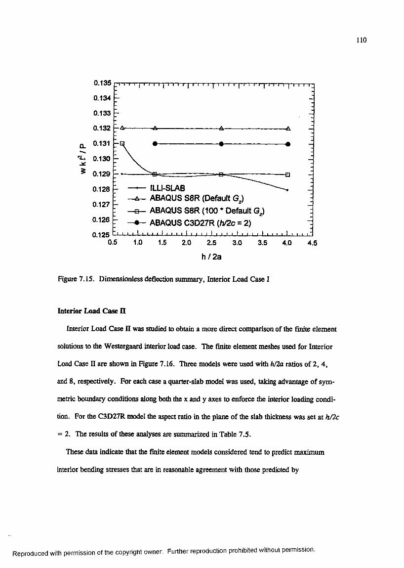
110
0.135
0.134
0.133
0.132
CL 0.131
0.130
$ 0.129
0.128
0.127
0.126
0.125
0.135 r r r i i - | i i i i [ i-|-i i | i -i i i | i r r i | i i T n | i t i-i | i i T
ILLI-SLAB ^ ABAQUS S8R (Default G^)
-B - ABAQUS S8R (100 * Defeult G^) ABAQUS C3D27R { h / 2 c = 2)
I I I I I I I I j I I I I I I I I I I I I I << I I I I I I I I ' I I I I I I '0.5 1.0 1.5 2.0 2.5 3.0 3.5 4.0 4.5
h / 2 a
Figure 7.15. Dimensionless deflection summary, Interior Load Case I
Interior Load Case II
Interior Load Case II was studied to obtain a more direct comparison of the finite element
solutions to the Westergaard interior load case. The finite element meshes used for Interior
Load Case II are shown in Figure 7.16. Three models were used with h/2a ratios of 2, 4,
and 8 , respectively. For each case a quarter-slab model was used, taking advantage of sym
metric boundary conditions along both the x and y axes to enforce the interior loading condi
tion. For the C3D27R model the aspect ratio in the plane of the slab thickness was set at h/2c
= 2. The results of these analyses are summarized in Table 7.5.
These data indicate that the finite element models considered tend to predict maximum
interior bending stresses that are in reasonable agreement with those predicted by
Reproduced with permission of the copyright owner. Further reproduction prohibited without permission.
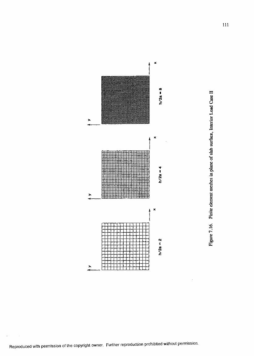
I l l
00II
a
i
MII
I
I•§
IO.•S
IIIK&
Reproduced with permission of the copyright owner. Further reproduction prohibited without permission.
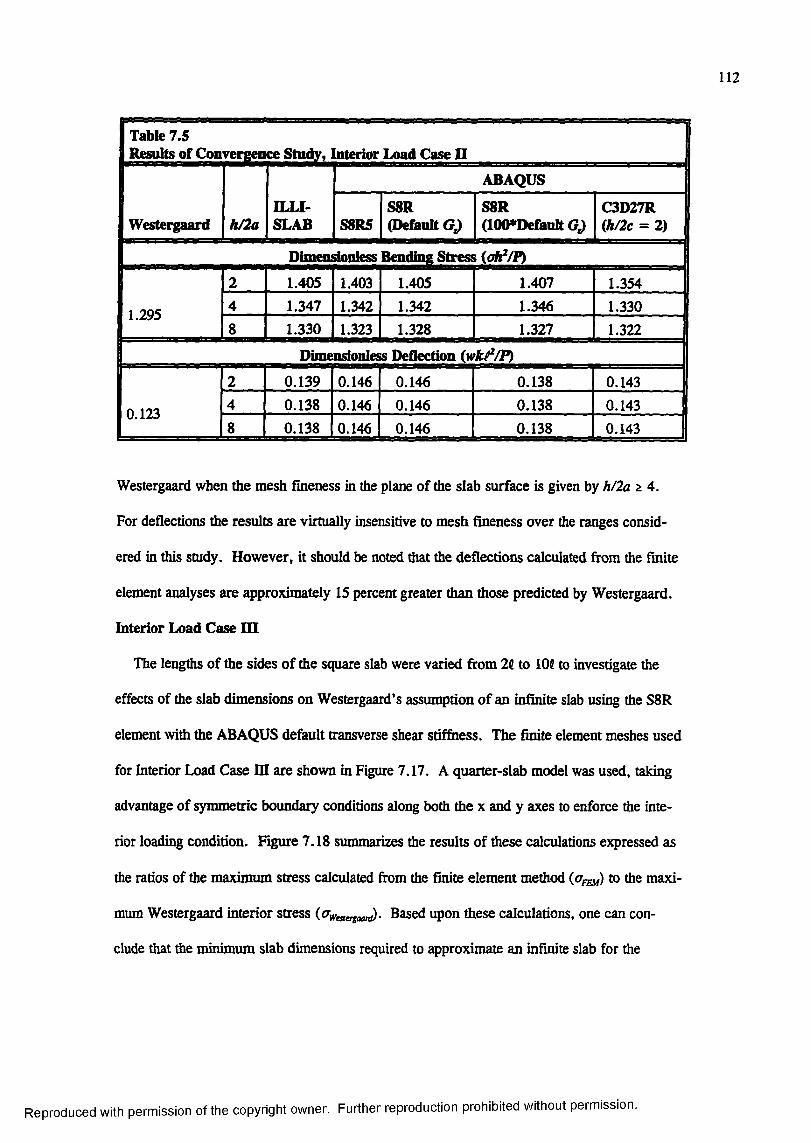
112
1 Table 7.51 Results of Convergence Study, Interior Load Case II
ABAQUS
Westergaard h/2aILLI-SLAB S8R5
S8R(Default Gp
S8R(IOO*Default GJ
C3D27R {Ji/2c = 2)
Dimensionless Bending Stress2 1.405 1.403 1.405 1.407 1.354
1.295 4 1.347 1.342 1.342 1.346 1.3308 1.330 1.323 1.328 1.327 1.322
Dimensionless Deflection {wkf /P)2 0.139 0.146 0.146 0.138 0.143
0.123 4 0.138 0.146 0.146 0.138 0.1438 0.138 0.146 0.146 0.138 0.143
Westergaard when the mesh fineness in the plane of the slab surface is given by h/2a ^ 4.
For deflections the results are virtually insensitive to mesh fineness over the ranges consid
ered in this study. However, it should be noted that the deflections calculated from the finite
element analyses are approximately IS percent greater than those predicted by Westergaard.
Interior Load Case HI
The lengths of the sides of the square slab were varied from 7A to 10( to investigate the
effects of the slab dimensions on Westergaard’s assumption of an infinite slab using the S8R
element with the ABAQUS default transverse shear stiffness. The finite element meshes used
for Interior Load Case lU are shown in Figure 7.17. A quarter-slab model was used, taking
advantage of symmetric boundary conditions along both the x and y axes to enforce the inte
rior loading condition. Figure 7.18 summarizes the results of these calculations expressed as
the ratios of the maximum stress calculated from the finite element method ( o ^ ) to the maxi
mum Westergaard interior stress (tVetf*r*aaJ- Based upon these calculations, one can con
clude that the minimum slab dimensions required to approximate an infinite slab for the
Reproduced with permission of the copyright owner. Further reproduction prohibited without permission.
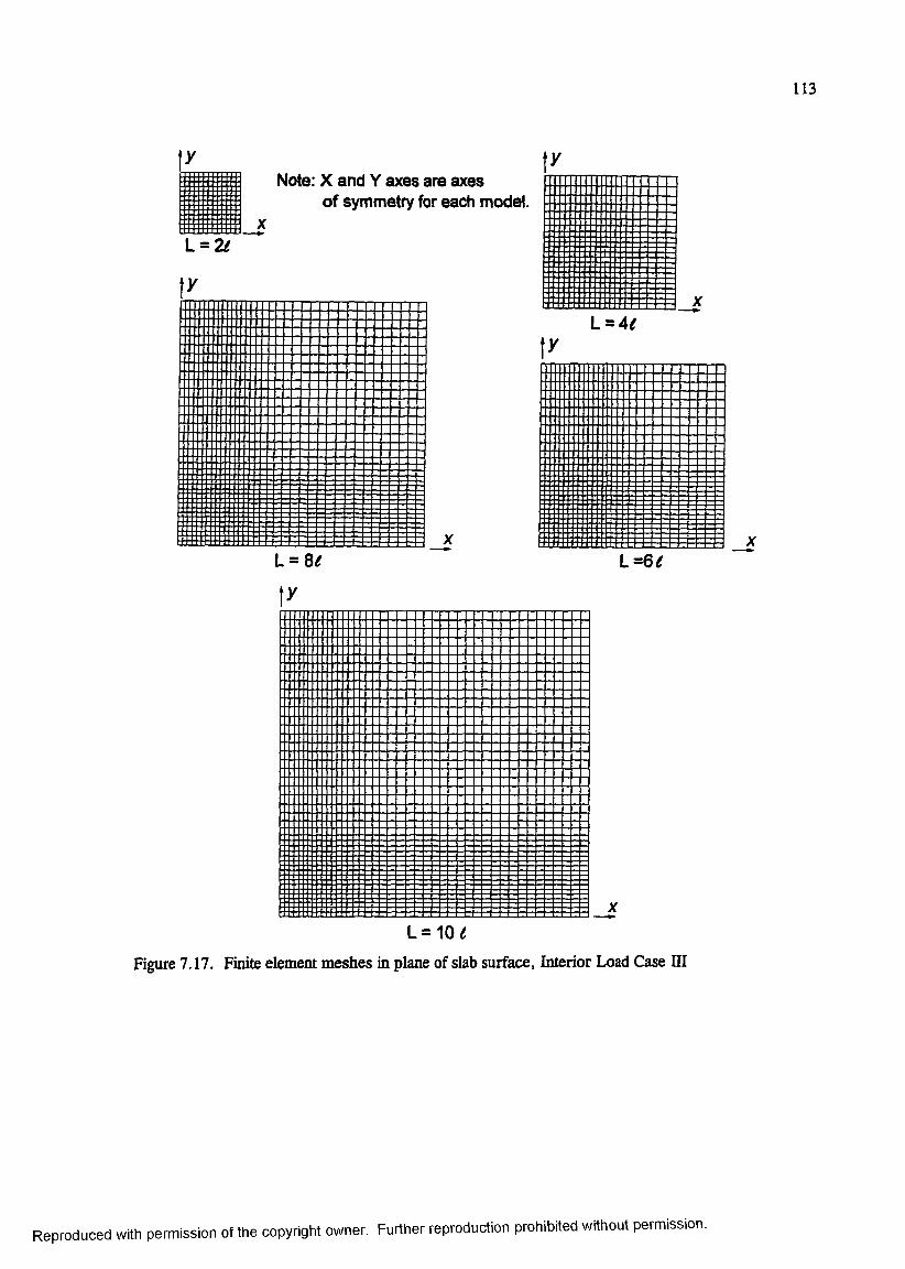
113
Note: X and Y axes are axes of symmetry for each model.
L = %
L = 8 f
L = 4 f
L= 6 f
L = 1 0 (
Figure 7.17. Finite element meshes in plane of slab surface, Interior Load Case III
Reproduced with permission of the copyright owner. Further reproduction prohibited without permission.
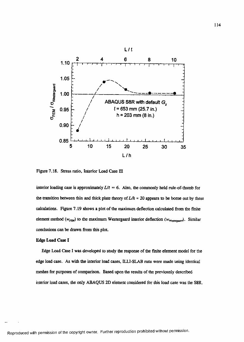
114
1ta
!
(Uu.D
1.10
1.05
1.00
0.95
0.90
0.85
L / l
6 8 10
//
\
/
ABAQUS S8R with default l = 653 mm (25.7 In.)
h = 203 mm (8 in.)/
k /
-1—1— I— L-J— 1 .1 1 I I I I I I I I I I I I I I I I I I I I I
5 10 15 20 25 30 35
L /h
Figure 7.18. Stress ratio, Interior Load Case lU
interior loading case is approximately L/i = 6 . Also, the commonly held rule-of-thumb for
the transition between thin and thick plate theory of L/% = 20 appears to be borne out by these
calculations. Figure 7.19 shows a plot of the maximum deflection calculated from the finite
element method (yvpEu) to the maximum Westergaard interior deflection Similar
conclusions can be drawn from this plot.
Edge Load Case I
Edge Load Case I was developed to study the response of the finite element model for the
edge load case. As with the interior load cases, ILLI-SLAB runs were made using identical
meshes for purposes of comparison. Based upon the results of the previously described
interior load cases, the only ABAQUS 2D element considered for this load case was the S8 R.
Reproduced with permission of the copyright owner. Further reproduction prohibited without permission.
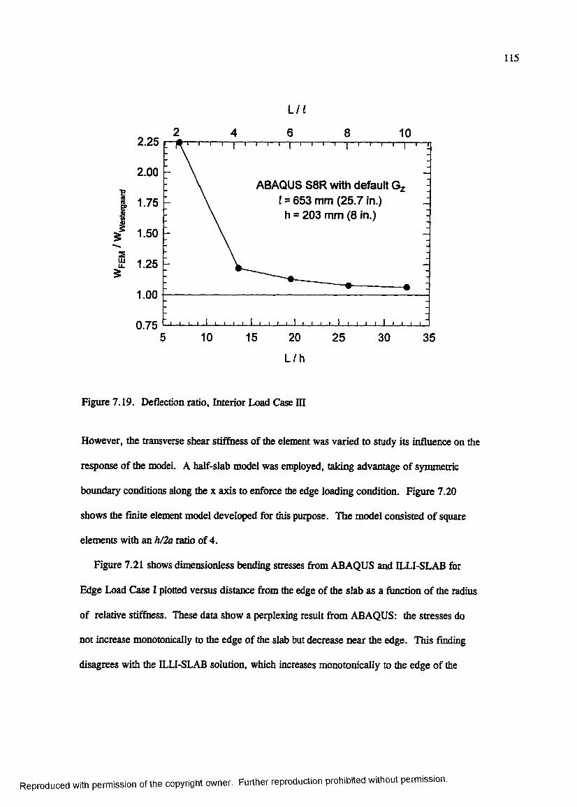
115
2.25
2.00
11 1.75s
1.50
stuU L 1.25
s
1.00
0.75
ABAQUS S8R with default t = 653 mm (25.7 in.)
h = 203 mm (8 In.)
10 15 20
L /h
25 30 35
Figure 7.19. Deflection ratio. Interior Load Case in
However, the transverse shear stif&iess of the element was varied to study its influence on the
response of the model. A half-slab model was employed, taking advantage of symmetric
boundary conditions along the x axis to enforce the edge loading condition. Figure 7.20
shows the finite element model developed for this purpose. The model consisted of square
elements with an h/2a ratio of 4.
Figure 7.21 shows dimensionless bending stresses from ABAQUS and ILLI-SLAB for
Edge Load Case I plotted versus distance from the edge of the slab as a function of the radius
of relative stiffness. These data show a perplexing result from ABAQUS: the stresses do
not increase monotonically to the edge of the slab but decrease near the edge. This finding
disagrees with the ILLl-SLAB solution, which increases monotonically to the edge of the
Reproduced with permission of the copyright owner. Further reproduction prohibited without permission.
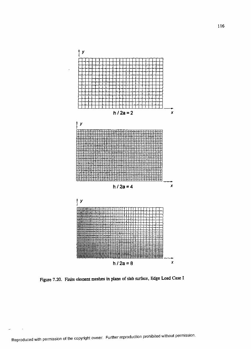
116
h / 2 a = 2
qj
J qj q qd j ] qj
b rb c bc rc cr[ crrcr b b r ttr b d r] 'r q
h / 2 a = 4
h / 2 a = 8 ^
Figure 7.20. Finite element meshes in plane of slab surface, Edge Load Case I
Reproduced with permissionof the copyright owner. Further reproduction prohibited without permission.

117
slab. Away from the edge of the slab, ILLI-SLAB and ABAQUS S8R agree quite well. In
fact, as the transverse shear stiAiess of the S8R element is increased, the response
^proaches that of ILLI-SLAB, until at a transverse shear stiffness of 100 times the default,
the ABAQUS S8 R response approximates the ILLI-SLAB response.
A 3D model was developed using the ABAQUS C3D27R element with three elements
through the thickness of the slab {h/2c = 1.67). In the plane o f the slab surface, the mesh
was identical to that shown in Figure 7.20. Figure 7.22 shows a plot of dimensionless bend
ing stresses from ABAQUS and ILLI-SLAB plotted versus distance from the edge of the slab
as a frmction of the radius of relative stiffriess including the ABAQUS C3D27R model. Also
shown in the plot are the responses predicted by the ABAQUS S8R element for three values
of transverse shear stiffriess; one, two and 100 times the ABAQUS default values. Interest
ingly enough, the ABAQUS C3D27R response more nearly matches the response of the S8 R
element with the default transverse shear stifrhess than the ILLI-SLAB response. In fact, the
3D model matches very closely the response from the S8R model when the default transverse
shear stiffness is twice the default value.
The above observations leads to a very significant and perhaps far-reaching conclusion:
the classical Kirchhoff assun^tions of thin plate theory, adopted by Westergaard, are not
strictly valid for the edge loading case in rigid pavements. It is interesting to note that
Timoshenko and Woinsowsky-Krieger (1959) in their now classical treatise on plates and
shells made the following observation:
The disregard of the deformation due to the transverse stress component obviously is equivalent to the assimçtion of a shear modulus = <»; proceeding in this way we replace the actual material of the plate, supposed to be isotropic, by a hypothetical material of no perfect isotropy.
Reproduced with permission of the copyright owner. Further reproduction prohibited without permission.
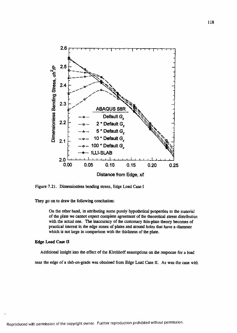
118
2. 6 i-r
ABAQUS S8R
Oerault 6
2 * Default GDefault G
10* Default G
—Ô-— 100 Default GILLI-SLAB
0.00 0.05 0.10 0.15 0.20 0.25
Distance from Edge, x H
Figure 7.21. Dimensionless bending stress. Edge Load Case I
They go on to draw the following conclusion;
On the other hand, in attributing some purely hypothetical properties to the material of the plate we cannot expect complete agreement of the theoretical stress distribution with the actual one. The inaccuracy of the customary thin-plate theory becomes of practical interest in the edge zones of plates and around holes that have a diameter which is not large in comparison with the thickness of the plate.
Edge Load Case II
Additional insight into the effect of the Kirchhoff assumptions on the response for a load
near the edge of a slab-on-grade was obtained from Edge Load Case U. As was the case with
Reproduced with permission of the copyright owner. Further reproduction prohibited without permission.
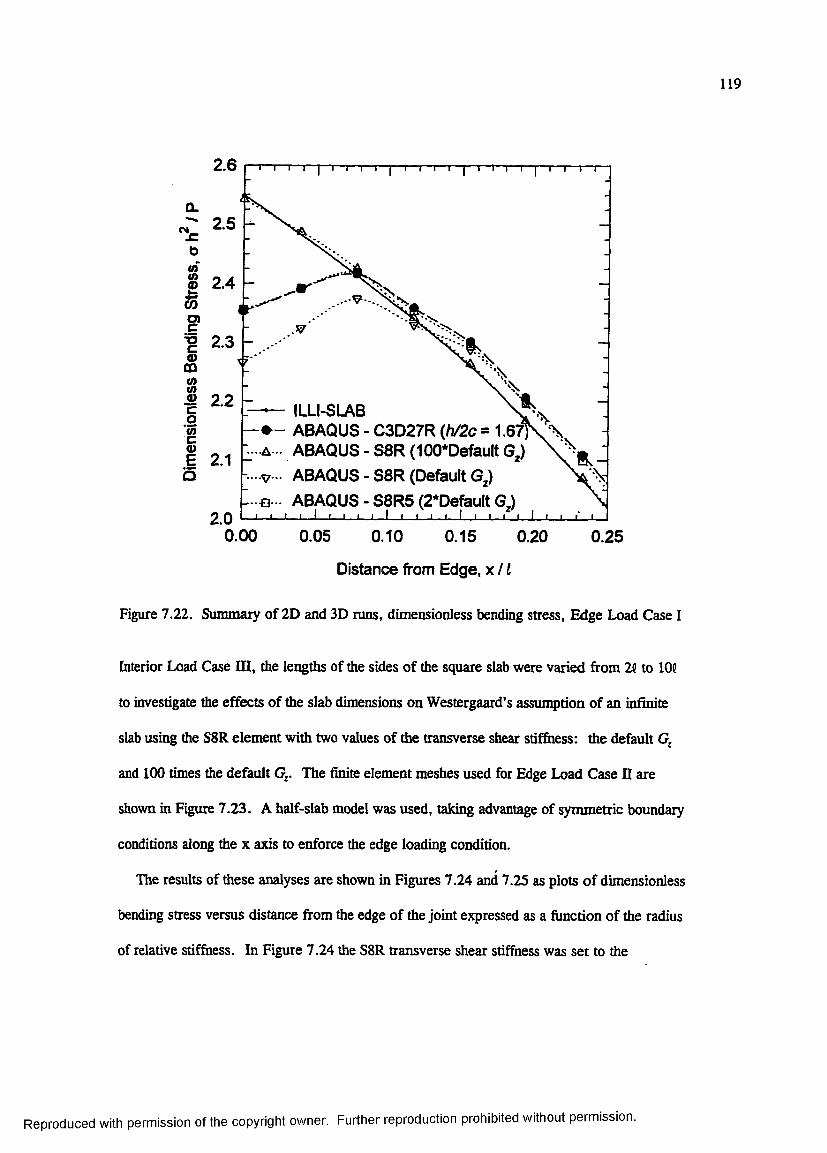
119
1 I I I I I I I I I I I I I I I I I I I I I— I r
ILLI-SLAB— ABAQUS - C3D27R (/i/2c = 1.671\*X 2; A - ABAQUS-S8R(100*DefaultG^) ^ ^
- -V.. ABAQUS - S8R (Default G^)- -Q - ABAQUS - S8R 5 (2*Default G )
I I I 1 I I I I 1 I I I I I I0.00 0.05 0.10 0.15 0.20 0.25
Distance from Edge, x / 1
Figure 7.22. Summary of 2D and 3D runs, dimensionless bending stress, Edge Load Case I
Interior Load Case HI, the lengths of the sides of the square slab were varied from 21 to 105
to investigate the effects of the slab dimensions on Westergaard’s assunçtion of an infinite
slab using the S8R element with two values of the transverse shear stif&iess: the default
and 100 times the default G . The finite element meshes used for Edge Load Case n are
shown in Figure 7.23. A half-slab model was used, taking advantage of symmetric boundary
conditions along the x axis to enforce the edge loading condition.
The results of these analyses are shown in Figures 7.24 and 7.25 as plots of dimensionless
bending stress versus distance from the edge of the joint expressed as a function of the radius
of relative stiffness. In Figure 7.24 the S8R transverse shear stiffness was set to the
Reproduced with permission of the copyright owner. Further reproduction prohibited without permission.
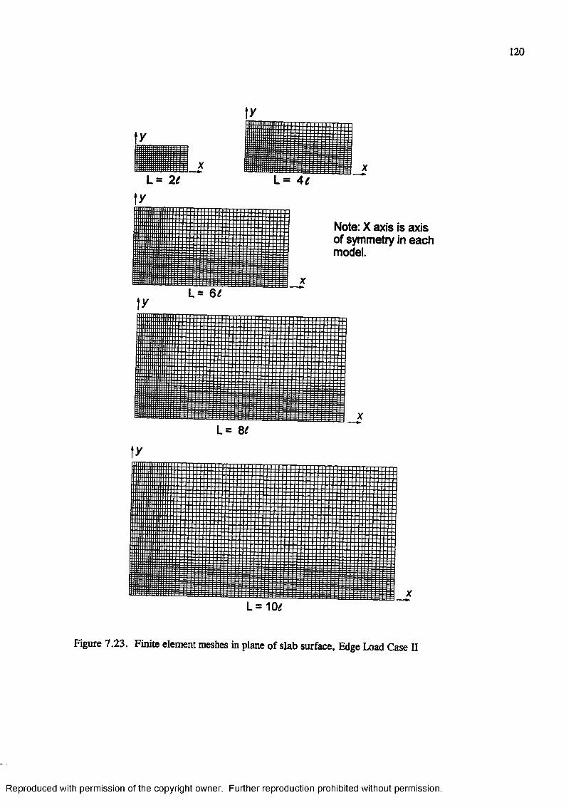
120
\ y
L - 2 e L = 4 f
L= 6f
L= 8f
Note; X axis is axis of symmetry in each model.
L = 1 0 ^
Figure 7.23. Finite element meshes in plane of slab surface. Edge Load Case II
Reproduced with permission of the copyright owner. Further reproduction prohibited without permission.
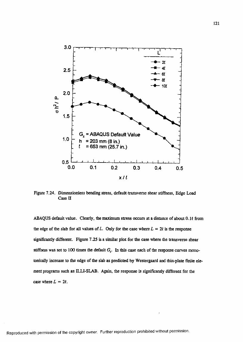
121
3.0
2.5
10£2.0
Q .
= ABAQUS Default Valueh = 203 mm (8 in.)I = 653 mm (25.7 In.)
0.50.0 0.1 0.2 0.3 0.4 0.5
x / l
Figure 7.24. Dimensionless bending stress, default transverse shear stiffness. Edge Load Case II
ABAQUS default value. Clearly, the maximum stress occurs at a distance of about 0.16 from
the edge of the slab for all values of L. Only for the case where L = 26 is the response
significandy different. Figure 7.25 is a similar plot for the case where the transverse shear
stiffness was set to 100 times the default G . In this case each of the response curves mono
tonically increase to the edge of the slab as predicted by Westergaard and thin-plate finite ele
ment programs such as ILLI-SLAB. Again, the response is significantly different for the
case where L = 26.
Reproduced with permission of the copyright owner. Further reproduction prohibited without permission.
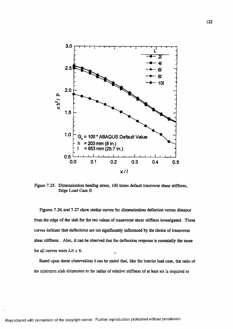
122
3.0
2.5
iœ
2.0CL
b1.5
1.0 . = 100 * ABAQUS Default Value- h = 203 mm (8 In.)- l = 653 mm (25.7 in.)
0.50.0 0.1 0.2 0.3 0.4 0.5
x / t
Figure 7.25. Dimensionless bending stress, 100 times default transverse shear stiffness, Edge Load Case n
Figures 7.26 and 7.27 show similar curves for dimensionless deflection versus distance
from the edge o f the slab for the two values of transverse shear stiffiiess investigated. These
curves indicate that deflections are not significantly influenced by the choice of transverse
shear stiffness. Also, it can be observed that the deflection response is essentially the same
for all curves were L/l 2 6 .
Based upon these observations it can be stated that, like the interior load case, the ratio of
the minimum slab dimension to the radius of relative stiffness of at least six is required to
Reproduced with permission of the copyright owner. Further reproduction prohibited without permission.
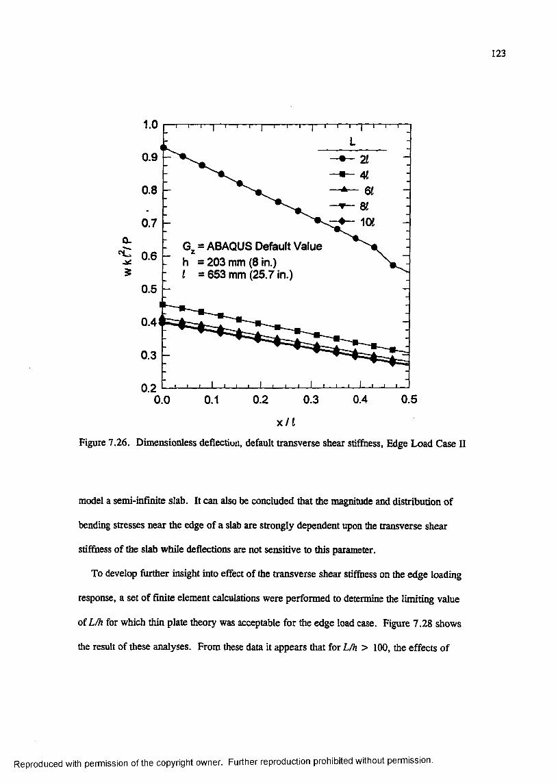
123
1.0
0.9
0.8
1Œ0.7CL
' S 0 6g
0.5
Gg = ABAQUS Default Valueh = 203 mm (8 in.) l = 653 mm (25.7 in.)
0.4
0.3
0.20.50.40.0 0.1 0.2 0.3
% U
Figure 7.26. Dimensionless deflection, default transverse shear stiffness, Edge Load Case II
model a semi-infinite slab. It can also be concluded that the magnitude and distribution of
bending stresses near the edge of a slab are strongly dependent upon the transverse shear
stifGaess of the slab while deflections are not sensitive to this parameter.
To develop further insight into effect of the transverse shear stiffness on the edge loading
response, a set of finite element calculations were performed to determine the limiting value
of L/h for which thin plate theory was acceptable for the edge load case. Figure 7.28 shows
the result of these analyses. From these data it appears that for L/h > 100, the effects of
Reproduced with permission of the copyright owner. Further reproduction prohibited without permission.
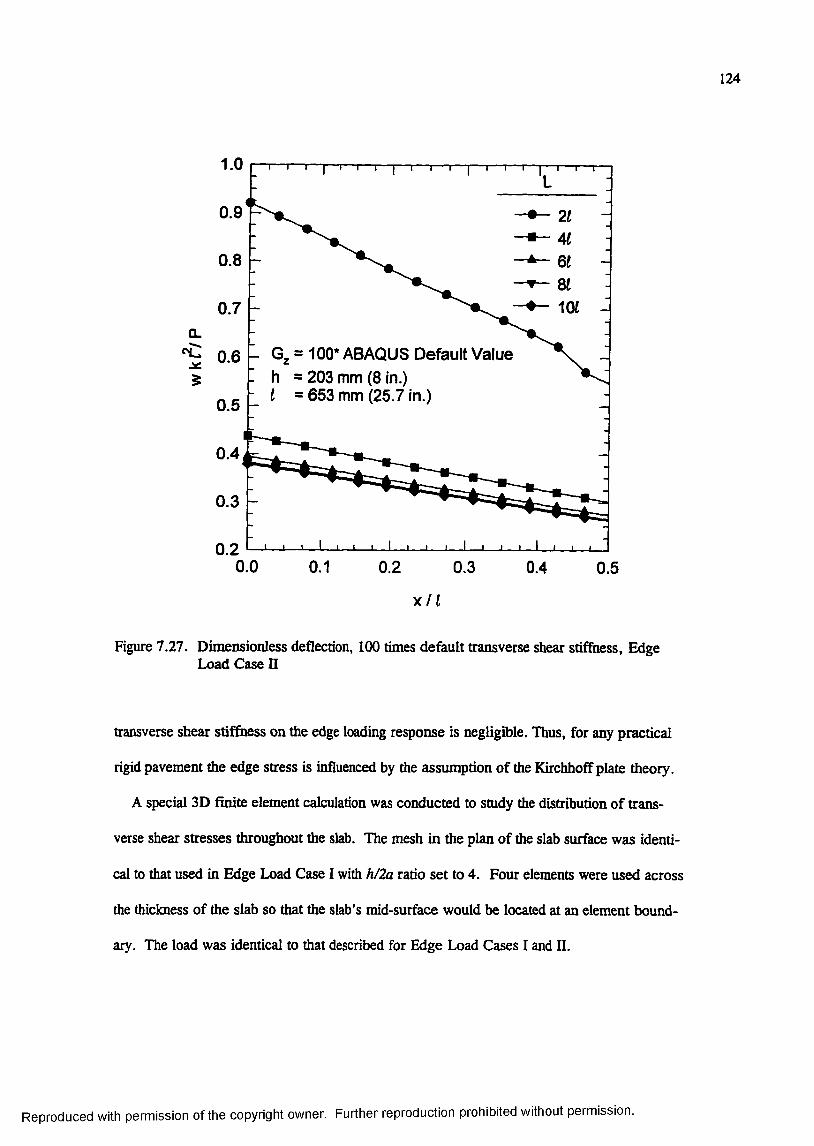
124
1.0
0.9
0.8
1Œ0.7Q.
"g 0.6
0.6
= 100* ABAQUS Default Valueh = 203 mm (8 in.) l = 653 mm (25.7 in.)
0 .4
0.3
0.20.0 0.1 0.2 0.3 0.4 0.5
X / 1
Figure 7.27. Dimensionless deflection, 100 times default transverse shear stiffness. Edge Load Case II
transverse shear stiffiiess on the edge loading response is negligible. Thus, for any practical
rigid pavement the edge stress is influenced by the assumption of the Kirchhoff plate theory.
A special 3D finite element calculation was conducted to study the distribution of trans
verse shear stresses throughout the slab. The mesh in the plan of the slab surface was identi
cal to that used in Edge Load Case I with h/2a ratio set to 4. Four elements were used across
the thickness of the slab so that the slab’s mid-surface would be located at an element bound
ary. The load was identical to that described for Edge Load Cases I and II.
Reproduced with permission of the copyright owner. Further reproduction prohibited without permission.
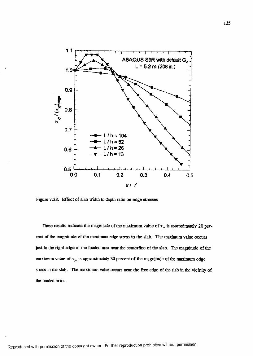
125
ABAQUS S9R with default G; L = 5.2 m (208 In.)
1.0
0.9
iÊ 0.8
5:b
0.7L /h = 104 L /h = 52 L /h = 26 L /h = 13
0.6
0.50.0 0.1 0.2 0.3 0.4 0.5
x / /
Figure 7.28. Effect of slab width to depth ratio on edge stresses
These results indicate the magnitude of the maximum value of is z^proximately 20 per
cent of the magnitude of the maximum edge stress in the slab. The maximum value occurs
just to the right edge of the loaded area near the centerline of the slab. The magnitude of the
maximum value of Xy is approximately 30 percent of the magnitude of the maximum edge
stress in the slab. The maximum value occurs near the free edge of the slab in the vicinity of
the loaded area.
Reproduced with permission of the copyright owner. Further reproduction prohibited without permission.
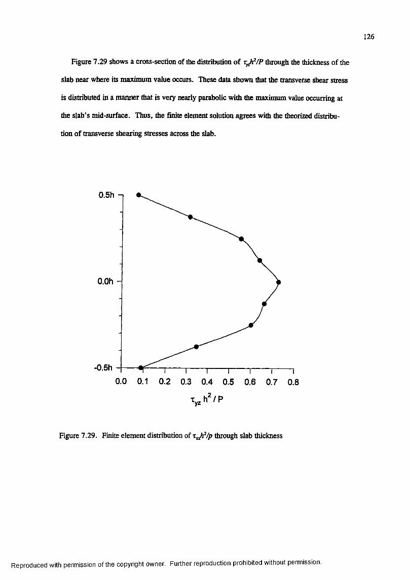
126
Figure 7.29 shows a cross-section of the distribution of through the thickness of the
slab near where its maximum value occurs. These data shown that the transverse shear stress
is distributed in a manner that is very nearly parabolic with the maximum value occurring at
the slab’s mid-surface. Thus, the finite element solution agrees with the theorized distribu
tion of transverse shearing stresses across the slab.
0.5h
O.Oh
-0.5h
0.0 0.1 0.2 0.3 0.4 0.5 0.6 0.7 0.8
Figure 7.29. Finite element distribution of through slab thickness
Reproduced with permission of the copyright owner. Further reproduction prohibited without permission.

127
Experimental data to confirm the above observations are inconclusive. Full-scale acceler
ated test tracks as well as small-scale model tests conducted by the Corps of Engineers have
indicated that the Westergaard analytical model overestimates the stresses and strains experi
enced in the pavement (Rollings and Pittman 1992). Similar trends are indicated by small-
scale model tests conducted by the Corps in the 1950s. Figure 7.30 shows results from
small-scale model tests conducted by the Corps of Engineers (1954). These data indicate that
the Westergaard theory solution is conservative for both edge and interior load cases. In
Figure 7.31 the ratio of the Westergaard theory stresses to the experimental stresses is shown
for a both interior and edge loads over a range of a/?. For these experiments the discrepancy
between theoretical and experimental stresses for the edge load case was less than that for the
interior load case. However, two factors may have led to some errors in this data:
• Stresses were not directly measured. Strains were measured by resistance strain
gages bonded to the slab. For the edge load case the strain gages were located at
some finite distance from the edge, and the strains were extrapolated to the edge.
This is effectively equivalent to assuming that the Kirchhoff theory applies.
• The modulus of subgrade reaction of the rubber foundation used in these tests was
estimated from the volume of the deflection basin produced by an edge loading and
an interior loading. This method, at best, gives a composite estimate of the modulus
of subgrade reaction but may lead to errors in the calculation of theoretical stresses.
JOINTED RIGID PAVEMENT MODELS
To extend the concepts established for single-slab models, 2D and 3D jointed rigid pave
ment models were developed. First, a two-slab jointed rigid pavement model with 2D shell
elements was developed to establish baseline response data for development of 3D jointed
pavement models and to further explore the effect of transverse shear stiffness on stresses at
Reproduced with permission of the copyright owner. Further reproduction prohibited without permission.
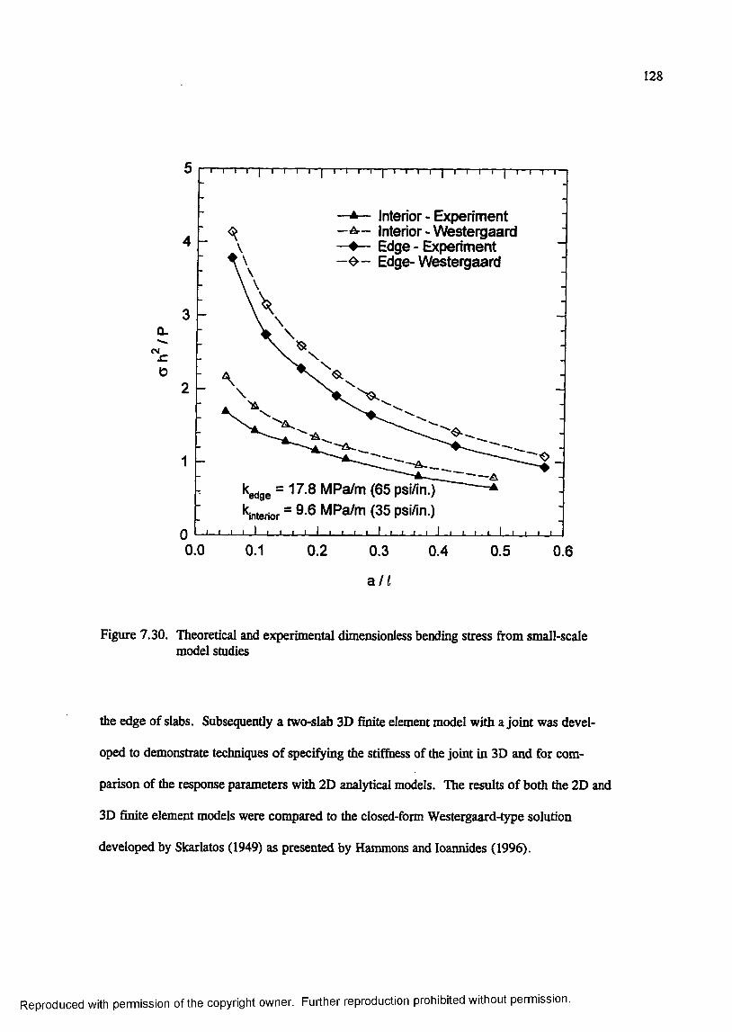
128
CM£
"T I I I I I I I I I I I I I I I I I I I I I I I I I— I— I— r
— Interior - Experiment — interior - W estergaard — Edge - Experiment
Edge-W estergaard
kg^ge = 17.8 MPa/m (65 psi/in.)interior = 9 6 MPa/m (35 psi/in.)
-I—I—I—I—I—I I I I I I I I I I I I I I I I I I I I I I I I0.0 0.1 0.2 0.3 0.4 0.5
a l l
0.6
Figure 7.30. Theoretical and experimental dimensionless bending stress from small-scale model studies
the edge of slabs. Subsequently a two-slab 3D finite element model with a joint was devel
oped to demonstrate techniques of specifying the stiffness of the joint in 3D and for com
parison of the response parameters with 2D analytical models. The results of both the 2D and
3D finite element models were compared to the closed-form Westergaard-type solution
developed by Skarlatos (1949) as presented by Hammons and loannides (1996).
Reproduced with permission of the copyright owner. Further reproduction prohibited without permission.
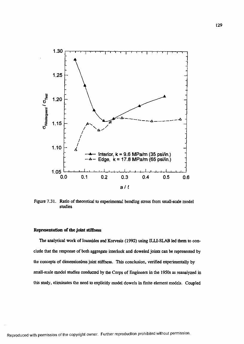
129
1.30
1.25
in 1.200
•s(Q
II 1.15
1.10—A— Interior, k = 9.6 MPa/m (35 psi/in.) - A - Edge, k = 17.8 MPa/m (65 psi/in.)
1.050.0 0.1 0.2 0.3 0.4 0.5 0.6
a / 1
Figure 7.31. Ratio of theoretical to experimental bending stress from small-scale model studies
Representation of the joint stiffness
The analytical work of loannides and Korvesis (1992) using ILLI-SLAB led them to con
clude that the response of both aggregate interlock and doweled joints can be represented by
the concepts of dimensionless joint stiffoess. This conclusion, verified experimentally by
small-scale model studies conducted by the Corps of Engineers in the 1950s as reanalyzed in
this study, eliminates the need to explicitly model dowels in finite element models. Coupled
Reproduced with permission of the copyright owner. Further reproduction prohibited without permission.
130
with the analytical developments of Skarlatos (1949) as presented by loannides and Hammons
(1996) a powerful, yet simple, way of characterizing the dimensionless joint stiffness for
finite element modeling emerges.
Selection of an appropriate ABAQUS finite element spring model for use modeling the
interaction of nodes across a joint was required. The ABAQUS element library contains a
collection of three simple spring models, each having its own unique properties. The
SPRINGA element is an axial spring between two nodes whose line of action is the line join
ing the two nodes. The SPRING2 element allows the user more control over the line of
action o f the spring than the SPRINGA element by acting only a user-specified direction. The
third simple spring element, the SPRING 1 element, is a spring between a node and ground (a
fixed, unmoveable fictitious node) which acts in a user-specified direction.
For each of these element types, the force-displacement relationship may be linear or non
linear. For a linear force-displacement relationship, the user simply inputs the spring
constant. For a nonlinear spring the user must input a table containing ordered pairs of force-
displacement data. ABAQUS then linearly interpolates between the input values to obtain a
complete nonlinear description of the force-displacement relation of the spring.
ABAQUS also includes a more general spring and dashpot element called the JOINTC
element. The JOINTC element, more formally known as flexible joint element, models the
interaction between two nodes which may have internal stiffiiess or damping. The stiffness
and damping properties, which may be linear or nonlinear, are defined by the user in three
orthogonal directions. In a static analysis damping is of no consequence and may be ignored;
therefore, the JOINTC element reduces to a general spring element which may have a user-
defined stiffness value in three orthogonal directions. Nonlinear force-displacement
Reproduced with permission of the copyright owner. Further reproduction prohibited without permission.

131
relationships for the JOINTC element are ii^>ut by the user in a manner identical to that for
the simple spring elements.
The stiffiiess of the joint in most finite element codes for rigid pavement analysis (such as
ILLI-SLAB) consists of springs which have stiffiiess in the vertical direction only. Following
this pattern, the interaction between nodes across a joint in ABAQUS could be modeled using
the SPRING2 element. In the shrillest case the stiffiiess of the JOINTC element could be
specified to be in the vertical direction only reducing its effect to that of the SPRING2 ele
ment. However, the additional capabilities of the truly general 3D JOINTC element render it
an attractive alternative to the more limited SPRING 1 element. For example for future
research studies in which dynamic analysis may be considered, or for environmental analysis
in which temperature and moisture gradients are important, the JOINTC element offers some
attractive capabilities. Based upon these considerations the JOINTC element was selected for
use in this study. However, where the stiffiiess of the JOINTC element is limited to only a
single direction and damping is ignored, the simpler SPRING2 element would give identical
results.
The dimensionless joint stiffness, as defined by Skarlatos (1949), is given by Equa
tion 4.10. For an aggregate interlock load transfer mechanism, the joint stiffness is pre
scribed by the parameter q, which defines the force transmitted per unit length along the joint
per unit differential deflection across the joint. This term is identical to the AGG term
defined in ILLI-SLAB. For the dowel load transfer mechanism, q is defined as
^ D^ = 7 (7.10)
where D is defined by Equation 5.1 and s is the dowel spacing.
Once q has been established, it is necessary to distribute the stiffness to the nodes along
the joint in a rational manner. One method of allocating the stiffness to the nodes is by using
Reproduced with permission of the copyright owner. Further reproduction prohibited without permission.

132
the concept of contributing area, which is commonly used in structural analysis. In this
method the stiffiiess values assigned to each node, k, are determined based upon the length
(in 2D) or area (in 3D) that contributes to the stiffiiess of the node. For equally spaced nodes
in a 2D model, the nodes along a joint may be categorized into one of two types: interior
nodes and edge nodes. Edge nodes are those which occupy the ends of the joint, while all
other nodes are interior nodes. Based upon the concepts of contributing area, the stiffiiess of
the interior nodes must be twice that of the edge nodes. If the length of the joint is given by
X, and the number of nodes along the joint (for a 2D model) is given by N, then
— qX" = - W T ) (7.11)
and
" r : f (7 .medge - ^
For 3D finite element models, the nodes along the face of the solid model at a joint must
be categorized into three types: comer, edge, and interior nodes. Comer nodes are those
nodes which occupy the four comers of the face, while edge nodes are all other nodes on the
edge of the face. Interior nodes make up the remainder of the nodes. If the spacing of the
nodes on the face of the joint is uniform, the unit stiffiiess value is given by
K =4(N„ - l)(Nc - 1)
where
(7.13)
- the number of rows of nodes on the face of the joint
Nc = number of columns of nodes on the face of the joint
The complete development of Equation 7.13 is given in Appendix C. Using the concept of
contributing areas, the following stiffness can be assigned to each type of node:
Reproduced with permission of the copyright owner. Further reproduction prohibited without permission.
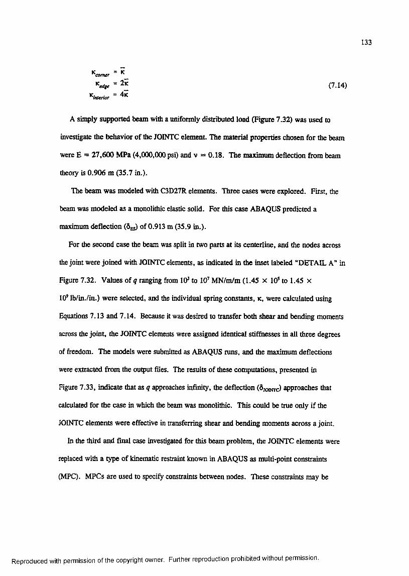
133
edge = 2k (7.14)' in.erior =
A simply supported beam with a uniformly distributed load (Figure 7.32) was used to
investigate the behavior of the JOINTC element. The material properties chosen for the beam
were E = 27,600 MPa (4,000,OCX) psi) and v = 0.18, The maximum deflection from beam
theory is 0.906 m (35.7 in.).
The beam was modeled with C3D27R elements. Three cases were explored. First, the
beam was modeled as a monolithic elastic solid. For this case ABAQUS predicted a
maximum deflection (Ôes) of 0.913 m (35.9 in.).
For the second case the beam was split in two parts at its centerline, and the nodes across
the joint were joined with JOINTC elements, as indicated in the inset labeled “DETAIL A” in
Figure 7.32. Values of q ranging from 10 to 10’ MN/m/m (1.45 x 10® to 1.45 x
10® Ib/in./in.) were selected, and the individual spring constants, k , were calculated using
Equations 7.13 and 7.14. Because it was desired to transfer both shear and bending moments
across the joint, the JOINTC elements were assigned identical stiffrtesses in all three degrees
of freedom. The models were submitted as ABAQUS runs, and the maximum deflections
were extracted from the output files. The results of these computations, presented in
Figure 7.33, indicate that as q approaches infinity, the deflection (ÔjoixTc) approaches that
calculated for the case in which the beam was monolithic. This could be true only if the
JOINTC elements were effective in transferring shear and bending moments across a joint.
In the third and final case investigated for this beam problem, the JOINTC elements were
replaced with a type of kinematic restraint known in ABAQUS as multi-point constraints
(MPC). MFCs are used to specify constraints between nodes. These constraints may be
Reproduced with permission of the copyright owner. Further reproduction prohibited without permission.
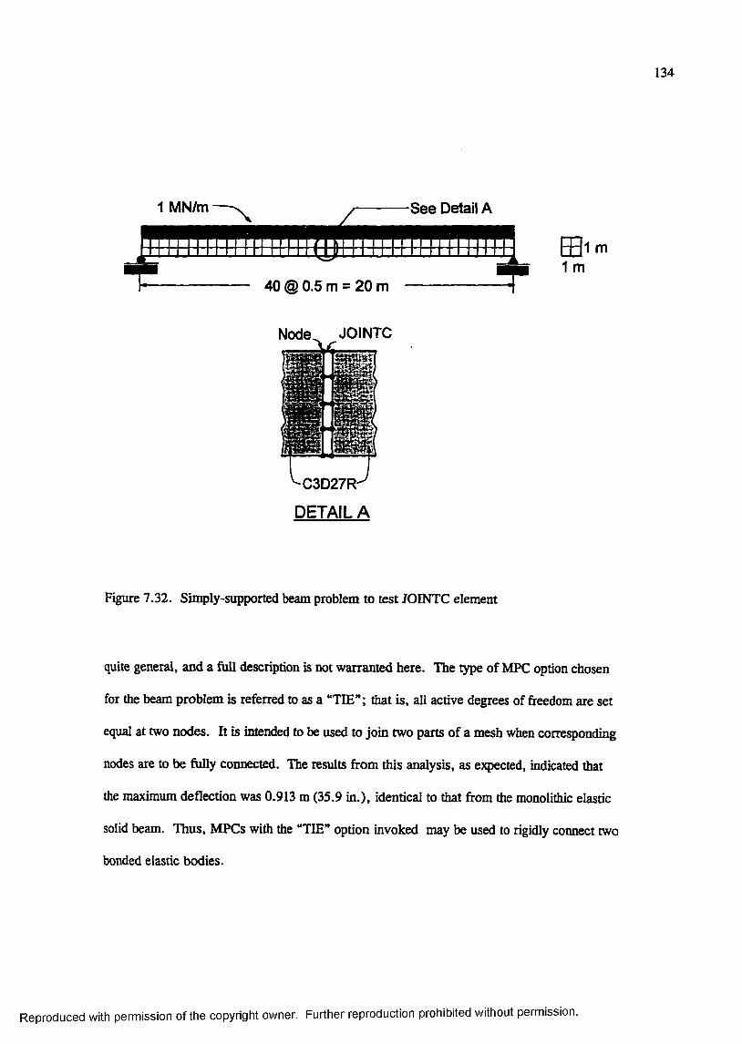
134
1 MN/m S ee Detail A
40 @ 0.5 m = 20 m
Node^ JOINTC
•C3D27R-
DETAIL A
m 1 m
Figure 7.32. Simply-supported beam problem to test JOINTC element
quite general, and a fiiU description is not warranted here. The type of MPC option chosen
for the beam problem is referred to as a “TIE”; that is, all active degrees of freedom are set
equal at two nodes. It is intended to be used to join two parts of a mesh when corresponding
nodes are to be fully connected. The results from this analysis, as expected, indicated that
the maximum deflection was 0.913 m (35.9 in.), identical to that from the monolithic elastic
solid beam. Thus, MFCs with the “TIE” option invoked may be used to rigidly connect two
bonded elastic bodies.
Reproduced with permission of the copyright owner. Further reproduction prohibited without permission.
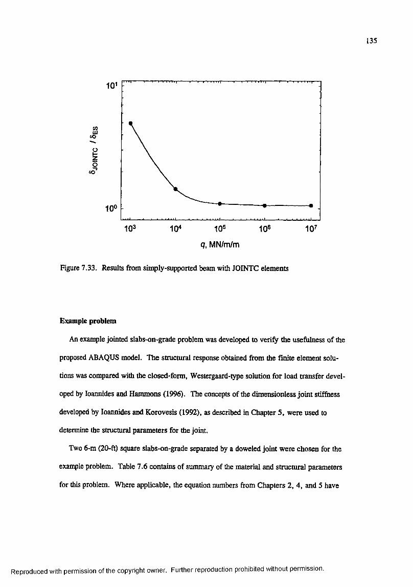
135
Izo
oO*
10°
10®
q, MN/m/m
Figure 7.33. Results from simply-supported beam with JOINTC elements
Example problem
An example jointed slabs-on-grade problem was developed to verify the usefulness of the
proposed ABAQUS model. The structural response obtained from the finite element solu
tions was compared with the closed-form, Westergaard-type solution for load transfer devel
oped by loannides and Hammons (1996). The concepts of the dimensionless joint stiffness
developed by loannides and Korovesis (1992), as described in Chapter 5, were used to
determine the structural parameters for the joint.
Two 6-m (20-ft) square slabs-on-grade separated by a doweled joint were chosen for the
example problem. Table 7.6 contains of summary of the material and structural parameters
for this problem. Where applicable, the equation numbers from Chapters 2, 4, and 5 have
Reproduced with permission of the copyright owner. Further reproduction prohibited without permission.
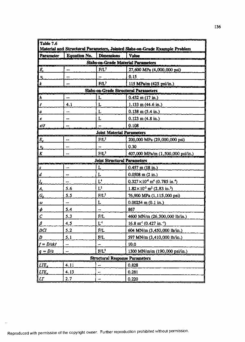
136
Table 7.6Material and Structural Parameters, Jointed Slabs-on-Grade Example ProblemParameter | Equation No. Dimensions | Value
Slabs-on-Grade Material ParametersE, —— vrU- 27,600 MPa (4,000,000 psi) |
Vs —— — 0.15
8< — 115 MPa/m (425 psi/in.)II Slabs-on-Grade Structtural Parameters
h — L 0.432 m (17 in.)I 4.1 L 1.133 m (44.6 in.)a — L 0.138 m (5.4 in.)e — L 0.123 m (4.8 in.)d l — — 0.108
Joint Material Parameters
E, _ — F/L^ 200,000 MPa (29,000,000 psi)
Vi — — 0.30K — F/L^ 407,000 MPa/m (1,500,000 psi/in.)
. bint Structural Parameterss — L 0.457 m (18 in.)d — L 0.0508 m (2 in.)
li — U 0.327xl0-‘ m (0.785 in.")
4 5.6 U 1.82x10"* m* (2.83 in.*)
% 5.5 V!\} 76,900 MPa (1,115,000 psi)0) — L 0.00254 m (0.1 in.)
d>__________________ 5.4 — 867c 5.3 F/L 4600 MN/m (26,300,000 lb/in.)
P 4.5 L ‘ 16.8 m-‘ (0.427 in."')DCI 5.2 F/L 604 MN/m (3,450,000 lb/in.)D 5.1 F/L 597 MN/m (3,410,000 lb/in.)f = D/skf —— — 10.0
q = D/s — F/L* 1300 MN/m/m (190,000 psi/in.)Structural Response Parameters
LIE, 4.11 — 0.828LTE„ 4.13 — 0.281LT 2.7 — 0 .220
Reproduced with permission of the copyright owner. Further reproduction prohibited without permission.

137
been listed in the table. The material parameters assumed in this problem were typical of
those commonly used in analysis. Similarly, the joint structural parameters were selected to
be representative o f those which might be expected in airport pavements. The load consisted
of a uniform pressure of (p = 2.5 MPa (360 psi)) distributed over an area o f 0.06 m^
(93 in.^). The structural response calculated from the Westergaard-^rpe solution is also
tabulated in Table 7.6.
2D shell element model
A 2D shell element model of the example problem was developed to obtain response
parameters for comparison with 3D models and to study the effect of the Kirchoff assump
tions on load transfer at a joint. Figure 7.34 shows a plot of the finite element mesh used for
this problem along with the material and structural properties assumed in the analysis. The
ABAQUS shell element used in this model was the S8R element. The shell elements were
supported on a bed of springs using the ABAQUS “FOUNDATION” option. Because calcu
lations using this element are relatively inexpensive on the Cray computer, a fine mesh was
employed to mitigate any effects ft'om mesh fineness concerns.
Analyses were conducted using several multiples of the default transverse shear stiffness
to investigate the effect this parameter might be having on load transfer. Figure 7.35 shows
plots of dimensionless bending stress versus distance from the joint. The loaded slab was to
the left of the joint. This plot shows that transverse shear stiffiiess has the same effect near a
joint as near a free edge. For values of transverse shear stiffiiess less than approximately
100 times the ABAQUS default value, the maximum transverse bending stress values were
predicted to be at some finite distance from the joint. This phenomenon is evident on both
the loaded and unloaded sides of the joint.
Reproduced with permission of the copyright owner. Further reproduction prohibited without permission.
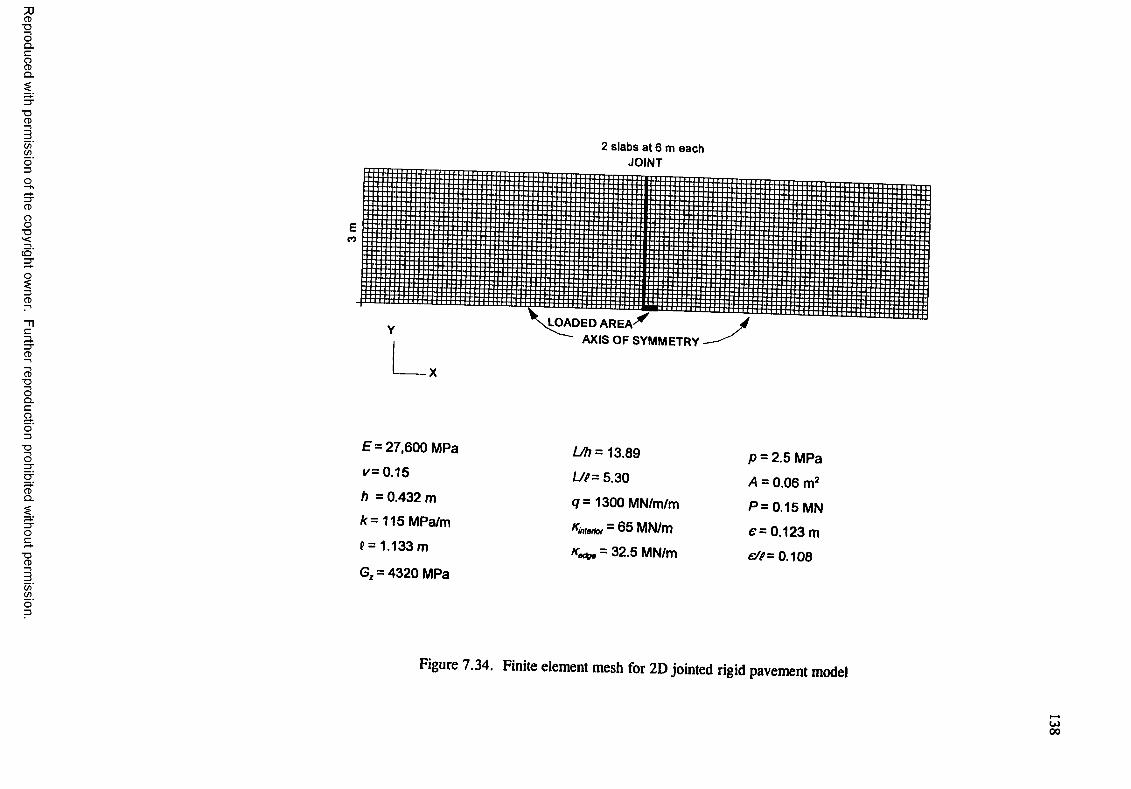
CD■DOQ .C
gQ .
■DCD
C/)Wo"303CD
8■D( O '3"
13CD
3.3"CD
CD■DOQ .C
aO3
■DO
CDQ .
■DCD
(/)(/)
E = 27,600 MPa
y= 0.15
h = 0.432 m
k= 115MPa/m
J = 1.133 m
G, = 4320 MPa
2 s l a b s a t 6 m e a c h
J O I N T
CO
L O A D E D A R E A - ^
A X IS O F S Y M M E T R Y
Uh= 13.89
Uf= 5.30
<7 = 1300 MN/m/m
Metior - 65 MN/m
= 32.5 MN/m
p = 2.5 MPa
4 = 0.06 m:
P=0.15M N
e = 0.123 m
©<?= 0.108
Figure 7.34. Finite element mesh for 2D jointed rigid pavement model
W00
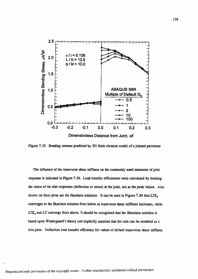
139
D
If"Ocd)CQ
IC
IIÛ
2.5
e/£ = 0.108 L /h = 13.9 q / k £ = 10.0
2.0
1.5
ABAQUS SBR Multiple of Default G
1.0
0.5
0.5
1000.0
-0.3 - 0.2 - 0.1 0.0 0.1 0.2 0.3
Dimensionless Distance from Joint, y ü l
Figure 7.35. Bending stresses predicted by 2D finite element model of a jointed pavement
The influence of the transverse shear stiffness on the commonly used measures of joint
response is indicated in Figure 7.36. Load transfer efficiencies were calculated by forming
the ratios of the slab responses (deflection or stress) at the joint, not at the peak values. Also
shown on these plots are the Skarlatos solutions. It can be seen in Figure 7.36 that LTEg
converges to the Skarlatos solution from below as transverse shear stiffness increases, while
LTEg and LT converge from above. It should be recognized that the Skarlatos solution is
based upon Westergaard’s theory and implicitly assumes that the slab can be modeled as a
thin plate. Deflection load transfer efficiency for values of default transverse shear stiffiiess
Reproduced with permission of the copyright owner. Further reproduction prohibited without permission.
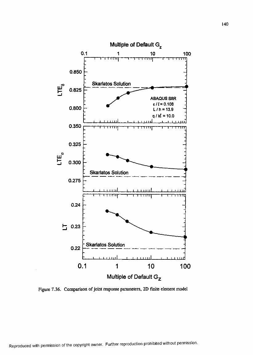
140
Multiple of Default G0.1
0.850
0.825
0.800
0.350
0.325
0.300
0.275
1 10 100TTTTTT]------- 1— I I i i i nj----- 1— r r r m n
Skarlatos Solution
J L J U LLI
ABAQUS S8 R e/« = 0.108 L /h = 13.9 -q/k( = 10.0
i L .I .I 1-1 llJ 1__ 1—1 1,1 LU1 I I I I I I I I I 1 TTT T T M 1 I ' l l
Skarlatos Solution
— 1— i - j - i . i . i i i i ________I I I 1 1 1 1 1 1 I I I 1 1 1 1 1 '
TTTTJ
0.24
h 0.23
r Skarlatos Solution0.22
0.1 1 10 100Multiple of Default
Figure 7.36. Comparison of joint response parameters, 2D finite element model
Reproduced with permission of the copyright owner. Further reproduction prohibited without permission.
141
greater than approximately 10 times the ABAQUS default values agrees well with the Skar
latos solution. However, load transfer and stress load transfer efficiencies predicted by the
finite element model are consistently greater than those predicted by Skarlatos.
3D mode!
A 3D finite element model using ABAQUS C3D27R elements was created and executed.
The mode! was identical in plan view to the 2D shell element model shown in Figure 7.34.
Four elements were used through the depth of the model. The lowest layer of elements were
supported on a bed of springs using the ABAQUS “FOUNDATION” option. All material
and structural parameters were the same as those used for the 2D shell element model (as
described in Figure 7.34). However, one exception should be noted. In 3D the individual
spring constants were assigned according to Equations 7.13 and 7.14 as follows
corner = 2 031 MN/m (11,600 lb/in.)edge = 4.063 MN/m (23,200 lb/in.) (7 15)
^imerior = 8125 MN/m (46,400 lb/in.)
Figure 7.37 shows the a plot of the dimensionless bending stress from the 3D model along
with selected data from the 2D shell element model. On the loaded side of the joint, the 3D
model predicted lower stress than the 2D models. As was the case for a free edge, the 3D
model predicts that the maximum stress does not occur at the joint but some small distance
away from the joint. The higher bending stresses predicted by the 2D model were believed to
be an artifact of the 2D shell element formulation, and the 3D bending stresses are likely
more accurate.
The 3D finite element model was repeatedly executed, varying the value of q to get a
range of responses. These data were then plotted against results from the relationships devel
oped by loannides and Hammons (1996) from the Skarlatos model. The results of these
Reproduced with permission of the copyright owner. Further reproduction prohibited without permission.
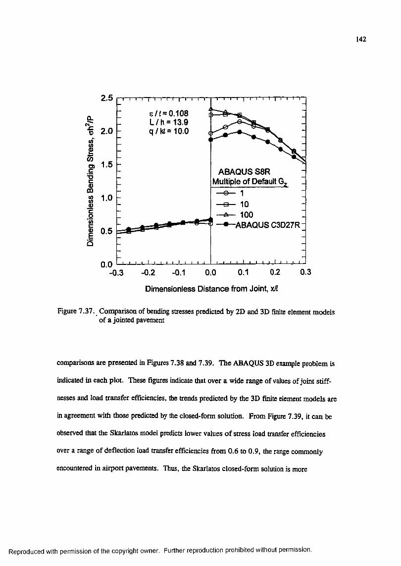
142
9:
Ig1fflCO
c.2gEQ
2.5
2.0
1.5ABAQUS S8R
Multiple of Default G.
1.0
ABAQUS C3D27R-0.5
0.0-0.3 0.30.20.1- 0.2 - 0.1 0.0
Dimensionless D istance from Joint, x/(
Figure 7.37. Comparison of bending stresses predicted by 2D and 3D finite element models of a jointed pavement
conçarisons are presented in Figures 7.38 and 7.39. The ABAQUS 3D example problem is
indicated in each plot. These figures indicate that over a wide range of values of Joint stiff
nesses and load transfer efficiencies, the trends predicted by the 3D finite element models are
in agreement with those predicted by the closed-form solution. From Figure 7.39, it can be
observed that the Skarlatos model predicts lower values o f stress load transfer efficiencies
over a range of deflection load transfer efficiencies from 0 .6 to 0 .9 , the range commonly
encountered in airport pavements. Thus, the Skarlatos closed-form solution is more
Reproduced with permission of the copyright owner. Further reproduction prohibited without permission.
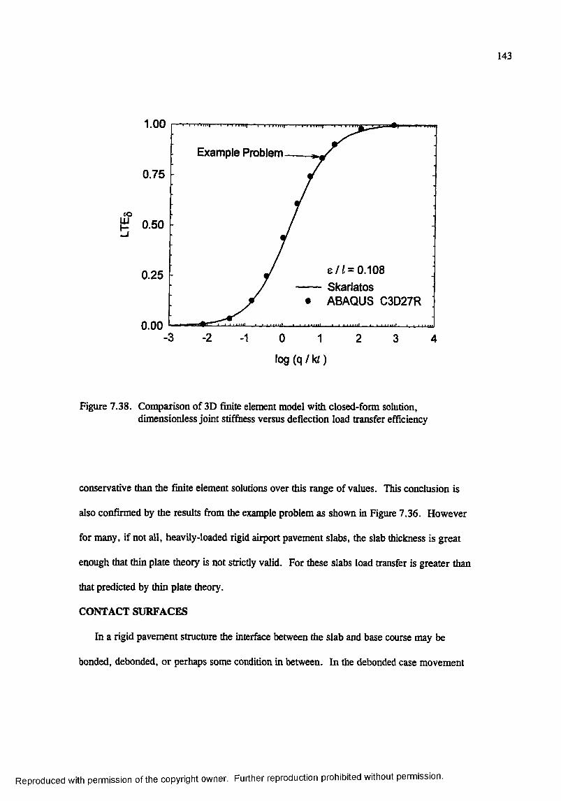
143
1.00
Example Problem
0.75
(O^ 0.50
e /^ = 0.108— Skarlatos # ABAQUS C3D27R
0.25
0.003 2 1 0 1 2 3 4
log (q / ta )
Figure 7.38. Comparison of 3D finite element model with closed-form solution, dimensionless joint stiffness versus deflection load transfer efficiency
conservative than the finite element solutions over this range of values. This conclusion is
also confirmed by the results from the example problem as shown in Figure 7.36. However
for many, if not all, heavily-loaded rigid airport pavement slabs, the slab thickness is great
enough that thin plate theory is not strictly valid. For these slabs load transfer is greater than
that predicted by thin plate theory.
CONTACT SURFACES
In a rigid pavement structure the interface between the slab and base course may be
bonded, debonded, or perhaps some condition in between. In the debonded case movement
Reproduced with permission of the copyright owner. Further reproduction prohibited without permission.
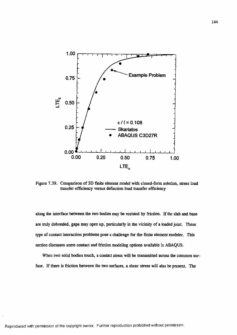
144
1.00
Example Problem0.75
CO
111
5
8 / f = 0.108 SkarlatosABAQUS C3D27R
0.25
0.25 0.50 0.75 1.00
LTE.
Figure 7.39. Comparison of 3D finite element model with closed-form solution, stress load transfer efficiency versus deflection load transfer efficiency
along the interface between the two bodies may be resisted by friction. If the slab and base
are truly debonded, gaps may open up, particularly in the vicinity of a loaded joint. These
type of contact interaction problems pose a challenge for the finite element modeler. This
section discusses some contact and friction modeling options available in ABAQUS.
When two solid bodies touch, a contact stress will be transmitted across the common sur
face. If there is friction between the two surfaces, a shear stress will also be present. The
Reproduced with permission of the copyright owner. Further reproduction prohibited without permission.

145
contact areas must be determined, and then the normal and shearing stresses transmitted
through the contact area must be calculated. This gives rise to a nonlinear problem which
requires an iterative solution procedure.
Two methods of modeling the mechanical interaction between element faces in ABAQUS
are germane to the rigid pavement problem. The first of these methods involves the use of
interface elements, referred to in ABAQUS as “INTER” elements, for contact and friction
analysis. These elements are formulated to calculate the contact direction, contact area; and
the normal and shear stresses transmitted across the contact surface. For 3D problems three
INTER elements are available in the ABAQUS element library: the INTER4 element,
intended for used with 8 -node hexahedral elements and 4-node shell elements; the INTERS
element, intended for used with 20-node hexahedral elements and 8-node shell elements; and
the INTER9 element, intended for used with 21- to 27 node hexahedral elements and 9-node
shell elements. Use of the INTERS element is discouraged, because uniform pressure on the
8-node surface produces negative contact forces at the comer nodes. The use of INTER ele
ments is tedious, since they require the creation of zero-thickness elements along the contact
interface.
The second method of modeling the contact and friction between two bodies is the
ABAQUS contact interaction option. This option, recently added to ABAQUS, is more con
venient than the INTER element, because creation of additional elements is not required.
The two surfaces which may be in contact are defined by the user along with a choice of sev
eral firiction models. Because of negative contact forces which arise at the comers of ele
ments with 8 nodes on a face, the use of contact interaction for 20 -nodes hexahedral elements
is not recommended. For purposes of this research a simple Coulomb fnction model was
adopted.
Reproduced with permission of the copyright owner. Further reproduction prohibited without permission.
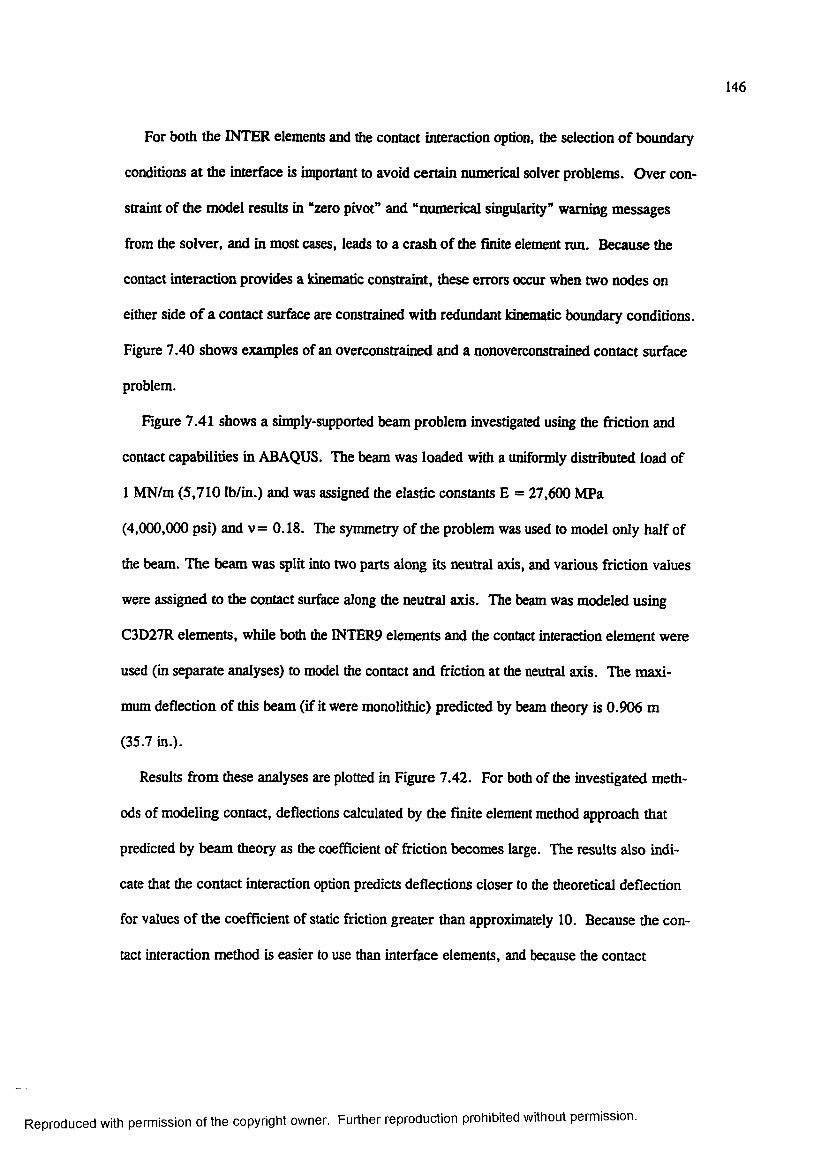
146
For both the INTER elements and the contact interaction option, the selection of boundary
conditions at the interface is important to avoid certain numerical solver problems. Over con
straint of the model results in “zero pivot” and “numerical singularity” warning messages
hrom the solver, and in most cases, leads to a crash of the finite element run. Because the
contact interaction provides a kinematic constraint, these errors occur when two nodes on
either side o f a contact surface are constrained with redundant kinematic boundary conditions.
Figure 7.40 shows examples of an overconstrained and a nonoverconstrained contact surface
problem.
Figure 7.41 shows a sinçly-supported beam problem investigated using the fnction and
contact capabilities in ABAQUS. The beam was loaded with a uniformly distributed load of
1 MN/m (5,710 lb/in.) and was assigned the elastic constants E = 27,600 MPa
(4,000,000 psi) and v= 0.18. The symmetry of the problem was used to model only half of
the beam. The beam was split into two parts along its neutral axis, and various friction values
were assigned to the contact surface along the neutral axis. The beam was modeled using
C3D27R elements, while both the INTER9 elements and the contact interaction element were
used (in separate analyses) to model the contact and fnction at the neutral axis. The maxi
mum deflection of this beam (if it were monolithic) predicted by beam theory is 0.906 m
(35.7 in.).
Results from these analyses are plotted in Figure 7.42. For both of the investigated meth
ods of modeling contact, deflections calculated by the finite element method approach that
predicted by beam theory as the coefficient of friction becomes large. The results also indi
cate that the contact interaction option predicts deflections closer to the theoretical deflection
for values of the coefficient of static fnction greater than approximately 10. Because the con
tact interaction method is easier to use than interface elements, and because the contact
Reproduced with permission of the copyright owner. Further reproduction prohibited without permission.
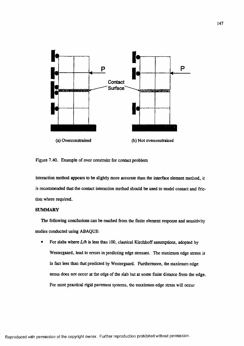
147
hContactSurface'
II
(a) Overconstrained (b) Not overconstrained
Figure 7.40. Exan^>le of over constraint for contact problem
interaction method appears to be slightly more accurate than the interface element method, it
is recommended that the contact interaction method should be used to model contact and fric
tion where required.
SUMMARY
The following conclusions can be reached from the finite element response and sensitivity
smdies conducted using ABAQUS;
• For slabs where L/h is less than 100, classical Kirchhoff assumptions, adopted by
Westergaard, lead to errors in predicting edge stresses. The maximum edge stress is
in fact less than that predicted by Westergaard. Furthermore, the maximum edge
stress does not occur at the edge of the slab but at some finite distance from the edge.
For most practical rigid pavement systems, the maximum edge stress will occur
Reproduced with permission of the copyright owner. Further reproduction prohibited without permission.
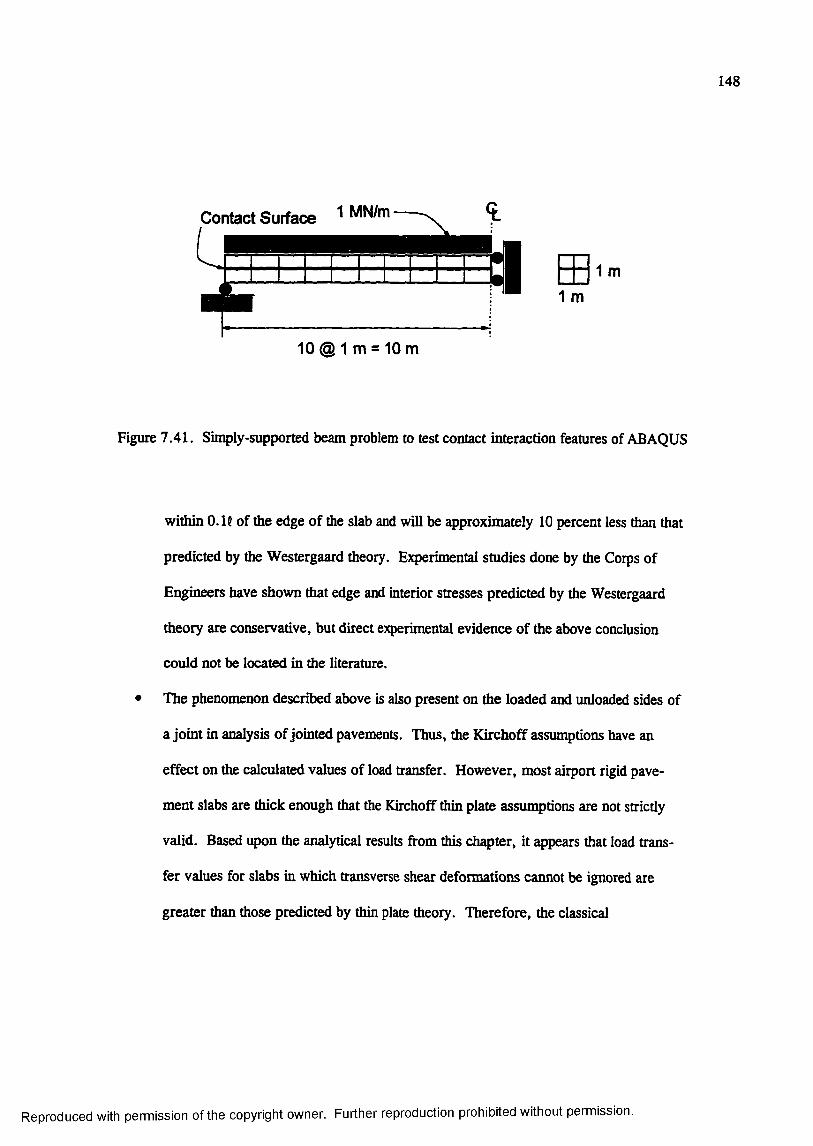
148
Contact Surface MN/m
L
fI
10 @ 1 m = 10 m
Figure 7.41. Simply-supported beam problem to test contact interaction features of ABAQUS
within 0.18 of the edge of the slab and will be approximately 10 percent less than that
predicted by the Westergaard theory. Experimental studies done by the Corps of
Engineers have shown that edge and interior stresses predicted by the Westergaard
theory are conservative, but direct experimental evidence of the above conclusion
could not be located in the literature.
• The phenomenon described above is also present on the loaded and unloaded sides of
a joint in analysis of jointed pavements. Thus, the Kirchoff assumptions have an
effect on the calculated values of load transfer. However, most airport rigid pave
ment slabs are thick enough that the Kirchoff thin plate assumptions are not strictly
valid. Based upon the analytical results from this chapter, it appears that load trans
fer values for slabs in which transverse shear deformations cannot be ignored are
greater than those predicted by thin plate theory. Therefore, the classical
Reproduced with permission of the copyright owner. Further reproduction prohibited without permission.
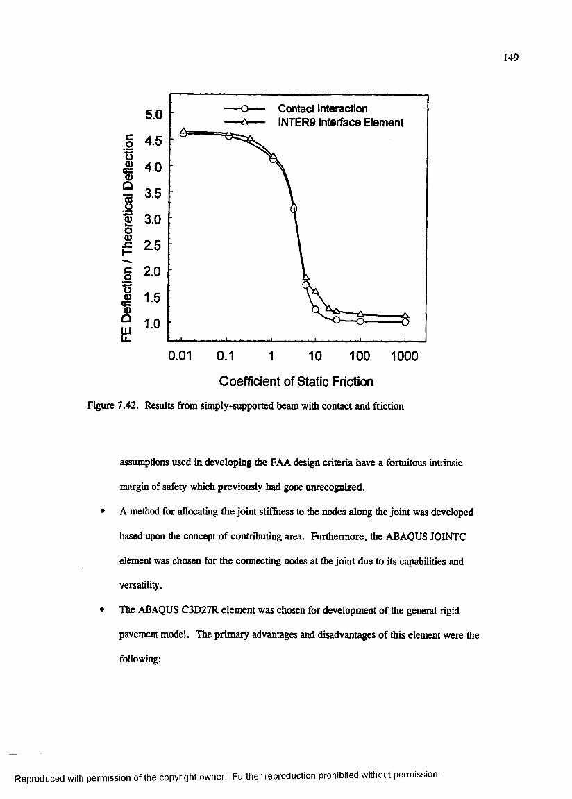
149
C0
1
s
o0)
0
1
1LULU
Contact Interaction INTER9 Interface Element
5.0
4.5
4.0
3.5
3.0
2.5
2.0
1.5
1.0
0.01 0.1 10 100 10001
Coefficient of Static Friction
Figure 7.42. Results from simply-supported beam with contact and friction
assumptions used in developing the FAA design criteria have a fortuitous intrinsic
margin of safety which previously had gone unrecognized.
• A method for allocating the joint stiffriess to the nodes along the joint was developed
based upon the concept of contributing area. Furthermore, the ABAQUS JOINTC
element was chosen for the connecting nodes at the joint due to its capabilities and
versatility.
• The ABAQUS C3D27R element was chosen for development of the general rigid
pavement model. The primary advantages and disadvantages of this element were the
following:
Reproduced with permission of the copyright owner. Further reproduction prohibited without permission.

150
(1) Accuracy. This Lagrangian quadratic element with reduced integration is not
subject to locking when the primary response mode is bending. Furthermore,
spurious, zero-energy displacement modes (hourglassing) cannot propagate
through the mesh; thus, hourglassing is not problematic.
(2) Compatibility with contact interaction model. The C3D27R element is conçati-
ble with both the INTER9 interface element and the contact surface method of
modeling contact interaction. Use of the C3D20R element leads to numerical
instability due to negative contact forces at the comer nodes.
(3) Computational efficiency. The primary disadvantage of the C3D27R element
lies in the fact that more computer time is required than for the corresponding
serendipity quadratic element (ABAQUS C3D20R).
• The multi-point kinematic constraint capability in ABAQUS (known as the MPC with
the “TIE” option envoked) can be used to rigidly coimect two bonded elastic bodies.
• Example 3D finite element calculations conducted for jointed slabs-on-grade indicated
that the finite element solution compares favorable with the closed-form
Westergaard-type solution of Skarlatos. Therefore, it is reasonable to extend the
techniques developed in this chapter to the more challenging problem of slabs resting
on stabilized bases.
• The ABAQUS contact interaction method is recommended in lieu of interface ele
ments for further use where contact and friction modeling is required.
Reproduced with permission of the copyright owner. Further reproduction prohibited without permission.
CHAPTER 8 ; EXPERIMENTS ON LABORATORY-SCALE PAVEMENT MODELS
INTRODUCTION
Laboratory-scale experiments were conducted on jointed rigid pavement models to supple
ment the data from the small-scale model studies conducted in the 19S0's (described in
Chapter 3). Specifically, the objectives of these experiments were to:
• Observe the qualitative response of the rigid pavement slab-joint-base system at the
phenomenological level.
• Obtain quantitative data to verify certain aspects of the analytical models developed in
this study.
This chapter includes a description of the experimental test plan and materials used to
construct the models as well as the results of the experiments are presented and discussed.
EXPERIMENTAL PLAN
Experiments were conducted on five laboratory-scale jointed rigid pavement models. A
matrix describing the parameters of each experiment is given in Table 8 .1. Each rigid pave
ment model consisted of two portland cement concrete slabs, 915 mm (36 in.) by 1,220 mm
(48 in.) by 51-mm (2-in.) thick, separated by a joint. In each experiment the subgrade was
modeled by a 1,800 mm (72 in.) by 1,200 mm (48 in.) by 300 mm (12 in.) thick rubber
block. This block, purchased by the Waterways Experiment Station about 1968 from the
Goodyear Tire and Rubber Company, was composed of styrene butadiene (automobile tire)
rubber.
The response of the joint was expected to depend upon the presence of discontinuities in
the base and the degree of bonding between the base course and the slabs. The slabs were
151
Reproduced with permission of the copyright owner. Further reproduction prohibited without permission.
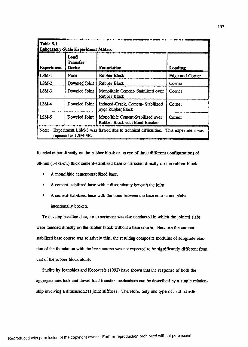
152
liab le 8.1 Laboratory-Scale Ehrperiment Matrix
Experiment
LoadTransferDevice Foundation Loading
LSM-1 None Rubber Block Edge and Comer
LSM-2 Doweled Joint Rubber Block Comer
LSM-3 Doweled Joint Monolithic Cement- Stabilized over Rubber Block
Comer
LSM-4 Doweled Joint Induced-Crack, Cement- Stabilized over Rubber Block
Comer
LSM-5 Doweled Joint Monolithic Cement-Stabilized over Rubber Block with Bond Breaker
Comer
Note: Experiment LSM-3 was flawed due to technical difficulties. This experiment was repeated as LSM-3R.
founded either directly on the rubber block or on one of three different configurations of
38-mm (1-1/2-in.) thick cement-stabilized base constructed directly on the rubber block:
• A monolithic cement-stabilized base.
• A cement-stabilized base with a discontinuity beneath the joint.
• A cement-stabilized base with the bond between the base course and slabs
intentionally broken.
To develop baseline data, an experiment was also conducted in which the jointed slabs
were founded directly on the rubber block without a base course. Because the cement-
stabilized base course was relatively thin, the resulting composite modulus of subgrade reac
tion of the foundation with the base course was not expected to be significantly different from
that of the rubber block alone.
Studies by loannides and Korovesis (1992) have shown that the response of both the
aggregate interlock and dowel load transfer mechanisms can be described by a single relation
ship involving a dimensionless joint stiffness. Therefore, only one type of load transfer
Reproduced with permission of the copyright owner. Further reproduction prohibited without permission.
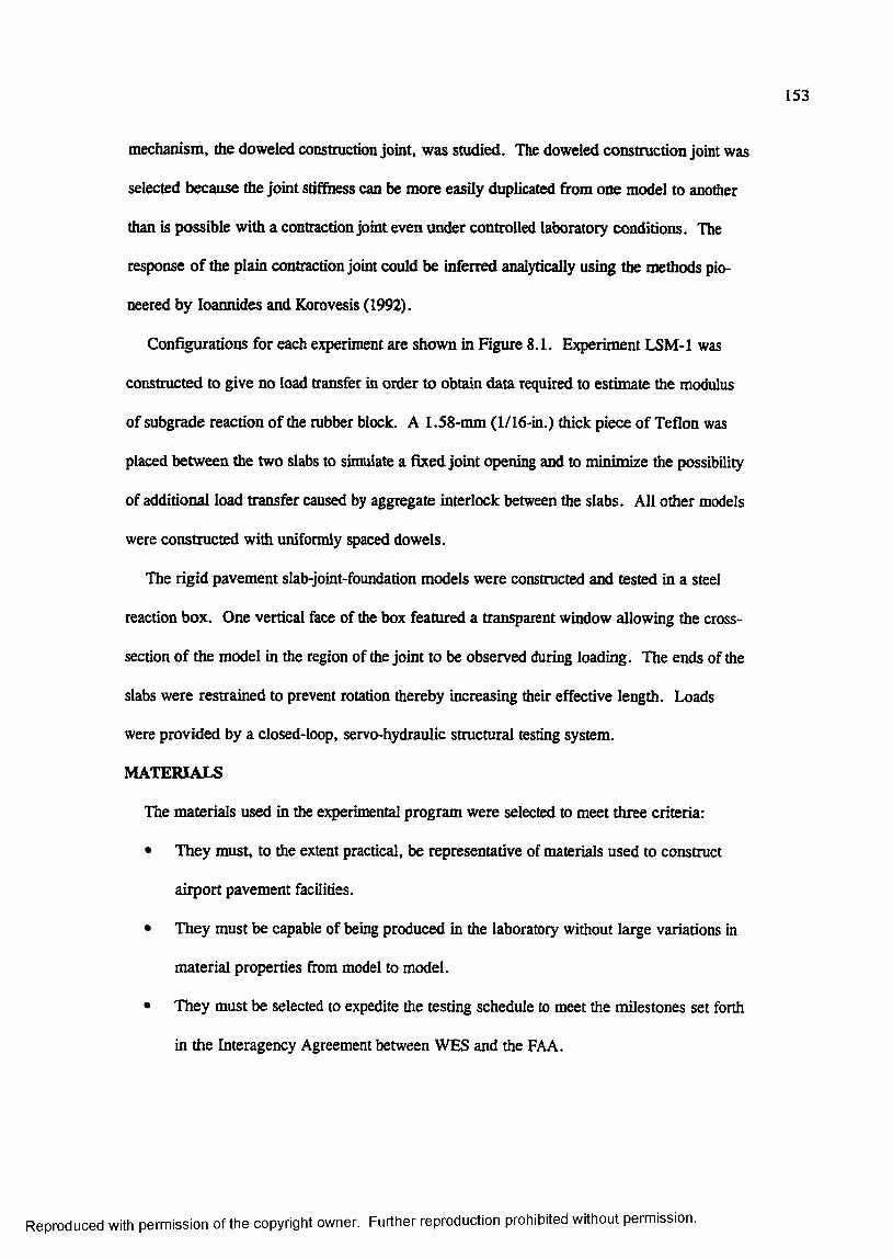
153
mechanism, the doweled construction joint, was studied. The doweled construction joint was
selected because the joint stiffness can be more easily duplicated from one model to another
than is possible with a contraction joint even under controlled laboratory conditions. The
response of the plain contraction joint could be inferred analytically using the methods pio
neered by loannides and Korovesis (1992).
Configurations for each experiment are shown in Figure 8.1. Experiment LSM-1 was
constructed to give no load transfer in order to obtain data required to estimate the modulus
of subgrade reaction of the rubber block. A 1.58-mm (1/16-in.) thick piece of Teflon was
placed between the two slabs to simulate a fixed joint opening and to minimize the possibility
of additional load transfer caused by aggregate interlock between the slabs. All other models
were constructed with uniformly spaced dowels.
The rigid pavement slab-joint-foundation models were constructed and tested in a steel
reaction box. One vertical face of the box featured a transparent window allowing the cross-
section of the model in the region of the joint to be observed during loading. The ends of the
slabs were restrained to prevent rotation thereby increasing their effective length. Loads
were provided by a closed-loop, servo-hydraulic structural testing system.
MATERIALS
The materials used in the experimental program were selected to meet three criteria:
• They must, to the extent practical, be representative of materials used to construct
airport pavement facilities.
• They must be capable of being produced in the laboratory without large variations in
material properties from model to model.
• They must be selected to expedite the testing schedule to meet the milestones set forth
in the Interagency Agreement between WES and the FAA.
Reproduced with permission of the copyright owner. Further reproduction prohibited without permission.
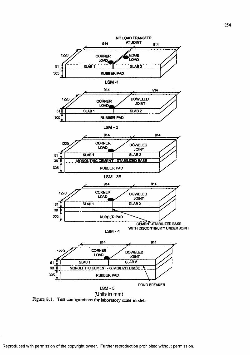
154
N O L O A D T R A N S F E R
A T J O I N T9 1 4 9 1 4
1220 E D G EL O A D
C O R N E RLOAD^
S L A B 1 S L A B 2
3 0 5 R U B B E R P A D
LSM -1
LSM -2
9 1 4 9 1 4
C O R N E RLO A D
51
3 8 '
3 0 5
D O W E L E D
J O I N T
S L A B 1 S L A B 2
M O N O L IT H IC C E M E N T - S T A B IU Z E D B A S E
R U B B E R P A D
LSM - 3R
9 1 4 9 1 4
D O W E L E D
J O I N T1220
C O R N E RL O A D #
S L A B 2S L A B 1
3 0 5 R U B B E R P A D
9 1 49 1 4
C O R N E RL O A D _
D O W E L E DJ O I N T
S L A B 2S L A B 1
3 0 5 R U B B E R P A D
C E M E N T -S T A B IU Z E D B A S E
LSM -4W IT H D IS C O N T IN U IT Y U N D E R J O I N T
/
51
3 8 '
3 0 5
9 1 4
C O R N E RL O A D
D O W E L E D J O I N T
SIA BI S L A B 2
M O N O L IT H IC C E M E N T - S T A B I U Z E D B A S E
R U B B E R P A D
9 1 4
LSM-5 (Units in mm)
Figure 8.1. Test configurations for laboratory scale models
B O N D B R E A K E R
Reproduced with permission of the copyright owner. Further reproduction prohibited without permission.

155
A discussion o f the selection of the concrete materials for the slabs, cement-stabilized
material for the base, and steel for the dowels follows.
Concrete materials
All slabs were portland cement concrete with 9.5-mm (3/8-in.) nominal maximum size
aggregate. The mixture was proportioned to obtain a conçressive strength o f approximately
27.6 MPa (4,000 psi) and an elastic modulus of approximately 27,600 MPa (4,000,000 psi)
at seven days with accelerated curing. To achieve these properties, a blend o f ASTM C 150,
Type I and Type HI, cements, in equal proportions, was used along with an ASTM C 494,
Type C, accelerating admixture. The fine and coarse aggregates chosen for this study were
from natural (uncrushed) river deposits, consisting primarily of rounded, dense chert and
silica particles.
The concrete mixture used for the slabs was selected from four trial concrete mixtures
prepared in the laboratory. Water-cement ratios (by mass) varied from 0.60 to 0.70. A set
of six 152 mm (6 in.) by 305 mm (12 in.) cylindrical concrete specimens was prepared from
each mixture. To expedite the testing schedule for the pavement models, accelerated curing
was investigated. Two curing regimens were evaluated:
• Continuous moist-curing at room temperature.
• Accelerated curing defined as two days moist-curing at room temperature, followed
by two days curing in an environmental chamber at 60"C (140°F), followed by
moist-curing at room temperature until time of testing.
The final concrete mixture proportions selected for the model along with a listing of the
sources of the materials are shown in Table 8.2. This mixture had a water-cement ratio of
0.64 by mass. Results of tests to determine compressive strength (per ASTM C 39) and
modulus of elasticity (per ASTM C 469) are presented in Table 8.3. Accelerated curing
Reproduced with permission of the copyright owner. Further reproduction prohibited without permission.
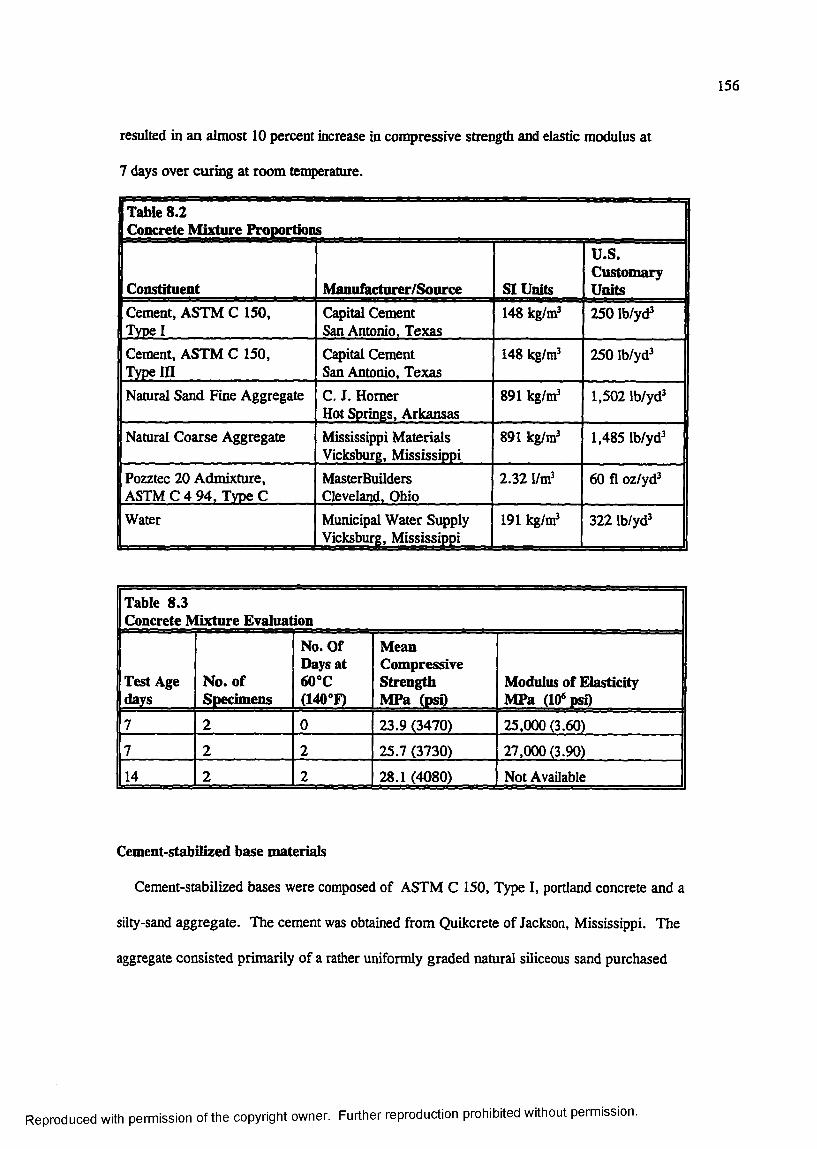
156
resulted in an almost 10 percent increase in compressive strength and elastic modulus at
7 days over curing at room temperature.
Table 8.2Concrete Mixture Proportions
Constituent Manufacturer/Source SI Units
U.S.CustomaryUnits
Cement, ASTM C 150, Type I _
Ct^ital Cement San Antonio, Texas
148 kglxD? 250 Ib/yd^
Cement, ASTM C 150, Type in
Capital Cement San Antonio, Texas
148 kg/ra^ 250 Ib/yd^
Natural Sand Fine Aggregate C. J. HomerHot Springs, Arkansas
891 kg/m^ 1,502 Ib/yd^
Natural Coarse Aggregate Mississippi Materials Vicksburg, Mississippi
891 kg/m^ 1,485 Ib/yd^
Pozztec 20 Admixture, ASTM C 4 94. Tvpe C
MasterBuilders Cleveland, Ohio
2 .321/m 60 fl oz/yà?
Water Municipal Water Supply Vicksburg, Mississippi
191 kg/m^ 322 Ib/yd^
1 Table 8.3 1 Concrete Mlixtnre Evaluation
Test Age days
No. of Specimens
No. Of Days at 60“C (140'F)
MeanCompressive Strength MPa (psQ
Modulus of Elasticity MPa (10*psO
7 2 0 23.9 (3470) 25,000 (3.60)
7 2 2 25.7 (3730) 27,000 (3.90)
14 2 2 28.1 (4080) Not Available
Cement-stabilized base materials
Cement-stabilized bases were composed of ASTM C 150, Type I, portland concrete and a
silty-sand aggregate. The cement was obtained from Quikcrete of Jackson, Mississippi. The
aggregate consisted primarily of a rather uniformly graded natural siliceous sand purchased
Reproduced with permission of the copyright owner. Further reproduction prohibited without permission.

157
from Mississippi Materials, Vicksburg, Mississippi. Additional fines in the form of silica
flour, passing a 75 (No. 200) sieve, manufactured by Haliburton Services of Duncan,
Oklahoma, were blended with the sand in the ratio of 10 percent silica flour to 90 percent
sand. A particle size analysis was conducted on the blend using the methods prescribed in
AASHTO T 8 8 . The gradation is shown in Figure 8.2.
General guidance for the cement-stabilized base was provided by FAA Advisory Circular
150/5370-10A, Item P-304 (FAA 1989). Based upon the recommendations in ACI
230.1R-90, “State-of-the-Art Report on Soil Cement” (American Concrete Institute 1994),
cement contents of 7.5 and 10 percent (by mass) were selected for evaluation. The protocol
in ASTM D 558 was used to determine moisture-density relationships for the silty-sand/
cement blend. Moisture-density curves for both cement contents are shown in Figure 8.3.
Maximum dry density for both mixtures occurred at a water content of approximately eight
percent. The mixture containing 10 percent cement bad a dry density approximately two
percent greater than the mixture containing 7.5 percent cement. Three curing treatments of
these mixtures were evaluated;
• Curing at room temperature for seven days.
• Curing at room temperature for 14 days.
• Curing at room temperature for three days followed by curing at 60®C (140°F) oven
for two days, followed by curing at room temperature until a total of seven days had
elapsed.
Compressive strength tests (three replicates per treatment) were conducted on 51-mm
(2-in.) by 102-mm (4-in.) cylinders for the two cement contents. Specimens were prepared at
a water content of eight percent and compacted to maximum density. The results of these
tests are presented graphically in Figure 8.4. The bar graphs present the mean value of the
Reproduced with permission of the copyright owner. Further reproduction prohibited without permission.
■oI sÛ .
■oCD
(/)cno'30
CD
8■av<ë '
13CD
Cp.3"CD
CD-oOQ .Cao■DO
CDQ .
T 3CD
C/>(/)
US. SMNDWO SENC OPEMNS N MOCS U& SUNMRO SIEVE (MfiEKS
100
ICO500 100 I 0Æ CRAM SIZE H MliJMEIERS
0.1 0.06 0.01 0.009 0.001
SANDEWE IÆBIUM EWE
Z66PROJECT FM
SLTY SAND (SP-SM), LIGHT BROWN VISUAL
BORING NO.
DEPTH/ELEV
SANO/SF 10% SAMPLE NO.
DATE 06 MAR 96I LABORATORY USAE WES - STF/G LGRADATION CURVE
Figure 8,2. Grain size distribution of sand/silica flour blend
U)00
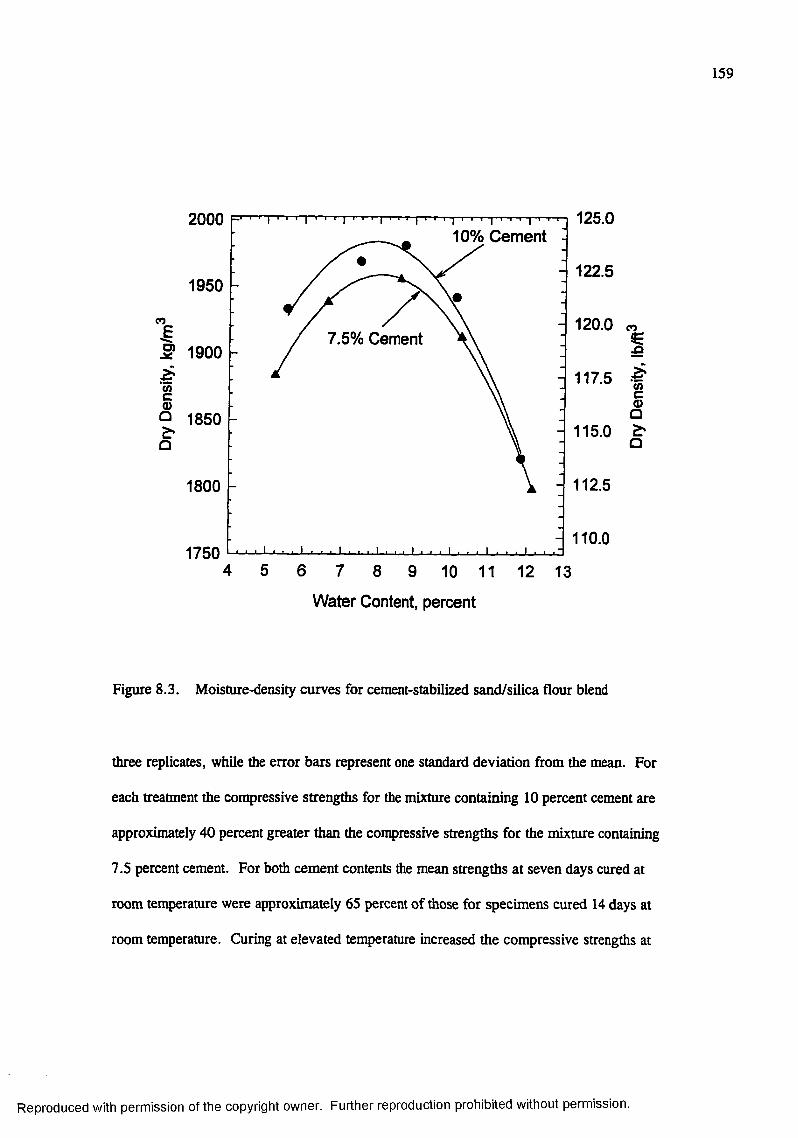
159
125.0200010% Cernent
122.51950
1* 1900
(A
5o 1850
O
120.07.5% Cernent
117.5
115.0
112.51800
110.01750
4 5 6 7 8 9 10 11 12 13
%
(A
5Q
W ater Content, percent
Figure 8.3. Moisture-density curves for cement-stabilized sand/silica flour blend
three replicates, while the error bars represent one standard deviation from the mean. For
each treatment the compressive strengths for the mixture containing 10 percent cement are
approximately 40 percent greater than the compressive strengths for the mixture containing
7.5 percent cement. For both cement contents the mean strengths at seven days cured at
room temperature were approximately 65 percent of those for specimens cured 14 days at
room temperature. Curing at elevated temperature increased the compressive strengths at
Reproduced with permission of the copyright owner. Further reproduction prohibited without permission.
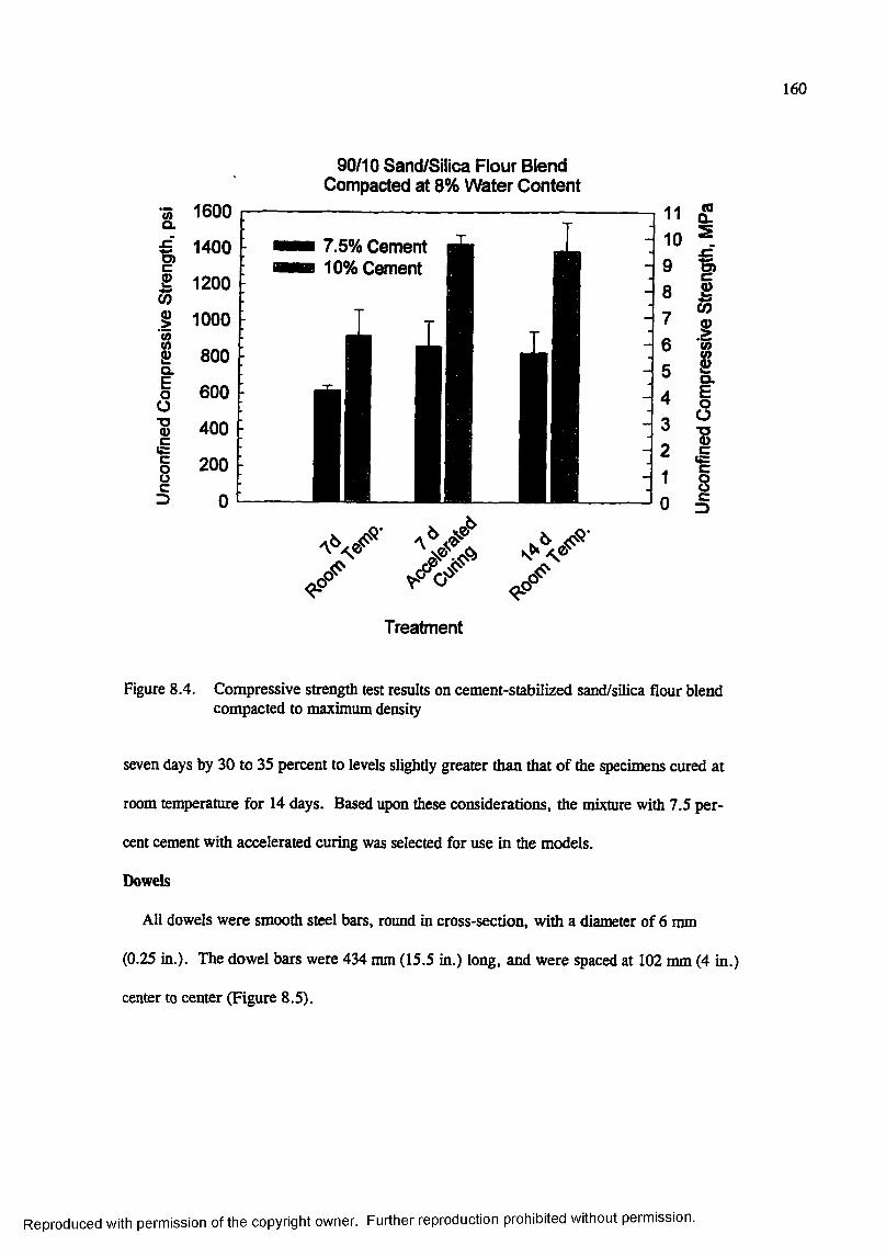
160
90/10 Sand/Silica Flour Blend Compacted at 8% W ater Content
1 1600
€c1400
11200
. 1 1000
2Q .
800EoO
600
1( C
400
1200
D 0
7.5% Cement 10% Cement
Treatment
Figure 8.4. Compressive strength test results on cement-stabilized sand/silica flour blend compacted to maximum density
seven days by 30 to 35 percent to levels slightly greater than that of the specimens cured at
room temperature for 14 days. Based upon these considerations, the mixture with 7.5 per
cent cement with accelerated curing was selected for use in the models.
Dowels
All dowels were smooth steel bars, round in cross-section, with a diameter of 6 mm
(0.25 in.). The dowel bars were 434 mm (15.5 in.) long, and were spaced at 102 mm (4 in.)
center to center (Figure 8.5).
Reproduced with permission of the copyright owner. Further reproduction prohibited without permission.
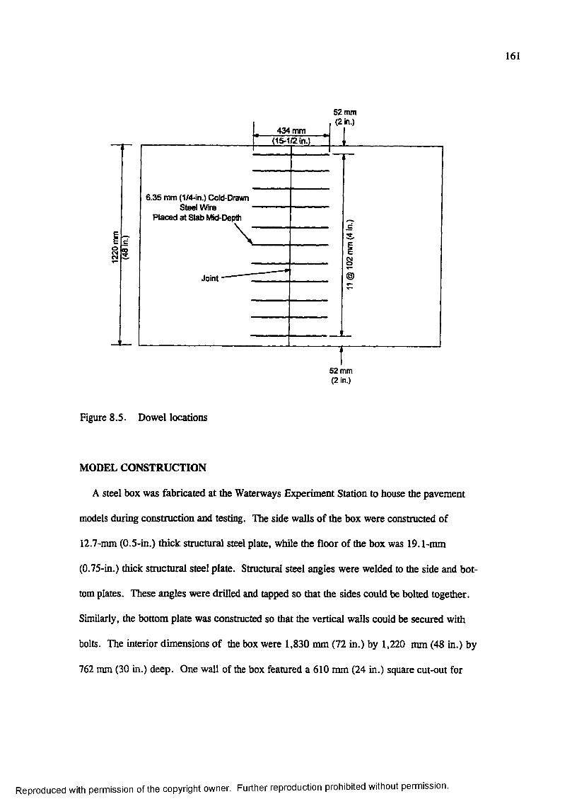
161
434 mm( 1 5 - 1 /2 in .)
5 2 m m ( 2 in .)
6 .3 5 m m (1 /4 - in .) C o ld -D ra w n
S te e l W ire P l a c e d a t S l a b M id -D e p th
VJ o in t
sIi)
5 2 m m (2 in.)
Figure 8.5. Dowel locations
MODEL CONSTRUCTION
A steel box was fabricated at the Waterways Experiment Station to house the pavement
models during construction and testing. The side walls of the box were constructed of
12.7-mm (0.5-in.) thick structural steel plate, while the floor of the box was 19.1-mm
(0.75-in.) thick structural steel plate. Structural steel angles were welded to the side and bot
tom plates. These angles were drilled and tapped so that the sides could be bolted together.
Similarly, the bottom plate was constructed so that the vertical walls could be secured with
bolts. The interior dimensions of the box were 1,830 mm (72 in.) by 1,220 mm (48 in.) by
762 mm (30 in.) deep. One wall of the box featured a 610 mm (24 in.) square cut-out for
Reproduced with permission of the copyright owner. Further reproduction prohibited without permission.
162
insertion of a transparent pane of plexiglass to allow observation of the model during testing.
Three 102 mm (4 in.) square structural steel tubes were tack-welded underneath the box’s
floor so that the assembled box could be transported about the laboratory by forklift. After
the reaction box was painted, the rubber block was placed on the floor of the reaction box,
and the vertical walls were assembled around the box and attached with bolts. Figure 8 .6
shows a photograph of the completed reaction box.
Figure 8 .6 . Photograph of completed reaction box
The testing proceeded along a two-week turnaround schedule as shown in Table 8.4. This
expedited schedule was made possible by the use of high-early-strength cement and an accel
erating admixture along with curing at elevated temperamre. The concrete reached a level of
maturity sufficient to produce the target strength and modulus of elasticity within approxi
mately one week of placement.
Reproduced with permission of the copyright owner. Further reproduction prohibited without permission.

163
1 Table 8.4Typical Physical Model Construction Schedule
WeekDay of Week Activity
Week 1 Monday Prepare materials for model construction
Tuesday Place base course
Wednesday Place first slab
Thursday Place second slab
Friday 3:00 p.m. Place reaction box in environmental chamber at 60°C (140°F) over weekend
Week 2 Monday 9:00 a.m. Remove from environmental chamber and allow to cool
Tuesday Instrument model
Wednesday Conduct experiment
Thursday Reduce data and conduct posttest photography
Friday Remove model and prepare reaction box for construction of next model
The physical models were constructed using the reaction box as a mold. The rubber block
and the walls of the reaction box were coated with a form release agent to insure that bonding
did not occur between the model and either the reaction box or rubber block.
Base course construction
The materials for the cement stabilized bases were mixed in the laboratory in a 0.17
(6 ft ) portable mortar mixer. The volume and maximum wet density of the compacted base
was used to calculate the mass of base material required to achieve the target density in the
reaction box. An oversize batch (approximately 0.085 m (3 ft*)) was prepared for each
placement and weighed on a scale in the laboratory. Material in excess of that required to
yield the target compacted density was removed and set aside for preparation of compressive
strength cylinders and flexural strength beams. The required mass of material was placed in
Reproduced with permission of the copyright owner. Further reproduction prohibited without permission.
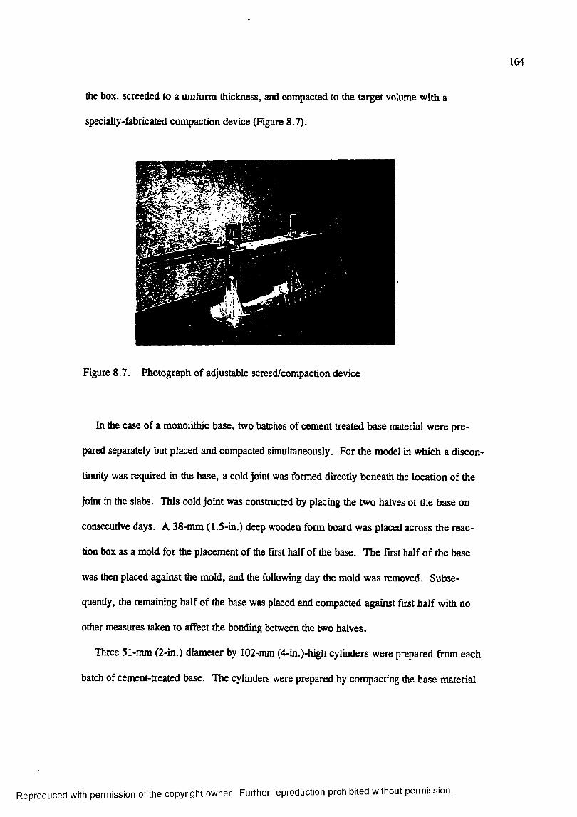
164
the box, screeded to a uniform thickness, and compacted to the target volume with a
specially-fabricated compaction device (Figure 8.7).
Figure 8.7. Photograph of adjustable screed/compaction device
In the case of a monolithic base, two batches of cement treated base material were pre
pared separately but placed and compacted simultaneously. For the model in which a discon
tinuity was required in the base, a cold joint was formed directly beneath the location of the
joint in the slabs. This cold joint was constructed by placing the two halves of the base on
consecutive days. A 38-mm (1.5-in.) deep wooden form board was placed across the reac
tion box as a mold for the placement of the first half of the base. The first half of the base
was then placed against the mold, and the following day the mold was removed. Subse
quently, the remaining half of the base was placed and compacted against first half with no
other measures taken to affect the bonding between the two halves.
Three 51-mm (2-in.) diameter by 102-mm (4-in.)-high cylinders were prepared from each
batch of cement-treated base. The cylinders were prepared by compacting the base material
Reproduced with permission of the copyright owner. Further reproduction prohibited without permission.
165
into heavy, brass molds with a small, hand-held tamper. Also, three 76-mm (3-in.) wide by
76-mm (3-in.) deep by 286-mm (11-1/4-in.) long beams were prepared from one batch of
cement-treated base per model. The base material was compacted into steel molds using a
hand-held tamper featuring a square fooq>rint. These cylinders and beams were cured under
the same conditions as the models and were tested on the date the corresponding experiment
was conducted to determine the compressive strength, flexural strength, and modulus of elas
ticity of the cement-treated base.
The bond breaker for Experiment LSM-5 was constructed o f two layers of 0.152-mm
(6-mil) polyethylene sheets separated by a thin layer of uniformly graded fine silica sand.
Prior to casting the concrete slabs, the first sheet of polyethylene was carefully cut and fitted
on top of the base as shown in the photograph in Figure 8 .8 . Next, a thin layer of uniform
sand was spread on top of the polyethylene sheet (Figure 8.9), and a second sheet covering
the entire surface was placed on top of the sand layer. Then, the slabs were placed on top the
bond-breaking layer. Figure 8 .10 is a photograph of the reaction box just prior to placement
of the loaded slab.
Slab construction
The two concrete slabs for each experiment were placed on consecutive days. The first
slab was placed against a 51-mm (2-in.) deep wooden mold faced with a 1.59-mm (1/16-in.)
thick sheet of Teflon. The dowels were inserted in 6 mm (0.25 in.) diameter holes which had
been predrilled through the mold and Teflon. Prior to their placement in the mold, a light
coating of rust scale was removed from the dowels. The position of the dowels in the mold
was adjusted to insure that equal lengths of dowel bars would be present in both slabs. A
clamping device composed of pieces of wood cut to the proper dimensions and held together
with screws was used to insure that the dowels were held orthogonal to the mold. The
Reproduced with permission of the copyright owner. Further reproduction prohibited without permission.

166
Figure 8 .8 . Installation of polyethylene film in reaction box
Figure 8.9. Placement of thin sand layer
Reproduced with permission of the copyright owner. Further reproduction prohibited without permission.
167
Figure 8 .10. Bond breaker and doweled joint just prior to concrete placement
bonded end of the dowel was in the first slab placed; therefore, care was taken to insure that
no form release agent, grease, or oil was present on the dowels.
The concrete was batched and mixed in the laboratory, carefully placed in the reaction
box, and consolidated with an external spud-type concrete vibrator. The surface was floated
and finished by hand, and the concrete was allowed to set for approximately 24 hrs.
After 24 hours the transverse mold along the joint was carefully removed. The free ends
of the dowels (unbonded ends) were greased with an automotive-type grease. To further
insure that no bond could be developed between the dowel bars and the slab, plastic drinking
straws with an inside diameter of 6 mm (0.25 in.) were slipped over the greased dowels. The
second slab was then placed, consolidated, and finished.
The ends of the slabs were constrained by 76 mm (3 in.) equal leg structural steel angles,
9.5 mm (3/8 in.) thick. One leg of the angle was embedded in the fresh concrete just after
Reproduced with permission of the copyright owner. Further reproduction prohibited without permission.
168
placement, and the other leg was bolted to the side of the reaction box with 12.7 mm (0.5 in.)
diameter steel bolts. The bolts were later torqued to near yield to maximize the clamping
force on the angles.
The slabs were moist cured using wet burlap and plastic sheeting at room tenq>erature
until they were placed in the environmental chamber at 60"C (140®F) over the weekend for
accelerated curing. After being removed from the environmental chamber, the slabs were
allowed to cool in the laboratory to room tenq>erature with no additional wet curing.
Three 152-mm (6-in.) diameter by 305-mm (12-in.)-high cylinders were cast from each
batch of concrete used to fabricate the model slabs. Also, a single 152-mm (6-in.) wide by
152-mm (6-in.) deep by 508-mm (20-in.) long beam was cast from one batch of concrete for
each model. These cylinders and beam were cured under the same accelerated curing con
ditions as the model slabs and were tested on the date the corresponding experiment was con
ducted to determine the compressive and flexural strengths, modulus of elasticiQ , and
Poisson’s ratio of the slabs.
LOADING
All experiments were conducted on the structural test floor at the Concrete and Materials
Division, Structures Laboratory, Waterways Eqwriment Station. Loads were applied to the
physical model by a closed-loop, servo-hydraulic materials testing system through a thin cir
cular rubber pad. The radius of the loaded area was 57 mm (2-1/4 in.). The testing system
was controlled by an MTS LoadStar digital controller which could be programmed through a
graphical user interface to ouçut the desired control signals to the system. So that post-peak
response could be captured, the load was applied in displacement control at a rate of
0.25 mm/min (0.01 in/min).
Reproduced with permission of the copyright owner. Further reproduction prohibited without permission.

169
The testing frame consisted of four vertical steel columns bolted to attachment points in
the structural test floor. A stiff, deep steel beam spanned the opening between the columns.
A 222-kN (50,000-lbs) capacity actuator attached to this beam provided the loading for the
experiment.
INSTRUMENTATION
Instrumentation for the physical model experiments consisted of the following:
• Applied load, measured by a load cell.
• Surface strains, measured by surface-applied, foil resistance strain gages.
• Displacement, measured by linear variable displacement transducers (LVDTs).
All strain and deformation measurements were made on the top surface of the slabs. The
load cell was located between the testing machine actuator and the slab. The m axim um range
of the load cell was ±222 kN (50,000 lb).
Strain gages employed for these experimental studies had an electrical resistance of
350 ohms and a gage length of 25 mm (1 in.). When the gage was strained, it experienced a
change in electrical resistance. These very small changes in resistance were measured by
placing the gage in one leg of a Wheatstone bridge circuit, which is sensitive to small resis
tance changes. The maximum range of the strain gages was ±50,000 microstrains.
The locations for the strain gages were prepared by first applying a thin coat of Epicast, a
low-modulus, white epoxy. This epoxy coat served two primary functions: to provide a
rnoismre barrier to prevent water in the concrete from affecting the strain gage and to provide
a smooth, uniform surface to which the strain gage could be bonded. After a 24 hour setting
period, the Epicast was sanded to a uniform thickness, and the strain gages were bonded
using Super Glue.
Reproduced with permission of the copyright owner. Further reproduction prohibited without permission.
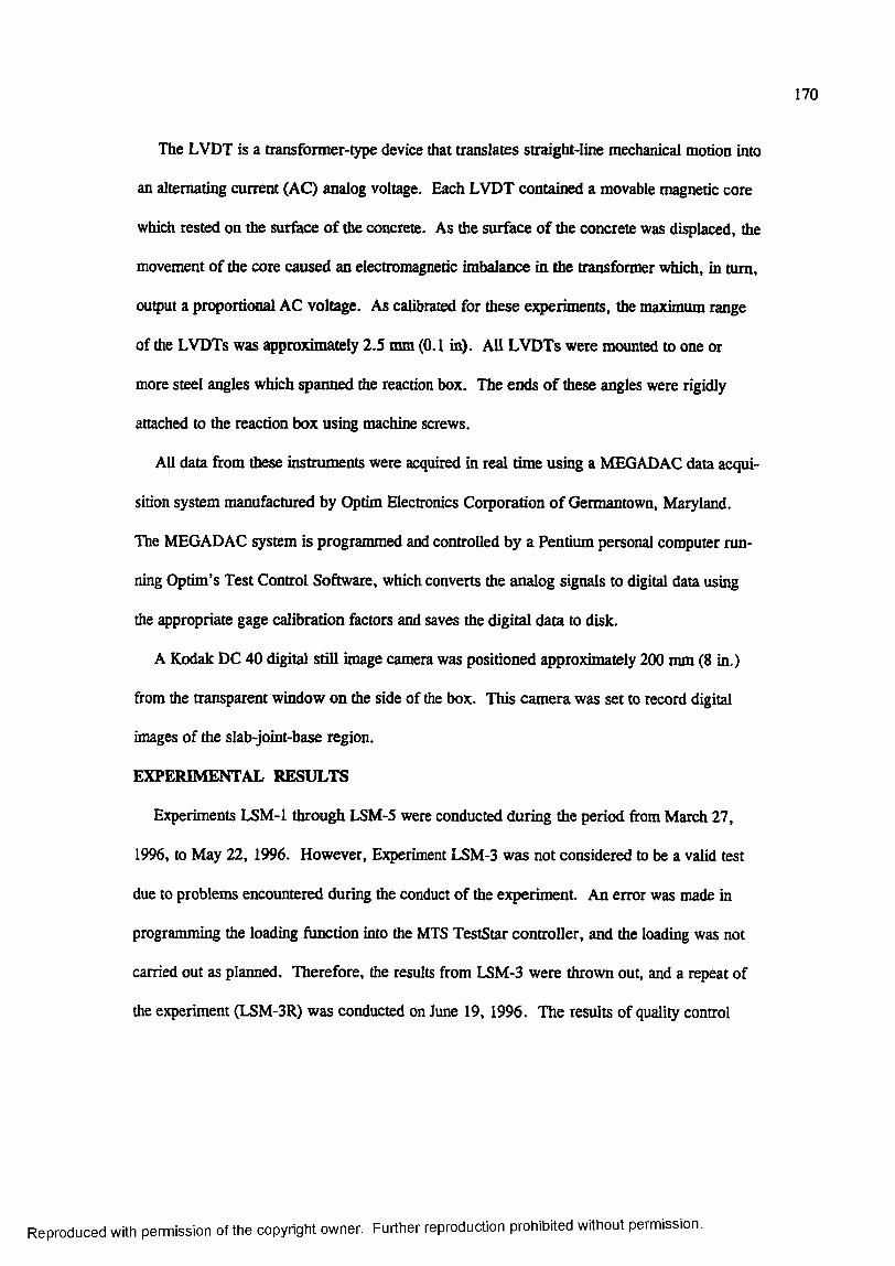
170
The LVDT is a transfonner-type device that translates straight-line mechanical motion into
an alternating current (AC) analog voltage. Each LVDT contained a movable magnetic core
which rested on the surface of the concrete. As the surface of the concrete was displaced, the
movement of the core caused an electromagnetic imbalance in the transformer which, in turn,
ou^ut a proportional AC voltage. As calibrated for these experiments, the maximum range
of the LVDTs was approximately 2.5 mm (0.1 in). All LVDTs were mounted to one or
more steel angles which spaimed the reaction box. The ends o f these angles were rigidly
attached to the reaction box using machine screws.
All data from these instruments were acquired in real time using a MEGADAC data acqui
sition system manufactured by Optim Electronics Corporation o f Germantown, Maryland.
The MEGADAC system is programmed and controlled by a Pentium personal computer run
ning Optim’s Test Control Software, which converts the analog signals to digital data using
the appropriate gage calibration factors and saves the digital data to disk.
A Kodak DC 40 digital still image camera was positioned approximately 200 mm (8 in.)
from the transparent window on the side of the box. This camera was set to record digital
images of the slab-joint-base region.
EXPERIMENTAL RESULTS
Experiments LSM-1 through LSM-5 were conducted during the period from March 27,
1996, to May 22, 1996. However, Experiment LSM-3 was not considered to be a valid test
due to problems encountered during the conduct of the experiment. An error was made in
programming the loading function into the MTS TestStar controller, and the loading was not
carried out as planned. Therefore, the results from LSM-3 were thrown out, and a repeat of
the experiment (LSM-3R) was conducted on June 19, 1996. The results of quality control
Reproduced with permission of the copyright owner. Further reproduction prohibited without permission.

171
tests conducted on the construction materials as well as data from Experiments LSM-1,
LSM-2, LSM-3R, LSM-4, and LSM-5 are presented and discussed in this section.
Materials
Cement-stabilized base
The results of the quality control tests on the cement stabilized bases are summarized in
Table 8.5. Compressive strength tests were conducted on 51 mm (2 in.) by 102 mm (4 in.)
cylindrical specimens. These results indicate that the compressive strengths were at or below
that expected from the seven day accelerated curing tests conducted during the initial mate
rials investigation (Figure 8.4). It is believed that the lower strengths can be attributed to
drying out of the cement/silty-sand material between batching and preparation of the test spe
cimens. The material to be used to make the specimens was set aside while the bases were
placed and compacted in the reaction box. Typically, more than one but less than two hours
elapsed between the batching of the base materials and preparation of the quality control spe
cimens. It is likely that some of the moisture evaporated during this period resulting in lower
densities and strengths in the quality control specimens.
The modulus of elasticity of the cement-stabilized base was determined from the compres
sive strength tests on the cylinders. The modulus of elasticity (in compression), as calculated
from the tangent to the steepest portion of the compressive stress-strain curve, is tabulated in
Table 8.5. These data indicate that as the compressive strength increases, the compressive
modulus of elasticity increases. The modulus of elasticity of the cement-stabilized base was
approximately 5 percent of the target modulus of elasticity of the portland cement concrete
slabs.
Reproduced with permission of the copyright owner. Further reproduction prohibited without permission.
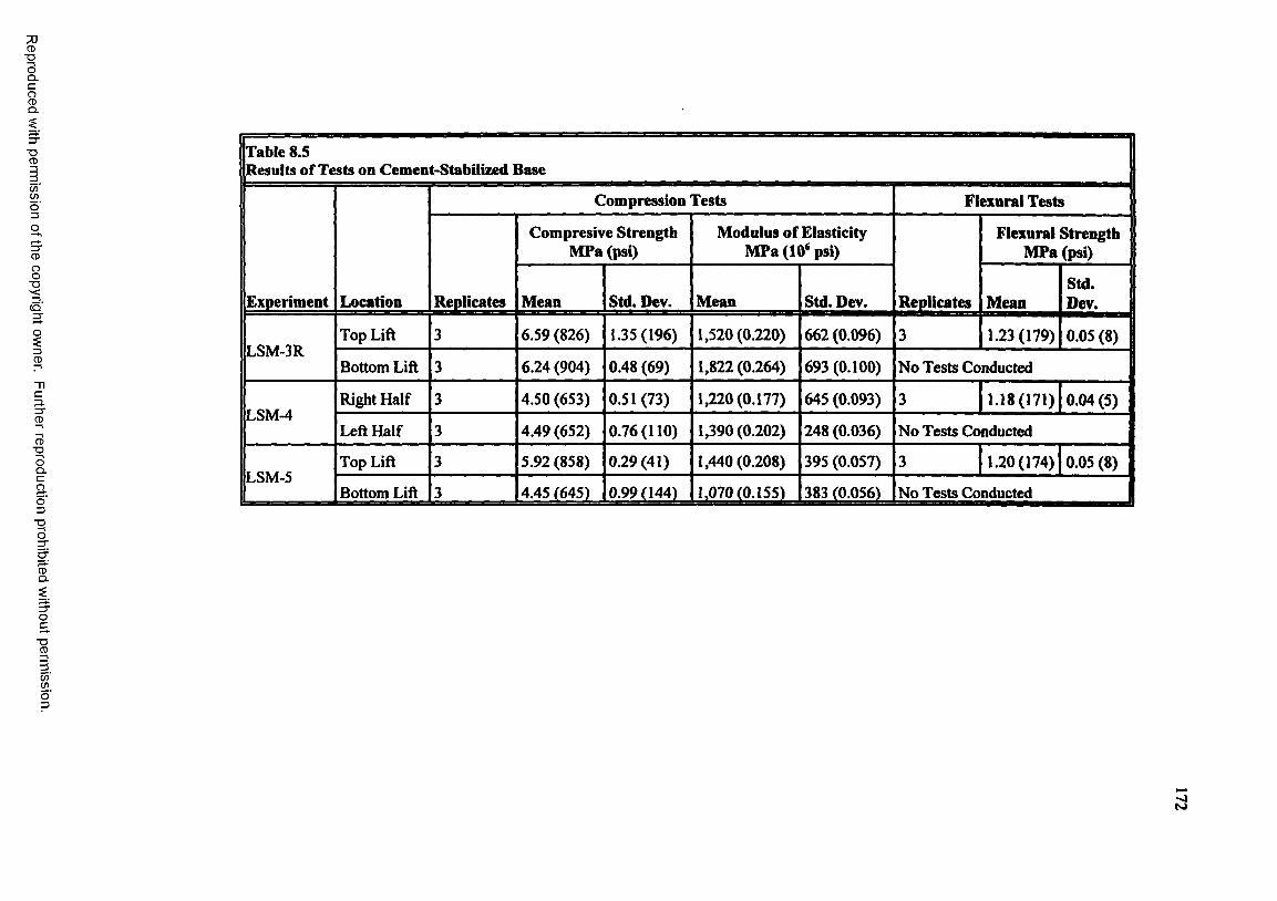
CD■DOQ .C
gQ .
■DCD
C/)
o’3O
8■ D
3 .<Û3 ;O
3 .3"CD
CD" O
OQ .
O3
■ O
O
Table 8.5Results of Tests on Cement-Stabilized Base
Experiment Location
Compression Tests Flexural Tests
Replicates
Compresive Strength MPa (psi)
Modulus of Elasticity MPa (10* psi)
Replicates
Flexural Strength MPa (psi)
Mean Std. Dev. Mean Std. Dev. MeanStd.Dev.
LSM-3RTop Lift 3 6.59(826) 1.35(196) 1,520(0.220) 662 (0.096) 3 1.23(179) 0.05(8) 1
Bottom Lift 3 6.24(904) 0.48 (69) 1,822(0.264) 693 (0.100) No Tests Conducted
LSM-4Right Half 3 4.50(653) 0.51(73) 1,220(0.177) 645 (0.093) 3 1.18(171) 0.04(5)
Left Half 3 4.49(652) 0.76(110) 1,390(0.202) 248 (0.036) No Tests Conducted
LSM-5Top Lift 3 5.92 (858) 0.29(41) 1,440(0.208) 395 (0.057) 3 1.20(174) 0.05 (8)
Bottom Lift 3 4.45 (645) 0.99(144) 1,070(0.155) 383 (0.056) No Tests Conducted
&
OcE
c / )
o'3
W

173
The modulus of rupture (flexural strength) of the cement stabilized base was determined
from tests on 76 mm (3 in.) by 76 mm (3 in.) by 286 mm (11-1/4 in.) beams loaded at the
third points. These data are also reported in Table 8.5.
Statistical techniques were employed to determine if the observed variations in the material
properties from batch to batch within an experiment and between experiments were statisti
cally significant at the 0.05 significance level. Student’s t-tests were conducted on the com
pressive strength and modulus of elasticity data from the two batches of base material within
each experiment. For each of the Experiments LSM-3R, LSM-4, and LSM-5, the differ
ences in the mean values of compressive strength and modulus of elasticity between batches
were not great enough to exclude the possibility that the differences were due to random sam
pling variability. Therefore, it can be concluded that there was no statistically significant dif
ference in compressive strength and elastic modulus between batches in any given experiment
at the 0.05 significance level.
One-way analysis of the variance (ANOVA) procedures were used to test for statistically-
significant differences in material properties between experiments. The results of these anal
yses indicated that for the case of compressive strength, the differences in the mean values of
compressive strength between experiments were greater than would be expected by chance at
the 0.05 significance level. A pairwise multiple comparison test indicated that the compres
sive strength values from Experiment LSM-3R were statistically different from those of
LSM-4 and LSM-5. However, for the cases of modulus o f elasticity and flexural strength,
the differences in the mean values between experiments was not great enough to exclude the
possibility that the difference was due to random sampling variability; therefore, no statisti
cally significant differences in these two parameters were detected at the 0.05 significance
level.
Reproduced with permission of the copyright owner. Further reproduction prohibited without permission.
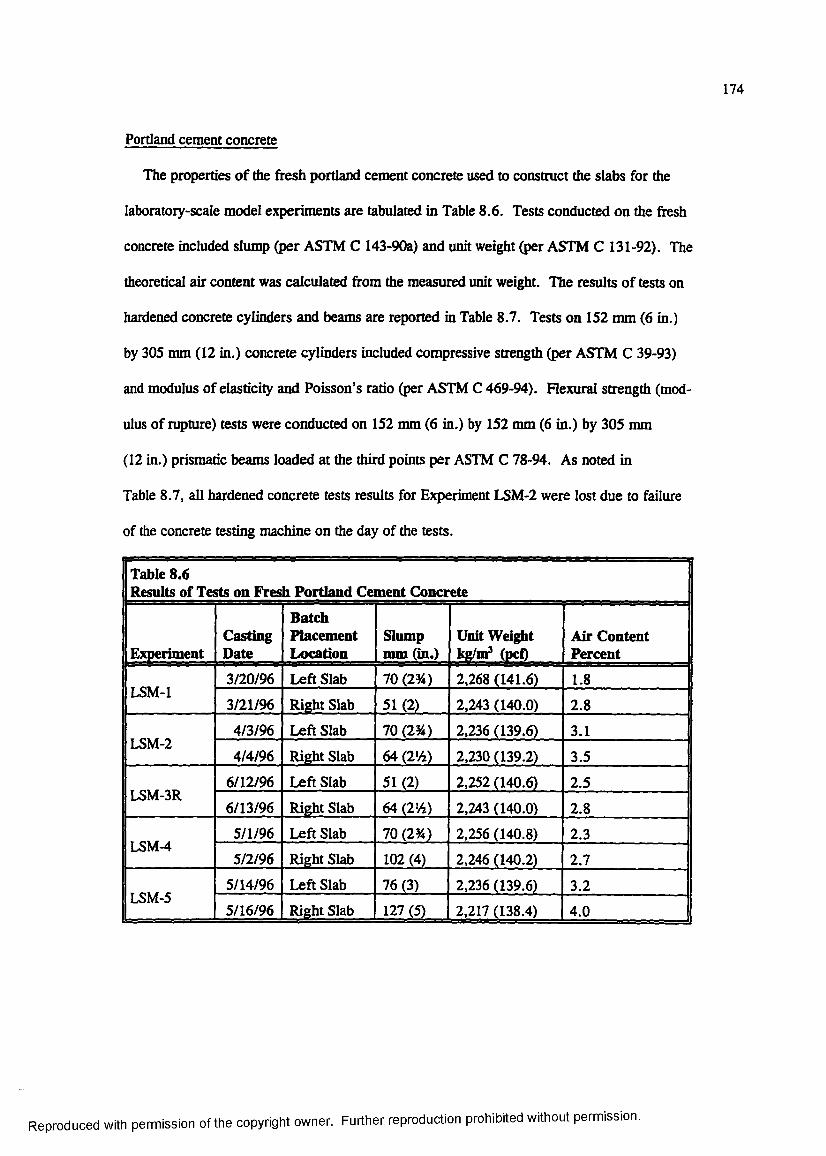
174
Portland cement concrete
The properties of the fresh portland cement concrete used to construct the slabs for the
laboratory-scale model experiments are tabulated in Table 8 .6 . Tests conducted on the fresh
concrete included slun^) (per ASTM C 143-90a) and unit weight (per ASTM C 131-92). The
theoretical air content was calculated from the measured unit weight. The results of tests on
hardened concrete cylinders and beams are reported in Table 8.7. Tests on 152 mm (6 in.)
by 305 mm (12 in.) concrete cylinders included compressive strength (per ASTM C 39-93)
and modulus of elasticity and Poisson’s ratio (per ASTM C 469-94). Flexural strength (mod
ulus of rupture) tests were conducted on 152 mm (6 in.) by 152 mm (6 in.) by 305 mm
(12 in.) prismatic beams loaded at the third points per ASTM C 78-94. As noted in
Table 8.7, all hardened concrete tests results for Experiment LSM-2 were lost due to failure
of the concrete testing machine on the day of the tests.
Table 8 .6Results of Tests on Fres 1 Portland Cement Concrete
ExperimentCastingDate
BatchPlacementLocation
Slump mm (in.)
Unit Weight kg/m^ (pcf)
Air Content Percent
LSM-13/20/96 Left Slab 70 (2 %) 2,268 (141.6) 1.8
3/21/96 Right Slab 51(2) 2,243 (140.0) 2 .8
LSM-24/3/96 Left Slab 70 (2%) 2,236 (139.6) 3.1
4/4/96 Right Slab 64 (2%) 2,230 (139.2) 3.5
LSM-3R6/12/96 Left Slab 51(2) 2,252 (140.6) 2.5
6/13/96 Right Slab 64 (2%) 2,243 (140.0) 2 .8
LSM-45/1/96 Left Slab 70 (2%) 2,256 (140.8) 2.3
5/2/96 Right Slab 102 (4) 2,246 (140.2) 2.7
LSM-55/14/96 Left Slab 76(3) 2,236 (139.6) 3.2
5/16/96 Right Slab 127 (5) 2,217 (138.4) 4.0
Reproduced with permission of the copyright owner. Further reproduction prohibited without permission.
7)CD
"DOQ .C
gQ .
■DCD
C /î
o"3O
8ci-
3.3"CD
CD-OOQ .
O3
■OO
&
OcE
c / )
o'3
Table 8.7Results of Tests on Hardened Portland Cernent Concrete
ExperimentCastingDate
TestingDate
Compressive Strength TestsElastic Modulus and Poisson’s Ratio
Tests Flexural Tests
Replicates
MeanMPa(psi)
Std.Dev.MPa(psi) Replicates
Modulus of Elasticity Mpa (10* psi)
Poisson’sRatio Replicates
Modulus of Rupture Mpa (psi)
LSM-1
3/20/963/27/96
3 29.0(4200)
0.51(75) No Tests Conducted
3/21/96 3 27.5(3990)
0.38(55) 1
26,800(3.90)
NotAvailable 1 3.07
(445)
LSM-24/3/96 4/10/96 No data available due to failure of test machine.4/4/96
LSM-3R
6/12/966/19/96
3 27.1(3930)
0.14(20) No Tests Conducted
6/13/96 3 26.3(3820)
0.72(105) 1
28,300(4.10)
0.181
2.90(420)
LSM-4
5/1/965/8/96
3 26.1(3790)
0.62(90) No Tests Conducted
5/2/96 3 26.1(3780)
2.21(320) 1
29,000(4.21)
0.171
3.28(475)
LSM-5
5/14/965/22/96
3 25.6(3710)
0.41(60) No Tests Conducted
5/16/96 3 25.7(3720)
0.17(25) 1 28,700
(4.17)0.19
1 3.211465)---------
Dl

176
The slump of the fresh concrete varied from 51 mm ( 2 in.) to 127 mm (5 in.), with the
majority of the measurements between 51 mm (2 in.) and 76 mm (3 in.). Models LSM-1,
LSM-2, and the left slab of LSM-4 were all fabricated from the same lot of Type HI cement,
while models LSM-3R, LSM-5, and the right slab of LSM-4 were fabricated from a different
lot of Type III cement from the same manufacturer. The higher slump values noted for mod
els LSM-4 (Right Slab) and LSM-5 were attributed to the changes in the cement between the
two lots. The second lot had less water demand than the first resulting in an increase in the
slump of the fresh concrete. This effect was mitigated for Experiment LSM-3R by reducing
the mix water 6 percent (by mass) thus bringing the slump back in line with the models
fabricated from the first lot of cement. Unit weights of the fresh concrete varied from
2,217 kg/m^ (138.4 pcf) to 2,268 kg/m^ (141.6 pcf), while air contents ranged from 1.8 to
4.0 percent.
The mean concrete compressive strengths ranged from a low of 25.6 MPa (3,710 psi) to a
high of 29.0 MPa (4,200 psi). The modulus of elasticity ranged from 26,800 MPa (3.9 x
10* psi) to 29,000 MPa (4.2 x 10* psi), while Poission’s ratio ranged from 0.17 to 0.19.
The modulus of rupture varied from a minimum of 2.90 MPa (420 psi) to a maximum of
3.28 MPA (475 psi).
For FAA rigid pavement structural design, the concrete material strength parameter used
to determine pavement thickness is 90-day modulus of rupture. A normal range of flexural
strength at an age of 90 days is from 3.45 MPa (500 psi) to 6.20 MPa (900 psi). Therefore,
the flexural strength of the slabs used in this experimental study were slightly lower than
those which would be expected in the field.
Statistical techniques were employed to determine if the observed variations in the com
pressive strengths from slab to slab within an experiment and between experiments were
Reproduced with permission of the copyright owner. Further reproduction prohibited without permission.
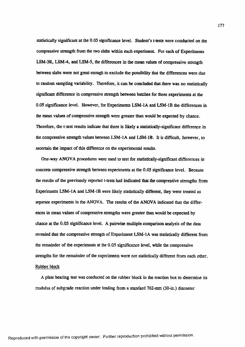
177
statistically significant at the 0.05 significance level. Student’s t-tests were conducted on the
compressive strength from the two slabs within each experiment. For each of Experiments
LSM-3R, LSM-4, and LSM-5, the differences in the mean values of compressive strength
between slabs were not great enough to exclude the possibility that the differences were due
to random sampling variability. Therefore, it can be concluded that there was no statistically
significant difference in compressive strength between batches for these experiments at the
0.05 significance level. However, for Experiments LSM-IA and LSM-IB the differences in
the mean values o f compressive strength were greater than would be expected by chance.
Therefore, the t-test results indicate that there is likely a statistically-significant difference in
the compressive strength values between LSM-1 A and LSM-IB. It is difficult, however, to
ascertain the impact of this difference on the experimental results.
One-way ANOVA procedures were used to test for statistically-significant differences in
concrete compressive strength between experiments at the 0.05 significance level. Because
the results of the previously reported t-tests had indicated that the conçressive strengths from
Experiments LSM-1 A and LSM-IB were likely statistically different, they were treated as
separate experiments in the ANOVA. The results of the ANOVA indicated that the differ
ences in mean values of compressive strengths were greater than would be expected by
chance at the 0.05 significance level. A pairwise multiple comparison analysis o f the data
revealed that the compressive strength of Experiment LSM-1 A was statistically different from
the remainder of the experiments at the 0.05 significance level, while the compressive
strengths for the remainder of the experiments were not statistically different from each other.
Rubber block
A plate bearing test was conducted on the rubber block in the reaction box to determine its
modulus of subgrade reaction under loading from a standard 762-mm (30-in.) diameter
Reproduced with permission of the copyright owner. Further reproduction prohibited without permission.
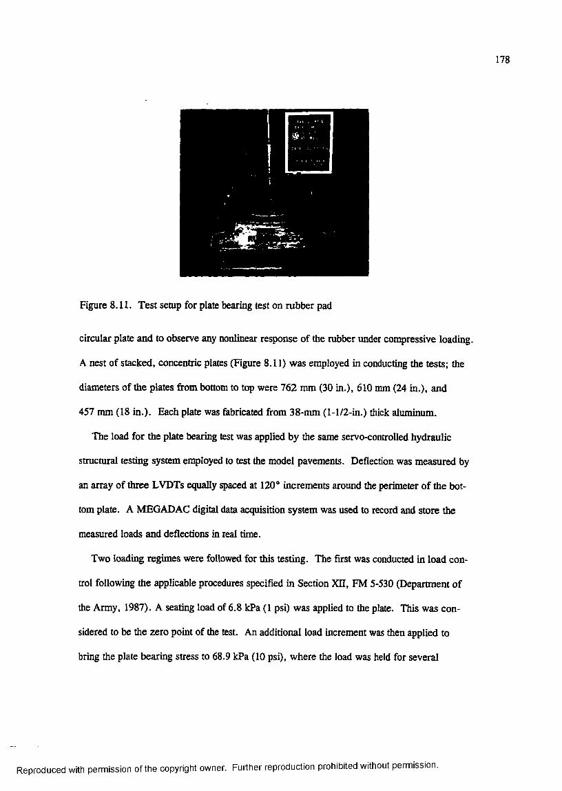
178
Figure 8.11. Test setup for plate bearing test on rubber pad
circular plate and to observe any nonlinear response of the rubber under compressive loading.
A nest of stacked, concentric plates (Figure 8.11) was employed in conducting the tests; the
diameters of the plates from bottom to top were 762 mm (30 in.), 610 nun (24 in.), and
457 mm (18 in.). Each plate was fabricated from 38-mm (1-1/2-in.) thick aluminum.
The load for the plate bearing test was applied by the same servo-controlled hydraulic
structural testing system employed to test the model pavements. Deflection was measured by
an array of three LVDTs equally spaced at 120® increments around the perimeter of the bot
tom plate. A MEGADAC digital data acquisition system was used to record and store the
measured loads and deflections in real time.
Two loading regimes were followed for this testing. The first was conducted in load con
trol following the applicable procedures specified in Section XU, FM 5-530 (Department of
the Army, 1987). A seating load of 6 .8 kPa (1 psi) was applied to the plate. This was con
sidered to be the zero point of the test. An additional load increment was then applied to
bring the plate bearing stress to 68.9 kPa (10 psi), where the load was held for several
Reproduced with permission of the copyright owner. Further reproduction prohibited without permission.
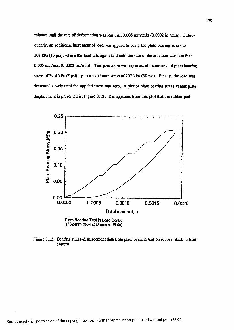
179
minutes until the rate of deformation was less than 0.005 mm/min (0.0002 in./min). Subse
quently, an additional increment of load was applied to bring the plate bearing stress to
103 kPa (15 psi), where the load was again held until the rate of deformation was less than
0.005 mm/min (0.0002 in./min). This procedure was repeated at increments of plate bearing
stress of 34.4 kPa (5 psi) up to a maximum stress of 207 kPa (30 psi). Finally, the load was
decreased slowly until the applied stress was zero. A plot of plate bearing stress versus plate
displacement is presented in Figure 8 .12. It is apparent from this plot that the rubber pad
0.25
« 0.20
0.15
O)c2 0.10
CQ
ÎE 0.05
0.000.0000 0.0005 0.0010 0.0015 0.0020
Displacement, m
Plate Bearing Test in Load Control (762-mm (30-in.) Diameter Plate)
Figure 8.12. Bearing stress-displacement data from plate bearing test on rubber block in load control
Reproduced with permission of the copyright owner. Further reproduction prohibited without permission.

180
crept during the portions of the tests where the plate bearing stress was held constant. It can
also be seen that the amount of creep deformation which occurs until the rate of creep defor
mation falls below 0.005 mm/min (0 .0002 in./min) increases with increasing plate bearing
sness. The accumulated creep deformation at the end of the loading was approximately
0.4 mm (0.016 in.). The data from this test were used to determine the modulus of sub
grade reaction, k, for the rubber block for the standard 762-mm (30-in.) diameter plate. Fig
ure 8.13 shows a plot of corrected plate bearing stress versus displacement as prescribed by
FM 5-530 (Department of the Army, 1987). Each of the data points denoted by the triangles
represents the deflection and stress at the end of each increment of applied stress, adjusted for
the 6 .8 kPa (1 psi) initial seating load. These data were then corrected, using the procedures
described in FM 5-530 (Department of the Army 1987), to account for bending of the plates.
From the slope of the corrected curve, the modulus of subgrade reaction was determined to
be 111 MPa/m (409 psi/in.). This value is high for a subgrade material, and would be more
representative o f the modulus of subgrade reaction for a dense, well-graded gravel.
The second loading regime was conducted in displacement control at a load rate of
0.25 mm/min (0.01 in./min) to mimic the loading conditions during testing of a pavement
model. The bearing plate was displaced continuously and monotonically until a maximum
bearing stress of 0.1 MPa (14.5 psi) was reached, at which point the displacement was
reversed continuously and monotonically until the bearing stress was reduced to zero. A plot
of bearing stress versus deformation is shown in Figure 8.14. In the range in which the bear
ing stress was less than 0.01 MPa (1.5 psi), the response was relatively soft. For bearing
stresses greater than approximately 0.1 MPa (1.5 psi) the response was stiffer. Upon unload
ing, the response was characterized by a hysterisis loop typical of viscoelastic materials.
Reproduced with permission of the copyright owner. Further reproduction prohibited without permission.
181
0.25
S,5
0.20Corrected for Plate Bending Data From Experiment
I 0.15
k = 111 MPa/m (409 psi/in.)
§ . 0.05
0.000.0000 0.0005 0.0010 0.0015 0.0020
Displacement, m 762-mm (30 in.) Diameter Plate
Figure 8.13. Corrected plate bearing stress
Thus, it can be concluded that the response of the rubber block in the reaction box was non
linear viscoelastic over the range of loading expected during testing of a pavement model.
These nonlinear responses of the rubber block are considerably different from those assumed
for the bed-of-springs foundation in Westergaard’s theory. The influence of the nonlinear
viscoelastic response on the pavement model is not known.
Experiment LSM-1
Experiment LSM-1 consisted of two 51-mm (2-in.) thick slabs founded directly on the
rubber subgrade. The right- and left-hand slabs were constructed with no load transfer capa
bilities from either dowel bars or aggregate interlock. A 5 mm (3/16 in.) gap separated the
Reproduced with permission of the copyright owner. Further reproduction prohibited without permission.
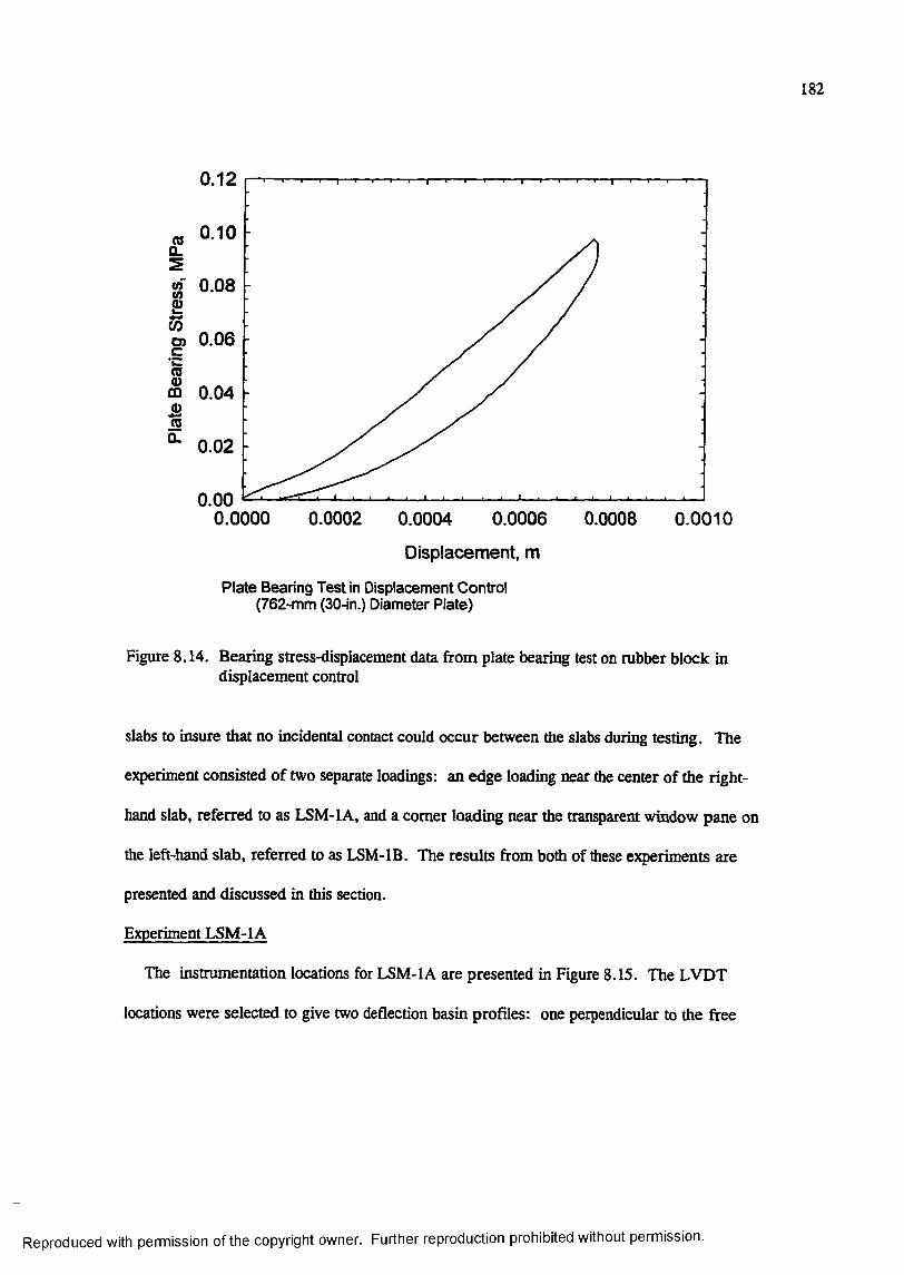
182
0.12
0.10
% 0.08
Io) 0.06•i3m 0.04
I0.02
0.000.0000 0.0002 0.0004 0.0006 0.0008 0 .0010
Displacement, m
Plate Bearing Test in Displacement Control (762-mm (30-in.) Diameter Plate)
Figure 8.14. Bearing stress-displacement data from plate bearing test on rubber block in displacement control
slabs to insure that no incidental contact could occur between the slabs during testing. The
experiment consisted of two separate loadings: an edge loading near the center of the right-
hand slab, referred to as LSM-1 A, and a comer loading near the transparent window pane on
the left-hand slab, referred to as LSM-IB. The results from both of these experiments are
presented and discussed in this section.
Experiment LSM-1 A
The instrumentation locations for LSM-1 A are presented in Figure 8.15. The LVDT
locations were selected to give two deflection basin profiles: one perpendicular to the free
Reproduced with permission of the copyright owner. Further reproduction prohibited without permission.
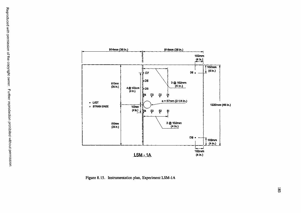
■oIc8Û .
■oCD
C/)Wo'3
3"CD
8■av<ë '
3CD
Cp.
CD■oOQ .CQ
■oO
CDQ .
■oCD
C/)C/Î
9 1 4 m m (3 6 In.) 9 1 4 m m (3 6 In.)
1 0 2 m m
(4 In.)
1 0 2 m m (4 In .)
• 0 7
• 0 63 @ 1 0 2 m m
( 4 In .)810mm (24 In.) g 102mm
(4 In.)• 0 5
a = 5 7 m m (2 -1 /4 In .)LVDT
STRAIN GAGE1 2 2 0 m m (4 8 In .)102mm
(4 In.)
3 @ 1 0 2 m m ( 4 In .)
610mm (24 In.)
0 9 .1 0 2 m m
(4 In.)
1 0 2 m m
LSM -1A (4 in.)
Figure 8.15. Instrumentation plan. Experiment LSM-1 A
SS
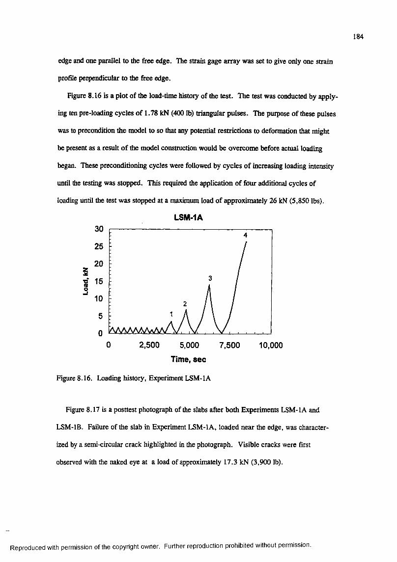
184
edge and one parallel to the free edge. The strain gage array was set to give only one strain
profile perpendicular to the free edge.
Figure 8.16 is a plot of the load-time history of the test. The test was conducted by apply
ing ten pre-loading cycles of 1.78 kN (400 lb) triangular pulses. The purpose of these pulses
was to precondition the model to so that any potential restrictions to deformation that might
be present as a result o f the model construction would be overcome before actual loading
began. These preconditioning cycles were followed by cycles of increasing loading intensity
until the testing was stopped. This required the application of four additional cycles of
loading until the test was stopped at a maximum load of approximately 26 kN (5,850 lbs).
LSM-1A
Q
30
25
20
15
10
5
00 2,500 5,000 7,500 10,000
Time, sec
Figure 8.16. Loading history. Experiment LSM-1 A
Figure 8.17 is a posttest photograph of the slabs after both Experiments LSM-1 A and
LSM-IB. Failure of the slab in Experiment LSM-IA, loaded near the edge, was character
ized by a semi-circular crack highlighted in the photograph. Visible cracks were first
observed with the naked eye at a load of approximately 17.3 kN (3,900 lb).
Reproduced with permission of the copyright owner. Further reproduction prohibited without permission.
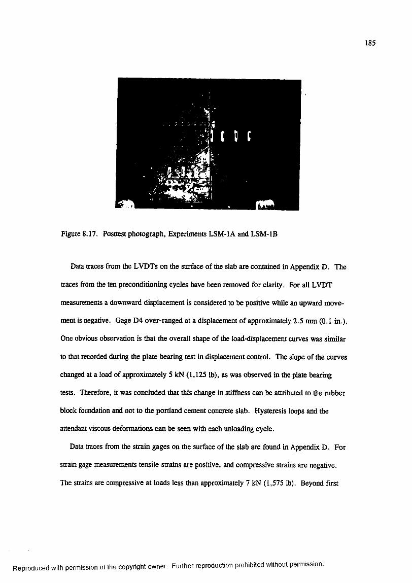
185
Figure 8.17. Posttest photograph. Experiments LSM-IA and LSM-IB
Data traces from the LVDTs on the surface of the slab are contained in Appendix D. The
traces from the ten preconditioning cycles have been removed for clarity. For all LVDT
measurements a downward displacement is considered to be positive while an upward move
ment is negative. Gage D4 over-ranged at a displacement of approximately 2.5 mm (0.1 in.).
One obvious observation is that the overall shape of the load-displacement curves was similar
to that recorded during the plate bearing test in displacement control. The slope of the curves
changed at a load of approximately 5 kN (1,125 lb), as was observed in the plate bearing
tests. Therefore, it was concluded that this change in stifkess can be attributed to the rubber
block foundation and not to the portland cement concrete slab. Hysteresis loops and the
attendant viscous deformations can be seen with each unloading cycle.
Data traces from the strain gages on the surface of the slab are found in Appendix D. For
strain gage measurements tensile strains are positive, and compressive strains are negative.
The strains are compressive at loads less than approximately 7 kN (1,575 lb). Beyond first
Reproduced with permission of the copyright owner. Further reproduction prohibited without permission.

186
cracking the gages nearest the edge of the slab (S4 and S3) reverse directions and go into the
tensile regime possibly indicating localized cracking.
In order to compare the data from this experiment with linear elastic calculations made
with a finite element code, it was desirable to correct the load-displacement data to remove
the nonlinear response of the rubber block. A technique similar to that used to correct for
nonlinear response in the plate bearing test was used to perform this correction. Figures 8.18
and 8.19 show the raw and corrected load-displacement curves for the third cycle of loading
for the LVDTs along a line perpendicular and parallel to the edge, respectively. The slopes of
the linear portions of the load-deflection curves (that portion of the curve above approxi
mately 5 kN (1,125 lb)) were determined numerically. The load-deflection curves were then
shifted to the right such that the extension of the linear portion of the curve would pass
through the origin as shown in Figures 8.18 and 8.19.
Deflection basins from the corrected load-deflection curves were then compared with
linear elastic finite element calculations made with ABAQUS using the S8R5 reduced
integration, second-order shell element. Initial calculations were made with the foundation
modulus of subgrade reaction set at k = 27, 54, 82, and 109 MPa/m (100, 200, 300, and
400 psi/in.). The ABAQUS deflection profiles at points identical to the locations of the
LVDTs along lines parallel and perpendicular to the edge were conçared with the experimen
tal deflection basin profiles.
Figure 8.20 shows a log-log plot obtained analytically of the modulus of subgrade reaction
versus deflection (w) at gage location D4 for a load of 6 kN (1,350 lb) from the ABAQUS
finite element calculations. This magnitude of load was chosen because it is midway between
the value at which the change in slope occurs in the response of the rubber foundation at 5 kN
(1,125 lb) and the load at which the onset of possible cracking occurred at 7 kN (1,575 lb).
Reproduced with permission of the copyright owner. Further reproduction prohibited without permission.
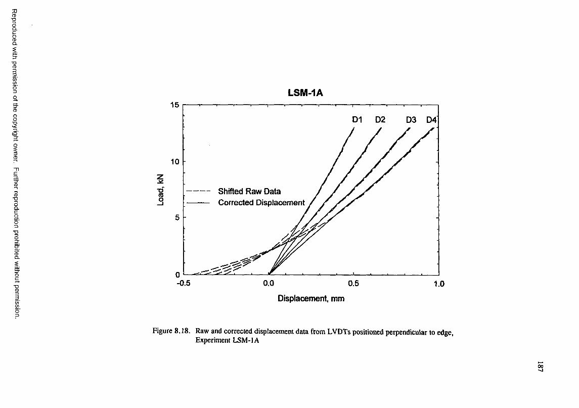
■oI sû .
■oCD
C/)
o'3
8■Ov<ë '
3CD
Cp.
CD■OOQ .C
aO3
■DO
CDQ .
■DCD
C/)C /)
LSM-1A15
D2 D3 D4
1Shifted Raw Data Corrected Displacement
-0.5 0.0 0.5 1.0
Displacement, mm
Figure 8.18. Raw and corrected displacement data from LVDTs positioned perpendicular to edge, Experiment LSM-IA
00
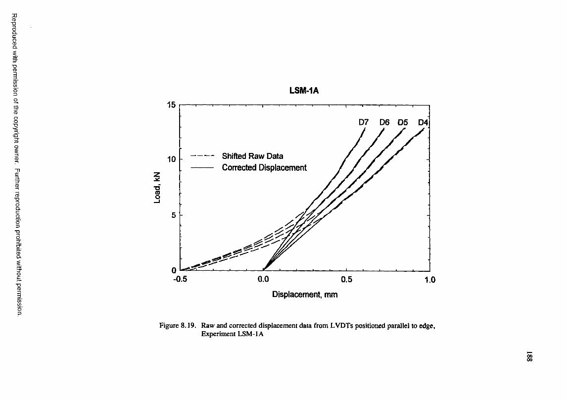
7JCD■DOQ .C
gQ .
■DCD
(/)(/)
CD
85cq'
3CD
C
CD■oOQ .CaO3■oO
&
oc%
C /)(go'3
1T3s
LSM-IA15
Shifted Raw Data Corrected Displacement
10
5
0-0.5 0.0 0.5
Displacement, mm
1.0
Figure 8.19. Raw and corrected displacement data from LVDTs positioned parallel to edge. Experiment LSM-IA
§s
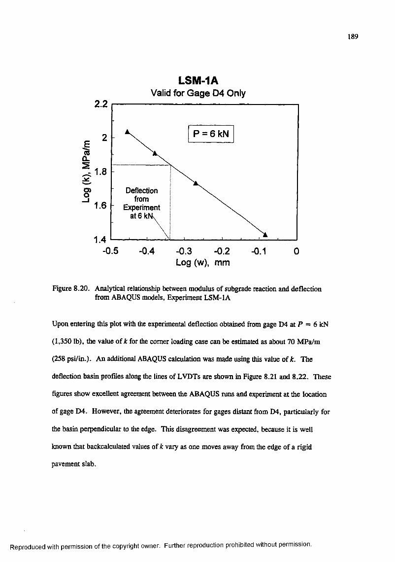
189
LSM-IAValid for Gage D4 Only
2.2
P = 6kN
IQ.5
Deflection from
Experiment a te klMv
g1.6
1.4-0.5 -0.4 -0.3 -0.2
Log (w), mm- 0.1
Figure 8.20. Analytical relationship between modulus of subgrade reaction and deflection from ABAQUS models, Experiment LSM-IA
Upon entering this plot with the experimental deflection obtained from gage D4 at P = 6 kN
(1,350 lb), the value of k for the comer loading case can be estimated as about 70 MPa/m
(258 psi/in.). An additional ABAQUS calculation was made using this value of k. The
deflection basin profiles along the lines of LVDTs are shown in Figure 8.21 and 8.22. These
figures show excellent agreement between the ABAQUS runs and experiment at the location
of gage D4. However, the agreement deteriorates for gages distant from D4, particularly for
the basin perpendicular to the edge. This disagreement was expected, because it is well
known that backcalculated values of k vary as one moves away from the edge of a rigid
pavement slab.
Reproduced with permission of the copyright owner. Further reproduction prohibited without permission.
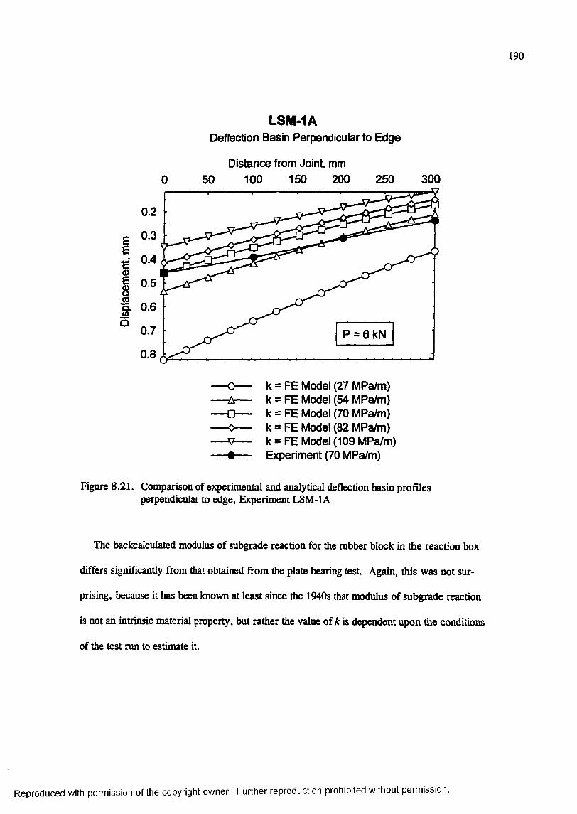
190
LSM-IADeflection Basin Perpendicular to Edge
Distance from Joint, mm 50 100 150 200 250 300
0.2
g 0.3
5 0.4
I “K . , P = 6kN
0.8
k = FE Model (27 MPa/m) k = FE Model (54 MPa/m) k = FE Model (70 MPa/m) k = FE Model (82 MPa/m) k= FE Model (109 MPa/m) Experiment (70 MPa/m)
Figure 8.21. Conçarison of experimental and analytical deflection basin profiles perpendicular to edge, Experiment LSM-IA
The backcalculated modulus of subgrade reaction for the rubber block in the reaction box
differs significantly from that obtained from the plate bearing test. Again, this was not sur
prising, because it has been known at least since the 1940s that modulus of subgrade reaction
is not an intrinsic material property, but rather the value of k is dependent upon the conditions
of the test run to estimate it.
Reproduced with permission of the copyright owner. Further reproduction prohibited without permission.
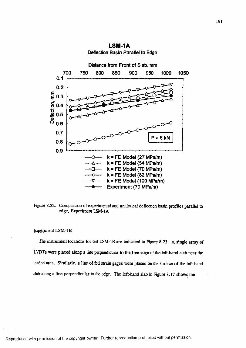
191
700
LSM-IADeflection Basin Parallel to Edge
Distance from Front of Slab, mm
750 800 850 900 950 1000 10500.1
0.2
E 0.3
o 0 .4
l o . S
0.6
0.7P = 6kN
0.8
0.9k = FE Model (27 MPa/m)k = FE Model (54 MPa/m) k = FE Model (70 MPa/m) k = FE Model (82 MPa/m) k = FE Model (109 MPa/m) Experiment (70 MPa/m)
Figure 8.22. Comparison of experimental and analytical deflection basin profiles parallel to edge. Experiment LSM-IA
Experiment LSM-IB
The instrument locations for test LSM-IB are indicated in Figure 8.23. A single array of
LVDTs were placed along a line perpendicular to the free edge of the left-hand slab near the
loaded area. Similarly, a line of foil strain gages were placed on the surface o f the left-hand
slab along a line perpendicular to the edge. The left-hand slab in Figure 8.17 shows the
Reproduced with permission of the copyright owner. Further reproduction prohibited without permission.
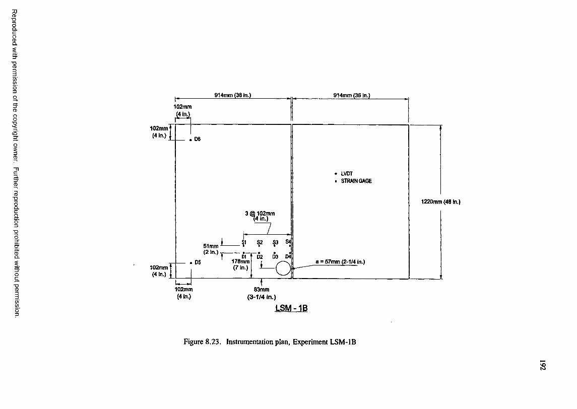
CD■DOQ .C
gQ .
■DCD
C/)C /)
CD
8
CD
3.3"CD
CD■DOQ .CaO3"OO
CDQ .
"DCD
C /)C /)
9 1 4 m m (3 6 In .) 9 1 4 m m (3 6 In.)
1 0 2 m m
1 0 2 m m (4 In .)
LVDT
STRAIN GAGE
1 2 2 0 m m (4 8 In.)
! 1 0 2 m m 4 in .)
5 1 m m (2 in .)
1 7 8 m m ( 7 In .)
a = 5 7 m m (2 -1 /4 In .)1 0 2 m m
(4 In.)
1 0 2 m m 8 3 m m(4 In.) ( 3 - 1 /4 in .)
LSM- IB
Figure 8.23. Instrumentation plan, Experiment LSM-IB
S
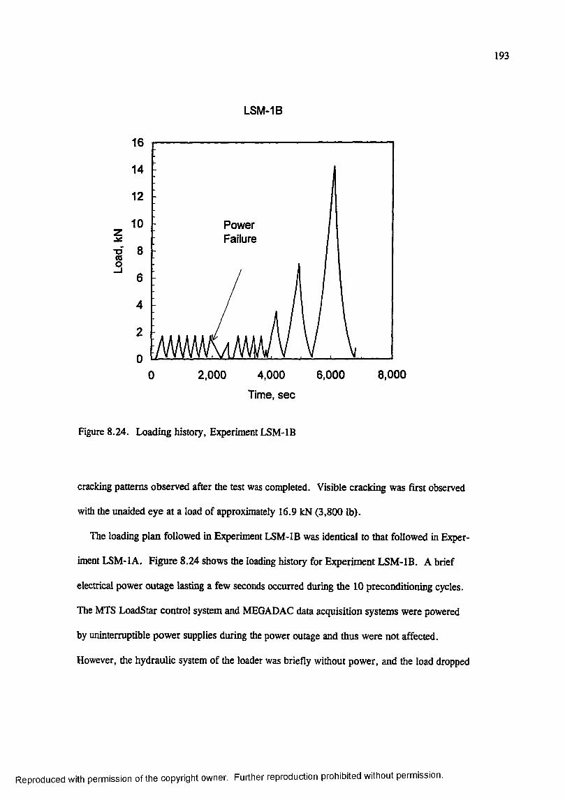
193
LSM-1 B
1■o'§
16
14
1 2
1 0 PowerFailure
8
6
4
2
0
8,0002,000 4,000 6,0000
Time, sec
Figure 8.24. Loading history, Experiment LSM-IB
cracking patterns observed after the test was completed. Visible cracking was first observed
with the unaided eye at a load of approximately 16.9 kN (3,800 lb).
The loading plan followed in Experiment LSM-IB was identical to that followed in Exper
iment LSM-IA. Figure 8.24 shows the loading history for Experiment LSM-IB. A brief
electrical power outage lasting a few seconds occurred during the 10 preconditioning cycles.
The MTS LoadStar control system and MEGADAC data acquisition systems were powered
by uninterruptible power supplies during the power outage and thus were not affected.
However, the hydraulic system of the loader was briefly without power, and the load dropped
Reproduced with permission of the copyright owner. Further reproduction prohibited without permission.

194
off until power was restored. At this point the control system reassumed control of the
loader, and the test was continued.
The load-deflection traces from the LVDTs are presented in Appendix D. The trends
observed in these traces are similar to those discussed for E^qperiment LSM-IA.
The plots from the strain gages are also presented in Appendix D. These data traces show
that the strain gages on the top surface of the slab registered tensile strains. Even though the
crack passed close to Gage SI, the occurrence of the cracking cannot be discerned in the
strain gage traces.
The load-deflection curves from LSM-IB were corrected for the nonlinear response of the
mbber foundation in the manner described for Experiment LSM-IA. The shifted raw data
traces along with the corrected data are presented in Figure 8.25. Deflection basins from the
corrected load-deflection curves were then compared with linear elastic finite element
calculations made with ABAQUS using the S8R5 reduced integration, second-order shell
elements. Again, initial calculations were made with the modulus of subgrade reaction set at
k = 27, 54, 82, and 109 MPa/m (100, 200, 300, and 400 psi/in.). The ABAQUS deflection
profiles at points identical to the locations of the LVDTs along were conq>ared with the
experimental deflection basin profile.
Figure 8.26 shows a log-log plot obtained analytically of the modulus of subgrade reaction
versus deflection (w) at gage location D4 for a load of 6.1 kN (1,370 lb) from the ABAQUS
finite element calculations. Entering this plot with the e;q)erimental deflection obtained from
gage D4 at P = 6.1 kN (1,370 lb), the value of k can be estimated as about 90 MPa/m
(330 psi/in.). An additional ABAQUS calculation was made using this value of k. The
deflection basin profiles along the line of LVDTs are shown in Figure 8.27. As was the case
Reproduced with permission of the copyright owner. Further reproduction prohibited without permission.
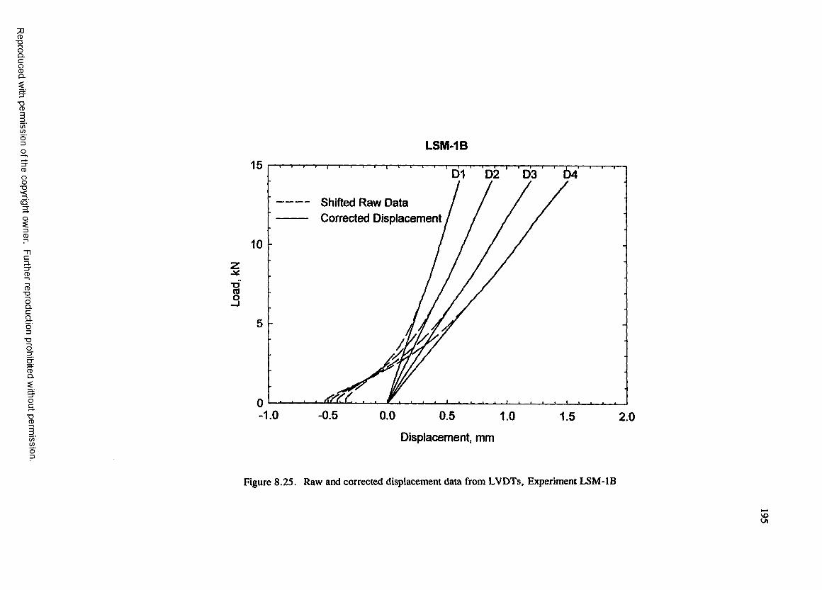
■ooû .cgQ .
■OCD
C /iWo’3O5CD
85(Q '
O
3.3"CD
CD■DOQ .Cg.o3"OO
LSM-IB
&
OC
■oCD
C/)(go'3
15D2 D3
Shifted Raw Data Corrected Displacement
1 0
5
0 L- - 1.0 -0.5 0.0 0.5 1.0 1.5 2.0
Displacement, mm
Figure 8.25. Raw and corrected displacement data from LVDTs, Experiment LSM-IB
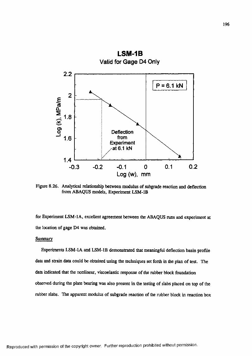
196
LSM-1 BValid for Gage D4 Only
(00 .5
O)o
2.2
P = 6.1 kN2
1.8
Deflection from
Experiment / a t 6.1 kN
1.6
1.40.20.10-0.3 - 0.2 - 0.1
Log (w), mm
Figure 8.26. Analytical relationship between modulus of subgrade reaction and deflection from ABAQUS models. Experiment LSM-IB
for Experiment LSM-IA, excellent agreement between the ABAQUS runs and experiment at
the location of gage D4 was obtained.
Summary
Experiments LSM-IA and LSM-IB demonstrated that meaningful deflection basin profile
data and strain data could be obtained using the techniques set forth in the plan of test. The
data indicated that the nonlinear, viscoelastic response of the mbber block foundation
observed during the plate bearing was also present in the testing of slabs placed on top of the
mbber slabs. The apparent modulus of subgrade reaction of the mbber block in reaction box
Reproduced with permission of the copyright owner. Further reproduction prohibited without permission.
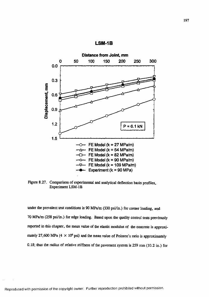
197
LSM-IB
Distance from Joint, mm50 100 150 200 250 300
0.0
0.3
II 0.6
I 0.9.2O
1 .2 P = 6.1 kN
1.5FE Model (k = 27 MPa/m) FE Model (k = 54 MPa/m) FE Model (k = 82 MPa/m) FE Model (k = 90 MPa/m) FE Model (k = 109 MPa/m) Experiment (k = 90 MPa)
Figure 8.27. Comparison of experimental and analytical deflection basin profiles. Experiment LSM-IB
under the prevalent test conditions is 90 MPa/m (330 psi/in.) for comer loading, and
70 MPa/m (258 psi/in.) for edge loading. Based upon the quality control tests previously
reported in this chapter, the mean value of the elastic modulus of the concrete is approxi
mately 27,600 MPa (4 x 10® psi) and the mean value of Poisson’s ratio is approximately
0.18; thus the radius of relative stiffness of the pavement system is 259 mm ( 1 0 .2 in.) for
Reproduced with permission of the copyright owner. Further reproduction prohibited without permission.
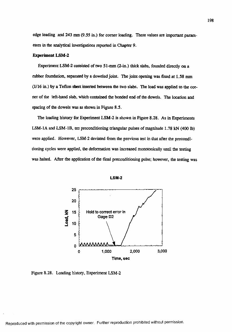
198
edge loading and 243 nun (9.55 in.) for comer loading. These values are important param
eters in the analytical investigations reported in Chapter 9.
Experiment LSM-2
Experiment LSM-2 consisted of two 51-mm (2-in.) thick slabs, founded directly on a
rubber foundation, separated by a doweled joint. The joint opening was fixed at 1.58 mm
(1/16 in.) by a Teflon sheet inserted between the two slabs. The load was applied to the cor
ner of the left-hand slab, which contained the bonded end of the dowels. The location and
spacing of the dowels was as shown in Figure 8.5.
The loading history for Experiment LSM-2 is shown in Figure 8.28. As in Experiments
LSM-IA and LSM-IB, ten preconditioning triangular pulses of magnitude 1.78 kN (400 lb)
were applied. However, LSM-2 deviated from the previous test in that after the precondi
tioning cycles were applied, the deformation was increased monotonically until the testing
was halted. After the application of the final preconditioning pulse; however, the testing was
LSM-2
25
20
i 15
19 10
Hold to correct error in Gage D2
AAAAAAAAAA-JL1,000 2,000
Time, sec
3,000
Figure 8.28. Loading history. Experiment LSM-2
Reproduced with permission of the copyright owner. Further reproduction prohibited without permission.

199
paused briefly to correct an error in one of the LVDTs. After this error was corrected, the
testing was resumed.
The instrumentation plan for E}q)eriment LSM-2 is presented in Figure 8.29. This is the
instrumentation plan which would be adhered to for the remainder of the experimental pro
gram. A line of LVDTs spanned across the joint to capture the deflection basin profile.
Also, a line of strain gages were placed on the top surface of the slabs.
A posttest photograph of the top surface of the slabs is shown in Figure 8.30. The crack
ing highlighted on the left (loaded) slab was first observed at a load of approximately 17 kN
(3,800 lb); while the cracking on the unloaded side was first observed at a load of approxi
mately 19.1 kN (4,3(X) lb). A series of three photographs taken through the transparent
window in the side of the reaction box is shown in Figure 8.31. The faint grids in the fore
ground of the photographs are spaced at 12.7 ram (‘A in.). As the load is increased from
zero to 13.3 kN (3,000 lb), the deflection of the top surface of the slabs is evident. Also note
that no visible cracking can be noted in sides of the slabs at 13.3 kN (3,000 lb). However,
once the load had increased to 17.8 kN (4,000 lb), a vertical crack was clearly visible directly
beneath the loaded area in the left slab. Also, a crack which runs more or less horizontally
from the Joint is visible in the right (unloaded) slab. A posttest examination of the crack
revealed that it originated at the dowel directly opposite the center of the loaded area and ran
out and down toward the edge and base of the right slab.
The load-displacement traces from the array of LVDTs are presented in Appendix D. As
noted in the figure. Gage D4 was over-ranged at a load of approximately 23 kN (5,000 lb).
These traces indicate clear evidence of cracking at loads greater than approximately 10 kN
(2,350 lb). Selected deflection basin profiles are plotted in Figure 8.32. Highly nonlinear
Reproduced with permission of the copyright owner. Further reproduction prohibited without permission.
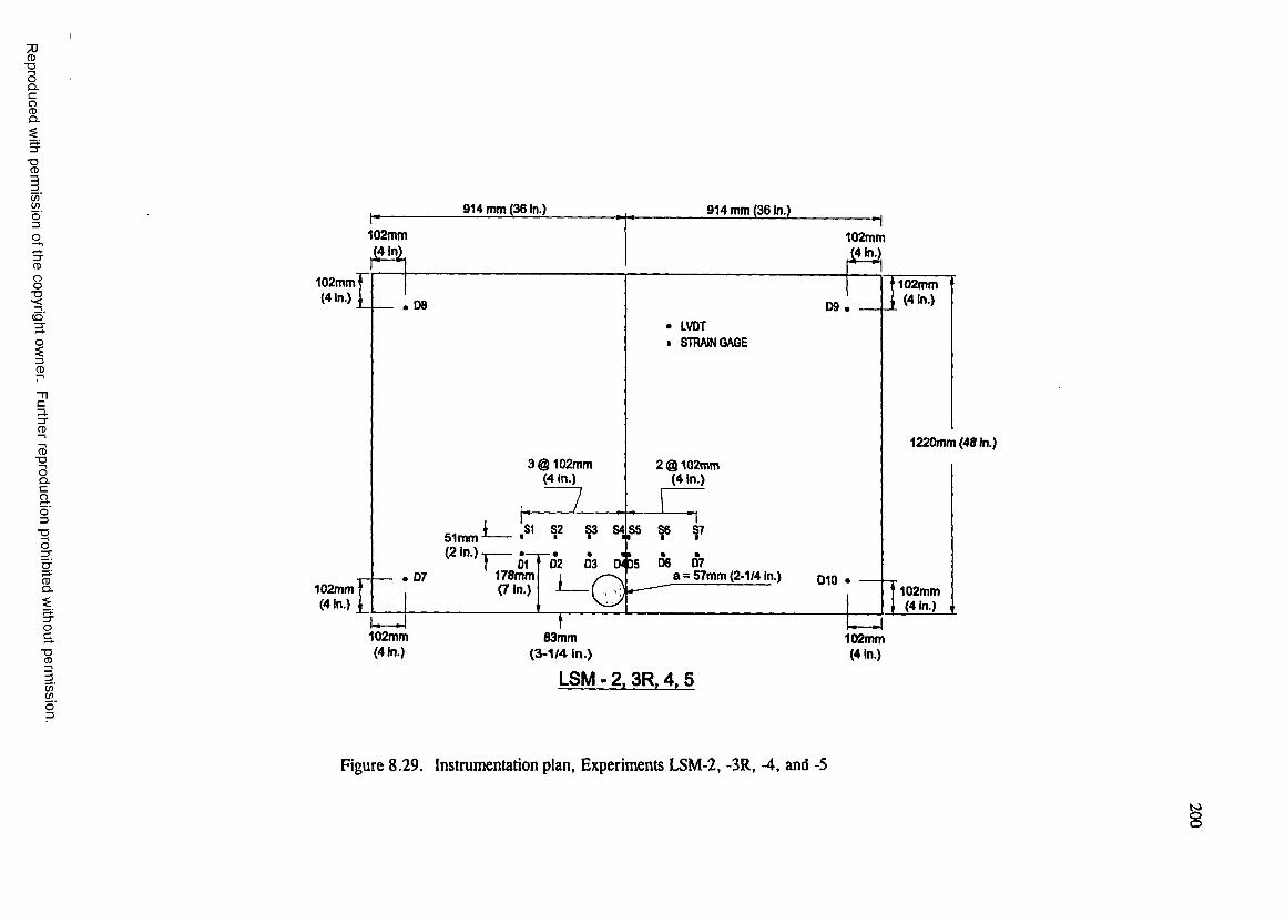
■ooQ .C
gQ .
■DCD
C /)Wo"3
5CD
8
CD
3.3"CD
CD■DOQ .C
aO3
■DO
CDQ .
OC
"8
(/)(go'3
9 1 4 m m (3 6 In, 9 1 4 m m (3 6 In .)
1 0 2 m m 1 0 2 m m
1 0 2 m m (4 In .)
1 0 2 m m( 4 l n . )
LVDT
STRAIN GAGE
1 2 2 0 m m (4 8 In .)
3 @ 1 0 2 m m (4 In .)
2 @ 1 0 2 m m ( 4 1 n . )
5 1 m m ( 2 in .)
1 7 8 m m( 7 l n . )
a = 5 7 m m (2 -1 /4 In .). 07 010 .1 0 2 m m
(4 In .)1 0 2 m m
(4 In .)
1 0 2 m m 8 3 m m 1 0 2 m m(4 In .) ( 3 - 1 /4 In .)
LSM-2. 3R.4 .5(4 In .)
Figure 8.29. Instrumentation plan, Experiments LSM-2, -3R, -4, and -5
w
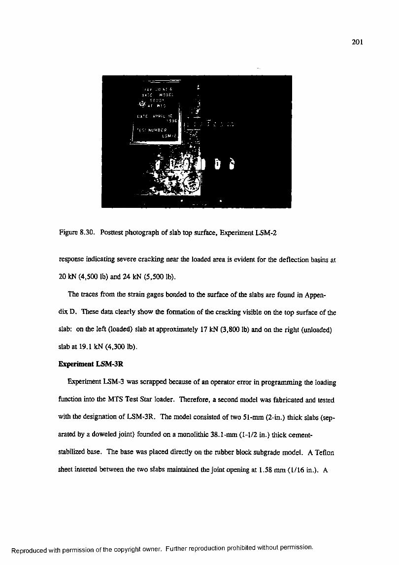
201
M I J O I N T &
û i o r H 0D £ L
CITC APP'L 1C '9 :T f S T N U M B E R
I 5M -2
Figure 8.30. Posttest photograph of slab top surface, Experiment LSM-2
response indicating severe cracking near the loaded area is evident for the deflection basins at
20 kN (4,500 lb) and 24 kN (5,500 lb).
The ttaces from the strain gages bonded to the surface of the slabs are found in Appen
dix D. These data clearly show the formation of the cracking visible on the top surface of the
slab: on the left (loaded) slab at approximately 17 kN (3,800 lb) and on the right (unloaded)
slab at 19.1 kN (4,300 lb).
Experiment LSM-3R
Experiment LSM-3 was scrapped because of an operator error in programming the loading
function into the MTS Test Star loader. Therefore, a second model was fabricated and tested
with the designation of LSM-3R. The model consisted of two 51-mm (2-in.) thick slabs (sep
arated by a doweled joint) founded on a monolithic 38.1-mm (1-1/2 in.) thick cement-
stabilized base. The base was placed directly on the rubber block subgrade model. A Teflon
sheet inserted between the two slabs maintained the joint opening at 1.58 mm (1/16 in.). A
Reproduced with permission of the copyright owner. Further reproduction prohibited without permission.
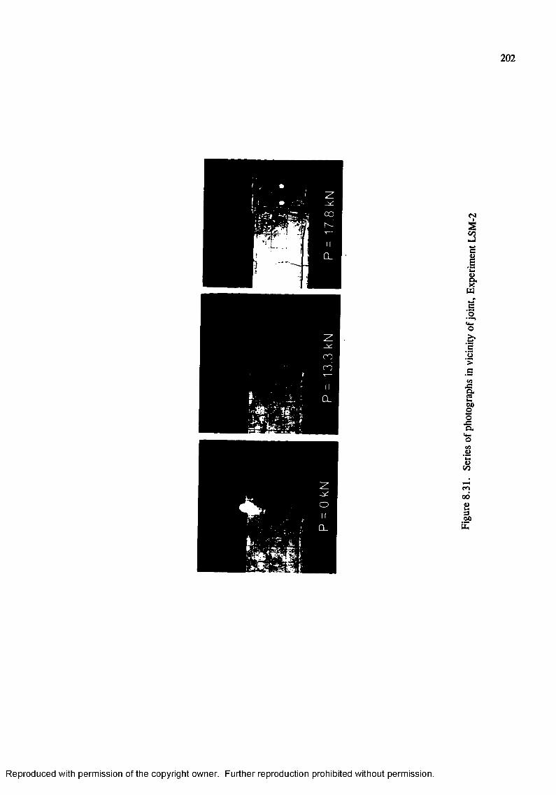
202
i
I; iO
■5.'y>ç
II■g.
s(%
en00
1k
Reproduced with permission of the copyright owner. Further reproduction prohibited without permission.
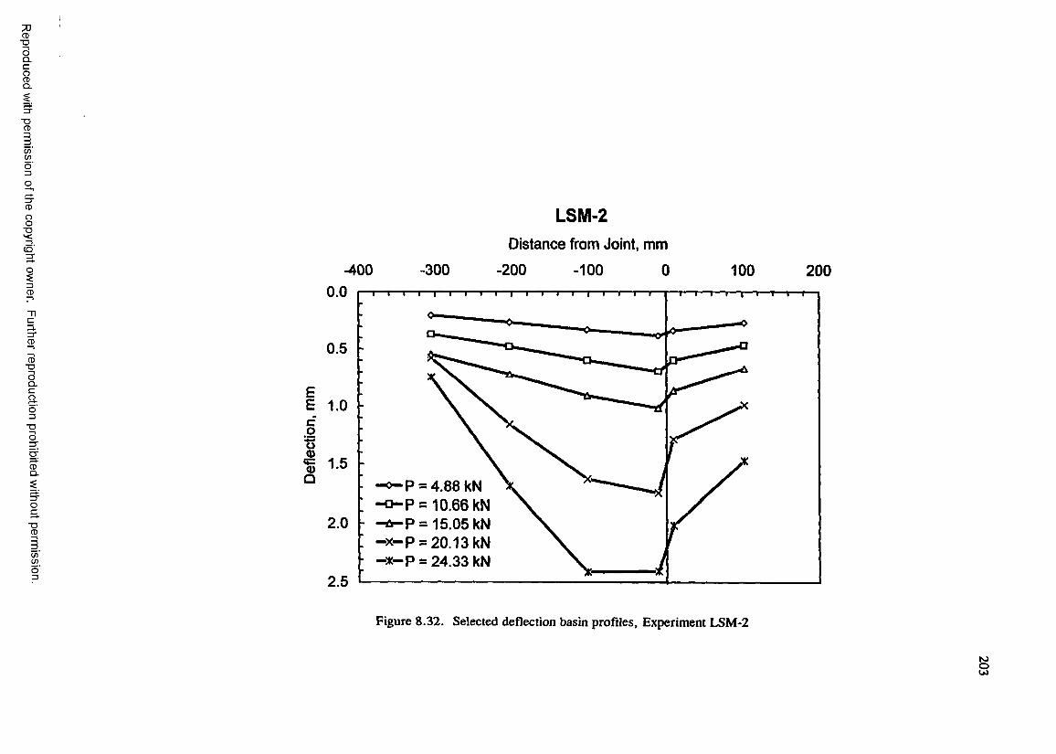
CD■DOQ .C
gQ .
"OCD
C /)Wo "3
8
CD
3.3"CD
CD■DOÛ .CaO3"OO
CDD .
■DCD
C /)(go "3
-400 -300
LSM-2Distance from Joint, mm
-200 -100 0 1 0 0 2 0 0
0.0
0.5
EEcQBQ>% 1.5 Q - o - P = 4.88 kN
- a - P = 10.66 kN - ^ P = 15.05 kN —X—P = 20.13 kN - x - P = 24.33 kN
2 .0
2.5
Figure 8.32. Selected deflection basin profiles, Experiment LSM-2
§
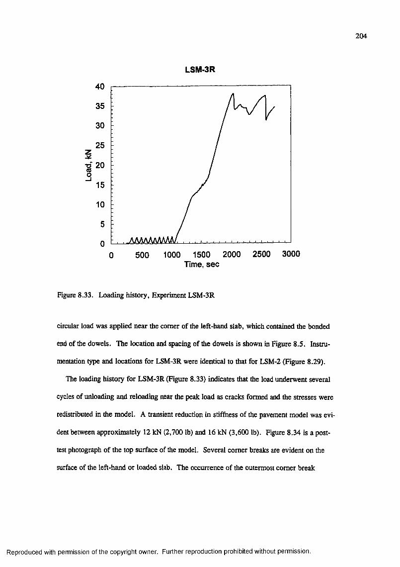
204
LSM-3R
1
(0Q
40
35
30
25
2 0
15
1 0
5
0
500 1000 1500 2000 2500 30000Time, s e c
Figure 8.33. Loading history. Experiment LSM-3R
circular load was applied near the comer of the left-hand slab, which contained the bonded
end of the dowels. The location and spacing of the dowels is shown in Figure 8.5. Instru
mentation type and locations for LSM-3R were identical to that for LSM-2 (Figure 8.29).
The loading history for LSM-3R (Figure 8.33) indicates that the load underwent several
cycles of unloading and reloading near the peak load as cracks formed and the stresses were
redistributed in the model. A transient reduction in stiffness of the pavement model was evi
dent between approximately 12 kN (2,700 lb) and 16 kN (3,600 lb). Figure 8.34 is a post
test photograph of the top surface of the model. Several comer breaks are evident on the
surface of the left-hand or loaded slab. The occurrence of the outermost comer break
Reproduced with permission of the copyright owner. Further reproduction prohibited without permission.
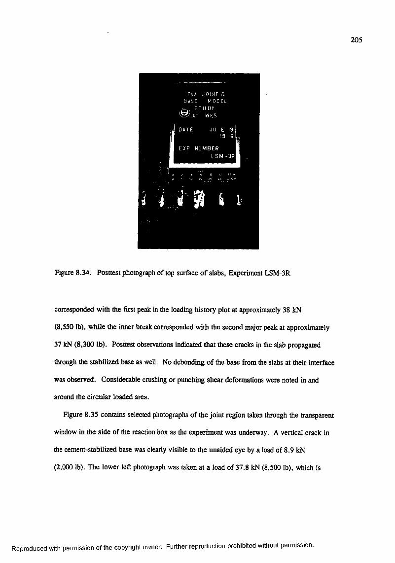
205
F A A J O I N T c. B A S F M O D E L
AT W E S
D A T E J U E 19 1 9 G
E X P N U M B E RL S M - 3 R
Figure 8.34. Posttest photograph of top surface of slabs. Experiment LSM-3R
corresponded with the first peak in the loading history plot at approximately 38 kN
(8,550 lb), while the inner break corresponded with the second major peak at approximately
37 kN (8,300 lb). Posttest observations indicated that these cracks in the slab propagated
through the stabilized base as well. No debonding of the base from the slabs at their interface
was observed. Considerable crushing or punching shear deformations were noted in and
around the circular loaded area.
Figure 8.35 contains selected photographs of the joint region taken through the transparent
window in the side of the reaction box as the experiment was underway. A vertical crack in
the cement-stabilized base was clearly visible to the unaided eye by a load of 8.9 kN
(2,000 lb). The lower left photograph was taken at a load of 37.8 kN (8,500 lb), which is
Reproduced with permission of the copyright owner. Further reproduction prohibited without permission.
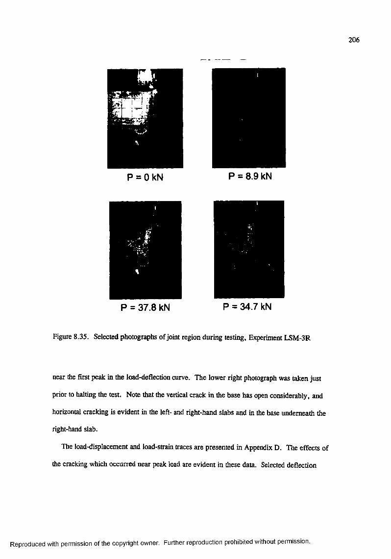
206
P = OkN P = 8.9 kN
P = 37.8 kN P = 34.7 kN
Figure 8.35. Selected photographs of joint region during testing, Experiment LSM-3R
near the first peak in the load-deflection curve. The lower right photograph was taken just
prior to halting the test. Note that the vertical crack in the base has open considerably, and
horizontal cracking is evident in the left- and right-hand slabs and in the base underneath the
right-hand slab.
The load-displacement and load-strain traces are presented in Appendix D. The effects of
the cracking which occurred near peak load are evident in these data. Selected deflection
Reproduced with permission of the copyright owner. Further reproduction prohibited without permission.
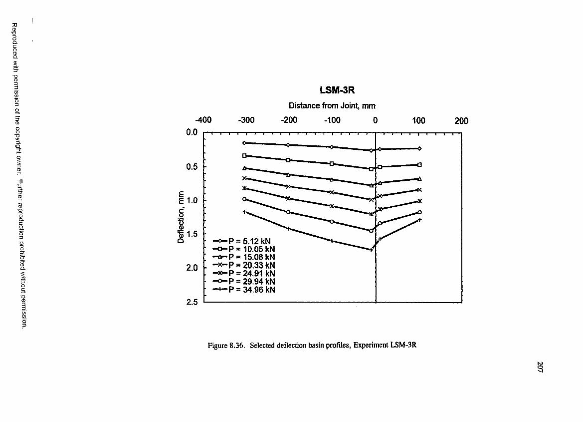
■ooQ .cgQ .
-oCD
C /)(/)
CD
8
( O '3"
3CD
C3-3"CD
CD■oICao3
■oo
&
oc■a
CD
-400 -300
LSM-3RDistance from Joint, mm
-200 -100 0 1 0 0 2000.0
-o0.5
E 1.0
1.5< ^ P = 5.12kN o - P = 10.05 kN ^ P = 15.08 kN ■x-p = 20.33 kN * - P = 24.91 kN o - P = 29.94 kN 4 - P = 34.96 kN
2.0
2.5C/)(/)
Figure 8,36. Selected deflection basin profiles. Experiment LSM-3R
§

208
basin profiles are plotted in Figure 8.36. Insight into the influence of the of the stabilized
base course on the post-cracking response of the slabs can be gained by comparing the
deflection basin profiles in Figure 8.36 with those from Experiment LSM-2 (Figure 8.32).
The basins fi-om Experiment LSM-2 (with no base course) are highly nonlinear after cracking
has occurred indicating the slab is tending to break apart under increasing loads. However,
for Experiment LSM-3R (with stabilized base), the post-cracking deflection basins do not
indicate that the slab response is nearly as nonlinear as that observed in Experiment LSM-2.
Experiment LSM-4
Two 51-mm (2-in.) thick slabs (separated by a doweled joint) founded on a 38.1-mm
(1-1/2 in.) thick cement-stabilized base were constructed and tested for Experiment LSM-4.
The base was divided into two equal halves by a cold joint discontinuity directly beneath the
slab construction joint. The base was founded directly on the rubber block subgrade model.
A Teflon sheet inserted between the two slabs maintained the slab joint opening at 1.58 mm
(1/16 in.). A circular load was applied near the comer of the left-hand slab, which contained
the bonded end o f the dowels. The location and spacing of the dowels is shown in Fig
ure 8.5. Instrumentation type and locations for LSM-4 were identical to that for LSM-2 and
LSM-3R (Figure 8.29).
The loading history for LSM-4 (Figure 8.37) is similar in form to that of LSM-3R. A
transient reduction in stiffness of the pavement model occurred in the vicinity of a load of
15 kN (3,400 lb). Figure 8.38 is a posttest photograph o f the top surface of the model. The
cracking highlighted in the photograph occurred on both the loaded and unloaded sides of the
joint and is nearly symmetrical about the joint. As was the case for Experiment LSM-3R, the
cracking pattern in the slabs was observed to be reflected in the base course as well. Again,
no debonding of the slab-base interface was observed.
Reproduced with permission of the copyright owner. Further reproduction prohibited without permission.
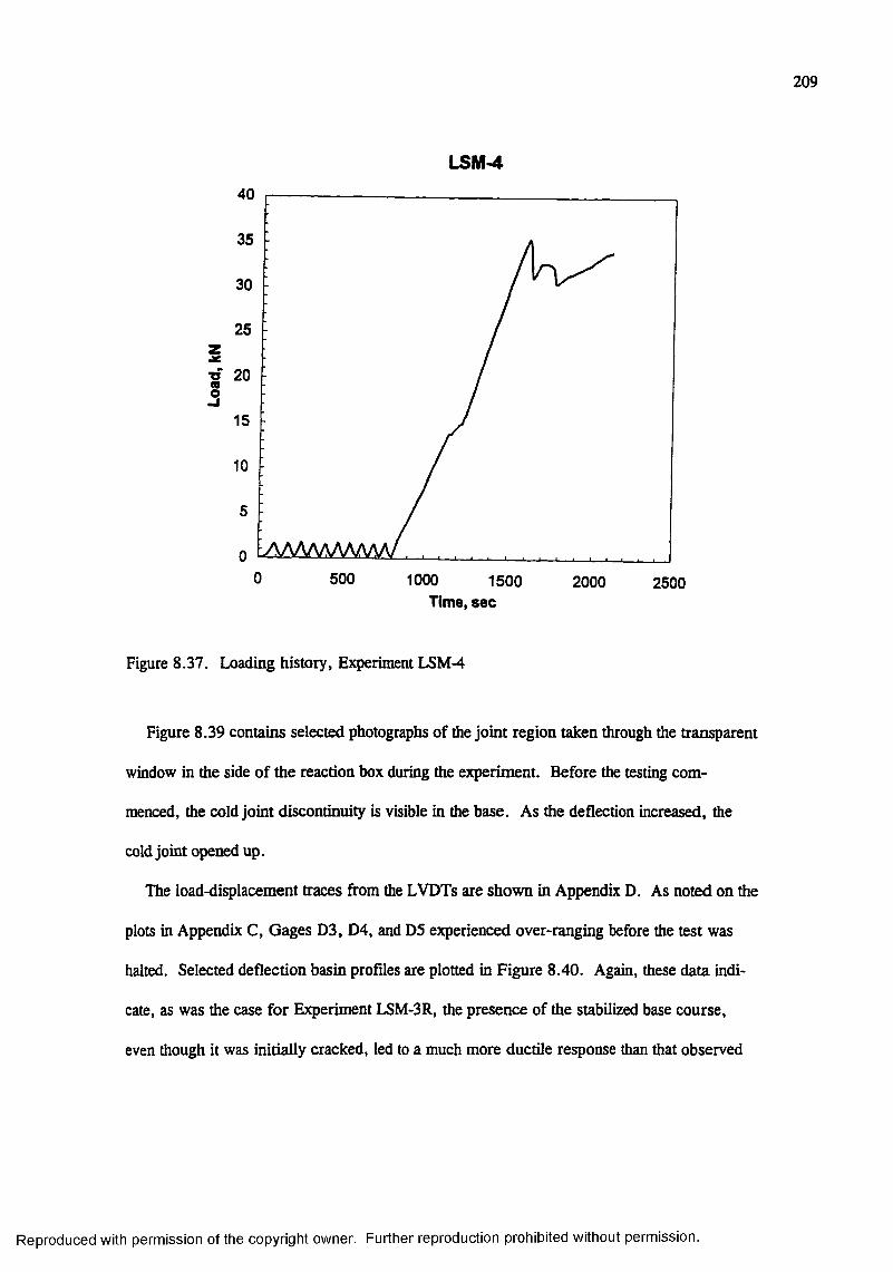
209
LSM-4
S
40
35
30
25
20
15
10
5
00 500 1000 1500 2000 2500
Time, sec
Figure 8.37. Loading history. Experiment LSM-4
Figure 8.39 contains selected photographs of the joint region taken through the transparent
window in the side of the reaction box during the experiment. Before the testing com
menced, the cold joint discontinuity is visible in the base. As the deflection increased, the
cold joint opened up.
The load-displacement traces from the LVDTs are shown in Appendix D. As noted on the
plots in Appendix C, Gages D3, D4, and D5 experienced over-ranging before the test was
halted. Selected deflection basin profiles are plotted in Figure 8.40. Again, these data indi
cate, as was the case for Experiment LSM-3R, the presence of the stabilized base course,
even though it was initially cracked, led to a much more ductile response than that observed
Reproduced with permission of the copyright owner. Further reproduction prohibited without permission.
210
F AA J O I N T & 3 A S E M O D E L
S T U D YAT W E G
E X P N U M B E R
L 5 3
Figure 8.38. Posttest photograph of top surface of slabs. Experiment LSM-4
for the slabs founded directly on the rubber pad (Experiment LSM-2). Strain gage traces are
also presented in Appendix D. Gage S5 failed during the test. It was postulated that the gage
was inadequately bonded to the slab.
Experiment LSM-5
A polyethylene-sand-polyethylene sandwich was constructed as a bond-breaking layer
between the two 51-mm (2-in.) thick slabs (separated by a doweled joint) and the 38.1-mm
(1-1/2 in.) thick cement-stabilized base for Experiment LSM-5. The monolithic base was
founded directly on the rubber block subgrade model. A Teflon sheet inserted between the
two slabs maintained the slab joint opening at 1.58 mm (1/16 in.). A circular load was
applied near the comer of the left-hand slab, which contained the bonded end of the dowels.
The location and spacing of the dowels is shown in Figure 8.5. Instrumentation type and
locations for LSM-5 were identical to that for LSM-2, LSM-3R, and LSM-4 (Figure 8.26).
Reproduced with permission of the copyright owner. Further reproduction prohibited without permission.
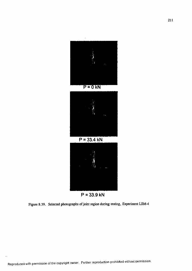
211
P = OkN
P = 33.4 kN
P = 33.9 kN
Figure 8.39. Selected photographs of joint region during testing. Experiment LSM-4
Reproduced with permission of the copyright owner. Further reproduction prohibited without permission.
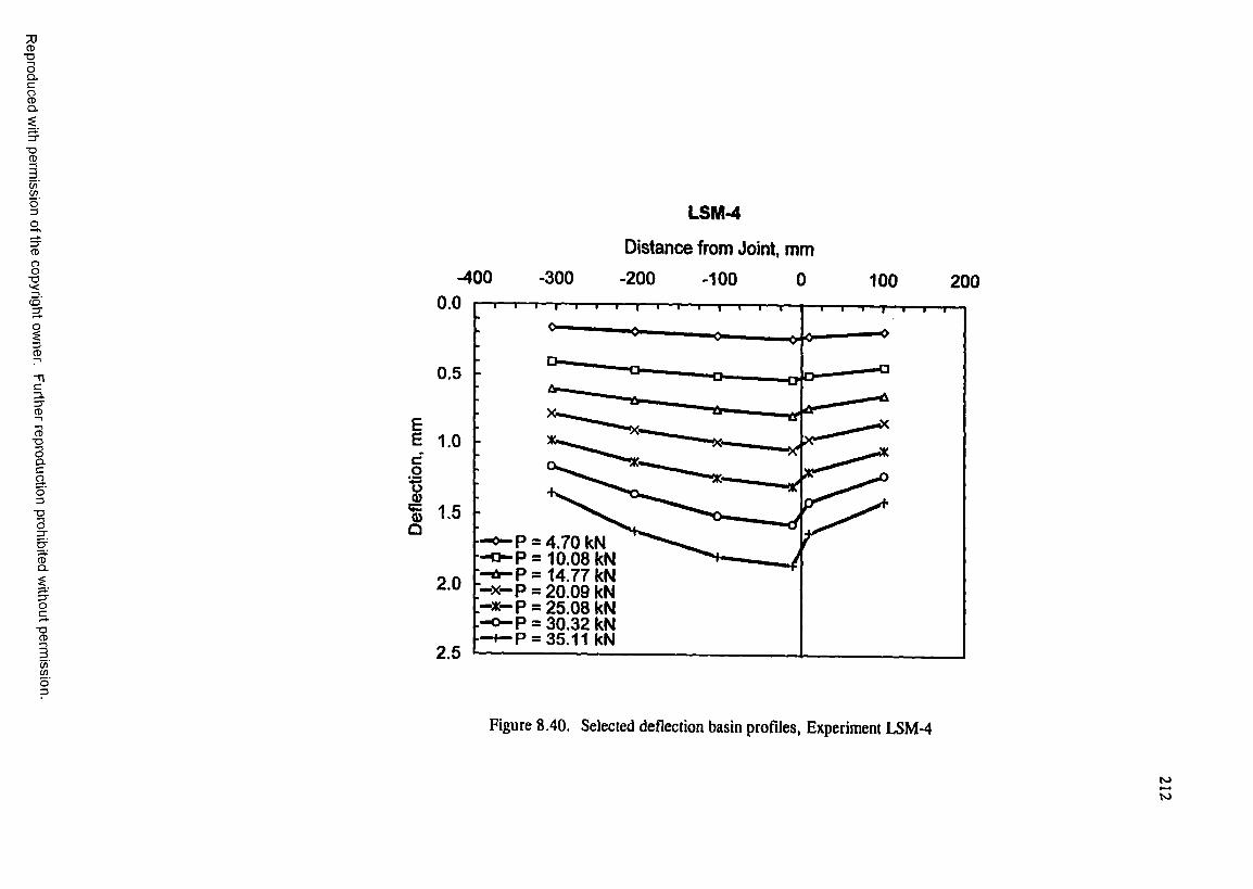
CD■DOQ .C
3Û .
■DCD
(/)(/)
Z3CD
C3.I TCD
CD■oICaO3■oO
&
oc■o
CD
(/)œd3
-400 -300
LSM-4
Distance from Joint, mm
-200 -100 0 100 2000.0
0.5
Ic0
1Q
“<*“ P = 4.70 kN - 0 - P = 10.08 kN -A r-P = 14.77 kN - x - p = 20.09 kN - x - P = 25.08 kN - o - p = 30.32 kN - + - P = 35.11 kN
2.0
2.5
Figure 8.40. Selected deflection basin profiles, Experiment LSM-4
N>N>
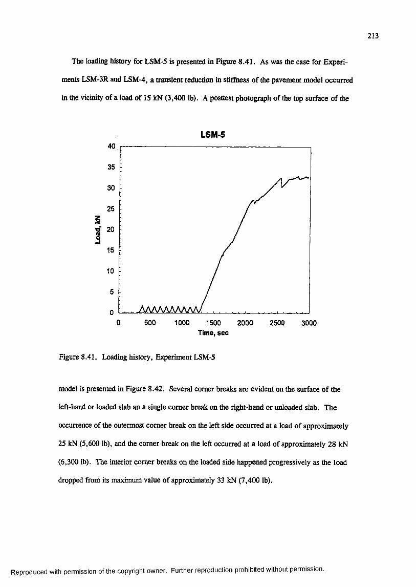
213
The loading history for LSM-5 is presented in Figure 8.41. As was the case for Experi
ments LSM-3R and LSM-4, a transient reduction in stiffness of the pavement model occurred
in the vicinity of a load of 15 kN (3,400 lb). A posttest photograph of the top surface of the
LSM-5
I
40
35
30
25
20
15
10
5
00 500 1000 2000 25001500 3000
Time, sec
Figure 8.41. Loading history. Experiment LSM-5
model is presented in Figure 8.42. Several comer breaks are evident on the surface of the
left-hand or loaded slab an a single comer break on the right-hand or unloaded slab. The
occurrence of the outermost comer break on the left side occurred at a load of approximately
25 kN (5,600 lb), and the comer break on the left occurred at a load of approximately 28 kN
(6,300 lb). The interior comer breaks on the loaded side happened progressively as the load
dropped from its maximum value of approximately 33 kN (7,400 lb).
Reproduced with permission of the copyright owner. Further reproduction prohibited without permission.
214
9ASL J:,, '- ' uc' k fll'
HfcTr MV<
[ I P N l MOF. pl : m - ' ,
C ÎÎ
Figure 8.42. Posttest photograph of top surface of slabs. Experiment LSM-5
Figure 8.43 contains selected photographs taken through the transparent window in the
side of the reaction box. Perhaps the most interesting observation from these photographs is
that no visible cracking was observed in the ceuient-stabiiized base. Based upon the results of
the previous experiments, it can be concluded that breaking the bond between the slabs and
base may reduce the potential for cracking beneath the surface joint.
The load-displacement and strain traces from the experiment are presented in Appendix D.
Gages D3, D4, and D5 experienced over-ranging before the test was halted. Selected deflec
tion basin profiles are plotted in Figure 8.44. It can be noted from Figure 8.44 that the
response was less ductile than that observed in Experiments LSM-3R and LSM-4 in which
bonding between the slabs and base was not prevented.
Reproduced with permission of the copyright owner. Further reproduction prohibited without permission.
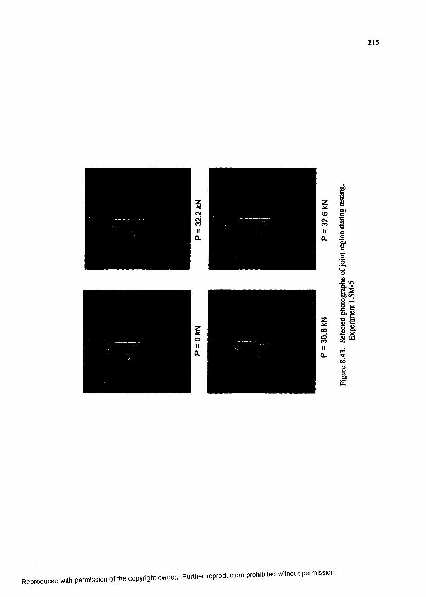
215
fï• i
II
U
Î 1
900K3)
Reproduced with perntissioh of the copyright ownec Further reproduction prohibited without permission.
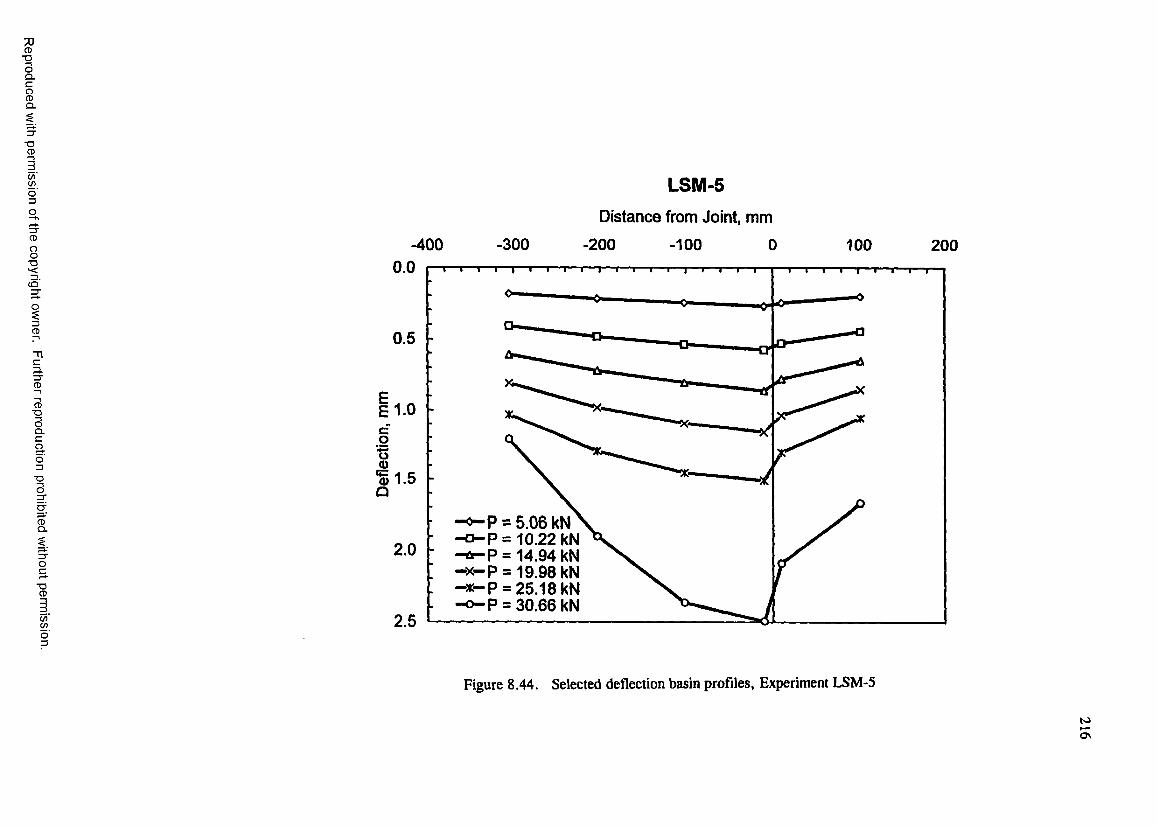
■ooQ .C
gQ .
■OCD
(/)(/)
8
3CD
3.3"CD
CD■OOÛ .C
aO3
■DO
CDQ .
■DCD
C/)(go"3
-400 -300
LSM-5Distance from Joint, mm
-200 -100 0 100 2000.0
0.6 -
E 1.0
= 5.06 kN o - p = 10.22 kN ^ P = 14.94 kN ■x-p = 19.98 kN •x-p = 25.18 kN o - P = 30.66 kN
2.0
2.5
Figure 8.44. Selected deflection basin profiles. Experiment LSM-5
N>ON
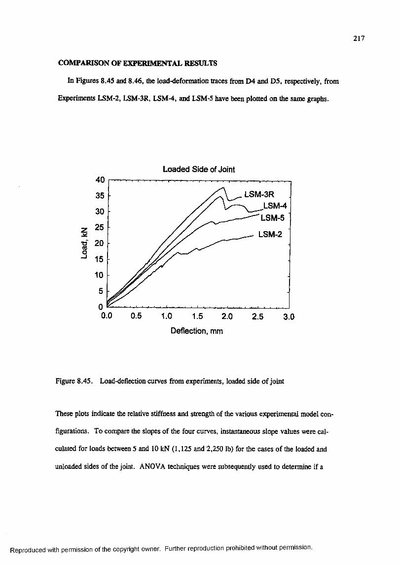
217
COMPARISON OF EXPERIMENTAL RESULTS
In Figures 8.45 and 8.46, the load-deformation traces from D4 and D5, respectively, from
Experiments LSM-2, LSM-3R, LSM-4, and LSM-5 have been plotted on the same graphs.
Loaded Side of Joint40
LSM-3R35,L8M -4LSM-5
30
25LSM-2
20
15
1 0
5
00.0 0.5 1.0 1.5 2.0 2.5 3.0
Deflection, mm
Figure 8.45. Load-deflection curves from experiments, loaded side of joint
These plots indicate the relative stiffness and strength of the various experimental model con
figurations. To compare the slopes of the four curves, instantaneous slope values were cal
culated for loads between 5 and 10 kN (1,125 and 2,250 lb) for the cases of the loaded and
unloaded sides of the Joint. ANOVA techniques were subsequently used to determine if a
Reproduced with permission of the copyright owner. Further reproduction prohibited without permission.
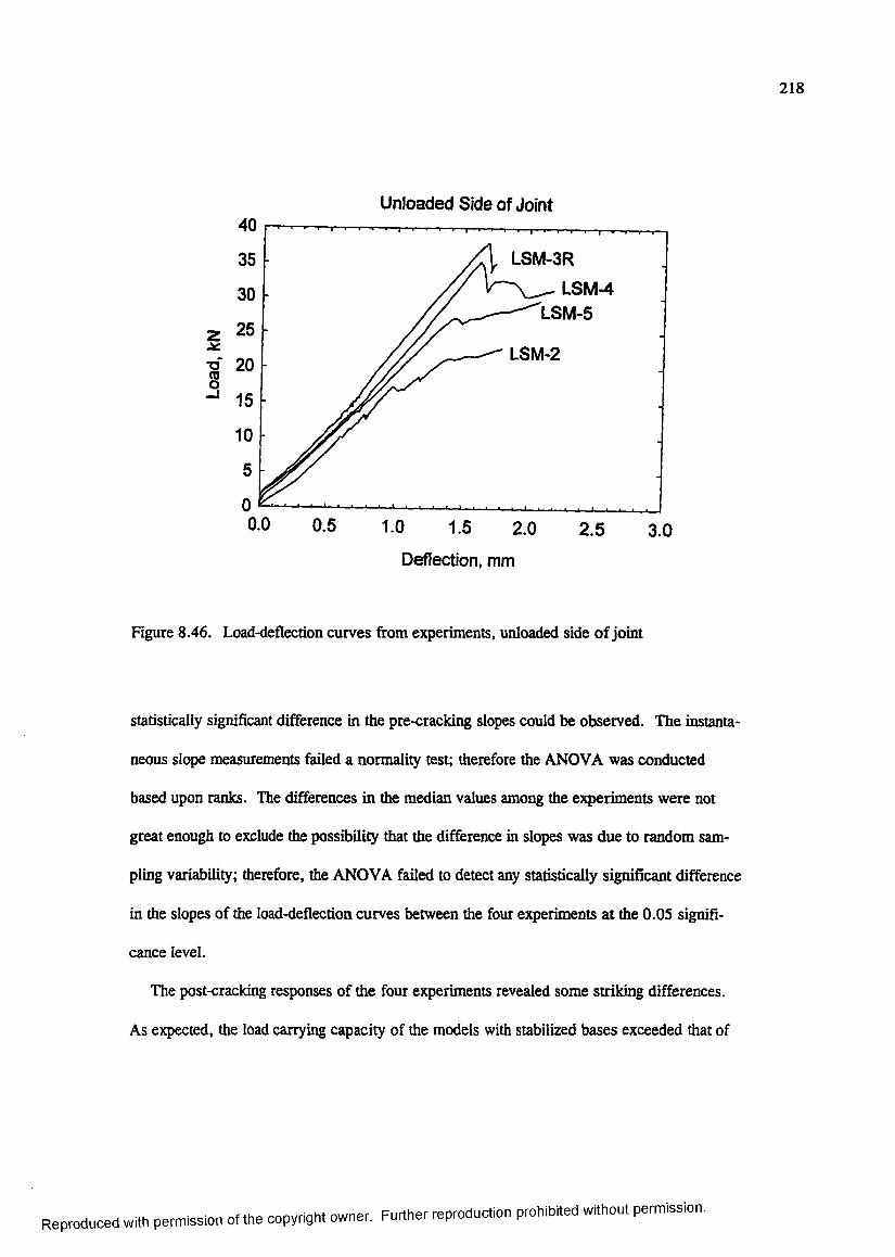
218
Unloaded Side of Joint
§
40
LSM-3R
^ LSM-4^ L S M - 5
35
30
25LSM-2
2 0
15
10
5
00.0 0.5 1.0 1.5 2.0 2.5 3.0
Deflection, mm
Figure 8.46. Load-deflection curves from experiments, unloaded side of joint
statistically significant difference in the pre-cracking slopes could be observed. The instanta
neous slope measurements failed a normality test; therefore the ANOVA was conducted
based upon ranks. The differences in the median values among the experiments were not
great enough to exclude the possibility that the difference in slopes was due to random sam
pling variability; therefore, the ANOVA failed to detect any statistically significant difference
in the slopes of the load-deflection curves between the four experiments at the 0.05 signifi
cance level.
The post-cracking responses of the four experiments revealed some striking differences.
As expected, the load carrying capacity of the models with stabilized bases exceeded that of
Reproduced with permission of the copyright owner. Further reproduction prohibited without permission.
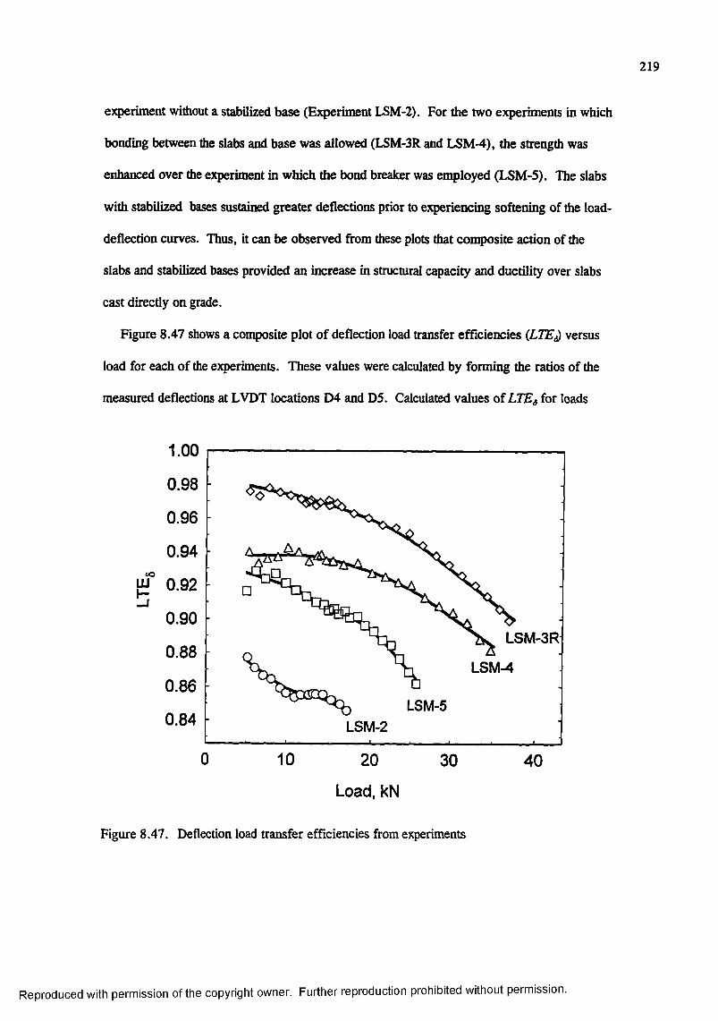
219
experiment without a stabilized base (Experiment LSM-2). For the two experiments in which
bonding between the slabs and base was allowed (LSM-3R and LSM-4), the strength was
enhanced over the experiment in which the bond breaker was employed (LSM-5). The slabs
with stabilized bases sustained greater deflections prior to experiencing softening of the load-
deflection curves. Thus, it can be observed from these plots that composite action of the
slabs and stabilized bases provided an increase in structural capacity and ductility over slabs
cast directly on grade.
Figure 8.47 shows a composite plot of deflection load transfer efficiencies (LTE^ versus
load for each of the experiments. These values were calculated by forming the ratios of the
measured deflections at LVDT locations D4 and D5. Calculated values of LTEg for loads
1.00
0.98
0.96
0.94
H I 0.92
0.90LSM-3R
0.88LSM-4
0.86LSM-5
0.84 LSM-2
0 10 20 30 40
Load, kN
Figure 8.47. Deflection load transfer efficiencies from experiments
Reproduced with permission of the copyright owner. Further reproduction prohibited without permission.
220
less than 5 kN (1,125 lb) were unreliable due to the small levels of deformation at low load
levels and due to seating of the slabs on the foundation. Thus, these measurements are not
plotted in Figure 8.47. Similarly, once the initial peak loads occurred (^ ic a lly associated
with visible cracking of the slabs), the calculated values of LTEg became unreliable.
Therefore, these values are also not plotted in Figure 8.47.
Several important observations can be made from Figure 8.47. First, it can be observed
that the greatest values of LTEg were obtaining from the slabs founding on the monolithic
stabilized base (LSM-3R), followed, in order, by slabs foimded on a cracked monolithic base,
foimded on a monolithic base with a bond breaker, and finally, founded directly on the rubber
pad. Secondly, each of the curves seem to have the same general shape indicating the maxi
mum load transfer efficiency occurred at low loads with decreasing effectiveness for increas
ing load. This phenomenon is likely caused by localized crushing of the slabs’ concrete in
the region of the dowels as the loads and resulting displacements increase. This crushing
occurs where high localized loads are being transferred from the concrete to the bars or visa
versa. This effect has been predicted by finite element modelers (Channakeshava, Barzegar,
and Voyiadjis 1993) and can also occur as the result of localized fatigue in pavement slabs
under the influence of repeated service loads.
The data in Figure 8.48 were used to evaluate the effectiveness of the structural steel
angles in restraining vertical translation of the ends of the slabs. These angles were placed on
the upper surface of the slabs in each experiment and bolted to the reaction box. Their pri
mary purpose was to prevent rigid body translation of the slabs due to the imposed comer
loading. LVDTs were installed at gage locations D7, D8 , D9, and DIO (Figure 8.29) to
monitor to vertical movements of the far comers of each slab.
Reproduced with permission of the copyright owner. Further reproduction prohibited without permission.

221
Data from Experiments LSM-2, LSM-3R, LSM-4, and LSM-5 are compared in Fig
ure 8.48. The upper plot shows the deflection at the gage locations D7 and D8 on the left
(loaded) slab, while the lower plot shows the deflections at gage locations D9 and DIO on the
right (unloaded) slab. The deflections shown in Figure 8.48 at a load of approximately
10 kN. In the case of Experiment LSM-2, very small movements either upward or down
ward were observed. However, downward displacements were observed at gage location D7
in Experiments LSM-3R, LSM-4, and LSM-5. For Experiment LSM-4 an upward displace
ment near the front of the right (unloaded) slab was observed at gage location DIO; however,
for all other experiments either very small displacements or downward displacements were
observed on the unloaded slab. Therefore, it can be concluded that the angles were margin
ally effective in preventing upward displacement of the slab comers. However, downward
deflections of the slab comers were commonly observed.
Certain observations from this experimental program point to some significant challenges
for modelers seeking to predict rigid pavement behavior and performance. Among these are
the following challenges:
• The presence of bonding between the slabs and base has an effect on the strength and
ductility of the rigid pavement stmcture. The concept of the composite or “top of the
base” modulus of subgrade reaction, which substitutes an inflated value of the sub
grade modulus to account for stabilized bases, ignores the composite action o f the
slab-stabilized base structural system. This concept, which was adopted out of neces
sity when the most reliable method of predicting rigid pavement behavior was the
Westergaard theory, should be abandoned in favor of a more realistic model that
explicitly includes the stmctural benefits of the stabilized base.
Reproduced with permission of the copyright owner. Further reproduction prohibited without permission.
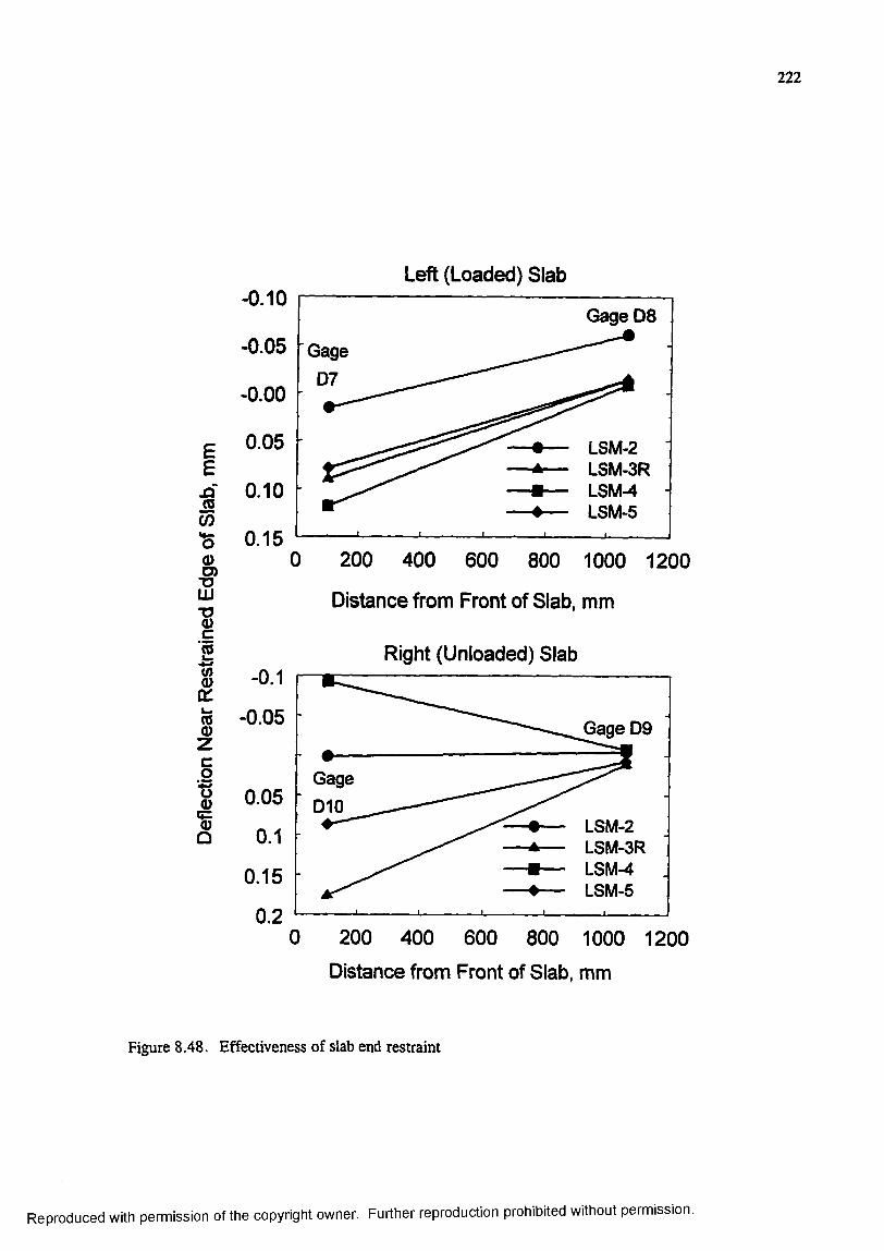
222
E£xT(0
CO*50
s
IIszCO■s0
%û
-0 .1 0
-0.05
- 0.00
0.05
0.10
0.15
Left (Loaded) Slab
G age D8
LSM-2LSM-3RLSM-4LSM-5
200 400 600 800 1000 1200
Distance from Front of Slab, mm
Right (Unloaded) Slab
LSM-2LSM-3RLSM-4LSM-5
200 400 600 800 1000 1200Distance from Front of Slab, mm
Figure 8.48. Effectiveness of slab end restraint
Reproduced with permission of the copyright owner. Further reproduction prohibited without permission.
223
• The presence and quali^ of stabilized base has an influence on the load transfer
effectiveness o f a rigid pavement joint. From the experimental data, it appears that a
monolithic stabilized base provides superior joint performance. However, field
observations by Grogan, Weiss, and Rollings (1996) at Dallas-Port Worth, Stapleton
(Denver), and Hartsfield (Atlanta) International Airports have indicated that the
majoriw of both the longitudinal and transverse cracking in cement stabilized bases
was found to occur under the joints in the rigid pavement surface. Thus, it may rea
sonably be expected that, for the majority of in-service rigid pavements, cracks are
present in the stabilized base in a pattern matching the jointing pattern of the slabs.
The net effect of this cracking is that the load transfer mechanism includes not only
the load transfer devices (dowels, aggregate interlock, key ways) in the slab, but also
some degree of load transfer due to aggregate interlock in the stabilized base. The
effectiveness of this aggregate interlock in the base is likely to depend upon the mag
nitude and cycles of loading, quality of the stabilized base materials, and moisture
and temperature (and attending volume changes) in the base.
• The presence and degree of bonding between the slabs and stabilized base course has
an influence on the structural capacity and load transfer capability of the rigid pave
ment structure. Research by Wesivich, McCullough, and Bums (1987) has shown
that the magnitude of friction between the slab and base is dependent upon bearing,
shear, and adhesion between the slab and base. They also concluded that if the adhe
sion is great enough, the failure plane will not be at the interface between the slab and
base, but rather within the base. Observations by Grogan, Weiss, and Rollings
(1996) indicated where slabs were being reconstructed at Hartsfield (Atlanta) Inter-
Reproduced with permission of the copyright owner. Further reproduction prohibited without permission.

224
national Airport that in some instances the cement stabilized base was adhered to the
slabs, while in other instances it was not.
The experiments conducted in this investigation conhrmed the observations and pre
dictions of other researchers that the effectiveness of the load transfer mechanism
decreases with localized damage in the immediate vicinity of the joint. This has sig
nificant in^lications in the modeling of the performance of rigid pavements. A non
linear model of decreasing Joint effectiveness with repetitions of load would be
necessary to model this aspect of rigid pavement performance. Additional testing and
research would be required to develop and calibrate such a model.
Reproduced with permission of the copyright owner. Further reproduction prohibited without permission.
CHAPTER 9: ANALYTICAL MODEL DEVELOPMENT AND VERIFICATION
ANALYTICAL MODEL DESCRIPTION
As described in Chapters 4 and S, most response models for rigid pavements, including
the Westergaard model and 2D finite element models, assume a single man-made layer rests
directly on a foundation that can be represented by a bed of springs. However, most modem
airport pavements are constructed on cement-stabilized bases that are of high quality and sub
stantial strength. The contribution of the base course to the strength of the pavement structure
is poorly understood. To account for the increased capaci^ of the foundation caused by a
stabilized layer, the modulus of subgrade reaction is increased in the Westergaard model.
This approach, in which the “top-of-the-base” modulus is determined empirically, is required
by the assumptions implied in the Westergaard solution. Similarly, 2D finite element plate
programs such as ILLI-SLAB may account for the stabilized layer by adding additional
stiffiiess to the plate elements based upon the concept of the transformed section.
The primary deficiency of these approaches is that neither directly addresses the influence
of the base course on the load transfer efficiency at a joint. In almost all instances stabilized
layers are constructed to be monolithic. However, field observations (Grogan, Weiss, and
Rollings, 1996) have indicated that cracks occur in the stabilized base in a pattern that directly
matches the jointing pattern in the surface layer. It is likely that some load transfer occurs
across these cracks by aggregate interlock.
As a part of the construction process, a bond breaker may be used between the surface
slabs and the base course; thus, it is possible that gaps may open between the slab and base
course. For those areas which remain in contact, shear stress may be transferred across the
225
Reproduced with permission of the copyright owner. Further reproduction prohibited without permission.

226
boundary by friction. In other cases, delamination of an initially bonded base course and slab
may occur from volume changes caused by moisture and tenqierature variations. In some
instances field investigations have indicated that délaminations have occurred, usually some
where beneath the interface between the slab and base course (Grogan, Weiss, and Rollings
1996). It is likely that shear stresses are transmitted across these delaminations by aggregate
interlock. It is also possible that gaps may form between the slabs and base. In order to
make a contribution to the state of the art in rigid pavement response modeling, these factors
must be considered.
Table 9.1 contains a matrix that summarizes these conditions and compares them to the
experiments described in Chapter 8 . To develop an analysis methodology that takes into con
sideration the influence of the stabilized base course on the joint response, a series of finite
element models were generated and executed. Figure 9.1 summarizes the cases described
and the model options chosen to represent the behavior of the major features of each case.
Table 9.1Considerations for Model Development
CaseAre base and slabs bonded?
Is base course cracked beneath slab joint?
Experiment Most Closely Matching Case
I No Base No Base LSM-2
n Yes No LSM-3R
m Yes Yes LSM-4
IV No No LSM-5
V No Yes Not in experimental matrix
A sample ABAQUS input file with explanatory comments is listed in Appendix E. The
slabs and base course continua were modeled by C3D27R reduced-integration Lagrangian
hexahedral elements. The joint between the slabs was modeled by JOINTC elements with
Reproduced with permission of the copyright owner. Further reproduction prohibited without permission.
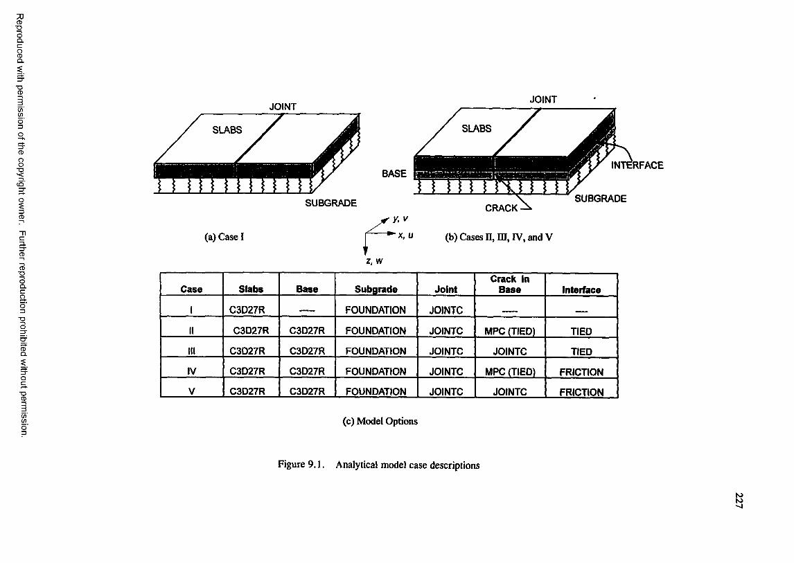
CD■DOQ .C
gQ .
■DCD
C /)Wo"303CD
8
ci'3"
13CD
"nc3.3"CD
CD■DOQ .CaO3
■DO
CDQ .
■DCD
(/)C/)
JOINT
SLABS
SUBGRADE
(a) Case I
JOINT
BASERFACE
SUBGRADECRACK
(b) Cases n, ffl, IV, andV
z, w
Case Slabs Base Subgrade JointCrack in
B ase Interface
1 C3D27R — ___ FOUNDATION JOINTC
II C3D27R C3D27R FOUNDATION JOINTC MPC (TIED) TIED
III C3D27R C3D27R FOUNDATION JOINTC JOINTC TIED
IV C3D27R C3D27R FOUNDATION JOINTC MPC (TIED) FRICTION
V C3D27R C3D27R FOUNDATION JOINTC JOINTC FRICTION
(c) Model Options
Figure 9 .1. Analytical model case descriptions
s
228
stiffnesses assigned in the z-direction direction only. Thus, the load transfer mechanism was
inçlicitly a shear only mechanism, with no load transfer due to bending. The interface
between the slabs and base course was modeled by the ABAQUS contact interaction feature.
Where the base and slabs were bonded (Cases n and ID), the “TIED” option was invoked to
force the displacements of all three degrees-of-freedom (n, v, and w) equal for all node pairs
across the interface. Where the slabs and base were not bonded (Cases IV and V), the
“FRICTION” option was used allow transfer of shear contact stresses across the interface.
For Cases O and IV in which the base course was not cracked, ABAQUS MFCs with the
“TIE” option invoked was used to set displacements («, v, and w) of corresponding node
pairs across the crack equal. Conversely, for Cases HI and V in which a crack was present
in the base course, JOINTC elements were employed to allow load transfer across to the
crack. Again, stif&iesses were assigned to the JOINTC elements in the z-direction only,
limiting them to load transfer due to shear only. For each of the cases, the subgrade was
modeled as a bed of springs using the ABAQUS “FOUNDATION” option. In all cases the
slabs and base were considered to be weightless.
ANALYTICAL MODEL RESULTS
Case I
The material and structural parameters from the experimental pavement models (siunma-
rized in Table 9.2) were used to develop the analytical model. Because of concerns about
execution times and memory requirements, a relatively coarse mesh (Figure 9.2) was
adopted. The aspect ratio for the elements in the plane of the slab surface were 1:1, while
the aspect ratio in the plane of the slab thickness was 4:1. The spring stiffnesses assigned to
the individual JOINTC elements were calculated from the data in Table 9.2 using Equa
tions 7.13 and 7.14. The loaded area was equal to that of the circular loaded area in the
Reproduced with permission of the copyright owner. Further reproduction prohibited without permission.
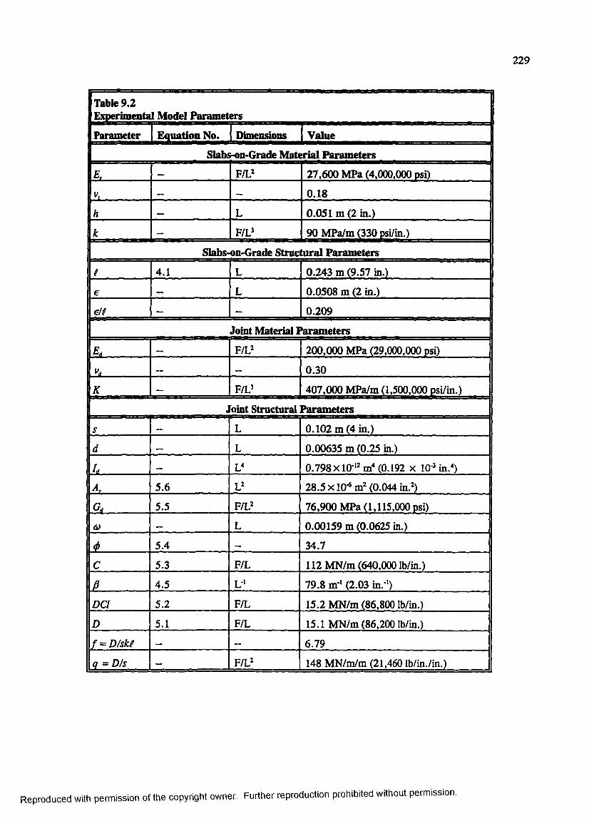
229
1 Table 9.21 Ebqierimentai Model Parameters
1 Parameter I Equation No. | Dimensions Value
1 Slabs-on-Grade Material Parameters—» F/L^ 27,600 MPa (4,000,000 psi)
r '— ___ 0.18
r 'h L 0.051 m (2 in.)
k — VU? 90 MPa/m (330 psi/in.)
Slabs-on-Grade Stnic tural Parameters
( 4.1 L 0.243 m (9.57 in.)
e L 0.0508 m (2 in.)
d l — — 0.209
Joint Material Param eters
E, — F/L^ 200,000 MPa (29,000,000 psi)
K, 0.30
K — F/U 407,000 MPa/m (1,500,000 psi/in.)
Joint Structural Param eters
s L 0.102 m (4 in.)
d L 0.00635 m (0.25 in.)
L _ _ V 0.798x10 " (0.192 x 10’ in.")
4 . . 5.6 V 28.5 X 10^ (0.044 in.^)
G. 5.5 ViV- 76,900 MPa (1,115,000 psi)
Û) L 0.00159 m (0.0625 in.)
<t> 5.4 — 34.7
C 5.3 F/L 112 MN/m (640,000 lb/in.)
0 4.5 L ' 79.8 m-‘ (2.03 in. ')
DC! 5.2 F/L 15.2 MN/m (86,800 lb/in.)
D 5.1 F/L 15.1 MN/m (86,200 lb/in.)
f = D/skf ___ 6.79
q = D/s — V/V 148 MN/m/m (21.460 Ib/in./in.)
Reproduced with permission of the copyright owner. Further reproduction prohibited without permission.
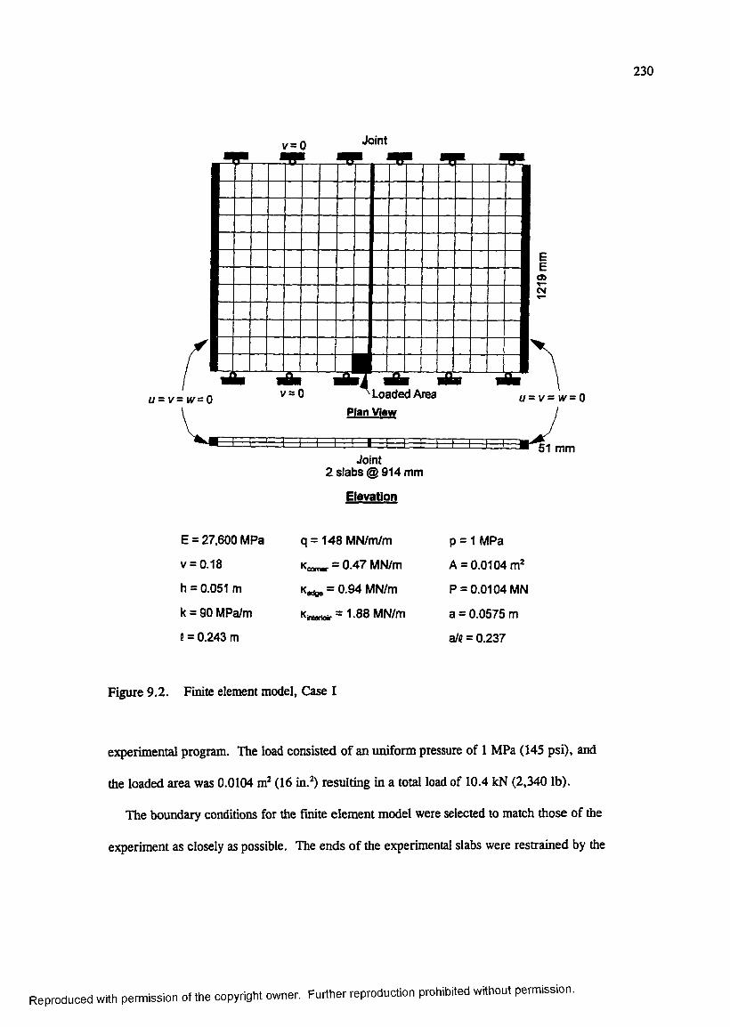
230
v= 0 Joint
v = 0 Loaded AreaPlan View
51 mmJoint
2 slabs @914 mm
Elevation
E = 27,600 MPa
v = 0.18
h = 0.051 m
k = 90 MPa/m
t = 0.243 m
q = 148 MN/m/m
= 0.47 MN/m
Kedge = 0.94 MN/m
= 1.88 MN/m
p = 1 MPa
A = 0.0104
P = 0.0104 MN
a = 0.0575 m
aJe = 0.237
Figure 9.2. Finite element model. Case I
experimental program. The load consisted of an uniform pressure of 1 MPa (145 psi), and
the loaded area was 0.0104 (16 in. > resulting in a total load of 10.4 kN (2,340 lb).
The boundary conditions for the finite element model were selected to match those of the
experiment as closely as possible. The ends of the experimental slabs were restrained by the
Reproduced with permission of the copyright owner. Further reproduction prohibited without permission.

231
stiff steel reaction box and by structural steel angles embedded in the top surface of each slab
and bolted to the reaction box. Thus, all three degrees of freedom were restrained {u = v = w
5 0) along these ends in the finite element model. The other sides of the experimental slabs
were prevented from deforming laterally by the steel reaction box. Therefore, in the finite
element model translation perpendicular to these sides of the box was restrained (v ^ 0 ).
Because the sides of the box were coated with a form-release agent prior to casting the slabs,
the other two degrees of freedom were not restrained.
The results from the finite element analysis was compared with results from Experiment
LSM-2. In order to directly compare the load-deflection results from the finite element
model to the experiment, the experimental load-deflection data were corrected to remove the
nonlinearity introduced by the rubber subgrade. This was accomplished in a manner identical
to that described in Chapter 8 for Experiments LSM-IA and LSM-IB. The original
experimental data along with the corrected experimental data (up to a load of 10 kN
(2,250 lb)) are shown in Figure 9.3. The resulting experimental deflection basin profiles at a
load of approximately 10 kN (2,250 lb) are shown in Figure 9.4 along with the deflection
basin profile from the finite element model. These data indicate that the finite element model
matches the corrected experimental data well.
Figure 9.5 shows a plot of LTEg (calculated as the ratio of LVDTs D5 and D4) as a func
tion of applied load. Superimposed on this data is the deflection load transfer efficiency
predicted at the location of LVDTs D5 and D4 by the finite element model. Again, the
agreement between the model and the experimental data is acceptable over the linear range of
response of the experimental slabs. At loads above approximately 17 kN (3,820 lb), signifi
cant cracking occurred in the experiment, thus changing the experimental boundary
conditions.
Reproduced with permission of the copyright owner. Further reproduction prohibited without permission.
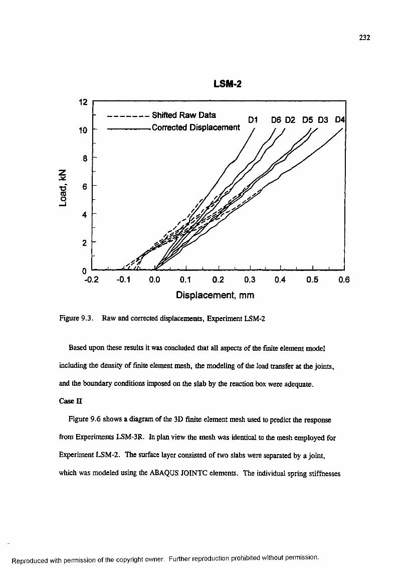
232
■a(0o
LSM-2
1 2
Shifted R aw D ata Corrected D isplacem ent
□6 02 05 03 041 0
8
6
4
2
0-0.2 -0.1 0.0 0.1 0.2 0.3 0.4 0.5 0.6
Displacement, mm
Figure 9.3. Raw and corrected displacements, Experiment LSM-2
Based upon these results it was concluded that all aspects of the finite element model
including the density of finite element mesh, the modeling of the load transfer at the joints,
and the boundary conditions imposed on the slab by the reaction box were adequate.
Case n
Figure 9.6 shows a diagram of the 3D finite element mesh used to predict the response
from Experiments LSM-3R. In plan view the mesh was identical to the mesh employed for
Experiment LSM-2. The surface layer consisted of two slabs were separated by a joint,
which was modeled using the ABAQUS JOINTC elements. The individual spring stiffnesses
Reproduced with permission of the copyright owner. Further reproduction prohibited without permission.
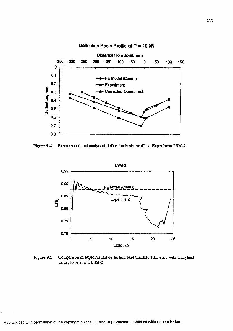
233
Deflection Basin Profile a t P - 10 kN
Distance from Joint, mm-350 -300 -250 -200 -150 -100 -50 0 50 100 150
0.1FE Model (Case I) Experiment Corrected Experiment
0.2
I 0.3c-9 0.4I 0.5
0.6
0.7
0.8
Figure 9.4. Experimental and analytical deflection basin profiles. Experiment LSM-2
LSM-20.95
0.90FE Moÿ!j_(C_ase J}
0.85ExperimentuT
50.80
0.75
0.7020 250 10 155
Load,kN
Figure 9.5 Comparison of experimental deflection load transfer efficiency with analytical value, Experiment LSM-2
Reproduced with permission of the copyright owner. Further reproduction prohibited without permission.
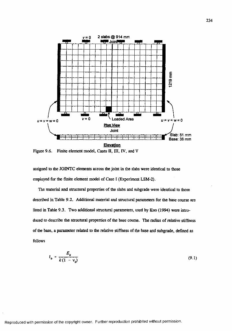
234
y = 0 2 slabs @ 914 mmJoinP^^
CM
Loaded Areau = v = w = 0Plan View
JointSlab: 51 mm Base: 38 mm
ElevationFigure 9.6. Finite element model, Cases n, HI, IV, and V
assigned to the JOINTC elements across the joint in the slabs were identical to those
employed for the finite element model of Case I (Experiment LSM-2).
The material and structural properties of the slabs and subgrade were identical to those
described in Table 9.2. Additional material and structural parameters for the base course are
listed in Table 9.3. Two additional structural parameters, used by Kuo (1994) were intro
duced to describe the structural properties of the base course. The radius of relative stiffness
of the base, a parameter related to the relative stiffness of the base and subgrade, defined as
follows
^ (1 - V*)(9.1)
Reproduced with permission of the copyright owner. Further reproduction prohibited without permission.
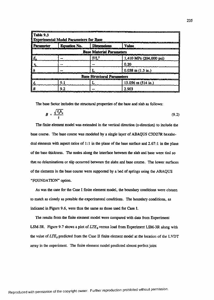
235
1 Table 9.31 Experimental Model Parameters for Base1 Parameter | Equation No. Dimensions Value1 Base Material Parameters
Eg — F IV 1,410 MPa (204,000 psi)— — 0.20
h — L 0.038 m (1.5 in.)Base Structural Parameters
4 9.1 L 13.056 m (514 in.)B 9.2 2.903
The base factor includes the structural properties of the base and slab as follows:
B = b"’b (9.2)
The finite element model was extended in the vertical direction (z-direction) to include the
base course. The base course was modeled by a single layer of ABAQUS C3D27R hexahe-
dral elements with aspect ratios of 1:1 in the plane of the base surface and 2.67:1 in the plane
of the base thickness. The nodes along the interface between the slab and base were tied so
that no delaminations or slip occurred between the slabs and base course. The lower surfaces
of the elements in the base course were supported by a bed of springs using the ABAQUS
“FOUNDATION” option.
As was the case for the Case I finite element model, the boundary conditions were chosen
to match as closely as possible the experimental conditions. The boundary conditions, as
indicated in Figure 9.6, were thus the same as those used for Case I.
The results from the finite element model were compared with data from Experiment
LSM-3R. Figure 9.7 shows a plot of LTE^ versus load from Experiment LSM-3R along with
the value of LTEg predicted from the Case II finite element model at the location of the LVDT
array in the experiment. The finite element model predicted almost perfect joint
Reproduced with permission o f the copyright owner. Further reproduction prohibited without permission.
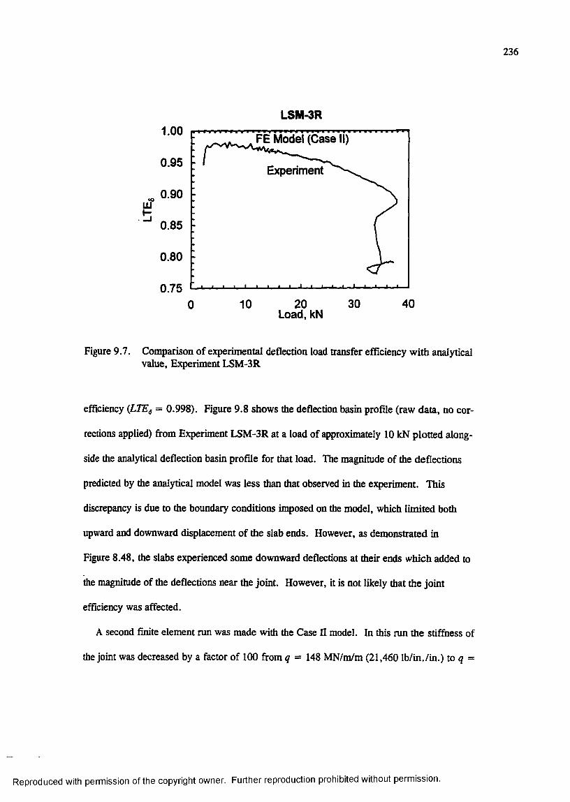
236
LSM-3R1.00
FE Model (Case II)
0.95Experiment
0.90
0.85
0.80
0.7530 401 0 2 00
Load, kN
Figure 9.7. Comparison of experimental deflection load transfer efficiency with analytical value. Experiment LSM-3R
efficiency (LTEg = 0.998). Figure 9.8 shows the deflection basin profile (raw data, no cor
rections applied) fi-om Experiment LSM-3R at a load of approximately 10 kN plotted along
side the analytical deflection basin profile for that load. The magnitude of the deflections
predicted by the analytical model was less than that observed in the experiment. This
discrepancy is due to the boundary conditions imposed on the model, which limited both
upward and downward displacement of the slab ends. However, as demonstrated in
Figure 8.48, the slabs experienced some downward deflections at their ends which added to
the magnitude of the deflections near the joint. However, it is not likely that the joint
efficiency was affected.
A second finite element run was made with the Case II model. In this run the stifftiess of
the joint was decreased by a factor of 1(K) from q = 148 MN/m/m (21,460 Ib/in./in.) to g =
Reproduced with permission of the copyright owner. Further reproduction prohibited without permission.
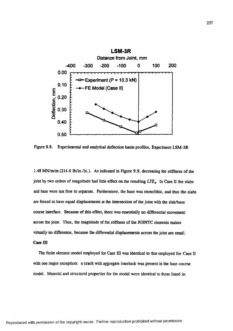
237
LSM-3RDistance from Joint, mm
-400 -300 -200 -100 0 100 200
EEco
Q
0.00Experiment (P = 10.3 kN)
- # - F E Mode! (C ase II)0.10
0.20
0.30
0.40
0.50
Figure 9.8. Experimental and analytical deflection basin profiles. Experiment LSM-3R
1.48 MN/m/m (214.6 Ib/in./in.). As indicated in Figure 9.9, decreasing the stif&ess of the
joint by two orders of magnitude had little effect on the resulting LTEg. In Case H the slabs
and base were not free to separate. Furthermore, the base was monolithic, and thus the slabs
are forced to have equal displacements at the intersection of the joint with the slab/base
course interface. Because of this effect, there was essentially no differential movement
across the joint. Thus, the magnitude of the stiffness of the JOINTC elements makes
virtually no difference, because the differential displacements across the joint are small.
Case m
The finite element model employed for Case HI was identical to that employed for Case II
with one major exception: a crack with aggregate interlock was present in the base course
model. Material and structural properties for the model were identical to those listed in
Reproduced with permission of the copyright owner. Further reproduction prohibited without permission.
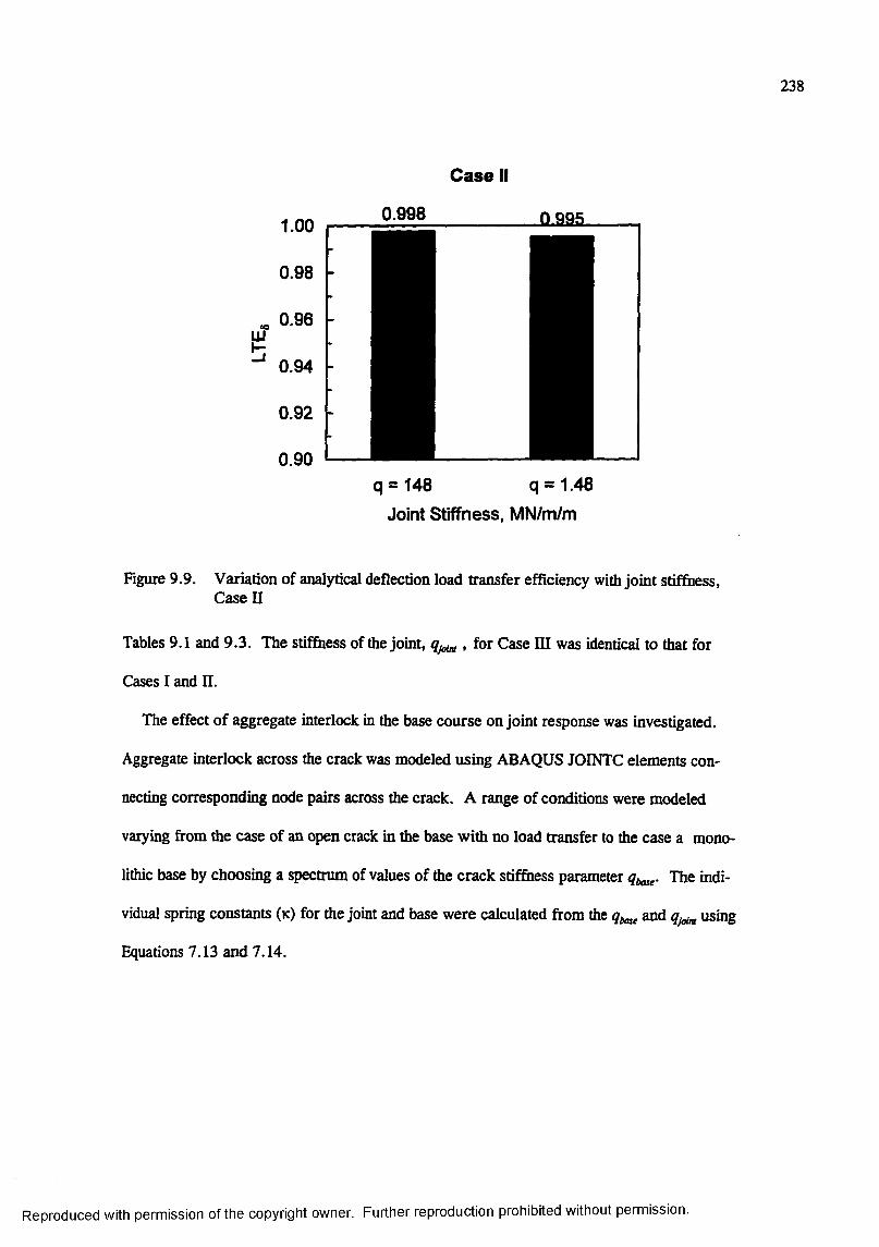
238
Case II
0.998 0.995
q = 148 q = 1.48
Joint Stiffness, MN/m/m
Figure 9.9. Variation of analytical deflection load transfer efficiency with joint stiffiiess. Case n
Tables 9.1 and 9.3. The stiffiiess of the Joint, , for Case III was identical to that for
Cases I and U.
The effect of aggregate interlock in the base course on joint response was investigated.
Aggregate interlock across the crack was modeled using ABAQUS JOINTC elements con
necting corresponding node pairs across the crack. A range of conditions were modeled
varying from the case of an open crack in the base with no load transfer to the case a mono
lithic base by choosing a spectrum of values of the crack stiffness parameter The indi
vidual spring constants ( k ) for the joint and base were calculated from the and using
Equations 7.13 and 7.14.
Reproduced with permission of the copyright owner. Further reproduction prohibited without permission.
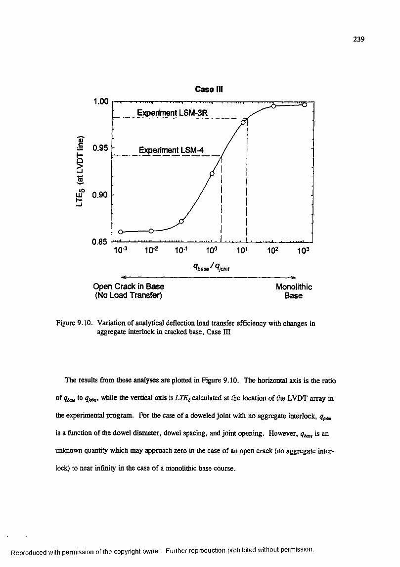
239
Case III1.00
Experiment LSM-3R
I 0.95 Experiment LSM-4
5
u f 0.90b
0.8510-3 10-2 10-1
'joint
Open Crack in B ase (No Load Transfer)
MonolithicB ase
Figure 9.10. Variation of analytical deflection load transfer efficiency with changes in aggregate interlock in cracked base. Case III
The results from these analyses are plotted in Figure 9.10. The horizontal axis is the ratio
of q ,^ to q j^ , while the vertical axis is LTEg calculated at the location of the LVDT array in
the experimental program. For the case of a doweled joint with no aggregate interlock, qjoi„
is a function of the dowel diameter, dowel spacing, and joint opening. However, is an
unknown quantity which may approach zero in the case of an open crack (no aggregate inter
lock) to near infinity in the case of a monolithic base course.
Reproduced with permission of the copyright owner. Further reproduction prohibited without permission.
240
Several important observations can be made concerning the analytical curve in Fig
ure 9.10. Results from the finite element analyses indicate that the amount of load transfer in
the base influences the deflection load transfer at the joint. As would be intuitively expected,
the deflection load transfer efficiency increases with increasing shear stiffiiess across the
crack in the base course.
The deflection load transfer efficiencies from Experiments LSM-3R and LSM-4 and the
predicted q ratio values are indicated by the dashed lines in Figure 9.10. The data from
LSM-4 indicates that one would predict that the crack stiffiiess due to aggregate interlock in
the base course was in excess of two times the stiffiiess of the doweled joint. However, this
result is irrational, because the dowels in the slabs should provide more shear stiffiiess than
the aggregate interlock in the base. Similarly, the data from LSM-3R indicates that the
experimental deflection load transfer efficiency intersects the curve in a location somewhat
below the point predicted for a monolithic base.
The stiffness of the doweled joint can be decomposed into components from shearing
action in the dowel, bending action in the dowel, and from direct bearing (or aggregate inter
lock) across the joint as follows:
joint ~ dowel shear ^ ^dowel bending ^ aggregate interlock ( 9 . 3 )
Most researchers have concluded that the component due to dowel bending is negligible, par
ticularly for the ranges of joint openings which typically occur in airport pavements. There
fore, the joint stiffiiess can be thought of as the sum of the components from dowel shear and
from aggregate interlock. In the case of the experimental program, the dowel shear compo
nent may be calculated directly from the dowel diameter, dowel spacing, and joint opening.
Even though the joint opening in the experiments contained a Teflon strip to minimize load
transfer due to direct bearing, it is likely that direct bearing made some contribution to the
Reproduced with permission of the copyright owner. Further reproduction prohibited without permission.
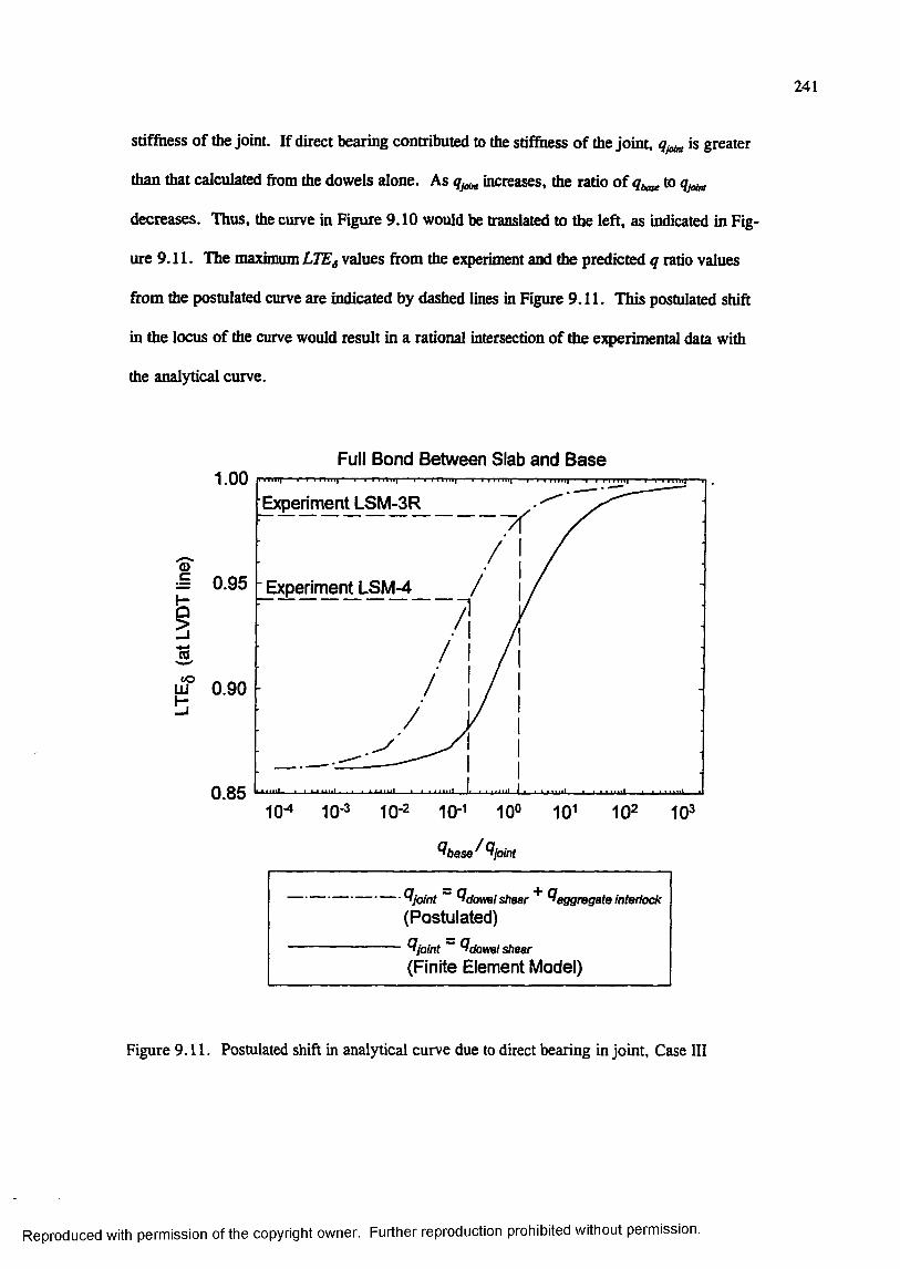
241
stiffness of the joint. If direct bearing contributed to the stiffness of the joint, is greater
than that calculated from the dowels alone. As increases, the ratio o f to
decreases. Thus, the curve in Figure 9.10 would be translated to the left, as indicated in Fig
ure 9.11. The maximum LTEg values from the experiment and the predicted q ratio values
from the postulated curve are indicated by dashed lines in Figure 9.11. This postulated shift
in the locus of the curve would result in a rational intersection of the experimental data with
the analytical curve.
Full Bond Between Slab and B ase1.00
Experiment LSM-3R
0)c 0.95 Experiment LSM-4
I05
u f 0.90
0.851 0 "» 10-3 10-2 1 0 -» 1 0 ° 1 0 » 1 0 2 1 0 °
^base^^i’j o i n t
• ^ J o i n t ~ ^ d o w e l s h e a r ^
(Postulated)
■ ^ j o i n t ~ ^ d o w e l s h e a r(Finite Element Model)
interlock
Figure 9.11. Postulated shift in analytical curve due to direct bearing in joint, Case III
Reproduced with permission of the copyright owner. Further reproduction prohibited without permission.
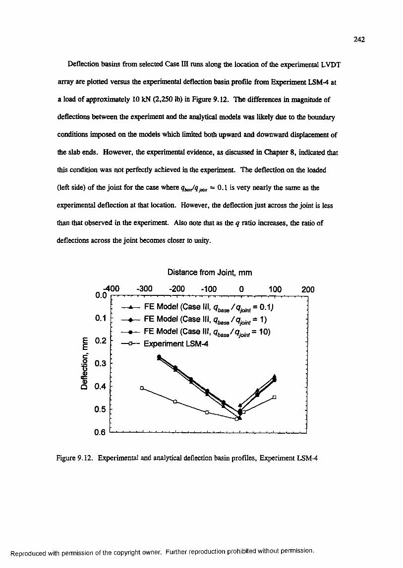
242
Deflection basins from selected Case HI runs along the location of the experimental LVDT
array are plotted versus the experimental deflection basin profile from E}q>eriment LSM-4 at
a load of approximately 10 kN (2,250 lb) in Figure 9.12. The differences in magnitude of
deflections between the experiment and the analytical models was likely due to the boundary
conditions inq>osed on the models which limited both upward and downward displacement of
the slab ends. However, the experimental evidence, as discussed in Chapter 8 , indicated that
this condition was not perfectly achieved in the experiment. The deflection on the loaded
(left side) of the joint for the case where = 0 .1 is very nearly the same as the
experimental deflection at that location. However, the deflection just across the joint is less
than that observed in the experiment. Also note that as the ^ ratio increases, the ratio of
deflections across the joint becomes closer to unity.
-400 0.0
Distance from Joint, mm
-300 -200 -100 0 100
0.1
I 0.2
I 0.3
L .0.5
0.6
FE Model (Case III, Q b a s e ^ ^ j o i n t ^ 1) FE Model (Case III, q ^ i n t ^ 10)
-o— Experiment LSM-4
200
FE Model (Case III, q t a s e ^ % i n t = 0 1 )
Figure 9.12. Experimental and analytical deflection basin profiles. Experiment LSM-4
Reproduced with permission of the copyright owner. Further reproduction prohibited without permission.
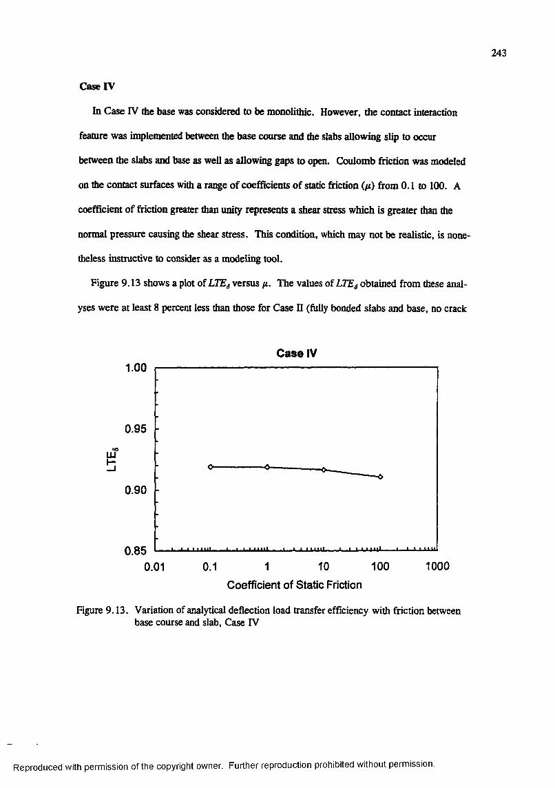
243
Case IV
In Case IV the base was considered to be monolithic. However, the contact interaction
feature was inçlemented between the base course and the slabs allowing slip to occur
between the slabs and base as well as allowing ga^s to open. Coulomb fnction was modeled
on the contact surfaces with a range of coefficients of static friction in) from 0.1 to 100. A
coefficient of friction greater than unity represents a shear stress which is greater than the
normal pressure causing the shear stress. This condition, which may not be realistic, is none
theless instructive to consider as a modeling tool.
Figure 9.13 shows a plot of LTEg versus fi. The values of LTEg obtained from these anal
yses were at least 8 percent less than those for Case H (fully bonded slabs and base, no crack
Case IV
UÎ
1.00
0.95
0.90
0.8510001001 100.01 0 .1
Coefficient of Static Friction
Figure 9.13. Variation of analytical deflection load transfer efficiency with friction between base course and slab. Case IV
Reproduced with permission of the copyright owner. Further reproduction prohibited without permission.
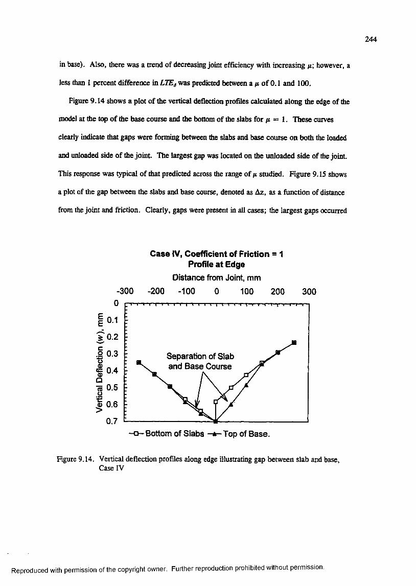
244
in base). Also, there was a trend of decreasing joint efficiency with increasing fi; however, a
less than 1 percent difference in LTEg was predicted between a o f 0.1 and 100.
Figure 9.14 shows a plot of the vertical deflection profiles calculated along the edge of the
model at the top of the base course and the bottom of the slabs for ^ = 1 . These curves
clearly indicate that gaps were forming between the slabs and base course on both the loaded
and unloaded side of the joint. The largest g ^ was located on the unloaded side of the joint.
This response was typical of that predicted across the range of (i studied. Figure 9.15 shows
a plot of the gap between the slabs and base course, denoted as Az, as a function of distance
from the joint and friction. Clearly, gaps were present in all cases; the largest gaps occurred
-300
Case IV, Coefficient of Friction = 1 Profile at Edge
D istance from Joint, mm
-200 -100 0 100 200 300
EE
Is•c
0
0 .1
0.2
0.3 Separation of Slab and B ase Course0.4
0.5
0.6
0.7Bottom of S labs Top of B ase.
Figure 9.14. Vertical deflection profiles along edge illustrating gap between slab and base, Case rv
Reproduced with permission of the copyright owner. Further reproduction prohibited without permission.
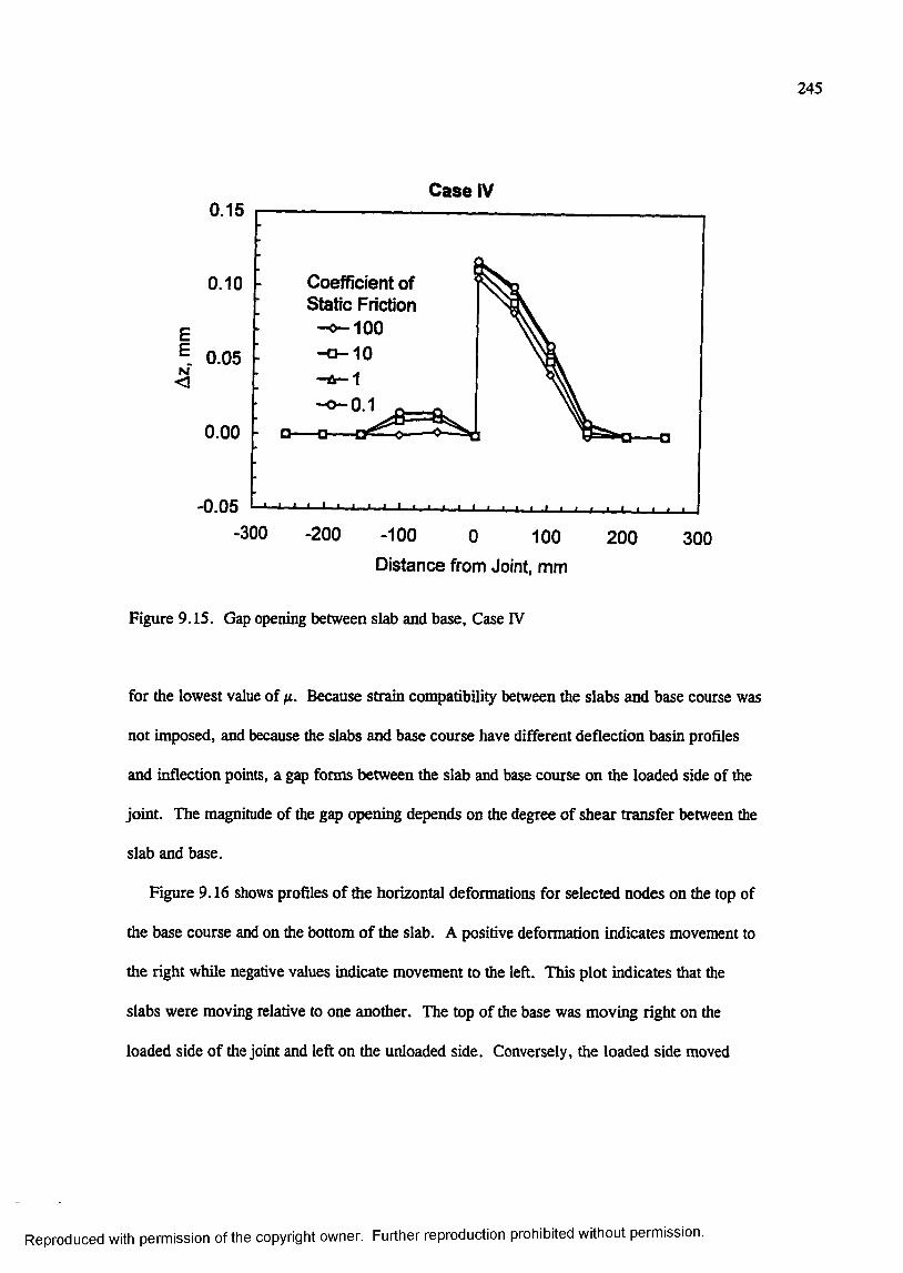
245
Case IV0.15
0.10
- 0.05<
0.00
Coefficient of Static Friction
—❖— 1 0 0
-CH-10
0.1
- 0 . 0 5 ' ' '— I ■ I I— I— I—j — I— u _ i — .................................. . ■ I . . . .
-300 -200 -100 0 100 200 300Distance from Joint, mm
Figure 9.15. Gap opening between slab and base. Case IV
for the lowest value of /i. Because strain compatibility between the slabs and base course was
not imposed, and because the slabs and base course have different deflection basin profiles
and inflection points, a gap forms between the slab and base course on the loaded side of the
joint. The magnitude of the g£ç opening depends on the degree of shear transfer between the
slab and base.
Figure 9.16 shows profiles of the horizontal deformations for selected nodes on the top of
the base course and on the bottom of the slab. A positive deformation indicates movement to
the right while negative values indicate movement to the left. This plot indicates that the
slabs were moving relative to one another. The top of the base was moving right on the
loaded side of the joint and left on the unloaded side. Conversely, the loaded side moved
Reproduced with permission of the copyright owner. Further reproduction prohibited without permission.
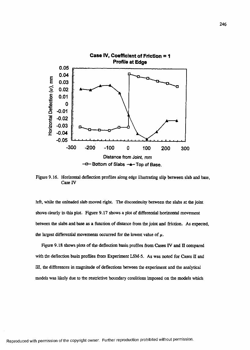
246
Case IV, Coefficient of Friction = 1 Profile at Edge
EE
g
IIë
0.050.040.030.020.01
0
- 0.01- 0.02-0.03-0.04-0.05
-300 -200 -100 0 100 200 300
Distance from Joint, mm Bottom of Slabs -A—Top of Base.
Figure 9.16. Horizontal deflection profiles along edge illustrating slip between slab and base, Case IV
left, while the unloaded slab moved right. The discontinuity between the slabs at the joint
shows clearly in this plot. Figure 9.17 shows a plot of differential horizontal movement
between the slabs and base as a function of distance from the joint and fnction. As expected,
the largest differential movements occurred for the lowest value of n.
Figure 9.18 shows plots of the deflection basin profiles from Cases IV and II compared
with the deflection basin profiles from Experiment LSM-5. As was noted for Cases n and
in, the differences in magnitude of deflections between the experiment and the analytical
models was likely due to the restrictive boundary conditions imposed on the models which
Reproduced with permission of the copyright owner. Further reproduction prohibited without permission.
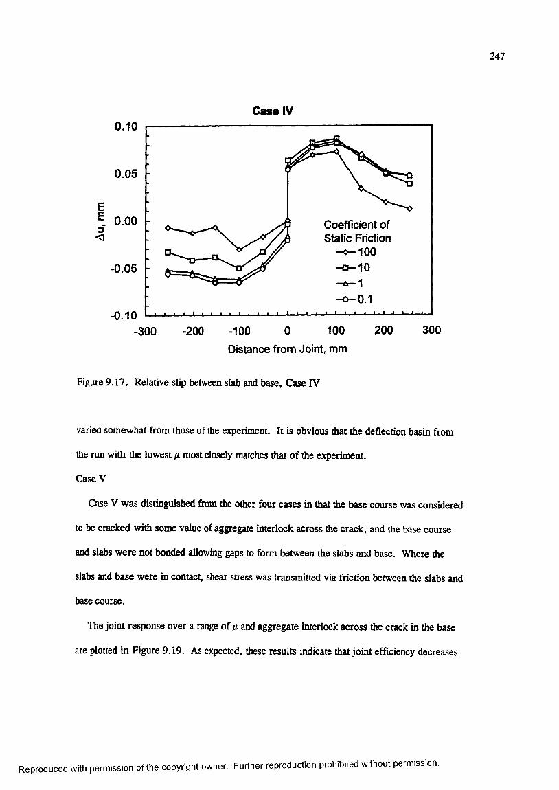
247
Case IV0.10
0.05
: 0.00 Coefficient of Static Friction
—0— 1 0 0
-0.05
0.1- 0.10
-300 -200 -100 0 100 Distance from Joint, mm
200 300
Figure 9.17. Relative slip between slab and base, Case IV
varied somewhat from those of the experiment. It is obvious that the deflection basin from
the run with the lowest fi most closely matches that of the experiment.
CaseV
Case V was distinguished from the other four cases in that the base course was considered
to be cracked with some value of z^gregate interlock across the crack, and the base course
and slabs were not bonded allowing gaps to form between the slabs and base. Where the
slabs and base were in contact, shear stress was transmitted via friction between the slabs and
base course.
The joint response over a range of ft and aggregate interlock across the crack in the base
are plotted in Figure 9.19. As expected, these results indicate that joint efficiency decreases
Reproduced with permission of the copyright owner. Further reproduction prohibited without permission.
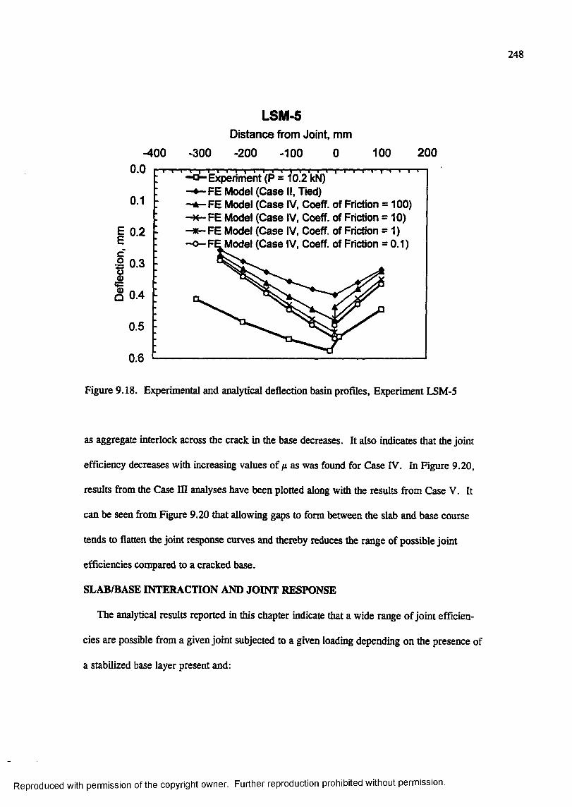
248
-400
LSM-5Distance from Joint, mm
-300 -200 -100 0 100 2000.0
0.1
I 0.2
I 0.3
Ia 0.4
0.5
0.6
T - i — I T " i I - r 1 n - f I - I ; \ i i i
'Experiment (P = 10.2 kN)FE Model (Case II, Tied)FE Model (Case IV, Coeff. of Friction = 100)
• FE Model (Case IV, Coeff. of Friction = 10) - * - F E Model (Case IV, Coeff. of Friction = 1) - o - F E Model (Case IV, Coeff. of Friction = 0.1)
Figure 9.18. Experimental and analytical deflection basin profiles. Experiment LSM-5
as aggregate interlock across the crack in the base decreases. It also indicates that the joint
efficiency decreases with increasing values of fi as was found for Case IV. In Figure 9.20,
results from the Case III analyses have been plotted along with the results from Case V. It
can be seen from Figure 9.20 that allowing gaps to form between the slab and base course
tends to flatten the joint response curves and thereby reduces the range of possible joint
efficiencies compared to a cracked base.
SLAB/BASE INTERACTION AND JOINT RESPONSE
The analytical results reported in this chapter indicate that a wide range of joint efficien
cies are possible from a given joint subjected to a given loading depending on the presence of
a stabilized base layer present and:
Reproduced with permission of the copyright owner. Further reproduction prohibited without permission.
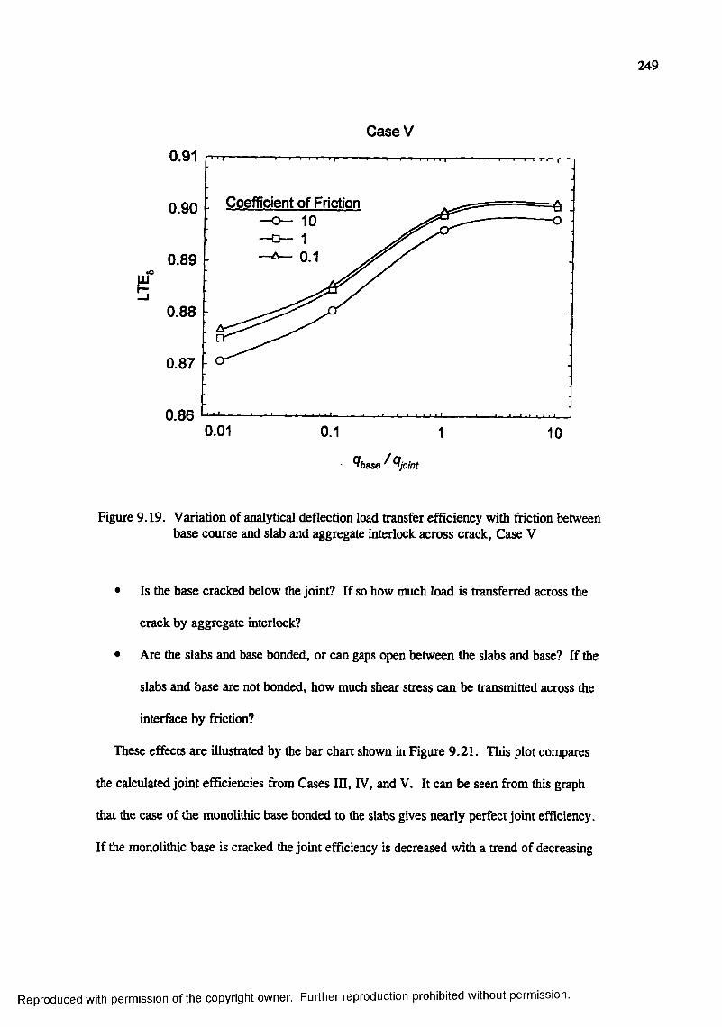
249
Case V0.91
Coefficient of Friction0.90
0.10.89c O
0.88
0.87
0.860.01 0.1 1 10
^ b a s e ^ ^ j o i n t
Figure 9.19. Variation of analytical deflection load transfer efficiency with fnction between base course and slab and aggregate interlock across crack, Case V
• Is the base cracked below the joint? If so how much load is transferred across the
crack by aggregate interlock?
• Are the slabs and base bonded, or can gaps open between the slabs and base? If the
slabs and base are not bonded, how much shear stress can be transmitted across the
interface by friction?
These effects are illustrated by the bar chart shown in Figure 9.21. This plot compares
the calculated joint efficiencies from Cases HI, IV, and V. It can be seen from this graph
that the case of the monolithic base bonded to the slabs gives nearly perfect joint efficiency.
If the monolithic base is cracked the joint efficiency is decreased with a trend of decreasing
Reproduced with permission of the copyright owner. Further reproduction prohibited without permission.
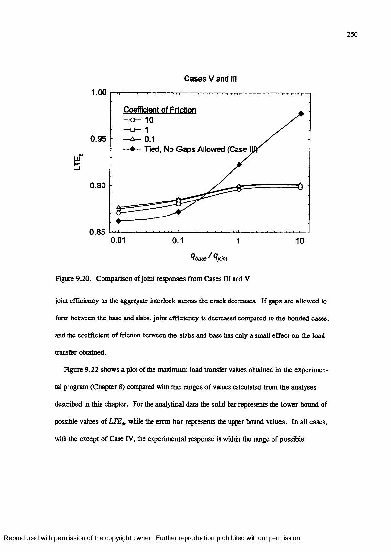
250
Cases V and
1.00
Coefficient of Friction
0.95 0.1Tied, No G ap s Allowed (Case I
0.90
0.850.01 0.1 1 10
^ b a s e j o i n t
Figure 9.20. Comparison of joint responses from Cases in and V
joint efficiency as the aggregate interlock across the crack decreases. If gaps are allowed to
form between the base and slabs, joint efficiency is decreased compared to the bonded cases,
and the coefficient of friction between the slabs and base has only a small effect on the load
transfer obtained.
Figure 9.22 shows a plot of the maximum load transfer values obtained in the experimen
tal program (Chapter 8 ) compared with the ranges of values calculated from the analyses
described in this cfiapter. For the analytical data the solid bar represents the lower bound of
possible values of LTEg, while the error bar represents the upper bound values. In all cases,
with the except of Case IV, the experimental response is within the range of possible
Reproduced with permission of the copyright owner. Further reproduction prohibited without permission.
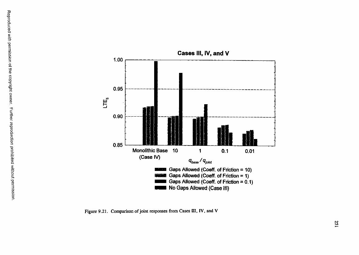
7)CD■DOQ .C
sQ .
■oCD
(/)o'3
CD
83S'=r
3CD
Cp.
CD■aIcaO3
■ao
CDQ .
oc"O
CD
(/)C/Î
Cases HI, IV, and V1.00
0.95
0.90
0.85 l iMonolithic B ase
(C ase IV)1
%ase
0.1 0.01
'Joint
G aps Allowed (Coeff. of Friction = 10) G aps Allowed (Coeff. of Friction = 1) G aps Allowed (Coeff. of Friction = 0.1) No G aps Allowed (C ase III)
Figure 9.21. Comparison of joint responses from Cases III, IV, and V
«
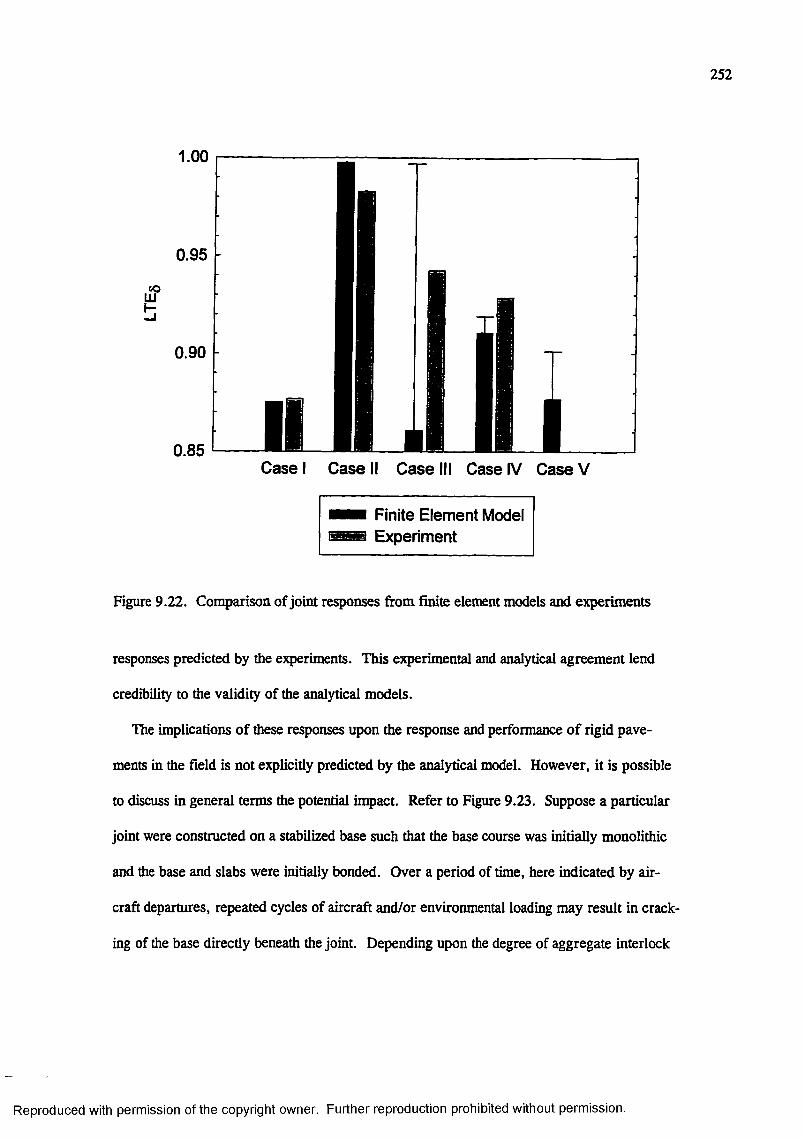
252
1.00
0.95
0.90
0.85 LiC ase I C ase II C ase III C ase IV C ase V
Finite Element Model Experiment
Figure 9.22. Comparison of joint responses from finite element models and experiments
responses predicted by the experiments. This experimental and analytical agreement lend
credibility to the validity of the analytical models.
The implications of these responses upon the response and performance of rigid pave
ments in the field is not explicitly predicted by the analytical model. However, it is possible
to discuss in general terms the potential impact. Refer to Figure 9.23. Suppose a particular
Joint were constructed on a stabilized base such that the base course was initially monolithic
and the base and slabs were initially bonded. Over a period of time, here indicated by air
craft deparmres, repeated cycles of aircraft and/or environmental loading may result in crack
ing of the base directly beneath the Joint. Depending upon the degree of aggregate interlock
Reproduced with permission of the copyright owner. Further reproduction prohibited without permission.
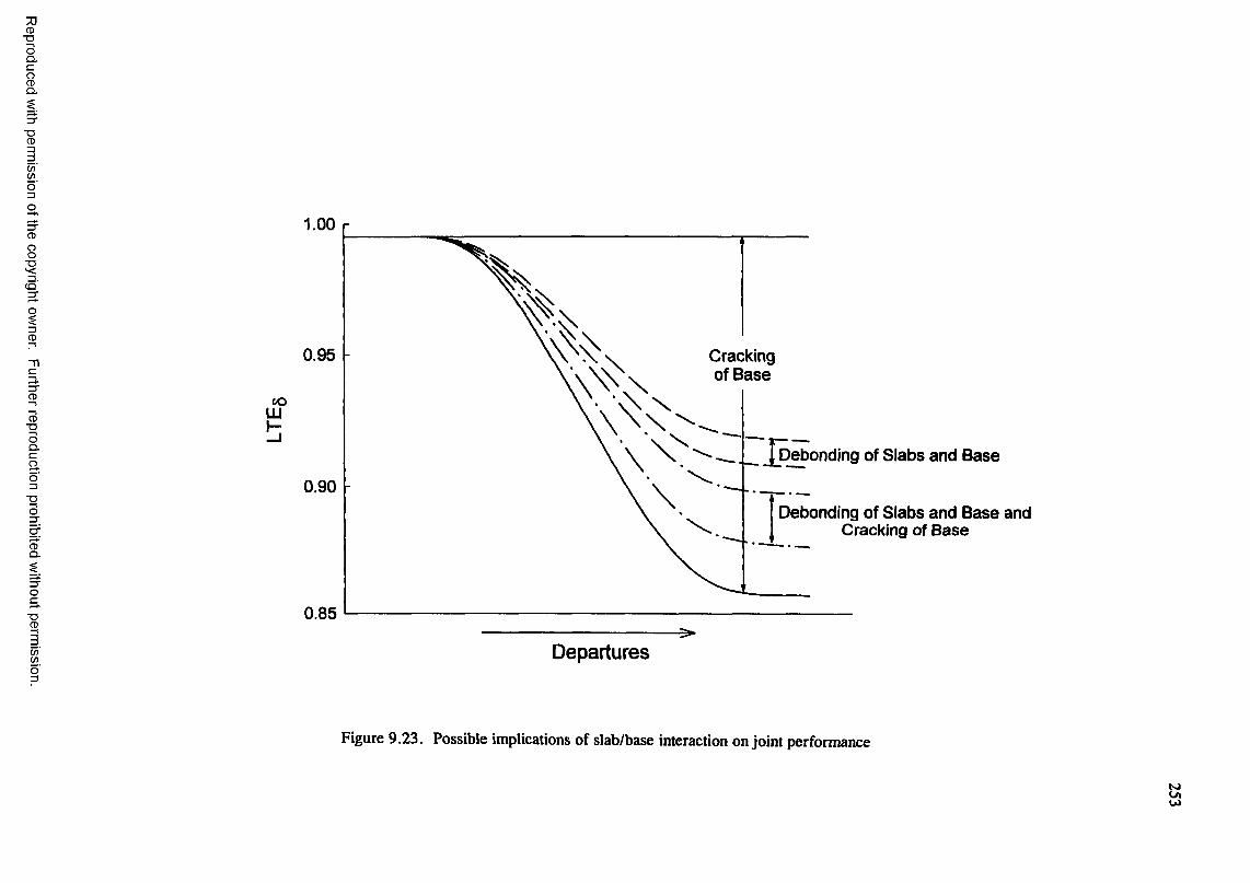
7JCD■oOQ .cga .
■DCD
(/)(/)
1.008
3-3"CD
CD■DOQ .Cao3"O
o
CDQ .
■DCD
C/Î
o '3
0.95
toLiih-
0.90
0.85
Cracking of Base
J^Debondjng of Slabs and Base
TDebonding of Slabs and Base and Cracking of Base
Departures
Figure 9.23. Possible implications of slab/base interaction on joint performance
W

254
across the crack in the base, the finite element analyses indicated that a range of responses
(indicated by the two solid curves in the Figure 9.23) is possible.
Next, suppose that an identical joint were constructed in the same manner. However, in
this case suppose that the base and slabs were debonded by repeated cycles of aircraft or
environmental loading such that it was possible that gq>s could form between the slabs and
base in the vicinity of the joint. For the sake of argument suppose that the base were mono
lithic. The finite element analyses indicate a range of possible responses, depending upon the
amount of shear stresses transmitted across the interface by friction, denoted by the dashed
curves in Figure 9.23. Note that the range of possible responses is much less than that possi
ble due to cracking of the base.
Finally, suppose that the identical joint were again constructed in the same maimer. Now,
in this case suppose that aircraft or environmental loadings cause the base to crack beneath
the joint and also cause delamination or debonding between the slabs and base. Again the
finite element models indicated a range of possible responses plotted as dash-dot curves in
Figure 9.23. The range of potential responses is much less than that for the cracked base
alone. However, as expected, the efficiency of a joint associated with a cracked and
debonded base is predicted to be less than that of the joint associated with a debonded base
without a crack.
It should be noted that the exact values of LTEg obtained in a particular case depend not
only on the slab/base interaction factors, but also upon the slab and base geometry, subgrade
strength, material properties, and load geometry. Therefore, the values plotted on the verti
cal axis in Figure 9.23 are intended to be representative values of the LTEg obtained in these
analytical cases.
Reproduced with permission of the copyright owner. Further reproduction prohibited without permission.
CHAPTER 10: CONCLUSIONS AND RECOMMENDATIONS
CONCLUSIONS
The response of the rigid pavement slab-joint-base structural system is complex, and accu
rately predicting the response of such a system requires a significant degree of analytical
sophistication. The research reported in this dissertation has defined some features required
to adequately model the system and has demonstrated a technique to develop a comprehensive
3D finite element model of the rigid pavement slab-joint-foundation structural system. These
findings represent a significant advancement in the state of the art of rigid pavement response
modeling. Specifically, the following conclusions can be drawn from this study:
• Analysis of experimental data obtained by the Corps of Engineers in the 1950s con
firms the usefulness of the concepts of dimensionless joint stiffiiess as a means of
characterizing the response of the doweled joint. Thus, the response of both the
aggregate interlock joint and the doweled joint can be characterized by the same fam
ily of curves. Explicit modeling of the dowel in the 3D finite element model, while
perhaps useful for research purposes, is urmecessary for predicting the gross response
of the structural system. The usefulness of the dimensionless joint stiffness for char
acterizing the response of the keyed joint was not addressed by this research. The
ease of application of the concepts of dimensionless joint stiffiiess has been increased
by the development of closed-form equations (Equations 4.11, 4.12, and 4.13) based
upon the theoretical developments of Skarlatos (1949).
• For most practical rigid pavement slabs, the classical Kirchhoff assumptions, adopted
by Westergaard and Skarlatos, lead to small errors in predicting edge stresses.
255
Reproduced with permission of the copyright owner. Further reproduction prohibited without permission.

256
Results from 3D finite element models show that the maximum edge stress does not
occur at the edge of the slab but at some finite distance from the edge. Fortimately,
the Westergaard edge stress is conservative; the analytical models predict that, for
most rigid pavement slabs, the maximum edge stress will occur within 0 . o f the
edge of the slab and will be approximately 10 percent less than that predicted by the
Westergaard theory.
Experimental evidence from this research suggests that the joint efficiency is signifi
cantly affected by the presence and condition o f a stabilized base. The presence of
cracking in the base and the degree of bonding between the slabs and stabilized base
course influences the structural capacity and load transfer capability of the rigid pave
ment structure. The greatest experimental values of joint efficiency were obtaining
from slabs founded on a monolithic stabilized base followed, in order, by slabs
founded on a cracked monolithic base, founded on a monolithic base with a bond
breaker, and finally, founded directly on a granular base or on a subgrade. Maxi
mum load transfer efficiency occurs at low loads with decreasing effectiveness for
increasing load. This phenomenon is likely caused by localized crushing of the con
crete in the region of the dowels as the loads and resulting displacements increase.
The finite element models developed in this research indicate that a comprehensive
3D finite element modeling technique provides a rational approach to modeling the
structural response of the jointed rigid airport pavement system. Modeling features
which are required include explicit 3D modeling of the slab continua, load transfer
capability at the joint (modeled by springs between the slabs), explicit 3D modeling of
tlie base course continua, aggregate interlock capability across the cracks in the base
course (again, modeled by springs across the crack), and contact interaction between
Reproduced with permission of the copyright owner. Further reproduction prohibited without permission.

257
the slabs and base course. The contact interaction model feature must allow gaps to
open between the slab and base. Furthermore, where the slabs and base are in con
tact, transfer of shear stresses across the interface via friction should be modeled.
RECOMMENDATIONS
The following recommendations are drawn from this research:
• Mechanistic design criteria for doweled joints should be developed using the concepts
of dimensionless joint stifihess in concert with the closed-form Westergaard-type
solution for load transfer in rigid pavements. Given the slab thickness, support
conditions, and loading, it is possible to use these developments to establish criteria
for dowel diameter and spacing for a critical joint opening. These criteria should
then be verified by full-scale testing.
• The concept of the composite or “top of the base” modulus of subgrade reaction
ignores the composite action of the slab-stabilized base structural system. This con
cept should be abandoned in favor of a more realistic model that explicitly includes
the structural benefits of the stabilized base. It may be possible to develop improved
design criteria which allow a reduction in the thickness of the portland cement con
crete surface layer if the increased strength, ductility, and load transfer capabilities
provided by the stabilized layer are considered in the structural analysis.
• Certain issues pertaining to the effects on new- and future-generation aircraft and
rigid pavement behavior and performance can be addressed by the finite element
modeling techniques developed in this research. A research study should be initiated
to study the effects of multiple-wheel loadings on the response of jointed rigid
pavements.
Reproduced with permission of the copyright owner. Further reproduction prohibited without permission.

258
• For rigid pavements the magnitude of responses due to environmental loadings may
be as great as those responses due to traffic loading. Thus, the effects of environ
mental factors on the findings of this research should be investigated. It should be
possible to add to the analytical complexity o f this research by superimposing the
effects o f temperature and moisture gradients on the response of the rigid pavement
structure. With the tools presented in this study, it is possible to develop and imple
ment an algorithm which could change the joint efficiency with joint opening.
• The 3D finite element model developed as a part of this study is limited to linear elas
tic material behavior, yet fracture and nonlinear material response clearly controls
failure o f the rigid pavement system. Future model developments should include
more sophisticated material models. For example fracture mechanics concepts should
be employed to study the effects of repeated traffic loading on the slabs and cement-
stabilized base course. Furthermore, a micro-mechanics approach should be imple
mented to model localized damage in the vicinity of the dowel-concrete interface.
• The results of this study point to some critical issues which should be considered by
the FAA in developing test plans for its full-scale, instrumented test facility currently
under construction. Specifically, instrumentation should be installed to detect the
presence o f cracking in the stabilized base course, particularly directly beneath the
joint. Also, instrumentation should be selected and installed to detect the presence of
gaps between the slabs and base course.
• The incremental finite element analysis procedure used to solve the contact interaction
problem can be computer intensive. In the event that solution times and memory
requirements exceed the available computer resources, the slabs can be modeled by
thick plate or shell elements with little sacrifice in accuracy. However, the capability
Reproduced with permission of the copyright owner. Further reproduction prohibited without permission.

259
to predict load transfer across cracks in the base course and debonding between the
slabs and base are critical and must be retained.
Reproduced with permission of the copyright owner. Further reproduction prohibited without permission.
REFERENCES
Ahlvin, R. G. 1971. “Multiple-Wheel Heavy Gear Load Pavement Tests," AFWL-TR-70- 113, Vol. I. Kirtland Air Force Base: Air Force Weapons Laboratory.
Ahlvin, R. G. 1991. "Origin of Developments for the Structural Design of Pavements,” Technical Report GL-91-26. Vicksburg, MS: U.S. Army Engineer Waterways Experiment Station.
American Concrete Institute. 1994. State-of-the-Art Report on Soil Cement. A C I230. IR- 90, Manual o f Concrete Practice, WoX. 1. Detroit: American Concrete Institute.
Barker, W. R. and C. R. Gonzalez. 1991. “Pavement Design by Elastic Layer Theory," Aircrc^/Pavement Interaction: An Integrated System. New York: American Society of Civil Engineers, pp. 21-43.
Bathe, K. J. 1982. Finite Element Procedures in Engineering Analysis. Englewood Cliffs, NJ: Prentice-Hall, Inc.
Behrmaim, R M. 1966. “Small-Scale Model Study to Determine the Effects o f Sawkerfs and Bored Recesses of Load-Carrying Capacity of Rigid Pavement,” Technical Report No. 4-38. Cincinnati: Ohio River Division Laboratories.
Behrmann, R. M. 1972. “Small-Scale Static Load Model Study: Behavior of Rigid Pavement Loaded Near the Edge,” Technical Report No. S-4. Champaign, IL: Construction Engineering Research Laboratory.
Bums, C. D. 1971. “Multiple-Wheel Heavy Gear Load Pavement Tests,” AFWL-TR-70- 113, Vol. n. Kirtland Air Force Base: Air Force Weapons Laboratory.
Carlton, P. F. and R. M. Behrmann. 1956. “A Model Study of Rigid Pavement Behavior Under Comer and Edge Loadings,” Proceedings, Highway Research Board, No. 35. Washington: Highway Research Board, pp. 139 - 146.
Channakeshava, C., F. Barzegar, and G. Z. Voyiadjis. 1993. “Nonlinear FE Analysis of Plain Concrete Pavements with Dowel Joints," Journal of Transportation Engineering, Vol. 119, No. 5, pp. 763-781.
Chatti, K. 1992. “Dynamic Analysis of Jointed Concrete Pavements Subjected to Moving Transient Loads,” PhD dissertation. Berkeley: University of California at Berkeley.
Chou, Y. T. 1981. “Structural Analysis Computer Programs for Rigid Multicomponent Pavement Structures with Discontinuities: WESLIQID and WESLAYER." Technical Report GL-81-6. Vicksburg, MS: U.S. Army Engineer Waterways Experiment Station.
260
Reproduced with permission of the copyright owner. Further reproduction prohibited without permission.
261
Corps of Engineers. 1954. “A Model Study of the Effect of High Contact Pressures on Stresses in Rigid Pavements.” Mariemont, OH: Ohio River Division Laboratories.
Corps of Engineers. 1962. “Small Scale Model Studies of Prestressed Rigid Pavements for Military Airfields, Part I, Development of the Model and Results of Exploratory Tests,” Technical Report 4-13. Cincinnati: Ohio River Division Laboratories.
Corps of Engineers. 1963. “Small Scale Model Studies of Prestressed Rigid Pavements for Military Airfields, Part H, Single-Wheel Loadings on Pre-tensioned and Post-tensioned Slabs,” Technical Report 4-25. Cincinnati: Ohio River Division Laboratories.
Crawford, J. E. and M. G. Katona. 1975. “State-of-the-Art for Prediction of Pavement Response,” Contract Report S-75-8. Vicksburg, MS: U.S. Army Engineer Waterways Experiment Station.
Darter, M. I., K. T. Hall, and C. H. Kuo. 1995. “Support Under Portland Cement Concrete Pavements,” National Cooperative Highway Research Program Report 372, Washington: National Academy Press.
Desai, C. S. and J. F. Able. 1972. Introduction to the Finite Element Method. New York: Van Nostrand Reinhold Company.
Department of the Army. 1987. “Materials Testing.” PM 5-530. Washington: Headquarters, Department of the Army.
Departments of the Army and the Air Force. 1988. “Rigid Pavement Design for Airfields: Elastic Layered Method,” Army TM 5-825-3-1 and Air Force AFM 88-6 , Chapter 3, Section A. Washington: Headquarters, Departments of the Army and the Air Force.
Departments of the Army and the Air Force. 1989. “Flexible Pavement Design for Airfields: Elastic Layered Method,” Army TM 5-825-2-1 and Air Force AFM 8 8 -6 , Chapter 2, Section A. Washington: Headquarters, Departments of the Army and the Air Force.
Federal Aviation Administration. 1989. “Standards for Specifying Construction o f Airports.” Advisory Circular 150/5370-10A. Washington: Department of Transportation.
Federal Aviation Administration. 1995. “Airport Pavement Design for the Boeing 777 Airplane,” Advisory Circular No. 150/5320-16. Washington: Federal Aviation Administration.
Fagan, M. J. 1992. Finite Element Analysis. Essex, UK: Longman Scientific and Technical.
Friberg, B. F. 1940. “Design of Dowels in Transverse Joints of Concrete Pavements,” Transactions o f the American Society o f Civil Engineers, Vol. 105, pp. 1076-1095.
Reproduced with permission of the copyright owner. Further reproduction prohibited without permission.
262
Grinter, L. E. 1931. “Design of Reinforced Concrete Road Slabs,” Bulletin No. 39. College Station, TX: Texas Engineering Experiment Station.
Grogan, W. P., C. A. Weiss, Jr., and R. S. Rollings. 1996. “Stabilized Base Courses for Advanced Pavement Design Report 1: Literature Review and Field Performance Data.” DOT/FAA/CT-96/XX. Atlantic City: FAA Technical Center.
Huang, Y. H. 1993. Mgid Pavement Analysis and Design. Englewood Cliffs, NJ: Prentice-Hall, Inc.
Hutchinson, R. L. 1966. “Basis for Rigid Pavement Design for Military Airfields,” Miscellaneous Paper No. 5-7. Cincinnati: Ohio River Division Laboratories.
loannides, A. M. 1984. “Analysis of Slabs-On-Grade for a Variety of Loading and Support Conditions,” PhD Dissertation. Urbana, IL: University of Illinois.
loannides, A. M., M. R. Thompson, and E. J. Barenberg. 1985. “Westergaard Solutions Transportation Research Record 1043. Washington: Transportation
Research Board, pp. 13-23.
loannides, A. M., M. R. Thompson, J. Doimelly, and E. J. Barenberg. 1986. “Three- Dimensional Finite Element Analysis of a Slab on Stress Dependent Elastic Solid Foundation.” Urbana, IL: University of Illinois.
loannides, A. M., Y. H. Lee, and M. I. Darter. 1990. “Control of Faulting Through Joint IjidATtsD sfet D esign” Transportation Research Record No. 1286. Washington: Transportation Research Board, pp. 49-56.
loannides, A. M. and G. T. Korovesis. 1990. “Aggregate Interlock: A Pure-Shear Load Transfer Mechanism,” Transportation Research Record 1286. Washington: Transportation Research Board, pp. 14-24.
loannides, A. M. and G. T. Korovesis. 1992. “Analysis and Design of Doweled Slab-on- Grade Pavement Systems,” Journal o f Transportation Engineering, Vol 118, No. 6 , pp. 745-768.
loannides, A. M. 1994. “Concrete Pavement Backcalculation using ILLI-BACK 3.0,” Nondestructive Testing o f Pavements and Backcalculation o f Moduli, STP 1198, Vol. 2. Philadelphia: American Society for Testing and Materials, pp. 103-124.
loannides, A. M. and M. I. Hammons. 1996. “A Westergaard - Type Solution for the Load Transfer Problem,” Transportation Research Record 1525. Washington: Transportation Research Board, pp. 28-34.
Kerr, A. D. 1964. “Elastic and Viscoelastic Foundation Models,” Journal o f Applied Mechanics, Vol. 31, No. 3.
Kerr, A. D. 1965. “A Study of a New Foundation Model,” Acta Mechanical, Vol. 1/2.
Reproduced with permission of the copyright owner. Further reproduction prohibited without permission.
263
Kerr, A. D. 1993. “Mathematical Modeling of Airport Pavements,” Airport Pavements Innovations: Theory to Practice. New York: American Society of Civil Engineers, pp. 31-45.
Khazanovich, L. and A. M. loannides. 1993. “Finite Element Analysis o f Slabs-On-Grade Using Higher Order Subgrade Models,” Airport Pavements Innovations: Theory to Practice. New York: American Society of Civil Engineers.
Korovesis, G. T. 1990. “Analysis of Slab-On-Grade Pavement Systems Subjected to Wheel and Temperature Loadings,” PhD Dissertation. Urbana, IL: University of Illinois.
Kuo, C. M. 1994. “Three-Dimensional Finite Element Analysis of Concrete Pavement,” PhD Dissertation. Urbana, IL: University of Illinois.
Kushing, J. W., and W. O. Fremont. 1940. “Design of Load Transfer Joints in Concrete Psvem&ats,'’ Proceedings, Highway Research Board, ^o . 20. Washington: Highway Research Board, pp. 481-493.
Larralde, J. and W. F. Chen. 1985. “Computer Model for Analysis of Rigid Pavements with Fatigue,” Proceedings, Third International Conference on Concrete Pavement Design and Rehabilitation. West Lafayette, IN: Purdue University.
Ledbetter, R. H. 1971a. “Multiple-Wheel Heavy Gear Load Pavement Tests,” AFWL-TR- 70-113, Vol. niA. Kirtland Air Force Base: Air Force Weapons Laboratory.
Ledbetter, R. H. 1971b. “Multiple-Wheel Heavy Gear Load Pavement Tests,” AFWL-TR- 70-113, Vol. m s . Kirtland Air Force Base: Air Force Weapons Laboratory.
Majidzadeh, K., G. H. lives, and R. McComb. 1981. “Mechanistic Design of Rigid Pavements,” Proceedings, Second International Conference on Concrete Pavement Design. West Lafayette, IN: Purdue University.
Mellinger, F. M. and P. F. Carlton. 1955. “Application of Models to Design Studies of Concrete Airfield Pavements,” Proceedings, Highway Research Board, No. 34. Washington: Highway Research Board, pp. 57-64.
Nishizawa, T., T. Fukuda, and S. Matsumo. 1989. “A Refined Model of Doweled Joints for Concrete Pavement Using FEM Analysis,” Proceedings, Fourth International Conference on Concrete Pavement Design. West Lafayette, IN: Purdue University.
Packard, R. G. No date. “Computer Program for Airport Pavement Design." Skokie, IL: Portland Cement Association.
Pickett, G. and G. K. Ray. 1951. “Infiuence Charts for Concrete Pavements,” Transactions o f the American Society o f Civil Engineers, Vol. 116, pp. 49-73.
Reproduced with permission of the copyright owner. Further reproduction prohibited without permission.
264
Pickett, G., M. E. Rayville, W. C. Jones, and F. J. McCormick. 1951. “Deflections, Moments, and Reactive Pressures for Concrete Pavements,” Kansas State College Bulletin No. 65. Manhatten KS: Kansas State College.
Rollings, R. S. 1989. “Developments in the Corps of Engineers Rigid Pavement Design Procedure,” Proceedings. Fourth International Corference on Concrete Pavement Design and Rehabilitation. West Lafayette, IN; Purdue University, pp. 405-418.
Rollings, R. W. and D. W. Pittman. 1992. “Field Instrumentation and Performance Monitoring of Rigid Pavements,” Journal o f Transportation Engineering, Vol 118, No. 3, pp. 361-370.
Sale, J. P., and R. L. Hutchinson. 1959. “Development of Rigid Pavement Design Criteria for Military Airfields,” Journal o f the Air Transport Division, Vol. 85, No. AT3, pp. 129-151.
Sale, J. P. 1977. “Rigid Pavement Design for Airfields,” Proceedings. First International Conference on Concrete Pavement Design. West Lafayette, IN: Purdue University, pp. 3-18.
Schnobrich, W. C. 1990. “Structural Analysis, Part 2. Continua: The Finite Element Method,” In Structural Engineering Handbook, Third Edition, E. H. Gaylord, Jr. and C. N. Gaylord, ed.. New York: McGraw-Hill.
Skarlatos, M. S. 1949. “Deflections and Stresses in Concrete Pavements of Airfields with Continuous Elastic Joints.” Mariemont, OH: Ohio River Division Labs.
Tabatabaie, A. M. 1978. “Structural Analysis of Concrete Pavement Joints," PhD Dissertation. Urbana, IL: University of Illinois.
Tayabji, S. D. and B. E. Colley. 1984. “Analysis of Jointed Concrete Pavements,” Report No. FHWA/RD-86/041. McClean, VA: Federal Highway Administration.
Tia, M., J. M. Armaghani, C. Wu, and K. L. Toye. 1987. “FEACONS III Computer Program for Analysis of Jointed Concrete Pavements," Transportation Research Record No 1136. Washington: Transportation Research Board.
Timoshenko, S. and J. M. Lessels. 1925. Applied Elasticity. Pittsburgh: Westinghouse Technical Night School Press.
Timoshenko, S. and S. Woinowsky-Krieger. 1959. Theory o f Plates and Shells. New York: McGraw-Hill Book Company.
Wesevich, J. W ., McCullough, B. P., and Bums, N. H. 1987. “Stabilized Subbase Friction Study for Concrete Pavements.” Research Report 459-1. Austin, Texas: Center for Transportation Research, University of Texas at Austin.
Reproduced with permission of the copyright owner. Further reproduction prohibited without permission.
265
Westergaard, H. M. 1923. “Om Beregning Af Plader Paa Elastisk Underlag Med Særligt Henblik Pass Ppergsmaalet Om Spændinger I Betonveje,” Ingenieren, No. 42, pp. 513- 524. (In Danish).
Westergaard, H. M. 1926. “Stresses in Concrete Pavements Conq>uted by Theoretical Analysis,” Public Roads, Vol. 7, No. 2, pp. 25-35.
Westergaard, H. M. 1928. “Spacing of Dowels,” Proceedings, Highway Research Board, No. 8 . Washington; Highway Research Board, pp. 154-158.
Westergaard, H. M. 1933. “Analytical Tools for Judging Results of Structural Tests of Concrete Pavements,” Public Roads, Vol. 14, No. 10, pp. 129-151.
Westergaard, H. M. 1939. “Stresses in Concrete Rimways of Airports,” Proceedings, Highway Research Board No. 19. Washington: National Research Council, pp. 197-205.
Westergaard, H. M. 1948. “New Formulas for Stresses in Concrete Pavements of Airfields,” Transactions, American Society o f Civil Engineers, Vol. 113, pp. 425-444.
Zaghloul, S. and T. White. 1993. “Non-Linear Dynamic Analysis of Concrete Pavements,” Proceedings, Fifth International Conference on Concrete Pavement Design and Rehabilitation, Vol. 1. West Lafayette, IN: Purdue, University, pp. 277-292.
Zienkiewicz, O. C. and Y. K. Cheung. 1967. The Finite Element Method o f Structural and Continuum Mechanics. London: McGraw-Hill Publishing Conçany Limited.
Reproduced with permission of the copyright owner. Further reproduction prohibited without permission.

APPENDIX A
STRAIN PLOTS FROM 1950S MODEL TESTS
266
Reproduced with permission of the copyright owner. Further reproduction prohibited without permission.
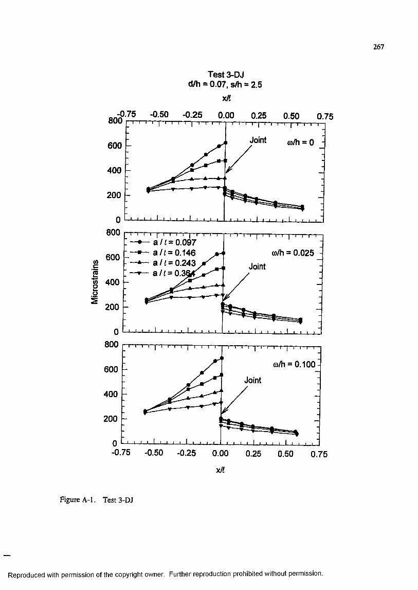
267
Test 3-DJd/h = 0.07, s/h = 2.5
x/(
-0 50 -0.25 0.00 0.25 0.50 0.75o U U i i I I I i I I I r I I 1 ~ i I ‘I i ~ I " I I I 1 I 1 T - — I - I I I : ,
Joint (o/h = 0600
400
200
g1 g 400
I I r I j T“T r "T“" |— I— n — r
• — d i l l - 0.097 a / ( = 0.146
I I r I I I I— I— I— I— I— I— 1— I
o)/h = 0.025^ a i l - 0.243 • — a i l - Q .
800
o /h = 0 .1 0 0 4600Joint
400
200
-0.75 -0.50 -0.25 0.00 0.25 0.50 0.75
x/(
Figure A-1. Test 3-DJ
Reproduced with permission of the copyright owner. Further reproduction prohibited without permission.
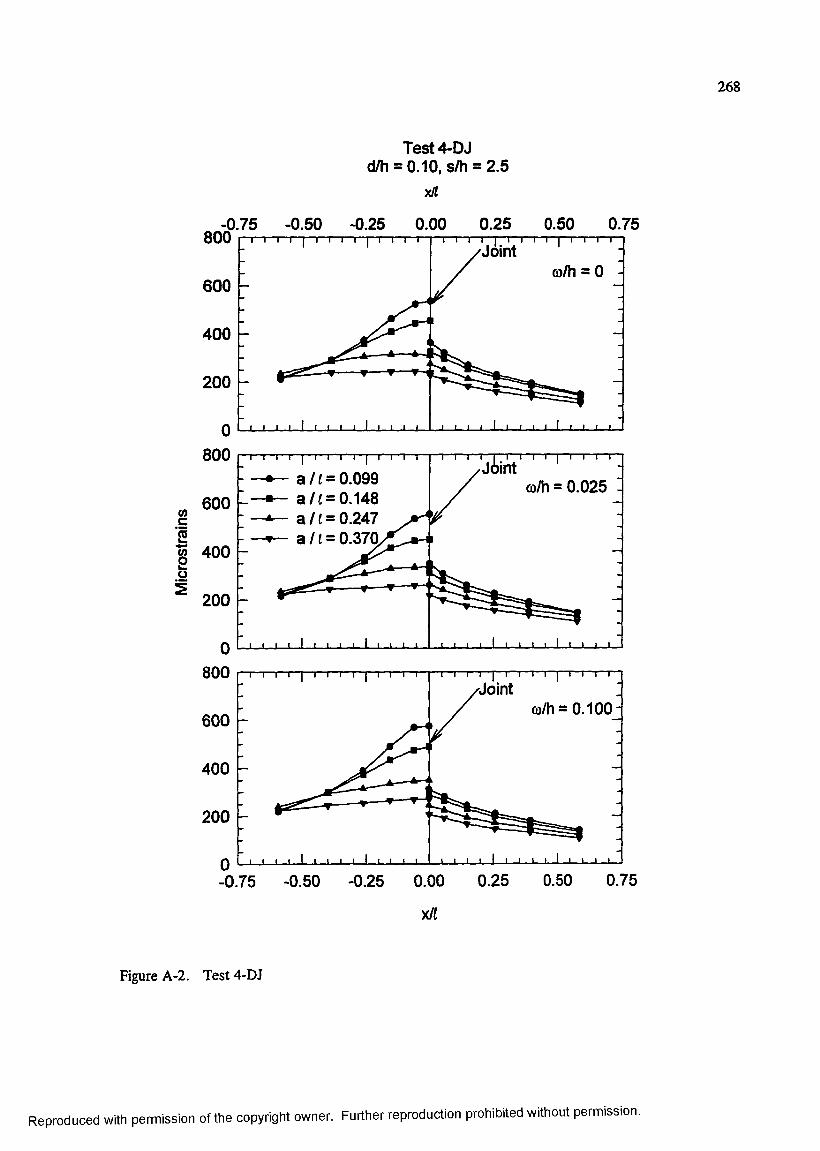
268
Test 4-DJd/h = 0.10, s/h = 2.5
xH
-0.75 -0.50 -0.25 0.00 0.25 0.50 0.75800
m/h = 0
600 -
Ig 400
200 -
T I I I I I I I I I I I I r
♦— a / ( = 0.099 «— a / ( = 0.148
m/h = 0.025 -
— a / ( = 0.247 -V— a / ( = 0.370
Q I I I ■ I I I I I
800Jo in t
m/h = 0 .1 0 0 '600
400
200
0.75-0.75 -0.50 -0.25 0.00 0.25 0.50
xll
Figure A-2. Test 4-DJ
Reproduced with permission of the copyright owner. Further reproduction prohibited without permission.
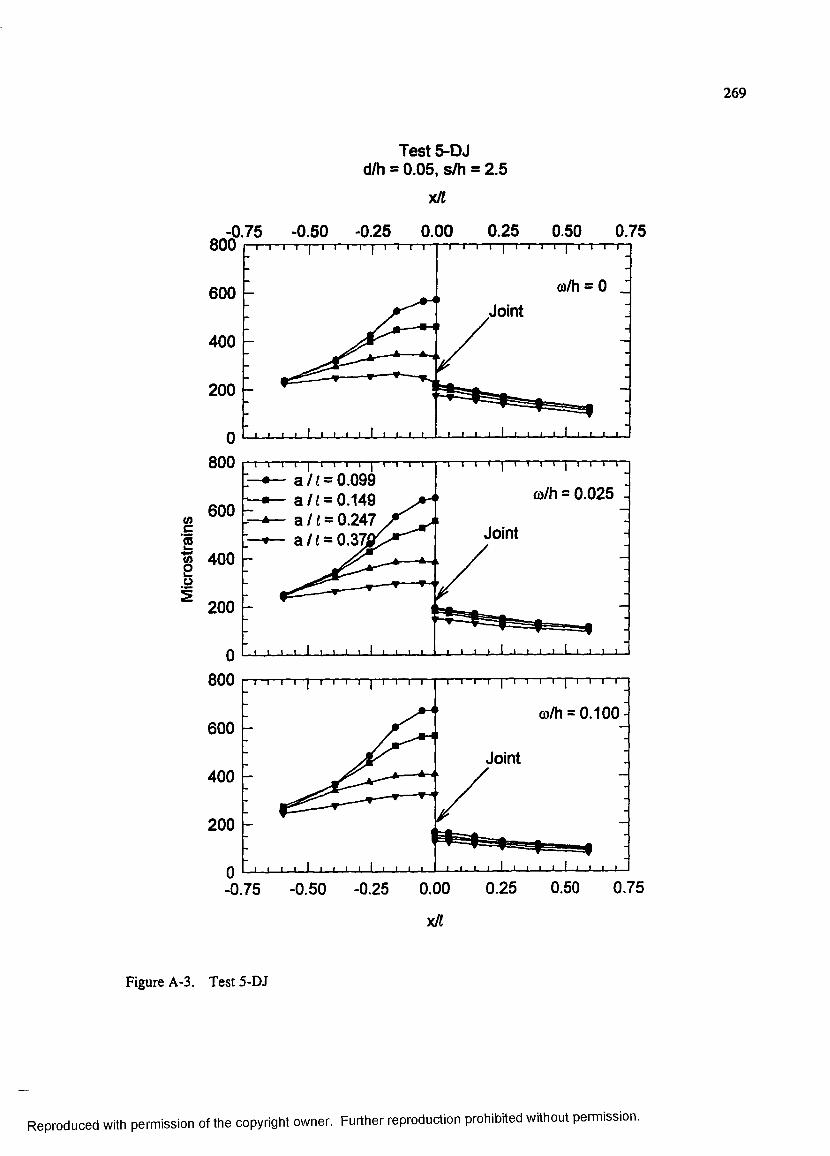
269
Test 5-DJ d/h = 0.05, s/h = 2.5
X/Ü
-0.75 -0.50 -0.25 0.00 0.25 0.50 0.75
(0.5
I
800
600Joint
400
200
800 T—\—\—I—I—r-1—I—r m — \— rT—I—!—r1— n r
m/h = 0.025 -*— a / ( = 0.149 ^ — a /£ = 0.247 ^— a / ( = 0 .3 %
600Joint
400
200
800
m/h = 0.100-600
Joint400
200
0.25 0.50 0.75-0.75 -0.50 -0.25 0.00
x/l
Figure A-3. Test 5-DJ
Reproduced with permission of the copyright owner. Further reproduction prohibited without permission.
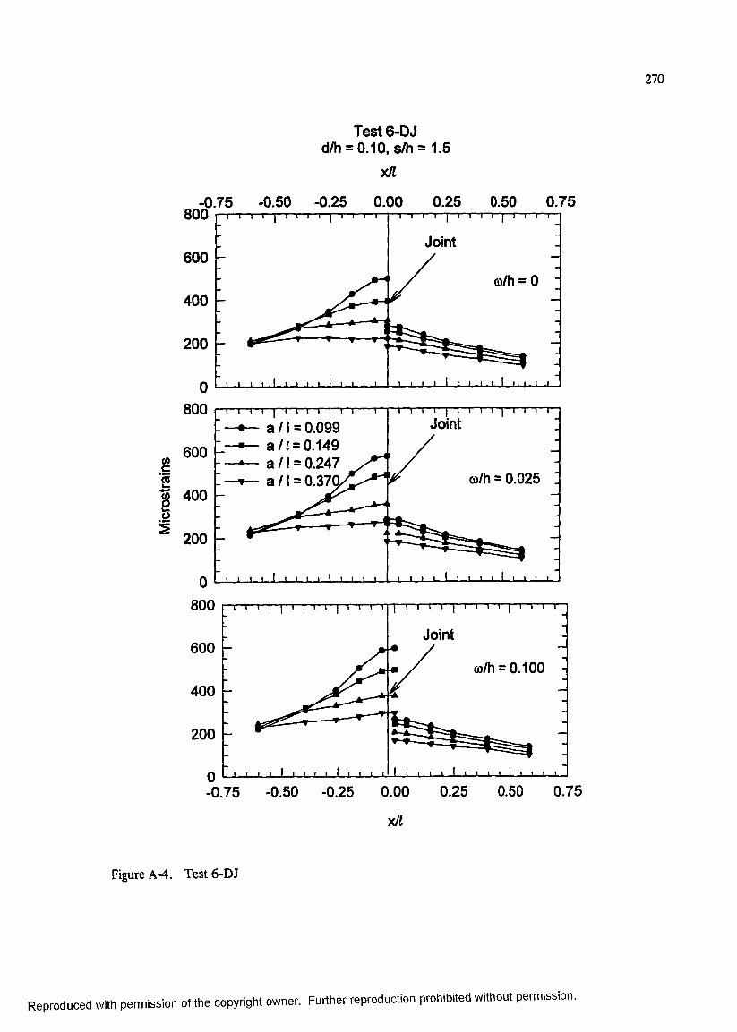
270
T est 6-DJ d/h = 0.10, s/h = 1.5
x n
-0.75 -0.50 -0.25 0 .00 0.25 0.50800 r 1 T -i T I i- i IT r I I -i r
0.75
m/h = 0
800Jointa / 1 = 0.099
*— a / ( = 0.149 ^ a /1 = 0.247 -r— a / 1 = 0.37a
600
m/h = 0.025400
i 200
800 T I I I I I I I I p n i I I rT—I—I—r
Joint600
m/h = 0 .1 0 0
400
200
-0.75 -0.50 -0.25 0.00 0.25 0.50 0.75
xJl
Figure A-4. Test 6 -DJ
Reproduced with permission of the copyright owner. Further reproduction prohibited without permission.
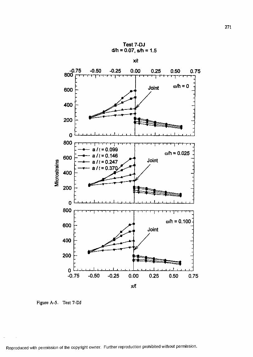
271
Test 7-DJd/h = 0.07, s/h = 1.5
-0.75 800
-0.50 -0.25T— I— r i ~ [ ~ i I ' I— n
Xll
0.00
600
400
200
Q — I I I 1 I I I I I I I I I I I I I I I I
0.25 0.50 0.75T I I I I I I I I I I I I—r
Joint m/h = 0 -
g"m
i
800— a / ( = 0.099
m/h = 0.025 -600 Jointa / ( = 0.247
a / ( = 0.37Q<400
200
0800 TH T 1—I—1—r T “T I T
m/h = 0.100-600
Joint
400
200
-0.75 -0.50 -0.25 0.00 0.25 0.50 0.75
x/(
Figure A-5. Test 7-DJ
Reproduced with permission of the copyright owner. Further reproduction prohibited without permission.
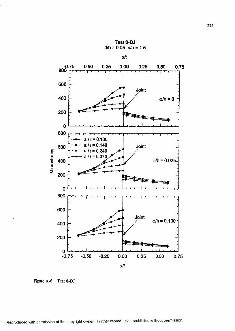
Test 8-DJd/h = 0.05, s/h = 1.5
yUl
272
-0.75 -0.50 -0.25 0.00 0.25 0.50 0.75800
a/h = 0
600 h
T I r n I I I I I I I I I r
#— a / ( = 0.100 «— a / ( = 0.149
(0 Ç '2w 400 u S
— a / ( = 0.249 -V— a / ( = 0.373
200 h
Q L - i 1 1 ! 1 1 I ■ I 1 I t I I I [ I I I I t L L J 1 - 1 i ,
Joint
a/h = 0 .025J
800
600
Jointa/h = 0 .1 0 0 1400
200
-0.75 -0.50 -0.25 0.00 0.25 0.50 0.75
x/(
Figure A-6 . Test 8 -DJ
Reproduced with permission of the copyright owner. Further reproduction prohibited without permission.
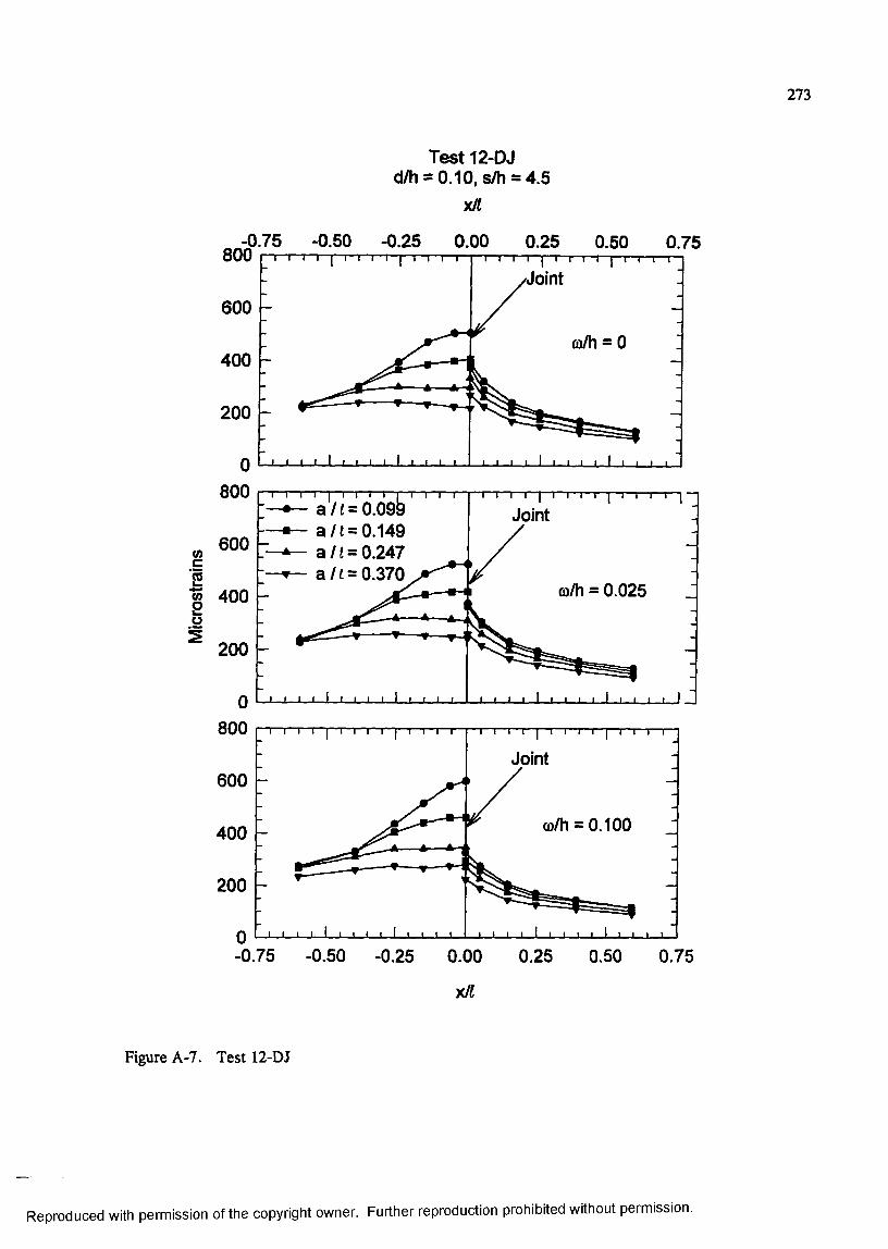
273
T est 12-DJ d/h = 0.10, s/h = 4.5
xH
-0.75 -0.50 -0.25 0.00 0.25 0.50 0.75800
600
400
200
0 800
g 600
■|§ 400 .2
^ 200 h
1 1 r “ 1 1 1 1 1 "|""x n 1 1 1 1 i j k 1 I r “| 1 I 1 r✓Joint
m/h = 0 I
^--- V—-v-!
L l _ l J_ 1 1 l_ 1 I 1 1 1 1 1 i_ J 1 1. 1 I 1 1 1 1 1 1 1 1
"1 I I 1 I I r 7 I [" T 1 r rI—I I—I—p-»— a / ( = 0.099
— a / ( = 0.149a / ( = 0.247
-V— a / I = 0.370
1 — r—I— r I 1— i— r—1— r -T —I— i— i— i —i
Joint
m/h = 0.025
Q I— I— I— I— I— I— L I .1 I_1 I l_ J I I I I I I I I I I I I I I
800Joint
600
m/h = 0 .1 0 0400
200
-0.75 -0.50 -0.25 0.00 0.25 0.50 0.75
x/l
Figure A-7. Test 12-DJ
Reproduced with permission of the copyright owner. Further reproduction prohibited without permission.
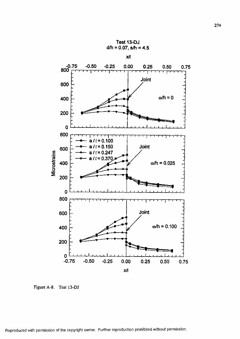
274
Test 13-DJd/h = 0.07, s/h = 4.5
0.25 0.50 0.75T ' I I T I I I I r [ I I I r
Joint
co/h = 0
g 1w 400
I I I I | i I I I— p T — I— r n
a / ( = 0.100 a / ( = 0.150
^— a / ( = 0.247 V— a / ( =
m/h = 0.025 -
800
Joint600
m/h = 0.100 J400
200
-0.75 -0.50 -0.25 0.00 0.25 0.50 0.75
xll
Figure A-8 . Test 13-DJ
Reproduced with permission of the copyright owner. Further reproduction prohibited without permission.
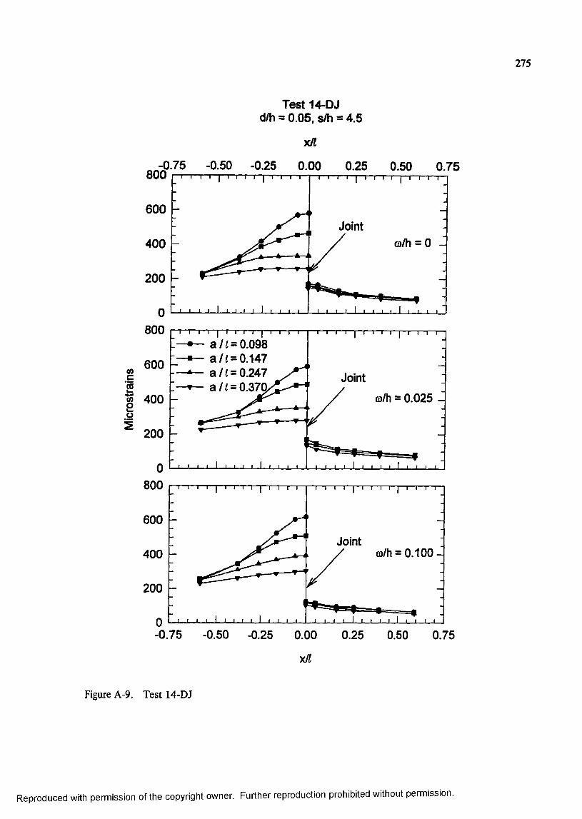
275
Test 14-DJd/h = 0.05, s/h = 4.5
%Jl
^^-0.75 -0.50 -0.25 0.00 0.25 0.50 0.75800 I I I I I n — I— I I— I— I— I— I— — I— I— I— I— I— I— I— I— I— I— I— I— I—
m/h = 0 -
600 -
T I I I I I I I I I I I— I r
—•— a / ( = 0.098 a / ( = 0.147
COc5g 400
— a / / = 0.247 -V— a / ( = i
200 -
m/h = 0.025 -
0 —I—1—I—I 1 1—LJ I -I I I I I 1 I 1 I I I I I l l ' l l !800
600
Jointm/h = 0.100 -400
200
-0.75 -0.50 -0.25 0.00 0.25 0.50 0.75
x/f
Figure A-9. Test 14-DJ
Reproduced with permission of the copyright owner. Further reproduction prohibited without permission.

APPENDIX B
TABULATED JOINT RESPONSES FROM I950S MODEL TESTS
2 7 6
Reproduced with permission of the copyright owner. Further reproduction prohibited without permission.
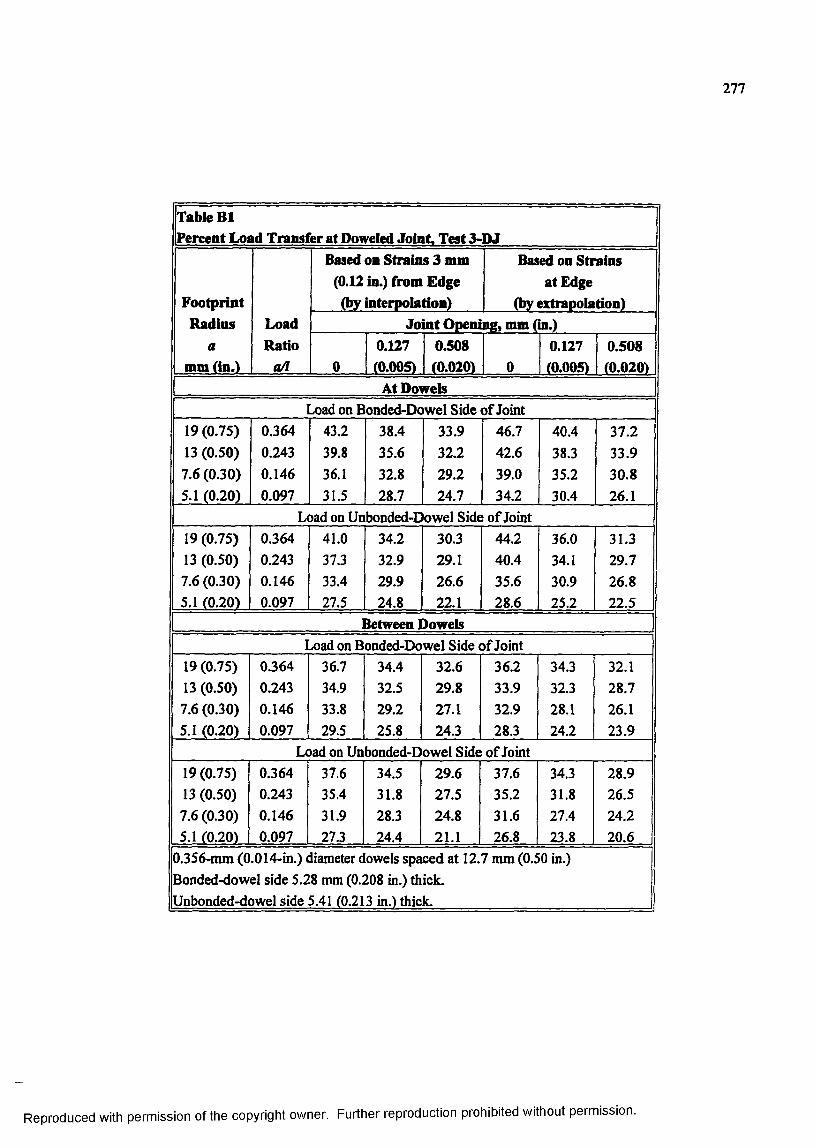
277
Table B1Percent Load Transfer at Doweled Joint. Test 3-DJ
FootprintRadius
amm (in.)
LoadRatio
0/7
Based on Strains 3 mm (0.12 in.) from Edge (by interpolation)
Based on Strains at Edge
(by extrapolation)Jomt Opening, mm (in.)
00.127(0.005)
0.508(0.020) 0
0.127(0.005)
0.508(0.020)
At Dowels.oad on Bonded-Dowel Side of Joint
19(0.75) 13 (0.50) 7.6(0.30) 5.1 (0.20)
0.3640.2430.1460.097
43.239.836.131.5
38.435.6 32.828.7
33.932.229.2 24.7
46.742.639.034.2
40.438.3 35.230.4
37.233.930.826.1
Load on Unbonded-Dowel Side of Joint19 (0.75) 13 (0.50) 7.6 (0.30) 5.1 (0.20)
0.3640.2430.1460.097
41.037.333.427.5
34.232.929.9 24.8
30.329.1 26.622.1
44.240.435.628.6
36.034.1 30.925.2
31.329.726.8 22.5
Between Dowels.oad on Bonded-Dowel Side of Joint
19 (0.75) 13 (0.50) 7.6 (0.30) 5.1 (0.20)
0.3640.2430.1460.097
36.7 34.933.8 29.5
34.432.5 29.2 25.8
32.629.827.124.3
36.233.932.928.3
34.332.3 28.1 24.2
32.1 28.726.1 23.9
Load on Unbonded-Dowel Side of Joint19 (0.75) 13 (0.50) 7.6 (0.30) 5.1 (0.20)
0.3640.2430.1460.097
37.635.431.927.3
34.531.828.324.4
29.627.524.821.1
37.6 35.231.6 26.8
34.331.827.423.8
28.926.5 24.220 .6
0.356-mm (0.014-in.) diameter dowels spaced at 12.7 mm (0.50 in.) Bonded-dowel side 5.28 mm (0.208 in.) thick.Unbonded-dowel side 5.41 (0.213 in.) thick.
Reproduced with permission of the copyright owner. Further reproduction prohibited without permission.
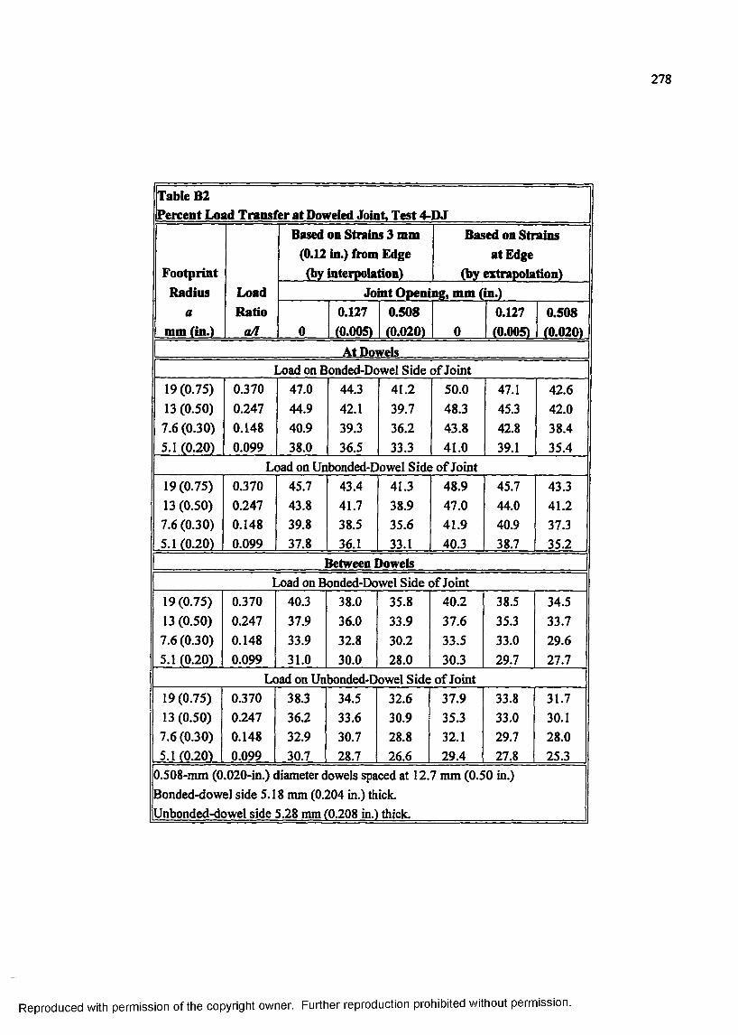
278
Table B2Percent Load Transfer at Doweled Joint, Test 4-DJ
FootprintRadius
amm fin.)
LoadRatio
0/7
Based on Strains 3 mm (0.12 in.) from Edge (by interpolation)
Based on Strains at Edge
(by extrapolation)Jomt Opening, mm (m.)
00.127(0.005)
0.508(0.020) 0
0.127(0.005)
0.508(0.020)
At Dowelsxiad on Bonded-Dowel Side of Joint
19 (0.75) 13 (0.50) 7.6 (0.30) 5.1 (0.20)
0.3700.2470.1480.099
47.044.940.938.0
44.3 42.139.3 36.5
41.2 39.736.233.3
50.0 48.3 43.841.0
47.1 45.3 42.839.1
42.642.038.435.4
Load on Unbonded-Dowel Side of Joint19(0.75) 13 (0.50) 7.6 (0.30) 5.1 (0.20)
0.3700.2470.1480.099
45.743.839.837.8
43.4 41.738.5 36.1
41.338.935.633.1
48.9 47.041.9 40.3
45.7 44.0 40.938.7
43.341.237.3 35.2
Between Dowelsj)ad on Bonded-Dowel Side of Joint
19(0.75) 13 (0.50) 7.6 (0.30) 5.1 (0.20)
0.3700.2470.1480.099
40.337.933.9 31.0
38.036.0 32.830.0
35.833.9 30.2 28.0
40.2 37.6 33.530.3
38.535.333.029.7
34.5 33.729.627.7
Load on Unbonded-Dowel Side of Joint19(0.75) 13 (0.50) 7.6 (0.30) 5.1 (0.20)
0.3700.2470.1480.099
38.336.232.930.7
34.533.630.728.7
32.6 30.9 28.826.6
37.935.3 32.129.4
33.833.029.727.8
31.730.128.025.3
0.508-mm (0.020-in.) diameter dowels spaced at 12.7 mm (0.50 in.) Bonded-dowel side 5.18 mm (0.204 in.) thick.Unbonded-dowel side 5.28 mm (0.208 in.) thick.
Reproduced with permission of the copyright owner. Further reproduction prohibited without permission.
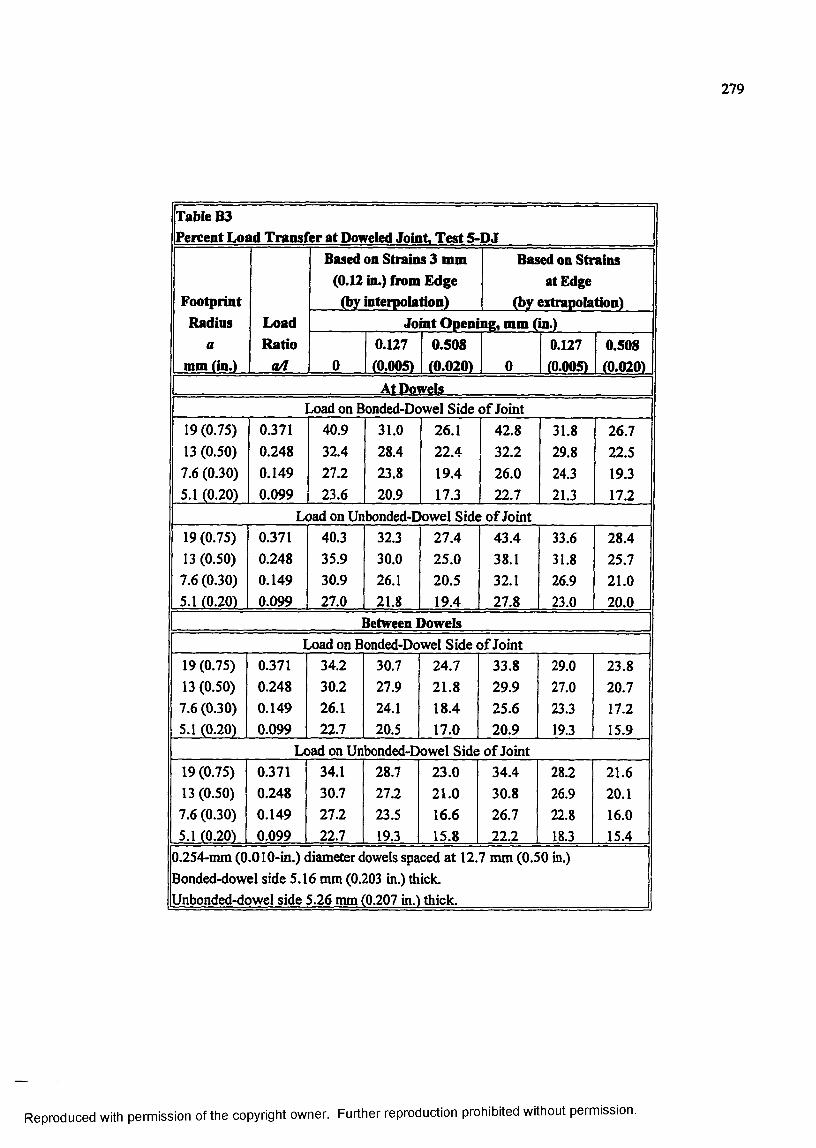
279
Table B3Percent Load Transfer at Doweled Joint Test 5-DJ
FootprintRadius
amm fin.)
LoadRatio
a/l
Based on Strains 3 mm (0.12 in.) from Edge (by interpolation)
Based on Strains at Edge
(by extrapolation)Jomt Opening, mm (m.)
00.127(0.005)
0.508(0.020) 0
0.127(0.005)
0.508(0.020)
At Dowelsx)ad on Bonded-Dowel Side o f Joint
19 (0.75) 13 (0.50) 7.6 (0.30) 5.1 (0.20)
0.3710.2480.1490.099
40.932.427.223.6
31.028.423.820.9
26.122.419.4 17.3
42.832.226.022.7
31.829.824.321.3
26.722.519.317.2
Load on Unbonded-Dowel Side of Joint19 (0.75) 13 (0.50) 7.6 (0.30) 5.1 (0.20)
0.3710.2480.1490.099
40.335.930.9 27.0
32.330.026.1 21.8
27.4 25.020.5 19.4
43.438.132.1 27.8
33.631.826.9 23.0
28.425.721.0
20 .0
Between Dowelsx)adonB onded-Dowel Side of Joint
19(0.75) 13 (0.50) 7.6 (0.30) 5.1 (0.20)
0.3710.2480.1490.099
34.230.2 26.1 22.7
30.727.924.120.5
24.72 1 .8
18.4 17.0
33.829.9 25.620.9
29.027.023.319.3
23.8 20.7 17.215.9
Load on Unbonded-Dowel Side of Joint19(0.75) 13 (0.50) 7.6 (0.30) 5.1 (0.20)
0.3710.2480.1490.099
34.130.727.222.7
28.727.2 23.519.3
23.02 1 .0
16.6 15.8
34.430.826.72 2 .2
28.226.922.8
18.3
21.6
20.1
16.015.4
0.254-mm (0.010-in.) diameter dowels spaced at 12.7 mm (0.50 in.) Bonded-dowel side 5.16 mm (0.203 in.) thick.Unbonded-dowel side 5.26 mm (0.207 in.) thick.
Reproduced with permission of the copyright owner. Further reproduction prohibited without permission.
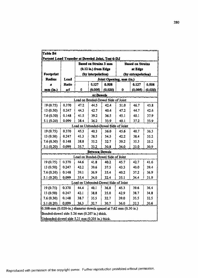
280
Table B4Percent Load Transfer at Doweled Joint, Test 6-DJ
FootprintRadios
amm (in.)
LoadRatio
0/7
Based on Strains 3 mm (0.12 in.) from Edge (by interpolation)
Based on Strains at Edge
(by extrapolation)JoInt Opening, mm (m.)
00.127(0.005)
0.508(0.020) 0
0.127(0.005)
0.508(0.020)
At Dowelsx)ad on Bonded-Dowel Side o f Joint
19 (0.75) 13 (0.50) 7.6(0.30) 5.1 (0.20)
0.3700.2470.1480.099
47.244.3 41.538.4
44.542.739.236.2
42.440.436.5 33.9
51.0 47.245.140.1
46.744.740.137.2
43.8 42.637.933.9
Load on Unbonded-Dowel Side o f Joint19 (0.75) 13 (0.50) 7.6(0.30) 5.1 (0.20)
0.3700.2470.1480.099
45.341.3 38.8 35.7
40.338.535.233.2
36.034.532.730.8
45.642.239.2 36.0
40.738.435.333.0
36.335.233.2 30.9
Between Dowels^ ad on Bonded-Dowel Side o f Joint
19 (0.75) 13 (0.50) 7.6 (0.30) 5.1 (0.20)
0.3700.2470.1480.099
44.642.239.135.4
41.8 39.636.9 34.0
40.237.535.432.4
45.743.340.235.1
42.740.037.234.4
41.639.436.931.9
Load on Unbonded-Dowel Side o f Joint19 (0.75) 13 (0.50) 7.6 (0.30) 5.1 (0.20)
0.3700.2470.1480.099
44.442.138.736.3
40.138.835.532.7
36.835.032.730.7
45.342.939.036.0
39.638.7 35.5 32.3
36.4 34.832.530.6
0.508-mm (0.020-in.) diameter dowels spaced at 7.62 mm (0.30 in.) Bonded-dowel side 5.26 mm (0.207 in.) thick.Unbonded-dowel side 5.21 mm (0.205 in.) thick.
Reproduced with permission of the copyright owner. Further reproduction prohibited without permission.
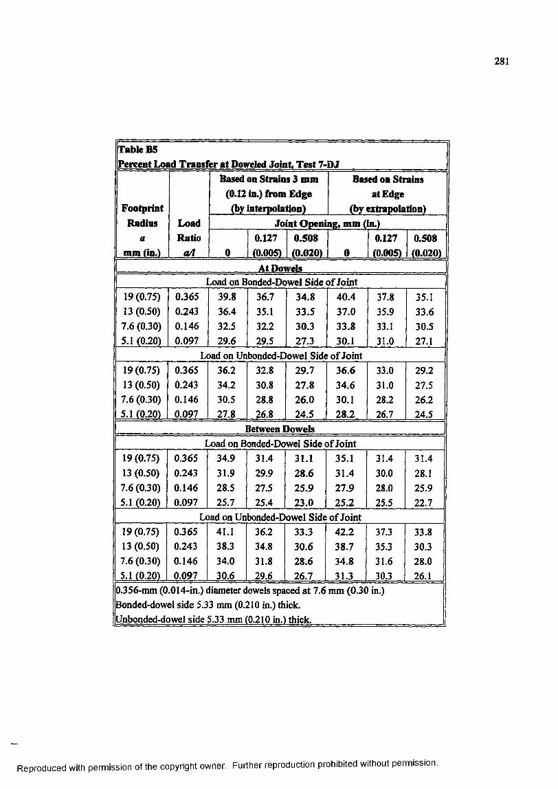
281
Table B5Percent Load Transfer at Doweled Joint Test 7-DJ
FootprintRadios
amm (In.)
LoadRatio
a/l
Based on Strains 3 mm (0.12 in.) from Edge (by interpolation)
Based on Strains at Edge
(by extrapolation)Jomt Opening, mm (in.)
00.127(0.0051
0.508(0.0201 0
0.127(0.005)
0.508(0.020)
At Dowelsx)ad on Bonded-Dowel Side of Joint
19(0.75) 13 (0.50) 7.6 (0.30) 5.1 (0.20)
0.3650.2430.1460.097
39.836.432.529.6
36.735.132.2 29.5
34.833.530.327.3 ^
40.437.0 33.830.1
37.835.9 33.1 31.0
35.1 33.6 30.527.1
Load on Unbonded>Dowei Side of Joint19(0.75) 13 (0.50) 7.6 (0.30) 5.1 (0.201
0.3650.2430.1460.097
36.234.2 30.5 27.8
32.830.828.8 26.8
29.727.8 26.0 24.5
36.634.630.128.2
33.031.0 28.2 26.7
29.227.526.224.5
Between Dowelsx)ad on Bonded-Dowel Side of Joint
19(0.75) 13 (0.50) 7.6 (0.30) 5.1 (0.20)
0.3650.2430.1460.097
34.931.9 28.5 25.7
31.4 29.927.5 25.4
31.128.625.923.0
35.1 31.4 27.925.2
31.430.028.025.5
31.428.125.922.7
Load on Unbonded-Dowel Side of Joint19 (0.75) 13 (0.50) 7.6 (0.30) 5.1 (0.201
0.3650.2430.1460.097
41.138.334.030.6
36.234.831.8 29.6
33.330.628.6 26.7
42.238.734.831.3
37.335.3 31.630.3
33.830.328.026.1
0.356-mm (0.014-in.) diameter dowels spaced at 7.6 mm (0.30 in.) Bonded-dowel side 5.33 mm (0.210 in.) thick.Unbonded-dowel side 5.33 mm (0.210 in.) thick.
Reproduced with permission of the copyright owner. Further reproduction prohibited without permission.

282
Table B6Percent Load Transfer at Doweled Joint, Test 8-DJ
FootprintRadius
amm (in.)
LoadRatio
a/l
Based on Strains 3 mm (0.12 in.) from Edge (by interpolation)
Based on Strains at Edge
(by extrapolation)Jomt Opening, mm (m.)
00.127(0.005)
0.508(0.020) 0
0.127(0.005)
0.508(0.020)
At Dowelsx)ad on Bonded-Dowel Side of Joint
19 (0.75) 13 (0.50) 7.6 (0.30) 5.1 (0.20)
0.3730.2490.1490.100
35.1 31.9 28.625.2
32.931.5 28.824.6
30.627.4 23.920.5
35.531.6 27.8 25.2
32.330.928.824.1
31.527.3 23.721.3
Load on Unbonded-Dowel Side o f Joint19 (0.75) 13 (0.50) 7.6 (0.30) 5.1 (0.20)
0.3730.2490.1490.100
37.834.330.125.2
33.531.9 29.724.9
27.6 26.223.6 19.5
39.236.1 30.726.1
33.731.930.225.0
28.626.824.820.4
Between Dowelsxiad on Bonded-Dowel Side o f Joint
19 (0.75) 13 (0.50) 7.6 (0.30) 5.1 (0.20)
0.3730.2490.1490.100
33.329.826.722.5
31.1 29.626.1 22.3
28.425.4 21.9 18.6
32.729.325.821.4
31.029.225.821.4
28.725.021.0
17.8Load on Unbonded-Dowel Side o f Joint
19(0.75) 13 (0.50) 7.6 (0.30) 5.1 (0.20)
0.3730.2490.1490.100
33.1 29.6 26.521.2
28.227.725.220.3
24.423.0 20.717.0
33.029.2 25.420 .2
28.527.4 24.819.4
23.922.420.2
16.10.254-nun (0.010-in.) diameter dowels spaced at 7.6 mm (0.30 in.) Bonded-dowel side 5.05 mm (0.199 in.) thick.Unbonded-dowel side 5.28 (0.208 in.) thick.
Reproduced with permission of the copyright owner. Further reproduction prohibited without permission.
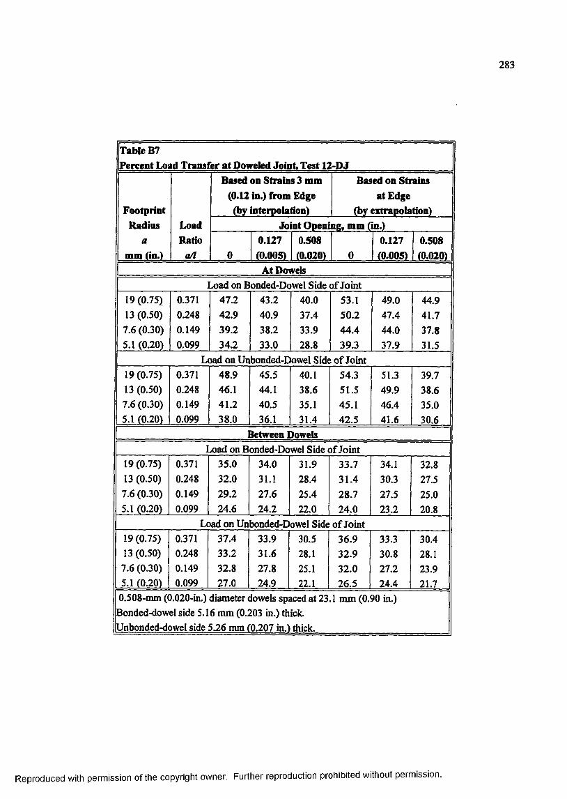
283
Table B7Percent Load Transfer at Doweled Joint Test 12-D J
FootprintRadius
amm fin.)
LoadRatio
aA
Based on Strains 3 mm (0.12 in.) from Edge (by interpolation)
Based on Strains at Edge
(by extrapolation)Jo nt Opening, mm (m.)
00.127(0.005)
0.508(0.020) 0
0.127(0.005)
0.508(0.020)
At Dowebx)ad on Bonded-Dowel Side of Joint
19(0.75) 13 (0.50) 7.6 (0.30) 5.1 (0.20)
0.3710.2480.1490.099
47.2 42.939.234.2
43.2 40.938.2 33.0
40.037.433.928.8
53.150.2 44.439.3
49.0 47.444.0 37.9
44.941.737.8 31.5
Load on Unbonded-Dowel Side of Joint19(0.75) 13 (0.50) 7.6 (0.30) 5.1 (0.20)
0.3710.2480.1490.099
48.946.141.2 38.0
45.544.140.536.1
40.1 38.635.1 31.4
54.351.5 45.142.5
51.3 49.946.4 41.6
39.738.6 35.030.6
Between Dowebvoad on Bonded-Dowel Side of Joint
19 (0.75) 13 (0.50) 7.6 (0.30) 5.1 (0.20)
0.3710.2480.1490.099
35.032.0 29.2 24.6
34.031.1 27.624.2
31.928.425.4 22.0
33.7 31.428.7 24.0
34.1 30.3 27.523.2
32.8 27.5 25.020.8
Load on Unbonded-Dowel Side of Joint19(0.75) 13 (0.50) 7.6 (0.30) 5.1 (0.20)
0.3710.2480.1490.099
37.433.232.827.0
33.931.627.824.9
30.528.125.122.1
36.932.9 32.0 26.5
33.3 30.8 27.224.4
30.428.123.921.7
0.508-mm (0.020-in.) diameter doweb spaced at 23.1 mm (0.90 in.) Bonded-dowel side 5.16 mm (0.203 in.) thick.Unbonded-dowel side 5.26 mm (0.207 in.) thick.
Reproduced with permission of the copyright owner. Further reproduction prohibited without permission.
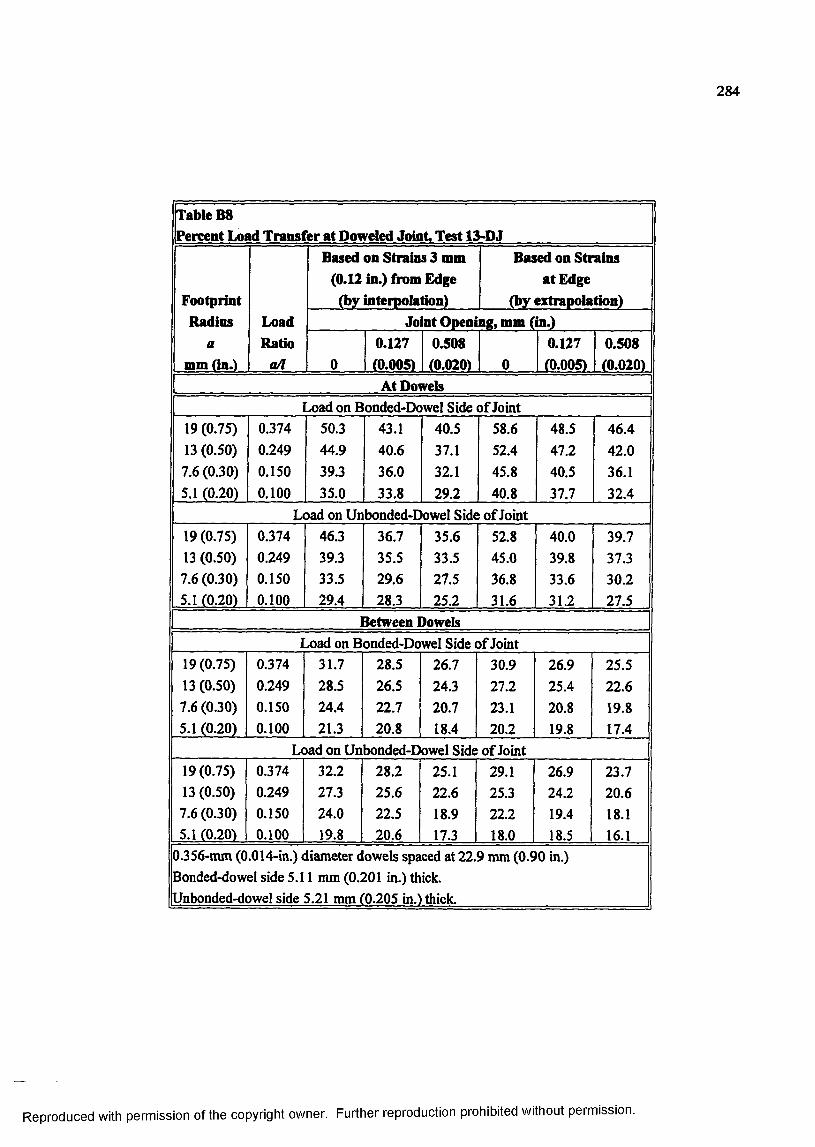
284
Table B8Percent Load Transfer at Doweled Joint, Test 13-DJ
FootprintRadius
amm (in.)
LoadRatio
a/l
Based on Strains 3 mm (0.12 in.) from Edge (by interpolation)
Based on Strains at Edge
(by extrapolation)Joint Opening, mm (m.)
00.127(0.005)
0.508(0.020) 0
0.127(0.005)
0.508(0.020)
At Dowelsx>ad on Bonded-Dowel Side of Joint
19 (0.75) 13 (0.50) 7.6 (0.30) 5.1 (0.20)
0.3740.2490.1500.100
50.3 44.939.3 35.0
43.140.636.033,8
40.537.132.129.2
58.652.445.840.8
48.5 47.240.5 37.7
46.442.036.132.4
Load on Unbonded-Dowel Side of Joint19 (0.75) 13 (0.50) 7.6(0.30) 5.1 (0.20)
0.3740.2490.1500.100
46.339.3 33.529.4
36.735.529.6 28.3
35.633.527.5 25.2
52.8 45.036.8 31.6
40.039.833.631.2
39.737.330.227.5
Between Dowelsx)ad on Bonded-Dowel Side of Joint
19 (0.75) 13 (0.50) 7.6 (0.30) 5.1 (0.20)
0.3740.2490.1500.100
31.728.524.421.3
28.526.522.720.8
26.724.320.718.4
30.927.223.120.2
26.925.420.8
19.8
25.522 .6
19.8 17.4
Load on Unbonded-Dowel Side of Joint19(0.75) 13 (0.50) 7.6 (0.30) 5.1 (0.20)
0.3740.2490.1500.100
32.227.3 24.0 19.8
28.225.622.520.6
25.122.6
18.917.3
29.1 25.322.2
18.0
26.924.219.418.5
23.720 .6
18.116.1
0.356-mm (0.014-in.) diameter dowels spaced at 22.9 mm (0.90 in.) Bonded-dowel side 5.11 mm (0.201 in.) thick.Unbonded-dowel side 5.21 mm (0.205 in.) thick.
Reproduced with permission of the copyright owner. Further reproduction prohibited without permission.

285
Table B9Percent Load Transfer at Doweled Joint, Test 14-DJ
FootprintRadius
amm (In.)
LoadRatio
a/l
Based on Strains 3 mm (0.12 in.) from Edge (by interpolation)
Based on Strains at Edge
(by extrapolation)Jomt Opening, mm (m.)
00.127(0.005)
0.508(0.020) 0
0.127(0.005)
0.508(0.020)
At Dowels.oad on Bonded-Dowel Side of Joint
19(0.75) 13 (0.50) 7.6(0.30) 5.1 (0.20)
0.3670.2440.1470.098
38.632.026.922.5
30.4 28.0 23.121.5
24.723.319.217.1
41.334.028.0 23.2
34.531.6 26.8 24.3
26.424.620.318.0
Load on Unbonded-Dowel Side o f Joint19(0.75) 13 (0.50) 7.6 (0.30) 5.1 (0.20)
0.3670.2440.1470.098
34.930.226.220.9
28.4 27.321.5 19.9
23.622.417.5 15.4
36.031.6 26.821.7
32.330.524.822.8
25.523.918.9 16.4
Between DowelsX)ad on Bonded-Dowel Side of Joint
19 (0.75) 13 (0.50) 7.6(0.30) 5.1 (0.20)
0.3670.2440.1470.098
26.522.719.315.0
24.321.8
17.716.1
18.9 16.6 14.512.9
24.42 1 .0
17.914.0
24.221.3 16.615.3
17.815.713.811.8
Load on Unbonded-Dowel Side of Joint19(0.75) 13 (0.50) 7.6 (0.30) 5.1 (0.20)
0.3670.2440.1470.098
25.8 22.417.9 13.6
21.8
20.1
15.813.9
17.215.411.5 11.7
24.321.516.912.8
20.719.0 15.213.0
16.514.6 10.9 11.1
0.254-mm (0.010-in.) diameter dowels spaced at 0.90 in. Bonded-dowel side 5.26 mm (0.207 in.) thick. Unbonded-dowel side 5.33 mm (0.210 in.) thick.
Reproduced with permission of the copyright owner. Further reproduction prohibited without permission.
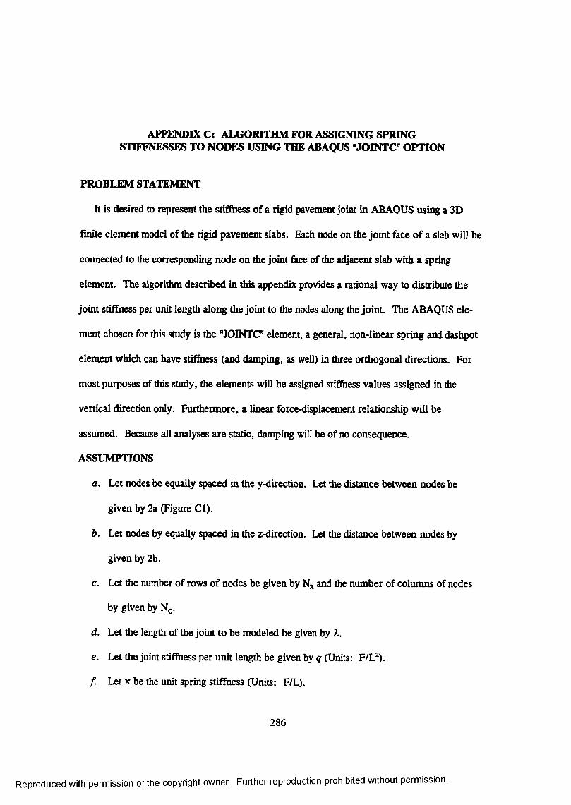
APPENDIX C: ALGORITHM FOR ASSIGNING SPRING STIFFNESSES TO NODES USING THE ABAQUS “JOINTC* OPTION
PROBLEM STATEMENT
It is desired to represent the sdfhess of a rigid pavement joint in ABAQUS using a 3D
finite element model of the rigid pavement slabs. Each node on the joint face o f a slab will be
connected to the corresponding node on the joint face of the adjacent slab with a spring
element. The algorithm described in this appendix provides a rational way to distribute the
joint stiffness per unit length along the joint to the nodes along the joint. The ABAQUS ele
ment chosen for this study is the “JOINTC” element, a general, non-linear spring and dashpot
element which can have stiffiiess (and damping, as well) in three orthogonal directions. For
most purposes of this study, the elements will be assigned stiffness values assigned in the
vertical direction only. Furthermore, a linear force-displacement relationship will be
assumed. Because all analyses are static, damping will be of no consequence.
ASSUMPTIONS
a. Let nodes be equally spaced in the y-direction. Let the distance between nodes be
given by 2a (Figure Cl).
b. Let nodes by equally spaced in the z-direction. Let the distance between nodes by
given by 2b.
c. Let the number of rows of nodes be given by Nr and the number of columns of nodes
by given by N^.
d. Let the length of the joint to be modeled be given by A..
e. Let the joint stiffness per unit length be given by q (Units: F/L^).
f . Let K be the unit spring stiffness (Units: F/L).
286
Reproduced with permission of the copyright owner. Further reproduction prohibited without permission.
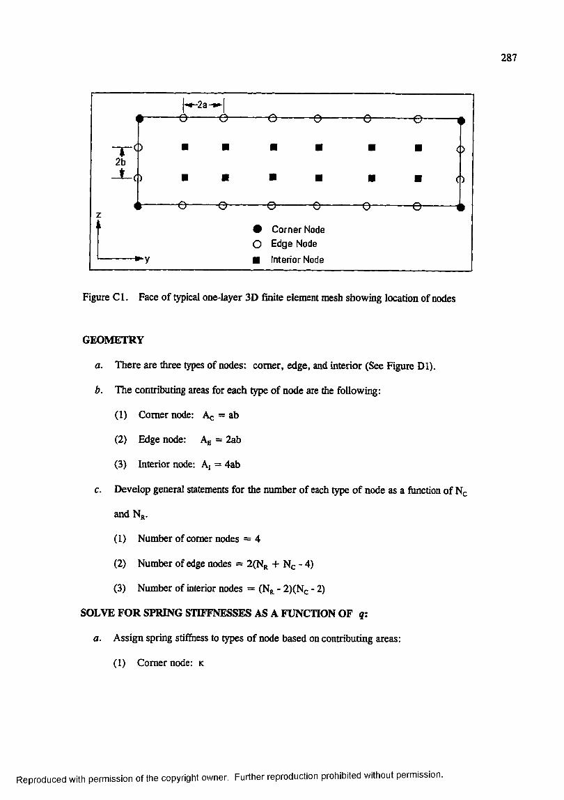
287
# Corner Node O Edge Node ■ Interior Node
Figure C l. Face of typical one-layer 3D finite element mesh showing location of nodes
GEOMETRY
a. There are three types of nodes: comer, edge, and interior (See Figure Dl).
b. The contributing areas for each type of node are the following:
(1) Comer node: Ac = ab
(2) Edge node: Ag = 2ab
(3) Interior node: A, = 4ab
c. Develop general statements for the number of each type of node as a function of Ng
and Nr.
(1) Number of comer nodes = 4
(2) Number of edge nodes = 2(Nr + Nc - 4)
(3) Number of interior nodes = ( N r - 2)(Ng - 2)
SOLVE FOR SPRING STIFFNESSES AS A FUNCTION OF q:
a. Assign spring stiffiiess to types of node based on contributing areas:
(1) Comer node: k
Reproduced with permission of the copyright owner. Further reproduction prohibited without permission.

288
(2) Edge node: 2k
(3) Interior node: 4k
b. Set joint stiffiiess equal to sum of spring stiffnesses.
^ X A = K X (Number of comer nodes) + 2k x (Number o f edge nodes) +
4k X (Number of interior nodes)
= K (4) + 2k[2(Nr + Nc - 4)] + 4k(Nr - 2)(Ng - 2)
= 4k(I + Nr + Nc - 4 + NrNc - 2Nr - 2 Nc + 4)
= 4k(Nr -1)(Nc -1)
Therefore:
K = ------- ^4(N^-lXNc-I)
Reproduced with permission of the copyright owner. Further reproduction prohibited without permission.

APPENDIX D
COMPILATION OF INSTRUMENTATION TRACES FROM EXPERIMENTS
289
Reproduced with permission of the copyright owner. Further reproduction prohibited without permission.
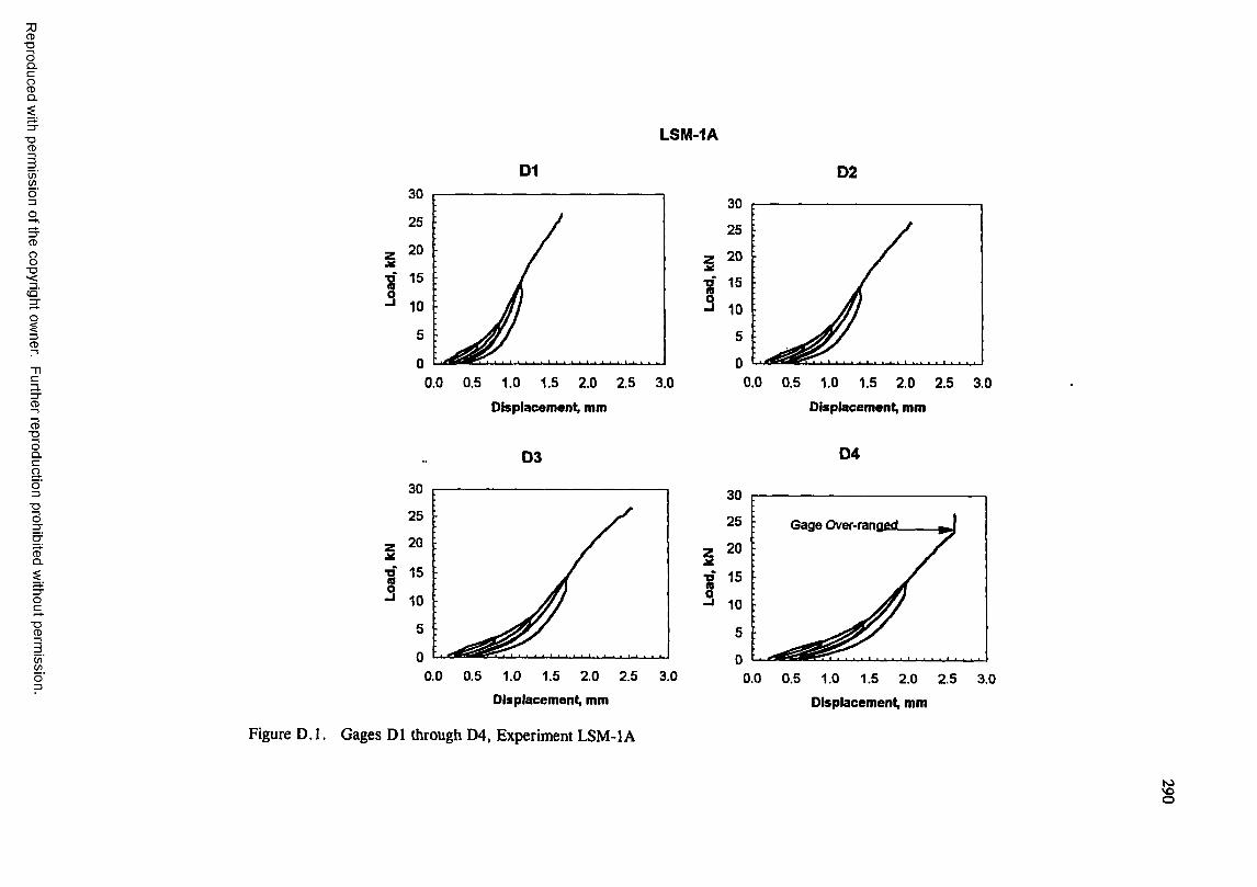
CD■OOQ .C
8Q .
"OCD
(/)o"3
8"Oë '3"
i3CD
3.3"CD
CD"DOQ .C
aO3
■DO
CDQ .
■DCD
C /iC/)
LSM-1A
I
Dl3 0
2 5
20
15
10
5
0
g
I
0 .0 0 .5 1 .0 1 .5 2 .0 2 .5 3 .0
Displacem ent, mm
03
3 0
2 5
20
15
10
5
00 .0 0 .5 1 .0 1 .5 2 .0 2 .5
Displacem ent, mm
Figure D .I. Gages Dl through D4, Experiment LSM-IA
3 .0
0 2
0 .0 0 .5 1 .0 1 .5 2 .0 2 .5 3 .0
Displacem ent, mm
04
2 5 Gage Over-ranged
1
I
0 .0 0 .5 1 .0 1 .5 2 .0 2 .5 3 .0
Displacement, mm
g
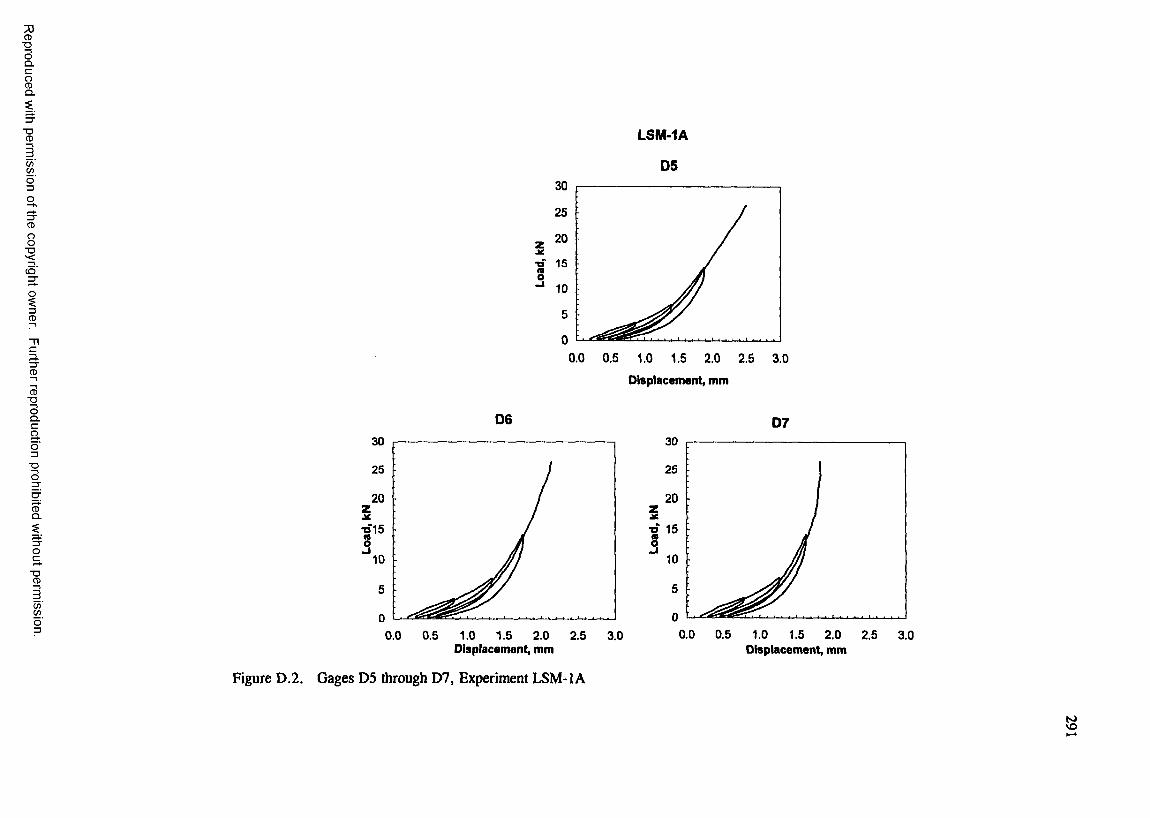
7)CD■DOQ .C
gQ .
■DCD
C /î
o"3
8
ci'
33"CD
CD■DOQ .CaO3
■DO
CDQ .
■DCD
C / )C / )
LSM-IA
05
o
30
2 5
20
1 5
10
5
00 . 0 0 . 5 1 .0 1 .5 2 .0 2 . 5 3 . 0
Displacement, mm
06 073 0
2 5
20
•0*15
10
5
00 . 0 0 . 5 1 .0 1 . 5 2 . 0 2 . 5 3 .0
3 0
•o 15
0 . 0 0 .5 1 .0 1 .5 2 . 0 2 .5 3 .0
Displacement, mm
Figure D.2. Gages D5 through D7, Experiment LSM-IA
Displacement, mm
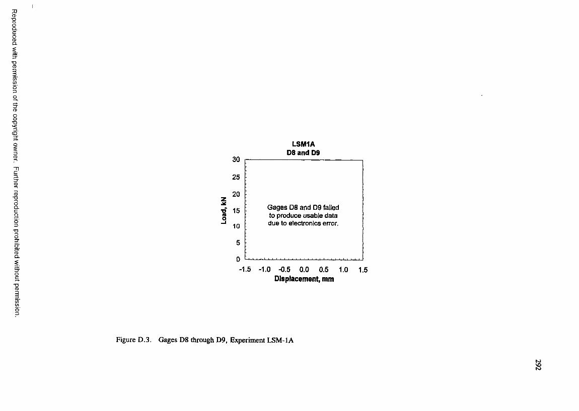
■ooÛ .cgû .
■oCD
8
c5'
3CD
p.3"CD
CD■OOQ .CaO3
■OO
CDQ .
TDCD
LSM1A D8 and D9
30
25
20z■o 15J
10
5
0
Gages 08 and 09 failed to produce usable data due to electronics error.
-1.5 -1.0 -0.5 0.0 0.5 1.0 1.5Displacement, mm
C/)cn
Figure D.3. Gages D8 through D9, Experiment LSM-IA
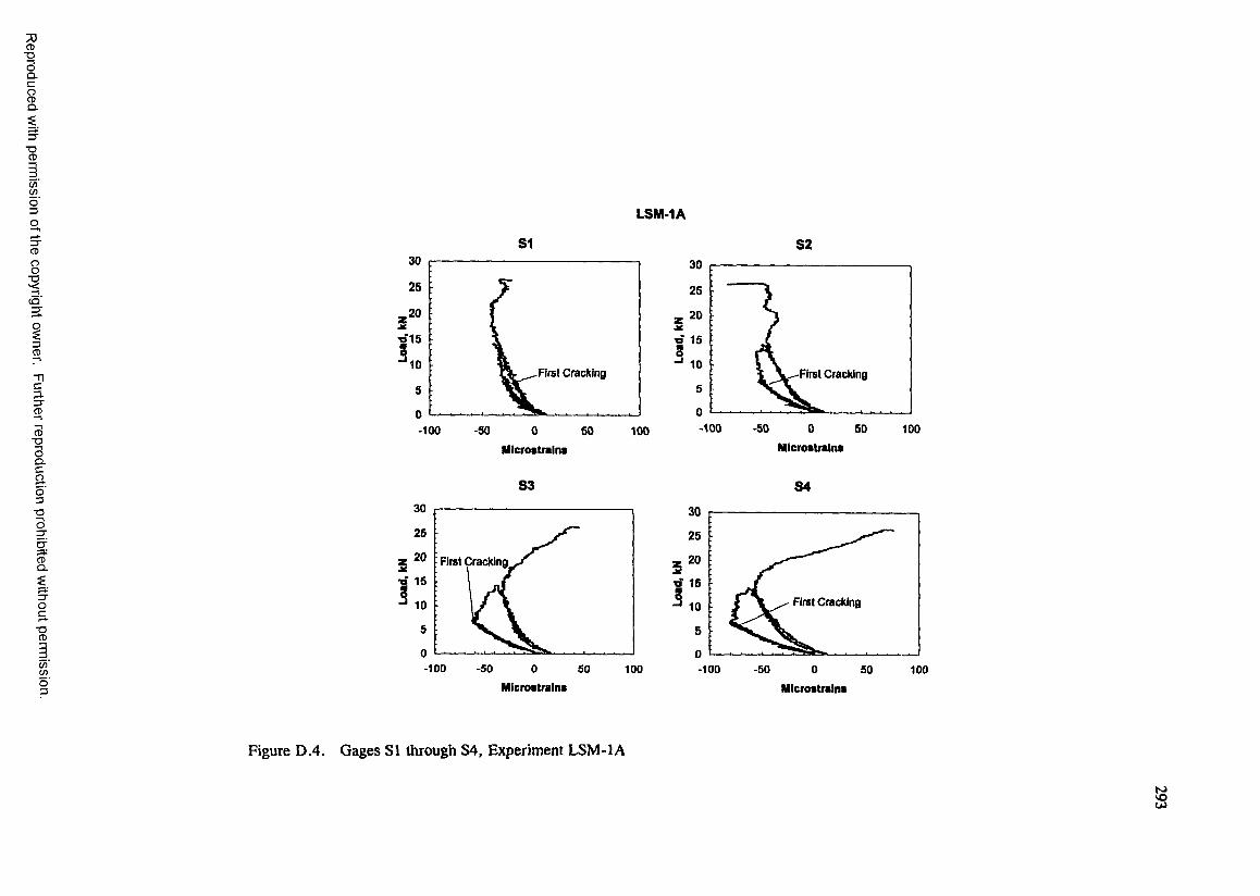
7)CD
"DOÛ .C
gQ .
■DCD
C /)(go "3 LSM-IA
CD
8
S'
i3CD
Cp.3"CD
CD■OICao3
■OO
SI
oc■ o
CD
C/)œo '3
30
2520
•015
10 First C racking5
0100 -50 0 50 100
Micros trains
S3
25
First C rack ing■o 15
-100 -50 0 50 100
8230
25
20
o 15
- * 10First C rack ing
5
0-100 -50 0 50 100
Microstrains
84
o 15F irst C rack ing
-100 -50 0 50 100Microstrains Microstrains
Figure D.4. Gages SI through 84, Experiment LSM-IA
§
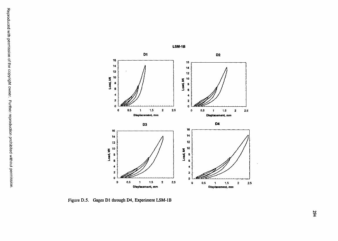
7)CD■OOQ .C
gQ .
■DCD
C /)
o"3O
8
ci'
3.3"CD
CD■DOQ .CaO3
■DO
CDÛ .
■DCD
C / )C / )
!
s3
LSM-1B
Dl16
14
121086
4
20
2.50 0.5 1 1.5 2Displacement, mm
0316
14
12
10
a6
4
2
00 0.5 1 1.5 2 2.5
S1
D216
1412108642Q
0 0.5 1 1.5 2 2.5Displacement, mm
0416
14
12
10
6
6
4
2
00 0.5 1.5 21 2.5
Displacement, mm Displacement, mm
Figure D.5. Gages Dl through D4, Experiment LSM-IB
g
CD■DOQ .C
gQ .
■DCD
C/)
o"3O
8
ci'
33"CD
CD■DOQ .CaO3
■DO
CDQ .
■DCD
C / )C / )
LSM1B 05 and 06
30
25
20zJC"i 15s
10
5
0
Gages 05 and 06 failed to produce usable data due to electronics
error.
-1.5 -1.0 -0.5 0.0 0.5 1.0 1.5Oisplacement, mm
Figure D.6. Gages D5 and 06 , Experiment LSM-IB
§
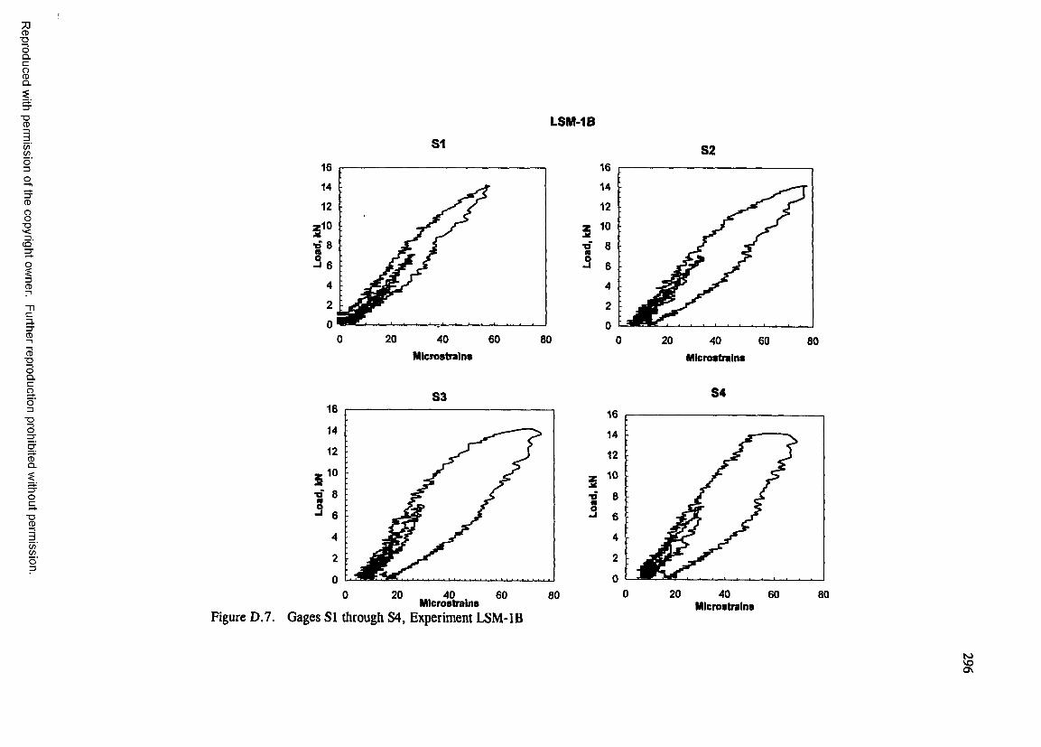
73CD■DOQ .C
gQ .
■DCD LSM-IB
c / )wo "305CD
8ci'3"
13( D
33"CD
CDT 3OQ .Cao3
T 3O
CDQ .
T 3CD
SI S2
(/)(/)
■o 8
- I 6
200 6 04 0 8 0
g
Microstrains
S31 6
14
12
10
8
6
4
2
0200 4 0
Microstrains6 0 8 0
T>g
1 6
1 4
12
10
8
6
4
2
0
I
2 0 4 0 6 0 8 0
Microstrains
S41 6
1 4
12
10
8
6
4
2
00 20 4 0 6 0 8 0
Figure D.7. Gages SI through S4, Experiment LSM-IBMicrostrains
;
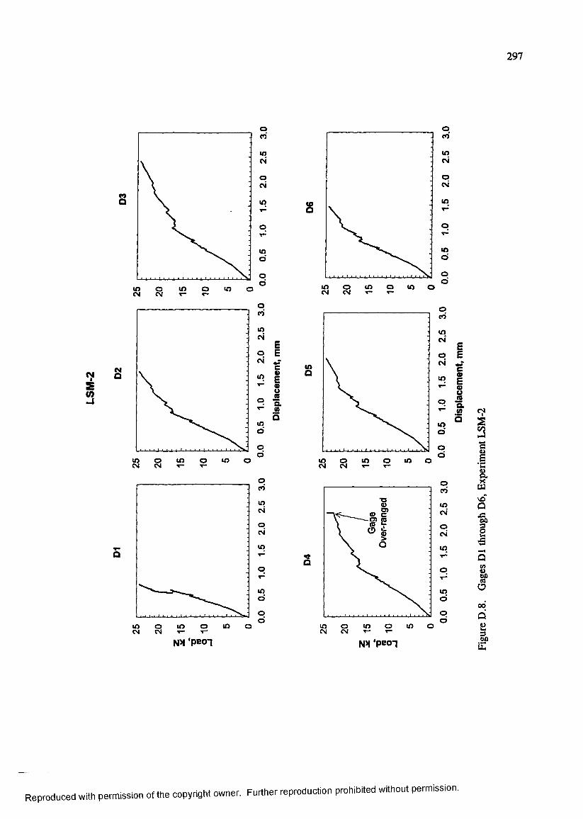
297
Q
l A «n
8
o LO o L O olO
omlONocm '
U )
L Odod
oenL OCM
A I
:i5
L O
L Od
qo
C M C M
L O
OL OO OL O O L O
L Oa
o
L O
ooo L O o
C M C M
PC MLO
L O
O
L O
OL O L O
I
Ia.JSa
CM C M
C O
L O
Q
o o
NX ‘PBOT NX 'Peoi
IIS!Q
I00
Q
I
Reproduced with permission of the copyright owner. Further reproduction prohibited without permission.
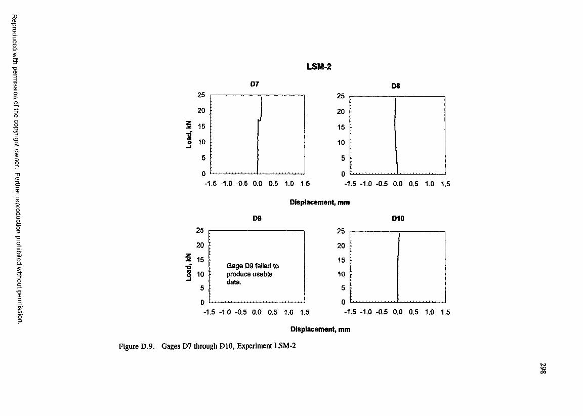
7)CD■OOQ .C
8Q .
■OCD
C/)(gd=3
2,
CD
8c5'Si3CD
Cp.3"CD
CD■OICao3
■OO
CDQ .
3"Oa■oCD
C/)
o"3
LSM-2
D7 08
SO 10
-1.5 -1.0 -0.5 0.0 0.5 1.0 1.5 -1.5 -1.0 -0.5 0.0 0.5 1.0 1.5
Displacement, mm
09 010
•ora
25 25
20 20
15 15Gage 09 failed to
10 produce usable 10data.
5 5
0 1 1 1 -1.1 ■_! 1 1- 1 1 1 . 1 1 . 1 1 , I 1 . I I 1 1 ■ 1 . 0 ............................................................
-1.5 -1.0 -0.5 0.0 0.5 1.0 1.5 -1.5 -1.0 -0.5 0.0 0.5 1.0 1.5
Displacement, mm
Figure D.9. Gages D7 through DIO, Experiment LSM-2
500
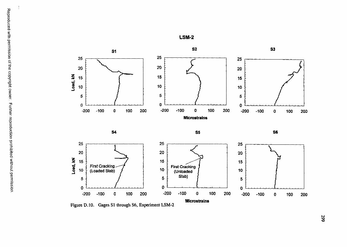
CD■DOÛ .C
gQ .
■DCD
C /)
o'3O
8
cq'3i3CD
C3.3"CD
CD■OICao3
■OO
&
oc■o
CD
C/)œo"3
%
Tïla
SI
25
20
15
10
5
0100 200-200 -100 0
84
25
20
15First Cracking (Loaded Slab)10
5
0-200 -100 0 100 200
25
20
15
10
5
0
LSM-2
82
25
20
15
10
5
0-200 -100 0 100 200
Microstrains
85
acking JFirst Cracking (Unloaded /
Slab)lb) i
Figure D, 10. Gages SI through 86, Experiment LSM-2
-200 -100 0 100
Microstrains
200
83
25
20
15
10
5
0-200 -100 0 100 200
8 6
25
20
15
10
5
0
-200 -100 0 100 200
g
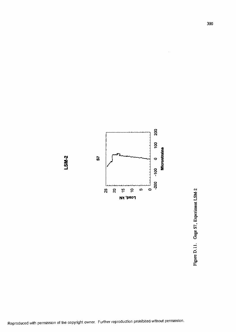
300
g(O
M O
oo
oo mo
IS
CM C M
NX 'p e o i1
IIS
IÛ
IiZ
Reproduced with permission of the copyright owner. Further reproduction prohibited without permission.
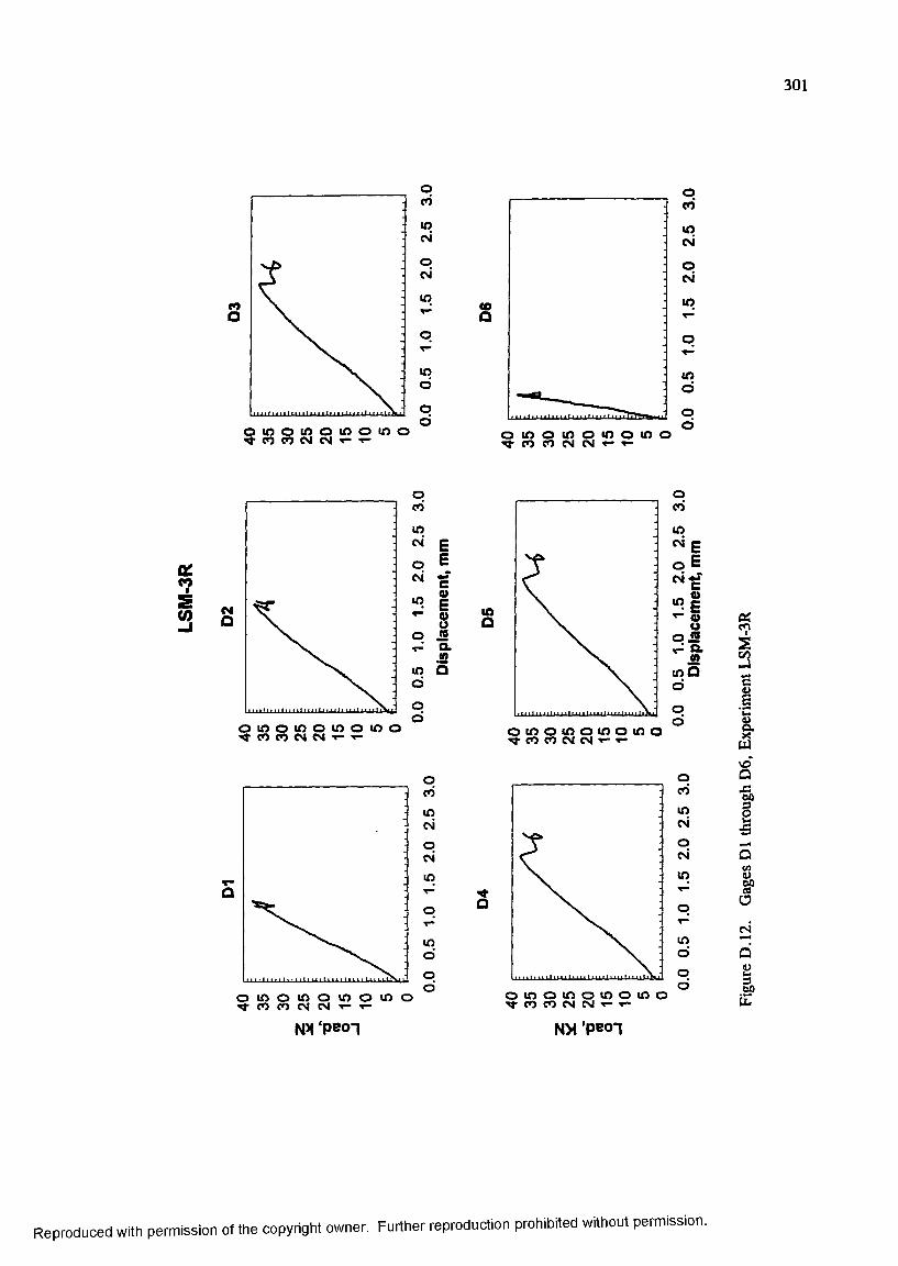
301
S
o m o i o o m o m o
oCO
lOCM*
ocm’
lO
lOdod
CO
taCM
PCM
lOQ
lOd
o^ CO CO CM CM O l O O l O O l O O l O O
^ CO CO CM CM
0 :
i
CO
CM
lOCM
o
oo m o i o o i o o i o o^ CO CO CM CM T - T—
EEï0 E
1Q .M□
o u n o m o t o o v o o
o(OU )CM
oCM
in
(Odod
lOQ
CO
0 .3
in Q
o m o t o o i o o i f l o^ CO CO CM CM T - T -
O
CM
m
o^ CO CO CM CM
NX peoi^ C O C O C M C M T - T -
m 'peoi
IIIÉ
!Q
IMQ
I
Reproduced with permission of the copyright owner. Further reproduction prohibited without permission.
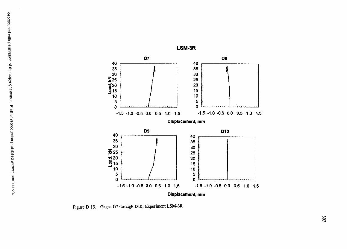
■ooQ .C
gQ .
■OCD
(/)o"3O
LSM-3R
CD
3.3"CD
CD■DOQ .CaO3
■OO
CDQ .
3 -O5-■o
CD
C/)
o'3
07 08403530
l 2 5-0 2 0015
1050
1.5 -1.0 -0.5 0.0 0.5 1.0 1.5
403530252 0151050
1.5 -1.0 -0.5 0.0 0.5 1.0 1.5
O isplacem ent, mm
09
1.5 -1.0 -0.5 0.0 0.5 1.0 1.5
010
-1.5 -1.0 -0.5 0.0 0.5 1.0 1.5
Displacement, mm
Figure D. 13. Gages D7 through DIO, Experiment LSM-3R
WS
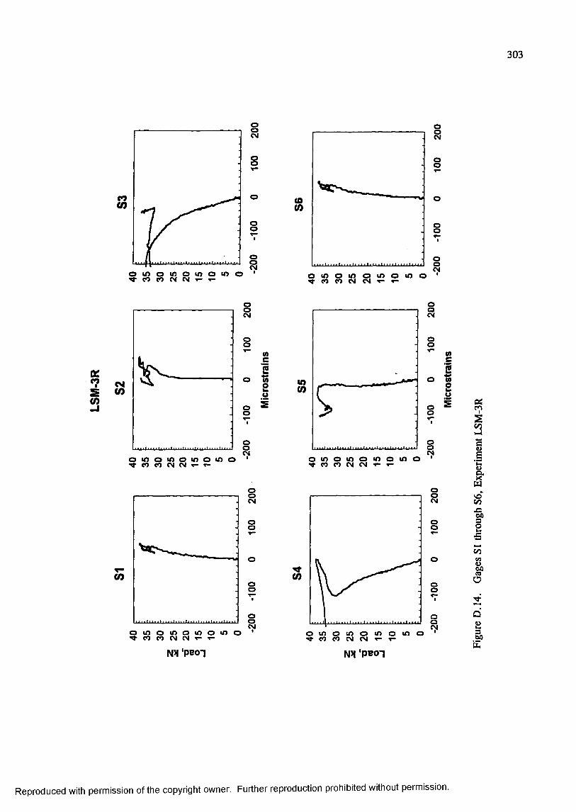
303
C M
S)
? m o co co i n o l oCM CM T -
o
(OCO
o
*?SUi
co
oC M
oo^ M
L C
1------------------------ O g u ,
2 (0U Io So7
oo
§
o m o m o i n o mV M m CM CM T - T -
C Mo m o i A O i o o mT f f O c o C M C M T - T -
s
i
Ii
co
oo
oo
m o i n o l oco co CM CM 1 -
o8
o m o
NX Peoi
o
o
(0oo
a i?
iII«
iV 3
Iûa
#
Reproduced with permission of the copyright owner. Further reproduction prohibited without permission.
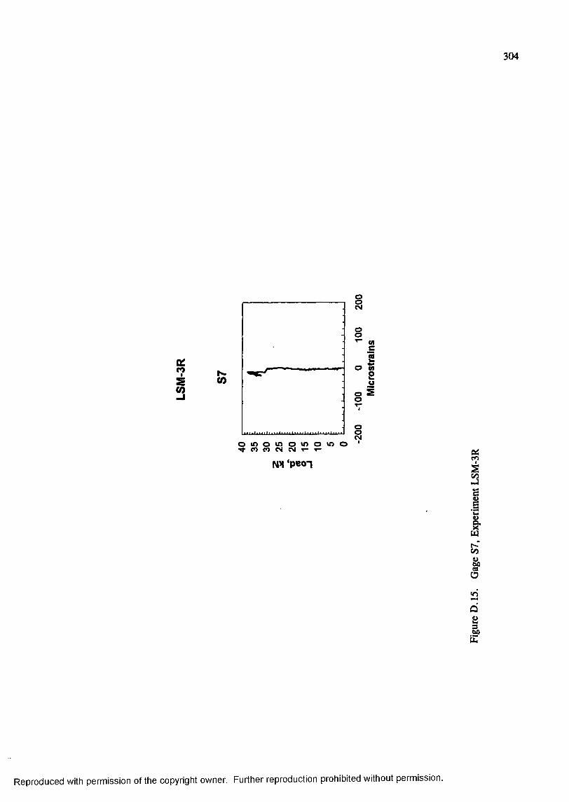
304
«?S(0
CM
O (0NCO
o S
oR
O to oO to O to^ (O CO CM
o to CM T -
NM ‘PCOTa:
I
IICO
I<o
I
Reproduced with permission of the copyright owner. Further reproduction prohibited without permission.
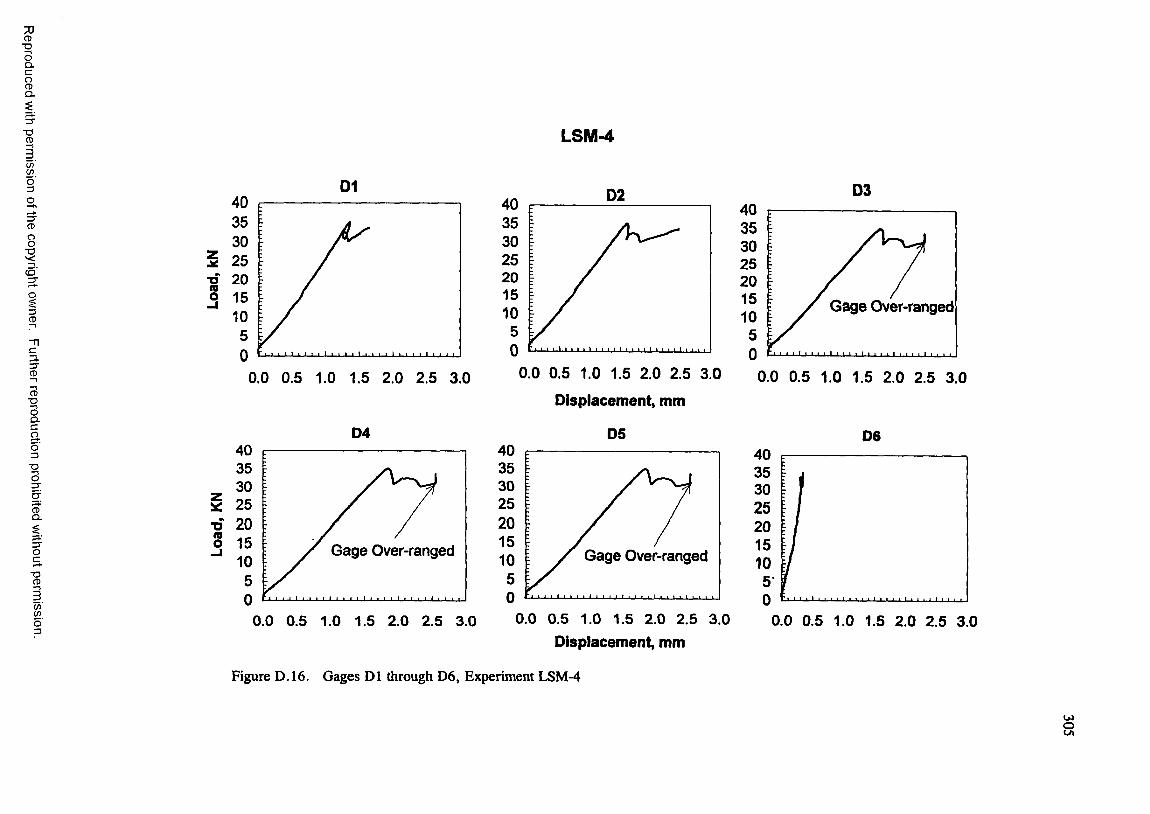
CD"DOQ .C
2O.
■DCD
C /Î
o'32 ,CD
85c q '3i3CD
C3.3"CD
CD■oICaO3
■oO
LSM-4
&
3"Oc5(/)COo'3
Dl
20
0.0 0.5 1.0 1.5 2.0 2.5 3.0
D4
■Ds
4035302520151050
Gage Over-ranged
0.0 0.5 1.0 1.5 2.0 2.5 3.0
20
0.0 0.5 1.0 1.5 2.0 2.5 3.0Displacement, mm
05
03
4035302520151050
Gage Over-ranged
0.0 0.5 1.0 1.5 2.0 2.5 3.0Displacement, mm
Figure D.16. Gages Dl through D6, Experiment LSM-4
252 0
Gage Over-ranged
0.0 0.5 1.0 1.5 2.0 2.5 3.0
D6403530252 0151 050
0.0 0.5 1.0 1.5 2.0 2.5 3.0
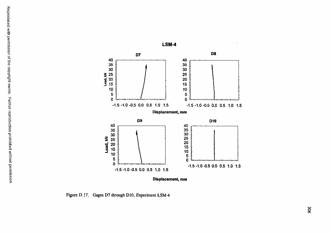
7)CD■DOQ .C
gQ .
■DCD
C/ÎWo'3O
8"O
3.3"CD
CD■DOQ .CaO3
"DO
CDQ .
■DCD
C / )C / )
LSM-4
074035
5 259 203 15
-1.5 -1.0 -0.5 0.0 0.5 1.0 1.5
084035302520151050
-1.5 -1.0 -0.5 0.0 0.5 1.0 1.5
Oisplacement, mm
09 010
30 5 25 ■o' 20
-1.5-1.0-0.5 0.0 0.5 1.0 1.5-1.5-1.0-0.5 0.0 0.5 1.0 1.5
Oisplacement, mm
Figure D. 17. Gages D7 through DIO, Experiment LSM-4
W§
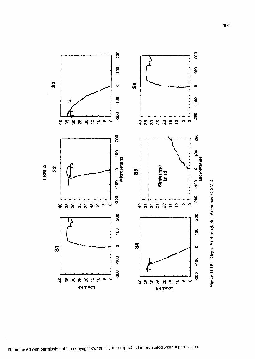
307
C M
O
CO
o mCM T -
o in o
CO(0
5Is
§
o m o m o^ CO CO CM CM
in o in oI
s(0
CM
OosË
CM(0
O U&
U)uÜ CD -a:
o
o
CM
T-(O
ooCM
§
s
m ‘PeoTm o m o mC O C O C M C M « -
o in o
NX 'pBOi
I
I
Î■S
I00
Û
I
Reproduced with permission of the copyright owner. Further reproduction prohibited without permission.
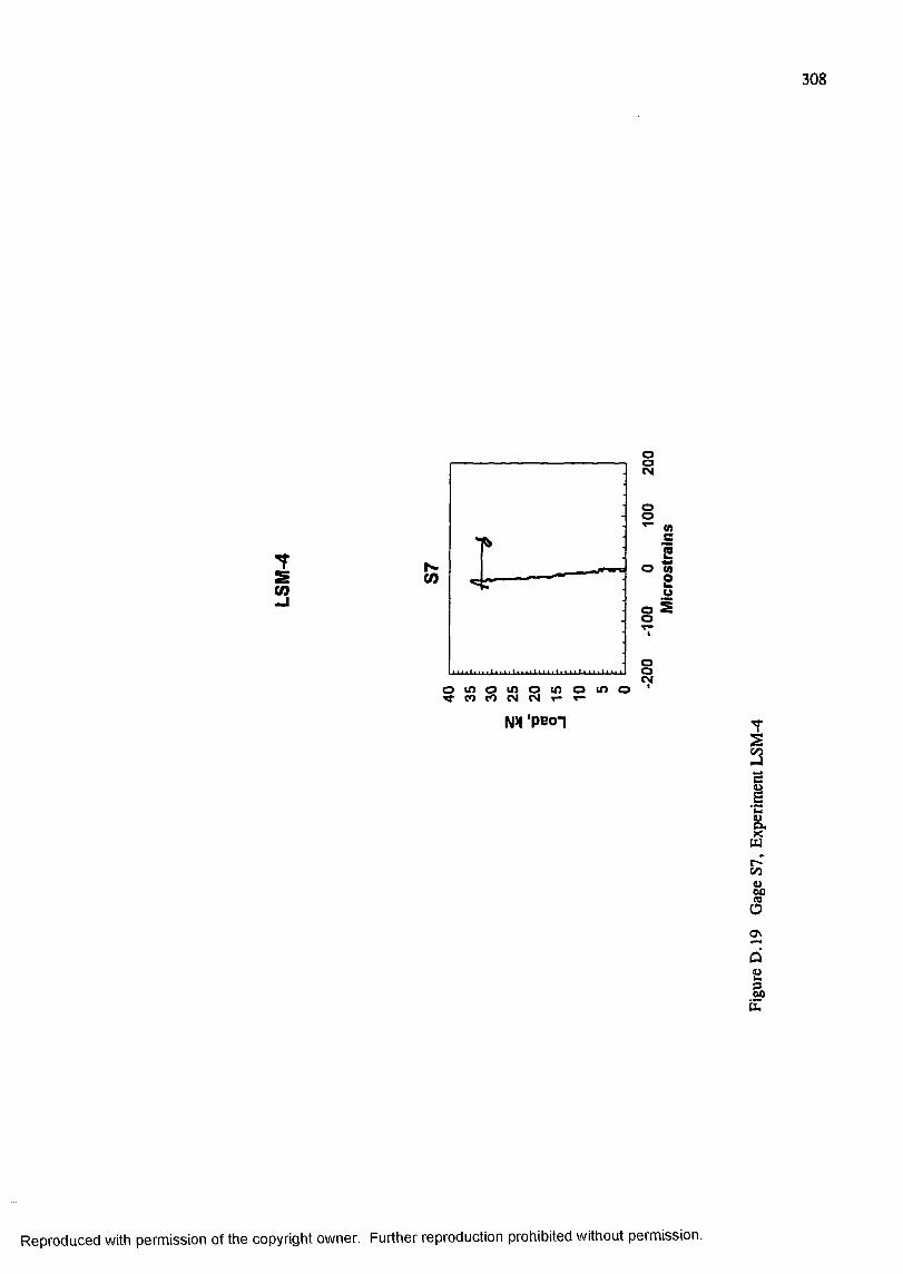
308
3
04
N(0
o (0
o s
CMO in Oo in
CM T -
m ‘PeoT
i
1a
Ia \
ÛHê
Reproduced with permission of the copyright owner. Further reproduction prohibited without permission.
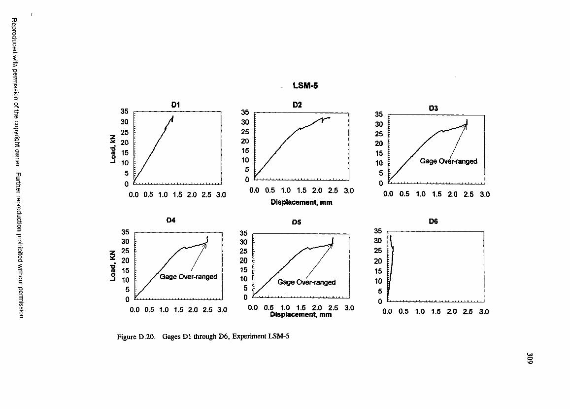
■ o
II■g
c / )COo '3
3"o8
â '3"
3CD
p.3"CD
CD■DOQ .Cao3
"Oo
CDQ .
"OCD
C /)(/)
D1
^ 20 ^ - i f -
10
0.0 0.5 1.0 1.5 2.0 2.5 3.0
0 4
w 15Gage Over-ranged
LSM-5
D2
20
0.0 0.5 1.0 1.5 2.0 2.5 3.0
D isplacem ent, mm
0 535302520151050
Gage Over-ranged
0.0 0.5 1.0 1.5 2.0 2.5 3.00.0 0.5 1.0 1.5 2.0 2.5 3.0 ,D isplacem ent, mm
Figure D.20. Gages D1 through D6, Experiment LSM-5
0 3
25
G age Over-ranged
0.0 0.5 1.0 1.5 2.0 2.5 3.0
0 635
25
0.0 0.5 1.0 1.5 2.0 2.5 3.0
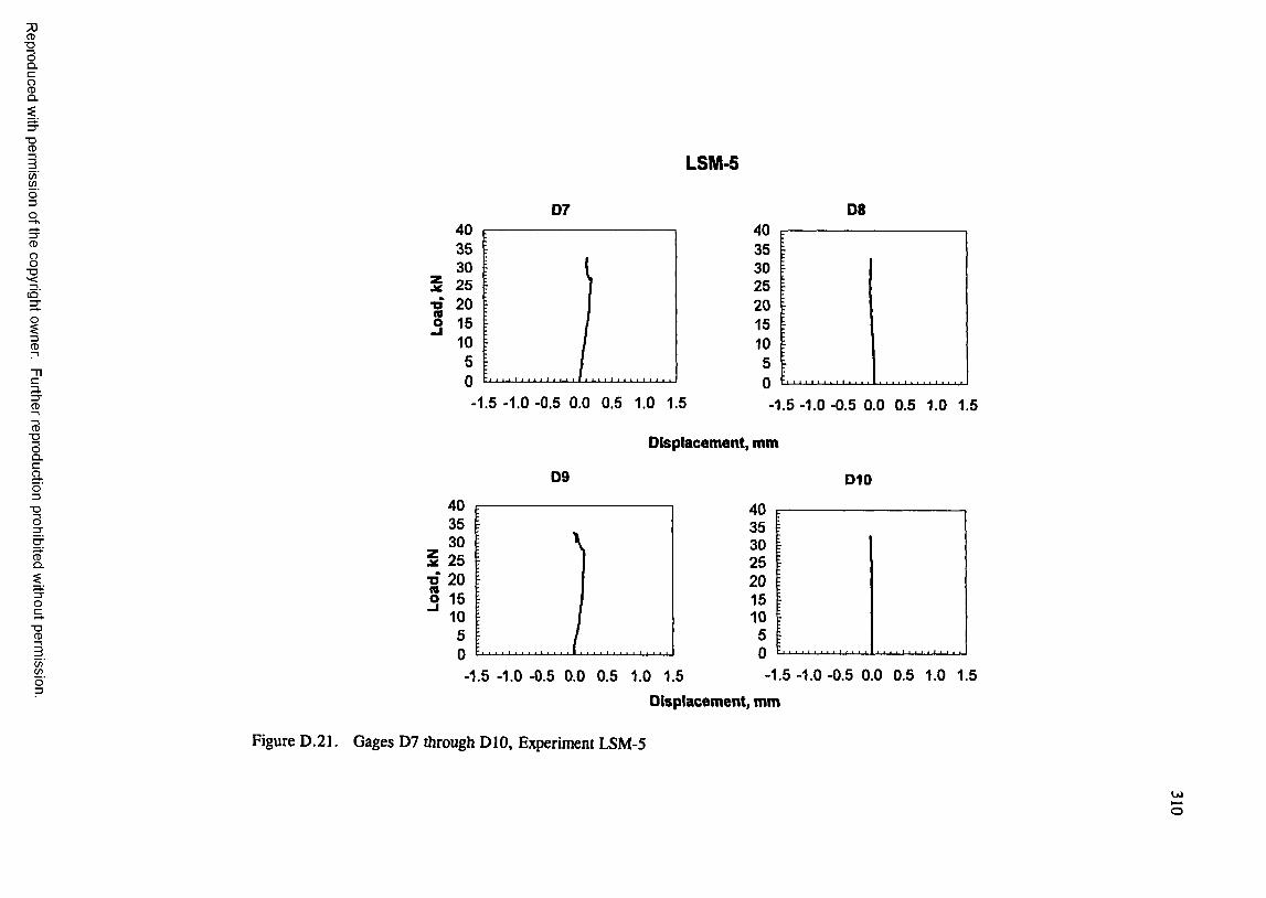
7)CD■DOQ .C
gQ .
"DCD
C/)Wo"3O
8
i3CD
3.3"CD
CD■DOQ .CgO3
"DO
CDQ .
■DCD
C / )C / )
LSM-5
07
25•o
1.5 -1.0 -0.5 0.0 0.5 1.0 1.5
09
-1.5 -1.0 -0.5 0.0 0.5 1.0 1.5
Oisplacement, mm
010
40
^ 25 •D 20 o 15
-1.5 -1.0 -0.5 0.0 0.5 1.0 1.5 -1.5 -1.0 -0.5 0.0 0.5 1.0 1.5
Displacement, mm
Figure D.21. Gages D7 through DIO, Experiment LSM-5
WO
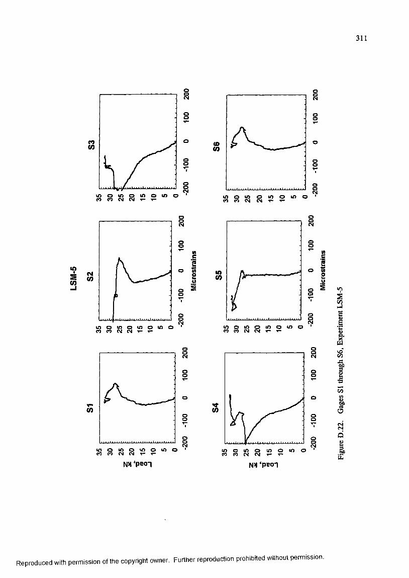
311
to
o
CM
CO<n
CM
•?
(0
oCM(0
oo
IÜ
o
T"(0
Io m oin oCO CO
8
■ACO
CM
O
(0
NX peon NX‘PBon
"9
I
1ICO
Ia
E
f
Reproduced with perrrisslon of the copyright owner. Further reproduction prohibited without permission.
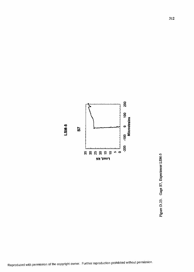
312
•?S(0 (0
Ioo
lo o m o toC O e o C M C N T -
o m o
Mc
o M
2 H
o s o
iNX p eo i S
2
Ico
tad2&
Reproduced with permission of the copyright owner. Further reproduction prohibited without permission.
APPENDIX E: SAMPLE ABAQUS INPUT FILE
A sample ABAQUS input file is listed in this appendix along with limited explanatory
comments. The purpose of including this sample h^ut file is to assist analysts familiar with
ABAQUS in duplicating the results described in this dissertation. An ABAQUS iiçut file
consists of three types of iiçut lines:
• Comment lines, which always begin with double asterisks (**)
• Keyword input lines, which always begin with a single asterisk (*)
• Data input lines
The outline of the input file is as follows:
• Model DefinitionNode Definitions Element Definitions Joint Property Definitions Multi-Point Constraint Definitions Contact Interaction Definitions
• Material DefinitionSolid Element Property Specifications Foundation Specification
• Boundary Condition DefinitionSpecify Nodal Displacement Constraints
• Solution Step DefinitionDefine Iterative Solution Step
• Output RequestsSpecify displacement, stress, and strain output
313
Reproduced with permission of the copyright owner. Further reproduction prohibited without permission.

314
In the sample input file those lines which are common to all cases are printed in normal
font. Those lines which are used optionally to define each of the cases described in Chapter 9
are printed in itaUc font. Because the input file is quite lengthy, selected lines have been
removed from the sample file for the sake of brevity. These locations are denoted in the
comments column.
Reproduced with permission of the copyright owner. Further reproduction prohibited without permission.
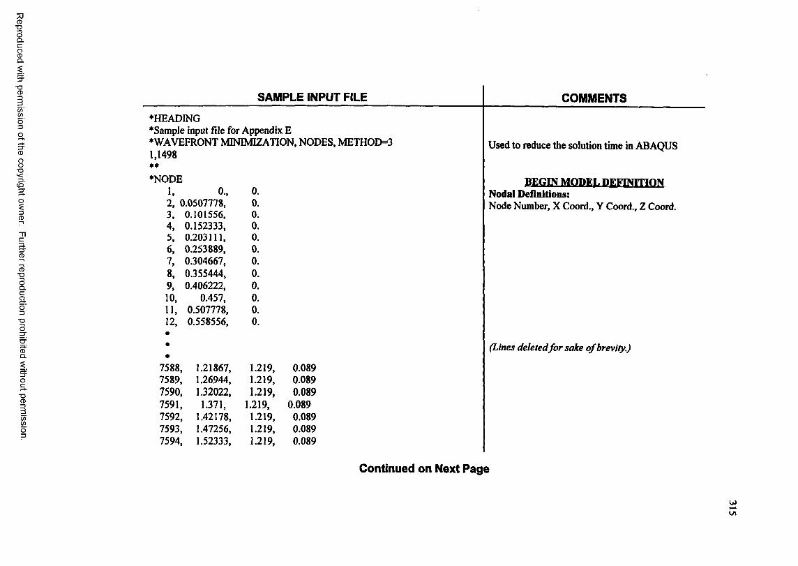
■oI
I■a
CD
C/)œo'3O
8
c5'
3CD
p.3"CD
CD■DOQ .Cao3
■DO
CDQ .
■oCD
C /)C /)
SAMPLE INPUT FILE COMMENTS♦HEADING♦Sample input file for Appendix E♦WAVEFRONT MINIMIZATION, NODES, METH0D=3 Used to reduce the solution time in ABAQUS1,1498**♦NODE
1, 0 ., 0 .BEGIN MODEL DEFINITION
Nodal Definitions:2, 0.0507778, 0 . Node Number, X Coord., Y Coord., Z Coord.3, 0.101556, 0 .4, 0.152333, 0 .5, 0.203111, 0 .6 , 0.253889, 0 .7, 0.304667, 0 .8, 0.355444, 0 .9, 0.406222, 0 .10, 0.457, 0 .11, 0.507778, 0 .12, 0.558556, 0 .
••
(Lines deleted for sake o f brevity.)
7588, 1.21867, 1.219, 0.0897589, 1.26944, 1.219, 0.0897590, 1.32022, 1.219, 0.0897591, 1.371, 1.219, 0.0897592, 1.42178, 1.219, 0.0897593, 1.47256, 1.219, 0.0897594, 1.52333, 1.219, 0.089
Continued on Next Page
Wul
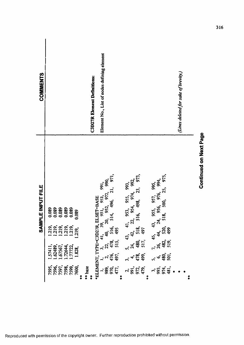
316
eo
o
m
es
O s 0 \ O s O s 0 \e o 00 e o o o 00 O sO o o o o 0 0
00
mO s O s O s O s O s
es es es es es
v n zs c;m ^e s 00
^ 80 0 O s
o s O s
e s O n cN ON C*- 0 \ ON ^
00
0O)S .
1c0T3»3C1 O O
Reproduced with permission of the copyright owner. Further reproduction prohibited without permission.
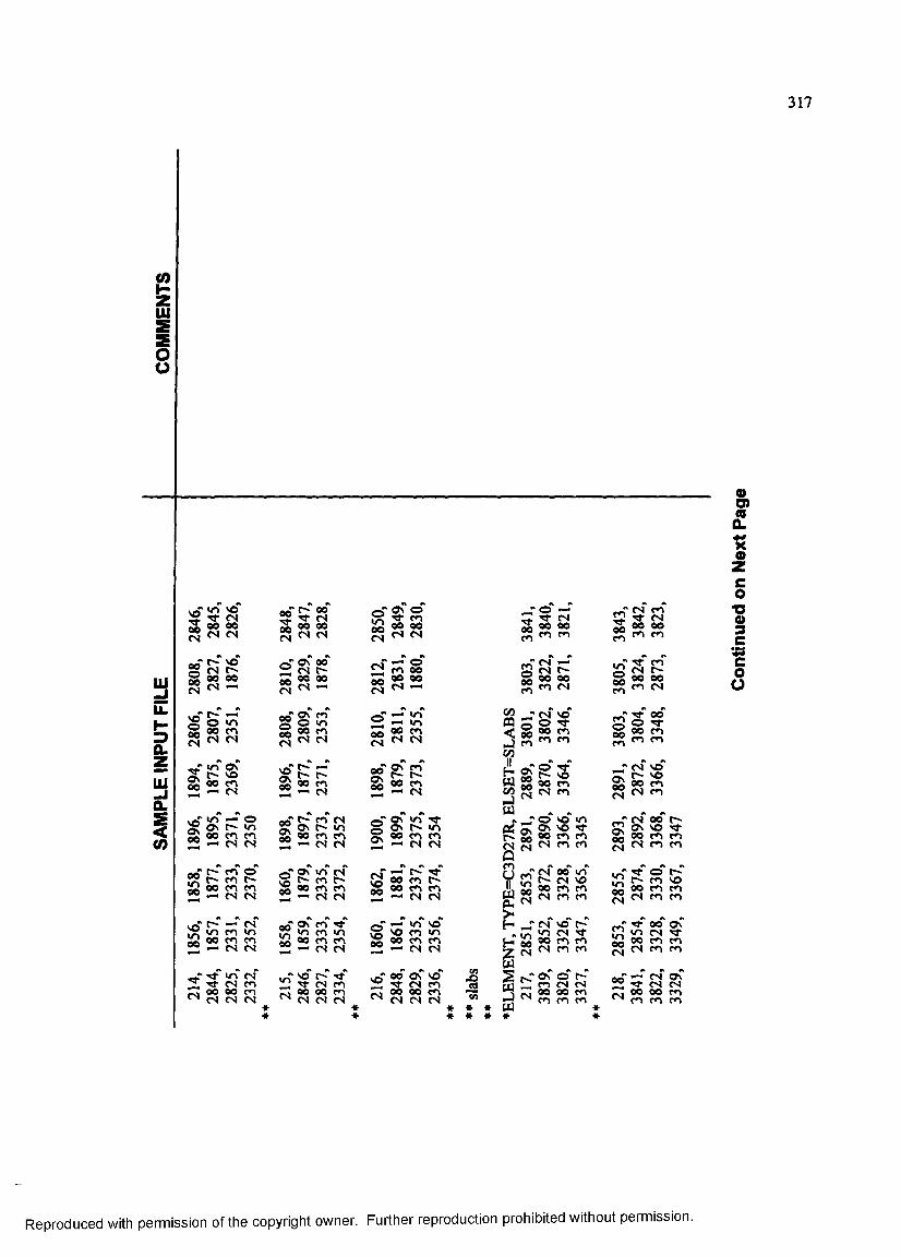
317
I
at Z5a.z
jI
i ' l l
0 0 V O
00 00 (S —<
r~" *—< o xr\ 0 0 c nfS <N
mm
ovno oC N
■ 'S i(S (S 00 00m c n
i S S
CN
o00c s
o\ m o in 00 m cs ts
m lisC m — o
0 \ >n 00 m m
|~sSi i s i
VO
O n C N c n00 m m
c s
o oc s
o o
o oO n
§
C ^ ^ C S vn m m 00 cn m m i
s i i i
%O O
V O
c s
«*
1- T oc n o o0 0 0 0c s
i ni n
0 0 c nc s c s
e v c nr -
0 0 c nc s
Ov i nO n c ^ i n0 0 c n c n
c s c s
0 0 c n r -0 0 c n c n«-irf c s c s
i n VOVO c n m0 0 c n c n* -* c s c s
0 0 O n VOCS c n
o o 0 0 c nc s c s c s
§m
c s ^ c s 00 00 m c s
CO9ii
CS r i ^
* % c s
V OT fmm
3mc n
c n
v no00m
800m
m cn
00 00 m c s
^ o oO TT O O c n c n m
00 m c s ms
c s
V O' O T f m m m m
00 vn c s VO m m m m
S f S S Ç 00 00 m mc s
vnino oc s
c s m m
^ o cn VO o o m m c s c n c n
-rS3 25 S;o o m m<N m M C S c s c n c n
I** « «
22 ^ 5 R r< 23 SS S3
&d!
I§%3C1Oo
Reproduced with permission of the copyright owner. Further reproduction prohibited without permission.
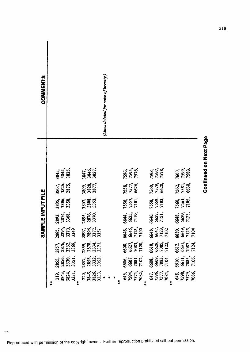
318
IOO
UJ
2Z111
I
II
îI
ë 'S i c 00 m
o o o o m CN
00m
o o m m en
s i ?tN M m
i S S S^ C N e n c n
%C N
00 e n e n C N e n e n
% (Z00( N
00 en en C N e n e n
e n e n e nC N
Se n
§e n
§e n
sC N
SC N
Osm00C N
r *m00C N
§»#
S O r -C N
0 0 0 0e n e n
0 0C N0 0 0 0e n C N
0 0 C No u n0 0 e ne n e n
s o O
0 0 e nC N e n
S O C NO s C ^ u n0 0 e n e nC N e n e n
0 0 T fe n C ^
0 0 e n e nC N e n e n
0 0 C N e nu n e n u n0 0 e n e nC N e n e n
u n s o e nC N e n
0 0 0 0 e ne n e n e n
SO Ov nvnr * ^
VOununr -
u n ' O 0 \u n u n
voCN un vô so
Osou n
Os 00CN
u n s © s o
su nr - *
r o00 e n u n \ o r - * s o
i s Ê
pê!
pi|'§s
lisv o SO
llii00
Iou nsoso
O s e n C N C N S O ^so r*-
O s u n ^ ^ C N O V O ^ *— «so
**
isoiI
î * e n pC N o o C Nvo o »-*vo c~ c^
— ÇNo oo o vo o — vo
T f < n CN O V c ^ 0 0in m o c c
SfiS se ÇSv o v o
V O O ^ VO r - t-"
2 S ^ 5v o s o
s o _ s o r -
iillS
s o T f O s r * * 0 0 u n u n o r-* r- r*-
s oso
00
5**
S O O ^ s o r - r -
0 0 O s s o O s 0 0 u n u n o r -
I
Ico■o§ëcoo
Reproduced with permission of the copyright owner. Further reproduction prohibited without permission.
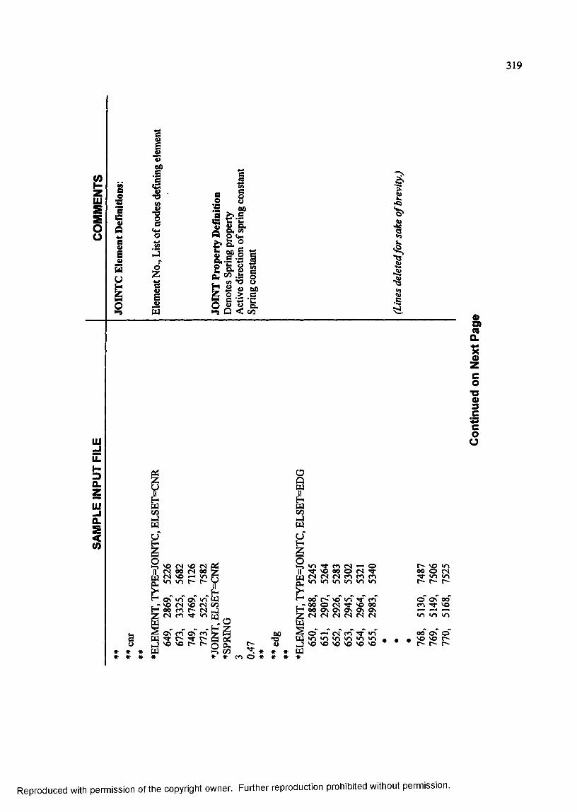
319
e o
en
O
S. &l ' s “ i
K/l
^ V O C N V O
jb 23 SS E!S »0 lOo ce o
r r i e s c s n e n a j «n <n <n m
00
r" 0 \ ui 0 \ » v o e s v o H 00 m ; Z c s m T f
v o 00 o\ Ov c s c s
“ 00 vo >n« o o o c s ^H 00 o v 0 \ o sZ c s c s c s e s in U-» «n
j v o v O t ~ -
00 Ov v o v o
• S O CS e n «OU 3 vr> <r> v n >cv > n v nJ v o v o v o v o v o v o
eo
4)O)a
Izc0■o0)3C1 O ü
Reproduced with permission of the copyright owner. Further reproduction prohibited without permission.
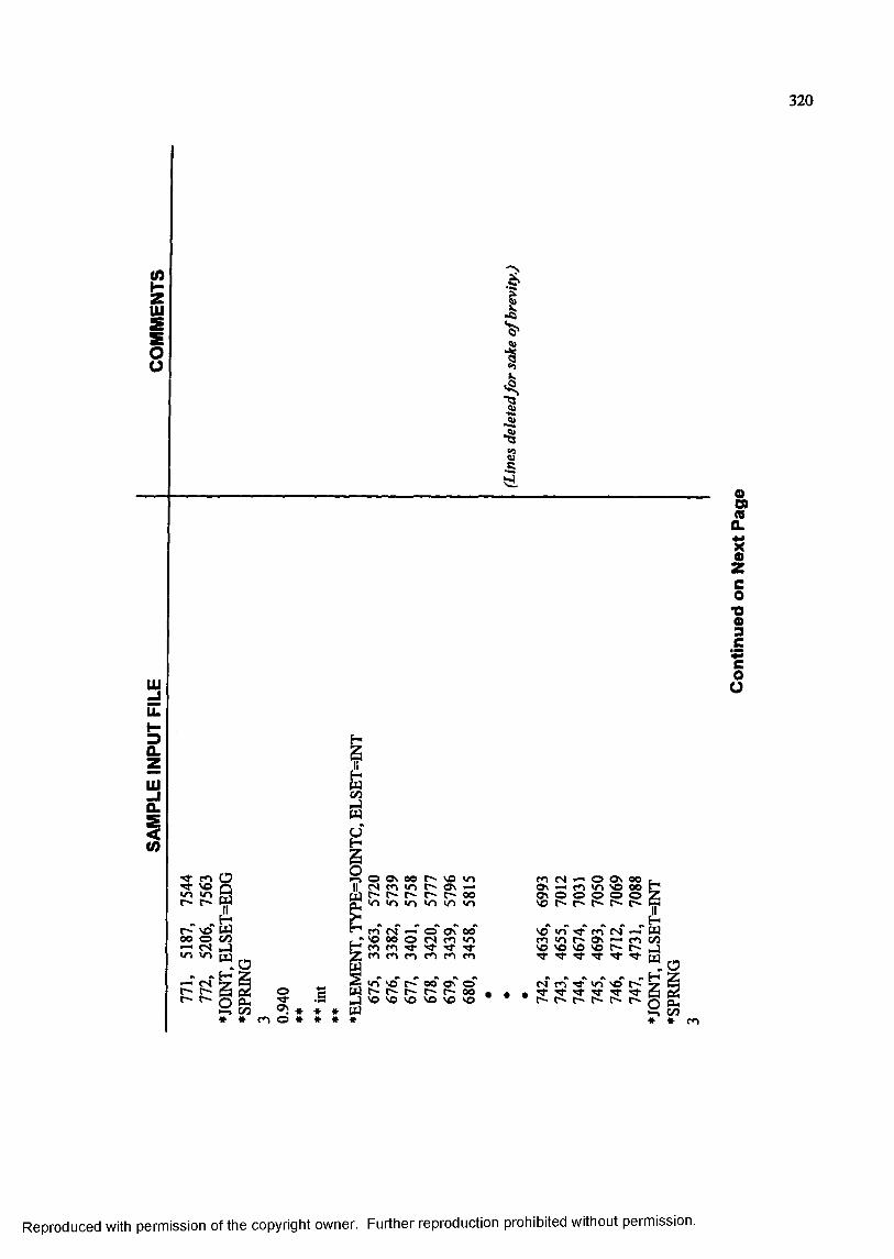
320
i -> o 0 \ o o v nII t s ir> ^ —
r r 1 C ' 0 0L x \ 1 ^ 1 ^ # / \ 1 ^
“ m f S O O n 0 0> o o o o < s m » n
r m m TT T f^ m m m c n M m
V O > o T j - c n C N c n < o c ~ O v •— ■. . . _ . c n c/3v o v o VÛ v o JT f T f ^ T f T f m
ÿ S i n VO t~ - OO OVB3 t~- t~' t~j v o v o v o v o v o
v no ov o
&S .
1Z
•§
§o
Reproduced with permission of the copyright owner. Further reproduction prohibited without permission.
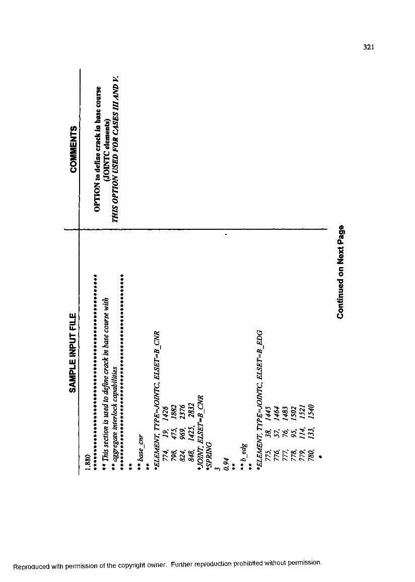
321
■S S S3
u.
w-T ip' t< 00 oT Cv. P-» Oo(—C\ N. 00 00 g 2 >OO00
Io.
Ie0
1 Iü
Reproduced with permission of the copyright owner. Further reproduction prohibited without permission.
322
<N<=T oC 00 ^ Prj ■> vo 00fr «1 (M-> (r I I O V ) -9-- > r r ^ U ~ l
00 oo 00 00»n <N ^ ^ <o I T ) I A | l o < 0
\o «0 0 0 0 C o 0 0
1 2 g 2Oo 00 00 Oo<n V <o vo> 5- 5: >Oo 0 0 0 0 0 0
200
0 D)
S .
1Z
"C0
eoO
Reproduced with permission of the copyright owner. Further reproduction prohibited without permission.
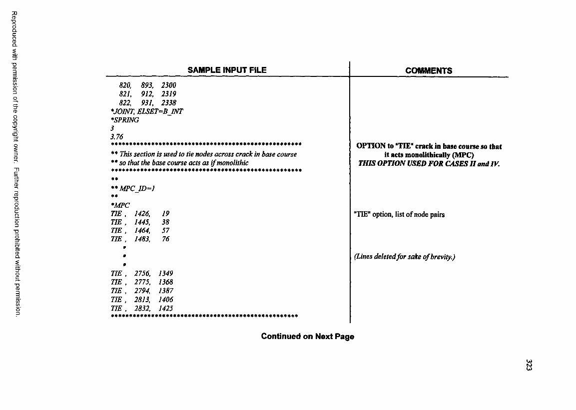
7 )CD
■ DOQ .C
gQ .
■DCD
C/)C /)
CD
8
CD
3.3"CD
CD■DOQ .CaO3"OO
CDQ .
■DCD
C/)C /)
SAMPLE INPUT FILE
820, 893, 2300821, 912, 2319822, 931, 2338
* JOINT, ELSET=BJNT*SPRING33.76
** This section is ttsed ta tie nodes across crack in base course ** so that the base course acts as i f monolithic
****MPC ID=1 ***MPCTIE , 1426,TIE , 1445,TIE , 1464,TIE , 1483,
9
9
19385776
TIE , 2756, 1349TIE , 2775, 1368TIE , 2794, 1387TIE , 2813, 1406TIE , 2832, 1425***************************************************
COMMENTS
OPTION to "TIE" crack in base course so that it acts monolitbically (MPC)
THIS OPTION USED FOR CASES II and IV.
"TIE" option, list of node pairs
(Lines deletedfor sake o f brevity.)
Continued on Next Page
a
■oII
(/)Ç2o'3
CD
8
c5'
3CD
Cp.3"CD
CD■oICao3
■oo
&
oc■o
CD
(/)o'3
SAMPLE INPUT FILE COMMENTS**** lh_b Defines an element set needed for FOUNDATION** definition♦ELSET, ELSET=LH B
1, 2 , 3, 4, 5, 6 , 7, 8 ,9, 10, 11, 12, 13, 14, 15, 16,17, 18, 19, 20, 21, 22, 23, 24,25, 26, 27, 28, 29, 30, 31, 32,33, 34, 35, 36, 37, 38, 39, 40,41, 42, 43, 44, 45, 46, 47, 48,49, 50, 51, 52, 53, 54, 55, 56,57, 58, 59, 60, 61, 62, 63, 64,65, 6 6 , 67, 68 , 69, 70, 71, 72,73, 74, 75, 76, 77, 78, 79, 80,81, 82, 83, 84, 85, 86 , 87, 88 ,89, 90, 91, 92, 93, 94, 95, 96,97, 98, 99, 100, 101, 102, 103, 104,105, 106, 107, 108
**** rh b**♦ELSET, ELSET=RH_B
109, 110, 111, 112, 113, 114, 115, 116, Defines an element set needed for FOUNDATION117, 118, 119, 120, 121, 122, 123, 124, definition125, 126, 127, 128, 129, 130, 131, 132,133, 134, 135, 136, 137, 138, 139, 140,141, 142, 143, 144, 145, 146, 147, 148,149, 150, 151, 152, 153, 154, 155, 156,
Continued on Next Page
325
Ii
_ » n »\ f» m m A m # * m m m mO O O ' O ' ^ C S O O O ' O ' ^ f S O O O ' O ■ ^ ■ ^ l O V O t ^ O O O O O N O - - - -
Ç S o o o V û 2 ; C N vo 00 00 On o C N C N
m •— ' O n r ~ v n c n v o C ^ 0 0 O n O
w> r» m _•» ■* V* mO n t - ' > n c n « - I c . r c n T j - v n N O r ~ - c ~ ' O o O N O
O N r - v n c n O n c ^ v n — C N c n
U.
C N o 0 0 v o ^ C N OVO 00 On O ^M « - 4 « -M 0 - ^ M c s C N
■' •* • ' w% V* m m mO O N O ^ C N O O O N o ^ C N O O O V O ' ^- ■ ^ ^ r r — c . o ’— ' ' C N e ncn ' ^vnvot^c~ooovO
— Oi c ^ v n e n v o N O 0 0 O n o o
O v_ " " *» • » » » • »r - N n c n - —' O N t — v n c n. . ^ , V *— V o v c ~ ~ v n c nc n v j - v n v o v o t ~ o o O N O O > — c N c n v f T f n - T r T r n - T f - N ' v n v n v n v n v n
c T 00 v o ^ C N c T o o " ^ N O V O t ^ O O O v O O r ^
m w es es5 2 v o T f c n " c T o o " v o v r c n “ o ' o o K c n r f v n v o N o r ^ o o o v o o S S S lO r’ r- n m * % # * # * # * * * •>
v n c n —' O N C ^ v n c n —' C . r» c n r f v n v n v o r - o o o v a v oVf" V*» *4. 44. 4*. -4. «4. -4. .44
O n v n e n- . . . . . . . . . . . . . . . . . . . . . . . . O n mv n v o t ^ o o o N O N O - ^
«—N 1 - M m - 4 #—4 ( N e sOv r - «n en
5 . •» A A A A A A A A A A A A AW v a - c N O O O V O r J - C N O O O V O v a - C N O O O j e n v j - v n v n v o c ^ o o o N O N O N — ' C N c n c n [ i ^ v f T f ^ T f T T ' f v a ' T f T r v n v n v n v n v n
O O N O v f c N O O O N O v fv n v o t ^ o o o v O N O —4
r ^ v n m —' O v r - ' v n c n v n v o C ' O o o o o N O —
W c n — ' O N t ~ ' v n m - - < O N t ^ v n c n c o c n N - ' ï - v n v o t ^ o o o o o N O ' - *
OO)
a
ïzc0■o<03C1 Oo
Reproduced with permission of the copyright owner. Further reproduction prohibited without permission.
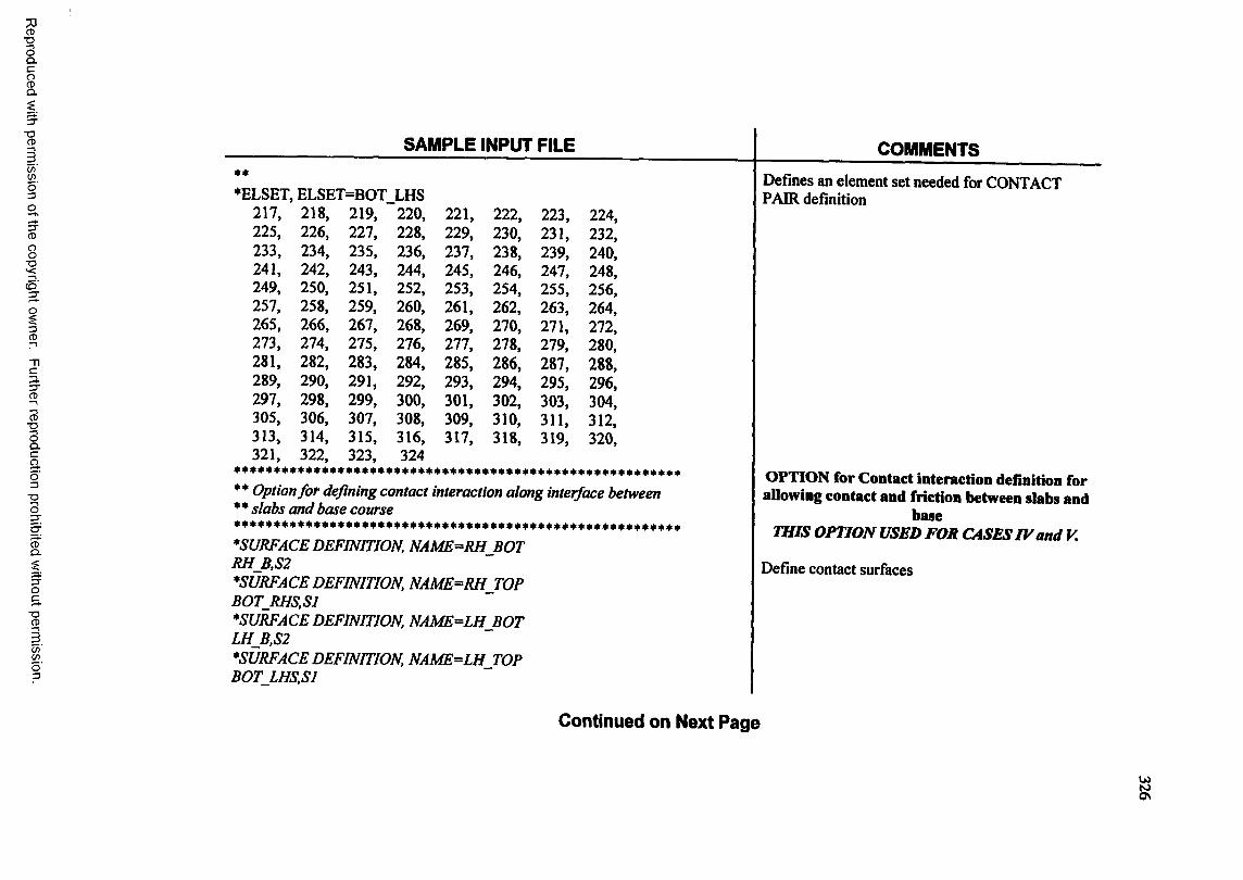
■oII-g
c/)wo'3
8c5'
3CD
Cp.
CD■OICao3
■OO
&
oc■o
CD
C/)Wo"3
SAMPLE INPUT FILE**♦ELSET, ELSET=BOT LHS
217, 218, 219, 220 , 221 , 22 2 , 223, 224,225, 226, 227, 228, 229, 230, 231, 232,233, 234, 235, 236, 237, 238, 239, 240,241, 242, 243, 244, 245, 246, 247, 248,249, 250, 251, 252, 253, 254, 255, 256,257, 258, 259, 260, 261, 262, 263, 264,265, 266, 267, 268, 269, 270, 271, 272,273, 274, 275, 276, 277, 278, 279, 280,281, 282, 283, 284, 285, 286, 287, 288,289, 290, 291, 292, 293, 294, 295, 296,297, 298, 299, 300, 301, 302, 303, 304,305, 306, 307, 308, 309, 310, 311, 312,313, 314. 315, 316, 317, 318, 319, 320,321, 322, 323, 324
** Option for defining contact interaction along interface between ** slabs and base course
*SURFACE DEFINITION, NAME^RHJBOT RH_B,S2*SURFACE DEFINITION, NAME=RHJOP BOT_RHS,Sl*SURFACE DEFINITION, NAME=LH_BOT LH_B,S2*SURFACE DEFINITION, NAME=LH_TOP BOT_LHS,Sl
COMMENTS
Defines an element set needed for CONTACT PAIR definition
OPTION for Contact interaction definition for allowing contact and friction between slabs and
baseTHIS OPTION USED FOR CASES IV and V.
Define contact surfaces
Continued on Next Page
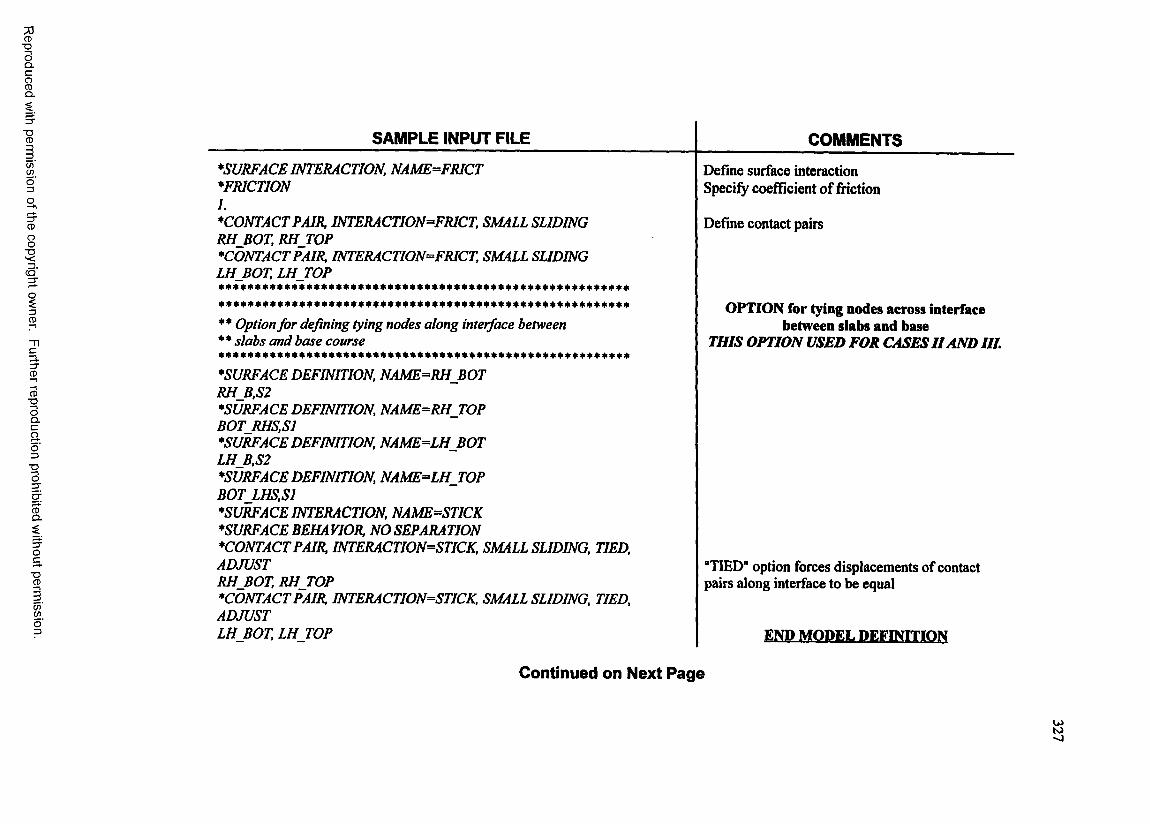
73CD■DOQ .C
8Q .
■DCD
(/>(go"3
8
cq '3"
3CD
C3.
CD■OICao3
■OO
SAMPLE INPUT FILE
&
OC%
C/Îcoo'3
*SURFACE INTERACTION, NAME=FRICT *FR1CTI0N 1.*CONTACT PAIR, INTERACTION=FRICT, SMALL SLIDING RH_BOT, RHJTOP*CONTACT PAIR, INTERACTION^FRICT, SMALL SLIDING LH BOT. LH TOP
** Option for defining tying nodes along interface between ** slabs and base course
*SURFACE DEFINITION, NAME=RH_BOT RH_B,S2*SURFACE DEFINITION, NAME=RH_TOP B0T_RHS,S1*SURFACE DEFINITION, NAME=LH_BOT LH_B,S2^SURFACE DEFINITION, NAME=LH_TOP B0T_LHS,S1^SURFACE INTERACTION, NAME=STICK*SURFACE BEHAVIOR, NO SEPARATION*CONTACTPAIR, INTERACTION^STICK, SMALL SLIDING. TIED,ADJUSTRHJBOT, RHjrOP^CONTACT PAIR, INTERACTION=STICK, SMALL SLIDING, TIED, ADJUSTLH BOT, LH TOP
COMMENTS
Define surface interaction Specify coefficient of friction
Define contact pairs
OPTION for tying nodes across interface between slabs and base
THIS OPTION USED FOR CASES I I AND III.
“TIED" option forces displacements of contact pairs along interface to be equal
E m MOPEL REEflf f r ro N
Continued on Next Page
a
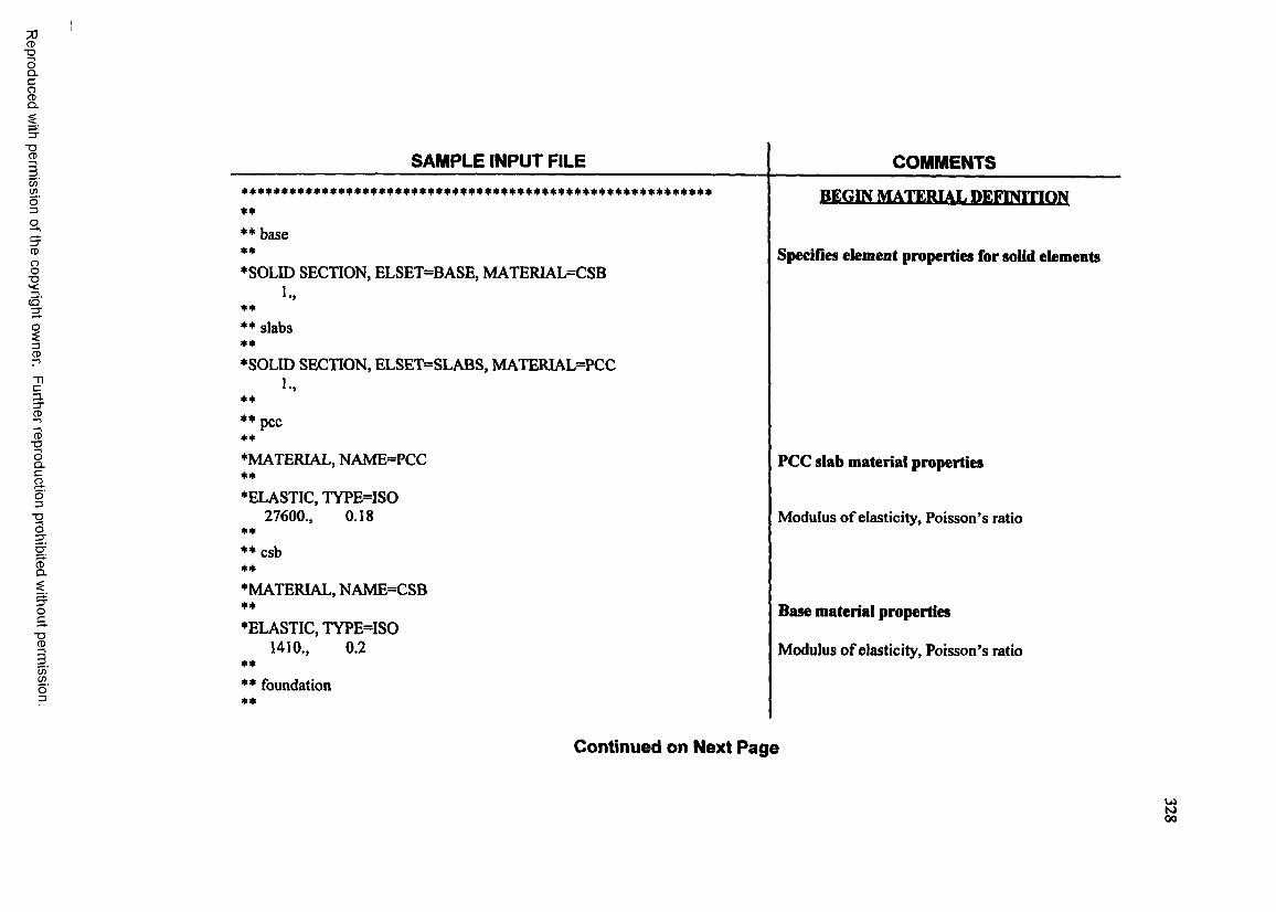
73CD-DOQ .C
3Q .
■OCD
C /)WO3
8cS'
3CD
Cp.
CD■OICao3
■OO
oc■o
CD
(/)œo"3
SAMPLE INPUT FILE COMMENTS
BEGIN MATERIAL DEFINITION**** base** Specifies element properties for solid elements*SOLID SECTION, ELSET=BASE, MATERIAL=CSB
1 •>**** slabs**•SOLID SECTION, ELSET=SLABS, MATERIAL=PCC
L,**•• pcc**•MATERIAL, NAME=PCC PCC slab material properties**•ELASTIC, TYPE=ISO
27600., 0.18 Modulus of elasticity, Poisson’s ratio**•• csb**•MATERIAL, NAME=CSB** Base material properties•ELASTIC, TYPE=ISO
1410., 0.2 Modulus of elasticity, Poisson’s ratio**•• foundation**
Continued on Next Page
00

7JCD
■ D
OQ .C
gQ .
■DCD
</>(/)
3CD
CD■oIcao3■oo
&
oc
c/i(go'3
SAMPLE INPUT FILE COMMENTS
♦FOUNDATION Specify properties of bed of springs foundationLH B, FI, 90.RH B,F1,90. Element set, active face of element, modulus of
** subgrade reaction*♦ ends END MATERIAL DEFINTION**♦BOUNDARY, OP=NEW BEGIN BOUNDARY CONDITION
I, 1,, 0 . DEFINITION1, 2„ 0 .1,3„ 0 . Node, degree of freedom, specified displacement
20 , 1„ 0 .20 , 2 ,, 0 .20, 3„ 0 .3 9 ,1„ 0 .39,2,, 0 .39, 3„ 0 .58, 1„ 0 .58, 2„ 0 .58,3,,#
0 .
#7524, 1„ 0 . (Lines deletedfor sake o f brevity.)7524, 2„ 0 .7524, 3„ 0 .7543,1„ 0 .7543, 2„ 0 .7543, 3„ 0 .
Continued on Next Page
73CD■DOQ .C
gQ .
■DCD
C/)C /)
8■D3 .CÛ
i
3.3"CD
CD■DOQ .C
aO3■OO
CDO .
OC
■oCD
C /)(go'3
SAMPLE INPUT FILE COMMENTS7562, 1„ 0 .7562,2„ 0 .7562,3,, 0 .7581,1„ 0 .7581,2,, 0 .7581,3,, 0 .7600, 1„ 0 .7600,2„ 0 .7600, 3„ 0 .
**** sides♦ ♦♦BOUNDARY, OP=NEW
2 , 2„ 0 .3.2„ 0 .4, 2„ 0 .5,2„ 0 .6 , 2„ 0 .7.2„ 0 .8. 2 „ 0 .9, 2„ 0 .10, 2 ,, 0 .11. 2 ,, 0 .###
7591,2,, 0 .7592,2„ 0 . (Lines deletedfor sake o f brevity.)
Continued on Next Page
WWO
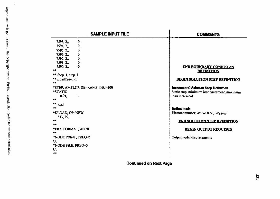
7 )CD
■ DOQ .C
gQ .
■DCD
C/Î
o'3
8
( O '
3.3"CD
CD■DOQ .Cao3
■DO
CDQ .
■DCD
C/)C /)
SAMPLE INPUT FILE COMMENTS7593,2,, 0 .7594,2,, 0 .7595,2,, 0 .7596,2,, 0 .7597, 2„ 0 .7598,2,, 0 .7599,2,, 0 . END BOUNDARY CONDITION
** DEFINITION** Step 1, step_l** LoadCase, Id BEGIN SOLUTION STEP DEFINITION♦ ♦*STEP, AMPLITUDE=RAMP, INC=100 Incremental Solution Step Definition♦STATIC Static step, minimum load increment, maximum
0 .01 , 1. load increment**♦ ♦ load** Define loads♦DLOAD, OP=NEW Element number, active face, pressure
333, P2, 1.****
END SOLUTION STEP DEFINITION
♦FILE FORMAT, ASCH BEGIN OUTPUT REOUESTS**♦NODE PRINT, FREQ=5 Output nodal displacementsu .♦NODE FILE, FREQ=5u .**
Continued on Next Page
WW
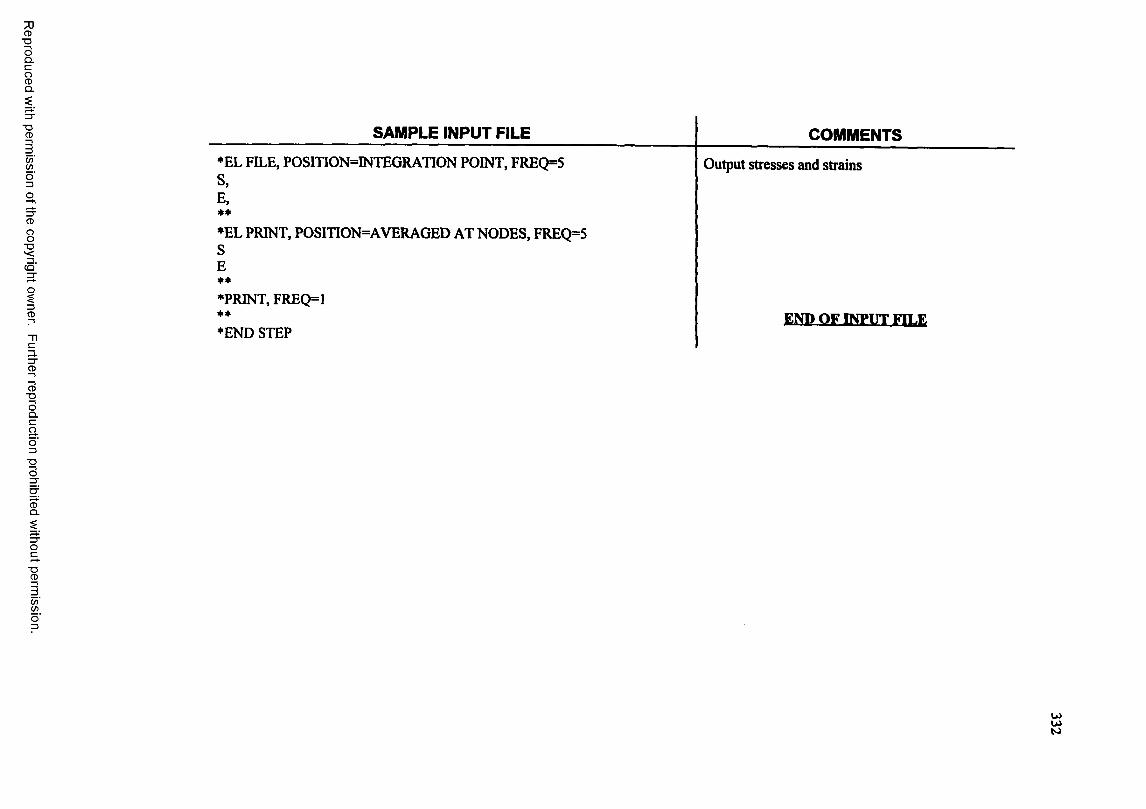
7 ]CD
■ DOQ .C
gQ .
■OCD
C/)Wo'3O
8■D
CD
3.3"CD
CD■DOQ .C
aO3
■DO
CDQ .
OC
"OCD
C/)C/)
SAMPLE INPUT FILE COMMENTS♦EL FILE, POSmON=INTEGRATION POINT, FREQ=5 Output stresses and strainsS,E,**♦EL PRINT, POSITION=AVERAGED AT NODES, FREQ=5CO
E**♦PRINT, FREQ=1** END OF INPUT FILE♦END STEP
VITA
Michael Ivan Hammons was bom on February 15,1958, in Ruston, Louisiana. Upon
graduating from Downsville High School, Downsviile, Louisiana, he entered Louisiana Tech
University in Ruston, Louisiana, in September 1976. While at Louisiana Tech, he was the
recipient of the R. A. McFarland Scholarship and was an active member in Chi Epsilon. In
May 1980 he graduated summa cum laude from Louisiana Tech with a bachelor of science in
Civil Engineering. In June 1980 he accepted a position as a research engineer at the
U.S. Army Engineer Waterways Experiment Station (WES), in Vicksburg, Mississippi,
where he has been continuously employed until the present. While working at WES, he
continued his education through the WES Graduate Center, and in August 1985, completed a
master of science in Civil Engineering at Mississippi State University, Starkville, Mississippi.
Subsequently, he continued his graduate education by entering a doctoral program at the Uni
versity of Colorado, Boulder, Colorado, during the 1985-1986 academic year and at the WES
Graduate Center. In September 1994 he was accepted to the doctoral program at Louisiana
State University. He has published numerous technical reports, papers in conference pro
ceedings, and journal articles. He is a member of the American Society of Civil Engineers
and sits on several technical committees. He is a Registered Professional Engineer in the
State of Mississippi. He expects to receive his doctoral degree in May 1997.
333
Reproduced with permission of the copyright owner. Further reproduction prohibited without permission.

DOCTORAL EXAMINATION AND DISSERTATION REPORT
Candidate:
Major Field:
Michael Ivan Hammons
Civil Engineering
Title of Dlasertation: Development of an Analysis System forDiscontinuities in Rigid Airfield Pavements
Approved:
Major" Professor add Chairman
Graduate School
EXAMINING COMMITTEE I
Date of Kxamination;
January 30, 1997
Reproduced with permission of the copyright owner. Further reproduction prohibited without permission.