Embed Size (px)
Citation preview

Development of an Autonomous Mobile Robot-Trailer System for UXO
Detection
Except where reference is made to the work of others, the work described in this thesis ismy own or was done in collaboration with my advisory committee. This thesis does not
include proprietary or classified information.
David W. Hodo
Certificate of Approval:
John Y. Hung, Co-ChairProfessorElectrical and Computer Engineering
David M. Bevly, Co-ChairAssociate ProfessorMechanical Engineering
Thaddeus A. RoppelAssociate ProfessorElectrical and Computer Engineering
Joe F. PittmanInterim DeanGraduate School

Development of an Autonomous Mobile Robot-Trailer System for UXO
Detection
David W. Hodo
A Thesis
Submitted to
the Graduate Faculty of
Auburn University
in Partial Fulfillment of the
Requirements for the
Degree of
Master of Science
Auburn, AlabamaAugust 4, 2007
Development of an Autonomous Mobile Robot-Trailer System for UXO
Detection
David W. Hodo
Permission is granted to Auburn University to make copies of this thesis at itsdiscretion, upon the request of individuals or institutions and at
their expense. The author reserves all publication rights.
Signature of Author
Date of Graduation
iii

Thesis Abstract
Development of an Autonomous Mobile Robot-Trailer System for UXO
Detection
David W. Hodo
Master of Science, August 4, 2007(B.E.E., Auburn University, 2005)
109 Typed Pages
Directed by John Y. Hung and David M. Bevly
The process of finding and removing unexploded ordnance (UXO) from contaminated
sites is an expensive and time consuming task. In this thesis, an autonomous mobile robot-
trailer system is developed for this purpose. It is proposed that an autonomous robot can
perform the task of UXO detected more efficiently and safely than current methods.
In this thesis, a method of complete coverage path planning is developed that allows
a path for surveying a field to be automatically generated. Simple methods of obstacle
avoidance are given that allow isolated, known obstacles in the field to be avoided. A
feedback control law is designed to guide a towed trailer to precisely follow a given path.
An experimental platform is designed consisting of a Segway RMP robot towing a trailer,
guided by a GPS/INS positioning system. Simulation and experimental results are provided
to validate the control law.
The effects of hitch angle measurement errors and noise in the GPS measurements
on path tracking performance are analyzed. The effects are examined for different sensor
iv

placements. Guidelines are provided for where the positioning sensors should be placed
based on expected sensor errors and controller tunings.
v
Acknowledgments
The author would like to express thanks to the members of his committee Dr. John
Hung, Dr. David Bevly, and Dr. Thaddeus Roppel for their assistance and guidance. Spe-
cial thanks are given to Dr. John Hung for the many hours of guidance and encouragement
he has provided during the project. Thanks also go to Dr. Lloyd Riggs for his assistance
with the geophysical instruments used.
Thanks are also expressed to the members of the GPS and Vehicle Dynamics Labora-
tory for their collaboration and the wealth of background knowledge they have provided.
Particular thanks go to Rob Daily whose work provided the basis for the path following
control described in this work, William Travis for his insights into the navigation sensors
used, and David Broderick who contributed to the software development effort.
This work would not have been possible without the funding and support provided by
the Environmental Technology Certification Program (ESTCP) through the Army Corp of
Engineers Huntsville Center. Special gratitude is expressed to Scott Millhouse for proposing
the project and providing guidance throughout it and Bob Selfridge for his assistance in
understanding and integrating the geophysical sensors used.
Finally, the author would especially like to thank his wife, Andrea Thompson Hodo,
for her moral support and encouragement.
vi

Style manual or journal used Journal of Approximation Theory (together with the style
known as “aums”). Bibliography uses the IEEE transactions LATEXformat.
Computer software used The document preparation package TEX (specifically LATEX)
together with the departmental style-file aums.sty.
vii
Table of Contents
List of Figures x
1 Introduction 11.1 Geophysical Surveys . . . . . . . . . . . . . . . . . . . . . . . . . . . . . . . 11.2 Motivation . . . . . . . . . . . . . . . . . . . . . . . . . . . . . . . . . . . . 21.3 Outline . . . . . . . . . . . . . . . . . . . . . . . . . . . . . . . . . . . . . . 4
2 System Design 52.1 Introduction . . . . . . . . . . . . . . . . . . . . . . . . . . . . . . . . . . . . 52.2 Robot Hardware . . . . . . . . . . . . . . . . . . . . . . . . . . . . . . . . . 52.3 Navigation Sensors . . . . . . . . . . . . . . . . . . . . . . . . . . . . . . . . 92.4 Geophysical Sensors . . . . . . . . . . . . . . . . . . . . . . . . . . . . . . . 112.5 Computer Hardware . . . . . . . . . . . . . . . . . . . . . . . . . . . . . . . 13
2.5.1 Robot Hardware . . . . . . . . . . . . . . . . . . . . . . . . . . . . . 132.5.2 Operator Control Hardware . . . . . . . . . . . . . . . . . . . . . . . 14
2.6 Software . . . . . . . . . . . . . . . . . . . . . . . . . . . . . . . . . . . . . . 142.6.1 Server Software . . . . . . . . . . . . . . . . . . . . . . . . . . . . . . 152.6.2 Client Software . . . . . . . . . . . . . . . . . . . . . . . . . . . . . . 15
2.7 UXO System Comparison . . . . . . . . . . . . . . . . . . . . . . . . . . . . 182.8 Conclusion . . . . . . . . . . . . . . . . . . . . . . . . . . . . . . . . . . . . 19
3 Path Planning 203.1 Introduction . . . . . . . . . . . . . . . . . . . . . . . . . . . . . . . . . . . . 203.2 Path Definition . . . . . . . . . . . . . . . . . . . . . . . . . . . . . . . . . . 203.3 Survey Path Planning Algorithm . . . . . . . . . . . . . . . . . . . . . . . . 213.4 Obstacle Avoidance . . . . . . . . . . . . . . . . . . . . . . . . . . . . . . . 303.5 Survey Obstacle Avoidance . . . . . . . . . . . . . . . . . . . . . . . . . . . 353.6 Conclusion . . . . . . . . . . . . . . . . . . . . . . . . . . . . . . . . . . . . 37
4 Control Design 394.1 Introduction . . . . . . . . . . . . . . . . . . . . . . . . . . . . . . . . . . . . 394.2 Vehicle Model . . . . . . . . . . . . . . . . . . . . . . . . . . . . . . . . . . . 404.3 Controller Design . . . . . . . . . . . . . . . . . . . . . . . . . . . . . . . . . 434.4 Simulation Results . . . . . . . . . . . . . . . . . . . . . . . . . . . . . . . . 444.5 Experimental Results . . . . . . . . . . . . . . . . . . . . . . . . . . . . . . . 454.6 Trailer Position Calculation Accuracy . . . . . . . . . . . . . . . . . . . . . 464.7 Conclusion . . . . . . . . . . . . . . . . . . . . . . . . . . . . . . . . . . . . 47
viii

5 Effects of Sensor Placement on Path Following 545.1 Introduction . . . . . . . . . . . . . . . . . . . . . . . . . . . . . . . . . . . . 545.2 Hitch Angle Sensor Errors . . . . . . . . . . . . . . . . . . . . . . . . . . . . 55
5.2.1 Effects of Quantization Error . . . . . . . . . . . . . . . . . . . . . . 575.2.2 Effects of Hitch Angle Bias . . . . . . . . . . . . . . . . . . . . . . . 60
5.3 Effect of heading noise . . . . . . . . . . . . . . . . . . . . . . . . . . . . . . 645.4 Validation . . . . . . . . . . . . . . . . . . . . . . . . . . . . . . . . . . . . . 66
5.4.1 Simulation Results . . . . . . . . . . . . . . . . . . . . . . . . . . . . 665.4.2 Experimental Results . . . . . . . . . . . . . . . . . . . . . . . . . . 695.4.3 Summary of Simulation and Experimental Results . . . . . . . . . . 70
5.5 Conclusions . . . . . . . . . . . . . . . . . . . . . . . . . . . . . . . . . . . . 73
6 Robotic UXO Mapping System Demonstrations 756.1 Introduction . . . . . . . . . . . . . . . . . . . . . . . . . . . . . . . . . . . . 756.2 Solar House Tests . . . . . . . . . . . . . . . . . . . . . . . . . . . . . . . . . 75
6.2.1 EM61 Tests - 11/17/2006 . . . . . . . . . . . . . . . . . . . . . . . . 756.3 APG Tests . . . . . . . . . . . . . . . . . . . . . . . . . . . . . . . . . . . . 78
6.3.1 Calibration Grid . . . . . . . . . . . . . . . . . . . . . . . . . . . . . 816.3.2 Open Field . . . . . . . . . . . . . . . . . . . . . . . . . . . . . . . . 81
6.4 Conclusion . . . . . . . . . . . . . . . . . . . . . . . . . . . . . . . . . . . . 88
7 Conclusion 897.1 Concluding Remarks . . . . . . . . . . . . . . . . . . . . . . . . . . . . . . . 897.2 Future Work . . . . . . . . . . . . . . . . . . . . . . . . . . . . . . . . . . . 90
Bibliography 92
Appendix 95
ix
List of Figures
2.1 Segway RMP 200 ATV . . . . . . . . . . . . . . . . . . . . . . . . . . . . . . 6
2.2 Segway RMP 400 with Tow Hitch . . . . . . . . . . . . . . . . . . . . . . . . 7
2.3 Trailer Hitch Angle Sensor . . . . . . . . . . . . . . . . . . . . . . . . . . . . 10
2.4 Robot with EM61-MK2 Trailer . . . . . . . . . . . . . . . . . . . . . . . . . 12
2.5 Robot with G-858 Magnetometer Trailer . . . . . . . . . . . . . . . . . . . . 12
2.6 PC Signal Tree . . . . . . . . . . . . . . . . . . . . . . . . . . . . . . . . . . 13
2.7 User Interface Screenshot . . . . . . . . . . . . . . . . . . . . . . . . . . . . 16
2.8 Survey Path Generation Tool . . . . . . . . . . . . . . . . . . . . . . . . . . 17
2.9 AFRL UXO Mapping System [1] . . . . . . . . . . . . . . . . . . . . . . . . 18
3.1 Example of RSL, RSR, and LRL Dubins’ Paths [2] . . . . . . . . . . . . . 22
3.2 Interleaving Path . . . . . . . . . . . . . . . . . . . . . . . . . . . . . . . . . 24
3.3 Survey Planner Parallel Passes . . . . . . . . . . . . . . . . . . . . . . . . . 28
3.4 Survey Path . . . . . . . . . . . . . . . . . . . . . . . . . . . . . . . . . . . . 29
3.5 Visibility Path . . . . . . . . . . . . . . . . . . . . . . . . . . . . . . . . . . 33
3.6 Collision Free Path . . . . . . . . . . . . . . . . . . . . . . . . . . . . . . . . 34
3.7 Survey Collision Free Path . . . . . . . . . . . . . . . . . . . . . . . . . . . . 36
3.8 Collision Free Path Comparison . . . . . . . . . . . . . . . . . . . . . . . . . 38
4.1 Vehicle Model Schematic . . . . . . . . . . . . . . . . . . . . . . . . . . . . . 41
4.2 Line Segment Errors . . . . . . . . . . . . . . . . . . . . . . . . . . . . . . . 43
x
4.3 Arc Segment Errors . . . . . . . . . . . . . . . . . . . . . . . . . . . . . . . 48
4.4 Reference Path . . . . . . . . . . . . . . . . . . . . . . . . . . . . . . . . . . 48
4.5 Path Following Simulation . . . . . . . . . . . . . . . . . . . . . . . . . . . . 49
4.6 Path Following Simulation Errors . . . . . . . . . . . . . . . . . . . . . . . . 49
4.7 Path Following Experimental Results . . . . . . . . . . . . . . . . . . . . . . 50
4.8 Path Following Experimental Result Errors . . . . . . . . . . . . . . . . . . 50
4.9 Trailer Position Validation Experiment Path Section . . . . . . . . . . . . . 51
4.10 Trailer Position Validation Lateral Error Histogram . . . . . . . . . . . . . 52
4.11 Trailer Position Validation Error Scatter Plot . . . . . . . . . . . . . . . . . 53
5.1 Effect of Hitch Angle Error on Error States . . . . . . . . . . . . . . . . . . 56
5.2 Control System Performance for Varying Encoder Resolutions . . . . . . . . 58
5.3 Simulation Result: GPS on Robot & lt = 6 m . . . . . . . . . . . . . . . . . 59
5.4 Simulation Result: GPS on Trailer & lt = 6 m . . . . . . . . . . . . . . . . . 61
5.5 Average Control Effort for Varying Encoder Resolutions . . . . . . . . . . . 61
5.6 Closed loop model with hitch angle bias - GPS on robot. . . . . . . . . . . . 62
5.7 Closed loop model with hitch angle bias - GPS on trailer. . . . . . . . . . . 63
5.8 Example Path . . . . . . . . . . . . . . . . . . . . . . . . . . . . . . . . . . . 67
5.9 Example Experimental Run (GPS on Robot) . . . . . . . . . . . . . . . . . 71
5.10 Example Experimental Run (GPS on Trailer) . . . . . . . . . . . . . . . . . 72
6.1 Solar House Field Aerial View . . . . . . . . . . . . . . . . . . . . . . . . . . 76
6.2 Aberdeen Proving Ground Site Map . . . . . . . . . . . . . . . . . . . . . . 77
6.3 Sample Ordnance Items . . . . . . . . . . . . . . . . . . . . . . . . . . . . . 78
xi

6.4 Geophysical Plot w/ Path Followed for 11-17-06 AM Test . . . . . . . . . . 79
6.5 Geophysical Plot for 11-17-06 PM Test . . . . . . . . . . . . . . . . . . . . . 80
6.6 APG Open Field Grids . . . . . . . . . . . . . . . . . . . . . . . . . . . . . . 82
6.7 Geophysical Plot of Calibration Grid using Man-portable EM61-MK2 . . . 83
6.8 Geophysical Plot of Calibration Grid using RMP400 towing EM61-MK2 . . 83
6.9 Geophysical Plot of Calibration Grid using RMP400 towing G-858 . . . . . 84
6.10 Geophysical Plot of Grid 4 using Man-portable EM61-MK2 . . . . . . . . . 85
6.11 Geophysical Plot of Grid 4 using RMP400 towing EM61-MK2 . . . . . . . . 86
6.12 Geophysical Plot of Open Field using RMP400 towing EM61-MK2 . . . . . 87
xii

Chapter 1
Introduction
According to a 2003 report [3] by the Department of Defense (DoD), there are currently
more than 10 million acres of land on around 1400 DoD sites that are thought to contain
unexploded ordnance (UXO). Clearing this land of unsafe materials is currently a very time
consuming and expensive task. It is estimated that it would cost tens of billions of dollars
to check and clear all of the possibly affected land. The DoD currently spends more than
$200 million a year on UXO related problems. There is currently a significant amount of
research being performed in an attempt to develop methods to clear these sites quickly
and easily. In this thesis a robotic system is proposed to automate the process of locating
ordnance on these sites. A robot-trailer system is developed for towing geophysical sensors
that is capable of both tele-operation and autonomous operation.
1.1 Geophysical Surveys
To clear a site of UXO, the ordnance must first be found. This is typically done by
performing what is known as a geophysical survey. A geophysical survey provides a complete
map of any detectable geophysical anomalies on a site. Several different sensors are used to
detect metal or ferrous objects on or below the ground. Once these anomalies are located,
they are either excavated by an explosives disposal team or more data is taken at their
locations to attempt to determine if the anomaly is a piece of ordnance before excavating
them.
1

When performing the survey, a site is divided up into grids. The grids are then surveyed
by hauling a geophysical sensor across them in parallel passes until the entire grid has been
covered. Currently this is done by attaching wheels to the sensors or placing them on a
trailer and having a person pull them. When doing this it is very important to cross the
grid in evenly spaced, parallel passes. If straight lines are not maintained, gaps will be
present in the data, which could cause small pieces of ordnance to be missed.
Several methods are used to insure complete coverage of a site. When the sensors are
being pulled by a person (man-portable survey), a three person team is often used. Tape
measures are stretched across the edges of the grid and flags or markers are placed at the
desired spacing for the survey. The person pulling the sensor starts on one marker and
attempts to walk a straight line to the complementary marker on the opposite side of the
field. The other two people stand at the markers on the opposing sides of the field and
provide hand signals to the person pulling the trailer to help keep them on a straight line.
All-terrain vehicles (ATVs) are also sometimes used as tow vehicles for geophysical
surveys. When towing the sensors behind an ATV, aircraft navigation instruments, spray
paint markers, or other methods are used to maintain straight lines and insure complete
survey coverage.
1.2 Motivation
The Army Corp of Engineers has partnered with Auburn University to design a dual-
mode autonomous and tele-operated mobile robot to take the place of a man or ATV when
performing geophysical surveys. It is proposed that a robot can do a better and more
2

efficient job of performing geophysical surveys than a man pulling an instrument by hand
can for several reasons:
• A robot, with the proper navigation sensors on board, can traverse a line more accu-
rately than a person can.
• The robot can maintain a more constant speed (particularly over rough terrain) than
a person can, resulting in higher quality geophysical data.
• No people are required to go onto the site to be surveyed, which is potentially haz-
ardous because of the presence of unexploded ordnance. The operator can maintain
a safe distance from the site while operating and monitoring the robot remotely.
• The ability to precisely and repeatedly tow a sensor along the same path could allow
the performance of various geophysical sensors to be compared.
• Using a robot frees up the geophysicist’s time, which can be better spent processing
and analyzing the data collected.
• A robot is capable of operating longer and under a wider range of conditions (e.g. at
night, stormy conditions, etc. ) than a person.
Auburn University was tasked with creating a robotic system to pull various geophysical
sensors. The requirements for the system are that it is to be capable of tele-operation with
video feedback at distances of up to 1000ft. The system should be capable of generating a
path to cover a given field and then autonomously follow it. The path should be followed
within 2cm standard deviation using a single differential global positioning system (DGPS)
receiver.
3

1.3 Outline
This thesis will discuss the development of a robotic system that meets the requirements
described above. In Chapter 2, the design of the system is given. The hardware and software
used is described. In Chapter 3, path planning algorithms are discussed. A method for
planning a path that completely covers a field is given. An algorithm is also developed to
allow isolated obstacles to be avoided, if their locations are known. In Chapter 4, a model
for the system is presented and a controller is designed to follow the paths generated with
the algorithms presented in Chapter 3. In Chapter 5, the effects of sensor errors on path
tracking performance are discussed. The contents of the chapter were previously published
in two conference papers [4, 5]. Chapter 6 provides experimental data taken during the
demonstration of the system at Aberdeen Proving Ground, Aberdeen, MD. The thesis is
concluded in Chapter 7 and suggested future work is discussed.
4
Chapter 2
System Design
2.1 Introduction
In this chapter a description of the robot-trailer system developed in this thesis will be
given. The robot used as a tow vehicle is described as well as the geophysical sensors towed.
The navigation sensors and other computer hardware will be discussed. An overview of the
software and user interface will be given. Finally, a similar system for autonomous mapping
of UXO developed by the University of Florida will be described.
2.2 Robot Hardware
The robot used as a tow vehicle in this thesis is a Segway Robotics Mobility Platform
(RMP) robot pulling a two wheeled trailer. Two versions of the Segway RMP were used
as test platforms. The first was a Segway RMP 200 ATV, which is a self-balancing, two-
wheeled robot. The second was a Segway RMP 400, which is a four-wheeled version of
the RMP 200, constructed by attaching the base of two RMP 200’s with a rigid case and
disabling the balancing function of the systems. The RMP 200 is shown in Figure 2.1
and the RMP 400 is shown in Figure 2.2. The Segway RMP line of robots were originally
developed for the Defense Advanced Research Projects Agency (DARPA) and several units
are currently being used by other institutions for robotics research under the direction of
the Space and Naval Warfare Center in San Diego, CA [6].
5
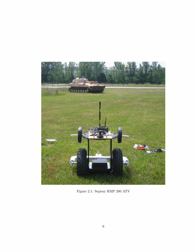
Figure 2.1: Segway RMP 200 ATV
6
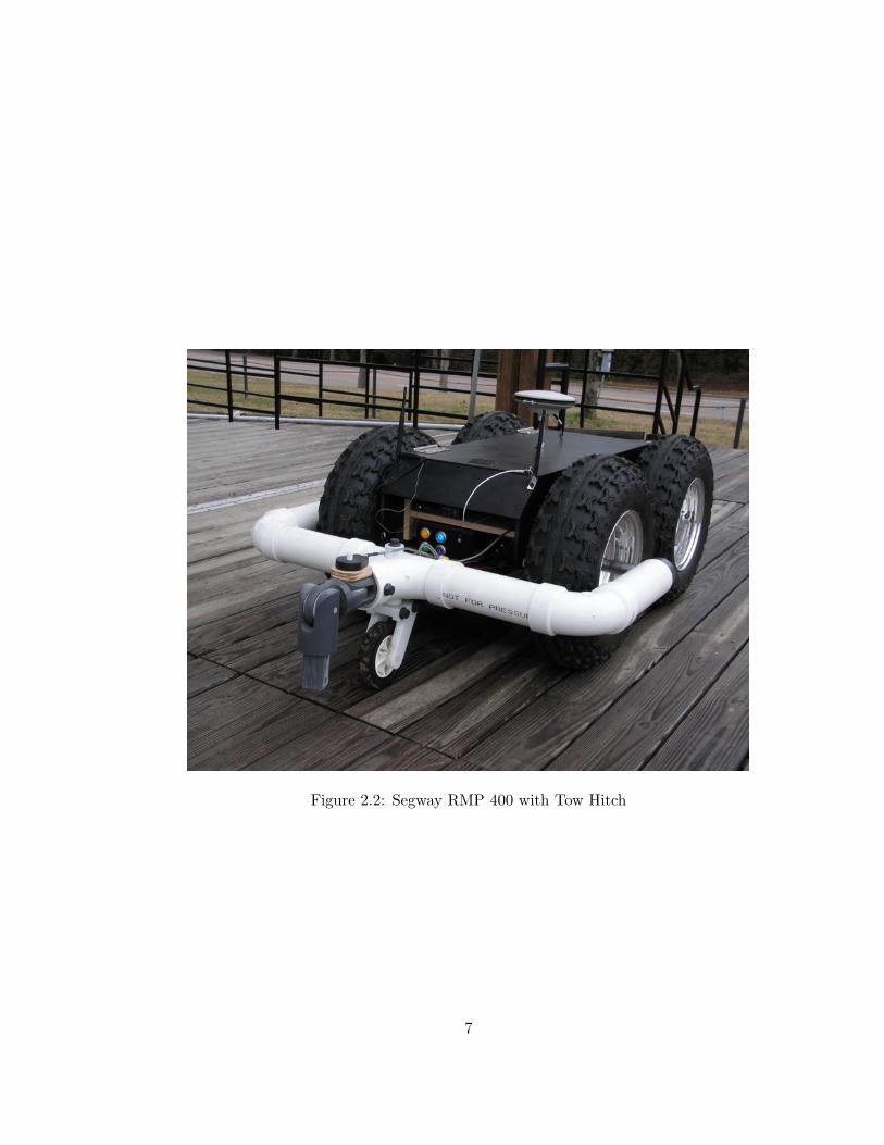
Figure 2.2: Segway RMP 400 with Tow Hitch
7
The Segway robots are controlled through a universal serial bus (USB) interface. Ve-
locity and turn commands are sent to the robot in counts, which directly relate to a longi-
tudinal velocity and yaw rate. The robots contain built in speed and yaw rate controllers
designed by Segway Inc. that control the individual motors based on the velocity and turn
commands. The internal controllers also allow the RMP 200 to balance itself. The robots
each contain five MEMS gyroscopes (two are used for redundancy purposes) and a wheel
encoder on each wheel, which are used by the internal controllers. The measurements from
these sensors as well as motor currents and battery voltages are accessible through the USB
interface. Initial tests showed the RMP200 to be unsuitable for traversing rough terrain
and so the remainder of the development effort concentrated on the RMP400.
A custom designed tow hitch was provided by the Army Corp of Engineers to allow a
trailer to be attached to either robot. The tow hitch is attached to the robot at its axles
so that it does not interfere with the balancing ability of the RMP200. A machined plastic
u-joint allows articulation between the robot and trailer. A picture of the Segway RMP 400
and the tow hitch is shown in Figure 2.2. The geophysical sensor trailers are attached to the
u-joint using a tow bar created from a piece of square fiberglass tubing attached with nylon
and fiberglass bolts. No metal parts (other than those in the encoder), which could affect
geophysical measurements, are used on any part of the tow hitch or trailer. The length
of the tow bar for each sensor towed was determined by a study performed by the Army
Corp of Engineers that analyzed the effects of the metal in the robot on the sensors used
at various distances.
8
2.3 Navigation Sensors
Navigation data for the system is provided by a NovAtel Synchronized Position Attitude
Navigation (SPAN) system. The SPAN system is a tightly coupled global positioning system
(GPS) / inertial navigation system (INS). The system combines a NovAtel DL-4plus dual-
frequency GPS receiver with a Honeywell HG1700 inertial measurement unit (IMU). The
IMU contains 3 ring laser gyroscopes and 3 accelerometers to provide 6 degree of freedom
(DOF) navigation information. Real time kinematic (RTK) corrections are sent to the
receiver from a local base station to provide centimeter level accurate (2 cm standard
deviation) GPS positions [7]. The system is capable of outputting GPS positions at a rate
of 5 Hz (20Hz when the IMU is not enabled). The IMU provides dead reckoning between
GPS measurements or during GPS outages. Blended GPS/INS position and attitude are
available at a rate of 100 Hz. The SPAN system is mounted at the center of the robot.
In order to accurately control the trailer’s placement, the position of the trailer must
also be known. Rather than placing a second GPS system on the trailer, which would in-
crease cost and place metal near the geophysical sensors, another sensor is used to determine
the trailer position relative to the robot’s position. An optical encoder is mounted to the
u-joint on the tow bar, shown in Figure 2.3, to measure the angle between the robot and
trailer in the plane of the robot. The encoder used is a U.S. Digital E5S-1800 incremental
optical encoder with a resolution of 1800 cycles per revolution (CPR), which corresponds
to an angular resolution of 0.05◦. Assuming the robot, hitch point, and trailer are coplanar
(the robot and trailer are on level ground), the trailer’s position can be accurately calculated
from the robot’s position and orientation and the output of the encoder.
9
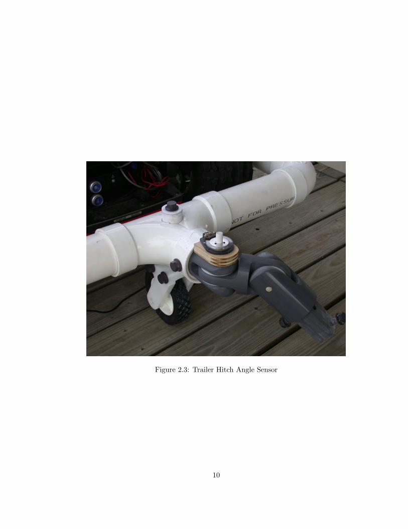
Figure 2.3: Trailer Hitch Angle Sensor
10

2.4 Geophysical Sensors
Although the system can be configured to tow any trailer, two common geophysical
sensors were used for testing and evaluation during this project. They are the Geonics
EM61-MK2 time domain metal detector and the Geometrics G-858 portable cesium vapor
magnetometer.
The EM61-MK2 consists of a 1m by 0.5m fiberglass coil, which contains coils of wire.
An electrical pulse is generated in one of the coils. The electric field created by this pulse
will then create surface currents in any conductive objects nearby. These surface currents
will in turn create a field that can be detected by the remaining coils. The response in
the various coils are measured at set time delays and an output is provided in mV. The
EM61-MK2 is therefore an active sensor and is capable of detecting any object made from
a conductive material. The EM61-MK2 trailer attached to the robot is shown in Figure 2.4.
The sensor can also be operated with another receiving coil mounted on standoffs above
the main coil.
The Geonics G-858 magnetometer is a passive sensor capable of detecting magnetic
fields. The G-858 is capable of detecting nearby ferrous objects. A ferrous object will cause
a change in the Earth’s magnetic field around it and this change can then be detected by the
magnetometer. Two G-858 magnetometers operating in a vertical gradient mode attached
to the robot are shown in Figure 2.5.
11

Figure 2.4: Robot with EM61-MK2 Trailer
Figure 2.5: Robot with G-858 Magnetometer Trailer
12

2.5 Computer Hardware
2.5.1 Robot Hardware
A small embedded PC is mounted on the robot to provide control and data logging
functionality. The PC used is a CappuccinoPC SlimPRO SP625. The unit has an Intel
Pentium M processor running at 1.6GHz, 512MB of RAM and an 8GB solid-state hard
disk. An 802.11g wireless network card is installed in the front PCMCIA slot to provide
wireless communications. The card used is a Buffalo Technologies WLI-CB-G54 PCMCIA
card with an external DLINK 5dBi dipole antenna.
The navigation and geophysical sensors discussed above as well as the Segway robot
are connected to this computer. All of the geophysical sensors used and the navigation
sensors are interfaced through a RS232 serial connection. The geophysical sensor currently
being used is connected directly to a RS232 port on the computer. The navigation sensors
are connected through USB-to-serial converters, which are run through an 8-port USB hub.
The Segway interfaces are also connected through the USB hub. A diagram showing the
various connections to the embedded computer (brick PC) is given in Figure 2.6.
Figure 2.6: PC Signal Tree
13

A USB video camera is also mounted on the robot and connected to the embedded PC
to provide video feedback for tele-operation. The camera used is a Digi Watchport USB
web camera. The camera is mounted on a TrackerPod, which is an active mount that allows
the camera to be panned and tilted. The TrackerPod is controlled via a USB interface as
well.
2.5.2 Operator Control Hardware
A laptop computer is used to provide a user interface to the system. The laptop is
connected to a DLINK DWL-2200AP 802.11g wireless access point via an ethernet cable,
which provides a wireless network connection to the embedded PC on the robot. A DLINK
ANT15-2400 high-gain omni-directional antenna is used to extend the range of the system.
According to the manufacturer’s specifications, the antenna has a 15dBi gain with a hori-
zontal half power beamwidth (HPBW) of 360◦ and a vertical HPBW of 5◦. A USB joystick
is also connected to the laptop to allow the robot to be manually driven.
2.6 Software
Software has been developed to allow for both autonomous path-following and tele-
operation of the robot and trailer, using a client-server software architecture. A server
program written in C++ runs on the embedded PC on the robot. A client graphical
user interface (GUI) developed in Visual Basic .NET runs on the remote laptop computer.
Commands and data are transferred between the client and server software over a TCP
connection using a custom set of ASCII text messages.
14

2.6.1 Server Software
The server software interfaces with the Segway and navigation sensors. Selected data
from these sensors is transmitted to the client software at regular intervals when a network
connection is available. The sensor data can also be written to one of three log files. Segway
sensor data, vehicle and trailer position data, and autonomous control algorithm values are
logged to separate files. These data files are initiated and terminated through the client
software interface. The format of the log files is given in Appendix 7.2.
The server software is responsible for running the autonomous control algorithm de-
scribed in Chapter 4. It also passes turn and velocity commands received from the client
software to the Segway when the system is operating in manual control mode. It provides
a NMEA standard position output containing the calculated position of the trailer over a
user selectable serial port. This can be used as an input to the various geophysical sen-
sor electronics to allow geophysical and position data to be recorded and time stamped
together.
2.6.2 Client Software
The client software provides a graphical user interface (GUI) to the system. This
GUI allows the user to tele-operate the robot, generate paths, start and stop autonomous
operation, monitor the robot’s position and status, start and stop data logging and various
other operations. A screenshot of the GUI is shown in Figure 2.7. An image from the video
camera mounted on the robot, the current reference and actual path, vehicle controls, and
displays from the various sensors are shown on the interface. Options in the View menu
15

allow the various windows to be displayed or hidden. Menu options also allow recording
system data to file as described in Section 2.6.1.
Figure 2.7: User Interface Screenshot
A path planning tool is provided in the GUI to generate paths to survey a given field.
The tool allows the user to enter four corner points in order to define a field. Obstacles
can also be entered by defining the vertices of a polygon that surrounds the obstacle. The
desired direction of travel and spacing between passes is also entered. A path is then
automatically generated that completely covers the field, as discussed in Chapter 3. The
entered values can be saved to and loaded from a file allowing them to be modified and new
paths generated at a later time. A screenshot of the path planning tool is given in Figure
2.8.
16

Figure 2.8: Survey Path Generation Tool
17
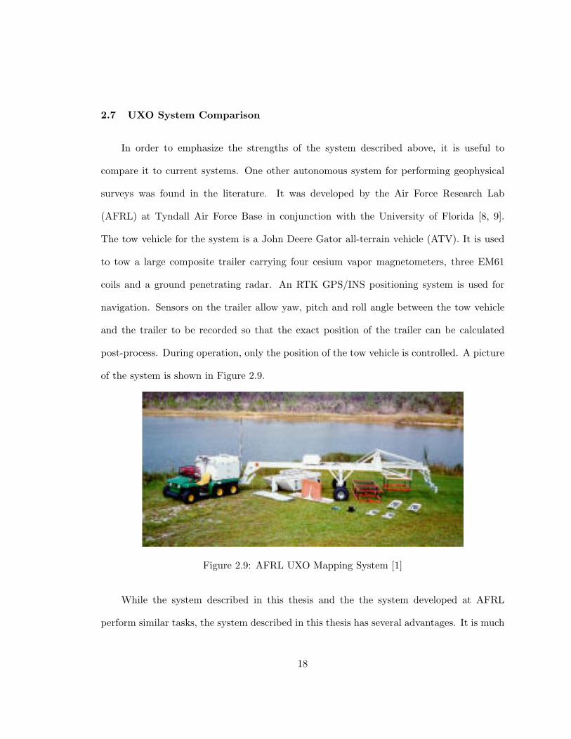
2.7 UXO System Comparison
In order to emphasize the strengths of the system described above, it is useful to
compare it to current systems. One other autonomous system for performing geophysical
surveys was found in the literature. It was developed by the Air Force Research Lab
(AFRL) at Tyndall Air Force Base in conjunction with the University of Florida [8, 9].
The tow vehicle for the system is a John Deere Gator all-terrain vehicle (ATV). It is used
to tow a large composite trailer carrying four cesium vapor magnetometers, three EM61
coils and a ground penetrating radar. An RTK GPS/INS positioning system is used for
navigation. Sensors on the trailer allow yaw, pitch and roll angle between the tow vehicle
and the trailer to be recorded so that the exact position of the trailer can be calculated
post-process. During operation, only the position of the tow vehicle is controlled. A picture
of the system is shown in Figure 2.9.
Figure 2.9: AFRL UXO Mapping System [1]
While the system described in this thesis and the the system developed at AFRL
perform similar tasks, the system described in this thesis has several advantages. It is much
18
smaller and and less complex than the AFRL system. The AFRL system uses a large ATV
as a tow vehicle as opposed to the small robot used in the system described. While the
ATV has the advantage of having a full suspension and being designed for towing, it has the
disadvantage of requiring custom modifications to allow steering, throttle, braking, etc. to
be controlled by a computer. The Segway robots have the advantage of being smaller, more
easily transported, and possibly cheaper due to the modifications required to the ATV. The
trailer in the AFRL system is also much larger and custom fabricated. The Segway system,
along with the geophysical sensor trailers used, can be easily packed into a 6 ft. × 10 ft.
trailer.
The accuracy of the systems are very similar. The AFRL system is capable of placing
the tow vehicle on the path within 2 to 10 cm 85% of the time [1]. Information about the
accuracy of the trailer’s position, however, is not available. The accuracy of the system
developed in this thesis is given in Chapter 4. Experiments show the trailer’s position to be
accurate to within 10 cm even with the relatively simple method of determining the trailer
position and control method used.
2.8 Conclusion
In this chapter, a description of the autonomous UXO detection system was given. The
Segway robots used as tow vehicles were described as well as the geophysical instruments
being towed. The design of the system including selection of computers and electronics
was provided as well as an overview of the various interfaces in the system and how they
are connected. Software to control the robot and provide a graphical user interface was
presented. Finally, a similar system for mapping UXO developed at AFRL was discussed.
19
Chapter 3
Path Planning
3.1 Introduction
In order to perform an autonomous survey, a path must first be defined. In this chapter,
a method for defining that path is given. An algorithm is developed that will generate a path
to completely cover a field given its corner points. The algorithm also provides methods for
known obstacles to be avoided, allowing areas to be defined in the field that are not to be
mapped. Note that ceiling d e and floor b c operators appear in several equations in this
chapter and should not be confused with matrix separators.
3.2 Path Definition
A common technique in robotic path following is to define the reference path as a series
of lines and circular arcs. These paths are commonly referred to as Dubins’s paths, after
L.E. Dubins who showed that the time optimal (neglecting vehicle dynamics), continuously
differentiable path between any two configurations in two-dimensional space consists of lines
and circular arcs of minimum radius [10]. A configuration is defined as a position (e, n), an
orientation or heading ψ, and a desired speed V . In the following sections configurations
will be written as a vector of the form:
C =[e n ψ V
](3.1)
20
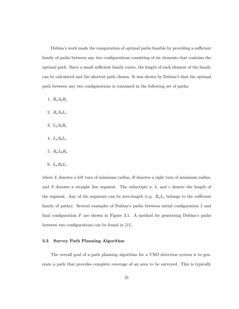
Dubins’s work made the computation of optimal paths feasible by providing a sufficient
family of paths between any two configurations consisting of six elements that contains the
optimal path. Since a small sufficient family exists, the length of each element of the family
can be calculated and the shortest path chosen. It was shown by Dubins’s that the optimal
path between any two configurations is contained in the following set of paths:
1. RaSbRc
2. RaSbLc
3. LaSbRc
4. LaSbLc
5. RaLbRc
6. LaRbLc
where L denotes a left turn of minimum radius, R denotes a right turn of minimum radius,
and S denotes a straight line segment. The subscripts a, b, and c denote the length of
the segment. Any of the segments can be zero-length (e.g. RaLc belongs to the sufficient
family of paths). Several examples of Dubins’s paths between initial configuration I and
final configuration F are shown in Figure 3.1. A method for generating Dubins’s paths
between two configurations can be found in [11].
3.3 Survey Path Planning Algorithm
The overall goal of a path planning algorithm for a UXO detection system is to gen-
erate a path that provides complete coverage of an area to be surveyed. This is typically
21
Figure 3.1: Example of RSL, RSR, and LRL Dubins’ Paths [2]
accomplished by towing the sensors in evenly spaced lines across the grid to be surveyed.
The spacing between these lines is determined by the coverage width of the sensor being
towed. The EM61-MK2 discussed in Section 2.4, for example, covers a 1m wide area on
each pass and so 1m spaced lines are used for surveys using that sensor.
In a typical geophysical survey, for a line spacing of k, a person will pull the sensor
to the end of a line, turn around, and start down another line a distance of k over. While
a person pulling a two-wheeled trailer is capable of pivoting the trailer in place, resulting
in a zero-turning radius, a wheeled mobile robot and trailer is subject to nonholonomic
constraints and cannot necessarily do this. A robot pulling a trailer has a minimum turning
radius R, which is determined by the geometry and dynamics of the system. If the line
spacing k is less than the minimum turning radius R of the system, then the robot will
not be able to maneuver the trailer from one line to an adjacent line in a single turning
maneuver. An algorithm is therefore needed to generate a path that covers the field that
the robot and trailer are capable of following.
The idea of generating a path that causes a robot to pass over every point in an area is
commonly known as coverage path planning. Coverage path planning has been extensively
22

studied in recent years for applications such as robotic demining, lawn mowing, snow re-
moval, etc. A survey of current techniques is given in [12]. Coverage planning algorithms
can be divided into two main categories, complete and randomized. Complete algorithms
plan out the path to be followed exactly and guarantee that the entire region is covered.
An alternative is to randomly search a region (e.g. turning when obstacles or boundaries
are reached) until the entire area has been covered. While complete algorithms guarantee
coverage of an area, they typically require more complex sensors and more computational
capability than random algorithms. Complete algorithms also often assume a priori knowl-
edge of the environment to be surveyed.
For the system being developed, complete knowledge of the site to be surveyed is
assumed and highly accurate navigation sensors are available, so a complete coverage al-
gorithm is an acceptable choice. The algorithm developed is similar to the Sets method
described in [8], which was developed as part of a similar UXO detection system.
The inputs to the algorithm are:
• the area to be surveyed defined by four corners points,
P =[
P1 P2 P3 P4
](3.2)
• the minimum turning radius of the vehicle, R
• the spacing between passes, k
• the direction of travel for the first pass, ψi
• the desired longitudinal speed for the survey, Vr
23

The algorithm generates a path that covers the area inside a given quadrilateral (defined
by P ), without covering the same line twice. Depending on the width of the region to be
surveyed, a buffer region of approximately 2R to 3R is required around the region to be
surveyed for making turns.
The path is generated using an interleaving pattern. An example is shown in Figure
3.2. On the far side of the field, a (R+ k) right turn is made. On the near side of the field
a R right turn is made. This process is repeated until a set has been completed. Each set
contains M = 4R+1 passes. Once a set has been completed, another set is started, turning
in the opposite direction. This process is repeated until there are no longer M passes left to
make. At that point, the rest of the passes are driven in order, making large looping turns
outside the field to maneuver to the next line.
Figure 3.2: Interleaving Path
The first step in the algorithm is to generate a set of lines that define the parallel passes
across the field to be surveyed. This requires a coordinate transformation be applied to the
24

field corners P to rotate the field so that the x-axis is aligned with the initial direction of
travel ψi. The transformation matrix is given by
cos θ sin θ
− sin θ cos θ
(3.3)
where θ = π2 − ψi. The minimum and maximum y values (ymin and ymax respectively) of
the rotated field are then determined. The number of passes N required to cover the field
can then be calculated as
N =⌊ymax − ymin
k
⌋+ 1 (3.4)
Starting and ending points on each side of the field for the passes are then determined.
Intersections between the lines defining the boundary of the rotated field with the line
y = ymax are calculated, in order to find two intersection points. The point with the
smallest x value is considered to be on the near side of the field (start point) and the other
point to be on the far side of the field (end point). The line is then shifted down by −k
and the intersections are calculated again. The process is repeated until y = ymin. The
result is a matrix of starting point coordinates (SP ) indexed from i = 1 to N and a matrix
of ending point coordinates (EP ) indexed from i = 1 to N . The passes required to survey
the field are defined by connecting each pair of intersections with a line. The result for an
example field is shown in Figure 3.3. The values used to generate the example field are
given in Table 3.1.
In order to generate a Dubins’s path, a set of configurations are required. Therefore, the
next step is to generate a list of configurations from the points determined in the previous
25

step. Pseudocode to generate a set of configurations is given in Algorithm 3.3.1. Once
configurations for all the interleaving sets have been defined, the remaining start and end
points are added to the list of configurations in order to define the rest of the passes. The
final path is generated by calculating Dubins’s paths between each of the configurations in
the list created. The example path generated is shown in Figure 3.4.
Table 3.1: Example Field Parameters
Parameter Symbol Valueturning radius r 3mline spacing k 1mdirection ψi 15◦
field boundary P
0 00 3030 3030 0
26

Algorithm 3.3.1: SurveyPlanner(N,M,SP,EP )
nextPoint← 1
dir ← −1
p← 1
comment: determine the number of passes that an be made using the interleaving method
k ← bNM cM
comment: generate the list of configurations
for i← 1 to k
do
comment: change direction when a set is finished
if i− 1 mod N = 0
then dir ← (−1)dir
if i mod 2 = 1
then AddOddNumPath(Algorithm3.3.2)
else AddEvenNumPath(Algorithm3.3.3)
Algorithm 3.3.2: AddOddNumPath(i)
configurations[p]← SP [i]
p← p+ 1
configurations[p]← EP [i]
p← p+ 1
if dir = 1
then nextPoint← nextPoint+ dM2 e
else nextPoint← nextPoint− bM2 c
27

0 5 10 15 20 25 300
5
10
15
20
25
30
North (m)
Eas
t (m
)
field boundarynear side pointsfar side pointspasses
Figure 3.3: Survey Planner Parallel Passes
Algorithm 3.3.3: AddEvenNumPath(i)
configurations[p]← EP [i]
p← p+ 1
configurations[p]← SP [i]
p← p+ 1
if dir = 1
then nextPoint← nextPoint− bM2 c
else nextPoint← nextPoint+ dM2 e
28

−10 −5 0 5 10 15 20 25 30 35 40
−5
0
5
10
15
20
25
30
35
East (m)
Nor
th (
m)
Figure 3.4: Survey Path
29
3.4 Obstacle Avoidance
For many typical fields, dividing the area to be surveyed into quadrilaterals that contain
no obstacles or obstructions can be difficult and is not very practical. As survey areas are
made smaller, the percentage of time spent turning around on either end of the field increases
and therefore mapping efficiency is reduced. A simple method is desired that will generate
a collision-free path (i.e. one that does not cause the vehicle to collide with an obstacle)
to survey an area with known obstacles. This allows larger fields to be defined by allowing
fields to include areas that are not to be mapped rather than having to define multiple,
smaller fields to avoid these areas.
Much research has been done in determining collision-free Dubins’s paths. One solution
to this problem known as the visibility graph search method is given in [13]. The authors
state that obstacle free paths consist of simple Dubins’s paths that begin and end on either
the initial configuration, the final configuration, the vertex of an obstacle, or the edge of an
obstacle. The size of the obstacles are expanded to account for the size of the vehicle. The
vehicle can then be considered to be a point. A graph based search algorithm is then used
to find the shortest feasible path.
The algorithm is based on the construction of a visibility graph. A visibility graph is
a weighted, directed graph constructed by defining the initial and final configurations, the
obstacle vertices, and points spaced a distance δ apart along the obstacle edges as nodes
in the graph. Dubins’s paths are then generated between each pair of nodes. These paths
are then checked for intersections with obstacles. If a path does not intersect an obstacle,
then a segment is defined in the graph between the start and end points of that path. An
30

algorithm such as Dijkstra’s algorithm [14] can then be used to search the graph for the
shortest path between the initial and final configuration.
A simplified algorithm based on the algorithm developed in [13] has been developed
to add obstacle avoidance capabilities to the survey planner described in Section 3.3. Line
segments defining parallel passes across the field are generated as before. Each line segment
is then run through the obstacle avoidance algorithm to check for collisions with obstacles.
If any collisions exist, it is replaced with a collision free path and the process continues.
The inputs to the algorithm are:
• A list of polygons defining the obstacles (defined by their vertices)
• The desired starting configuration, Ci
• The desired ending configuration, Cf
• Minimum turning radius, r
The first step in the algorithm is to create the visibility graph. The start and goal
configurations and the vertices of the obstacle polygons are added as nodes to the graph.
Next, visibility between the nodes is checked. This is done by defining a line segment
between pairs of nodes and checking for intersections between that segment and the segments
that define the edges of the obstacles. If no intersection is found, the nodes in the graph are
considered visible and an edge is created in the graph structure to connect them. The weight
of the edge is the length of the line segment that connects the two nodes. The process is
continued until every combination of nodes is checked. Note that because a directed graph
is used, two edges must be added for every pair of nodes that are visible. For example, if
31

nodes 1 and 3 are visible, an edge must be created between nodes 1 and 3 and between
nodes 3 and 1.
Once the visibility graph has been created, it can then be searched for the minimum
length path between the start and goal nodes. This is done using a Dijkstra search. The
result of the search is a list of nodes that define the shortest straight-line path between the
start and goal configurations. A list of configurations is then created from the coordinates
of the nodes returned from the search. The heading for each configuration is set to the
heading of the line between the start and goal nodes. A Dubins’s path, which goes from the
start configuration to the end configuration, avoiding any obstacles, is then created using
the list of configurations.
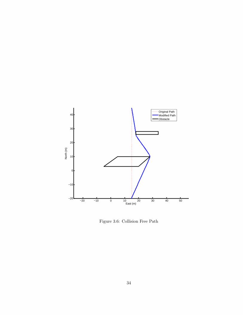
As an example, a collision free Dubins’s path is created between two configurations in
the presence of two four-sided obstacles. The starting configuration Ci is[
15 −20 0 0.75
]and the ending configuration Cf is
[15 45 0 0.75
]. The vertices of polygon 1 are
20 3
−5 3
5 10
28 10
(3.5)
and the vertices of polygon 2 are
34 28
24 26
18 26
18 28
(3.6)
32

The resulting visibility graph is shown in Figure 3.5 and the original and collision free
paths are shown in Figure 3.6.
−5 0 5 10 15 20 25 30 35−20
−10
0
10
20
30
40
50
1
2
3
4
5 6
7 8
9
10
EdgesShortest PathObstacles
Figure 3.5: Visibility Path
There are several restrictions on the start and goal configurations and the geometry of
the obstacles passed into the algorithms. The original path must intersect with obstacles
only on line segments. The algorithm is not capable of generating collision free paths for
arc segments that intersect with an obstacle (i.e. all obstacles must lie within survey area
boundaries). Also a distance of 2R must be present between obstacles and between all
obstacles and the edge of the field where a turn takes place.
33
−20 −10 0 10 20 30 40 50−20
−10
0
10
20
30
40
East (m)
Nor
th (
m)
Original PathModified PathObstacle
Figure 3.6: Collision Free Path
34
3.5 Survey Obstacle Avoidance
While the obstacle avoidance algorithm discussed in the previous section successfully
generates a collision free path between two configurations, it is not suitable for geophysical
mapping purposes. Examining Figure 3.6, it can be seen that the collision free path gener-
ated covers very little of the original path. When performing a survey, it is important that
as much of each pass generated by the survey planner be covered as possible. Therefore, a
modification is needed to the visibility graph algorithm to cause the resulting collision free
paths to more closely follow the original paths. The modification proposed adds additional
configurations to the path referred to as offset points that cause the collision free path to
follow the original path for as long as possible before deviating to avoid an obstacle. The
result is referred to as a survey collision free path.
The survey collision free path is generated by adding an additional step to the beginning
of the visibility graph obstacle avoidance algorithm previously discussed. A line segment
between the start and end configurations is checked for intersections with all of the obstacle
polygons. If any intersections are found, additional configurations are added by adding
points a distance 2R along the original path in each direction from the obstacle. This
is illustrated in Figure 3.7. A distance shorter than 2R could result in the robot getting
trapped against the obstacle (i.e. does not have enough space to avoid the obstacle by
turning and would therefore be required to back up). These offset points are then passed
into the visibility graph obstacle avoidance algorithm as start and goal configurations and a
shortest distance, collision-free path is created between them. The complete path will then
consist of a line segment between the original goal configuration and the first offset point,
the collision-free path generated using the visibility graph algorithm between the first and
35

second offset point, and then another line segment between the 2nd offset point and the
final configuration.
Figure 3.7: Survey Collision Free Path
Using this method, the path between the original start configuration and the first offset
point and the path between the second offset point and the original goal configuration will
consist of only a line segment and will follow the original path exactly. The vehicle will not
deviate from the original path until it is a distance of 2R from the obstacle and will return
to the original path a distance 2R past the obstacle. A path generated with this modified
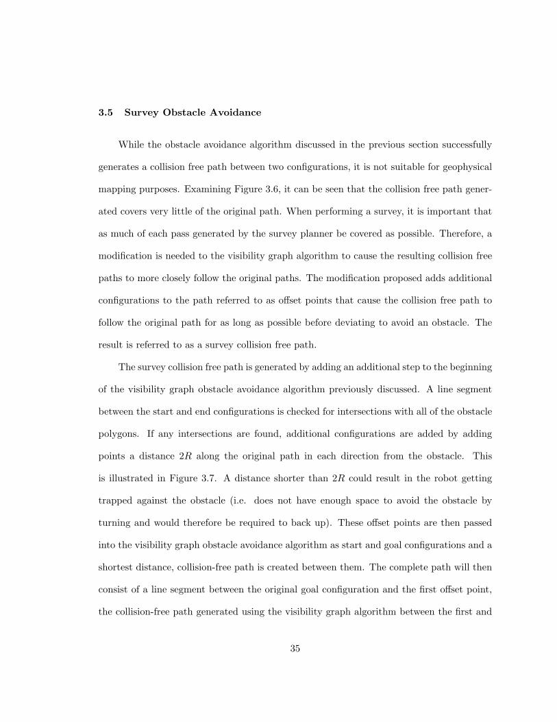
method is compared to the paths generated in the previous section in Figure 3.8. It can
be seen that the survey collision free path more closely follows the original path, than the
path generated using the visibility graph method alone does. Using survey collision free
paths will allow a greater percentage of a site to be surveyed when compared to using the
collision free paths discussed in the previous section.
36

3.6 Conclusion
In this chapter a method of planning paths for the purpose of geophysical mapping
has been presented. A method of defining paths as a series of lines and circular arcs was
discussed. An algorithm was developed for creating these paths to cover a four-sided field.
A common method of planning paths that avoid obstacles was introduced. A modification
was then made to this method to cause the collision free paths generated to more closely
follow the original paths, allowing more of a field to be covered.
37
−20 −10 0 10 20 30 40 50−20
−10
0
10
20
30
40
East (m)
Nor
th (
m)
Original PathCollision Free PathSurvey Col. Free PathOffset PointsObstacle
Figure 3.8: Collision Free Path Comparison
38
Chapter 4
Control Design
4.1 Introduction
Once a suitable reference path has been created, a controller is needed to guide the
trailer to follow the given path. Path following control for mobile robots pulling trailers has
been extensively explored in recent research. Many methods have been developed to control
a robot to follow a path, including control via approximate linearization, exact feedback
linearization, full-state linearization via dynamic feedback, and time-varying feedback. A
good overview of the various methods can be found in [15]. Many of these methods can be
extended to control a mobile robot towing a trailer. Exact linearization was used in [16] to
control a robot with a trailer along a straight line. That work was extended to allow the
system to follow straight lines and circular arcs in [17]. Other methods for path following
control of a mobile robot having one or more trailers are described in [18, 19, 20, 21].
Much of the above research has been motivated by applications in the world of factory
automation. Problems being addressed include obstacle avoidance and complex maneuvers,
such as the backing-up of a trailer. In the application being consider for this project,
however, the precise control of the trailer’s path is desirable. Autonomous trailer path
control has been achieved in the agriculture industry, where control systems have been
developed for tractors to precisely control the position of a towed implement. In [22],
researchers designed a control system that utilizes differential GPS to control the position
of an implement towed behind a tractor. The system used two separate GPS receiver
antennas, one on the tractor and one on the implement.
39

The system developed in this thesis is a lower cost system, with only a single GPS
receiver. Rather than adding a second GPS receiver to measure the trailer’s position, an
optical encoder (hitch angle sensor) is used to measure the orientation between the robot
and the trailer. The combination of instruments make it possible to precisely control the
position of the trailer.
4.2 Vehicle Model
For the purpose of mapping unexploded ordnance, the robot is required to move at a
slow speed (≤ 1m/s). Therefore, factors such as the vehicle’s inertia and wheel slippage
can reasonably be ignored. This allows a kinematic model rather than a full dynamic model
can be used. The dynamics of the mobile robots used in this work can be modeled using
three state variables to represent position and orientation in two dimensional space. For
the case of a mobile robot pulling a trailer, a fourth state variable is added to describe
the orientation between the robot and trailer. The kinematic model for a robot with a
trailer connected using off-axle hitching is given in [23]. Off-axle hitching (as apposed to
on-axle hitching) refers to the fact that the trailer is connected at a point that is not at the
center of the rear-axle of the tow vehicle. This results in a non-minimum phase zero (i.e.
a zero in the right half plane) being present in the model. A coordinate transformation
from Cartesian coordinates to universal transverse mercator (UTM) coordinates yields the
40
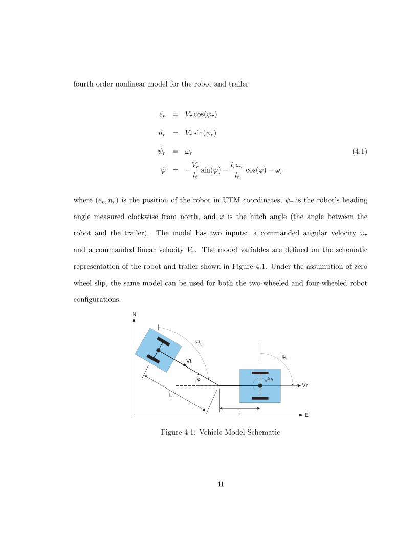
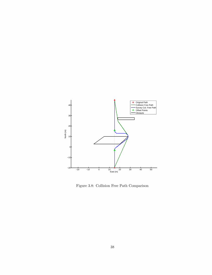
fourth order nonlinear model for the robot and trailer
er = Vr cos(ψr)
nr = Vr sin(ψr)
ψr = ωr (4.1)
ϕ = −Vr
ltsin(ϕ)− lrωr
ltcos(ϕ)− ωr
where (er, nr) is the position of the robot in UTM coordinates, ψr is the robot’s heading
angle measured clockwise from north, and ϕ is the hitch angle (the angle between the
robot and the trailer). The model has two inputs: a commanded angular velocity ωr
and a commanded linear velocity Vr. The model variables are defined on the schematic
representation of the robot and trailer shown in Figure 4.1. Under the assumption of zero
wheel slip, the same model can be used for both the two-wheeled and four-wheeled robot
configurations.
ωrφ
N
E
Ψr
lr
lt
Vr
Vt
Ψt
Figure 4.1: Vehicle Model Schematic
41

Since the goal is to control the position and orientation of the trailer, it is desirable to
describe the model in terms of trailer variables rather than robot variables. The relationships
between the positions, orientations, and velocities of the robot and trailer are given by:
et = er − lr sin(ψr)− lt sin(ψr + ϕ)
nt = nr − lr cos(ψr)− lt cos(ψr + ϕ)
ψt = ψr + ϕ (4.2)
Vt = Vr cos(ϕ)− lrω sin(ϕ)
where (et, nt) is the position of the trailer, ψt is the heading of the trailer, and Vt is the
linear velocity of the trailer. These equations are also used to calculate the position of
the trailer/robot from the position of the robot/trailer using hitch angle measurements.
Applying mapping (4.2) to the model (4.1) yields the dynamic model of the trailer under
tow:
et = Vt cos(ψt)
nt = Vt sin(ψt)
ψt = −Vr
ltsin(ϕ)− lrωr
ltcos(ϕ) (4.3)
ϕ = −Vr
ltsin(ϕ)− lrωr
ltcos(ϕ)− ωr
42

4.3 Controller Design
In this section, A control law is designed that will cause the trailer to accurately follow
a desired path. As discussed in Section 3.2, the reference path is defined as a series of line
segments and circular arcs of minimum radius.
In order to design a controller, the model (4.3) is rewritten in terms of errors from the
path. These errors are shown graphically in Figure 4.2 for line segments and Figure 4.3 for
arc segments.
(e1 ,n1)
(e2 ,n2)
(eact ,nact)
Ψact
ΨdesΨerr
Yerr
Yerr2
Figure 4.2: Line Segment Errors
The linearized dynamics of the error x are given by:
x =
˙yterr
˙ψterr
˙ψrerr
=
Vrψterr
−Vrlt
(ψterr − ψrerr)− lrωrlt
ωr
(4.4)
where yterr and ψterr are the lateral and heading error of the trailer respectively, and ψrerr
is the heading error of the robot. The order of the model (4.4) is reduced from the model
43

(4.3) because the vehicle is moving at a fixed speed. Therefore, the linear velocity Vr is
assumed to be constant and so is treated as a parameter rather than an input. A linear
state feedback control law is then determined to be:
ωr = −Kx (4.5)
ωr = −k1yterr − k2ψterr − k3ψrerr
The gains K are chosen using standard pole placement techniques.
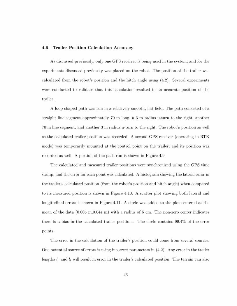
4.4 Simulation Results
The controller presented above is verified using a simulation in Matlab. The system
was simulated for approximately 25 minutes while following the path shown in Figure 4.4.
The parameters used in the simulation are given in Table 4.1.
Table 4.1: Simulation model parameters
Parameter Symbol Value UnitsRobot speed Vr 0.75 m/s
Robot tongue length lr 0.95 mTrailer tongue length lt 2.11 m
Robot angular rate limit |ωr|max 3 rad/sTrailer lateral error gain K1 845Trailer heading error gain K2 1279Robot heading error gain K3 1620
Simulation duration tsim 1572 sec.
A portion of the results of the simulation are shown in Figure 4.5, which shows the set
of turns on the north end of the field. It can be seen that the trailer successfully follows the
reference path. The controller inputs (trailer lateral error, trailer heading error, and robot
44
heading error) and output (turn command) are shown in Figure 4.6. The root mean square
(RMS) lateral error for the simulation was 5.6 cm.
No sensor error or noise was included in the simulation. The major source of error is
the presence of transients, which occur when the trailer transitions from a line segment to
an arc segment or from an arc segment to a line segment. These transients can be seen
at the beginning and ending of the turns in Figure 4.5. They are a result of the reference
path chosen. While a Dubins’s path is continuously differentiable, its second derivative or
curvature is not continuous. This results in a step change in the desired robot heading at
every transition between a line and arc segment. The transients are exaggerated by the
effects of off-axle hitching, which causes there to also be a discontinuity in the desired robot
position, making it not physically possible for the robot to move in such a way as to make
the trailer follow the desired path.
4.5 Experimental Results
The controller performance was also validated experimentally. The path simulated in
the previous section (Figure 4.4) was followed by the robot pulling the EM61-MK2 trailer.
The gains given in Table 4.1 were also used in the experiment. A portion of the results
of the experiment are shown in Figure 4.7. The controller inputs and output are shown in
Figure 4.8. The results very closely match the results seen in simulation. The root mean
square (RMS) lateral error for the experiment was 6.7 cm. The experimental results contain
GPS measurement noise that was not simulated, which could account for the slight increase
in error when compared to the simulation results.
45
4.6 Trailer Position Calculation Accuracy
As discussed previously, only one GPS receiver is being used in the system, and for the
experiments discussed previously was placed on the robot. The position of the trailer was
calculated from the robot’s position and the hitch angle using (4.2). Several experiments
were conducted to validate that this calculation resulted in an accurate position of the
trailer.
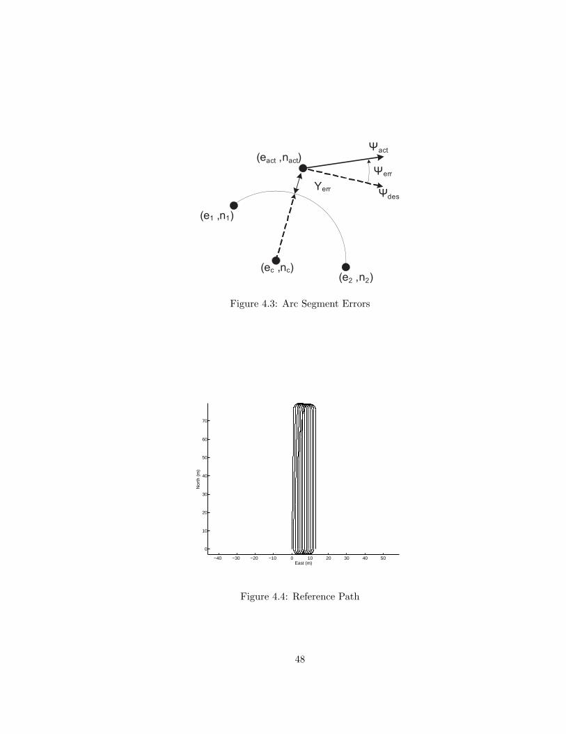
A loop shaped path was run in a relatively smooth, flat field. The path consisted of a
straight line segment approximately 70 m long, a 3 m radius u-turn to the right, another
70 m line segment, and another 3 m radius u-turn to the right. The robot’s position as well
as the calculated trailer position was recorded. A second GPS receiver (operating in RTK
mode) was temporarily mounted at the control point on the trailer, and its position was
recorded as well. A portion of the path run is shown in Figure 4.9.
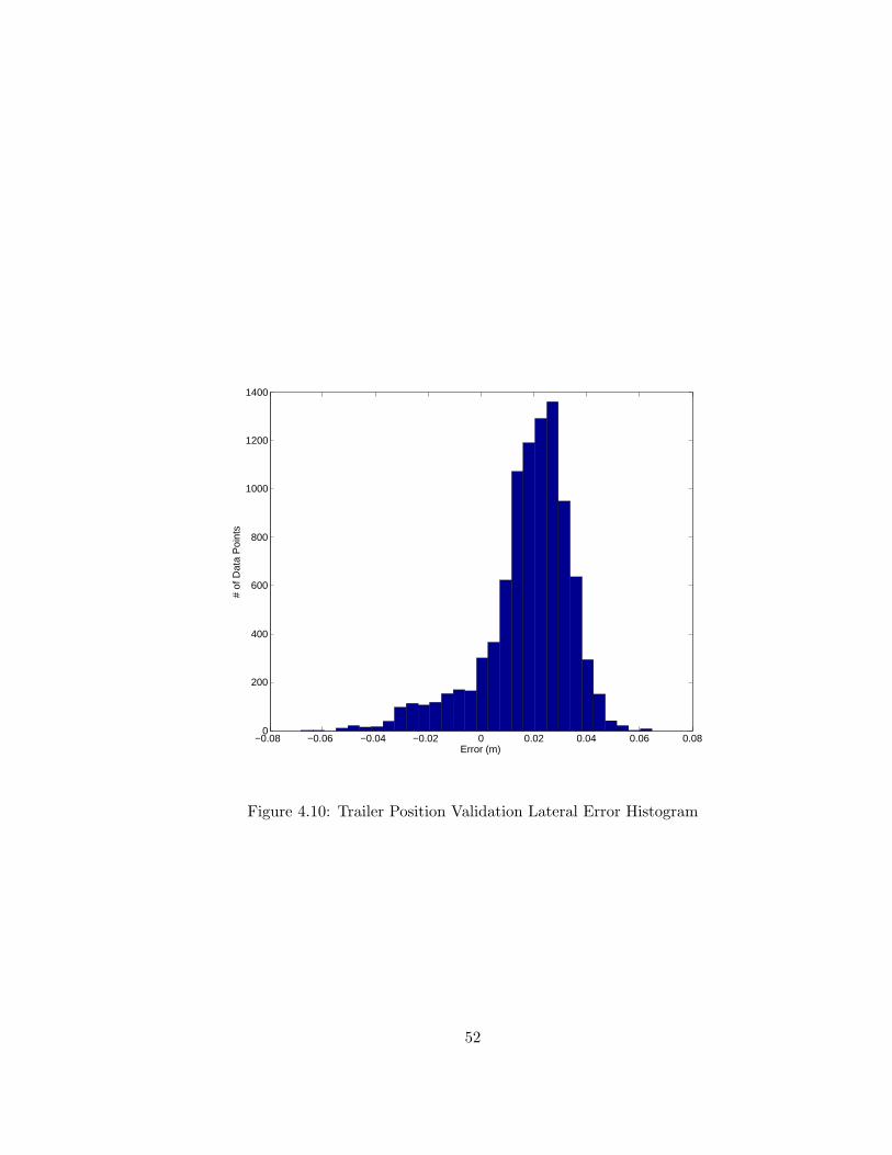
The calculated and measured trailer positions were synchronized using the GPS time
stamp, and the error for each point was calculated. A histogram showing the lateral error in
the trailer’s calculated position (from the robot’s position and hitch angle) when compared
to its measured position is shown in Figure 4.10. A scatter plot showing both lateral and
longitudinal errors is shown in Figure 4.11. A circle was added to the plot centered at the
mean of the data (0.005 m,0.044 m) with a radius of 5 cm. The non-zero center indicates
there is a bias in the calculated trailer positions. The circle contains 99.4% of the error
points.
The error in the calculation of the trailer’s position could come from several sources.
One potential source of errors is using incorrect parameters in (4.2). Any error in the trailer
lengths lr and lt will result in error in the trailer’s calculated position. The terrain can also
46

introduce errors. The calculation of the trailer’s position assumes that robot, hitch point,
and trailer are coplanar. If the terrain is not perfectly level, errors will result.
Bias in the measured hitch angle will also introduce error. An incremental encoder with
an index channel is used to measure the angle between the robot and the trailer. The point
where the encoder measures a hitch angle of 0◦ is determined by the location of the index
mark on the encoder. If the index mark is not perfectly aligned with a true hitch angle
of 0◦, a bias in the measurement will result. Experiments can be performed to attempt to
estimate this bias, but cannot determine it perfectly.
4.7 Conclusion
In this chapter, a state-space model for a mobile robot towing a trailer was presented.
The model was rewritten in terms of errors from a given reference path. A controller was
designed using standard pole placement principles to guide the trailer to follow the path.
The controller design was validated through simulation and experiment and was shown to
successfully control the trailer to the path.
47
(e1 ,n1)
(e2 ,n2)
(eact ,nact)Ψact
Ψdes
Ψerr
Yerr
(ec ,nc)
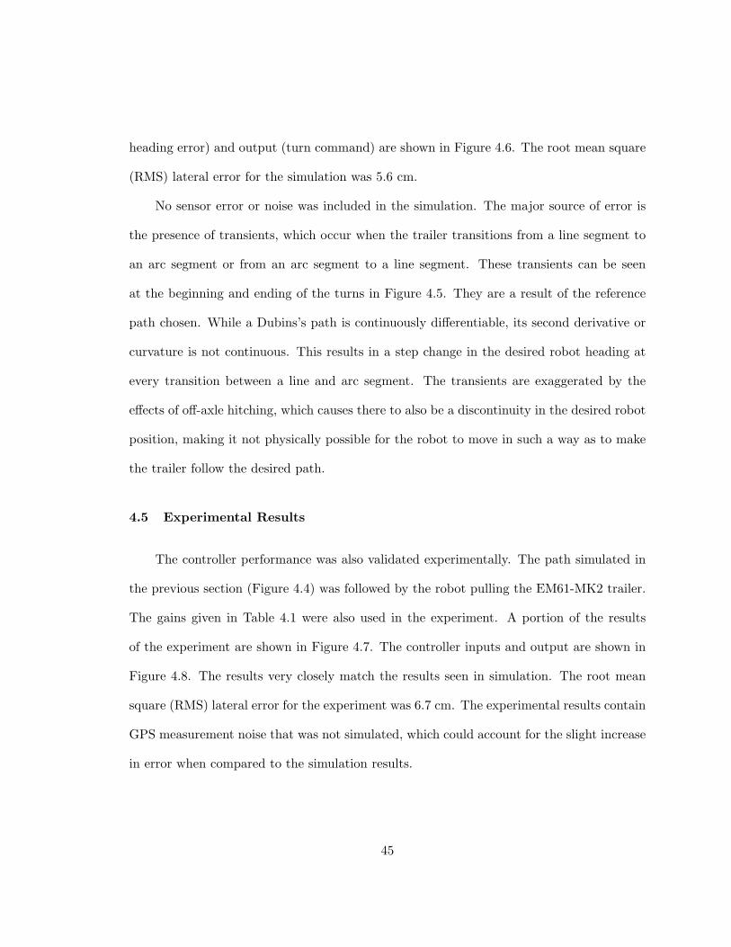
Figure 4.3: Arc Segment Errors
−40 −30 −20 −10 0 10 20 30 40 50
0
10
20
30
40
50
60
70
East (m)
Nor
th (
m)
Figure 4.4: Reference Path
48

2 4 6 8 10 12 14 16
70
72
74
76
78
80
East (m)
Nor
th (
m)
PathRobotTrailer
Figure 4.5: Path Following Simulation
0 200 400 600 800 1000 1200 1400 1600
−0.2
0
0.2
y terr (
m)
0 200 400 600 800 1000 1200 1400 1600
−10
0
10
ψ terr (
° )
0 200 400 600 800 1000 1200 1400 1600
−10
0
10
ψ rerr (
° )
0 200 400 600 800 1000 1200 1400 1600−50
0
50
100
150
ω r (co
unts
)
time sec
Figure 4.6: Path Following Simulation Errors
49

0 2 4 6 8 10 12 14 16
68
70
72
74
76
78
80
East (m)
Nor
th (
m)
PathRobotTrailer
Figure 4.7: Path Following Experimental Results
200 400 600 800 1000 1200 1400 1600 1800
−0.2
0
0.2
y terr (
m)
200 400 600 800 1000 1200 1400 1600 1800
−10
0
10
ψ terr (
° )
200 400 600 800 1000 1200 1400 1600 1800
−10
0
10
ψ rerr (
° )
200 400 600 800 1000 1200 1400 1600 1800
−200
0
200
ω r (co
unts
)
time (sec)
Figure 4.8: Path Following Experimental Result Errors
50
1 2 3 4 5 6
72.5
73
73.5
74
74.5
75
75.5
76
76.5
east (m)
nort
h (m
)
RobotEstimated TrailerActual Trailer
Figure 4.9: Trailer Position Validation Experiment Path Section
51
−0.08 −0.06 −0.04 −0.02 0 0.02 0.04 0.06 0.080
200
400
600
800
1000
1200
1400
Error (m)
# of
Dat
a P
oint
s
Figure 4.10: Trailer Position Validation Lateral Error Histogram
52

−0.08 −0.06 −0.04 −0.02 0 0.02 0.04 0.06 0.08−0.06
−0.04
−0.02
0
0.02
0.04
0.06
0.08
0.1
Lateral Error (m)
Long
itudi
nal E
rror
(m
)
Figure 4.11: Trailer Position Validation Error Scatter Plot
53

Chapter 5
Effects of Sensor Placement on Path Following
5.1 Introduction
For the control law presented in Chapter 4, knowledge of both robot and trailer states
is required. Since only one GPS receiver is to be used, the positions and orientations of both
the robot and trailer cannot be measured directly. Instead, an optical encoder is used to
measure the angle between the robot and trailer. This makes two different configurations
possible: (a) place the positioning system on the robot and calculate the position and
orientation of the trailer, or (b) place the positioning system on the trailer and calculate
the position and orientation of the robot. In either case, the state of either the robot or the
trailer must be calculated based on (4.2), using a measurement of the hitch angle. From a
mathematical point of view, both cases yield identical information for the robot and trailer
states. In the presence of sensor errors, however, the placement of the positioning system
can have an effect on system performance. The information in this chapter is taken from
two previous conference papers written by the author [4, 5].
There are several good qualitative arguments for placing the positioning system on the
robot. Since the system input is the robot angular velocity ωr, one can avoid problems
associated with non-collocated actuators and sensors by placing the sensors on the robot.
From the viewpoint of electrical wiring, it is more convenient to place the positioning system
as close as possible to the electrical power source and control computer, both of which are
mounted on the robot. When towing geophysical sensors, it is advantageous to place the
positioning system on the robot to reduce the effect of any metal in the system on the
54
geophysical sensors. While placing the positioning system on the robot seems practical for
the reasons given, effects of potential errors in the navigation sensors should be considered
when deciding on its placement. Effects of errors in both the positioning system and the
hitch angle measurement will be analyzed in the following sections. This analysis will be
done assuming only the GPS is used without the IMU. Placing the IMU on the trailer is
not a viable option due to the effect it would have on the geophysical sensors.
5.2 Hitch Angle Sensor Errors
The first source of error considered, is error caused by the optical encoder used to
measure the hitch angle. Errors in hitch angle measurement can arise from several sources,
including quantization error, joint backlashes, the robot and trailer being non-coplanar on
rough terrain, and calibration errors caused by not having the encoder “home”, or zero
angle position properly aligned. A general model of hitch angle errors was examined by
Park et al [24, 25]. They concluded that hitch angle error could produce a constant lateral
offset from the desired path when the position and orientation of the robot were measured
and that of the trailer were calculated from the hitch angle. Divelbiss and Wen also found
that very careful calibration is essential if trailer state is to be estimated from hitch angle
measurement [20].
The hitch angle error ε is illustrated in Figure 5.1. When the positioning system is
located on the robot, only the robot heading is measured directly. The trailer heading and
lateral error must be calculated from the hitch angle and are therefore affected by any errors
in the hitch angle measurement. The errors introduced into the state variables by the hitch
55

angle error are:
yterr(ε) = lt sin(ε)
ψterr(ε) = −ε (5.1)
ψrerr(ε) = 0
Figure 5.1: Effect of Hitch Angle Error on Error States
When the positioning system is located on the trailer, the hitch angle measurement
error does not affect measurement of trailer lateral position and trailer heading. In this
case, the only error that arises from hitch angle imperfection is the heading error of the
robot. Consequently, the error variables as functions of hitch angle error ε are:
yterr(ε) = 0
ψterr(ε) = 0 (5.2)
ψrerr(ε) = −ε
56

5.2.1 Effects of Quantization Error
One source of error in the hitch angle measurement is due to the limited resolution of
the optical encoder used to measure the hitch angle. This results in quantization error in
the measurement. Simulations were used to study the effect of quantization error on system
performance and determine an encoder resolution that gives acceptable performance. An
S-shaped path was created as shown in Figure 5.3 and Figure 5.4. A 60 second simulation
was run for various sensor configurations. The model parameters used in the simulations
are given in Table 5.1.
Table 5.1: Simulation model parameters
Parameter Symbol Value UnitsRobot speed Vr 1 m/s
Robot tongue length lr 0.1 mTrailer tongue length lt [2, 6] m
Robot angular rate limit |ωr|max 3 rad/sClosed loop natural frequency ωn π rad/sClosed loop damping factor ζ 0.707
Time constant of third closed loop pole τ3 0.5 s
Controller gains were calculated using pole placement techniques. Closed loop poles
were described by a pair of complex conjugate poles (natural frequency ωn and damping
factor ζ) and a third real pole with time constant τ3. The controller gains for the three
different values of trailer tongue length lt used in the simulations are given in Table 5.2.
Figure 5.2 shows the lateral mean square error between the trailer and the path as a
function of encoder resolution for various configurations. For the gains used, the lateral error
of the trailer increases with quantization error when the positioning system is mounted on
the robot (square, ×, and diamond curves). In contrast, increasing quantization has little
57

effect on system performance when the positioning system is on the trailer (solid and dotted
curves). The plot also shows that sensitivity to quantization error increases with increases
in the trailer tongue length (lt) when the positioning system is on the robot. Increasing
trailer length has minimal effect, however, when the positioning system is on the trailer.
100 200 300 400 500 600 700 800 900 1000
0
0.5
1
1.5
2
2.5
3
3.5
4
4.5
x 10−3
Encoder Resolution (CPR)
Late
ral M
ean
Squ
are
Err
or (
m2 )
GPS on Trailer (lt=2m)
GPS on Robot (lt=2m)
GPS on Robot (lt=4m)
GPS on Robot (lt=6m)
GPS on Trailer (lt=6m)
Figure 5.2: Control System Performance for Varying Encoder Resolutions
Table 5.2: Controller gains for various trailer tongue lengths
lt Controller gain, K
2 K =[
9.87 19.7 5.4]
4 K =[
19.7 44.5 5.8]
6 K =[
29.6 69.6 5.9]
58
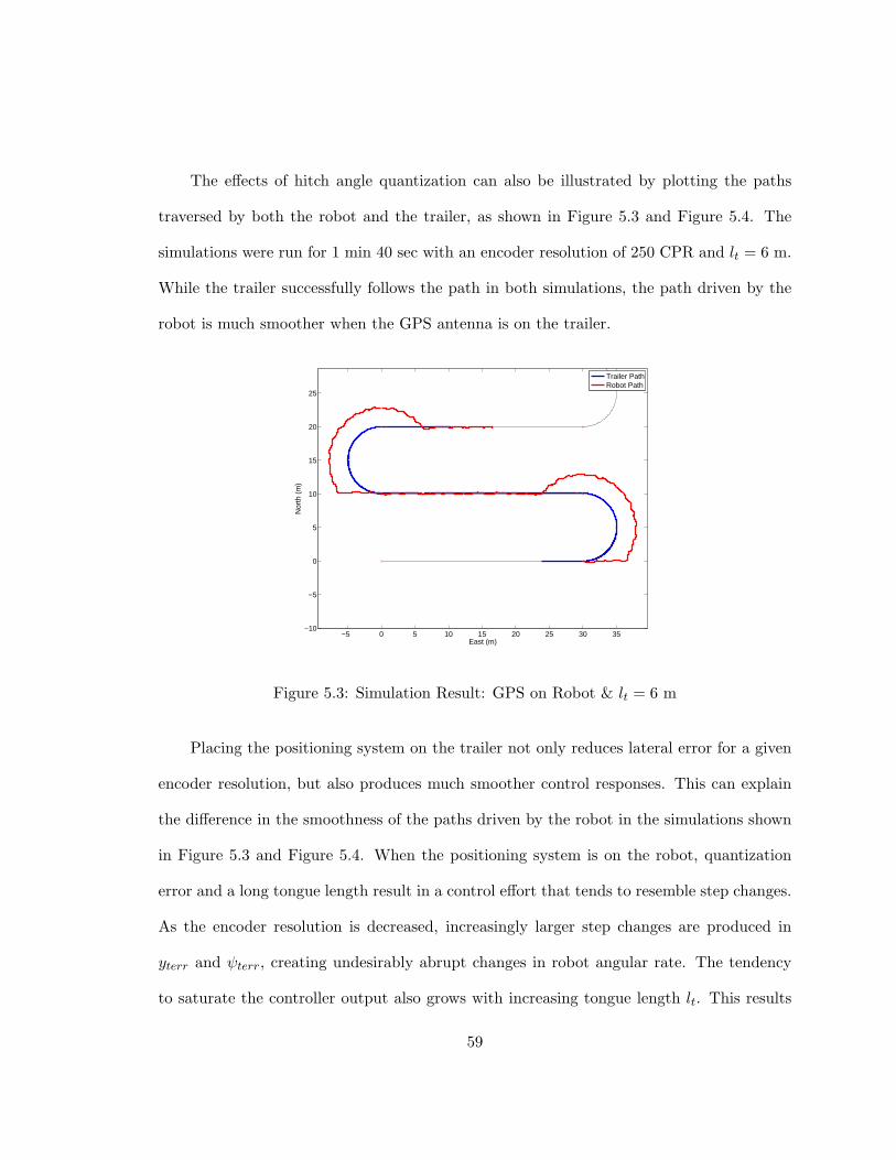
The effects of hitch angle quantization can also be illustrated by plotting the paths
traversed by both the robot and the trailer, as shown in Figure 5.3 and Figure 5.4. The
simulations were run for 1 min 40 sec with an encoder resolution of 250 CPR and lt = 6 m.
While the trailer successfully follows the path in both simulations, the path driven by the
robot is much smoother when the GPS antenna is on the trailer.
−5 0 5 10 15 20 25 30 35−10
−5
0
5
10
15
20
25
East (m)
Nor
th (
m)
Trailer PathRobot Path
Figure 5.3: Simulation Result: GPS on Robot & lt = 6 m
Placing the positioning system on the trailer not only reduces lateral error for a given
encoder resolution, but also produces much smoother control responses. This can explain
the difference in the smoothness of the paths driven by the robot in the simulations shown
in Figure 5.3 and Figure 5.4. When the positioning system is on the robot, quantization
error and a long tongue length result in a control effort that tends to resemble step changes.
As the encoder resolution is decreased, increasingly larger step changes are produced in
yterr and ψterr, creating undesirably abrupt changes in robot angular rate. The tendency
to saturate the controller output also grows with increasing tongue length lt. This results
59

in the system approaching the limits of stability. However, when the positioning system is
located on the trailer, these quantization errors occurs only in robot heading error ψrerr,
and therefore have less effect on the trailer path tracking error. Figure 5.5 shows the average
control effort as a function of encoder resolution, for various combinations of positioning
system placement and trailer tongue length.
5.2.2 Effects of Hitch Angle Bias
Another error source considered is the effect of bias in the hitch angle measurement.
Bias in the hitch angle sensor is a practical problem arising from the difficulty in obtaining
perfect alignment between the sensor, robot and trailer. This error affects the system
differently depending on where the GPS receiver is mounted.
GPS on robot
Robot heading error ψr is measured directly and thus not affected by hitch angle bias ε
when the GPS receiver is mounted on the robot. A bias does, however, affect the estimate
of trailer position and orientation as described in (5.1). The effect of bias ε can be analyzed
by linearizing (5.1) and substituting into (4.5). The new expression for the control law
(including the effects of encoder bias) is given by:
ωr = −k1(yterr + ltε)− k2(ψterr − ε)− k3ψrerr (5.3)
The block diagram model of the new closed loop system is shown in Figure 5.6. Apply-
ing Mason’s Gain Rule to the block diagram given in the figure, followed by the Laplace
60
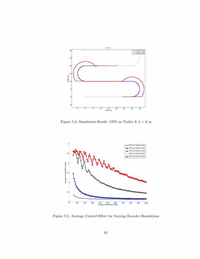
−5 0 5 10 15 20 25 30 35
−5
0
5
10
15
20
25
30
East (m)
Nor
th (
m)
Path Driven
Trailer PathRobot Path
Figure 5.4: Simulation Result: GPS on Trailer & lt = 6 m
0 100 200 300 400 500 600 700 800 900 10000
0.5
1
1.5
2
2.5
3
Encoder Resolution (CPR)
Ave
rage
Con
trol
Effo
rt (
rad/
s)
GPS on Trailer (lt=2m)
GPS on Robot (lt=2m)
GPS on Robot (lt=4m)
GPS on Trailer (lt=6m)
GPS on Robot (lt=6m)
Figure 5.5: Average Control Effort for Varying Encoder Resolutions
61

transform final value theorem yields the DC gain between sensor bias and trailer lateral
error:
yt
ε=k2 − k1lt
k1(5.4)
∫∫ yt
ε
ψtψrωr∫ Vr
lt
-k3
-k2
-k1
Vrlt
lrlt
Figure 5.6: Closed loop model with hitch angle bias - GPS on robot.
GPS on the trailer
When the GPS unit is mounted on the trailer, the trailer lateral position measurement
and trailer heading measurement are no longer affected by hitch angle sensor bias. The
estimate of robot heading error will be biased, however, so ψr is replaced by ψr + ε in the
state feedback equation resulting in:
ωr = −k1yterr − k2ψterr − k3(ψrerr − ε) (5.5)
62

The resulting block diagram model for this case is shown in Figure 5.7. Applying the same
analysis approach as before yields a different DC gain between the hitch angle and the
trailer lateral error:
yt
ε= −k3
k1(5.6)
∫∫ yt
e
ytyrwr
∫ Vr
-k3
-k2
-k1
Vrlt
lrlt
Figure 5.7: Closed loop model with hitch angle bias - GPS on trailer.
Mounting GPS receiver to minimize effect of hitch angle error
Bias in the hitch angle sensor affects trailer lateral error yt, regardless of whether the
GPS receiver is mounted on the robot or trailer. Comparing the DC gains (5.4) and (5.6),
however, leads to the conclusion that mounting the GPS receiver on the trailer is favored
under the condition
|k3| < |k2 − k1lt| (5.7)
On the other hand, placing the GPS receiver on the robot is favored for controller gains
that more heavily weight the robot heading error ψr.
63
5.3 Effect of heading noise
Navigation instrument noise is another significant error that must be considered, par-
ticularly the effect of noise in the heading measurement. Because the navigation system
consists of only a single-antenna GPS receiver, there is no way to measure the true orien-
tation or heading of the vehicle. Instead, the GPS course measurement, which is a measure
of the direction of the instantaneous velocity of the vehicle, is used in place of a heading
measurement. This measurement is noisy and can introduce errors caused by motion that
is not in the direction of the vehicle heading (such as rolling or lateral velocities induced by
sideslip).
GPS on the robot
When navigation instruments are placed on the robot, robot heading error is directly
measured with noise w. The trailer heading error ψterr and trailer lateral error yterr must
be estimated from the kinematic model. Specifically, the tongue length lt and hitch angle
ϕ must be known. The estimated trailer heading error is given by:
ψt = ψr + w − ϕ (5.8)
where w is the heading noise, and ϕ is the hitch angle. Assuming small hitch angle ϕ, the
trailer lateral error is estimated as:
yt = −(lr + lt)ψt (5.9)
64

Substituting (5.8) and (5.9) into the state feedback control (4.5) results in
ωr = k1(lr + lt)(ψr + w − ϕ)− k2(ψr + w − ϕ)− k3(ψr + w) (5.10)
This leads to the conclusion that heading noise contributes an error to the controller
output ωr. The gain Nr on the heading noise is found by rearranging (5.10):
ωr = −k1(lr + lt)w + k2w + k3w + f(ψr, ϕ) (5.11)
= Nrw + f(ψr, ϕ) (5.12)
Therefore, the gain Nr on the heading noise is:
Nr = k1(lr + lt)− k2 − k3 (5.13)
GPS on the trailer
With navigation instruments on the trailer, both the trailer heading error and trailer
lateral position are measured directly. Robot heading error must be estimated from the
relationship:
ψr = ψt + w + ϕ (5.14)
In this case, the gain Nt on the heading noise is of the form
Nt = −k2 − k3 (5.15)
65

Mounting GPS receiver to minimize effects of heading noise
Comparing (5.13) and (5.15) leads to the the conclusion that it is preferable to mount
the GPS receiver on the robot for controller gains where
|Nr| < |Nt|
|k1(lr + lt)− k2 − k3| ≤ | − k2 − k3| (5.16)
5.4 Validation
5.4.1 Simulation Results
Several simulations were run to study the performance of the system in the presence
of both hitch angle error and heading noise. The models and analysis presented in the
preceding sections were validated using these simulations. An S-shaped path consisting of
several parallel line segments joined by 180 degree arcs as shown in Figure 5.8 was created.
Several simulations were run with various sensor configurations and the resulting errors
compared to those predicted in the previous sections. The model and controller parameters
used in the simulations are given in Table 5.3.
The variance of the course measurement given in Table 5.1 is calculated using [26]:
σν =σv
V(5.17)
where σv (m/sec) is the variance of the GPS receiver’s velocity measurement and V (m/s)
is the vehicle’s speed. The velocity variance σv is defined in the receiver’s specifications as
0.03 m/s.
66
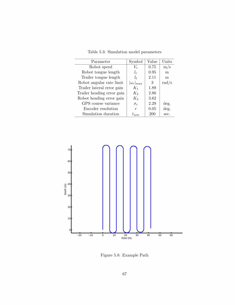
Table 5.3: Simulation model parameters
Parameter Symbol Value UnitsRobot speed Vr 0.75 m/s
Robot tongue length lr 0.95 mTrailer tongue length lt 2.11 m
Robot angular rate limit |ωr|max 3 rad/sTrailer lateral error gain K1 1.89Trailer heading error gain K2 2.86Robot heading error gain K3 3.62
GPS course variance σc 2.29 deg.Encoder resolution r 0.05 deg.Simulation duration tsim 200 sec.
−20 −10 0 10 20 30 40 50 60
0
10
20
30
40
50
60
70
East (m)
Nor
th (
m)
Figure 5.8: Example Path
67

Simulations were run for various hitch angle biases from 0 degrees to 15 degrees for
the case when the GPS is mounted on the robot and when it is mounted on the trailer.
Zero mean, Gaussian noise with variance σν was added to the course measurements. It was
assumed that the mean difference between the course measurement and vehicle heading
was zero (i.e. no side slip). Hitch angle quantization effects were also included in the
simulation using an encoder resolution of 1800 CPR. For each simulation, lateral root mean
squared error (RMSE) and average error (bias) were calculated. The predicted bias of the
lateral error was also calculated for each case using (5.4) and (5.6). The results are given
in Table 5.4 for the GPS on the robot and in Table 5.5 for the GPS on the trailer.
Table 5.4: Simulation Results (GPS on Robot)
Bias(deg) RMSE(m) Avg. Error(m) Predicted Bias(m)0 0.0447 0.0138 0.05 0.0700 -0.0595 -0.052110 0.1122 -0.1053 -0.104015 0.1578 -0.1508 -0.1561
Comparing the third and fourth columns in Tables 5.4 and 5.5, it can be seen that
(5.4) and (5.6) very closely predict the bias in the lateral error that will be produced by a
given hitch angle bias.
Table 5.5: Simulation Results (GPS on Trailer)
Bias(deg) RMSE(m) Avg. Error(m) Predicted Bias(m)0 0.0480 0.0216 0.05 0.1709 -0.1641 -0.167410 0.3362 -0.3296 -0.334415 0.4988 -0.4917 -0.5019
68

5.4.2 Experimental Results
Several experimental runs were made using the same path that was used for the sim-
ulations. The Segway RMP400 was used for all experiments. Artificial hitch angle biases
ranging from 0 deg to 15 deg were added to the system in real-time. A single GPS receiver
on either the robot or the trailer and the hitch angle encoder were used for control of the
system. A second antenna was placed on the trailer when the primary antenna was on the
robot. This second antenna was not used for control, but only to measure the position and
heading of the trailer for analysis purposes. For each run, lateral root mean squared error
(RMSE) and average error or bias were calculated, just as was done for the simulations.
The results are given in Table 5.6 for the GPS on the robot and in Table 5.7 for the GPS
on the trailer.
Table 5.6: Experimental Results (GPS on Robot)
Bias(deg) RMSE(m) Avg. Error(m) Predicted Bias(m)0 0.0100 0.0034 0.05 0.0510 -0.0500 -0.052110 0.1030 -0.1021 -0.104015 0.1480 -0.1471 -0.1561
Table 5.7: Experimental Results (GPS on Trailer)
Bias(deg) RMSE(m) Avg. Error(m) Predicted Bias(m)0 0.0707 0.0226 0.05 0.1900 -0.1771 -0.167410 0.3801 -0.3772 -0.334415 0.5572 -0.5551 -0.5019
69
As in the simulation results, comparing the third and fourth columns in Tables 5.6
and 5.7, further verifies that (5.4) and (5.6) closely predict the bias in the lateral error.
A section of an experimental run where the system was tracking a straight line segment
with zero added bias for both the GPS on the robot and on the trailer are given in Figures
5.9 and 5.10 respectively. The effect of noise in the course measurement can be clearly seen
in both figures. The uncertainty in the system’s orientation essentially pivots or swings
the estimate of the system about the GPS antenna position causing the drastic jumps in
the estimated trailer or robot position. The magnitude of the position estimate error is a
function of both the course noise (σν) and the trailer and hitch lengths (lr and lt).
5.4.3 Summary of Simulation and Experimental Results
The simulation and experimental results provided are consistent with the analysis of
hitch angle bias and heading noise presented in the previous sections. For the system under
consideration, the transfer functions given in (5.4) and (5.6) accurately predict the bias in
the lateral error, due to a bias in the hitch angle measurement for both the simulated and
experimental results.
The guideline given for choosing the GPS sensor location in the presence of a hitch angle
bias also correctly predicted the sensor location that produces the best tracking performance
in terms of lateral mean square error. Substituting the parameters and gains from Table 5.1
into (5.7) results in 3.62 > 1.1279 which suggests that the effect of a hitch angle bias would
be minimized by placing the GPS on the robot. When zero bias was used in simulation,
the results for the GPS on the robot and on the trailer were almost identical. This is as
expected, since in the absence of sensor imperfections, sensor placement should have no
70

−0.6 −0.4 −0.2 0 0.2 0.4
39.2
39.3
39.4
39.5
39.6
39.7
39.8
39.9
40
East (m)
Nor
th (
m)
Trailer EstimateRobot
Figure 5.9: Example Experimental Run (GPS on Robot)
71

11.4 11.6 11.8 12 12.2 12.4 12.6 12.8
49
49.2
49.4
49.6
49.8
50
East (m)
Nor
th (
m)
Robot EstimateTrailer
Figure 5.10: Example Experimental Run (GPS on Trailer)
72

effect on system performance. As the bias increases, however, the average error when the
GPS is on the robot is significantly smaller than the average error when the GPS is on the
trailer, as is predicted.
The guideline for placing the GPS receiver to minimize the effect of heading noise also
correctly predicted the correct GPS placement. Substituting the parameters and gains used
into (5.16) results in 2.492 < 6.48 which suggests that having the GPS on the robot is the
better placement. It can be observed in both the simulation and experimental results that
the lateral mean square error is approximately an order of magnitude larger when the GPS
is placed on the trailer, which again agrees with the predicted results.
5.5 Conclusions
This chapter has shown that when implementing a robotic tractor-trailer system, mea-
surement imperfections can have a significant impact on control system performance and
should be taken into account. The analysis given can help to predict the effect various
measurement errors will have on the system and suggest a sensor placement to minimize
their effects.
The effects of both hitch angle sensor bias and GPS heading noise on a robotic tractor-
trailer system have been considered. Transfer functions were derived that allow the bias in
the trailer lateral error to be calculated for a given hitch angle bias. Equations were also
provided that allow the effect on the controller output of course noise to be determined.
From these equations it was shown that certain controller gains and vehicle parameters
favor certain sensor placements. Guidelines were given for where the GPS receiver should
73

be placed to minimize the effects of these errors based on those parameters and control
gains.
74
Chapter 6
Robotic UXO Mapping System Demonstrations
6.1 Introduction
The performance of the system developed in this thesis was evaluated by performing
geophysical surveys at two sites. Preliminary tests were done in a field owned by Auburn
University located on Donahue Drive. The Auburn University Solar House is located in one
corner of the field and so it will be referred to as the Solar House Field in the discussions that
follow. An aerial photo of the site with the area mapped marked in yellow is shown in Figure
6.1. The final evaluation of the system was performed at the Standardized UXO Test Site at
Aberdeen Proving Ground (APG), Aberdeen, Maryland, which is an 18 acre site containing
several areas seeded with inert ordnance items. A map of the site is shown in Figure 6.2.
In this chapter, results from these demonstrations are given, including geophysical plots of
the areas surveyed.
6.2 Solar House Tests
6.2.1 EM61 Tests - 11/17/2006
The first attempt at performing a survey with the system occurred at the Solar House
Field on November 17, 2006. A 30 m × 80 m field was surveyed. Several pieces of inert
ordnance were laid in rows on the field. Examples of the test items are shown in Figure 6.3.
Pieces of steel rebar were laid across the south edge of the field. The EM61-MK2 sensor
was towed autonomously by the robot. There was no integration between the geophysical
75

Figure 6.1: Solar House Field Aerial View
76
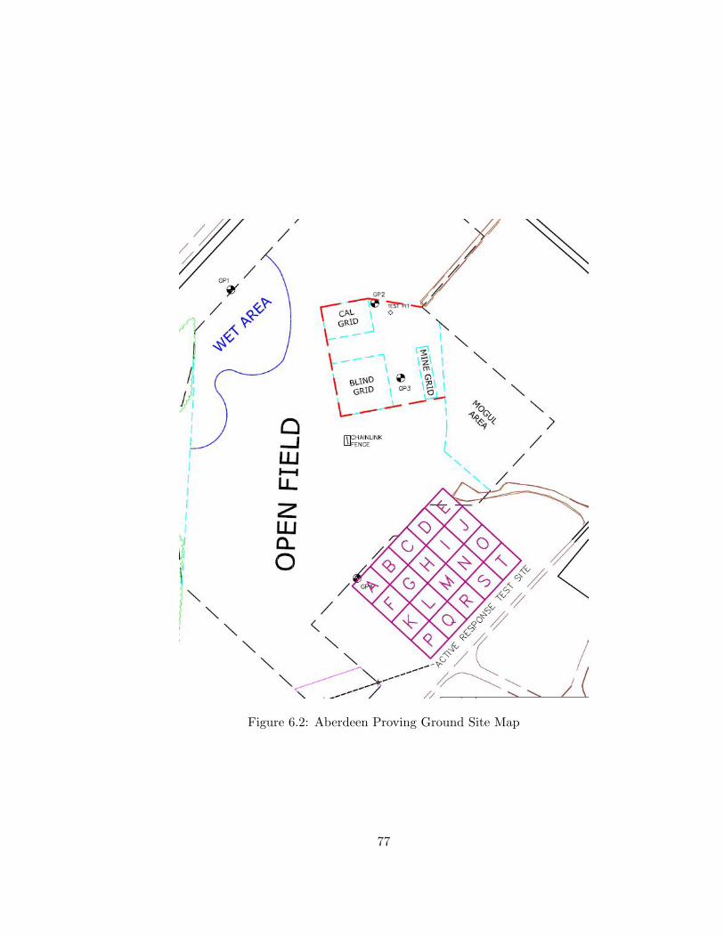
Figure 6.2: Aberdeen Proving Ground Site Map
77

sensor electronics and the embedded PC on the Segway for these tests. The geophysical
data was recorded on the data recorder included with the sensor. The trailer’s position was
logged on the embedded PC and the two sets of data were synchronized post-process. The
field was surveyed twice, once in the morning and once in the afternoon. The results of the
morning survey are shown in Figure 6.4 and the afternoon survey in Figure 6.5. The item
locations are shown with plus signs on the plots. Problems with the robot system caused
the survey to be ended prematurely in both tests, resulting in the white stripe seen in the
data on both figures.
Figure 6.3: Sample Ordnance Items
6.3 APG Tests
A final demonstration of the system was performed at APG on May 14-22, 2007. The
site was mapped using both the traditional man-towed method and autonomously using the
Segway RMP400 as a tow vehicle. Two areas of the site were surveyed: the calibration grid
78

Figure 6.4: Geophysical Plot w/ Path Followed for 11-17-06 AM Test
79

Figure 6.5: Geophysical Plot for 11-17-06 PM Test
80

and portions of the open field. These two areas can be seen on the map in Figure 6.2. The
calibration grid and open field grid 4 were mapped both autonomously and manually. The
remaining open field grids were only mapped autonomously. The open field and calibration
lanes were mapped using the EM61-MK2 and the calibration grid only was mapped using
the G-858 magnetometer. The resulting geophysical plots are given in the following sections.
6.3.1 Calibration Grid
The calibration grid is a 0.3 acre area containing various buried inert ordnance items,
steel spheres, and wire hoops. The items are laid out in rows spaced 1 m apart and their
locations have been surveyed and are known. The perimeter of the area is defined by
buried steel spheres. This area was mapped using the EM61-MK2 in both a man-towed
and autonomous configuration. The results of the man-towed survey are shown in Figure
6.7. The results of the survey performed autonomously with the RMP400 are shown in
Figure 6.8. The location of the seeded items are shown on the plots with small black circles.
The calibration grid was also mapped autonomously using the G-858 magnetometer and
the results are shown in Figure 6.9.
6.3.2 Open Field
The open field area is 13.68 acres and is also seeded with various inert ordnance items.
Their locations, however, are not known. A 2.8 acre section of the open field was chosen
to be mapped. This area was then divided into smaller grids for surveying. These grids
are shown on the map in Figure 6.6. Grid 4 was surveyed using using both a man-towed
and autonomous RMP400 towed EM61-MK2. The results of the man-portable survey are
shown in Figure 6.10, while the results of the autonomous survey are shown in Figure 6.11.
81
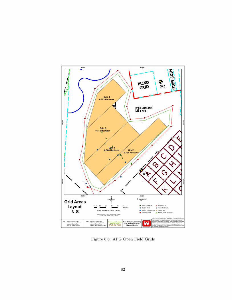
")
")
")
")
")
")")
")
Grid 30.312 Hectares
Grid 20.306 Hectares
Grid 40.203 Hectares
Grid 10.304 Hectares
402700
402700
402800
402800
4369
400
4369
400
4369
500
4369
500
Road Track PointHazard PointHazard 1meter BufferTraverse Point
Traverse Line") Perimeter Point
Layout N-S4meter inside boundary
Legend0 10 20 30 40 505 Meters
.
MXD:
EPUB-GIS TEAMU.S. Army Engineering
And Support CenterHuntsville, AL
Drawn By:DISCLAIMER - The data represent the results of data collection/processing for a specific U.S. Army Corps of Engineers activity andindicates the general existing conditions. As such, it is only validfor its intended use, content, time, and accuracy specifications.The user is responsible for the results of any application of the datafor other than its intended purpose.
Date Drawn: Plot Date:
& Utilities BranchEnvironmental ProtectionPDF: \PROJECTS\States\MD
\Aberdeen_Proving_Ground\National_Test_Site\PDF\NS_test_14MAR2007.pdf
\PROJECTS\States\MD\Aberdeen_Proving_Ground\National_Test_Site\MXD\Segway_test_14MAR2007.mxd
DBR 14MAR2007 14MAR2007
Data is projected to the UTM Coordinate System:Zone 18 North, NAD83, Units in Meters.
1 inch equals 26.16657 meters
Grid AreasLayout
N-S
Figure 6.6: APG Open Field Grids
82
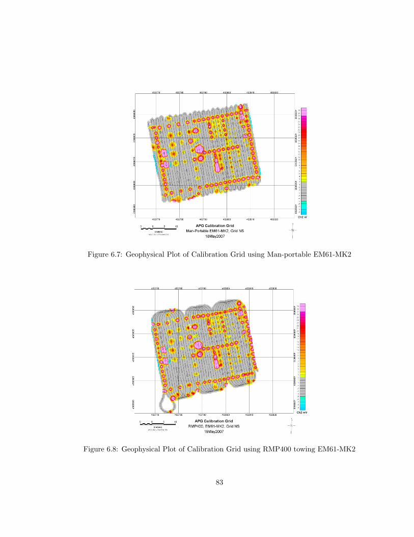
Figure 6.7: Geophysical Plot of Calibration Grid using Man-portable EM61-MK2
Figure 6.8: Geophysical Plot of Calibration Grid using RMP400 towing EM61-MK2
83

Figure 6.9: Geophysical Plot of Calibration Grid using RMP400 towing G-858
84

Figure 6.10: Geophysical Plot of Grid 4 using Man-portable EM61-MK2
85

Figure 6.11: Geophysical Plot of Grid 4 using RMP400 towing EM61-MK2
86
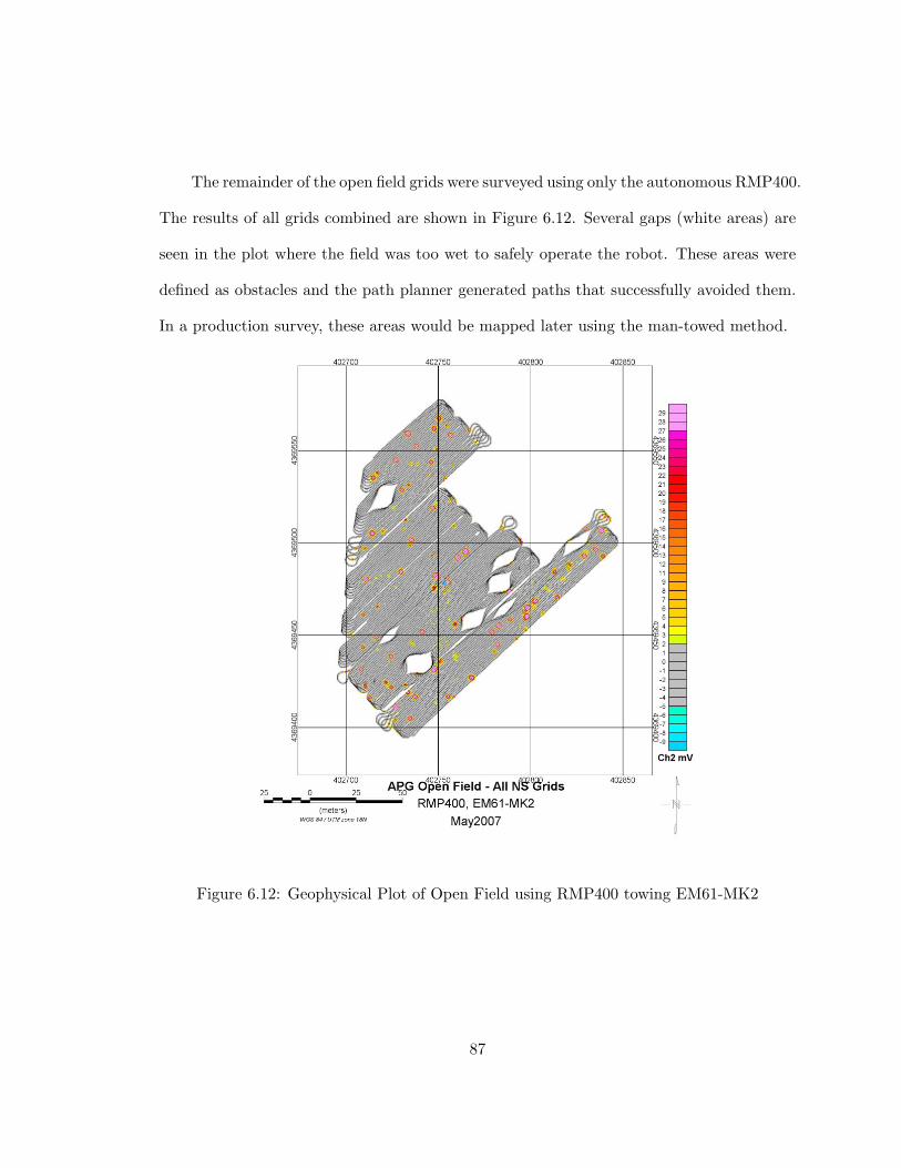
The remainder of the open field grids were surveyed using only the autonomous RMP400.
The results of all grids combined are shown in Figure 6.12. Several gaps (white areas) are
seen in the plot where the field was too wet to safely operate the robot. These areas were
defined as obstacles and the path planner generated paths that successfully avoided them.
In a production survey, these areas would be mapped later using the man-towed method.
Figure 6.12: Geophysical Plot of Open Field using RMP400 towing EM61-MK2
87

6.4 Conclusion
The results of testing the system at two sites, the Auburn University Solar House and
Aberdeen Proving Ground, have been given. Both the EM61-MK2 and G-858 magnetometer
were successfully towed using the path planning and control algorithms developed in this
thesis. The results given in this chapter show that the system is capable of autonomously
navigating a site while collecting geophysical data.
88

Chapter 7
Conclusion
7.1 Concluding Remarks
In this thesis, the development of a tele-operated and autonomous system for mapping
unexploded ordnance has been presented. In Chapter 1, background information on the
problem of unexploded ordnance detection was given as well as the motivation for the
system being developed. Chapter 2 provided a description of the various hardware and
software that make up the system. The hardware used for navigation and control, the
geophysical instruments, and the software used on both the robot and remote laptop were
described. In Chapter 3, an algorithm for planning paths needed to survey a field was
developed. The algorithm was then extended to include a method of obstacle avoidance
found in the literature. A modification to a commonly used obstacle avoidance algorithm
was developed to generate paths that instead of being time optimal, more closely follow
the original paths in order to survey as much of a field as possible. A model of the system
was given in Chapter 4, and a state space control law was designed. The performance of
the controller was tested using simulations and experiments and is shown to be capable of
placing the trailer on the desired path within approximately 10 cm. In Chapter 5, the effects
of sensor errors on the controller performance were analyzed and guidelines were given to
suggest where the positioning sensors should be located based on controller gains and model
parameters. Finally Chapter 6 presented survey results using the complete system.
The system developed in this thesis has been shown to be an effective solution for
performing autonomous geophysical surveys. Relatively simple technical approaches were
89

used for path planning, obstacle avoidance, and control allowing the system to be developed
in a short time (just over a year), while still providing satisfactory system performance.
Using these simple techniques and a small, commercially available robot for the tow vehicle
also allows the system costs to be kept low. The cost of the robot, navigation sensors,
and all other various hardware is less than $80,000. The system is easy to transport and
use. The small size of the robot and trailer allow the entire system, including geophysical
sensors to be packed into a 6 ft. × 10 ft. utility trailer, with room left for other equipment.
The graphical user interface developed allows the system to be started with just a few
mouse clicks. It also provides complete information about the status and performance of
the system to the operator while in use.
7.2 Future Work
Several aspects of the system could be improved in future revisions. A main goal of any
future work should be to eliminate or reduce the transients that occur at the intersections
of line and arc segments. As was discussed in Chapter 4, this is caused by the fact that the
dynamics of a robot-trailer system make it impossible for the trailer to follow the reference
paths chosen. A more suitable reference path should be researched or developed in the
future to eliminate the tracking error at the transitions between segments, thus improving
the accuracy of the system. Nonlinear control designs should also be examined to determine
if they can improve performance.
New functionality should also be added to the user interface software to make it easier
to use and more user friendly. One such improvement would be to add the ability to define
obstacles by manually driving around them with the robot.
90

Another improvement that can be made in future versions of the system is to improve
the obstacle avoidance algorithm. The algorithm developed in this thesis, makes several
assumptions that place restrictions on how the algorithm can be used (e.g. obstacles cannot
be avoided if they are in an area where the system is turning). A more robust algorithm
should be developed that is capable of handling any circumstances that are likely to be seen
when performing a geophysical survey in the field. The algorithm currently implemented is
also computationally intensive. A faster algorithm will be needed if it is to be run in real
time for avoiding obstacles that are detected while the robot is running.
91
Bibliography
[1] M. Kerr, “Multi-sensor ordnance detection and mapping system.”
[2] P. K. Agarwal, T. Biedl, S. Lazard, S. Robbins, S. Suri, and S. Whitesides, “Curvature-constrained shortest paths in a convex polygon,” in Proceedings of the 14th AnnualSymposium on Computational Geometry, Minneapolis, Minnesota, 1998, pp. 392–401.
[3] T. Office of the Under Secretary of Defense for Acquisition and Logistics, “Report ofthe defense science board task force on unexploded ordnance,” November 2003.
[4] D. Hodo, J. Hung, D. Bevly, and S. Millhouse, “Effects of sensor placement and er-rors on path following control of a mobile robot-trailer system.” ACC, July 2007,(Submitted to 2007 American Control Conference).
[5] ——, “Linear analysis of trailer lateral error with sensor noise for a mobile robot-trailersystem,” in Proceedings of the 2007 International Symposium on Industrial Electronics.Vigo, Spain: ISIE, June 2007.
[6] H. Nguyen, J. Morrell, K. Mullens, A. Burmeister, S. Miles, N. Farrington, K. Thomas,and D. Gage, “Segway robotic mobility platform,” SPIE Proceedings, vol. 5609, 2004.
[7] J. James J. Spilker, “Fundamentals of signal tracking theory,” in Global PositioningSystem: Theory and Applications, Volume 1, ser. Progress in Astronautics and Aero-nautics, B. W. Parkinson, Ed. Washington, DC: American Institute of Aeronauticsand Astronautics, 1996, vol. 163, ch. 4.
[8] A. L. Rankin, “Autonomous path planning navigation system used for site character-ization,” in Proceedings of SPIE – The International Society for Optical Engineering,vol. 2738, April 1996.
[9] ——, “Development of path tracking software for an autonomous steered-wheeledrobotic vehicle and its trailer,” Ph.D. dissertation, University of Florida, 1997.
[10] L. Dubins, “On curves of minimal length with a constraint on average curvature andwith prescribed initial and terminal positions and tangents,” American Journal ofMathematics, vol. 79, no. 3, pp. 497–516, July 1957.
[11] D. Anisi, “Optimal motion control of a ground vehicle,” Swedish Defense ResearchAgency, Tech. Rep., July 2003.
[12] H. Choset, “Coverage for robotics - a survey of recent results,” Annals of Mathematicsand Artificial Intelligence, vol. 31, no. 1-4, pp. 113–126, October 2001.
92

[13] P. Jacobs and J. Canny, “Planning smooth paths for mobile robots,” in Proceedings ofIEEE International Conference on Robotics and Automation, 1989, pp. 2–7.
[14] E. W. Dijkstra, “A note on two problems in connexion with graphs,” NumerischeMathematik, vol. 1, pp. 269–271, 1959.
[15] S. De Luca, Oriolo, Robot Motion Planning and Control. Spring, 1998, ch. FeedbackControl of a Nonholonomic Car-like Robot, pp. 343–427.
[16] M. Sampei, T. Tamura, T. Itoh, and M. Nakamichi, “Path tracking control of trailer-like mobile robot,” IEEE/RSJ International Workshop on Intelligent Robots and Sys-tems, 1991.
[17] M. Nakamura and S. Yuta, “Trajectory control of trailer type mobilie robots,” inIEEE/RSJ International Conference on Intelligent Robots and Systems, July 1993.
[18] F. Lamiraux and J. P. Laumond, “A practical approach to feedback control for a mobilerobot with trailer,” in Proceedings of 1998 IEEE International Conference on Roboticsand Automation, Leuven, Belgium, 1998, pp. 3291–3296.
[19] S. Sekhavat, F. Lamiraux, J. P. Laumond, G. Bauzil, and A. Ferrand, “Motion planningand control for Hilare pulling a trailer: experimental issues,” in Proceedings of the 1997IEEE International Conference on Robotics and Automation, Albuquerque, NM, April1997, pp. 3306–3311.
[20] A. W. Divelbiss and J. T. Wen, “Trajectory tracking control of a car-trailer system,”IEEE Transactions on Control Systems Technology, vol. 5, no. 3, pp. 269–278, May1997.
[21] F. Cuesta, F. Gomez-Bravo, and A. Ollero, “Parking maneuvers of industrial-like elec-trical vehicles with and without trailer,” IEEE Transactions on Industrial Electronics,vol. 51, no. 2, pp. 257–269, April 2004.
[22] D. Bevly and B. Parkinson, “Carrier-phase differential gps for control of a tractor towedimplement,” in Proceedings of the 2000 ION-GPS Meeting, September 2000.
[23] F. Lamiraux, S. Sekhavat, and J. Laumond, “Motion planning and control for hilarepulling a trailer,” IEEE Transactions on Robotics and Automation, vol. 15, no. 4, pp.640–652, August 1999.
[24] M. Park, W. Chung, and M. Kim, “Experimental research of a passive multiple trailersystem for backward motion control,” in Proceedings of the 2005 IEEE InternationalConference on Robotics and Automation, Barcelona, Spain, April 2005, pp. 105–110.
[25] M. Park and W. Chung, “Control of a mobile robot with passive multiple trailers,” inProceedings of the 2004 IEEE International Conference on Robotics and Automation,New Orleans, LA, April 2004.
93

[26] R. Daily and D. Bevly, “The use of gps for vehicle stability control systems,” IEEETransactions on Industrial Electronics, vol. 51, no. 2, April 2004.
94

Appendix - Log File Definitions
Segway Sensor Log File
Column Description1 Global Time Stamp2 Pitch Rate3 Pitch Angle4 Roll Angle5 Roll Rate6 Left Wheel Speed7 Right Wheel Speed8 Left Wheel Distance9 Right Wheel Distance10 Distance Traveled11 Integrated Yaw Position12 Servo frames since power on13 Battery Power14 Yaw Rate15 Left Motor Current16 Right Motor Current17 Controller Mode18 Powerbase Battery Voltage19 UI Battery Voltage20 Gain Mode21 Last Velocity Command22 Last Turn Command
Sent Commands Log File
Column Description1 Global Time Stamp2 Controller Time Stamp3 Turn Command4 Velocity Command
95
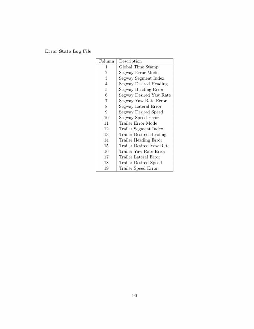
Error State Log File
Column Description1 Global Time Stamp2 Segway Error Mode3 Segway Segment Index4 Segway Desired Heading5 Segway Heading Error6 Segway Desired Yaw Rate7 Segway Yaw Rate Error8 Segway Lateral Error9 Segway Desired Speed10 Segway Speed Error11 Trailer Error Mode12 Trailer Segment Index13 Trailer Desired Heading14 Trailer Heading Error15 Trailer Desired Yaw Rate16 Trailer Yaw Rate Error17 Trailer Lateral Error18 Trailer Desired Speed19 Trailer Speed Error
96
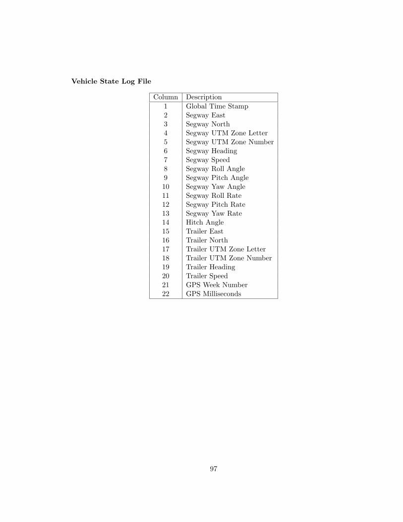
Vehicle State Log File
Column Description1 Global Time Stamp2 Segway East3 Segway North4 Segway UTM Zone Letter5 Segway UTM Zone Number6 Segway Heading7 Segway Speed8 Segway Roll Angle9 Segway Pitch Angle10 Segway Yaw Angle11 Segway Roll Rate12 Segway Pitch Rate13 Segway Yaw Rate14 Hitch Angle15 Trailer East16 Trailer North17 Trailer UTM Zone Letter18 Trailer UTM Zone Number19 Trailer Heading20 Trailer Speed21 GPS Week Number22 GPS Milliseconds
97


![[ , ] Autonomous Human Robot Interactive Skills](https://img.pdfslide.net/doc/110x75/577cc35f1a28aba71195d883/-autonomous-human-robot-interactive-skills.jpg)