Development of an Efficient Regional Four-Dimensional Variational DataAssimilation System for WRF

XIN ZHANG, XIANG-YU HUANG, AND JIANYU LIU

National Center for Atmospheric Research,* Boulder, Colorado

JONATHAN POTERJOY, YONGHUI WENG, AND FUQING ZHANG

Department of Meteorology, The Pennsylvania State University, University Park, Pennsylvania

HONGLI WANG

National Center for Atmospheric Research,* Boulder, Colorado

(Manuscript received 25 March 2013, in final form 2 August 2014)

ABSTRACT

This paper presents the development of a single executable four-dimensional variational data assimilation

(4D-Var) system based on the Weather Research and Forecasting (WRF) Model through coupling the

variational data assimilation algorithm (WRF-VAR) with the newly developed WRF tangent linear and

adjoint model (WRFPLUS). Compared to the predecessor Multiple ProgramMultiple Data version, the new

WRF 4D-Var system achieves major improvements in that all processing cores are able to participate in the

computation and all information exchanges between WRF-VAR and WRFPLUS are moved directly from

disk to memory. The single executable 4D-Var system demonstrates desirable acceleration and scalability in

terms of the computational performance, as demonstrated through a series of benchmarking data assimilation

experiments carried out over a continental U.S. domain. To take into account the nonlinear processes with the

linearized minimization algorithm and to further decrease the computational cost of the 4D-Var minimization,

a multi-incremental minimization that uses multiple horizontal resolutions for the inner loop has been developed.

The method calculates the innovations with a high-resolution grid and minimizes the cost function with a lower-

resolution grid. The details regarding the transition between the high-resolution outer loop and the low-resolution

inner loop are introduced. Performance of the multi-incremental configuration is found to be comparable to that

with the full-resolution 4D-Var in terms of 24-h forecast accuracy in the week-long analysis and forecast exper-

iment over the continental U.S. domain. Moreover, the capability of the newly developed multi-incremental

4D-Var system is further demonstrated in the convection-permitting analysis and forecast experiment for

Hurricane Sandy (2012), which was hardly computationally feasible with the predecessor WRF 4D-Var system.

1. Introduction

Since the 1980s, the four-dimensional variational data

assimilation (4D-Var) technique (LeDimet and Talagrand

1986; Lewis and Derber 1985) has become one of the most

widely used advanced analysis methods in atmospheric

and oceanic research and operational centers. The Eu-

ropean Centre for Medium-Range Weather Forecasts

(ECMWF)was the first operational center to implement

the 4D-Var system (Courtier et al. 1994; Rabier et al.

2000). Following ECMWF, other national centers im-

plemented 4D-Var in their operational applications,

including Météo-France (Gauthier and Thépaut 2001),the Met Office (Lorenc and Rawlins 2005; Rawlins et al.

2007), the Japan Meteorological Agency (JMA; Honda

et al. 2005; Kawabata et al. 2007), Environment Canada

(Gauthier et al. 2007), the Swedish Meteorological and

Hydrological Institute (Huang et al. 2002; Gustafsson

et al. 2012), and the Naval Research Laboratory (Xu

et al. 2005; Rosmond and Xu 2006).

* The National Center for Atmospheric Research is sponsored

by the National Science Foundation.

Corresponding author address: Dr. Xin Zhang, MMM, NCAR,

P.O. Box 3000, Boulder, CO 80307.

E-mail: xinzhang@ucar.edu

DECEMBER 2014 ZHANG ET AL . 2777

DOI: 10.1175/JTECH-D-13-00076.1

� 2014 American Meteorological Society

The success of the 4D-Var system in improving global

forecasts provided enough encouragement to develop

a regional 4D-Var for mesoscale and thunderstorm

scales. Several regional 4D-Var research and/or opera-

tional systems have been developed so far, including

1) one based on the Fifth-generation Pennsylvania State

University–National Center for Atmospheric Research

(PSU–NCAR)MesoscaleModel (MM5; Zou et al. 1995,

1997; Ruggiero et al. 2006); 2) one based on the National

Centers for Environmental Prediction (NCEP) EtaModel

(Zupanski 1993); 3) the 4D-Var-based Regional Atmo-

spheric Modeling Data Assimilation System (RAMDAS;

Zupanski et al. 2005); 4) the Variational Doppler Radar

Assimilation System (VDRAS) for convective-scale as-

similation of radar data (Sun and Crook 1997); 5) the

JMA Nonhydrostatic Model (NHM) 4D-Var (Kawabata

et al. 2007); 6) a 4D-Var system for the High Resolution

Limited Area Model (HIRLAM) forecasting system

(Gustafsson et al. 2012); 7) the four-dimensional varia-

tional data assimilation for the Canadian Regional De-

terministic Prediction System (REG-4D; Tanguay et al.

2012); and finally 8) a 4D-Var system for the Weather

Research and Forecasting (WRF) Model (Skamarock

et al. 2008; Huang et al. 2009, hereafter H09) that has

been under development at NCAR since 2005. We will

discuss the framework of the current WRF 4D-Var

system in this paper.

We recently redeveloped theWRF tangent linear and

adjoint model (WRFPLUS) based on the latest WRF

Model (Zhang et al. 2013). Compared to the previous

version of the WRF tangent linear and adjoint models

[denoted WRF adjoint modeling system (WAMS) in

Xiao et al. (2008)], the performance of WRFPLUS has

been dramatically improved. The WRF 4D-Var system

described in H09 is a Multiple Program Multiple Data

(MPMD) system with a loose coupling of the variational

data assimilation algorithm (WRF-VAR), WRF, and

WAMS. In the MPMD system, different processors

execute different programs on different data. With the

loose coupling approach adopted in theWRF 4D-Var of

H09, the information to be communicated among the

components is written to and read from disk files. The

disk input–output (IO) is easy to implement when cou-

pling several stand-alone components for a new system.

However, this disk IO communication is highly inefficient

on modern distributed-memory high-performance com-

puters. Moreover, the MPMD framework uses only a sub-

set of the total number of processors at anymoment, owing

to the sequential nature of the 4D-Var minimization

algorithm. Leveraging the development of WRFPLUS,

we revisited the software design of WRF 4D-Var and

coupledWRF-VARwithWRFPLUS seamlessly into

a Single Program Multiple Data (SPMD) system.

The current work presents a significant improvement

in computational efficiency for the WRF 4D-Var

system.

The 4D-Var approach requires many more compu-

tations than the three-dimensional variational data as-

similation (3D-Var) approach does. To reduce the

computational cost of 4D-Var and to complete the

computations within the operational time constraint,

most operational centers have adopted an approxima-

tion of 4D-Var, namely, the multi-incremental 4D-Var.

The multi-incremental approach achieves reductions in

computational cost in a manner consistent with the

nonlinear estimation theory. The key strategy of this

approach is to linearize the problem along high-resolution

reference trajectories and to use the tangent linear model

(TLM) and the adjointmodel (ADM)at lower resolutions.

This method involves calculating innovations on a high-

resolution grid with the nonlinear forward model for

outer loops, while minimizing the cost function on

a lower-resolution grid for inner loops. Different inner

loops may have different resolutions. To address the

need of an operational WRF 4D-Var implementation,

we developed the capability of multi-incremental con-

figuration and carried out preliminary experiments to

validate the multi-incremental WRF 4D-Var against its

full-resolution counterpart. Compared to other 4D-Var

systems, the WRF 4D-Var system has several unique

features: 1) it is the only publicly released and supported

4D-Var system for community users; 2) it is built by the

coupling of two stand-alone systems (WRF-VAR and

WRFPLUS), which is described in this paper; 3) to the

best of our knowledge, this method addresses for the

first time some of the practical issues with multi-

incremental 4D-Var in a regional gridpoint model,

such as the control variable transfer between different

horizontal resolutions for different outer loops, updates

to lateral boundary conditions (LBCs), and basic-state

interpolation in multi-incremental configuration.

This article is organized as follows. In section 2, we

present the details for constructing a single executable

WRF 4D-Var system and its computational benefits

over the MPMDWRF 4D-Var system. This section also

introduces the gradient check capability that ensures the

correctness and accuracy of the calculated gradient in

the new system. Section 3 provides the technical details of

the multi-incremental WRF 4D-Var configuration. The

computational benefits of applying multi-incremental

WRF 4D-Var are demonstrated in this section, along

with results from two week-long experiments that dem-

onstrate the scientific impact of adopting this method

for regional-scale analysis and forecasting. Results are

also presented from a second set of cycling experiments

using the multi-incremental system to produce

2778 JOURNAL OF ATMOSPHER IC AND OCEAN IC TECHNOLOGY VOLUME 31

convective-permitting analyses ofHurricane Sandy (2012).

The summary and discussion are given in section 4.

2. Single executable 4D-Var system

a. Coupling WRF-VAR and WRFPLUS

NCAR began developing the first versions of the

TLM and ADM for the Advanced Research WRF

(ARW) dynamic core in 2005 (Xiao et al. 2008). The

WRF TLM and ADM and the WRF nonlinear forward

model [NLM (also known as FWM)] were originally

coupled with WRF-VAR using the MPMD method to

form the WRF 4D-Var system. Three multiprocessed

programs—WRF-VAR, NLM, and WAMS (includes

the TLM and ADM)—were required for launching the

older MPMD 4D-Var system. TheWRF-VAR program

calls WRF NLM, TLM, and ADM via system calls, and

they communicate information with each other via disk

file IO; refer to Fig. A1 in H09.

For high-resolution applications that require modern

supercomputers with a large number of distributed-

memory nodes, the MPMD 4D-Var system has severe

limitations on the number of processors that can be used

effectively, which leads to poor scalability. During the

MPMD 4D-Var minimization, the NLM integration

saves the basic-state trajectories to disk files at certain

time intervals [refer to BS(0), . . . , BS(N) in Fig. A1 of

H09]; these basic states are read in to derive the non-

linear coefficients for the TLM and the ADM in-

tegrations, respectively. The TLM integration then

saves the instantaneous perturbation snapshots to disk

files at the observation times [refer to TL(1), . . . , TL(K)

in Fig. A1 of H09], which are read in WRF-VAR to

calculate the residuals. Finally, the residuals are con-

verted to the adjoint forcing files [refer to AD(1), . . . ,

AD(K) in Fig. A1 of H09] in WRF-VAR, which are

input into the ADM for calculating the gradient. Even

though the basic-state trajectories [BS(0), . . . , BS(N)]

are read in once and stored in memory for the rest of the

iterations, the cost of the remaining disk IO across

a large number of distributed processors is still high.

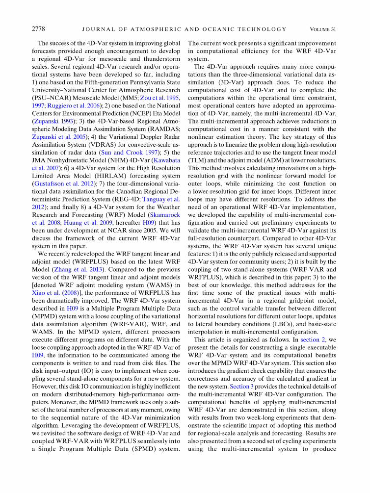
Figure 1 (top) illustrates the logic for running the

MPMD WRF 4D-Var; it requires dividing the set of

processors into three subsets forWRF-VAR, NLM, and

TLM–ADM, respectively (the vertical axis represents

the processing core space). Because of the sequential

nature of variational data assimilation, only one pro-

gram of theMPMD 4D-Var system runs at anymoment,

which means that only the subset of cores associated

with the running program are used while the rest of the

processors wait. One aspect of theMPMD system that is

especially troublesome is the fact that the NLM runs

only once for each outer loop; therefore, the cores al-

located for the NLM are idle during most of the mini-

mization process.

WRF-VAR,NLM, andWAMS share the same variable

definitions, coordinate system, and software infrastructure,

so it is natural to propose a single executableWRF4D-Var

system by coupling each component seamlessly with the

SPMDmethod. The strategy for the new SPMDversion of

the WRF 4D-Var system is as follows. WRF NLM, TLM,

FIG. 1. Flowchart of the (top) MPMD coupling and (bottom) SPMD coupling; vertical axis

represents the required computing cores to participate in the calculation.

DECEMBER 2014 ZHANG ET AL . 2779

and ADM are denoted by WRF-VAR with simple inter-

faces consisting of the initialization, integration, and final-

izing stages of running the model. Routines are developed

to exchange data via memory amongWRF-VAR, NLM,

TLM, and ADM. WRF-VAR is also modified to add

interfaces to call NLM, TLM, and ADM. Finally,

NLM, TLM, and ADM are compiled as a library that is

linked with WRF-VAR to build an SPMD WRF 4D-Var

system. Figure 1 (bottom) illustrates the logic of the SPMD

WRF 4D-Var. The disc IO communication is eliminated

using this approach, but the most important improvement

over the MPMD method is that all required computing

cores participate in the calculations from end to end, so the

computing resources are fully utilized.

The WRF Model and WRF-VAR have evolved con-

siderably since they were first introduced, but no up-

dates have been made to the WAMS since it was

completed in 2008. To accommodate the requirements

of building a single executableWRF 4D-Var system, the

WAMS required some upgrades. We redeveloped the

TLM and ADM of the ARW core based on the latest

WRF Model, starting from version 3.2 in 2010. We call

this upgraded version WRFPLUS, since it not only in-

cludes the full-physics ARW but also includes the TLM

and ADM (Zhang et al. 2013). Compared to WAMS,

WRFPLUS has the following major improvements: 1) it

is consistent with the latest WRF Model developments;

the upgraded TLM and ADM are always synchronized

with changes to the WRF code; 2) it has significantly

improved parallel efficiency; the Registry is augmented

to generate tangent and adjoint codes for halo ex-

changes automatically; and 3) it has improved physics

packages. In addition to vertical diffusion and surface

drag, we also include a simplified microphysics parame-

terization scheme and a simplified cumulus parameteri-

zation scheme. The WRF NLM already has well-defined

interfaces that initialize, advance, and finalize the model.

New interface routines are coded to initialize, advance,

and finalize the TLM and ADM.

By using a consistent model infrastructure between

WRF-VAR and WRFPLUS, we no longer need

regridding algorithms, which are usually required in

coupling systems because of different coordinate sys-

tems and parallel strategies between components. Sim-

ilar to the function of a coupler, a set of global data

structures was introduced in WRFPLUS, which sits be-

tween WRF-VAR and WRFPLUS to exchange data

between the coupled components. The data to be ex-

changed include the basic-state trajectories, the pertur-

bation snapshots, and the adjoint forcing and gradient

data that should be accessible from both sides of the

system via simple memory copying. Because 4D-Var

users may change the assimilation time window length,

time step, or 4D-Var subwindow length to fit the avail-

able observation types, domain size, and horizontal grid

resolution, the global data structure should be flexible

enough to accommodate the lengths of different tra-

jectories on the fly. The linked-list data structure was

adopted for this purpose. The first linked list being al-

located stores the basic-state trajectories from theNLM.

The required basic-state variables are packed into

a vector at every time step of the NLM integration,

which is stored on one node of the linked list. Because

the basic-state trajectory is used to derive the nonlinear

coefficients for the TLM and ADM integration re-

peatedly at every iteration, this linked list is designed to

be persistent for an outer loop. It is destroyed at the

end of each outer loop and reallocated and initialized at

the beginning of the next outer loop. The other two

allocated linked lists store the model perturbation

snapshots from the TLM integration and the adjoint

forcing inputs for ADM integration, respectively.

These two linked lists are persistent for only one inner-

loop iteration. They are initialized at the beginning of

each inner-loop iteration and are destroyed at the end

of the iteration. The linked list to store the basic-state

trajectory is the main memory consumer for the 4D-Var

minimization, as it stores the snapshots of the atmospheric

basic states. The number of stored snapshots depends on

how many time step integrations occur within the assim-

ilation window. Therefore, the memory requirement to

run this single executable WRF 4D-Var is increased

dramatically with increased horizontal resolution.

The interface and the coupling technique imple-

mented in the upgradedWRFPLUS have been designed

for coupling the TLM and ADM with other systems

easily. We have also coupled WRFPLUS with the

Community Gridpoint Statistical Interpolation (GSI;

http://www.dtcenter.org/com-GSI/users/) to build the

GSI-based WRF 4D-Var (Zhang and Huang 2013).

Because of the different grids and parallel strategies in

WRFPLUS and GSI, a parallel regridding algorithm is

required for the GSI-based WRF 4D-Var.

b. Performance and scalability of the singleexecutable WRF 4D-Var system

To compare the computational performance of the

single executable WRF 4D-Var system with the MPMD

WRF 4D-Var system, a series of benchmarking experi-

ments are carried out over a continental U.S. (CONUS)

domain. This configuration uses a 222 3 129 gridpoint

domain with 45 vertical s levels. The domain grid

spacing is 45 km and is centered at 408N, 988W. The

4D-Var analysis background is valid at 0900UTC 8 June

2012, and the assimilation time window is 6 h from 0900

to 1500 UTC 8 June 2012. The assimilated observations

2780 JOURNAL OF ATMOSPHER IC AND OCEAN IC TECHNOLOGY VOLUME 31

include conventional Global Telecommunication Sys-

tem (GTS) data and GPS radio occultation data from

NCEP. The basic-state trajectory produced by the NLM

is a full-physics model integration with WRF single-

moment 3-class (WSM3) microphysics scheme, the

Kain–Fritsch cumulus parameterization scheme (Kain

2004), the Yonsei University (YSU) planetary boundary

layer (PBL) scheme (Hong et al. 2006), and the Rapid

Radiative Transfer Model (RRTM) and Dudia schemes

for long- and shortwave radiation. The integrations of

the TLM and ADM use simplified microphysics, cu-

mulus, and PBL schemes that are included in the current

version of WRFPLUS. The integration time step for the

NLM, TLM, and ADM is 240 s.

The performance tests are carried out on the NCAR

‘‘Lynx’’ machine and all executables are compiled by

Intel compilers with default optimization levels. Lynx is

a single-cabinet Cray XT5m supercomputer, comprising

76 computingnodes, eachwith twohex-coreAMD2.2-GHz

Opteron chips for 12 total computing cores. Each Lynx

computing node has 16GB of memory (https://www2.

cisl.ucar.edu/supercomputer/lynx). To run the MPMD

WRF 4D-Var, the required computing cores are

divided into three subsets among WRF-VAR, NLM,

and TLM–ADM. TLM and ADM are well known for

their high computing costs; therefore, most of the com-

puting resources are allocated to WRF TLM–ADM. In

general, finding the best allocation strategy for parallel

performance requires experimenting with various config-

urations. In this paper, we allocate 5% of the processing

cores toWRFNLMand another 5% toWRF-VAR,while

the WRF TLM–ADM takes the remaining 90% of the

processing cores. Running the SPMD WRF 4D-Var is

straightforward; all requested computing cores will be

dedicated to computation at all times.

To accommodate the memory requirement of this 6-h

4D-Var case, we run the experiment starting with 12

nodes and use only one core per node to take advantage

of all 192GB of memory across the nodes. The maxi-

mum number of CPU cores that we tried is 192 cores for

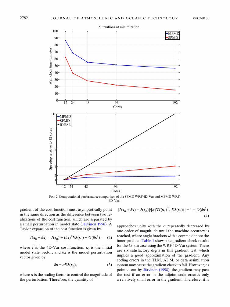
this medium size case. Figure 2 shows the wall clock time

and speedup relative to 12 cores for five iterations of the

minimization as a function of the number of CPU cores.

Compared to the MPMD version, the SPMD WRF

4D-Var is approximately 40%–200% faster using 12–192

cores, with the greatest efficiency gains corresponding

to higher numbers of cores. The results confirm that the

MPMD 4D-Var, which suffers from the overhead of

disk IO communications and the inefficient usage of re-

quested processing cores, performs worse with increasing

parallelization. The cost of gathering and broadcasting

operations associated with the disk IO tends to be worse

with larger numbers of cores/nodes, and the parallel

scalability heavily depends on the bandwidth and latency

of the network connecting the nodes.

c. Gradient check in the WRF 4D-Var system

One of the most important factors to consider when

testing the reliability of a 4D-Var is the mathematical

correctness of the tangent linear and adjoint codes, for

example, observation operators, variable transforma-

tions, and the simplified forecast model. The accuracies

of the TLMandADM inWRFPLUS (Zhang et al. 2013)

have been confirmed following the method of Navon

et al. (1992). Let f(x), g_f(x, g_x), and a_f(x, a_x) denote

an NLM, a TLM, and an ADM, respectively, where

x, g_x, and a_x are the column vectors of model state

variables, perturbations of state variables, and adjoint

forcings, respectively. The TLM and ADM must satisfy

hg_f(x, g_x), g_f(x, g_x)i5 ha_f[x, g_f(x, g_x)], g_xi .(1)

To check the accuracy of the model and observation

operator adjoints in the WRF 4D-Var system, we run

the adjoint check on the same 45-km grid-spaced 6-h

assimilation window case as in section 2b. In addition to

the conventional observations and GPS radio occulta-

tion observations, satellite radiance observations from

Advanced Microwave Sounding Unit-A (AMSU-A),

Advanced Microwave Sounding Unit-B (AMSU-B),

High Resolution Infrared Radiation Sounder-3 (HIRS-3),

High Resolution Infrared Radiation Sounder-4 (HIRS-4),

and Microwave Humidity Sounder (MHS) are also

assimilated. In total, there are 350 329 observations

(233 476 from radiances) assimilated between 0009

and 0015 UTC 8 June 2012. The left- and right-hand

sides of the adjoint relationship [Eq. (1)] are

1.909 375 417 539 27 3 107 and 1.909 375 417 539 29 3107, respectively, representing a 13-digit accuracy on

the 64-bit machines. Results from the adjoint check

confirm the mathematical accuracy of the WRFPLUS,

variable transformation, and observation operator

codes.

The adjoint check alone is insufficient to ensure that

the system is correctly constructed, as it only checks the

coding and the mathematical accuracy of the adjoint

codes in the system. Because of potential errors of

implementing the tangent linear and the adjoint codes in

the minimization algorithm, it is possible to still find that

the minimization does not converge to a solution.

Therefore, a gradient check is needed to validate the

gradient computed via the adjoint and to test its imple-

mentation in the SPMD WRF 4D-Var system. The

method of testing the gradient of the cost function is

similar to that of testing the tangent linear code; the

DECEMBER 2014 ZHANG ET AL . 2781

gradient of the cost function must asymptotically point

in the same direction as the difference between two re-

alizations of the cost function, which are separated by

a small perturbation in model state (Järvinen 1998). ATaylor expansion of the cost function is given by

J(x01 dx)5 J(x0)1 (dx)T$J(x0)1O(dx2) , (2)

where J is the 4D-Var cost function, x0 is the initial

model state vector, and dx is the model perturbation

vector given by

dx5a$J(x0) , (3)

where a is the scaling factor to control the magnitude of

the perturbation. Therefore, the quantity of

[J(x01 dx)2 J(x0)]/[ah$J(x0)T, $J(x0)i]5 12O(dx2)

(4)

approaches unity with the a repeatedly decreased by

one order of magnitude until the machine accuracy is

reached, where angle brackets with a comma denote the

inner product. Table 1 shows the gradient check results

for the 45-km case using theWRF 4D-Var system. There

are six satisfactory digits in this gradient test, which

implies a good approximation of the gradient. Any

coding errors in the TLM, ADM, or data assimilation

systemmay cause the gradient check to fail. However, as

pointed out by Järvinen (1998), the gradient may pass

the test if an error in the adjoint code creates only

a relatively small error in the gradient. Therefore, it is

FIG. 2. Computational performance comparison of the SPMDWRF 4D-Var andMPMDWRF

4D-Var.

2782 JOURNAL OF ATMOSPHER IC AND OCEAN IC TECHNOLOGY VOLUME 31

important to check both the gradient and the adjoint

before a production run.

3. Multi-incremental WRF 4D-Var

a. Implementation

The WRF 4D-Var system employs the incremental

4D-Var formulation that is commonly used in opera-

tional analysis systems (section 2 in H09). An iterative

algorithm is used to solve the quadratic minimization

problem. When the solution is found by linearizing the

model and observation operators about a basic state, the

minimization in 4D-Var is called an inner loop. To ap-

proximate the nonlinear problem that exists in data as-

similation, multiple inner-loop minimizations might be

carried out. After every inner-loop minimization, both

the model and observation operators are relinearized

based on the solution of the previous inner-loop mini-

mization, the basic-state trajectory, and the innovations

(observations minus first guess) are recalculated as well.

We call the updating of the nonlinear solution the outer

loop, which can be repeated several times. In summary,

the incremental formulation of 4D-Var includes 1) the

basic-state trajectory produced by the NLM integration;

2) the innovations calculated by comparing the basic-

state trajectory to the observations; and 3) the inner

loops to minimize the cost function.

To further reduce the computing cost of the 4D-Var

algorithm, operational centers typically perform the

inner-loop minimizations at a lower horizontal resolu-

tion than the outer loop and forecast. For example, at

the time of this writing, the JMA mesoscale 4D-Var

system runs outer loops with 5-km horizontal resolution

and inner loops with 15 km. The JMA’s global 4D-Var

analysis runs outer loops on T959 and inner loops on

T319 (Takeuchi et al. 2013). If there is more than one

outer loop, then different inner loops may have different

horizontal resolutions (Veersé and Thépaut 1998;Rabier et al. 2000; Trémolet 2007; Kawabata et al. 2007;

Gustafsson et al. 2012). We call this a multi-incremental

4D-Var algorithm. For example, the ECMWF opera-

tional 4D-Var now runs outer loops with T1279L91

(’16 km) and three inner loops with T159, T255, and

T255 (’125, 80, 80 km, respectively). Another advan-

tage of introducing the different horizontal resolutions

stepwise into the minimization is to take nonlinear

processes into account with reinitializations in the line-

arized minimization algorithm (Gustafsson et al. 2012).

Similar to the ECMWF 4D-Var configuration, illus-

trated schematically by Fig. 1 in Trémolet (2007), weimplement the multi-incremental algorithm in theWRF

4D-Var system as well. The key feature of multi-

incremental 4D-Var is that the outer loops use a high-

resolution first guess to calculate the nonlinear model

basic-state trajectory, which is compared with observa-

tions to generate the innovations. This ensures the highest

possible accuracy for calculating the innovations, which are

the primary input for the data assimilation. The innovations

calculated by the high-resolutionmodel trajectory are used

in the low-resolution inner-loop minimization. For im-

plementation simplicity, the low-resolution domain for the

inner loop is required to have exactly the same vertical

levels as the outer loop, as well as similar physical prop-

erties, in order to directly use the innovations calculated

from the high-resolution grid. Before entering into the

inner-loop minimization, the high-resolution first-guess

fields are interpolated horizontally to the low-resolution

domain to generate the first guess for the inner loops.

Advanced interpolation methods, such as bilinear or

spline interpolation, can be used here to include the

high-resolution features that can be represented (with-

out aliasing) on the coarse-resolution grids. All 2D and

3D fields are interpolated horizontally, which includes

the static fields representing the land surface charac-

teristics. Because the control of the LBCs is an optional

capability in WRF 4D-Var (Zhang et al. 2011), the low-

resolution LBCs are also needed for the integrations of

the low-resolution TLM and ADM during the 4D-Var

inner-loopminimization. For a regionalmodel, the input

data from a previously run external analysis or forecast

model are available at every LBC update interval up to

the forecast length, so the low-resolution LBCs can be

calculated from two low-resolution states that are valid

at the beginning and end of the assimilation time win-

dow from interpolated high-resolution states. In the

ECMWF’s multi-incremental 4D-Var implementation,

the low-resolution basic-state trajectory used to derive

the nonlinear coefficients for the TLMandADM in inner

loops is interpolated spectrally from the high-resolution

basic-state trajectory produced by the high-resolution

NLM integration. In the WRF 4D-Var implementation,

we have two options designed to generate the low-

resolution basic-state trajectory for running the TLM

TABLE 1. Ratio of norms between the differences of the two cost

functions and the gradient of the cost function. The norm is defined

as the summation of the squares of all elements of the vector. Here,

a is the perturbation scaling factors of the initial perturbation.

a Ratio

1.000 3 10210 0.999 999 816 641 043

1.000 3 1029 0.999 997 946 421 285

1.000 3 1028 0.999 978 759 846 319

1.000 3 1027 0.999 787 540 378 143

1.000 3 1026 0.997 875 415 827 577

1.000 3 1025 0.978 754 158 734 996

1.000 3 1024 0.787 541 587 277 100

DECEMBER 2014 ZHANG ET AL . 2783

and ADM. The first option follows the method used by

the ECMWF in which the high-resolution basic-state

trajectory is saved to files and interpolated to a low-

resolution domain before the inner loop starts. The

second option uses a low-resolution trajectory from an

additional low-resolution WRF NLM run. The JMA’s

operational mesoscale 4D-Var system also uses a lower-

resolution simplified NLM (inner model) to provide

trajectories (Takeuchi et al. 2013). We compared the

impact of the two options on the 4D-Var analyses with

extensive experiments and have not found any signifi-

cant differences. The second option does not require the

storage of high-resolution trajectory files on disk, nor

does this option necessitate interpolating files to low-

resolution domain or reading files in TLM and ADM.

For these reasons, we chose the second option as the

default for the production run. After the inner-loop

minimization, the low-resolution analysis increments

are interpolated back to high-resolution grids and added

to the high-resolution first guess to produce the analysis

solution for this outer loop. This analysis solution is the

first guess for the next outer loop, if needed.

The multi-incremental minimization requires the

control variables to be transferred between the different

outer-loop iterations. The low-resolution control vari-

ables are saved at the end of the inner-loop minimiza-

tion and are used to initialize the starting point of

control variables for the next inner-loop minimization.

If two consecutive inner loops have different horizontal

resolutions, such as the first (T159) and second (T255)

inner loops of the ECMWF operational 4D-Var run,

then the saved control variables from the first inner loop

have to be transformed to the higher horizontal resolu-

tion of the second inner loop. For control variables on

spectral space, it is very easy to use different resolutions

in different outer loops. If we go from a low-resolution

increment (control variable) in spectral space to a full-

resolution increment, we just fill in zeroes in the higher-

resolution wave coefficients, carry out the inverse FFT,

and add the increment to the full-resolution gridpoint

model background. (N. Gustafsson 2014, personal commu-

nication). Among the current operational regional 4D-Var

systems, the reference HIRLAM is a gridpoint model, but

the HIRLAM 4D-Var is based on a spectral version of

HIRLAM, so theTLM,ADM, and control variables are in

spectral space (Gustafsson et al. 2012). The JMA meso-

scale 4D-Var system uses gridpoint models, but it does not

apply a multi-incremental minimization (Takeuchi et al.

2013). Therefore, the appropriate method of transfer for

control variables on gridpoint space is critical for the

implementation of multi-incremental WRF 4D-Var.

Starting with WRF-VAR, version 3.1, users have

three choices to define the background error covariance

(BE), called CV3, CV5, and CV6 (where CV stands for

control variable). CV3 is the NCEP global BE, which is

estimated in grid space using the National Meteorologi-

cal Center (NMC) method (Parrish and Derber 1992).

While CV3 can be used for any domain, CV5 andCV6 are

domain dependent, and must be generated using forecast

data from the same domain that is used for performing the

data assimilation. With CV3 and CV5, the background

errors are applied to the same set of the control variables

that are used byWRF-VAR: streamfunction, unbalanced

potential velocity, unbalanced temperature, unbalanced

surface pressure, and pseudorelative humidity (Barker

et al. 2004). However, for CV6 the moisture control var-

iable is the unbalanced part of pseudorelative humidity.

With CV3 the control variables are in physical space,

while with CV5 and CV6, the control variables are in

eigenvector space. The major difference between these

two kinds of BE is the vertical covariance, which is mod-

eled with a recursive filter in CV3, and with empirical

orthogonal functions (EOFs) in CV5 and CV6.

To reduce the condition number and accelerate the

minimization, the cost function is preconditioned via

a control variable transform (Barker et al. 2004):

vn5U21(xn2 xn21) , (5)

where n is the outer-loop index,B is the BE,U is defined

as B 5 UUT, and vn is the control variable vector after

the nth outer loop. The analysis increment from outer

loop (n 2 1) to n is

xn 2 xn215Uvn . (6)

Equation (7) of H09 shows that, during the calculation

of the cost function gradient for the background error

part, the contributions from the earlier outer loops to

the control variable must be added. If the nth outer loop

has a different horizontal resolution than the (n 1 1)

outer loop, then the vn has to be transferred to the res-

olution of the (n 1 1) outer loop.

Because the control variables with CV3 are in physical

space, it is straightforward to linearly or bilinearly in-

terpolate the saved control variables from one hori-

zontal resolution to another. To validate the horizontal

interpolation of vn, a multi-incremental experiment is

designed. The case in section 2 is used with the same

domain size, location, and map projection but with the

horizontal grid spacing and time step reduced to 15 km

and 60 s, respectively. The grid size used for the exper-

iment is 676 3 379 with 45 vertical s levels. The multi-

incremental configuration has a 15-km outer loop and

three inner loops of 135, 45, and 45 km. The maximum

number of inner-loop iterations is limited to 20, and the

2784 JOURNAL OF ATMOSPHER IC AND OCEAN IC TECHNOLOGY VOLUME 31

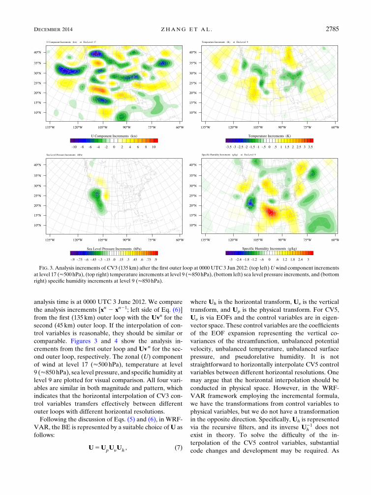
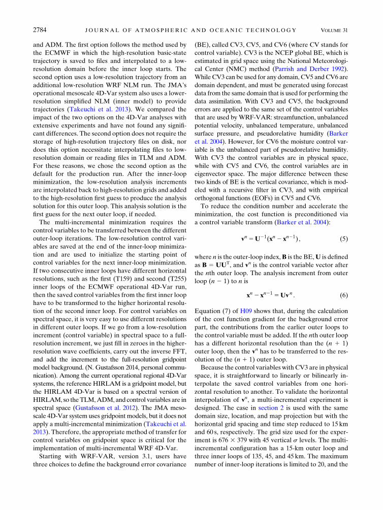
analysis time is at 0000 UTC 3 June 2012. We compare

the analysis increments [xn 2 xn21; left side of Eq. (6)]

from the first (135 km) outer loop with the Uvn for the

second (45 km) outer loop. If the interpolation of con-

trol variables is reasonable, they should be similar or

comparable. Figures 3 and 4 show the analysis in-

crements from the first outer loop and Uvn for the sec-

ond outer loop, respectively. The zonal (U) component

of wind at level 17 (’500 hPa), temperature at level

9 (’850 hPa), sea level pressure, and specific humidity at

level 9 are plotted for visual comparison. All four vari-

ables are similar in both magnitude and pattern, which

indicates that the horizontal interpolation of CV3 con-

trol variables transfers effectively between different

outer loops with different horizontal resolutions.

Following the discussion of Eqs. (5) and (6), in WRF-

VAR, the BE is represented by a suitable choice ofU as

follows:

U5UpUyUh , (7)

where Uh is the horizontal transform, Uy is the vertical

transform, and Up is the physical transform. For CV5,

Uy is via EOFs and the control variables are in eigen-

vector space. These control variables are the coefficients

of the EOF expansion representing the vertical co-

variances of the streamfunction, unbalanced potential

velocity, unbalanced temperature, unbalanced surface

pressure, and pseudorelative humidity. It is not

straightforward to horizontally interpolate CV5 control

variables between different horizontal resolutions. One

may argue that the horizontal interpolation should be

conducted in physical space. However, in the WRF-

VAR framework employing the incremental formula,

we have the transformations from control variables to

physical variables, but we do not have a transformation

in the opposite direction. Specifically,Uh is represented

via the recursive filters, and its inverse U21h does not

exist in theory. To solve the difficulty of the in-

terpolation of the CV5 control variables, substantial

code changes and development may be required. As

FIG. 3. Analysis increments of CV3 (135 km) after the first outer loop at 0000 UTC 3 Jun 2012: (top left)Uwind component increments

at level 17 (’500 hPa), (top right) temperature increments at level 9 (’850 hPa), (bottom left) sea level pressure increments, and (bottom

right) specific humidity increments at level 9 (’850 hPa).

DECEMBER 2014 ZHANG ET AL . 2785

demonstrated above, since it is physically reasonable

to interpolate CV3 control variables between different

horizontal resolutions, in this study, we only use CV3

in all multi-incremental experiments throughout this

paper.

b. Computational performance and scientific impact

A series of experiments are carried out to evaluate the

computational performance and scientific impact of

applying multi-incremental 4D-Var for model initiali-

zation. Two configurations with three inner loops are

tested. One uses the full-resolution configuration in

which the outer and inner loops use the same resolution

(15, 15, and 15 km), and the other uses the multi-

incremental configuration with a 15-km outer loop and

three inner loops of 135-, 45-, and 45-km grid spacing.

Each inner loop has up to 20 iterations. The computing

cost is estimated and compared between the two con-

figurations on NCAR’s Yellowstone supercomputer

(http://www2.cisl.ucar.edu/resources/yellowstone). The

Yellowstone system is based on IBM’s iDataPlex ar-

chitecture with 74 592 processor cores on 4662 IBM

dx360M4 nodes at the time of this study. Each node has

dual 2.6-GHz Intel Sandy Bridge efficient performance

(EP) processors and 32GB of memory. The 14 data rate

(FDR)Mellanox InfiniBand is used for interconnection.

Table 2 shows the wall clock time for completing 20

iterations for each inner loop with different numbers of

processing cores for 15-, 15-, and 15-km and 135-, 45-,

and 45-km configurations. For the full-resolution con-

figuration, 32 nodes with one core per node (32 cores in

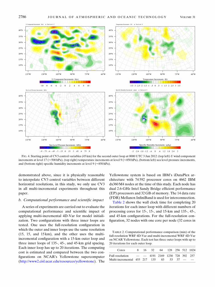
FIG. 4. Starting point of CV3 control variables (45 km) for the second outer loop at 0000 UTC 3 Jun 2012: (top left)U wind component

increments at level 17 (’500 hPa), (top right) temperature increments at level 9 (’850 hPa), (bottom left) sea level pressure increments,

and (bottom right) specific humidity increments at level 9 (’850 hPa).

TABLE 2. Computational performance comparison (min) of the

full-resolution WRF 4D-Var and multi-incremental WRF 4D-Var

on NCARYellowstone. Each test has three outer loops with up to

20 iterations for each outer loop.

Cores 8 16 32 64 128 256 512 1024

Full resolution — — 4191 2169 1230 728 392 257

Multi-incremental 455 217 135 83 53 37 — —

2786 JOURNAL OF ATMOSPHER IC AND OCEAN IC TECHNOLOGY VOLUME 31

total) is the minimum number of cores we used due to

the constrained memory on each node and the large

memory requirement for this case. The 60 total itera-

tions need approximately 70 h to finish with 32 cores.

Nevertheless, this case scales very well with an in-

creasing number of cores, and it is able to complete the

60 iterations in 4.3 h with 1024 cores. The case that uses

a multi-incremental configuration starts by using eight

nodes with one core per node (eight cores in total). With

a reasonable maximum of 256 cores (16 cores per node),

this case executes within 37min. The timing results show

that the computational cost has been substantially re-

duced, because we are able to run 4D-Var using a 6-h

window on a relatively large 15-km grid spacing domain

with minimal computing resources.

We use additional data assimilation experiments to

evaluate the performance of the multi-incremental

WRF 4D-Var configuration. Two one-week experi-

ments are carried out to compare verification scores of

the analyses and forecasts from the full-resolution and

multi-incremental configurations. We use the same

configurations as the CV3 test case described above,

but the analyses are performed every 12 h between

0000 UTC 1 June and 1200 UTC 8 June 2012 with 24-h

forecasts run from them. The analyses and 24-h forecasts

are verified against the NCEP final analyses (FNL) that

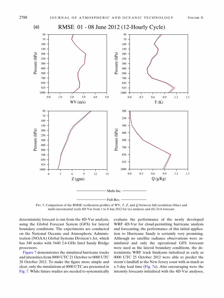
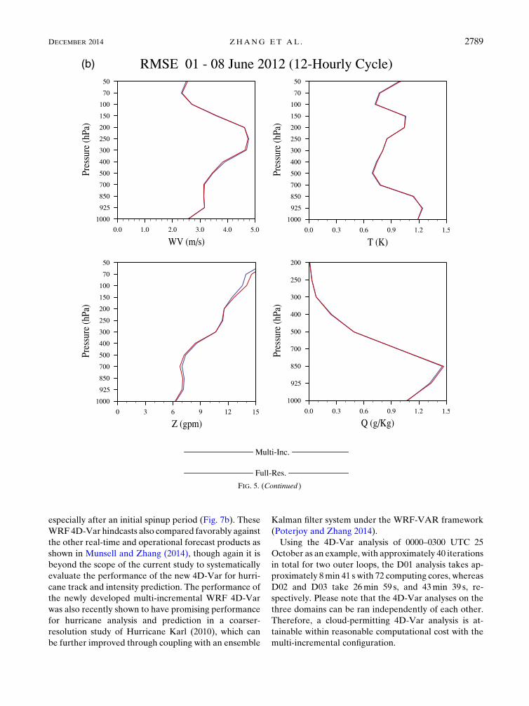
are valid at the same times. Figure 5 shows the average

root-mean-square error (RMSE) profiles for the two

configurations, which measure the differences of wind

WV, temperature T, geopotential height Z, and water

vapor Q between the analyses or forecasts and FNL. In

terms of the quality of the analyses, Fig. 5a indicates that

the multi-incremental configuration only slightly de-

grades the analyses of all variables compared to full-

resolution runs. Even though the analysis is degraded

slightly, Fig. 5b shows that the 24-h forecasts from the

multi-incremental configuration are comparable to

those of the full-resolution configuration. In this case,

the multi-incremental configuration has slightly better

scores for winds below 200 hPa and geopotential height

below 300 hPa. Figure 6 shows the time series of 24-h

RMSE at 850 and 500 hPa. This experiment confirms

that the multi-incremental 4D-Var configuration con-

sistently produces 24-h forecasts that are as accurate

as the full-resolution configuration over the 15 cycles.

Please note that there are many factors that could

impact the analysis quality and subsequent forecast

performance, such as background error statistics,

observations, quality control, and the consistency be-

tween the analysis system and the model. We cannot

claim that either configuration outperforms the others.

The conclusion we can draw based on the one-week

experiments is that the multi-incremental WRF 4D-Var

configuration does not exhibit negative impacts on

forecast performance with the benefit of reduced com-

putational cost.

c. Application to convection-permitting analyses andforecasts for Hurricane Sandy (2012)

The newly developed single executable, multi-

incremental 4D-Var system is further examined

through application to the convection-permitting anal-

ysis of Hurricane Sandy (2012), which was nearly un-

affordable computationally with the predecessor WRF

4D-Var system. Sandy was the most destructive hurri-

cane of the 2012 Atlantic hurricane season. The exper-

iment design is based on a cloud-permitting hurricane

analysis and prediction system including an ensemble

Kalman filter for the WRF Model (Weng and Zhang

2014). The WRF Model has three two-way-nested do-

mains with 3793 244 (D01), 3043 304 (D02), and 3043304 (D03) horizontal grid points with horizontal grid

spacings of 27, 9, and 3 km, respectively. All model do-

mains use 44 vertical levels and a pressure top at 50 hPa.

D01 is fixed to cover the central to eastern three-

quarters of the CONUS, the tropical and subtropical

North Atlantic, and the two inner domains follow the

observed hurricane position between data assimilation

cycles using the preset moves option in WRF. In de-

terministic forecasts from the 4D-Var analyses, the two

inner domains follow the storm center using the WRF

vortex-following technique. These experiments use the

same physical parameterization schemes described in

section 2 but use the Grell–Devenyi scheme for cumulus

parameterization (D1 only; D2 and D3 fully explicit),

the WRF single-moment 6-class microphysics scheme

(WSM6), and the five-layer thermal diffusion land sur-

face model [for the details of these schemes, refer to

Skamarock et al. (2008) and references therein]. An

empirical scheme implemented in Green and Zhang

(2013) is used to estimate the bulk drag and enthalpy

coefficients (CD/CK). This ad hoc scheme has been

found to improve the tropical cyclone (TC) wind pres-

sure relationship forecasts.

The cycling 4D-Var system is initialized at 1200 UTC

20 October and is ended at 1200 UTC 28 October

2012; the first background field is taken from a 12-h

forecast at 0000 UTC 21 October 2012. The assimilation

window is 3 h and all conventional observations,

satellite-derived winds, airborne reconnaissance drop-

sondes, and flight-level in situ measurements are as-

similated with 4D-Var using two outer loops for the

minimization. We picked a 1:9 grid size ratio between

the first outer loop and its inner loops, as well as a 1:3

grid size ratio between the second outer loop and its

inner loops for each domain. Every 6 h, a 144-h

DECEMBER 2014 ZHANG ET AL . 2787

deterministic forecast is run from the 4D-Var analysis,

using the Global Forecast System (GFS) for lateral

boundary conditions. The experiments are conducted

on the National Oceanic and Atmospheric Adminis-

tration (NOAA) Global Systems Division’s Jet, which

has 340 nodes with 5440 2.6-GHz Intel Sandy Bridge

processors.

Figure 7 demonstrates the simulated hurricane tracks

and intensities from 0000 UTC 21 October to 0000 UTC

28 October 2012. To make the figure more simple and

clear, only the simulations at 0000 UTC are presented in

Fig. 7. While future studies are needed to systematically

evaluate the performance of the newly developed

WRF 4D-Var for cloud-permitting hurricane analysis

and forecasting, the performance of this initial applica-

tion to Hurricane Sandy is certainly very promising.

Although no satellite radiance observations were as-

similated and only the operational GFS forecasts

were used as the lateral boundary conditions, the de-

terministic WRF track hindcasts initialized as early as

0000 UTC 25 October 2012 were able to predict the

storm’s landfall at the New Jersey coast with as much as

a 5-day lead time (Fig. 7a). Also encouraging were the

intensity forecasts initialized with the 4D-Var analyses,

FIG. 5. Comparison of the RMSE verification profiles of WV, T, Z, and Q between full-resolution (blue) and

multi-incremental (red) 4D-Var from 1 to 8 Jun 2012 for (a) analyses and (b) 24-h forecast.

2788 JOURNAL OF ATMOSPHER IC AND OCEAN IC TECHNOLOGY VOLUME 31

especially after an initial spinup period (Fig. 7b). These

WRF 4D-Var hindcasts also compared favorably against

the other real-time and operational forecast products as

shown in Munsell and Zhang (2014), though again it is

beyond the scope of the current study to systematically

evaluate the performance of the new 4D-Var for hurri-

cane track and intensity prediction. The performance of

the newly developed multi-incremental WRF 4D-Var

was also recently shown to have promising performance

for hurricane analysis and prediction in a coarser-

resolution study of Hurricane Karl (2010), which can

be further improved through coupling with an ensemble

Kalman filter system under the WRF-VAR framework

(Poterjoy and Zhang 2014).

Using the 4D-Var analysis of 0000–0300 UTC 25

October as an example, with approximately 40 iterations

in total for two outer loops, the D01 analysis takes ap-

proximately 8min 41 s with 72 computing cores, whereas

D02 and D03 take 26min 59 s, and 43min 39 s, re-

spectively. Please note that the 4D-Var analyses on the

three domains can be ran independently of each other.

Therefore, a cloud-permitting 4D-Var analysis is at-

tainable within reasonable computational cost with the

multi-incremental configuration.

FIG. 5. (Continued)

DECEMBER 2014 ZHANG ET AL . 2789

4. Summary and discussion

This paper discussed the technical implementation

and the computational performance of single executable

and multi-incremental WRF 4D-Var. In general, the

computing cost of a Single ProgramMultiple DataWRF

4D-Var system is much lower than the predecessor

Multiple Program Multiple Data version.

In the single executable WRF 4D-Var system, the

NLM, TLM, and ADM in WRFPLUS are compiled as

a library and linked with WRF-VAR to build an SPMD

system. The interfaces to call the TLM and ADM from

the minimization algorithm were added into WRF-

VAR, and the routines to initialize, advance, and final-

ize the TLM and ADM were also constructed in the

WRFPLUS. A set of global data structures between

FIG. 6. Comparison of the time series of the verification RMSE of 24-h forecasts for WV, T, Z, and Q between

full-resolution (blue) and multi-incremental (red) 4D-Var from 1 to 8 Jun 2012 for (a) 850 and (b) 500 hPa.

2790 JOURNAL OF ATMOSPHER IC AND OCEAN IC TECHNOLOGY VOLUME 31

WRF-VAR and WRFPLUS exchanges the data via

memory copying, which is crucial for improving the

computational efficiency of WRF 4D-Var. The execu-

tion of the single executable system is simpler because

processors no longer need to be allocated for separate

executables.

To validate the single executable WRF 4D-Var sys-

tem, a gradient check was used to ensure the mathe-

matical correctness of the tangent linear and adjoint

code in the variational data assimilation system. The

gradient check not only tests the correctness of the

tangent linear and adjoint coding but also checks for

errors in the variational assimilation system. Testing the

tangent linear and adjoint codes, plus the gradient

check, ensures the accuracy of the variational data as-

similation system.

Themulti-incremental 4D-Var configuration has been

implemented to further reduce the computational cost

FIG. 6. (Continued)

DECEMBER 2014 ZHANG ET AL . 2791

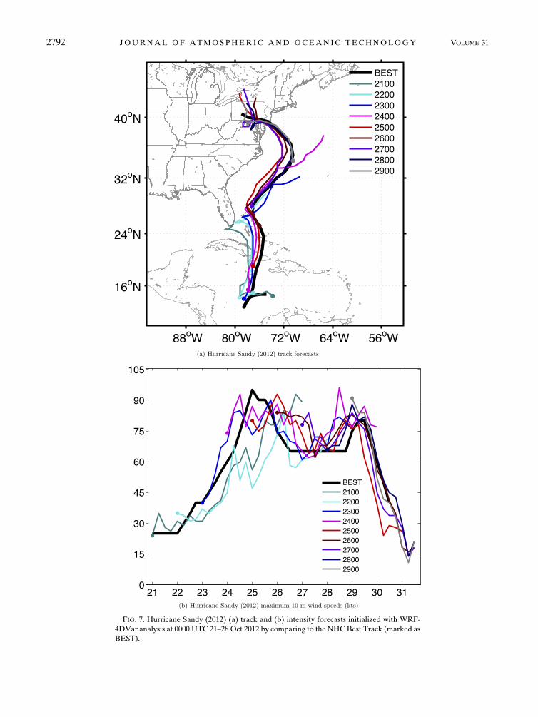
FIG. 7. Hurricane Sandy (2012) (a) track and (b) intensity forecasts initialized with WRF-

4DVar analysis at 0000 UTC 21–28 Oct 2012 by comparing to the NHCBest Track (marked as

BEST).

2792 JOURNAL OF ATMOSPHER IC AND OCEAN IC TECHNOLOGY VOLUME 31

of WRF 4D-Var. The initial implementation works well

and the computational cost is reduced dramatically.

Week-long experiments using a CONUS model domain

indicate that the performance of multi-incremental 4D-

Var is comparable to the full-resolution configuration. A

second set of experiments for Hurricane Sandy shows

that the multi-incremental WRF 4D-Var can be per-

formed for a cloud-permitting grid spacing with an af-

fordable computational cost, and both the track and

intensity forecasts were promising. In addition to ap-

plying a stepwise increase in horizontal resolution for

the inner loops, different quality control strategies may

also be introduced, as well as more advanced physics

packages at various stages of the minimization.

Leveraging the developments in this study, the multi-

incremental configuration for the GSI-based WRF

4D-Var (Zhang and Huang 2013) should be im-

plemented easily because the GSI uses similar CV3

control variables.

Regarding the difficulty of the interpolation of the

CV5 control variables discussed in section 3a, one pro-

posed solution is to exchange the order of Uy and Uh in

Eq. (7), which means the vertical transformation should

be applied to control variables before the horizontal

transformation in Eq. (6). Therefore, it is reasonable to

conduct the horizontal interpolation on the in-

termediate product Uyvn, followed by a U21

y , which

converts the intermediate product back to control vari-

able space (N. Gustafsson 2014, personal communica-

tion). The development ofU21y should be possible, but it

would be a major coding effort. This change will be

considered in our future developmental plans.

Acknowledgments. This work is supported by the Air

ForceWeather Agency. Partial support also comes from

NSF Grant 1305798 and ONR Grant N000140910526.

We thank Dong-Kyou Lee and Gyu-Ho Lim of Seoul

National University for their comments on the manu-

script and generous support through the Korea–U.S.

Weather andClimate Center. Junmei Ban helped to plot

most of the figures. Michael Kavulich and Steven Olson

helped to edit the manuscript.

REFERENCES

Barker, D. M., W. Huang, Y.-R. Guo, A. J. Bourgeois, and Q. N.

Xiao, 2004: A three-dimensional variational data assimilation

system for MM5: Implementation and initial results. Mon.

Wea. Rev., 132, 897–914, doi:10.1175/1520-0493(2004)132,0897:

ATVDAS.2.0.CO;2.

Courtier, P., J.-N. Thépaut, and A. Hollingsworth, 1994: A strategy

for operational implementation of 4D-Var, using an in-

cremental approach. Quart. J. Roy. Meteor. Soc., 120, 1367–

1387, doi:10.1002/qj.49712051912.

Gauthier, P., and J.-N. Thépaut, 2001: Impact of the digital filter as

a weak constraint in the preoperational 4DVAR assimilation

system of Météo-France. Mon. Wea. Rev., 129, 2089–2102,

doi:10.1175/1520-0493(2001)129,2089:IOTDFA.2.0.CO;2.

——, M. Tanguay, S. Laroche, and S. Pellerin, 2007: Extension of

3DVAR to 4DVAR: Implementation of 4DVAR at the Me-

teorological Service of Canada. Mon. Wea. Rev., 135, 2339–

2364, doi:10.1175/MWR3394.1.

Green, B. W., and F. Zhang, 2013: Impacts of air–sea flux parameter-

izations on the intensity and structure of tropical cyclones. Mon.

Wea. Rev., 141, 2308–2324, doi:10.1175/MWR-D-12-00274.1.

Gustafsson, N., X.-Y. Huang, X. Yang, K.Mogensen,M. Lindskog,

O. Vignes, T. Wilhelmsson, and S. Thorsteinsson, 2012: Four-

dimensional variational data assimilation for a limited area

model. Tellus, 64A, 14985, doi:10.3402/tellusa.v64i0.14985.

Honda, Y., M. Nishijima, K. Koizumi, Y. Ohta, K. Tamiya,

T. Kawabata, and T. Tsuyuki, 2005: A pre-operational varia-

tional data assimilation system for a non-hydrostatic model at

the Japan Meteorological Agency: Formulation and pre-

liminary results. Quart. J. Roy. Meteor. Soc., 131, 3465–3475,

doi:10.1256/qj.05.132.

Hong, S.-Y., Y. Noh, and J. Dudhia, 2006: A new vertical diffusion

package with an explicit treatment of entrainment processes.

Mon. Wea. Rev., 134, 2318–2341, doi:10.1175/MWR3199.1.

Huang, X.-Y., X. Yang, N. Gustafsson, K. Mogensen, and

M. Lindskog, 2002: Four-dimensional variational data assim-

ilation for a limited area model. HIRLAM Tech. Rep. 57, 41

pp. [Available from SMHI, S-601 76 Norrkoping, Sweden.]

——, and Coauthors, 2009: Four-dimensional variational data as-

similation for WRF: Formulation and preliminary results.

Mon. Wea. Rev., 137, 299–314, doi:10.1175/2008MWR2577.1.

Järvinen, H., 1998: Observations and diagnostic tools for data as-

similation. ECMWFMeteorological Training Course Lecture

Series, 19 pp. [Available online at http://old.ecmwf.int/

newsevents/training/lecture_notes/pdf_files/ASSIM/Diagtool.pdf.]

Kain, J. S., 2004: The Kain–Fritsch convective parameterization:

An update. J. Appl. Meteor., 43, 170–181, doi:10.1175/

1520-0450(2004)043,0170:TKCPAU.2.0.CO;2.

Kawabata, T., H. Seko, K. Saito, T. Kuroda, K. Tamiya, T. Tsuyuki,

Y. Honda, and Y. Wakazuki, 2007: An assimilation and

forecasting experiment of the Nerima heavy rainfall with

a cloud-resolving nonhydrostatic 4-dimensional variational

data assimilation system. J. Meteor. Soc. Japan, 85, 255–276,

doi:10.2151/jmsj.85.255.

Le Dimet, F., and O. Talagrand, 1986: Variational algorithms for

analysis and assimilation of meteorological observations:

Theoretic aspects. Tellus, 38A, 97–110, doi:10.1111/

j.1600-0870.1986.tb00459.x.

Lewis, J., and J. Derber, 1985: The use of adjoint equations to solve

a variational adjustment problem with advective constraints.

Tellus, 37A, 309–227, doi:10.1111/j.1600-0870.1985.tb00430.x.

Lorenc, A. C., and F. Rawlins, 2005: Why does 4D-Var beat 3D-

Var?Quart. J. Roy. Meteor. Soc., 131, 3247–3257, doi:10.1256/

qj.05.85.

Munsell, E. B., and F. Zhang, 2014: Prediction and uncertainty of

Hurricane Sandy (2012) explored through a real-time cloud-

permitting ensemble analysis and forecast system assimilating

airborne Doppler observations. J. Adv. Model. Earth Syst., 6,

38–58, doi:10.1002/2013MS000297.

Navon, I. M., X. Zou, J. Derber, and J. Sela, 1992: Variational data

assimilation with an adiabatic version of the NMC spectral

model. Mon. Wea. Rev., 120, 1433–1446, doi:10.1175/

1520-0493(1992)120,1433:VDAWAA.2.0.CO;2.

DECEMBER 2014 ZHANG ET AL . 2793

Parrish, D. F., and J. C. Derber, 1992: The National Meteorological

Center’s spectral statistical interpolation analysis system. Mon.

Wea. Rev., 120, 1747–1763, doi:10.1175/1520-0493(1992)120,1747:

TNMCSS.2.0.CO;2.

Poterjoy, J., and F. Zhang, 2014: Intercomparison and coupling of en-

semble and four-dimensional variational data assimilationmethods

for the analysis and forecasting of Hurricane Karl (2010). Mon.

Wea. Rev., 142, 3347–3364, doi:10.1175/MWR-D-13-00394.1.

Rabier, F., H. Järvinen, E. Klinker, J.-F. Mahfouf, and A. Simmons,

2000: The ECMWF operational implementation of four-

dimensional variational assimilation. Part I: Experimental re-

sults with simplified physics. Quart. J. Roy. Meteor. Soc., 126,1143–1170, doi:10.1002/qj.49712656415.

Rawlins, F., S. P. Ballard, K. J. Bovis, A. M. Clayton, D. Li, G. W.

Inverarity, A. C. Lorenc, and T. J. Payne, 2007: TheMetOffice

global four-dimensional data assimilation system. Quart.

J. Roy. Meteor. Soc., 133, 347–362, doi:10.1002/qj.32.

Rosmond, T., and L. Xu, 2006: Development of NAVDAS-AR:

Non-linear formulation and outer loop tests. Tellus, 58A, 45–58, doi:10.1111/j.1600-0870.2006.00148.x.

Ruggiero, F. H., J. Michalakes, T. Nehrkorn, G. D. Modica, and

X. Zou, 2006: Development and tests of a new distributed-

memory MM5 adjoint. J. Atmos. Oceanic Technol., 23, 424–436, doi:10.1175/JTECH1862.1.

Skamarock, W. C., and Coauthors, 2008: A description of the

Advanced Research WRF version 3. NCAR Tech. Note

NCAR/TN-4751STR, 113 pp. [Available online at http://

www.mmm.ucar.edu/wrf/users/docs/arw_v3_bw.pdf.]

Sun, J., and N. A. Crook, 1997: Dynamical and microphysical re-

trieval from Doppler radar observations using a cloud model

and its adjoint. Part I: Model development and simulated data

experiments. J. Atmos. Sci., 54, 1642–1661, doi:10.1175/

1520-0469(1997)054,1642:DAMRFD.2.0.CO;2.

Takeuchi, Y., and Coauthors, 2013: Outline of the operational

numerical weather prediction at the Japan Meteorological

Agency. Japan Meteorological Agency Tech. Rep., 188 pp.

[Available online at http://www.jma.go.jp/jma/jma-eng/

jma-center/nwp/outline2013-nwp/index.htm.]

Tanguay, M., F. Luc, E. Lapalme, and M. Lajoie, 2012: Four-

dimensional variational data assimilation for the Canadian

Regional Deterministic Prediction System. Mon. Wea. Rev.,

140, 1517–1538, doi:10.1175/MWR-D-11-00160.1.

Trémolet, Y., 2007: Incremental 4D-Var convergence study.Tellus,

59A, 706–718, doi:10.1111/j.1600-0870.2007.00271.x.

Veersé, F., and J.-N. Thépaut, 1998: Multi-truncation incremental ap-

proach for four-dimensional variational data assimilation. Quart.

J. Roy. Meteor. Soc., 124, 1889–1908, doi:10.1002/qj.49712455006.

Weng, Y., and F. Zhang, 2014: The impact of reconnaissance data

on hurricane intensity forecasts with a cycling WRF-EnKF

system. 18th Conf. on Integrated Observing and Assimilation

Systems for the Atmosphere, Oceans, and Land Surface

(IOAS-AOLS), Atlanta, GA, Amer. Meteor. Soc., 8.3.

[Available online at https://ams.confex.com/ams/94Annual/

webprogram/Paper240719.html.]

Xiao, Q., and Coauthors, 2008: Application of an adiabatic WRF

adjoint to the investigation of the May 2004 McMurdo, Ant-

arctica, severe wind event. Mon. Wea. Rev., 136, 3696–3713,

doi:10.1175/2008MWR2235.1.

Xu, L., T. Rosmond, and R. Daley, 2005: Development

of NAVDAS-AR: Formulation and initial tests of the

linear problem. Tellus, 57A, 546–559, doi:10.1111/

j.1600-0870.2005.00123.x.

Zhang, X., and X.-Y. Huang, 2013: Development of GSI-based

WRF 4D-Var system. 17th Conf. on Integrated Observing and

Assimilation Systems for the Atmosphere, Oceans, and Land

Surface (IOAS-AOLS), Austin, TX, Amer. Meteor. Soc.,

4A.2. [Available online at https://ams.confex.com/ams/

93Annual/webprogram/Paper217182.html.]

——, ——, and N. Gustafsson, 2011: Control of lateral boundary

conditions in WRF 4D-Var. Ninth Int. Workshop on Adjoint

Model Applications in Dynamic Meteorology, Cefalu, Sicily,

Italy, NASA GMAO. [Available online at http://gmao.gsfc.

nasa.gov/events/adjoint_workshop-9/presentations/Zhang.pdf.]

——, ——, and N. Pan, 2013: Development of the upgraded

tangent linear and adjoint of the Weather Research and

Forecasting (WRF) Model. J. Atmos. Oceanic Technol., 30,

1180–1188, doi:10.1175/JTECH-D-12-00213.1.

Zou, X., Y.-H. Kuo, and Y.-R. Guo, 1995: Assimilation of at-

mospheric radio refractivity using a nonhydrostatic adjoint

model Mon. Wea. Rev., 123, 2229–2249, doi:10.1175/

1520-0493(1995)123,2229:AOARRU.2.0.CO;2.

——, F. Vandenberghe, M. Pondeca, and Y.-H. Kuo, 1997: In-

troduction to adjoint techniques and the MM5 adjoint mod-

eling system. NCAR Tech. Note NCAR/TN-4351STR, 110

pp. [Available from UCAR Communications, P.O. Box 3000,

Boulder, CO 80307-3000.]

Zupanski, M., 1993: Regional four-dimensional variational data

assimilation in a quasi-operational forecasting environment.Mon.

Wea. Rev., 121, 2396–2408, doi:10.1175/1520-0493(1993)121,2396:

RFDVDA.2.0.CO;2.

——, D. Zupanski, T. Vukicevic, K. Eis, and T. V. Haar, 2005:

CIRA/CSU four-dimensional variational data assimilation

system. Mon. Wea. Rev., 133, 829–843, doi:10.1175/

MWR2891.1.

2794 JOURNAL OF ATMOSPHER IC AND OCEAN IC TECHNOLOGY VOLUME 31