Development of an Ensemble Gridded Hydrometeorological Forcing Dataset over the Contiguous United States

Andrew J. Newman1, Martyn P. Clark1, Jason Craig1, Bart Nijssen2, Andrew Wood1, Ethan Gutmann1, Naoki Mizukami1, Levi Brekke3, and Jeff R. Arnold4

 1 National Center for Atmospheric Research, Boulder CO, USA2 University of Washington, Seattle WA, USA3U.S. Department of Interior, Bureau of Reclamation, Denver CO, USA4 U. S. Army Corps of Engineers, Institute for Water Resources, Seattle WA, USA

Outline

•Motivation•Methodology•Example output•Validation

▫Comparisons to deterministic▫Statistical properties

•Summary

Opportunities for hydrologic prediction

Hydrological Prediction: How well can we estimate the amount of water stored?

Accuracy in precipitation estimatesFidelity of hydro model simulationsEffectiveness of hydrologic data assimilation methods

Water Cycle (from NASA)

Meteorological predictability: How well can we forecast the weather and climate?

Opportunity: Characterize historical forcing uncertainty -> improve water stored estimates• Current uncertainties for

land-surface modeling are generally order of magnitude

• Can we begin to quantify space-time uncertainty?

hydrological predictabilitymeteorological predictability

Motivation Methodology Input Data SummaryValidationExample Output

Precipitation Data Uncertainty

Motivation Methodology Input Data SummaryValidationExample Output

Gauge separation distance (km)

Corr

elat

ion

coef

ficie

nt

0 1 2 3 4 5 6 70

0.2

0.4

0.6

0.8

1

adjusted

light rain

heavy rain

•Point to grid uncertainties:▫Measurement errors

Gauge placement issues (e.g. roof) Is a gauge working properly?

▫Measurement representativeness Sub-pixel variability Take closest measurement? Interpolate nearby gauges?

▫Missing Data Interpolate available obs? Fill missing data?

Step 1:Locally weighted regression at each grid cell: Probability of Precipitation (PoP) via logistic regression, then amount and uncertainty (least squares mean & residuals)

observations

Example over the Colorado HeadwatersEnsemble Generation

Clark & Slater (2006), Newman et al. (2014, in prep)

Motivation Methodology

Input Data SummaryValidationExample Output

Example over the Colorado Headwaters

Step 2:Synthesize ensemblesfrom PoP, amount & uncertainty using spatially correlated random fields (SCRFs)

Example over the Colorado Headwaters

observations

Clark & Slater (2006), Newman et al. (2014, in prep)

Ensemble GenerationMotivation Methodolog

yInput Data SummaryValidationExample

Output

•Other Methodological choices:•Topographic lapse rates derived at each grid cell for each day vs. climatology (e.g. PRISM)•Used serially complete (filled) station data rather than only available obs vs. using only available observations•Included SNOTEL observations vs. excluding

•Final Product: 12 km, daily 1980-2012, 100 members, precipitation & temperature (1.5 TB)

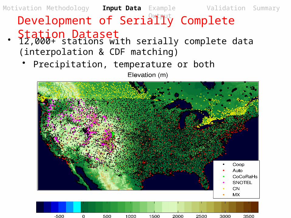
• 12,000+ stations with serially complete data (interpolation & CDF matching)• Precipitation, temperature or both

Development of Serially Complete Station Dataset

Motivation Methodology Input Data SummaryValidationExample Output

• GHCN-Daily(Cooperative networks, Automated (ASOS/AWOS)) in US, Canada and Mexico (thanks to Kyoko Ikeda)

• Use QC from National Climatic Data Center (NCDC)• SNOwpack TELemetry (SNOTEL) observations from National

Resource Conservation Service (NRCS) have no QC• Applied QC from Serreze et al. (1999)• Removes gross temperature and precipitation errors

• Also corrects for gauge under-catch using large accumulation events -> Precip to SWE ratio

Development of Serially Complete Station Dataset

Motivation Methodology Input Data SummaryValidationExample Output

• Variable station data availability• Stations come and go, have missing data

• Use all stations with > 10 years of data and > 10 years of overlap with ≥ 30 stations within 500 km (generally following Eischeid et al. 2000)

• Interpolate temperature gaps of 1-2 days• Use CDF matching from best available rank correlated station

to fill larger temperature gaps and all precipitation missing data• Assumes stationary CDF in time

Development of Serially Complete Station Dataset

Motivation Methodology Input Data SummaryValidationExample Output

Example Output

Motivation Methodology Input Data SummaryValidationExample Output

• Central US Flood of 1993• June 1993 total precipitation

Validation: Comparisons to other datasets (temperature)

• Minimal differences in mean temperature• Except in

intermountain west• Maurer uses constant

elevation lapse rate (-6.5 K km-1)

• Ensemble lapse rate derived from station data (including Snotel)

• Maurer shown to be too cold in higher elevations (e.g. Mizukami et al. 2014)

• Ensemble warmer than Maurer in high terrain

Motivation Methodology Input Data SummaryValidationExample Output

Validation: Comparisons to other datasets (PoP)

• Maurer et al. (2002)• Interpolation

between observations increases precip occurrence

• Ensemble:• SCRFs applied to

PoP field more realistic PoP

• Generally reduces PoP

• Data differences may be responsible for PoP increases

Motivation Methodology Input Data SummaryValidationExample Output

Validation: Comparisons to other datasets (amount)

• Ensemble - MaurerMaurer et al. (2002)

• NLDAS - MaurerXia et al. (2012)

• Daymet - MaurerThornton et al. (2014) Version 2 (regridded

to 12km)

Motivation Methodology Input Data SummaryValidationExample Output

Validation: Comparisons to other datasets (amount)• CONUS precip difference PDFs

• NLDAS & Maurer agree very closely (both use PRISM correction, similar input gauges)

• Daymet wettest• Slightly larger spread in ensemble – most distinctly

different

Motivation Methodology Input Data SummaryValidationExample Output

Validation: Discrimination & Reliability • Reliability (blue & black lines)

• Want to be close to 1-1 line (predicted = observed probabilities)

• Generally good reliability

Motivation Methodology Input Data SummaryValidationExample Output

>0 mm

>13 mm

>25 mm

>50 mm

>0 mm

>13 mm

>25 mm

>50 mm

Validation: Discrimination & Reliability • Discrimination (red & black lines)

• Want to maximize separation of PDFs• Generally good separation

Motivation Methodology Input Data SummaryValidationExample Output

>0 mm

>13 mm

>25 mm

>50 mm

>0 mm

>13 mm

>25 mm

>50 mm

Example Application• Snowmelt dominated basin in Colorado Rockies• Example water year daily temperature (a)• Snow water equivalent accumulation (b)

• Simple temperature index model (optimized for Daymet (green))

Motivation Methodology Input Data SummaryValidationExample Output

Summary• Developed ensemble hydrometeorolgical dataset• Required development of serially complete station dataset

• Both will be available for download at: http://ral.ucar.edu/projects/hap/flowpredict/subpages/pqpe.php

• Methodology follows Clark and Slater (2006) but for CONUS

• Ensemble has:• Realistic probability of precipitation (PoP)• Estimate of forcing uncertainty

• Quantification of uncertainty for data assimilation• Potential Applications:

• Propagation of forcing uncertainty into model states• Useful for state uncertainty estimation (e.g. SWE)

• Ensemble calibrations can allow for estimates of parameter uncertainty (impact of noise on parameter estimation)

Motivation Methodology Input Data SummaryValidationExample Output

Next Steps• Include downward shortwave and humidity in ensemble

• Improved downward shortwave radiation product (Slater et al., in prep)• Stations across US at many elevations, climatic

conditions• Will allow for improved temperature/moisture –

shortwave relationships• Include ensemble into data assimilation system(s)

• Particle filter and ensemble Kalman filter• Can we improve daily to seasonal streamflow

prediction using automated systems?

Motivation Methodology Input Data SummaryValidationExample Output