Development of An ERROR ESTIMATE

P M V SubbaraoProfessor

Mechanical Engineering Department

A Tolerance to Error Generates New Information….

Development of Fundamental Knowledge • The Basic Knowledge: Evaluation of properties of engineering

materials.

• Equation of State: A first scientific and engineering revolution.

• EOS for gases and vapours -- Initiated by:

• Boyle's Law was perhaps the first expression of an equation of state. In 1662, the noted Irish physicist and chemist Robert Boyle performed a series of experiments.

• In 1787 the French physicist Jacques Charlesfound that oxygen, nitrogen, hydrogen, carbon dioxide, and air expand to the same extent over the same 80 Kelvin interval.

• Later, in 1802, Joseph Louis Gay-Lussac published results of similar experiments.

Information with Error

V, ml

T, K

Every Knowledge is A Geometry!!!

The Ultimate Result

• A mathematical Model of EOS of Gas, known as an Ideal Gas.

TRnpVmRTpV~

& • Lead to development of Pfaffian Differential Equation.

• Johann Friedrich Pfaffian was a German mathematician.

• He was described as one of Germany's most eminent mathematicians during the 19th century.

• A Pfaffian Total Differential Equation:

0,,,,,, dzzyxRdyzyxQdxzyxP

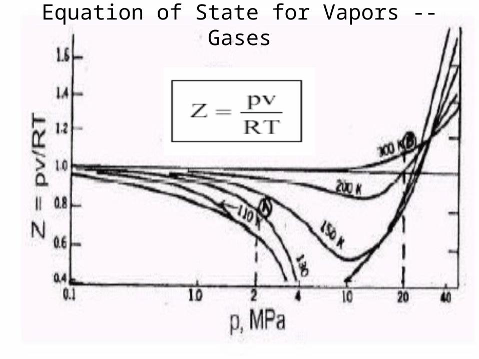
Equation of State for Vapors -- Gases

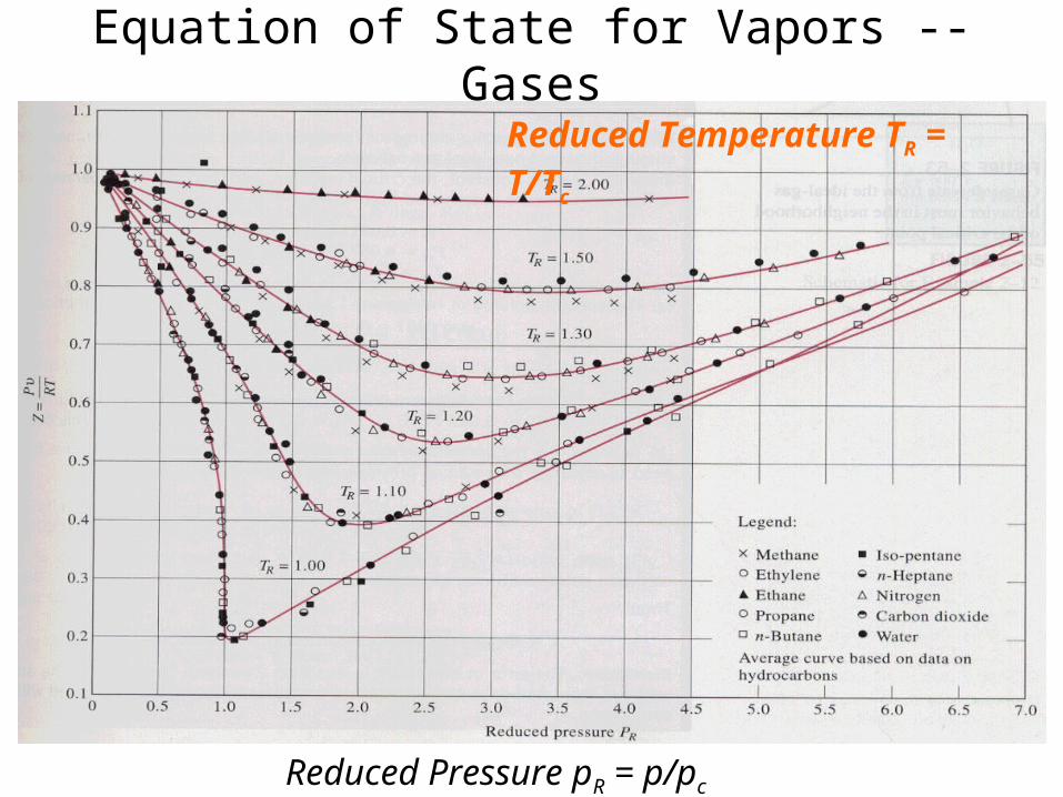
Equation of State for Vapors -- Gases

Reduced Pressure pR = p/pc

Reduced Temperature TR = T/Tc

Measurement equation

• The case of interest is where the quantity Y being measured, called the measurand.

• It is never measured directly, but is determined from N other quantities X1, X2, . . . , XN through a functional relation f, often called the measurement equation

Y = f(X1, X2, . . . , XN)

•Included among the quantities Xi are corrections (or correction factors), as well as quantities that take into account other sources of variability, •such as different observers, •instruments, •samples, •laboratories, and •times at which observations are made (e.g., different days).

• Thus, the function f of equation  should express not simply a physical law but a measurement process.

• In particular, it should contain all quantities that can contribute a significant variation to the measurement result.

• An estimate of the measurand or output quantity Y, denoted by y, is obtained from previous equation using

• input estimates x1, x2, . . . , xN for the values of the N input quantities X1, X2, . . . , XN.

• Thus, the output estimate y, which is the result of the measurement, is given by

y = f(x1, x2, . . . , xN).

The measure of a measurand is not only different from true value, but also random !!!!

Uncertainty

• "A parameter associated with the result of a measurement, that characterizes the dispersion of the values that could reasonably be attributed to the measurand“

• The word uncertainty relates to the general concept of doubt.

• The word uncertainty also refers to the limited knowledge about a particular value.

• Uncertainty of measurement does not imply doubt about the validity of a measurement;

• On the contrary, knowledge of the uncertainty implies increased confidence in the validity of a measurement result.

Error and Uncertainty• It is important to distinguish between error and uncertainty. • Error is defined as the difference between an individual result

and the true value of the measurand. • Error is a single value. • In principle, the value of a known error can be applied as a

correction to the result.• Error is an idealized concept and a single number, which cannot

be known exactly.• Uncertainty takes the form of a range, and, if estimated from an

analytical procedure and a defined sample type, may apply to all determinations so described.

• In general, the value of the uncertainty cannot be used to correct a measurement result.

• The difference between error and uncertainty should always be borne in mind.

• The result of a measurement after correction can unknowably be very close to the unknown value of the measurand, and thus have negligible error,

• Even though it may have a large uncertainty

The Uncertainty

• The uncertainty of the measurement result y arises from the uncertainties u (xi) (or ui for brevity) of the input estimates xi that enter equation.

• Components of uncertainty may be categorized according to the method used to evaluate them.

Components of Uncertainty

• “Component of uncertainty arising from a random effect” : Type A

• These are evaluated by statistical methods.

• “Component of uncertainty arising from a systematic effect,”: Type B

• These are evaluated by other means.

Definitions

• Let x be the value of a measured quantity.

• Let ux be the uncertainty associated with x.

• When we write

• x = xmeasured ± ux (20:1)

• we mean that• x is the best estimate of the measure value,

• xmeasured is the value of x obtained by correction of the measured value of x,

• ux is the uncertainty at stated odds.

• Usually 20:1 odds

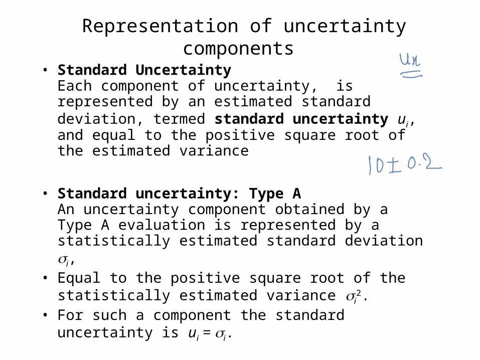
Representation of uncertainty components

• Standard UncertaintyEach component of uncertainty, is represented by an estimated standard deviation, termed standard uncertainty ui, and equal to the positive square root of the estimated variance

• Standard uncertainty: Type AAn uncertainty component obtained by a Type A evaluation is represented by a statistically estimated standard deviation i,

• Equal to the positive square root of the statistically estimated variance i

2.• For such a component the standard uncertainty is ui = i.

Repeated Measurand of Peak Pressure in Diesel Engine

5.15

5.2

5.25

5.3

5.35

5.4

0 50 100 150 200 250 300

No. of Measurements

ppeak

0

5

10

15

20

25

30

35

40

45

50

PDF of Measurand of Peak Pressure

5.15 – 5.165.29 – 5.30

Mean and standard deviation

Consider an input quantity Xi whose value is estimated from n independent observations Xi ,k of Xi obtained under the same conditions of measurement. In this case the input estimate xi is usually the simple mean

n

kkiii X

nXx

1,

1

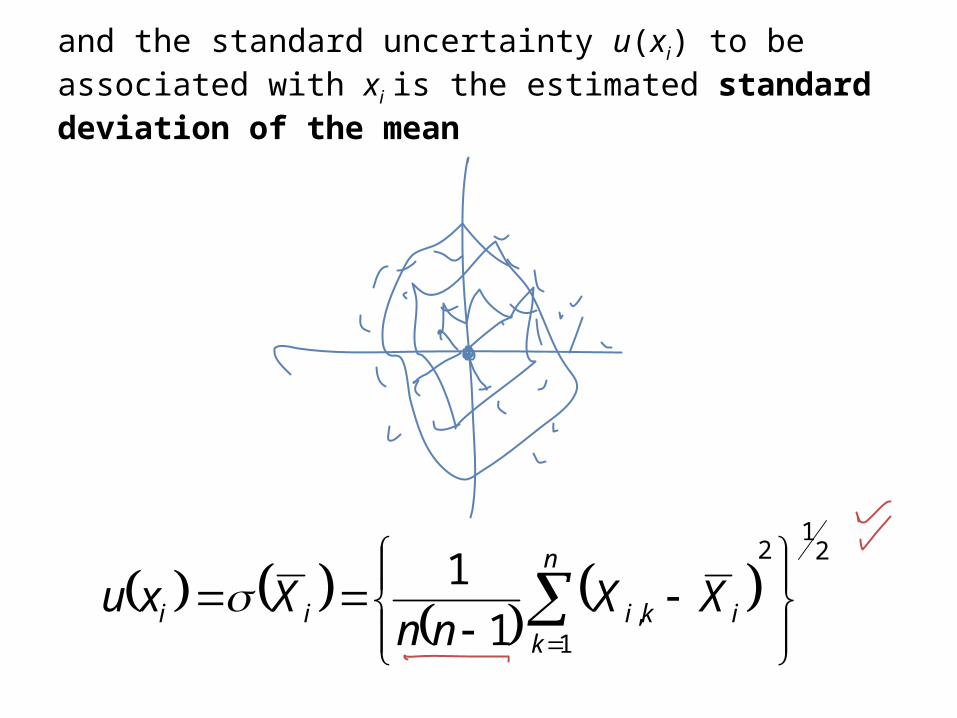
and the standard uncertainty u(xi) to be associated with xi is the estimated standard deviation of the mean

2

12

1,1

1

n

kikiii XX

nnXxu

Standard uncertainty: Type B

• This uncertainty is represented by a quantity uj , • May be considered as an approximation to the

corresponding standard deviation; which is it is equal to the positive square root of uj

2.• uj

2 may be considered an approximation to the corresponding variance and which is obtained from an assumed probability distribution based on all the available information.

• Since the quantity uj2 is treated like a variance and uj like a

standard deviation, • for such a component the standard uncertainty is simply uj.

Evaluating uncertainty components: Type B

• A Type B evaluation of standard uncertainty is usually based on scientific judgment using all of the relevant information available, which may include:

• previous measurement data, • experience with, or general knowledge of, the behavior and

property of relevant materials and instruments, • manufacturer's specifications, • data provided in calibration and other reports, and • uncertainties assigned to reference data taken from handbooks. • Broadly speaking, the uncertainty is either obtained from an

outside source, or obtained from an assumed distribution.

Uncertainty obtained from an outside source

• Procedure:  Convert an uncertainty quoted in a handbook, manufacturer's specification, calibration certificate, etc.,

• Multiple of a standard deviation • A stated multiple of an estimated standard deviation to a

standard uncertainty.• Confidence interval • This defines a "confidence interval" having a stated level

of confidence, such as 95 % or 99 %, to a standard uncertainty.

Uncertainty obtained from an assumed distribution

• Normal distribution: "1 out of 2" • Procedure:  Model the input quantity in question

by a normal probability distribution.• Estimate lower and upper limits a- and a+ such

that the best estimated value of the input quantity is (a+ + a-)/2

• There is 1 chance out of 2 (i.e., a 50 % probability) that the value of the quantity lies in the interval a- to a+.

• Then uj is approximately 1.48 a, where a = (a+ - a-)/2 is the half-width of the interval.

Uncertainty obtained from an assumed distribution

• Normal distribution: "2 out of 3" • Procedure:  Model the input quantity in question by a

normal probability distribution.• Estimate lower and upper limits a- and a+ such that the

best estimated value of the input quantity is (a+ + a-)/2 • and there are 2 chances out of 3 (i.e., a 67 %

probability) that the value of the quantity lies in the interval a- to a+.

• Then uj is approximately a, where a = (a+ - a-)/2 is the half-width of the interval

Normal distribution: "99.73 %"

• Procedure:  If the quantity in question is modeled by a normal probability distribution, there are no finite limits that will contain 100 % of its possible values.

• Plus and minus 3 standard deviations about the mean of a normal distribution corresponds to 99.73 % limits.

• Thus, if the limits a- and a+ of a normally distributed quantity with mean (a+ + a-)/2 are considered to contain "almost all" of the possible values of the quantity,

• that is, approximately 99.73 % of them, then uj is approximately a/3,

• where a = (a+ - a-)/2 is the half-width of the interval.

For a normal distribution, ± u encompases about 68 % of the distribution; for a uniform distribution, ± u encompasses about 58 % of the distribution; and for a triangular distribution, ± u encompasses about 65 % of the distribution.

Propagation of Uncertainty in Independent Measurements