Embed Size (px)
Citation preview

waterbouwkundiglaboratorium.be
00_131_2WL rapporten
Development of conceptual models for an integrated catchment management
Subreport 2 Literature review of DSS en WQ
DEPARTEMENTMOBILITEIT &OPENBARE WERKEN
Development of conceptual models for an integrated catchment management
Subreport 2 – Literature review of DSS en WQ
Velez, C.; Van Griensven, A.; Bauwens, W.; Pereira, F.; Vanderkimpen, P.; Nossent, J.; Verwaest, T.; Mostaert, F.
June 2016
WL2016R00_131_2

F-WL-PP10-2 Version 05 VALID AS FROM: 7/01/2016
This publication must be cited as follows:
Velez, C.; Van Griensven, A.; Bauwens, W.; Pereira, F.; Vanderkimpen, P.; Nossent, J.; Verwaest, T.; Mostaert, F. (2016). Development of conceptual models for an integrated catchment management: Subreport 2 – Literature review of DSS en WQ. Version 4.0. WL Rapporten, 00_131. Flanders Hydraulics Research: Antwerp, Belgium.
DEPARTEMENT MOBILITY AND PUBLIC WORKS
Flanders Hydraulics Research
Berchemlei 115, 2140 Antwerpen T +32 (0)3 224 60 35 F +32 (0)3 224 60 36 [email protected] mow.vlaanderen.be waterbouwkundiglaboratorium.be
Nothing from this publication may be duplicated and/or published by means of print, photocopy, microfilm or otherwise, without the written consent of the publisher.

F‐WL‐PP10‐2 Version 05 VALID AS FROM: 7/01/2016
Documentidentification
Title: Development of conceptual models for an integrated catchment management: Subreport 2 – Literature review of DSS en WQ
Customer: Waterbouwkundig Laboratorium Ref.: WL2016R00_131_2
Keywords (3‐5): Conceptual models, Water Management, water quality
Text (p.): 52 Appendices (p.): /
Confidentiality: ☐ Yes Exceptions: ☐ Customer
☐ Internal
☐ Flemish government
Released as from: /
☒ No ☒ Available online
Approval
Author
Velez, C.
Van Griensven A.
Bauwens, W
Reviser
Nossent, J.
Vanderkimpen, P.
Project Leader
Pereira, F.
Research &
Consulting Manager
Verwaest, T.
Head of Division
Mostaert, F.
Revisions
Nr. Date Definition Author(s)
1.0 24/01/2014 Concept version Velez, C.
2.0 05/11/2014 Substantive revision Nossent, J.; Vanderkimpen, P.
3.0 14/03/2016 Revision customer Pereira, F.
4.0 26/05/2016 Final version Van Griensven, A.
Abstract
An overview of the state‐of‐the‐art of water quality modelling for water quality management is presented. There are different types of models: data driven black box models, empirical/conceptual models and physically‐based models. Models are needed to represent the sewer‐waterwater‐river‐catchment system. Also sediment transport is a very important but complex part of water quality modelling. We can observe a variety in complexity, also within the DSS systems. For example, at the catchment domain the generation of water quality components can be as simple as imposing a concentration at the outlet (e.g EMC) as in WaterCAST to a more complex process based approach as in LASCAM. In‐river water quality processes are also modelled with different degrees of complexity, from the extended Streeter and Phelps equation in StreamPlan to a multi‐level of complexity as in AQUATOOL.
At present, most applied models are physically based, but the integration of complex physically based models in integrated systems may become too complex. There is hence a need for simplified models that can easily be integrated in an integrated water quality model system.
Abstract
Het rapport geeft een overzicht van waterkwaliteitsmodellen en hun gebruik in beslissingsondersteunende systemen (BOS). Er zijn verschillende soorten modellen in gebruik: fysiche modellen, conceptuele modellen, empirische modellen en datadriven modellen.
Samengevat kan er gesteld worden dat er verschillende graden van complexiteit gebruikt worden, ook binnen BOS.

F-WL-PP10-2 Version 05 VALID AS FROM: 7/01/2016
Rivierbekkenmodellen kunnen zeer sterk vereenvoudigd zijn, van een constante concentratie in de rivier (e.g. EMC) tot een complex procesgebaseerde modellering zoals in LACSAM. Bij de rivierwaterkwaliteitsprocessen zien we ook verschillende niveau's van complexiteit, van een 'Streeter-Phelps' vergelijking in StreamPlan tot een multi-niveau complexe modellering zoals in AQUATOOL.
Veel toepassingen van waterkwaliteitsmodelleringsmodellen maken gebruik van complexe modellen, maar de integratie van deze modellen is moeilijk en doorgaans niet gebruiksvriendelijk. Om die reden is er een nood aan eenvoudige modellen die gemakkelijk geïntegreerd kunnen worden binnen beslissingsondersteunende systemen.

Development of conceptual models for an integrated catchment management: Subreport 2 – Literature review of DSS en WQ
Final version WL2016R00_131_2 I F-WL-PP10-2 Version 05 VALID AS FROM: 7/01/2016
CONTENTS
Contents ................................................................................................................................................................... I
List of tabels ............................................................................................................................................................ III
list of figures .......................................................................................................................................................... IV
1 Literatuuroverzicht conceptuele modelstructuren .......................................................................................... 1
1.1 Inleiding ..................................................................................................................................................... 1 1.1.1 Doelstellingen ..................................................................................................................................... 1 1.1.2 Soorten modellen ............................................................................................................................... 2
1.2 Waterkwaliteitsmodellering ...................................................................................................................... 2 1.2.1 Vereisten ............................................................................................................................................. 2 1.2.2 Modellering van waterkwaliteitscomponenten ................................................................................. 2
1.3 Beslissingsondersteunende systemen voor waterkwaliteitsbeheer ......................................................... 2 1.4 Conclusie .................................................................................................................................................... 3
2 Introduction to modeling concepts .................................................................................................................. 4
2.1 General framework .................................................................................................................................... 4 2.2 Model types ............................................................................................................................................... 5
2.2.1 Empirical and data driven models ...................................................................................................... 5 2.2.2 Physically-based models ..................................................................................................................... 6 2.2.3 Conceptual models ............................................................................................................................. 7
3 Water quality modelling ................................................................................................................................... 8
3.1 Requirements for water quality modelling................................................................................................ 8 3.1.1 Software Requirements ...................................................................................................................... 8 3.1.2 Requirements of Process and Water Quality Components ................................................................ 9
3.2 Important water quality concepts ............................................................................................................. 9 3.2.1 Qual2E ................................................................................................................................................. 9 3.2.2 RWQM ................................................................................................................................................. 9
3.3 Conclusion................................................................................................................................................ 10
4 Modelling approaches of pollutant transport ................................................................................................ 11
4.1 Advection and diffusion processes .......................................................................................................... 11 4.2 Sediment transport .................................................................................................................................. 12 4.3 Conceptual advection-dispersion model for rivers ................................................................................. 13 4.4 Analytical solutions of the advection-dispersion equation ..................................................................... 14 4.5 Some conceptual sediment/pollutant transport models ........................................................................ 16
4.5.1 The LASCAM sediment transport model .......................................................................................... 16 4.6 The AGNPS sediment transport model .................................................................................................... 18
4.6.1 The GESZ sediment transport model ................................................................................................ 19 4.6.2 The linear reservoir pollutant transport model ................................................................................ 21
4.7 Conclusions .............................................................................................................................................. 21

Development of conceptual models for an integrated catchment management: Subreport 2 – Literature review of DSS en WQ
Final version WL2016R00_131_2 II F-WL-PP10-2 Version 05 VALID AS FROM: 7/01/2016
5 Modelling approaches for pollutant transport in sewers ............................................................................... 23
5.1 Introduction ............................................................................................................................................. 23 5.2 Some conceptual sewer models in use for pollutant transport .............................................................. 26
5.2.1 KOSIM ............................................................................................................................................... 26 5.2.2 The parsimonious sewer wash-off and transport model by Willems ............................................... 27
5.3 Conclusions .............................................................................................................................................. 27
6 Modelling the fate of water quality components in catchments ................................................................... 28
6.1 Pollutant generation in natural catchments ............................................................................................ 28 6.2 Sediment and nutrient load estimation techniques ................................................................................ 29
6.2.1 Load estimation using field data ....................................................................................................... 29 6.2.2 Empirical models ............................................................................................................................... 32
6.3 Erosion and sediment/nutrient transport modelling .............................................................................. 33 6.3.1 Empirical models ............................................................................................................................... 33 6.3.2 Conceptual models ........................................................................................................................... 34 6.3.3 Physically-based models ................................................................................................................... 34
7 Some water quality models ............................................................................................................................ 36
7.1.1 The WEST model ............................................................................................................................... 36 7.1.2 SOBEK model..................................................................................................................................... 37 7.1.3 The SWAT model ............................................................................................................................... 37
8 Decision support systems for water quality management ............................................................................. 39
8.1 Classification and Components................................................................................................................ 39 8.1.1 Situation and problem specific EDSS ................................................................................................ 39 8.1.2 Problem specific EDSS ....................................................................................................................... 39
8.2 Features and Components of an EDSS .................................................................................................... 40 8.3 Problems Addressed by Environmental Decision Support Systems ........................................................ 42 8.4 Examples of Decision Support Systems for Water Quality Management ............................................... 42
8.4.1 Overview ........................................................................................................................................... 42 8.4.2 Domain and problems addressed ..................................................................................................... 44 8.4.3 Modelling tools ................................................................................................................................. 45 8.4.4 Conclusion ......................................................................................................................................... 47
9 References ...................................................................................................................................................... 48

Development of conceptual models for an integrated catchment management: Subreport 2 – Literature review of DSS en WQ
Final version WL2016R00_131_2 III F-WL-PP10-2 Version 05 VALID AS FROM: 7/01/2016
LIST OF TABELS Table 1 - Schematic overview of different model types. After (Willems, 2000). .................................................... 6
Table 2 - Direct estimation techniques (Letcher et al., 1999). .............................................................................. 31
Table 3 - Domain and problems addressed by environmental decision support systems.................................... 45
Table 4 - Water quality variables used as indicators in the decision support systems ......................................... 45
Table 5 - Modelling tools used by the decision support systems. ......................................................................... 46

Development of conceptual models for an integrated catchment management: Subreport 2 – Literature review of DSS en WQ
Final version WL2016R00_131_2 IV F-WL-PP10-2 Version 05 VALID AS FROM: 7/01/2016
LIST OF FIGURES Figure 1 - Scheme used for building a conceptual model based on the results of a process-based model. .......... 7
Figure 2 - Schematic showing the process of longitudinal dispersion. Tracer is injected uniformly at (a.) and stretched by the shear profile at (b.). At (c.) vertical diffusion has homogenized the vertical gradients and a depth-averaged Gaussian distribution is expected in the concentration profiles (Socolofsky and Jirka, 2005). . 11
Figure 3 - Schematic of processes occurring at the sediment-water interface, in the water column and in the sediment bed ......................................................................................................................................................... 13
Figure 4 - Structure of the sediment transport algorithm (Viney and Sivapalan, 1999) ....................................... 17
Figure 5 - Schematic representation of the a) dispersion; b) advection processes in a tank or sewer system with linear reservoir representation (Willems, 2010) ........................................................................................... 24
Figure 6 - Components of Environmental Decision Support Systems. Modified from (Denzer, 2005) ................. 41

Development of conceptual models for an integrated catchment management: Subreport 2 – Literature review of DSS en WQ
Final version WL2016R00_131_2 1 F-WL-PP10-2 Version 05 VALID AS FROM: 7/01/2016
1 LITERATUUROVERZICHT CONCEPTUELE MODELSTRUCTUREN
Nederlandse samenvatting
1.1 Inleiding 1.1.1 Doelstellingen
Dankzij het werk van de verschillende waterbeheerders in Vlaanderen in de voorbije jaren, beschikt de regio over een uitgebreid model instrumentarium ter ondersteuning van de verschillende waterbeheerders en het waterbeleid. Deze modellen beperken zich echter meestal tot individuele deelcomponenten van het watersysteem en hebben nauwelijks interactie met elkaar. Bovendien zijn de studiegebieden van deze modellen meestal overlappend wat resulteert in gebieden die 2 à 3 keer gemodelleerd zijn met verschillende soorten modellen en door verschillende administraties.
Zo zijn in Vlaanderen gedetailleerde hydrodynamische modellen opgebouwd voor de bevaarbare en de onbevaarbare waterlopen, met behulp van verschillende software en in handen van verschillende administraties. De meeste stroomgebieden hebben ook meer dan één hydrologisch model, en het rioolstelsel is gemodelleerd met nog andere software. Rekening houdende met de evolutie van kennis en modellen verwacht men eerder dat het gebruik van verschillende soorten modellen nog zal toenemen (waterkwaliteit, sediment, ecologische modellen, waterbalans, enz.) niet alleen in Vlaanderen maar ook in de naburige regio’s en landen (Wallonië, Brussel, Frankrijk en Nederland).
Om de huidige evolutie naar een integraal en geïntegreerd waterbeheer op stroomgebiedsniveau voldoende te kunnen ondersteunen is er een integratie nodig van de hogervermelde modellen, rekening houdend met de volgende aspecten:
• Verschillende doelstelling van de modellen. • Verschillende tijds- en ruimteschaal van de processen. • Accumulatie van onzekerheden bij elk systeemmodel. • Interactie van de modellen, waardoor een verbinding tussen modellen noodzakelijk is. • Verschillend detailniveau van de modellen.
Deze “integrale modellering” wordt vandaag aangepakt door de verschillende leveranciers van software met de beperking dat ze compatibel moeten blijven met de huidige en toekomstige producten van die specifieke leverancier, wat in veel gevallen niet compatibel is met de software van andere leveranciers.
Vertrekkend vanuit de bovenvermelde noden heeft de huidige studie als hoofdoel:
• De ontwikkeling en toepassing van een methodologie voor de integraalmodellering van het watersysteem gebaseerd op het gebruik van conceptuele modellen.
De methodologie en toepassing moet toelaten om maximaal gebruik te maken van de bestaande modellen van de verschillende deelsystemen, en moet voldoende ‘open’ zijn om elke uitbreiding met andere deelmodellen mogelijk te maken. De systeemontwikkeling beperkt zich in eerste instantie tot de waterbeheersaspecten: waterkwantiteit en fysico-chemische waterkwaliteit. Het systeem wordt voldoende ‘open’ opgebouwd om een uitbreiding naar andere aspecten zoals ecologie mogelijk te maken. Tijdens de ontwikkeling kunnen rivier-oppervlaktewater, grondwater, rioolstelsels en RWZI’s worden beschouwd.
Het voorliggende rapport kadert in de eerste deelopdracht van de studie, nl. een identificatie en veralgemening van mogelijke conceptuele modelstructuren. Hierbij is er gekeken naar modellen en technieken die op wereldschaal dikwijls toegepast worden voor de simulatie van de verschillende onderdelen van het geïntegreerde watersysteem, en die bovendien toelaten om langdurige simulaties uit te voeren in een zeer korte termijn. De beschouwde componenten van het watersysteem zijn: waterwegen en rivieren (met overstromingsgebieden), estuaria en tijgebonden rivieren, rioleringsstelsels, oppervlakte hydrologie en
Development of conceptual models for an integrated catchment management: Subreport 2 – Literature review of DSS en WQ
Final version WL2016R00_131_2 2 F-WL-PP10-2 Version 05 VALID AS FROM: 7/01/2016
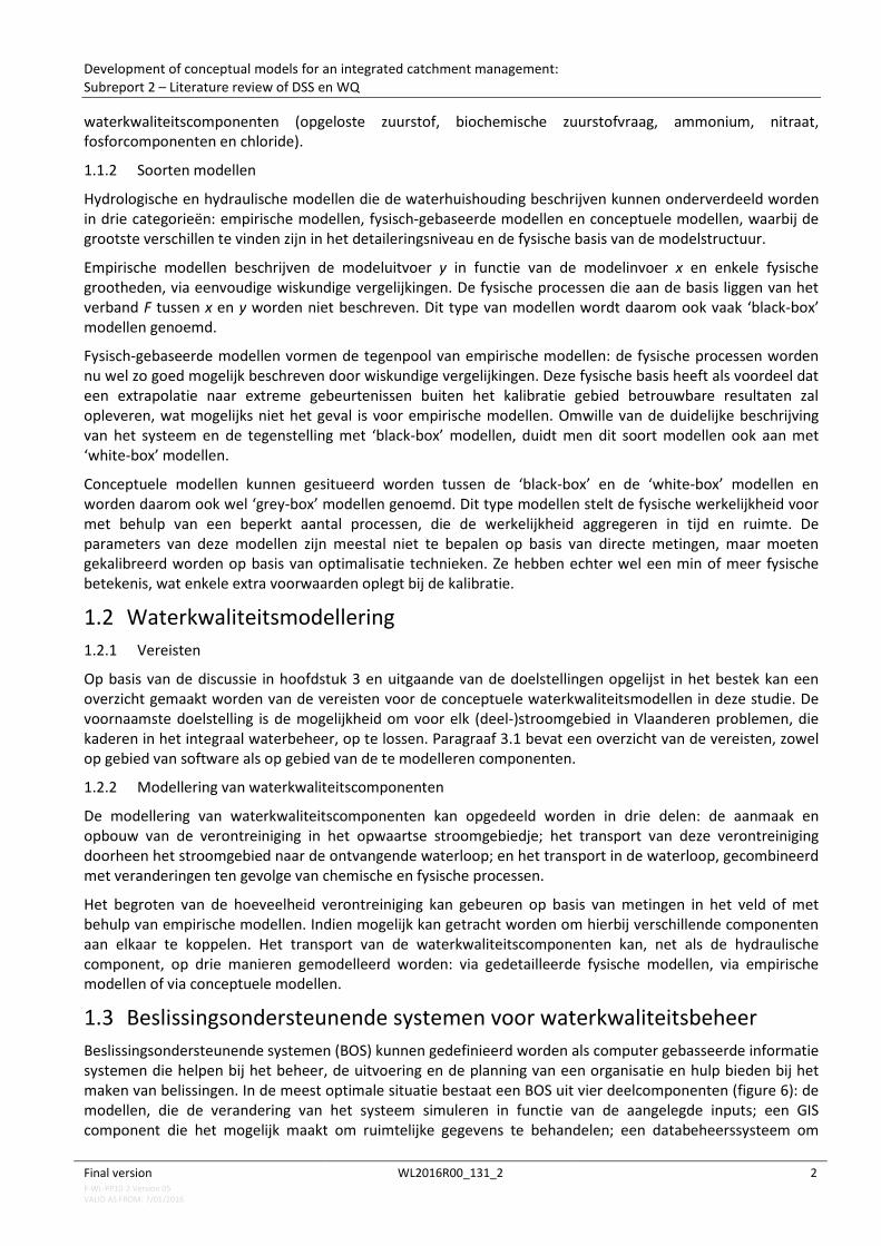
waterkwaliteitscomponenten (opgeloste zuurstof, biochemische zuurstofvraag, ammonium, nitraat, fosforcomponenten en chloride).
1.1.2 Soorten modellen
Hydrologische en hydraulische modellen die de waterhuishouding beschrijven kunnen onderverdeeld worden in drie categorieën: empirische modellen, fysisch-gebaseerde modellen en conceptuele modellen, waarbij de grootste verschillen te vinden zijn in het detaileringsniveau en de fysische basis van de modelstructuur.
Empirische modellen beschrijven de modeluitvoer y in functie van de modelinvoer x en enkele fysische grootheden, via eenvoudige wiskundige vergelijkingen. De fysische processen die aan de basis liggen van het verband F tussen x en y worden niet beschreven. Dit type van modellen wordt daarom ook vaak ‘black-box’ modellen genoemd.
Fysisch-gebaseerde modellen vormen de tegenpool van empirische modellen: de fysische processen worden nu wel zo goed mogelijk beschreven door wiskundige vergelijkingen. Deze fysische basis heeft als voordeel dat een extrapolatie naar extreme gebeurtenissen buiten het kalibratie gebied betrouwbare resultaten zal opleveren, wat mogelijks niet het geval is voor empirische modellen. Omwille van de duidelijke beschrijving van het systeem en de tegenstelling met ‘black-box’ modellen, duidt men dit soort modellen ook aan met ‘white-box’ modellen.
Conceptuele modellen kunnen gesitueerd worden tussen de ‘black-box’ en de ‘white-box’ modellen en worden daarom ook wel ‘grey-box’ modellen genoemd. Dit type modellen stelt de fysische werkelijkheid voor met behulp van een beperkt aantal processen, die de werkelijkheid aggregeren in tijd en ruimte. De parameters van deze modellen zijn meestal niet te bepalen op basis van directe metingen, maar moeten gekalibreerd worden op basis van optimalisatie technieken. Ze hebben echter wel een min of meer fysische betekenis, wat enkele extra voorwaarden oplegt bij de kalibratie.
1.2 Waterkwaliteitsmodellering 1.2.1 Vereisten
Op basis van de discussie in hoofdstuk 3 en uitgaande van de doelstellingen opgelijst in het bestek kan een overzicht gemaakt worden van de vereisten voor de conceptuele waterkwaliteitsmodellen in deze studie. De voornaamste doelstelling is de mogelijkheid om voor elk (deel-)stroomgebied in Vlaanderen problemen, die kaderen in het integraal waterbeheer, op te lossen. Paragraaf 3.1 bevat een overzicht van de vereisten, zowel op gebied van software als op gebied van de te modelleren componenten.
1.2.2 Modellering van waterkwaliteitscomponenten
De modellering van waterkwaliteitscomponenten kan opgedeeld worden in drie delen: de aanmaak en opbouw van de verontreiniging in het opwaartse stroomgebiedje; het transport van deze verontreiniging doorheen het stroomgebied naar de ontvangende waterloop; en het transport in de waterloop, gecombineerd met veranderingen ten gevolge van chemische en fysische processen.
Het begroten van de hoeveelheid verontreiniging kan gebeuren op basis van metingen in het veld of met behulp van empirische modellen. Indien mogelijk kan getracht worden om hierbij verschillende componenten aan elkaar te koppelen. Het transport van de waterkwaliteitscomponenten kan, net als de hydraulische component, op drie manieren gemodelleerd worden: via gedetailleerde fysische modellen, via empirische modellen of via conceptuele modellen.
1.3 Beslissingsondersteunende systemen voor waterkwaliteitsbeheer Beslissingsondersteunende systemen (BOS) kunnen gedefinieerd worden als computer gebasseerde informatie systemen die helpen bij het beheer, de uitvoering en de planning van een organisatie en hulp bieden bij het maken van belissingen. In de meest optimale situatie bestaat een BOS uit vier deelcomponenten (figure 6): de modellen, die de verandering van het systeem simuleren in functie van de aangelegde inputs; een GIS component die het mogelijk maakt om ruimtelijke gegevens te behandelen; een databeheerssysteem om
Development of conceptual models for an integrated catchment management: Subreport 2 – Literature review of DSS en WQ
Final version WL2016R00_131_2 3 F-WL-PP10-2 Version 05 VALID AS FROM: 7/01/2016
zowel inputs als outputs van de verschillende onderdelen te beheren en data-acquisitie mogelijk te maken; en de beslissingsondersteunende component die de vragen van de gebruiker omzet naar scenario’s om door te rekenen met de modellen en de resultaten hiervan terugkoppelt naar de gebruiker. In deze studie zal vooral de model component van belang zijn, bijvoorbeeld de ontwikkeling van nieuwe modellen. Het is echter belangrijk om hierbij steeds rekening te houden met de andere componenten van het systeem.
Paragraaf 4.1 ontleedt een tiental bestaande beslissingsondersteunende systemen die voornamelijk gericht zijn op waterkwaliteitsaspecten. De meeste van deze systemen bestaan niet uit de vier hierboven genoemde componenten, maar uit slechts één of twee. De systemen verschillen bovendien ook erg in complexiteit en niveau van detaillering.
1.4 Conclusie Het rapport geeft een overzicht van waterkwaliteitsmodellering en hun gebruik in beslissingsondersteunende systemen (BOS). Samengevat kan er gesteld worden dat er verschillende graden van complexiteit gebruikt worden, ook binnen BOS. Rivierbekkenmodellen kunnen zeer sterk vereenvoudigd zijn, tot een constante concentratie in de rivier (e.g. EMC) tot een complex procesgebaseerde modellering zoals in LACSAM. Bij de rivierwaterkwaliteitsprocessen zien we ook verschillende niveau's van complexiteit, van een 'Streeter-Phel)lps' vergelijking in StreamPlan tot een multi-niveau complexe modellering zoals in AQUATOOL. Veel toepassingen van waterkwaliteitsmodelleringsmodellen maken gebruik van complexe modellen, maar de integratie van deze modellen is moeilijk en doorgaans niet gebruiksvriendelijk. Om die reden is er een nood aan eenvoudige modellen die gemakkelijk geïntegreerd kunnen worden binnen beslissingsondersteunende systemen.

Development of conceptual models for an integrated catchment management: Subreport 2 – Literature review of DSS en WQ
Final version WL2016R00_131_2 4 F-WL-PP10-2 Version 05 VALID AS FROM: 7/01/2016
2 INTRODUCTION TO MODELING CONCEPTS 2.1 General framework Over the last decades the different water managers in the Flanders region have developed and constructed a large number of models to support their tasks in water management and policy. Despite the undeniable advantages of these models, problems arise when one tries to combine them: the models are mostly limited to individual components of the water system, can hardly interact with each other and are all computationally demanding. Furthermore, there exists an overlap in the study areas of the models, resulting in areas that are modelled twice or more with different model types and by different water managers or public services.
In the Flanders region, detailed hydrodynamic models have been constructed of the navigable and the unnavigable river courses, with different software packages and by different water managers. Most catchments have more than one rainfall-runoff model and sewer systems are modelled with yet another software package. It is expected that the number of models will not decrease over the next years, but quite the opposite: thanks to the increase in computer power and extended knowledge of the different processes (e.g. water quality, sediment transport, ecological models, …) an increase in the number of models can be expected. This increase is of course not limited to the Flanders region, but will also take place in the neighboring regions and countries (Wallonia, Brussels, France and the Netherlands), resulting in yet more (incompatible) models.
To support the current evolution towards an integral and integrated catchment modelling and management in an adequate way, an integration of the different hydrodynamic models will be necessary. This integration should bear in mind the following important topics: the different intentions of the original models, the different time and space scales of the modelled processes, the accumulation of uncertainties of each (sub)component, the interaction and connection of the models and the different level of detail of each model. The currenct policy of most software suppliers, regarding integrated catchment modelling, is to allow and support this kind of modelling with the important limitation that the models have to be compatible with their specific current and future modelling products, which are mostly not compatible with the software of other suppliers.
Based on the needs of the water managers and the problems concerning the interaction and compatibility of the different models, the main purpose of this study is:
The development and application of a methodology for an integrated catchment modelling, based on the use of conceptual models.
This methodology should allow to use the existing models of the different components of the water system (rivers and surface waters, groundwater, sewer systems and waste water treatment plants) at a maximum extent and has to be ‘open’ enough to allow an extension with other (sub)components. This study is limited to the current water management aspects: water quantity and physico-chemical water quality, but should allow future extensions to other aspects, like for example ecology.
The current study consists of five subtasks or work packages. This report is situated in the first work package of the study, whose main objectives are the identification of different types of conceptual models that are (on a global scale) most commonly used for modelling the various components and aspects considered part of integrated catchment modelling; and a generalization of the listed conceptual models to make them applicable for the different components and aspects of the system. This identification and generalization is based on a literature review, which forms the main subject of this report.
The second work package comprises the construction of the chosen model structures and calibration of their parameter values. This should result in a calibration tool that allows a semi-automatic calibration of the conceptual model components, based on the simulation results of fully detailed models. Semi-automatic implies that an interaction with the user is provided to account for expert knowledge.

Development of conceptual models for an integrated catchment management: Subreport 2 – Literature review of DSS en WQ
Final version WL2016R00_131_2 5 F-WL-PP10-2 Version 05 VALID AS FROM: 7/01/2016
In a third work package the conceptual models and model structures are subjected to an uncertainty analysis. This should allow to quantify the reliability of the results of both the (sub)components and the conceptual integrated catchment model. The uncertainty analysis will focus on different types of uncertainties (input values, model parameter values, model structure, measurement errors, …) and their propagation, on the way of quantifying and incorporating these uncertainties, and on the influence of one type of uncertainties on the overall model result.
A decision support system (DSS) for integrated catchment modelling will be built in the fourth workpackage. This decision support system is regarded as an open software tool that incorporates the results of the previous three work packages: identification and calibration of the conceptual model structures, combined with the techniques for uncertainty analysis. The main intention of the DSS is to use the integrated catchment model for simulating the important components of the water system and hereby supporting the decisions of water managers.
In the fifth and last work package the developed techniques, strategies and systems will be demonstrated for two cases: the river Zenne catchment and the river Dender catchment. Both case studies will also be used throughout the study during the execution of the other work packages.
2.2 Model types Different model types are available for simulating the different components of the water system. They range from physically-based models to simplified conceptual and empirical models. The main differences between these models are the level of detail and the physical basis of the model structure. This section gives a brief overview of these three model types.
2.2.1 Empirical and data driven models
Empirical models attempt to find a relation between a model input x and the physical quantities and model outputs y that are the subject of the model. Because a physical basis for the relation F between x and y is missing for these models, they are often referred to as ‘black-box models’. The models are built and calibrated with simultaneous measurements of x and y, which therefore need to be representative and sufficiently long. Furthermore, the model structure might depend on the period that was selected for calibration, with the consequence that extrapolation outside the calibration range (e.g. to extreme events) might be very inaccurate. Application of empirical models is workable when the amount of data is sufficiently large and the model structure is very simple. (Willems, 2013) Although this is mostly not the case for hydrologic and hydraulic systems, some examples of empirical models for the different components of the water system can be found in literature. Examples are the simplified rainfall-runoff models of section, like the rational and SCS method, and the response surface method for water level prediction in tidal rivers.
In the past two decades a new type of black-box models has been increasingly applied: data driven models. These techniques make use of computational intelligence methods (particularly machine learning) in building models. Machine learning is an area of computer science that concentrates on the theoretical foundations of learning from data (Solomatine and Ostfeld, 2008). The technique takes a known set of input data and known responses to the data, and seeks to build a predictor model that generates reasonable predictions for the response to new data. Data driven models have the same problems as empirical models: they provide little physical insight into the system and are therefore likely to be less robust and possibly unreliable outside the calibration range (Lees, 2000; Lekkas et al., 2001). An overview of the application of data driven models to the different components of the water system can be found in (Lockus et al., 2005) and (Solomatine and Ostfeld, 2008).
A limited number of empirical and data driven models (further referred to as black-box models) are considered in this report, because they have been applied in the Flanders region before. The intention is, however, to disregard these black-box models in the next subtasks of the study because of the earlier mentioned drawbacks.

Development of conceptual models for an integrated catchment management: Subreport 2 – Literature review of DSS en WQ
Final version WL2016R00_131_2 6 F-WL-PP10-2 Version 05 VALID AS FROM: 7/01/2016
Table 1 - Schematic overview of different model types. After (Willems, 2000).
Modelling types
Incr
easin
g le
vel o
f phy
sical
ly-b
ased
m
odel
ling
Physically- based models White box Most model parameters
can be measured e.g. Hydrodynamic models
Conceptual models Grey box
Model parameters need calibration (e.g. using measurements for model output variables)
e.g. Linear reservoir models
Empirical models Data driven models Black box
Also the model structure building depends on the measurements for the model output variables
e.g. Artificial Neural Networks
2.2.2 Physically-based models
Physically based models are the opposite of empirical models, because they do describe the physical processes between model inputs and outputs, with mathematical equations. Since it is impossible to describe and calculate each single one of these physical processes, the models are limited to the main processes that describe the largest part of the relation between x and y. Because of the link with the physical processes underlying the description of the input-output relation, the model structure is transparent. The models are therefore often called ‘mechanistic’ or ‘internally descriptive’ or ‘white box models’. (Willems, 2000; Willems, 2013)
The physical processes modelled in physically-based models can be described mathematically on a macroscopic or microscopic scale. The former uses mathematical equations to describe the processes as they can be observed or perceived, whereas the latter tries to model the processes on a microscopic scale that are responsible of the macroscopic observations. The second approach will contribute to a better understanding of the macroscopic processes, but offers too few advantages when modelling on catchment scale and will have a large impact on the calculation times of the model. (Willems, 2013)
Physically based models for hydrologic and hydraulic applications are based on two conservation laws, which govern the behavior of a fluid. These laws involve the conservation of mass or volume, known as continuity, and the conservation of momentum or conservation of energy (Zoppou, 2001):
0=∂∂
+∂∂
xQ
tA
hu
gqSS
xh
xu
gu
tu
g f ⋅−−=∂∂
+∂∂⋅+
∂∂⋅ 0
1
( 2.1 )
( 2.2 )
With A the cross-sectional area, Q the discharge, u the average current velocity, g the gravitational acceleration, h the water height or depth, S0 the bed slope and Sf the friction slope. Equations ( 2.1 ) and ( 2.2 ) are also known as the ‘shallow water equations’ or the ‘de Saint-Venant equations’. The continuity equation ( 2.1 ) states that the rate of change in water depth (or cross-sectional area) with time in a slice of the channel equals the net inflow into the slice of channel. The momentum equation ( 2.2 ) expresses that the rate of change in momentum within a slice of the channel is equal to the sum of forces acting on the slice. (Zoppou, 2001)

Development of conceptual models for an integrated catchment management: Subreport 2 – Literature review of DSS en WQ
Final version WL2016R00_131_2 7 F-WL-PP10-2 Version 05 VALID AS FROM: 7/01/2016
The ‘de Saint-Venant’ equations form a system of quasi-linear, hyperbolic partial differential equations. They can be solved fully or with a simplified form of the momentum equation, when some terms are neglected. It is important to notice that these simplified solutions are only accurate in situations where the approximations are valid. The full hydrodynamic de Saint-Venant equations (thus with the complete momentum equation) provide an accurate solution under different boundary conditions and a wide range of possible configurations of river networks. (Willems, 2013) A number of different solution schemes exist for fhese full hydrodynamic solutions (implicit, explicit, 1D, 2D, quasi-2D), which all can be time consuming. This issue will become problematic in applications like real-time control or another type of optimization, uncertainty analysis and long term simulations. (Villazon, 2011)
2.2.3 Conceptual models
Conceptual models attempt to simulate the most important perceived processes in a lumped way: they are aggregated in space and time into a number of key responses. This type of models can be regarded as physically-inspired or quasi-physical, in-stead of physically-based, since they have a structure that is based on a simplified representation of the physical process that take place in reality. (Knight and Shamseldin, 2006) Because the physical reality (and its underlying processes) are less transparent than for a detailed physically-based model, a conceptual model is also called a ‘grey-box model’ (Willems, 2000).
Conceptual model parameters usually refer to a collection of aggregated processes and may cover a large number of subprocesses that are not covered by the model structure (Wagener et al., 2004). The parameters can be divided in two classes: those with a direct physical significance that may be determined by measurements or from general knowledge or experience; and those which can not be measured directly but must be calibrated by optimization, usually subjected to physical limits based on their interpretation (Knight and Shamseldin, 2006). The second type of parameters forms the vast majority.
In reality, the number of observation points is insufficient to allow an adequate calibration of conceptual models. That is why in this study they will be calibrated based on the previously constructed physically-based models, so that the information that is available within these models is used to a maximum extent. The suggested procedure to go from the real water system to a conceptual model of it can be summarized as follows (Vanrolleghem et al., 2005):
I. Determine the system under study, its boundaries and the problem to be solved. II. Collect data on the system to calibrate a complex mechanistic model.
III. Calibrate and validate the complex mechanistic model. IV. Generate data with the complex model to calibrate the surrogate model. V. Calibrate and validate the surrogate model.
A scheme of the procedure is presented in Figure 1. In general, the approach has been applied to build conceptual and data driven models that replicate complex process-based models.
Figure 1 - Scheme used for building a conceptual model based on the results of a process-based model.
Development of conceptual models for an integrated catchment management: Subreport 2 – Literature review of DSS en WQ
Final version WL2016R00_131_2 8 F-WL-PP10-2 Version 05 VALID AS FROM: 7/01/2016
3 WATER QUALITY MODELLING 3.1 Requirements for water quality modelling The key to the development of a successful software is the correct understanding of the problem by the developer (Ghiaseddin, 1986). This section intends to summarize the key points that were discussed earlier in this document and relate those to what could be the requirements for the conceptual models in general, and in particular for water quality modelling.
3.1.1 Software Requirements
From the perspective of this study, the tools for a DSS will fit within the “problem specific” category. In other words, the models developed should address problems within the domain of integrated water resources management (IWRM), but should be customizable to generate a DSS that addresses the specific situation of each catchment in Flanders. Therefore the modelling tools should have:
- The ability to support quick production of decision support systems. - Inherent features of modifiability as well as extendibility. - The ability for model reusability. This is a software development premise: use as much as possible
existing code instead of developing everything from scratch. - The ability for model coupling. Models of different domains within a water system should be linkable. - The adaptability to changes in the modelling system, in order to deal with changes in the environment
or in the decision making approach. - Any interface that facilitates the use by non-computer literate users.
Based on their experience with EDSS, Argent et al. (2009) produced a set of requirements for the new modelling system:
- Transparent modelling, wherein a modeller is able to explore, write and record, model parameters and state variables at any and/or every time step. Such a system also supports transparency for end users, albeit through customised user interfaces.
- Support for choice of alternative models, methods and systems, wherever possible. This reflects not only the frustration arising from systems with only one option for e.g. a runoff model, catchment delineation, or output, but also the desire to make best use of software engineering concepts such as inheritance and instantiation. It is important to be able to choose between different levels of complexity for the representation of the system.
- Flexible representation of space and time in modelling, with a software architecture that uses neither a fixed spatial scale or discretisation method nor a fixed time step for modelling.
- Support for quick model set-up, requiring only delineation of a catchment to produce a ‘working’ specific DSS, with all other processes (e.g. runoff, routing) to be defined and calibrated later
- Other desirable features, such as advanced tools for model calibration and the flexibility to select which output variables would be recorded in a model run, were also identified, arising, again, from experience with the high and lows of existing modelling systems.
The nature of the problems addressed by environmental managers is diverse and very complex. The complexity of environmental problems most likely will continue forcing the use of complex process-based models when searching for solutions. For this study there are two more requirements that have not been mentioned before and are perhaps some of the most important:
- The conceptual models should be able to represent the water system as accurate as the process-based model does.
- The conceptual models should be significantly faster than the complex process-based models. In other words they should be computationally very efficient.

Development of conceptual models for an integrated catchment management: Subreport 2 – Literature review of DSS en WQ
Final version WL2016R00_131_2 9 F-WL-PP10-2 Version 05 VALID AS FROM: 7/01/2016
3.1.2 Requirements of Process and Water Quality Components
The IWRM approach implies the use of models for different domains: catchment drainage, urban drainage, wastewater treatment and rivers or other receiving systems. This implies the integration of models for different components of the water system. Therefore, some of the requirements are:
- The ability to generate, route, transform, extract, add, monitor and control flow and constituents through the system. These requirements are fundamental to application of models in management.
- A capacity for modelling one or more conservative and non- conservative water constituents, arising from needs of different problem situations.
- Based on the problems presented in the review of the RBMPs for Flanders, the priority for modelling constituents should be given to water pollution with nutrients and oxygen-binding substances (BOD, COD).
- Diffuse pollution appears to be the first cause of surface water impairment. Modelling tools should allow the implementation of control strategies to deal with this kind of pollution.
- The need to increase the urban wastewater treatment in terms of quantity and efficiency is another scenario that should be readily available for implementation within the set of conceptual models
- The modelling tools should be able to represent and manipulate flow control structures. - The models should also be able to represent water quality components that are used for operational
purposes. Here the parameters requested by FHR are: salinity, chloride and suspended sediments.
The requirements presented hereabove are used in the next section to organize the discussion of existing conceptual models that could fulfil the requirements of this project.
3.2 Important water quality concepts 3.2.1 Qual2E
The traditional Qual2E model is based on the phenomenological approach of the Streeter-Phelps equations. The main state variables are the BOD (Biological Oxygen Demand) and DO (Dissolved Oxygen). Later, new state variables and processes have been added, resulting in a 3-layer model (Masliev et al. 1995):
• The phenomenological level: the traditional Streeter-Phelps state variables BOD and Dissolved Oxygen (DO);
• The biochemical level: the extended Streeter-Phelps model variables ammonia, nitrate, nitrite and Sediment Oxygen Demand (SOD);
• The ecological level: the algae model variables organic nitrogen, organic phosphorus, dissolved phosphorus and algae biomass (as chlorophyll-a).
Due to these different levels, the mass balances are not always consistent (Masliev et al., 1995; Shanahan et al., 1998). For instance the processes dealing with the sediments are not linked to the river column processes, allowing a higher release by the river bed than what has historically deposited. Also, using BOD as a measure for organic carbon is not directly fitting in mass balances, as it is not a quantitative mass value but only has a biological meaning. BOD is also harder to estimate than COD (Chemical Oxygen Demand). However, the equations can transformed to be applicable for slow and fast COD variables.
3.2.2 RWQM
The River Water Quality Model (RWQM) (Reichert et al., 2001) has its roots in the Activated Sludge Model (ASM) for Waste Water Treatment Plants (WWTP) (Henze et al., 1995). To take the activated sludge processes as the basis for a river model is quite logic, as both river and WWTP pollutants undergo common processes such as bio-oxidation, bio-deoxygenating or bio-denitrification. Other processes - such as photosynthesis - occur more typically in rivers, and had to be added to the ASM. The ASM is characterised by a high level of complexity in process formulation, state variables and parameters, whereby a consistent mass balance is

Development of conceptual models for an integrated catchment management: Subreport 2 – Literature review of DSS en WQ
Final version WL2016R00_131_2 10 F-WL-PP10-2 Version 05 VALID AS FROM: 7/01/2016
respected at all levels. In an activated sludge basin, the process of pollutant removal is based and controlled by the presence of microbial organisms and hence is modelled as such in ASM.
The RWQM has thus also a strong physical/biological basis. The main problem is that the high complexity leads to a high number of variables and - most of all - parameters (24 variables, 36 kinetic parameters, 6 equilibrium parameters, 13 stoechiometric parameters, 36 mass fractions if only the water column is taken into account). The parameter estimation problems seem to be the biggest disadvantage of the model (Maryns and Bauwens, 1997).
Also, the use of state variables for the microbial biomass is not appropriate for rivers. In a WWTP, these microbial biomasses are already difficult to monitor and to model. This is certainly the case for a river due to its higher level of complexity in time, space and ecology. These bio-masses are not generally included in a river-monitoring program. The calibration of these biomasses processes is hard to perform, as growth, respiration and decay of biomasses behave interactively. They can therefore not easily be distinguished. Even in a WWTP, dynamic measurements as OUR (oxygen uptake rate) are needed to allow for a very reliable calibration and reliable simulations (Henze et al., 1995).
To overcome this complexity, the IAWQ task group suggests simplifying the model by selecting the case specific dominant sub-models. To exclude the bacterial biomasses, they propose a solution where the bacterial biomass is kept constant by considering growth and decay as equal (Vanrolleghem et al., 2001). This solution is however only valid for steady state, as this implies a constant oxygen and COD concentration in the Monod limitations.
Another approach is proposed by Reichert (2001) where a constant biomass concentration is defined and substituted as such in the rate equations. This can be justified for slow growing organisms and for a relative short simulation time. In other cases, this might lead to mass balance errors, as differences between the growth and decay are not included in the mass balance.
3.3 Conclusion
QUAL2E model is the simplest water quality concept involving fewer parameters that is observed to give comparable results with the detailed water quality models. Hence, it would be used to conceptualize the pollutant transformation processes in the river.

Development of conceptual models for an integrated catchment management: Subreport 2 – Literature review of DSS en WQ
Final version WL2016R00_131_2 11 F-WL-PP10-2 Version 05 VALID AS FROM: 7/01/2016
4 MODELLING APPROACHES OF POLLUTANT TRANSPORT 4.1 Advection and diffusion processes The transport of dissolved or suspended substances is dependent on the interaction between differential convection and turbulent diffusion which are both dependent up on the flow velocity field (Cunge et al., 1980). The gradients of concentration and velocity in the vertical direction (see.Figure 2) are responsible for the increased longitudinal dispersion (Socolofsky and Jirka, 2005). Hence, the results of unsteady flow simulations are often used as the hydrodynamic basis for water quality models (Cunge et al., 1980).
Majority of pollutants mix feely with water (James, 2005) hence advection-dispersion equation is widely used to predict the concentration of suspended sediments and water quality indicator variables in sewers (Garsdal et al., 1995) and along rivers and channels (Kashefipour and Falconer, 2002).
While Advection is defined as a mass transport of solute at the velocity of the bulk fluid, dispersion is the spreading of a pollutant following the concentration gradient (James, 2005). Pollutant dispersion process occurs due to three phenomena: molecular diffusion, turbulent diffusion and mechanical dispersion (Cunge et al., 1980). Turbulent diffusion is much greater than molecular diffusion and mechanical dispersion coefficients are much larger than turbulent diffusion coefficients hence only turbulent diffusion and mechanical dispersion can be considered in stream pollutant transport (Cunge et al., 1980; Socolofsky and Jirka, 2005).
Figure 2 - Schematic showing the process of longitudinal dispersion. Tracer is injected uniformly at (a.) and stretched by the shear profile at (b.). At (c.) vertical diffusion has homogenized the vertical gradients and a depth-averaged Gaussian
distribution is expected in the concentration profiles (Socolofsky and Jirka, 2005).
Modelling of these processes becomes increasingly critical to assess evolution of accidental spills of pollutants in water bodies so that stake holders can identify critical zones and be prepared for counteract measures (Ani et al., 2010a).
For a conservative pollutant driven by advection-dispersion processes, the one dimensional transport can be described by the principle of Fick’s law (4.1).
xcV
xcD
xtc
∂∂
−
∂∂
∂∂
=∂∂ )(
(4.1)

Development of conceptual models for an integrated catchment management: Subreport 2 – Literature review of DSS en WQ
Final version WL2016R00_131_2 12 F-WL-PP10-2 Version 05 VALID AS FROM: 7/01/2016
Where, c (mg/L) is the pollutant concentration in time (t (s)) along the river length (x (m));
D (m2/s) is the longitudinal dispersion coefficient; V (m/s) is the convective velocity;
For the non-conservative pollutant, the one dimensional advection-dispersion equation can would be modified by introducing transformation term (4.2) (Ani et al., 2011; Ani et al., 2010).
Kcx
cVxcD
xtc
±∂
∂−
∂∂
∂∂
=∂∂ )(
(4.2)
Where, K (1/s) gives the pollutant transformations;
The dispersion coefficient implicitly contains the effect of mechanical dispersion and turbulent diffusion. As discussed earlier, the molecular diffusion coefficient can be ignored unless the fluid is at rest.
Advection and dispersion processes are dominant modes of transport during accidental spills and need to be modelled as accurate as possible without being computationally demanding. Despite being accurate, numerical models are computationally demanding hence the use of conceptual models become increasingly important for certain purposes like real time forecast of pollutant concentration following accidental spills and uncertainty analysis. Equally, analytical solutions of advection-dispersion models are fast and accurate (Ani et al., 2009; Ani et al., 2010a) which makes them potential candidate for the desired purpose.
4.2 Sediment transport Sediment transport plays significant role in characterizing the water quality behaviour of rivers and sewers. Several pollutants are transported attached to the suspended sediments hence sediments are reservoirs of pollutants (Jamieson et al., 2005; Ouattara et al., 2011). Besides, sediment deposition affects the conveyance capacity and navigability in rivers and canals, respectively and conveyance capacity in sewers.
Large proportion of phosphorus and organic nitrogen is transported from catchment (Viney et al., 2000) and agricultural catchment (Miller et al., 1982) being adsorbed to sediment particles. Phosphorus is readily adsorbed to Fe and Al oxides and hydroxides (Peters and Donohue, 2001). In this regards, sedimentation and re-suspension processes play significant role in modifying the concentration of organic phosphprus (OP) (Ani et al., 2011) as shown in the equations under pollutant transformation section. Similarly, sediment resuspension is often a cause for contamination of water by micro-organisms (Crabill et al., 1999). Besides, the transport behaviour of most organic compounds and heavy metals is controlled by sorption chemistry hence limits the concentration of dissolved contaminant and causes much of the contaminant to be transported with the sediment (Socolofsky and Jirka, 2005). For instance, approximately 67% to 93% of DDT (increasing with concentration of suspended solids) is transported in association with suspended matter (Ongley, 1996).
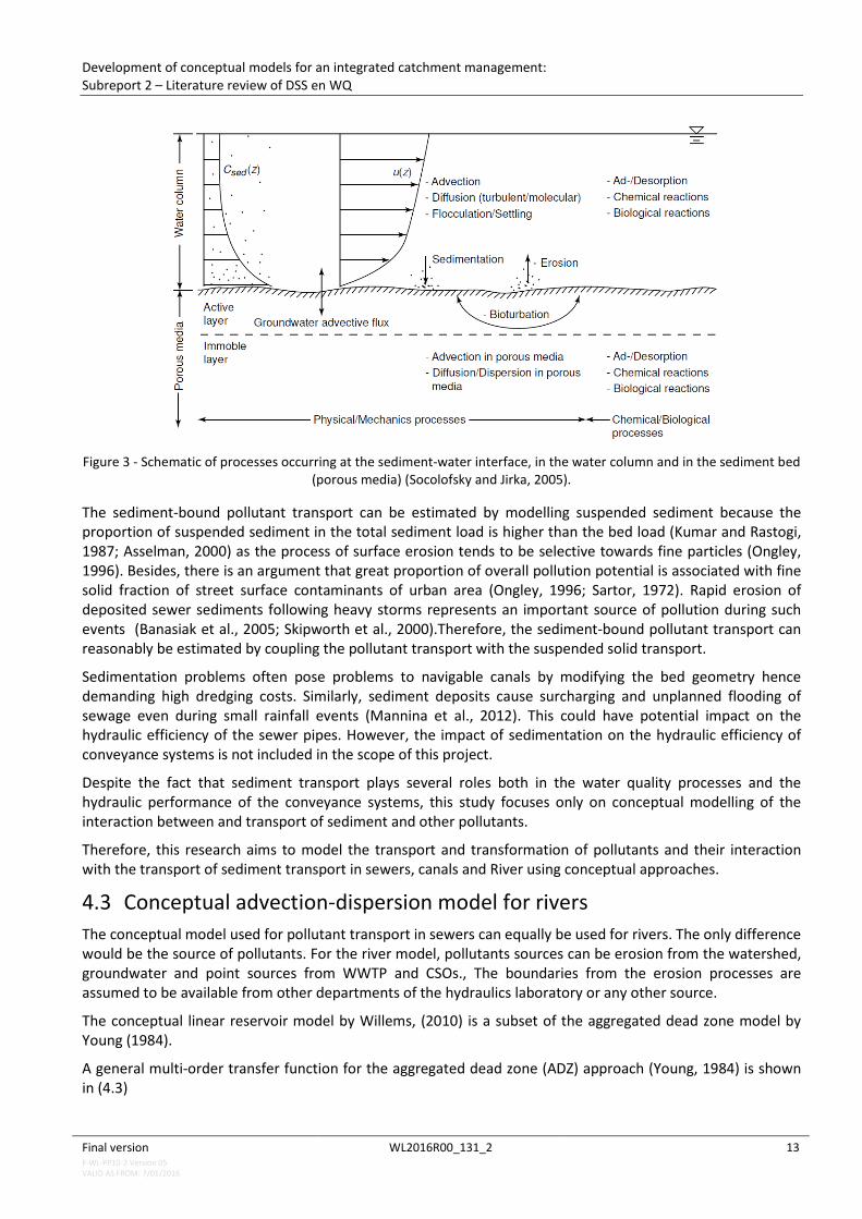
Mineralizable organic matter from decomposing macrophytes makes the bed sediments nutrient-rich at the end of winter and a short term flow increase following this period could trigger resuspension of nutrient-rich sediment hence increase of ammonium and nitrate in the water column (Ani et al., 2011). Also, bioturbation (mixing of sediment by animals living in the sediment) (see Figure 3) could play role in sediment resuspension (Socolofsky and Jirka, 2005). However, modelling the bioturbation is complex and is not in the scope of this project.
Development of conceptual models for an integrated catchment management: Subreport 2 – Literature review of DSS en WQ
Final version WL2016R00_131_2 13 F-WL-PP10-2 Version 05 VALID AS FROM: 7/01/2016
Figure 3 - Schematic of processes occurring at the sediment-water interface, in the water column and in the sediment bed
(porous media) (Socolofsky and Jirka, 2005).
The sediment-bound pollutant transport can be estimated by modelling suspended sediment because the proportion of suspended sediment in the total sediment load is higher than the bed load (Kumar and Rastogi, 1987; Asselman, 2000) as the process of surface erosion tends to be selective towards fine particles (Ongley, 1996). Besides, there is an argument that great proportion of overall pollution potential is associated with fine solid fraction of street surface contaminants of urban area (Ongley, 1996; Sartor, 1972). Rapid erosion of deposited sewer sediments following heavy storms represents an important source of pollution during such events (Banasiak et al., 2005; Skipworth et al., 2000).Therefore, the sediment-bound pollutant transport can reasonably be estimated by coupling the pollutant transport with the suspended solid transport.
Sedimentation problems often pose problems to navigable canals by modifying the bed geometry hence demanding high dredging costs. Similarly, sediment deposits cause surcharging and unplanned flooding of sewage even during small rainfall events (Mannina et al., 2012). This could have potential impact on the hydraulic efficiency of the sewer pipes. However, the impact of sedimentation on the hydraulic efficiency of conveyance systems is not included in the scope of this project.
Despite the fact that sediment transport plays several roles both in the water quality processes and the hydraulic performance of the conveyance systems, this study focuses only on conceptual modelling of the interaction between and transport of sediment and other pollutants.
Therefore, this research aims to model the transport and transformation of pollutants and their interaction with the transport of sediment transport in sewers, canals and River using conceptual approaches.
4.3 Conceptual advection-dispersion model for rivers The conceptual model used for pollutant transport in sewers can equally be used for rivers. The only difference would be the source of pollutants. For the river model, pollutants sources can be erosion from the watershed, groundwater and point sources from WWTP and CSOs., The boundaries from the erosion processes are assumed to be available from other departments of the hydraulics laboratory or any other source.
The conceptual linear reservoir model by Willems, (2010) is a subset of the aggregated dead zone model by Young (1984).
A general multi-order transfer function for the aggregated dead zone (ADZ) approach (Young, 1984) is shown in (4.3)

Development of conceptual models for an integrated catchment management: Subreport 2 – Literature review of DSS en WQ
Final version WL2016R00_131_2 14 F-WL-PP10-2 Version 05 VALID AS FROM: 7/01/2016
𝑌𝑘 =𝑏0 + 𝑏1𝑍−1 +⋯+ 𝑏𝑚𝑍−𝑚
1 + 𝑎1𝑍−1 +⋯+ 𝑎𝑛𝑍−𝑛𝑋𝑘−𝛿
(4.3)
Where, n stands for the number of first order ADZ elements that describe the dispersion properties of the reach;
m depends on the presence of non-integral pure time delay or the presence of additional parallel dead zones.
4.4 Analytical solutions of the advection-dispersion equation The analytical solution of the advection-dispersion equation is successfully used in several previous studies of accidental spill and customary discharge of pollutants (Fischer, 1979; Pujol and Sanchez-Cabeza, 2000; Runkel and Bencala, 1995).
The analytical solution of the conservative advection-dispersion model is given by (Thomann and Mueller, 1987) and used by (Ani et al., 2010a, 2010b; Thomann and Mueller, 1987) as shown in(4.4):
𝑐(𝑥, 𝑡) =𝑀
2𝐴√𝜋𝜋𝑡𝑒𝑥𝑒 �
−(𝑥 − 𝑣𝑡)2
4𝜋𝑡�
(4.4)
Where, M [M] is the mass of contaminant in the spill;
A [L2] is the stream’s cross-sectional area;
X[L] is the distance in the downstream direction;
D is the longitudinal dispersion coefficient ([L2T-1];
t is the time since pollutant spill [T].
The analytical solution of the conservative advection-dispersion model by (Socolofsky and Jirka, 2005) as used by (Ani et al., 2011; Ani et al., 2010a; Ani et al., 2009; Ani et al. 2010)) can be used for leaking scenarios and is given as follows (4.5).
𝑐(𝑥, 𝑡) = 𝑐0 +(𝑐𝑠 − 𝑐0)
2 �𝑒𝑒𝑒𝑐 �𝑥 − 𝑣𝑡√4𝜋𝑡
� + 𝑒𝑥𝑒 �−𝑥𝑣𝜋� 𝑒𝑒𝑒𝑐 �
𝑥 + 𝑣𝑡√4𝜋𝑡
��
(4.5)
Where, c0 (mg/L) is the initial concentration along the river stretch (x (m)), assuming nonzero initial condition throughout the river; and cS (mg/L) is the concentration at the source.
Advantages of the analytical model over the numerical approach include, among others, the fact that it requires less resources and provides results in a shorter time compared to the numerical model, it facilitates the simultaneous computation for all the experiments, while the numerical model is only capable of simulating one experiment at a time, it simplifies the representation of the physical processes more than the numerical model by using spatially constant parameters for each reach, as defined by the modeller, to have homogeneous hydraulic properties ( Ani et al., 2009). Ani et al. (2009) compared the analytical solution and detailed numerical model and concluded that while both approaches capture the observed pollutants’ concentration-time pattern comparably, the analytical model slightly outperformed the numerical model in some reaches. However, this method has a limitation with regards to boundary conditions.
The advection-dispersion model could be combined with transformation models for non-conservative pollutants.
In the analytical solution approach, it is shown that non-uniform hydraulic characteristics of a river and tributaries, pollution sources and abstractions can be represented by dividing the river stretch into reaches
Development of conceptual models for an integrated catchment management: Subreport 2 – Literature review of DSS en WQ
Final version WL2016R00_131_2 15 F-WL-PP10-2 Version 05 VALID AS FROM: 7/01/2016
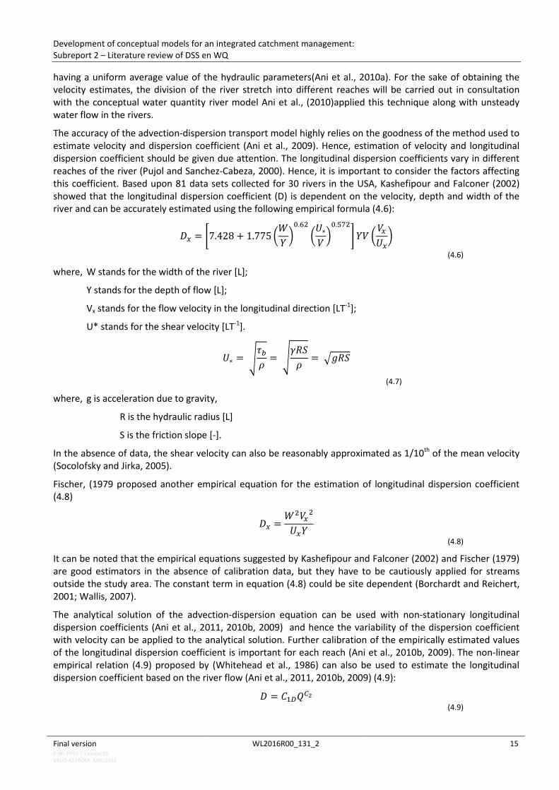
having a uniform average value of the hydraulic parameters(Ani et al., 2010a). For the sake of obtaining the velocity estimates, the division of the river stretch into different reaches will be carried out in consultation with the conceptual water quantity river model Ani et al., (2010)applied this technique along with unsteady water flow in the rivers.
The accuracy of the advection-dispersion transport model highly relies on the goodness of the method used to estimate velocity and dispersion coefficient (Ani et al., 2009). Hence, estimation of velocity and longitudinal dispersion coefficient should be given due attention. The longitudinal dispersion coefficients vary in different reaches of the river (Pujol and Sanchez-Cabeza, 2000). Hence, it is important to consider the factors affecting this coefficient. Based upon 81 data sets collected for 30 rivers in the USA, Kashefipour and Falconer (2002) showed that the longitudinal dispersion coefficient (D) is dependent on the velocity, depth and width of the river and can be accurately estimated using the following empirical formula (4.6):
𝜋𝑥 = �7.428 + 1.775 �𝑊𝑌�0.62
�𝑈∗𝑉�0.572
� 𝑌𝑉 �𝑉𝑥𝑈𝑥�
(4.6)
where, W stands for the width of the river [L];
Y stands for the depth of flow [L];
Vx stands for the flow velocity in the longitudinal direction [LT-1];
U* stands for the shear velocity [LT-1].
𝑈∗ = �𝜏𝑏𝜌
= �𝛾𝛾𝛾𝜌
= �𝑔𝛾𝛾
(4.7)
where, g is acceleration due to gravity,
R is the hydraulic radius [L]
S is the friction slope [-].
In the absence of data, the shear velocity can also be reasonably approximated as 1/10th of the mean velocity (Socolofsky and Jirka, 2005).
Fischer, (1979 proposed another empirical equation for the estimation of longitudinal dispersion coefficient (4.8)
𝜋𝑥 =𝑊2𝑉𝑥2
𝑈𝑥𝑌
(4.8)
It can be noted that the empirical equations suggested by Kashefipour and Falconer (2002) and Fischer (1979) are good estimators in the absence of calibration data, but they have to be cautiously applied for streams outside the study area. The constant term in equation (4.8) could be site dependent (Borchardt and Reichert, 2001; Wallis, 2007). The analytical solution of the advection-dispersion equation can be used with non-stationary longitudinal dispersion coefficients (Ani et al., 2011, 2010b, 2009) and hence the variability of the dispersion coefficient with velocity can be applied to the analytical solution. Further calibration of the empirically estimated values of the longitudinal dispersion coefficient is important for each reach (Ani et al., 2010b, 2009). The non-linear empirical relation (4.9) proposed by (Whitehead et al., 1986) can also be used to estimate the longitudinal dispersion coefficient based on the river flow (Ani et al., 2011, 2010b, 2009) (4.9):
𝜋 = 𝐶1𝐷𝑄𝐶2 (4.9)

Development of conceptual models for an integrated catchment management: Subreport 2 – Literature review of DSS en WQ
Final version WL2016R00_131_2 16 F-WL-PP10-2 Version 05 VALID AS FROM: 7/01/2016
where, C1D and C2D are empirical coefficients that are dependent on discharge range and Q is the river discharge.
Equation(4.9) is also used to calculate dispersion coefficients for water quality modelling in the well-known river modelling software, MIKE11 (DHI, 2000).
As discussed earlier, the analytical solution of the advection-dispersion equation can be applied for suspended sediment and other pollutants (with emphasis on accidental spills) transport processes.
Although the conceptual model and analytical solution of advection-dispersion can estimate the real physical processes, they do not take the sediment carrying capacity of the flow into account. Several studies showed that there is a limiting sediment quantity that a given flow can carry in a given river (Bagnold, 1966; Prosser and Rustomji, 2000; Yalin, 1972; Yang, 1972).
Because the processes of transformation and deposition-resuspension of pollutants are not represented in the analytical model, it can be coupled with the conceptual sediment deposition-resuspension model of LASCAM (see section 4.5.1) based on sediment carrying capacity and affinity of the pollutants to the suspended sediment. For instance, the customary pollutant, inorganic phosphorus shows high affinity to suspended sediments. This model can also be coupled with the water quality variables’ transformation and bacterial models.
Salt intrusion in estuaries can be modelled with the use of an analytical solution of the conservative advection-dispersion equation but simulated in reverse direction from the mouth of the river up to the upstream extent of the tidal effect when there is negative flow. The extent of the tidal effect can be determined a priori based on the simulation results of the quantity variables. This is to overcome the limitation of imposing the downstream boundary condition in the analytical solution approach.
Unlike the river model, the analytical solution of the advection-dispersion equation can’t be extended to a conceptual sewer model where a number of sewer pipes are lumped together and velocity representation within such sewer representation can’t be realistic.
4.5 Some conceptual sediment/pollutant transport models 4.5.1 The LASCAM sediment transport model
LASCAM (Viney & Sivapalan, 1999) is a large-scale conceptual catchment model of streamflow, salinity, sediments and Nutrients. The processes of channel deposition, re-entrainment and bed degradation in sediment transport are all assumed to be governed by a stream sediment capacity. Viney & Sivapalan (1999) adapted the stream sediment capacity, Z (tonnes), from the SPNM (Sediment–Phosphorus–Nitrogen Model) model (Williams, 1980) in to the LASCAM model as follows (4.10).
𝑍 = 𝛼𝑣3/2�𝑞𝑣�
𝛽
𝐴0.5 (4.10)
where, Z is the daily sediment load (tonnes)
q is the daily stream flow volume (ML), v is the stream velocity (km/day), A is the catchment area (km2) and α and β are optimizable parameters.
It is assumed that the term q/v approximates the stream cross-sectional area and that stream depth is proportional to (q/v)1/2. A stream flow of a given volume is able to carry a mass Z of sediment in suspension, provided sufficient material is available either from the hillslope, from upstream or from previously deposited channel sediment.
Sediment re-entrainment, R (tonnes), is thus given by (4.11)
𝛾 = 𝑚𝑚𝑚{𝑍 − 𝑌𝑖 − 𝐸, 𝛾} (4.11)

Development of conceptual models for an integrated catchment management: Subreport 2 – Literature review of DSS en WQ
Final version WL2016R00_131_2 17 F-WL-PP10-2 Version 05 VALID AS FROM: 7/01/2016
Where, Yi is the sediment inflow (M) from upstream subcatchments (upstream channel or boundary);
S is the amount of loose sediment (M) on the channel floor available for re-entrainment;
E is the erosion (M) from lateral catchment area.
The first argument in (4.11)represents the stream's sediment demand, while the second term represents the available sediment supply. If R is negative, part of the incoming sediment is deposited into S. On the other hand, if re-entrainment fully depletes the supply, S, without satisfying the demand, 𝑍 − 𝑌𝑖 − 𝐸, then the stream seeks to partially fulfil demand by bed and bank degradation. This degradation (tonnes), which is assumed to occur at a rate governed by stream power and the USLE crop factor (Williams, 1980), is given by (4.12)
𝐵 = 𝑚𝑚𝑚{𝜀𝐶𝐼𝑍,𝑍 − 𝑌𝑖 − 𝐸 − 𝛾} (4.12)
Where, ε is a calibration parameter;
C is the USLE crop factor
l is the reach length (L)
Figure 4 - Structure of the sediment transport algorithm (Viney and Sivapalan, 1999)

Development of conceptual models for an integrated catchment management: Subreport 2 – Literature review of DSS en WQ
Final version WL2016R00_131_2 18 F-WL-PP10-2 Version 05 VALID AS FROM: 7/01/2016
Viney and Sivapalan (1999) conceptualized the sediment delivery ratio 𝜓 from Arnold et al. (1995). It is given by (4.13)
𝜓 = �1 − 0.5𝑋, 𝑚𝑒 𝑋 < 11
2𝑋 𝑚𝑒 𝑋 ≥ 1
(4.13)
where, ψ is the delivery ratio (-)
𝑋 = ζ 𝑙(𝑞𝑞)0.5 is fictitious parameter and ζ is calibration parameter.
The delivery ratio is the proportion of suspended sediment that leaves the subcatchment carried by the stream flow of the day under consideration. The remainder is assumed to settle to the channel bottom and becomes readily available for re-entrainment on subsequent days.
The sediment yield Y0 (tonnes) from a subcatchment is then given by (4.14)
𝑌0 = 𝜓(𝑌𝑖 + 𝐸 + 𝛾 + 𝐵) (4.14)
The change in channel sediment store (tonnes) is therefore estimated using (4.15)
Δ𝛾 = (1 − 𝜓)(𝑌𝑖 + 𝐸 + 𝛾 + 𝐵) − 𝛾 (4.15)
The LASCAM sediment model thus requires optimization of six new parameters (α,β,γ,δ,ɛ and ζ) and also requires the maintenance of a channel sediment store for each subcatchment. The same parameter value is used in each subcatchment; there is no recalibration for different subcatchments. For a sediment transport process in the river, the lateral sediment inputs and soil erosion from upstream boundary catchments can be obtained from a separate soil erosion model coupled with the rainfall-runoff model.
4.6 The AGNPS sediment transport model AGNPS (AGricultural NonPoint Source) is an event-based model, that simulates runoff, sediment and nutrient transport from agricultural watersheds. The model contains a mix of empirical and physics based components. It is developed by the US Department of Agriculture, Agricultural Research Service (USDA-ARS) in cooperation with the Minnesota Pollution Control Agency and the Soil Conservation Service (SCS) in the USA (Young et al., 1989).
The model uses the steady-state continuity equation (4.16) for routing sediments.
𝛾𝑥 = 𝛾𝑖𝑛 + 𝛾𝑙𝑙𝑙 �𝑥𝐿𝑟� − �(𝑥)𝑤𝜋(𝑥)𝑑𝑥
𝑥
0
(4.16)
where, Sx is the sediment discharge (M) at the downstream end;
Sin is the sediment inflow (M) from upstream boundary of the reach;
Slat is the lateral sediment inflow (M);
X is the downstream distance;b
Lr is the reach length (L);
W is the reach width (L);
D(x) is the deposition rate (ML-2).

Development of conceptual models for an integrated catchment management: Subreport 2 – Literature review of DSS en WQ
Final version WL2016R00_131_2 19 F-WL-PP10-2 Version 05 VALID AS FROM: 7/01/2016
The deposition rate is estimated as (4.17):
𝜋(𝑥) = 𝑉𝑠𝑞(𝑥)
[𝑔𝑠′(𝑥) − 𝑞𝑠(𝑥)]
(4.17)
where, D(x) is the deposition rate (ML-2)
Vs is the particle settling velocity (LS-2);
q(x) is the discharge per unit width (L2T);
gs’(x) is the sediment load per unit width;
qs(x) is the effective transport capacity per unit width as computed using the Bagnold’s stream power equation.
The model divides the sediment in to five classes based on the particle sizes and uses the solution of equation (4.16) to compute the sediment load for each class leaving a given cell (4.18):
𝛾𝑥(𝑥) = �2𝑞(𝑥)
2𝑞(𝑥) + Δ𝑥𝑉𝑠� �𝛾𝑖𝑛 + 𝛾𝑙𝑙𝑙
𝑥𝐿−𝑤Δ𝑥
2�
𝑉𝑠𝑞(𝑥)𝑖𝑛
�𝑞𝑠,𝑖𝑛 − 𝑔𝑠,𝑖𝑛′� −
𝑉𝑠𝑞(𝑥)𝑔𝑠
(𝑥)��
(4.18)
4.6.1 The GESZ sediment transport model
The GESZ (Good Ecological Status for Zenne River) sediment transport simulator (Shrestha, 2013) estimates the total suspended load based on the concept of critical shear stress and hence critical particle diameter for motion initiation of cohesion-less bed particles. The sediment transport capacity of a given flow is imposed by using Velikanov’s energy equation (Velikanov, 1954), an implementation proposed and tested by (Zug et al., 1998).
The approach used by this simulator is not classified among the simplest methods. However, given that it is going to be used as a reference model for calibrating the conceptual model, the governing equations used by the simulator are presented in this section. Besides, simplification of some part of the model structure and incorporating it in the conceptual model is considered important.
The simulator makes use of the algebraic equation proposed by (Soulsby and Whitehouse, 1997) to fit to Shields’ curve (Shields, 1936). The algebraic equation relates the dimensionless grain size (D*) to the dimensionless shear stress (θ) as presented in equation (4.19)
𝜃 =0.24𝜋𝑥
+ 0.055(1− 𝑒−0.02𝐷𝑥) 𝑤𝑚𝑡ℎ 𝜋𝑥 = �(𝑠 − 1)𝜈2
𝑑3
(4.19)
where, θ is the dimensionless shear stress;
D* is the dimensionless grain size;
s is the specific grain gravity.
The dimensionless shear stress (θ) is empirically related to particle Reynolds number (R*) (Shields, 1963) as shown in equations (4.20) and (4.21).
𝜃 =𝜏
(𝜌𝑠 − 𝜌)𝑔𝑑=
𝑈∗2𝜌(𝜌𝑠 − 𝜌)𝑔𝑑
(4.20)
𝛾∗ =𝑈∗𝜈 =
�𝑔𝛾𝑠𝜈
(4.21)
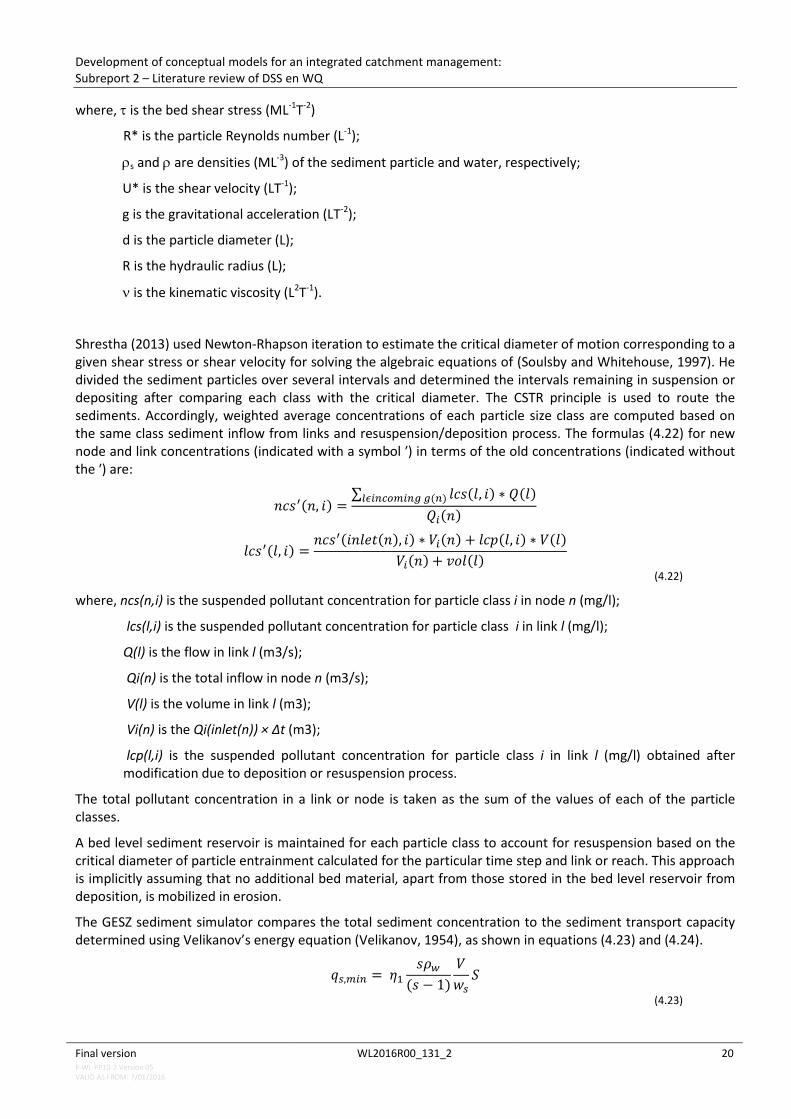
Development of conceptual models for an integrated catchment management: Subreport 2 – Literature review of DSS en WQ
Final version WL2016R00_131_2 20 F-WL-PP10-2 Version 05 VALID AS FROM: 7/01/2016
where, τ is the bed shear stress (ML-1T-2)
R* is the particle Reynolds number (L-1);
ρs and ρ are densities (ML-3) of the sediment particle and water, respectively;
U* is the shear velocity (LT-1);
g is the gravitational acceleration (LT-2);
d is the particle diameter (L);
R is the hydraulic radius (L);
ν is the kinematic viscosity (L2T-1).
Shrestha (2013) used Newton-Rhapson iteration to estimate the critical diameter of motion corresponding to a given shear stress or shear velocity for solving the algebraic equations of (Soulsby and Whitehouse, 1997). He divided the sediment particles over several intervals and determined the intervals remaining in suspension or depositing after comparing each class with the critical diameter. The CSTR principle is used to route the sediments. Accordingly, weighted average concentrations of each particle size class are computed based on the same class sediment inflow from links and resuspension/deposition process. The formulas (4.22) for new node and link concentrations (indicated with a symbol ′) in terms of the old concentrations (indicated without the ′) are:
𝑚𝑐𝑠′(𝑚, 𝑚) =∑ 𝑙𝑐𝑠(𝑙, 𝑚) ∗ 𝑄(𝑙)𝑙𝑙𝑖𝑛𝑙𝑙𝑚𝑖𝑛𝑙 𝑙(𝑛)
𝑄𝑖(𝑚)
𝑙𝑐𝑠′(𝑙, 𝑚) =𝑚𝑐𝑠′(𝑚𝑚𝑙𝑒𝑡(𝑚), 𝑚) ∗ 𝑉𝑖(𝑚) + 𝑙𝑐𝑒(𝑙, 𝑚) ∗ 𝑉(𝑙)
𝑉𝑖(𝑚) + 𝑣𝑣𝑙(𝑙)
(4.22)
where, ncs(n,i) is the suspended pollutant concentration for particle class i in node n (mg/l);
lcs(l,i) is the suspended pollutant concentration for particle class i in link l (mg/l);
Q(l) is the flow in link l (m3/s);
Qi(n) is the total inflow in node n (m3/s);
V(l) is the volume in link l (m3);
Vi(n) is the Qi(inlet(n)) × Δt (m3);
lcp(l,i) is the suspended pollutant concentration for particle class i in link l (mg/l) obtained after modification due to deposition or resuspension process.
The total pollutant concentration in a link or node is taken as the sum of the values of each of the particle classes.
A bed level sediment reservoir is maintained for each particle class to account for resuspension based on the critical diameter of particle entrainment calculated for the particular time step and link or reach. This approach is implicitly assuming that no additional bed material, apart from those stored in the bed level reservoir from deposition, is mobilized in erosion.
The GESZ sediment simulator compares the total sediment concentration to the sediment transport capacity determined using Velikanov’s energy equation (Velikanov, 1954), as shown in equations (4.23) and (4.24).
𝑞𝑠,𝑚𝑖𝑛 = 𝜂1𝑠𝜌𝑤
(𝑠 − 1)𝑉𝑤𝑠
𝛾
(4.23)
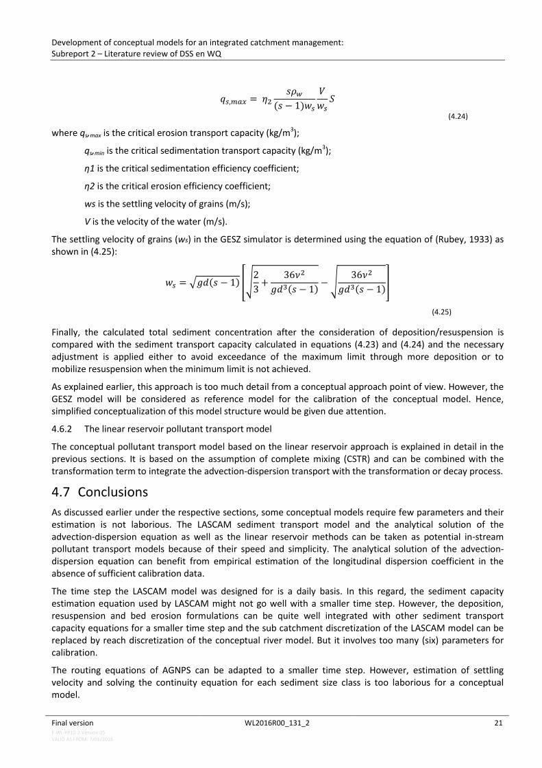
Development of conceptual models for an integrated catchment management: Subreport 2 – Literature review of DSS en WQ
Final version WL2016R00_131_2 21 F-WL-PP10-2 Version 05 VALID AS FROM: 7/01/2016
𝑞𝑠,𝑚𝑙𝑥 = 𝜂2𝑠𝜌𝑤
(𝑠 − 1)𝑤𝑠𝑉𝑤𝑠
𝛾
(4.24)
where qs,max is the critical erosion transport capacity (kg/m3);
qs,min is the critical sedimentation transport capacity (kg/m3);
η1 is the critical sedimentation efficiency coefficient;
η2 is the critical erosion efficiency coefficient;
ws is the settling velocity of grains (m/s);
V is the velocity of the water (m/s).
The settling velocity of grains (ws) in the GESZ simulator is determined using the equation of (Rubey, 1933) as shown in (4.25):
𝑤𝑠 = �𝑔𝑑(𝑠 − 1) ��23
+36𝜈2
𝑔𝑑3(𝑠 − 1) −�
36𝜈2
𝑔𝑑3(𝑠 − 1)�
(4.25)
Finally, the calculated total sediment concentration after the consideration of deposition/resuspension is compared with the sediment transport capacity calculated in equations (4.23) and (4.24) and the necessary adjustment is applied either to avoid exceedance of the maximum limit through more deposition or to mobilize resuspension when the minimum limit is not achieved.
As explained earlier, this approach is too much detail from a conceptual approach point of view. However, the GESZ model will be considered as reference model for the calibration of the conceptual model. Hence, simplified conceptualization of this model structure would be given due attention.
4.6.2 The linear reservoir pollutant transport model
The conceptual pollutant transport model based on the linear reservoir approach is explained in detail in the previous sections. It is based on the assumption of complete mixing (CSTR) and can be combined with the transformation term to integrate the advection-dispersion transport with the transformation or decay process.
4.7 Conclusions As discussed earlier under the respective sections, some conceptual models require few parameters and their estimation is not laborious. The LASCAM sediment transport model and the analytical solution of the advection-dispersion equation as well as the linear reservoir methods can be taken as potential in-stream pollutant transport models because of their speed and simplicity. The analytical solution of the advection-dispersion equation can benefit from empirical estimation of the longitudinal dispersion coefficient in the absence of sufficient calibration data.
The time step the LASCAM model was designed for is a daily basis. In this regard, the sediment capacity estimation equation used by LASCAM might not go well with a smaller time step. However, the deposition, resuspension and bed erosion formulations can be quite well integrated with other sediment transport capacity equations for a smaller time step and the sub catchment discretization of the LASCAM model can be replaced by reach discretization of the conceptual river model. But it involves too many (six) parameters for calibration.
The routing equations of AGNPS can be adapted to a smaller time step. However, estimation of settling velocity and solving the continuity equation for each sediment size class is too laborious for a conceptual model.

Development of conceptual models for an integrated catchment management: Subreport 2 – Literature review of DSS en WQ
Final version WL2016R00_131_2 22 F-WL-PP10-2 Version 05 VALID AS FROM: 7/01/2016
Overall, the linear reservoir approach and the analytical solution approach, coupled with sediment resuspension and deposition processes, could be preferential for their parsimony as long as no complex boundary conditions are imposed. However, the settlement and resuspension of sediments only based on carrying capacity approach seems to ignore the critical conditions of incipient motion and settlement.
Salt intrusion in to the freshwater of the river can be modelled with the analytical solution of the advection-dispersion equation or the linear reservoir approach applied in the reverse direction after the quantity simulation is completed.

Development of conceptual models for an integrated catchment management: Subreport 2 – Literature review of DSS en WQ
Final version WL2016R00_131_2 23 F-WL-PP10-2 Version 05 VALID AS FROM: 7/01/2016
5 MODELLING APPROACHES FOR POLLUTANT TRANSPORT IN SEWERS
5.1 Introduction Modelling of urban pollutant dynamics is often represented with three distinct processes (Ciaponi et al., 2002; Willems, 2010):
a) The accumulation of pollutants during dry weather on catchment surfaces (build-up); b) The removal of accumulated pollutants by runoff (Wash-off); c) The transport and deposition of pollutants due to drainage flows.
Due to the deposition of wind-blown dust, soil, organic matter nutrients and heavy metals can accumulate on impervious surfaces (Donn and Barron, 2012; Sartor, 1972). Stormwater nutrient concentrations and loads are therefore dependent on rainfall intensity and the duration between rainfall events which influence nutrient mobilisation and accumulation, respectively (Donn and Barron, 2012).
Ciaponi et al., (2002 and Willems, (2010) used the linear reservoir concept for sewer pollutant’s transport. Willems (2010) extended the concepts of linear reservoir to conservative contaminant transport as shown below (5.1).
𝑑𝑚(𝑡)𝑑𝑡
= 𝑐𝑖𝑛(𝑡)𝑄𝑖𝑛(𝑡) − 𝑐𝑙𝑜𝑙(𝑡)𝑄𝑙𝑜𝑙(𝑡)
(5.1)
where, m = pollutant mass (M);
C = pollutant concentration (ML-3);
Qin= discharge (L-3T);
Qout= discharge (L-3T);
For a perfect mixing,
𝑚(𝑡) = 𝐶𝑙𝑜𝑙𝕧(𝑡) = 𝐶𝑙𝑜𝑙[𝑘𝑄(𝑡)] (5.2)
Where, 𝕧 (t) stands for water volume in the system at time step t.
Willems (2010) showed that for a steady flow, with both 𝕧 and qin=qout constant, this equation turns into the linear reservoir model 𝑑𝑚(𝑙)𝑑𝑙
= 𝑑(𝕧(𝑙) 𝐶(𝑙))𝑑𝑙
= 𝑐𝑖𝑛(𝑡)𝑄𝑖𝑛(𝑡) − 𝑐𝑙𝑜𝑙(𝑡)𝑄𝑙𝑜𝑙(𝑡)
(5.3)
is further simplified to d c(t)dt
= cin(t) Q(t)𝕧− cout(t)Q(t)
𝕧= cin(t) Q(t)
𝕧− c(t) Q(t)
𝕧
(5.4)
𝑑(𝑙(𝑙))𝑑𝑙
= − 1𝑘
{[𝑐(𝑡) − 𝑐𝑖𝑛(𝑡)]}
(5.5)

Development of conceptual models for an integrated catchment management: Subreport 2 – Literature review of DSS en WQ
Final version WL2016R00_131_2 24 F-WL-PP10-2 Version 05 VALID AS FROM: 7/01/2016
This means that for a system with given inflow of pollutant mass and dispersion large enough to assume perfect mixing (see 5.1), the output concentrations evolve with exponential function and the recession time of the pollutant concentration evolution is equal to the recession time k of the water flow in the reach.
Denoting with x(t) = cin (t) Q(t) the mass flow rate entering the system (input loadograph) and denoting with y(t) = cout (t) Q(t) the mass flow rate leaving the system (output loadograph), from the linear combination of equations (5.1) and (5.2), a linear differential equation with constant coefficients is obtained (5.6))
𝑘𝑑𝑑(𝑡)𝑑𝑡
= 𝑥(𝑡) − 𝑑(𝑡)
(5.6)
where, y (MT-1) is the pollutant/sediment mass flow rate at the desired end of reach;
x (MT-1) is the inflow pollutant/sediment mass flow rate at the inlet to the reach under consideration;
Figure 5 - Schematic representation of the a) dispersion; b) advection processes in a tank or sewer system
with linear reservoir representation (Willems, 2010)
Integrating equation (5.6) with the initial condition that at the beginning of the effective precipitation there is no mass rate leaving the system, the well-known expression for the convolution integral is obtained:
𝑑(𝑡) = � 𝑥(𝜏)1𝑘
𝑙
0𝑒𝑥𝑒 �−
𝑡 − 𝜏𝑘
�𝑑𝜏
(5.7)

Development of conceptual models for an integrated catchment management: Subreport 2 – Literature review of DSS en WQ
Final version WL2016R00_131_2 25 F-WL-PP10-2 Version 05 VALID AS FROM: 7/01/2016
Equation (5.7) shows that the pollutant mass rate leaving the drainage system depends on the pollutant mass rate removed from the catchment surface by the rainfall and on the reservoir constant which characterises the rainfall-runoff process.
The analytical solution of differential equation (5.6) is
𝑑(𝑡) = exp �−1𝑘�𝑑(𝑡 − ∆𝑡) + �1 − 𝑒𝑥𝑒 �−
1𝑘�� 𝑥(𝑡)
(5.8)
Detailed physically based models require detailed basin characteristics and network geometry. Conceptual models can give good approximations of the results of detailed physically based models when the pollutant transport is dominated by convection like the case of passive pollutant transport in separate sewer systems or combined sewer systems of moderate to high slopes where particulate sedimentation and resuspension phenomena can be reasonably ignored (Ciaponi et al., 2002).
Introduction of proper time lag to the input variables (x) in the conceptual dispersion model (5.8) would account for the advective processes (Willems, 2010) and the conceptual advection-dispersion model would be as shown in (5.9).
𝑑(𝑡) = 𝑒𝑥𝑒 �−1𝑘�𝑑(𝑡 − ∆𝑡) + �1 − 𝑒𝑥𝑒 �
−1𝑘�𝑥(𝑡 − 𝑑)�
(5.9)
where, y (MT-1) is the predicted pollutant/sediment concentration at the desired end of reach;
x (MT-1)is the inflow pollutant/concentration at the inlet to the reach under consideration;
d (T) is a pure time delay that represents the translation caused by advection;
k is the reservoir/recession constant (T);
t is the time (T)
This conceptual representation requires dividing the river reach according to the conceptual water quantity model.
The advection and dispersion processes of water collection systems can adequately be conceptualized by a simple lag and route model (Cunge, 1969). The advection process is represented by the time delay and the dispersion process (and also the increase in recession time due to spatially distributed input in sewers) is modelled by the linear reservoir concept.
(Willems, 2010) also showed that when both advection and dispersion processes are considered, the mean travel time (Tr) of a plug entering the sewer system is taken as the sum of recession constant (k) and the delay time (d).
The fraction k/Tr is called dispersive fraction (DF). This fraction is considered as the measure of the fractional volume responsible for the dispersive process (Beer and Young, 1983). In the “aggregated dead zone (ADZ)” concept they introduced for river reaches, DF is defined as the fraction of the active mixing volume in the reach to the total volume of the reach or the ratio of time the pollutant is dispersed in the reach to the total time it spends in the reach and the fully mixed “dead”zones in the reach volume are responsible for the dispersion process. The dead zones are the active mixing volumes according to the concept. In the conceptual reservoir model, only the active mixing volume should be used as reservoir volume to describe the perfect mixing. The difference in volume between total volume and active mixing volume is used with the proper time delay (d) to model the pure advection process. The time lag (d) equals the ratio of non-dispersive fraction of

Development of conceptual models for an integrated catchment management: Subreport 2 – Literature review of DSS en WQ
Final version WL2016R00_131_2 26 F-WL-PP10-2 Version 05 VALID AS FROM: 7/01/2016
the total reach volume and the discharge: 𝑑 = (1−𝐷𝐷)𝑉𝑞𝑜𝑜𝑜
(Willems, 2010). The parameters k and d need to be
calibrated.
It has to be noted, here, that the entire complex processes of molecular diffusion, turbulent diffusion and mechanical dispersion are represented in a lumped way as dispersion.
Due to the fact that the pollutant concentration in the first flush is reported to be even higher than the one existing in the foul sewer in dry weather conditions (Artina et al., 1999; Vladimir and Gordon, 1981), it is necessary to model this phenomenon in the impervious urban areas and sewers or obtain boundaries from previously built models.
Coupling equation (26) or (5.9) with a model suitable for the estimation of x(t), it is then possible to get the loadographs relative to the considered section once the effective rainfall input and the waste water flow are known.
The input pollutant mass flow rate x(t) can be estimated as the pollutant from waste water and the wash-off load which is dependent on the pollutant mass accumulated on the impervious area and the rainfall intensity.
5.2 Some conceptual sewer models in use for pollutant transport 5.2.1 KOSIM
The KOSIM (Kontinuierliche Simulation) model (Durchschlag and Harms, 1989; Preul et al., 1990) was established in Germany to design storm tanks. The hydrodynamic part is composed of linear reservoirs in cascade.
The three main assumptions in KOSIM as reviewed by Krajewski and Jean-Luc (2006) are:
− the TSS concentrations in storm water are supposed to be constant in time − the TSS sources are domestic sewage, storm water from impervious areas and storm water
from pervious areas − the TSS load is always in direct ratio to the flow rate.
The TSS concentration at the outlet is computed as():
𝑐(𝑡) =𝑄𝑑𝑙𝑚𝐶𝑑𝑙𝑚 + 𝑄𝑝𝑝𝑟𝑞𝐶𝑝𝑝𝑟𝑞 + 𝑄𝑖𝑚𝑝𝐶𝑖𝑚𝑝
𝑄𝑑𝑙𝑚 + 𝑄𝑝𝑝𝑟𝑞 + 𝑄𝑖𝑚𝑝
(5.10)
Where, C(t) TSS is concentration at the outlet in mixed water;
Qdom, Cdom are flow rate and TSS concentration of domestic sewage;
Qperv, Cperv are flow rate and TSS concentration of water from pervious area;
Qimp, Cimp are flow rate and TSS concentration of water from impervious area.
The second version of the model (Ries, 1990) as reviewed by Krajewski and Jean-Luc (2006) has been proposed with the following improvements(see equations (5.11) &(27)) :
− The growing of deposits in sewers :
𝑃(𝑡) = 𝑃𝑚𝑙𝑥 − (𝑃𝑚𝑙𝑥 − 𝑃(𝑡 − ∆𝑡)𝑒−𝐾1𝑙 (5.11)
− Erosion of the deposited sediments:
𝑃𝑝𝑟𝑙𝑠(𝑡) = 𝑃(𝑡 − ∆𝑡)𝑒(−𝐾2[𝑄(𝑙)−𝑄𝑙𝑙𝑙]𝑙)
(5.12)

Development of conceptual models for an integrated catchment management: Subreport 2 – Literature review of DSS en WQ
Final version WL2016R00_131_2 27 F-WL-PP10-2 Version 05 VALID AS FROM: 7/01/2016
Where, P(t) is solid deposition (M) at time t
Peros is solid erosion (M) at time t
Pmax is maximum mass of deposits in sewers (M)
Q(t) is flow rate (L3T-1) at time t
Qlim critical flow rate (L3T-1) under which there is no erosion
K1 and K2 are constants
5.2.2 The parsimonious sewer wash-off and transport model by Willems
The parsimonious sewer conceptual model (Willems, 2010) uses a linear reservoir approach to estimate the pollutant transport, pollutant build-up and wash-off processes. This model makes use of the same model structure for both the pollutant build-up and wash-off processes, hence few parameters are involved. Details of the model structure were presented earlier.
5.3 Conclusions Many sewer conceptual models are in use. Most of them use the same modelling approach. Hence, only the basic approach is presented in this document without listing the conceptual models one by one.
The transport process can be modelled using the conceptual approach: the linear reservoir model combined with the pollutant transformation terms.
Overall, the selection of a model structure should be made in view of the types of scenarios to be investigated and their performance in terms of reproducing the observations.

Development of conceptual models for an integrated catchment management: Subreport 2 – Literature review of DSS en WQ
Final version WL2016R00_131_2 28 F-WL-PP10-2 Version 05 VALID AS FROM: 7/01/2016
6 MODELLING THE FATE OF WATER QUALITY COMPONENTS IN CATCHMENTS
Information on the sources of pollutants in catchments and on the response of water quality to changing land use practices or the effect of changes in the precipitation volumes and patterns are some of the scenarios that the conceptual water quality models should address. Modelling water quality in catchment systems requires an understanding of the processes involved.
6.1 Pollutant generation in natural catchments For instance, to model suspended solids we may need to consider soil erosion processes, sediment transport and sediment deposition.
Catchment sediment processes can be categorised into erosion, delivery, and export. The eventual export of sediment out of a catchment is a function of many interacting processes. There is an uncertainty associated with random components, such as rainfall, antecedent soil moisture, and soil cover. In general, sediment erosion increases as rainfall intensity and slope increase and as vegetation cover decreases (Finlayson, 1996). Rainfall drops hit the catchment surface, breaking up larger soil particles as well as providing a flotation medium. Slope determines the velocity of runoff, which directly affects the sediment detachment. Soil structure, texture, and composition also help to determine soil erosivity which, together with the soil roughness, also affects the velocity of the runoff, which determines entrainment of sediment (Novotny, 1989). Vegetation cover reduces soil erosion by reducing the impact velocity of rain drops and reducing runoff through interception, evapotranspiration and the binding of the soil together by plant roots.
Sediment eroded from catchment surfaces and stream channels may either be re-deposited within the catchment system or be exported from the catchment as fluvial sediment load. The amount of sediment transported from the catchment may be an order of magnitude less than the amount of soil erosion (Novotny, 1989). This is caused by ‘flow competency’ either in-channel or during overland flow. If at any time during sediment transport the carrying capacity of the flow is exceeded by sediment supply, then excess sediment will be deposited. This illustrates a start–stop motion typical of sediment transport. The ratio of eroded sediment carried by a stream outlet from a catchment to the on-site erosion within the catchment is termed ‘the delivery ratio’. Although convenient in concept, the idea of a delivery ratio has been severely criticised because of the way it spatially and temporally averages a given catchment area. Sediment erosion and transport operate on a wide variety of time scales including diurnal and seasonal. The delivery ratio has also been criticised for spatially averaging a given catchment area. For instance, a catchment area that is disturbed and eroding rapidly, but spatially removed (either by distance or by an obstacle) from a stream, may deliver less sediment to the stream than an area of low erosion potential in close proximity to the stream (Novotny and Chesters, 1989). Wasson (1996) suggested that the link between water quality and land use varies with position in the catchment, because of variation in connectivity between hill slopes, flood plains and channels. These concepts may be of great importance when modelling other pollutants associated with sediment (Novotny, 1989).
Nitrogen occurs naturally in catchment soils, being fixed from the atmosphere by both symbiotic and non-symbiotic microbes in soils, associated with plant roots, and on the surfaces of plant leaves and stems (Attiwill, 1987). Nitrogen is additionally washed out of the atmosphere by rainfall (Correll, 1982; Meybeck, 1982; Hinga, 1991). Nitrogen content in rocks is very low (Meybeck, 1982). Nitrogen sources from erosion of the parent rock are usually considered unimportant. In contrast, phosphorus is common in igneous rocks and, unlike nitrogen, most naturally occurring phosphorus in catchments is ultimately derived from the weathering of parent substrate (Attiwill, 1987; Wasson, 1996).
Anthropogenic activities within catchments have highly modified catchment nutrient cycles through the introduction of domestic animals and addition of nitrogen and phosphorus fertilisers to pastures and crops (CSIRO, 1992). For example, organic manures derived from intensive animal husbandry are reused to enhance

Development of conceptual models for an integrated catchment management: Subreport 2 – Literature review of DSS en WQ
Final version WL2016R00_131_2 29 F-WL-PP10-2 Version 05 VALID AS FROM: 7/01/2016
crop production, while waste and runoff from urban areas and factories are discharged to catchment waterways.
Nutrients stored in or supplied to catchments may be leached or eroded during storm events and subsequently transported from the catchment surfaces to the drainage network. Meybeck (1982) summarised this, suggesting that suspended pollutants can be derived from three origins: erosion and dissolution of inorganic nutrients, leaching of inorganic nutrients derived from mineralisation of terrestrial organic matter, and leaching and erosion of organic soil components. The dominant pathway that a nutrient follows is catchment specific and depends on the nutrient source, catchment slope, rainfall and runoff relationships, soil properties, the affinity of the nutrient to soils, rates of biological uptake, and the nutrient form. For instance, phosphorus has a high affinity to soil particles. The transport of phosphorus is usually associated with soil particles, and particulate phosphorus can be up to 77% of the total phosphorus loads in rivers (e.g. Cosser, 1989; McKee, 1996). Therefore, changes in catchment sedimentary cycles also have implications for the transport of phosphorus.
The majority of nitrogen transported in world rivers is in dissolved organic forms (Meybeck, 1982) and, on a catchment scale, nitrate is recognised as highly leachable. As a result, a proportion of nitrogen added to crops and pastures may be leached to waterways. Despite differences in chemical affinity, the majority of both nitrogen and phosphorus loads are transported in catchments during flood discharge. Knowledge of flow paths may be important for nutrient management on a farm scale, whereby nutrient losses are reduced by avoiding fertilisation during seasons with high runoff or by using slow-release fertilisers that are less likely to leach to groundwater. Such knowledge will also be important for the nutrient component of water quality modelling as this will affect the relationships that are used in modelling.
6.2 Sediment and nutrient load estimation techniques There are several techniques available for the estimation of sediment and nutrient loads, falling into two main categories: field data and empirical methods. Field data methods include a variety of averaging, ratio and regression methods. These methods can be used when streamflow and nutrient/sediment load concentration measurements are available. Empirical methods are used to estimate loads when there is an absence of such observed data. The nutrient or sediment load for a river can be predicted using relationships between sediment and nutrients and other readily available environmental attributes, such as population.
6.2.1 Load estimation using field data
Estimation of the load of suspended sediment and other pollutants is an important part of analysing the response of a catchment to rainfall events. Loads are not generally measured directly in-stream; rather, load estimates are inferred from measurements of pollutant concentration and water discharge in-stream.
In general, the pollutant load L over a time period T can be represented by the equation:
∫ ⋅⋅=T
dtQCL0
( 6.1 )
Where C is the pollutant concentration and Q is the water discharge. A close approximation to this load equation is given by:
tQCLN
iii δ⋅⋅= ∑
=1 ( 6.2 )
where the sampling interval δt (= T/N), is short compared to the period of time over which the discharge and concentration vary. Most techniques for pollutant load estimation are based on this equation involving concentration and water discharge. In practice, this equation is usually not able to be used directly to calculate pollutant loads, as the sampling period for discharge and/or concentration is longer than the period over

Development of conceptual models for an integrated catchment management: Subreport 2 – Literature review of DSS en WQ
Final version WL2016R00_131_2 30 F-WL-PP10-2 Version 05 VALID AS FROM: 7/01/2016
which concentration and discharge are invariant. However, when the sampling interval approaches the concentration variability with flow, the method of linear interpolation can be used to generate ‘real’ nutrient and sediment loads. As such, linear interpolation has been used in studies which test the accuracy and bias of the other methods (e.g. Young and DePinto, 1988; Kronvang and Bruhn, 1996). Linear interpolation can be described by the following equation (Kronvang and Bruhn 1996):
( ) ( )∑ ∑+
= ≤< +
+
+
+
−
−+−⋅
1
1 1
1
1
1n
i
i
ttt ii
ititt
ii
ii
ttttCttC
q ( 6.3 )
where concentrations are denoted Cti, ti, i = 1,...,n are the times at which concentration is measured, t1 and tn+1 are the times at the start and end of each subinterval, and qt is the discharge for each time step. There are many different techniques used for calculating load estimates, differing in complexity, accuracy and bias. Within them we can mention: averaging, ratio estimators and regression estimators.
Averaging
Averaging methods are generally considered to be the simplest available techniques for pollutant load estimation, and are often applied because of a lack of more appropriate techniques. Estimates of load over a time period are made by using averages of discharge, concentration or load for a given subinterval and then summing these over the entire period. These averages may be over different time periods, such as monthly, quarterly or yearly, and can combine discharge and concentration in a number of different ways (Table 2). Whilst these methods are easy to apply, the assumptions implicit behind such calculations, including independent and identically distributed data, are rarely met. This leads to bias in the estimation of loads, especially if the sampling program does not collect data from the entire range of discharge and concentration variability.
Ratio estimators
Ratio estimators aim to take advantage of correlation within a sample. Generally discharge data is used as an auxiliary variable xi with load data treated as a dependent variable yi. The ratio estimate is usually calculated as:
XxyYR ⋅= ( 6.4 )
where y and x are the sample means of yi and xi respectively, YR is the ratio estimate of load and X is the discharge. If yi/xi is nearly the same for all sampling units, y/x varies little from one sample to another and the ratio estimate is of high precision.
The ratio estimator is the best linear unbiased estimator under two conditions:
- the relationship between xi and yi is a straight line passing through the origin - the variance of yi about the line is proportional to xi.
In general these conditions will not be met, so that the ratio estimator is biased, although consistent. Preston et al. (1989) found that the ratio estimators they considered (table 2) were more often less precise than other approaches considered, but were virtually unbiased in each test case. This most likely reflected that the underlying distributions of the data considered for each test case were appropriate for ratio estimation.
Regression Estimators
Regression estimators, also commonly referred to as rating curves, have been widely applied to estimating suspended sediment loads. Regression estimators are based on extrapolating a limited number of concentration measurements over the entire period of interest by developing a relationship between pollutant concentration or load and stream discharge, and applying this relationship to the entire discharge record. Typically this relationship is considered to be log–log, that is, the log of pollutant load or concentration is

Development of conceptual models for an integrated catchment management: Subreport 2 – Literature review of DSS en WQ
Final version WL2016R00_131_2 31 F-WL-PP10-2 Version 05 VALID AS FROM: 7/01/2016
assumed to be a linear relationship of the log of stream discharge. This relationship is generally applied because both discharge and concentration are often best described by a bivariate log–normal distribution.
It has been found in a number of studies that the regression curve estimates based on this log–log relationship are biased, systematically under-predicting sediment loads. The reasons for this bias have been analysed and discussed by a number of authors (Preston et al., 1989; Ferguson, 1986, 1987; Singh and Durgunoglu, 1989). Essentially, whilst parameters are unbiased in log–log space, the process of transforming parameter estimates back to the stream discharge or stream load space introduces bias into the parameter estimates due to the non-linearity. This means that the rating curve that is calculated underestimates the pollutant yield.
Table 2 - Direct estimation techniques (Letcher et al., 1999).
Method Description Load Equation 1 Source
Averaging methods
Average sample concentration × average sample discharge, scaled for time
∑∑==
n
i
in
i
i
nq
nc
k11
Walling and Webb (1981)
Average sample load, scaled for time.
⋅∑=
n
i
ii
nqc
k1
Walling and Webb (1981)
Average sample concentration × annual discharge ∑
=
n
i
i
nc
Q1
Concentration for a sample interval × discharge for a sample interval i
n
i
ii qcc
⋅+∑
=
+
1
1
2
Lesack (1993)
Ratio estimator
Flow weighted concentration × annual discharge
÷
⋅ ∑∑==
n
i
in
i
ii
nq
nqc
Q11
Preston et al. (1989)
Regression analysis
Log space discharge - concentration regression ( )( )[ ]∑
=
⋅+365
110 lnˆˆexp
iii qbbq
Kronvang and Bruhn (1996)
Flow duration curve
The total load rate is calculated by integrating the area under the load duration curve
∫ ⋅%100
%0
365 dpli Robinson and Hatfield (1992)
1 Where: ci is the pollutant concentration, n is the number of days sampled, Q is the total discharge, qi is the discharge during sampling interval, k is a scaling factor for length of period (number of days over which the load is being calculated), li is the instantaneous load,
i is an index value, and b0, b1 are coefficients determined by linear regression against observed data.
The choice of technique may depend on the data resolution, the mathematical ability of the operator, the available computer technology, or the relationships within the data and between various pollutant concentrations. Ideally, data should be collected to suit a particular river and a particular method of load estimation. However, more often data are collected without clear objectives thus reducing collection efficiency and usefulness. The selection of an appropriate load estimation technique therefore depends not only on the availability of concentration and discharge data, but also on the hydrological characteristics of the catchment being considered, the desired accuracy of estimates and the preferred complexity of the load estimation technique. No single technique has been found to be optimal in the literature, with all techniques having some

Development of conceptual models for an integrated catchment management: Subreport 2 – Literature review of DSS en WQ
Final version WL2016R00_131_2 32 F-WL-PP10-2 Version 05 VALID AS FROM: 7/01/2016
disadvantages associated with their use. The choice of technique will depend on the characteristics of the catchment being considered, and the availability of data for that catchment.
6.2.2 Empirical models In the absence of field-collected data, the nutrient or sediment load in a river draining to a receiving water body can be predicted by relationships generated using data from other catchments, either nearby or in other parts of the world. This section describes the predictive ability of relationships between nitrogen, phosphorus and suspended sediments and other readily available environmental attributes. The discussion will be limited to total nitrogen, total phosphorus, and suspended sediments, however, similar relationships may be derived for other nutrient forms (e.g. nitrate, phosphate) or contaminants.
Population density as a predictor of nutrient loads The presence of a human population in a catchment causes disturbance that leads to greater nutrient inputs to the catchment as well as greater release of nutrients stored within vegetation and soils. Several studies have shown significant relationships between population and nitrate-nitrogen and phosphate-phosphorus in 42 major rivers of the world (Cole et al., 1993; Caraco, 1995).
Fertiliser addition as a predictor of nutrient export Excessive use, methods of application, and the timing of the application of fertilisers in rural catchments are often indicated as contributing to eutrophication of adjacent water bodies (Lukatelich et al., 1987). As such, it seems likely that the fertiliser loading in a catchment may correlate with riverine nutrient export (e.g. Birch, 1982).
Relationships between nutrients and suspended sediment A proportion of nitrogen and phosphorus in river systems is transported in association with inorganic and organic soil particles. For example, 77% of phosphorus export in the South Pine River, south-eastern Queensland, is particulate phosphorus and 29% of nitrogen exported in the Richmond River is transported as particulate organic nitrogen (Cosser, 1989; McKee and Eyre, 1996). Many authors have reported relationships between particulate matter and nitrogen (e.g. Meybeck, 1982) and phosphorus (Kronvang, 1992).
Land use and sediment and nutrient exports Land used for different purposes may be ‘disturbed’ to differing degrees depending on, for example, tillage practices, fertiliser application rates and timing, stocking densities, urbanisation, and industrialisation. Although there is much variation, average nutrient exports appear to be horticulture > cropland > urban > improved pasture > pasture >forest (Beaulac and Reckhow, 1982; Frink, 1991; Young et al., 1996). For sediment export, the order (on average) is overgrazed pasture > crop land > native pasture > undisturbed forest (e.g. Neil and Fogarty, 1991; Hill and Peart, 1998). An estimate of total nutrient and sediment export from a catchment area can be made if the area of each broad land use category is known and a nutrient or sediment generation rate is applied. This concept has been developed by CSIRO into the computer modelling package CMSS and has also been used in catchments in other parts of the world (e.g. Haith and Shoemaker, 1987; Mattikalli and Richards, 1996).
Multi-factor empirical modelling approach A modelling approach was used to derive nitrogen, phosphorus and suspended sediment exports from Queensland coastal catchments (Moss et al., 1993). The models employed are expressed in the following equations:
Suspended sediment = RDREL ⋅⋅⋅
Nutrient export = RCFDRERSCEL ⋅⋅⋅⋅⋅⋅
( 6.5 )
(6.6 )
With:
AQR = ( 6.7 )

Development of conceptual models for an integrated catchment management: Subreport 2 – Literature review of DSS en WQ
Final version WL2016R00_131_2 33 F-WL-PP10-2 Version 05 VALID AS FROM: 7/01/2016
Where L is the area of a specified land use, E the erosion rate for a specified land use, DR the delivery ratio for a specified land use, R the runoff correction factor for a specified land use, SC the soil nitrogen or phosphorus content, ER the enrichment ratio (phosphorus only), CF the dissolved nitrogen or phosphorus compensation factor, Q the storm discharge and A the catchment area.
Turbidity as a predictor of nutrient and sediment exports Turbidity is commonly found to positively correlate with other water quality parameters such as nutrients and suspended sediments. Poor relationships between suspended sediment concentrations and turbidity are commonly found when a low range of suspended sediment concentrations is used, but the relationships improve when a larger range is considered (e.g. Gippel, 1989; Eyre et al., 1997). Nutrients also show a poor correlation with turbidity in the lower range; this may be due to dissolved nutrient sources (point sources), biological processes, or sediment–water interactions increasing nutrient concentration without any effect on turbidity. Continuous turbidity records collected using automated optical sensors can be calibrated with routinely collected water quality samples to derive a continuous record of sediment concentration (Webb and Walling, 1982; Walling et al., 1997).
6.3 Erosion and sediment/nutrient transport modelling Computer models of erosion and sediment/nutrient transport fall into three broad categories: empirical models, conceptual models and physically-based models. Physically-based models are grounded on the solution of fundamental physical equations of flow and transport. Each of these classes of models has a number of advantages and disadvantages. Many models are not clearly definable as belonging to any one category, but possess a combination of components from different classes. Also, the categories used to classify models are not universally agreed upon by the modelling community. A number of different classification groups, as well as definitions of model types, may be found in literature. The best model will depend on a number of factors, including the intended use of the model, the data and computing resources available and the expertise of the model user.
6.3.1 Empirical models
Empirical models are generally based on simple stochastic or empirically determined relationships found between observed variables. Empirical models are generally the simplest of all three model types being capable of being supported by coarse measurements. This means that the computational and data requirements for such models are usually smaller than for conceptual and physically-based models. Jakeman et al. (1997) state that ‘the feature of this class of models is their high level of spatial and temporal aggregation and their incorporation of a small number of causal variables’. Many empirical models are based on the analysis of catchment data using statistical techniques, and as such are ideal tools for the analysis of data within catchments. Such models are particularly useful as a first step in identifying sources of sediment and nutrient generation.
Most empirical models do not attempt to represent the physical processes involved in sediment generation. For this reason many empirical models tend to be catchment specific, that is, they apply only to the catchment for which they have been developed, and often under the specific land use conditions existing within the catchment at that time. This means that the ability of empirical models to predict the effects of changes in catchment characteristics, such as land use, on water quality and sediment yields can be limited. Empirical models also tend not to be event-responsive (or responsive to antecedent conditions), ignoring the processes of rainfall-runoff in the catchment being modelled.
Empirical models are often criticised for employing unrealistic assumptions about the physics of the catchment system, ignoring the heterogeneity of catchment inputs and characteristics, such as rainfall and soil types, and the inherent nonlinearities in the response of the catchment system. Such models are also generally based on the assumption that underlying conditions remain unchanged for the duration of the study period. Walton and Hunter (1996) mention two empirical models, CMSS and AEAM. They state that these models rely on estimation of parameters through either local knowledge or expert knowledge or from previous model

Development of conceptual models for an integrated catchment management: Subreport 2 – Literature review of DSS en WQ
Final version WL2016R00_131_2 34 F-WL-PP10-2 Version 05 VALID AS FROM: 7/01/2016
application. They suggest that these models are intended only as initial planning tools and state that ‘they do not provide highly accurate prediction of water quality or quantity’.
6.3.2 Conceptual models
Conceptual models are typically based on the representation of the catchment as a configuration of internal storages and pathways. Physical relationships are not considered explicitly but are represented in general terms through the conceptualisation of the catchment. Conceptual models usually incorporate the (catchment-scale) underlying physical mechanisms of sediment and runoff generation within their structure, representing flow paths within the catchment as a series of storages, each requiring some characterisation of its dynamic behaviour. Conceptual models are usually not spatially distributed and tend to lump representative processes over the scale at which outputs are simulated(Jakeman et al., 1997). Thought this can not be generalised completely. Parameter values for conceptual models have typically been obtained through calibration against observed data such as stream discharge and concentration measurements.
Due to the requirement that parameter values are determined through calibration against observed data, conceptual models tend to suffer from problems associated with the identifiability of their parameter values. Most calibration techniques used for conceptual models of medium complexity (say more than half a dozen parameters) are capable of finding only local optima at best. Often the calibration of parameters in a conceptual model identifies only a set of sufficiently accurate parameter values which reproduce observed behaviour in some sense, but not necessarily the globally most optimal set. This means that there are many possible ‘best’ parameter sets available.
The lack of uniqueness in parameter values for conceptual models means that the parameters in such models have limited physical interpretability. However, this problem can also be associated with empirical and physics-based models. Physics-based models in particular are often over-parameterised whereas empirical models tend to be naturally much simpler in their level of parameterisation.
6.3.3 Physically-based models
Physically-based models are grounded on the solution of fundamental physical equations describing streamflow and sediment and nutrient generation within the catchment. Standard equations used in such physically-based models are the equations of conservation of mass and momentum for flow and the equation of conservation of mass for sediment (e.g. Bennett, 1974).
In theory, the parameters used in physically-based models are measurable within the catchment and so are ‘known’. However, in practice, the large number of parameters involved and the heterogeneity of important characteristics within the catchment means that these parameters must typically be calibrated against observed data. This creates additional uncertainty in parameter values. Also, even in situations where parameters can be ‘measured’ within the catchment, errors in the measurement of important characteristics will create additional uncertainty as to the veracity of model outcomes. Where parameters cannot be measured within the catchment they must be determined through calibration against observed data. Given the large number (possibly hundreds) of parameter values needed to be estimated using such a process, problems with the lack of identifiability of model parameters and non-uniqueness of ‘best fit’ solutions can be expected. There is likely to be a large number of parameter values for which the model gives an adequate fit. Thus the physical interpretability of model parameters is questionable.
In general the equations governing the processes in physics-based models are derived for small-scale models under very specific physical conditions. However, in physically based models these equations are used at much greater scales, and under different physical conditions. The equations are generally derived for use with continuous spatial and temporal data, but the data used in these models is often point-source data taken to represent an entire grid cell within the catchment. The derivation of mathematical expressions describing individual processes in physically-based models is subject to numerous assumptions that may not be relevant in many real-world situations (Dunin, 1975). The viability of lumping up small-scale physics to the scale of the spatial grid used in many physically-based models is also questionable (Beven, 1989). Specifically there is a lack

Development of conceptual models for an integrated catchment management: Subreport 2 – Literature review of DSS en WQ
Final version WL2016R00_131_2 35 F-WL-PP10-2 Version 05 VALID AS FROM: 7/01/2016
of theoretical justification for assuming that equations apply equally well at the grid scale, at which they are representing the lumped aggregate of heterogeneous subgrid processes (Beven, 1989).
Physically-based models also tend to have greater data and computational requirements than other model types. Parameter values must be measured both spatially and temporally within the catchment. The use of such models has been limited by the lack of observed physical and biological data within catchments, and by the larger computing costs involved in their use. The tradeoff between model complexity and accuracy is not simply that increased model complexity increases model accuracy. Simpler catchment models perform equally well or at least are not substantially outperformed by more complex models (Loague and Freeze, 1985). Jakeman and Hornberger (1993) confirmed this result for different levels of complexity in conceptual models.

Development of conceptual models for an integrated catchment management: Subreport 2 – Literature review of DSS en WQ
Final version WL2016R00_131_2 36 F-WL-PP10-2 Version 05 VALID AS FROM: 7/01/2016
7 SOME WATER QUALITY MODELS Water quality models are widely used all over the world and largely driven by legislation and regulations, thus, there is difference in applications of water quality modelling between countries due to variation in regulatory frameworks (Rauch et al, 1998). Cox B.A (2003) reviewed the available in-stream water quality models capable to simulate dissolved oxygen in freshwater river systems including SIMCAT, TOMCAT, QUAL2E, QUASAR, MIKE 11 and ISIS. SIMCAT is a stochastic, 1D steady state, deterministic model which simulates the behaviour of solutes including Chloride, BOD, ammonia and DO from point sources effluent discharges. SIMCAT simulates river reaches as a CSTRs model assuming that the stream condition does not change with time. The approach of SIMCAT is evaluated as over-simplistic and limited in modelling temporal variability which can be important in lowland rivers (Cox, 2003). The conceptualisation of TOMCAT is absolutely similar to SIMCAT, i.e. a stochastic steady state CSTRs model, but it allows modelling more complex temporal correlation. However, the lack of dynamic modelling and over-simplistic processes limit the TOMCAT model simply in simulating the general condition of a river. Although the QUAL2E model (Brown and Barnwell, 1987) is also a steady state model like the two previous models, the conceptualisation is much more advanced which is able to simulate DO and up to 15 associated water quality variables. Different from SIMCAT and TOMCAT in which flow, solute transport and transformation are solved simultaneously, QUAL2E simulates flow in all reaches first and then the solute transport and water quality. The QUAL2E water modelling concept is applied in the SWAT model for in-stream water quality module and is described more details later. QUASAR (Whitehead et al., 1997) is able to model the time varying transport and transformation of solutes in river systems using 1D ordinary, lumped parameter differential equations of mass conservation. Compared with the three models mentioned before, this model improves many of the insufficiency of SIMCAT and TOMCAT with much more complete processes and is also more advanced than QUAL2E in that it can run dynamically and stochastically, however, the data requirements for dynamic simulations are extensive. MIKE 11 and ISIS as well as SOBEK 1D which was applied in the paper are considerably comprehensive models for flow and water quality which are capable to solve full hydrodynamic equations for flow and advection-dispersion equations to simulate solute transport in rivers. The disadvantages of these models are the requirement of extensive amount of data which are not always available. Therefore, these models allow the users to run the models at different levels of water quality complexity depending on the purpose of modelling.
7.1.1 The WEST model
WEST (MOSTforWATER NV, Kortrijk, Belgium) is a multi-platform modelling and experimentation system (Vanhooren et al., 2003). WEST has been recently widely used in to model the processes of wastewater treatment plants, but was developed to simulate any system that can be expressed by differential and algebraic equations.
For the hydraulic routing, WEST uses the simplified model of Continuous Stirred Tank Reactors (CSTRs) in series. Each tank receives the output from the previous tank and the contents of the tanks are supposed to be instantaneously mixed. In the CSTR approach, water can flow only in one direction, upstream to downstream and from one tank to another. Each tank receives inflow from the upstream tank and possibly from one or more lateral inputs. All the tanks are supposed to be instantaneously mixed and are characterised by a horizontal water surface and thus by a unique value of water level.
The implementation of tanks-in-series approach implies some limitations. First, any change in the water level as well as any flood wave upstream or downstream within a tank cannot be represented. Second, flood wave propagation between tanks can be modelled only in the downstream direction. Therefore, backwater effects is not taken into account (Benedetti and Sforzi, 1999).
Biochemical model
The biochemical model for the selected reach was implementing in WEST using a simplified version of the River Water Quality No.1 (RWQM1) by (Ghermandi et al., 2009). The simplified model includes 16 state
Development of conceptual models for an integrated catchment management: Subreport 2 – Literature review of DSS en WQ
Final version WL2016R00_131_2 37 F-WL-PP10-2 Version 05 VALID AS FROM: 7/01/2016
variables and 16 processes. RWQM1 simulates the variation of water quality variables through the biological processes (growth, respiration, death) of organisms. Several basic simplifying assumptions of RWQM1 are as follows:
• The elemental composition of all compounds and organisms, as well as the stoichiometry of all processes, is assumed to be constant in time for each model application.
• No adaptation of specific organisms takes place and changes in the composition within organism classes are neglected.
• It is assumed that oxygen and/or nitrate are always available. • The effect of macrophytes on oxygen levels as well as on the surface available for sessile micro-
organisms is not considered in the model.
7.1.2 SOBEK model
SOBEK has been developed by WL|Delft Hydraulics in partnership with the National Dutch Institute of Inland Water Management and Wastewater Treatment (RIZA), and the major Dutch consulting companies. SOBEK has three basic product lines including SOBEK-Rural, SOBEK-Urban and SOBEK-River.
SOBEK-Rural gives regional water managers a high-quality tool for modelling irrigation systems, drainage systems, natural streams in lowlands and hilly areas. Applications are typically related to optimizing agricultural production flood control, irrigation, canal automation, reservoir operation, and water quality control. SOBEK-Rural can also answer questions about increased pollution loads in response to growing urbanisation.
To model the flow and water quality of the river in this study, 1DFLOW and 1DWAQ of SOBEK-Rural are used.
7.1.3 The SWAT model
Nitrogen processes in the SWAT model
Nitrogen processes are modelled by SWAT in the soil profile, in the shallow aquifer and in the river reaches. SWAT monitors five different pools of nitrogen in the soil. Two inorganic forms of nitrogen are NH4-N and NO3-N and 3 organic forms of nitrogen are fresh organic N which is associated with crop residue and microbial biomass, active and stable organic N associated with the soil humus. Nitrogen processes in the soil include: mineralization, residue decomposition, immobilization, nitrification, ammonia volatilization, plant uptake and denitrification. Ammonium is assumed to be easily adsorbed by soil particles, thus, it is not considered in the nutrient transport. Nitrate which is very susceptible to leaching can be lost through surface runoff, lateral flow and percolate out of the soil profile and enter the shallow aquifer. Nitrate in the shallow aquifer may remain in the aquifer, move with the recharge to the deep aquifer, move with groundwater flow into the stream or move back to the soil zone in response to water deficiencies. Nitrate in the shallow aquifer may also be lost due to the uptake by the presence of bacteria, by chemical transformation driven by the change in redox potential of the aquifer and other processes. These processes are lumped together to represent the loss of nitrate in the aquifer by the nitrate half-life parameter.
The transformation of nitrate loss to the main stream can be modelled using the QUAL2E concept in SWAT.
Phosphorus processes in the SWAT model
Different from the mobility of nitrogen, phosphorus solubility in most environment is limited. Phosphorus usually combines with other ions to form insoluble compounds that precipitate out of solution, which contribute to a build-up of phosphorus near the soil surface that is readily available for transport in surface runoff (Neitsch et al., 2005). Consequently, surface runoff is the primary transport mechanism by which phosphorus is exported from most catchments (Sharpley and Syers, 1979).

Development of conceptual models for an integrated catchment management: Subreport 2 – Literature review of DSS en WQ
Final version WL2016R00_131_2 38 F-WL-PP10-2 Version 05 VALID AS FROM: 7/01/2016
SWAT simulates six different pools of phosphorus in the soil, three of which are inorganic and the other three are organic forms. Soil organic phosphorus is divided into three pools: fresh organic phosphorus which is associated with crop residue and microbial biomass, active and stable organic phosphorus associated with the soil humus. Soil inorganic phosphorus consists of solution, active and stable pools. Phosphorus processes occurring in the soil profile include: mineralization, residue decomposition, immobilization, plant uptake and sorption of inorganic phosphorus. Because of the immobility of phosphorus, it is assumed that there is only interaction between surface runoff with solution phosphorus in the top 10mm of soil, moreover, leaching of solution phosphorus only occur from 10mm of soil into the first soil layer.
The in-stream phosphorus cycle is also based on the QUAL2E concept but much simpler than nitrogen cycle with only two components: organic phosphorus and inorganic/soluble phosphorus. The amount of organic phosphorus in the stream may be increased by the conversion of algal biomass phosphorus to organic phosphorus. A part of organic phosphorus is then mineralized to inorganic phosphorus, the other part settles with sediment in streambed. There is also diffusion of inorganic phosphorus from the streambed sediment to the water. The soluble inorganic phosphorus concentration may be decreased by the uptake by algae for its growth.

Development of conceptual models for an integrated catchment management: Subreport 2 – Literature review of DSS en WQ
Final version WL2016R00_131_2 39 F-WL-PP10-2 Version 05 VALID AS FROM: 7/01/2016
8 DECISION SUPPORT SYSTEMS FOR WATER QUALITY MANAGEMENT
A Decision Support System (DSS) is a computer-based information system that supports business or organizational decision-making activities. DSSs serve the management, operations, and planning levels of an organization and help to make decisions, which may be rapidly changing and not easily specified in advance (Wikipedia, 2013). Even though there are many definitions, authors coincide that a DSS is a specific and well-delineated class of computer-based systems (Stabell, 1987).
Sprague (1980) characterized DSSs as follows:
- DSS tends to be aimed at the less well structured and underspecified problems - DSS attempts to combine the use of models or analytic techniques with traditional data access and
retrieval functions - DSS specifically focuses on features which make them easy to use by non-computer people - DSS emphasizes flexibility and adaptability to accommodate changes in the environment and the
decision making approach of the user.
Rizzoli and Young (1997) differentiate modelling software and a DSS as follows: “while single models can directly support decision making process, often the complexity of environmental systems, and the multi-faceted nature of environmental problems, means that decision makers commonly require access to a range of models, data and other information”. Thus, computer-based systems that integrate models, databases and decision aids in a way that decision-makers can use it, are referred to as Decision Support Systems (DSS). Those that are developed for use in environmental domains are named by Rizzoli and Young (1997) as Environmental DSS (EDSS).
From the characteristics of DSSs some possible requirements can be identified for the conceptual models under research. For instance, the adaptability to changes in the modelling system in order to deal with changes in the environment or in the decision making approach. It can also be expected that at research stage the user must have a computer background, but the end product will need to facilitate the use of the tool by non-computer literate users.
8.1 Classification and Components There are different ways to classify DSSs. Authors classify them based on the components included or the type of data used. Here we adopt two categories as defined by Rizzoli & Young (1997). They divide the EDSS into two separate categories: situation and problem specific EDSS, and problem specific EDSS.
8.1.1 Situation and problem specific EDSS
Situation and problem specific EDSS are intended to be applied to a particular problem in a given place, and cannot be easily modified for use in new locations. Customising such software for new situations would require extensive programming effort by the original system developers. The Colorado River Decision Support System (USBR, 1988) is an example given by Rizzoli & Young (1997) of a situation specific EDSS. It is a data-centred system integrating several models to help water users and water managers make more informed decisions.
8.1.2 Problem specific EDSS
A problem specific EDSS can be used to solve problems relating to a specific domain of knowledge. For example, we find EDSS to assess and monitor water quality in streams, to evaluate the effects of runoff in urban areas. An example of a problem specific EDSS is CMSS (Catchment Management Support System), a software tool developed by CSIRO Land and Water, Australia for assessing the impact of alternative catchment management policies on nutrient export (Davis & Farley, 1997). CMSS is a problem specific tool which can be tailored to a particular situation by a Sensitivity Analysis to be then used by small community groups and

Development of conceptual models for an integrated catchment management: Subreport 2 – Literature review of DSS en WQ
Final version WL2016R00_131_2 40 F-WL-PP10-2 Version 05 VALID AS FROM: 7/01/2016
catchment managers. Another example of DSS generators is the Mulino DSS (Mysiak et al., 2005). Mulino is designed to be used for water resource management at the catchment scale and to meet the requirements of the EU water framework directive (WFD).
From the perspective of the Conceptual Model Project, we are developing tools for a DSS that will classify in the Problem specific category. In other words, the models developed should address problems within the domain of IWRM but should be customizable to generate a DSS that addresses the specific situation of each catchment in Flanders.
8.2 Features and Components of an EDSS Based on the characteristics of environmental systems, Rizzoli and Young (1997) developed a set of desirable features for EDSS. These features are:
- The ability to acquire, represent and structure the knowledge in the domain under study. This knowledge should be stored in what is called the domain base.
- The domain base allows the separation of data from models (for model reusability and prototyping). This is achieved by interfacing the domain base with the model base and the data base.
- The ability to deal with spatial data (the GIS component). - The ability to provide expert knowledge specific to the domain of interest. This kind of knowledge
should be stored in the knowledge base. - The ability to be used effectively for diagnosis, planning, management and optimisation. - The ability to assist the user during problem formulation and selecting the solution methods.
If the DSS is intended as a development tool of EDSSs, the first two desirable features are very important. In addition, Ghiaseddin (1986) suggest three more features for DSS generators:
- The ability to support quick production of decision support systems. - The decision support systems should be produced with inherent features of modifiability as well as
extensibility. - The ability to support rapid modification and production of extensions to the DSS.
These desirable features are quite general, and describe the ideal EDSS. The prominence given to each of these features in a particular EDSS will depend upon the nature of the problem, the situation, and the users.
One of the interesting features is the need of the DSS to interpret user questions and translate these into the necessary computations (simulations and optimization). Rizzoli and Young (1997) suggest to insert Meta-Knowledge on the EDSS itself, thus making the tool capable of understanding which problems it can solve. They suggest the creation of a problem definition module which, interfacing with the human user, helps in formulating questions to the EDSS, and finds the right algorithms and models to answer those questions. Within the CM project, we need to create our “problem definition module”, thus we can select the right algorithms and models.
Following the desired features of an EDSS, four main components can be distinguished: models, GIS, Data management and Decision Support tools (Figure 5). These are the main building blocks that Denzer (2005) suggests an EDSS should have. However, he mentions that many EDSS have a combination of at least two of these building blocks. Many others have only one building block (models, GIS or DSS), but should at least have a second one, namely a proper data management system.

Development of conceptual models for an integrated catchment management: Subreport 2 – Literature review of DSS en WQ
Final version WL2016R00_131_2 41 F-WL-PP10-2 Version 05 VALID AS FROM: 7/01/2016
Figure 6 - Components of Environmental Decision Support Systems. Modified from (Denzer, 2005)
A brief description of each component is presented below and is based on the arguments of Rizzoli and Young (1997), Denzer (2005) and GWP (2013).
- Decision Support Tools are tools that provide expert support on the decision making process. Expert help can be provided by tools such as expert system shells, hypertextual help systems, multimedia presentations, and context-based interfaces which can assist the EDSS user. The main technology used in the implementation of expert help modules is expert systems, which are now a mature artificial intelligence technology. Tools used include logic programming, constraint programming, semantic networks, optimization algorithms and scenario techniques.
- GIS tools: Spatial data management and analysis is usually necessary in an EDSS and software for geographical information systems (GIS) handle these very well. The user needs to propose scenarios and investigate results, and these should be undertaken in a manner which reflects the nature of the modelling being undertaken; that is, its spatial resolution and the complexity of spatial relationships.
- Data management systems: denotes database systems, including meta databases and networked information systems. The available technologies are object oriented data bases and dedicated knowledge acquisition and representation tools. These tools provide the user with facilities to design and implement data structures and use statistical tools needed for data analysis.
- Modelling tools: denotes stand-alone models or modelling suites. Most of the EDSS available are modelling and simulation tools which allow the user to investigate the outcomes of different scenarios. For more than four decades it has been an important scientific activity to develop mathematical simulation software (models) to describe the whole or parts of the hydrological system; describing specific water resources and environmentally oriented processes, or describing management oriented processes, e.g. how water could be best used and allocated. Such model codes can vary in complexity, ranging from simple empirical relationships, to process-oriented descriptions, which attempt to mirror the natural system in a physically-based manner taking into account spatial and temporal variations in catchment characteristics. Model codes are indispensable analytical tools because they allow decision makers to conduct structured analyses of complex phenomena, which often require massive amounts of spatially and temporally varying data. With these tools, it is possible to make more reliable interpolations and extrapolations from existing data measured in the field and, thereby, enhance the information obtained from monitoring programs.
In this study the main focus lies in the modelling block, however it is important to consider all the interactions that exist between this block and the other components of a DSS. The challenge in the CM project is to make algorithms sufficiently accurate and fast to be used in combination with the other tools in a DSS to find optimum solutions. Many human decision makers still do not trust existing modelling tools even when their

Development of conceptual models for an integrated catchment management: Subreport 2 – Literature review of DSS en WQ
Final version WL2016R00_131_2 42 F-WL-PP10-2 Version 05 VALID AS FROM: 7/01/2016
efficiency and quality have been proven. Therefore another challenge will be to prove the ability of the CMs to address the problems of interest for the community, users and managers of the water systems in Flanders. The following section presents a review of EDSS and the problems they address.
8.3 Problems Addressed by Environmental Decision Support Systems Donovan (1976), cited by Ghiaseddin (1986), describes the characteristics of problems to be solved through the use of DSS as follows:
- the problem is continuously changing, - the answers are needed quickly, - data are continuously changing and come from a variety of sources, - data must be processed into different kinds of data representations, and - when computer support is required, one is more concerned with rapid implementations than with
long-term efficiency.
Even though the reference mentioned above is old, the characteristics have not changed significantly. Even more, one could say that the requirements for DSS have augmented. For instance, the use of DSS for early warning and forecasting systems, demands a rapid respond to facilitate decision making. With respect to computer support, we could say that not only rapid implementation but also a computationally efficient hardware and software are required (Vélez et al., 2013).
The nature of the problems addressed by environmental managers is diverse, ranging across scales both temporally and spatially, including discrete events, long term averages, daily and seasonal dynamics, point and spatial estimates and total catchment outputs (Argent et al., 2009). The complexity of environmental problems most likely will continue forcing the use of complex process-based models when searching for solutions. However, some applications will certainly benefit from the use of fast computational modelling tools like conceptual models. For instance in: integrated catchment approaches, early warning systems, operation and real time control. Other applications that may benefit from the use of conceptual models are: analysis of modelling tools (e.g. sensitivity and uncertainty), design and optimization process. It is in those applications where a surrogate model might bring success supporting decision makers (Vélez et al., 2013).
8.4 Examples of Decision Support Systems for Water Quality Management This section presents an overview of ten DSSs in which water quality problems in different water resources are addressed. Notice that this is a small sample of DSS from which we cannot generalize. It is, however, possible to get an idea of on the development of DSS that deal with water quality problems. The review is focussed on the identification of the problems addressed by the EDSS, the modelling tools used and the water quality indicators used. In what follows, a brief overview of each EDSS is presented.
8.4.1 Overview
Watershed Model Integration Tool (WAMIT)
An EDSS approach was developed for a water quality trading program intended to implement the Total Maximum Daily Load (TMDL) for phosphorus in the non-tidal Passaic River basin of New Jersey. The presence of periodic surface water diversions in the watershed introduces great complexity to the problem of trading and hot-spot avoidance. The applied EDSS enabled selection of a water quality trading framework that protects the watershed from phosphorus-induced hot spots under surface water diversion scenarios (Obropta et al., 2008). Within the framework of the project a set of algorithms named WAMIT where developed to link existing software, and support the decision making process (Omni Environmental, 2007).
SPAtially Referenced Regressions On Watershed Attributes (SPARROW)
SPARROW is a source-transport model that provides the capability to predict constituent loads, concentration, and yield in streams over regional and continental spatial scales. SPARROW is a hybrid empirical, process-based, mass-balance model that can be used to estimate the major sources and environmental factors that

Development of conceptual models for an integrated catchment management: Subreport 2 – Literature review of DSS en WQ
Final version WL2016R00_131_2 43 F-WL-PP10-2 Version 05 VALID AS FROM: 7/01/2016
affect the long-term supply, transport, and fate of contaminants in streams (Booth et al., 2011). SPARROW models have been developed for seven large regions of the conterminous United States. Results from the models can be used to compare nutrient sources and watersheds that contribute elevated nutrient loads to downstream receiving waters, such as the South Atlantic and Gulf of Mexico, inland and coastal waters of the Northeast, the Upper Mississippi and Great Lakes, and Puget Sound. In the southwest, a SPARROW salinity model is used to estimate the spatial distribution of total dissolved solids and the natural human factors controlling salinity. A SPARROW nutrient model is also being developed for California (USGS, n.d.).
The Large Scale Catchment Model (LASCAM)
LASCAM has been developed to predict the impact of land use and climate change on the stream flow, salinity, sediment and nutrient loads in large catchments over long time periods (Sivapalan et al., 1996). LASCAM is a complex conceptual model with a daily time step. The basic building blocks are sub-catchments organised around the river network. All hydrological and water quality processes are modelled at the sub-catchment scale; the resultant flows and loads are aggregated via the stream network to yield the response of the catchment at the main outlet and at any number of intermediate points on the stream network. This DSS has been used to test potential scenarios for any impact on the water quality of inflows to the Peel-Harvey Estuary (Zammit et al., 2006).
Spreadsheet Tool for River Environmental Assessment Management and Planning (StreamPlan)
A distinctive feature of StreamPlan is the integration of a detailed model of wastewater generation on the municipal level with water quality modelling and policy analysis tools on a river basin scale. The model is steady state. It assumes that both flows and emissions are steady. The approach also assumes that advection (i.e. the movement of pollutants downstream) is the only form of pollutant transport and that dispersion through turbulent mixing is not significant. Distributed flows and emissions, such as run-off and nonpoint source pollution can be modelled indirectly as point sources. Finally, complete mixing is also assumed (Jolma et al., 1997).
Water and Contaminant Analysis and Simulation Tool (WaterCAST)
WaterCAST is an integrated catchment model which has been developed by the eWater CRC. WaterCAST is a tool for generating catchment hydrology and water quality DSSs. The conceptual structure of functional units (FUs), sub-catchment, nodes and links, combined with an appropriate level of abstraction and representation of processes through component models, gives a DSS generator capable of producing specific DSSs for a broad range of land and water management needs (Argent et al., 2009). Models created with WaterCAST will be able to predict the hydrologic behaviour of catchments of a range of sizes, from backyards to basins. Subcatchment processes are modelled by a combination of up to three types of processes-runoff generation, constituent generation and filtering. Similarly, processes occurring along flow links are grouped into routing and in-stream processing. Spatial data of elevation, land use and management, climate, geology and soils are often used in modelling with this sub- catchment-node-link structure (Argent et al., 2008).
AQUATOOL Decision Support System Shell
AQUATOOL is a tool to generate a decision support system which was originally designed for the planning stage of decision-making associated with complex river basins. Subsequently, it was expanded to incorporate modules relating to the operational stage of decision-making. Computer-aided design modules allow any complex water-resource system to be represented in graphical form, giving access to geographically referenced databases and knowledge bases. The modelling capability includes basin simulation and optimization modules, an aquifer flow modelling module and two modules for risk assessment (Andreu et al., 1996). AQUATOOL includes models for water quantity (SIMGES) and for water quality (GESCAL). SIMGES is a model for simulation of integrated management of water resource systems, including elements such as natural streams, aquifers, reservoirs, water conveyance facilities, irrigation, urban, hydroelectric demands, and the operating rules to manage the system. GESCAL is a model to simulate water quality for an entire water resources system from the flows and volumes provided by SIMGES (Paredes et al., 2010).

Development of conceptual models for an integrated catchment management: Subreport 2 – Literature review of DSS en WQ
Final version WL2016R00_131_2 44 F-WL-PP10-2 Version 05 VALID AS FROM: 7/01/2016
HYDRA Project.
The research of the HYDRA project is concentrating on building an experimental DSS for water quality management in the Hawkesbury-Nepean catchment. HYDRA simulates for extended periods of time the hydrologic, and associated water quality, processes on pervious and impervious land surfaces and in streams and well-mixed impoundments. The starting point for design of the current form of HYDRA was two solvers: HSPF and SALMON-Q. SALMON-Q solver can model tidal flows in channels but not surface flows across land, while the HSPF solver can model flows across land and in channels but does not support tidal flow (Abel et al., 1996).
Mulino DSS
Mulino is a DSS generator that has been designed to be used for water resource management at the catchment scale and to meet the requirements of the WFD. The Mulino DSS software does not provide modelling routines, but facilitates loose coupling and post-processing of model outputs. It also provides a function for full coupling of external models, which may be ran from within mDSS, provided that they comply with a specific communication standard (Giupponi, 2007). It mainly operates at the catchment level and one case study was the River Dyle in Belgium. The decision context was river quality recovery: the abatement of nitrate concentrations in ground water (Mysiak et al., 2005).
The Suzhou Creek Rehabilitation Project (SCRP) Shanghai, China
Within the SCRP a problem and situation specific DSS was developed. The DSS includes the following components: a GIS-based analysis employing Component technology; a data smart for multi-dimensional, multi-level, integrated, dynamic, and flexible data querying; and a set of customized process-based models for hydrodynamics and water quality which can simulate complex tidal river networks (Liao et al., 2011).
Songhua River Basin Project, China
This project developed a problem and situation specific DSS for the water quality management of the Songhua River Basin. The model system was built based on the DHI MIKE software comprising of a basin rainfall-runoff module, a basin pollution load evaluation module, a river hydrodynamic module and a river water quality module. The system can be used for planning design, surveillance of river water quality, or warning of water quality damage owing to an accidental spill (Zhang et al., 2010).
8.4.2 Domain and problems addressed
Following the classification of Rizzoli and Young (1997), a differentiation of 10 examples according to their capacity to become a generator of DSSs (i.e. Problem specific category). Each of the DSSs classified with a “Y” in column 2 of table 3. is a DSS generator or has the potential to become a “generator” of DSSs. Notice that the majority of the examples can be classified as generator. Next to it, the third column identifies the domain in which the EDSS are applicable. 70% of them include the catchment and 50% has a catchment-river domain. Only two DSSs deal with the river alone. This could be associated with the fact that decision makers are more aware of the importance of an integrated view of the water resources and therefore the catchment-river approach is more logic in the context of IWRM.
The DSS were selected because the main problem addressed is related with water quality. The fifth column in table 3 shows an identifier of the main problem addressed by each EDSS. We could say that most of them are on the management level, some are at the control level, and only one (the Songhua River Project) seems to include some kind of operational level. It includes a layer for a water quality warning system in case of spills. However, the sample here is biased because it does not include early warning systems that to the authors knowledge could be classified as DSSs. Going further with the analysis of the problems addressedthe variables are listed that were used as water quality indicators. Table 4 shows the variables used for the projects or case studies reported with the DSSs listed above. The first column shows the frequency that they were used. It seems that there is a tendency to use traditional variables in the DSSs. That is, problems addressed are mainly related with organic matter (BOD), dissolved oxygen (DO) and nutrients (N and P). Only 1 in 10 deal with

Development of conceptual models for an integrated catchment management: Subreport 2 – Literature review of DSS en WQ
Final version WL2016R00_131_2 45 F-WL-PP10-2 Version 05 VALID AS FROM: 7/01/2016
biological indicators like chlorophyll (Ch-a) or Fecal Coliforms (Fecal C) or with complex substances like Pesticides (Pest).
Table 3 - Domain and problems addressed by environmental decision support systems
Name EDSS/GUI DSS Generator Water system Objective
Y/N Catchment River
WAMIT Y X X Total maximum daily load (TMDL) for phosporus
SPARROW Y X X Estimates of mass contributions from sources to streams
LASCAM Y X Predict the impact of land use and climate change
StreamPlan Y X Analize WQ management policies on river basin level
WaterCAST / E2 Y X Hydrology and water quality management
AQUATOOL/GESCAL Y X Assess ecological status and optimise investments x WFD
HYDRA project N X X Water quality management
MULINO Y X Water resource management at catchment scale x WFD
Suzhou Creek Project N X Suzhou Creek Rehabilitation Project
Songhua River Project N X X Daily water quality management and emergency manag.
Table 4 - Water quality variables used as indicators in the decision support systems
Freq. Variable 6 DO, BOD, NH4, NO3, Ntot, Ptot
5 Temp, PO4
4 SS
3 Norg, Algae
2 COD, Porg, DS/Cl-
1 Cond, CH-a, Fecal C, Pest, pH, Conifers
For the CM project, the two tools dealing with the implementation of the WFD could be explored in more detail (i.e. AQUATOOL and MULINO). In addition, for instance the Water Framework Directive Explorer from Deltares should be included in the further analysis. It appears that there are some local experiences with DSS within Flanders that could also be added to this list. However, they are not visible in the scientific literature and, therefore, the information must be collected using a different approach. In terms of the water quality problems to be included, the table above could well support the starting idea by addressing those problems related with organic matter and nutrients.
8.4.3 Modelling tools
In terms of modelling tools there is a wide variety of models and software used, as it can be seen in table 5. There is also the case where the DSS do not have a modelling tool but provide coupling facilities as in MULINO DSS. Others have opted for the complex process-based models like the Mike suite in the Songhua River Project, WASP7 – EUTRO in the WAMIT DSS, SALMON-Q in the HYDRA Project or a customized version like in

Development of conceptual models for an integrated catchment management: Subreport 2 – Literature review of DSS en WQ
Final version WL2016R00_131_2 46 F-WL-PP10-2 Version 05 VALID AS FROM: 7/01/2016
the Suzhou Creek project. What can also be highlighted is that 6 out of 10 DSS use some kind of simplified model for water quantity and water quality. In what follows, a brief description of the simplified models used for water quality is presented.
Table 5 - Modelling tools used by the decision support systems.
Name EDSS/GUI Water Quantity Model / Software Water Quality Model / Software WAMIT DAFLOW (1D, difusive, lagraninag) EMC & WASP 7 - EUTRO
SPARROW Nonlinear statistical models
LASCAM Conceptual Hydrological Model Conceptual models for salt, sediments and nutrients
StreamPlan Steady state model Extended Streeter-Phelps (advection)
WaterCAST / E2 HydCM, Simple lags or Muskingum-Cunge
ERM, EMC/DWC, OC - Exponential decay and deposition
AQUATOOL/GESCAL Power equations and Manning equations
First order kinetic process and sedimentation (3L complex)
HYDRA project HSPF x hydrological and channel flow & SALMON x tidal flow HSPF and SALMON-Q
MULINO Doesn't include modelling tools but coupling facilities Has been coupled with SWAT or CRASH
Suzhou Creek Project One-dimensional open channel flow One-dimensional convection and diffusion equation
Songhua River Project MIKE 11 NAM + MIKE 11 HD Mike Load, Mike 11 AD, and ECOlab
SPARROW
The model relates in-stream water-quality measurements to spatially referenced characteristics of watersheds, including contaminant sources and factors influencing the terrestrial and aquatic transport. SPARROW empirically estimates the origin and fate of contaminants in river networks and quantifies uncertainties in model predictions. The watershed-modelling approach uses nonlinear statistical methods to define conceptual and spatial relations among quantities of contaminant sources, monitored contaminant flux, aquatic transport processes, and the physical characteristics that potentially affect contaminant transport to and within streams (Booth et al., 2011).
WaterCAST
WaterCAST uses default routing models including simple lags, Laurenson non-linear models (Laurenson and Mein, 1997) and Muskingum–Cunge routing (Miller and Cunge,1975), while in-stream processing can be represented through exponential decay, and sediment and nutrient deposition models. Storages are also represented by link models due to their routing and processing effects. In a standard implementation, runoff is first generated using either a conceptual rainfall–runoff model such as AWBM (Boughton, 1993) or SimHyd (Chiew and McMahon, 1991), via baseflow separation (Nathan and McMahon, 1990), or by loading a time series of observed flow. Sacramento (Burnash et al., 1973) and SMAR (Nash and Barsi,1983; Tan and O’Connor,1996) are offered as plug-in alternatives to the standard models, and custom built models (Argent et al., 2009).
Standard Water Quality Constituent Generation models are: Export Rate model, with a single exported load value for each FU; Event Mean Concentration/Dry Weather Concentration (EMC/DWC), where concentrations are combined with quick and slow flows, respectively, to form components of total catchment load, and Observed Concentration, which allows a value of concentration to be imposed upon quick flow, without an associated slow flow load (Argent et al., 2009).

Development of conceptual models for an integrated catchment management: Subreport 2 – Literature review of DSS en WQ
Final version WL2016R00_131_2 47 F-WL-PP10-2 Version 05 VALID AS FROM: 7/01/2016
This software includes some models for constituent removal named “filters”. Filters represent the effects of riparian filter strips, artificial wetlands, farm dams and similar management treatments. Fluxes from each FU will be able to be passed through separate “filters” (Argent et al., 2008). Filter models include:
- Load based sediment or nutrient delivery ratios, where the efficiency of the filter is a function of the filter type and the incoming constituent load
- "Percentage passed through", where a fixed percentage of incoming constituent loads are passed through the filter
- Riparian Particulate Model, a conceptual model of particulate trapping in riparian buffers
LASCAM
LASCAM includes complex conceptual models for salt, sediments and nutrients (N and P) with a daily time step. The sediment balance model predicts surface erosion and the in-stream processes of deposition, bank and bed erosion, re-entrainment and settling. Sediment generation is assumed to occur by upslope erosion processes associated with surface run-off. The phosphorus model describes the processes of precipitation, fertilization, plant up-take, residue decay, sorption, harvest losses, erosion, surface entrainment and base-flow discharge. Even though phosphorus is modelled as a single pool, it is possible to portion it into soluble and particulate forms. The nitrogen model is similar in structure to the phosphorus model with the added complexity of the need to model separately the nitrate and ammonium forms of the soluble inorganic component. That means the inclusion of nitrification to account for the nitrogen cycle between these two forms. In addition, the processes of volatilization, denitrification and nitrogen fixation are modelled (Sivapalan et al., 1996).
StreamPlan
The water quality model included in StreamPlan is based on an extended Streeter-Phelps type of equation (derivation of the model is given in (De Marchi et al., 1996)). In this formulation the DO level is influenced by the decay of organic material (BOD), natural re-aeration, oxidation of ammonium, and sediment oxygen demand. The concentration of NH4-N declines due to nitrification. The concentration of NO3-N is the net result of the nitrification and denitrification processes. P declines due to settling. Temperature, water velocity, and water depth influence the rates of some of these processes (Jolma et al., 1997).
AQUATOOL
In AQUATOOL, hydraulic parameters in the rivers are estimated by power equations and Manning equations. Water temperature can be modelled using the equilibrium temperature approach, or using a complete heat balance. Alternatively, water temperature can be introduced as an input. Several arbitrary constituents, defined as those for which degradation can be modelled as a first order kinetic process, and/or with a sedimentation velocity, can be considered. Dissolved oxygen can be considered with three possible levels of complexity. The simplest level considers CBOD and dissolved oxygen. The second level considers the cycle of nitrogen, and the effect over the dissolved oxygen. Ammonia, nitrites, and nitrates are considered. Finally, the highest level of complexity allows CBOD, nitrogen cycles, phytoplankton, and phosphorus to be modelled together with their relationships and their effects on dissolved oxygen (Paredes et al., 2010).
8.4.4 Conclusion
In summary, we can observe a variety in complexity, even within the DSSs that use simplified or conceptual models. For example, at the catchment domain the generation of water quality components can be as simple as imposing a concentration at the outlet (e.g EMC) as in WaterCAST to a more complex process based approach as in LASCAM. In-river water quality processes are also modelled with different degrees of complexity, from the extended Streeter and Phelps equation in StreamPlan to a multi-level of complexity as in AQUATOOL.

Development of conceptual models for an integrated catchment management: Subreport 2 – Literature review of DSS en WQ
Final version WL2016R00_131_2 48 F-WL-PP10-2 Version 05 VALID AS FROM: 7/01/2016
9 REFERENCES Ani, E.C., Hutchins, M., Kraslawski, A., Agachi, P.S., 2011. Mathematical model to identify nitrogen variability in large rivers. River Res. Appl. 27, 1216–1236. doi:10.1002/rra.1418
Ani, E.C., Hutchins, M.G., Agachi, and P.S., 2010a. ADVECTION-DISPERSION MODEL FOR NUTRIENT DYNAMICS IN RIVER SWALE, in: XVIII International Conference on Water Resources. CIMNE, Barcelona.
Ani, E.C., Hutchins, M.G., Kraslawski, A., Agachi, P.S., 2010b. Assessment of pollutant transport and river water quality using mathematical models. Rev. Roum. Chim. 55, 285–291.
Ani, E.C., Steve, W., Andrzej, K., Agachi, P.S., 2009. Development, calibration and evaluation of two mathematical models for pollutant transport in a small river. Environ. Model. Softw. 24, 1139–1152. doi:10.1016/j.envsoft.2009.03.008
Arnold, J., Williams, J., Maidment, D., 1995. Continuous-Time Water and Sediment-Routing Model for Large Basins. J. Hydraul. Eng. 121, 171–183. doi:10.1061/(ASCE)0733-9429(1995)121:2(171)
Arnold, J.G., Srinivasan, R., Muttiah, R.S., Williams, J.R., 1998. LARGE AREA HYDROLOGIC MODELING AND ASSESSMENT PART I: MODEL DEVELOPMENT. J. Am. Water Resour. Assoc. 34, 73–89.
Artina, S., Bardasi, G., Borea, F., Franco, C., Maglionico, M., 1999. Water quality modelling in ephemeral streams receiving urban overflows. The pilot study in Bologna. Proc. the Eighth International Conference on Urban Storm Drainage.
Asselman, N.E.M., 2000. Fitting and interpretation of sediment rating curves. J. Hydrol. 234, 228–248. doi:10.1016/S0022-1694(00)00253-5
Bagnold, R.., 1966. The Physics of Sediment Transport by Wind and Water: A Collection of Hallmark Papers, in: An Approach to the Sediment Transport Problem from General Physics. US Geological Survey, Washington, DC.
Bagnold, R.A., 1980. An Empirical Correlation of Bedload Transport Rates in Flumes and Natural Rivers. Proc. R. Soc. London. A. Math. Phys. Sci. 372, 453–473. doi:10.1098/rspa.1980.0122
Bagnold, R.A., 1977. Bed load transport by natural rivers. Water Resour. Res. 13, 303–312. doi:10.1029/WR013i002p00303
Banasiak, R., Verhoeven, R., De Sutter, R., Tait, S., 2005. The erosion behaviour of biologically active sewer sediment deposits: Observations from a laboratory study. Water Res. 39, 5221–5231. doi:10.1016/j.watres.2005.10.011
Beer, T., Young, P., 1983. Longitudinal Dispersion in Natural Streams. J. Environ. Eng. 109, 1049–1067. doi:10.1061/(ASCE)0733-9372(1983)109:5(1049)
Benedetti, L., Sforzi, F., 1999. Dynamic Integrated Modelling: A case Study on the Lambro Catchment. Univ. Gent, Fac. Agric. Appl. Biol. Sci.
Bertrand-Krajewski, J.-L., 2006. Modelling of sewer solids production and transport. Cours DEA “Hydrologie Urbaine.
Borchardt, D., Reichert, P., 2001. River water quality model no. 1: compartmentalisation approach applied to oxygen balances in the river Lahn (Germany). Water Sci. Technol. 43, 41–49.
Bowden, K., Brown, S.R., 1984. Relating Effluent Control Parameters to River Quality Objectives Using a Generalised Catchment Simulation Model. Water Sci. Technol. 16, 197–206.

Development of conceptual models for an integrated catchment management: Subreport 2 – Literature review of DSS en WQ
Final version WL2016R00_131_2 49 F-WL-PP10-2 Version 05 VALID AS FROM: 7/01/2016
Brown, L.C.;, Barnwell, T.O., 1987. The Enhanced Stream Water Quality Model QUAL2E and QUAL2E-UNCAS: Documentation and User’s Manual.
Ciaponi, C., Mutti, M., Papiri, S., 2002. A conceptual model for the estimation of loadographs in sewer networks during meteorological events, in: Atti Della 2nd International Conference: New Trends in Water and Environmental Engineering, Capri (Italy).
Cox, B., 2003. A review of currently available in-stream water-quality models and their applicability for simulating dissolved oxygen in lowland rivers. Sci. Total Environ. 314-316, 335–377. doi:10.1016/S0048-9697(03)00063-9
Crabill, C., Donald, R., Snelling, J., Foust, R., Southam, G., 1999. The impact of sediment fecal coliform reservoirs on seasonal water quality in Oak Creek, ARIZONA. Water Res. 33, 2163–2171. doi:10.1016/S0043-1354(98)00437-0
Cunge, J., Holly, F., Verwey, A., 1980. Practical aspects of computational river hydraulics. Pitman Publishing.
Cunge, J.A., 1969. On The Subject Of A Flood Propagation Computation Method (Musklngum Method). J. Hydraul. Res. 7, 205–230. doi:10.1080/00221686909500264
Deltares, 2013. Sobek user Manual.
DHI, S., 2000. MIKE 11. A Modelling System for Rivers and Channels. User Guide. DHI Water & Environment Institute, Denmark.
Donn, M., Barron, o., 2012. Water quality in the urban main drains managed by the Water Corporation of Western Australia: Research outcomes and implications for land and water management. Water Corporation of Western Australia, Western Australia.
Durchschlag, A., Harms, R.., 1989. Mikrocomputer in der Stadtentwässerung - Mischwasserentlastungen. Institut für Wasserwirtschaft der Universität Hannover, Hannover (Deutschland).
EEA, 2003. Europe’s water: An indicator-based assessment.
Fischer, H.B., 1979. Mixing in Inland and Coastal Waters. Academic Press.
Fronteau, C., Bauwens, W., Vanrolleghem, P.A., 1997. Integrated modelling: Comparison of state variables, processes and parameters in sewer and wastewater treatment plant models. Water Sci. Technol. 36, 373–380.
Garsdal, H., Mark, O., Dørge, J., Jepsen, S.-E., 1995. MOUSETRAP: Modelling of water quality processes and the interaction of sediments and pollutants in sewers. Water Sci. Technol. 31, 33–41. doi:10.1016/0273-1223(95)00320-M
Ghermandi, A., Vandenberghe, V., Benedetti, L., Bauwens, W., Vanrolleghem, P.A., 2009. Model-based assessment of shading effect by riparian vegetation on river water quality. Ecol. Eng. 35, 92–104. doi:10.1016/j.ecoleng.2008.09.014
Henze, M., Gujer, W., Mino, T., Matsuo, T., Wentzel, M., Marais, G. v R., 1995. Activated Sludge Model No. 2 (IAWQ Scientific and Technical Report No. 3). London, UK.
Innovyze, 2012. InfoWorks ICM (Integrated Catchment Modeling) v.2.5. User manual references.
James, A., 2005. Chemical transport in rivers. Department of Civil Engineering, Uni versity of Newcastle upon Tyne, UK.
Jamieson, R., Joy, D., D., M., Lee, H., Kostaschuk, R., Gordon, R., 2005. Transport and deposition of sediment-associated Escherichia coli in natural streams. Water Res. 39, 2665–2675.

Development of conceptual models for an integrated catchment management: Subreport 2 – Literature review of DSS en WQ
Final version WL2016R00_131_2 50 F-WL-PP10-2 Version 05 VALID AS FROM: 7/01/2016
Kashefipour, S.M., Falconer, R.A., 2002. Longitudinal dispersion coefficients in natural channels. Water Res. 36, 1596–1608. doi:10.1016/S0043-1354(01)00351-7
Kumar, S., Rastogi, R.A., 1987. A conceptual catchment model for estimating suspended sediment flow. J. Hydrol. 95, 155–163. doi:10.1016/0022-1694(87)90122-3
Mannina, G., Schellart, a. N. a., Tait, S., Viviani, G., 2012. Uncertainty in sewer sediment deposit modelling: Detailed vs simplified modelling approaches. Phys. Chem. Earth, Parts A/B/C 42-44, 11–20. doi:10.1016/j.pce.2011.04.003
Maryns, F., Bauwens, W., 1997. The application of the activated sludge model no.1 to a river environment. Water Sci. Technol. 36, 201–208. doi:10.1016/S0273-1223(97)00475-7
Masliev, I., Somlyody, L., Koncsos, L., Analysis, I.I. for A.S., 1995. On Reconciliation of Traditional Water Quality Models and Activated Sludge Models.
Miller, G.A., Amemiya, M., Jolly, R.W., Melvin, S.W., Nowak, P.J., 1982. Soil Erosion and the Iowa Soil 2000 Program (Staff General Research Paper No. 11462). Iowa State University, Department of Economics.
Neitsch, S.L., Arnold, J.G., Kiniry, J.R., Williams, J.R., King, K.W., 2005. Soil and Water Assessment tool theoretical documentation version 2005. Texas Water Resources Institute, College Station, Texas.
Novotny, V., 1999. Integrating Diffuse/Nonpoint Pollution Control and Water Body Restoration into Watershed Management. J. Am. Water Resour. Assoc. 35, 717–727.
Novotny, V., Olem, H., 1994. Water quality prevention, identification, and management of Diuse pollution. Van Nostrand Reinhold, New York.
Ongley, O.E.D., 1996. Control of water pollution from agriculture - FAO irrigation and drainage paper 55. Food and Agriculture Organization of the United Nations, Rome.
Ouattara, N., Passerat, J., Servais, P., 2011. Faecal contamination of water and sediment in the rivers of the Scheldt drainage network. Environ. Monit. Assess. 1–15.
Peters, N.E., Donohue, R., 2001. Nutrient transport to the Swan - Canning Estuary, Western Australia. Hydrol. Process. 15, 2555–2577. doi:10.1002/hyp.304
Preul, H.C., Harms, R., Sieker, F., 1990. Technical approaches for combined sewer overflow control in West Germany. Osaka, Japan, pp. 1435–1440.
Prosser, I.P., Rustomji, P., 2000. Sediment transport capacity relations for overland flow. Prog. Phys. Geogr. 24, 179–193. doi:10.1177/030913330002400202
Pujol, L., Sanchez-Cabeza, J.A., 2000. Use of tritium to predict soluble pollutants transport in Ebro River waters (Spain). Environ. Pollut. 108, 257–269. doi:10.1016/S0269-7491(99)00185-2
Rauch, W., Henze, M., Koncsos, L., Reichert, P., Shanahan, P., Somlyody, L., Vanrolleghem, P., 1998. River water quality modelling: I. State of the art. Water Sci. Technol. 38, 237–244. doi:10.1016/S0273-1223(98)00660-X
Reichert, P., Borchardt, D., Henze, M., Rauch, W., Shanahan, P., Somlyódy, L., Vanrolleghem, P., 2001. River water quality model no. 1 (RWQM1): II. Biochemical process equations. Water Sci. Technol. 43, 11–30.
Ries, J.-M., 1990. Analyse et simulation des rejets unitaires et des bassins de pollution par temps de pluie. ENITRTS, mémoire de Mastère, Strasbourg (France).
Development of conceptual models for an integrated catchment management: Subreport 2 – Literature review of DSS en WQ
Final version WL2016R00_131_2 51 F-WL-PP10-2 Version 05 VALID AS FROM: 7/01/2016
Rubey, W.W., 1933. Settling velocities of gravel sand and silt particles. Am. J. Sci. 25, 325–338.
Runkel, R.L., Bencala, K.E., 1995. Transport of reacting solutes in rivers and streams, in: Singh, P.V.P. (Ed.), Environmental Hydrology. Springer Netherlands, pp. 137–164.
Sartor, J., 1972. Water Pollution Aspects of Street Surface Contaminants. U.S. Environmental protection agency, Washington, D.C.
Shanahan, P., Henze, M., Koncsos, L., Rauch, W., Reichert, L., Somlyody, L., Vanrolleghem, P., 1998a. river water quality modelling II problems of the art.pdf. Water Sci. Technol. 38, 245–252.
Shanahan, P., Henze, M., Koncsos, L., Rauch, W., Reichert, P., Somlyódy, L., Vanrolleghem, P., 1998b. River water quality modelling: II. Problems of the art. Water Sci. Technol. 38, 245–252.
Sharpley, A.N., Syers, J.K., 1979. Phosphorus inputs into a stream draining an agricultural watershed. Water. Air. Soil Pollut. 11, 417–428. doi:10.1007/BF00283433
Shields, A., 1936. Application of Similarity Principles and Turbulence Research to Bed-Load Movement, Mitt. Preuss. Versuchsanst. Wasserbau Schiffbau.
Shrestha, N.K., 2013. Development of OpenMI compliant simulators for integrated water quality management, with application on the River Zenne (Belgium), PhD thesis. Vrije Universiteit Brussel, Brussels.
Skipworth, P.J., Tait, S.J., Saul, A.J., 2000. The first foul flush in combined sewers: an investigation of the causes. Urban Water 2, 317–325. doi:10.1016/S1462-0758(01)00009-7
Socolofsky, S.A., Jirka, G.H., 2005. Special Topics in Mixing and Transport Processes in the Environment.
Soulsby, R.L., Whitehouse, R.J.., 1997. Threshold of sediment motion in coastal environments. Proc. Pacific Coasts Ports 1997 Conf. 1, 149–154.
Thomann, R. V, Mueller, J.A., 1987. Principles of surface water quality modeling and control. Harper & Row, New York.
Thomas, H. A., J., 1948. pollution load capacity of streams. Water Sew. Work. 95, 409–413.
Van Griensven, A., Bauwens, W., 2003. River Water Quality Management for the Senne River Basin ( Belgium ) 9–15.
Vanhooren, H., Meirlaen, J., Amerlinck, Y., Claeys, F., Vangheluwe, H., Vanrolleghem, P., 2003. WEST: modelling biological wastewater treatment. J. Hydroinformatics 5, 27–50.
Vanrolleghem, P., Borchardt, D., Henze, M., Rauch, W., Reichert, P., Shanahan, P., Somlyódy, L., 2001. River water quality model no. 1 (RWQM1): III. Biochemical submodel selection. Water Sci. Technol. 43, 31–40.
Velikanov, M.A., 1954. Gravitational Theory of Sediment Transport. J. Sci. Sov. Union, Geophys. Russ. 4.
Viney, N.R., Sivapalan, M., 1999. A conceptual model of sediment transport: application to the Avon River Basin in Western Australia. Hydrol. Process. 13, 727–743. doi:10.1002/(SICI)1099-1085(19990415)13:5<727::AID-HYP776>3.0.CO;2-D
Viney, N.R., Sivapalan, M., Deeley, D., 2000. A conceptual model of nutrient mobilisation and transport applicable at large catchment scales. J. Hydrol. 240, 23–44. doi:10.1016/S0022-1694(00)00320-6
Vladimir, N., Gordon, C., 1981. Handbook of nonpoint pollution: sources and management. Van Nostrand Reinhold Environ. Eng. Ser. (USA).

Development of conceptual models for an integrated catchment management: Subreport 2 – Literature review of DSS en WQ
Final version WL2016R00_131_2 52 F-WL-PP10-2 Version 05 VALID AS FROM: 7/01/2016
Wallis, S., 2007. On the numerical solution of the ADZ model. J. Hydrol. 67, 1–11. doi:10.1016/0022-1694(84)90228-2
Whitehead, P.G., Williams, R.J., Hornberger, G.M., 1986. On the identification of pollutant or tracer sources using dispersion theory. J. Hydrol. 84, 273–286. doi:10.1016/0022-1694(86)90127-7
Whitehead, P.G., Williams, R.J., Lewis, D.R., 1997. Quality simulation along river systems (QUASAR): model theory and development. Sci. Total Environ. 194-195, 447–456. doi:10.1016/S0048-9697(96)05382-X
Willems, P., 2010. Parsimonious Model for Combined Sewer Overflow Pollution. J. Environ. Eng. 136, 316–325. doi:10.1061/(ASCE)EE.1943-7870.0000151
Williams, J.R., 1980. Spnm, a Model for Predicting Sediment, Phosphorus, and Nitrogen Yields from Agricultural Basins1. JAWRA J. Am. Water Resour. Assoc. 16, 843–848. doi:10.1111/j.1752-1688.1980.tb02497.x
Yalin, M.S., 1972. Mechanics of sediment transport. pergamon press, Newyork.
Yang, C., 1979. Unit stream power equations for total load. J. Hydrol. 123–138.
Yang, C.T., 1972. Unit Stream Power and Sediment Transport. J. Hydraul. Div. 98, 1805–1826.
Young, P., 1984. Recursive estimation and time-series analysis: an introduction. Springer-Verlag New York, Inc.
Young, R.A., Onstad, C.A., Bosch, D.D., Anderson, W.P., 1989. AGNPS: A nonpoint-source pollution model for evaluating agricultural watersheds. J. Soil Water Conserv. 44, 168–173.
Zug, M., Bellefleur, D., Phan, L., Scrivener, O., 1998. Sediment transport model in sewer networks - a new utilisation of the Velikanov model. Water Sci. Technol. 37, 187–196. doi:10.1016/S0273-1223(97)00769-5

DEPARTEMENT MOBILITY AND PUBLIC WORKS
Flanders Hydraulics Research
Berchemlei 115, 2140 Antwerpen T +32 (0)3 224 60 35 F +32 (0)3 224 60 36 [email protected] mow.vlaanderen.be
waterbouwkundiglaboratorium.be
//////////////////////////////////////////////////////////////////////////////////////////////////////////////////

DEPARTEMENT MOBILITEIT & OPENBARE WERKENWaterbouwkundig Laboratorium
Berchemlei 115, 2140 AntwerpenT +32 (0)3 224 60 35F +32 (0)3 224 60 [email protected] www.waterbouwkundiglaboratorium.be