Development of Finite Element Models for Studying Multi ...Engineers at the decommissioned Gallipolis Locks and Dam in Gallipolis Ferry, WV, and to forces calculated using the U.S

Str

uct

ure

s R

esea

rch

R

epor

t 2

01

2/

87

75

4

University of FloridaCivil and Coastal Engineering

Final Report February 2012

Development of Finite Element Models for Studying Multi-barge Flotilla Impacts Principal investigator:

Gary R. Consolazio, Ph.D. Graduate research assistants:

Robert A. Walters Zachary S. Harper Department of Civil and Coastal Engineering University of Florida P.O. Box 116580 Gainesville, Florida 32611 Sponsor: C. C. Smith LLC U.S. Department of the Army Point of Contact:

Robert C. Patev, Senior Risk Advisor, Risk Management Center, US Army Corps of Engineers Contract: UF Project No. 87754 U

niv

ersi

ty o

f Fl

orid

a

Civ

il an

d C

oast

al E

ng

inee

rin

g

ii

DISCLAIMER

The opinions, findings, and conclusions expressed in this publication are those of the authors and not necessarily those of the U.S. Army Corps of Engineers or C. C. Smith LLC.

iii

ACKNOWLEDGEMENTS

The authors would like to thank the U.S. Army Corps of Engineers and C. C. Smith LLC for providing the funding that made this research possible.

iv

EXECUTIVE SUMMARY

Current practices in the United States for the design of rigid and flexible waterway structures subjected to barge impact loading are believed to be conservative in many cases. Conservatism in the design of guidance and protection structures stems from limited availability of barge flotilla impact force data, both experimentally and analytically derived. In order to begin generating impact force data that can be used to refine the relevant design guidelines, dynamic nonlinear finite element models of barge flotillas are developed that employ both accurate barge force-deformation relationships and accurate modeling of wire-rope lashings. The models are subsequently used to conduct finite element simulations of barge flotilla impacts on rigid wall structures—at various angles of obliquity and initial velocities—to quantify flotilla impact forces. Impact force data obtained from numerical simulations are compared to experimental data collected during an earlier U.S. Army Corps of Engineers full-scale barge flotilla impact test program. Additionally, finite element simulation data are compared to impact force data computed using an applicable U.S. Army Corps of Engineers rigid structure design guideline (ETL 563). These comparisons demonstrate that, over a wide range of impact momentums, the design guideline is conservative in comparison to the finite element simulation data.

v

TABLE OF CONTENTS

Disclaimer ....................................................................................................................................... ii

Acknowledgements ........................................................................................................................ iii

Executive summary ........................................................................................................................ iv

Chapter 1. Introduction ....................................................................................................................1

1.1 Introduction .........................................................................................................................1 1.2 Objectives ...........................................................................................................................1 1.3 Scope ...................................................................................................................................1

Chapter 2. Flotilla model .................................................................................................................3

2.1 Flotilla overview .................................................................................................................3 2.2 Development of bitt locations .............................................................................................6 2.3 Lashing configurations .......................................................................................................7

Chapter 3. Finite element modeling of barges ...............................................................................11

3.1 Overview ...........................................................................................................................11 3.2 Finite element modeling of the impacting barge ..............................................................11

3.2.1 Structural modeling ................................................................................................11 3.2.2 Payload ...................................................................................................................17 3.2.3 Buoyancy effects ....................................................................................................18 3.2.4 Contact definitions ..................................................................................................21

3.3 Finite element modeling of the non-impacting barge .......................................................23 3.3.1 Structural model .....................................................................................................23 3.3.2 Payload ...................................................................................................................25 3.3.3 Buoyancy ................................................................................................................25 3.3.4 Contact definitions ..................................................................................................25

3.4 Development of rigid contact crush curves ......................................................................26

Chapter 4. Finite element modeling of lashings ............................................................................29

4.1 Introduction .......................................................................................................................29 4.2 Lashing material model ....................................................................................................29

4.2.1 Overview ................................................................................................................30 4.2.2 Development of wire rope material model .............................................................31

4.3 Development of lashing finite element model ..................................................................32 4.3.1 Lashing elements ....................................................................................................34 4.3.2 Sliprings ..................................................................................................................34 4.3.3 Tensioning cable .....................................................................................................35 4.3.4 Failure spring ..........................................................................................................36 4.3.5 Retractor .................................................................................................................36

vi

Chapter 5. Impact simulations and results .....................................................................................38

5.1 Overview ...........................................................................................................................38 5.2 Rigid wall model ...............................................................................................................38 5.3 Finite element modeling of load-measurement system ....................................................40 5.4 Simulations of instrumented barge impacts at the Robert C. Byrd Locks and Dam ........42 5.5 Impact conditions simulated .............................................................................................44 5.6 Impact force time-histories predicted by impact simulation ............................................45 5.7 Comparison of finite element simulation data and ETL 563 ............................................51

Chapter 6. Conclusions ..................................................................................................................54

References ......................................................................................................................................55

1

CHAPTER 1 INTRODUCTION

1.1 Introduction

Throughout the United States, many navigable waterways have the capacity to allow for mass transit of materials through the use of barge flotillas. During transit, flotillas must often navigate within close proximity to critical waterway structures, which can result in accidental barge impacts. Loads generated by such impacts often control the design of guidance structures and protection systems on waterways. However, the limited availability of data relating to barge flotilla impact loads leads to conservatism in the formulation of design loads, which may then increase the cost of construction. With research pertaining to loads generated from dynamic barge flotilla impacts being relatively limited, it is desirable to develop numerical simulation (finite element) models that can be used to quantify impact loads for varied impact conditions and flotilla configurations. In conjunction with available experimental data, the development of a versatile finite element model of a barge flotilla is paramount to the creation of safe and efficient guidelines for designing waterway structures.

1.2 Objectives

The primary objectives of this study are to develop high-resolution dynamic nonlinear finite element (FE) barge flotilla models and to use those models in rigid-wall impact simulations to predict impact loads. Particular focus in the model development process is given to accurate representation of impact-zone force-deformation relationships; wire-rope lashing behavior; and barge-to-barge contact. Impact forces predicted using the model are compared to experimental data obtained from a full-scale barge flotilla impact study conducted by the U.S. Army Corps of Engineers at the decommissioned Gallipolis Locks and Dam in Gallipolis Ferry, WV, and to forces calculated using the U.S. Army Corps of Engineers’ Engineer Technical Letter 1110-2-563 design methodology for predicting low-momentum barge flotilla impact loads.

1.3 Scope

Each barge flotilla model developed in this study consists of several individual jumbo hopper barges that are joined together by lashings. Each flotilla model is then impacted into a rigid wall to quantify impact forces and gain insights into the dynamic characteristics of the flotilla system. Focus in these simulations is on glancing impacts (< 30°) with velocities between one (1) fps (foot per second) and five (5) fps. In this study, developing barge flotilla models and quantifying impact loads on rigid walls consisted of completing the following tasks:

• Develop nonlinear finite element barge models (single-raked and double-raked).

• Develop a nonlinear lashing model with the ability to account for lashing failure.

• Assemble barge flotilla models using appropriate lashing models and individual barge models.

• Assign proper contact schemes to individual barges within each flotilla.

2

• Use high-resolution, dynamic, nonlinear finite element barge flotilla models to simulate impacts on rigid walls to quantify impact forces for various impact conditions.

• Compare finite element impact simulation results to experimental data from the full-scale flotilla impact study conducted at the decommissioned Gallipolis Locks.

• Compare finite element impact simulation results to forces calculated using the procedure outlined in Engineer Technical Letter 1110-2-563 “Barge Impact Analysis for Rigid Walls”.

3

CHAPTER 2 FLOTILLA MODEL

2.1 Flotilla overview

In this study, high-resolution finite element models of barge flotillas have been developed to conduct dynamic impact simulations. A barge flotilla is an assembly of individual barges (Figure 2.1), typically of similar size and configuration, which are temporarily constrained together by a series of wire ropes (lashings). Two specific barge flotilla configurations are considered in this study: a 3x5 barge flotilla (three columns by five rows – 15 barges total) and a 3x3 barge flotilla (three columns by three rows – 9 barges total).

Figure 2.1. Typical 3x5 barge flotilla in transit (after USACE 2007)

Flotillas considered in this study are composed of individual jumbo hopper barges measuring 195 ft long by 35 ft wide and weighing 2000 tons (where 1 ton = 2000 lb). The barge weight of 2000 tons matches that of the barges in the Gallipolis Locks experimental flotilla impact study (Patev et al. 2003). Two configurations of the jumbo hopper barge are present in each flotilla model: single-raked and double-raked. A schematic for each of these models is provided in Figure 2.2. Single-raked barges are raked (tapered in depth) at the bow only, whereas

4

double-raked barges are raked at both the bow and stern. In the 3x5 and 3x3 flotillas considered in this study, single-raked barges are present in the bow and stern rows of each flotilla, and double-raked barges are present in the interior rows of each flotilla.

BowStarboard

Port

Ste

rn

195 ft

35 f

t

Hopper region

BowStern

12 f

t2

ft

12.5

ft

35 ft 162 ft 27.5 ft5.5 ft

Stern

a)

BowStarboard

Port

Ste

rn

195 ft

35 f

t

Hopper region

BowStern 12

ft

2 ft35 ft 140 ft 27.5 ft27.5 ft

Stern

12 f

t2

ft

b)

Figure 2.2. Jumbo hopper barge schematics a) Single-raked barge; b) Double-raked barge

The 3x5 flotilla has overall dimensions of 975 ft long by 105 ft wide (with a total weight of 30,000 tons) and the 3x3 flotilla has overall dimensions of 585 ft long by 105 ft wide (with a total weight of 18,000 tons). The two flotilla configurations used in this study are shown in Figure 2.3.

Barges within a flotilla are joined together through the use of wire ropes (often referred to as lashings) that wrap around bitts (cylindrical posts) which are mounted on the barge decks. The specific lashing configurations used in this study are consistent with schematics provided in the documentation of the full-scale flotilla impact study conducted at the Gallipolis Locks (Patev et al. 2003). Depending on the location of each wire rope within the flotilla (described in detail later), an appropriate ultimate tensile capacity of either 90 kips (1 in. diameter) or 120 kips (1¼ in. diameter) is assigned. Each wire rope lashing is assigned material properties that correctly represent lashing stiffness, lashing geometry, and a failure criterion based on ultimate capacity. Note that if a sufficient quantity of wire ropes fail, the flotilla will experience either a partial or full break-up, wherein barges have the ability to separate from the flotilla and move independently.

5

975 ft105

ft

a)

975 ft

14 ft

b)

105ft

585 ft

c)

14 ft

585 ft

d)

Figure 2.3. Jumbo hopper barge flotilla schematics a) 3x5 plan view; b) 3x5 elevation view; c) 3x3 plan view; d) 3x3 elevation view

Each barge in a flotilla also has the ability to generate contact forces that act on adjacent barges. Barge-to-barge contact definitions have been developed such that any barge that is initially adjacent to other barges (at the beginning of an impact simulation) will have contact pairings with adjacent barges. However, for purposes of numerical efficiency, barges that are not initially in contact with each other do not have contact pairings associated between them. For instance, a barge within the bow row of a flotilla has no contact pair associated with a barge in the stern row of a flotilla. For any barge in the flotilla, there are three types of contact pairings that can be assigned to the barge of concern: side-to-side contact, bow-to-bow contact, or bow-to-stern contact.

Vertical buoyancy forces acting on each barge within a flotilla are also incorporated into the finite element models and are accompanied by the application of a gravity field. The addition of buoyancy (and accompanying gravity) in the simulations allows the barges to reasonably emulate the characteristics of pitching and rolling that may occur during impact. Each barge has an independently applied buoyancy system so that barges continue to emulate these effects even after a flotilla break-up.

In each impact simulation, a barge flotilla (either a 3x3 or 3x5) is positioned to impact a rigid wall with an angle of obliquity (θ) (Figure 2.4) and is given an initial velocity (V0). The finite element barge flotilla models (Figure 2.5) are used to conduct thirty (30) impact

6

simulations at varying angles of obliquity (10° through 30°) and at varying initial velocities for each angle (1 fps through 8 fps).

θ V0

Rigid wall

Figure 2.4. Impact simulation schematic showing a 3x3 barge flotilla

Figure 2.5. Typical 3x3 barge flotilla finite element model (mesh and lashings not shown for clarity)

2.2 Development of bitt locations

Every barge has multiple structures affixed to the deck that act as connection points for wire rope lashings. Specifically, bitts are cylindrical posts that a lashing can be wrapped or pivoted around and cavels are smaller handle-shaped structures to which the end of a lashing can be secured. These structures are present on every barge, but the exact locations are not standardized and tend to vary by barge manufacturer. Photographs of the Gallipolis Locks and Dam impact tests have been analyzed to determine appropriate bitt and cavel locations for the barges in this study (Figure 2.6). These structures are placed symmetrically at every corner so that each barge has a total of 8 bitts and 4 cavels.

7

1.5

ft

6.5

ft

3 ft2 ft

4 ft

Bitts

Cavel

Bow

Ste

rn

Port Side

Figure 2.6. Bitt and cavel locations (shown port side only)

2.3 Lashing configurations

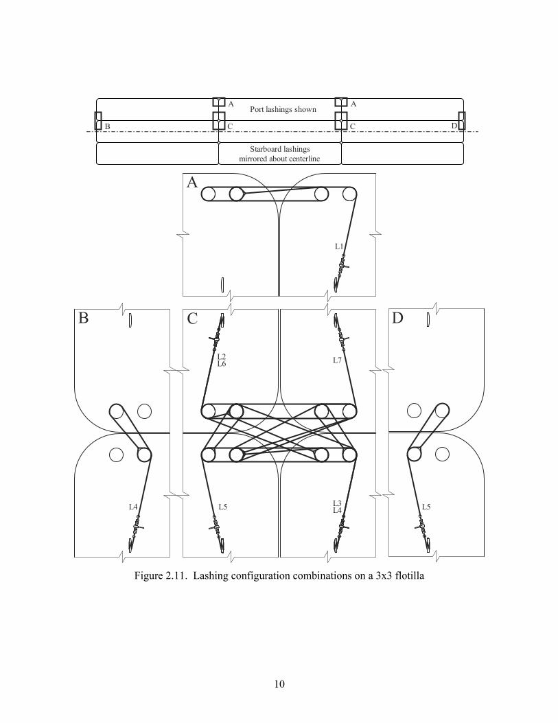
Each pair of adjacent barges in a flotilla is lashed together by wrapping the barge bitts in a specific pattern, referred to as a lashing configuration. Different configurations are used to lash different types of barge pairs (end-to-end, side-to-side, or diagonal) and to resist different loads induced by common flotilla maneuvers. When more than one configuration is required at the same location, they are layered on top of each other. This study employs seven (7) distinct lashing configurations which are divided into groups according to their function. Note that the configurations are presented here as they appear on the port side of the flotilla. Starboard lashings are identical, but mirrored about the flotilla centerline.

Fore/aft wires (Figures 2.7–2.8) are used to secure end-to-end barge pairs together at the shared corners, providing longitudinal rigidity to each barge column. The configuration used along the exterior edges of the flotilla (L1) is unique in that it employs a 1 in. diameter wire rope which is rated at 90 kips break strength. Every other configuration in the flotilla, including the fore/aft wires along the interior edges (L2–L3), uses a 1¼ in. diameter rope rated at 120 kips.

Breast wires (Figure 2.9) are used to connect side-to-side barge pairs together at shared corners, and act to keep the port and starboard columns from lagging behind the center column during travel. Because of their different orientations, they are sometimes referred to separately as towing wires (L4) that are engaged when the center column is pushed forwards, and backing wires (L5) that are engaged when the center column is pulled backward.

Scissor wires (L6–L7, Figure 2.10) connect diagonal barge pairs together at every 4-corner interface. They serve to straighten out the flotilla and increase its flexural rigidity so that it is easier to steer from behind.

In a fully-lashed flotilla, there are only four (4) unique combinations of lashing configurations (shown on a 3x3 flotilla in Figure 2.11). A 3x5 flotilla is analogous to the 3x3 flotilla, but with additional A and C regions inserted. Only the 4-corner interface (C) requires multiple layers of lashings.

8

Direction of flotilla motion

L1

Por

t bar

ge c

olum

n

Figure 2.7. Exterior fore/aft wires (rated at 90 kips break strength)

L2

L3


Cen

ter

barg

e co

lum

nP

ort

barg

e co

lum

n

Figure 2.8. Interior fore/aft wires (rated at 120 kips break strength)

9


Cen

ter

barg

e co

lum

nPo

rt b

arge

col

umn

L4 L5

Figure 2.9. Breast wires (rated at 120 kips)


L6 L7

Cen

ter

barg

e co

lum

nP

ort

barg

e co

lum

n

Figure 2.10. Scissor wires (rated at 120 kips)

10

A

B C D

B C D

A

C

Starboard lashings mirrored about centerline

L1

L4 L5L5

L7

L4L3

L6L2

Port lashings shown

A

Figure 2.11. Lashing configuration combinations on a 3x3 flotilla

11

CHAPTER 3 FINITE ELEMENT MODELING OF BARGES

3.1 Overview

Two types of individual barge finite element models have been developed for use in the flotilla models constructed in this study. The contrasting barge types are differentiated primarily by their roles within the flotilla. A highly discretized barge model has been developed for use as the impacting barge where the high level of discretization is necessary to enable accurate data collection from the contact interaction between the rigid wall and the impacting barge. The impacting barge is the only barge in each flotilla configuration (3x5, 3x3) that makes contact with the rigid wall; the remaining barges in the flotilla are therefore referred to as non-impacting barges. The primary role of non-impacting barges is to accurately capture the dynamic effects associated with contact between barges during impact, throughout the flotilla. Being derived from the highly discretized barge model, non-impacting barge models have a much lower discretization level (coarser mesh) which enables the flotilla model, as a whole, to be as numerically efficient as possible. Since the individual barge models have been developed separately, and for different purposes within the flotilla, they will be discussed independently in the sections that follow.

3.2 Finite element modeling of the impacting barge

3.2.1 Structural modeling

A single-raked jumbo hopper barge measuring 195 ft long by 35 ft wide is used as the impacting barge in all flotilla models considered in this study. The barge is divided into three zones longitudinally along the barge: 27.5 ft for the bow; 162 ft for the hopper; and 5.5 ft for the stern. Watertight bulkheads present within the jumbo hopper barges are used as dividing planes to compartmentalize the barge; bulkheads are spaced at 40.5 ft intervals throughout the hopper zone. Figure 3.1 shows a schematic of the impacting barge in plan and elevation views.

Bow

Starboard

Port

Ster

n

195 ft

35 f

t

a)

Hopper region BowStern

12 f

t2

ft

12.5

ft

35 ft 162 ft 27.5 ft5.5 ft

Stern Watertight bulkhead

40.5 ft (typ.)

b)

Figure 3.1. Impacting jumbo hopper barge schematic: a) Plan; b) Elevation

12

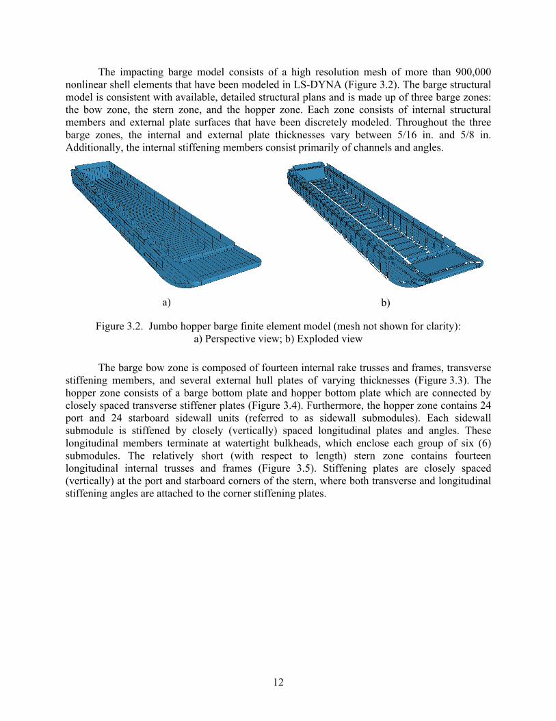
The impacting barge model consists of a high resolution mesh of more than 900,000 nonlinear shell elements that have been modeled in LS-DYNA (Figure 3.2). The barge structural model is consistent with available, detailed structural plans and is made up of three barge zones: the bow zone, the stern zone, and the hopper zone. Each zone consists of internal structural members and external plate surfaces that have been discretely modeled. Throughout the three barge zones, the internal and external plate thicknesses vary between 5/16 in. and 5/8 in. Additionally, the internal stiffening members consist primarily of channels and angles.

a)

b)

Figure 3.2. Jumbo hopper barge finite element model (mesh not shown for clarity): a) Perspective view; b) Exploded view

The barge bow zone is composed of fourteen internal rake trusses and frames, transverse stiffening members, and several external hull plates of varying thicknesses (Figure 3.3). The hopper zone consists of a barge bottom plate and hopper bottom plate which are connected by closely spaced transverse stiffener plates (Figure 3.4). Furthermore, the hopper zone contains 24 port and 24 starboard sidewall units (referred to as sidewall submodules). Each sidewall submodule is stiffened by closely (vertically) spaced longitudinal plates and angles. These longitudinal members terminate at watertight bulkheads, which enclose each group of six (6) submodules. The relatively short (with respect to length) stern zone contains fourteen longitudinal internal trusses and frames (Figure 3.5). Stiffening plates are closely spaced (vertically) at the port and starboard corners of the stern, where both transverse and longitudinal stiffening angles are attached to the corner stiffening plates.

13

Internal rake truss

Top hull plate

Bottom hull plate

Headlog plate

Hopperzone

Bowzone

a)

b)

Figure 3.3. Barge bow section: a) Structural configuration; b) Finite element mesh

Sidewall submodule

Bargebottom plate

Hopperbottom plate

Sidewallstiffeningmembers

Transverse connector plate betweenbarge bottom and hopper bottom

Figure 3.4. Barge bow-hopper zone interface (partial mesh shown for clarity)

14

Corner stiffening plate

Internal truss

a)

b)

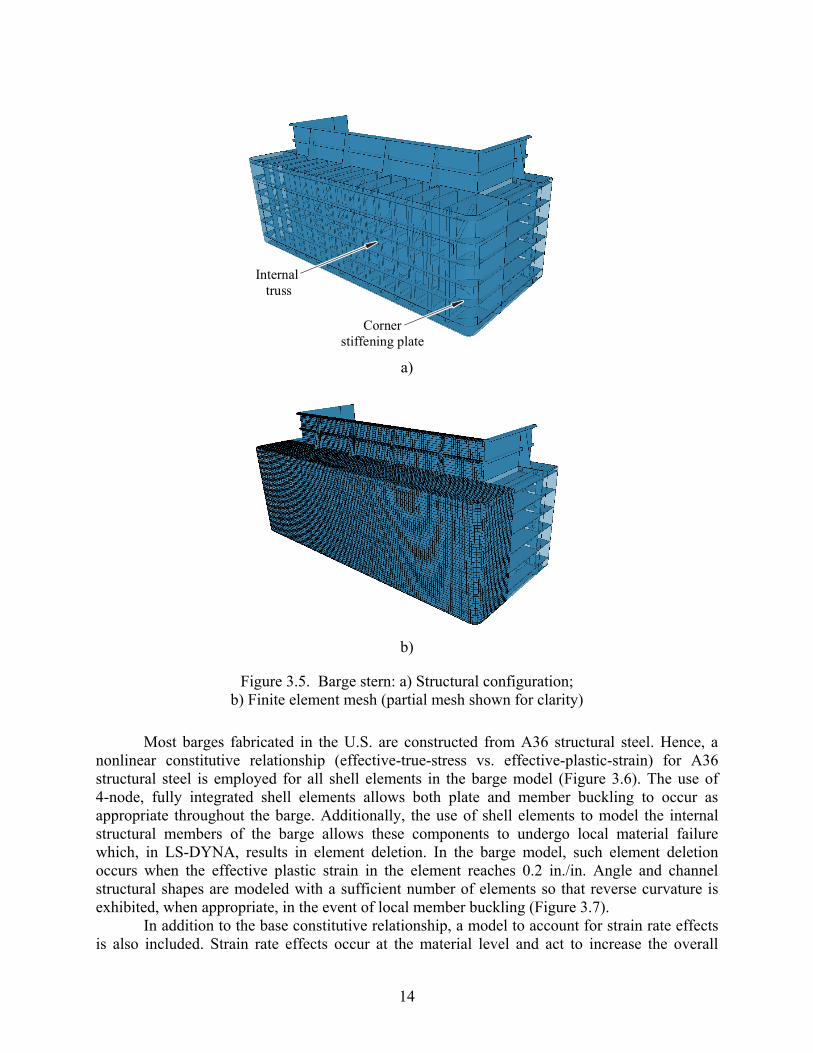
Figure 3.5. Barge stern: a) Structural configuration; b) Finite element mesh (partial mesh shown for clarity)

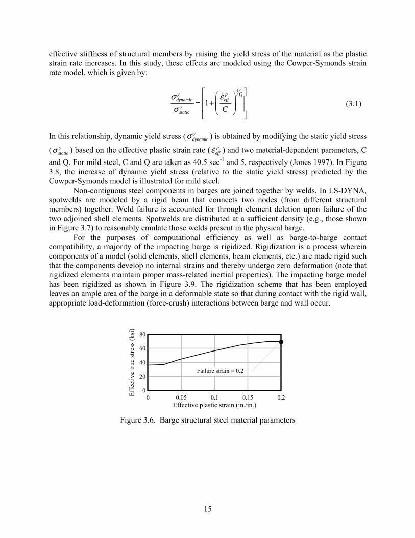
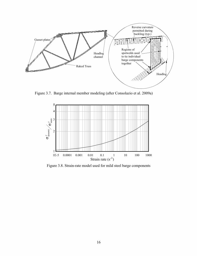
Most barges fabricated in the U.S. are constructed from A36 structural steel. Hence, a nonlinear constitutive relationship (effective-true-stress vs. effective-plastic-strain) for A36 structural steel is employed for all shell elements in the barge model (Figure 3.6). The use of 4-node, fully integrated shell elements allows both plate and member buckling to occur as appropriate throughout the barge. Additionally, the use of shell elements to model the internal structural members of the barge allows these components to undergo local material failure which, in LS-DYNA, results in element deletion. In the barge model, such element deletion occurs when the effective plastic strain in the element reaches 0.2 in./in. Angle and channel structural shapes are modeled with a sufficient number of elements so that reverse curvature is exhibited, when appropriate, in the event of local member buckling (Figure 3.7).

In addition to the base constitutive relationship, a model to account for strain rate effects is also included. Strain rate effects occur at the material level and act to increase the overall

15

effective stiffness of structural members by raising the yield stress of the material as the plastic strain rate increases. In this study, these effects are modeled using the Cowper-Symonds strain rate model, which is given by:

1

1y p Qdynamic eff

ystatic C

σ εσ

= +

(3.1)

In this relationship, dynamic yield stress ( y

dynamicσ ) is obtained by modifying the static yield stress

( ystaticσ ) based on the effective plastic strain rate ( p

effε ) and two material-dependent parameters, C

and Q. For mild steel, C and Q are taken as 40.5 sec-1 and 5, respectively (Jones 1997). In Figure 3.8, the increase of dynamic yield stress (relative to the static yield stress) predicted by the Cowper-Symonds model is illustrated for mild steel.

Non-contiguous steel components in barges are joined together by welds. In LS-DYNA, spotwelds are modeled by a rigid beam that connects two nodes (from different structural members) together. Weld failure is accounted for through element deletion upon failure of the two adjoined shell elements. Spotwelds are distributed at a sufficient density (e.g., those shown in Figure 3.7) to reasonably emulate those welds present in the physical barge.

For the purposes of computational efficiency as well as barge-to-barge contact compatibility, a majority of the impacting barge is rigidized. Rigidization is a process wherein components of a model (solid elements, shell elements, beam elements, etc.) are made rigid such that the components develop no internal strains and thereby undergo zero deformation (note that rigidized elements maintain proper mass-related inertial properties). The impacting barge model has been rigidized as shown in Figure 3.9. The rigidization scheme that has been employed leaves an ample area of the barge in a deformable state so that during contact with the rigid wall, appropriate load-deformation (force-crush) interactions between barge and wall occur.

Effective plastic strain (in./in.)

Eff

ectiv

e tr

ue s

tres

s (k

si)

0 0.05 0.1 0.15 0.20

20

40

60

80

Failure strain = 0.2

Figure 3.6. Barge structural steel material parameters

16

Gusset plates

Raked Truss

Headlogchannel

Regions of spotwelds usedto tie individualbarge componentstogether

Headlog

Reverse curvature permitted during buckling (typ.)

Figure 3.7. Barge internal member modeling (after Consolazio et al. 2009a)

Strain rate (s-1)1E-5 0.0001 0.001 0.01 0.1 1 10 100 10001

2

3

4

55

y dyna

mic

σy stat

icσ

Figure 3.8. Strain-rate model used for mild steel barge components

17

Rigidized

Deformable

Figure 3.9. Partial rigidization of impacting barge model

3.2.2 Payload

The bare steel weight of the single-raked barge model is 285 tons (1 ton = 2000 lbs). The payload for the simulations conducted within this study has been configured so that the weight of a fully-loaded barge would result in a total barge plus payload weight of 2000 tons. This weight is chosen to emulate the individual barge weights used in the full-scale barge flotilla impact study at the Gallipolis Locks (Patev et al. 2003) and slightly exceeds the AASHTO specified loaded displacement tonnage for a jumbo hopper barge of 1900 tons (AASHTO 2009).

For the impacting barge, the payload system is modeled using a series of concentrated nodal masses that are distributed along the centerline of the hopper zone. Specifically, 27 payload mass nodes are placed at a height of 5.4 ft above the hopper bottom plate (the mid-height of the hopper region) and spaced uniformly at 6 ft intervals along the longitudinal axis of the barge. A series of rigid links are used to attach the concentrated payload masses to the barge mesh (Figure 3.10). Total weight for all payload concentrated masses is 1715 tons for the single-raked hopper barge.

Payload mass node

Rigid links

Figure 3.10. Impacting barge finite element model with payload

18

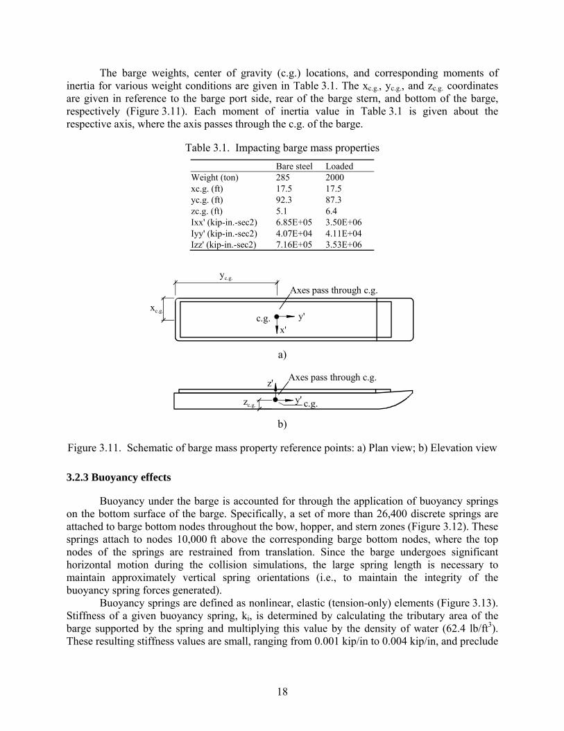
The barge weights, center of gravity (c.g.) locations, and corresponding moments of inertia for various weight conditions are given in Table 3.1. The xc.g., yc.g., and zc.g. coordinates are given in reference to the barge port side, rear of the barge stern, and bottom of the barge, respectively (Figure 3.11). Each moment of inertia value in Table 3.1 is given about the respective axis, where the axis passes through the c.g. of the barge.

Table 3.1. Impacting barge mass properties

Bare steel Loaded Weight (ton) 285 2000 xc.g. (ft) 17.5 17.5 yc.g. (ft) 92.3 87.3 zc.g. (ft) 5.1 6.4 Ixx' (kip-in.-sec2) 6.85E+05 3.50E+06 Iyy' (kip-in.-sec2) 4.07E+04 4.11E+04 Izz' (kip-in.-sec2) 7.16E+05 3.53E+06

yc.g.

c.g.x'

y'

Axes pass through c.g.

xc.g.

a)

c.g.

z'

y'zc.g.

Axes pass through c.g.

b)

Figure 3.11. Schematic of barge mass property reference points: a) Plan view; b) Elevation view

3.2.3 Buoyancy effects

Buoyancy under the barge is accounted for through the application of buoyancy springs on the bottom surface of the barge. Specifically, a set of more than 26,400 discrete springs are attached to barge bottom nodes throughout the bow, hopper, and stern zones (Figure 3.12). These springs attach to nodes 10,000 ft above the corresponding barge bottom nodes, where the top nodes of the springs are restrained from translation. Since the barge undergoes significant horizontal motion during the collision simulations, the large spring length is necessary to maintain approximately vertical spring orientations (i.e., to maintain the integrity of the buoyancy spring forces generated).

Buoyancy springs are defined as nonlinear, elastic (tension-only) elements (Figure 3.13). Stiffness of a given buoyancy spring, ki, is determined by calculating the tributary area of the barge supported by the spring and multiplying this value by the density of water (62.4 lb/ft3). These resulting stiffness values are small, ranging from 0.001 kip/in to 0.004 kip/in, and preclude

19

the advent of unrealistically concentrated buoyant forces. Furthermore, the stiffness values vary due to variations in the (element mesh-based) surface area of barge supported by each spring.

Buoyancy spring

Spring attached to bottom surface of barge (typ.)

Translationalrestraint (typ.)

1000

0 ft

8.5 ft

Foremost buoyancy spring

4.75 ft

Figure 3.12. Barge buoyancy spring schematic

During impact, a barge can undergo various motions, such as pitching and rolling, that would require additional buoyancy springs to be active (in tension) than are active during the initial resting state. In order to achieve this effect, two variants of buoyancy springs are created. The bottommost portions in the hopper and stern zones (a 34 ft wide by 167.5 ft long region, as shown in Figure 3.13a) have been fitted with buoyancy springs that remain “submerged” (active or in tension) for the duration of the collision simulations. However, this is not the case for portions of the barge in the bow zone (a 28.5 ft wide by 22.75 ft long region). To ensure that buoyancy forces are only generated during times in which a specific node would be considered submerged, gaps are incorporated into the buoyancy spring force-deformation definitions. These gaps are specifically introduced for springs that attach to barge bottom nodes in the bow zone (Figure 3.13b). For a given buoyancy spring in the bow zone, with nodal height hi relative to the barge bottom elevation in the hopper and stern zones, a gap of hi is incorporated into the corresponding force-deformation relationship.

20

22.75 ft

Buoyancy springs Buoyancy springs with gaps

167.5 ft

28.5 ft34 f

t

a)

hi

Buoyancy spring i(gap = hi)

Pi

Δzi

ki

hi

Pj

Δzj

kj

Buoyancy spring j(no gap)

Bow zone

Hopper zone

b)

Figure 3.13. Barge buoyancy spring definitions: a) Plan view of regions fitted with springs; b) Schematic

Gravitational forces are present in all impact simulations conducted. In conjunction with the application of gravity loading, a buoyancy spring calibration scheme is employed to ensure that appropriate buoyant forces are generated (Figure 3.14). Employing buoyancy springs without calibration, in a gravity field, would result in non-physical, unwarranted dynamic excitation.

The buoyancy spring calibration process for the loaded impacting barge is shown in Figure 3.14. First, in this process, gravity loading Pbody(t) is applied to the barge FE model in a quasi-static manner (i.e., over a large time tramp, as shown in Figure 3.14b). The quasi-statically applied gravity loads produce vertical steady-state displacements in the barge and buoyancy springs (Figure 3.14c). Subsequently, the steady-state displacement of each buoyancy spring (e.g., Δz

i for buoyancy spring i) is used to define an initial offset in that same buoyancy spring force-deformation relationship. Then, for all collision simulations conducted, gravity is applied in an instantaneous and constant manner (Figure 3.14d). However, because the buoyancy springs now contain initial offsets corresponding to the steady-state displaced configuration of the barge, the buoyancy spring forces and gravity loads are initialized in dynamic equilibrium. Hence, only minimal levels of artificial dynamic excitation occur in the buoyancy springs during the collision simulations, where such excitation is directly in response to the application of gravity loads. Furthermore, by employing this calibration scheme, the profile of buoyancy spring forces

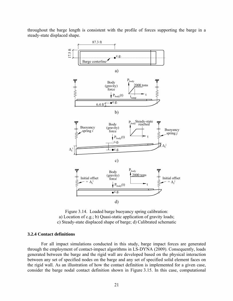
21

throughout the barge length is consistent with the profile of forces supporting the barge in a steady-state displaced shape.

87.3 ft

c.g.

Barge centerline

17.5

ft

a)

c.g.6.4 ft

ttramp

Body (gravity)

force

Pbody(t)

2000 tons

Pbody

b)

c.g.

Δzj

Buoyancy spring i Buoyancy

spring jt

Steady-statereached

Δzi

Body (gravity)

force

Pbody(t)

Pbody

c)

Initial offset =

c.g.

Pbody

tΔz

iInitial offset = Δz

j

2000 tonsBody

(gravity) force

Pbody(t)

d)

Figure 3.14. Loaded barge buoyancy spring calibration: a) Location of c.g.; b) Quasi-static application of gravity loads;

c) Steady-state displaced shape of barge; d) Calibrated schematic

3.2.4 Contact definitions

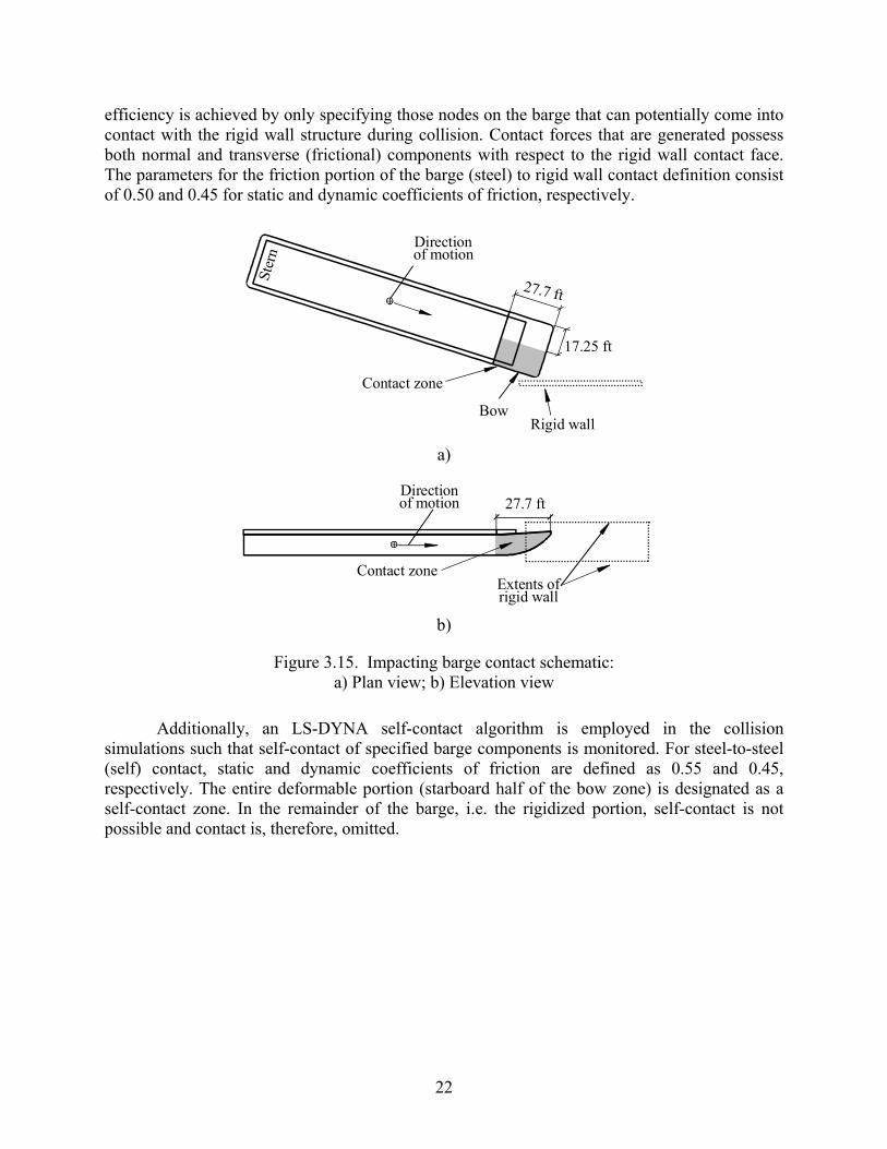
For all impact simulations conducted in this study, barge impact forces are generated through the employment of contact-impact algorithms in LS-DYNA (2009). Consequently, loads generated between the barge and the rigid wall are developed based on the physical interaction between any set of specified nodes on the barge and any set of specified solid element faces on the rigid wall. As an illustration of how the contact definition is implemented for a given case, consider the barge nodal contact definition shown in Figure 3.15. In this case, computational

22

efficiency is achieved by only specifying those nodes on the barge that can potentially come into contact with the rigid wall structure during collision. Contact forces that are generated possess both normal and transverse (frictional) components with respect to the rigid wall contact face. The parameters for the friction portion of the barge (steel) to rigid wall contact definition consist of 0.50 and 0.45 for static and dynamic coefficients of friction, respectively.

17.25 ft

27.7 ft

Contact zone

Direction of motion

Ster

n

BowRigid wall

a)

27.7 ft

Contact zoneExtents of rigid wall

Direction of motion

b)

Figure 3.15. Impacting barge contact schematic: a) Plan view; b) Elevation view

Additionally, an LS-DYNA self-contact algorithm is employed in the collision simulations such that self-contact of specified barge components is monitored. For steel-to-steel (self) contact, static and dynamic coefficients of friction are defined as 0.55 and 0.45, respectively. The entire deformable portion (starboard half of the bow zone) is designated as a self-contact zone. In the remainder of the barge, i.e. the rigidized portion, self-contact is not possible and contact is, therefore, omitted.

23

3.3 Finite element modeling of the non-impacting barge

3.3.1 Structural model

The primary role of the non-impacting barge finite element model is to provide a means of representing mass-related barge inertial properties and dynamic interactions between barges as accurately as possible during and after impact. However, using a fully-discretized high-resolution deformable barge model at each position within a flotilla is computationally infeasible. For this reason, non-impacting barge models are similar to the impacting barge in terms of external geometry, but the internal structural configurations have been wholly modified to improve numerical efficiency.

In the non-impacting barge model, all shell elements on the exterior surfaces of the barge are rigidized. Deformability of the perimeter of the barge, as it relates to interactions between contacting barges, is modeled instead in the contact definitions themselves (discussed later) rather than through detailed modeling of the barge perimeter with deformable shell elements. Therefore, given that the outer surface of the non-impact barge model is completely rigid, internal structural shell elements (making up beams, plates, and frames) serve no purpose and are removed from the model. Additionally, a headlog extension (Figure 3.16) has been added to the bow of the non-impact barge model to approximate the role that head log knees serve during bow-to-stern barge contact interactions. Although major modifications to the structural configuration of the non-impacting barge are made, specific features within LS-DYNA (discussed in subsequent text) allow all non-impacting barges to mimic the mass-related attributes of the high-resolution, deformable impacting barge such as mass moments of inertia and translational mass.

In the high-resolution impacting barge model, shell elements on the outer hull surfaces are approximately 3 in. x 3 in. in size. In the simplified non-impacting barge model, however, shell element sizes are increased to approximately 36 in. x 36 in. As a result, each non-impact barge model contains only about 4000 shell elements, whereas the high-resolution impact barge contains more than 900,000 shell elements. In the reduced resolution non-impact barge model, shell elements are only used to represent the correct outer hull geometry (for contact purposes), not the internal structural stiffness of the barge perimeter, hence a much lower resolution mesh suffices for this purpose.

Two variations of the non-impacting barge model are used within each flotilla model: a single-raked barge model (Figure 3.16a) and a double-raked barge model (Figure 3.16b). A schematic of the double-raked barge is shown in Figure 3.17; this barge maintains the same overall dimensions as the non-impacting single-raked barge. The primary difference between the single and double raked models is that the double-raked barge is raked at both the bow and stern. Additionally, the headlog of the double-raked model is more finely discretized than the headlog of the single-raked model. The change in discretization level ensures robust detection of contact in both bow-to-bow or bow-to-stern contact situations.

24

Headlog extension a)

Headlog extension b)

Figure 3.16. Non-impacting jumbo hopper barge FE model (Perspective view): a) Single-raked model; b) Double-raked model

Hopper region Bow

12 f

t2

ft139.75 ft 27.5 ft

Bow

27.5 ft

a)

Bow

Starboard

Port

195 ft

35 ft

Bow

b)

Figure 3.17. Schematic of non-impacting double-raked jumbo hopper barge: a) Plan view; b) Elevation view

25

3.3.2 Payload

Barge and payload weights (and masses) for the non-impacting single and double-raked barges are the same as for the impacting barge (1715 tons payload, 285 tons bare steel barge). However, the modeling of weight (and mass) in the non-impact barges is handled differently than in the high-resolution impact barge model. In the non-impact barge models, all internal components have been removed and no longer contribute mass, therefore the correct mass-related properties must be specified through a different modeling mechanism to ensure correct dynamic response during impact. For a rigid body, such as the single and double-raked non-impact barges, mass-related inertial properties of the entire rigid barge model can be specified at a single node that is located at the center of gravity (c.g.) of the body. Mass-related c.g. attributes such as translational mass and the inertial tensor are derived from corresponding highly-discretized models of single and double-raked barges (using ~900,000 elements). Properties derived from these models are then specified as c.g. properties in the low-resolution (~4000 elements) non-impact barge models.

For each non-impact barge model, a finite element node is added at the location of the c.g. and rigidly attached to the rest of the barge model (rigid outer shell). Mass properties necessary to correctly represent the single or double-raked barges are then assigned to the newly added c.g. node. Barge weights, c.g. locations, and corresponding mass moments of inertia for the single- and double-raked models are given in Table 3.2. The xc.g., yc.g., and zc.g. coordinates are given in reference to the barge port side, rear of the barge stern, and bottom of the barge, respectively (recall Figure 3.11). Each moment of inertia value in Table 3.2 is given about the respective axis, where the axis passes through the c.g. of the barge.

Table 3.2. Non-impacting barge mass properties

Single-raked Double-raked Weight (ton) 2000 2000 xc.g. (ft) 17.5 17.5 yc.g. (ft) 87.3 97.5 zc.g. (ft) 6.4 6.4 Ixx' (kip-in.-sec2) 3.50E+06 2.69E+06 Iyy' (kip-in.-sec2) 4.11E+04 3.84E+04 Izz' (kip-in.-sec2) 3.53E+06 2.71E+06

3.3.3 Buoyancy

Buoyancy for the non-impacting barges has been modeled in the same manner as that used for the impacting barge except that far fewer discrete buoyancy springs (~900) are used due to the lower mesh resolution of the non-impacting barge models. Buoyancy springs in the non-impact barges use the same force-deformation relationships, offset schemes, and calibration schemes that were previously discussed (Section 3.2.3).

3.3.4 Contact definitions

As mentioned previously, one of the primary roles of the non-impacting barges is to simulate the dynamic effects stemming from barge-to-barge contact during flotilla impacts. Because non-impacting barges are structurally rigid and not deformable, a standard deformable contact-impact algorithm cannot be used to calculate barge-to-barge contact forces.

26

In order to accurately model this contact between rigid barges (where no structural deformation occurs), a rigid body contact algorithm must be employed. This contact algorithm employs a user-specified, nonlinear force-deformation relationship to quantify normal force applied to a node versus penetration of that node through a surface on a per-node basis for a specific contact set (LS-DYNA 2009). As a result, when two barges come into contact, a restoring force (based on the user-defined force-deformation relationship) is applied to each penetrating (or contacting) node and this force is increased, as penetration is increased, until sufficient force is generated from the algorithm to offset (cancel) the nodal penetrations.

In this study, user-defined force-deformation relationships—used in the rigid contact definitions between barges—are derived from a series of high-resolution barge crush simulations (described in the following section) and then assigned to appropriate contact zones with each flotilla: bow-to-bow, bow-to-stern, and side-to-side (Figure 3.18). Hence, although the non-impact single and double-raked barges are modeled using structurally rigid shell elements, the perimeters of these models are effectively deformable by means of the manner in which contact between barges is modeled. Computational efficiency is thus gained by rigidizing the non-impact barges, but proper contact deformability is maintained through specification of nonlinear force-deformation relationships for the rigid contact definitions.

Side-to-sideBow-to-bowBow-to-stern

a)

Side-to-sideBow-to-bowBow-to-stern

b)

Figure 3.18. Rigid contact types within a 3x5 barge flotilla: a) Plan view; b) Elevation view

3.4 Development of rigid contact crush curves

To simulate contact between rigidized non-impacting barges, a rigid body contact algorithm is used that applies a nonlinear force-deformation relationship (stiffness) to a rigid body contact interface to approximate expected stiffness during rigid body contact. As noted above, three types of contact are expected to occur amongst barges: bow-to-bow contact; side-to-side contact; and bow-to-stern contact. High-resolution barge crush simulations are therefore performed to develop force-deformation relationships for use in each of these three types of contact definition. A barge crushing simulation is a finite element simulation wherein two finite

27

element models (e.g. two fully deformable, highly discretized barges positioned in incipient contact with each other) are impacted into each other at a constant, prescribed deformation rate. Time histories of force and deformation can be extracted from such simulations to form force-deformation relationships that are used in rigid body contact. A perspective view of a barge crush simulation is shown in Figure 3.19 wherein a bow-to-stern crush is performed. Note that in this figure, the bow zone is not rigidized, but is stiffer than the stern zone, so little deformation in the bow occurs.

a) b)

Figure 3.19. Bow-to-stern crush simulation (mesh not shown for clarity): a) Before crush; b) During crush

The resultant force-deformation relationships typically exhibit small magnitude, high-frequency oscillations that develop due to localized failures of elements in the finite element model during the crush simulation. Oscillations of this type are not critically important in terms of predicting peak global forces. Therefore, a Gaussian kernel smoothing algorithm is used to remove local oscillations from the force-deformation data. Gaussian kernel smoothing is applied to the bow-to-stern and bow-to-bow force-deformation data using a bandwidth of 5 in. The side-to-side force-deformation curve cannot be smoothed with a bandwidth of 5 in. because crushing is only performed to approximately 3 in. Therefore, a bandwidth of 0.1 in. is used to smooth the side-to-side force-deformation data.

For each smoothed curve, a perfectly-plastic force-deformation point is determined such that all behavior past this point can be adequately approximated as perfectly-plastic. Perfectly plastic behavior has been defined as occurring at 2 in., 60 in., and 72 in. of crush for the side-to-side, bow-to-bow, and bow-to-stern cases, respectively. The resulting smoothed force-deformation relationships (Figure 3.20) are used in the flotilla models to approximate the stiffness of two rigid bodies (non-impacting barges) interacting with each other.

28

Deformation (in)

For

ce (

kip)

0 1 2 3 4 5 6 7 8 9 100

1000

2000

3000

4000

5000

6000

7000

8000

Simulation dataSmoothed curve

a)

Deformation (in)

For

ce (

kip)

0 10 20 30 40 50 60 70 80 90 1000

1000

2000

3000

4000

5000

6000

7000

8000Simulation dataSmoothed curve

b)

Deformation (in)

For

ce (

kip)

0 10 20 30 40 50 60 70 80 90 1000

1000

2000

3000

4000

5000

6000

7000

8000Simulation dataSmoothed curve

c)

Figure 3.20. Various contact crush curves for emulating rigid body contact: a) Side-to-side; b) Bow-to-bow; c) Bow-to-stern

29

CHAPTER 4 FINITE ELEMENT MODELING OF LASHINGS

4.1 Introduction

A barge flotilla consists of a group of individual barges that are temporarily constrained together to enable them to transit, as a unit, along a given waterway. In order to achieve this unity, varying configurations of lashings are used to introduce inter-barge stiffnesses into the flotilla unit. With a lashing system in place, barges no longer act independently of one another but rather distribute applied forces (e.g. due to impact) throughout the entire barge flotilla. Development of a suitable finite element representation of lashings requires that the lashing model be capable of modeling both the material-level behavior of wire rope (e.g. stress-strain curves) as well as physical-level behavior (e.g., lashing pretension, slip of lashings around barge bitts, and lashing failure).

4.2 Lashing material model

Stranded wire rope is the typical type of wire rope chosen for use in mooring applications (Gaythwaite 2004). Wire rope is generally composed of steel wire strands arranged in a helical pattern in one or more layers around a (fiber or steel) inner core. Such rope can be made from several different grades of steel and can have multiple physical configurations (strand patterns and shapes) (ASTM A1023-09 2009). A typical wire rope used in marine mooring applications consists of six strands and is within the 6x24, 6x36, or 6x37 classifications (also called constructions) of wire rope (Gaythwaite 2004). These classifications are given in the form of AxB where A represents the number of strand assemblies in the wire rope and B represents the number of steel wires in each strand assembly (see Figure 4.1 for a sample wire rope cross section). In accordance with ASTM A1023-09 (2009), the individual steel wires that compose the wire rope strands are required to have a tensile failure stress between 227 ksi and 284 ksi though this standard does not specify that the final stranded wire rope assembly must have a tensile failure within that range. The tensile breaking strengths, or ultimate strengths, for most wire rope configurations with common grades of steel are defined separately in the reference tables of ASTM A1023.

When considering the load-elongation behavior of wire rope, the inner core material, physical strand configuration, and grade of steel can all have a significant influence. In addition to these characteristics, physical deterioration, connection type, and bend radii can further influence this relationship and complicate the material model. Such a detailed model is not warranted, however, given the scope of the present study. Instead, to mitigate several unknowns, several assumptions are made about the wire rope that enables flotilla impact forces to be conservatively estimated. For all wire rope lashings considered in this study, the wire rope is assumed to be in new or very good condition (no prior yielding, no physical deterioration) and is assumed to have connections and bend radii that maintain no losses in material efficiency. Such assumptions will generally lead to conservatively high predictions of barge flotilla impact forces and therefore are considered acceptable.

30

4.2.1 Overview

The barge flotilla lashings in the barge flotilla impact study at the Gallipolis Locks employed two different wire ropes that have different breaking strengths (ultimate strengths): 90 kip (1 in. dia.) and 120 kip (1¼ in. dia.) (Patev et al. 2003). Several types of wire rope closely meet these criteria in the ASTM A1023 reference tables; one of which is the 6x25 filler wire, fiber core wire rope. This type of wire rope, a cross section of which is provided in Figure 4.1, is composed of six (6) strand assemblies that are laid helically around a fiber core. Each strand assembly is composed of 25 steel wires that are also arranged helically about their respective centers. Note that in the present study, the cross section is not discretely modeled in three dimensions, but instead is modeled using discretized one-dimensional elements with the appropriately specified material properties.

6 strand assemblies25 wires per strand

Fiber core

1” or 1 / ”1

4

Strand assembly

Individual steel wire

Figure 4.1. 6x25 filler wire, fiber core wire rope cross section (After ASTM A1023-09, 2009)

In 1990, experiments were conducted in which many samples of 6x25 and 6x19 wire rope were tested in tension to failure (McKewan and Miscoe 1990). Force and elongation data were recorded for each test, from which stresses and strains could be calculated. This study focused on testing wire rope constructions that are typically used in mining operations. The testing itself, however, was independent of association with mining-related structural mechanisms. Therefore, the wire rope stress-strain data could be generally applied to a wire rope in tension in any environment.

Two of the wire ropes tested by McKewan and Miscoe were 6x25 filler wire, fiber core wire ropes with diameters of 1 in. and 1¼ in. and breaking strengths of 84 kips and 129 kips, respectively. These wire ropes closely match both the ASTM-specified breaking strengths as well as the diameters listed in the flotilla impact study at the Gallipolis Locks (Patev et al. 2003). Therefore, it is deemed reasonable to use material properties from the McKewan and Miscoe study to aid in the formation of material models for the wire ropes used in the flotilla impact study at the Gallipolis Locks.

31

4.2.2 Development of wire rope material model

The study by McKewan and Miscoe provides basic material properties for wire ropes, consisting of modulus of elasticity (E), yield stress (σy), yield strain (εy), ultimate failure stress (σult), and ultimate failure strain (εult). In the study, two additional types of wire rope were provided with extensive stress-strain data points through rope failure. This full stress-strain data is beneficial because it can be used to develop generalized stress-strain expressions for this particular configuration of wire rope. Once the general expressions are developed, the basic stress and strain data (for the 6x25 wire ropes in question) can be fit to the expressions and material models can then be created for the wire rope of concern.

The qualitative characteristics of the stress-strain curves of the wire rope in the McKewan and Miscoe study are very similar to those seen in prestressing strand material models (PCI 2004). With that in mind, the stress-strain data from the McKewan and Miscoe study is used to develop a piecewise material model that uses a linear expression to model elastic behavior (Eq. 4.1) and the functional form used for prestressing strand to model nonlinear, inelastic behavior (Eq. 4.2). In the equations below, A, B, C, and E are constants that are algebraically derived from the application of the subsequently discussed criteria. A generalized form of each equation is plotted in Figure 4.2.

Eσ ε= ⋅ for 0 < ε < εy (4.1)

BA

Cσ

ε= −

− for εy < ε < εult (4.2)

Strain ( )ε

Str

ess

()

for 0 < < ε yε

εy εult

σy

σult

1

E

Elastic expression

Plastic expression

Slope of elastic and plasticexpressions equal at yield

0

for < < ε ultε εy

BA

Cσ

ε= −

−

Eσ ε= ⋅

Figure 4.2. General form of piecewise material model expressions

32

Three criteria are applied to develop the piecewise material model expression using the basic stress-strain data with the above-mentioned functional forms. These criteria are:

1. The linear elastic expression must originate at a value of zero stress and zero strain

and extend linearly to the yield stress/yield strain point. 2. The nonlinear inelastic expression must pass through the yield stress/yield strain point

as well as the failure stress/failure strain point and must follow the functional form provided in Eq. 4.2.

3. The slope at yield from the linear elastic expression (where ε = εy) and the slope at yield from the nonlinear inelastic expression (where ε = εy) must be equal.

Using these criteria, the variables of the inelastic material model expression (A, B, and C) and the single variable of the elastic material model expression (E) can be determined. Once an expression has been developed for each wire rope strength in question (90 kip and 120 kip), the expressions are modified slightly such that both failure strains occur at 0.04 in./in. and also such that their respective breaking strengths match those in the abovementioned flotilla impact study. These additional modifications have no detrimental effect on the integrity of the material model approximation and only serve to improve consistency. The final expressions and stress-strain relationships for both material models are given in Figure 4.3.

Strain (in/in)

Stre

ss(k

si)

0 0.005 0.01 0.015 0.02 0.025 0.03 0.035 0.040

25

50

75

100

125

150

175

200

225

Breaking Strength - 90 kipBreaking Strength - 120 kip

8458

0.330236

0.015

σ ε

σε

= ⋅

= −−

for 0 < < 0.022ε

for 0.022 < < 0.040ε

80440.171

1970.015

σ ε

σε

= ⋅

= −− for 0.020 < < 0.040ε

for 0 < < 0.020ε

Figure 4.3. Fitted stress-strain relationships for various lashing types

4.3 Development of lashing finite element model

A single flotilla lashing consists of a length of wire rope that is wrapped around a sequence of barge bitts and tensioned to hold the barges in place. Each bitt acts as a pivot point for the lashing, but does not structurally restrain the lashing from slipping around it. Resultant forces on the bitts are a function of the tension developed in each straight (bitt-to-bitt) segment of the lashing. However, because the lashing is a continuous cable, those segments must remain in

33

static equilibrium with each other. If the flotilla lashing system is perturbed, slippage around the bitts is often required to maintain equilibrium.

These complex interactions can have a significant influence on the dynamics of a flotilla during impact. This study employs a robust lashing model that captures the following key aspects of lashing behavior:

• Material model: The lashing has a nonlinear stiffness in tension that is characteristic of

wire rope. No forces are generated in compression.

• Continuity: Equilibrium is maintained throughout the total length of the lashing.

• Slippage: The lashing is able to slip freely around the bitts.

• Pretensioning: Tension is ramped up during an initialization period until the target initial tension is reached, regardless of losses due to elastic shortening. This is consistent with manual tensioning procedures performed on actual flotillas.

• Lashing failure: When the breaking strength is exceeded, the lashing fails and ceases to carry any tension.

• Layers: Multiple layers of lashings can act independently while occupying the same location on the flotilla.

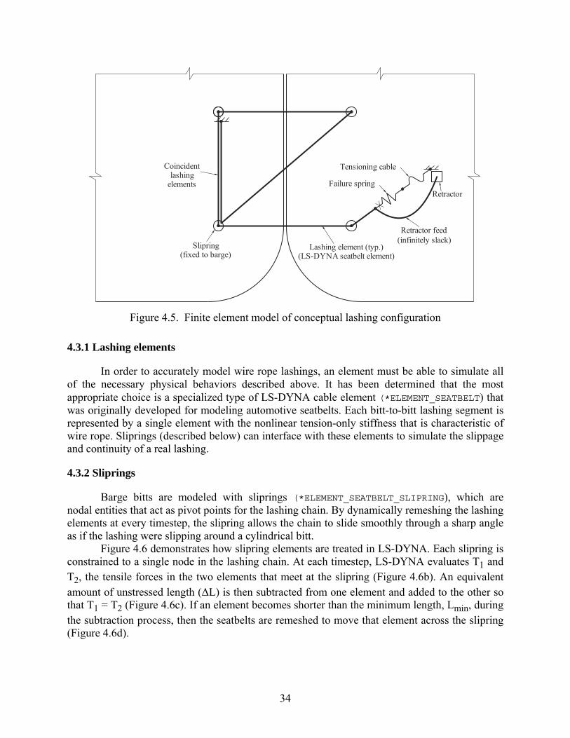
To facilitate discussion of the lashing model and its components, consider the conceptual lashing configuration shown in Figure 4.4. This configuration has been developed to clearly demonstrate all of the computational features of the lashing model, but it does not correspond to any specific configuration used in the actual flotilla model. A diagram of the equivalent finite element representation of the lashing is provided in Figure 4.5.

Barge bitt (typ.)

Cable winch(Come-a-long)

Flotilla barges

Wire rope lashing

Cavel

Figure 4.4. Conceptual lashing configuration (for demonstrative purposes only)

34

Failure spring

Tensioning cable

Retractor

Retractor feed(infinitely slack)

Slipring (fixed to barge)

Coincidentlashing

elements

Lashing element (typ.)(LS-DYNA seatbelt element)

Figure 4.5. Finite element model of conceptual lashing configuration

4.3.1 Lashing elements

In order to accurately model wire rope lashings, an element must be able to simulate all of the necessary physical behaviors described above. It has been determined that the most appropriate choice is a specialized type of LS-DYNA cable element (*ELEMENT_SEATBELT) that was originally developed for modeling automotive seatbelts. Each bitt-to-bitt lashing segment is represented by a single element with the nonlinear tension-only stiffness that is characteristic of wire rope. Sliprings (described below) can interface with these elements to simulate the slippage and continuity of a real lashing.

4.3.2 Sliprings

Barge bitts are modeled with sliprings (*ELEMENT_SEATBELT_SLIPRING), which are nodal entities that act as pivot points for the lashing chain. By dynamically remeshing the lashing elements at every timestep, the slipring allows the chain to slide smoothly through a sharp angle as if the lashing were slipping around a cylindrical bitt.

Figure 4.6 demonstrates how slipring elements are treated in LS-DYNA. Each slipring is constrained to a single node in the lashing chain. At each timestep, LS-DYNA evaluates T1 and T2, the tensile forces in the two elements that meet at the slipring (Figure 4.6b). An equivalent amount of unstressed length (ΔL) is then subtracted from one element and added to the other so that T1 = T2 (Figure 4.6c). If an element becomes shorter than the minimum length, Lmin, during the subtraction process, then the seatbelts are remeshed to move that element across the slipring (Figure 4.6d).

35

Bitt

T2

T1

Lashing

a)

T2

T1

2

1

34

Slipring fixed to barge(constrains lashing node 3)

Seatbelt element (typ.)

b)

T1

T2

< LMin

1

2

3

Element lengthened by LΔ

Element shortened by LΔ

c)

T1

T2

1

432

Element moved across slipring

Slipring constraint changed to node 2

d)

Figure 4.6. Behavior of slipring elements at each timestep: a) Real lashing equivalent; b) T2 > T1; c) Material transfer until T1 = T2; d) Remeshed to move element across slipring

4.3.3 Tensioning cable

Rather than use an offset to generate initial tension, the lashing model includes an LS-DYNA cable element that simulates the effect of a cable winch (Fig. 4.7). During flotilla initialization, the element internal force ramps from zero to the desired pretension. It then holds that tension constant while the flotilla reaches equilibrium. By dynamically adjusting the unstressed length of the element, a constant tension is maintained regardless of elastic shortening effects caused by the deformation of the barges. This process is analogous to the manner in which lashings are tensioned in a real flotilla—i.e. the lashings are tightened manually until the desired tension is reached. Once initialization is complete, the unstressed length of each element becomes fixed, and the tensioning cable behaves like a normal lashing element with the same nonlinear stiffness.

Failure Spring Tensioning Cable

Slipring

Lashing Elements

Figure 4.7. Close-up view of tensioning cable and failure spring

36

4.3.4 Failure spring

Lashing failure is modeled by means of a dedicated failure spring connected in series between the tensioning cable and the chain of lashing elements (Fig. 4.7). Like the rest of the lashing, the spring has the equivalent nonlinear stiffness of wire rope. When the spring is subjected to a critical elongation (which corresponds to the ultimate breaking strength), it “fails” and is deleted from the analysis. This occurrence severs the load path of the lashing, leaving it unable to carry tension and therefore unable to restrain the connected barges from drifting apart.

4.3.5 Retractor

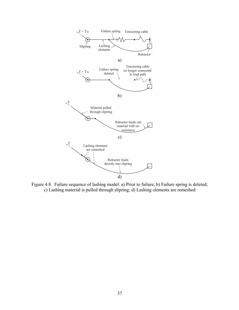
When the failure spring is deleted, the connected lashing element is left with a free node: a situation that LS-DYNA does not allow. To prevent this, another lashing element is added to the model, with one end connected to the offending node and the other attached to a retractor (Fig. 4.8a). When a tension force is applied to the element, the retractor will freely add material to lengthen it, rather than allow it to carry load. Effectively, the element has zero stiffness, so it does not affect the total stiffness of the lashing system

With the addition of a retractor, deletion of the failure spring no longer creates a free node (Fig. 4.8b). As the barges separate, lashing material is pulled through the sliprings and the retractor freely feeds out material to replace it (Fig. 4.8c). Once the lashing is pulled far enough, the elements are remeshed (Fig. 4.8d). This leaves the retractor feeding directly into the slipring. Although the barges remain “connected” throughout the process, the stiffness of the connection is effectively zero, and the movements of the barges are unaffected.

37

T < TBr

Slipring

Retractor

Failure spring Tensioning cable

Lashingelements

a)

T = TBrFailure spring

deleted

Tensioning cable no longer connected

to load path

b)

T

Retractor feeds out material with no

resistance

Material pulled through slipring

c)

Lashing elements are remeshed

Retractor feeds directly into slipring

T

d)

Figure 4.8. Failure sequence of lashing model: a) Prior to failure; b) Failure spring is deleted; c) Lashing material is pulled through slipring; d) Lashing elements are remeshed

38

CHAPTER 5 IMPACT SIMULATIONS AND RESULTS

5.1 Overview

For the simulations conducted in this study, a multi-barge finite element flotilla model is impacted into a rigid wall at varying degrees of obliquity (θ) with various initial velocities (V0). Two barge flotilla models have been developed for this purpose which are a 3x5 barge flotilla (three columns by five rows) and a 3x3 barge flotilla (three columns by three rows). Each barge flotilla model contains a single highly discretized, deformable barge, which is utilized to directly impact a rigid wall. The flotilla model additionally uses a series of low-resolution rigid barges to emulate the dynamic effects of the other barges within the flotilla.

Impact simulations discussed in this chapter are conducted for the purposes of quantifying impact forces, observing dynamic effects within the flotilla, and enabling comparisons between simulation data and experimental data collected during the previously conducted barge flotilla impact study at the Gallipolis Locks. Additionally, simulation results are compared to the U.S. Army Corps of Engineers ETL 563 (specifically Engineer Technical Letter 1110-2-563 “Barge Impact Analysis for Rigid Walls,”) design methodology which is capable of estimating impact forces on a rigid wall due to a glancing blow (θ < 30°) from a barge flotilla (USACE 2004). For purposes of brevity in discussion, each finite element simulation will be referred to in the following format: Flotilla Type – Impact Angle – Impact Velocity – Lashing Pretension. For instance, a 3x5 barge flotilla impacting a rigid wall at 30 degrees of obliquity, at 5 feet per second, and with a lashing pretension equal to 50% of rated lashing capacity, will be referred to as a 3x5 – 30° – 5 fps – 50% simulation.

5.2 Rigid wall model

In each impact simulation, the barge flotilla is positioned to impact the rigid wall at a specific angle of obliquity (θ) and initial velocity (V0). Rigid solid elements (approximately 36 in. cubes) compose the wall model (Figure 5.1), which has dimensions of 100 ft by 3 ft by 15 ft (L x W x H). Furthermore, the rigid wall is fixed in space at the specified angle, θ, and is positioned in a manner consistent with Figure 5.2 such that the barge will impact the wall with a sufficient buffer of contact area on all sides of the initial impact point. For all simulations, the contact surface on the rigid wall is defined along the surface of the wall that is in contact with the barge flotilla.

39

100 ft

3 ft

a)

100 ft

15 f

t

b)

Figure 5.1. Schematic of the rigid wall with mesh shown: a) Plan view; b) Elevation view

Direction of initial velocity

Rigid wall

Barge flotilla θ

Initial impact point

Y

X

V0

a)

Rigid wall

Direction of initial velocityInitial impact pointZ

XV0

b)

Figure 5.2. Impact simulation schematic: a) Plan view; b) Elevation view

40

5.3 Finite element modeling of load-measurement system

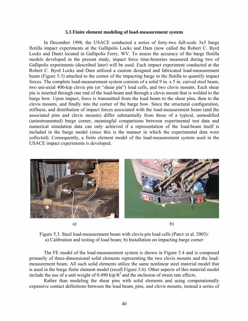
In December 1998, the USACE conducted a series of forty-two full-scale 3x5 barge flotilla impact experiments at the Gallipolis Locks and Dam (now called the Robert C. Byrd Locks and Dam) located in Gallipolis Ferry, WV. To assess the accuracy of the barge flotilla models developed in the present study, impact force time-histories measured during two of Gallipolis experiments (described later) will be used. Each impact experiment conducted at the Robert C. Byrd Locks and Dam utilized a custom designed and fabricated load-measurement beam (Figure 5.3) attached to the corner of the impacting barge in the flotilla to quantify impact forces. The complete load-measurement system consists of a solid 9 in. x 5 in. curved steel beam, two uni-axial 400-kip clevis pin (or “shear pin”) load cells, and two clevis mounts. Each shear pin is inserted through one end of the load-beam and through a clevis mount that is welded to the barge bow. Upon impact, force is transmitted from the load beam to the shear pins, then to the clevis mounts, and finally into the corner of the barge bow. Since the structural configuration, stiffness, and distribution of impact forces associated with the load-measurement beam (and the associated pins and clevis mounts) differ substantially from those of a typical, unmodified (uninstrumented) barge corner, meaningful comparisons between experimental test data and numerical simulation data can only achieved if a representation of the load-beam itself is included in the barge model (since this is the manner in which the experimental data were collected). Consequently, a finite element model of the load-measurement system used in the USACE impact experiments is developed.

a)

b)

Figure 5.3. Steel load-measurement beam with clevis-pin load cells (Patev et al. 2003): a) Calibration and testing of load beam; b) Installation on impacting barge corner

The FE model of the load-measurement system is shown in Figure 5.4 and is composed primarily of three-dimensional solid elements representing the two clevis mounts and the load-measurement beam. All such solid elements utilize the same nonlinear steel material model that is used in the barge finite element model (recall Figure 3.6). Other aspects of this material model include the use of a unit weight of 0.490 kip/ft3 and the inclusion of strain rate effects.

Rather than modeling the shear pins with solid elements and using computationally expensive contact definitions between the load beam, pins, and clevis mounts, instead a series of

41

nodal rigid bodies are used to emulate the function of the pins. A nodal rigid body in an LS-DYNA finite element model consists of a collection of nodes that are constrained to move as a single rigid body (i.e., the distances between the nodes within the body remain constant, even as the overall body translates and rotates through space).

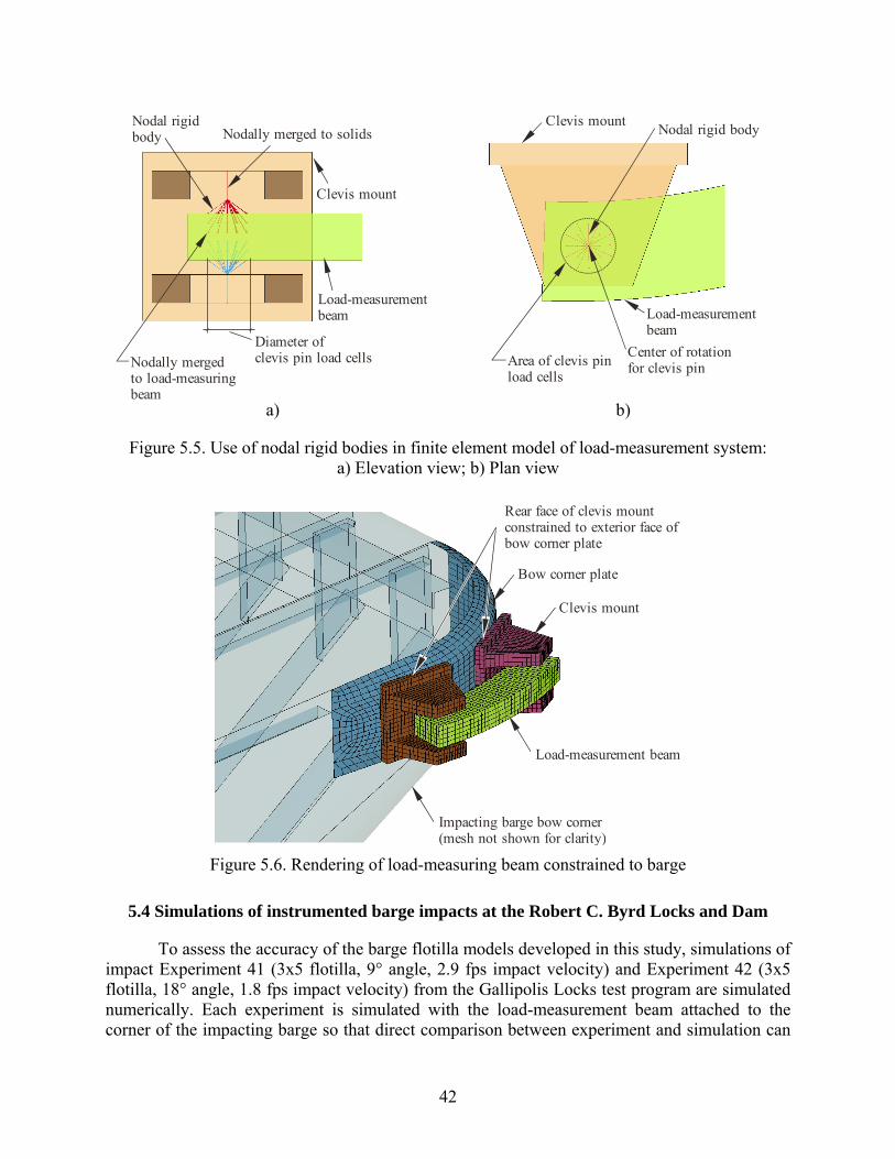
As illustrated in Figure 5.5, at each end of the load-measurement beam, a nodal rigid body is defined to tie (constrain) nodes within the footprint of the clevis pin to a single line of nodes lying inside the clevis mount. Note that the nodal line inside the clevis mount corresponds to the hypothetical longitudinal axis of the shear pin. This modeling technique results in a computationally efficient means of allowing the end of the load beam to rotate within the clevis mesh in a way that emulates the rotation that would be permitted by a pin. For purposes of attaching the clevis mounts to the corner of the barge bow model, translational constraints are introduced between nodes on the rear faces of the clevis mounts and the nearest corresponding nodes on the bow corner plate (Figure 5.6).

Clevis mount

Load-measurement beam

Figure 5.4. Overview of finite element model of load-measurement system

42

Load-measurementbeam

Clevis mount

Nodal rigidbody

Diameter ofclevis pin load cells

Nodally merged to solids

Nodally mergedto load-measuringbeam

a)

Load-measurementbeam

Area of clevis pinload cells

Clevis mount

Center of rotationfor clevis pin

Nodal rigid body

b)

Figure 5.5. Use of nodal rigid bodies in finite element model of load-measurement system: a) Elevation view; b) Plan view

Load-measurement beam

Clevis mount

Bow corner plate

Impacting barge bow corner(mesh not shown for clarity)

Rear face of clevis mountconstrained to exterior face ofbow corner plate

Figure 5.6. Rendering of load-measuring beam constrained to barge

5.4 Simulations of instrumented barge impacts at the Robert C. Byrd Locks and Dam

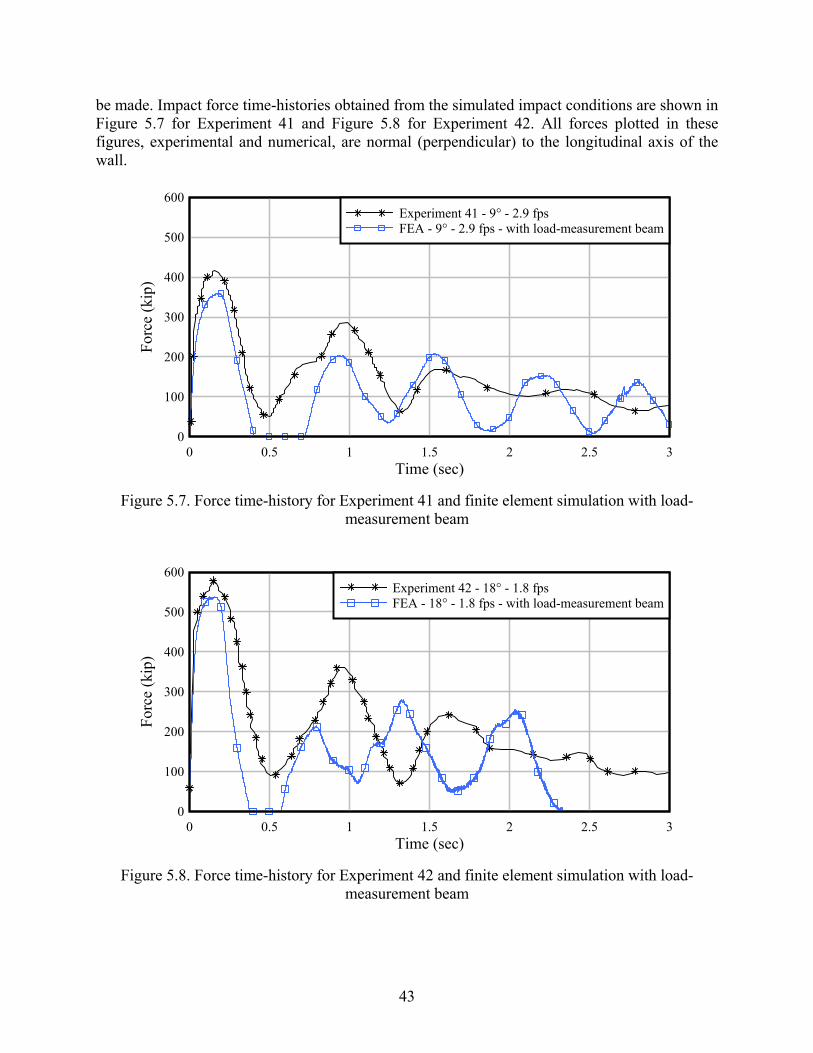
To assess the accuracy of the barge flotilla models developed in this study, simulations of impact Experiment 41 (3x5 flotilla, 9° angle, 2.9 fps impact velocity) and Experiment 42 (3x5 flotilla, 18° angle, 1.8 fps impact velocity) from the Gallipolis Locks test program are simulated numerically. Each experiment is simulated with the load-measurement beam attached to the corner of the impacting barge so that direct comparison between experiment and simulation can

43

be made. Impact force time-histories obtained from the simulated impact conditions are shown in Figure 5.7 for Experiment 41 and Figure 5.8 for Experiment 42. All forces plotted in these figures, experimental and numerical, are normal (perpendicular) to the longitudinal axis of the wall.

Time (sec)

For

ce (

kip)

0 0.5 1 1.5 2 2.5 30

100

200

300

400

500

600Experiment 41 - 9° - 2.9 fpsFEA - 9° - 2.9 fps - with load-measurement beam

Figure 5.7. Force time-history for Experiment 41 and finite element simulation with load-measurement beam

Time (sec)

For

ce (

kip)

0 0.5 1 1.5 2 2.5 30

100

200

300

400

500

600Experiment 42 - 18° - 1.8 fpsFEA - 18° - 1.8 fps - with load-measurement beam

Figure 5.8. Force time-history for Experiment 42 and finite element simulation with load-measurement beam

44

In Figure 5.7 (Experiment 41), the peak impact force measured experimentally, using the load-beam pictured in Figure 5.3, was 417 kips. Numerical impact simulation of the same condition, with inclusion of the load beam finite element model depicted in Figure 5.6, predicts an impact force of 360 kips (14% less than the experimental value). In Figure 5.8 (Experiment 42), the peak impact force measured experimentally was 579 kips, whereas the numerical simulation predicts a force of 539 kips (7% less than the experimental value). Hence, good agreement is observed between test data and simulation data and the accuracy of the barge flotilla model is deemed acceptable for purposes intended in this study.

5.5 Impact conditions simulated

Using the barge flotilla and rigid wall finite element models discussed above, numerical simulations of the impact conditions summarized in Tables 5.3 through 5.6 are conducted. However, since the goal in conducting these simulations is to quantify peak impact forces for collisions from typical uninstrumented commercial barge flotillas, the simulations are conducted using flotilla models (3x3 and 3x5) in which the load-measurement beam, discussed above, is excluded. Denoted within Tables 5.3 through 5.6 are flotilla type (3x3 or 3x5), lashing pretension level (as a percentage of ultimate capacity), impact angle in degrees, and impact velocity in feet per second (fps). Each simulation is carried out until impact forces on the wall have completely subsided and zero impact force is measured over a sustained duration of time.

Table 5.3. Flotilla impact cases with an impact angle of 10°

Flotilla type Impact angle (°)

Impact velocity (fps)

Lashing pretension (%)

3x5 10 1 10 3x5 10 2 10 3x5 10 3 10 3x5 10 1 50 3x5 10 2 50 3x5 10 3 50 3x5 10 4 50 3x5 10 5 50 3x3 10 1 10 3x3 10 1 50





3x5 20 1 10 3x5 20 2 10 3x5 20 1 50 3x5 20 2 50 3x5 20 3 50 3x5 20 4 50 3x5 20 5 50 3x3 20 3 10 3x3 20 3 50

45





3x5 25 3 10

3x5 25 3 50





3x5 30 1 10 3x5 30 2 10 3x5 30 0.5 50 3x5 30 1 50 3x5 30 2 50 3x5 30 3 50 3x5 30 4 50 3x5 30 5 50 3x5 30 8 50

5.6 Impact force time-histories predicted by impact simulation

In the figures below, impact force time-histories from the finite element simulations are presented for each simulation configuration listed in the above tables. Specifically for the 50% lashing pretension cases, the figures are presented so that for each plot of a specific impact angle, all initial velocities for that angle are plotted within the same figure. For most plots, initial velocities of 1 fps through 5 fps are shown with bounding velocity cases being plotted separately. The bounding cases are a 3x5 – 30° – 8 fps – 50% simulation and a 3x5 – 30° – 0.5 fps – 50% simulation. Figures 5.9 through 5.16 present all 3x5 barge flotilla impact force histories and Figure 5.17 presents all 3x3 barge flotilla impact force histories. All forces plotted are the components of impact force normal to the rigid wall.

All data presented visually in the figures below is summarized in Table 5.7 and Table 5.8. Table 5.7 presents simulation data related to the 10% lashing pretension simulations while Table 5.8 presents the simulation data related to the 50% lashing pretension simulations. These tables show maximum impact forces normal to the wall and parallel to the wall (friction) as well as the maximum utilization of each lashing type as a percentage of their ultimate capacities. A lashing utilization value of 100% indicates that at least one lashing has reached its ultimate capacity and failed. Only in the 3x5 – 30° – 8 fps – 50% barge flotilla simulation has more than one lashing failed; in this particular simulation, five lashings failed although it did not result in either a partial or full flotilla break-up.

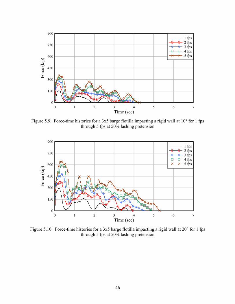
46

Time (sec)

For

ce (

kip)

0 1 2 3 4 5 6 70

150

300

450

600

750

9001 fps2 fps3 fps4 fps5 fps

Figure 5.9. Force-time histories for a 3x5 barge flotilla impacting a rigid wall at 10° for 1 fps through 5 fps at 50% lashing pretension

Time (sec)

For

ce (

kip)

0 1 2 3 4 5 6 70

150

300

450

600

750



47

Time (sec)

For

ce (

kip)

0 1 2 3 4 5 6 70

150

300

450

600

750

90010% lashing pretension50% lashing pretension

Figure 5.11. Force-time histories for a 3x5 barge flotilla impacting a rigid wall at 25° for 3 fps at various lashing pretensions

Time (sec)

For

ce (

kip)

0 1 2 3 4 5 6 70

150

300

450

600

750



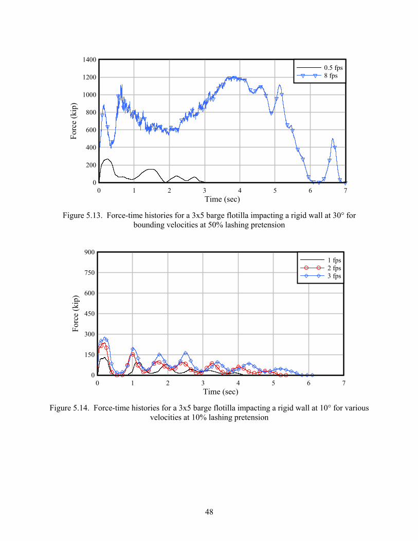
48

Time (sec)

For

ce (

kip)

0 1 2 3 4 5 6 70

200

400

600

800

1000

1200

14000.5 fps8 fps

Figure 5.13. Force-time histories for a 3x5 barge flotilla impacting a rigid wall at 30° for bounding velocities at 50% lashing pretension

Time (sec)

For

ce (

kip)

0 1 2 3 4 5 6 70

150

300

450

600

750

9001 fps2 fps3 fps

Figure 5.14. Force-time histories for a 3x5 barge flotilla impacting a rigid wall at 10° for various velocities at 10% lashing pretension

49

Time (sec)

For

ce (

kip)

0 1 2 3 4 5 6 70

150

300

450

600

750

9001 fps2 fps


Time (sec)

For

ce (

kip)

0 1 2 3 4 5 6 70

150

300

450

600

750

9001 fps2 fps


50

Time (sec)

For

ce (

kip)

0 1 2 3 4 5 6 70

150

300

450

600

750

90010° - 1 fps - 10% lashing pretension10° - 1 fps - 50% lashing pretension20° - 3 fps - 10% lashing pretension20° - 3 fps - 50% lashing pretension

Figure 5.17. Force-time histories for all 3x3 barge flotilla simulations

Table 5.7. Maximum forces for various barge flotilla impact simulations at 10% lashing pretension

Flotilla Model

Impact Angle (°)

Velocity (fps)

Normal Force (kip)

Friction Force (kip)

Lashing Utilization (%)

120 kip 90 kip

3x3 10 1 130 58 14.5 % 16.3 % 3x3 20 3 447 201 50.4 % 47.9 % 3x5 10 1 130 58 16.8 % 17.1 % 3x5 10 2 238 107 25.8 % 22.8 % 3x5 10 3 279 126 37.0 % 29.6 % 3x5 20 1 255 115 24.8 % 23.5 % 3x5 20 2 355 160 46.3 % 34.9 % 3x5 25 3 586 264 85.9 % 61.1 % 3x5 30 1 334 150 34.7 % 30.2 % 3x5 30 2 505 226 67.6 % 47.9 %

51

Table 5.8. Maximum forces for various barge flotilla impact simulations at 50% lashing pretension

Flotilla Model

Impact Angle (°)

Velocity (fps)

Normal Force (kip)

Friction Force (kip)

Lashing Utilization (%)

120 kip 90 kip

3x3 10 1 146 62 55.6 % 58.6 % 3x3 20 3 478 214 81.7 % 77.2 % 3x5 10 1 167 71 59.2 % 58.6 % 3x5 10 2 242 108 66.8 % 62.2 % 3x5 10 3 282 127 77.0 % 69.0 % 3x5 10 4 320 144 85.7 % 75.6 % 3x5 10 5 355 160 90.8 % 80.8 % 3x5 20 1 301 131 68.8 % 62.9 % 3x5 20 2 387 172 86.5 % 74.5 % 3x5 20 3 481 215 93.8 % 83.5 % 3x5 20 4 607 272 97.6 % 90.3 % 3x5 20 5 652 292 100 % 96.4 % 3x5 25 3 627 280 96.3 % 85.7 % 3x5 30 0.5 269 112 62.3 % 60.3 % 3x5 30 1 353 156 78.6 % 67.8 % 3x5 30 2 549 246 93.5 % 77.8 % 3x5 30 3 775 345 98.9 % 81.8 % 3x5 30 4 848 374 100 % 95.9 % 3x5 30 5 857 385 100 % 97.4 % 3x5 30 8 1206 542 100 % 98.8 %

5.7 Comparison of finite element simulation data and ETL 563

The U.S. Army Corps of Engineers document ETL 563 (Engineer Technical Letter 1110-2-563, “Barge Impact Analysis for Rigid Walls”) can be used to quantify impact forces for “rigid navigation structures such as lock walls, approach walls, channel walls, revetments, and [other] coastal structures,” (USACE 2004). ETL 563 uses an empirically derived equation to predict impact forces due to barge flotilla impacts. This equation is specifically intended for use in quantifying forces of glancing blows (where 0° < θ < 30°); thus, neither head-on nor side-on impacts may be analyzed. Additionally, ETL 563 is valid only to a ceiling of 800 kips of normal impact force; above this point, additional guidance must be sought in quantifying potential impact loads.

ETL 563 uses an empirical correlation between momentum and impact forces normal to the rigid structure to determine the maximum impact force for design. The empirical correlation from ETL 563 is given below in Eq. 5.1 (USACE 2004). In this equation, m represents total mass

of the flotilla (kip/(ft/sec2)), V0x represents the impact velocity component parallel to the barge columns (ft/sec), and V0y represents the impact velocity component transverse to the barge columns (along the rows) (ft/sec). Eq. 5.1 is plotted together with all finite element simulation results in Figure 5.18. Figures 5.19 and 5.20 present comparisons of the normal impact forces between the ETL 563 and finite element data for the 10% and 50% lashing pretension simulation sets, respectively.

52

max 0 0( ) 0.435 ( sin cos )w x yF m V Vθ θ= ⋅ ⋅ ⋅ + ⋅ (5.1)

Figure 5.18 indicates that for relatively low-momentum impacts (impacts less than

approximately 500 kip-sec) the ETL 563 approximation is a reasonable estimate of the impact forces generated normal to the wall. For relatively larger momentum impacts (above 500 kip-sec) the ETL 563 approximation becomes increasingly conservative in comparison to the finite element simulation data. The notable exception to this trend is simulation case 3x5 – 30° – 8 fps – 50% with a very high momentum of approximately 7500 kip-sec. For this severe impact condition, crushing of corner of the impacting barge model is large enough that the effective stiffness of the deformed corner increases and an impact force in excess of 1000 kips is generated. For a high energy and high momentum impact condition of this type, ETL 563 is not applicable.

Momentum normal to rigid wall (kip-sec)

Nor

mal

impa

ct f

orce

(ki

p)

0 1000 2000 3000 4000 5000 6000 7000 80000

200

400

600

800

1000

1200

1400FEAETL 563

Figure 5.18. Comparison of ETL 563 and finite element analysis (FEA) results

53

0

200

400

600

800

1000

1200

Nor

mal

impa

ct f

orce

(ki

p) .

Impact conditionFEA Simulation ETL 563

Figure 5.19. Comparison of normal impact forces between ETL 563 and finite element simulations with 10% lashing pretension

0

200

400

600

800

1000

1200

1400

Nor

mal

impa

ct f

orce

(ki

p) .

Impact conditionFEA Simulation ETL 563

Figure 5.20. Comparison of normal impact forces between ETL 563 and finite element simulations with 50% lashing pretension

54

CHAPTER 6 CONCLUSIONS

Current practices in the United States for the design of rigid and flexible waterway

structures subjected to barge impact loading are believed to be conservative in many cases. Conservatism in the design of guidance and protection structures stems from limited availability of barge flotilla impact force data, both experimentally and analytically derived. In order to begin generating impact force data that can be used to refine the relevant design guidelines, in this study, dynamic nonlinear finite element models of barge flotillas have been developed that employ both accurate barge force-deformation relationships and accurate modeling of wire-rope lashings.

Assessment of the accuracy of the flotilla models has been carried out by conducting simulations of two full-scale impact experiments conducted by the US Army Corps of Engineers (USACE) at the Gallipolis Locks and Dam (now called the Robert C. Byrd Locks and Dam) located in Gallipolis Ferry, WV. Because the physical experiments conducted at the Gallipolis Locks utilized a relatively stiff steel load-measurement beam that was affixed to the impacting barge, a finite element model of this same load-measurement device has been developed in this study and included in selected finite element impact simulations. Force time-history data gathered during two of the Gallipolis impact experiments have been compared to results from numerical simulations of corresponding impact conditions. For the two conditions examined, peak impact forces from the simulations were within 15% of the peak forces measured during the experiments—a level of accuracy deemed acceptable for the purposes intended in this study

An additional set of thirty (30) dynamic, nonlinear finite element impact simulations have also been conducted—using both 3x3 and 3x5 barge flotilla models, and a range of different impact angles and velocities—to quantify impact forces as a function of impact angle, impact velocity, and flotilla size. Since the goal in conducting these simulations was to quantify peak impact forces for collisions from typical uninstrumented commercial barge flotillas, the simulations have been conducted using flotilla models in which the load-measurement beam was excluded.

Finite element simulation data have also been compared to impact force data computed using U.S. Army Corps of Engineers rigid structure design guideline ETL 563. These comparisons demonstrate that over a wide range of impact momentums, the ETL 563 design guideline is conservative in comparison to the finite element simulation data. The only notable exception to this trend was found for very high momentum impacts where the ETL 563 design guideline is both unconservative and non-applicable.

55

REFERENCES American Association of State Highway and Transportation Officials (AASHTO), Guide

Specifications and Commentary for Vessel Collision Design of Highway Bridges, 2nd Edition, AASHTO, Washington D.C., 2009.

American Society for Testing and Materials, “Standard Specification for Stranded Carbon Steel Wire Ropes for General Purposes”, American Society for Testing and Materials, ASTM A1023-09, West Conshohocken, PA, 2009.

Consolazio, G.R., Davidson, M.T., and Cowan, D.R., “Barge Bow Force-Deformation Relationships for Barge-Bridge Collision Analysis”, Journal of the Transportation Research Board, 2009.

Gaythwaite, J.W., Design of Marine Facilities for the Berthing, Mooring, and Repair of Vessels, 2nd Edition, American Society of Civil Engineers, Reston, VA, 2004.

LSTC, LS-DYNA Keyword User’s Manual: Version 971, Livermore Software Technology Corporation, Livermore, CA, 2009.

McKewan, W.M., Miscoe, A.J., Baseline Tensile Testing at the Wire Rope Research Laboratory, U.S. Department of the Interior: Bureau of Mines Pittsburgh Research Center, Pittsburgh, PA, 1990.

Patev, R.C., Barker, B.C., Koestler III, L.V., Full-Scale Barge Impact Experiments, Robert C. Byrd Lock and Dam, Gallipolis Ferry, West Virginia, U.S. Army Corps of Engineers Research and Development Center, ERDC/ITL TR-03-7, Vicksburg, MS, 2003.

U.S. Army Corps of Engineers, Barge Impact Analysis for Rigid Walls, Engineer Technical Letter 1110-2-563, U.S. Army Corps of Engineers, Washington D.C., 2004.

U.S. Army Corps of Engineers, 2007 Flood Control and Navigation Maps: Mississippi River, U.S. Army Corps of Engineers, Washington D.C., 2007.

Documents

Development of Finite Element Models for Studying Multi ...Engineers at the decommissioned Gallipolis Locks and Dam in Gallipolis Ferry, WV, and to forces calculated using the U.S