DEVELOPMENT OF FORWARD FLIGHT TRIM AND …etd.lib.metu.edu.tr/upload/12610391/index.pdf · development of forward flight trim and longitudinal dynamic stability codes and their application

DEVELOPMENT OF FORWARD FLIGHT TRIM AND LONGITUDINAL DYNAMIC STABILITY CODES AND THEIR APPLICATION TO A UH-60

HELICOPTER

A THESIS SUBMITTED TO THE GRADUATE SCHOOL OF NATURAL AND APPLIED SCIENCES

OF MIDDLE EAST TECHNICAL UNIVERSITY

BY

SEVİNÇ ÇALIŞKAN

IN PARTIAL FULFILLMENT OF THE REQUIREMENTS FOR

THE DEGREE OF MASTER OF SCIENCE IN

AEROSPACE ENGINEERING

FEBRUARY 2009

Approval of the thesis:


HELICOPTER

submitted by SEVİNÇ ÇALIŞKAN in partial fulfillment of the requirements for the degree of Master of Science in Aerospace Engineering Department, Middle East Technical University by, Prof. Dr. Canan Özgen Dean, Graduate School of Natural and Applied Sciences Prof. Dr. İ. Hakkı Tuncer Head of Department, Aerospace Engineering Prof. Dr. Yusuf Özyörük Supervisor, Aerospace Engineering Dept., METU Examining Committee Members: Prof. Dr. Nafiz Alemdaroğlu Aerospace Engineering Dept., METU Prof. Dr. Yusuf Özyörük Aerospace Engineering Dept., METU Assoc. Prof. Dr. Serkan Özgen Aerospace Engineering Dept., METU Prof. Dr. Ozan Tekinalp Aerospace Engineering Dept., METU Vahit ÖZVEREN, M.Sc. Senior Expert Engineer, ASELSAN

Date: 02.02.2009

iii

I hereby declare that all information in this document has been obtained and presented in accordance with academic rules and ethical conduct. I also declare that, as required by these rules and conduct, I have fully cited and referenced all material and results that are not original to this work.

Name, Surname: Sevinç ÇALIŞKAN

Signature:

iv

ABSTRACT


HELICOPTER

Çalışkan, Sevinç

M. Sc., Department of Aerospace Engineering

Supervisor : Prof. Dr. Yusuf Özyörük

Co-Supervisor : Assoc. Prof. Dr. Serkan Özgen

February 2009, 141 pages

This thesis describes the development of a series of codes for trim and

longitudinal stability analysis of a helicopter in forward flight. In general,

particular use of these codes can be made for parametric investigation of

the effects of the external and internal systems integrated to UH-60

helicopters. However, in this thesis the trim analysis results are obtained for

a clean UH-60 configuration and the results are compared with the flight test

data that were acquired by ASELSAN, Inc.

The first of the developed trim codes, called TRIM-CF, is based on closed-

form equations which give the opportunity of having quick results. The

second code stems from the trim code of Prouty. That code is modified and

improved during the course of this study based on the theories outlined in

[3], and the resultant code is named TRIM-BE. These two trim codes are

verified by solving the trim conditions of the example helicopter of [3]. Since

it is simpler and requires fewer input parameters, it is more often more

v

convenient to use the TRIM-CF code. This code is also verified by analyzing

the Bo105 helicopter with the specifications given in [2]. The results are

compared with the Helisim results and flight test data given in this reference.

The trim analysis results of UH-60 helicopter are obtained by the TRIM-CF

code and compared with flight test data.

A forward flight longitudinal dynamic stability code, called DYNA-STAB, is

also developed in the thesis. This code also uses the methods presented in

[3]. It solves the longitudinal part of the whole coupled matrix of equations of

motion of a helicopter in forward flight. The coupling is eliminated by

linearization. The trim analysis results are used as inputs to the dynamic

stability code and the dynamic stability characteristics of a forward flight trim

case of the example helicopter [3] are analyzed. The forward flight stability

code is applied to UH-60 helicopter.

The codes are easily applicable to a helicopter equipped with external

stores. The application procedures are also explained in this thesis.

Keywords: Helicopter, UH-60, Bo105, forward flight, hover, longitudinal,

trim, dynamic stability, short period mode, phugoid mode, flight test,

disturbance, data logging, onboard, flight certified data acquisition system,

closed form equation, external store.

vi

ÖZ

DÜZ UÇUŞ DURUMU İÇİN BİR DENGE VE DİNAMİK KARARLILIK KODU GELİŞTİRİLMESİ VE UH-60 HELİKOPTERİ ÜZERİNDE UYGULANMASI

Çalışkan, Sevinç

Yüksek Lisans, Havacılık ve Uzay Mühendisliği Bölümü

Tez Yöneticisi : Prof. Dr. Yusuf Özyörük

Ortak Tez Yöneticisi : Doç. Dr. Serkan Özgen

Şubat 2009, 141 sayfa

Bu rapor, bir helikopterin düz uçuştaki performansını, denge durumunu ve

dinamik kararlılığını analiz eden bir dizi yazılımın geliştirilmesi çalışmalarını

sunmaktadır. Bu kodların özel bir kullanımı, UH-60 helikopterlerine entegre

edilen çeşitli sistemlerin etkilerinin parametrik araştırması için

gerçekleştirilebilmektedir. Temiz bir UH-60 helikopteri konfigürasyonu için

denge analizi sonuçları, ASELSAN, A.Ş. tarafından gerçekleştirilen uçuş

testleri sonuçları ile karşılaştırılmaktadır.

Geliştirilen ilk yazılım, [3] referansında verilen kapalı-form denklemleri

kullanmaktadır. TRIM-CF adını alan bu kodun en kullanışlı özelliği,

parametrelerin çok hızlı hesaplanmasına olanak vermesidir. İkinci kod,

Prouty tarafından geliştirilen denge yazılımını temel almaktadır. Yazılım, bu

tez çalışması sırasında, [3] referans kitabında anlatılan teoriler esas

alınarak değiştirilmiş ve iyileştirilmiştir. Elde edilen koda TRIM-BE adı

verilmiştir. Her iki denge yazılımı, [3]’te verilen örnek helikopter üzerinde

doğrulanmıştır. Daha basit olması ve daha az girdi gerektirmesi sebebiyle,

vii

TRIM-CF yazılımını kullanmak sıklıkla daha elverişlidir. Bu kod, [2] referans

kitabında verilen Bo105 helikopteri analiz edilerek de doğrulanmıştır. Analiz

sonuçları, referans kitapta verilen Helisim yazılımı sonuçları ve uçuş test

sonuçları ile karşılaştırılmıştır. UH-60 helikopterinin denge analizi TRIM-CF

yazılımı kullanılarak gerçekleştirilmiştir ve uçuş test sonuçları ile

karşılaştırılmıştır.

Tez kapsamında, [3] referans kitabında yer alan yöntemleri kullanan DYNA-

STAB adlı bir düz uçuş boylamsal kararlılık analiz yazılımı geliştirilmiştir.

Yazılım, bağımlı-birleşik olan düz uçuş hareket denklemleri matrisinin

boylamsal kısmını çözümlemektedir. Bağımlı-birleşik denklem çözümü

doğrusallaştırma yöntemi ile gerçekleştirilmektedir. Denge yazılımlarının

çıktıları, kararlılık yazılımına girdi olarak kullanılmaktadır. Yazılım ile, [3]

fererans kitabında yer alan örnek helikopterin, belirli bir ileri hızdaki kararlılık

karakteristikleri incelenmiştir. Düz uçuş boylamsal kararlılık analiz yazılımı

kullanılarak UH-60 helikopteri üzerinde inceleme gerçekleştirilmiş ve

sonuçlar bu raporda sunulmuştur.

Yazılımlar, harici yük taşıyan helikopterlerin incelenmesine de olanak

sağlamaktadır. Bu raporda, yazılımların bu helikopterlere uyarlanması

konusuna da değinilmektedir.

Anahtar kelimeler: Helikopter, UH-60, Bo105, düz uçuş, hover, boylamsal,

denge, dinamik kararlılık, short-period modu, phugoid modu, uçuş testi,

bozanetken, veri kaydı, uçuş sertifikalı veri toplama sistemi, kapalı form

denklem, harici yük.

viii

To my close friends, to my family and

to my love,

ix

ACKNOWLEDGEMENTS The author wishes to express her gratitude to Drs. Yusuf ÖZYÖRÜK and

Serkan ÖZGEN for guiding this work. Thanks to Dr. Yusuf ÖZYÖRÜK for

his sincere supervision and continuous patience.

Special thanks go to my colleague and close friend Vahit ÖZVEREN for his

leadership, encouragement, considerable patience and friendship. This

thesis would not be possible without his support.

Thanks to my family and my close friends, who showed great understanding

and encouragement.

Special thanks to my darling for his magnificent love and understanding.

This study was supported by ASELSAN.

x

TABLE OF CONTENTS

ABSTRACT .................................................................................................. iv

ÖZ ................................................................................................................ vi

ACKNOWLEDGEMENTS ............................................................................ ix

TABLE OF CONTENTS ................................................................................ x

LIST OF TABLES........................................................................................ xiii

LIST OF FIGURES .................................................................................... xiv

LIST OF SYMBOLS .................................................................................. xviii

CHAPTERS .................................................................................................. 1

1. INTRODUCTION ...................................................................................... 1

1.1 BACKGROUND .............................................................................. 1

1.2 UH-60 HELICOPTER ..................................................................... 3

1.3 OBJECTIVE OF THE THESIS ........................................................ 6

1.4 SCOPE OF THE THESIS ............................................................... 6

2. TRIM AND STABILITY CODE DEVELOPMENT .................................... 11

2.1 FORCES AND MOMENTS ACTING ON A HELICOPTER IN

FLIGHT ................................................................................................... 11

2.2 HELICOPTER ROTOR SYSTEM ................................................. 13

2.3 HELICOPTER ROTOR AERODYNAMICS ................................... 16

2.4 TRIM AND STABILITY ................................................................. 23

2.5 THEORY AND CODE DEVELOPMENT ....................................... 25

xi

2.5.1 TRIM-BE CODE ........................................................................ 29

2.5.2 TRIM-CF CODE ........................................................................ 33

2.5.3 DYNA-STAB CODE .................................................................. 36

2.6 VERIFICATION ............................................................................ 39

2.6.1 PROUTY’S EXAMPLE HELICOPTER ...................................... 39

2.6.2 PADFIELD’S EXAMPLE HELICOPTER .................................... 44

3. TRIM ANALYSIS OF UH-60 ................................................................... 54

3.1 FLIGHT TESTS ............................................................................ 54

3.1.1 INSTRUMENTATION................................................................ 54

3.1.2 DATA LOGGING ....................................................................... 55

3.1.3 DATA PROCESSING AND RESULTS...................................... 56

3.2 TRIM ANALYSIS OF UH-60 HELICOPTER ................................. 57

4. STABILITY ANALYSIS OF UH-60 HELICOPTER .................................. 82

5. CONCLUSIONS AND FUTURE WORK ................................................. 90

REFERENCES ........................................................................................... 91

APPENDICES ............................................................................................. 94

A. TRIM-BE CODE ..................................................................................... 94

A.1 MAIN ROTOR PARAMETERS ..................................................... 94

A.1.1 CALCULATIONS OF LOCAL FORCES .................................... 96

A.1.2 INTEGRATION ....................................................................... 113

A.1.3 WHOLE ROTOR PARAMETERS ........................................... 116

A.2 FUSELAGE PARAMETERS ....................................................... 119

A.3 EMPENNAGE PARAMETERS ................................................... 120

A.4 CONVERGENCE CRITERIA ...................................................... 122

A.5 TAIL ROTOR PARAMETERS .................................................... 123

xii

B. TRIM-CF CODE ................................................................................... 128

B.1 MAIN ROTOR PARAMETERS ................................................... 128

B.1.1 COLLECTIVE ANGLE CALCULATIONS ................................ 129

B.1.2 FORCES, MOMENTS AND POWER ....................................... 133

B.2 TOTAL FORCES AND MOMENTS ............................................ 134

C. DYNA-STAB CODE ............................................................................. 136

C.1 MAIN ROTOR STABILITY DERIVATIVES ................................. 136

C.2 HORIZONTAL STABILIZER STABILITY DERIVATIVES............ 138

C.3 VERTICAL STABILIZER STABILITY DERIVATIVES ................. 140

C.4 FUSELAGE STABILITY DERIVATIVES ..................................... 140

C.5 TOTAL STABILITY DERIVATIVES ............................................ 141

xiii

LIST OF TABLES

TABLES Table 2-1: Example helicopter input parameters in [3] ................................ 40

Table 2-2: TRIM-BE and TRIM-CF results for the example helicopter [3] ... 42

Table 2-3: Example helicopter input parameters in [2] ................................ 45

xiv

LIST OF FIGURES

FIGURES Figure 1-1: UH-60 Helicopter ................................................................................ 4

Figure 1-2: Stabilator pozition vs. airspeed ........................................................ 5

Figure 1-3: Interfaces of the codes ...................................................................... 8

Figure 2-1: Forces and moments acting on a helicopter ................................ 12

Figure 2-2: Hinges on an articulated rotor [22] ................................................ 14

Figure 2-3: Teetering rotor [22] .......................................................................... 15

Figure 2-4: Hingeless rotor [22] .......................................................................... 16

Figure 2-5: The streamtube in the momentum theory [22] ............................. 18

Figure 2-6: Blade element theory [22] ............................................................... 19

Figure 2-7: Local velocity sketch over the rotor [1] .......................................... 21

Figure 2-8: The pressure distribitution over the rotor [1] ................................. 21

Figure 2-9: The dynamic stall effect on the lift .................................................. 22

Figure 2-10: Forces and moments acting on a helicopter [3] ......................... 27

Figure 2-11: The thrust vector on main rotor .................................................... 28

Figure 2-12: Flowchart of TRIM-BE code .......................................................... 30

Figure 2-13: Flowchart of TRIM-CF code .......................................................... 34

Figure 2-14: The Phugoid and Short Period Modes ........................................ 37

Figure 2-15: The example helicopter in [3] ....................................................... 40

Figure 2-16: Bo105 helicopter [2] ....................................................................... 45

Figure 2-17: Lift per unit dynamic pressure obtained from the fuselage on

Bo105 [2] ........................................................................................... 47

Figure 2-18: Drag per unit dynamic pressure obtained from the fuselage on

Bo105 [2] ........................................................................................... 47

Figure 2-19: Pitching moment per unit dynamic pressure obtained from the

fuselage on Bo105 [2] ...................................................................... 48

xv

Figure 2-20: Main rotor torque compared with flight test data and Helisim

results for Bo105 [2] ......................................................................... 49

Figure 2-21: Main rotor torque and power for Bo105 [2] ................................. 50

Figure 2-22: Collective angle compared with flight test data and Helisim

results for Bo105 [2] ......................................................................... 51

Figure 2-23: Longitudinal cyclic angle compared with flight test data and

Helisim results for Bo105 [2] .......................................................... 51

Figure 2-24: Tail rotor collective (pedals) angle compared with flight test

data and Helisim results for Bo105 [2] .......................................... 52

Figure 2-25: Fuselage pitch attitude compared with flight test data and

Helisim results for Bo105 [2] .......................................................... 53

Figure 3-1: A snap-shot of the software ............................................................ 56

Figure 3-2: Fuselage pitch attitude vs. advance ratio ..................................... 58

Figure 3-3: Total torque vs. advance ratio ........................................................ 58

Figure 3-4: Main rotor thrust coefficient vs. advance ratio ............................. 59

Figure 3-5: Main rotor H-force coefficient vs. advance ratio .......................... 60

Figure 3-6: Main rotor power vs. advance ratio ................................................ 61

Figure 3-7: Total power required vs. forward velocity ..................................... 62

Figure 3-8: Main rotor torque vs. advance ratio ............................................... 63

Figure 3-9: TPP angle of attack vs. advance ratio ........................................... 64

Figure 3-10: Induced velocity vs. advance ratio ............................................... 64

Figure 3-11: Inflow ratio vs. advance ratio ........................................................ 65

Figure 3-12: Collective angle vs. advance ratio ............................................... 66

Figure 3-13: Coning angle vs. advance ratio .................................................... 67

Figure 3-14: Longitudinal flapping angle vs. advance ratio ............................ 68

Figure 3-15: Longitudinal cyclic angle vs. advance ratio ................................ 68

Figure 3-16: Tail rotor thrust coefficient vs. advance ratio ............................. 69

Figure 3-17: Tail rotor H-force coefficient vs. advance ratio .......................... 69

Figure 3-18: Tail rotor torque coefficient vs. advance ratio ............................ 71

Figure 3-19: Tail rotor inflow ratio vs. advance ratio ....................................... 71

xvi

Figure 3-20: Tail rotor coning angle vs. advance ratio .................................... 72

Figure 3-21: Tail rotor longitudinal flapping angle vs. advance ratio ............ 72

Figure 3-22: Tail rotor lateral flapping angle vs. advance ratio ...................... 73

Figure 3-23: Tail rotor pedals angle vs. advance ratio .................................... 74

Figure 3-24: Fuselage angle of attack vs. advance ratio ................................ 74

Figure 3-25: Fuselage lift vs. advance ratio ...................................................... 75

Figure 3-26: Fuselage drag vs. advance ratio .................................................. 76

Figure 3-27: Fuselage pitching moment vs. advance ratio ............................. 76

Figure 3-28: Horizontal stabilator angle of attack vs. advance ratio ............. 78

Figure 3-29: Horizontal stabilator lift vs. advance ratio ................................... 78

Figure 3-30: Horizontal stabilator drag vs. advance ratio ............................... 79

Figure 3-31: Vertical stabilizer sideward force vs. advance ratio .................. 79

Figure 3-32: Vertical stabilizer drag vs. advance ratio .................................... 80

Figure 3-33: Fuselage lift (empennage on) vs. advance ratio ....................... 80

Figure 3-34: Fuselage drag (empennage on) vs. advance ratio ................... 81

Figure 4-1: Derivative of pitching moment with respect to the vertical velocity

............................................................................................................. 82

Figure 4-2: Routh’s Discriminant and the coefficients of characteristic eqn. 83

Figure 4-3: Root Locus ......................................................................................... 84

Figure 4-4: Period values belonging to the phugoid mode ............................. 86

Figure 4-5: Time-to-Double values belonging to the phugoid mode ............. 87

Figure 4-6: Time-to-double values belonging to the non-oscillatory roots ... 87

Figure 4-7: Drag Damping ................................................................................... 88

Figure 4-8: Vertical Damping ............................................................................... 89

Figure 4-9: Pitch Damping ................................................................................... 89

Figure A- 1: Fuselage angles, forces and moments [3]. .............................. 94

Figure A- 2: Main rotor, empennage and fuselage angles, forces and

moments [3]. ............................................................................ 95

Figure A- 3: Reference planes and angles on the main rotor [3]. ................ 97

xvii

Figure A- 4: Induced velocities in the vicinity of a hovering rotor [3]. .......... 99

Figure A- 5: The induced velocity on an aircraft [3]. .................................. 101

Figure A- 6: Local induced velocity distribution on the main rotor [3]. ....... 102

Figure A- 7: Distortion factor of the local induced velocity distribution [3]. 103

Figure A- 8: Local velocity components acting on the blade section [3]. ... 105

Figure A- 9: Local velocity components and the reverse flow region [3]. .. 111

Figure A- 10: Normal and chordwise force coefficients [3]. ....................... 112

Figure A- 11: Function xf sin= (black curve) is calculated with Simpson’s

rule (blue lines) and by trapezoidal rule (red line) [36]. .......... 115

Figure A- 12: Delta-3 angle [3]. ................................................................. 124

Figure A- 13: Tail rotor and vertical stabilizer angles, forces and moments

[3]. .......................................................................................... 127

Figure B- 1: The sign change of the lift at the reverse flow region [3] ........ 130

xviii

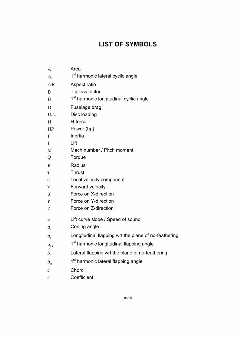
LIST OF SYMBOLS A Area

1A 1st harmonic lateral cyclic angle

..RA Aspect ratio B Tip loss factor

1B 1st harmonic longitudinal cyclic angle

D Fuselage drag ..LD Disc loading

H H-force HP Power (hp) I Inertia L Lift M Mach number / Pitch moment Q Torque

R Radius T Thrust U Local velocity component V Forward velocity X Force on X-direction Y Force on Y-direction Z Force on Z-direction

a Lift curve slope / Speed of sound

0a Coning angle

1a Longitudinal flapping wrt the plane of no-feathering

Sa1 1st harmonic longitudinal flapping angle

1b Lateral flapping wrt the plane of no-feathering

Sb1 1st harmonic lateral flapping angle

c Chord c Coefficient

xix

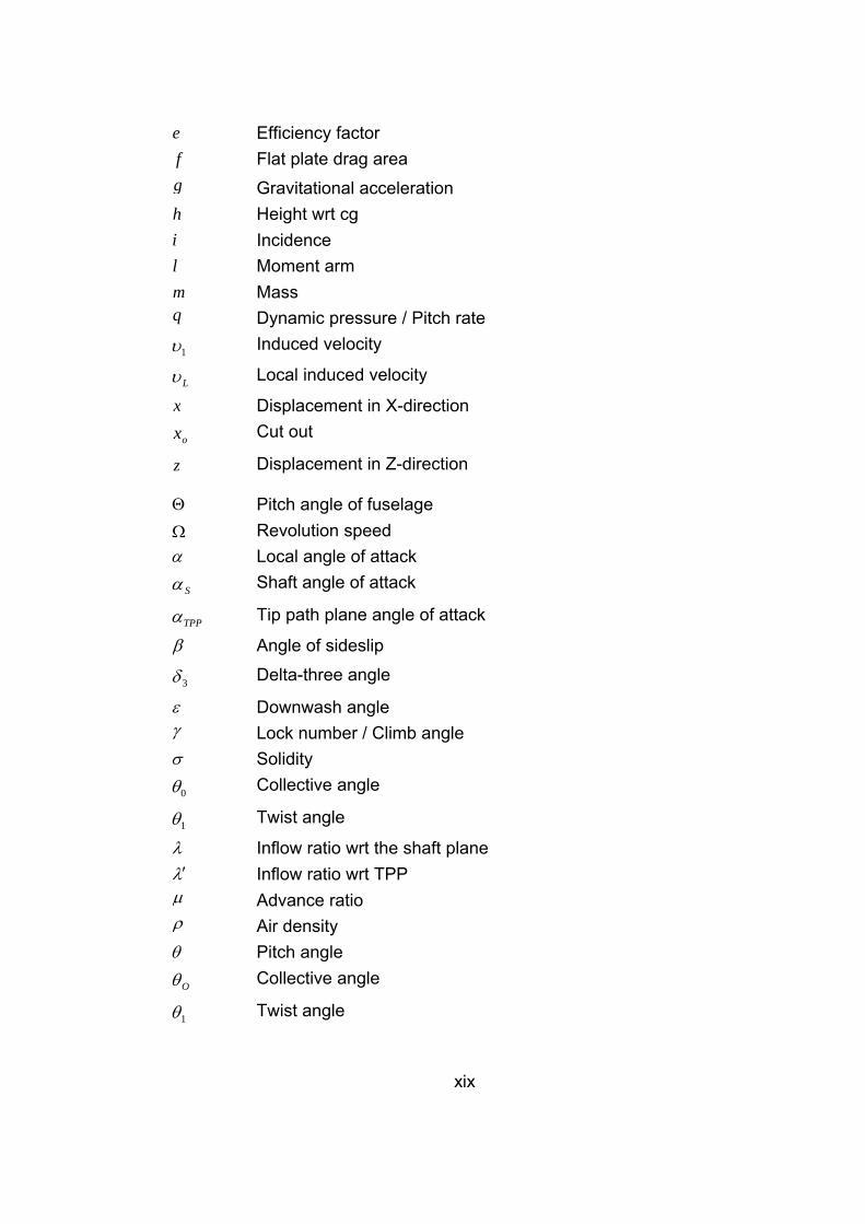
e Efficiency factor f Flat plate drag area g Gravitational acceleration h Height wrt cg i Incidence l Moment arm m Mass q Dynamic pressure / Pitch rate

1υ Induced velocity

Lυ Local induced velocity

x Displacement in X-direction

ox Cut out

z Displacement in Z-direction

Θ Pitch angle of fuselage Ω Revolution speed α Local angle of attack

Sα Shaft angle of attack

TPPα Tip path plane angle of attack

β Angle of sideslip

3δ Delta-three angle

ε Downwash angle γ Lock number / Climb angle σ Solidity

0θ Collective angle

1θ Twist angle

λ Inflow ratio wrt the shaft plane λ′ Inflow ratio wrt TPP μ Advance ratio ρ Air density θ Pitch angle

Oθ Collective angle

1θ Twist angle

xx

ψ Azimuth angle υ Local induced velocity η Sidewash angle Subscripts: T Tail rotor / Thrust / Tangential F Fuselage Q Torque

H H-force / Horizontal stabilizer P Perpendicular R Radial N Normal M Pitching moment R Rolling moment V Vertical stabilizer W Wing / Weight b Blade comp Compressible eff Effective ind Induced int Interference l Lift d Drag f Frictional para Parasite pro Profile tot Total

Other parameters are clearly defined wherever applicable.

1

CHAPTER 1

INTRODUCTION 1.1 BACKGROUND

A helicopter is an aircraft that uses rotating wings to provide lift, control, and

forward, backward and sideward propulsion. Because of the rotating parts, it

has much more capability of maneuvering, while having restrictions on high

speeds and high altitudes. Unlike aircraft, the helicopter has the possibilities

of vertical landing and takeoff, low speed flight, hover and safe autorotation.

For these reasons, helicopters are used in low-altitude; small range combat

and search-and-rescue purposes as well as pleasure travels.

For several years ASELSAN, Inc. has been conducting avionics systems

integration projects on helicopters. Such integration work requires

certification flight tests before entry of the modified aircraft into the service.

However, prior to the certification phase, extensive investigations are

needed to determine the effects of particularly the external stores on the

aerodynamics, performance and stability characteristics of the aircraft, and

to identify probability of any risks and consequently propose design or

integration changes. Although there are some commercial computational

fluid dynamics (CFD) programs which may readily be used for helicopter

aerodynamic analyses, there are not many off-the-shelf programs for

analyzing trim and dynamic stability characteristics of rotorcraft. Therefore,

ASELSAN Inc. has developed several codes to analyze the trim

characteristics as well as the dynamic stability characteristics of helicopters.

Many of these codes interface with each other. One really much needed

and extensively used feature that can be benefited from such codes during

an aerodynamic analysis phase is the ability to link to some routines through

2

which the trim parameters such as the main rotor tip path plane (TPP)

angle, collective angle, longitudinal and lateral cyclic angles, etc. can be

acquired and placed very conveniently in hundreds of input files read in by

the aerodynamic analysis codes, such as VSAERO and USAERO.

ASELSAN has also been performing certification flight tests after integration

of a system cleared by aerodynamic, trim, performance and stability

analyses. These tests aim to analyze the effects of the external stores and

the systems integrated on the performance of the air vehicle. Flight data are

recorded using a comprehensive data acquisition system and then

analyzed. Helicopter handling qualities are also evaluated by using the

Cooper-Harper Rating Scale.

Trim of a helicopter is the situation in which all the forces, inertial and

gravitational, as well as the overall moment vectors are in balance in the

three mutually perpendicular axes. Stability is the tendency of a trimmed

aircraft to return to the trim condition after a disturbance is applied. Static

stability analyzes the initial tendency, while the dynamic stability considers

the subsequent motion in time. The aircraft is said to be stable if it returns to

equilibrium, and unstable if diverges. The case in which the aircraft has no

change in motion is called neutral stability. The motion can be oscillatory or

non-oscillatory.

Trim and dynamic stability analysis combination composes a full dynamic

helicopter flight model. In order to develop such a model, the five modules

listed below should be completed and interfaced with each other:

1. Aircraft input parameters module,

2. Full trim module,

3. Static stability module,

3

4. Longitudinal and lateral dynamic stability module, including the coupling

effects,

5. Control module

All modules are applicable to a continuous velocity range, from hover to

maximum velocity.

Although a full model should be used if a comprehensive helicopter dynamic

stability analysis is to be performed, it is possible to look at a partial analysis

using engineering judgments. Longitudinal and lateral dynamic stability can

be differentiated. Also, since the transition from hover to a low-speed

forward flight (e.g. 30 knots) is continuous, the hover and forward flight

cases can be analyzed separately.

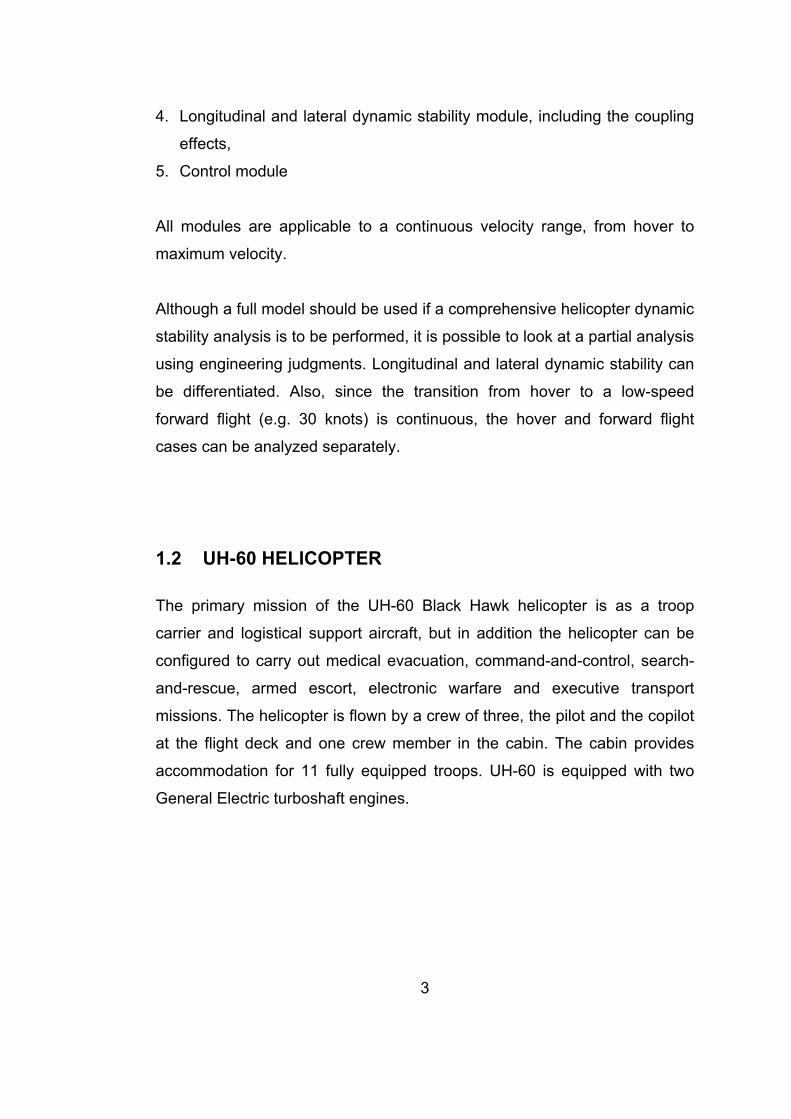
1.2 UH-60 HELICOPTER

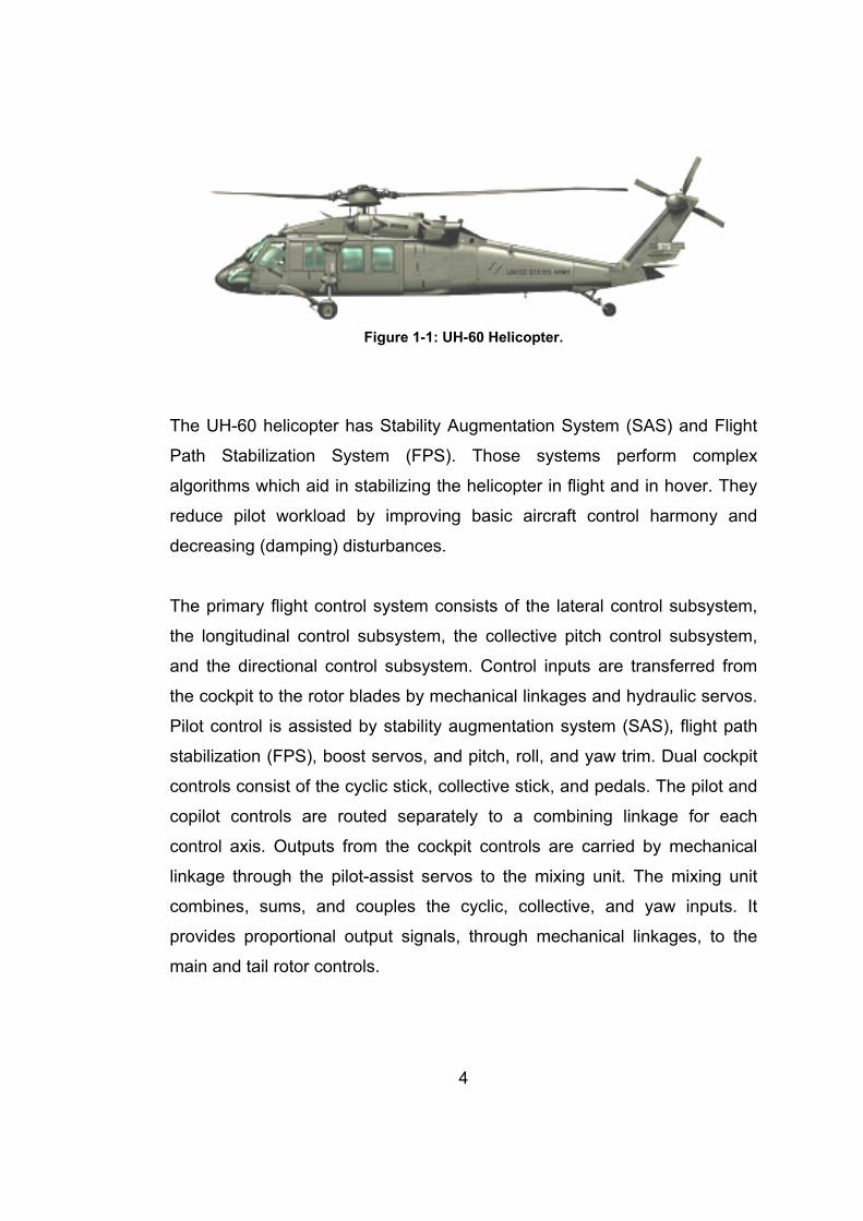
The primary mission of the UH-60 Black Hawk helicopter is as a troop

carrier and logistical support aircraft, but in addition the helicopter can be

configured to carry out medical evacuation, command-and-control, search-

and-rescue, armed escort, electronic warfare and executive transport

missions. The helicopter is flown by a crew of three, the pilot and the copilot

at the flight deck and one crew member in the cabin. The cabin provides

accommodation for 11 fully equipped troops. UH-60 is equipped with two

General Electric turboshaft engines.

4

Figure 1-1: UH-60 Helicopter.

The UH-60 helicopter has Stability Augmentation System (SAS) and Flight

Path Stabilization System (FPS). Those systems perform complex

algorithms which aid in stabilizing the helicopter in flight and in hover. They

reduce pilot workload by improving basic aircraft control harmony and

decreasing (damping) disturbances.

The primary flight control system consists of the lateral control subsystem,

the longitudinal control subsystem, the collective pitch control subsystem,

and the directional control subsystem. Control inputs are transferred from

the cockpit to the rotor blades by mechanical linkages and hydraulic servos.

Pilot control is assisted by stability augmentation system (SAS), flight path

stabilization (FPS), boost servos, and pitch, roll, and yaw trim. Dual cockpit

controls consist of the cyclic stick, collective stick, and pedals. The pilot and

copilot controls are routed separately to a combining linkage for each

control axis. Outputs from the cockpit controls are carried by mechanical

linkage through the pilot-assist servos to the mixing unit. The mixing unit

combines, sums, and couples the cyclic, collective, and yaw inputs. It

provides proportional output signals, through mechanical linkages, to the

main and tail rotor controls.

5

The Automated Flight Computer System (AFCS) enhances the stability and

handling qualities of the helicopter. It is comprised of four basic subsystems:

stabilator, SAS, trim systems, and FPS. The stabilator system improves

flying qualities by positioning the stabilator by means of electromechanical

actuators in response to collective, airspeed, pitch rate, and lateral

acceleration inputs. The SAS provides short term rate damping in the pitch,

roll, and yaw axes. Trim/FPS system provides control positioning and force

gradient functions as well as basic autopilot functions with FPS engaged.

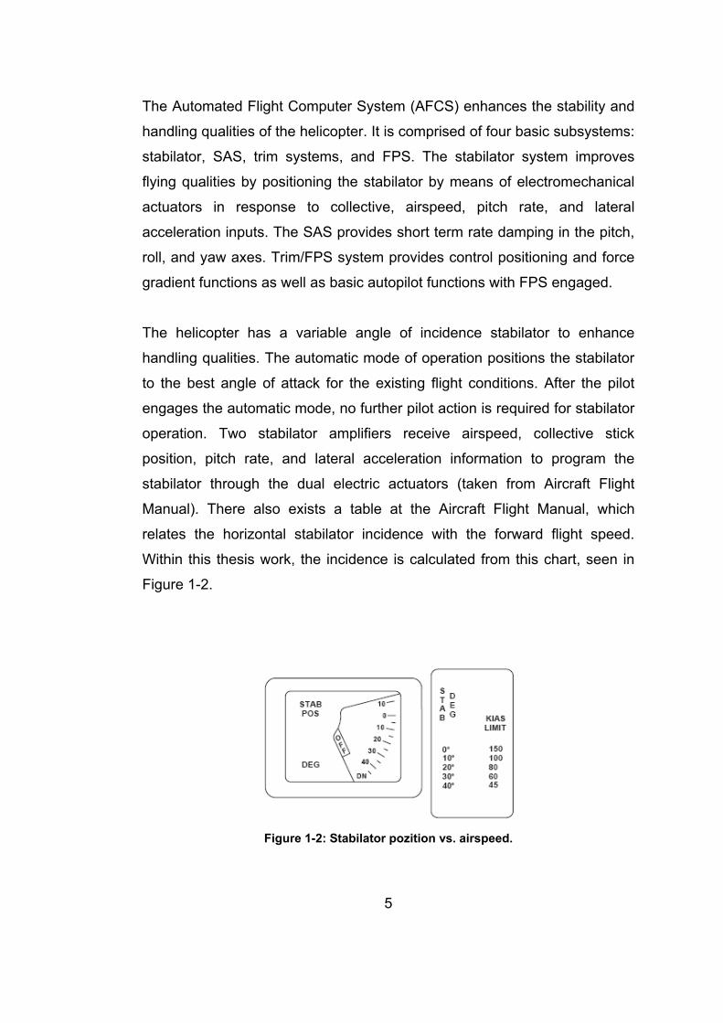
The helicopter has a variable angle of incidence stabilator to enhance

handling qualities. The automatic mode of operation positions the stabilator

to the best angle of attack for the existing flight conditions. After the pilot

engages the automatic mode, no further pilot action is required for stabilator

operation. Two stabilator amplifiers receive airspeed, collective stick

position, pitch rate, and lateral acceleration information to program the

stabilator through the dual electric actuators (taken from Aircraft Flight

Manual). There also exists a table at the Aircraft Flight Manual, which

relates the horizontal stabilator incidence with the forward flight speed.

Within this thesis work, the incidence is calculated from this chart, seen in

Figure 1-2.

Figure 1-2: Stabilator pozition vs. airspeed.

6

1.3 OBJECTIVE OF THE THESIS

In summary, one of the goals of this thesis is to develop a series of codes

that can be linked together and used for helicopter trim and dynamic stability

analyses practically by industrial companies working on helicopter

production and modifications. The mathematical development behind all

these codes includes many simplifications and assumptions, which are

explained in Chapter 2. Therefore, it should be remarked that the codes are

applicable only to preliminary-design process and the analysis should be

verified with extensive flight testing. The trim modules shall provide basic

rotor parameters, such as flapping, to existing CFD codes and to the

dynamic stability module.

Another goal of the thesis is to verify the developed codes by solving some

example helicopter cases, then to apply the codes to a UH-60 helicopter

and compare with flight test data.

1.4 SCOPE OF THE THESIS

In the first chapter of the thesis, some background information on the

present problem is given, besides stating the scope and the objectives of

the thesis. The second chapter is devoted to explain the basic theories

behind the developed codes and their validation studies. These studies are

performed on two examples but realistic helicopter configurations given in

Prouty [3] and Padfield [2], respectively. Chapter 3 presents the trim

solutions obtained for the UH-60 helicopter. This chapter also presents the

flight test results for this helicopter in comparison with the trim analysis

results. The fourth chapter involves the dynamic stability analysis for

forward flight. The last chapter gives some future work plans and the main

7

conclusions drawn from this thesis work. Finally, some appendices are

included at the end of the thesis giving some detailed formulations used in

the development of the aforementioned codes.

The codes developed within the scope of this thesis involve

1) a general input module

2) two trim codes for forward flight, TRIM-CF and TRIM-BE, and

3) a longitudinal dynamic stability code for forward flight, DYNA-STAB

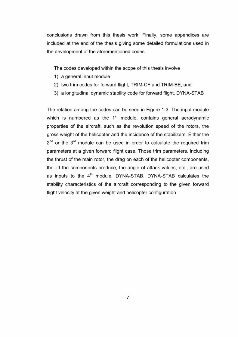
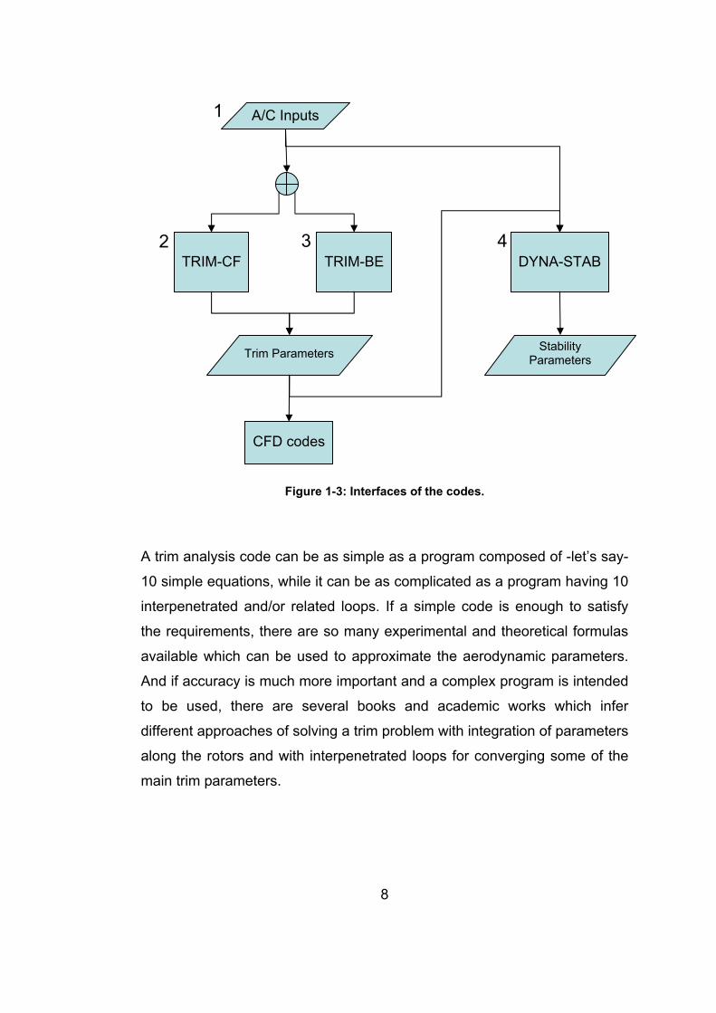
The relation among the codes can be seen in Figure 1-3. The input module

which is numbered as the 1st module, contains general aerodynamic

properties of the aircraft, such as the revolution speed of the rotors, the

gross weight of the helicopter and the incidence of the stabilizers. Either the

2nd or the 3rd module can be used in order to calculate the required trim

parameters at a given forward flight case. Those trim parameters, including

the thrust of the main rotor, the drag on each of the helicopter components,

the lift the components produce, the angle of attack values, etc., are used

as inputs to the 4th module, DYNA-STAB. DYNA-STAB calculates the

stability characteristics of the aircraft corresponding to the given forward

flight velocity at the given weight and helicopter configuration.

8

Figure 1-3: Interfaces of the codes.

A trim analysis code can be as simple as a program composed of -let’s say-

10 simple equations, while it can be as complicated as a program having 10

interpenetrated and/or related loops. If a simple code is enough to satisfy

the requirements, there are so many experimental and theoretical formulas

available which can be used to approximate the aerodynamic parameters.

And if accuracy is much more important and a complex program is intended

to be used, there are several books and academic works which infer

different approaches of solving a trim problem with integration of parameters

along the rotors and with interpenetrated loops for converging some of the

main trim parameters.

A/C Inputs

TRIM-CF

TRIM-BE

DYNA-STAB

Trim Parameters Stability Parameters

1

2 3 4

CFD codes

9

This thesis includes a semi-simple code and a complex code for trim

analysis. The simple one, TRIM-CF, is based on approximated closed form

equations which are used to linearize and solve the equations of motion,

and the trim parameters are obtained straight forwardly with many

simplifications. The complex code, TRIM-BE, also uses some simplifications

however it has a 3-loop structure looking for convergence of three trim

parameters and it calculates the main rotor parameters with an integration

method, while the tail rotor, fuselage and empennage parameters are again

calculated using closed form equations. TRIM-BE is originally written by

R.W. Prouty and is called Forward. Since it was rather poor on catching the

correct trim parameter values, many modifications are implied and the code

was modified according to the methods given in [3] during this thesis work

and TRIM-BE was obtained. The codes are explained in detail in Chapter 2

of this thesis. Since TRIM-CF code requires less parameters and gives

almost the same accuracy faster, it was decided to use TRIM-CF for the

dynamic stability analysis. TRIM-CF, is verified by the example helicopter

given in [3] and one of the example helicopters (Bo105) given in [2]. There

are flight test data for Bo105 helicopter presented in the reference book,

and the analysis results are compared with flight test data also. The trim

analysis results of UH-60 helicopter obtained by TRIM-CF code are

presented and compared with flight test data within this report.

Forward flight longitudinal dynamic stability code named DYNA-STAB and

developed in this thesis uses the methods and formulas presented in [3] and

it solves the longitudinal part of the whole coupled matrix of equations of

motion of a helicopter in forward flight. The coupling is eliminated by

linearization. The trim analysis parameters are used as inputs to the

dynamic stability code and the Short Period and Phugoid modes of a

forward flight trim case of the example helicopter [3] were analyzed. The

forward flight stability code is applied on UH-60 helicopter and the results

are presented.

10

The codes are easily applicable to a helicopter equipped with external

stores.

The codes were developed on MATLAB® environment.

The flight test data given for the UH-60 helicopter were logged with an

advanced flight certified data acquisition system which includes proprietary

software for logging, displaying the data onboard and analyzing.

11

CHAPTER 2

TRIM AND STABILITY CODE DEVELOPMENT 2.1 FORCES AND MOMENTS ACTING ON A HELICOPTER

IN FLIGHT

The helicopters come in many sizes and shapes, but most share the same

major components. The main rotor is the main airfoil surface that produces

lift. The main rotor is the main control mechanism. A helicopter can have a

single main rotor, two rotors can be mounted coaxially or they can be in

tandem configuration. The main rotor provides the speed and maneuvering

controls, as well as the lift needed for the helicopter to fly. The tail rotor is

required from the torque effect produced by spinning the main rotor. There

are some helicopters which does not have a tail rotor but have a “fan-in-tail”

design (Fenestron) (like in Eurocopter EC 135 T2) or use an air blowing

system (NOTAR) (like in MD 520N) in order to supply the anti-torque. The

rotors are driven through a transmission system by one or two engines,

generally being gas turbine engines. The horizontal stabilator serves as a

wing which produces lift and helps stabilizing the helicopter in forward

direction. The vertical stabilizer generally has a wing-like geometry which

produces side force and helps stabilizing the helicopter in lateral directions.

Some helicopters have wings too. The wings are mostly used for carrying

weapons, as well as their lifting surface effect.

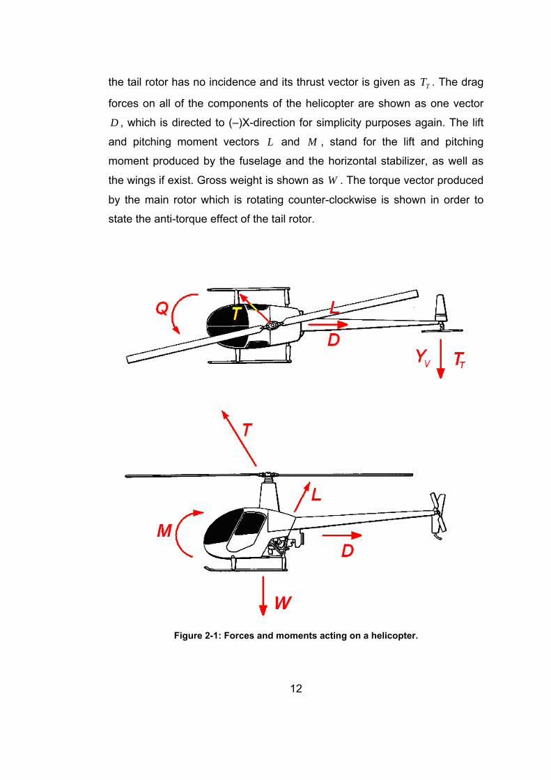
In Figure 2-1, the forces and moments acting on a helicopter in trim position

are shown. In the figure, the vertical stabilizer side force is given as VY , in

ideal case it is not directed straight to the side and has an angle, but for

simplicity purposes it is shown as directed to (-)Y-axis. It is assumed that

12

the tail rotor has no incidence and its thrust vector is given as TT . The drag

forces on all of the components of the helicopter are shown as one vector

D , which is directed to (–)X-direction for simplicity purposes again. The lift

and pitching moment vectors L and M , stand for the lift and pitching

moment produced by the fuselage and the horizontal stabilizer, as well as

the wings if exist. Gross weight is shown as W . The torque vector produced

by the main rotor which is rotating counter-clockwise is shown in order to

state the anti-torque effect of the tail rotor.

Figure 2-1: Forces and moments acting on a helicopter.

13

2.2 HELICOPTER ROTOR SYSTEM

There are four primary types of rotor systems: articulated, teetering, semi-

rigid and hingeless. The articulated rotor system first appeared on the

autogyros of the 1920s and is the oldest and most widely used type of rotor

system. The rotor blades in this type of system can move in three ways as it

turns around the rotor hub and each blade can move independently of the

others. They can move up and down (flapping), back and forth in the

horizontal plane, and can change in the pitch angle (the tilt of the blade).

UH-60 helicopters have fully-articulated main rotor configuration. In the

semi-rigid rotor system, the blades are attached rigidly to the hub but the

hub itself can tilt in any direction about the top of the mast. This system

generally appears on helicopters with two rotor blades. The teetering rotor

system resembles a seesaw, when one blade is pushed down, the opposite

one rises. The hingeless rotor system functions much as the articulated

system does, but uses elastomeric bearings and composite flextures to

allow for flapping and lead-lag movements of the blades in place of

conventional hinges. Its advantages are improved control response with

less lag and substantial improvements in vibration control. It does not have

the risk of ground-resonance associated with the articulated type, but it is

considerably more expensive.

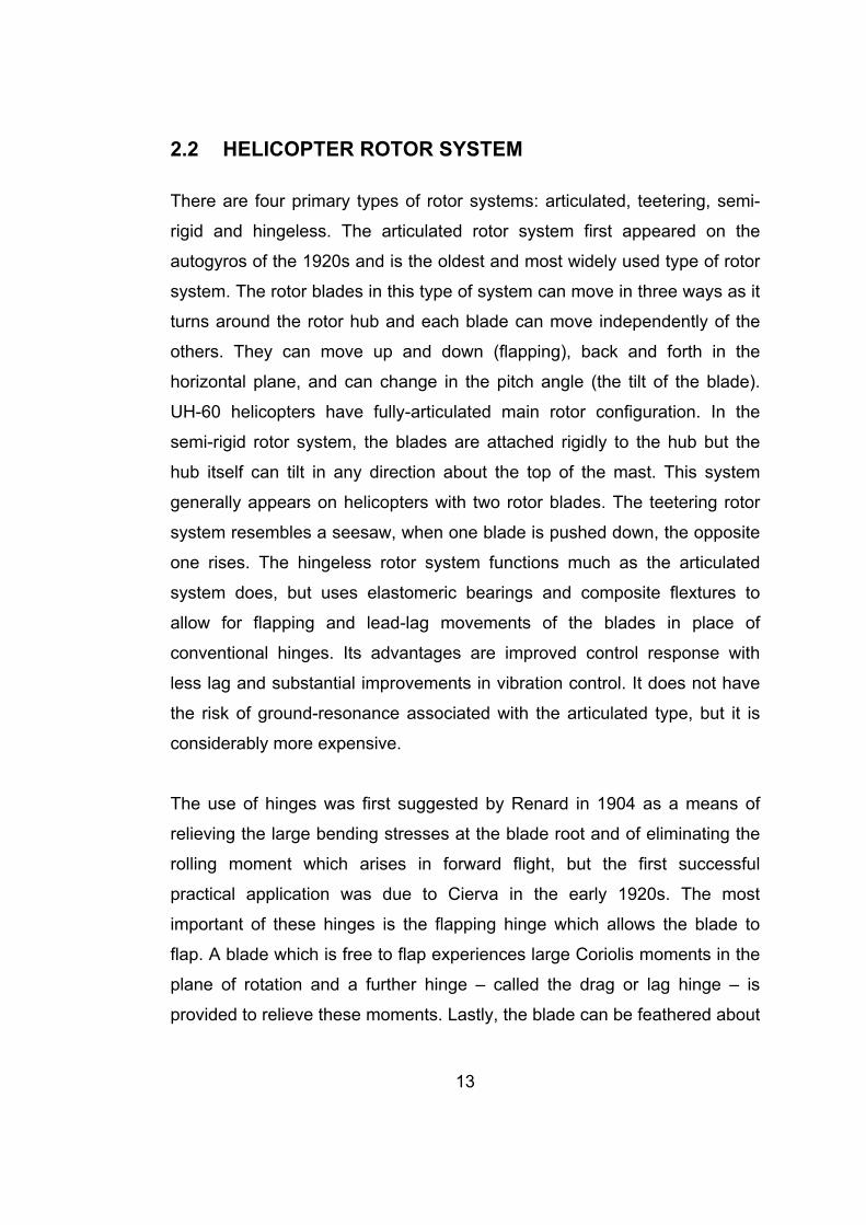
The use of hinges was first suggested by Renard in 1904 as a means of

relieving the large bending stresses at the blade root and of eliminating the

rolling moment which arises in forward flight, but the first successful

practical application was due to Cierva in the early 1920s. The most

important of these hinges is the flapping hinge which allows the blade to

flap. A blade which is free to flap experiences large Coriolis moments in the

plane of rotation and a further hinge – called the drag or lag hinge – is

provided to relieve these moments. Lastly, the blade can be feathered about

14

a third axis, parallel to the blade span, to enable the blade pitch angle to be

changed. The hinges are shown in Figure 2-2, where an articulated rotor is

demonstrated.

Figure 2-2: Hinges on an articulated rotor [22].

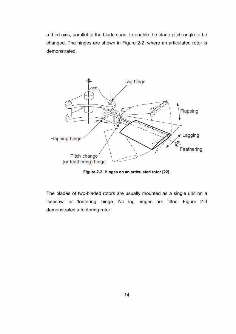
The blades of two-bladed rotors are usually mounted as a single unit on a

‘seesaw’ or ‘teetering’ hinge. No lag hinges are fitted. Figure 2-3

demonstrates a teetering rotor.

15

Figure 2-3: Teetering rotor [22].

The semi-rigid rotor resembles the teetering rotor, but now the hub itself

also moves about the top of the mast. The hub is strictly attached to the

blades.

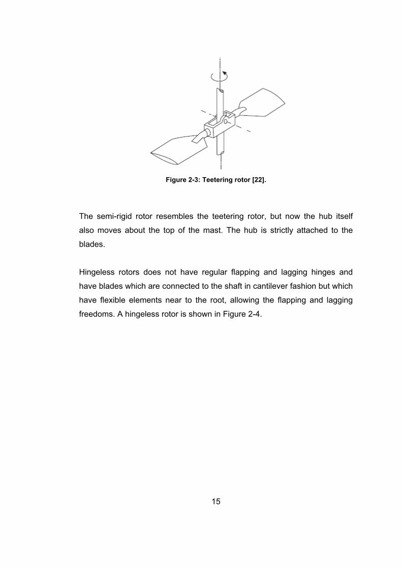
Hingeless rotors does not have regular flapping and lagging hinges and

have blades which are connected to the shaft in cantilever fashion but which

have flexible elements near to the root, allowing the flapping and lagging

freedoms. A hingeless rotor is shown in Figure 2-4.

16

Figure 2-4: Hingeless rotor [22].

The collective changes the pitch angle of the rotor blades causing the

helicopter to climb and descend. Through the swash plate, the cyclic

controls the pitch angle distribution over the main rotor disc and by this way

the disc is tilted sideways or backwards in order to turn, go backwards or

change the speed of the helicopter. The anti-torque pedals control the

helicopters tail rotor and are used to point the nose of the helicopter in the

desired direction. The function of the throttle is to regulate the engine r.p.m.

2.3 HELICOPTER ROTOR AERODYNAMICS

There are two basic theoretical approaches to understand the generation of

thrust from a rotor system: momentum theory and blade element theory.

The momentum theory approximates the local forces and moments on the

blades and assumes that the rotor is an ‘actuator’ disc which is uniformly

loaded with an infinite number of blades so that there is no periodicity in the

17

wake. The theory solves the energy and momentum equations and relates

the induced velocity parameter with the forward velocity.

The momentum theory makes certain additional assumptions, which limit

the accuracy:

• The flow both upstream and downstream of the disk is uniform,

occurs at constant energy and is contained within a streamtube.

• No rotation is imparted on the fluid by the action of the rotor.

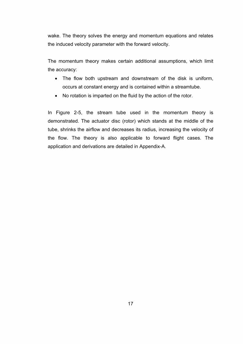
In Figure 2-5, the stream tube used in the momentum theory is

demonstrated. The actuator disc (rotor) which stands at the middle of the

tube, shrinks the airflow and decreases its radius, increasing the velocity of

the flow. The theory is also applicable to forward flight cases. The

application and derivations are detailed in Appendix-A.

18

Figure 2-5: The streamtube in the momentum theory [22].

19

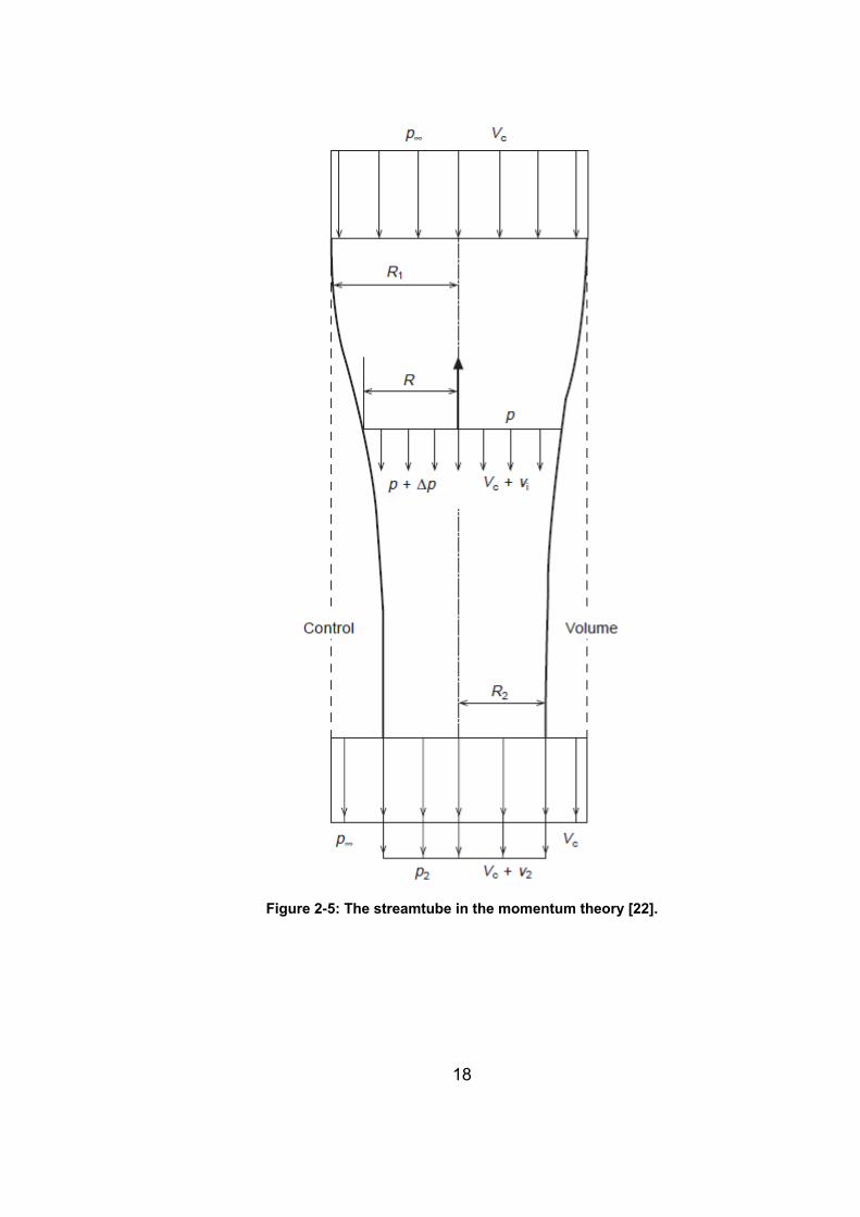
The blade element theory is based upon the idea that the rotor blades

function as high aspect ratio wings constrained to rotate around a central

mast as the rotor system advances through the air. It considers the local

aerodynamic forces on the blade at radial and azimuthal sections, and

integrates the forces to find the overall thrust and drag on the rotor. The

momentum theory cannot be used to predict the magnitude of any losses

associated with realistic flow around rotor blades, and the blade element

theory overcomes some of the restrictions inherent in the momentum

theory. The applications of the blade element theory on trim analysis are

explained in detail in Appendix-A, on which the TRIM-BE module is based.

Figure 2-6: Blade element theory [22].

The finite number of blades leads to a rotor performance loss not accounted

for by the actuator disk analysis. The lift at the blade tips decreases to zero

over a finite radial distance, rather than extending all the way out to the

edge of the disk. Thus, there will be a reduction in the thrust, or increase in

the induced power of the rotor.

20

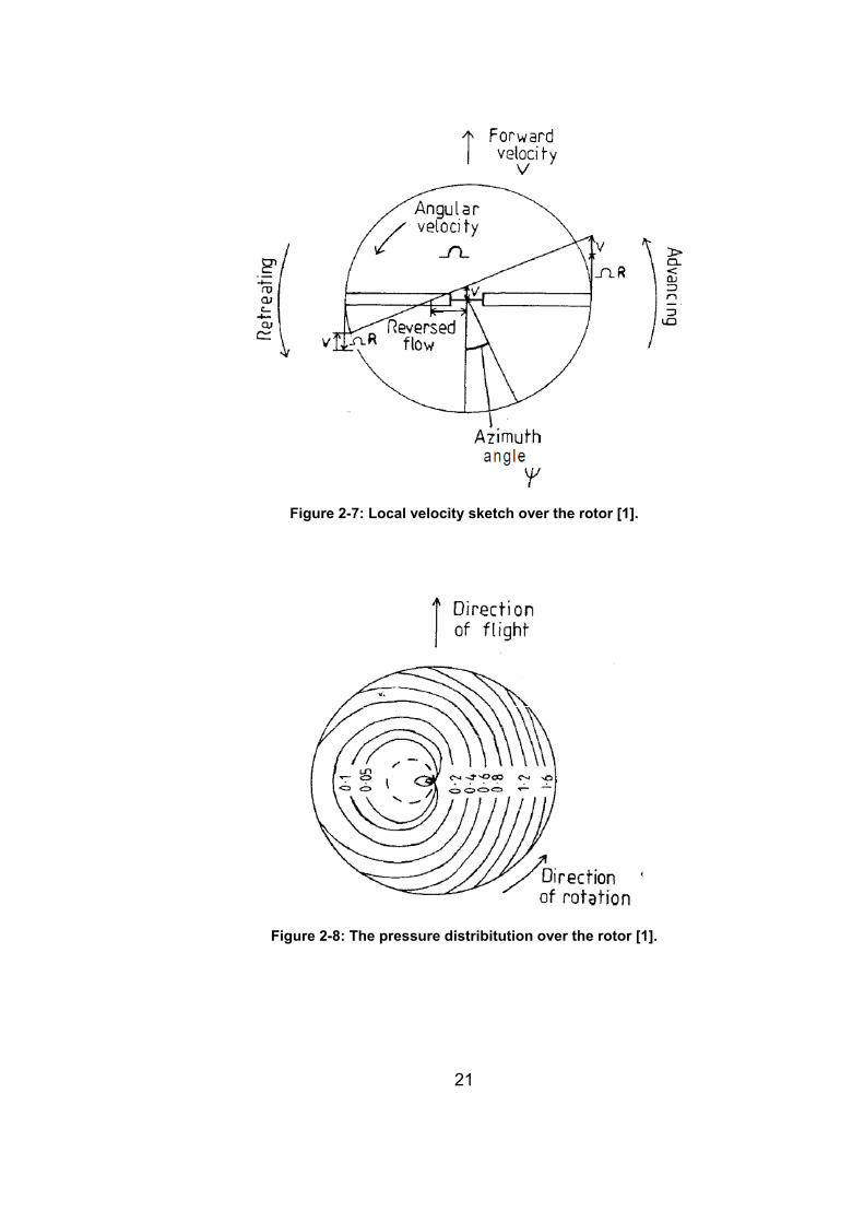
Forward flight is a more complex situation compared to the hover. Because

of the forward velocity, the relative speed of the blade sections differ around

the azimuth, and therefore, an imbalance of aerodynamic forces occur along

the main rotor disc. The advancing blade has a velocity relative to the air

higher than the rotational velocity, while the retreating blade has a lower

velocity relative to the air. This lateral asymmetry has a major influence on

the rotor and its analysis in forward flight.

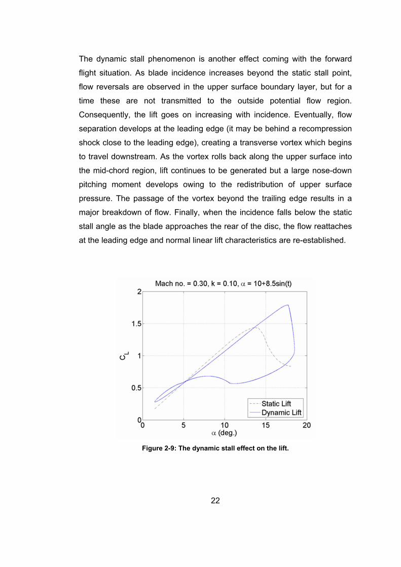
One of the major characteristics of the forward flight aerodynamics is the

reversed flow region. Depending on the forward speed, there occurs a

region on the retreating side where the local velocity on the blade section

becomes reversed (the velocity relative to the blade is directed from the

trailing edge to the leading edge), and therefore the lift is dropped down.

One other feature belonging to forward flight is the compressibility effect

seen on the advancing side at the tips of the blades where the local speed

is greatest and approaches almost the speed of sound. Since it increases

the drag drastically, the blade tips are swept back to decrease its effects.

Figure 2-7 and Figure 2-8 explain these phenomena.

21

Figure 2-7: Local velocity sketch over the rotor [1].

Figure 2-8: The pressure distribitution over the rotor [1].

22

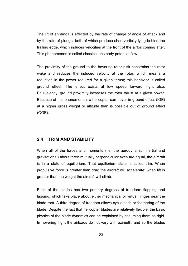
The dynamic stall phenomenon is another effect coming with the forward

flight situation. As blade incidence increases beyond the static stall point,

flow reversals are observed in the upper surface boundary layer, but for a

time these are not transmitted to the outside potential flow region.

Consequently, the lift goes on increasing with incidence. Eventually, flow

separation develops at the leading edge (it may be behind a recompression

shock close to the leading edge), creating a transverse vortex which begins

to travel downstream. As the vortex rolls back along the upper surface into

the mid-chord region, lift continues to be generated but a large nose-down

pitching moment develops owing to the redistribution of upper surface

pressure. The passage of the vortex beyond the trailing edge results in a

major breakdown of flow. Finally, when the incidence falls below the static

stall angle as the blade approaches the rear of the disc, the flow reattaches

at the leading edge and normal linear lift characteristics are re-established.

Figure 2-9: The dynamic stall effect on the lift.

23

The lift of an airfoil is affected by the rate of change of angle of attack and

by the rate of plunge, both of which produce shed vorticity lying behind the

trailing edge, which induces velocities at the front of the airfoil coming after.

This phenomenon is called classical unsteady potential flow. The proximity of the ground to the hovering rotor disk constrains the rotor

wake and reduces the induced velocity at the rotor, which means a

reduction in the power required for a given thrust; this behavior is called

ground effect. The effect exists at low speed forward flight also.

Equivalently, ground proximity increases the rotor thrust at a given power.

Because of this phenomenon, a helicopter can hover in ground effect (IGE)

at a higher gross weight or altitude than is possible out of ground effect

(OGE).

2.4 TRIM AND STABILITY

When all of the forces and moments (i.e. the aerodynamic, inertial and

gravitational) about three mutually perpendicular axes are equal, the aircraft

is in a state of equilibrium. That equilibrium state is called trim. When

propulsive force is greater than drag the aircraft will accelerate; when lift is

greater than the weight the aircraft will climb.

Each of the blades has two primary degrees of freedom: flapping and

lagging, which take place about either mechanical or virtual hinges near the

blade root. A third degree of freedom allows cyclic pitch or feathering of the

blade. Despite the fact that helicopter blades are relatively flexible, the basic

physics of the blade dynamics can be explained by assuming them as rigid.

In hovering flight the airloads do not vary with azimuth, and so the blades

24

flap up and lag back with respect to the hub and reach a steady equilibrium

position under a simple balance of aerodynamic and centrifugal forces.

However, in forward flight the fluctuating airloads cause continuous flapping

motion and give rise to aerodynamic, inertial, and Coriolis forces on the

blades that result in a dynamic response. The flapping hinge allows the

effects of the cyclically varying airloads to reach an equilibrium with airloads

produced by the blade flapping motion. The flapping motion is highly

damped by the aerodynamic forces.

The part played by the rotor is highly complicated, because strictly each

blade possesses its own degrees of freedom and makes an individual

contribution to any disturbed motion. Fortunately, however, analysis can

almost always be made satisfactorily by considering the behavior of the

rotor as a whole.

Considering the flapping, feathering, lead-lag motion of the blades of both

main rotor and the tail rotor, as well as the motion of the main rotor with

respect to the fuselage, the swash plate mechanism and the moving

horizontal stabilators in some of the helicopters, there are so many

equations of motion that one should solve in order to analyze.

Because of the fact that a helicopter has so many degrees of freedom, it is

much more difficult to analyze. The fuselage has 6 degrees of freedom, the

main rotor has 4 DOF, 3 for rotor flapping and one for the rotation of the

rotor (throttle), tail rotor has also 4 DOF, etc. However, with some feasible

assumptions, the helicopter system can be reduced to 6 DOF like a fixed-

wing aircraft, three for translation and three for rotation.

The static stability of an air vehicle is the tendency of the vehicle to return to

its trimmed condition following a disturbance. Meanwhile, the dynamic

stability considers the subsequent motion in time. If the aircraft tends to

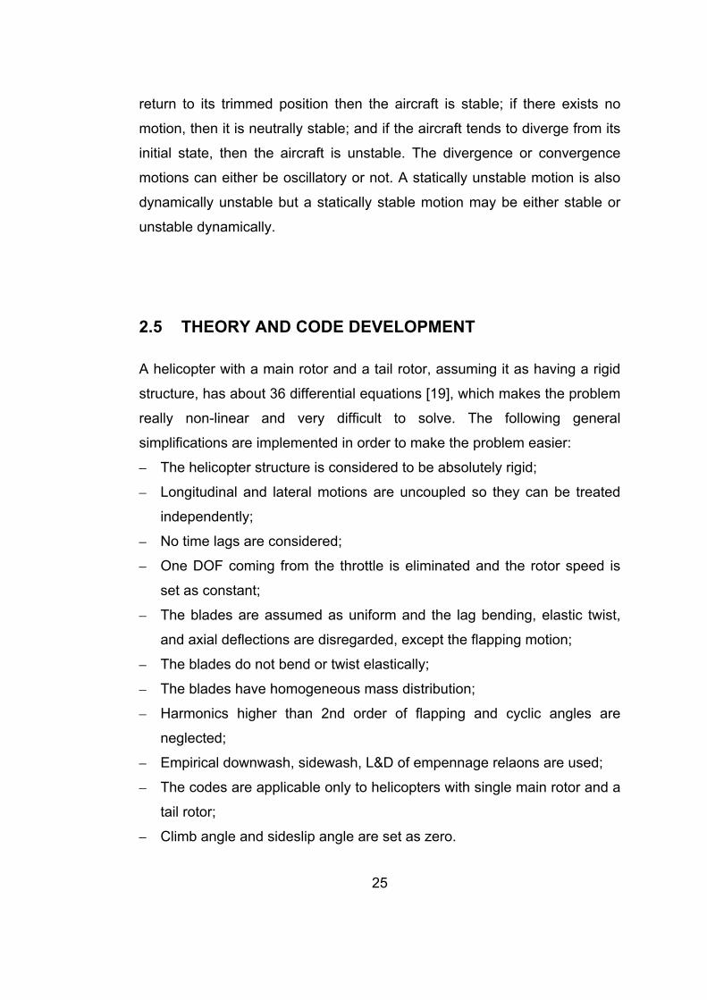
25

return to its trimmed position then the aircraft is stable; if there exists no

motion, then it is neutrally stable; and if the aircraft tends to diverge from its

initial state, then the aircraft is unstable. The divergence or convergence

motions can either be oscillatory or not. A statically unstable motion is also

dynamically unstable but a statically stable motion may be either stable or

unstable dynamically.

2.5 THEORY AND CODE DEVELOPMENT

A helicopter with a main rotor and a tail rotor, assuming it as having a rigid

structure, has about 36 differential equations [19], which makes the problem

really non-linear and very difficult to solve. The following general

simplifications are implemented in order to make the problem easier:

– The helicopter structure is considered to be absolutely rigid;

– Longitudinal and lateral motions are uncoupled so they can be treated

independently;

– No time lags are considered;

– One DOF coming from the throttle is eliminated and the rotor speed is

set as constant;

– The blades are assumed as uniform and the lag bending, elastic twist,

and axial deflections are disregarded, except the flapping motion;

– The blades do not bend or twist elastically;

– The blades have homogeneous mass distribution;

– Harmonics higher than 2nd order of flapping and cyclic angles are

neglected;

– Empirical downwash, sidewash, L&D of empennage relaons are used;

– The codes are applicable only to helicopters with single main rotor and a

tail rotor;

– Climb angle and sideslip angle are set as zero.

26

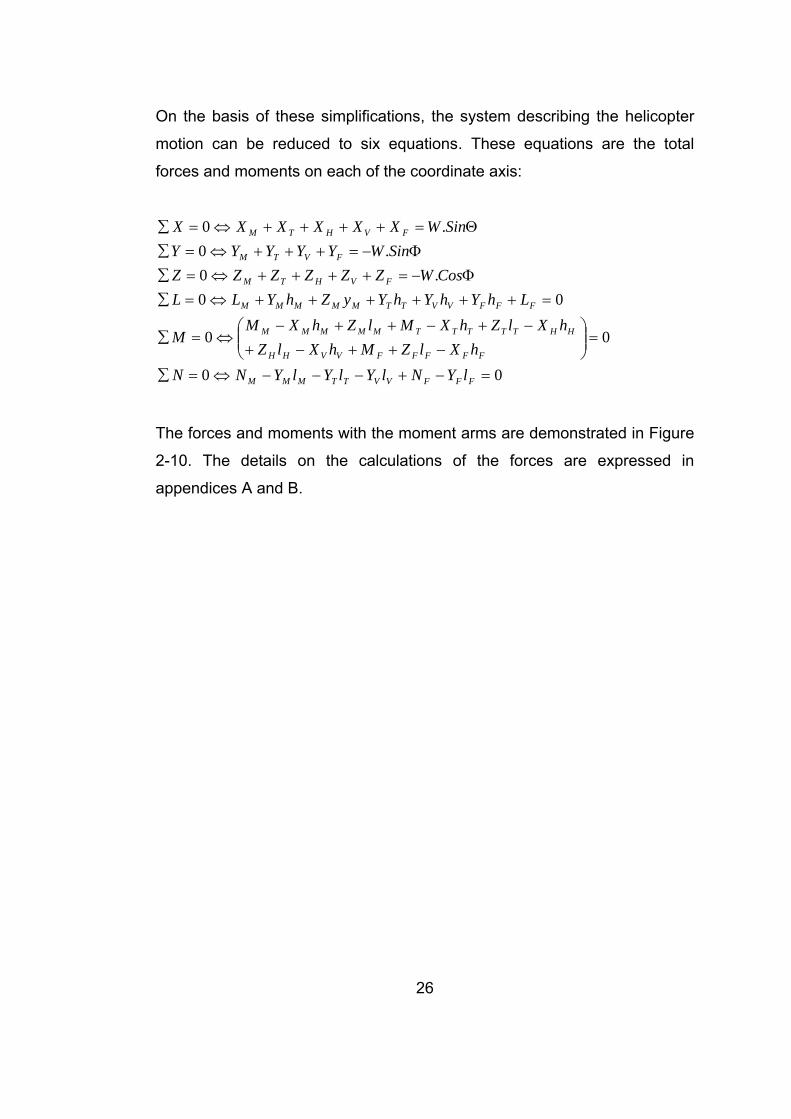
On the basis of these simplifications, the system describing the helicopter

motion can be reduced to six equations. These equations are the total

forces and moments on each of the coordinate axis:

00

00

00.0

.0.0

=−+−−−⇔=∑

=⎟⎟⎠

⎞⎜⎜⎝

⎛−++−+

−+−++−⇔=∑

=++++++⇔=∑Φ−=++++⇔=∑

Φ−=+++⇔=∑Θ=++++⇔=∑

FFFVVTTMMM

FFFFFVVHH

HHTTTTTMMMMM

FFFVVTTMMMMM

FVHTM

FVTM

FVHTM

lYNlYlYlYNNhXlZMhXlZ

hXlZhXMlZhXMM

LhYhYhYyZhYLLCosWZZZZZZ

SinWYYYYYSinWXXXXXX

The forces and moments with the moment arms are demonstrated in Figure

2-10. The details on the calculations of the forces are expressed in

appendices A and B.

27

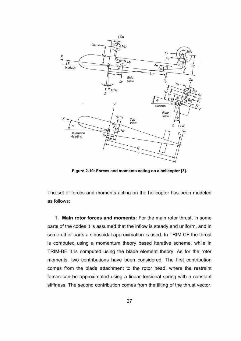
Figure 2-10: Forces and moments acting on a helicopter [3].

The set of forces and moments acting on the helicopter has been modeled

as follows:

1. Main rotor forces and moments: For the main rotor thrust, in some

parts of the codes it is assumed that the inflow is steady and uniform, and in

some other parts a sinusoidal approximation is used. In TRIM-CF the thrust

is computed using a momentum theory based iterative scheme, while in

TRIM-BE it is computed using the blade element theory. As for the rotor

moments, two contributions have been considered. The first contribution

comes from the blade attachment to the rotor head, where the restraint

forces can be approximated using a linear torsional spring with a constant

stiffness. The second contribution comes from the tilting of the thrust vector.

28

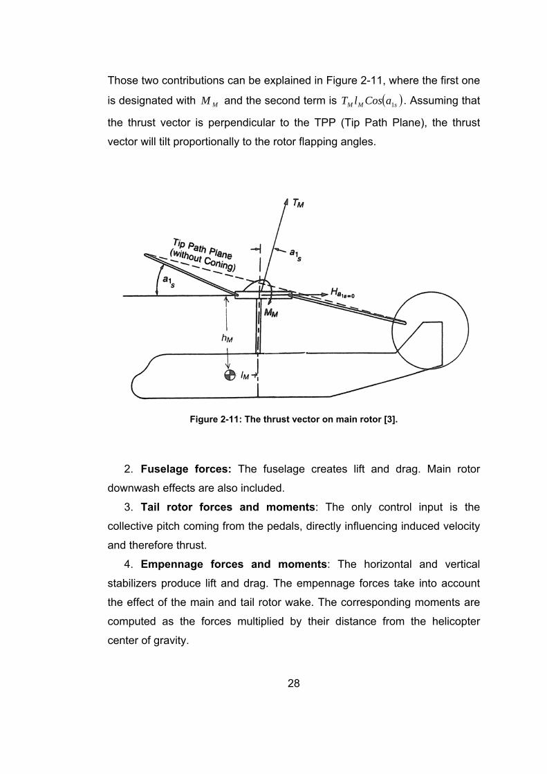
Those two contributions can be explained in Figure 2-11, where the first one

is designated with MM and the second term is ( )sMM aCoslT 1 . Assuming that

the thrust vector is perpendicular to the TPP (Tip Path Plane), the thrust

vector will tilt proportionally to the rotor flapping angles.

Figure 2-11: The thrust vector on main rotor [3].

2. Fuselage forces: The fuselage creates lift and drag. Main rotor

downwash effects are also included.

3. Tail rotor forces and moments: The only control input is the

collective pitch coming from the pedals, directly influencing induced velocity

and therefore thrust.

4. Empennage forces and moments: The horizontal and vertical

stabilizers produce lift and drag. The empennage forces take into account

the effect of the main and tail rotor wake. The corresponding moments are

computed as the forces multiplied by their distance from the helicopter

center of gravity.

29

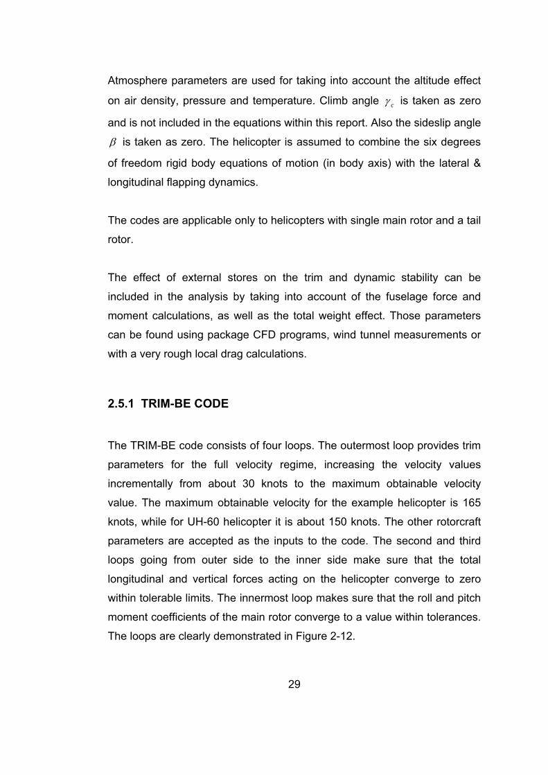
Atmosphere parameters are used for taking into account the altitude effect

on air density, pressure and temperature. Climb angle cγ is taken as zero

and is not included in the equations within this report. Also the sideslip angle

β is taken as zero. The helicopter is assumed to combine the six degrees

of freedom rigid body equations of motion (in body axis) with the lateral &

longitudinal flapping dynamics.

The codes are applicable only to helicopters with single main rotor and a tail

rotor.

The effect of external stores on the trim and dynamic stability can be

included in the analysis by taking into account of the fuselage force and

moment calculations, as well as the total weight effect. Those parameters

can be found using package CFD programs, wind tunnel measurements or

with a very rough local drag calculations.

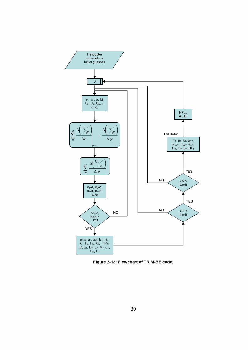
2.5.1 TRIM-BE CODE

The TRIM-BE code consists of four loops. The outermost loop provides trim

parameters for the full velocity regime, increasing the velocity values

incrementally from about 30 knots to the maximum obtainable velocity

value. The maximum obtainable velocity for the example helicopter is 165

knots, while for UH-60 helicopter it is about 150 knots. The other rotorcraft

parameters are accepted as the inputs to the code. The second and third

loops going from outer side to the inner side make sure that the total

longitudinal and vertical forces acting on the helicopter converge to zero

within tolerable limits. The innermost loop makes sure that the roll and pitch

moment coefficients of the main rotor converge to a value within tolerances.

The loops are clearly demonstrated in Figure 2-12.

30

Figure 2-12: Flowchart of TRIM-BE code.

cT/σ, cQ/σ, cH/σ, cM/σ,

cR/σ

ΔcM/σ, ΔcR/σ <

Limit

NO

YES

NO

YES

NO

YES

αTPP, a0, a1S, b1S, θ0, λ΄, TM, HM, QM, HPM, Θ, αF, DF, LF, MF, αH,

DH, LH

TT, μT, λT, a0,T, a1S,T, b1S,T, θ0,T, HT, QT, LT, HPT

HPtop, A1, B1

V

ΣX < Limit

ΣZ < Limit

Helicopter parameters,

Initial guesses

Tail Rotor

θ, ν1 , α, M, UP, UT, UR, a,

cl, cd

ψσσ

ψ

Δ

⎟⎠⎞⎜

⎝⎛Δ

=Δ

⎟⎠⎞⎜

⎝⎛Δ

=

∑i

c

Ri C

r

C

0

∑ Δ

⎟⎠⎞⎜

⎝⎛Δπ

ψσ2

0

iC

31

The assumptions used in the module are the general assumptions listed in

the previous section, as well as the items given below:

– Among the blade characteristics, the twist is assumed as constant [15];

20 degrees sweep on the tip region of the blade is ignored; the blade

section from the cut-out section to the radial station of 0.1925R where

SC1095 airfoil section is started is assumed as having an airfoil section

SC1095; the chord increase in the swept region and the trim tab region

(between 0.7316R and 0.8629R) are ignored; the cord difference

between the two airfoil sections are ignored and an approximate cord is

used; the zero lift angle of attack is taken as an approximate value,

comparing to the -0.2 degrees for the SC1095 airfoil and -1.5 degrees

for SC1094 R8 airfoil.

– Momentum theory used to find the average induced velocity. The

induced velocity distribution is a sinusoidal function through the azimuth.

– Empirical A/F parameters aree used.

Within the core of the program, the local lift and drag coefficients of the main

rotor blades’ sections corresponding to the assigned azimuthal and radial

stations are calculated using the experimental two-dimensional airfoil lift and

drag coefficients. Lift and drag coefficients are used to calculate the three-

dimensional force coefficients. The code accounts for the reverse flow, the

compressibility effect occurring on the advancing side in high speeds,

dynamic stall effect, root and tip losses, drag divergence effects and

unsteady aerodynamics. The local lift and drag coefficients are used to

calculate the local thrust, torque, H-force and moment coefficients, which

are integrated to obtain the main rotor total force and moment values.

Simpson’s Rule is used as the integration method. The blades are divided

into 10 radial sections and the disc is divided into 36 azimuthal angle

sections. Although the code can be modified to solve for different

increments of blade and azimuth angles, the present values are accepted

32

as giving satisfactory accuracy for a trim analysis. The integration method

allows us to exclude the tip and root losses with simple subtractions.

One of the empirical approaches used in the code is relating the roll and

pitch moment coefficients to the first harmonics of the blade feathering. The

innermost loop of the code is completed after those related parameters are

converged to tolerable values. Some other empirical approaches are

relating the total longitudinal and vertical forces acting on the helicopter to

the inflow ratio and to the collective angle. Those relations compose the

criteria of the second and third loops.

The limitations and assumptions additional to the ones listed before are:

1. Obtaining performance and trim conditions is the primary objective,

while still the first flapping harmonics are calculated.

2. Two dimensional main rotor airfoil and drag characteristics are

available.

3. The blades do not bend or twist elastically

4. The induced velocity distribution is a sinusoidal function through the

azimuth.

The tail rotor trim parameters are calculated using closed-form equations.

The power losses introduced by the power generators, hydraulic system

and transmission system are also taken into account in the power

calculations.

The code is able to calculate the effects of load carrying wings if there exist

any.

The formulations and detailed theory used in the code are given in

Appendix-A.

33

2.5.2 TRIM-CF CODE

The motion of a helicopter in trim is governed by 6 equations, three for total

forces acting on the aircraft and three for the total moments on each

coordinate of the body frame. One can separate the longitudinal and lateral

equations and solve for the related parameters without much degradation

on the accuracy. Therefore, the code solves for only three equations, which

are the total forces on the longitudinal and vertical axes and the total

moments on the lateral axis.

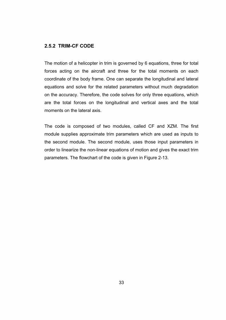
The code is composed of two modules, called CF and XZM. The first

module supplies approximate trim parameters which are used as inputs to

the second module. The second module, uses those input parameters in

order to linearize the non-linear equations of motion and gives the exact trim

parameters. The flowchart of the code is given in Figure 2-13.

34

Figure 2-13: Flowchart of TRIM-CF code.

The additional assumptions, after the general assumptions given before are:

• Momentum theory is used to find the induced velocity

• Approximated rotor characteristics are used

• Flapping motion of individual blades replaced by the motion of the

cone

• Actions of the MR and TR replaced by forces and moments applied

to hubs

The equations used in the TRIM-CF code are closed form equations. The

code is applicable to flight velocities higher than 30 knots. This is because

the angle of attack over the empennage diverges to unreasonable values.

R/C parameters, İnitial assignments

ν1, αTPP, a0, θ0, λ΄, cT/σ, cQ/σ, cH/σ, TM, HM, QM, Θ, αF, DF, LF, MF, αH,

DH, LH, LV, DV, TT, μT, λT, a0,T, a1S,T, b1S,T, θ0,T, HT, QT, LT

ν1, αTPP, a0, θ0, λ΄, cT/σ, cQ/σ, cH/σ, TM, HM, QM, Θ, αF, DF, LF, MF, αH,

DH, LH, LV, DV, TT, μT, λT, a0,T, a1S,T, b1S,T, θ0,T, HT, QT, LT, A1, B1

ΣX = 0 ΣZ = 0 ΣM = 0

TM, a1S, Θ

35

In the CF module the first harmonic flapping angles sa1 and sb1 are set to

zero, i.e. the first order harmonics are also neglected. Those flapping angles

are computed at the XZM module.

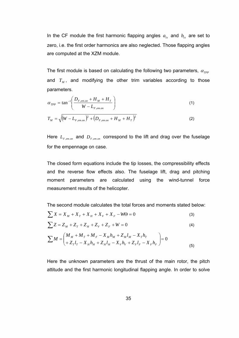
The first module is based on calculating the following two parameters, TPPα

and MT , and modifying the other trim variables according to those

parameters.

⎟⎟⎠

⎞⎜⎜⎝

⎛

−

++= −

onemF

TMonemFTPP LW

HHD

.,

.,1tanα (1)

( ) ( )2.,2

., TMonemFonemFM HHDLWT +++−= (2)

Here onemFL ., and onemFD ., correspond to the lift and drag over the fuselage

for the empennage on case.

The closed form equations include the tip losses, the compressibility effects

and the reverse flow effects also. The fuselage lift, drag and pitching

moment parameters are calculated using the wind-tunnel force

measurement results of the helicopter.

The second module calculates the total forces and moments stated below:

0=Θ−++++=∑ WXXXXXX FVHTM (3)

0=+++++=∑ WZZZZZZ FVHTM (4)

0=⎟⎟⎠

⎞⎜⎜⎝

⎛−+−+−+

−+−++=∑

FFFFVVHHHHTT

TTMMMMFTM

hXlZhXlZhXlZhXlZhXMMM

M (5)

Here the unknown parameters are the thrust of the main rotor, the pitch

attitude and the first harmonic longitudinal flapping angle. In order to solve

36

those coupled equations, some of the variables are taken as constant, the

values of which are calculated with the CF module.

The thrust of the tail rotor is found from the main rotor torque. To find the

pedals angle, the precone angle of the tail rotor of the UH-60 helicopter is

subtracted from the calculated T

a0 value. The 20 degrees inclination of the

tail rotor is also included in the calculations.

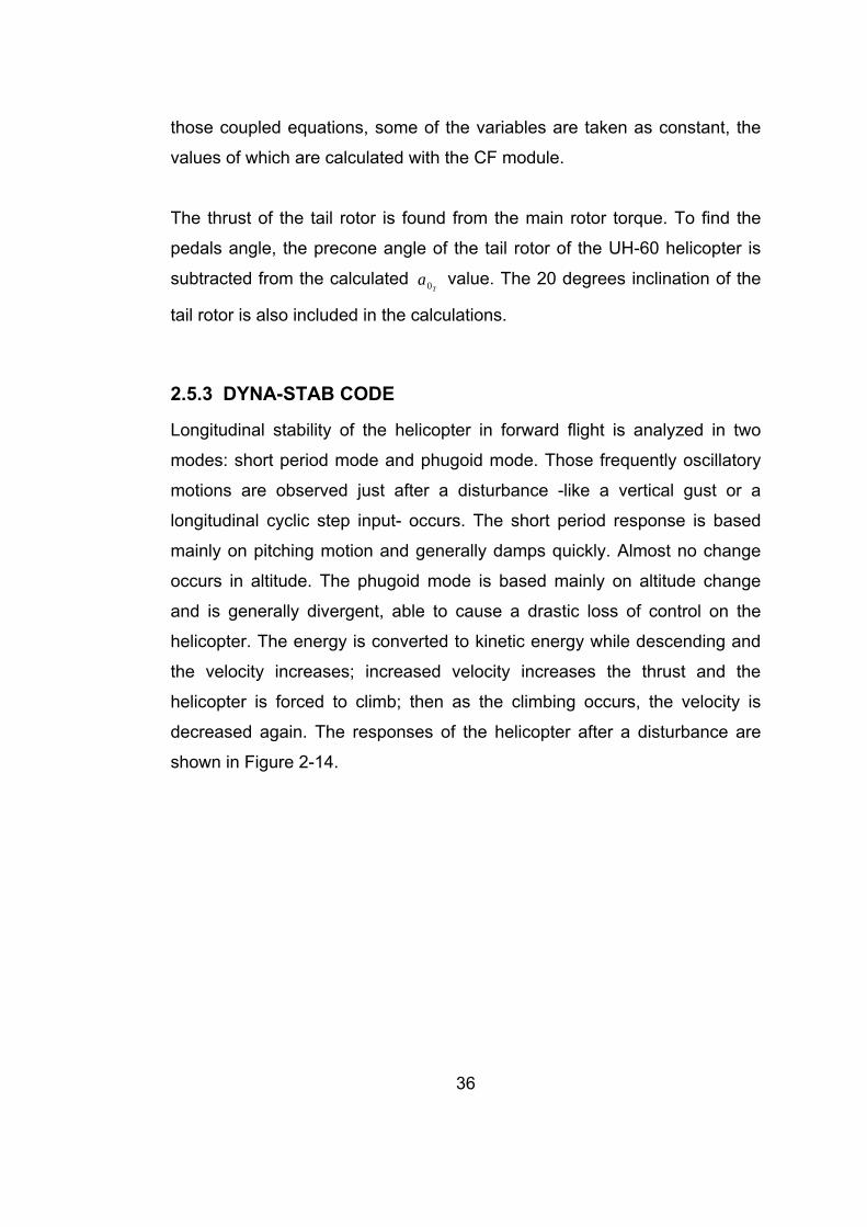
2.5.3 DYNA-STAB CODE

Longitudinal stability of the helicopter in forward flight is analyzed in two

modes: short period mode and phugoid mode. Those frequently oscillatory

motions are observed just after a disturbance -like a vertical gust or a

longitudinal cyclic step input- occurs. The short period response is based

mainly on pitching motion and generally damps quickly. Almost no change

occurs in altitude. The phugoid mode is based mainly on altitude change

and is generally divergent, able to cause a drastic loss of control on the

helicopter. The energy is converted to kinetic energy while descending and

the velocity increases; increased velocity increases the thrust and the

helicopter is forced to climb; then as the climbing occurs, the velocity is

decreased again. The responses of the helicopter after a disturbance are

shown in Figure 2-14.

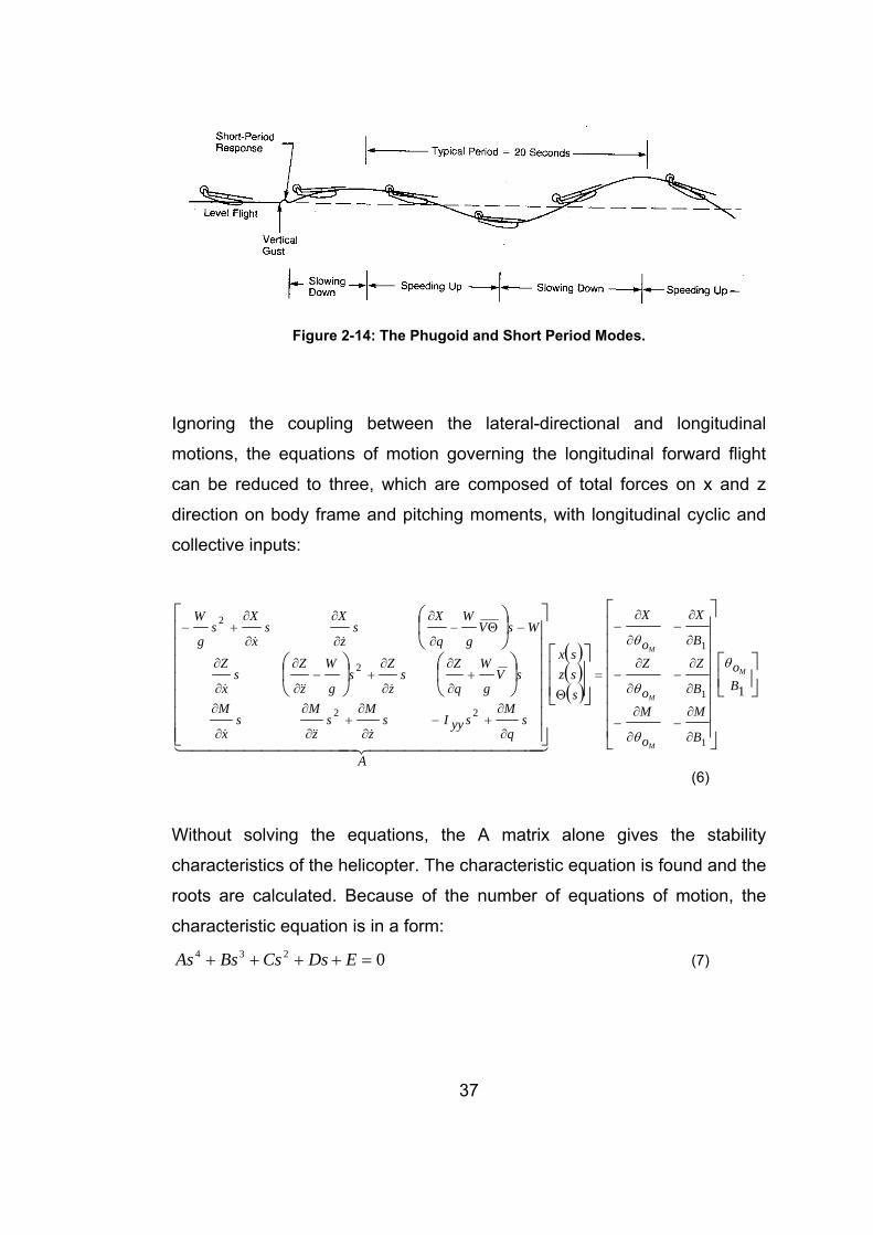
37

Figure 2-14: The Phugoid and Short Period Modes.

Ignoring the coupling between the lateral-directional and longitudinal

motions, the equations of motion governing the longitudinal forward flight

can be reduced to three, which are composed of total forces on x and z

direction on body frame and pitching moments, with longitudinal cyclic and

collective inputs:

( )( )( ) ⎥⎦

⎤⎢⎣⎡

⎥⎥⎥⎥⎥⎥⎥

⎦

⎤

⎢⎢⎢⎢⎢⎢⎢

⎣

⎡

⎥⎥⎦

⎤

⎢⎢⎣

⎡

⎥⎥⎥⎥⎥⎥⎥

⎦

⎤

⎢⎢⎢⎢⎢⎢⎢

⎣

⎡

⎟⎠⎞

⎜⎝⎛

⎟⎠⎞

⎜⎝⎛

⎟⎠⎞

⎜⎝⎛

∂

∂−

∂

∂−

∂

∂−

∂

∂−

∂

∂−

∂

∂−

=Θ

∂

∂+−

∂

∂+

∂

∂

∂

∂

+∂

∂

∂

∂+−

∂

∂

∂

∂

−Θ−∂

∂

∂

∂

∂

∂+−

1

1

1

1

22

2

2

Bo

B

M

o

M

B

Z

o

Z

B

X

o

X

sszsx

A

sq

MsyyIs

z

Ms

z

Ms

x

M

sVg

W

q

Zs

z

Zs

g

W

z

Zs

x

Z

WsVg

W

q

Xs

z

Xs

x

Xs

g

W

M

M

M

M

θ

θ

θ

θ

4444444444 34444444444 21&&&&

&&&&

&&

(6)

Without solving the equations, the A matrix alone gives the stability

characteristics of the helicopter. The characteristic equation is found and the

roots are calculated. Because of the number of equations of motion, the

characteristic equation is in a form:

0234 =++++ EDsCsBsAs (7)

38

And the Routh’s Discriminant (Routh’s Test) is described as:

ADBCDR −=.. (8)

A negative Routh Discriminant shows that the system is unstable, while a

positive value indicates that no unstable oscillation occurs. Also, if all

coefficients of the characteristic equation are positive, the system in that

condition has no positive real root and therefore no pure divergence occurs.

If the constant D is zero, there will be one zero root and one degree of

freedom will have non-oscillatory neutral stability. If one of the coefficients is

negative, then there will be either a pure divergence or an unstable

oscillation.

The roots of the characteristic equation give the details of the oscillations,

such as the frequency. If the real part of one root is negative, then that root

introduces a convergent motion, and vice versa. If an imaginary part exists,

two roots being complex conjugate, those two roots introduce an oscillatory

motion, the convergence depending on the real part.

The period, frequency and the time-to-double parameters are calculated as

described below:

The period of the oscillation:

( ) .2sim

T π= (9)

Here s is a complex root.

The time-to-double:

( )( ) .2lnsre

tdouble = (10)

And the neutral frequency of the oscillation is:

( )simn =ω (11)

39

The DYNA-STAB code calculates the required stability derivatives, the

characteristic equation and the roots, and determines about the stability of

the helicopter after a step disturbance given by the longitudinal cyclic, the

collective or due to a vertical gust. The calculations of the stability

derivatives are given in Appendix C.

Some of the inputs the DYNA-STAB code uses are the wind tunnel test

results for the fuselage lift, drag and pitching moment as a function of angle

of attack. Those parameters can also be calculated using package CFD

programs.

2.6 VERIFICATION

2.6.1 PROUTY’S EXAMPLE HELICOPTER

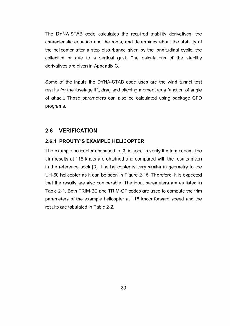
The example helicopter described in [3] is used to verify the trim codes. The

trim results at 115 knots are obtained and compared with the results given

in the reference book [3]. The helicopter is very similar in geometry to the

UH-60 helicopter as it can be seen in Figure 2-15. Therefore, it is expected

that the results are also comparable. The input parameters are as listed in

Table 2-1. Both TRIM-BE and TRIM-CF codes are used to compute the trim

parameters of the example helicopter at 115 knots forward speed and the

results are tabulated in Table 2-2.

40

Figure 2-15: The example helicopter in [3].

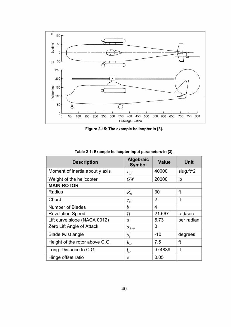
Table 2-1: Example helicopter input parameters in [3].

Description Algebraic Symbol Value Unit

Moment of inertia about y axis yyI 40000 slug.ft^2

Weight of the helicopter GW 20000 lb MAIN ROTOR Radius MR 30 ft Chord Mc 2 ft Number of Blades b 4 Revolution Speed Ω 21.667 rad/sec Lift curve slope (NACA 0012) a 5.73 per radianZero Lift Angle of Attack 0=Lα 0

Blade twist angle 1θ -10 degrees Height of the rotor above C.G. Mh 7.5 ft Long. Distance to C.G. Ml -0.4839 ft Hinge offset ratio e 0.05

41

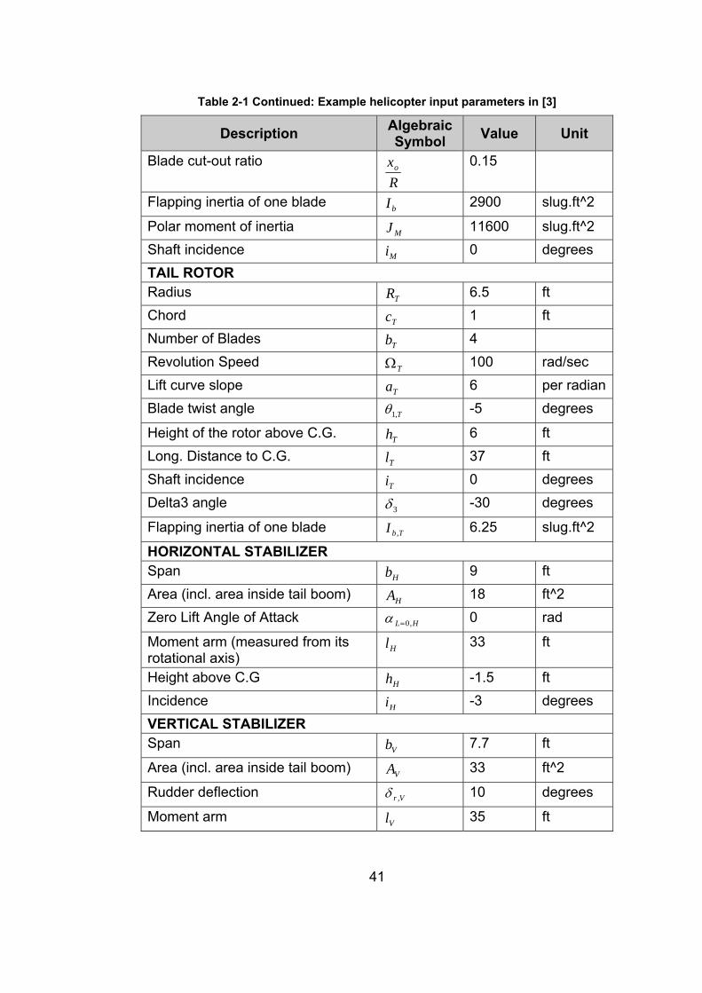
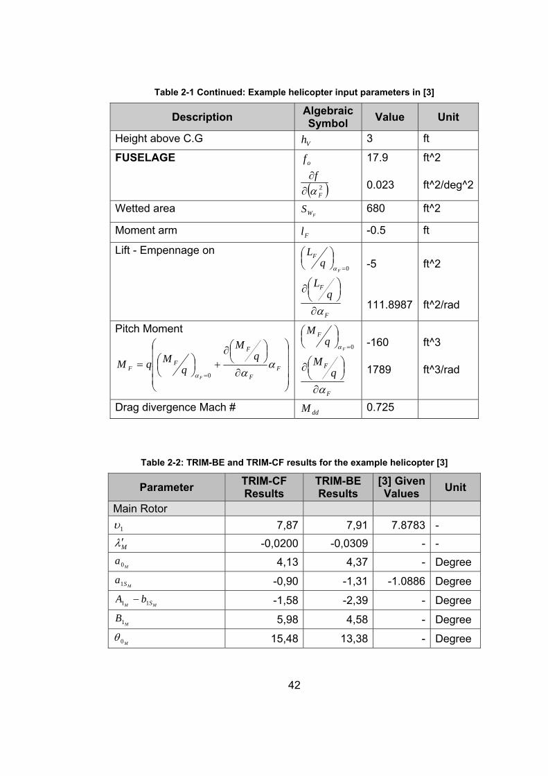
Table 2-1 Continued: Example helicopter input parameters in [3]


Blade cut-out ratio Rxo

0.15

Flapping inertia of one blade bI 2900 slug.ft^2

Polar moment of inertia MJ 11600 slug.ft^2 Shaft incidence Mi 0 degrees TAIL ROTOR Radius TR 6.5 ft Chord Tc 1 ft Number of Blades Tb 4 Revolution Speed TΩ 100 rad/sec Lift curve slope Ta 6 per radianBlade twist angle T,1θ -5 degrees

Height of the rotor above C.G. Th 6 ft Long. Distance to C.G. Tl 37 ft Shaft incidence Ti 0 degrees Delta3 angle 3δ -30 degrees

Flapping inertia of one blade TbI , 6.25 slug.ft^2

HORIZONTAL STABILIZER Span Hb 9 ft Area (incl. area inside tail boom) HA 18 ft^2 Zero Lift Angle of Attack HL ,0=α 0 rad

Moment arm (measured from its rotational axis)

Hl 33 ft

Height above C.G Hh -1.5 ft Incidence Hi -3 degrees VERTICAL STABILIZER Span Vb 7.7 ft

Area (incl. area inside tail boom) VA 33 ft^2

Rudder deflection Vr ,δ 10 degrees

Moment arm Vl 35 ft

42



Height above C.G Vh 3 ft

FUSELAGE of

( )2F

fα∂∂

17.9 0.023

ft^2 ft^2/deg^2

Wetted area FWS 680 ft^2

Moment arm Fl -0.5 ft

Lift - Empennage on 0=

⎟⎠⎞⎜

⎝⎛

Fq

LF

α

F

Fq

L

α∂

⎟⎠⎞⎜

⎝⎛∂

-5 111.8987

ft^2 ft^2/rad

Pitch Moment

⎟⎟⎟⎟

⎠

⎞

⎜⎜⎜⎜

⎝

⎛

∂

⎟⎠⎞⎜

⎝⎛∂

+⎟⎠⎞⎜

⎝⎛=

=F

F

F

FF

qM

qMqM

F

ααα 0

0=⎟⎠⎞⎜

⎝⎛

Fq

M F

α

F

Fq

M

α∂

⎟⎠⎞⎜

⎝⎛∂

-160 1789

ft^3 ft^3/rad

Drag divergence Mach # ddM 0.725

Table 2-2: TRIM-BE and TRIM-CF results for the example helicopter [3]

Parameter TRIM-CF Results

TRIM-BE Results

[3] Given Values Unit

Main Rotor

1υ 7,87 7,91 7.8783 -

Mλ′ -0,0200 -0,0309 - -

Ma0 4,13 4,37 - Degree

MSa1 -0,90 -1,31 -1.0886 Degree

MM SbA 11 − -1,58 -2,39 - Degree

MB1 5,98 4,58 - Degree

M0θ 15,48 13,38 - Degree

43

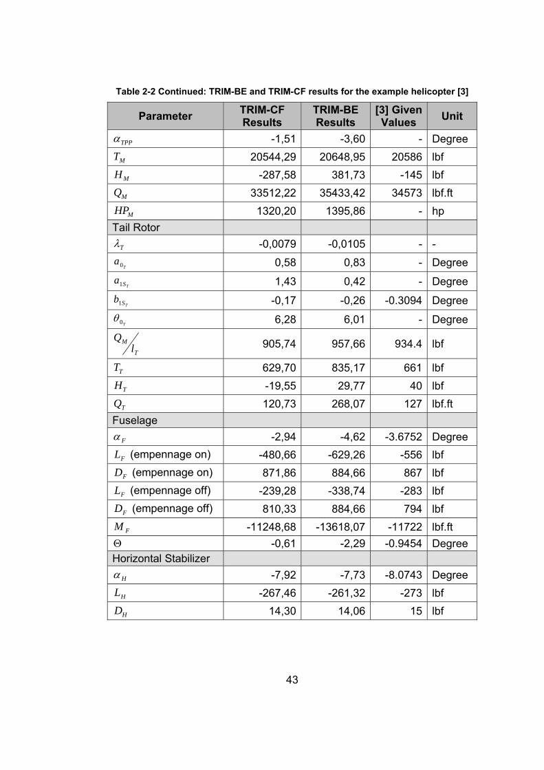
Table 2-2 Continued: TRIM-BE and TRIM-CF results for the example helicopter [3]


TRIM-BE Results


TPPα -1,51 -3,60 - Degree

MT 20544,29 20648,95 20586 lbf

MH -287,58 381,73 -145 lbf

MQ 33512,22 35433,42 34573 lbf.ft

MHP 1320,20 1395,86 - hp Tail Rotor

Tλ -0,0079 -0,0105 - -

Ta0 0,58 0,83 - Degree

TSa1 1,43 0,42 - Degree

TSb1 -0,17 -0,26 -0.3094 Degree

T0θ 6,28 6,01 - Degree

T

Ml

Q 905,74 957,66 934.4 lbf

TT 629,70 835,17 661 lbf

TH -19,55 29,77 40 lbf

TQ 120,73 268,07 127 lbf.ft Fuselage

Fα -2,94 -4,62 -3.6752 Degree

FL (empennage on) -480,66 -629,26 -556 lbf

FD (empennage on) 871,86 884,66 867 lbf

FL (empennage off) -239,28 -338,74 -283 lbf

FD (empennage off) 810,33 884,66 794 lbf

FM -11248,68 -13618,07 -11722 lbf.ft Θ -0,61 -2,29 -0.9454 Degree Horizontal Stabilizer

Hα -7,92 -7,73 -8.0743 Degree

HL -267,46 -261,32 -273 lbf

HD 14,30 14,06 15 lbf

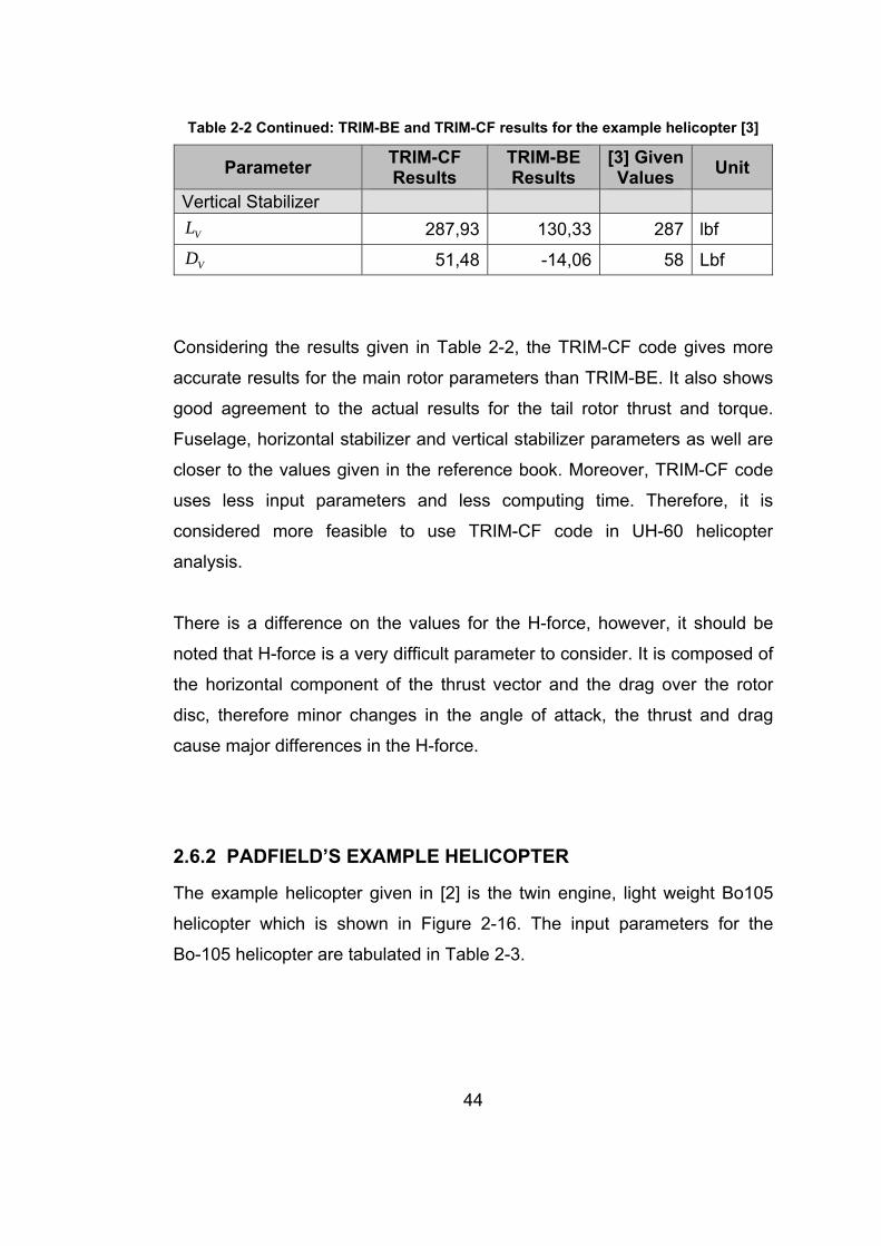
44

Table 2-2 Continued: TRIM-BE and TRIM-CF results for the example helicopter [3]


TRIM-BE Results


Vertical Stabilizer

VL 287,93 130,33 287 lbf

VD 51,48 -14,06 58 Lbf Considering the results given in Table 2-2, the TRIM-CF code gives more

accurate results for the main rotor parameters than TRIM-BE. It also shows

good agreement to the actual results for the tail rotor thrust and torque.

Fuselage, horizontal stabilizer and vertical stabilizer parameters as well are

closer to the values given in the reference book. Moreover, TRIM-CF code

uses less input parameters and less computing time. Therefore, it is

considered more feasible to use TRIM-CF code in UH-60 helicopter

analysis.

There is a difference on the values for the H-force, however, it should be

noted that H-force is a very difficult parameter to consider. It is composed of

the horizontal component of the thrust vector and the drag over the rotor

disc, therefore minor changes in the angle of attack, the thrust and drag

cause major differences in the H-force.

2.6.2 PADFIELD’S EXAMPLE HELICOPTER

The example helicopter given in [2] is the twin engine, light weight Bo105

helicopter which is shown in Figure 2-16. The input parameters for the

Bo-105 helicopter are tabulated in Table 2-3.

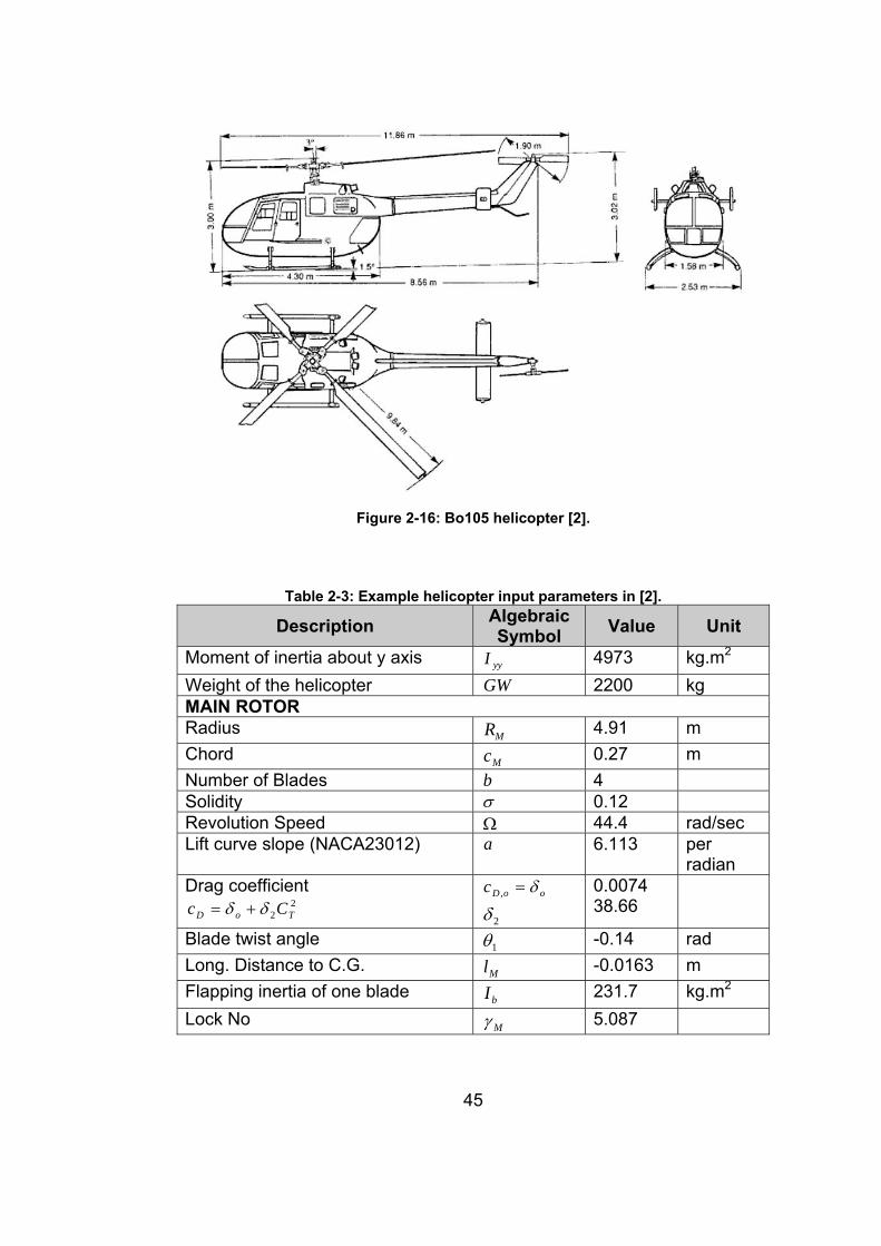
45

Figure 2-16: Bo105 helicopter [2].

Table 2-3: Example helicopter input parameters in [2].


Moment of inertia about y axis yyI 4973 kg.m2 Weight of the helicopter GW 2200 kg MAIN ROTOR Radius MR 4.91 m Chord Mc 0.27 m Number of Blades b 4 Solidity σ 0.12 Revolution Speed Ω 44.4 rad/sec Lift curve slope (NACA23012) a 6.113 per

radian Drag coefficient

22 ToD Cc δδ +=

ooDc δ=,

2δ 0.0074 38.66

Blade twist angle 1θ -0.14 rad Long. Distance to C.G. Ml -0.0163 m Flapping inertia of one blade bI 231.7 kg.m2 Lock No Mγ 5.087

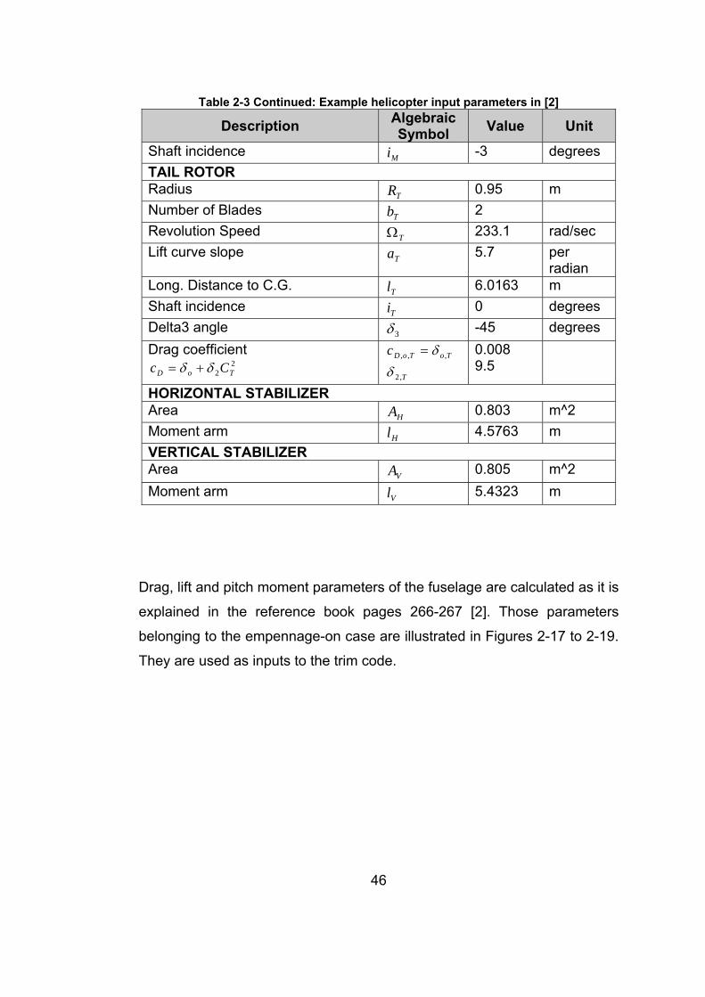
46



Shaft incidence Mi -3 degrees TAIL ROTOR Radius TR 0.95 m Number of Blades Tb 2 Revolution Speed TΩ 233.1 rad/sec Lift curve slope Ta 5.7 per

radian Long. Distance to C.G. Tl 6.0163 m Shaft incidence Ti 0 degrees Delta3 angle 3δ -45 degrees Drag coefficient

22 ToD Cc δδ +=

ToToDc ,,, δ=

T,2δ 0.008 9.5

HORIZONTAL STABILIZER Area HA 0.803 m^2 Moment arm Hl 4.5763 m VERTICAL STABILIZER Area VA 0.805 m^2 Moment arm Vl 5.4323 m

Drag, lift and pitch moment parameters of the fuselage are calculated as it is

explained in the reference book pages 266-267 [2]. Those parameters

belonging to the empennage-on case are illustrated in Figures 2-17 to 2-19.

They are used as inputs to the trim code.

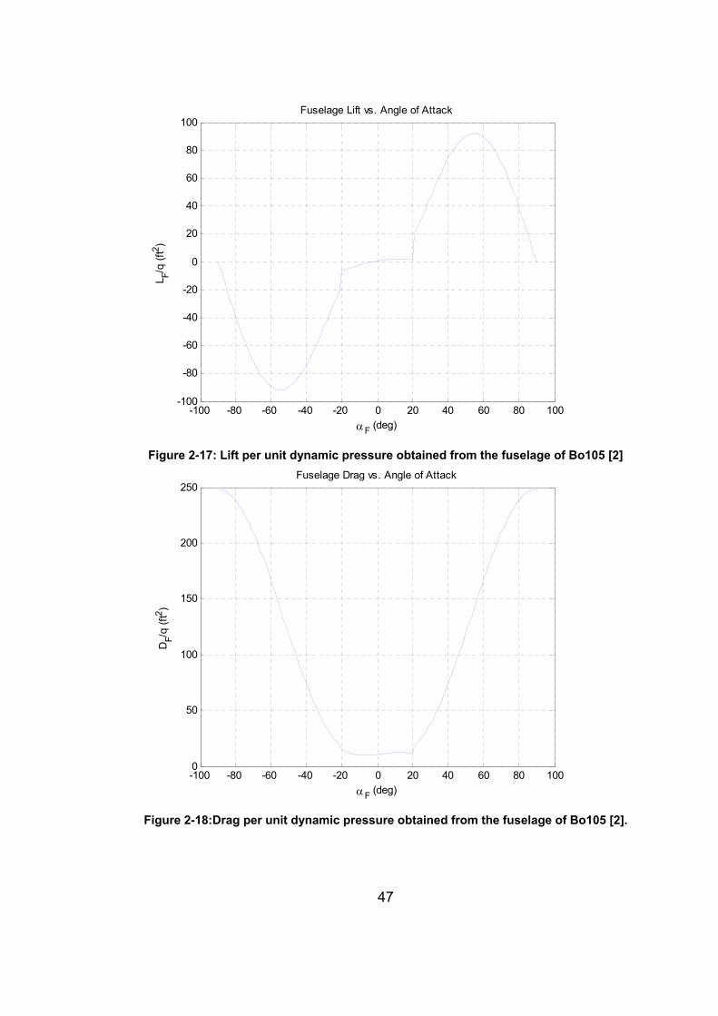
47

-100 -80 -60 -40 -20 0 20 40 60 80 100-100

-80

-60

-40

-20

0

20

40

60

80

100

αF (deg)

L F/q (f

t2 )

Fuselage Lift vs. Angle of Attack

Figure 2-17: Lift per unit dynamic pressure obtained from the fuselage of Bo105 [2]

-100 -80 -60 -40 -20 0 20 40 60 80 1000

50

100

150

200

250

αF (deg)

DF/q

(ft2 )

Fuselage Drag vs. Angle of Attack

Figure 2-18:Drag per unit dynamic pressure obtained from the fuselage of Bo105 [2].

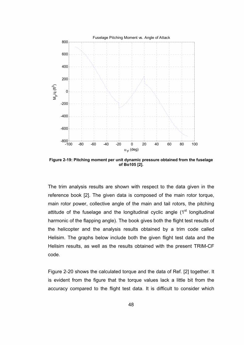
48

-100 -80 -60 -40 -20 0 20 40 60 80 100-800

-600

-400

-200

0

200

400

600

800

αF (deg)

MF/q

(ft3 )

Fuselage Pitching Moment vs. Angle of Attack

Figure 2-19: Pitching moment per unit dynamic pressure obtained from the fuselage

of Bo105 [2]. The trim analysis results are shown with respect to the data given in the

reference book [2]. The given data is composed of the main rotor torque,

main rotor power, collective angle of the main and tail rotors, the pitching

attitude of the fuselage and the longitudinal cyclic angle (1st longitudinal

harmonic of the flapping angle). The book gives both the flight test results of

the helicopter and the analysis results obtained by a trim code called

Helisim. The graphs below include both the given flight test data and the

Helisim results, as well as the results obtained with the present TRIM-CF

code.

Figure 2-20 shows the calculated torque and the data of Ref. [2] together. It

is evident from the figure that the torque values lack a little bit from the

accuracy compared to the flight test data. It is difficult to consider which

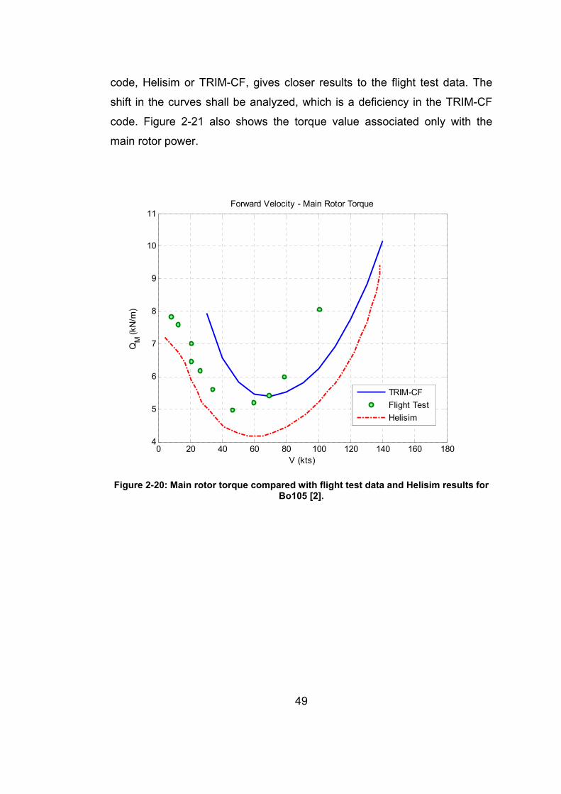
49

code, Helisim or TRIM-CF, gives closer results to the flight test data. The

shift in the curves shall be analyzed, which is a deficiency in the TRIM-CF

code. Figure 2-21 also shows the torque value associated only with the

main rotor power.

0 20 40 60 80 100 120 140 160 1804

5

6

7

8

9

10

11

V (kts)

QM

(kN

/m)

Forward Velocity - Main Rotor Torque

TRIM-CFFlight TestHelisim

Figure 2-20: Main rotor torque compared with flight test data and Helisim results for

Bo105 [2].

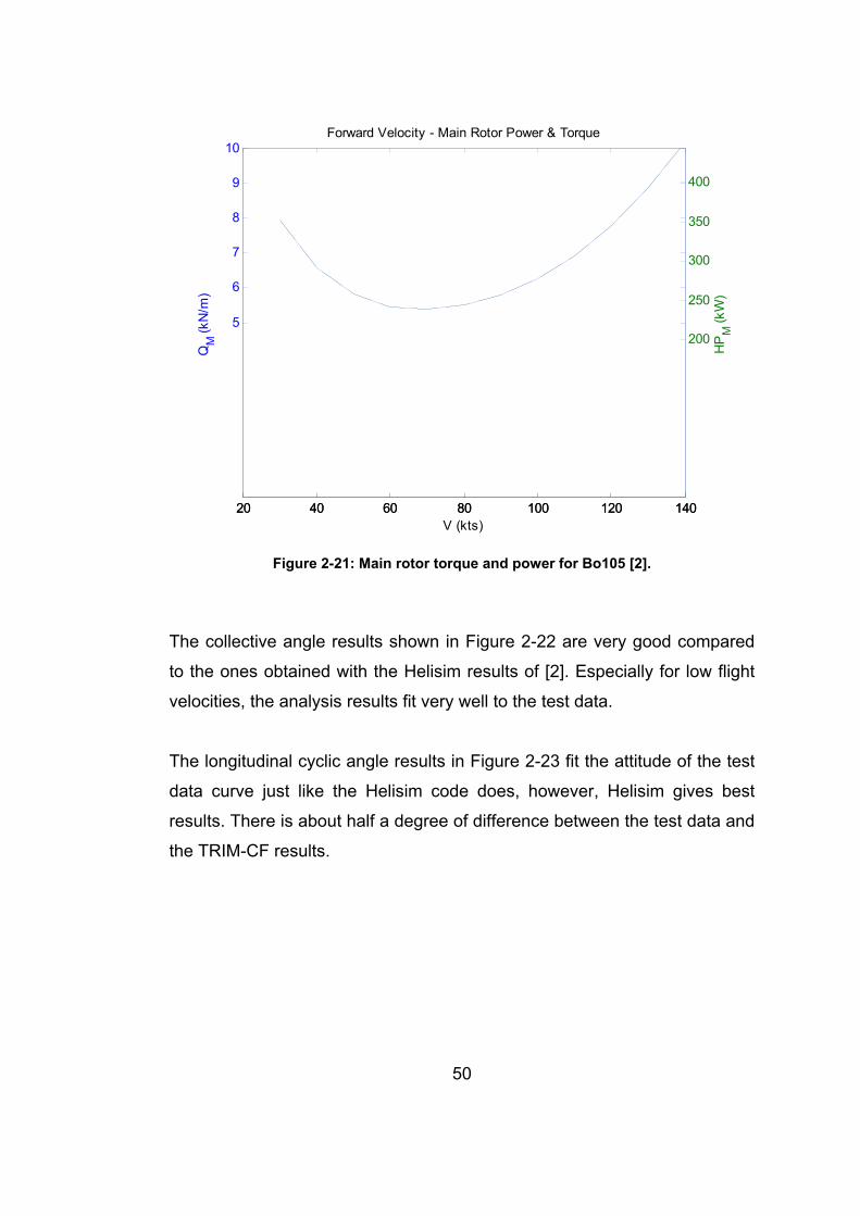
50

20 40 60 80 100 120 140

5

6

7

8

9

10Forward Velocity - Main Rotor Power & Torque

V (kts)

QM

(kN

/m)

20 40 60 80 100 120 140

200

250

300

350

400

HP

M (k

W)

Figure 2-21: Main rotor torque and power for Bo105 [2].

The collective angle results shown in Figure 2-22 are very good compared

to the ones obtained with the Helisim results of [2]. Especially for low flight

velocities, the analysis results fit very well to the test data.

The longitudinal cyclic angle results in Figure 2-23 fit the attitude of the test

data curve just like the Helisim code does, however, Helisim gives best

results. There is about half a degree of difference between the test data and

the TRIM-CF results.

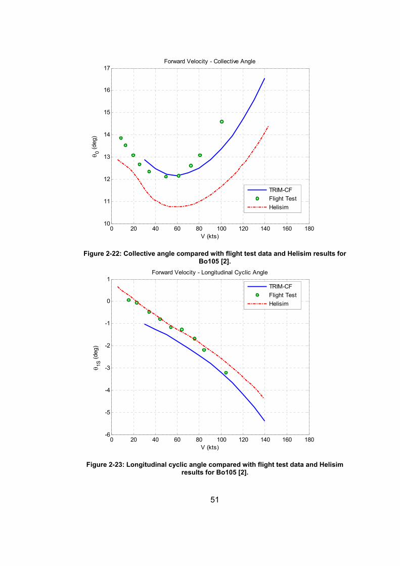
51

0 20 40 60 80 100 120 140 160 18010

11

12

13

14

15

16

17

V (kts)

θ 0 (d

eg)

Forward Velocity - Collective Angle


Figure 2-22: Collective angle compared with flight test data and Helisim results for

Bo105 [2].

0 20 40 60 80 100 120 140 160 180-6

-5

-4

-3

-2

-1

0

1

V (kts)

θ 1S (d

eg)

Forward Velocity - Longitudinal Cyclic Angle


Figure 2-23: Longitudinal cyclic angle compared with flight test data and Helisim

results for Bo105 [2].

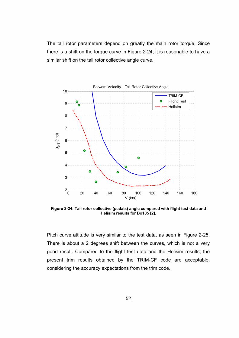
52

The tail rotor parameters depend on greatly the main rotor torque. Since

there is a shift on the torque curve in Figure 2-24, it is reasonable to have a

similar shift on the tail rotor collective angle curve.

0 20 40 60 80 100 120 140 160 1802

3

4

5

6

7

8

9

10

V (kts)

θ 0.T

(deg

)

Forward Velocity - Tail Rotor Collective Angle


Figure 2-24: Tail rotor collective (pedals) angle compared with flight test data and

Helisim results for Bo105 [2]. Pitch curve attitude is very similar to the test data, as seen in Figure 2-25.

There is about a 2 degrees shift between the curves, which is not a very

good result. Compared to the flight test data and the Helisim results, the

present trim results obtained by the TRIM-CF code are acceptable,

considering the accuracy expectations from the trim code.

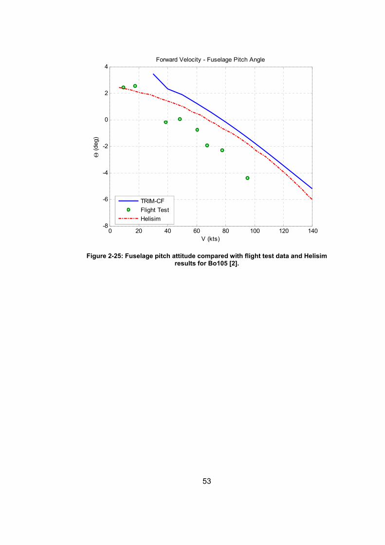
53

0 20 40 60 80 100 120 140-8

-6

-4

-2

0

2

4

V (kts)

Θ (d

eg)

Forward Velocity - Fuselage Pitch Angle


Figure 2-25: Fuselage pitch attitude compared with flight test data and Helisim

results for Bo105 [2].

54

CHAPTER 3

TRIM ANALYSIS OF UH-60 In this chapter, the trim characteristics of a UH-60 helicopter are analyzed

using TRIM-CF code and compared with the flight test data.

3.1 FLIGHT TESTS

Extensive flight tests were performed on the UH-60 helicopter by ASELSAN

Inc. The flight profiles included forward flight at every 10 knots incremental

forward velocities from maximum achievable forward flight speed, which is

approximately 150 knots for the UH-60 helicopters, to 10 knots. The test

instrumentation, data logging process and analysis steps are all explained in

the following sub-chapters.

3.1.1 INSTRUMENTATION

The instrumentation was composed of mainly a data acquisition system,

KAM-500, which is a flight certified modular data acquisition system

produced in ACRA CONTROL, Inc. The DAS can be used to gather, store

and analyze data coming from different sensors which produce voltage or

current. It can also log analog or digital data; ethernet, GPS and data

coming from ARINC, MIL-STD-1553, RS-232, RS-422 and RS-485 busses.

The DAS combines high reliability with high performance in a compact

modular system. Over 50 plug-in modules including advanced signal

conditioning, avionics bus monitoring, video/audio compression, integrated

data logging and multiple output formats are supported within a single unit

or master/slave network distributed system. KAM-500 is designed for harsh

airborne environments where space and power are limited.

55

For our flight test purposes, we used KAM-500 to gather data coming from

the Multi-Functional Display (MFD) and EGI (Embedded INS & GPS). The

synchronization was important, since flight test data are difficult to analyze.

We tapped to the related connectors of the instruments to log the flight data.

Pitch angle values are supplied from EGI; true airspeed (TAS) and

barometric altitude values are supplied from MFD; and torque and fuel

quantity values are supplied from their gauges.

3.1.2 DATA LOGGING

The data logged can be listed as:

1. TAS [knots]

2. Barometric altitude [ft]

3. Pitch [deg]

4. Total torque [%]

5. Fuel quantity [lb]

The raw data were logged online to the laptop PC. The acquisition interface

of the software of the DAS allows the user to see the data in any format

during the flight. The software is capable of logging high speed data and it

offers an extensive analysis tool, which includes adding conversion factors,

doing mathematical and logical operations, taking the average, finding the

standard deviation, calculating the Fast Fourier Transformation etc. Figure

3-1 shows the interface of the software.

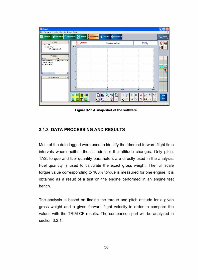
56

Figure 3-1: A snap-shot of the software.

3.1.3 DATA PROCESSING AND RESULTS

Most of the data logged were used to identify the trimmed forward flight time

intervals where neither the altitude nor the attitude changes. Only pitch,

TAS, torque and fuel quantity parameters are directly used in the analysis.

Fuel quantity is used to calculate the exact gross weight. The full scale

torque value corresponding to 100% torque is measured for one engine. It is

obtained as a result of a test on the engine performed in an engine test

bench.

The analysis is based on finding the torque and pitch attitude for a given

gross weight and a given forward flight velocity in order to compare the

values with the TRIM-CF results. The comparison part will be analyzed in

section 3.2.1.

57

It should be noted that during the flight the gross weight decreases. As

stated in section 3.2, the analysis is performed taking the weight change

into account.

3.2 TRIM ANALYSIS OF UH-60 HELICOPTER

The test data were taken during a single flight. To account for the weight

decrease during the flight as a result of fuel consumption, the forward

velocity was decreased incrementally. In order to compare the test results of

the UH-60 helicopter with the trim code results, the trim analysis is

performed for the weights the flight data were taken at. The pitch attitude

and torque values are compared with the test data. Parameters are

nondimensionalized with some reference values.

Fuselage forces and moments are calculated using the force versus angle

of attack curves given in [16], which are based on wind tunnel

measurements.

The pitch attitude was predicted close to the flight test data, as seen in

Figure 3-2. However, it should be reminded that the helicopter used in flight

test has a Stability Augmentation System (SAS) and a Flight Path

Stabilization System (FPS) which help the pilot with smooth flight.

Therefore, it is not expected that the analysis results fit exactly the test

results, but expected to be close enough. Looking at Figure 3-3, there is a

drift between the total torque flight test data and the analysis results curves.

The code does not seem to calculate the torque values very accurately.

However, since the attitudes of the curves resemble each other, the results

can be accepted as fairly good enough.

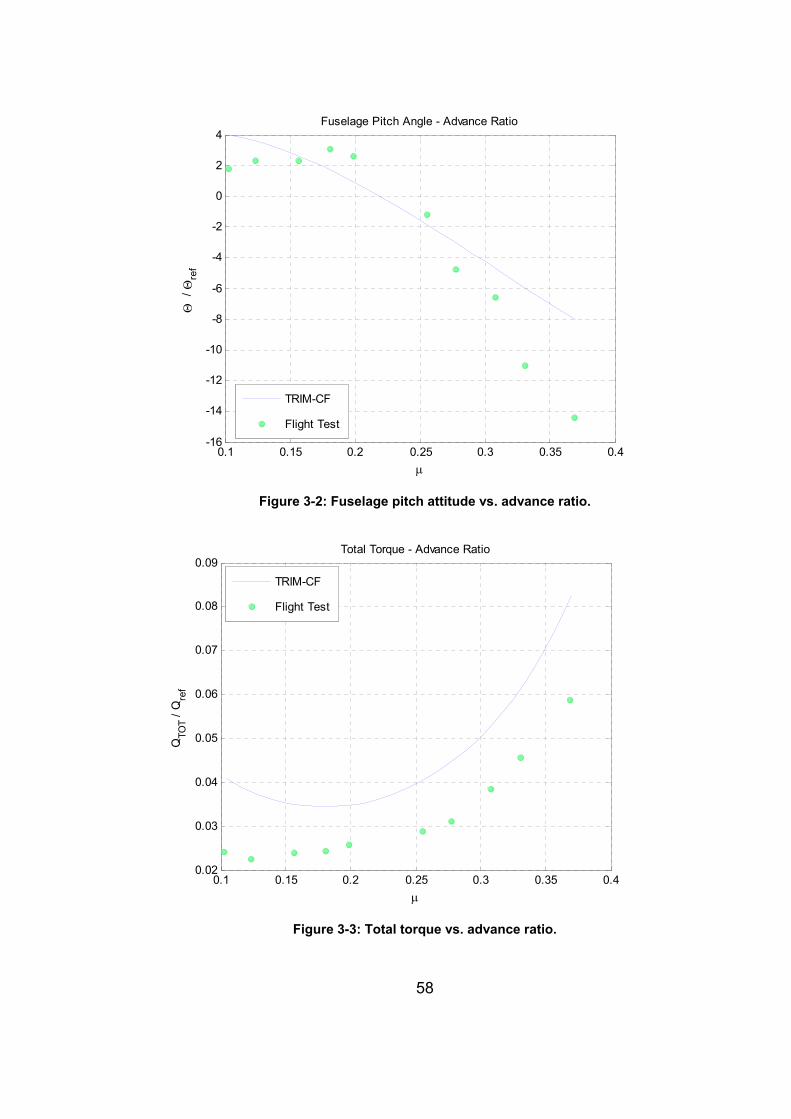
58

0.1 0.15 0.2 0.25 0.3 0.35 0.4-16

-14

-12

-10

-8

-6

-4

-2

0

2

4

μ

Θ /

Θre

f

Fuselage Pitch Angle - Advance Ratio

TRIM-CF

Flight Test

Figure 3-2: Fuselage pitch attitude vs. advance ratio.

0.1 0.15 0.2 0.25 0.3 0.35 0.40.02

0.03

0.04

0.05

0.06

0.07

0.08

0.09

μ

QTO

T / Q

ref

Total Torque - Advance Ratio

TRIM-CF

Flight Test

Figure 3-3: Total torque vs. advance ratio.

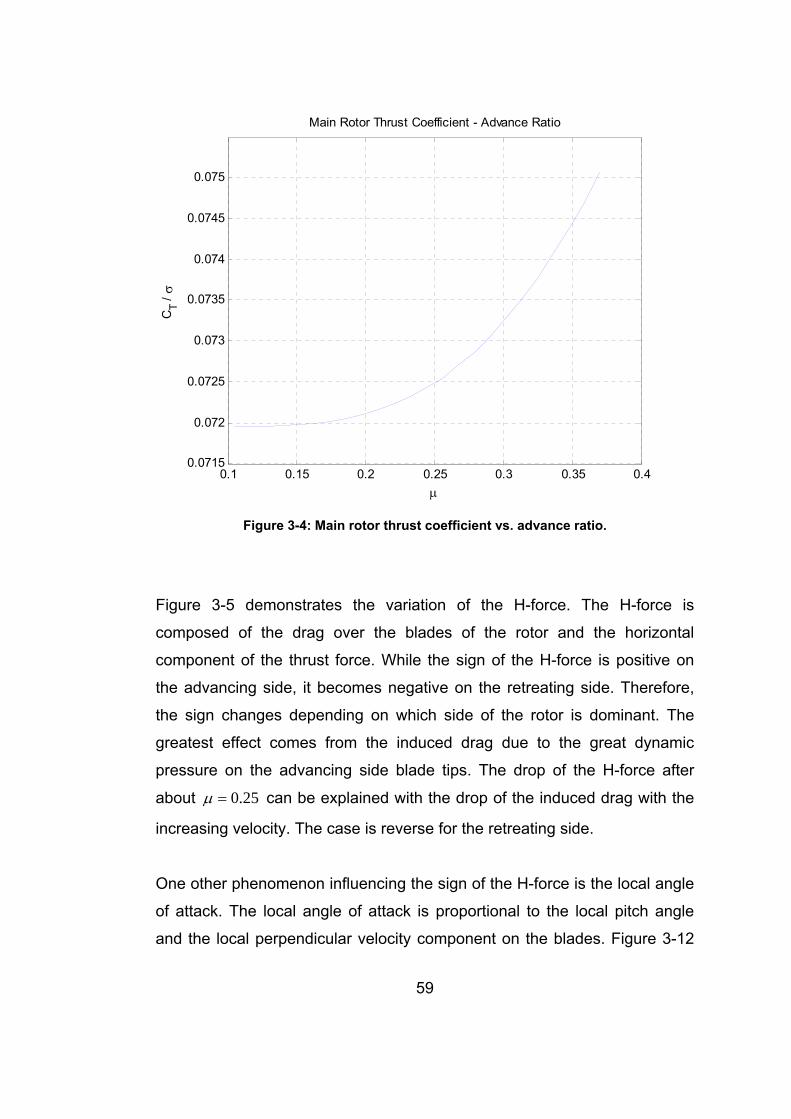
59

0.1 0.15 0.2 0.25 0.3 0.35 0.40.0715

0.072

0.0725

0.073

0.0735

0.074

0.0745

0.075

μ

CT /

σ

Main Rotor Thrust Coefficient - Advance Ratio

Figure 3-4: Main rotor thrust coefficient vs. advance ratio.

Figure 3-5 demonstrates the variation of the H-force. The H-force is

composed of the drag over the blades of the rotor and the horizontal

component of the thrust force. While the sign of the H-force is positive on

the advancing side, it becomes negative on the retreating side. Therefore,

the sign changes depending on which side of the rotor is dominant. The

greatest effect comes from the induced drag due to the great dynamic

pressure on the advancing side blade tips. The drop of the H-force after

about 25.0=μ can be explained with the drop of the induced drag with the

increasing velocity. The case is reverse for the retreating side.

One other phenomenon influencing the sign of the H-force is the local angle

of attack. The local angle of attack is proportional to the local pitch angle

and the local perpendicular velocity component on the blades. Figure 3-12

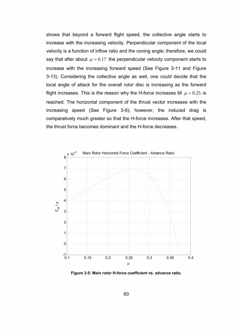
60

shows that beyond a forward flight speed, the collective angle starts to

increase with the increasing velocity. Perpendicular component of the local

velocity is a function of inflow ratio and the coning angle; therefore, we could

say that after about 17.0=μ the perpendicular velocity component starts to

increase with the increasing forward speed (See Figure 3-11 and Figure

3-13). Considering the collective angle as well, one could decide that the

local angle of attack for the overall rotor disc is increasing as the forward

flight increases. This is the reason why the H-force increases till 25.0=μ is

reached. The horizontal component of the thrust vector increases with the

increasing speed (See Figure 3-9); however, the induced drag is

comparatively much greater so that the H-force increases. After that speed,

the thrust force becomes dominant and the H-force decreases.

0.1 0.15 0.2 0.25 0.3 0.35 0.4-1

0

1

2

3

4

5

6

7

8x 10-4

μ

CH /

σ

Main Rotor Horizontal Force Coefficient - Advance Ratio

Figure 3-5: Main rotor H-force coefficient vs. advance ratio.

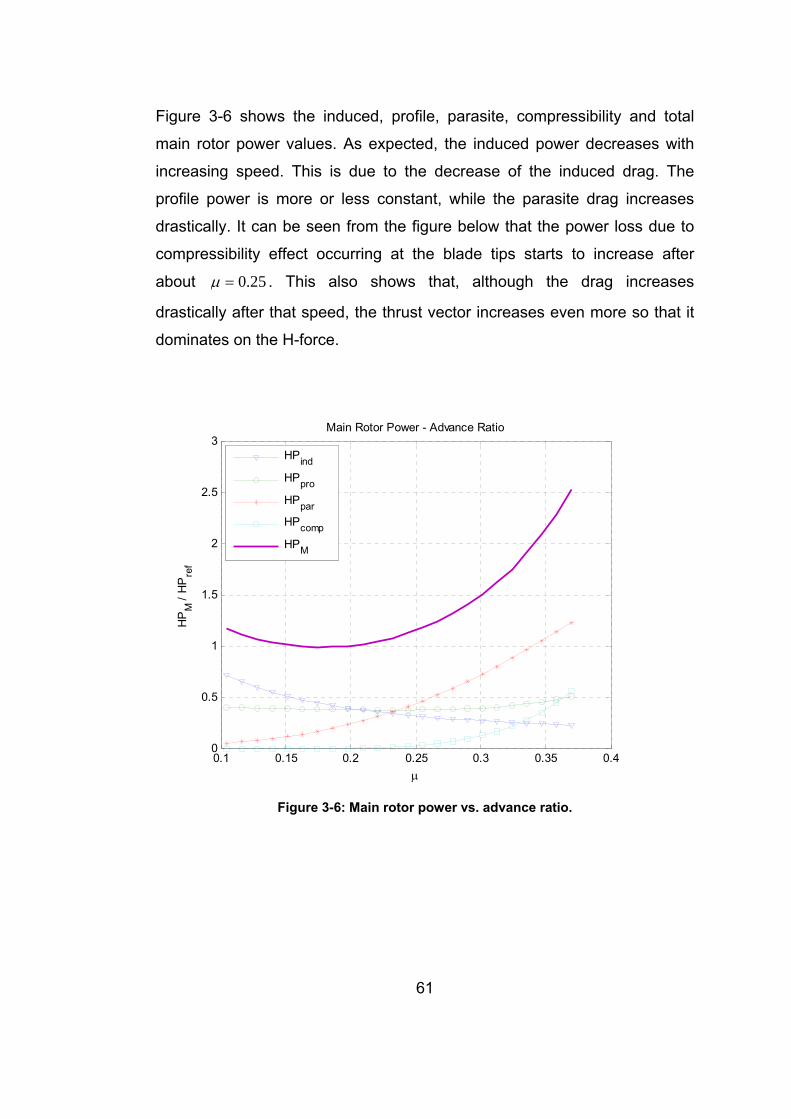
61

Figure 3-6 shows the induced, profile, parasite, compressibility and total

main rotor power values. As expected, the induced power decreases with

increasing speed. This is due to the decrease of the induced drag. The

profile power is more or less constant, while the parasite drag increases

drastically. It can be seen from the figure below that the power loss due to

compressibility effect occurring at the blade tips starts to increase after

about 25.0=μ . This also shows that, although the drag increases

drastically after that speed, the thrust vector increases even more so that it

dominates on the H-force.

0.1 0.15 0.2 0.25 0.3 0.35 0.40

0.5

1

1.5

2

2.5

3

μ

HP

M /

HP

ref

Main Rotor Power - Advance Ratio

HPind

HPpro

HPparHPcomp

HPM

Figure 3-6: Main rotor power vs. advance ratio.

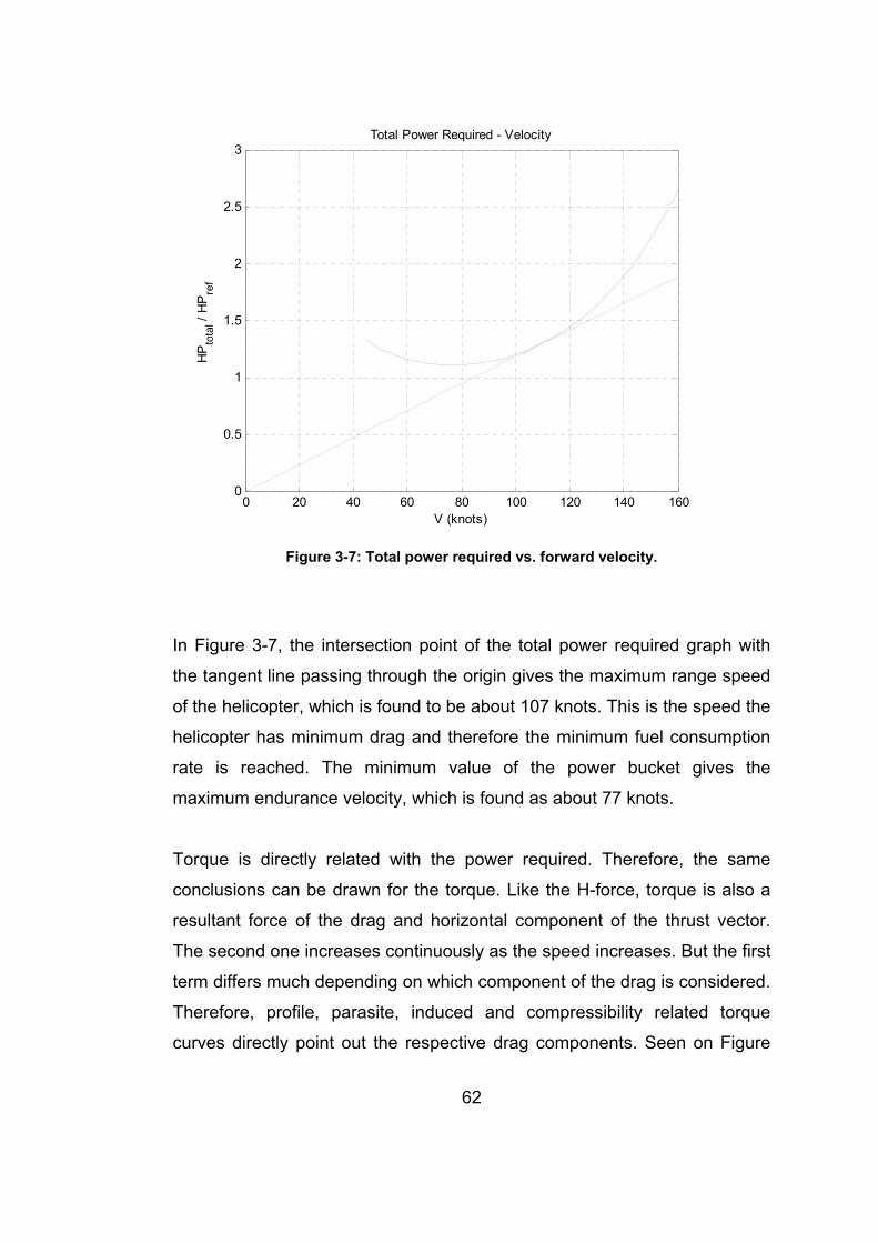
62

0 20 40 60 80 100 120 140 1600

0.5

1

1.5

2

2.5

3

V (knots)

HP

tota

l / H

Pre

f

Total Power Required - Velocity

Figure 3-7: Total power required vs. forward velocity.

In Figure 3-7, the intersection point of the total power required graph with

the tangent line passing through the origin gives the maximum range speed

of the helicopter, which is found to be about 107 knots. This is the speed the

helicopter has minimum drag and therefore the minimum fuel consumption

rate is reached. The minimum value of the power bucket gives the

maximum endurance velocity, which is found as about 77 knots.

Torque is directly related with the power required. Therefore, the same

conclusions can be drawn for the torque. Like the H-force, torque is also a

resultant force of the drag and horizontal component of the thrust vector.

The second one increases continuously as the speed increases. But the first

term differs much depending on which component of the drag is considered.

Therefore, profile, parasite, induced and compressibility related torque

curves directly point out the respective drag components. Seen on Figure

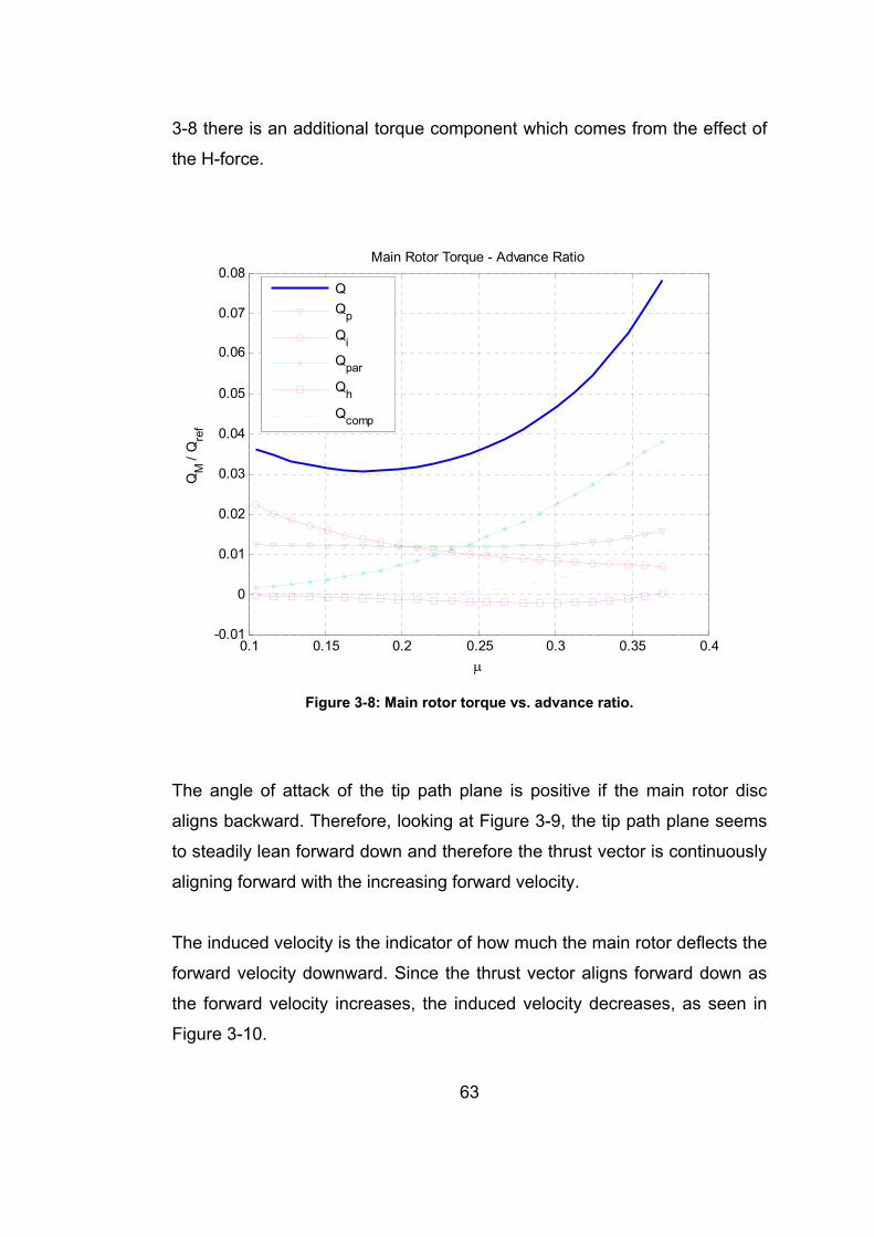
63

3-8 there is an additional torque component which comes from the effect of

the H-force.

0.1 0.15 0.2 0.25 0.3 0.35 0.4-0.01

0

0.01

0.02

0.03

0.04

0.05

0.06

0.07

0.08

μ

QM

/ Q

ref

Main Rotor Torque - Advance Ratio

QQp

QiQpar

Qh

Qcomp

Figure 3-8: Main rotor torque vs. advance ratio.

The angle of attack of the tip path plane is positive if the main rotor disc

aligns backward. Therefore, looking at Figure 3-9, the tip path plane seems

to steadily lean forward down and therefore the thrust vector is continuously

aligning forward with the increasing forward velocity.

The induced velocity is the indicator of how much the main rotor deflects the

forward velocity downward. Since the thrust vector aligns forward down as

the forward velocity increases, the induced velocity decreases, as seen in

Figure 3-10.

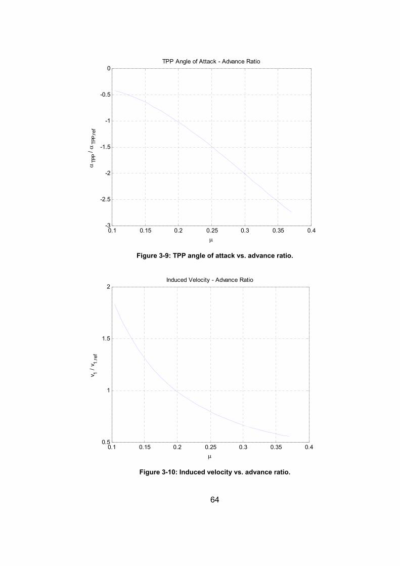
64

0.1 0.15 0.2 0.25 0.3 0.35 0.4-3

-2.5

-2

-1.5

-1

-0.5

0

μ

αTP

P / α

TPP.

ref

TPP Angle of Attack - Advance Ratio

Figure 3-9: TPP angle of attack vs. advance ratio.

0.1 0.15 0.2 0.25 0.3 0.35 0.40.5

1

1.5

2

μ

v 1 / v 1.

ref

Induced Velocity - Advance Ratio

Figure 3-10: Induced velocity vs. advance ratio.

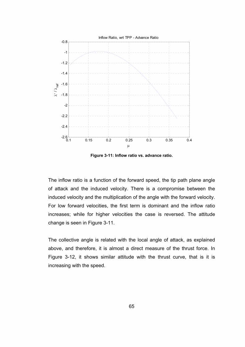
65

0.1 0.15 0.2 0.25 0.3 0.35 0.4-2.6

-2.4

-2.2

-2

-1.8

-1.6

-1.4

-1.2

-1

-0.8

μ

λ′ / λ r

ef

Inflow Ratio, wrt TPP - Advance Ratio

Figure 3-11: Inflow ratio vs. advance ratio.

The inflow ratio is a function of the forward speed, the tip path plane angle

of attack and the induced velocity. There is a compromise between the

induced velocity and the multiplication of the angle with the forward velocity.

For low forward velocities, the first term is dominant and the inflow ratio

increases; while for higher velocities the case is reversed. The attitude

change is seen in Figure 3-11.

The collective angle is related with the local angle of attack, as explained

above, and therefore, it is almost a direct measure of the thrust force. In

Figure 3-12, it shows similar attitude with the thrust curve, that is it is

increasing with the speed.

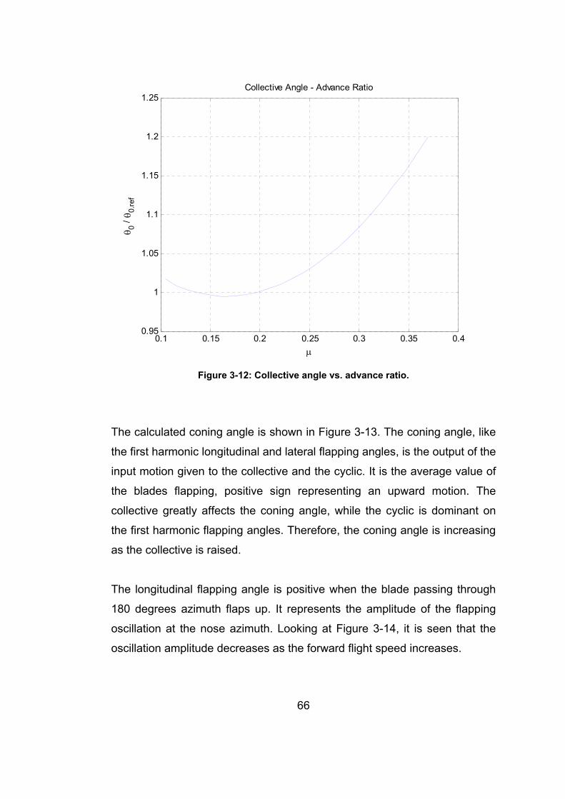
66

0.1 0.15 0.2 0.25 0.3 0.35 0.40.95

1

1.05

1.1

1.15

1.2

1.25

μ

θ 0 / θ 0

.ref

Collective Angle - Advance Ratio

Figure 3-12: Collective angle vs. advance ratio.

The calculated coning angle is shown in Figure 3-13. The coning angle, like

the first harmonic longitudinal and lateral flapping angles, is the output of the

input motion given to the collective and the cyclic. It is the average value of

the blades flapping, positive sign representing an upward motion. The

collective greatly affects the coning angle, while the cyclic is dominant on

the first harmonic flapping angles. Therefore, the coning angle is increasing

as the collective is raised.

The longitudinal flapping angle is positive when the blade passing through

180 degrees azimuth flaps up. It represents the amplitude of the flapping

oscillation at the nose azimuth. Looking at Figure 3-14, it is seen that the

oscillation amplitude decreases as the forward flight speed increases.

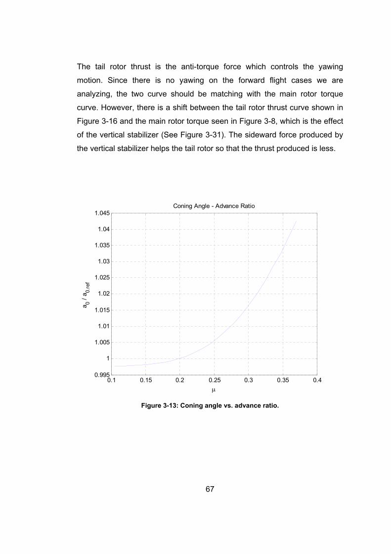
67

The tail rotor thrust is the anti-torque force which controls the yawing

motion. Since there is no yawing on the forward flight cases we are

analyzing, the two curve should be matching with the main rotor torque

curve. However, there is a shift between the tail rotor thrust curve shown in

Figure 3-16 and the main rotor torque seen in Figure 3-8, which is the effect

of the vertical stabilizer (See Figure 3-31). The sideward force produced by

the vertical stabilizer helps the tail rotor so that the thrust produced is less.

0.1 0.15 0.2 0.25 0.3 0.35 0.40.995

1

1.005

1.01

1.015

1.02

1.025

1.03

1.035

1.04

1.045

μ

a 0 / a 0.

ref

Coning Angle - Advance Ratio

Figure 3-13: Coning angle vs. advance ratio.

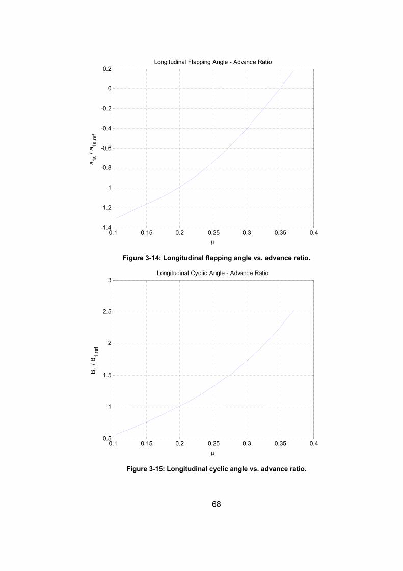
68

0.1 0.15 0.2 0.25 0.3 0.35 0.4-1.4

-1.2

-1

-0.8

-0.6

-0.4

-0.2

0

0.2

μ

a 1s /

a 1s.re

f

Longitudinal Flapping Angle - Advance Ratio

Figure 3-14: Longitudinal flapping angle vs. advance ratio.

0.1 0.15 0.2 0.25 0.3 0.35 0.40.5

1

1.5

2

2.5

3

μ

B1 /

B1.

ref

Longitudinal Cyclic Angle - Advance Ratio

Figure 3-15: Longitudinal cyclic angle vs. advance ratio.

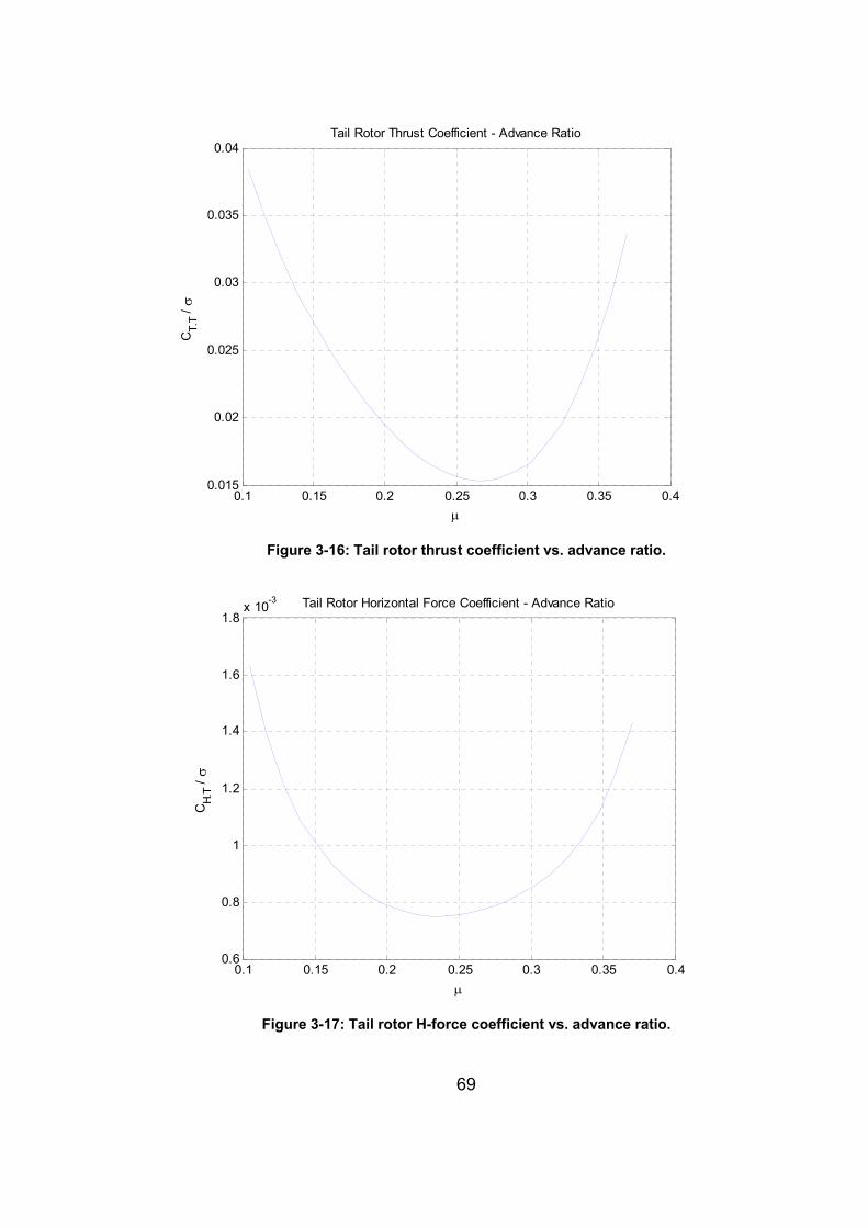
69

0.1 0.15 0.2 0.25 0.3 0.35 0.40.015

0.02

0.025

0.03

0.035

0.04

μ

CT.

T / σ

Tail Rotor Thrust Coefficient - Advance Ratio

Figure 3-16: Tail rotor thrust coefficient vs. advance ratio.

0.1 0.15 0.2 0.25 0.3 0.35 0.40.6

0.8

1

1.2

1.4

1.6

1.8x 10-3

μ

CH.

T / σ

Tail Rotor Horizontal Force Coefficient - Advance Ratio

Figure 3-17: Tail rotor H-force coefficient vs. advance ratio.

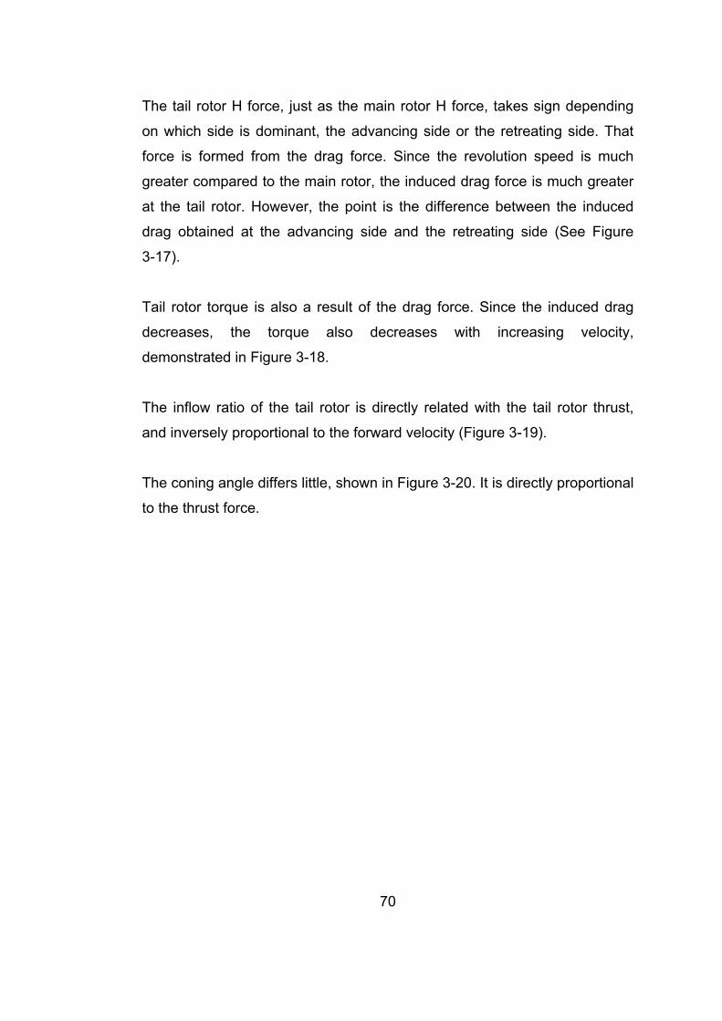
70

The tail rotor H force, just as the main rotor H force, takes sign depending

on which side is dominant, the advancing side or the retreating side. That

force is formed from the drag force. Since the revolution speed is much

greater compared to the main rotor, the induced drag force is much greater

at the tail rotor. However, the point is the difference between the induced

drag obtained at the advancing side and the retreating side (See Figure

3-17).

Tail rotor torque is also a result of the drag force. Since the induced drag

decreases, the torque also decreases with increasing velocity,

demonstrated in Figure 3-18.

The inflow ratio of the tail rotor is directly related with the tail rotor thrust,

and inversely proportional to the forward velocity (Figure 3-19).

The coning angle differs little, shown in Figure 3-20. It is directly proportional

to the thrust force.

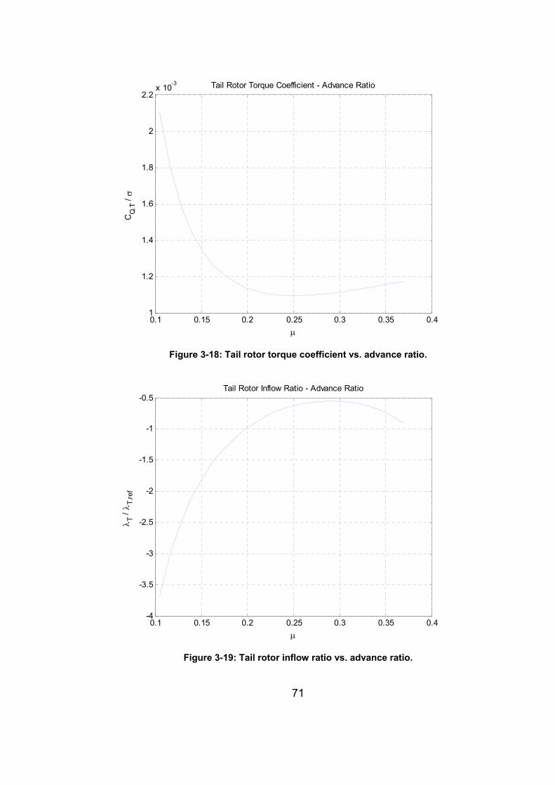
71

0.1 0.15 0.2 0.25 0.3 0.35 0.41

1.2

1.4

1.6

1.8

2

2.2x 10-3

μ

CQ

.T / σ

Tail Rotor Torque Coefficient - Advance Ratio

Figure 3-18: Tail rotor torque coefficient vs. advance ratio.

0.1 0.15 0.2 0.25 0.3 0.35 0.4-4

-3.5

-3

-2.5

-2

-1.5

-1

-0.5

μ

λ T / λ T

.ref

Tail Rotor Inflow Ratio - Advance Ratio

Figure 3-19: Tail rotor inflow ratio vs. advance ratio.

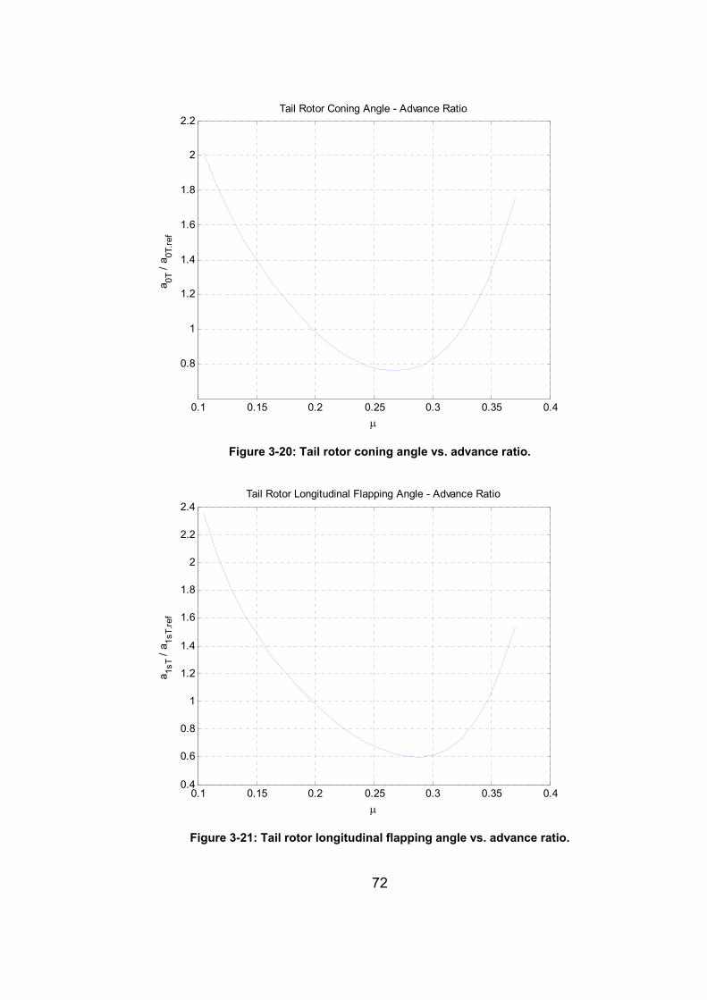
72

0.1 0.15 0.2 0.25 0.3 0.35 0.4

0.8

1

1.2

1.4

1.6

1.8

2

2.2

μ

a 0T /

a 0T.re

f

Tail Rotor Coning Angle - Advance Ratio

Figure 3-20: Tail rotor coning angle vs. advance ratio.

0.1 0.15 0.2 0.25 0.3 0.35 0.40.4

0.6

0.8

1

1.2

1.4

1.6

1.8

2

2.2

2.4

μ

a 1sT /

a 1sT.

ref

Tail Rotor Longitudinal Flapping Angle - Advance Ratio

Figure 3-21: Tail rotor longitudinal flapping angle vs. advance ratio.

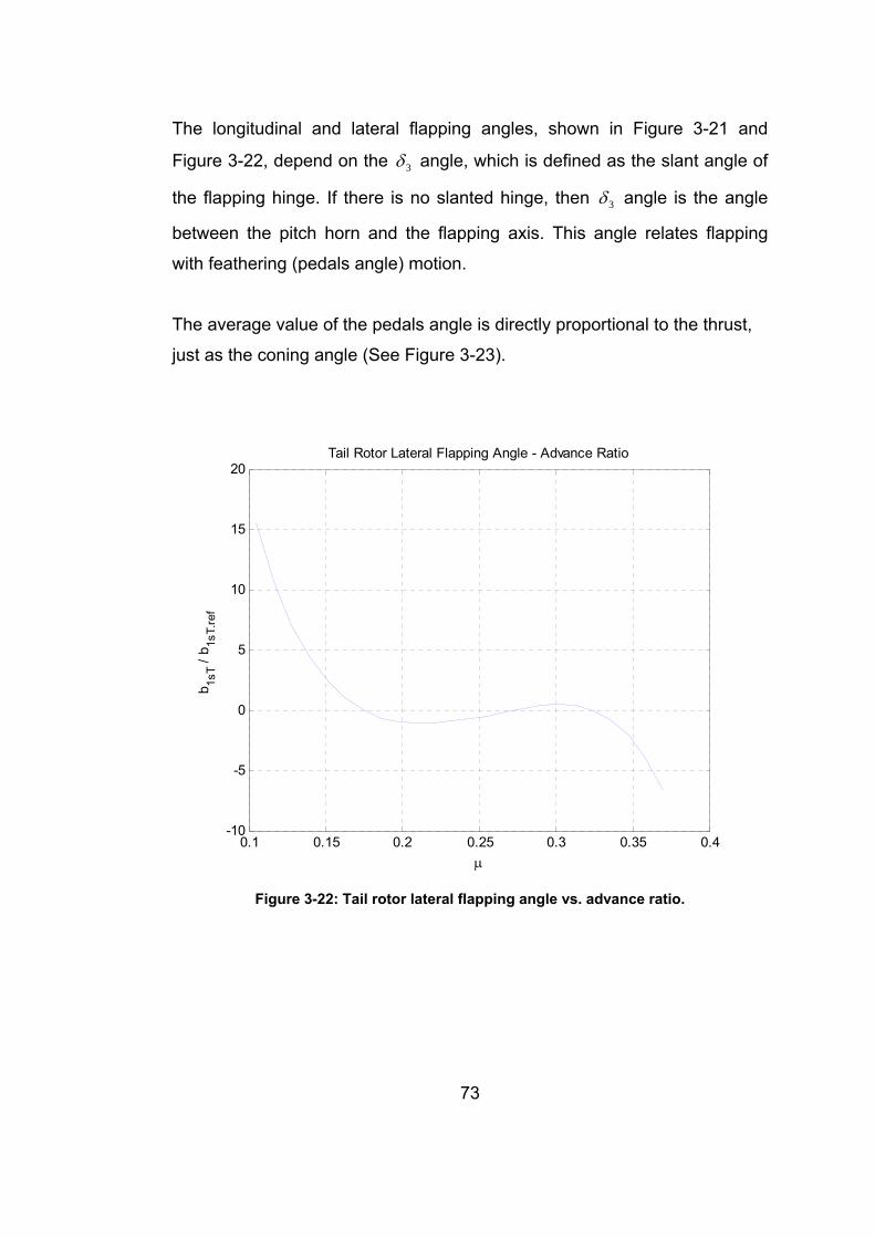
73

The longitudinal and lateral flapping angles, shown in Figure 3-21 and

Figure 3-22, depend on the 3δ angle, which is defined as the slant angle of

the flapping hinge. If there is no slanted hinge, then 3δ angle is the angle

between the pitch horn and the flapping axis. This angle relates flapping

with feathering (pedals angle) motion.

The average value of the pedals angle is directly proportional to the thrust,

just as the coning angle (See Figure 3-23).

0.1 0.15 0.2 0.25 0.3 0.35 0.4-10

-5

0

5

10

15

20

μ

b 1sT /

b 1sT.

ref

Tail Rotor Lateral Flapping Angle - Advance Ratio

Figure 3-22: Tail rotor lateral flapping angle vs. advance ratio.

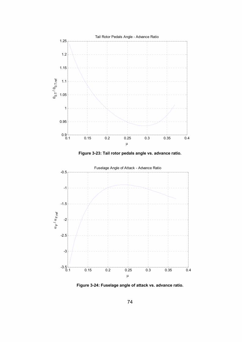
74

0.1 0.15 0.2 0.25 0.3 0.35 0.40.9

0.95

1

1.05

1.1

1.15

1.2

1.25

μ

θ 0.T

/ θ 0

.T.re

f

Tail Rotor Pedals Angle - Advance Ratio

Figure 3-23: Tail rotor pedals angle vs. advance ratio.

0.1 0.15 0.2 0.25 0.3 0.35 0.4-3.5

-3

-2.5

-2

-1.5

-1

-0.5

μ

αF /

αF.

ref

Fuselage Angle of Attack - Advance Ratio

Figure 3-24: Fuselage angle of attack vs. advance ratio.

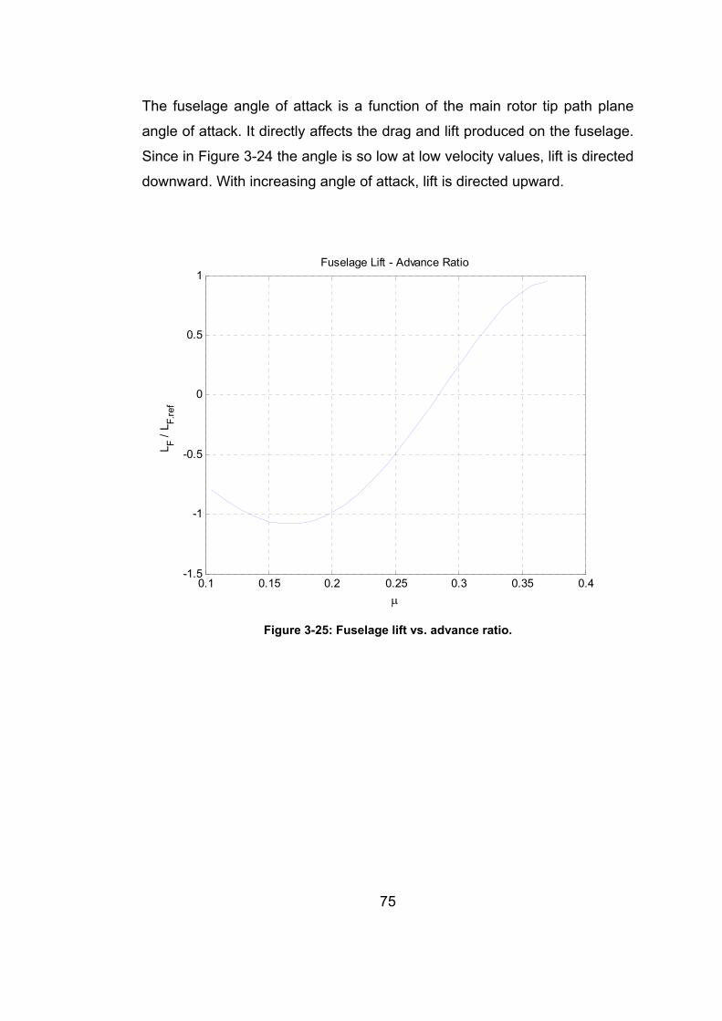
75

The fuselage angle of attack is a function of the main rotor tip path plane

angle of attack. It directly affects the drag and lift produced on the fuselage.

Since in Figure 3-24 the angle is so low at low velocity values, lift is directed

downward. With increasing angle of attack, lift is directed upward.

0.1 0.15 0.2 0.25 0.3 0.35 0.4-1.5

-1

-0.5

0

0.5

1

μ

L F / L F.

ref

Fuselage Lift - Advance Ratio

Figure 3-25: Fuselage lift vs. advance ratio.

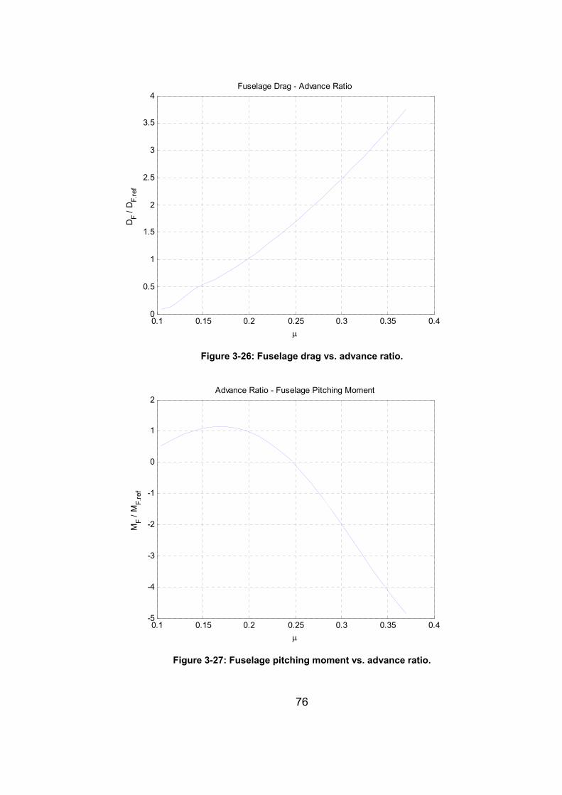
76

0.1 0.15 0.2 0.25 0.3 0.35 0.40

0.5

1

1.5

2

2.5

3

3.5

4

μ

DF /

DF.

ref

Fuselage Drag - Advance Ratio

Figure 3-26: Fuselage drag vs. advance ratio.

0.1 0.15 0.2 0.25 0.3 0.35 0.4-5

-4

-3

-2

-1

0

1

2

μ

MF /

MF.

ref

Advance Ratio - Fuselage Pitching Moment

Figure 3-27: Fuselage pitching moment vs. advance ratio.

77

Similar to the lift force, for low angles of attack at low velocities the pitcing

moment is positive, while the sign reverses at high velocities (Figure 3-25

and Figure 3-27).

Horizontal stabilator angle of attack depends on the fuselage angle of attack

and the forward speed. As the forward speed increases, the stabilator

automatically turns up, decreasing the incidence. Therefore, the angle of

attack also decreases. The effect of a decreased angle of attack shows

itself with a decrease in lift in Figure 3-28.

The sidewash angles induced by the rotors and the fuselage are calculated

and are used to compute the side force created by the vertical stabilizer

shown in Figure 3-31.

The drag of the fuselage for the empennage on case (Figure 3-34) are

similar to the empennage off case (Figure 3-26), since the effects of the

vertical stabilizer and the horizontal stabilator are negligible. However, the

fuselage lift (Figure 3-25) and the horizontal stabilizer lift (Figure 3-29)

values are comparative.

Compared with the flight test data and explained with theoretical logic, we

can say that the forward flight trim results are reasonable and acceptable for

the stability analysis.

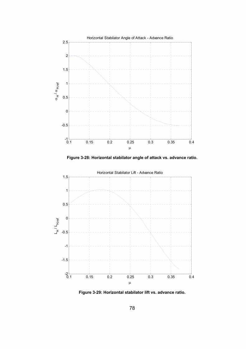
78

0.1 0.15 0.2 0.25 0.3 0.35 0.4-1

-0.5

0

0.5

1

1.5

2

2.5

μ

αH /

αH.

ref

Horizontal Stabilator Angle of Attack - Advance Ratio

Figure 3-28: Horizontal stabilator angle of attack vs. advance ratio.

0.1 0.15 0.2 0.25 0.3 0.35 0.4-2

-1.5

-1

-0.5

0

0.5

1

1.5

μ

L H / L H.

ref

Horizontal Stabilator Lift - Advance Ratio

Figure 3-29: Horizontal stabilator lift vs. advance ratio.

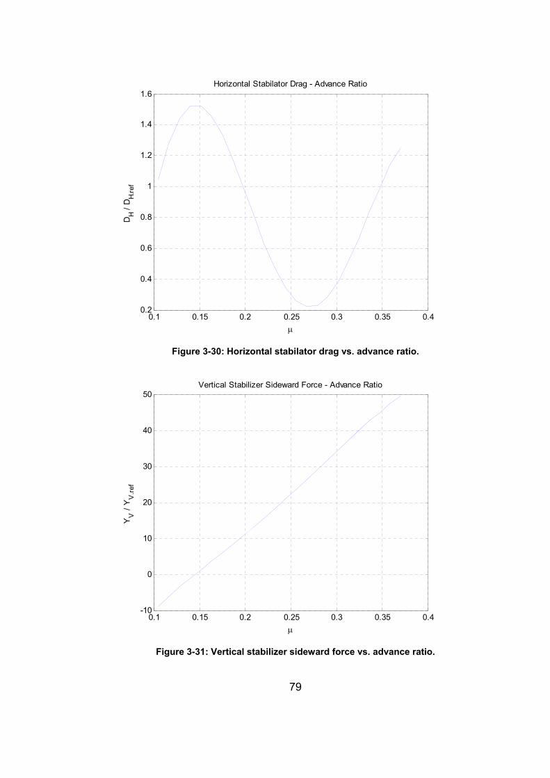
79

0.1 0.15 0.2 0.25 0.3 0.35 0.40.2

0.4

0.6

0.8

1

1.2

1.4

1.6

μ

DH /

DH.

ref

Horizontal Stabilator Drag - Advance Ratio

Figure 3-30: Horizontal stabilator drag vs. advance ratio.

0.1 0.15 0.2 0.25 0.3 0.35 0.4-10

0

10

20

30

40

50

μ

YV

/ Y

V.re

f

Vertical Stabilizer Sideward Force - Advance Ratio

Figure 3-31: Vertical stabilizer sideward force vs. advance ratio.

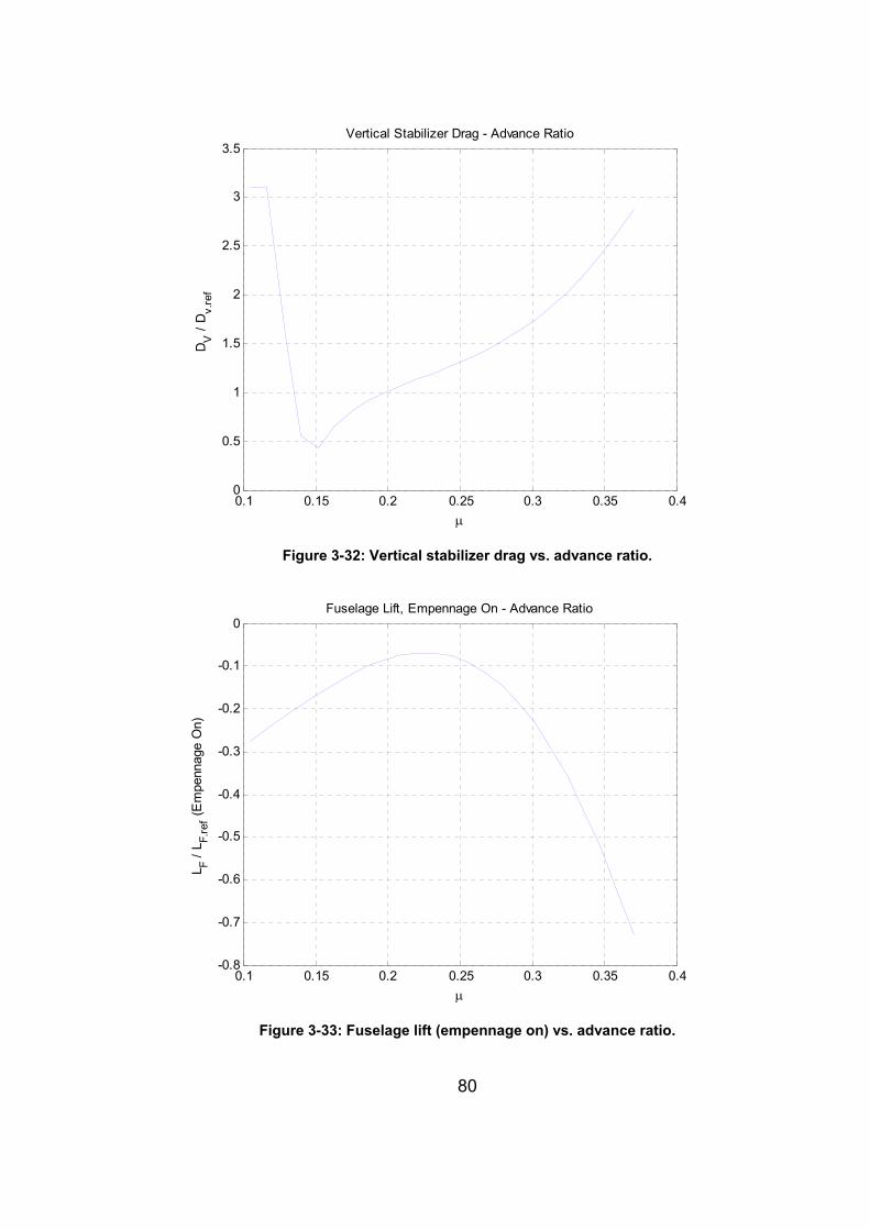
80

0.1 0.15 0.2 0.25 0.3 0.35 0.40

0.5

1

1.5

2

2.5

3

3.5

μ

DV

/ D

v.re

f

Vertical Stabilizer Drag - Advance Ratio

Figure 3-32: Vertical stabilizer drag vs. advance ratio.

0.1 0.15 0.2 0.25 0.3 0.35 0.4-0.8

-0.7

-0.6

-0.5

-0.4

-0.3

-0.2

-0.1

0

μ

L F / L F.

ref (E

mpe

nnag

e O

n)

Fuselage Lift, Empennage On - Advance Ratio

Figure 3-33: Fuselage lift (empennage on) vs. advance ratio.

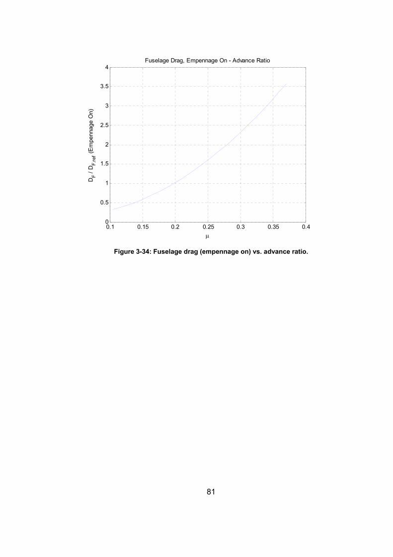
81

0.1 0.15 0.2 0.25 0.3 0.35 0.40

0.5

1

1.5

2

2.5

3

3.5

4

μ

DF /

DF.

ref (E

mpe

nnag

e O

n)

Fuselage Drag, Empennage On - Advance Ratio

Figure 3-34: Fuselage drag (empennage on) vs. advance ratio.

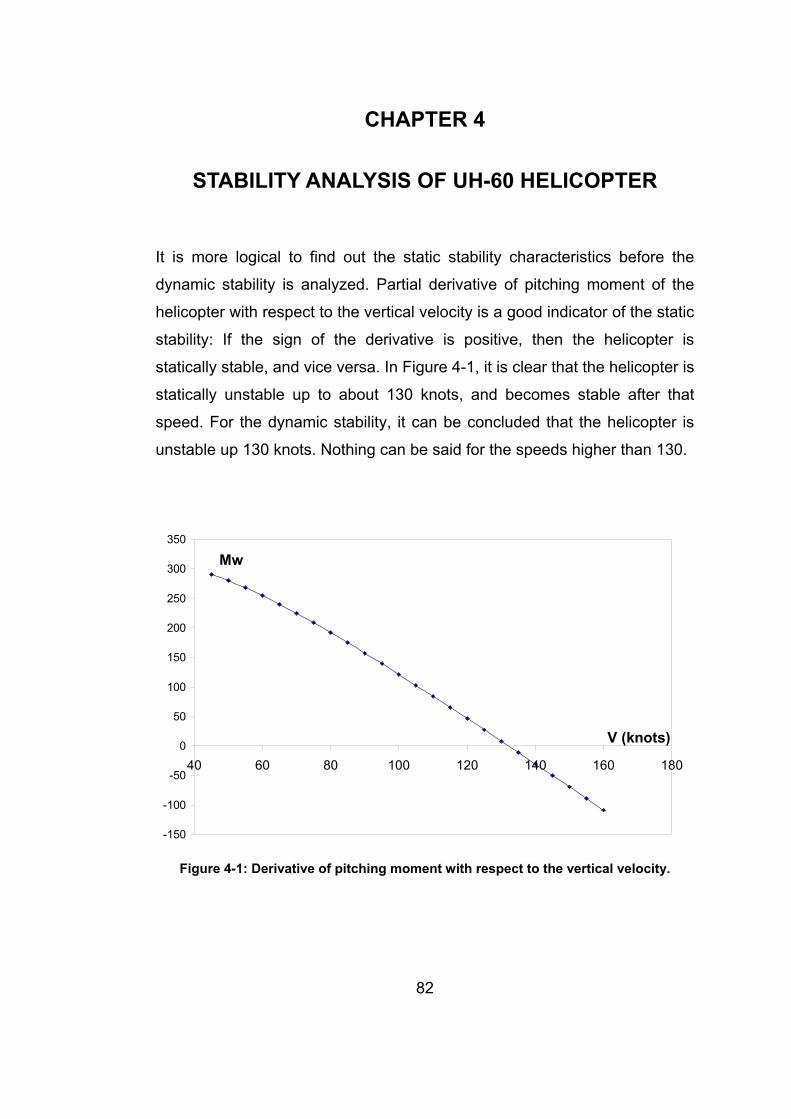
82

CHAPTER 4

STABILITY ANALYSIS OF UH-60 HELICOPTER It is more logical to find out the static stability characteristics before the

dynamic stability is analyzed. Partial derivative of pitching moment of the

helicopter with respect to the vertical velocity is a good indicator of the static

stability: If the sign of the derivative is positive, then the helicopter is

statically stable, and vice versa. In Figure 4-1, it is clear that the helicopter is

statically unstable up to about 130 knots, and becomes stable after that

speed. For the dynamic stability, it can be concluded that the helicopter is

unstable up 130 knots. Nothing can be said for the speeds higher than 130.

-150

-100

-50

0

50

100

150

200

250

300

350

40 60 80 100 120 140 160 180

V (knots)

Mw

Figure 4-1: Derivative of pitching moment with respect to the vertical velocity.

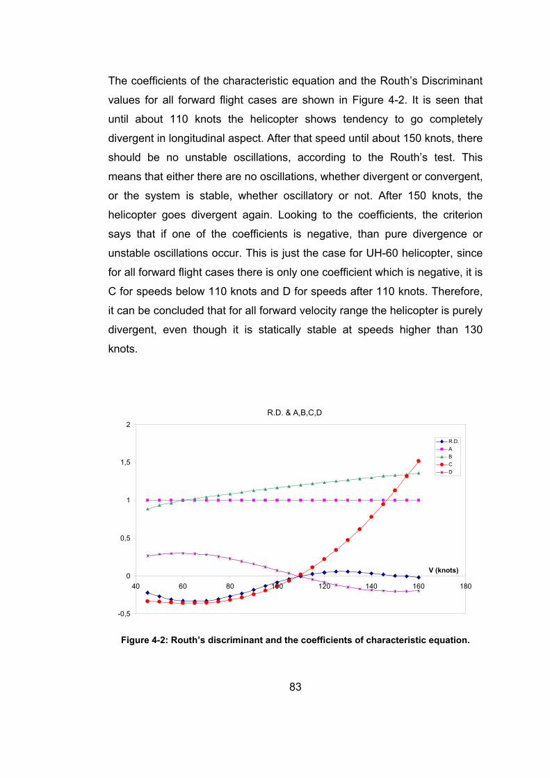
83

The coefficients of the characteristic equation and the Routh’s Discriminant

values for all forward flight cases are shown in Figure 4-2. It is seen that

until about 110 knots the helicopter shows tendency to go completely

divergent in longitudinal aspect. After that speed until about 150 knots, there

should be no unstable oscillations, according to the Routh’s test. This

means that either there are no oscillations, whether divergent or convergent,

or the system is stable, whether oscillatory or not. After 150 knots, the

helicopter goes divergent again. Looking to the coefficients, the criterion

says that if one of the coefficients is negative, than pure divergence or

unstable oscillations occur. This is just the case for UH-60 helicopter, since

for all forward flight cases there is only one coefficient which is negative, it is

C for speeds below 110 knots and D for speeds after 110 knots. Therefore,

it can be concluded that for all forward velocity range the helicopter is purely

divergent, even though it is statically stable at speeds higher than 130

knots.

R.D. & A,B,C,D

-0,5

0

0,5

1

1,5

2

40 60 80 100 120 140 160 180

V (knots)

R.D.ABCD

Figure 4-2: Routh’s discriminant and the coefficients of characteristic equation.

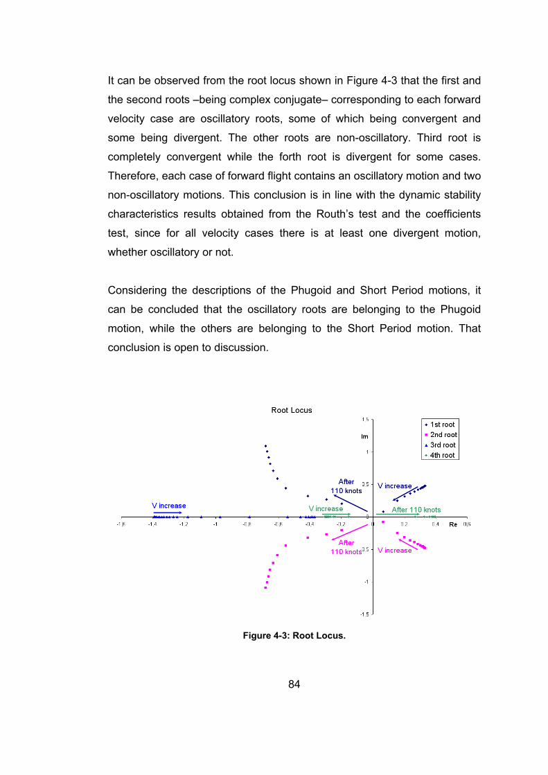
84

It can be observed from the root locus shown in Figure 4-3 that the first and

the second roots –being complex conjugate– corresponding to each forward

velocity case are oscillatory roots, some of which being convergent and

some being divergent. The other roots are non-oscillatory. Third root is

completely convergent while the forth root is divergent for some cases.

Therefore, each case of forward flight contains an oscillatory motion and two

non-oscillatory motions. This conclusion is in line with the dynamic stability

characteristics results obtained from the Routh’s test and the coefficients

test, since for all velocity cases there is at least one divergent motion,

whether oscillatory or not.

Considering the descriptions of the Phugoid and Short Period motions, it

can be concluded that the oscillatory roots are belonging to the Phugoid

motion, while the others are belonging to the Short Period motion. That

conclusion is open to discussion.

Figure 4-3: Root Locus.

85

Depending on the strength of the roots, the helicopter shows different

characteristics. To give an example; the roots corresponding to 45 knots are

-1.27, -0.24, 0.31±0.45i (See Figure 4-3). The smaller the non-oscillatory

root (i.e. the greater in absolute value), the faster the motion damps.

Therefore, the first root shows greater damping characteristics than the

second one. The phugoid roots are divergent and have an oscillation period

of about 13 seconds. The period seems reasonable, since generally the

phugoid mode has a period between 10 and 30 seconds.

Looking to Figure 4-3, it can be concluded that the change of the attitude

from divergent to convergent at about 110 knots is due to the phugoid roots,

i.e. the oscillatory roots. In order to analyze the short period roots, it could

be more reasonable to give attention to the sum of the two roots which

correspond to that mode. The sum of the roots shows a turn to divergent at

about 150 knots, which can be the explanation of why the Routh’s

Discriminant changed sign at that speed. This means that, for very high

speeds the short period motion is dominant on the stability characteristics of

the helicopter, while for lower speeds the Phugoid motion takes the place.

The Phugoid motion characteristics change with changing speed (See

Figure 4-4). The period values are very reasonable up to a point where the

period goes to very high values. After that speed the attitude changes from

divergent to convergent and the period tends to decrease. 110 knots is very

likely to be the maximum range speed. The relation which can be occurring

between the maximum range speed and the speed which changes the

dynamic stability attitude of the helicopter is a good point of discussion.

The divergency / convergency characteristics of phugoid motion are pretty

obvious in Figure 4-5. The time-to-double values change sign at the speed

the roots change sign. It is obvious that the motion changes attitude from

divergent to convergent at about 110 knots.

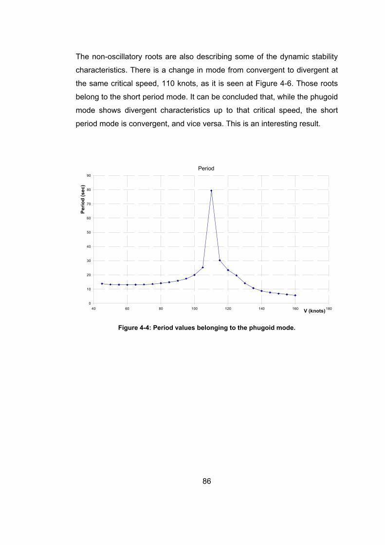
86

The non-oscillatory roots are also describing some of the dynamic stability

characteristics. There is a change in mode from convergent to divergent at

the same critical speed, 110 knots, as it is seen at Figure 4-6. Those roots

belong to the short period mode. It can be concluded that, while the phugoid

mode shows divergent characteristics up to that critical speed, the short

period mode is convergent, and vice versa. This is an interesting result.

Period

0

10

20

30

40

50

60

70

80

90

40 60 80 100 120 140 160 180V (knots)

Perio

d (s

ec)

Figure 4-4: Period values belonging to the phugoid mode.

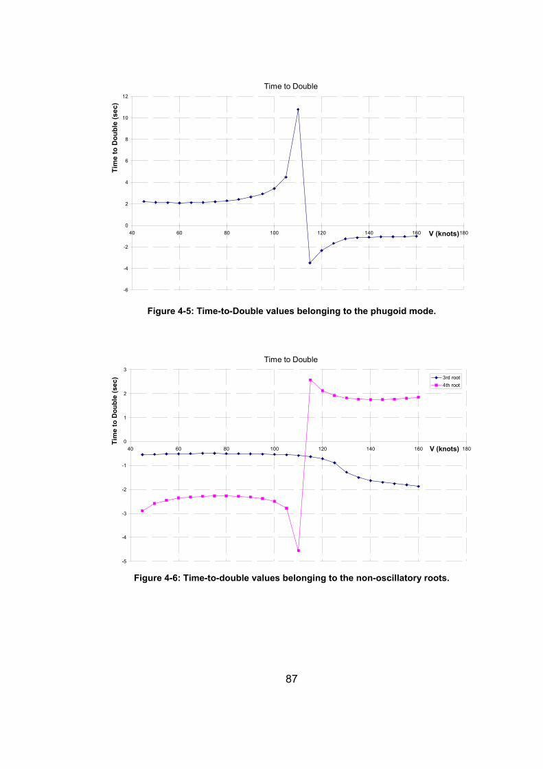
87

Time to Double

-6

-4

-2

0

2

4

6

8

10

12

40 60 80 100 120 140 160 180V (knots)

Tim

e to

Dou

ble

(sec

)

Figure 4-5: Time-to-Double values belonging to the phugoid mode.

Time to Double

-5

-4

-3

-2

-1

0

1

2

3

40 60 80 100 120 140 160 180V (knots)

Tim

e to

Dou

ble

(sec

) 3rd root4th root

Figure 4-6: Time-to-double values belonging to the non-oscillatory roots.

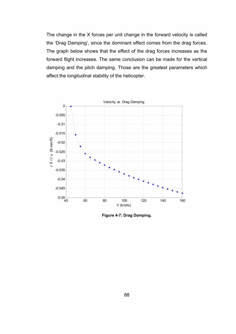
88

The change in the X forces per unit change in the forward velocity is called

the ‘Drag Damping’, since the dominant effect comes from the drag forces.

The graph below shows that the effect of the drag forces increases as the

forward flight increases. The same conclusion can be made for the vertical

damping and the pitch damping. Those are the greatest parameters which

affect the longitudinal stability of the helicopter.

40 60 80 100 120 140 160-0.05

-0.045

-0.04

-0.035

-0.03

-0.025

-0.02

-0.015

-0.01

-0.005

0

V (knots)

∂ X

/ ∂

u (l

b.se

c/ft)

Velocity vs. Drag Damping

Figure 4-7: Drag Damping.

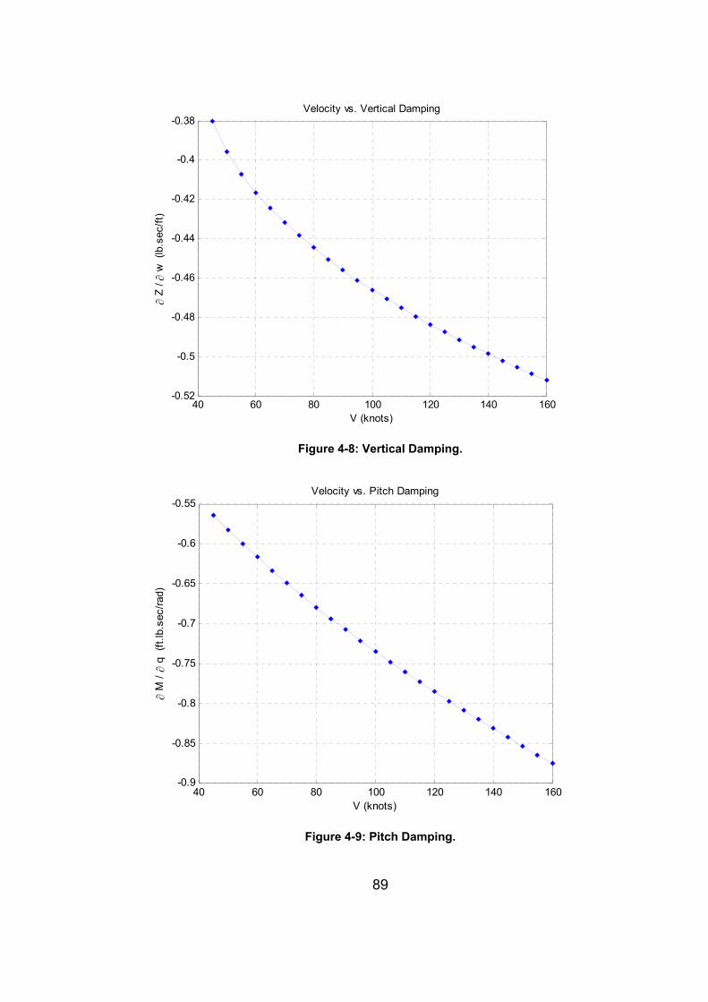
89

40 60 80 100 120 140 160-0.52

-0.5

-0.48

-0.46

-0.44

-0.42

-0.4

-0.38

V (knots)

∂ Z

/ ∂ w

(lb

.sec

/ft)

Velocity vs. Vertical Damping

Figure 4-8: Vertical Damping.

40 60 80 100 120 140 160-0.9

-0.85

-0.8

-0.75

-0.7

-0.65

-0.6

-0.55

V (knots)

∂ M

/ ∂

q (f

t.lb.

sec/

rad)

Velocity vs. Pitch Damping

Figure 4-9: Pitch Damping.

90

CHAPTER 5

CONCLUSIONS AND FUTURE WORK This thesis describes the development of a series of codes for trim and

longitudinal stability analysis of a helicopter in forward flight. The trim

analysis results are obtained for a clean UH-60 configuration and the results

are compared with flight test data. One of the trim codes is based on

momentum theory, while the other one is based on the blade element

theory. These codes include many simplifying assumptions such as

empirical uniform wake model. Nevertheless, application of these codes to

some example helicopters indicated reasonably good agreement with the

other available data, particularly for the main rotor performance. The results

indicated that, improvements are needed in calculation of the torque, and

thereby the parameters related to the tail rotor.

There are several possibilities to improve these codes, which include

modifications of the wake models; and extension of the codes to low speed

performance, trim and stability calculations. Other future work may include

preparation of a graphical user interface and a full Simulink® model.

91

REFERENCES

1. Seddon, J., Basic Helicopter Aerodynamics, AIAA Education Series, 1990.

2. Padfield, G. D., Helicopter Flight Dynamics: The Theory and Application of Flying Qualities and Simulation Modeling, 1995

3. Prouty, R.W., Helicopter Performance, Stability, and Control, Krieger Publishing Company, 1995.

4. Cooke, A.K., Fitzpatrick, E.W.H., Helicopter Test and Evaluation, AIAA Education Series, 2002.

5. Leishman, J.G., Principles of Helicopter Aerodynamics, Cambridge University Press, 2000.

6. U.S. Army Helicopter Design Datcom, Volume I – Airfoils, Boeing Doc. No. D210-11097-1, 1976.

7. Hoerner, Fluid Dynamic Drag, Published by Author, 1965.

8. MATLAB Getting Started Guide

9. MATLAB help files

10. MATHWORKS Company, www.mathworks.com, last visited on 21.06.2007

11. Method for Studying Helicopter Longitudinal Maneuver Stability, NACA TN 3022, 1953

12. Longitudinal Stability and Control of the Single-Rotor Helicopter, Aeronautical Research Council Reports And Memoranda, A.R.C. Technical Report, R.&M. No:3104, 1959

13. An Analysis of the Longitudinal Stability and Control of a Single-Rotor Helicopter, Aeronautical Research Council Reports And Memoranda, A.R.C. Technical Report, R.&M. No:2958, 1957

14. Stability And Control Of Helicopters, AE397 BTech Seminar Report, Department of Aerospace Engineering, Indian Institute of Technology, Bombay, Khadilkar Harshad Dilip, Dr. Ashok Joshi, 2008

92

15. Aerodynamic Characteristics of SC1095 and SC1094 R8 Airfoils, William G. BOUSMAN, Aeroflightdynamics Directorate U.S. Army Research, Development, and Engineering Command Ames Research Center, NASA/TP–2003-212265, AFDD/TR-04-003, December 2003

16. A Mathematical Model of the UH-60 Helicopter, NASA Technical Memorandum 85890, USAAVSCOM Technical Memorandum 84-A-2, Kathryn B. Hilbert, Aeromechanics Laboratory, U.S. Army Research and Technology Laboratories - AVSCOM Ames Research Center, Moffett Field, California

17. Power balance method in calculation of helicopter maneuverability taking into account specific operational conditions, Allerton Press, Inc. S. A. Mikhailov Contact Information and A. Yu. Onushkin

18. Analytical Calculation of Helicopter Main Rotor Blade Flight Loads in Hover and Forward Flight, Ki C. Kim, Survivability/Lethality Analysis Directorate, Army Research Laboratory, ARL-TR-3180, April 2004

19. Johnson W., Helicopter Theory, 1980

20. Bramwell A. R. S., Done G., Balmford D., Bramwell’s Helicopter Dynamics, Butterworth-Heinemann, ISBN 0 7506 5075 3, 2001

21. Wikipedia, http://en.wikipedia.org/wiki, last visited on 04.10.2008

22. Imperial College London, http://www3.imperial.ac.uk/aeronautics/wingcentre/aerodynamics, last visited on 04.09.2008

23. Aerospaceweb.org, http://www.aerospaceweb.org/aircraft/helicopter-m/uh60/ , last visited on 04.10.2008

24. Demand Media, Inc., http://www.airliners.net/aircraft-data, last visited on 27.09.2008

25. http://www.zap16.com/mil%20fact/Bo105.htm, last visited on 29.09.2008

26. FAS Military Analysis Network, http://www.fas.org/man/dod-101/sys/ac/row/bo105.htm, last visited on 29.09.2008

27. All The World’s Rotorcraft, http://www.aviastar.org/helicopters_eng/mbb-105.php, last visited on 29.09.2008

93

28. Tom Speer, http://www.tspeer.com/NACA23012/N23012wflap.htm, last visited on 29.09.2008

29. Public Domain Aeronautical Software (PDAS), http://www.pdas.com/naca456samples.htm, last visited on 29.09.2008

30. Defence Journal, http://www.defencejournal.com/jan99/s-70a.htm, last visited on 04.10.2008

31. All The World’s Rotorcraft, http://www.aviastar.org/helicopters_eng/sik_s-70.php, last visited on 04.10.2008

32. Forecast International, http://www.dfeeler.com/forecastinc/sampledocs/MilitaryAircraft/Sikorsky.doc, last visited on 04.10.2008

33. Wikimedia Foundation, Inc., http://en.wikipedia.org/wiki/Simpson's_rule, last visited on 15.04.2008

34. Metric, http://www.metric.ma.ic.ac.uk/integration/techniques/definite/numerical-methods/simpsons-rule/index.html, last visited on 15.04.2008

35. Wolfram Research, Inc., http://mathworld.wolfram.com/SimpsonsRule.html, last visited on 15.04.2008

36. California State University, Fullerton, http://math.fullerton.edu/mathews/n2003/SimpsonsRuleMod.html, last visited on 15.04.2008

37. University of Maryland, http://terpconnect.umd.edu/~leishman/Aero/tailrotors.html, last visited on 12.10.2008

38. Air Force Technology, http://www.airforce-technology.com/projects/black_hawk/, last visited on 12.10.2008

39. Lycos,http://www.angelfire.com/pa3/cadet985/aviation/blackhawk.html, last visited on 12.10.2008

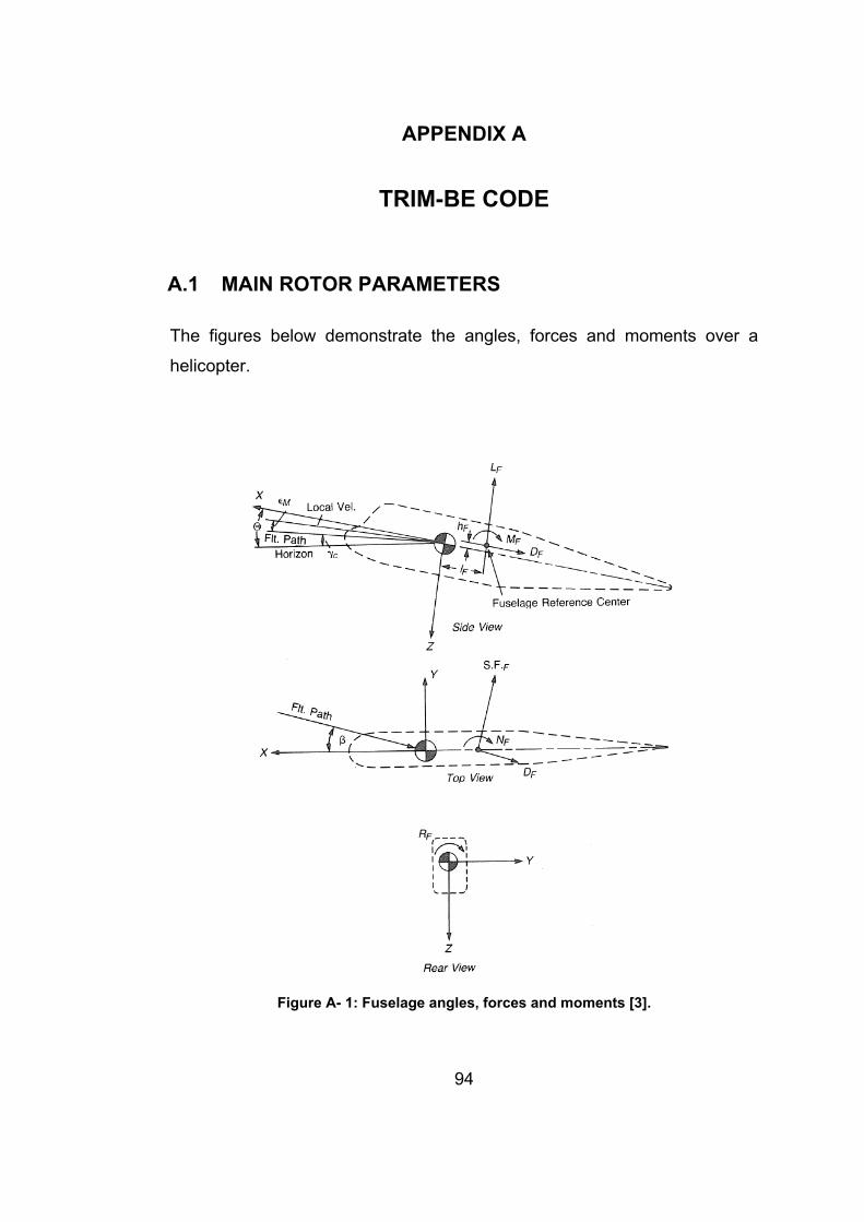
94

APPENDIX A

TRIM-BE CODE A.1 MAIN ROTOR PARAMETERS

The figures below demonstrate the angles, forces and moments over a

helicopter.

Figure A- 1: Fuselage angles, forces and moments [3].

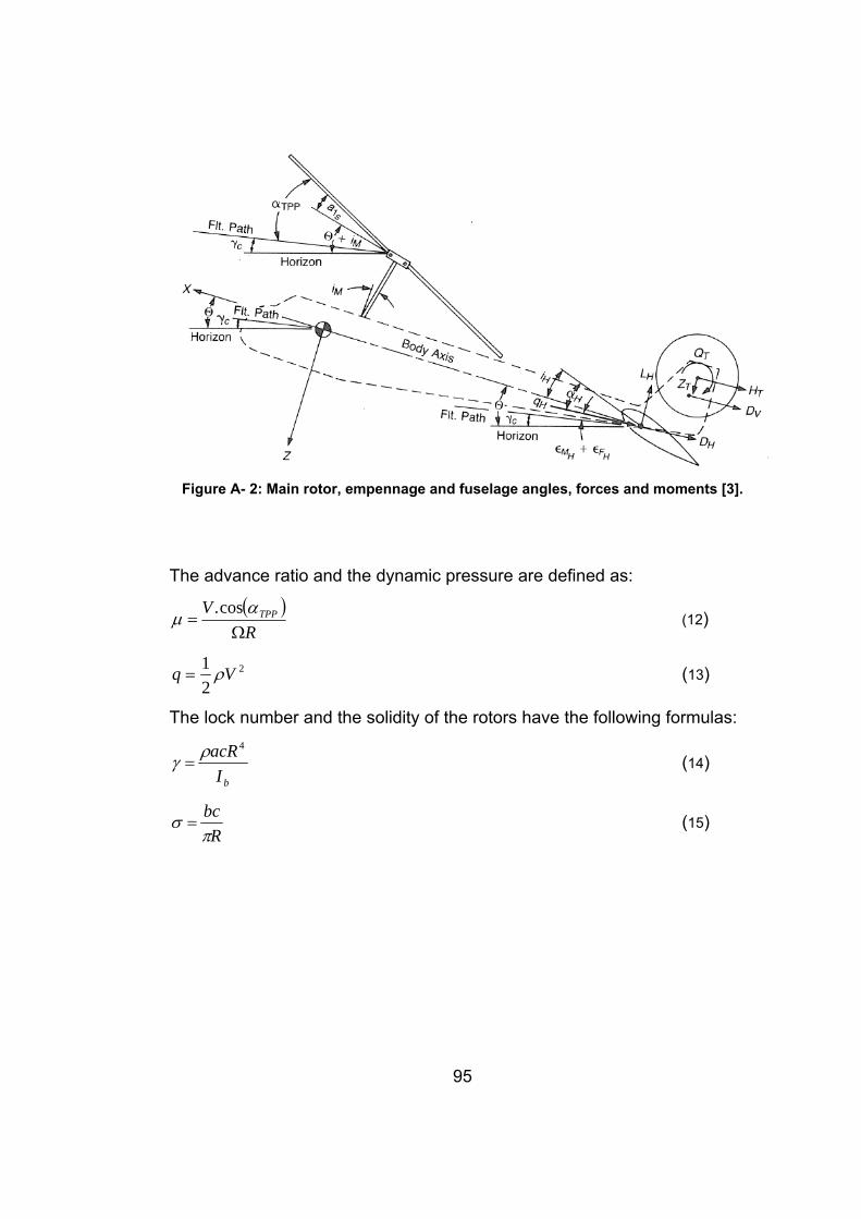
95

Figure A- 2: Main rotor, empennage and fuselage angles, forces and moments [3].

The advance ratio and the dynamic pressure are defined as:

( )R

V TPP

Ω=

αμ

cos. (12)

2

21 Vq ρ= (13)

The lock number and the solidity of the rotors have the following formulas:

bIacR4ργ = (14)

Rbcπ

σ = (15)

96

A.1.1 CALCULATIONS OF LOCAL FORCES

The following procedures explain the calculations of the local lift and drag

coefficients, used in the core of the code.

Total pitching angle of the main rotor blades:

ψψθθθ sincos 1110 BARr

−−+= (16)

Here 0θ is named collective angle, the coefficient of the third term 1A is first

harmonic lateral pitching coefficient (lateral cyclic angle), and the forth term

coefficient 1B is first harmonic longitudinal pitching coefficient (longitudinal

cyclic angle). The angle in the second term 1θ is the twist angle of the blade.

See Figure A- 3 for the angles.

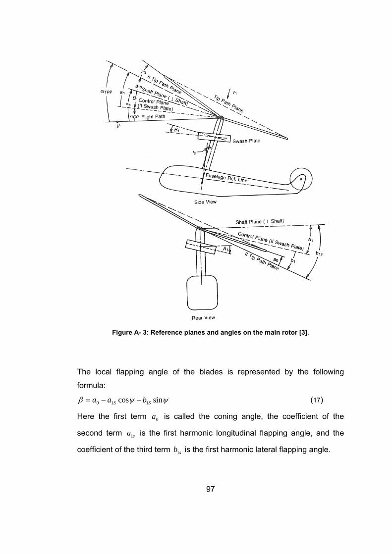
97

Figure A- 3: Reference planes and angles on the main rotor [3].

The local flapping angle of the blades is represented by the following

formula:

ψψβ sincos 110 SS baa −−= (17)

Here the first term 0a is called the coning angle, the coefficient of the

second term sa1 is the first harmonic longitudinal flapping angle, and the

coefficient of the third term sb1 is the first harmonic lateral flapping angle.

98

The difference between the first harmonic lateral pitching coefficient (lateral

cyclic angle) and the first harmonic lateral flapping angle ( )11 Ab s − gives the

total lateral flapping angle 1b with respect to the no-feathering plane (or

control plane which is parallel to the swash plate). Similarly, the difference

between the first harmonic longitudinal pitching coefficient (lateral cyclic

angle) and the first harmonic longitudinal flapping angle ( )saB 11 + gives the

total longitudinal flapping angle 1a with respect to the no-feathering plane.

See Figure A- 3.

As far as rotor aerodynamics is concerned, one degree of cyclic pitch

produces the same effect as one degree of flapping. Therefore, this

combination of cyclic pitch and flapping is referred to as flapping with

respect to the “Plane of No-Feathering” and is designated as 111 Baa S += .

The longitudinal cyclic angle is half the difference in pitch between the

advancing and retreating blades. It is positive when the pitching on the

retreating blade is greater than the pitch on the advancing blade.

A.1.1.1. Induced Velocity Calculation Using the Momentum Theory

Using the conservation of mass and energy rule on the actuator disc of a

hovering helicopter (See Figure A- 4), it can be obtained that:

υΔ= mT & , Am 1ρυ=& , 02 υυυ −=Δ (18)

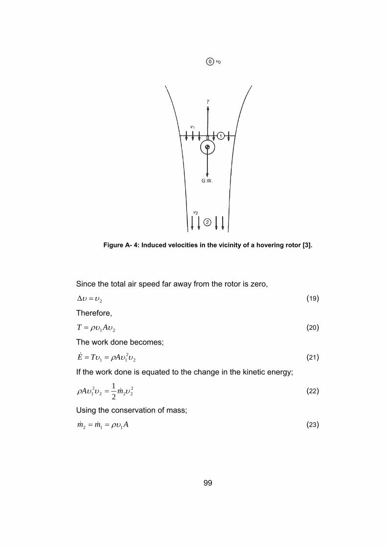
99

Figure A- 4: Induced velocities in the vicinity of a hovering rotor [3].

Since the total air speed far away from the rotor is zero,

2υυ =Δ (19)

Therefore,

21 υρυ AT = (20)

The work done becomes;

2211 υυρυ ATE ==& (21)

If the work done is equated to the change in the kinetic energy;

2222

21 2

1 υυυρ mA &= (22)

Using the conservation of mass;

Amm 112 ρυ== && (23)

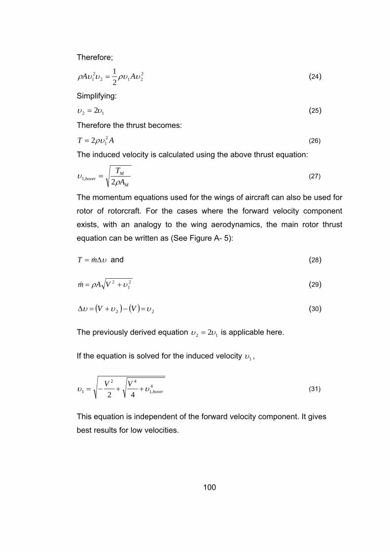
100

Therefore;

2212

21 2

1 υρυυυρ AA = (24)

Simplifying:

12 2υυ = (25)

Therefore the thrust becomes:

AT 212ρυ= (26)

The induced velocity is calculated using the above thrust equation:

M

Mhover A

Tρ

υ2,1 = (27)

The momentum equations used for the wings of aircraft can also be used for

rotor of rotorcraft. For the cases where the forward velocity component

exists, with an analogy to the wing aerodynamics, the main rotor thrust

equation can be written as (See Figure A- 5):

υΔ= mT & and (28)

21

2 υρ += VAm& (29)

( ) ( ) 22 υυυ =−+=Δ VV (30)

The previously derived equation 12 2υυ = is applicable here.

If the equation is solved for the induced velocity 1υ ,

4,1

42

1 42 hoverVV υυ ++−= (31)

This equation is independent of the forward velocity component. It gives

best results for low velocities.

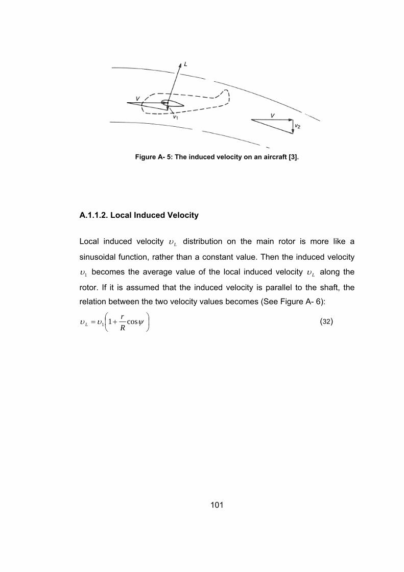
101

Figure A- 5: The induced velocity on an aircraft [3].

A.1.1.2. Local Induced Velocity

Local induced velocity Lυ distribution on the main rotor is more like a

sinusoidal function, rather than a constant value. Then the induced velocity

1υ becomes the average value of the local induced velocity Lυ along the

rotor. If it is assumed that the induced velocity is parallel to the shaft, the

relation between the two velocity values becomes (See Figure A- 6):

⎟⎠⎞

⎜⎝⎛ += ψυυ cos11 R

rL (32)

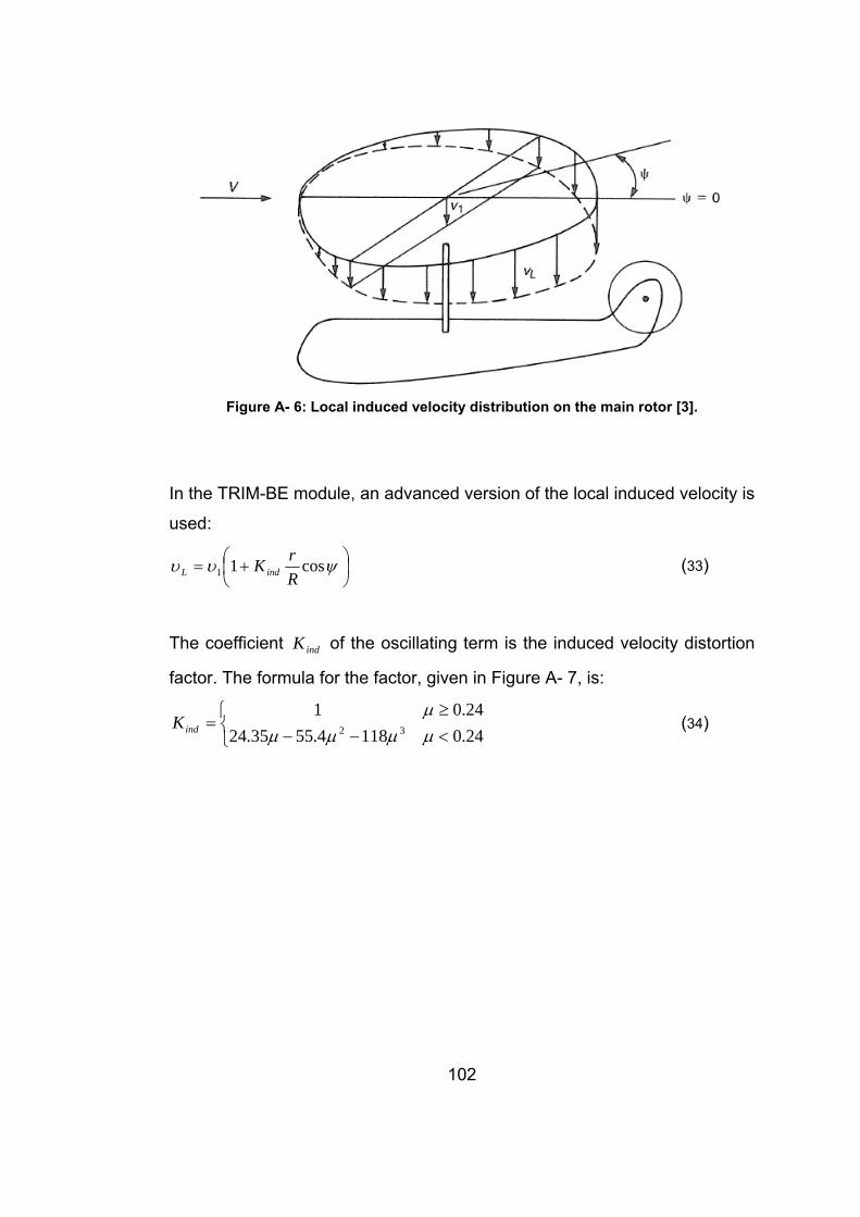
102

Figure A- 6: Local induced velocity distribution on the main rotor [3].

In the TRIM-BE module, an advanced version of the local induced velocity is

used:

⎟⎠⎞

⎜⎝⎛ += ψυυ cos11 R

rKindL (33)

The coefficient indK of the oscillating term is the induced velocity distortion

factor. The formula for the factor, given in Figure A- 7, is:

⎩⎨⎧

<−−≥

=24.01184.5535.2424.01

32 μμμμμ

indK (34)

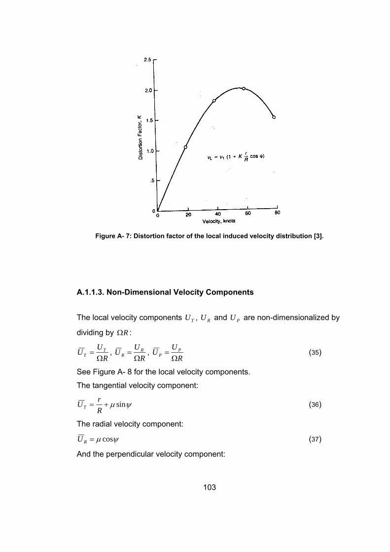
103

Figure A- 7: Distortion factor of the local induced velocity distribution [3].

A.1.1.3. Non-Dimensional Velocity Components

The local velocity components TU , RU and PU are non-dimensionalized by

dividing by RΩ :

RUU T

T Ω= ,

RUU R

R Ω= ,

RUU P

P Ω= (35)

See Figure A- 8 for the local velocity components.

The tangential velocity component:

ψμ sin+=RrUT (36)

The radial velocity component:

ψμ cos=RU (37)

And the perpendicular velocity component:

104

ψυ

ψμλ coscos 10 R

rKR

aU indP Ω−−′= (38)

The derivation of the last equation is given below:

The perpendicular velocity in dimensional form is:

ψββυα cosVrVU LSP −−−= & (39)

It is more convenient to use the TPP angle of attack instead of the shaft

angle of attack:

SSTPP a1−= αα (40)

If it is assumed that the forward velocity is much bigger than the induced

velocity, using equation 3:

21TCR

μυ Ω

= (41)

Using the general formula for the flapping angle and taking its derivative:

ψψβ sincos 110 SS baa −−= (42)

( )dtdba SSψψψβ cossin 11 −=& (43)

( )Ω−= ψψβ cossin 11 SS ba& (44)

If the 10th-12th equations are gathered:

⎟⎟⎟⎟⎟

⎠

⎞

⎜⎜⎜⎜⎜

⎝

⎛

+⎥⎦

⎤⎢⎣

⎡−⎟

⎠⎞

⎜⎝⎛

Ω−+

−−Ω

−=

Ω=

ψψμψμυ

ψμψυ

μα

cossincos

sinsin

101

1

211

1

SS

SSTPPP

P

baRr

Rb

aaRr

RR

UU (45)

If the first harmonic flapping angles sa1 and sb1 are taken as zero, and the

velocity component is non-dimesionalized, the 9th equation is obtained. It is

acceptable to assume the flapping angles as zero at that stage of the

module.

Some other velocity components can be introduced for the ease of the

calculations:

22RT UUU += (46)

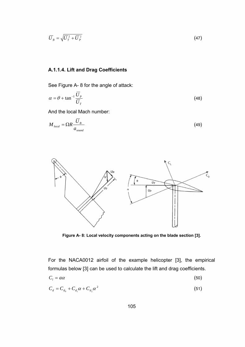
105

22PTB UUU += (47)

A.1.1.4. Lift and Drag Coefficients

See Figure A- 8 for the angle of attack:

T

P

UU1tan−+= θα (48)

And the local Mach number:

sound

Blocal a

URM Ω= (49)

Figure A- 8: Local velocity components acting on the blade section [3].

For the NACA0012 airfoil of the example helicopter [3], the empirical

formulas below [3] can be used to calculate the lift and drag coefficients.

αaCl = (50)

2210αα dddd CCCC ++= (51)

106

Those formulas are for low angles of attack. Some modifications should be

used in order to cover higher angles of attack. The modifications are

explained below.

The Mach number at which the drag coefficient reaches twice the value of

the incompressible drag coefficient is called the drag divergence Mach

number, ddM . Depending on ddM , the angle of attack and force coefficients

of the blades (having a profile NACA0012) are expressed by the following

formulas:

⎪⎩

⎪⎨⎧

>−

<−−=

dd

dd

MMM

MMMMa

,744.0677.0

,01.01

1.02 (52)

The angle of attack at which the lift coefficient first shows the effect of stall is

defined as Lα .

⎩⎨⎧

><−

=dd

ddL MM

MMM,4.3

,1615α (53)

The lift coefficient:

( )⎩⎨⎧

>−−<+

=dddd

dd

MMMMMMM

K,144.00575.0

,342.00233.044.0

15.7

1 (54)

MK 95.005.22 −= (55)

( )⎩⎨⎧

>−−<

=L

KL

Ll Ka

aC

αααααααα

21

(56)

( ) 6642min,0,, 10.0046.0226.08.65 −+−+= αααdincompd CC (57)

The angle at which the individual drag curves break away from the

incompressible curve of drag coefficient is defined as Dα .

107

⎩⎨⎧

><−

=dd

ddD MM

MMM,0

,4.2317α (58)

⎩⎨⎧

><

=dd

dd

MMMM

K,00035.0,00066.0

3 (59)

54.24 =K (60)

215 =K (61)

2.36 =K (62)

( )( ) ( )⎪

⎩

⎪⎨

⎧

>−+−+><−+<<

=

ddK

ddK

Dincompd

DddK

Dincompd

Dddincompd

d

MMMMKKCMMKCMMC

C64

4

53,

3,

,

,,

αααααααα

(63)

The lift and drag coefficients expressed above are only applicable to hover.

The corrections below are applied to cover forward flight:

( )

( )

( )⎪⎪⎪⎪

⎩

⎪⎪⎪⎪

⎨

⎧

°<<°°<<°

<<°°<<°°−°<<°−°<<°

°<

=

3603403402012sin15.12011997.01991731801.01731617.0

161202sin15.120,

ααααααααα

α

l

l

l

C

C

C (64)

( )⎪⎩

⎪⎨

⎧

°<<°°<<°−

°<=

360340340202cos02.103.1

20

ααα

α

d

d

d

C

CC (65)

The drag coefficient above is the steady flow drag coefficient, steadyLC , . The

unsteady flow effect will be discussed in the following pages.

108

When airfoils rapidly change the angle of attack, a non-linear unsteady

phenomenon, called Dynamic Stall, occurs. The rapid change can cause a

strong vortex to be shed from the leading edge of the aerofoil, and travel

backwards above the wing / blade. The vortex, containing high velocity

airflows, briefly increases the lift produced by the wing. As soon as it passes

behind the trailing edge, however, the lift reduces dramatically, and the wing

is in normal stall. Dynamic stall is an effect most associated with helicopters

and flapping wings. During forward flight, some regions of a helicopter blade

may incur flow that reverses (compared to the direction of blade movement),

and thus includes rapidly changing angles of attack.

Dynamic stall is a process resulting from a series of events, which involve a

hysteresis loop in the aerofoil-lift curve and account for a higher maximum

lift force than that achieved in the static curve, during a cycle of pitching

motion. Helicopter, turbine and windmill blades may all be affected by this

phenomenon, which increases forces and moments applied to the blade

and its root, and reduces fatigue life.

The increase in angle of attack of the blade due to dynamic stall can be

expressed with the following equation:

360

141

ψα

πγα

ΔΔ

=ΔB

dsstall URc

(66)

Here dsγ is a function depending on Mach number:

⎟⎠⎞

⎜⎝⎛=

Mds6.0ln.76.1γ (67)

ψΔ is the angle difference between the previous azimuthal station and the

present station. αΔ is the angle of attack difference between those two

azimuthal stations. It is subtracted from Lα :

stalleffLL ααα Δ−= , (68)

109

The lift of an airfoil is affected by the rate of change of angle of attack and

by the rate of plunge, both of which produce shed vorticity lying behind the

trailing edge, which induces velocities at the front of the airfoil coming after.

This phenomenon is called classical unsteady potential flow. The effect of

classical unsteady potential flow is taken into account by the formulas

below.

For an airfoil that is pitching about its quarter chord – a good assumption for

most rotors – the equation for lift coefficient may be written as:

⎪⎭

⎪⎬⎫

⎪⎩

⎪⎨⎧

Ω⎟⎠⎞

⎜⎝⎛+

Ω+⎥

⎦

⎤⎢⎣

⎡Ω

+Ω

+⎥⎦

⎤⎢⎣

⎡Ω

+Δ+= 2

2

2 22θαθαθαα&&&&&&& kkkGkFaC meanl (69)

This theory assumes that the blade flaps about a mean angle of attack with

a frequency. The reduced frequency k is the angular displacement during

the time the air moves half a cord:

URck

21

= (70)

The mean angle of attack:

⎟⎟⎠

⎞⎜⎜⎝

⎛−′

+⎟⎟⎠

⎞⎜⎜⎝

⎛+′

+⎟⎟⎠

⎞⎜⎜⎝

⎛ ′++= −−−

μλ

μλλθθα

RrRrRrRr

mean111

10 tan41tan

41tan

21 (71)

Therefore, the additional lift coefficient due to unsteady potential flow can be

expressed as:

( )( )⎪⎭

⎪⎬⎫

⎪⎩

⎪⎨⎧

Ω⎟⎠⎞

⎜⎝⎛+

Ω+⎥

⎦

⎤⎢⎣

⎡Ω

+Ω

+Ω

+−−=Δ 2

2

2, 221 θαθαθαα

&&&&&&& kkkGFkFaC meanunsteadyl (72)

110

The functions G and F and the pitching derivatives are calculated with the

following formulas:

( )⎪⎩

⎪⎨

⎧

>+=

<−−=

151,0024.0864.0

151,11500178.09.02

kkF

kkF (73)

kG 0025.02.0 +−= (74)

ψψθ cossin 11 BA −=Ω

& (75)

ψψθ sincos 112 BA +=Ω

&& (76)

The final lift coefficient is obtained by adding the unsteady effect to the

steady value:

unsteadylsteadyll CCC ,, Δ+= (77)

For high forward velocities ( 25.0≥μ ), there occurs a reverse flow region at

the retreating side of the rotor (see Figure A- 9). Within the reverse flow

region, the tangential velocity component changes sign and the lift changes

direction. The region can be modeled as:

0≤TU (78)

0sin ≤+ ψμRr (79)

ψμ sin−≤Rr (80)

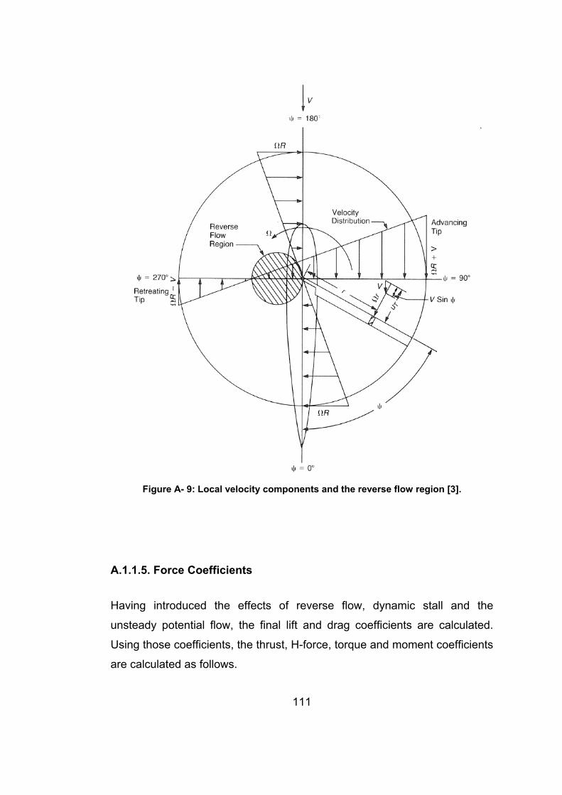
111

Figure A- 9: Local velocity components and the reverse flow region [3].

A.1.1.5. Force Coefficients

Having introduced the effects of reverse flow, dynamic stall and the

unsteady potential flow, the final lift and drag coefficients are calculated.

Using those coefficients, the thrust, H-force, torque and moment coefficients

are calculated as follows.

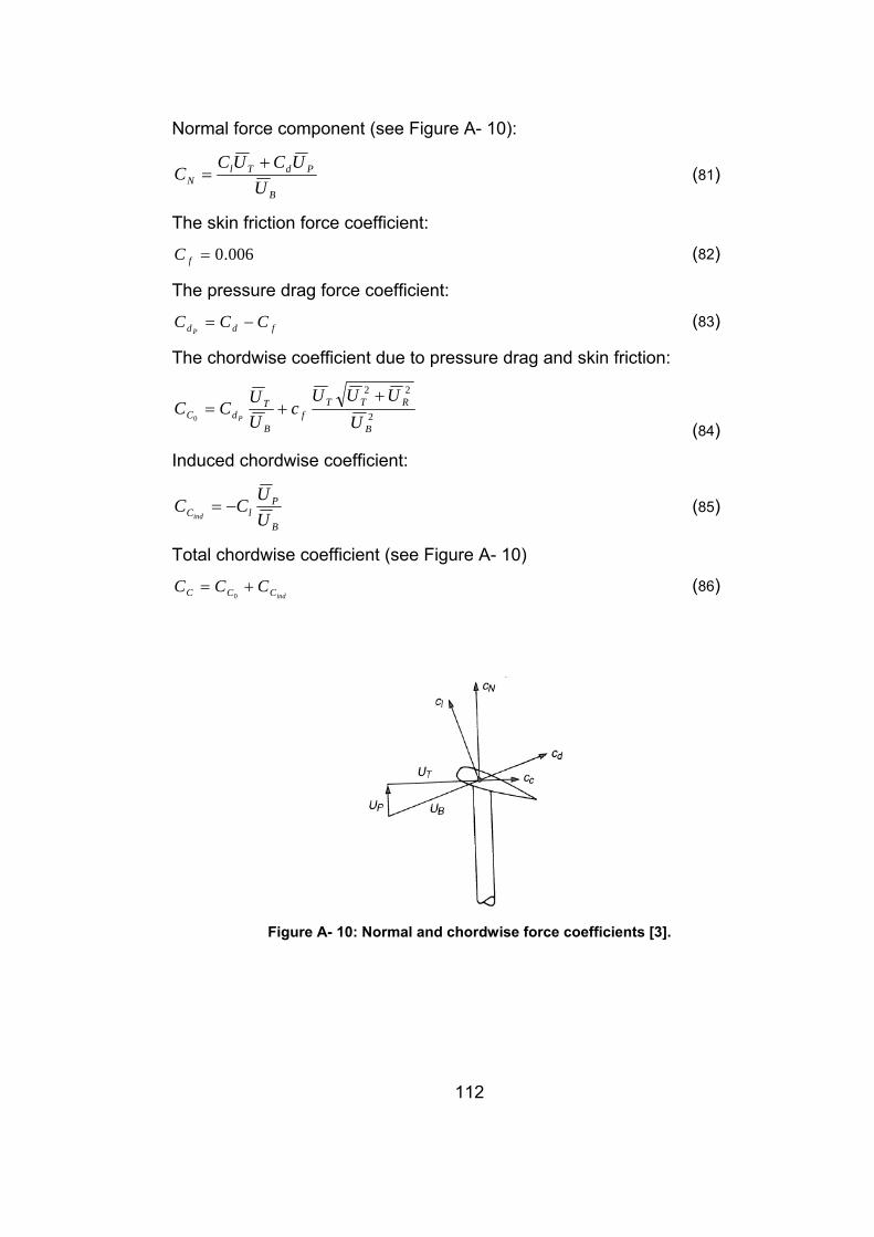
112

Normal force component (see Figure A- 10):

B

PdTlN U

UCUCC

+= (81)

The skin friction force coefficient:

006.0=fC (82)

The pressure drag force coefficient:

fdd CCCP

−= (83)

The chordwise coefficient due to pressure drag and skin friction:

2

22

0B

RTTf

B

TdC U

UUUc

UU

CCP

++=

(84)

Induced chordwise coefficient:

B

PlC UUCC

ind−= (85)

Total chordwise coefficient (see Figure A- 10)

indCCC CCC +=0

(86)

Figure A- 10: Normal and chordwise force coefficients [3].

113

A.1.2 INTEGRATION

The following procedures explain the integrations.

The thrust coefficient:

( ) NB

T

CU

Rr

C

2

2

=⎟⎟⎟⎟

⎠

⎞

⎜⎜⎜⎜

⎝

⎛

∂

⎟⎠⎞⎜

⎝⎛∂

∂∂ σψ

(87)

The torque coefficient due to profile drag:

( ) 02

2

CB

profile

Q

CRrU

Rr

C

=⎟⎟⎟⎟

⎠

⎞

⎜⎜⎜⎜

⎝

⎛

∂

⎟⎠⎞

⎜⎝⎛∂

∂∂ σ

ψ (88)

The torque coefficient due to induced drag:

( ) indCB

induced

Q

CRrU

Rr

C

2

2

=⎟⎟⎟⎟

⎠

⎞

⎜⎜⎜⎜

⎝

⎛

∂

⎟⎠⎞

⎜⎝⎛∂

∂∂ σ

ψ (89)

H-force coefficient due to drag:

( ) ψσ

ψsin

2 0

2

_

CB

oncontributiDrag

H

CU

Rr

C

=⎟⎟⎟⎟

⎠

⎞

⎜⎜⎜⎜

⎝

⎛

∂

⎟⎠⎞⎜

⎝⎛∂

∂∂

(90)

H-force coefficient due to lift:

( ) ψσ

ψsin

2

2

_

indCB

oncontributiLift

H

CU

Rr

C

=⎟⎟⎟⎟

⎠

⎞

⎜⎜⎜⎜

⎝

⎛

∂

⎟⎠⎞⎜

⎝⎛∂

∂∂

(91)

Roll moment coefficient:

( ) ( ) ψσ

ψσ

ψsin

Rr

Rr

C

Rr

C TR

⎟⎟⎟⎟

⎠

⎞

⎜⎜⎜⎜

⎝

⎛

∂

⎟⎠⎞⎜

⎝⎛∂

∂∂

−=⎟⎟⎟⎟

⎠

⎞

⎜⎜⎜⎜

⎝

⎛

∂

⎟⎠⎞⎜

⎝⎛∂

∂∂

(92)

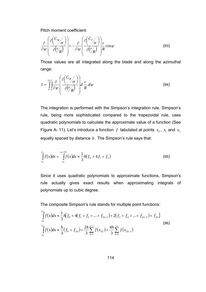
114

Pitch moment coefficient:

( ) ( ) ψσ

ψσ

ψcos

Rr

Rr

C

Rr

C TM

⎟⎟⎟⎟

⎠

⎞

⎜⎜⎜⎜

⎝

⎛

∂

⎟⎠⎞⎜

⎝⎛∂

∂∂

−=⎟⎟⎟⎟

⎠

⎞

⎜⎜⎜⎜

⎝

⎛

∂

⎟⎠⎞⎜

⎝⎛∂

∂∂

(93)

Those values are all integrated along the blade and along the azimuthal

range:

( )∫ ∫⎟⎟⎟⎟

⎠

⎞

⎜⎜⎜⎜

⎝

⎛

∂

⎟⎠⎞⎜

⎝⎛∂

∂∂

=π

ψσ

ψ

2

0

1

0

.. dRrd

Rr

C

IM

(94)

The integration is performed with the Simpson’s integration rule. Simpson’s

rule, being more sophisticated compared to the trapezoidal rule, uses

quadratic polynomials to calculate the approximate value of a function (See

Figure A- 11). Let’s introduce a function f tabulated at points 0x , 1x and 2x

equally spaced by distance h . The Simpson’s rule says that:

( ) ( ) ( )210

2

4310

0

2

0

fffhdxxfdxxfhx

x

x

x

++≈= ∫∫+

(95)

Since it uses quadratic polynomials to approximate functions, Simpson's

rule actually gives exact results when approximating integrals of

polynomials up to cubic degree.

The composite Simpson’s rule stands for multiple point functions:

( ) ( ) ( )[ ]

( ) ( ) ( ) ( )∑∑∫

∫

=−

−

=

−−

+++≈

+++++++++≈

n

kk

n

kkn

x

x

nnn

x

x

xfhxfhffhdxxf

ffffffffhdxxf

n

n

112

1

1220

2224212310

34

32

3

...2...431

2

0

2

0 (96)

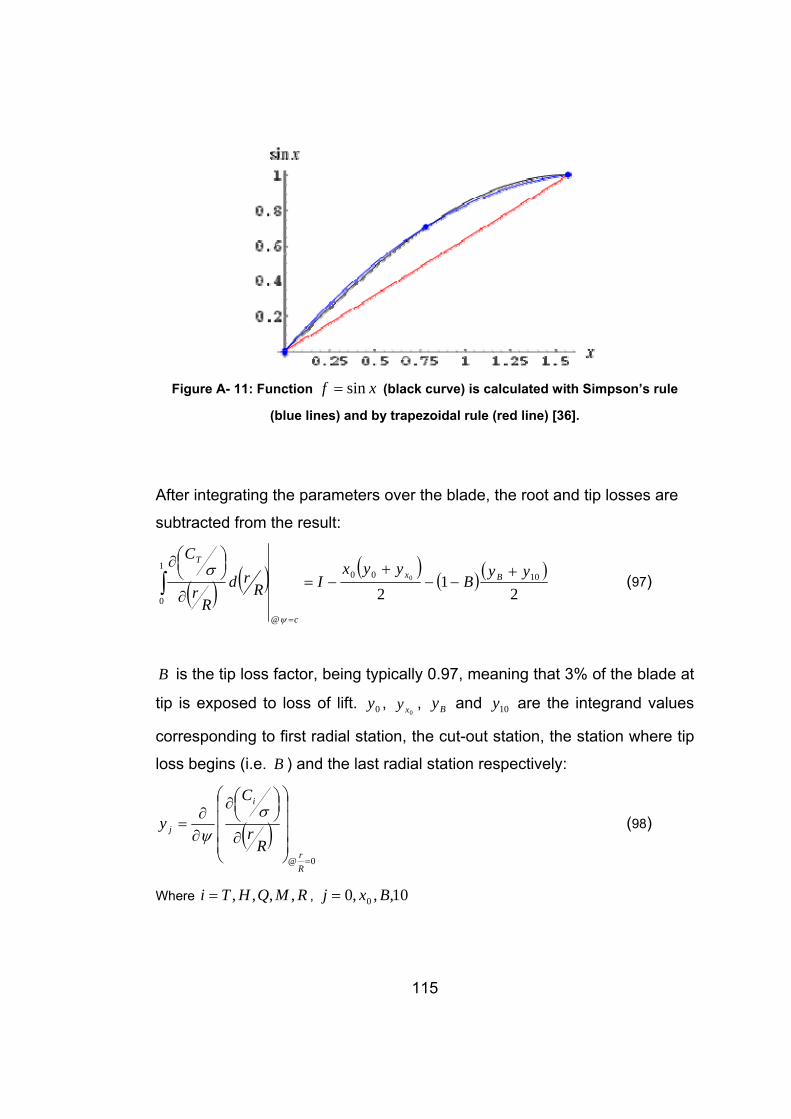
115

Figure A- 11: Function xf sin= (black curve) is calculated with Simpson’s rule

(blue lines) and by trapezoidal rule (red line) [36].

After integrating the parameters over the blade, the root and tip losses are

subtracted from the result:

( ) ( ) ( )( ) ( )

21

21000

@

1

0

0 yyB

yyxIR

rdR

r

CBx

c

T+

−−+

−=∂

⎟⎠⎞⎜

⎝⎛∂

=

∫ψ

σ (97)

B is the tip loss factor, being typically 0.97, meaning that 3% of the blade at

tip is exposed to loss of lift. 0y , 0xy , By and 10y are the integrand values

corresponding to first radial station, the cut-out station, the station where tip

loss begins (i.e. B ) and the last radial station respectively:

( )0@ =

⎟⎟⎟⎟

⎠

⎞

⎜⎜⎜⎜

⎝

⎛

∂

⎟⎠⎞⎜

⎝⎛∂

∂∂

=

Rr

i

j

Rr

C

yσ

ψ (98)

Where RMQHTi ,,,,= , 10,,,0 0 Bxj =

116

The inflow ratio is defined as:

RR TPPTPP Ω−≅

Ω−=′ 11sin υ

μαυ

αμλ (99)

The TPP angle of attack can be obtained from the inflow ratio as:

μ

υλ

μ

υλ

α RRTPP

Ω+′

≅⎟⎟⎟⎟

⎠

⎞

⎜⎜⎜⎜

⎝

⎛Ω

+′= −

11

1sin (100)

Or an alternative equation can be used:

MsTPP ia ++Θ= 1α (101)

A.1.3 WHOLE ROTOR PARAMETERS

Whole rotor parameters obtained after the integration process are defined in

this section.

A.1.3.1. Coning Angle

The coning angle 0a is derived from equating the total moments at the

flapping hinge to zero:

0.. =++= wfclifthinge MMMM (102)

Here the moment due to lift:

( ) 422

0

2

0

132

2acR

aCdrrRacrdr

drdLM T

tt

RR

lift ρσ

φθρΩ=−Ω== ∫∫ (103)

The moment due to centrifugal forces:

( ) b

R

fc IardramrM 20

00

2.. Ω=Ω−= ∫ (104)

117

And the moment due to the weight only:

b

R

w IRggmrdrM

23

0

−=−= ∫ (105)

Where bI is the flapping inertia of the blade.

∫=R

b drmrI0

2 (106)

The blade is assumed to have a homogeneous mass distribution.

The coning angle is found from the total moments equation:

( )2023

32

R

gR

a

Ca

T

Ω−= σγ (107)

That equation is written for a hovering rotor with ideal twist, but it gives very

good results for forward flight and for teetering and rigid rotors.

The Lock Number γ is the ratio of the aerodynamic forces to the inertial

forces and is defined as:

bIacR4ργ = (108)

A.1.3.2. Forces, Moments and Power

The thrust, H-force and torque are calculated as:

( )2RACT bT

M Ω= ρσ

(109)

( )2RACH bH

M Ω= ρσ

(110)

( ) RRAC

Q bQ

M2Ω= ρ

σ (111)

The total forces on the main rotor longitudinal axis can be expressed as:

118

∑ −−= MTPPM HTX αtan (112)

The induced and profile required power of the main rotor can be calculated

as:

( )550

3RACHP bQ

MΩ

=ρ

σ (113)

The total power is calculated using transmission, generator and hydraulic

system losses. The transmission losses are calculated using the equation

below:

( )TXTHPMXMHPconstXTrans HPCHPCHPHP ,,,,, ++= ρ (114)

Here constXHP , stands for the constant transmission losses, XMHPC ,, and

XTHPC ,, are main rotor and tail rotor transmission system power losses

respectively. The total power:

HydGenTransTM HPHPHPHPHPHP ++++= (115)

Where GenHP and HydHP are generator and hydraulic system power losses.

A.1.3.3. First Harmonic Flapping Angles

Pitch and roll moments are used in order to find the 1st harmonic flapping

angles:

( )γ

ρ Mb

S

M aReAdadM 2

,1 43 Ω

= (116)

MMS

M

FTTHHTTTMMMMS

hTdadM

MlLlLhHQhHlTa+

+++−+−=

,1

,1 (117)

MMS

M

TTS

hTdadM

hTb+

−=

,1

,1 (118)

119

The effects of the components of the helicopter on lift and drag are mainly

due to the induced velocities. The main rotor induces velocity on fuselage

and on empennage, the tail rotor and the fuselage induce velocity on the

empennage, a wing -if exists- induces velocity on the empennage. The

parameters below are angle of attack components due to the induced

velocities. The first subscript indicates the component which induces, and

the second indicates the one which is exposed to the induced velocity.

M

MFWDM qA

TVF 41

1.. υ

υυαε ==Δ= (119)

M

MFHHHHM qA

TqLD

VVH 44..

111

1

1 υυ

υυ

υυυ

υυυ

ε ==== (120)

The sidewash term, VMη , is a component to be added to the sideslip angle.

A.2 FUSELAGE PARAMETERS

The angle of attack of the fuselage can be calculated using different

formulas below:

sMF

M

MFMF

sMMTPPF

ai

qAT

V

ai

F

F

1

1

1

1

4

−−′

=

−Θ=−Θ=−Θ=

−−−=

μλα

υυυ

εα

εαα

(121)

The fuselage lift, drag and pitch moments are obtained with the following

equations, which are supplied either by the wind tunnel measurements, or

CFD programs:

120

⎟⎟⎟⎟

⎠

⎞

⎜⎜⎜⎜

⎝

⎛

∂

⎟⎠⎞⎜

⎝⎛∂

+⎟⎠⎞⎜

⎝⎛=

=F

F

F

FF

qL

qLqL

F

ααα 0

(122)

( ) ⎟⎟⎠

⎞⎜⎜⎝

⎛∂∂

+= 220 FF

FffqD αα

(123)

⎟⎟⎟⎟

⎠

⎞

⎜⎜⎜⎜

⎝

⎛

∂

⎟⎠⎞⎜

⎝⎛∂

+⎟⎠⎞⎜

⎝⎛=

=F

F

F

FF

qM

qMqM

F

ααα 0

(124)

Here the unknown parameters are found either by wind tunnel tests of the

fuselage, or by extensive static aerodynamic analysis on fuselage.

The pitch attitude of the fuselage can be found using:

HH

F

FMHH

MsTPP

MF

iia

εεαα

εα

++−=Θ−−=Θ

+=Θ

1 (125)

The sidewash angle induced by the fuselage on the vertical stabilizer is

obtained by an empirical formula:

βη 06.0=VF (126)

A.3 EMPENNAGE PARAMETERS

The angle of attack the horizontal stabilator will see can be obtained from

different ways:

HH

HHF

HH

FMHsMTPPH

FMHMFH

FMHH

iai

i

i

εεαα

εεεαα

εεα

−−+−−=

−−++=

−−+Θ=

1

(127)

121

The lift produced by the horizontal stabilator:

( )HLHHH

HH aqA

qq

L 0=−= αα (128)

The induced and profile drag:

HMHindH LD ε=, (129)

HDHproH CqAD =, (130)

proHindHH DDD ,, += (131)

The sideslip angle of the vertical stabilizer is:

VVVV FTMLV ηηηαββ ++++= =0 (132)

The lift (i.e. the side force parallel to the Vβ sideslip angle) can be obtained

(see Figure A- 13):

VVVV

V aAq

qqL β−= (133)

The side force generated by the vertical stabilizer perpendicular to the

longitudinal axis:

( ) ( )VVVVV DLY ββ sincos −= (134)

If wings exist on the rotorcraft, then the following equations are used to

count for their effects:

The angle of attack of the wing:

WFW i+=αα (135)

Lift:

WWWW aqAL α= (136)

The induced velocity on the wings:

VbL

W

WW 2

22 ⎟⎠⎞⎜

⎝⎛

=ρπ

υ (137)

The induced angle of attack by the main rotor on the wings:

122

VW

MWi W

υεα ==, (138)

Therefore, the induced drag is:

W

MWindW e

LD Wε

=, (139)

Where We term is the Oswald efficiency factor for the wings.

The profile drag:

WDWproW CqAD =, (140)

And the total drag :

proWindWW DDD ,, += (141)

A.4 CONVERGENCE CRITERIA

Total integration over the rotor is followed by corrections to the 1st harmonic

cyclic angles which are the convergence parameters of the innermost loop

of the code:

( ) σμ RCB −−=Δ 11001 (142)

( ) σμ MCA 21 230 +−=Δ (143)

The coefficients are chosen with trial and error and they give best

convergence rate and accuracy. Considering the cyclic angles convergence,

therefore, means considering the moment coefficients convergence.

A loop is constructed to analyze the total forces on the vertical axis. The

following error is defined on the vertical forces:

WLLTZ HFTPPMerr −++=Δ αcos (144)

123

This error can be related to the collective angle in order to change a

parameter within the loop.

errZk Δ−=Δ 10θ (145)

Similarly, an error is introduced on the longitudinal forces and the error is

related to the inflow ratio:

TRHFerr HDDXX −−−=Δ ∑ (146)

errXk Δ=′Δ 2λ (147)

The coefficients 1k and 2k are chosen by trial and error method which give

best convergence.

A.5 TAIL ROTOR PARAMETERS

The advance ratio for the tail rotor is:

( )TT RV

Ω=μ (148)

The disc loading of the tail rotor is defined as:

T

T

VV

T

M

T All

Ll

Q

LD−

=.. (149)

Where the nominator is approximately the thrust of tail rotor:

T

VV

T

MT l

lY

lQT −= (150)

The thrust coefficient of the tail rotor:

( )2, RATC

Tb

T

T

T

Ω=⎟

⎠⎞

ρσ (151)

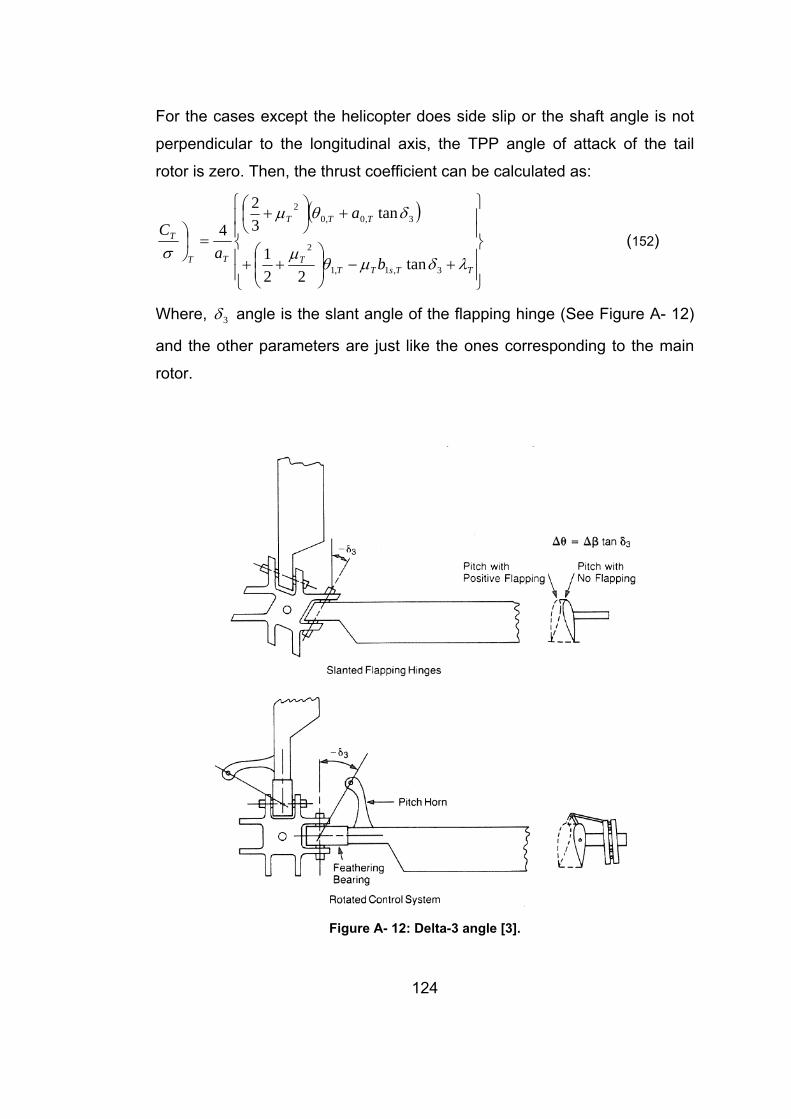
124

For the cases except the helicopter does side slip or the shaft angle is not

perpendicular to the longitudinal axis, the TPP angle of attack of the tail

rotor is zero. Then, the thrust coefficient can be calculated as:

( )

⎪⎪

⎭

⎪⎪

⎬

⎫

⎪⎪

⎩

⎪⎪

⎨

⎧

+−⎟⎟⎠

⎞⎜⎜⎝

⎛++

+⎟⎠⎞

⎜⎝⎛ +

=⎟⎠⎞

TTsTTT

TTT

TT

T

b

a

aC

λδμθμ

δθμ

σ3,1,1

2

3,0,02

tan22

1

tan32

4 (152)

Where, 3δ angle is the slant angle of the flapping hinge (See Figure A- 12)

and the other parameters are just like the ones corresponding to the main

rotor.

Figure A- 12: Delta-3 angle [3].

125

The coning angle:

( )2,023

32

T

T

T

T

T

TT R

gR

a

C

aΩ

−⎟⎠⎞⎜

⎝⎛

=σ

γ (153)

The inflow ratio for the case the shaft is perpendicular to the longitudinal

axis:

T

T

T

TT

Cμσ

σλ

2.

⎟⎠⎞

⎜⎝⎛−= (154)

The pitching angle of the tail rotor is denoted by:

( ) TTsTTsT

TTTT baRra ψδψδθδθθ sintancostantan 3,13,1,13,0,0 −−⎟⎠⎞++= (155)

Here it is apparent that the effective fist harmonic pitching angles can be

introduced as:

3,1,1

3,1,1

tan

tan

δ

δ

Tseff

Tseff

bB

aA

=

= (156)

The thrust coefficient equation is used to obtain the collective angle of the tail

rotor:

T

sT

T ab

aC

⎪⎪⎭

⎪⎪⎬

⎫

⎪⎪⎩

⎪⎪⎨

⎧

−+

−+⎟⎟⎠

⎞⎜⎜⎝

⎛+−

= 302

311

2

,0 tan

32

tan22

14

δμ

λδμθμσ

θ (157)

Therefore, the flapping angles with respect to the control plane can be

expressed as:

( ) ( )⎥⎦⎤

⎢⎣⎡ ++++

+=+ TTsTTTT

T

TTsTs aaba λμθδθ

μ

μδ ,1,13,0,0

23,1,1 22tan

38

231

tan (158)

( )

21

34

tan 2

,1,0

3,1,1T

T

TTT

TsTsR

aab

μ

υμ

δ+

Ω+

=− (159)

126

Those two equations with two unknowns are solved and the flapping angles

are found as:

( )

( )T

T

T

TT

Ts

Ca

CCa

a

⎪⎭

⎪⎬⎫

⎪⎩

⎪⎨⎧

⎥⎥⎦

⎤

⎢⎢⎣

⎡⎟⎟⎠

⎞⎜⎜⎝

⎛+

−++−

⎟⎟⎟⎟⎟⎟⎟⎟

⎠

⎞

⎜⎜⎜⎜⎜⎜⎜⎜

⎝

⎛

⎥⎥⎦

⎤

⎢⎢⎣

⎡⎟⎟⎠

⎞⎜⎜⎝

⎛+

−

⎥⎥⎥⎥

⎦

⎤

⎢⎢⎢⎢

⎣

⎡

+

+−

⎪⎭

⎪⎬⎫

⎪⎩

⎪⎨⎧

−+⎥⎦

⎤⎢⎣

⎡+−⎟⎟

⎠

⎞⎜⎜⎝

⎛+

++

=2

3

2

22

2

3

2

22

0

112

22

,1

tan32

4132

2

tan32

412

234

2

221

24

324

324

δμμ

μμ

δμμ

μμσ

σμ

μσ

σθ

θμ

σμσ

μμμ

(160)

3,12

0

,1 tan2

234

2 δμ

μσ

σμ

Ts

T

T

Ts a

Ca

b +

⎥⎥⎥⎥

⎦

⎤

⎢⎢⎢⎢

⎣

⎡

+

+= (161)

The torque and the H-force coefficients of the tail rotor:

( ) ( )

( )

T

Ts

s

sD

T

H

Ca

RRa

a

a

aaaC

C

⎪⎪⎪⎪⎪

⎭

⎪⎪⎪⎪⎪

⎬

⎫

⎪⎪⎪⎪⎪

⎩

⎪⎪⎪⎪⎪

⎨

⎧

+⎥⎥⎦

⎤

⎢⎢⎣

⎡⎟⎠

⎞⎜⎝

⎛Ω

+Ω

+⎟⎟⎠

⎞⎜⎜⎝

⎛+

⎥⎥⎥⎥

⎦

⎤

⎢⎢⎢⎢

⎣

⎡

++

⎥⎥⎥⎥

⎦

⎤

⎢⎢⎢⎢

⎣

⎡

+−⎟⎠⎞

⎜⎝⎛ +−+

⎟⎠⎞

⎜⎝⎛ +−+

⎥⎥⎥⎥

⎦

⎤

⎢⎢⎢⎢

⎣

⎡

+

+−

=⎟⎠

⎞

συυ

μμ

μ

μ

μλμθ

μδθ

μ

μλμμ

σ

1

211

0

220

2

121

2300

2

1

81

31

291

2211

231

2

23

31tan

23144

(162)

( )T

HTD

T

Q CCCC

⎭⎬⎫

⎩⎨⎧ −−+=⎟⎟

⎠

⎞σ

μσ

λμσ

2318

(163)

And the torque and H-force values:

( )2, TTb

T

HT RACH Ω⎟

⎠⎞

⎜⎝⎛= ρσ

(164)

( ) TTTbT

QT RRA

CQ 2

, Ω⎟⎟⎠

⎞⎜⎜⎝

⎛= ρ

σ (165)

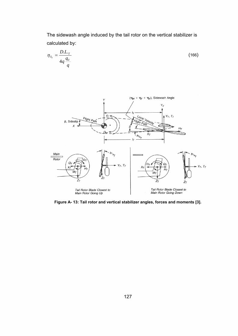
127

The sidewash angle induced by the tail rotor on the vertical stabilizer is

calculated by:

qq

q

LDV

TTV

4

..=η (166)

Figure A- 13: Tail rotor and vertical stabilizer angles, forces and moments [3].

128

APPENDIX B

TRIM-CF CODE

Some of the formulations not stated in this appendix are written in

Appendix-A.

B.1 MAIN ROTOR PARAMETERS

The tip path plane angle of attack:

⎟⎟⎠

⎞⎜⎜⎝

⎛−

++= −

F

TMFTPP LW

HHD1tanα (167)

The main rotor thrust:

( ) ( )22TMFFM HHDLWT +++−= (168)

The lift and drag values of fuselage belong to the empennage on case.

First harmonic pitch angles (cyclic angles) are found using the first harmonic

flapping angles:

⎟⎟⎠

⎞⎜⎜⎝

⎛−+

⎥⎦

⎤⎢⎣

⎡⎟⎟⎠

⎞⎜⎜⎝

⎛+

Ω+⎟

⎠⎞

⎜⎝⎛ +

−=

2421

241

4516

34

42

414

0

11 μμ

μυμ

πμ

Ra

bA s (169)

⎟⎟⎠

⎞⎜⎜⎝

⎛−+

⎥⎦

⎤⎢⎣

⎡′⎟⎟

⎠

⎞⎜⎜⎝

⎛−+⎟⎟

⎠

⎞⎜⎜⎝

⎛++⎟⎟

⎠

⎞⎜⎜⎝

⎛+

+−=

245

231

22

122

4532

38

42

2

1

4

0

3

11 μμ

λμθμθπμμ

saB (170)

129

B.1.1 COLLECTIVE ANGLE CALCULATIONS

The collective angle is derived by the following integral calculations. The lift

force over an azimuthal station and a radial station is defined as:

rcaUL MMMT Δ=Δ αρ 2

21

MMMT caUrL αρ 2

21

=ΔΔ (171)

where TU is the tangential component of the local velocity vector at that

blade section (See Figure A- 8) and rΔ is the blade section.

The parameter is integrated over the blade and then over the azimuthal

range to find the total lift produced by the main rotor:

drrLL

R

b ∫ ΔΔ

=0

ψ (172)

ψπ

ψdLL bb ∫∑ =

2

0

(173)

The lift produced by one blade at a specific azimuth angle is approximated

as:

ψπ

π

ψdLL bb ∫=

2

021 (174)

And the total thrust force is calculated by multiplying the lift by the number of

blades:

⎪⎭

⎪⎬⎫

⎪⎩

⎪⎨⎧

ΔΔ

−ΔΔ

+ΔΔ

= ∫ ∫∫ ∫∫ ∫−

−

π

π

ψμπ

π ψμ

π

ψψψπ

2 sin2

sin0 00

...2 x

BB

xM d

Rrd

rLd

Rrd

rLd

Rrd

rLbRT (175)

Here the integrals are taken from the cut-out ( ox ) to the loss factor ( B )

station, in order to eliminate the root and tip losses. The integration limits

are arranged in order to take the reverse flow effect into account. The limits

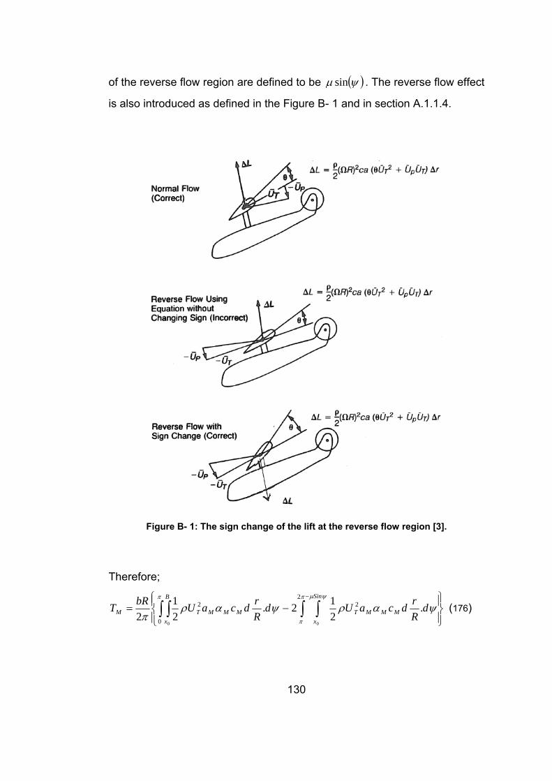
130

of the reverse flow region are defined to be ( )ψμ sin . The reverse flow effect

is also introduced as defined in the Figure B- 1 and in section A.1.1.4.

Figure B- 1: The sign change of the lift at the reverse flow region [3].

Therefore;

⎪⎭

⎪⎬⎫

⎪⎩

⎪⎨⎧

−= ∫ ∫∫ ∫−π

π

ψμπ

ψαρψαρπ

22

0

2

00

.212.

21

2

Sin

xMMMT

B

xMMMTM d

RrdcaUd

RrdcaUbRT (176)

131

⎪⎭

⎪⎬⎫

⎪⎩

⎪⎨⎧

−= ∫ ∫∫ ∫−π

π

ψμπ

ψαψαπ

ρ 22

0

2

00

.2.4

Sin

xMT

B

xMT

MMM d

RrdUd

RrdUcabRT (177)

⎪⎭

⎪⎬⎫

⎪⎩

⎪⎨⎧

−= ∫ ∫∫ ∫−π

π

ψμπ

ψαψαπσ

22

0

2

00

.2.4

Sin

xMT

B

xMT

MT dRrdUd

RrdU

aC (178)

The local angle of attack is as defined before in Appendix A:

⎟⎟⎠

⎞⎜⎜⎝

⎛+= −

T

P

UU1tanθα (179)

The angle can be approximated with small angle assumption:

T

P

UU

+≅θα (180)

where the velocity components are non-dimensionalized by the tip speed

RΩ .

The thrust coefficient becomes:

( ) ( )⎪⎭

⎪⎬⎫

⎪⎩

⎪⎨⎧

+−+= ∫ ∫∫ ∫−π

π

ψμπ

ψθψθπσ

22

0

2

00

.2.4

Sin

xPTT

B

xPTT

MT dRrdUUUd

RrdUUU

aC (181)

Introducing the pitch angle:

ψψθθθ sincos 1110 BARr

−−+= (182)

The tangential velocity is as given before:

ψμ sin+=RrUT (183)

The perpendicular velocity component:

ψββυα oscVrVU LSP −−−= & (184)

The tipp path plane angle of attack is used instead of the shaft angle of

attack:

SSTPP a1−= αα (185)

The induced velocity can be approximated with the following formula,

assuming that it is much greater than the forward speed:

132

21TCR

μυ Ω

= (186)

The flapping angle can be derived as:

ψψβ sincos 110 SS baa −−= (187) ( )Ω−= ψψβ cossin 11 SS ba& (188)

Taking the last equations, normalized perpendicular velocity component

becomes:

⎟⎟⎟⎟⎟

⎠

⎞

⎜⎜⎜⎜⎜

⎝

⎛

+⎥⎦

⎤⎢⎣

⎡−⎟

⎠⎞

⎜⎝⎛

Ω−+

−−Ω

−=

Ω=

ψψμψμυ

ψμψυ

μα

cossincos

sinsin

101

1

211

1

SS

SSTPPP

P

baRr

Rb

aaRr

RR

UU (189)

Solving the integrals at the 154th equation:

( ) ( ) ( )

( ) ( ) ⎪⎪

⎭

⎪⎪

⎬

⎫

⎪⎪

⎩

⎪⎪

⎨

⎧

+⎟⎟⎠

⎞⎜⎜⎝

⎛+−−′⎟⎟

⎠

⎞⎜⎜⎝

⎛+−+

⎟⎟⎠

⎞⎜⎜⎝

⎛−−+−+⎟⎟

⎠

⎞⎜⎜⎝

⎛−−+−

=

S

MT

aBxBxB

xBxBxBxBaC

11

320

22

20

2

14

20

2240

40

3

022

02

42

2898

32

4 μμλμ

θμμθπμμ

σ

(190)

Using the above equations, we obtain the collective equation:

⎟⎟⎠

⎞⎜⎜⎝

⎛+−−+−−

⎟⎟⎟⎟⎟

⎠

⎞

⎜⎜⎜⎜⎜

⎝

⎛

′⎟⎟⎠

⎞⎜⎜⎝

⎛++−

⎟⎟⎠

⎞⎜⎜⎝

⎛−−+−−⎟

⎠⎞

⎜⎝⎛ −+

=

πμμμ

πμμ

πμ

λμμ

θμμμμσμμ

θ

135245

4592

3625

98

32

32

4824131

21923

169

6231

245

2314

765432

64

1864

242

0

TCa

(191)

133

B.1.2 FORCES, MOMENTS AND POWER

Derivations similar to the ones of thrust coefficient are made in order to find

the following torque and H-force coefficients:

( )σ

μσ

μλμμσ

HTS

DQ CCacC−−′−⎟

⎠⎞

⎜⎝⎛ ++= 1

42

8331

8 (192)

⎪⎪⎪⎪⎪⎪⎪⎪⎪⎪⎪⎪⎪

⎭

⎪⎪⎪⎪⎪⎪⎪⎪⎪⎪⎪⎪⎪

⎬

⎫

⎪⎪⎪⎪⎪⎪⎪⎪⎪⎪⎪⎪⎪

⎩

⎪⎪⎪⎪⎪⎪⎪⎪⎪⎪⎪⎪⎪

⎨

⎧

⎪⎪⎪⎪⎪⎪⎪⎪⎪⎪⎪⎪

⎭

⎪⎪⎪⎪⎪⎪⎪⎪⎪⎪⎪⎪

⎬

⎫

⎪⎪⎪⎪⎪⎪⎪⎪⎪⎪⎪⎪

⎩

⎪⎪⎪⎪⎪⎪⎪⎪⎪⎪⎪⎪

⎨

⎧

+

⎪⎪⎪⎪⎪⎪⎪⎪

⎭

⎪⎪⎪⎪⎪⎪⎪⎪

⎬

⎫

⎪⎪⎪⎪⎪⎪⎪⎪

⎩

⎪⎪⎪⎪⎪⎪⎪⎪

⎨

⎧

⎥⎦

⎤⎢⎣

⎡+−−⎟

⎠

⎞⎜⎝

⎛Ω

+

⎥⎥⎥⎥

⎦

⎤

⎢⎢⎢⎢

⎣

⎡

+−

−−

Ω+

⎥⎥⎥⎥

⎦

⎤

⎢⎢⎢⎢

⎣

⎡

⎟⎠⎞

⎜⎝⎛ −−

−−+

⎟⎟⎠

⎞⎜⎜⎝

⎛−+

−

⎥⎥⎥⎥⎥

⎦

⎤

⎢⎢⎢⎢⎢

⎣

⎡

⎟⎟⎠

⎞⎜⎜⎝

⎛−′+⎟⎟

⎠

⎞⎜⎜⎝

⎛−−−−+

⎟⎟⎠

⎞⎜⎜⎝

⎛+−−+−−

⎟⎟⎠

⎞⎜⎜⎝

⎛−+

′

−

⎟⎟⎠

⎞⎜⎜⎝

⎛+

=

sT

M

d

H

aC

R

Ra

a

a

c

C

1

64221

53

2

10

622

432

20

42

42

6421

54320

42

3

144821

81

95158

6581

3

961

45128

613564

491

2

421

489632

41

2

3085

15106

2341

3

245

231

4

44

σ

μμμυ

πμ

πμ

μπμ

μυ

μπ

μπμμ

μμμ

μμλμμμθ

πμμ

πμμ

πμθ

μμλμ

μμ

σ

(193)

And the forces are calculated:

( ) RRAC

Q bQ

M2Ω= ρ

σ (194)

( )2RACH bH

M Ω= ρσ

(195)

Power required is calculated with the following formulas:

VeATHP

M

MindM ρ1100

2

, = (196)

134

1100

3

,fVHP paraMρ

= (197)

( ) ( )550

318

23

,μρ +

Ω= dbproM

cRAHP (198)

( )paraMproMindMQ

comp

Q

compM HPHPHPC

C

HP ,,,, ++⎟⎟⎠

⎞Δ

=

σ

σ (199)

compMparaMproMindMM HPHPHPHPHP ,,,, +++= (200)

B.2 TOTAL FORCES AND MOMENTS

The forces can be calculated by the following formulas. The parameters with

bars overhead are the output parameters supplied by the CF module. This

approximation is used in order to linearize the equations.

MMSMaM iTaTHXMS

−−−= = 101 (201)

TT HX −= (202)

( ) ( )H

H

HH

H DHH

H

i

FL

HHHHFHHH CA

qqq

ARi

aLLX,0

1

0−

+⎟⎟⎠

⎞⎜⎜⎝

⎛−−

+−−=

= πδ

εαα

εα (203)

( )VV TMVVV LDX ηη +−−= (204)

FFFF LDX α+−= (205)

MM TZ −= (206)

TST TbZT1= (207)

( ) ( )HHH FHHFLHHHH

HH DiaA

qq

qZ εαεαα −−−−+−= =0 (208)

( )( ) ⎟⎟⎠

⎞⎜⎜⎝

⎛−−Θ++−=

VVV FM

MVFMVVV qA

TLDZ ε

υυ

ηη41

(209)

135

FFFF

F

FF D

qL

qLqZ

F

αααα

−⎟⎟⎟⎟

⎠

⎞

⎜⎜⎜⎜

⎝

⎛

∂

⎟⎠⎞⎜

⎝⎛∂

+⎟⎠⎞⎜

⎝⎛−=

=0 (210)

SS

M aaMM 1

1∂∂

= (211)

TT QM −= (212)

⎟⎟⎟⎟

⎠

⎞

⎜⎜⎜⎜

⎝

⎛

∂

⎟⎠⎞⎜

⎝⎛∂

+⎟⎠⎞⎜

⎝⎛=

=F

F

F

FF

qM

qMqM

F

ααα 0

(213)

Total forces and moments:

0=Θ−++++=∑ WXXXXXX FVHTM (214)

0=+++++=∑ WZZZZZZ FVHTM (215)

0=⎟⎟⎠

⎞⎜⎜⎝

⎛−+−+−+

−+−++=∑

FFFFVVHHHHTT

TTMMMMFTM

hXlZhXlZhXlZhXlZhXMMM

M (216)

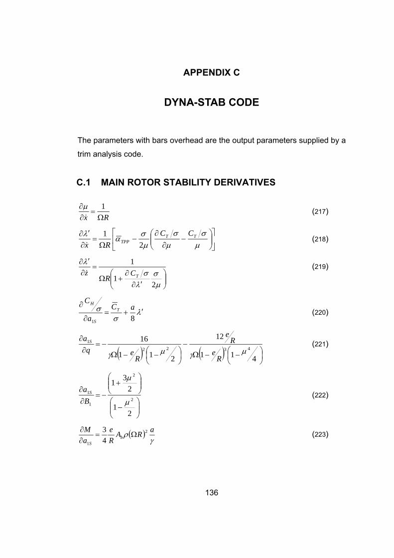
136

APPENDIX C

DYNA-STAB CODE

The parameters with bars overhead are the output parameters supplied by a

trim analysis code.

C.1 MAIN ROTOR STABILITY DERIVATIVES

Rx Ω=

∂∂ 1&

μ (217)

⎥⎦

⎤⎢⎣

⎡⎟⎟⎠

⎞⎜⎜⎝

⎛−

∂∂

−Ω

=∂′∂

μσ

μσ

μσαλ TT

TPPCC

Rx 21

& (218)

⎟⎟⎠

⎞⎜⎜⎝

⎛′∂

∂+Ω

=∂′∂

μσ

λσ

λ

21

1

TCR

z& (219)

λσ

σ ′+=∂

∂

81

aCa

CT

S

H

(220)

( ) ( ) ⎟⎠⎞

⎜⎝⎛ −−Ω

−⎟⎠⎞

⎜⎝⎛ −−Ω

−=∂∂

411

12

211

164322

1

μγμγ Re

Re

Req

a S (221)

⎟⎟⎠

⎞⎜⎜⎝

⎛−

⎟⎟⎠

⎞⎜⎜⎝

⎛+

−=∂∂

21

231

2

2

1

1

μ

μ

Ba S (222)

( )γ

ρ aRARe

aM

bS

2

1 43

Ω=∂∂ (223)

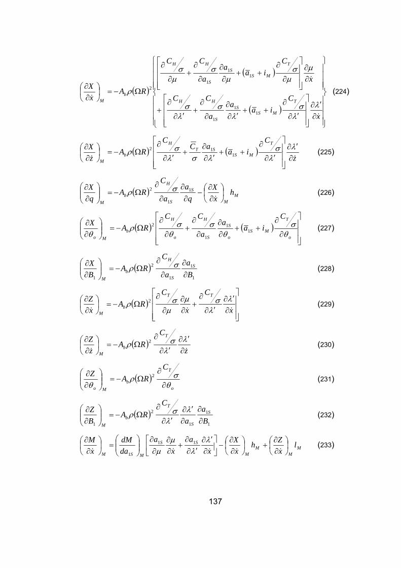
137

( )

( )

( )⎪⎪⎪⎪

⎭

⎪⎪⎪⎪

⎬

⎫

⎪⎪⎪⎪

⎩

⎪⎪⎪⎪

⎨

⎧

∂′∂

⎥⎥⎥

⎦

⎤

⎢⎢⎢

⎣

⎡

′∂

∂++

′∂∂

∂

∂+

′∂

∂+

∂∂

⎥⎥⎥

⎦

⎤

⎢⎢⎢

⎣

⎡

∂

∂++

∂∂

∂

∂+

∂

∂

Ω−=⎟⎠⎞

⎜⎝⎛∂∂

x

Cia

aa

CC

x

Cia

aa

CC

RAxX

T

MSS

S

HH

T

MSS

S

HH

bM

&

&

&λ

λσ

λσ

λσ

μμσ

μσ

μσ

ρ

11

1

11

12 (224)

( ) ( )z

Cia

aCC

RAzX T

MSST

H

bM && ∂

′∂

⎥⎥⎥

⎦

⎤

⎢⎢⎢

⎣

⎡

′∂

∂++

′∂∂

+′∂

∂Ω−=⎟

⎠⎞

⎜⎝⎛∂∂ λ

λσ

λσλσρ 1

12 (225)

( ) MM

S

S

H

bM

hxX

qa

a

CRA

qX

⎟⎠⎞

⎜⎝⎛∂∂

−∂∂

∂

∂Ω−=⎟⎟

⎠

⎞⎜⎜⎝

⎛∂∂

&1

1

2 σρ (226)

( ) ( )⎥⎥⎥

⎦

⎤

⎢⎢⎢

⎣

⎡

∂

∂++

∂∂

∂

∂+

∂

∂Ω−=⎟⎟

⎠

⎞⎜⎜⎝

⎛∂∂

o

T

MSo

S

S

H

o

H

bMo

Cia

aa

CCRAX

θσ

θσ

θσρ

θ 11

1

2 (227)

( )1

1

1

2

1 Ba

a

CRA

BX S

S

H

bM

∂∂

∂

∂Ω−=⎟⎟

⎠

⎞⎜⎜⎝

⎛∂∂ σρ (228)

( )⎥⎥⎥

⎦

⎤

⎢⎢⎢

⎣

⎡

∂′∂

′∂

∂+

∂∂

∂

∂Ω−=⎟

⎠⎞

⎜⎝⎛∂∂

x

C

x

CRA

xZ TT

bM &&&

λλσμ

μσρ 2 (229)

( )z

CRA

zZ T

bM && ∂

′∂′∂

∂Ω−=⎟

⎠⎞

⎜⎝⎛∂∂ λ

λσρ 2 (230)

( )o

T

bMo

CRAZ

θσρ

θ ∂

∂Ω−=⎟⎟

⎠

⎞⎜⎜⎝

⎛∂∂ 2 (231)

( )1

1

1

2

1 Ba

a

CRA

BZ S

S

T

bM

∂∂

∂′∂

′∂

∂Ω−=⎟⎟

⎠

⎞⎜⎜⎝

⎛∂∂ λ

λσρ (232)

MM

MM

SS

MSM

lxZh

xX

xa

xa

dadM

xM

⎟⎠⎞

⎜⎝⎛∂∂

+⎟⎠⎞

⎜⎝⎛∂∂

−⎥⎦

⎤⎢⎣

⎡∂′∂

′∂∂

+∂∂

∂∂

⎟⎟⎠

⎞⎜⎜⎝

⎛=⎟

⎠⎞

⎜⎝⎛∂∂

&&&&&

λλ

μμ

11

1

(233)

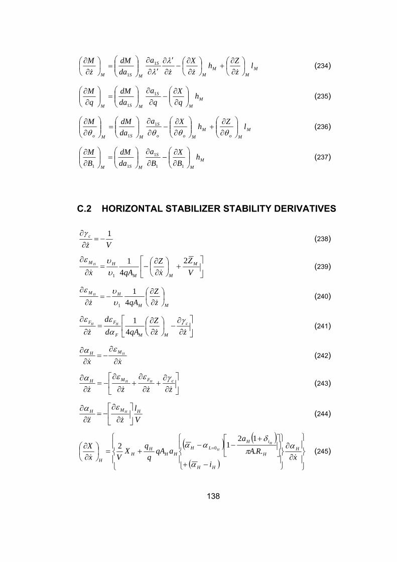
138

MM

MM

S

MSM

lzZh

zX

za

dadM

zM

⎟⎠⎞

⎜⎝⎛∂∂

+⎟⎠⎞

⎜⎝⎛∂∂

−∂′∂

′∂∂

⎟⎟⎠

⎞⎜⎜⎝

⎛=⎟

⎠⎞

⎜⎝⎛∂∂

&&&&

λλ

1

1

(234)

MM

S

MSM

hqX

qa

dadM

qM

⎟⎟⎠

⎞⎜⎜⎝

⎛∂∂

−∂∂

⎟⎟⎠

⎞⎜⎜⎝

⎛=⎟⎟

⎠

⎞⎜⎜⎝

⎛∂∂ 1

1

(235)

MMo

MMoo

S

MSMo

lZhXadadMM

⎟⎟⎠

⎞⎜⎜⎝

⎛∂∂

+⎟⎟⎠

⎞⎜⎜⎝

⎛∂∂

−∂∂

⎟⎟⎠

⎞⎜⎜⎝

⎛=⎟⎟

⎠

⎞⎜⎜⎝

⎛∂∂

θθθθ1

1

(236)

MM

S

MSM

hBX

Ba

dadM

BM

⎟⎟⎠

⎞⎜⎜⎝

⎛∂∂

−∂∂

⎟⎟⎠

⎞⎜⎜⎝

⎛=⎟⎟

⎠

⎞⎜⎜⎝

⎛∂∂

11

1

11

(237)

C.2 HORIZONTAL STABILIZER STABILITY DERIVATIVES

Vzc 1

−=∂∂&

γ (238)

⎥⎦

⎤⎢⎣

⎡+⎟

⎠⎞

⎜⎝⎛∂∂

−=∂

∂

VZ

xZ

qAxM

MM

HM H 24

1

1 && υυε

(239)

MM

HM

zZ

qAzH ⎟

⎠⎞

⎜⎝⎛∂∂

−=∂

∂

&& 41

1υυε

(240)

⎥⎦

⎤⎢⎣

⎡∂∂

−⎟⎠⎞

⎜⎝⎛∂∂

=∂

∂

zzZ

qAdd

zc

MMF

FF HH

&&&

γαεε

41 (241)

xxHMH

&& ∂

∂−=

∂∂ εα (242)

⎥⎦

⎤⎢⎣

⎡∂∂

+∂

∂+

∂

∂−=

∂∂

zzzzcFMH HH

&&&&

γεεα (243)

Vl

zzHMH H

⎥⎦

⎤⎢⎣

⎡∂

∂−=

∂∂

&&&

εα (244)

( ) ( )

( ) ⎪⎭

⎪⎬

⎫

⎪⎩

⎪⎨

⎧

∂∂

⎪⎭

⎪⎬

⎫

⎪⎩

⎪⎨

⎧

−+

⎥⎦

⎤⎢⎣

⎡ +−−

+=⎟⎠⎞

⎜⎝⎛∂∂ =

xi

RAa

aqAq

qX

VxX H

HH

H

iHLH

HHH

HH

H

H

&&

α

α

πδ

αα..

1212 0 (245)

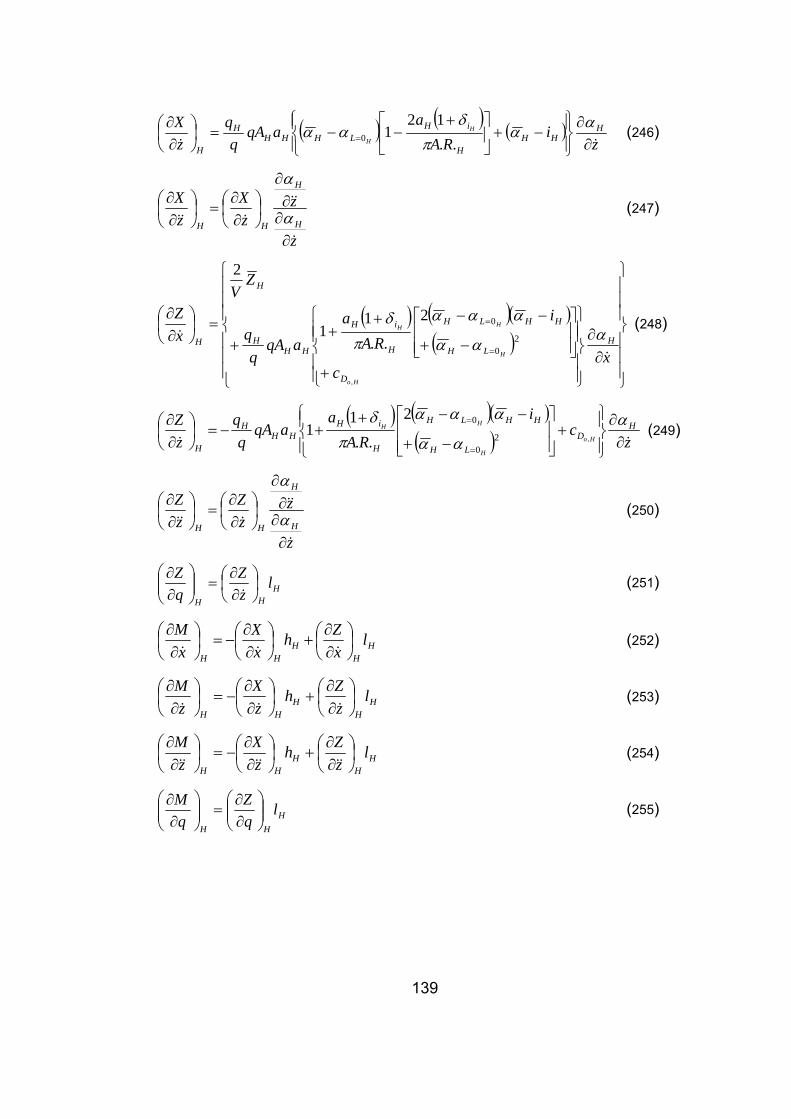
139

( ) ( ) ( )z

iRA

aaqA

qq

zX H

HHH

iHLHHH

H

H

H

H && ∂∂

⎪⎭

⎪⎬⎫

⎪⎩

⎪⎨⎧

−+⎥⎦

⎤⎢⎣

⎡ +−−=⎟

⎠⎞

⎜⎝⎛∂∂

=αα

πδ

αα..

1210 (246)

z

zzX

zX

H

H

HH

&

&&&&&

∂∂∂∂

⎟⎠⎞

⎜⎝⎛∂∂

=⎟⎠⎞

⎜⎝⎛∂∂

α

α

(247)

( ) ( )( )( )

⎪⎪⎪

⎭

⎪⎪⎪

⎬

⎫

⎪⎪⎪

⎩

⎪⎪⎪

⎨

⎧

∂∂

⎪⎪⎭

⎪⎪⎬

⎫

⎪⎪⎩

⎪⎪⎨

⎧

+

⎥⎥⎦

⎤

⎢⎢⎣

⎡

−+

−−++

+=⎟

⎠⎞

⎜⎝⎛∂∂

=

=

xc

i

RAa

aqAq

q

ZV

xZ

H

D

LH

HHLH

H

iH

HHH

H

H

Ho

H

HH

&

& ααα

ααα

πδ

,

20

02

..1

1

2

(248)

( ) ( )( )( ) z

ci

RAa

aqAq

qzZ H

DLH

HHLH

H

iHHH

H

HHo

H

HH

&& ∂∂

⎪⎭

⎪⎬⎫

⎪⎩

⎪⎨⎧

+⎥⎥⎦

⎤

⎢⎢⎣

⎡

−+

−−++−=⎟

⎠⎞

⎜⎝⎛∂∂

=

= ααα

ααα

πδ

,20

02

..1

1 (249)

z

zzZ

zZ

H

H

HH

&

&&&&&

∂∂∂∂

⎟⎠⎞

⎜⎝⎛∂∂

=⎟⎠⎞

⎜⎝⎛∂∂

α

α

(250)

HHH

lzZ

qZ

⎟⎠⎞

⎜⎝⎛∂∂

=⎟⎟⎠

⎞⎜⎜⎝

⎛∂∂

& (251)

HH

HHH

lxZh

xX

xM

⎟⎠⎞

⎜⎝⎛∂∂

+⎟⎠⎞

⎜⎝⎛∂∂

−=⎟⎠⎞

⎜⎝⎛∂∂

&&& (252)

HH

HHH

lzZh

zX

zM

⎟⎠⎞

⎜⎝⎛∂∂

+⎟⎠⎞

⎜⎝⎛∂∂

−=⎟⎠⎞

⎜⎝⎛∂∂

&&& (253)

HH

HHH

lzZh

zX

zM

⎟⎠⎞

⎜⎝⎛∂∂

+⎟⎠⎞

⎜⎝⎛∂∂

−=⎟⎠⎞

⎜⎝⎛∂∂

&&&&&& (254)

HHH

lqZ

qM

⎟⎟⎠

⎞⎜⎜⎝

⎛∂∂

=⎟⎟⎠

⎞⎜⎜⎝

⎛∂∂ (255)

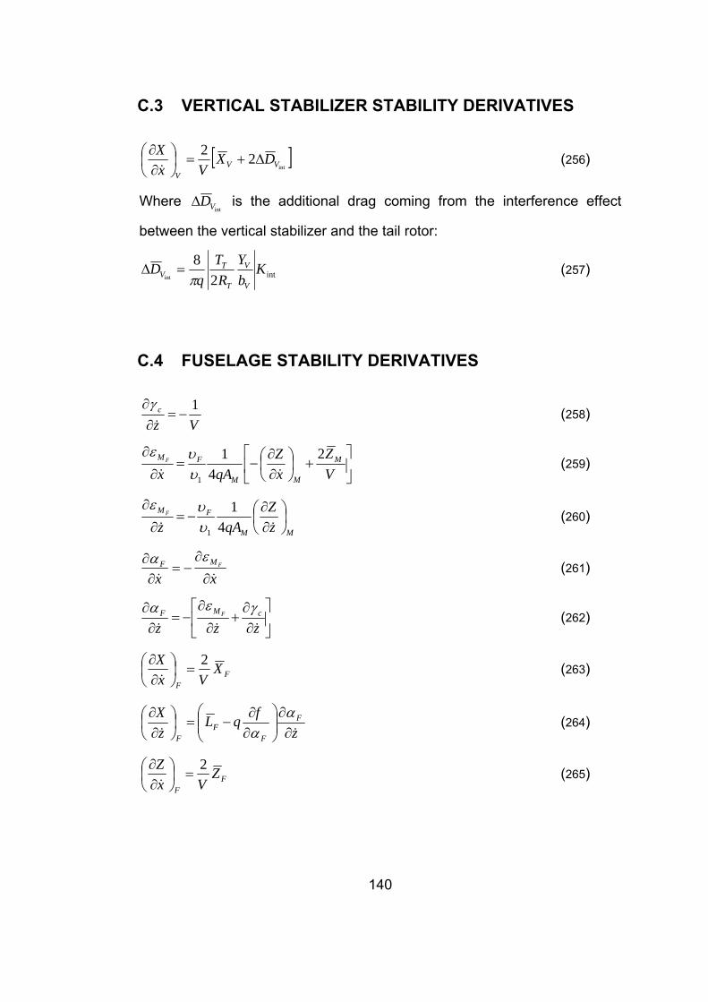
140

C.3 VERTICAL STABILIZER STABILITY DERIVATIVES

[ ]int

22VV

V

DXVx

XΔ+=⎟

⎠⎞

⎜⎝⎛∂∂&

(256)

Where intVDΔ is the additional drag coming from the interference effect

between the vertical stabilizer and the tail rotor:

int28

intK

bY

RT

qD

V

V

T

TV π

=Δ (257)

C.4 FUSELAGE STABILITY DERIVATIVES

Vzc 1

−=∂∂&

γ (258)

⎥⎦

⎤⎢⎣

⎡+⎟

⎠⎞

⎜⎝⎛∂∂

−=∂

∂

VZ

xZ

qAxM

MM

FM F 24

1

1 && υυε

(259)

MM

FM

zZ

qAzF ⎟

⎠⎞

⎜⎝⎛∂∂

−=∂

∂&& 4

1

1υυε

(260)

xxFMF

&& ∂

∂−=

∂∂ εα (261)

⎥⎦

⎤⎢⎣

⎡∂∂

+∂

∂−=

∂∂

zzzcMF F

&&&

γεα (262)

FF

XVx

X 2=⎟

⎠⎞

⎜⎝⎛∂∂&

(263)

zfqL

zX F

FF

F && ∂∂

⎟⎟⎠

⎞⎜⎜⎝

⎛∂∂

−=⎟⎠⎞

⎜⎝⎛∂∂ α

α (264)

FF

ZVx

Z 2=⎟

⎠⎞

⎜⎝⎛∂∂&

(265)

141

zq

LqD

zZ F

FF

F && ∂∂

⎟⎟⎟

⎠

⎞

⎜⎜⎜

⎝

⎛

∂

∂+−=⎟

⎠⎞

⎜⎝⎛∂∂ α

α (266)

xq

MqM

VxM F

FF

F && ∂∂

∂

∂+=⎟

⎠⎞

⎜⎝⎛∂∂ α

α2 (267)

zq

Mq

zM F

FF && ∂∂

∂

∂=⎟

⎠⎞

⎜⎝⎛∂∂ α

α (268)

C.5 TOTAL STABILITY DERIVATIVES

The total derivatives are found by adding the corresponding terms of main

rotor, tail rotor, empennage and the fuselage:

Fi

i

VSi

i

HSi

i

Ti

i

Mi

i

i

i

xX

xX

xX

xX

xX

xX

⎟⎟⎠

⎞⎜⎜⎝

⎛∂∂

+⎟⎟⎠

⎞⎜⎜⎝

⎛∂∂

+⎟⎟⎠

⎞⎜⎜⎝

⎛∂∂

+⎟⎟⎠

⎞⎜⎜⎝

⎛∂∂

+⎟⎟⎠

⎞⎜⎜⎝

⎛∂∂

=∂∂ (269)

Where MZXX i ,,= and 1,,,,, Bqzzxx oi θ&&&&=

Documents

DEVELOPMENT OF FORWARD FLIGHT TRIM AND …etd.lib.metu.edu.tr/upload/12610391/index.pdf · development of forward flight trim and longitudinal dynamic stability codes and their application