Embed Size (px)
Citation preview

Development of Methodologies for Strain
Measurement and Surface Energy
Characterization
by
Yougun Han
A thesis
presented to the University of Waterloo
in fulfillment of the
thesis requirement for the degree of
Master of Applied Science
in
Mechanical Engineering
Waterloo, Ontario, Canada, 2011
© Yougun Han 2011

ii
Author's Declaration
I hereby declare that I am the sole author of this thesis. This is a true copy of the thesis, including
any required final revisions, as accepted by my examiners.
I understand that my thesis may be made electronically available to the public.

iii
Abstract
Development of new scientific disciplines such as bioengineering and micro-nano engineering
adopting nonconventional materials requests innovative methodologies that can accurately measure
the mechanical properties of soft biological materials and characterize surface energy and adhesion
properties of them, independent of measurement conditions. One of emerging methods to measure the
deformation of materials under stress is digital image correlation (DIC) technique. As a noncontact
strain measurement method, DIC has the advantages of prevention of experimental errors caused by
the use of contact type sensors and of flexibility in its application to soft materials that are hard to be
tested by conventional method. In the first part of the thesis, 2 dimensional and 3 dimensional DIC
codes were developed and optimized, and then applied to two critical applications: 1) determining the
stress-strain behaviour of polydimethylsiloxane (PDMS) sample, as a model soft material, using the
optical images across large deformation region, and 2) detecting the stiffness variation within the gel
mimicking the breast tumour using ultrasound images. The results of this study showed the capability
of DIC as a strain sensor and suggested its potential as a diagnosing tool for the malignant lesion
causing local stiffness variation.
In the characterization of surface energy and adhesion properties of materials, two most common
methods are contact angle measurement and JKR-type indentation test. In the second part of the thesis,
the experimental set-up for these methods were developed and verified by using the PDMS in static
(quasi equilibrium) state. From the dynamic tests, it showed its possible usage in studying adhesion
hysteresis with respect to speed. The adhesion hysteresis was observed at high speed condition in
both contact angle measurement and JKR-type indentation tests.

iv
Acknowledgements
I would like to express my deepest gratitude to my two supervisors, Dr. HJ Kwon for introducing me
to the area of digital image technology and Dr. Boxin Zhao for giving me a chance to know about
surface technology. I want to show them my thanks for not only, as mentors in research, their
knowledgeable guidance, invaluable insight into research, but also their gracious patience, numerous
encouragements for my progress throughout the whole process of my MASc program. I also
appreciate their concerns to show me what is important in life. Without their considerate support, it is
impossible for me to fulfill the degree. What they did to me is beyond my expectations and will
continue to inspire me in my career and life in the future.
My thanks also should go to some of my colleagues. I would like to thank my lab colleague,
Allan who shared his idea with me and helped me polish my first manuscript. I could not have
achieved it without him. I would like to thank Dr. Dongwoo Kim for planning and designing the
ultrasound experiments from the scratch with me. The list would be incomplete if I do not thank my
lab mates, Hadi and Kuo, in Nanoadhesion Lab for making cheerful working environment.
Finally, I would like to express my greatest thanks to my family. I express my thanks to my
parents, who raised me, inspired me to pursue my own goals, and trust me all the time. I express my
thanks to my graceful wife, Rui, for her love, moral support, and getting over all the difficulties with
me. I think this achievement is a small return for their constant support.
v
Table of Contents Author's Declaration ............................................................................................................................... ii
Abstract ................................................................................................................................................. iii
Acknowledgements ............................................................................................................................... iv
Table of Contents ................................................................................................................................... v
List of Figures ...................................................................................................................................... vii
List of Tables ......................................................................................................................................... ix
Chapter 1 Introduction ............................................................................................................................ 1
Chapter 2 Development of a Strain Measurement Method Using DIC and its Application .................. 4
2.1 Introduction .................................................................................................................................. 4
2.2 Theoretical Background ............................................................................................................... 5
2.2.1 Fundamental of Cross Correlation ......................................................................................... 5
2.2.2 Sub-Pixel Algorithm ............................................................................................................ 10
2.2.3 Data Smoothing ................................................................................................................... 11
2.3 The Application of Digital Image Techniques to Determine the Large Stress-Strain Behaviours
of Soft Materials ............................................................................................................................... 15
2.3.1 Introduction ......................................................................................................................... 15
2.3.2 Experimental ....................................................................................................................... 16
2.3.3 Results and Discussion ........................................................................................................ 21
2.3.4 Conclusion ........................................................................................................................... 31
2.4 Diagnosis of Breast Tumour Using 2D and 3D Ultrasound Images .......................................... 32
2.4.1 Introduction ......................................................................................................................... 32
2.4.2 Experimental ....................................................................................................................... 33
2.4.3 Results and Discussion ........................................................................................................ 36
2.4.4 Conclusion ........................................................................................................................... 39
Chapter 3 Development of Apparatuses for Characterizing Surface Energy ....................................... 41
3.1 Introduction ................................................................................................................................ 41
3.2 Theoretical Background ............................................................................................................. 42
3.2.1 The Contact Angle of a Liquid on a Solid Surface .............................................................. 42
3.2.2 The Theory on the Contacts Between Solids ....................................................................... 48
3.3 Experimental Setup .................................................................................................................... 61
3.3.1 Contact Angle Measurement ............................................................................................... 62

vi
3.3.2 JKR-type Indentation .......................................................................................................... 64
3.4 Test ............................................................................................................................................. 66
3.4.1 Sample Preparation ............................................................................................................. 66
3.4.2 Contact Angle ..................................................................................................................... 66
3.4.3 JKR-type Indentation .......................................................................................................... 66
3.5 Results and Discussion .............................................................................................................. 67
3.5.1 Contact Angle ..................................................................................................................... 67
3.5.2 JKR-type Indentation .......................................................................................................... 72
3.6 Conclusion ................................................................................................................................. 75
Chapter 4 Summary and Recommendation ......................................................................................... 76
4.1 Summary .................................................................................................................................... 76
4.2 Recommendations ...................................................................................................................... 77
Bibliography ........................................................................................................................................ 79

vii
List of Figures FIGURE 2.1. (A) THE GEOMETRIES OF THE SPECIMENS, AND (B) THE GAUGE SECTION IMAGE UNDER TENSION
ON WHICH GRID POINTS FOR DIC ANALYSIS ARE INDICATED: UNDEFORMED (XI, YI) AND DEFORMED (XI,
YI) POSITIONS OF GRID POINTS. .................................................................................................................. 17
FIGURE 2.2. QUALITATIVE COMPARISON OF IMAGE TRACKING ABILITIES: (A) FIXED REFERENCING, AND (B)
DYNAMIC REFERENCING. THE ENGINEERING STRAINS WERE MEASURED UNDER DYNAMIC REFERENCING.
..................................................................................................................................................................... 21
FIGURE 2.3. PLOTS OF AVERAGE NORMALIZED CORRELATION COEFFICIENTS (NCC) AND THEIR STANDARD
DEVIATIONS (STD) UNDER FIXED AND DYNAMIC REFERENCING. ................................................................ 22
FIGURE 2.4. THE DEPENDENCE OF DIC PERFORMANCE ON IMAGE FRAME RATE. 9.95 MM TRANSLATION WAS
MEASURED BY DIC USING THE IMAGES TAKEN AT DIFFERENT FRAME RATES UNDER DYNAMIC
REFERENCING. ............................................................................................................................................. 23
FIGURE 2.5. ENGINEERING STRESS-STRAIN CURVES FROM CYCLIC TENSILE TESTS ON DUMBBELL SPECIMENS
MEASURED BY CONVENTIONAL SCHEME (CS), CORRECTED CONVENTIONAL SCHEME (CS-C), AND DIC. ... 24
FIGURE 2.6. ENGINEERING STRESS-STRAIN CURVES FROM THE CYCLIC TENSILE TESTS ON STRIP SPECIMENS. .. 27
FIGURE 2.7. TRUE STRESS-STRAIN CURVES FROM DIC, SS, CS-C, AND REF. (49). ................................................. 28
FIGURE 2.8. LOAD-DISPLACEMENT CURVES FROM EXPERIMENT () AND THE FEM SIMULATIONS ADOPTING
CONSTITUTIVE EQUATIONS FOR DIC, SS, CS-S, AND REF. (49). ................................................................... 30
FIGURE 2.9. THE SCHEMATICS OF PROCEDURES FOR MAKING PHANTOM AND 2D US TEST SETUP: (A)
SOLUTION CONTAINING 5% GELATIN WAS POURED INTO THE MOLD IN HALF. (B) ONCE THE
TEMPERATURE DROPPED TO 35 °C THE PREPARED INCLUSION CONTAINING 20% GELATIN WAS PLACED
ON TOP OF IT. (C) THEN, THE SOLUTION WAS POURED TO FILL THE MOLD. (D) IN 2D US TEST, THE
PHANTOM WAS UNIAXIALLY COMPRESSED WHILE THE US PROBE ACQUIRED US IMAGE OF DEFORMED
PHANTOM .................................................................................................................................................... 34
FIGURE 2.10. THE SCHEMATIC OF 3D TEST. LATERAL CROSS SECTIONAL 2D US IMAGES ARE TAKEN MOVING
THE POSITION OF THE PROBE STEP BY STEP ALONG THE SAMPLE. (B) 3D US IMAGES ARE GENERATED BY
STACKING ON 2D US IMAGES . .................................................................................................................... 35
FIGURE 2.11. B-MODE, DISPLACEMENT FIELD, AND STRAIN FIELD IMAGES OF PHANTOM IN DEFORMATION. . 36
FIGURE 2.12. THE EFFECT OF APPLICATION OF SMOOTHING ALGORITHM: SMOOTHING STRAIN ONLY,
SMOOTHING DISPLACEMENT ONLY, AND SMOOTHING BOTH DISPLACEMENT AND STRAIN. ................... 37
FIGURE 2.13. (A) 3D DISPLACEMENT FIELD, (B) 3D STRAIN FIELD WITHOUT SMOOTHING. (C) 3D STRAIN FIELD
WITH SMOOTHING, AND (D) EXTRACTED INCLUSION SHAPE. .................................................................... 38
FIGURE 3.1. INTERFACE BETWEEN TWO DIFFERENT BULK FLUIDS ...................................................................... 43

viii
FIGURE 3.2. A DROPLET ON A SOLID SURFACE .................................................................................................... 45
FIGURE 3.3. MATHEMATICAL CONTACT OF TWO BODIES WHOSE SURFACES CAN BE EXPRESSED IN EQUATIONS
OF THE SECOND DEGREE ............................................................................................................................ 49
FIGURE 3.4. TWO BODIES IN CONTACT UNDER THE FORCE APPLYING PARALLEL TO THE Z-AXIS ...................... 53
FIGURE 3.5. TWO STAGES IN HYPOTHETICAL DEFORMATION HISTORY: (A) NEGLECTING THE SURFACE ENERGY,
TWO SPHERES ARE LOADED AGAINST EACH OTHER FOLLOWING THE HERTZ MODEL, (B) TURNING ON
SURFACE INTERACTION AND KEEPING THE CONTACT RADIUS CONSTANT, THE TWO SPHERES ARE
UNLOADED UNTIL THE EQUILIBRIUM STATE. ............................................................................................. 57
FIGURE 3.6. CONTACT (A) BETWEEN A FLAT, RIGID, AND CYLINDRICAL INDENTER AND AN HALF-SPACED
ELASTIC LAYER AND (B) BETWEEN TWO CURVED ELASTIC HALF-SPACES ................................................... 60
FIGURE 3.7. SCHEMATIC OF CONTACT ANGLE MEASUREMENT SYSTEM ............................................................ 63
FIGURE 3.8. PROCEDURE OF DETERMINING THE DIAMETER OF SL INTERFACE, DROPLET VOLUME, AND LEFT
AND RIGHT CONTACT ANGLES; (A) ORIGINAL IMAGE, (B) EDGE DETECTED IMAGE, AND (C) EDGE
DETECTED IMAGE WITH CONTACT ANGLES. .............................................................................................. 64
FIGURE 3.9. (A) SCHEMATIC OF JKR-TYPE INDENTATION APPARATUS, (B) RADIUS OF THE TIP MEASUREMENT,
AND (C) THE RADIUS OF THE CONTACT AREA ............................................................................................ 65
FIGURE 3.10. CONTACT ANGLES, DROP VOLUME, AND CONTACT RADIUS FOR (A) V=300ΜL/MIN, (B)
V=100ΜL/MIN, (C) V=10ΜL/MIN, AND (D) 2ΜL/MIN. ............................................................................... 68
FIGURE 3.11. CONTACT ANGLES AND SURFACE ENERGY DEPENDING ON THE FLOW RATE ............................... 70
FIGURE 3.12. LOAD AND CONTACT RADIUS CURVES AND JKR FITTINGS TO THE LOADING PORTIONS. ............. 73

ix
List of Tables TABLE 2-1. CONSTANTS IN EQ. (14) FOR THE STRESS-STRAIN CURVES FROM DIC, SS, CS-C, AND REF. (49) ........ 29
TABLE 2-2. R-SQUARED VALUES FOR THE LOAD-DISPLACEMENT CURVES FROM EXPERIMENT AND THE
SIMULATIONS ADOPTING DIFFERENT STRESS-STRAIN CURVES .................................................................. 30
TABLE 2-3. MODULUS RATIO BETWEEN INCLUSION AND OUTER PART AND ESTIMATED DIAMETER OF
INCLUSION ................................................................................................................................................... 39
TABLE 3-1. MAIN COMPONENTS OF THE EXPERIMENTAL SETUP ........................................................................ 62
TABLE 3-2. CONTACT ANGLES AND SURFACE ENERGY DEPENDING ON THE FLOW RATE ................................... 69
TABLE 3-3. CHARACTERISTIC PARAMETERS FROM JKR-TYPE INDENTATION TESTS ............................................. 73

1
Chapter 1 Introduction
The knowledge on materials and the selection of optimum materials are arguably the most essential
part in engineering which determines the performances of the resulted system. Numerous material
properties such as density, toughness, conductivity, elasticity, viscosity, chemical reactivity and heat
transfer should be considered for the successful application. This involves acquiring accurate
information of the properties through the measurement methods adopting suitable sensors and
instruments. Therefore, instrumentation has always been a critical path into the success of engineering.
Among various material properties, stress-strain behaviour, or simply elastic modulus
representing the stress-strain behaviour in a small deformation domain, is one of the most dominant
factors in mechanical engineering since different applications require different strain responses to the
given stress. Conventionally accurate evaluation of stress-strain behaviour of soft biological materials
in large deformation domain has been regarded as extremely difficult, especially in vivo, and the
adoption of relatively rough information has been traditionally allowed. However, as new emerging
disciplines focusing on bio-related applications such as bioengineering develops, sometimes it is very
critical to understand accurate stress-strain behaviour. For example the mechanical properties of
human organs such as skin and cartilage would be of interest in designing prosthesis and should be
determined precisely [1,2]. Aside from the issue of accuracy, it is also a big challenge to develop a
viable solution for in vivo mechanical testing of human organs and tissues, which is more essential in
medical practice for diagnosis and surgery planning as well as organ replacement engineering [3,4].
The use of conventional mechanical strain sensors is generally limited in performing mechanical
testing for biological applications due to their restriction in space and low accuracy in large
deformation. Therefore, precise biomechanical characterization of soft tissues through image analysis
has recently attracted much attention [4,5].
Digital image cross correlation (DIC) technique is one of the methods frequently employed for
accurate strain measurement of biological tissues [5,6]. This method tracks the movement of multiple
points on the digital images of objects by comparing images from different deformed states to a
reference image through a certain mathematical algorithm. Using relative displacements of the points,
deformation of objects can be estimated. There are various tracking algorithms such as cross-

2
correlation [7], gradient descent search [8], snake method [9], sum of squared differences [10], and
fast normalized cross-correlation (FNCC) algorithm [11].
On the other hand, one of material properties that are receiving more attention ever than before is
surface energy and adhesion hysteresis of materials as the technology develops in the micro and nano
scale. The effect of contact between two materials becomes more prominent as the length scale
decreases and plays a significant role in the performance of the materials and devices when the
contacting bodies are sufficiently small. Micro molding would be a good example where the most
difficulties of this process arise from demolding because of adhesion forces between the sample and
the mold [12]. Also inspired by the hierarchical structures with dimensions ranging from the
macroscale to the nanoscale on biological surface and their effects on interaction or adhesion between
two surfaces, a large number of researchers have tried to mimic such natural surface structures at ever
small scales to solve engineering problems [13]. Gecko foot exhibiting reversible adhesion [14] and
lotus leaf performing self-cleaning [13] are well known newly emerging topics.
The two most common methods in studying surface energy and adhesive hysteresis are contact
angle measurement and JKR-type indentation test. In contact angle measurement, the angle that forms
between liquid and flat solid surface is measured and used to characterize the surface property of the
material. In the JKR-type indentation test two solids are brought in direct contact while recording the
interacting force, displacement between materials, and the images of contact spot. With these
information one can characterize the surface energy of materials using the JKR equation [15].
This thesis comprises two independent studies performed in my Master’s study: (i) establishing
an accurate strain measurement tool using DIC and its application; (ii) developing contact angle
measurement system and JKR-type indentation tester to study surface energy and adhesion behaviour
of materials. The first study is described in chapter 2 where the mathematics of DIC algorithm is
introduced rigorously. Then the DIC is adopted for two critical applications: 1) determining the
stress-strain behaviour of soft material in large deformation region, and 2) detecting the inclusion
within the gel mimicking the breast tumour using ultrasound images. The result of first application
showed the capability of DIC as a strain sensor that can be used to determine the accurate stress-strain
behaviour across large deformation domain which could not be accessed by conventional contact type
method. The second application demonstrated the potential of 2D- and 3D- DIC as diagnosing tools
for the diseased lesion having different stiffness from the surrounding tissue. Chapter 3 presents the
second study in regards to surface energy. The concept of surface energy in relation to the contact

3
angle and JKR theory is introduced first. Then, two experimental setups developed to measure the
contact angle and to perform JKR-type indentation are described. PDMS is used as a model material
to validate the contact angle measurement system and JKR-type indentation tester. The surface
energies estimated by the methods based on both experimental setups in static or quasi equilibrium
states show excellent agreement and are within the range of literature values. A set of dynamic test is
also performed and the results suggest its potential as a tool to study adhesion hysteresis.

4
Chapter 2 Development of a Strain Measurement Method Using DIC
and its Application
2.1 Introduction
Digital image cross-correlation (DIC) is an optical method that employs tracking & image recognition
techniques for accurate 2D and 3D measurements of changes in images. This is often used to measure
deformation, displacement, and strain by tracking multiple points on images of an object or material.
The material is usually decorated with speckle patterns; the tracking is achieved by comparing the
patterns in the digital images taken before and after deformation. Since it is a non-contact
measurement technique, it has advantage of reducing experimental error coming from contacting
sensors used by the conventional methods and is very useful when the uses of contact sensors are
limited due to certain given experimental conditions [16]. Therefore, its application is rapidly
growing in various fields such as biomechanics and metal characterization [17]. For example
Thompson et al. employed DIC technique to investigate the local distribution of mechanical strain
within regenerating soft tissue sections [5]. Some researchers apply DIC method to study fracture and
fatigue behaviours of material [18,19].
Chapter 2 mainly deals with development of in-house developed DIC (2D) and DVC (digital
volume cross-correlation, 3D) codes written in Matlab and their applications to two fields: (i)
determining the stress-strain behaviour of soft material under large deformation and (ii) diagnosis of
malignant tissue in breast. Specifically in section 2.2, the theoretical background on cross correlation
and supplementary algorithms (sub-pixel algorithm and data smoothing algorithm) to enhance the
accuracy of DIC and DVC performance are discussed rigorously. In section 2.3, DIC is applied to
determine the large stress-strain behaviours of soft materials. Optimization of DIC is also fulfilled
with respect to referencing method and image frame rate in this section. In the section 2.4, Both DIC
and DVC codes were applied to the ultrasound images to obtain full strain field within the phantom
which mimics the human breast tissue to validate the possible application of DIC and DVC to
diagnosing the cancer in breast.
5
2.2 Theoretical Background
2.2.1 Fundamental of Cross Correlation
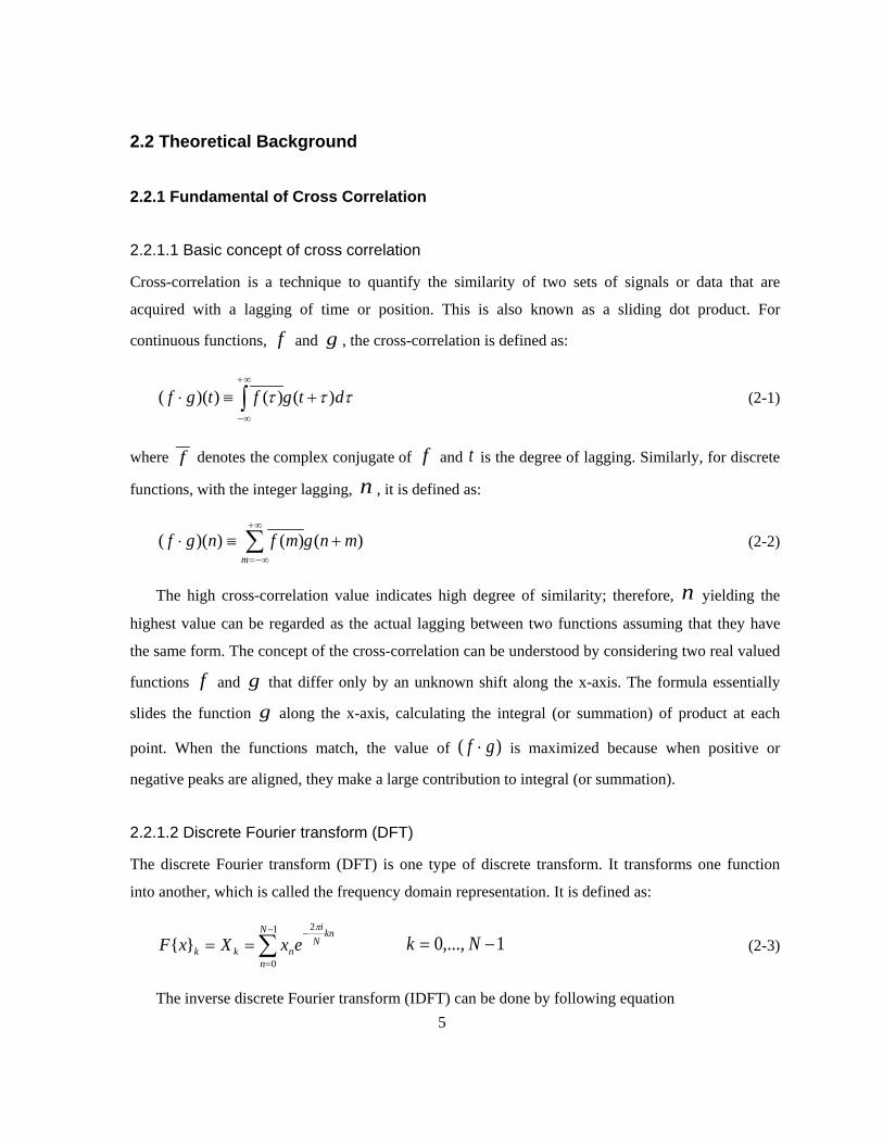
2.2.1.1 Basic concept of cross correlation
Cross-correlation is a technique to quantify the similarity of two sets of signals or data that are
acquired with a lagging of time or position. This is also known as a sliding dot product. For
continuous functions, f and g , the cross-correlation is defined as:
τττ dtgftgf )()())((∞
∞
+≡⋅ ∫+
−
(2-1)
where f denotes the complex conjugate of f and t is the degree of lagging. Similarly, for discrete
functions, with the integer lagging, n , it is defined as:
∑+
−=
+≡⋅∞
∞)()())((
mmngmfngf (2-2)
The high cross-correlation value indicates high degree of similarity; therefore, n yielding the
highest value can be regarded as the actual lagging between two functions assuming that they have
the same form. The concept of the cross-correlation can be understood by considering two real valued
functions f and g that differ only by an unknown shift along the x-axis. The formula essentially
slides the function g along the x-axis, calculating the integral (or summation) of product at each
point. When the functions match, the value of )( gf ⋅ is maximized because when positive or
negative peaks are aligned, they make a large contribution to integral (or summation).
2.2.1.2 Discrete Fourier transform (DFT)
The discrete Fourier transform (DFT) is one type of discrete transform. It transforms one function
into another, which is called the frequency domain representation. It is defined as:
∑−
=
−==
1
0
2
}{N
n
knN
i
nkk exXxFπ
1,...,0 −= Nk (2-3)
The inverse discrete Fourier transform (IDFT) can be done by following equation

6
∑−
=
− ==1
0
21 1}{
N
k
knN
i
knn eXN
xXFπ
1,...,0 −= Nn (2-4)
2.2.1.3 Convolution, and Convolution theorem
In mathematics convolution is a mathematical operation of two functions f and g producing a
third function that is usually considered as modified version of one of the original functions by the
other function called weighting function. It is defined as the integral of the product of the two
function after one is reversed and shifted by t .
∫+
−
−≡∗∞
∞
)()())(( τττ dtgftgf (2-5)
It may be described as the average of the function f at the moment t weighted by the reverse of the
function g . Similarly for discrete functions, it is defined as:
∑+
−=
−≡∗∞
∞)()())((
mmngmfngf
(2-6)
And assuming f and g are periodic with period N and if we limit the duration to the interval [0, N-
1], the equation can be modified to
∑=
−≡∗1-N
0)()())((
mmngmfngf (2-7)
We can apply the convolution theorem to this equation. The convolution theorem states that the
Fourier transform of a convolution is the pointwise product of Fourier transforms. In this case it is
expressed as:
kkkm
yFxFmnymxF }{}{})()({1-N
0⋅=−∑
=
1,...,0 −= Nk (2-8)
7
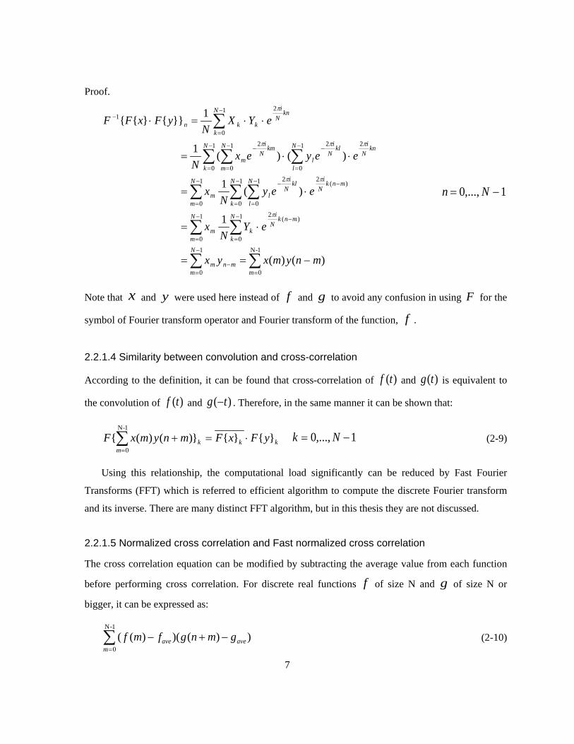
Proof.
∑∑
∑∑
∑ ∑∑
∑∑ ∑
∑
=
−
=−
−−
=
−
=
−−
=
−−
=
−
=
−−
=
−
=
−−
=
−
=
−
−==
⋅=
⋅=
⋅⋅=
⋅⋅=⋅
1-N
0
1
0
)(21
0
1
0
)(21
0
21
0
1
0
221
0
1
0
21
0
21
0
1
)()(
1
)(1
)()(1
1}}{}{{
m
N
mmnm
mnkN
iN
kk
N
mm
mnkN
iN
k
klN
iN
ll
N
mm
knN
iklN
iN
ll
N
k
kmN
iN
mm
knN
i
k
N
kkn
mnymxyx
eYN
x
eeyN
x
eeyexN
eYXN
yFxFF
π
ππ
πππ
π
1,...,0 −= Nn
Note that x and y were used here instead of f and g to avoid any confusion in using F for the
symbol of Fourier transform operator and Fourier transform of the function, f .
2.2.1.4 Similarity between convolution and cross-correlation
According to the definition, it can be found that cross-correlation of )(tf and )(tg is equivalent to
the convolution of )(tf and )( tg − . Therefore, in the same manner it can be shown that:
kkkm
yFxFmnymxF }{}{})()({1-N
0⋅=+∑
=
1,...,0 −= Nk (2-9)
Using this relationship, the computational load significantly can be reduced by Fast Fourier
Transforms (FFT) which is referred to efficient algorithm to compute the discrete Fourier transform
and its inverse. There are many distinct FFT algorithm, but in this thesis they are not discussed.
2.2.1.5 Normalized cross correlation and Fast normalized cross correlation
The cross correlation equation can be modified by subtracting the average value from each function
before performing cross correlation. For discrete real functions f of size N and g of size N or
bigger, it can be expressed as:
∑=
−+−1-N
0))()()((
maveave gmngfmf (2-10)

8
Note that since we are dealing with real value, complex conjugate symbol is not used here.
Digital image is a matrix of pixels, and for 8-bit grey image each pixel is expressed in terms of
numeric between 0 and 255. The tone gradually changes from black to white as the value increases
from 0 to 255. When the functions f and g are cross correlated by Eq. (2-2) the contributions from
the pixels with a high grey value are maximized; however, those from the pixels with low grey values
are ignored. Eq. (2-10) makes the minimum values negative peaks and take full advantage of the
contribution of them while keeping the maximum values as positive peak and their contribution. It
also produces negative contribution when two opposite values overlap. Therefore, the resulting
correlation values have a better contrast in expressing similarity.
The accuracy of cross-correlation can be further improved by normalizing Eq. (2-10) as:
5.01-N
0
2,
1-N
0
2
1-N
0,
]))((}{))(([{
))()()((
∑∑
∑
==
=
−+−
−+−
mnave
mave
mnaveave
gmngfmf
gmngfmf (2-11)
This is called the normalized cross correlation (NCC) and yields a value of 1 when two data sets are
exactly matched and close to 0 when no match is made. Note that in real application g is not
periodic and its size is usually bigger than the size of f . Due to the non-periodicity of g and size
differences between f and g , computational problems arise. Looking into the numerator which is
the same as Eq.(2-10) and the second half of the denominator of Eq. (2-11), respectively, we have,
∑∑
∑∑
==
==
+−+=
−+=−+−
1-N
0
1-N
0
,
1-N
0
1-N
0,
)()()(
)()())()()((
mave
m
avenavemm
naveave
mngfmngmf
fNgmngmfgmngfmf (2-12)
21-N
0
1-N
0
2
1-N
0,
1-N
0
2
1-N
0
2,,
21-N
0
2,
})({1})({
)(})({
})(2)({))((
∑∑
∑∑
∑∑
==
==
==
+−+=
+−+=
++−+=−+
mm
mnave
m
mnavenave
mnave
mngN
mng
mnggmng
ggmngmnggmng
(2-13)
9
When the sizes of f and g are different, we cannot apply convolution theorem and FFT to the
first term of Eq. (2-12), ∑=
+1-N
0)()(
mmngmf resulting in huge computation load. Nevertheless, this can
be easily solved by padding zeros to f and increasing its size up to that of g . However, the terms,
∑=
+1-N
0)(
mmng and ∑
=
+1-N
0
2})({m
mng are still problematic regarding the computational load as the
number of n increases since one has to calculate the local sum of g and 2g for each n . This
problem can be relieved by adopting the sum table suggested by Louis [11]. Sum table is the pre-
calculated look-up table over the whole region of function g , and is referred to each time local sum
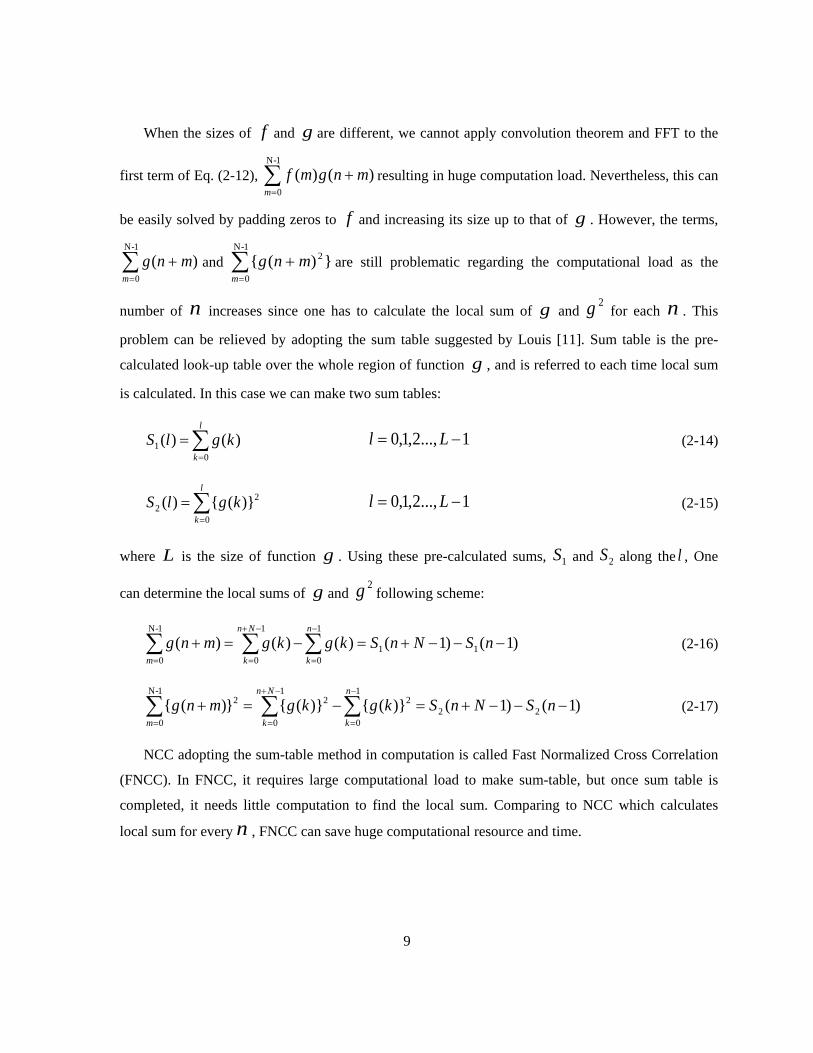
is calculated. In this case we can make two sum tables:
∑=
=l
kkglS
01 )()( 1...,2,1,0 −= Ll (2-14)
∑=
=l
kkglS
0
22 )}({)( 1...,2,1,0 −= Ll (2-15)
where L is the size of function g . Using these pre-calculated sums, 1S and 2S along the l , One
can determine the local sums of g and 2g following scheme:
)1()1()()()( 11
1
0
1
0
1-N
0−−−+=−=+ ∑∑∑
−
=
−+
==
nSNnSkgkgmngn
k
Nn
km (2-16)
)1()1()}({)}({})({ 22
1
0
21
0
221-N
0−−−+=−=+ ∑∑∑
−
=
−+
==
nSNnSkgkgmngn
k
Nn
km (2-17)
NCC adopting the sum-table method in computation is called Fast Normalized Cross Correlation
(FNCC). In FNCC, it requires large computational load to make sum-table, but once sum table is
completed, it needs little computation to find the local sum. Comparing to NCC which calculates
local sum for every n , FNCC can save huge computational resource and time.
10
2.2.1.6 Multidimensional expansion and its application to images processing (DIC and DVC)
The concepts of DFT, convolution, cross-correlation, NCC, and FNCC can be expanded to
multidimensional function or dataset. For digital-image-processing, 2D and 3D images are usually
expressed positive two-dimensional and three-dimensional matrix of pixels, respectively. Applying
the above algorithms one can track points of interesting by finding the maximum cross-correlation
value effectively while sliding latter images over the original or previous image with high efficiency.
Based on this, DIC (Digital Image Correlation) and DVC (Digital Volume Correlation) algorithms
have been developed for 2D images with 2D matrix data sets and for 3D images composed of 2D
image stacks, respectively, using Matlab.
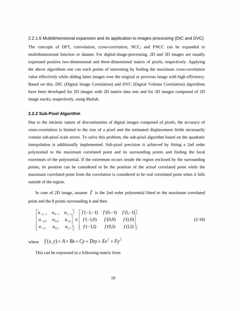
2.2.2 Sub-Pixel Algorithm
Due to the intrinsic nature of discontinuities of digital images composed of pixels, the accuracy of
cross-correlation is limited to the size of a pixel and the estimated displacement fields necessarily
contain sub-pixel scale errors. To solve this problem, the sub-pixel algorithm based on the quadratic
interpolation is additionally implemented. Sub-pixel precision is achieved by fitting a 2nd order
polynomial to the maximum correlated point and its surrounding points and finding the local
extremum of the polynomial. If the extremum occurs inside the region enclosed by the surrounding
points, its position can be considered to be the position of the actual correlated point while the
maximum correlated point from the correlation is considered to be real correlated point when it falls
outside of the region.
In case of 2D image, assume f is the 2nd order polynomial fitted to the maximum correlated
point and the 8 points surrounding it and then
−−
−−−−≅
−
−
−−−−
)1,1()1,0()1,1()0,1()0,0()0,1()1,1()1,0()1,1(
1,11,01,1
0,10,00,1
1,11.01,1
fffffffff
uuuuuuuuu
(2-18)
where22),( FyExDxyCyBxAyxf +++++=
This can be expressed in a following matrix form
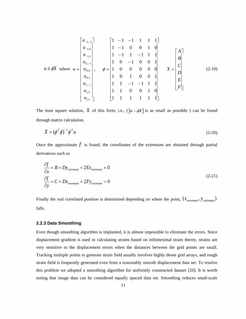
11
Xu φ≅ where
=
−−
−−−
−−−
=
=
−
−
−
−
−−
FEDCBA
X
uuuuuuuuu
u
111111010011111111100101000001100101111111010011111111
,
1,1
0,1
1,1
1,0
0,0
1,0
1,1
0,1
1,1
φ (2-19)
The least square solution, X of this form, i.e., ( Xu φ− is as small as possible ) can be found
through matrix calculation.
uX TT φφφ 1)( −= (2-20)
Once the approximate f is found, the coordinates of the extremum are obtained through partial
derivatives such as
02
02
=++=∂∂
=++=∂∂
extremumextremum
extremumextremum
FyDxCyf
ExDyBxf
(2-21)
Finally the real correlated position is determined depending on where the point, ),( extremumextremum yx
falls.
2.2.3 Data Smoothing
Even though smoothing algorithm is implanted, it is almost impossible to eliminate the errors. Since
displacement gradient is used in calculating strains based on infinitesimal strain theory, strains are
very sensitive to the displacement errors when the distances between the grid points are small.
Tracking multiple points to generate strain field usually involves highly dense grid arrays, and rough
strain field is frequently generated even from a reasonably smooth displacement data set. To resolve
this problem we adopted a smoothing algorithm for uniformly constructed dataset [20]. It is worth
noting that image data can be considered equally spaced data set. Smoothing reduces small-scale
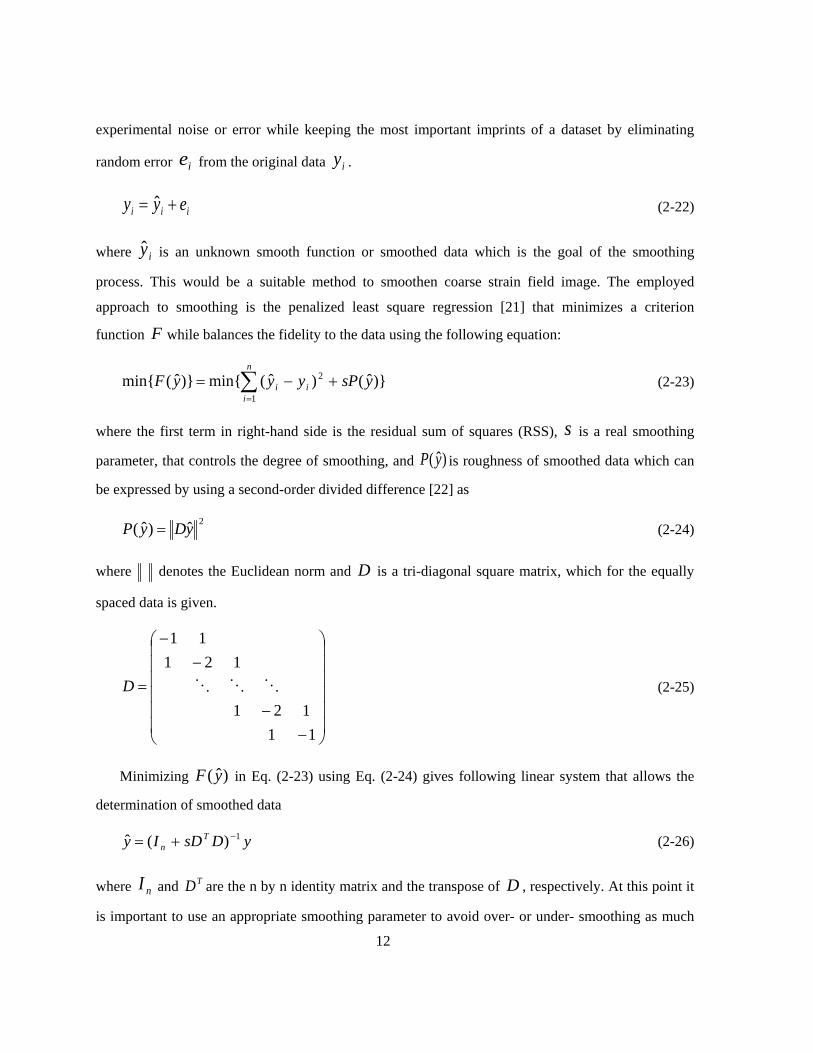
12
experimental noise or error while keeping the most important imprints of a dataset by eliminating
random error ie from the original data iy .
iii eyy += ˆ (2-22)
where iy is an unknown smooth function or smoothed data which is the goal of the smoothing
process. This would be a suitable method to smoothen coarse strain field image. The employed
approach to smoothing is the penalized least square regression [21] that minimizes a criterion
function F while balances the fidelity to the data using the following equation:
)}ˆ()ˆ(min{)}ˆ(min{1
2 ysPyyyFn
iii +−= ∑
=
(2-23)
where the first term in right-hand side is the residual sum of squares (RSS), s is a real smoothing
parameter, that controls the degree of smoothing, and )ˆ(yP is roughness of smoothed data which can
be expressed by using a second-order divided difference [22] as
2ˆ)ˆ( yDyP = (2-24)
where denotes the Euclidean norm and D is a tri-diagonal square matrix, which for the equally
spaced data is given.
−−
−−
=
11121
12111
D (2-25)
Minimizing )ˆ(yF in Eq. (2-23) using Eq. (2-24) gives following linear system that allows the
determination of smoothed data
yDsDIy Tn
1)(ˆ −+= (2-26)
where nI and TD are the n by n identity matrix and the transpose of D , respectively. At this point it
is important to use an appropriate smoothing parameter to avoid over- or under- smoothing as much
13
as possible. Such a correct value can be estimated by the method of generalized cross validation(GCV)
introduced by Wahba [21]. Assuming that one wants to solve the smoothing linear system
ysHy )(ˆ = (2-27)
where H is the so-called hat matrix ( here, 1)()( −+= DsDIsH Tn ), the GCV method picks the
parameter s that minimizes the GCV score given by
21
2
)/)(1(
/)ˆ()(
nHTr
nyysGCV
n
iii
−
−≡∑= (2-28)
where Tr denotes the matrix trace, which can be simply reduced to
∑= +
=n
i isHTr
121
1)(λ
(2-29)
where nii ,...,2,12 )( =λ are the eigenvalues of DDT . The GCV score thus reduces to
2
12
1
2
)1
1(
)ˆ()(
∑
∑
=
=
+−
−≡ n
i i
n
iii
sn
yynsGCV
λ
(2-30)
By finding the s value that minimizes the GCV score yielded by Eq. (2-30) makes the
smoothing algorithm fully automated. However, because the components of y appear in the
expression of the GCV score, y has to be calculated at each step of the minimization process
resulting in huge computational load. Nonetheless in our case this can be avoided since the data set is
equally spaced.
An eigendecomposition of the tri-diagonal square matrix D for the equally spaced yields
1−Λ= UUD (2-31)
where Λ is the diagonal matrix containing the eigenvalues of D defined by Yueh [23]:
),...,( 1 ndiag λλ=Λ with )/)1cos((22 nii πλ −+−= (2-32)
14
and U is a unitary matrix (i.e. TUU =−1 and nT IUU = ), in which TU and U are n-by-n type-2
discrete cosine transform (DCT) and inverse discrete cosine transform matrices (IDCT), respectively
[24]. Therefore, we can rewrite Eq. (2-26)
))(()(ˆ 12 yDCTIDCTyUUyUsIUy TTn Γ=Γ≡Λ+= − (2-33)
where the components of the diagonal matrix Г are given by
jiifandnis iiii ≠=Γ−−+=Γ − 0]))/)1cos((22(1[ ,12
, π (2-34)
Moreover, using Eq.(2-33). the residual sum of squares (RSS) can be written as
∑
∑
=
−
=
−+
=
−Λ+=
−=−
n
ii
i
nn
n
iii
yDCTs
yDCTIsI
yyyy
1
222
212
2
1
2
)()11
1(
)())((
ˆ)ˆ(
λ
(2-35)
where iDCT refers to the i th component of the discrete cosine transform. Note unitary
matrix preserves length. Substituting Eq. (2--34) into Eq. (2-30) gives
2
12
1
222
)1
1(
)()11
1()(
∑
∑
=
=
+−
−+
≡ n
i i
n
ii
i
sn
yDCTs
nsGCV
λ
λ (2-36)
The computation of the GCV score from this equation is straightforward and does not require any
matrix operation and manipulation, which makes the automated smoothing very fast. Once s value is
determined, smoothed function, y can be obtained by Eq. (2-26).
15
2.3 The Application of Digital Image Techniques to Determine the Large Stress-Strain Behaviours of Soft Materials
2.3.1 Introduction
Soft materials such as elastomers, hydrogels and biological tissues have much more complex
behaviours and are less understood than pure solids and liquids, but play increasingly important roles
in biomedical engineering and micro to nano scale technologies [25-29]. For instance, polyacrylamide
chemical gels are employed as the substrate in cell mechanics studies [30], while silicone rubbers are
used as implantable cosmetic reconstructive materials due to their biocompatibility and tissue-like
mechanical properties [1]. One of the applications in which reliable mechanical properties might be
critical is the injection of bio-polymer based hydrogels into the highly stressed environment of the
heart wall to ward off end stage heart failure[31].
Accurate strain measurement in a large deformation region is particularly challenging for soft
materials. Standard tensile test schemes [32,33] use dumbbell shaped specimens. These schemes
minimize the effect of grip region tri-axial stress state observed in stress-strain results generated with
straight (strip) specimens [34] , but typically necessitate the use of contact type sensors to isolate
gauge section response from the overall deformation. Unfortunately the stiffness of contact type
sensors prevents their applications to soft materials. Under the assumption that deformation primarily
takes place in the gauge section, gauge response is frequently approximated by overall elongation
[35-37]. However, at high strains deformation outside the gauge section becomes considerable which
makes this approach inaccurate [37]. Recognizing this problem, some researchers introduced a
constant correction factor determined by manual measurement or FEM (finite element method)
simulation, to convert the overall strain to the gauge section strain [37]. Use of a constant correction
factor is valid at small strains or when a constant ratio is maintained between strains inside and
outside of the gauge section; however, the nonlinear stress-strain relationships common in soft
materials result in strain ratios that are functions of elongation. Another confounding factor when
gauge length elongation is not directly measured is the slip between the sample and the grips [38,39].
Self tightening grips may not respond properly to specimens below certain stiffness while fixed grips
cannot respond to the thickness reduction induced by an axial deformation.
To directly measure the gauge section strains, non-contact sensors such as video and laser
extensometers are used. Analyzing video data from a tensile test using digital image cross correlation
16
(DIC) [16,40,41] is one of the most popular methods since it can measure the strain field in a large
domain. This method tracks the movement of multiple points on the sample surface by comparing
images from different deformed states to a reference image. Using relative displacements of the
points the complete strain field can be estimated with sub-pixel accuracy [7,16].
Two types of referencing schemes are possible. Under fixed referencing an image from the
undeformed state is used as a reference image [42]. This scheme is not susceptible to accumulated
error as all comparisons are made back to the undeformed state; however, when specimen
deformation becomes severe the difference between images may prevent accurate results from being
obtained. Dynamic referencing overcomes this difficulty by using the previous deformed state as a
reference but at the cost of allowing the potential for accumulated error. Many studies, e.g. [40,43] ,
have used DIC to characterize mechanical properties of materials; however, few studies published in
the open literature have considered the effect of referencing scheme on the performance of DIC. This
may be partly because the commercial codes utilized do not allow dynamic referencing [44].
This study used polydemethylsiloxane (PDMS) elastomer as a model soft material due to its
purely elastic behaviour and the ease of fabrication. There have been a few studies applying DIC to
PDMS under several deformation modes, (Berfield et. al. [40]: under tensile, Nunes [41]: under
shear); however, these studies were limited to the small deformation regime. This study investigated
the performance of various testing methods including DIC by applying them to large deformation of
PDMS, and validated the results with virtual test procedure. We expect that the testing methods
proposed in this study can be applied to characterize the large deformation behaviour of other soft
materials.
2.3.2 Experimental
2.3.2.1 Specimen preparation
PDMS was prepared from a two-component kit (Sylgard Elastomer 184, Dow Corning Corporation,
Midland, MI). The base and cross-linker were mixed at a ratio of 10:1 for 10 minutes, degassed in a
desiccator for 15 minutes and cast into a Teflon mold. Samples were cured in an oven at 90 °C for 90
minutes under an unconfined condition, i.e. the mold was not capped during curing. Dumbbell and
strip specimens with geometries shown in Fig. 2.1(a) were produced.
17
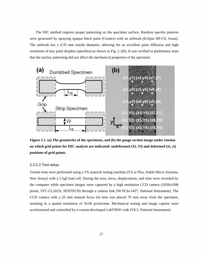
The DIC method requires proper patterning on the specimen surface. Random speckle patterns
were generated by spraying opaque black paint (Createx) with an airbrush (Eclipse HP-CS, Iwata).
The airbrush has a 0.35 mm nozzle diameter, allowing for an excellent paint diffusion and high
resolution of tiny paint droplets (speckles) as shown in Fig. 2.1(b). It was verified in preliminary tests
that the surface patterning did not affect the mechanical properties of the specimen.
Figure 2.1. (a) The geometries of the specimens, and (b) the gauge section image under tension
on which grid points for DIC analysis are indicated: undeformed (Xi, Yi) and deformed (xi, yi)
positions of grid points.
2.3.2.2 Test setup
Tensile tests were performed using a TA material testing machine (TA.xt Plus, Stable Micro Systems,
New Jersey) with a 5 kgf load cell. During the tests, force, displacement, and time were recorded by
the computer while specimen images were captured by a high resolution CCD camera (1028x1008
pixels, STC-CL202A, SENTECH) through a camera link (NI PCIe-1427, National Instrument). The
CCD camera with a 25 mm manual focus iris lens was placed 70 mm away from the specimen,
resulting in a spatial resolution of 56.06 pixels/mm. Mechanical testing and image capture were
synchronized and controlled by a custom developed LabVIEW code (V8.5, National Instrument).
18
2.3.2.3 Tensile tests
Both dumbell and strip type specimens were used for tensile tests. To determine the influence of strip
specimen aspect ratio, the length to width ratio was varied between 1 and 15, (L0/W in Fig. 2.1(a)).
Cyclic tensile tests, consisting of five loading-unloading cycles, were used to examine the error
accumulation and grip slippage. In each cycle, tensile loading was applied until the engineering stress
reached 2 MPa. Unloading continued until the cross-head returned to its initial position. Between
cycles any residual compressive stress or change in specimen shape was noted and released by
moving the cross-head until the load became zero. Ultimate tensile tests were also conducted to
determine the overall stress-strain curve and failure point. A constant crosshead speed of 12mm/min
was used for all tests (loading and unloading).
2.3.2.4 Stress / Strain calculation
Engineering stress, Eσ and strain, Eε were calculated using the following relationships,
0AF
E =σ
(2-37)
0LL
E∆
=ε
(2-38)
where F is the force measured by the load cell, 0A initial cross-sectional area, 0L original length and
L∆ elongation. Strains were estimated in two ways. In conventional testing schemes (CS) using
overall elongation [33-35], crosshead displacement was measured to be used as L∆ in Eq. (2-38). In
the tests using dumbbell specimens, GL in Fig. 2.1(a) was taken as 0L , while initial distance
between the grips was regarded as 0L for strip specimens. In DIC method (DIC), nine rectangular
grid points were chosen in the middle of the gauge section following ASTM standard [45] to be
tracked by the FNCC algorithm, as shown in Fig. 2.1(b). The engineering strain was calculated by
averaging the strains of those points as:
)()()(
741963
741963741963
0 YYYYYYYYYYYYyyyyyy
LL
E −−−++−−−++−−−−++
=∆
=ε (2-39)
19
where iY are the y-directional coordinates of grid points on the undeformed image, and iy y-
coordinates of the same grid points on the deformed images tracked by DIC. True strains in x- and y-
axis directions were also calculated from the displacements of grid points as
)()(lnln)(
741963
741963
0 XXXXXXxxxxxx
LLf
Tx −−−++−−−++
==ε (2-40)
)()(lnln)(
741963
741963
0 YYYYYYyyyyyy
LLf
Ty −−−++−−−++
==ε (2-41)
Note that displacement rate (i.e. infinitesimal strains, )//(5.0 ijjiij xuxu ∂∂+∂∂=ε ) are commonly
adopted for strains in DIC applications; however, this is not valid in large deformations.
By assuming a plane stress condition in the gauge section, Poisson’s ratio ν was determined by
using Eqs. 2-40 and 2-41:
Ty
Tx
)()(
εεν −=
(2-42)
2.3.2.5 DIC optimization
The effect of referencing scheme on DIC performance was investigated by applying fixed and
dynamic referencing schemes to a simple tensile test. Images were taken during the test using the
dumbbell specimen elongated up to 70 %. The images were analyzed using both schemes.
The effect of frame rate using dynamic referencing was examined by a simple translation test. In
this test a speckle patterned glass plate clamped in the TA testing machine was moved vertically
upward at a speed of 20 µm/s while pictures were taken at 5 frames per second. Different frame rates
of 2.5, 1.67, 1.25, 1, 0.5, 0.25, 0.125, and 0.066 fps were achieved by skipping images at fixed
intervals in the DIC analysis to simulate a range of frame rates. The corresponding displacements of
the reference image were 0.112, 0.224, 0.449, 0.676, 0.897, 1.121, 2.24, 4.49, 8.97, and 17.94 pixels
per frame. Error was determined by comparing the average displacement calculated for nine points to
the known displacement.

20
2.3.2.6 Virtual tensile test
To estimate the accuracies of the stress-strain curves determined by various testing methods, tensile
tests were simulated using FEM. In this simulation, load-displacement curves were produced by 3-D
FEM model (ABAQUS 6.5 Standard) of dumbbell specimen consisting of 1024 20-node quadratic
brick elements, employing each stress-strain curve as a material property. Considering the
geometrical symmetry of the specimens, only half quarters of the specimens were modeled. The
empirical constitutive equation obtained through curve-fitting to experimental stress-strain curve was
coded into the FEM model using UMAT that is a user-defined module in ABAQUS for material
properties.
Since the empirical constitutive equation is highly nonlinear, the stress-strain relationship based
on linear elasticity (Hooke’s law) cannot be used for UMAT. Also other nonlinear elastic stress-strain
functions provided by ABAQUS such as hyperelasticity cannot be matched with the stress-strain
curve. Therefore, new stress-strain relations based on the proposed constitutive equation should be
defined. For this, experimentally determined uniaxial stress-strain curve was regarded as effective
stress-strain curve, and assumed to be the stress function for the deformation. For monotonically
increasing loading, nonlinear elastic deformation and plastic deformation cannot be discerned;
therefore, the incremental deformation theory of plasticity [46] could be invoked as:
)(εσ f=
(2-43)
[ ])( zyxx dddddd σσνσσεε +−=
(2-44)
[ ])( xzyy dddddd σσνσσεε +−=
(2-45)
[ ])( yxzz dddddd σσνσσεε +−=
(2-46)
xyxy dddd τσενγ )1(2 +=
(2-47)
yzyz dddd τσενγ )1(2 +=
(2-48)
21
zxzx dddd τσενγ )1(2 +=
(2-49)
where )(εσ f= is the newly proposed constitutive equation where σ and ε are the effective
stress and effective strain, respectively. ijdε and ijdγ are the strain increment tensors at each step.
2.3.3 Results and Discussion
2.3.3.1 DIC optimization
2.3.3.1.1 Referencing optimization
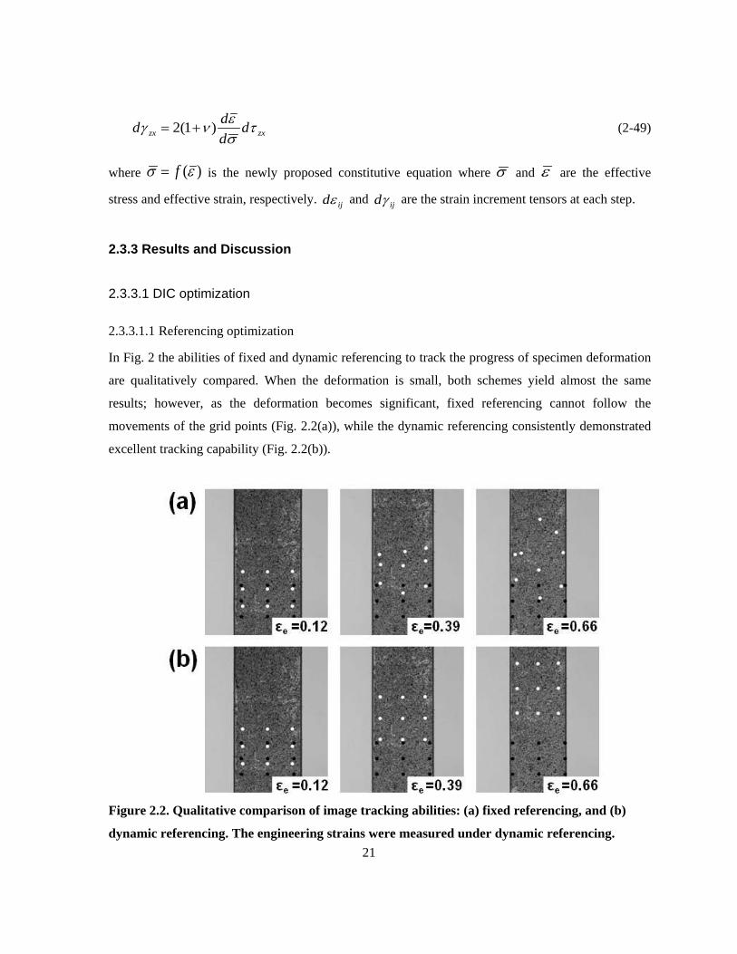
In Fig. 2 the abilities of fixed and dynamic referencing to track the progress of specimen deformation
are qualitatively compared. When the deformation is small, both schemes yield almost the same
results; however, as the deformation becomes significant, fixed referencing cannot follow the
movements of the grid points (Fig. 2.2(a)), while the dynamic referencing consistently demonstrated
excellent tracking capability (Fig. 2.2(b)).
Figure 2.2. Qualitative comparison of image tracking abilities: (a) fixed referencing, and (b)
dynamic referencing. The engineering strains were measured under dynamic referencing.
22
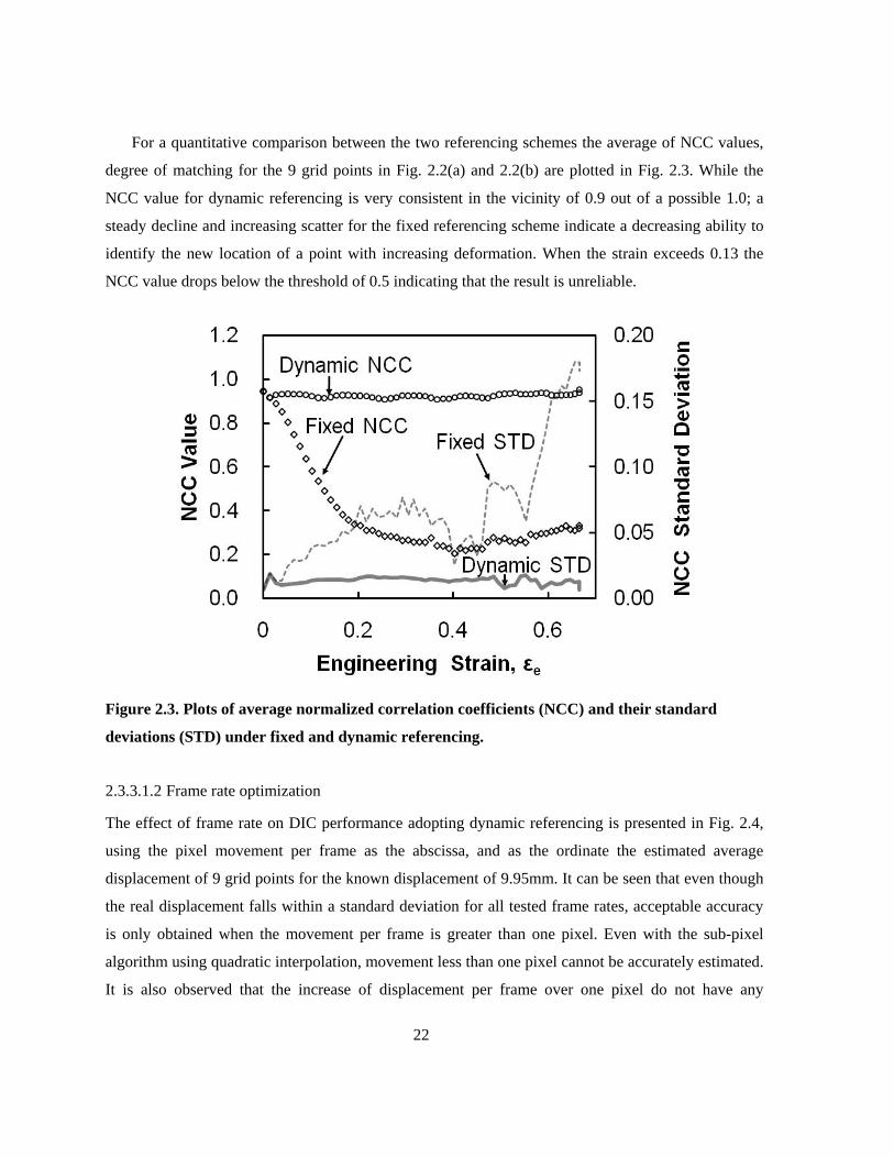
For a quantitative comparison between the two referencing schemes the average of NCC values,
degree of matching for the 9 grid points in Fig. 2.2(a) and 2.2(b) are plotted in Fig. 2.3. While the
NCC value for dynamic referencing is very consistent in the vicinity of 0.9 out of a possible 1.0; a
steady decline and increasing scatter for the fixed referencing scheme indicate a decreasing ability to
identify the new location of a point with increasing deformation. When the strain exceeds 0.13 the
NCC value drops below the threshold of 0.5 indicating that the result is unreliable.
Figure 2.3. Plots of average normalized correlation coefficients (NCC) and their standard
deviations (STD) under fixed and dynamic referencing.
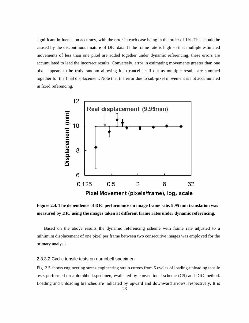
2.3.3.1.2 Frame rate optimization
The effect of frame rate on DIC performance adopting dynamic referencing is presented in Fig. 2.4,
using the pixel movement per frame as the abscissa, and as the ordinate the estimated average
displacement of 9 grid points for the known displacement of 9.95mm. It can be seen that even though
the real displacement falls within a standard deviation for all tested frame rates, acceptable accuracy
is only obtained when the movement per frame is greater than one pixel. Even with the sub-pixel
algorithm using quadratic interpolation, movement less than one pixel cannot be accurately estimated.
It is also observed that the increase of displacement per frame over one pixel do not have any
23
significant influence on accuracy, with the error in each case being in the order of 1%. This should be
caused by the discontinuous nature of DIC data. If the frame rate is high so that multiple estimated
movements of less than one pixel are added together under dynamic referencing, these errors are
accumulated to lead the incorrect results. Conversely, error in estimating movements greater than one
pixel appears to be truly random allowing it to cancel itself out as multiple results are summed
together for the final displacement. Note that the error due to sub-pixel movement is not accumulated
in fixed referencing.
Figure 2.4. The dependence of DIC performance on image frame rate. 9.95 mm translation was
measured by DIC using the images taken at different frame rates under dynamic referencing.
Based on the above results the dynamic referencing scheme with frame rate adjusted to a
minimum displacement of one pixel per frame between two consecutive images was employed for the
primary analysis.
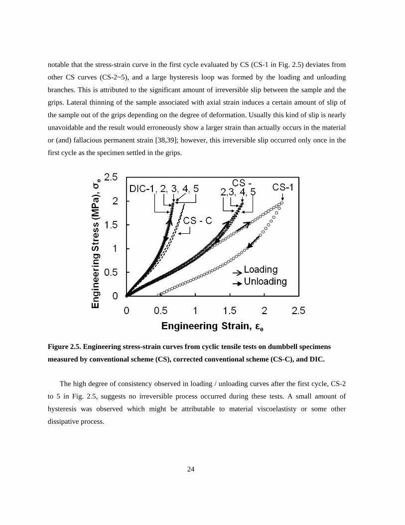
2.3.3.2 Cyclic tensile tests on dumbbell specimen
Fig. 2.5 shows engineering stress-engineering strain curves from 5 cycles of loading-unloading tensile
tests performed on a dumbbell specimen, evaluated by conventional scheme (CS) and DIC method.
Loading and unloading branches are indicated by upward and downward arrows, respectively. It is
24
notable that the stress-strain curve in the first cycle evaluated by CS (CS-1 in Fig. 2.5) deviates from
other CS curves (CS-2~5), and a large hysteresis loop was formed by the loading and unloading
branches. This is attributed to the significant amount of irreversible slip between the sample and the
grips. Lateral thinning of the sample associated with axial strain induces a certain amount of slip of
the sample out of the grips depending on the degree of deformation. Usually this kind of slip is nearly
unavoidable and the result would erroneously show a larger strain than actually occurs in the material
or (and) fallacious permanent strain [38,39]; however, this irreversible slip occurred only once in the
first cycle as the specimen settled in the grips.
Figure 2.5. Engineering stress-strain curves from cyclic tensile tests on dumbbell specimens
measured by conventional scheme (CS), corrected conventional scheme (CS-C), and DIC.
The high degree of consistency observed in loading / unloading curves after the first cycle, CS-2
to 5 in Fig. 2.5, suggests no irreversible process occurred during these tests. A small amount of
hysteresis was observed which might be attributable to material viscoelastisty or some other
dissipative process.
25
Little or no hysteresis was observed in DIC results which are all in good agreement with one
another and fall onto a single curve (DIC-1~5). This suggests that DIC method is highly robust to slip
and can yield consistent result irrespective of slip.
It is interesting to note that the DIC stress-strain curves are significantly different from those
given by CS-2~5, with the stress level in DIC curves more than twice of that in CS at the same strain.
It is known that the CS overestimates the strain due to the deformation outside the gauge section
[36,37]. Schneider et al. [37] multiplied the measured strain by a correction factor of m = 0.49~0.50
to convert the overall strain to gauge section strain. Following this scheme CS-C in Fig. 2.5 was
generated. While it is much closer to the DIC curve, differences still exist in magnitude of stress and
the level of hysteresis loop. Adjusting correction factor cannot resolve the difference.
The difference was further investigated to estimate the reliabilities of CS and DIC based
measurements.
2.3.3.3 Hysteresis analysis
Hysteresis loop in cyclic stress-strain curve is one of the properties typifying visco-elastic materials.
Other visco-elastic properties include stress relaxation and creep. To verify the visco-elastic
properties of tested PDMS, specimens were loaded at constant strain and at constant stress,
respectively, for 24 hours to investigate the stress relaxation and creep behaviours. The test results
(not included in this paper) show that stress relaxation or creep did not occur in the tested PDMS.
This is consistent with the previous reports suggesting that fully cured PDMS is purely elastic at room
temperature [47,48]. Therefore, we concluded that the tested PDMS should not have visco-elastic
properties and the hysteresis loop presented by CS-C curve must have come from some other cause.
Careful examination of the gripping area revealed that a small portion of the specimen slipped out
from the grip region under tensile loading but retracted to its original position when it was unloaded.
This slip resulted in a changing effective gauge length during CS based measurements. The frictional
forces between the grip surfaces and sample at the slip region oppose movement resulting in differing
effective gauge lengths at the same load in the loading and unloading branches, which should have
caused the hysteresis loop. The overlapping of the CS-2~5 curves indicated that this type of slip was
reversible and no sign of slip left after unloading, which makes the detection extremely difficult. On
the contrary, DIC measurements guarantee a constant gauge length and are made only in the middle
of the gauge section where the uniaxial stress assumption is most valid and so avoid this difficulty.
26
The fact that this slip in the grips can introduce hysteresis must be considered in studies dedicated to
viscoelastic properties, particularly in the large deformation/non-linear region.
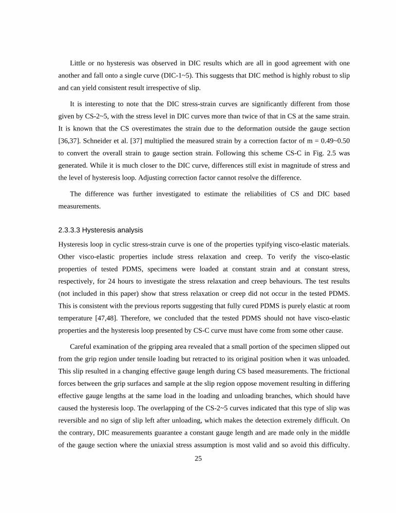
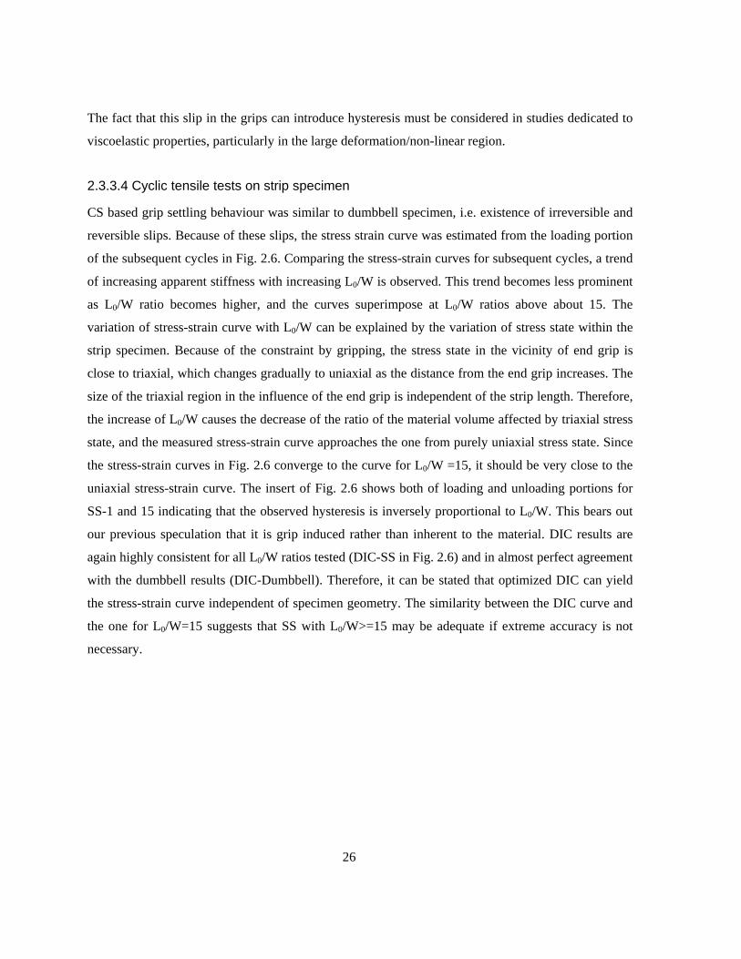
2.3.3.4 Cyclic tensile tests on strip specimen
CS based grip settling behaviour was similar to dumbbell specimen, i.e. existence of irreversible and
reversible slips. Because of these slips, the stress strain curve was estimated from the loading portion
of the subsequent cycles in Fig. 2.6. Comparing the stress-strain curves for subsequent cycles, a trend
of increasing apparent stiffness with increasing L0/W is observed. This trend becomes less prominent
as L0/W ratio becomes higher, and the curves superimpose at L0/W ratios above about 15. The
variation of stress-strain curve with L0/W can be explained by the variation of stress state within the
strip specimen. Because of the constraint by gripping, the stress state in the vicinity of end grip is
close to triaxial, which changes gradually to uniaxial as the distance from the end grip increases. The
size of the triaxial region in the influence of the end grip is independent of the strip length. Therefore,
the increase of L0/W causes the decrease of the ratio of the material volume affected by triaxial stress
state, and the measured stress-strain curve approaches the one from purely uniaxial stress state. Since
the stress-strain curves in Fig. 2.6 converge to the curve for L0/W =15, it should be very close to the
uniaxial stress-strain curve. The insert of Fig. 2.6 shows both of loading and unloading portions for
SS-1 and 15 indicating that the observed hysteresis is inversely proportional to L0/W. This bears out
our previous speculation that it is grip induced rather than inherent to the material. DIC results are
again highly consistent for all L0/W ratios tested (DIC-SS in Fig. 2.6) and in almost perfect agreement
with the dumbbell results (DIC-Dumbbell). Therefore, it can be stated that optimized DIC can yield
the stress-strain curve independent of specimen geometry. The similarity between the DIC curve and
the one for L0/W=15 suggests that SS with L0/W>=15 may be adequate if extreme accuracy is not
necessary.
27
Figure 2.6. Engineering stress-strain curves from the cyclic tensile tests on strip specimens.
2.3.3.5 Ultimate tensile tests
The results from ultimate tensile tests were analyzed by DIC and Schneider et al’s corrected
crosshead displacement scheme [37], CS-C. In Fig. 2.7 they are compared to the results obtained by
Khanafer and coworkers [49] for the same material using crosshead displacement. Note that Ref. [49]
proposed a 3rd order polynomial equation for the curve fitting. The curve from strip specimen for
L0/W=15 were converted into true stress-true strain curve using Eq. (2-41) and also plotted (SS) in
Fig. 2.7. Poisson’s ratio was required for this conversion of engineering stress into true stress. From
axial and transverse true strains measured by DIC and Eq. (2-42), Poisson’s ratio was determined to
be 0.5±0.03 which is consistent with the common belief that fully cross-linked PDMS is be
incompressible [50,51]. From this result, Poisson’s ratio was assumed to be 0.5.
28
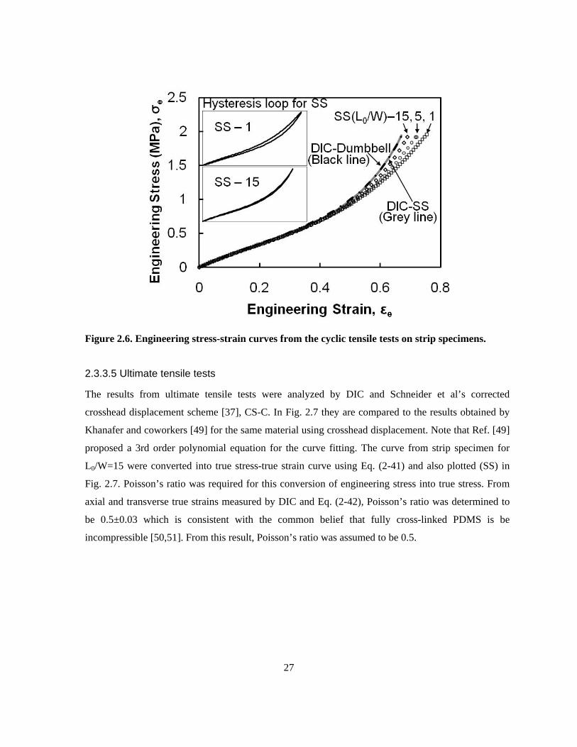
Figure 2.7. True stress-strain curves from DIC, SS, CS-C, and Ref. (49).
All four curves overlap in small strain region, showing almost linear increasing trend up to
around 0.2. They start rising exponentially beyond that strain, indicating that strain-hardening
becomes more significant with the progress of deformation. Different hardening behaviours are
demonstrated by different curves, with DIC being the most significant followed by SS, CS-C, and the
curve from Ref. [49]. DIC and SS curves look very similar; however, the magnified view in the insert
shows that there is a difference.
Note that the severe strain hardening behaviours in DIC or SS curves in Fig. 2.7 cannot be fitted
by the 3rd order polynomial proposed by Ref. [49]. We had also attempted to use common
constitutive models such as rubber elasticity [52], Mooney and Rivlin [53], BST equation[54], G’Sell
and Jonas [55] to describe the observed non-linear behaviours. However, none of them provided good
agreements except the BST equation, which has a very complex form with 4 fitting parameters. The
resulting fitting parameters in BST equation do not have any intrinsic meaning, and it is difficult to
make a link to the deformation mechanism [56].
Based on the observed strong strain-hardening behaviour with an almost vertical asymptote at
large strain, we proposed the following form of constitutive equation to describe the stress-strain
behaviour across large strain region:
29
−
+=T
AT
TT BE
εεεσ )(
(2-50)
where E is elastic modulus; A and B are two fitting constants related to the strain-hardening
behaviour. Eq. (2-50) has enough flexibility to fit all four curves in Fig. 2.7 almost perfectly using the
fitting constants in Table 2.1 that are evaluated by least square fitting method. The first term in Eq.
(2-50) dominates true stress when strain is small, while the importance of second term increases with
the increase of strain. Note that Eq. (2-50) has the vertical asymptote at BT =ε , which implies that
the stiffness approaches infinity as the strain is getting close to B . The specimen could not be
deformed up to asymptotic strain, as the specimen failed before gauge section strain reached that
strain because of the stress concentration at the round corner between gauge and nongauge sections.
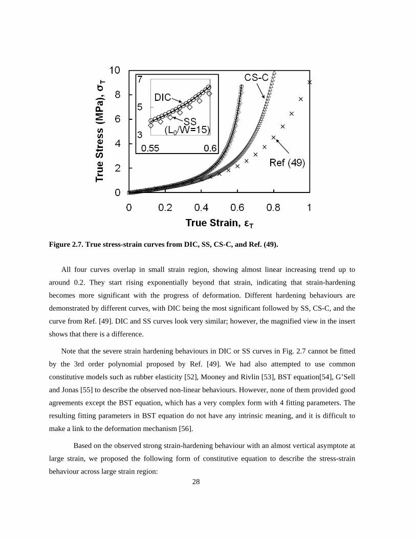
Table 2-1. Constants in Eq. (14) for the stress-strain curves from DIC, SS, CS-C, and Ref. (49)
E (MPa) A B
DIC 1.980 2.537 0.701
SS (L0/W=15) 1.922 2.610 0.704
CS-C 2.197 2.603 0.958
Ref. (49) 2.379 2.537 1.345
2.3.3.6 Virtual tensile test using FEM
Fig. 2.8 shows the load-displacement curves from the FEM simulations and the experiment. The FEM
simulation adopting the DIC stress-strain curve shows an excellent agreement with the experimental
data (circle), while other simulation results deviate from the experimental data in the similar manner
as their stress-strain curves deviate from DIC stress-strain curve. The deviations are noticeable in
large strain region; however, the magnified view in small strain region (insert in Fig. 2.8) also
illustrates that simulation result using DIC curve is in much better agreement with the experimental
data than any others. The errors between the load-displacement curves from the experiment and
simulations are quantified by using the R-squared value for the load-displacement curves, with R-
squared value being 1 when two curves are perfectly matched. Table 2.2 shows that the R-squared
value for the simulation curve adopting DIC stress-strain curve is almost 1, while those from other
simulations are getting lower than 1 in the order of SS, CS-C and literature. These results indicate that
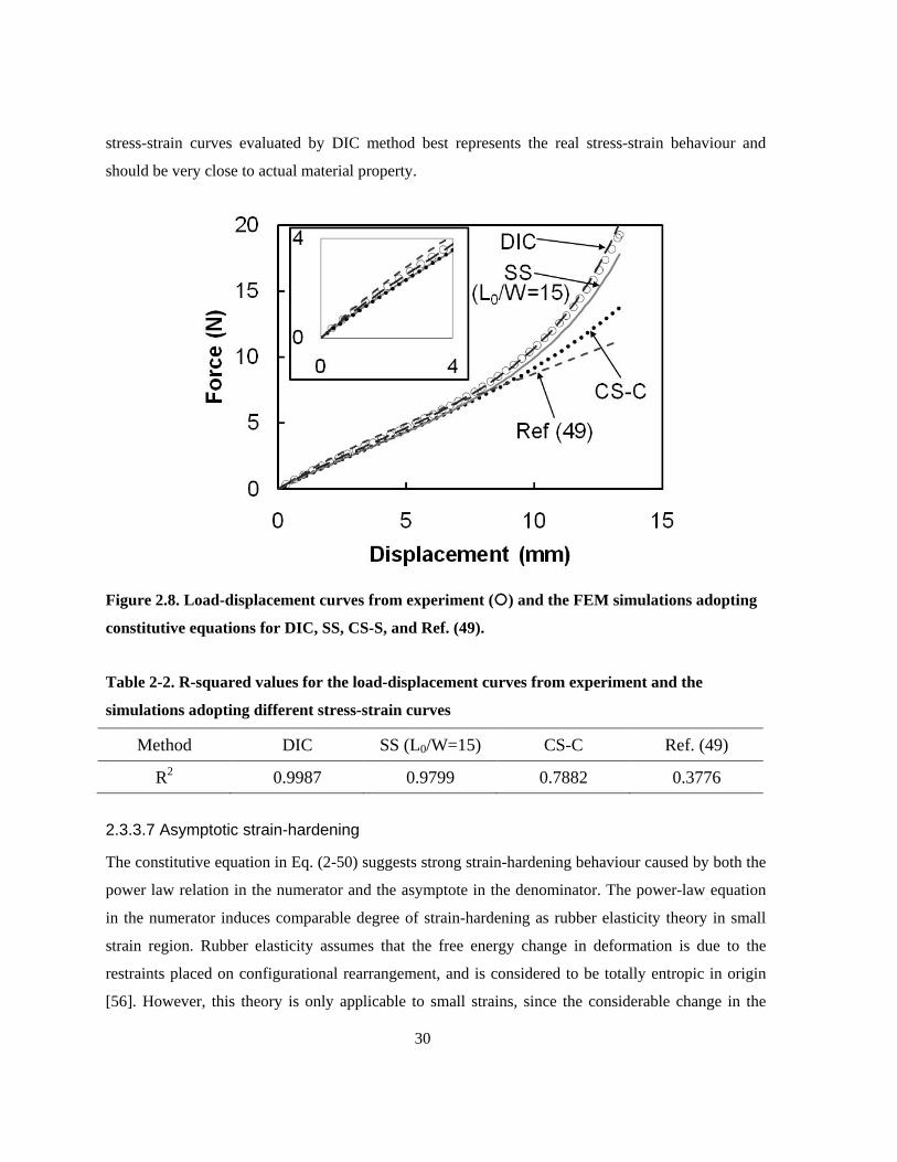
30
stress-strain curves evaluated by DIC method best represents the real stress-strain behaviour and
should be very close to actual material property.
Figure 2.8. Load-displacement curves from experiment () and the FEM simulations adopting
constitutive equations for DIC, SS, CS-S, and Ref. (49).
Table 2-2. R-squared values for the load-displacement curves from experiment and the
simulations adopting different stress-strain curves
Method DIC SS (L0/W=15) CS-C Ref. (49)
R2 0.9987 0.9799 0.7882 0.3776
2.3.3.7 Asymptotic strain-hardening
The constitutive equation in Eq. (2-50) suggests strong strain-hardening behaviour caused by both the
power law relation in the numerator and the asymptote in the denominator. The power-law equation
in the numerator induces comparable degree of strain-hardening as rubber elasticity theory in small
strain region. Rubber elasticity assumes that the free energy change in deformation is due to the
restraints placed on configurational rearrangement, and is considered to be totally entropic in origin
[56]. However, this theory is only applicable to small strains, since the considerable change in the
31
end-to-end distance of the network chains would distort the Gaussian distribution of the statistical
elements.
As the strain increases and approaches the asymptotic strain =Tε 0.701, different type of
hardening takes place in a much more significant manner. This strain hardening may be induced by
strain crystallization [57,58], alignment of covalent-bonded polymer chains in the stretching direction.
When PDMS is moderately deformed under tension, polymer chains are disentangled and re-oriented
to be aligned along the loading direction, which can be represented by the power law relation in the
numerator in Eq. (2-50) or rubber elasticity model. As the strain approaches asymptotic strain,
polymer chains are pulled taut that the forces are mostly carried by covalently bonded polymer chains,
and the measured stiffness approaches that of polymer chains. Since the covalent bonding is
extremely stiff compared to other types of bondings and stiffening mechanisms, the stress-strain
curve takes the form of vertical asymptote as presented in Fig. 2.7.
2.3.4 Conclusion
This study showed that the selection of reference image has a major influence on the accuracy of DIC
results and the adoption of dynamic referencing with a suitable frame rate in DIC analysis can yield
much better results than fixed referencing. Optimized DIC method was applied to a large deformation
of soft materials. PDMS was used as model soft material and its stress-strain relationship across a
large deformation region was evaluated. The comparative study of the stress-strain curves obtained
from the conventional tensile test schemes and DIC method suggested that the DIC technique is
robust to the slip between the sample and the grips while the accuracy of conventional test scheme is
highly affected. The true stress-strain relationship of PDMS in tension evaluated by DIC showed a
significant strain-hardening behaviour, with a vertical asymptote at strain =Tε 0.701. Based on this
behaviour a new type of constitutive equation was proposed to account for the significant strain-
hardening in large strain region, and showed excellent agreement with the experimental stress-strain
curves. FEM simulation adopting the constitutive equation successfully produced the load-
displacement curve showing excellent agreement with experimental data. This suggests that the
stress-strain curves determined by the DIC can be used to represent the actual stress-strain behaviour
of PDMS. Poisson’s ratio of PDMS was also verified to be 0.5 in tension. The optimized DIC
technique and analysis method used here may be able to be applied to the studies of other elastomers,
gels and biological tissues.
32
2.4 Diagnosis of Breast Tumour Using 2D and 3D Ultrasound Images
2.4.1 Introduction
Cancer is the top leading cause of death in North America [59,60]. Among the various cancers, breast
cancer is the most common malignancy in women and the second most common cause of cancer-
related death [60]. In the past several years, the early detection and treatment of breast carcinoma has
received increased attention [61]. Prior to the advent of diagnostic imaging, the detection involved
palpation. Malignant tumours feel harder than benign ones which is related to the pathological
changes in their elastic and visco-elastic mechanical properties [62]. While palpation is simple, it is
just a qualitative assessment and can only be applied to superficial organs. The results are also open
to user interpretation [63]. Recently mammography has been widely used for the early detection of
breast cancer [64]. Even though it has contributed to the reduction of mortality, high false positive
causing additional testing or biopsy, and the possibility of overdiagnosis and overtreatment arguably
outweigh the benefits [65]. The addition of MRI (magnetic resonance imaging) to the screening
algorithm adds considerable cost over $50,000 per cancer [64]. Ultrasound imaging is relatively
affordable and accessible; thus it has been given interests as a modality to supplement or replace
mammography, especially for the women with dense breasts [66]. However, in many cases, the lesion
may not possess sufficient echo graphic properties and therefore, it is hard to detect using B mode
ultrasound image (sonogram).
Recently, elastography has received an attention as a method to estimate the elastic properties of
biological tissues [62,67-70]. Elastograms are obtained by estimating the strain variations using the
time-gradient of ultrasound echo data, obtained before and after a slight compression of the tissue, i.e.
ab
abab
tttttte
11
221111
)()(−
−−−=
(2-51)
where 𝑡1𝑎 and 𝑡1𝑏 are the arrival times of the pre-compression echoes from the proximal and distal
windows, respectively; 𝑡2𝑎 and 𝑡2𝑏 are the arrival times of the post-compression echoes from the
proximal and distal windows, respectively [62]. The resulting strain fields are displayed as an image,
where soft areas appear white and hard areas appear black. The mean depth and width of the lesion on
the elastogram and sonogram were measured and used as parameter for differentiating benign and
33
malignant lesions [66,71,72]. Since elastogram images can be displayed almost simultaneously with
sonogram images, it is a very useful practice in diagnosing disease. However, it is hard to be used as a
tool for material characterization of tissues, as elastogram is highly degraded in large strain
deformations because of the decorrelation due to lateral and elevational deformation [69]. Moreover
the direction of loading should be the same as that of ultrasound wave; thus only the axial strain in the
loading direction can be estimated. Also the deformation under tension is hard to be investigated.
Other drawbacks include the lack of 3D capability.
We applied Digital Image Correlation (DIC) method to 2D sonogram images to characterize the
mechanical properties of the phantom mimicking breast tissue. The displacement and the strain fields
around the cylindrical inclusion were estimated by DIC implemented with smoothing algorithm.
Using the estimated strain field, the stiffness of the inclusion representing carcinoma could be
accurately estimated. This study was extended to full 3D analysis of 3D sonogram images using in-
house developed Digital Volume Correlation (DVC) algorithm. The 3D shape of the inclusion and the
stiffness of the inclusion can be estimated by this analysis.
2.4.2 Experimental
2.4.2.1 Sample Preparation
Soft and hard gels were made with 1% agarose (by weight), 2% glutar aldehide, 5% propanol, 5% and
20% gelatin, respectively, and water (the remaining weight %). Hard and soft gels were used for the
inclusion and the outer material, respectively.
Samples preparation procedure was as follows: After water was heated up to 85°C, agarose,
gelatin, and propanol were added in order. After 3 min of solution time, glutar-aldehide was added,
and was heated for 4 more min. The solution containing 20% gelatin was suck into a 3 ml syringe
(inner diameter of 8.6 mm) and kept at room temperature for 48 hours for gelation. Then, the
resulting gel was taken out and stored in water to prevent shrinkage. Using the same protocol, the
solution with 5% gelatin content was prepared and poured into a long cylindrical mold (diameter of 4
cm and height of 8 cm) in half. When temperature decreased to 35°C, the prepared inclusion
containing 20% gelatin was placed on top of the solution and gelled for 5 minutes. Then, the solution
was added up to the end of the mold and kept for 48 more hours. This procedure is illustrated in
shown in Fig. 2.9. The sample from this mold is referred as the phantom in the rest of the thesis.
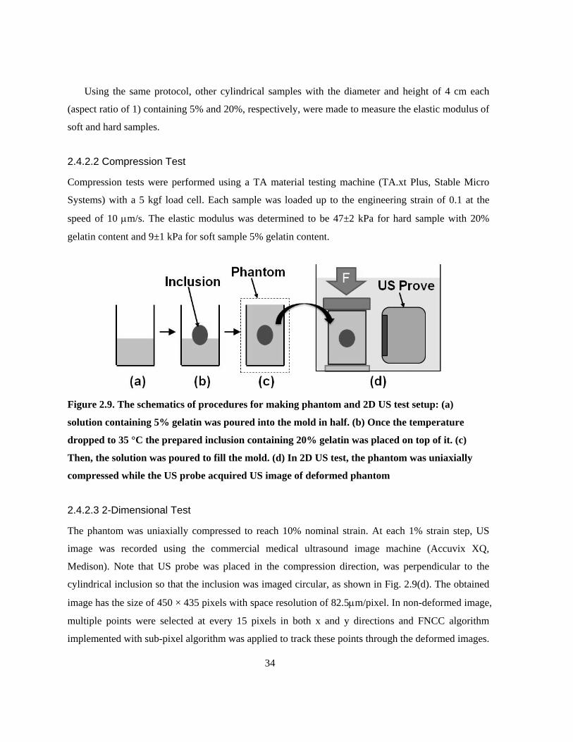
34
Using the same protocol, other cylindrical samples with the diameter and height of 4 cm each
(aspect ratio of 1) containing 5% and 20%, respectively, were made to measure the elastic modulus of
soft and hard samples.
2.4.2.2 Compression Test
Compression tests were performed using a TA material testing machine (TA.xt Plus, Stable Micro
Systems) with a 5 kgf load cell. Each sample was loaded up to the engineering strain of 0.1 at the
speed of 10 µm/s. The elastic modulus was determined to be 47±2 kPa for hard sample with 20%
gelatin content and 9±1 kPa for soft sample 5% gelatin content.
Figure 2.9. The schematics of procedures for making phantom and 2D US test setup: (a)
solution containing 5% gelatin was poured into the mold in half. (b) Once the temperature
dropped to 35 °C the prepared inclusion containing 20% gelatin was placed on top of it. (c)
Then, the solution was poured to fill the mold. (d) In 2D US test, the phantom was uniaxially
compressed while the US probe acquired US image of deformed phantom
2.4.2.3 2-Dimensional Test
The phantom was uniaxially compressed to reach 10% nominal strain. At each 1% strain step, US
image was recorded using the commercial medical ultrasound image machine (Accuvix XQ,
Medison). Note that US probe was placed in the compression direction, was perpendicular to the
cylindrical inclusion so that the inclusion was imaged circular, as shown in Fig. 2.9(d). The obtained
image has the size of 450 × 435 pixels with space resolution of 82.5µm/pixel. In non-deformed image,
multiple points were selected at every 15 pixels in both x and y directions and FNCC algorithm
implemented with sub-pixel algorithm was applied to track these points through the deformed images.

35
Since 10% strain is relatively large, instead of fixed reference scheme (using the non-deformed image
as the reference), dynamic referencing scheme (updating and using the previous deformed state as a
reference for the processing image) was employed. Based on the acquired relative displacements of
points of interests, displacement and strain (gradient of displacement) field were drawn in the
direction of compression.
2.4.2.4 3-Dimensional Test
For the 3D test the probe was installed on a motorized linear stage (T-LSM050A, Zaber) in the
direction perpendicular to the loading direction, as shown in the Fig. 2.10(a). 500 2D US images were
taken by moving the probe stepwise along the height of the sample before and after compression of 1%
strain. 3D image stacks were generated by piling up these 2D images as shown in Fig. 2.10(b).
Resulting 3D image has a size of 430 × 230 x 500 pixels. Tracking points were selected at every 10
pixels in all the direction from the undeformed 3D image. The modified FNCC algorithm was
employed to estimate the displacement of each tracking point. Based on the relative displacements of
the tracking points, displacement and strain fields were estimated in the direction of compression.
Figure 2.10. The schematic of 3D test. Lateral cross sectional 2D US images are taken moving
the position of the probe step by step along the sample. (b) 3D US images are generated by
stacking on 2D US images .
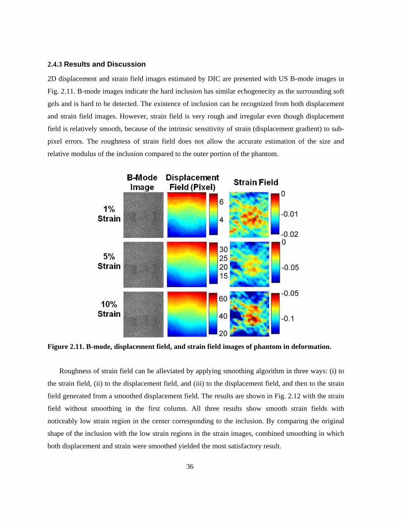
36
2.4.3 Results and Discussion
2D displacement and strain field images estimated by DIC are presented with US B-mode images in
Fig. 2.11. B-mode images indicate the hard inclusion has similar echogenecity as the surrounding soft
gels and is hard to be detected. The existence of inclusion can be recognized from both displacement
and strain field images. However, strain field is very rough and irregular even though displacement
field is relatively smooth, because of the intrinsic sensitivity of strain (displacement gradient) to sub-
pixel errors. The roughness of strain field does not allow the accurate estimation of the size and
relative modulus of the inclusion compared to the outer portion of the phantom.
Figure 2.11. B-mode, displacement field, and strain field images of phantom in deformation.
Roughness of strain field can be alleviated by applying smoothing algorithm in three ways: (i) to
the strain field, (ii) to the displacement field, and (iii) to the displacement field, and then to the strain
field generated from a smoothed displacement field. The results are shown in Fig. 2.12 with the strain
field without smoothing in the first column. All three results show smooth strain fields with
noticeably low strain region in the center corresponding to the inclusion. By comparing the original
shape of the inclusion with the low strain regions in the strain images, combined smoothing in which
both displacement and strain were smoothed yielded the most satisfactory result.
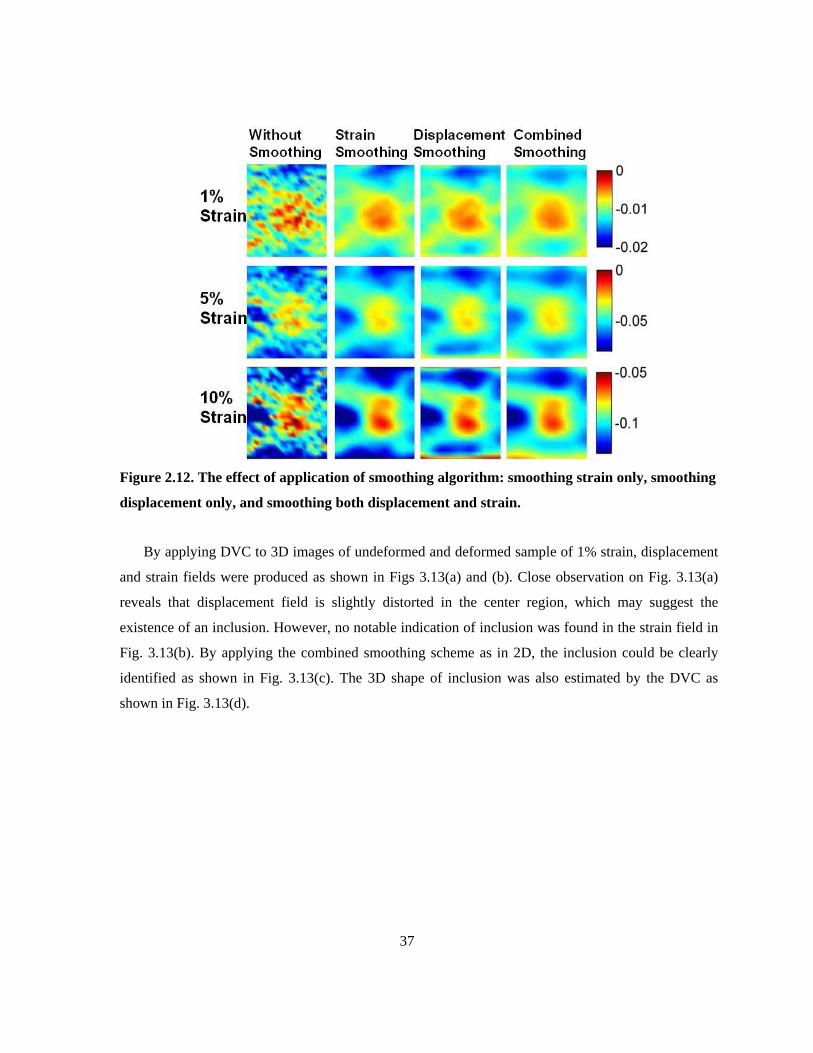
37
Figure 2.12. The effect of application of smoothing algorithm: smoothing strain only, smoothing
displacement only, and smoothing both displacement and strain.
By applying DVC to 3D images of undeformed and deformed sample of 1% strain, displacement
and strain fields were produced as shown in Figs 3.13(a) and (b). Close observation on Fig. 3.13(a)
reveals that displacement field is slightly distorted in the center region, which may suggest the
existence of an inclusion. However, no notable indication of inclusion was found in the strain field in
Fig. 3.13(b). By applying the combined smoothing scheme as in 2D, the inclusion could be clearly
identified as shown in Fig. 3.13(c). The 3D shape of inclusion was also estimated by the DVC as
shown in Fig. 3.13(d).
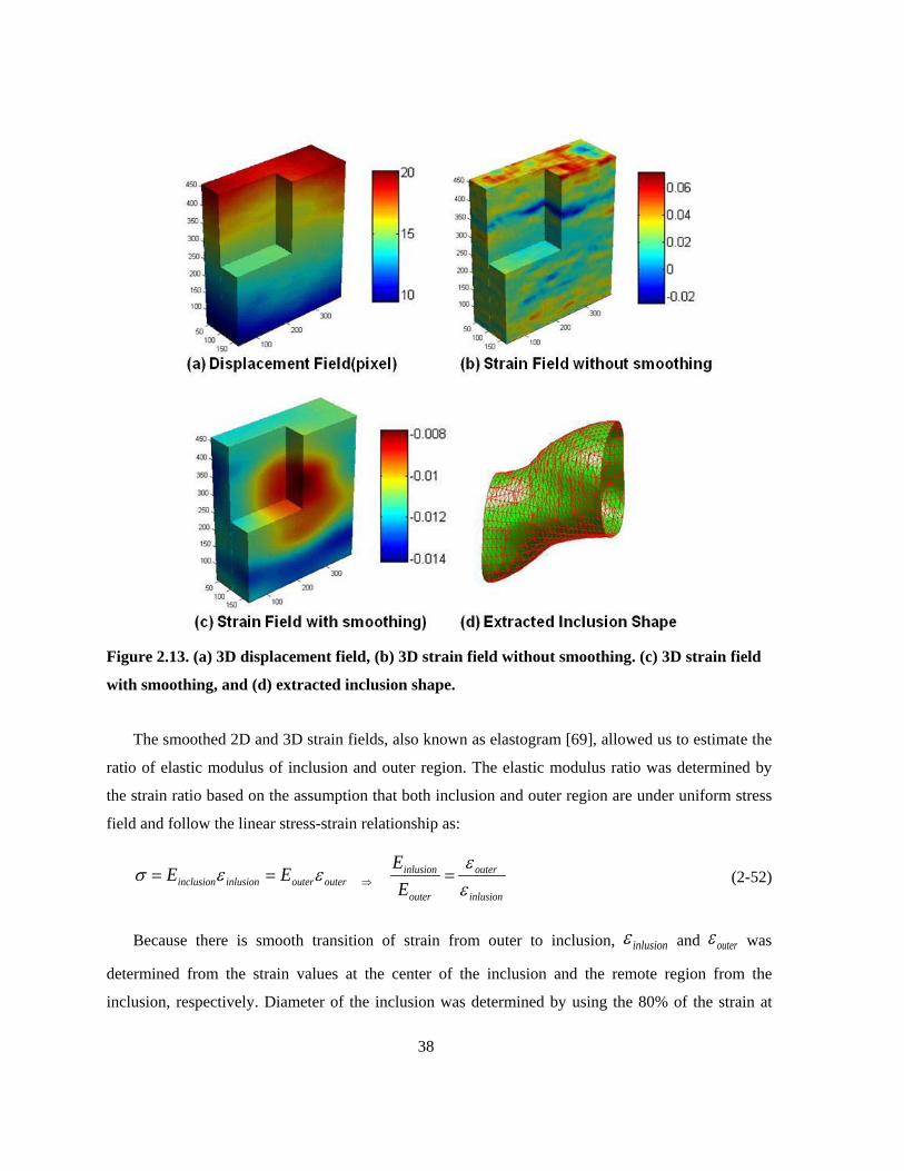
38
Figure 2.13. (a) 3D displacement field, (b) 3D strain field without smoothing. (c) 3D strain field
with smoothing, and (d) extracted inclusion shape.
The smoothed 2D and 3D strain fields, also known as elastogram [69], allowed us to estimate the
ratio of elastic modulus of inclusion and outer region. The elastic modulus ratio was determined by
the strain ratio based on the assumption that both inclusion and outer region are under uniform stress
field and follow the linear stress-strain relationship as:
inlusion
outer
outer
inlusionouterouterinlusioninclusion E
EEEεε
εεσ === ⇒ (2-52)
Because there is smooth transition of strain from outer to inclusion, inlusionε and outerε was
determined from the strain values at the center of the inclusion and the remote region from the
inclusion, respectively. Diameter of the inclusion was determined by using the 80% of the strain at
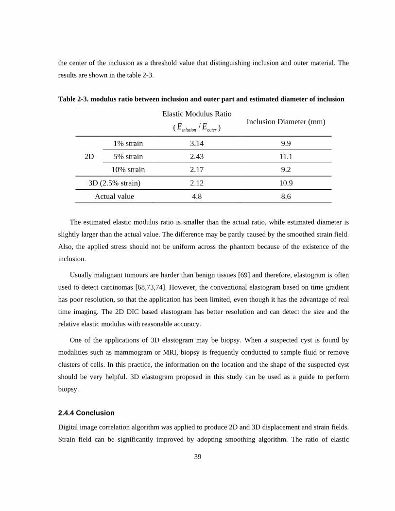
39
the center of the inclusion as a threshold value that distinguishing inclusion and outer material. The
results are shown in the table 2-3.
Table 2-3. modulus ratio between inclusion and outer part and estimated diameter of inclusion
Elastic Modulus Ratio
( outerinlusion EE / ) Inclusion Diameter (mm)
2D
1% strain 3.14 9.9
5% strain 2.43 11.1
10% strain 2.17 9.2
3D (2.5% strain) 2.12 10.9
Actual value 4.8 8.6
The estimated elastic modulus ratio is smaller than the actual ratio, while estimated diameter is
slightly larger than the actual value. The difference may be partly caused by the smoothed strain field.
Also, the applied stress should not be uniform across the phantom because of the existence of the
inclusion.
Usually malignant tumours are harder than benign tissues [69] and therefore, elastogram is often
used to detect carcinomas [68,73,74]. However, the conventional elastogram based on time gradient
has poor resolution, so that the application has been limited, even though it has the advantage of real
time imaging. The 2D DIC based elastogram has better resolution and can detect the size and the
relative elastic modulus with reasonable accuracy.
One of the applications of 3D elastogram may be biopsy. When a suspected cyst is found by
modalities such as mammogram or MRI, biopsy is frequently conducted to sample fluid or remove
clusters of cells. In this practice, the information on the location and the shape of the suspected cyst
should be very helpful. 3D elastogram proposed in this study can be used as a guide to perform
biopsy.
2.4.4 Conclusion
Digital image correlation algorithm was applied to produce 2D and 3D displacement and strain fields.
Strain field can be significantly improved by adopting smoothing algorithm. The ratio of elastic

40
modulus of inclusion to that of outer material and the diameter of inclusion in phantom were
estimated from strain field.
This study shows the potential to apply DIC and DVC algorithms with smoothing function to the in-
vivo diagnosis of pathological tissue within the body, and to provide new information that is related
to tissue structure and or pathology.
41
Chapter 3 Development of Apparatuses for Characterizing Surface
Energy
3.1 Introduction
As future technological innovations gear toward miniaturizing machines and maximizing
performance density, the contact between similar or dissimilar materials has become one of the most
critical technical concerns in designing materials both chemically and mechanically. The surface
effects (adhesion, surface energy, and associated micro-mechanical properties) play an important role
in the performance of the materials and devices at small length scales. For example, in the processes
of micro-molding and nano-imprinting, the adhesion and subsequent detachment between the
polymer and micro/nano-structured templates are essential steps during the transfer of the
micro/nanoscale patterns [75]. Not only the contact between solids, but also the contact between solid
and liquid is of great interest and has been studied extensively. The ability of pond skaters to walk on
the surface of water has attracted many researchers. In mimicking this ability of pond skaters, the
interaction between water and material may be one of the most important factors [13] .
When liquid is in contact with a surface, it forms different shapes depending on the wetting
capability of the liquid on the surface. The main parameter that characterizes wetting is the contact
angle, which is defined as the angle that forms between the liquid and the surface. Conventionally it is
defined that the surface is hydrophilic if the contact angle of water is between 0° and 90° whereas the
surface is hydrophobic if the contact angle of water is between 90° and 180°.
Studying the wetting behaviour on the surface of a material is of interest in various applications,
including biomimetic materials and biomaterials. Biomimetic is the study of nature, its models,
systems, and processes to solve engineering problems. Applying self-cleaning phenomenon known as
the “Lotus effect” to self-cleaning windows, windshields, exterior paints for buildings and navigation
ships would be examples of biomimetic [13]. Biomaterials are nonviable materials used in a medical
device, indented to interact with biological system. In implantation of biomedical devices and
prostheses, one has to consider the foreign body reaction to their material and surfaces such as
inflammation since these implanted devices would be degraded by the response of the body.
Generally it is known that hydrophilic surface prevents the cells from adhering to the surface and thus

42
from affecting the materials [3, 4]. Therefore, in designing the biomaterial, its hydrophobicity has to
be taken into account.
The contact between solids has also been an important issue in various applications in terms of
external force, material deformation, and contact area and mainly pioneered by Hertz’s early work
back in 1886 [78]. The conventional application would be contact between rail wheels and roads.
Recently the contact problem at the micro or nano scales starts to gain attention and but cannot be
explained by Hertz theory because Hertz theory ignored the surface interaction between the solids.
Johnson et al [15] took the surface interaction into account and developed the Johnson-Kendall-
Roberts (JKR) theory. The effect of surface interaction is significant at small length scales and
therefore, should be considered in the micro and nano technology. The JKR theory based indentation
test is becoming standard method to study surface property of materials and their interaction [75,79-
81].
This chapter consists of three parts. In section 3.2, the theoretical backgrounds on contact angle
and contact mechanics are discussed. The meaning of contact angle is described in terms of
thermodynamic concepts. Hertz and JKR theories are rigorously derived, and the way surface energy
is related to JKR theory is explained. In section 3.3, custom developed contact angle measurement
system and JKR-type indentation tester are introduced. Lastly, section 3.4 presents the study of
dynamic contact behaviour of PDMS examined by both contact angle measurement (PDMS-water)
and JKR-type indentation test (PDMS-PDMS).
3.2 Theoretical Background
3.2.1 The Contact Angle of a Liquid on a Solid Surface
The following theoretical treatment is based on the reference [82].
3.2.1.1 Interfacial tension
Interfacial tension (or surface energy) is defined to be an additional free energy per unit area caused
by the presence of an interface. In thermodynamics, the attraction between a fluid A molecule and a
fluid B molecule must be less than the average of that between two A molecules and that between
two B molecules to separate fluids A and B and to form the interfacial region as shown in Fig.
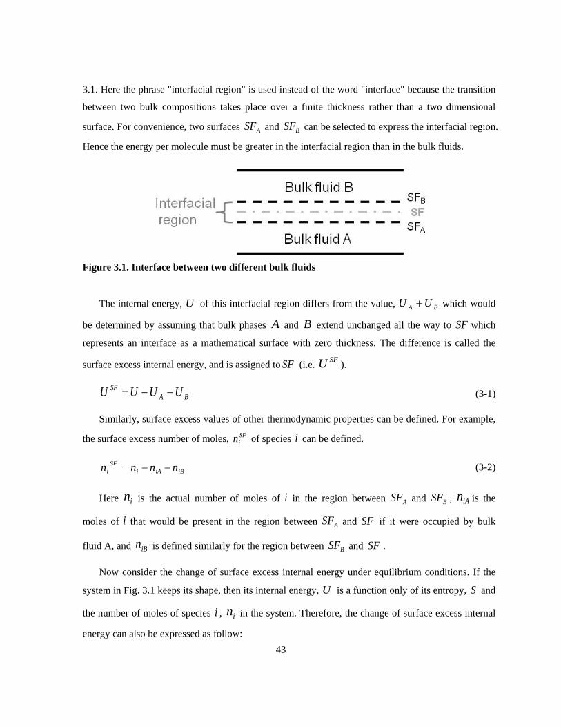
43
3.1. Here the phrase "interfacial region" is used instead of the word "interface" because the transition
between two bulk compositions takes place over a finite thickness rather than a two dimensional
surface. For convenience, two surfaces ASF and BSF can be selected to express the interfacial region.
Hence the energy per molecule must be greater in the interfacial region than in the bulk fluids.
Figure 3.1. Interface between two different bulk fluids
The internal energy, U of this interfacial region differs from the value, BA UU + which would
be determined by assuming that bulk phases A and B extend unchanged all the way to SF which
represents an interface as a mathematical surface with zero thickness. The difference is called the
surface excess internal energy, and is assigned to SF (i.e. SFU ).
BASF UUUU −−= (3-1)
Similarly, surface excess values of other thermodynamic properties can be defined. For example,
the surface excess number of moles, SFin of species i can be defined.
iBiAiSF
i nnnn −−= (3-2)
Here in is the actual number of moles of i in the region between ASF and BSF , iAn is the
moles of i that would be present in the region between ASF and SF if it were occupied by bulk
fluid A, and iBn is defined similarly for the region between BSF and SF .
Now consider the change of surface excess internal energy under equilibrium conditions. If the
system in Fig. 3.1 keeps its shape, then its internal energy, U is a function only of its entropy, S and
the number of moles of species i , in in the system. Therefore, the change of surface excess internal
energy can also be expressed as follow:

44
∑+=i
SFii
SFSF dnuTdSdU (3-3)
If the reference surface, SF deforms so that the area of SF changes, then
∑ ++=i
SFii
SFSF dAdnuTdSdU γ (3-4)
It was mentioned that the energy per molecule must be greater in the interfacial region than in the
bulk fluids. Therefore, the energy of interfacial region increases and γ is positive. It should be noted
that curvature of SF also change when the surface deforms, but we can expect the effect to be small
if the radii of curvature are much larger than the interfacial thickness.
The Helmholtz free energy F for the interfacial region is defined in the usual way.
TSUF −= (3-5)
We can also think about surface excess Helmholtz free energy F for the interfacial region
SFSFSF TSUF −= (3-6)
Differentiating Eq. (3-6) and substituting Eq. (3-4) gives
∑ ++−=i
SFii
SFSF dAdnudTSdF γ (3-7)
It is clear from this equation that given the temperature without mass transfer the interfacial
tension can be written in terms of the surface excess free energy as
SFinT
SF
AF
,)(∂∂
=γ (3-8)
Using Gibbs free energy instead of Helmholtz free energy in the derivation gives the same result
under the assumption that pressure and volume of the system are constant.
3.2.1.2 Liquid contact angle on a solid surface
Considering the change in Helmholtz free energy of the total system in the previous section (3.2.1.1),
we can write

45
∑
∑
∑
−+−
−+−
++−=
++=
iBBiBiB
iAAiAiA
i
SFii
SF
BASF
dVpdnudTS
dVpdnudTS
dAdnudTS
dFdFdFdF
γ
(3-9)
Now let’s consider a liquid droplet on a smooth solid surface as shown in Fig. 3.2. There are three
interfaces: the solid(S)-liquid(L), the liquid-vapor(V), and the solid-vapor. Thus, there exists three
interfacial tensions SLγ , SVγ , and LVγ . The angle that forms between the liquid and the surface is
called the contact angle. The relationship between three interfacial tensions and the contact angle can
be found in the following thermodynamic consideration.
Figure 3.2. A droplet on a solid surface
By generalizing Eq. (3-9), small changes in Helmholtz free energy for multiple interfaces can be
determined. If the temperature and the individual phase volumes are constant for the case in Fig. 3.2,
SLSLLVLVSVSV
i
Vi
Li
Sii
i
SLi
SVi
LVii
dAdAdA
dndndnudndndnudF
γγγ +++
+++++= ∑∑ )()( (3-10)
If there is no mass transfer with surrounding, the number of moles remains unchanged,
,0)()( ==+++++ iTV
iL
iS
iSL
iSV
iLV
i dndndndndndndn (3-11)
Then one has
SLSLLVLVSVSV dAdAdAdF γγγ +++= (3-12)
46
By the geometry
LVSLSV dAdAdAθcos
1=−= (3-13)
Substituting Eq. (3-12) into Eq. (3-13) and rearranging gives
θγγγ cosLVSVSLSLA
F+−=
∂∂
(3-14)
At equilibrium, F has to be a minimum with respect to SLdA and consequently 0=∂∂ SLAF
and Eq. (3-14) can be rewritten
SVSLLV γγθγ +−=cos (3-15)
This is called Young's equation. For this equation to be valid, it is assumed that there is no
adsorption at the interfaces. Another assumption is to neglect the additional effect of line tension that
may be caused by a linear excess of free energy due to the appearance of the junction of three
different matters. In fact, it was found that the effect of line tension is negligible in contact angle
measurements for drops with a radius larger than a few millimeters [83].
3.2.1.3 Finding the interfacial tension
Eq. (3-15) can be used to find interfacial tension between solid and liquid, SLγ with known values of
SVγ and LVγ , but cannot be used directly to determine either SVγ or LVγ when the other value is
known unless one has the information of SLγ . The main sources of the interfacial tensions are the
London dispersion forces due to the intermolecular potential and polar forces due to the polarity of
molecules in terms of acidity and basicity and expressed the sum of them.
ABd121212 γγγ += (3-16)
where 1 and 2 indicates two materials in contact. There are several theories to express 12γ in terms of
d1γ ,
d2γ ,
AB1γ , and
AB2γ such as Fowkes theory [84,85], Wu theory [86], and Van Oss Theory [87,88].
In Fowkes theory
47
)(2 22112211221112ABABdd γγγγγγγ +−+= (3-17)
Wu theory uses harmonic means rather than geometric means, so that
)22(22211
2211
2211
2211221112 ABAB
ABAB
dd
dd
γγγγ
γγγγ
γγγ+
++
−+= (3-18)
Van Oss Theory further divides the polar component into two parts: the surface energy due to
acidic interaction, Aγ and due to basic interaction,
Bγ .
BAd12121212 γγγγ ++= (3-19)
In the interfacial region, the acid components on surface theoretically have polar interactions with
basic components on the other surface and vice versa. In the similar way to Fowkes theory
)(2 221122112211221112ABBAdd γγγγγγγγγ ++−+= (3-20)
Combining Eqs. (3-17), (3-18), and (3-19) with Eq. (3-15) and rearranging them give following
relationships, respectively
ABSV
ABLV
dSV
dLV
LV γγγγθγ
+=+
2)1(cos (3-21)
ABSV
ABLV
ABSV
ABLV
dSV
dLV
dSV
dLVLV
γγγγ
γγγγθγ
++
+=
+4
)1(cos (3-22)
ASV
BLV
BSV
ALV
dSV
dLV
LV γγγγγγθγ
++=+
2)1(cos (3-23)
Through these equations one can determine the surface tension of a solid surface and its
component using 2 known liquid probes for Eqs. (3-21) and (3-22), and 3 for Eq. (3-23). If the solid
does not have polarity, one liquid probe is sufficient for this purpose.
3.2.1.4 Contact angle hysteresis
There are three types of contact angles: (i) static contact angle, which is the contact angle when the
droplet is stationary (at equilibrium stage); (ii) advancing contact angle, which is the contact angle
when the contact line is advancing to a new position over a dry solid surface; (iii) receding contact
48
angle, which is the contact angle when the contact line is receding into the region previously wet by
the liquid. (ii) and (iii) are together called dynamic contact angle. These values are not often the same
and the difference between advancing and receding contact angles is called contact angle hysteresis.
There are several factors that cause this hysteresis such as impurities, roughness, and heterogeneity of
a surface, adsorption and permeability of a liquid to the surface, and rotation of polar groups of
surface depending on polarity of liquid. Especially the effect of roughness on hysteresis has been
studied extensively being inspired by the hierarchical structure of natural lotus leaves and their self
cleaning effect [13].
Thermodynamically contact angle hysteresis can be considered as a measure of energy dissipation
during the flow of a droplet along a solid surface [2, 3]. Low hysteresis means that small energy
dissipation is required for a droplet to move or flow. Many studies used the tilting method to
determine the advancing and receding contact angle with another hysteresis indicator, roll-off tilting
angle where the droplet starts to roll. However, in the tilting method, since advancing and receding
contact angles are determined through one droplet where advancing interfacial tension may affect
receding contact angle as well as advancing contact angle and vice versa, it may not be a good
method to find advancing or receding interfacial tension.
Another way to study contact angle hysteresis is the sessile drop method in which liquid is
supplied or withdrawn so that one can observe advancing and receding contact angles, respectively
while a contact line moves [90-92]. However, it is tricky to use these contact angles to calculate the
interfacial tensions because a droplet may not be at the equilibrium state and the angle may be
affected by the droplet speed. Nevertheless, contact angle measurement system based on the sessile
drop method was developed and employed to study the contact line speed dependence of contact
angles and to find the interfacial tension of the material in section 3.3-3.5 .
3.2.2 The Theory on the Contacts Between Solids
The following theoretical treatment is based on the references [15,89,93].
3.2.2.1 Hertz model
The mathematical theory for the general three-dimensional contact problem was first given by Hertz
for isotropic linear elastic material [78]. Including linear elasticity, several assumptions are made that
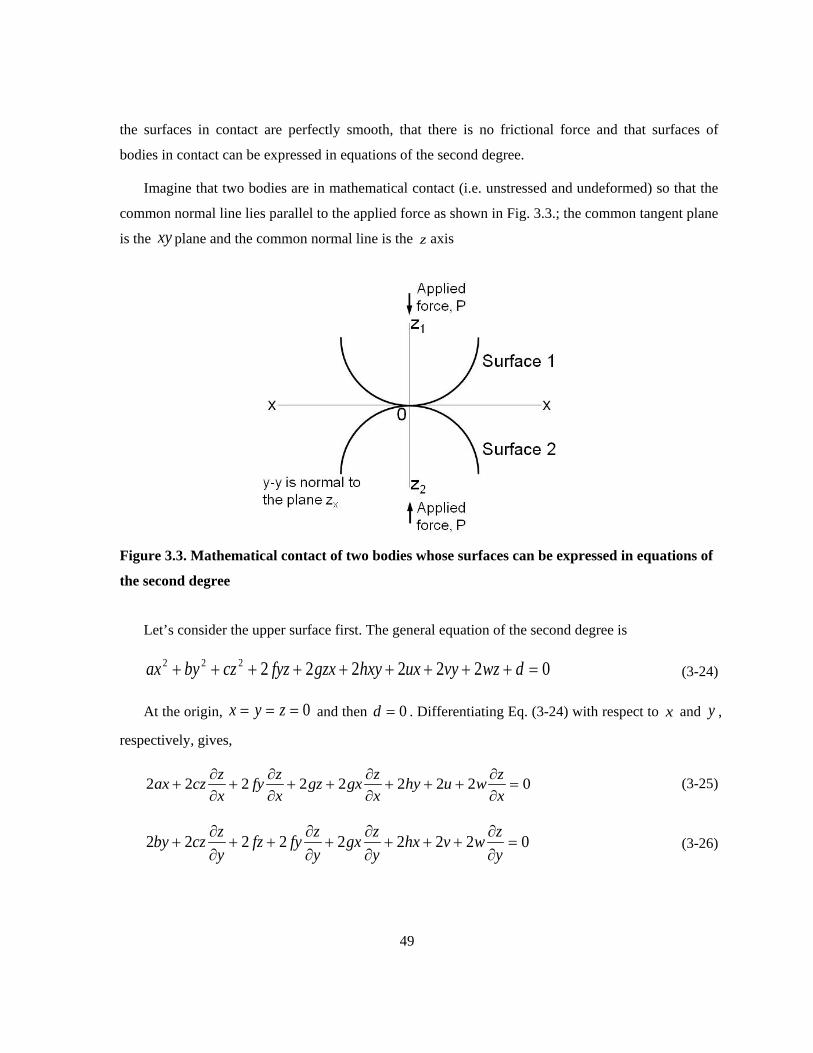
49
the surfaces in contact are perfectly smooth, that there is no frictional force and that surfaces of
bodies in contact can be expressed in equations of the second degree.
Imagine that two bodies are in mathematical contact (i.e. unstressed and undeformed) so that the
common normal line lies parallel to the applied force as shown in Fig. 3.3.; the common tangent plane
is the xy plane and the common normal line is the z axis
Figure 3.3. Mathematical contact of two bodies whose surfaces can be expressed in equations of
the second degree
Let’s consider the upper surface first. The general equation of the second degree is
0222222222 =+++++++++ dwzvyuxhxygzxfyzczbyax (3-24)
At the origin, 0=== zyx and then 0=d . Differentiating Eq. (3-24) with respect to x and y ,
respectively, gives,
022222222 =∂∂
+++∂∂
++∂∂
+∂∂
+xzwuhy
xzgxgz
xzfy
xzczax (3-25)
022222222 =∂∂
+++∂∂
+∂∂
++∂∂
+yzwvhx
yzgx
yzfyfz
yzczby (3-26)

50
At the origin, 0=∂∂
=∂∂
===yz
xzzyx and then 0== vu . Therefore, Eq. (3-24) can be
written as
02222222 =++++++ wzhxygzxfyzczbyax (3-27)
Differentiating Eqs. (3-24) and (3-25) with respect to x and y , respectively, and Eq.(3-24) once
more with respect to y ,
022222)(222 2
2
2
2
2
22
2
2
=∂∂
+∂∂
+∂∂
+∂∂
+∂∂
+∂∂
+∂∂
+x
zwx
zgxxzg
xzg
xzfy
xzc
xzcza (3-28)
022222)(222 2
2
2
2
2
22
2
2
=∂∂
+∂∂
+∂∂
+∂∂
+∂∂
+∂∂
+∂∂
+y
zwy
zgxy
zfyyzf
yzf
yzc
yzczb (3-29)
0222222222222
=∂∂
∂++
∂∂∂
+∂∂
+∂∂
∂+
∂∂
+∂∂
∂+
∂∂
∂∂
yxzwh
yxzgx
yzg
yxzfy
xzf
yxzcz
yz
xzc (3-30)
At the origin, 0=∂∂
=∂∂
===yz
xzzyx , and substituting this into Eqs. (3-28), (3-29), and (3-30)
gives, respectively
wa
xz
xzwa −=
∂∂
→=∂∂
+ 2
2
2
2
022 (3-31)
wb
yz
yzwb −=
∂∂
→=∂∂
+ 2
2
2
2
022 (3-32)
wh
yxz
yxzwh −=
∂∂∂
→=∂∂
∂+
22
022 (3-33)
Let ),( yxfz = then, by using the Taylor’s series, we can obtain the approximation to Eq. (3-27)
around the origin point ( 0== yx ). then
51
)(
)}0,0()0,0(2)0,0({!2
1
)0,0()0,0()0,0(),(
22
neglectedtermsorderhigher
fyyfxfx
yfxffyxfz
yyxyxx
yx
+
∂+∂∂+∂+
∂+∂+=∂∂=
(3-34)
where ,,,, 2
2
2
2
yzf
xzf
yzf
xzf yyxxyx ∂
∂=
∂∂
=∂∂
=∂∂
= andyxzf xy ∂∂
∂=
2
. Since it is the approximation
around the origin, we can replace x∂ and y∂ by x and y, respectively. Substituting
0)0,0()0,0()0,0( === yx fff and Eqs (3-31), (3-32), and (3-33) into Eq (3-34) gives
}2{21),( 22 y
wbxy
whx
wayxfz −−−==
(3-35)
In any given plane parallel to the xy plane in Fig. 3.3, z is constant, and then Eq (3-35) is an
ellipse with its principal axes rotated with respect to its coordinate axes. If we rotate axes so that the
principal axes are aligned with the coordinate axes, the xy term will vanish.
θθ sincos YXx += (3-36)
θθ cossin YXy +−= (3-37)
Substituting Eqs (3-36) and (3-37) into Eq (3-35) gives
)}2(cos2sin){(
)}sin(cos2cossin2cossin2(
)sincos2cossin(
)sincos2sincos({21
22
22
222
222
θθβα
θθθθθθ
θθθθ
θθθθ
wh
wbaXYYX
wh
wb
waXY
wh
wb
waY
wh
wb
waXz
+−
−×+×=
−+−+
+++
−+−=
(3-38)
where α and β are constants. When h
ab −=θ2tan , the XY term vanishes. By replacing X and
Y by x and y , respectively, the equation becomes
22 ByAxz += (3-39)

52
where A and B are constants. We can determine these constants in terms of dimensions of the
respective bodies. Let R and 'R be the principle radii of curvature of the body for the planes 0=y
and 0=x , respectively. In the planes 0=y and 0=x , we have zAx =2 and zBy =2 ,
respectively. Here z is small enough so that zz <<2 . Therefore, we can assume that the curvature
in the plane 0=y is circular with a following equation,
222 )( RRzx =−+ (3-40)
Reversely ignoring the second-order term of the small quantity z ,
Rzx 22 = (3-41)
Since zAx =2 , therefore,
RA
21
= (3-42)
Similarly
'21R
B = (3-43)
Therefore, now we can have the equation for upper body by substituting Eqs. (3-42) and (3-43)
into the equation (3-39):
'22 1
2
1
22
12
11 Ry
RxyBxAz +=+= (3-44)
And similarly we can find the equation for lower body
'22 2
2
2
22
22
22 Ry
RxyBxAz +=+= (3-45)
2z should be used instead of 2z because it is minus, but for convenience 2z is indicating 2z
in the rest of derivation. These equations can be combined into a single equation by adding.
222
21
2
2121 )
'21
'21()
21
21( ByAxy
RRx
RRzzz +=+++=+= (3-46)
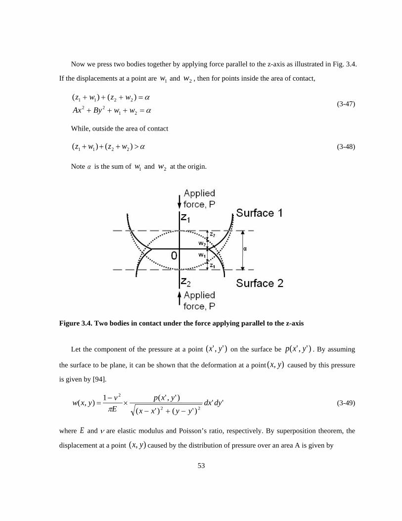
53
Now we press two bodies together by applying force parallel to the z-axis as illustrated in Fig. 3.4.
If the displacements at a point are 1w and 2w , then for points inside the area of contact,
α
α
=+++
=+++
2122
2211 )()(
wwByAxwzwz
(3-47)
While, outside the area of contact
α>+++ )()( 2211 wzwz (3-48)
Note α is the sum of 1w and 2w at the origin.
Figure 3.4. Two bodies in contact under the force applying parallel to the z-axis
Let the component of the pressure at a point )','( yx on the surface be )','( yxp . By assuming
the surface to be plane, it can be shown that the deformation at a point ),( yx caused by this pressure
is given by [94].
'')'()'(
)','(1),(22
2
dydxyyxx
yxpEvyxw
−+−×
−=
π (3-49)
where E and ν are elastic modulus and Poisson’s ratio, respectively. By superposition theorem, the
displacement at a point ),( yx caused by the distribution of pressure over an area A is given by

54
∫∫−+−
×−
=A
dydxyyxx
yxpEvyxw ''
)'()'()','(1),(
22
2
π (3-50)
Substituting Eq. (3-50) into Eq. (3-47) gives
∫∫ −−=−+−
×−
+−
AByAxdydx
yyxxyxp
Ev
Ev 22
222
22
1
21 ''
)'()'()','()11( α
ππ (3-51)
where the subscripts 1 and 2 designate the elastic constants for the two bodies. A solution of Eq. (3-
50) yields expression for the area of contact, the pressure distribution over the area, and the
compression. This solution can be found by analogy with a problem in potential theory [95].
If an ellipsoid 122
2
2
22
=++ cz
by
ax has a uniform volume, charge of density ρ , then it can
be shown that the potential for points inside the ellipsoid is given by
2/12220
2
2
2
2
2
2
)))()((()1(),,(
ψψψψ
ψψψπρφ
++++−
+−
+−= ∫
∞
cbad
cz
by
axabczyx (3-52)
If the ellipsoid is very much flattened, so that c becomes very small, we may write
2/1220
2
2
2
2
)))((()1(),(
ψψψψ
ψψπρφ
++×
+−
+−= ∫
∞
bad
by
axabcyx (3-53)
The potential can also be expressed in a more elementary way as
∫∫∫ −+−+−=
V zzyyxxdzdydxzyx 2/1222 })'()'()'{(
'''),,( ρφ (3-54)
If the ellipsoid is very much flattened, z and z' cab be written as zero in Eq. (3-54). Therefore, the
resulting expression is integrated with respect to z' over the range )/'()/'(1 2222 byaxc −−±
∫∫−+−
−−=22
2/12
2
2
2
)'()'('']''1[2),(
yyxxdydx
by
axcyx ρφ (3-55)
Equating Eqs. (3-53) and (3-55) gives

55
2/1220
2
2
2
2
22
2/12
2
2
2
)))((()1(
21
)'()'('']''1[
ψψψψ
ψψπ
++×
+−
+−=
−+−−−
∫
∫∫∞
bad
by
axab
yyxxdydx
by
ax
(3-56)
Comparing Eqs (3-51) with (3-56), it will be seen that, if the right-hand sides are viewed as
quadratics in x and y , they have the identical form, while the left-hand sides are integrals of the
same form
2/12
2
2
2
)1(),(by
axkyxp −−= (3-57)
Equating the integral ∫∫A dxdyyxp ),( to the total force P, compressing the two bodies gives
abPk π2/3= so
2/12
2
2
2
)1(23),(
by
ax
abPyxp −−=π
(3-58)
Substituting Eq. (3-58) into Eq. (3-51) and using Eq. (3-56)
222/122
02
2
2
2
)))((()1( ByAx
bad
by
ax
KP
−−=++
×+
−+
−∫∞
αψψψ
ψψψπ
(3-59)
where )11(431
2
22
1
21
EEKνν −
+−
= and K is called "effective modulus of the contacting particles"
As this expression must hold for all values of x and y within contact ellipse, expressions for α ,
A , and B can be obtained by equating coefficients on both sides of Eq. (3-59).
∫∞
++=
02/122 )))((( ψψψ
ψπ
δbad
KP (3-60)
∫∞
+++=
02/1222 )))()((( ψψψψ
ψπ baa
dKPA
(3-61)

56
∫∞
+++=
02/1222 )))()((( ψψψψ
ψπ bab
dKPB (3-62)
Note that A and B are geometric factors, )2/12/1( 21 RR + and )'2/1'2/1( 21 RR + given by Eq.
(3-46). The constants a and b appeared in Eq. (3-60) are generally unknown, and are determined
from the known geometric factors A and B through Eqs. (3-61) and (3-62).
3.2.2.2 Two spheres in contact by Hertz model
In case of two spheres whose radiuses are 1R and 2R in contact
RRR
RRRRBA
2)(2)2
121(11 1
21
211
21
=+
=+== −− (3-63)
where R is called combined radii. Eqs. (3-61) and (3-62) become identical and can be written
∫∞
+===
02/122 )(2
1ψψ
ψπ a
dKP
RBA (3-64)
Also Eq. (3-60) can be written
∫∞
+=
02/12 )( ψψ
ψπ
δa
dKP (3-65)
where a is the radius of contact area. Note in case of two spherical surfaces, contact area has the
shape of a circle. By putting ρψ =2/1
30
222 2)(2
21
aKP
ad
KP
Rπ
πρρ
=+
= ∫∞
KPRa =→ 3 (3-66)
aKP
ad
KP π
πρρ
πδ =
+= ∫
∞
022
2 KaP
=→δ (3-67)
3.2.2.3 Two spheres in contact by JKR model
According to the Hertz model, it is the distribution of elastic forces that determines the equilibrium
geometry of two solids in contact ignoring other factors such as friction. However, under light loading,
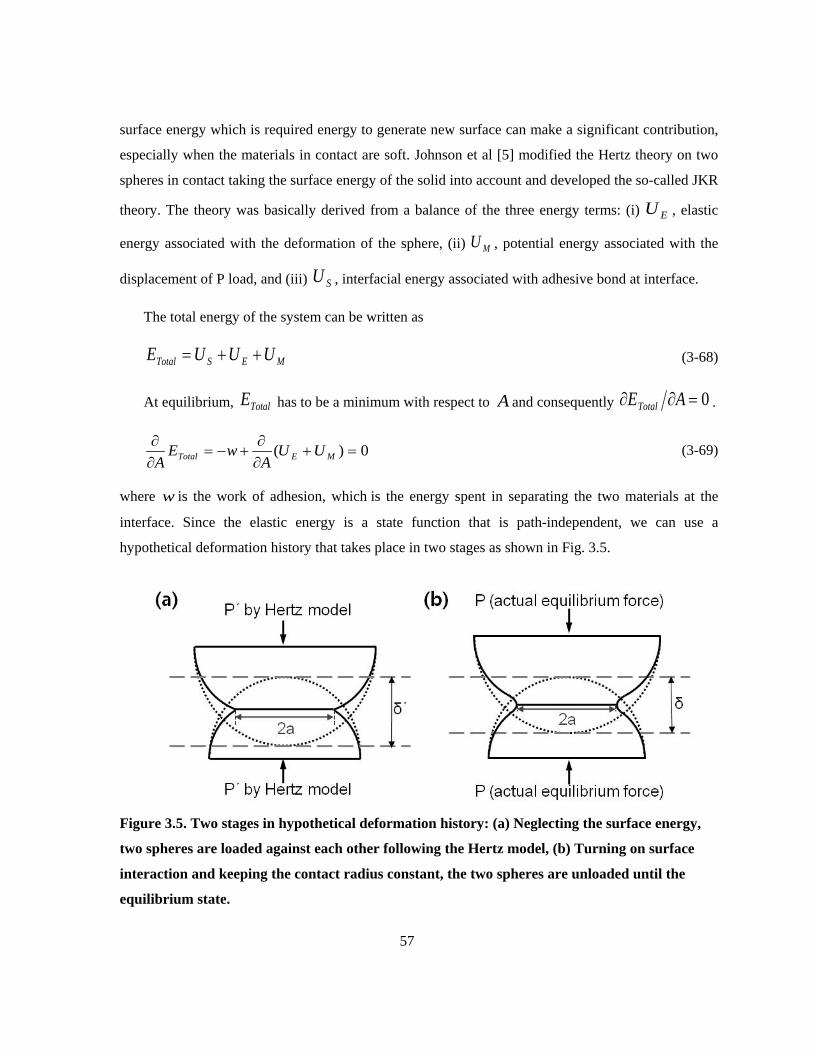
57
surface energy which is required energy to generate new surface can make a significant contribution,
especially when the materials in contact are soft. Johnson et al [5] modified the Hertz theory on two
spheres in contact taking the surface energy of the solid into account and developed the so-called JKR
theory. The theory was basically derived from a balance of the three energy terms: (i) EU , elastic
energy associated with the deformation of the sphere, (ii) MU , potential energy associated with the
displacement of P load, and (iii) SU , interfacial energy associated with adhesive bond at interface.
The total energy of the system can be written as
MESTotal UUUE ++= (3-68)
At equilibrium, TotalE has to be a minimum with respect to A and consequently 0=∂∂ AETotal .
0)( =+∂∂
+−=∂∂
METotal UUA
wEA
(3-69)
where w is the work of adhesion, which is the energy spent in separating the two materials at the
interface. Since the elastic energy is a state function that is path-independent, we can use a
hypothetical deformation history that takes place in two stages as shown in Fig. 3.5.
Figure 3.5. Two stages in hypothetical deformation history: (a) Neglecting the surface energy,
two spheres are loaded against each other following the Hertz model, (b) Turning on surface
interaction and keeping the contact radius constant, the two spheres are unloaded until the
equilibrium state.
58
In the first stage neglecting the surface energy-induced force, the system is loaded until the
contact area becomes 2aA π= as illustrated in Fig. 3.5(a). The elastic energy associated with this
portion of the deformation from mathematical contact, 1U is
∫=)('
01 'a
dPUδ
δ (3-70)
where 'P and 'δ define the load and displacement neglecting adhesive interactions (following the
Hertz model) in the first hypothetical stage.
In the second stage of the hypothetical deformation process, the contact radius is fixed due to
interfacial interactions, and the displacement (or load) decreases until it is equal to the value of
interest (= value at equilibrium state) as illustrated in Fig. 3.5(b). Looking at the deformed profile of
each sphere immediately outside the contact area, it is shown that in the second stage two spheres
meet at the interface perpendicularly with the contact surface due to the adhesive force while in the
previous stage they meet tangentially to each other. The energy, 2U , associated with this portion of
deformation is
a
P
PPdU ∫= '2 δ (3-71)
This quantity can be rewritten if we use the definition of compliance: a
PC )( ∂∂= δ , Assuming
C is constant at a given contact area.
)2'
2(
22
''2PPCPdPCPdU
a
P
Pa
P
P−=== ∫∫ δ (3-72)
Then the overall elastic energy is determined as the sum of 1U and 2U
)2'
2('
22'
021PPCdPUUU E −+=+= ∫
δδ (3-73)
The mechanical potential energy is determined by the distance over which the load has been
moved, or δPU M −= . Since we assumed that compliance is constant.
PPC
−−
='' δδ (3-74)
59
Therefore, we have
)}'('{( PPCPU M −−−= δ (3-75)
Substituting Eqs. (3-73) and (3-75) into Eq. (3-69) gives
APPPC
AP
APPPC
ACPPdP
A
PPCPPPCdPA
UUA
w ME
∂∂
−−+∂∂
−∂∂
−−∂∂−
−∂∂
=
−−−−+∂∂
=+∂∂
=
∫
∫
}')'({'')'(2
)'('
)}]'('{()2'
2('[)(
2'
0
22'
0
δδδ
δδ
δ
δ
(3-76)
Note that A was determined by 'P in the first hypothetical deformation not by P . So we can
consider 0/ =∂∂ AP . Therefore, we have
AP
APPPC
ACPPdP
Aw
∂∂
−∂∂
−−∂∂−
−
∂∂
= ∫'')'(
2)'('
2'
0
δδδ
(3-77)
By using the following two expressions:
APdP
Aw
∂∂
=
∂∂
= ∫'''
'
0
δδδ
(3-78)
APC
AP
PA ∂∂
=∂∂
∂∂
=∂∂ ''
''' δδ (3-79)
Resulting equation is
aC
aPP
ACPPw
∂∂−
−=∂∂−
−=π4
)'(2
)'( 22
(3-80)
According to the Hertz model RKaP /' 3= . C can be approximated by generalizing contact
between a flat, rigid, and cylindrical indenter and an half-spaced elastic layer into one between two
curved elastic half-spaces as shown in Fig. 3.6.
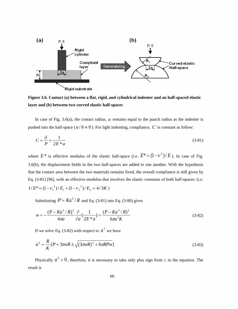
60
Figure 3.6. Contact (a) between a flat, rigid, and cylindrical indenter and an half-spaced elastic
layer and (b) between two curved elastic half-spaces
In case of Fig. 3.6(a), the contact radius, a remains equal to the punch radius as the indenter is
pushed into the half-space ( 0/ ≈ha ). For light indenting, compliance, C is constant as follow:
aEPC
*21
==δ (3-81)
where *E is effective modulus of the elastic half-space (i.e. EE /)1(* 2ν−= ). In case of Fig.
3.6(b), the displacement fields in the two half-spaces are added to one another. With the hypothesis
that the contact area between the two materials remains fixed, the overall compliance is still given by
Eq. (3-81) [96], with an effective modulus that involves the elastic constants of both half-spaces: (i.e.
KEEE 3/4/)1(/)1(*/1 22
212
1 =−+−= νν )
Substituting RKaP /' 3= and Eq. (3-81) into Eq. (3-80) gives
KaRKaP
aEaaRKaPw 3
2323
6)/()
*21(
4)/(
ππ−
=∂∂−
−= (3-82)
If we solve Eq. (3-82) with respect to 3a we have
}6)3(3{ 23 RPwwRwRPKRa πππ +±+= (3-83)
Physically 03 >a , therefore, it is necessary to take only plus sign from ± in the equation. The
result is

61
}6)3(3{ 23 RPwwRwRPKRa πππ +++= (3-84)
This is the well-known JKR equation. When 0=w , this reverts to the simple Hertz equation
KPRa /3 = .
3.2.2.4 Relation between work of adhesion and surface energy
Work of adhesion between materials a and b , abw is directly related to their surface energies.
Opening the interface between a and b generates two new surfaces of A and B. Therefore, from the
energy point of view, we can write
abbbaaabw γγγ −+= (3-85)
Using the Eqs. (3-17) and (3-18), we have
)(2 ABbb
ABaa
dbb
daaabw γγγγ += (3-86)
)22(2 ABbb
ABaa
ABbb
ABaa
dbb
daa
dbb
daa
abwγγγγ
γγγγ
++
+= (3-87)
If the materials are the same, both Eqs. (3-86) and (3-87) give
aaABaa
daaaaw γγγ 2)(2 =+= (3-88)
In following sections (3.3-3.5), JKR-type indentation tests were performed on PDMS with
different speeds: Hemispherical PDMS was brought (loading) into contact with PDMS sheet and
detached (unloading) and the experimental data were fitted to the JKR equation. Hysteresis behaviour
that occurs between load and unloading portions was discussed with its dependence on the
contacting/separating speed.
3.3 Experimental Setup
To study the surface property of materials such as surface energy and adhesion hysteresis, contact
angle measurement system and micro-indentation system with real-time bottom view set-up (so-
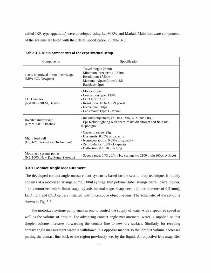
62
called JKR-type apparatus) were developed using LabVIEW and Matlab. Main hardware components
of the systems are listed with their detail specification in table 3-1.
Table 3-1. Main components of the experimental setup
Components Specification
1 axis motorized micro linear stage (MFA-CC, Newport)
- Travel range : 25mm - Minimum increment : 100nm - Resolution: 17.5nm - Maximum Speed(mm/s): 2.5 - Backlash: 2μm
CCD camera (scA1000-30FM, Basler)
- Monochrome - Connection type: 1394b - CCD size: 1/3in - Resolution: 1034 X 779 pixels - Frame rate: 30fps - Lens mount type: C-Mount
Inverted microscope (OMM300T, Omano)
- Includes objectives(4X, 10X, 20X, 40X, and 80X) - Epi-Kohler lighting with aperture iris diaphragm and field iris diaphragm.
Micro load cell (GSO-25, Transducer Techniques)
- Capacity range: 25g - Hysteresis: 0.05% of capacity - Nonrepeatability: 0.05% of capacity - Zero Balance: 1.0% of capacity - Deflection: 0.1016 mm /25g
Motorized syringe pump (NE-1000, New Era Pump Systems) - Speed range: 0.73 µL/hr (1cc syringe) to 2100 ml/hr (60cc syringe)
3.3.1 Contact Angle Measurement
The developed contact angle measurement system is based on the sessile drop technique. It mainly
consists of a motorized syringe pump, 500ul syringe, thin polymer tube, syringe barrel, barrel holder,
1 axis motorized micro linear stage, xy axis manual stage, sharp needle (outer diameter of 0.21mm),
LED light and CCD camera installed with microscope objective lens. The schematic of the set-up is
shown in Fig. 3.7.
The motorized syringe pump enables one to control the supply of water with a specified speed as
well as the volume of droplet. For advancing contact angle measurement, water is supplied so that
droplet volume increases forwarding the contact line to new dry surface. Similarly for receding
contact angle measurement water is withdrawn in a opposite manner so that droplet volume decreases
pulling the contact line back to the region previously wet by the liquid. An objective lens magnifies
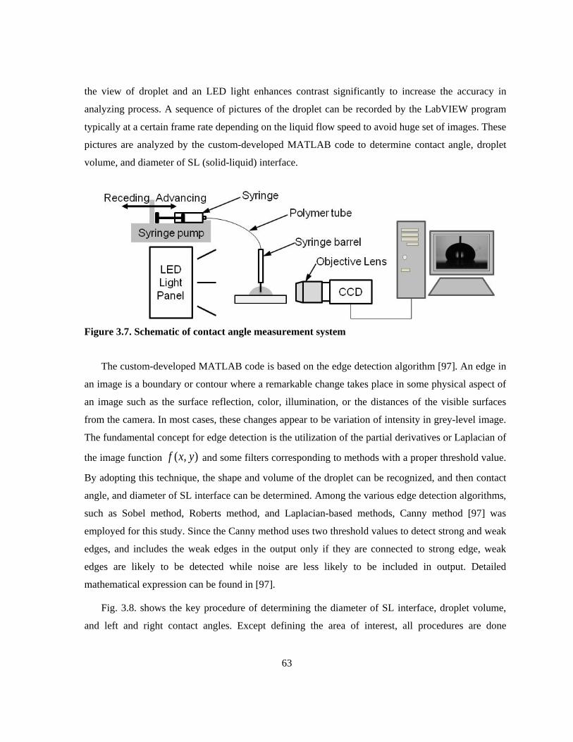
63
the view of droplet and an LED light enhances contrast significantly to increase the accuracy in
analyzing process. A sequence of pictures of the droplet can be recorded by the LabVIEW program
typically at a certain frame rate depending on the liquid flow speed to avoid huge set of images. These
pictures are analyzed by the custom-developed MATLAB code to determine contact angle, droplet
volume, and diameter of SL (solid-liquid) interface.
Figure 3.7. Schematic of contact angle measurement system
The custom-developed MATLAB code is based on the edge detection algorithm [97]. An edge in
an image is a boundary or contour where a remarkable change takes place in some physical aspect of
an image such as the surface reflection, color, illumination, or the distances of the visible surfaces
from the camera. In most cases, these changes appear to be variation of intensity in grey-level image.
The fundamental concept for edge detection is the utilization of the partial derivatives or Laplacian of
the image function ),( yxf and some filters corresponding to methods with a proper threshold value.
By adopting this technique, the shape and volume of the droplet can be recognized, and then contact
angle, and diameter of SL interface can be determined. Among the various edge detection algorithms,
such as Sobel method, Roberts method, and Laplacian-based methods, Canny method [97] was
employed for this study. Since the Canny method uses two threshold values to detect strong and weak
edges, and includes the weak edges in the output only if they are connected to strong edge, weak
edges are likely to be detected while noise are less likely to be included in output. Detailed
mathematical expression can be found in [97].
Fig. 3.8. shows the key procedure of determining the diameter of SL interface, droplet volume,
and left and right contact angles. Except defining the area of interest, all procedures are done
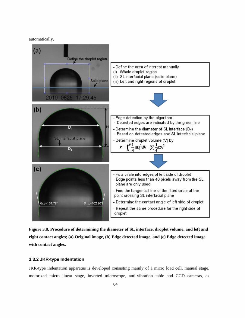
64
automatically.
Figure 3.8. Procedure of determining the diameter of SL interface, droplet volume, and left and
right contact angles; (a) Original image, (b) Edge detected image, and (c) Edge detected image
with contact angles.
3.3.2 JKR-type Indentation
JKR-type indentation apparatus is developed consisting mainly of a micro load cell, manual stage,
motorized micro linear stage, inverted microscope, anti-vibration table and CCD cameras, as
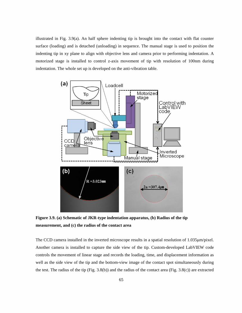
65
illustrated in Fig. 3.9(a). An half sphere indenting tip is brought into the contact with flat counter
surface (loading) and is detached (unloading) in sequence. The manual stage is used to position the
indenting tip in xy plane to align with objective lens and camera prior to performing indentation. A
motorized stage is installed to control z-axis movement of tip with resolution of 100nm during
indentation. The whole set up is developed on the anti-vibration table.
Figure 3.9. (a) Schematic of JKR-type indentation apparatus, (b) Radius of the tip
measurement, and (c) the radius of the contact area
The CCD camera installed in the inverted microscope results in a spatial resolution of 1.035μm/pixel.
Another camera is installed to capture the side view of the tip. Custom-developed LabVIEW code
controls the movement of linear stage and records the loading, time, and displacement information as
well as the side view of the tip and the bottom-view image of the contact spot simultaneously during
the test. The radius of the tip (Fig. 3.8(b)) and the radius of the contact area (Fig. 3.8(c)) are extracted
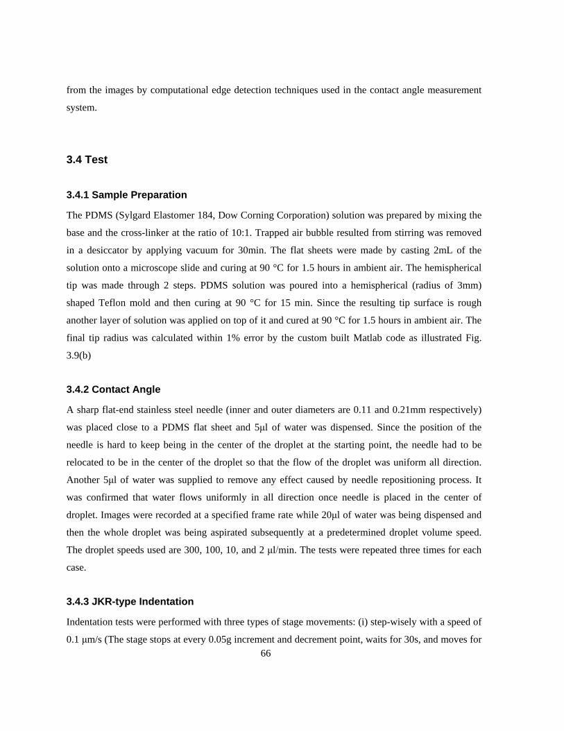
66
from the images by computational edge detection techniques used in the contact angle measurement
system.
3.4 Test
3.4.1 Sample Preparation
The PDMS (Sylgard Elastomer 184, Dow Corning Corporation) solution was prepared by mixing the
base and the cross-linker at the ratio of 10:1. Trapped air bubble resulted from stirring was removed
in a desiccator by applying vacuum for 30min. The flat sheets were made by casting 2mL of the
solution onto a microscope slide and curing at 90 °C for 1.5 hours in ambient air. The hemispherical
tip was made through 2 steps. PDMS solution was poured into a hemispherical (radius of 3mm)
shaped Teflon mold and then curing at 90 °C for 15 min. Since the resulting tip surface is rough
another layer of solution was applied on top of it and cured at 90 °C for 1.5 hours in ambient air. The
final tip radius was calculated within 1% error by the custom built Matlab code as illustrated Fig.
3.9(b)
3.4.2 Contact Angle
A sharp flat-end stainless steel needle (inner and outer diameters are 0.11 and 0.21mm respectively)
was placed close to a PDMS flat sheet and 5μl of water was dispensed. Since the position of the
needle is hard to keep being in the center of the droplet at the starting point, the needle had to be
relocated to be in the center of the droplet so that the flow of the droplet was uniform all direction.
Another 5μl of water was supplied to remove any effect caused by needle repositioning process. It
was confirmed that water flows uniformly in all direction once needle is placed in the center of
droplet. Images were recorded at a specified frame rate while 20μl of water was being dispensed and
then the whole droplet was being aspirated subsequently at a predetermined droplet volume speed.
The droplet speeds used are 300, 100, 10, and 2 μl/min. The tests were repeated three times for each
case.
3.4.3 JKR-type Indentation
Indentation tests were performed with three types of stage movements: (i) step-wisely with a speed of
0.1 μm/s (The stage stops at every 0.05g increment and decrement point, waits for 30s, and moves for

67
the next increment or decrement point); (ii) continuously with a speed of 0.1 μm/s; (iii) continuously
with a speed of 1 μm/s. PDMS hemisphere tip was translated by the linear stage at the specified
motion to be brought into contact with PDMS flat sheet attached and supported by a microscope slide
glass and withdrawn at the same speed. The total indentation depth was determined at a loading force
of 0.5g. For quantitative analysis, three characteristic parameters were determined using the contact
radius vs. force curves: (i) Effective modulus of the contacting surfaces, K ; (ii) the work of adhesion,
w ; (iii) the maximum force required to separate the tip from the substrate, so-called pull-off force
sP . w and K were extracted by fitting the contact radius a and external force P of loading
portion to Eq. (3-84) through the least square method. The tests were repeated three times for each
case.
3.5 Results and Discussion
3.5.1 Contact Angle
The typical test results for each case are shown in Fig. 3.10. As shown, 5 points were selected where
noticeable changes occur ; t0: contact line starts to move forward, t1: contact line stops moving, t2: the
volume of droplet starts to decrease, t3: contact line starts to withdraw, and t4: contact angle starts to
decrease significantly or to be unstable. Based on these 5 points, the results were divided into 6
domains for 300μl/min, 200μl/min, and 10μl/min cases, and 5 regions for 2μl/min case where t1 and t2
overlaps.
Contact angle and volume increase while the contact line is stationary in the first region, showing
that static and advancing contact angles are different at this point. The second region is characterized
by a nearly constant contact angle, where advancing contact angle was determined as the average
value in this region. The average speeds of contact lines in this region are calculated and inserted in
Fig. 3.10. At the third region, the volume is maximum and the contact angle decreases and is
stabilized from advancing to static. The fourth region is transition zone where contact angle changes
from static to receding. Fifth regions are characterized by a nearly constant contact angle, where the
receding contact angle is determined as the average value in this region. The sixth region is
meaningless because drop size is so small that the needle affects the angles.
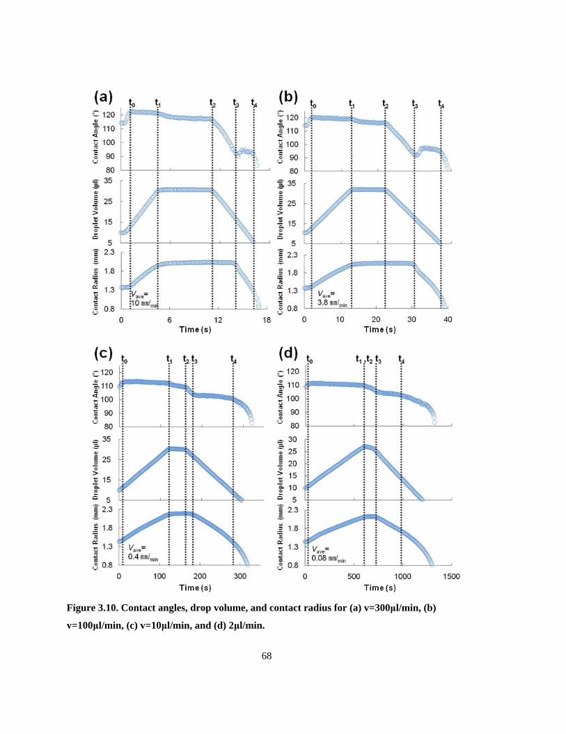
68
Figure 3.10. Contact angles, drop volume, and contact radius for (a) v=300μl/min, (b)
v=100μl/min, (c) v=10μl/min, and (d) 2μl/min.
69
It is interesting that at high speeds (300 and 100 μl/min) the contact line pinned and jumped to a
new location with sharp increment of contact angle when transferring from fourth to fifth regions
while smooth transition occurs at low speeds (10 and 2 μl/min). Stick-slip pattern of receding liquid
on a solid surface is described by Lam et al [92]. They explained that ‘pinning’ of the three-phase line
could be due to a particularly strong interaction, e.g. a chemical bond. However, their case was
repeated stick-slip which differs from non-repeating stick-slip observed here. The reason why speed-
dependant stick-slip occurs is a hard question to answer and ambiguous, but that might be related with
viscosity or friction of the water rather than chemical bonding.
The measured contact angles are summarized in the table 3.2 and depicted in Fig. 3. The dynamic
contact angles of PDMS used in this study have been studied extensively by other researchers [98-
100]. Advancing contact angle, Aθ ranges from 110° to 118° and receding contact angle, Rθ ranges
from 82° to 106°. Only one value of static contact angle, Sθ was available as 105° from the literature
review [100]. Our dynamic contact angle data are very similar to the literature values, but static data
show slight difference. In fact, there is no clear boundary between static contact angle and
advancing/receding contact angles. Some people use advancing and receding contact angles as upper
and low bound of static one while some other people consider advancing contact angle as equilibrium
static contact angle [90-92]. This may be one of the reasons why only 105° could be found from the
literature review and its value is different from our data.
Table 3-2. Contact angles and surface energy depending on the flow rate
Flow rate
(μl/min)
Average contact
line speed
(mm/min)
Contact angle (°) Surface energy (mJ/m2)
Sθ Aθ Rθ Hysθ Sγ Aγ Rγ Hysγ
300 10 117.02±0.27 121.49±0.39 94.13±0.71 27.37 15.92 12.96 46.89 33.93
100 3.8 116.33±0.04 120.06±0.28 97.11±0.10 22.95 16.43 13.85 40.28 26.43
10 0.4 109.98±0.03 112.95±0.12 103.29±0.42 10.72 21.93 19.16 29.88 10.71
2 0.08 109.58±0.41 110.55±0.18 104.10±0.70 6.46 22.34 21.37 28.77 7.40
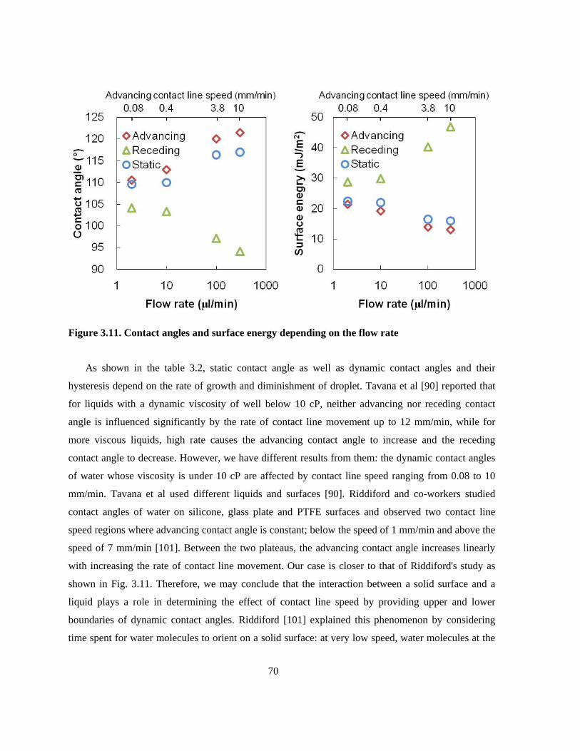
70
Figure 3.11. Contact angles and surface energy depending on the flow rate
As shown in the table 3.2, static contact angle as well as dynamic contact angles and their
hysteresis depend on the rate of growth and diminishment of droplet. Tavana et al [90] reported that
for liquids with a dynamic viscosity of well below 10 cP, neither advancing nor receding contact
angle is influenced significantly by the rate of contact line movement up to 12 mm/min, while for
more viscous liquids, high rate causes the advancing contact angle to increase and the receding
contact angle to decrease. However, we have different results from them: the dynamic contact angles
of water whose viscosity is under 10 cP are affected by contact line speed ranging from 0.08 to 10
mm/min. Tavana et al used different liquids and surfaces [90]. Riddiford and co-workers studied
contact angles of water on silicone, glass plate and PTFE surfaces and observed two contact line
speed regions where advancing contact angle is constant; below the speed of 1 mm/min and above the
speed of 7 mm/min [101]. Between the two plateaus, the advancing contact angle increases linearly
with increasing the rate of contact line movement. Our case is closer to that of Riddiford's study as
shown in Fig. 3.11. Therefore, we may conclude that the interaction between a solid surface and a
liquid plays a role in determining the effect of contact line speed by providing upper and lower
boundaries of dynamic contact angles. Riddiford [101] explained this phenomenon by considering
time spent for water molecules to orient on a solid surface: at very low speed, water molecules at the

71
contact line have sufficient time to settle on the surface while at very high speed they are in the state
of completion of disorientation.
At the beginning of the previous paragraph, it was mentioned that even the static contact angle
depends on the speed of contact line; values from high droplet speeds are even higher than advancing
contact angles from low speeds. This is against the concept that advancing contact angle is an upper
bound of static contact angle. It was presumed that static contact angles from high speeds are under
thermodynamically metastable condition while static contact angles from low speeds are stable and
close to the actual value. At the stationary state, disoriented water molecules caused by the high
speeds of contact line movement may not be able to develop full orientation because they are
confined by neighboring molecules, resulting in metastable state.
The effective surface energies are calculated based on Wu method for each case and shown in the
table 3-2. It should be noted that PDMS does not have polar component and consequently water
droplet is enough to find surface energy of PDMS. PDMS is known to have the surface energy of
20~24mJ/m2 [102-104], which is consistent with our data from static contact angle tests and slightly
higher than the values from advancing contact angles at two low speeds (2 and 10 μl/min). We can
conclude that low droplet speed should be used for measuring static contact angle.
With the assumption of the quasi equilibrium at the speed of 2μl/min, advancing and receding
contact angles can be considered as "static" advancing and receding contact angles and used to apply
the Young equation. Riddiford and co-workers also considered the contact angles in the lower plateau
region where the angles barely changed as the thermodynamic equilibrium angles to be used in the
Young equation [101]. At this low speed range, the hysteresis is relatively small.
For the high speed range, it is not proper to calculate surface energy with Young equation.
However, instead of surface energy, we may evaluate the hysteresis of the effective work of adhesion
or energy release rate between PDMS and water by using the equation if the contact line moves at
constant speed; [89].
)cos1( sLVLVSVLVss wg θγγγγ +=−+== At equilibrium (3-89)
)cos1(_ ALVdissALVSVLVAA wg θγγγγγ +=−−+== At advancing (3-90)
)cos1(_ RLVdissRLVSVLVRR wg θγγγγγ +=+−+== At receding (3-91)
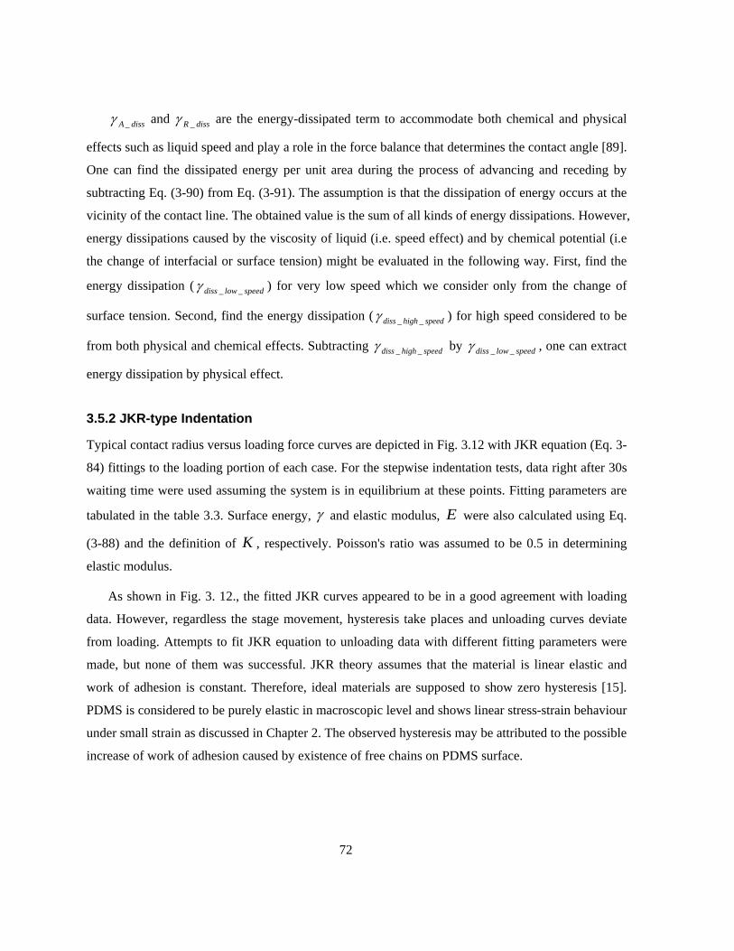
72
dissA _γ and dissR _γ are the energy-dissipated term to accommodate both chemical and physical
effects such as liquid speed and play a role in the force balance that determines the contact angle [89].
One can find the dissipated energy per unit area during the process of advancing and receding by
subtracting Eq. (3-90) from Eq. (3-91). The assumption is that the dissipation of energy occurs at the
vicinity of the contact line. The obtained value is the sum of all kinds of energy dissipations. However,
energy dissipations caused by the viscosity of liquid (i.e. speed effect) and by chemical potential (i.e
the change of interfacial or surface tension) might be evaluated in the following way. First, find the
energy dissipation ( speedlowdiss __γ ) for very low speed which we consider only from the change of
surface tension. Second, find the energy dissipation ( speedhighdiss __γ ) for high speed considered to be
from both physical and chemical effects. Subtracting speedhighdiss __γ by speedlowdiss __γ , one can extract
energy dissipation by physical effect.
3.5.2 JKR-type Indentation
Typical contact radius versus loading force curves are depicted in Fig. 3.12 with JKR equation (Eq. 3-
84) fittings to the loading portion of each case. For the stepwise indentation tests, data right after 30s
waiting time were used assuming the system is in equilibrium at these points. Fitting parameters are
tabulated in the table 3.3. Surface energy, γ and elastic modulus, E were also calculated using Eq.
(3-88) and the definition of K , respectively. Poisson's ratio was assumed to be 0.5 in determining
elastic modulus.
As shown in Fig. 3. 12., the fitted JKR curves appeared to be in a good agreement with loading
data. However, regardless the stage movement, hysteresis take places and unloading curves deviate
from loading. Attempts to fit JKR equation to unloading data with different fitting parameters were
made, but none of them was successful. JKR theory assumes that the material is linear elastic and
work of adhesion is constant. Therefore, ideal materials are supposed to show zero hysteresis [15].
PDMS is considered to be purely elastic in macroscopic level and shows linear stress-strain behaviour
under small strain as discussed in Chapter 2. The observed hysteresis may be attributed to the possible
increase of work of adhesion caused by existence of free chains on PDMS surface.
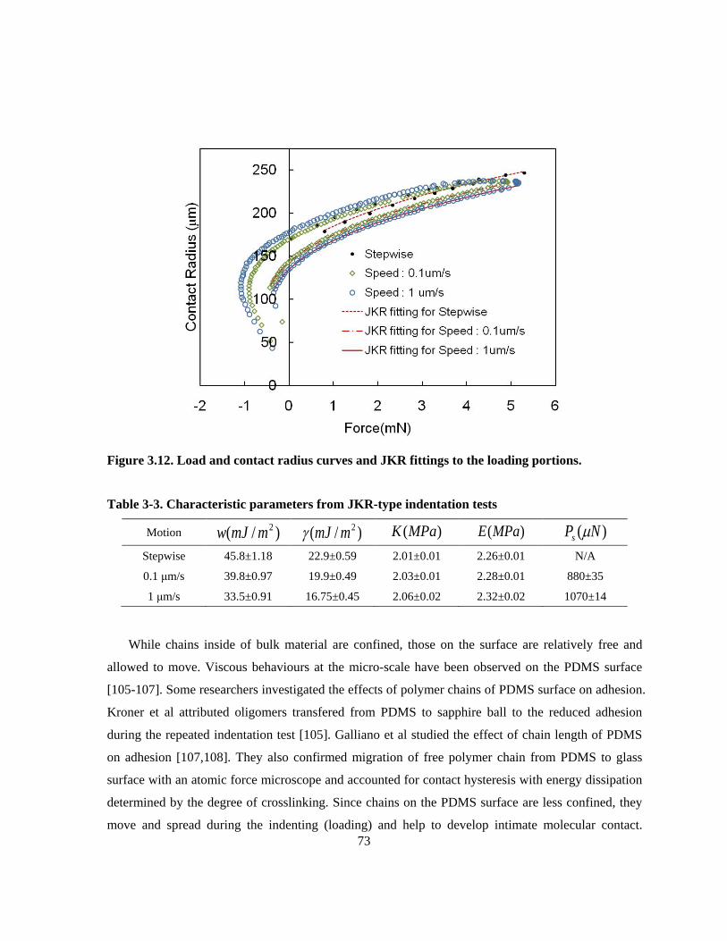
73
Figure 3.12. Load and contact radius curves and JKR fittings to the loading portions.
Table 3-3. Characteristic parameters from JKR-type indentation tests
Motion )/( 2mmJw )/( 2mmJγ )(MPaK )(MPaE )( NPs µ
Stepwise 45.8±1.18 22.9±0.59 2.01±0.01 2.26±0.01 N/A
0.1 μm/s 39.8±0.97 19.9±0.49 2.03±0.01 2.28±0.01 880±35
1 μm/s 33.5±0.91 16.75±0.45 2.06±0.02 2.32±0.02 1070±14
While chains inside of bulk material are confined, those on the surface are relatively free and
allowed to move. Viscous behaviours at the micro-scale have been observed on the PDMS surface
[105-107]. Some researchers investigated the effects of polymer chains of PDMS surface on adhesion.
Kroner et al attributed oligomers transfered from PDMS to sapphire ball to the reduced adhesion
during the repeated indentation test [105]. Galliano et al studied the effect of chain length of PDMS
on adhesion [107,108]. They also confirmed migration of free polymer chain from PDMS to glass
surface with an atomic force microscope and accounted for contact hysteresis with energy dissipation
determined by the degree of crosslinking. Since chains on the PDMS surface are less confined, they
move and spread during the indenting (loading) and help to develop intimate molecular contact.
74
Eventually they start to migrate between contact surfaces and entangle with each other as loading
increases. Because of these intimate contact and entanglement, more energy is required to separate
the two surfaces causing loading-unloading hysteresis. Also if we assume that higher pressure
between surfaces strengthen chain entanglement, degree of entanglement decreases along the contact
radius direction and therefore, so does work of adhesion. This would be the reason why JKR equation
cannot fitted into the unloading data.
As seen in the Fig. 3. 12, the hysteresis increases with the speed. It can also be explained by the
chain entanglement. During the chain disentangling process, it would be the friction between chains
that mainly causes the hysteresis. Under the condition of low speed or step-wise tests, free chains on
the surfaces have enough time to flow and develop intimate molecular contact during the loading and
disentangle relatively smoothly during the unloading. However, if the speed is too fast for the chains
to either rearrange or pass through each other gradually, they rather hinder contact between surfaces
during loading and may become a source of excess frictions in molecular level and even consume
more energy due to their breakage during unloading. This might be the reason why loading curve is
lower and unloading curve is higher at high speed. Using the same concept, the observation of higher
pull-off force sP at the speed of 1μm/s than that at 0.1μm/s can be explained. (Pull-off force is only
available at dynamic test not at the step-wise test.)
Among the characteristic quantities obtained from the loading curves, resulted surface energy
falls within the literature range [102-104] at the stepwise test and deceases as the test speed increases.
For the elastic modulus, it was observed that modulus increases as the speed increases but by very
small amount. This would be also attributed to the free chains on PDMS surface. Under loading, the
free chains flow gradually and it takes time for the chains to settle and develop intimate contact
between surfaces. Therefore, we can also consider that free chains form a very thin viscous layer.
This likely viscous layer on the surface would affect in estimating the elastic modulus by JKR fitting
depending on the testing speed. However, the effect would be minor considering its thickness as
shown in the Table 3.3. This suggests that even though the material is considered elastic in bulk, there
may be a possible thin viscous layer on the surface due to free chains.

75
3.6 Conclusion
As the importance of surface property of material increases, it is necessary to use proper tools to
investigate them. The two most common experimental methods characterizing surface energy of
material were developed and tested with PDMS as a model material. The tests verified the two
experimental set-up with theories on contact angle and JKR equation showing a good agreement with
literature values of PDMS surface energy under (quasi) equilibrium state (at very low speed test
condition). From the dynamics tests, hysteresis behaviour and deviation of surface energy were
qualitatively discussed with their dependence on the rate of contact development and sources. It is
very complicated to incorporate the sources of hysteresis such as chemical interaction between
contacting material, existence of free chains on the surface, chain entanglement, and viscosity of
material into analytical equation. However, considering its applications such as self cleaning surface,
adhesives, and interaction between materials in micro fabrication, these hysteresis behaviour and
methods to manipulate should be investigated further.
76
Chapter 4 Summary and Recommendation
4.1 Summary
Two independent studies were performed. In the first study, custom 2D and 3D digital image
correlation codes were developed to measure the deformation of materials accurately regardless of
test conditions. Supplementary algorithms (sub-pixel and smoothing algorithms) were also developed
to enhance the accuracy of measurement. Developed codes were employed in two applications:
(i) Determining the stress-strain behaviour of soft material under large deformation.
DIC technique was further optimized for large strain measurement regarding referencing scheme
and image frame rate. Dynamic referencing scheme with a proper frame rate in DIC analysis is more
suitable than fixed referencing scheme in large deformation. A series of comparative studies with
conventional method and FEM results suggest that optimized DIC technique can yield accurate stress
strain curve even in large deformation region while conventional methods showed poor performance
as the deformation becomes significant. This is because DIC technique is robust to the slip between
the sample and the grips while the accuracy of conventional test scheme is highly affected by the slip.
Based on the stress strain curve obtained from DIC technique, an empirical constitutive equation of
PDMS across large deformation domain was proposed considering its significant strain-hardening
behaviour. The proposed constitutive equation was verified by the virtual tension test using FEM
simulation. The optimized DIC technique and analysis method used here may be able to be applied to
the studies of other elastomers, gels and biological tissues.
(ii) Possibility of diagnosis of malignant tissue in breast.
A breast phantom was made with agarose and gelatin gel. This phantom contains an inclusion
with different stiffness. Elastic moduli of outer and inclusion parts were altered by changing gelatin
concentration. 2D and 3D displacement and strain fields of phantom under deformation were
generated by DIC and DVC, respectively. With the aid of smoothing algorithm, both DIC and DVC
techniques were able to detect the existence of inclusion mimicking tumour and its position in the
phantom accurately. The ratio of elastic modulus of inclusion to that of outer material and the
diameter of inclusion in phantom were also estimated from strain field. This study shows the potential
77
application of DIC and DVC algorithms combined with smoothing function to diagnosing
pathological tissue within the body in-vivo.
In the second study, two most common experimental set-ups (contact angle measurement system
and JKR-type indentation tester) characterizing surface energy and adhesion of material were also
custom-developed. Using PDMS as a model material, dynamic tests were performed with both
apparatuses: In contact angle measurement, water flow of both advancing and receding modes was
controlled by changing droplet volume rate (μl/min) while in JKR-type indentation test, the speed of
contact between surfaces was controlled by changing the speed of linear stage. When contact between
materials develops under very low speed test condition, surface energy obtained from both
experiments are almost the same and within the range of literature value verifying the experimental
set-ups. From the tests with high speed, hysteresis behaviour and deviation of surface energy were
observed and qualitatively discussed with their dependence on the rate of contact development and
sources such as chemical interaction between contacting material, existence of free chains on the
surface, chain entanglement, and viscosity of material.
4.2 Recommendations
For the future work, the following recommendations are suggested:
(i) In DIC-based strain measurement, smoothing algorithm was adopted to increase the accuracy of its
performance in generating the strain field. However, smoothing algorithm may distort the original
data. Therefore, the effect of smoothing parameter that controls the degree of smoothing should be
further investigated and optimized in the way that accuracy of tracking should be maximized while
the distortion of the data be kept minimal. Even though GCV method introduced in the section 2.2.3
was used for this purpose, it would be worth trying to optimize it with respect to pixel-spacing
between neighboring points tracked by DIC, because GCV method does not take absolute spacing
between neighboring data into consideration.
(ii) The relationship between friction and adhesion has been one of the conventional issues in
studying interaction between two materials in contact. Therefore, friction test set-up should be added
to JKR-type indentation test set-up for in-depth and comprehensive analysis in contact problem. To
do so, a linear stage for later movement and another load cell are required.
(iii) During the JKR-type indentation test, accessible visual information is limited to 2D images of
contact spot between materials. Employing fluorescent microscope instead of normal optical

78
microscope, 3D images of contact region can be obtained. Furthermore applying DVC code
developed in this work may allow 3 dimensional measurement of deformation during the contact.
Since the fluorescent particles should be mixed with object material for this purpose. the adhesion
behaviour of material may be altered by these particle. Nevertheless, it should be able to give deep
insight of contact behaviour of materials.

79
Bibliography
[1] D.H. Lewis and D.J. Castleberry, “An assessment of recent advances in external maxillofacial materials,” The Journal of Prosthetic Dentistry, vol. 43, 1980, pp. 426-432.
[2] F. Li, Y. Su, D. Shi, and C. Wang, “Comparison of human articular cartilage and polyvinyl alcohol hydrogel as artificial cartilage in microstructure analysis and unconfined compression,” Advanced Polymer Processing, vol. 87-88, 2010, pp. 188-193.
[3] A. Nava, E. Mazza, M. Furrer, P. Villiger, and W.H. Reinhart, “In vivo mechanical characterization of human liver,” Medical image analysis, vol. 12, 2008, pp. 203-216.
[4] M. Kauer, V. Vuskovic, J. Dual, G. Szekely, and M. Bajka, “Inverse finite element characterization of soft tissues,” Medical image analysis, vol. 6, 2002, pp. 275-287.
[5] M.S. Thompson, H. Schell, J. Lienau, and G.N. Duda, “Digital image correlation: a technique for determining local mechanical conditions within early bone callus,” Medical engineering & physics, vol. 29, 2007, pp. 820-823.
[6] D. Zhang and D.D. Arola, “Applications of digital image correlation to biological tissues,” Journal of biomedical optics, vol. 9, 2004, pp. 691-699.
[7] T.C. Chu, W.F. Ranson, and M. a Sutton, “Applications of digital-image-correlation techniques to experimental mechanics,” Experimental Mechanics, vol. 25, 1985, pp. 232-244.
[8] B.D. Lucas and T. Kanade, “An iterative image registration technique with an application to stereo vision,” Imaging, vol. 130, 1981, pp. 121-129.
[9] M. Kass, A. Witkin, and D. Terzopoulos, “Snakes: Active contour models,” International Journal of Computer Vision, vol. 1, 1988, pp. 321-331.
[10] N.P. Papanikolopoulos, “Selection of features and evaluation of visual measurements during robotic visual servoing tasks,” Journal of Intelligent & Robotic Systems, vol. 13, 1995, pp. 279-304.
[11] J. Lewis, “Fast template matching,” Vision Interface, 1995, pp. 120–123.
[12] Y. Guo, G. Liu, Y. Xiong, and Y. Tian, “Study of the demolding process—implications for thermal stress, adhesion and friction control,” Journal of Micromechanics and Microengineering, vol. 17, 2007, pp. 9-19.
80
[13] B. Bhushan and Y.C. Jung, “Natural and biomimetic artificial surfaces for superhydrophobicity, self-cleaning, low adhesion, and drag reduction,” Progress in Materials Science, vol. 56, 2011, pp. 1-108.
[14] H. Gao, X. Wang, H. Yao, S. Gorb, and E. Arzt, “Mechanics of hierarchical adhesion structures of geckos,” Mechanics of Materials, vol. 37, 2005, pp. 275-285.
[15] K. Johnson, K. Kendall, and A. Roberts, “Surface energy and the contact of elastic solids,” Proceedings of the Royal Society of London. A. Mathematical and Physical Sciences, vol. 324, 1971, pp. 301-313.
[16] F. Hild and S. Roux, “Digital Image Correlation: from displacement measurement to identification of elastic properties - a Review,” Strain, vol. 42, 2006, pp. 69-80.
[17] S. Mguil-touchal, F. Morestin, and M. Brunet, “Various experimental applcations of digital image correlation method,” Contact and Structural Mechanics Laboratory. Laboratoire de Mécanique des Solides, University de Lyon
[18] R. Hamam, F. Hild, and S. Roux, “Stress Intensity Factor gauging by digital image correlation: application in cyclic fatigue,” Strain, vol. 43, 2007, pp. 181-192.
[19] M.S. Kirugulige, H.V. Tippur, and T.S. Denney, “Measurement of transient deformations using digital image correlation method and high-speed photography: application to dynamic fracture,” Applied optics, vol. 46, 2007, pp. 5083-5096.
[20] D. Garcia, “Robust smoothing of gridded data in one and higher dimensions with missing values,” Computational Statistics & Data Analysis, vol. 54, 2010, pp. 1167-1178.
[21] G. Wahba, “Spline Models for Observational Data,” Society for Industrial and Applied Mathematics, 1990.
[22] H.L. Weinert, “Efficient computation for Whittaker–Henderson smoothing,” Computational Statistics & Data Analysis, vol. 52, 2007, pp. 959-974.
[23] W. Yueh, “Eigenvalues of several tridiagonal matrices,” Applied Mathematics E-Notes, vol. 5, 2005, pp. 66-74.
[24] G. Strang, “The discrete cosine transform,” SIAM Review, vol. 41, 1999, p. 135.
[25] U.S. Schwarz, N.Q. Balaban, D. Riveline, A. Bershadsky, B. Geiger, and S.A. Safran, “Calculation of forces at focal adhesions from elastic substrate data: the effect of localized force and the need for regularization,” Biophysical journal, vol. 83, 2002, pp. 1380-1394.
81
[26] C. Vaquette, C. Frochot, R. Rahouadj, S. Muller, and X. Wang, “Mechanical and biological characterization of a porous poly‐ L ‐lactic acid‐co‐ϵ‐caprolactone scaffold for tissue engineering,” Soft Materials, vol. 6, 2008, pp. 25-33.
[27] B. Hinz, G. Celetta, J.J. Tomasek, G. Gabbiani, and C. Chaponnier, “Alpha-smooth muscle actin expression upregulates fibroblast contractile activity,” Molecular biology of the cell, vol. 12, 2001, pp. 2730-2741.
[28] T.R. Hoare and D.S. Kohane, “Hydrogels in drug delivery: Progress and challenges,” Polymer, vol. 49, 2008, pp. 1993-2007.
[29] C. Creton, “Pressure-sensitive adhesives : An Introductory Course,” MRS Bulletin, 2003, pp. 434-439.
[30] C.E. Kandow, P.C. Georges, P.A. Janmey, and K.A. Beningo, “Polyacrylamide hydrogels for cell mechanics: Steps toward optimization and alternative uses,” Methods in Cell Biology, vol. 83, 2007, pp. 29-46.
[31] D.M. Nelson, Z. Ma, K.L. Fujimoto, R. Hashizume, and W.R. Wagner, “Intra-myocardial biomaterial injection therapy in the treatment of heart failure: Materials, outcomes and challenges,” Acta biomaterialia, vol. 7, 2011, pp. 1-15.
[32] “Testing of rubber: determination of tensile strength at break, tensile stress at yield, elongation at break, and stress values in a tensile test,” German Industry Standard, DIN 53504, 1994.
[33] “Physical testing of rubber: Method for determination of tensile stress-strain properties,” British Standard, BS 903-A2, 1995.
[34] “Standard Test Method for Vulcanized Rubber and Thermoplastic Elastomers—Tension,” Annual Book of ASTM Standards, D412-06a, 2008.
[35] T. Aziz, M. Waters, and R. Jagger, “Analysis of the properties of silicone rubber maxillofacial prosthetic materials.,” Journal of dentistry, vol. 31, 2003, pp. 67-74.
[36] H. Kwon, A.D. Rogalsky, C. Kovalchick, and G. Ravichandran, “Application of digital image correlation method to biogel,” Polymer Engineering and Science, vol. 50, 2010, p. 1585–1593.
[37] F. Schneider, T. Fellner, J. Wilde, and U. Wallrabe, “Mechanical properties of silicones for MEMS,” Journal of Micromechanics and Microengineering, vol. 18, 2008, p. 065008.
82
[38] C.B. Churchill, J. A. Shaw, and M. A. Iadicola, “Tips and tricks for characterizing shape memory alloy wire: Part 2-Fundamental isothermal responses,” Experimental Techniques, vol. 33, 2009, pp. 51-62.
[39] J. Dournaux, S. Bouvier, A. Aouafi, and P. Vacher, “Full-field measurement technique and its application to the analysis of materials behaviour under plane strain mode,” Materials Science and Engineering: A, vol. 500, 2009, pp. 47-62.
[40] T.A. Berfield, J.K. Patel, R.G. Shimmin, P.V. Braun, J. Lambros, and N.R. Sottos, “Micro- and nanoscale deformation measurement of surface and internal planes via digital image correlation,” Experimental Mechanics, 2007, pp. 51-62.
[41] L.C.S. Nunes, “Shear modulus estimation of the polymer polydimethylsiloxane (PDMS) using digital image correlation,” Materials & Design, vol. 31, 2010, pp. 583-588.
[42] H. Lu and P.D. Cary, “Deformation measurements by digital image correlation: Implementation of a second-order displacement gradient,” Experimental Mechanics, vol. 40, 2000, pp. 393-400.
[43] S.R. Heinz and J.S. Wiggins, “Uniaxial compression analysis of glassy polymer networks using digital image correlation,” Polymer Testing, vol. 29, 2010, pp. 925-932.
[44] R. Cintron and V. Saouma, “Strain measurements with the digital image correlation system vic-2D,” Architectural Engineering. University of Colorado, 2008.
[45] “Standard Test Method for Linear-Elastic Plane-Strain Fracture Toughness of Metallic Materials,” Annual Book of ASTM Standards, E399-09, 2009.
[46] G. Emanuel. E, "Fracture mechanics: an introduction, " Springer, 2005.
[47] K.G. Sharp, G.S. Blackman, N.J. Glassmaker, A. Jagota, and C.-Y. Hui, “Effect of stamp deformation on the quality of micro contact printing: theory and experiment.,” Langmuir : the ACS journal of surfaces and colloids, vol. 20, 2004, pp. 6430-6438.
[48] J.C. Lotters, W. Olthuis, P.H. Veltink, and P. Bergveld, “The mechanical properties of the rubber elastic polymer poly dimethylsiloxane for sensor applications,” Journal of Micromechanics and Microengineering, vol. 7, 1997, pp. 145-147
[49] K. Khanafer, A. Duprey, M. Schlicht, and R. Berguer, “Effects of strain rate , mixing ratio , and stress – strain definition on the mechanical behavior of the polydimethylsiloxane ( PDMS ) material as related to its biological applications,” Biomed Microdevices, 2009, pp. 503-508.

83
[50] C. Chiang, C. Klin, and M. Ju, “An implantable capacitive pressure sensor for biomedical applications,” Sensors and Actuators A: Physical, vol. 134, 2007, pp. 382-388.
[51] T. Gervais, J. El-Ali, A. Günther, and K.F. Jensen, “Flow-induced deformation of shallow microfluidic channels,” Lab on a chip, vol. 6, 2006, pp. 500-507.
[52] L.R.J. Treloar, “The Physics of Rubber Elasticity,” Oxford: Clarendon Press, 1975.
[53] M. Mooney, “A theory of large elastic deformation,” Journal of Applied Physics, vol. 24, 1940, pp. 582-592.
[54] P.J. Blatz, “Strain energy function for rubberlike materials based on a generalized measure of strain,” Journal of Rheology, vol. 18, 1974, pp. 145-161.
[55] G. Gsell and J.J. Jonas, “Determination of the plastic behaviour of solid polymers at constant true strain rate,” Journal of materials science, vol. 14, 1979, pp. 583-591.
[56] R.D. Groot, A. Bot, and W.G.M. Agterof, “Molecular theory of strain hardening of a polymer gel: Application to gelatin,” The Journal of Chemical Physics, vol. 104, 1996, pp. 9202-9219.
[57] A. N. Gent, “Crystallization and the relaxation of stress in stretched natural rubber vulcanizates,” Transactions of the Faraday Society, vol. 50, 1954, p. 521-533.
[58] S. Toki, “Strain-induced crystallization of natural rubber as detected real-time by wide-angle X-ray diffraction technique,” Polymer, vol. 41, 2000, pp. 5423-5429.
[59] Statistics Canada, Causes of death, 2007, 2010.
[60] A. Jemal, R. Siegel, J. Xu, and E. Ward, “Cancer statistics, 2010,” CA: a cancer journal for clinicians, 2010.
[61] R. A. Smith, V. Cokkinides, and H.J. Eyre, “American Cancer Society guidelines for the early detection of cancer,” CA: a cancer journal for clinicians, vol. 56, 2006, pp. 11-25.
[62] J. Ophir, I. Cespedes, B. Garra, H. Ponnekanti, Y. Huang, and N. Maklad, “Elastography: Ultrasonic imaging of tissue strain and elastic modulus in vivo,” European Journal of Ultrasound, vol. 3, 1996, pp. 49-70.
[63] M. Doyley, “A freehand elastographic imaging approach for clinical breast imaging: system development and performance evaluation,” Ultrasound in Medicine & Biology, vol. 27, 2001, pp. 1347-1357.

84
[64] C.H. Lee, D.D. Dershaw, D. Kopans, P. Evans, B. Monsees, D. Monticciolo, R.J. Brenner, L. Bassett, W. Berg, S. Feig, E. Hendrick, E. Mendelson, C. DʼOrsi, E. Sickles, and L.W. Burhenne, “Breast cancer screening with imaging: recommendations from the Society of Breast Imaging and the ACR on the use of mammography, breast MRI, breast ultrasound, and other technologies for the detection of clinically occult breast cancer,” Journal of the American College of Radiology : JACR, vol. 7, 2010, pp. 18-27.
[65] P. Skrabanek, “Mass mammography. The time for reappraisal,” International Journal of Technology Assessment in Health Care, vol. 5, 1989, pp. 423-430.
[66] H. Zhi, B. Ou, B.M. Luo, X. Feng, and Y.L. Wen, “Comparison of ultrasound elastography, mammography, and sonography in the diagnosis of solid breast lesions,” Journal of Ultrasound In Medicine, vol. 26, 2007, pp. 807-815.
[67] T.J. Hall, “AAPM/RSNA physics tutorial for residents: topics in US: beyond the basics: elasticity imaging with US,” Radiographics, vol. 23, 2003, pp. 1657-1671.
[68] J. Ophir, F. Kallel, T. Vargese, E. Konofagou, S.K. Alam, T. Krouskop, B. Garra, and R. Righetti, “Elastography,” Optical and Acoustical Imaging of Biological Media, vol. 2, 2001, pp. 1193-1212.
[69] J. Ophir, S.K. Alam, B. Garra, F. Kallel, E. Konofagou, T. Krouskop, and T. Varghese, “Elastography: ultrasonic estimation and imaging of the elastic properties of tissues,” Proceedings of the Institution of Mechanical Engineers. Part H, vol. 213, 1999, pp. 203-233.
[70] F. Lanza di Scalea, S.S. Hong, and G.L. Cloud, “Whole-field strain measurement in a pin-loaded plate by electronic speckle pattern interferometry and the finite element method,” Experimental Mechanics, vol. 38, 1998, pp. 55-60.
[71] A. Lyshchik, T. Higashi, J.J. Mai, C. Pellot-barakat, M.F. Insana, and A.B. Brill, “Thyroid gland tumor diagnosis at US elastography 1,” Head and Neck Imaging. Radiology, 2005, pp. 202-237
[72] T. Rago, F. Santini, M. Scutari, A. Pinchera, and P. Vitti, “Elastography: new developments in ultrasound for predicting malignancy in thyroid nodules,” The Journal of clinical endocrinology and metabolism, vol. 92, 2007, pp. 2917-2922.
[73] T. Krouskop, T. Wheeler, F. Kallel, and B. Garra, “Elastic moduli of breast and prostate tissues under compression,” Ultrasonic imaging, Vol. 20, 1998, pp. 260-274
[74] K.J. Parker, M.M. Doyley, and D.J. Rubens, “Imaging the elastic properties of tissue: the 20 year perspective,” Physics in Medicine and Biology, vol. 56, 2011, pp. R1-R29.
85
[75] B. Zhao, H. Zeng, Y. Tian, and J. Israelachvili, “Adhesion and detachment mechanisms of sugar surfaces from the solid (glassy) to liquid (viscous) states,” Proceedings of the National Academy of Sciences of the United States of America, vol. 103, 2006, pp. 19624-19629.
[76] L.C. Xu and C. A. Siedlecki, “Effects of surface wettability and contact time on protein adhesion to biomaterial surfaces,” Biomaterials, vol. 28, 2007, pp. 3273-3283.
[77] W.G. Brodbeck, J. Patel, G. Voskerician, E. Christenson, M.S. Shive, Y. Nakayama, T. Matsuda, N.P. Ziats, and J.M. Anderson, “Biomaterial adherent macrophage apoptosis is increased by hydrophilic and anionic substrates in vivo,” Proceedings of the National Academy of Sciences of the United States of America, vol. 99, 2002, pp. 10287-10292.
[78] H. Hertz, “On the contact of elastic solids,” JourTialfur die reine und angewandte Matlumatilc, vol. 92, 1881, pp. 156-171.
[79] X.D. Wang, Z.X. Shen, J.L. Zhang, H.F. Jiao, X.B. Cheng, X.W. Ye, L.Y. Chen, and Z.S. Wang, “Contact between submicrometer silica spheres.,” Langmuir : the ACS journal of surfaces and colloids, vol. 26, 2010, pp. 5583-5586.
[80] E. Charrault, C. Gauthier, P. Marie, and R. Schirrer, “Experimental and theoretical analysis of a dynamic JKR contact,” Langmuir : the ACS journal of surfaces and colloids, vol. 25, 2009, pp. 5847-5854.
[81] Y. Morishita, H. Morita, D. Kaneko, and M. Doi, “Contact dynamics in the adhesion process between spherical polydimethylsiloxane rubber and glass substrate,” Langmuir : the ACS journal of surfaces and colloids, vol. 24, 2008, pp. 14059-14065.
[82] C.A. Miller and P. Neogi, “Interfacial phenomena: equilibrium and dynamic effects, second edition,” CRC Press, Taylor & Francis Group, 2008.
[83] A. Mu and A.W. Neumann, “Measurements of line Tension for solid-liquid-vapor systems using drop size dependence of contact angles and its Correlation with solid-liquid interfacial tension,” Langmuir, vol. 16, 2000, pp. 2024-2031.
[84] F.M. Fowkes, “Attractive forces at interfaces,” Industrial & Engineering Chemistry, vol. 56, 1964, p. 40–52.
[85] F.M. Fowkes, “Chemistry and physics of interfaces,” American Chemical Society, 1965, pp. 1-12.
[86] S. Wu, “Calculation of interfacial tension in polymer systems,” Journal of Polymer Science Part C: Polymer Symposia, 1971, pp. 19-30.

86
[87] C. Van Oss, M. Chaudhury, and R. Good, “Monopolar surfaces,” Advances in colloid and interface science, vol. 28, 1987, p. 35–64.
[88] C.J. Van Oss, R.J. Good, and M.K. Chaudhury, “Additive and nonadditive surface tension components and the interpretation of contact angles,” Langmuir, vol. 4, 1988, pp. 884-891.
[89] K. Shull, “Contact mechanics and the adhesion of soft solids,” Materials Science and Engineering: R: Reports, vol. 36, 2002, pp. 1-45.
[90] H. Tavana and a Neumann, “On the question of rate-dependence of contact angles,” Colloids and Surfaces A: Physicochemical and Engineering Aspects, vol. 282-283, 2006, pp. 256-262.
[91] D. Kwok, T. Gietzelt, K. Grundke, H.J. Jacobasch, and A. Neumann, “Contact angle measurements and contact angle interpretation. 1. Contact angle measurements by axisymmetric drop shape analysis and a goniometer sessile drop technique,” Langmuir, vol. 13, 1997, pp. 2880–2894.
[92] C.N.C. Lam, R. Wu, D. Li, M.L. Hair, and A.W. Neumann, “Study of the advancing and receding contact angles : liquid sorption as a cause of contact angle hysteresis,” 2002, pp. 169-191.
[93] M.J. Puttock and E.G. Thwaite, “Elastic compression of spheres and cylinders at point and line contact,” Industrial Research, 1969.
[94] J. Prescott, “Applied elasticity,” Longmans, Green and Co, 1924.
[95] O.D. Kellogg, “Foundations of potential theory,” New York: Murray Printng Company, 1929.
[96] K.L. Johnson, “Contact mechanics,” Cambridge: Cambridge University Press, 1985.
[97] J. Canny, “A computational approach to edge detection,” IEEE Transactions on Pattern Analysis and Machine Intelligence, vol. PAMI-8, 1986, pp. 679-698.
[98] D. Xiao, H. Zhang, and M. Wirth, “Chemical modification of the surface of poly(dimethylsiloxane) by atom-transfer radical polymerization of acrylamide,” Langmuir, vol. 18, 2002, pp. 9971-9976.
[99] C. Gupta, G. A. Mensing, M. a Shannon, and P.J. A. Kenis, “Double transfer printing of small volumes of liquids,” Langmuir : the ACS journal of surfaces and colloids, vol. 23, 2007, pp. 2906-2914.

87
[100] H. Chen, Z. Zhang, Y. Chen, M.A. Brook, and H. Sheardown, “Protein repellant silicone surfaces by covalent immobilization of poly ( ethylene oxide ),” Interface, vol. 26, 2005, pp. 2391-2399.
[101] G. Elliott and A. Riddiford, “Dynamic contact angles I. The effect of impressed motion,” Journal of colloid and interface science, vol. 23, 1967, pp. 389-398.
[102] M.K. Chaudhury and G.M. Whitesides, “Direct measurement of interfacial interactions between semispherical lenses and flat sheets of poly(dimethylsiloxane) and their chemical derivatives,” Langmuir, vol. 7, 1991, pp. 1013-1025.
[103] P. Silberzan, S. Perutz, E.J. Kramer, and M.K. Chaudhury, “Study of the self-adhesion hysteresis of a siloxane elastomer using the JKR method,” Langmuir, vol. 10, 1994, pp. 2466-2470.
[104] A. Olah and G. Vancso, “Characterization of adhesion at solid surfaces: Development of an adhesion-testing device,” European Polymer Journal, vol. 41, 2005, pp. 2803-2823.
[105] E. Kroner, R. Maboudian, and E. Arzt, “Effect of repeated contact on adhesion measurements involving polydimethylsiloxane structural material,” IOP Conference Series: Materials Science and Engineering, vol. 5, 2009, pp. 012004.
[106] I. Lin, Y. Liao, Y. Liu, K. Chen, and X. Zhang, “Elastic and viscoelastic characterization of polydimethylsiloxane (PDMS) for cell-mechanics applications,” Materials Research Society Symposium Proceedings, 2008, pp. 81-86.
[107] A. Galliano, S. Bistac, and J. Schultz, “The role of free chains in adhesion and friction of poly(dimethylsiloxane) (PDMS) networks,” The Journal of Adhesion, vol. 79, 2003, pp. 973-991.
[108] A. Galliano, “Adhesion and friction of PDMS networks: molecular weight effects,” Journal of Colloid and Interface Science, vol. 265, 2003, pp. 372-379.


![Strain Gage Measurement[1]](https://img.pdfslide.net/doc/110x75/577d1ec11a28ab4e1e8f2adc/strain-gage-measurement1.jpg)