Development of Micro-Spatial Electricity Load Forecasting

Pertanika J. Sci. & Technol. 29 (4): 2565 - 2578 (2021)

ISSN: 0128-7680e-ISSN: 2231-8526

Journal homepage: http://www.pertanika.upm.edu.my/

© Universiti Putra Malaysia Press

SCIENCE & TECHNOLOGY

Article history:Received: 09 April 2021Accepted: 05 July 2021Published: 08 October 2021

ARTICLE INFO

DOI: https://doi.org/10.47836/pjst.29.4.18

E-mail addresses:[email protected] (Adri Senen)[email protected] (Christine Widyastuti)[email protected] (Oktaria Handayani)[email protected] (Perdana Putera)* Corresponding author

Development of Micro-Spatial Electricity Load Forecasting Methodology Using Multivariate Analysis for Dynamic Area in Tangerang, Indonesia

Adri Senen1*, Christine Widyastuti1, Oktaria Handayani1 and Perdana Putera2,3 1Electrical Engineering Department, Institut Teknologi PLN, Menara PLN, Jl. Lingkar Luar Barat, Duri Kosambi, Cengkareng, Jakarta Barat 11750, Indonesia 2Agricultural Technology Department, Politeknik Pertanian Negeri Payakumbuh, Jalan Raya Negara km 7 Tanjung Pati 50 Kota Sumatera Barat 26271, Indonesia 3Electrical and Electronic Engineering Department, University of Nottingham, PEMC building Jubilee Campus Nottingham NG8 1BB, United Kingdom

ABSTRACT

Dynamic population and land use significantly affect future energy demand. This paper proposes a suitable method to forecast load growth in a dynamic area in Tangerang, Indonesia. This research developed micro-spatial load forecasting, which can show load centres in microgrids, estimate the capacity and locate the distribution station precisely. Homogenous grouping implemented the method into clusters consisted of microgrids. It involves multivariate variables containing 12 electric and non-electric variables. Multivariate analysis is conducted by carrying out Principal Component Analysis (PCA) and Factor Analysis. The forecasting results can predict load growth, time, and location, which can later be implemented as the basis of a master electricity distribution plan because it provides an accurate long-term forecast.

Keywords: Dynamic area, load forecasting, micro-spatial, multivariate

INTRODUCTION

Demographic change combined with the depletion of our natural resources is re-modelling how society in using energy. As the population increases or decreases, accurate load forecasting is the first step in planning the expansion of electric power to estimate energy demand or prioritise

2566 Pertanika J. Sci. & Technol. 29 (4): 2565 - 2578 (2021)

Adri Senen, Christine Widyastuti, Oktaria Handayani and Perdana Putera

renewable energy installation acceleration in the future and reduce the negative effect of global warming (Lagaaij, 2018).

By far, one of the most trending methods is sectoral load forecasting. This technique is straightforward but lacks accuracy in areas with impoverished data available and dynamic service areas. It means on an area with rapid change on land use because of economic growth and population, the results are still macro and cannot precisely depict load centres in smaller area service (grid) and cannot determine the substation’s location.

Therefore, a smaller area or micro-spatial technique may play an essential role in ensuring load forecast. Methods to forecast small area loads fall into two major categories (Carvallo et al., 2016; Fu et al., 2018; Kobylinski et al., 2020), trending and simulation. Trending methods work with present and past-small area load data, extrapolating past load growth trends to project future load. It uses some techniques like time series (Avazov et al., 2019), curve fitting (El Kafazi et al., 2017), ARIMA (Al Amin & Hoque, 2019). The proposed model has the capability of filtering datasets and improving forecasting performance. However, these forecast methods do not deal with the area with no historical data and do not show the interaction of factors that influence load growth. However, the current method is more accurate when it is used for short-term load forecasting. It did not show the interaction of factors that affect the load growth. Generally, the load forecasting algorithm is built by involving 2 to 4 variables and ignored changes in land use and spatial planning. The result is biased in the medium and long term when applied to power distribution networks in the dynamic area.

The latest method facilitates forecasting based on the value of past requests and other factors that influence it, for instance, population and weather (Mukhopadhyay et al., 2017). For time-series data that have two or more variables. Certainly, it would not be too appropriate if the analysis was done using time series models (Avazov et al., 2019) because it does not rule out the possibility of interrelationships between one data with the other data. Therefore, multivariate models were needed. The models included in the multivariate analysis are more complicated than the univariate models (Jimenez et al., 2019). The multivariate model itself can be in the form of bivariate data analysis (only two-time series data) and the form of multivariate data (more than two-time series data). Multivariate models include transfer function models, intervention analysis, Fourier analysis, spectral analysis and vector time series models. Microspatial simulation methods (Babcock et al., 2013; Jimenez et al., 2019) perform detailed multivariate modelling. They work with land-use, demographic, geographic and end-use information in addition to electrical load data and attempt to reproduce, or simulate, the process of growth.

This paper developed a suitable methodology for areas experiencing dynamic regional use changes (urban area) while still involving many variables that influence the load growth itself. The case study in this article is Tangerang, Indonesia. The micro-spatial method is

2567Pertanika J. Sci. & Technol. 29 (4): 2565 - 2578 (2021)

Development of Micro-Spatial Electricity Load Forecasting

based on clustering to show and simulate different factors that cause load growth for each cluster, according to the area’s characteristics. Whilst the previous method simulated the factors causing the same load growth for each grid, even though, in reality, each cluster has different regional characteristics. Moreover, the factors that cause load growth have not directly shown a correlation to load growth. Therefore, this methodology fits to project load growth over a small area with an accurate forecast result. The number of load points can be estimated on each grid according to its geographic structure. In addition, the accumulation of load growth in every grid is considered the region’s growth (macro).

METHODS

Microspatial simulation methods of small area load forecasting employ a land use or class-based customer framework. This method often utilises an “urban model’’ of population, commerce, and socio-economic factors to explain and forecast changes in the magnitude and location of various classes of electric load growth. Information on land use pattern development is then used to project or forecast future load growth. This method is best suited to a high spatial resolution grid of cells, long-range forecasting, and it is appropriate for multi-scenario planning. In contrast to trending methods, simulation requires substantially more well-organised data in databases and is collected systematically and adequately. Generally, these methods divide the service area into a smaller set of areas (grid). The size of the grid depends on data availability and load forecasting methods that will be used.

Load forecasting methods use land-use simulation, project type and load density into electrical service areas based on existing and future land use exchange. As a result, load growth can be determined in a smaller area, and the forecasting results are precise. The development of load growth will be presented into load density in every grid per year review.

Models and Parameters

The forecast is initially begun by collecting and compiling variables into a grid. The variables consist of existing land use conditions expressed as a large percentage (representing geography and land use aspect), residential (representing demographic aspect), PDRB (representing economic aspect), and electric load demand present in each grid (size of grids is subdistrict). End review data refers to a neighbourhood and hamlet called RT/RW (Rencana Tata Ruang dan Wilayah).

Grid values have been arranged and compiled based on the grid data to determine grids subdivision (clustering analysis). The goal is to merge grids that have the same characteristics. This grid forms one cluster. The next step is analysing variables based on principal component analysis (PCA) in every cluster. It helps to understand the covariance structure in the original variables and/or create a smaller number of variables using this



structure. The technique will produce dominant variables to load density in every cluster. After that, variables will be used to calculate load density growth models. Every model that is produced will do a standard statistic test to ensure the model is correct. The load density, as a result, will be projected into electric load per year in the future based on the land use in every grid.

Data Requirement

Data are divided into two major groups generally: electrical data and nonelectrical data. Electrical data used in this methodology consist of load per sector (residential, commercial, industry and public) and load density in sub-districts. Non-electrical data consists of residential numbers, PDRB, land use for each subdistrict and RT/RW’s data.

The selection and determination of the variables used are based on existing data in each predicted area. It is understood that the techniques developed are generally implemented in developed areas, where data collection is updated regularly. However, in developing countries, there will be problems with the availability of such data. It is exacerbated by the demand for the availability of electrical energy that is so fast to support the regional economic level.

The method is basically can use many variables (more than 12 as implemented in this article). However, in determining the variable, some characteristics of the variable must be known. In this study, the characteristic of the variables is derived from determining the estimated error of the predetermined model by testing on the residual value whether it is normally distributed.

Micro-Spatial Load Forecasting Using Multivariate Analysis

Identification Stage. Clustering Analysis. Cluster analysis classifies a set of observations into two or more mutually exclusive unknown groups based on combinations of interval variables. The purpose of cluster analysis is to discover a system of organising observations (grid) into groups, where members share properties in common. It is cognitively easier to predict the behaviour or properties of objects based on group membership in which all of them share similar properties. On the other hand, it is generally cognitively difficult to deal with individuals and predict behaviour or properties based on observations of other behaviours or properties. The procedure of clustering analysis consists of the following steps:

• Arranging distance matrix (matrix’s size is N x N) of which the element is euclidean’s distance between N object. Name this matrix as a space matrix

D = ; = 1,2,3,…,N



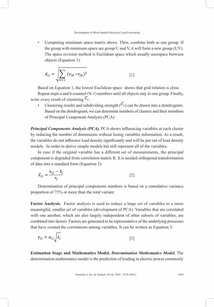
• Computing minimum space matrix above. Then, combine both as one group. If the group with minimum space are group U and V, it will form a new group (UV). The space revision method is Euclidean space which usually usesspace between objects (Equation 1).

[1]

Based on Equation 1, the lowest Euclidean space shows that grid relation is close.Repeat steps a and b counted (N-1) numbers until all objects stay in one group. Finally,

write every result of clustering .• Clustering results and subdividing strength ( ) can be drawn into a dendrogram.

Based on the dendrogram, we can determine numbers of clusters and their members of Principal Component Analysis (PCA)

Principal Components Analysis (PCA). PCA shows influencing variables at each cluster by reducing the number of dimensions without losing variables information. As a result, the variables do not influence load density significantly and will be put out of load density models. In order to derive simple models but still represent all of the variables.

In case if the original variable has a different set of measurements, the principal component is degraded from correlation matrix R. It is needed orthogonal transformation of data into a standard form (Equation 2):

[2]

Determination of principal components numbers is based on a cumulative variance proportion of 75% or more than the total variant.

Factor Analysis. Factor analysis is used to reduce a large set of variables to a more meaningful, smaller set of variables (development of PCA). Variables that are correlated with one another, which are also largely independent of other subsets of variables, are combined into factors. Factors are generated to be representative of the underlying processes that have created the correlations among variables. It can be written as Equation 3:

[3]

Estimation Stage and Mathematics Model. Determination Mathematics Model. The determination mathematics model is the prediction of loading in electric power commonly



exposed in a linear model. Based on this, model construction can be formulated in terms of double regression, which is built based on mathematics model, that is Equation 4:

[4]

This mathematics model is a group linear equation with a multivariable and simplified in a matrix, written as Equation 5:

[5]

Where:

In order to get b values, sum square deviation has to be minimised as Equation 6:

[6]

Where, e’=Y (Xb)’, so that (Equation 7)

[7]

Correlation Analysis. Correlation analysis determines which variable has a stronger correlation (significant) with the initial response. So this variable will be possible to give a significant effect. So correlation with X and Y written as Equation 8:

[8]

If r > 0,5, that variable will have a significant effect on the load density variable. However, that limit is not absolute as it depends on the condition and variable needed.

Examination and Mathematics Model Test. Examination and mathematics model test are done to examine whether statistically, mathematics model has been proper or not, using F test (parameter test), t-test (parameter coefficient test) and multicollinearity test (Jimenez et al., 2019; Sun et al., 2017).



Forecasting Stage. Variable Trend. To get load density growth every year based on the model before, the first step in this process is to make a trend in each variable (except the area variable) to get growth model every year from each variable. Then, selecting the best trend from each variable is made based on the smallest error value (MAPE).

Land use alteration is trended based on RT/RW from a related area, RT/RW data use are up to 2010, and change of land use between 2011 – 2016 is seen from the growth trend area from several years before.

Load Density for Cluster Forecasting Base on Mathematics Model. Based on the result from the getting variable, the trend growth model variable is used to predict load density in each cluster. This model agrees with the model that has been derived previously.

Calculation of Peak Load Forecasting. The result of forecasting density per year from this cluster is used to calculate the load density of each area at the same cluster. Change of wide-area refers to RT/RW data.

The following process calculates of the total power of the political district by adding power in each sector (residential, commercial industry and public) at the political district. Mathematically can be written as Equation 9:

[9]

RESULT AND DISCUSSION

Forming Cluster

The forming cluster aims to group objects (districts) into clusters in which each cluster consists of districts with homogeneous characteristics.

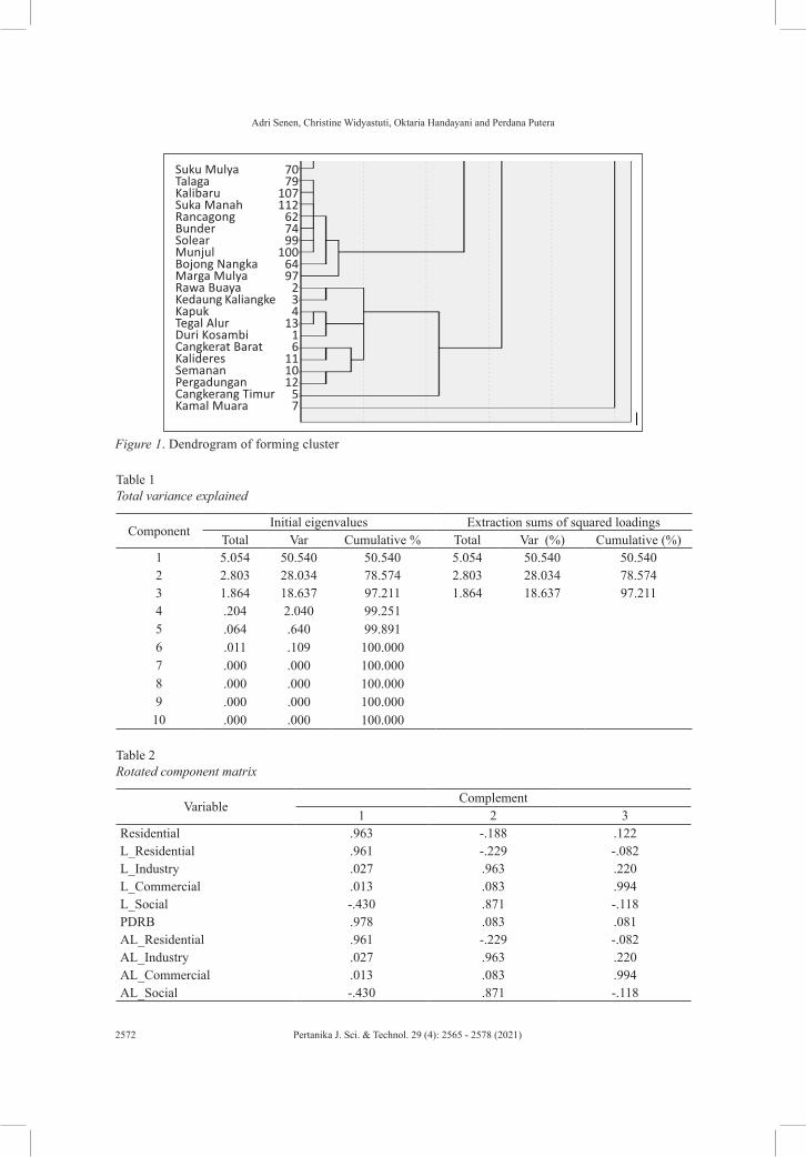
Object (districts) grouping is conducted using the clustering technique. Results of the correlation matrix process between district variables are described in the dendrogram below in Figure 1.

Results from clustering obtained 5 clusters with an entire grid of 114 districts. Further, load forecasting will be implemented in each cluster for the next ten years. The sample taken for this research is the calculation of cluster 4.

Principal Component and Factor Analysis

PCA is performed after grids are obtained. Then, it is applied by transforming original variables into new variables (principal component) in the form of a linear combination that reduces and explains the variance of original variables. Results of the correlation matrix process of each variable at each cluster towards load density per district and component matrix are described in Tables 1 and 2, respectively.



Table 1Total variance explained

ComponentInitial eigenvalues Extraction sums of squared loadings

Total Var Cumulative % Total Var (%) Cumulative (%)1 5.054 50.540 50.540 5.054 50.540 50.5402 2.803 28.034 78.574 2.803 28.034 78.5743 1.864 18.637 97.211 1.864 18.637 97.2114 .204 2.040 99.2515 .064 .640 99.8916 .011 .109 100.0007 .000 .000 100.0008 .000 .000 100.0009 .000 .000 100.00010 .000 .000 100.000

Table 2Rotated component matrix

VariableComplement

1 2 3Residential .963 -.188 .122L_Residential .961 -.229 -.082L_Industry .027 .963 .220L_Commercial .013 .083 .994L_Social -.430 .871 -.118PDRB .978 .083 .081AL_Residential .961 -.229 -.082AL_Industry .027 .963 .220AL_Commercial .013 .083 .994AL_Social -.430 .871 -.118

Figure 1. Dendrogram of forming cluster

Suku MulyaTalagaKalibaruSuka ManahRancagongBunderSolearMunjulBojong NangkaMarga MulyaRawa BuayaKedaung KaliangkeKapukTegal AlurDuri KosambiCangkerat BaratKalideresSemananPergadunganCangkerang TimurKamal Muara

7079

107112

627499

1006497

234

1316

111012

57



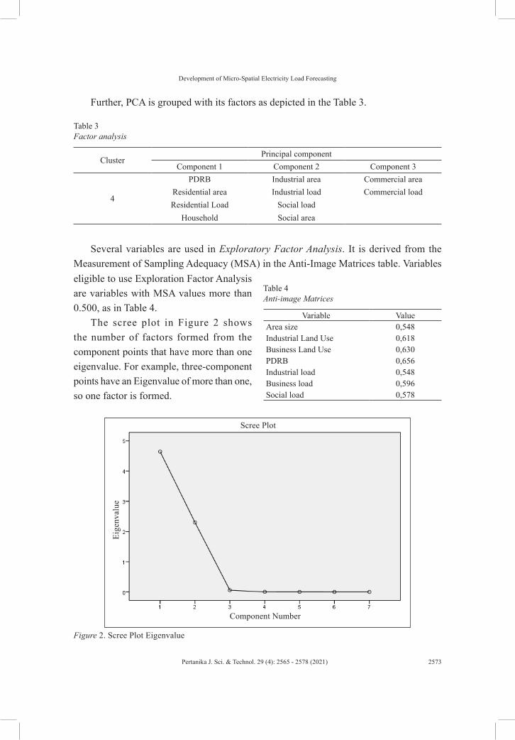
Further, PCA is grouped with its factors as depicted in the Table 3.

Table 3Factor analysis

ClusterPrincipal component

Component 1 Component 2 Component 3

4

PDRB Industrial area Commercial areaResidential area Industrial load Commercial loadResidential Load Social load

Household Social area

Several variables are used in Exploratory Factor Analysis. It is derived from the Measurement of Sampling Adequacy (MSA) in the Anti-Image Matrices table. Variables

Table 4 Anti-image Matrices

Variable ValueArea size 0,548Industrial Land Use 0,618Business Land Use 0,630PDRB 0,656Industrial load 0,548Business load 0,596Social load 0,578

Figure 2. Scree Plot Eigenvalue

Scree Plot

Component Number

Eige

nval

ue

eligible to use Exploration Factor Analysis are variables with MSA values more than 0.500, as in Table 4.

The scree plot in Figure 2 shows the number of factors formed from the component points that have more than one eigenvalue. For example, three-component points have an Eigenvalue of more than one, so one factor is formed.



The statistical test shows that each factor has the greatest value of 0.5. For example, component one, two and three is 0.901, 0.732 and 0.799 respectively with the first factor 54.5%, the second factor 22.6% and the third factor 18, 7%.

Correlation Analysis

The analysis correlation coefficient of each variable towards the response variable (load density) obtains variables whose correlation with the initial response is close. They are housing (land use), a social area (land use), commerce and average load of electricity for business. The calculation results show that variables can explain the variance from a rating value of 96.1 %, which is statistically good.

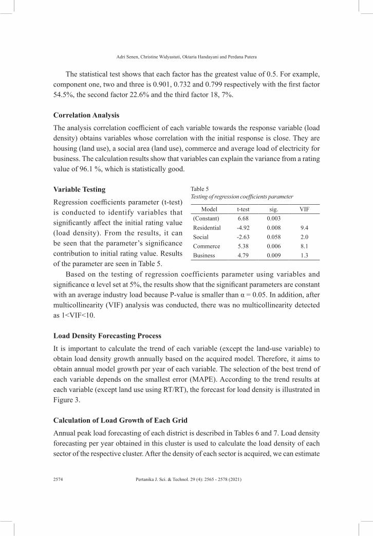
Table 5Testing of regression coefficients parameter

Model t-test sig. VIF(Constant) 6.68 0.003Residential -4.92 0.008 9.4Social -2.63 0.058 2.0Commerce 5.38 0.006 8.1Business 4.79 0.009 1.3

Variable Testing

Regression coefficients parameter (t-test) is conducted to identify variables that significantly affect the initial rating value (load density). From the results, it can be seen that the parameter’s significance contribution to initial rating value. Results of the parameter are seen in Table 5.

Based on the testing of regression coefficients parameter using variables and significance α level set at 5%, the results show that the significant parameters are constant with an average industry load because P-value is smaller than α = 0.05. In addition, after multicollinearity (VIF) analysis was conducted, there was no multicollinearity detected as 1<VIF<10.

Load Density Forecasting Process

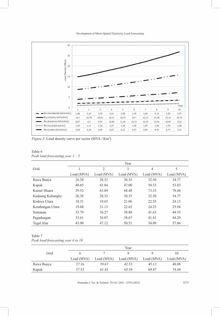
It is important to calculate the trend of each variable (except the land-use variable) to obtain load density growth annually based on the acquired model. Therefore, it aims to obtain annual model growth per year of each variable. The selection of the best trend of each variable depends on the smallest error (MAPE). According to the trend results at each variable (except land use using RT/RT), the forecast for load density is illustrated in Figure 3.

Calculation of Load Growth of Each Grid

Annual peak load forecasting of each district is described in Tables 6 and 7. Load density forecasting per year obtained in this cluster is used to calculate the load density of each sector of the respective cluster. After the density of each sector is acquired, we can estimate



Figure 3. Load density curve per sector (MVA / Km2)

Table 6Peak load forecasting year 1 – 5

GridYear

1 2 3 4 5Load (MVA) Load (MVA) Load (MVA) Load (MVA) Load (MVA)

Rawa Buaya 26.38 28.32 30.35 32.50 34.77Kapuk 40.85 43.84 47.00 50.33 53.83Kamal Muara 59.52 63.89 68.48 73.33 78.44Kedaung Kaliangke 26.38 28.32 30.35 32.50 34.77Kedoya Utara 18.31 19.65 21.06 22.55 24.13Kembangan Utara 19.68 21.13 22.65 24.25 25.94Semanan 33.79 36.27 38.88 41.63 44.53Pegadungan 33.61 36.07 38.67 41.41 44.29Tegal Alur 43.90 47.12 50.51 54.09 57.86

Table 7Peak load forecasting year 6 to 10

GridYear


Rawa Buaya 37.16 39.67 42.33 45.13 48.08Kapuk 57.53 61.43 65.54 69.87 74.44



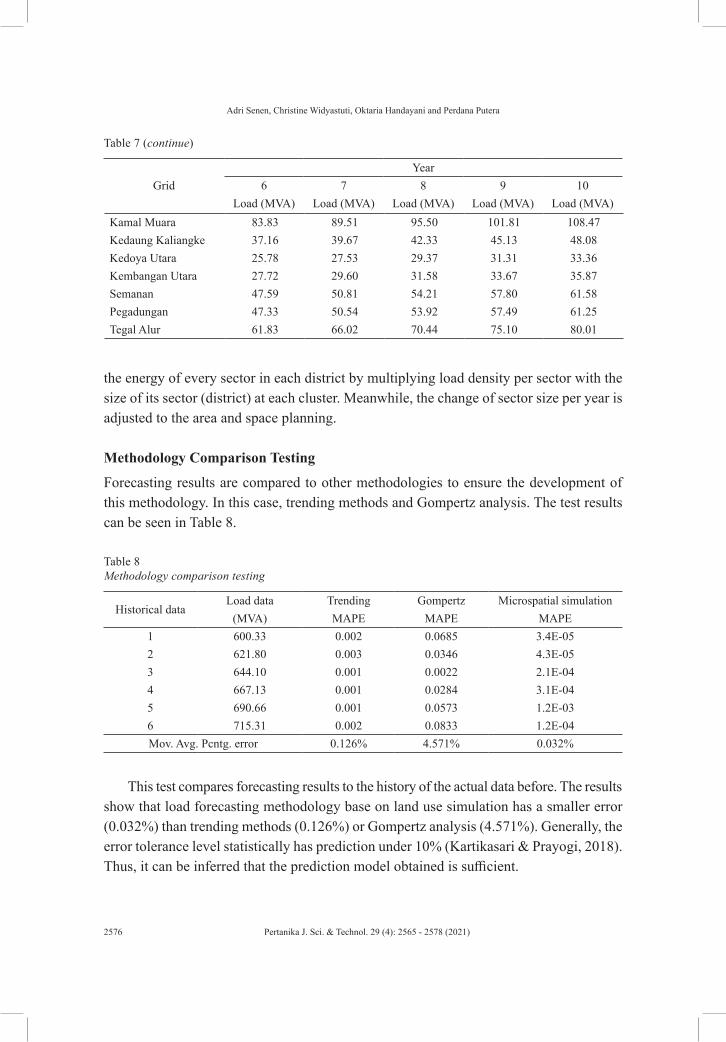
the energy of every sector in each district by multiplying load density per sector with the size of its sector (district) at each cluster. Meanwhile, the change of sector size per year is adjusted to the area and space planning.

Methodology Comparison Testing

Forecasting results are compared to other methodologies to ensure the development of this methodology. In this case, trending methods and Gompertz analysis. The test results can be seen in Table 8.

Table 8Methodology comparison testing

Historical dataLoad data Trending Gompertz Microspatial simulation

(MVA) MAPE MAPE MAPE1 600.33 0.002 0.0685 3.4E-052 621.80 0.003 0.0346 4.3E-053 644.10 0.001 0.0022 2.1E-044 667.13 0.001 0.0284 3.1E-045 690.66 0.001 0.0573 1.2E-036 715.31 0.002 0.0833 1.2E-04Mov. Avg. Pcntg. error 0.126% 4.571% 0.032%

This test compares forecasting results to the history of the actual data before. The results show that load forecasting methodology base on land use simulation has a smaller error (0.032%) than trending methods (0.126%) or Gompertz analysis (4.571%). Generally, the error tolerance level statistically has prediction under 10% (Kartikasari & Prayogi, 2018). Thus, it can be inferred that the prediction model obtained is sufficient.

Kamal Muara 83.83 89.51 95.50 101.81 108.47Kedaung Kaliangke 37.16 39.67 42.33 45.13 48.08Kedoya Utara 25.78 27.53 29.37 31.31 33.36Kembangan Utara 27.72 29.60 31.58 33.67 35.87Semanan 47.59 50.81 54.21 57.80 61.58Pegadungan 47.33 50.54 53.92 57.49 61.25Tegal Alur 61.83 66.02 70.44 75.10 80.01

Table 7 (continue)

GridYear




CONCLUSION

The development of micro-spatial load forecasting based on multivariate analysis is extended from the macro, sectoral load forecasting method, which can provide solutions and information such as load calculation, time of the incident, and its location in higher precision. Therefore, it is more appropriate to be applied as a basic tool in developing electrical distribution plan for a dynamic area such as Tangerang.

Comparing to micro-spatial load forecasting methods, which have already been developed before (Kobylinski et al., 2020; Raza et al., 2020; Sun et al., 2017), this method has a complicated algorithm solution, but returning with the more accurate result and reducing the problem with a big volume counting process.

The complication rate rises occurs because the clustering algorithm was done before the principal component analysis process (from the previous method). As a result, the level of complicity became N times, in which N indicated the number of clusters.

This method will be more accurate to be implemented in the smaller area because the base of the load variable is the load density of the service area (in this case study, it used sub-district as the smallest area).

ACKNOWLEDGEMENTS

The authors would like to thank the Ministry of Education and Culture of Indonesia and Institut Teknologi PLN for supporting this project.

REFERENCESAl Amin, M. A., & Hoque, M. A. (2019). Comparison of ARIMA and SVM for short-term load forecasting.

In 2019 9th Annual Information Technology, Electromechanical Engineering and Microelectronics Conference (IEMECON) (pp. 1-6). IEEE Publishing. https://doi.org/10.1109/IEMECONX.2019.8877077

Avazov, N., Liu, J., & Khoussainov, B. (2019). Periodic neural networks for multivariate time series analysis and forecasting. In 2019 International Joint Conference on Neural Networks (IJCNN) (pp. 1-8). IEEE Publishing. https://doi.org/10.1109/IJCNN.2019.8851710

Babcock, C., Matney, J., Finley, A. O., Weiskittel, A., & Cook, B. D. (2013). Multivariate spatial regression models for predicting individual tree structure variables using LiDAR data. IEEE Journal of Selected Topics in Applied Earth Observations and Remote Sensing, 6(1), 6-14. https://doi.org/10.1109/JSTARS.2012.2215582

Carvallo, J. P., Larsen, P. H., Sanstad, A. H., & Goldman, C. A. (2016). Load forecasting in electric utility integrated resource planning. LBNL Publications.

El Kafazi, I., Bannari, R., Abouabdellah, A., Aboutafail, M. O., & Guerrero, J. M. (2017). Energy production: A comparison of forecasting methods using the polynomial curve fitting and linear regression. In 2017 International Renewable and Sustainable Energy Conference (IRSEC) (pp. 1-5). IEEE Publishing. https://doi.org/10.1109/IRSEC.2017.8477278



Fu, Q., Lai, R., Shan, Y., & Geng, X. (2018). A spatial forecasting method for photovoltaic power generation combined of improved similar historical days and dynamic weights allocation. In 2018 IEEE Innovative Smart Grid Technologies - Asia (ISGT Asia) (pp. 1195-1198). IEEE Publishing. https://doi.org/10.1109/ISGT-Asia.2018.8467889

Jimenez, J., Pertuz, A., Quintero, C., & Montana, J. (2019). Multivariate statistical analysis based methodology for long-term demand forecasting. IEEE Latin America Transactions, 17(01), 93-101. https://doi.org/10.1109/TLA.2019.8826700

Kartikasari, M. D., & Prayogi, A. R. (2018). Demand forecasting of electricity in Indonesia with limited historical data. Journal of Physics: Conference Series, 974, Article 012040. https://doi.org/10.1088/1742-6596/974/1/012040

Kobylinski, P., Wierzbowski, M., & Piotrowski, K. (2020). High-resolution net load forecasting for micro-neighbourhoods with high penetration of renewable energy sources. International Journal of Electrical Power & Energy Systems, 117, Article 105635. https://doi.org/10.1016/j.ijepes.2019.105635

Lagaaij, A. (2018). Accelerating solar for decelerating climate change in time. In 2018 IEEE 7th World Conference on Photovoltaic Energy Conversion (WCPEC) (A Joint Conference of 45th IEEE PVSC, 28th PVSEC & 34th EU PVSEC) (pp. 2392-2394). IEEE Publishing. https://doi.org/10.1109/PVSC.2018.8547702

Mukhopadhyay, P., Mitra, G., Banerjee, S., & Mukherjee, G. (2017). Electricity load forecasting using fuzzy logic: Short term load forecasting factoring weather parameter. In 2017 7th International Conference on Power Systems (ICPS) (pp. 812-819). IEEE Publishing. https://doi.org/10.1109/ICPES.2017.8387401

Raza, M. Q., Mithulananthan, N., Li, J., & Lee, K. Y. (2020). Multivariate ensemble forecast framework for demand prediction of anomalous days. IEEE Transactions on Sustainable Energy, 11(1), 27-36. https://doi.org/10.1109/TSTE.2018.2883393

Sun, X., Ouyang, Z., & Yue, D. (2017). Short-term load forecasting based on multivariate linear regression. In 2017 IEEE Conference on Energy Internet and Energy System Integration (EI2) (pp. 1-5). IEEE Publishing. https://doi.org/10.1109/EI2.2017.8245401

Documents

Development of Micro-Spatial Electricity Load Forecasting