Embed Size (px)
Citation preview
DEVELOPMENT OF MULTIVARIABLE
CONTROL SYSTEMS
MAUNG MAUNG LATT
SCHOOL OF ELECTRICAL AND ELECTRONIC ENGINEERING
A DISSERTATION SUBMITTED IN PARTIAL FULFILMENT OF
THE REQUIREMENTS FOR THE DEGREE OF
MASTER OF SCIENCE IN COMPUTER CONTROL & AUTOMATION
2008

i
Acknowledgements
Firstly, I would like to express the deepest appreciation to my supervisor, Assoc. Prof.
CAI Wenjian, for giving me the opportunity to work in a very interesting area, and
his continuous guidance, encouragement, and invaluable comments during this work.
Without his help, this dissertation would not have been possible.
In addition, I would like to express my gratitude to Nanyang Technological University
(NTU) Library for the technical books and electronic resources, and the technical staff
of the Process Instrumentation Laboratory, Mr. Yock and his colleagues for their
assistance in hardware and software requirements.
Lastly, but most importantly, I am forever indebted to my parents and my friends for
their understanding, endless patience, and continuous encouragement during this
dissertation.
ii
Summary
This dissertation presents three decentralized control systems for the three distillation
systems in the literature. The loop pairing and controller design methods are:
1. RGA based Biggest Log Modulus Tuning (BLT) method
2. dRI based Skogestad Internal Model Control (SIMC) method
3. ERGA based PID control method
Firstly, we discuss the basic theory of a distillation column. In this dissertation, we
assume that we have the transfer function models for the processes to be controlled.
Then we present the usefulness of decentralized control system and, explain loop
pairing methods and the controller design methods in detail. We create programming
codes and block diagrams to simulate the decentralized control systems using
Matlab/Simulink application software. We also discuss performance analysis for each
control method using IAE, ISE, and ITAE.
Finally, the simulation results from this small work can result in the invaluable
conclusion and recommendation for the decentralized control system.
iii
Table of Contents
Acknowledgements ..................................................................................................... i
Summary .................................................................................................................... ii
Table of Contents ...................................................................................................... iii
List of Figures ............................................................................................................ v
List of Tables ........................................................................................................... vii
1 Introduction ............................................................................................................. 1
1.1 Motivation ........................................................................................................ 1
1.2 Objectives ......................................................................................................... 3
1.3 Major Contribution of the Thesis ...................................................................... 3
2 Distillation Column ................................................................................................. 4
2.1 Introduction ...................................................................................................... 4
2.2 System Identification ........................................................................................ 6
2.3 Distillation Models ........................................................................................... 8
3 Decentralized Control ............................................................................................ 10
3.1 Introduction .................................................................................................... 10
3.2 Control Structure ............................................................................................ 10
3.3 Advantages of Decentralized Control .............................................................. 11
3.4 Disadvantages of Decentralized Control .......................................................... 12
3.5 Interaction Measure and Loop Pairing ............................................................. 12
3.6 Some Important Factors in MIMO System Analysis........................................ 14
4 Controller Design Methods .................................................................................... 17
4.1 Introduction .................................................................................................... 17
4.2 BLT Tuning Method based on RGA Paring Criteria ........................................ 19
4.2.1 Interaction Measure and Loop Pairing ...................................................... 19
4.2.2 Decentralized Controller Design............................................................... 22
4.3 SIMC Tuning Method based on dRI Loop Pairing Criteria .............................. 26
4.3.1 Interaction Measure and Loop Pairing ...................................................... 28
4.3.2 Algorithm for Loop Pairing ...................................................................... 35
4.3.3 Dynamic Relative Interaction ................................................................... 37
4.3.4 Decentralized Controller Design............................................................... 42
4.3.5 Algorithm for Decentralized Controller Design ........................................ 50
iv
4.4 GPM Tuning Method based on ERGA Pairing Criteria ................................... 51
4.4.1 Interaction Measure and Loop Pairing ...................................................... 51
4.4.2 Decentralized Control System Design ...................................................... 57
5 Simulation and Performance Analysis.................................................................... 66
5.1 Introduction .................................................................................................... 66
5.2 Simulation and Discussion for Vinante and Luyben System (1972) ................. 66
5.2.1 BLT ......................................................................................................... 67
5.2.2 SIMC ....................................................................................................... 68
5.2.3 ERGA ...................................................................................................... 69
5.3 Simulation and Discussion for Ogunnaike and Ray System (1979).................. 72
5.3.1 BLT ......................................................................................................... 75
5.3.2 SIMC ....................................................................................................... 76
5.3.3 ERGA ...................................................................................................... 79
5.4 Simulation and Discussion for Alatiqi case 1 System (1985) ........................... 80
5.4.1 BLT ......................................................................................................... 84
5.4.2 SIMC ....................................................................................................... 87
5.4.3 ERGA ...................................................................................................... 89
5.5 Performance Analysis ..................................................................................... 91
6 Conclusion and Recommendation .......................................................................... 97
6.1 Conclusion ...................................................................................................... 97
6.2 Recommendation for further research ............................................................. 98
Bibliography........................................................................................................... 100
A Simulink Block Diagram for 2x2 Decentralized Control System ..................... 107
B Simulink Block Diagram for 3x3 Decentralized Control System ..................... 109
C Simulink Block Diagram for 4x4 Decentralized Control System ..................... 110
D Matlab Program for 2x2 Decentralized Control System ................................... 111
E Matlab Program for 3x3 Decentralized Control System ................................... 123
F Matlab Program for 4x4 Decentralized Control System ................................... 137
v
List of Figures
Figure 2.1 Diagram of typical industrial distillation column ........................................ 4
Figure 2.2 Photo of typical industrial distillation column ............................................ 5
Figure 3.1 Typical block diagram of decentralized control structure ......................... 11
Figure 4.1 all loops are open ..................................................................................... 28
Figure 4.2 only loop i jy u is open ........................................................................... 29
Figure 4.3 only loop i jy u is closed ........................................................................ 30
Figure 4.4 all loops are closed .................................................................................. 32
Figure 4.5 Flow chart of variable pairing selection procedure ................................... 36
Figure 4.6 Structure of loop i iy u by structural decomposition................................ 38
Figure 4.7 Closed loop system with control loop i iy u presented explicitly ............. 40
Figure 4.8 Procedure for the independent design of a decentralized PID controller ... 49
Figure 4.9 Frequency response curves and the energy of ( )ijg j (bandwidth,b ij ) .... 53
Figure 4.10 Frequency response curve and effective energy of ( )ijg j (ultimate
frequency,u ij ) ......................................................................................................... 54
Figure 4.11 Interaction mode with 1, 1ii ii ....................................................... 60
Figure 4.12 Interaction mode with 1, 1ii ii ....................................................... 61
Figure 4.13 f Interaction mode with 1, 1ii ii ..................................................... 62
Figure 4.14 Interaction mode with 1, 1ii ii ....................................................... 62
Figure 5.1 Closed loop step responses of y1 for VL System (1972)........................... 71
Figure 5.2 Closed loop step responses of y2 for VL System (1972)........................... 71
Figure 5.3 Step responses for g33 and g33new for OR System (1979) ...................... 74
Figure 5.4 Closed loop step responses of y1 for OR system (1979) ........................... 77
Figure 5.5 Closed loop step responses of y2 for OR system (1979) ........................... 77
Figure 5.6 Closed loop step responses of y3 for OR system (1979) ........................... 78
Figure 5.7 Step responses for g12 and g12new for A1 System (1985) ....................... 85
Figure 5.8 Step responses for g42 and g42new for A1 System (1985) ....................... 85
Figure 5.9 Step responses of y1 for A1 System (1985) .............................................. 91
Figure 5.10 Step responses of y2 for A1 System (1985) ............................................ 92
vi
Figure 5.11 Step responses of y3 for A1 System (1985) ............................................ 92
Figure 5.12 Step responses of y4 for A1 System (1985) ............................................ 93
Figure 6.1 Screenshot of SISO Design Tool .............................................................. 98
Figure 6.2 Screenshot of Decentralized Control ........................................................ 99
Figure A.1 Simulink block diagram for 2x2 decentralized control system ............... 107
Figure A.2 subsystem1 ........................................................................................... 108
Figure A.3 Subsystem2 ........................................................................................... 108
Figure B.1 Simulink block diagram for 3x3 decentralized control system ............... 109
Figure C.1 Simulink block diagram for 4x4 decentralized control system ............... 110
vii
List of Tables
Table 4.1 Four Interaction scenarios for loop i jy u ................................................ 28
Table 4.2 Typical Gain and Phase Margin Values ..................................................... 65
Table 4.3 Decentralized Controller Design ............................................................... 65
Table 5.1 The ultimate values and ZN tuning parameters .......................................... 67
Table 5.2 Tuning parameter ...................................................................................... 68
Table 5.3 Decentralized Controllers for VL System (1972) ....................................... 70
Table 5.4 The ultimate values and ZN tuning parameters .......................................... 75
Table 5.5 Tuning parameters .................................................................................... 75
Table 5.6 Decentralized Controllers for OR System (1979) ...................................... 80
Table 5.7 The ultimate values and ZN tuning parameters .......................................... 86
Table 5.8 Tuning parameters .................................................................................... 86
Table 5.9 Decentralized Controllers for A1 System (1985) ....................................... 90
Table 5.10 Performance Analysis for VL System (1972) .......................................... 95
Table 5.11 Performance Analysis for OR System (1979) .......................................... 95
Table 5.12 Performance Analysis for A1 System (1985) ........................................... 96
1
1 Introduction
1.1 Motivation
Distillation accounts for approximately 95% of the separation systems used by the
refining and chemical industries around the world. (Hurowitz1, et al., 2003)
Distillation has a major impact upon the product quality, energy usage, and plant
throughput of these industries. Within the USA, there are an estimated 40,000
columns, which consume 3% of the total US energy usage. (Ramchandran, et al.,
1995) Moreover, Oil price has increased since 2003. On January 2, 2008, a single
trade was made at $100 per barrel, but the price did not stay above $100 until late
February. Oil price broke through the $110 per barrel mark on March 12, 2008 and on
May 9, 2008, the oil price exceeded $125 per barrel for the first time.(Wikipedia,
2008) Therefore, improved distillation control technique can have a significant impact
on reducing energy consumption, improving product quality, and protecting
environmental resources. Distillation control is a challenging problem because of the
nonlinearity, the presence of several couplings for dual composition control, no
stationary behavior, and many disturbances. It has been considered a well-known
process from control engineering point of view.
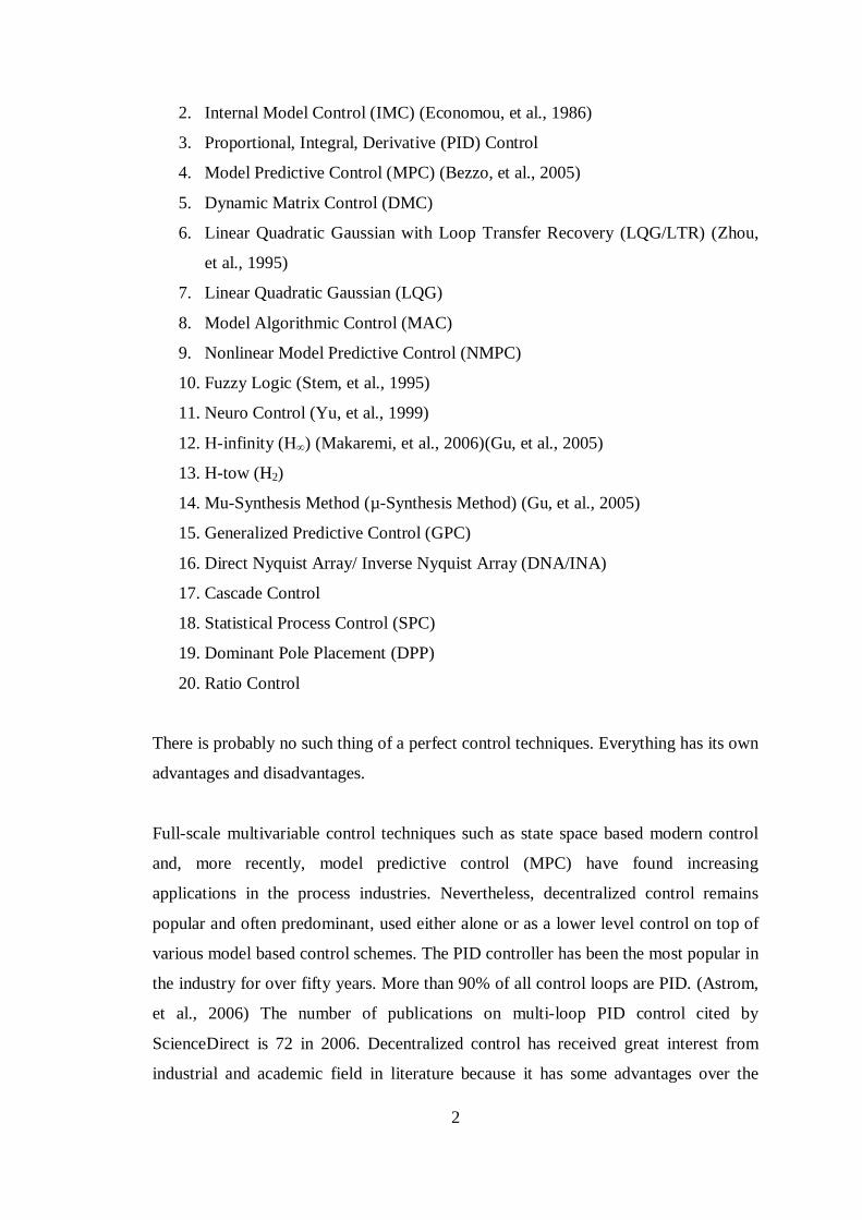
Various control techniques for controlling distillation columns have been reported in
the literature. We can divide the control techniques from various points of view. They
are:
1. Centralized and Decentralized Control
2. Classical and Advanced Control
3. Linear and Non-linear Control
4. Feedback and Feedforward Control
The popular control techniques are listed below.
1. Biggest Log Modulus Tuning (BLT) (Luyben, 1986)(Yu, et al., 1986)(Monica,
et al., 1988)
2
2. Internal Model Control (IMC) (Economou, et al., 1986)
3. Proportional, Integral, Derivative (PID) Control
4. Model Predictive Control (MPC) (Bezzo, et al., 2005)
5. Dynamic Matrix Control (DMC)
6. Linear Quadratic Gaussian with Loop Transfer Recovery (LQG/LTR) (Zhou,
et al., 1995)
7. Linear Quadratic Gaussian (LQG)
8. Model Algorithmic Control (MAC)
9. Nonlinear Model Predictive Control (NMPC)
10. Fuzzy Logic (Stem, et al., 1995)
11. Neuro Control (Yu, et al., 1999)
12. H-infinity (H∞) (Makaremi, et al., 2006)(Gu, et al., 2005)
13. H-tow (H2)
14. Mu-Synthesis Method (µ-Synthesis Method) (Gu, et al., 2005)
15. Generalized Predictive Control (GPC)
16. Direct Nyquist Array/ Inverse Nyquist Array (DNA/INA)
17. Cascade Control
18. Statistical Process Control (SPC)
19. Dominant Pole Placement (DPP)
20. Ratio Control
There is probably no such thing of a perfect control techniques. Everything has its own
advantages and disadvantages.
Full-scale multivariable control techniques such as state space based modern control
and, more recently, model predictive control (MPC) have found increasing
applications in the process industries. Nevertheless, decentralized control remains
popular and often predominant, used either alone or as a lower level control on top of
various model based control schemes. The PID controller has been the most popular in
the industry for over fifty years. More than 90% of all control loops are PID. (Astrom,
et al., 2006) The number of publications on multi-loop PID control cited by
ScienceDirect is 72 in 2006. Decentralized control has received great interest from
industrial and academic field in literature because it has some advantages over the
3
others. It is, therefore, interesting to develop an appropriate approach to tune the
parameters of the PI and PID controllers for the control of distillation columns.
1.2 Objectives
Choosing between the control techniques depends on understanding the process and its
interactions. When designing a new process, it is important to exercise some decision-
making methods. The choice of control technique should not be decided until the
project has been qualified and reasonable objectives have been established.
Overlooking this basic principle has caused companies to waste a lot of time and
money.
To be a reliable reference for industrial control engineers and research control
engineers by using the simulation results and conclusions getting from this small work
in selecting the most suitable control technique to design a decentralized control
system for a distillation process is the main objective of this dissertation.
1.3 Major Contribution of the Thesis
This dissertation is organized into six chapters to meet the requirements of this
dissertation. An introductory chapter presents the factors what motivate to do this
dissertation and the purposes of doing this dissertation, and briefly description of each
chapter in this dissertation. Chapter 2 presents the introduction of distillation column,
the importance of system identification and different types of distillation process
models to be used in this dissertation. Chapter 3 focuses on decentralized control
including basic multivariable system analysis. The following chapter presents the
theoretical backgrounds of BLT, SIMC, and ERGA. Emphasis is placed on Chapter 5,
which deals with the simulation and performance analysis of each control method.
This is a key chapter that provides the comparison results from all of the methods by
using the high-level simulation package, Matlab/Simulink. The invaluable conclusions
and, the advantages and disadvantages of different control methods are presented in
the last chapter. A number of appendices include simulation diagrams and
programming codes to help in the reading of the main body of the dissertation.
4
2 Distillation Column
2.1 Introduction
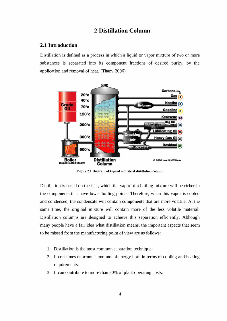
Distillation is defined as a process in which a liquid or vapor mixture of two or more
substances is separated into its component fractions of desired purity, by the
application and removal of heat. (Tham, 2006)
Figure 2.1 Diagram of typical industrial distillation column
Distillation is based on the fact, which the vapor of a boiling mixture will be richer in
the components that have lower boiling points. Therefore, when this vapor is cooled
and condensed, the condensate will contain components that are more volatile. At the
same time, the original mixture will contain more of the less volatile material.
Distillation columns are designed to achieve this separation efficiently. Although
many people have a fair idea what distillation means, the important aspects that seem
to be missed from the manufacturing point of view are as follows:
1. Distillation is the most common separation technique.
2. It consumes enormous amounts of energy both in terms of cooling and heating
requirements.
3. It can contribute to more than 50% of plant operating costs.
5
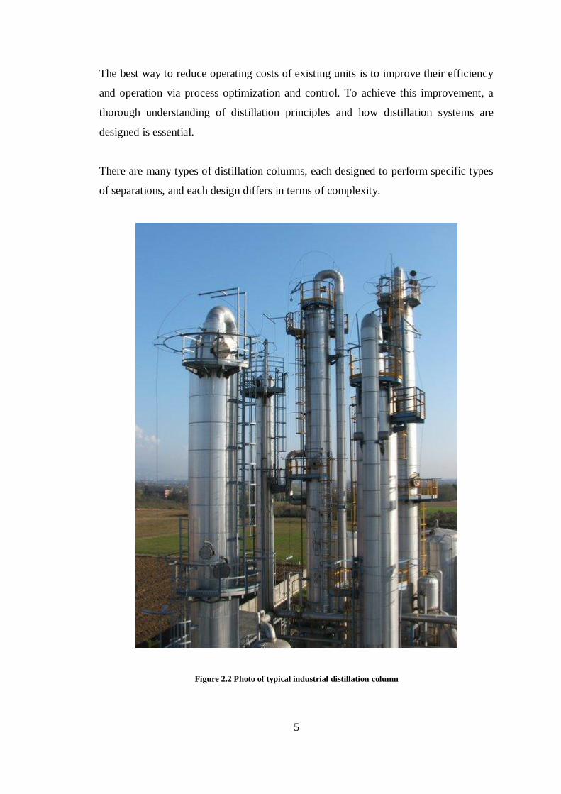
The best way to reduce operating costs of existing units is to improve their efficiency
and operation via process optimization and control. To achieve this improvement, a
thorough understanding of distillation principles and how distillation systems are
designed is essential.
There are many types of distillation columns, each designed to perform specific types
of separations, and each design differs in terms of complexity.
Figure 2.2 Photo of typical industrial distillation column
6
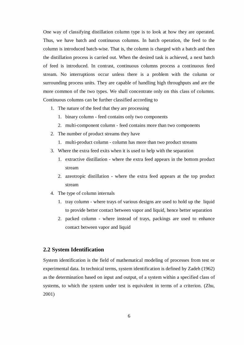
One way of classifying distillation column type is to look at how they are operated.
Thus, we have batch and continuous columns. In batch operation, the feed to the
column is introduced batch-wise. That is, the column is charged with a batch and then
the distillation process is carried out. When the desired task is achieved, a next batch
of feed is introduced. In contrast, continuous columns process a continuous feed
stream. No interruptions occur unless there is a problem with the column or
surrounding process units. They are capable of handling high throughputs and are the
more common of the two types. We shall concentrate only on this class of columns.
Continuous columns can be further classified according to
1. The nature of the feed that they are processing
1. binary column - feed contains only two components
2. multi-component column - feed contains more than two components
2. The number of product streams they have
1. multi-product column - column has more than two product streams
3. Where the extra feed exits when it is used to help with the separation
1. extractive distillation - where the extra feed appears in the bottom product
stream
2. azeotropic distillation - where the extra feed appears at the top product
stream
4. The type of column internals
1. tray column - where trays of various designs are used to hold up the liquid
to provide better contact between vapor and liquid, hence better separation
2. packed column - where instead of trays, packings are used to enhance
contact between vapor and liquid
2.2 System Identification
System identification is the field of mathematical modeling of processes from test or
experimental data. In technical terms, system identification is defined by Zadeh (1962)
as the determination based on input and output, of a system within a specified class of
systems, to which the system under test is equivalent in terms of a criterion. (Zhu,
2001)

7
For an industry control related project, it normally involves the following steps
:(Cai, 2007)
1. Benefit Analysis and Functional Design
2. Pre-testing
3. Identification Test and Model Identification
4. Controller Tuning and Simulation
5. Controller Commissioning
6 . Controller Maintenance
From above procedures, we can see that dynamic models play a central role in process
control. It is essential to know and understand a system before handling it. A system is
known through modeling and identification and understood by analysis. They are
prerequisites to the practice of automatic control.
Several approaches and techniques are available in the literature for deriving the
desired process model. Standard modeling approaches include two main streams:
1. First-principle (white-box approach)
2. Identification of the parameters (black-box approach)
The system identification procedure has the following basic steps:
1. Identification tests or experiments
2. Model order/structure selection
3. Parameter estimation
4. Model validation
Unfortunately, there is no room to describe in full detail of the system identification of
the processes to be used. This dissertation presents decentralized controller design
methods for MIMO systems and all methods are model-based. In this dissertation, we
assume that we have a MIMO transfer function model for the process to be controlled.
8
2.3 Distillation Models
Three distillation systems from the literature will be studied. All the processes vary
from two-input two-output systems up to four-input four-output systems. These three
distillation systems are:
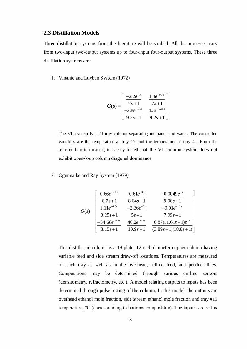
1. Vinante and Luyben System (1972)
The VL system is a 24 tray column separating methanol and water. The controlled
variables are the temperature at tray 17 and the temperature at tray 4 . From the
transfer function matrix, it is easy to tell that the VL column system does not
exhibit open-loop column diagonal dominance.
2. Ogunnaike and Ray System (1979)
2.6 3.5
6.5 3 1.2
9.2 9.4
0.66 0.61 0.0049
6.7 1 8.64 1 9.06 1
1.11 2.36 0.01( )
3.25 1 5 1 7.09 1
34.68 46.2 0.87(11.61 1)
8.15 1 10.9 1 (3.89 1)(18.8 1)
s s s
s s s
s s s
e e e
s s s
e e eG s
s s s
e e s e
s s s s
This distillation column is a 19 plate, 12 inch diameter copper column having
variable feed and side stream draw-off locations. Temperatures are measured
on each tray as well as in the overhead, reflux, feed, and product lines.
Compositions may be determined through various on-line sensors
(densitometry, refractometry, etc.). A model relating outputs to inputs has been
determined through pulse testing of the column. In this model, the outputs are
overhead ethanol mole fraction, side stream ethanol mole fraction and tray #19
temperature, °C (corresponding to bottoms composition). The inputs are reflux
0.3
1.8 0.35
2.2 1.3
7 1 7 1( )
2.8 4.3
9.5 1 9.2 1
s s
s s
e e
s sG s
e e
s s
9
flow rate, gpm (m3/s), side stream product flow rate, gpm (m
3/s) and reboiler
stream pressure, psig (kPa).
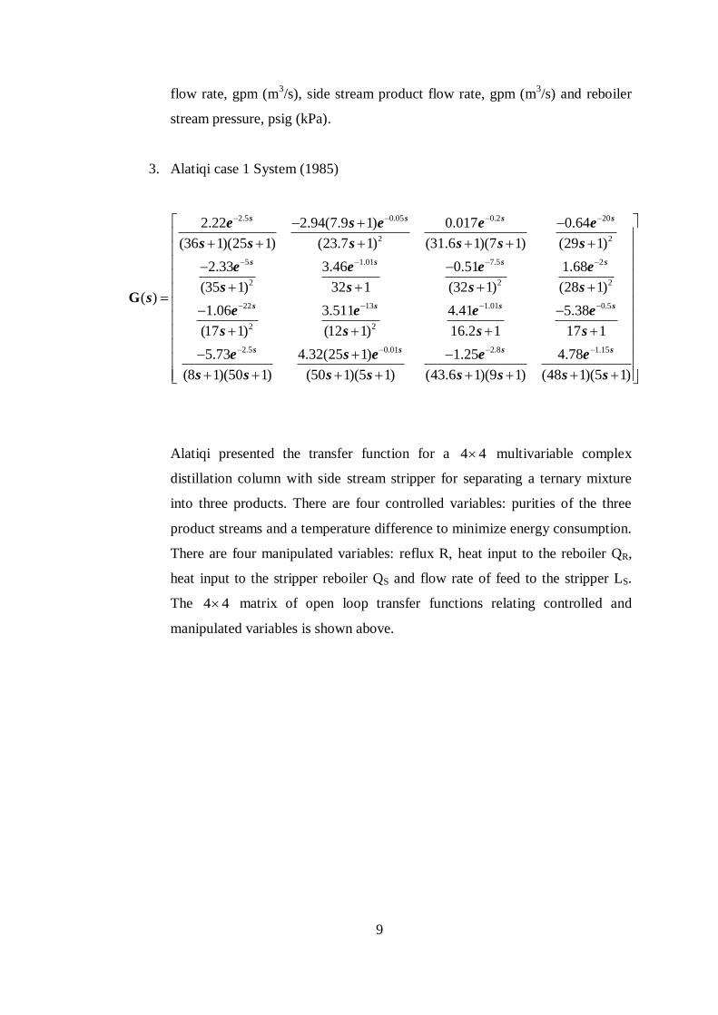
3. Alatiqi case 1 System (1985)
Alatiqi presented the transfer function for a 4 4 multivariable complex
distillation column with side stream stripper for separating a ternary mixture
into three products. There are four controlled variables: purities of the three
product streams and a temperature difference to minimize energy consumption.
There are four manipulated variables: reflux R, heat input to the reboiler QR,
heat input to the stripper reboiler QS and flow rate of feed to the stripper LS.
The 4 4 matrix of open loop transfer functions relating controlled and
manipulated variables is shown above.
2.5 0.05 0.2 20
2 2
5 1.01 7.5 2
2 2 2
22 13
2
2.22 2.94(7.9 1) 0.017 0.64
(36 1)(25 1) (23.7 1) (31.6 1)(7 1) (29 1)
2.33 3.46 0.51 1.68
(35 1) 32 1 (32 1) (28 1)( )
1.06 3.511
(17 1) (
G
s s s s
s s s s
s s
e s e e e
s s s s s s
e e e e
s s s ss
e e
s
1.01 0.5
2
2.5 0.01 2.8 1.15
4.41 5.38
12 1) 16.2 1 17 1
5.73 4.32(25 1) 1.25 4.78
(8 1)(50 1) (50 1)(5 1) (43.6 1)(9 1) (48 1)(5 1)
s s
s s s s
e e
s s s
e s e e e
s s s s s s s s
10
3 Decentralized Control
3.1 Introduction
The historically first approach to multivariable control in industry was dividing the
sensors and actuators into n subsets and designing control loops using one of the
sensor sets and one of the actuator sets, which is usually denoted as input/output
pairing. In this way, a complex control problem is divided into n supposedly simpler
ones, with no information exchange between those controllers. This strategy is called
multi-loop, decentralized, or diagonal control.
The decentralized control is also the simplest approach to multivariable control. This
works well if the plant ( )G s is close to diagonal because the plant to be controlled is
essentially a collection of independent sub-plants, and each element in ( )G s may be
designed independently. However, if off-diagonal elements in ( )G s are large, then the
performance with decentralized control may be poor because no attempt is made to
counteract the interactions.
For decentralized controller design, we have to consider the effects of interaction on
multivariable system behavior, assuming that the process has a controllable input-
output selection. The goal for decentralized controller design is to find out how the
responses of a control system are influenced by interaction. The design of multiple
single-loop controllers for multivariable systems processes in two stages:
1. Judicious choice of loop pairing (control configuration selection)
2. Controller tuning for individual loop
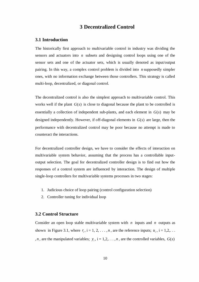
3.2 Control Structure
Consider an open loop stable multivariable system with n inputs and n outputs as
shown in Figure 3.1, where ir , i = 1, 2, . . . , n , are the reference inputs; iu , i = 1,2,. . .
, n , are the manipulated variables; iy , i = 1,2,. . . , n , are the controlled variables, ( )G s
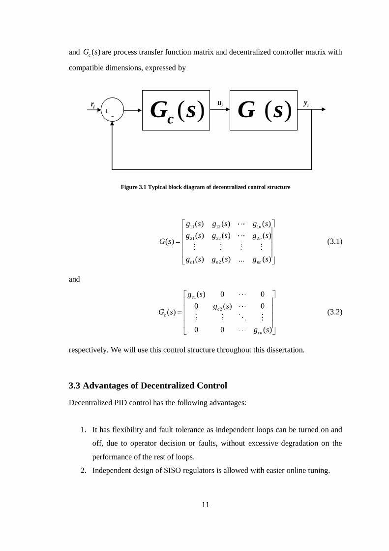
11
and ( )cG s are process transfer function matrix and decentralized controller matrix with
compatible dimensions, expressed by
Figure 3.1 Typical block diagram of decentralized control structure
11 12 1
21 22 2
1 2
( ) ( ) ( )
( ) ( ) ( )( )
( ) ( ) ... ( )
n
n
n n nn
g s g s g s
g s g s g sG s
g s g s g s
(3.1)
and
1
2
( ) 0 0
0 ( ) 0( )
0 0 ( )
c
c
c
cn
g s
g sG s
g s
(3.2)
respectively. We will use this control structure throughout this dissertation.
3.3 Advantages of Decentralized Control
Decentralized PID control has the following advantages:
1. It has flexibility and fault tolerance as independent loops can be turned on and
off, due to operator decision or faults, without excessive degradation on the
performance of the rest of loops.
2. Independent design of SISO regulators is allowed with easier online tuning.
iu
iy
ir
+
- ( )G s
( )c
G s

12
3 . The cost of implementation of a decentralized control system is
significantly lower than that of a centralized controller.
4 . It can save on modeling effort.
5 . They are often easier to understand by operators.
6 . They reduce the need for control links.
7 . Their tuning parameters have a direct effect.
8 . They tend to be less sensitive to uncertainty, for example, in the input
channels.
9 . Computation load in decentralized control is lesser than that in centralized
control.
10. It is simplicity for implementation and manual tuning.
11. The controller structure is simple and easy to handle loop failure.
12. We can use the standard equipment.
13. Decentralized controllers involve far fewer parameters, resulting in a
significant reduction in the time and cost of tuning.
3.4 Disadvantages of Decentralized Control
1. It may not work in strongly coupled systems.
2. The optimal solution is very difficult mathematically.
3. A number of pairing option is !n for a n n plant and thus increase
exponentially with the size of the plant.
4. The optimal controller is in general of infinite order and may be non-unique.
5. It has a lack of flexibility for interaction adjustment and few powerful tools for
its design compared with general multivariable control.
3.5 Interaction Measure and Loop Pairing
In this section, we will present various interaction measure and loop pairing methods
from literature because it is one of the two main steps to design decentralized
controllers for multivariable processes.
The main difference between a scalar SISO system and a MIMO system is the
presence of directions in the latter. Compared with single-input single-output (SISO)
counterparts, MIMO systems are more difficult to control due to the existence of
13
interactions between input and output variables. Tuning the controller parameters of
one loop can affect the performance of the others. For interactive plants and finite
bandwidth controllers, there is a performance loss with decentralized control because
of the interactions caused by non-zero off-diagonal elements in plant transfer function.
The interaction may also cause stability problems. To apply multi-loop control
successfully, a methodology to assess the degree of interaction between the loops is
needed.
The number of combinations is !n so some criteria should be used in deciding loop
pairing. In fact, poor control performance can result from the improper choice of
manipulated/controlled variable pairings. Loop pairing is a vitally important aspect of
multivariable processes such as distillation process. A key element in decentralized
control is therefore to select good pairings of inputs and outputs, such that the effect of
the interactions is minimized.
Several interaction measure and loop-pairing methods have been proposed in the
literature starting from Bristol to present. The popular loop pairing methods are shown
below.
1. Relative Gain Array (RGA) (Bristol, 1966)
2. Niederlinski Index (NI) (Niederlinski, 1971)
3. Relative Interaction (RI) (Bristol, 1967)
4. Dynamic Relative Interaction (dRI) (He, et al., 2006)
5. Generalized Relative Dynamic Gain (GRDG) (Gagnon, et al., 1999)
6. Decomposed Relative Gain Array (DRGA) (Avoy, et al., 2003)
7. Effective Relative Gain Array (ERGA) (Xiong, et al., 2005)
8. IMC Interaction Measure (Economou, et al., 1986)
9. Rijnsdorp’s Interaction Measure (Rijnsdorp, 1965)
10. Nyquist Array (NA) (Grosdidier, et al., 1986)
11. Generalized Interaction (GI) (He, et al., 2004)
12. Interaction Measure (Grosdidier, et al., 1986)
13. Gramian based Interaction Measure (Conley, et al., 2000)
14
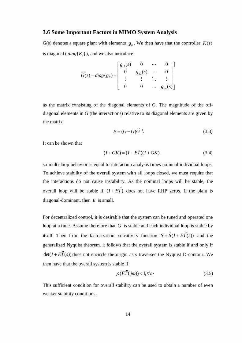
3.6 Some Important Factors in MIMO System Analysis
G(s) denotes a square plant with elements ijg . We then have that the controller ( )K s
is diagonal ( { }idiag K ), and we also introduce
11
22
( ) 0 0
0 ( ) 0( ) { }
0 0 ... ( )
ii
nn
g s
g sG s diag g
g s
as the matrix consisting of the diagonal elements of G. The magnitude of the off-
diagonal elements in G (the interactions) relative to its diagonal elements are given by
the matrix
1( ) .E G G G (3.3)
It can be shown that
( ) ( )( )I GK I ET I GK (3.4)
so multi-loop behavior is equal to interaction analysis times nominal individual loops.
To achieve stability of the overall system with all loops closed, we must require that
the interactions do not cause instability. As the nominal loops will be stable, the
overall loop will be stable if ( )I ET does not have RHP zeros. If the plant is
diagonal-dominant, then E is small.
For decentralized control, it is desirable that the system can be tuned and operated one
loop at a time. Assume therefore that G is stable and each individual loop is stable by
itself. Then from the factorization, sensitivity function ( ( ))S S I ET s and the
generalized Nyquist theorem, it follows that the overall system is stable if and only if
det( ( ))I ET s does not encircle the origin as s traverses the Nyquist D-contour. We
then have that the overall system is stable if
( ( )) 1,ET j (3.5)
This sufficient condition for overall stability can be used to obtain a number of even
weaker stability conditions.
15
For the least conservative approach by using the structured singular value, the entire
system is closed-loop stable if
( ) max 1/ ( ) iT t E (3.6)
where ( )E is called the structured singular value interaction measure, and is
computed with respect to the diagonal structure ofT .
Another approach is to use Gershgorin’s theorem, we then derive the following
sufficient condition for overall stability in terms of the rows ofG :
( ) 1
( ) ,( )( )
ii
i
iijj i
g jt j i
g j
(3.7)
These conditions refer to row sums. Substituting ijg for
jig results in a different
condition based on column sums. This is a sufficient condition for closed loop
stability. If ,ijg j i are small, i.e., diagonal dominant, the above bound is a large
number, indicating that good control can be achieved at that frequency. The frequency
for which ( ) 0.5i can be considered as an orientative designed bandwidth limit for
multi-loop control.
When considering decentralized control of a plant, we should first check that the plant
is controllable with any controller.
A desirable property of the decentralized control system is that it has integrity, that is ,
the closed loop system should remain stable as subsystem controller are brought in and
out of service of when inputs saturate. The decentralized controller ( )C s can be
decomposed into ( ) ( ) /C s N s K s , where ( )N s is the transfer function matrix of the
dynamic compensator, which is diagonal and stable and does not contain integral
action, and diag , 1,2,...,iK k i n diag , 1,2,...,iK k i n . In the design of
decentralized control system, it is desirable to choose input/output-pairings such that
the system possesses the property of DCLI. It is defined that a stable plant is said to be
DCLI, if it can be stabilized by a stable decentralized controller, which contains
integral action and if it remains stable after failure occurs in one or more of the
16
feedback loops. Given an n n stable process ( )G s , the closed-loop system of
decentralized feedback structure possesses DCLI only if
( ) 0, 1,... ; 1,...m iiG m n i m (3.8)
or
0, 1,...,mNI G m n (3.9)
where mG an arbitrary m m principal submatrix of G . Either RGA or NI can be used
as a necessary condition to examine the DCLI of decentralized control systems.
17
4 Controller Design Methods
4.1 Introduction
Many design methods based on decentralized control have been reported in literature.
The popular controller design methods are listed below.
1. The biggest log modulus (BLT) tuning approach proposed by Luyben and
co-workers (Luyben, 1986)(Yu, et al., 1986)(Monica, et al., 1988)
2. IMC-PID Controller Based on dRI Analysis proposed by Mao-Jun He,
Wen-Jian Cai and Bing-Fang Wu (He, et al., 2006)
3. Effective transfer function method in terms of ERGA interaction
measurement method proposed by Qiang Xiong and Wen-Jian Cai(Q.
Xiong, 2006)
4. Analytical Design by extending the generalized IMC–PID method for
single input/single output (SISO) systems proposed by M. Lee, K. Lee, C.
Kim and J. Lee (Lee, et al., 2004)
5. Simple tuning method derived from controller synthesis method proposed
by I-Lung Chien, Hsiao-Ping Huang and Jen-Chien Yang(Chien, et al.,
1999)
6. Design by method of inequalities proposed by R. Balachandran and M.
Chidambaram (Balachandran, et al., 1997)
7. Ziegler–Nichols with detuning factor approach proposed by McAvoy
(McAvoy, 1985)
8. Sequential loop tuning approach proposed by Shen and Yu (Shen, et al.,
1994)
9. Relay based auto-tuning approach proposed by Loh et al. (Loh, et al., 1993)
10. Describing function matrix approach proposed by Loh and Vasnani (Loh,
et al., 1994)
11. Nyquist stability analysis based tuning approach proposed by Dan Chen
and Dale E. Seborg (Chen, et al., 2003)
12. Design of Multi-loop PID Controllers Based on the Generalized IMC-PID
Method with Mp Criterion proposed by Truong Nguyen Luan Vu, Jietae
Lee, and Moonyong Lee(Vu, et al., 2007)
18
13. Dominant Pole Placement method proposed by Yu Zhang, Qing-Guo Wang
and K. J. Astrom (Zhang, et al., 2005)
14. Internal Model Control (IMC) based on Dynamic Interaction Measure by
Relative Error Matrix proposed by Jietae Lee and Thomas F. Edgar (Lee, et
al., 2004)
15. SSV-IM interaction measure based Decentralized control proposed by
Pirere Grosdidier and Manfred Morari (Grosdidier, et al., 1986)
16. Multiloop IMC Design proposed by Constantin G. Economou and Manfred
Morari (Economou, et al., 1986)
17. Continuation method proposed by Jietae Lee and Thomas F. Edgar (Lee, et
al., 2006)
18. Mp Criterion Based Multiloop PID Controllers Tuning method proposed
by Dong-Yup Lee, Moonyong Lee, Yongho Lee and Sunwon Park (Lee, et
al., 2003)
19. Iterative continuous cycling (ICC) method proposed by Jietae Lee, Wonhui
Cho and Thomas F. Edgar (Lee, et al., 1998)
20. DynPLS (Dynamic Partial Least Squares) model-based multiloop PID
controller design proposed by Junghui Chen, Yi-Chun Cheng and Yuezhi
Yea (Chen, et al., 2005)
21. Multi-loop version of the modified Ziegler-Nichols method proposed by
Qing-Guo Wang, Tong-Heng Lee and Yu Zhang (Wang, et al., 1998)
22. Independent Design method proposed by Sigurd Skogestad and Manfred
Morari (Skogestad, et al., 1989)
23. Multiloop PID Controller Tuning approach based on Gain and Phase
Margin Specifications (Ho, et al., 1997)
24. Direct method based on Effective Open-loop Process (EOP) proposed by
Hsiao-Ping Huang, Jyh-Cheng Jeng, Chih-Hung Chiang and Wen Pan
(Huang, et al., 2003)
25. Singular Value Decomposition (SVD) based method proposed by
Goshaidas Ray, A.N. Prasad and T.K. Bhattacharyya (Raya, et al., 1999)
We select the first three of the controller design methods mentioned above for this
dissertation. We select BLT tuning method because it is the first approach to
19
decentralized or multi-loop multivariable control. It is also a benchmark method for
decentralized control. ERGA is interesting because it considers four combination
modes of gain and phase changes for a particular loop when other loops are closed.
This equivalent transfer function can effectively approximate the dynamic interactions
among loops. Consequently, the decentralized controllers can be independently
designed by employing the single loop tuning techniques. The method is simple,
straightforward, easy to understand and implemented by field engineers. dRI analysis
is also reasonable and it combines with the famous SIMC-PID tuning method.
(Luyben, 1986) (Q. Xiong, 2006) (He, et al., 2006)
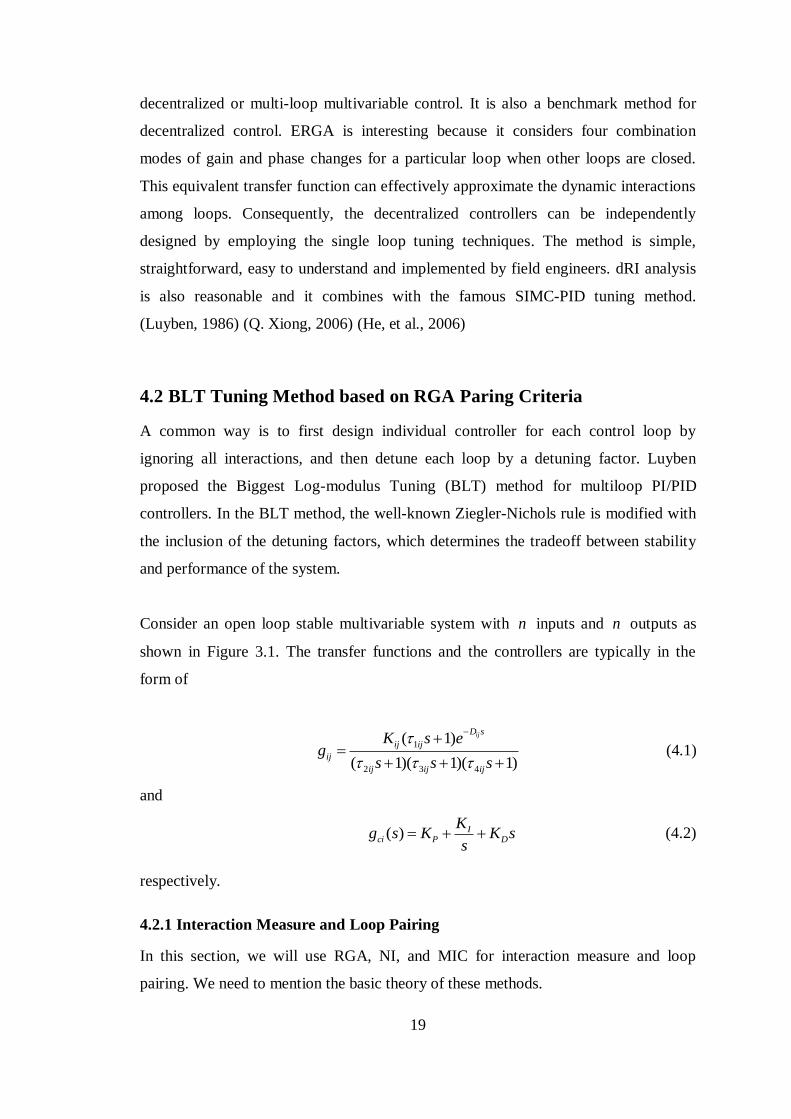
4.2 BLT Tuning Method based on RGA Paring Criteria
A common way is to first design individual controller for each control loop by
ignoring all interactions, and then detune each loop by a detuning factor. Luyben
proposed the Biggest Log-modulus Tuning (BLT) method for multiloop PI/PID
controllers. In the BLT method, the well-known Ziegler-Nichols rule is modified with
the inclusion of the detuning factors, which determines the tradeoff between stability
and performance of the system.
Consider an open loop stable multivariable system with n inputs and n outputs as
shown in Figure 3.1. The transfer functions and the controllers are typically in the
form of
1
2 3 4
( 1)
( 1)( 1)( 1)
ijD s
ij ij
ij
ij ij ij
K s eg
s s s
(4.1)
and
( ) Ici P D
Kg s K K s
s (4.2)
respectively.
4.2.1 Interaction Measure and Loop Pairing
In this section, we will use RGA, NI, and MIC for interaction measure and loop
pairing. We need to mention the basic theory of these methods.
20
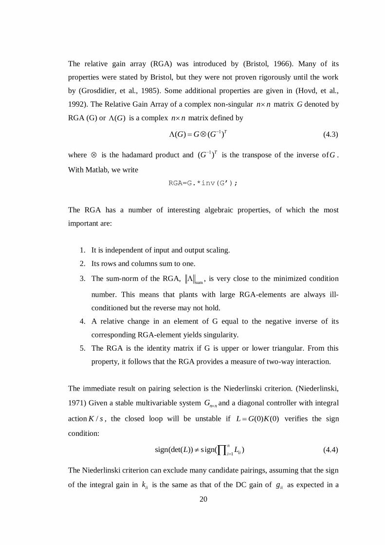
The relative gain array (RGA) was introduced by (Bristol, 1966). Many of its
properties were stated by Bristol, but they were not proven rigorously until the work
by (Grosdidier, et al., 1985). Some additional properties are given in (Hovd, et al.,
1992). The Relative Gain Array of a complex non-singular n n matrix G denoted by
RGA (G) or ( )G is a complex n n matrix defined by
1( ) ( )TG G G (4.3)
where is the hadamard product and 1( )TG
is the transpose of the inverse ofG .
With Matlab, we write
RGA=G.*inv(G’);
The RGA has a number of interesting algebraic properties, of which the most
important are:
1. It is independent of input and output scaling.
2. Its rows and columns sum to one.
3. The sum-norm of the RGA, sum
, is very close to the minimized condition
number. This means that plants with large RGA-elements are always ill-
conditioned but the reverse may not hold.
4. A relative change in an element of G equal to the negative inverse of its
corresponding RGA-element yields singularity.
5. The RGA is the identity matrix if G is upper or lower triangular. From this
property, it follows that the RGA provides a measure of two-way interaction.
The immediate result on pairing selection is the Niederlinski criterion. (Niederlinski,
1971) Given a stable multivariable system n nG and a diagonal controller with integral
action /K s , the closed loop will be unstable if (0) (0)L G K verifies the sign
condition:
1
sign(det( )) sign( )n
iiiL L
(4.4)
The Niederlinski criterion can exclude many candidate pairings, assuming that the sign
of the integral gain in iik is the same as that of the DC gain of iig as expected in a
21
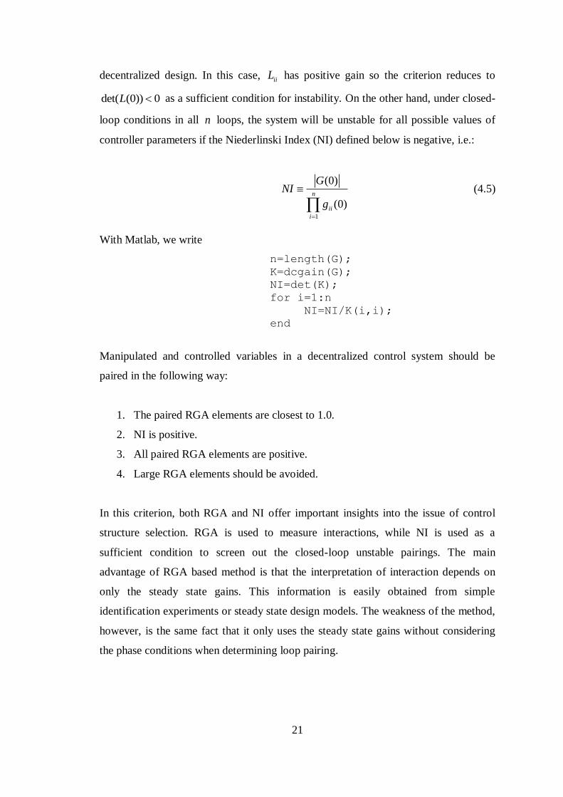
decentralized design. In this case, iiL has positive gain so the criterion reduces to
det( (0)) 0L as a sufficient condition for instability. On the other hand, under closed-
loop conditions in all n loops, the system will be unstable for all possible values of
controller parameters if the Niederlinski Index (NI) defined below is negative, i.e.:
1
(0)
(0)n
ii
i
GNI
g
(4.5)
With Matlab, we write
n=length(G);
K=dcgain(G);
NI=det(K);
for i=1:n
NI=NI/K(i,i);
end
Manipulated and controlled variables in a decentralized control system should be
paired in the following way:
1. The paired RGA elements are closest to 1.0.
2. NI is positive.
3. All paired RGA elements are positive.
4. Large RGA elements should be avoided.
In this criterion, both RGA and NI offer important insights into the issue of control
structure selection. RGA is used to measure interactions, while NI is used as a
sufficient condition to screen out the closed-loop unstable pairings. The main
advantage of RGA based method is that the interpretation of interaction depends on
only the steady state gains. This information is easily obtained from simple
identification experiments or steady state design models. The weakness of the method,
however, is the same fact that it only uses the steady state gains without considering
the phase conditions when determining loop pairing.
22
Algorithm for loop pairing
1. Eliminate pairings with negative RGAs. Pairing on negative RGA’s is
undesirable because it produces either an unstable system or a system that
lacks integrity.
2. Eliminate pairings with negative Niederlinski Indexes. The Niederlinski Index
(NI) is defined as shown in Equation (4.5). If all the SISO controllers contain
integral action and have positive loop gains, a negative value of the
Niederlinski Index shows that the system will be closed-loop unstable with this
variable pairing for any controller tuning.(Niederlinski, 1971)
All the remaining pairing possibilities must be examined. For each case, controllers
are tuned by using the BLT procedure. Then the closed-loop load-rejection
performances are compared in order to find the pairing, which does the best job of
keeping controlled variables constant in the face of load disturbances.
4.2.2 Decentralized Controller Design
BLT-1: The first step in BLT-1 tuning method is to calculate the Ziegler-Nichols
setting for each individual loop. The ultimate gain uK and ultimate frequency u of
each diagonal transfer function are calculated in the classical SISO way. To do this
numerically, a value of the frequency is guessed. The phase angle is calculated, and
frequency is varied until the phase angle is equal to 180 . This frequency is u . The
ultimate gain is the reciprocal of the real part of ( )iig s at u . There are several ways to
find the ultimate data settings, including the method of sustained oscillations, the relay
experiment, or even straightforward Nyquist plotting using software like MATLAB.
Next, a factor F is assumed. Typical values vary from 2 to 5. The gains of all
feedback controllers CK are calculated by dividing the Ziegler-Nichols gain iZNK by
the factor ,F
iZN
Ci
KK
F (4.6)
23
where,
2.2
i
i
u
ZN
KK (4.7)
The reset times ( I ) of all controllers are calculated by multiplying the Ziegler-
Nichols reset times ( ZN ) by the same factor ,F
iIi ZNF (4.8)
where,
2
1.2iZN
ui
(4.9)
The F factor can be considered a detuning factor, which is applied to all loops. The
larger the value of F, the more stable the system will be but the more sluggish will be
the set point and load responses. The method outlined below yields a value of F ,
which gives a reasonable compromise between stability and performance in
multivariable systems.
The closed-loop system can be expressed by
( )cy Gu GG r y (4.10)
Solving for y gives,
1
c cy I GG GG r
(4.11)
Since the inverse of a matrix has the determinant of the matrix in the denominator, the
closed-loop characteristic equation of the multivariable system is the scalar equation
det( ) 0cI GG (4.12)
The number of right half plane zeros of the closed-loop characteristic equation can be
found by plotting the left side of Equation (4.12) as a function of frequency and
looking at the encirclements of the origin. In order to make this multivariable plot look
just like the SISO scalar Nyquist plot, we subtract one from Equation (4.12) and look
at the encirclements of the (-1,0) point. It is convenient to define a new function
( ) 1 det( )( )cW s I GG s (4.13)
24
W is plotted as a function of frequency. The closer W approaches the (-1,0) point,
the closer the multivariable system is to closed-loop instability. The quantity
( )
1 ( )
W s
W s (4.14)
will be similar to the closed-loop servo-transfer function for a SISO loop
( ) ( )
1 ( ) ( )
c
c
g s g s
g s g s (4.15)
Therefore, based on intuition and empirical grounds, a multivariable closed-loop log
modulus cmL are defined as
20 log1
cm
WL
W
(4.16)
The proposed tuning method is based on varying the factor F until the biggest log
modulus max( )cmL is equal to some reasonable number. Thus, the proposed tuning
method is called the biggest log modulus tuning (BLT).
Now we must determine what is a reasonable value to use for max( )cmL for different
orders of the systems. For a SISO system where N = 1, we know from long experience
that a value of 2 dB for max( )cmL gives reasonable time domain responses for set
point and load disturbances. The best tuning criterion for this method is
max( ) 2cmL N (4.17)
For 1N , this reduces to the classical +2dB criterion. For a 4 4 system, a max( )cmL
of 8 should be used. These empirical findings suggest that the higher the order of the
system, the more under damped the closed-loop system must be to achieve reasonable
responses.
This tuning method should be viewed as giving preliminary controller settings, which
can be used as a benchmark for comparative studies. Note that this procedure
guarantees that the system is stable with all controllers on automatic and that each
individual loop will be stable if all others are on manual. Thus, a portion of the
integrity question is automatically answered.
25
The method weighs each loop equally; i.e., each loop is detuned by the same factor F.
If it is more important to keep tighter control of some variable than the others, the
method can be easily modified by using different weighting factors for different
controlled variables. The less-important loop could be detuned more than the more-
important loop.
We will summarize BLT-1 tuning procedures mentioned above as follow.
1. Compute the Ziegler-Nichols tuning parameters of the diagonal elements of the
process transfer function matrix ( )iig s as though the diagonal elements
represented SISO systems.
2. Choose a detuning factor F . F should be greater than one.
3. Compute CiK , and Ii for each loop by
iZN
Ci
KK
F (4.18)
iIi ZNF (4.19)
where iZNK and
iZN are the Ziegler-Nichols PI values.
4. Calculate the function W over the appropriate frequency range (i.e., near the
( 1,0) point), where
1 det ( ) ( )cW I G j G j (4.20)
5. Compute the function ( )cL j where
( ) 20 log1
c
WL j
W
(4.21)
6. Adjust F until the peak in the cL log modulus curve cmL is equal to 2N ,i.e.,
max 2cL N , where cmL is the biggest log modulus in the cL curve and N is the
number of SISO loops in the multivariable system.
It is important when applying this procedure to confirm the form of the Nyquist plot of
the function W , because the log modulus function merely denotes nearness to the
26
critical point. An unstable system could be tuned to a maximum log modulus of 2N
because it encircles the ( 1,0) point but is not near it.
BLT-2: After tuning by BLT-1, derivative action can be incorporated through the
steps that follow. We will consider derivative action for SOPTD processes in this
dissertation.
1. Choose a second detuning factor DF . It should be greater than one.
2. Compute Di , where
Di ZNDi
DF
(4.22)
and Di ZN is the Ziegler-Nichols value for Di and is equal to
0.125Di ZN uP .- (4.23)
3. Repeat steps 4 and 5 of the BLT-1 procedure. Change DF until max
cL
is
minimized, maintaining 1.DF The trivial case may result where max
cL is
minimized for DF , i.e., no derivative action.
4. Reduce DF , and repeat steps 3, 4, and 5 of the BLT-1 procedure until
max 2 .cL N
5. Repeat steps 4 and 5 above until no further reduction in F is possible. By this
process, we are shifting the phase angle of the closed-loop characteristic
equation Nyquist contour by tuning the derivative terms so that they have the
greatest effect near the closed-loop resonant frequency.
4.3 SIMC Tuning Method based on dRI Loop Pairing Criteria
In this section, a simple yet effective decentralized PID controller design methodology
will be presented based on dynamic interaction analysis and Skogestad Internal Model
Control (SIMC) principle. Based on structure decomposition, the dynamic relative
interaction (dRI) is defined and represented by the process model and controller
explicitly. An initial decentralized controller is designed first by using the diagonal
elements and then implemented to estimate the dynamic relative interaction to
27
individual control loop from all others. With the obtained dRI, the multiplicate model
factor (MMF) is derived, and then simplified to a pure time delay function at the
neighborhood of each control loop critical frequency to obtain the equivalent transfer
function for the particular control loop. Consequently, appropriate controller
parameters for individual control loop are determined by applying the SIMC-PID
tuning rules for the equivalent transfer function.
Consider an open loop stable multivariable system with n inputs and n outputs as
shown in Figure 3.1. ijG denotes the matrix G with its thi row and thj column
removed. , ,r u and y are vectors of references and manipulated and controlled
variables, while , ,i ir u and iy are the ith references and manipulated and controlled
variables, and , ,i ir u and iy denote the reference, input, and output vectors with
variables , ,i ir u and iy removed. The process transfer functions and the controllers1
are typically of the form as
'
( ) , ' .( 1)( 1)
ijs
ij
ij ij ij
ij ij
k eg s
s
(4.24)
and in parallel form as
1
( ) (1 )i Pi Di
Ii
C s k ss
(4.25)
or in series form as
1
( ) (1 )( 1).i Pi Di
Ii
C s k ss
(4.26)
respectively. And to investigate the interactions between an arbitrary loop i jy u and
all other loops of the multivariable system, the process from u to y can be explicitly
expressed by
ij j
i ij j i
i ij ij j
j j
y g u g u
y g u G u
(4.27)
1 ( ) ( ).cC s G s
28
where ij
ig and ij
jg denote the ith row vector and the thj column vector of matrix G
with element ijg removed.
4.3.1 Interaction Measure and Loop Pairing
For an arbitrary loop i jy u
and the remaining subsystem block, there are four
interaction scenarios corresponding to the combination of their open and closed states,
which are listed in Table 4.1 and indicated in Figure 4.1 to Figure 4.4.
Case loop i jy u All other loops Figure
1 open loop open loop Figure 4.1
2 open loop closed loop Figure 4.2
3 closed loop open loop Figure 4.3
4 closed loop closed loop Figure 4.3
Table 4.1 Four Interaction scenarios for loop i jy u
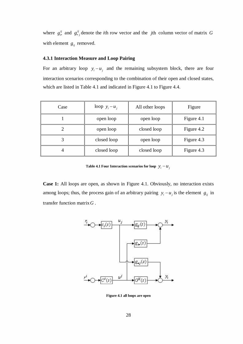
Case 1: All loops are open, as shown in Figure 4.1. Obviously, no interaction exists
among loops; thus, the process gain of an arbitrary pairing i jy u is the element
ijg in
transfer function matrixG .
Figure 4.1 all loops are open
29
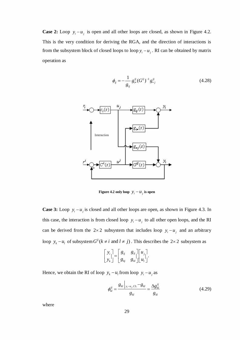
Case 2: Loop i jy u
is open and all other loops are closed, as shown in Figure 4.2.
This is the very condition for deriving the RGA, and the direction of interactions is
from the subsystem block of closed loops to loopi jy u . RI can be obtained by matrix
operation as
11( )ij ij ij
ij i j
ij
g G gg
(4.28)
Figure 4.2 only loop i jy u is open
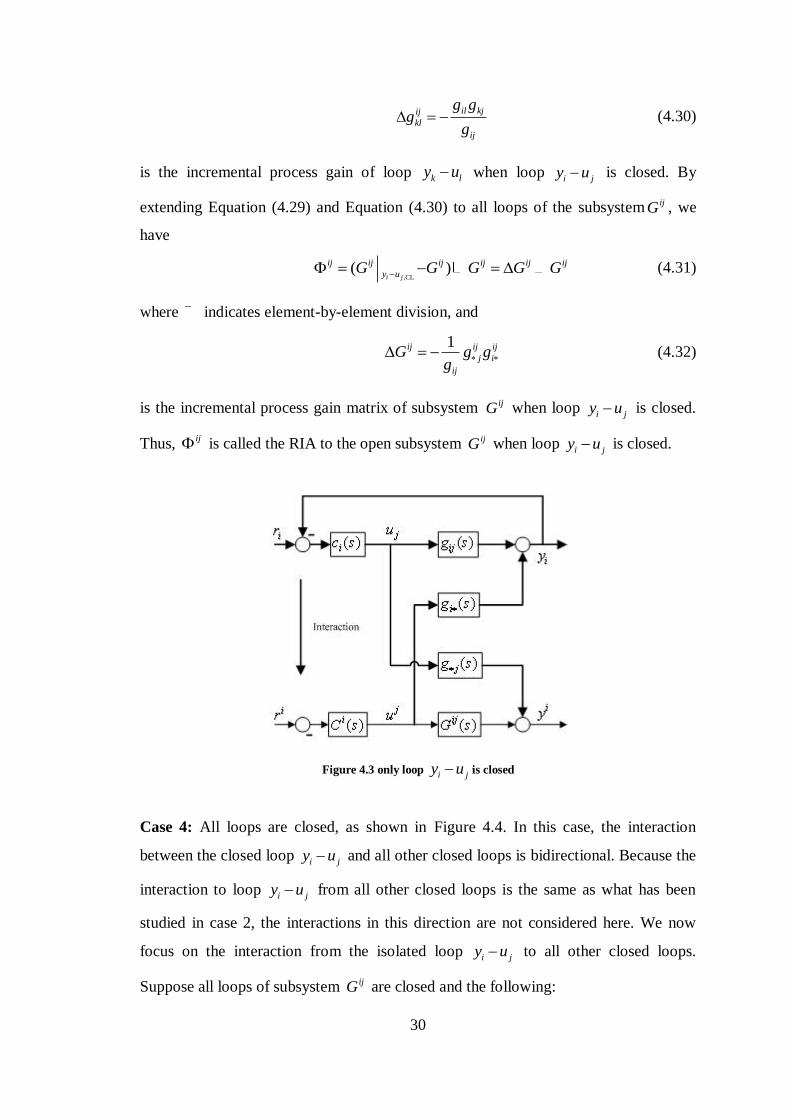
Case 3: Loop i jy u is closed and all other loops are open, as shown in Figure 4.3. In
this case, the interaction is from closed loop i jy u to all other open loops, and the RI
can be derived from the 2 2 subsystem that includes loop i jy u and an arbitrary
loop k ly u of subsystem ( and )ijG k i l j . This describes the 2 2 subsystem as
.ij ili j
kj klk l
g gy u
g gy u
Hence, we obtain the RI of loop k ly u from loop i jy u as
,CLi j
ijkl y u klij kl
kl
kl kl
g g g
g g
(4.29)
where
30
il kjij
kl
ij
g gg
g (4.30)
is the incremental process gain of loop k ly u
when loop i jy u is closed. By
extending Equation (4.29) and Equation (4.30) to all loops of the subsystem ijG , we
have
,CL
( )i j
ij ij ij ij ij ij
y uG G G G G (4.31)
where indicates element-by-element division, and
1ij ij ij
j i
ij
G g gg
(4.32)
is the incremental process gain matrix of subsystem ijG when loop i jy u is closed.
Thus, ij is called the RIA to the open subsystem ijG when loop
i jy u is closed.
Figure 4.3 only loop i jy u is closed
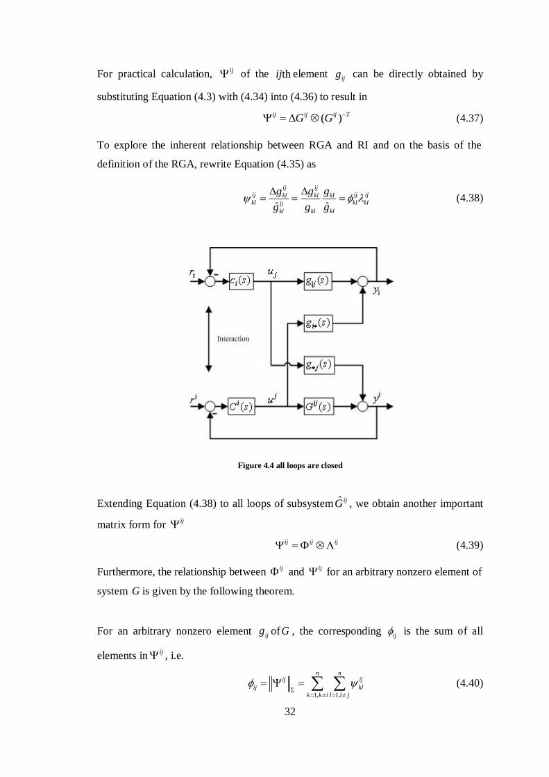
Case 4: All loops are closed, as shown in Figure 4.4. In this case, the interaction
between the closed loop i jy u and all other closed loops is bidirectional. Because the
interaction to loop i jy u from all other closed loops is the same as what has been
studied in case 2, the interactions in this direction are not considered here. We now
focus on the interaction from the isolated loop i jy u to all other closed loops.
Suppose all loops of subsystem ijG are closed and the following:
31
1. If loop i jy u is open, then the gain of an arbitrary loop k ly u is affected by
the RGA value of ijG ; therefore, according to the definition of RGA, it is
ˆ klkl ij
kl
gg
(4.33)
where arc indicates the changed process gain in the closed subsystem ijG .
When Equation (4.33) is extended to all loops of subsystem ijG , the closed-
loop transfer function matrix is obtained as
ˆ ij ij ijG G (4.34)
2. If loop i jy u is closed, then the subsystem that includes loops
i jy u and
k ly u in the closed subsystem ˆ ijG is given as
.ˆ
ij ili j
kj klk l
g gy u
g gy u
Thus, the RI from loop i jy u to loop k ly u is obtained as
,CL
ˆ ˆ
ˆ ˆ
i j
ijkl y u klij kl
kl
kl kl
g g g
g g
(4.35)
where ij
klg is the increment of closed-loop process gain ˆklg after loop
i jy u is
closed and it is the same as that shown in Equation (4.32). Extending Equation (4.35)
to all loops of the subsystem ˆ ijG , we obtain
,CL
ˆ ˆ ˆ ˆ( )i j
ij ij ij ij ij ij
y uG G G G G (4.36)
where ijG is the incremental matrix of subsystem ˆ ijG after loop i jy u is closed and
it is the same as that shown in Equation (4.32). Thus, ij is called the RIA to the
closed subsystem ˆ ijG , which reflects the interactions to ˆ ijG when loop i jy u is
closed.
As an arbitrary element ofG , ijg may be zero. In such a case, the values of ij
kl and
ij
klg in Equation (4.29) and (4.30) are indefinite. Fortunately, those variables are only
used during the course of derivation (where 0 may be used to replace the zero
elements).
32
For practical calculation, ij of the thij element ijg can be directly obtained by
substituting Equation (4.3) with (4.34) into (4.36) to result in
( )ij ij ij TG G (4.37)
To explore the inherent relationship between RGA and RI and on the basis of the
definition of the RGA, rewrite Equation (4.35) as
ˆ ˆ
ij ijij ij ijkl kl klkl kl klij
kl kl kl
g g g
g g g
(4.38)
Figure 4.4 all loops are closed
Extending Equation (4.38) to all loops of subsystem ˆ ijG , we obtain another important
matrix form for ij
ij ij ij (4.39)
Furthermore, the relationship between ij and
ij for an arbitrary nonzero element of
system G is given by the following theorem.
For an arbitrary nonzero element ijg ofG , the corresponding ij is the sum of all
elements inij , i.e.
1, 1,
n nij ij
ij kl
k k i l l j
(4.40)
33
where
is the summation of all matrix elements. Using Equation (4.28), Equation
(4.31) and Equation (4.32), we have
Then from Equation (4.37), we obtain the result of Equation (4.40).
Because ij reveals the information on loop-by-loop interaction, we define it as DRIA.
We can summarize as follows:
1. The pairing structure with a small value of ij
kl , i.e., 0ij
kl , should be
preferred.
2. A large value of ij
kl implies that the interaction from the closed loop i jy u an
arbitrary loop k ly u in the closed subsystem ˆ ijG is large. Therefore, the
corresponding pairing structure should be avoided.
3. Since the RI from loop i jy u to loop k ly u in the closed subsystem ˆ ijG is
the product of ij
kl and ij
kl , and the ideal situation is 1ij
kl and 0ij
kl , ij
kl
should be 0ij
kl for minimal interactions.
4. Compared with Case 3, the RI from loop i jy u to an arbitrary loop k ly u of
the subsystem ijG in Case 4 is changed by a factor of ij
kl , whereas this RGA
is determined by the other loops of subsystem ijG ; thus, the element ij
kl of
DRIA reflects more information on the interaction effect to i jy u from all of
the other loops working together. Apparently, the best pairing structure should
be 1ij
kl , which is consistent with the conventional pairing rule.
11( )
1( )
( ) ( )
ij ij ij
ij i j
ij
ij ij ij T
j i
ij
ij ij T
g G gg
g g Gg
G G
34
5. ij given in a matrix form provides loop-by-loop information of the RIs
between i jy u and all other loops as well as their distributions; therefore, it is
more precise than ij in measuring the loop interactions.
The analysis above suggests that the RGA and RI may not be able to reflect the
interactions among loops accurately, while through DRIA analysis, loop interactions
in the matrix form can be revealed categorically.
Based on the DRIA, we can now define loop-by-loop interaction energy. The GI ij is
the interaction energy (2-norm) of matrix ij , and correspondingly
ij is the thij
element of the GI array (GIA)
2, , 1,2,...,ij
ij ij i j (4.41)
where 2
denotes the 2-norm of the matrix defined as
max2( ).ij ij
Equation (4.41) represents the interaction energy to all closed loops of the subsystem
ijG from loopi jy u . Moreover, it also reflects the interaction energy to loop
i jy u
from all remaining 1n closed loops in G . Therefore, GI reflects the intensity of the
interactions among all loops. In analogy to RGA and NI, we here provide some
important properties of the GI:
1. The GI only depends on the steady-state gain of the multivariable system.
2. The GI is not affected by any permutation ofG .
3. The GI is scaling-independent.
4. If the transfer function matrix G is diagonal or triangular, the corresponding
GI is equal to zero.
Manipulated and controlled variables in a decentralized control system should be
paired in such a way that
1. All paired RGA elements are positive.
35
2. NI is positive.
3. The pairings have the smallest ij value.
For two or more pairing structures that have passed all three variable pairing steps but
with similar GI values, the pairing structure that has th9e smallest product of all GIs
are preferred because the interactions are transferable through interactive loops, i.e.,
selecting
1
minn
i
i
(4.42)
where i is the GI corresponding to the ith output.
4.3.2 Algorithm for Loop Pairing
Based on this loop-pairing criterion, an algorithm to select the best control structure
can be summarized as follows:
1. For a given transfer function ( )G s , obtain steady-state gain matrix (0)G .
2. Calculate RGA and NI.
3. Eliminate pairs having negative RGA and NI values.
4. Calculate ijG andij .
5. Calculate ij and form .
6. Select the pairing that has the smallest value of ij in .
7. Select the best one if two or more pairings have similar GI values.
8. End
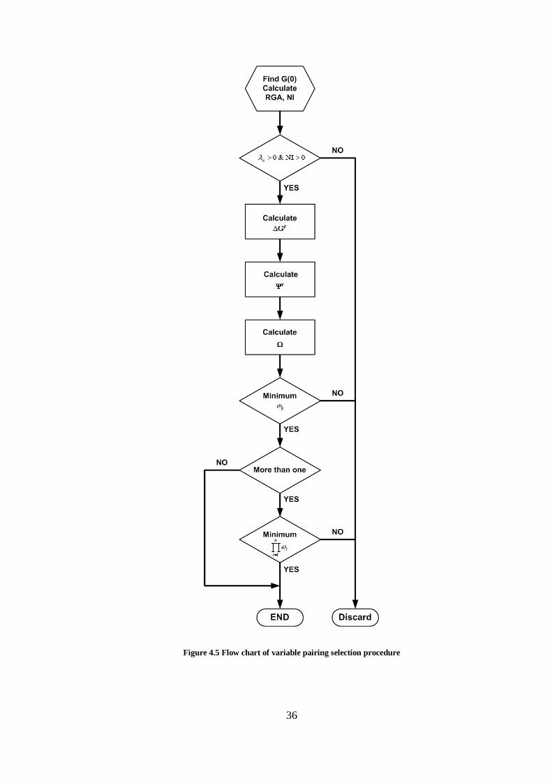
The procedure for the variable-pairing selection is demonstrated by the flowchart as
shown in Figure 4.5.
For the system that has the pure integral element, GIA and DRIA can be calculated by
using a method similar to that proposed by Arkun and Downs (Arkun, et al., 1990).
For 2×2 system, we obtain the GI value of element 11g as
22 11
11 11 22 11 22 .
36
Figure 4.5 Flow chart of variable pairing selection procedure
37
Furthermore, from properties of RGA and RI, we can obtain an equation as
11 12 11 121 1
which indicates 11 and 12 must have the same sign, and a smaller 11 means less
interaction. Therefore, selecting the pairings that have the smallest GIA elements is
equivalent to the RGA-based loop-pairing criterion to select the RGA value closest to
unity. Even though the procedure to derive the new loop-pairing criterion is tedious,
the calculation for the control structure configuration can be achieved automatically
and can easily be programmed into a computer by using Matlab/Simulink application
software.
4.3.3 Dynamic Relative Interaction
To examine the transmittance of interactions between an individual control loop and
the others, the decentralized control system can be structurally decomposed into n
individual SISO control loops with the coupling among all loops explicitly exposed
and embedded in each loop.
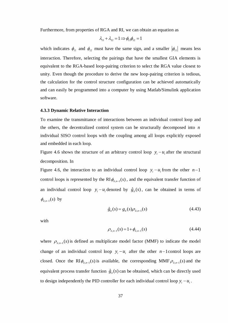
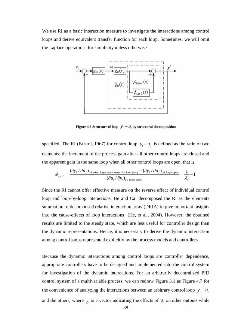
Figure 4.6 shows the structure of an arbitrary control loop i iy u after the structural
decomposition. In
Figure 4.6, the interaction to an individual control loop i iy u from the other 1n
control loops is represented by the RI, 1( )ii n s
, and the equivalent transfer function of
an individual control loop i iy u denoted by ˆ ( )iig s , can be obtained in terms of
, 1( )ii n s by
, 1
ˆ ( ) ( ) ( )ii ii ii ng s g s s (4.43)
with
, 1 , 1( ) 1 ( )ii n ii ns s (4.44)
where , 1( )ii n s is defined as multiplicate model factor (MMF) to indicate the model
change of an individual control loop i iy u after the other 1n control loops are
closed. Once the RI , 1( )ii n s is available, the corresponding MMF , 1( )ii n s and the
equivalent process transfer function ˆ ( )iig s can be obtained, which can be directly used
to design independently the PID controller for each individual control loop i iy u .
38
We use RI as a basic interaction measure to investigate the interactions among control
loops and derive equivalent transfer function for each loop. Sometimes, we will omit
the Laplace operator s for simplicity unless otherwise
Figure 4.6 Structure of loop i iy u by structural decomposition
specified. The RI (Bristol, 1967) for control loop i jy u is defined as the ratio of two
elements: the increment of the process gain after all other control loops are closed and
the apparent gain in the same loop when all other control loops are open, that is
, 1
( / ) ( / ) 11
( / )
i j all other loops close except for loop yi uj i j all loops open
ij n
i i all loops open ij
y u y u
u y
Since the RI cannot offer effective measure on the reverse effect of individual control
loop and loop-by-loop interactions, He and Cai decomposed the RI as the elements
summation of decomposed relative interaction array (DRIA) to give important insights
into the cause-effects of loop interactions (He, et al., 2004). However, the obtained
results are limited to the steady state, which are less useful for controller design than
the dynamic representations. Hence, it is necessary to derive the dynamic interaction
among control loops represented explicitly by the process models and controllers.
Because the dynamic interactions among control loops are controller dependence,
appropriate controllers have to be designed and implemented into the control system
for investigation of the dynamic interactions. For an arbitrarily decentralized PID
control system of a multivariable process, we can redraw Figure 3.1 as Figure 4.7 for
the convenience of analyzing the interactions between an arbitrary control loop i iy u
and the others, where iy is a vector indicating the effects of iu on other outputs while
39
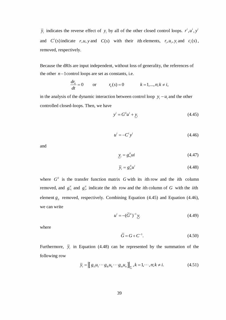
iy indicates the reverse effect of iy by all of the other closed control loops. , ,i i ir u y
and ( )iC s indicate , ,r u y and ( )C s with their thi elements, , ,i i ir u y and ( )ic s ,
removed, respectively.
Because the dRIs are input independent, without loss of generality, the references of
the other 1n control loops are set as constants, i.e.
0 or ( ) 0 1,..., ; ,kk
drr s k n k i
dt
in the analysis of the dynamic interaction between control loop i iy u and the other
controlled closed-loops. Then, we have
i ii i
iy G u y (4.45)
i i iu C y (4.46)
and
ii
i iy g ui (4.47)
ii i
i iy g u (4.48)
where iiG is the transfer function matrix G with its thi row and the thi column
removed, and *
ii
ig and *
ii
ig indicate the thi row and the thi column of G with the thii
element iig removed, respectively. Combining Equation (4.45) and Equation (4.46),
we can write
1( )i ii
iu G y (4.49)
where
1.G G C (4.50)
Furthermore, iy in Equation (4.48) can be represented by the summation of the
following row
1 1 , 1, , ; .i i ik k in ny g u g u g u k n k i
(4.51)
40
Figure 4.7 Closed loop system with control loop i iy u presented explicitly
where A
is the summation of all elements in a matrix .A Using Equation (4.47) –
Equation (4.51), we obtain
* *
* *
* *
( )
( )
( ) .
ii ii ii
i i i i
ii ii ii T
i i i
ii iiii Ti i
ii i
ii
y g G g u
g g G u
g gG g u
g
Consequently, those steady state relationships provided in [42] can be extended as
follows. Define
, 1
1 ii ii
ii n i i
ii
G g gg
as the incremental process gain matrix of subsystem iiG when control loop i iy u is
closed, then the dynamic DRIA (dDRIA) of individual control loop i iy u in an n n
system can be described as
, 1 , 1 ( )ii T
ii n ii nG G
(4.52)
and the dRI , 1ii n , is the summation of all elements of , 1ii n , i.e.
, 1 , 1 , 1 ( )ii T
ii n ii n ii nG G
(4.53)
where the Hadamard product and ( )ii TG is the transpose of the inverse of matrix
41
.iiG From Equation (4.50), G can be factorized as
11 1 12 1
21 22 2 2
1 2
1/
1/
1/
n
n
n n nn n
g c g g
g g c gG
g g g c
G P
where
11 11
11 1
22 22
22 2
11 1
11 1
11 1 nn nn
nn n
g c
g c
g c
g cP
g c
g c
G P
(4.54)
Hence, the dDRIA and dRI can be obtained respectively by,
, 1 , 1 ( )ii ii T
ii n ii nG G P
(4.55)
and
, 1 , 1 ( )ii ii T
ii n ii nG G P
(4.56)
In dDRIA and dRI of Equation (4.55) and Equation (4.56), there exists an additional
matrix P , which explicitly reveals interactions to an arbitrary loop by all the other
1n closed loops under band-limited control conditions. Thus, for the given
decentralized PID controllers, the dynamic interaction among control loops at an
arbitrary frequency can be easily investigated through the matrix P , moreover, the
calculation remains simple even for high dimensional processes.
For decentralized PI or PID control, we have
1( 0) 0C j
and
( 0) ( 0)G j G j
which implies that the RI and the dRI are equivalent at steady state. However, because
42
the dRI measure interactions under practical unperfected control conditions at some
specified frequency points, it is more accurate in estimating the dynamic loop
interactions and more effective in designing decentralized controllers.
The significance of above development is as follows:
1. The interaction to an individual control loop from the other loops is derived in
matrix form, and the relationship between RI and DRIA is extended to the
whole frequency domain from the steady state;
2. Equation (4.52) and Equation (4.53) indicate that the dRI is a combination of
the interactions to individual control loops from the others; there may exist
cause-effect cancelation among them such that selecting of loop pairings by
dRI may be inaccurate (He, et al., 2004).
3. Because interactions among control loops are controllers dependent, the
dDRIA represents how the decentralized controllers interact with each other,
while the dRI provides the overall effect to an individual control loop from the
others.
4. The dRI can be obtained easily once process transfer function elements and
controllers are available, which is not limited by the system dimension.
4.3.4 Decentralized Controller Design
This method involves three main steps in designing decentralized controllers for
multivariable processes:
1. the design of individual controllers by ignoring the loop interactions;
2. the determination of the equivalent transfer function for each individual loop
through use of the dRI;
3. the fine-tuning of each controller parameter based on the equivalent
transfer function.
Because the interactions among control loops are ignored in the first step, all
available SISO PID controller design techniques can be applied to the design of
the initial individual controllers for the diagonal elements. Thus, according to the
43
expected control performance, one can select the most suitable tuning rules, such
as Ziegler and Nichols tuning, IMC tuning, and some other optimal design
methods. O bviously, different tuning rules provide different controller settings
and, correspondingly, different estimations of loop interactions. Even these
different estimations will affect the decentralized controllers designed in the third
step; they have no influence on the design mechanism of this method.
The IMC design procedure is brief studied as follows. The process model g is
factorized into an all-pass portion g and minimum phase portion g , that is
.g g g
The all-pass portion g includes all the open right half plane zeros and delays of
g and has the form
( 1), Re{ } 0,s
i
i
g e s
where 0 is the time delay and 1
i
is the right-half-plane zero in the process
model.
Then the IMC controller and the complementary sensitivity function are derived
respectively as
1 ,cg g f
and
,T g f
where f is the IMC filter and has the form
1,
( 1)r
C
fs
where the filter order r is selected large enough to make cg proper, and the
adjustable filter parameter C provides the tradeoff between performance and
robustness. The key advantage of the IMC design procedure is that all controller
parameters are related in a unique, straightforward manner to the model
parameters. There is only one adjustable parameter C which has intuitive appeal
44
because it determines the speed of response of the system. Furthermore, C is
approximately proportional to the closed-loop bandwidth, which must always be
smaller than the bandwidth over which the process model is valid.
Even though more precise higher order process models can be obtained by either
physical model construction (following the mass and energy balance principles)
or the classical parameter identification methods, from a p ractical point of view,
the lower order process model is more convenient for controller design.
For the SO PDT SISO system given by Equation(4.24), the SIMC-PID settings in
the form of Equation (4.26) was suggested as
1 ii
Pi
ii Ci ii
kk
(4.57)
min{ ,4( )}Ii ii Ci ii (4.58)
'
Di ii (4.59)
where, Ci is the desired closed-loop time constant. It is recommended to select
the value of Ci as ii for a tradeoff between:
1. the fast speed of the response and good disturbance rejection (favored by a
small value of Ci );
2. the stability, robustness, and small input variation (favored by a large value of
Ci );
Step 1: Let diagG G . The initial controllers C can be designed for G through the
SIMC-PID tuning rules, such that
11 1
11 1
0 0
0 0
0 0 nn n
g c
g cGC
g c
45
with the open loop transfer function for each individual control loop is
1
.( )
iis
ii i
Ci ii
g c es
(4.60)
Using first order Taylor series expansion for (4.60), the closed-loop transfer
function, open-loop gain crossover frequency ci and matrix P , can be obtained
respectively by
1
1iisi
i Ci
ye
r s
1
,ci
Ci ii
(4.61)
and
11
22
1
2
( 1) 1 1
1 ( 1) 1
1 1 ( 1) nn
s
C
s
C
s
Cn
s e
s eP
s e
(4.62)
Because each controller is designed around the critical frequency of its transfer
function, the dRI of individual control loop i iy u can be estimated at the critical
frequency crij
, 1 , 1( ) ( ) ( ( ) ( )) .ii ii T
ii n cri ii n cri cri crij G j G j P j
(4.63)
For interactive multivariable processG , it is desirable to have the same open-loop
transfer function as multivariable control system GC . Because controller C is
designed for the diagonal elements of G without considering the couplings
between control loops, the designed controller should be detuned by
, 1 , 11
i ii
ii n ii n
c cc
(4.64)
to result in approximately the same closed-loop control performance. However,
it is impractical to use , 1ii n directly to fine-tune the controller because it has
different values at different frequencies. To solve this problem, one possible way
is to use some appropriate transfer functions to identify those MMFs. Because at
46
the neighborhood of the critical point the transmission interaction can be
considered as a linear function, it is reasonable to represent the MMF by a low-
order transfer function involving the first two items of its Taylor series, which can
be further simplified for controller design by a pure time-delay transfer function
as
, 1
, 1 , 1 ,i n s
ii n i nk e
(4.65)
where,
, 1 , 1 , 1( ) 1 ( )i n ii n cri ii n crik j j (4.66)
and
, 1 , 1
, 1
arg( ( )) arg(1 ( )),
ii n cri ii n cri
i n
cri cri
j j
(4.67)
with cri indicating the critical frequency of the thi control loop i iy u .
O bviously, the positive/ negative , 1i n
indicates that the interactions from other
control loops bring a phase lag/ lead of individual control loops.
Step 2: From Equation (4.24) and Equation (4.26), the equivalent transfer function
for loop i iy u can be expressed by
'
ˆ ( ) ,( 1)( 1)
i iif ski iiii
ii ii
f kg s e
s s
(4.68)
where,
, 1max 1, ,ki i nf k (4.69)
and
, 1
max 1,1 .i n
i
ii
f
(4.70)
The open-loop transfer function for each individual control loop given by
Equation (4.60) is determined by the SIMC-PID tuning settings. If other tuning
47
rules are applied, some different forms may be derived, and ii ig c always has the
form
( )s
ii i
keg c h s
s
where, ( )h s is proper and rational with ( 0) 0h j .
Because the region between ( 1)ci ii ig c and 180(arg( ) 180 )ii ig c is most
critical for individual control loop design, the crossover frequency of iig c can be
adopted as the critical frequency point for determining the dRI to the particular
loop i iy u to obtain ˆiig .
In Equation (4.69) and Equation(4.70), the factors kif and if are selected to be
not smaller than 1 , such that the equivalent open loop gain and the time delay of
ˆiig are not smaller than those of iig . The reason for such a selection is to make
the resultant controller settings more conservative than those of ˆiig so that loop
failure tolerance property can be preserved.
Step 3: Using tuning rules of Equation (4.57) to Equation (4.59), the controller
parameters for the individual equivalent transfer function of Equation (4.68) can be
determined as
1 ii
Pi
ki ii Ci i ii
kf k f
(4.71)
min{ ,4( )}Ii ii Ci i iif (4.72)
'
Di ii (4.73)
Furthermore, by selecting the desired closed-loop time constant Ci to be the same
value as the time delay i iif , we can obtain a set of simple rules for designing the
parameters of a decentralized PID controller as,
48
1 1 1
2
iiPi
ki i ii ii
kf f k
(4.74)
min{ ,( ,8 )}Ii ii ii i iif (4.75)
'
Di ii (4.76)
Once the closed-loop properties of the diagonal elements and the critical frequencies
of all individual control loops are determined, the dRI and MMF can be obtained
through calculation of the matrix P and dDRIA. Then, the parameters of the PID
controllers can be calculated based on the equivalent transfer function of each
control
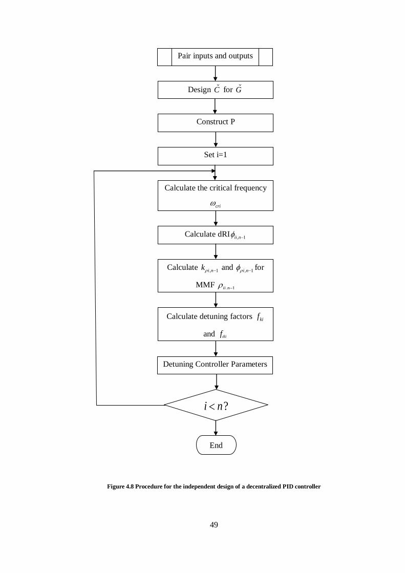
49
Figure 4.8 Procedure for the independent design of a decentralized PID controller
Pair inputs and outputs
?i n
End
Design C for G
Construct P
Set i=1
Calculate the critical frequency
cri
Calculate , 1i nk
and , 1i n
for
MMF , 1ii n
Calculate dRI, 1ii n
Calculate detuning factors kif
and if
Detuning Controller Parameters
50
loop and the SIMC-PID tuning rules. In such a design procedure, the overall control
system stability is assured if the loop pairing is structurally stable. This can be
explained as follows:
1. Each ic is designed without considering loop interaction; it is more aggressive
to control loop i iy u than the final control setting ic . Generally, we have
1 2( ) ( ) as , 1max 1, 1ii n , where ( )A is the maximum singular
value of matrix A , 1
1 (1 )GC GC and 1
2 (1 )GC GC .
2. Let 1( )M G G G , and following the definition of the structured singular
value (SSV) :
1
( )min ( ) det( ) 0 for structured m
MI k M
we have 1 2( ) ( )M M which implies there exist smaller interactions
among control loops when the detuned controller C is applied.
3. Because the bigger dRI , 1ii n
is used to determine the detuning factors and kif
and if are not smaller than 1, the resultant controller ic will be more
conservative, with a smaller gain and crossover frequency compared with ic .
4. Conservative control action in each loop presents smaller interaction to other
loops. Because the design based on ˆiig for loop i iy u will end up with a more
conservative ic the stability margin for each individual loop will be further
increased compared with that using the true , 1ii n
4.3.5 Algorithm for Decentralized Controller Design
As a summary of the above results, an algorithm for the design of a decentralized PID
controller for general multivariable processes is given as below.
1. For multivariable process G , pair the inputs and outputs based on the method
given above.
2. Design an individual controller for the diagonal elements of the process
transfer function matrix.
51
3. Construct matrix P .
4. Let 1i , go to step 5.
5. Calculate critical frequency cri , dRI and , 1( )ii n crij
.
6. Determine , 1i nk
and , 1i n
for MMF, , 1ii n
.
7. Obtain the factors kif and if .
8. Fine-tune the controller parameters.
9. If , 1i n i i , go to step 5. Otherwise, go to step 10;
10. End.
The procedure for the independent design of a decentralized PID controller by using
the proposed method is illustrated in Figure 4.8.
4.4 GPM Tuning Method based on ERGA Pairing Criteria
In this section, a novel equivalent transfer function in terms of effective relative gain
array (ERGA) for multivariable processes will be presented. By considering four
combination modes of gain and phase changes for a particular loop when other loops
are closed, this equivalent transfer function can effectively approximate the dynamic
interactions among loops. Consequently, the decentralized controllers can be
independently designed by employing the single loop tuning techniques. The method
is simple, straightforward, easy to understand and implement by field engineers.
Consider an open loop stable multivariable system with n inputs and n outputs as
shown in Figure 3.1.
4.4.1 Interaction Measure and Loop Pairing
In decentralized control system design, individual loop is tuned around its critical
frequency region of the transfer function. Thus, this frequency region should be
focused upon when considering the effect of interactions. Therefore, two factors in the
open loop transfer functions will affect the loop pairing decision:
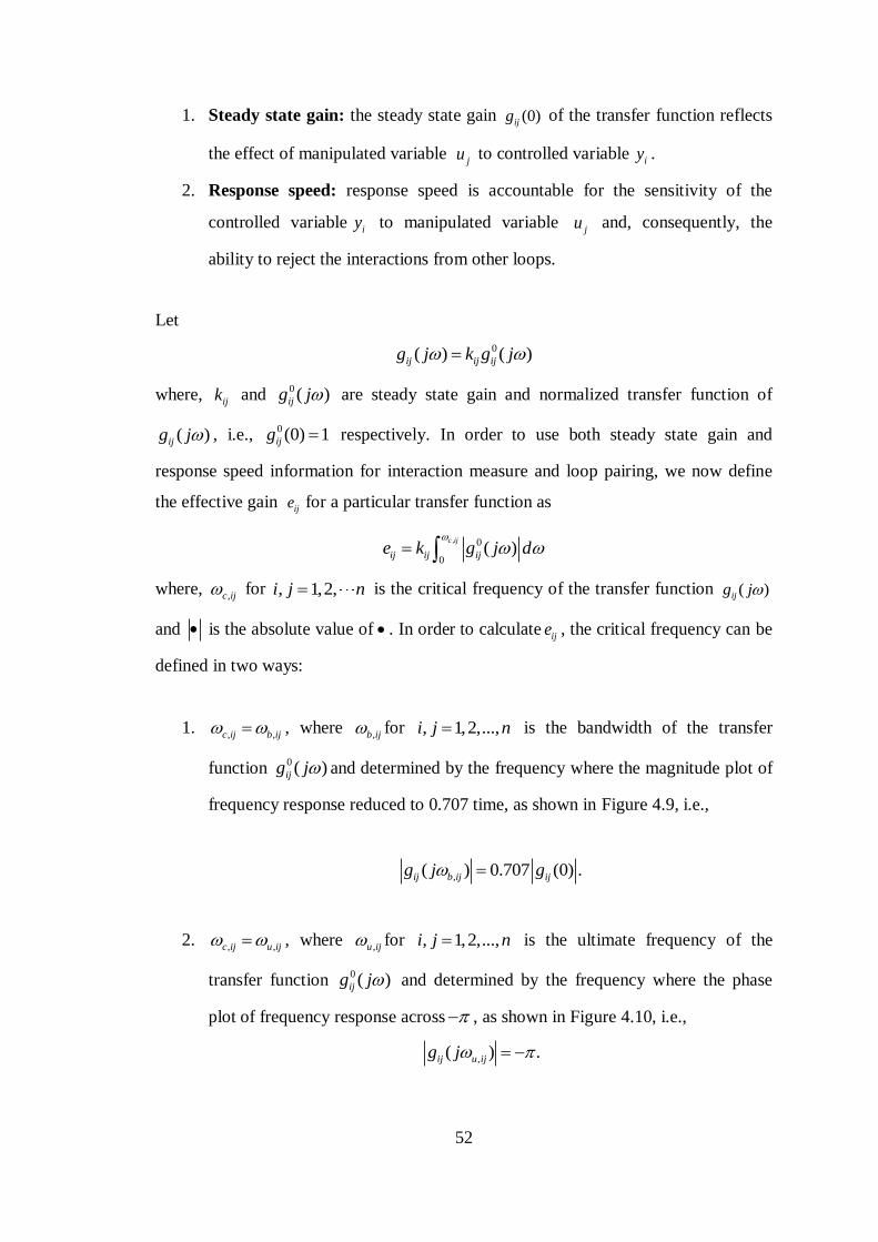
52
1. Steady state gain: the steady state gain of the transfer function reflects
the effect of manipulated variable to controlled variable .
2. Response speed: response speed is accountable for the sensitivity of the
controlled variable to manipulated variable and, consequently, the
ability to reject the interactions from other loops.
Let
0( ) ( )ij ij ijg j k g j
where, ijk and
0 ( )ijg j are steady state gain and normalized transfer function of
( )ijg j , i.e., 0 (0) 1ijg respectively. In order to use both steady state gain and
response speed information for interaction measure and loop pairing, we now define
the effective gain for a particular transfer function as
, 0
0( )
c ij
ij ij ije k g j d
where, ,c ij for is the critical frequency of the transfer function
and is the absolute value of . In order to calculateije , the critical frequency can be
defined in two ways:
1. , ,c ij b ij , where
,b ij for , 1,2,...,i j n is the bandwidth of the transfer
function 0 ( )ijg j and determined by the frequency where the magnitude plot of
frequency response reduced to 0.707 time, as shown in Figure 4.9, i.e.,
,( ) 0.707 (0) .ij b ij ijg j g
2. , ,c ij u ij , where ,u ij for , 1,2,...,i j n is the ultimate frequency of the
transfer function 0 ( )ijg j and determined by the frequency where the phase
plot of frequency response across , as shown in Figure 4.10, i.e.,
,( ) .ij u ijg j
(0)ijg
ju iy
iyju
ije
, 1,2,i j n ( )ijg j
53
For transfer function matrices with some elements without phase crossover
frequencies, such as first order or second order without time delay, it is necessary to
use corresponding bandwidths as critical frequencies to calculate ije . However, it is
worth to point out that the phase crossover frequency information, i.e., ultimate
frequency ,u ij is recommended if applicable for calculation of
ije , since it is closely
linked to system dynamic performance and control system design. Without loss of
generality, we will use ,u ij as the bases for the following development.
For the frequency response of ( )ijg j as shown in Figure 4.10, ije is the area covered
by ( )ijg j up to ,u ij . Since 0 ( )ijg j represents the magnitude of the transfer
function at various frequencies, ije is considered to be the energy transmission ratio
from the manipulated variable ju to the controlled variable iy .
Figure 4.9 Frequency response curves and the energy of ( )ijg j (bandwidth ,b ij )
Express the energy transmission ratio array as
11 12 1
21 22 2
1 2
...
...
... ... ... ...
...
n
n
n n nn
e e e
e e eE
e e e
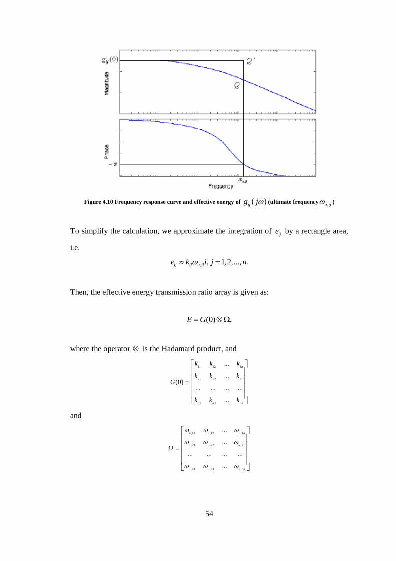
54
Figure 4.10 Frequency response curve and effective energy of ( )ijg j (ultimate frequency,u ij )
To simplify the calculation, we approximate the integration of ije by a rectangle area,
i.e.
, , 1,2,..., .ij ij u ije k i j n
Then, the effective energy transmission ratio array is given as:
(0) ,E G
where the operator is the Hadamard product, and
11 12 1
21 22 2
1 2
...
...(0)
... ... ... ...
...
n
n
n n nn
k k k
k k kG
k k k
and
,11 ,12 ,1
,21 ,22 ,2
, 1 , 1 ,
...
...
... ... ... ...
...
u u u n
u u u n
u n u n u nn
55
are the steady state gain array and the critical frequency array respectively. Since ije is
an indication of energy transmission ratio for loopi jy u , the bigger the
ije value is,
the more dominant of the loop will be.
Similar to the definition of relative gain, the effective relative gainij , between output
variable iy and input variable ju is defined as the ratio of two effective energy
transmission ratios:
ˆ
ij
ij
ij
e
e (4.77)
where ije is the effective energy transmission ratio between output variable iy and
input variable ju when all other loops are closed. When the effective relative gains are
calculated for all the input/output combinations of a multivariable process, it results in
an array, ERGA, which can be calculated by
11 12 1
21 22 2
1 2
...
...
... ... ... ...
...
n
n
n n nn
TE E
The introduction of energy transmission ratio is to mathematically represent the
effectiveness of a control loop which is affected by two key factors, i.e., the steady
state gain of the transfer function reflecting the effect of the manipulated variable ju
to the controlled variable iy , and the response speed reflecting the sensitivity of the
controlled variable iy to the manipulated variable ju and, consequently, the ability to
reject the interactions from other loops. Since ERGA is a relative measure, using the
multiplication of the two parameters to approximate the energy transmission ratio in
ij can simplify the calculation while captures the key elements in a multivariable
control system.
The ERGA is used to determine the best variable paring. In the following sections, we
56
will employ this interaction measure to develop effective transfer functions (ETFs)
under decentralized control structure.
Since both RGA and ERGA use relative gains, the properties of RGA can be directly
extended to ERGA:
1. The value of is a measure of the effective interaction expected in the
loop if its output is paired with .
2. The elements of the ERGA across any row, or down any column, sum up to 1,
i.e.
.
3. Let ije represent the loop effective gain when all the other loops are closed,
whereas represents the normal, open loop effective gain, then:
1ˆ
ij
ij ije e
.
4. When is negative, with other loops open, produces a change in in
response to a change in totally opposite in direction to that when the other
loops are closed.
As 0NI , based on steady state information provides a sufficient condition for the
loop configuration to be unstable, it can used to eliminate those structure unstable
pairing options. Similar to RGA and NI based pairing rules, the ERGA, and NI based
loop pairing rules requires that manipulated and controlled variables in a decentralized
control system be paired:
1. Corresponding ERGA elements are closest to 1.0.
2. The NI is positive.
3. All paired ERGA elements are positive.
4. Large ERGA elements should be avoided.
Here, both ERGA and NI play important roles for control structure selection. ERGA is
used to measure interactions, while NI is used as a sufficient condition to rule out the
ijthi
iy ju
1 1
1n n
ij ij
i j
i
ij
ij iy
ju
57
closed loop unstable pairings. Since we are using effective gains instead of simply
steady state gains, transient response can be effectively reflected. Therefore,
comparing REGA method with RGA and DRGA, we may expect that:
1. In additional to steady state gains, only time constant and time delay are
required in ERGA method, it is far easier to calculate than those DRGA
methods.
2. ERGA combines both steady state gains and equivalent error in measuring the
loop interactions, it should provide better pairing results than that of RGA
based pairing and comparable with DRGA ones.
3. Since ERGA only uses information of open loop process transfer functions, it
is controller type independent.
4.4.2 Decentralized Control System Design
This method involves two main steps in designing decentralized controllers for
multivariable processes:
1. the determination of the equivalent transfer function for each individual loop
through use of the ERGA
2. the tuning of each controller parameter based on the equivalent transfer
function
Step 1: Suppose that the best loop configuration has been determined and the best pair
is diagonally placed in the transfer function matrix as shown in Figure 3.1. Similar to
the open loop gain, we let the effective energy transmission ratio ije when all other
loops are closed be ,ˆˆ ˆ (0) , 1,2,..., ,ij ij u ije g i j n where ˆ (0)ijg and ,
ˆu ij are the steady
state gain and ultimate frequency between output variable iy and input variable iu
when all other loops are closed, respectively. Then, from Equation (4.77)
,
,
(0)ˆˆ (0) .
ij u ij
ij u ij
ij
gg
(4.78)
By the definition of RGA, we have
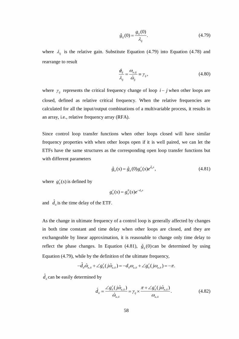
58
(0)
ˆ (0) .ij
ij
ij
gg
(4.79)
where ij is the relative gain. Substitute Equation (4.79) into Equation (4.78) and
rearrange to result
,
,ˆ
ij u ij
ij
ij ij
(4.80)
where ij represents the critical frequency change of loop i j when other loops are
closed, defined as relative critical frequency. When the relative frequencies are
calculated for all the input/output combinations of a multivariable process, it results in
an array, i.e., relative frequency array (RFA).
Since control loop transfer functions when other loops closed will have similar
frequency properties with when other loops open if it is well paired, we can let the
ETFs have the same structures as the corresponding open loop transfer functions but
with different parameters
ˆ
ˆ ˆ( ) (0) ( ) ,iid sr
ii ii iig s g g s e (4.81)
where ( )r
iig s is defined by
0( ) ( ) iid sr
ii iig s g s e
and ˆiid is the time delay of the ETF.
As the change in ultimate frequency of a control loop is generally affected by changes
in both time constant and time delay when other loops are closed, and they are
exchangeable by linear approximation, it is reasonable to change only time delay to
reflect the phase changes. In Equation (4.81), ˆ (0)ijg can be determined by using
Equation (4.79), while by the definition of the ultimate frequency,
, , , ,ˆ ˆ ˆ( ) ( ) .r r
ii u ii ii u ii ii u ii ii u iid g j d g j
ˆiid can be easily determined by
, ,
, ,
ˆ ˆ( ) ( )ˆ .ˆ
r r
ii u ii ii u ii
ii ij
u ii u ii
g j g jd
(4.82)
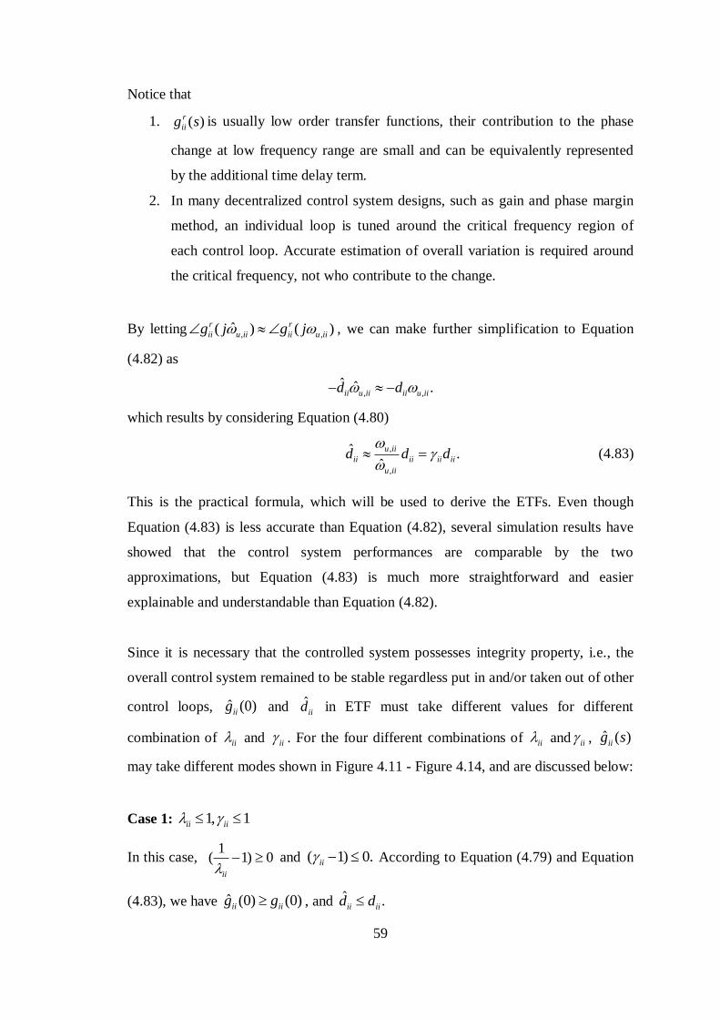
59
Notice that
1. ( )r
iig s is usually low order transfer functions, their contribution to the phase
change at low frequency range are small and can be equivalently represented
by the additional time delay term.
2. In many decentralized control system designs, such as gain and phase margin
method, an individual loop is tuned around the critical frequency region of
each control loop. Accurate estimation of overall variation is required around
the critical frequency, not who contribute to the change.
By letting , ,ˆ( ) ( )r r
ii u ii ii u iig j g j , we can make further simplification to Equation
(4.82) as
, ,ˆ ˆ .ii u ii ii u iid d
which results by considering Equation (4.80)
,
,
ˆ .ˆ
u ii
ii ii ii ii
u ii
d d d
(4.83)
This is the practical formula, which will be used to derive the ETFs. Even though
Equation (4.83) is less accurate than Equation (4.82), several simulation results have
showed that the control system performances are comparable by the two
approximations, but Equation (4.83) is much more straightforward and easier
explainable and understandable than Equation (4.82).
Since it is necessary that the controlled system possesses integrity property, i.e., the
overall control system remained to be stable regardless put in and/or taken out of other
control loops, ˆ (0)iig and ˆiid in ETF must take different values for different
combination of ii and ii . For the four different combinations of ii and ii , ˆ ( )iig s
may take different modes shown in Figure 4.11 - Figure 4.14, and are discussed below:
Case 1: 1, 1ii ii
In this case, 1
( 1) 0ii
and ( 1) 0.ii According to Equation (4.79) and Equation
(4.83), we have ˆ (0) (0)ii iig g , and ˆ .ii iid d
60
1. ˆ (0) (0)ii iig g , this means that the magnitude of the frequency response when
the other loops closed is not less than that of when the other loops open. Since
the retaliatory effect from the other loops magnifies the main effect of iu on iy ,
we need to reduce the controller gain to assure system stability. In this case, the
gain is by Equation (4.79)
(0)ˆ (0) .ii
ii
ii
gg
Figure 4.11 Interaction mode with 1, 1ii ii
2. ˆii iid d , this means that the time delay when the other loops closed is not
bigger than that of when other loops open. The reduced time delay will
increase the phase margin. However, by considering the control system
integrity, the time delay needs to be kept as before, i.e.,
ˆ .ii iid d
Case 2: 1, 1ii ii
In this case, 1
( 1) 0ii
and ( 1) 0.ii According to Equation (4.79) and Equation
(4.83), we have ˆ (0) (0)ii iig g , and ˆ .ii iid d
1. ˆ (0) (0)ii iig g , same as in Case 1,
61
(0)ˆ (0) .ii
ii
ii
gg
2. ˆ .ii iid d , this means that the time delay when the other loops closed is bigger
than that of when the other loops open. The enlarged time delay will reduce the
phase margin. In this case, the time delay is determined by Equation (4.83)
ˆ .ii ii iid d
Figure 4.12 Interaction mode with 1, 1ii ii
Case 3: 1, 1ii ii
In this case, 1
( 1) 0ii
and ( 1) 0.ii According to Equation (4.79) and Equation
(4.83), we have ˆ (0) (0)ii iig g , and ˆ .ii iid d
1. ˆ (0) (0)ii iig g , this means that the magnitude of the frequency response when
the other loops closed is smaller than that of when the other loops open. Even
if the retaliatory effect from other loops acts in opposition to the main effect of
iu on iy , we cannot enlarge the controller gain for better performance due to the
system integrity consideration. Hence, the gain should be unchanged, i.e.,
ˆ (0) (0).ii iig g
2. ˆ .ii iid d , same as in Case 1
ˆ .ii iid d
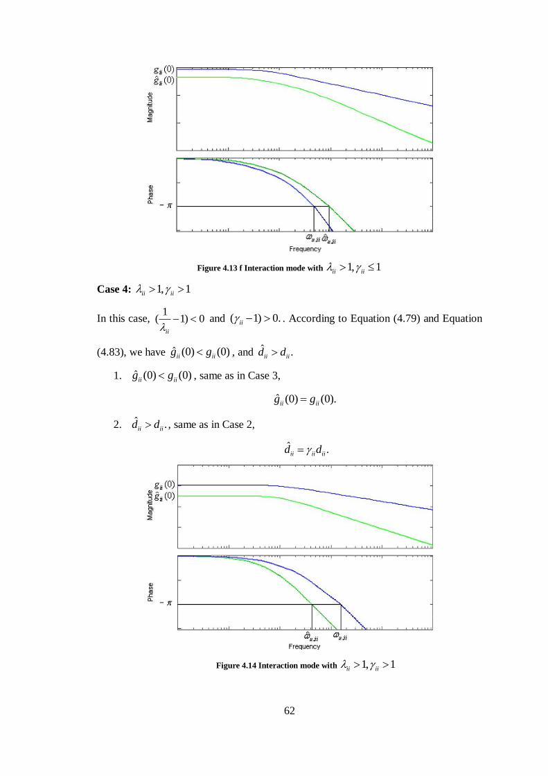
62
Figure 4.13 f Interaction mode with 1, 1ii ii
Case 4: 1, 1ii ii
In this case, 1
( 1) 0ii
and ( 1) 0.ii . According to Equation (4.79) and Equation
(4.83), we have ˆ (0) (0)ii iig g , and ˆ .ii iid d
1. ˆ (0) (0)ii iig g , same as in Case 3,
ˆ (0) (0).ii iig g
2. ˆ .ii iid d , same as in Case 2,
ˆ .ii ii iid d
Figure 4.14 Interaction mode with 1, 1ii ii
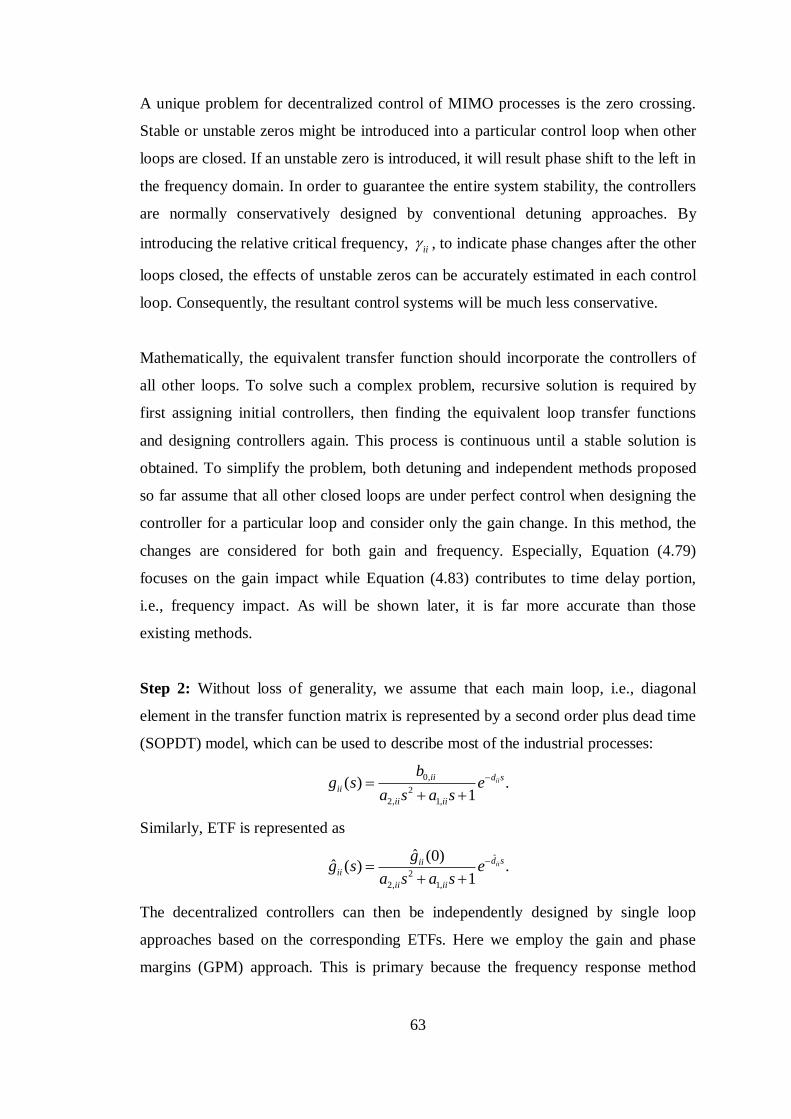
63
A unique problem for decentralized control of MIMO processes is the zero crossing.
Stable or unstable zeros might be introduced into a particular control loop when other
loops are closed. If an unstable zero is introduced, it will result phase shift to the left in
the frequency domain. In order to guarantee the entire system stability, the controllers
are normally conservatively designed by conventional detuning approaches. By
introducing the relative critical frequency, ii , to indicate phase changes after the other
loops closed, the effects of unstable zeros can be accurately estimated in each control
loop. Consequently, the resultant control systems will be much less conservative.
Mathematically, the equivalent transfer function should incorporate the controllers of
all other loops. To solve such a complex problem, recursive solution is required by
first assigning initial controllers, then finding the equivalent loop transfer functions
and designing controllers again. This process is continuous until a stable solution is
obtained. To simplify the problem, both detuning and independent methods proposed
so far assume that all other closed loops are under perfect control when designing the
controller for a particular loop and consider only the gain change. In this method, the
changes are considered for both gain and frequency. Especially, Equation (4.79)
focuses on the gain impact while Equation (4.83) contributes to time delay portion,
i.e., frequency impact. As will be shown later, it is far more accurate than those
existing methods.
Step 2: Without loss of generality, we assume that each main loop, i.e., diagonal
element in the transfer function matrix is represented by a second order plus dead time
(SOPDT) model, which can be used to describe most of the industrial processes:
0,
2
2, 1,
( ) .1
iiii d s
ii
ii ii
bg s e
a s a s
Similarly, ETF is represented as
ˆ
2
2, 1,
ˆ (0)ˆ ( ) .
1iid sii
ii
ii ii
gg s e
a s a s
The decentralized controllers can then be independently designed by single loop
approaches based on the corresponding ETFs. Here we employ the gain and phase
margins (GPM) approach. This is primary because the frequency response method
64
provides good performance in the face of uncertainty in both plant model and
disturbances.
The PID controller of each loop is supposed of the following standard form:
,
, ,( ) .i i
ci p i d i
kg s k k s
s
The controller can be rewritten as
2 2, , ,
( )d i p i i i
ci
k s k s k As Bs Cg s k
s s
where , ,/ , /k i p iA k k B k k and
, / .i iC k k
By selecting 2 1,A a B a and 1C , the open loop transfer function becomes
ˆˆ (0)ˆ( ) ( ) .iid sii
ci ii
gg s g s k e
s
Denoting the gain and phase margin specifications as ,m iA and
,m i , and their
crossover frequencies as ,g i and
,p i respectively, we have
, , ,
, , , ,
, , ,
, , , ,
ˆarg ( ) ( )
ˆ( ) ( ) 1
ˆ( ) ( ) 1
ˆarg ( ) ( ) .
c i g i ii g i
m i c i g i ii g i
c i p i ii p i
m i c i p i ii p i
g j g j
A g j g j
g j g j
g j g j
By substitution and simplification to above equations, we obtain
,
,
,
,
, ,
ˆ2
ˆ (0)
ˆ (0)
ˆ2
g i ii
g i
m i
ii
ii p i
m i p i ii
d
Akg
kg
d
which results
,
,
,
1(1 )
2
.ˆ ˆ2 (0)
m i
m i
m i ii ii
A
kA d g
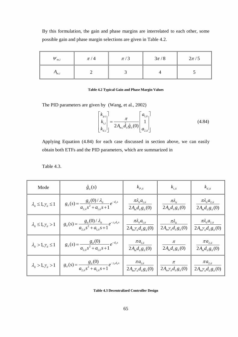
65
By this formulation, the gain and phase margins are interrelated to each other, some
possible gain and phase margin selections are given in Table 4.2.
,m i / 4 / 3 3 / 8 2 / 5
,m iA 2 3 4 5
Table 4.2 Typical Gain and Phase Margin Values
The PID parameters are given by (Wang, et al., 2002)
, 1,
,
,, 2,
1ˆ ˆ2 (0)
p i ii
i i
m i ii iid i ii
k a
kA d g
k a
(4.84)
Applying Equation (4.84) for each case discussed in section above, we can easily
obtain both ETFs and the PID parameters, which are summarized in
Table 4.3.
Mode ˆ ( )iig s ,P iik ,i iik
,d iik
1, 1ii ii 2
2, 1,
(0) /( )
1iid sii ii
ii
ii ii
gg s e
a s a s
1,
2 (0)
ii ii
m ii ii
a
A d g
2 (0)
ii
m ii iiA d g
2,
2 (0)
ii ii
m ii ii
a
A d g
1, 1ii ii 2
2, 1,
(0) /( )
1ii iid sii ii
ii
ii ii
gg s e
a s a s
1,
2 (0)
ii ii
m ii ii ii
a
A d g
2 (0)
ii
m ii ii iiA d g
2,
2 (0)
ii ii
m ii ii ii
a
A d g
1, 1ii ii 2
2, 1,
(0)( )
1iid sii
ii
ii ii
gg s e
a s a s
1,
2 (0)
ii
m ii ii
a
A d g
2 (0)m ii iiA d g
2,
2 (0)
ii
m ii ii
a
A d g
1, 1ii ii 2
2, 1,
(0)( )
1ii iid sii
ii
ii ii
gg s e
a s a s
1,
2 (0)
ii
m ii ii ii
a
A d g
2 (0)m ii ii iiA d g
2,
2 (0)
ii
m ii ii ii
a
A d g
Table 4.3 Decentralized Controller Design
66
5 Simulation and Performance Analysis
5.1 Introduction
We have three typical control structures, which are shown in Appendix A, Appendix
B, and Appendix C respectively. We also have three typical programs for 2 2 , 3 3
and 4 4 systems. They are shown in Appendix D, Appendix E, and Appendix F
respectively. We do parameter estimation for some transfer functions. Performance
analysis is done based on IAE, ISE and ITAE for all systems. One click solution is
also provided to execute the programs, which means that sim command calls and
executes the Simulink block diagram and, the responses for the individual loops will
be come out sequentially with a single click on Run command from Debug menu.
5.2 Simulation and Discussion for Vinante and Luyben System (1972)
Firstly, we start with 2x2 Vinante and Luyben System (1972) whose transfer function
matrix is given as
0.3
1.8 0.35
2.2 1.3
7 1 7 1( ) .
2.8 4.3
9.5 1 9.2 1
s s
s s
e e
s sG s
e e
s s
The dimension of the plant is 2 2 and so the pairing option is 2!, which is equal to 2.
The DC gains and NI values for all possible pairings for this process are
1
1.3 2.2
4.3 2.8k
and 2
2.2 1.3,
2.8 4.3k
and
Pairing 1 2
NI -1.5989
0.6152
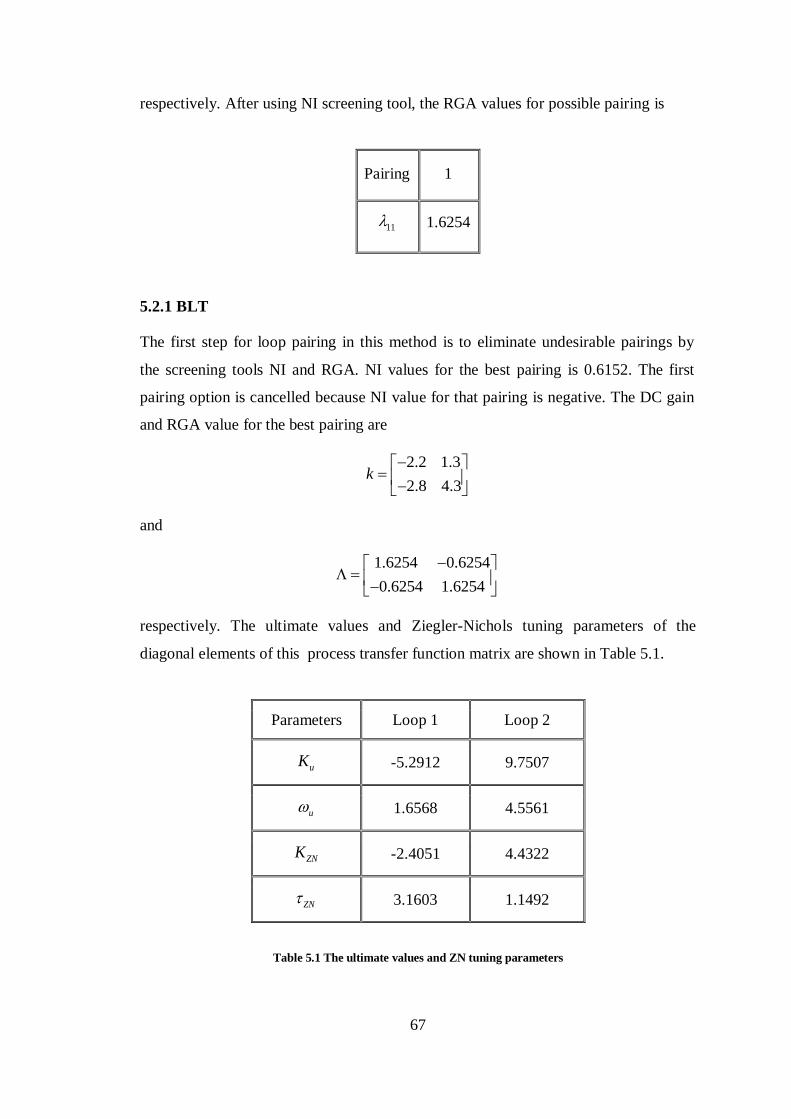
67
respectively. After using NI screening tool, the RGA values for possible pairing is
Pairing 1
11
1.6254
5.2.1 BLT
The first step for loop pairing in this method is to eliminate undesirable pairings by
the screening tools NI and RGA. NI values for the best pairing is 0.6152. The first
pairing option is cancelled because NI value for that pairing is negative. The DC gain
and RGA value for the best pairing are
2.2 1.3
2.8 4.3k
and
1.6254 0.6254
0.6254 1.6254
respectively. The ultimate values and Ziegler-Nichols tuning parameters of the
diagonal elements of this process transfer function matrix are shown in Table 5.1.
Parameters Loop 1 Loop 2
uK -5.2912 9.7507
u 1.6568 4.5561
ZNK -2.4051 4.4322
ZN 3.1603 1.1492
Table 5.1 The ultimate values and ZN tuning parameters
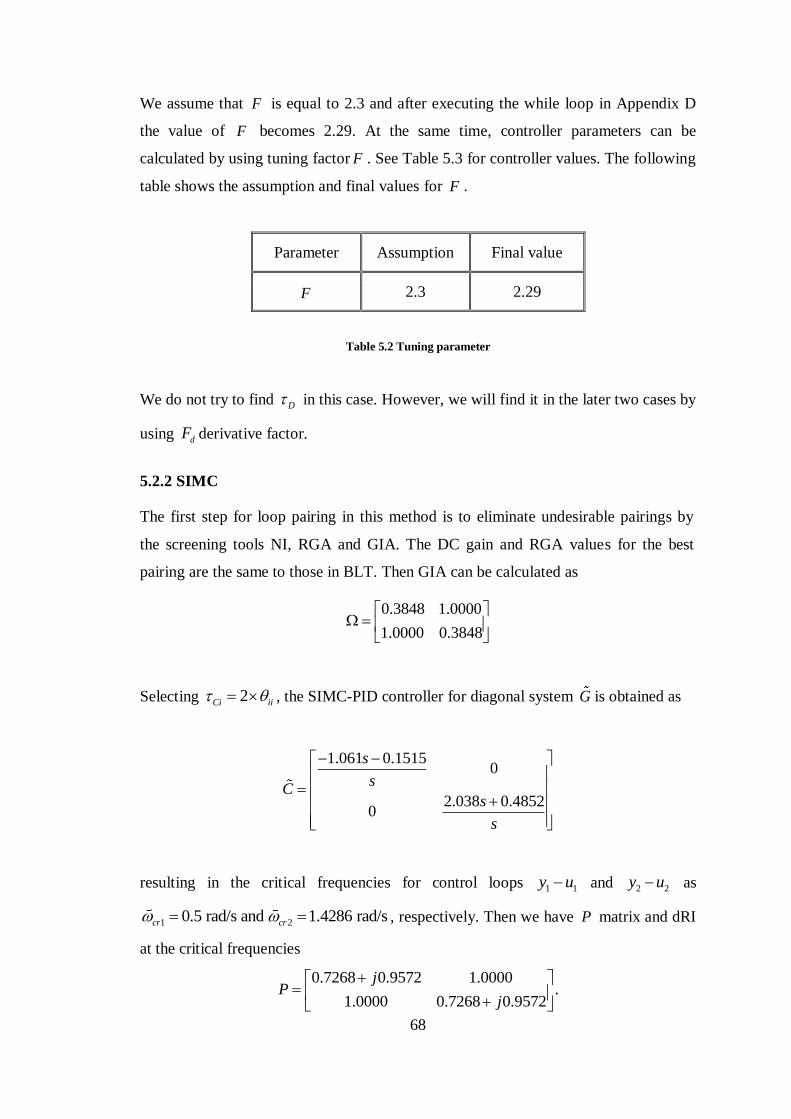
68
We assume that F is equal to 2.3 and after executing the while loop in Appendix D
the value of F becomes 2.29. At the same time, controller parameters can be
calculated by using tuning factor F . See Table 5.3 for controller values. The following
table shows the assumption and final values for F .
Parameter Assumption Final value
F 2.3 2.29
Table 5.2 Tuning parameter
We do not try to find D in this case. However, we will find it in the later two cases by
using dF derivative factor.
5.2.2 SIMC
The first step for loop pairing in this method is to eliminate undesirable pairings by
the screening tools NI, RGA and GIA. The DC gain and RGA values for the best
pairing are the same to those in BLT. Then GIA can be calculated as
0.3848 1.0000
1.0000 0.3848
Selecting 2Ci ii , the SIMC-PID controller for diagonal system G is obtained as
1.061 0.15150
2.038 0.48520
s
sC
s
s
resulting in the critical frequencies for control loops 1 1y u and 2 2y u as
1 20.5 rad/s and 1.4286 rad/scr cr , respectively. Then we have P matrix and dRI
at the critical frequencies
0.7268 0.9572 1.0000.
1.0000 0.7268 0.9572
jP
j
69
and
11,1
22,1
( 0.5) 0.3900 - 0.3206
( 1.4286) 0.0033 + 0.0476
j j
j j
respectively. Subsequently MMF can be calculated as
0.6800
11,1
( 0.0498)
22,1
1.4265
1.0044
s
s
e
e
and 1 11.4265 and 1.6800kf f and, 2 21.0044 and 1.0000kf f are used to fine-
tune the PI/PID controller setting for each control loop. Then the equivalent transfer
functions of both control loops are constructed as
1.68
11
0.35
22
3.138ˆ
7 1
4.319ˆ .
9.2 1
s
s
eg
s
eg
s
Consequently, the decentralized PI controller parameters are determined by SIMC and
shown in Table 5.3. Figure 5.1 and Figure 5.2 shows the responses for each control
loop.
5.2.3 ERGA
In this section, the loop pairing is based on the criterion of ERGA plus Niederlinski
index (NI). The gain and phase margin for all loops are specified to be 3 and / 3 ,
respectively. These margins are generally regarded as making the best compromise
between performance and robustness in process control.
The DC gain, Critical Frequency Array, RGA, ERGA and RFA are
2.2 1.3
2.8 4.3k
,
0.1425 0.1425
0.1050 0.1084
1.6254 -0.6254,
-0.6254 1.6254
1.5939 -0.5939
-0.5939 1.5939
and
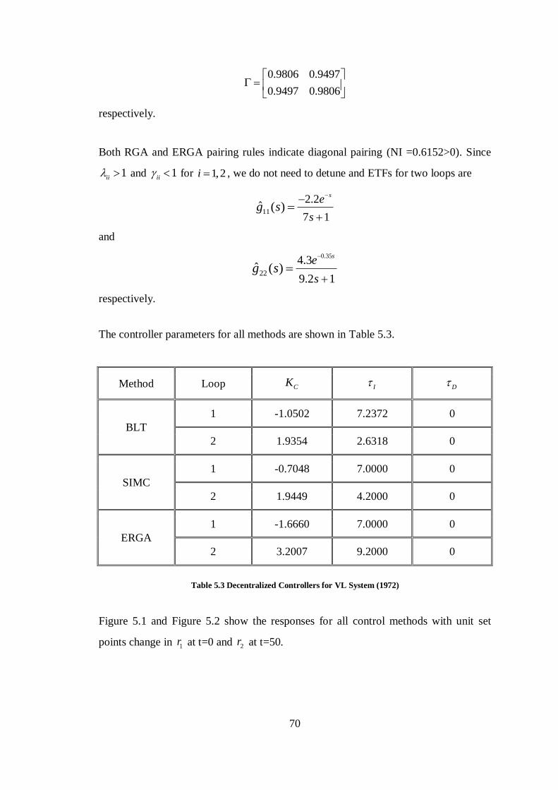
70
0.9806 0.9497
0.9497 0.9806
respectively.
Both RGA and ERGA pairing rules indicate diagonal pairing (NI =0.6152>0). Since
1ii and 1ii for 1,2i , we do not need to detune and ETFs for two loops are
11
2.2
7 1ˆ ( )
se
sg s
and
0.35
22
4.3
9.2 1ˆ ( )
se
sg s
respectively.
The controller parameters for all methods are shown in Table 5.3.
Method Loop CK I D
BLT
1 -1.0502 7.2372 0
2 1.9354 2.6318 0
SIMC
1 -0.7048 7.0000 0
2 1.9449 4.2000 0
ERGA
1 -1.6660 7.0000 0
2 3.2007 9.2000 0
Table 5.3 Decentralized Controllers for VL System (1972)
Figure 5.1 and Figure 5.2 show the responses for all control methods with unit set
points change in 1r at t=0 and 2r at t=50.
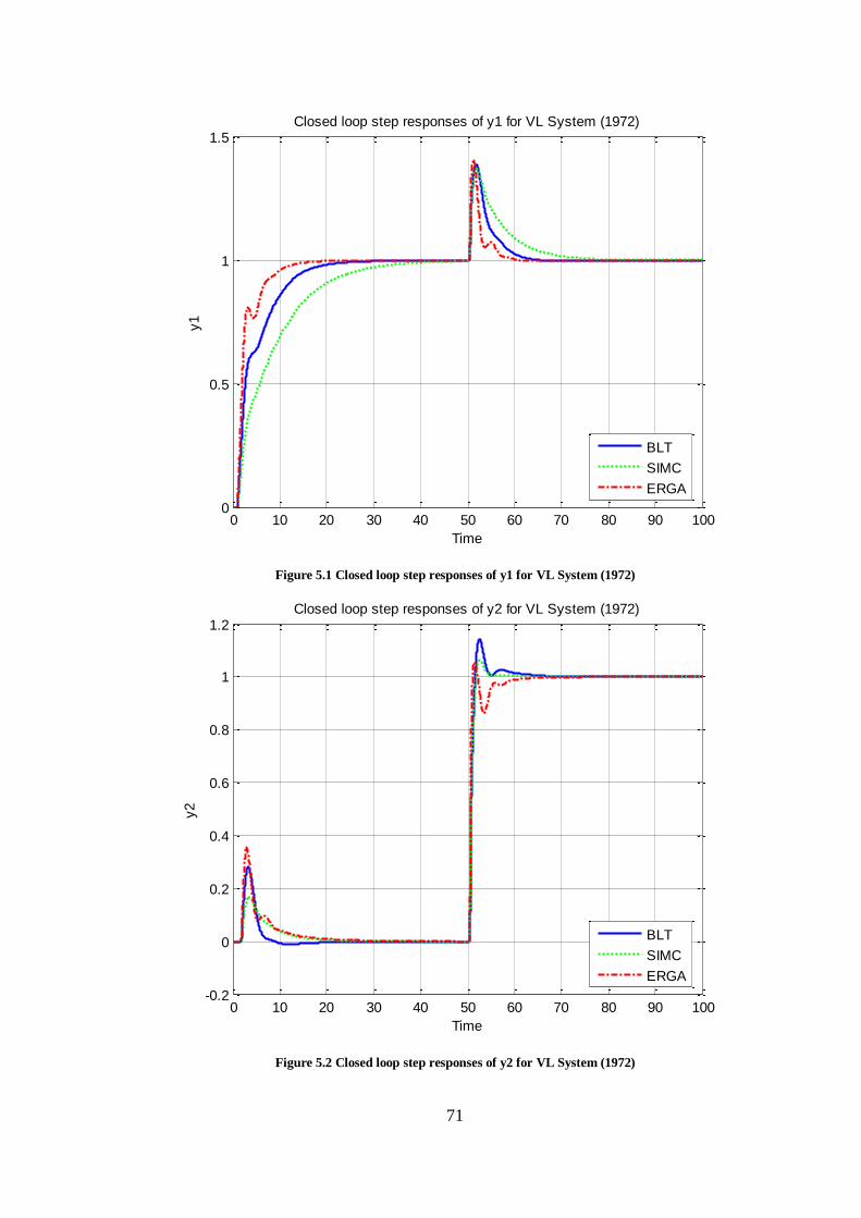
71
Figure 5.1 Closed loop step responses of y1 for VL System (1972)
Figure 5.2 Closed loop step responses of y2 for VL System (1972)
0 10 20 30 40 50 60 70 80 90 1000
0.5
1
1.5
y1
Time
Closed loop step responses of y1 for VL System (1972)
BLT
SIMC
ERGA
0 10 20 30 40 50 60 70 80 90 100-0.2
0
0.2
0.4
0.6
0.8
1
1.2
y2
Time
Closed loop step responses of y2 for VL System (1972)
BLT
SIMC
ERGA
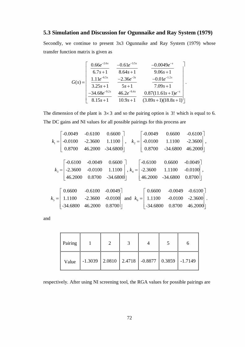
72
5.3 Simulation and Discussion for Ogunnaike and Ray System (1979)
Secondly, we continue to present 3x3 Ogunnaike and Ray System (1979) whose
transfer function matrix is given as
2.6 3.5
6.5 3 1.2
9.2 9.4
0.66 0.61 0.0049
6.7 1 8.64 1 9.06 1
1.11 2.36 0.01( ) .
3.25 1 5 1 7.09 1
34.68 46.2 0.87(11.61 1)
8.15 1 10.9 1 (3.89 1)(18.8 1)
s s s
s s s
s s s
e e e
s s s
e e eG s
s s s
e e s e
s s s s
The dimension of the plant is 3 3 and so the pairing option is 3! which is equal to 6.
The DC gains and NI values for all possible pairings for this process are
1
-0.0049 -0.6100 0.6600
-0.0100 -2.3600 1.1100 ,
0.8700 46.2000 -34.6800
k
2
-0.0049 0.6600 -0.6100
-0.0100 1.1100 -2.3600 ,
0.8700 -34.6800 46.2000
k
3
-0.6100 -0.0049 0.6600
-2.3600 -0.0100 1.1100 ,
46.2000 0.8700 -34.6800
k
4
-0.6100 0.6600 -0.0049
-2.3600 1.1100 -0.0100 ,
46.2000 -34.6800 0.8700
k
5
0.6600 -0.6100 -0.0049
1.1100 -2.3600 -0.0100 and
-34.6800 46.2000 0.8700
k
6
0.6600 -0.0049 -0.6100
1.1100 -0.0100 -2.3600 .
-34.6800 0.8700 46.2000
k
and
Pairing 1 2 3 4 5 6
Value -1.3039
2.0810 2.4718 -0.8877 0.3859 -1.7149
respectively. After using NI screening tool, the RGA values for possible pairings are
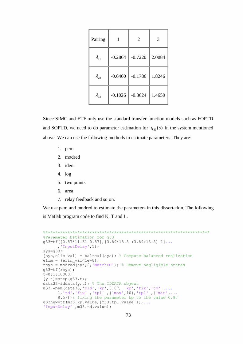
73
Pairing 1 2 3
11
-0.2864
-0.7220 2.0084
22 -0.6460 -0.1786 1.8246
33 -0.1026 -0.3624 1.4650
Since SIMC and ETF only use the standard transfer function models such as FOPTD
and SOPTD, we need to do parameter estimation for 33( )g s in the system mentioned
above. We can use the following methods to estimate parameters. They are:
1. pem
2. modred
3. ident
4. log
5. two points
6. area
7. relay feedback and so on.
We use pem and modred to estimate the parameters in this dissertation. The following
is Matlab program code to find K, T and L.
%*******************************************************************
%Parameter Estimation for g33
g33=tf([0.87*11.61 0.87],[3.89*18.8 (3.89+18.8) 1]...
,'InputDelay',1);
sys=g33;
[sys,elim_val] = balreal(sys); % Compute balanced realization
elim = (elim_val<1e-8);
rsys = modred(sys,2,'MatchDC'); % Remove negligible states
g33=tf(rsys);
t=0:1:10000;
[y t]=step(g33,t);
data33=iddata(y,t); % The IDDATA object
m33 =pem(data33,'p1d','kp',0.87, 'kp','fix','td' ,...
1,'td','fix' ,'tp1' ,{'max',10},'tp1' ,{'min',...
8.5});% fixing the parameter kp to the value 0.87
g33new=tf(m33.kp.value,[m33.tp1.value 1],...
'InputDelay' ,m33.td.value);
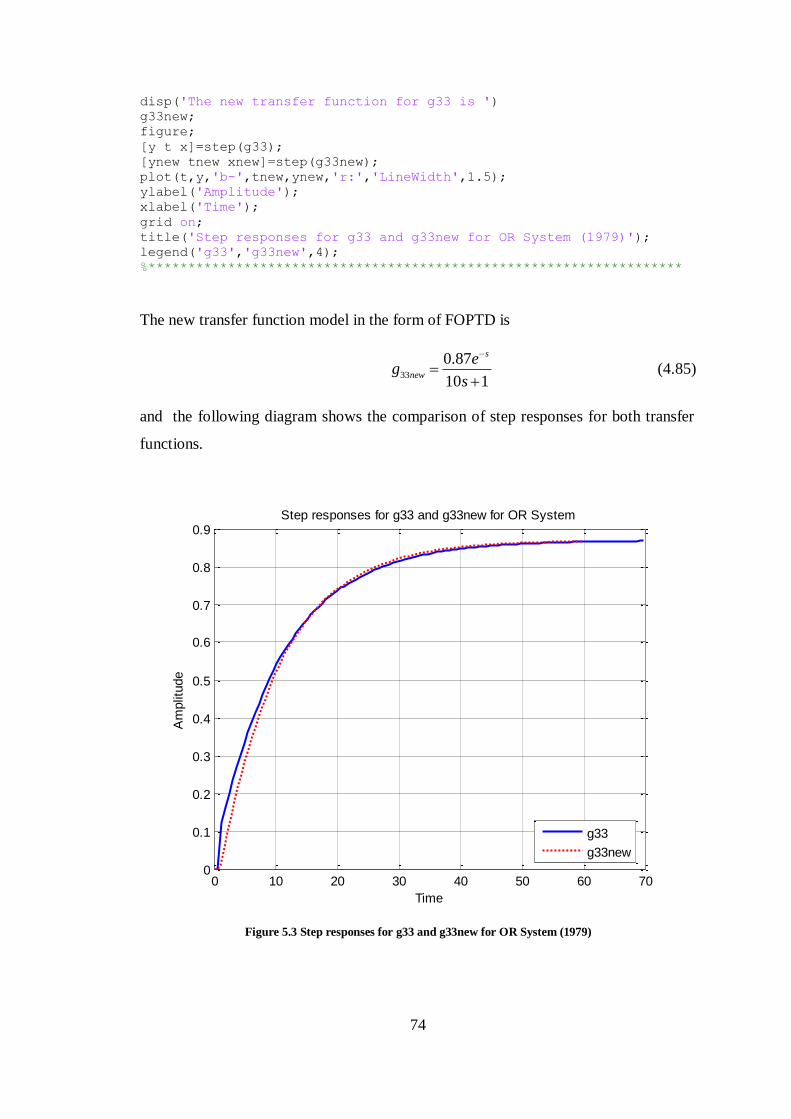
74
disp('The new transfer function for g33 is ')
g33new;
figure;
[y t x]=step(g33);
[ynew tnew xnew]=step(g33new);
plot(t,y,'b-',tnew,ynew,'r:','LineWidth',1.5);
ylabel('Amplitude');
xlabel('Time');
grid on;
title('Step responses for g33 and g33new for OR System (1979)');
legend('g33','g33new',4);
%*******************************************************************
The new transfer function model in the form of FOPTD is
33
0.87
10 1
s
new
eg
s
(4.85)
and the following diagram shows the comparison of step responses for both transfer
functions.
Figure 5.3 Step responses for g33 and g33new for OR System (1979)
0 10 20 30 40 50 60 700
0.1
0.2
0.3
0.4
0.5
0.6
0.7
0.8
0.9
Am
plit
ude
Time
Step responses for g33 and g33new for OR System
g33
g33new
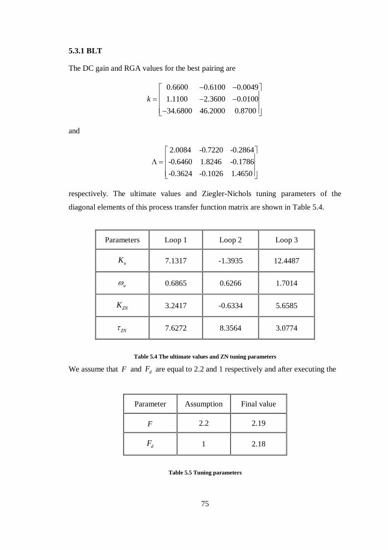
75
5.3.1 BLT
The DC gain and RGA values for the best pairing are
0.6600 0.6100 0.0049
1.1100 2.3600 0.0100
34.6800 46.2000 0.8700
k
and
2.0084 -0.7220 -0.2864
-0.6460 1.8246 -0.1786
-0.3624 -0.1026 1.4650
respectively. The ultimate values and Ziegler-Nichols tuning parameters of the
diagonal elements of this process transfer function matrix are shown in Table 5.4.
Parameters Loop 1 Loop 2 Loop 3
uK 7.1317 -1.3935 12.4487
u 0.6865 0.6266 1.7014
ZNK 3.2417 -0.6334 5.6585
ZN 7.6272 8.3564 3.0774
Table 5.4 The ultimate values and ZN tuning parameters
We assume that F and dF are equal to 2.2 and 1 respectively and after executing the
Parameter Assumption Final value
F 2.2 2.19
dF 1 2.18
Table 5.5 Tuning parameters
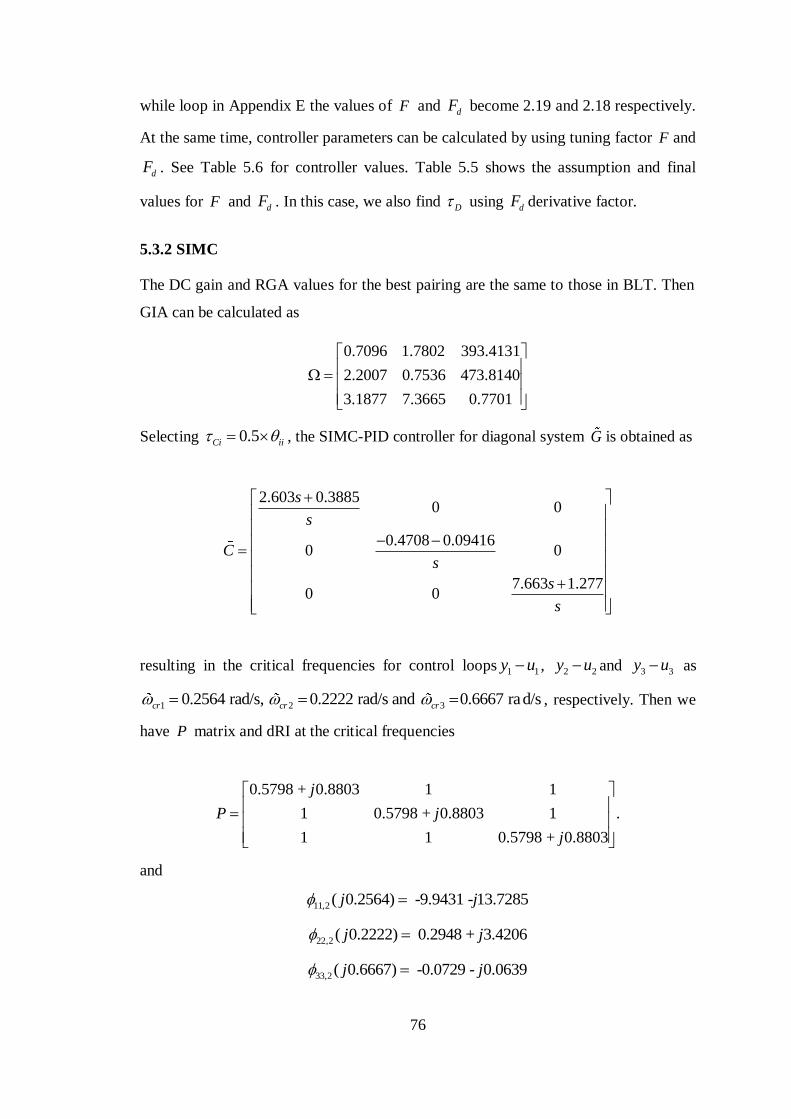
76
while loop in Appendix E the values of F and dF become 2.19 and 2.18 respectively.
At the same time, controller parameters can be calculated by using tuning factor F and
dF . See Table 5.6 for controller values. Table 5.5 shows the assumption and final
values for F and dF . In this case, we also find D using dF derivative factor.
5.3.2 SIMC
The DC gain and RGA values for the best pairing are the same to those in BLT. Then
GIA can be calculated as
0.7096 1.7802 393.4131
2.2007 0.7536 473.8140
3.1877 7.3665 0.7701
Selecting 0.5Ci ii , the SIMC-PID controller for diagonal system G is obtained as
2.603 0.38850 0
0.4708 0.094160 0
7.663 1.2770 0
s
s
Cs
s
s
resulting in the critical frequencies for control loops 1 1y u , 2 2y u and 3 3y u as
1 2 30.2564 rad/s, 0.2222 rad/s and 0.6667 rad/scr cr cr , respectively. Then we
have P matrix and dRI at the critical frequencies
0.5798 + 0.8803 1 1
1 0.5798 + 0.8803 1 .
1 1 0.5798 + 0.8803
j
P j
j
and
11,2( 0.2564) -9.9431 - 13.7285j j
22,2( 0.2222) 0.2948 + 3.4206j j
33,2( 0.6667) -0.0729 - 0.0639j j
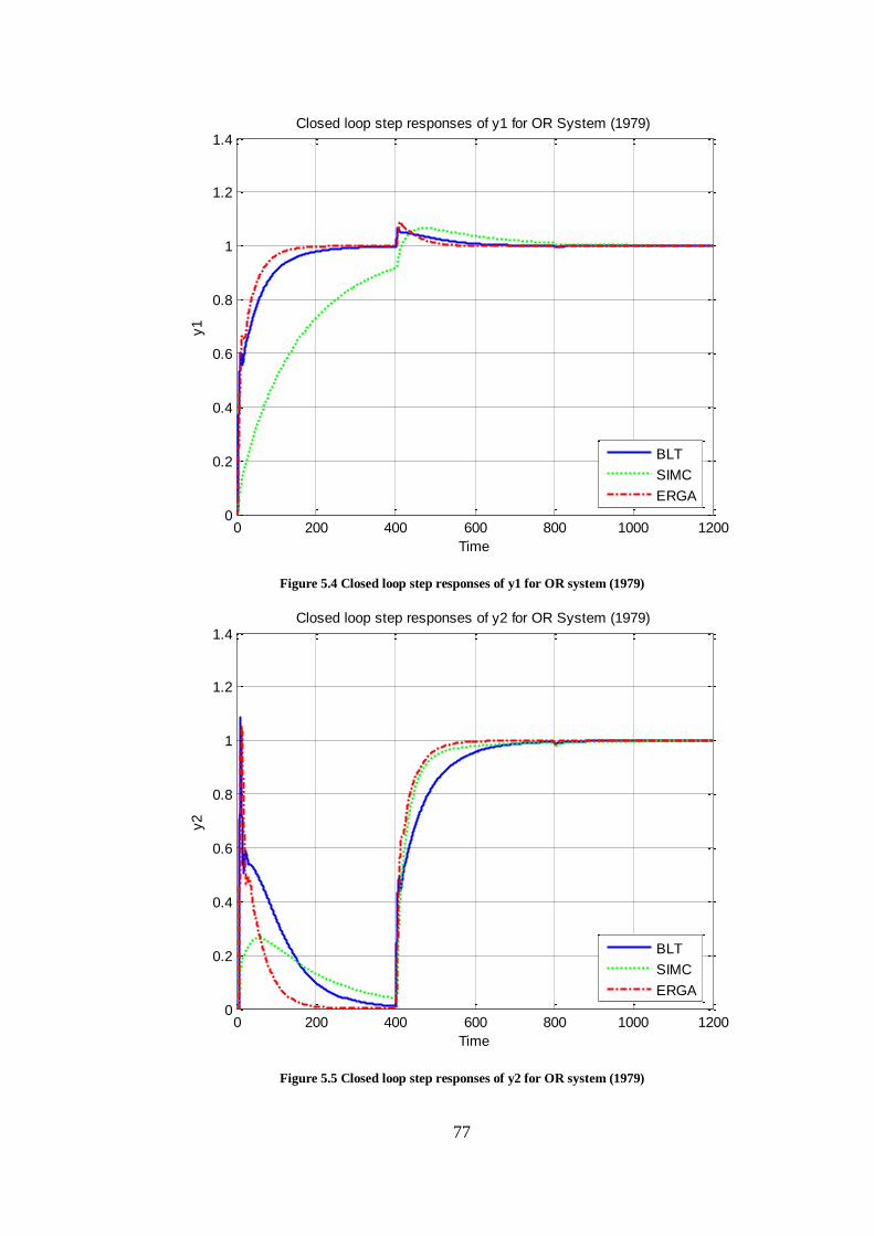
77
Figure 5.4 Closed loop step responses of y1 for OR system (1979)
Figure 5.5 Closed loop step responses of y2 for OR system (1979)
0 200 400 600 800 1000 12000
0.2
0.4
0.6
0.8
1
1.2
1.4
y1
Time
Closed loop step responses of y1 for OR System (1979)
BLT
SIMC
ERGA
0 200 400 600 800 1000 12000
0.2
0.4
0.6
0.8
1
1.2
1.4
y2
Time
Closed loop step responses of y2 for OR System (1979)
BLT
SIMC
ERGA
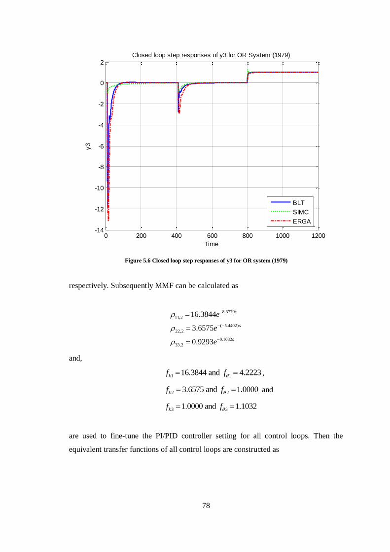
78
Figure 5.6 Closed loop step responses of y3 for OR system (1979)
respectively. Subsequently MMF can be calculated as
8.3779
11,2
( 5.4402)
22,2
0.1032
33,2
16.3844
3.6575
0.9293
s
s
s
e
e
e
and,
1 116.3844 and 4.2223kf f ,
2 23.6575 and 1.0000kf f and
3 31.0000 and 1.1032kf f
are used to fine-tune the PI/PID controller setting for all control loops. Then the
equivalent transfer functions of all control loops are constructed as
0 200 400 600 800 1000 1200-14
-12
-10
-8
-6
-4
-2
0
2
y3
Time
Closed loop step responses of y3 for OR System (1979)
BLT
SIMC
ERGA
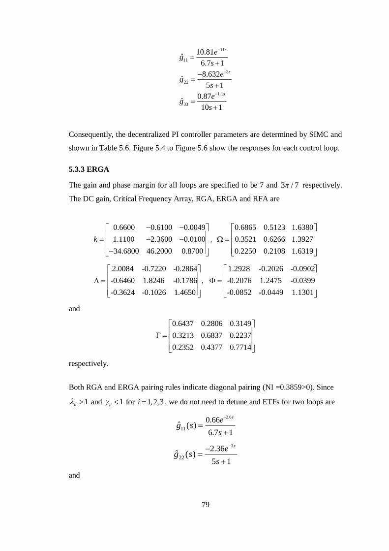
79
11
11
3
22
1.1
33
10.81ˆ
6.7 1
8.632ˆ
5 1
0.87ˆ
10 1
s
s
s
eg
s
eg
s
eg
s
Consequently, the decentralized PI controller parameters are determined by SIMC and
shown in Table 5.6. Figure 5.4 to Figure 5.6 show the responses for each control loop.
5.3.3 ERGA
The gain and phase margin for all loops are specified to be 7 and 3 / 7 respectively.
The DC gain, Critical Frequency Array, RGA, ERGA and RFA are
0.6600 0.6100 0.0049
1.1100 2.3600 0.0100
34.6800 46.2000 0.8700
k
,
0.6865 0.5123 1.6380
0.3521 0.6266 1.3927
0.2250 0.2108 1.6319
2.0084 -0.7220 -0.2864
-0.6460 1.8246 -0.1786 ,
-0.3624 -0.1026 1.4650
1.2928 -0.2026 -0.0902
-0.2076 1.2475 -0.0399
-0.0852 -0.0449 1.1301
and
0.6437 0.2806 0.3149
0.3213 0.6837 0.2237
0.2352 0.4377 0.7714
respectively.
Both RGA and ERGA pairing rules indicate diagonal pairing (NI =0.3859>0). Since
1ii and 1ii for 1,2,3i , we do not need to detune and ETFs for two loops are
2.6
11
0.66
6.7 1ˆ ( )
se
sg s
3
22
2.36
5 1ˆ ( )
se
sg s
and
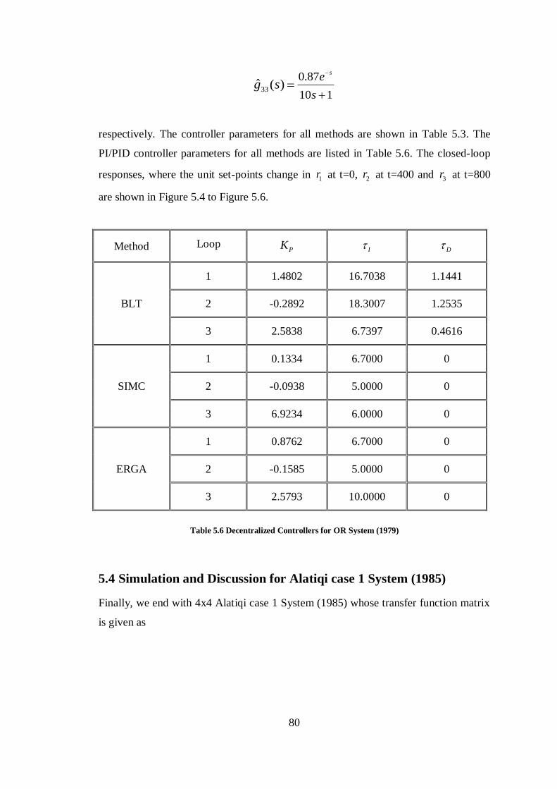
80
33
0.87
10 1ˆ ( )
se
sg s
respectively. The controller parameters for all methods are shown in Table 5.3. The
PI/PID controller parameters for all methods are listed in Table 5.6. The closed-loop
responses, where the unit set-points change in 1r at t=0, 2r at t=400 and 3r at t=800
are shown in Figure 5.4 to Figure 5.6.
Method Loop PK I D
BLT
1 1.4802 16.7038 1.1441
2 -0.2892 18.3007 1.2535
3 2.5838 6.7397 0.4616
SIMC
1 0.1334 6.7000 0
2 -0.0938 5.0000 0
3 6.9234 6.0000 0
ERGA
1 0.8762 6.7000 0
2 -0.1585 5.0000 0
3 2.5793 10.0000 0
Table 5.6 Decentralized Controllers for OR System (1979)
5.4 Simulation and Discussion for Alatiqi case 1 System (1985)
Finally, we end with 4x4 Alatiqi case 1 System (1985) whose transfer function matrix
is given as
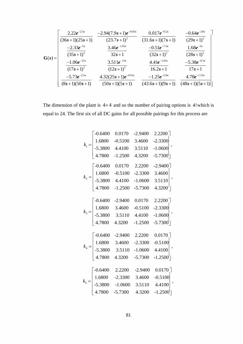
81
The dimension of the plant is 4 4 and so the number of pairing options is 4!which is
equal to 24. The first six of all DC gains for all possible pairings for this process are
1
-0.6400 0.0170 -2.9400 2.2200
1.6800 -0.5100 3.4600 -2.3300,
-5.3800 4.4100 3.5110 -1.0600
4.7800 -1.2500 4.3200 -5.7300
k
2
-0.6400 0.0170 2.2200 -2.9400
1.6800 -0.5100 -2.3300 3.4600,
-5.3800 4.4100 -1.0600 3.5110
4.7800 -1.2500 -5.7300 4.3200
k
3
-0.6400 -2.9400 0.0170 2.2200
1.6800 3.4600 -0.5100 -2.3300,
-5.3800 3.5110 4.4100 -1.0600
4.7800 4.3200 -1.2500 -5.7300
k
4
-0.6400 -2.9400 2.2200 0.0170
1.6800 3.4600 -2.3300 -0.5100,
-5.3800 3.5110 -1.0600 4.4100
4.7800 4.3200 -5.7300 -1.2500
k
5
-0.6400 2.2200 -2.9400 0.0170
1.6800 -2.3300 3.4600 -0.5100,
-5.3800 -1.0600 3.5110 4.4100
4.7800 -5.7300 4.3200 -1.2500
k
2.5 0.05 0.2 20
2 2
5 1.01 7.5 2
2 2 2
22 13
2
2.22 2.94(7.9 1) 0.017 0.64
(36 1)(25 1) (23.7 1) (31.6 1)(7 1) (29 1)
2.33 3.46 0.51 1.68
(35 1) 32 1 (32 1) (28 1)( )
1.06 3.511
(17 1) (
G
s s s s
s s s s
s s
e s e e e
s s s s s s
e e e e
s s s ss
e e
s
1.01 0.5
2
2.5 0.01 2.8 1.15
4.41 5.38
12 1) 16.2 1 17 1
5.73 4.32(25 1) 1.25 4.78
(8 1)(50 1) (50 1)(5 1) (43.6 1)(9 1) (48 1)(5 1)
s s
s s s s
e e
s s s
e s e e e
s s s s s s s s
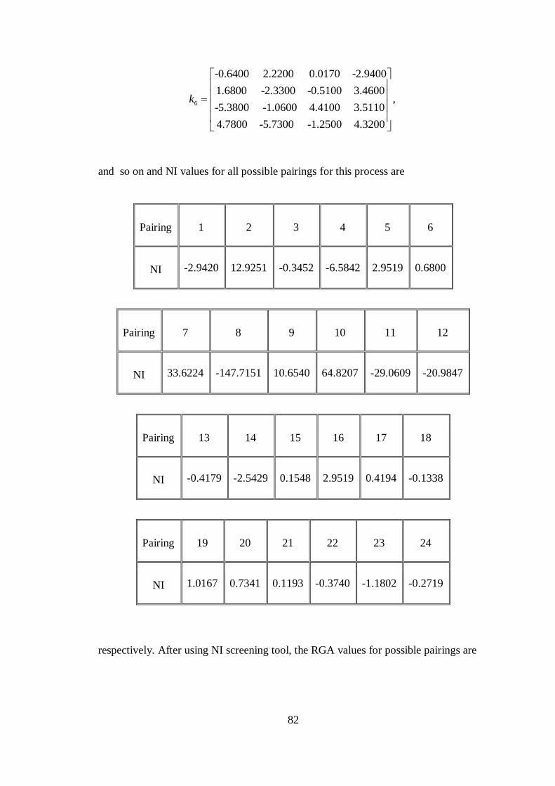
82
6
-0.6400 2.2200 0.0170 -2.9400
1.6800 -2.3300 -0.5100 3.4600,
-5.3800 -1.0600 4.4100 3.5110
4.7800 -5.7300 -1.2500 4.3200
k
and so on and NI values for all possible pairings for this process are
Pairing 1 2 3 4 5 6
NI -2.9420
12.9251 -0.3452 -6.5842 2.9519 0.6800
Pairing 7 8 9 10 11 12
NI 33.6224
-147.7151 10.6540 64.8207 -29.0609 -20.9847
Pairing 13 14 15 16 17 18
NI -0.4179
-2.5429 0.1548 2.9519 0.4194 -0.1338
Pairing 19 20 21 22 23 24
NI 1.0167
0.7341 0.1193 -0.3740 -1.1802 -0.2719
respectively. After using NI screening tool, the RGA values for possible pairings are
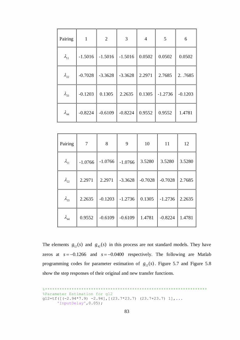
83
Pairing 1 2 3 4 5 6
11
-1.5016
-1.5016 -1.5016
0.0502 0.0502 0.0502
22 -0.7028 -3.3628 -3.3628 2.2971 2.7685 2. .7685
33 -0.1203 0.1305 2.2635 0.1305 -1.2736 -0.1203
44 -0.8224 -0.6109 -0.8224 0.9552 0.9552 1.4781
Pairing 7 8 9 10 11 12
11
-1.0766 -1.0766 -1.0766 3.5280 3.5280 3.5280
22 2.2971 2.2971 -3.3628 -0.7028 -0.7028 2.7685
33 2.2635 -0.1203 -1.2736 0.1305 -1.2736 2.2635
44 0.9552 -0.6109 -0.6109 1.4781 -0.8224 1.4781
The elements 12 ( )g s and 42 ( )g s in this process are not standard models. They have
zeros at 0.1266s and 0.0400s respectively. The following are Matlab
programming codes for parameter estimation of 12 ( )g s . Figure 5.7 and Figure 5.8
show the step responses of their original and new transfer functions.
%*******************************************************************
%Parameter Estimation for g12
g12=tf([(-2.94*7.9) -2.94],[(23.7*23.7) (23.7+23.7) 1],...
'InputDelay',0.05);
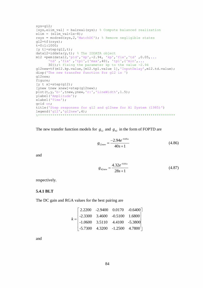
84
sys=g12;
[sys,elim_val] = balreal(sys); % Compute balanced realization
elim = (elim_val<1e-8);
rsys = modred(sys,2,'MatchDC'); % Remove negligible states
g12=tf(rsys);
t=0:1:1000;
[y t]=step(g12,t);
data12=iddata(y,t); % The IDDATA object
m12 =pem(data12,'p1d','kp',-2.94, 'kp','fix','td' ,0.05,...
'td' ,'fix' ,'tp1',{'max',40}, 'tp1',{'min',...
30});% fixing the parameter kp to the value -2.94
g12new=tf(m12.kp.value,[m12.tp1.value 1],'InputDelay',m12.td.value);
disp('The new transfer function for g12 is ')
g12new;
figure;
[y t x]=step(g12);
[ynew tnew xnew]=step(g12new);
plot(t,y,'b-',tnew,ynew,'r:','LineWidth',1.5);
ylabel('Amplitude');
xlabel('Time');
grid on;
title('Step responses for g12 and g12new for A1 System (1985)')
legend('g12','g12new',4);
%*******************************************************************
The new transfer function models for 12g and 42g in the form of FOPTD are
0.05
12
2.94
40 1
s
new
eg
s
(4.86)
and
0.01
42
4.32
28 1
s
new
eg
s
(4.87)
respectively.
5.4.1 BLT
The DC gain and RGA values for the best pairing are
2.2200 -2.9400 0.0170 -0.6400
-2.3300 3.4600 -0.5100 1.6800
-1.0600 3.5110 4.4100 -5.3800
-5.7300 4.3200 -1.2500 4.7800
k
and
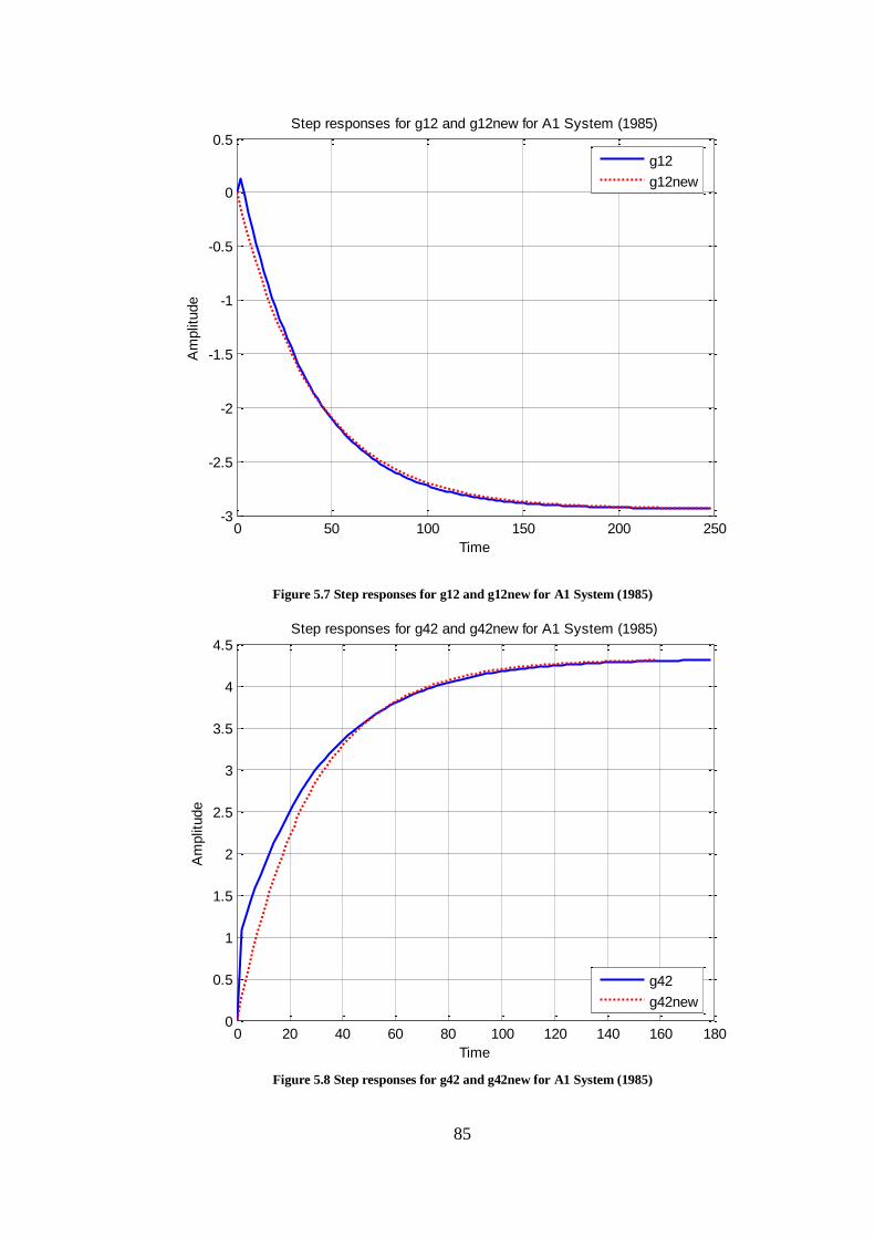
85
Figure 5.7 Step responses for g12 and g12new for A1 System (1985)
Figure 5.8 Step responses for g42 and g42new for A1 System (1985)
0 50 100 150 200 250-3
-2.5
-2
-1.5
-1
-0.5
0
0.5
Am
plit
ude
Time
Step responses for g12 and g12new for A1 System (1985)
g12
g12new
0 20 40 60 80 100 120 140 160 1800
0.5
1
1.5
2
2.5
3
3.5
4
4.5
Am
plit
ude
Time
Step responses for g42 and g42new for A1 System (1985)
g42
g42new
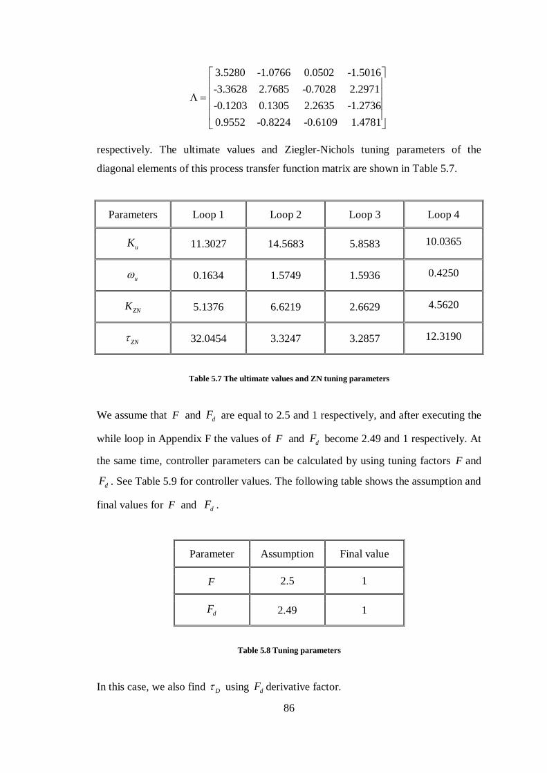
86
3.5280 -1.0766 0.0502 -1.5016
-3.3628 2.7685 -0.7028 2.2971
-0.1203 0.1305 2.2635 -1.2736
0.9552 -0.8224 -0.6109 1.4781
respectively. The ultimate values and Ziegler-Nichols tuning parameters of the
diagonal elements of this process transfer function matrix are shown in Table 5.7.
Parameters Loop 1 Loop 2 Loop 3 Loop 4
uK 11.3027 14.5683 5.8583 10.0365
u 0.1634 1.5749 1.5936 0.4250
ZNK 5.1376 6.6219 2.6629 4.5620
ZN 32.0454 3.3247 3.2857 12.3190
Table 5.7 The ultimate values and ZN tuning parameters
We assume that F and dF are equal to 2.5 and 1 respectively, and after executing the
while loop in Appendix F the values of F and dF become 2.49 and 1 respectively. At
the same time, controller parameters can be calculated by using tuning factors F and
dF . See Table 5.9 for controller values. The following table shows the assumption and
final values for F and dF .
Parameter Assumption Final value
F 2.5 1
dF 2.49 1
Table 5.8 Tuning parameters
In this case, we also find D using dF derivative factor.
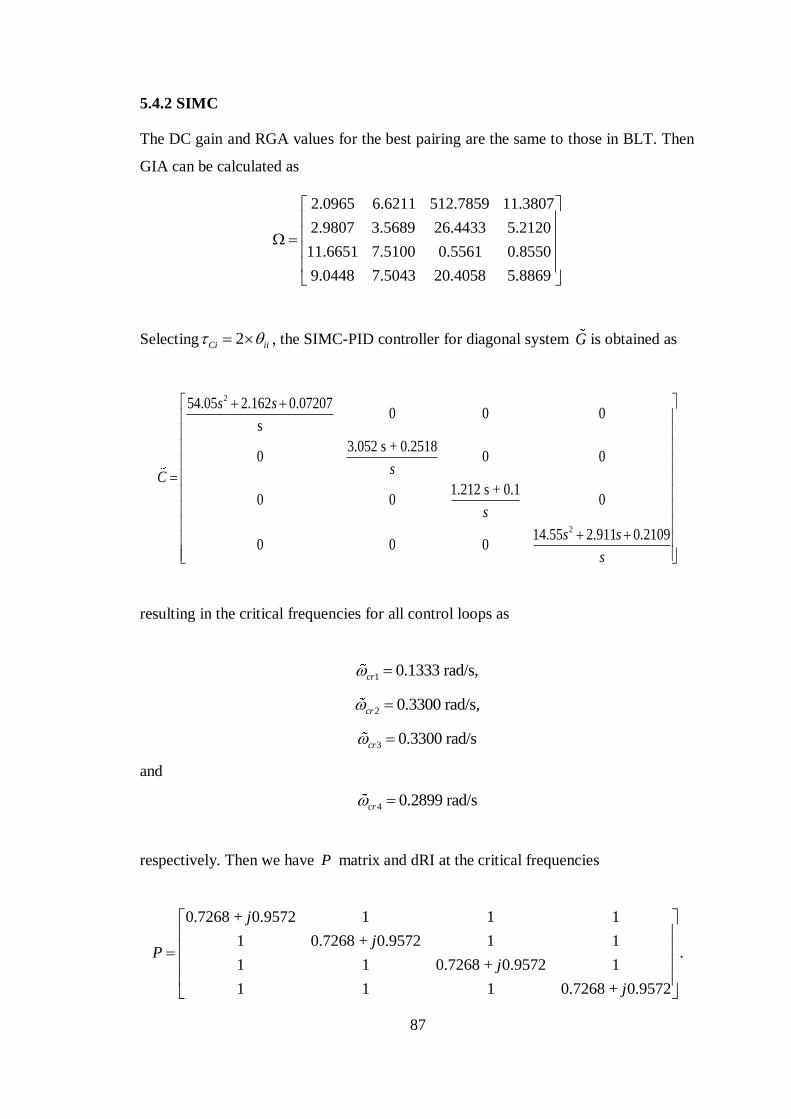
87
5.4.2 SIMC
The DC gain and RGA values for the best pairing are the same to those in BLT. Then
GIA can be calculated as
2.0965 6.6211 512.7859 11.3807
2.9807 3.5689 26.4433 5.2120
11.6651 7.5100 0.5561 0.8550
9.0448 7.5043 20.4058 5.8869
Selecting 2Ci ii , the SIMC-PID controller for diagonal system G is obtained as
2
2
0 0 0s
3.052 s + 0.25180 0 0
1.212 s
54.05 2.162 0.07207
14.55 2.911 0.2109
+ 0.10 0 0
0 0 0
sC
s
s
s s
s s
resulting in the critical frequencies for all control loops as
1 0.1333 rad/s,cr
2 0.3300 rad/s,cr
3 0.3300 rad/scr
and
4 0.2899 rad/scr
respectively. Then we have P matrix and dRI at the critical frequencies
0.7268 + 0.9572 1 1 1
1 0.7268 + 0.9572 1 1.
1 1 0.7268 + 0.9572 1
1 1 1 0.7268 + 0.9572
j
jP
j
j
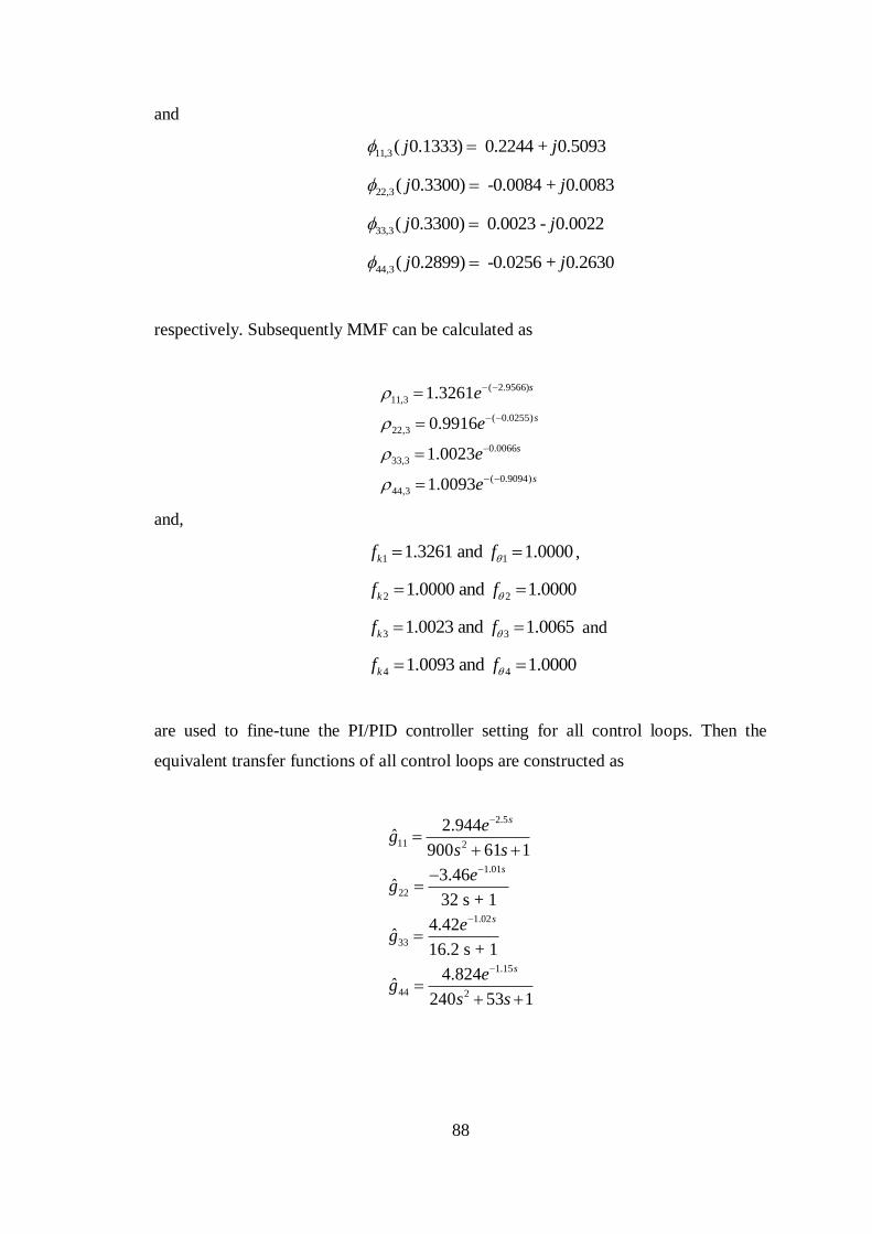
88
and
11,3( 0.1333) 0.2244 + 0.5093j j
22,3( 0.3300) -0.0084 + 0.0083j j
33,3( 0.3300) 0.0023 - 0.0022j j
44,3( 0.2899) -0.0256 + 0.2630j j
respectively. Subsequently MMF can be calculated as
( 2.9566)
11,3
( 0.0255)
22,3
0.0066
33,3
( 0.9094)
44,3
1.3261
0.9916
1.0023
1.0093
s
s
s
s
e
e
e
e
and,
1 11.3261 and 1.0000kf f ,
2 21.0000 and 1.0000kf f
3 31.0023 and 1.0065kf f and
4 41.0093 and 1.0000kf f
are used to fine-tune the PI/PID controller setting for all control loops. Then the
equivalent transfer functions of all control loops are constructed as
2.5
11
1.01
2
2
22
1.02
33
1.15
44
2.944ˆ
3.46ˆ
32 s + 1
4.42ˆ
16.2 s + 1
4.82
900 61 1
2ˆ
40 5
4
3 1
s
s
s
s
eg
eg
eg
s s
s s
eg
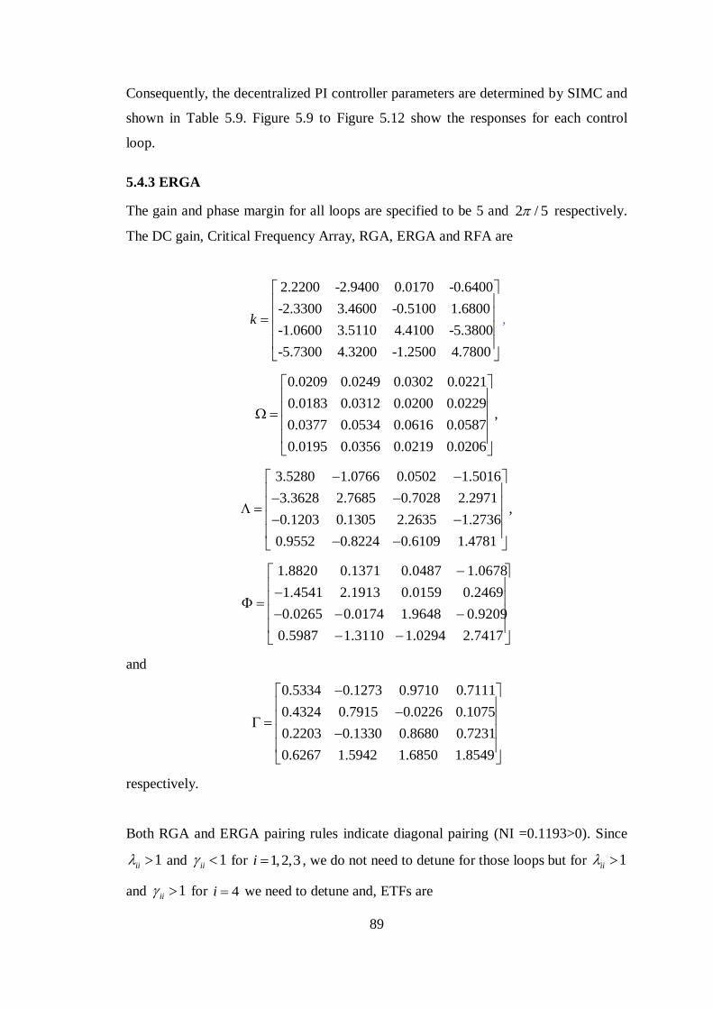
89
Consequently, the decentralized PI controller parameters are determined by SIMC and
shown in Table 5.9. Figure 5.9 to Figure 5.12 show the responses for each control
loop.
5.4.3 ERGA
The gain and phase margin for all loops are specified to be 5 and 2 / 5 respectively.
The DC gain, Critical Frequency Array, RGA, ERGA and RFA are
2.2200 -2.9400 0.0170 -0.6400
-2.3300 3.4600 -0.5100 1.6800
-1.0600 3.5110 4.4100 -5.3800
-5.7300 4.3200 -1.2500 4.7800
k
,
0.0209 0.0249 0.0302 0.0221
0.0183 0.0312 0.0200 0.0229,
0.0377 0.0534 0.0616 0.0587
0.0195 0.0356 0.0219 0.0206
3.5280 1.0766 0.0502 1.5016
3.3628 2.7685 0.7028 2.2971,
0.1203 0.1305 2.2635 1.2736
0.9552 0.8224 0.6109 1.4781
1.8820 0.1371 0.0487 1.0678
1.4541 2.1913 0.0159 0.2469
0.0265 0.0174 1.9648 0.9209
0.5987 1.3110 1.0294 2.7417
and
0.5334 0.1273 0.9710 0.7111
0.4324 0.7915 0.0226 0.1075
0.2203 0.1330 0.8680 0.7231
0.6267 1.5942 1.6850 1.8549
respectively.
Both RGA and ERGA pairing rules indicate diagonal pairing (NI =0.1193>0). Since
1ii and 1ii for 1,2,3i , we do not need to detune for those loops but for 1ii
and 1ii for 4i we need to detune and, ETFs are
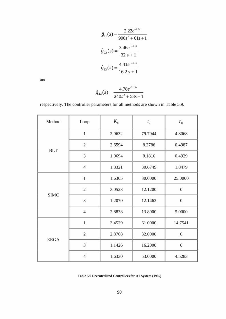
90
2.
2
5
11
2.22
900 61 1ˆ ( )
se
s sg s
1.01
22
3.46
32 s + 1ˆ ( )
se
g s
1.01
33
4.41
16.2 s + 1ˆ ( )
se
g s
and
2.13
244240 5
4
3
7
1
. 8ˆ ( )
se
s sg s
respectively. The controller parameters for all methods are shown in Table 5.9.
Method Loop CK I D
BLT
1 2.0632 79.7944 4.8068
2 2.6594 8.2786 0.4987
3 1.0694 8.1816 0.4929
4 1.8321 30.6749 1.8479
SIMC
1 1.6305 30.0000 25.0000
2 3.0523 12.1200 0
3 1.2070 12.1462 0
4 2.8838 13.8000 5.0000
ERGA
1 3.4529 61.0000 14.7541
2 2.8768 32.0000 0
3 1.1426 16.2000 0
4 1.6330 53.0000 4.5283
Table 5.9 Decentralized Controllers for A1 System (1985)
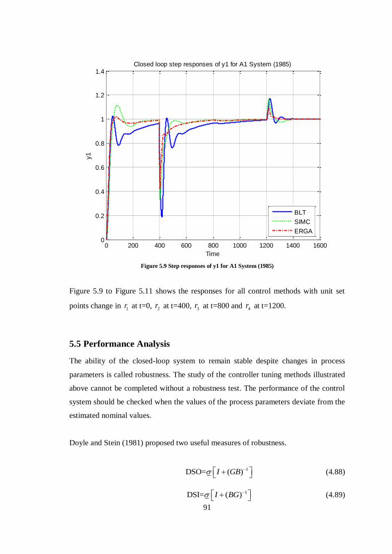
91
Figure 5.9 Step responses of y1 for A1 System (1985)
Figure 5.9 to Figure 5.11 shows the responses for all control methods with unit set
points change in 1r at t=0, 2r at t=400, 3r at t=800 and 4r at t=1200.
5.5 Performance Analysis
The ability of the closed-loop system to remain stable despite changes in process
parameters is called robustness. The study of the controller tuning methods illustrated
above cannot be completed without a robustness test. The performance of the control
system should be checked when the values of the process parameters deviate from the
estimated nominal values.
Doyle and Stein (1981) proposed two useful measures of robustness.
1DSO= ( )I GB (4.88)
1DSI= ( )I BG (4.89)
0 200 400 600 800 1000 1200 1400 16000
0.2
0.4
0.6
0.8
1
1.2
1.4
y1
Time
Closed loop step responses of y1 for A1 System (1985)
BLT
SIMC
ERGA
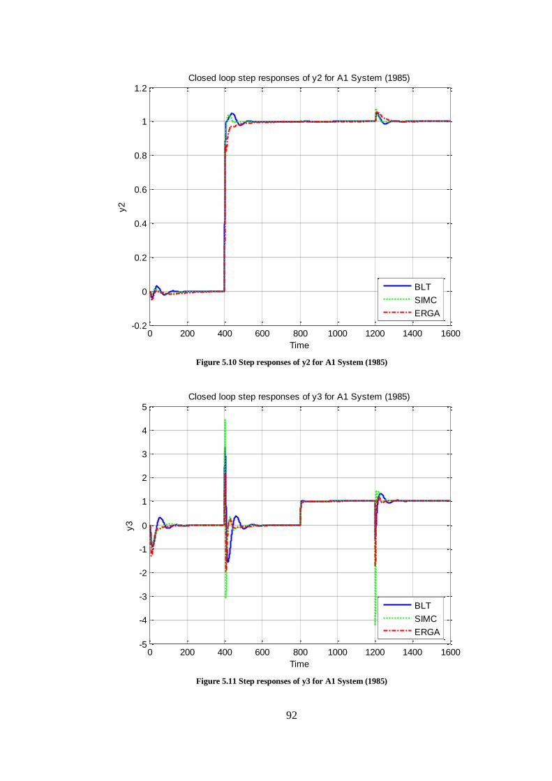
92
Figure 5.10 Step responses of y2 for A1 System (1985)
Figure 5.11 Step responses of y3 for A1 System (1985)
0 200 400 600 800 1000 1200 1400 1600-0.2
0
0.2
0.4
0.6
0.8
1
1.2
y2
Time
Closed loop step responses of y2 for A1 System (1985)
BLT
SIMC
ERGA
0 200 400 600 800 1000 1200 1400 1600-5
-4
-3
-2
-1
0
1
2
3
4
5
y3
Time
Closed loop step responses of y3 for A1 System (1985)
BLT
SIMC
ERGA
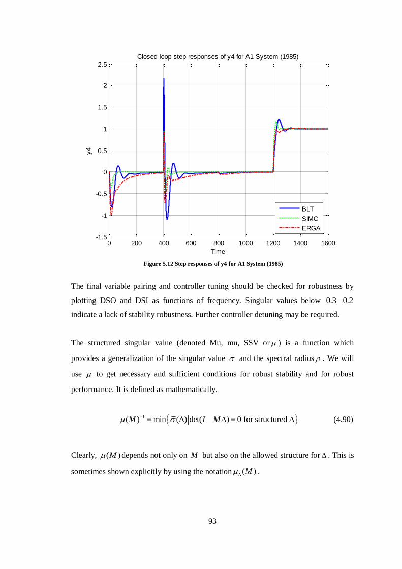
93
Figure 5.12 Step responses of y4 for A1 System (1985)
The final variable pairing and controller tuning should be checked for robustness by
plotting DSO and DSI as functions of frequency. Singular values below 0.3 0.2
indicate a lack of stability robustness. Further controller detuning may be required.
The structured singular value (denoted Mu, mu, SSV or ) is a function which
provides a generalization of the singular value and the spectral radius . We will
use to get necessary and sufficient conditions for robust stability and for robust
performance. It is defined as mathematically,
1( ) min ( ) det( ) 0 for structured M I M (4.90)
Clearly, ( )M depends not only on M but also on the allowed structure for . This is
sometimes shown explicitly by using the notation ( )M .
0 200 400 600 800 1000 1200 1400 1600-1.5
-1
-0.5
0
0.5
1
1.5
2
2.5
y4
Time
Closed loop step responses of y4 for A1 System (1985)
BLT
SIMC
ERGA
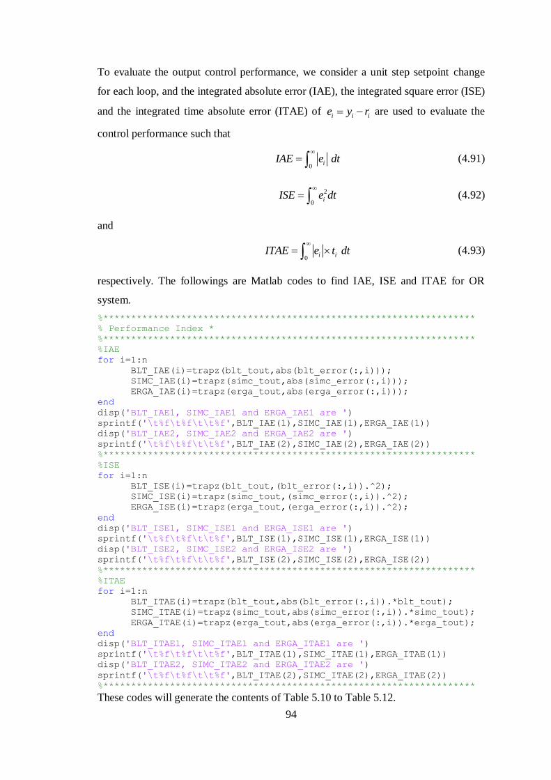
94
To evaluate the output control performance, we consider a unit step setpoint change
for each loop, and the integrated absolute error (IAE), the integrated square error (ISE)
and the integrated time absolute error (ITAE) of i i ie y r are used to evaluate the
control performance such that
0
iIAE e dt
(4.91)
2
0iISE e dt
(4.92)
and
0
i iITAE e t dt
(4.93)
respectively. The followings are Matlab codes to find IAE, ISE and ITAE for OR
system.
%*******************************************************************
% Performance Index *
%*******************************************************************
%IAE
for i=1:n
BLT_IAE(i)=trapz(blt_tout,abs(blt_error(:,i)));
SIMC_IAE(i)=trapz(simc_tout,abs(simc_error(:,i)));
ERGA_IAE(i)=trapz(erga_tout,abs(erga_error(:,i)));
end
disp('BLT_IAE1, SIMC_IAE1 and ERGA_IAE1 are ')
sprintf('\t%f\t%f\t\t%f',BLT_IAE(1),SIMC_IAE(1),ERGA_IAE(1))
disp('BLT_IAE2, SIMC_IAE2 and ERGA_IAE2 are ')
sprintf('\t%f\t%f\t\t%f',BLT_IAE(2),SIMC_IAE(2),ERGA_IAE(2))
%*******************************************************************
%ISE
for i=1:n
BLT_ISE(i)=trapz(blt_tout,(blt_error(:,i)).^2);
SIMC_ISE(i)=trapz(simc_tout,(simc_error(:,i)).^2);
ERGA_ISE(i)=trapz(erga_tout,(erga_error(:,i)).^2);
end
disp('BLT_ISE1, SIMC_ISE1 and ERGA_ISE1 are ')
sprintf('\t%f\t%f\t\t%f',BLT_ISE(1),SIMC_ISE(1),ERGA_ISE(1))
disp('BLT_ISE2, SIMC_ISE2 and ERGA_ISE2 are ')
sprintf('\t%f\t%f\t\t%f',BLT_ISE(2),SIMC_ISE(2),ERGA_ISE(2))
%*******************************************************************
%ITAE
for i=1:n
BLT_ITAE(i)=trapz(blt_tout,abs(blt_error(:,i)).*blt_tout);
SIMC_ITAE(i)=trapz(simc_tout,abs(simc_error(:,i)).*simc_tout);
ERGA_ITAE(i)=trapz(erga_tout,abs(erga_error(:,i)).*erga_tout);
end
disp('BLT_ITAE1, SIMC_ITAE1 and ERGA_ITAE1 are ')
sprintf('\t%f\t%f\t\t%f',BLT_ITAE(1),SIMC_ITAE(1),ERGA_ITAE(1))
disp('BLT_ITAE2, SIMC_ITAE2 and ERGA_ITAE2 are ')
sprintf('\t%f\t%f\t\t%f',BLT_ITAE(2),SIMC_ITAE(2),ERGA_ITAE(2))
%*******************************************************************
These codes will generate the contents of Table 5.10 to Table 5.12.

95
Methods Controller IAE ISE ITAE
BLT
Loop 1 6.700269 3.041136 113.736678
Loop 2 2.142164 0.890127 73.807713
SIMC
Loop 1 11.055941 4.879077 215.310918
Loop 2 2.104946 0.810928 64.872263
ERGA
Loop 1 4.141611 2.054463 65.335278
Loop 2 2.541929 0.827885 71.617611
Table 5.10 Performance Analysis for VL System (1972)
Methods Controller IAE ISE ITAE
BLT
Loop 1 40.669637 11.913219 5207.841148
Loop 2 122.673663 47.662144 29961.832043
Loop 3 213.878712 1092.095839 29028.759469
SIMC
Loop 1 154.647127 71.142149 26730.952140
Loop 2 90.409888 24.020309 24398.624396
Loop 3 65.994708 19.914998 16407.995639
ERGA
Loop 1 31.766417 11.258064 3374.608357
Loop 2 70.727090 31.085399 14662.244667
Loop 3 350.391320 2003.041302 48476.558050
Table 5.11 Performance Analysis for OR System (1979)
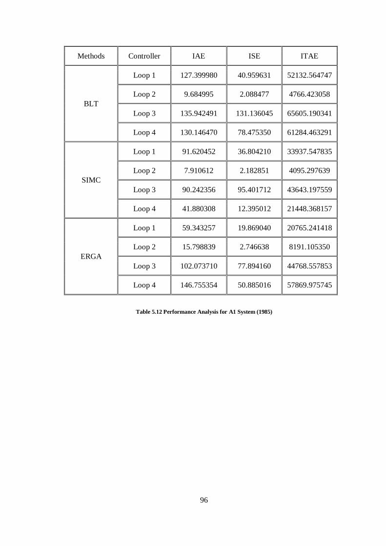
96
Methods Controller IAE ISE ITAE
BLT
Loop 1 127.399980 40.959631 52132.564747
Loop 2 9.684995 2.088477 4766.423058
Loop 3 135.942491 131.136045 65605.190341
Loop 4 130.146470 78.475350 61284.463291
SIMC
Loop 1 91.620452 36.804210 33937.547835
Loop 2 7.910612 2.182851 4095.297639
Loop 3 90.242356 95.401712 43643.197559
Loop 4 41.880308 12.395012 21448.368157
ERGA
Loop 1 59.343257 19.869040 20765.241418
Loop 2 15.798839 2.746638 8191.105350
Loop 3 102.073710 77.894160 44768.557853
Loop 4 146.755354 50.885016 57869.975745
Table 5.12 Performance Analysis for A1 System (1985)
97
6 Conclusion and Recommendation
6.1 Conclusion
The results show that the BLT settings give stable and reasonable responses. In all
cases, the BLT method converged very quickly to settings that worked. The
computation horsepower required to implement the basic method is quite nominal. The
only calculation required is the evaluation of the determinant of a N N matrix. No
matrix inversion or eigenvalue calculations are required. These calculations are well
within the capability of a personal computer.
The simplicity and effectiveness of the model is based on the energy transmission ratio
of each individual transfer function which provides necessary information of gain and
frequency changes when all other loops are closed. Consequently, the decentralized
controllers can be obtained by simply using single loop design approaches. Simulation
results for variety of industrial 2 2 , 3 3 and 4 4 processes show that ERGA
method provides overall better performance compared to other reported design
approaches. The advantage of ERGA method is even more significant when applied to
higher dimensional processes with complicated interaction modes. The method can be
easily integrated into an auto-tuning control structure combined with some on line
parameter identification module and implemented for industrial control systems.
dRI based Skogestad Internal Model Control (SIMC) method is a simple and effective
design method for decentralized PID controller design. On the basis of structure
decomposition, the dynamic relative interaction was defined and represented by the
process model and controller explicitly. An initial decentralized controller was
designed first by using the diagonal elements and then implemented to estimate the
dRI to individual control loop from all others.
According to the simulation results in chapter 5, we conclude that the three
decentralized control methods presented in this dissertation can be easily applied to
high dimensional processes with complicated interaction modes such as distillation
column.
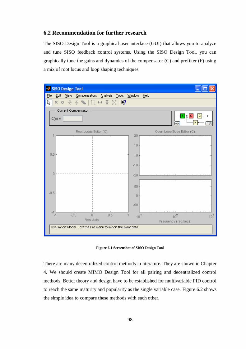
98
6.2 Recommendation for further research
The SISO Design Tool is a graphical user interface (GUI) that allows you to analyze
and tune SISO feedback control systems. Using the SISO Design Tool, you can
graphically tune the gains and dynamics of the compensator (C) and prefilter (F) using
a mix of root locus and loop shaping techniques.
Figure 6.1 Screenshot of SISO Design Tool
There are many decentralized control methods in literature. They are shown in Chapter
4. We should create MIMO Design Tool for all pairing and decentralized control
methods. Better theory and design have to be established for multivariable PID control
to reach the same maturity and popularity as the single variable case. Figure 6.2 shows
the simple idea to compare these methods with each other.
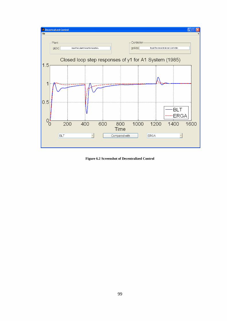
99
Figure 6.2 Screenshot of Decentralized Control
100
Bibliography
1. Albertos P. and Sala A. Multivariable Control Systems [Book]. - London :
Springer, 2004. - ISBN 1-85233-738-9.
2. Arkun Y. and Downs Y. J. A general method t calculate input-output gains and
the RGA for integrating processes [Journal] // Comp.Chem. Eng.. - 1990. - Vol.
14. - pp. 1101-1110.
3. Astrom K. J. and Hagglund T. Advanced PID Control [Book]. - [s.l.] :
Instrumentation, Systems, and Automation Society (ISA), 2006. - pp. 87-89;193-
196;174-189. - ISBN1-55617-942-1.
4. Astrom K. J. and Hagglund T. The future of PID control [Journal] // Control
Engineering Practice. - [s.l.] : Elsevier Science Ltd., 2001. - Vol. 9. - pp. 1163–
1175.
5. Avoy Thomas Mc [et al.] A new approach to defining a dynamic relative gain
[Journal] // Control Engineering Practice. - [s.l.] : Elsevier Science Ltd., 2003. -
Vol. 11. - pp. 907–914.
6. Balachandran R. and Chidambaram M. Decentralized control of crude unit
distillation towers [Journal] // Computers chem. Engng. - [s.l.] : Elsevier Science
Ltd, 1997. - 8 : Vol. 21. - pp. 783-786.
7. Bezzo F. [et al.] Using MPC to control middle-vessel continuous distillation
columns [Journal] // Journal of Process Control. - [s.l.] : Elsevier Ltd., 2005. - Vol.
15. - pp. 925–930.
8. Bristol E. H. On a New Measure of Interactions for Multivariable Process Control
[Journal] // IEEE Transactions on Automatic Control. - 1966. - Vol. 11. - pp. 133-
134.
9. Bristol E. H. On a Philosophy of Interaction in a Multiloop World [Book]. - [s.l.] :
ISA Chemical & Petroleum Division Chempid Symposium, 1967.
10. Cai W. J. Decentralized Control for MIMO Processes [Book Section] // Lecture
Note for Process Control. - Singapore : NTU, 2007.
11. Cai Wen-Jian Fundamentals of Empirical Modeling and Identification [Book
Section] // Lecture Notes for Process Control. - [s.l.] : NTU, 2007.
101
12. Chen D. and Seborg D.E. Design of Decentralized PI Control Systems based on
Nyquist Stability Analysis [Journal] // Journal of Process Control. - [s.l.] : Elsevier,
2003. - 1 : Vol. 13. - pp. 27–39.
13. Chen J., Cheng Y. and Yea Y. Multiloop PID Controller Design using Partial
Least Squares Decoupling Structure [Journal] // Korean J. Chem. Eng.. - [s.l.] : 22,
2005. - Vol. 2. - pp. 173-183.
14. Chien I-Lung, Huang Hsiao-Ping and Yang Jen-Chien A Simple Multiloop
Tuning Method for PID Controllers with No Proportional Kick [Journal] // Ind.
Eng. Chem. Res.. - [s.l.] : American Chemical Society, 1999. - 4 : Vol. 38. - pp.
1456-1468.
15. Christen Urs, Musch Hans E. and Steiner Max Robust control of distillation
columns: Mu & H-infinity -synthesis [Journal] // J. Proc. Cont.. - [s.l.] : Elsevier
Science Ltd., 1997. - 1 : Vol. 7. - pp. 19-30.
16. Conley A. and Salgado M. E. Gramian based interaction measure [Conference] //
In 34th CDC Conference Proceedings. - Sydney, Australia : [s.n.], 2000.
17. Economou C. G. and Morari M. Internal Model Control. 6. Multiloop Design
[Journal] // Ind. Eng. Chem. Process Des. Dev.. - [s.l.] : American Chemical
Society, 1986. - Vol. 25. - pp. 411-419.
18. Gagnon E., Desbiens A. and Pomerleau A. Selection of pairing and constrained
robust decentralized PI controllers [Conference] // In Proceedings of the American
Control Conference. - 1999. - pp. 4343–4347.
19. Ganguly S. and Saraf D. N. A semi-rigorous dynamic distillation model for on-
line optimization and nonlinear control [Journal] // J. Proc. Cont.. - [s.l.] :
Butterworth-Heinemann Ltd, 1993. - 3 : Vol. 3.
20. Grosdidier P. and Morari M. Interaction Measures for Systems Under
Decentralized Control [Journal] // Automatica. - 1986. - 3 : Vol. 22. - pp. 309-319.
21. Grosdidier P., Morari M. and Holt B. R. Closed-loop properties from steady-
state gain information [Journal] // Industrial and Engineering Chemistry Process
Design and Development. - 1985. - Vol. 24. - pp. 221–235.
22. Gu D.-W., Petkov P. Hr. and Konstantinov M. M. Robust Control Design with
MATLAB [Book]. - [s.l.] : Springer-Verlag London Limited, 2005. - ISBN-10:
1852339837.
102
23. He Mao-Jun, Cai Wen-Jian and Li Shao-Yuan New Criterion for Control Loop
Configuration of Multivariable Processes [Journal] // Ind. Eng. Chem. Res.. -
2004. - Vol. 43. - pp. 7057-7064.
24. He Mao-Jun, Cai Wen-Jian and Wu Bing-Fang Design of Decentralized IMC-
PID Controller Based on dRI Analysis [Journal] // AIChE Journal. - [s.l.] : Wiley
InterScience, 2006. - 11 : Vol. 52.
25. Ho W. K., Lee T. H. and Gan O. P. Tuning of Multiloop Proportional-Integral-
Derivative Controllers Based on Gain and Phase Margin Specifications [Journal] //
Ind. Eng. Chem. Res.. - 1997. - Vol. 36. - pp. 2231-2238.
26. Hovd M. and Skogestad S. Simple frequency-dependent tools control system
analysis, structure selection and design [Journal] // Automatical. - 1992. - 5 : Vol.
28. - pp. 989-996.
27. Huang Hsiao-Ping [et al.] A direct method for multi-loop PI/PID controller
design [Journal] // Journal of Process Control. - 2003. - Vol. 13. - pp. 769–786.
28. Humphrey J. L., Seibert A. F. and Koort R. A. Separation Technologies-
Advances and Priorities [Book]. - [s.l.] : DOE Contract AC07–901D12920,
February 1991.
29. Humphrey J. L., Seibert A. F. and Koort R. A. Separation Technologies—
Advances and Priorities [Journal] // U.S. Department of Energy, Office of
Industrial Technologies. - February 1991. - Vol. DOE/ID/129201.
30. Hurowitz1 Scott [et al.] Distillation control configuration selection [Journal] //
Journal of Process Control. - 2003. - Vol. 13. - pp. 357–362.
31. Lee Dong-Yup [et al.] Mp Criterion Based Multiloop PID Controllers Tuning for
Desired Closed Loop Responses [Journal] // Korean J. Chem. Eng.. - 2003. - 1 :
Vol. 20. - pp. 8-13.
32. Lee J. and Edgar T. F. Dynamic Interaction Measures for Decentralized Control
of Multivariable Processes [Journal] // Ind. Eng. Chem. Res.. - [s.l.] : American
Chemical Society, 2004. - Vol. 43. - pp. 283-287.
33. Lee J. and Edgarb T. F. Multiloop PI/PID control system improvement via
adjusting the dominant pole or the peak amplitude ratio [Journal] // Chemical
Engineering Science 61 (2006) . - [s.l.] : Elsevier Ltd., 2006. - Vol. 61. - pp. 1658
– 1666.
103
34. Lee J., Cho W. and Edgar T. F. Multiloop PI controller tuning for interacting
multivariable processes [Journal] // Computers Chem. Engng.. - [s.l.] : Elsevier
Science Ltd, 1998. - 11 : Vol. 22. - pp. 1711-1723.
35. Lee M. [et al.] Analytical Design of Multiloop PID Controllers for Desired
Closed-Loop Responses [Journal]. - [s.l.] : Wiley InterScience, 2004. - 7 : Vol.
50. - pp. 1631-1635.
36. Loh A. P. [et al.] Autotuning of Multiloop Proportional-integral Controllers using
Relay Feedback [Journal] // Industrial and Engineering Chemistry Research. -
1993. - Vol. 32. - pp. 1102–1107.
37. Loh A. P. and Vasnani V. U. Describing Function Matrix for Multivariable
Systems and its use in Multiloop PI Design [Journal] // Journal of Process
Control. - 1994. - Vol. 4. - pp. 115–120.
38. Luyben N. Doukas and W.L. Control of Sidestream columns Separating Ternary
Mixtures [Journal] // Instrum. Technol. - 1978. - 43 : Vol. 25.
39. Luyben W.L. Simple Method for Tuning SISO Controllers in Multivariable
Systems [Journal] // Ind. Eng. Chem. Process Des. Dev.. - 1986. - 3 : Vol. 25. - pp.
654–660.
40. Makaremi I. and Labibi B. Control of a Distillation Column: A Decentralized
Approach [Conference] // Proceedings of the 2006 IEEE International Conference
on Control Applications. - Munich, Germany : [s.n.], 2006. - pp. 711-714.
41. McAvoy T. Interaction Analysis: Principles and Applications [Book]. - [s.l.] :
Instrument Society of America, 1985.
42. Monica T. J., Yu C. C. and Luyben W. L. Improved Multiloop Single -
Input/Single - Output (SISO) Controllers for Multivariable Processes [Journal] //
Ind. Eng. Chem. Res.. - [s.l.] : ACS Publications, 1988. - Vol. 27. - pp. 969-973.
43. Niederlinski A. A Heuristic Approach to the Design of Linear Multivariable
Interacting Control Systems [Journal] // Automatica. - 1971. - Vol. 7. - pp. 691-
701.
44. Q. Xiong W.-J. Cai, Effective transfer function method for decentralized control
system design of multi-input multi-output processes [Journal] // Journal of Process
Control. - 2006. - pp. 773-784.
104
45. Qiang Xiong Wen-Jian Cai and Mao-Jun He A practical loop pairing criterion
for multivariable processes [Journal] // Journal of Process Control. - 2005. - pp.
741-747.
46. Qiang Xiong Wen-Jian Cai and Mao-Jun He Equivalent transfer function
method for PI/PID controller design of MIMO processes [Journal] // Journal of
Process Control. - 2007. - pp. 665-673.
47. Ramchandran S. and Rhinehart R. R. A very simple structure for neural
network control of distillation [Journal] // J. Proc. Cont.. - 1995. - 2 : Vol. 5. - pp.
115-128.
48. Raya Goshaidas, Prasadb A.N. and Bhattacharyya T.K. Design of
decentralized robust load-frequency controller [Journal] // Computers and
Electrical Engineering. - 1999. - Vol. 25. - pp. 477-492.
49. Rijnsdorp J. E. Interaction in Two-Variable Control Systems for Distillation
Columns-I [Journal] // Automatica. - 1965. - Vol. 1. - pp. 15-28.
50. Salgado M. E. and CONLEY A. MIMO interaction measure and controller
structure selection [Journal] // INT. J. CONTROL. - 2004. - Vol. 4. - pp. 367–383.
51. Shen S. H. and Yu C. C. Use of Relay-feedback Test for Autotuning of
Multivariable Systems [Journal] // American Institute of Chemical Engineers
Journal. - 1994. - Vol. 40. - pp. 627–646.
52. Skogestad S. and Morari M. Robust Performance of Decentralized Control
Systems by Independent Designs [Journal] // Automaaca. - 1989. - 1 : Vol. 25. -
pp. 119-125.
53. Skogestad S. and Postlethwaite I. Multivariable Feedback Control - Analysis and
Design [Book]. - [s.l.] : John Wiley & Sons, 2005. - 2nd Edition. - ISBN 0-470-
01167-X.
54. Stem R. and Kuhn U. Automation of a Batch Distillation Column Using Fuzzy
and Conventional Control [Journal] // IEEE Transactions on Control Systems
Technology. - [s.l.] : IEEE, 1995. - 2 : Vol. 3. - pp. 171-176.
55. Tham M. T. Distillation- An Introduction [Online] // Distillation. - 2006. -
http://lorien.ncl.ac.uk/ming/distil/distil0.htm.
56. Tyréus Björn D. Multivariable Control System Design for an Industrial
Distillation Column [Journal] // Ind. Eng. Chem. Proc. Des. Dev.. - 1979. - 1 : Vol.
18. - pp. 177-182.
105
57. Vu T. N. L, Lee J. and Lee M. Design of Multi-loop PID Controllers Based on
the Generalized IMC-PID Method with Mp Criterion [Journal] // International
Journal of Control, Automation, and Systems. - 2007. - 2 : Vol. 5. - pp. 212-217.
58. Wang Qing-Guo, Lee Tong-Heng and Zhang Yu Multiloop Version of the
Modified Ziegler-Nichols Method for Two Input Two Output Processes
[Journal] // Ind. Eng. Chem. Res.. - [s.l.] : American Chemical Society, 1998. -
Vol. 37. - pp. 4725-4733.
59. Wang Y.-G. and Cai W.-J. Advanced proportional–integral–derivative tuning for
integrating and unstable processes with gain and phase margin specifications
[Journal] // Industrial and Engineering Chemistry Research. - 2002. - Vol. 41. - pp.
2910–2914.
60. Wikipedia Price of petroleum [Online] // Wikipedia. - 2008. -
http://en.wikipedia.org/wiki/Crude_oil_price.
61. Wikipedia Price of Petroleum [Online] // Wikipedia. - 2008. -
http://en.wikipedia.org/wiki/Crude_oil_price.
62. Wood R. K. and Berry M. W. Terminal Composition Control of a Binary
Distillation Column [Journal] // Chemical Engineering Science. - 1973. - 9 : Vol.
28. - pp. 1707-1717.
63. Xiong Qiang, Cai Wen-Jian and He Mao-Jun A practical loop pairing criterion
for multivariable processes [Journal] // Journal of Process Control. - [s.l.] : Elsevier
Ltd., 2005. - Vol. 15. - pp. 741–747.
64. Yu C. C. and Luyben W. L. Design of Multiloop SISO Controllers in
Multivariavle Processes [Journal] // Ind. Eng. Chem. Process Des. Dev.. - 1986. -
2 : Vol. 25. - pp. 498-503.
65. Yu W., Poznyak A. S. and Alvarez J. Neuro Control for Multicomponent
Distillation Column [Conference] // 14th World Congress of IFAC. - 1999. - pp.
378-384. - ISBN 0 08 043248 4.
66. Zhang Yu and Wang Qing-Guo Design of Multi-Loop and Multivariable PID
Controllers [Book Section] // PID Contrtol / book auth. Johnson Michael A.,
Crowe J. and Moradi Mohammad Hassan. - [s.l.] : Springer, 2005. -
ISBN:1852337028.
67. Zhou C. [et al.] Application of Enhanced LQG/LTR for Distillation Column
[Journal] // IEEE Control Systems. - [s.l.] : IEEE, 1995. - pp. 56-63.

106
68. Zhu Yucai Multivariable System Identification for Process Control [Book]. -
London : Elsevier Science & Technology Books, 2001. - 0080439853.
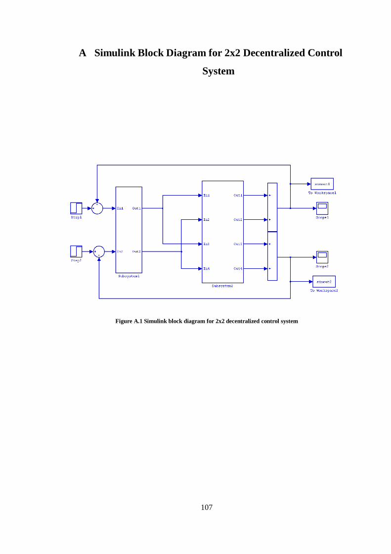
107
A Simulink Block Diagram for 2x2 Decentralized Control
System
Figure A.1 Simulink block diagram for 2x2 decentralized control system
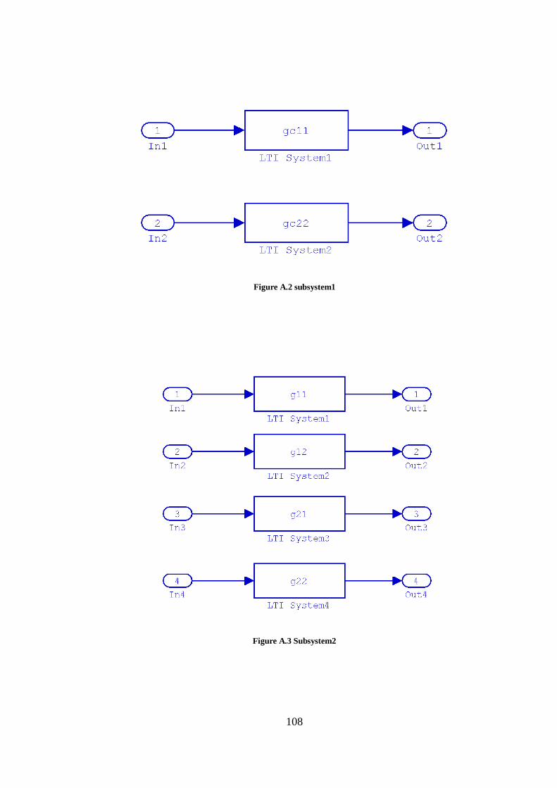
108
Figure A.2 subsystem1
Figure A.3 Subsystem2
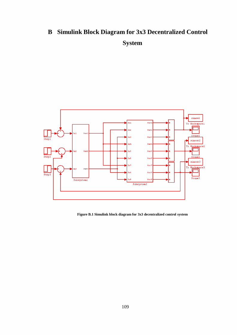
109
B Simulink Block Diagram for 3x3 Decentralized Control
System
Figure B.1 Simulink block diagram for 3x3 decentralized control system
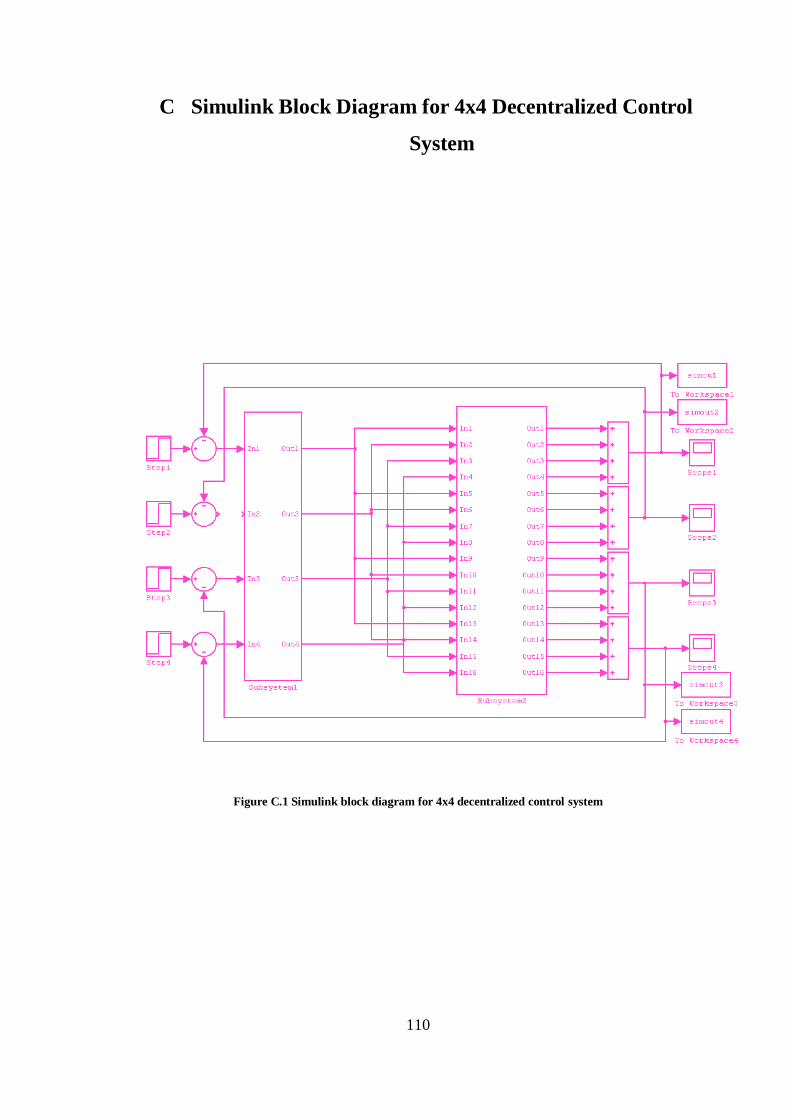
110
C Simulink Block Diagram for 4x4 Decentralized Control
System
Figure C.1 Simulink block diagram for 4x4 decentralized control system
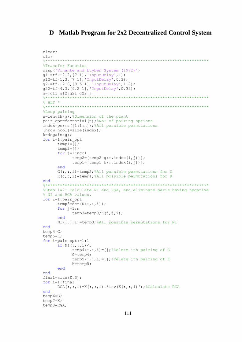
111
D Matlab Program for 2x2 Decentralized Control System
clear;
clc;
%*******************************************************************
%Transfer Function
disp('Vinante and Luyben System (1972)')
g11=tf(-2.2,[7 1],'InputDelay',1);
g12=tf(1.3,[7 1],'InputDelay',0.3);
g21=tf(-2.8,[9.5 1],'InputDelay',1.8);
g22=tf(4.3,[9.2 1],'InputDelay',0.35);
g=[g11 g12;g21 g22];
%*******************************************************************
% BLT *
%*******************************************************************
%Loop pairing
n=length(g);%Dimension of the plant
pair_opt=factorial(n);%No: of pairing options
index=perms([1:1:n]);%All possible permutations
[nrow ncol]=size(index);
k=dcgain(g);
for i=1:pair_opt
temp1=[];
temp2=[];
for j=1:ncol
temp2=[temp2 g(:,index(i,j))];
temp1=[temp1 k(:,index(i,j))];
end
G(:,:,i)=temp2;%All possible permutations for G
K(:,:,i)=temp1;%All possible permutations for K
end
%*******************************************************************
%Step 1&2: Calculate NI and RGA, and eliminate paris having negative
% NI and RGA values.
for i=1:pair_opt
temp3=det(K(:,:,i));
for j=1:n
temp3=temp3/K(j,j,i);
end
NI(:,:,i)=temp3;%All possible permutations for NI
end
temp4=G;
temp5=K;
for i=pair_opt:-1:1
if NI(:,:,i)<0
temp4(:,:,i)=[];%Delete ith pairing of G
G=temp4;
temp5(:,:,i)=[];%Delete ith pairing of K
K=temp5;
end
end
final=size(K,3);
for i=1:final
RGA(:,:,i)=K(:,:,i).*inv(K(:,:,i)');%Calculate RGA
end
temp6=G;
temp7=K;
temp8=RGA;
112
final=size(RGA,3);
for i=final:-1:1
if RGA(1,1,i)<0 | RGA(2,2,i)<0
temp6(:,:,i)=[];%Delete ith pairing of G
temp7(:,:,i)=[];%Delete ith pairing of K
temp8(:,:,i)=[];%Delete ith pairing of RGA
G=temp6;
K=temp7;
RGA=temp8;
end
end
final=size(K,2);
final1=size(K,3);
for i=1:final1
for j=1:final
K_dia(j,j,i)=diag(K(j,j,i));
end
end
final=size(K,3);
for i=1:final
E(:,:,i)=(K(:,:,i)-K_dia(:,:,i))*(K_dia(:,:,i))^-1;
E_tf=ss(E(:,:,i));
[ssv_value(i),non]=ssv(E_tf.a,E_tf.b,E_tf.c...
,E_tf.d,0);
end
[val_min,nmin]=min(ssv_value);%Minimum Structured Singular value
G=G(:,:,nmin);
K=K(:,:,nmin);
RGA=RGA(:,:,nmin);
%*******************************************************************
%Controller
%Step 1: Compute the Ziegler-Nichols tuning parameters of the
% diagonal elements of the process transfer function matrix.
for a=1:n
if sign(K(a,a))==1
S(a)=allmargin(G(a,a));
else
S(a)=allmargin(-G(a,a));
S(a).GainMargin=-S(a).GainMargin;
end
Ku(a)=S(a).GainMargin(1,1);
Wu(a)=S(a).GMFrequency(1,1);
end
for b=1:n
KcZN(b,b)=S(b).GainMargin(1,1)/2.2;
TauiZN(b,b)=2*pi/(1.2*S(b).GMFrequency(1,1));
end
p=sym('p');
[n,m]=size(G);
Gs=zeros(n,m);
Gs=sym(Gs);
for i=1:n
for j=1:m
[num,den]=tfdata(G(i,j),'v');
l=length(den);
order=l;
for k=1:l
A(order,1)=p^(k-1);
order=order-1;
end
n=num*A;
113
d=den*A;
Gs(i,j)=n/d;
clear A;
end
end
Gs=simple(Gs);
delays=exp(-totaldelay(G)*p);
Gs=Gs.*delays;%Transform transrer function into symbolic matrix.
%*******************************************************************
%Step 2: Choose a detuning factor.
F=2.3;%Initial value
df=0.01;%Increament
%*******************************************************************
%Step 3,4,5&6: Compute F, Kc and Taui.
n=length(G);
wrange=logspace(-1,0.8,200);
j=sqrt(-1);%Imaginary unit
s=j*wrange;
m=1;%Initialization
flagm=-1;%Initialization
flagp=-1;%Initialization
while m<10
Kc=KcZN/F;
Taui=TauiZN*F;
nwtot=length(wrange);
for w=1:nwtot
Gs_value=subs(Gs,s(w));
Gcs(1,1)=Kc(1,1)+Kc(1,1)/(Taui(1,1)*s(w));
Gcs(2,2)=Kc(2,2)+Kc(2,2)/(Taui(2,2)*s(w));
wnyquist(w)=-1+det(eye(size(Gs_value))+Gs_value*Gcs);
Lc(w)=wnyquist(w)/(1+wnyquist(w));%Calculate Lc function
dbcl(w)=20*log10(abs(Lc(w)));
end
[dbmax,nmax]=max(dbcl);%Pick off peak closed-loop log modulus
wmax=wrange(nmax);
m=m+1;
if dbmax>2*n%Test if +4 dB and regusee F factor
if flagp>0
df=df/2;
end
flagm=1;
F=F+df;
else
if flagm<0
df=df/2;
end
flagp=1;
F=F-df;
if F<1
F=1;
end
end
end%End of while loop to find correct F factor
F%Final value of F
Kp=Kc;
Ki=Kc./Taui;
n=length(G);%Dimension of the plant
for i=1:n
Gc(i,i)=tf([Kp(i,i) Ki(i,i)],[1 0]);
end
disp('**********The controller one for BLT **********')
114
Gc11=Gc(1,1)
disp('**********The controller two for BLT **********')
Gc22=Gc(2,2)
%*******************************************************************
tStart=0;
tFinal=100;
timespan=[tStart tFinal];
sim('blt2x2',timespan);%Simulation
blt_tout=tout;%From Simulink
blt_simout;%From Simulink
blt_error;%From Simulink
%*******************************************************************
% SIMC *
%*******************************************************************
%Loop pairing
%Step 1: Obtain steady state gain matrix.
n=length(g);%Dimension of the plant
pair_opt=factorial(n);%No: of pairing options
index=perms([1:1:n]);%All possible permutations
[nrow ncol]=size(index);
k=dcgain(g);
for i=1:pair_opt
temp1=[];
temp2=[];
for j=1:ncol
temp1=[temp1 k(:,index(i,j))];
temp2=[temp2 g(:,index(i,j))];
end
K(:,:,i)=temp1;%All possible permutations for K
G(:,:,i)=temp2;%All possible permutations for G
end
%*******************************************************************
%Step 2&3: Calculate NI and RGA, and eliminate paris having negative
% NI and RGA values.
for i=1:pair_opt
temp3=det(K(:,:,i));
for j=1:n
temp3=temp3/K(j,j,i);
end
NI(:,:,i)=temp3;%All possible permutations for NI
end
temp4=G;
temp5=K;
for i=pair_opt:-1:1
if NI(:,:,i)<0
temp4(:,:,i)=[];%Delete ith pairing of G
G=temp4;
temp5(:,:,i)=[];%Delete ith pairing of K
K=temp5;
end
end
final=size(K,3);
for i=1:final
RGA(:,:,i)=K(:,:,i).*inv(K(:,:,i)');%Calculate RGA
end
temp6=G;
temp7=K;
temp8=RGA;
final=size(RGA,3);
for i=final:-1:1
if RGA(1,1,i)<0 | RGA(2,2,i)<0
115
temp6(:,:,i)=[];%Delete ith pairing of G
temp7(:,:,i)=[];%Delete ith pairing of K
temp8(:,:,i)=[];%Delete ith pairing of RGA
G=temp6;
K=temp7;
RGA=temp8;
end
end
%*******************************************************************
%Step 4: Calculate delijG and ijPsi.
final=size(K,3);
for t=1:final
l=1;
temp9=K(:,:,t);
for i=1:n
for j=1:n
temp9(i,:)=[];
temp9(:,j)=[];
ijG(:,:,l,t)=temp9;
temp9=K(:,:,t);
l=l+1;
end
temp9=K(:,:,t);
end
end
final=size(K,3);
for t=1:final
l=1;
temp10=K(:,:,t);
for i=1:n
for j=1:n
row=temp10(i,:);
row(:,i)=[];
column=temp10(:,i);
column(i,:)=[];
delijG(:,:,l,t)=-(column*row)/temp10(i,j);
l=l+1;
end
end
end
final=size(ijG,4);
for t=1:final
temp11=ijG(:,:,:,t);
temp12=delijG(:,:,:,t);
final1=size(ijG,3);
for i=1:final1
ijPsi(:,:,i,t)=temp12(:,:,i).*inv(temp11(:,:,i)');
end
end
%*******************************************************************
%Step 5: Calculate Omega.
final3=size(ijG,4);
for t=1:final3
final4=size(ijG,3);
for j=1:final4
w(:,:,j,t)=norm(ijPsi(:,:,j,t),2);
end
end
final5=size(ijG,4);
for t=1:final5
Omega(:,:,t)=[w(:,:,1,t) w(:,:,2,t);w(:,:,3,t) w(:,:,4,t)];
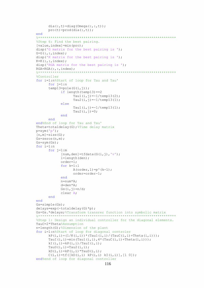
116
dia(:,t)=diag(Omega(:,:,t));
pro(t)=prod(dia(:,t));
end
%*******************************************************************
%Step 6: Find the best pairing.
[value,index]=min(pro);
disp('G matrix for the best pairing is ');
G=G(:,:,index);
disp('K matrix for the best pairing is ');
K=K(:,:,index);
disp('RGA matrix for the best pairing is ');
RGA=RGA(:,:,index);
%*******************************************************************
%Controller
for i=1:n%Start of loop for Tau and Tau'
for j=1:n
temp13=pole(G(i,j));
if length(temp13)==2
Tau1(i,j)=-1/temp13(2);
Tau2(i,j)=-1/temp13(1);
else
Tau1(i,j)=-1/temp13(1);
Tau2(i,j)=0;
end
end
end%End of loop for Tau and Tau'
Theta=totaldelay(G);%Time delay matrix
p=sym('p');
[n,m]=size(G);
Gs=zeros(n,m);
Gs=sym(Gs);
for i=1:n
for j=1:m
[num,den]=tfdata(G(i,j),'v');
l=length(den);
order=l;
for k=1:l
A(order,1)=p^(k-1);
order=order-1;
end
n=num*A;
d=den*A;
Gs(i,j)=n/d;
clear A;
end
end
Gs=simple(Gs);
delays=exp(-totaldelay(G)*p);
Gs=Gs.*delays;%Transform transrer function into symbolic matrix
%*******************************************************************
%Step 1: Design an individual controller for the diagonal elements.
TauC=2*Theta%Assumption
n=length(G);%Dimension of the plant
for i=1:n%Start of loop for diagonal controler
kP(i,i)=(1/K(i,i))*(Tau1(i,i)/(TauC(i,i)+Theta(i,i)));
TauI(i,i)=min(Tau1(i,i),4*(TauC(i,i)+Theta(i,i)));
kI(i,i)=kP(i,i)/TauI(i,i);
TauD(i,i)=Tau2(i,i);
kD(i,i)=kP(i,i)*TauD(i,i);
C(i,i)=tf([kD(i,i) kP(i,i) kI(i,i)],[1 0]);
end%end of loop for diagonal controller
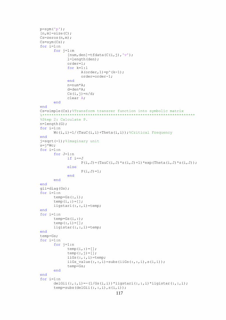
117
p=sym('p');
[n,m]=size(C);
Cs=zeros(n,m);
Cs=sym(Cs);
for i=1:n
for j=1:m
[num,den]=tfdata(C(i,j),'v');
l=length(den);
order=l;
for k=1:l
A(order,1)=p^(k-1);
order=order-1;
end
n=num*A;
d=den*A;
Cs(i,j)=n/d;
clear A;
end
end
Cs=simple(Cs);%Transform transrer function into symbolic matrix
%*******************************************************************
%Step 2: Calculate P.
n=length(G);
for i=1:n
Wc(i,i)=1/(TauC(i,i)+Theta(i,i));%Critical Frequency
end
j=sqrt(-1);%Imaginary unit
s=j*Wc;
for i=1:n
for J=1:n
if i==J
P(i,J)=(TauC(i,J)*s(i,J)+1)*exp(Theta(i,J)*s(i,J));
else
P(i,J)=1;
end
end
end
gii=diag(Gs);
for i=1:n
temp=Gs(:,i);
temp(i,:)=[];
iigstari(:,:,i)=temp;
end
for i=1:n
temp=Gs(i,:);
temp(:,i)=[];
iigistar(:,:,i)=temp;
end
temp=Gs;
for i=1:n
for j=1:n
temp(i,:)=[];
temp(:,j)=[];
iiGs(:,:,i)=temp;
iiGs_value(:,:,i)=subs(iiGs(:,:,i),s(i,i));
temp=Gs;
end
end
for i=1:n
delGii(:,:,i)=-(1/Gs(i,i))*iigstari(:,:,i)*iigistar(:,:,i);
temp=subs(delGii(:,:,i),s(i,i));
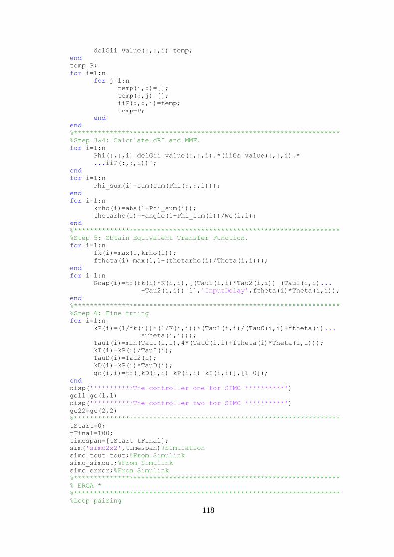
118
delGii_value(:,:,i)=temp;
end
temp=P;
for i=1:n
for j=1:n
temp(i,:)=[];
temp(:,j)=[];
iiP(:,:,i)=temp;
temp=P;
end
end
%*******************************************************************
%Step 3&4: Calculate dRI and MMF.
for i=1:n
Phi(:,:,i)=delGii_value(:,:,i).*(iiGs_value(:,:,i).*
...iiP(:,:,i))';
end
for i=1:n
Phi_sum(i)=sum(sum(Phi(:,:,i)));
end
for i=1:n
krho(i)=abs(1+Phi_sum(i));
thetarho(i)=-angle(1+Phi_sum(i))/Wc(i,i);
end
%*******************************************************************
%Step 5: Obtain Equivalent Transfer Function.
for i=1:n
fk(i)=max(1,krho(i));
ftheta(i)=max(1,1+(thetarho(i)/Theta(i,i)));
end
for i=1:n
Gcap(i)=tf(fk(i)*K(i,i),[(Tau1(i,i)*Tau2(i,i)) (Tau1(i,i)...
+Tau2(i,i)) 1],'InputDelay',ftheta(i)*Theta(i,i));
end
%*******************************************************************
%Step 6: Fine tuning
for i=1:n
kP(i)=(1/fk(i))*(1/K(i,i))*(Tau1(i,i)/(TauC(i,i)+ftheta(i)...
*Theta(i,i)));
TauI(i)=min(Tau1(i,i),4*(TauC(i,i)+ftheta(i)*Theta(i,i)));
kI(i)=kP(i)/TauI(i);
TauD(i)=Tau2(i);
kD(i)=kP(i)*TauD(i);
gc(i,i)=tf([kD(i,i) kP(i,i) kI(i,i)],[1 0]);
end
disp('**********The controller one for SIMC **********')
gc11=gc(1,1)
disp('**********The controller two for SIMC **********')
gc22=gc(2,2)
%*******************************************************************
tStart=0;
tFinal=100;
timespan=[tStart tFinal];
sim('simc2x2',timespan)%Simulation
simc_tout=tout;%From Simulink
simc_simout;%From Simulink
simc_error;%From Simulink
%*******************************************************************
% ERGA *
%*******************************************************************
%Loop pairing
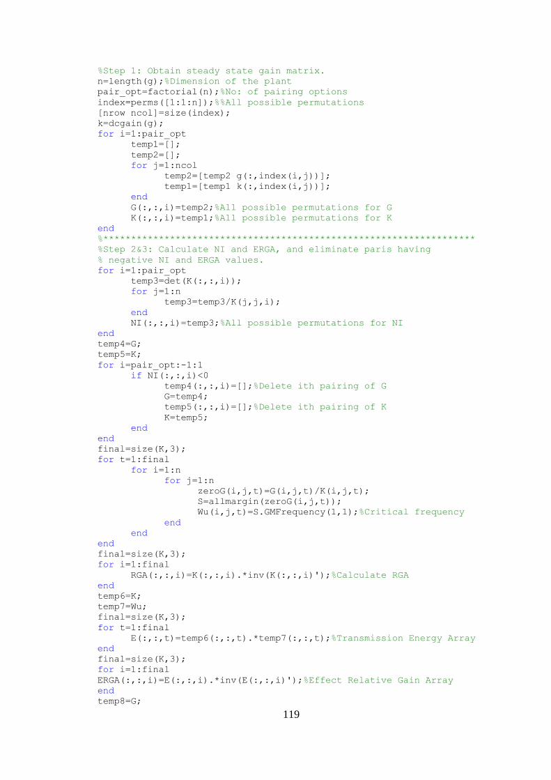
119
%Step 1: Obtain steady state gain matrix.
n=length(g);%Dimension of the plant
pair_opt=factorial(n);%No: of pairing options
index=perms([1:1:n]);%%All possible permutations
[nrow ncol]=size(index);
k=dcgain(g);
for i=1:pair_opt
temp1=[];
temp2=[];
for j=1:ncol
temp2=[temp2 g(:,index(i,j))];
temp1=[temp1 k(:,index(i,j))];
end
G(:,:,i)=temp2;%All possible permutations for G
K(:,:,i)=temp1;%All possible permutations for K
end
%*******************************************************************
%Step 2&3: Calculate NI and ERGA, and eliminate paris having
% negative NI and ERGA values.
for i=1:pair_opt
temp3=det(K(:,:,i));
for j=1:n
temp3=temp3/K(j,j,i);
end
NI(:,:,i)=temp3;%All possible permutations for NI
end
temp4=G;
temp5=K;
for i=pair_opt:-1:1
if NI(:,:,i)<0
temp4(:,:,i)=[];%Delete ith pairing of G
G=temp4;
temp5(:,:,i)=[];%Delete ith pairing of K
K=temp5;
end
end
final=size(K,3);
for t=1:final
for i=1:n
for j=1:n
zeroG(i,j,t)=G(i,j,t)/K(i,j,t);
S=allmargin(zeroG(i,j,t));
Wu(i,j,t)=S.GMFrequency(1,1);%Critical frequency
end
end
end
final=size(K,3);
for i=1:final
RGA(:,:,i)=K(:,:,i).*inv(K(:,:,i)');%Calculate RGA
end
temp6=K;
temp7=Wu;
final=size(K,3);
for t=1:final
E(:,:,t)=temp6(:,:,t).*temp7(:,:,t);%Transmission Energy Array
end
final=size(K,3);
for i=1:final
ERGA(:,:,i)=E(:,:,i).*inv(E(:,:,i)');%Effect Relative Gain Array
end
temp8=G;
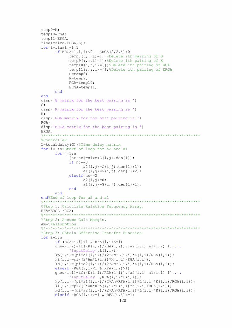
120
temp9=K;
temp10=RGA;
temp11=ERGA;
final=size(ERGA,3);
for i=final:-1:1
if ERGA(1,1,i)<0 | ERGA(2,2,i)<0
temp8(:,:,i)=[];%Delete ith pairing of G
temp9(:,:,i)=[];%Delete ith pairing of K
temp10(:,:,i)=[];%Delete ith pairing of RGA
temp11(:,:,i)=[];%Delete ith pairing of ERGA
G=temp8;
K=temp9;
RGA=temp10;
ERGA=temp11;
end
end
disp('G matrix for the best pairing is ')
G;
disp('K matrix for the best pairing is ')
K;
disp('RGA matrix for the best pairing is ')
RGA;
disp('ERGA matrix for the best pairing is ')
ERGA;
%*******************************************************************
%Controller
L=totaldelay(G);%Time delay matrix
for i=1:n%Start of loop for a2 and a1
for j=1:n
[nr nc]=size(G(i,j).den{1});
if nc==3
a2(i,j)=G(i,j).den{1}(1);
a1(i,j)=G(i,j).den{1}(2);
elseif nc==2
a2(i,j)=0;
a1(i,j)=G(i,j).den{1}(1);
end
end
end%End of loop for a2 and a1
%*******************************************************************
%Step 1: Calculate Ralative Ferquency Array.
RFA=ERGA./RGA;
%*******************************************************************
%Step 2: Assume Gain Margin.
Am=5%Assumption
%*******************************************************************
%Step 3: Obtain Effective Transfer Function.
for i=1:n
if (RGA(i,i)<1 & RFA(i,i)<=1)
gnew(i,i)=tf((K(i,i)/RGA(i,i)),[a2(i,i) a1(i,i) 1],...
'InputDelay',L(i,i));
kp(i,i)=(pi*a1(i,i))/(2*Am*L(i,i)*K(i,i)/RGA(i,i));
ki(i,i)=pi/(2*Am*L(i,i)*K(i,i)/RGA(i,i));
kd(i,i)=(pi*a2(i,i))/(2*Am*L(i,i)*K(i,i)/RGA(i,i));
elseif (RGA(i,i)<1 & RFA(i,i)>1)
gnew(i,i)=tf((K(i,i)/RGA(i,i)),[a2(i,i) a1(i,i) 1],...
'InputDelay' ,RFA(i,i)*L(i,i));
kp(i,i)=(pi*a1(i,i))/(2*Am*RFA(i,i)*L(i,i)*K(i,i)/RGA(i,i));
ki(i,i)=pi/(2*Am*RFA(i,i)*L(i,i)*K(i,i)/RGA(i,i));
kd(i,i)=(pi*a2(i,i))/(2*Am*RFA(i,i)*L(i,i)*K(i,i)/RGA(i,i));
elseif (RGA(i,i)>=1 & RFA(i,i)<=1)
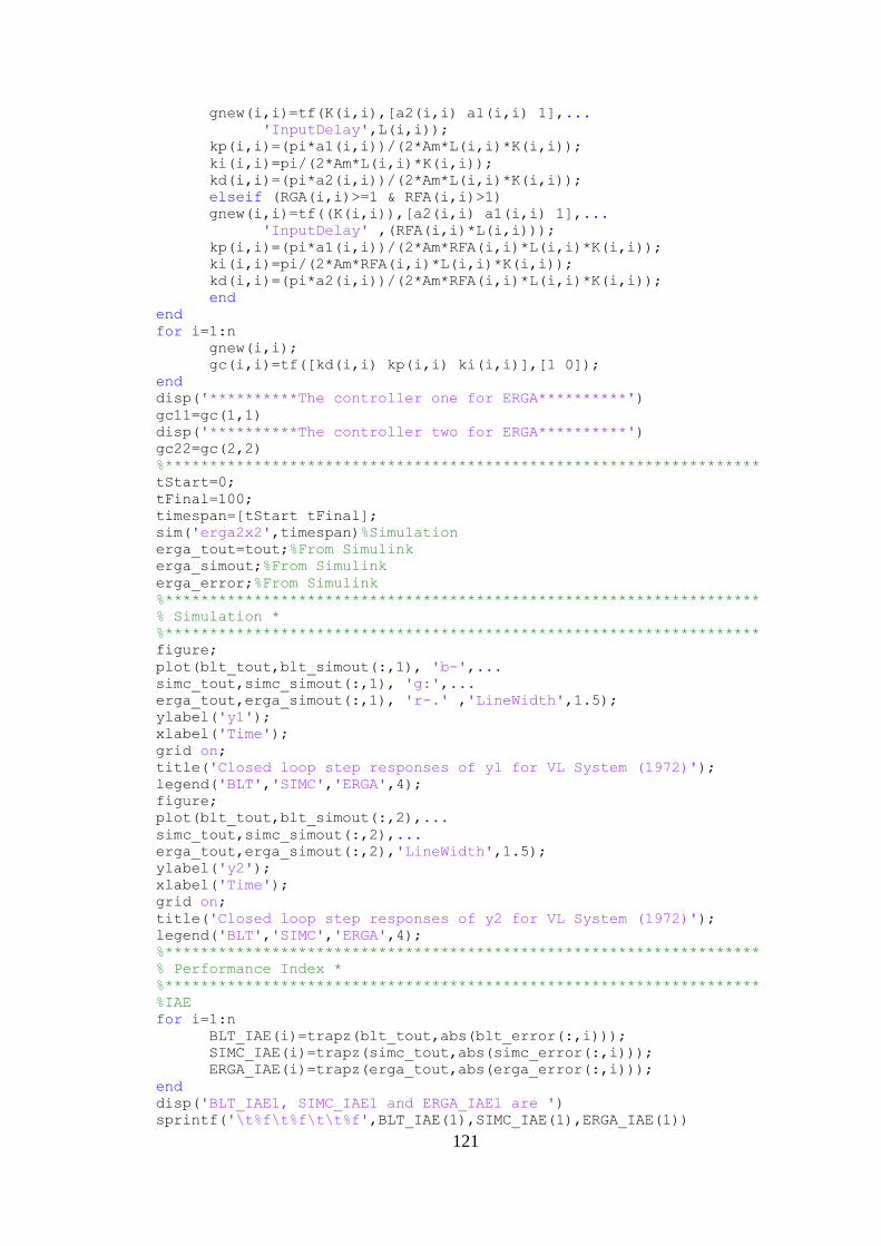
121
gnew(i,i)=tf(K(i,i),[a2(i,i) a1(i,i) 1],...
'InputDelay',L(i,i));
kp(i,i)=(pi*a1(i,i))/(2*Am*L(i,i)*K(i,i));
ki(i,i)=pi/(2*Am*L(i,i)*K(i,i));
kd(i,i)=(pi*a2(i,i))/(2*Am*L(i,i)*K(i,i));
elseif (RGA(i,i)>=1 & RFA(i,i)>1)
gnew(i,i)=tf((K(i,i)),[a2(i,i) a1(i,i) 1],...
'InputDelay' ,(RFA(i,i)*L(i,i)));
kp(i,i)=(pi*a1(i,i))/(2*Am*RFA(i,i)*L(i,i)*K(i,i));
ki(i,i)=pi/(2*Am*RFA(i,i)*L(i,i)*K(i,i));
kd(i,i)=(pi*a2(i,i))/(2*Am*RFA(i,i)*L(i,i)*K(i,i));
end
end
for i=1:n
gnew(i,i);
gc(i,i)=tf([kd(i,i) kp(i,i) ki(i,i)],[1 0]);
end
disp('**********The controller one for ERGA**********')
gc11=gc(1,1)
disp('**********The controller two for ERGA**********')
gc22=gc(2,2)
%*******************************************************************
tStart=0;
tFinal=100;
timespan=[tStart tFinal];
sim('erga2x2',timespan)%Simulation
erga_tout=tout;%From Simulink
erga_simout;%From Simulink
erga_error;%From Simulink
%*******************************************************************
% Simulation *
%*******************************************************************
figure;
plot(blt_tout,blt_simout(:,1), 'b-',...
simc_tout,simc_simout(:,1), 'g:',...
erga_tout,erga_simout(:,1), 'r-.' ,'LineWidth',1.5);
ylabel('y1');
xlabel('Time');
grid on;
title('Closed loop step responses of y1 for VL System (1972)');
legend('BLT','SIMC','ERGA',4);
figure;
plot(blt_tout,blt_simout(:,2),...
simc_tout,simc_simout(:,2),...
erga_tout,erga_simout(:,2),'LineWidth',1.5);
ylabel('y2');
xlabel('Time');
grid on;
title('Closed loop step responses of y2 for VL System (1972)');
legend('BLT','SIMC','ERGA',4);
%*******************************************************************
% Performance Index *
%*******************************************************************
%IAE
for i=1:n
BLT_IAE(i)=trapz(blt_tout,abs(blt_error(:,i)));
SIMC_IAE(i)=trapz(simc_tout,abs(simc_error(:,i)));
ERGA_IAE(i)=trapz(erga_tout,abs(erga_error(:,i)));
end
disp('BLT_IAE1, SIMC_IAE1 and ERGA_IAE1 are ')
sprintf('\t%f\t%f\t\t%f',BLT_IAE(1),SIMC_IAE(1),ERGA_IAE(1))
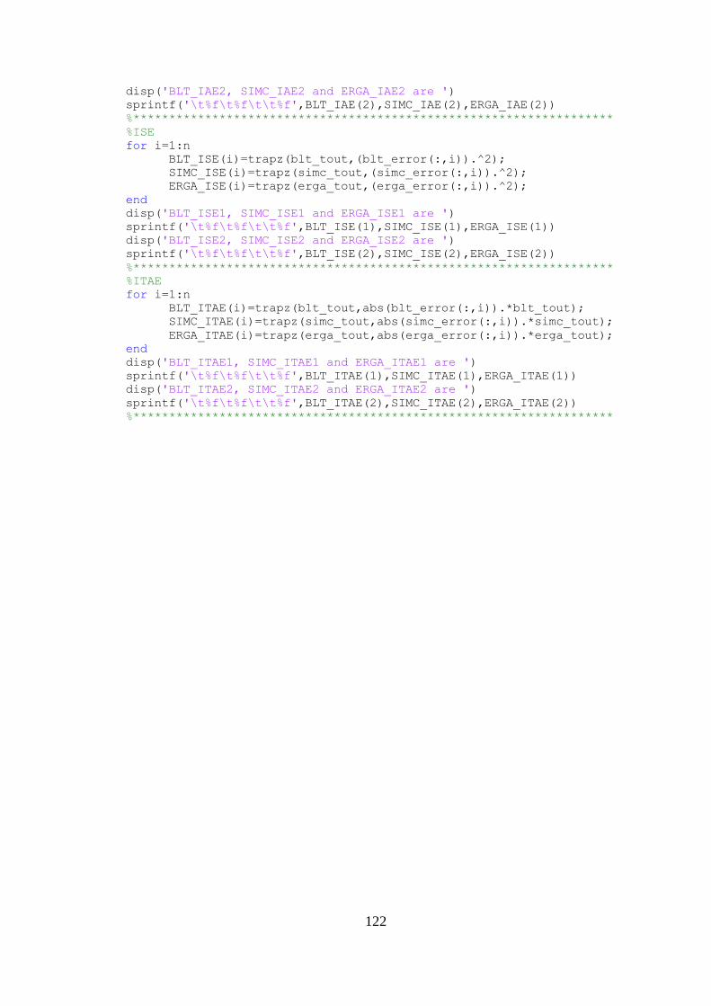
122
disp('BLT_IAE2, SIMC_IAE2 and ERGA_IAE2 are ')
sprintf('\t%f\t%f\t\t%f',BLT_IAE(2),SIMC_IAE(2),ERGA_IAE(2))
%*******************************************************************
%ISE
for i=1:n
BLT_ISE(i)=trapz(blt_tout,(blt_error(:,i)).^2);
SIMC_ISE(i)=trapz(simc_tout,(simc_error(:,i)).^2);
ERGA_ISE(i)=trapz(erga_tout,(erga_error(:,i)).^2);
end
disp('BLT_ISE1, SIMC_ISE1 and ERGA_ISE1 are ')
sprintf('\t%f\t%f\t\t%f',BLT_ISE(1),SIMC_ISE(1),ERGA_ISE(1))
disp('BLT_ISE2, SIMC_ISE2 and ERGA_ISE2 are ')
sprintf('\t%f\t%f\t\t%f',BLT_ISE(2),SIMC_ISE(2),ERGA_ISE(2))
%*******************************************************************
%ITAE
for i=1:n
BLT_ITAE(i)=trapz(blt_tout,abs(blt_error(:,i)).*blt_tout);
SIMC_ITAE(i)=trapz(simc_tout,abs(simc_error(:,i)).*simc_tout);
ERGA_ITAE(i)=trapz(erga_tout,abs(erga_error(:,i)).*erga_tout);
end
disp('BLT_ITAE1, SIMC_ITAE1 and ERGA_ITAE1 are ')
sprintf('\t%f\t%f\t\t%f',BLT_ITAE(1),SIMC_ITAE(1),ERGA_ITAE(1))
disp('BLT_ITAE2, SIMC_ITAE2 and ERGA_ITAE2 are ')
sprintf('\t%f\t%f\t\t%f',BLT_ITAE(2),SIMC_ITAE(2),ERGA_ITAE(2))
%*******************************************************************
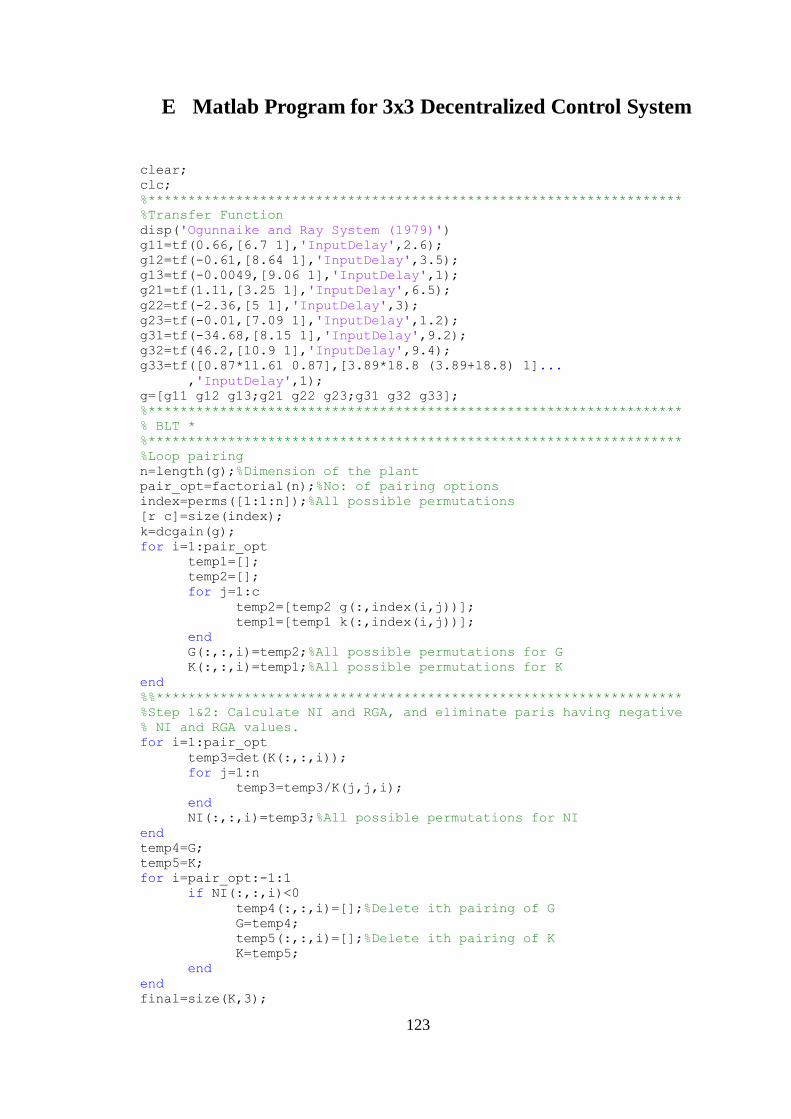
123
E Matlab Program for 3x3 Decentralized Control System
clear;
clc;
%*******************************************************************
%Transfer Function
disp('Ogunnaike and Ray System (1979)')
g11=tf(0.66,[6.7 1],'InputDelay',2.6);
g12=tf(-0.61,[8.64 1],'InputDelay',3.5);
g13=tf(-0.0049,[9.06 1],'InputDelay',1);
g21=tf(1.11,[3.25 1],'InputDelay',6.5);
g22=tf(-2.36,[5 1],'InputDelay',3);
g23=tf(-0.01,[7.09 1],'InputDelay',1.2);
g31=tf(-34.68,[8.15 1],'InputDelay',9.2);
g32=tf(46.2,[10.9 1],'InputDelay',9.4);
g33=tf([0.87*11.61 0.87],[3.89*18.8 (3.89+18.8) 1]...
,'InputDelay',1);
g=[g11 g12 g13;g21 g22 g23;g31 g32 g33];
%*******************************************************************
% BLT *
%*******************************************************************
%Loop pairing
n=length(g);%Dimension of the plant
pair_opt=factorial(n);%No: of pairing options
index=perms([1:1:n]);%All possible permutations
[r c]=size(index);
k=dcgain(g);
for i=1:pair_opt
temp1=[];
temp2=[];
for j=1:c
temp2=[temp2 g(:,index(i,j))];
temp1=[temp1 k(:,index(i,j))];
end
G(:,:,i)=temp2;%All possible permutations for G
K(:,:,i)=temp1;%All possible permutations for K
end
%%******************************************************************
%Step 1&2: Calculate NI and RGA, and eliminate paris having negative
% NI and RGA values.
for i=1:pair_opt
temp3=det(K(:,:,i));
for j=1:n
temp3=temp3/K(j,j,i);
end
NI(:,:,i)=temp3;%All possible permutations for NI
end
temp4=G;
temp5=K;
for i=pair_opt:-1:1
if NI(:,:,i)<0
temp4(:,:,i)=[];%Delete ith pairing of G
G=temp4;
temp5(:,:,i)=[];%Delete ith pairing of K
K=temp5;
end
end
final=size(K,3);
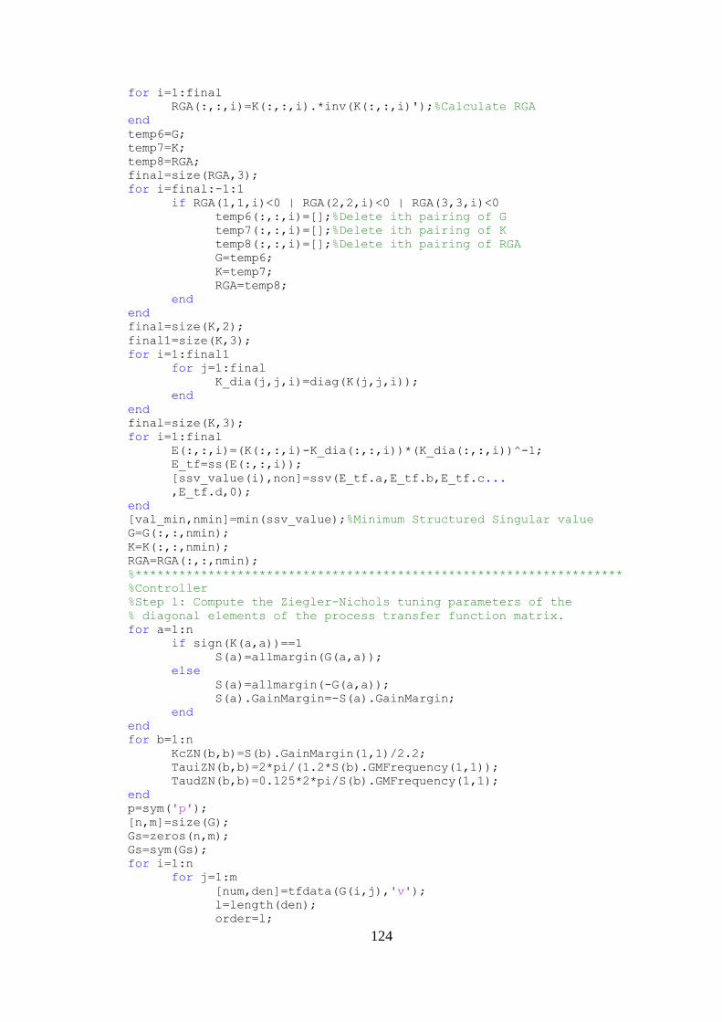
124
for i=1:final
RGA(:,:,i)=K(:,:,i).*inv(K(:,:,i)');%Calculate RGA
end
temp6=G;
temp7=K;
temp8=RGA;
final=size(RGA,3);
for i=final:-1:1
if RGA(1,1,i)<0 | RGA(2,2,i)<0 | RGA(3,3,i)<0
temp6(:,:,i)=[];%Delete ith pairing of G
temp7(:,:,i)=[];%Delete ith pairing of K
temp8(:,:,i)=[];%Delete ith pairing of RGA
G=temp6;
K=temp7;
RGA=temp8;
end
end
final=size(K,2);
final1=size(K,3);
for i=1:final1
for j=1:final
K_dia(j,j,i)=diag(K(j,j,i));
end
end
final=size(K,3);
for i=1:final
E(:,:,i)=(K(:,:,i)-K_dia(:,:,i))*(K_dia(:,:,i))^-1;
E_tf=ss(E(:,:,i));
[ssv_value(i),non]=ssv(E_tf.a,E_tf.b,E_tf.c...
,E_tf.d,0);
end
[val_min,nmin]=min(ssv_value);%Minimum Structured Singular value
G=G(:,:,nmin);
K=K(:,:,nmin);
RGA=RGA(:,:,nmin);
%*******************************************************************
%Controller
%Step 1: Compute the Ziegler-Nichols tuning parameters of the
% diagonal elements of the process transfer function matrix.
for a=1:n
if sign(K(a,a))==1
S(a)=allmargin(G(a,a));
else
S(a)=allmargin(-G(a,a));
S(a).GainMargin=-S(a).GainMargin;
end
end
for b=1:n
KcZN(b,b)=S(b).GainMargin(1,1)/2.2;
TauiZN(b,b)=2*pi/(1.2*S(b).GMFrequency(1,1));
TaudZN(b,b)=0.125*2*pi/S(b).GMFrequency(1,1);
end
p=sym('p');
[n,m]=size(G);
Gs=zeros(n,m);
Gs=sym(Gs);
for i=1:n
for j=1:m
[num,den]=tfdata(G(i,j),'v');
l=length(den);
order=l;
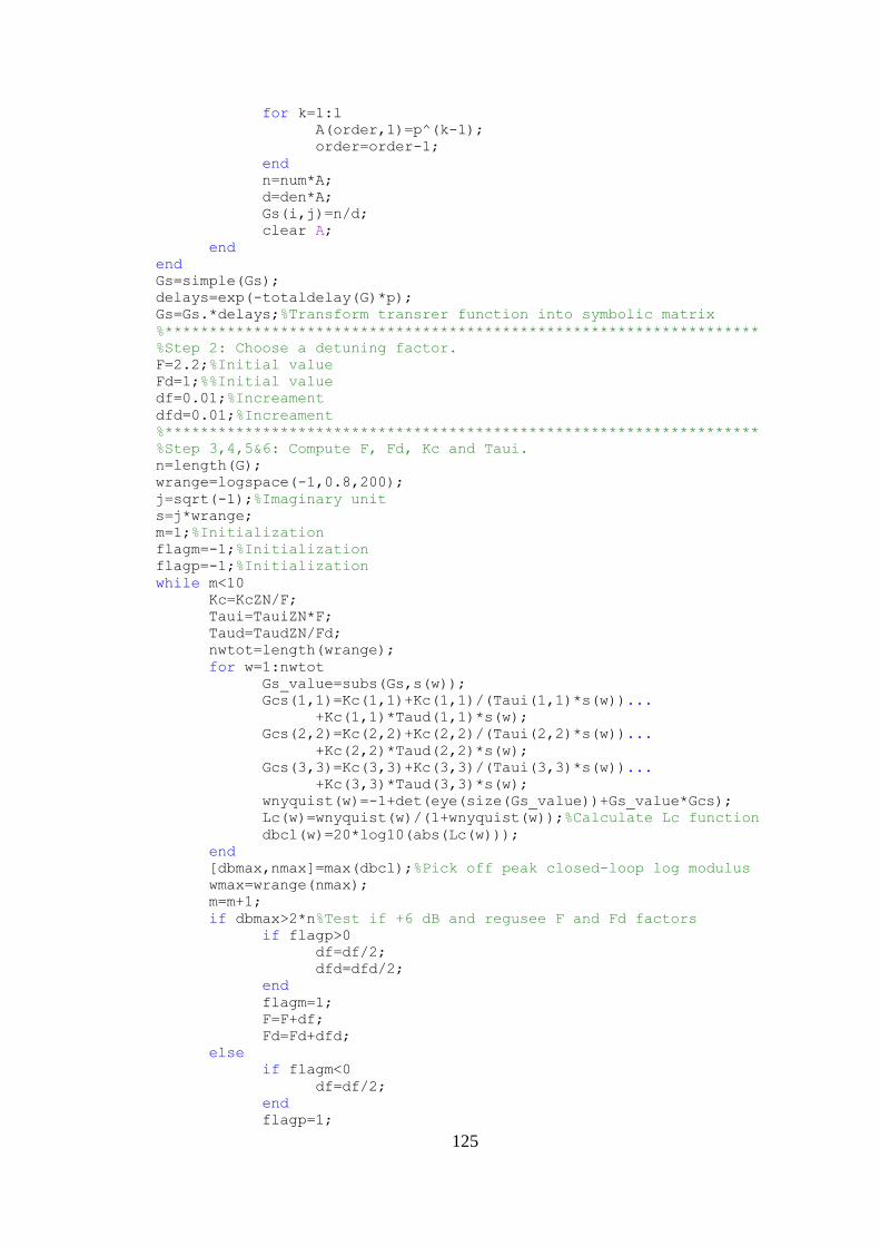
125
for k=1:l
A(order,1)=p^(k-1);
order=order-1;
end
n=num*A;
d=den*A;
Gs(i,j)=n/d;
clear A;
end
end
Gs=simple(Gs);
delays=exp(-totaldelay(G)*p);
Gs=Gs.*delays;%Transform transrer function into symbolic matrix
%*******************************************************************
%Step 2: Choose a detuning factor.
F=2.2;%Initial value
Fd=1;%%Initial value
df=0.01;%Increament
dfd=0.01;%Increament
%*******************************************************************
%Step 3,4,5&6: Compute F, Fd, Kc and Taui.
n=length(G);
wrange=logspace(-1,0.8,200);
j=sqrt(-1);%Imaginary unit
s=j*wrange;
m=1;%Initialization
flagm=-1;%Initialization
flagp=-1;%Initialization
while m<10
Kc=KcZN/F;
Taui=TauiZN*F;
Taud=TaudZN/Fd;
nwtot=length(wrange);
for w=1:nwtot
Gs_value=subs(Gs,s(w));
Gcs(1,1)=Kc(1,1)+Kc(1,1)/(Taui(1,1)*s(w))...
+Kc(1,1)*Taud(1,1)*s(w);
Gcs(2,2)=Kc(2,2)+Kc(2,2)/(Taui(2,2)*s(w))...
+Kc(2,2)*Taud(2,2)*s(w);
Gcs(3,3)=Kc(3,3)+Kc(3,3)/(Taui(3,3)*s(w))...
+Kc(3,3)*Taud(3,3)*s(w);
wnyquist(w)=-1+det(eye(size(Gs_value))+Gs_value*Gcs);
Lc(w)=wnyquist(w)/(1+wnyquist(w));%Calculate Lc function
dbcl(w)=20*log10(abs(Lc(w)));
end
[dbmax,nmax]=max(dbcl);%Pick off peak closed-loop log modulus
wmax=wrange(nmax);
m=m+1;
if dbmax>2*n%Test if +6 dB and regusee F and Fd factors
if flagp>0
df=df/2;
dfd=dfd/2;
end
flagm=1;
F=F+df;
Fd=Fd+dfd;
else
if flagm<0
df=df/2;
end
flagp=1;
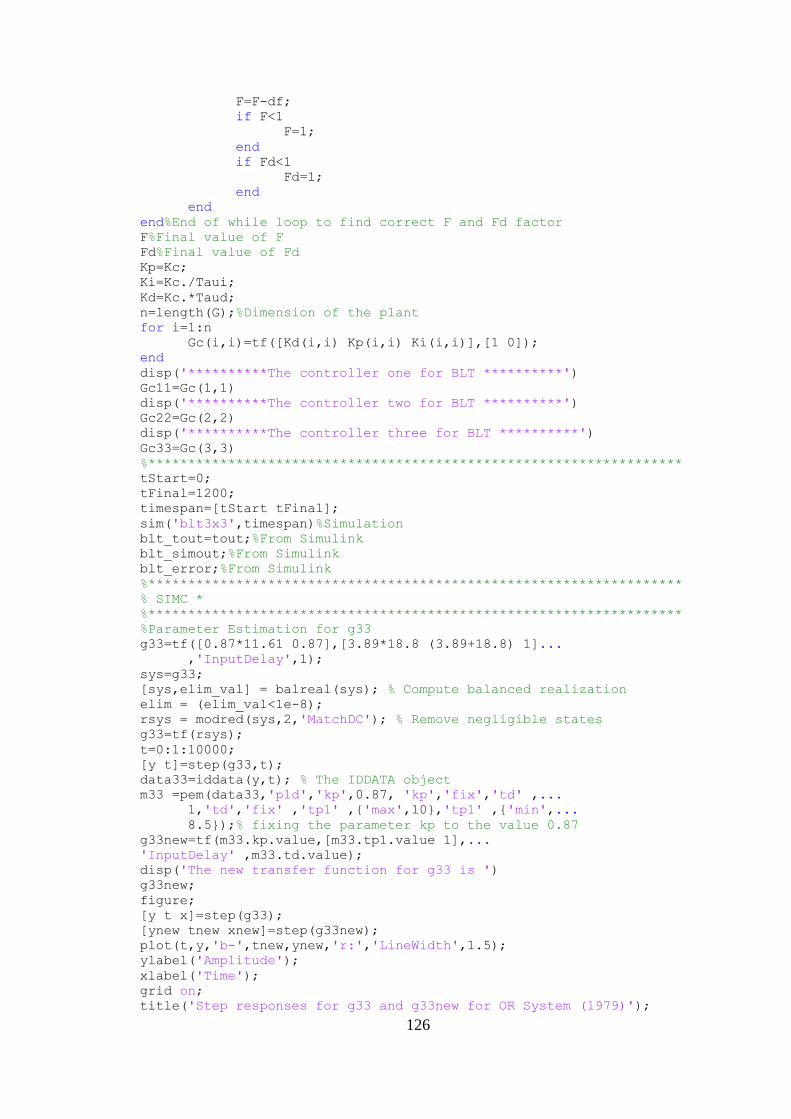
126
F=F-df;
if F<1
F=1;
end
if Fd<1
Fd=1;
end
end
end%End of while loop to find correct F and Fd factor
F%Final value of F
Fd%Final value of Fd
Kp=Kc;
Ki=Kc./Taui;
Kd=Kc.*Taud;
n=length(G);%Dimension of the plant
for i=1:n
Gc(i,i)=tf([Kd(i,i) Kp(i,i) Ki(i,i)],[1 0]);
end
disp('**********The controller one for BLT **********')
Gc11=Gc(1,1)
disp('**********The controller two for BLT **********')
Gc22=Gc(2,2)
disp('**********The controller three for BLT **********')
Gc33=Gc(3,3)
%*******************************************************************
tStart=0;
tFinal=1200;
timespan=[tStart tFinal];
sim('blt3x3',timespan)%Simulation
blt_tout=tout;%From Simulink
blt_simout;%From Simulink
blt_error;%From Simulink
%*******************************************************************
% SIMC *
%*******************************************************************
%Parameter Estimation for g33
g33=tf([0.87*11.61 0.87],[3.89*18.8 (3.89+18.8) 1]...
,'InputDelay',1);
sys=g33;
[sys,elim_val] = balreal(sys); % Compute balanced realization
elim = (elim_val<1e-8);
rsys = modred(sys,2,'MatchDC'); % Remove negligible states
g33=tf(rsys);
t=0:1:10000;
[y t]=step(g33,t);
data33=iddata(y,t); % The IDDATA object
m33 =pem(data33,'p1d','kp',0.87, 'kp','fix','td' ,...
1,'td','fix' ,'tp1' ,{'max',10},'tp1' ,{'min',...
8.5});% fixing the parameter kp to the value 0.87
g33new=tf(m33.kp.value,[m33.tp1.value 1],...
'InputDelay' ,m33.td.value);
disp('The new transfer function for g33 is ')
g33new;
figure;
[y t x]=step(g33);
[ynew tnew xnew]=step(g33new);
plot(t,y,'b-',tnew,ynew,'r:','LineWidth',1.5);
ylabel('Amplitude');
xlabel('Time');
grid on;
title('Step responses for g33 and g33new for OR System (1979)');
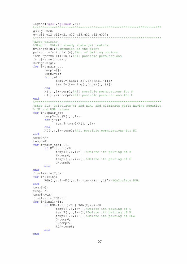
127
legend('g33','g33new',4);
%*******************************************************************
g33=g33new;
g=[g11 g12 g13;g21 g22 g23;g31 g32 g33];
%*******************************************************************
%Loop pairing
%Step 1: Obtain steady state gain matrix.
n=length(g);%Dimension of the plant
pair_opt=factorial(n);%No: of pairing options
index=perms([1:1:n]);%All possible permutations
[r c]=size(index);
k=dcgain(g);
for i=1:pair_opt
temp1=[];
temp2=[];
for j=1:c
temp1=[temp1 k(:,index(i,j))];
temp2=[temp2 g(:,index(i,j))];
end
K(:,:,i)=temp1;%All possible permutations for K
G(:,:,i)=temp2;%All possible permutations for G
end
%*******************************************************************
%Step 2&3: Calculate NI and RGA, and eliminate paris having negative
% NI and RGA values.
for i=1:pair_opt
temp3=det(K(:,:,i));
for j=1:n
temp3=temp3/K(j,j,i);
end
NI(:,:,i)=temp3;%All possible permutations for NI
end
temp4=K;
temp5=G;
for i=pair_opt:-1:1
if NI(:,:,i)<0
temp4(:,:,i)=[];%Delete ith pairing of K
K=temp4;
temp5(:,:,i)=[];%Delete ith pairing of G
G=temp5;
end
end
final=size(K,3);
for i=1:final
RGA(:,:,i)=K(:,:,i).*inv(K(:,:,i)');%Calculate RGA
end
temp6=G;
temp7=K;
temp8=RGA;
final=size(RGA,3);
for i=final:-1:1
if RGA(1,1,i)<0 | RGA(2,2,i)<0
temp6(:,:,i)=[];%Delete ith pairing of G
temp7(:,:,i)=[];%Delete ith pairing of K
temp8(:,:,i)=[];%Delete ith pairing of RGA
G=temp6;
K=temp7;
RGA=temp8;
end
end
128
%********************************************************************
**
%Step 4: Calculate delijG and ijPsi.
final=size(K,3);
for t=1:final
l=1;
temp9=K(:,:,t);
for i=1:n
for j=1:n
temp9(i,:)=[];
temp9(:,j)=[];
ijG(:,:,l,t)=temp9;
temp9=K(:,:,t);
l=l+1;
end
temp9=K(:,:,t);
end
end
final=size(K,3);
for t=1:final
l=1;
temp10=K(:,:,t);
for i=1:n
for j=1:n
row=temp10(i,:);
row(:,i)=[];
column=temp10(:,i);
column(i,:)=[];
delijG(:,:,l,t)=-(column*row)/temp10(i,j);
l=l+1;
end
end
end
final=size(ijG,4);
for t=1:final
temp11=ijG(:,:,:,t);
temp12=delijG(:,:,:,t);
final1=size(ijG,3);
for i=1:final1
ijPsi(:,:,i,t)=temp12(:,:,i).*inv(temp11(:,:,i)');
end
end
%*******************************************************************
%Step 5: Calculate Omega.
final3=size(ijG,4);
for t=1:final3
final4=size(ijG,3);
for j=1:final4
w(:,:,j,t)=norm(ijPsi(:,:,j,t),2);
end
end
final5=size(ijG,4);
for t=1:final5
Omega(:,:,t)=[w(:,:,1,t) w(:,:,2,t) w(:,:,3,t);
w(:,:,4,t) w(:,:,5,t) w(:,:,6,t);
w(:,:,7,t) w(:,:,8,t) w(:,:,9,t)];
dia(:,t)=diag(Omega(:,:,t));
pro(t)=prod(dia(:,t));
end
%*******************************************************************
%Step 6: Find the best pairing.
129
[value,index]=min(pro);
disp('G matrix for the best pairing is ')
G=G(:,:,index);
disp('K matrix for the best pairing is ')
K=K(:,:,index);
disp('RGA matrix for the best pairing is ')
RGA=RGA(:,:,index);
%********************************************************************
**
%Controller
for i=1:n%Start of loop for Tau and Tau'
for j=1:n
temp=pole(G(i,j));
if length(temp)==2
Tau1(i,j)=-1/temp(2);
Tau2(i,j)=-1/temp(1);
else
Tau1(i,j)=-1/temp(1);
Tau2(i,j)=0;
end
end
end%End of loop for Tau and Tau'
Theta=totaldelay(G);
p=sym('p');
[n,m]=size(G);
Gs=zeros(n,m);
Gs=sym(Gs);
for i=1:n
for j=1:m
[num,den]=tfdata(G(i,j),'v');
l=length(den);
order=l;
for k=1:l
A(order,1)=p^(k-1);
order=order-1;
end
n=num*A;
d=den*A;
Gs(i,j)=n/d;
clear A;
end
end
Gs=simple(Gs);
delays=exp(-totaldelay(G)*p);
Gs=Gs.*delays;%Transform transrer function into symbolic matrix
%*******************************************************************
%Step 1: Design an individual controller for the diagonal elements.
TauC=0.5*Theta;%Assumption
n=length(G);%Dimension of the plant
for i=1:n%Start of loop for diagonal controler
kP(i,i)=(1/K(i,i))*(Tau1(i,i)/(TauC(i,i)+Theta(i,i)));
TauI(i,i)=min(Tau1(i,i),4*(TauC(i,i)+Theta(i,i)));
kI(i,i)=kP(i,i)/TauI(i,i);
TauD(i,i)=Tau2(i,i);
kD(i,i)=kP(i,i)*TauD(i,i);
C(i,i)=tf([kD(i,i) kP(i,i) kI(i,i)],[1 0]);
end%end of loop for diagonal controller
p=sym('p');
[n,m]=size(C);
Cs=zeros(n,m);
Cs=sym(Cs);
130
for i=1:n
for j=1:m
[num,den]=tfdata(C(i,j),'v');
l=length(den);
order=l;
for k=1:l
A(order,1)=p^(k-1);
order=order-1;
end
n=num*A;
d=den*A;
Cs(i,j)=n/d;
clear A;
end
end
Cs=simple(Cs);%Transform transrer function into symbolic matrix
%*******************************************************************
%Step 2: Calculate P.
n=length(G);
for i=1:n
Wc(i,i)=1/(TauC(i,i)+Theta(i,i));
end
j=sqrt(-1);%Imaginary unit
s=j*Wc;
for i=1:n
for J=1:n
if i==J
P(i,J)=(TauC(i,J)*s(i,J)+1)*exp(Theta(i,J)*s(i,J));
else
P(i,J)=1;
end
end
end
gii=diag(Gs);
for i=1:n
temp=Gs(:,i);
temp(i,:)=[];
iigstari(:,:,i)=temp;
end
for i=1:n
temp=Gs(i,:);
temp(:,i)=[];
iigistar(:,:,i)=temp;
end
temp=Gs;
for i=1:n
for j=1:n
temp(i,:)=[];
temp(:,j)=[];
iiGs(:,:,i)=temp;
iiGs_value(:,:,i)=subs(iiGs(:,:,i),s(i,i));
temp=Gs;
end
end
for i=1:n
delGii(:,:,i)=-(1/Gs(i,i))*iigstari(:,:,i)*iigistar(:,:,i);
temp=subs(delGii(:,:,i),s(i,i));
delGii_value(:,:,i)=temp;
end
temp=P;
for i=1:n
131
temp(i,:)=[];
temp(:,i)=[];
iiP(:,:,i)=temp;
temp=P;
end
%*******************************************************************
%Step 3&4: Calculate dRI and MMF.
for i=1:n
Phi(:,:,i)=delGii_value(:,:,i).*(iiGs_value(:,:,i).*...
iiP(:,:,i))';
end
for i=1:n
Phi_sum(i)=sum(sum(abs(Phi(:,:,i))));
end
for i=1:n
krho(i)=abs(1+Phi_sum(i));
thetarho(i)=-angle(1+Phi_sum(i))/Wc(i,i);
end
%*******************************************************************
%Step 5: Obtain Equivalent Transfer Function.
for i=1:n
fk(i)=max(1,krho(i));
ftheta(i)=max(1,1+(thetarho(i)/Theta(i,i)));
end
for i=1:n
Gcap(i)=tf(fk(i)*K(i,i),[(Tau1(i,i)*Tau2(i,i)) (Tau1(i,i)...
+Tau2(i,i)) 1],'InputDelay',ftheta(i)*Theta(i,i));
end
%*******************************************************************
%Step 6: Fine tuning
for i=1:n
kP(i,i)=(1/fk(i))*(1/K(i,i))*(Tau1(i,i)/(TauC(i,i)+ftheta(i)...
*Theta(i,i)));
TauI(i,i)=min(Tau1(i,i),4*(TauC(i,i)+ftheta(i)*Theta(i,i)));
kI(i,i)=kP(i,i)/TauI(i,i);
TauD(i,i)=Tau2(i,i);
kD(i,i)=kP(i,i)*TauD(i,i);
gc(i,i)=tf([kD(i,i) kP(i,i) kI(i,i)],[1 0]);
end
disp('**********The controller one for SIMC **********')
gc11=gc(1,1)
disp('**********The controller two for SIMC **********')
gc22=gc(2,2)
disp('**********The controller three for SIMC **********')
gc33=gc(3,3)
%*******************************************************************
tStart=0;
tFinal=1200;
timespan=[tStart tFinal];
sim('simc3x3',timespan)%Simulation
simc_tout=tout;%From Simulink
simc_simout;%From Simulink
simc_error;%From Simulink
%*******************************************************************
% ERGA *
%*******************************************************************
%Parameter Estimation for g33
g33=tf([0.87*11.61 0.87],[3.89*18.8 (3.89+18.8) 1]...
,'InputDelay',1);
sys=g33;
[sys,elim_val] = balreal(sys); % Compute balanced realization
132
elim = (elim_val<1e-8);
rsys = modred(sys,2,'MatchDC'); % Remove negligible states
g33=tf(rsys);
t=0:1:10000;
[y t]=step(g33,t);
data33=iddata(y,t); % The IDDATA object
m33 =pem(data33,'p1d','kp',0.87, 'kp','fix','td' ,...
1,'td','fix' ,'tp1' ,{'max',10},'tp1' ,{'min',...
8.5});% fixing the parameter kp to the value 0.87
g33new=tf(m33.kp.value,[m33.tp1.value 1],...
'InputDelay' ,m33.td.value);
disp('The new transfer function for g33 is ')
g33new;
figure;
[y t x]=step(g33);
[ynew tnew xnew]=step(g33new);
plot(t,y,'b-',tnew,ynew,'r:','LineWidth',1.5);
ylabel('Amplitude');
xlabel('Time');
grid on;
title('Step responses for g33 and g33new for OR System');
legend('g33','g33new',4);
%*******************************************************************
g33=g33new;
g=[g11 g12 g13;g21 g22 g23;g31 g32 g33];
%*******************************************************************
%Loop pairing
%Step 1: Obtain steady state gain matrix.
n=length(g);%Dimension of the plant
pair_opt=factorial(n);%No: of pairing options
index=perms([1:1:n]);%%All possible permutations
[nrow ncol]=size(index);
k=dcgain(g);
for i=1:pair_opt
temp1=[];
temp2=[];
for j=1:ncol
temp1=[temp1 k(:,index(i,j))];
temp2=[temp2 g(:,index(i,j))];
end
K(:,:,i)=temp1;%All possible permutations for K
G(:,:,i)=temp2;%All possible permutations for G
end
%*******************************************************************
%Step 2&3: Calculate NI and ERGA, and eliminate paris having
% negative NI and ERGA values.
for i=1:pair_opt
temp3=det(K(:,:,i));
for j=1:n
temp3=temp3/K(j,j,i);
end
NI(:,:,i)=temp3;%All possible permutations for NI
end
temp4=K;
temp5=G;
for i=pair_opt:-1:1
if NI(:,:,i)<0
temp4(:,:,i)=[];%Delete ith pairing of K
K=temp4;
temp5(:,:,i)=[];%Delete ith pairing of G
G=temp5;
133
end
end
final=size(K,3);
for t=1:final
for i=1:n
for j=1:n
zeroG(i,j,t)=G(i,j,t)/K(i,j,t);
S=allmargin(zeroG(i,j,t));
Wu(i,j,t)=S.GMFrequency(1,1);%Critical frequency
end
end
end
final=size(K,3);
for i=1:final
RGA(:,:,i)=K(:,:,i).*inv(K(:,:,i)');%Calculate RGA
end
temp6=K;
temp7=Wu;
final=size(K,3);
for t=1:final
E(:,:,t)=temp6(:,:,t).*temp7(:,:,t);%Transmission Energy Array
end
final=size(K,3);
for i=1:final
ERGA(:,:,i)=E(:,:,i).*inv(E(:,:,i)');%Effect Relative Gain Array
end
temp8=G;
temp9=K;
temp10=RGA;
temp11=ERGA;
final=size(ERGA,3);
for i=final:-1:1
if ERGA(1,1,i)<0 | ERGA(2,2,i)<0 | ERGA(3,3,i)<0
temp8(:,:,i)=[];%Delete ith pairing of G
temp9(:,:,i)=[];%Delete ith pairing of K
temp10(:,:,i)=[];%Delete ith pairing of RGA
temp11(:,:,i)=[];%Delete ith pairing of ERGA
G=temp8;
K=temp9;
RGA=temp10;
ERGA=temp11;
end
end
disp('G matrix for the best pairing is ')
G;
disp('K matrix for the best pairing is ')
K;
disp('RGA matrix for the best pairing is ')
RGA;
disp('ERGA matrix for the best pairing is ')
ERGA;
%*******************************************************************
%Controller
L=totaldelay(G);%Time delay matrix
for i=1:n%Start of loop for a2 and a1
for j=1:n
[nr nc]=size(G(i,j).den{1});
if nc==3
a2(i,j)=G(i,j).den{1}(1);
a1(i,j)=G(i,j).den{1}(2);
elseif nc==2
134
a2(i,j)=0;
a1(i,j)=G(i,j).den{1}(1);
end
end
end%End of loop for a2 and a1
%*******************************************************************
%Step : Calculate Ralative Ferquency Array.
RFA=ERGA./RGA;
%*******************************************************************
%Step 2: Assume Gain Margin.
Am=8%Assumption
%*******************************************************************
%Step 3: Obtain Effective Transfer Function.
for i=1:n
if (RGA(i,i)<1 & RFA(i,i)<=1)
gnew(i,i)=tf((K(i,i)/RGA(i,i)),[a2(i,i) a1(i,i) 1],...
'InputDelay',L(i,i));
kp(i,i)=(pi*a1(i,i))/(2*Am*L(i,i)*K(i,i)/RGA(i,i));
ki(i,i)=pi/(2*Am*L(i,i)*K(i,i)/RGA(i,i));
kd(i,i)=(pi*a2(i,i))/(2*Am*L(i,i)*K(i,i)/RGA(i,i));
elseif (RGA(i,i)<1 & RFA(i,i)>1)
gnew(i,i)=tf((K(i,i)/RGA(i,i)),[a2(i,i) a1(i,i) 1],...
'InputDelay' ,RFA(i,i)*L(i,i));
kp(i,i)=(pi*a1(i,i))/(2*Am*RFA(i,i)*L(i,i)*...
K(i,i)/RGA(i,i));
ki(i,i)=pi/(2*Am*RFA(i,i)*L(i,i)*K(i,i)...
/RGA(i,i));
kd(i,i)=(pi*a2(i,i))/(2*Am*RFA(i,i)*L(i,i)*...
K(i,i)/RGA(i,i));
elseif (RGA(i,i)>=1 & RFA(i,i)<=1)
gnew(i,i)=tf(K(i,i),[a2(i,i) a1(i,i) 1],...
'InputDelay',L(i,i));
kp(i,i)=(pi*a1(i,i))/(2*Am*L(i,i)*K(i,i));
ki(i,i)=pi/(2*Am*L(i,i)*K(i,i));
kd(i,i)=(pi*a2(i,i))/(2*Am*L(i,i)*K(i,i));
elseif (RGA(i,i)>=1 & RFA(i,i)>1)
gnew(i,i)=tf((K(i,i)),[a2(i,i) a1(i,i) 1],...
'InputDelay' ,(RFA(i,i)*L(i,i)));
kp(i,i)=(pi*a1(i,i))/(2*Am*RFA(i,i)*L(i,i)...
*K(i,i));
ki(i,i)=pi/(2*Am*RFA(i,i)*L(i,i)*K(i,i));
kd(i,i)=(pi*a2(i,i))/(2*Am*RFA(i,i)*L(i,i)...
*K(i,i));
end
end
for i=1:n
gnew(i,i);
gc(i,i)=tf([kd(i,i) kp(i,i) ki(i,i)],[1 0]);
end
disp('**********The controller one for ERGA**********')
gc11=gc(1,1)
disp('**********The controller two for ERGA**********')
gc22=gc(2,2)
disp('**********The controller two for ERGA**********')
gc33=gc(3,3)
%*******************************************************************
tStart=0;
tFinal=1200;
timespan=[tStart tFinal];
sim('erga3x3',timespan)%Simulation
erga_tout=tout;%From Simulink
135
erga_simout;%From Simulink
erga_error;%From Simulink
%*******************************************************************
% Simulation *
%*******************************************************************
figure;
plot(blt_tout,blt_simout(:,1),'b-',...
simc_tout,simc_simout(:,1),'g:',...
erga_tout,erga_simout(:,1),'r-.','LineWidth',1.5);
ylabel('y1');
xlabel('Time');
grid on;
title('Step responses of y1 for OR System (1979)');
legend('BLT','SIMC','ERGA',4);
figure;
plot(blt_tout,blt_simout(:,2),'b-',...
simc_tout,simc_simout(:,2),'g:',...
erga_tout,erga_simout(:,2),'r-.','LineWidth',1.5);
ylabel('y2');
xlabel('Time');
grid on;
title('Step responses of y2 for OR System (1979)');
legend('BLT','SIMC','ERGA',4);
figure;
plot(blt_tout,blt_simout(:,3),'b-',...
simc_tout,simc_simout(:,3),'g:',...
erga_tout,erga_simout(:,3),'r-.','LineWidth',1.5);
ylabel('y3');
xlabel('Time');
grid on;
title('Step responses of y3 for OR System (1979)');
legend('BLT','SIMC','ERGA',4);
%*******************************************************************
% Performance Index *
%*******************************************************************
%IAE
for i=1:n
BLT_IAE(i)=trapz(blt_tout,abs(blt_error(:,i)));
SIMC_IAE(i)=trapz(simc_tout,abs(simc_error(:,i)));
ERGA_IAE(i)=trapz(erga_tout,abs(erga_error(:,i)));
end
disp('BLT_IAE1, SIMC_IAE1 and ERGA_IAE1 are ')
sprintf('\t%f\t%f\t\t%f',BLT_IAE(1),SIMC_IAE(1),ERGA_IAE(1))
disp('BLT_IAE2, SIMC_IAE2 and ERGA_IAE3 are ')
sprintf('\t%f\t%f\t\t%f',BLT_IAE(2),SIMC_IAE(2),ERGA_IAE(2))
disp('BLT_IAE3, SIMC_IAE3 and ERGA_IAE3 are ')
sprintf('\t%f\t%f\t\t%f',BLT_IAE(3),SIMC_IAE(3),ERGA_IAE(3))
%*******************************************************************
%ISE
for i=1:n
BLT_ISE(i)=trapz(blt_tout,(blt_error(:,i)).^2);
SIMC_ISE(i)=trapz(simc_tout,(simc_error(:,i)).^2);
ERGA_ISE(i)=trapz(erga_tout,(erga_error(:,i)).^2);
end
disp('BLT_ISE1, SIMC_ISE1 and ERGA_ISE1 are ')
sprintf('\t%f\t%f\t\t%f',BLT_ISE(1),SIMC_ISE(1),ERGA_ISE(1))
disp('BLT_ISE2, SIMC_ISE2 and ERGA_ISE2 are ')
sprintf('\t%f\t%f\t\t%f',BLT_ISE(2),SIMC_ISE(2),ERGA_ISE(2))
disp('BLT_ISE3, SIMC_ISE3 and ERGA_ISE3 are ')
sprintf('\t%f\t%f\t\t%f',BLT_ISE(3),SIMC_ISE(3),ERGA_ISE(3))
%*******************************************************************
136
%ITAE
for i=1:n
BLT_ITAE(i)=trapz(blt_tout,abs(blt_error(:,i)).*blt_tout);
SIMC_ITAE(i)=trapz(simc_tout,abs(simc_error(:,i)).*simc_tout);
ERGA_ITAE(i)=trapz(erga_tout,abs(erga_error(:,i)).*erga_tout);
end
disp('BLT_ITAE1, SIMC_ITAE1 and ERGA_ITAE1 are ')
sprintf('\t%f\t%f\t\t%f',BLT_ITAE(1),SIMC_ITAE(1),ERGA_ITAE(1))
disp('BLT_ITAE2, SIMC_ITAE2 and ERGA_ITAE2 are ')
sprintf('\t%f\t%f\t\t%f',BLT_ITAE(2),SIMC_ITAE(2),ERGA_ITAE(2))
disp('BLT_ITAE3, SIMC_ITAE3 and ERGA_ITAE3 are ')
sprintf('\t%f\t%f\t\t%f',BLT_ITAE(3),SIMC_ITAE(3),ERGA_ITAE(3))
%*******************************************************************
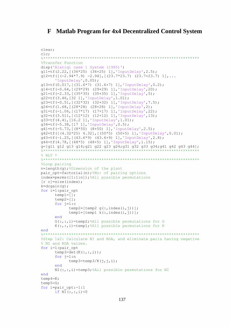
137
F Matlab Program for 4x4 Decentralized Control System
clear;
clc;
%*******************************************************************
%Transfer Function
disp('Alatiqi case 1 System (1985)')
g11=tf(2.22,[(36*25) (36+25) 1],'InputDelay',2.5);
g12=tf([(-2.94*7.9) -2.94],[(23.7*23.7) (23.7+23.7) 1],...
'InputDelay',0.05);
g13=tf(0.017,[(31.6*7) (31.6+7) 1],'InputDelay',0.2);
g14=tf(-0.64,[(29*29) (29+29) 1],'InputDelay',20);
g21=tf(-2.33,[(35*35) (35+35) 1],'InputDelay',5);
g22=tf(3.46,[32 1],'InputDelay',1.01);
g23=tf(-0.51,[(32*32) (32+32) 1],'InputDelay',7.5);
g24=tf(1.68,[(28*28) (28+28) 1],'InputDelay',2);
g31=tf(-1.06,[(17*17) (17+17) 1],'InputDelay',22);
g32=tf(3.511,[(12*12) (12+12) 1],'InputDelay',13);
g33=tf(4.41,[16.2 1],'InputDelay',1.01);
g34=tf(-5.38,[17 1],'InputDelay',0.5);
g41=tf(-5.73,[(8*50) (8+50) 1],'InputDelay',2.5);
g42=tf([(4.32*25) 4.32],[(50*5) (50+5) 1],'InputDelay',0.01);
g43=tf(-1.25,[(43.6*9) (43.6+9) 1],'InputDelay',2.8);
g44=tf(4.78,[(48*5) (48+5) 1],'InputDelay',1.15);
g=[g11 g12 g13 g14;g21 g22 g23 g24;g31 g32 g33 g34;g41 g42 g43 g44];
%*******************************************************************
% BLT *
%*******************************************************************
%Loop pairing
n=length(g);%Dimension of the plant
pair_opt=factorial(n);%No: of pairing options
index=perms([1:1:n]);%All possible permutations
[r c]=size(index);
k=dcgain(g);
for i=1:pair_opt
temp1=[];
temp2=[];
for j=1:c
temp2=[temp2 g(:,index(i,j))];
temp1=[temp1 k(:,index(i,j))];
end
G(:,:,i)=temp2;%All possible permutations for G
K(:,:,i)=temp1;%All possible permutations for K
end
%*******************************************************************
%Step 1&2: Calculate NI and RGA, and eliminate paris having negative
% NI and RGA values.
for i=1:pair_opt
temp3=det(K(:,:,i));
for j=1:n
temp3=temp3/K(j,j,i);
end
NI(:,:,i)=temp3;%All possible permutations for NI
end
temp4=K;
temp5=G;
for i=pair_opt:-1:1
if NI(:,:,i)<0
138
temp4(:,:,i)=[];%Delete ith pairing of K
K=temp4;
temp5(:,:,i)=[];%Delete ith pairing of G
G=temp5;
end
end
final=size(K,3);
for i=1:final
RGA(:,:,i)=K(:,:,i).*inv(K(:,:,i)');%Calculate RGA
end
temp6=G;
temp7=K;
temp8=RGA;
final=size(RGA,3);
for i=final:-1:1
if RGA(1,1,i)<0 | RGA(2,2,i)<0 | RGA(3,3,i)<0 | RGA(4,4,i)<0
temp6(:,:,i)=[];%Delete ith pairing of G
temp7(:,:,i)=[];%Delete ith pairing of K
temp8(:,:,i)=[];%Delete ith pairing of RGA
G=temp6;
K=temp7;
RGA=temp8;
end
end
final=size(K,2);
final1=size(K,3);
for i=1:final1
for j=1:final
K_dia(j,j,i)=diag(K(j,j,i));
end
end
final=size(K,3);
for i=1:final
E(:,:,i)=(K(:,:,i)-K_dia(:,:,i))*(K_dia(:,:,i))^-1;
E_tf=ss(E(:,:,i));
[ssv_value(i),non]=ssv(E_tf.a,E_tf.b,E_tf.c...
,E_tf.d,0);
end
[val_min,nmin]=min(ssv_value);%Minimum Structured Singular value
G=G(:,:,nmin);
K=K(:,:,nmin);
RGA=RGA(:,:,nmin);
%*******************************************************************
%Controller
%Step 1: Compute the Ziegler-Nichols tuning parameters of the
% diagonal elements of the process transfer function matrix.
for a=1:n
if sign(K(a,a))==1
S(a)=allmargin(G(a,a));
else
S(a)=allmargin(-G(a,a));
S(a).GainMargin=-S(a).GainMargin;
end
end
for b=1:n
KcZN(b,b)=S(b).GainMargin(1,1)/2.2;
TauiZN(b,b)=2*pi/(1.2*S(b).GMFrequency(1,1));
TaudZN(b,b)=0.125*2*pi/S(b).GMFrequency(1,1);
end
p=sym('p');
[n,m]=size(G);
139
Gs=zeros(n,m);
Gs=sym(Gs);
for i=1:n
for j=1:m
[num,den]=tfdata(G(i,j),'v');
l=length(den);
order=l;
for k=1:l
A(order,1)=p^(k-1);
order=order-1;
end
n=num*A;
d=den*A;
Gs(i,j)=n/d;
clear A;
end
end
Gs=simple(Gs);
delays=exp(-totaldelay(G)*p);
Gs=Gs.*delays;%Transform transrer function into symbolic matrix
%*******************************************************************
%Step 2: Choose a detuning factor.
F=2.5;%Initial value
Fd=1;%%Initial value
df=0.01;%Increament
dfd=0.01;%Increament
%*******************************************************************
%Step 3,4,5&6: Compute F, Fd, Kc and Taui.
n=length(G);
wrange=logspace(-1,0.8,200);
j=sqrt(-1);%Imaginary unit
s=j*wrange;
m=1;%Initialization
flagm=-1;%Initialization
flagp=-1;%Initialization
while m<10
Kc=KcZN/F;
Taui=TauiZN*F;
Taud=TaudZN/Fd;
nwtot=length(wrange);
for w=1:nwtot
Gs_value=subs(Gs,s(w));
Gcs(1,1)=Kc(1,1)+Kc(1,1)/(Taui(1,1)*s(w))+Kc(1,1)...
*Taud(1,1)*s(w);
Gcs(2,2)=Kc(2,2)+Kc(2,2)/(Taui(2,2)*s(w))+Kc(2,2)...
*Taud(2,2)*s(w);
Gcs(3,3)=Kc(3,3)+Kc(3,3)/(Taui(3,3)*s(w))+Kc(3,3)...
*Taud(3,3)*s(w);
Gcs(4,4)=Kc(4,4)+Kc(4,4)/(Taui(4,4)*s(w))+Kc(4,4)...
*Taud(4,4)*s(w);
wnyquist(w)=-1+det(eye(size(Gs_value))+Gs_value*Gcs);
Lc(w)=wnyquist(w)/(1+wnyquist(w));%Calculate Lc function
dbcl(w)=20*log10(abs(Lc(w)));
end
[dbmax,nmax]=max(dbcl);%Pick off peak closed-loop log modulus
wmax=wrange(nmax);
m=m+1;
if dbmax>2*n%Test if +8 dB and regusee F and Fd factors
if flagp>0
df=df/2;
dfd=dfd/2;
140
end
flagm=1;
F=F+df;
Fd=Fd+dfd;
else
if flagm<0
df=df/2;
end
flagp=1;
F=F-df;
if F<1
F=1;
end
if Fd<1
Fd=1;
end
end
end%End of while loop to find correct F and Fd factors
F%Final value of F
Fd%Final value of Fd
Kp=Kc;
Ki=Kc./Taui;
Kd=Kc.*Taud;
n=length(G);%Dimension of the plant
for i=1:n
Gc(i,i)=tf([Kd(i,i) Kp(i,i) Ki(i,i)],[1 0]);
end
disp('**********The controller one for BLT **********')
Gc11=Gc(1,1)
disp('**********The controller two for BLT **********')
Gc22=Gc(2,2)
disp('**********The controller three for BLT **********')
Gc33=Gc(3,3)
%*******************************************************************
tStart=0;
tFinal=1600;
timespan=[tStart tFinal];
sim('blt4x4',timespan)%Simulation
blt_tout=tout;%From Simulink
blt_simout;%From Simulink
blt_error;%From Simulink
%*******************************************************************
% SIMC *
%*******************************************************************
%Parameter Estimation for g12
g12=tf([(-2.94*7.9) -2.94],[(23.7*23.7) (23.7+23.7) 1],...
'InputDelay',0.05);
sys=g12;
[sys,elim_val] = balreal(sys); % Compute balanced realization
elim = (elim_val<1e-8);
rsys = modred(sys,2,'MatchDC'); % Remove negligible states
g12=tf(rsys);
t=0:1:1000;
[y t]=step(g12,t);
data12=iddata(y,t); % The IDDATA object
m12 =pem(data12,'p1d','kp',-2.94, 'kp','fix','td' ,0.05,...
'td' ,'fix' ,'tp1',{'max',40}, 'tp1',{'min',...
30});% fixing the parameter kp to the value -2.94
g12new=tf(m12.kp.value,[m12.tp1.value 1],'InputDelay',m12.td.value);
disp('The new transfer function for g12 is ')
g12new;
141
figure;
[y t x]=step(g12);
[ynew tnew xnew]=step(g12new);
plot(t,y,'b-',tnew,ynew,'r:','LineWidth',1.5);
ylabel('Amplitude');
xlabel('Time');
grid on;
title('Step responses for g12 and g12new for A1 System (1985)')
legend('g12','g12new',4);
%*******************************************************************
%Parameter Estimation for g42
g42=tf([(4.32*25) 4.32],[(50*5) (50+5) 1],'InputDelay',0.01);
sys=g42;
[sys,elim_val] = balreal(sys); % Compute balanced realization
elim = (elim_val<1e-8);
rsys = modred(sys,2,'MatchDC'); % Remove negligible states
g42=tf(rsys);
t=0:1:1000;
[y t]=step(g42,t);
data42=iddata(y,t); % The IDDATA object
m42 =pem(data12,'p1d','kp',4.32, 'kp','fix','td' ,0.01,...
'td' ,'fix' ,'tp1',{'max',28}, 'tp1',{'min',...
20});% fixing the parameter kp to the value 4.32
g42new=tf(m42.kp.value,[m42.tp1.value 1],'InputDelay',m42.td.value);
disp('The new transfer function for g12 is ')
g42new;
figure;
[y t x]=step(g42);
[ynew tnew xnew]=step(g42new);
plot(t,y,'b-',tnew,ynew,'r:','LineWidth',1.5);
ylabel('Amplitude');
xlabel('Time');
grid on;
title('Step responses for g42 and g42new for A1 System (1985)')
legend('g42','g42new',4);
%*******************************************************************
g12=g12new;
g42=g42new;
g=[g11 g12 g13 g14;g21 g22 g23 g24;g31 g32 g33 g34;g41 g42 g43 g44];
%*******************************************************************
%Loop pairing
%Step 1: Obtain steady state gain matrix.
n=length(g);%Dimension of the plant
pair_opt=factorial(n);%No: of pairing options
index=perms([1:1:n]);%All possible permutations
[r c]=size(index);
k=dcgain(g);
for i=1:pair_opt
temp1=[];
temp2=[];
for j=1:c
temp1=[temp1 k(:,index(i,j))];
temp2=[temp2 g(:,index(i,j))];
end
K(:,:,i)=temp1;%All possible permutations for K
G(:,:,i)=temp2;%All possible permutations for G
end
%*******************************************************************
%Step 2&3: Calculate RGA and NI and eliminate paris having negative
% RGA and NI values.
for i=1:pair_opt
142
temp3=det(K(:,:,i));
for j=1:n
temp3=temp3/K(j,j,i);
end
NI(:,:,i)=temp3;%All possible permutations for NI
end
temp4=K;
temp5=G;
for i=pair_opt:-1:1
if NI(:,:,i)<0
temp4(:,:,i)=[];%Delete ith pairing of K
K=temp4;
temp5(:,:,i)=[];%Delete ith pairing of G
G=temp5;
end
end
final=size(K,3);
for i=1:final
RGA(:,:,i)=K(:,:,i).*inv(K(:,:,i)');%Calculate RGA
end
temp6=G;
temp7=K;
temp8=RGA;
final=size(RGA,3);
for i=final:-1:1
if RGA(1,1,i)<0 | RGA(2,2,i)<0
temp6(:,:,i)=[];%Delete ith pairing of G
temp7(:,:,i)=[];%Delete ith pairing of K
temp8(:,:,i)=[];%Delete ith pairing of RGA
G=temp6;
K=temp7;
RGA=temp8;
end
end
%*******************************************************************
%Step 4: Calculate delijG and ijPsi.
final=size(K,3);
for t=1:final
l=1;
temp9=K(:,:,t);
for i=1:n
for j=1:n
temp9(i,:)=[];
temp9(:,j)=[];
ijG(:,:,l,t)=temp9;
temp9=K(:,:,t);
l=l+1;
end
temp9=K(:,:,t);
end
end
final=size(K,3);
for t=1:final
l=1;
temp10=K(:,:,t);
for i=1:n
for j=1:n
row=temp10(i,:);
row(:,i)=[];
column=temp10(:,i);
column(i,:)=[];
143
delijG(:,:,l,t)=-(column*row)/temp10(i,j);
l=l+1;
end
end
end
final=size(ijG,4);
for t=1:final
temp11=ijG(:,:,:,t);
temp12=delijG(:,:,:,t);
final1=size(ijG,3);
for i=1:final1
ijPsi(:,:,i,t)=temp12(:,:,i).*inv(temp11(:,:,i)');
end
end
%*******************************************************************
%Step 5: Calculate Omega.
final3=size(ijG,4);
for t=1:final3
final4=size(ijG,3);
for j=1:final4
w(:,:,j,t)=norm(ijPsi(:,:,j,t),2);
end
end
final5=size(ijG,4);
for t=1:final5
Omega(:,:,t)=[w(:,:,1,t) w(:,:,2,t) w(:,:,3,t) w(:,:,4,t);
w(:,:,5,t) w(:,:,6,t) w(:,:,7,t) w(:,:,8,t);
w(:,:,9,t) w(:,:,10,t) w(:,:,11,t) w(:,:,12,t);
w(:,:,13,t) w(:,:,14,t) w(:,:,15,t) w(:,:,16,t)];
dia(:,t)=diag(Omega(:,:,t));
pro(t)=prod(dia(:,t));
end
%*******************************************************************
%Step 6: Find the best pairing.
[value,index]=min(pro);
disp('G matrix for the best pairing is ')
G=G(:,:,index);
disp('K matrix for the best pairing is ')
K=K(:,:,index);
disp('RGA matrix for the best pairing is ')
RGA=RGA(:,:,index);
%*******************************************************************
%Controller
for i=1:n%Start of loop for Tau and Tau'
for j=1:n
temp=pole(G(i,j));
if length(temp)==2
Tau1(i,j)=-1/temp(2);
Tau2(i,j)=-1/temp(1);
else
Tau1(i,j)=-1/temp(1);
Tau2(i,j)=0;
end
end
end%End of loop for Tau and Tau'
Theta=totaldelay(G);
p=sym('p');
[n,m]=size(G);
Gs=zeros(n,m);
Gs=sym(Gs);
for i=1:n
144
for j=1:m
[num,den]=tfdata(G(i,j),'v');
l=length(den);
order=l;
for k=1:l
A(order,1)=p^(k-1);
order=order-1;
end
n=num*A;
d=den*A;
Gs(i,j)=n/d;
clear A;
end
end
Gs=simple(Gs);
delays=exp(-totaldelay(G)*p);
Gs=Gs.*delays;%Transform transrer function into symbolic matrix
%*******************************************************************
%Step 1: Design an individual controller for the diagonal elements.
TauC=2*Theta;%Assumption
n=length(G);%Dimension of the plant
for i=1:n%Start of loop for diagonal controler
kP(i,i)=(1/K(i,i))*(Tau1(i,i)/(TauC(i,i)+Theta(i,i)));
TauI(i,i)=min(Tau1(i,i),4*(TauC(i,i)+Theta(i,i)));
kI(i,i)=kP(i,i)/TauI(i,i);
TauD(i,i)=Tau2(i,i);
kD(i,i)=kP(i,i)*TauD(i,i);
C(i,i)=tf([kD(i,i) kP(i,i) kI(i,i)],[1 0]);
end%end of loop for diagonal controller
p=sym('p');
[n,m]=size(C);
Cs=zeros(n,m);
Cs=sym(Cs);
for i=1:n
for j=1:m
[num,den]=tfdata(C(i,j),'v');
l=length(den);
order=l;
for k=1:l
A(order,1)=p^(k-1);
order=order-1;
end
n=num*A;
d=den*A;
Cs(i,j)=n/d;
clear A;
end
end
Cs=simple(Cs);%Transform transrer function into symbolic matrix
%*******************************************************************
%Step 2: Calculate P.
n=length(G);
for i=1:n
Wc(i,i)=1/(TauC(i,i)+Theta(i,i));
end
j=sqrt(-1);%Imaginary unit
s=j*Wc;
for i=1:n
for J=1:n
if i==J
P(i,J)=(TauC(i,J)*s(i,J)+1)*exp(Theta(i,J)*s(i,J));
145
else
P(i,J)=1;
end
end
end
gii=diag(Gs);
for i=1:n
temp=Gs(:,i);
temp(i,:)=[];
iigstari(:,:,i)=temp;
end
for i=1:n
temp=Gs(i,:);
temp(:,i)=[];
iigistar(:,:,i)=temp;
end
temp=Gs;
for i=1:n
for j=1:n
temp(i,:)=[];
temp(:,j)=[];
iiGs(:,:,i)=temp;
iiGs_value(:,:,i)=subs(iiGs(:,:,i),s(i,i));
temp=Gs;
end
end
for i=1:n
delGii(:,:,i)=-(1/Gs(i,i))*iigstari(:,:,i)*iigistar(:,:,i);
temp=subs(delGii(:,:,i),s(i,i));
delGii_value(:,:,i)=temp;
end
temp=P;
for i=1:n
temp(i,:)=[];
temp(:,i)=[];
iiP(:,:,i)=temp;
temp=P;
end
%*******************************************************************
%Step 3&4: Calculate dRI and MMF.
for i=1:n
Phi(:,:,i)=delGii_value(:,:,i).*(iiGs_value(:,:,i).*....
iiP(:,:,i))';
end
for i=1:n
Phi_sum(i)=sum(sum(abs(Phi(:,:,i))));
end
for i=1:n
krho(i)=abs(1+Phi_sum(i));
thetarho(i)=-angle(1+Phi_sum(i))/Wc(i,i);
end
%*******************************************************************
%Step 5: Obtain Equivalent Transfer Function.
for i=1:n
fk(i)=max(1,krho(i));
ftheta(i)=max(1,1+(thetarho(i)/Theta(i,i)));
end
for i=1:n
Gcap(i)=tf(fk(i)*K(i,i),[(Tau1(i,i)...
*Tau2(i,i)) (Tau1(i,i)...
+Tau2(i,i)) 1],'InputDelay',...
146
ftheta(i)*Theta(i,i));
end
%*******************************************************************
%Step 6: Fine tuning
for i=1:n
kP(i,i)=(1/fk(i))*(1/K(i,i))*(Tau1(i,i)/...
(TauC(i,i)+ftheta(i)...
*Theta(i,i)));
TauI(i,i)=min(Tau1(i,i),4*(TauC(i,i)+...
ftheta(i)*Theta(i,i)));
kI(i,i)=kP(i,i)/TauI(i,i);
TauD(i,i)=Tau2(i,i);
kD(i,i)=kP(i,i)*TauD(i,i);
gc(i,i)=tf([kD(i,i) kP(i,i) kI(i,i)],[1 0]);
end
disp('**********The controller one for SIMC **********')
gc11=gc(1,1)
disp('**********The controller two for SIMC **********')
gc22=gc(2,2)
disp('**********The controller three for SIMC **********')
gc33=gc(3,3)
disp('**********The controller three for SIMC **********')
gc44=gc(4,4)
%*******************************************************************
tStart=0;
tFinal=1600;
timespan=[tStart tFinal];
sim('simc4x4',timespan)%Simulation
simc_tout=tout;%From Simulink
simc_simout;%From Simulink
simc_error;%From Simulink
%*******************************************************************
% ERGA *
%*******************************************************************
%Parameter Estimation for g12
g12=tf([(-2.94*7.9) -2.94],[(23.7*23.7) (23.7+23.7) 1],...
'InputDelay',0.05);
sys=g12;
[sys,elim_val] = balreal(sys); % Compute balanced realization
elim = (elim_val<1e-8);
rsys = modred(sys,2,'MatchDC'); % Remove negligible states
g12=tf(rsys);
t=0:1:1000;
[y t]=step(g12,t);
data12=iddata(y,t); % The IDDATA object
m12 =pem(data12,'p1d','kp',-2.94, 'kp','fix','td' ,0.05,...
'td' ,'fix' ,'tp1',{'max',40}, 'tp1',{'min',...
30});% fixing the parameter kp to the value -2.94
g12new=tf(m12.kp.value,[m12.tp1.value 1],...
'InputDelay' ,m12.td.value);
disp('The new transfer function for g12 is ')
g12new;
figure;
[y t x]=step(g12);
[ynew tnew xnew]=step(g12new);
plot(t,y,'b-',tnew,ynew,'r:','LineWidth',1.5);
ylabel('Amplitude');
xlabel('Time');
grid on;
title('Step responses for g12 and g12new for A1')
legend('g12','g12new',1);
147
%*******************************************************************
%Parameter Estimation for g42
g42=tf([(4.32*25) 4.32],[(50*5) (50+5) 1],'InputDelay',0.01);
sys=g42;
[sys,elim_val] = balreal(sys); % Compute balanced realization
elim = (elim_val<1e-8);
rsys = modred(sys,2,'MatchDC'); % Remove negligible states
g42=tf(rsys);
t=0:1:1000;
[y t]=step(g42,t);
data42=iddata(y,t); % The IDDATA object
m42 =pem(data12,'p1d','kp',4.32, 'kp','fix','td' ,0.01,...
'td' ,'fix' ,'tp1',{'max',28}, 'tp1',{'min',...
20});% fixing the parameter kp to the value 4.32
g42new=tf(m42.kp.value,[m42.tp1.value 1],...
'InputDelay' ,m42.td.value);
disp('The new transfer function for g12 is ')
g42new;
figure;
[y t x]=step(g42);
[ynew tnew xnew]=step(g42new);
plot(t,y,'b-',tnew,ynew,'r:','LineWidth',1.5);
ylabel('Amplitude');
xlabel('Time');
grid on;
title('Step responses for g42 and g42new for A1')
legend('g42','g42new',4);
%*******************************************************************
g12=g12new;
g42=g42new;
g=[g11 g12 g13 g14;g21 g22 g23 g24;g31 g32 g33 g34;g41 g42 g43 g44];
%*******************************************************************
%Loop pairing
%Step 1: Obtain steady state gain matrix.
n=length(g);%Dimension of the plant
pair_opt=factorial(n);%No: of pairing options
index=perms([1:1:n]);%%All possible permutations
[nrow ncol]=size(index);
k=dcgain(g);
for i=1:pair_opt
temp1=[];
temp2=[];
for j=1:ncol
temp1=[temp1 k(:,index(i,j))];
temp2=[temp2 g(:,index(i,j))];
end
K(:,:,i)=temp1;%All possible permutations for K
G(:,:,i)=temp2;%All possible permutations for G
end
%*******************************************************************
%Step 2&3: Calculate NI and ERGA, and eliminate paris having
% negative NI and ERGA values.
for i=1:pair_opt
temp3=det(K(:,:,i));
for j=1:n
temp3=temp3/K(j,j,i);
end
NI(:,:,i)=temp3;%All possible permutations for NI
end
temp4=K;
temp5=G;
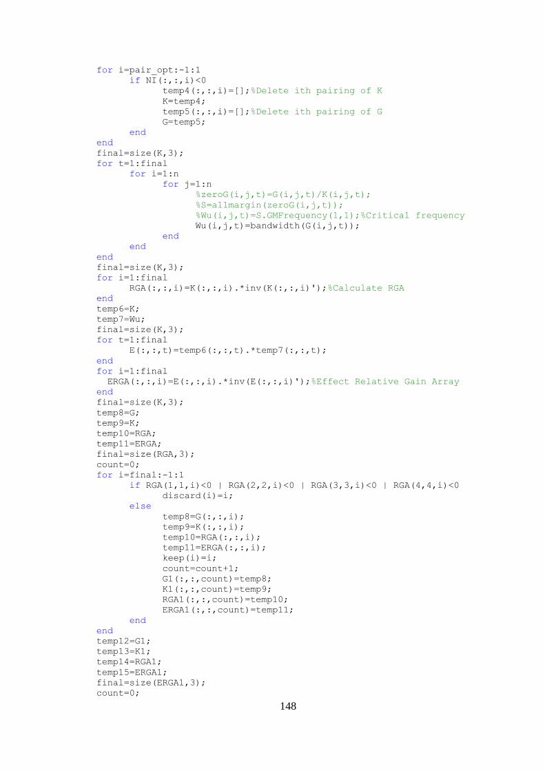
148
for i=pair_opt:-1:1
if NI(:,:,i)<0
temp4(:,:,i)=[];%Delete ith pairing of K
K=temp4;
temp5(:,:,i)=[];%Delete ith pairing of G
G=temp5;
end
end
final=size(K,3);
for t=1:final
for i=1:n
for j=1:n
%zeroG(i,j,t)=G(i,j,t)/K(i,j,t);
%S=allmargin(zeroG(i,j,t));
%Wu(i,j,t)=S.GMFrequency(1,1);%Critical frequency
Wu(i,j,t)=bandwidth(G(i,j,t));
end
end
end
final=size(K,3);
for i=1:final
RGA(:,:,i)=K(:,:,i).*inv(K(:,:,i)');%Calculate RGA
end
temp6=K;
temp7=Wu;
final=size(K,3);
for t=1:final
E(:,:,t)=temp6(:,:,t).*temp7(:,:,t);
end
for i=1:final
ERGA(:,:,i)=E(:,:,i).*inv(E(:,:,i)');%Effect Relative Gain Array
end
final=size(K,3);
temp8=G;
temp9=K;
temp10=RGA;
temp11=ERGA;
final=size(RGA,3);
count=0;
for i=final:-1:1
if RGA(1,1,i)<0 | RGA(2,2,i)<0 | RGA(3,3,i)<0 | RGA(4,4,i)<0
discard(i)=i;
else
temp8=G(:,:,i);
temp9=K(:,:,i);
temp10=RGA(:,:,i);
temp11=ERGA(:,:,i);
keep(i)=i;
count=count+1;
G1(:,:,count)=temp8;
K1(:,:,count)=temp9;
RGA1(:,:,count)=temp10;
ERGA1(:,:,count)=temp11;
end
end
temp12=G1;
temp13=K1;
temp14=RGA1;
temp15=ERGA1;
final=size(ERGA1,3);
count=0;
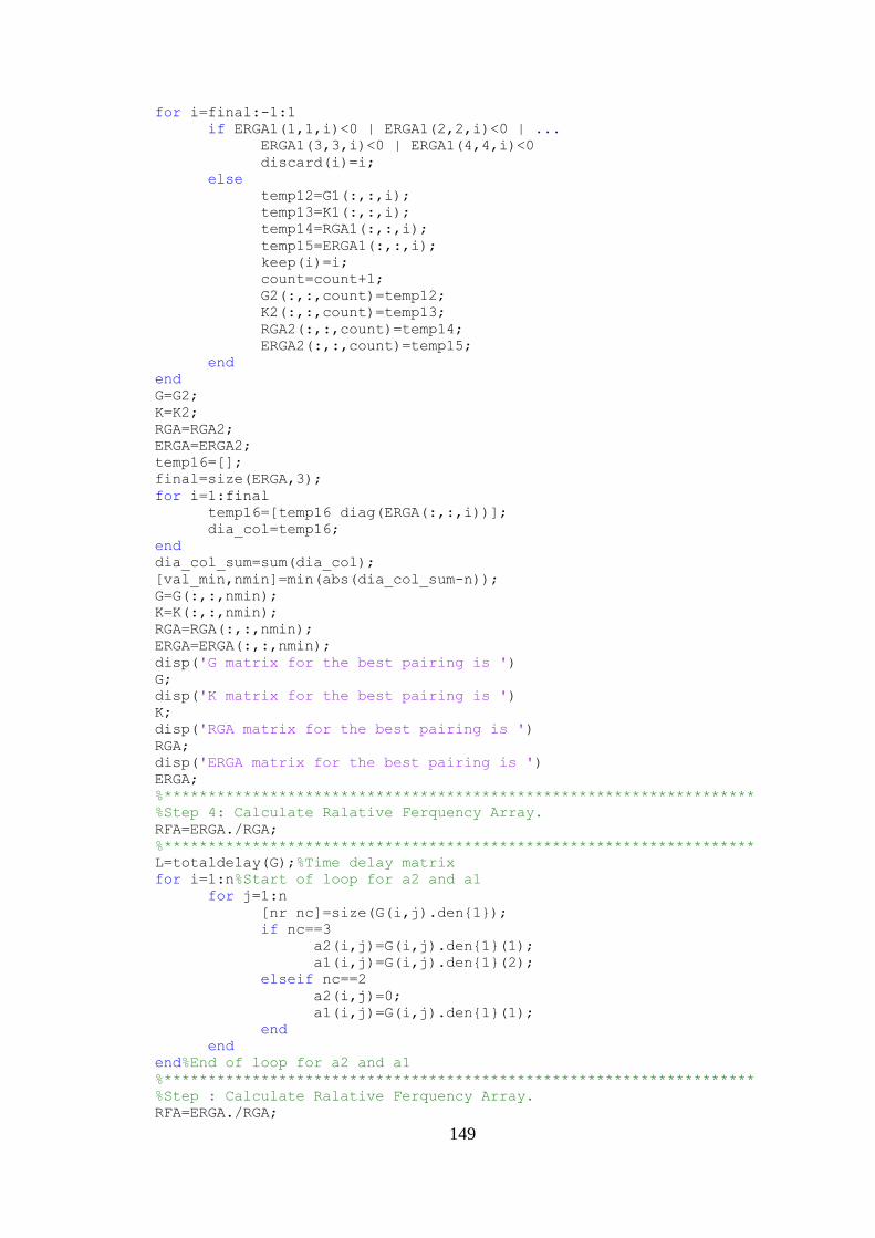
149
for i=final:-1:1
if ERGA1(1,1,i)<0 | ERGA1(2,2,i)<0 | ...
ERGA1(3,3,i)<0 | ERGA1(4,4,i)<0
discard(i)=i;
else
temp12=G1(:,:,i);
temp13=K1(:,:,i);
temp14=RGA1(:,:,i);
temp15=ERGA1(:,:,i);
keep(i)=i;
count=count+1;
G2(:,:,count)=temp12;
K2(:,:,count)=temp13;
RGA2(:,:,count)=temp14;
ERGA2(:,:,count)=temp15;
end
end
G=G2;
K=K2;
RGA=RGA2;
ERGA=ERGA2;
temp16=[];
final=size(ERGA,3);
for i=1:final
temp16=[temp16 diag(ERGA(:,:,i))];
dia_col=temp16;
end
dia_col_sum=sum(dia_col);
[val_min,nmin]=min(abs(dia_col_sum-n));
G=G(:,:,nmin);
K=K(:,:,nmin);
RGA=RGA(:,:,nmin);
ERGA=ERGA(:,:,nmin);
disp('G matrix for the best pairing is ')
G;
disp('K matrix for the best pairing is ')
K;
disp('RGA matrix for the best pairing is ')
RGA;
disp('ERGA matrix for the best pairing is ')
ERGA;
%*******************************************************************
%Step 4: Calculate Ralative Ferquency Array.
RFA=ERGA./RGA;
%*******************************************************************
L=totaldelay(G);%Time delay matrix
for i=1:n%Start of loop for a2 and a1
for j=1:n
[nr nc]=size(G(i,j).den{1});
if nc==3
a2(i,j)=G(i,j).den{1}(1);
a1(i,j)=G(i,j).den{1}(2);
elseif nc==2
a2(i,j)=0;
a1(i,j)=G(i,j).den{1}(1);
end
end
end%End of loop for a2 and a1
%*******************************************************************
%Step : Calculate Ralative Ferquency Array.
RFA=ERGA./RGA;
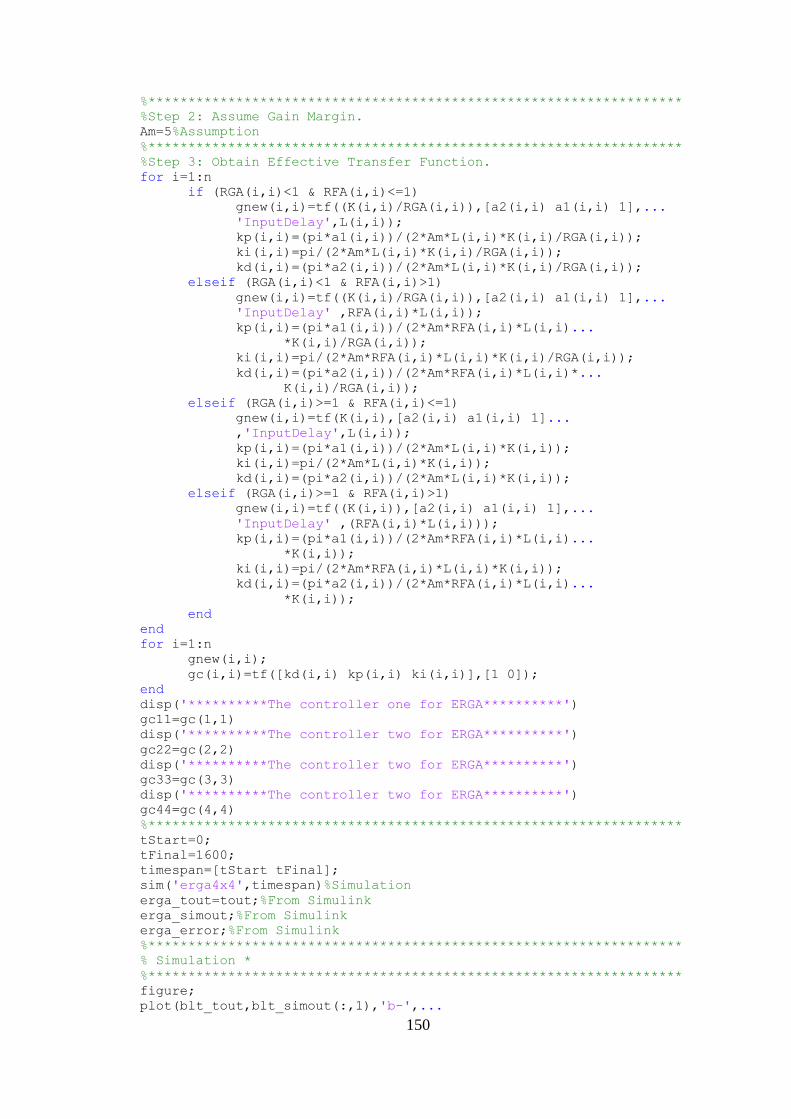
150
%*******************************************************************
%Step 2: Assume Gain Margin.
Am=5%Assumption
%*******************************************************************
%Step 3: Obtain Effective Transfer Function.
for i=1:n
if (RGA(i,i)<1 & RFA(i,i)<=1)
gnew(i,i)=tf((K(i,i)/RGA(i,i)),[a2(i,i) a1(i,i) 1],...
'InputDelay',L(i,i));
kp(i,i)=(pi*a1(i,i))/(2*Am*L(i,i)*K(i,i)/RGA(i,i));
ki(i,i)=pi/(2*Am*L(i,i)*K(i,i)/RGA(i,i));
kd(i,i)=(pi*a2(i,i))/(2*Am*L(i,i)*K(i,i)/RGA(i,i));
elseif (RGA(i,i)<1 & RFA(i,i)>1)
gnew(i,i)=tf((K(i,i)/RGA(i,i)),[a2(i,i) a1(i,i) 1],...
'InputDelay' ,RFA(i,i)*L(i,i));
kp(i,i)=(pi*a1(i,i))/(2*Am*RFA(i,i)*L(i,i)...
*K(i,i)/RGA(i,i));
ki(i,i)=pi/(2*Am*RFA(i,i)*L(i,i)*K(i,i)/RGA(i,i));
kd(i,i)=(pi*a2(i,i))/(2*Am*RFA(i,i)*L(i,i)*...
K(i,i)/RGA(i,i));
elseif (RGA(i,i)>=1 & RFA(i,i)<=1)
gnew(i,i)=tf(K(i,i),[a2(i,i) a1(i,i) 1]...
,'InputDelay',L(i,i));
kp(i,i)=(pi*a1(i,i))/(2*Am*L(i,i)*K(i,i));
ki(i,i)=pi/(2*Am*L(i,i)*K(i,i));
kd(i,i)=(pi*a2(i,i))/(2*Am*L(i,i)*K(i,i));
elseif (RGA(i,i)>=1 & RFA(i,i)>1)
gnew(i,i)=tf((K(i,i)),[a2(i,i) a1(i,i) 1],...
'InputDelay' ,(RFA(i,i)*L(i,i)));
kp(i,i)=(pi*a1(i,i))/(2*Am*RFA(i,i)*L(i,i)...
*K(i,i));
ki(i,i)=pi/(2*Am*RFA(i,i)*L(i,i)*K(i,i));
kd(i,i)=(pi*a2(i,i))/(2*Am*RFA(i,i)*L(i,i)...
*K(i,i));
end
end
for i=1:n
gnew(i,i);
gc(i,i)=tf([kd(i,i) kp(i,i) ki(i,i)],[1 0]);
end
disp('**********The controller one for ERGA**********')
gc11=gc(1,1)
disp('**********The controller two for ERGA**********')
gc22=gc(2,2)
disp('**********The controller two for ERGA**********')
gc33=gc(3,3)
disp('**********The controller two for ERGA**********')
gc44=gc(4,4)
%*******************************************************************
tStart=0;
tFinal=1600;
timespan=[tStart tFinal];
sim('erga4x4',timespan)%Simulation
erga_tout=tout;%From Simulink
erga_simout;%From Simulink
erga_error;%From Simulink
%*******************************************************************
% Simulation *
%*******************************************************************
figure;
plot(blt_tout,blt_simout(:,1),'b-',...
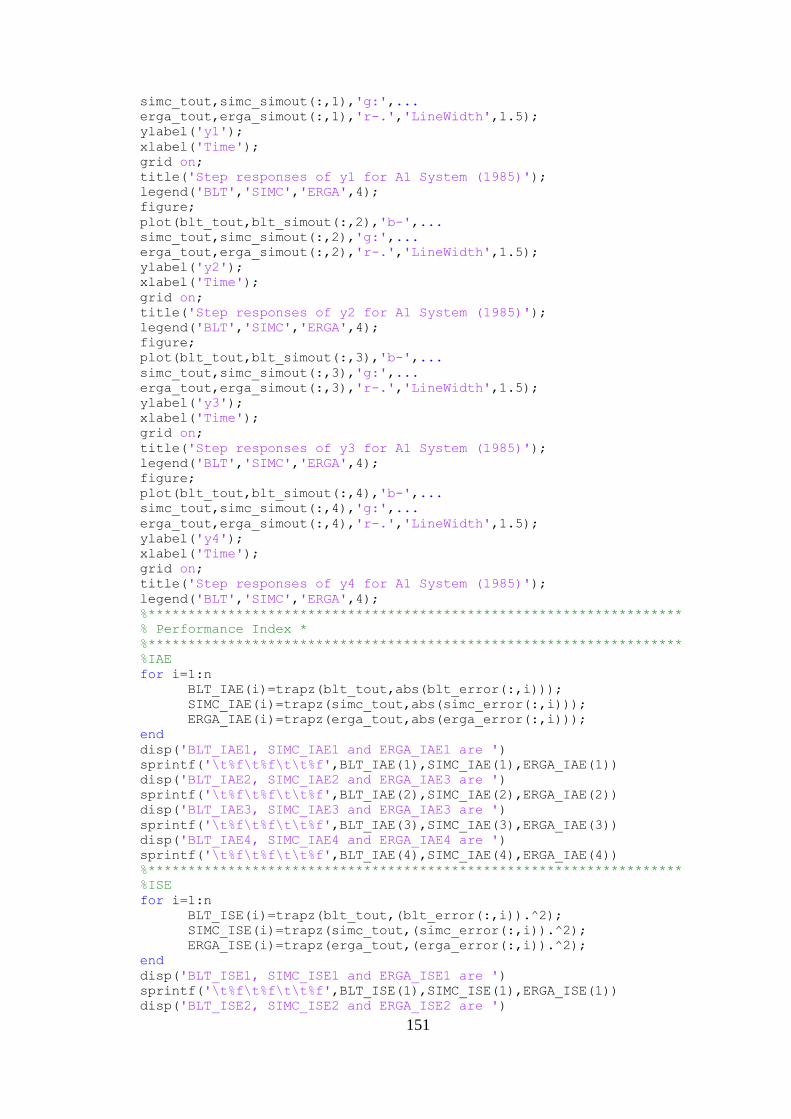
151
simc_tout,simc_simout(:,1),'g:',...
erga_tout,erga_simout(:,1),'r-.','LineWidth',1.5);
ylabel('y1');
xlabel('Time');
grid on;
title('Step responses of y1 for A1 System (1985)');
legend('BLT','SIMC','ERGA',4);
figure;
plot(blt_tout,blt_simout(:,2),'b-',...
simc_tout,simc_simout(:,2),'g:',...
erga_tout,erga_simout(:,2),'r-.','LineWidth',1.5);
ylabel('y2');
xlabel('Time');
grid on;
title('Step responses of y2 for A1 System (1985)');
legend('BLT','SIMC','ERGA',4);
figure;
plot(blt_tout,blt_simout(:,3),'b-',...
simc_tout,simc_simout(:,3),'g:',...
erga_tout,erga_simout(:,3),'r-.','LineWidth',1.5);
ylabel('y3');
xlabel('Time');
grid on;
title('Step responses of y3 for A1 System (1985)');
legend('BLT','SIMC','ERGA',4);
figure;
plot(blt_tout,blt_simout(:,4),'b-',...
simc_tout,simc_simout(:,4),'g:',...
erga_tout,erga_simout(:,4),'r-.','LineWidth',1.5);
ylabel('y4');
xlabel('Time');
grid on;
title('Step responses of y4 for A1 System (1985)');
legend('BLT','SIMC','ERGA',4);
%*******************************************************************
% Performance Index *
%*******************************************************************
%IAE
for i=1:n
BLT_IAE(i)=trapz(blt_tout,abs(blt_error(:,i)));
SIMC_IAE(i)=trapz(simc_tout,abs(simc_error(:,i)));
ERGA_IAE(i)=trapz(erga_tout,abs(erga_error(:,i)));
end
disp('BLT_IAE1, SIMC_IAE1 and ERGA_IAE1 are ')
sprintf('\t%f\t%f\t\t%f',BLT_IAE(1),SIMC_IAE(1),ERGA_IAE(1))
disp('BLT_IAE2, SIMC_IAE2 and ERGA_IAE3 are ')
sprintf('\t%f\t%f\t\t%f',BLT_IAE(2),SIMC_IAE(2),ERGA_IAE(2))
disp('BLT_IAE3, SIMC_IAE3 and ERGA_IAE3 are ')
sprintf('\t%f\t%f\t\t%f',BLT_IAE(3),SIMC_IAE(3),ERGA_IAE(3))
disp('BLT_IAE4, SIMC_IAE4 and ERGA_IAE4 are ')
sprintf('\t%f\t%f\t\t%f',BLT_IAE(4),SIMC_IAE(4),ERGA_IAE(4))
%*******************************************************************
%ISE
for i=1:n
BLT_ISE(i)=trapz(blt_tout,(blt_error(:,i)).^2);
SIMC_ISE(i)=trapz(simc_tout,(simc_error(:,i)).^2);
ERGA_ISE(i)=trapz(erga_tout,(erga_error(:,i)).^2);
end
disp('BLT_ISE1, SIMC_ISE1 and ERGA_ISE1 are ')
sprintf('\t%f\t%f\t\t%f',BLT_ISE(1),SIMC_ISE(1),ERGA_ISE(1))
disp('BLT_ISE2, SIMC_ISE2 and ERGA_ISE2 are ')
152
sprintf('\t%f\t%f\t\t%f',BLT_ISE(2),SIMC_ISE(2),ERGA_ISE(2))
disp('BLT_ISE3, SIMC_ISE3 and ERGA_ISE3 are ')
sprintf('\t%f\t%f\t\t%f',BLT_ISE(3),SIMC_ISE(3),ERGA_ISE(3))
disp('BLT_ISE4, SIMC_ISE4 and ERGA_ISE4 are ')
sprintf('\t%f\t%f\t\t%f',BLT_ISE(4),SIMC_ISE(4),ERGA_ISE(4))
%*******************************************************************
%ITAE
for i=1:n
BLT_ITAE(i)=trapz(blt_tout,abs(blt_error(:,i)).*blt_tout);
SIMC_ITAE(i)=trapz(simc_tout,abs(simc_error(:,i)).*simc_tout);
ERGA_ITAE(i)=trapz(erga_tout,abs(erga_error(:,i)).*erga_tout);
end
disp('BLT_ITAE1, SIMC_ITAE1 and ERGA_ITAE1 are ')
sprintf('\t%f\t%f\t\t%f',BLT_ITAE(1),SIMC_ITAE(1),ERGA_ITAE(1))
disp('BLT_ITAE2, SIMC_ITAE2 and ERGA_ITAE2 are ')
sprintf('\t%f\t%f\t\t%f',BLT_ITAE(2),SIMC_ITAE(2),ERGA_ITAE(2))
disp('BLT_ITAE3, SIMC_ITAE3 and ERGA_ITAE3 are ')
sprintf('\t%f\t%f\t\t%f',BLT_ITAE(3),SIMC_ITAE(3),ERGA_ITAE(3))
disp('BLT_ITAE4, SIMC_ITAE4 and ERGA_ITAE4 are ')
sprintf('\t%f\t%f\t\t%f',BLT_ITAE(4),SIMC_ITAE(4),ERGA_ITAE(4))
%*******************************************************************