Development of pump geometry for engine cooling system824390/FULLTEXT01.pdf · Development of pump geometry ... includes the main head losses that occur within a centrifugal pump

Master of Science Thesis

KTH School of Industrial Engineering and Management

Energy Technology EGI-2015-039MSC EKV1093

Division of Heat and Power Technology

SE-100 44 STOCKHOLM

Development of pump geometry for

engine cooling system

Joel Björkman

Master of Science Thesis EGI-2015-039MSC

EKV1093

Development of pump geometry for engine

cooling system

Joel Björkman

Approved

20150609

Examiner

Paul Petrie-Repar

Supervisor

Jens Fridh

Commissioner

Contact person

Abstract

The engine cooling system is an important part of the engine’s performance to achieve optimum

temperatures in cylinders and provide cooling to subsystems. With increasing emission demands from

legislation, further development of the cooling system is necessary. An important component in the engine

cooling system is the pump that produces the necessary flow rate to cool down the components. The pump

is connected to the drive shaft with a pulley so improvements in the pumps efficiency will directly affect the

fuel efficiency of the vehicle. With more variations and increasingly complex system design different

performance stages of the pump are necessary to provide desired flow rates depending on system design.

To enable a rapid design of performance stages of pumps, a calculation model is constructed to predict the

performance of an engine cooling pump based on the geometry of the impeller and pump casing. The model

includes the main head losses that occur within a centrifugal pump both in the impeller and pump casing.

The model is based on quasi one-dimensional calculations of velocity triangles in impeller and pump casing.

The head losses are modelled with correlations from literature that are compared to test data from reference

pumps. The developed model provides a pump - , hydraulic efficiency – and power curve based on main

geometrical parameters. A design tool and procedure is constructed to suggest main geometry parameters

for the impeller based on a desired operational point. The design tool is constructed on design coefficients

based on reference pumps test data and correlations from literature. Together with the calculation model

an impeller flow channel can be designed to achieve the desired operational point. Two impellers are

designed and manufactured by rapid prototyping that are tested by an experimental test to verify the model

and design tool.

The result show that the calculation model captures the general behaviour of the pump curve and is within

1-10% accuracy. The calculation model and the design tool are designed to assess the performance of the

main geometry parameters in the impeller and pump casing. Further optimization and studies of the

complete flow field to assess secondary flows and cavitation behaviour can be done by numerical methods.

The calculation model and design tool constructed provides a rapid way of designing new impellers and an

easy method to perform parameter studies on changes in impeller geometry.

Sammanfattning

Motorns kylsystem är en viktig del av motorns prestanda för att uppnå optimal temperatur i cylindrarna och

för att tillhandahålla kylning till de olika delsystem. Med ökade utsläppskrav från lagstiftning har kylsystemet

och dess fortsatta utveckling en viktig roll för att möta dessa. En viktig komponent i kylsystemet är pumpen

som tillhandahåller den nödvändiga flödeshastigheten för att kyla ner de ingående komponenterna. Pumpen

drivs av drivaxeln med remdrift vilket medför att verkningsgraden på pumpen direkt påverkar

bränsleförbrukningen. Utvecklingen går mot att kylsystemet blir mer varierat och snabbt ska kunna anpassa

sig till nya kylbehov vilket medför att olika prestandasteg på pumpen är nödvändiga för att kunna garantera

tillräcklig flödeshastighet.

För att förkorta ledtiderna i processen av att designa olika prestandasteg av en kylvätskepump har en

beräkningsmodell utvecklats som kan förutsäga pumpens prestanda baserat på impellerns och pumphusets

geometri. I modellen ingår de största strömningsförlusterna som uppstår i en centrifugalpump både i

impellern och i pumphuset. För att modellera förlusterna som uppstår används korrelationer som är

anpassade och korrelerade mot test data från referenspumpar. Modellen beräknar en pumpkurva, hydraulisk

verkningsgradskurva och en effektkurva baserat på pumpens geometri. Ett designverktyg och ett

tillvägagångssätt för att designa impellrar är också framtaget som är baserat på beräkningsmodellen samt en

given designpunkt. Designverktyget använder olika designkoefficienter som är baserade på tidigare test data

samt etablerade korrelationer. Tillsammans med beräkningsmodellen kan flödeskanalen designas baserat på

en given designpunkt av flöde, tryckhöjd och rotationshastighet. Med hjälp av designverktyget är två

impellrar designade och tillverkade genom friformsframställning vilka provas för att verifiera modellen och

designverktyget.

Resultatet visar att beräkningsmodellen kan prediktera pumpkurvans beteende med en noggrannhet på 1-

10%. Beräkningsmodellen samt designverktyget är baserat på de huvudsakliga geometriparametrarna i

impellern och pumphuset. För att fullständigt analysera flödesfältet i pumpen samt optimera designen och

bedöma kavitationsrisken krävs en numerisk analys. Beräkningsmodellen och designverktyget ger ett snabbt

tillvägagångssätt för att designa och utvärdera prestandan i en pump samt göra enkla parameterstudier av

designparameterar i pumpen.

Table of Contents

1 Introduction .......................................................................................................................................................... 1

Background .................................................................................................................................................................... 2

1.1 Engine cooling system ................................................................................................................................ 2

1.1.1 Thermal load ....................................................................................................................................... 3

1.2 Pumps ........................................................................................................................................................... 4

1.2.1 Impeller ................................................................................................................................................ 5

1.2.2 Velocity vectors .................................................................................................................................. 6

1.2.3 Euler head ........................................................................................................................................... 7

1.2.4 Slip ........................................................................................................................................................ 8

1.2.5 Inlet-rotation ....................................................................................................................................... 9

1.2.6 Cavitation & NPSH .........................................................................................................................10

1.2.7 Pump casing ......................................................................................................................................11

1.2.8 Bearings and seals ............................................................................................................................12

1.2.9 Pump curve .......................................................................................................................................12

1.2.10 System curve .....................................................................................................................................15

1.2.11 Pumps in engine cooling system ...................................................................................................16

1.2.12 Case of Reference engine ................................................................................................................16

2 Delimitations .......................................................................................................................................................18

2.1.1 In system design ...............................................................................................................................18

2.1.2 In pump design.................................................................................................................................18

3 Objectives ............................................................................................................................................................18

4 Methodology .......................................................................................................................................................19

4.1 Numerical method ....................................................................................................................................20

4.1.1 Pre-processing ..................................................................................................................................20

4.1.2 Calculation .........................................................................................................................................20

4.1.3 Post-processing ................................................................................................................................20

4.2 Reference pumps .......................................................................................................................................20

5 Modelling .............................................................................................................................................................21

5.1 Pump geometry .........................................................................................................................................21

5.2 Impeller .......................................................................................................................................................22

5.2.1 Impeller inlet .....................................................................................................................................22

5.2.2 Impeller outlet ..................................................................................................................................24

5.3 Head losses in the impeller ......................................................................................................................25

5.3.1 Friction ..............................................................................................................................................26

5.3.2 Incidence ...........................................................................................................................................27

5.3.3 Leakage ..............................................................................................................................................29

5.3.4 Diffusion ...........................................................................................................................................30

5.3.5 Recirculation .....................................................................................................................................31

5.3.6 Total impeller losses ........................................................................................................................31

5.4 Losses in the pump casing .......................................................................................................................32

5.4.1 Friction ..............................................................................................................................................33

5.4.2 Radial loss ..........................................................................................................................................33

5.4.3 Volute head loss ...............................................................................................................................34

5.4.4 Diffuser ..............................................................................................................................................35

5.4.5 Outlet loss .........................................................................................................................................36

5.4.6 Total pump casing losses ................................................................................................................37

5.4.7 Total losses ........................................................................................................................................37

5.5 Power and efficiency.................................................................................................................................38

5.5.1 Disk friction ......................................................................................................................................38

5.5.2 Efficiency ..........................................................................................................................................39

6 Design program ..................................................................................................................................................41

6.1 Design coefficients ....................................................................................................................................41

6.1.1 Head coefficient ...............................................................................................................................41

6.1.2 Flow coefficient ................................................................................................................................43

6.2 Calculation of design parameters ............................................................................................................44

6.2.1 Designing impeller outlet ................................................................................................................44

6.2.2 Designing impeller inlet ..................................................................................................................45

6.3 Limits and requirements ..........................................................................................................................46

6.4 Impeller design ..........................................................................................................................................46

6.5 Cavitation ...................................................................................................................................................47

7 Experimental test................................................................................................................................................48

7.1 Objectives of experimental test ..............................................................................................................48

7.2 Setup ............................................................................................................................................................48

7.3 Procedure ...................................................................................................................................................49

7.3.1 Limitations ........................................................................................................................................49

8 Result ....................................................................................................................................................................50

8.1 Correlation/Comparison with previous test data ................................................................................50

8.2 New impeller design .................................................................................................................................54

8.2.1 New impeller comparison with test data ......................................................................................59

8.2.2 New impeller comparison with CFD ...........................................................................................61

9 Mesh dependency study ....................................................................................................................................63

10 Conclusions & Discussion ................................................................................................................................64

10.1 Conclusions ................................................................................................................................................64

10.2 Discussion ..................................................................................................................................................64

11 Future recommendations ..................................................................................................................................65

Bibliography .................................................................................................................................................................66

12 Appendix 1 ..........................................................................................................................................................68

13 Appendix 2 ..........................................................................................................................................................69

Table of Figures

Figure 1 Basic circuit of the engine cooling system (Pang, 2012) ........................................................................ 2

Figure 2 A truck engine with the cooling system highlighted, courtesy of Scania ............................................ 3

Figure 3 Traditional centrifugal pump with impeller and pump casing (Gulich, 2014) ................................... 4

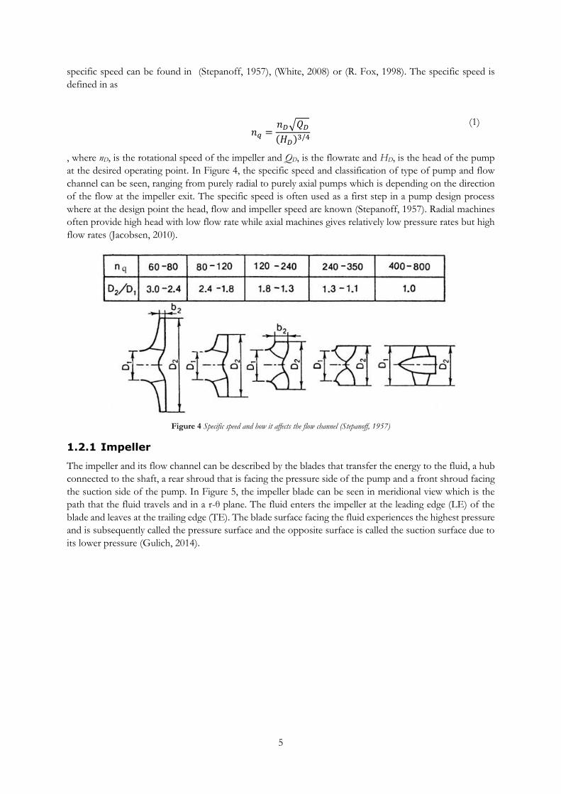
Figure 4 Specific speed and how it affects the flow channel (Stepanoff, 1957) ................................................ 5

Figure 5 Impeller blade in a) Meridional view and b) r-θ plane (Gulich, 2014) ................................................. 6

Figure 6 Difference between a) open and b) closed impeller ............................................................................... 6

Figure 7 Velocity vectors at 1) Inlet and 2) Outlet from the impeller (Jacobsen, 2010) .................................. 7

Figure 8 Velocity triangles related to the blade of the impeller (Jacobsen, 2010) ............................................. 7

Figure 9 Relative eddy in flow channel (Gulich, 2014) .......................................................................................... 8

Figure 10 Outlet velocity vectors with slip (Jacobsen, 2010) ................................................................................ 8

Figure 11 Pre-swirl and its effect on the inlet velocity triangle (Jacobsen, 2010) ............................................. 9

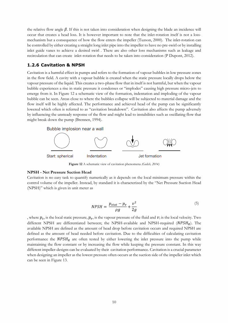
Figure 12 A schematic view of cavitation phenomena (Gulich, 2014) ..............................................................10

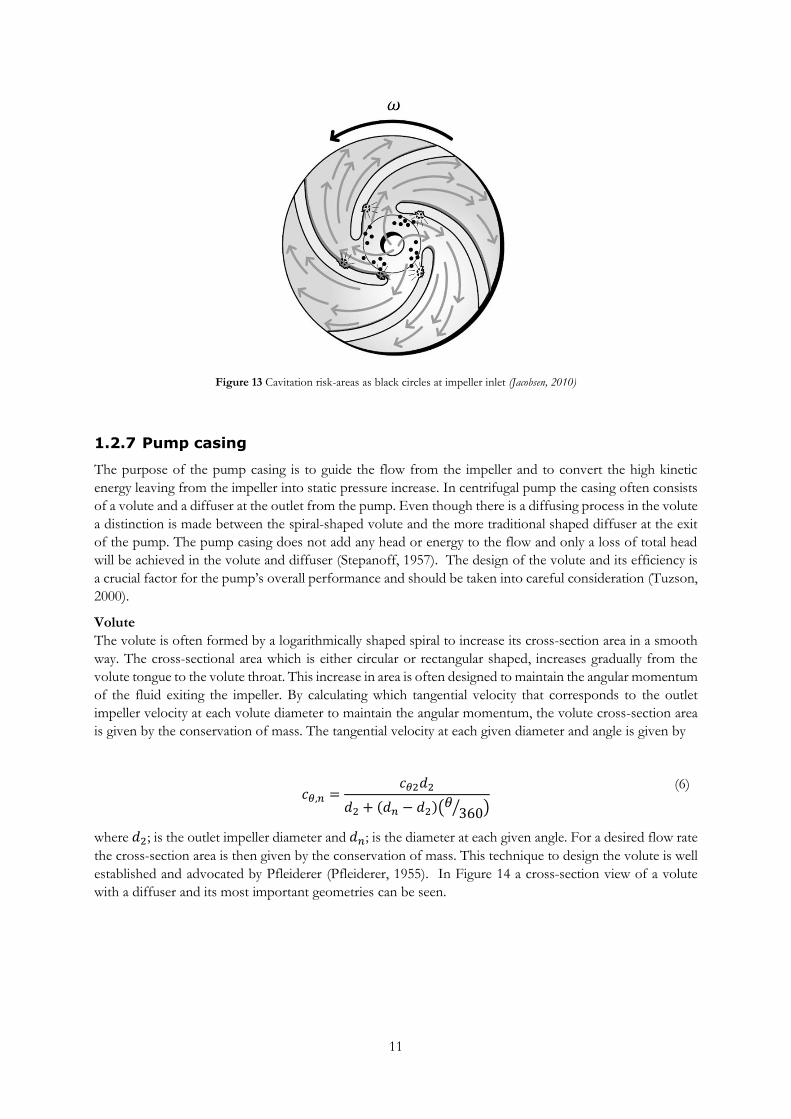
Figure 13 Cavitation risk-areas as black circles at impeller inlet (Jacobsen, 2010) ..........................................11

Figure 14 Cross-section view of the pump casing and its important parts .......................................................12

Figure 15 Idealized pump curve as a function of different blade outlet angles ...............................................13

Figure 16 How the blade outlet angle affects the blade design (Jacobsen, 2010) ............................................13

Figure 17 Pump curve and system curve with the operational point, shut-off point and run-out point.....14

Figure 18 Hydraulic and supplied power (Jacobsen, 2010) .................................................................................15

Figure 19 System curve with marked geodetic head .............................................................................................15

Figure 20 Truck engine with pump highlighted in blue, courtesy of Scania ....................................................16

Figure 21 Exploded view of a typical pump assembly, courtesy of Scania .......................................................17

Figure 22 Cross-section view of an engine cooling pump, courtesy of Scania ................................................17

Figure 23 View of the fluid path in the pump, courtesy of Scania ....................................................................17

Figure 24 Work flow chart .......................................................................................................................................19

Figure 25 Chart over defining loss correlations ....................................................................................................19

Figure 26 The different stages of the pump ..........................................................................................................21

Figure 27 Inlet pump geometry, a) radial, b) semi-axial (Jacobsen, 2010) ........................................................22

Figure 28 The different head losses and difference between Euler head and the pump curve (Jacobsen,

2010) ..............................................................................................................................................................................25

Figure 29 Incidence at leading edge of the blade (Gulich, 2014) .......................................................................27

Figure 30 Incidence model as a parabola (Jacobsen, 2010).................................................................................27

Figure 31 Plot of Incidence loss and incidence as a function of the flowrate ..................................................28

Figure 32 a) Leakage over annular seal in closed impeller, b) Leakage over tip gap in open impeller

(Jacobsen, 2010) ...........................................................................................................................................................29

Figure 33 Recirculation zones in the impeller as a function of the flow rate (A. Predin, 2003) ...................31

Figure 34 Plot of the modelled losses for a reference impeller ..........................................................................32

Figure 35 Volute as a triangle ...................................................................................................................................33

Figure 36 Inlet to volute (Braembussche, 2006) ...................................................................................................34

Figure 37 Defined diameters in volute head loss calculations ............................................................................35

Figure 38 Pressure recovery coefficient .................................................................................................................36

Figure 39 Pump casing losses calculated on reference pump .............................................................................37

Figure 40 Different power curves in a pump (Jacobsen, 2010)..........................................................................38

Figure 41 Power curves from model .......................................................................................................................39

Figure 42 Efficiency curves for a reference pump ...............................................................................................40

Figure 43 Head coefficient as a function of the specific speed calculated from reference impellers ..........42

Figure 44 Hydraulic efficiency as a function of the head coefficient calculated from the reference impellers

........................................................................................................................................................................................42

Figure 45 Flow coefficient out from the impeller as a function of the specific speed calculated on reference

impellers ........................................................................................................................................................................43

Figure 46 Hydraulic efficiency as a function of the flow coefficient calculated from the reference impellers

........................................................................................................................................................................................44

Figure 47 Stepanoff’s constant for diameter ratio curve-fitted ..........................................................................45

Figure 48 How the blade arc is created (Gulich, 2014) .......................................................................................47

Figure 49 A CAD-model of the pump rig .............................................................................................................48

Figure 50 Schematic view of the pump rig ............................................................................................................49

Figure 51 Comparison between calculation model and reference pump 1 at different speeds .....................50

Figure 52 Detailed study on one engine speed, 1400 RPM ................................................................................51

Figure 53 Comparison of calculation model and test data of reference pump 2 on different speeds .........51

Figure 54 Detailed study on one engine speed, 1400 RPM ................................................................................52



Figure 57 Work flow of design process..................................................................................................................55

Figure 58 Plot of modelled pump and efficiency curves for impeller 1 ............................................................56

Figure 59 CAD-model of impeller 1 ......................................................................................................................57

Figure 60 Plot of calculated pump and efficiency curves for impeller 2 ...........................................................57

Figure 61 CAD-model of impeller 2 .......................................................................................................................58

Figure 62 Plot of the calculated and tested pump curve for Impeller 1 ...........................................................59

Figure 63 Detailed comparison of calculated and tested pump curve of impeller 1, engine speed 1200 rpm

........................................................................................................................................................................................60

Figure 64 Plot of the calculated and tested pump curve for Impeller 2 ...........................................................60


........................................................................................................................................................................................61

Figure 66 Plot of the calculation model and CFD result and two engine speeds, 1200 and 1900 rpm .......62

Figure 67 Plot of the calculation model and CFD result at an engine speed of 1200 rpm ............................62

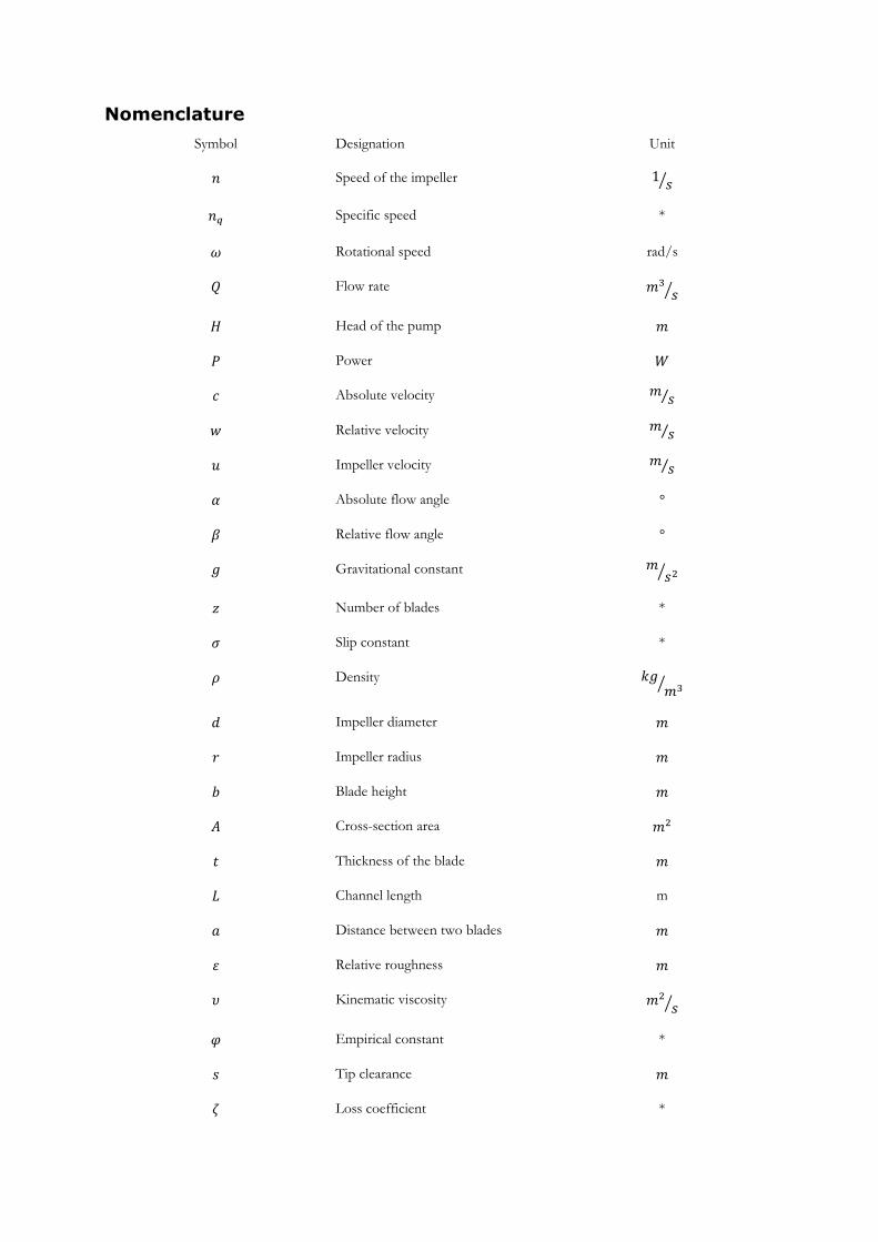
Nomenclature

Symbol Designation Unit

𝑛 Speed of the impeller 1𝑠⁄

𝑛𝑞 Specific speed *

𝜔 Rotational speed rad/s

𝑄 Flow rate 𝑚3

𝑠⁄

𝐻 Head of the pump 𝑚

𝑃 Power 𝑊

𝑐 Absolute velocity 𝑚𝑠⁄

𝑤 Relative velocity 𝑚𝑠⁄

𝑢 Impeller velocity 𝑚𝑠⁄

𝛼 Absolute flow angle °

𝛽 Relative flow angle °

𝑔 Gravitational constant 𝑚𝑠2⁄

𝑧 Number of blades *

𝜎 Slip constant *

𝜌 Density 𝑘𝑔𝑚3⁄

𝑑 Impeller diameter 𝑚

𝑟 Impeller radius 𝑚

𝑏 Blade height 𝑚

𝐴 Cross-section area 𝑚2

𝑡 Thickness of the blade 𝑚

𝐿 Channel length m

𝑎 Distance between two blades 𝑚

𝜀 Relative roughness 𝑚

𝜐 Kinematic viscosity 𝑚2

𝑠⁄

𝜑 Empirical constant *

𝑠 Tip clearance 𝑚

𝜁 Loss coefficient *

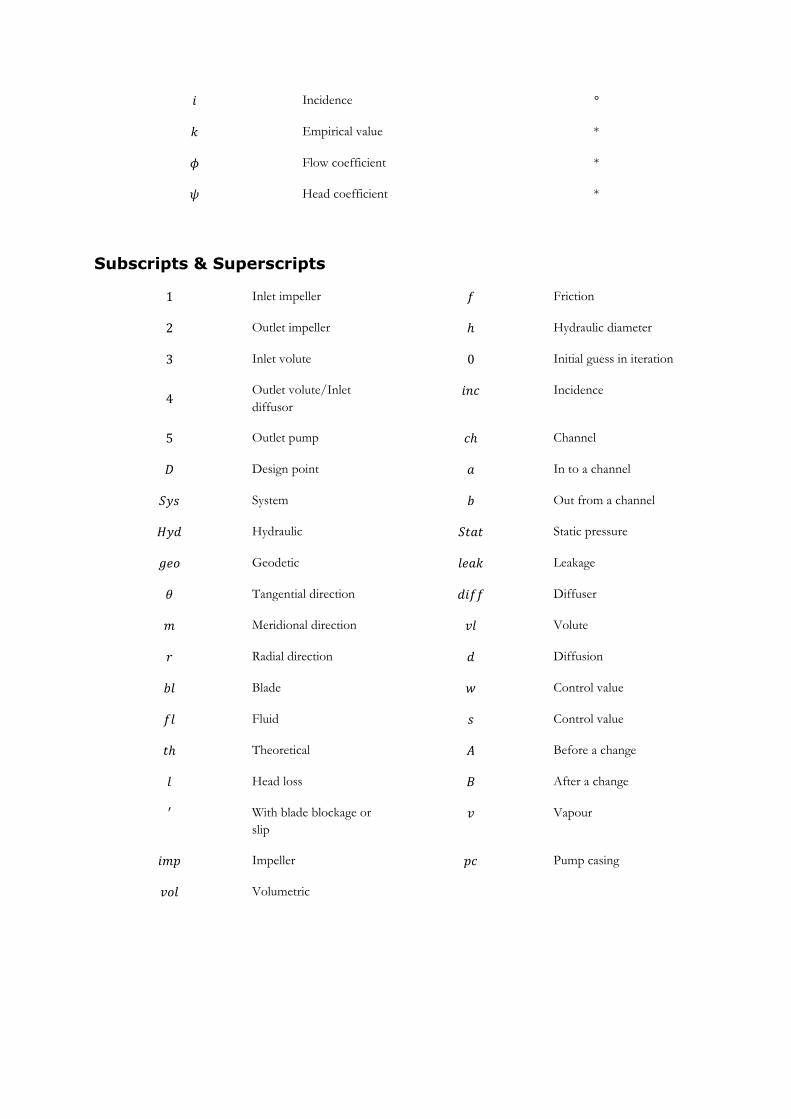
𝑖 Incidence °

𝑘 Empirical value *

𝜙 Flow coefficient *

𝜓 Head coefficient *

Subscripts & Superscripts

1 Inlet impeller 𝑓 Friction

2 Outlet impeller ℎ Hydraulic diameter

3 Inlet volute 0 Initial guess in iteration

4 Outlet volute/Inlet

diffusor

𝑖𝑛𝑐 Incidence

5 Outlet pump 𝑐ℎ Channel

𝐷 Design point 𝑎 In to a channel

𝑆𝑦𝑠 System 𝑏 Out from a channel

𝐻𝑦𝑑 Hydraulic 𝑆𝑡𝑎𝑡 Static pressure

𝑔𝑒𝑜 Geodetic 𝑙𝑒𝑎𝑘 Leakage

𝜃 Tangential direction 𝑑𝑖𝑓𝑓 Diffuser

𝑚 Meridional direction 𝑣𝑙 Volute

𝑟 Radial direction 𝑑 Diffusion

𝑏𝑙 Blade 𝑤 Control value

𝑓𝑙 Fluid 𝑠 Control value

𝑡ℎ Theoretical 𝐴 Before a change

𝑙 Head loss 𝐵 After a change

′ With blade blockage or

slip

𝑣 Vapour

𝑖𝑚𝑝 Impeller 𝑝𝑐 Pump casing

𝑣𝑜𝑙 Volumetric

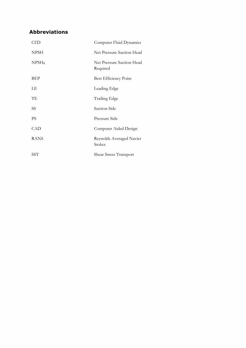
Abbreviations

CFD Computer Fluid Dynamics

NPSH Net Pressure Suction Head

NPSHR Net Pressure Suction Head

Required

BEP Best Efficiency Point

LE Leading Edge

TE Trailing Edge

SS Suction Side

PS Pressure Side

CAD Computer Aided Design

RANS Reynolds Averaged Navier

Stokes

SST Shear Stress Transport

1

1 Introduction

New Euro standards in Europe and corresponding in the US drives forward the development of new

reciprocating internal combustion engines with low emissions. The trend is also that the trailer weight is

increasing which leads to that the customer demands high power engines with good performance and

together with high fuel prices also low fuel consumption (Cipollone, 2013).

A long-term target for 2020 is set for 95 g CO2/km and the distance from the target to the industry is still

significant. Thermal management and optimization of the cooling system have a high cost to benefit ratio

and recent studies have shown that for an automotive car it has an additional cost of 30-40€ per saved

percentage of CO2 and a total of 4-5 g CO2/km. This makes it a suitable area to start to improve to reduce

the emissions and fuel consumption (Cipollone, 2013). The study also concludes that the main interest in

the engine cooling system is to renew standard components such as the water pump, radiator fan and the

thermostat. Proposed alternations to the mechanical water pump are variable-speed pumps, electromagnetic

clutches, driven by electric motors and visco-coolant pumps. All these alternatives need an extensive design-

phase where performance of the pump needs to be matched to the system.

Today the water pumps are often designed with the help of numerical simulations and practical tests and

often external consultants are hired to design the initial impeller and volute design. Computations are costly,

need a large number of flow field evaluations – especially when a large number of design parameters are

involved and when the entire 3D-domain is simulated and calculated (Anagnostopulos, 2009). Today there

is a time-gap between knowing how the system behaves and what the pump will provide due to time-

consuming development with CFD and experimental tests. Therefore a preliminary design tool is needed

to predict how the pump will perform based on pump-geometry and operating conditions that can serve as

an initial result and later be fine-tuned with the aid of CFD and experimental tests. This will save time in

the development process of new engine cooling systems and increase the knowledge of the developer of

how different geometry changes affect the pump performance.

2

Background

To be able to model the pump accurately it is important to understand its boundary conditions and its

interface with the engine. The cooling load and the piping will provide its operating conditions and the

physical limitations of the engine compartment will provide the upper size limit of the pump diameter.

Therefore both how a pump operates and how the engine cooling system is designed will be discussed here.

1.1 Engine cooling system

The engine cooling system have two main functions, the main purpose is to cool the engine parts and

remove that heat during operation since the combustion takes place at temperatures higher than the melting

temperatures of the metal that surrounds it. The other is to heat the engine to working temperature faster

during start-up to improve its efficiency and reduce emissions. The cooling load in the vehicle depends on

which components needs to be cooled but the main cooling is done to the cylinder head (Pang, 2012). The

engine can be both air and liquid cooled where the focus in this report will be on liquid cooled internal

combustion engines for trucks. The engine cooling system was first invented by Karl Benz in 1885 when he

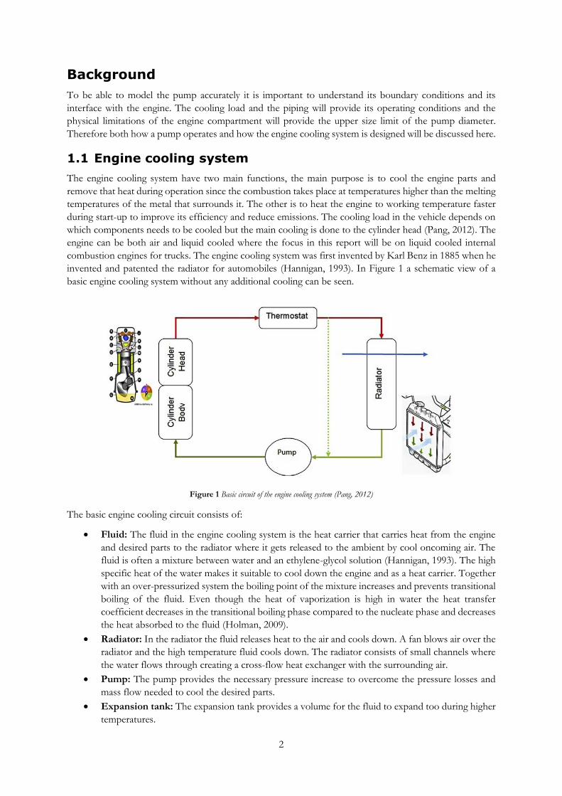
invented and patented the radiator for automobiles (Hannigan, 1993). In Figure 1 a schematic view of a

basic engine cooling system without any additional cooling can be seen.

Figure 1 Basic circuit of the engine cooling system (Pang, 2012)

The basic engine cooling circuit consists of:

Fluid: The fluid in the engine cooling system is the heat carrier that carries heat from the engine

and desired parts to the radiator where it gets released to the ambient by cool oncoming air. The

fluid is often a mixture between water and an ethylene-glycol solution (Hannigan, 1993). The high

specific heat of the water makes it suitable to cool down the engine and as a heat carrier. Together

with an over-pressurized system the boiling point of the mixture increases and prevents transitional

boiling of the fluid. Even though the heat of vaporization is high in water the heat transfer

coefficient decreases in the transitional boiling phase compared to the nucleate phase and decreases

the heat absorbed to the fluid (Holman, 2009).

Radiator: In the radiator the fluid releases heat to the air and cools down. A fan blows air over the

radiator and the high temperature fluid cools down. The radiator consists of small channels where

the water flows through creating a cross-flow heat exchanger with the surrounding air.

Pump: The pump provides the necessary pressure increase to overcome the pressure losses and

mass flow needed to cool the desired parts.

Expansion tank: The expansion tank provides a volume for the fluid to expand too during higher

temperatures.

3

Thermostat: The thermostat regulates when the fluid is released to the radiator for cooling or

when it is kept in a close loop with the engine and pump to heat up the engine quickly. The

thermostat keeps the engine neither too hot nor too cold.

1.1.1 Thermal load

In heavy duty vehicles there are usually several components that need cooling and the thermal load can vary

greatly depending on the configuration. The thermal load refers to the gas temperature and heat flux the

investigated component is exposed for. Modern heavy duty diesel engines often need excessive cooling of

the cylinder head such as brake compressor cooling, cooling of retarder and cooling of EGR. The system

also provides excess heat to the cabin. Turbocharged diesel engines also have a higher cooling need than

diesel engines without turbo installed due to the higher thermal load on the engine (Woodhead, 2011). In

Figure 2 a typical cooling system to a 8 cylinder truck engine can be seen.

Figure 2 A truck engine with the cooling system highlighted, courtesy of Scania

4

1.2 Pumps

A pump is a hydraulic turbomachine that increases the total energy in the fluid by exerting work onto the

fluid by a hydraulic component. The pump is classified depending on how the total energy is transferred

into the fluid such as rotodynamic, displacement and special effects pumps. Rotodynamic pumps have an

open volume that the fluid is transported through and work is done by changing the velocity of the fluid

and is categorized by how the flow channel is diverted such as axial flow, mixed flow and radial or centrifugal

pumps. Displacement pumps have an enclosed volume that exerts work into the fluid by changing the

volume of the fluid and could be reciprocating by a piston or rotary by a vane, screw or gear. Special effects

pumps include ejector or electromagnetic pumps. In this study the focus will be on rotodynamic pumps in

general and centrifugal pumps specifically .

Pumps generally consists of three main parts; the hydraulic unit that is in contact with the fluid, a drive unit

that exerts the work onto the hydraulic component and a sealing that connects the drive unit with the

hydraulic component and prevents water to leak into the drive unit. The hydraulic unit is everything that is

in contact with the fluid within a pump and consists of a rotating part called rotor that changes the velocity

of the fluid and non-rotating parts called diffusers that recover the velocity into static pressure. In centrifugal

pumps the rotor is called an impeller and the pressure recovery unit is called a pump casing with a volute

and diffuser.

Centrifugal pumps

In centrifugal pumps the fluid enters axially into the impeller and exists radially into the volute. The impeller

transfers energy from the motor onto the fluid, accelerates it and redirects it in a circumferential direction

into the volute where the fluids static pressure is recovered. The difference in inlet and outlet diameter

together with a change in blade height creates strong centrifugal forces that imposes the change in total

energy in the fluid by raising the pressure and velocity (Jacobsen, 2010). The outlet often consists of a

diffuser to further recover velocity into pressure. The pump also consists of necessary shaft seals, bearings

and inlet and outlet flanges depending on the design and application. Depending on the application the

centrifugal pump can be either single stage with only one impeller or multistage with several impellers to

further increase the pressure head (Gulich, 2014). In Appendix 1 a figure of a complete traditional single

stage centrifugal pump with all its parts can be seen.

Figure 3 Traditional centrifugal pump with impeller and pump casing (Gulich, 2014)

Specific speed To be able to compare geometrically similar pumps and to classify rotodynamic pumps the specific speed

is derived by a non-dimensional analysis with the Buckingham pi-theorem. A complete derivation of the

5

specific speed can be found in (Stepanoff, 1957), (White, 2008) or (R. Fox, 1998). The specific speed is

defined in as

𝑛𝑞 =

𝑛𝐷√𝑄𝐷(𝐻𝐷)

3/4

(1)

, where nD, is the rotational speed of the impeller and QD, is the flowrate and HD, is the head of the pump

at the desired operating point. In Figure 4, the specific speed and classification of type of pump and flow

channel can be seen, ranging from purely radial to purely axial pumps which is depending on the direction

of the flow at the impeller exit. The specific speed is often used as a first step in a pump design process

where at the design point the head, flow and impeller speed are known (Stepanoff, 1957). Radial machines

often provide high head with low flow rate while axial machines gives relatively low pressure rates but high

flow rates (Jacobsen, 2010).

Figure 4 Specific speed and how it affects the flow channel (Stepanoff, 1957)

1.2.1 Impeller

The impeller and its flow channel can be described by the blades that transfer the energy to the fluid, a hub

connected to the shaft, a rear shroud that is facing the pressure side of the pump and a front shroud facing

the suction side of the pump. In Figure 5, the impeller blade can be seen in meridional view which is the

path that the fluid travels and in a r-θ plane. The fluid enters the impeller at the leading edge (LE) of the

blade and leaves at the trailing edge (TE). The blade surface facing the fluid experiences the highest pressure

and is subsequently called the pressure surface and the opposite surface is called the suction surface due to

its lower pressure (Gulich, 2014).

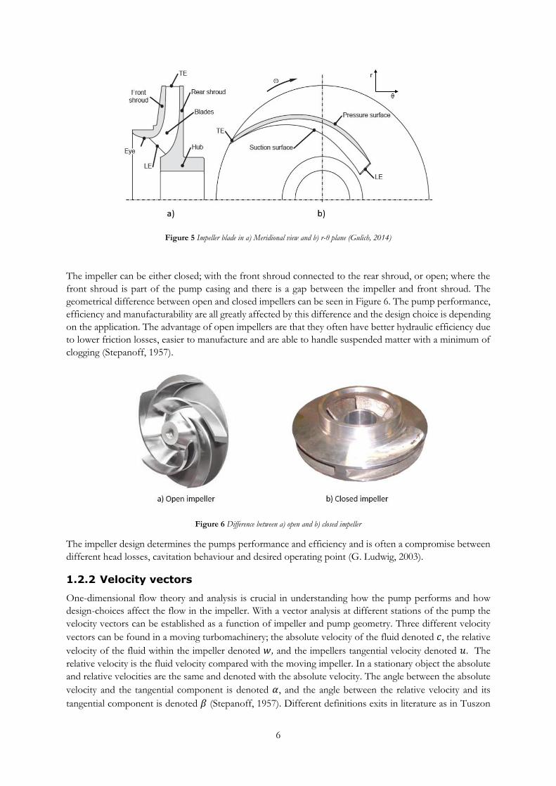
6

Figure 5 Impeller blade in a) Meridional view and b) r-θ plane (Gulich, 2014)

The impeller can be either closed; with the front shroud connected to the rear shroud, or open; where the

front shroud is part of the pump casing and there is a gap between the impeller and front shroud. The

geometrical difference between open and closed impellers can be seen in Figure 6. The pump performance,

efficiency and manufacturability are all greatly affected by this difference and the design choice is depending

on the application. The advantage of open impellers are that they often have better hydraulic efficiency due

to lower friction losses, easier to manufacture and are able to handle suspended matter with a minimum of

clogging (Stepanoff, 1957).

Figure 6 Difference between a) open and b) closed impeller

The impeller design determines the pumps performance and efficiency and is often a compromise between

different head losses, cavitation behaviour and desired operating point (G. Ludwig, 2003).

1.2.2 Velocity vectors

One-dimensional flow theory and analysis is crucial in understanding how the pump performs and how

design-choices affect the flow in the impeller. With a vector analysis at different stations of the pump the

velocity vectors can be established as a function of impeller and pump geometry. Three different velocity

vectors can be found in a moving turbomachinery; the absolute velocity of the fluid denoted 𝑐, the relative

velocity of the fluid within the impeller denoted 𝑤, and the impellers tangential velocity denoted 𝑢. The

relative velocity is the fluid velocity compared with the moving impeller. In a stationary object the absolute

and relative velocities are the same and denoted with the absolute velocity. The angle between the absolute

velocity and the tangential component is denoted 𝛼, and the angle between the relative velocity and its

tangential component is denoted 𝛽 (Stepanoff, 1957). Different definitions exits in literature as in Tuszon

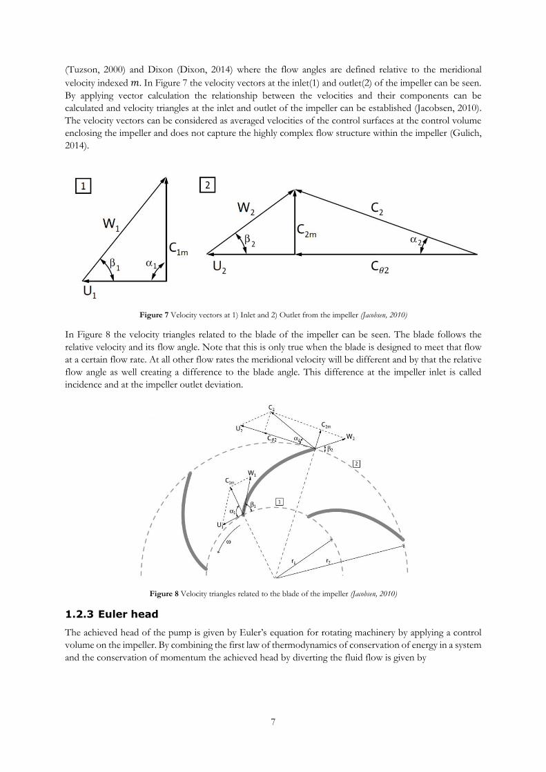
7

(Tuzson, 2000) and Dixon (Dixon, 2014) where the flow angles are defined relative to the meridional

velocity indexed 𝑚. In Figure 7 the velocity vectors at the inlet(1) and outlet(2) of the impeller can be seen.

By applying vector calculation the relationship between the velocities and their components can be

calculated and velocity triangles at the inlet and outlet of the impeller can be established (Jacobsen, 2010).

The velocity vectors can be considered as averaged velocities of the control surfaces at the control volume

enclosing the impeller and does not capture the highly complex flow structure within the impeller (Gulich,

2014).

Figure 7 Velocity vectors at 1) Inlet and 2) Outlet from the impeller (Jacobsen, 2010)

In Figure 8 the velocity triangles related to the blade of the impeller can be seen. The blade follows the

relative velocity and its flow angle. Note that this is only true when the blade is designed to meet that flow

at a certain flow rate. At all other flow rates the meridional velocity will be different and by that the relative

flow angle as well creating a difference to the blade angle. This difference at the impeller inlet is called

incidence and at the impeller outlet deviation.

Figure 8 Velocity triangles related to the blade of the impeller (Jacobsen, 2010)

1.2.3 Euler head

The achieved head of the pump is given by Euler’s equation for rotating machinery by applying a control

volume on the impeller. By combining the first law of thermodynamics of conservation of energy in a system

and the conservation of momentum the achieved head by diverting the fluid flow is given by

8

𝐻𝑡ℎ =

1

𝑔(𝑢2𝑐𝜃2 − 𝑢1𝑐𝜃1)

(2)

, where 𝑢, is the impeller velocity, 𝑐𝜃, is the tangential component of the absolute velocity and 𝑔, is the

gravitational constant. For a complete derivation of Euler’s equation see White (White, 2008) or Dixon

(Dixon, 2014). Equation (2) states that the theoretical achieved head is given by a change in flow velocities

at the impeller inlet and outlet. In ideal conditions with no inlet-rotation at the impeller inlet the fluid enters

radially into the impeller with no tangential component and the theoretical achieved head is only a function

of impeller velocity and absolute tangential component at impeller outlet. In real applications the fluid is

subjected to a number of different losses both hydraulically and mechanically and is always lower than the

theoretically achieved head (Jacobsen, 2010). The head of the pump is often by tradition given in unit meters

from how high a pump would be able to pump a certain volume of water (Stepanoff, 1957).

1.2.4 Slip

The velocity triangles gives the impression that the flow angle and the blade angle are the same, in reality

however the flow angle usually deviates with a flow angle smaller than the blade angle. This due to the fact

of a relative eddy imposed in the blade channel between the suction and pressure side of the blade with the

same angular velocity as the impeller but counter-rotating. The concept of a relative eddy is illustrated in

Figure 9.

Figure 9 Relative eddy in flow channel (Gulich, 2014)

At the impeller outlet the relative flow velocity 𝑤2, can then be considered as a flow with the relative eddy

superimposed. The effect is a change of the relative flow and in a direction opposite to the impeller motion

that is expressed with a slip factor. In Figure 10, the velocity vectors at the impeller outlet can be seen with

a reduction of the absolute tangential component due to the slip factor.

Figure 10 Outlet velocity vectors with slip (Jacobsen, 2010)

A review of the different methods to account for the slip factor with correlation to test-data is done by

Weisner (Weisner, 1967), which found that correlations corresponds very well and proposed an empirical

9

expression as a function of the outlet blade angle 𝛽2, and the number of blades 𝑧. The expression is given

in (3) as

𝜎 = 1 −

sin𝛽2𝑧0,7

(3)

The expression in (3) is well established in both industry and in academic work and has proven to be reliable

to account for the deviation by the blades (Tuzson, 2000), (El-Naggar, 2013). The equation also states that

with an infinite number of blades the flow angle would be identical with the blade angle. However, in reality

finite number of blades with a finite thickness will impose an eddy in the blade channel. It is important to

note that slip is not a loss mechanism but a function of how the fluid is deflected by the blade (Gulich,

2014).

1.2.5 Inlet-rotation

If the flow enters the impeller without any disturbances the flow will ideally have no swirl and an absolute

inlet flow angle of 𝛼 = 90°, leading to an absolute tangential velocity component of zero. According to

Euler’s equation at (4) the equation will be reduced to

𝐻𝑡ℎ =

𝑢2𝑐𝜃2𝑔

(4)

where the head only is affected by the outlet impeller velocity and outlet swirl (Jacobsen, 2010). However,

in reality it is very rare to have such a situation and should more be seen as an initial first guess at what head

the impeller design will theoretically achieve. In a 1D-analysis of the flow at the impeller inlet there can be

three conditions: no swirl, co-rotation - where the fluid has a pre-rotation at the same direction as the

impeller and counter-rotation, where the fluid is rotating against the rotation of the impeller. According to

Euler’s equation at (2) the inlet swirl will affect the theoretical achieved head in a positive or negative way

depending on its direction of rotation. A study of how the inlet-rotation affects the inlet velocity triangle

can be seen in Figure 11.

Figure 11 Pre-swirl and its effect on the inlet velocity triangle (Jacobsen, 2010)

The rotation velocity of the impeller, 𝑢1, and the meridionial velocity, 𝑐𝑚1, stays the same in all cases.

Depending on if the absolute inlet flow angle, 𝛼, is separated from 90° a tangential component will occur.

According to Euler’s equation at (2) a co-rotation flow will lower the achieved head and a counter-rotating

flow will create a higher achieved head. However, since the flow is three-dimensional and viscous such

assumptions may not always hold in reality. In Figure 11 it can also be seen that the inlet-rotation also affects

10

the relative flow angle 𝛽. If this is not taken into consideration when designing the blade an incidence will

occur that creates a head loss. It is however important to note that the inlet-rotation itself is not a loss-

mechanism but a consequence of how the flow enters the impeller (Tuzson, 2000). The inlet-rotation can

be controlled by either creating a straight long inlet pipe into the impeller to have no pre-swirl or by installing

inlet guide vanes to achieve a desired swirl . There are also other loss mechanisms such as leakage and

recirculation that can create inlet-rotation that needs to be taken into consideration (P Dupont, 2012).

1.2.6 Cavitation & NPSH

Cavitation is a harmful effect in pumps and refers to the formation of vapour bubbles in low pressure zones

in the flow field. A cavity with a vapour bubble is created when the static pressure locally drops below the

vapour pressure of the liquid. This creates a two-phase flow that in itself is not harmful, but when the vapour

bubble experiences a rise in static pressure it condenses or “implodes” causing high pressure micro-jets to

emerge from it. In Figure 12 a schematic view of the formation, indentation and imploding of the vapour

bubble can be seen. Areas close to where the bubbles collapse will be subjected to material damage and the

flow itself will be highly affected. The performance and achieved head of the pump can be significantly

lowered which often is referred to as “cavitation breakdown”. Cavitation also affects the pump adversely

by influencing the unsteady response of the flow and might lead to instabilities such as oscillating flow that

might break down the pump (Brennen, 1994).

Figure 12 A schematic view of cavitation phenomena (Gulich, 2014)

NPSH - Net Pressure Suction Head

Cavitation is no easy task to quantify numerically as it depends on the local minimum pressure within the

control volume of the impeller. Instead, by standard it is characterized by the “Net Pressure Suction Head

(NPSH)” which is given in unit meter as

𝑁𝑃𝑆𝐻 =

𝑝𝑠𝑡𝑎𝑡 − 𝑝𝑣𝜌𝑔

+𝑣2

2𝑔

(5)

, where 𝑝𝑠, is the local static pressure, 𝑝𝑣 , is the vapour pressure of the fluid and 𝑣; is the local velocity. Two

different NPSH are differentiated between; the NPSH-available and NPSH-required (𝑁𝑃𝑆𝐻𝑅). The

available NPSH are defined as the amount of head drop before cavitation occurs and required NPSH are

defined as the amount of head needed before cavitation. Due to the difficulties of calculating cavitation

performance the 𝑁𝑃𝑆𝐻𝑅 are often tested by either lowering the inlet pressure into the pump while

maintaining the flow constant or by increasing the flow while keeping the pressure constant. In this way

different impeller-designs can be evaluated by their cavitation performance. Cavitation is a crucial parameter

when designing an impeller as the lowest pressure often occurs at the suction side of the impeller inlet which

can be seen in Figure 13.

11

Figure 13 Cavitation risk-areas as black circles at impeller inlet (Jacobsen, 2010)

1.2.7 Pump casing

The purpose of the pump casing is to guide the flow from the impeller and to convert the high kinetic

energy leaving from the impeller into static pressure increase. In centrifugal pump the casing often consists

of a volute and a diffuser at the outlet from the pump. Even though there is a diffusing process in the volute

a distinction is made between the spiral-shaped volute and the more traditional shaped diffuser at the exit

of the pump. The pump casing does not add any head or energy to the flow and only a loss of total head

will be achieved in the volute and diffuser (Stepanoff, 1957). The design of the volute and its efficiency is

a crucial factor for the pump’s overall performance and should be taken into careful consideration (Tuzson,

2000).

Volute

The volute is often formed by a logarithmically shaped spiral to increase its cross-section area in a smooth

way. The cross-sectional area which is either circular or rectangular shaped, increases gradually from the

volute tongue to the volute throat. This increase in area is often designed to maintain the angular momentum

of the fluid exiting the impeller. By calculating which tangential velocity that corresponds to the outlet

impeller velocity at each volute diameter to maintain the angular momentum, the volute cross-section area

is given by the conservation of mass. The tangential velocity at each given diameter and angle is given by

𝑐𝜃,𝑛 =

𝑐𝜃2𝑑2

𝑑2 + (𝑑𝑛 − 𝑑2)(𝜃360⁄ )

(6)

where 𝑑2; is the outlet impeller diameter and 𝑑𝑛; is the diameter at each given angle. For a desired flow rate

the cross-section area is then given by the conservation of mass. This technique to design the volute is well

established and advocated by Pfleiderer (Pfleiderer, 1955). In Figure 14 a cross-section view of a volute

with a diffuser and its most important geometries can be seen.

12

Figure 14 Cross-section view of the pump casing and its important parts

An important parameter when designing the volute is the tongue distance – the distance between the outlet

impeller diameter and the diameter circling the tongue. Studies have shown that smaller tongue distances

increases the volute efficiency and prevents the fluid from re-circling into the volute again (Alenius, 2001).

Diffuser

The diffuser in the pump casing is there to further lower the velocity of the fluid and raise the static pressure

to increase the efficiency of the pump. The diffuser has at a certain maximum angle so that flow losses due

to separation and mixing losses are kept small (R. Fox, 1998). This angle depends on the area ratio and

length of the diffuser (White, 2008).

1.2.8 Bearings and seals

Important mechanical parts to consider that affects the overall pump efficiency are the different seals such

as the shaft seal, inlet wear ring and bearings to the shaft. Depending on drive-unit the pump might also

have a coupling or gear that provides a mechanical loss. The inlet wear ring is a seal that prevents backflow

from the pressure-side of the impeller blade to the suction side. Leakage is a loss mechanism that greatly

affects the performance of the pump by reducing the achieved head and lowers the volumetric efficiency.

The shaft seal prevents the liquid to escape from the pump into the drive unit or outside of the pump

depending on the application and design (Tuzson, 2000). The mechanical loss in pumps can be considered

as parasitic losses and are constant over the flow span of the pump and added as a loss in efficiency to the

total efficiency of the pump (Jacobsen, 2010). Even though the machine design of these components does

not affect the hydraulic efficiency of the pump they need to be taken in careful consideration to achieve a

stable and safe operation of the pump (Turton, 1994). In Appendix 1 a cross-section figure of a traditional

centrifugal pump with both hydraulic and mechanical parts can be seen.

1.2.9 Pump curve

The pump curve is a way to graphically view how the pump behaves at a certain flowrate and pressure

increase. An idealized pump curve is a function of the main impeller geometry parameters such as outlet

blade angle, 𝛽2, outlet diameter; 𝑑2, as well as the outlet blade height; 𝑏2. Utilizing vector algebra from the

velocity triangles in combination with the mass conservation law, Euler’s equation (2) with no inlet-rotation

can be re-written as

𝐻𝑡ℎ =𝑢22

𝑔−

𝑢2𝜋𝑑2𝑏2𝑔𝑡𝑎𝑛𝛽2

(7)

13

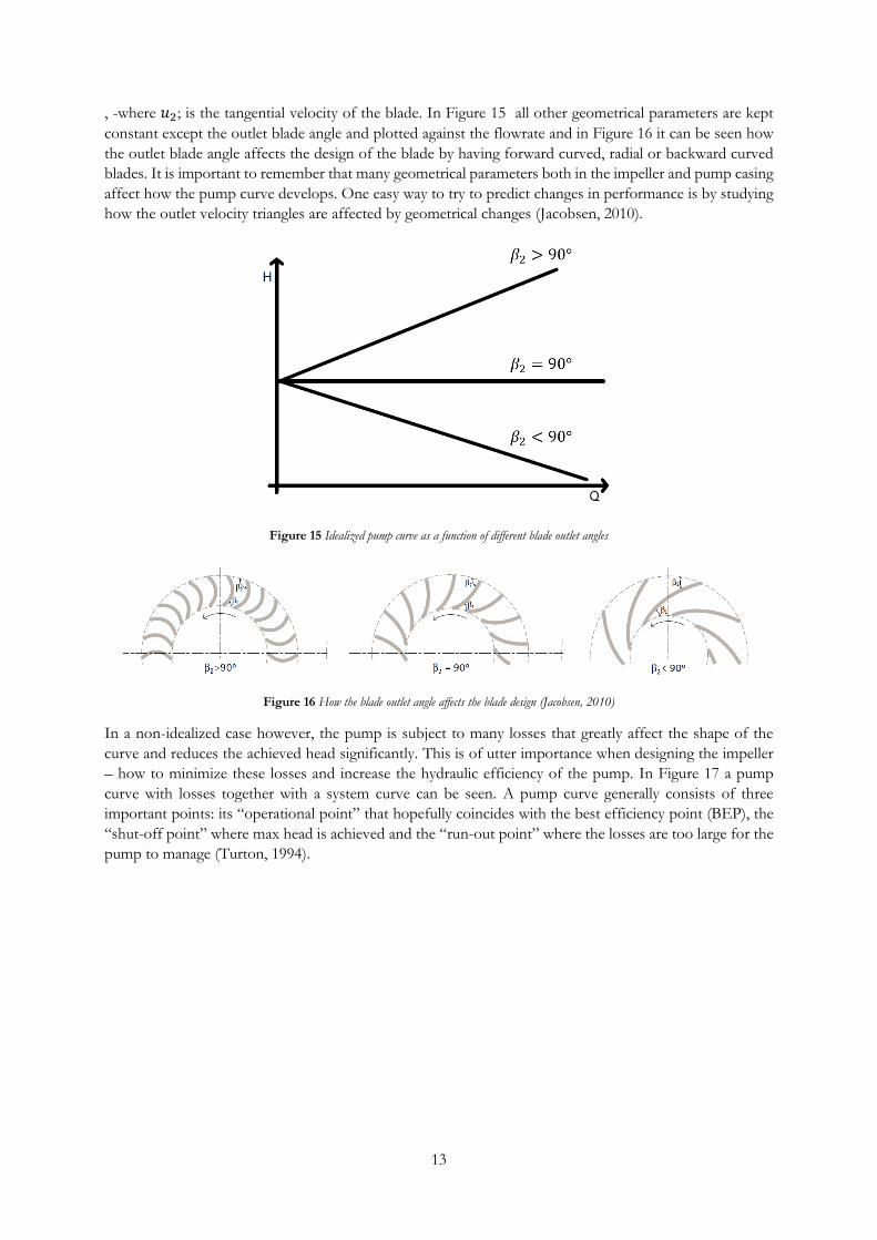
, -where 𝑢2; is the tangential velocity of the blade. In Figure 15 all other geometrical parameters are kept

constant except the outlet blade angle and plotted against the flowrate and in Figure 16 it can be seen how

the outlet blade angle affects the design of the blade by having forward curved, radial or backward curved

blades. It is important to remember that many geometrical parameters both in the impeller and pump casing

affect how the pump curve develops. One easy way to try to predict changes in performance is by studying

how the outlet velocity triangles are affected by geometrical changes (Jacobsen, 2010).

Figure 15 Idealized pump curve as a function of different blade outlet angles

Figure 16 How the blade outlet angle affects the blade design (Jacobsen, 2010)

In a non-idealized case however, the pump is subject to many losses that greatly affect the shape of the

curve and reduces the achieved head significantly. This is of utter importance when designing the impeller

– how to minimize these losses and increase the hydraulic efficiency of the pump. In Figure 17 a pump

curve with losses together with a system curve can be seen. A pump curve generally consists of three

important points: its “operational point” that hopefully coincides with the best efficiency point (BEP), the

“shut-off point” where max head is achieved and the “run-out point” where the losses are too large for the

pump to manage (Turton, 1994).

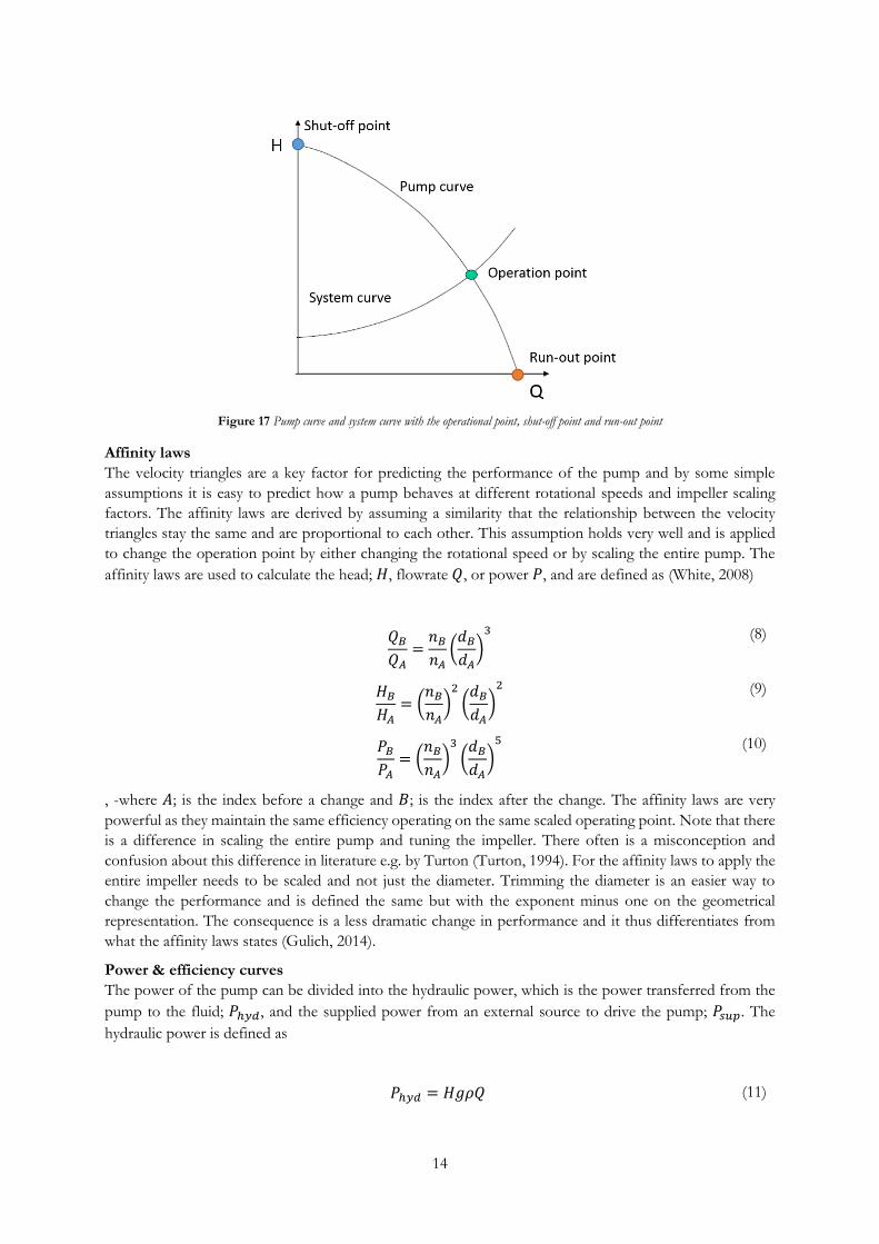
14

Figure 17 Pump curve and system curve with the operational point, shut-off point and run-out point

Affinity laws

The velocity triangles are a key factor for predicting the performance of the pump and by some simple

assumptions it is easy to predict how a pump behaves at different rotational speeds and impeller scaling

factors. The affinity laws are derived by assuming a similarity that the relationship between the velocity

triangles stay the same and are proportional to each other. This assumption holds very well and is applied

to change the operation point by either changing the rotational speed or by scaling the entire pump. The

affinity laws are used to calculate the head; 𝐻, flowrate 𝑄, or power 𝑃, and are defined as (White, 2008)

𝑄𝐵𝑄𝐴

=𝑛𝐵𝑛𝐴

(𝑑𝐵𝑑𝐴)3

(8)

𝐻𝐵

𝐻𝐴= (

𝑛𝐵𝑛𝐴)2

(𝑑𝐵𝑑𝐴)2

(9)

𝑃𝐵𝑃𝐴

= (𝑛𝐵𝑛𝐴)3

(𝑑𝐵𝑑𝐴)5

(10)

, -where 𝐴; is the index before a change and 𝐵; is the index after the change. The affinity laws are very

powerful as they maintain the same efficiency operating on the same scaled operating point. Note that there

is a difference in scaling the entire pump and tuning the impeller. There often is a misconception and

confusion about this difference in literature e.g. by Turton (Turton, 1994). For the affinity laws to apply the

entire impeller needs to be scaled and not just the diameter. Trimming the diameter is an easier way to

change the performance and is defined the same but with the exponent minus one on the geometrical

representation. The consequence is a less dramatic change in performance and it thus differentiates from

what the affinity laws states (Gulich, 2014).

Power & efficiency curves

The power of the pump can be divided into the hydraulic power, which is the power transferred from the

pump to the fluid; 𝑃ℎ𝑦𝑑, and the supplied power from an external source to drive the pump; 𝑃𝑠𝑢𝑝. The

hydraulic power is defined as

𝑃ℎ𝑦𝑑 = 𝐻𝑔𝜌𝑄 (11)

15

which is always smaller than the supplied power (R. Fox, 1998). Equation (11) states that the power increases

with the flow rate and in Figure 18 a trend plot of typical hydraulic and supplied power can be seen. The

supplied power both consist of the power needed to drive the shaft with its mechanical losses and the power

transferred to the fluid from the impeller.

Figure 18 Hydraulic and supplied power (Jacobsen, 2010)

The efficiency of the pump can consequently be divided into the hydraulic efficiency, mechanical efficiency

and the total efficiency and is defined as the ratio between the previous stated power values. Pumps are

often designed to operate at its best efficiency point (BEP) and one of the challenges in pump design is to

match the demanded operating point and the pumps BEP (G. Ludwig, 2003).

1.2.10 System curve

The system curve can be defined as the total amount of pressure increase the system needs to overcome at

each given flow rate. By dividing it into a pressure, velocity, static head and loss components it can be

defined in unit meters as

𝐻𝑠𝑦𝑠 =

∆𝑝

𝜌𝑔+𝑣𝐵2 − 𝑣𝐴

2

𝜌𝑔+ ∆ℎ + 𝐻𝑙

(12)

, - where ∆ℎ; is the geodetic head, 𝐻𝑔𝑒𝑜, which is the actual physical height that the pump need to transport

water, and 𝐻𝑙, is all the losses in the system that the pump needs to overcome. By examining an arbitrary

system curve in Figure 19 it clearly shows a constant geodetic head over the flow span and an increasing

head as the losses rise with the velocity of the fluid. The system curve can be altered by changing the pipe

diameter or installing throttling valves (Turton, 1994).

Figure 19 System curve with marked geodetic head

16

1.2.11 Pumps in engine cooling system

The engine cooling pump is normally installed and mounted on the engine with a pulley connected to the

drive shaft with a fixed ratio belt (S. Zoz, 2001). In Figure 20 a complete truck engine with the pump

highlighted in blue can be seen illustrating the complex interface to the engine.

Figure 20 Truck engine with pump highlighted in blue, courtesy of Scania

The pump in an engine cooling system is limited to a number of different factors in no subsequent order

that affects its design (S. Zoz, 2001):

Performance - the pump shall provide the necessary flow rate at different shaft speeds

Efficiency – every percent of efficiency gained directly affects fuel consumption

Cost – low cost is important when manufacturing large volumes

Robustness – reliability across the flow span and during cold starts

Volume – Often the pump has strict physical volume limitations

Interface to engine – the boundary to the engine is often fixed regarding inlet and outlet to the

pump

A common design philosophy in the industry is to use a centrifugal pump that is over-sized to compensate

for design changes in the system layout where the cooling need increases. This often leads to unnecessary

power consumption from the engine and consumes more physical volume (S. Zoz, 2001). Since the pump

is driven directly by the shaft of the engine by a pulley, unnecessary flow rate and power consumption might

occur depending on the speed of the shaft. New designs try to solve this problem by installing a clutch e.g.

visco-clutch or an electromechanical clutch (Y. Shin, 2013). A design variation recently adopted when

manufacturability issues have been resolved is closed impellers where an outer shroud is designed to prevent

tip leakage (see 1.2.1). However, leakage will instead occur between the front shroud and casing and the

wetted surface of the impeller will increase and by that the friction loss. This leads to that it is a design

choice of which loss is most significant and the designer wish to decrease (Stepanoff, 1957).

1.2.12 Case of Reference engine

The reference engine’s cooling pump is a centrifugal pump mounted on the engine with a pulley connected

with a belt to the drive shaft. Depending on the engine platform, – straight or v-type engine, – and of the

cooling load needed from the system, different configurations exits. Often the design of the impeller is

varied to account for different performance steps and the pump casing is constant across an engine platform.

This is an easy way to vary the operational point on the system curve even though a mismatch between

impeller and volute can introduce additional losses (Alenius, 2001). In Figure 21 an exploded view of a

17

typical engine cooling pump can be seen with all its components. This is a typical pump for trucks with a 6-

bladed open impeller and the inlet and volute incorporated within the pump house and lid. In Figure 22 a

cross-section view of the pump can be seen.

Figure 21 Exploded view of a typical pump assembly, courtesy of Scania

Figure 22 Cross-section view of an engine cooling pump, courtesy of Scania

In Figure 23 the fluid volume of a pump can be seen which clearly illustrates one of the many challenges

when designing an engine cooling pump with its interface to the engine and its sharp bends.

Figure 23 View of the fluid path in the pump, courtesy of Scania

Seal

Pulley

Lid

Bearing

Impeller

Gasket

Pump house

Pump lid

18

2 Delimitations

In order to develop the model limitations to both the system and pump are applied in this study.

2.1.1 In system design

The system will be modelled with a system curve where a specific operating point is specified based on

rotational speed of the shaft, flow-rate to achieve desired cooling and increased pressure head by the pump

that is applied to a truck. To account for different shaft speeds the rotational speed of the shaft will be

changed from 1000 RPM up to 2000 RPM. The system is assumed to be in nominal conditions and fully

pressurized. The flow-rates investigated will range from 50 – 1000 l/min as this corresponds to operating

conditions for an engine cooling pump. The system will be modelled based on pure water and with no

density fluctuations due to temperature changes.

2.1.2 In pump design

The fluid flow in the pump with impeller including hub and blades together with the volute will be modelled

in 1D. Hydraulic losses will be accounted for and based on the geometry present in the pump. Mechanical

losses will not be modelled as they can be assumed to be constant across the flow span. The blade will be

modelled with an inlet and outlet metal-angle and the blade thickness will be assumed to be evenly

distributed across the cord and blade height. The blade metal angles will be assumed to be constant across

the blade height. Numerical calculations will be done on steady-state conditions with only the rotor due to

limitations in academic licenses.

3 Objectives

The objective of this work is to develop and validate a quasi 1D model that analysis the pump impeller and

volute. The model will provide a tool that can evaluate changes in pump geometry and how they affect the

pump performance. In order to improve and establish the models accuracy the result will be compared and

correlated to experimental tests and numerical calculations. This can be expressed in a main and sub-

objective below as:

Main objective: To design a calculation model based on impeller and volute geometry that

provides a pump curve for desired flow capacities including the main flow losses occurring within

the pump.

Sub objective: Based on the calculation model, produce a design tool and procedure that suggests

suitable impeller main geometry parameters to achieve a desired operating point.

The objectives can be summarized into a list of input and output data of the model which can be seen in

Table 1.

Table 1 Input and output data from the model and design tool

Main objective: Calculation model

INPUT OUTPUT

Pump geometry Pump curve

Power curve

Efficiency curve

Sub objective: Design tool

Operating point Main impeller geometry parameters

19

4 Methodology

The work can be divided into several steps and a flow chart of the overall process can be seen in Figure 24.

A calculation model will be developed to predict the achived head and flow based on impeller and volute

geometry. By using this model a new impeller design can be developed and by rapid prototyping a protype

can be produced to test the accuracy of the model. By doing an experimental test in a pump rig a pump

curve will be achieved based on real data. The new geometry will also be used to do a numerical simulation

in a CFD software at some desired operating conditions. With the result from the experimental test and the

numerical solution the accuracy of the developed model can be evaluated.

Figure 24 Work flow chart

The flow inside the pump is affected by different hydraulic and mechanical losses which are hard to calculate

accurately. Normally these losses and how they affect the performance of the pump are highly indivudal for

each pump or type of pump. To be able to model these losses they will be correlated to previous reference

test data acquired available on existing pumps referred to as reference pumps. By inserting the geometry of

an existing pump and comparing the theoretical Euler head with test result, total losses at each operating

point can be established. By modelling the different losses seperately using developed methods from

litterature, correlations for the real losses can be established by comparing to the test data. The process of

finding these loss correlations can be seen in Figure 25.

Figure 25 Chart over defining loss correlations

The geometry on existing pumps (reference pumps) is taken from Catia v5 CAD-models and hydraulic

diameters in volute and diffusor are calculated with Gem GT-Suite.

ModelExperimental

testNumerical simulation

Analysis Result

Compare with test

data

Euler head

Add hydraulic

losses

Calculate efficiency

and power

Modify correlations

20

4.1 Numerical method

CFD calculations are done on impellers to compare hydraulic losses to the calculation model. The program

platform used is an academic license of ANSYS®, Release 15. The license has a limitation on number of

nodes calculated to 521 000. Due to this limitation and limitations in computational power, only steady-

state analysis is done. New impeller designs are created within the software to calculate its achieved head to

compare to the calculation model. ANSYS Workbench is used to setup the connection between the different

programs. The numerical method can be divided into three phases; a pre-processing phase, a calculation

phase and a post-processing phase.

4.1.1 Pre-processing

Impeller main geometry parameters are created with the ANSYS®, Vista CPD software where impeller flow

channel can be determined. The impeller geometry is then exported with ANSYS®, Design Modeller to the

grid-generation software for turbomachinery ANSYS®, Turbogrid. An automatic grid generation is applied

with tetrahedral and hexa-elements. The boundary layers are captured with a y+-model based on the

Reynolds number (ANSYS, 2013).

4.1.2 Calculation

The numerical calculation is done with the ANSYS®, CFX-solver where the problem is defined in CFX-

Pre. Due to limitations in license and computational power, the problem is restricted to one flow channel

with periodic interfaces to adjacent blades. The problem is defined as steady-state with a stage interface to

the outlet. To simulate rotating machinery, the stage interface calculates with averaged variables across the

outlet boundary to simulate a rotation. The other option in steady-state simulations is to use frozen-rotor

interface where the instantaneous position of the blade is calculated with. Since the overall performance of

the impeller is of interest, the stage interface is used. The turbulence is modelled with a RANS eddy-viscosity

model where the SST model is applied. The SST model is more suitable than k-ε or 𝑘 − 𝜔 models to

capture the effects of separation in turbomachinery (ANSYS, 2015).

4.1.3 Post-processing

The problem is analysed in ANSYS® CFX-Post where necessary data is acquired. Mass flow averaged values

of total pressure is taken from the impeller inlet and outlet.

4.2 Reference pumps

Four different reference impellers in combination with two different pump casings are used to correlate

previous test data with the model. The different impellers in one pump casing is due to different power

demands from the cooling system and subsequently needs a different operating point from the pump. The

necessary geometry parameters needed for the calculation model discussed in chapter 5 are taken from the

reference pumps which then can be modelled and compared to previous test data. In Table 2 the

configuration of the different reference pumps are seen. The geometrical characteristics of the different

reference impellers are distinguished by two dimensionless ratios and the blade angle difference as: inlet to

outlet diameter d1/d2, inlet to outlet blade height b1/b2 and blade angle difference from inlet to outlet as ∆𝛽.

Table 2 Configuration of the different reference pumps

Name Impeller d1/d2 b1/b2 |∆𝛽| Pump casing

Reference 1 Impeller 1 0.52 2.31 36 Pump casing 1




21

5 Modelling

The pump performance is modelled with quasi 1D calculations by calculating the theoretical achieved head

by Euler’s equation in (2) and deducting the modelled flow losses in the pump. The achieved head can then

be expressed as

𝐻 = 𝐻𝑡ℎ −𝐻𝑙 (13)

, -where the flow losses 𝐻𝑙, includes the losses both in the impeller and the pump casing. As the head is a

function of the flowrate 𝑄, the theoretical achieved head and hydraulic losses need to be calculated at a flow

span to depict the performance of the pump. The model then predicts the achieved head at a given flowrate

which is in contrast with an experimental test where a valve often is used to create a pressure resistance and

the achieved flowrate then can be measured (Gulich, 2014). This section will describe the entire calculation

model on how the pump performance is calculated and how the flow losses are modelled as a function of

the flowrate. In section 5.1 to 5.4 it is shown how the velocity vectors are calculated from the pump

geometry and flow rate and in section 5.3 to 5.4 all the losses in the pump are modelled as a function of

pump geometry and flow rate. Finally how the estimated power and efficiency of the pump are modelled is

discussed in section 5.5.

5.1 Pump geometry

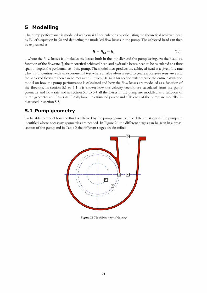
To be able to model how the fluid is affected by the pump geometry, five different stages of the pump are

identified where necessary geometries are needed. In Figure 26 the different stages can be seen in a cross-

section of the pump and in Table 3 the different stages are described.

Figure 26 The different stages of the pump

22

Table 3 Different stages of the pump

Stage Description

1 Inlet impeller

2 Outlet impeller

3 Inlet volute

4 Outlet volute/Inlet diffusor

5 Outlet pump

5.2 Impeller

The impeller adds energy to the fluid and creates the total pressure increase and the geometry of the impeller

is of great importance of how the pump performs. In quasi 1D calculations the performance of the pump

depends on Euler’s equation which once again will be stated as

𝐻𝑡ℎ =

1

𝑔(𝑢2𝑐𝜃2 − 𝑢1𝑐𝜃1)

(14)

The main impeller geometry parameters are the inlet and outlet diameters, blade height and the blade angles.

These greatly affects the velocity triangles and by that the theoretical achieved head in Euler’s equation.

Equation (7) showed a rewriting of Euler’s equation in an idealized case with no inlet rotation. However,

the model needs to account for inlet rotation so the original form of Euler’s equation in equation (14) will

here be used.

5.2.1 Impeller inlet

The area at the inlet of the impeller depends on if it is completely radial or has a semi-axial inlet. In Figure

27 a), a radial inlet and in b), a semi-axial inlet can be seen.

Figure 27 Inlet pump geometry, a) radial, b) semi-axial (Jacobsen, 2010)

23

With a completely radial inlet the area is expressed as the product of the circumference at inlet and the blade

height as

𝐴1 = 𝜋𝑑1𝑏1 (15)

, - where 𝑑1; is the impeller inlet diameter and 𝑏1; is the inlet blade height. With semi-axial inlet the area is

expressed similarly but with the diameter expressed as an average between the hub and shroud diameters

as

𝐴1 = 𝜋 (

𝑑ℎ𝑢𝑏1 + 𝑑𝑠ℎ𝑟𝑜𝑢𝑑12

)𝑏1 (16)

The entire flow must pass through this area and by using the equation for conservation of mass for

incompressible flow the meridional velocity at the inlet can be expressed as

𝑐𝑚1 =

𝑄

𝐴1

(17)

, which is the velocity of the fluid approaching the impeller. At the impeller the fluid is blocked by the blades

and to calculate the velocity just inside the impeller a new area needs to be calculated where the area blocked

by the blades is deducted. The new area can be expressed as

𝐴′1 = 𝐴1 − 𝑡𝑧𝑏1 (18)

, - where 𝑡; is the thickness of the blade and 𝑧; is the number of blades. The meridional velocity entering

the impeller is the defined by the conservation of mass as

𝑐𝑚1 =

𝑄

𝐴′1

(19)

The tangential velocity of the impeller is expressed as the product of the radius and the rotational speed of

the impeller as

𝑢1 =

𝑑12𝜔 =𝑟1

2𝜋𝑛

60

(20)

, - where 𝑛; is the speed of the impeller. By using vector calculations and trigonometry on the inlet vector

triangle described in section 1.2.2 all the velocity components can be calculated. The absolute tangential

component 𝑐𝜃1, is as a function of the absolute flow angle 𝛼, and the meridional component as

𝑐𝜃1 =𝑐𝑚1

tan𝛼1

(21)

As previously discussed in section 1.2.5 the absolute flow angle at the inlet is in an undisturbed flow field

90° to the tangential plane, which renders that equation (21) equals to zero. In the model the absolute inflow

angle is an input parameter and thereby a design choice of the model. When the tangential component is

calculated the absolute velocity can then be calculated as

𝑐1 = √𝑐𝑚1

2 + 𝑐𝜃12

(22)

The relative tangential component can by using vector addition of the other tangential components be

expressed as

𝑤𝜃1 = 𝑢1 −𝑐𝜃1 (23)

24

According to the inlet velocity triangle the absolute and relative meridional velocities are the same which

gives that the relative velocity can be expressed as

𝑤1 = √𝑐𝑚1

2 +𝑤𝜃2

(24)

The relative flow angle which is the angle that the fluid has into the impeller is expressed as

𝛽1.𝑓𝑙 = tan−1

𝑐𝑚1

𝑤𝜃1

(25)

which is a function of the flow rate and the absolute flow angle into the impeller. The blade has a fixed

metal angle 𝛽1,𝑏𝑙, and the difference between the flow angle and the blade angle is called incidence and is

defined as

𝑖 = 𝛽1,𝑏𝑙 − 𝛽1,𝑓𝑙 (26)

The incidence has great impact on the pumps performance and is often designed to be zero or a few degrees

at the pumps design point.

5.2.2 Impeller outlet

The area at the impeller outlet is blocked by the blades and is expressed as

𝐴2 = 𝜋𝑑2𝑏2 − 𝑡𝑧𝑏2 (27)

With the area and flow rate known the meridional velocity can be calculated by the conservation of mass by

𝑐𝑚2 =

𝑄

𝐴2

(28)

The tangential velocity of the impeller outlet is calculated similarly as in the inlet as

𝑢2 =

𝑑22𝜔

(29)

The phenomenon of “slip” and how it affects the velocity triangle at the impeller outlet is discussed in

section 1.2.4 and it is clear that its effect need to be accounted for when modelling the fluid in the impeller.

The slip factor is modelled by Weisner’s expression for slip in equation (3) (Weisner, 1967) and the slip

factor itself is the ratio between the absolute tangential velocity without slip 𝑐𝜃2, and with slip 𝑐′𝜃2,

expressed as

𝜎 =

𝑐′𝜃2𝑐𝜃2

(30)

The absolute tangential velocity without slip is defined as

𝑐𝜃2 = 𝑢2 −𝑤𝜃2 (31)

, where the relative tangential velocity is defined by the blade angle as

𝑤𝜃2 =𝑐𝑚2

tan𝛽2,𝑏𝑙

(32)

Combining equations (30) and (31), the absolute tangential velocity with slip can then be described as

𝑐′𝜃2 = 𝜎(𝑢2 −𝑤𝜃2) (33)

25

The relative tangential velocity including the slip factor can then be calculated as

𝑤′𝜃2 = 𝑢2 − 𝑐′𝜃2 (34)

The relative flow angle which is the angle that the fluid has out from the impeller can then be calculated as

𝛽2,𝑓𝑙 = tan−1

𝑐𝑚2

𝑤′𝜃2

(35)

Finally the theoretically achieved head without flow losses also called Euler head can be calculated as

𝐻𝑡ℎ =

1

𝑔(𝑢2𝑐′𝜃2 − 𝑢1𝑐𝜃1)

(36)

The Euler head is then a function of the flow rate, the geometrical design of the impeller, the pre-rotation

of the fluid and how the slip phenomenon is modelled and approximated.

5.3 Head losses in the impeller

The Euler head presented in equation (36) is with no losses applied and often very different from the actual

achieved head in a measured pump curve. It is therefore important to model these losses as accurately as

possible to be able to predict the performance of a pump across the flow span. The flow losses affect the

pump performance with a head loss or a higher power consumption that both lead to a lower efficiency.

This section will discuss which hydraulic losses exits in the impeller and how they can be modelled. An

illustrative figure of how the hydraulic losses are compared to the Euler head and the pump curve is

illustrated in Figure 28.

Figure 28 The different head losses and difference between Euler head and the pump curve (Jacobsen, 2010)

According to Tuzson, (Tuzson, 2000) a diffusion loss needs to be added as well as separation will occur in

the impeller. The losses within the impeller are highly complex and hard to predict so a simplification are

done to easier model these losses. The head losses taken into account in the model are: friction loss,

incidence loss, diffusion loss and leakage. Aside from that recirculation losses will be discussed and

suggestions on how it can be modelled will be shown.

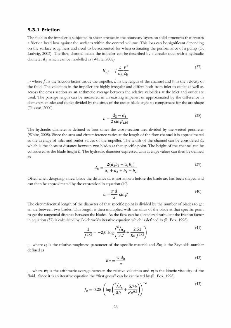
26

5.3.1 Friction

The fluid in the impeller is subjected to shear stresses in the boundary layers on solid structures that creates

a friction head loss against the surfaces within the control volume. This loss can be significant depending

on the surface roughness and need to be accounted for when estimating the performance of a pump (G.

Ludwig, 2003). The flow channel inside the impeller can be described by a circular duct with a hydraulic

diameter 𝑑ℎ which can be modelled as (White, 2008)

𝐻𝑙,𝑓 = 𝑓

𝐿

𝑑ℎ

𝑣2

2𝑔

(37)

, - where 𝑓; is the friction factor inside the impeller, 𝐿; is the length of the channel and 𝑣; is the velocity of

the fluid. The velocities in the impeller are highly irregular and differs both from inlet to outlet as well as

across the cross section so an arithmetic average between the relative velocities at the inlet and outlet are

used. The passage length can be measured in an existing impeller, or approximated by the difference in

diameters at inlet and outlet divided by the sinus of the outlet blade angle to compensate for the arc shape

(Tuzson, 2000)

𝐿 =

𝑑2 − 𝑑12 sin𝛽2,𝑏𝑙

(38)

The hydraulic diameter is defined as four times the cross-section area divided by the wetted perimeter

(White, 2008). Since the area and circumference varies at the length of the flow channel it is approximated

as the average of inlet and outlet values of the impeller. The width of the channel can be considered 𝑎;

which is the shortest distance between two blades at that specific point. The height of the channel can be

considered as the blade height 𝑏. The hydraulic diameter expressed with average values can then be defined

as

𝑑ℎ =

2(𝑎2𝑏2 + 𝑎1𝑏1)

𝑎1 + 𝑎2 + 𝑏1 + 𝑏2

(39)

Often when designing a new blade the distance 𝑎, is not known before the blade arc has been shaped and

can then be approximated by the expression in equation (40).

𝑎 ≈

𝜋𝑑

𝑧sin𝛽

(40)

The circumferential length of the diameter of that specific point is divided by the number of blades to get

an arc between two blades. This length is then multiplied with the sinus of the blade at that specific point

to get the tangential distance between the blades. As the flow can be considered turbulent the friction factor

in equation (37) is calculated by Colebrook’s iterative equation which is defined as (R. Fox, 1998)

1

𝑓1/2= −2,0 log(

𝜀𝑑ℎ⁄

3,7+

2,51

𝑅𝑒𝑓1/2)

(41)

, - where 𝜀; is the relative roughness parameter of the specific material and 𝑅𝑒; is the Reynolds number

defined as

𝑅𝑒 =

�̅�𝑑ℎ𝜐

(42)

, - where �̅�; is the arithmetic average between the relative velocities and 𝜐; is the kinetic viscosity of the

fluid. Since it is an iterative equation the “first guess” can be estimated by (R. Fox, 1998)

𝑓0 = 0,25 (log(

𝜀𝑑ℎ⁄

3,7+

5,74

𝑅𝑒0,9))

−2

(43)

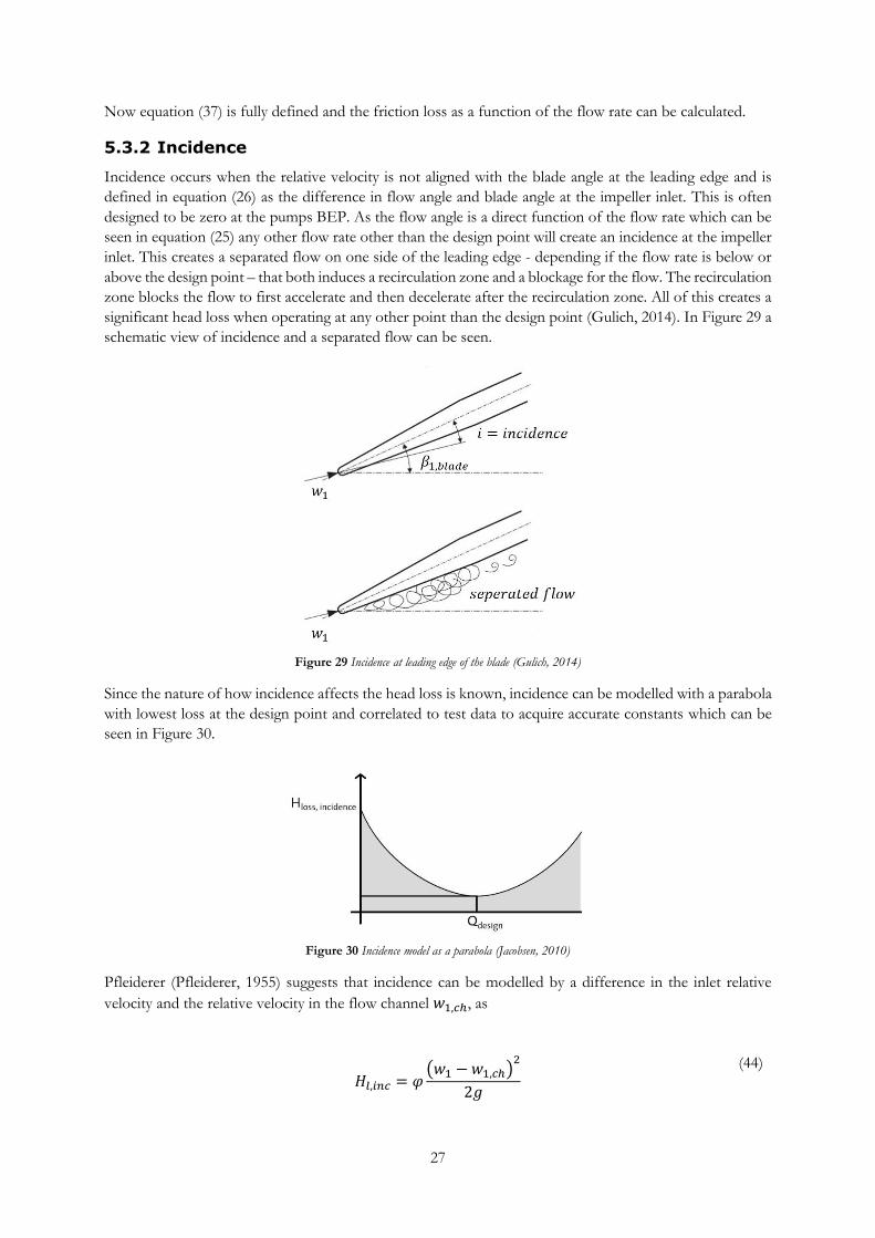
27

Now equation (37) is fully defined and the friction loss as a function of the flow rate can be calculated.

5.3.2 Incidence

Incidence occurs when the relative velocity is not aligned with the blade angle at the leading edge and is

defined in equation (26) as the difference in flow angle and blade angle at the impeller inlet. This is often

designed to be zero at the pumps BEP. As the flow angle is a direct function of the flow rate which can be

seen in equation (25) any other flow rate other than the design point will create an incidence at the impeller

inlet. This creates a separated flow on one side of the leading edge - depending if the flow rate is below or

above the design point – that both induces a recirculation zone and a blockage for the flow. The recirculation

zone blocks the flow to first accelerate and then decelerate after the recirculation zone. All of this creates a

significant head loss when operating at any other point than the design point (Gulich, 2014). In Figure 29 a

schematic view of incidence and a separated flow can be seen.

Figure 29 Incidence at leading edge of the blade (Gulich, 2014)

Since the nature of how incidence affects the head loss is known, incidence can be modelled with a parabola

with lowest loss at the design point and correlated to test data to acquire accurate constants which can be

seen in Figure 30.

Figure 30 Incidence model as a parabola (Jacobsen, 2010)

Pfleiderer (Pfleiderer, 1955) suggests that incidence can be modelled by a difference in the inlet relative

velocity and the relative velocity in the flow channel 𝑤1,𝑐ℎ, as

𝐻𝑙,𝑖𝑛𝑐 = 𝜑(𝑤1 −𝑤1,𝑐ℎ)

2

2𝑔

(44)

28

, - where 𝜑; is an empirical constant depending on the recirculation zone. Both these models rely on

empirical methods with correlation to test data while Cornell (Cornell, 1962) solves a potential flow model

by conformal transformation that entirely depends on the pump geometry. The model is based on a

separated zone behind the leading edge that creates a sudden expansion loss when the separated flow mixes.

The model is based on a flow ratio of the inlet velocity and the velocity at separation defined as

𝜆 =sin𝛽1,𝑓𝑙

sin(2𝛽1,𝑓𝑙 − 𝛽1,𝑏𝑙)− [

sin2 𝛽1,𝑓𝑙 − sin𝛽1,𝑏𝑙 sin(2𝛽1,𝑓𝑙 − 𝛽1,𝑏𝑙)

(sin(2𝛽1,𝑓𝑙 − 𝛽1,𝑏𝑙))2 ]

1/2

(45)

This constant is then used in the following expression for the incidence head loss as

𝐻𝑙,𝑖𝑛𝑐 =

𝑤12

2𝑔(1

𝜆)2

(1 −𝜆 sin𝛽1,𝑓𝑙

sin 𝛽1,𝑏𝑙)

2

(46)

which models the incidence only on the difference in angles between the flow and the blade. If the incidence

model in equation (46) is used on a reference impeller a plot of the incidence loss and incidence as a function

of the flow rate can be done which is seen in Figure 31. The model behaves as predicted with lowest head

loss around zero incidence and with increasing loss on both sides of the lowest value. This without any

specified design point which is a clear advantage to other incidence models.

Figure 31 Plot of Incidence loss and incidence as a function of the flowrate

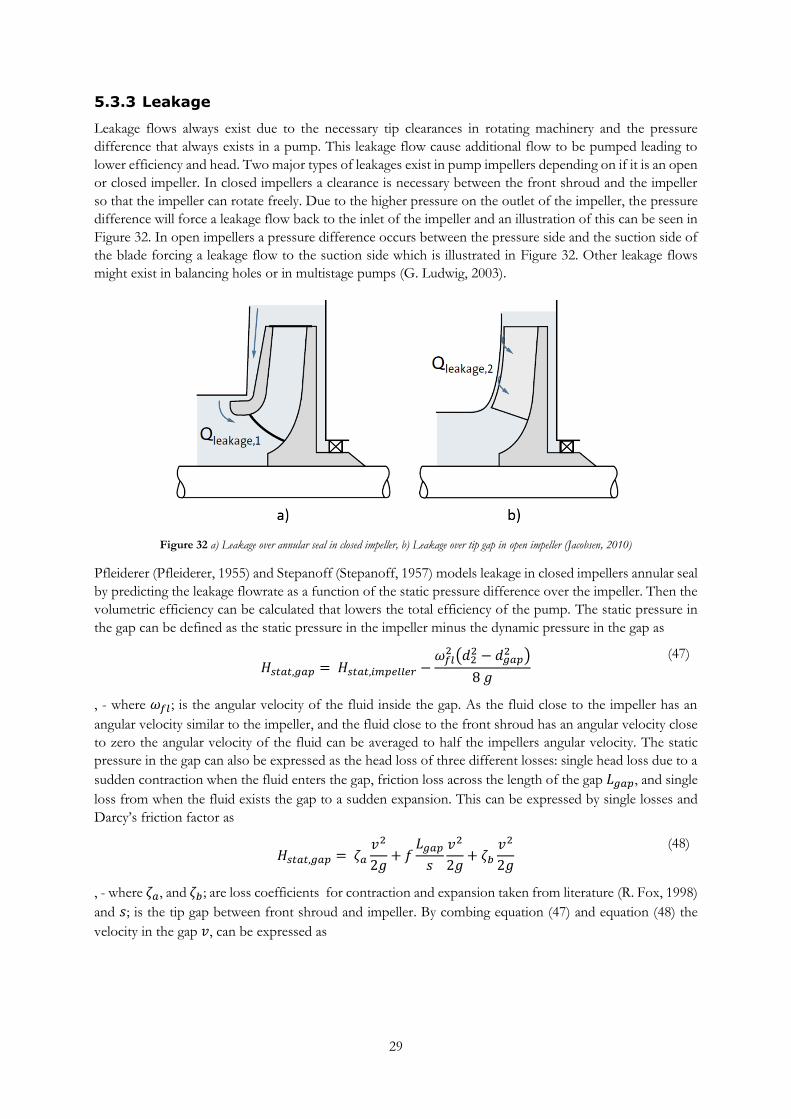
29

5.3.3 Leakage

Leakage flows always exist due to the necessary tip clearances in rotating machinery and the pressure

difference that always exists in a pump. This leakage flow cause additional flow to be pumped leading to

lower efficiency and head. Two major types of leakages exist in pump impellers depending on if it is an open

or closed impeller. In closed impellers a clearance is necessary between the front shroud and the impeller

so that the impeller can rotate freely. Due to the higher pressure on the outlet of the impeller, the pressure

difference will force a leakage flow back to the inlet of the impeller and an illustration of this can be seen in

Figure 32. In open impellers a pressure difference occurs between the pressure side and the suction side of

the blade forcing a leakage flow to the suction side which is illustrated in Figure 32. Other leakage flows

might exist in balancing holes or in multistage pumps (G. Ludwig, 2003).

Figure 32 a) Leakage over annular seal in closed impeller, b) Leakage over tip gap in open impeller (Jacobsen, 2010)

Pfleiderer (Pfleiderer, 1955) and Stepanoff (Stepanoff, 1957) models leakage in closed impellers annular seal

by predicting the leakage flowrate as a function of the static pressure difference over the impeller. Then the

volumetric efficiency can be calculated that lowers the total efficiency of the pump. The static pressure in

the gap can be defined as the static pressure in the impeller minus the dynamic pressure in the gap as

𝐻𝑠𝑡𝑎𝑡,𝑔𝑎𝑝 =𝐻𝑠𝑡𝑎𝑡,𝑖𝑚𝑝𝑒𝑙𝑙𝑒𝑟 −

𝜔𝑓𝑙2 (𝑑2

2 − 𝑑𝑔𝑎𝑝2 )

8𝑔

(47)

, - where 𝜔𝑓𝑙 ; is the angular velocity of the fluid inside the gap. As the fluid close to the impeller has an

angular velocity similar to the impeller, and the fluid close to the front shroud has an angular velocity close

to zero the angular velocity of the fluid can be averaged to half the impellers angular velocity. The static

pressure in the gap can also be expressed as the head loss of three different losses: single head loss due to a

sudden contraction when the fluid enters the gap, friction loss across the length of the gap 𝐿𝑔𝑎𝑝, and single

loss from when the fluid exists the gap to a sudden expansion. This can be expressed by single losses and

Darcy’s friction factor as

𝐻𝑠𝑡𝑎𝑡,𝑔𝑎𝑝 =𝜁𝑎

𝑣2

2𝑔+ 𝑓

𝐿𝑔𝑎𝑝

𝑠

𝑣2

2𝑔+ 𝜁𝑏

𝑣2

2𝑔

(48)

, - where 𝜁𝑎, and 𝜁𝑏; are loss coefficients for contraction and expansion taken from literature (R. Fox, 1998)

and 𝑠; is the tip gap between front shroud and impeller. By combing equation (47) and equation (48) the

velocity in the gap 𝑣, can be expressed as

30

𝑣 = √2𝑔𝐻𝑠𝑡𝑎𝑡,𝑔𝑎𝑝

𝑓𝐿𝑔𝑎𝑝𝑠

+ 𝜁𝑎 + 𝜁𝑏

(49)

, - where the friction factor can be assumed to be the same as in equation (41). With the area of the gap,

𝐴𝑔𝑎𝑝, known the leakage flow rate can be calculated as

𝑄𝑙𝑒𝑎𝑘 = 𝑣𝐴𝑔𝑎𝑝 (50)

Then the volumetric efficiency can be calculated as

𝜂𝑣𝑜𝑙 =

𝑄

𝑄 + 𝑄𝑙𝑒𝑎𝑘

(51)

,- where 𝑄; is the flow rate going through the impeller and pump (Pfleiderer, 1955). For open impellers the

leakage across the tip of the blade could be calculated with the same method but difficulties occur since the

pressure difference varies greatly at the length of the blade. Studies show that the leakage also depends

greatly on both tip clearance and the blade angles. This could be explained by that different outlet blade

angles have various tangential components that increases or decreases the leakage flow (Gulich, 2014). It

has been concluded that lower outlet blade angles increases the leakage flow rate. Gulich (Gulich, 2014)

suggest an empirical model for open impellers that is correlated against a vast number of experimental tests.

The correlation gives a percentage loss of the Euler head as

𝐻𝑡ℎ −𝐻𝑙,𝑙𝑒𝑎𝑘

𝐻𝑡ℎ=

2,5𝑠𝑑2

√𝑏2𝑑2

(1 −𝑑1𝑑2) (

𝑡𝑎2) 𝑛𝑞

0,1(sin 𝛽2)1,2(sin𝛽1)

0,4

(52)

The expression suggests that the head loss increases with: larger tip clearance 𝑠, in itself and as a ratio to

outlet diameter 𝑑2, and lower outlet blades angles 𝛽2. This corresponds to how the head loss behaves

compared to experimental tests (Gulich, 2014).

5.3.4 Diffusion

Diffusion is a mixing loss that occurs when the flow separates or where eddies are formed. The velocity

distribution in the flow field in an impeller can be considered non-uniform and highly irregular. This

increases when the flow decelerates in the flow channel which generates turbulent dissipation by exchange

of momentum across the streamlines (Gulich, 2014). When the relative velocity is much higher at the inlet

then at the outlet of the impeller one can assume that a portion of the velocity head difference is lost

(Tuzson, 2000). This is often hard to predict but Tuzson (Tuzson, 2000) suggests a simple loss correlation

that is based on the relative velocities. If the ratio of the relative velocities 𝑤1

𝑤2⁄ , exceeds 1,4 a quarter of

the velocity head achieved at the inlet is lost as

𝐻𝑙,𝑑 = 0,25

𝑤12

2𝑔

(53)

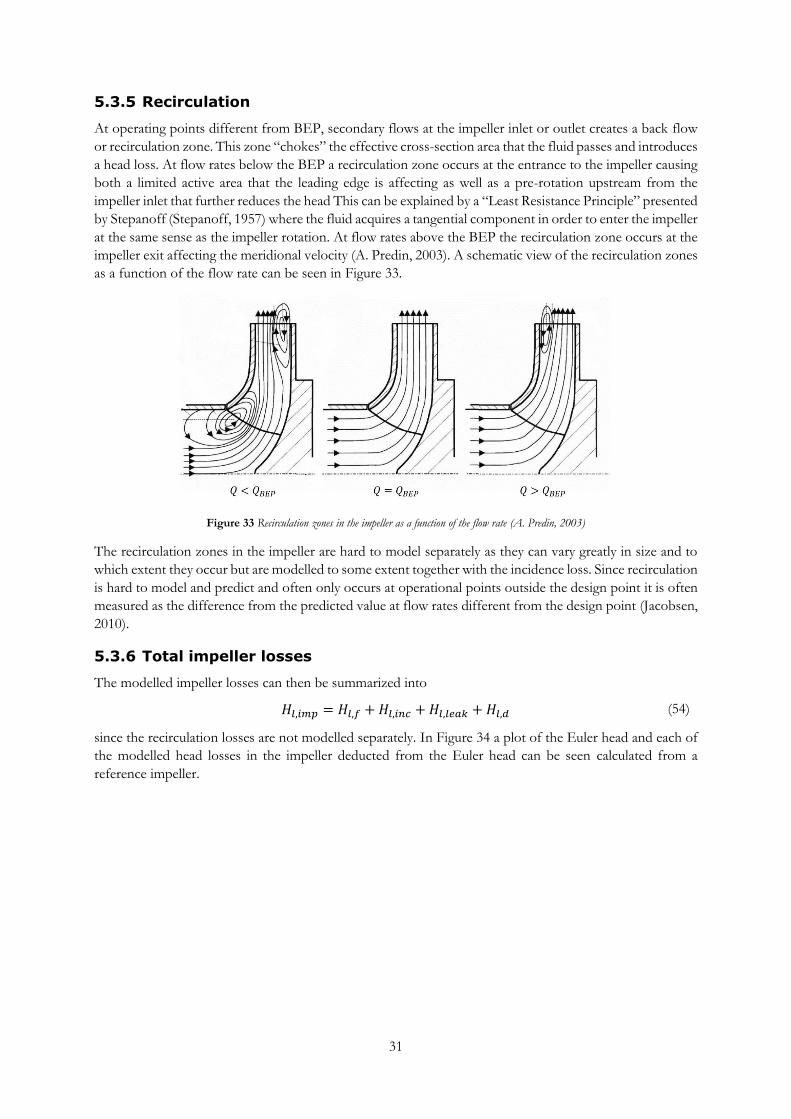
31

5.3.5 Recirculation

At operating points different from BEP, secondary flows at the impeller inlet or outlet creates a back flow

or recirculation zone. This zone “chokes” the effective cross-section area that the fluid passes and introduces

a head loss. At flow rates below the BEP a recirculation zone occurs at the entrance to the impeller causing

both a limited active area that the leading edge is affecting as well as a pre-rotation upstream from the

impeller inlet that further reduces the head This can be explained by a “Least Resistance Principle” presented

by Stepanoff (Stepanoff, 1957) where the fluid acquires a tangential component in order to enter the impeller

at the same sense as the impeller rotation. At flow rates above the BEP the recirculation zone occurs at the

impeller exit affecting the meridional velocity (A. Predin, 2003). A schematic view of the recirculation zones

as a function of the flow rate can be seen in Figure 33.

Figure 33 Recirculation zones in the impeller as a function of the flow rate (A. Predin, 2003)

The recirculation zones in the impeller are hard to model separately as they can vary greatly in size and to

which extent they occur but are modelled to some extent together with the incidence loss. Since recirculation

is hard to model and predict and often only occurs at operational points outside the design point it is often

measured as the difference from the predicted value at flow rates different from the design point (Jacobsen,

2010).

5.3.6 Total impeller losses

The modelled impeller losses can then be summarized into

𝐻𝑙,𝑖𝑚𝑝 = 𝐻𝑙,𝑓 +𝐻𝑙,𝑖𝑛𝑐 +𝐻𝑙,𝑙𝑒𝑎𝑘 +𝐻𝑙,𝑑 (54)

since the recirculation losses are not modelled separately. In Figure 34 a plot of the Euler head and each of

the modelled head losses in the impeller deducted from the Euler head can be seen calculated from a

reference impeller.

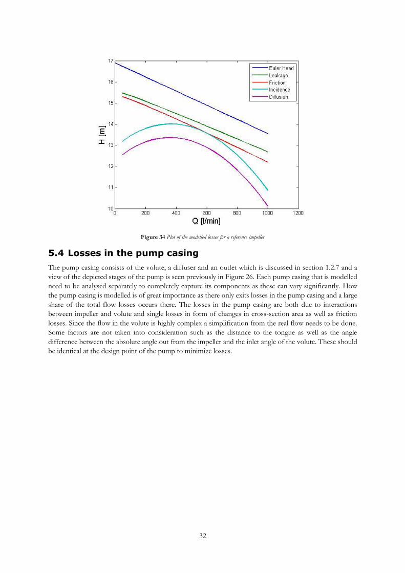
32

Figure 34 Plot of the modelled losses for a reference impeller

5.4 Losses in the pump casing

The pump casing consists of the volute, a diffuser and an outlet which is discussed in section 1.2.7 and a

view of the depicted stages of the pump is seen previously in Figure 26. Each pump casing that is modelled

need to be analysed separately to completely capture its components as these can vary significantly. How

the pump casing is modelled is of great importance as there only exits losses in the pump casing and a large

share of the total flow losses occurs there. The losses in the pump casing are both due to interactions

between impeller and volute and single losses in form of changes in cross-section area as well as friction

losses. Since the flow in the volute is highly complex a simplification from the real flow needs to be done.

Some factors are not taken into consideration such as the distance to the tongue as well as the angle

difference between the absolute angle out from the impeller and the inlet angle of the volute. These should

be identical at the design point of the pump to minimize losses.

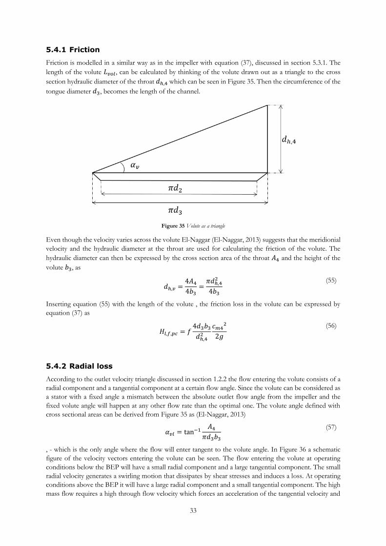
33

5.4.1 Friction

Friction is modelled in a similar way as in the impeller with equation (37), discussed in section 5.3.1. The

length of the volute 𝐿𝑣𝑜𝑙, can be calculated by thinking of the volute drawn out as a triangle to the cross

section hydraulic diameter of the throat 𝑑ℎ,4 which can be seen in Figure 35. Then the circumference of the

tongue diameter 𝑑3, becomes the length of the channel.

Figure 35 Volute as a triangle

Even though the velocity varies across the volute El-Naggar (El-Naggar, 2013) suggests that the meridionial

velocity and the hydraulic diameter at the throat are used for calculating the friction of the volute. The

hydraulic diameter can then be expressed by the cross section area of the throat 𝐴4 and the height of the

volute 𝑏3, as

𝑑ℎ,𝑣 =

4𝐴44𝑏3

=𝜋𝑑ℎ,4

2

4𝑏3

(55)

Inserting equation (55) with the length of the volute , the friction loss in the volute can be expressed by

equation (37) as

𝐻𝑙,𝑓,𝑝𝑐 = 𝑓

4𝑑3𝑏3

𝑑ℎ,42

𝑐𝑚42

2𝑔

(56)

5.4.2 Radial loss

According to the outlet velocity triangle discussed in section 1.2.2 the flow entering the volute consists of a

radial component and a tangential component at a certain flow angle. Since the volute can be considered as

a stator with a fixed angle a mismatch between the absolute outlet flow angle from the impeller and the

fixed volute angle will happen at any other flow rate than the optimal one. The volute angle defined with

cross sectional areas can be derived from Figure 35 as (El-Naggar, 2013)

𝛼𝑣𝑙 = tan−1

𝐴4𝜋𝑑3𝑏3

(57)

, - which is the only angle where the flow will enter tangent to the volute angle. In Figure 36 a schematic

figure of the velocity vectors entering the volute can be seen. The flow entering the volute at operating

conditions below the BEP will have a small radial component and a large tangential component. The small

radial velocity generates a swirling motion that dissipates by shear stresses and induces a loss. At operating

conditions above the BEP it will have a large radial component and a small tangential component. The high

mass flow requires a high through flow velocity which forces an acceleration of the tangential velocity and

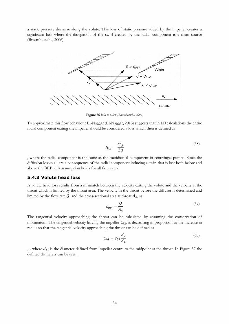
34

a static pressure decrease along the volute. This loss of static pressure added by the impeller creates a

significant loss where the dissipation of the swirl created by the radial component is a main source

(Braembussche, 2006).

Figure 36 Inlet to volute (Braembussche, 2006)

To approximate this flow behaviour El-Naggar (El-Naggar, 2013) suggests that in 1D calculations the entire

radial component exiting the impeller should be considered a loss which then is defined as

𝐻𝑙,𝑟 =

𝑐𝑟,22

2𝑔

(58)

, where the radial component is the same as the meridionial component in centrifugal pumps. Since the

diffusion losses all are a consequence of the radial component inducing a swirl that is lost both below and

above the BEP this assumption holds for all flow rates.

5.4.3 Volute head loss

A volute head loss results from a mismatch between the velocity exiting the volute and the velocity at the

throat which is limited by the throat area. The velocity in the throat before the diffuser is determined and

limited by the flow rate 𝑄, and the cross-sectional area at throat 𝐴4, as

𝑐𝑚4 =

𝑄

𝐴4

(59)

The tangential velocity approaching the throat can be calculated by assuming the conservation of

momentum. The tangential velocity leaving the impeller 𝑐𝜃2, is decreasing in proportion to the increase in

radius so that the tangential velocity approaching the throat can be defined as

𝑐𝜃4 = 𝑐𝜃2

𝑑2𝑑4

(60)

, - where 𝑑4; is the diameter defined from impeller centre to the midpoint at the throat. In Figure 37 the

defined diameters can be seen.

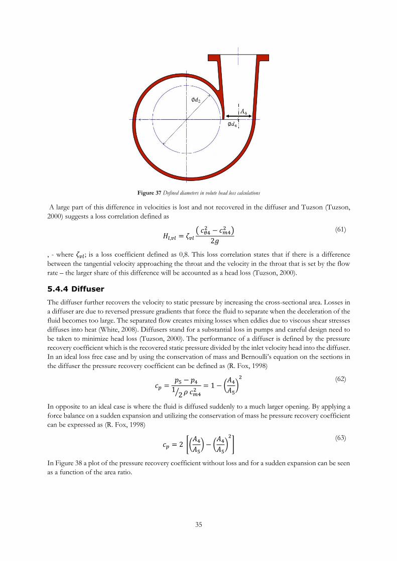
35

Figure 37 Defined diameters in volute head loss calculations

A large part of this difference in velocities is lost and not recovered in the diffuser and Tuzson (Tuzson,

2000) suggests a loss correlation defined as

𝐻𝑙,𝑣𝑙 = 𝜁𝑣𝑙

(𝑐𝜃42 − 𝑐𝑚4

2 )

2𝑔

(61)

, - where 𝜁𝑣𝑙; is a loss coefficient defined as 0,8. This loss correlation states that if there is a difference

between the tangential velocity approaching the throat and the velocity in the throat that is set by the flow

rate – the larger share of this difference will be accounted as a head loss (Tuzson, 2000).

5.4.4 Diffuser

The diffuser further recovers the velocity to static pressure by increasing the cross-sectional area. Losses in

a diffuser are due to reversed pressure gradients that force the fluid to separate when the deceleration of the

fluid becomes too large. The separated flow creates mixing losses when eddies due to viscous shear stresses

diffuses into heat (White, 2008). Diffusers stand for a substantial loss in pumps and careful design need to

be taken to minimize head loss (Tuzson, 2000). The performance of a diffuser is defined by the pressure

recovery coefficient which is the recovered static pressure divided by the inlet velocity head into the diffuser.

In an ideal loss free case and by using the conservation of mass and Bernoulli’s equation on the sections in

the diffuser the pressure recovery coefficient can be defined as (R. Fox, 1998)

𝑐𝑝 =

𝑝5 − 𝑝412⁄ 𝜌𝑐𝑚4

2= 1 − (

𝐴4𝐴5)2

(62)

In opposite to an ideal case is where the fluid is diffused suddenly to a much larger opening. By applying a

force balance on a sudden expansion and utilizing the conservation of mass he pressure recovery coefficient

can be expressed as (R. Fox, 1998)

𝑐𝑝 = 2 [(

𝐴4𝐴5) − (

𝐴4𝐴5)2

] (63)

In Figure 38 a plot of the pressure recovery coefficient without loss and for a sudden expansion can be seen

as a function of the area ratio.

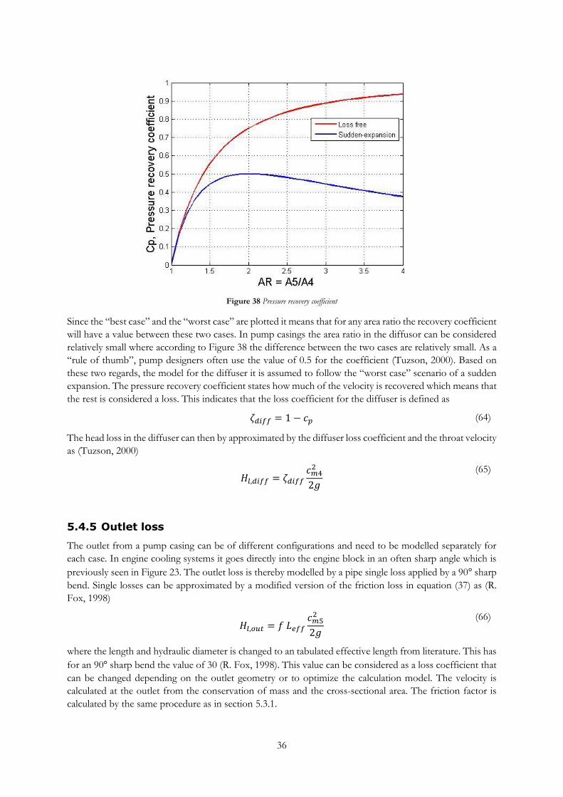
36

Figure 38 Pressure recovery coefficient

Since the “best case” and the “worst case” are plotted it means that for any area ratio the recovery coefficient

will have a value between these two cases. In pump casings the area ratio in the diffusor can be considered

relatively small where according to Figure 38 the difference between the two cases are relatively small. As a

“rule of thumb”, pump designers often use the value of 0.5 for the coefficient (Tuzson, 2000). Based on

these two regards, the model for the diffuser it is assumed to follow the “worst case” scenario of a sudden

expansion. The pressure recovery coefficient states how much of the velocity is recovered which means that

the rest is considered a loss. This indicates that the loss coefficient for the diffuser is defined as

𝜁𝑑𝑖𝑓𝑓 = 1 − 𝑐𝑝 (64)

The head loss in the diffuser can then by approximated by the diffuser loss coefficient and the throat velocity

as (Tuzson, 2000)

𝐻𝑙,𝑑𝑖𝑓𝑓 = 𝜁𝑑𝑖𝑓𝑓

𝑐𝑚42

2𝑔

(65)

5.4.5 Outlet loss

The outlet from a pump casing can be of different configurations and need to be modelled separately for

each case. In engine cooling systems it goes directly into the engine block in an often sharp angle which is

previously seen in Figure 23. The outlet loss is thereby modelled by a pipe single loss applied by a 90° sharp

bend. Single losses can be approximated by a modified version of the friction loss in equation (37) as (R.

Fox, 1998)

𝐻𝑙,𝑜𝑢𝑡 = 𝑓𝐿𝑒𝑓𝑓

𝑐𝑚52

2𝑔

(66)

where the length and hydraulic diameter is changed to an tabulated effective length from literature. This has

for an 90° sharp bend the value of 30 (R. Fox, 1998). This value can be considered as a loss coefficient that

can be changed depending on the outlet geometry or to optimize the calculation model. The velocity is

calculated at the outlet from the conservation of mass and the cross-sectional area. The friction factor is

calculated by the same procedure as in section 5.3.1.

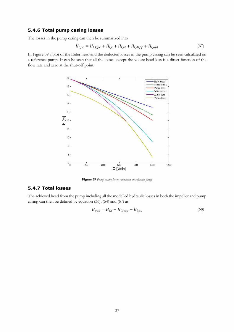
37

5.4.6 Total pump casing losses

The losses in the pump casing can then be summarized into

𝐻𝑙,𝑝𝑐 = 𝐻𝑙,𝑓,𝑝𝑐 +𝐻𝑙,𝑟 +𝐻𝑙,𝑣𝑙 + 𝐻𝑙,𝑑𝑖𝑓𝑓 +𝐻𝑙,𝑜𝑢𝑡 (67)

In Figure 39 a plot of the Euler head and the deducted losses in the pump casing can be seen calculated on

a reference pump. It can be seen that all the losses except the volute head loss is a direct function of the

flow rate and zero at the shut-off point.

Figure 39 Pump casing losses calculated on reference pump

5.4.7 Total losses

The achieved head from the pump including all the modelled hydraulic losses in both the impeller and pump

casing can then be defined by equation (36), (54) and (67) as

𝐻𝑜𝑢𝑡 = 𝐻𝑡ℎ −𝐻𝑙,𝑖𝑚𝑝 − 𝐻𝑙,𝑝𝑐 (68)

38

5.5 Power and efficiency

The power in a pump can be divided at several steps ranging from the supplied shaft power from the drive

unit to the achieved hydraulic power acting on the fluid. In Figure 40 a plot of the supplied shaft power and

its subsequent power loss can be seen. The shaft power has to drive the mechanical losses, disk friction loss

and hydraulic losses. The power is calculated by equation (11) and depending on which head is inserted

different type of power in the pump is calculated. In this model mechanical losses are not taken into

consideration.

Figure 40 Different power curves in a pump (Jacobsen, 2010)

5.5.1 Disk friction

When the impeller rotates in the fluid that is enclosed by the pump casing it is subjected to a circumferential

frictional force that absorbs shaft power. The fluid particles enclosed in the space between the rotating

impeller and the stationary front shroud are affected by two vortexes; one primary vortex and one secondary.

The primary vortex rotates with the same direction and magnitude as the impeller close to the impeller

surface while it is zero close to the stationary front shroud. This vortex is thereby often modelled with half

the angular velocity of the impeller (Jacobsen, 2010). The secondary vortex is a result of centrifugal forces

that pushes particles outward while being replaced by new particles and a circulation is established

(Stepanoff, 1957). Pfleiderer (Pfleiderer, 1955) suggests that the added power caused by disk friction can be

modelled by

𝑃𝑑𝑖𝑠𝑘 = 𝑘𝜌𝑢23𝑑2(𝑑2 + 5𝑠) (69)

, - where 𝑠; is the tip clearance between the impeller and front shroud and 𝑘; is an empirical value determined

by

𝑘 = 7,3 ∙ 10−4 (

2𝜐 ∙ 106

𝑢2𝑑2)

𝑚

(70)

, - where 𝑚; is an exponent that varies from 1/7 to 1/9 depending on the surface roughness. For the model,

an arithmetic average of 1/8 is used. The disk friction applies by the affinity laws discussed in section 1.2.9

and changes with the fifth power of the diameter when changing the diameter which results in significant

power changes (Tuzson, 2000).

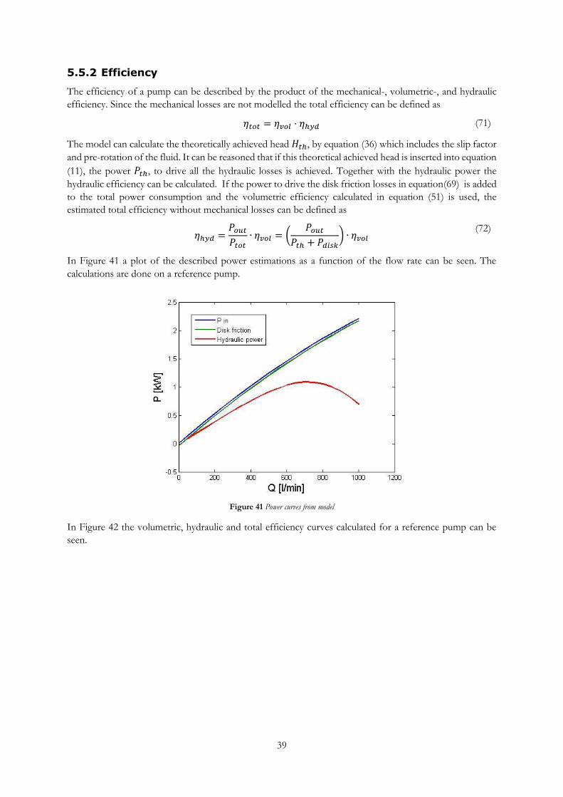
39

5.5.2 Efficiency

The efficiency of a pump can be described by the product of the mechanical-, volumetric-, and hydraulic

efficiency. Since the mechanical losses are not modelled the total efficiency can be defined as

𝜂𝑡𝑜𝑡 = 𝜂𝑣𝑜𝑙 ⋅ 𝜂ℎ𝑦𝑑 (71)

The model can calculate the theoretically achieved head 𝐻𝑡ℎ, by equation (36) which includes the slip factor

and pre-rotation of the fluid. It can be reasoned that if this theoretical achieved head is inserted into equation

(11), the power 𝑃𝑡ℎ, to drive all the hydraulic losses is achieved. Together with the hydraulic power the

hydraulic efficiency can be calculated. If the power to drive the disk friction losses in equation(69) is added

to the total power consumption and the volumetric efficiency calculated in equation (51) is used, the

estimated total efficiency without mechanical losses can be defined as

𝜂ℎ𝑦𝑑 =

𝑃𝑜𝑢𝑡𝑃𝑡𝑜𝑡

∙ 𝜂𝑣𝑜𝑙 = (𝑃𝑜𝑢𝑡

𝑃𝑡ℎ + 𝑃𝑑𝑖𝑠𝑘) ∙ 𝜂𝑣𝑜𝑙

(72)

In Figure 41 a plot of the described power estimations as a function of the flow rate can be seen. The

calculations are done on a reference pump.

Figure 41 Power curves from model

In Figure 42 the volumetric, hydraulic and total efficiency curves calculated for a reference pump can be

seen.

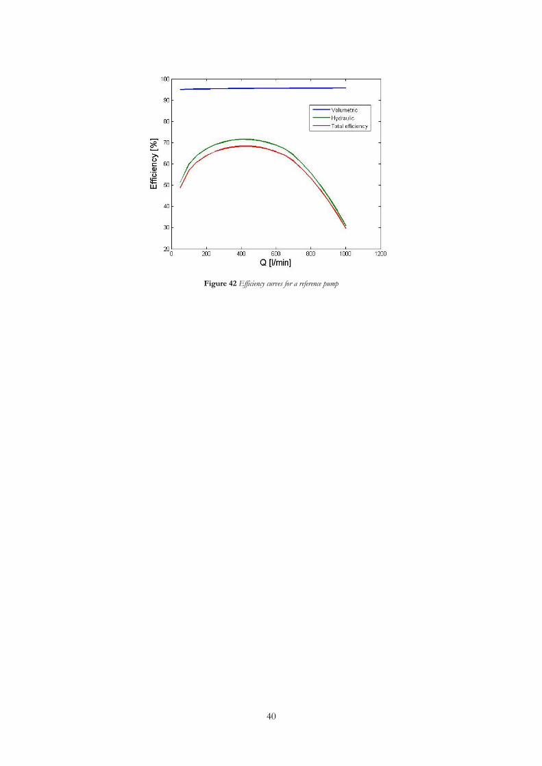
40

Figure 42 Efficiency curves for a reference pump

41

6 Design program

When a model of how different design parameters affect the pumps performance are done – which is

discussed previously in chapter 5 – a design program can be established based on the estimations from the

calculation model. By utilizing the calculation model together with previous test-data, design coefficients

can be established that help to design the main design parameters of the impeller. The design program is

designed to suggest main design parameters based on a design point. This is done with pump design

coefficients and correlations from literature. The suggested design is then compared against control values

of diffusion and stability factors. If their requirements are met the design can be inserted into the calculation

model to determine the pumps efficiency and if it reaches its design with all the hydraulic losses. If not, the

design coefficients can be altered until the desired operational characteristics have been reached. Together

with a parameterized Catia v5 CAD-model where the outputs from the design program can be inserted a

complete 3D-model of the impeller can be made.

6.1 Design coefficients

Impeller design consists of a vast number of geometry parameters that can be varied indefinitely to achieve

a desired operational point. To narrow down the possibilities, design coefficients are introduced to aid with

the design of the main parameters. By doing a dimensional analysis with the Buckingham Π-theorem, design

coefficients are constructed to aid the design of machines with geometrical same attributes (Stepanoff,

1957). In the design program, the specific speed, head coefficient and the flow coefficient are used to design

the impeller. The design coefficients are calculated and plotted on previous test data on the reference

impellers to help the designer on an initial starting point. The head and flow coefficient are plotted as a

function of the specific speed. By knowing a desired design point of flow 𝑄𝐷, head 𝐻𝐷, and speed of the

pump 𝑛𝑑, the specific speed can be calculated by

𝑛𝑞 =

𝑛𝐷√𝑄𝐷(𝐻𝐷)

3/4

(73)

By knowing the specific speed, the head and flow coefficient of earlier designs are known which can be used

in a first iteration in the design phase.

6.1.1 Head coefficient

The head coefficient can be seen as a normalized constant for how much head that can be achieved based

on the maximum theoretical head from that specific geometry. The head coefficient is defined as (Stepanoff,

1957)

𝜓 =

𝑔𝐻

𝑢22

(74)

, - where the numerator 𝐻; is the head achieved by the pump and the denominator is maximum head

achieved when the absolute tangential component equals the tip blade speed. In Figure 43 a plot of the head

coefficient as a function of the specific speed is calculated from the four reference pumps. Stepanoff

(Stepanoff, 1957) and Pfleiderer (Pfleiderer, 1955) states that the head coefficient normally equals 0.5 for

centrifugal pumps. Studying the plot shows that most previous designs have a similar value across the

specific speed range calculated. In Figure 44 a plot of the hydraulic efficiency calculated with the calculation

model as a function of the head coefficient of the reference pumps can be seen. These two plots will help

the designer to choose the starting value of the head coefficient for the impeller design.

42

Figure 43 Head coefficient as a function of the specific speed calculated from reference impellers

In Figure 44 a plot of the hydraulic efficiency calculated with the calculation model as a function of the head

coefficient of the reference pumps can be seen. These two plots will help the designer to choose the starting

value of the head coefficient for the impeller design. The hydraulic efficiency in Figure 44 of the reference

pumps show the same tendency as the previous plot with most values around 0.5 except for reference

pump -1.

Figure 44 Hydraulic efficiency as a function of the head coefficient calculated from the reference impellers

43

6.1.2 Flow coefficient

The flow coefficient can be seen as a normalized flow where the meridional velocity 𝑐𝑚, is normalized by

the blade velocity 𝑢. Since in centrifugal machines the meridional and blade speed varies across the stages,

it can be calculated at both the impeller inlet and outlet. The flow coefficient is defined as

𝜙 =

𝑐𝑚𝑢

(75)

In Figure 45 a plot of the flow coefficient out from the impeller as a function of the specific speed can be

seen. The reference impellers show a relatively homogenous behaviour where the flow coefficient is

proportional to the flow, as expected.

Figure 45 Flow coefficient out from the impeller as a function of the specific speed calculated on reference impellers

In Figure 46 a plot of the hydraulic efficiency calculated with the calculation model as a function of the flow

coefficient of the reference pumps can be seen. These two plots will help the designer to choose the starting

value of the head coefficient for the impeller design. The reference pumps show a relatively homogenous

behaviour except reference pump -4 that has significantly lower hydraulic efficiency across the flow span.

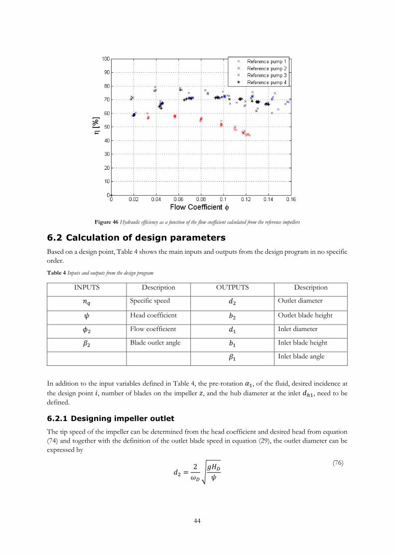
44

Figure 46 Hydraulic efficiency as a function of the flow coefficient calculated from the reference impellers

6.2 Calculation of design parameters

Based on a design point, Table 4 shows the main inputs and outputs from the design program in no specific

order.

Table 4 Inputs and outputs from the design program

INPUTS Description OUTPUTS Description

𝑛𝑞 Specific speed 𝑑2 Outlet diameter

𝜓 Head coefficient 𝑏2 Outlet blade height

𝜙2 Flow coefficient 𝑑1 Inlet diameter

𝛽2 Blade outlet angle 𝑏1 Inlet blade height

𝛽1 Inlet blade angle

In addition to the input variables defined in Table 4, the pre-rotation 𝛼1, of the fluid, desired incidence at

the design point 𝑖, number of blades on the impeller 𝑧, and the hub diameter at the inlet 𝑑ℎ1, need to be

defined.

6.2.1 Designing impeller outlet

The tip speed of the impeller can be determined from the head coefficient and desired head from equation

(74) and together with the definition of the outlet blade speed in equation (29), the outlet diameter can be

expressed by

𝑑2 =2

𝜔𝐷√𝑔𝐻𝐷

𝜓

(76)

45

The blade height is determined by first estimating what the meridional velocity is at the outlet from equation

(75). Using the conservation of mass with blade blockage from equation (27) the blade height can be

expressed as

𝑏2 =

𝑄𝐷𝜙2𝑢2(𝜋𝑑2 − 𝑡𝑧)

(77)

This method to calculate the outlet blade height only take into consideration previous designs since it is

based on the flow coefficient. The blade height can also be calculated as a function of the blade outlet angle

to provide the necessary flow rate. The meridional velocity can be described by a re-writing of equation (32)

as

𝑐𝑚,2 = 𝑤𝜃2 ∙ tan𝛽2,𝑏𝑙 (78)

which defines that the meridional velocity increases with the blade angle. At the same time the desired flow

rate need to be had at the flow channel of the impeller outlet. This suggests that - according to the

conservation of mass - the blade height needs to be smaller to maintain the flowrate. The program uses the

flow coefficient to calculate the blade height but controls its value against equation (78) so that the flow rate

is maintained.

6.2.2 Designing impeller inlet

For the impeller inlet diameter 𝑑1, approximations from literature are used. Stepanoff (Stepanoff, 1957) did

an extensive study on successful pump design and the geometry relations involved. The study suggested

empirical constants as a function of the specific speed to define geometrical representations. In Appendix

2 a plot of these empirical constants can be seen. The design program uses the empirical constant for the

relationship between inlet diameter 𝑑1, and outlet diameter 𝑑2. Values taken from Stepanoff’s diagram in

Appendix 2 is fitted to a curve by a polynomial expression is defined as

𝐾𝑑 = 10−13 ∙ 𝑛𝑠3 − 7 ∙ 10−9 ∙ 𝑛𝑠

2 + 10−4 ∙ 𝑛𝑠 + 0,2661 (79)

, - where 𝑛𝑠; is an alteration of the specific speed defined as

𝑛𝑠 = 51,55 ∙ 𝑛𝑞 (80)

In Figure 47 a plot of the expression in equation (79) can be seen.

Figure 47 Stepanoff’s constant for diameter ratio curve-fitted

The inlet diameter can then be defined as

46

𝑑1 = 𝐾𝑑 𝑑2 (81)

The inlet blade height is determined by the difference in radius of the hub diameter 𝑑ℎ1, and the inlet

diameter as

𝑏1 =

𝑑1 − 𝑑ℎ12

(82)

The inlet blade angle is determined by the flow angle at the design point and the specified incidence at the

design point. To minimize hydraulic losses it is desirable that the incidence is zero at the design point. The

inlet velocity triangles are calculated in the same procedure as described in section 5.2.1 depending on radial

or semi-axial inlet. The designed inlet blade angle can then be determined by

𝛽1,𝑏𝑙 = (tan−1

𝑐𝑚1

𝑤𝜃2) + 𝑖

(83)

Then the main impeller geometry parameters are determined as a function of a design point.

6.3 Limits and requirements

The suggested design is compared to control values taken from literature on impeller design as well as

limitations in physical size on some dimensions. These limitations are set up in order for the impeller to fit

in an existing pump casing. The first limitation is set on the outlet diameter which always has to be lower

than the diameter to the tongue 𝑑3. Since it is a centrifugal impeller, the outlet diameter also has to be larger

than the inlet diameter. The other limitation is set on the inlet blade height which always has to be lower

than the total axial length of the impeller. To achieve a stable pump curve it also has to be larger than the

outlet blade height (Tuzson, 2000). These physical limitations can be summarized into

𝑑1 < 𝑑2 < 𝑑𝑚𝑎𝑥 (84)

𝑏2 < 𝑏1 < 𝑏𝑚𝑎𝑥 (85)

The design is also limited against two control values based on the stability of the pump curve. Analysis of

tests shows that when the difference in relative velocities is small – instabilities of the pump curve are very

unlikely. Tuzson (Tuzson, 2000) suggests that to lower the excessive diffusion in the impeller the normalized

difference in relative velocities defined as

𝐾𝑤 =𝑤1 −𝑤2

𝑤1

(86)

, should always be lower than 0.25. When the relative velocities are the same a stability factor can be

expressed as (ANSYS, 2013)

𝐾𝑠 =𝑢2 − 𝑢1𝑐𝜃2

(87)

, which should be lower than 0.9. These two constants together with the aforementioned limits are used

to control that the design is delivering a stable pump curve.

6.4 Impeller design

When the main parameters of the impeller are established a blade arc can be created for which the impeller

blade is based on. In order to determine the blade arc the in- and outlet diameter 𝑑1, 𝑑2, and the blade

angles 𝛽1, and 𝛽2, need to be determined. In Figure 48 a figure of a blade arc can be seen. The blade arc is

constructed in the CAD software Catia v5 by the following workflow and referring to Figure 48. Starting in

point A, a tangent with the angle 𝛽2, to the horizontal plane is drawn. A circle is then specified to the

program with the following restrictions:

47

It must intersect with point A, on the diameter 𝑑2, having a tangent with the angle of 𝛽2

It also must intersect somewhere on the diameter 𝑑1, having a tangent with the angle of 𝛽1creating

point B.

This creates a circle intersecting point A, and point B, with a radius from point C. With a limitation that the

circle is only drawn between point A, and B, a circular blade arc is created.

Figure 48 How the blade arc is created (Gulich, 2014)

To further refine the blade shape, a quadratic Bezier curve is specified in the program. Bezier curves are

used to create a blade shape that is smoother than a circular one (W. Qinghuan, 1988). Three points are

needed to create a quadratic Bezier which is defined by point A, B, and C. When the blade arc is done a

desired thickness is added. This thickness is already determined when calculating with meridional velocity

with blade blockage. The blade is designed to have no blade angle variations depending on the blade height.

6.5 Cavitation

Cavitation performances are very hard to predict and is often assessed by numerical methods to approximate

where cavitation problems might occur (Tuzson, 2000). Since cavitation depends on absolute pressure

values and the calculation model only relies on computing with pressure differences, predicting cavitation

behaviour is further complicated. However, by utilizing cavitation coefficients from literature an assessment

of the cavitation performance of one impeller design over another can be established. A cavitation number

can be defined as (Steck, 2008)

𝜏 =𝑝𝑠 − 𝑝𝑣12⁄ 𝜌𝑤1

2

(88)

, - where 𝑝𝑠; is the unknown absolute static pressure and 𝑝𝑣 ; is the vapour pressure which is known for a

specific temperature. Since cavitation often occurs at the inlet of an impeller, the relative velocity at the inlet

is used. Koivula (Koivula, 2000) studied cavitation in orifices – which the blade inlet passage can be seen as

– and defines that incipient or critical cavitation occurs when the cavitation number is between 0.2 and 1.5.

By utilizing this, equation (88) can be rewritten to

𝑝𝑠 = 𝑝𝑣 + 𝜏 1 2⁄ 𝜌𝑤12 (89)

which gives an approximation on when cavitation might occur. This should not be interpreted as an absolute

value but an assessment of different impeller designs.

48

7 Experimental test

An experimental test is performed on new impeller design to assess the performance of them. The tests are

done on a rig designated to measure the performance of engine cooling pumps. Previous test data from

reference impellers tested in the same test rig are also used to compare against the calculation. In Figure 49

a CAD-model of the test rig can be seen. In this section a description of the test rig and how a test is done

will be discussed.

Figure 49 A CAD-model of the pump rig

7.1 Objectives of experimental test

The objective of the experimental tests is to measure pressure differences and flow rate over the pump at

various operating conditions to determine a pump curve for a specific pump.

7.2 Setup

The rig is designed to test the performance of engine cooling pumps in a laboratory environment. In Figure

50 a schematic view of the layout of the experimental setup can be seen.

49

Figure 50 Schematic view of the pump rig

The pump is connected to a water tank that both acts like a storage and as a heater to heat up the water to

desired temperature. Two thermostats measure the water temperature in the tank. A control valve is

installed after the pump where the resistance is changed to alter the necessary head provided by the pump.

A flow meter is installed after the control valve where the flow rate is measured. The flow meter is an

Krohne DN50 electromagnetic flow meter that is connected to a digital display. Two pressure taps are

installed that measure the pressure before and after the pump. The pressure taps are connected to an

Ipetronik M-SENS converter that converts the analog signals to digital ones before connected to a

computer. The computer software Vision is used to record the pressure measurements. The RPM of the

pump is measured by an optical tachometer.

7.3 Procedure

The pump is tested at several different rpm’s ranging from 1000-2200 RPM of the engine. The pump speed

is measured which is set to the engine speed times the ratio of the pulley. The control is varied at fixed

points where the data is measured. Since the measurements vary marginal over time a signal of one

measurement point is recorded with the computer software Vision. An average of the recording is taken as

the measurement point. The different data measured and calculated from a test can be seen in Table 5. The

pressure difference is calculated as the difference in outlet and inlet pressure. With data for the pressure

difference and flow rate at each operational point a flow curve can be plotted.

Table 5 Measured data from experimental test

Engine speed

[rpm]

Pump speed

[rpm]

Coolant flow

[l/min]

Inlet pressure

[bar]

Outlet

pressure [bar]

Pressure

difference [bar]

𝑛𝑒 𝑛 𝑄 𝑝𝑖𝑛 𝑝𝑜𝑢𝑡 ∆𝑝

7.3.1 Limitations

There is no possibility to measure the torque of the engine and by that the efficiency cannot be calculated.

50

8 Result

The calculation model is applied on reference impellers to compare previous test data to calculated pump

curves. Two new impellers are designed based on the methodology presented in chapter 6. These new

impellers are manufactured by rapid prototyping and tested by an experimental test in the test rig explained

in chapter 7. The test result is then compared to the model results. A CFD analysis is done on one designed

impeller and compared to the calculation model.

8.1 Comparison with previous test data

The calculation model is compared with four different reference pumps with configurations discussed in

section 4.2. The necessary geometry parameters needed to the calculation model is discussed in section 5.

The dimensions are extracted from existing CAD-models on the reference pumps and inserted into the

model. The test-data were previously determined when developing the reference pumps and are all tested

at the same test rig discussed in chapter 7. The test data is taken from several impeller speeds simulating an

engine speed ranging from 1000 to 2200 rpm. With a pulley ratio to the pump of 1,83 the pump has a speed

of 1830 to 4026 rpm. In Figure 51 a plot of the calculation model and test data of reference pump 1 can be

seen at different impeller speeds. The lower impeller speeds refers to lower achieved head and higher

impeller speeds refers to the plots of higher achieved head. The curves have the same tendencies and follow

each other fairly accurately. The test data and the calculation model divert some at higher flow rates where

the head loss increases for the test data. This is probably due to the fact that the impeller starts to cavitate

when the flow rate increases and a new head loss is introduced. The difference in head loss seems to increase

with the impeller speed similar to a head difference according to the affinity laws.

Figure 51 Comparison between calculation model and reference pump 1 at different speeds

In Figure 52 a detailed plot of only one speed of the impeller can be seen. The model captures the general

behaviour of the test and is within a few percent margin of error at flow rates ranging from 300 – 450 l/min,

while slightly more off at flow rates below and above.

51

Figure 52 Detailed study on one engine speed, 1400 RPM

In Figure 53 a plot of the comparison of the calculation model and test data from reference pump -2 can

be seen. This pump has the same volute as reference pump -1 but has another impeller design. The impellers

have the same main geometry values except the blade angles and blade arc. The correlation between the

calculation model and the test data is accurate and follow the same behaviour. It can be clearly seen that in

the test data at higher speeds the pump cavitates and drops head quickly. This behaviour does not the

calculation model capture.

Figure 53 Comparison of calculation model and test data of reference pump 2 on different speeds

In Figure 54 plot of the calculation model and test data for an engine speed of 1200 rpm can be seen. The

correlation is accurate and follows the tendency of the curve across the flow span. The percentage difference

between the two curves is as most at around 350 l/min at 2%.

52

Figure 54 Detailed study on one engine speed, 1400 RPM

Reference pump 3 and 4 have the same pump casing but different impeller designs. They are designed to

be different performance stages in a cooling system to provide the necessary flow rate. Here, the blade

angles are chosen to be the same while the blade height is varied to achieve a different flow rate. In Figure

55 a plot of the comparison between the calculation model and test data from reference pump 3 on different

engine speeds ranging from 1200 to 2200 rpm can be seen. This impeller is designed to be the performance

stage with higher achieved head. The model captures the behaviour of the pump curve at mid and high flow

rates but is slightly too conservative at lower flowrates. This could be an indication that the model

overcompensates for incidence losses at flowrates below the optimum one or that the inlet flow is subjected

to a pre-swirl in the test data. By varying the absolute inlet flow angle it has been found that a better

correlation is found with a slight co-rotation of 85°. However, since it cannot be known that this is the case

further studies on the subject needs to be done.


53

In Figure 56 a plot of the calculation model and test data for reference pump 4 at different impeller speeds

can be seen. This pump acts as the lower performance step compared to the pump plotted in Figure 55

which can be seen when comparing achieved head at the same impeller speed. The difference in head loss

increases with the speed of the impeller and the model does not entirely capture the curve behaviour at high

speeds and flow rate. This can be an indication that cavitation is appearing in the test data which the model

does not capture. If comparing Figure 55 and Figure 56 they seem to capture the pump curve similarly with

too large head difference in lower flow rates and to low head loss with higher flow rates. This should be the

case since it is very small differences in impeller design but the model still captures the increased achieved

head even though the outlet diameter and blade angle is constant between the two cases. By studying the

pre-rotation it can also here be established that a co-rotation of 70° correlates better with the test data.


The calculation model correlates to the test data of all the reference impellers with an accuracy ranging from

1 to 10 % if not including suspected cavitation areas. Where cavitation is present at higher speeds and flow

rates an additional head loss is introduced that not is modelled. Additional differences on reference pumps

-3 and 4, might be due to a slight pre-swirl of the flow in the test data. By varying the absolute inlet flow

angle it can be seen that a better correlation is had with a co-rotation that lowers the achieved head.

However, since it cannot be known that this is the case further studies need to be done to determine the

pre-swirl at test data.

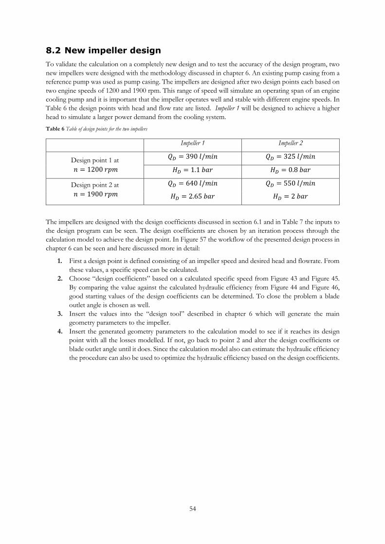
54

8.2 New impeller design

To validate the calculation on a completely new design and to test the accuracy of the design program, two

new impellers were designed with the methodology discussed in chapter 6. An existing pump casing from a

reference pump was used as pump casing. The impellers are designed after two design points each based on

two engine speeds of 1200 and 1900 rpm. This range of speed will simulate an operating span of an engine

cooling pump and it is important that the impeller operates well and stable with different engine speeds. In

Table 6 the design points with head and flow rate are listed. Impeller 1 will be designed to achieve a higher

head to simulate a larger power demand from the cooling system.

Table 6 Table of design points for the two impellers

Impeller 1 Impeller 2

Design point 1 at

𝑛 = 1200𝑟𝑝𝑚

𝑄𝐷 = 390𝑙/𝑚𝑖𝑛 𝑄𝐷 = 325𝑙/𝑚𝑖𝑛

𝐻𝐷 = 1.1𝑏𝑎𝑟 𝐻𝐷 = 0.8𝑏𝑎𝑟

Design point 2 at

𝑛 = 1900𝑟𝑝𝑚

𝑄𝐷 = 640𝑙/𝑚𝑖𝑛 𝑄𝐷 = 550𝑙/𝑚𝑖𝑛

𝐻𝐷 = 2.65𝑏𝑎𝑟 𝐻𝐷 = 2𝑏𝑎𝑟

The impellers are designed with the design coefficients discussed in section 6.1 and in Table 7 the inputs to

the design program can be seen. The design coefficients are chosen by an iteration process through the

calculation model to achieve the design point. In Figure 57 the workflow of the presented design process in

chapter 6 can be seen and here discussed more in detail:

1. First a design point is defined consisting of an impeller speed and desired head and flowrate. From

these values, a specific speed can be calculated.

2. Choose “design coefficients” based on a calculated specific speed from Figure 43 and Figure 45.

By comparing the value against the calculated hydraulic efficiency from Figure 44 and Figure 46,

good starting values of the design coefficients can be determined. To close the problem a blade

outlet angle is chosen as well.

3. Insert the values into the “design tool” described in chapter 6 which will generate the main

geometry parameters to the impeller.

4. Insert the generated geometry parameters to the calculation model to see if it reaches its design

point with all the losses modelled. If not, go back to point 2 and alter the design coefficients or

blade outlet angle until it does. Since the calculation model also can estimate the hydraulic efficiency

the procedure can also be used to optimize the hydraulic efficiency based on the design coefficients.

55

Figure 57 Work flow of design process

Table 7 Main input design coefficients for the two impellers

𝜓 𝜙2 𝛽2,𝑏𝑙

Impeller 1 0.5 0.12 23°

Impeller 2 0.5 0.08 30°

In Figure 58 a plot of the modelled pump and efficiency curves for Impeller 1 can be seen. The efficiency

plotted is the hydraulic efficiency calculated by the method described in section 5.5. The efficiency at BEP

is calculated to be 67% with a power demand of 1 and 4 kW depending on design point. In Table 8 the

calculated geometry for Impeller 1 based on the input design coefficients can be seen. The outlet tip diameter

is a consequence of the design point and chosen head coefficient as well as the blade height is a consequence

of the flow coefficient.

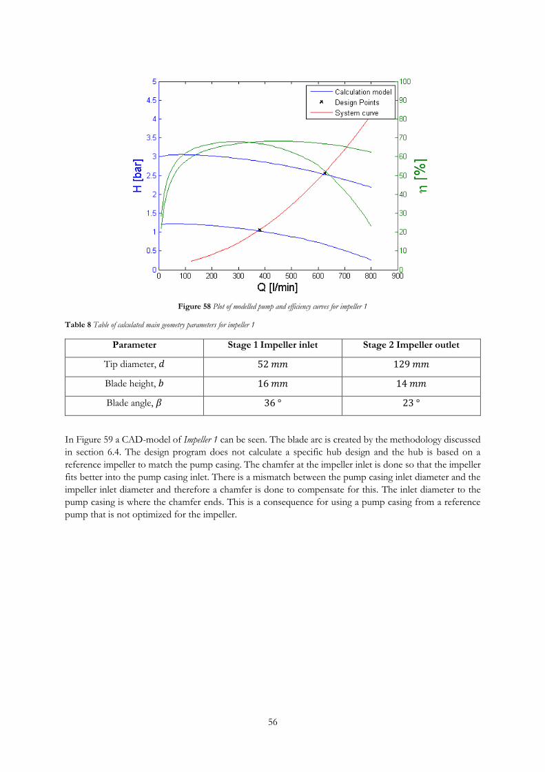
56

Figure 58 Plot of modelled pump and efficiency curves for impeller 1

Table 8 Table of calculated main geometry parameters for impeller 1

Parameter Stage 1 Impeller inlet Stage 2 Impeller outlet

Tip diameter, 𝑑 52𝑚𝑚 129𝑚𝑚

Blade height, 𝑏 16𝑚𝑚 14𝑚𝑚

Blade angle, 𝛽 36° 23°

In Figure 59 a CAD-model of Impeller 1 can be seen. The blade arc is created by the methodology discussed

in section 6.4. The design program does not calculate a specific hub design and the hub is based on a

reference impeller to match the pump casing. The chamfer at the impeller inlet is done so that the impeller

fits better into the pump casing inlet. There is a mismatch between the pump casing inlet diameter and the

impeller inlet diameter and therefore a chamfer is done to compensate for this. The inlet diameter to the

pump casing is where the chamfer ends. This is a consequence for using a pump casing from a reference

pump that is not optimized for the impeller.

57

Figure 59 CAD-model of impeller 1

In Figure 60 a plot of the calculated pump and efficiency curves for Impeller 2 can be seen. It has a maximum

calculated efficiency of 72% with a power demand of 0.6 and 2.5 kW. Comparing to Impeller 1, this is

significantly lower. This is a consequence of the much lower outlet tip diameter that reduces the head

provided and thus the power consumption. In Table 9 the calculated main design parameters based on the

input design coefficients can be seen. It has smaller outlet tip diameter to reduce the achieved head. The

outlet blade angle is balanced with the outlet blade height to achieve the design point. The inlet blade angle,

is designed to reach zero incidence at the design point to minimize incidence losses.

Figure 60 Plot of calculated pump and efficiency curves for impeller 2

58

Table 9 Table of calculated main geometry parameters for impeller 2

Parameter Stage 1 Impeller inlet Stage 2 Impeller outlet

Tip diameter, 𝑑 60𝑚𝑚 110𝑚𝑚

Blade height, 𝑏 20𝑚𝑚 14𝑚𝑚

Blade angle, 𝛽 21° 30°

In Figure 61 a CAD-model of Impeller 2 can be seen. The hub design is as previously based on a reference

impeller. The chamfer at the top of the blade after the leading edge is due to a mismatch between the

impeller inlet diameter and the inlet diameter of the pump casing as previously discussed.

Figure 61 CAD-model of impeller 2

59

8.2.1 New impeller comparison with test data

The impellers are manufactured with rapid prototyping and mounted in an existing pump casing from a

reference pump. The pump performance is then tested in the test rig by the procedure discussed in chapter

7 to get data for a pump curve. In Figure 62 a plot of the calculation model and test data for Impeller 1 are

seen at two engine speeds, 1200 and 1900 rpm corresponding to the lower and higher curve. The calculation

model captures the main behaviour of the pump curve with differences at the higher and lower tested flow

rates.

Figure 62 Plot of the calculated and tested pump curve for Impeller 1

In Figure 63 a plot of the calculation model and test data for Impeller 1, at an engine speed of 1200 rpm can

be seen. The modelled pump curve is calculated at exactly the same flow rates as in the test to be able to

compare point by point. The calculation model is within 5 percent’s difference at the first four points while

the difference is 11 and 16 percent at the points above 500 l/min. The model captures the general behaviour

of the pump curve but calculates with a too large head loss at the last points. This could be due to that the

pump is subjected to an inlet rotation that the model does not account for or that the outlet loss is less than

predicted.

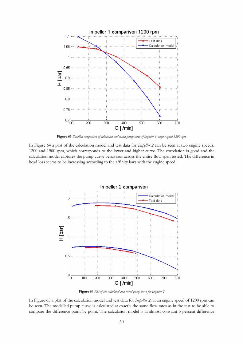
60


In Figure 64 a plot of the calculation model and test data for Impeller 2 can be seen at two engine speeds,

1200 and 1900 rpm, which corresponds to the lower and higher curve. The correlation is good and the

calculation model captures the pump curve behaviour across the entire flow span tested. The difference in

head loss seems to be increasing according to the affinity laws with the engine speed.

Figure 64 Plot of the calculated and tested pump curve for Impeller 2

In Figure 65 a plot of the calculation model and test data for Impeller 2, at an engine speed of 1200 rpm can

be seen. The modelled pump curve is calculated at exactly the same flow rates as in the test to be able to

compare the difference point by point. The calculation model is at almost constant 5 percent difference

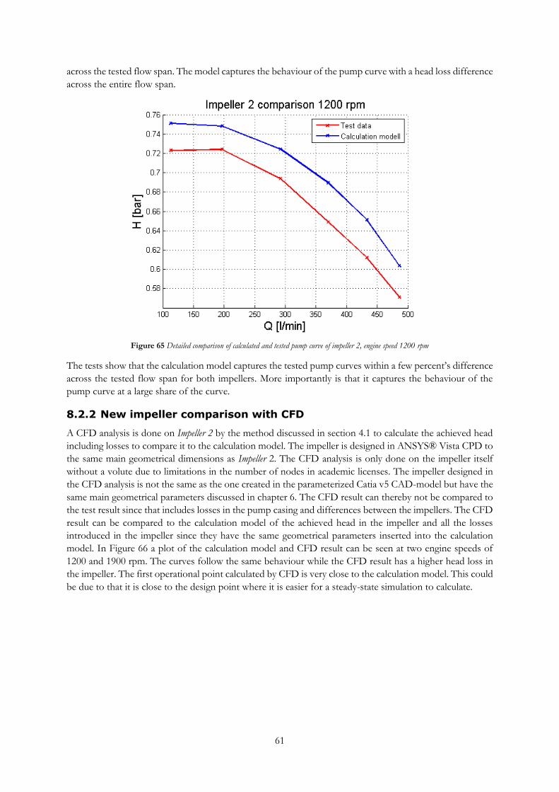
61

across the tested flow span. The model captures the behaviour of the pump curve with a head loss difference

across the entire flow span.


The tests show that the calculation model captures the tested pump curves within a few percent’s difference

across the tested flow span for both impellers. More importantly is that it captures the behaviour of the

pump curve at a large share of the curve.

8.2.2 New impeller comparison with CFD

A CFD analysis is done on Impeller 2 by the method discussed in section 4.1 to calculate the achieved head

including losses to compare it to the calculation model. The impeller is designed in ANSYS® Vista CPD to

the same main geometrical dimensions as Impeller 2. The CFD analysis is only done on the impeller itself

without a volute due to limitations in the number of nodes in academic licenses. The impeller designed in

the CFD analysis is not the same as the one created in the parameterized Catia v5 CAD-model but have the

same main geometrical parameters discussed in chapter 6. The CFD result can thereby not be compared to

the test result since that includes losses in the pump casing and differences between the impellers. The CFD

result can be compared to the calculation model of the achieved head in the impeller and all the losses

introduced in the impeller since they have the same geometrical parameters inserted into the calculation

model. In Figure 66 a plot of the calculation model and CFD result can be seen at two engine speeds of

1200 and 1900 rpm. The curves follow the same behaviour while the CFD result has a higher head loss in

the impeller. The first operational point calculated by CFD is very close to the calculation model. This could

be due to that it is close to the design point where it is easier for a steady-state simulation to calculate.

62

Figure 66 Plot of the calculation model and CFD result and two engine speeds, 1200 and 1900 rpm

In Figure 67 a plot of the CFD result and the calculation model for an engine speed of 1200 rpm can be

seen. The model is calculated at the same flow rates as the simulation to be able to compare the result at

point by point. The CFD result and calculation model has a convergence that is decreasing with the flow

rate and with a 9 percent difference at the first point and a 20 percent difference at the highest flow rate.

Figure 67 Plot of the calculation model and CFD result at an engine speed of 1200 rpm

The CFD result and the calculation for the rotor of Impeller 2 follow the same curve behaviour with a slightly

steeper curve for the CFD head result. The CFD has a constant higher head loss across the flow span

compared to the calculation model. This difference can be due to that the model is designed with a pump

casing so that the total losses across the pump are comparable to the losses in a pump. Due to difficulties

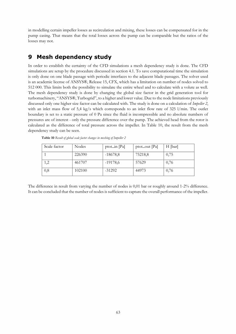
63

in modelling certain impeller losses as recirculation and mixing, these losses can be compensated for in the

pump casing. That means that the total losses across the pump can be comparable but the ratios of the

losses may not.

9 Mesh dependency study

In order to establish the certainty of the CFD simulations a mesh dependency study is done. The CFD

simulations are setup by the procedure discussed in section 4.1. To save computational time the simulation

is only done on one blade passage with periodic interfaces to the adjacent blade passages. The solver used

is an academic license of ANSYS®, Release 15, CFX, which has a limitation on number of nodes solved to

512 000. This limits both the possibility to simulate the entire wheel and to calculate with a volute as well.

The mesh dependency study is done by changing the global size factor in the grid generation tool for

turbomachinery, “ANSYS®, Turbogrid”, to a higher and lower value. Due to the node limitations previously

discussed only one higher size factor can be calculated with. The study is done on a calculation of Impeller 2,

with an inlet mass flow of 5,4 kg/s which corresponds to an inlet flow rate of 325 l/min. The outlet

boundary is set to a static pressure of 0 Pa since the fluid is incompressible and no absolute numbers of

pressures are of interest - only the pressure difference over the pump. The achieved head from the rotor is

calculated as the difference of total pressure across the impeller. In Table 10, the result from the mesh

dependency study can be seen.

Table 10 Result of global scale factor changes in meshing of Impeller 2

Scale factor Nodes ptot_in [Pa] ptot_out [Pa] H [bar]

1 226390 -18678,8 75218,8 0,75

1,2 461707 -19178,6 57629 0,76

0,8 102100 -31292 44973 0,76

The difference in result from varying the number of nodes is 0,01 bar or roughly around 1-2% difference.

It can be concluded that the number of nodes is sufficient to capture the overall performance of the impeller.

64

10 Conclusions & Discussion

The following conclusions and discussion of the project can be held.

10.1 Conclusions

The model is verified by both previous and new test data to provide a reasonable performance

prediction of a pump curve. The model captures the head losses and their behaviour both at BEP

and off-design satisfactorily.

The modelled pump curve with the modelled head losses changes its behaviour depending on the

input geometry parameters

The model can by that serve as a first step in an impeller design process to predict what operating

condition impeller geometry will provide. The model can also be used to perform a parameter

study on how different geometry parameters affect the pump performance.

By utilizing design coefficients, the presented design tool suggests reasonable impeller designs

rapidly.

The design process presented can together with the calculation model be used as a first iteration of

determining the main impeller parameters. Important parameters for the pump performance such

as leading edge design and lean angles can then be determined by CFD.

The model is able to predict the hydraulic efficiency but its accuracy have not been verified

10.2 Discussion

The calculation model can predict the general behaviour of a pump curve based on the reference pumps

and the new impellers deigned. It does have to be noted that the model has limits and is based on a limited

number of geometry parameters and many others may affect the performance of the pump. The model is

based on 1D – velocity triangles and does not capture the entire flow field. For a full performance analysis

of a pump, secondary flows and risk areas for cavitation need to be assessed. Cavitation behaviour depends

largely of leading edge design and a full analysis of the relative velocities present needs to be done to fully

predict the behaviour of the pump. This leads to that the model does not capture the effects of incipient

cavitation that can be seen when comparing to test data. However, the model does predict the total head

loss occurring in a pump both at BEP and off-design. This does not mean that the ratios of the specific

head losses are correct, but in total are of the same magnitude as in test data. It should be noted that the

specific head losses e.g. friction loss or incidence loss, are very hard to predict either numerically by CFD

or by experimental tests. All of the loss correlations are modelled to behave as suggested by literature but

they can never capture a true flow field within a pump.

The uncertainty in modelling the head loss within a pump suggests that an uncertainty analysis of the model

does not serve any purpose. The uncertainty that can be discussed is the inlet flow angle that has a significant

impact on the pump’s performance. It is up to the user to have knowledge of the flow before the impeller

inlet to accurately predict the performance of the pump. Since the inlet flow angle of the test data is not

known, better correlation could be had if this was determined. The model is focused on the impeller losses

and velocity triangles present there but a better correlation could be obtained if the volute was modelled

more in detail. The interaction between the impeller and volute and especially the outlet flow angle from

the impeller and the inlet angle of the volute could be incorporated in the model as well as studies have

shown that it has an impact on head loss (Alenius, 2001).

The design tool presented combines both methods from literature and tries to build on previous knowledge

from the reference impellers. By utilizing the design coefficients, reasonable impeller designs can be

designed rapidly. By further studying how the design coefficients affect the impeller design and performance

of the pump new knowledge can continuously be added to the pool of reference impellers. An improvement

of the design tool should be to incorporate the design of volute and diffuser. The model and design tool

65

servers as an initial tool to assess the performance of the pump while optimization studies can be done by

the more time consuming numerical methods to fully comprehend all secondary losses.

The CFD studies done should be considered as a comparison of head losses in general and not to

specifically asses single losses. CFD simulations of impeller and volute at off design conditions demands

unsteady calculations that could not be done. Due to limitations in student licenses, only steady impeller

simulations could be done. To further studies it is suggested to compare the result with full unsteady CFD

analysis of both impeller and volute.

11 Future recommendations

The following future recommendations of the calculation model and design tool are here presented:

On calculation model

Verify the predicted hydraulic efficiency by experimental tests.

Compare the calculation model with a full CFD analysis of the impeller and volute

Expand the pump casing model with tongue distance and mismatch between impeller and volute

flow angle

On design program

Expand design tool to incorporate the pump casing as well

Continue to study the effect of varying the design coefficients in impeller design

To continue to evaluate test data with the aid of design coefficients to further extend the database

when designing new impellers and pumps.

66

Bibliography

A. Predin, I. Bilus. 2003. Influence of Additional Inlet Flow on the Pre-rotation and Performance of

Centrifugal Impellers. Journal of Hydraulics Research Vol 41. s.l. : International Association of Hydraulics

Engineering and Research, 2003.

Alenius, Sven. 2001. Influence of Some Design Parameters on Flow Losses in a Pump Casing - a CFD

Investigation. Scientific Impeller. s.l. : Flygt, ITT Industries, 2001.

Anagnostopulos, John S. 2009. A fast numerical method for flow analysis and blade design in cetrifugal

pump impellers. s.l. : Computers & Fluids, 2009, Vol. 38.

ANSYS. 2013. Academic Research, Release 15, Help System, Turbosystem. 2013.

ANSYS, Release 16.0. 2015. Introduction to ANSYS CFD, Lecture 10: Turbulence. 2015.

AVL. 2009. Water pump calculation. s.l. : AVL List GMBH, 2009.

B. Stoffel, S. Meschkat, G. Mollenkopf. 2003. Thermodynamic On-Site Measurement of the Efficiency

of Centrifugal Water Supply Pumps in the Frame of Condition Orientated Maintenace. Energy efficiency in

Motor Driven Systems. s.l. : Springer Verlag, 2003.

Braembussche, R.A Van den. 2006. Flow and Loss Mechanisms in Volutes of Centrifugal Pumps. In

Design and Anylisis of High Speed Pumps, Educational notes. s.l. : RTO, 2006.

Brennen, C.E. 1994. Hydrodynamics of pumps. s.l. : Concept NREC & Oxford University Press, 1994.

Cipollone. 2013. A novel engine cooling system with two circuits operating at different temperatures. s.l. : Energy

Conversion and Management, 2013. Vol. 75.

Cornell, W.G. 1962. The stall performance of cascades. U.S National Congress on Applied Mechanics. s.l. :

ASME, 1962.

Dixon, S.L. 2014. Fluid Mechanics and Thermodynamics of Turbomachinery. s.l. : Elsevier, 2014.

El-Naggar, Mohammed Ahmed. 2013. A One_Dimensional Flow Analysis for the Prediction of

Centrifugal Pump Performance Characteristics. s.l. : Hindawi Publish Corporation, 2013, Vol. International

Journal of Rotating Machinery.

G. Ludwig, S. Meschkat, B. Stoffel. 2003. Design Factors Affecting Pump Efficiency. Energy Efficiency in

Motor Driven Systems. s.l. : Springer Verlag, 2003.

Gulich, Johann Friedrich. 2014. Centrifugal Pumps 3rd Edition. s.l. : Springer, 2014.

Hannigan, H.J. 1993. A Review of Automotive Engine Coolant Technology. Engine Coolant Testing: Third

Volume. s.l. : American Society for Testing and Materials, 1993.

Hölcke, Jan. 2002. Hydrauliska Strömningsmaskiner. s.l. : KTH Heat and Power Technology, 2002.

Holman, Jack P. 2009. Heat Transfer. s.l. : McGraw Hill Education, 2009.

Jacobsen. 2010. The Centrifugal Pump, Grundfos. s.l. : Grundfos, 2010.

Koivula, T. 2000. On Cavitation in Fluid Power. s.l. : Institute of Hydraulics and Automation, 2000.

P Dupont, A C Bayeul-Laine, A Dazin, G Bois, O Roussette and Q Si. 2012. Leakage flow simulation

in a specific pump model. s.l. : IOP Publishing, 2012.

Pang, et al. 2012. A review on air flow and coolant flow circuit in vehicles' cooling system. International

Journal of Heat and Mass Transfer. s.l. : International Journal of Heat and Mass Transfer, 2012, Vol. 55.

Pfleiderer, C. 1955. Die Kreiselpumpen fur Flussigkeiten und Gase. s.l. : Springer Verlag, 1955.

R. Fox, A. McDonald. 1998. Introduction to Fluid Mechanics 5th ed. s.l. : John Wiley & Sons, 1998.

67

S. Zoz, W. Thelen. T. Alcenius, M. Wiseman. 2001. Validation of Methods for Rapid Design and

Performance Prediction of Water Pumps. The proceedings of the 2001 Vehicle Thermal Management Systems

Conference. s.l. : SAE Technical Paper Series, 2001.

Steck, B. 2008. Avoiding Cavitation on Wet Cylinder Liners of Heavy Duty Diesel Engines by Parameter

Changes. s.l. : SAE Technical Paper Series. MAHLE International GmbH, 2008.

Stepanoff, Alexy J. 1957. Centrifugal and Axial Flow Pumps. s.l. : John Wiley & Sons, 1957.

Turton, R.K. 1994. Rotodynamic Pump Design. s.l. : Cambridge University Press, 1994.

Tuzson, John. 2000. Centrifugal Pump Design. s.l. : John Wiley & Sons, 2000.

W. Qinghuan, H. Xiaoyan. 1988. The Use of Bezier Polynomial Patches to Define the Geometrical Shape

of the Flow Channels of Compressors. s.l. : The American Society of Mechanical Engineers, 1988.

Weisner, F.J. 1967. A Review of Slip Factors for Centrifugal Impellers. 1967.

White, Frank M. 2008. Fluid Mechanics. s.l. : Graw Hill, 2008.

Woodhead. 2011. Diesel Engine Heat Rejection & Cooling. 2011.

Y. Shin, S. Kim, M. Kim. 2013. Use of Electromagnetic Clutch Water Pumps in Vehicle Engine Cooling

Systems to Reduce Fuel Consumption. s.l. : Energy, 2013.

68

12 Appendix 1

Cross-section of complete pump

(Jacobsen, 2010)

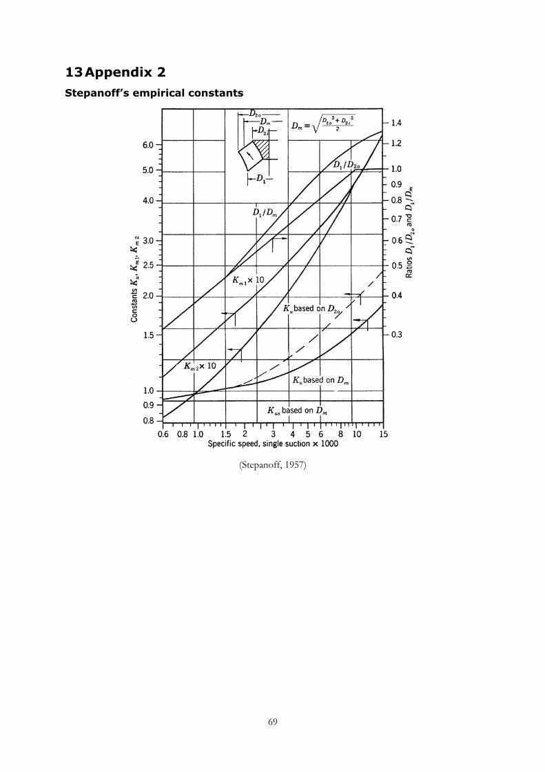
69

13 Appendix 2

Stepanoff’s empirical constants

(Stepanoff, 1957)

Documents

Development of pump geometry for engine cooling system824390/FULLTEXT01.pdf · Development of pump geometry ... includes the main head losses that occur within a centrifugal pump