Embed Size (px)
Citation preview
CER
N-T
HES
IS-2
015-
040
24/0
3/20
15
Università degli Studi di Milano Bicocca
FACOLTÁ DI SCIENZE MATEMATICHE, FISICHE E NATURALI
Tesi di Laurea Magistrale in Fisica
Development of "same side" flavour tagging algorithms
for measurements of flavour oscillations and
CP violation in the B0 mesons system
Relatore: Prof.ssa Marta Calvi
Correlatore: Dott. Basem Khanji
Candidato: Davide Fazzini
Matricola n◦: 727161
Anno Accademico 2013 - 2014

I’ll hold on to the world tight someday.
I’ve got one finger on it now; that’s a beginning.
Ray Bradbury, Farenheit 451
I
Abstract
In this thesis new developments of Flavour Tagging algorithms for the LHCb experiment
are presented. The Flavour Tagging is a very usefull tool which allows to determine the
flavour of the reconstructed particles, such as the B0 mesons. A correctly identification of
the flavour is fundamental in certain measurements such as time-dependent CP violation
asymmetries or the B0 ↔ B0 oscillations. Both these type of measurements are exploited by
LHCb experiment in the research of new physics beyond the Standard Model.
The new developments achieved in this work concern an optimization of the Same Side
Tagger algorithms, using protons and pions correlated in charge with the signal B0 to infer
its initial flavour. Then two combinations are implemented: the first is a combination of
the SS Pion Tagger (SSπ) and the SS Proton Tagger (SSp) in a unique Same Side (SS) tagging
algorithm; the second one is the final combination (SS +OS) of this new SS Tagger with the
Opposite Side (OS) Tagger combination already implemented.
To unfold the signal from the background events it has taken advantage of the sPlot
technique, which allows to calculate a per-event sWeight exploiting a discriminant variable,
i.e. the invariant mass of the B0 meson. The new SS taggers are implemented by means a
multivariate analysis based on a Boost Decision Tree (BDT) algorithm. The goal of this BDT
is to optimize the separation between “signal” (right charge correlated) and “background”
(wrong charge correlated) particles and to identify the most probable tagger candidate. The
input variables used to train the BDT include both kinematic and geometric variables. Then
the sample is divided in categories according to the BDT output value and for each one a
mistag probability is estimated by means an unbinned fit on the asymmetry oscillations.
This procedure allows to predict the mistag value (η) of a certain event directly from the
BDT response.
This analysis is performed on the data sample collected by the LHCb experiment in 2012,
corresponding to the B0 −→ D−(→ K+π−π−)π+ decay channel. Then the data samples
collected in the 2011, corresponding to the same decay channel and using two different
II

event selections, are used to obtain a validation of the flavour oscillation calibration. In
order to verify the goodness of the calibration both samples are divided in categories and
the true mistag (ω) is calculated through an unbinned fit. Thus a plot η vs ω can be used
to check the corrected calibration. An additional validation is performed on a different data
sample corresponding to the B0 −→ K−π+ decay mode. As last step the systematic effects
are studied to check the dependence of the tagging response on the event properties.
The new SSπ provides a tagging effective efficiency εe f f = 1.64± 0.07%, showing an
improvement of the performance by about 20% with respect to previous tuning. On the
other hand the new SSp yields a tagging power compatible to the result achieved with the
previous tuning (i.e. εe f f = 0.47± 0.04%). The two combinations SS and SS + OS provide
a tagging effective efficiency εe f f = 1.97± 0.10% and εe f f = 5.09± 0.15% respectively. The
algorithms developed in this thesis will be available as new taggers for the next CP violation
measurements at the LHCb experiment.
III
Sintesi
In questo progetto di tesi sono presentati nuovi sviluppi riguardanti gli algoritmi di “etichet-
tatura del sapore” (Flavour Tagging) per l’esperimento LHCb. Al centro degli studi condotti
a LHCb vi sono l’osservazione di decadimenti rari dei quark b e c e le misurazioni di vi-
olazione di CP, che potrebbero rivelare un nuovo tipo di fisica non spiegabile tramite il
Modello Standard. Per raggiungere l’elevata precisione richiesta da queste misure, è di fon-
damentale importanza ottenere una corretta identificazione del “sapore” degli adroni pe-
santi ricostruiti, come ad esempio i mesoni B0. A tale scopo la tecnica di Flavour Tagging si è
dimostrata essere un metodo molto efficace.
In particolare gli sviluppi ottenuti riguardano un’ottimizzazione degli algoritmi di “Same
Side Tagging” che, sfruttando la correlazione di carica presente tra il mesone di segnale e
il pione (SSπ), o protone (SSp), generato dalla sua frammentazione, cercano di determi-
narne il sapore. Successivamente le risposte di questi due tagger sono state combinate tra
di loro, così da ottenere un unico algoritmo di “Same Side Tagging” (SS); in un’ultima fase
si è proseguito con la sua combinazione con un “Opposite Side Tagger” (OS) generale, già
implementato.
Per separare i contributi di segnale e fondo presenti nelle n-tuple utilizzate, è stata imp-
iegata la tecnica degli sPlot la quale, sfruttando la massa invariante del mesone di segnale
come “variabile discriminante”, permette di attribuire a ciascun evento un peso (sWeight).
L’implementazione degli algoritmi è stata sviluppata attraverso un’analisi multi-variata
basata su un “Albero di Decisione Potenziato” (Boost Decision Tree, BDT), il cui obiet-
tivo è quello di ottimizzare la separazione delle tracce di segnale (correttamente correlate
in carica) da quelle di fondo (con la correlazione di carica errata) e di identificare il miglior
candidato per il tagging. Per migliorare l’efficacia di questa identificazione la BDT viene
allenata sia con variabili cinematiche che geometriche. In seguito il campione analizzato
viene diviso in categorie secondo la risposta fornita dalla BDT stessa e per ognuna di esse
viene effettuato un fit non binnato alle oscillazioni di sapore per determinare la probabilità
IV
di errata etichettatura (mistag). Tramite questo procedimento è possibile predire la mistag
(η) associata ad ogni evento direttamente dal valore fornito dalla BDT.
L’analisi è stata effettuata su un campione di dati corrispondente al canale di decadi-
mento B0 −→ D−(→ K+π−π−)π+, raccolto da LHCb nel corso del 2012. Per eseguire
dei controlli sulla stabilità degli algoritmi implementati, sono stati utilizzati due campioni
contenenti eventi raccolti durante il 2011 nello stesso canale di decadimento. La differenza
nei due casi risiede nel diverso contributo della componente di fondo, dovuta ad una se-
lezione degli eventi di segnale più larga in uno dei due casi. Per verificare la bontà della
calibrazione entrambi i campioni sono stati suddivisi in categorie, in modo da poterne cal-
colare la reale mistag (ω) attraverso un fit non binnato delle oscillazioni di sapore. É stato
quindi possibile controllare la calibrazione attraverso un grafico che mettesse in relazione
ω con η. È stato effettuato successivamente anche un controllo su un differente canale di
decadimento utilizzando un campione di eventi B0 −→ K−π+. Infine alcune sistematiche
sono state studiate in modo tale da poter valutare la presenza di eventuali dipendenze dalle
proprietà degli eventi.
I risultati finali ottenuti con il SSπ mostrano un’efficienza efficace di tagging εe f f =
1.64± 0.07% con un miglioramento delle prestazioni del 20% rispetto al tagger precedente-
mente sviluppato. L’efficienza del SSp è compatibile con quella raggiunta dal tagger attuale,
εe f f = 0.47± 0.04%. Le due combinazioni, SS e SS + OS invece forniscono rispettivamente
un’efficienza efficace di εe f f = 1.97± 0.10% e εe f f = 5.09± 0.15%. Gli algoritmi sviluppati
in questa tesi saranno disponibili come nuovi tagger per le prossime misure di violazione
di CP eseguite a LHCb.
V

Table of Contents
Frontispiece I
Abstract II
Sintesi IV
Table of Contents VIII
List of Figure XI
List of Table XV
Introduction 1
1 Theoretical Introduction 3
1.1 The Standard Model 3
1.2 Fermions and Bosons 5
1.3 The interactions in the SM 6
1.3.1 The electroweak interaction 6
1.3.2 The strong interaction 7
1.3.3 The Higgs mechanism 8
1.4 The CKM formalism 9
1.5 CP violation 13
1.5.1 Mixing of neutral pseudoscalar mesons 14
1.5.2 Types of CP Violation 16
2 The LHCb experiment 20
2.1 The Large Hadron Collider 20
2.2 b production at LHCb 22
VI

2.3 The LHCb detector 23
2.3.1 The beam pipe 24
2.3.2 The VErtex Locater 24
2.3.3 The Tracking System 25
2.3.4 The Magnet 28
2.3.5 The Ring Imaging Cherenkov 30
2.3.6 The calorimeter system 32
2.3.7 The Muon Stations 34
2.3.8 Trigger 35
3 Same Side Pion Tagger 37
3.1 The Flavour Tagging 37
3.1.1 Definitions 38
3.1.2 Same Side Taggers 40
3.2 Same Side tagger 41
3.3 SSπ tagger development using 2012 data sample 42
3.3.1 sWeights estimation 42
3.3.2 Training of the SS pion tagger 45
3.3.3 Performance and calibration 49
3.4 Validation on the 2011 data sample 55
3.5 Validation on the B0 → K+π− 2012 data sample 58
4 Same Side Proton Tagger 65
4.1 SSp tagger development using the 2012 data sample 65
4.1.1 SS proton training 65
4.1.2 Performance and calibration 69
4.2 Validation on the 2011 data sample 72
4.3 Validation on the B0 → K+π− 2012 data sample 74
5 Tagger combination 76
5.1 Combination of taggers 76
5.2 SSp and SSπ combination 77
5.2.1 Combination of the SS taggers on the B0 → D−π+ 2012 data sample 78
5.2.2 Combination on B0 → D−π+ 2011 data sample 80
5.2.3 Combination on the B0 → K+π− 2012 data sample 82
VII

5.3 SS and OS combination 83
5.3.1 Combination of SS taggers with the OS tagger on the B0 → D−π+
2012 data sample 84
5.3.2 Combination on the B0 −→ D−π+2011 data sample 87
5.3.3 Combination on the B0 → K+π− 2012 data sample 89
5.4 Measurement of ∆md 90
6 Systematics 93
6.1 Systematic uncertainties 93
6.2 Dependence of the SS tagging on pT of the signal B 94
6.3 Dependence of the SS tagging on the magnet polarity 98
6.4 Dependence of the SS tagging performances on the B flavour 99
6.4.1 Dependence on the B flavour at decay 99
6.4.2 Dependence on the B flavour at production 101
7 Conclusion 104
A sPlots technique 106
A.1 sPlot properties 108
A.2 sPlot application 108
B Boost Decision Tree classifier 110
B.1 Boosting method 112
C Monte-Carlo analyses 113
D Validation on a different cuts selection 116
D.1 Validation for the SS Pion Tagger 119
D.2 Validation for the Proton Tagger 119
D.3 Validation for the SS Tagger combination 120
D.4 Validation for the SS+OS Tagger combination 121
Bibliografia 124
Ringraziamenti 125
VIII

List of Figures
1.1 B0d and B0
s Unitary Triangles 11
1.2 Combined fit results of the B0d Unitarity Triangle 14
1.3 Box diagrams of B-mixing 18
1.4 Diagrams of CPV in interference 18
2.1 A schematic representation of the LHC collider 21
2.2 Feymann diagrams for the bb production 22
2.3 The LHCb acceptance 23
2.4 A y-z section of the LHCb detector 24
2.5 Layout of TT detection layers 26
2.6 Layout of IT detectors 26
2.7 A section of OT station 27
2.8 Track classification 28
2.9 Tracking system in the magnet 29
2.10 Dominant component of the magnetic field 29
2.11 Perspective view of the LHCb dipole magnet 30
2.12 Schematic view of RICH detectors 31
2.13 Cherenkov angle vs particle momentum for RICH radiators 31
2.14 Kaon(left) and proton(right) identification and pion misidentification as a
function of the track momentum measured on 2011 data. Plots for two differ-
ent ∆ log L are shown. 32
2.15 Side view of the LHCb muon system 34
3.1 B tagging sketch 38
3.2 Feymann diagrams for the B0 hadronization 41
3.3 Mass fit for the B0 → D−(Kππ)π+ 2012 data sample 44
IX

3.4 Output of the SSπ BDT 48
3.5 Distribution of the input variables used in the SSπ BDT 49
3.6 Time distribution of the events in 2012 data sample 50
3.7 Mixing asymmetry for signal events 52
3.8 Calibration plots for the B0 → D−π+ 2012 data sample 54
3.9 Mass fit for the B0 → D−(Kππ)π+ 2011 data sample 56
3.10 Time distribution of the events in 2011 data sample 56
3.11 Calibration for the B0 → D−π+ 2011 data sample 57
3.12 Calibration for the B0 → D−π+ 2011+2012 data sample 58
3.13 Mass fit for the B0 → K+π− 2012 data sample 60
3.14 Time distribution of the events in B0 → K+π− 2012 data sample 62
3.15 Calibration for the B0 → K+π− 2012 data sample 63
3.16 Comparison of the Bpt distributions for different decay channels 64
4.1 Output of the SSp BDT 67
4.2 Distribution of the input variables used in the SSp BDT 68
4.3 Mixing asymmetry for signal events 70
4.4 Calibration plots for the B0 → D−π+ 2012 data sample 71
4.5 Calibration for the B0 → D−π+ 2011 data sample 73
4.6 Calibration for the B0 → D−π+ 2011+2012 data sample 73
4.7 Calibration for the B0 → K+π− 2012 data sample 74
5.1 Mixing asymmetry for signal events for the B0 → D−π+ 2012 data sample 79
5.2 Calibration for the B0 → D−π+ 2012 data sample 80
5.3 Calibration for the B0 → D−π+ 2011 data sample 81
5.4 Calibration for the B0 → K+π− 2012 data sample 82
5.5 OS calibration for the B0 → D−π+ 2012 data sample 84
5.6 Mixing asymmetry for the B0 → D−π+ 2011 data sample 85
5.7 OS calibration for the B0 → D−π+ 2012 data sample 86
5.8 Calibration for the B0 → D−π+ 2011 data sample 88
5.9 SS+OS calibration for the B0 → K+π− 2012 data sample 90
5.10 Mixing asymmetry plots to estimate ∆md using the B0 → D−π+ 2011 data
sample 91
6.1 BpT distribution and the splitting in three bins 95
X

6.2 Calibration plots for the SS pion in BpT bins 96
6.3 Calibration plots for the SS proton in BpT bins 97
6.4 Calibration plots for the SS pion according to the magnet polarity 98
6.5 Calibration plots for the SS proton according to the magnet polarity 99
6.6 Calibration plots for the SS pion according to the Bid defined from the final
state 100
6.7 Calibration plots for the SS proton according to the Bid by the final state 101
6.8 Calibration plots for the SS pion according to the Bid from the tagger charge 102
6.9 Calibration plots for the SS proton according to the Bid from the tagger charge 103
A.1 Distributions of signal and background for some variables 109
B.1 Sketch of a decision tree 111
D.1 Mass fit for the B0 → D−(Kππ)π+ 2011 data sample 118
D.2 Time distribution of the events in 2011 data sample 118
D.3 Calibration for the B0 → D−π+ 2011 data sample 119
D.4 Calibration for the B0 → D−π+ 2011 data sample 120
D.5 Calibration for the B0 → D−π+ 2011 data sample 121
D.6 SS+OS calibration for the B0 → D−π+ 2011 data sample 122
XI

List of Tables
1.1 Fermions list in the Standard Model 5
1.2 Boson list in Standard Model 6
1.3 Weak flavor quantum numbers of leptons and quarks 8
1.4 Angles of B0d triangle from UTfit 12
1.5 Value of Wolfenstein parameters from UTfit 13
1.6 Experimental values of VCKM parameters 13
2.1 Integrated luminosity delivered to LHCb 22
3.1 Selection cuts for the decay channel B0 → D−π+ 43
3.2 Results of the fit to the mass distribution 2012 data sample 44
3.3 Preselection cuts applied for SS pion tagging algorithm 46
3.4 Input variables used to train SSπ 47
3.5 Input variables ranking 48
3.6 Acceptance parameters for the 2012 data sample 50
3.7 Performances for the BDT categories determined from the asymmetry fit 51
3.8 Parameters of the 3rd polynomial for the B0 → D−π+ 53
3.9 Calibration parameters and tagging performances for the B0 → D−π+ 2012
data sample 53
3.10 Performance of the current SSπ tagger on the B0 → D−π+ 54
3.11 Results of the fit to the mass distribution 2011 data sample 55
3.12 Acceptance parameters for the 2011 data sample 55
3.13 Calibration parameters and tagging performances for the B0 → D−π+ 2011
data sample 57
3.14 Calibration parameters and tagging performances for the B0 → D−π+ 2011+2012
data sample 57
XII

3.15 Selection cuts for the decay channel B0 −→ K+π− 59
3.16 Results of the fit to the mass distribution B0 → K+π− 2012 data sample 61
3.17 Acceptance parameters for the B0 → K+π− 2012 data sample 62
3.18 Calibration parameters and tagging performances for the B0 → K+π− 2012
data sample 62
3.19 Comparison between the tagging powers for B0 → K+π− data sample 64
4.1 Preselection cuts applied for SS proton tagging algorithm 66
4.2 Input variables used to train SSp 67
4.3 Input variables ranking 68
4.4 Performances for the BDT categories determined from the asymmetry fit 69
4.5 Parameters of the 3rd polynomial for the B0 → D−π+ 71
4.6 Calibration parameters and tagging performances for the B0 → D−π+ 2012
data sample 71
4.7 Performance of the current SSp tagger on the B0 → D−π+ 72
4.8 Calibration parameters and tagging performances for the B0 → D−π+ 2011
data sample 72
4.9 Calibration parameters and tagging performances for the B0 → D−π+ 2011+2012
data sample 73
4.10 Calibration parameters and tagging performances for the B0 → K+π− 2012
data sample 74
4.11 Comparison between the tagging powers for B0 → K+π− data sample 75
5.1 Performances of the sub-sample with both taggers for the B0 → D−π+ 2012
data sample 78
5.2 Calibration parameters for the B0 −→ D−(→ Kππ)π+ 2012 data sample 79
5.3 Performances of the SS combination on the 2012 data sample with 79
5.4 Performance of the current SS tagger on the B0 → D−π+ 80
5.5 Calibration parameters for the B0 −→ D−(→ Kππ)π+ 2011 data sample 80
5.6 Performances of the SS combination on the 2011 data sample 81
5.7 Performances of the SS combination on the B0 → D−π+ 2011+2012 data sample 82
5.8 Calibration parameters of the SS combination for the B0 → K+π− 2012 data
sample 82
5.9 Performances of the SS combination on the B0 → K+π− 2012 data sample 83
XIII

5.10 OS calibration parameters and tagging performances for the B0 → D−π+
2012 data sample 84
5.11 SS+OS calibration parameters for the B0 −→ D−(→ Kππ)π+ 2012 data sample 85
5.12 SS+OS performances of the sub-sample with both taggers for the B0 → D−π+
2012 data sample 86
5.13 Performances of the OS combination on the 2012 data sample 87
5.14 Performance of the current SS + OS tagger on the B0 → D−π+ 87
5.15 OS calibration parameters and tagging performances for the B0 → D−π+
2011 data sample 87
5.16 SS+OS calibration parameters for the B0 −→ D−π+ 2011 data sample 87
5.17 Performances of the SS+OS combination on the 2011 data sample 88
5.18 Performances of the SS+OS combination on the B0 → D−π+ 2011+2012 data
sample 88
5.19 OS calibration parameters and tagging performances for the B0 → K+π−
2012 data sample 89
5.20 SS+OS calibration parameters for the B0 → K+π− 2012 data sample 89
5.21 SS+OS tagging performances for the B0 −→ K+π− 2012 data sample 89
5.22 Fit results to estimate ∆md 92
5.23 Comparison of the mixing frequency ∆md results 92
6.1 Calibration parameters for the SS pion in BpT bins 95
6.2 Calibration parameters for the SS proton in BpT bins 97
6.3 Calibration parameters for the SS pion according to the magnet polarity 98
6.4 Calibration parameters for the SS proton according to the magnet polarity 99
6.5 Calibration parameters for the SS pion according to the Bid defined by the
final state 100
6.6 Calibration parameters for the SS proton according to the Bid defined by the
final state 101
6.7 Calibration parameters for the SS pion according to the Bid defined by the
tagger charge 102
6.8 Calibration parameters for the SS proton according to the Bid defined by the
tagger charge 103
C.1 Origin of the right charged correlated pions 113
C.2 Origin of the wrong charged correlated pions 114
XIV
C.3 Comparison of the results provide with MC and data 114
D.1 Results of the fit to the mass distribution 2011 data sample 116
D.2 Selection cuts for the decay channel B0 −→ D−(Kππ)π+ 117
D.3 Acceptance parameters for the 2011 data sample 118
D.4 Calibration parameters and tagging performances for the B0 → D−π+ 2011
data sample 119
D.5 Calibration parameters and tagging performances for the B0 → D−π+ 2011
data sample 120
D.6 Calibration parameters for the B0 −→ D−(→ Kππ)π+ 2011 data sample 120
D.7 Performances of the SS combination on the 2011 data sample with the second
event selection 121
D.8 OS calibration parameters and tagging performances for the B0 → D−π+
2011 data sample 121
D.9 SS+OS calibration parameters for the B0 → D−π+ 2011 data sample 122
D.10 SS+OS performances of the SS combination on the 2011 data sample with the
second cuts selection 122
XV
Introduction
The Standard Model (SM) is a relativistic quantum field theory which describes successfully
the interactions of fundamental particles up to the actual energies except the gravity. In this
theory when a physical system is invariant under a particular transformation a symmetry
arises and, as the Noether’s theorem stands, it is related to a conservation law by a one-
to-one correspondence. There are two types of symmetry: continuous, as rotations in space
or translation in time, and discrete, like charge conjugation (C) or parity (P). As it was
discovered in 1957 and in 1964, the weak interactions don’t conserve both P and C and
neither their product (CP).
The LHCb experiment is devoted to to the study of the b and c hadrons decay, and
in particular in the measurements of CP violation. To provide these measurements the
“Flavour Tagging” technique is exploited in order to know the initial flavour of the meson
reconstructed, such as a B0d. This procedure is performed by means of several algorithms,
using the informations from the b quark fragmentation which originates the signal B me-
son (Same Side tagging - SS) or the informations from the decay chain of the opposite B
(Opposite Side tagging - OS).
The aim of this thesis is to present some new developments of Flavour Tagging algo-
rithms for the LHCb experiment. In particular this thesis provides an optimization of the SS
taggers which use a pion or a proton created during the hadronization process of the sig-
nal B meson to infer its initial flavour. This new algorithms exploit a multivariate classifier
based on a “Boost Decision Tree” to choose the best tagger candidate providing a proba-
bility of the tagging decision to be correct. In order to improve this selection the BDT uses
both geometrical and kinematic variables related to the tracks, to the B meson or to the
event itself.
1

LIST OF TABLES
The data sample used to develop the two algorithms corresponds to B0 −→ D−(→
K+π−π−)π+ decay mode collected during the 2012 by LHCb. Then the 2011 data samples
corresponding to the same decay mode, but with different background contribution, are
used to test the performances and the calibration of the estimated tagging probability.
Then the results obtained with the SSπ and the SSp taggers are combined, in a first
time, in a unique SS tagger to achieve better performances and in a second time this new
SS tagger is combined with a general OS tagger, already implemented.
In Chapter 1 a summary of the theoretical background of the physics studied by LHCb
is reported. In Chapter 2 the LHCb spectrometer is described. In Chapter 3 the details of
the SSπ tagger implementation,its performances and calibration are reported. In Chapter 4
the development of the SSp tagger is described and its performances are shown. In Chapter
5 the combination of a unique SS tagger and the final combination of a SS + OS tagger
are described, showing their performances and calibration. In Chapter 6 some systematic
effects are analyzed for the SSπ and the SSp taggers. In Chapter 7 a summary of all the
results is reported.
2
1
Theoretical Introduction
Contents
1.1 The Standard Model 3
1.2 Fermions and Bosons 5
1.3 The interactions in the SM 6
1.3.1 The electroweak interaction 6
1.3.2 The strong interaction 7
1.3.3 The Higgs mechanism 8
1.4 The CKM formalism 9
1.5 CP violation 13
1.5.1 Mixing of neutral pseudoscalar mesons 14
1.5.2 Types of CP Violation 16
In this chapter the Standard Model (SM) of particle physics is shortly described. The
subatomic particles and the fundamental interactions are described in section 1.2 and in
section 1.3. The SM describes particles as fermion fields and their interactions are mediated
by the exchange of boson fields. Then a brief description of CP violation and the flavour
tagging technique are given in section 1.5 and 3.1.
1.1 The Standard Model
The Standard Model (SM) of particle physics is a quantum field theory which, combin-
ing the special relativity with quantum mechanics, describes three of the four fundamental
forces of nature (the Electromagnetic Force, the Weak Force and the Strong force).
Its Lagrangian is symmetric under the transformations of the SU(3) × SU(2) × U(1)
gauge group. SU(3) group describes the strong coupling while the SU(2)×U(1) describes
3
1 - Theoretical Introduction
the electroweak interaction (the unification of the weak and the electromagnetic forces pre-
dict by the model).
The Gravitational Force is not accounted in the Standard Model, though some theories
to unify the gravity with the Strong and Electroweak Forces are in development phase.
One hypothesis predicts that the gravitational force is mediated by a single boson, named
graviton, which posses an intrinsic spin of two unit.
The Standard Model consists of two type of elementary particles: fermions, which have
a odd-half integral spin, and bosons, which have an integer spin. The fermions (leptons
and quarks) are the building block of the matter and anti-matter. A description of a group
of fermion must be antisymmetric under interchange of two particles, it means that they
obey to the Fermi-Dirac statistic:
|1, , 2, ..., i, ..., j, ...N〉 = −|1, , 2, ..., j, ..., i, ...N〉
On the other hand the bosons are mediators of the interactions between the particles. A
description of a group of bosons must be symmetric under interchange of two particles and
thus they obey to the Bose-Einstein statistic:
|1, , 2, ..., i, ..., j, ...N〉 = |1, , 2, ..., j, ..., i, ...N〉
The last particle observed, foreseen by the Standard Model, is the Higgs Boson. It is a
massive, chargeless, boson with zero spin (thus, it’s a scalar boson). The Higgs field, trough
the mechanism of “Spontaneous Symmetry Breaking”, is the reason why some fundamen-
tal particles are massive, even though the symmetries controlling their interactions require
them to be massless. It also answers several other long-standing puzzles in physics, such as
the reason the weak force has a much shorter range than the electromagnetic force.
A relativistic quantum field theory based on a hermitian Lagrangian, invariant under
Lorentz transformations, is also invariant under the product of the tree operators C,P,T (CPT
theorem) but not under one transformation separately. C denotes the charge conjugation
transformation, turning particles in their respective anti-particles; the parity transformation
P inverts the space coordinates of the field while the time reversal operator change the sign
of time coordinate. According to CPT theorem particles and anti-particles must have equal
masses and decay times.
4

1 - Theoretical Introduction
1st generation 2nd generation 3rd generation
Leptonsνe < 2 eV νµ < 2 eV ντ < 2 eV
e 511 KeV µ 105.7 MeV τ 1.78 GeV
Quarksu 2 MeV c 1.27 GeV t 173 GeV
d 5 MeV s 95 MeV b 4.18 GeV
Table 1.1: Fermions described in the Standard Model. The respective masses are given in parenthesis
1.2 Fermions and Bosons
The fermions are the matter constituents and can be divided in leptons and quarks. Accord-
ing to the Standard Model there are three generations of fermions organized by increasing
mass. Each generation consisting of a lepton, a neutrino, a positively charged quark, a neg-
ative charged quark and their respective anti-particles.
The leptons described in the theory are the electron (e−), the muon (µ−), the tau (τ−)
and their associated neutrinos (νe, νµ and ντ). Each lepton posses an anti-particle which is
exactly the same in all the observable ways except the charge, that is opposite in sign. They
are denoted as e+, µ+, τ+, νe, νµ, ντ1.
Six quarks exist: up (u), down (d), charm (c), strange (s), top (t), bottom (b). The posi-
tively charged quarks (u,c,t) carry 23 of the fundamental unit charge, while the negatively
charged quarks (d,s,b) carry −13 of the fundamental unit charge. Their relatively anti-particles
are denoted as u, d, c, s, t and b. Leptons and quarks are listed in Table 1.1 [1]. The quarks
posses an additional property, called color charge. There are three varieties of color: red,
green and blue and the respective anti-colors. The color charge is related to the strong force
just like the electric charge is related to the electromagnetic force.
Because of the Color Confinement (see section 1.3) quarks cannot be isolated singularly,
and therefore cannot be directly observed. Instead they clump together to form hadrons.
There are two types of hadrons:
• “mesons”: consist of bound states quark anti-quark pairs (qq) and have integral spin;
1The relationship between neutrinos and their anti-neutrinos, both chargeless, is more complicated than
charge conjugation.
5

1 - Theoretical Introduction
interaction bosons mass relative strength
Electromagnetic γ 0 αem ∼ O(10−2)
WeakW± 80.4 GeV
αW ∼ O(10−6)Z0 91.2 GeV
Strong g (g1, . . . , g8) 0 αs ∼ O(1)
- H0 125.9 GeV -
Table 1.2: Bosons described in the Standard Model with their mass and relative strength of the in-
teraction.
• “baryons”: consist of bound states of three quarks (or anti-quarks) and have odd-half
integral spin;
Even though bound states of five quarks, called penta-quarks, are expected they have yet
to be observed.
Because the strong force doesn’t interact with hadrons, each quark bound state must be
colorless, just like the leptons. For the mesons this condition can happen combining a color
with its anti-color (e.g. red plus anti-red), while the baryons must posses a quark for each
color (thus, red plus green plus blue is equal to colorless).
1.3 The interactions in the SM
The bosons are the force-carries (γ, W±, Z0), which mediate the interaction between the
fermions and the Higgs boson (H0) that gives mass to the particles. These particles are
listed in Table 1.2 [1]. The interactions are introduced in the theory requiring that the the
SM Lagrangian is invariant under local gauge transformations of the SU(3)× SU(2)×U(1)
group.
1.3.1 The electroweak interaction
The photon (γ) is a massless, chargeless particle with a unit spin. It is the gauge boson
associated to the electromagnetic force. This interaction acts on all the charged particles
and it is easily visible at a macroscopic level. This force is described through the Quantum
Electrodynamics (QED) and is associated to the symmetry generated by the U(1) gauge
group.
6
1 - Theoretical Introduction
The weak force is mediated by the Z0 and the W± gauge bosons.This interaction acts
only on the left-handed particles2, this is an effect of the V-A form (Vector minus Axial)
form of the Lagrangian, which contains terms that project out the left-handed component
of the state. For this reason the left-handed particles are represented as a isospin doublet,
while the right-handed particles are considered as isospin singlet. The symmetry associated
to this interaction is generated by the SU(2) gauge group.
The Standard Model predicts the unification of these two interactions into the SU(2)×
U(1) gauge symmetry, associating the massless gauge bosons ~Wµ = (W1µ, W2
µ, W3µ) and Bµ.
However this symmetry is broken by the Higgs mechanism, which decouples the weak
and the electromagnetic forces originating the photon (gauge field Aµ) and the three weak
bosons (gauge field Wµ and Zµ).
W±µ =W1
µ ± iW2µ√
2
Aµ = − sin θWW3µ + cos θW Bµ
Zµ = cos θWW3µ + sin θW Bµ
(1.1)
In these formulas θW is the Weinberg angle defined as θW = arctan (g′/g), where g and
g′ are the U(1)Y and SU(2)L couplings constant.
The weak Lagrangian that describes the coupling of the charged gauge bosons to the
fermions is:
Lew = − g√2
W+µ (νγµ(1− γ5)l + quγµ(1− γ5)qd + h.c.) (1.2)
The weak flavour quantum numbers related to the SM fermions are reported in Table
1.3.
1.3.2 The strong interaction
The strong interaction is described trough the Quantum Chromodynamics (QCD), a non-
Abelian gauge theory, introducing a new quantum number, named color. The color struc-
ture can be represented by the SU(3) gauge group. This force is mediated by 8 massless,2The handedness of a particles refers to its chirality determined by whether the particle transforms in a right-
or left-handed representation of the Poincaré group. However the Dirac spinors representation have both the
components, thus it is possible to define the projection operators which project out the component of the state.
The form of these operators is: (1± γ5)/2. If the particle is massless the chirality is the same as helicity, defined
as the projection of its spin relative to the direction of its momentum
7
1 - Theoretical Introduction
generations I I3 Y Q
νeL
eL
νµL
µL
ντL
τL
1/2+1/2 -1/2 0
-1/2 -1/2 -1
eR µR τR 0 0 -1 -1uL
d′L
cL
s′L
tL
b′L
1/2+1/2 +1/6 +2/3
-1/2 +1/6 -1/3
uR cR tR 0 0 +2/3 +2/3
d′R s′R b′R 0 0 -1/3 -1/3
Table 1.3: The symbol I denotes the weak isospin and I3 is its third component, Q is the electric
charge (given in unity of the elementary charge e) and Y = Q − I3 is the weak hyper-
charge. The weak eigenstates (d’, s’, b’) are related to the mass eigenstates (d, s, b) trough
the CKM matrix, described in section 1.4
chargeless gauge bosons, called gluons, that posses two color varieties and can self-interact.
The gluons and the quarks are the only particles that carry non-vanishing color charge and
thus participate in strong interactions.
Unlike the other interactions, the strong force doesn’t diminish in strength with increas-
ing distance, the effect is the “color confinement”. Because of this phenomenon, when two
quarks become separated, at some point it is more energetically favorable for a new quark-
antiquark pair to spontaneously appear. As a result, instead of seeing the individual quarks
in detectors, many "jets" of color-neutral particles (mesons and baryons) are observed. This
process of particles production is called “hadronization” or “fragmentation”.
On the other hand, at short distance the QCD coupling decreases and thus the quarks
behave as free particles (in terms of strong interaction). This phenomenon is known as
“asymptotic freedom”.
1.3.3 The Higgs mechanism
The Higgs mechanism is a mathematical model that explains why and how gauge bosons
could still be massive despite their governing symmetry. The “Higgs field” breaks the sym-
metry laws of the electroweak interaction and the weak bosons are able to have mass. The
introduction of a scalar field, with a potential V(Φ) = −µ2|Φ|2 + λ2|Φ|4, breaks the sym-
8

1 - Theoretical Introduction
metry of the theory choosing spontaneously one of the degenerate ground states as the true
ground, resulting in the appearance of massless Goldstone bosons. The Higgs field can be
represented as a doublet of complex scalar fields:
Φ(x) ≡
Φ+(x)
Φ0(x)
(1.3)
The minimum of the potential is chosen as:
Φ(x) =1√2
( 0√−µ2
λ + h(x)
)(1.4)
with expectation value on vacuum state equal to: |〈0|Φ0(x)|0〉| ≡ v√2, where v = −µ√
λ. The
Higgs field is responsible also for the mass of the fermions through the extension of the
Higgs mechanics to Yukawa’s interaction. For each fermion’s generation the Yukawa’s La-
grangian can be written as:
LY = − 1√2(v + H)(cddd + cuuu + cl ll + cννν) (1.5)
where u = type-up quark, d = type-down quark and l = lepton and ν = neutrino. The fermion
masses are calculated as:
Mi = civ√2
(1.6)
where i = u, d, l, ν.
1.4 The CKM formalism
The fermions and the bosons should be massless in order for the electroweak interaction
to be invariant under local gauge transformations. However due to the coupling to the
Higgs field they acquire mass trough the Spontaneous Symmetry Breaking mechanism.
The resulting mass eigenstates are not the same as the eigenstates of the weak interaction
but a their linear combination, as Cabibbo suggests in 1963 [2].
The Cabibbo-Kobayashi-Maskawa (CKM) matrix (VCKM) is the quark mixing matrix in-
troduced to describe the transformation needed to switch from the quark mass eigenstates
to the weak ones and vice versa. This transformation consist in a rotation of the down-type
quarks:
d′
s′
b′
= VCKM
d
s
b
(1.7)
9
1 - Theoretical Introduction
where VCKM is a unitary matrix3 defined as:
VCKM =
Vud Vus Vub
Vcd Vcs Vcb
Vtd Vts Vtb
(1.8)
In general a n × n complex matrix possess a priori 2n2 real parameters, however the
unitary conditions introduce 2 · 12 · n · (n − 1) = n2 − n constraints for the off-diagonal
elements and n for the diagonal elements. Through a redefinition of the quark fields 2n− 1
phases can be removed.
The final number of the parameters is:
Npar = 2n2 − n− (n2 − n)− (2n− 1) = n2 − 2n + 1 = (n− 1)2 (1.9)
In the quark case n = 3 thus the matrix can be completely defined by 4 parameters: three
real rotation angles and one phase δ responsible for all CP-violating (CPV) phenomena in
flavor-changing processes. These parameters are free in Standard Model so they should be
determined experimentally.
The unitary constraints are:
1)VusV∗ub + VcsV∗cb + VtsVtb = 0
2)VudV∗ub + VcdV∗cb + VtdVtb = 0
3)VudV∗us + VcdV∗cs + VtdV∗ts = 0
4)VudV∗td + VusV∗ts + VubV∗tb = 0
5)VcdV∗tb + VcsV∗ts + VcbV∗tb = 0
6)VudV∗cd + VusV∗cs + VubV∗cb = 0
(1.10)
These conditions can be resumed as follows:
3
∑k=1
Vki ·Vkj = δij (1.11)
Each condition can be geometrically represented as a triangle in the complex plane,
called “Unitary Triangle”. In total there are six equivalent triangles in the Standard Model
and their area4 value is a direct measure for the predicted amount of CP-violation. The
3It means that VCKMV†CKM = 1
4The area of the Unitary Triangles is equal to half of the Jarlskog invariant defined as: Im[VijVklV∗ij V∗kl ] =
J ∑m,n εikmε jln
10

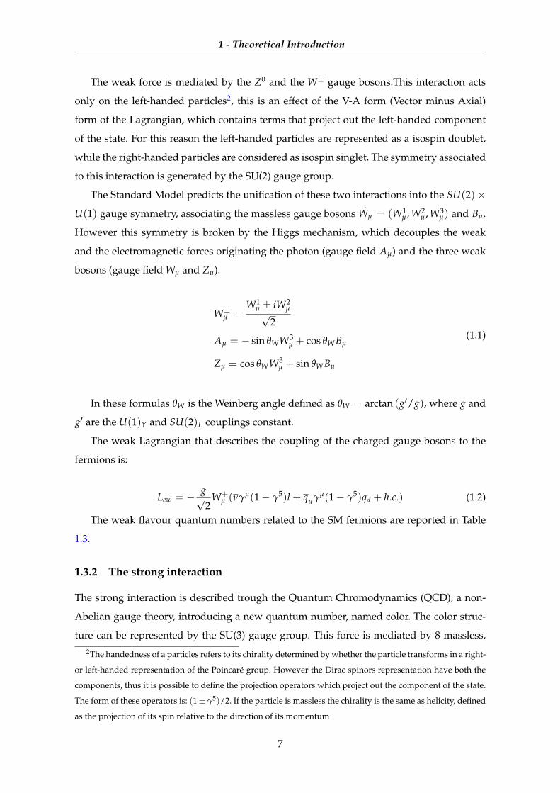
1 - Theoretical Introduction
conditions 2) and 4) in equation 1.10 are very important for the CPV studies because of the
similar lengths of their three sides and amplitudes of their internal angles. They are shown
in Figure 1.1. These characteristics provide tests of the CKM matrix because they can lead
to large CP violating asymmetries between the matrix elements. The other triangles posses
a very short side, thus they are very close to degenerate in a line.
(0, 0)(1, 0)
(ρ, η)
Re
Im
∣∣∣VtsV∗usVcdV∗cb
∣∣∣
∣∣∣VudV∗ubVcdV∗cb
∣∣∣∣∣∣ VtdV∗tb
VcdV∗cb
∣∣∣γ β
α
(0, 0) (1− λ2
2 + ρλ2, ηλ2)
(ρ, η)
Re
Im
∣∣∣VtsV∗usVcdV∗cb
∣∣∣∣∣∣VtbV∗ub
VcdV∗cb
∣∣∣∣∣∣VtdV∗ud
VcdV∗cb
∣∣∣γ′
β′α′
βs
Figure 1.1: The two main important Unitary Triangles. On the left the triangle from 2) and on the
right the triangle from 4).The sides are scaled of a factor |VcdV∗cb| = Aλ3, while the ver-
tices are calculated using the Wolfenstein parameterization, explained at the of this sec-
tion
The triangle 2) is known also as “B0d triangle” because its angles and sides can be mea-
sured through the B0d decays. The values of the angles are given by:
α = arctanVtdV∗tbVudV∗ub
β = arctanVcdV∗cbVtdV∗tb
γ = arctanVudV∗ubVcdV∗cb
(1.12)
where α+ β+ γ = π. The angles of the triangle 4) are related to the α, β and γ in agreement
to the following relations:
α′ = α β′ = β− βs γ′ = γ + βs (1.13)
where βs is the angle between the real axis and the lower side of the triangle. Experimentally
βs is found close to 1◦ (βs = 0.0182± 0.0009 [3]).
The constraints on these angles can be obtained from measurements of many processes
and, through a global fit, the values extrapolated can provide a test for the Standard Model
accuracy. Values different from the expected ones would be a confirmation of new physics
as many extensions to the Standard Model predict.
The global fit performed by UTfit group achieved the results reported in Table 1.4.
11

1 - Theoretical Introduction
Parameter Final value
α 88.6± 3.3
β 22.03± 0.86
γ 69.2± 3.4
Table 1.4: Estimated values of the angles of B0d Unitary Triangle trough a global fit performed by
UTfit group[4].
A parameterization of the CKM matrix is the “Chau-Keung parameterization”, where
VCKM = R23 × R13 × R12.
R12 =
c12 s12 0
−s12 c12 0
0 0 1
R23 =
1 0 0
0 c23 s23
0 −s23 c23
R13 =
c13 0 s13e−iδ
0 1 0
−s13eiδ 0 c13
(1.14)
VCKM =
c12c13 s12c13 s13e−iδ
−s12c23 − c12s23s13eiδ c12c23 − s12s23s13eiδ s23c13
s12s23 − c12c23s13eiδ −c12s23 − s12c23s13eiδ c23c13
(1.15)
where sij = sin θij, cij = cos θij and i, j = 1, 2, 3 are the generations5. The angles θij must
be chosen in the first quarter, while δ is the only one parameter which can introduce effects
of CP violation and must be: 0 < δ < 2π.
Another parameterization, known as “Wolfenstein parameterization”, is obtained ex-
panding as a power series of the parameter λ = |Vus|:
VCKM =
1− λ2
2 λ Aλ3(ρ− iη)
−λ 1− λ2
2 Aλ2
Aλ3(1− ρ− iη) −Aλ2 1
+ O(λ4) (1.16)
where
λ =|Vus|√
|Vud|2 + |Vus|2= sin θc
Aλ2 = λ∣∣∣Vcb
Vus|
Aλ3(ρ + iη) = V∗ub
(1.17)
5The angle θ12 is known also as Cabibbo angle (θc).
12
1 - Theoretical Introduction
Parameter Final value
A 0.821± 0.012
λ 0.22534± 0.00065
ρ 0.132± 0.023
η 0.352± 0.014
Table 1.5: Estimated values of the Wolfenstein parameters trough a global fit performed by UTfit
group [4].
Element Value Measurement Channel
|Vud| 0.97425± 0.00018 Nuclear beta decays
|Vus| 0.22543± 0.00077 Semileptonic kaon decays
|Vcd| 0.22529± 0.00077 ν scattering from valence d quarks
|Vcs| 0.97342+0.00021−0.00019 Semileptonic D meson decays
|Vcb| 0.04128+0.00058−0.00129 Semileptonic B meson decays
|Vub| 0.00354+0.00016−0.00014 Semileptonic B meson decays
|Vtd| 0.00858+0.00030−0.00034 B0 mixing assuming |Vtb| = 1
|Vts| 0.04054+0.00057−0.00129 B0
s mixing assuming |Vtb| = 1
|Vtb| 0.99914+0.00005−0.00003 Single-top-quark production
Table 1.6: The current values of VCKM matrix elements [5]
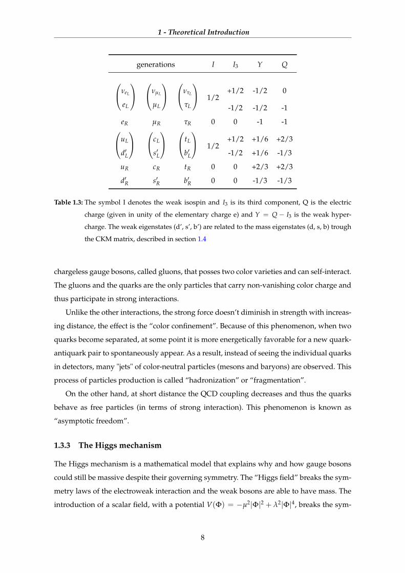
The constraints on this parameters estimated by means of a global fit performed by UTfit
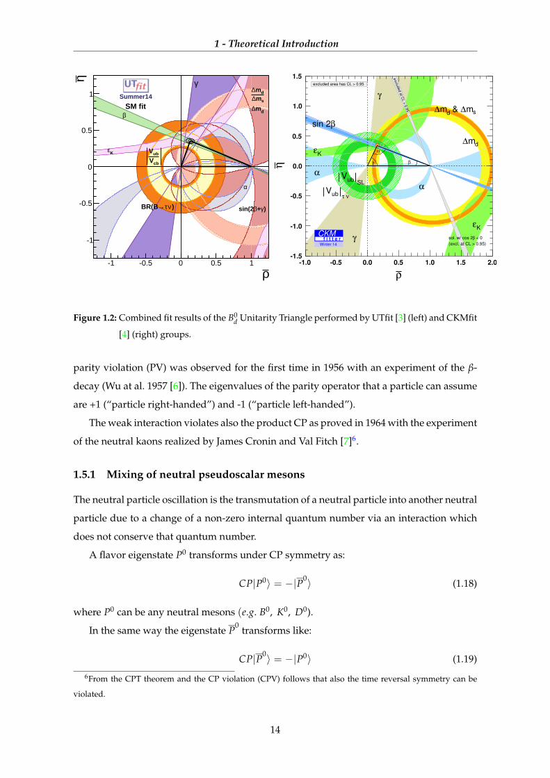
and CKMfitter groups are shown in Figure 1.2, while the experimentally values obtained
by UTfit are reported in Table 1.5, where ρ = ρ
(1− λ2
2
)and η = η
(1− λ2
2
).
Input to these global fits are the measurements of the angles and sides of the Unitary
Triangles from meson decays and mixing as reported in Table 1.6. .
1.5 CP violation
The electromagnetic and strong forces are invariant under parity symmetry and charge
conjugation, on the other hand the weak interaction violates both in a maximal way. The
13
1 - Theoretical Introduction
ρ-1 -0.5 0 0.5 1
η
-1
-0.5
0
0.5
1γ
β
α
)γ+βsin(2
sm∆dm∆
dm∆
Kε
cbVubV
)ντ→BR(B
Summer14
SM fitγ
γ
α
α
dm∆
Kε
Kε
sm∆ & dm∆
SLubV
ν τubV
βsin 2
(excl. at CL > 0.95)
< 0βsol. w/ cos 2
exc
luded a
t CL >
0.9
5
α
βγ
ρ
1.0 0.5 0.0 0.5 1.0 1.5 2.0
η
1.5
1.0
0.5
0.0
0.5
1.0
1.5
excluded area has CL > 0.95
Winter 14
CKMf i t t e r
Figure 1.2: Combined fit results of the B0d Unitarity Triangle performed by UTfit [3] (left) and CKMfit
[4] (right) groups.
parity violation (PV) was observed for the first time in 1956 with an experiment of the β-
decay (Wu at al. 1957 [6]). The eigenvalues of the parity operator that a particle can assume
are +1 (“particle right-handed”) and -1 (“particle left-handed”).
The weak interaction violates also the product CP as proved in 1964 with the experiment
of the neutral kaons realized by James Cronin and Val Fitch [7]6.
1.5.1 Mixing of neutral pseudoscalar mesons
The neutral particle oscillation is the transmutation of a neutral particle into another neutral
particle due to a change of a non-zero internal quantum number via an interaction which
does not conserve that quantum number.
A flavor eigenstate P0 transforms under CP symmetry as:
CP|P0〉 = −|P0〉 (1.18)
where P0 can be any neutral mesons (e.g. B0, K0, D0).
In the same way the eigenstate P0 transforms like:
CP|P0〉 = −|P0〉 (1.19)
6From the CPT theorem and the CP violation (CPV) follows that also the time reversal symmetry can be
violated.
14

1 - Theoretical Introduction
These two transformations lead to write the CP eigenstates as linear combination of the
flavor eigenstates:
|PCP evens 〉 = 1√
2(|Ps〉 − |Ps〉)
|PCP odds 〉 = 1√
2(|Ps〉+ |Ps〉)
(1.20)
The time evolution of the flavor eigenstates is described by the Schrödinger equation:
iδ
δtΨ(t) = HΨ(t) (1.21)
where H = Hweak because only the weak interactions can induce transitions with flavour
change. Ψ(t) =
a(t)
b(t)
is the state function assuming as initial state:
Ψ(0) = a(0)|P〉+ b(0)|P〉 (1.22)
The Hamiltonian operator can be written as:
H = M− i2
Γ =
M11 − i2 Γ11 M12 − i
2 Γ12
M21 − i2 Γ21 M22 − i
2 Γ22
(1.23)
where the mass matrix M and the decay matrix Γ are hermitian 2× 2 matrices, thus M12 =
M∗21 and Γ12 = Γ∗21. M12 is the dispersive part of the transition amplitude, while Γ12 is the
absorptive part.
Diagonalizing the Hamiltonian lead to the following mass eigenstates:
|PL〉 = p|P0〉+ q|P0〉
|PH〉 = p|P0〉 − q|P0〉(1.24)
where |q|2 + |p|2 = 1. If q = p = 1/√
2 the mass and CP eigenstates are equal.
Using the eigenvalues ωL and ωR, the mass and width differences can be calculated as:
∆m ≡ mH −mL = Re(ωH −ωL)
∆Γ ≡ ΓH − ΓL = −2Im(ωH −ωL)(1.25)
where the index H or L is related to the “heavy” and the “light” mass eigenstate.
Solving the eigenvalues problem the relation of the ratio q/p with the off-diagonal ele-
ments, M12 and Γ12, it is found:
qp=
√M∗12 −
i2 Γ∗12
M12 − i2 Γ12
(1.26)
15

1 - Theoretical Introduction
where δm = M11 −M22 and δΓ = Γ11 − Γ22.
The flavor eigenstates evolve according to the following expressions:
|P0(t)〉 = g+(t)|P0〉 − qp
g−(t)|P0〉
|P0(t)〉 = g+(t)|P
0〉 − qp
g−(t)|P0〉(1.27)
where
g±(t) =12
(e−imH t− 1
2 ΓH t ± e−imLt− 12 ΓLt)
(1.28)
represent the time dependent probabilities of the state remaining unchanged (+) or oscillat-
ing into its charge conjugate state (-).
Introducing the the average values of mass and lifetime as:
m =mH + ML
2Γ =
ΓH + ΓL
2
it follows that:
g+(t) = e−imteΓt/2[
cosh(
∆Γ4
t)
cos(
∆m2
t)− sinh
(∆Γ4
t)
sin(
∆m2
t)]
g−(t) = e−imteΓt/2[− sinh
(∆Γ4
t)
cos(
∆m2
t)+ i cosh
(∆Γ4
t)
sin(
∆m2
t)] (1.29)
|g±(t)|2 =e−Γt
2
[cosh
(∆Γ2
t)± cos (∆m t)
]g∗+(t)g−(t) =
e−Γt
2
(− sinh
(∆Γt
2
)+ i sin (∆mt)
) (1.30)
These equations demonstrate that the probability of P0 to become a P0, or vice versa,
oscillates as a function of time and depends on the mass difference ∆m and on lifetime
difference ∆Γ.
1.5.2 Types of CP Violation
The CP Violation indicate a difference between a process and its CP conjugate. Considering
a neutral meson decay in a certain final state “f”, or in its conjugate, the decay rate of the
process Γ is calculated using the equation 1.31.
Γ f (t) ≡ Γ(P0(t)→ f ) =∣∣〈 f |H|P0(t)〉
∣∣2Γ f (t) ≡ Γ(P0
(t)→ f ) =∣∣〈 f |H|P0
(t)〉∣∣2 (1.31)
The CPV arises if Γ f 6= Γ f
It can happen in three different ways in neutral meson decay:
16

1 - Theoretical Introduction
• CP violation in the Decay
• CP violation in Mixing
• CP violation in the Interference of Mixing and Decay
CP Violation in the Decay
Direct CP violation takes place when the rate of a process and of its conjugate are different.
In order that this condition occurs it is necessary that the decay amplitude consists at least of
two elements. The term of interference must contain a “weak” phase (φ), which change sign
under CP transformation, and a “strong” phase (δ), that preserves CP. Direct CP violation
is the only type of CP violation possible for charged mesons.
The decay amplitudes A f and A f are defined as:
A f = 〈 f |H|P0(t)〉 A f = 〈 f |H|P0(t)〉 (1.32)
where f is a flavor-specific final state.
The time-independent CP asymmetry is written as:
ACP =Γ(P→ f )− Γ(P→ f )Γ(P→ f )− Γ(P→ f )
=1−
∣∣∣ A fA f
∣∣∣21 +
∣∣∣ A fA f
∣∣∣2 (1.33)
Values of A fA f6= 1 would indicate effects of CPV.
CP violation in Mixing
This kind of violation takes place in neutral mesons mixing and is possible to the difference
between mass and CP eigenstates. The evolution of the physical mass state are described in
equation 1.27.
The p and q coefficients denote the relative proportions of B and B states making up the
mass eigenstates and play an important role in Indirect CP violation. A values of the ratio
q/p different from 1 demonstrates that CP symmetry is violated.
∣∣∣∣ qp
∣∣∣∣ 6= 1 =⇒ Prob(P0 → P0) 6= Prob(P0 → P0) (1.34)
The time-dependent asymmetry can be written as:
ACP(t) =Γ(|P0(t)〉 → f )− Γ(|P0
(t)〉 → f )
Γ(|P0(t)〉 → f )− Γ(|P0(t)〉 → f )
=1−
∣∣ qp
∣∣41 +
∣∣ qp
∣∣4 (1.35)
17

1 - Theoretical Introduction
B0s,d
s, d
s, d
t, c, u
W
b
W
b t, c, u
B0
s,d B0s,d
s, d
s, d
t, c, u
W−
b
b
t, c, u
W+
B0
s,d
Figure 1.3: Example of leading order box diagrams involved in B0d- B0
d mixing.
where f is a flavour−specific final state (e.g. the semileptonic decay). The Feymann dia-
grams for the leading order box interactions involved in B0d-B0
d mixing are shown in Figure
1.3.
CP Violation from the interference
If the final state studied is accessible to both P0 and P0 the effects of CP Violation can still
occur even if there is no CPV neither in the decay nor in the mixing individually. The time-
dependent decay rate contains a term λ f defined as:
λ f =qp
A f
A f(1.36)
According to this definition λ f is invariant under arbitrary re-phasing of the initial and
final states, thus it is a potential observable in neutral mesons decays.
CPV effects take place if λ f 6= ±1 and this condition can be satisfied even if |q/p| = 1 and
|A f /A f | if Im(λ f ) 6= 0.
B0d
d
d
c
b
W
t, c, u
W
t, c, u b
W−
c
s }K0
}J/Ψ
B0d
d
c
s
W+ c
b
}J/Ψ
}K0
Figure 1.4: The CP Violation can be caused from the interference of these two diagrams.
18

1 - Theoretical Introduction
The time-dependent asymmetry, if ∆Γ = 0, can be written as:
ACP(t) =Γ(|P0(t)〉 → fCP)− Γ(|P0
(t)〉 → fCP)
Γ(|P0(t)〉 → fCP)− Γ(|P0(t)〉 → fCP)
=
= S fCP sin (∆mt) + C fCP cos (∆mt)
(1.37)
where the coefficients S fCP and C fCP are equal to:
S fCP =2Im(λ fCP
1 + |λ fCP |2C fCP =
1− |λ fCP |2
1 + |λ fCP |2(1.38)
In case of absence of CP violation in mixing and in decay, that occurs when |λ fCP | = 1,
CP Violation in the interference can take place from the sine term: S fCP = Im(λ fCP). For the
B0d system the CPV can be caused from the interference of the diagrams shown in Figure
1.4.
19
2
The LHCb experiment
Contents
2.1 The Large Hadron Collider 20
2.2 b production at LHCb 22
2.3 The LHCb detector 23
2.3.1 The beam pipe 24
2.3.2 The VErtex Locater 24
2.3.3 The Tracking System 25
2.3.4 The Magnet 28
2.3.5 The Ring Imaging Cherenkov 30
2.3.6 The calorimeter system 32
2.3.7 The Muon Stations 34
2.3.8 Trigger 35
LHCb (Large Hadron Collider Beauty) experiment is one of the four main experiments
at the LHC (Large Hadron Collider). It is specialized in b-physics and its goal is to search
for physics beyond the Standard Model in the CP violation and rare decays sectors. These
searches can shed a light on the matter-antimatter asymmetry puzzle in the Universe.
2.1 The Large Hadron Collider
The Large Hadron Collider (LHC), represented schematically in Figure 2.1, is the world
largest particle accelerator. In The LHC consists of a 27Km ring of superconducting magnets
with a number of accelerating structures to boost the energy of the particles along the way.
20
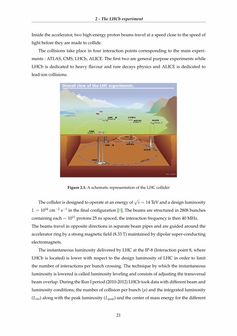
2 - The LHCb experiment
Inside the accelerator, two high-energy proton beams travel at a speed close to the speed of
light before they are made to collide.
The collisions take place in four interaction points corresponding to the main experi-
ments : ATLAS, CMS, LHCb, ALICE. The first two are general purpose experiments while
LHCb is dedicated to heavy flavour and rare decays physics and ALICE is dedicated to
lead-ion collisions.
Figure 2.1: A schematic representation of the LHC collider
The collider is designed to operate at an energy of√
s = 14 TeV and a design luminosity
L = 1034 cm−2 s−1 in the final configuration [8]. The beams are structured in 2808 bunches
containing each ∼ 1011 protons 25 ns spaced, the interaction frequency is then 40 MHz.
The beams travel in opposite directions in separate beam pipes and are guided around the
accelerator ring by a strong magnetic field (8.33 T) maintained by dipolar super-conducting
electromagnets.
The instantaneous luminosity delivered by LHC at the IP-8 (Interaction point 8, where
LHCb is located) is lower with respect to the design luminosity of LHC in order to limit
the number of interactions per bunch crossing. The technique by which the instantaneous
luminosity is lowered is called luminosity leveling and consists of adjusting the transversal
beam overlap. During the Run I period (2010-2012) LHCb took data with different beam and
luminosity conditions; the number of collision per bunch (µ) and the integrated luminosity
(Lint) along with the peak luminosity (Lpeak) and the center of mass energy for the different
21
2 - The LHCb experiment
data taking are reported in Table 2.1.
Year Lint√
s µ Lpeak
2010 37 pb−1 7 TeV 1− 2.5 1.6 · 1032 cm−2 s−1
2011 1.0 fb−1 7 TeV 1.5− 2.5 4.0 · 1032 cm−2 s−1
2012 2.2 fb−1 8 TeV ' 1.8 4.0 · 1032 cm−2 s−1
Table 2.1: the data taking condition at LHCb during the Run I period (2010-2012).
2.2 b production at LHCb
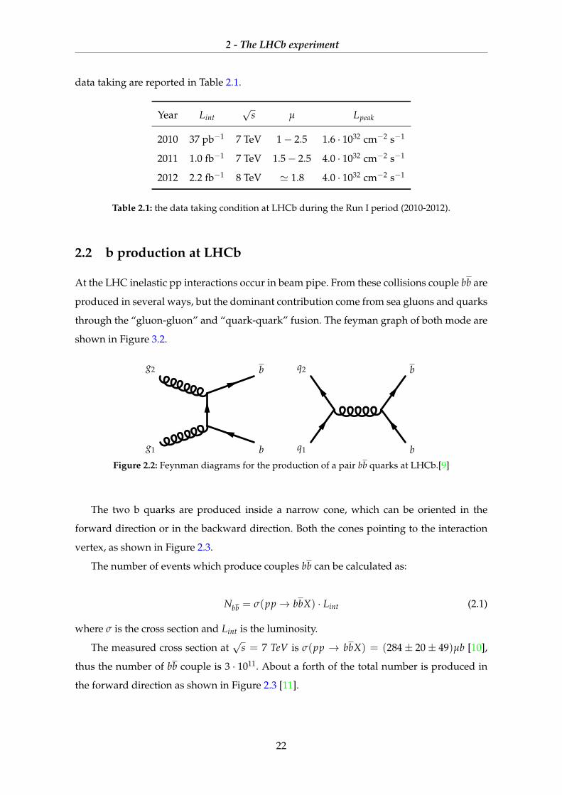
At the LHC inelastic pp interactions occur in beam pipe. From these collisions couple bb are
produced in several ways, but the dominant contribution come from sea gluons and quarks
through the “gluon-gluon” and “quark-quark” fusion. The feyman graph of both mode are
shown in Figure 3.2.
g1
g2
b
b
q1
q2
b
b
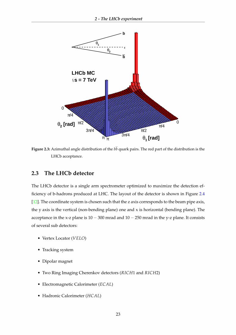
Figure 2.2: Feynman diagrams for the production of a pair bb quarks at LHCb.[9]
The two b quarks are produced inside a narrow cone, which can be oriented in the
forward direction or in the backward direction. Both the cones pointing to the interaction
vertex, as shown in Figure 2.3.
The number of events which produce couples bb can be calculated as:
Nbb = σ(pp→ bbX) · Lint (2.1)
where σ is the cross section and Lint is the luminosity.
The measured cross section at√
s = 7 TeV is σ(pp → bbX) = (284± 20± 49)µb [10],
thus the number of bb couple is 3 · 1011. About a forth of the total number is produced in
the forward direction as shown in Figure 2.3 [11].
22
2 - The LHCb experiment
0/4π
/2π/4π3
π
0
/4π
/2π
/4π3
π [rad]1θ
[rad]2θ
1θ
2θ
b
b
z
LHCb MC = 7 TeVs
Figure 2.3: Azimuthal angle distribution of the bb quark pairs. The red part of the distribution is the
LHCb acceptance.
2.3 The LHCb detector
The LHCb detector is a single arm spectrometer optimized to maximize the detection ef-
ficiency of b-hadrons produced at LHC. The layout of the detector is shown in Figure 2.4
[12]. The coordinate system is chosen such that the z axis corresponds to the beam pipe axis,
the y axis is the vertical (non-bending plane) one and x is horizontal (bending plane). The
acceptance in the x-z plane is 10− 300 mrad and 10− 250 mrad in the y-z plane. It consists
of several sub detectors:
• Vertex Locator (VELO)
• Tracking system
• Dipolar magnet
• Two Ring Imaging Cherenkov detectors (RICH1 and RICH2)
• Electromagnetic Calorimeter (ECAL)
• Hadronic Calorimeter (HCAL)
23

2 - The LHCb experiment
• Muon detector
In the following section, each of these sub-detectors will be described along with the
trigger system.
Figure 2.4: A y-z section of the LHCb detector
2.3.1 The beam pipe
The proton beams circulate in an Ultra High Vacuum pipe, called “beam pipe”. The beam
pipe consists of four sections, three of them are made of beryllium while the fourth sec-
tion is made of stainless steel. Beryllium is chosen in order to minimize the probability of
the particles produced in the interaction point to create secondary particles. In the VELO
(described in section 2.3.2) region it is made of high strength aluminum alloys.
2.3.2 The VErtex Locater
The VErtex Locator (VELO) is the part of the LHCb spectrometer closest to the collision
region, inside the LHC vacuum pipe. It allows to observe and reconstruct the decays of
B-mesons, which have displaced decay vertex ( ∼ 0.5 cm) because of their relatively long
lifetimes. The precise measurement of primary and secondary vertexes (PV and SV) of
the decays is fundamental for CP violation time dependent measurements and also to re-
duce the combinatorial background. For B-mesons the resolution of the PV depends on the
number of tracks in the event. On average it’s 60 µm in the z direction and 10 µm in the
perpendicular direction. The sub-detector consists of two rows of half-moon-shaped silicon
stations, each 0.3 mm thick. A small cutout in the center of stations allows the main LHC
24

2 - The LHCb experiment
beam to pass through freely. The stations are made by two type of sensors: r sensors mea-
sure the radial distance of the particle tracks from beam axis while the φ sensors measure
their polar angle. The first two stations are used for the L0 trigger level. The tracks can be
reconstructed with polar angles between 15 mrad and 390 mrad. The VELO is also impor-
tant for the impact parameter measurement, the resolution is ∼ 15 µm at high transverse
momentum (∼ 10 GeV) and ∼ 300 µm at low transverse momentum (∼ 0.3 GeV)
2.3.3 The Tracking System
The tracking system enables the trajectory of each particle passing through the detector
and their momentum to be recorded and is absolutely crucial for reconstructing B-particle
decays.
It comprises four large rectangular stations, each covering an area of about 40 m2 : one
station (TT) is located between RICH-1 and the dipole magnet, while the other three stations
(T1-T3) are located over 3 meters between the magnet and RICH-2.
Two detector technologies are employed:
1. The Silicon Tracker: uses silicon microstrip detectors It comprises the entire TT station
and a cross-shaped area (the Inner Tracker) around the beam pipe in stations T1-T3.
Its total sensitive surface is approximately 11 m2 .
2. The Outer Tracker: uses straw-tube drift chambers with 5 mm cell diameter and covers
the largest fraction of the detector sensitive area in stations T1-T3. The total sensitive
area is 80.6 m2.
The Silicon Tracker
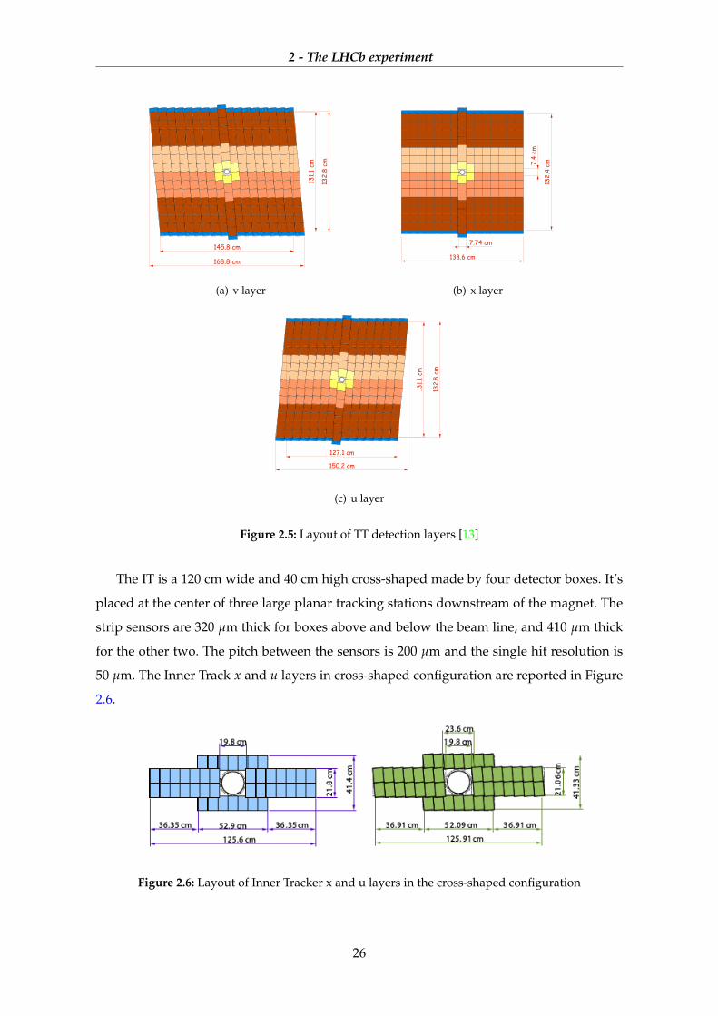
The Silicon Tracker (ST), which is placed close to the beam pipe, uses silicon microstrip de-
tectors with a strip pitch of approximately 200 µm. Each of the four Silicon Tracker stations
consists of four detection layers. The vertical layers are called x-layers, while the u and v-
layers are rotated by an angle of 5◦ and −5◦ The first two x-u layers are separated by the
others two v-x layers by 27 cm along the beam axis.
The TT detection layers are shown in Figure 2.5. The ST comprise two detectors: the Tracker
Turicensis (TT) and the Inner Tracker (IT).
The TT is a 150 cm wide and 130 cm high planar tracking station that is placed upstream
of the LHCb dipole magnet and covers the full acceptance of the experiment. The strips are
500 µm thick with a pitch of 183 µm and the single hit resolution of the TT is about 50 µm.
25
2 - The LHCb experiment
(a) v layer
132 .
4 cm
7.74 cm
138.6 cm
7.4
cm
(b) x layer
150.2 cm
131.1
cm
127.1 cm
132.
8 cm
(c) u layer
Figure 2.5: Layout of TT detection layers [13]
The IT is a 120 cm wide and 40 cm high cross-shaped made by four detector boxes. It’s
placed at the center of three large planar tracking stations downstream of the magnet. The
strip sensors are 320 µm thick for boxes above and below the beam line, and 410 µm thick
for the other two. The pitch between the sensors is 200 µm and the single hit resolution is
50 µm. The Inner Track x and u layers in cross-shaped configuration are reported in Figure
2.6.
Figure 2.6: Layout of Inner Tracker x and u layers in the cross-shaped configuration
26
2 - The LHCb experiment
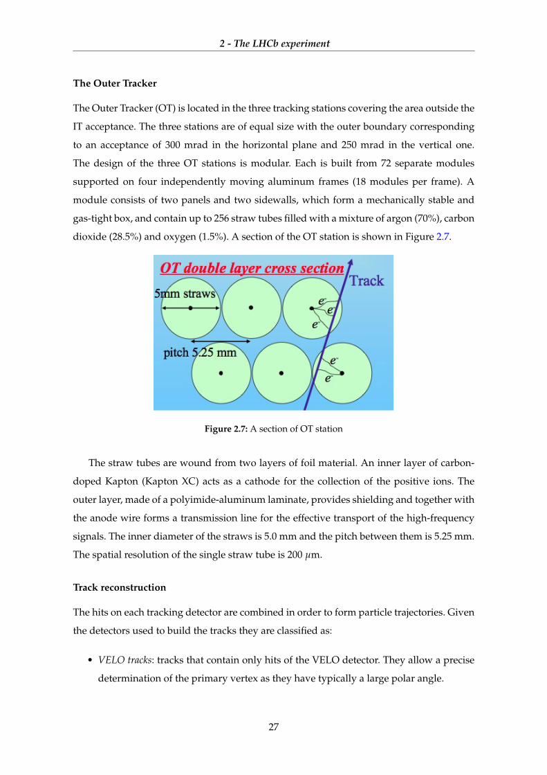
The Outer Tracker
The Outer Tracker (OT) is located in the three tracking stations covering the area outside the
IT acceptance. The three stations are of equal size with the outer boundary corresponding
to an acceptance of 300 mrad in the horizontal plane and 250 mrad in the vertical one.
The design of the three OT stations is modular. Each is built from 72 separate modules
supported on four independently moving aluminum frames (18 modules per frame). A
module consists of two panels and two sidewalls, which form a mechanically stable and
gas-tight box, and contain up to 256 straw tubes filled with a mixture of argon (70%), carbon
dioxide (28.5%) and oxygen (1.5%). A section of the OT station is shown in Figure 2.7.
Figure 2.7: A section of OT station
The straw tubes are wound from two layers of foil material. An inner layer of carbon-
doped Kapton (Kapton XC) acts as a cathode for the collection of the positive ions. The
outer layer, made of a polyimide-aluminum laminate, provides shielding and together with
the anode wire forms a transmission line for the effective transport of the high-frequency
signals. The inner diameter of the straws is 5.0 mm and the pitch between them is 5.25 mm.
The spatial resolution of the single straw tube is 200 µm.
Track reconstruction
The hits on each tracking detector are combined in order to form particle trajectories. Given
the detectors used to build the tracks they are classified as:
• VELO tracks: tracks that contain only hits of the VELO detector. They allow a precise
determination of the primary vertex as they have typically a large polar angle.
27
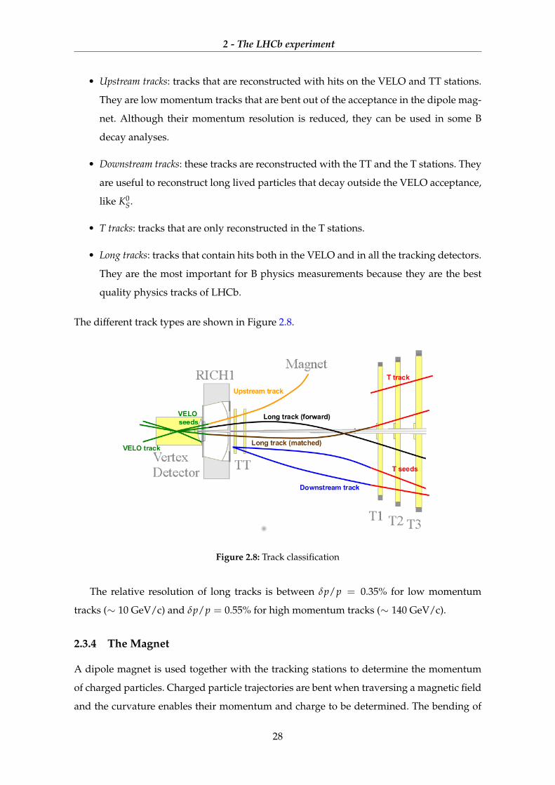
2 - The LHCb experiment
• Upstream tracks: tracks that are reconstructed with hits on the VELO and TT stations.
They are low momentum tracks that are bent out of the acceptance in the dipole mag-
net. Although their momentum resolution is reduced, they can be used in some B
decay analyses.
• Downstream tracks: these tracks are reconstructed with the TT and the T stations. They
are useful to reconstruct long lived particles that decay outside the VELO acceptance,
like K0S.
• T tracks: tracks that are only reconstructed in the T stations.
• Long tracks: tracks that contain hits both in the VELO and in all the tracking detectors.
They are the most important for B physics measurements because they are the best
quality physics tracks of LHCb.
The different track types are shown in Figure 2.8.
Figure 2.8: Track classification
The relative resolution of long tracks is between δp/p = 0.35% for low momentum
tracks (∼ 10 GeV/c) and δp/p = 0.55% for high momentum tracks (∼ 140 GeV/c).
2.3.4 The Magnet
A dipole magnet is used together with the tracking stations to determine the momentum
of charged particles. Charged particle trajectories are bent when traversing a magnetic field
and the curvature enables their momentum and charge to be determined. The bending of
28
2 - The LHCb experiment
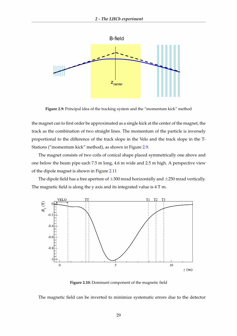
Figure 2.9: Principal idea of the tracking system and the “momentum kick” method
the magnet can to first order be approximated as a single kick at the center of the magnet, the
track as the combination of two straight lines. The momentum of the particle is inversely
proportional to the difference of the track slope in the Velo and the track slope in the T-
Stations (“momentum kick” method), as shown in Figure 2.9.
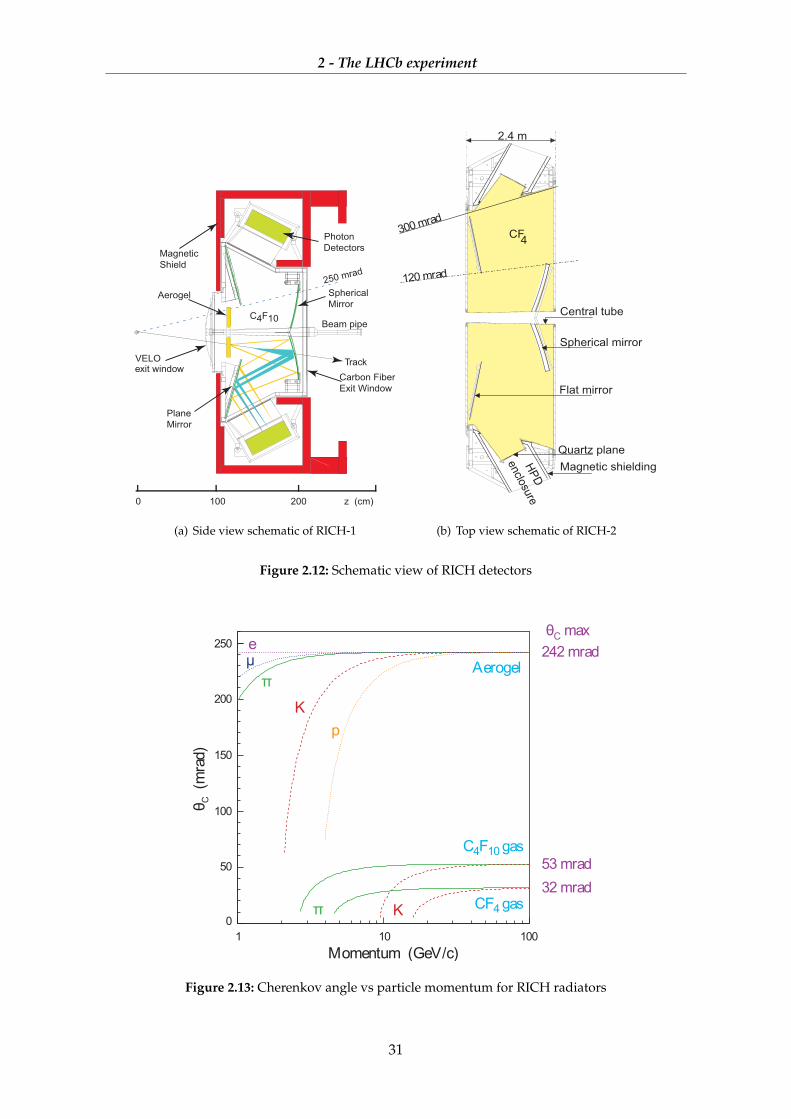
The magnet consists of two coils of conical shape placed symmetrically one above and
one below the beam pipe each 7.5 m long, 4.6 m wide and 2.5 m high. A perspective view
of the dipole magnet is shown in Figure 2.11
The dipole field has a free aperture of±300 mrad horizontally and±250 mrad vertically.
The magnetic field is along the y axis and its integrated value is 4 T·m.
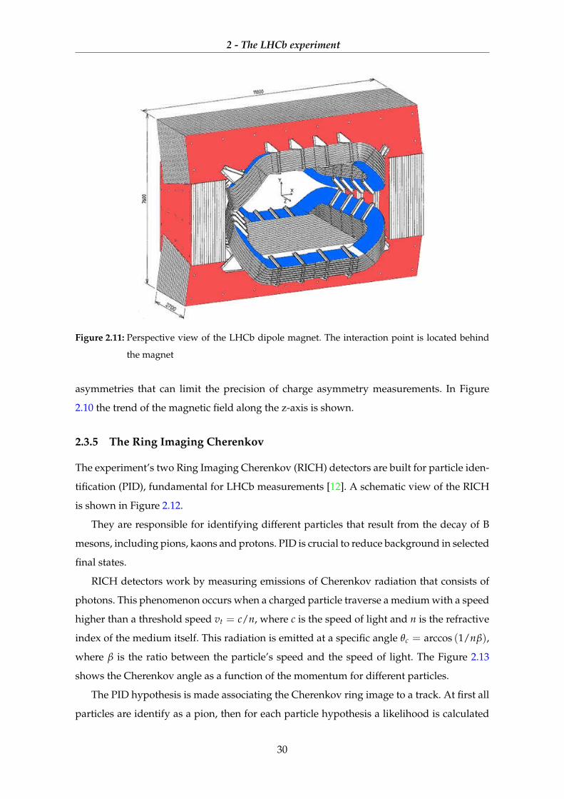
Figure 2.10: Dominant component of the magnetic field
The magnetic field can be inverted to minimize systematic errors due to the detector
29
2 - The LHCb experiment
Figure 2.11: Perspective view of the LHCb dipole magnet. The interaction point is located behind
the magnet
asymmetries that can limit the precision of charge asymmetry measurements. In Figure
2.10 the trend of the magnetic field along the z-axis is shown.
2.3.5 The Ring Imaging Cherenkov
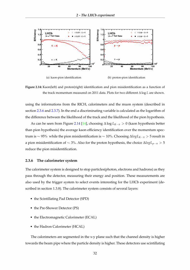
The experiment’s two Ring Imaging Cherenkov (RICH) detectors are built for particle iden-
tification (PID), fundamental for LHCb measurements [12]. A schematic view of the RICH
is shown in Figure 2.12.
They are responsible for identifying different particles that result from the decay of B
mesons, including pions, kaons and protons. PID is crucial to reduce background in selected
final states.
RICH detectors work by measuring emissions of Cherenkov radiation that consists of
photons. This phenomenon occurs when a charged particle traverse a medium with a speed
higher than a threshold speed vt = c/n, where c is the speed of light and n is the refractive
index of the medium itself. This radiation is emitted at a specific angle θc = arccos (1/nβ),
where β is the ratio between the particle’s speed and the speed of light. The Figure 2.13
shows the Cherenkov angle as a function of the momentum for different particles.
The PID hypothesis is made associating the Cherenkov ring image to a track. At first all
particles are identify as a pion, then for each particle hypothesis a likelihood is calculated
30
2 - The LHCb experiment
250 mrad
Track
Beam pipe
Photon
Detectors
Aerogel
VELOexit window
Spherical
Mirror
Plane
Mirror
C4F10
0 100 200 z (cm)
Magnetic
Shield
Carbon Fiber
Exit Window
(a) Side view schematic of RICH-1
120mrad
Flat mirror
Spherical mirror
Central tube
Quartz plane
Magnetic shieldingHPD
enclosure
2.4 m
300mrad
CF4
(b) Top view schematic of RICH-2
Figure 2.12: Schematic view of RICH detectors
θC
(mra
d)
250
200
150
100
50
0
1 10 100
Momentum (GeV/c)
Aerogel
C4F10 gas
CF4 gas
eµ
p
K
π
242 mrad
53 mrad
32 mrad
θC max
Kπ
Figure 2.13: Cherenkov angle vs particle momentum for RICH radiators
31
2 - The LHCb experiment
(a) kaon-pion identification (b) proton-pion identification
Figure 2.14: Kaon(left) and proton(right) identification and pion misidentification as a function of
the track momentum measured on 2011 data. Plots for two different ∆ log L are shown.
using the informations from the RICH, calorimeters and the muon system (described in
section 2.3.6 and 2.3.7). In the end a discriminating variable is calculated as the logarithm of
the difference between the likelihood of the track and the likelihood of the pion hypothesis.
As can be seen from Figure 2.14 [14], choosing ∆ log LK−π > 0 (kaon hypothesis better
than pion hypothesis) the average kaon efficiency identification over the momentum spec-
trum is∼ 95% while the pion misidentification is ∼ 10%. Choosing ∆logLK−π > 5 result in
a pion misidentification of ∼ 3%. Also for the proton hypothesis, the choice ∆logLp−π > 5
reduce the pion misidentification.
2.3.6 The calorimeter system
The calorimeter system is designed to stop particles(photon, electrons and hadrons) as they
pass through the detector, measuring their energy and position. These measurements are
also used by the trigger system to select events interesting for the LHCb experiment (de-
scribed in section 1.3.8). The calorimeter system consists of several layers:
• the Scintillating Pad Detector (SPD)
• the Pre-Shower Detector (PS)
• the Electromagnetic Calorimeter (ECAL)
• the Hadron Calorimeter (HCAL)
The calorimeters are segmented in the x-y plane such that the channel density is higher
towards the beam pipe where the particle density is higher. These detectors use scintillating
32

2 - The LHCb experiment
materials to detect the shower of photons, electrons and positrons produced when particles
pass through them. The angular acceptance is between 300 mrad and 30 mrad horizontally
and 250 mrad vertically.
The Scintillating Pad Detector and the Pre-Shower
The SPD and PS indicate the electromagnetic character of the particles hitting the calorime-
ter system, i.e. they determine if the particles are charged or neutral. They are used at the
trigger level (L0) in association with the ECAL to indicate the presence of electrons, pho-
tons, and neutral pions.
The SPD and PS consist of scintillating pads with a thickness of 15 mm, inter spaced
with a 2.5X0 lead converter. They are placed right after the first muon station and collecting
the light using wavelength-shifting (WLS) fibers.
The Electromagnetic Calorimeter
The showers initiate in PS are detected by the ECAL. It employs “shashlik” technology of
alternating scintillating tiles (2 mm thick) and lead plates (4 mm thick). The cells’ surface
is 4 cm × 4 cm , 6 cm × 6 cm and 12 cm × 12 cm in the inner, middle and outer parts of
the detector, respectively. The overall detector’s dimensions are 7.76 m × 6.30 m, covering
an acceptance of 25 mrad < θx < 300 mrad in the horizontal plane and 25 mrad < θy <
250 mrad in the vertical one. Light is collected by WaveLength-Shifting (WLS) fibers and
PhotoMultiplier Tubes (PMTs).
The ECAL energy resolution is given by :
σ(E)E
=10%√
E⊕ 1.5%
where E is the energy and ⊕mean the sum in quadrature.
The Hadronic Calorimeter
The HCAL is positioned outside the ECAL and detects particles originated in hadronic
showers. Its internal structure consists of thin iron plates absorber inter spaced with scintil-
lating tiles arranged parallel to the beam pipe. Like ECAL, the inner and outer parts of the
calorimeter have different cell dimensions: 13 cm × 13 cm and 26 cm × 26 cm,respectively.
In the lateral direction tiles are inter spaced with 1 cm of iron matching with the hadron
radiation length in iron (X0); while in the longitudinal direction the length of tiles and iron
33

2 - The LHCb experiment
spacers corresponds to the hadron interaction length (λI) in iron. Light is collected with the
same principle used in ECAL.
The HCAL energy resolution is given by :
σ(E)E
=80%√
E⊕ 10%
2.3.7 The Muon Stations
The muon is the only detectable particle that is able to pass through the calorimeters with-
out losing completely its energy. Muons are present in the final states of many CP-sensitive
B decays and play a major role in CP asymmetry and oscillation measurements. LHCb ex-
periment uses five muon stations (M1-M5), gradually increasing in size, to identify and
reconstruct muons. The system covers an acceptance between±300− 20 mrad horizontally
and ±258 − 16 mrad vertically. Each station is divided into four regions, R1 to R4, with
increasing distance from the beam axis The stations M2-M4 are interleaved by 80 cm thick
iron wall to absorb hadronic particles. Average muon identification efficiencies of 98% can
be obtained with a level of pion and kaon misidentification below 1%. The hadron misiden-
tification probabilities are below 0.6%. A side view of the muon stations is shown in Figure
2.15.
Figure 2.15: Side view of the LHCb muon system, showing the position of the five stations. The first
station is placed before the calorimeters and the other four after them, interleaved with
the muon shield. [12]
34

2 - The LHCb experiment
2.3.8 Trigger
The LHC bunch crossing frequency is 40 MHz, of which the LHCb detector at nominal
luminosity (2 · 1032 cm−2s−1 [8]) will see events with at least one visible interaction 1 at a
rate of 10 MHz. The purpose of the LHCb trigger system is to reduce the event rate from 40
MHz to 2 KHz. The LHCb trigger consists of two stages:
• Level-0 (L0) trigger synchronous with the bunch crossing frequency, is implemented
in hardware and reduces the event rate to less than 1.1 MHz
• High Level Trigger (HLT), is a C++ software trigger and runs on a dedicated Event
Filter Farm (EFF);it reduces the event rate to 2 KHz
Level-0 Trigger
Using informations from VELO, L0 trigger estimates the number of primary interactions
in each bunch crossing and also provides the possibility to veto events with multiple PV
(pile-up trigger).
Because B mesons have a large mass, they often decay producing particles with large
transverse momentum (pT) and energy (ET). The L0 trigger attempts to reconstruct:
• the highest ET hadron, electron and photon using the calorimeters’ informations. The
event is triggered if the ET is greater than a certain threshold.
• the two highest pT muons combining the informations of the five muon stations. The
event is triggered if the pT is greater than a certain threshold (single-muon) or if the
sum of the two highest momenta is greater than a certain threshold (di-muon).
The total latency of the L0 trigger is 4 µs, including time-of-flight of the particles, cable
delays, delays in the front-end electronics and the time necessary to process the data and to
derive a decision.
High Level Trigger
The High Level Trigger (HLT) analyses the events that are selected by the L0 trigger. HLT
consists of two level named HLT-1 and HLT-2.1An interaction is defined to be visible if it produces at least two charged particles with sufficient hits in the
VELO and T1âT3 to allow them to be reconstructible
35

2 - The LHCb experiment
• HLT-1: its purpose is to reduce the rate to 30 kHz allowing a full pattern recogni-
tion on the remaining events. Information from a tracking sub detector and applying
requirements on the pT and the impact parameter (IP) with respect to the primary
vertex (PV) are added. This reduces the CPU time needed for decoding and pattern
recognition algorithms.
• HLT-2: It performs a full event reconstruction using the Kalman Filter algorithm to fit
the tracks. After the track fit, the HLT-2 stage applies cuts either on invariant mass,
or on pointing of the B momentum towards the primary vertex. The resulting ex-
clusive and inclusive selections, called topological lines, aim to reduce the rate to 2
KHz,which is the final output rate of LHCb trigger system.
In the topological lines a multi body candidate is built, starting from two particles to
make a two-body object.
36
3
Same Side Pion Tagger
Contents
3.1 The Flavour Tagging 37
3.1.1 Definitions 38
3.1.2 Same Side Taggers 40
3.2 Same Side tagger 41
3.3 SSπ tagger development using 2012 data sample 42
3.3.1 sWeights estimation 42
3.3.2 Training of the SS pion tagger 45
3.3.3 Performance and calibration 49
3.4 Validation on the 2011 data sample 55
3.5 Validation on the B0 → K+π− 2012 data sample 58
In this chapter the development of a new Same Side Pion tagger is described. The al-
gorithm implementation uses a sample with the B0 −→ D−π+ decay channel, collected
by LHCb in 2012 corresponding to 2 f b−1 of pp collisions at√
s = 8TeV. It is described in
section 6.4.2. A first validity check is performed using the data of 2011 of the same channel
corresponding to 1 f b−1 taken at√
s = 7TeV, it is described in section D.1, then another
check is performed using a different event selection as described in section ??.
3.1 The Flavour Tagging
The Flavour Tagging (FT) at LHCb is a fundamental tool to study the b-hadron decays and
the CP violation. These measurements require the knowledge of the quark content in the B
37
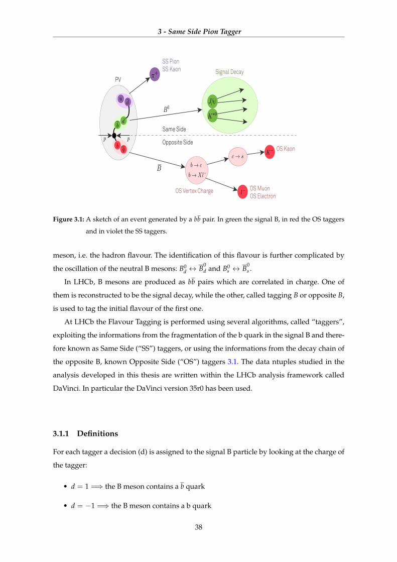
3 - Same Side Pion Tagger
3/20 Ulrich Eitschberger | Updates on Flavour Tagging | 72nd LHCb week | June 19th, 2014
Flavour Tagging: Determine B production flavours SS Pion SS Kaon Signal Decay
Same Side
Opposite Side
OS Vertex Charge OS Muon OS Electron
OS Kaon
PV
Figure 3.1: A sketch of an event generated by a bb pair. In green the signal B, in red the OS taggers
and in violet the SS taggers.
meson, i.e. the hadron flavour. The identification of this flavour is further complicated by
the oscillation of the neutral B mesons: B0d ↔ B0
d and B0s ↔ B0
s .
In LHCb, B mesons are produced as bb pairs which are correlated in charge. One of
them is reconstructed to be the signal decay, while the other, called tagging B or opposite B,
is used to tag the initial flavour of the first one.
At LHCb the Flavour Tagging is performed using several algorithms, called “taggers”,
exploiting the informations from the fragmentation of the b quark in the signal B and there-
fore known as Same Side (“SS”) taggers, or using the informations from the decay chain of
the opposite B, known Opposite Side (“OS”) taggers 3.1. The data ntuples studied in the
analysis developed in this thesis are written within the LHCb analysis framework called
DaVinci. In particular the DaVinci version 35r0 has been used.
3.1.1 Definitions
For each tagger a decision (d) is assigned to the signal B particle by looking at the charge of
the tagger:
• d = 1 =⇒ the B meson contains a b quark
• d = −1 =⇒ the B meson contains a b quark
38
3 - Same Side Pion Tagger
• d = 0 =⇒ no particle is available to identify the meson
Each event is classified as:
• correctly tagged (R), if the tag decision is equal to the B flavour at the production
• incorrectly tagged (W), if the tag decision is different to the B flavour at the production
• untagged (U), if the tag decision is equal to 0
The ratio of tagged events is represented by the tagging efficiency (εtag) and can be
calculated as:
εtag =R + W
R + W + U(3.1)
In the same way is possible to determine the fraction of wrong tagged events, called
“mistag fraction” (ω), like:
ω =W
W + R(3.2)
The mistag fraction can be calculated directly only using flavour specific decays (i.e the
charge of the decay products is correlated with the flavour of the B particle) for charged
mesons , such as Bu; in these cases the mistag estimation is straight forward because the
wrong and the right tagged events can be identified comparing the tagger decision to the
charge of the Bu particle. For the Bd and Bs decays there is an additional complication:
due to flavour oscillation only the flavour of the Bd (or Bs) particle at decay can be known
from decay products. In this particular case the mistag must be extracted from a fit to the
time-dependent asymmetry of the flavour oscillations. For the B decays in CP state, such
as Bs −→ J/ΨΦ, there is no way to determine the mistag directly in this channel hence
the mistag for these decays has to come from an external flavour-specific decays; those are
named the calibration channels.
Assuming that the “mistag fraction” and the “tagging efficiency” are not depending
from the initial flavour,the decay rate (Γ) and the CP asymmetry are written as:
Γm(B(t)→ f ) = εtag[(1−ω)Γ(B(t)→ f ) + ωΓ(B(t)→ f )]
Γm(B(t)→ f ) = εtag[(1−ω)Γ(B(t)→ f ) + ωΓ(B(t)→ f )](3.3)
where Γm and Γm are the measured decay rate of B meson to a final state (f) and its CP
conjugate.
39

3 - Same Side Pion Tagger
Am =Γm(B(t)→ f )− Γm(B(t)→ f )Γm(B(t)→ f ) + Γm(B(t)→ f )
= (1− 2ω)A(t) = DA(t) (3.4)
where
• Am is the measured asymmetry and A is the true asymmetry
• D = 1− 2ω is the dilution term, which has the effect to decrease the amplitude of the
oscillation
The real asymmetry and its statistical error is given by:
A =Am
1− 2ωσA =
σAm
1− 2ω(3.5)
where the error on ω has been neglected.
Using the error propagation on 3.4 and knowing that
1− A2m =
4ΓmΓm
(Γm + Γm)2(3.6)
the error on the measured asymmetry is:
σAm =
√4ΓmΓm
(Γm + Γm)3=
√1− A2
m
Γm + Γm=
√1− A2
mNtag
=
√1− A2
mεtagN
(3.7)
where Ntag is the number of events in which the initial flavour is known and N is the total
number of events. Thus the error on the true asymmetry is evaluated as:
σA =σAm
1− 2ω=
√1− A2
m√εtagN(1− 2ω)
(3.8)
From the equation 3.8 it follows that to improve the statistical error on the asymmetry it
is necessary to maximize the “effective tagging efficiency” or “tagging power”(εe f f ) [15],
defined as:
εe f f = εtagD2 = εtag(1− 2ω)2 (3.9)
3.1.2 Same Side Taggers
Same Side tagger algorithms exploit the charge correlation in the fragmentation chain of the
signal meson to define its flavour. In this thesis the signal channel B0 −→ D−π+ is studied.
In the case of B0 (bd) a d quark is available to produce particles like: π+, π0, p, Λ0. If the
additional particle is charged, it can be used to identify the flavour of the B meson. The
particles which are studied in this thesis are:
40
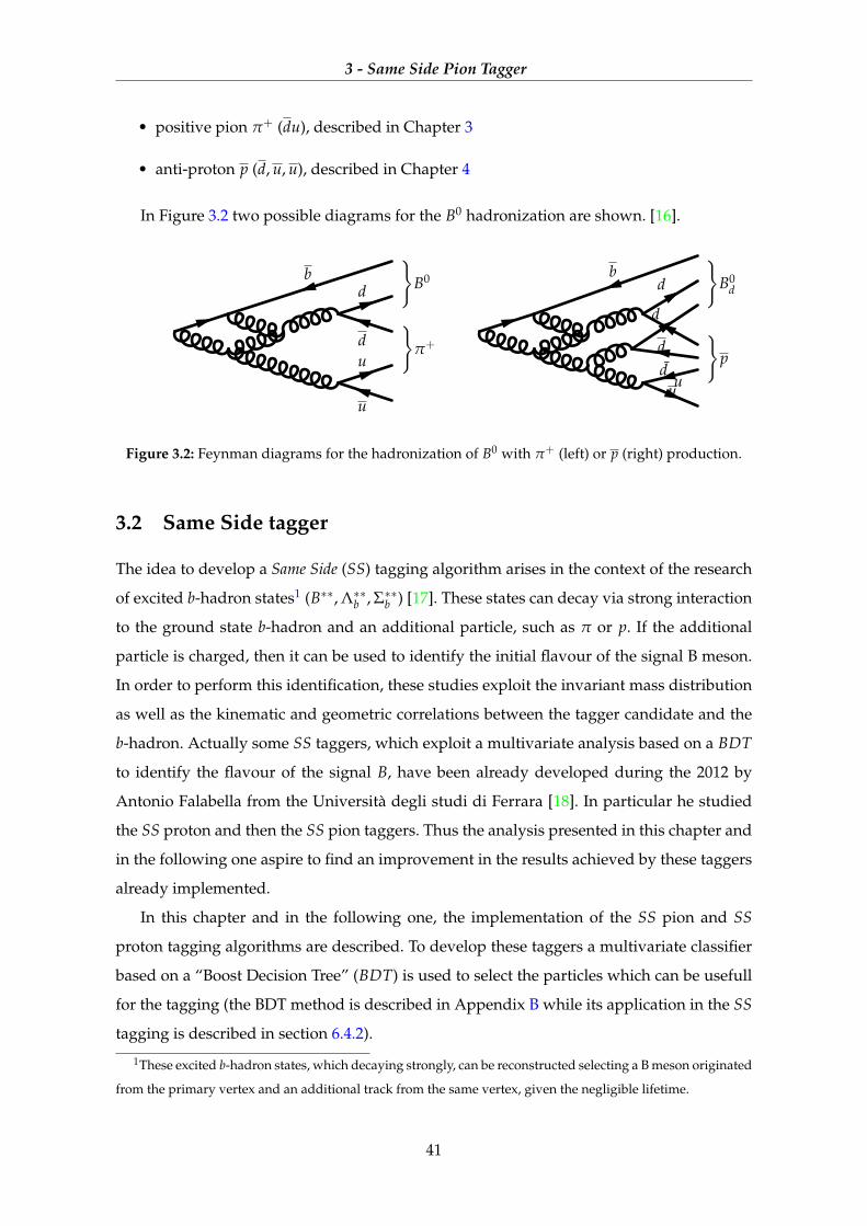
3 - Same Side Pion Tagger
• positive pion π+ (du), described in Chapter 3
• anti-proton p (d, u, u), described in Chapter 4
In Figure 3.2 two possible diagrams for the B0 hadronization are shown. [16].
u
d
bd
u
}π+
}B0
ud̄d
bd
u
d }p
}B0
d
Figure 3.2: Feynman diagrams for the hadronization of B0 with π+ (left) or p (right) production.
3.2 Same Side tagger
The idea to develop a Same Side (SS) tagging algorithm arises in the context of the research
of excited b-hadron states1 (B∗∗, Λ∗∗b , Σ∗∗b ) [17]. These states can decay via strong interaction
to the ground state b-hadron and an additional particle, such as π or p. If the additional
particle is charged, then it can be used to identify the initial flavour of the signal B meson.
In order to perform this identification, these studies exploit the invariant mass distribution
as well as the kinematic and geometric correlations between the tagger candidate and the
b-hadron. Actually some SS taggers, which exploit a multivariate analysis based on a BDT
to identify the flavour of the signal B, have been already developed during the 2012 by
Antonio Falabella from the Università degli studi di Ferrara [18]. In particular he studied
the SS proton and then the SS pion taggers. Thus the analysis presented in this chapter and
in the following one aspire to find an improvement in the results achieved by these taggers
already implemented.
In this chapter and in the following one, the implementation of the SS pion and SS
proton tagging algorithms are described. To develop these taggers a multivariate classifier
based on a “Boost Decision Tree” (BDT) is used to select the particles which can be usefull
for the tagging (the BDT method is described in Appendix B while its application in the SS
tagging is described in section 6.4.2).
1These excited b-hadron states, which decaying strongly, can be reconstructed selecting a B meson originated
from the primary vertex and an additional track from the same vertex, given the negligible lifetime.
41
3 - Same Side Pion Tagger
The sample chosen to tune these BDT corresponds to the B0 −→ D−(→ K+π−π−)π+
sample collected by the LHCb experiment during the 2012 data taking. The reason of this
choise lies in the nature itself of this decay channel: as explained in the section 3.1, the
flavour tagging technique can be applied only on a flavour specific channel, like the B0 −→
D−π+. In this channel indeed the additional particle (π or p) produced by the b-fragmentation
allows to tag the flavour of the signal B at the production, not at the decay because of the
flavour time-dependent oscillations.
The BDT training can occur in two possible ways: the first consists in the use of a data
sample while the second in the use of a Monte-Carlo (MC) simulation. In a first time the
MC sample was chosen because of the possibility to know the MC-truth about the event
properties. In particular, some analysis about the origin of the many pions created in the
events was performed in order to possibly increase the separation ability of the BDT. They
are reported in Appendix C. However in a second time the train on a data sample was
preferred, because the MC did not reproduce correctly the data, thus it was not possible to
fully trust its response. The analysis and the results reported in the following chapters don’t
take in account the training performed on the MC sample.
The main difference between a MC sample and a data sample is that the first one con-
tains only the signal events while the second one is polluted with background events. In
this thesis the sPlot technique has been exploited in order to get rid the background con-
tribution. According to this method, described in Appendix A, known the distributions of
the invariant mass of the signal B,it is possible to obtain a per-event sWeight which can be
used to weight the data distribution and thus unfold the signal from the background. This
procedure is described in detail in the following section.
3.3 SSπ tagger development using 2012 data sample
3.3.1 sWeights estimation
In this section the analysis of B0 −→ D−(→ K+π−π−)π+ 2012 data sample is described.
To select the B0 candidate and to reduce as much as possible the background events in the
sample the cuts, reported in Table 3.1 [18], are applied. Using the sPlot technique, briefly
illustrated in Appendix A, a per-event weight is calculated allowing to unfold the contribu-
tions of background and signal.
42
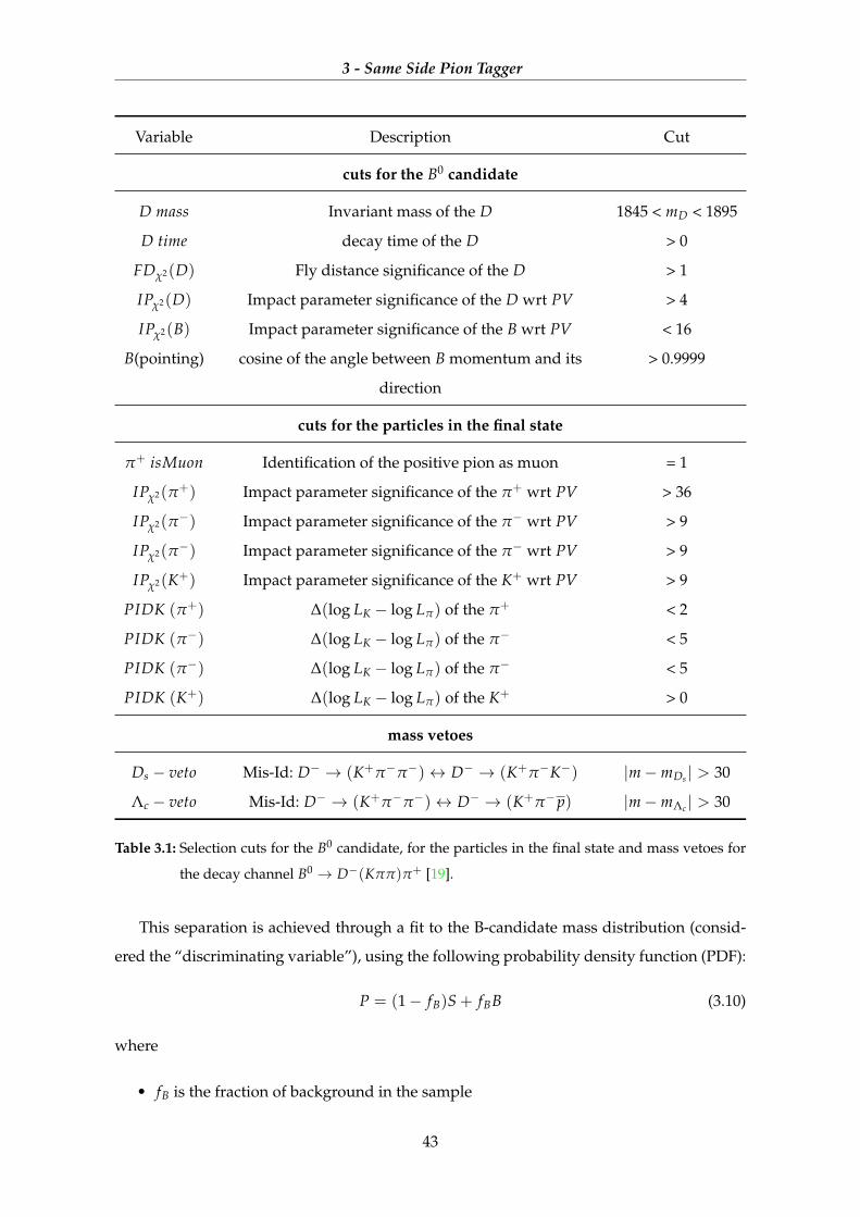
3 - Same Side Pion Tagger
Variable Description Cut
cuts for the B0 candidate
D mass Invariant mass of the D 1845 < mD < 1895
D time decay time of the D > 0
FDχ2(D) Fly distance significance of the D > 1
IPχ2(D) Impact parameter significance of the D wrt PV > 4
IPχ2(B) Impact parameter significance of the B wrt PV < 16
B(pointing) cosine of the angle between B momentum and its
direction
> 0.9999
cuts for the particles in the final state
π+ isMuon Identification of the positive pion as muon = 1
IPχ2(π+) Impact parameter significance of the π+ wrt PV > 36
IPχ2(π−) Impact parameter significance of the π− wrt PV > 9
IPχ2(π−) Impact parameter significance of the π− wrt PV > 9
IPχ2(K+) Impact parameter significance of the K+ wrt PV > 9
PIDK (π+) ∆(log LK − log Lπ) of the π+ < 2
PIDK (π−) ∆(log LK − log Lπ) of the π− < 5
PIDK (π−) ∆(log LK − log Lπ) of the π− < 5
PIDK (K+) ∆(log LK − log Lπ) of the K+ > 0
mass vetoes
Ds − veto Mis-Id: D− → (K+π−π−)↔ D− → (K+π−K−) |m−mDs | > 30
Λc − veto Mis-Id: D− → (K+π−π−)↔ D− → (K+π−p) |m−mΛc | > 30
Table 3.1: Selection cuts for the B0 candidate, for the particles in the final state and mass vetoes for
the decay channel B0 → D−(Kππ)π+ [19].
This separation is achieved through a fit to the B-candidate mass distribution (consid-
ered the “discriminating variable”), using the following probability density function (PDF):
P = (1− fB)S + fBB (3.10)
where
• fB is the fraction of background in the sample
43
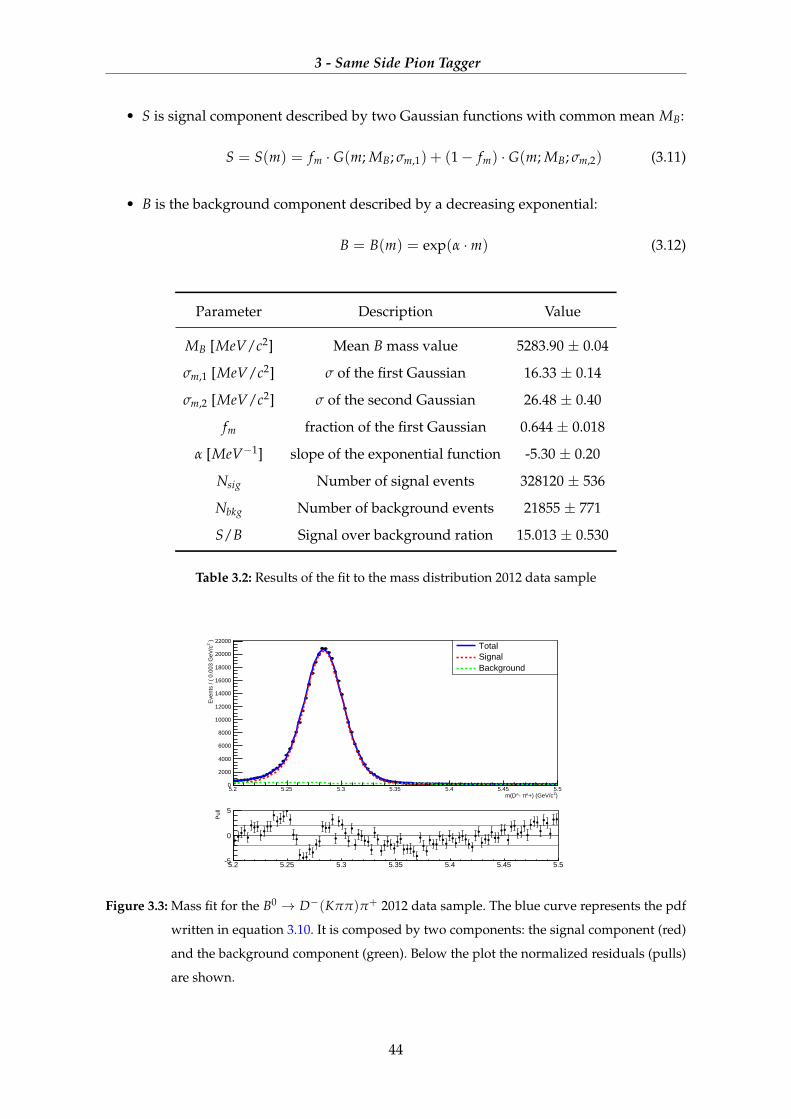
3 - Same Side Pion Tagger
• S is signal component described by two Gaussian functions with common mean MB:
S = S(m) = fm · G(m; MB; σm,1) + (1− fm) · G(m; MB; σm,2) (3.11)
• B is the background component described by a decreasing exponential:
B = B(m) = exp(α ·m) (3.12)
Parameter Description Value
MB [MeV/c2] Mean B mass value 5283.90 ± 0.04
σm,1 [MeV/c2] σ of the first Gaussian 16.33 ± 0.14
σm,2 [MeV/c2] σ of the second Gaussian 26.48 ± 0.40
fm fraction of the first Gaussian 0.644 ± 0.018
α [MeV−1] slope of the exponential function -5.30 ± 0.20
Nsig Number of signal events 328120 ± 536
Nbkg Number of background events 21855 ± 771
S/B Signal over background ration 15.013 ± 0.530
Table 3.2: Results of the fit to the mass distribution 2012 data sample
)2^+) (GeV/cπm(D^- 5.2 5.25 5.3 5.35 5.4 5.45 5.5
)2E
vent
s / (
0.0
03 G
eV/c
0
2000
4000
6000
8000
10000
12000
14000
16000
18000
20000
22000TotalSignalBackground
5.2 5.25 5.3 5.35 5.4 5.45 5.5
Pul
l
-5
0
5
Figure 3.3: Mass fit for the B0 → D−(Kππ)π+ 2012 data sample. The blue curve represents the pdf
written in equation 3.10. It is composed by two components: the signal component (red)
and the background component (green). Below the plot the normalized residuals (pulls)
are shown.
44
3 - Same Side Pion Tagger
In Figure 3.3 the plot of the fit to the mass distribution on the 2012 data sample is shown
while in Table 3.2 the results for the PDF parameters are reported. In the following analysis
the background contribution will be removed from the data samples weighting each event
with its sWeight estimated by the mass fit described above.
3.3.2 Training of the SS pion tagger
To determine the flavour of the B signal meson is necessary to develop a tagging algorithm
to identify the particle which is rightly correlated in charge. To perform this aim as better as
possible a multivariate technique is implemented using kinematic and geometric variables
to select the best candidate to be used for tagging. The algorithm implemented is based on a
“Boost Decision Tree” (BDT) classifier [20] using the “MisClassificatorError” as separation
criterion and the “AdaBoost” as boosting method (more details in Appendix B). A BDT
algorithm has been preferred respect a naive cut-based approach because, as demonstrated
in other similar analysis, it provides better performance [18]. To develop the BDT algorithm
the sample has been divided in three sub-samples: the first sub-sample is used to perform
the BDT training, the second sub-sample uses the BDT training results to choose the right
tagger candidate and in the third sub-sample a calibration of the BDT is performed. Then
an efficiency value of the tagging method is calculated using the second sub-sample. The
events has been divided according to the following relation:
Ns = Neventmod3 (3.13)
where Nevent is the number associated to the event and Ns is the number of events in sub-
sample. The track charge is used to classify the tracks with the right or wrong charge corre-
lation with respect the B signal meson. For the Same Side pion such correlation is defined
as:
Right −→ B0π+ or B0π−
Wrong −→ B0π− or B0π+
However using a neutral channel calls for some caution because the B0 mesons can
undergo flavour oscillation reversing the charge correlation. To reduce the contribution of
flavour-oscillated events during the BDT training, a cut on the decay time has been applied
to t < 2.2 ps. This cut allows to remove the greater part of the oscillated events without
reducing drastically the statistics of the sample. To perform the BDT training the first sample
is divided further in two subsamples: the first is used for the BDT training phase (“training
45
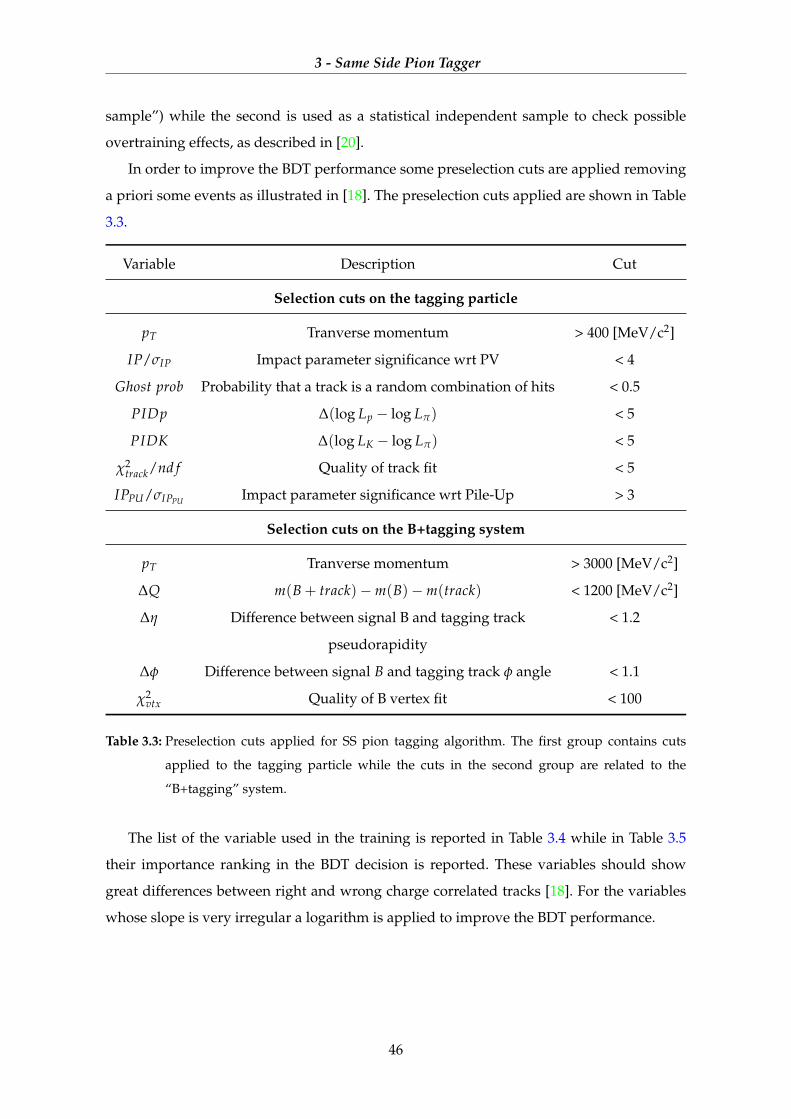
3 - Same Side Pion Tagger
sample”) while the second is used as a statistical independent sample to check possible
overtraining effects, as described in [20].
In order to improve the BDT performance some preselection cuts are applied removing
a priori some events as illustrated in [18]. The preselection cuts applied are shown in Table
3.3.
Variable Description Cut
Selection cuts on the tagging particle
pT Tranverse momentum > 400 [MeV/c2]
IP/σIP Impact parameter significance wrt PV < 4
Ghost prob Probability that a track is a random combination of hits < 0.5
PIDp ∆(log Lp − log Lπ) < 5
PIDK ∆(log LK − log Lπ) < 5
χ2track/nd f Quality of track fit < 5
IPPU/σIPPU Impact parameter significance wrt Pile-Up > 3
Selection cuts on the B+tagging system
pT Tranverse momentum > 3000 [MeV/c2]
∆Q m(B + track)−m(B)−m(track) < 1200 [MeV/c2]
∆η Difference between signal B and tagging track
pseudorapidity
< 1.2
∆φ Difference between signal B and tagging track φ angle < 1.1
χ2vtx Quality of B vertex fit < 100
Table 3.3: Preselection cuts applied for SS pion tagging algorithm. The first group contains cuts
applied to the tagging particle while the cuts in the second group are related to the
“B+tagging” system.
The list of the variable used in the training is reported in Table 3.4 while in Table 3.5
their importance ranking in the BDT decision is reported. These variables should show
great differences between right and wrong charge correlated tracks [18]. For the variables
whose slope is very irregular a logarithm is applied to improve the BDT performance.
46
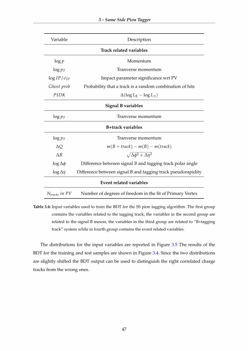
3 - Same Side Pion Tagger
Variable Description
Track related variables
log p Momentum
log pT Tranverse momentum
log IP/σIP Impact parameter significance wrt PV
Ghost prob Probability that a track is a random combination of hits
PIDK ∆(log LK − log Lπ)
Signal B variables
log pT Tranverse momentum
B+track variables
log pT Tranverse momentum
∆Q m(B + track)−m(B)−m(track)
∆R√
∆φ2 + ∆η2
log ∆φ Difference between signal B and tagging track polar angle
log ∆η Difference between signal B and tagging track pseudorapidity
Event related variables
Ntracks in PV Number of degrees of freedom in the fit of Primary Vertex
Table 3.4: Input variables used to train the BDT for the SS pion tagging algorithm. The first group
contains the variables related to the tagging track, the variables in the second group are
related to the signal B meson, the variables in the third group are related to “B+tagging
track” system while in fourth group contains the event related variables.
The distributions for the input variables are reported in Figure 3.5 The results of the
BDT for the training and test samples are shown in Figure 3.4. Since the two distributions
are slightly shifted the BDT output can be used to distinguish the right correlated charge
tracks from the wrong ones.
47

3 - Same Side Pion Tagger
Rank Variable Variable Importance
1 log(Ptrackt ) 1.522e-01
2 ∆Q 1.495e-01
3 ∆R 1.181e-01
4 log(PVndo f ) 1.174e-01
5 log(∆φ) 8.398e-02
6 log(Ptott ) 7.564e-02
7 log(P) 7.368e-02
8 log(BPt) 5.395e-02
9 log(∆η) 4.417e-02
10 gprob 3.719e-02
11 log(ipsig) 3.481e-02
12 PIDK 1.453e-02
Table 3.5: Ranking of the input variables according to their importance in the BDT response.
ssPion response
0.6 0.4 0.2 0 0.2 0.4 0.6 0.8 1
dx
/ (1
/N)
dN
0
0.5
1
1.5
2
2.5 Signal (test sample)
Background (test sample)
Signal (training sample)
Background (training sample)
KolmogorovSmirnov test: signal (background) probability = 0.000195 (0.00584)
U/O
flo
w (
S,B
): (
0.0
, 0.0
)% / (
0.0
, 0.0
)%
TMVA overtraining check for classifier: ssPion
Figure 3.4: Output of the SS pion BDT. The red distribution is related to the right charge correlated
tracks while the blue distribution corresponds to the wrong charge correlated tracks.
Both the distributions are normalized to their own number of entries.
48
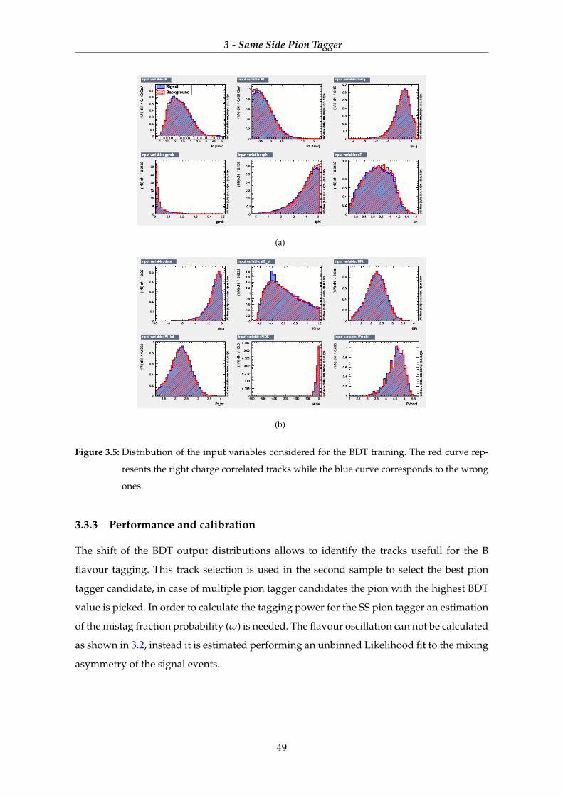
3 - Same Side Pion Tagger
(a)
(b)
Figure 3.5: Distribution of the input variables considered for the BDT training. The red curve rep-
resents the right charge correlated tracks while the blue curve corresponds to the wrong
ones.
3.3.3 Performance and calibration
The shift of the BDT output distributions allows to identify the tracks usefull for the B
flavour tagging. This track selection is used in the second sample to select the best pion
tagger candidate, in case of multiple pion tagger candidates the pion with the highest BDT
value is picked. In order to calculate the tagging power for the SS pion tagger an estimation
of the mistag fraction probability (ω) is needed. The flavour oscillation can not be calculated
as shown in 3.2, instead it is estimated performing an unbinned Likelihood fit to the mixing
asymmetry of the signal events.
49
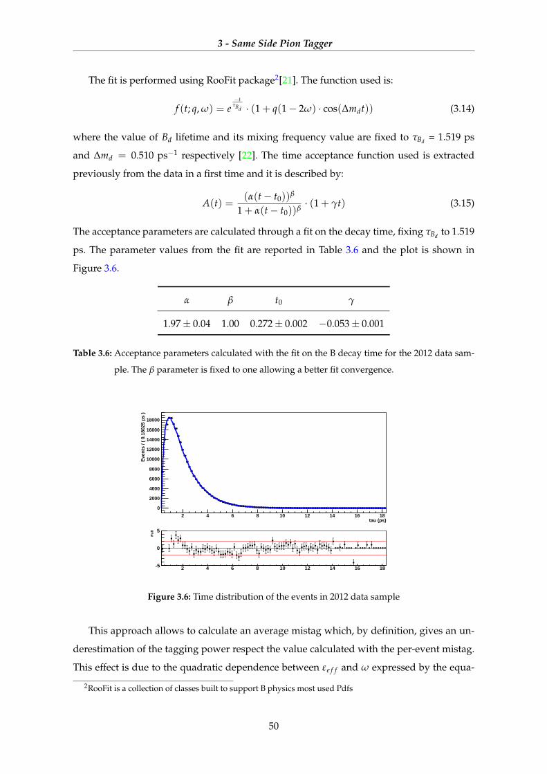
3 - Same Side Pion Tagger
The fit is performed using RooFit package2[21]. The function used is:
f (t; q, ω) = e−t
τBd · (1 + q(1− 2ω) · cos(∆mdt)) (3.14)
where the value of Bd lifetime and its mixing frequency value are fixed to τBd = 1.519 ps
and ∆md = 0.510 ps−1 respectively [22]. The time acceptance function used is extracted
previously from the data in a first time and it is described by:
A(t) =(α(t− t0))β
1 + α(t− t0))β· (1 + γt) (3.15)
The acceptance parameters are calculated through a fit on the decay time, fixing τBd to 1.519
ps. The parameter values from the fit are reported in Table 3.6 and the plot is shown in
Figure 3.6.
α β t0 γ
1.97± 0.04 1.00 0.272± 0.002 −0.053± 0.001
Table 3.6: Acceptance parameters calculated with the fit on the B decay time for the 2012 data sam-
ple. The β parameter is fixed to one allowing a better fit convergence.
tau (ps)2 4 6 8 10 12 14 16 18
Eve
nts
/ (
0.18
025
ps
)
0
2000
4000
6000
8000
10000
12000
14000
16000
18000
time distribution
2 4 6 8 10 12 14 16 18
Pu
ll
-5
0
5
Figure 3.6: Time distribution of the events in 2012 data sample
This approach allows to calculate an average mistag which, by definition, gives an un-
derestimation of the tagging power respect the value calculated with the per-event mistag.
This effect is due to the quadratic dependence between εe f f and ω expressed by the equa-
2RooFit is a collection of classes built to support B physics most used Pdfs
50
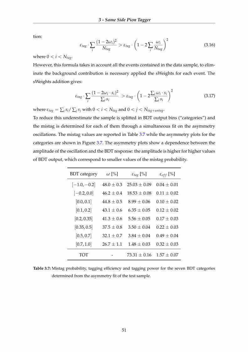
3 - Same Side Pion Tagger
tion:
εtag ·∑i
(1− 2ωi)2
Ntag> εtag ·
(1− 2 ∑
i
ωi
Ntag
)2
(3.16)
where 0 < i < Ntag.
However, this formula takes in account all the events contained in the data sample, to elim-
inate the background contribution is necessary applied the sWeights for each event. The
sWeights addition gives:
εtag ·∑i
(1− 2ωi · si)2
∑i si> εtag ·
(1− 2∑i ωi · si
∑i si
)2
(3.17)
where εtag = ∑i si/ ∑j sj with 0 < i < Ntag and 0 < j < Ntag+untag.
To reduce this underestimate the sample is splitted in BDT output bins (“categories”) and
the mistag is determined for each of them through a simultaneous fit on the asymmetry
oscillations. The mistag values are reported in Table 3.7 while the asymmetry plots for the
categories are shown in Figure 3.7. The asymmetry plots show a dependence between the
amplitude of the oscillation and the BDT response: the amplitude is higher for higher values
of BDT output, which correspond to smaller values of the mistag probability.
BDT category ω [%] εtag [%] εe f f [%]
[−1.0,−0.2] 48.0 ± 0.3 25.03 ± 0.09 0.04 ± 0.01
[−0.2, 0.0] 46.2 ± 0.4 18.53 ± 0.08 0.11 ± 0.02
[0.0, 0.1] 44.8 ± 0.5 8.99 ± 0.06 0.10 ± 0.02
[0.1, 0.2] 43.1 ± 0.6 6.35 ± 0.05 0.12 ± 0.02
[0.2, 0.35] 41.3 ± 0.6 5.56 ± 0.05 0.17 ± 0.03
[0.35, 0.5] 37.5 ± 0.8 3.50 ± 0.04 0.22 ± 0.03
[0.5, 0.7] 32.1 ± 0.7 3.84 ± 0.04 0.49 ± 0.04
[0.7, 1.0] 26.7 ± 1.1 1.48 ± 0.03 0.32 ± 0.03
TOT - 73.31 ± 0.16 1.57 ± 0.07
Table 3.7: Mistag probability, tagging efficiency and tagging power for the seven BDT categories
determined from the asymmetry fit of the test sample.
51
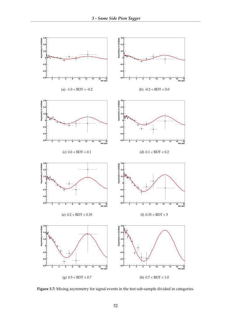
3 - Same Side Pion Tagger
tau (ps)2 4 6 8 10 12 14 16 18
As
ym
me
try
in
mix
Sta
te
0.6
0.4
0.2
0
0.2
0.4
0.6
cat0
(a) -1.0 < BDT < -0.2
tau (ps)2 4 6 8 10 12 14 16 18
As
ym
me
try
in
mix
Sta
te
0.6
0.4
0.2
0
0.2
0.4
0.6
cat1
(b) -0.2 < BDT < 0.0
tau (ps)2 4 6 8 10 12 14 16 18
As
ym
me
try
in
mix
Sta
te
0.6
0.4
0.2
0
0.2
0.4
0.6
cat2
(c) 0.0 < BDT < 0.1
tau (ps)2 4 6 8 10 12 14 16 18
As
ym
me
try
in
mix
Sta
te
0.6
0.4
0.2
0
0.2
0.4
0.6
cat3
(d) 0.1 < BDT < 0.2
tau (ps)2 4 6 8 10 12 14 16 18
As
ym
me
try
in
mix
Sta
te
0.6
0.4
0.2
0
0.2
0.4
0.6
cat4
(e) 0.2 < BDT < 0.35
tau (ps)2 4 6 8 10 12 14 16 18
As
ym
me
try
in
mix
Sta
te
0.6
0.4
0.2
0
0.2
0.4
0.6
cat5
(f) 0.35 < BDT < 5
tau (ps)2 4 6 8 10 12 14 16 18
As
ym
me
try
in
mix
Sta
te
0.6
0.4
0.2
0
0.2
0.4
0.6
cat6
(g) 0.5 < BDT < 0.7
tau (ps)2 4 6 8 10 12 14 16 18
As
ym
me
try
in
mix
Sta
te
0.6
0.4
0.2
0
0.2
0.4
0.6
cat7
(h) 0.7 < BDT < 1.0
Figure 3.7: Mixing asymmetry for signal events in the test sub-sample divided in categories.
52

3 - Same Side Pion Tagger
Fitting the dependence of ω vs BDT output a per-event mistag value (η) can be esti-
mated. A 3rd order polynomial function is found to fit well the data:
ηi = p0 + p1 · BDTi + p2 · BDT2i + p3 · BDT3
i (3.18)
where ηi is the average expected mistag in the i− th BDT bin. The η distribution is shown
in Figure 3.8.
Then the BDT calibration is performed on the third sample, statistically independent
from the samples used so far. In this sample the ω is calculated through the asymmetry
plots dividing the data in BDT bins, as done previously. Thus a plot of ω vs η is fitted with
a linear function:
ω = p0 + p1 · (η − 〈η〉) (3.19)
where 〈η〉 is the average predicted mistag on the full sample. If η is correctly calibrated p0
should be equal to 〈η〉 and p1 should be equal to 1.
The parameters estimated from the two fit are reported in Table 3.8 and in Table 3.9,
while the fit plots are shown in Figure 3.8.
In the third sample a per-event mistag is determined through the polynomial and the
linear fits starting from the BDT output. In this way it has been possible to calculate a more
precise tagging power, as it has been described in equation 3.16. The results achieved are
reported in Table 3.9.
p0 p1 p2 p3
0.452± 0.003 −0.12± 0.01 −0.12± 0.04 −0.08± 0.07
Table 3.8: Parameters of the 3rd polynomial for the B0 −→ D−(→ Kππ)π+ 2012 data sample (test
sub-sample).
p0 p1 〈η〉 εtag [%] εe f f [%]
0.441± 0.003 0.982± 0.049 0.444 71.83± 0.22 1.64± 0.10
Table 3.9: Calibration parameters and tagging performances for the B0 −→ D−(→ Kππ)π+ 2012
data sample (calibration sub-sample).
In this case the events with a per-event mistag larger than 0.5 are discarded and con-
sidered untagged. The results indicate that the calibration is correct within the statistical
53
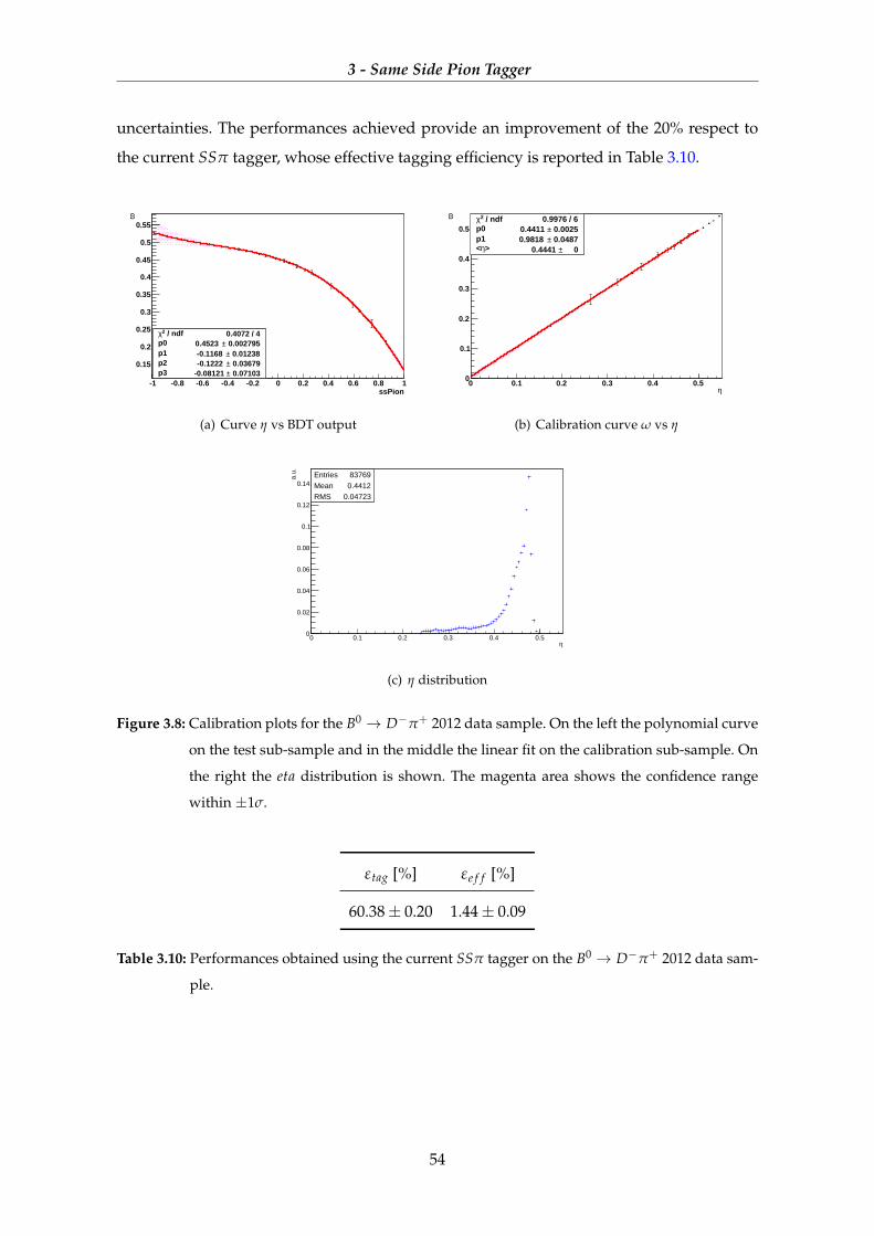
3 - Same Side Pion Tagger
uncertainties. The performances achieved provide an improvement of the 20% respect to
the current SSπ tagger, whose effective tagging efficiency is reported in Table 3.10.
ssPion-1 -0.8 -0.6 -0.4 -0.2 0 0.2 0.4 0.6 0.8 1
ω
0.15
0.2
0.25
0.3
0.35
0.4
0.45
0.5
0.55
/ ndf 2χ 0.4072 / 4p0 0.002795± 0.4523 p1 0.01238± -0.1168 p2 0.03679± -0.1222 p3 0.07103± -0.08121
/ ndf 2χ 0.4072 / 4p0 0.002795± 0.4523 p1 0.01238± -0.1168 p2 0.03679± -0.1222 p3 0.07103± -0.08121
(a) Curve η vs BDT output
η0 0.1 0.2 0.3 0.4 0.5
ω
0
0.1
0.2
0.3
0.4
0.5 / ndf 2χ 0.9976 / 6
p0 0.0025± 0.4411 p1 0.0487± 0.9818
> η< 0± 0.4441
/ ndf 2χ 0.9976 / 6p0 0.0025± 0.4411 p1 0.0487± 0.9818
> η< 0± 0.4441
(b) Calibration curve ω vs η
Entries 83769Mean 0.4412RMS 0.04723
η0 0.1 0.2 0.3 0.4 0.5
a.u.
0
0.02
0.04
0.06
0.08
0.1
0.12
0.14Entries 83769Mean 0.4412RMS 0.04723
eta_histo
(c) η distribution
Figure 3.8: Calibration plots for the B0 → D−π+ 2012 data sample. On the left the polynomial curve
on the test sub-sample and in the middle the linear fit on the calibration sub-sample. On
the right the eta distribution is shown. The magenta area shows the confidence range
within ±1σ.
εtag [%] εe f f [%]
60.38± 0.20 1.44± 0.09
Table 3.10: Performances obtained using the current SSπ tagger on the B0 → D−π+ 2012 data sam-
ple.
54
3 - Same Side Pion Tagger
3.4 Validation on the 2011 data sample
A first validation has been performed on the B0 −→ D−(→ Kππ)π+ events collected
in 2011 corresponding to 1 fb−1 taken at√
s = 7 TeV. The cuts applied to select the B
candidates in this sample are the same as the ones described in Table 3.1. The aim is to
verify that the algorithm developed can be used on a data sample completely different
from the one used for the tuning without losing its tagging ability. The analysis follows the
same path described in the previous section. The sWeights are calculated with the same
parametrization used in the 2012 data. In Figure 3.9 the fit mass distribution is shown and
in the Table 3.11 the fit parameters are reported.
Parameter Description Value
MB [MeV/c2] Mean B mass value 5283.80 ± 0.06
σm,1 [MeV/c2] σ of the first Gaussian 16.01 ± 0.24
σm,2 [MeV/c2] σ of the second Gaussian 25.63 ± 0.61
fm fraction of the first Gaussian 0.609 ± 0.032
α [MeV−1] slope of the exponential function -6.18 ± 0.30
Nsig Number of signal events 133410 ± 494
Nbkg Number of background events 8719 ± 345
S/B Signal over background ration 15.301 ± 0.608
Table 3.11: Results of the fit to the mass distribution 2011 data sample
Then the sample is divided in categories and for each one the value of a “predicted
mistag” (η) is calculated through the parameters of the 3rd polynomial function, calculated
with the 2012 sample, and using the BDT response as independent variable. The true mistag
(ω) is calculated through an unbinned Likelihood fit using the formula reported in equation
3.14 and dividing the sample into categories.
α β t0 γ
2.17± 0.05 1.00 0.27± 0.03 −0.05± 0.01
Table 3.12: Acceptance parameters calculated with the fit on the B decay time for the 2011 data sam-
ple. The β parameter is fixed to one allowing a better fit convergence.
The acceptance parameters are estimated in this new sample through a fit on the decay
55
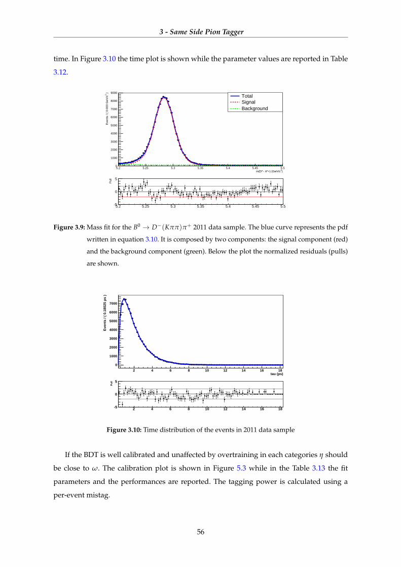
3 - Same Side Pion Tagger
time. In Figure 3.10 the time plot is shown while the parameter values are reported in Table
3.12.
)2^+) (GeV/cπm(D^- 5.2 5.25 5.3 5.35 5.4 5.45 5.5
)2E
vent
s / (
0.0
03 G
eV/c
0
1000
2000
3000
4000
5000
6000
7000
8000
9000TotalSignalBackground
5.2 5.25 5.3 5.35 5.4 5.45 5.5
Pul
l
-5
0
5
Figure 3.9: Mass fit for the B0 → D−(Kππ)π+ 2011 data sample. The blue curve represents the pdf
written in equation 3.10. It is composed by two components: the signal component (red)
and the background component (green). Below the plot the normalized residuals (pulls)
are shown.
tau (ps)2 4 6 8 10 12 14 16 18
Eve
nts
/ (
0.18
025
ps
)
0
1000
2000
3000
4000
5000
6000
7000
time distribution
2 4 6 8 10 12 14 16 18
Pu
ll
-5
0
5
Figure 3.10: Time distribution of the events in 2011 data sample
If the BDT is well calibrated and unaffected by overtraining in each categories η should
be close to ω. The calibration plot is shown in Figure 5.3 while in the Table 3.13 the fit
parameters and the performances are reported. The tagging power is calculated using a
per-event mistag.
56
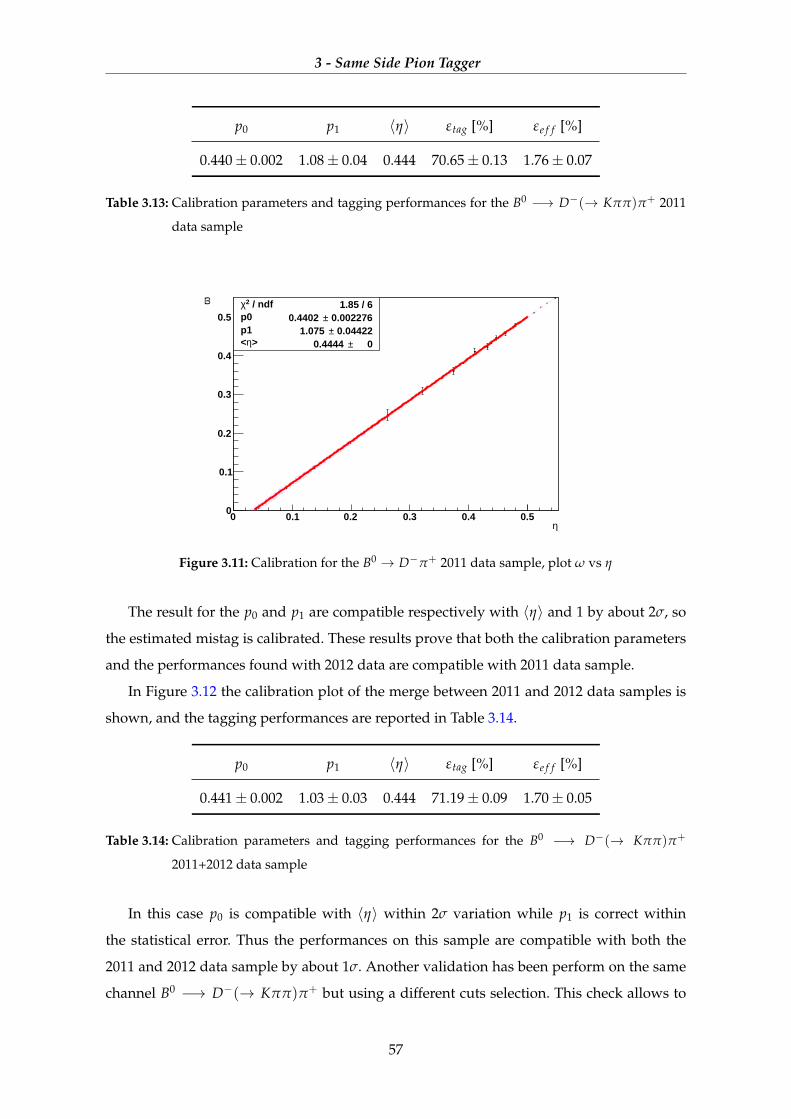
3 - Same Side Pion Tagger
p0 p1 〈η〉 εtag [%] εe f f [%]
0.440± 0.002 1.08± 0.04 0.444 70.65± 0.13 1.76± 0.07
Table 3.13: Calibration parameters and tagging performances for the B0 −→ D−(→ Kππ)π+ 2011
data sample
η0 0.1 0.2 0.3 0.4 0.5
ω
0
0.1
0.2
0.3
0.4
0.5 / ndf 2χ 1.85 / 6
p0 0.002276± 0.4402 p1 0.04422± 1.075
> η< 0± 0.4444
/ ndf 2χ 1.85 / 6p0 0.002276± 0.4402 p1 0.04422± 1.075
> η< 0± 0.4444
Figure 3.11: Calibration for the B0 → D−π+ 2011 data sample, plot ω vs η
The result for the p0 and p1 are compatible respectively with 〈η〉 and 1 by about 2σ, so
the estimated mistag is calibrated. These results prove that both the calibration parameters
and the performances found with 2012 data are compatible with 2011 data sample.
In Figure 3.12 the calibration plot of the merge between 2011 and 2012 data samples is
shown, and the tagging performances are reported in Table 3.14.
p0 p1 〈η〉 εtag [%] εe f f [%]
0.441± 0.002 1.03± 0.03 0.444 71.19± 0.09 1.70± 0.05
Table 3.14: Calibration parameters and tagging performances for the B0 −→ D−(→ Kππ)π+
2011+2012 data sample
In this case p0 is compatible with 〈η〉 within 2σ variation while p1 is correct within
the statistical error. Thus the performances on this sample are compatible with both the
2011 and 2012 data sample by about 1σ. Another validation has been perform on the same
channel B0 −→ D−(→ Kππ)π+ but using a different cuts selection. This check allows to
57
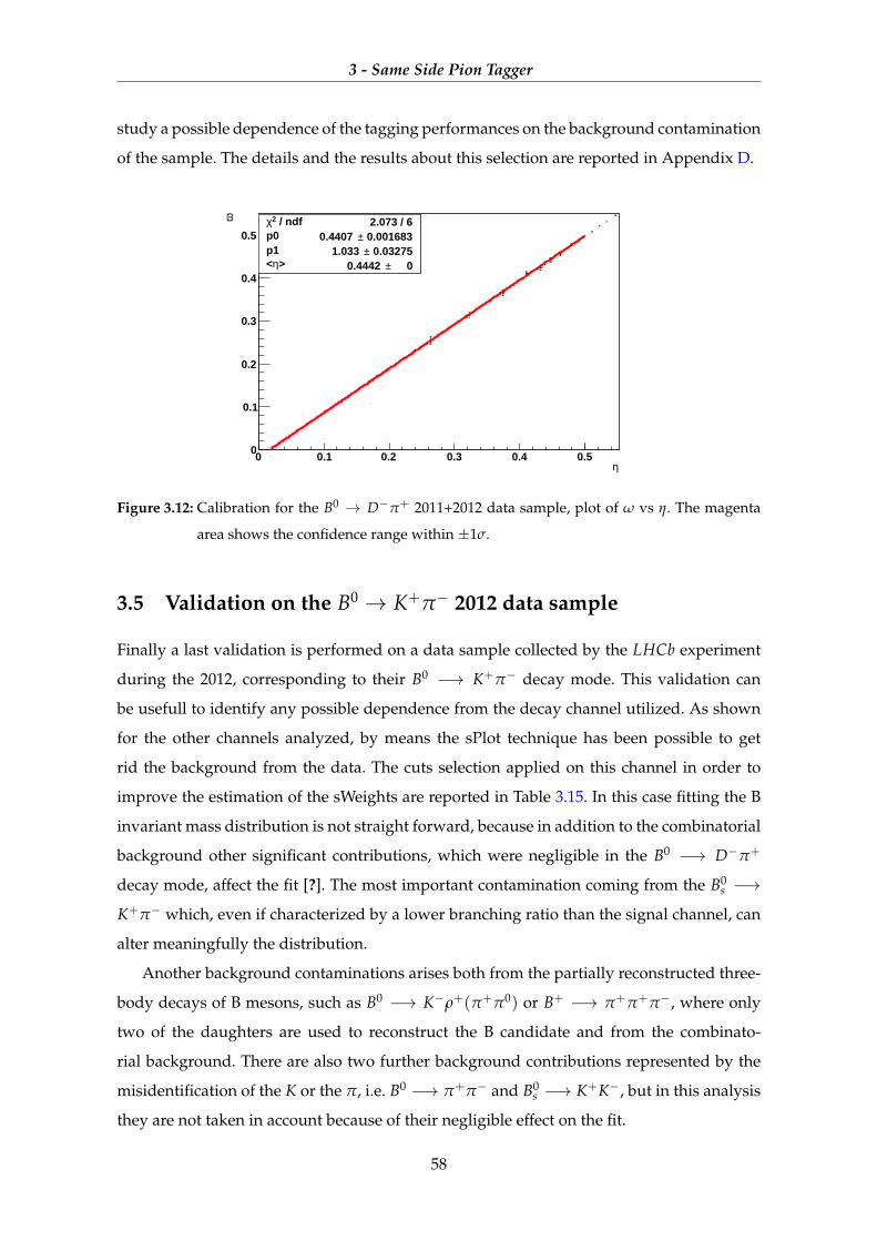
3 - Same Side Pion Tagger
study a possible dependence of the tagging performances on the background contamination
of the sample. The details and the results about this selection are reported in Appendix D.
η0 0.1 0.2 0.3 0.4 0.5
ω
0
0.1
0.2
0.3
0.4
0.5 / ndf 2χ 2.073 / 6
p0 0.001683± 0.4407 p1 0.03275± 1.033
> η< 0± 0.4442
/ ndf 2χ 2.073 / 6p0 0.001683± 0.4407 p1 0.03275± 1.033
> η< 0± 0.4442
Figure 3.12: Calibration for the B0 → D−π+ 2011+2012 data sample, plot of ω vs η. The magenta
area shows the confidence range within ±1σ.
3.5 Validation on the B0 → K+π− 2012 data sample
Finally a last validation is performed on a data sample collected by the LHCb experiment
during the 2012, corresponding to their B0 −→ K+π− decay mode. This validation can
be usefull to identify any possible dependence from the decay channel utilized. As shown
for the other channels analyzed, by means the sPlot technique has been possible to get
rid the background from the data. The cuts selection applied on this channel in order to
improve the estimation of the sWeights are reported in Table 3.15. In this case fitting the B
invariant mass distribution is not straight forward, because in addition to the combinatorial
background other significant contributions, which were negligible in the B0 −→ D−π+
decay mode, affect the fit [?]. The most important contamination coming from the B0s −→
K+π− which, even if characterized by a lower branching ratio than the signal channel, can
alter meaningfully the distribution.
Another background contaminations arises both from the partially reconstructed three-
body decays of B mesons, such as B0 −→ K−ρ+(π+π0) or B+ −→ π+π+π−, where only
two of the daughters are used to reconstruct the B candidate and from the combinato-
rial background. There are also two further background contributions represented by the
misidentification of the K or the π, i.e. B0 −→ π+π− and B0s −→ K+K−, but in this analysis
they are not taken in account because of their negligible effect on the fit.
58
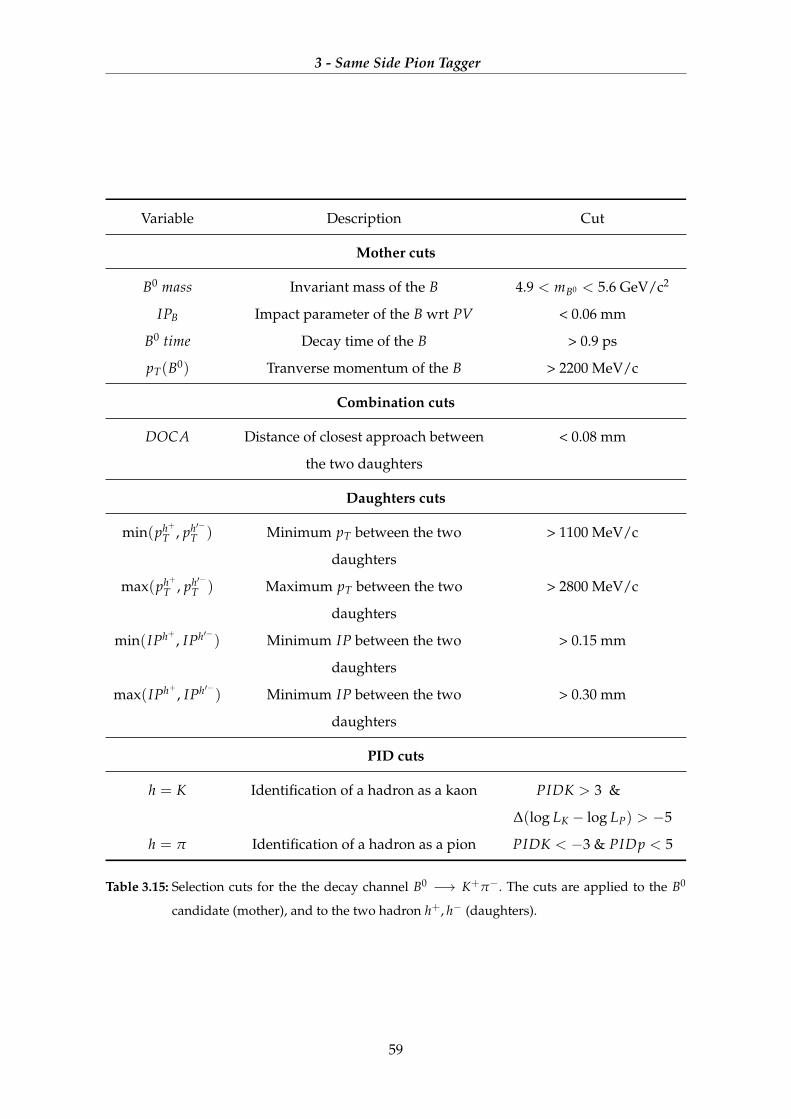
3 - Same Side Pion Tagger
Variable Description Cut
Mother cuts
B0 mass Invariant mass of the B 4.9 < mB0 < 5.6 GeV/c2
IPB Impact parameter of the B wrt PV < 0.06 mm
B0 time Decay time of the B > 0.9 ps
pT(B0) Tranverse momentum of the B > 2200 MeV/c
Combination cuts
DOCA Distance of closest approach between
the two daughters
< 0.08 mm
Daughters cuts
min(ph+T , ph′−
T ) Minimum pT between the two
daughters
> 1100 MeV/c
max(ph+T , ph′−
T ) Maximum pT between the two
daughters
> 2800 MeV/c
min(IPh+ , IPh′−) Minimum IP between the two
daughters
> 0.15 mm
max(IPh+ , IPh′−) Minimum IP between the two
daughters
> 0.30 mm
PID cuts
h = K Identification of a hadron as a kaon PIDK > 3 &
∆(log LK − log LP) > −5
h = π Identification of a hadron as a pion PIDK < −3 & PIDp < 5
Table 3.15: Selection cuts for the the decay channel B0 −→ K+π−. The cuts are applied to the B0
candidate (mother), and to the two hadron h+, h− (daughters).
59
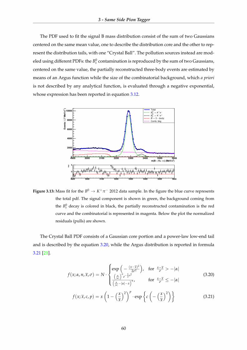
3 - Same Side Pion Tagger
The PDF used to fit the signal B mass distribution consist of the sum of two Gaussians
centered on the same mean value, one to describe the distribution core and the other to rep-
resent the distribution tails, with one “Crystal Ball”. The pollution sources instead are mod-
eled using different PDFs: the B0s contamination is reproduced by the sum of two Gaussians,
centered on the same value, the partially reconstructed three-body events are estimated by
means of an Argus function while the size of the combinatorial background, which a priori
is not described by any analytical function, is evaluated through a negative exponential,
whose expression has been reported in equation 3.12.
)2) (MeV/cπ K+ →m(B4900 5000 5100 5200 5300 5400 5500 5600
)2
Even
ts / (
7 M
eV
/c
0
2000
4000
6000
8000
10000
Kpi→B
Total
B0d → K
+π −
B0s → K
−π +
B→ 3 − body
Comb. bkg
4900 5000 5100 5200 5300 5400 5500 5600
Pu
ll
5
0
5
Figure 3.13: Mass fit for the B0 → K+π− 2012 data sample. In the figure the blue curve represents
the total pdf. The signal component is shown in green, the background coming from
the B0s decay is colored in black, the partially reconstructed contamination is the red
curve and the combinatorial is represented in magenta. Below the plot the normalized
residuals (pulls) are shown.
The Crystal Ball PDF consists of a Gaussian core portion and a power-law low-end tail
and is described by the equation 3.20, while the Argus distribution is reported in formula
3.21 [21].
f (x; α, n, x, σ) = N ·
exp
(− (x−x)2
2σ2
), for x−x
σ > −|α|(n|α|
)ne−
12 α2(
n|α|−|α|−x
)n , for x−xσ ≤ −|α|
(3.20)
f (x; x, c, p) = x(
1−( x
x
)2)p
· exp{
c(−( x
x
)2)}
(3.21)
60
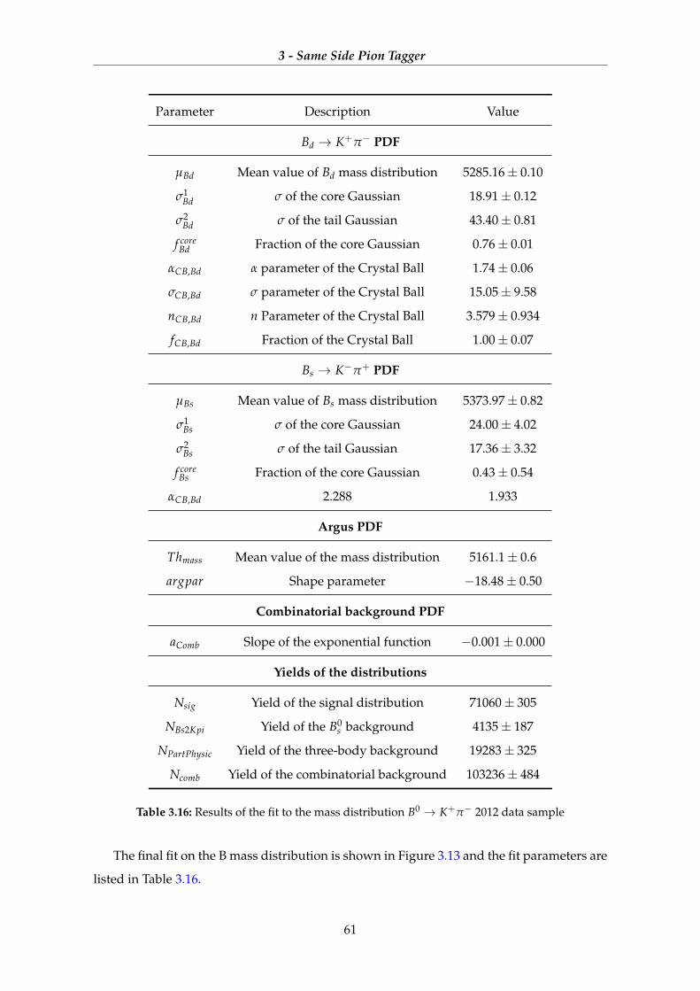
3 - Same Side Pion Tagger
Parameter Description Value
Bd → K+π− PDF
µBd Mean value of Bd mass distribution 5285.16± 0.10
σ1Bd σ of the core Gaussian 18.91± 0.12
σ2Bd σ of the tail Gaussian 43.40± 0.81
f coreBd Fraction of the core Gaussian 0.76± 0.01
αCB,Bd α parameter of the Crystal Ball 1.74± 0.06
σCB,Bd σ parameter of the Crystal Ball 15.05± 9.58
nCB,Bd n Parameter of the Crystal Ball 3.579± 0.934
fCB,Bd Fraction of the Crystal Ball 1.00± 0.07
Bs → K−π+ PDF
µBs Mean value of Bs mass distribution 5373.97± 0.82
σ1Bs σ of the core Gaussian 24.00± 4.02
σ2Bs σ of the tail Gaussian 17.36± 3.32
f coreBs Fraction of the core Gaussian 0.43± 0.54
αCB,Bd 2.288 1.933
Argus PDF
Thmass Mean value of the mass distribution 5161.1± 0.6
argpar Shape parameter −18.48± 0.50
Combinatorial background PDF
aComb Slope of the exponential function −0.001± 0.000
Yields of the distributions
Nsig Yield of the signal distribution 71060± 305
NBs2Kpi Yield of the B0s background 4135± 187
NPartPhysic Yield of the three-body background 19283± 325
Ncomb Yield of the combinatorial background 103236± 484
Table 3.16: Results of the fit to the mass distribution B0 → K+π− 2012 data sample
The final fit on the B mass distribution is shown in Figure 3.13 and the fit parameters are
listed in Table 3.16.
61
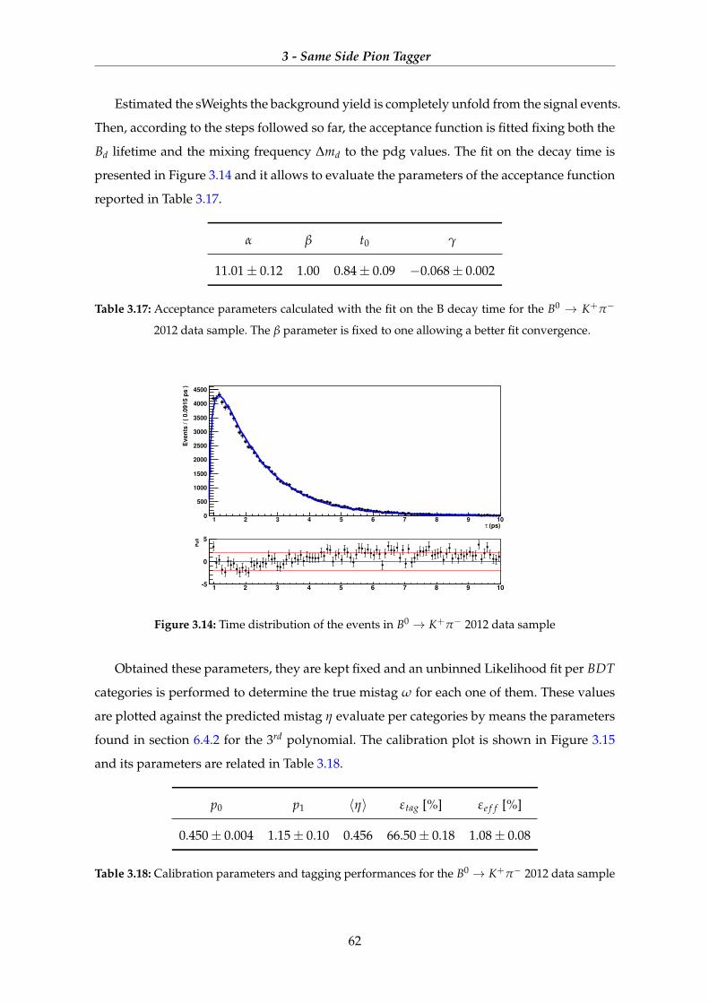
3 - Same Side Pion Tagger
Estimated the sWeights the background yield is completely unfold from the signal events.
Then, according to the steps followed so far, the acceptance function is fitted fixing both the
Bd lifetime and the mixing frequency ∆md to the pdg values. The fit on the decay time is
presented in Figure 3.14 and it allows to evaluate the parameters of the acceptance function
reported in Table 3.17.
α β t0 γ
11.01± 0.12 1.00 0.84± 0.09 −0.068± 0.002
Table 3.17: Acceptance parameters calculated with the fit on the B decay time for the B0 → K+π−
2012 data sample. The β parameter is fixed to one allowing a better fit convergence.
(ps)τ
1 2 3 4 5 6 7 8 9 10
Even
ts / (
0.0
915 p
s )
0
500
1000
1500
2000
2500
3000
3500
4000
4500
time distribution
1 2 3 4 5 6 7 8 9 10
Pu
ll
5
0
5
Figure 3.14: Time distribution of the events in B0 → K+π− 2012 data sample
Obtained these parameters, they are kept fixed and an unbinned Likelihood fit per BDT
categories is performed to determine the true mistag ω for each one of them. These values
are plotted against the predicted mistag η evaluate per categories by means the parameters
found in section 6.4.2 for the 3rd polynomial. The calibration plot is shown in Figure 3.15
and its parameters are related in Table 3.18.
p0 p1 〈η〉 εtag [%] εe f f [%]
0.450± 0.004 1.15± 0.10 0.456 66.50± 0.18 1.08± 0.08
Table 3.18: Calibration parameters and tagging performances for the B0 → K+π− 2012 data sample
62
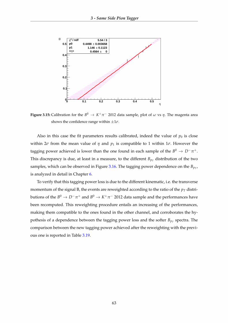
3 - Same Side Pion Tagger
η0 0.1 0.2 0.3 0.4 0.5
ω
0
0.1
0.2
0.3
0.4
0.5 / ndf 2χ 5.54 / 3
p0 0.003658± 0.4498 p1 0.1123± 1.146
> η< 0± 0.4564
/ ndf 2χ 5.54 / 3p0 0.003658± 0.4498 p1 0.1123± 1.146
> η< 0± 0.4564
Figure 3.15: Calibration for the B0 → K+π− 2012 data sample, plot of ω vs η. The magenta area
shows the confidence range within ±1σ.
Also in this case the fit parameters results calibrated, indeed the value of p0 is close
within 2σ from the mean value of η and p1 is compatible to 1 within 1σ. However the
tagging power achieved is lower than the one found in each sample of the B0 → D−π+.
This discrepancy is due, at least in a measure, to the different BpT distribution of the two
samples, which can be observed in Figure 3.16. The tagging power dependence on the BpT ,
is analyzed in detail in Chapter 6.
To verify that this tagging power loss is due to the different kinematic, i.e. the transverse
momentum of the signal B, the events are reweighted according to the ratio of the pT distri-
butions of the B0 → D−π+ and B0 → K+π− 2012 data sample and the performances have
been recomputed. This reweighting procedure entails an increasing of the performances,
making them compatible to the ones found in the other channel, and corroborates the hy-
pothesis of a dependence between the tagging power loss and the softer BpT spectra. The
comparison between the new tagging power achieved after the reweighting with the previ-
ous one is reported in Table 3.19.
63
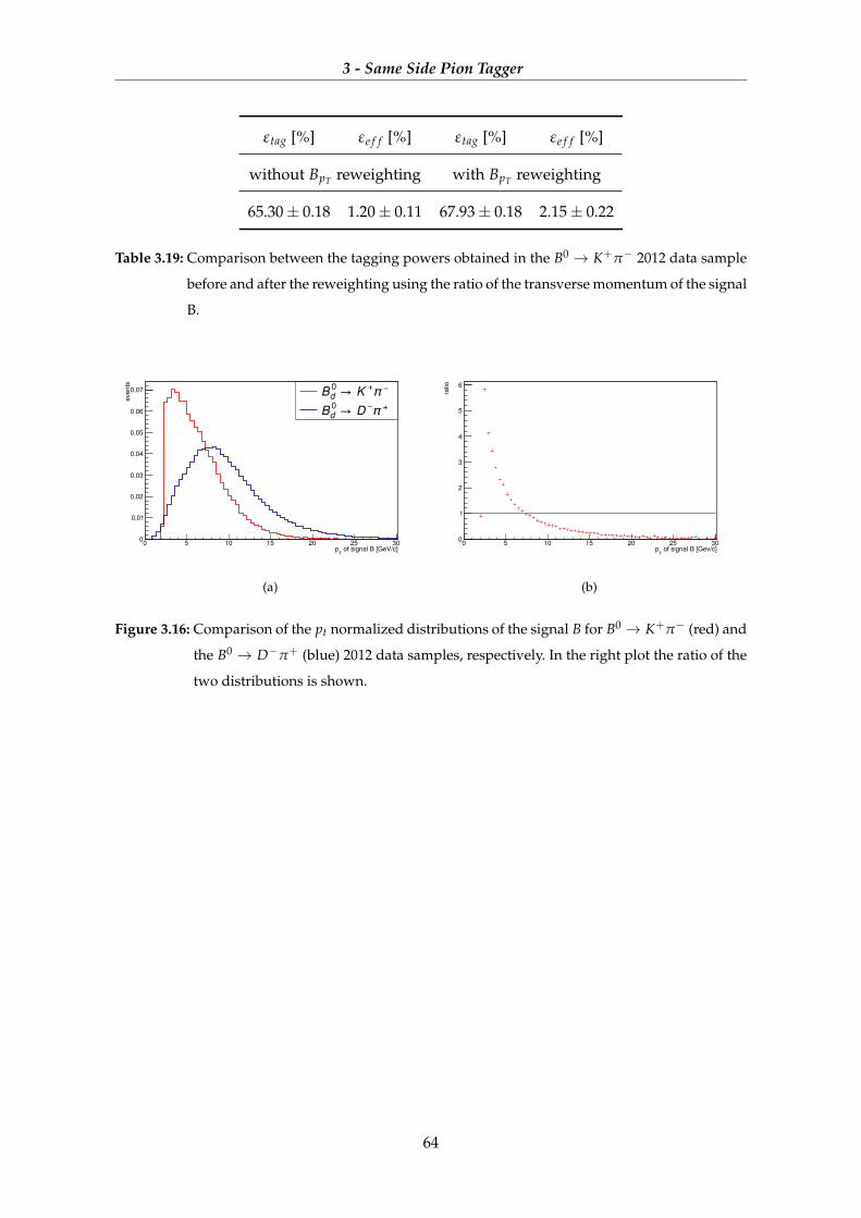
3 - Same Side Pion Tagger
εtag [%] εe f f [%] εtag [%] εe f f [%]
without BpT reweighting with BpT reweighting
65.30± 0.18 1.20± 0.11 67.93± 0.18 2.15± 0.22
Table 3.19: Comparison between the tagging powers obtained in the B0 → K+π− 2012 data sample
before and after the reweighting using the ratio of the transverse momentum of the signal
B.
Pt_sig_Kpi
Entries 5937106
Mean 6.376
RMS 3.229
of signal B [GeV/c]T
p0 5 10 15 20 25 30
events
0
0.01
0.02
0.03
0.04
0.05
0.06
0.07
Pt_sig_Kpi
Entries 5937106
Mean 6.376
RMS 3.229
B0d → K
+π −
B0d → D
−π +
(a)
Pt_ratio
Entries 41
Mean 6.544
RMS 4.996
of signal B [Gev/c]T
p0 5 10 15 20 25 30
ratio
0
1
2
3
4
5
6
Pt_ratio
Entries 41
Mean 6.544
RMS 4.996
Pt_ratio
(b)
Figure 3.16: Comparison of the pt normalized distributions of the signal B for B0 → K+π− (red) and
the B0 → D−π+ (blue) 2012 data samples, respectively. In the right plot the ratio of the
two distributions is shown.
64
4
Same Side Proton Tagger
Contents
4.1 SSp tagger development using the 2012 data sample 65
4.1.1 SS proton training 65
4.1.2 Performance and calibration 69
4.2 Validation on the 2011 data sample 72
4.3 Validation on the B0 → K+π− 2012 data sample 74
In this chapter a development of a Same Side Proton tagger is illustrated. The step fol-
lowed are similar to the ones described in the previous chapter for the SS pion. The BDT
training is performed on the B0 −→ D−π+ data sample collected in 2012 and it is described
in 6.4.2, then the validation using the B0 −→ D−π+ 2011 data sample is described in section
4.2 and using the second event selection in section D.2. Because the sWeights are indepen-
dent from the tagger chosen they are not recalculated in this chapter, but each sample uses
the sWeights estimated in the previous chapter.
4.1 SSp tagger development using the 2012 data sample
4.1.1 SS proton training
As shown in Figure 3.2 the fragmentation of the b quark can produce also protons in addic-
tion to the signal B0d. Thus also the charge of the proton, because of the quark correlation,
can be used to infer the flavour of the signal B meson. However in this case the charge cor-
relation is the opposite with respect to the SS pion’s one, thus the tagging decision used to
implement the BDT is defined as:
Right −→ B0 p̄ or B̄0 p
65
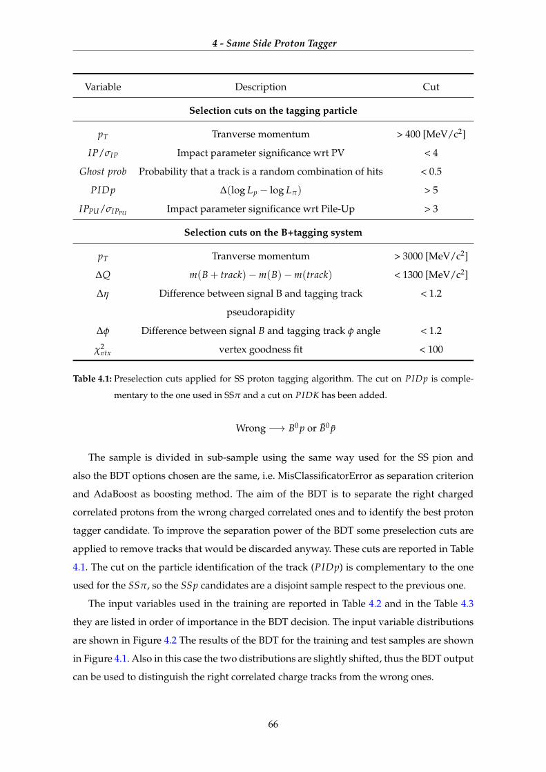
4 - Same Side Proton Tagger
Variable Description Cut
Selection cuts on the tagging particle
pT Tranverse momentum > 400 [MeV/c2]
IP/σIP Impact parameter significance wrt PV < 4
Ghost prob Probability that a track is a random combination of hits < 0.5
PIDp ∆(log Lp − log Lπ) > 5
IPPU/σIPPU Impact parameter significance wrt Pile-Up > 3
Selection cuts on the B+tagging system
pT Tranverse momentum > 3000 [MeV/c2]
∆Q m(B + track)−m(B)−m(track) < 1300 [MeV/c2]
∆η Difference between signal B and tagging track
pseudorapidity
< 1.2
∆φ Difference between signal B and tagging track φ angle < 1.2
χ2vtx vertex goodness fit < 100
Table 4.1: Preselection cuts applied for SS proton tagging algorithm. The cut on PIDp is comple-
mentary to the one used in SSπ and a cut on PIDK has been added.
Wrong −→ B0 p or B̄0 p̄
The sample is divided in sub-sample using the same way used for the SS pion and
also the BDT options chosen are the same, i.e. MisClassificatorError as separation criterion
and AdaBoost as boosting method. The aim of the BDT is to separate the right charged
correlated protons from the wrong charged correlated ones and to identify the best proton
tagger candidate. To improve the separation power of the BDT some preselection cuts are
applied to remove tracks that would be discarded anyway. These cuts are reported in Table
4.1. The cut on the particle identification of the track (PIDp) is complementary to the one
used for the SSπ, so the SSp candidates are a disjoint sample respect to the previous one.
The input variables used in the training are reported in Table 4.2 and in the Table 4.3
they are listed in order of importance in the BDT decision. The input variable distributions
are shown in Figure 4.2 The results of the BDT for the training and test samples are shown
in Figure 4.1. Also in this case the two distributions are slightly shifted, thus the BDT output
can be used to distinguish the right correlated charge tracks from the wrong ones.
66
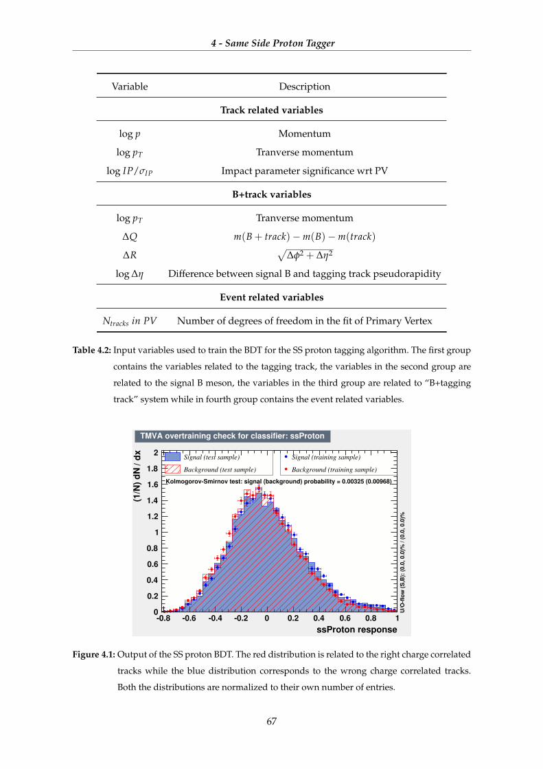
4 - Same Side Proton Tagger
Variable Description
Track related variables
log p Momentum
log pT Tranverse momentum
log IP/σIP Impact parameter significance wrt PV
B+track variables
log pT Tranverse momentum
∆Q m(B + track)−m(B)−m(track)
∆R√
∆φ2 + ∆η2
log ∆η Difference between signal B and tagging track pseudorapidity
Event related variables
Ntracks in PV Number of degrees of freedom in the fit of Primary Vertex
Table 4.2: Input variables used to train the BDT for the SS proton tagging algorithm. The first group
contains the variables related to the tagging track, the variables in the second group are
related to the signal B meson, the variables in the third group are related to “B+tagging
track” system while in fourth group contains the event related variables.
ssProton response
0.8 0.6 0.4 0.2 0 0.2 0.4 0.6 0.8 1
dx
/ (1
/N)
dN
0
0.2
0.4
0.6
0.8
1
1.2
1.4
1.6
1.8
2Signal (test sample)
Background (test sample)
Signal (training sample)
Background (training sample)
KolmogorovSmirnov test: signal (background) probability = 0.00325 (0.00968)
U/O
flo
w (
S,B
): (
0.0
, 0.0
)% / (
0.0
, 0.0
)%
TMVA overtraining check for classifier: ssProton
Figure 4.1: Output of the SS proton BDT. The red distribution is related to the right charge correlated
tracks while the blue distribution corresponds to the wrong charge correlated tracks.
Both the distributions are normalized to their own number of entries.
67
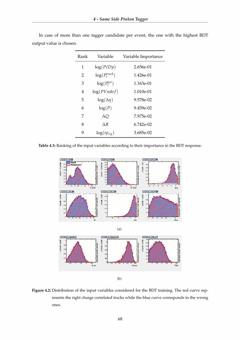
4 - Same Side Proton Tagger
In case of more than one tagger candidate per event, the one with the highest BDT
output value is chosen.
Rank Variable Variable Importance
1 log(PIDp) 2.656e-01
2 log(Ptrackt ) 1.426e-01
3 log(Ptott ) 1.163e-01
4 log(PVndo f ) 1.010e-01
5 log(∆η) 9.578e-02
6 log(P) 9.459e-02
7 ∆Q 7.975e-02
8 ∆R 6.742e-02
9 log(ipsig) 3.685e-02
Table 4.3: Ranking of the input variables according to their importance in the BDT response.
(a)
(b)
Figure 4.2: Distribution of the input variables considered for the BDT training. The red curve rep-
resents the right charge correlated tracks while the blue curve corresponds to the wrong
ones.
68
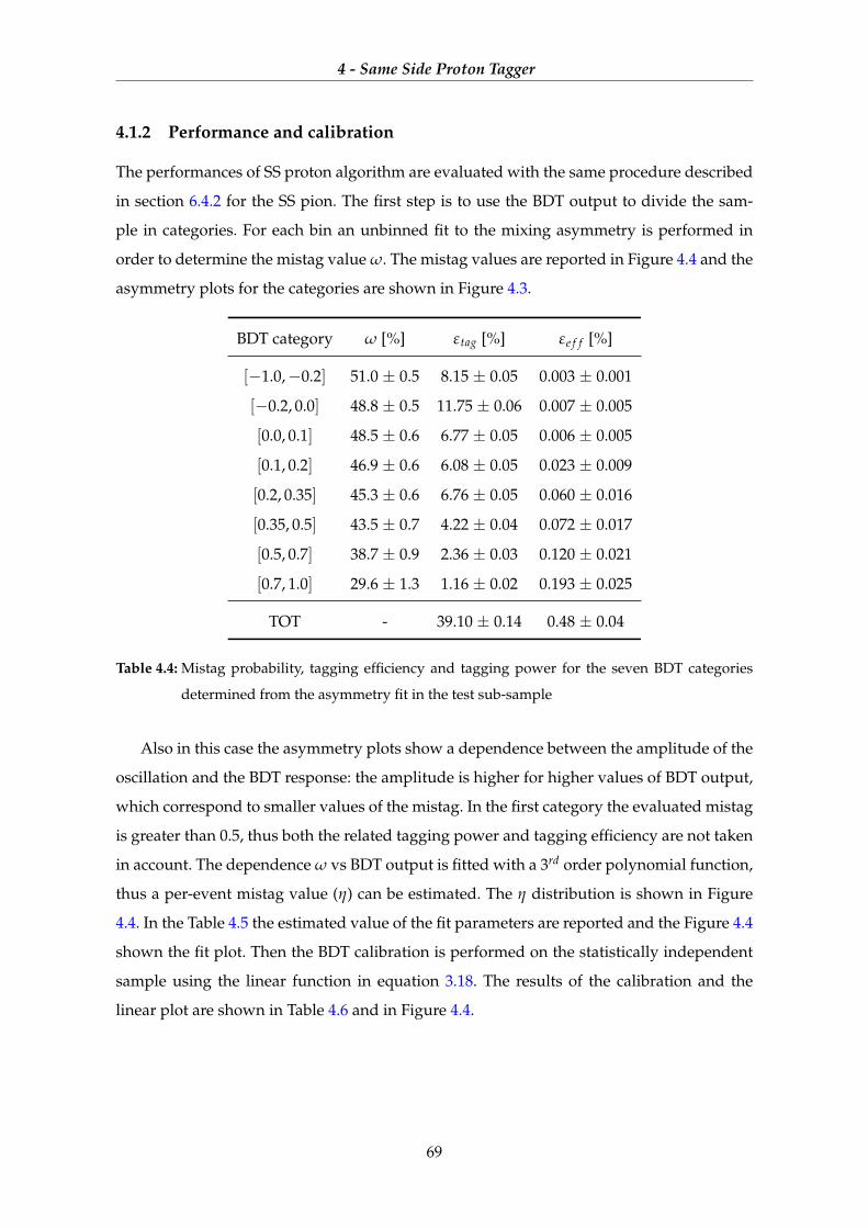
4 - Same Side Proton Tagger
4.1.2 Performance and calibration
The performances of SS proton algorithm are evaluated with the same procedure described
in section 6.4.2 for the SS pion. The first step is to use the BDT output to divide the sam-
ple in categories. For each bin an unbinned fit to the mixing asymmetry is performed in
order to determine the mistag value ω. The mistag values are reported in Figure 4.4 and the
asymmetry plots for the categories are shown in Figure 4.3.
BDT category ω [%] εtag [%] εe f f [%]
[−1.0,−0.2] 51.0 ± 0.5 8.15 ± 0.05 0.003 ± 0.001
[−0.2, 0.0] 48.8 ± 0.5 11.75 ± 0.06 0.007 ± 0.005
[0.0, 0.1] 48.5 ± 0.6 6.77 ± 0.05 0.006 ± 0.005
[0.1, 0.2] 46.9 ± 0.6 6.08 ± 0.05 0.023 ± 0.009
[0.2, 0.35] 45.3 ± 0.6 6.76 ± 0.05 0.060 ± 0.016
[0.35, 0.5] 43.5 ± 0.7 4.22 ± 0.04 0.072 ± 0.017
[0.5, 0.7] 38.7 ± 0.9 2.36 ± 0.03 0.120 ± 0.021
[0.7, 1.0] 29.6 ± 1.3 1.16 ± 0.02 0.193 ± 0.025
TOT - 39.10 ± 0.14 0.48 ± 0.04
Table 4.4: Mistag probability, tagging efficiency and tagging power for the seven BDT categories
determined from the asymmetry fit in the test sub-sample
Also in this case the asymmetry plots show a dependence between the amplitude of the
oscillation and the BDT response: the amplitude is higher for higher values of BDT output,
which correspond to smaller values of the mistag. In the first category the evaluated mistag
is greater than 0.5, thus both the related tagging power and tagging efficiency are not taken
in account. The dependence ω vs BDT output is fitted with a 3rd order polynomial function,
thus a per-event mistag value (η) can be estimated. The η distribution is shown in Figure
4.4. In the Table 4.5 the estimated value of the fit parameters are reported and the Figure 4.4
shown the fit plot. Then the BDT calibration is performed on the statistically independent
sample using the linear function in equation 3.18. The results of the calibration and the
linear plot are shown in Table 4.6 and in Figure 4.4.
69
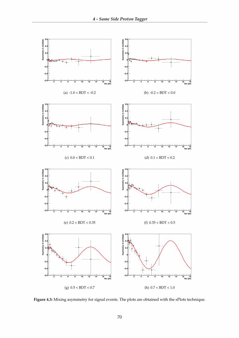
4 - Same Side Proton Tagger
tau (ps)2 4 6 8 10 12 14 16 18
As
ym
me
try
in
mix
Sta
te
0.6
0.4
0.2
0
0.2
0.4
0.6
cat0
(a) -1.0 < BDT < -0.2
tau (ps)2 4 6 8 10 12 14 16 18
As
ym
me
try
in
mix
Sta
te
0.6
0.4
0.2
0
0.2
0.4
0.6
cat1
(b) -0.2 < BDT < 0.0
tau (ps)2 4 6 8 10 12 14 16 18
As
ym
me
try
in
mix
Sta
te
0.6
0.4
0.2
0
0.2
0.4
0.6
cat2
(c) 0.0 < BDT < 0.1
tau (ps)2 4 6 8 10 12 14 16 18
As
ym
me
try
in
mix
Sta
te
0.6
0.4
0.2
0
0.2
0.4
0.6
cat3
(d) 0.1 < BDT < 0.2
tau (ps)2 4 6 8 10 12 14 16 18
As
ym
me
try
in
mix
Sta
te
0.6
0.4
0.2
0
0.2
0.4
0.6
cat4
(e) 0.2 < BDT < 0.35
tau (ps)2 4 6 8 10 12 14 16 18
As
ym
me
try
in
mix
Sta
te
0.6
0.4
0.2
0
0.2
0.4
0.6
cat5
(f) 0.35 < BDT < 0.5
tau (ps)2 4 6 8 10 12 14 16 18
As
ym
me
try
in
mix
Sta
te
0.6
0.4
0.2
0
0.2
0.4
0.6
cat6
(g) 0.5 < BDT < 0.7
tau (ps)2 4 6 8 10 12 14 16 18
As
ym
me
try
in
mix
Sta
te
0.6
0.4
0.2
0
0.2
0.4
0.6
cat7
(h) 0.7 < BDT < 1.0
Figure 4.3: Mixing asymmetry for signal events. The plots are obtained with the sPlots technique.
70
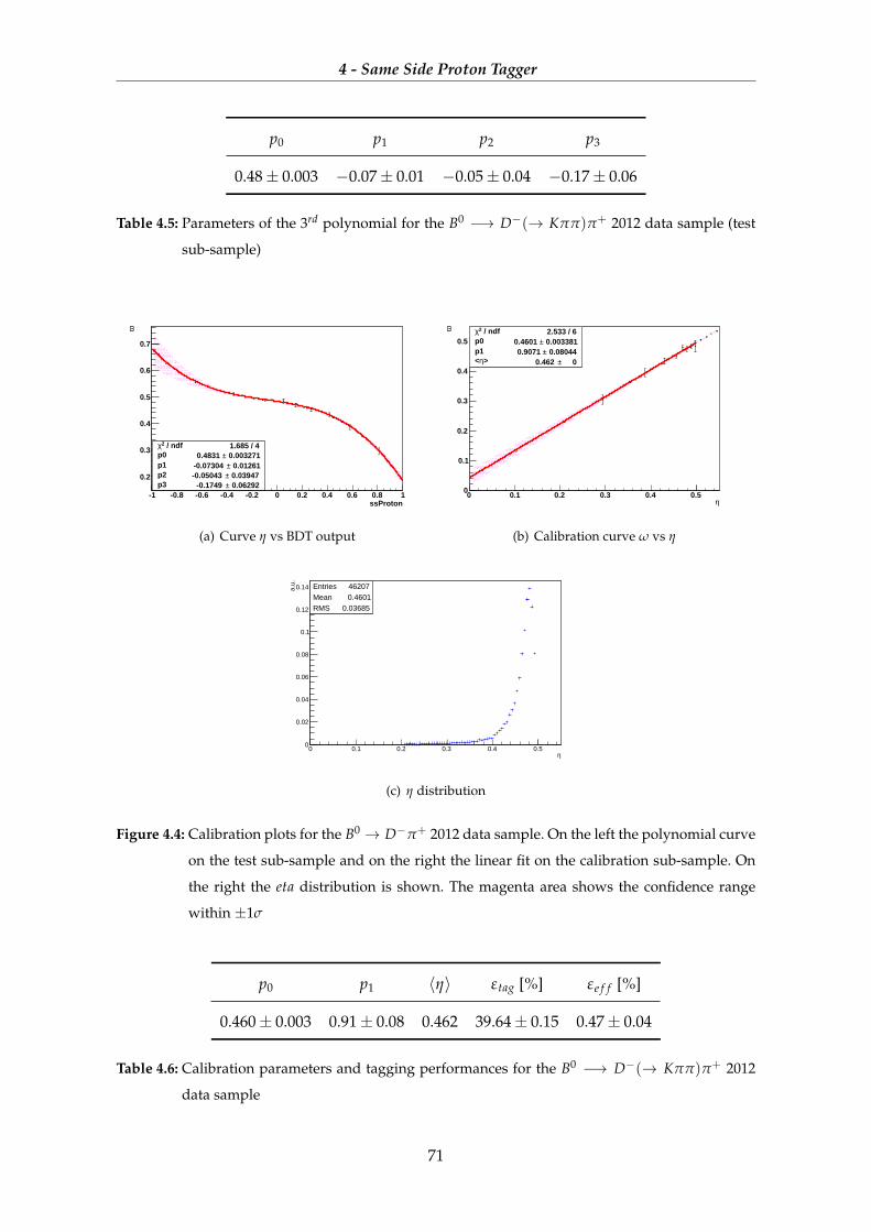
4 - Same Side Proton Tagger
p0 p1 p2 p3
0.48± 0.003 −0.07± 0.01 −0.05± 0.04 −0.17± 0.06
Table 4.5: Parameters of the 3rd polynomial for the B0 −→ D−(→ Kππ)π+ 2012 data sample (test
sub-sample)
ssProton-1 -0.8 -0.6 -0.4 -0.2 0 0.2 0.4 0.6 0.8 1
ω
0.2
0.3
0.4
0.5
0.6
0.7
/ ndf 2χ 1.685 / 4p0 0.003271± 0.4831 p1 0.01261± -0.07304 p2 0.03947± -0.05043 p3 0.06292± -0.1749
/ ndf 2χ 1.685 / 4p0 0.003271± 0.4831 p1 0.01261± -0.07304 p2 0.03947± -0.05043 p3 0.06292± -0.1749
(a) Curve η vs BDT output
η0 0.1 0.2 0.3 0.4 0.5
ω
0
0.1
0.2
0.3
0.4
0.5 / ndf 2χ 2.533 / 6
p0 0.003381± 0.4601 p1 0.08044± 0.9071
> η< 0± 0.462
/ ndf 2χ 2.533 / 6p0 0.003381± 0.4601 p1 0.08044± 0.9071
> η< 0± 0.462
(b) Calibration curve ω vs η
Entries 46207Mean 0.4601RMS 0.03685
η0 0.1 0.2 0.3 0.4 0.5
a.u.
0
0.02
0.04
0.06
0.08
0.1
0.12
0.14 Entries 46207Mean 0.4601RMS 0.03685
eta_histo
(c) η distribution
Figure 4.4: Calibration plots for the B0 → D−π+ 2012 data sample. On the left the polynomial curve
on the test sub-sample and on the right the linear fit on the calibration sub-sample. On
the right the eta distribution is shown. The magenta area shows the confidence range
within ±1σ
p0 p1 〈η〉 εtag [%] εe f f [%]
0.460± 0.003 0.91± 0.08 0.462 39.64± 0.15 0.47± 0.04
Table 4.6: Calibration parameters and tagging performances for the B0 −→ D−(→ Kππ)π+ 2012
data sample
71

4 - Same Side Proton Tagger
εtag [%] εe f f [%]
33.16± 0.14 0.51± 0.03
Table 4.7: Performances obtained using the current SSp tagger on the B0 → D−π+ 2012 data sam-
ple.
As done for the SS pion, the tagging power is calculated using using the per-event
mistag, determined with the polynomial function. The results achieved are reported in Ta-
ble 4.6. The events with a per-event mistag greater than 0.5 are discarded and considered
untagged. In this case p0 is compatible with 〈η〉 within the statistical error, while p1 is com-
patible to 1 within 1σ. In Table 4.7 the performances obtained using the SSp available in the
sample are shown. The tagging power achieved with the two algorithms are compatible
within the statistical error.
4.2 Validation on the 2011 data sample
The same validation on the sample done for SS proton studies using B0 −→ D−(→ Kππ)π+
events collected in 2011 corresponding to 1 fb−1 taken at√
s = 7 TeV center of mass energy.
The calibration plot is shown in Figure 4.5 while in the Table 4.8 the fit parameters and the
performances are reported. The tagging power is calculated using a per-event mistag.
p0 p1 〈η〉 εtag [%] εe f f [%]
0.469± 0.003 1.06± 0.07 0.461 41.11± 0.13 0.48± 0.04
Table 4.8: Calibration parameters and tagging performances for the B0 −→ D−(→ Kππ)π+ 2011
data sample
The result for the p0 and p1 are compatible respectively with 〈η〉 and 1 by about 2σ, so
the estimated mistag is calibrated. These results prove that both the calibration parameters
and the performances found with 2012 data are compatible with 2011 data sample.
In Figure 4.6 the calibration plot of the merge between 2011 and 2012 data samples is
shown, and the tagging performances are reported in Table 4.9.
72
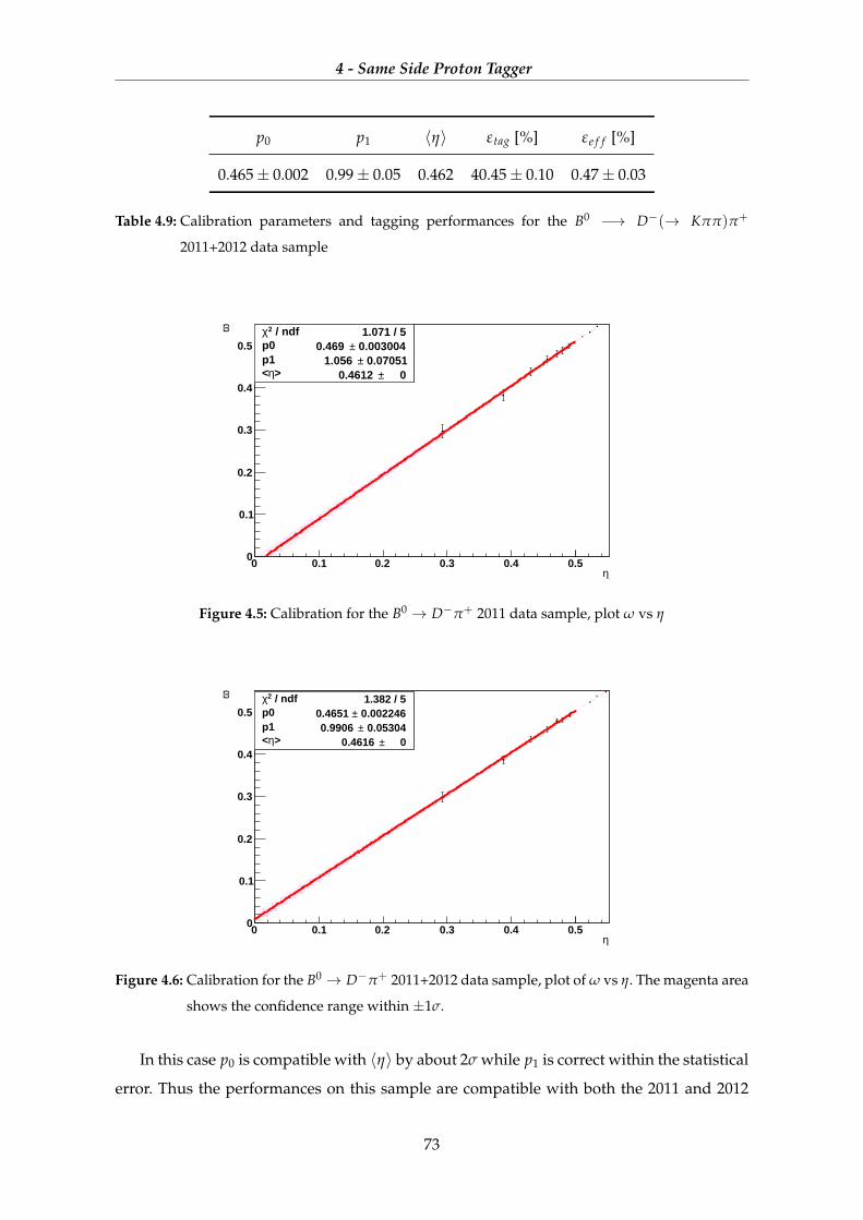
4 - Same Side Proton Tagger
p0 p1 〈η〉 εtag [%] εe f f [%]
0.465± 0.002 0.99± 0.05 0.462 40.45± 0.10 0.47± 0.03
Table 4.9: Calibration parameters and tagging performances for the B0 −→ D−(→ Kππ)π+
2011+2012 data sample
η0 0.1 0.2 0.3 0.4 0.5
ω
0
0.1
0.2
0.3
0.4
0.5 / ndf 2χ 1.071 / 5
p0 0.003004± 0.469 p1 0.07051± 1.056
> η< 0± 0.4612
/ ndf 2χ 1.071 / 5p0 0.003004± 0.469 p1 0.07051± 1.056
> η< 0± 0.4612
Figure 4.5: Calibration for the B0 → D−π+ 2011 data sample, plot ω vs η
η0 0.1 0.2 0.3 0.4 0.5
ω
0
0.1
0.2
0.3
0.4
0.5 / ndf 2χ 1.382 / 5
p0 0.002246± 0.4651 p1 0.05304± 0.9906
> η< 0± 0.4616
/ ndf 2χ 1.382 / 5p0 0.002246± 0.4651 p1 0.05304± 0.9906
> η< 0± 0.4616
Figure 4.6: Calibration for the B0 → D−π+ 2011+2012 data sample, plot of ω vs η. The magenta area
shows the confidence range within ±1σ.
In this case p0 is compatible with 〈η〉 by about 2σ while p1 is correct within the statistical
error. Thus the performances on this sample are compatible with both the 2011 and 2012
73
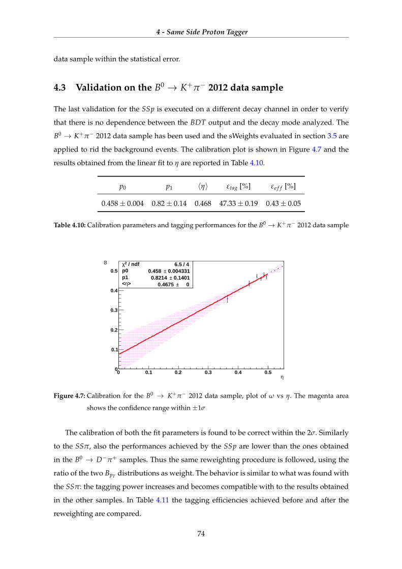
4 - Same Side Proton Tagger
data sample within the statistical error.
4.3 Validation on the B0 → K+π− 2012 data sample
The last validation for the SSp is executed on a different decay channel in order to verify
that there is no dependence between the BDT output and the decay mode analyzed. The
B0 → K+π− 2012 data sample has been used and the sWeights evaluated in section 3.5 are
applied to rid the background events. The calibration plot is shown in Figure 4.7 and the
results obtained from the linear fit to η are reported in Table 4.10.
p0 p1 〈η〉 εtag [%] εe f f [%]
0.458± 0.004 0.82± 0.14 0.468 47.33± 0.19 0.43± 0.05
Table 4.10: Calibration parameters and tagging performances for the B0 → K+π− 2012 data sample
η0 0.1 0.2 0.3 0.4 0.5
ω
0
0.1
0.2
0.3
0.4
0.5 / ndf 2χ 6.5 / 4
p0 0.004331± 0.458 p1 0.1401± 0.8214
> η< 0± 0.4675
/ ndf 2χ 6.5 / 4p0 0.004331± 0.458 p1 0.1401± 0.8214
> η< 0± 0.4675
Figure 4.7: Calibration for the B0 → K+π− 2012 data sample, plot of ω vs η. The magenta area
shows the confidence range within ±1σ
The calibration of both the fit parameters is found to be correct within the 2σ. Similarly
to the SSπ, also the performances achieved by the SSp are lower than the ones obtained
in the B0 → D−π+ samples. Thus the same reweighting procedure is followed, using the
ratio of the two BpT distributions as weight. The behavior is similar to what was found with
the SSπ: the tagging power increases and becomes compatible with to the results obtained
in the other samples. In Table 4.11 the tagging efficiencies achieved before and after the
reweighting are compared.
74

4 - Same Side Proton Tagger
εtag [%] εe f f [%] εtag [%] εe f f [%]
without BpT reweighting with BpT reweighting
47.33± 0.19 0.43± 0.05 49.75± 0.19 0.53± 0.06
Table 4.11: Comparison between the tagging powers obtained in the B0 → K+π− 2012 data sample
before and after the reweighting using the ratio of the transverse momentum of the signal
B.
75

5
Tagger combination
Contents
5.1 Combination of taggers 76
5.2 SSp and SSπ combination 77
5.2.1 Combination of the SS taggers on the B0 → D−π+ 2012 data sample 78
5.2.2 Combination on B0 → D−π+ 2011 data sample 80
5.2.3 Combination on the B0 → K+π− 2012 data sample 82
5.3 SS and OS combination 83
5.3.1 Combination of SS taggers with the OS tagger on the B0 → D−π+
2012 data sample 84
5.3.2 Combination on the B0 −→ D−π+2011 data sample 87
5.3.3 Combination on the B0 → K+π− 2012 data sample 89
5.4 Measurement of ∆md 90
In this chapter the SS tagger combination (SS pion + SS proton) 5.2 and the combination
SS tagger + OS tagger 5.3 are studied. The theoretical formulas used to achieve the com-
bination of the properties of all available taggers are reported in section 5.1. In section 5.4
the tagging decisions of the final tagger combination (SS+OS) are used to estimate ∆md by
means a simultaneous unbinned fit on the categories.
5.1 Combination of taggers
When more than one tagger is available per event the tagging decisions and mistag proba-
bilities provided by each tagger can be combined into a final decision on the initial flavour
76
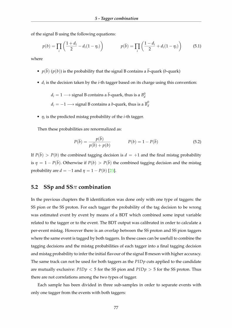
5 - Tagger combination
of the signal B using the following equations:
p(b) = ∏i
(1 + di
2− di(1− ηi)
)p(b) = ∏
i
(1− di
2+ di(1− ηi)
)(5.1)
where
• p(b) (p(b)) is the probability that the signal B contains a b-quark (b-quark)
• di is the decision taken by the i-th tagger based on its charge using this convention:
di = 1 −→ signal B contains a b-quark, thus is a B0d
di = −1 −→ signal B contains a b-quark, thus is a B0d
• ηi is the predicted mistag probability of the i-th tagger.
Then these probabilities are renormalized as:
P(b) =p(b)
p(b) + p(b)P(b) = 1− P(b) (5.2)
If P(b) > P(b) the combined tagging decision is d = +1 and the final mistag probability
is η = 1− P(b). Otherwise if P(b) > P(b) the combined tagging decision and the mistag
probability are d = −1 and η = 1− P(b) [23].
5.2 SSp and SSπ combination
In the previous chapters the B identification was done only with one type of taggers: the
SS pion or the SS proton. For each tagger the probability of the tag decision to be wrong
was estimated event by event by means of a BDT which combined some input variable
related to the tagger or to the event. The BDT output was calibrated in order to calculate a
per-event mistag. However there is an overlap between the SS proton and SS pion taggers
where the same event is tagged by both taggers. In these cases can be usefull to combine the
tagging decisions and the mistag probabilities of each tagger into a final tagging decision
and mistag probability to infer the initial flavour of the signal B meson with higher accuracy.
The same track can not be used for both taggers as the PIDp cuts applied to the candidate
are mutually exclusive: PIDp < 5 for the SS pion and PIDp > 5 for the SS proton. Thus
there are not correlations among the two types of tagger.
Each sample has been divided in three sub-samples in order to separate events with
only one tagger from the events with both taggers:
77
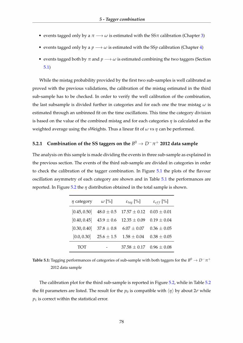
5 - Tagger combination
• events tagged only by a π −→ ω is estimated with the SSπ calibration (Chapter 3)
• events tagged only by a p −→ ω is estimated with the SSp calibration (Chapter 4)
• events tagged both by π and p −→ ω is estimated combining the two taggers (Section
5.1)
While the mistag probability provided by the first two sub-samples is well calibrated as
proved with the previous validations, the calibration of the mistag estimated in the third
sub-sample has to be checked. In order to verify the well calibration of the combination,
the last subsample is divided further in categories and for each one the true mistag ω is
estimated through an unbinned fit on the time oscillations. This time the category division
is based on the value of the combined mistag and for each categories η is calculated as the
weighted average using the sWeights. Thus a linear fit of ω vs η can be performed.
5.2.1 Combination of the SS taggers on the B0 → D−π+ 2012 data sample
The analysis on this sample is made dividing the events in three sub-sample as explained in
the previous section. The events of the third sub-sample are divided in categories in order
to check the calibration of the tagger combination. In Figure 5.1 the plots of the flavour
oscillation asymmetry of each category are shown and in Table 5.1 the performances are
reported. In Figure 5.2 the η distribution obtained in the total sample is shown.
η category ω [%] εtag [%] εe f f [%]
[0.45, 0.50] 48.0 ± 0.5 17.57 ± 0.12 0.03 ± 0.01
[0.40, 0.45] 43.9 ± 0.6 12.35 ± 0.09 0.19 ± 0.04
[0.30, 0.40] 37.8 ± 0.8 6.07 ± 0.07 0.36 ± 0.05
[0.0, 0.30] 25.6 ± 1.5 1.58 ± 0.04 0.38 ± 0.05
TOT - 37.58 ± 0.17 0.96 ± 0.08
Table 5.1: Tagging performances of categories of sub-sample with both taggers for the B0 → D−π+
2012 data sample
The calibration plot for the third sub-sample is reported in Figure 5.2, while in Table 5.2
the fit parameters are listed. The result for the p0 is compatible with 〈η〉 by about 2σ while
p1 is correct within the statistical error.
78
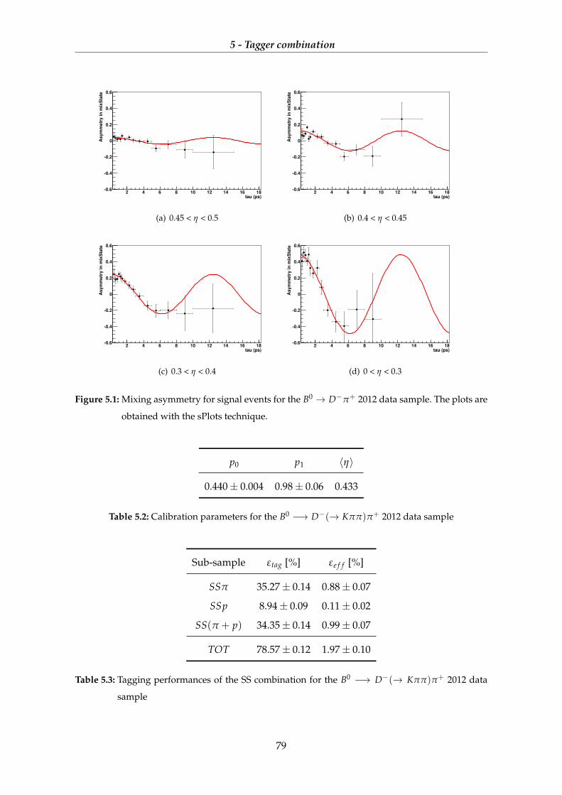
5 - Tagger combination
tau (ps)2 4 6 8 10 12 14 16 18
As
ym
me
try
in
mix
Sta
te
0.6
0.4
0.2
0
0.2
0.4
0.6
cat3
(a) 0.45 < η < 0.5
tau (ps)2 4 6 8 10 12 14 16 18
As
ym
me
try
in
mix
Sta
te
0.6
0.4
0.2
0
0.2
0.4
0.6
cat2
(b) 0.4 < η < 0.45
tau (ps)2 4 6 8 10 12 14 16 18
As
ym
me
try
in
mix
Sta
te
0.6
0.4
0.2
0
0.2
0.4
0.6
cat1
(c) 0.3 < η < 0.4
tau (ps)2 4 6 8 10 12 14 16 18
As
ym
me
try
in
mix
Sta
te
0.6
0.4
0.2
0
0.2
0.4
0.6
cat0
(d) 0 < η < 0.3
Figure 5.1: Mixing asymmetry for signal events for the B0 → D−π+ 2012 data sample. The plots are
obtained with the sPlots technique.
p0 p1 〈η〉
0.440± 0.004 0.98± 0.06 0.433
Table 5.2: Calibration parameters for the B0 −→ D−(→ Kππ)π+ 2012 data sample
Sub-sample εtag [%] εe f f [%]
SSπ 35.27± 0.14 0.88± 0.07
SSp 8.94± 0.09 0.11± 0.02
SS(π + p) 34.35± 0.14 0.99± 0.07
TOT 78.57± 0.12 1.97± 0.10
Table 5.3: Tagging performances of the SS combination for the B0 −→ D−(→ Kππ)π+ 2012 data
sample
79
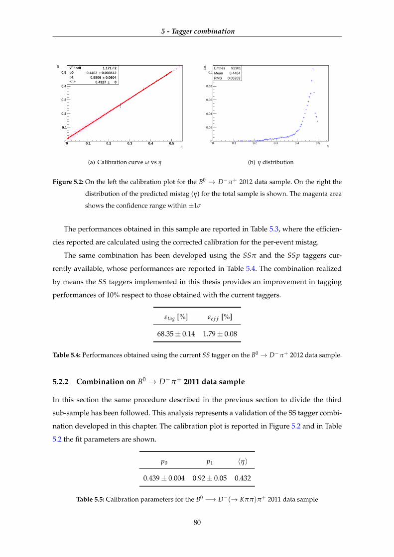
5 - Tagger combination
η0 0.1 0.2 0.3 0.4 0.5
ω
0
0.1
0.2
0.3
0.4
0.5 / ndf 2χ 1.171 / 2
p0 0.003512± 0.4402 p1 0.0604± 0.9806
> η< 0± 0.4327
/ ndf 2χ 1.171 / 2p0 0.003512± 0.4402 p1 0.0604± 0.9806
> η< 0± 0.4327
(a) Calibration curve ω vs η
Entries 91301Mean 0.4404RMS 0.05203
η0 0.1 0.2 0.3 0.4 0.5
a.u.
0
0.02
0.04
0.06
0.08
0.1Entries 91301Mean 0.4404RMS 0.05203
eta_SS_histo
(b) η distribution
Figure 5.2: On the left the calibration plot for the B0 → D−π+ 2012 data sample. On the right the
distribution of the predicted mistag (η) for the total sample is shown. The magenta area
shows the confidence range within ±1σ
The performances obtained in this sample are reported in Table 5.3, where the efficien-
cies reported are calculated using the corrected calibration for the per-event mistag.
The same combination has been developed using the SSπ and the SSp taggers cur-
rently available, whose performances are reported in Table 5.4. The combination realized
by means the SS taggers implemented in this thesis provides an improvement in tagging
performances of 10% respect to those obtained with the current taggers.
εtag [%] εe f f [%]
68.35± 0.14 1.79± 0.08
Table 5.4: Performances obtained using the current SS tagger on the B0 → D−π+ 2012 data sample.
5.2.2 Combination on B0 → D−π+ 2011 data sample
In this section the same procedure described in the previous section to divide the third
sub-sample has been followed. This analysis represents a validation of the SS tagger combi-
nation developed in this chapter. The calibration plot is reported in Figure 5.2 and in Table
5.2 the fit parameters are shown.
p0 p1 〈η〉
0.439± 0.004 0.92± 0.05 0.432
Table 5.5: Calibration parameters for the B0 −→ D−(→ Kππ)π+ 2011 data sample
80

5 - Tagger combination
In this case both p0 and p1 are compatible respectively with 〈η〉 and 1 by about 2σ.
η0 0.1 0.2 0.3 0.4 0.5
ω
0
0.1
0.2
0.3
0.4
0.5 / ndf 2χ 0.1982 / 2
p0 0.00315± 0.4393 p1 0.05066± 0.9242
> η< 0± 0.432
/ ndf 2χ 0.1982 / 2p0 0.00315± 0.4393 p1 0.05066± 0.9242
> η< 0± 0.432
Figure 5.3: Calibration for the B0 → D−π+ 2011 data sample, plot of ω vs η. The magenta area
shows the confidence range within ±1σ.
The final performances obtained in this sample are reported in Table 5.6, where the
efficiencies reported are calculated using the corrected per-event mistag.
Sub-sample εtag [%] εe f f [%]
SSπ 33.46± 0.13 0.91± 0.06
SSp 7.76± 0.07 0.12± 0.02
SS(π + p) 36.47± 0.13 1.02± 0.07
TOT 77.69± 0.12 2.05± 0.07
Table 5.6: Tagging performances of the SS combination for the B0 −→ D−(→ Kππ)π+ 2011 data
sample
As done in the previous chapters the 2012 and 2011 data samples are merged in a only
one sample to decrease the statistical uncertainties. The performances obtained in this new
sample are reported in Table 5.7. The tagging power found in the 2012,2011 and 2011+2012
data samples are compatible within the statistical errors.
81

5 - Tagger combination
Sub-sample εtag [%] εe f f [%]
SSπ 34.28± 0.10 0.90± 0.05
SSp 7.93± 0.05 0.10± 0.02
SS(π + p) 35.61± 0.10 1.01± 0.06
TOT 77.81± 0.08 2.01± 0.06
Table 5.7: Tagging performances of the SS combination for the B0 −→ D−(→ Kππ)π+ 2011+2012
data sample.
5.2.3 Combination on the B0 → K+π− 2012 data sample
The performances and the calibration have been also cross-checked on the B0 → K+π− 2012
data sample. The calibration parameters extrapolated by the linear fit are listed in Table 5.8
while the plot is shown in Figure 5.8.
p0 p1 〈η〉
0.450± 0.005 0.90± 0.09 0.440
Table 5.8: Calibration parameters of the SS combination for the B0 → K+π− 2012 data sample
η0 0.1 0.2 0.3 0.4 0.5
ω
0
0.1
0.2
0.3
0.4
0.5p0 0.004633± 0.4499
p1 0.08923± 0.9036
> η< 0± 0.4404
p0 0.004633± 0.4499
p1 0.08923± 0.9036
> η< 0± 0.4404
Figure 5.4: Calibration for the B0 → K+π− 2012 data sample, plot of ω vs η. The magenta area
shows the confidence range within ±1σ.
In this calibration the p1 parameter is correct within the statistical error while p0 is com-
patible to the mean value of η within 2σ. The tagging efficiencies for each sub-sample and
82

5 - Tagger combination
Sub-sample εtag [%] εe f f [%]
SSπ 24.97± 0.16 0.55± 0.07
SSp 12.52± 0.12 0.12± 0.03
SS(π + p) 39.21± 0.18 0.78± 0.08
TOT 76.70± 0.25 1.44± 0.11
Table 5.9: Tagging performances of the SS combination for each sub-sample of the B0 −→ K+π−
2012 data sample.
the total ones are reported in Table 5.9
Also in this case, it is observable a tagging power loss, which can be accounted to the
dependence of the SS taggers on the different BpT spectra of the decay modes.
5.3 SS and OS combination
As shown in the previous section, combining two taggers allows to improve the tagging
performances. Thus as a last step of this analysis the combination of the general SS tagger
and Opposite Side tagger (OS) is performed. The general OS tagger represents the combi-
nation of OS electron, OS muon, OS kaon and OS vertex charge which is based on the
inclusive reconstruction of a secondary vertex corresponding to the Opposite B decay.
Using the same procedure used in the previous section, each sample is divided in three
sub-samples in order to separate events with only one tagger from the events with both
taggers:
• events tagged only by a SS tagger −→ ω is estimated with the SS calibration (Section
5.2)
• events tagged only by OS tagger −→ ω is estimated with the OS calibration
• events tagged both by SS and OS taggers −→ ω is estimated combining the two tag-
gers (Section 5.1)
Also in this case the mistag estimated in the third sub-sample has to be check, thus the
sub-sample is divided in categories according to the eta value and for each one the true
mistag ω is estimated through an unbinned fit on the time oscillations.Then a linear fit of ω
vs η can be performed.
83
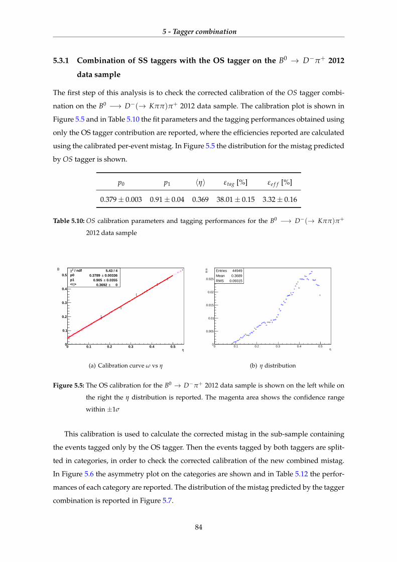
5 - Tagger combination
5.3.1 Combination of SS taggers with the OS tagger on the B0 → D−π+ 2012
data sample
The first step of this analysis is to check the corrected calibration of the OS tagger combi-
nation on the B0 −→ D−(→ Kππ)π+ 2012 data sample. The calibration plot is shown in
Figure 5.5 and in Table 5.10 the fit parameters and the tagging performances obtained using
only the OS tagger contribution are reported, where the efficiencies reported are calculated
using the calibrated per-event mistag. In Figure 5.5 the distribution for the mistag predicted
by OS tagger is shown.
p0 p1 〈η〉 εtag [%] εe f f [%]
0.379± 0.003 0.91± 0.04 0.369 38.01± 0.15 3.32± 0.16
Table 5.10: OS calibration parameters and tagging performances for the B0 −→ D−(→ Kππ)π+
2012 data sample
η0 0.1 0.2 0.3 0.4 0.5
ω
0
0.1
0.2
0.3
0.4
0.5 / ndf 2χ 5.43 / 4
p0 0.00336± 0.3789 p1 0.0355± 0.905
> η< 0± 0.3692
/ ndf 2χ 5.43 / 4p0 0.00336± 0.3789 p1 0.0355± 0.905
> η< 0± 0.3692
(a) Calibration curve ω vs η
Entries 44949Mean 0.3689RMS 0.09315
η0 0.1 0.2 0.3 0.4 0.5
a.u.
0
0.005
0.01
0.015
0.02
0.025
Entries 44949Mean 0.3689RMS 0.09315
eta_OS_histo
(b) η distribution
Figure 5.5: The OS calibration for the B0 → D−π+ 2012 data sample is shown on the left while on
the right the η distribution is reported. The magenta area shows the confidence range
within ±1σ
This calibration is used to calculate the corrected mistag in the sub-sample containing
the events tagged only by the OS tagger. Then the events tagged by both taggers are split-
ted in categories, in order to check the corrected calibration of the new combined mistag.
In Figure 5.6 the asymmetry plot on the categories are shown and in Table 5.12 the perfor-
mances of each category are reported. The distribution of the mistag predicted by the tagger
combination is reported in Figure 5.7.
84
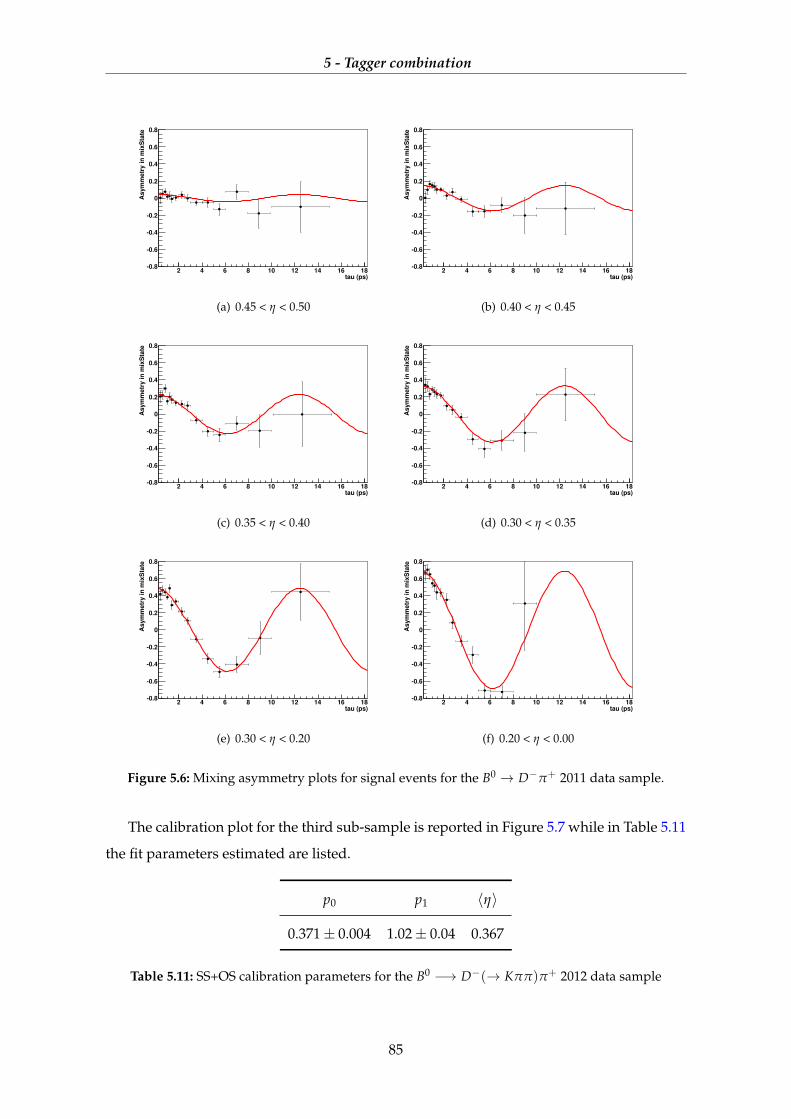
5 - Tagger combination
tau (ps)2 4 6 8 10 12 14 16 18
As
ym
me
try
in
mix
Sta
te
0.8
0.6
0.4
0.2
0
0.2
0.4
0.6
0.8
cat5
(a) 0.45 < η < 0.50
tau (ps)2 4 6 8 10 12 14 16 18
As
ym
me
try
in
mix
Sta
te
0.8
0.6
0.4
0.2
0
0.2
0.4
0.6
0.8
cat4
(b) 0.40 < η < 0.45
tau (ps)2 4 6 8 10 12 14 16 18
As
ym
me
try
in
mix
Sta
te
0.8
0.6
0.4
0.2
0
0.2
0.4
0.6
0.8
cat3
(c) 0.35 < η < 0.40
tau (ps)2 4 6 8 10 12 14 16 18
As
ym
me
try
in
mix
Sta
te
0.8
0.6
0.4
0.2
0
0.2
0.4
0.6
0.8
cat2
(d) 0.30 < η < 0.35
tau (ps)2 4 6 8 10 12 14 16 18
As
ym
me
try
in
mix
Sta
te
0.8
0.6
0.4
0.2
0
0.2
0.4
0.6
0.8
cat1
(e) 0.30 < η < 0.20
tau (ps)2 4 6 8 10 12 14 16 18
As
ym
me
try
in
mix
Sta
te
0.8
0.6
0.4
0.2
0
0.2
0.4
0.6
0.8
cat0
(f) 0.20 < η < 0.00
Figure 5.6: Mixing asymmetry plots for signal events for the B0 → D−π+ 2011 data sample.
The calibration plot for the third sub-sample is reported in Figure 5.7 while in Table 5.11
the fit parameters estimated are listed.
p0 p1 〈η〉
0.371± 0.004 1.02± 0.04 0.367
Table 5.11: SS+OS calibration parameters for the B0 −→ D−(→ Kππ)π+ 2012 data sample
85
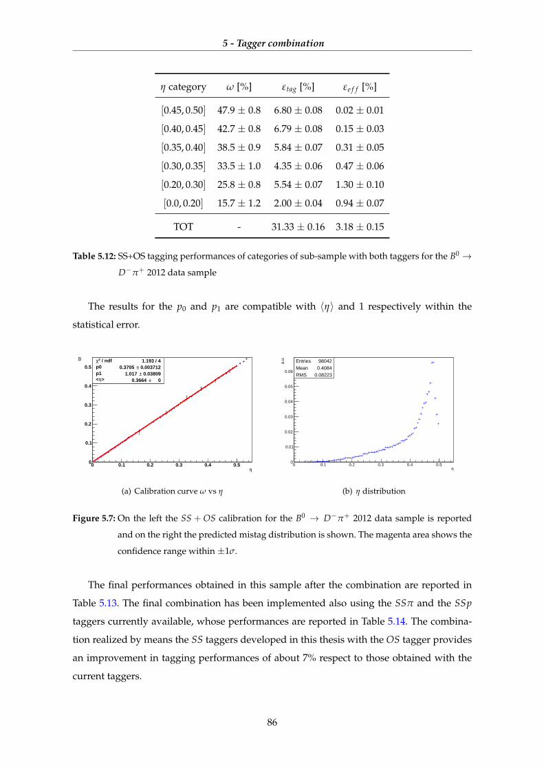
5 - Tagger combination
η category ω [%] εtag [%] εe f f [%]
[0.45, 0.50] 47.9 ± 0.8 6.80 ± 0.08 0.02 ± 0.01
[0.40, 0.45] 42.7 ± 0.8 6.79 ± 0.08 0.15 ± 0.03
[0.35, 0.40] 38.5 ± 0.9 5.84 ± 0.07 0.31 ± 0.05
[0.30, 0.35] 33.5 ± 1.0 4.35 ± 0.06 0.47 ± 0.06
[0.20, 0.30] 25.8 ± 0.8 5.54 ± 0.07 1.30 ± 0.10
[0.0, 0.20] 15.7 ± 1.2 2.00 ± 0.04 0.94 ± 0.07
TOT - 31.33 ± 0.16 3.18 ± 0.15
Table 5.12: SS+OS tagging performances of categories of sub-sample with both taggers for the B0 →
D−π+ 2012 data sample
The results for the p0 and p1 are compatible with 〈η〉 and 1 respectively within the
statistical error.
η0 0.1 0.2 0.3 0.4 0.5
ω
0
0.1
0.2
0.3
0.4
0.5 / ndf 2χ 1.193 / 4
p0 0.003712± 0.3705 p1 0.03809± 1.017
> η< 0± 0.3664
/ ndf 2χ 1.193 / 4p0 0.003712± 0.3705 p1 0.03809± 1.017
> η< 0± 0.3664
(a) Calibration curve ω vs η
Entries 98042Mean 0.4084RMS 0.08223
η0 0.1 0.2 0.3 0.4 0.5
a.u.
0
0.01
0.02
0.03
0.04
0.05
0.06
Entries 98042Mean 0.4084RMS 0.08223
eta_histo
(b) η distribution
Figure 5.7: On the left the SS + OS calibration for the B0 → D−π+ 2012 data sample is reported
and on the right the predicted mistag distribution is shown. The magenta area shows the
confidence range within ±1σ.
The final performances obtained in this sample after the combination are reported in
Table 5.13. The final combination has been implemented also using the SSπ and the SSp
taggers currently available, whose performances are reported in Table 5.14. The combina-
tion realized by means the SS taggers developed in this thesis with the OS tagger provides
an improvement in tagging performances of about 7% respect to those obtained with the
current taggers.
86
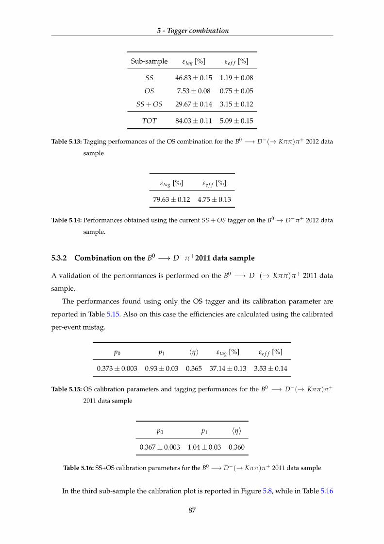
5 - Tagger combination
Sub-sample εtag [%] εe f f [%]
SS 46.83± 0.15 1.19± 0.08
OS 7.53± 0.08 0.75± 0.05
SS + OS 29.67± 0.14 3.15± 0.12
TOT 84.03± 0.11 5.09± 0.15
Table 5.13: Tagging performances of the OS combination for the B0 −→ D−(→ Kππ)π+ 2012 data
sample
εtag [%] εe f f [%]
79.63± 0.12 4.75± 0.13
Table 5.14: Performances obtained using the current SS + OS tagger on the B0 → D−π+ 2012 data
sample.
5.3.2 Combination on the B0 −→ D−π+2011 data sample
A validation of the performances is performed on the B0 −→ D−(→ Kππ)π+ 2011 data
sample.
The performances found using only the OS tagger and its calibration parameter are
reported in Table 5.15. Also on this case the efficiencies are calculated using the calibrated
per-event mistag.
p0 p1 〈η〉 εtag [%] εe f f [%]
0.373± 0.003 0.93± 0.03 0.365 37.14± 0.13 3.53± 0.14
Table 5.15: OS calibration parameters and tagging performances for the B0 −→ D−(→ Kππ)π+
2011 data sample
p0 p1 〈η〉
0.367± 0.003 1.04± 0.03 0.360
Table 5.16: SS+OS calibration parameters for the B0 −→ D−(→ Kππ)π+ 2011 data sample
In the third sub-sample the calibration plot is reported in Figure 5.8, while in Table 5.16
87
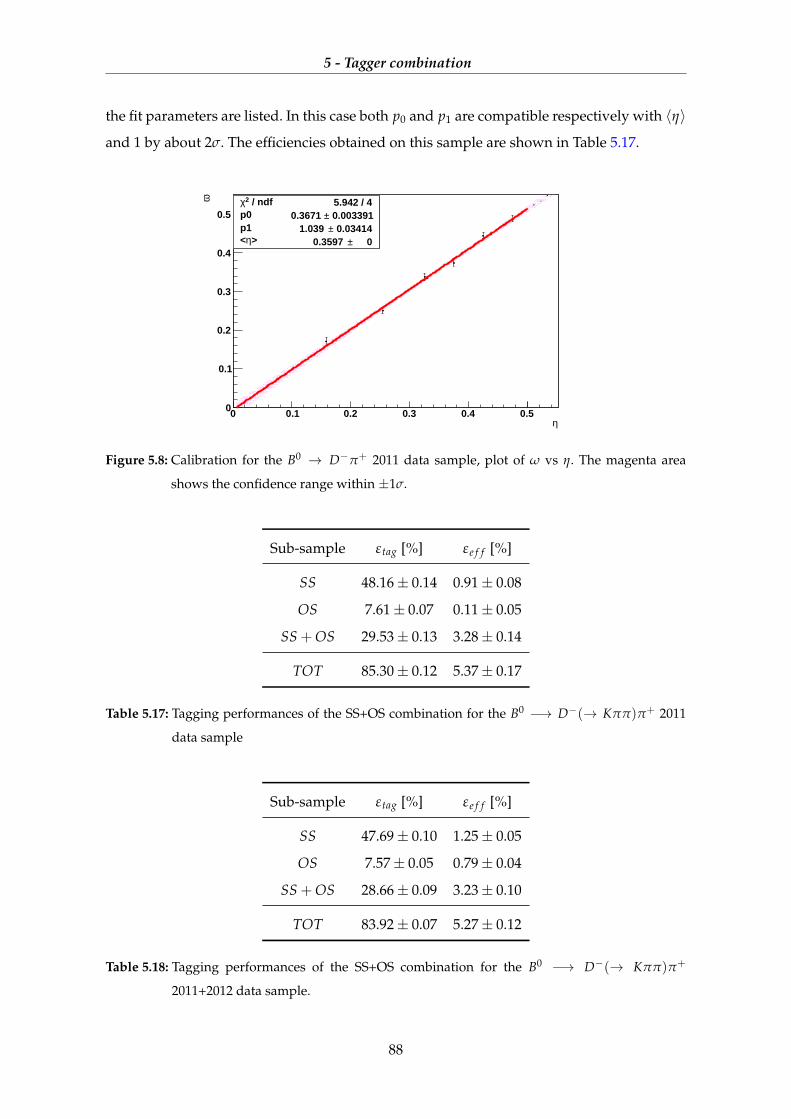
5 - Tagger combination
the fit parameters are listed. In this case both p0 and p1 are compatible respectively with 〈η〉
and 1 by about 2σ. The efficiencies obtained on this sample are shown in Table 5.17.
η0 0.1 0.2 0.3 0.4 0.5
ω
0
0.1
0.2
0.3
0.4
0.5 / ndf 2χ 5.942 / 4
p0 0.003391± 0.3671 p1 0.03414± 1.039
> η< 0± 0.3597
/ ndf 2χ 5.942 / 4p0 0.003391± 0.3671 p1 0.03414± 1.039
> η< 0± 0.3597
Figure 5.8: Calibration for the B0 → D−π+ 2011 data sample, plot of ω vs η. The magenta area
shows the confidence range within ±1σ.
Sub-sample εtag [%] εe f f [%]
SS 48.16± 0.14 0.91± 0.08
OS 7.61± 0.07 0.11± 0.05
SS + OS 29.53± 0.13 3.28± 0.14
TOT 85.30± 0.12 5.37± 0.17
Table 5.17: Tagging performances of the SS+OS combination for the B0 −→ D−(→ Kππ)π+ 2011
data sample
Sub-sample εtag [%] εe f f [%]
SS 47.69± 0.10 1.25± 0.05
OS 7.57± 0.05 0.79± 0.04
SS + OS 28.66± 0.09 3.23± 0.10
TOT 83.92± 0.07 5.27± 0.12
Table 5.18: Tagging performances of the SS+OS combination for the B0 −→ D−(→ Kππ)π+
2011+2012 data sample.
88
5 - Tagger combination
The performances obtained merging the 2012 and 2011 data samples in a only one sam-
ple, in order to decrease the statistical uncertainties, are reported in Table 5.18. The effective
tagging efficiency is compatible with the one found in 2012 and 2011 data samples within
the statistical error.
5.3.3 Combination on the B0 → K+π− 2012 data sample
The last validation for the final SS + OS tagger is performed using the B0 −→ K+π− 2012
sample. The performances found using only the OS tagger and its calibration parameter are
reported in Table 5.19.
p0 p1 〈η〉 εtag [%] εe f f [%]
0.386± 0.003 1.10± 0.04 0.376 34.67± 0.16 3.61± 0.27
Table 5.19: OS calibration parameters and tagging performances for the B0 −→ K+π− 2012 data
sample
The sub-sample containing the events tagged by both OS and SS tagger is splitted in
categories and the calibration results are reported in Table 5.20. The linear fit is shown in
Figure 5.9.
p0 p1 〈η〉
0.375± 0.006 1.12± 0.07 0.366
Table 5.20: SS+OS calibration parameters for the B0 −→ K+π− 2012 data sample
In this case both p0 and p1 are compatible within the statistical error to 〈η〉 and 1, re-
spectively.
Sub-sample εtag [%] εe f f [%]
SS 49.67± 0.19 0.97± 0.09
OS 6.73± 0.09 0.87± 0.07
SS + OS 23.67± 0.16 3.05± 0.17
TOT 80.09± 0.26 4.89± 0.20
Table 5.21: Tagging performances of the SS+OS combination on the B0 −→ K+π− 2012 data sample.
89

5 - Tagger combination
η0 0.1 0.2 0.3 0.4 0.5
ω
0
0.1
0.2
0.3
0.4
0.5p0 0.005582± 0.3745
p1 0.05092± 1.119
> η< 0± 0.3655
p0 0.005582± 0.3745
p1 0.05092± 1.119
> η< 0± 0.3655
Figure 5.9: SS+OS calibration for the B0 −→ K+π− 2012 data sample, plot of ω vs η. The magenta
area shows the confidence range within ±1σ.
The final performances obtained in this sample are reported in Table 5.21. Also for the
final SS +OS tagger the effective tagging efficiency is found lower than the one obtained in
the first decay channel. This loss is accounted only to the SS tagger as the tagging power of
the OS tagger, reported in Table 5.19, is compatible within the statistical error to the values
achieved in the B0 → D−π+ decay channel.
5.4 Measurement of ∆md
The first observation of the B0 ↔ B0 mixing and the measurement of its strength were per-
formed in 1987 [24]. The oscillation frequency in the B0 − B0 system (∆md) is given by the
mass difference between the heavy and light mass eigenstates. The world average measure-
ment is ∆md = 0.510± 0.003 ps−1 [25].
In this analysis the results achieved with the final tagger combination are used to esti-
mate the value of ∆md on the 2011 data sample corresponding to the B0 → D−π+ decay
mode, using the event selection which involves a low background contribution. This sample
is chosen because it contains independent events from the ones used to tune the SS taggers.
To estimate ∆md the sample is divided in BDT categories and then an unbinned simultane-
ous fit on the asymmetry oscillations is performed on each category. In the previous fits the
∆md parameter was fixed to the world average value while here it is floated.
The asymmetry plots are shown in Figure 5.10 and in Table 5.22 the ∆md and the mistag
values are reported.
90
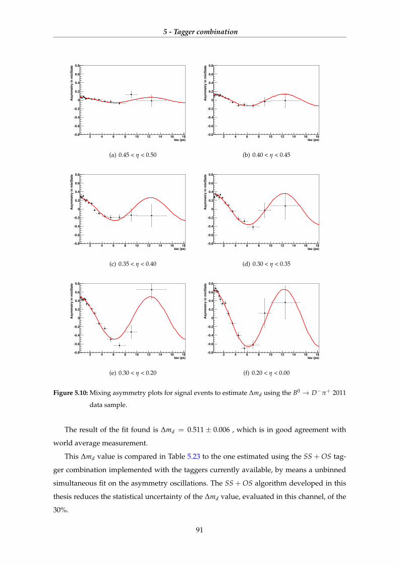
5 - Tagger combination
tau (ps)2 4 6 8 10 12 14 16 18
As
ym
me
try
in
mix
Sta
te
0.8
0.6
0.4
0.2
0
0.2
0.4
0.6
0.8
cat5
(a) 0.45 < η < 0.50
tau (ps)2 4 6 8 10 12 14 16 18
As
ym
me
try
in
mix
Sta
te
0.8
0.6
0.4
0.2
0
0.2
0.4
0.6
0.8
cat4
(b) 0.40 < η < 0.45
tau (ps)2 4 6 8 10 12 14 16 18
As
ym
me
try
in
mix
Sta
te
0.8
0.6
0.4
0.2
0
0.2
0.4
0.6
0.8
cat3
(c) 0.35 < η < 0.40
tau (ps)2 4 6 8 10 12 14 16 18
As
ym
me
try
in
mix
Sta
te
0.8
0.6
0.4
0.2
0
0.2
0.4
0.6
0.8
cat2
(d) 0.30 < η < 0.35
tau (ps)2 4 6 8 10 12 14 16 18
As
ym
me
try
in
mix
Sta
te
0.8
0.6
0.4
0.2
0
0.2
0.4
0.6
0.8
cat1
(e) 0.30 < η < 0.20
tau (ps)2 4 6 8 10 12 14 16 18
As
ym
me
try
in
mix
Sta
te
0.8
0.6
0.4
0.2
0
0.2
0.4
0.6
0.8
cat0
(f) 0.20 < η < 0.00
Figure 5.10: Mixing asymmetry plots for signal events to estimate ∆md using the B0 → D−π+ 2011
data sample.
The result of the fit found is ∆md = 0.511± 0.006 , which is in good agreement with
world average measurement.
This ∆md value is compared in Table 5.23 to the one estimated using the SS + OS tag-
ger combination implemented with the taggers currently available, by means a unbinned
simultaneous fit on the asymmetry oscillations. The SS + OS algorithm developed in this
thesis reduces the statistical uncertainty of the ∆md value, evaluated in this channel, of the
30%.
91

5 - Tagger combination
Parameter ω using ∆md floated ω using ∆md fixed
ω[0.45,0.50] 46.9 ± 0.3 47.5 ± 0.3
ω[0.40,0.45] 43.1 ± 0.4 43.9 ± 0.5
ω[0.35,0.40] 36.7 ± 0.6 37.3 ± 0.6
ω[0.30,0.35] 31.9 ± 0.7 32.7 ± 0.8
ω[0.20,0.30] 25.4 ± 0.6 25.0 ± 0.7
ω[0.0,0.20] 16.8 ± 1.0 17.0 ± 1.1
∆md 0.511± 0.006 0.510
Table 5.22: Parameter values found from the simultaneous fit to estimate ∆md. The values are com-
pared to the one obtained dividing the sample in the same categories and fixing ∆md to
the world average measurement.
∆md world ∆md current ∆md new
0.510± 0.003 0.508± 0.008 0.511± 0.006
Table 5.23: Comparison of the mixing frequency ∆md results: the first one is the world average value,
the second value is the one provided with the current taggers and the last one is the value
estimated using the taggers developed in this thesis.
92
6Systematics
Contents
6.1 Systematic uncertainties 93
6.2 Dependence of the SS tagging on pT of the signal B 94
6.3 Dependence of the SS tagging on the magnet polarity 98
6.4 Dependence of the SS tagging performances on the B flavour 99
6.4.1 Dependence on the B flavour at decay 99
6.4.2 Dependence on the B flavour at production 101
In order to not compromise the statistical precision obtainable on any CPV measurement
at LHCb, a good control of the systematic uncertainties on the tagging parameters must be
achieved. In this chapter some possible sources of systematic uncertainty are discussed.
6.1 Systematic uncertainties
The time-dependent CP violation asymmetries measurements require the reconstruction of
the final state and frequently the determination of the initial state flavour. Same charge and
flavour dependent effects may exist, which can indeed bias the measurement. The most
important ones are:
• Production asymmetries: as the LHC collider is a proton-proton machine, the initial frac-
tion of b and b hadrons is not expected to be the same. This asymmetry at b production
is a function of rapidity and pt, reaching values of few percent, as reported in [26] and
[27].
• Charge dependence: because of the different particle/antiparticle interaction with mat-
ter, the calibration of the mistag probability of different B flavour might be different.
93
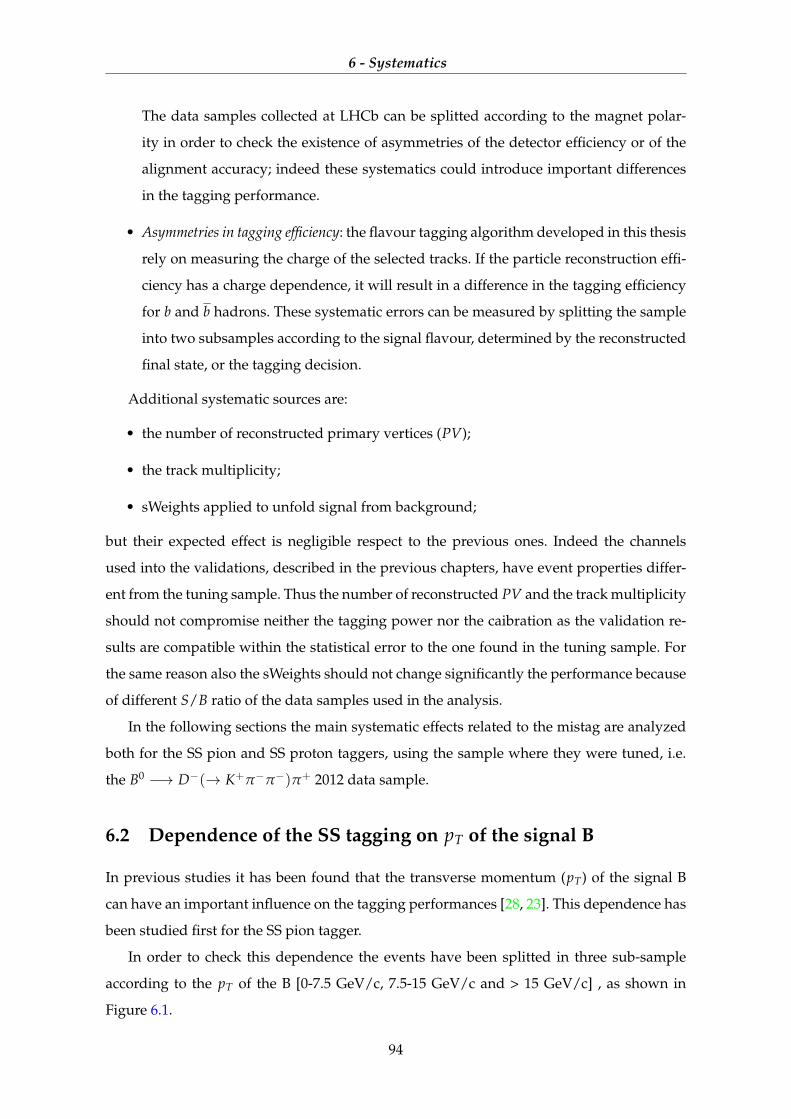
6 - Systematics
The data samples collected at LHCb can be splitted according to the magnet polar-
ity in order to check the existence of asymmetries of the detector efficiency or of the
alignment accuracy; indeed these systematics could introduce important differences
in the tagging performance.
• Asymmetries in tagging efficiency: the flavour tagging algorithm developed in this thesis
rely on measuring the charge of the selected tracks. If the particle reconstruction effi-
ciency has a charge dependence, it will result in a difference in the tagging efficiency
for b and b hadrons. These systematic errors can be measured by splitting the sample
into two subsamples according to the signal flavour, determined by the reconstructed
final state, or the tagging decision.
Additional systematic sources are:
• the number of reconstructed primary vertices (PV);
• the track multiplicity;
• sWeights applied to unfold signal from background;
but their expected effect is negligible respect to the previous ones. Indeed the channels
used into the validations, described in the previous chapters, have event properties differ-
ent from the tuning sample. Thus the number of reconstructed PV and the track multiplicity
should not compromise neither the tagging power nor the caibration as the validation re-
sults are compatible within the statistical error to the one found in the tuning sample. For
the same reason also the sWeights should not change significantly the performance because
of different S/B ratio of the data samples used in the analysis.
In the following sections the main systematic effects related to the mistag are analyzed
both for the SS pion and SS proton taggers, using the sample where they were tuned, i.e.
the B0 −→ D−(→ K+π−π−)π+ 2012 data sample.
6.2 Dependence of the SS tagging on pT of the signal B
In previous studies it has been found that the transverse momentum (pT) of the signal B
can have an important influence on the tagging performances [28, 23]. This dependence has
been studied first for the SS pion tagger.
In order to check this dependence the events have been splitted in three sub-sample
according to the pT of the B [0-7.5 GeV/c, 7.5-15 GeV/c and > 15 GeV/c] , as shown in
Figure 6.1.
94
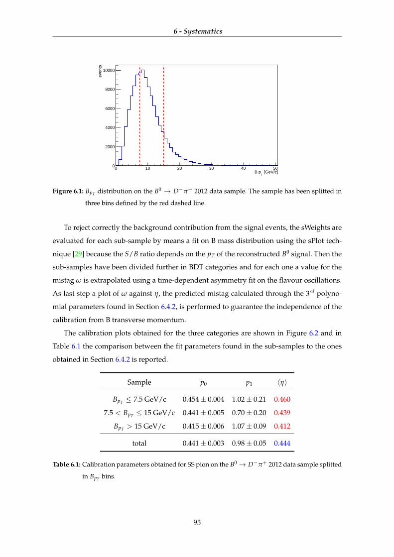
6 - Systematics
htempEntries 116656
Mean 9.795
RMS 5.007
[GeV/c]T
B p0 10 20 30 40 50
even
ts
0
2000
4000
6000
8000
10000
htempEntries 116656
Mean 9.795
RMS 5.007
BPt
Figure 6.1: BpT distribution on the B0 → D−π+ 2012 data sample. The sample has been splitted in
three bins defined by the red dashed line.
To reject correctly the background contribution from the signal events, the sWeights are
evaluated for each sub-sample by means a fit on B mass distribution using the sPlot tech-
nique [29] because the S/B ratio depends on the pT of the reconstructed B0 signal. Then the
sub-samples have been divided further in BDT categories and for each one a value for the
mistag ω is extrapolated using a time-dependent asymmetry fit on the flavour oscillations.
As last step a plot of ω against η, the predicted mistag calculated through the 3rd polyno-
mial parameters found in Section 6.4.2, is performed to guarantee the independence of the
calibration from B transverse momentum.
The calibration plots obtained for the three categories are shown in Figure 6.2 and in
Table 6.1 the comparison between the fit parameters found in the sub-samples to the ones
obtained in Section 6.4.2 is reported.
Sample p0 p1 〈η〉
BpT ≤ 7.5 GeV/c 0.454± 0.004 1.02± 0.21 0.460
7.5 < BpT ≤ 15 GeV/c 0.441± 0.005 0.70± 0.20 0.439
BpT > 15 GeV/c 0.415± 0.006 1.07± 0.09 0.412
total 0.441± 0.003 0.98± 0.05 0.444
Table 6.1: Calibration parameters obtained for SS pion on the B0 → D−π+ 2012 data sample splitted
in BpT bins.
95
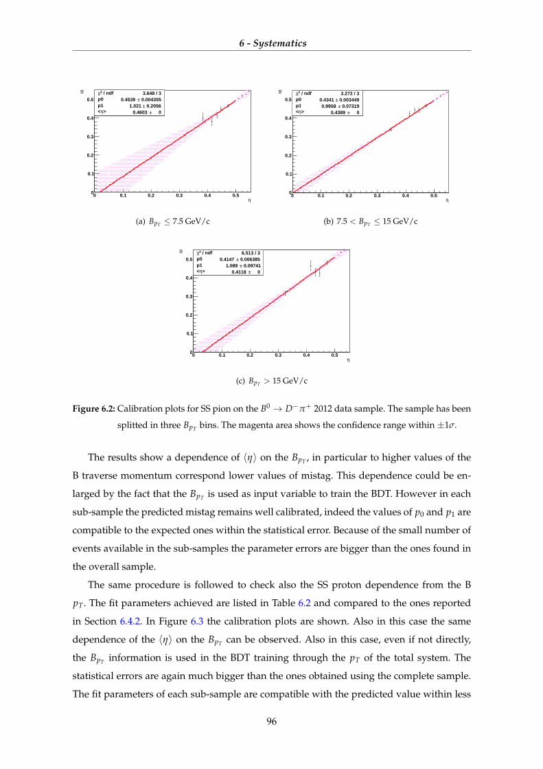
6 - Systematics
η0 0.1 0.2 0.3 0.4 0.5
ω
0
0.1
0.2
0.3
0.4
0.5 / ndf 2χ 3.648 / 3
p0 0.004305± 0.4539 p1 0.2056± 1.021
> η< 0± 0.4603
/ ndf 2χ 3.648 / 3p0 0.004305± 0.4539 p1 0.2056± 1.021
> η< 0± 0.4603
(a) BpT ≤ 7.5 GeV/c
η0 0.1 0.2 0.3 0.4 0.5
ω
0
0.1
0.2
0.3
0.4
0.5 / ndf 2χ 3.272 / 3
p0 0.003449± 0.4341 p1 0.07319± 0.9958
> η< 0± 0.4389
/ ndf 2χ 3.272 / 3p0 0.003449± 0.4341 p1 0.07319± 0.9958
> η< 0± 0.4389
(b) 7.5 < BpT ≤ 15 GeV/c
η0 0.1 0.2 0.3 0.4 0.5
ω
0
0.1
0.2
0.3
0.4
0.5 / ndf 2χ 6.513 / 3
p0 0.006385± 0.4147 p1 0.09741± 1.089
> η< 0± 0.4118
/ ndf 2χ 6.513 / 3p0 0.006385± 0.4147 p1 0.09741± 1.089
> η< 0± 0.4118
(c) BpT > 15 GeV/c
Figure 6.2: Calibration plots for SS pion on the B0 → D−π+ 2012 data sample. The sample has been
splitted in three BpT bins. The magenta area shows the confidence range within ±1σ.
The results show a dependence of 〈η〉 on the BpT , in particular to higher values of the
B traverse momentum correspond lower values of mistag. This dependence could be en-
larged by the fact that the BpT is used as input variable to train the BDT. However in each
sub-sample the predicted mistag remains well calibrated, indeed the values of p0 and p1 are
compatible to the expected ones within the statistical error. Because of the small number of
events available in the sub-samples the parameter errors are bigger than the ones found in
the overall sample.
The same procedure is followed to check also the SS proton dependence from the B
pT. The fit parameters achieved are listed in Table 6.2 and compared to the ones reported
in Section 6.4.2. In Figure 6.3 the calibration plots are shown. Also in this case the same
dependence of the 〈η〉 on the BpT can be observed. Also in this case, even if not directly,
the BpT information is used in the BDT training through the pT of the total system. The
statistical errors are again much bigger than the ones obtained using the complete sample.
The fit parameters of each sub-sample are compatible with the predicted value within less
96
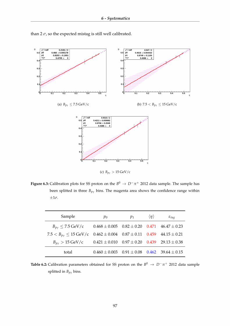
6 - Systematics
than 2 σ, so the expected mistag is still well calibrated.
η0 0.1 0.2 0.3 0.4 0.5
ω
0
0.1
0.2
0.3
0.4
0.5 / ndf 2χ 0.2191 / 2
p0 0.005178± 0.468 p1 0.1951± 0.8203
> η< 0± 0.4705
/ ndf 2χ 0.2191 / 2p0 0.005178± 0.468 p1 0.1951± 0.8203
> η< 0± 0.4705
(a) BpT ≤ 7.5 GeV/c
η0 0.1 0.2 0.3 0.4 0.5
ω
0
0.1
0.2
0.3
0.4
0.5 / ndf 2χ 4.547 / 2
p0 0.004432± 0.4616 p1 0.1105± 0.8749
> η< 0± 0.4586
/ ndf 2χ 4.547 / 2p0 0.004432± 0.4616 p1 0.1105± 0.8749
> η< 0± 0.4586
(b) 7.5 < BpT ≤ 15 GeV/c
η0 0.1 0.2 0.3 0.4 0.5
ω
0
0.1
0.2
0.3
0.4
0.5 / ndf 2χ 0.9315 / 2
p0 0.009982± 0.4211 p1 0.2049± 0.9706
> η< 0± 0.4386
/ ndf 2χ 0.9315 / 2p0 0.009982± 0.4211 p1 0.2049± 0.9706
> η< 0± 0.4386
(c) BpT > 15 GeV/c
Figure 6.3: Calibration plots for SS proton on the B0 → D−π+ 2012 data sample. The sample has
been splitted in three BpT bins. The magenta area shows the confidence range within
±1σ.
Sample p0 p1 〈η〉 εtag
BpT ≤ 7.5 GeV/c 0.468± 0.005 0.82± 0.20 0.471 46.47± 0.23
7.5 < BpT ≤ 15 GeV/c 0.462± 0.004 0.87± 0.11 0.459 44.15± 0.21
BpT > 15 GeV/c 0.421± 0.010 0.97± 0.20 0.439 29.13± 0.38
total 0.460± 0.003 0.91± 0.08 0.462 39.64± 0.15
Table 6.2: Calibration parameters obtained for SS proton on the B0 → D−π+ 2012 data sample
splitted in BpT bins.
97
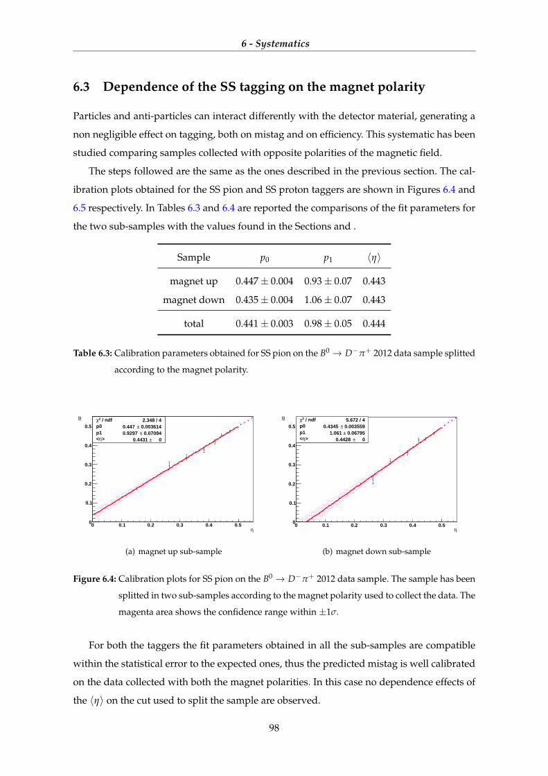
6 - Systematics
6.3 Dependence of the SS tagging on the magnet polarity
Particles and anti-particles can interact differently with the detector material, generating a
non negligible effect on tagging, both on mistag and on efficiency. This systematic has been
studied comparing samples collected with opposite polarities of the magnetic field.
The steps followed are the same as the ones described in the previous section. The cal-
ibration plots obtained for the SS pion and SS proton taggers are shown in Figures 6.4 and
6.5 respectively. In Tables 6.3 and 6.4 are reported the comparisons of the fit parameters for
the two sub-samples with the values found in the Sections and .
Sample p0 p1 〈η〉
magnet up 0.447± 0.004 0.93± 0.07 0.443
magnet down 0.435± 0.004 1.06± 0.07 0.443
total 0.441± 0.003 0.98± 0.05 0.444
Table 6.3: Calibration parameters obtained for SS pion on the B0 → D−π+ 2012 data sample splitted
according to the magnet polarity.
η0 0.1 0.2 0.3 0.4 0.5
ω
0
0.1
0.2
0.3
0.4
0.5 / ndf 2χ 2.348 / 4
p0 0.003614± 0.447 p1 0.07094± 0.9297
> η< 0± 0.4431
/ ndf 2χ 2.348 / 4p0 0.003614± 0.447 p1 0.07094± 0.9297
> η< 0± 0.4431
(a) magnet up sub-sample
η0 0.1 0.2 0.3 0.4 0.5
ω
0
0.1
0.2
0.3
0.4
0.5 / ndf 2χ 5.672 / 4
p0 0.003559± 0.4345 p1 0.06795± 1.061
> η< 0± 0.4428
/ ndf 2χ 5.672 / 4p0 0.003559± 0.4345 p1 0.06795± 1.061
> η< 0± 0.4428
(b) magnet down sub-sample
Figure 6.4: Calibration plots for SS pion on the B0 → D−π+ 2012 data sample. The sample has been
splitted in two sub-samples according to the magnet polarity used to collect the data. The
magenta area shows the confidence range within ±1σ.
For both the taggers the fit parameters obtained in all the sub-samples are compatible
within the statistical error to the expected ones, thus the predicted mistag is well calibrated
on the data collected with both the magnet polarities. In this case no dependence effects of
the 〈η〉 on the cut used to split the sample are observed.
98
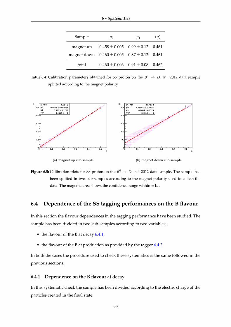
6 - Systematics
Sample p0 p1 〈η〉
magnet up 0.458± 0.005 0.99± 0.12 0.461
magnet down 0.460± 0.005 0.87± 0.12 0.461
total 0.460± 0.003 0.91± 0.08 0.462
Table 6.4: Calibration parameters obtained for SS proton on the B0 → D−π+ 2012 data sample
splitted according to the magnet polarity.
η0 0.1 0.2 0.3 0.4 0.5
ω
0
0.1
0.2
0.3
0.4
0.5 / ndf 2χ 0.71 / 3
p0 0.004664± 0.4582 p1 0.1205± 0.986
> η< 0± 0.4614
/ ndf 2χ 0.71 / 3p0 0.004664± 0.4582 p1 0.1205± 0.986
> η< 0± 0.4614
(a) magnet up sub-sample
η0 0.1 0.2 0.3 0.4 0.5
ω
0
0.1
0.2
0.3
0.4
0.5 / ndf 2χ 4.572 / 3
p0 0.004587± 0.4596 p1 0.1175± 0.8684
> η< 0± 0.4614
/ ndf 2χ 4.572 / 3p0 0.004587± 0.4596 p1 0.1175± 0.8684
> η< 0± 0.4614
(b) magnet down sub-sample
Figure 6.5: Calibration plots for SS proton on the B0 → D−π+ 2012 data sample. The sample has
been splitted in two sub-samples according to the magnet polarity used to collect the
data. The magenta area shows the confidence range within ±1σ.
6.4 Dependence of the SS tagging performances on the B flavour
In this section the flavour dependences in the tagging performance have been studied. The
sample has been divided in two sub-samples according to two variables:
• the flavour of the B at decay 6.4.1;
• the flavour of the B at production as provided by the tagger 6.4.2
In both the cases the procedure used to check these systematics is the same followed in the
previous sections.
6.4.1 Dependence on the B flavour at decay
In this systematic check the sample has been divided according to the electric charge of the
particles created in the final state:
99

6 - Systematics
• D−π+ −→ B0
• D+π− −→ B0
In the Figure 6.6 the calibration plot for the two independent sub-sample are shown for
the SS pion tagger and in Table 6.5 the fit parameters extrapolated are compared to the one
obtained in Chapter
Sample p0 p1 〈η〉
B0 0.441± 0.004 0.94± 0.07 0.443
B0 0.438± 0.004 1.05± 0.07 0.443
total 0.441± 0.003 0.98± 0.05 0.444
Table 6.5: Calibration parameters obtained for SS pion on the B0 → D−π+ 2012 data sample splitted
according to the flavour of the B at decay defined by the particle charge of the final state.
η0 0.1 0.2 0.3 0.4 0.5
ω
0
0.1
0.2
0.3
0.4
0.5 / ndf 2χ 3.533 / 4
p0 0.003579± 0.4405 p1 0.07024± 0.9378
> η< 0± 0.4431
/ ndf 2χ 3.533 / 4p0 0.003579± 0.4405 p1 0.07024± 0.9378
> η< 0± 0.4431
(a) B0 sub-sample
η0 0.1 0.2 0.3 0.4 0.5
ω
0
0.1
0.2
0.3
0.4
0.5 / ndf 2χ 0.6063 / 4
p0 0.003619± 0.4382 p1 0.06998± 1.046
> η< 0± 0.4432
/ ndf 2χ 0.6063 / 4p0 0.003619± 0.4382 p1 0.06998± 1.046
> η< 0± 0.4432
(b) B0 sub-sample
Figure 6.6: Calibration plots for SS pion on the B0 → D−π+ 2012 data sample. The sample has been
splitted in two sub-samples according to the B flavour at decay identified by the electric
charge of the particles in the final state. The magenta area shows the confidence range
within ±1σ.
Looking at the results reported in Table 6.5 no difference on the calibration performances
is found in the two sub-samples. The fit parameters are the corrected ones within the sta-
tistical errors, thus there are no significant dependences of the tagging calibration on the B
flavor, identified from the charged particles observed in the final state.
The results obtained for the SS proton tagger are shown in Figure 6.7 and in Table 6.6
where they are compared to the ones obtained in Section
100
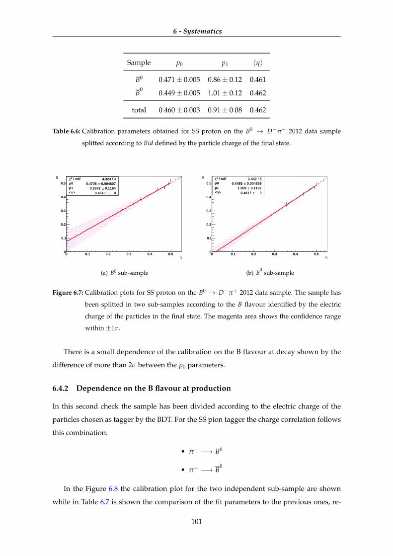
6 - Systematics
Sample p0 p1 〈η〉
B0 0.471± 0.005 0.86± 0.12 0.461
B0 0.449± 0.005 1.01± 0.12 0.462
total 0.460± 0.003 0.91± 0.08 0.462
Table 6.6: Calibration parameters obtained for SS proton on the B0 → D−π+ 2012 data sample
splitted according to Bid defined by the particle charge of the final state.
η0 0.1 0.2 0.3 0.4 0.5
ω
0
0.1
0.2
0.3
0.4
0.5 / ndf 2χ 4.323 / 3
p0 0.004607± 0.4706 p1 0.1194± 0.8572
> η< 0± 0.4613
/ ndf 2χ 4.323 / 3p0 0.004607± 0.4706 p1 0.1194± 0.8572
> η< 0± 0.4613
(a) B0 sub-sample
η0 0.1 0.2 0.3 0.4 0.5
ω
0
0.1
0.2
0.3
0.4
0.5 / ndf 2χ 1.442 / 3
p0 0.004639± 0.4485 p1 0.1192± 1.009
> η< 0± 0.4617
/ ndf 2χ 1.442 / 3p0 0.004639± 0.4485 p1 0.1192± 1.009
> η< 0± 0.4617
(b) B0 sub-sample
Figure 6.7: Calibration plots for SS proton on the B0 → D−π+ 2012 data sample. The sample has
been splitted in two sub-samples according to the B flavour identified by the electric
charge of the particles in the final state. The magenta area shows the confidence range
within ±1σ.
There is a small dependence of the calibration on the B flavour at decay shown by the
difference of more than 2σ between the p0 parameters.
6.4.2 Dependence on the B flavour at production
In this second check the sample has been divided according to the electric charge of the
particles chosen as tagger by the BDT. For the SS pion tagger the charge correlation follows
this combination:
• π+ −→ B0
• π− −→ B0
In the Figure 6.8 the calibration plot for the two independent sub-sample are shown
while in Table 6.7 is shown the comparison of the fit parameters to the previous ones, re-
101
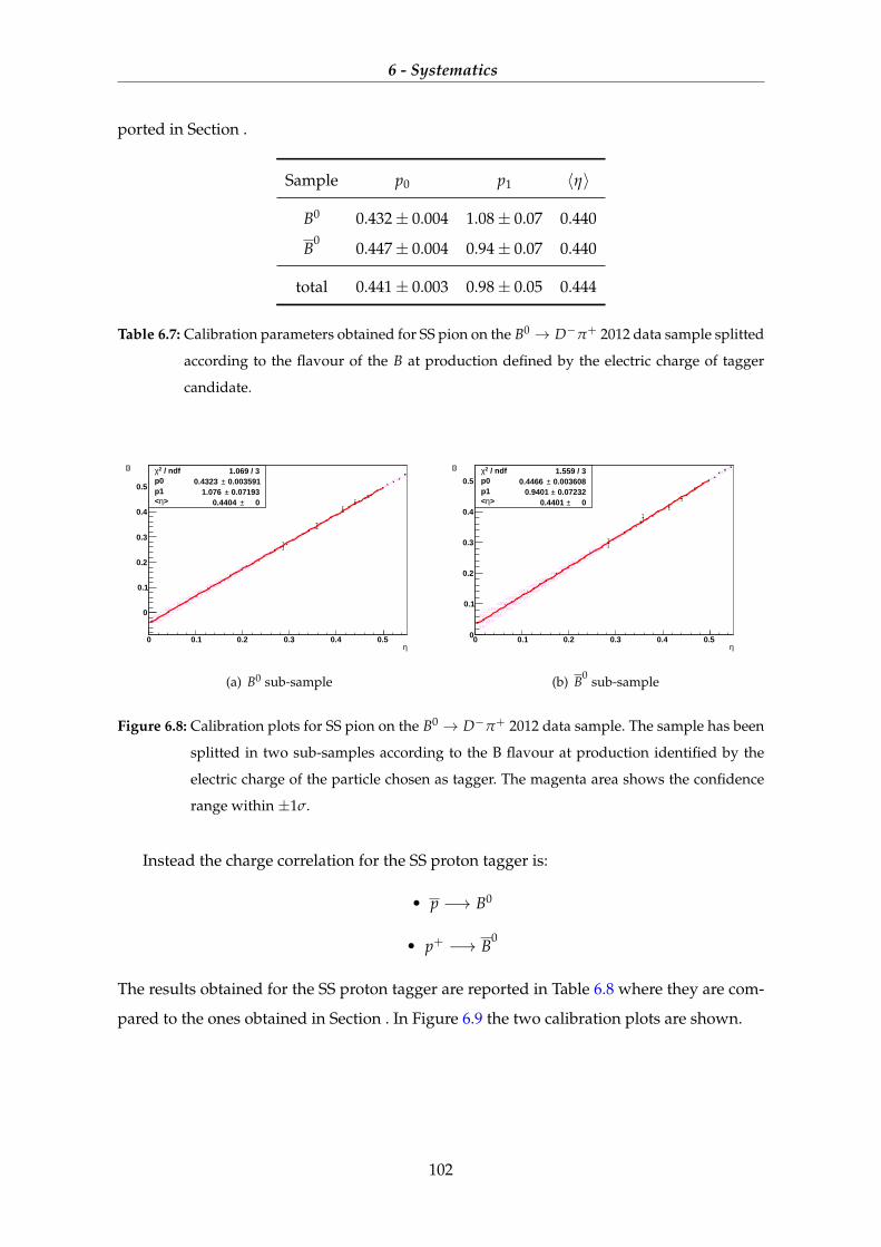
6 - Systematics
ported in Section .
Sample p0 p1 〈η〉
B0 0.432± 0.004 1.08± 0.07 0.440
B0 0.447± 0.004 0.94± 0.07 0.440
total 0.441± 0.003 0.98± 0.05 0.444
Table 6.7: Calibration parameters obtained for SS pion on the B0 → D−π+ 2012 data sample splitted
according to the flavour of the B at production defined by the electric charge of tagger
candidate.
η0 0.1 0.2 0.3 0.4 0.5
ω
0
0.1
0.2
0.3
0.4
0.5
/ ndf 2χ 1.069 / 3p0 0.003591± 0.4323 p1 0.07193± 1.076
> η< 0± 0.4404
/ ndf 2χ 1.069 / 3p0 0.003591± 0.4323 p1 0.07193± 1.076
> η< 0± 0.4404
(a) B0 sub-sample
η0 0.1 0.2 0.3 0.4 0.5
ω
0
0.1
0.2
0.3
0.4
0.5 / ndf 2χ 1.559 / 3
p0 0.003608± 0.4466 p1 0.07232± 0.9401
> η< 0± 0.4401
/ ndf 2χ 1.559 / 3p0 0.003608± 0.4466 p1 0.07232± 0.9401
> η< 0± 0.4401
(b) B0 sub-sample
Figure 6.8: Calibration plots for SS pion on the B0 → D−π+ 2012 data sample. The sample has been
splitted in two sub-samples according to the B flavour at production identified by the
electric charge of the particle chosen as tagger. The magenta area shows the confidence
range within ±1σ.
Instead the charge correlation for the SS proton tagger is:
• p −→ B0
• p+ −→ B0
The results obtained for the SS proton tagger are reported in Table 6.8 where they are com-
pared to the ones obtained in Section . In Figure 6.9 the two calibration plots are shown.
102
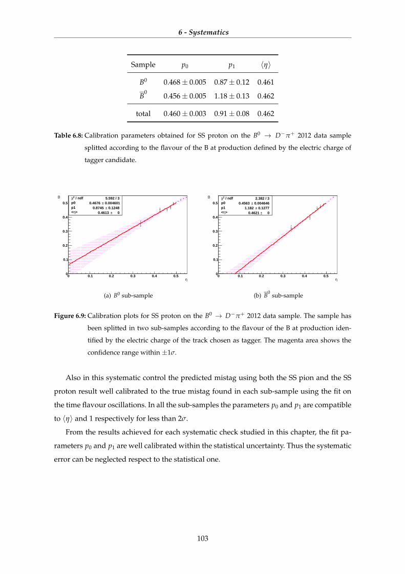
6 - Systematics
Sample p0 p1 〈η〉
B0 0.468± 0.005 0.87± 0.12 0.461
B0 0.456± 0.005 1.18± 0.13 0.462
total 0.460± 0.003 0.91± 0.08 0.462
Table 6.8: Calibration parameters obtained for SS proton on the B0 → D−π+ 2012 data sample
splitted according to the flavour of the B at production defined by the electric charge of
tagger candidate.
η0 0.1 0.2 0.3 0.4 0.5
ω
0
0.1
0.2
0.3
0.4
0.5 / ndf 2χ 5.592 / 3
p0 0.004601± 0.4676 p1 0.1248± 0.8745
> η< 0± 0.4613
/ ndf 2χ 5.592 / 3p0 0.004601± 0.4676 p1 0.1248± 0.8745
> η< 0± 0.4613
(a) B0 sub-sample
η0 0.1 0.2 0.3 0.4 0.5
ω
0
0.1
0.2
0.3
0.4
0.5 / ndf 2χ 2.382 / 3
p0 0.004646± 0.4563 p1 0.1277± 1.182
> η< 0± 0.4621
/ ndf 2χ 2.382 / 3p0 0.004646± 0.4563 p1 0.1277± 1.182
> η< 0± 0.4621
(b) B0 sub-sample
Figure 6.9: Calibration plots for SS proton on the B0 → D−π+ 2012 data sample. The sample has
been splitted in two sub-samples according to the flavour of the B at production iden-
tified by the electric charge of the track chosen as tagger. The magenta area shows the
confidence range within ±1σ.
Also in this systematic control the predicted mistag using both the SS pion and the SS
proton result well calibrated to the true mistag found in each sub-sample using the fit on
the time flavour oscillations. In all the sub-samples the parameters p0 and p1 are compatible
to 〈η〉 and 1 respectively for less than 2σ.
From the results achieved for each systematic check studied in this chapter, the fit pa-
rameters p0 and p1 are well calibrated within the statistical uncertainty. Thus the systematic
error can be neglected respect to the statistical one.
103
7
Conclusion
In this thesis the optimization and the calibration of the Same Side Pion (SSπ) and the
Same Side Proton (SSp) taggers have been presented. These taggers use the pion or the
proton produced in the hadronization of the b quark to the signal B meson to tag its initial
flavour. A multivariate classifier based on “Boost Decision Tree” (BDT) method [20] has
been exploited to select the best tagger candidate, among the track in the event, and to
estimate the probability of the tagging decision to be correct.
All the analyses are developed after the unfolding of the background contribution by
means the sPlot technique [29], using the B invariant mass as “discriminant variable”. The
BDT-based algorithms are trained on the B0 −→ D−(→ K+π−π−)π+ data sample col-
lected by LHCb experiment during the 2012. The training exploits both kinematic and ge-
ometric variables related to the track or to the event to discriminate the right charge corre-
lated particles from the wrong charge correlated ones. The BDT output is used to evaluate
the per-event mistag probability after a calibration procedure.
The new tuning for the SSπ, applied on the B0 −→ D−(→ K+π−π−)π+ 2012 data
sample, provides a effective tagging efficiency of εe f f = 1.64 ± 0.07% which is ∼ 20%
larger than the current result obtained from a similar tagger [18, 23]. The tuning for the SSp
provides an tagging power of εe f f = 0.47± 0.04%, which is compatible within the statistical
errors to the current performance [18].
These results are checked on various independent data samples, for each case the per-
formances and the calibration are consistent within the statistical errors with the ones ob-
tained in the tuning sample. In particular for the SSπ, the tagging power obtained in the
the B0 −→ D−(→ K+π−π−)π+ 2011 data sample is εe f f = 1.76 ± 0.07% and in the
B0 −→ K+π− 2012 data sample is εe f f = 1.08± 0.08%. For the SSp the two tagging powers
obtained in the B0 −→ D−(→ K+π−π−)π+ 2011 data sample and in B0 −→ K+π− 2012
104
7 - Conclusion
data sample are εe f f = 0.48± 0.04% and εe f f = 0.43± 0.05%, respectively. The differences
in the tagging power achieved in the B0 −→ K+π− decay mode both for the SSπ and for
SSp, respect to the B0 −→ D−π+, can be accounted to the different kinematic properties of
the signal B in the two channels.
Some systematics have also been studied in order to observe possible dependences of
the tagging performances on the event properties. The source of possible systematic errors
analyzed in this thesis are the BpT dependence, the dependence on the magnet polarity and
the dependence on the flavour at decay of the B signal meson, identified by the charge of
the particles produced in the final state or the flavour at production identified by the charge
of the tagger candidate (tagging decision). The mistag calibration obtained in the different
cases remain consistent within the statistical errors. A dependence of 〈η〉 on the BpT has
been found, as reported also in some previous analyses.
The combination of the tagger responses entails an improvement on the tagging per-
formances [23]. For this reason the last part of this thesis is focused on the combination
of the SSπ and the SSp taggers in a unique Same Side Tagger (SS) and then on the fi-
nal combination of the SS tagger with the OS general tagger, already implemented. The
SS tagger provides an effective tagging efficiency of εe f f = 1.97 ± 0.10% on the B0 −→
D−(→ K+π−π−)π+ 2012 data sample. This value is consistent to the one found in the
B0 −→ D−(→ K+π−π−)π+ 2011 sample (εe f f = 2.05± 0.07%) and in the B0 −→ K+π−
2012 data sample (εe f f = 1.44 ± 0.11%). The results provides by the final combination
SS + OS are: εe f f = 5.09± 0.15% for the B0 −→ D−(→ K+π−π−)π+ 2012 data sample,
εe f f = 5.27± 0.12% for the validation on the B0 −→ D−(→ K+π−π−)π+ 2011 sample and
εe f f = 4.89± 0.20% for the cross-check on the B0 −→ K+π− 2012 data sample.
This final tagger combination has been used to evaluate the oscillation frequency in
the B0 − B0 system (∆md), given by the mass difference between the heavy and light mass
eigenstates. The value obtained in the B0 −→ D−π+ data sample (1 fb−1) is ∆md = 0.511±
0.006 , which is in good agreement with world average measurement (i.e. ∆md = 0.510±
0.003 ps−1). The statistical error related to this value is reduced of 30% respect to the one
evaluated with the current taggers.
The improvements introduced by these optimized SS algorithms and by the two tagger
combinations will contribute to increase the precision of the measurement based on the
flavour identification in the B0d system, such as the evaluation of sin 2β [24].
105

A
sPlots technique
This technique analyzes the events of a sample assuming that they are characterized by two
set of variables:
• the first one is a set of variables for which the distributions of all the sources of events
are known (“discriminating variables”)
• the second one is a set of variables for which the distributions of some sources of
events are either truly unknown (“control variables”)
The sPlot technique allows to reconstruct the distributions for the control variables with-
out making use of any a priori knowledge on this variable [29]. An essential assumption
is that the control variables are uncorrelated with the discriminating variables. This tech-
nique exploits the maximum Likelihood method using the discriminating variables. The
log-Likelihood used is:
L =N
∑e=1
ln{ Ns
∑i=1
Ni fi(ye)}−
Ns
∑i=1
Ni (A.1)
where
• N is the total number of events considered
• Ns is the number of species of events populating the data sample (signal and back-
ground)
• Ni is the number of events expected on the average for the ith species
• y represents the set of “discriminating variables”, which can be correlated with each
other
• fi(ye) is the value of the pdf of y for the ith species and for the event e
106

A - sPlots technique
The set of “control variables” x doesn’t explicitly appear into the log-Likelihood. The
aim of the sPlot technique is to unfold the true distribution (Mn(x)) of x for events with
nth species, from the knowledge of the pdfs ( fi) of y. If x and y are two set of uncorrelated
variables, the total pdf fi(x, y) can be factorized into products Mn(x) fi(y). An estimate (M̃n)
of x for the nth species can be built as:⟨Nm M̃n(x)
⟩=∫
dydxNs
∑j=1
Nj Mj(x) f j(y)δ(x− x)Pn
= Nm
Ns
∑j=1
Mj(x)Nj
∫dy
fn(y) f j(y)
∑Nsk=1 Nk fk(y)
(A.2)
where Pn1 is the naive weight defined for each event. Using the inverse of the covariance
matrix V−1nj defined as:
V−1nj =
∂2(−L)∂Nn∂Nj
=N
∑e=1
fn(ye) f j(ye)
(∑Nsk=1 Nk fk(ye))2
(A.3)
Introducing the average of covariance matrix:
〈V−1nj 〉 =
∫dy
fn(y) f j(y)
∑Nsk=1 Nk fk(y)
(A.4)
the equation A.2 can be rewritten as:⟨M̃n(x)
⟩=
Ns
∑j=1
Mj(x)Nj〈V−1nj 〉 (A.5)
Inverting this matrix equation, the distribution Mn(x) can be obtained:
Nm Mn(x) =Ns
∑j=1〈Vnj〉
⟨M̃j(x)
⟩(A.6)
Thus the appropriate weight is the covariance-weighted quantity defined by:
sPn(ye) =∑Ns
i=1 Vnj f j(ye)
∑Nsk=1 Nk fk(ye)
(A.7)
Using this sWeight the distribution of x can be obtained from the sPlot histogram:
Nn s M̃n(x)δx ≡ ∑e⊂δx
sPn(ye), (A.8)
which reproduces, on average, the true binned distribution:⟨Nm s M̃n(x)
⟩= Nm Mn(x) (A.9)
Because the covariance matrix enters explicitly in the definition of sWeight, these values can
be positive or negative, and the estimators of the true pdfs are not constrained to be strictly
positive.
1Pn = Pn(ye) =Nn fn(ye)
∑Nsk=1 Nk fk(ye)
is the correct weight if x is totally correlated with y.
107

A - sPlots technique
A.1 sPlot properties
The distribution s M̃n is guaranteed to be normalized to unity and the sum over the species
reproduces the data sample distribution of x. Thus the sPlots technique satisfies other two
properties:
• Each x-distribution is properly normalized. The sum over the x-bins of Nn s M̃δx is
equal to Nn:N
∑e=1
=s Pn(ye) = Nn (A.10)
• In each bin the sum over all species of the expected numbers of events equals to the
number of events actually observed. For any event:
Ns
∑j=1
sPj(ye) = 1 (A.11)
For this reasons, the sPlot return a correct representation of the distribution of each
control variable in the set x.
A.2 sPlot application
The sPlot technique prove itself to be a very usefull tool to unfold the background and
signal contributions. Indeed to eliminate the background is sufficient weighting each event
for the sWeight evaluated by means a fit on the “discriminating variables”. In this work
thesis the variable chosen as the discriminant one is the invariant mass of the B meson.
A simple application of the sPlot technique can be exploited to separate the distribution
of the event and track variables. For some variables the comparisons of the normalized
distributions of signal and background are shown in Figures A.1.
In the case of the decay time τ the signal distribution slope is larger than the background
one, the reason can be found in combinatorial nature of the background itself, described
properly by a simple exponential function, while the signal distribution is determined by
the B0d lifetime and it is represented by a convolution between an exponential function and
a resolution model function.
108
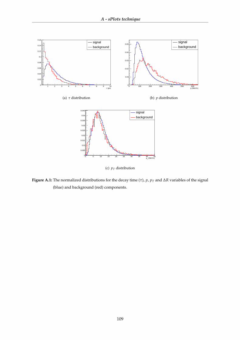
A - sPlots technique
time_sigEntries 349966
Mean 2.107
RMS 1.437
(ps)τ1 2 3 4 5 6 7 8 9 10
0
0.02
0.04
0.06
0.08
0.1
0.12
0.14
0.16
time_sigEntries 349966
Mean 2.107
RMS 1.437
signalsignal
background
(a) τ distribution
P_sigEntries 349966
Mean 136
RMS 79.95
p (MeV/c)0 100 200 300 400 500 600
0
0.01
0.02
0.03
0.04
0.05
P_sigEntries 349966
Mean 136
RMS 79.95
signal
signalbackground
(b) p distribution
Pt_sigEntries 349966Mean 9.788RMS 4.905
(MeV/c)T
p0 5 10 15 20 25 30 35 40 45
0
0.005
0.01
0.015
0.02
0.025
0.03
0.035
0.04
0.045
Pt_sigEntries 349966Mean 9.788RMS 4.905
signal
signal
background
(c) pT distribution
Figure A.1: The normalized distributions for the decay time (τ), p, pT and ∆R variables of the signal
(blue) and background (red) components.
109
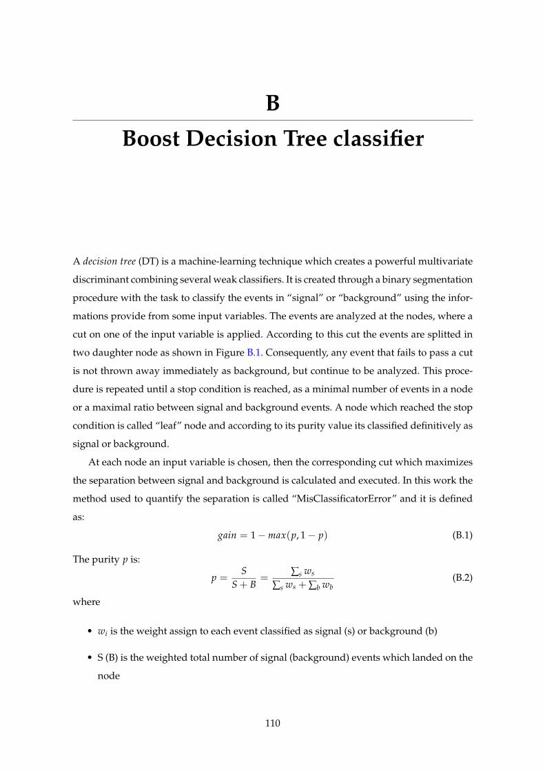
B
Boost Decision Tree classifier
A decision tree (DT) is a machine-learning technique which creates a powerful multivariate
discriminant combining several weak classifiers. It is created through a binary segmentation
procedure with the task to classify the events in “signal” or “background” using the infor-
mations provide from some input variables. The events are analyzed at the nodes, where a
cut on one of the input variable is applied. According to this cut the events are splitted in
two daughter node as shown in Figure B.1. Consequently, any event that fails to pass a cut
is not thrown away immediately as background, but continue to be analyzed. This proce-
dure is repeated until a stop condition is reached, as a minimal number of events in a node
or a maximal ratio between signal and background events. A node which reached the stop
condition is called “leaf” node and according to its purity value its classified definitively as
signal or background.
At each node an input variable is chosen, then the corresponding cut which maximizes
the separation between signal and background is calculated and executed. In this work the
method used to quantify the separation is called “MisClassificatorError” and it is defined
as:
gain = 1−max(p, 1− p) (B.1)
The purity p is:
p =S
S + B=
∑s ws
∑s ws + ∑b wb(B.2)
where
• wi is the weight assign to each event classified as signal (s) or background (b)
• S (B) is the weighted total number of signal (background) events which landed on the
node
110
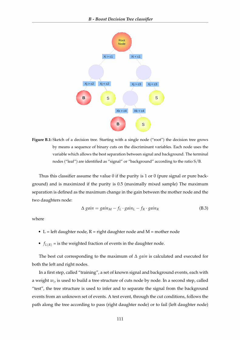
B - Boost Decision Tree classifier
RootNode
Xi > c1 Xi < c1
Xj > c2
Xi > c1
Xj < c2 Xj > c3 Xj < c3
B S S
SB
Xk < c4Xk > c4
Figure B.1: Sketch of a decision tree. Starting with a single node (“root”) the decision tree grows
by means a sequence of binary cuts on the discriminant variables. Each node uses the
variable which allows the best separation between signal and background. The terminal
nodes (“leaf”) are identified as “signal” or “background” according to the ratio S/B.
Thus this classifier assume the value 0 if the purity is 1 or 0 (pure signal or pure back-
ground) and is maximized if the purity is 0.5 (maximally mixed sample) The maximum
separation is defined as the maximum change in the gain between the mother node and the
two daughters node:
∆ gain = gainM − fL · gainL − fR · gainR (B.3)
where
• L = left daughter node, R = right daughter node and M = mother node
• fL(R) = is the weighted fraction of events in the daughter node.
The best cut corresponding to the maximum of ∆ gain is calculated and executed for
both the left and right nodes.
In a first step, called “training”, a set of known signal and background events, each with
a weight wi, is used to build a tree structure of cuts node by node. In a second step, called
“test”, the tree structure is used to infer and to separate the signal from the background
events from an unknown set of events. A test event, through the cut conditions, follows the
path along the tree according to pass (right daughter node) or to fail (left daughter node)
111

B - Boost Decision Tree classifier
until it lands on a leaf. The classifier value, i.e. the decision tree result, D(i) for a test event
is equal to the purity of the leaf which it reached.
B.1 Boosting method
The Boosting is a technique to enhance and to increase the stability with respect the sta-
tistical fluctuations in the classification and regression performance. The improvement is
achieved creating several decision trees (100-1000 trees) and combining their results to pro-
vide a final classifier value. A decision tree classifier to which is applied a boost method is
called Boost Decision Tree (BDT).
In this work an adaptive boost, called “AdaBoost”, is chosen. The basic idea of the Ad-
aBoost is to attribute a higher weight wi to the misclassified events during the training of
the following tree. According to the following definitions for the ith event:
• yi the true nature of the event: +1→ signal and −1→ background
• cmi (xi) the response of the mth tree: +1→ signal and −1→ background
where x is the tuple of the input variables, the ith event is misclassified if yi 6= cmi (xi)
Thus the first training starts with the original event weights1 while the subsequent trees
are trained using a modified sample where the weights of previously misclassified events
are multiplied by a common boost weight αm, defined as:
αm =1− errm−1
errm−1(B.4)
where errm−1 is the misclassification rate of the previous tree and is calculated like:
errm = ∑yi 6=cm
i (xi)
wi (B.5)
The weights of the new sample are renormalized such that the sum of weights remains
constant.
The final classifier value is calculated as:
Ci(xi) =1
Ntrees·
Ntrees
∑m=1
ln αm · cmi (xi) (B.6)
A small value for Ci(xi) is a sign of background-like event, while large value indicates a
signal-like event.
1In general the weights are initialized to 1
112
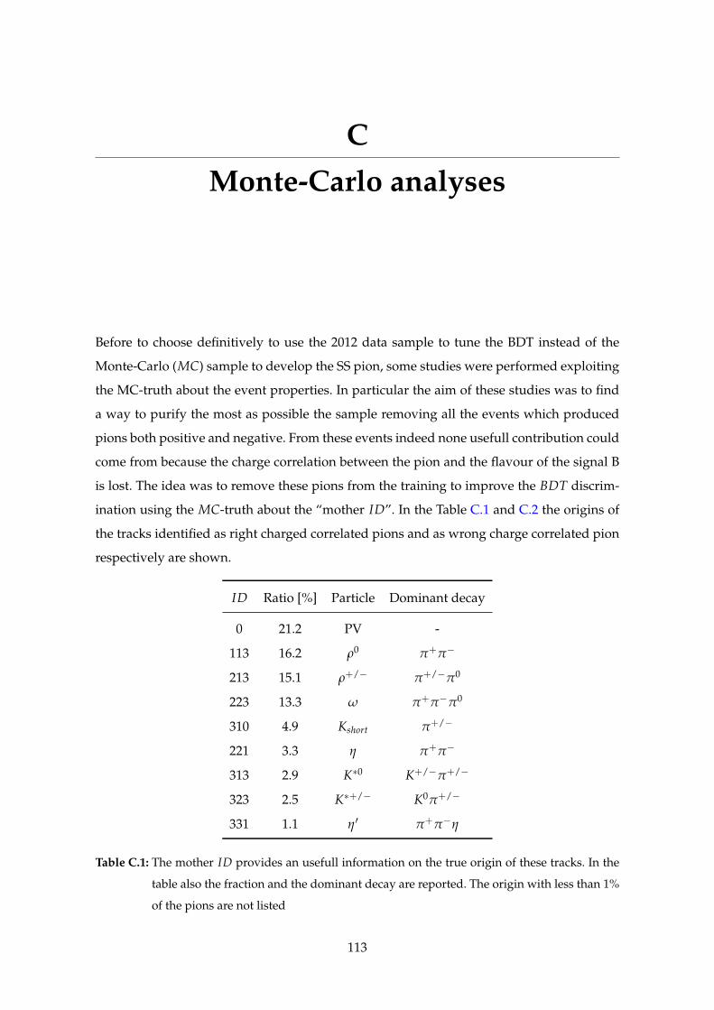
C
Monte-Carlo analyses
Before to choose definitively to use the 2012 data sample to tune the BDT instead of the
Monte-Carlo (MC) sample to develop the SS pion, some studies were performed exploiting
the MC-truth about the event properties. In particular the aim of these studies was to find
a way to purify the most as possible the sample removing all the events which produced
pions both positive and negative. From these events indeed none usefull contribution could
come from because the charge correlation between the pion and the flavour of the signal B
is lost. The idea was to remove these pions from the training to improve the BDT discrim-
ination using the MC-truth about the “mother ID”. In the Table C.1 and C.2 the origins of
the tracks identified as right charged correlated pions and as wrong charge correlated pion
respectively are shown.
ID Ratio [%] Particle Dominant decay
0 21.2 PV -
113 16.2 ρ0 π+π−
213 15.1 ρ+/− π+/−π0
223 13.3 ω π+π−π0
310 4.9 Kshort π+/−
221 3.3 η π+π−
313 2.9 K∗0 K+/−π+/−
323 2.5 K∗+/− K0π+/−
331 1.1 η′ π+π−η
Table C.1: The mother ID provides an usefull information on the true origin of these tracks. In the
table also the fraction and the dominant decay are reported. The origin with less than 1%
of the pions are not listed
113
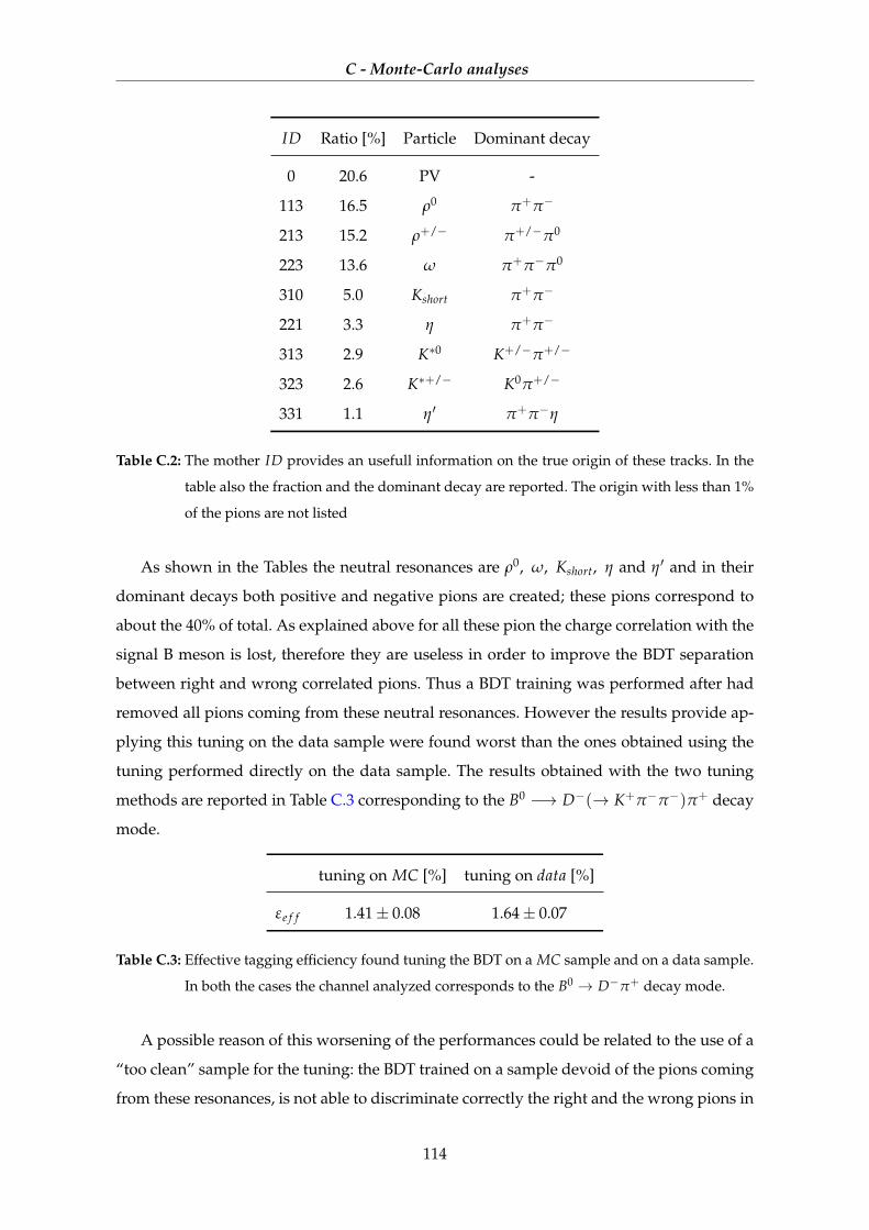
C - Monte-Carlo analyses
ID Ratio [%] Particle Dominant decay
0 20.6 PV -
113 16.5 ρ0 π+π−
213 15.2 ρ+/− π+/−π0
223 13.6 ω π+π−π0
310 5.0 Kshort π+π−
221 3.3 η π+π−
313 2.9 K∗0 K+/−π+/−
323 2.6 K∗+/− K0π+/−
331 1.1 η′ π+π−η
Table C.2: The mother ID provides an usefull information on the true origin of these tracks. In the
table also the fraction and the dominant decay are reported. The origin with less than 1%
of the pions are not listed
As shown in the Tables the neutral resonances are ρ0, ω, Kshort, η and η′ and in their
dominant decays both positive and negative pions are created; these pions correspond to
about the 40% of total. As explained above for all these pion the charge correlation with the
signal B meson is lost, therefore they are useless in order to improve the BDT separation
between right and wrong correlated pions. Thus a BDT training was performed after had
removed all pions coming from these neutral resonances. However the results provide ap-
plying this tuning on the data sample were found worst than the ones obtained using the
tuning performed directly on the data sample. The results obtained with the two tuning
methods are reported in Table C.3 corresponding to the B0 −→ D−(→ K+π−π−)π+ decay
mode.
tuning on MC [%] tuning on data [%]
εe f f 1.41± 0.08 1.64± 0.07
Table C.3: Effective tagging efficiency found tuning the BDT on a MC sample and on a data sample.
In both the cases the channel analyzed corresponds to the B0 → D−π+ decay mode.
A possible reason of this worsening of the performances could be related to the use of a
“too clean” sample for the tuning: the BDT trained on a sample devoid of the pions coming
from these resonances, is not able to discriminate correctly the right and the wrong pions in
114

C - Monte-Carlo analyses
the data, where these resonances can not be eliminated. Because of this studies have been
proved themselves useless in order to obtain an improvement of the tagging performances,
they have not been execute for the SS proton.
115
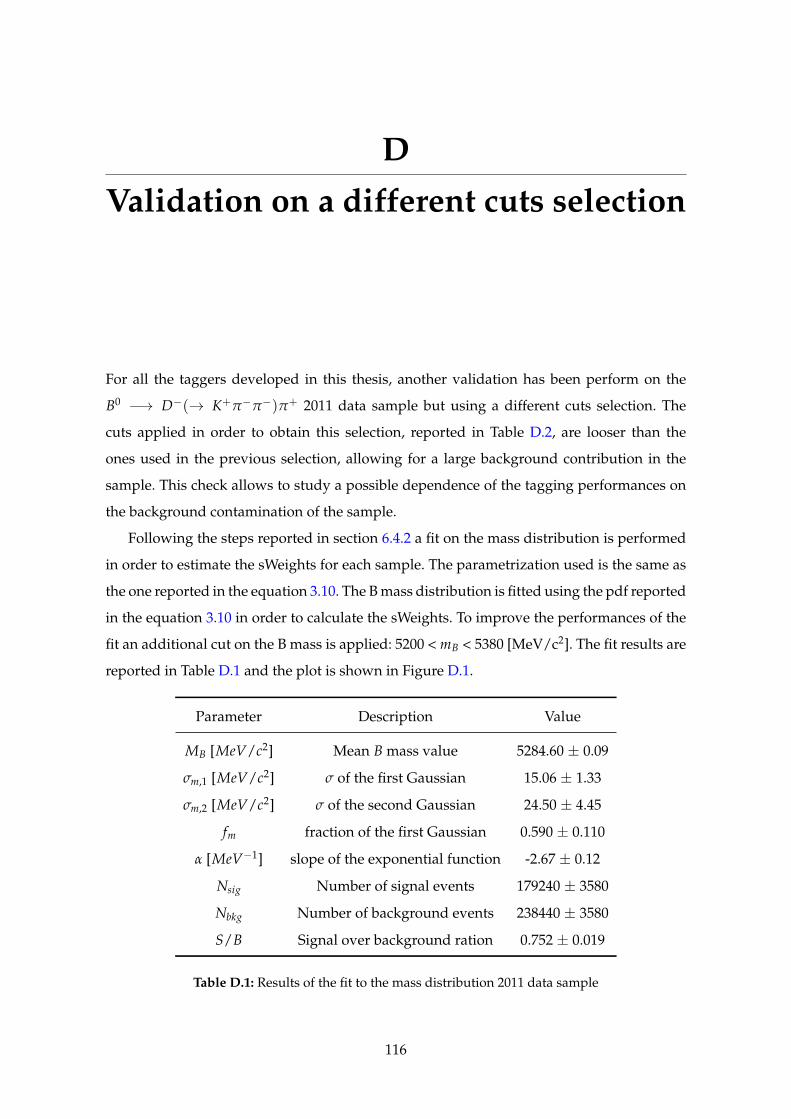
D
Validation on a different cuts selection
For all the taggers developed in this thesis, another validation has been perform on the
B0 −→ D−(→ K+π−π−)π+ 2011 data sample but using a different cuts selection. The
cuts applied in order to obtain this selection, reported in Table D.2, are looser than the
ones used in the previous selection, allowing for a large background contribution in the
sample. This check allows to study a possible dependence of the tagging performances on
the background contamination of the sample.
Following the steps reported in section 6.4.2 a fit on the mass distribution is performed
in order to estimate the sWeights for each sample. The parametrization used is the same as
the one reported in the equation 3.10. The B mass distribution is fitted using the pdf reported
in the equation 3.10 in order to calculate the sWeights. To improve the performances of the
fit an additional cut on the B mass is applied: 5200 < mB < 5380 [MeV/c2]. The fit results are
reported in Table D.1 and the plot is shown in Figure D.1.
Parameter Description Value
MB [MeV/c2] Mean B mass value 5284.60 ± 0.09
σm,1 [MeV/c2] σ of the first Gaussian 15.06 ± 1.33
σm,2 [MeV/c2] σ of the second Gaussian 24.50 ± 4.45
fm fraction of the first Gaussian 0.590 ± 0.110
α [MeV−1] slope of the exponential function -2.67 ± 0.12
Nsig Number of signal events 179240 ± 3580
Nbkg Number of background events 238440 ± 3580
S/B Signal over background ration 0.752 ± 0.019
Table D.1: Results of the fit to the mass distribution 2011 data sample
116
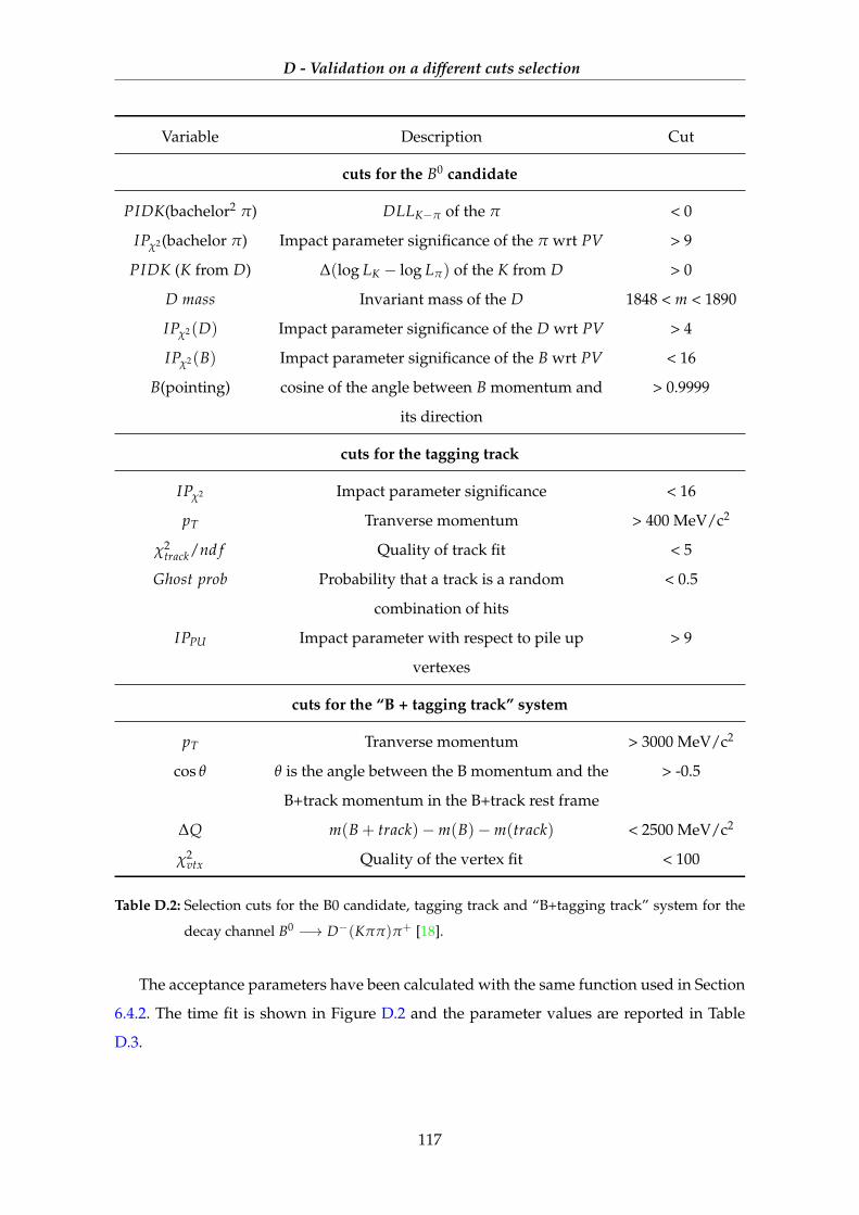
D - Validation on a different cuts selection
Variable Description Cut
cuts for the B0 candidate
PIDK(bachelor2 π) DLLK−π of the π < 0
IPχ2(bachelor π) Impact parameter significance of the π wrt PV > 9
PIDK (K from D) ∆(log LK − log Lπ) of the K from D > 0
D mass Invariant mass of the D 1848 < m < 1890
IPχ2(D) Impact parameter significance of the D wrt PV > 4
IPχ2(B) Impact parameter significance of the B wrt PV < 16
B(pointing) cosine of the angle between B momentum and
its direction
> 0.9999
cuts for the tagging track
IPχ2 Impact parameter significance < 16
pT Tranverse momentum > 400 MeV/c2
χ2track/nd f Quality of track fit < 5
Ghost prob Probability that a track is a random
combination of hits
< 0.5
IPPU Impact parameter with respect to pile up
vertexes
> 9
cuts for the “B + tagging track” system
pT Tranverse momentum > 3000 MeV/c2
cos θ θ is the angle between the B momentum and the
B+track momentum in the B+track rest frame
> -0.5
∆Q m(B + track)−m(B)−m(track) < 2500 MeV/c2
χ2vtx Quality of the vertex fit < 100
Table D.2: Selection cuts for the B0 candidate, tagging track and “B+tagging track” system for the
decay channel B0 −→ D−(Kππ)π+ [18].
The acceptance parameters have been calculated with the same function used in Section
6.4.2. The time fit is shown in Figure D.2 and the parameter values are reported in Table
D.3.
117
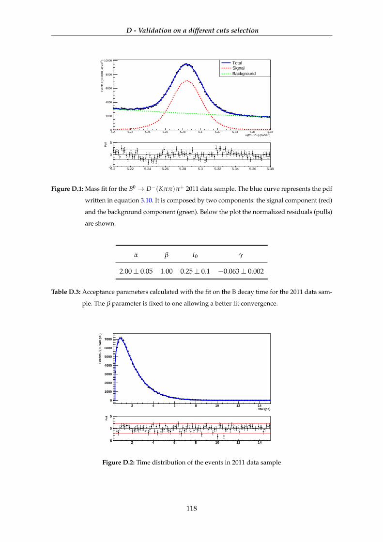
D - Validation on a different cuts selection
)2^+) (GeV/cπm(D^- 5.2 5.22 5.24 5.26 5.28 5.3 5.32 5.34 5.36 5.38
)2E
vent
s / (
0.0
018
GeV
/c
0
2000
4000
6000
8000
10000TotalSignalBackground
5.2 5.22 5.24 5.26 5.28 5.3 5.32 5.34 5.36 5.38
Pul
l
-5
0
5
Figure D.1: Mass fit for the B0 → D−(Kππ)π+ 2011 data sample. The blue curve represents the pdf
written in equation 3.10. It is composed by two components: the signal component (red)
and the background component (green). Below the plot the normalized residuals (pulls)
are shown.
α β t0 γ
2.00± 0.05 1.00 0.25± 0.1 −0.063± 0.002
Table D.3: Acceptance parameters calculated with the fit on the B decay time for the 2011 data sam-
ple. The β parameter is fixed to one allowing a better fit convergence.
tau (ps)2 4 6 8 10 12 14
Eve
nts
/ (
0.14
8 p
s )
0
1000
2000
3000
4000
5000
6000
7000
time distribution
2 4 6 8 10 12 14
Pu
ll
-5
0
5
Figure D.2: Time distribution of the events in 2011 data sample
118
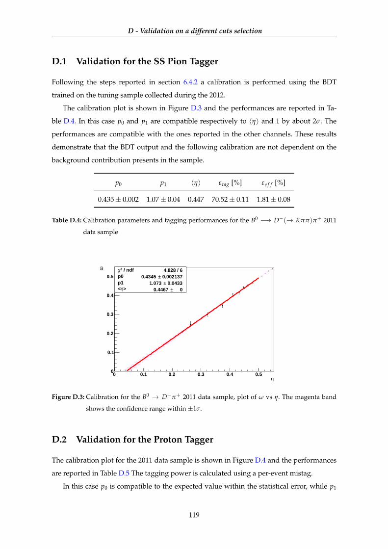
D - Validation on a different cuts selection
D.1 Validation for the SS Pion Tagger
Following the steps reported in section 6.4.2 a calibration is performed using the BDT
trained on the tuning sample collected during the 2012.
The calibration plot is shown in Figure D.3 and the performances are reported in Ta-
ble D.4. In this case p0 and p1 are compatible respectively to 〈η〉 and 1 by about 2σ. The
performances are compatible with the ones reported in the other channels. These results
demonstrate that the BDT output and the following calibration are not dependent on the
background contribution presents in the sample.
p0 p1 〈η〉 εtag [%] εe f f [%]
0.435± 0.002 1.07± 0.04 0.447 70.52± 0.11 1.81± 0.08
Table D.4: Calibration parameters and tagging performances for the B0 −→ D−(→ Kππ)π+ 2011
data sample
η0 0.1 0.2 0.3 0.4 0.5
ω
0
0.1
0.2
0.3
0.4
0.5 / ndf 2χ 4.828 / 6
p0 0.002137± 0.4345 p1 0.0433± 1.073
> η< 0± 0.4467
/ ndf 2χ 4.828 / 6p0 0.002137± 0.4345 p1 0.0433± 1.073
> η< 0± 0.4467
Figure D.3: Calibration for the B0 → D−π+ 2011 data sample, plot of ω vs η. The magenta band
shows the confidence range within ±1σ.
D.2 Validation for the Proton Tagger
The calibration plot for the 2011 data sample is shown in Figure D.4 and the performances
are reported in Table D.5 The tagging power is calculated using a per-event mistag.
In this case p0 is compatible to the expected value within the statistical error, while p1
119
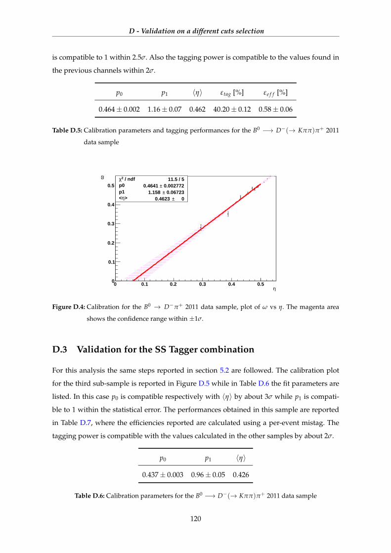
D - Validation on a different cuts selection
is compatible to 1 within 2.5σ. Also the tagging power is compatible to the values found in
the previous channels within 2σ.
p0 p1 〈η〉 εtag [%] εe f f [%]
0.464± 0.002 1.16± 0.07 0.462 40.20± 0.12 0.58± 0.06
Table D.5: Calibration parameters and tagging performances for the B0 −→ D−(→ Kππ)π+ 2011
data sample
η0 0.1 0.2 0.3 0.4 0.5
ω
0
0.1
0.2
0.3
0.4
0.5 / ndf 2χ 11.5 / 5
p0 0.002772± 0.4641 p1 0.06723± 1.158
> η< 0± 0.4623
/ ndf 2χ 11.5 / 5p0 0.002772± 0.4641 p1 0.06723± 1.158
> η< 0± 0.4623
Figure D.4: Calibration for the B0 → D−π+ 2011 data sample, plot of ω vs η. The magenta area
shows the confidence range within ±1σ.
D.3 Validation for the SS Tagger combination
For this analysis the same steps reported in section 5.2 are followed. The calibration plot
for the third sub-sample is reported in Figure D.5 while in Table D.6 the fit parameters are
listed. In this case p0 is compatible respectively with 〈η〉 by about 3σ while p1 is compati-
ble to 1 within the statistical error. The performances obtained in this sample are reported
in Table D.7, where the efficiencies reported are calculated using a per-event mistag. The
tagging power is compatible with the values calculated in the other samples by about 2σ.
p0 p1 〈η〉
0.437± 0.003 0.96± 0.05 0.426
Table D.6: Calibration parameters for the B0 −→ D−(→ Kππ)π+ 2011 data sample
120
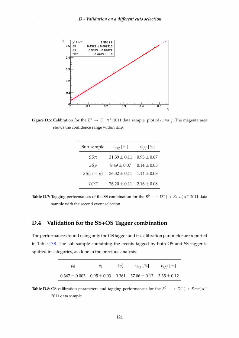
D - Validation on a different cuts selection
η0 0.1 0.2 0.3 0.4 0.5
ω
0
0.1
0.2
0.3
0.4
0.5 / ndf 2χ 1.965 / 2
p0 0.002915± 0.4373 p1 0.04677± 0.9553
> η< 0± 0.4263
/ ndf 2χ 1.965 / 2p0 0.002915± 0.4373 p1 0.04677± 0.9553
> η< 0± 0.4263
Figure D.5: Calibration for the B0 → D−π+ 2011 data sample, plot of ω vs η. The magenta area
shows the confidence range within ±1σ.
Sub-sample εtag [%] εe f f [%]
SSπ 31.39± 0.11 0.93± 0.07
SSp 8.49± 0.07 0.14± 0.03
SS(π + p) 36.32± 0.11 1.14± 0.08
TOT 76.20± 0.11 2.16± 0.08
Table D.7: Tagging performances of the SS combination for the B0 −→ D−(→ Kππ)π+ 2011 data
sample with the second event selection.
D.4 Validation for the SS+OS Tagger combination
The performances found using only the OS tagger and its calibration parameter are reported
in Table D.8. The sub-sample containing the events tagged by both OS and SS tagger is
splitted in categories, as done in the previous analysis.
p0 p1 〈η〉 εtag [%] εe f f [%]
0.367± 0.003 0.95± 0.03 0.361 37.06± 0.13 3.35± 0.12
Table D.8: OS calibration parameters and tagging performances for the B0 −→ D−(→ Kππ)π+
2011 data sample
121
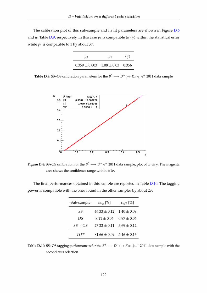
D - Validation on a different cuts selection
The calibration plot of this sub-sample and its fit parameters are shown in Figure D.6
and in Table D.9, respectively. In this case p0 is compatible to 〈η〉 within the statistical error
while p1 is compatible to 1 by about 3σ.
p0 p1 〈η〉
0.359± 0.003 1.08± 0.03 0.356
Table D.9: SS+OS calibration parameters for the B0 −→ D−(→ Kππ)π+ 2011 data sample
η0 0.1 0.2 0.3 0.4 0.5
ω
0
0.1
0.2
0.3
0.4
0.5 / ndf 2χ 5.597 / 4
p0 0.003222± 0.3587 p1 0.03048± 1.079
> η< 0± 0.3556
/ ndf 2χ 5.597 / 4p0 0.003222± 0.3587 p1 0.03048± 1.079
> η< 0± 0.3556
Figure D.6: SS+OS calibration for the B0 −→ D−π+ 2011 data sample, plot of ω vs η. The magenta
area shows the confidence range within ±1σ.
The final performances obtained in this sample are reported in Table D.10. The tagging
power is compatible with the ones found in the other samples by about 2σ.
Sub-sample εtag [%] εe f f [%]
SS 46.33± 0.12 1.40± 0.09
OS 8.11± 0.06 0.97± 0.06
SS + OS 27.22± 0.11 3.69± 0.12
TOT 81.66± 0.09 5.46± 0.16
Table D.10: SS+OS tagging performances for the B0 −→ D−(→ Kππ)π+ 2011 data sample with the
second cuts selection
122
Bibliography
[1] J. Beringer et al.(Particle Data Group). Review of particle physics. Phys. Rev. D,
86:010001, Jul 2012.
[2] Nicola Cabibbo. Unitary symmetry and leptonic decays. Phys. Rev. Lett., 10:531–533,
Jun 1963.
[3] The CKM Fitter group. http://ckmfitter.in2p3.fr.
[4] The UT Fitter group. http://utfit.org.
[5] K. Nakamura et al.(Particle Data Group). Review of particle physics, 2010-2011.
[6] C. S. Wu, E. Ambler, R. W. Hayward, D. D. Hoppes, and R. P. Hudson. Experimental
test of parity conservation in beta decay. Phys. Rev., 105:1413–1415, Feb 1957.
[7] J. H. Christenson, J. W. Cronin, V. L. Fitch, and R. Turlay. Evidence for the 2π decay of
the k02 meson. Phys. Rev. Lett., 13:138–140, Jul 1964.
[8] LHCb Collaboration . Lhcb detector performance. International Journal of Modern
Physics A, 30(07):1530022, 2015.
[9] J M Campbell, J W Huston, and W J Stirling. Hard interactions of quarks and gluons:
a primer for lhc physics. Reports on Progress in Physics, 70(1):89, 2007.
[10] LHCb Collaboration. Measurement of σ(pp → b− bx) at√
s = 7 tev in the forward
region. Physics Letters B, 694(3):209 – 216, 2010.
[11] http://lhcb.web.cern.ch/lhcb/speakersbureau/excel/default.html.
123
BIBLIOGRAPHY
[12] LHCb Collaboration et al. The lhcb detector at the lhc. Journal of Instrumentation, 3:8005,
2008.
[13] LHCb Silicon Tracker. http://lhcb.physik.uzh.ch/st/public/.
[14] LHCb Collaboration et al. Performance of the lhcb rich detector at the lhc. The European
Physical Journal C, 73(5), 2013.
[15] M. Calvi, O. Dormond, and M. Musy. Lhcb flavour tagging performance. 2003.
[16] M. Grabalosa. Flavour Tagging developments within the LHCb experiment. Doctorat de
investigación en física, Universitat de Barcelona, 2012.
[17] LHCb Collaboration. Observations of Orbitally Excited B∗∗(s) Mesons. LHCb-CONF-
2011-053.
[18] A. Falabella. New Developments of the Flavour Tagging Algorithms for the LHCb Experi-
ment. Dottorato di ricerca in fisica, Università degli studi di Ferrara, 2013.
[19] https://indico.cern.ch/event/329775/contribution/2/material/slides/0.pdf.
[20] Hoecker, Andreas and Speckmayer, Peter and Stelzer, Joerg and Therhaag, Jan and von
Toerne, Eckhard and Voss, Helge. TMVA: Toolkit for Multivariate Data Analysis. PoS,
ACAT:040, 2007.
[21] http://roofit.sourceforge.net/docs/roofit users manual 2.07-29.pdf.
[22] K.A. Olive et al. Review of particle physics. Chin.Phys., C38:090001, 72014.
[23] LHCb Collaboration. Opposite-side flavour tagging of b mesons at the lhcb experi-
ment. The European Physical Journal C, 72(6), 2012.
[24] Albrecht et al. (Argus Collaboration. Observation of B0 − B0 mixing. Physics Letters B,
192(1-2):245 – 252, 1987.
[25] http://pdg.lbl.gov/2014/reviews/rpp2014-rev-b-bbar-mixing.pdf.
[26] B decays at the LHC, hep-ph/0003238. (CERN-TH-2000-101):112 p, Mar 2000.
[27] Bottom production, hep-ph/0003142v2.
[28] Calvi, M and Leroy, O and Musy, M. Flavour Tagging Algorithms and Performances
in LHCb. LHCb-2007-058. Technical report.
124

BIBLIOGRAPHY
[29] splot : A statistical tool to unfold data distributions. Nuclear Instruments and Methods in
Physics Research Section A: Accelerators, Spectrometers, Detectors and Associated Equipment.
125

Ringraziamenti
Giunto alla conclusione di questo lavoro, vorrei ringraziare innanzitutto la mia relatrice,
Prof.ssa Marta Calvi, per l’opportunità concessami di lavorare su una tematica interessante
e stimolante, facendomi apprezzare il mondo della ricerca universitaria.
In ugual modo ringrazio anche il mio correlatore, Dott. Basem Khanji, per essersi di-
mostrato sempre disponibile a fornirmi utili consigli e spiegazioni per superare i problemi
che man mano ho incontrato nello sviluppo del presente lavoro.
Vorrei ringraziare anche la la Dott.ssa Stefania Vecchi dell’Università di Ferrara per il
tempestivo supporto fornito nella preparazione dei set di dati necessari alle analisi svolte
in questa tesi.
Ringrazio i miei compagni di corso Fra, Mannu, Fra e tutti gli altri per tutti i consigli
dati in questi anni e sopratutto in questo periodo.
Ringrazio allo stesso modo i miei amici Gian, Riki, Mary, Nicco, Marco, Vale e Carlo per
il loro sostegno e per essere stati sempre presenti. Grazie per tutti i bei momenti passati
assieme.
Ringrazio infine tutta la mia famiglia per essermi sempre stata vicino, per avermi aiutato
in questo periodo universitario ed avermi sempre spinto ad andare avanti, permettendomi
così di arrivare dove sono ora.
Tutti voi, chi più chi meno, avete contribuito a rendermi la persona che sono in questo
momento.
Grazie!
126