Embed Size (px)
Citation preview

DEVELOPMENT OF
SENSITIVITY ANALYSIS AND OPTIMIZATION
FOR MICROWAVE CIRCUITS AND ANTENNAS IN
THE FREQUENCY DOMAIN


DEVELOPMENT OF
SENSITIVITY ANALYSIS AND OPTIMIZATION
FOR MICROWAVE CIRCUITS AND ANTENNAS IN
THE FREQUENCY DOMAIN
By
Jiang Zhu, B. Sc. (Eng.)
A Thesis
Submitted to the School of Graduate Studies
in Partial Fulfillment of the Requirements
for the Degree
Master of Applied Science
McMaster University
© Copyright by Jiang Zhu, June 2006
ii
MASTER OF APPLIED SCIENCE (2006) McMASTER UNIVERSITY
(Electrical and Computer Engineering) Hamilton, Ontario
TITLE: Development of Sensitivity Analysis and Optimization for
Microwave Circuits and Antennas in the Frequency Domain
AUTHOR: Jiang Zhu
B.Sc. (Eng) (Electrical Engineering, Zhejiang University)
SUPERVISORS: Natalia Nikolova, Associate Professor,
Department of Electrical and Computer Engineering
Dipl.Eng. (Technical University of Varna)
Ph.D. (University of Electro-Communication)
P.Eng. (Province of Ontario)
Senior Member, IEEE
J.W. Bandler, Professor Emeritus,
Department of Electrical and Computer Engineering
B.Sc.(Eng), Ph.D., D.Sc.(Eng) (University of London)
D.I.C. (Imperial College)
P.Eng. (Province of Ontario)
C.Eng., FIEE (United Kingdom)
Fellow, IEEE
Fellow, Royal Society of Canada
Fellow, Engineering Institute of Canada
Fellow, Canadian Academy of Engineering
NUMBER OF PAGES: xviii, 137
iii
ABSTRACT
This thesis contributes to the development of adjoint variable methods
(AVM) and space mapping (SM) technology for computer-aided electromagnetics
(EM)-based modeling and design of microwave circuits and antennas.
The AVM is known as an efficient approach to design sensitivity analysis
for problems of high complexity. We propose a general self-adjoint approach to
the sensitivity analysis of network parameters for an Method of Moments (MoM)
solver. It requires neither an adjoint problem nor analytical system matrix
derivatives. For the first time, we suggest practical and fast sensitivity solutions
realized entirely outside the EM solver, which simplifies the implementation. We
discuss: (1) features of commercial EM solvers which allow the user to compute
network parameters and their sensitivities through a single full-wave simulation;
(2) the accuracy of the computed derivatives; (3) the overhead of the sensitivity
computation. Our approach is demonstrated by FEKO, which employs an MoM
solver.
One motivation for sensitivity analysis is gradient-based optimization. The
sensitivity evaluation providing the Jacobian is a bottleneck of optimization with
full-wave simulators. We propose an approach, which employs the self-adjoint
ABSTRACT
iv
sensitivity analysis of network parameters and Broyden’s update for practical EM
design optimization. The Broyden’s update is carried out at the system matrix
level, so that the computational overhead of the Jacobian is negligible while the
accuracy is acceptable for optimization. To improve the robustness of the
Broyden update in the sensitivity analysis, we propose a switching criterion
between the Broyden and the finite-difference estimation of the system matrix
derivatives.
In the second part, we apply for the first time a space mapping technique
to antenna design. We exploit a coarse mesh MoM solver as the coarse model and
align it with the fine mesh MoM solution through space mapping. Two SM plans
are employed: I. implicit SM and output SM, and II. input SM and output SM. A
novel local meshing method is proposed to avoid inconsistencies in the coarse
model. The proposed techniques are implemented through the new user-friendly
SMF system. In a double annular ring antenna example, the S-parameter is
optimized. The finite ground size effect for the MoM is efficiently solved by SM
Plan I and the design specification is satisfied after only three iterations. In a
patch antenna example, we optimize the impedance through both plans.
Comparisons are made. Coarseness in the coarse model and its effect on the SM
performance is also discussed.
v
ACKNOWLEDGEMENTS
The author wishes to express his sincere appreciation to his supervisors
Dr. Natalia K. Nikolova and Dr. John. W. Bandler, the Computational
Electromagnetics Laboratory and the Simulation Optimization Systems Research
Laboratory, McMaster University, for their expert supervision, continuing
encouragement and constant support during the course of this work.
The author would like to express his appreciation to Dr. Mohamed H.
Bakr, Dr. Slawomir Koziel, Dr. Ahmed S. Mohamed, Dr. Qingsha Cheng, Mr.
Dongying Li and Mr. Wenhuan Yu, his colleagues from the Computational
Electromagnetics Laboratory and the Simulation Optimization Systems Research
Laboratory of the Department of Electrical and Computer Engineering at
McMaster University, for useful collaboration and stimulating discussions.
The author wishes to acknowledge Dr. C. J. Reddy, Dr. Rensheng Sun,
from EM Software & System (USA), Inc., for making the FEKO system available
and for useful discussions.
The author gratefully acknowledges the financial assistance provided by
the Natural Sciences and Engineering Research Council of Canada under Grants
OGP0007239 and STGP269760, by Bandler Corporation and by the Department

ACKNOWLEDGEMENTS
vi
of Electrical and Computer Engineering, McMaster University, through a
Research Assistantship.
Finally, special thanks go to my family for encouragement, understanding
and continuous support.
vii
CONTENTS ABSTRACT iii
ACKNOWLEDGMENTS v
LIST OF FIGURES xi
LIST OF TABLES xv
LIST OF ACRONYMS xvii
CHAPTER 1 INTRODUCTION 1
1.1 Motivation……………………………………... 1
1.2 Outline of Thesis………………………………. 2
1.3 Contributions…………………………………... 5
References…………….……………………………... 7
CHAPTER 2 SOME RELEVANT FEATURES OF THE METHOD OF MOMENTS 11
2.1 Brief Introduction to the Method of Moments… 11
2.2 CPU Time Cost Versus Mesh Density................ 14
2.3 Mesh Refinement……………………................ 15
2.4 Modeling of Dielectric Materials……………… 16
CONTENTS
viii
References………………………………………….... 18
PART I SENSITIVITY ANALYSIS IN THE FREQUENCY DOMAIN 21
CHAPTER 3 SELF-ADJOINT SENSITIVITY ANALYSIS IN THE METHOD OF MOMENTS 23
3.1 Introduction…………………………………..... 23
3.2 Frequency Domain Adjoint Variable Method 25
3.2.1 Sensitivity of Linear Complex Systems………………………………. 25
3.2.2 Sensitivities Expression for Linear-Network Parameters…………………. 28
3.3 Network Parameter Sensitivities with Current Solutions……………………………………….. 29
3.3.1 Sensitivities of S-Parameters…….......... 29
3.3.2 Sensitivities of Input Impedance……… 32
3.4 General Procedure……………………………... 33
3.5 Software Requirements and Implementation in FEKO………………………………………….. 35
3.5.1 Software Requirements……………….. 35
3.5.2 FEKO Implementation………………... 36
3.6 Validation……………………………………. 38
3.6.1 Input Impedance Sensitivities of a
Microstrip-Fed Patch Antenna………... 38
3.6.2 S-Parameter Sensitivities of the
Bandstop Filter………………………... 40
CONTENTS
ix
3.6.3 S-Parameter Sensitivities of HTS
Filter………………………................... 43
3.7 Discussion: MoM Matrix Symmetry Versus Convergence of Solution………………………. 45
3.8 Computational Overhead of the Self-Adjoint Sensitivity Analysis…………………………... 51
3.9 Concluding Remarks…………………………... 56
References………………………………………….... 57
CHAPTER 4 EM OPTIMIZATION USING SENSITIVITY ANALYSIS IN THE FREQUENCY DOMAIN 61
4.1 Introduction……………………………………. 61
4.2 The Derivatives of the System Matrix 63
4.3 Sensitivity Analysis in the Method of Moments Exploiting Broyden Update……………………. 64
4.4 Mixed Self-Adjoint Sensitivity Analysis Method and Switch Criteria…………………… 66
4.5 Example: The Optimization of a Double Annular Ring Antenna…….....………………... 66
4.6 Concluding Remarks……….....……………….. 71
References…………………………………………… 72
PART II ANTENNA DESIGN THROUGH SPACE MAPPING OPTIMIZATION 76
CHAPTER 5 ANTENNA DESIGN THROUGH SPACE MAPPING OPTIMIZATION 77
5.1 Introduction……………………………………. 77
CONTENTS
x
5.2 Coarse Model and Fine Model………………… 79
5.3 Space Mapping-Based Surrogate Models…… 80
5.3.1 Mathematical Formulations…………... 80
5.3.2 Algorithm……………………………... 82
5.4 SMF: Space Mapping Framework 83
5.4.1 Brief Introduction to SMF 83
5.4.2 SMF Design Flow 84
5.5 Examples…………………….....…………….... 86
5.5.1 Double Annular Ring Antenna……….. 86
5.5.2 Patch Antenna……………………….. 96
5.6 Concluding Remarks……….....……………….. 102
References…………………………………………… 104
PART III CONCLUSIONS 107
APPENDIX NETWORK PARAMETER CALCULATION IN FEKO 111
BIBLIOGRAPHY 115
AUTHOR INDEX 123
SUBJECT INDEX 131

xi
LIST OF FIGURES Fig. 3.1 Demonstration of mesh control in FEKO………………… 37
Fig. 3.2 Microstrip-fed patch antenna with design parameters. The view shows the actual mesh………………………………. 39
Fig. 3.3 Derivatives of inZ with respect to the length L of the patch antenna at 2.0f = GHz. Width is at 85W = mm…. 40
Fig. 3.4 Microstrip bandstop filter with design parameters [ ]TL W=p . The view shows the actual mesh………...…. 41
Fig. 3.5 Derivatives of the S-parameter magnitudes of the bandstop filter with respect to the stub length L at 4.0f = GHz. Width is 4.6W = mm…………………………………….. 42
Fig. 3.6 Derivatives of the S-parameter phases of the bandstop filter with respect to the stub length L at 4.0f = GHz. Width is 4.6W = mm…………………………………….. 42
Fig. 3.7 The demonstration of the HTS filter……………………… 44
Fig. 3.8 Derivatives of 21S with respect to 1S at f=4.0 GHz for the HTS filter…………………………………………………. 44
Fig. 3.9 Derivatives of 21( )Sϕ with respect to 1S at f=4.0 GHz for the HTS filter in radians per meter………………………... 45
LIST OF FIGURES
xii
Fig. 3.10 The folded dipole and one of its coarse nonuniform segmentations in FEKO (32 segments). The radius of the wire is 410a λ−= and the spacing between the wires is
310s λ−= . L is a design parameter, 0.2 1.2Lλ λ≤ ≤ . The arrow in the center of the lower wire indicates the feed point 48
Fig. 3.11 The matrix asymmetry measure and the error of the computed derivative /inZ L∂ ∂ (at 0.5L λ= ) as a function of the convergence error of the analysis in the folded-dipole example……………………………………………. 50
Fig. 3.12 The ratio between the time required to solve the linear system and the time required to assemble the system matrix in and FEKO® (MoM)…………………………….. 55
Fig. 4.1 Geometry of a stacked probe-fed printed double annular ring antenna……………………………………………….. 68
Fig. 4.2 Demonstration of local meshing of the stacked probe-fed printed double ring antenna……………………………….. 68
Fig. 4.3 Parameter step size vs. optimization iterations using TR-minimax in the double annular ring example……………... 70
Fig. 4.4 Objective function vs. optimization iterations using TR-minimax in the double annular ring example……………... 70
Fig. 4.5 Responses at the initial design and the optimal designs in the double annular ring example………………………….. 71
Fig. 5.1 Demonstration of our approach to implicit, input and output SM…………………………………………………. 82
Fig. 5.2 Flowchart of the optimization module in the SMF system 85
Fig. 5.3 Demonstration of local meshing of the annular ring in the coarse-mesh coarse model for a stacked probe-fed printed double ring antenna example……………………………... 88
Fig. 5.4 Direct coarse model optimization interface in the SMF system……………………………………………………... 90
Fig. 5.5 SM arguments setup in the SMF system…………………... 90
LIST OF FIGURES
xiii
Fig. 5.6 Space mapping options setup in the SMF system…………. 91
Fig. 5.7 FEKO driver setup in the SMF system……………………. 91
Fig. 5.8 Auxiliary setup in the SMF system: parameter extraction, surrogate optimization and trust region options…………… 92
Fig. 5.9 Initial fine and surrogate responses corresponding to the coarse model optimal solution for the double annular ring antenna…………………………………………………….. 93
Fig. 5.10 Final fine and surrogate responses for the double annular ring antenna example……………………………………… 93
Fig. 5.11 Objective function value versus iteration number in the double annular ring antenna example…………………….... 94
Fig. 5.12 Execution interface of SMF after the optimization procedure has stopped……………………………………... 95
Fig. 5.13 Demonstration of the coarse model and the fine model. (a) The coarse model with three mesh edges along and seven mesh edges along W. (b) The fine model with global mesh density of 30 meshes per wavelength……………………… 96
Fig. 5.14 Objective function value versus iteration number for the microstrip patch antenna example…………………………. 98
Fig. 5.15 The SMF system execution window for the patch antenna example (SM plan I: implicit SM and output SM)………… 100
Fig. 5.16 The SMF execution window for the patch antenna example (SM plan II: input SM and output SM)……………………. 101
Fig. A.1 Demonstration of a two-port network……………………... 111

LIST OF FIGURES
xiv
xv
LIST OF TABLES TABLE 2.1 Differential equation methods vs. integral equation methods… 14
TABLE 2.2 Time domain vs. frequency domain………...………………… 14
TABLE 3.1 Asymmetry measures of MoM matrices in validation examples………………………………………………………. 46
TABLE 3.2 Convergence error and matrix asymmetry measures in the mesh refinement for the folded dipole………………………... 48
TABLE 3.3 Comparison of sensitivity computation overhead…………….. 52
TABLE 3.4 FEKO computational overhead of sensitivity analysis with the self-adjoint method and with the finite differences (N=1)……. 55
TABLE 3.5 FEKO computational overhead of sensitivity analysis with the self-adjoint method and with the finite differences (M=10680) 56
TABLE 5.1 Fine model and coarse model in double annular ring antenna... 89
TABLE 5.2 Initial and final design of the double annular ring antenna…… 94
TABLE 5.3 Optimization results for the patch antenna example………….. 99
TABLE 5.4 The effect of local meshing on SM performance for the patch antenna………………………………………………………... 102

LIST OF TABLES
xvi

xvii
LIST OF ACRONYMS B-SASA Broyden-update Self-adjoint Sensitivity Analysis
BLC Boundary-layer Concept
CAD Computer-Aided Design
CEM Computational Electromagnetics
EFIE Electric Field Integral Equation
EM Electromagnetics
FAST Feasible Adjoint Sensitivity Technique
FD-SASA Finite-difference Self-adjoint Sensitivity Analysis
FDTD Finite Difference Time Domain
FEM Finite Element Method
GUI Graphical User Interface
HFSS High Frequency Structure Simulator
HTS High-Temperature Superconductor
ISM Implicit Space Mapping
MFIE Magnetic Field Integral Equation
MLFMM Multilevel Fast Multipole Method

LIST OF ACRONYM
xviii
MoM Method of Moments
OSM Output Space Mapping
PCB Printed Circuit Board
PE Parameter Extraction
PMCHW Poggio, Miller, Chang, Harrington, Wu
RF Radio Frequency
SASA Self-adjoint Sensitivity Analysis
SEP Surface Equivalent Principle
SM Space Mapping
SMF Space Mapping Framework
SQP Sequential Quadratic Programming
TLM Transmission-Line Matrix (Modeling)
TR Trust Regions
1
CHAPTER 1
INTRODUCTION
1.1 MOTIVATION
The computer-aided engineering for high-frequency structures
(microwave and millimeter-wave circuits and antennas) originated in the early
1950s with the advent of first-generation computers. Since then, the design and
modeling of microwave circuits applying optimization techniques have been
extensively researched [1]-[3].
As computing resources became more powerful and widely available, the
computational electromagnetics (CEM) emerged and spurred a variety of
numerical algorithms for full-wave EM analysis, including the method of
moments (MoM), the finite element method (FEM), the finite difference-time
domain method (FDTD), the transmission line method (TLM), etc. They solve
Maxwell’s equations for structures of arbitrary geometrical shapes and offer
superior accuracy and complete field representation—as long as the theoretical
model includes all EM field interactions. Ansoft HFSS [4], ADS Momentum [5],

CHAPTER 1 INTRODUCTION
2
Sonnet em [6], XFDTD [7], FEKO [8] and MEFiSTo-3D [9] are some common
commercial full-wave analysis solvers.
However, these algorithms are extremely demanding in terms of computer
memory and time. Even today, full-wave analysis appears prohibitively slow for
the purposes of modeling and design of a complete microwave circuit. The
problem of efficient sensitivity estimation and optimization with full-wave EM
analysis remains a challenge [10].
1.2 OUTLINE OF THESIS
In this thesis, we approach solving this problem from two sides:
1) Self-adjoint sensitivity analysis (SASA) method for fast sensitivity
computation and its application to EM optimization;
2) The space mapping (SM) technique for microwave circuit
optimization.
We first review some relevant concepts from the method of moments [11]-
[13], which is the primary numerical analysis method throughout this research.
We formulate a general self-adjoint approach to the sensitivity analysis of
network parameters, which requires neither an adjoint problem nor analytical
system matrix derivatives [14]-[16]. Then, we propose an approach for EM design
optimization, which employs the self-adjoint sensitivity analysis of network
parameters and Broyden’s update [17]. After that, we apply the SM techniques to
antenna design. A practical SM design framework is formalized, especially
CHAPTER 1 INTRODUCTION
3
suitable for antennas as well as planar microwave circuit design [18][19]. We
conclude by suggesting a combined application of the SM technique and the
SASA method. This thesis is grouped into two parts.
Chapters 3 to 4 in Part I describe the self-adjoint sensitivity analysis
(SASA) method and its application to EM design optimization.
Chapter 3 presents the self-adjoint formulas for network-parameter
sensitivity calculation in the MoM. It requires neither an adjoint problem nor
analytical system matrix derivatives. The derivative of the system matrix is
obtained by the finite-difference method, so this approach is also referred to as the
FD-SASA. We outline the features of the commercial EM solvers, which enable
independent network-parameter sensitivity analysis. We implement our technique
in FEKO, which employs MoM. Numerical examples, the patch antenna and the
microstrip bandstop filter, demonstrate our approach, followed by a discussion of
the MoM matrix symmetry versus convergence of the solution. Then, the
computational overhead associated with the sensitivity analysis is discussed and
recommendations are given for further reduction of the computational cost
whenever software changes are possible.
In Chapter 4, we study EM optimization using sensitivity analysis in the
frequency domain. We investigate the feasibility of the Broyden update in the
computation of the system matrix derivatives [20][21] for use with our self-
adjoint formula during optimization. We refer to this approach as the Broyden-
update self-adjoint sensitivity analysis (B-SASA). It is applicable to sensitivity

CHAPTER 1 INTRODUCTION
4
analysis for optimization purposes due to the iterative nature of Broyden’s
formula. This improvement is significant compared with the FD-SASA which is
proposed in Chapter 3. The B-SASA method may offer inaccurate gradient
information under certain conditions. We develop a set of criteria for switching
back and forth throughout the optimization process between the robust but more
time-demanding FD-SASA and the B-SASA. This hybrid approach (B/FD-SASA)
guarantees good accuracy of gradient information with minimal computational
time.
Chapter 5 in Part II presents the antenna design optimization exploiting
SM techniques.
In Chapter 5, we apply space mapping technique (see [1]-[3], [22]-[25]) to
antenna design. We exploit a coarse-mesh MoM solver as the coarse model and
align it with the fine-mesh MoM solution through SM. We employ two space
mapping plans. The first plan includes implicit SM and output SM. The second
plan includes input SM and output SM. A novel local meshing method avoids
inconsistencies in the coarse model. The proposed techniques are implemented
through the SMF (Space Mapping Framework) system. In a double annular ring
antenna example, the S-parameter is optimized. The finite ground size effect for
the MoM is effectively solved by space mapping plan I and the design
specification is satisfied after only three iterations. In a patch antenna example,
we optimize the impedance with both plans. Comparisons are made. Coarseness
CHAPTER 1 INTRODUCTION
5
in the coarse model and its effect on the space mapping performance are
discussed.
The thesis is concluded with suggestions for further research. For
convenience, a bibliography is given at the end of thesis.
1.3 CONTRIBUTIONS
The author contributed substantially to the following original
developments presented in this thesis:
I. Development of a self-adjoint sensitivity analysis algorithm for the
method of moments.
II. Implementation of the self-adjoint sensitivity analysis algorithm with
the commercial EM software FEKO.
III. Development of a mixed self-adjoint sensitivity analysis algorithm
(B/FD-SASA) for frequency domain EM optimization using
sensitivity analysis.
IV. Development and implementation of a CAD algorithm for antenna
design utilizing space mapping.
V. Development of a coarse-mesh surrogate model optimization
algorithm for the method of moments.

CHAPTER 1 INTRODUCTION
6
VI. Contribution to developing the FEKO driver of the SMF system
which automatically executes FEKO, updates parameters and extracts
responses in Mablab.
CHAPTER 1 INTRODUCTION
7
REFERENCES
[1] A.S. Mohamed, Recent Trends in CAD Tools for Microwave Circuit Design Exploiting Space Mapping Technology, PhD Thesis, Department of Electrical and Computer Engineering, McMaster University, 2005.
[2] Q. Cheng, Advances in Space Mapping Technology Exploiting Implicit
Space Mapping and Output Space Mapping, PhD Thesis, Department of Electrical and Computer Engineering, McMaster University, 2004.
[3] M.H. Bakr, Advances in Space Mapping Optimization of Microwave
Circuits, PhD Thesis, Department of Electrical and Computer Engineering, McMaster University, 2000.
[4] Ansoft HFSS, Ansoft Corporation, 225 West Station Square Drive, Suite
200, Pittsburgh, PA 15219, USA. [5] Agilent ADS, Agilent Technologies, 1400 Fountaingrove Parkway, Santa
Rosa, CA 95403-1799, USA. [6] em, Sonnet Software, Inc. 100 Elwood Davis Road, North Syracuse, NY
13212, USA. [7] XFDTD, Remcom Inc., 315 South Allen Street, Suite 222, State College,
PA 16801, USA. [8] FEKO, Suite 4.2, June 2004, EM Software & Systems-S.A. (Pty) Ltd, 32
Techno lane, Technopark, Stellenbosch, 7600, South Africa. [9] MEFiSTo-3D, Faustus Scientific Corporation, 1256 Beach Drive,
Victoria, BC, V8S 2N3, Canada. [10] N.K. Nikolova, J.W. Bandler and M.H. Bakr, “Adjoint techniques for
sensitivity analysis in high-frequency structure CAD,” IEEE Trans. Microwave Theory Tech., vol. 52, Jan. 2004, pp. 403-419.
[11] D.G. Swanson, Jr. and W.J.R. Hoefer, Microwave Circuit Modeling Using
Electromagnetic Filed Simulation, Artech House, 2003. [12] I.D. Robertson and S. Lucyszyn, RFIC and MMIC design and technology,
IEE Circuits, Device and System, Series 13, 2001.
CHAPTER 1 INTRODUCTION
8
[13] L. Daniel, Simulation and Modeling Techniques for Signal Integrity and Electromagnetic Interference on High Frequency Electronic Systems, PhD Thesis, Electrical Engineering and Computer Science, University of California at Berkeley.
[14] N.K. Nikolova, J. Zhu, D. Li, M.H. Bakr and J.W. Bandler, “Sensitivity
analysis of network parameters with electromagnetic frequency-domain simulators,” IEEE Trans. Microwave Theory Tech., vol. 54, Feb. 2006, pp. 670-681.
[15] N.K. Nikolova, J. Zhu, D. Li and M.H. Bakr, “Extracting the derivatives
of network parameters from frequency-domain electromagnetic solutions,” the XXVIIIth General Assembly of the International Union of Radio Science, CDROM, Oct. 2005.
[16] J. Zhu, N.K. Nikolova and J. W. Bandler, “Self-adjoint sensitivity analysis
of high-frequency structures with FEKO,” the 22nd International Review of Progress in Applied Computational Electromagnetics Society (ACES 2006), Miami, Florida, pp. 877-880.
[17] D. Li, J. Zhu, N.K. Nikolova, M.H. Bakr and J.W. Bandler, “EM
optimization using sensitivity analysis in the frequency domain,” submitted to IEEE Trans. Antennas Propagat., Special Issue on Synthesis and Optimization Techniques in Electromagnetics and Antenna System Design, Jan. 2007.
[18] J. Zhu, J.W. Bandler, N.K. Nikolova and S. Koziel, “Antenna optimization
through space mapping,” submitted to IEEE Trans. Antennas Propagat., Special Issue on Synthesis and Optimization Techniques in Electromagnetics and Antenna System Design, Jan. 2007.
[19] J. Zhu, J.W. Bandler, N.K. Nikolova and S. Koziel, “Antenna design
through space mapping optimization,” IEEE MTT-S Int. Microwave Symp., San Francisco, California, 2006.
[20] N.K Nikolova, R. Safian, E.A. Soliman, M.H. Bakr and J.W. Bandler,
“Accelerated gradient based optimization using adjoint sensitivities,” IEEE Trans. Antenna Propagat. vol. 52, Aug. 2004, pp. 2147-2157.
[21] J.W. Bandler, S.H. Chen, S. Daijavad and K. Madsen, “Efficient
optimization with integrated gradient approximations,” IEEE Trans. Microwave Theory Tech., vol. 36, Feb. 1988, pp. 444-455.
CHAPTER 1 INTRODUCTION
9
[22] J.W. Bandler, Q.S. Cheng, S.A. Dakroury, A.S. Mohamed, M.H. Bakr, K. Madsen and J. Søndergaard, “Trends in space mapping technology for engineering optimization,” 3rd Annual McMaster Optimization Conference: Theory and Applications, MOPTA03, Hamilton, ON, Aug. 2003.
[23] J.W. Bandler, Q. Cheng, S.A. Dakroury, A.S. Mohamed, M.H. Bakr, K.
Madsen and J. Søndergaard, “Space mapping: the state of the art,” in SBMO MTT-S International Microwave and Optoelectronics Conference (IMOC 2003), Parana, Brazil, Sep. 2003, vol. 2, pp. 951-956.
[24] J.W. Bandler, Q. Cheng, S.A. Dakroury, A.S. Mohamed, M.H. Bakr, K.
Madsen and J. Søndergaard, “Space mapping: the state of the art,” IEEE Trans. Microwave Theory and Tech., vol. 52, Jan. 2004, pp. 337-361.
[25] J.W. Bandler, Q.S. Cheng, D.M. Hailu, A.S. Mohamed, M.H. Bakr, K.
Madsen and F. Pedersen, “Recent trends in space mapping technology,” in Proc. 2004 Asia-Pacific Microwave Conf. APMC04 New Delhi, India, Dec. 2004.

CHAPTER 1 INTRODUCTION
10
11
CHAPTER 2
SOME RELEVANT FEATURES OF
THE METHOD OF MOMENTS
2.1 BRIEF INTRODUCTION TO THE METHOD OF
MOMENTS
The need for full-wave EM solvers is obvious. The major advantage of
numerical techniques is that they can be applied to a structure of arbitrary shape
and provide excellent accuracy.
The method of moments (MoM) is probably the most popular full-wave
approach to the analysis of planar structures. Many of the well known commercial
software packages exploit this method. Some notable packages are Agilent
Momentum from Agilent Technologies [1], Sonnet em from Sonnet Software Inc.
[2], Ansoft Ensemble from Ansoft Corporation [3], and FEKO from EMSS [4].
The method of moments is the primary numerical method used in this research on
the self-adjoint sensitivity analysis [5]-[8] and space mapping for antenna
optimization [9][10].

CHAPTER 2 SOME RELEVANT FEATURES OF THE METHOD OF MOMENTS
12
The method of moments was created to numerically solve systems of
integral-differential equations. The simplest MoM employs pulse expansion
functions and Dirac testing function (collocation). Harrington [11] has extended
this concept by describing it in terms such that it is essentially identical to the
general method of projective approximation, including collocation as a special
case [12][13].
In a narrower sense, MoM is the method of choice for solving problems
stated in the form of an electric field integral equation (EFIE) or a magnetic field
integral equation (MFIE):
1EFIE : eL− =J E (2.1)
1MFIE : mL− =J H (2.2)
E and H are the field vectors, and J is the source function (current density). In
most of the cases, these integral equations are formulated in the frequency domain
although time domain applications exist. Instead of the fields E and H, we may
also formulate the problem in terms of scalar and vector potentials.
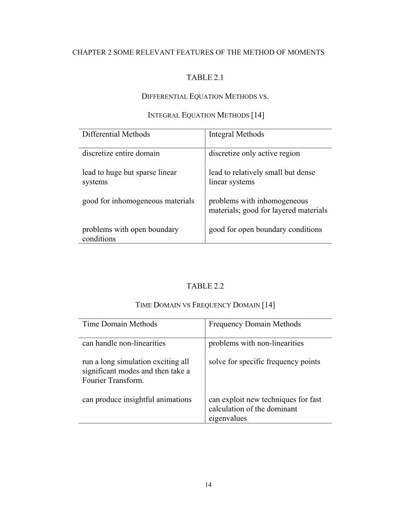
In the above sense, the MoM is an integral equation method for the
frequency-domain analysis. Table 2.1 and Table 2.2 give the basic features of the
integral methods versus the differential-methods and the frequency-domain
methods versus the time domain methods, respectively [14].
In the MoM, only the surfaces of the objects are discretized. The linear
system resulting from the discretization is much smaller compared to the FDTD
and the FEM system matrices. The system is unfortunately very dense, because

CHAPTER 2 SOME RELEVANT FEATURES OF THE METHOD OF MOMENTS
13
every surface element interacts with every other surface element. This method is
ideal for open field environment simulations and can handle very efficiently
antenna application.
2.2 CPU TIME COST VERSUS MESH DENSITY [15]
The CPU time for a MoM simulation can be expressed as
2 3CPU time = + + + A BN CN DN (2.2)
where N is the number of unknowns. A, B, C and D are constants independent of
N. A accounts for the simulation set-up time. The meshing of the structure leads to
the linear term BN. The filling of the system matrix is responsible for the
quadratic term, and solving the matrix equation for the cubic term. The values of
A, B, C and D depend on the problem at hand.
The quadratic and cubic terms dominate. For small to medium size
problems, as the constant C is much larger than D, the solution time is dominated
by the matrix fill. For large scale problems, the matrix solving time with its cubic
term will eventually dominate the CPU-time cost. Thus, for medium to large scale
problems, the time saving by using coarse-mesh coarse models will be significant.
CHAPTER 2 SOME RELEVANT FEATURES OF THE METHOD OF MOMENTS
14
TABLE 2.1
DIFFERENTIAL EQUATION METHODS VS.
INTEGRAL EQUATION METHODS [14]
Differential Methods Integral Methods
discretize entire domain discretize only active region
lead to huge but sparse linear systems
lead to relatively small but dense linear systems
good for inhomogeneous materials problems with inhomogeneous materials; good for layered materials
problems with open boundary conditions
good for open boundary conditions
TABLE 2.2
TIME DOMAIN VS FREQUENCY DOMAIN [14]
Time Domain Methods Frequency Domain Methods
can handle non-linearities problems with non-linearities
run a long simulation exciting all significant modes and then take a Fourier Transform.
solve for specific frequency points
can produce insightful animations can exploit new techniques for fast calculation of the dominant eigenvalues

CHAPTER 2 SOME RELEVANT FEATURES OF THE METHOD OF MOMENTS
15
2.3 MESH REFINEMENT [16]
The accuracy of any simulation is dependent on the quality of the
approximations being made. In the method of moments, the surface currents are
approximated by a set of currents over a number of surface triangles.
Frequency domain models (including the finite element method and the
method of moments) should be checked for mesh convergence. This is done by
varying the size of the mesh element from one simulation to the next, and keeping
all other model parameters the same. The results of these two simulations can
then be compared. If there is a significant difference in the results, the surfaces
are not adequately discretized and a finer mesh is needed.
The most common way to do a mesh convergence test is to reduce the
global size of the mesh element. However, global refinement results in additional
resource requirement throughout the model. This is a very safe way of checking
convergence, but experienced users will be able to make a very good guess about
where refinement might be necessary. In these cases, it would be far more
efficient to refine the mesh locally, rather than globally.
2.4 MODELING OF DIELECTRIC MATERIALS [17][18]
Today’s EM problems are very complex in general. It is vital to take into
account the effects of lossy dielectric and magnetic materials into account, such
as antenna radomes, dielectric substrates, biological tissue, etc. The traditional
Special Green’s Functions technique, which only models the metallic surface,

CHAPTER 2 SOME RELEVANT FEATURES OF THE METHOD OF MOMENTS
16
cannot fulfill such requirements. Techniques based on the volume or surface
equivalent principles within the MoM aim at solving such problems.
I. The Special Green’s Function technique.
A Green’s function describes the response in space to a point excitation or
source. The simplest form of a Green’s function is the free space Green’s
function. It is possible to use a Special Green’s Function to incorporate features of
the propagation space into the model. Only the surface of metallic meshes has to
be modeled. This means that the properties of the remainder of the structure are
modeled implicitly, which is very computer resource efficient but is limited to a
few special cases, such as the layered dielectrics.
II. The Surface Equivalent Principle (SEP) technique.
The MoM for metallic structures solves for the electric currents on the
surface of all metallic objects in order to determine the electromagnetic
observables, e.g., current densities at the port. When using the SEP, the surfaces
of a dielectric are discretised for both the electric and the magnetic currents on the
surface. All sides of a dielectric have to be modeled, making a closed solid. This
means that there are now two basis functions for each triangle pair which
correlates to a memory requirement of four times what it would be if the same
structure was metallic.
One can imagine that for a planar structure with a finite ground, the
Special Green’s Function technique provides an efficient but less accurate
solution, since an infinite ground plane is assumed. In contrast, since the SEP

CHAPTER 2 SOME RELEVANT FEATURES OF THE METHOD OF MOMENTS
17
model takes the finite ground effects into account by modeling all metallic and
dielectric surfaces, its solution is accurate but more time-consuming.
In the double annular ring antenna example in Section 5.5.1, we use the
Special Green’s Function as the coarse model and the SEP as the fine model.
Then we optimize its S-parameter in an efficient way by exploiting the space
mapping technique.
CHAPTER 2 SOME RELEVANT FEATURES OF THE METHOD OF MOMENTS
18
REFERENCES
[1] Agilent ADS, Agilent Technologies, 1400 Fountaingrove Parkway, Santa Rosa, CA 95403-1799, USA.
[2] em, Sonnet Software, Inc., 100 Elwood Davis Road, North Syracuse, NY
13212, USA. [3] Ansoft Ensemble, Ansoft Corporation, 225 West Station Square Drive,
Suite 200, Pittsburgh, PA 15219, USA. [4] FEKO, Suite 4.2, June 2004, EM Software & Systems-S.A. (Pty) Ltd, 32
Techno lane, Technopark, Stellenbosch, 7600, South Africa. [5] N.K. Nikolova, J. Zhu, D. Li, M.H. Bakr and J.W. Bandler, “Sensitivity
analysis of network parameters with electromagnetic frequency-domain simulators,” IEEE Trans. Microwave Theory Tech., vol. 54, Feb. 2006, pp. 670-681.
[6] N.K. Nikolova, J. Zhu, D. Li and M.H. Bakr, “Extracting the derivatives
of network parameters from frequency-domain electromagnetic solutions,” the XXVIIIth General Assembly of the International Union of Radio Science, Oct. 2005.
[7] J. Zhu, N.K. Nikolova and J. W. Bandler, “Self-adjoint sensitivity analysis
of high-frequency structures with FEKO,” the 22nd International Review of Progress in Applied Computational Electromagnetics Society (ACES 2006), Miami, Florida, pp. 877-880.
[8] D. Li, J. Zhu, N.K. Nikolova, M.H. Bakr and J.W. Bandler, “EM
optimization using sensitivity analysis in the frequency domain,” submitted to IEEE Trans. Antennas Propagat., Special Issue on Synthesis and Optimization Techniques in Electromagnetics and Antenna System Design, Jan. 2007.
[9] J. Zhu, J.W. Bandler, N.K. Nikolova and S. Koziel, “Antenna optimization
through space mapping,” submitted to IEEE Trans. Antennas Propagat., Special Issue on Synthesis and Optimization Techniques in Electromagnetics and Antenna System Design, Jan. 2007.
[10] J. Zhu, J. W. Bandler, N. K. Nikolova and S. Koziel, “Antenna design
through space mapping optimization,” IEEE MTT-S Int. Microwave Symp., San Francisco, California, 2006.
CHAPTER 2 SOME RELEVANT FEATURES OF THE METHOD OF MOMENTS
19
[11] R.F. Harrington, Field Computation by Moment Methods, New York, NY:
Macmillan, 1968. [12] D.G. Swanson, Jr. and W.J.R. Hoefer, Microwave Circuit Modeling Using
Electromagnetic Field Simulation, Artech House, Boston. London, 2003. [13] C.A. Balanis, Antenna Theory: Analysis and Design, New York: Wiley,
1997. [14] L. Daniel, Simulation and Modeling Techniques for Signal Integrity and
Electromagnetic Interference on High Frequency Electronic Systems, PhD Thesis, Electrical Engineering and Computer Science, University of California at Berkeley.
[15] Advanced Design System 2003C, User’s Manual, Agilent Technologies,
395 Page Mill Road, Palo Alto, CA 94304, USA. [16] “Mesh refinement,” FEKO Quarterly, December 2004. [17] “Modelling of dielectric materials in FEKO,” FEKO Quarterly, Mar.
2005. [18] U. Jakobus, “Comparison of different techniques for the treatment of lossy
dielectric/magnetic bodies within the method of moments formulation,” AEÜ International Journal of Electronics and Communications, vol. 54, 2000, pp. 163-173.

CHAPTER 2 SOME RELEVANT FEATURES OF THE METHOD OF MOMENTS
20

21
PART I
SENSITIVITY ANALYSIS IN THE
FREQUENCY DOMAIN

22

23
CHAPTER 3
SELF-ADJOINT SENSITIVITY
ANALYSIS IN THE METHOD OF
MOMENTS
3.1 INTRODUCTION
The goal of frequency domain sensitivity analysis is to evaluate the
gradient of the response of a system to variations of its design parameters [1]. In
high-frequency structure analysis, the design parameters typically describe the
structure’s geometry and the electromagnetic properties of the media involved.
The computation of the gradient is often carried out using finite
differences where the structure is analyzed an additional time for each
independent variable. It should be obvious that this approach is viable only when
the requirements of an analysis in terms of CPU times and computer memory are
reasonably small [2].
The adjoint-variable method is known to be the most efficient approach to
design sensitivity analysis for problems of high complexity where the number of

CHAPTER 3 SELF-ADJOINT SENSITIVITY … METHOD OF MOMENTS
24
state variables is much greater than the number of the required response
derivatives [3]-[5]. General adjoint-based methodologies have been available for
some time in control theory [3], and techniques complementary to the finite-
element method (FEM) have been developed in structural [4],[5] and electrical
[6]-[11] engineering. However, feasible implementations remain a challenge. The
reason lies mainly in the complexity of these techniques.
Recently, a simpler and more versatile approach has been adopted [1]
[12]-[13] for analyses with the MoM and the frequency-domain transmission-line
method. The effort to formulate analytically the system matrix derivative—which
is an essential component of the sensitivity formula—was abandoned as
impractical for a general-purpose sensitivity solver. Instead, approximations of
the system-matrix derivatives are employed using either finite differences [1] or
discrete step-wise changes [12], [13] as dictated by the nature of the discretization
grid. Neither the accuracy nor the computational speed is sacrificed.
All of the above approaches require the analysis of an adjoint problem
whose excitation is response dependent. Not only does this mean one additional
full-wave simulation but it also requires modification of the EM analysis engine
due to the specifics of the adjoint-problem excitation. Notably, Akel et al. [8] has
pointed out that in the case of the FEM with tetrahedral edge elements, the
sensitivity of the S-matrix can be derived without an adjoint simulation.
Here, we formulate a general self-adjoint approach to the sensitivity
analysis of network parameters [14]-[16]. It requires neither an adjoint problem

CHAPTER 3 SELF-ADJOINT SENSITIVITY … METHOD OF MOMENTS
25
nor analytical system matrix derivatives. We focus on the linear problem in the
method of moments, which is at the core of a number of commercial high-
frequency simulators. Thus, for the first time, we suggest practical and fast
sensitivity solutions realized entirely outside the framework of the EM solver.
These standalone algorithms can be incorporated in an automated design to
perform optimization, modeling, or tolerance analysis of high-frequency
structures with any commercial solver, which exports the system matrix and the
solution vector.
In the next section, we state the adjoint-based sensitivity formula and the
definition of a self-adjoint problem. We then introduce the self-adjoint formulas
for network-parameter sensitivity calculations. We outline the features of the
commercial EM solvers, which enable independent network-parameter sensitivity
analysis. Numerical validation and comparisons are presented in Section 3.5.
Section 3.6 discusses the computational overhead associated with the sensitivity
analysis. We give recommendations for further reduction of the computational
cost whenever software changes are possible, and conclude with a summary.
3.2 FREQUENCY DOMAIN ADJOINT VARIABLE
METHOD [14]

CHAPTER 3 SELF-ADJOINT SENSITIVITY … METHOD OF MOMENTS
26
3.2.1 Sensitivities of Linear Complex Systems [14]
A time-harmonic EM problem involving linear materials can be cast in a
linear system of complex equations by the use of a variety of numerical
techniques:
=Ax b (3.1)
The system matrix M M×∈A is a function of the shape and material parameters,
some of which comprise the vector of designable parameters 1N×∈p , i.e., A(p).
Thus, the vector of state variables 1M ×∈x is a function of p, x(p). The right-
hand side b results from the EM excitation and/or the inhomogeneous boundary
conditions. Typically, in a problem of finding the sensitivities of network
parameters, b is independent of p, because the waveguide structures launching the
incident waves (the ports) serve as a reference and are not a subject to design
changes: ∇ = 0pb .
For the purposes of optimization, the system performance is evaluated
through a scalar real-valued objective function ( , )F x p . In tolerance analysis or
model generation, we may consider a set of responses, some of which are
complex. We first consider a single, possibly complex, function F, and we refer to
it as the response. It is computed from the solution x of (3.1) for a given design.
Through x, F is an implicit function of p. It may also have an explicit
dependence on p. Explicit dependence on a shape parameter ip ( / 0eiF p∂ ∂ ≠ )
arises when F depends on the field/current solution at points whose coordinates in

CHAPTER 3 SELF-ADJOINT SENSITIVITY … METHOD OF MOMENTS
27
space are affected by a change in ip . An example is the explicit dependence of an
antenna gain on the position/shape of the wires [1] carrying the radiating currents.
Explicit dependence with respect to a material parameter arises when F depends
on the field/current solution at points whose constitutive parameters are affected
by its change. An example is the stored energy in a volume of changing
permittivity. The network parameters, however, are computed from the solution at
the ports, whose shape and materials do not change. Thus, when F is a network
parameter, e F∇ = 0p .
The derivatives of a complex response R IF F jF= + ( 1j = − ) with
respect to the design parameters 1[ ]TNp p=p can be efficiently calculated
using the adjoint-variable sensitivity formula [11][13]:
ˆ , 1, 2, ,e
T
i i i i
F F i Np p p p
⎛ ⎞∂ ∂ ∂ ∂= + ⋅ − ⋅ =⎜ ⎟∂ ∂ ∂ ∂⎝ ⎠…b Ax x . (3.2)
In a compact gradient notation, (3.2) becomes
( )ˆe TF F∇ = ∇ + ⋅∇ −p p px b Ax (3.3)
We refer to F∇ p as the response sensitivity. The adjoint-variable vector
x is the solution to
ˆ ( )T TF =⋅ = ∇x x xA x (3.4)
where F∇x is a row of the derivatives of F with respect to the state variables ix ,
1, ,i M= … , evaluated at the current solution =x x . In the case of complex
systems, it involves the real Rx and the imaginary Ix parts of the state variables.

CHAPTER 3 SELF-ADJOINT SENSITIVITY … METHOD OF MOMENTS
28
As detailed in [13], the complex-response analysis (3.2)-(3.4) is valid if F
is an analytic function of the state variables x, in which case, the Cauchy-
Riemann conditions [17] are fulfilled. A convenient form of the adjoint excitation
ˆ ( )TF= ∇xb is
1 1
ˆ ( ) ( )RR R R R
TR I R I T T
M M
F F F Fj j F Fx x x x
⎡ ⎤⎛ ⎞ ⎛ ⎞∂ ∂ ∂ ∂= + + = ∇ = ∇⎢ ⎥⎜ ⎟ ⎜ ⎟∂ ∂ ∂ ∂⎝ ⎠ ⎝ ⎠⎣ ⎦x xb (3.5)
3.2.2 Sensitivity Expression for Linear-network Parameters [14]
For a network parameter sensitivity, the gradients ∇ pb and e F∇ p in (3.3)
vanish, which leads to the sensitivity expression
( )ˆTF∇ = − ⋅∇p px Ax . (3.6)
We emphasize that in (3.6) x is fixed, and only A is differentiated, as in (3.2).
The sensitivity formula (3.6) uses three quantities: the solution x of the
original problem (3.1), the set of system matrix derivatives / ip∂ ∂A , 1, ,i N= … ,
and the solution x to the adjoint problem (3.4). The first one is available from the
EM simulation. Also, we assume that the system matrix derivatives have been
already computed, e.g., using finite differences [1] or Broyden’s update [18][19].
We next show that in the case of the network parameters, the adjoint solution x is
equal to x multiplied by a complex factor κ . Thus, the solution of (3.4) is
unnecessary. We employ the above adjoint-variable theory to determine κ for
different network parameters. For that, we also need to know the dependence of
CHAPTER 3 SELF-ADJOINT SENSITIVITY … METHOD OF MOMENTS
29
the particular network parameter on the distributed field/current solution. We
discuss this dependence below.
3.3 NETWORK PARAMETER SENSITIVITIES WITH
CURRENT SOLUTIONS
3.3.1 Sensitivities of S-parameters
The S-parameters in the MoM depend on the current density solutions
produced by the MoM solvers through simple linear relations. More specifically,
the current solution at the ports is needed.
We implement our technique through FEKO® [20]. FEKO is primarily an
antenna CAD software. It uses the EFIE for metallic objects, and the EFIE with
specialized Green’s functions for planar layered (printed) circuits. For dielectric
objects, it uses a coupled field integral equation (PMCHW) technique. It also
employs a fast multipole method (MLFMM) for large problems (does not support
specialized Green’s functions).
Consider the calculation of the S-parameters of a network of system
impedance 0Z by FEKO:
0 ,2 k jkj kj e
j
Z IS
Vδ= − , , 1, ,j k K= … . (3.7)
Here, ejV is the jth port voltage source (usually set equal to 1) of internal
impedance 0Z , and ,k jI is the resulting current at the kth port when the jth port is

CHAPTER 3 SELF-ADJOINT SENSITIVITY … METHOD OF MOMENTS
30
excited (the rest of the ports are loaded with 0Z ). The right-hand side of (3.1)
corresponding to ejV is bj.
If the structure consists of thin wires discretized into segments, the
currents ,k jI are the elements of the solution vector jx obtained with j=b b .
Then, each partial derivative
0
,
2kje
k j j
S ZI V
∂= −
∂, , 1, ,j k K= … (3.8)
gives the only nonzero element of the respective adjoint excitation vector kjb . Its
position corresponds exactly to the position of the only nonzero element ekV of
the original excitation at the kth port kb . This is because ,k jI is computed at the
very same segment where ekV is applied when the kth port is excited. Thus,
0
2ˆ kj ke ejk
ZV V
= −b b , , 1, ,j k K= … (3.9)
If the structure and in particular its ports involve planar or curved metallic
surfaces, FEKO applies triangular surface elements accordingly, and computes
the surface current distribution [20]. In this case, each of the port currents is
obtained from the current densities at the edge of its port:
, ,k
i ik j k j k
iI J l
∈= ∆∑
S, , 1, ,j k K= … (3.10)
where k denotes the port where the current is computed, and j denotes the port
being excited. ,ik jJ is the component of the surface current density normal to the

CHAPTER 3 SELF-ADJOINT SENSITIVITY … METHOD OF MOMENTS
31
edge of the ith element of port k whose length is ikl∆ . The current densities ,
ik jJ ,
ki ∈S , are elements of the solution vector jx , where kS is the set of their
indices.
We compute the elements of the adjoint excitation vector ˆkjb as the
derivatives of kjS with respect to ,ik jJ , ki ∈S :
0,( ) ( )
,
2ˆ[ ] kjkj i k ij j
ek i
S Zb lJ V
∂= = − ⋅∆
∂, ki ∈S . (3.11)
All elements, for which ki ∉S , are zero.
On the other hand, the excitation vector kb , corresponding to the kth port
excitation of the original problem, also has nonzero elements, whose indices are
those in kS . Moreover, to ensure uniform excitation across the port, these
excitation elements are equal to the applied excitation voltage ekV , scaled by the
edge element ikl∆ [21]:
[ ] e ik i k kb V l= ⋅∆ , ki ∈S . (3.12)
Comparing (3.11) and (3.12), we conclude that the adjoint vectors kjb relate to
the original excitation ( )kb as in (3.9).
If the MoM matrix fulfills the symmetry condition T=A A , the adjoint
solution vectors ˆkjx , , 1, ,j k K= … , obtained from the adjoint excitations ˆ kjb
relate to the original solution vectors kx , 1, ,k K= … , as

CHAPTER 3 SELF-ADJOINT SENSITIVITY … METHOD OF MOMENTS
32
ˆkj kj kκ= ⋅x x , 0( ) ( )2
kj k je e
ZV V
κ = − . (3.13)
However, the matrices arising in the large variety of MoM techniques are
not always symmetric when a non-uniform unstructured mesh is used, which is
the usual case. It would seem that in the case of an asymmetric MoM matrix, the
solution of the adjoint problem is unavoidable. On the other hand, a linear EM
problem is intrinsically reciprocal, and in the limit of an infinitely fine mesh, the
MoM techniques tend to produce nearly symmetrical system matrices. In Section
3.7, we show an important result: if the mesh is fine enough to achieve a solution
convergence error below 10 %, then the asymmetry of the system matrix is
negligibly small as far as the sensitivity calculation is concerned. Consequently,
the self-adjoint sensitivity analysis using (3.13) is adequate with a convergent
MoM solution. Its sensitivities are practically indistinguishable from those
produced by solving the adjoint problem.
To summarize the above theory, we state the sensitivity formula for the
self-adjoint S-parameter problem:
( )( )Tkj kj k jS κ∇ = − ⋅∇p px Ax , , 1, ,j k K= … (3.14)
Here, kjκ is a constant, which depends on the powers incident upon the jth and
kth ports, as per (3.13).
3.3.2 Input Impedance Sensitivities
The S-parameters relate to all other types of network parameters through

CHAPTER 3 SELF-ADJOINT SENSITIVITY … METHOD OF MOMENTS
33
known analytical formulas [22]. Thus, the S-parameter sensitivities can be
converted to any other type of network-parameter sensitivities using chain
differentiation.
On the other hand, the MoM is well suited for the computation of the input
impedance inZ of one-port structures, e.g., antennas. Input-impedance
sensitivities have been already considered in [1], [18] and [19]. There, however,
the self-adjoint nature of the problem has not been recognized. As a result, the
implementation uses in-house MoM codes, which are modified to carry out the
adjoint-problem solution.
Below, we give the coefficient κ in the self-adjoint sensitivity expression
for inZ computed with the MoM. Making use of the MoM port representation
explained previously, the relation between the adjoint and the original excitation
vectors is obtained as
2ˆinI −= − ⋅b b (3.15)
regardless of whether the port consists of a single or multiple wire segments or
metallic triangles. Thus, the self-adjoint sensitivity formula for inZ is the same as
(3.14) after replacing kjS with inZ and kjκ with 2inI −− . Here, inI is the complex
current at the port known already from the system analysis.
3.4 GENERAL PROCEDURE
Assume that the basic steps in the EM structure analysis have already been

CHAPTER 3 SELF-ADJOINT SENSITIVITY … METHOD OF MOMENTS
34
carried out. These include:
(1) A geometrical model of the structure has been built through the
graphic user interface of the simulator;
(2) A mesh has been generated;
(3) The system matrix A has been assembled;
(4) The system equations have been solved for all K port excitations,
and the original solution vectors kx , 1, ,k K= … , of the nominal
structure have been found with sufficient accuracy.
The self-adjoint sensitivity analysis is then carried out with the following
steps:
Step 1 Parameterization: identify design parameters ip , 1, ,i = … N;
Step 2 Generation of matrix derivatives;
Step 3 Sensitivity computations: use (3.14) with the proper constant κ .
To get the derivative of the system matrix at Step 2, we perturb the
structure slightly for each ip , (with about 1 % of the nominal ip value) while
keeping the other parameters at their nominal values. We re-generate the system
matrix ( )ii ip+ ∆ ⋅A = A p u , where iu is a 1N × vector whose elements are all
zero except the ith one, 1iu = . We compute the N derivatives of the system
matrix via finite differences:
i
i i ip p p∂ ∆ −≈ =∂ ∆ ∆
A A A A , 1, ,i N= … (3.16)
CHAPTER 3 SELF-ADJOINT SENSITIVITY … METHOD OF MOMENTS
35
Note that (3.16) is applicable only if A and iA are of the same size, i.e.,
the two respective meshes contain the same number of nodes and elements.
Moreover, the numbering of these nodes and elements must correspond to the
same locations (within the prescribed perturbation) in the original and perturbed
structures.
3.5 SOFTWARE REQUIREMENTS AND
IMPLEMENTATION IN FEKO
3.5.1 Software Requirements
The above steps show that the EM simulator must have certain features,
which enable the self-adjoint sensitivity analysis.
(1) It must be able to export the system matrix so that the user can
compute the system matrix derivatives with (3.16).
(2) It must allow some control over the mesh generation, so that (3.16)
is physically meaningful.
(3) It must export the field/current solution vector so that we can
compute the sensitivities with (3.14).
The second and third features are available with practically all commercial
EM simulators. The first feature deserves more attention. In the MoM, the matrix
is dense, and writing to the disk may be time consuming. Also, only a few of the
commercial simulators give access to the generated system matrices. This is the

CHAPTER 3 SELF-ADJOINT SENSITIVITY … METHOD OF MOMENTS
36
reason why our numerical experiments are carried out with FEKO. This solver is
based on the MoM, and it has the option to export the system matrix to a file
stored to the disk. It also exports the solution vector with the computed current
distribution.
3.5.2 Implementation in FEKO
A. Data Extraction
FEKO provides a PS Card, which allows us to export the system matrix
and the solution (current vector I ). They are stored in *.mat file and *.str file,
respectively. The *.mat is a binary file, written on the Intel platform. It has a
Fortran block structure using the double complex data type. We can read such
data through MatLab. Special care must be taken:
1) Before we access the matrix, 19 4× bytes offsets must be skipped
immediately after opening the binary files.
2) Each record is 8 bytes longer than the actual data (4 bytes before and 4 bytes
after the data). So for instance for a matrix with 21 21× elements the length
of the file is not 21 21 16 7056× × = bytes (16 for double complex), but
rather
21 8 for each record 21 21 16 for the actual matrix 7224 bytes.
×+ × ×=
B. Mesh Control

CHAPTER 3 SELF-ADJOINT SENSITIVITY … METHOD OF MOMENTS
37
FEKO defines its mesh by setting the maximum mesh edge size for each
geometrical part. We could assign a different maximum mesh edge size for each
part. Within each part, the size of the mesh edge is the same. For example, let the
design parameter be the length of the microstrip line shown in Fig. 1. At the ith
iteration, the length is iL and at the (i + 1)th iteration, the length increases to 1iL + .
We usually define the maximum size along the y-axis at the ith iteration as
, 1, 2 , , i
iy
LL i nN
∆ = = … (3.17)
where n is the maximum iteration number and N is the number of mesh edges
along the y-axis.
In this definition, the number of mesh edges along the y-axis remains N,
regardless of the value of iL , see Fig. 3.1.
1i iL L L+ = + ∆
i
iy
LLN
∆ =
iL
1
1i
iy
LLN+
+∆ =
Fig. 3.1. Demonstration of mesh control in FEKO.
3.6 VALIDATION

CHAPTER 3 SELF-ADJOINT SENSITIVITY … METHOD OF MOMENTS
38
We compute the network-parameter sensitivities with our self-adjoint
formula and compare the results with those obtained by a forward finite-
difference approximation applied directly at the level of the response. This second
approach requires a full-wave simulation for each designable parameter. In all
plots, our results are marked with SASA (for self-adjoint sensitivity analysis),
while the results obtained through direct finite differencing are marked with FD.
Our self-adjoint results are compared with the response derivatives obtained with
the finite-difference approximation, which uses 1 % parameter perturbation.
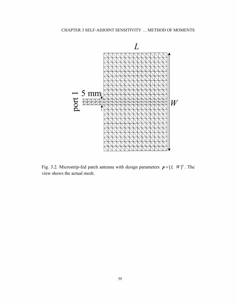
3.6.1 Input Impedance Sensitivities of a Microstrip-Fed Patch Antenna
The microstrip-fed patch antenna [18] is printed on a substrate of relative
dielectric constant 2.32rε = and height 1.59h = mm. The design parameters are
its width W and length L shown in Fig. 3.2. The figure shows also the mesh of the
metal layer. We compute the sensitivities of the antenna input impedance inZ .
Our derivatives with respect to the antenna length L ( 45 55L≤ ≤ mm) for a width
85W = mm and a frequency of 2.0 GHz are plotted together with the finite-
difference results in Fig. 3.3.
CHAPTER 3 SELF-ADJOINT SENSITIVITY … METHOD OF MOMENTS
39
L
Wport
1 5 mm
Fig. 3.2. Microstrip-fed patch antenna with design parameters [ ]TL W=p . The view shows the actual mesh.
CHAPTER 3 SELF-ADJOINT SENSITIVITY … METHOD OF MOMENTS
40
0.045 0.047 0.049 0.051 0.053 0.055-3
-2.5
-2
-1.5
-1
-0.5
0
0.5
1
1.5 x 10⁵
L (m)
deriv
ativ
e ( Ω
⋅m-1
)
Re Zin (FD)
Re Zin (SASA)
Im Zin (FD)
Im Zin (SASA)
Derivatives of:
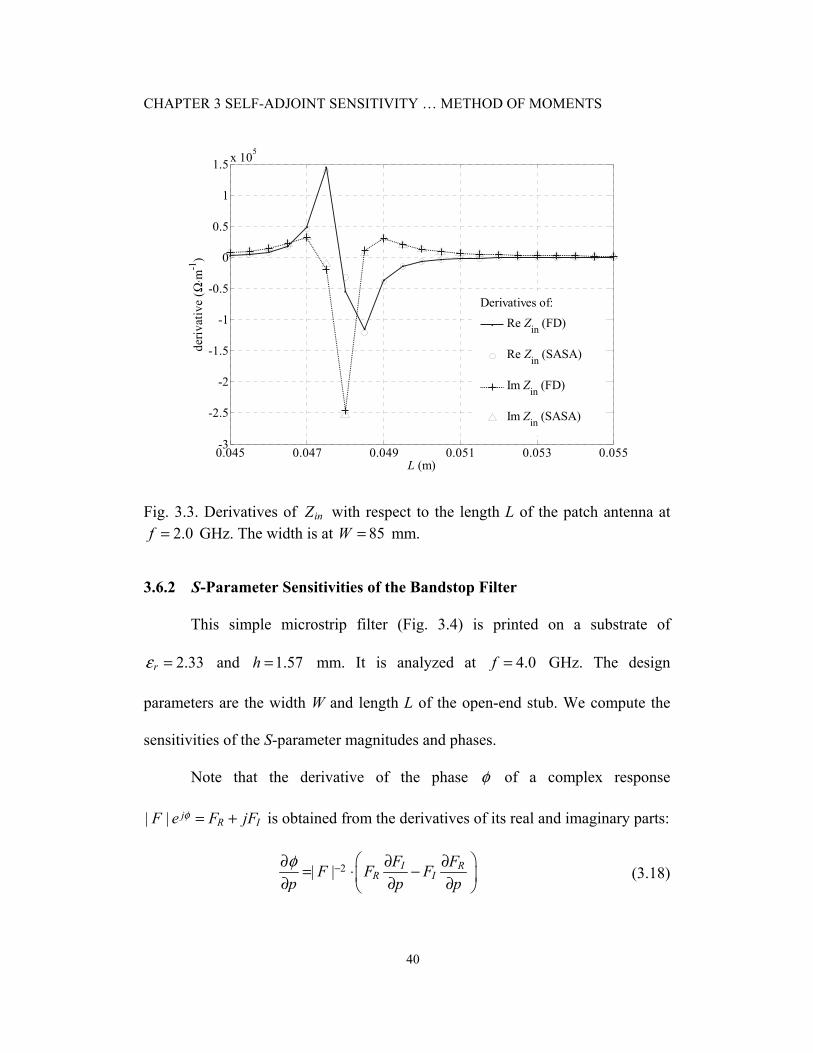
Fig. 3.3. Derivatives of inZ with respect to the length L of the patch antenna at 2.0f = GHz. The width is at 85W = mm.
3.6.2 S-Parameter Sensitivities of the Bandstop Filter
This simple microstrip filter (Fig. 3.4) is printed on a substrate of
2.33rε = and 1.57h = mm. It is analyzed at 4.0f = GHz. The design
parameters are the width W and length L of the open-end stub. We compute the
sensitivities of the S-parameter magnitudes and phases.
Note that the derivative of the phase φ of a complex response
| | jR IF e F jFφ = + is obtained from the derivatives of its real and imaginary parts:
2| | I RR I
F FF F Fp p pφ − ⎛ ⎞∂ ∂ ∂= ⋅ −⎜ ⎟∂ ∂ ∂⎝ ⎠
(3.18)
CHAPTER 3 SELF-ADJOINT SENSITIVITY … METHOD OF MOMENTS
41
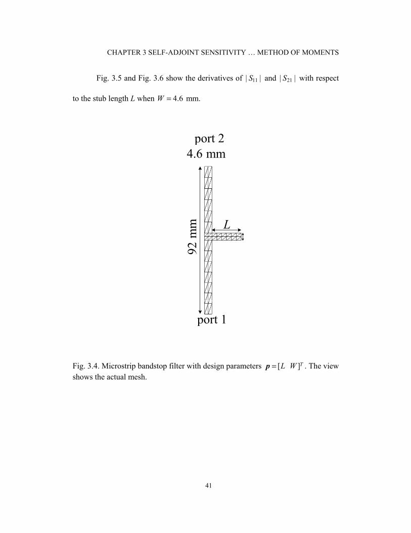
Fig. 3.5 and Fig. 3.6 show the derivatives of 11| |S and 21| |S with respect
to the stub length L when 4.6W = mm.
L
port 1
port 2
92 m
m
4.6 mm
Fig. 3.4. Microstrip bandstop filter with design parameters [ ]TL W=p . The view shows the actual mesh.
CHAPTER 3 SELF-ADJOINT SENSITIVITY … METHOD OF MOMENTS
42
0.01 0.0125 0.015 0.0175 0.02 0.0225 0.025-250
-200
-150
-100
-50
0
50
100
150
200
250
L (m)
deriv
ativ
e (m
-1)
S11 (FD)
S11 (SASA)
S21 (FD)
S21 (SASA)
Derivatives of:
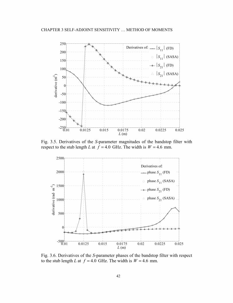
Fig. 3.5. Derivatives of the S-parameter magnitudes of the bandstop filter with respect to the stub length L at 4.0f = GHz. The width is 4.6W = mm.
0.01 0.0125 0.015 0.0175 0.02 0.0225 0.025-500
0
500
1000
1500
2000
2500
L (m)
deriv
ativ
e (r
ad ⋅ m
-1)
phase S11 (FD)
phase S11 (SASA)
phase S21 (FD)
phase S21 (SASA)
Derivatives of:
Fig. 3.6. Derivatives of the S-parameter phases of the bandstop filter with respect to the stub length L at 4.0f = GHz. The width is 4.6W = mm.

CHAPTER 3 SELF-ADJOINT SENSITIVITY … METHOD OF MOMENTS
43
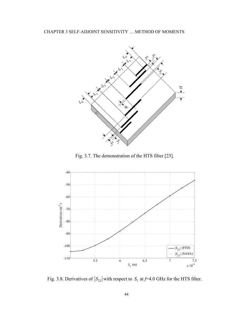
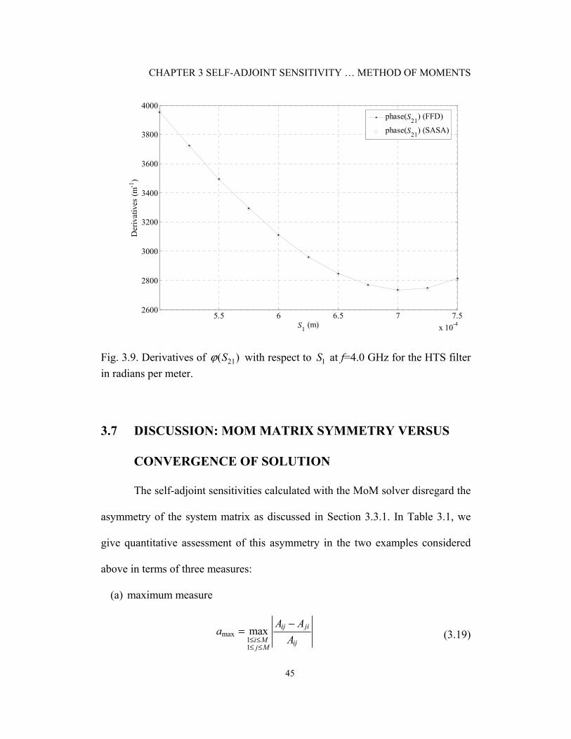
3.6.3 S-Parameter Sensitivities of the HTS Filter
We consider the high-temperature superconducting (HTS) bandpass filter
of [23][24] (see the inset of Fig. 3.7). This filter is printed on a substrate with
relative dielectric constant 23.425rε = , height 0.508 mmh = and substrate
dielectric loss tangent of 53 10−× . Design variables are the lengths of the coupled
lines and the separations between them, namely, 1 2 3 1 2 3[ ]TS S S L L L=p . The
length of the input and output lines is 0 1.27 mmL = . The lines are of width
0.1778 mmW = . The filter is analyzed at 4.0 GHzf = . The derivatives of the
system matrix are derived with 1 % perturbations. We compute the self-adjoint
sensitivities of the S21 magnitude and phase, and compare it with the finite-
difference approach with the same perturbations. Fig. 3.8 shows the derivatives of
21S with respect to the spacing between the first coupled lines 1S
( 10.5 0.75 mmS≤ ≤ ) when 2 3 1 2 3[ ]TS S L L L =[2.3764 2.6634 4.7523 4.8590
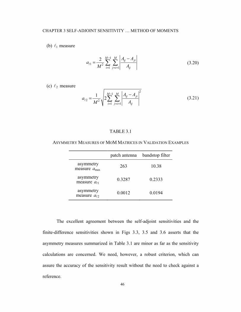
4.7490]T . Fig. 3.9 shows the derivatives of the respective phase. Good agreement
is observed between the self-adjoint derivatives and the respective finite-
difference estimates.
CHAPTER 3 SELF-ADJOINT SENSITIVITY … METHOD OF MOMENTS
44
Fig. 3.7. The demonstration of the HTS filter [23].
5.5 6 6.5 7 7.5x 10⁻⁴
-110
-100
-90
-80
-70
-60
-50
-40
S1 (m)
Der
ivat
ives
(m-1
)
|S21| (FFD)
|S21| (SASA)
Fig. 3.8. Derivatives of 21S with respect to 1S at f=4.0 GHz for the HTS filter.
CHAPTER 3 SELF-ADJOINT SENSITIVITY … METHOD OF MOMENTS
45
5.5 6 6.5 7 7.5x 10⁻⁴
2600
2800
3000
3200
3400
3600
3800
4000
S1 (m)
Der
ivat
ives
(m-1
)
phase(S21) (FFD)
phase(S21) (SASA)
Fig. 3.9. Derivatives of 21( )Sϕ with respect to 1S at f=4.0 GHz for the HTS filter in radians per meter.
3.7 DISCUSSION: MOM MATRIX SYMMETRY VERSUS
CONVERGENCE OF SOLUTION
The self-adjoint sensitivities calculated with the MoM solver disregard the
asymmetry of the system matrix as discussed in Section 3.3.1. In Table 3.1, we
give quantitative assessment of this asymmetry in the two examples considered
above in terms of three measures:
(a) maximum measure
max11
max ij ji
i M ijj M
A Aa
A≤ ≤≤ ≤
−= (3.19)
CHAPTER 3 SELF-ADJOINT SENSITIVITY … METHOD OF MOMENTS
46
(b) 1 measure
1
1 21 1
2 M Mij ji
i j i ij
A Aa
AM
−
= = +
−= ∑ ∑ (3.20)
(c) 2 measure
21
2 21 1
1 2M M
ij ji
i j i ij
A Aa
AM
−
= = +
−= ∑ ∑ (3.21)
TABLE 3.1
ASYMMETRY MEASURES OF MOM MATRICES IN VALIDATION EXAMPLES
patch antenna bandstop filter
asymmetry measure maxa 263 10.38
asymmetry measure 1a 0.3287 0.2333
asymmetry measure 2a 0.0012 0.0194
The excellent agreement between the self-adjoint sensitivities and the
finite-difference sensitivities shown in Figs 3.3, 3.5 and 3.6 asserts that the
asymmetry measures summarized in Table 3.1 are minor as far as the sensitivity
calculations are concerned. We need, however, a robust criterion, which can
assure the accuracy of the sensitivity result without the need to check against a
reference.

CHAPTER 3 SELF-ADJOINT SENSITIVITY … METHOD OF MOMENTS
47
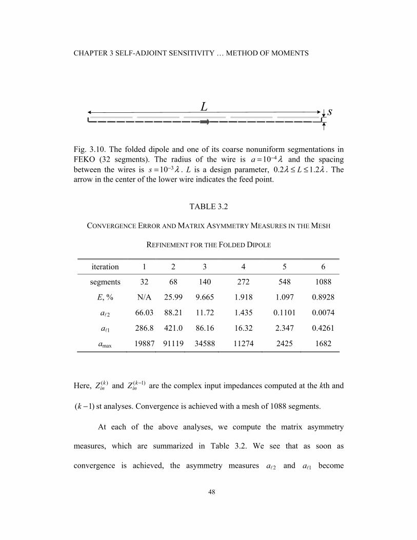
We carry out the following experiment. We analyze the folded dipole
shown in Fig. 3.10. The radius of the wire is 410a λ−= and the spacing between
the two wires is 310s λ−= . The length L varies from 0.2λ to 1.2λ . The response
is the antenna input impedance inZ . We force the maximum segment size on one
of the two parallel wires to be 5 times larger than that on the other wire. This
leads to very different segment lengths along the two parallel wires [see Fig.
3.10]. Since the two wires are very close, the MoM matrix is quite asymmetric.
We emphasize that this is an abnormal (not recommended) segmentation allowing
us to investigate a worst-case scenario. Normally, the user sets a global maximum
segment length, which is applied to the entire structure, the result being a
relatively uniform segmentation or mesh.
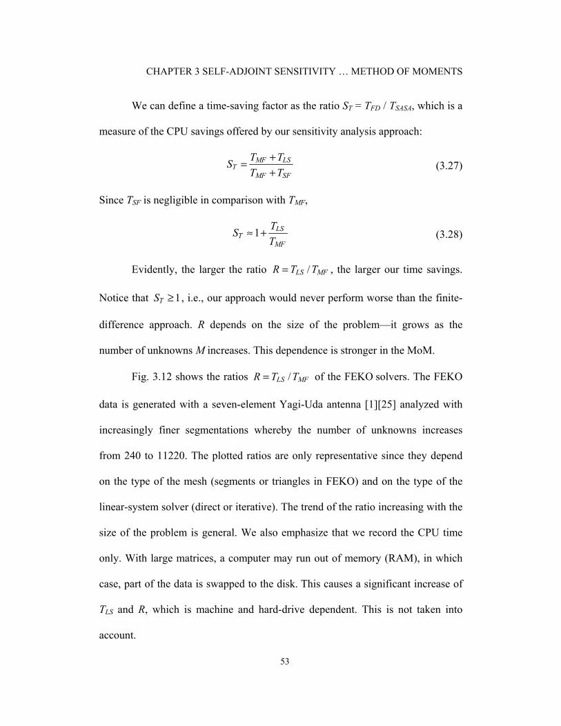
We next perform mesh refinement starting from a coarse mesh of 32
segments. Each iteration of the mesh refinement involves: 1) a decrease of the
mesh elements by a certain factor, and 2) full-wave analysis with the current
mesh. We decrease the maximum element size by approximately 50 % for each of
the two parallel wires of the folded dipole. The ratio of 5 between them is
preserved. The mesh refinement continues until a convergence error less than 1 %
is achieved. The convergence error at the kth iteration is defined as
( ) ( 1)( )
( )100
k kin ink
kin
Z ZE
Z
−−= ⋅ % (3.22)
CHAPTER 3 SELF-ADJOINT SENSITIVITY … METHOD OF MOMENTS
48
L s
Fig. 3.10. The folded dipole and one of its coarse nonuniform segmentations in FEKO (32 segments). The radius of the wire is 410a λ−= and the spacing between the wires is 310s λ−= . L is a design parameter, 0.2 1.2Lλ λ≤ ≤ . The arrow in the center of the lower wire indicates the feed point.
TABLE 3.2
CONVERGENCE ERROR AND MATRIX ASYMMETRY MEASURES IN THE MESH
REFINEMENT FOR THE FOLDED DIPOLE
iteration 1 2 3 4 5 6
segments 32 68 140 272 548 1088
E, % N/A 25.99 9.665 1.918 1.097 0.8928
2a 66.03 88.21 11.72 1.435 0.1101 0.0074
1a 286.8 421.0 86.16 16.32 2.347 0.4261
maxa 19887 91119 34588 11274 2425 1682
Here, ( )kinZ and ( 1)k
inZ − are the complex input impedances computed at the kth and
( 1)k − st analyses. Convergence is achieved with a mesh of 1088 segments.
At each of the above analyses, we compute the matrix asymmetry
measures, which are summarized in Table 3.2. We see that as soon as
convergence is achieved, the asymmetry measures 2a and 1a become

CHAPTER 3 SELF-ADJOINT SENSITIVITY … METHOD OF MOMENTS
49
comparable to those in the validation examples [see Table 3.1].
At every iteration of the mesh refinement, we also compute the derivative
/inZ L∂ ∂ (at 0.5L λ= ) with our self-adjoint approach, i.e., ignoring the system
matrix asymmetry. We compare the self-adjoint result for each mesh with its
respective reference sensitivity. The reference sensitivity is computed with our
original adjoint technique, which solves the adjoint problem, i.e., it fully accounts
for the asymmetry of the system matrix. We define the asymmetry error in the
computed response derivative D as
| | 100| |D
D DeD−= ⋅ % (3.23)
where D is the reference derivative.
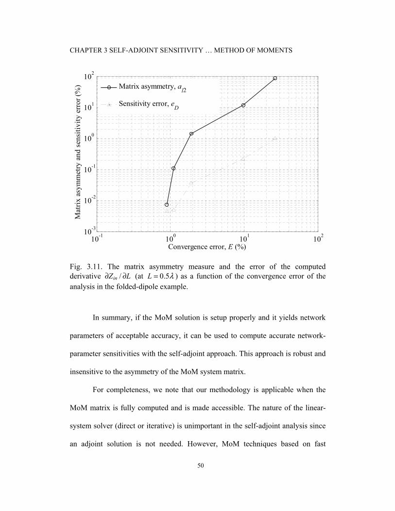
In Fig. 3.11, we plot the asymmetry derivative error De for /inZ L∂ ∂ and
the matrix asymmetry measure 2a versus the convergence error E of the MoM
solution [see (3.22)]. First, we see that 2a increases as the convergence error E
increases with a slope, which is very similar to that of De (unlike 1a and maxa ).
Apparently, 2a is the matrix asymmetry measure, which can serve as a criterion
for an accurate self-adjoint sensitivity calculation. As long as its value is below 2
%, we can expect eD to be well below 1 %. Second, we conclude that as soon as
an acceptable convergence is achieved in the response calculation ( 10E ≤ %), we
can have confidence in the self-adjoint response sensitivity calculation since its
asymmetry error De is well below E, typically by two orders of magnitude.
CHAPTER 3 SELF-ADJOINT SENSITIVITY … METHOD OF MOMENTS
50
10-1 100 101 10210-3
10-2
10-1
100
101
102
Convergence error, E (%)
Mat
rix a
sym
met
ry a
nd s
ensi
tivity
err
or (%
) Matrix asymmetry, al2
Sensitivity error, eD
Fig. 3.11. The matrix asymmetry measure and the error of the computed derivative /inZ L∂ ∂ (at 0.5L λ= ) as a function of the convergence error of the analysis in the folded-dipole example.
In summary, if the MoM solution is setup properly and it yields network
parameters of acceptable accuracy, it can be used to compute accurate network-
parameter sensitivities with the self-adjoint approach. This approach is robust and
insensitive to the asymmetry of the MoM system matrix.
For completeness, we note that our methodology is applicable when the
MoM matrix is fully computed and is made accessible. The nature of the linear-
system solver (direct or iterative) is unimportant in the self-adjoint analysis since
an adjoint solution is not needed. However, MoM techniques based on fast

CHAPTER 3 SELF-ADJOINT SENSITIVITY … METHOD OF MOMENTS
51
multipole expansions never fully compute the matrix and are thus not well suited
for adjoint-based sensitivity analysis. For them, specialized adjoint-based
algorithms need to be developed and, at this stage, applications with commercial
solvers do not seem feasible. Response sensitivities with finite differences,
however, are an option.
3.8 COMPUTATIONAL OVERHEAD OF THE SELF-
ADJOINT SENSITIVITY ANALYSIS
The computational overhead associated with the self-adjoint sensitivity
analysis is due to two types of calculations: 1) the system matrix derivatives,
/ ip∂ ∂A , 1, ,i N= … , and 2) the row-matrix-column multiplications involved in
the sensitivity formula (3.14). Compared to the full-wave analysis, the sensitivity
formula (3.14) requires insignificant CPU time, which is often neglected. We
denote the time required to compute one derivative with the sensitivity formula as
SFT . In comparison, the calculation of the N system matrix derivatives is much
more time consuming. Whether it employs finite differences or analytical
expressions, it is roughly equivalent to N matrix fills. A matrix fill, especially in
the MoM, can be time-consuming. We denote the time for one matrix fill as MFT .
Thus, the overhead time required by the self-adjoint sensitivity analysis is
SASA MF SFT N T N T= ⋅ + ⋅ (3.24)
On the other hand, if we employ forward finite differences directly at the
CHAPTER 3 SELF-ADJOINT SENSITIVITY … METHOD OF MOMENTS
52
level of the response in order to compute the N derivatives of the network
parameters, we need N additional full analyses, each involving a matrix fill and a
linear system solution. Thus, the overhead of the finite-difference sensitivity
analysis is
FD MF LST N T N T= ⋅ + ⋅ (3.25)
where TLS is the time required to solve (3.1).
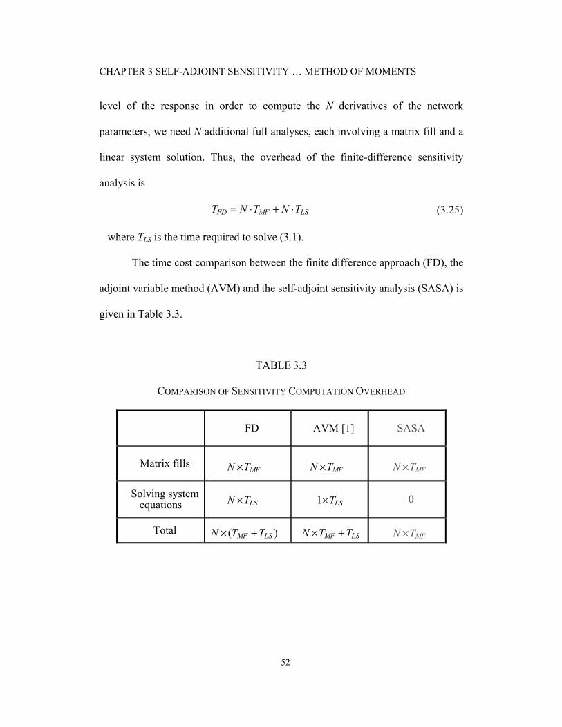
The time cost comparison between the finite difference approach (FD), the
adjoint variable method (AVM) and the self-adjoint sensitivity analysis (SASA) is
given in Table 3.3.
TABLE 3.3
COMPARISON OF SENSITIVITY COMPUTATION OVERHEAD
FD AVM [1] SASA
Matrix fills
Solving system equations
0
Total
MFN T× MFN T× MFN T×
LSN T× 1 LST×
( )MF LSN T T× + MF LSN T T× + MFN T×
CHAPTER 3 SELF-ADJOINT SENSITIVITY … METHOD OF MOMENTS
53
We can define a time-saving factor as the ratio ST = TFD / TSASA, which is a
measure of the CPU savings offered by our sensitivity analysis approach:
MF LST
MF SF
T TST T
+=+
(3.27)
Since TSF is negligible in comparison with TMF,
1 LST
MF
TST
≈ + (3.28)
Evidently, the larger the ratio /LS MFR T T= , the larger our time savings.
Notice that 1TS ≥ , i.e., our approach would never perform worse than the finite-
difference approach. R depends on the size of the problem—it grows as the
number of unknowns M increases. This dependence is stronger in the MoM.
Fig. 3.12 shows the ratios /LS MFR T T= of the FEKO solvers. The FEKO
data is generated with a seven-element Yagi-Uda antenna [1][25] analyzed with
increasingly finer segmentations whereby the number of unknowns increases
from 240 to 11220. The plotted ratios are only representative since they depend
on the type of the mesh (segments or triangles in FEKO) and on the type of the
linear-system solver (direct or iterative). The trend of the ratio increasing with the
size of the problem is general. We also emphasize that we record the CPU time
only. With large matrices, a computer may run out of memory (RAM), in which
case, part of the data is swapped to the disk. This causes a significant increase of
TLS and R, which is machine and hard-drive dependent. This is not taken into
account.

CHAPTER 3 SELF-ADJOINT SENSITIVITY … METHOD OF MOMENTS
54
In Table 3.4, we show the actual CPU time spent for response sensitivity
calculations with our self-adjoint approach and the finite-difference
approximation using the FEKO solver. We consider the case of one design
parameter ( 1N = ), i.e., a single derivative is computed. The size of the system M
varies. The increase of the time-saving factor TS as the number of unknowns
increases corresponds closely to the ratio curves /LS MFR T T= plotted in Fig. 3.12
in accordance with (3.28). The analyzed structures are the same as those used to
investigate the /LS MFT T ratios.
We also carry out a time comparison between our approach and the finite-
difference approach when the size of the system M is fixed but the number of
design parameters N varies. The MoM results are summarized in Table 3.5. As
predicted by (3.28), the time savings are practically independent of the number of
design parameters.
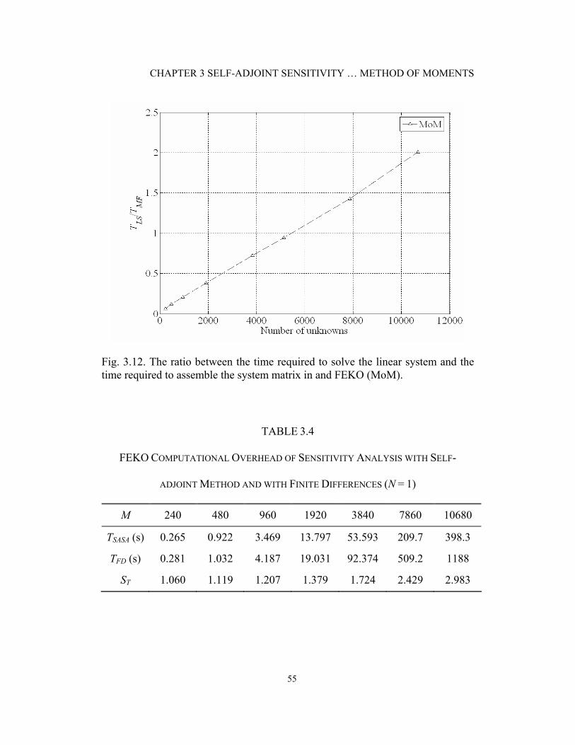
CHAPTER 3 SELF-ADJOINT SENSITIVITY … METHOD OF MOMENTS
55
Fig. 3.12. The ratio between the time required to solve the linear system and the time required to assemble the system matrix in and FEKO (MoM).
TABLE 3.4
FEKO COMPUTATIONAL OVERHEAD OF SENSITIVITY ANALYSIS WITH SELF-
ADJOINT METHOD AND WITH FINITE DIFFERENCES (N = 1)
M 240 480 960 1920 3840 7860 10680
TSASA (s) 0.265 0.922 3.469 13.797 53.593 209.7 398.3
TFD (s) 0.281 1.032 4.187 19.031 92.374 509.2 1188
ST 1.060 1.119 1.207 1.379 1.724 2.429 2.983

CHAPTER 3 SELF-ADJOINT SENSITIVITY … METHOD OF MOMENTS
56
TABLE 3.5
FEKO COMPUTATIONAL OVERHEAD OF SENSITIVITY ANALYSIS WITH SELF-
ADJOINT METHOD AND WITH FINITE DIFFERENCES (M = 10680)
N 1 3 5 7 9 11
TSASA (s) 398.34 1193.7 1988.0 2782.3 3576.4 4371.3
TFD (s) 1188.3 3560.0 5925.8 8292.1 10660 13024
ST 2.9831 2.9823 2.9808 2.9803 2.9807 2.9794
3.9 CONCLUDING REMARKS
We re-iterate that in optimization, the Broyden update is a far more efficient
alternative to the computation of the system matrix derivatives [18][19][26]. With
it, TS becomes roughly proportional to ( ) /MF LS SFT T T+ , which is normally a
very large ratio. The application of this algorithm in optimization is to be
discussed in the following chapter.
CHAPTER 3 SELF-ADJOINT SENSITIVITY … METHOD OF MOMENTS
57
REFERENCES
[1] N.K. Georgieva, S. Glavic, M.H. Bakr, and J.W. Bandler, “Feasible adjoint sensitivity technique for EM design optimization,” IEEE Trans. Microwave Theory Tech., vol. 50, Dec. 2002, pp. 2751-2758.
[2] S. Amari, “Numerical cost of gradient computation within the method of
moments and its reduction by means of a novel boundary-layer concept,” IEEE MTT-S Int. Microwave Symp. Digest, 2001, pp.1945-1948.
[3] D.G. Cacuci, Sensitivity & Uncertainty Analysis, Volume 1: Theory. Boca
Raton, FL: Chapman & Hall/CRC, 2003. [4] A.D Belegundu and T.R. Chandrupatla, Optimization Concepts and
Applications in Engineering. Upper Saddle River, NJ: Prentice-Hall, 1999. [5] E.J. Haug, K.K. Choi, and V. Komkov, Design Sensitivity Analysis of
Structural Systems. Orlando, FL: Academic, 1986. [6] P. Neittaanmäki, M. Rudnicki, and A. Savini, Inverse Problems and
Optimal Design in Electricity and Magnetism. New York: Oxford University Press, 1996, Chapter 4.
[7] Hong-bae Lee and T. Itoh, “A systematic optimum design of waveguide-
to-microstrip transition,” IEEE Trans. Microwave Theory Tech., vol. 45, May 1997, pp. 803-809.
[8] H. Akel and J.P. Webb, “Design sensitivities for scattering-matrix
calculation with tetrahedral edge elements,” IEEE Trans. Magnetics, vol. 36, July 2000, pp. 1043-1046.
[9] J.P. Webb, “Design sensitivity of frequency response in 3-D finite-
element analysis of microwave devices,” IEEE Trans. Magnetics, vol. 38, Mar. 2002, pp. 1109-1112.
[10] Y.S. Chung, C. Cheon, I.H. Park and S.Y. Hahn, “Optimal design method
for microwave device using time domain method and design sensitivity analysis—part I: FETD case,” IEEE Trans. Magnetics, vol. 37, Sep. 2001, pp. 3289-3293.
[11] N.K. Nikolova, J.W. Bandler and M.H. Bakr, “Adjoint techniques for
sensitivity analysis in high-frequency structure CAD,” IEEE Trans. Microwave Theory Tech., vol. 52, Jan. 2004, pp. 403-419.
CHAPTER 3 SELF-ADJOINT SENSITIVITY … METHOD OF MOMENTS
58
[12] S.M. Ali, N.K. Nikolova and M.H. Bakr, “Recent advances in sensitivity
analysis with frequency-domain full-wave EM solvers,” Applied Computational Electromagnetics Society Journal, vol. 19, Nov. 2004, pp. 147-154.
[13] M.H. Bakr and N.K. Nikolova, “An adjoint variable method for frequency
domain TLM problems with conducting boundaries,” IEEE Microwave and Wireless Components Letters, vol. 13, Sept. 2003, pp. 408-410.
[14] N.K. Nikolova, J. Zhu, D. Li, M.H. Bakr and J.W. Bandler, “Sensitivity
analysis of network parameters with electromagnetic frequency-domain simulators,” IEEE Trans. Microwave Theory Tech., vol. 54, Feb. 2006, pp. 670-681.
[15] J. Zhu, N.K. Nikolova and J. W. Bandler, “Self-adjoint sensitivity analysis
of high-frequency structures with FEKO,” the 22nd International Review of Progress in Applied Computational Electromagnetics Society (ACES 2006), Miami, Florida, pp. 877-880.
[16] N.K. Nikolova, J. Zhu, D. Li and M.H. Bakr, “Extracting the derivatives
of network parameters from frequency-domain electromagnetic solutions,” the XXVIIIth General Assembly of the International Union of Radio Science, CDROM, Oct. 2005.
[17] M.D. Greenberg, Advanced Engineering Mathematics. Upper Saddle
River, N.J.: Prentice Hall, 1998, pp. 1138-1140. [18] N.K. Nikolova, R. Safian, E.A. Soliman, M.H. Bakr and J.W. Bandler,
“Accelerated gradient based optimization using adjoint sensitivities,” IEEE Trans. Antennas Propagat., vol. 52, Aug. 2004, pp. 2147-2157.
[19] E.A. Soliman, M.H. Bakr and N.K. Nikolova, “Accelerated gradient-based
optimization of planar circuits,” IEEE Trans. Antennas Propagat., vol. 53, Feb. 2005, pp. 880-883.
[20] FEKO® User’s Manual, Suite 4.2, June 2004, EM Software & Systems-
S.A. (Pty) Ltd, 32 Techno lane, Technopark, Stellenbosch, 7600, South Africa, http://www.feko.info. In the USA: EM Software & Systems (USA), Inc., 24 Research Drive, Hampton, VA 23666, USA, http://www.emssusa.com/.
CHAPTER 3 SELF-ADJOINT SENSITIVITY … METHOD OF MOMENTS
59
[21] J. Zhu, “Sensitivity analysis of high-frequency structures with commercial software based on the method of moments,” Computational Electromagnetics Res. Lab., McMaster University, CEM-R-23, June 2005.
[22] D. M. Pozar, Microwave Engineering, 2nd ed., New York: John Wiley &
Sons, 1998, Chapter 4. [23] J.W. Bandler, R.M. Biernacki, S.H. Chen, W.J. Getsinger, P. A. Grobelny,
C. Moskowitz and S.H. Talisa, “Electromagnetic design of high temperature superconducting microwave filters,” Int. J. RF Microwave Computer-Aided Eng., vol. 5, 1995, pp. 331-343.
[24] J.W. Bandler, Q.S. Cheng, N.K. Nikolova and M.A. Ismail, “Implicit
space mapping optimization exploiting preassigned parameters,” IEEE Trans. Microw. Theory Tech., vol. 52, no. 1, Jan. 2004, pp. 378-385.
[25] J. Zhu, “Time comparison and error estimation of the self-adjoint
sensitivity analysis of network parameters with the method of moments,” Computational Electromagnetics Res. Lab., McMaster University, CEM-R-24, June 2005.
[26] D. Li, J. Zhu, N.K. Nikolova, M.H. Bakr and J.W. Bandler, “EM
optimization using sensitivity analysis in the frequency domain,” submitted to IEEE Trans. Antennas Propagat., Special Issue on Synthesis and Optimization Techniques in Electromagnetics and Antenna System Design, Jan. 2007.

CHAPTER 3 SELF-ADJOINT SENSITIVITY … METHOD OF MOMENTS
60
61
CHAPTER 4
EM OPTIMIZATION USING
SENSITIVITY ANALYSIS IN THE
FREQUENCY DOMAIN
4.1 INTRODUCTION
The previous implementation of the self-adjoint sensitivity analysis
(SASA) technique provides us with accurate sensitivities in an efficient way.
Sensitivities can be used for gradient-based optimization algorithms based on
quasi-Newton, sequential quadratic programming (SQP) and trust-region
methods, which need the objective function Jacobian and/or Hessian in addition
to the objective function itself. These optimization methods search for a local
optimal point. A gradient-based algorithm is expected to converge much faster,
i.e., with fewer system analyses, than non-gradient optimization algorithms. Its
drawback is that a global minimum is not guaranteed, and failure to converge is a
possibility. Naturally, the solution provided by a gradient-based local
optimization algorithm depends on the quality of the initial design. For a realistic

CHAPTER 4 EM OPTIMIZATION … THE FREQUENCY DOMAIN
62
3D EM-based design problem with an acceptable starting point, gradient-based
optimization is to be preferred [1].
The efficiency of a successful gradient-based optimization process
depends mainly on two factors: (1) the number of the iterations required to
achieve convergence, and (2) the number of simulation calls per iteration. The
first factor depends largely on the nature of the algorithm, on the proper
formulation of the objective or cost function, and the accuracy of the response
Jacobians and/or Hessian. The second factor depends mostly on the method used
to compute the Jacobians and/or Hessian, which are necessary to determine the
search direction and the step in the design parameter space.
The sensitivity analysis, which provides the Jacobians through response-
level approximations, is very time consuming. Our self-adjoint sensitivity
analysis method [2]-[5] discussed in the last chapter, produces the response and
its Jacobian with a single full-wave analysis when the objective function depends
on the network parameters, e.g., the S-parameters and the input impedance. The
major overhead of the sensitivity computation with this technique is due to the
computation of the system matrix derivatives, whose overhead is equivalent to N
matrix fills. N is the number of design parameters. A fast approach to the
derivatives of the system matrix becomes necessary.
In this chapter, we firstly review the previous work related to the
evaluation of the derivatives of the system matrix. Then, we propose a hybrid
approach (B/FD-SASA) which employs both the finite-difference self-adjoint

CHAPTER 4 EM OPTIMIZATION … THE FREQUENCY DOMAIN
63
sensitivity analysis (FD-SASA) method and Broyden-update self-adjoint
sensitivity analysis (B-SASA) method. The latter is especially suitable for
gradient-based EM optimization [1]. We develop a set of criteria for switching
back and forth throughout the optimization process between the robust but more
time-demanding FD-SASA and the B-SASA. This hybrid technique guarantees
good accuracy of the gradient information with minimal computational time.
We implement our technique in the MoM through FEKO. We demonstrate
our approach through the optimization of a double annular ring antenna. We
compare its optimization performance with FD-SASA.
4.2 THE DERIVATIVES OF THE SYSTEM MATRIX [6]
In the self-adjoint sensitivity analysis, it is necessary to evaluate the
derivatives of the system matrix with respect to all the design variables
1 2[ ]Tnp p p= …p :
, 1, 2, , i
i np
∂ =∂
…A . (4.1)
There are several ways to obtain the derivatives of the system matrix [6][7].
Method 1: The analytical derivatives of the system matrix A with respect
to the design variables—if available—lead to exact response sensitivities.
However, the analytical form of system matrix is hard to be determined in the
general case.
CHAPTER 4 EM OPTIMIZATION … THE FREQUENCY DOMAIN
64
Method 2: Forward finite differences give the simplest procedure. The
sensitivities are calculated by:
( ) ( ) , 1, 2 i i
i i
p i np p
∂ + ∆ −= =∂ ∆
…A A p e A p (4.2)
where
0
th row1
0
i i
⎡ ⎤⎢ ⎥⎢ ⎥⎢ ⎥=⎢ ⎥⎢ ⎥⎢ ⎥⎣ ⎦
e . (4.3)
The self-adjoint sensitivity analysis using finite differences to evaluate the
derivatives of the system matrix is referred to as FD-SASA. It provides accurate
sensitivity and therefore is often used as a reference [2]-[5].
Method 3: The boundary-layer concept (BLC). The BLC in sensitivity
analysis was first proposed by Amari [8]. It can be applied with solvers which
allow non-uniform discretization and/or unstructured grids, e.g., the FEM and the
MoM [7]. The idea is to perturb a certain geometrical parameter (the design
parameter ip ) of a structure by respective deformations of as few grid elements
as possible. This makes most of the system matrix coefficients insensitive to the
perturbation. Consequently, the matrix derivative ip
∂∂
A is mostly sparse and
only few nonzero coefficients need to be calculated. This is in contrast with
Method 2, where full remeshing is applied to the perturbed structure, which

CHAPTER 4 EM OPTIMIZATION … THE FREQUENCY DOMAIN
65
results in a full ip
∂∂
A matrix. In this method, we must have full control over the
meshing.
Method 4: The Broyden update is discussed in Section 4.3.
4.3 SENSITIVITY ANALYSIS IN THE METHOD OF
MOMENTS EXPLOITING THE BROYDEN UPDATE
Since in the FD-SASA the derivatives of the system matrix are computed
with a finite-difference approximation, it requires at least N matrix fills. To
eliminate this overhead, here, we compute the system matrix derivative applying
Broyden’s formula [9] to the elements of A
( )
( )( ) ( ) ( )( 1) ( )
( )( ) ( )
( ) ( ), 1, ,
k
kk k kjk k
jj kik T k
i i
hp
h i Np p
+⎛ ⎞∂+ − − ⎜ ⎟∂⎛ ⎞ ⎛ ⎞∂ ∂ ⎝ ⎠= + =⎜ ⎟ ⎜ ⎟∂ ∂⎝ ⎠ ⎝ ⎠
∑…
AA p h A pA A
h h.
(4.4
)
( )( )kA p is the system matrix at the kth iteration, when the design parameter space
is ( )kp , and ( )kh is the increment vector in the design parameter space between
the kth and (k+1)st iteration. The resulting sensitivity-analysis algorithm is
referred to as B-SASA. With it, the derivatives of the system matrix in the first
optimization iteration are obtained using a forward finite-difference
approximation. They are updated iteratively thereafter. The iterative update
requires negligible computational resources compared to a matrix fill.
CHAPTER 4 EM OPTIMIZATION … THE FREQUENCY DOMAIN
66
4.4 MIXED SELF-ADJOINT SENSITIVITY ANALYSIS
METHOD AND SWITCHING CRITERIA
The derivatives of the Broyden update are less accurate than those in the
FD-SASA [7]. The inaccuracy tends to be significant when the increment of the
design parameters is very small, e.g., near a local minimum, as catastrophic
cancellation occurs. We propose two criteria to switch from B-SASA to FD-
SASA:
1) ( ) ( 2)( ) ( )k kG G −>p p , or
2) ( )k d≤h .
Here G is the objective function and d is the minimum edge length of the
mesh elements. The algorithm checks the criteria at each iteration. After a switch
from B-SASA to FD-SASA occurs, only one optimization iteration is performed
with the FD-SASA, after which the algorithm returns to B-SASA. This B/FD-
SASA method is simple and guarantees acceptable accuracy of the system matrix
derivatives even for small increments in the design-parameter space.
4.5 EXAMPLE: THE OPTIMIZATION OF A DOUBLE
ANNULAR RING ANTENNA
We perform gradient-based optimization using the response Jacobian
provided by: (1) the proposed hybrid B/FD SASA approach, (2) the FD-SASA.
We compare the performance of the optimization algorithm with the three

CHAPTER 4 EM OPTIMIZATION … THE FREQUENCY DOMAIN
67
sensitivity-analysis approaches in terms of the number of iterations and the
overall CPU time.
We consider the stacked probe-fed printed annular ring antenna of [10],
which is shown in Fig. 4.1. The simulations are performed with FEKO [11]. The
antenna is printed on a printed circuit board (PCB) with 1 2.2rε = , 1 6.096d = mm
for the lower substrate, and 2 1.07rε = , 2 8.0d = mm for the upper substrate. The
dielectric loss tangent is 0.001 for both layers. The radius of the feed pin is
0 0.325r = mm. The design variables are the outer and inner radius of each ring
and the feed position, namely, 1 2 1 2[ ]Tpa a b b ρ=p . The design specification is
11 10 dB for 1.75 GHz 2.15 GHzS f≤ − ≤ ≤ .
Our technique requires the system matrix size fixed between iterations,
regardless of the variation in the design parameters. It is realized by local meshing
[12]. As shown in Fig. 4.2, the number of mesh edges along the five loops (thick
lines) is topologically fixed at 13, 19, 25, 32 and 39, respectively.
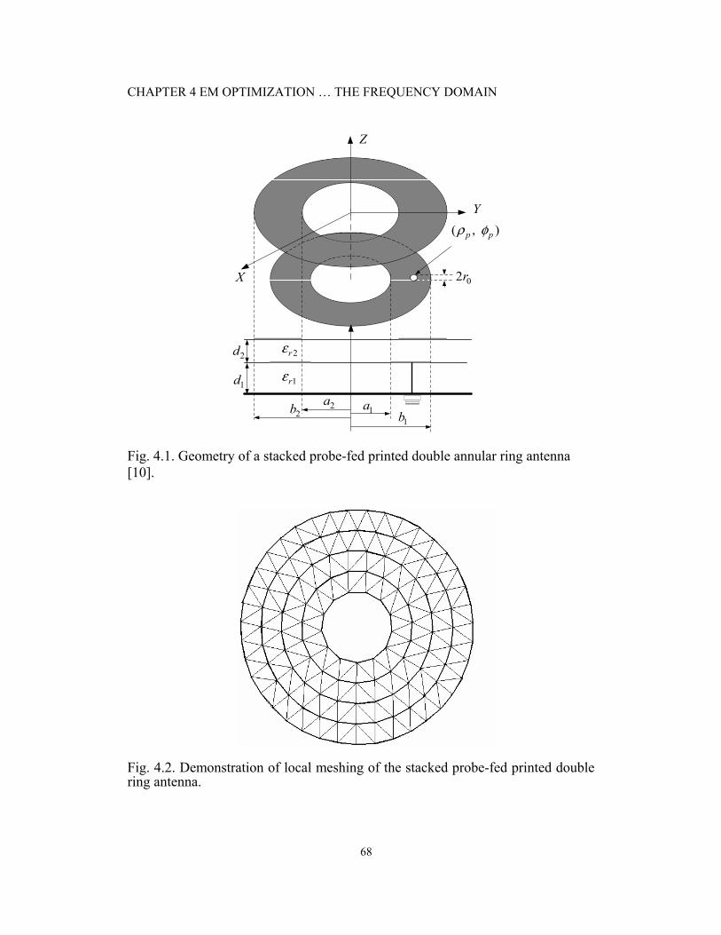
CHAPTER 4 EM OPTIMIZATION … THE FREQUENCY DOMAIN
68
2a2b 1a
1b
1d
2d
1rε
2rε
( , )p pρ φ
02r
Z
X
Y
Fig. 4.1. Geometry of a stacked probe-fed printed double annular ring antenna [10].
Fig. 4.2. Demonstration of local meshing of the stacked probe-fed printed double ring antenna.
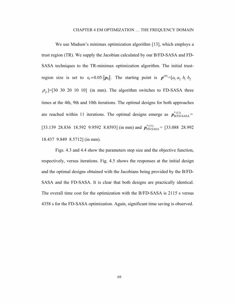
CHAPTER 4 EM OPTIMIZATION … THE FREQUENCY DOMAIN
69
We use Madsen’s minimax optimization algorithm [13], which employs a
trust region (TR). We supply the Jacobian calculated by our B/FD-SASA and FD-
SASA techniques to the TR-minimax optimization algorithm. The initial trust-
region size is set to 0 00.05r = ⋅ p . The starting point is (0)1 2 1 2=[ a a b bp
]=[30 30 20 10 10]pρ (in mm). The algorithm switches to FD-SASA three
times at the 4th, 9th and 10th iterations. The optimal designs for both approaches
are reached within 11 iterations. The optimal designs emerge as * (11)B/FD-SASA =p
[33.139 28.836 18.592 9.9592 8.8593] (in mm) and * (11)FD-SASA =p [33.088 28.992
18.437 9.849 8.5712] (in mm).
Figs. 4.3 and 4.4 show the parameters step size and the objective function,
respectively, versus iterations. Fig. 4.5 shows the responses at the initial design
and the optimal designs obtained with the Jacobians being provided by the B/FD-
SASA and the FD-SASA. It is clear that both designs are practically identical.
The overall time cost for the optimization with the B/FD-SASA is 2115 s versus
4358 s for the FD-SASA optimization. Again, significant time saving is observed.
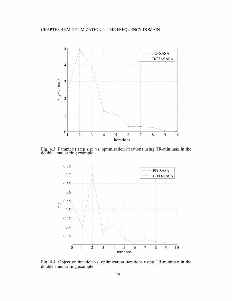
CHAPTER 4 EM OPTIMIZATION … THE FREQUENCY DOMAIN
70
1 2 3 4 5 6 7 8 9 100
1
2
3
4
5
Iterations
|x i+1-x
i| (m
m)
FD-SASAB/FD-SASA
Fig. 4.3. Parameter step size vs. optimization iterations using TR-minimax in the double annular ring example.
0 1 2 3 4 5 6 7 8 9 10
0.35
0.4
0.45
0.5
0.55
0.6
0.65
0.7
0.75
Iterations
f (x)
FD-SASAB/FD-SASA
Fig. 4.4. Objective function vs. optimization iterations using TR-minimax in the double annular ring example.
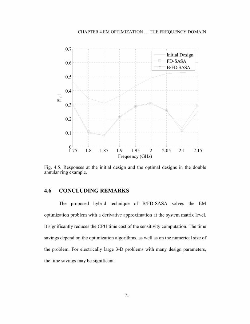
CHAPTER 4 EM OPTIMIZATION … THE FREQUENCY DOMAIN
71
1.75 1.8 1.85 1.9 1.95 2 2.05 2.1 2.150
0.1
0.2
0.3
0.4
0.5
0.6
0.7
Frequency (GHz)
|S11
|Initial DesignFD-SASAB/FD SASA
Fig. 4.5. Responses at the initial design and the optimal designs in the double annular ring example.
4.6 CONCLUDING REMARKS
The proposed hybrid technique of B/FD-SASA solves the EM
optimization problem with a derivative approximation at the system matrix level.
It significantly reduces the CPU time cost of the sensitivity computation. The time
savings depend on the optimization algorithms, as well as on the numerical size of
the problem. For electrically large 3-D problems with many design parameters,
the time savings may be significant.
CHAPTER 4 EM OPTIMIZATION … THE FREQUENCY DOMAIN
72
REFERENCES
[1] D. Li, J. Zhu, N.K. Nikolova, M.H. Bakr and J.W. Bandler, “EM
optimization using sensitivity analysis in the frequency domain,” submitted to IEEE Trans. Antennas Propagat., Special Issue on Synthesis and Optimization Techniques in Electromagnetics and Antenna System Design, Jan. 2007.
[2] N.K. Nikolova, J. Zhu, D. Li, M.H. Bakr and J.W. Bandler, “Sensitivity
analysis of network parameters with electromagnetic frequency-domain simulators,” IEEE Trans. Microwave Theory Tech., vol. 54, Feb. 2006, pp. 670-681.
[3] D. Li and N. K. Nikolova, “S-parameter sensitivity analysis of waveguide
structures with FEMLAB,” COMSOL Multiphysics Conf., Cambridge, MA, Oct. 2005, pp. 267-271.
[4] J. Zhu, N.K. Nikolova and J. W. Bandler, “Self-adjoint sensitivity analysis
of high-frequency structures with FEKO,” the 22nd International Review of Progress in Applied Computational Electromagnetics Society (ACES 2006), Miami, Florida, pp. 877-880.
[5] N.K. Nikolova, J. Zhu, D. Li and M.H. Bakr, “Extracting the derivatives
of network parameters from frequency-domain electromagnetic solutions,” the XXVIIIth General Assembly of the International Union of Radio Science, Oct. 2005.
[6] R. Safian, “Electromagnetic design sensitivity analysis exploiting the
Broyden update,” Master Thesis, Department of Electrical and Computer Engineering, McMaster University.
[7] N.K Nikolova, R. Safian, E.A. Soliman, M.H. Bakr and J.W. Bandler,
“Accelerated gradient based optimization using adjoint sensitivities,” IEEE Trans. Antenna Propagat. vol. 52, Aug. 2004, pp. 2147-2157.
[8] S. Amari, “Numerical cost of gradient computation within the method of
moments and its reduction by means of a novel boundary-layer concept,” in Proc. IEEE MTT-S Int. Symp. Dig., vol. 3, 2001, pp. 1945-1948.
[9] C. G. Broyden, “A class of methods for solving nonlinear simultaneous equations,” Mathematics of Computation, vol. 19, 1965, pp. 577-593.
CHAPTER 4 EM OPTIMIZATION … THE FREQUENCY DOMAIN
73
[10] D. M. Kotokoff, J. T. Aberle and R. B. Waterhouse, “Rigorous analysis of probe-fed printed annular ring antennas,” IEEE Trans. Antennas Propagat, vol. 47, Feb. 1999, pp. 384-388.
[11] FEKO® , User’s Manual, Suite 4.2, June 2004, EM Software & Systems-
S.A. (Pty) Ltd, 32 Techno Lane, Technopark, Stellenbosch, 7600, South Africa.
[12] “Mesh refinement,” FEKO Quarterly, Dec. 2004. [13] J.W. Bandler, W. Kellerman and K. Madsen, “A superlinearly convergent
minimax algorithm for microwave circuit design,” IEEE Trans. Microwave Theory Tech., vol. MTT-33, Dec. 1985, pp. 1519-1530.

CHAPTER 4 EM OPTIMIZATION … THE FREQUENCY DOMAIN
74

75
PART II
ANTENNA OPTIMIZATION
THROUGH SPACE MAPPING

76

77
CHAPTER 5
ANTENNA DESIGN THROUGH
SPACE MAPPING OPTIMIZATION
5.1 INTRODUCTION
The method of moments (MoM) is one of the most popular numerical
techniques for antenna and microwave device analysis. An accurate MoM
simulation is CPU intensive. This cost may be prohibitive for complex design
problems. Alternatively, a coarse mesh MoM simulation is fast but poor in
accuracy.
The space mapping (SM) technique takes advantage of the efficiency of a
coarse mesh MoM simulation and the accuracy of the fine mesh simulation. SM
aligns coarse models with fine models [1]-[8]. Here, the fine model is the fine
mesh MoM solution. The coarse model is the coarse mesh solution.
For the first time, we apply the SM technique to antenna design. Both fine
and coarse models are defined within FEKO [9]. We propose a new meshing
method. The topology of the mesh is preserved throughout the optimization which
CHAPTER 5 ANTENNA DESIGN THROUGH SPACE MAPPING OPTMIZATION
78
makes the coarse-model response in the design parameter space smooth and
consistent.
In the parameter extraction (PE) process, we implement implicit/input SM
and output SM sequentially [10]. In a preliminary PE, we roughly align the coarse
model with the fine model through implicit/input SM. Then output SM aims at
locally matching the surrogate with the fine model.
The novel SMF (Space Mapping Framework) system [11] implements our
approach. SMF is a prototype GUI (Graphical User Interface) oriented software
package that implements a number of SM optimization algorithms. The system
aims at making SM accessible to engineers inexperienced in space mapping. It
provides sockets to popular simulators (including FEKO, Sonnet em and ADS)
that allow automatic fine/coarse model data acquisition and, consequently, fully
automatic space mapping optimization. SMF also provides interfaces for SM
modeling and statistical analysis.
Two examples are given to demonstrate our approach. We consider a
double annular ring antenna and a patch antenna. In the first example, we exploit
the CPU-intensive surface equivalence principle (SEP) as a fine model and the
special Green’s function with a coarse mesh as a coarse model. The S-parameter
response is optimized in three iterations. In the second example, we optimize
impedance at a single frequency using two SM plans. The comparisons show a
larger time saving in SM plan I. At last, we discuss the coarseness in the coarse
model and its effect on the SM performance.

CHAPTER 5 ANTENNA DESIGN THROUGH SPACE MAPPING OPTMIZATION
79
5.2 COARSE MODEL AND FINE MODEL
As we discussed in Section 2.3, the mesh convergence needs to be
checked to get an accurate simulation result. This is done by refining the mesh
from one simulation to the next, and keeping all model parameters the same. If
the results are significantly different, the antenna surfaces are not adequately
discretized and we need to refine the mesh [12].
The coarse-mesh coarse model does not need to achieve mesh
convergence. Consequently, if the mesh topology and number of mesh elements
vary due to the variation of geometrical design parameters during optimization,
inconsistent results are obtained. To overcome this problem, we force the mesh
number and topology to remain unchanged during optimization. This is done by
local meshing in FEKO.
In the fine model, where mesh convergence is satisfied, we use global
meshing. We define the mesh density by the number of meshes per wavelength.

CHAPTER 5 ANTENNA DESIGN THROUGH SPACE MAPPING OPTMIZATION
80
5.3 SPACE MAPPING-BASED SURROGATE MODELS [7][8]
5.3.1 Mathematical Formulations
We are concerned with a class of optimization algorithms that exploit
surrogate models [13]. Let : mf fX R→R denote the response vector of the so-
called fine model of a given object, where nfX R⊆ . Our goal is to solve
arg min ( ( ))f f
f f fX
U∗
∈=
xx R x (5.1)
where U is a suitable objective function.
SM assumes the existence of a less accurate but much faster coarse
model. Let : mc c pX X R× →R denote the response vectors of the coarse model,
where Xc⊆Rn is the design variable domain (we assume here that Xc⊆Xf) and
Xp⊆Rq is the domain of auxiliary (preassigned) coarse model parameters. Typical
preassigned parameters px are the dielectric constant and the height of a
dielectric layer. By c∗x we denote the optimal solution of the coarse model, i.e.,
(0)arg min ( ( ))c
c c pX
U ,∗
∈xx R x x (5.2)
where (0)px denotes the initial preassigned parameter values.
We consider the fine model to be expensive to compute and solving (5.1)
by direct optimization to be impractical. Instead, we use surrogate models, i.e.,
models that are not as accurate as the fine model but are computationally cheap,
CHAPTER 5 ANTENNA DESIGN THROUGH SPACE MAPPING OPTMIZATION
81
hence suitable for iterative optimization. We consider an optimization algorithm
that generates a sequence of points ( ) , 1, 2, ,iff X i∈ = …x so that
( 1) ( )arg min ( ( ))c
i isf
XU+
∈=
xx R x . (5.3)
Here, ( ) :i ms cX R→R is the surrogate model at iteration i, which uses the coarse
model and the fine model data.
In this work, we use a surrogate model based on input SM [13], implicit
SM [2] and output SM [3]. The surrogate model at iteration i is defined as
( ) ( ) ( ) ( ) ( )( ) ( , )i i i i is c p= +R x R B x + c x ∆R (5.4)
where
( ) ( ) ( ) ( )
( , , )( , , ) arg min ( , , )
p
i i i ip pε=
B c xB c x B c x (5.5)
and
( ) ( ) ( ) ( ) ( ) ( ) ( )( ) ( , )i i i i i i ic pf f−f∆R = R x R B x + c x (5.6)
The matrices B(i)∈Mn×n, c(i)∈Mn×1, and the vector ( )ipx are obtained using
parameter extraction applied to the matching condition ε(i). Vector ∆R(i)∈Mm×1 is
calculated using formula (5.6) after having determined B(i), c(i) and xp(i). A general
form of the matching condition is
( ) ( ) ( ) ( )0
( , , ) || ( ) ( , ) ||ii k k kp k f f c f f pk
wε=
= − ⋅ + ⋅ +∑B c x R x R B x c G x x (5.7)
In our examples we use w1=1 and wk=0, k=2,…,i (i.e., we only use the last
iteration point to match the models).
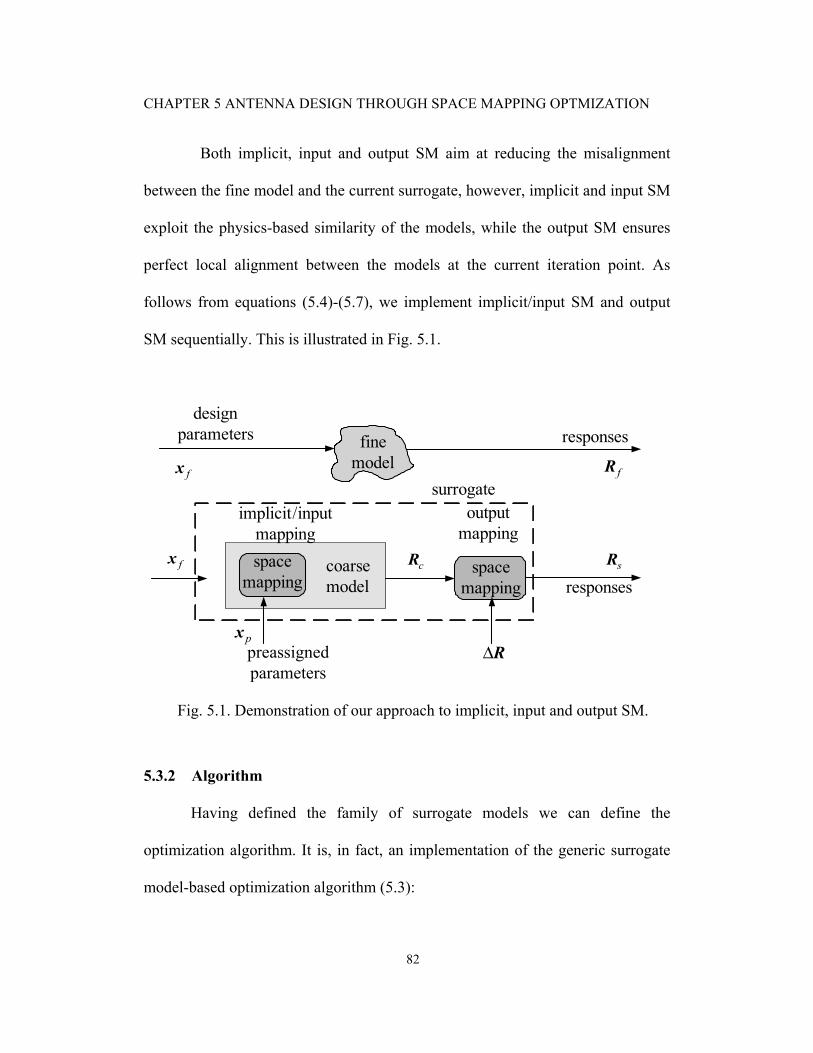
CHAPTER 5 ANTENNA DESIGN THROUGH SPACE MAPPING OPTMIZATION
82
Both implicit, input and output SM aim at reducing the misalignment
between the fine model and the current surrogate, however, implicit and input SM
exploit the physics-based similarity of the models, while the output SM ensures
perfect local alignment between the models at the current iteration point. As
follows from equations (5.4)-(5.7), we implement implicit/input SM and output
SM sequentially. This is illustrated in Fig. 5.1.
responses
surrogate
design parameters responsesfine
model
space mapping
outputmapping
coarse model
space mapping
implicit/inputmapping
cR sRfx
fx fR
px∆Rpreassigned
parameters
Fig. 5.1. Demonstration of our approach to implicit, input and output SM.
5.3.2 Algorithm
Having defined the family of surrogate models we can define the
optimization algorithm. It is, in fact, an implementation of the generic surrogate
model-based optimization algorithm (5.3):
CHAPTER 5 ANTENNA DESIGN THROUGH SPACE MAPPING OPTMIZATION
83
Step 1 Choose a proper coarse-mesh coarse model as well as
preassigned parameters. Set 0i = .
Step 2 Solve (5.2) to find the surrogate optimal solution c∗x and let
(0)cf∗=x x .
Step 3 Evaluate the fine model to find ( )( )if fR x .
Step 4 Update the surrogate model ( )isR according to (5.4)-(5.6).
Step 5 Solve (5.3) and obtain ( 1)if
+x .
Step 6 If the termination condition is satisfied (convergence
achieved or the design specification satisfied.), stop;
otherwise, set i = i+1 and go to Step 3.
5.4 SMF: SPACE MAPPING FRAMEWORK [11]
5.4.1 Brief Introduction to SMF
SMF [11] is designed to make space mapping accessible to engineers not
experienced in this technology. It is a GUI based Matlab system that can perform
space mapping based constrained optimization, modeling and statistical analysis.
It implements existing SM approaches, including input, output, implicit and
frequency SM. It contains drivers for commercial simulators (Sonnet em,
MEFiSTo, ADS, FEKO) that allow linking of the fine/coarse model to the
algorithm and to make the optimization process fully automatic.

CHAPTER 5 ANTENNA DESIGN THROUGH SPACE MAPPING OPTMIZATION
84
5.4.2 SMF Design Flow
In this thesis, we only focus on one aspect of SMF, a module for
automatic space mapping optimization. We have used it to solve the example
antenna design problems considered in Chapter VI.
Fig. 5.2 shows a block diagram of the optimization module in SMF.
Optimization is performed in several steps. First, the user enters problem
arguments, including starting point, frequency sweep, optimization type and
specifications. Next, the user sets up space mapping itself, i.e., the kind of space
mapping to be used (e.g., input, output, implicit), specifies the termination
condition, parameter extraction options, and optional constrains.
The next step is to link the fine and coarse models to SMF by setting up
the data that will be used to create model drivers. Using the user-provided data
(e.g., simulator input files and design variable identification data), SMF creates
drivers that are later used to evaluate fine/coarse models for any necessary design
variable values. Model evaluation is accomplished by generating the simulator
input file corresponding to the required design, running the simulator and
acquiring the results.
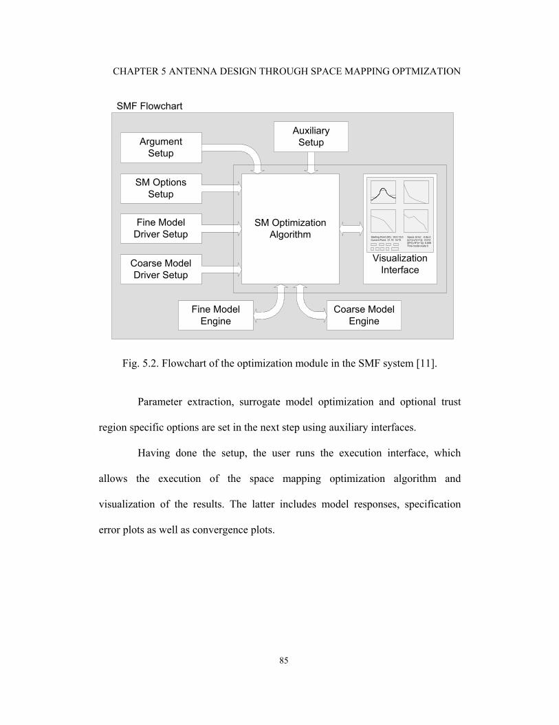
CHAPTER 5 ANTENNA DESIGN THROUGH SPACE MAPPING OPTMIZATION
85
SMF Flowchart
Argument Setup
SM Options Setup
Fine Model Driver Setup
Coarse Model Driver Setup
SM Optimization Algorithm
VisualizationInterface
Fine Model Engine
Coarse Model Engine
Auxiliary Setup
Starting Point (X0): 30.0 15.0 Specs. Error: -2.6e-2Current Point: 31.15 14.72 ||x^(i)-x^(i+1)||: 0.012
||R^(i)-R^(i+1)||: 0.008 Fine model evals: 5
Fig. 5.2. Flowchart of the optimization module in the SMF system [11].
Parameter extraction, surrogate model optimization and optional trust
region specific options are set in the next step using auxiliary interfaces.
Having done the setup, the user runs the execution interface, which
allows the execution of the space mapping optimization algorithm and
visualization of the results. The latter includes model responses, specification
error plots as well as convergence plots.

CHAPTER 5 ANTENNA DESIGN THROUGH SPACE MAPPING OPTMIZATION
86
5.5 EXAMPLES
5.5.1 Double Annular Ring Antenna
We consider the stacked probe-fed printed annular ring antenna of [14],
which is shown in Fig. 4.1. The antenna is printed on a PCB with 1 2.2rε = ,
1 6.096d = mm for the lower substrate and 2 1.07rε = , 2 8.0d = mm for the upper
substrate. The dielectric loss tangent is 0.001 for both layers.
Note that in this example, finite ground is used. The finite ground size is
100 100× mm. The radius of the feed pin is 0 0.325r = mm. Design variables are
the outer and inner radius of each ring and the feed position, namely,
1 2 1 2[ ]Tpa a b b ρ . The design specification is
11 10 dB for 1.75 GHz 2.15 GHzS ω≤ − ≤ ≤ .
In an MoM solver like FEKO, special Green’s functions are usually
implemented to model multi-layer substrates, where the ground and the substrate
are assumed infinite in extent. It is computer-resource efficient, since only the
finite metallic surfaces are discretized. However, in many microwave and RF
applications, the infinite ground plane assumption is not acceptable for accurate
simulations. The ground size has a strong effect on the performance of microstrip
antennas [15][16].
The surface equivalence principle (SEP) addresses this problem. The
surface of a dielectric is discretized and both the electric and magnetic surface

CHAPTER 5 ANTENNA DESIGN THROUGH SPACE MAPPING OPTMIZATION
87
currents are computed. All sides of a dielectric have to be meshed, making a
closed solid. In this approach, the memory requirement is four times what it
would be if the same structure was metallic [17]. A detailed discussion can be
found in Section 2.4.
We choose the SEP model as the fine model and the special Green’s
function, which does not consider the finite ground size effect, as the coarse
model. To further reduce the simulation time in the coarse model, we apply a
coarser mesh by local meshing. As shown in Fig. 5.3, the number of mesh edges
along the three loops (thick lines) is topologically fixed at 5, 10 and 15,
respectively, regardless of the variation in the design parameter values. The
detailed fine and coarse models are summarized in Table 5.1.
Here, we show how to set up and run the SM optimization for this problem
using SMF. Fig. 5.4 shows the direct coarse model optimization interface, which
was used to find the starting point for the SM optimization of the fine model. Fig.
5.5 shows the setup of the starting point, the frequency sweep, the optimization
type and specifications within SMF. Fig. 5.6 shows the space mapping options
interface. Here, the user can set up the termination conditions of the algorithm in
terms of maximum number of iterations or fine model evaluations, or in terms of
tolerances in arguments/function values; then, the space mapping algorithm to be
used (checkboxes A, B, C, D, E and F as well as implicit SM panel at the bottom
left corner of the interface); at last, the parameter extraction options (e.g., the
number of responses used while matching the models), as well as constraints for

CHAPTER 5 ANTENNA DESIGN THROUGH SPACE MAPPING OPTMIZATION
88
the coarse/fine model, regular SM parameters and implicit parameters. In our
example, we only use term D (output SM) and implicit SM.
Fig. 5.3. Demonstration of local meshing of the annular ring in the coarse-mesh coarse model for a stacked probe-fed printed double ring antenna example.
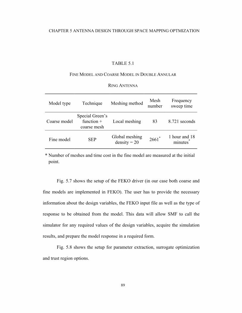
CHAPTER 5 ANTENNA DESIGN THROUGH SPACE MAPPING OPTMIZATION
89
TABLE 5.1
FINE MODEL AND COARSE MODEL IN DOUBLE ANNULAR
RING ANTENNA
Model type Technique Meshing method Mesh number
Frequency sweep time
Coarse modelSpecial Green’s
function + coarse mesh
Local meshing 83 8.721 seconds
Fine model SEP Global meshing density = 20 2661* 1 hour and 18
minutes*
* Number of meshes and time cost in the fine model are measured at the initial point.
Fig. 5.7 shows the setup of the FEKO driver (in our case both coarse and
fine models are implemented in FEKO). The user has to provide the necessary
information about the design variables, the FEKO input file as well as the type of
response to be obtained from the model. This data will allow SMF to call the
simulator for any required values of the design variables, acquire the simulation
results, and prepare the model response in a required form.
Fig. 5.8 shows the setup for parameter extraction, surrogate optimization
and trust region options.
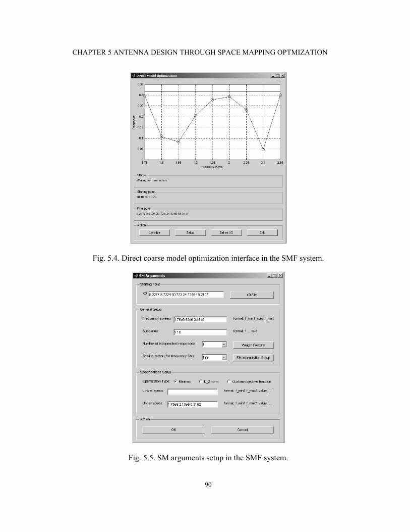
CHAPTER 5 ANTENNA DESIGN THROUGH SPACE MAPPING OPTMIZATION
90
Fig. 5.4. Direct coarse model optimization interface in the SMF system.
Fig. 5.5. SM arguments setup in the SMF system.
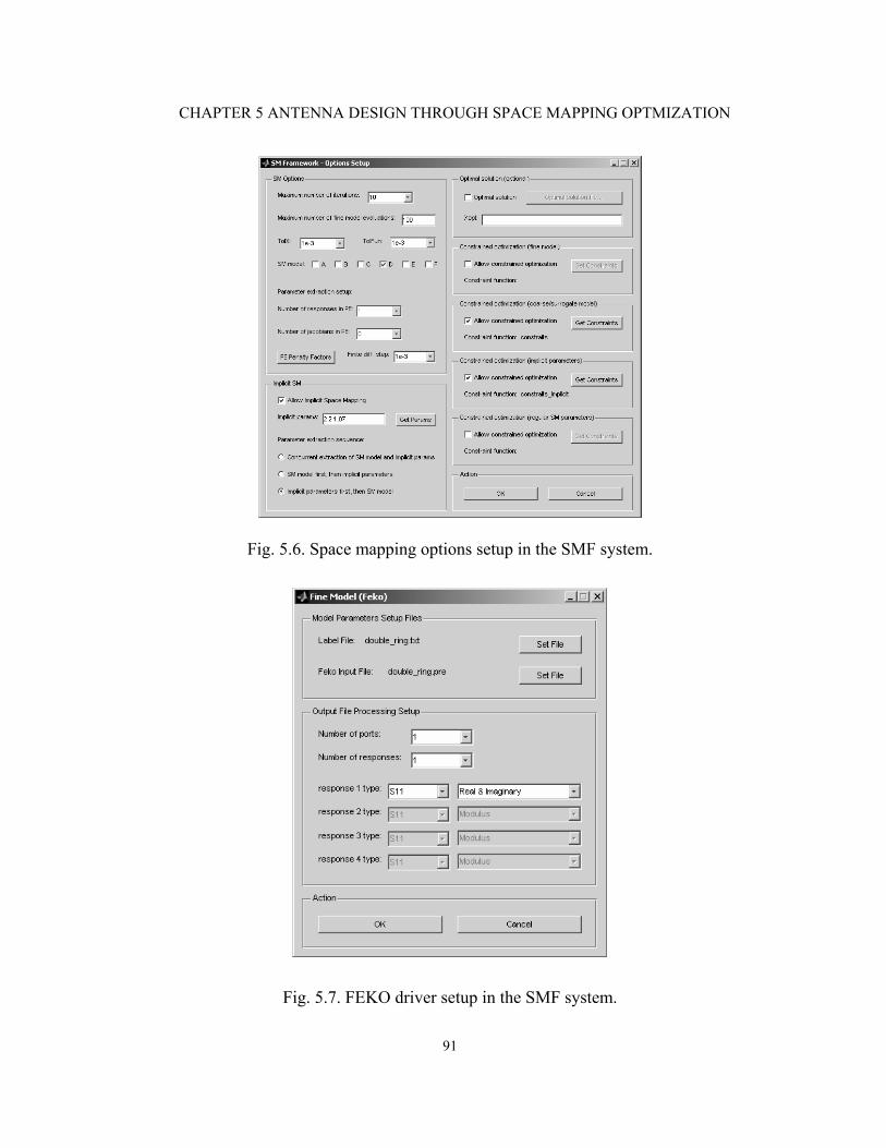
CHAPTER 5 ANTENNA DESIGN THROUGH SPACE MAPPING OPTMIZATION
91
Fig. 5.6. Space mapping options setup in the SMF system.
Fig. 5.7. FEKO driver setup in the SMF system.
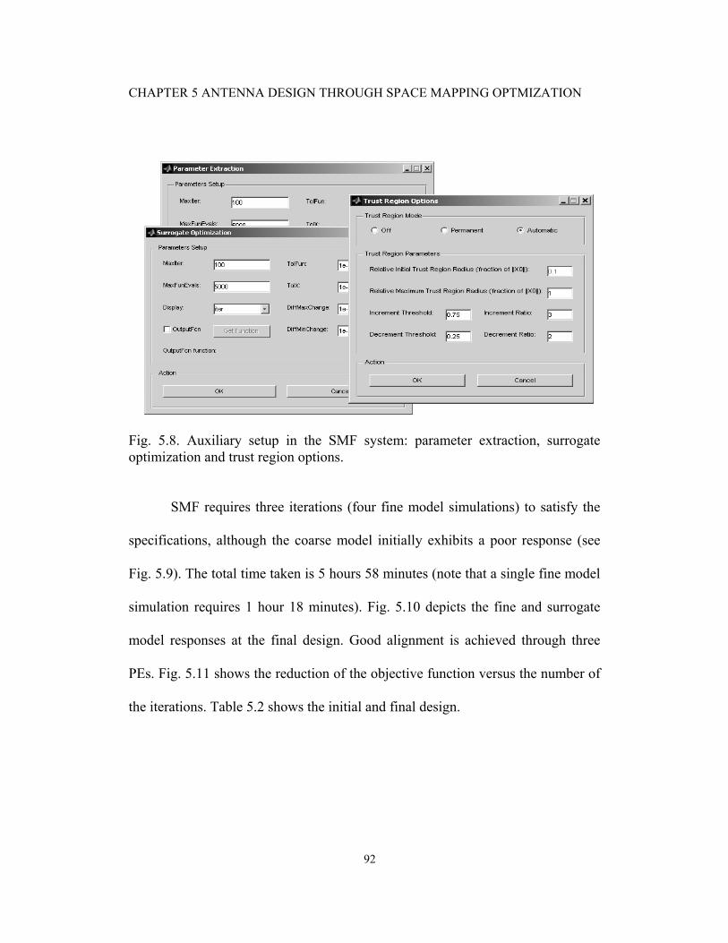
CHAPTER 5 ANTENNA DESIGN THROUGH SPACE MAPPING OPTMIZATION
92
Fig. 5.8. Auxiliary setup in the SMF system: parameter extraction, surrogate optimization and trust region options.
SMF requires three iterations (four fine model simulations) to satisfy the
specifications, although the coarse model initially exhibits a poor response (see
Fig. 5.9). The total time taken is 5 hours 58 minutes (note that a single fine model
simulation requires 1 hour 18 minutes). Fig. 5.10 depicts the fine and surrogate
model responses at the final design. Good alignment is achieved through three
PEs. Fig. 5.11 shows the reduction of the objective function versus the number of
the iterations. Table 5.2 shows the initial and final design.
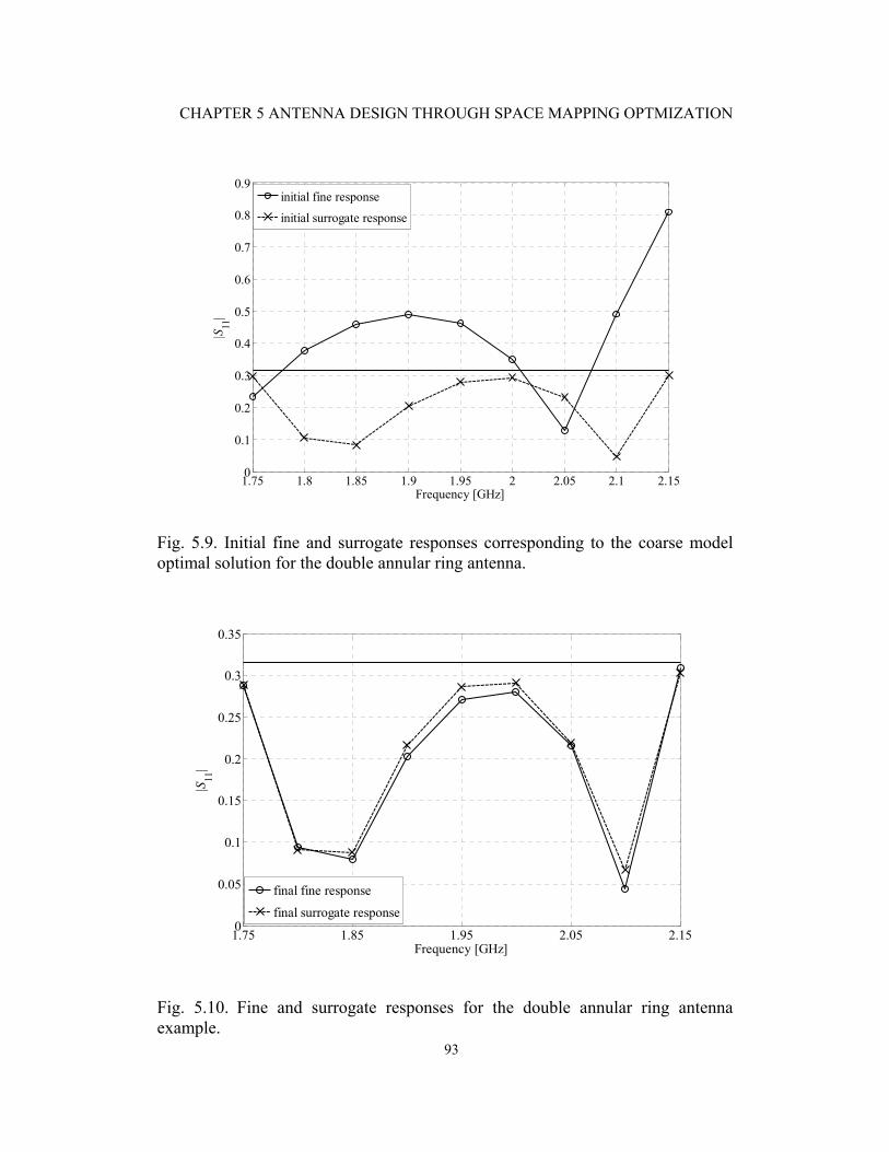
CHAPTER 5 ANTENNA DESIGN THROUGH SPACE MAPPING OPTMIZATION
93
1.75 1.8 1.85 1.9 1.95 2 2.05 2.1 2.150
0.1
0.2
0.3
0.4
0.5
0.6
0.7
0.8
0.9
Frequency [GHz]
|S11
|
initial fine response
initial surrogate response
Fig. 5.9. Initial fine and surrogate responses corresponding to the coarse model optimal solution for the double annular ring antenna.
1.75 1.85 1.95 2.05 2.150
0.05
0.1
0.15
0.2
0.25
0.3
0.35
Frequency [GHz]
|S11
|
final fine response
final surrogate response
Fig. 5.10. Fine and surrogate responses for the double annular ring antenna example.
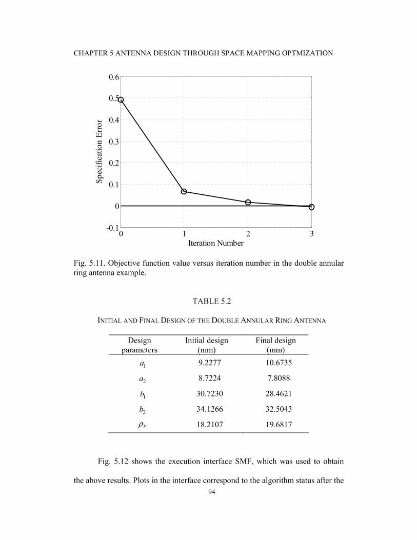
CHAPTER 5 ANTENNA DESIGN THROUGH SPACE MAPPING OPTMIZATION
94
0 1 2 3-0.1
0
0.1
0.2
0.3
0.4
0.5
0.6
Iteration Number
Spec
ifica
tion
Erro
r
Fig. 5.11. Objective function value versus iteration number in the double annular ring antenna example.
TABLE 5.2
INITIAL AND FINAL DESIGN OF THE DOUBLE ANNULAR RING ANTENNA
Design parameters
Initial design (mm)
Final design (mm)
1a 9.2277 10.6735
2a 8.7224 7.8088
1b 30.7230 28.4621
2b 34.1266 32.5043
pρ 18.2107 19.6817
Fig. 5.12 shows the execution interface SMF, which was used to obtain
the above results. Plots in the interface correspond to the algorithm status after the
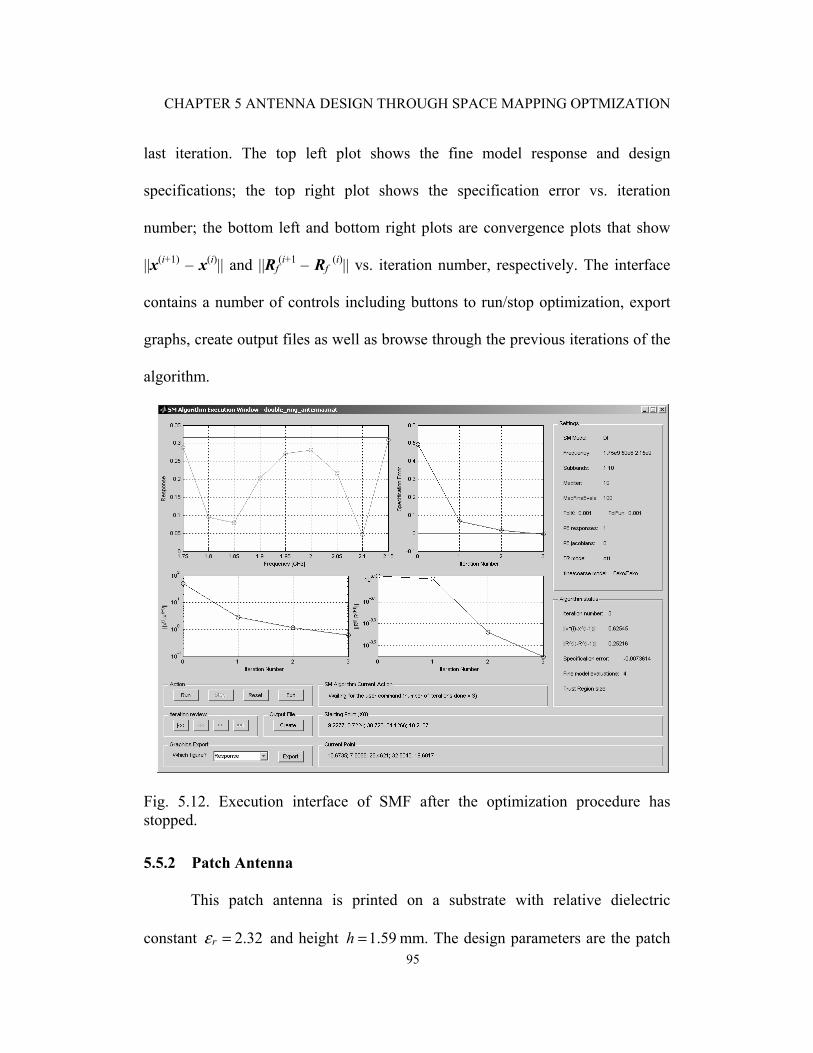
CHAPTER 5 ANTENNA DESIGN THROUGH SPACE MAPPING OPTMIZATION
95
last iteration. The top left plot shows the fine model response and design
specifications; the top right plot shows the specification error vs. iteration
number; the bottom left and bottom right plots are convergence plots that show
||x(i+1) – x(i)|| and ||Rf(i+1 – Rf
(i)|| vs. iteration number, respectively. The interface
contains a number of controls including buttons to run/stop optimization, export
graphs, create output files as well as browse through the previous iterations of the
algorithm.
Fig. 5.12. Execution interface of SMF after the optimization procedure has stopped.
5.5.2 Patch Antenna
This patch antenna is printed on a substrate with relative dielectric
constant 2.32rε = and height 1.59h = mm. The design parameters are the patch

CHAPTER 5 ANTENNA DESIGN THROUGH SPACE MAPPING OPTMIZATION
96
length and width, i.e., [ ]Tf L W=x . The objective is to obtain 50 Ω input
impedance at 2 GHz. The objective function is 50inZ − .
In the fine model, the global mesh density is 30 meshes per wavelength. In
the coarse model, the mesh number and topology are fixed through local meshing.
We choose three mesh edges along L and seven along W . See Fig. 5.13. We use
implicit SM and output SM. The selected preassigned SM parameter is rε=x . In
the PE, we match the complex S11 instead of the input impedance.
The initial design point is the coarse model optimal solution
(0) [47.1285 100.470]f =x mm. SMF requires five iterations (six fine model
simulations). Fig. 14 shows the reduction of the objective function versus the
number of iterations. The final design is * (4) [46.7294 99.6875]f f= =x x mm.
Table 5.3 shows the optimization results for the design parameters, the objective
function value, the preassigned parameter and the output SM parameter at each
iteration. Computation time is 341 s, compared with 2816 s for direct fine model
optimization. The SMF execution window is shown in Fig. 5.15.
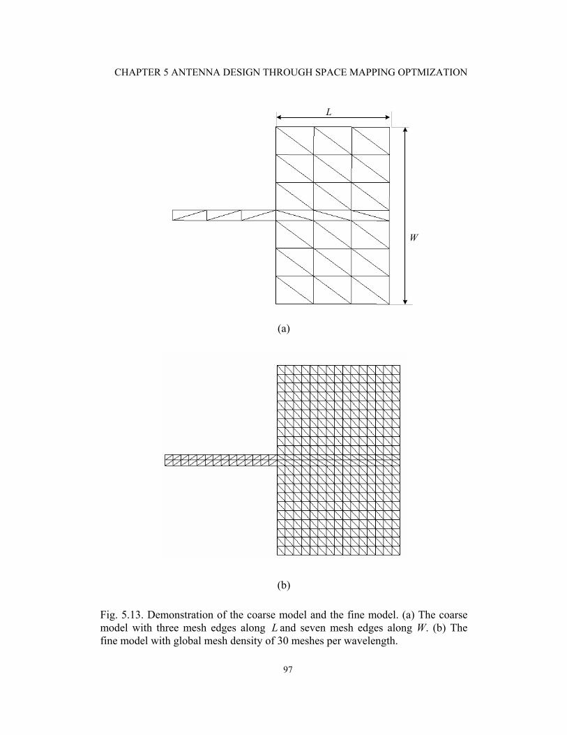
CHAPTER 5 ANTENNA DESIGN THROUGH SPACE MAPPING OPTMIZATION
97
L
W
(a)
(b)
Fig. 5.13. Demonstration of the coarse model and the fine model. (a) The coarse model with three mesh edges along L and seven mesh edges along W. (b) The fine model with global mesh density of 30 meshes per wavelength.
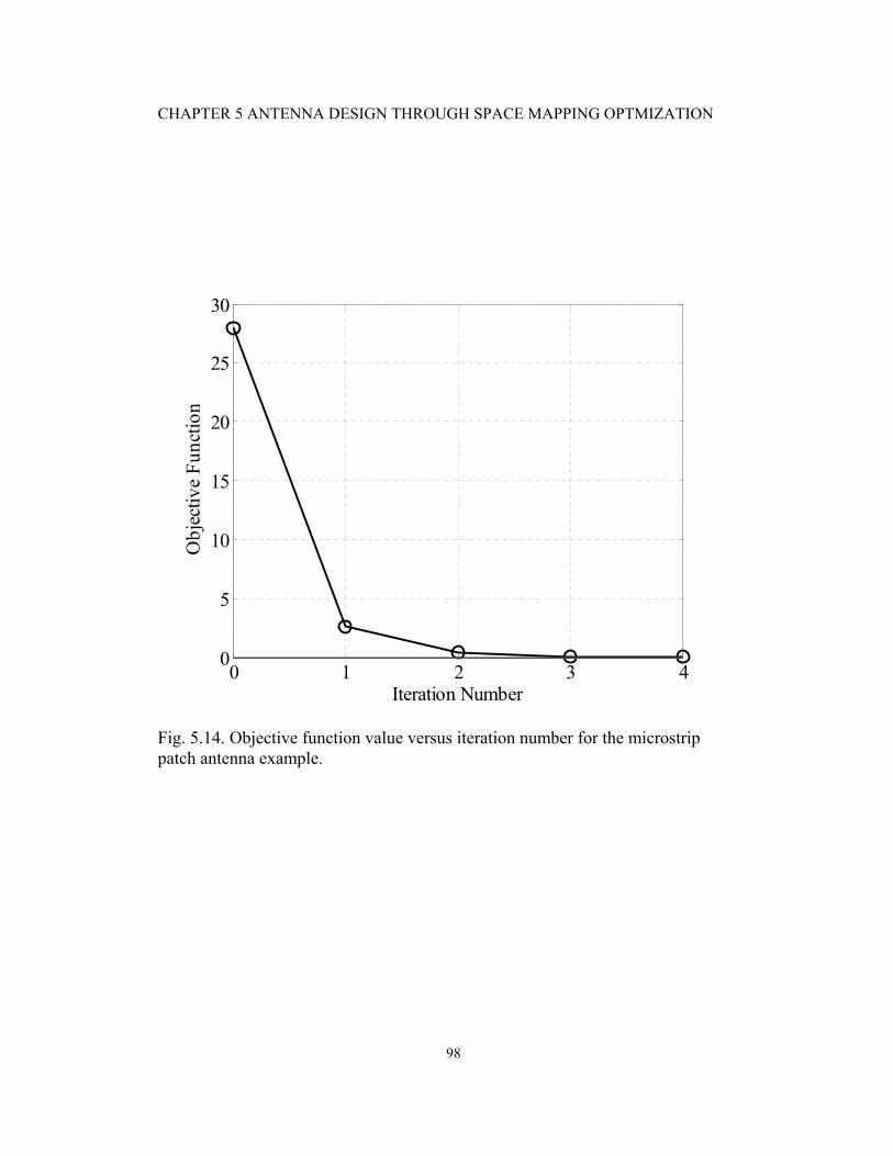
CHAPTER 5 ANTENNA DESIGN THROUGH SPACE MAPPING OPTMIZATION
98
0 1 2 3 40
5
10
15
20
25
30
Iteration Number
Obj
ectiv
e Fu
nctio
n
Fig. 5.14. Objective function value versus iteration number for the microstrip patch antenna example.
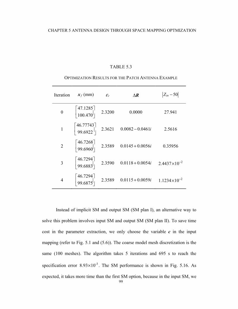
CHAPTER 5 ANTENNA DESIGN THROUGH SPACE MAPPING OPTMIZATION
99
TABLE 5.3
OPTIMIZATION RESULTS FOR THE PATCH ANTENNA EXAMPLE
Iteration fx (mm) rε ∆R 50inZ −
0 47.1285100.470⎡ ⎤⎢ ⎥⎣ ⎦
2.3200 0.0000 27.941
1 46.7774399.6922
⎡ ⎤⎢ ⎥⎣ ⎦
2.3621 0.0082 0.0461i− 2.5616
2 46.726899.6960⎡ ⎤⎢ ⎥⎣ ⎦
2.3589 0.0145 0.0056i+ 0.35956
3 46.729499.6883⎡ ⎤⎢ ⎥⎣ ⎦
2.3590 0.0118 0.0054i+ 22.4437 10−×
4 46.729499.6875⎡ ⎤⎢ ⎥⎣ ⎦
2.3589 0.0115 0.0059i+ 21.1234 10−×
Instead of implicit SM and output SM (SM plan I), an alternative way to
solve this problem involves input SM and output SM (SM plan II). To save time
cost in the parameter extraction, we only choose the variable c in the input
mapping (refer to Fig. 5.1 and (5.6)). The coarse model mesh discretization is the
same (100 meshes). The algorithm takes 5 iterations and 695 s to reach the
specification error -38.93 10× . The SM performance is shown in Fig. 5.16. As
expected, it takes more time than the first SM option, because in the input SM, we
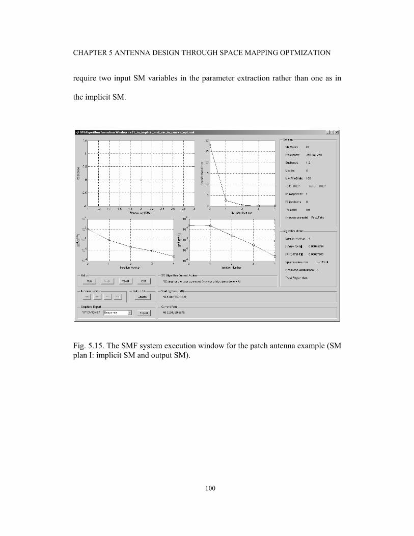
CHAPTER 5 ANTENNA DESIGN THROUGH SPACE MAPPING OPTMIZATION
100
require two input SM variables in the parameter extraction rather than one as in
the implicit SM.
Fig. 5.15. The SMF system execution window for the patch antenna example (SM plan I: implicit SM and output SM).
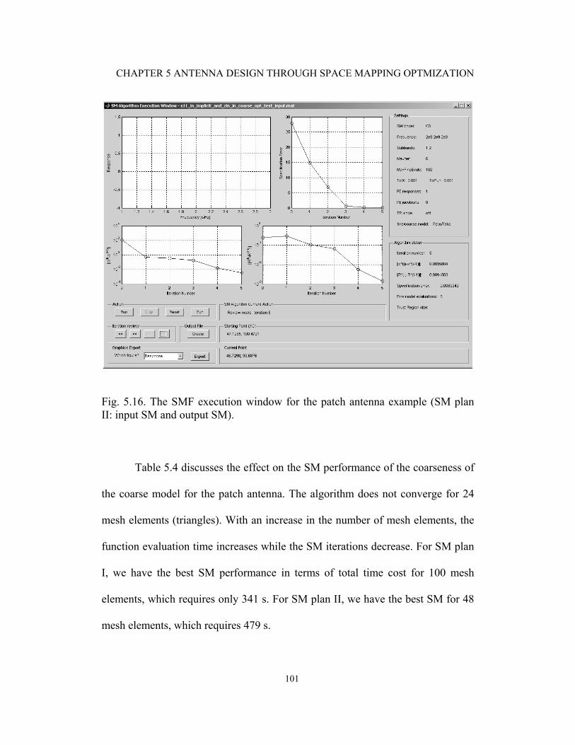
CHAPTER 5 ANTENNA DESIGN THROUGH SPACE MAPPING OPTMIZATION
101
Fig. 5.16. The SMF execution window for the patch antenna example (SM plan II: input SM and output SM).
Table 5.4 discusses the effect on the SM performance of the coarseness of
the coarse model for the patch antenna. The algorithm does not converge for 24
mesh elements (triangles). With an increase in the number of mesh elements, the
function evaluation time increases while the SM iterations decrease. For SM plan
I, we have the best SM performance in terms of total time cost for 100 mesh
elements, which requires only 341 s. For SM plan II, we have the best SM for 48
mesh elements, which requires 479 s.
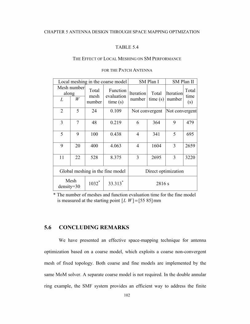
CHAPTER 5 ANTENNA DESIGN THROUGH SPACE MAPPING OPTMIZATION
102
TABLE 5.4
THE EFFECT OF LOCAL MESHING ON SM PERFORMANCE
FOR THE PATCH ANTENNA
Local meshing in the coarse model SM Plan I SM Plan II Mesh number
along L W
Total mesh
number
Function evaluation
time (s)
Iteration number
Total time (s)
Iteration number
Total time (s)
2 5 24 0.109 Not convergent Not convergent
3 7 48 0.219 6 364 9 479
5 9 100 0.438 4 341 5 695
9 20 400 4.063 4 1604 3 2659
11 22 528 8.375 3 2695 3 3220
Global meshing in the fine model Direct optimization
Mesh density=30 1032* 33.313* 2816 s
* The number of meshes and function evaluation time for the fine model is measured at the starting point [ ] [55 85]L W = mm
5.6 CONCLUDING REMARKS
We have presented an effective space-mapping technique for antenna
optimization based on a coarse model, which exploits a coarse non-convergent
mesh of fixed topology. Both coarse and fine models are implemented by the
same MoM solver. A separate coarse model is not required. In the double annular
ring example, the SMF system provides an efficient way to address the finite

CHAPTER 5 ANTENNA DESIGN THROUGH SPACE MAPPING OPTMIZATION
103
ground size problem. We solve the optimal impedance of a patch antenna problem
using two SM plans. The coarseness in the coarse model and its effect on the
space mapping performance are discussed. Although we demonstrate our
approach through antenna design, it is applicable to other planar structures.
CHAPTER 5 ANTENNA DESIGN THROUGH SPACE MAPPING OPTMIZATION
104
REFERENCES
[1] J.W. Bandler, R.M. Bienacki, S.H. Chen, P.A. Grobelny and R.H. Hemmers, “Space mapping technique for electromagnetic optimization,” IEEE Trans. Microwave Theory Tech., vol. 42, Dec. 1994, pp. 2536-2544.
[2] J.W. Bandler, Q.S. Cheng, N.K. Nikolova and M. A. Ismail, “Implicit
space mapping optimization exploiting preassigned parameters,” IEEE Trans. Microwave Theory Tech., vol. 52, Jan. 2004, pp. 378-385.
[3] J.W. Bandler, Q.S. Cheng, D. Gebre-Mariam, K. Madsen, F. Pedersen and
J. Søndergaard, “EM-based surrogate modeling and design exploiting implicit, frequency and output space mappings,” in IEEE MTT-S IMS Dig., June. 2003, pp.1003-1006.
[4] M.H. Bakr, J.W. Bandler, M.A. Ismail, J.E. Rayas-Sánchez and Q.J.
Zhang, “Neural space-mapping optimization for EM-based design,” IEEE Trans. Microwave Theory Tech., vol. 48, Dec. 2000, pp. 2307-2315.
[5] M.A. Ismail, D. Smith, A. Panariello, Y. Wang and M. Yu, “EM-based
design of large-scale dielectric-resonator filters and multiplexers by space mapping,” IEEE Trans. Microwave Theory Tech., vol. 52, Jan. 2004, pp. 386-392.
[6] K.-L. Wu, Y.-J. Zhao, J. Wang, and M.K.K Cheng, “An effective dynamic
coarse model for optimization design of LTCC RF circuits with aggressive space mapping,” IEEE Trans. Microwave Theory Tech., vol. 52, Jan. 2004, pp. 393-402.
[7] J. Zhu, J.W. Bandler, N.K. Nikolova and S. Koziel, “Antenna design
through space mapping optimization,” IEEE MTT-S Int. Microwave Symp., San Francisco, California, 2006.
[8] J. Zhu, J.W. Bandler, N.K. Nikolova and S. Koziel, “Antenna optimization
through space mapping,” submitted to IEEE Trans. Antennas Propagat., Special Issue on Synthesis and Optimization Techniques in Electromagnetics and Antenna System Design, Jan. 2007.
[9] FEKO® User’s Manual, Suite 4.2, June 2004, EM Software & Systems-
S.A. (Pty) Ltd, 32 Techno Lane, Technopark, Stellenbosch, 7600, South Africa, http://www.feko.info. In the USA: EM Software & Systems (USA), Inc., 24 Research Drive, Hampton, VA 23666, USA, http://www.emssusa.com/.
CHAPTER 5 ANTENNA DESIGN THROUGH SPACE MAPPING OPTMIZATION
105
[10] J.W. Bandler, A.S. Mohamed and M.H. Bakr, “TLM-based modeling and
design exploiting space mapping,” IEEE Trans. Microwave Theory Tech., vol. 53, Sep. 2005, pp. 2801-2811.
[11] SMF, Bandler Corporation, P.O. Box 8083, Dundas, ON, Canada L9H
5E7, 2006. [12] “Mesh refinement,” FEKO Quarterly, December 2004. [13] S. Koziel, J.W. Bandler and K. Madsen, “Towards a rigorous formulation
of the space mapping technique for engineering design,” Proc. ISCAS, Kobe, Japan, Jun. 2005, pp. 5605-5608.
[14] D.M. Kotokoff, J.T. Aberle and R.B. Waterhouse, “Rigorous analysis of
probe-fed printed annular ring antennas,” IEEE Trans. Antennas Propagat, vol. 47, Feb. 1999, pp. 384-388.
[15] F. Tavakkol-Hamedani, L. Shafai and G.Z. Rafi, “The effects of substrate
and ground plane size on the performance of finite rectangular microstrip antennas,” IEEE AP-S/URSI Int. Symp. on Antennas Propagat., Jun. 2002.
[16] A.K. Bhattacharyya, “Effects of ground plane truncation on the impedance
of a patch antenna,” IEE proceedings-H, vol. 138, Dec. 1991, pp. 560-564. [17] “Modeling of dielectric materials in FEKO,” FEKO Quarterly, March
2005.

CHAPTER 5 ANTENNA DESIGN THROUGH SPACE MAPPING OPTMIZATION
106

107
PART III
CONCLUSIONS
CONCLUSIONS
108
The thesis presents novel methods for the computer-aided design of
microwave circuits and antennas exploiting adjoint-variable and space mapping
(SM) technologies. These technologies are demonstrated by various examples.
In Chapter 2, some relevant features of the method of moments (MoM) are
reviewed. These features are related to further developments in this thesis,
especially the developments of the self-adjoint sensitivity analysis and the coarse-
mesh surrogate model optimization technique. After a brief introduction to the
MoM, the CPU time cost versus mesh density is discussed, followed by mesh
refinement and mesh convergence. A discussion on the modeling of dielectric
objects with the MoM is also given.
In Part I (Chapters 3 and 4), we investigate the sensitivity analysis in the
frequency domain. In Chapter 3, we propose the self-adjoint sensitivity analysis
(SASA) method for network parameter sensitivity calculation in the MoM. It
reduces the computational cost of the AVM by avoiding the adjoint analysis.
Since the derivative of system matrix is obtained using finite differences, this
technique is also referred to as finite-difference self-adjoint sensitivity analysis
(FD-SASA). We propose a general procedure to implement the FD-SASA
technique and demonstrate how it works with the commercial solver FEKO. The
MoM matrix symmetry versus the convergence of the solution and the
computational overhead associated with the sensitivity analysis are rigorously
discussed at the end of this chapter.
CONCLUSIONS
109
In Chapter 4, the EM optimization using sensitivity analysis in the
frequency domain is studied. The Broyden update is utilized in the iterative
computation of the system matrix derivatives, which are then used in the self-
adjoint formula to obtain the response Jacobian. This SASA method is referred to
as B-SASA. It significantly reduces the computational overhead compared with
the FD-SASA proposed in Chapter 3. Two criteria are used to switch back and
forth throughout the optimization process between the robust but more time-
demanding FD-SASA and the B-SASA. Thus, we avoid the inaccuracy, which
may accumulate in the B-SASA method, while in the same time fully exploit its
computational efficiency. This hybrid approach (B/FD-SASA) guarantees good
accuracy of the gradient information with minimal computational time.
Chapter 5 in Part II presents the antenna design optimization exploiting
space mapping techniques. We exploit a coarse-mesh MoM solver as the coarse
model and align it with the fine-mesh MoM solution through space mapping. Two
space mapping plans are employed: (1) implicit space mapping and output space
mapping, (2) input space mapping and output space mapping. A novel local
meshing method avoids inconsistencies in the coarse model. The proposed plans
are implemented through SMF. Our approach is illustrated with the MoM-based
design of a double annular ring antenna and a patch antenna. The SMF algorithms
converge to a good design in spite of the poor initial behavior of the coarse-mesh
MoM surrogate.

CONCLUSIONS
110
The Appendix shows the calculation of the S-parameters from the current
solution of the MoM. It is needed in Chapter 3 in order to derive the S-parameter
self-adjoint sensitivity analysis formulas.
The following research topics should be addressed in future developments.
(1) Exploiting the self-adjoint sensitivity analysis technique for the
gradient-based SM optimization and modeling.
(2) Investigating the multi-level MoM and model order reduction (MOR)
techniques to build robust surrogate models.
(3) Investigating further the properties of the coarse-mesh coarse models
in MoM simulations. Focus should be on robust criteria to evaluate
the suitability of the coarse models.
111
APPENDIX
NETWORK PARAMETER
CALCULATION IN FEKO
In this section, we show how to calculate the two-port S-parameters based
on the solution (current vector) available from FEKO.
According to the network theory,
1 11 12 1
2 21 22 2
U Z Z IU Z Z I⎡ ⎤ ⎡ ⎤ ⎡ ⎤
= ⋅⎢ ⎥ ⎢ ⎥ ⎢ ⎥⎣ ⎦ ⎣ ⎦ ⎣ ⎦
(A.1)
When Port 1 is excited,
1 0 11 11 11 12 21V Z I Z I Z I− = + (A.2)
0 21 21 11 22 21Z I Z I Z I− = + (A.3)
when Port 2 is excited,
2 0 22 21 12 22 22V Z I Z I Z I− = + (A.4)
0 12 11 12 12 22Z I Z I Z I− = + (A.5)
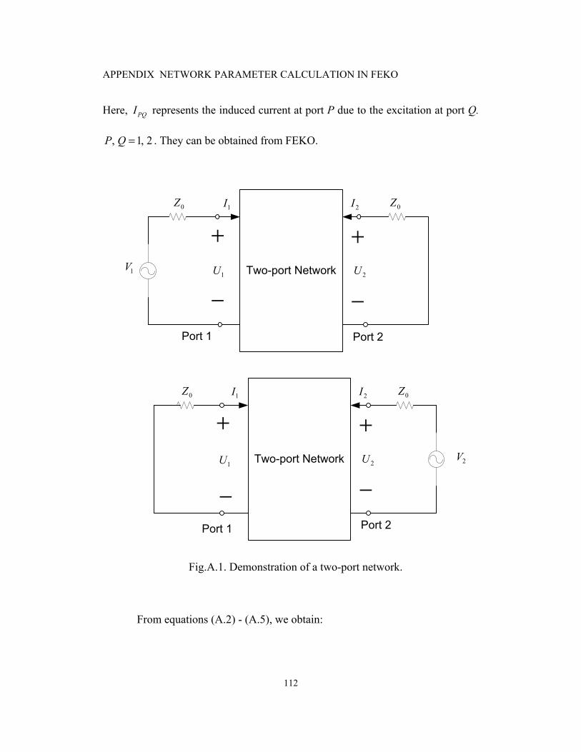
APPENDIX NETWORK PARAMETER CALCULATION IN FEKO
112
Here, PQI represents the induced current at port P due to the excitation at port Q.
, 1, 2P Q = . They can be obtained from FEKO.
Two-port Network
0Z
1V
0Z
1U
2I1I
Two-port Network
0Z 0Z
1U
2I1I
2V
Port 1
Port 1 Port 2
Port 2
+
+
−
−
+
−2U
+
−2U
Fig.A.1. Demonstration of a two-port network.
From equations (A.2) - (A.5), we obtain:
APPENDIX NETWORK PARAMETER CALCULATION IN FEKO
113
1 2211 0
12 21 11 22
V IZ ZI I I I
= − −−
(A.6)
1 1212
12 21 11 22
V IZI I I I
=−
(A.7)
2 2121
12 21 11 22
V IZI I I I
=−
(A.8)
2 1122 0
12 21 11 22
V IZ ZI I I I
= − −−
(A.9)
We use the relationship between the Z- and the S-parameters as
1 211 0 22 0 12 21
11 22 12 21
( )( )
VVZ Z Z Z Z Z ZI I I I
∆ = + + − =− (A.10)
11 0 22 0 12 2111
1 22 2 11 1 12 2 210
12 21 11 22 12 21 11 22 12 21 11 22 12 21 11 22
1 2
11 22 12 21
0 11
1
( )( + )
(2 )
2 1
Z Z Z Z Z ZSZ
V I V I V I V IZI I I I I I I I I I I I I I I I
VVI I I I
Z IV
− −=∆
+ ⋅ − ⋅− − − −=
−
= − +
(A.11)
APPENDIX NETWORK PARAMETER CALCULATION IN FEKO
114
0 1 12
12 0 0 1212 21 11 2212
1 2 2
11 22 12 21
22 2
Z V IZ Z Z II I I IS VVZ V
I I I I
−−= = =∆
−
(A.12)
0 2 21
21 0 0 2112 21 11 2221
1 2 1
11 22 12 21
22 2
Z V IZ Z Z II I I IS VVZ V
I I I I
−−= = =∆
−
(A.13)
11 0 22 0 12 2122
1 22 2 11 1 12 2 210
12 21 11 22 12 21 11 22 12 21 11 22 12 21 11 22
1 2
11 22 12 21
0 22
2
( )( )
(2 )
2 1
Z Z Z Z Z ZSZ
V I V I V I V IZI I I I I I I I I I I I I I I I
VVI I I I
Z IV
+ − −=∆
⋅ + − ⋅− − − −=
−
= − +
(A.14)
For N-port S-parameter calculation, we can obtain a more general
expression in the same way:
0
0
21 when
2, when
,PQ
QPQ
PQ
Q
Z IP Q
VS
Z IP Q
V
−⎧+ =⎪
⎪= ⎨−⎪ ≠⎪⎩
(A.15)
115
BIBLIOGRAPHY
Advanced Design System 2003C, User’s Manual, Agilent Technologies, 395 Page Mill Road, Palo Alto, CA 94304, USA. Agilent ADS, Agilent Technologies, 1400 Fountaingrove Parkway, Santa Rosa, CA 95403-1799, USA. H. Akel and J.P. Webb, “Design sensitivities for scattering-matrix calculation with tetrahedral edge elements,” IEEE Trans. Magnetics, vol. 36, July 2000, pp. 1043-1046. S.M. Ali, N.K. Nikolova and M.H. Bakr, “Recent advances in sensitivity analysis with frequency-domain full-wave EM solvers,” Applied Computational Electromagnetics Society Journal, vol. 19, Nov. 2004, pp. 147-154. S. Amari, “Numerical cost of gradient computation within the method of moments and its reduction by means of a novel boundary-layer concept,” IEEE MTT-S Int. Microwave Symp. Digest, 2001, pp.1945-1948. Ansoft HFSS, Ansoft Corporation, 225 West Station Square Drive, Suite 200, Pittsburgh, PA 15219, USA. M.H. Bakr, Advances in Space Mapping Optimization of Microwave Circuits, PhD Thesis, Department of Electrical and Computer Engineering, McMaster University, 2000. M.H. Bakr, J.W. Bandler and N. Georgieva, “An aggressive approach to parameter extraction,” IEEE Trans. Microwave Theory Tech., vol. 47, Dec. 1999, pp. 2428-2439. M.H. Bakr, J.W. Bandler, M.A. Ismail, J.E. Rayas-Sánchez and Q.J. Zhang, “Neural space-mapping optimization for EM-based design,” IEEE Trans. Microwave Theory Tech., vol. 48, Dec. 2000, pp. 2307-2315.
BIBLIOGRAPHY
116
M.H. Bakr, J.W. Bandler, K. Madsen and J. Søndergaard, “An introduction to the space mapping technique,” Optimization Eng., vol. 2, 2001, pp.369-384. M.H. Bakr and N.K. Nikolova, “An adjoint variable method for frequency domain TLM problems with conducting boundaries,” IEEE Microwave and Wireless Components Letters, vol. 13, Sep. 2003, pp. 408-410. C.A. Balanis, Antenna Theory: Analysis and Design, New York: Wiley, 1997. J.W. Bandler, R.M. Biernacki and S.H. Chen, “Fully automated space mapping optimization of 3D structures,” in IEEE MTT-S Int. Microwave Symp. Dig., San Francisco, CA, 1996, pp. 753-756. J.W. Bandler, R.M. Biernacki, S.H. Chen, W.J. Getsinger, P.A. Grobelny, C. Moskowitz and S.H. Talisa, “Electromagnetic design of high temperature superconducting microwave filters,” Int. J. RF Microwave Computer-Aided Eng., vol. 5, 1995, pp. 331-343. J.W. Bandler, R.M. Biernacki, S.H. Chen, P.A. Grobelny and R.H. Hemmers, “Space mapping technique for electromagnetic optimization,” IEEE Trans. Microwave Theory Tech., vol. 42, 1994, pp. 2536-2544. J.W. Bandler, R.M. Biernacki, S.H. Chen and Y.F. Huang, “Design optimization of interdigital filters using aggressive space mapping and decomposition,” IEEE Trans. Microwave Theory Tech., vol. 45, May 1997, pp. 761-769. J.W. Bandler, R.M. Biernacki, S.H. Chen and D. Omeragic, “Space mapping optimization of waveguide filters using finite element and mode-matching electromagnetic simulators,” Int. J. RF Microwave Computer-Aided Eng., vol. 9, 1999, pp. 54-70. J.W. Bandler, S.H. Chen, S. Daijavad and K. Madsen, “Efficient optimization with integrated gradient approximations,” IEEE Trans. Microwave Theory Tech., vol. 36, Feb. 1988, pp. 444-455. J.W. Bandler, Q.S. Cheng, S.A. Dakroury, A.S. Mohamed, M.H. Bakr, K. Madsen and J. Søndergaard, “Trends in space mapping technology for engineering optimization,” 3rd Annual McMaster Optimization Conference: Theory and Applications, MOPTA03, Hamilton, ON, Aug. 2003. J.W. Bandler, Q. Cheng, S.A. Dakroury, A.S. Mohamed, M.H. Bakr, K. Madsen and J. Søndergaard, “Space mapping: the state of the art,” in SBMO/MTT-S
BIBLIOGRAPHY
117
International Microwave and Optoelectronics Conference (IMOC 2003), Parana, Brazil, Sep. 2003, vol. 2, pp. 951-956. J.W. Bandler, Q. Cheng, S.A. Dakroury, A.S. Mohamed, M.H. Bakr, K. Madsen and J. Søndergaard, “Space mapping: the state of the art,” IEEE Trans. Microwave Theory and Tech., vol. 52, Jan. 2004, pp. 337-361. J.W. Bandler, Q.S. Cheng, D. Gebre-Mariam, K. Madsen, F. Pedersen and J. Søndergaard, “EM-based surrogate modeling and design exploiting implicit, frequency and output space mappings,” in IEEE MTT-S Int. Microwave Symp. Dig., Philadelphia, PA, 2003, pp. 1003-1006. J.W. Bandler, Q.S. Cheng, D.M. Hailu, A.S. Mohamed, M.H. Bakr, K. Madsen and F. Pedersen, "Recent trends in space mapping technology," in Proc. 2004 Asia-Pacific Microwave Conf. APMC04, New Delhi, India, Dec. 2004. J.W. Bandler, Q.S. Cheng and S. Koziel, "Implementable space mapping approach to enhancement of microwave device models," IEEE MTT-S Int. Microwave Symp. Dig. (Long Beach, CA, June 2005) pp. 1139-1142. J.W. Bandler, Q.S. Cheng, N.K. Nikolova and M.A. Ismail, “Implicit space mapping optimization exploiting preassigned parameters,” IEEE Trans. Microw. Theory Tech., vol. 52, Jan. 2004, pp. 378-385. J.W. Bandler, D.M. Hailu, K. Madsen and F. Pedersen, “A space-mapping interpolating surrogate algorithm for highly optimized EM-based design of microwave devices,” IEEE Trans. Microwave Theory and Tech., vol. 52, Nov. 2004, pp. 2593-2600. J.W. Bandler, M.A. Ismail and J.E. Rayas-Sánchez, “Expanded space mapping EM-based design framework exploiting preassigned parameters,” IEEE Trans. Circuits Syst.-I, vol. 49, Dec. 2002, pp. 1833-1838. J.W. Bandler, W. Kellerman and K. Madsen, “A superlinearly convergent minimax algorithm for microwave circuit design,” IEEE Trans. Microwave Theory Tech., vol. MTT-33, Dec. 1985, pp. 1519-1530. J.W. Bandler, A.S. Mohamed and M.H. Bakr, “TLM-based modeling and design exploiting space mapping,” IEEE Trans. Microwave Theory Tech., vol. 53, 2005, pp. 2801-2811.
BIBLIOGRAPHY
118
J. W. Bandler, A. S. Mohamed, M. H. Bakr, K. Madsen and J. Søndergaard, “EM-based optimization exploiting partial space mapping and exact sensitivities,” IEEE Trans. Microwave Theory Tech., vol. 50, Dec. 2002, pp. 2741-2750. A.D Belegundu and T.R. Chandrupatla, Optimization Concepts and Applications in Engineering. Upper Saddle River, NJ: Prentice-Hall, 1999. A. K. Bhattacharyya, “Effects of ground plane truncation on the impedance of a patch antenna,” IEE proceedings-H, vol. 138, Dec. 1991, pp. 560-564. R.M. Biernacki, J.W. Bandler, J. Song and Q.J. Zhang, “Efficient quadratic approximation for statistical design,” IEEE Trans. Circuits Syst., vol. 36, Nov. 1989, pp. 1449-1454. C.G. Broyden, “A class of methods for solving nonlinear simultaneous equations,” Mathematics of Computation, vol. 19, 1965, pp. 577-593. D.G. Cacuci, Sensitivity & Uncertainty Analysis, Volume 1: Theory. Boca Raton, FL: Chapman & Hall/CRC, 2003. Q. Cheng, Advances in Space Mapping Technology Exploiting Implicit Space Mapping and Output Space Mapping, PhD Thesis, Department of Electrical and Computer Engineering, McMaster University, 2004. Y.S. Chung, C. Cheon, I.H. Park and S.Y. Hahn, “Optimal design method for microwave device using time domain method and design sensitivity analysis—part I: FETD case,” IEEE Trans. Magnetics, vol. 37, Sep. 2001, pp. 3289-3293. L. Daniel, Simulation and Modeling Techniques for Signal Integrity and Electromagnetic Interference on High Frequency Electronic Systems, PhD thesis, Electrical Engineering and Computer Science, University of California at Berkeley. em, Sonnet Software, Inc. 100 Elwood Davis Road, North Syracuse, NY 13212, USA. FEKO® User’s Manual, Suite 4.2, June 2004, EM Software & Systems-S.A. (Pty) Ltd, 32 Techno Lane, Technopark, Stellenbosch, 7600, South Africa, http://www.feko.info. In the USA: EM Software & Systems (USA), Inc., 24 Research Drive, Hampton, VA 23666, USA, http://www.emssusa.com/. M.D. Greenberg, Advanced Engineering Mathematics. Upper Saddle River, N.J.: Prentice Hall, 1998, pp. 1138-1140.
BIBLIOGRAPHY
119
N.K. Georgieva, S. Glavic, M.H. Bakr and J.W. Bandler, “Feasible adjoint sensitivity technique for EM design optimization,” IEEE Trans. Microwave Theory Tech., vol. 50, Dec. 2002, pp. 2751-2758. P.A. Grobelny, Integrated Numerical Modeling Techniques for Nominaland Statistical Circuit Design, Ph.D. Thesis, Department of Electrical and Computer Engineering, McMaster University, Hamilton, ON, Canada,1995. E.J. Haug, K.K. Choi and V. Komkov, Design Sensitivity Analysis of Structural Systems. Orlando, FL: Academic, 1986. R.F. Harrington, Field Computation by Moment Methods, New York, NY: Macmillan, 1968. M.A. Ismail, D. Smith, A. Panariello, Y. Wang and M. Yu, “EM-based design of large-scale dielectric-resonator filters and multiplexers by space mapping,” IEEE Trans. Microwave Theory Tech., vol. 52, Jan. 2004, pp. 386-392. U. Jakobus, “Comparison of different techniques for the treatment of lossy dielectric/magnetic bodies within the method of moments formulation,” AEÜ International Journal of Electronics and Communications, vol. 54, 2000, pp. 163-173. D. M. Kotokoff, J. T. Aberle and R. B. Waterhouse, “Rigorous analysis of probe-fed printed annular ring antennas,” IEEE Trans. Antennas Propagat, vol. 47, Feb. 1999, pp. 384-388. S. Koziel, J.W. Bandler and K. Madsen, “Towards a rigorous formulation of the space mapping technique for engineering design,” Proc. ISCAS, Kobe, Japan, June. 2005, pp. 5605-5608. S. Koziel, J.W. Bandler, A.S. Mohamed and K. Madsen "Enhanced surrogate models for statistical design exploiting space mapping technology," IEEE MTT–S Int. Microwave Symp. Dig. (Long Beach, CA, June 2005) pp.1609-1612. Hong-bae Lee and T. Itoh, “A systematic optimum design of waveguide-to-microstrip transition,” IEEE Trans. Microwave Theory Tech., vol. 45, May 1997, pp. 803-809. D. Li and N. K. Nikolova, “S-parameter sensitivity analysis of waveguide structures with FEMLAB,” COMSOL Multiphysics Conf., Cambridge, MA, Oct. 2005, pp. 267-271.
BIBLIOGRAPHY
120
D. Li, J. Zhu, N.K. Nikolova, M.H. Bakr and J.W. Bandler, “EM optimization using sensitivity analysis in the frequency domain,” submitted to IEEE Trans. Antennas Propagat., Special Issue on Synthesis and Optimization Techniques in Electromagnetics and Antenna System Design, Jan. 2007. MEFiSTo-3D, Faustus Scientific Corporation, 1256 Beach Drive, Victoria, BC, V8S 2N3, Canada. “Mesh refinement,” FEKO Quarterly, December 2004. “Modelling of dielectric materials in FEKO,” FEKO Quarterly, Mar. 2005. A.S. Mohamed, Recent Trends in CAD Tools for Microwave Circuit Design Exploiting Space Mapping Technology, PhD Thesis, Department of Electrical and Computer Engineering, McMaster University, 2005. N.K. Nikolova, J.W. Bandler and M.H. Bakr, “Adjoint techniques for sensitivity analysis in high-frequency structure CAD,” IEEE Trans. Microwave Theory Tech., vol. 52, Jan. 2004, pp. 403-419. P. Neittaanmäki, M. Rudnicki and A. Savini, Inverse Problems and Optimal Design in Electricity and Magnetism. New York: Oxford University Press, 1996, Chapter 4. N.K Nikolova, R. Safian, E.A. Soliman, M.H. Bakr and J.W. Bandler, “Accelerated gradient based optimization using adjoint sensitivities,” IEEE Trans. Antenna Propagat. vol. 52, Aug. 2004, pp. 2147-2157. N.K. Nikolova, J. Zhu, D. Li and M.H. Bakr, “Extracting the derivatives of network parameters from frequency-domain electromagnetic solutions,” the XXVIIIth General Assembly of the International Union of Radio Science, CDROM, Oct. 2005. N.K. Nikolova, J. Zhu, D. Li, M.H. Bakr and J.W. Bandler, “Sensitivity analysis of network parameters with electromagnetic frequency-domain simulators,” IEEE Trans. Microwave Theory Tech., vol. 54, Feb. 2006, pp. 670-681. D. M. Pozar, Microwave Engineering, 2nd ed., New York: John Wiley & Sons, 1998, Chapter 4. I.D. Robertson and S. Lucyszyn, RFIC and MMIC design and technology, IEE Circuits, Device and System, Series 13, 2001.

BIBLIOGRAPHY
121
R. Safian, Electromagnetic design sensitivity analysis exploiting the Broyden update, Master Thesis, Department of Electrical and Computer Engineering, McMaster University. SMF, Bandler Corporation, P.O. Box 8083, Dundas, ON, Canada L9H 5E7, 2006. E.A. Soliman, M.H. Bakr and N.K. Nikolova, “Accelerated gradient-based optimization of planar circuits,” IEEE Trans. Antennas Propagat., vol. 53, Feb. 2005, pp. 880-883. M. B. Steer, J.W. Bandler and C. M. Snowden, “Computer-aided design of RF and microwave circuits and systems,” IEEE Trans. Microwave Theory Tech., vol. 50, Mar. 2002, pp. 996-1005. D.G. Swanson, Jr. and W.J.R. Hoefer, Microwave Circuit Modeling Using Electromagnetic Filed Simulation, Artech House, 2003. F. Tavakkol-Hamedani, L.Shafai and G. Z. Rafi, “The effects of substrate and ground plane size on the performance of finite rectangular microstrip antennas,” IEEE AP-S/URSI Int. Symp. on Antennas Propagat., June 2002. J.P. Webb, “Design sensitivity of frequency response in 3-D finite-element analysis of microwave devices,” IEEE Trans. Magnetics, vol. 38, Mar. 2002, pp. 1109-1112. K.-L. Wu, Y.-J. Zhao, J. Wang and M.K.K Cheng, “An effective dynamic coarse model for optimization design of LTCC RF circuits with aggressive space mapping,” IEEE Trans. Microwave Theory Tech., vol. 52, Jan. 2004, pp. 393-402. XFDTD, Remcom Inc., 315 South Allen Street, Suite 222, State College, PA 16801, USA. J. Zhu, “Sensitivity analysis of high-frequency structures with commercial software based on the method of moments,” Computational Electromagnetics Res. Lab., McMaster University, CEM-R-23, Jun. 2005. J. Zhu, “Time comparison and error estimation of the self-adjoint sensitivity analysis of network parameters with the method of moments,” Computational Electromagnetics Res. Lab., McMaster University, CEM-R-24, Jun. 2005.

BIBLIOGRAPHY
122
J. Zhu, J. W. Bandler, N. K. Nikolova and S. Koziel, “Antenna design through space mapping optimization,” IEEE MTT-S Int. Microwave Symp., San Francisco, California, 2006. J. Zhu, J.W. Bandler, N.K. Nikolova and S. Koziel, “Antenna optimization through space mapping,” submitted to IEEE Trans. Antennas Propagat., Special Issue on Synthesis and Optimization Techniques in Electromagnetics and Antenna System Design, Jan. 2007. J. Zhu, N.K. Nikolova and J. W. Bandler, “Self-adjoint sensitivity analysis of high-frequency structures with FEKO,” the 22nd International Review of Progress in Applied Computational Electromagnetics Society (ACES 2006), Miami, Florida, pp. 877-880.
123
AUTHOR INDEX A
Aberle 67, 68, 86
Ali 24
Amari 23, 64
B
Bakr 1, 2, 3, 4, 11, 23, 24, 25, 26, 27, 28,
33, 53, 54, 55, 62, 63, 78
Balanis 12
Bandler 2, 3, 4, 11, 23, 24, 25, 26, 27, 28, 33,
44, 45, 53, 54, 57, 62, 63, 69, 77, 78,
80, 81
Belegundu 24
Biernacki 44, 45, 77
AUTHOR INDEX
124
Broyden 65
Bhattacharyya 86
C
Chandrupatla 24
Chen, S.H. 3, 44, 45, 77
Cheng, M.K.K. 77
Cheng, Q.S. 1, 4, 77, 81
Cheon 24
Choi 24
Chung, Y.S. 24
D
Daijavad 3
Dakroury 4
Daniel
2, 12, 14
AUTHOR INDEX
125
G
Getsinger 44, 45
Glavic 23, 27, 33, 53, 54
Greenberg 28
Grobelny
44, 45, 77
H
Hahn 24
Hailu 4
Harrington 12
Haug 24
Hemmers 77
Hoefer 2, 11
I

AUTHOR INDEX
126
Ismail 77
Itoh 24
J
Jackobus 15
K
Kellerman 69
Komkov 24
Kotokoff 67, 68, 86
Koziel 3, 11, 77, 80, 81
L
Lee, H.B. 24
Li, D 2, 25, 26, 28, 62, 63
Lucyszyn 2

AUTHOR INDEX
127
M
Madsen 3, 4, 69
Mohamed 1, 4, 78
Moskowitz 44, 45
N
Neittaanmäki 24
Nikolova 2, 11, 23, 24, 25, 26, 27, 28, 33, 38,
54, 55, 58, 62, 63, 77
P
Panariello 77
Park 24
Pozar 33
R
AUTHOR INDEX
128
Rafi 86
Rayas-Sánchez 77
Robertson 2
Rudnicki 24
S
Safian 3, 28, 33, 38, 57, 63, 64, 66
Savini 24
Shafai 86
Smith, D. 77
Soliman 3, 28, 33, 38, 57, 63, 64, 66
Swanson 2, 11
Søndergaard 4
T
Talisa 44, 45

AUTHOR INDEX
129
Tavakkol-Hamedani 86
W
Wang, J.
77
Wang, Y. 77
Waterhouse 69, 70, 86
Webb 24
Wu 77
Y
Yu, M. 77
Z
Zhang, Q.J. 77
Zhao 77
Zhu 2, 3, 11, 26, 28, 31, 54, 57, 62, 63, 77

AUTHOR INDEX
130

131
SUBJECT INDEX A
adjoint variable method 25, 52, 108
ADS 1, 79
Agilent 11
Ansoft 1, 11
AVM 52, 108
B
boundary-layer concept 66
B-SASA 4, 63, 65, 66, 108,109
B/FD-SASA 4, 5, 63, 66, 69, 71, 109
Broyden update 2, 3, 4, 28, 56, 63, 65, 66, 108
SUBJECT INDEX
132
C
CAD 5, 29
coarse model
4, 5, 13, 17, 77, 78, 79, 80, 81, 83, 84,
87, 88, 89, 90, 92, 93, 96, 97, 99, 101,
102, 103, 109
coarse-mesh 4, 5, 13, 79, 83, 88, 109
computational electromagnetics 1
computer-aided design 107
D
direct optimization 80, 102
double annular ring antenna 4, 17, 63, 66, 68, 76, 86, 93, 94, 109
E
electric field integral equation 12
EM 1, 2, 3, 5, 11, 15, 24, 25, 26, 28, 32,
34, 35, 61, 62, 63, 71, 108
SUBJECT INDEX
133
F
FD-SASA 63, 64, 65, 66, 69, 108
FDTD 1, 12
FEKO 2, 3, 5, 6, 11, 29, 30, 35, 36, 37, 48,
53, 54, 55, 56, 63, 67, 77, 78, 79, 84,
86, 89, 91, 108, 111, 112
FEM 1, 13, 24, 64
fine model 17, 77, 78, 79, 80, 81, 82, 83, 87, 88,
89, 92, 95, 96, 97, 102
finite ground 4, 17, 79, 86, 87, 103
finite-difference self-adjoint
sensitivity analysis
63
folded dipole 47, 48
G
graphical user interface 78
SUBJECT INDEX
134
GUI 78, 83
gradient 4, 23, 27, 28, 61, 62, 63, 109
gradient-based optimization 61, 62, 63
H
HFSS 1
HTS filter 43, 44, 45
I
implicit SM 81, 88, 96, 99, 100
infinite ground 17, 86
input impedance 5, 32, 33, 38, 47, 48, 62, 96
input SM 4, 78, 81, 82, 99, 100, 101
Ansoft 1, 11
J
Jacobian 61, 62, 66, 69
SUBJECT INDEX
135
M
Magnetic field integral equation 12
Matlab 36, 83
mesh convergence 15, 79
Method of Moments 1, 2, 5, 11, 12, 15, 23, 25, 65, 77
minimax 69, 70
MLFMM 29
MoM 1, 4, 11, 12, 13, 16, 24, 29, 31, 32, 33,
35, 36, 45, 46, 47, 49, 50, 51, 53, 54,
55, 63, 64, 77, 86, 102, 108, 109
MoM matrix symmetry 3, 45, 108
Momentum 1, 11
O
output SM 4, 78, 81, 82, 88, 96, 99, 100, 101
P

SUBJECT INDEX
136
patch antenna 3, 4, 38, 39, 40, 46, 78, 96, 98, 99,
100, 101, 102, 103, 109
parameter extraction 78, 81, 84, 85, 88, 89, 92, 99, 100
PE 78, 92, 96
PMCHW 29
preassigned parameter 80, 83, 96
printed circuit board (PCB) 67, 86
S
SASA 2, 3, 38, 52, 61, 108
self-adjoint sensitivity analysis 2, 3, 4, 5, 11, 23, 32, 34, 35, 38, 51,
52, 61, 62, 63, 64, 66, 108, 109
sequential quadratic programming
(SQP)
61
Sonnet 1, 11, 78
space mapping framework (SMF) 4, 6, 78, 83, 84, 85, 87, 89, 90, 91, 92,
95, 96, 100, 101, 103, 109

SUBJECT INDEX
137
special Green’s function technique 16, 78, 86, 87
surface equivalent principle (SEP) 16, 17, 78, 87, 89
surrogate model 5, 78, 80, 81, 82, 83, 85, 89, 92
system matrix 2, 3, 13, 24, 25, 26, 28, 32, 34, 35, 36,
43, 45, 49, 50, 51, 55, 56, 62, 63, 64,
65, 66, 67, 71, 108, 109
T
TLM 1
trust region (TR) 71, 85, 89, 92