DESY Summer student programme 2014

Hamburg, July 22 – September 11

Development of software for design, optimization and operation of

X-ray compound refractive lens systems

Roman Kirtaev

Moscow Institute of Physics and Technology

Supervised by Dmitri Novikov

DESY Photon Science

2

Contents

1 Introduction and motivation ................................................................................................................. 3

1.1 Construction of new beamlines of PETRA extension ................................................................... 3

1.2 Russian-German nanodiffraction beamline (P23) at PETRA extension ....................................... 4

1.3 Beamline layout. ............................................................................................................................ 6

2 Beamline optics .................................................................................................................................... 7

2.1 Necessary requirements to the beamline optics. ............................................................................ 7

2.2 Beamline optics layout. Source properties .................................................................................... 7

3 Focusing with lenses .......................................................................................................................... 10

3.1 Basic facts: geometrical optics .................................................................................................... 10

3.2 Coherent X-ray focusing. Ray transfer matrix analysis .............................................................. 12

4 Software implementation ................................................................................................................... 15

4.1 General calculation flow, optics optimization and geometry ...................................................... 15

4.2 Transmission and beam loss factor .............................................................................................. 17

4.3 Output .......................................................................................................................................... 17

5 Application examples ......................................................................................................................... 19

5.1 Single transfocator ....................................................................................................................... 19

5.2 Two transfocators (parallel beam) ............................................................................................... 20

5.3 Two transfocators (“aperture matching”) .................................................................................... 21

5.4 Selection of beam size calculation method ................................................................................. 23

Conclusion ............................................................................................................................................. 24

Acknowledgement ................................................................................................................................. 24

References ............................................................................................................................................. 24

3

1 Introduction and motivation

The main aim of my work was to create a software package that can be used for designing a

configuration of CRL-based (compound refractive lens) optics in accordance with:

type of the experiment (make divergent/convergent/parallel beam)

minimization of total amount and types of lenses

maximization of photon flux after the optical system

The optimized design of the CRL optics should be capable of covering the working X-ray energy

range from 15keV to 35 keV

1.1 Construction of new beamlines of PETRA extension

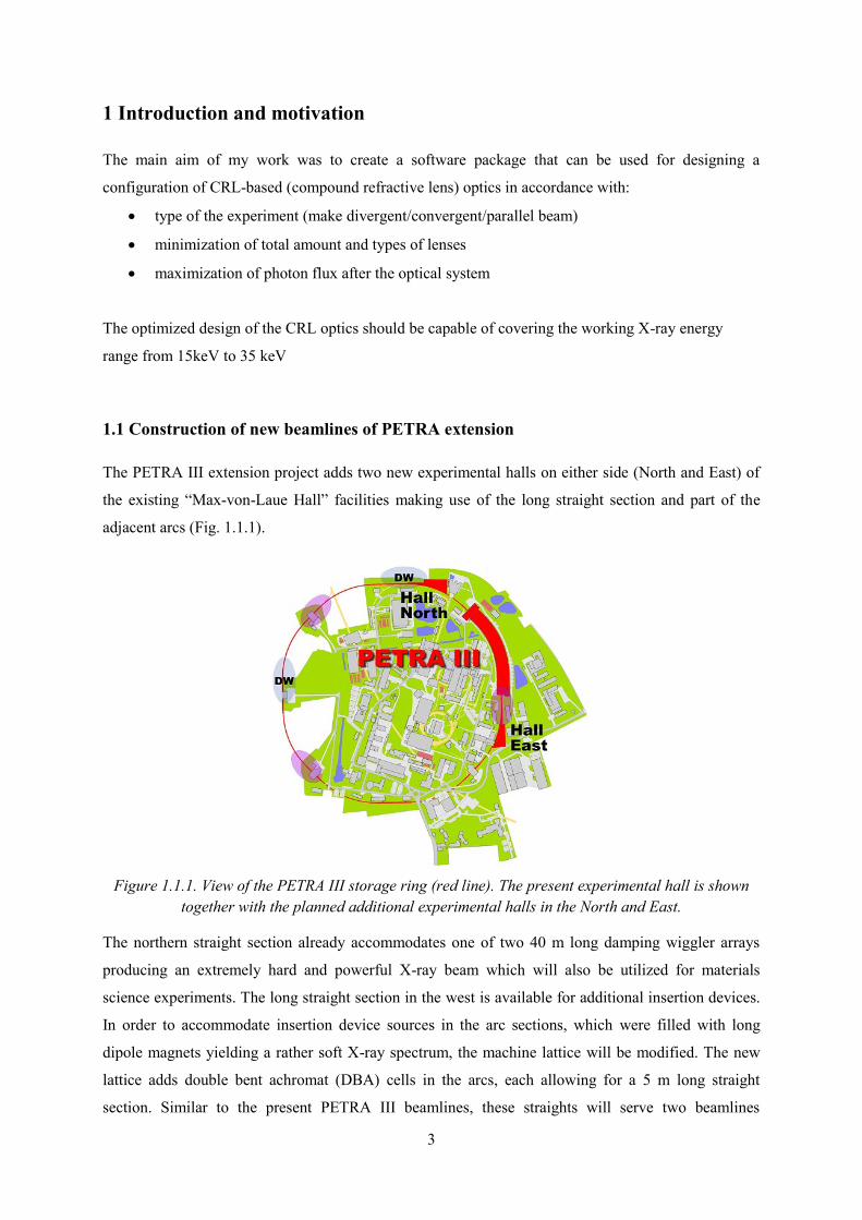
The PETRA III extension project adds two new experimental halls on either side (North and East) of

the existing “Max-von-Laue Hall” facilities making use of the long straight section and part of the

adjacent arcs (Fig. 1.1.1).

Figure 1.1.1. View of the PETRA III storage ring (red line). The present experimental hall is shown

together with the planned additional experimental halls in the North and East.

The northern straight section already accommodates one of two 40 m long damping wiggler arrays

producing an extremely hard and powerful X-ray beam which will also be utilized for materials

science experiments. The long straight section in the west is available for additional insertion devices.

In order to accommodate insertion device sources in the arc sections, which were filled with long

dipole magnets yielding a rather soft X-ray spectrum, the machine lattice will be modified. The new

lattice adds double bent achromat (DBA) cells in the arcs, each allowing for a 5 m long straight

section. Similar to the present PETRA III beamlines, these straights will serve two beamlines

4

independently by use of canting dipoles resulting in two separate 2 m long straights. Different from

the present 5 mrad canting scheme, a canting angle of 20 mrad was chosen at the extension beamlines

to provide more spatial flexibility for the experiments further downstream. In total, the new lattice

provides eight short straight high-β sections in the two arcs making them very suitable for the use of

undulators. Overall, 11 new beamlines will be built in different phases. Five of the new beamlines will

be designed as "short undulator" beamlines continuing most of the productive techniques formerly

provided at DORIS III bending magnet beamlines. These sources will not only be very well suited for

the spectrum of applications to be relocated from DORIS III but also provide a considerably brighter

beam. In addition, four high-brilliance long undulator beamlines will be built in PETRA III hall East,

three of them in collaboration with international partners, Sweden, India and Russia.

1.2 Russian-German nanodiffraction beamline (P23) at PETRA extension

The main focus of the beamline will be on the application of in situ and in operando diffraction

techniques for the study of low-dimensional and nanoscale systems, i.e. structural properties and

especially their evolution during chemical processes or under non-ambient conditions, such as high

pressure, low temperature, electrical and magnetic fields, laser irradiation etc.

Examples of scientific cases are:

Space averaging methods

The most common and demanded application of X-ray diffraction is conventional space averaging

scattering from bulk and surface objects. One major focus lies on the investigation of catalytic

processes and relevant materials. Conventional averaging X-ray diffraction techniques are e.g. being

used for the investigation of atomic structure of surfaces. A large part of the in situ research is

dedicated to liquid/solid interfaces, e.g. the growth of complex functional nanomaterials and their

properties. Progress has especially been achieved in time-resolved investigations of phase

transformations, such as crystallization of immobilized nanoparticles from the amorphous phase,

electric field induced phase transitions and ferroelectric switching mechanisms.

Diffraction microscopy of bulk objects

Diffraction using X-ray microbeams has considerably widened the research possibilities at the

nanoscale. This applies not only to novel nanoscaled objects, but also to investigations of already well-

studied materials that can be re-visited with access to ultra-short length scales. The basic diffraction

tomography analysis can be combined with X-ray fluorescence spectroscopy and XANES. Along with

the phase analysis in complex polycrystalline structures, pencil beams are also used for the

investigation of local strain tensors, stress and microstructure evolution in nanocrystalline materials.

This technique is applicable to single crystals, composite and functional graded materials.

Diffraction microscopy of nanosized objects

5

Microbeam X-ray diffraction is gaining importance as an effective tool for studying single

nanocrystalline objects and oriented arrays of such objects. Technically, the studies of individual

objects at the nanoscale are very challenging and require, along with an extraordinary stability of the

instrument and the X-ray optical system, a parallel application of state-of-the-art nano-sample

handling and characterization techniques. Combination of microbeam diffraction with anomalous

scattering to investigate distortions in scanning probe nanolithography demonstrated an opportunity to

use nanoscale strain variations for the selection of the initial material state in ferroelectrics, dielectrics,

and other complex oxides. Additional opportunities arise through the parallel use of atomic force

microscopy which allows selective introduction of defects or simultaneous probing of elastic

properties in single nanocrystals.

Coherent diffraction imaging of nanosized objects

Coherent Diffraction Imaging (CDI) can be applied to investigate two- and three-dimensional

structures with a resolution at 10 nm scales. CDI has developed into a characterization method capable

of observing also the inner structure of complex nanoparticles and measuring internal strain evolution

in nanoparticles under extreme conditions.

X‑ray Bragg diffraction ptychography

The advantages of CDI can be combined with the structural sensitivity of conventional X-ray

diffraction which is utilized in Bragg Diffraction Ptychography (BDP). The BDP method was also

shown to deliver detailed information on the strain field around single dislocations in silicon. With a

focal spot as large as 1 µm, it was possible to resolve the strain with a resolution down to 50 nm. This

value could be further improved by increasing the photon flux in the focal spot. BDP is a unique tool

for the investigation of domain structures and domain wall configurations in complex ferroelectric and

multiferroic thin film systems, which is hardly obtainable with any other method. Bragg diffraction

ptychography is very relevant for the scientific case of the beamline. A constraint on its applicability

could be the short focal length of the optics necessary to reach focal spots at the diffraction limit.

However, improved methods of data evaluation with partially coherent beams could allow to

overcome this condition and make it available for in situ measurements.

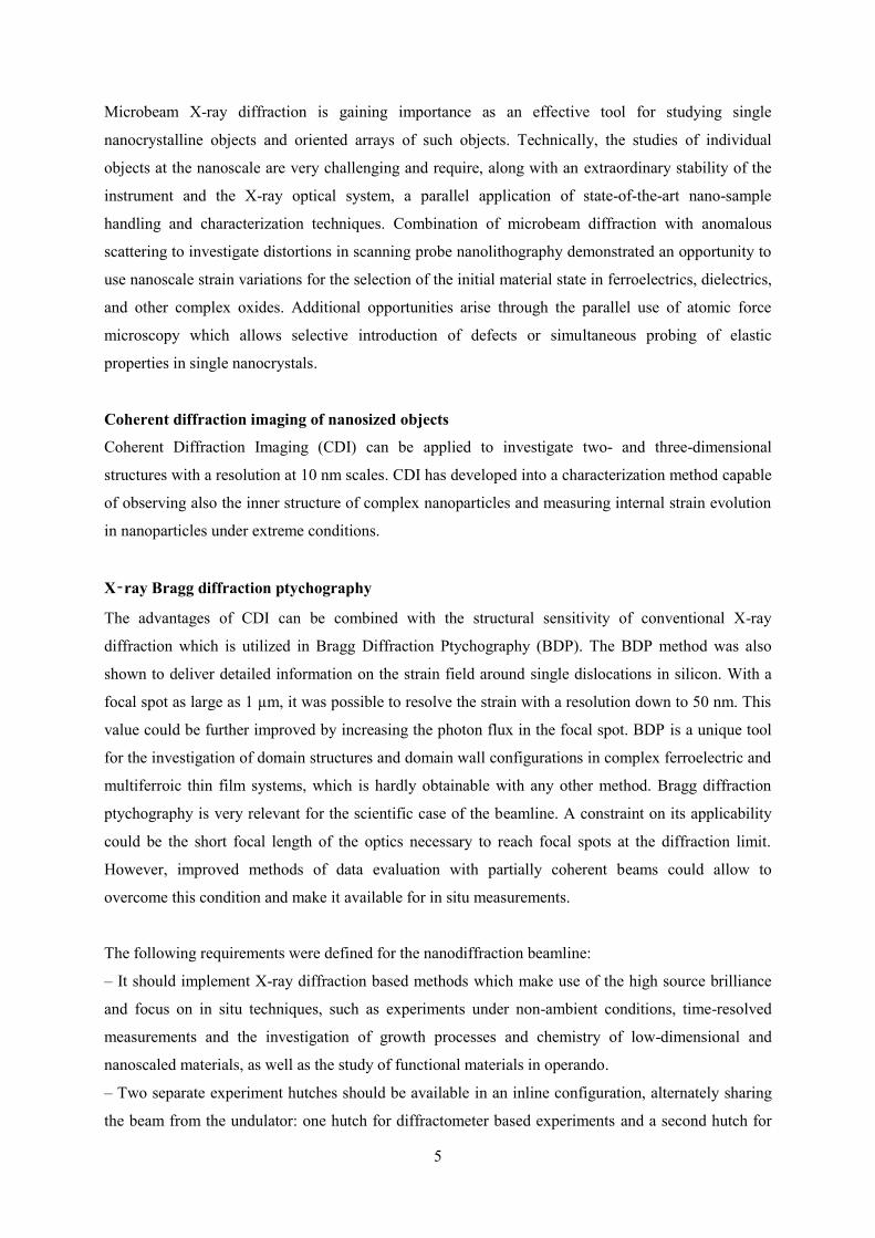
The following requirements were defined for the nanodiffraction beamline:

– It should implement X-ray diffraction based methods which make use of the high source brilliance

and focus on in situ techniques, such as experiments under non-ambient conditions, time-resolved

measurements and the investigation of growth processes and chemistry of low-dimensional and

nanoscaled materials, as well as the study of functional materials in operando.

– Two separate experiment hutches should be available in an inline configuration, alternately sharing

the beam from the undulator: one hutch for diffractometer based experiments and a second hutch for

6

accommodating rather large and complex instrumentation for sample growth and characterization

including a UHV facility.

– The diffractometer must allow for heavy in situ sample environments for the investigation of growth,

electrochemistry, chemical reactions, catalysis, etc.

– A set of dedicated sample cells should be developed for the beamline and be made available for user

groups. The decision on the types of sample cells will be made later depending on user demand.

– The X-ray optics of the beamline should provide a high brilliance monochromatic beam in the

energy range from 5 keV to 35 keV and a photon flux ~1013

photons/sec at 10 keV.

– The beam spot at the sample position should vary from ~ 0.3×0.3 mm2 down to sub-micrometer

dimensions.

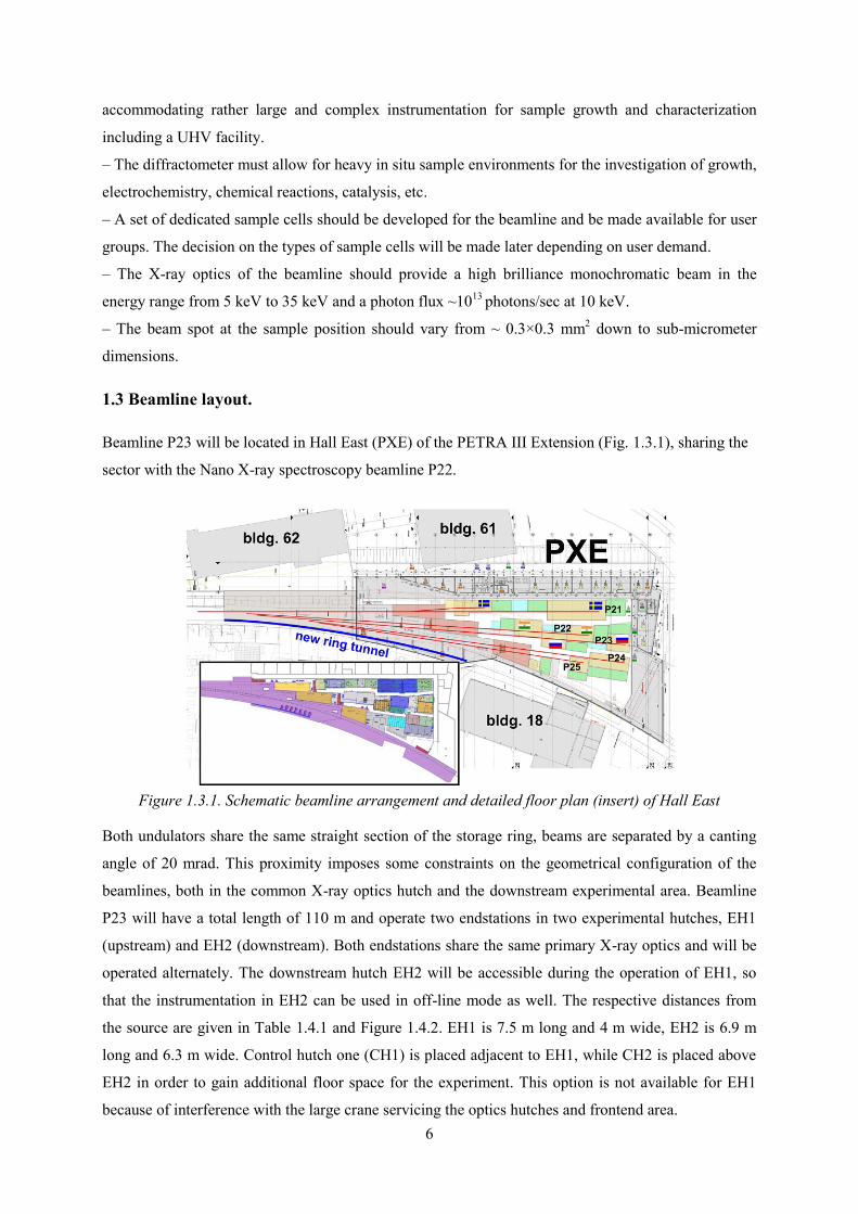
1.3 Beamline layout.

Beamline P23 will be located in Hall East (PXE) of the PETRA III Extension (Fig. 1.3.1), sharing the

sector with the Nano X-ray spectroscopy beamline P22.

Figure 1.3.1. Schematic beamline arrangement and detailed floor plan (insert) of Hall East

Both undulators share the same straight section of the storage ring, beams are separated by a canting

angle of 20 mrad. This proximity imposes some constraints on the geometrical configuration of the

beamlines, both in the common X-ray optics hutch and the downstream experimental area. Beamline

P23 will have a total length of 110 m and operate two endstations in two experimental hutches, EH1

(upstream) and EH2 (downstream). Both endstations share the same primary X-ray optics and will be

operated alternately. The downstream hutch EH2 will be accessible during the operation of EH1, so

that the instrumentation in EH2 can be used in off-line mode as well. The respective distances from

the source are given in Table 1.4.1 and Figure 1.4.2. EH1 is 7.5 m long and 4 m wide, EH2 is 6.9 m

long and 6.3 m wide. Control hutch one (CH1) is placed adjacent to EH1, while CH2 is placed above

EH2 in order to gain additional floor space for the experiment. This option is not available for EH1

because of interference with the large crane servicing the optics hutches and frontend area.

7

2 Beamline optics

2.1 Necessary requirements to the beamline optics.

The following requirements for the beam parameters in nanoscale X-ray diffraction have been

compiled:

spot cleanliness. It is important to notice that high-resolution diffraction experiments are

sensitive both to the spatial and angular distribution of the photons, in contrast to other

techniques such as small angle X-ray scattering or chemical analysis microscopy.

high stability against mechanical drifts and vibrations. To meet this requirement, demanding

design efforts will be needed in case of in-situ sample environments and especially for heavy

sample cells.

focal distance. Long focal distances are very desirable not only to preserve a low beam

divergence but also to leave sufficient space for larger sample environments. Obviously,

longer distances lead to larger focal spot sizes and also additional challenges to handle

stability issues.

wavefront distortion for coherent beam experiments. The form of the incident wavefront is an

important parameter in the data evaluation procedures used in coherent scattering methods. A

complex wavefront profile that could arise due to optics imperfection can strongly impede the

convergence of numerical evaluation procedures, while any instability in this parameter would

in most case make the data evaluation completely impossible.

maximal possible photon flux density in the focal spot.

Energy tunability and resolution at the beamline should be sufficient for XANES and resonant X-ray

scattering measurements as well as for wavelength scans of Bragg reflections. The latter option can be,

in many cases, a solution to the problem of sample displacements during angular scanning. The

beamline optics must be designed to meet these requirements, but also to allow accommodation of

further optical elements for future developments. The optical system should be reliably switchable

between different configurations.

2.2 Beamline optics layout. Source properties

The focusing optics must provide focused beams at two endstations positioned in EH1 and EH2 at

distances of ~88 m and ~108 m from the source. The targeted values of beam cross sections in

different operation modes, as discussed above, vary from ~0.3 mm down to ~1 µm in an energy range

from 4 keV to 35 keV. Smaller beams can be realized, but at the expense of reduced flux caused by

limiting apertures.

It is planned to employ two main beam focusing schemes: mirror-based for energies below 15 keV and

CRL-based for energies above 15 keV. There is a certain overlap of energy ranges optimal for both

8

approaches, which allows combined variants depending on the application. Moreover, at all energies

the CRLs will be complemented with flat mirrors for harmonics suppression. The focusing elements

close to the sample may also vary: for lower energies, KB systems will be preferably used. However,

in some cases one might also utilize Fresnel zone plates, especially for ultra-compact and/or in-

vacuum installations. For high energies, CRLs will be most effective and flexible for X-ray focusing.

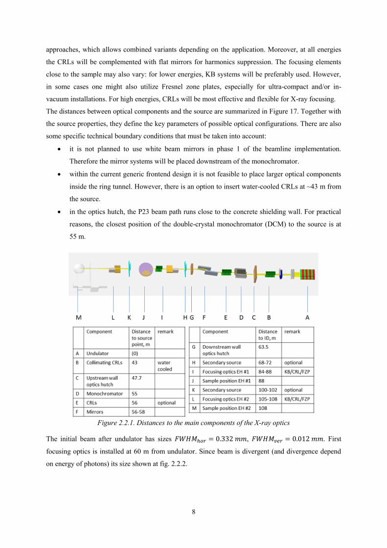
The distances between optical components and the source are summarized in Figure 17. Together with

the source properties, they define the key parameters of possible optical configurations. There are also

some specific technical boundary conditions that must be taken into account:

it is not planned to use white beam mirrors in phase 1 of the beamline implementation.

Therefore the mirror systems will be placed downstream of the monochromator.

within the current generic frontend design it is not feasible to place larger optical components

inside the ring tunnel. However, there is an option to insert water-cooled CRLs at ~43 m from

the source.

in the optics hutch, the P23 beam path runs close to the concrete shielding wall. For practical

reasons, the closest position of the double-crystal monochromator (DCM) to the source is at

55 m.

Figure 2.2.1. Distances to the main components of the X-ray optics

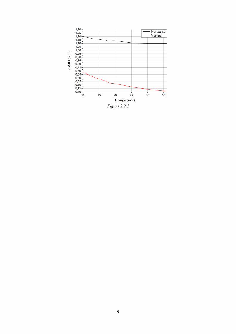
The initial beam after undulator has sizes , . First

focusing optics is installed at 60 m from undulator. Since beam is divergent (and divergence depend

on energy of photons) its size shown at fig. 2.2.2.

9

Figure 2.2.2

10

3 Focusing with lenses

3.1 Basic facts: geometrical optics

The lens-maker formula for a lens made from material with a refractive index with radii of curvature

of surfaces , and distance between them reads as:

( ) (

( )

) (3.1.1)

For a convex ( ) thin lens ( ) with equal radii of curvature on both sides eq.

3.1.1 transforms to:

( ) (3.1.2)

A refractive index:

(3.1.3)

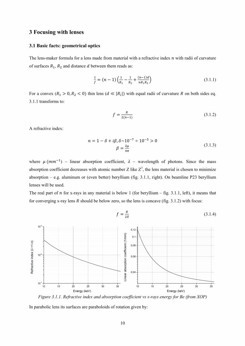
where ( ) – linear absorption coefficient, – wavelength of photons. Since the mass

absorption coefficient decreases with atomic number Z like Z3, the lens material is chosen to minimize

absorption – e.g. aluminum or (even better) beryllium (fig. 3.1.1, right). On beamline P23 beryllium

lenses will be used.

The real part of for x-rays in any material is below 1 (for beryllium – fig. 3.1.1, left), it means that

for converging x-ray lens should be below zero, so the lens is concave (fig. 3.1.2) with focus:

(3.1.4)

Figure 3.1.1. Refractive index and absorption coefficient vs x-rays energy for Be (from XOP)

In parabolic lens its surfaces are paraboloids of rotation given by:

11

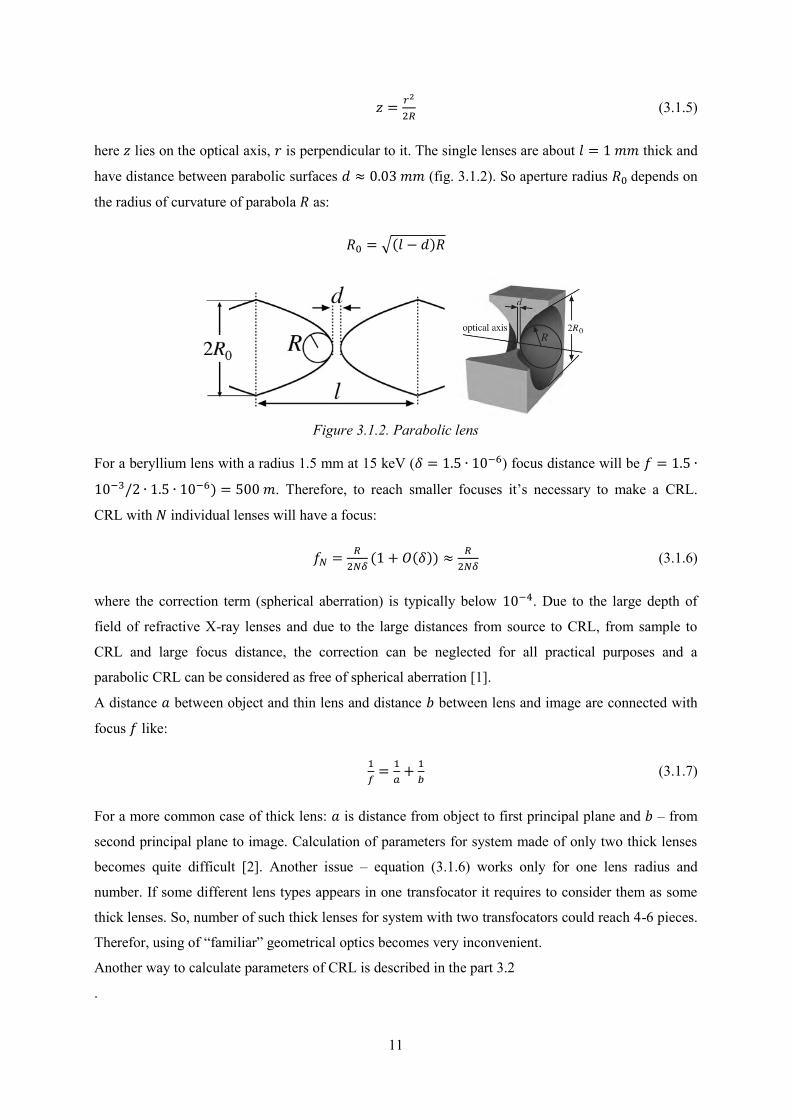
(3.1.5)

here lies on the optical axis, is perpendicular to it. The single lenses are about thick and

have distance between parabolic surfaces (fig. 3.1.2). So aperture radius depends on

the radius of curvature of parabola as:

√( )

Figure 3.1.2. Parabolic lens

For a beryllium lens with a radius 1.5 mm at 15 keV ( ) focus distance will be

) . Therefore, to reach smaller focuses it’s necessary to make a CRL.

CRL with individual lenses will have a focus:

( ( ))

(3.1.6)

where the correction term (spherical aberration) is typically below . Due to the large depth of

field of refractive X-ray lenses and due to the large distances from source to CRL, from sample to

CRL and large focus distance, the correction can be neglected for all practical purposes and a

parabolic CRL can be considered as free of spherical aberration [1].

A distance between object and thin lens and distance between lens and image are connected with

focus like:

(3.1.7)

For a more common case of thick lens: is distance from object to first principal plane and – from

second principal plane to image. Calculation of parameters for system made of only two thick lenses

becomes quite difficult [2]. Another issue – equation (3.1.6) works only for one lens radius and

number. If some different lens types appears in one transfocator it requires to consider them as some

thick lenses. So, number of such thick lenses for system with two transfocators could reach 4-6 pieces.

Therefor, using of “familiar” geometrical optics becomes very inconvenient.

Another way to calculate parameters of CRL is described in the part 3.2

.

12

3.2 Coherent X-ray focusing. Ray transfer matrix analysis

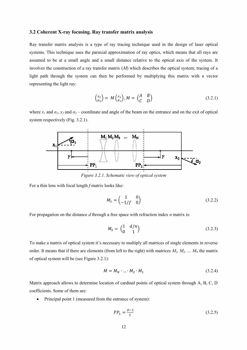
Ray transfer matrix analysis is a type of ray tracing technique used in the design of laser optical

systems. This technique uses the paraxial approximation of ray optics, which means that all rays are

assumed to be at a small angle and a small distance relative to the optical axis of the system. It

involves the construction of a ray transfer matrix (M) which describes the optical system; tracing of a

light path through the system can then be performed by multiplying this matrix with a vector

representing the light ray:

( ) (

) (

) (3.2.1)

where x1 and α1, x2 and α2 – coordinate and angle of the beam on the entrance and on the exit of optical

system respectively (Fig. 3.2.1).

Figure 3.2.1. Schematic view of optical system

For a thin lens with focal length f matrix looks like:

(

) (3.2.2)

For propagation on the distance d through a free space with refraction index n matrix is:

(

) (3.2.3)

To make a matrix of optical system it’s necessary to multiply all matrices of single elements in reverse

order. It means that if there are elements (from left to the right) with matrices M1, M2, … MN the matrix

of optical system will be (see Figure 3.2.1):

(3.2.4)

Matrix approach allows to determine location of cardinal points of optical system through A, B, C, D

coefficients. Some of them are:

Principal point 1 (measured from the entrance of system):

(3.2.5)

13

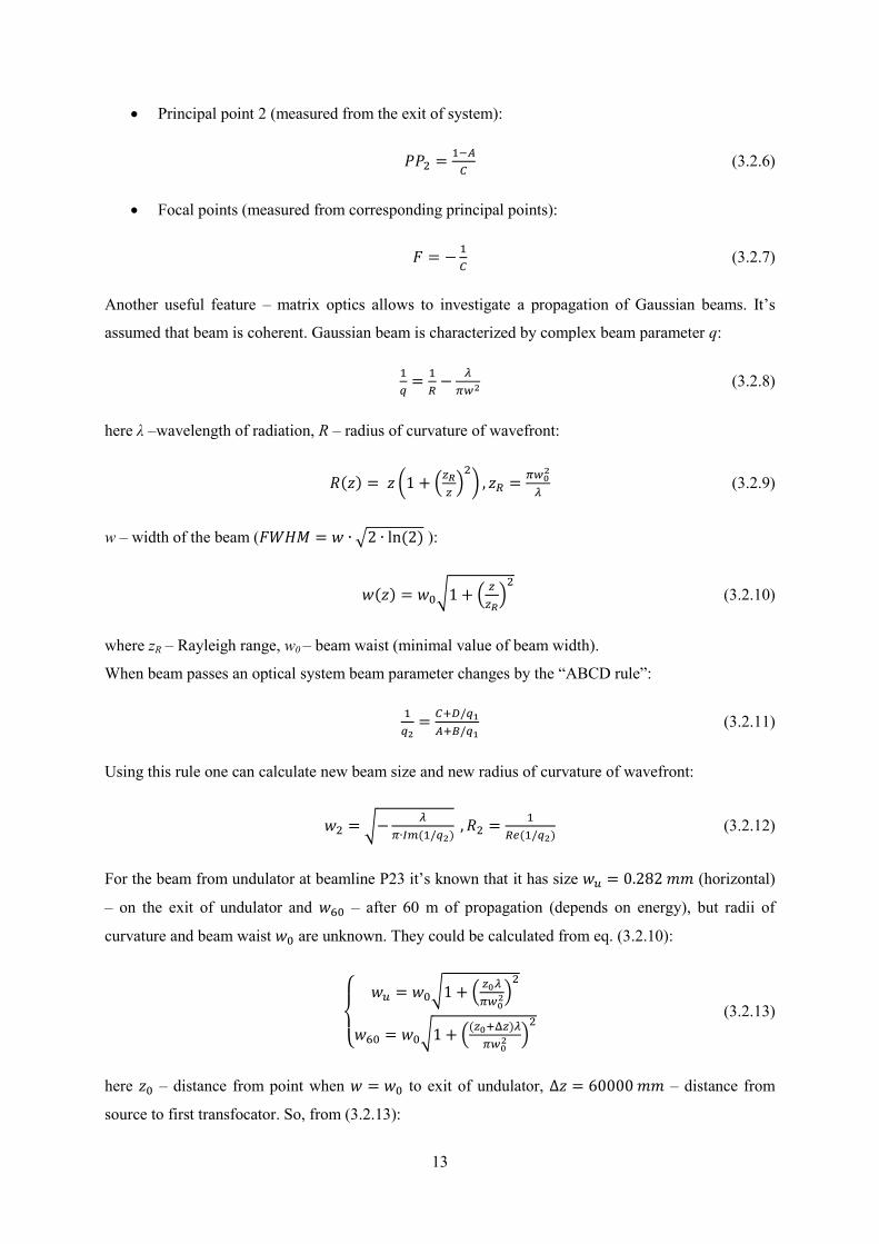
Principal point 2 (measured from the exit of system):

(3.2.6)

Focal points (measured from corresponding principal points):

(3.2.7)

Another useful feature – matrix optics allows to investigate a propagation of Gaussian beams. It’s

assumed that beam is coherent. Gaussian beam is characterized by complex beam parameter q:

(3.2.8)

here λ –wavelength of radiation, R – radius of curvature of wavefront:

( ) ( (

) )

(3.2.9)

w – width of the beam ( √ ( ) ):

( ) √ (

) (3.2.10)

where zR – Rayleigh range, w0 – beam waist (minimal value of beam width).

When beam passes an optical system beam parameter changes by the “ABCD rule”:

(3.2.11)

Using this rule one can calculate new beam size and new radius of curvature of wavefront:

√

( )

( ) (3.2.12)

For the beam from undulator at beamline P23 it’s known that it has size (horizontal)

– on the exit of undulator and – after 60 m of propagation (depends on energy), but radii of

curvature and beam waist are unknown. They could be calculated from eq. (3.2.10):

{

√ (

)

√ (( )

)

(3.2.13)

here – distance from point when to exit of undulator, – distance from

source to first transfocator. So, from (3.2.13):

14

√

√

( )

(

)

(

) ( )

(3.2.14)

15

4 Software implementation

Software is written in Python programming language with Python(x,y) development kit – it is a free

scientific and engineering development software for numerical computations, data analysis and data

visualization based on Python v.2.7.

Software for calculation parameters of CRL optic system has 3 modules:

1) Main module (“TS_matrix_optics_XX”) is responsible for:

Choosing and optimizing CRL transfocators in conformity with geometry of the setup

and x-ray source properties.

Calculation ray transfer matrices for optical systems.

Calculation of beam size at any point of optical system.

Managing other modules and general calculation flow.

This module is described in details in 4.1.

2) Module for calculation of photon flux transmitted through transfocators

(“TS_transmission_gauss_module_XX”). The description is in part 4.2.

3) Service module (“TS_read_data”) which is used for reading miscellaneous data (initial beam

sizes, optical constants, etc.) from hard disk. It has 3 fiunctions:

size_calc – reads size of beam (FWHM) on 60 m from undulator for chosen

energy of photons.

delta_calc – reads refraction index for chosen x-ray energy.

mu_calc – reads linear absorption coefficient for chosen energy (Energy) of

photons.

Note: In modules functions/classes with names started from “_” are used only as an auxiliary ones for

other modules/classes. Only “user-available” functions will be described below.

4.1 General calculation flow, optics optimization and geometry

The current version of software allows to calculate parameters of two transfocators (and their

combinations) from given lens setup and, vice versa, to select best combination of lenses in

transfocators to achieve desirable imaging conditions.

In software transfocators are represented as list objects in format:

[[N1, N2, …], [R1, R2, …], [d1, d2, …], l]

here Ni – number of lenses one type, Ri – radius of curvature of parabola, di – distance between peeks

of parabolic surfaces in lens, l – thickness of one lens (see part 3.1).

Global input parameters are:

– energy_min, energy_max, energy_step – range of energy for calculation: [energy_min,

energy max] with step energy_step.

16

– dist_Src_TS1, dist_TS1_TS2, dist_TS2_Sample – distances from undulator to first

transfocator, between transfocators, from second transfocator to sample respectively.

– dist_TS1_image1 (dist_TS2_image2) – desirable distance from first (second) transfocator to

image created by it.

– Source_hor_0 (Source_ver_0) – beam size (FWHM) on the exit of the undulator.

– R_set1 (R_set2) – list of radii of lenses that are allowed to use in first (second) transfocator.

– lens_groups11 (lens_groups21) – groups of lenses of 1st radius that are allowed to use in 1st

(2nd) transfocator.

– lens_groups12 (lens_groups22) – groups of lenses of 2nd radius that are allowed to use in 1st

(2nd) transfocator.

Choosing the transfocator

build_TS_from_dist – Makes a list of transfocators from specified group of lenses with specified

radii which create an image of object on appropriate distance from transfocator.

Matrix optics

All_elements (class) – the object of this class is a list of all elements in optical system. This list

contains an index number of the element, information about type of element (free space or lens) and

parameter of every element (length of space of focus of lens), it looks like:

n type parameter

0 ‘space’ 60000

1 ‘lens’ 495000

2 ‘space’ 1

3 ‘lens’ 495000

… … …

system_matrix – makes a matrix of optical system from the list of elements (‘All_elements’ class

object). It uses matrix formalism from part 3.2 (eq. 3.2.1 – 3.2.4).

cardinal_points – calculates distances to cardinal points of the optical system – see eq. 3.2.5 -

3.2.7

Beam size calculation

size_calc_geometry – calculates size of beam on the out of optical system using conventional

geometrical optics laws:

(4.1.1)

here is distance from object to first principal plane, – from second principal plane to image, –

size of object and – size of image in the image plane. To know size of beam not only in image

plane, approximate equation is used:

(4.1.2)

17

where – coordinate of beam that entered the system at optical axis with angle ( – beam

divergency):

(

) (

)( ) (4.1.3)

size_calc_wave_parameter – calculates beam size from transformation of complex beam parameter–

see eq. 3.2.8 – 3.2.13.

4.2 Transmission and beam loss factor

Absorption of monochromatic beam in matter is described with Beer–Lambert law:

( ) (4.2.1)

where is a linear absorption coefficient, – thickness of material, and – initial intensity of x-

rays and intensity after propagation through material.

For a CRL with parabolic lenses with radius of aperture , radius of curvature of parabolas and

distance between parabolas (fig. 3.1.2) beam loss factor is [3]:

( )

( ( ))

(4.2.2)

Unfortunately, this equation works only for beams with uniform distribution of intensity. For beam

with Gaussian distribution (with standard deviations , in horizontal and vertical directions) of

intensity:

(

) (

) (4.2.3)

beam loss factor is calculated analytically in quite complex way [1]. But it’s easy to calculate beam

loss factor numerically: just use eq. 4.2.1 in every point of every lens and then divide sum of intensity

after the CRL by sum of intensity before CRL.

There is only one user-available function in TS_transmission_gauss_module: calculate – it calculates

the transmission numerically as described above. One important thing – it’s assumed that paraxial

approximation for optical system is working (== size of beam is changed negligible during

propagation through CRL).

4.3 Output

18

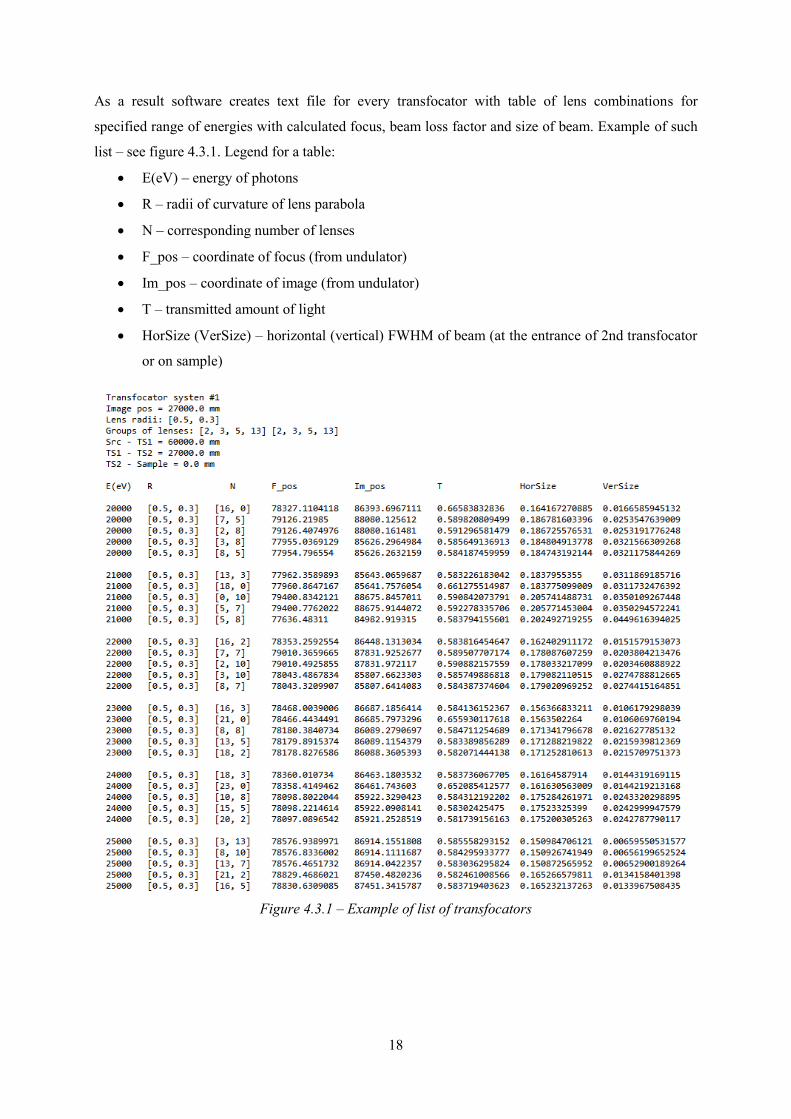
As a result software creates text file for every transfocator with table of lens combinations for

specified range of energies with calculated focus, beam loss factor and size of beam. Example of such

list – see figure 4.3.1. Legend for a table:

E(eV) – energy of photons

R – radii of curvature of lens parabola

N – corresponding number of lenses

F_pos – coordinate of focus (from undulator)

Im_pos – coordinate of image (from undulator)

T – transmitted amount of light

HorSize (VerSize) – horizontal (vertical) FWHM of beam (at the entrance of 2nd transfocator

or on sample)

Figure 4.3.1 – Example of list of transfocators

19

5 Application examples

The typical distances between optical components in P23 could be: undulator - transfocator 1 – 60 m,

transfocator 1 - transfocator 2 – 26 m, transfocator 2 - sample – 1 m. This values will be used for

examples in this chapter.

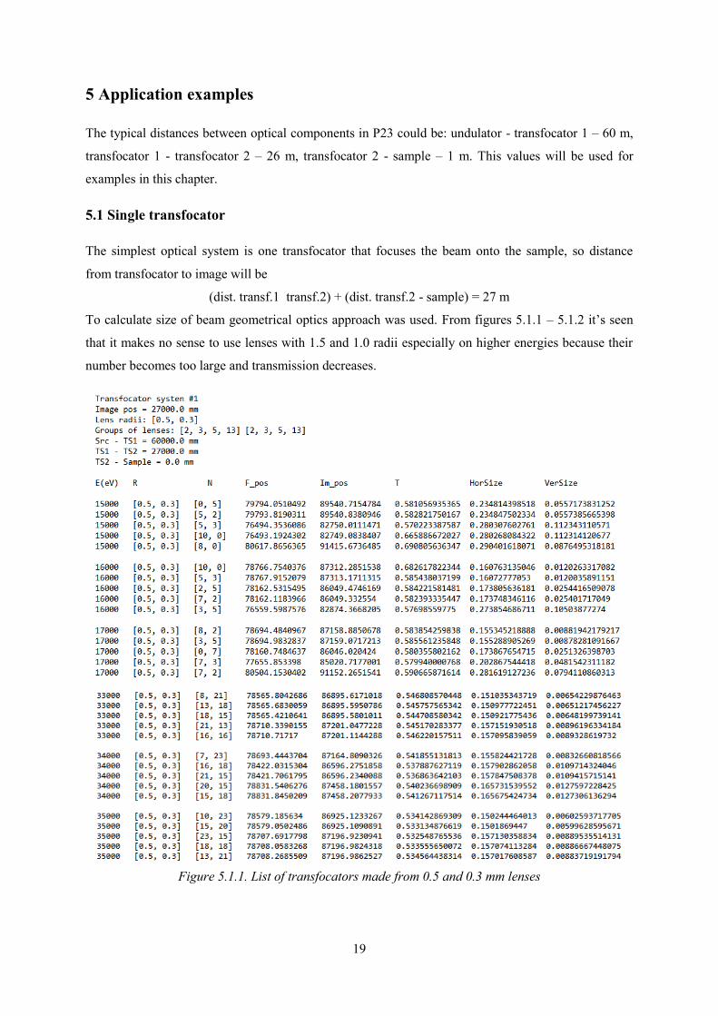
5.1 Single transfocator

The simplest optical system is one transfocator that focuses the beam onto the sample, so distance

from transfocator to image will be

(dist. transf.1 transf.2) + (dist. transf.2 - sample) = 27 m

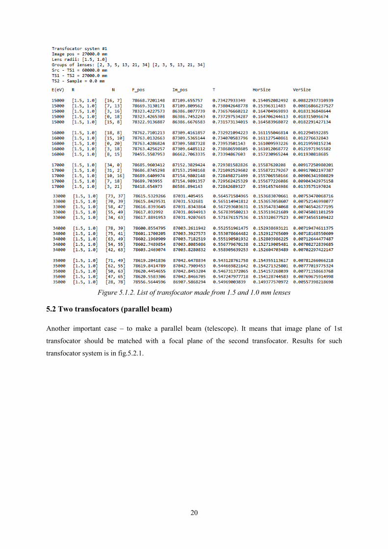
To calculate size of beam geometrical optics approach was used. From figures 5.1.1 – 5.1.2 it’s seen

that it makes no sense to use lenses with 1.5 and 1.0 radii especially on higher energies because their

number becomes too large and transmission decreases.

Figure 5.1.1. List of transfocators made from 0.5 and 0.3 mm lenses

20

Figure 5.1.2. List of transfocator made from 1.5 and 1.0 mm lenses

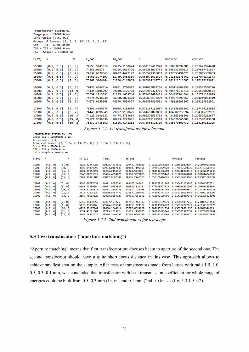
5.2 Two transfocators (parallel beam)

Another important case – to make a parallel beam (telescope). It means that image plane of 1st

transfocator should be matched with a focal plane of the second transfocator. Results for such

transfocator system is in fig.5.2.1.

21

Figure 5.2.1. 1st transfocators for telescope

Figure 5.2.2. 2nd transfocators for telescope

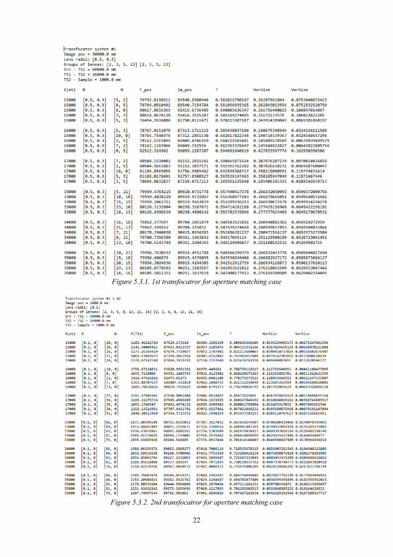
5.3 Two transfocators (“aperture matching”)

“Aperture matching” means that first transfocator pre-focuses beam to aperture of the second one. The

second transfocator should have a quite short focus distance in this case. This approach allows to

achieve smallest spot on the sample. After tests of transfocators made from lenses with radii 1.5, 1.0,

0.5, 0.3, 0.1 mm, was concluded that transfocator with best transmission coefficient for whole range of

energies could be built from 0.5, 0,3 mm (1st tr.) and 0.1 mm (2nd tr.) lenses (fig. 5.3.1-5.3.2).

22

Figure 5.3.1. 1st transfocatror for aperture matching case

Figure 5.3.2. 2nd transfocatror for aperture matching case

23

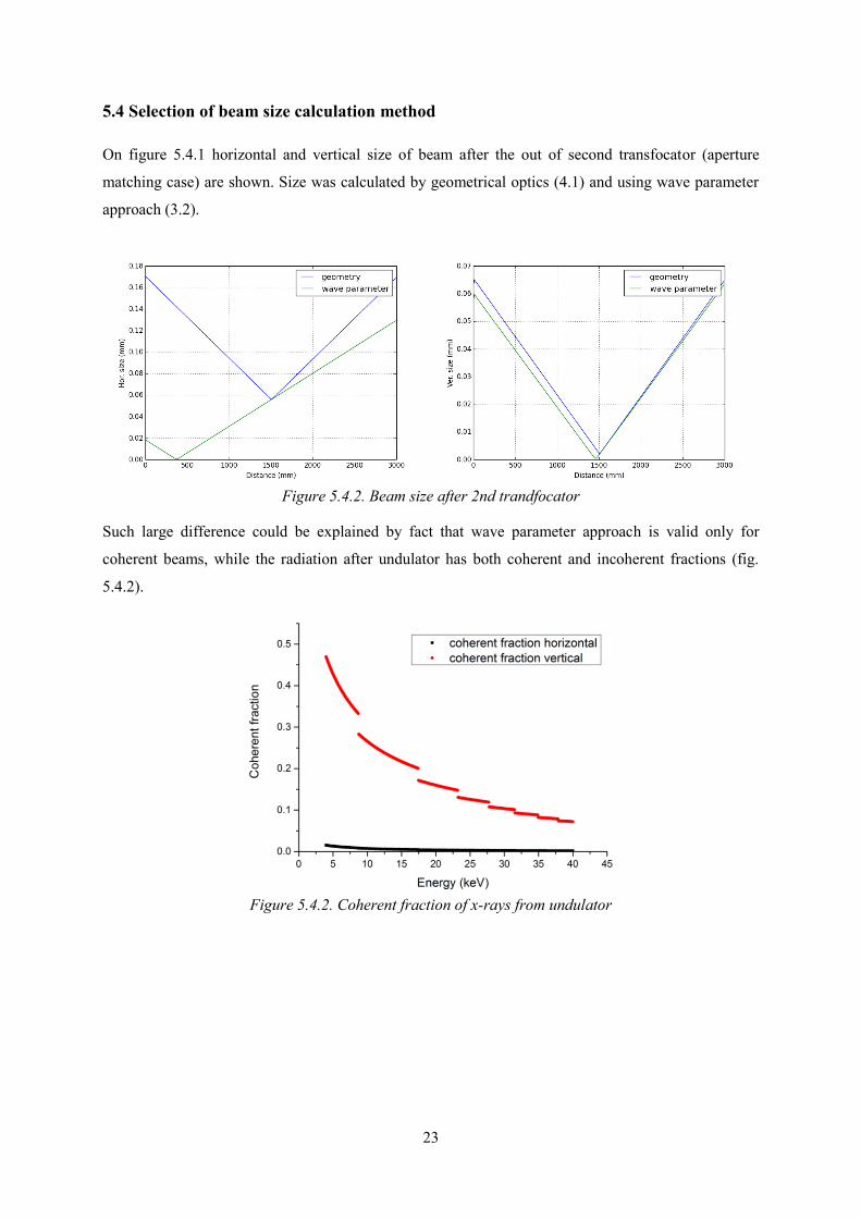
5.4 Selection of beam size calculation method

On figure 5.4.1 horizontal and vertical size of beam after the out of second transfocator (aperture

matching case) are shown. Size was calculated by geometrical optics (4.1) and using wave parameter

approach (3.2).

Figure 5.4.2. Beam size after 2nd trandfocator

Such large difference could be explained by fact that wave parameter approach is valid only for

coherent beams, while the radiation after undulator has both coherent and incoherent fractions (fig.

5.4.2).

Figure 5.4.2. Coherent fraction of x-rays from undulator

24

Conclusion

A new software package was created, tested and used for beamline CRL optics design. Software is

written in Python, has a modular structure. Typical scenarios of beamline CRL layout were tested: one

transfocator, telescope, aperture matching. The modules developed in this work will become a part of

beamline operation software at the Russian-German nanodiffraction beamline at PETRA.

Acknowledgement

I would like to thank Jana Raabe for her friendly support and cooperation during my stay at DESY.

References

[1] B. Lengeler et al., Imaging by parabolic refractive lenses in the hard X-ray range, (2000)

[2] Eugene Hecht, Optics, (2002)

[3] B. Lengeler et al., Transmission and gain of singly and doubly focusing refractive x-ray lenses,

(1998)