Embed Size (px)
Citation preview
RUHR-UNIVERSITÄT BOCHUM
DEVELOPMENT OF THE
INTERMODULATED DIFFERENTIAL IMMITTANCE
SPECTROSCOPY FOR
ELECTROCHEMICAL ANALYSIS
DISSERTATION
SUBMITTED FOR THE DEGREE OF
DOCTOR OF NATURAL SCIENCES (DR. RER. NAT.)
FAKULTÄT FÜR CHEMIE UND BIOCHEMIE
Zentrum für Elektrochemie - CES
BOCHUM, JUNE 2014
ALBERTO BATTISTEL
The work presented in this thesis was carried out during my doctoral studies from
November 2010 to June 2014 in the group of Dr. Fabio La Mantia; Center for
Electrochemical Sciences (CES) - Semiconductor Electrochemistry & Energy
Conversion, Ruhr-Universität Bochum.
Date of submission
Chair of examination board
First supervisor
Dr. La Mantia
Second supervisor
Prof. Dr. W. Schuhmann

Dedico questo lavoro di tesi a mio padre


i
ACKNOWLEDGEMENTS
This thesis represents some of the professional achievements I collected in the last
three and a half years, but it would have been not possible without the help and
support of many.
I am extremely grateful to my supervisor Dr. Fabio La Mantia. I must say he was far
more than a simple guide during these years. He helped and supported me inside
and outside the lab. From him I have learnt that dedication, hard work, and
especially studying always pay back. I enjoyed a lot our endless discussions about
science, history, sociology, and politic… I regret I did not have time and energy
enough to put into practice some of the fabulous ideas we discussed. Dr. Fabio La
Mantia is for me the SuperV, an example, and a friend.
I thank Prof. Wolfgang Schuhmann my second supervisor. We first met four years
ago during my master and he gave me the possibility to come back here for my PhD.
He is the person created and keep running the group of analytical chemistry where I
could meet, discuss, and collaborate with many persons in the last years.
I should also mention that I am very thankful for the great effort both my
supervisors put in the last weeks in order to allow me to submit this thesis in time.
I want to thank Bettina Stetzka and Monika Niggemeyer for their patience with me: I
know I am really a disaster about administration!
I would like to thank who helped me in correcting and improving this thesis: Giorgia
Zampardi, Dr. Rosalba Rincon, Andrea Contin, Jan Clausmeyer, Dr. Guoqing Du,
Andjela Petkovic, and Rebecca Straub.
Heartfelt thanks goes to my girlfriend Rebecca Straub who rescues my soul from
science and shows me how important are other things of the life. Thank you!
A special thanks goes to Dr. Mauro Pasta who showed me that you have to be crazy
and determined in the life. You have not to care about what the others think and that
what you do you do it for yourself.
I am thankful to a lot of persons who in these years were close to me. Persons I met
here in Bochum, persons with whom I worked, studied, discussed, joked, hanged
out… A simple list cannot show my thanksgiving: Giorgia Zampardi, Dr. Rosalba
Rincon, Andrea Contin, Jan Clausmeyer, Dr. Guoqing Du, Dr. Aleksandar Zeradjanin,
Mu Fan, Dr. Jelena Stojadinovic, Dr. Edgar Ventosa, Dr. Rafael Trocoli Jimenez,
Bernhard Neuhaus, Dr. Jorge Eduardo Yánez Heras, Dr. Freddy Oropeza, Dr. Mauro
Pasta, Alberto Ganassin, Dr. Magdalena Gebala, Dr. Nicolas Plumere, Alex
Alborghetti, and Dr. Stefan Klink. These persons helped directly or indirectly in my
human and professional development and only a small fraction of what I have shared
with them can be placed on paper.

ii
I want to thank also my flatmates: Dr. Stefan Klink, Christian Sorgenfrei, and Arne
Wege for the nice time shared together at home.
I am grateful to Dr. Nicolas Plumere, Stéphanie Huss and the little Luop for the nice
time spent together, for the crazy Fridays, the walk to the lake, and the long travels
together (which I mostly spent sleeping ). Furthermore, they fed and influenced my
vision and interpretation of the life and of the world.
I want to thank Prof. Salvatore Daniele and all the members of his group who taught
me electrochemistry back in the time in Venice.
Un ringraziamento va alla mia famiglia e in particolare a mio padre. Sono fortunate:
mi é stato insegnato cosa vuol dire usare la propria testa e mantenere uno spirito
critico, ma senza cattiveria, nella vita. Quello che sono e dove sono arrivato lo devo a
voi. Grazie di cuore!
Grazie anche a tutti gli amici in Italia, che mi accolgono sempre a braccia aperte
quando torno a casa anche se non mi faccio mai sentire.
iii
CONTENTS
Acknowledgements .................................................................... i
Contents ................................................................................... iii
List of symbols and abbreviations ............................................ vi
1 Introduction ......................................................................... 1
1.1 State of the art .................................................................................... 2
1.1.1 History of impedance spectroscopy .................................................. 2
1.1.2 Nonlinear analysis .......................................................................... 4
1.1.3 Electrochemical noise ................................................................... 10
1.1.4 Gas-evolving electrodes and bubble effects ..................................... 12
1.2 Motivation and aims ........................................................................... 18
1.3 Final remarks and outlines .................................................................. 20
2 Theory ................................................................................ 22
2.1 Basic concept of electrochemistry ........................................................ 23
2.2 Linear systems and electrochemical impedance spectroscopy .................. 26
2.2.1 Transfer functions ........................................................................ 26
2.2.2 Electrochemical impedance spectroscopy ........................................ 27
2.3 Development of the nonlinear system ................................................... 35
2.3.1 Intermodulation ........................................................................... 36
2.3.2 Definitions and development of new transfer functions ..................... 36
2.3.3 Simplified case ............................................................................ 39
2.3.4 Ideal nonlinear case: diode ........................................................... 40
2.3.5 Electrochemical case: redox couple ................................................ 41
2.3.6 Mathematical simulation of the redox couple ................................... 43
2.3.7 Resistance compensation .............................................................. 53
2.4 Development of the nonlinear time varying system ................................ 55
3 Experimental part ............................................................... 59
3.1 Potentiostat and impedance measurement ............................................ 60
3.1.1 Potentiostat ................................................................................ 60
iv
3.1.2 Impedance measurements ............................................................ 62
3.2 Development of the IDIS instrumental setup ......................................... 67
3.2.1 Lock-in setup .............................................................................. 68
3.2.2 Oscilloscope setup........................................................................ 70
3.3 Electrochemical cell ............................................................................ 74
3.3.1 Capacitor bridge .......................................................................... 74
3.3.2 Coaxial cell ................................................................................. 75
3.4 Materials and procedures .................................................................... 78
3.4.1 Chemicals and electrodes .............................................................. 78
3.4.2 Standard electrochemical characterization and procedures ................ 80
3.4.3 IDIS instrument and parameters.................................................... 81
3.4.4 Potentiostat transimpedance and lock-in amplifier transfer function ... 82
3.4.5 Fitting procedure ......................................................................... 83
3.4.6 Uncompensated resistance correction ............................................. 83
4 Results and discussion ....................................................... 85
4.1 Instrument calibration and artifacts in impedance .................................. 86
4.1.1 Potentiostat transimpedance ......................................................... 86
4.1.2 Lock-in transfer function ............................................................... 89
4.1.3 Cell geometry and capacitor bridge ................................................ 90
4.2 Ideal nonlinear system: diode .............................................................. 96
4.2.1 Diode characterization .................................................................. 96
4.2.2 IDIS of the diode: nonlinear capacitance ......................................... 97
4.2.3 Uncompensated resistance correction ........................................... 101
4.3 Real electrochemical system: redox couple ......................................... 105
4.3.1 Characterization of the redox couple ............................................ 105
4.3.2 IDIS of the redox couple ............................................................. 107
4.3.3 Fitting of the differentials ............................................................ 109
4.4 Time variant system: gas-evolving electrode ....................................... 114
4.4.1 Characterization of the oxygen evolution reaction .......................... 114
4.4.2 Bubble evolution as a time variant system .................................... 116
v
4.4.3 Normalized impedance ............................................................... 119
4.5 Final remarks .................................................................................. 127
5 Conclusion ........................................................................ 129
5.1 Main contributions ............................................................................ 130
5.2 Further development ........................................................................ 133
Appendix ............................................................................... 135
A. Mass transport operator .................................................................... 135
B. Intermodulated differential immittance spectroscopy in impedance format
137
C. Relaxation of the a priori separation of faradaic and capacitive current ... 138
Bibliography .......................................................................... 140
List of publications ................................................................ 150
Patent ...................................................................................................... 150
Published peer-reviewed articles ................................................................. 150
Accepted work .......................................................................................... 150
Works in preparation ................................................................................. 150
Talks at international conferences ................................................................ 151
Posters at international conferences ............................................................. 151
vi
LIST OF SYMBOLS AND ABBREVIATIONS
Abbreviations
AC Alternating current
CE Counter electrode
CPE Constant-phase element
DC Direct current
EFM Electrochemical frequency modulation
EIS Electrochemical impedance spectroscopy
FFT Fast Fourier transform
FRA Frequency response analyzer
IDIS Intermodulated differential immittance spectroscopy
MICTF Modulation of interface capacitance transfer function
NLEIS Nonlinear impedance spectroscopy
PDS Power density spectrum
PSD Phase-sensitive detector
RE Reference electrode
WE Working electrode
Lower case symbols
a Surface area of the electrode [cm-2]
c Concentration [M]
cOx Concentration of oxidized species [M]
cRed Concentration of reduced species [M]
dG Differential conductance [S V-1]
vii
dR Differential resistance [Ω V-1]
dX Differential reactance [Ω V-1]
dY Differential admittance [S V-1]
dZ Differential impedance [Ω V-1]
e Elementary charge [C]
f Generic function -
i Current [A]
i0 Exchange current [A]
ic Capacitive current [A]
iF Faradaic current [A]
il Leakage current [A]
j Imaginary unit -
kB Boltzman constant -
m Mass transport operator [M A-1]
mOx Mass transport operator for the oxidized species [M A-1]
mRed Mass transport operator for the reduced species [M A-1]
n Number of electrons involved in the reaction -
u Potential [V]
Upper case symbols
A Generic vector -
B Susceptance [Ω]
C Capacitance [F]
Cdl Double layer capacitance [F]

viii
CSC Semiconductor capacitance [F]
D Diffusion coefficient [cm s-2]
DOx Diffusion coefficient of the oxidized species [cm s-2]
DRed Diffusion coefficient of the reduced species [cm s-2]
F Faraday constant [C mol-1]
G Conductance [Ω]
H Hessian matrix -
HF Faradaic Hessian -
Im(•) Imaginary argument -
J Jacobian vector -
ND Doping level [cm-3]
R Gas constant; Resistance [J K-1 mol-1]
Rct Charge transfer resistance [Ω]
Re(•) Real argument -
T Absolute temperature [K]
V Different of potential [V]
X Vector of variables -
Y Admittance [S]
Yc Capacitive admittance [S]
YF Faradaic admittance [S]
Z Impedance [Ω]
ZA Normalized impedance [Ω]
Zm Mean impedance [Ω]
ZW Warburg impedance [Ω]
ix
Greek symbols
Symmetry factor -
Symmetry of mass transport -
Double layer capacitance variation [F V-1]
electric permittivity [F m-1]
F m-1
r relative permittivity -
overpotential [V]
a Activation overpotential [V]
ohm Concentration overpotential [V]
conc Ohmic overpotential [V]
Warburg coefficient [Ω rad0.5 s-0.5]
Double layer capacitance time constant [s]
Stimulus angular frequency; stimulus subscription [rad-1]; -
Probe angular frequency; probe subscription [rad-1]; -
Signs
•T Transpose vector -
F Fourier transform operator -
Sign of time derivative -
Sign of time oscillation -
Sign of anti-differential -
•* Complex conjugated -

1
1 INTRODUCTION
The first chapter of this thesis starts with an historical overview of the
electrochemical impedance. Later on, I proceed with the main features of the
nonlinear analysis in electrochemistry. In particular, I describe the characteristics of
the nonlinear impedance spectroscopy, of the electrochemical frequency modulation,
and of the modulation of interface capacitance transfer function technique. By
showing the features of these approaches, I introduce the main problems which are
not considered in these techniques. Most of these problems are addressed in the
development of the intermodulated differential immittance spectroscopy in the
following chapter.
In the last part of the section, I discuss about the electrochemical noise and how this
is related with the bubble generation during electrochemical evolution of gas.
Besides, I report the main achievements concerning gas-evolving electrodes
especially by the means of approaches based on the interpretation of the
phenomenon in the frequency domain.
Later on, I proceed with the motivation which moved this work and the aims I had in
mind in developing and applying the concept of intermodulation. In particular, I show
a couple of examples where the electrochemical impedance spectroscopy cannot
provide all the information of the investigated system, which is the starting point of
this thesis.
Besides, a short outline of the thesis is reported. In this outline, the most important
parts of the work are listed.
2
1.1 STATE OF THE ART
The first section contains a brief review of the state of the art. Initially, I shortly
report the history of the impedance spectroscopy. In the second subsection, I discuss
about the nonlinear analysis in electrochemistry. In particular, I speak of nonlinear
impedance spectroscopy, of electrochemical frequency modulation, and of the
modulation of interface capacitance transfer function technique. The latter represents
the starting point of this thesis. I describe which nonlinear parts of the
electrochemical systems are usually considered and in which way. This part is
connected with the development of the theoretical part for the intermodulation in the
second chapter (Section 2.3) and with the results concerning the diode and the redox
couple in the fourth chapter (Section 4.2 and 4.3).
In the third subsection, I proceed speaking about the electrochemical noise and the
problems concerning performing electrochemical impedance spectroscopy in these
conditions. The last part discusses the electrochemical noise generated by bubble
evolution during electrochemical production of gas as for example hydrogen and
oxygen. I describe which models are available and which effects the gas phase has in
regard to the electrochemical reaction. In the second chapter (Section 2.4), I report
which approach was used in this work to explore the gas-evolving electrode during
oxygen bubble formation.
1.1.1 HISTORY OF IMPEDANCE SPECTROSCOPY
In the late nineteenth century, during his studies on telegraphy and electrical
circuits, Heaviside introduced what later became the basis for operational calculus
[1]. The extraordinary achievement was accomplished through Laplace transforms.
This allowed converting differential equations into algebraic equations. Every electric
element of an electric circuit can be written as a simple equation in which the
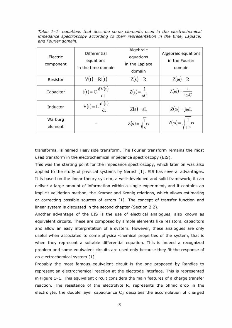
variable is the Laplace frequency or the angular frequency. Table 1–1 shows these
relationships. As one can see, the differential equations, defining the potential or the
current in the second column are converted into simple equations in the third and
fourth column. These equations are called transfer functions and are the base for the
operational calculus.
The fact that the names of these transfer functions such as impedance, admittance,
and reactance, which were given by Heaviside, are still used nowadays, underlines
the importance of his approach. Bode much later introduced the concept of
immittance to characterize both impedance and admittance [2]. Furthermore, the
conversion of the Laplace frequency into the imaginary frequency, used in the Fourier
3
transforms, is named Heaviside transform. The Fourier transform remains the most
used transform in the electrochemical impedance spectroscopy (EIS).
This was the starting point for the impedance spectroscopy, which later on was also
applied to the study of physical systems by Nernst [1]. EIS has several advantages.
It is based on the linear theory system, a well-developed and solid framework, it can
deliver a large amount of information within a single experiment, and it contains an
implicit validation method, the Kramer and Kronig relations, which allows estimating
or correcting possible sources of errors [1]. The concept of transfer function and
linear system is discussed in the second chapter (Section 2.2).
Another advantage of the EIS is the use of electrical analogues, also known as
equivalent circuits. These are composed by simple elements like resistors, capacitors
and allow an easy interpretation of a system. However, these analogues are only
useful when associated to some physical-chemical properties of the system, that is
when they represent a suitable differential equation. This is indeed a recognized
problem and some equivalent circuits are used only because they fit the response of
an electrochemical system [1].
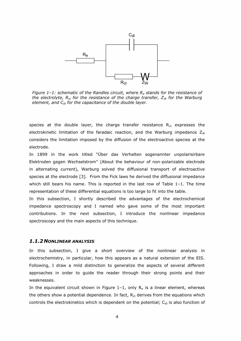
Probably the most famous equivalent circuit is the one proposed by Randles to
represent an electrochemical reaction at the electrode interface. This is represented
in Figure 1–1. This equivalent circuit considers the main features of a charge transfer
reaction. The resistance of the electrolyte Re represents the ohmic drop in the
electrolyte, the double layer capacitance Cdl describes the accumulation of charged
Table 1–1: equations that describe some elements used in the electrochemical
impedance spectroscopy according to their representation in the time, Laplace,
and Fourier domain.
Electric
component
Differential
equations
in the time domain
Algebraic
equations
in the Laplace
domain
Algebraic equations
in the Fourier
domain
Resistor
Capacitor
Inductor
Warburg
element –
4
species at the double layer, the charge transfer resistance Rct expresses the
electrokinetic limitation of the faradaic reaction, and the Warburg impedance ZW
considers the limitation imposed by the diffusion of the electroactive species at the
electrode.
In 1899 in the work titled ―Über das Verhalten sogenannter unpolarisirbare
Elektroden gegen Wechselstrom‖ (About the behaviour of non-polarizable electrode
in alternating current), Warburg solved the diffusional transport of electroactive
species at the electrode [3]. From the Fick laws he derived the diffusional impedance
which still bears his name. This is reported in the last row of Table 1–1. The time
representation of these differential equations is too large to fit into the table.
In this subsection, I shortly described the advantages of the electrochemical
impedance spectroscopy and I named who gave some of the most important
contributions. In the next subsection, I introduce the nonlinear impedance
spectroscopy and the main aspects of this technique.
1.1.2 NONLINEAR ANALYSIS
In this subsection, I give a short overview of the nonlinear analysis in
electrochemistry, in particular, how this appears as a natural extension of the EIS.
Following, I draw a mild distinction to generalize the aspects of several different
approaches in order to guide the reader through their strong points and their
weaknesses.
In the equivalent circuit shown in Figure 1–1, only Re is a linear element, whereas
the others show a potential dependence. In fact, Rct derives from the equations which
controls the electrokinetics which is dependent on the potential; Cdl is also function of
Figure 1–1: schematic of the Randles circuit, where Re stands for the resistance of
the electrolyte, Rct for the resistance of the charge transfer, ZW for the Warburg
element, and Cdl for the capacitance of the double layer.
5
potential as shown by Grahame [4]; and ZW which represents the diffusion limitation
is dependent on the current which is function of potential.
During electrochemical impedance spectroscopy, the system is perturbed by a
sinusoidal potential perturbation and the current responds with a periodic transient.
In the case of a linear system the current is a sinusoidal wave as well. However, in
the case of a nonlinear system, the current is not a pure sinusoidal oscillation, but
contains other waves. These are named harmonics and represent the nonlinearity of
the system. The harmonics oscillate at an integer multiple of the frequency of the
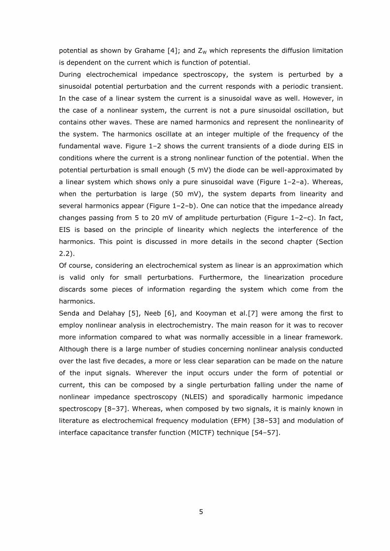
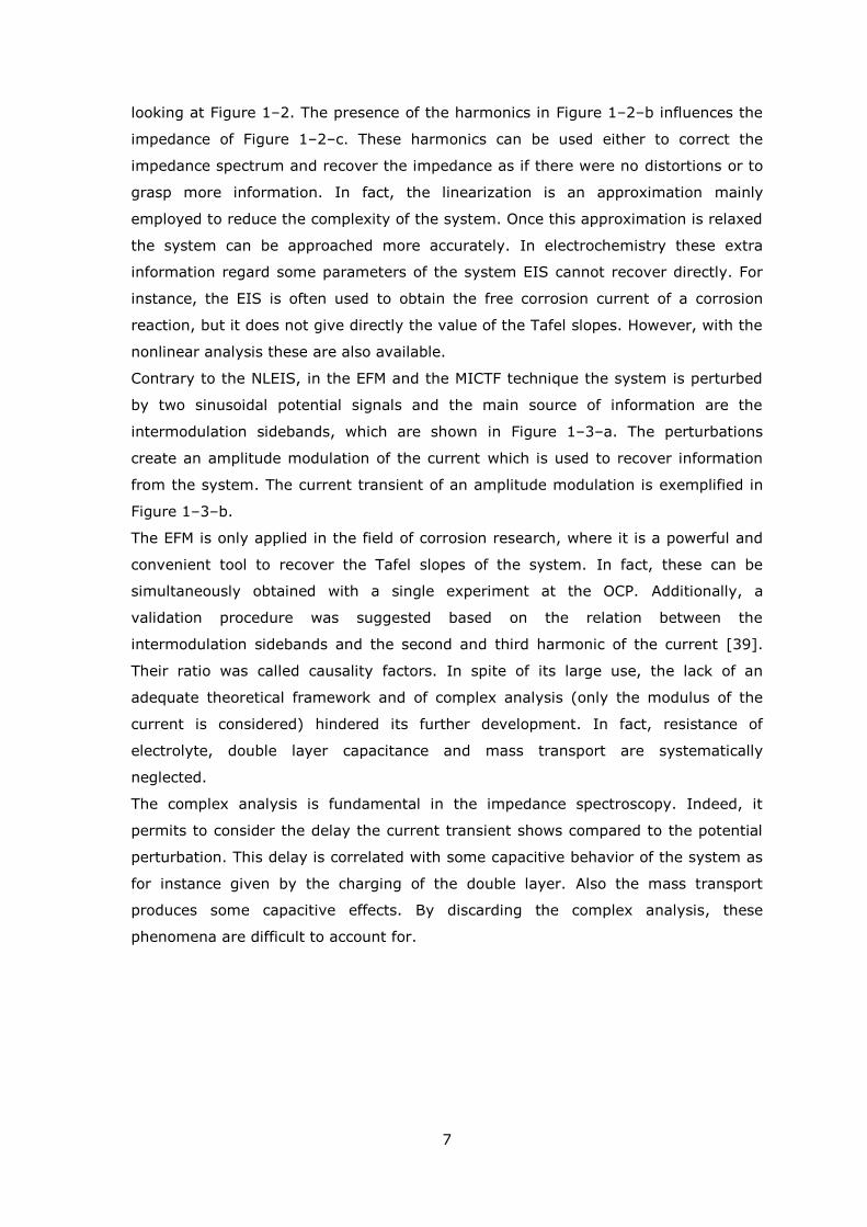
fundamental wave. Figure 1–2 shows the current transients of a diode during EIS in
conditions where the current is a strong nonlinear function of the potential. When the
potential perturbation is small enough (5 mV) the diode can be well-approximated by
a linear system which shows only a pure sinusoidal wave (Figure 1–2–a). Whereas,
when the perturbation is large (50 mV), the system departs from linearity and
several harmonics appear (Figure 1–2–b). One can notice that the impedance already
changes passing from 5 to 20 mV of amplitude perturbation (Figure 1–2–c). In fact,
EIS is based on the principle of linearity which neglects the interference of the
harmonics. This point is discussed in more details in the second chapter (Section
2.2).
Of course, considering an electrochemical system as linear is an approximation which
is valid only for small perturbations. Furthermore, the linearization procedure
discards some pieces of information regarding the system which come from the
harmonics.
Senda and Delahay [5], Neeb [6], and Kooyman et al.[7] were among the first to
employ nonlinear analysis in electrochemistry. The main reason for it was to recover
more information compared to what was normally accessible in a linear framework.
Although there is a large number of studies concerning nonlinear analysis conducted
over the last five decades, a more or less clear separation can be made on the nature
of the input signals. Wherever the input occurs under the form of potential or
current, this can be composed by a single perturbation falling under the name of
nonlinear impedance spectroscopy (NLEIS) and sporadically harmonic impedance
spectroscopy [8–37]. Whereas, when composed by two signals, it is mainly known in
literature as electrochemical frequency modulation (EFM) [38–53] and modulation of
interface capacitance transfer function (MICTF) technique [54–57].
6
In the NLEIS, the authors look at the higher harmonics given by a sinusoidal
perturbation to find additional valuable information or to correct the errors arising
from the oversimplified linearization of the system. One can understand this point
Figure 1–2: comparison of linear and nonlinear system. a) current transient of a
nonlinear system well-approximated to a linear system by the small perturbation
amplitude (5 mV); b) current transient of a nonlinear system with a large
perturbation amplitude (50 mV); c) impedance of the system as function of the
amplitude of the potential perturbation.
7
looking at Figure 1–2. The presence of the harmonics in Figure 1–2–b influences the
impedance of Figure 1–2–c. These harmonics can be used either to correct the
impedance spectrum and recover the impedance as if there were no distortions or to
grasp more information. In fact, the linearization is an approximation mainly
employed to reduce the complexity of the system. Once this approximation is relaxed
the system can be approached more accurately. In electrochemistry these extra
information regard some parameters of the system EIS cannot recover directly. For
instance, the EIS is often used to obtain the free corrosion current of a corrosion
reaction, but it does not give directly the value of the Tafel slopes. However, with the
nonlinear analysis these are also available.
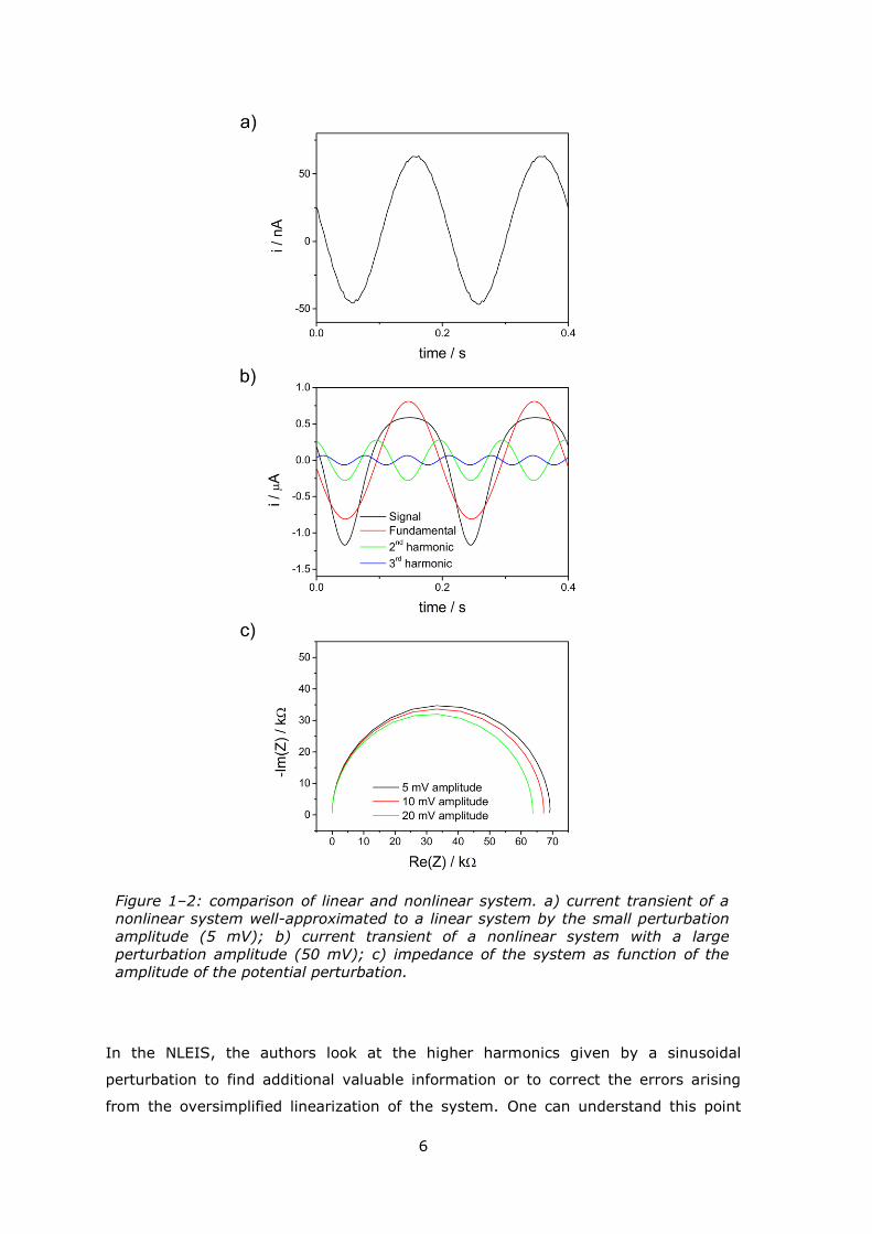
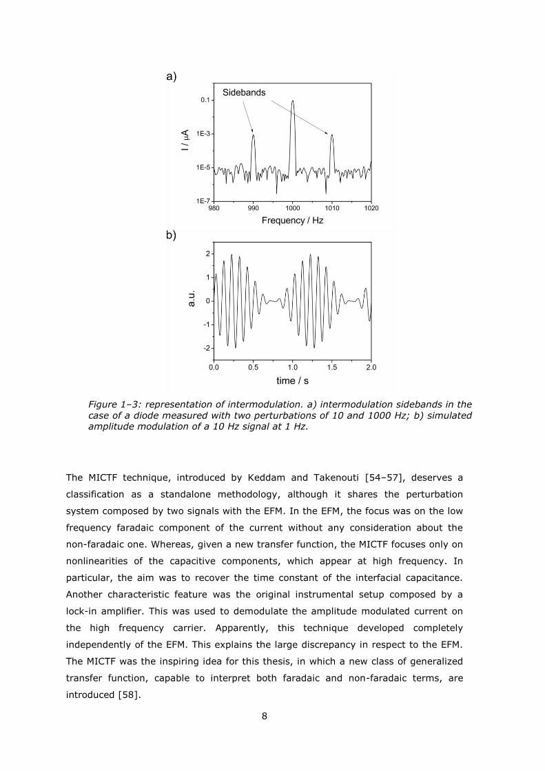
Contrary to the NLEIS, in the EFM and the MICTF technique the system is perturbed
by two sinusoidal potential signals and the main source of information are the
intermodulation sidebands, which are shown in Figure 1–3–a. The perturbations
create an amplitude modulation of the current which is used to recover information
from the system. The current transient of an amplitude modulation is exemplified in
Figure 1–3–b.
The EFM is only applied in the field of corrosion research, where it is a powerful and
convenient tool to recover the Tafel slopes of the system. In fact, these can be
simultaneously obtained with a single experiment at the OCP. Additionally, a
validation procedure was suggested based on the relation between the
intermodulation sidebands and the second and third harmonic of the current [39].
Their ratio was called causality factors. In spite of its large use, the lack of an
adequate theoretical framework and of complex analysis (only the modulus of the
current is considered) hindered its further development. In fact, resistance of
electrolyte, double layer capacitance and mass transport are systematically
neglected.
The complex analysis is fundamental in the impedance spectroscopy. Indeed, it
permits to consider the delay the current transient shows compared to the potential
perturbation. This delay is correlated with some capacitive behavior of the system as
for instance given by the charging of the double layer. Also the mass transport
produces some capacitive effects. By discarding the complex analysis, these
phenomena are difficult to account for.
8
The MICTF technique, introduced by Keddam and Takenouti [54–57], deserves a
classification as a standalone methodology, although it shares the perturbation
system composed by two signals with the EFM. In the EFM, the focus was on the low
frequency faradaic component of the current without any consideration about the
non-faradaic one. Whereas, given a new transfer function, the MICTF focuses only on
nonlinearities of the capacitive components, which appear at high frequency. In
particular, the aim was to recover the time constant of the interfacial capacitance.
Another characteristic feature was the original instrumental setup composed by a
lock-in amplifier. This was used to demodulate the amplitude modulated current on
the high frequency carrier. Apparently, this technique developed completely
independently of the EFM. This explains the large discrepancy in respect to the EFM.
The MICTF was the inspiring idea for this thesis, in which a new class of generalized
transfer function, capable to interpret both faradaic and non-faradaic terms, are
introduced [58].
Figure 1–3: representation of intermodulation. a) intermodulation sidebands in the
case of a diode measured with two perturbations of 10 and 1000 Hz; b) simulated amplitude modulation of a 10 Hz signal at 1 Hz.
9
The main fields of application of the NLEIS were corrosion [10–12,15,18,23–25,29]
and fuel cells [26,30,59,33,60,31]. Given a very solid theoretical background, several
systems were investigated. A diode has shown to be a good benchmark for the NLEIS
and was employed several times to simulate the exponential dependency of the
current on the potential [12,13,32]. The primary focus was on tafelian systems
[9,12,13,17–21,23,36], but several works dealt also with reversible systems
following the Butler and Volmer equation [7–9,16,27,28,37], and adsorptions or
multistep reactions [14,20,21]. Despite the large amount of literature, many authors
neglected the influence of the resistance of electrolytes, double layer, and mass
transport.
The double layer was mainly either considered linear (or with a negligible
nonlinearity) or neglected in the treatment using the low frequency approximation.
These limitations were overcome by some authors, which addressed the dependency
of the double layer capacitance on the potential [5,9,35,61–66]. Dickinson and
Compton considered, that the non-faradaic current is also dependent on the
frequency i.e. on time [67]. This point was the reason for the development of the
MICTF technique.
Although the resistance of the electrolyte is a linear term, i.e. it does not depend on
the potential, its presence affects the observation of the nonlinearities. The nonlinear
components of the current, the harmonics or the intermodulation sidebands, are
dumped and phase-shifted by other linear elements. Any nonlinear term can be
described by a virtual potential source which produces a current [64]. This current,
passing through a passive resistance, generates an ohmic drop opposite to the virtual
source. Diard et al. considered this problem as a source of error [9].
Mass transport is hardly considered in the nonlinear analysis. Although its effect can
be negligible, it does affect the system, especially when electrokinetics plays a minor
role. Xu and Riley computed the diffusion in their treatment numerically [37]. Some
other authors did solve it analytically [7,9,16] and Darowicki used their results to
calculate the diffusion coefficients of one of the redox species which were involved in
the reaction [8].
The lack of an adequate mathematical framework in the nonlinear analysis often
leads to problems and some authors tried to shape the nonlinear terms as impedance
[16,28]. This is fundamentally wrong, because second terms cannot have the same
dimension of the linear terms (i.e. the resistance is measured in Ohm, but its
variation on the potential is measured in Ohm V-1). A second possibility is to consider
only the current instead of a transfer function. This was done, for example, by Xu
and Ripley [35,37] and is common used with the EFM. However, doing so prevents
from performing a complex analysis, which results in a large loss of information. In
10
this case, the plots always show the amplitude of the current as a function of the
frequency. The meaning of the transfer function lies also in normalizing the values:
for example, in the case where the potential perturbation is not constant in all the
frequency range, the current amplitude is not only the function of the pure answer of
the system, but also of some instrumental conditions. Therefore, a normalizing
procedure is required.
A mathematical and theoretical framework was introduced in the 1970s by
Rangarajan. He showed an elegant matrix formalism on which he built a theoretical
framework to embrace all kinds of phenomena in electrochemistry under the view of
impedance or admittance [68–71]. He showed ―how to arrive at the results for even
the most complex models without tears‖ [68]. Later on, he expanded his framework
to consider nonlinear systems [62,63]. Instead of Taylor series, he employed Volterra
series which give a memory effect to the series expansion. Despite his elegant and
sophisticated approach, this proved to be too complex.
In this subsection, I showed a brief historical overview of the nonlinear analysis in
electrochemistry and its link with EIS. Some general limitations and approximations
were discussed according to the distinction between the single input approach,
nonlinear impedance spectroscopy (NLEIS), and the double input approaches,
electrochemical frequency modulation (EFM) and modulation of interface capacitance
transfer function (MICTF) technique. In particular, the specular character of the last
two techniques was underlined. In the end, a small parenthesis was opened on the
necessity and advantage of having a proper mathematical and theoretical framework.
In the next section, the concept of EIS and nonlinear analysis is expanded to the field
of time variant systems. Also, a short overview of the gas-evolving electrode is
presented and discussed in the framework of impedance spectroscopy.
1.1.3 ELECTROCHEMICAL NOISE
Almost a century ago, Morgan observed the formation of bubbles while adding formic
acid to concentrated sulphuric acid [72]. He recorded the pressure fluctuations and
carefully described his findings. The reaction initially proceeded with an oscillatory
character and then reached a steady-state condition when the reactant was
consumed. This phenomenon was later called gas oscillator [73–76]. Much later,
Barker was one of the first to describe flicker noise in electrochemistry [77,78]. This
was produced by the hydrogen evolution reaction on a mercury electrode. He could
not properly explain the source of this noise which appeared as fluctuation of the
recorded current, but the term noise remained in the literature meaning a non-
stationary behavior of a reaction giving rise to periodical or stochastic variation in the
11
recorded signal (current or potential). He also suggested the use of electrodes of
small size and believed that the study of noise could give important mechanistic
information.
For certain, the effect of a gas evolution on the current, which begins to fluctuate
because of the birth, growth and departure of many fine bubbles on the surface of
the electrode, is well known. This is not only a source of disturbance, which
deteriorates the quality of the recorded data, but also limits the possibilities to
perform certain experiments. Appearing of noise in a cyclic voltammetry affects the
quality of the result, but the collected data can still be interpreted in a meaningful
way. The case of EIS is different. This technique requires a suitable steady-state
condition to operate, which is often missing in the case of bubble formation on the
electrolyte-electrode interface. Besides being an instrumental requirement (the
instrument would return unreliable values), a steady-state condition is also dictated
by the theory of linear time-invariant systems, which is the base of EIS [1]. In fact,
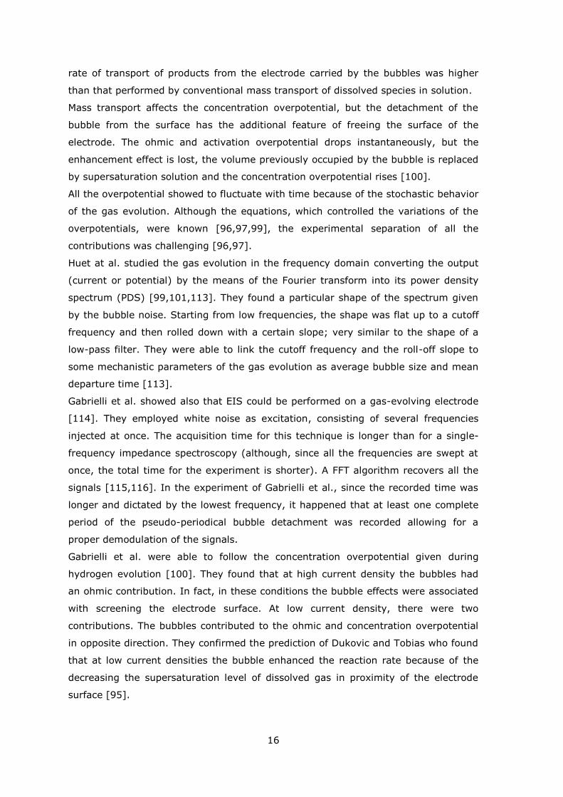
several authors reported the problem connected with performing EIS in presence of
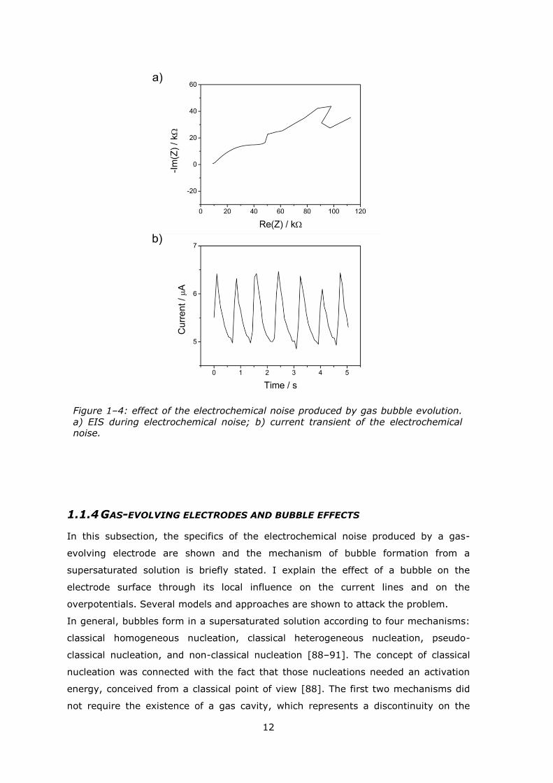
gas evolution [79–83]. Figure 1–4–a is an example of this problem. It shows the
Nyquist plot of an impedance measurement performed on a cavity microelectrode
filled with ruthenium oxide during the generation of oxygen bubbles. At high
frequencies the variation of the current due to the gas-evolution was slow compared
with the measurement perturbation, the system was well approximated by a steady
state, it was steady as ‖seen‖ by a quick perturbation. There was a condition stable
enough in the operating time scale. When the frequency decreased approaching the
frequency range of the noise the steadiness was lost and the data appear scattered.
In this case, the impedance is a time-variant quantity and the EIS has no meaning in
this condition [1].
Steady state means that all the properties of the system are not changing in a
suitable lapse of time, i.e. for potentiostatic control the current is flat. When instead
bubbles are produced at the electrode the current shows periodic, pseudo-periodic,
or stochastic variations as reported in Figure 1–4–b, which is an example of a current
transient measured at the gas-evolving electrode. A strategy to recover some control
over these phenomena is to partially relax the requirement of steady state to
embrace the concept of periodic steady state [84–87]. In this framework, the
properties of the system are allowed to vary, but their variation has to be periodic, so
that the behavior of the system can still be predicted.
12
1.1.4 GAS-EVOLVING ELECTRODES AND BUBBLE EFFECTS
In this subsection, the specifics of the electrochemical noise produced by a gas-
evolving electrode are shown and the mechanism of bubble formation from a
supersaturated solution is briefly stated. I explain the effect of a bubble on the
electrode surface through its local influence on the current lines and on the
overpotentials. Several models and approaches are shown to attack the problem.
In general, bubbles form in a supersaturated solution according to four mechanisms:
classical homogeneous nucleation, classical heterogeneous nucleation, pseudo-
classical nucleation, and non-classical nucleation [88–91]. The concept of classical
nucleation was connected with the fact that those nucleations needed an activation
energy, conceived from a classical point of view [88]. The first two mechanisms did
not require the existence of a gas cavity, which represents a discontinuity on the
Figure 1–4: effect of the electrochemical noise produced by gas bubble evolution.
a) EIS during electrochemical noise; b) current transient of the electrochemical noise.
13
surface in contact with the solution which provides a small concavity with a small gas
pocket. However, the curvature radius of these gas pockets is a key point of
understanding nucleation in gas evolution reactions. If this radius is smaller than the
critical curvature radius for bubble nucleation, this is the pseudo-classical nucleation
mechanism, the gas phase preferentially forms at the cavity because less activation
energy is required there.
Without a gas cavity, the bubble would form only at very high levels of
supersaturation [91]. In the case where the curvature radius of the gas cavity is
bigger than the nucleation radius, this is referred to as the non-classical nucleation
mechanism: no activation energy is required to form a bubble leading to a
spontaneous evolution at that spot. These last two mechanisms of bubble nucleation
are of primary importance, because they link the morphological properties of an
electrode to its efficiency in evolving a gas phase.
Of course, a gas evolving electrode produces a great supersaturation in its proximity
and this leads to the formation, growth and departure of bubbles. These bubbles
have several effects on the electrochemical reaction, on the electrode surface, and on
the mass transport of the products. This point is sometimes mentioned as
macrokinetics [92].
The total overpotential at the electrode surface is given by the sum of the ohmic
overpotential, the activation overpotential, and the concentration overpotential. The
first one is given by the resistance of the electrolyte, the second is connected with
the activation energy needed to drive the reaction and the third is connected with the
energy required to drive the mass transport of the reactant and product at the
surface. All three overpotentials are affected by the presence, birth, growth and
departure of bubbles at the electrode surface.
The ohmic overpotential is given by the ohmic drop produced by the passage of
current through the electrolyte and it is strongly dependent on the section of solution
directly in contact with the electrode. Several studies addressed how the ohmic drop
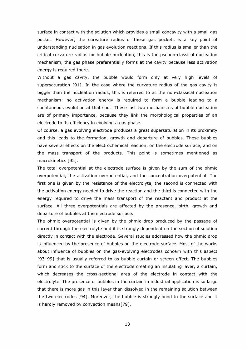
is influenced by the presence of bubbles on the electrode surface. Most of the works
about influence of bubbles on the gas-evolving electrodes concern with this aspect
[93–99] that is usually referred to as bubble curtain or screen effect. The bubbles
form and stick to the surface of the electrode creating an insulating layer, a curtain,
which decreases the cross-sectional area of the electrode in contact with the
electrolyte. The presence of bubbles in the curtain in industrial application is so large
that there is more gas in this layer than dissolved in the remaining solution between
the two electrodes [94]. Moreover, the bubble is strongly bond to the surface and it
is hardly removed by convection means[79].
14
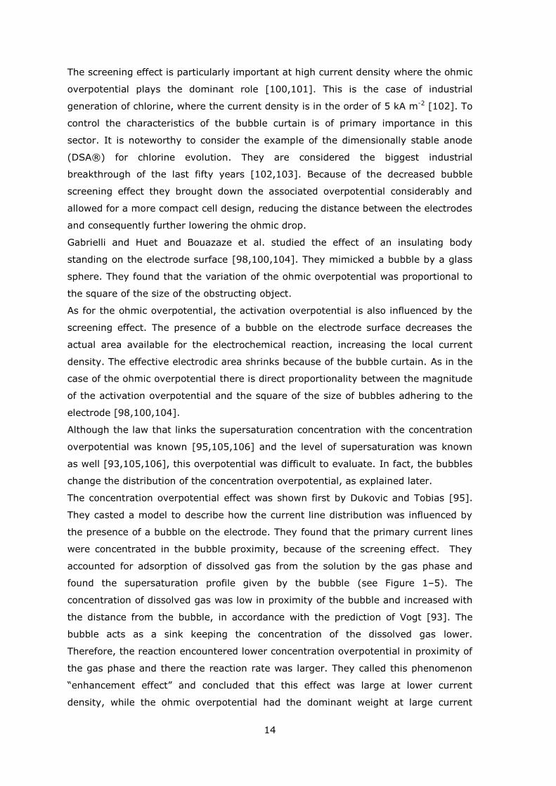
The screening effect is particularly important at high current density where the ohmic
overpotential plays the dominant role [100,101]. This is the case of industrial
generation of chlorine, where the current density is in the order of 5 kA m-2 [102]. To
control the characteristics of the bubble curtain is of primary importance in this
sector. It is noteworthy to consider the example of the dimensionally stable anode
(DSA®) for chlorine evolution. They are considered the biggest industrial
breakthrough of the last fifty years [102,103]. Because of the decreased bubble
screening effect they brought down the associated overpotential considerably and
allowed for a more compact cell design, reducing the distance between the electrodes
and consequently further lowering the ohmic drop.
Gabrielli and Huet and Bouazaze et al. studied the effect of an insulating body
standing on the electrode surface [98,100,104]. They mimicked a bubble by a glass
sphere. They found that the variation of the ohmic overpotential was proportional to
the square of the size of the obstructing object.
As for the ohmic overpotential, the activation overpotential is also influenced by the
screening effect. The presence of a bubble on the electrode surface decreases the
actual area available for the electrochemical reaction, increasing the local current
density. The effective electrodic area shrinks because of the bubble curtain. As in the
case of the ohmic overpotential there is direct proportionality between the magnitude
of the activation overpotential and the square of the size of bubbles adhering to the
electrode [98,100,104].
Although the law that links the supersaturation concentration with the concentration
overpotential was known [95,105,106] and the level of supersaturation was known
as well [93,105,106], this overpotential was difficult to evaluate. In fact, the bubbles
change the distribution of the concentration overpotential, as explained later.
The concentration overpotential effect was shown first by Dukovic and Tobias [95].
They casted a model to describe how the current line distribution was influenced by
the presence of a bubble on the electrode. They found that the primary current lines
were concentrated in the bubble proximity, because of the screening effect. They
accounted for adsorption of dissolved gas from the solution by the gas phase and
found the supersaturation profile given by the bubble (see Figure 1–5). The
concentration of dissolved gas was low in proximity of the bubble and increased with
the distance from the bubble, in accordance with the prediction of Vogt [93]. The
bubble acts as a sink keeping the concentration of the dissolved gas lower.
Therefore, the reaction encountered lower concentration overpotential in proximity of
the gas phase and there the reaction rate was larger. They called this phenomenon
―enhancement effect‖ and concluded that this effect was large at lower current
density, while the ohmic overpotential had the dominant weight at large current
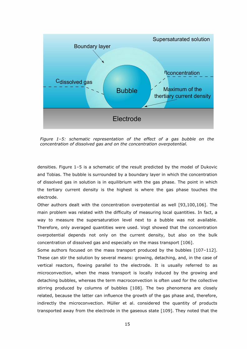
15
densities. Figure 1–5 is a schematic of the result predicted by the model of Dukovic
and Tobias. The bubble is surrounded by a boundary layer in which the concentration
of dissolved gas in solution is in equilibrium with the gas phase. The point in which
the tertiary current density is the highest is where the gas phase touches the
electrode.
Other authors dealt with the concentration overpotential as well [93,100,106]. The
main problem was related with the difficulty of measuring local quantities. In fact, a
way to measure the supersaturation level next to a bubble was not available.
Therefore, only averaged quantities were used. Vogt showed that the concentration
overpotential depends not only on the current density, but also on the bulk
concentration of dissolved gas and especially on the mass transport [106].
Some authors focused on the mass transport produced by the bubbles [107–112].
These can stir the solution by several means: growing, detaching, and, in the case of
vertical reactors, flowing parallel to the electrode. It is usually referred to as
microconvection, when the mass transport is locally induced by the growing and
detaching bubbles, whereas the term macroconvection is often used for the collective
stirring produced by columns of bubbles [108]. The two phenomena are closely
related, because the latter can influence the growth of the gas phase and, therefore,
indirectly the microconvection. Müller et al. considered the quantity of products
transported away from the electrode in the gaseous state [109]. They noted that the
Figure 1–5: schematic representation of the effect of a gas bubble on the concentration of dissolved gas and on the concentration overpotential.
16
rate of transport of products from the electrode carried by the bubbles was higher
than that performed by conventional mass transport of dissolved species in solution.
Mass transport affects the concentration overpotential, but the detachment of the
bubble from the surface has the additional feature of freeing the surface of the
electrode. The ohmic and activation overpotential drops instantaneously, but the
enhancement effect is lost, the volume previously occupied by the bubble is replaced
by supersaturation solution and the concentration overpotential rises [100].
All the overpotential showed to fluctuate with time because of the stochastic behavior
of the gas evolution. Although the equations, which controlled the variations of the
overpotentials, were known [96,97,99], the experimental separation of all the
contributions was challenging [96,97].
Huet at al. studied the gas evolution in the frequency domain converting the output
(current or potential) by the means of the Fourier transform into its power density
spectrum (PDS) [99,101,113]. They found a particular shape of the spectrum given
by the bubble noise. Starting from low frequencies, the shape was flat up to a cutoff
frequency and then rolled down with a certain slope; very similar to the shape of a
low-pass filter. They were able to link the cutoff frequency and the roll-off slope to
some mechanistic parameters of the gas evolution as average bubble size and mean
departure time [113].
Gabrielli et al. showed also that EIS could be performed on a gas-evolving electrode
[114]. They employed white noise as excitation, consisting of several frequencies
injected at once. The acquisition time for this technique is longer than for a single-
frequency impedance spectroscopy (although, since all the frequencies are swept at
once, the total time for the experiment is shorter). A FFT algorithm recovers all the
signals [115,116]. In the experiment of Gabrielli et al., since the recorded time was
longer and dictated by the lowest frequency, it happened that at least one complete
period of the pseudo-periodical bubble detachment was recorded allowing for a
proper demodulation of the signals.
Gabrielli et al. were able to follow the concentration overpotential given during
hydrogen evolution [100]. They found that at high current density the bubbles had
an ohmic contribution. In fact, in these conditions the bubble effects were associated
with screening the electrode surface. At low current density, there were two
contributions. The bubbles contributed to the ohmic and concentration overpotential
in opposite direction. They confirmed the prediction of Dukovic and Tobias who found
that at low current densities the bubble enhanced the reaction rate because of the
decreasing the supersaturation level of dissolved gas in proximity of the electrode
surface [95].
17
In this subsection, I gave an overview of the phenomenon of bubble formation at the
electrode-electrolyte interface. I described the mechanism of nucleation of the gas
phase and how this is related with the morphology of the electrode. Furthermore, I
reported the effects of the bubble dynamics on the overpotentials and the mass
transport. In particular, I showed that the activation and ohmic overpotential always
increase because of the bubble effect. Whereas, the concentration overpotential
decreases because of the enhancement effect. One problem was that these
overpotentials change in time and space and only averaged quantities were usually
available.
Besides, the bubbles affect the mass transport. In fact, through micro- and
macroconvection they influence the transfer of products. It also happens that the
bubble itself carries more efficiently the products away from the electrode interface,
hence decreasing the concentration overpotential.
Therefore, the gas phase at the interface has a double role in the electrochemical
reaction. It can either hinder or enhance the reaction rate. Several approaches were
proposed by the authors. Some valuable observations came from those approaches
which looked at the phenomenon in the frequency domain (PDS). In fact, a periodic
or pseudo-periodic event is more meaningful when decomposed in its characteristic
oscillations. However, the fact that the phenomenon was non-steady played several
problems for the main frequency domain approach: the EIS.
18
1.2 MOTIVATION AND AIMS
The main aim of this doctoral thesis was to introduce, characterize, and apply a new
electrochemical technique, the Intermodulated Differential Immittance Spectroscopy
(IDIS), designed to implement the electrochemical impedance spectroscopy (EIS).
The IDIS is based on the phenomenon of the intermodulation which appears when
two periodic stimuli with different frequencies interact in a nonlinear system creating
an amplitude modulation. As described in the state of the art (Subsection 1.1.2)
similar approach was used by other two techniques: the electrochemical frequency
modulation (EFM) and the modulation of interface capacitance transfer function
(MICTF) technique. The former aimed only at the faradaic process, whereas the latter
investigated only the double layer response. The IDIS merges both features and
represents a generalization of the two.
I developed the IDIS because this technique gives a deeper insight than a simple
electrochemical impedance spectroscopy. In fact, the symmetry of energetic barrier
and of mass transport, the time constant and the variation of the double layer
capacitance are all available. Usually several experiments are necessary to recover
these information (if possible) whereas with the IDIS, these can be obtained in a
single spectrum. This is not only an achievement concerning the number of
experiments one has to perform: for example, to recover the symmetry factor of an
electrochemical reaction either the potential or the concentration of the redox species
in solution must be changed. With the IDIS this is not necessary. Therefore, the
assumption that the symmetry factor is neither dependent on potential nor
concentrations is required.
In particular, the time constant of the double layer capacitance and the symmetry of
mass transport are usually not achievable through EIS. Furthermore, these
parameters were usually overlooked in most nonlinear analysis. However, because of
the nature of the intermodulation, the IDIS can easily recover them.
In order to develop the IDIS, a mathematical framework for the intermodulation is
necessary. This is required by the complexity of the nonlinear analysis. However, a
virtue is made out of necessity. The aim is to provide a general and elegant model
which can be used later for future development. This framework has to extend that of
the impedance spectroscopy where the use of transfer functions allows a handy
employment of several differential equations. Furthermore, it has to be suitable to
account for all the nonlinearities of the faradaic and capacitive current and to
consider the effect of the resistance of the electrolyte.
The electrochemical noise generated by the dynamics of gas bubbles evolution during
electrochemical generation of oxygen is a challenging system. In this condition a
19
reasonable steady state is never reached and the electrochemical impedance
spectroscopy can be only partially applied. However, when the noise is periodic the
system response is similar to that of an intermodulation. Starting from the
mathematical framework of the IDIS, the aim is to create a model to parameterize
the system in order to understand the effect of the dynamicity of the bubble
evolution on the electrochemical reaction. In particular, it is important to understand
the balance between the enhancement effect and the screening effect given by the
bubbles on the electrode surface. Besides, the effect of mass transport given by
microconvection is also important and it can be identified with a proper complex
analysis.
In the next section, I summarize what presented so far and I give a brief outline of
the thesis.
20
1.3 FINAL REMARKS AND OUTLINES
In the first chapter with the state of the art, I introduced the main aspects of the
nonlinear analysis (Subsection 1.1.2). I drew attention on how other authors dealt
with the description of the faradaic and capacitive current. In particular, I showed
that although the electrokinetics was subject of several investigations the mass
transport and the double layer were often disregarded. Besides, also the resistance of
the electrolyte was mainly neglected.
In the Subsection 1.1.4, I described the phenomenon of bubble evolution at the
electrode-electrolyte interface. In particular, I showed the effects of the gas phase on
the electrochemical evolution of gas and how this was observed by other authors.
In the second section, the motivation and the aims of this work were reported. In
particular, in which way the intermodulated differential immittance spectroscopy
(IDIS) represents a generalization of the electrochemical frequency modulation (EFM)
and the modulation of interface capacitance transfer function (MICTF) technique. The
aim of the IDIS is to recover information concerning the electrokinetics, the mass
transport, and the double layer. Besides, the intermodulation can be used to
parameterize the gas-evolving reaction when there is periodic formation of gas
bubbles.
In the next chapter, the basis of electrochemistry necessary for this work is reported.
Furthermore, the mathematical framework in which the intermodulation is developed
is described. One can find the model used to consider the faradaic and the capacitive
current in the Subsection 2.3.5 and 2.3.6. The parametric model to study the gas-
evolution reaction is reported in the Section 2.4 which discusses in general the
nonlinear time varying systems. In particular, the model shows how is possible to
normalize the impedance by the surface area really available for the electrochemical
reaction.
In the third chapter, I give an overview on the instruments, materials and procedures
employed in this thesis. In particular, the instrumental setups developed for the IDIS
and the expedients employed to mitigate the artifacts arising during the impedance
measurements are shown in Section 3.3 and 3.4, respectively.
The results are described in the fourth chapter. The application of the model
developed in the second chapter (Subsection 2.3.5 and 2.3.6) is reported and
discussed in the Section 4.3 where a best fit is used to recover the parameters of the
electrokinetics, mass transport, and double layer. Following the model reported in the
second chapter (Section 2.4), the results of the parameterization of the gas-evolving
electrode are described in the Section 4.4. In particular, the impedance normalized
by the surface area of the electrode free from gas phase is shown.

21
In the last chapter, I summarize the main contributions of this thesis and suggest
some future developments. In particular, I propose some modification of the IDIS
where the intermodulation can be also used with non-electric perturbations.
22
2 THEORY
This chapter contains all the definitions and the models developed in this work. In the
first section, I briefly introduce some concepts of electrochemistry necessary during
the elaboration. In particular, I describe the faradaic and capacitive current and the
basic equations which control them.
Later on, I explain the linear system theory and how this is connected with the
electrochemical impedance spectroscopy. Starting from the definition of transfer
function, some examples of applications of impedance spectroscopy are presented.
These are the starting points for the further development of the nonlinear treatment
and intermodulation.
In the third section, I introduce the concept of nonlinear system and show the origin
of the intermodulation. Following the examples of the second section, I describe the
model developed for intermodulated differential immittance spectroscopy (IDIS)
using three different cases. In the last example, the IDIS spectra are mathematically
simulated. These simulations are used as comparison and pattern recognition later in
the fourth chapter (Subsection 4.2.3 and 4.2.4).
In the last section of this chapter, I discuss about the nonlinear time varying system.
In particular, I introduce the case of gas-evolving electrodes where the periodic
formation, growth, and departure of a gas bubble obstruct the electrode surface.
Recalling the concept of periodic steady state and linear parametric varying system, I
show the model developed in this work to recover the effect of the bubble dynamics
on the electrochemical reaction.
23
2.1 BASIC CONCEPT OF ELECTROCHEMISTRY
Electrochemistry concerns with the study of the heterogeneous reduction and
oxidation (redox) reaction and accumulation of charged species at an electrode-
electrolyte interface. The electrode can behave as an inert spectator of the reaction,
in which case it solely provides the polarization of the interface, or being actively part
of the electrochemical reaction as in the case, for example, of metal dissolution. The
electrolyte is an ionic conducting phase, usually liquid, composed by a solution with
some dissolved ionic solutes.
Through the use of a potentiostat, whose working principle is reported in the third
chapter (Subsection 3.1.1), it is possible to finely control the potential difference
between the electrode and the electrolyte, without considering the treatment of an
additional electrode.
The electrode, referred as working electrode, is usually composed by a metallic phase
which cannot support an electric field inside. For this reason the electrons, needed to
balance the difference of potential, accumulate in a nearly infinitesimal region at the
metal boundary.
Compared with the electrode, the electrolyte has a finite and low amount of charged
species. These accumulate at the electrolyte interface forming the so-called double
layer, which has a finite thickness. The inner layer, represented by the centre of
mass of the desolvated ions adsorbed to the metal surface, is called Inner Helmholtz
plane (IHP). The outer Helmholtz plane (OHP), instead, represents the centre of
mass of the solvated ions. This is the layer of the closest proximity to the electrode a
nonspecifically adsorbed species can reach. Beyond the OHP, the charged species
necessary to balance the charge at the electrode are distributed because of thermal
agitation in a three-dimensional region called diffuse layer. This extends from the
OHP to the bulk of the solution. The total charge given by the double layer is equal
and opposite in sign to the charge accumulated on the metal side.
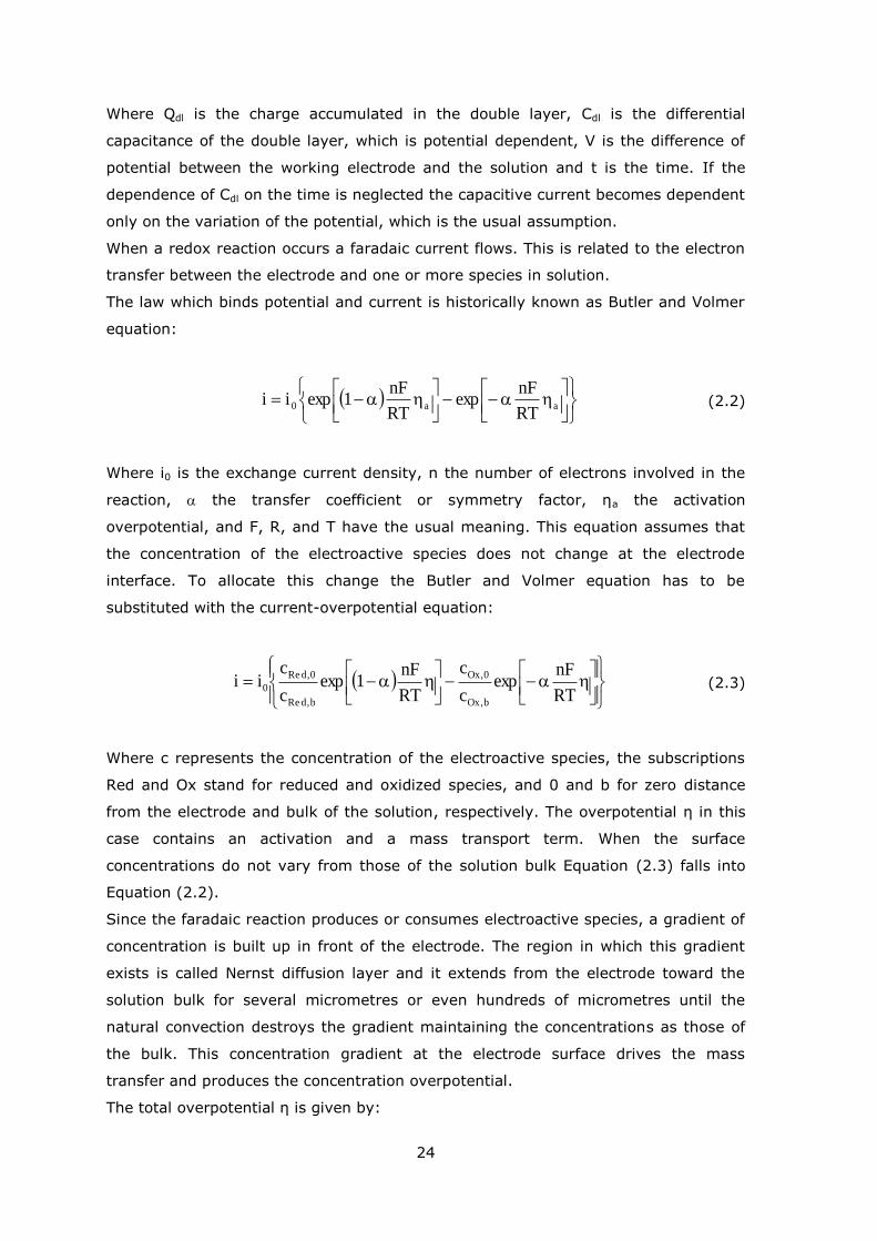
When the electrode potential is changed a flow of current arises at the interface
because of migration of the charged species in the double layer. This current which
has a transient nature is called capacitive or non-faradaic current and is given by the
accumulation and depletion of ions in the double layer. The capacitive current ic is
given by:
dt
dCV
dt
dVC
dt
dQi dl
dldl
c (2.1)
24
Where Qdl is the charge accumulated in the double layer, Cdl is the differential
capacitance of the double layer, which is potential dependent, V is the difference of
potential between the working electrode and the solution and t is the time. If the
dependence of Cdl on the time is neglected the capacitive current becomes dependent
only on the variation of the potential, which is the usual assumption.
When a redox reaction occurs a faradaic current flows. This is related to the electron
transfer between the electrode and one or more species in solution.
The law which binds potential and current is historically known as Butler and Volmer
equation:
aa0
RT
nFexp
RT
nF1expii (2.2)
Where i0 is the exchange current density, n the number of electrons involved in the
reaction, the transfer coefficient or symmetry factor, ηa the activation
overpotential, and F, R, and T have the usual meaning. This equation assumes that
the concentration of the electroactive species does not change at the electrode
interface. To allocate this change the Butler and Volmer equation has to be
substituted with the current-overpotential equation:
RT
nFexp
c
c
RT
nF1exp
c
cii
b,Ox
0,Ox
b,dRe
0,dRe
0 (2.3)
Where c represents the concentration of the electroactive species, the subscriptions
Red and Ox stand for reduced and oxidized species, and 0 and b for zero distance
from the electrode and bulk of the solution, respectively. The overpotential η in this
case contains an activation and a mass transport term. When the surface
concentrations do not vary from those of the solution bulk Equation (2.3) falls into
Equation (2.2).
Since the faradaic reaction produces or consumes electroactive species, a gradient of
concentration is built up in front of the electrode. The region in which this gradient
exists is called Nernst diffusion layer and it extends from the electrode toward the
solution bulk for several micrometres or even hundreds of micrometres until the
natural convection destroys the gradient maintaining the concentrations as those of
the bulk. This concentration gradient at the electrode surface drives the mass
transfer and produces the concentration overpotential.
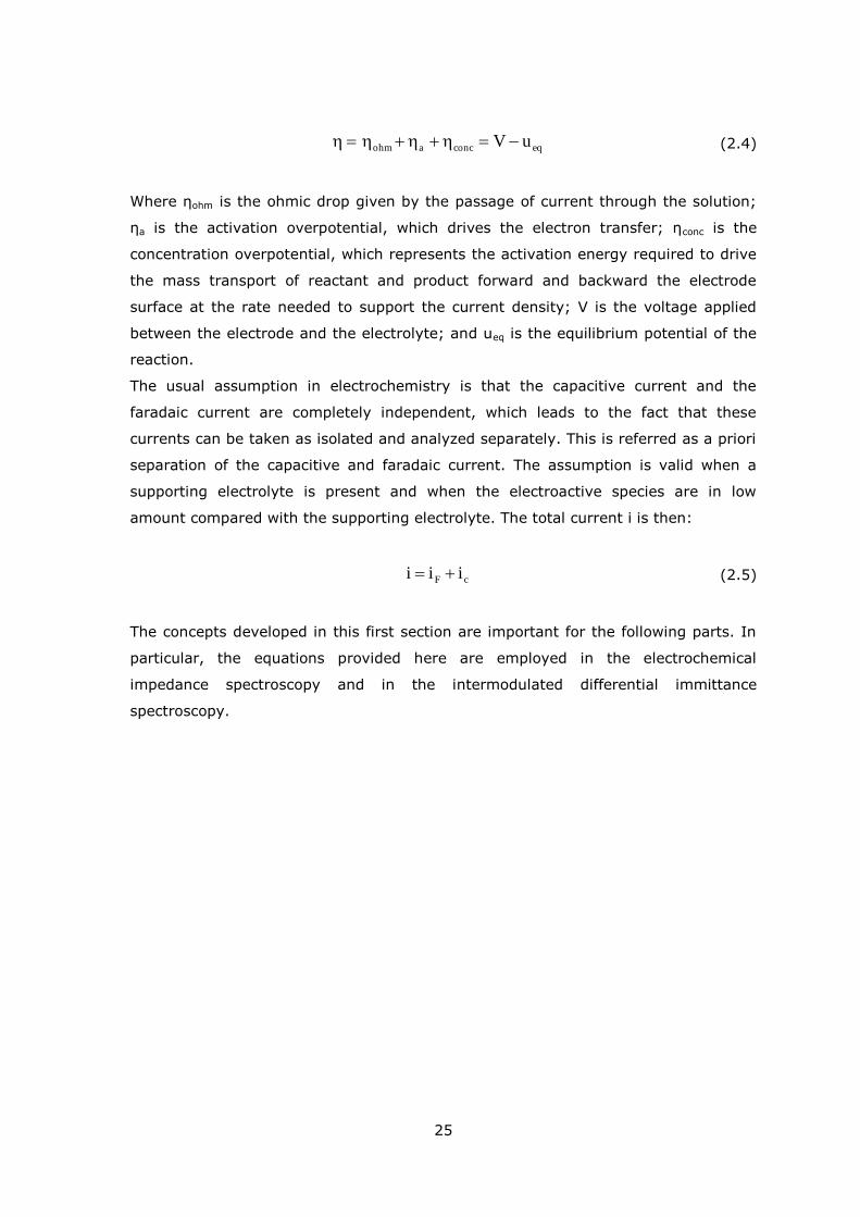
The total overpotential η is given by:
25
eqconcaohm uV (2.4)
Where ηohm is the ohmic drop given by the passage of current through the solution;
ηa is the activation overpotential, which drives the electron transfer; ηconc is the
concentration overpotential, which represents the activation energy required to drive
the mass transport of reactant and product forward and backward the electrode
surface at the rate needed to support the current density; V is the voltage applied
between the electrode and the electrolyte; and ueq is the equilibrium potential of the
reaction.
The usual assumption in electrochemistry is that the capacitive current and the
faradaic current are completely independent, which leads to the fact that these
currents can be taken as isolated and analyzed separately. This is referred as a priori
separation of the capacitive and faradaic current. The assumption is valid when a
supporting electrolyte is present and when the electroactive species are in low
amount compared with the supporting electrolyte. The total current i is then:
cF iii (2.5)
The concepts developed in this first section are important for the following parts. In
particular, the equations provided here are employed in the electrochemical
impedance spectroscopy and in the intermodulated differential immittance
spectroscopy.
26
2.2 LINEAR SYSTEMS AND ELECTROCHEMICAL IMPEDANCE SPECTROSCOPY
A linear system is a mathematical model based on the use of a linear operator. An
operator is linear when it satisfies the properties of superposition and scaling. Given
two inputs x1(t) and x2(t) and two outputs y1(t) and y2(t) such that:
txHty 11 (2.6)
txHty 22 (2.7)
The operator H is defined as linear if it satisfies the following relation:
tbxtaxHtbytay 2121 (2.8)
Where a and b are two scalar numbers. The system is then defined by the operator
H.
The two properties of linearity allow the system to be decomposed in the response of
simple signals. Almost any system can be linearized in a small domain to be suitable
for a linear treatment. This is for example the case of the electrochemical systems
when EIS is employed.
2.2.1 TRANSFER FUNCTIONS
The transfer function is the mathematical representation of the relation between
(co)sinusoidal input and output signals in a linear system and it describes the
amplitude and phase relation between the two. It is usually defined through the
Laplace or the Fourier transform of the two signals. As common in electrochemistry,
the Fourier transform and, therefore, the frequency domain is employed also in this
thesis. The advantage of the transfer function is that differential equations are
converted into algebraic equation.
If the system is perturbed by a potential sinusoidal signal as it is common in EIS, the
admittance should be defined as the complex ratio of the Fourier transform of the
potential, u(t), to the Fourier transform of the current, i(t), at the frequency ω:
U
I
tu
tiY F
F (2.9)
27
Where the italic F stands for the Fourier transform at the angular frequency ω. It is
often used, and preferred in this thesis, to represent the transformed variables with
capital letters followed by the angular frequency. For a function x(t), the Fourier
transform is defined as:
dtetxX tj (2.10)
These variables pass from real values to complex values in the frequency domain.
Therefore, the admittance Y is also in general a complex number. Using this
definition of transfer function, the linear operator H defined by Equations (2.6) and
(2.8) can be converted into its frequency response.
Although the admittance should be employed in the case the potential is used as
input, the impedance is often preferred. This is simply the reciprocal of the
admittance. They are collected together into the concept of immittance. The
possibility to pass from a transfer function to another is a peculiarity of this
mathematical framework.
The Impedance can be seen as the generalization of the Ohm‘s law to alternating
current regimes as function of the angular frequency.
The real part of the admittance is called conductance and the imaginary part is called
susceptance. Similar separation is valid for the impedance, where the resistance is
the real part and the reactance is the imaginary one.
In the EIS the systems can be seen as a combination of electric elements to form a
circuit called electric analog or equivalent circuit. This is particularly useful when
associated with the a priori separation of the capacitive and faradaic current. In fact
two circuits can be used to represent the capacitive current and the faradaic current
and they can be combined to construct the electric analog of the total electrochemical
system.
2.2.2 ELECTROCHEMICAL IMPEDANCE SPECTROSCOPY
In this subsection, the concept of transfer function is applied into the electrochemical
systems, leading to the basis of electrochemical impedance spectroscopy.
Let assume a potential (co)sinusoidal perturbation:
tj*tj
0eUeUutu (2.11)
28
Where the amplitude U is small enough to accomplish the assumption of small signal
approximation. The system is assumed to be linear. Therefore the current responds
with a (co)sinusoidal wave:
tj*tj
0eIeIiti (2.12)
Which possesses the same frequency but it is scaled in modulus and shifted in phase.
Following, some cases are demonstrated in order to show how to develop the
impedance.
2.2.2.1 DIODE
The first case I show is that of a diode. According to the Equation (2.5) the total
current is simply the sum of the capacitive and faradaic current, which leads to the
fact that the admittance is also simply the sum of the capacitive and faradaic
admittances as if there are two independent branches in the circuit.
A diode in reverse bias fits nicely this situation and the Nyquist plot of the impedance
is a perfect semicircle, where the faradaic current is substituted by the leakage
current il of the device, given by the Shockley equation:
Tk
euexp1ii
B
sl (2.13)
Where is is the saturation current in reverse bias given by thermo-emission of
electrons and movement of the holes in the valence band, u is the polarization
potential, e is the electron charge, and kB is the Boltzmann constant. For large and
positive potential il ≈ is.
The capacitive current is given by Equation (2.1), where time dependence of the
capacitance is neglected and Cdl is substituted by the following semiconductor
capacitance:
2
1
Bfb
D0r
SCe
Tkuu
2
NeεεuC
(2.14)
29
where εr is the relative dielectric constant, ε0 the permittivity of vacuum, ND the
concentration of dopants, and ufb the flat band voltage. Equation (2.14) is known as
the Mott-Schottky equation.
The current can be linearized around the point i0 of interest:
uuCuiu
ii 0SCl0
(2.15)
The partial derivative of the leakage current has the unit of Siemens and corresponds
to a leakage conductance Gl.
Passing to the admittance as shown by Equation (2.9), one yields:
SCl CjGY (2.16)
Which gives as impedance:
2SCl
SC
2
l
CR1
CRjRZ
(2.17)
Where Rl corresponds to the resistance at the leakage current.
The case of a real electrochemical system is shown in the next subsection.
2.2.2.2 ELECTROKINETICS OF A REDOX COUPLE IN SOLUTION
In this subsection the simplest electrochemical case is presented. Suppose that the
redox reaction of a fast redox couple in solution is given as:
RedneOx (2.18)
Where Ox and Red are the oxidized and reduced species, respectively. In order to
model the impedance several assumptions are made:
1. Pure diffusion mass transport. The redox couple is present in such a low
amount with respect to the supporting electrolyte that the transport number
of the redox species can be neglected.
2. A priori separation of faradaic and charging currents. The faradaic current and
the charging current are fully separable and independent.
30
3. The electrochemical reaction is first order with respect to reactants and
products.
4. The small signal approximation holds. In respect to the perturbation, the first
and second order terms are linear and quadratic, respectively.
5. The semi-infinite diffusion model is valid.
6. A negligible resistance of the electrolyte is present.
It should be noted that the first assumption is a necessary condition of the second.
As shown by Equation (2.3) the faradaic current is a function of the overpotential (u)
and the concentration of redox species (cred,0 and cox,0) at the electrode-electrolyte
interface. The capacitive current is defined in general as a function of only the
potential drop (u) and its variation in time ( ). As consequence of the a priori
separation of faradaic and capacitive current the total current i is:
u,uic,c,uii c0,Ox0,dReF (2.19)
In order to linearize Equation (2.19) it is convenient to employ immediately the
Fourier transform with the means of a matrix notation as shown by Rangarajan [68–
71]. For the faradaic current this leads to:
XJIT
FF (2.20)
Where JF is the faradaic Jacobian and X is the vector of physical variables x (u, cRed,0
and cOx,0), and the superscription T stands for transpose. JF and X are defined by:
Ox,0
F
oRed,
F
F
F
c
i
c
iu
i
J (2.21)
And
Ox,0
oRed,
C
C
U
X (2.22)
31
The usefulness of such a notation is that additional operators can be employed as in
the case of the mass transport. The variations of the concentrations at the interface
are dictated by the flux J, which is eventually related to the faradaic current.
Everything is translated by the operator mi as:
ωIωmωC Fii,0 (2.23)
Where the subscription i runs on Red and Ox. A plain derivation of m is reported in
Appendix A. With equation (2.23) it is possible to substitute Ci in Equation (2.22).
Equation (2.20) contains now only IF and U and after rearrangement leads to:
FOx
FdRe
T
FF
Ym
Ym
1
JY (2.24)
Where YF is the faradaic admittance.
After computing the matrix multiplication and rearranging:
Oxd
F
mm
Y
Ox,0
FRe
oRed,
F
F
c
i
c
i1
u
i
(2.25)
Which leads to the faradaic impedance ZF:
u
i
mc
im
c
i1
ZF
Ox
Ox,0
FdRe
oRed,
F
F
(2.26)
The charge transfer resistance is defined as the reciprocal of the derivative of the
faradaic current on the potential:
1
F
ctu
iR
(2.27)
32
And it represents the kinetic resistance at the electron transfer. At the OCP Rct is
related to the exchange current i0:
0
ctnFi
RTR (2.28)
And from i0 the standard heterogeneous rate constant k0 can be derived:
b,dRe
1
b,Ox00 ccaFki (2.29)
Where a is the surface area of the electrode and the subscription b refers to the bulk
of the solution.
Collecting all the terms dependent on the frequency in Equation (2.26), one has:
WctF ZRZ (2.30)
Where ZW is the Warburg impedance defined for a semi-infinite diffusion profile as:
j
1ZW (2.31)
Where Warburg coefficient ζ is given by:
OxbOx,RedbRed,
2Dc
1
Dc
1
nFa
RT (2.32)
Where a is the surface area of the electrode and Di are the diffusion coefficients. The
Warburg impedance represents the resistance given by the mass transport of
reactants and products driven by diffusion.
The capacitive current is given by Equation (2.1), which leads to the capacitive
admittance Yc:
dlc CjωY (2.33)
The total impedance is the reciprocal of the total admittance, which is the sum of the
faradaic and capacitive one. In order to visualize the effect of the terms of the
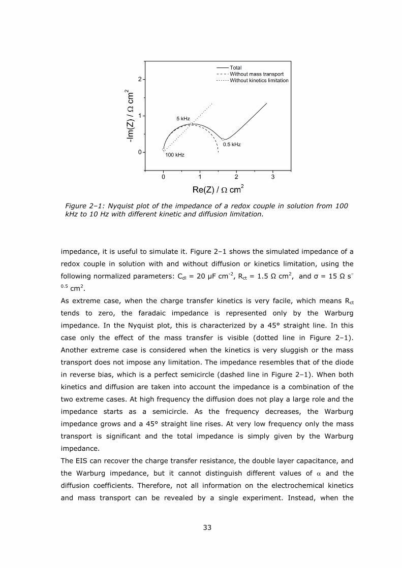
33
impedance, it is useful to simulate it. Figure 2–1 shows the simulated impedance of a
redox couple in solution with and without diffusion or kinetics limitation, using the
following normalized parameters: Cdl = 20 μF cm-2, Rct = 1.5 Ω cm2, and ζ = 15 Ω s–
0.5 cm2.
As extreme case, when the charge transfer kinetics is very facile, which means Rct
tends to zero, the faradaic impedance is represented only by the Warburg
impedance. In the Nyquist plot, this is characterized by a 45° straight line. In this
case only the effect of the mass transfer is visible (dotted line in Figure 2–1).
Another extreme case is considered when the kinetics is very sluggish or the mass
transport does not impose any limitation. The impedance resembles that of the diode
in reverse bias, which is a perfect semicircle (dashed line in Figure 2–1). When both
kinetics and diffusion are taken into account the impedance is a combination of the
two extreme cases. At high frequency the diffusion does not play a large role and the
impedance starts as a semicircle. As the frequency decreases, the Warburg
impedance grows and a 45° straight line rises. At very low frequency only the mass
transport is significant and the total impedance is simply given by the Warburg
impedance.
The EIS can recover the charge transfer resistance, the double layer capacitance, and
the Warburg impedance, but it cannot distinguish different values of and the
diffusion coefficients. Therefore, not all information on the electrochemical kinetics
and mass transport can be revealed by a single experiment. Instead, when the
Figure 2–1: Nyquist plot of the impedance of a redox couple in solution from 100
kHz to 10 Hz with different kinetic and diffusion limitation.

34
electrochemical system is treated as nonlinear, the amount of information available is
larger as shown in the next section.
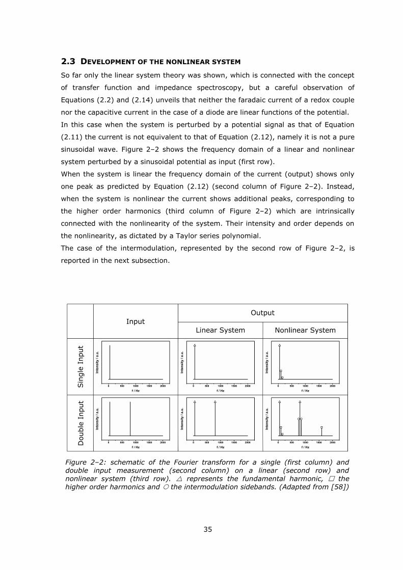
35
2.3 DEVELOPMENT OF THE NONLINEAR SYSTEM
So far only the linear system theory was shown, which is connected with the concept
of transfer function and impedance spectroscopy, but a careful observation of
Equations (2.2) and (2.14) unveils that neither the faradaic current of a redox couple
nor the capacitive current in the case of a diode are linear functions of the potential.
In this case when the system is perturbed by a potential signal as that of Equation
(2.11) the current is not equivalent to that of Equation (2.12), namely it is not a pure
sinusoidal wave. Figure 2–2 shows the frequency domain of a linear and nonlinear
system perturbed by a sinusoidal potential as input (first row).
When the system is linear the frequency domain of the current (output) shows only
one peak as predicted by Equation (2.12) (second column of Figure 2–2). Instead,
when the system is nonlinear the current shows additional peaks, corresponding to
the higher order harmonics (third column of Figure 2–2) which are intrinsically
connected with the nonlinearity of the system. Their intensity and order depends on
the nonlinearity, as dictated by a Taylor series polynomial.
The case of the intermodulation, represented by the second row of Figure 2–2, is
reported in the next subsection.
Figure 2–2: schematic of the Fourier transform for a single (first column) and
double input measurement (second column) on a linear (second row) and
nonlinear system (third row). represents the fundamental harmonic, the
higher order harmonics and the intermodulation sidebands. (Adapted from [58])
36
2.3.1 INTERMODULATION
During the intermodulation the system is perturbed by two sinusoidal potential waves
of different frequencies, as schematized by the first column and second row of Figure
2–2. The lower frequency signal is called stimulus (frequency fω and angular
frequency ω) and the higher frequency one probe (frequency fΩ and angular
frequency Ω). Under such conditions, the output of a linear system is composed by
two sine-waves with the same frequencies fω and fΩ, but different modulus and phase
(second column of Figure 2–2), as for a single sinusoidal perturbation.
However, for nonlinear systems the situation is considerably different: in addition to
the higher order harmonics of the stimulus and probe, symmetric peaks around the
probe frequency are observed (third column of Figure 2–2). These are called
sidebands. Sidebands are generated by the second order polynomial in the Taylor
series of the nonlinear system and are located at fΩ – fω and fΩ + fω. The output of
the probe and the sidebands in the time domain (t-domain) represent the envelope
of the amplitude modulation of the stimulus on the probe signal. This is the so-called
phenomenon of the intermodulation, and it contains information coming from the
stimulus, the probe and the characteristics of the system. An important feature of the
sidebands is that the intensity of these signals is in general higher than the intensity
of second harmonics [38].
Employing the small signal approximation, it is possible to develop the system in a
similar fashion of the linear system theory. This approximation leads to the fact that
the first order signals in the third column of Figure 2–2 are linear with the input and
that the second order signals, second harmonics and sidebands, are proportional to a
combination of the square of the inputs. In this way the immittance transfer
functions can still be successfully employed together with a new set of transfer
functions defined in the next subsection.
2.3.2 DEFINITIONS AND DEVELOPMENT OF NEW TRANSFER FUNCTIONS
In this subsection, I introduce the new class of transfer function developed in this
work to handle the intermodulation.
The potential perturbation u(t) during an intermodulation experiment is composed by
two sine-waves of angular frequency ω and Ω superimposed to a DC potential u0:
tj*tjωtj*ωtj
0 eUeUeωUeωUutu (2.34)
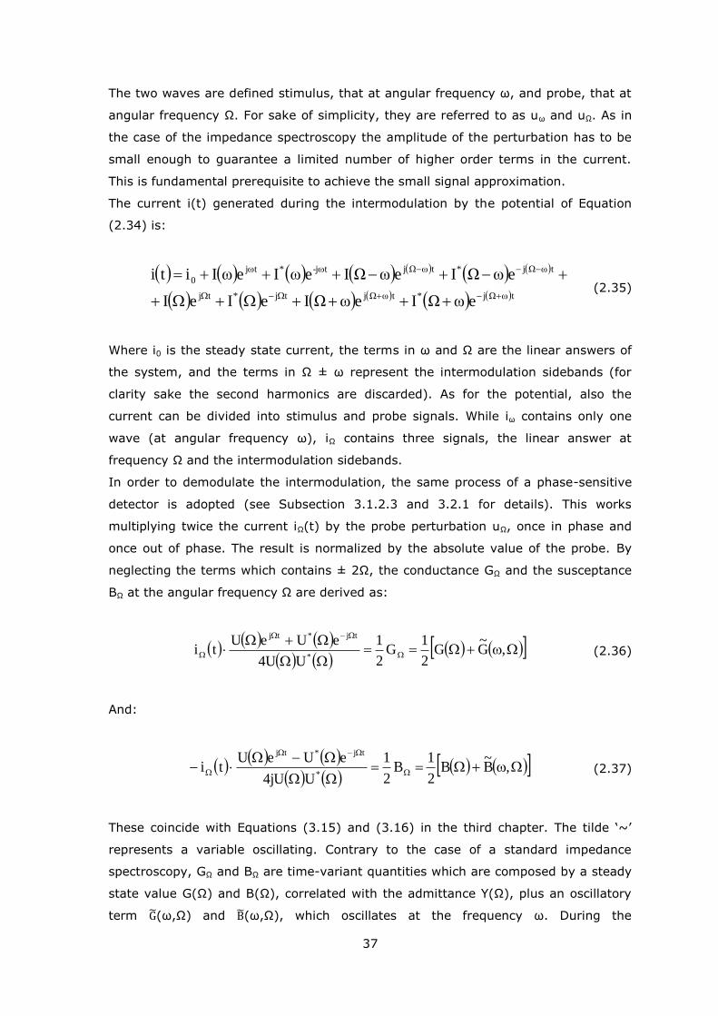
37
The two waves are defined stimulus, that at angular frequency ω, and probe, that at
angular frequency Ω. For sake of simplicity, they are referred to as uω and uΩ. As in
the case of the impedance spectroscopy the amplitude of the perturbation has to be
small enough to guarantee a limited number of higher order terms in the current.
This is fundamental prerequisite to achieve the small signal approximation.
The current i(t) generated during the intermodulation by the potential of Equation
(2.34) is:
tωΩj*tωΩjtj*tj
tωΩj*tωΩjt-j*tj
0
eωΩIeωΩIeIeI
eωΩIeωΩIeωIeωIiti
(2.35)
Where i0 is the steady state current, the terms in ω and Ω are the linear answers of
the system, and the terms in Ω ± ω represent the intermodulation sidebands (for
clarity sake the second harmonics are discarded). As for the potential, also the
current can be divided into stimulus and probe signals. While iω contains only one
wave (at angular frequency ω), iΩ contains three signals, the linear answer at
frequency Ω and the intermodulation sidebands.
In order to demodulate the intermodulation, the same process of a phase-sensitive
detector is adopted (see Subsection 3.1.2.3 and 3.2.1 for details). This works
multiplying twice the current iΩ(t) by the probe perturbation uΩ, once in phase and
once out of phase. The result is normalized by the absolute value of the probe. By
neglecting the terms which contains ± 2Ω, the conductance GΩ and the susceptance
BΩ at the angular frequency Ω are derived as:
,G~
G2
1G
2
1
U4U
eUeUti
*
tj*tj
(2.36)
And:
,B~
B2
1B
2
1
U4jU
eUeUti
*
tj*tj
(2.37)
These coincide with Equations (3.15) and (3.16) in the third chapter. The tilde ‗~‘
represents a variable oscillating. Contrary to the case of a standard impedance
spectroscopy, GΩ and BΩ are time-variant quantities which are composed by a steady
state value G(Ω) and B(Ω), correlated with the admittance Y(Ω), plus an oscillatory
term (ω,Ω) and (ω,Ω), which oscillates at the frequency ω. During the
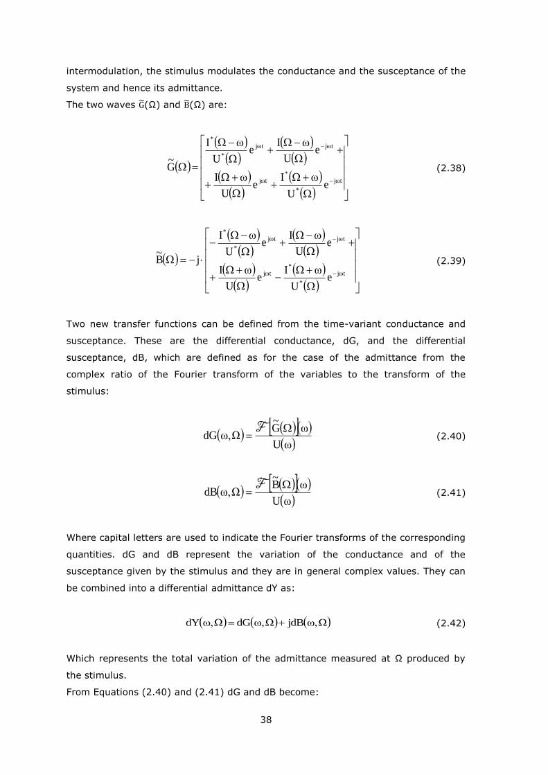
38
intermodulation, the stimulus modulates the conductance and the susceptance of the
system and hence its admittance.
The two waves (Ω) and (Ω) are:
tj
*
*tj
tjtj
*
*
eU
Ie
U
I
eU
Ie
U
I
G~
(2.38)
tj
*
*tj
tjtj
*
*
eU
Ie
U
I
eU
Ie
U
I
jB~
(2.39)
Two new transfer functions can be defined from the time-variant conductance and
susceptance. These are the differential conductance, dG, and the differential
susceptance, dB, which are defined as for the case of the admittance from the
complex ratio of the Fourier transform of the variables to the transform of the
stimulus:
ωU
ωG~
Ωω,dG
F
(2.40)
ωU
ωB~
Ωω,dB
F
(2.41)
Where capital letters are used to indicate the Fourier transforms of the corresponding
quantities. dG and dB represent the variation of the conductance and of the
susceptance given by the stimulus and they are in general complex values. They can
be combined into a differential admittance dY as:
Ωω,jdBΩω,dGΩω,dY (2.42)
Which represents the total variation of the admittance measured at Ω produced by
the stimulus.
From Equations (2.40) and (2.41) dG and dB become:
39
ω2U
ΩU
ωΩI
ΩU
ωΩI
dG*
*
(2.43)
ω2U
ΩU
ωΩI
ΩU
ωΩI
jdB*
*
(2.44)
Plugging them into Equation (2.42) dY becomes:
ωUΩU
ωΩIΩω,dY
(2.45)
Which is given by the right (upper) sideband alone. Similarly, the anti-differential
admittance d can be defined for the left (bottom) sideband as:
ωUΩU
ωΩIΩω,Yd
*
* (2.46)
By Equations (2.45) and (2.46) dG and dB can be rewritten as:
2
ωΩ,dYωΩ,YdωΩ,dG
(2.47)
2
ωΩ,dYωΩ,YdjωΩ,dB
(2.48)
In the Appendix B, from dY also the differential impedance dZ is derived.
In the next subsection, there are some examples where these transfer functions are
employed.
2.3.3 SIMPLIFIED CASE
In order to understand which information lay in the intermodulation, in this
subsection a simple case is introduced. Let assume a current i = f(u), which can be
expressed in a Taylor expansion up to the second order as:
40
2
2
2
0 Δudu
fd
2
1Δu
du
dfufi (2.49)
The derivatives are real values and both current, i, and potential, u, are given by
Equation (2.34) and (2.35). Expanding the term Δu2 and passing to the frequency
domain the following identities are found:
ΩUωUdu
fdωΩI *
2
2* (2.50)
ΩUωUdu
fdωΩI
2
2
(2.51)
And from the definition of dY and d given by Equations (2.45) and (2.46):
2
2
*
*
du
fd
ΩUωU
ωΩIωΩ,Yd
(2.52)
2
2
du
fd
ΩUωU
ωΩIωΩ,dY
(2.53)
Equations (2.52) and (2.53) show the connection between the intermodulation and
the second derivatives of the investigated system in a similar fashion as for the EIS
and the first derivatives.
From Equations (2.47) and (2.48), dG and dB are found. In this simple case, the left
and right sidebands are equal and only the real part of dG is non-zero. Furthermore,
if one calculated the causality factor as suggested by Bosch et al. [39], this would be
equal to two. In general, this is not true as it is proved in the fourth chapter
(Subsection 4.3.2).
In the next subsections, some real cases are examined when the intermodulation is
applied.
2.3.4 IDEAL NONLINEAR CASE: DIODE
In the Subsection 2.2.2.1, the example of the diode is reported in reverse bias as
ideal case during an impedance experiment. The stimulus, affecting the potential
41
across the system, modulates the value of the capacitance of the diode, which is the
origin of the amplitude modulation of the probe current at the stimulus frequency.
The leakage current can be considered linear with the potential and only the
capacitive current contributes to the secondary response of the system. Its second
derivative calculated using Equation (2.14) leads to:
23
Bfb0
D0r
e
Tkuu
2
Neεε
2
1jdG
(2.52)
23
Bfb0
D0r
e
Tkuu
2
Neεε
2
1ΩdB
(2.53)
It is worth to note that dG should be negative and imaginary, while dB, although
negative, should be real. Both terms are related to the variation of the capacitance
with the potential, however, the value of dG is proportional to ω, while the value of
dB is proportional to Ω.
An IDIS can be used in combination with an EIS to recover the flat band potential of
the device as shown in the fourth chapter (Section 4.2).
2.3.5 ELECTROCHEMICAL CASE: REDOX COUPLE
The case of a redox couple is shown here. This follows Subsection 2.2.2.2.
If the system is nonlinear, not only the current, but all physical variables show the
intermodulation sidebands in the frequency domain. These appear at angular
frequencies Ω + ω and Ω – ω (see Figure 2–2). In addition to the faradaic Jacobian,
JF, and the vector of physical variables, X, defined by Equations (2.21) and (2.22),
the faradaic Hessian, HF, is given by:
00cu
i
00cu
i
cu
i
cu
i
u
i
H
Ox,0
F
2
Red,0
F
2
Ox,0
F
2
Red,0
F
2
2
F
2
F (2.56)
42
Which represents the matrix collecting all the second derivatives. As for the previous
cases (Subsection 2.2.2.2), the currents as well as the sidebands are calculated for
the faradaic (IF) and capacitive (Ic) current.
ωXHΩXωΩXJωΩI F
TT
FF (2.57)
ωXHΩXωΩXJωΩI F
*T*T
F
*
F (2.58)
And
ωUΩΩωUu
CωUΩUωΩ
u
CjωΩI dldl
c
(2.59)
ωUΩΩωUu
CωUΩUωΩ
u
CjωΩI dldl*
c
(2.60)
It is noteworthy that Equations (2.57) and (2.58) contain both first and second
derivatives of the current contrary to Equations (2.59) and (2.60), because the
potential is the only quantity that does not oscillate at Ω ω. It is clear from this set
of equations the usefulness of a matrix formalism to develop the secondary effects
during an intermodulation.
As for X(ω) in Equation (2.24), also the vectors X(Ω+ω) and X*(Ω–ω) depend on the
values of IF(Ω+ω) and IF*(Ω–ω) through the mass transport operator m.
The faradaic sidebands are:
ωΩmc
iωΩm
c
i1
ωXHΩXωΩI
Ox
Ox,0
FRed
Red,0
F
F
T
F
(2.61)
ωΩmc
iωΩm
c
i1
ωXHΩXωΩI
*
Ox
Ox,0
F*
Red
Red,0
F
F
*T*
F
(2.62)
Which lead to the faradaic differential and anti-differential admittance dYF and d F:
43
ωΩmc
iωΩm
c
i1
ωAHΩA
ωUΩU
ωΩIωΩ,dY
Ox
Ox,0
FRed
Red,0
F
F
T
FF
(2.63)
ωΩmc
iωΩm
c
i1
ωAHΩA
ωUΩU
ωΩIωΩ,Yd
*
Ox
Ox,0
F*
Red
Red,0
F
F
*T
*
*
FF
(2.64)
Where the vector A is defined for brevity as:
ωYωm
ωYωm
1
ωU
ωCωU
ωC
1
ωA
FOx
FRed
oOx,
oRed, (2.65)
Capacitive differential and anti-differential admittance dYc and d c are given by:
Ωωu
CωΩ
u
Cj
ωUΩU
ωΩIωΩ,dY dldlc
c
(2.66)
Ωωu
CωΩ
u
Cj
ωUΩU
ωΩIωΩ,Yd dldl
*
*
c
c
(2.67)
The total differential and anti-differential admittance are then the sum of the faradaic
and capacitive terms, which are used through Equations (2.47) and (2.48) to recover
dG and dB.
Given the complexity of Equations (2.64) - (2.67), a straightforward interpretation of
dG and dB is impossible and the simulated results are reported in the following
subsections.
2.3.6 MATHEMATICAL SIMULATION OF THE REDOX COUPLE
The mathematical simulation of the intermodulation on a redox couple is shown in
this and next subsections. In Table 2–1 the parameters describing the system and
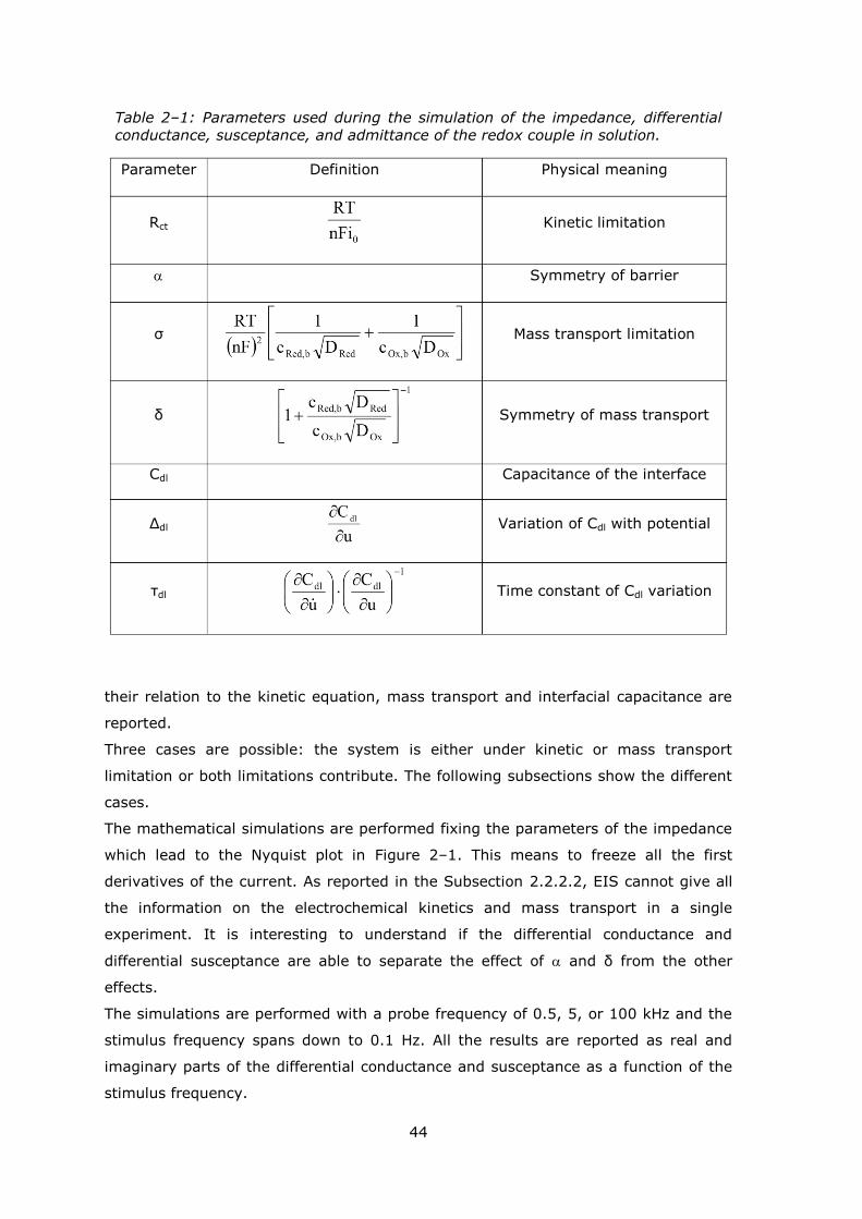
44
their relation to the kinetic equation, mass transport and interfacial capacitance are
reported.
Three cases are possible: the system is either under kinetic or mass transport
limitation or both limitations contribute. The following subsections show the different
cases.
The mathematical simulations are performed fixing the parameters of the impedance
which lead to the Nyquist plot in Figure 2–1. This means to freeze all the first
derivatives of the current. As reported in the Subsection 2.2.2.2, EIS cannot give all
the information on the electrochemical kinetics and mass transport in a single
experiment. It is interesting to understand if the differential conductance and
differential susceptance are able to separate the effect of and δ from the other
effects.
The simulations are performed with a probe frequency of 0.5, 5, or 100 kHz and the
stimulus frequency spans down to 0.1 Hz. All the results are reported as real and
imaginary parts of the differential conductance and susceptance as a function of the
stimulus frequency.
Table 2–1: Parameters used during the simulation of the impedance, differential
conductance, susceptance, and admittance of the redox couple in solution.
Parameter Definition Physical meaning
Rct Kinetic limitation
Symmetry of barrier
ζ Mass transport limitation
δ Symmetry of mass transport
Cdl Capacitance of the interface
Δdl Variation of Cdl with potential
ηdl Time constant of Cdl variation
45
Next subsection starts from the analysis of the charging current, which is an
extension of what already observed for the diode (Subsection 2.3.4).
2.3.6.1 CAPACITIVE CURRENT
The capacitive current has two nonlinear terms, which cannot be excluded a priori
(even in the simplified case of excess of supporting electrolyte and no adsorption
phenomena): the first is relative to the variation of the capacitance of the interface
with the potential, Δdl (e.g. for the diode), as given by the Stern model; the second is
the time constant of the charging of the interface, ηdl.
If only the capacitive terms are considered, dG and dB can be written as:
dl jωωΩ,dG (2.68)
dldl ηjω1ΩΔωΩ,dB (2.69)
dB is related to the interface capacitance transfer function proposed by Keddam and
Takenouti [54–57].
The simulation is performed keeping the probe frequency fixed at 5 kHz and
spanning the stimulus down to 0.1 Hz.
Figure 2–3–a shows the effect of Δdl on the differential immittance spectra of a redox
couple. Δdl affects both the imaginary part of the differential conductance, dG, and
the real part of the differential susceptance, dB. As seen before (Subsection 2.3.4),
Δdl affects dG and dB proportionally to ω and Ω, respectively. The immittance Bode
plot of dG shows the frequency dependence of a capacitor and the plot of dB that of a
resistor.
Figure 2–3–b reports the effect of ηdl on the differential immittance spectra. It
combines the effect of Δdl with a linear variation of the imaginary part of dB. This is
one of major contributions on Im(dB).
ηdl and Δdl are closely related. In fact, in presence of ηdl, Δdl cannot be zero. Indeed,
being ηdl the time necessary for the capacitance of the interface to change its value,
it has no physical meaning if the value of the capacitance of the interface does not
change.
The time constant of the double layer was predicted [67] and experimentally
observed by others [54–57].
In the differential immittance Bode plot, dG still shows the frequency dependence of
a capacitor, while dB resembles the admittance spectra of a resistor in parallel to a
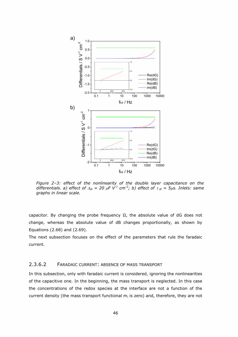
46
capacitor. By changing the probe frequency Ω, the absolute value of dG does not
change, whereas the absolute value of dB changes proportionally, as shown by
Equations (2.68) and (2.69).
The next subsection focuses on the effect of the parameters that rule the faradaic
current.
2.3.6.2 FARADAIC CURRENT: ABSENCE OF MASS TRANSPORT
In this subsection, only with faradaic current is considered, ignoring the nonlinearities
of the capacitive one. In the beginning, the mass transport is neglected. In this case
the concentrations of the redox species at the interface are not a function of the
current density (the mass transport functional mi is zero) and, therefore, they are not
Figure 2–3: effect of the nonlinearity of the double layer capacitance on the
differentials. a) effect of dl = 20 F V-1 cm-2; b) effect of dl = 5s. Inlets: same
graphs in linear scale.
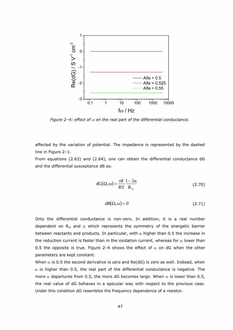
47
affected by the variation of potential. The impedance is represented by the dashed
line in Figure 2–1.
From equations (2.63) and (2.64), one can obtain the differential conductance dG
and the differential susceptance dB as:
ctR
α21
RT
nFωΩ,dG
(2.70)
0ωΩ,dB (2.71)
Only the differential conductance is non-zero. In addition, it is a real number
dependent on Rct and which represents the symmetry of the energetic barrier
between reactants and products. In particular, with higher than 0.5 the increase in
the reduction current is faster than in the oxidation current, whereas for lower than
0.5 the opposite is true. Figure 2–4 shows the effect of on dG when the other
parameters are kept constant.
When is 0.5 the second derivative is zero and Re(dG) is zero as well. Instead, when
is higher than 0.5, the real part of the differential conductance is negative. The
more departures from 0.5, the more dG becomes large. When is lower than 0.5,
the real value of dG behaves in a specular way with respect to the previous case.
Under this condition dG resembles the frequency dependence of a resistor.
Figure 2–4: effect of on the real part of the differential conductance.
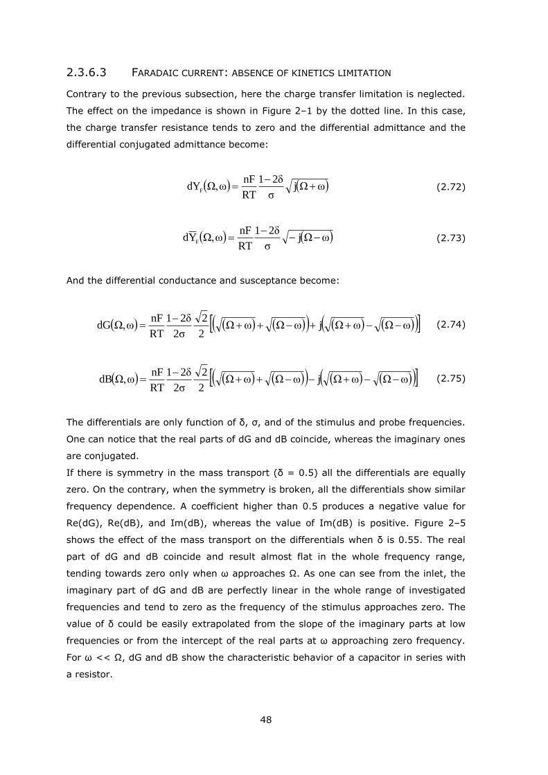
48
2.3.6.3 FARADAIC CURRENT: ABSENCE OF KINETICS LIMITATION
Contrary to the previous subsection, here the charge transfer limitation is neglected.
The effect on the impedance is shown in Figure 2–1 by the dotted line. In this case,
the charge transfer resistance tends to zero and the differential admittance and the
differential conjugated admittance become:
ωΩjζ
δ21
RT
nFωΩ,dY
F
(2.72)
ωΩjζ
δ21
RT
nFωΩ,Yd
F
(2.73)
And the differential conductance and susceptance become:
ωΩωΩjωΩωΩ2
2
2ζ
δ21
RT
nFωΩ,dG
(2.74)
ωΩωΩjωΩωΩ2
2
2ζ
2δ1
RT
nFωΩ,dB
(2.75)
The differentials are only function of δ, ζ, and of the stimulus and probe frequencies.
One can notice that the real parts of dG and dB coincide, whereas the imaginary ones
are conjugated.
If there is symmetry in the mass transport (δ = 0.5) all the differentials are equally
zero. On the contrary, when the symmetry is broken, all the differentials show similar
frequency dependence. A coefficient higher than 0.5 produces a negative value for
Re(dG), Re(dB), and Im(dB), whereas the value of Im(dB) is positive. Figure 2–5
shows the effect of the mass transport on the differentials when δ is 0.55. The real
part of dG and dB coincide and result almost flat in the whole frequency range,
tending towards zero only when ω approaches Ω. As one can see from the inlet, the
imaginary part of dG and dB are perfectly linear in the whole range of investigated
frequencies and tend to zero as the frequency of the stimulus approaches zero. The
value of δ could be easily extrapolated from the slope of the imaginary parts at low
frequencies or from the intercept of the real parts at ω approaching zero frequency.
For ω << Ω, dG and dB show the characteristic behavior of a capacitor in series with
a resistor.
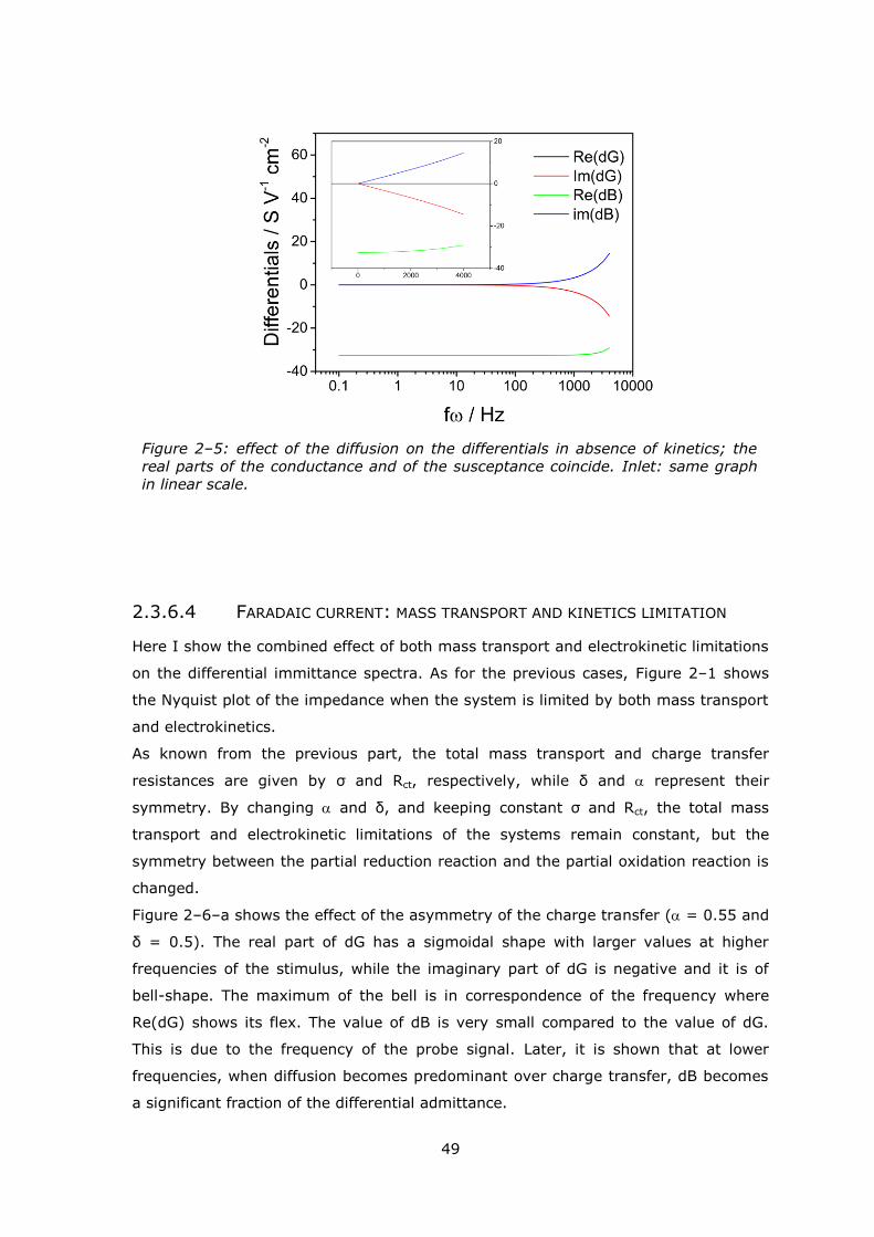
49
2.3.6.4 FARADAIC CURRENT: MASS TRANSPORT AND KINETICS LIMITATION
Here I show the combined effect of both mass transport and electrokinetic limitations
on the differential immittance spectra. As for the previous cases, Figure 2–1 shows
the Nyquist plot of the impedance when the system is limited by both mass transport
and electrokinetics.
As known from the previous part, the total mass transport and charge transfer
resistances are given by ζ and Rct, respectively, while δ and represent their
symmetry. By changing and δ, and keeping constant ζ and Rct, the total mass
transport and electrokinetic limitations of the systems remain constant, but the
symmetry between the partial reduction reaction and the partial oxidation reaction is
changed.
Figure 2–6–a shows the effect of the asymmetry of the charge transfer ( = 0.55 and
δ = 0.5). The real part of dG has a sigmoidal shape with larger values at higher
frequencies of the stimulus, while the imaginary part of dG is negative and it is of
bell-shape. The maximum of the bell is in correspondence of the frequency where
Re(dG) shows its flex. The value of dB is very small compared to the value of dG.
This is due to the frequency of the probe signal. Later, it is shown that at lower
frequencies, when diffusion becomes predominant over charge transfer, dB becomes
a significant fraction of the differential admittance.
Figure 2–5: effect of the diffusion on the differentials in absence of kinetics; the
real parts of the conductance and of the susceptance coincide. Inlet: same graph
in linear scale.
50
Figure 2–6–b reports the complementary case: only the mass transport is
asymmetric ( = 0.5 and δ = 0.6). Both real and imaginary part of dG and dB show
similar features as before. However, the sigmoidal shape of Re(dG) is inverted and
tends to zero for high frequencies. Instead, Im(dG) is positive. The presence of a
hook at the higher frequencies is a feature common to the real and imaginary parts
of all differentials and it is a special feature given by the asymmetry of mass
transport.
If both mass transport and charge transfer asymmetries are present, the final effect
is just the sum of the two. This is summarized in Figure 2–6–c and –d, where =
0.6, and = 0.55 and 0.45, respectively. All features observed in the two previous
cases appear in Figure 2–6–c. One can imagine the complete case as composed by
two parallel circuital branches each one having only one asymmetry. It is interesting
to observe Figure 2–6–d. In this case, the asymmetries of mass transport and of
electrokinetics are in opposite direction (δ > 0.5 and < 0.5) and the real part of dG
crosses the x-axis.
It is important to observe what happens when and are equal. This is shown in
Figure 2–7. All differentials are flat for a large range of frequencies and the imaginary
Figure 2–6: effect of mass transport and kinetics limitation on the differentials; a)
asymmetry of kinetics; b) asymmetry of diffusion; c) both kinetics and diffusion asymmetric; d) opposite symmetry for diffusion and kinetics.
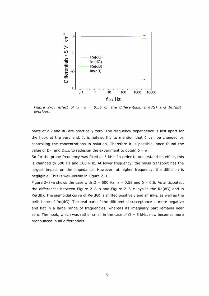
51
parts of dG and dB are practically zero. The frequency dependence is lost apart for
the hook at the very end. It is noteworthy to mention that δ can be changed by
controlling the concentrations in solution. Therefore it is possible, once found the
value of DOx and DRed, to redesign the experiment to obtain δ = .
So far the probe frequency was fixed at 5 kHz. In order to understand its effect, this
is changed to 500 Hz and 100 kHz. At lower frequency, the mass transport has the
largest impact on the impedance. However, at higher frequency, the diffusion is
negligible. This is well-visible in Figure 2–1.
Figure 2–8–a shows the case with Ω = 500 Hz, = 0.55 and δ = 0.6. As anticipated,
the differences between Figure 2–8–a and Figure 2–6–c lays in the Re(dG) and in
Re(dB). The sigmoidal curve of Re(dG) is shifted positively and shrinks, as well as the
bell-shape of Im(dG). The real part of the differential susceptance is more negative
and flat in a large range of frequencies, whereas its imaginary part remains near
zero. The hook, which was rather small in the case of Ω = 5 kHz, now becomes more
pronounced in all differentials.
Figure 2–7: effect of = = 0.55 on the differentials. Im(dG) and Im(dB) overlaps.
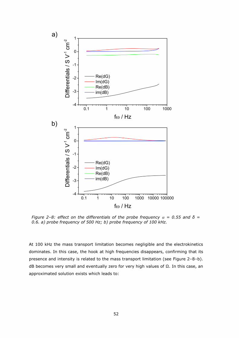
52
At 100 kHz the mass transport limitation becomes negligible and the electrokinetics
dominates. In this case, the hook at high frequencies disappears, confirming that its
presence and intensity is related to the mass transport limitation (see Figure 2–8–b).
dB becomes very small and eventually zero for very high values of Ω. In this case, an
approximated solution exists which leads to:
Figure 2–8: effect on the differentials of the probe frequency = 0.55 and δ =
0.6. a) probe frequency of 500 Hz; b) probe frequency of 100 kHz.
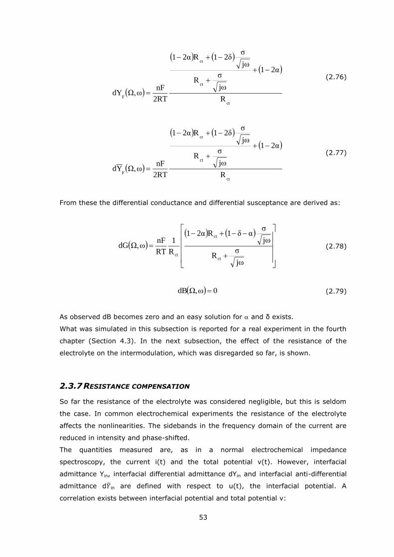
53
ct
ct
ct
F R
α21
jω
ζR
jω
ζδ21Rα21
2RT
nFωΩ,dY
(2.76)
ct
ct
ct
F R
α21
jω
ζR
jω
ζδ21Rα21
2RT
nFωΩ,Yd
(2.77)
From these the differential conductance and differential susceptance are derived as:
jω
ζR
jω
ζαδ1Rα21
R
1
RT
nFωΩ,dG
ct
ct
ct
(2.78)
0ωΩ,dB (2.79)
As observed dB becomes zero and an easy solution for and δ exists.
What was simulated in this subsection is reported for a real experiment in the fourth
chapter (Section 4.3). In the next subsection, the effect of the resistance of the
electrolyte on the intermodulation, which was disregarded so far, is shown.
2.3.7 RESISTANCE COMPENSATION
So far the resistance of the electrolyte was considered negligible, but this is seldom
the case. In common electrochemical experiments the resistance of the electrolyte
affects the nonlinearities. The sidebands in the frequency domain of the current are
reduced in intensity and phase-shifted.
The quantities measured are, as in a normal electrochemical impedance
spectroscopy, the current i(t) and the total potential v(t). However, interfacial
admittance Yin, interfacial differential admittance dYin and interfacial anti-differential
admittance d in are defined with respect to u(t), the interfacial potential. A
correlation exists between interfacial potential and total potential v:
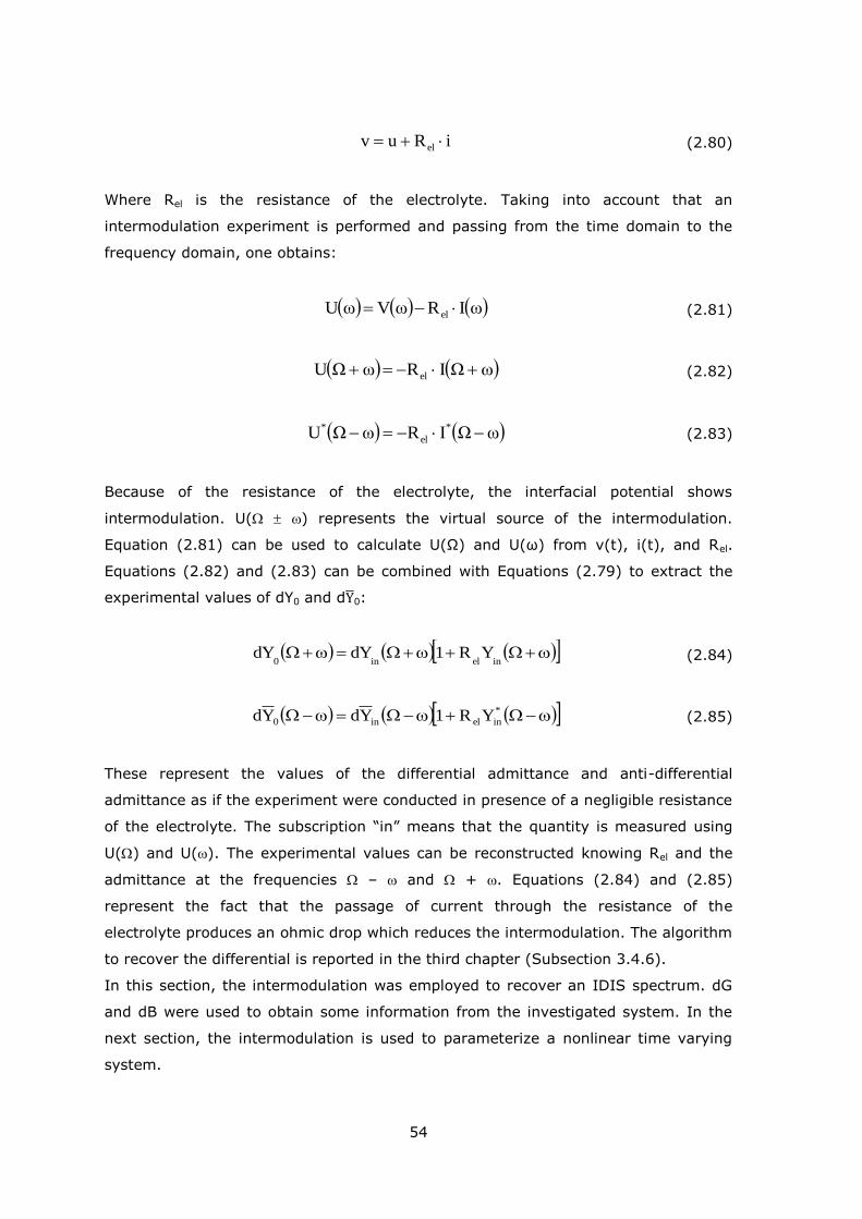
54
iRuv el (2.80)
Where Rel is the resistance of the electrolyte. Taking into account that an
intermodulation experiment is performed and passing from the time domain to the
frequency domain, one obtains:
ωIRωVωU el (2.81)
ωΩIRωΩU el (2.82)
ωΩIRωΩU *
el
* (2.83)
Because of the resistance of the electrolyte, the interfacial potential shows
intermodulation. U( ) represents the virtual source of the intermodulation.
Equation (2.81) can be used to calculate U(Ω) and U(ω) from v(t), i(t), and Rel.
Equations (2.82) and (2.83) can be combined with Equations (2.79) to extract the
experimental values of dY0 and d 0:
inelin0
YR1dYdY (2.84)
*
inelin0 YR1YdYd (2.85)
These represent the values of the differential admittance and anti-differential
admittance as if the experiment were conducted in presence of a negligible resistance
of the electrolyte. The subscription ―in‖ means that the quantity is measured using
U() and U(). The experimental values can be reconstructed knowing Rel and the
admittance at the frequencies – and + . Equations (2.84) and (2.85)
represent the fact that the passage of current through the resistance of the
electrolyte produces an ohmic drop which reduces the intermodulation. The algorithm
to recover the differential is reported in the third chapter (Subsection 3.4.6).
In this section, the intermodulation was employed to recover an IDIS spectrum. dG
and dB were used to obtain some information from the investigated system. In the
next section, the intermodulation is used to parameterize a nonlinear time varying
system.
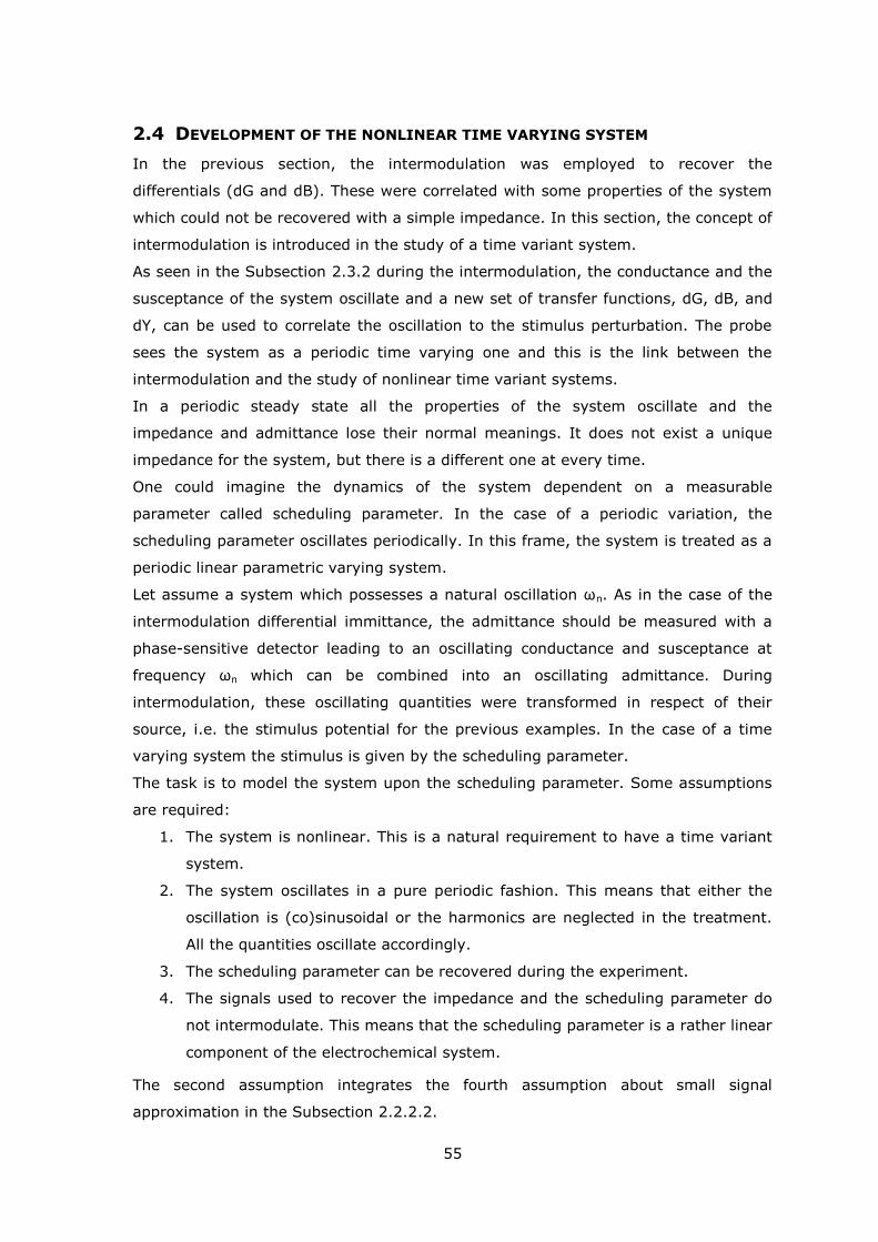
55
2.4 DEVELOPMENT OF THE NONLINEAR TIME VARYING SYSTEM
In the previous section, the intermodulation was employed to recover the
differentials (dG and dB). These were correlated with some properties of the system
which could not be recovered with a simple impedance. In this section, the concept of
intermodulation is introduced in the study of a time variant system.
As seen in the Subsection 2.3.2 during the intermodulation, the conductance and the
susceptance of the system oscillate and a new set of transfer functions, dG, dB, and
dY, can be used to correlate the oscillation to the stimulus perturbation. The probe
sees the system as a periodic time varying one and this is the link between the
intermodulation and the study of nonlinear time variant systems.
In a periodic steady state all the properties of the system oscillate and the
impedance and admittance lose their normal meanings. It does not exist a unique
impedance for the system, but there is a different one at every time.
One could imagine the dynamics of the system dependent on a measurable
parameter called scheduling parameter. In the case of a periodic variation, the
scheduling parameter oscillates periodically. In this frame, the system is treated as a
periodic linear parametric varying system.
Let assume a system which possesses a natural oscillation ωn. As in the case of the
intermodulation differential immittance, the admittance should be measured with a
phase-sensitive detector leading to an oscillating conductance and susceptance at
frequency ωn which can be combined into an oscillating admittance. During
intermodulation, these oscillating quantities were transformed in respect of their
source, i.e. the stimulus potential for the previous examples. In the case of a time
varying system the stimulus is given by the scheduling parameter.
The task is to model the system upon the scheduling parameter. Some assumptions
are required:
1. The system is nonlinear. This is a natural requirement to have a time variant
system.
2. The system oscillates in a pure periodic fashion. This means that either the
oscillation is (co)sinusoidal or the harmonics are neglected in the treatment.
All the quantities oscillate accordingly.
3. The scheduling parameter can be recovered during the experiment.
4. The signals used to recover the impedance and the scheduling parameter do
not intermodulate. This means that the scheduling parameter is a rather linear
component of the electrochemical system.
The second assumption integrates the fourth assumption about small signal
approximation in the Subsection 2.2.2.2.
56
The model is built upon a system composed by a gas-evolving electrode working at a
potential high enough to evolve oxygen bubbles. These bubbles give rise to the
electrochemical noise in the current. As scheduling parameter, the surface area a(t)
of the electrode is taken. This is periodically occupied by a bubble.
In order to recover the surface area, a high frequency signal perturbation is used.
Simultaneously, the impedance is measured at the frequency . The current i(t) is
given by:
k
tkω-j
n
*tkω-j
n
tj*tj
k
tkω-ωj
n
*tkω-ωj
n
tj-*tj
k
t-jk
n
*tjk
n0
nn
nn
nn
ekω-Iekω-IeIeI
ekω-ωIekω-ωIeωIeωI
ekωIekωIiti
(2.86)
The terms in kωn belong to the electrochemical noise and they are collected into iωn.
The terms containing only ω and Ω are the linear responses of the system. The
electrochemical noise intermodulates with both ω and Ω. Figure 2–9 shows the
schematic of the frequency domain for Equation (2.86), according to the assumption
k = 1.
Following the names used for Equation (2.35), the current i(t) is divided into iωn, iω
which contains the intermodulation of the noise at the frequency ω, and iΩ which
contains the intermodulation of the noise at the frequency Ω. From iΩ the scheduling
Figure 2–9: Fourier transform of a nonlinear time variant system given by Equation (2.84) with k = 1. represents the electrochemical noise, the fundamental harmonic, and the intermodulation sidebands.
57
parameter, a(t) is recovered from the real part of the admittance as done in Equation
(2.36). Subsequently, the variation of the surface area a(t) in its Fourier
representation ( (ωn,Ω)) is defined as:
*
00
n
*
n
*
0
n
nYY
U
I
U
I
YRe
,G~
,A~
(2.87)
Where Re[Y0(Ω)] is taken from an experiment performed without bubble evolution.
This is required to normalize the admittance to the surface area. The scheduling
parameter represents the stimulus which perturbs the impedance. Therefore, from
Equation (2.40) and (2.41), one can write:
,A~
,dZZ~
nnn (2.88)
As shown in Appendix B, dZ can be derived from dY as:
2
n
nY
,dY,dZ
(2.89)
Where Y(ω) is the admittance at the probe frequency. In this case, dY is defined as:
,A~
U
I,dY
n
n
n (2.90)
Where it is clear that the perturbation ω represents the probe and ωn the stimulus.
Combining Equation (2.88) - (2.90) one yields:
I
I
,A~
Z
,A~Z~
n
nn
n (2.91)
Which is a new transfer function named ZA. This transfer function represents the
normalization of the oscillating impedance on the source of the oscillation which is
the changing of the surface area of the electrode.
In the fourth chapter (Section 4.4), I describe how this model is employed, focusing
on the oscillation of the admittance and of the scheduling parameter. From the

58
comparison of the mean impedance Zm and ZA the effect of the bubble on the oxygen
evolution reaction is explained.
59
3 EXPERIMENTAL PART
In this chapter, I give an overview on the instruments, materials and procedures
employed in this thesis. In the first section I describe the most common working
process of a potentiostat and of the electrochemical impedance spectroscopy. In
particular, I focus on the limitations of the instruments. In the second section, I
report the two instrumental configurations for the intermodulated differential
immittance spectroscopy (IDIS) developed in this work and I explain their
advantages and disadvantages. In section 3.3 I discuss the electrochemical cell
geometry according to the artifacts and the distortions observed in an
electrochemical impedance spectrum. In order to obtain reliable IDIS experiments,
and therefore reliable impedance experiments, particular care was posed in the
optimization of the electrochemical cell employed in this thesis. The optimizations
concerned both the artifacts coming from the stray capacitance and the improper
disposition of the electrodes in the cell.
Finally, in the last section the materials, the instruments, and the procedures
employed in this thesis are listed.
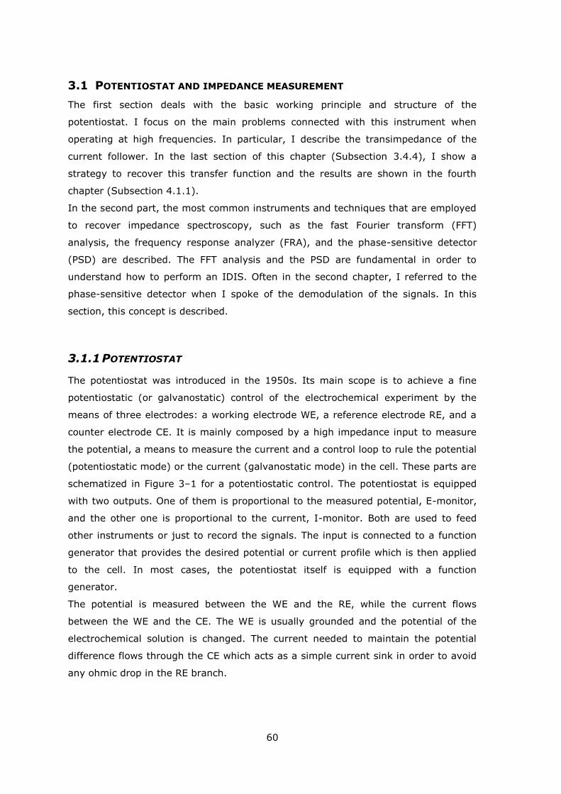
60
3.1 POTENTIOSTAT AND IMPEDANCE MEASUREMENT
The first section deals with the basic working principle and structure of the
potentiostat. I focus on the main problems connected with this instrument when
operating at high frequencies. In particular, I describe the transimpedance of the
current follower. In the last section of this chapter (Subsection 3.4.4), I show a
strategy to recover this transfer function and the results are shown in the fourth
chapter (Subsection 4.1.1).
In the second part, the most common instruments and techniques that are employed
to recover impedance spectroscopy, such as the fast Fourier transform (FFT)
analysis, the frequency response analyzer (FRA), and the phase-sensitive detector
(PSD) are described. The FFT analysis and the PSD are fundamental in order to
understand how to perform an IDIS. Often in the second chapter, I referred to the
phase-sensitive detector when I spoke of the demodulation of the signals. In this
section, this concept is described.
3.1.1 POTENTIOSTAT
The potentiostat was introduced in the 1950s. Its main scope is to achieve a fine
potentiostatic (or galvanostatic) control of the electrochemical experiment by the
means of three electrodes: a working electrode WE, a reference electrode RE, and a
counter electrode CE. It is mainly composed by a high impedance input to measure
the potential, a means to measure the current and a control loop to rule the potential
(potentiostatic mode) or the current (galvanostatic mode) in the cell. These parts are
schematized in Figure 3–1 for a potentiostatic control. The potentiostat is equipped
with two outputs. One of them is proportional to the measured potential, E-monitor,
and the other one is proportional to the current, I-monitor. Both are used to feed
other instruments or just to record the signals. The input is connected to a function
generator that provides the desired potential or current profile which is then applied
to the cell. In most cases, the potentiostat itself is equipped with a function
generator.
The potential is measured between the WE and the RE, while the current flows
between the WE and the CE. The WE is usually grounded and the potential of the
electrochemical solution is changed. The current needed to maintain the potential
difference flows through the CE which acts as a simple current sink in order to avoid
any ohmic drop in the RE branch.
61
A potentiostat can present problems when not operating in DC mode. The operational
amplifiers which compose the instrument depart from the ideality when the
instrument works in AC condition and increasing the frequency of operation the
results get worse and worse [117]. There are three kinds of problem.
One is connected with the control loop. At high frequency the response of the
potentiostat is slower and weaker. This means that the signal applied to the cell is
phase-shifted and smaller in amplitude than the one received from the input. This
problem can be circumnavigated by using larger inputs and monitoring the real signal
applied to the cell, how it is done usually.
The second problem, somehow more involved, is connected with the current reading
which is implemented as a current to voltage converter. The conversion unit is volt
on ampere, that is ohm as for the impedance. This conversion is also called
transimpedance which is a shorthand for transfer impedance.
The transimpedance Ht of a current to voltage converter is frequency dependent. The
converter gain is not constant and decreases with the frequency. It is overlapped
with a low-pass filter: the greater the gain, i.e. the lower the current range, the
lower the cutoff frequency of the filter. The cutoff is sometimes called the bandwidth
of the converter (although the same term is also used for the control loop). Typical
potentiostats show a bandwidth of 1 MHz at 1 mA full scale, but they can go as low
as 10-100 Hz at 1 nA full scale. In normal cases, the transimpedance can also be
dependent on the impedance of the investigated system.
In order to stabilize the converter or to reduce the noise, additional filters are placed
on the current reader. These influence the transimpedance decreasing the bandwidth
of the device. It is important to know the transimpedance of the instrument,
Figure 3–1: schematic of a potentiostat electric circuit for potentiodynamic experiments from reference [117].
62
especially when operating near or above its bandwidth. Section 3.4.4 explains the
strategy to study the potentiostat transimpedance and in fourth chapter (Subsection
4.1.1) some results are shown.
The third problem of the potentiostat is connected with the non-infinite impedance of
the RE input, which at high frequencies becomes small enough to allow some leakage
current to flow into the reference circuit. In Subsection 3.3.1, this issue is discussed
regarding the artifacts which can be originated during an electrochemical impedance
spectroscopy.
In the next subsection, the most common strategies to recover the impedance from
an EIS are shown.
3.1.2 IMPEDANCE MEASUREMENTS
The most common setups and instruments to perform the electrochemical impedance
spectroscopy are shown in this subsection. In potentiostatic mode, the impedance is
measured superimposing a sinusoidal perturbation to a DC potential.
All methods described in this subsection require the connection with the E- and I-
monitor outputs of the potentiostat and, if the potentiostat is not ideal, the correction
of its transimpedance. The methods can be divided into time domain, fast Fourier
transform (FFT) analysis, and into frequency domain techniques, frequency response
analyzer (FRA) and phase-sensitive detector (PSD). Their difference lies in the way
and in the domain in which they perform the integral transformation which then leads
to the impedance.
The impedance, Z, is defined as the complex ratio of the Fourier transform of the
potential, u(t), to the Fourier transform of the current, i(t), at the frequency ω:
I
U
ti
tuZ F
F (3.1)
Where capital letters are shorthand for the Fourier transform. It is clear from
Equation (3.1) that Z(ω) is a function of the frequency. Besides, it is in general a
complex number. Therefore, it is expressed in cartesian coordinates as:
ZImjZReZ (3.2)
Where Re and Im stand for the real and the imaginary argument and j is the
imaginary unit. In polar coordinates the impedance is:
63
jeZZ (3.3)
Where |Z| is the absolute value of the impedance and θ is the phase-shift.
For the sake of simplicity, the different methods to recover the impedance are
discussed only for a single input i(t), the I-monitor. Let assume that this input is
composed by a sinusoidal signal with angular frequency ω, amplitude I and phase-
shift θ. Let also disregard any conversion factor, transimpedance correction, and DC
component. Hence, i(t) is defined as:
tcosIti (3.4)
The impedance is simply calculated from the ratio of the integral transform between
the potential and the current.
3.1.2.1 FAST FOURIER TRANSFORM ANALYSIS
The fast Fourier transform (FFT) analysis first requires the digitalization of the signal
and then its elaboration; the latter can be carried out by a computational unit in the
same device or by a personal computer. The main advantage of this method is its
flexibility, because a large range of mathematical calculation can be performed on a
digital signal.
The analog to digital conversion (ADC) is the key point of this method and plays a big
role in the resolution of the technique. Nowadays, the ADCs are capable of extremely
high performances with a sampling rate as high as several megahertz and almost
endless recording time. The only limitation, under this point of view, appears to be
the capability and the memory of the calculation unit.
The ADC transforms the continuous signal into a time- and band-limited signal. This
places some restrictions. First, the digital signal is limited in time (this is indeed a
limitation always presents), and second, it is chopped into a sequence of data
separated by a time step given by the sampling rate of the acquisition. Ideally every
data point should be recorded for an infinitesimal small amount of time; in real
devices this is not the case and every single data is actually an average over a short
time of the recorded signal. This is usually referred as the analog bandwidth of the
ADC.
After the digitalization, the signal is only suitable for the discrete Fourier transform,
implemented as FFT, which is an algorithm to optimize calculation. This algorithm
64
was a breakthrough in the field of signal processing allowing the expansion of the
nuclear magnetic resonance and infrared spectroscopy.
The FFT analysis, as opposite to the other methods described later on (Subsections
3.1.2.2 and 3.1.2.3), shows the total frequency domain of the signal, noise,
harmonics and spurious signals included. A glance at the whole spectrum is a good
way to control the quality of one‘s instrumental setup and to understand the noise
sources. Moreover, this technique can resolve also synchronous noise closely
interacting with the investigated signal.
From the spectrum the complex value of the transform of the signal is taken at the
frequency of interest. This corresponds to the first coefficient c of the complex
Fourier series. For the signal i(t) given by equation (3.4):
T
0
tj dteiT
2c (3.5)
Where T is the recorded time.
The inverse of the recorded time represents the frequency steps in the frequency
domain. A low frequency signal or a dense frequency domain require a long
acquisition time. Moreover, according to the Nyquist theorem, the sampling rate has
to be at least twice as high as the highest investigated frequency in order to achieve
a perfect reconstruction of the signal in the discrete domain. This is connected with
the aliasing. Half of the sampling rate (called Nyquist frequency) represents the top
limit of the discrete Fourier transform in the frequency domain. After this frequency
the spectrum is simply repeated endless times.
If, for example, the investigated signal is at 1 kHz but the sampling rate is 200 Hz,
only one point is taken every five periods of the signal. Intuitively this leads to an
improper picture of the real signal. The signal cannot be reconstructed properly,
which leads to the appearance of some ghost waves (aliases) that actually do not
exist and are only a consequence of the low sampling rate. One can recall this
phenomenon in old western movies when the wheels of the wagons sometimes
seemed spinning in the opposite direction from their true rotation. The aliasing and
its implication are discussed in more detail in the Subsection 3.2.2 about
undersampling in the oscilloscope setup for the IDIS.
3.1.2.2 FREQUENCY RESPONSE ANALYZER
The frequency response analyzer (FRA) is probably the most used device to recover
the impedance in electrochemistry and it is usually integrated in most commercial
65
potentiostats. It employs the cross-correlation between the input signal i(t) and two
sinusoidal reference signals, Rin (Rin = cos(ωt)) and Rout (Rout = –sin(ωt)) at the
investigated frequency ω.
nT
0
indtRinT
2a (3.6)
nT
0
outdtRinT
2b (3.7)
The integral is performed on n periods T of the reference wave. The reference signals
are in quadrature and the results of the Equations (3.6) and (3.7) correspond to the
first two Fourier coefficients of a Fourier series expressed as:
cosIa (3.8)
sinIb (3.9)
The cross-correlation is extremely effective in rejecting the asynchronous noise and
the harmonics present in the signal. The accuracy in the recovery of the signal
increases with square root of the integration time nT.
3.1.2.3 PHASE-SENSITIVE DETECTOR
The phase-sensitive detector (PSD), also known as lock-in amplifier, is composed by
a frequency mixer and one or more filters. It has the particularity that it outputs two
signals. As for the FRA, two references in quadrature are used to recover the signal.
The frequency mixer multiplies the input signal with the references. The results, one
for each reference, pass subsequently to an integrator and to a low-pass filter.
Contrary to the FFT analysis and to the FRA, a lock-in amplifier does not provide a
value but two outputs, X and Y, which can be used to feed other instruments or
simply be recorded for elaboration. The outputs after the mixer and the integrator
are:
t
t-t
in
CC
dtRit
1X (3.6)
66
t
t-t
out
C C
dtRit
1Y (3.7)
Where tc represents the time constant of the integrator. Equations (3.6) and (3.7)
lead to the demodulation of i(t) as:
tscos2
ItX
X (3.8)
tssin2
ItY Y (3.9)
Which are two time dependent signals. sX(t) and sY(t) contain the higher harmonics
of the signal i(t) and those arising from the demodulation plus any other synchronous
and asynchronous noise. The value of the time constant is critical in the noise
rejection. A large tc allows for a clean demodulation, while a small one enables the
demodulation to follow fast variation in the signal.
The low-pass filters, added after the integrator, are necessary to remove sX and sY.
They apply their transfer function to X and Y, which is an important point to handle
the intermodulation as explained in Subsection 3.2.1 about the lock-in setup for the
IDIS. The variation of the impedance in time can be observed due to the
transformation of the lock-in amplifier, which is an important point in the time-
variant systems.
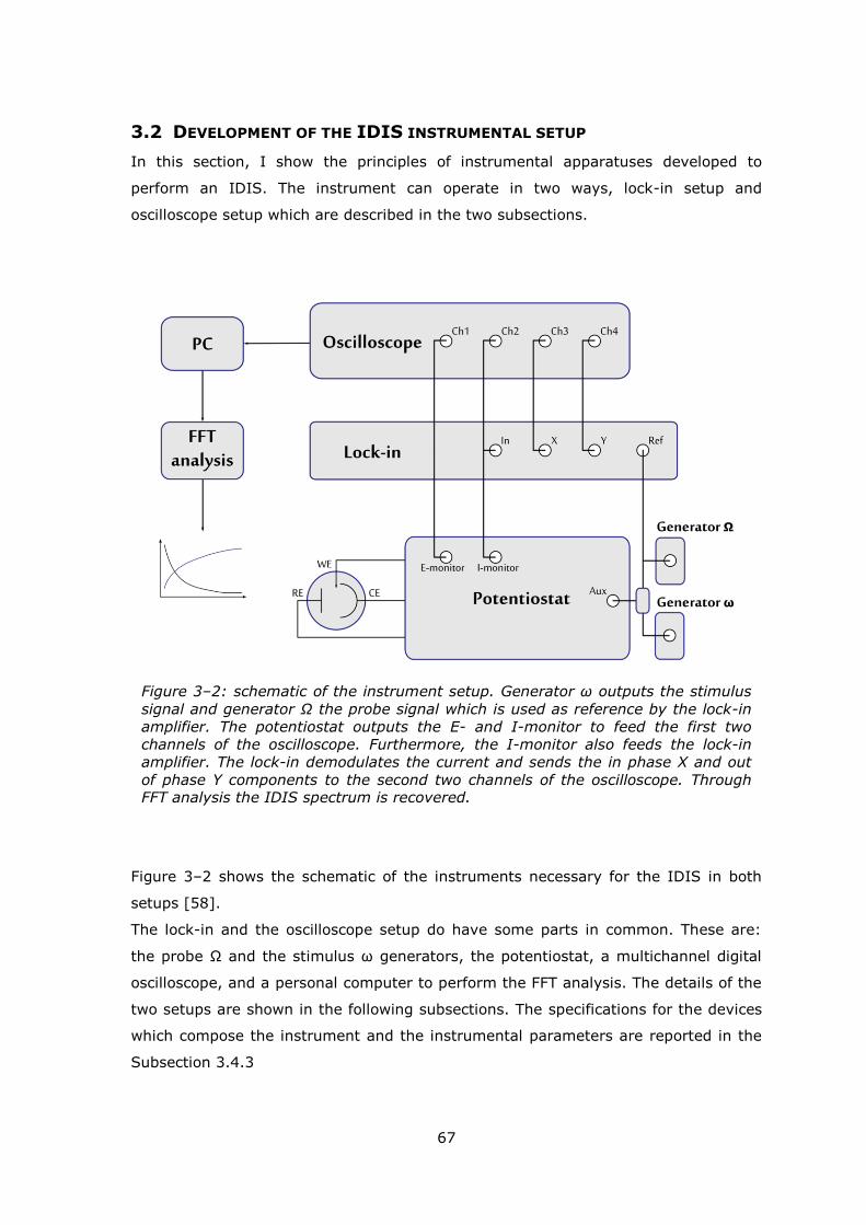
67
3.2 DEVELOPMENT OF THE IDIS INSTRUMENTAL SETUP
In this section, I show the principles of instrumental apparatuses developed to
perform an IDIS. The instrument can operate in two ways, lock-in setup and
oscilloscope setup which are described in the two subsections.
Figure 3–2 shows the schematic of the instruments necessary for the IDIS in both
setups [58].
The lock-in and the oscilloscope setup do have some parts in common. These are:
the probe Ω and the stimulus ω generators, the potentiostat, a multichannel digital
oscilloscope, and a personal computer to perform the FFT analysis. The details of the
two setups are shown in the following subsections. The specifications for the devices
which compose the instrument and the instrumental parameters are reported in the
Subsection 3.4.3
Figure 3–2: schematic of the instrument setup. Generator ω outputs the stimulus
signal and generator Ω the probe signal which is used as reference by the lock-in
amplifier. The potentiostat outputs the E- and I-monitor to feed the first two
channels of the oscilloscope. Furthermore, the I-monitor also feeds the lock-in
amplifier. The lock-in demodulates the current and sends the in phase X and out
of phase Y components to the second two channels of the oscilloscope. Through FFT analysis the IDIS spectrum is recovered.
68
3.2.1 LOCK-IN SETUP
The key part of lock-in setup is the phase-sensitive device that, as explained in
subsection 3.1.2.3, outputs two signals X and Y. The I-monitor of the potentiostat
feeds the input of the lock-in where the signal is further on demodulated according to
the probe generator as shown in Figure 3–2. Note that a 4-channel oscilloscope is
necessary in this configuration. The lock-in amplifier performs its activity only on the
probe signals. In this case, the first two channels of the oscilloscope are only
necessary to recover the stimulus signals. The best configuration for this setup
requires the splitting of the I-monitor in two and the use of four additional low-pass
filters (not shown in Figure 3–2). These low-pass filters are placed before the 4-
channel oscilloscope in such a way that all the recorded signals are filtered likewise.
This configuration was used by Keddam and Takenouti to implement the MICTF
technique [54–57]. It is useful to filter the probe signal from the E- and I-monitor,
to lower the sample frequency of the oscilloscope without incurring in aliasing
problems or in order to employ a multichannel FRA as done by Keddam and
Takenouti. The second connection of the I-monitor goes to the lock-in for the
demodulation. Besides, the X and Y outputs feed, possibly through the filters, the
oscilloscope.
The total current during an intermodulation experiment is:
ωΩωΩ
Ωω0
θtωΩcosIθtωΩcosI
θΩtcosIθωtcosIii
(3.10)
Where I is the current amplitudes, θ the phase shift, and the subscript refers to the
angular frequency to which the properties are related. The last two terms of the right
hand side of Equation (3.10) are the intermodulation sidebands. During the phase-
sensitive demodulation, the in phase component X and the out of phase component Y
from the lock-in amplifier are determined.
They are obtained by first multiplying i ∙ Rin and i ∙ –Rout, respectively, and then
integrating the results in the time constant tC, as described in subsection 3.1.2.3:
ωΩωΩωΩωΩΩ θωtcosI2
1θωtcosI
2
1θcosI
2
1X (3.11)
2
πθωtcosI
2
1
2
πθωtcosI
2
1θsinI
2
1Y ωΩωΩ-Ω (3.12)
69
Calculating the conductance G and the susceptance B from X and Y, the following
relations are obtained:
ωΩωΩΩΩ θωtcos
U
Iθωtcos
U
Iθcos
U
IG
(3.13)
2
πθωtcos
U
I
2
πθωtcos
U
Iθsin
U
IB ωΩωΩΩ (3.14)
Using the definitions of differential conductance and differential susceptance given in
Equation (2.39) and (2.40) and applying them to Equation (3.13) and (3.14), one
obtains:
ωΩ
ω
ω
ωΩ
ω
ω jθexpUU
Ijθexp
UU
I
2
1dG (3.15)
ωΩ
ω
ω
ωΩ
ω
ω jθexpUU
Ijθexp
UU
I
2
jdB (3.16)
Where Uω is the amplitude of the stimulus frequency and j the imaginary unit.
Equations (3.15) and (3.16) are equivalent to:
ω2U
ΩU
ωΩI
ΩU
ωΩI
dG*
*
(3.17)
ω2U
ΩU
ωΩI
ΩU
ωΩI
jdB*
*
(3.18)
So far two problems were disregarded: the phase-shift between the probe reference
and the potential signal inside the electrochemical cell, given by the bandwidth of the
control loop of the potentiostat, and the transfer function of the low-pass filter of the
lock-in amplifier. The first issue is easily manageable if the lock-in amplifier can be
synchronized with the probe frequency coming from the E-monitor. This is indeed the
70
case for the instrument built up during this work. Otherwise, an addition control
procedure, either performed during the experiment or aside, is necessary to get the
phase-shift of the control loop and to correct it.
The second issue requires a suitable way to find the transfer function of the built-in
filters of the lock-in amplifier. The easiest way is to compare the results of an IDIS
performed with the lock-in setup with those coming from the oscilloscope setup for
different time constants. This procedure is reported in details in subsection 3.4.4 and
the result is shown in the fourth chapter (Subsection 4.1.1).
The main advantage of the lock-in setup, especially if equipped with four additional
low-pass filters, is the possibility to have large probe frequencies and low stimulus
frequency at the same time without overloading the oscilloscope. Moreover, the
sensitivity of the PSD is higher than the one of the oscilloscope setup. A comparison
is shown in the Section 4.2.
The main disadvantage is the necessity of a 4-channel oscilloscope and eventually
additional low-pass filters. Furthermore, the lock-in amplifier places some limitations
on the stimulus and probe frequency. A ratio of one to ten is necessary to achieve a
suitable demodulation without overly reducing the time constant of the integrator,
and introducing a high level of noise.
3.2.2 OSCILLOSCOPE SETUP
The oscilloscope setup simplifies the instrumental design. Only a dual channel digital
oscilloscope is necessary and the IDIS is performed through FFT analysis. Another
advantage is the flexibility gained for the stimulus and probe frequencies. There is no
constrain in their relative values and the stimulus could even approach and cross the
probe frequency. The only limitation is the memory capability of the computer, where
datasets larger than few millions show to be difficult to handle.
There is one important aspect of the FTT analysis that is fundamental for
intermodulation: the spectrum leakage. The spectrum leakage is due to the finite size
of the recorded signal and appears as a blurring effect, given by the side lobes which
surround the frequency peaks in the F-domain. Figure 3–3 shows the spectrum
leakage of an IDIS dataset recorded on a Schottky diode. The side lobes extend to a
large part of the spectrum and easily obscure the intermodulated sidebands.
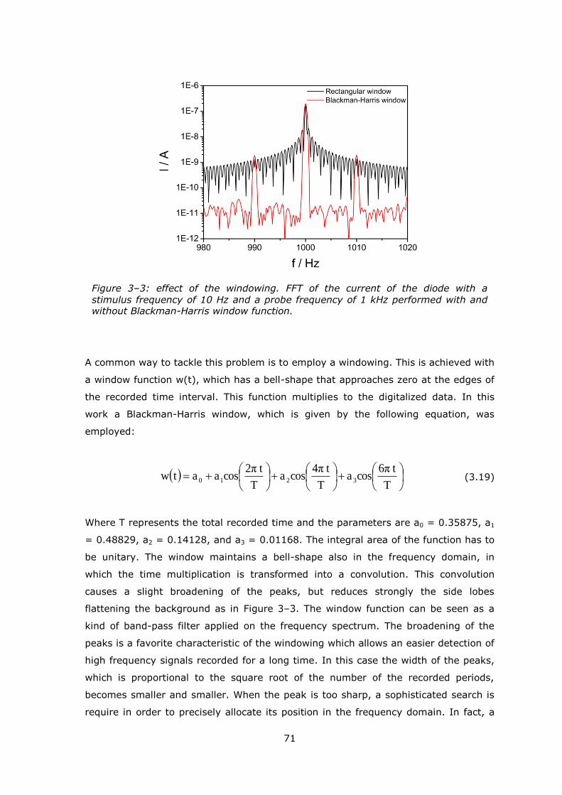
71
A common way to tackle this problem is to employ a windowing. This is achieved with
a window function w(t), which has a bell-shape that approaches zero at the edges of
the recorded time interval. This function multiplies to the digitalized data. In this
work a Blackman-Harris window, which is given by the following equation, was
employed:
T
t6πcosa
T
t4πcosa
T
t2πcosaatw 3210 (3.19)
Where T represents the total recorded time and the parameters are a0 = 0.35875, a1
= 0.48829, a2 = 0.14128, and a3 = 0.01168. The integral area of the function has to
be unitary. The window maintains a bell-shape also in the frequency domain, in
which the time multiplication is transformed into a convolution. This convolution
causes a slight broadening of the peaks, but reduces strongly the side lobes
flattening the background as in Figure 3–3. The window function can be seen as a
kind of band-pass filter applied on the frequency spectrum. The broadening of the
peaks is a favorite characteristic of the windowing which allows an easier detection of
high frequency signals recorded for a long time. In this case the width of the peaks,
which is proportional to the square root of the number of the recorded periods,
becomes smaller and smaller. When the peak is too sharp, a sophisticated search is
require in order to precisely allocate its position in the frequency domain. In fact, a
Figure 3–3: effect of the windowing. FFT of the current of the diode with a
stimulus frequency of 10 Hz and a probe frequency of 1 kHz performed with and without Blackman-Harris window function.
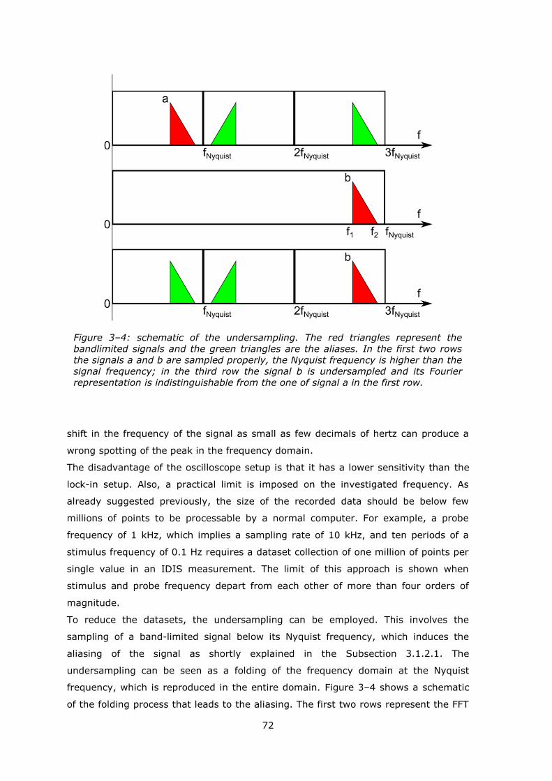
72
shift in the frequency of the signal as small as few decimals of hertz can produce a
wrong spotting of the peak in the frequency domain.
The disadvantage of the oscilloscope setup is that it has a lower sensitivity than the
lock-in setup. Also, a practical limit is imposed on the investigated frequency. As
already suggested previously, the size of the recorded data should be below few
millions of points to be processable by a normal computer. For example, a probe
frequency of 1 kHz, which implies a sampling rate of 10 kHz, and ten periods of a
stimulus frequency of 0.1 Hz requires a dataset collection of one million of points per
single value in an IDIS measurement. The limit of this approach is shown when
stimulus and probe frequency depart from each other of more than four orders of
magnitude.
To reduce the datasets, the undersampling can be employed. This involves the
sampling of a band-limited signal below its Nyquist frequency, which induces the
aliasing of the signal as shortly explained in the Subsection 3.1.2.1. The
undersampling can be seen as a folding of the frequency domain at the Nyquist
frequency, which is reproduced in the entire domain. Figure 3–4 shows a schematic
of the folding process that leads to the aliasing. The first two rows represent the FFT
Figure 3–4: schematic of the undersampling. The red triangles represent the
bandlimited signals and the green triangles are the aliases. In the first two rows
the signals a and b are sampled properly, the Nyquist frequency is higher than the
signal frequency; in the third row the signal b is undersampled and its Fourier
representation is indistinguishable from the one of signal a in the first row.
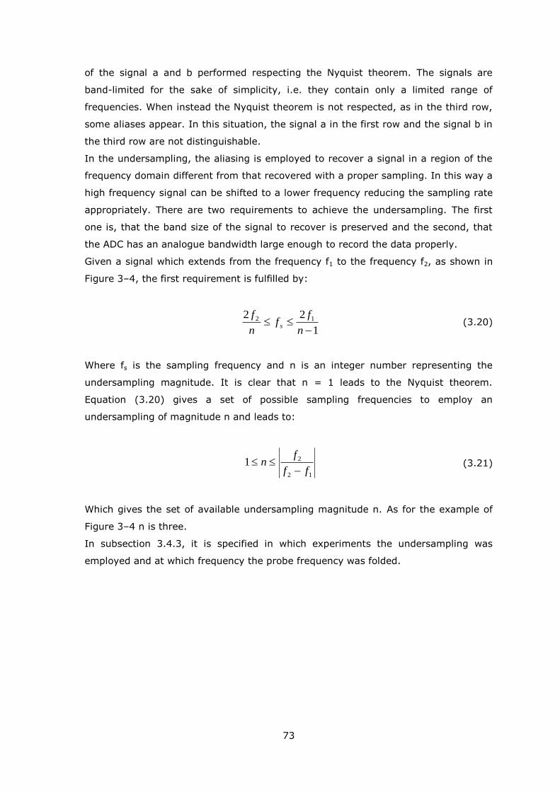
73
of the signal a and b performed respecting the Nyquist theorem. The signals are
band-limited for the sake of simplicity, i.e. they contain only a limited range of
frequencies. When instead the Nyquist theorem is not respected, as in the third row,
some aliases appear. In this situation, the signal a in the first row and the signal b in
the third row are not distinguishable.
In the undersampling, the aliasing is employed to recover a signal in a region of the
frequency domain different from that recovered with a proper sampling. In this way a
high frequency signal can be shifted to a lower frequency reducing the sampling rate
appropriately. There are two requirements to achieve the undersampling. The first
one is, that the band size of the signal to recover is preserved and the second, that
the ADC has an analogue bandwidth large enough to record the data properly.
Given a signal which extends from the frequency f1 to the frequency f2, as shown in
Figure 3–4, the first requirement is fulfilled by:
1
22 12
n
ff
n
fs
(3.20)
Where fs is the sampling frequency and n is an integer number representing the
undersampling magnitude. It is clear that n = 1 leads to the Nyquist theorem.
Equation (3.20) gives a set of possible sampling frequencies to employ an
undersampling of magnitude n and leads to:
12
21ff
fn
(3.21)
Which gives the set of available undersampling magnitude n. As for the example of
Figure 3–4 n is three.
In subsection 3.4.3, it is specified in which experiments the undersampling was
employed and at which frequency the probe frequency was folded.
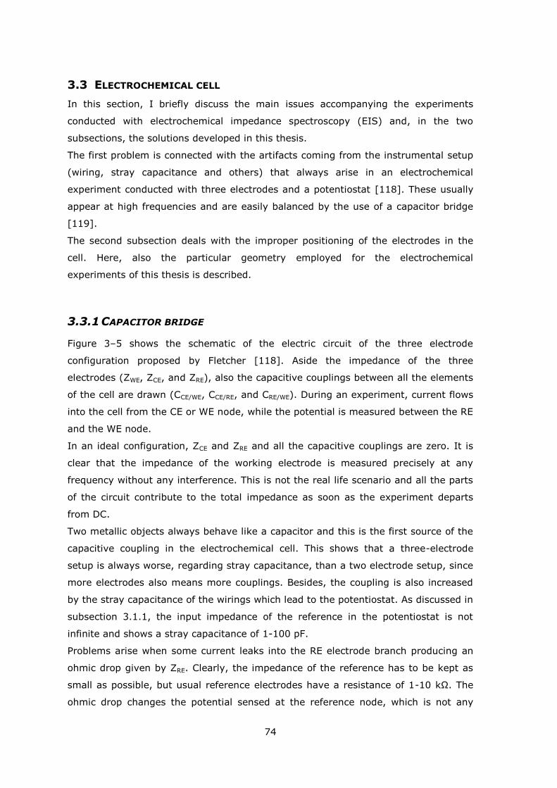
74
3.3 ELECTROCHEMICAL CELL
In this section, I briefly discuss the main issues accompanying the experiments
conducted with electrochemical impedance spectroscopy (EIS) and, in the two
subsections, the solutions developed in this thesis.
The first problem is connected with the artifacts coming from the instrumental setup
(wiring, stray capacitance and others) that always arise in an electrochemical
experiment conducted with three electrodes and a potentiostat [118]. These usually
appear at high frequencies and are easily balanced by the use of a capacitor bridge
[119].
The second subsection deals with the improper positioning of the electrodes in the
cell. Here, also the particular geometry employed for the electrochemical
experiments of this thesis is described.
3.3.1 CAPACITOR BRIDGE
Figure 3–5 shows the schematic of the electric circuit of the three electrode
configuration proposed by Fletcher [118]. Aside the impedance of the three
electrodes (ZWE, ZCE, and ZRE), also the capacitive couplings between all the elements
of the cell are drawn (CCE/WE, CCE/RE, and CRE/WE). During an experiment, current flows
into the cell from the CE or WE node, while the potential is measured between the RE
and the WE node.
In an ideal configuration, ZCE and ZRE and all the capacitive couplings are zero. It is
clear that the impedance of the working electrode is measured precisely at any
frequency without any interference. This is not the real life scenario and all the parts
of the circuit contribute to the total impedance as soon as the experiment departs
from DC.
Two metallic objects always behave like a capacitor and this is the first source of the
capacitive coupling in the electrochemical cell. This shows that a three-electrode
setup is always worse, regarding stray capacitance, than a two electrode setup, since
more electrodes also means more couplings. Besides, the coupling is also increased
by the stray capacitance of the wirings which lead to the potentiostat. As discussed in
subsection 3.1.1, the input impedance of the reference in the potentiostat is not
infinite and shows a stray capacitance of 1-100 pF.
Problems arise when some current leaks into the RE electrode branch producing an
ohmic drop given by ZRE. Clearly, the impedance of the reference has to be kept as
small as possible, but usual reference electrodes have a resistance of 1-10 kΩ. The
ohmic drop changes the potential sensed at the reference node, which is not any
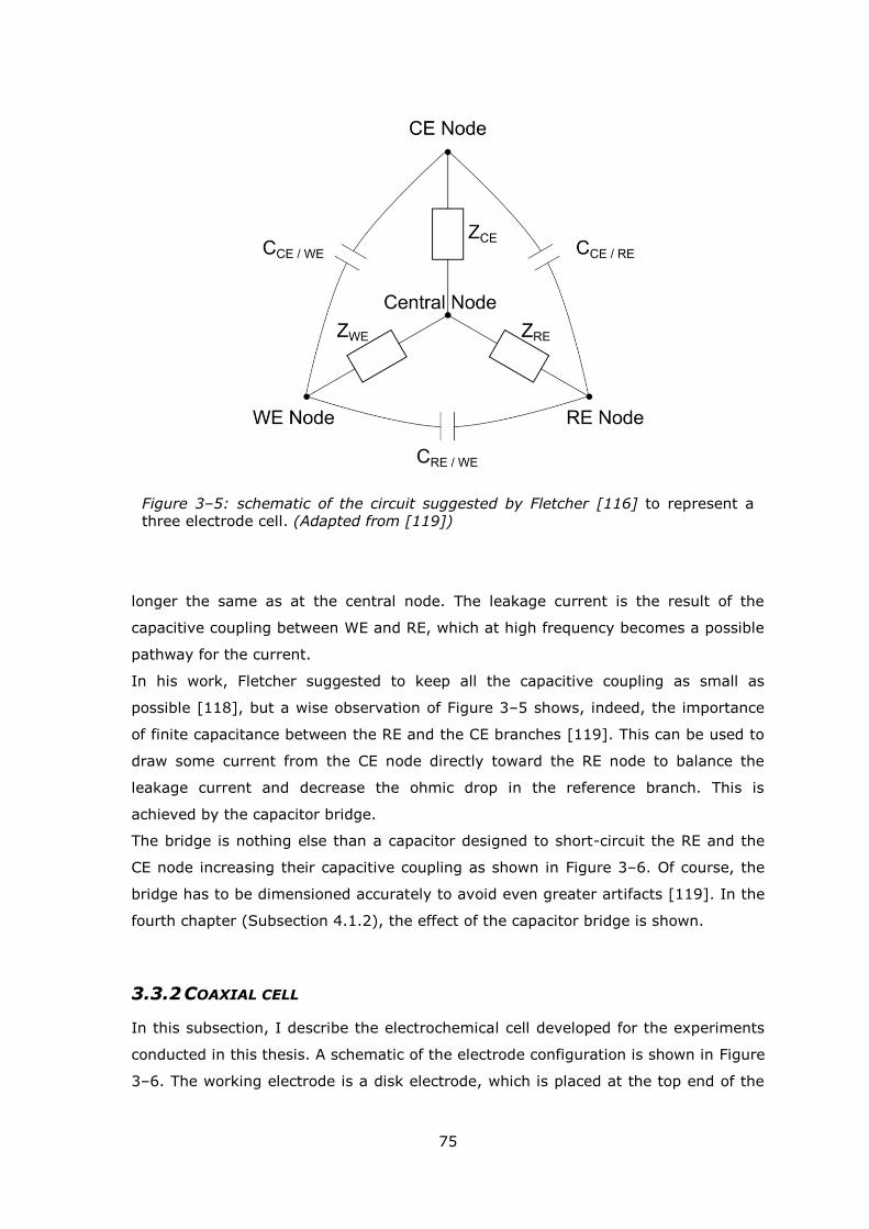
75
longer the same as at the central node. The leakage current is the result of the
capacitive coupling between WE and RE, which at high frequency becomes a possible
pathway for the current.
In his work, Fletcher suggested to keep all the capacitive coupling as small as
possible [118], but a wise observation of Figure 3–5 shows, indeed, the importance
of finite capacitance between the RE and the CE branches [119]. This can be used to
draw some current from the CE node directly toward the RE node to balance the
leakage current and decrease the ohmic drop in the reference branch. This is
achieved by the capacitor bridge.
The bridge is nothing else than a capacitor designed to short-circuit the RE and the
CE node increasing their capacitive coupling as shown in Figure 3–6. Of course, the
bridge has to be dimensioned accurately to avoid even greater artifacts [119]. In the
fourth chapter (Subsection 4.1.2), the effect of the capacitor bridge is shown.
3.3.2 COAXIAL CELL
In this subsection, I describe the electrochemical cell developed for the experiments
conducted in this thesis. A schematic of the electrode configuration is shown in Figure
3–6. The working electrode is a disk electrode, which is placed at the top end of the
Figure 3–5: schematic of the circuit suggested by Fletcher [116] to represent a three electrode cell. (Adapted from [119])
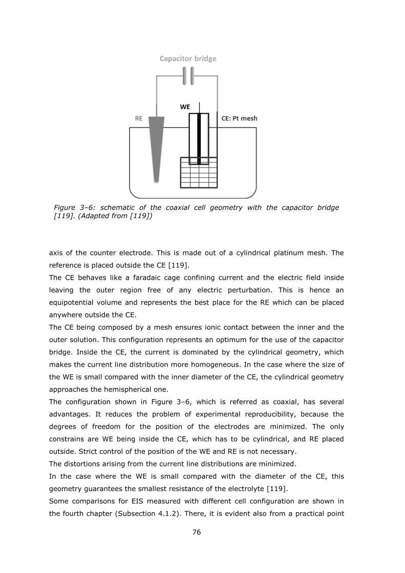
76
axis of the counter electrode. This is made out of a cylindrical platinum mesh. The
reference is placed outside the CE [119].
The CE behaves like a faradaic cage confining current and the electric field inside
leaving the outer region free of any electric perturbation. This is hence an
equipotential volume and represents the best place for the RE which can be placed
anywhere outside the CE.
The CE being composed by a mesh ensures ionic contact between the inner and the
outer solution. This configuration represents an optimum for the use of the capacitor
bridge. Inside the CE, the current is dominated by the cylindrical geometry, which
makes the current line distribution more homogeneous. In the case where the size of
the WE is small compared with the inner diameter of the CE, the cylindrical geometry
approaches the hemispherical one.
The configuration shown in Figure 3–6, which is referred as coaxial, has several
advantages. It reduces the problem of experimental reproducibility, because the
degrees of freedom for the position of the electrodes are minimized. The only
constrains are WE being inside the CE, which has to be cylindrical, and RE placed
outside. Strict control of the position of the WE and RE is not necessary.
The distortions arising from the current line distributions are minimized.
In the case where the WE is small compared with the diameter of the CE, this
geometry guarantees the smallest resistance of the electrolyte [119].
Some comparisons for EIS measured with different cell configuration are shown in
the fourth chapter (Subsection 4.1.2). There, it is evident also from a practical point
Figure 3–6: schematic of the coaxial cell geometry with the capacitor bridge
[119]. (Adapted from [119])

77
of view, that there are problems connected with an incorrect geometry which can
lead to erroneous results.
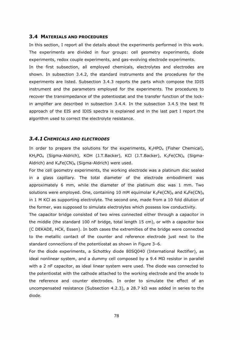
78
3.4 MATERIALS AND PROCEDURES
In this section, I report all the details about the experiments performed in this work.
The experiments are divided in four groups: cell geometry experiments, diode
experiments, redox couple experiments, and gas-evolving electrode experiments.
In the first subsection, all employed chemicals, electrolytes and electrodes are
shown. In subsection 3.4.2, the standard instruments and the procedures for the
experiments are listed. Subsection 3.4.3 reports the parts which compose the IDIS
instrument and the parameters employed for the experiments. The procedures to
recover the transimpedance of the potentiostat and the transfer function of the lock-
in amplifier are described in subsection 3.4.4. In the subsection 3.4.5 the best fit
approach of the EIS and IDIS spectra is explained and in the last part I report the
algorithm used to correct the electrolyte resistance.
3.4.1 CHEMICALS AND ELECTRODES
In order to prepare the solutions for the experiments, K2HPO4 (Fisher Chemical),
KH2PO4 (Sigma-Aldrich), KOH (J.T.Backer), KCl (J.T.Backer), K3Fe(CN)6 (Sigma-
Aldrich) and K4Fe(CN)6 (Sigma-Aldrich) were used.
For the cell geometry experiments, the working electrode was a platinum disc sealed
in a glass capillary. The total diameter of the electrode embodiment was
approximately 6 mm, while the diameter of the platinum disc was 1 mm. Two
solutions were employed. One, containing 10 mM equimolar K3Fe(CN)6 and K4Fe(CN)6
in 1 M KCl as supporting electrolyte. The second one, made from a 10 fold dilution of
the former, was supposed to simulate electrolytes which possess low conductivity.
The capacitor bridge consisted of two wires connected either through a capacitor in
the middle (the standard 100 nF bridge, total length 15 cm), or with a capacitor box
(C DEKADE, HCK, Essen). In both cases the extremities of the bridge were connected
to the metallic contact of the counter and reference electrode just next to the
standard connections of the potentiostat as shown in Figure 3–6.
For the diode experiments, a Schottky diode 80SQ040 (International Rectifier), as
ideal nonlinear system, and a dummy cell composed by a 9.4 MΩ resistor in parallel
with a 2 nF capacitor, as ideal linear system were used. The diode was connected to
the potentiostat with the cathode attached to the working electrode and the anode to
the reference and counter electrodes. In order to simulate the effect of an
uncompensated resistance (Subsection 4.2.3), a 28.7 kΩ was added in series to the
diode.
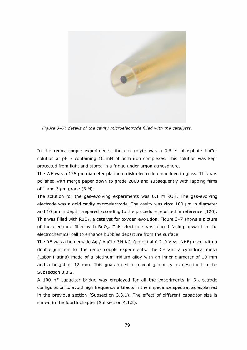
79
In the redox couple experiments, the electrolyte was a 0.5 M phosphate buffer
solution at pH 7 containing 10 mM of both iron complexes. This solution was kept
protected from light and stored in a fridge under argon atmosphere.
The WE was a 125 μm diameter platinum disk electrode embedded in glass. This was
polished with merge paper down to grade 2000 and subsequently with lapping films
of 1 and 3 m grade (3 M).
The solution for the gas-evolving experiments was 0.1 M KOH. The gas-evolving
electrode was a gold cavity microelectrode. The cavity was circa 100 μm in diameter
and 10 μm in depth prepared according to the procedure reported in reference [120].
This was filled with RuO2, a catalyst for oxygen evolution. Figure 3–7 shows a picture
of the electrode filled with RuO2. This electrode was placed facing upward in the
electrochemical cell to enhance bubbles departure from the surface.
The RE was a homemade Ag / AgCl / 3M KCl (potential 0.210 V vs. NHE) used with a
double junction for the redox couple experiments. The CE was a cylindrical mesh
(Labor Platina) made of a platinum iridium alloy with an inner diameter of 10 mm
and a height of 12 mm. This guaranteed a coaxial geometry as described in the
Subsection 3.3.2.
A 100 nF capacitor bridge was employed for all the experiments in 3-electrode
configuration to avoid high frequency artifacts in the impedance spectra, as explained
in the previous section (Subsection 3.3.1). The effect of different capacitor size is
shown in the fourth chapter (Subsection 4.1.2).
Figure 3–7: details of the cavity microelectrode filled with the catalysts.

80
3.4.2 STANDARD ELECTROCHEMICAL CHARACTERIZATION AND PROCEDURES
Three different potentiostats were used in this work: a Zahner Zennium (Zahner), a
VSP-300 (BioLogic), and a Solartron ModuLab potentiostat/galvanostat (AMETEK).
The first was employed for the experiments concerning the Schottky diode, the
second for the cell-geometry and redox couple experiments, and the third for the
experiments with the gas-evolving electrode.
The potentiostatic EIS performed on the commercial instruments were made between
1 MHz (100 kHz for the experiments with the diode) and 100 mHz with 10
frequencies per decade and 10 mV of potential perturbation.
For the experiments with the Schottky diode, the cyclic voltammetry were performed
at 10 mV s-1 between 0 V and 2 V. The diode was connected according to the IUPAC
official setup, with the cathode attached to the working electrode and the anode to
the reference and counter electrodes. The Mott-Schottky analysis to obtain the flat-
band potential of the diode was performed between 0 V and 2 V with an EIS every
100 mV.
For the redox couple experiments, the following procedure was employed. The
Fe(II)/Fe(III) cyanide solution was first placed in the sealed electrochemical cell and
sparged with argon while waiting to reach a stable temperature. As control, a series
of cyclic voltammetries were performed with a freshly polished working electrode and
a freshly annealed counter electrode at 50 mV s-1 between -250 and +250 mV vs.
the OCP (circa 250 mV vs. RE) until the voltammogram was stable. In the case
where the voltammograms were not satisfactory, the WE was removed and polished
one more time. When major problems appeared, also the solution was changed. After
the cyclic voltammetry also some EIS were performed as control.
With careful regard to the argon atmosphere, the electrochemical cell was moved to
the IDIS instrument where an additional EIS and the intermodulation were applied.
These were performed at the OCP. As final validation of the series of experiments, a
last EIS was performed in the end to ensure that the argon atmosphere was still in
good conditions and that poisoning was not occurring at the last stage.
For the experiments with the gas-evolving electrode the working electrode was
placed facing upward. The linear sweep voltammetry was performed between 0.95
VRHE and 1.75 VRHE at 5 mV s-1. Before passing to the intermodulation an EIS at 1.45
VRHE was performed to recover the resistance of the electrolyte without bubble
evolution. The intermodulation was made between 1.6 VRHE and 1.75 VRHE.
In the next subsection, I report the parameters of the IDIS and of the EIS used in
the experiments with the diode, the redox couple, and the intermodulation of the
gas-evolving electrode.
81
3.4.3 IDIS INSTRUMENT AND PARAMETERS
In this subsection I present the IDIS instrument composition along with the relevant
parameters employed during the experiments.
The instrument was composed by a potentiostat PG_310USB (HEKA Elektronik), a 2-
channels lock-in amplifier HF2LI (Zurich Instruments), a 4-channels oscilloscope
PicoScope 4424 (Pico Technology), and a personal computer to perform the FFT
analysis. As generator for the stimulus and the probe, the two internal generators of
the lock-in amplifier were used. The FFT analysis and the instrument control were
performed through a homemade collection of routines run with Matlab (MathWorks).
The probe generator was used as internal reference by the lock-in to demodulate the
high frequency signal and the control loop phase-shift was controlled and
synchronized before proceeding with the data acquisition routine.
To improve the resolution and dampen the high frequency noise, the additional 4th
order Bessel filter (10 KHz cutoff frequency) of the potentiostat was employed
together with a lower control loop bandwidth (10-30 kHz).
The routine automatically controlled the lock-in amplifier time constant to match a
stimulus to cutoff frequency ratio as close as possible to ω/Δω = 0.2 for every
stimulus frequency.
The sampling rate of the oscilloscope was between five and twenty times as high as
the probe frequency. The other parameters, such as stimulus, probe frequency,
amplitude, and the acquisition time, are reported in Table 3–1. The amplitudes
shown in Table 3–1 were higher than those effectively applied in the cell, especially
at high frequency because of the speed of the control loop (Subsection 3.1.1). As
example, an amplitude of 20 mV led to circa 13 mV at 10 kHz of real perturbation at
the ends of the WE and RE.
To ensure the maximum accuracy, the acquisition was delayed for every stimulus
frequency of at least one period or one second.
For the gas-evolving electrode experiments, the undersampling was employed to
reduce the dataset size. The probe and sideband signals were folded either to circa
120 Hz or to 1000 Hz, keeping the total size of the dataset in the range of one million
points.
In the FFT analysis, a procedure to find the right frequency position of the peaks was
employed. The stimulus and the probe frequency were first searched in the frequency
domain of the potential, looking for local maxima. The results were then used for the
FFT analysis of the current.
The potentiostat transimpedance and the lock-in transfer function were applied to the
result after the FFT analysis.
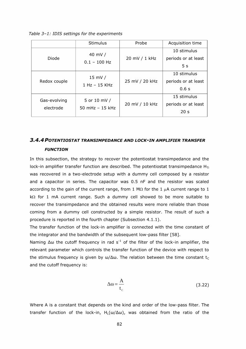
82
3.4.4 POTENTIOSTAT TRANSIMPEDANCE AND LOCK-IN AMPLIFIER TRANSFER
FUNCTION
In this subsection, the strategy to recover the potentiostat transimpedance and the
lock-in amplifier transfer function are described. The potentiostat transimpedance HTi
was recovered in a two-electrode setup with a dummy cell composed by a resistor
and a capacitor in series. The capacitor was 0.5 nF and the resistor was scaled
according to the gain of the current range, from 1 M for the 1 A current range to 1
k for 1 mA current range. Such a dummy cell showed to be more suitable to
recover the transimpedance and the obtained results were more reliable than those
coming from a dummy cell constructed by a simple resistor. The result of such a
procedure is reported in the fourth chapter (Subsection 4.1.1).
The transfer function of the lock-in amplifier is connected with the time constant of
the integrator and the bandwidth of the subsequent low-pass filter [58].
Naming Δω the cutoff frequency in rad s-1 of the filter of the lock-in amplifier, the
relevant parameter which controls the transfer function of the device with respect to
the stimulus frequency is given by ω/Δω. The relation between the time constant tC
and the cutoff frequency is:
C
t
AΔω (3.22)
Where A is a constant that depends on the kind and order of the low-pass filter. The
transfer function of the lock-in, HL(ω/Δω), was obtained from the ratio of the
Table 3–1: IDIS settings for the experiments
Stimulus Probe Acquisition time
Diode 40 mV /
0.1 – 100 Hz 20 mV / 1 kHz
10 stimulus
periods or at least
5 s
Redox couple 15 mV /
1 Hz – 15 KHz 25 mV / 20 kHz
10 stimulus
periods or at least
0.6 s
Gas-evolving
electrode
5 or 10 mV /
50 mHz – 15 kHz 20 mV / 10 kHz
15 stimulus
periods or at least
20 s
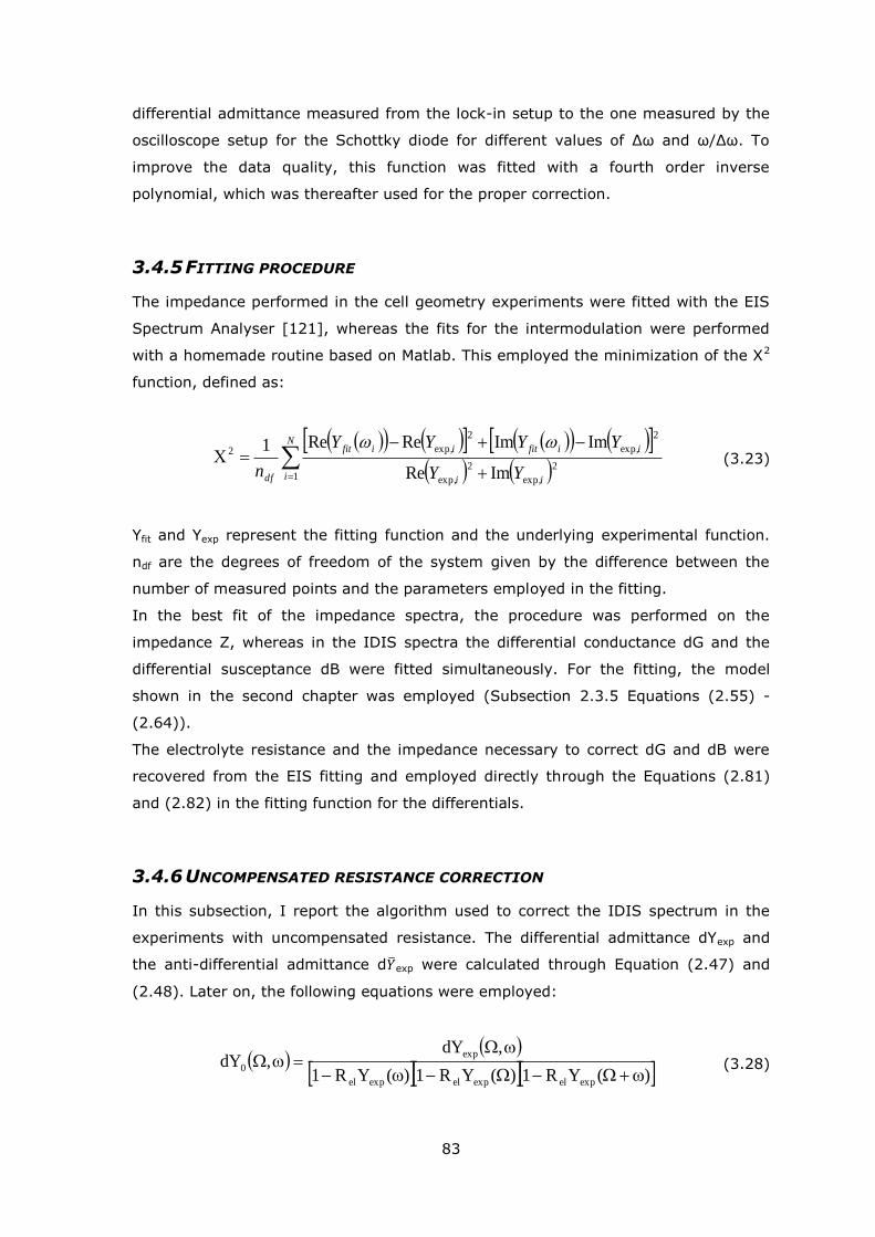
83
differential admittance measured from the lock-in setup to the one measured by the
oscilloscope setup for the Schottky diode for different values of Δω and ω/Δω. To
improve the data quality, this function was fitted with a fourth order inverse
polynomial, which was thereafter used for the proper correction.
3.4.5 FITTING PROCEDURE
The impedance performed in the cell geometry experiments were fitted with the EIS
Spectrum Analyser [121], whereas the fits for the intermodulation were performed
with a homemade routine based on Matlab. This employed the minimization of the Χ2
function, defined as:
N
i ii
iifitiifit
df YY
YYYY
n 12
exp,
2
exp,
2
exp,
2
exp,2
ImRe
ImImReRe1 (3.23)
Yfit and Yexp represent the fitting function and the underlying experimental function.
ndf are the degrees of freedom of the system given by the difference between the
number of measured points and the parameters employed in the fitting.
In the best fit of the impedance spectra, the procedure was performed on the
impedance Z, whereas in the IDIS spectra the differential conductance dG and the
differential susceptance dB were fitted simultaneously. For the fitting, the model
shown in the second chapter was employed (Subsection 2.3.5 Equations (2.55) -
(2.64)).
The electrolyte resistance and the impedance necessary to correct dG and dB were
recovered from the EIS fitting and employed directly through the Equations (2.81)
and (2.82) in the fitting function for the differentials.
3.4.6 UNCOMPENSATED RESISTANCE CORRECTION
In this subsection, I report the algorithm used to correct the IDIS spectrum in the
experiments with uncompensated resistance. The differential admittance dYexp and
the anti-differential admittance d exp were calculated through Equation (2.47) and
(2.48). Later on, the following equations were employed:
)(YR1)(YR1)(YR1
,dY,dY
expelexpelexpel
exp
0
(3.28)
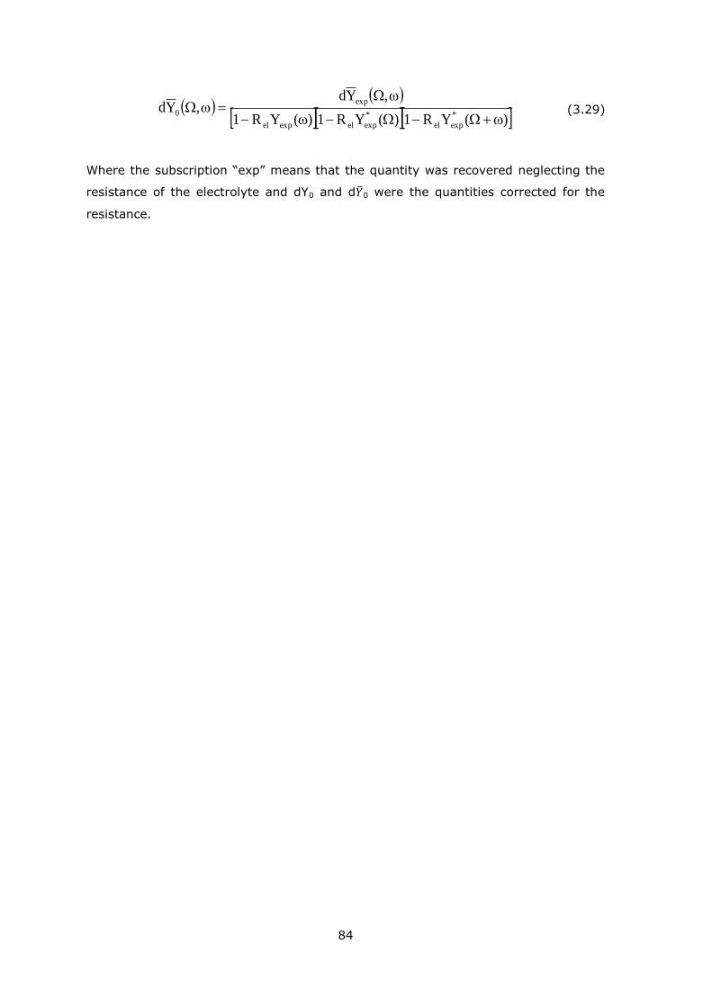
84
)(YR1)(YR1)(YR1
,Yd,Yd
*
expel
*
expelexpel
exp
0
(3.29)
Where the subscription ―exp‖ means that the quantity was recovered neglecting the
resistance of the electrolyte and dY0 and d 0 were the quantities corrected for the
resistance.
85
4 RESULTS AND DISCUSSION
In this chapter, I report and discuss the experimental results of this thesis. In the
first section, the results concerning the potentiostat transimpedance and the lock-in
transfer function are reported. Besides, I show the effect of the capacitor bridge and
of a proper electrodes‘ disposition in the electrochemical cell to achieve reliable
impedance measurements.
The intermodulated differential immittance spectroscopy (IDIS) was applied as proof
of concept to an ideal nonlinear system, a Schottky diode (Section 4.2). This section
follows the equations described in the Subsection 2.3.4. Through intermodulation the
flat-band potential and the doping level of device were recovered. The diode was also
used as benchmark to determine the resolution of the instrumental setups and the
uncompensated resistance correction (Subsection 2.3.7).
Subsequently, I show the results concerning the redox couple experiments and how
the EIS and IDIS were used to recover the electrokinetic and mass transport
parameters (Section 4.3). In this section the model developed in the Subsection
2.3.5 is employed.
In the last part, I present the gas-evolving electrode and how the concepts of
intermodulation and transfer functions developed in the second chapter (Section 2.4)
are applied.
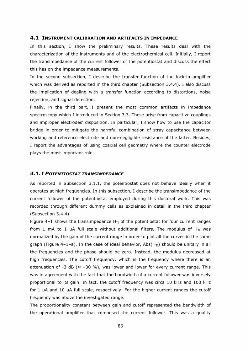
86
4.1 INSTRUMENT CALIBRATION AND ARTIFACTS IN IMPEDANCE
In this section, I show the preliminary results. These results deal with the
characterization of the instruments and of the electrochemical cell. Initially, I report
the transimpedance of the current follower of the potentiostat and discuss the effect
this has on the impedance measurements.
In the second subsection, I describe the transfer function of the lock-in amplifier
which was derived as reported in the third chapter (Subsection 3.4.4). I also discuss
the implication of dealing with a transfer function according to distortions, noise
rejection, and signal detection.
Finally, in the third part, I present the most common artifacts in impedance
spectroscopy which I introduced in Section 3.3. These arise from capacitive couplings
and improper electrodes‘ disposition. In particular, I show how to use the capacitor
bridge in order to mitigate the harmful combination of stray capacitance between
working and reference electrode and non-negligible resistance of the latter. Besides,
I report the advantages of using coaxial cell geometry where the counter electrode
plays the most important role.
4.1.1 POTENTIOSTAT TRANSIMPEDANCE
As reported in Subsection 3.1.1, the potentiostat does not behave ideally when it
operates at high frequencies. In this subsection, I describe the transimpedance of the
current follower of the potentiostat employed during this doctoral work. This was
recorded through different dummy cells as explained in detail in the third chapter
(Subsection 3.4.4).
Figure 4–1 shows the transimpedance HTi of the potentiostat for four current ranges
from 1 mA to 1 μA full scale without additional filters. The modulus of HTi was
normalized by the gain of the current range in order to plot all the curves in the same
graph (Figure 4–1–a). In the case of ideal behavior, Abs(HTi) should be unitary in all
the frequencies and the phase should be zero. Instead, the modulus decreased at
high frequencies. The cutoff frequency, which is the frequency where there is an
attenuation of -3 dB (≈ –30 %), was lower and lower for every current range. This
was in agreement with the fact that the bandwidth of a current follower was inversely
proportional to its gain. In fact, the cutoff frequency was circa 10 kHz and 100 kHz
for 1 μA and 10 μA full scale, respectively. For the higher current ranges the cutoff
frequency was above the investigated range.
The proportionality constant between gain and cutoff represented the bandwidth of
the operational amplifier that composed the current follower. This was a quality
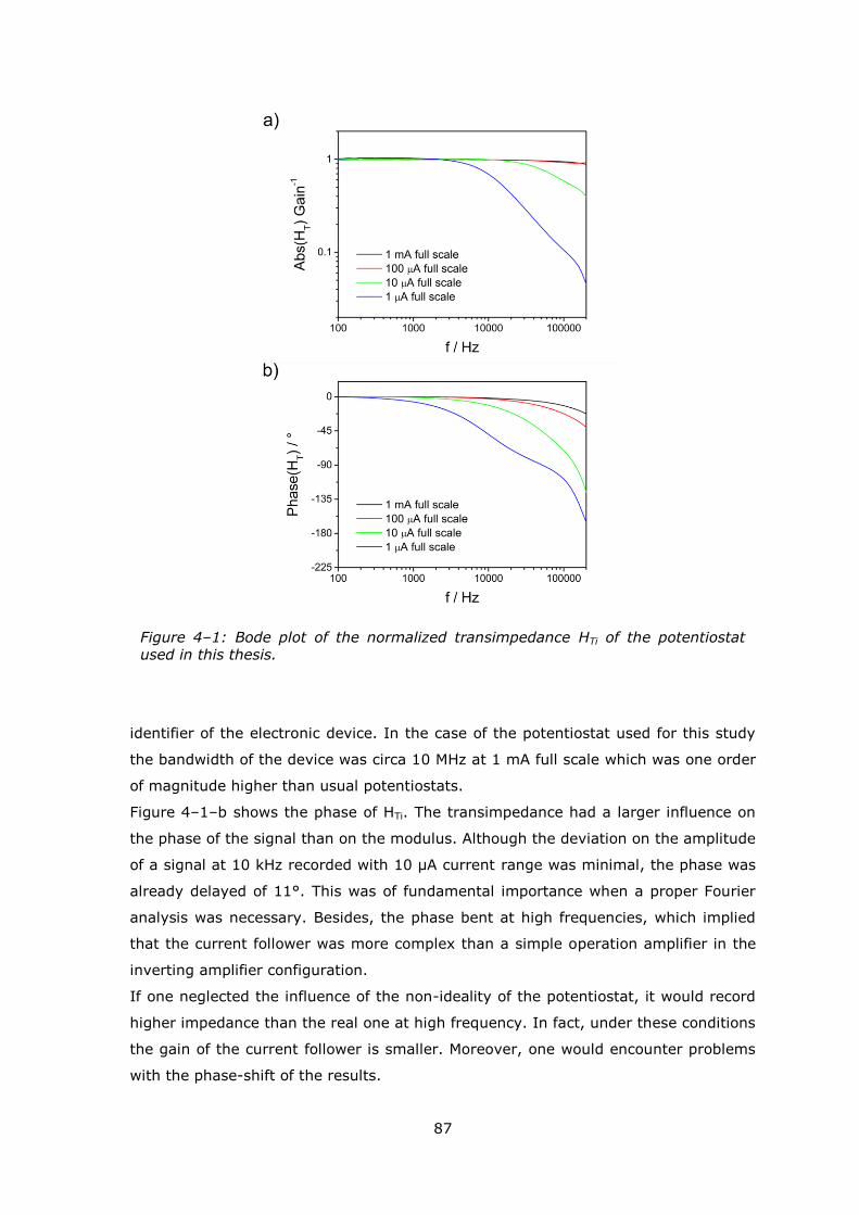
87
identifier of the electronic device. In the case of the potentiostat used for this study
the bandwidth of the device was circa 10 MHz at 1 mA full scale which was one order
of magnitude higher than usual potentiostats.
Figure 4–1–b shows the phase of HTi. The transimpedance had a larger influence on
the phase of the signal than on the modulus. Although the deviation on the amplitude
of a signal at 10 kHz recorded with 10 μA current range was minimal, the phase was
already delayed of 11°. This was of fundamental importance when a proper Fourier
analysis was necessary. Besides, the phase bent at high frequencies, which implied
that the current follower was more complex than a simple operation amplifier in the
inverting amplifier configuration.
If one neglected the influence of the non-ideality of the potentiostat, it would record
higher impedance than the real one at high frequency. In fact, under these conditions
the gain of the current follower is smaller. Moreover, one would encounter problems
with the phase-shift of the results.
Figure 4–1: Bode plot of the normalized transimpedance HTi of the potentiostat used in this thesis.
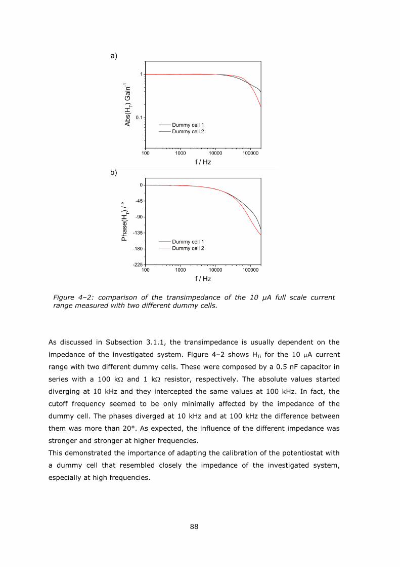
88
As discussed in Subsection 3.1.1, the transimpedance is usually dependent on the
impedance of the investigated system. Figure 4–2 shows HTi for the 10 A current
range with two different dummy cells. These were composed by a 0.5 nF capacitor in
series with a 100 k and 1 k resistor, respectively. The absolute values started
diverging at 10 kHz and they intercepted the same values at 100 kHz. In fact, the
cutoff frequency seemed to be only minimally affected by the impedance of the
dummy cell. The phases diverged at 10 kHz and at 100 kHz the difference between
them was more than 20°. As expected, the influence of the different impedance was
stronger and stronger at higher frequencies.
This demonstrated the importance of adapting the calibration of the potentiostat with
a dummy cell that resembled closely the impedance of the investigated system,
especially at high frequencies.
Figure 4–2: comparison of the transimpedance of the 10 μA full scale current range measured with two different dummy cells.
89
4.1.2 LOCK-IN TRANSFER FUNCTION
The transfer function HL of the lock-in amplifier was recovered comparing the results
of the IDIS for the diode between the oscilloscope setup and the lock-in setup as
explained in the third chapter (Subsection 3.4.4) [58].
Figure 4–3 reports the Bode representation of the transfer function HL of the lock-in
amplifier. A fourth order inverse polynomial was used to fit the experimental data.
Later on, this polynomial was used for the correction of the intermodulation signals.
ω/Δω = 1 represented the normalized cutoff frequency. At this frequency, the
attenuation of the signal was -3 dB and the phase-shift was circa -90°. When ω/Δω
was greater than one, HL strongly attenuated and delayed the intermodulation signal,
however larger frequencies were measurable. On the other hand, for ω/Δω < 1, HL
tended to unity and the phase-shift tended to zero degrees. Although in this case the
transfer function had little influences, stimulus frequencies close to the probe
Figure 4–3: Bode plots of the lock-in amplifier transfer function HLI, with fourth
order inverse polynomial fit. a) absolute value; b) phase-shift. (Replotted from [58])
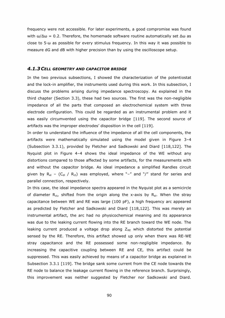
90
frequency were not accessible. For later experiments, a good compromise was found
with ω/Δω = 0.2. Therefore, the homemade software routine automatically set Δω as
close to 5∙ω as possible for every stimulus frequency. In this way it was possible to
measure dG and dB with higher precision than by using the oscilloscope setup.
4.1.3 CELL GEOMETRY AND CAPACITOR BRIDGE
In the two previous subsections, I showed the characterization of the potentiostat
and the lock-in amplifier, the instruments used during this work. In this subsection, I
discuss the problems arising during impedance spectroscopy. As explained in the
third chapter (Section 3.3), these had two sources. The first was the non-negligible
impedance of all the parts that composed an electrochemical system with three
electrode configuration. This could be regarded as an instrumental problem and it
was easily circumvented using the capacitor bridge [119]. The second source of
artifacts was the improper electrodes‘ disposition in the cell [119].
In order to understand the influence of the impedance of all the cell components, the
artifacts were mathematically simulated using the model given in Figure 3–4
(Subsection 3.3.1), provided by Fletcher and Sadkowski and Diard [118,122]. The
Nyquist plot in Figure 4–4 shows the ideal impedance of the WE without any
distortions compared to those affected by some artifacts, for the measurements with
and without the capacitor bridge. As ideal impedance a simplified Randles circuit
given by Rel – (Cdl / Rct) was employed, where ―–‖ and ―/‖ stand for series and
parallel connection, respectively.
In this case, the ideal impedance spectra appeared in the Nyquist plot as a semicircle
of diameter Rct, shifted from the origin along the x-axis by Rel. When the stray
capacitance between WE and RE was large (100 pF), a high frequency arc appeared
as predicted by Fletcher and Sadkowski and Diard [118,122]. This was merely an
instrumental artifact, the arc had no physicochemical meaning and its appearance
was due to the leaking current flowing into the RE branch toward the WE node. The
leaking current produced a voltage drop along ZRE which distorted the potential
sensed by the RE. Therefore, this artifact showed up only when there was RE-WE
stray capacitance and the RE possessed some non-negligible impedance. By
increasing the capacitive coupling between RE and CE, this artifact could be
suppressed. This was easily achieved by means of a capacitor bridge as explained in
Subsection 3.3.1 [119]. The bridge sank some current from the CE node towards the
RE node to balance the leakage current flowing in the reference branch. Surprisingly,
this improvement was neither suggested by Fletcher nor Sadkowski and Diard.
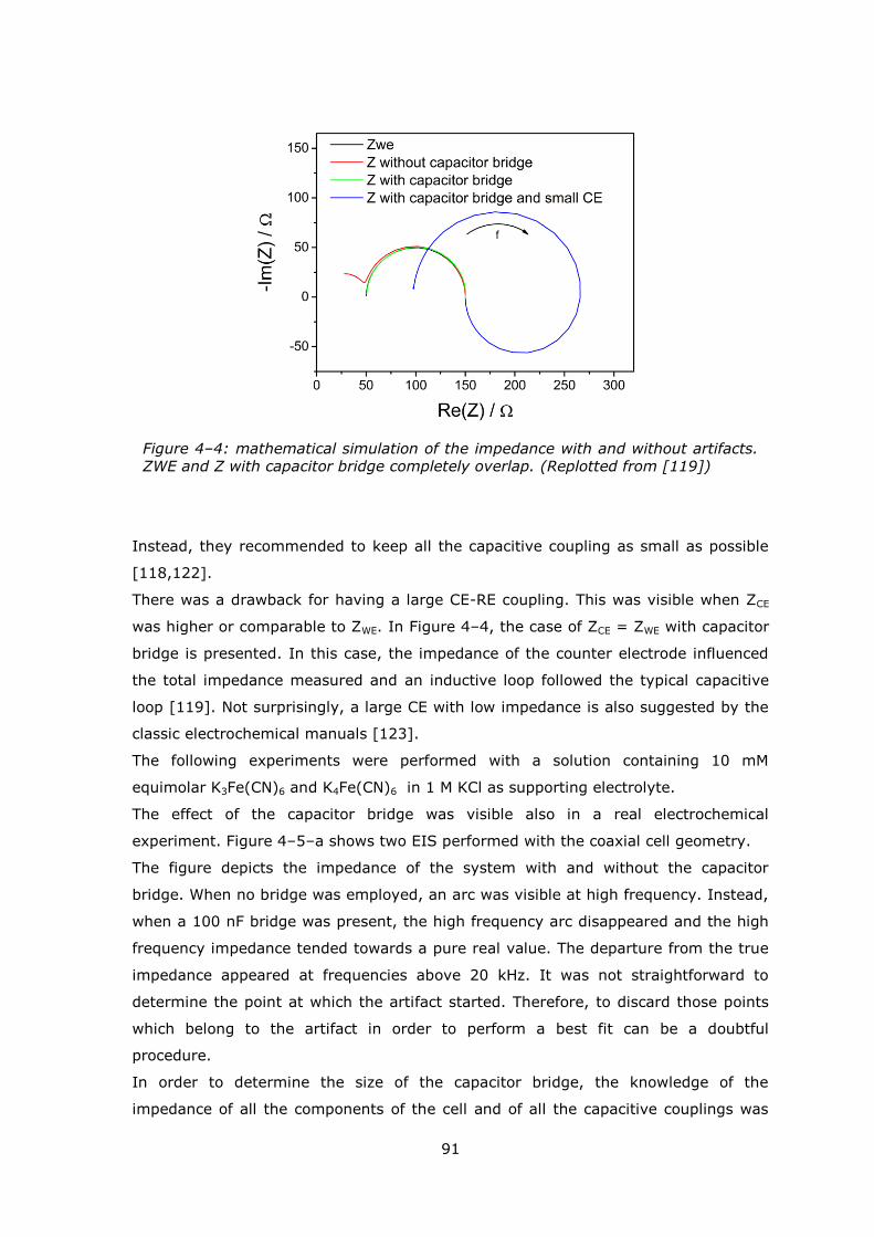
91
Instead, they recommended to keep all the capacitive coupling as small as possible
[118,122].
There was a drawback for having a large CE-RE coupling. This was visible when ZCE
was higher or comparable to ZWE. In Figure 4–4, the case of ZCE = ZWE with capacitor
bridge is presented. In this case, the impedance of the counter electrode influenced
the total impedance measured and an inductive loop followed the typical capacitive
loop [119]. Not surprisingly, a large CE with low impedance is also suggested by the
classic electrochemical manuals [123].
The following experiments were performed with a solution containing 10 mM
equimolar K3Fe(CN)6 and K4Fe(CN)6 in 1 M KCl as supporting electrolyte.
The effect of the capacitor bridge was visible also in a real electrochemical
experiment. Figure 4–5–a shows two EIS performed with the coaxial cell geometry.
The figure depicts the impedance of the system with and without the capacitor
bridge. When no bridge was employed, an arc was visible at high frequency. Instead,
when a 100 nF bridge was present, the high frequency arc disappeared and the high
frequency impedance tended towards a pure real value. The departure from the true
impedance appeared at frequencies above 20 kHz. It was not straightforward to
determine the point at which the artifact started. Therefore, to discard those points
which belong to the artifact in order to perform a best fit can be a doubtful
procedure.
In order to determine the size of the capacitor bridge, the knowledge of the
impedance of all the components of the cell and of all the capacitive couplings was
Figure 4–4: mathematical simulation of the impedance with and without artifacts. ZWE and Z with capacitor bridge completely overlap. (Replotted from [119])
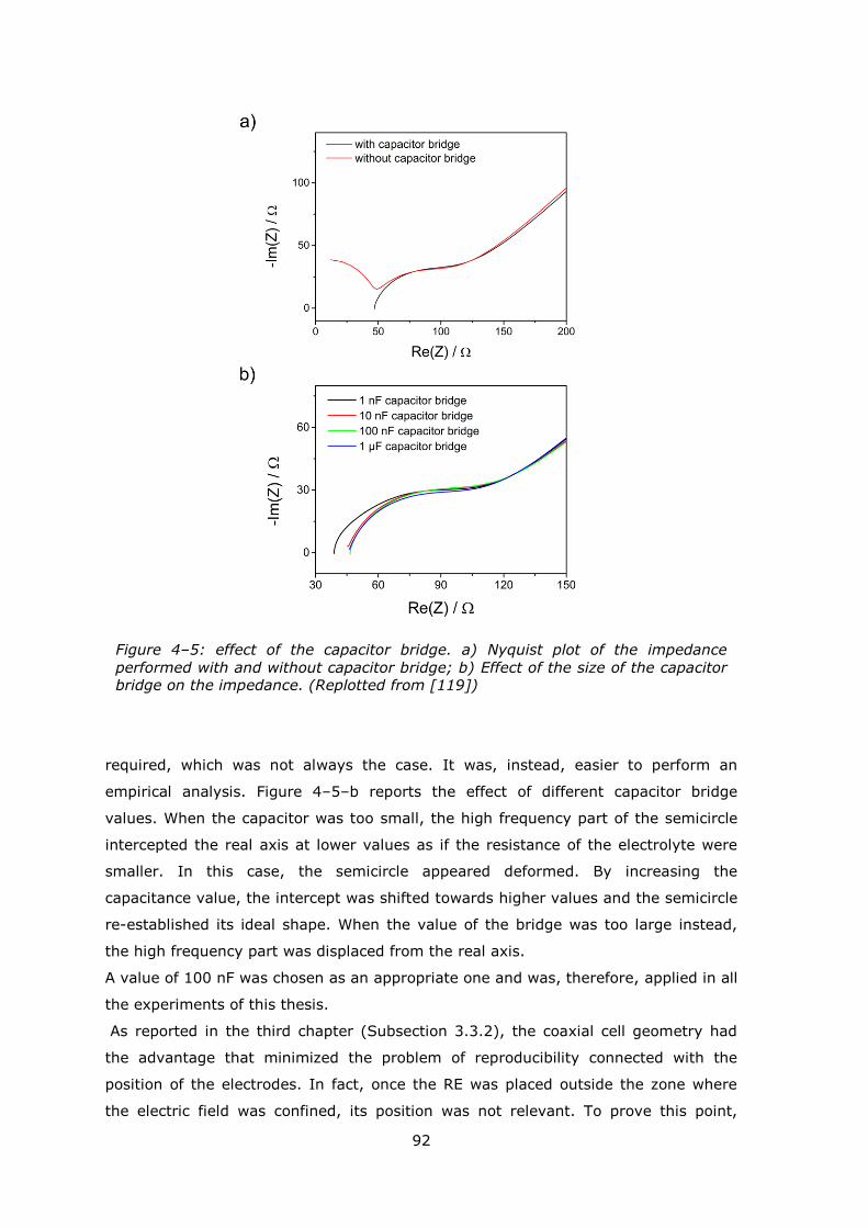
92
required, which was not always the case. It was, instead, easier to perform an
empirical analysis. Figure 4–5–b reports the effect of different capacitor bridge
values. When the capacitor was too small, the high frequency part of the semicircle
intercepted the real axis at lower values as if the resistance of the electrolyte were
smaller. In this case, the semicircle appeared deformed. By increasing the
capacitance value, the intercept was shifted towards higher values and the semicircle
re-established its ideal shape. When the value of the bridge was too large instead,
the high frequency part was displaced from the real axis.
A value of 100 nF was chosen as an appropriate one and was, therefore, applied in all
the experiments of this thesis.
As reported in the third chapter (Subsection 3.3.2), the coaxial cell geometry had
the advantage that minimized the problem of reproducibility connected with the
position of the electrodes. In fact, once the RE was placed outside the zone where
the electric field was confined, its position was not relevant. To prove this point,
Figure 4–5: effect of the capacitor bridge. a) Nyquist plot of the impedance
performed with and without capacitor bridge; b) Effect of the size of the capacitor bridge on the impedance. (Replotted from [119])
93
three experiments with the coaxial cell geometry in a 10-fold diluted solution with a
100 nF capacitor bridge were performed. In these experiments, the position of the
reference electrode was changed. Lower electrolyte resistance strongly affected the
ohmic drop between WE and RE. It is usually suggested in the manuals to keep the
RE close to the WE to minimize the ohmic drop, especially when working with low
electrolyte conductivity [123]. Figure 4–6 shows three EIS spectra, first with the RE
placed in the proximity of the CE (approximately 1 mm distance), second at the
distance of approximately 1 cm, and third with the RE inside the platinum mesh of
the counter electrode.
As expected, the position of the RE had no influence on the measured impedance. In
fact, the curves with the RE next and far from the CE coincided. This confirmed that
the entire zone outside the CE was equipotential and, hence, that the current and the
electric field were successfully confined inside the CE mesh cylinder, leaving an
unperturbed equipotential volume outside. Interestingly, also the impedance
measured with the RE inside the CE shielding was perfectly overlapping with the
previous ones. This suggested that the quasi-spherical geometry was neither
sensitive to an insulator body placed in the middle of the electric field nor to the
different position of the RE.
In order to show the other advantages of the coaxial cell geometry, three EIS
measurements were performed with three different electrodes configurations:
coaxial, aligned, and triangular. Figure 4–7 reports the three measured spectra which
Figure 4–6: Nyquist plot of EIS performed with the coaxial cell geometry, with 100
nF capacitor bridge, and three different positions of the RE, once in the proximity of the CE, once far, and once inside the CE shielding. (Replotted from [119])
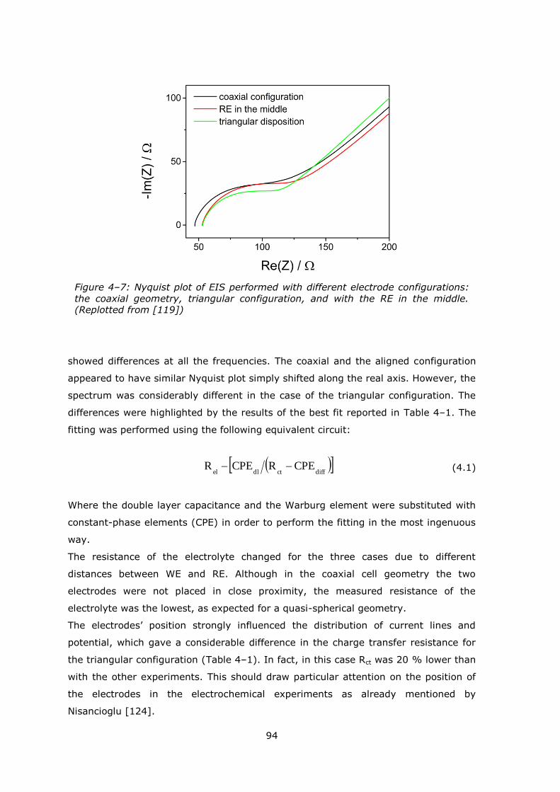
94
showed differences at all the frequencies. The coaxial and the aligned configuration
appeared to have similar Nyquist plot simply shifted along the real axis. However, the
spectrum was considerably different in the case of the triangular configuration. The
differences were highlighted by the results of the best fit reported in Table 4–1. The
fitting was performed using the following equivalent circuit:
diffctdlel
CPERCPER (4.1)
Where the double layer capacitance and the Warburg element were substituted with
constant-phase elements (CPE) in order to perform the fitting in the most ingenuous
way.
The resistance of the electrolyte changed for the three cases due to different
distances between WE and RE. Although in the coaxial cell geometry the two
electrodes were not placed in close proximity, the measured resistance of the
electrolyte was the lowest, as expected for a quasi-spherical geometry.
The electrodes‘ position strongly influenced the distribution of current lines and
potential, which gave a considerable difference in the charge transfer resistance for
the triangular configuration (Table 4–1). In fact, in this case Rct was 20 % lower than
with the other experiments. This should draw particular attention on the position of
the electrodes in the electrochemical experiments as already mentioned by
Nisancioglu [124].
Figure 4–7: Nyquist plot of EIS performed with different electrode configurations:
the coaxial geometry, triangular configuration, and with the RE in the middle. (Replotted from [119])
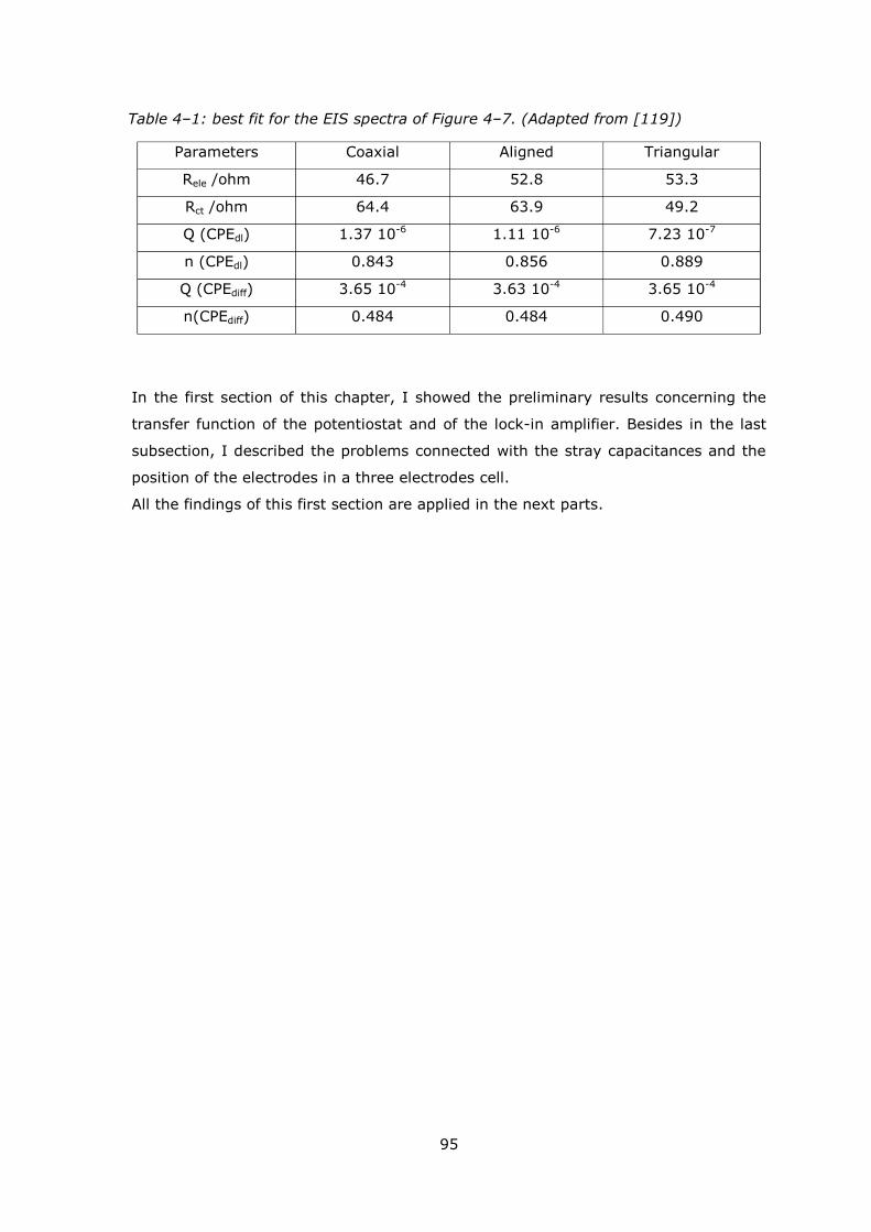
95
In the first section of this chapter, I showed the preliminary results concerning the
transfer function of the potentiostat and of the lock-in amplifier. Besides in the last
subsection, I described the problems connected with the stray capacitances and the
position of the electrodes in a three electrodes cell.
All the findings of this first section are applied in the next parts.
Table 4–1: best fit for the EIS spectra of Figure 4–7. (Adapted from [119])
Parameters Coaxial Aligned Triangular
Rele /ohm 46.7 52.8 53.3
Rct /ohm 64.4 63.9 49.2
Q (CPEdl) 1.37 10-6 1.11 10-6 7.23 10-7
n (CPEdl) 0.843 0.856 0.889
Q (CPEdiff) 3.65 10-4 3.63 10-4 3.65 10-4
n(CPEdiff) 0.484 0.484 0.490
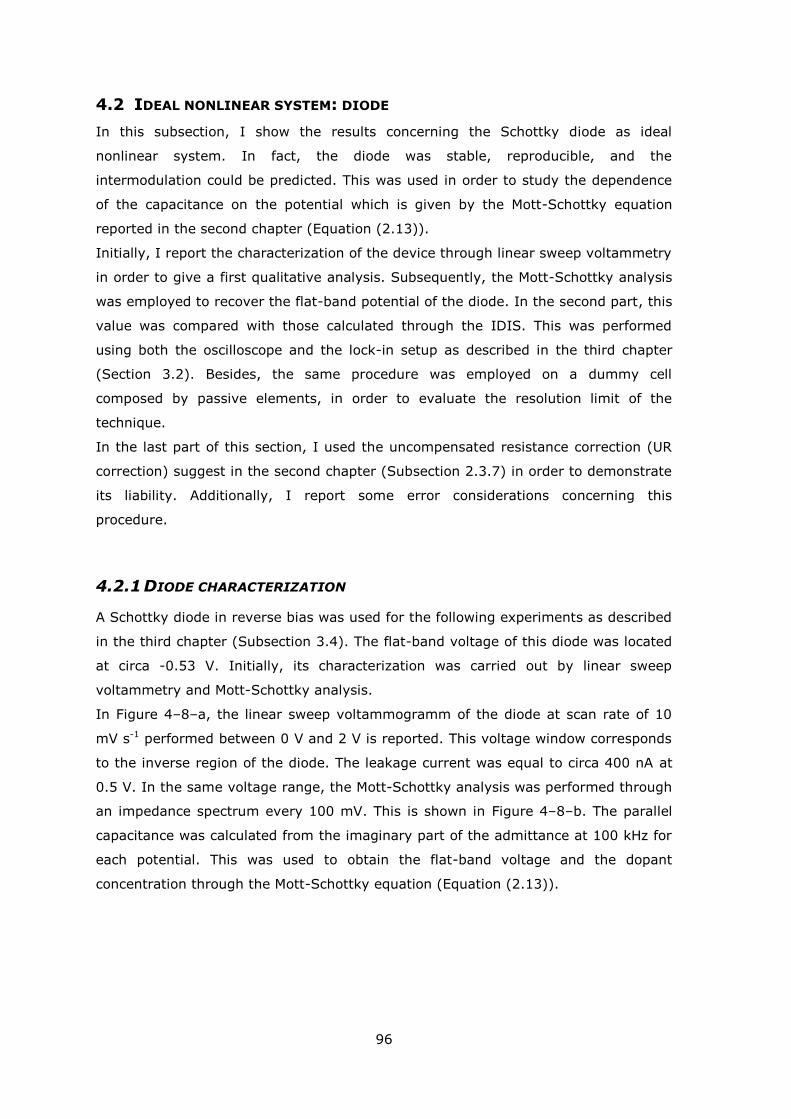
96
4.2 IDEAL NONLINEAR SYSTEM: DIODE
In this subsection, I show the results concerning the Schottky diode as ideal
nonlinear system. In fact, the diode was stable, reproducible, and the
intermodulation could be predicted. This was used in order to study the dependence
of the capacitance on the potential which is given by the Mott-Schottky equation
reported in the second chapter (Equation (2.13)).
Initially, I report the characterization of the device through linear sweep voltammetry
in order to give a first qualitative analysis. Subsequently, the Mott-Schottky analysis
was employed to recover the flat-band potential of the diode. In the second part, this
value was compared with those calculated through the IDIS. This was performed
using both the oscilloscope and the lock-in setup as described in the third chapter
(Section 3.2). Besides, the same procedure was employed on a dummy cell
composed by passive elements, in order to evaluate the resolution limit of the
technique.
In the last part of this section, I used the uncompensated resistance correction (UR
correction) suggest in the second chapter (Subsection 2.3.7) in order to demonstrate
its liability. Additionally, I report some error considerations concerning this
procedure.
4.2.1 DIODE CHARACTERIZATION
A Schottky diode in reverse bias was used for the following experiments as described
in the third chapter (Subsection 3.4). The flat-band voltage of this diode was located
at circa -0.53 V. Initially, its characterization was carried out by linear sweep
voltammetry and Mott-Schottky analysis.
In Figure 4–8–a, the linear sweep voltammogramm of the diode at scan rate of 10
mV s-1 performed between 0 V and 2 V is reported. This voltage window corresponds
to the inverse region of the diode. The leakage current was equal to circa 400 nA at
0.5 V. In the same voltage range, the Mott-Schottky analysis was performed through
an impedance spectrum every 100 mV. This is shown in Figure 4–8–b. The parallel
capacitance was calculated from the imaginary part of the admittance at 100 kHz for
each potential. This was used to obtain the flat-band voltage and the dopant
concentration through the Mott-Schottky equation (Equation (2.13)).
97
From the linear regression of the Mott-Schottky plot, a flat-band potential of -0.536
± 0.005 V and a dopant concentration of 3.61 1017 ± 1015 cm-3 were calculated (εr =
11.68). The same results were achieved using lower frequencies (down to 1 kHz) and
restricting the potential range from 0.2 V to 2 V.
In the next subsection, I show how the same results are found with the IDIS.
4.2.2 IDIS OF THE DIODE: NONLINEAR CAPACITANCE
During an IDIS experiment two potential perturbations were sent to the system: the
stimulus and the probe. The former was spanned through a range of frequencies
while the latter was kept constant. In this case, the stimulus was between 0.1 and
100 Hz while the probe was 1 kHz. The experiments were performed at 0.5 V. From
the stimulus signal, the impedance spectrum of the system could be obtained.
Whereas, from the intermodulation sidebands, the nonlinear behavior of the diode
Figure 4–8: a) linear sweep voltammetry of the diode between 0 V and 2 V at 10
mV s-1; b) Mott-Schottky plot of the capacitance of the diode measured at 100 kHz with linear regression. (Replotted from [58])
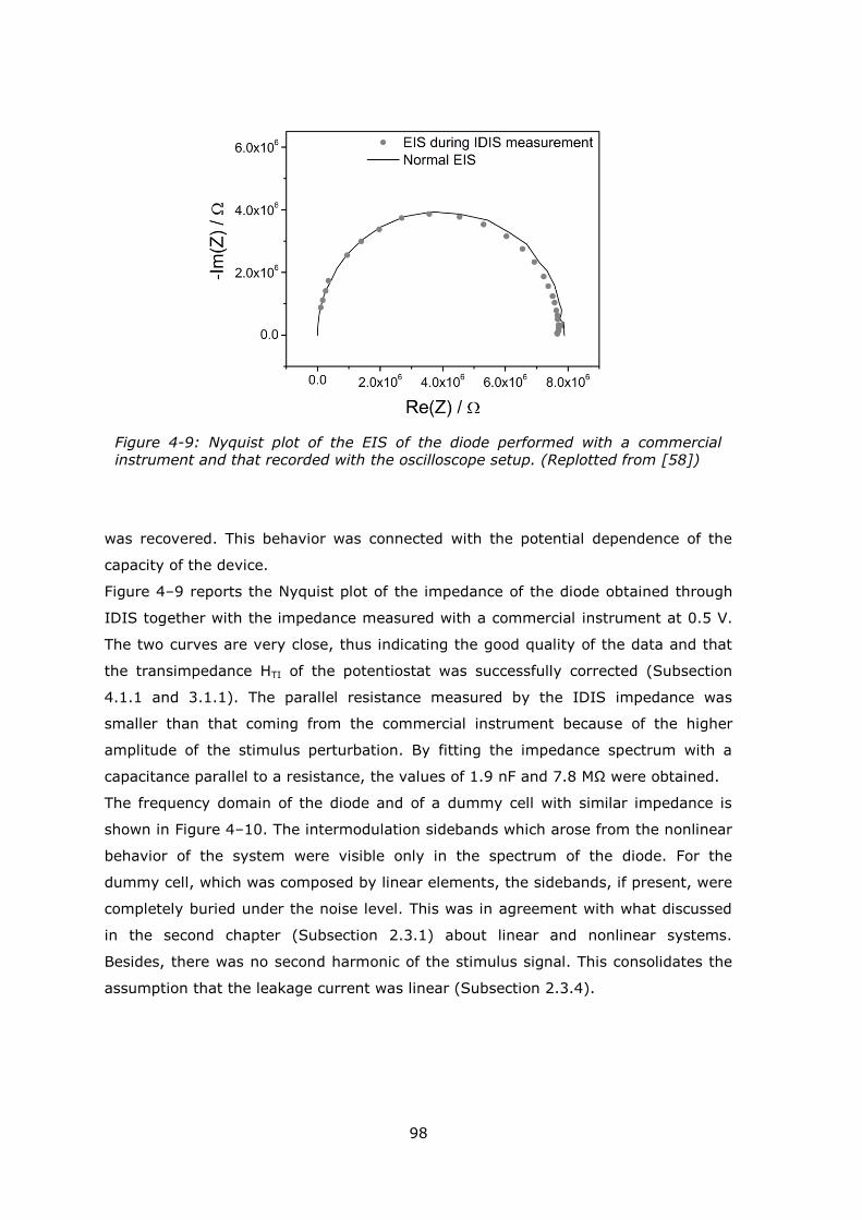
98
was recovered. This behavior was connected with the potential dependence of the
capacity of the device.
Figure 4–9 reports the Nyquist plot of the impedance of the diode obtained through
IDIS together with the impedance measured with a commercial instrument at 0.5 V.
The two curves are very close, thus indicating the good quality of the data and that
the transimpedance HTI of the potentiostat was successfully corrected (Subsection
4.1.1 and 3.1.1). The parallel resistance measured by the IDIS impedance was
smaller than that coming from the commercial instrument because of the higher
amplitude of the stimulus perturbation. By fitting the impedance spectrum with a
capacitance parallel to a resistance, the values of 1.9 nF and 7.8 MΩ were obtained.
The frequency domain of the diode and of a dummy cell with similar impedance is
shown in Figure 4–10. The intermodulation sidebands which arose from the nonlinear
behavior of the system were visible only in the spectrum of the diode. For the
dummy cell, which was composed by linear elements, the sidebands, if present, were
completely buried under the noise level. This was in agreement with what discussed
in the second chapter (Subsection 2.3.1) about linear and nonlinear systems.
Besides, there was no second harmonic of the stimulus signal. This consolidates the
assumption that the leakage current was linear (Subsection 2.3.4).
Figure 4-9: Nyquist plot of the EIS of the diode performed with a commercial instrument and that recorded with the oscilloscope setup. (Replotted from [58])
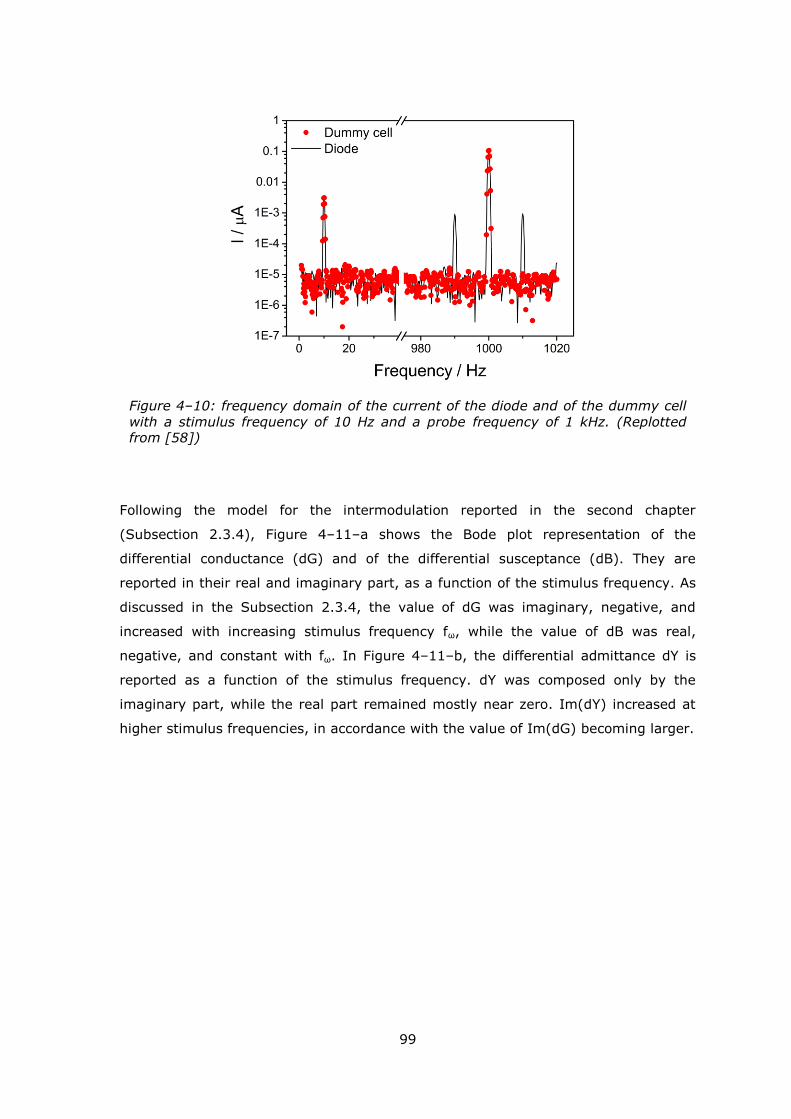
99
Following the model for the intermodulation reported in the second chapter
(Subsection 2.3.4), Figure 4–11–a shows the Bode plot representation of the
differential conductance (dG) and of the differential susceptance (dB). They are
reported in their real and imaginary part, as a function of the stimulus frequency. As
discussed in the Subsection 2.3.4, the value of dG was imaginary, negative, and
increased with increasing stimulus frequency fω, while the value of dB was real,
negative, and constant with fω. In Figure 4–11–b, the differential admittance dY is
reported as a function of the stimulus frequency. dY was composed only by the
imaginary part, while the real part remained mostly near zero. Im(dY) increased at
higher stimulus frequencies, in accordance with the value of Im(dG) becoming larger.
Figure 4–10: frequency domain of the current of the diode and of the dummy cell
with a stimulus frequency of 10 Hz and a probe frequency of 1 kHz. (Replotted from [58])
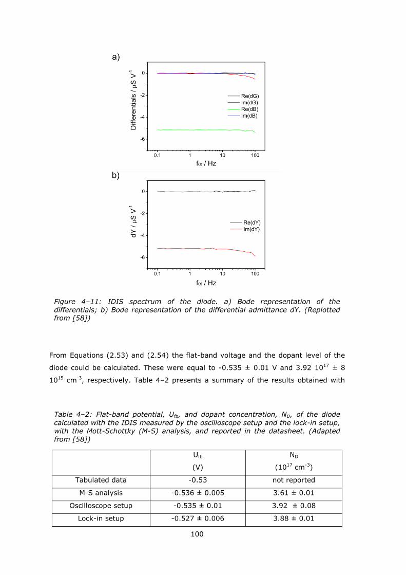
100
From Equations (2.53) and (2.54) the flat-band voltage and the dopant level of the
diode could be calculated. These were equal to -0.535 ± 0.01 V and 3.92 1017 ± 8
1015 cm-3, respectively. Table 4–2 presents a summary of the results obtained with
Figure 4–11: IDIS spectrum of the diode. a) Bode representation of the
differentials; b) Bode representation of the differential admittance dY. (Replotted from [58])
Table 4–2: Flat-band potential, Ufb, and dopant concentration, ND, of the diode
calculated with the IDIS measured by the oscilloscope setup and the lock-in setup,
with the Mott-Schottky (M-S) analysis, and reported in the datasheet. (Adapted
from [58])
Ufb
(V)
ND
(1017 cm-3)
Tabulated data -0.53 not reported
M-S analysis -0.536 ± 0.005 3.61 ± 0.01
Oscilloscope setup -0.535 ± 0.01 3.92 ± 0.08
Lock-in setup -0.527 ± 0.006 3.88 ± 0.01
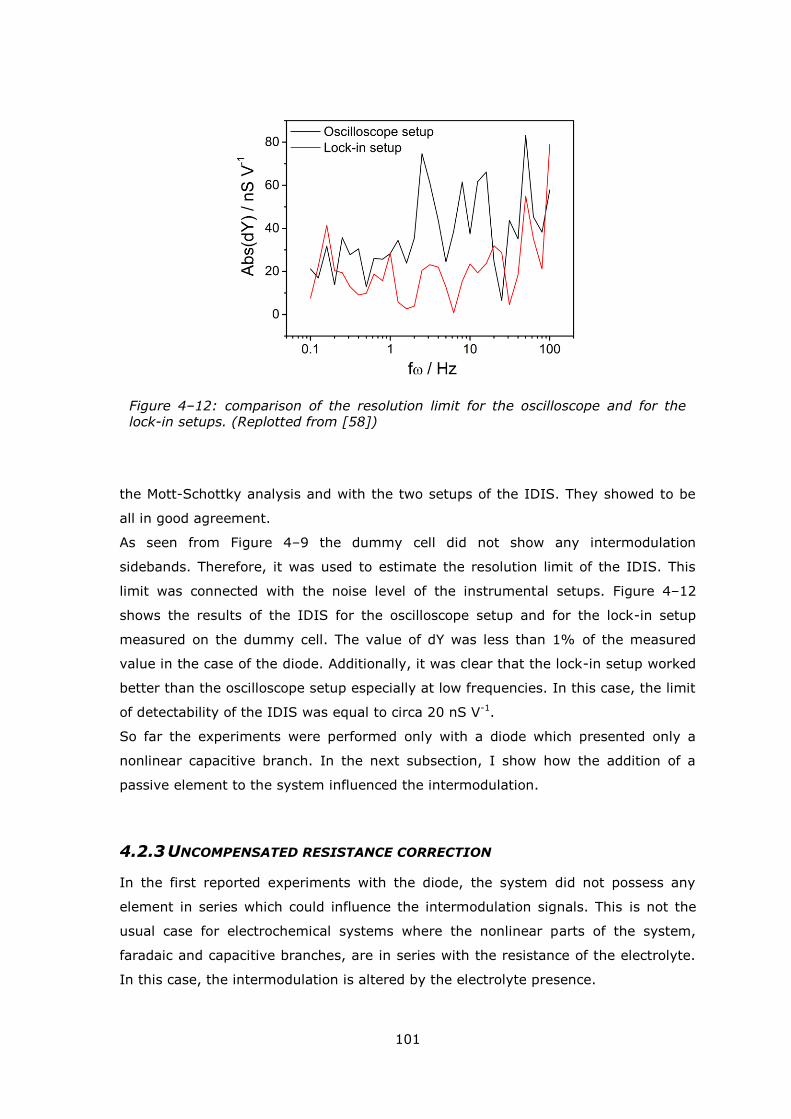
101
the Mott-Schottky analysis and with the two setups of the IDIS. They showed to be
all in good agreement.
As seen from Figure 4–9 the dummy cell did not show any intermodulation
sidebands. Therefore, it was used to estimate the resolution limit of the IDIS. This
limit was connected with the noise level of the instrumental setups. Figure 4–12
shows the results of the IDIS for the oscilloscope setup and for the lock-in setup
measured on the dummy cell. The value of dY was less than 1% of the measured
value in the case of the diode. Additionally, it was clear that the lock-in setup worked
better than the oscilloscope setup especially at low frequencies. In this case, the limit
of detectability of the IDIS was equal to circa 20 nS V-1.
So far the experiments were performed only with a diode which presented only a
nonlinear capacitive branch. In the next subsection, I show how the addition of a
passive element to the system influenced the intermodulation.
4.2.3 UNCOMPENSATED RESISTANCE CORRECTION
In the first reported experiments with the diode, the system did not possess any
element in series which could influence the intermodulation signals. This is not the
usual case for electrochemical systems where the nonlinear parts of the system,
faradaic and capacitive branches, are in series with the resistance of the electrolyte.
In this case, the intermodulation is altered by the electrolyte presence.
Figure 4–12: comparison of the resolution limit for the oscilloscope and for the lock-in setups. (Replotted from [58])
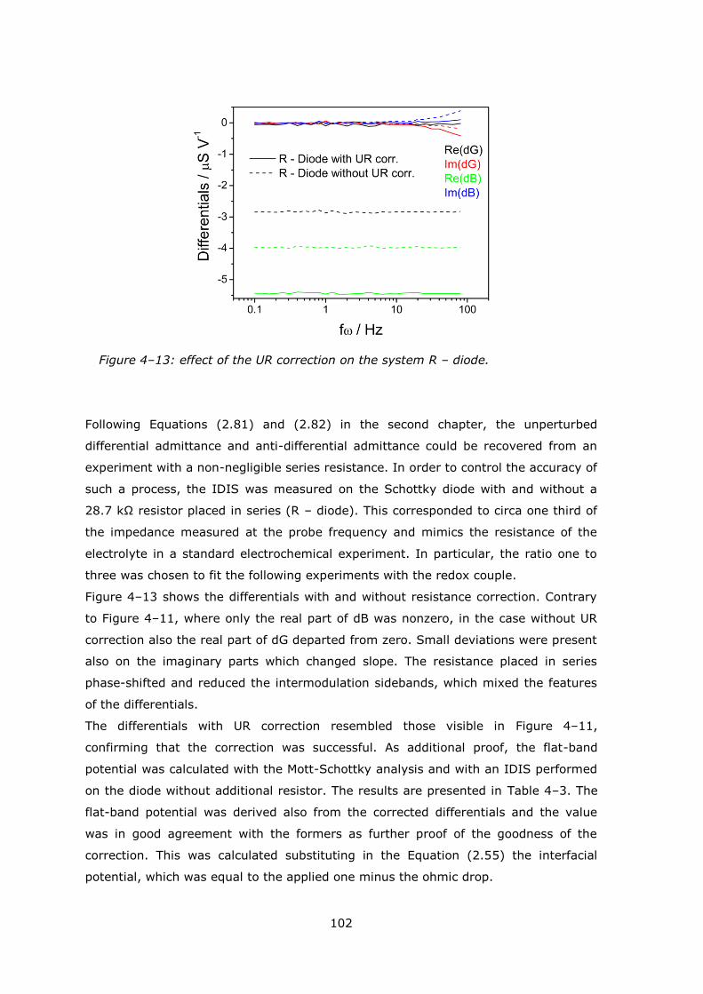
102
Following Equations (2.81) and (2.82) in the second chapter, the unperturbed
differential admittance and anti-differential admittance could be recovered from an
experiment with a non-negligible series resistance. In order to control the accuracy of
such a process, the IDIS was measured on the Schottky diode with and without a
28.7 kΩ resistor placed in series (R – diode). This corresponded to circa one third of
the impedance measured at the probe frequency and mimics the resistance of the
electrolyte in a standard electrochemical experiment. In particular, the ratio one to
three was chosen to fit the following experiments with the redox couple.
Figure 4–13 shows the differentials with and without resistance correction. Contrary
to Figure 4–11, where only the real part of dB was nonzero, in the case without UR
correction also the real part of dG departed from zero. Small deviations were present
also on the imaginary parts which changed slope. The resistance placed in series
phase-shifted and reduced the intermodulation sidebands, which mixed the features
of the differentials.
The differentials with UR correction resembled those visible in Figure 4–11,
confirming that the correction was successful. As additional proof, the flat-band
potential was calculated with the Mott-Schottky analysis and with an IDIS performed
on the diode without additional resistor. The results are presented in Table 4–3. The
flat-band potential was derived also from the corrected differentials and the value
was in good agreement with the formers as further proof of the goodness of the
correction. This was calculated substituting in the Equation (2.55) the interfacial
potential, which was equal to the applied one minus the ohmic drop.
Figure 4–13: effect of the UR correction on the system R – diode.
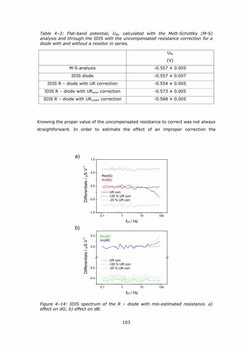
103
Knowing the proper value of the uncompensated resistance to correct was not always
straightforward. In order to estimate the effect of an improper correction the
Table 4–3: Flat-band potential, Ufb, calculated with the Mott-Schottky (M-S)
analysis and through the IDIS with the uncompensated resistance correction for a
diode with and without a resistor in series.
Ufb
(V)
M-S analysis -0.557 ± 0.005
IDIS diode -0.557 ± 0.007
IDIS R – diode with UR correction -0.554 ± 0.005
IDIS R – diode with URover correction -0.573 ± 0.005
IDIS R – diode with URunder correction -0.568 ± 0.005
Figure 4–14: IDIS spectrum of the R – diode with mis-estimated resistance. a) effect on dG; b) effect on dB.
104
procedure was repeated overestimating and underestimating the resistance of 20 %.
The results on the differentials are reported in Figure 4–14. The biggest effects were
visible on the real parts of the differentials. Re(dG) which should lay on zero, moved
positively or negatively with an overestimated and underestimated correction,
respectively. Re(dB), instead, moved always toward less negative values. On the
imaginary parts the effects were less marked and Im(dB) showed a marginal
deviation only at high frequencies, while Im(dG) was completely insensitive to the
magnitude of the UR correction. The Ufb calculated by the mis-estimated resistance
are also shown in Table 4–3. The Ufb were in both cases more negative that the real
one, which was in accordance with the fact that Re(dB) moved in both cases toward
less negative values.
In this section, I presented the results of the intermodulation on a diode. This was
taken as ideal nonlinear system. In the next subsection instead, I show what
happened in the case of a real electrochemical system.
105
4.3 REAL ELECTROCHEMICAL SYSTEM: REDOX COUPLE
In this section, I show the results of the intermodulation on a real electrochemical
system. A well-known and fast redox couple was chosen as target. The goal of the
experiments was to show whether the IDIS could be employed to recover, for
instance, the symmetry of barrier and the diffusion coefficients of the redox couple.
Besides, the results demonstrated that also the double layer responded to the
intermodulation and that it was possible to estimate the time constant of changing of
the capacitive current upon a potential variation.
First, I characterized the system through cyclic voltammetry and EIS. The resistance
of the electrolyte and the value of the mass transport limitation recovered from the
fitting of the EIS spectrum served in the second subsection. In the second
subsection, the results of the intermodulated differential spectroscopy were reported
together with the effect of the UR correction.
Finally, in the third subsection, I show the results of the best fit of the IDIS
spectrum. These follow what reported in the second chapter in the Subsection 2.3.5
and 2.3.6. The results demonstrated the possibility to employ the IDIS to obtain
information on the kinetics, mass transport, and double layer. These pieces of
information were not directly achievable through EIS. In fact, in order to quantify the
kinetic and mass transport parameters several impedance spectra were necessary.
These were usually obtained by changing either the potential or the composition of
the electrolyte. Therefore, some assumptions on the non-dependence of the
parameters on these factors were necessary.
In particular in the last subsection, I investigated several parameters which affected
the final results. For instance, the frequency extent in which the fitting was
performed and the resistance of the electrolyte employed in the UR correction greatly
influenced the quality of the fitting but had very small influence on the derivation of
the kinetic and mass transport parameters.
4.3.1 CHARACTERIZATION OF THE REDOX COUPLE
The experiments reported in this section were performed on a 125 μm diameter
platinum disk electrode in a 10 mM equimolar solution of K3Fe(CN)6 and K4Fe(CN)6
with 0.5 M phosphate buffer at pH 7 as supporting electrolyte. The coaxial cell with a
100 nF capacitor was employed as described in the Subsection 3.3.2 and 4.1.3.
Figure 4–15–a shows the cyclic voltammetry of the redox couple. The curve
resembled the typical sigmoid given by a reversible system. Because of the larger
diffusion coefficient of the oxidized species, the cathodic peak was greater than the
anodic. The existence of these peaks guaranteed that, despite the small dimension of
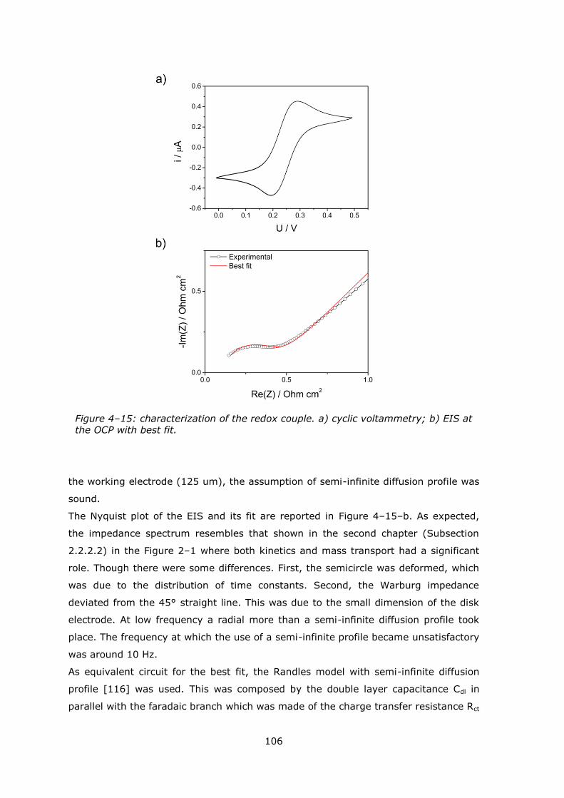
106
the working electrode (125 um), the assumption of semi-infinite diffusion profile was
sound.
The Nyquist plot of the EIS and its fit are reported in Figure 4–15–b. As expected,
the impedance spectrum resembles that shown in the second chapter (Subsection
2.2.2.2) in the Figure 2–1 where both kinetics and mass transport had a significant
role. Though there were some differences. First, the semicircle was deformed, which
was due to the distribution of time constants. Second, the Warburg impedance
deviated from the 45° straight line. This was due to the small dimension of the disk
electrode. At low frequency a radial more than a semi-infinite diffusion profile took
place. The frequency at which the use of a semi-infinite profile became unsatisfactory
was around 10 Hz.
As equivalent circuit for the best fit, the Randles model with semi-infinite diffusion
profile [116] was used. This was composed by the double layer capacitance Cdl in
parallel with the faradaic branch which was made of the charge transfer resistance Rct
Figure 4–15: characterization of the redox couple. a) cyclic voltammetry; b) EIS at the OCP with best fit.
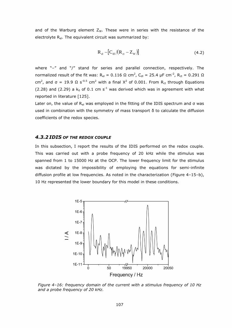
107
and of the Warburg element ZW. These were in series with the resistance of the
electrolyte Rel. The equivalent circuit was summarized by:
Wctdlel ZRCR (4.2)
where ―–‖ and ―/‖ stand for series and parallel connection, respectively. The
normalized result of the fit was: Rel = 0.116 Ω cm2, Cdl = 25.4 μF cm-2, Rct = 0.291 Ω
cm2, and ζ = 19.9 Ω s-0.5 cm2 with a final Χ2 of 0.001. From Rct through Equations
(2.28) and (2.29) a k0 of 0.1 cm s-1 was derived which was in agreement with what
reported in literature [125].
Later on, the value of Rel was employed in the fitting of the IDIS spectrum and ζ was
used in combination with the symmetry of mass transport δ to calculate the diffusion
coefficients of the redox species.
4.3.2 IDIS OF THE REDOX COUPLE
In this subsection, I report the results of the IDIS performed on the redox couple.
This was carried out with a probe frequency of 20 kHz while the stimulus was
spanned from 1 to 15000 Hz at the OCP. The lower frequency limit for the stimulus
was dictated by the impossibility of employing the equations for semi-infinite
diffusion profile at low frequencies. As noted in the characterization (Figure 4–15–b),
10 Hz represented the lower boundary for this model in these conditions.
Figure 4–16: frequency domain of the current with a stimulus frequency of 10 Hz
and a probe frequency of 20 kHz.
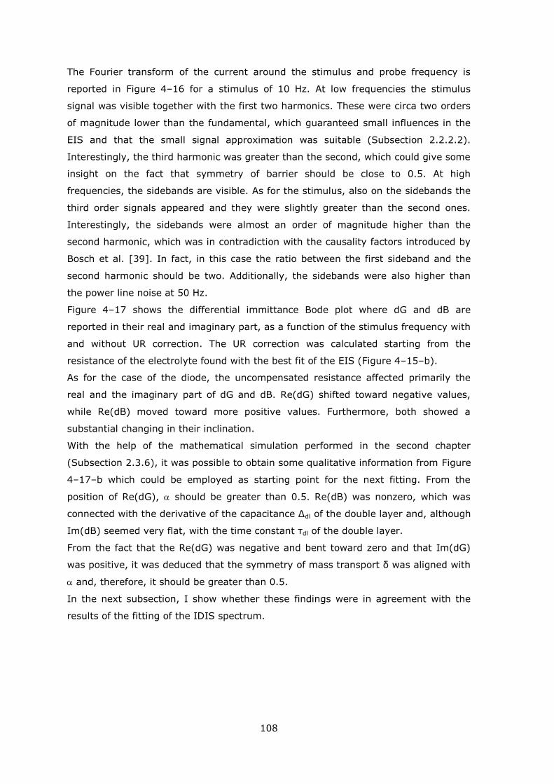
108
The Fourier transform of the current around the stimulus and probe frequency is
reported in Figure 4–16 for a stimulus of 10 Hz. At low frequencies the stimulus
signal was visible together with the first two harmonics. These were circa two orders
of magnitude lower than the fundamental, which guaranteed small influences in the
EIS and that the small signal approximation was suitable (Subsection 2.2.2.2).
Interestingly, the third harmonic was greater than the second, which could give some
insight on the fact that symmetry of barrier should be close to 0.5. At high
frequencies, the sidebands are visible. As for the stimulus, also on the sidebands the
third order signals appeared and they were slightly greater than the second ones.
Interestingly, the sidebands were almost an order of magnitude higher than the
second harmonic, which was in contradiction with the causality factors introduced by
Bosch et al. [39]. In fact, in this case the ratio between the first sideband and the
second harmonic should be two. Additionally, the sidebands were also higher than
the power line noise at 50 Hz.
Figure 4–17 shows the differential immittance Bode plot where dG and dB are
reported in their real and imaginary part, as a function of the stimulus frequency with
and without UR correction. The UR correction was calculated starting from the
resistance of the electrolyte found with the best fit of the EIS (Figure 4–15–b).
As for the case of the diode, the uncompensated resistance affected primarily the
real and the imaginary part of dG and dB. Re(dG) shifted toward negative values,
while Re(dB) moved toward more positive values. Furthermore, both showed a
substantial changing in their inclination.
With the help of the mathematical simulation performed in the second chapter
(Subsection 2.3.6), it was possible to obtain some qualitative information from Figure
4–17–b which could be employed as starting point for the next fitting. From the
position of Re(dG), should be greater than 0.5. Re(dB) was nonzero, which was
connected with the derivative of the capacitance Δdl of the double layer and, although
Im(dB) seemed very flat, with the time constant ηdl of the double layer.
From the fact that the Re(dG) was negative and bent toward zero and that Im(dG)
was positive, it was deduced that the symmetry of mass transport δ was aligned with
and, therefore, it should be greater than 0.5.
In the next subsection, I show whether these findings were in agreement with the
results of the fitting of the IDIS spectrum.
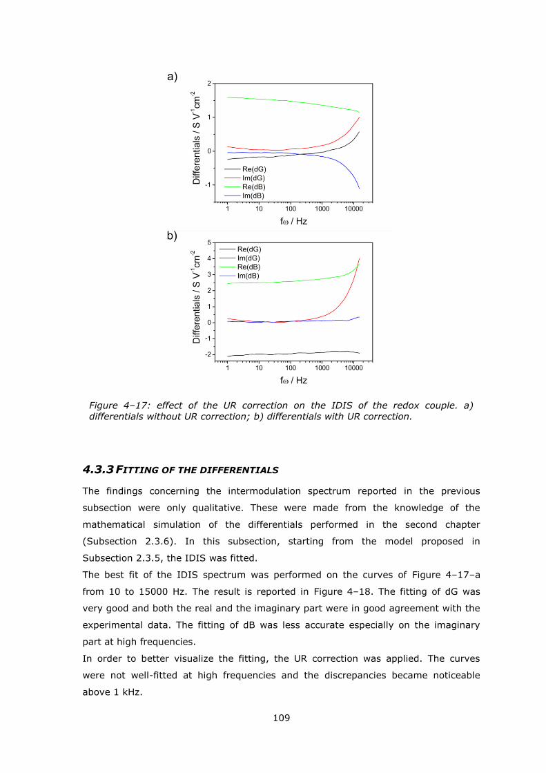
109
4.3.3 FITTING OF THE DIFFERENTIALS
The findings concerning the intermodulation spectrum reported in the previous
subsection were only qualitative. These were made from the knowledge of the
mathematical simulation of the differentials performed in the second chapter
(Subsection 2.3.6). In this subsection, starting from the model proposed in
Subsection 2.3.5, the IDIS was fitted.
The best fit of the IDIS spectrum was performed on the curves of Figure 4–17–a
from 10 to 15000 Hz. The result is reported in Figure 4–18. The fitting of dG was
very good and both the real and the imaginary part were in good agreement with the
experimental data. The fitting of dB was less accurate especially on the imaginary
part at high frequencies.
In order to better visualize the fitting, the UR correction was applied. The curves
were not well-fitted at high frequencies and the discrepancies became noticeable
above 1 kHz.
Figure 4–17: effect of the UR correction on the IDIS of the redox couple. a) differentials without UR correction; b) differentials with UR correction.

110
To understand which parameters controlled the accuracy of the fitting in the high
frequency region, this was repeated changing the upper boundary frequency from
0.5 to 15 kHz. The results are reported in Table 4–4 together with Χ2. As predicted
previously (Subsection 4.3.2) and visible in Table 4–4, the symmetry of the barrier
was higher than 0.5 and it was aligned with the symmetry of the mass transport δ
which was also higher than 0.5. Moreover, the time constant of the double layer ηdl
was experimentally observed. This was associated with the variation of the double
layer Δdl.
The values associated with the faradaic current were rather insensitive to the
frequency extent of the fitting. On the other hand, the parameters of the capacitive
current changed. Although Δdl varied only of 10 %, meaning that it was a good
result, ηdl changed considerably.
Figure 4–18: best fit of the differentials with UR correction. a) fitting of dG; b) fitting of dB.
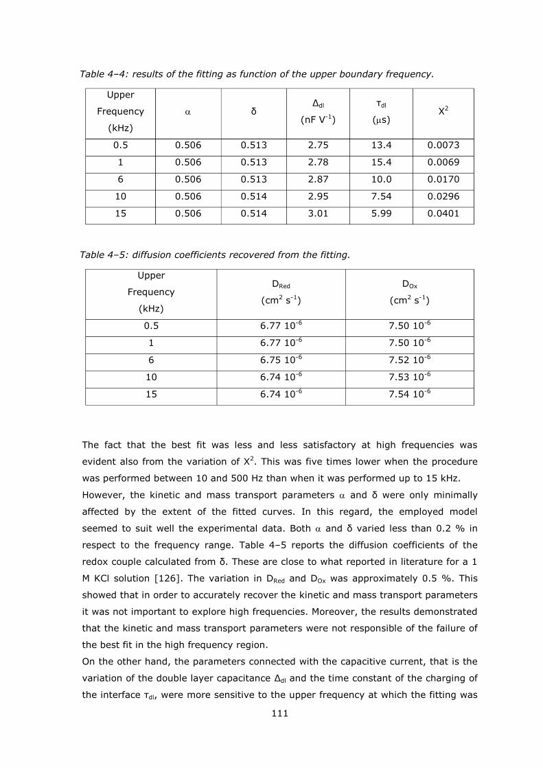
111
The fact that the best fit was less and less satisfactory at high frequencies was
evident also from the variation of Χ2. This was five times lower when the procedure
was performed between 10 and 500 Hz than when it was performed up to 15 kHz.
However, the kinetic and mass transport parameters and δ were only minimally
affected by the extent of the fitted curves. In this regard, the employed model
seemed to suit well the experimental data. Both and δ varied less than 0.2 % in
respect to the frequency range. Table 4–5 reports the diffusion coefficients of the
redox couple calculated from δ. These are close to what reported in literature for a 1
M KCl solution [126]. The variation in DRed and DOx was approximately 0.5 %. This
showed that in order to accurately recover the kinetic and mass transport parameters
it was not important to explore high frequencies. Moreover, the results demonstrated
that the kinetic and mass transport parameters were not responsible of the failure of
the best fit in the high frequency region.
On the other hand, the parameters connected with the capacitive current, that is the
variation of the double layer capacitance Δdl and the time constant of the charging of
the interface ηdl, were more sensitive to the upper frequency at which the fitting was
Table 4–4: results of the fitting as function of the upper boundary frequency.
Upper
Frequency
(kHz)
δ Δdl
(nF V-1)
ηdl
(s) Χ2
0.5 0.506 0.513 2.75 13.4 0.0073
1 0.506 0.513 2.78 15.4 0.0069
6 0.506 0.513 2.87 10.0 0.0170
10 0.506 0.514 2.95 7.54 0.0296
15 0.506 0.514 3.01 5.99 0.0401
Table 4–5: diffusion coefficients recovered from the fitting.
Upper
Frequency
(kHz)
DRed
(cm2 s-1)
DOx
(cm2 s-1)
0.5 6.77 10-6 7.50 10-6
1 6.77 10-6 7.50 10-6
6 6.75 10-6 7.52 10-6
10 6.74 10-6 7.53 10-6
15 6.74 10-6 7.54 10-6
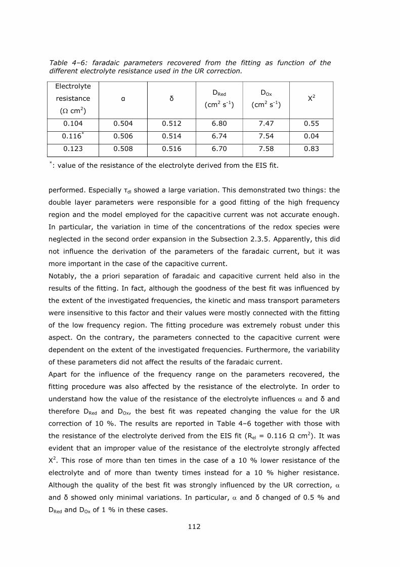
112
performed. Especially ηdl showed a large variation. This demonstrated two things: the
double layer parameters were responsible for a good fitting of the high frequency
region and the model employed for the capacitive current was not accurate enough.
In particular, the variation in time of the concentrations of the redox species were
neglected in the second order expansion in the Subsection 2.3.5. Apparently, this did
not influence the derivation of the parameters of the faradaic current, but it was
more important in the case of the capacitive current.
Notably, the a priori separation of faradaic and capacitive current held also in the
results of the fitting. In fact, although the goodness of the best fit was influenced by
the extent of the investigated frequencies, the kinetic and mass transport parameters
were insensitive to this factor and their values were mostly connected with the fitting
of the low frequency region. The fitting procedure was extremely robust under this
aspect. On the contrary, the parameters connected to the capacitive current were
dependent on the extent of the investigated frequencies. Furthermore, the variability
of these parameters did not affect the results of the faradaic current.
Apart for the influence of the frequency range on the parameters recovered, the
fitting procedure was also affected by the resistance of the electrolyte. In order to
understand how the value of the resistance of the electrolyte influences and δ and
therefore DRed and DOx, the best fit was repeated changing the value for the UR
correction of 10 %. The results are reported in Table 4–6 together with those with
the resistance of the electrolyte derived from the EIS fit (Rel = 0.116 Ω cm2). It was
evident that an improper value of the resistance of the electrolyte strongly affected
Χ2. This rose of more than ten times in the case of a 10 % lower resistance of the
electrolyte and of more than twenty times instead for a 10 % higher resistance.
Although the quality of the best fit was strongly influenced by the UR correction,
and δ showed only minimal variations. In particular, and δ changed of 0.5 % and
DRed and DOx of 1 % in these cases.
Table 4–6: faradaic parameters recovered from the fitting as function of the
different electrolyte resistance used in the UR correction.
Electrolyte
resistance
( cm2)
α δ DRed
(cm2 s-1)
DOx
(cm2 s-1) Χ2
0.104 0.504 0.512 6.80 7.47 0.55
0.116* 0.506 0.514 6.74 7.54 0.04
0.123 0.508 0.516 6.70 7.58 0.83
*: value of the resistance of the electrolyte derived from the EIS fit.
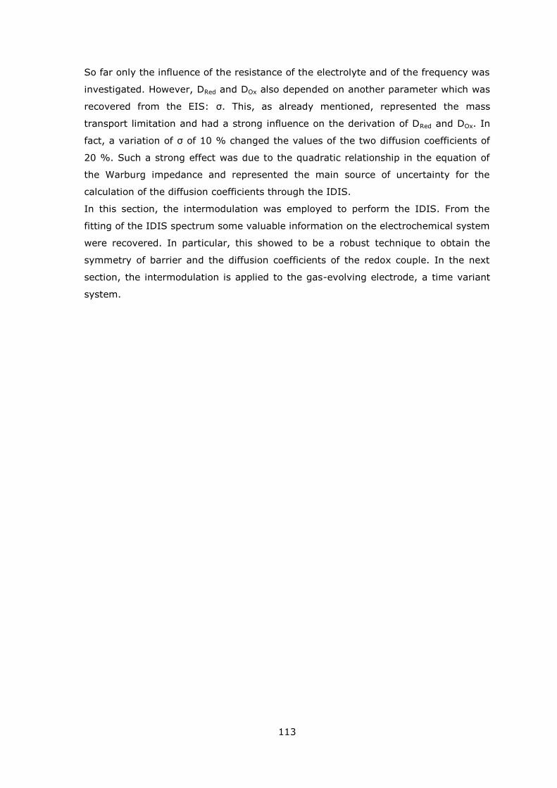
113
So far only the influence of the resistance of the electrolyte and of the frequency was
investigated. However, DRed and DOx also depended on another parameter which was
recovered from the EIS: ζ. This, as already mentioned, represented the mass
transport limitation and had a strong influence on the derivation of DRed and DOx. In
fact, a variation of ζ of 10 % changed the values of the two diffusion coefficients of
20 %. Such a strong effect was due to the quadratic relationship in the equation of
the Warburg impedance and represented the main source of uncertainty for the
calculation of the diffusion coefficients through the IDIS.
In this section, the intermodulation was employed to perform the IDIS. From the
fitting of the IDIS spectrum some valuable information on the electrochemical system
were recovered. In particular, this showed to be a robust technique to obtain the
symmetry of barrier and the diffusion coefficients of the redox couple. In the next
section, the intermodulation is applied to the gas-evolving electrode, a time variant
system.
114
4.4 TIME VARIANT SYSTEM: GAS-EVOLVING ELECTRODE
I present in this section the part of the experiments concerning the gas-evolving
electrode understood as a time variant system. In these experiments the concept of
intermodulation was employed not to recover an intermodulated differential
immittance spectrum as done for the diode and the redox couple, but to study the
effect of the gas bubble formation, expansion, and departure on the impedance of
the electrode. In this case, the system was treated as a time variant system where
the scheduling parameter was the variation of the surface area of the electrode upon
bubble formation and departure as explained in the second chapter (Section 2.4).
In the first subsection, I show the characterization of the system with linear sweep
voltammetry and EIS. The EIS was performed before any bubbles were evolved. This
represented the starting point for the treatment. In fact, in this condition, the
resistance of the electrolyte is related to the total surface area of the electrode
normally available for the electrochemical reaction.
Later on, in the second part, I describe the problem as a time variant system.
Through digital filtering, the variables of the system: current, admittance and surface
area, are shown as function of time. This represented a first intuitive approach for
the further analysis performed in the last subsection.
In the third subsection, the concept of intermodulation and Fourier analysis were
used as developed in the second chapter (Section 2.4). Two results were noteworthy
in this part. The first one was the clear impedance spectrum of the system recovered
during bubble evolution. As reported in literature [79–83], this was not a trivial
problem. The second result was connected with the normalized impedance ZA the
transfer function described in the second chapter (Section 2.4). ZA permitted to
understand the influence of the bubble evolution on the impedance and the effect of
the current density.
4.4.1 CHARACTERIZATION OF THE OXYGEN EVOLUTION REACTION
All the experiments of this section were performed on a cavity microelectrode filled
with RuO2, a well-known catalyst for oxygen evolution in a 0.1 M KOH solution.
Figure 4–19 shows a linear sweep voltammetry performed on the cavity
microelectrode at 5 mV s-1. The curve was flat until 1.4 VRHE and then started to rise
due to water oxidation. Over 1.5 VRHE the first sign of the electrochemical noise was
visible and above 1.6 VRHE the current was strongly affected by the bubble evolution.
At 1.7 VRHE the slope of the voltammogram started to flatten.
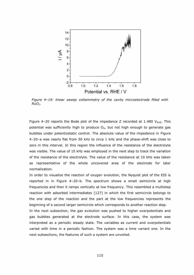
115
Figure 4–20 reports the Bode plot of the impedance Z recorded at 1.480 VRHE. This
potential was sufficiently high to produce O2, but not high enough to generate gas
bubbles under potentiostatic control. The absolute value of the impedance in Figure
4–20–a was nearly flat from 50 kHz to circa 1 kHz and the phase-shift was close to
zero in this interval. In this region the influence of the resistance of the electrolyte
was visible. The value of 10 kHz was employed in the next step to track the variation
of the resistance of the electrolyte. The value of the resistance at 10 kHz was taken
as representative of the whole uncovered area of the electrode for later
normalization.
In order to visualize the reaction of oxygen evolution, the Nyquist plot of the EIS is
reported in in Figure 4–20–b. The spectrum shows a small semicircle at high
frequencies and then it ramps vertically at low frequency. This resembled a multistep
reaction with adsorbed intermediates [127] in which the first semicircle belongs to
the one step of the reaction and the part at the low frequencies represents the
beginning of a second larger semicircle which corresponds to another reaction step.
In the next subsection, the gas evolution was pushed to higher overpotentials and
gas bubbles generated at the electrode surface. In this case, the system was
interpreted as a periodic steady state. The variables as current and overpotentials
varied with time in a periodic fashion. The system was a time variant one. In the
next subsections, the features of such a system are unveiled.
Figure 4–19: linear sweep voltammetry of the cavity microelectrode filled with RuO2.
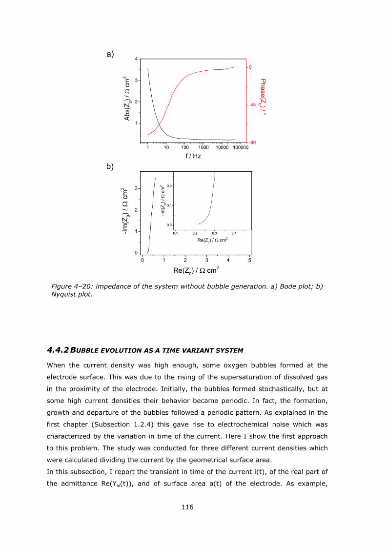
116
4.4.2 BUBBLE EVOLUTION AS A TIME VARIANT SYSTEM
When the current density was high enough, some oxygen bubbles formed at the
electrode surface. This was due to the rising of the supersaturation of dissolved gas
in the proximity of the electrode. Initially, the bubbles formed stochastically, but at
some high current densities their behavior became periodic. In fact, the formation,
growth and departure of the bubbles followed a periodic pattern. As explained in the
first chapter (Subsection 1.2.4) this gave rise to electrochemical noise which was
characterized by the variation in time of the current. Here I show the first approach
to this problem. The study was conducted for three different current densities which
were calculated dividing the current by the geometrical surface area.
In this subsection, I report the transient in time of the current i(t), of the real part of
the admittance Re(Yω(t)), and of surface area a(t) of the electrode. As example,
Figure 4–20: impedance of the system without bubble generation. a) Bode plot; b) Nyquist plot.
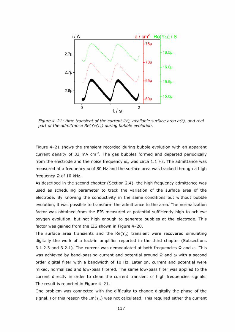
117
Figure 4–21 shows the transient recorded during bubble evolution with an apparent
current density of 33 mA cm-2. The gas bubbles formed and departed periodically
from the electrode and the noise frequency ωn was circa 1.1 Hz. The admittance was
measured at a frequency ω of 80 Hz and the surface area was tracked through a high
frequency Ω of 10 kHz.
As described in the second chapter (Section 2.4), the high frequency admittance was
used as scheduling parameter to track the variation of the surface area of the
electrode. By knowing the conductivity in the same conditions but without bubble
evolution, it was possible to transform the admittance to the area. The normalization
factor was obtained from the EIS measured at potential sufficiently high to achieve
oxygen evolution, but not high enough to generate bubbles at the electrode. This
factor was gained from the EIS shown in Figure 4–20.
The surface area transients and the Re(Yω) transient were recovered simulating
digitally the work of a lock-in amplifier reported in the third chapter (Subsections
3.1.2.3 and 3.2.1). The current was demodulated at both frequencies Ω and ω. This
was achieved by band-passing current and potential around Ω and ω with a second
order digital filter with a bandwidth of 10 Hz. Later on, current and potential were
mixed, normalized and low-pass filtered. The same low-pass filter was applied to the
current directly in order to clean the current transient of high frequencies signals.
The result is reported in Figure 4–21.
One problem was connected with the difficulty to change digitally the phase of the
signal. For this reason the Im(Yω) was not calculated. This required either the current
Figure 4–21: time transient of the current i(t), available surface area a(t), and real part of the admittance Re(Y(t)) during bubble evolution.
118
or the potential to be placed out of phase with the original signal. Moreover, to
handle the signal in time the transimpedance of the potentiostat had to be
considered through convolution.
The current i(t) was not a pure sinusoidal signal and, noise aside, resembled a
sawtooth wave. A similar shape was already reported for gas-evolving reactions [98].
The minima of the curve represent the time at which the bubble reached the maximal
size before departing. At this point, the surface was left free and the current could
rise rapidly. At the maxima of the current the bubble started to nucleate and the
growth was manifested by the slow decrease of the current. Similar behavior was
observed for a(t) which had a very similar shape as i(t).
All three transients were in phase. This was expected for i(t) and a(t). However, the
behavior of Re(Yω) was more complicated. In fact Re(Yω) was only the projection of
Yω(t) and this in general has no defined phase-shift in regard to a(t). Yω(t) was a
circular or elliptical polarized wave with the time coordinate as axis. The wave
oscillated both in the real and in the imaginary plane of the admittance. The ratio
between the real and the imaginary projection was correlated with the phase of the
polarized wave.
The curves show different levels of noise which came mostly from signals at higher
frequencies. The cleanest transient was a(t). In fact, no coherent signal was injected
at frequencies higher than Ω. Both Re(Yω) and i(t), instead suffered from the Ω signal
and in the case of i(t) also from the ω signal.
In Table 4–7, the parameters recovered by the current and surface area transients
are reported for the three apparent current densities. The geometrical area A0 of the
electrode was 78.54 10-6 cm-2. One could notice that the available surface area was
in average between 79 % and 87 % of this value, meaning that the electrode was
never completely free from the bubbles‘ influence.
Furthermore, the available surface area never reached A0 and approached 88 % of
this value as maximum. In fact, the electrode, because of its porosity, contained at
least one gas cavity. This cavity behaved as a stable and instantaneous source of
bubble nucleation, as explained by the non-classical type of nucleation [90]. Besides,
one should consider that the measured resistance of the electrolyte was not only
influenced by the surface area of the electrode, but also by the cross section of the
electrolyte in proximity of the electrode. As soon as a bubble departed from the
surface, this was for a very short time free (as short as permitted by the gas cavity),
but the bubble still occupied some volume in the electrolyte next to the electrode.
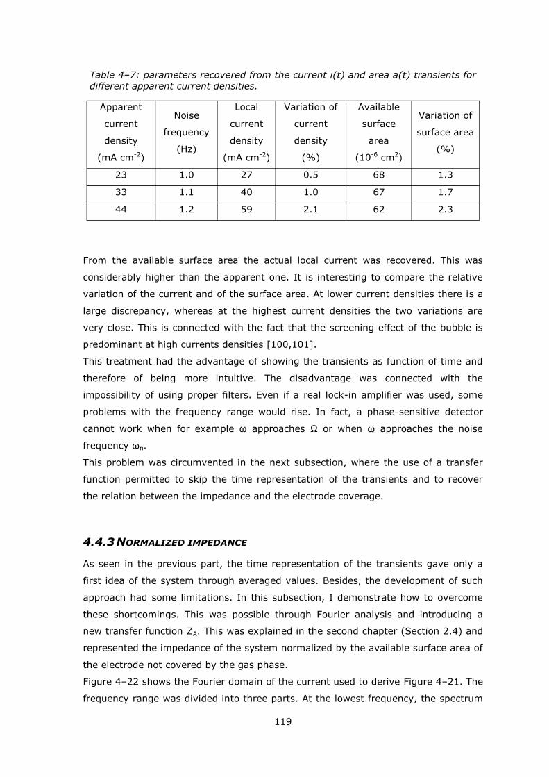
119
From the available surface area the actual local current was recovered. This was
considerably higher than the apparent one. It is interesting to compare the relative
variation of the current and of the surface area. At lower current densities there is a
large discrepancy, whereas at the highest current densities the two variations are
very close. This is connected with the fact that the screening effect of the bubble is
predominant at high currents densities [100,101].
This treatment had the advantage of showing the transients as function of time and
therefore of being more intuitive. The disadvantage was connected with the
impossibility of using proper filters. Even if a real lock-in amplifier was used, some
problems with the frequency range would rise. In fact, a phase-sensitive detector
cannot work when for example ω approaches Ω or when ω approaches the noise
frequency ωn.
This problem was circumvented in the next subsection, where the use of a transfer
function permitted to skip the time representation of the transients and to recover
the relation between the impedance and the electrode coverage.
4.4.3 NORMALIZED IMPEDANCE
As seen in the previous part, the time representation of the transients gave only a
first idea of the system through averaged values. Besides, the development of such
approach had some limitations. In this subsection, I demonstrate how to overcome
these shortcomings. This was possible through Fourier analysis and introducing a
new transfer function ZA. This was explained in the second chapter (Section 2.4) and
represented the impedance of the system normalized by the available surface area of
the electrode not covered by the gas phase.
Figure 4–22 shows the Fourier domain of the current used to derive Figure 4–21. The
frequency range was divided into three parts. At the lowest frequency, the spectrum
Table 4–7: parameters recovered from the current i(t) and area a(t) transients for
different apparent current densities.
Apparent
current
density
(mA cm-2)
Noise
frequency
(Hz)
Local
current
density
(mA cm-2)
Variation of
current
density
(%)
Available
surface
area
(10-6 cm2)
Variation of
surface area
(%)
23 1.0 27 0.5 68 1.3
33 1.1 40 1.0 67 1.7
44 1.2 59 2.1 62 2.3
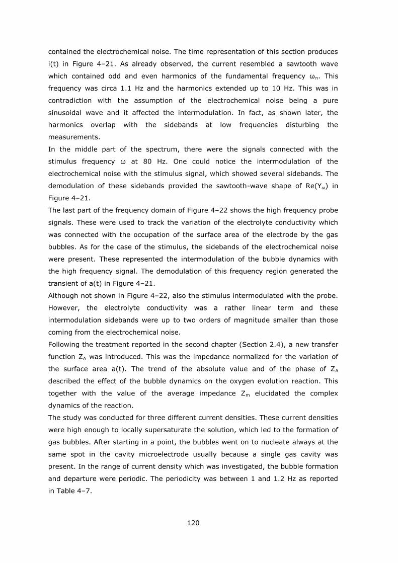
120
contained the electrochemical noise. The time representation of this section produces
i(t) in Figure 4–21. As already observed, the current resembled a sawtooth wave
which contained odd and even harmonics of the fundamental frequency ωn. This
frequency was circa 1.1 Hz and the harmonics extended up to 10 Hz. This was in
contradiction with the assumption of the electrochemical noise being a pure
sinusoidal wave and it affected the intermodulation. In fact, as shown later, the
harmonics overlap with the sidebands at low frequencies disturbing the
measurements.
In the middle part of the spectrum, there were the signals connected with the
stimulus frequency ω at 80 Hz. One could notice the intermodulation of the
electrochemical noise with the stimulus signal, which showed several sidebands. The
demodulation of these sidebands provided the sawtooth-wave shape of Re(Yω) in
Figure 4–21.
The last part of the frequency domain of Figure 4–22 shows the high frequency probe
signals. These were used to track the variation of the electrolyte conductivity which
was connected with the occupation of the surface area of the electrode by the gas
bubbles. As for the case of the stimulus, the sidebands of the electrochemical noise
were present. These represented the intermodulation of the bubble dynamics with
the high frequency signal. The demodulation of this frequency region generated the
transient of a(t) in Figure 4–21.
Although not shown in Figure 4–22, also the stimulus intermodulated with the probe.
However, the electrolyte conductivity was a rather linear term and these
intermodulation sidebands were up to two orders of magnitude smaller than those
coming from the electrochemical noise.
Following the treatment reported in the second chapter (Section 2.4), a new transfer
function ZA was introduced. This was the impedance normalized for the variation of
the surface area a(t). The trend of the absolute value and of the phase of ZA
described the effect of the bubble dynamics on the oxygen evolution reaction. This
together with the value of the average impedance Zm elucidated the complex
dynamics of the reaction.
The study was conducted for three different current densities. These current densities
were high enough to locally supersaturate the solution, which led to the formation of
gas bubbles. After starting in a point, the bubbles went on to nucleate always at the
same spot in the cavity microelectrode usually because a single gas cavity was
present. In the range of current density which was investigated, the bubble formation
and departure were periodic. The periodicity was between 1 and 1.2 Hz as reported
in Table 4–7.
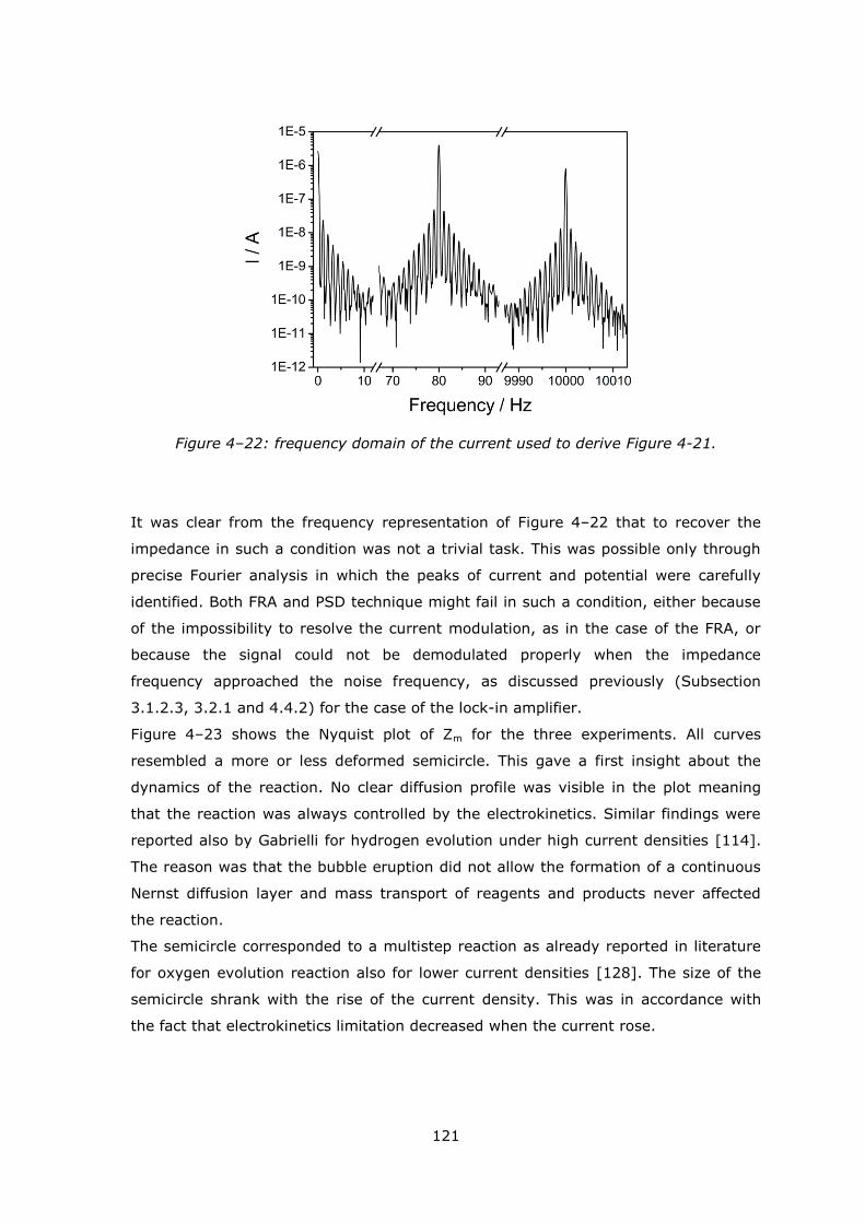
121
It was clear from the frequency representation of Figure 4–22 that to recover the
impedance in such a condition was not a trivial task. This was possible only through
precise Fourier analysis in which the peaks of current and potential were carefully
identified. Both FRA and PSD technique might fail in such a condition, either because
of the impossibility to resolve the current modulation, as in the case of the FRA, or
because the signal could not be demodulated properly when the impedance
frequency approached the noise frequency, as discussed previously (Subsection
3.1.2.3, 3.2.1 and 4.4.2) for the case of the lock-in amplifier.
Figure 4–23 shows the Nyquist plot of Zm for the three experiments. All curves
resembled a more or less deformed semicircle. This gave a first insight about the
dynamics of the reaction. No clear diffusion profile was visible in the plot meaning
that the reaction was always controlled by the electrokinetics. Similar findings were
reported also by Gabrielli for hydrogen evolution under high current densities [114].
The reason was that the bubble eruption did not allow the formation of a continuous
Nernst diffusion layer and mass transport of reagents and products never affected
the reaction.
The semicircle corresponded to a multistep reaction as already reported in literature
for oxygen evolution reaction also for lower current densities [128]. The size of the
semicircle shrank with the rise of the current density. This was in accordance with
the fact that electrokinetics limitation decreased when the current rose.
Figure 4–22: frequency domain of the current used to derive Figure 4-21.
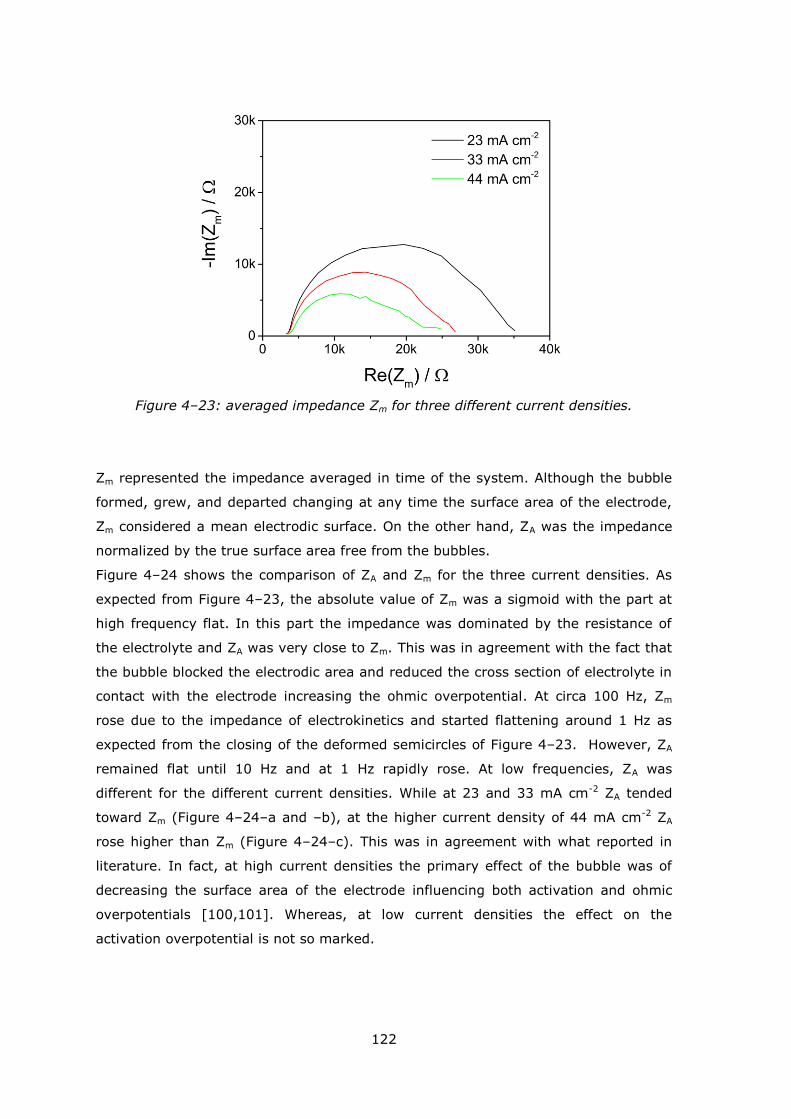
122
Zm represented the impedance averaged in time of the system. Although the bubble
formed, grew, and departed changing at any time the surface area of the electrode,
Zm considered a mean electrodic surface. On the other hand, ZA was the impedance
normalized by the true surface area free from the bubbles.
Figure 4–24 shows the comparison of ZA and Zm for the three current densities. As
expected from Figure 4–23, the absolute value of Zm was a sigmoid with the part at
high frequency flat. In this part the impedance was dominated by the resistance of
the electrolyte and ZA was very close to Zm. This was in agreement with the fact that
the bubble blocked the electrodic area and reduced the cross section of electrolyte in
contact with the electrode increasing the ohmic overpotential. At circa 100 Hz, Zm
rose due to the impedance of electrokinetics and started flattening around 1 Hz as
expected from the closing of the deformed semicircles of Figure 4–23. However, ZA
remained flat until 10 Hz and at 1 Hz rapidly rose. At low frequencies, ZA was
different for the different current densities. While at 23 and 33 mA cm-2 ZA tended
toward Zm (Figure 4–24–a and –b), at the higher current density of 44 mA cm-2 ZA
rose higher than Zm (Figure 4–24–c). This was in agreement with what reported in
literature. In fact, at high current densities the primary effect of the bubble was of
decreasing the surface area of the electrode influencing both activation and ohmic
overpotentials [100,101]. Whereas, at low current densities the effect on the
activation overpotential is not so marked.
Figure 4–23: averaged impedance Zm for three different current densities.
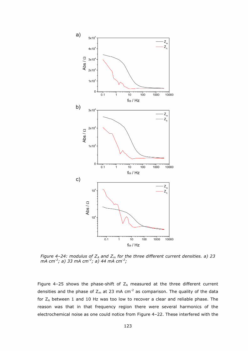
123
Figure 4–25 shows the phase-shift of ZA measured at the three different current
densities and the phase of Zm at 23 mA cm-2 as comparison. The quality of the data
for ZA between 1 and 10 Hz was too low to recover a clear and reliable phase. The
reason was that in that frequency region there were several harmonics of the
electrochemical noise as one could notice from Figure 4–22. These interfered with the
Figure 4–24: modulus of ZA and Zm for the three different current densities. a) 23 mA cm-2; a) 33 mA cm-2; a) 44 mA cm-2;
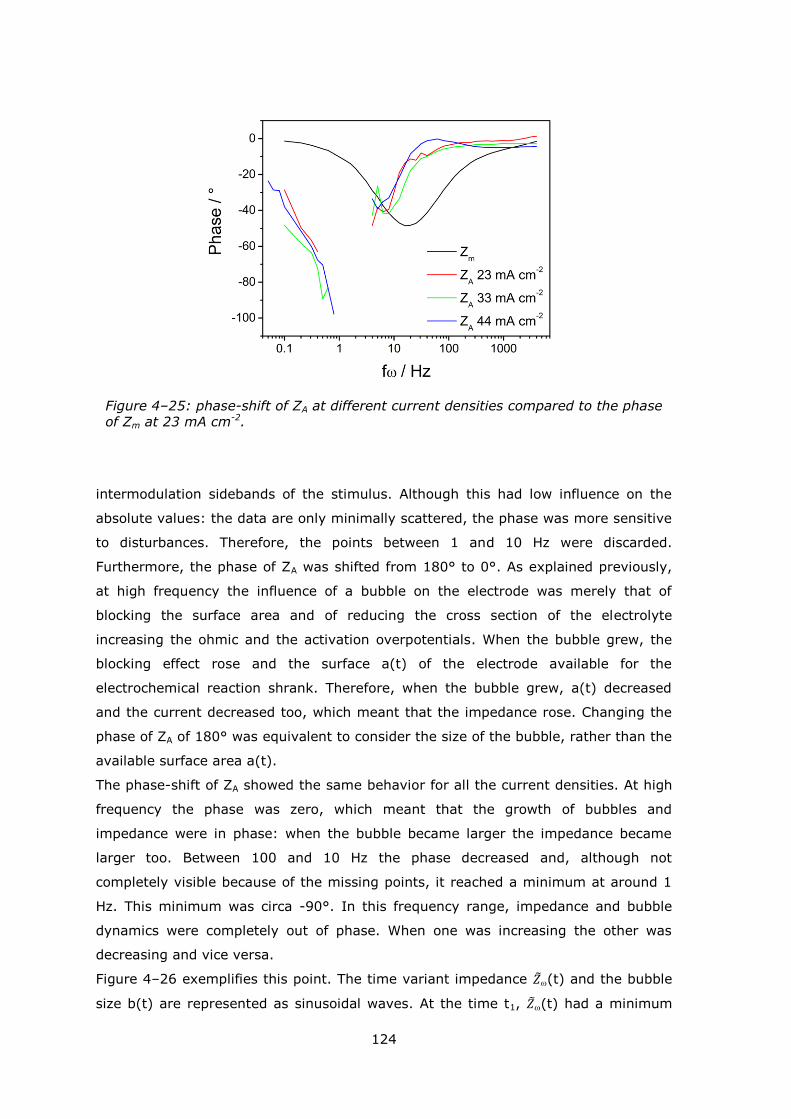
124
intermodulation sidebands of the stimulus. Although this had low influence on the
absolute values: the data are only minimally scattered, the phase was more sensitive
to disturbances. Therefore, the points between 1 and 10 Hz were discarded.
Furthermore, the phase of ZA was shifted from 180° to 0°. As explained previously,
at high frequency the influence of a bubble on the electrode was merely that of
blocking the surface area and of reducing the cross section of the electrolyte
increasing the ohmic and the activation overpotentials. When the bubble grew, the
blocking effect rose and the surface a(t) of the electrode available for the
electrochemical reaction shrank. Therefore, when the bubble grew, a(t) decreased
and the current decreased too, which meant that the impedance rose. Changing the
phase of ZA of 180° was equivalent to consider the size of the bubble, rather than the
available surface area a(t).
The phase-shift of ZA showed the same behavior for all the current densities. At high
frequency the phase was zero, which meant that the growth of bubbles and
impedance were in phase: when the bubble became larger the impedance became
larger too. Between 100 and 10 Hz the phase decreased and, although not
completely visible because of the missing points, it reached a minimum at around 1
Hz. This minimum was circa -90°. In this frequency range, impedance and bubble
dynamics were completely out of phase. When one was increasing the other was
decreasing and vice versa.
Figure 4–26 exemplifies this point. The time variant impedance (t) and the bubble
size b(t) are represented as sinusoidal waves. At the time t1, (t) had a minimum
Figure 4–25: phase-shift of ZA at different current densities compared to the phase of Zm at 23 mA cm-2.
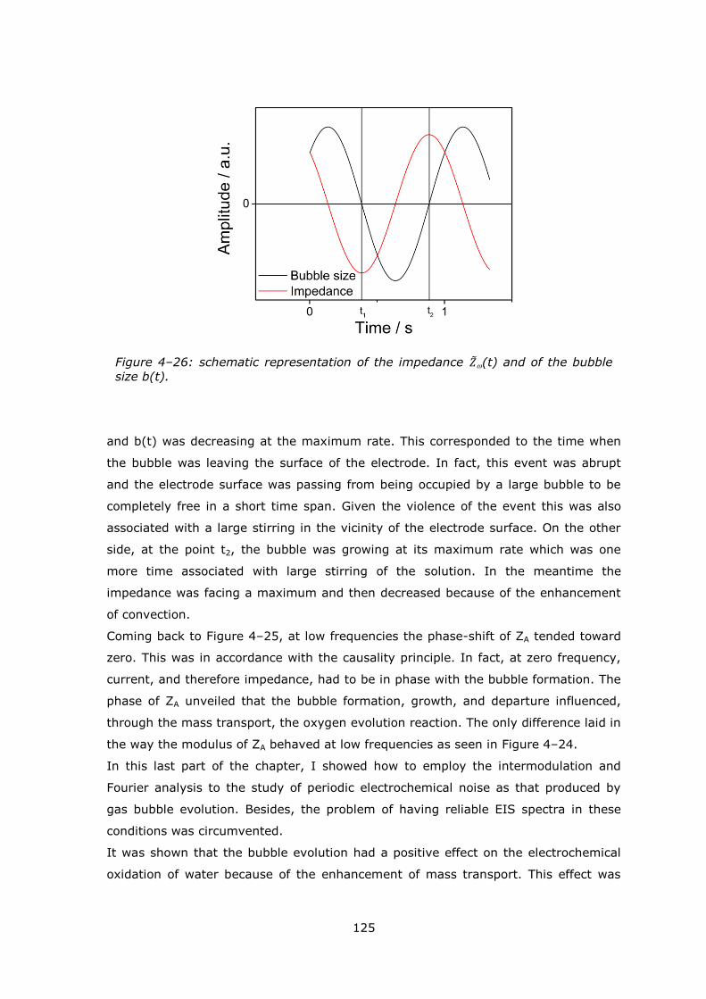
125
and b(t) was decreasing at the maximum rate. This corresponded to the time when
the bubble was leaving the surface of the electrode. In fact, this event was abrupt
and the electrode surface was passing from being occupied by a large bubble to be
completely free in a short time span. Given the violence of the event this was also
associated with a large stirring in the vicinity of the electrode surface. On the other
side, at the point t2, the bubble was growing at its maximum rate which was one
more time associated with large stirring of the solution. In the meantime the
impedance was facing a maximum and then decreased because of the enhancement
of convection.
Coming back to Figure 4–25, at low frequencies the phase-shift of ZA tended toward
zero. This was in accordance with the causality principle. In fact, at zero frequency,
current, and therefore impedance, had to be in phase with the bubble formation. The
phase of ZA unveiled that the bubble formation, growth, and departure influenced,
through the mass transport, the oxygen evolution reaction. The only difference laid in
the way the modulus of ZA behaved at low frequencies as seen in Figure 4–24.
In this last part of the chapter, I showed how to employ the intermodulation and
Fourier analysis to the study of periodic electrochemical noise as that produced by
gas bubble evolution. Besides, the problem of having reliable EIS spectra in these
conditions was circumvented.
It was shown that the bubble evolution had a positive effect on the electrochemical
oxidation of water because of the enhancement of mass transport. This effect was
Figure 4–26: schematic representation of the impedance 𝑍(t) and of the bubble
size b(t).

126
present at all the current densities, but at the highest density the decreasing of the
surface area of the electrode overcame it.
127
4.5 FINAL REMARKS
In this chapter, I described and discussed the findings of this thesis. In the first
section I showed which were the major problems encountered in an impedance
measurement. These were connected both with the instrumental setup and with the
electrochemical cell. In particular, I reported the results of the transimpedance of the
potentiostat and how this affected the EIS. Furthermore, I showed the influences of
the proper design of the electrochemical cell on the impedance. This demonstrated
the importance of the capacitor bridge and of the wise placement of the electrodes.
In the first part I also reported the transfer function of the lock-in amplifier. This was
particularly important for the use of the lock-in setup in the IDIS.
In the second part the IDIS was applied to a diode. This was taken as ideal nonlinear
system and represented the benchmark of the technique. Both instrumental setups of
the IDIS were tested with this system and both showed good performances.
From the IDIS spectrum it was possible to recover the flat band potential and the
doping level of the device. These were in agreement with what was calculated
through the Mott-Schottky analysis. Besides, the UR correction described in the
second chapter was tested on the diode. It proved to work properly and this allowed
its employment for the following experiments.
After the diode the IDIS was applied, in the third section, to a real electrochemical
system. This was composed by a redox couple in solution as ideal reversible system.
The UR correction and the model developed in the second chapter were applied to
this system. It was possible to recover the parameters of the faradaic and capacitive
current. The symmetry of the barrier and of the mass transport, the variation and the
time constant of the double layer capacitance were all unveiled by the results.
The model proved to be robust in regard to the faradaic parameters and the results
were insensitive to the variation of the fitting procedure. On the other hand, the
capacitive parameters were more affected by the high frequency part of the spectrum
and suffered more from the fitting procedure.
In the last section I applied the intermodulation to the study of the electrochemical
noise. This was generated by the periodic formation of gas bubbles at the electrode
upon strong oxygen evolution. Following the principles reported in the second
chapter, the system was analyzed as a time variant system. The surface area of the
electrode was employed as scheduling parameter. This was recovered by the high
frequency part of the impedance spectrum and later used to normalize the
impedance. The normalized impedance was used to understand the effect of the
bubble dynamics on the oxygen evolution reaction. Two features were discovered.
First, the bubbles enhanced the mass transport of the products. This feature was
common to all the experiments. Second, in the experiment performed at higher

128
current density the normalized impedance rose higher than the mean impedance.
This was correlated with the fact that the bubbles partially blocked the surface of the
electrode reducing the area available to sustain the electrochemical reaction affecting
the activation overpotential, which overcame the positive effect of the increased
mass transport.
The next chapter is the conclusion of this thesis. It summarizes all the work and
suggests further development and applications for the IDIS.
129
5 CONCLUSION
In this chapter, I first give a short summary of the work treated in this thesis and
then describe its main achievement, followed by some further developments.
In the first chapter, I reported a short overview of the state of the art regarding the
nonlinear analysis (Subsection 1.2.2), the electrochemical noise (Subsection 1.2.3),
and the gas-evolving electrodes (Subsection 1.2.4).
In the second chapter, I described the mathematical framework which was developed
for the Intermodulated Differential Immittance Spectroscopy (IDIS). Two examples,
the diode (Subsection 2.4.4) and the redox couple (Section 2.5), were used to
illustrate the application and the modus operandi of the technique. The results
concerning these experiments were reported in the fourth chapter (Section 4.2 and
4.3).
In the last part of the second chapter, I showed how the intermodulation was used to
investigate a time variant system (Section 2.6). The case of a gas-evolving electrode
was analyzed. The results of this model were described in the last part of the fourth
chapter (Section 4.4).
The experimental part was described in the third chapter. There, the instrumental
setups developed to perform the IDIS are discussed (Section 3.2). Furthermore, I
explained the major sources of disturbances in working with AC signals. These can be
given by the instrumentation (Section 3.1) or by the electrochemical cell (Section
3.3).
In the following section, I report the main contributions achieved in this work and I
suggest some further developments.
130
5.1 MAIN CONTRIBUTIONS
The aim of this doctoral thesis was to introduce, characterize, and apply a new
electrochemical technique, IDIS, designed to implement the electrochemical
impedance spectroscopy.
The IDIS was based on the phenomenon of the intermodulation. This phenomenon
appears when two periodic stimuli with different frequencies interact in a nonlinear
system creating an amplitude modulation.
Three new transfer functions were derived. These were the differential conductance,
the differential susceptance, and the differential admittance which represented the
variation of the equivalent quantities with the potential. They were correlated with
the nonlinearity of the system and provided some insights into its properties.
The IDIS represented the merging of the electrochemical frequency modulation
(EFM) proposed by Bosch and Bogaerts [38,39] and the modulation of interface
capacitance transfer function (MICTF) technique proposed by Keddam and Takenouti
[54–57]. In fact, the EFM and the MICTF technique were designed to study only the
faradaic current and only the capacitive one, respectively. Furthermore, the transfer
functions and the mathematical framework developed in this thesis overcame the
limitations of these techniques and of several nonlinear approaches.
The IDIS was first applied to the study of an ideal nonlinear system, a Schottky
diode. In this case, the flat-band potential and the doping level of the device were
recovered. These were in good agreement with the tabulated data and with the
results coming from the Mott-Schottky analysis. Interestingly, the Mott-Schottky
analysis requires a series of impedance spectroscopy performed at different
potentials, whereas in the IDIS only a single experiment was necessary.
These experiments showed the reliability of the technique and of the
instrumentation. Furthermore, in a counter test performed on a dummy cell, no
intermodulation was detected. This experiment was used to quantify the error level
for the technique which was less than 1%.
Subsequently, the IDIS was applied to the study of an ideal electrochemical system,
the electrochemical reaction of a redox couple, in order to quantify the parameters of
the faradaic and of the capacitive current. The faradaic current is controlled by the
electrokinetics and by the mass transport. With the IDIS, it was possible to recover
the symmetry factor of the electrochemical reaction and the diffusion coefficients of
the redox couple. Apart from that, also the variation of the double layer capacitance
upon potential change and its time constant were experimentally measured. All these
quantities were not directly accessible via impedance spectroscopy and mostly
overlooked in the nonlinear analysis.
131
This achievement was possible via the mathematical framework developed for the
analysis of the differential immittance spectra. The system was modeled on the basis
of the a priori separation of the faradaic and capacitive current. Under this
assumption, it was possible to divide the faradaic current into electrokinetic and mass
transport contributions.
This model was one of the few examples where the nonlinearities of the double layer
were considered. Furthermore, a procedure to eliminate the effect of the electrolyte
resistance was suggested and proved.
The model was implemented as a best fit algorithm. This procedure was extremely
robust in regard to the faradaic parameters. In fact, these suffered only marginally
from the different factors of the fitting. However, these factors did affect the
capacitive parameters which were successfully recovered, but showed large
dependence on the fitting procedure.
The intermodulation was also applied to the study of the macrokinetic effect of gas
bubbles on the oxygen evolution reaction. In this case, the periodic bubble formation,
growth, and departure from the electrode surface produced the electrochemical noise
observed in the current transient. Through precise Fourier analysis, it was possible to
record the impedance spectrum of the reaction also in the conditions of
electrochemical noise. The impedance showed that, stirring the solution near the
electrode, the bubbles cancelled the mass transport limitation. Furthermore, the
system was modeled upon a periodic nonlinear time variant model. The surface area
of the electrode was taken as scheduling parameter. In fact, under bubble evolution,
this was periodically blocked by gas phase. The impedance normalized by the real
surface area of the electrode was recovered. This showed the effect of the bubble
evolution on the electrochemical reaction. The effect was different for different
current densities. In fact, at low current densities, the main result was the stirring of
the solution and the cancelling of the mass transport limitation, whereas, at high
current densities, this effect was overcome by the obstructing of the electrode
surface.
Besides, two instrumental setups to perform the IDIS were developed. In the first
one, a lock-in amplifier was used to increase the resolution of the technique. In the
second one, the spectra were recovered by Fourier analysis. This second setup
offered more flexibility in the experiments. In fact, it had fewer limitations in the
choice of the investigated frequency, whereas, with the lock-in amplifier, there was a
practical limit in the ratio of the stimulus to the probe frequency.
Some strategies to perform the IDIS were discussed. In order to achieve high quality
results, several points had to be taken into account. First, the potentiostat and the
lock-in amplifier imposed their fingerprints on the signals. In this work, the way to

132
recover and correct these fingerprints was discussed and reported. Second, the
measurement of AC perturbation suffered from artifacts, especially at high
frequencies. These could be corrected by the use of a capacitor bridge. Besides, a
proper geometry for the electrochemical cell was suggested. This geometry
guaranteed several advantages such as low resistance of the electrolyte, high
reproducibility, and low distortions.
In the next section, I suggest some developments based on the work reported in this
thesis.
133
5.2 FURTHER DEVELOPMENT
There are several implementations for the IDIS. For instance, a multisine excitation
could be associated with the intermodulation. This excitation is composed by several
harmonic perturbations sent simultaneously to the system. An example of such an
approach is the odd random phase multisine [129]. The multisine improves the
experimental efficiency of the technique, because more frequencies can be
investigated at once. Besides, it offers a sophisticated analysis of the errors which is
of great importance in a second order analysis. In this case, the signals to seek are
usually very small compared with the first order terms. It is also interesting to extend
the concept of differentials transfer function to the second harmonics. These contain
the same information of the intermodulation sidebands, but in a different
combination.
There are various examples where the IDIS could be employed successfully. For
instance, it can be applied to the study of mass transport in lithium ion batteries. In
this case, it could be possible to recover the diffusion coefficients of the ions into the
host electrode. Another possible application is the study of multistep reactions. The
feature of the IDIS of characterizing the capacitive current could give some insight
into those reactions which undergo adsorption. For instance, it could be possible to
recover the reaction path in the hydrogen evolution reaction.
Because the IDIS can recover the time constant of the interfacial capacitance, it
could be used in the study of transport and the trapping of carriers in
semiconductors. In fact, in this case the capacitance is frequency dependent.
So far, the stimulus frequency was spanned whereas the probe was kept constant. It
is interesting to change both frequencies and to allow the stimulus to cross the
probe. Stimulus and probe are completely exchangeable: the sidebands appear
around the highest frequency signal. When stimulus and probe are close, a quartet of
peaks appears in the frequency domain.
A fascinating development is the generalization of intermodulated differential transfer
function. In fact, one of the electric perturbations can be substituted with another
signal. There are several possible combinations. For instance, the intermodulation
can be coupled with the electrohydrodynamic impedance. In the electrohydrodynamic
impedance, a rotation speed perturbation of the electrode is employed [130]. This
affects the mass transport at the interface. In this case, the stimulus can be given by
the rotation speed perturbation and the probe remains a potential signal. With this
configuration, it is possible to investigate the influence of mass transport on the
impedance. In particular, the effect of the diffusion of electroactive species on the
double layer should be visible.
134
A second possible combination for the intermodulation can be with the intensity-
modulated photocurrent spectroscopy (IMPS) [131]. This technique employs a
sinusoidal modulation of the intensity of the incident light in order to investigate the
response of photoactive materials. In this case, the light modulation could act as
stimulus while the probe is a high frequency potential signal. This could be used to
investigate the changes in the capacitance of the semiconductor upon light
excitation.
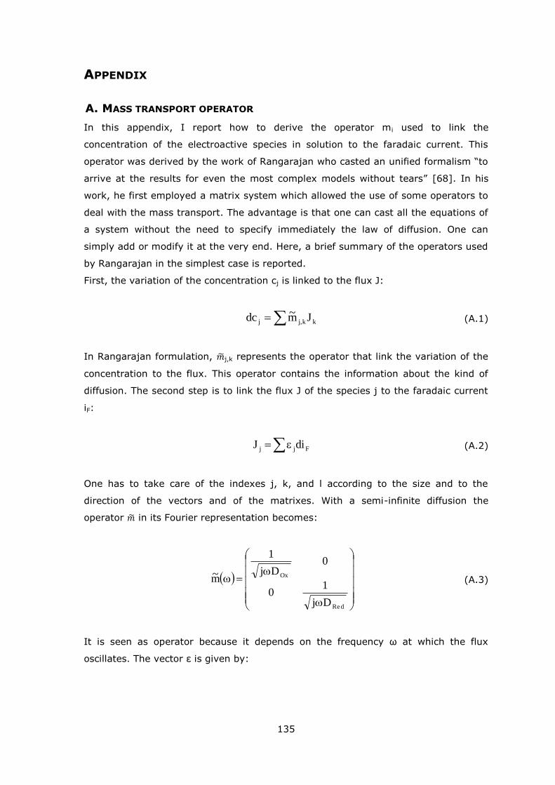
135
APPENDIX
A. MASS TRANSPORT OPERATOR
In this appendix, I report how to derive the operator mi used to link the
concentration of the electroactive species in solution to the faradaic current. This
operator was derived by the work of Rangarajan who casted an unified formalism ―to
arrive at the results for even the most complex models without tears‖ [68]. In his
work, he first employed a matrix system which allowed the use of some operators to
deal with the mass transport. The advantage is that one can cast all the equations of
a system without the need to specify immediately the law of diffusion. One can
simply add or modify it at the very end. Here, a brief summary of the operators used
by Rangarajan in the simplest case is reported.
First, the variation of the concentration cj is linked to the flux J:
kk,jj Jm~cd (A.1)
In Rangarajan formulation, j,k represents the operator that link the variation of the
concentration to the flux. This operator contains the information about the kind of
diffusion. The second step is to link the flux J of the species j to the faradaic current
iF:
Fjj diJ (A.2)
One has to take care of the indexes j, k, and l according to the size and to the
direction of the vectors and of the matrixes. With a semi-infinite diffusion the
operator in its Fourier representation becomes:
dRe
Ox
Dj
10
0Dj
1
m~ (A.3)
It is seen as operator because it depends on the frequency ω at which the flux
oscillates. The vector ε is given by:
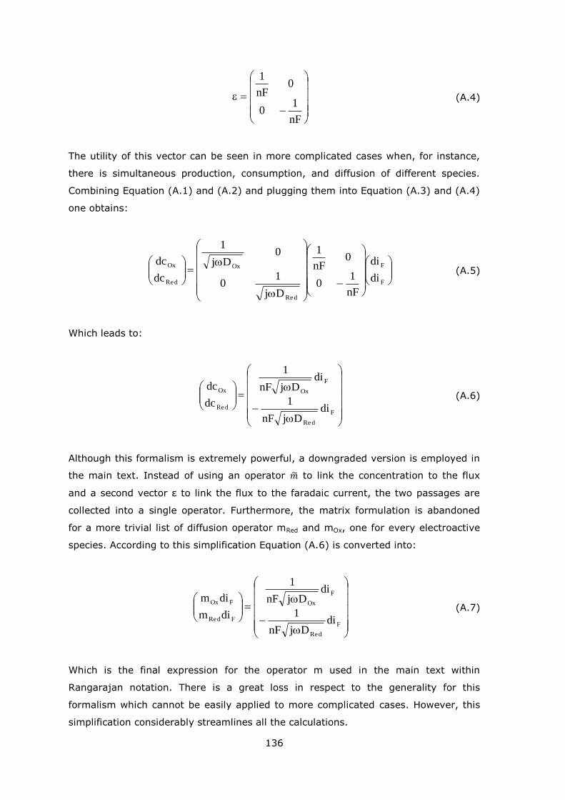
136
nF
10
0nF
1
(A.4)
The utility of this vector can be seen in more complicated cases when, for instance,
there is simultaneous production, consumption, and diffusion of different species.
Combining Equation (A.1) and (A.2) and plugging them into Equation (A.3) and (A.4)
one obtains:
F
F
dRe
Ox
dRe
Ox
di
di
nF
10
0nF
1
Dj
10
0Dj
1
dc
dc (A.5)
Which leads to:
F
dRe
F
Ox
dRe
Ox
diDjnF
1
diDjnF
1
dc
dc (A.6)
Although this formalism is extremely powerful, a downgraded version is employed in
the main text. Instead of using an operator to link the concentration to the flux
and a second vector ε to link the flux to the faradaic current, the two passages are
collected into a single operator. Furthermore, the matrix formulation is abandoned
for a more trivial list of diffusion operator mRed and mOx, one for every electroactive
species. According to this simplification Equation (A.6) is converted into:
F
dRe
F
Ox
FdRe
FOx
diDjnF
1
diDjnF
1
dim
dim (A.7)
Which is the final expression for the operator m used in the main text within
Rangarajan notation. There is a great loss in respect to the generality for this
formalism which cannot be easily applied to more complicated cases. However, this
simplification considerably streamlines all the calculations.
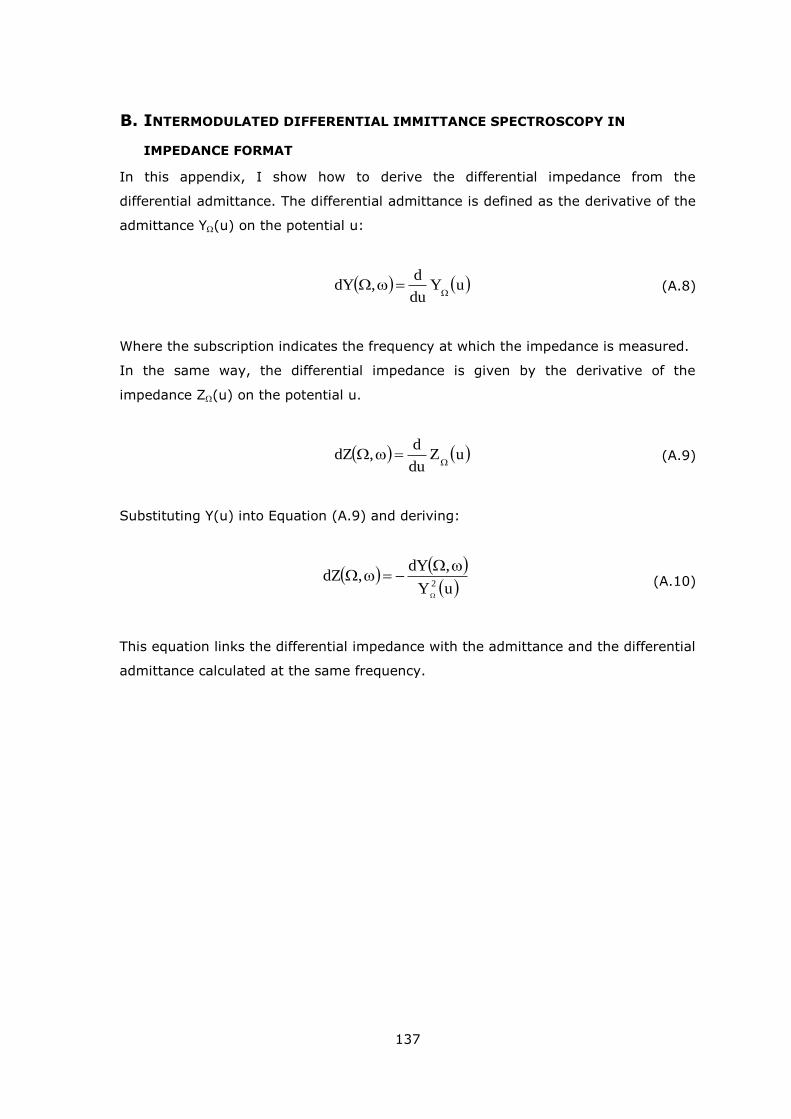
137
B. INTERMODULATED DIFFERENTIAL IMMITTANCE SPECTROSCOPY IN
IMPEDANCE FORMAT
In this appendix, I show how to derive the differential impedance from the
differential admittance. The differential admittance is defined as the derivative of the
admittance Y(u) on the potential u:
uYdu
d,dY
(A.8)
Where the subscription indicates the frequency at which the impedance is measured.
In the same way, the differential impedance is given by the derivative of the
impedance Z(u) on the potential u.
uZdu
d,dZ
(A.9)
Substituting Y(u) into Equation (A.9) and deriving:
uY
,dY,dZ
2
(A.10)
This equation links the differential impedance with the admittance and the differential
admittance calculated at the same frequency.
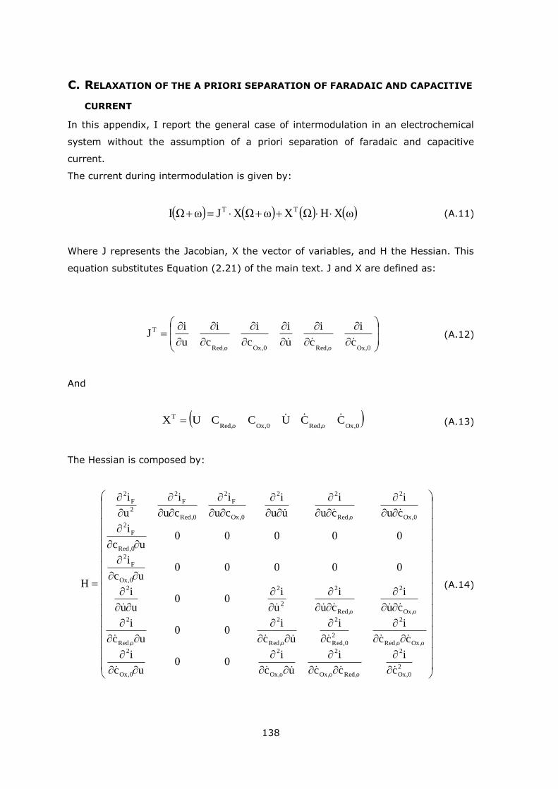
138
C. RELAXATION OF THE A PRIORI SEPARATION OF FARADAIC AND CAPACITIVE
CURRENT
In this appendix, I report the general case of intermodulation in an electrochemical
system without the assumption of a priori separation of faradaic and capacitive
current.
The current during intermodulation is given by:
ωXHΩXωΩXJωΩI TT (A.11)
Where J represents the Jacobian, X the vector of variables, and H the Hessian. This
equation substitutes Equation (2.21) of the main text. J and X are defined as:
Ox,0oRed,Ox,0oRed,
T
c
i
c
i
u
i
c
i
c
i
u
iJ
(A.12)
And
Ox,0oRed,Ox,0oRed,
T CCUCCUX (A.13)
The Hessian is composed by:
2
Ox,0
2
oRed,oOx,
2
oOx,
2
Ox,0
2
oOx,oRed,
2
2
Red,0
2
oRed,
2
oRed,
2
oOx,
2
oRed,
2
2
22
Ox,0
F
2
Red,0
F
2
Ox,0
2
oRed,
22
Ox,0
F
2
Red,0
F
2
2
F
2
c
i
cc
i
uc
i00
uc
i
cc
i
c
i
uc
i00
uc
i
cu
i
cu
i
u
i00
uu
i
00000uc
i
00000uc
i
cu
i
cu
i
uu
i
cu
i
cu
i
u
i
H
(A.14)
139
The mass transport operator used in the main text (Equation (2.11)) cannot be
employed in this treatment. In fact, in this condition not only the Fick‘s law, but also
migration has to be considered. Therefore, the equations become extremely complex.

140
BIBLIOGRAPHY
[1] D.D. Macdonald, Reflections on the history of electrochemical impedance
spectroscopy, Electrochimica Acta. 51 (2006) 1376–1388.
[2] H.W. Bode, Network analysis and feedback amplifier design., New York,
1949.
[3] E. Warburg, Ueber das Verhalten sogenannter unpolarisirbarer Elektroden
gegen Wechselstrom, Annalen Der Physik. 303 (1899) 493–499.
[4] D.C. Grahame, The Electrical Double Layer and the Theory of
Electrocapillarity., Chemical Reviews. 41 (1947) 441–501.
[5] M. Senda, P. Delahay, Rectification by the Electrical Double Layer and
Adsorption Kinetics, J. Am. Chem. Soc. 83 (1961) 3763–3766.
[6] R. Neeb, Intermodulations-Polarographie, Naturwissenschaften. 49 (1962)
447–447.
[7] D.J. Kooyman, M. Sluyters-Rehbach, J.H. Sluyters, Linearization of the
current/voltage characteristic of an electrode process. application to relaxation
methods, Electrochimica Acta. 11 (1966) 1197–1204.
[8] K. Darowicki, Fundamental-harmonic impedance of first-order electrode
reactions, Electrochimica Acta. 39 (1994) 2757–2762.
[9] J.-P. Diard, B. Le Gorrec, C. Montella, Impedance measurement errors due to
non-linearities—I. Low frequency impedance measurements, Electrochimica Acta. 39
(1994) 539–546.
[10] L. Mészáros, G. Mészáros, B. Lengyel, Application of Harmonic Analysis in the
Measuring Technique of Corrosion, Journal of The Electrochemical Society. 141
(1994) 2068–2071.
[11] K. Darowicki, Corrosion rate measurements by non-linear electrochemical
impedance spectroscopy, Corrosion Science. 37 (1995) 913–925.
[12] K. Darowicki, Frequency dispersion of harmonic components of the current of
an electrode process, Journal of Electroanalytical Chemistry. 394 (1995) 81–86.
[13] K. Darowicki, The amplitude analysis of impedance spectra, Electrochimica
Acta. 40 (1995) 439–445.
[14] K. Darowicki, Theoretical description of fundamental-harmonic impedance of
a two-step electrode reaction, Electrochimica Acta. 40 (1995) 767–774.
[15] J.-P. Diard, B.L. Gorrec, C. Montella, Comment on ―Application of Harmonic
Analysis in the Measuring Technique of Corrosion‖ [J. Electrochem. Soc., 141, 2068],
Journal of The Electrochemical Society. 142 (1995) 3612–3612.
141
[16] D.K. Wong, D.R. MacFarlane, Harmonic impedance spectroscopy. Theory and
experimental results for reversible and quasi-reversible redox systems, The Journal
of Physical Chemistry. 99 (1995) 2134–2142.
[17] J.-P. Diard, B. Le Gorrec, C. Montella, Deviation from the polarization
resistance due to non-linearity I - theoretical formulation, Journal of Electroanalytical
Chemistry. 432 (1997) 27–39.
[18] J.-P. Diard, B. Le Gorrec, C. Montella, Deviation of the polarization resistance
due to non-linearity II. Application to electrochemical reactions, Journal of
Electroanalytical Chemistry. 432 (1997) 41–52.
[19] J.-P. Diard, B. Le Gorrec, C. Montella, Deviation of the polarization resistance
due to non-linearity. III—Polarization resistance determination from non-linear
impedance measurements, Journal of Electroanalytical Chemistry. 432 (1997) 53–62.
[20] J.-P. Diard, B. Le Gorrec, C. Montella, Non-linear impedance for a two-step
electrode reaction with an intermediate adsorbed species, Electrochimica Acta. 42
(1997) 1053–1072.
[21] D.A. Harrington, Theory of electrochemical impedance of surface reactions:
second-harmonic and large-amplitude response, Canadian Journal of Chemistry. 75
(1997) 1508–1517.
[22] K. Darowicki, J. Majewska, The effect of a polyharmonic structure of the
perturbation signal on the results of harmonic analysis of the current of a first-order
electrode reaction, Electrochimica Acta. 44 (1998) 483–490.
[23] J.-P. Diard, B. Le Gorrec, C. Montella, Corrosion rate measurements by non-
linear electrochemical impedance spectroscopy. Comments on the paper by K.
Darowicki, Corros. Sci. 37, 913 (1995), Corrosion Science. 40 (1998) 495–508.
[24] K. Darowicki, J. Majewska, Harmonic Analysis Of Electrochemical and
Corrosion Systems-A Review, Corrosion Reviews. 17 (1999) 383–400.
[25] E. Van Gheem, R. Pintelon, A. Hubin, J. Schoukens, P. Verboven, O. Blajiev,
et al., Electrochemical impedance spectroscopy in the presence of non-linear
distortions and non-stationary behaviour: Part II. Application to crystallographic
pitting corrosion of aluminium, Electrochimica Acta. 51 (2006) 1443–1452.
[26] J.R. Wilson, D.T. Schwartz, S.B. Adler, Nonlinear electrochemical impedance
spectroscopy for solid oxide fuel cell cathode materials, Electrochimica Acta. 51
(2006) 1389–1402.
[27] M. Kiel, O. Bohlen, D.U. Sauer, Harmonic analysis for identification of
nonlinearities in impedance spectroscopy, Electrochimica Acta. 53 (2008) 7367–
7374.
[28] V.F. Lvovich, M.F. Smiechowski, Non-linear impedance analysis of industrial
lubricants, Electrochimica Acta. 53 (2008) 7375–7385.
142
[29] H. Xiao, S.B. Lalvani, A Linear Model of Alternating Voltage-Induced
Corrosion, Journal of The Electrochemical Society. 155 (2008) C69–C74.
[30] A.T. DeMartini, A. Unemoto, T. Kawada, S. Adler, Nonlinear Analysis of the
Oxygen Surface Reaction and Thermodynamic Behavior of La, in: ECS, 2009: pp. 47–
67.
[31] T. Kadyk, R. Hanke-Rauschenbach, K. Sundmacher, Nonlinear frequency
response analysis of PEM fuel cells for diagnosis of dehydration, flooding and CO-
poisoning, Journal of Electroanalytical Chemistry. 630 (2009) 19–27.
[32] W. Lai, Fourier analysis of complex impedance (amplitude and phase) in
nonlinear systems: A case study of diodes, Electrochimica Acta. 55 (2010) 5511–
5518.
[33] C. Kreller, M. Drake, S.B. Adler, H.-Y. Chen, H.-C. Yu, K. Thornton, et al.,
Modeling SOFC Cathodes Based on 3-D Representations of Electrode Microstructure,
in: 2011: pp. 815–822.
[34] M.F. Smiechowski, V.F. Lvovich, S. Srikanthan, R.L. Silverstein, Non-linear
impedance characterization of blood cells-derived microparticle biomarkers
suspensions, Electrochimica Acta. 56 (2011) 7763–7771.
[35] N. Xu, J. Riley, Nonlinear analysis of a classical system: The double‐layer
capacitor, Electrochemistry Communications. 13 (2011) 1077–1081.
[36] C. Montella, Combined effects of Tafel kinetics and Ohmic potential drop on
the nonlinear responses of electrochemical systems to low-frequency sinusoidal
perturbation of electrode potential – New approach using the Lambert W-function,
Journal of Electroanalytical Chemistry. 672 (2012) 17–27.
[37] N. Xu, D.J. Riley, Nonlinear analysis of a classical system: The Faradaic
process, Electrochimica Acta. 94 (2013) 206–213.
[38] R.W. Bosch, W.F. Bogaerts, Instantaneous Corrosion Rate Measurement with
Small-Amplitude Potential Intermodulation Techniques: Corrosion, Corrosion. 52
(1996) 204–212.
[39] R.W. Bosch, J. Hubrecht, W.F. Bogaerts, B.C. Syrett, Electrochemical
Frequency Modulation: A New Electrochemical Technique for Online Corrosion
Monitoring: Corrosion, Corrosion. 57 (2001) 60–70.
[40] S.S. Abdel-Rehim, K.F. Khaled, N.S. Abd-Elshafi, Electrochemical frequency
modulation as a new technique for monitoring corrosion inhibition of iron in acid
media by new thiourea derivative, Electrochimica Acta. 51 (2006) 3269–3277.
[41] E. Kuş, F. Mansfeld, An evaluation of the electrochemical frequency
modulation (EFM) technique, Corrosion Science. 48 (2006) 965–979.
143
[42] L. Han, S. Song, A measurement system based on electrochemical frequency
modulation technique for monitoring the early corrosion of mild steel in seawater,
Corrosion Science. 50 (2008) 1551–1557.
[43] K.F. Khaled, Application of electrochemical frequency modulation for
monitoring corrosion and corrosion inhibition of iron by some indole derivatives in
molar hydrochloric acid, Materials Chemistry and Physics. 112 (2008) 290–300.
[44] M.A. Amin, S.S. Abd El Rehim, H.T.M. Abdel-Fatah, Electrochemical frequency
modulation and inductively coupled plasma atomic emission spectroscopy methods
for monitoring corrosion rates and inhibition of low alloy steel corrosion in HCl
solutions and a test for validity of the Tafel extrapolation method, Corrosion Science.
51 (2009) 882–894.
[45] K.F. Khaled, Evaluation of electrochemical frequency modulation as a new
technique for monitoring corrosion and corrosion inhibition of carbon steel in
perchloric acid using hydrazine carbodithioic acid derivatives, Journal of Applied
Electrochemistry. 39 (2009) 429–438.
[46] A. Rauf, W.F. Bogaerts, Monitoring of crevice corrosion with the
electrochemical frequency modulation technique, Electrochimica Acta. 54 (2009)
7357–7363.
[47] A. Rauf, W.F. Bogaerts, Employing electrochemical frequency modulation for
pitting corrosion, Corrosion Science. 52 (2010) 2773–2785.
[48] N.A. Al-Mobarak, K.F. Khaled, M.N.H. Hamed, K.M. Abdel-Azim, Employing
electrochemical frequency modulation for studying corrosion and corrosion inhibition
of copper in sodium chloride solutions, Arabian Journal of Chemistry. 4 (2011) 185–
193.
[49] A. Rauf, E. Mahdi, Evaluating Corrosion Inhibitors with the Help of
Electrochemical Measurements Including Electrochemical Frequency Modulation, Int.
J. Electrochem. Sci. 7 (2012) 4673–4685.
[50] A. Rauf, E. Mahdi, Reliability and Usefulness of Causality Factors of
Electrochemical Frequency Modulation, Int. J. Electrochem. Sci. 7 (2012) 10108–
10120.
[51] P. Beese, H. Venzlaff, J. Srinivasan, J. Garrelfs, M. Stratmann, K.J.J.
Mayrhofer, Monitoring of anaerobic microbially influenced corrosion via
electrochemical frequency modulation, Electrochimica Acta. 105 (2013) 239–247.
[52] M.N. El-Haddad, Chitosan as a green inhibitor for copper corrosion in acidic
medium, International Journal of Biological Macromolecules. 55 (2013) 142–149.
[53] S. Junaedi, A. Al-Amiery, A. Kadihum, A. Kadhum, A. Mohamad, Inhibition
Effects of a Synthesized Novel 4-Aminoantipyrine Derivative on the Corrosion of Mild
144
Steel in Hydrochloric Acid Solution together with Quantum Chemical Studies,
International Journal of Molecular Sciences. 14 (2013) 11915–11928.
[54] R. Antaño-Lopez, M. Keddam, H. Takenouti, A new experimental approach to
the time-constants of electrochemical impedance: frequency response of the double
layer capacitance, Electrochimica Acta. 46 (2001) 3611–3617.
[55] R. Antaño-Lopez, M. Keddam, H. Takenouti, Interface capacitance at mercury
and iron electrodes in the presence of organic compound, Corrosion Engineering,
Science and Technology. 39 (2004) 59–64.
[56] H. Cachet, M. Keddam, H. Takenouti, R. Antaño-Lopez, T. Stergiopoulos, P.
Falaras, Capacitance probe of the electron displacement in a dye sensitised solar cell
by an intermodulation technique: a quantitative model, Electrochimica Acta. 49
(2004) 2541–2549.
[57] E.R. Larios-Durán, R. Antaño-Lopez, M. Keddam, Y. Meas, H. Takenouti, V.
Vivier, Dynamics of double-layer by AC Modulation of the Interfacial Capacitance and
Associated Transfer Functions: IMPEDANCE SPECTROSCOPY AND TRANSFER
FUNCTIONS, Electrochimica Acta. 55 (2010) 6292–6298.
[58] A. Battistel, F. La Mantia, Nonlinear Analysis: The Intermodulated Differential
Immittance Spectroscopy, Analytical Chemistry. 85 (2013) 6799–6805.
[59] C.R. Kreller, S. Adler, Insight into Rate Limiting Mechanisms of Porous La, in:
ECS, 2009: pp. 2743–2752.
[60] T.J. McDonald, S. Adler, (Invited) Theory and Application of Nonlinear
Electrochemical Impedance Spectroscopy, ECS Transactions. 45 (2012) 429–439.
[61] S.K. Rangarajan, High amplitude periodic signal theory: I. Potential
controlled, Journal of Electroanalytical Chemistry and Interfacial Electrochemistry. 56
(1974) 55–71.
[62] S.K. Rangarajan, Non-linear relaxation methods: I. An operator formalism,
Journal of Electroanalytical Chemistry and Interfacial Electrochemistry. 56 (1974) 1–
25.
[63] S.K. Rangarajan, Non-linear relaxation methods: II. A unified approach to
sinusoidal and modulation techniques, Journal of Electroanalytical Chemistry and
Interfacial Electrochemistry. 56 (1974) 27–53.
[64] M. Sluyters-Rehbach, J. Struys, J.H. Sluyters, On second order effects in a
glavanic cell: Part II. A unified treatment of the theoretical principles of the second
order techniques for the study of electrode processes and for electrochemical
analysis, Journal of Electroanalytical Chemistry and Interfacial Electrochemistry. 100
(1979) 607–624.
145
[65] J. Struijs, M. Sluyters-Rehbach, J.H. Sluyters, On second-order effects in a
galvanic cell: Part IV. A theory of demodulation polarography, Journal of
Electroanalytical Chemistry and Interfacial Electrochemistry. 143 (1983) 37–59.
[66] R.S. Hansen, K.G. Baikerikar, Frequency dependence of capacitance at the
desorption potentials of organic molecules, Journal of Electroanalytical Chemistry and
Interfacial Electrochemistry. 82 (1977) 403–412.
[67] E.J.F. Dickinson, R.G. Compton, How well does simple RC circuit analysis
describe diffuse double layer capacitance at smooth micro- and nanoelectrodes?,
Journal of Electroanalytical Chemistry. 655 (2011) 23–31.
[68] S.K. Rangarajan, A unified approach to linear electrochemical systems: I. The
formalism, Journal of Electroanalytical Chemistry and Interfacial Electrochemistry. 55
(1974) 297–327.
[69] S.K. Rangarajan, A unified approach to linear electrochemical systems: II.
Phenomenological coupling, Journal of Electroanalytical Chemistry and Interfacial
Electrochemistry. 55 (1974) 329–335.
[70] S.K. Rangarajan, A unified theory of linear electrochemical systems: III. The
hierarchy of special cases, Journal of Electroanalytical Chemistry and Interfacial
Electrochemistry. 55 (1974) 337–361.
[71] S.K. Rangarajan, A unified theory of linear electrochemical systems: IV.
Electron transfer through adsorbed modes, Journal of Electroanalytical Chemistry and
Interfacial Electrochemistry. 55 (1974) 363–374.
[72] J.S. Morgan, XXX.—The periodic evolution of carbon monoxide, Journal of the
Chemical Society, Transactions. 109 (1916) 274–283.
[73] P.G. Bowers, R.M. Noyes, Chemical oscillations and instabilities. 51. Gas
evolution oscillators. 1. Some new experimental examples, Journal of the American
Chemical Society. 105 (1983) 2572–2574.
[74] K.W. Smith, R.M. Noyes, Gas evolution oscillators. 3. A computational model
of the Morgan reaction, The Journal of Physical Chemistry. 87 (1983) 1520–1524.
[75] K.W. Smith, R.M. Noyes, P.G. Bowers, Chemical oscillations and instabilities.
Part 52. Gas evolution oscillators. 2. A reexamination of formic acid dehydration, The
Journal of Physical Chemistry. 87 (1983) 1514–1519.
[76] R.M. Noyes, Gas-evolution oscillators. 4. Characteristics of the steady state
for gas evolution, The Journal of Physical Chemistry. 88 (1984) 2827–2833.
[77] G.C. Barker, Noise connected with electrode processes, Journal of
Electroanalytical Chemistry and Interfacial Electrochemistry. 21 (1969) 127–136.
[78] G.C. Barker, Flicker noise connected with the hydrogen evolution reaction on
mercury, Journal of Electroanalytical Chemistry and Interfacial Electrochemistry. 39
(1972) 484–488.

146
[79] L. Bai, D.A. Harrington, B.E. Conway, Behavior of overpotential—deposited
species in Faradaic reactions—II. ac Impedance measurements on H2 evolution
kinetics at activated and unactivated Pt cathodes, Electrochimica Acta. 32 (1987)
1713–1731.
[80] Y. Choquette, L. Brossard, A. Lasia, H. Menard, Study of the Kinetics of
Hydrogen Evolution Reaction on Raney Nickel Composite‐Coated Electrode by AC
Impedance Technique, Journal of The Electrochemical Society. 137 (1990) 1723–
1730.
[81] Y. Choquette, L. Brossard, A. Lasia, H. Ménard, Investigation of hydrogen
evolution on Raney-Nickel composite-coated electrodes, Electrochimica Acta. 35
(1990) 1251–1256.
[82] P. Ekdunge, K. Jüttner, G. Kreysa, T. Kessler, M. Ebert, W.J. Lorenz,
Electrochemical Impedance Study on the Kinetics of Hydrogen Evolution at
Amorphous Metals in Alkaline Solution, Journal of The Electrochemical Society. 138
(1991) 2660–2668.
[83] I. Herraiz-Cardona, E. Ortega, L. Vázquez-Gómez, V. Pérez-Herranz, Double-
template fabrication of three-dimensional porous nickel electrodes for hydrogen
evolution reaction, International Journal of Hydrogen Energy. 37 (2012) 2147–2156.
[84] P.M. Senik, A periodic steady-state process in autonomous, essentially
nonlinear systems, Soviet Applied Mechanics. 4 (1968) 38–42.
[85] J. Aprille, T.J., T.N. Trick, Steady-state analysis of nonlinear circuits with
periodic inputs, Proceedings of the IEEE. 60 (1972) 108–114.
[86] L.O. Chua, A. Ushida, Algorithms for computing almost periodic steady-state
response of nonlinear systems to multiple input frequencies, IEEE Transactions on
Circuits and Systems. 28 (1981) 953–971.
[87] A. Semlyen, A. Medina, Computation of the periodic steady state in systems
with nonlinear components using a hybrid time and frequency domain methodology,
IEEE Transactions on Power Systems. 10 (1995) 1498–1504.
[88] J. Feder, K.C. Russell, J. Lothe, G.M. Pound, Homogeneous nucleation and
growth of droplets in vapours, Advances in Physics. 15 (1966) 111–178.
[89] A. Volanschi, W. Olthuis, P. Bergveld, Gas bubbles electrolytically generated
at microcavity electrodes used for the measurement of the dynamic surface tension
in liquids, Sensors and Actuators A: Physical. 52 (1996) 18–22.
[90] S.F. Jones, G.M. Evans, K.P. Galvin, Bubble nucleation from gas cavities — a
review, Advances in Colloid and Interface Science. 80 (1999) 27–50.
[91] S.F. Jones, G.M. Evans, K.P. Galvin, The cycle of bubble production from a
gas cavity in a supersaturated solution, Advances in Colloid and Interface Science. 80
(1999) 51–84.
147
[92] A.R. Zeradjanin, E. Ventosa, A.S. Bondarenko, W. Schuhmann, Evaluation of
the Catalytic Performance of Gas-Evolving Electrodes using Local Electrochemical
Noise Measurements, ChemSusChem. 5 (2012) 1905–1911.
[93] H. Vogt, On the supersaturation of gas in the concentration boundary layer of
gas evolving electrodes, Electrochimica Acta. 25 (1980) 527–531.
[94] H. Vogt, The incremental ohmic resistance caused by bubbles adhering to an
electrode, Journal of Applied Electrochemistry. 13 (1983) 87–88.
[95] J. Dukovic, C.W. Tobias, The Influence of Attached Bubbles on Potential Drop
and Current Distribution at Gas‐Evolving Electrodes, Journal of The Electrochemical
Society. 134 (1987) 331–343.
[96] J.A. Leistra, P.J. Sides, Hyperpolarization of gas evolving electrodes—I.
Aqueous electrolysis, Electrochimica Acta. 32 (1987) 1489–1494.
[97] J.A. Leistra, P.J. Sides, Voltage Components at Gas Evolving Electrodes,
Journal of The Electrochemical Society. 134 (1987) 2442–2446.
[98] C. Gabrielli, F. Huet, M. Keddam, A. Macias, A. Sahar, Potential drops due to
an attached bubble on a gas-evolving electrode, Journal of Applied Electrochemistry.
19 (1989) 617–629.
[99] C. Gabrielli, F. Huet, M. Keddam, A. Sahar, Investigation of water electrolysis
by spectral analysis. I. Influence of the current density, Journal of Applied
Electrochemistry. 19 (1989) 683–696.
[100] C. Gabrielli, F. Huet, R.P. Nogueira, Fluctuations of concentration
overpotential generated at gas-evolving electrodes, Electrochimica Acta. 50 (2005)
3726–3736.
[101] J.M. Silva, R.P. Nogueira, L. de Miranda, F. Huet, Hydrogen Absorption
Estimation on Pd Electrodes from Electrochemical Noise Measurements in Single-
Compartment Cells, Journal of The Electrochemical Society. 148 (2001) E241–E247.
[102] S. Trasatti, Electrocatalysis: understanding the success of DSA®,
Electrochimica Acta. 45 (2000) 2377–2385.
[103] H.B. Beer, The Invention and Industrial Development of Metal Anodes,
Journal of The Electrochemical Society. 127 (1980) 303C–307C.
[104] H. Bouazaze, J. Fransaer, F. Huet, P. Rousseau, V. Vivier, Electrolyte-
resistance change due to an insulating sphere in contact with a disk electrode,
Electrochimica Acta. 55 (2010) 1645–1655.
[105] S. Shibata, The Concentration of Molecular Hydrogen on the Platinum
Cathode, Bulletin of the Chemical Society of Japan. 36 (1963) 53–57.
[106] H. Vogt, The Concentration Overpotential of Gas Evolving Electrodes as a
Multiple Problem of Mass Transfer, Journal of The Electrochemical Society. 137
(1990) 1179–1184.
148
[107] K. Stephan, H. Vogt, A model for correlating mass transfer data at gas
evolving electrodes, Electrochimica Acta. 24 (1979) 11–18.
[108] H. Vogt, Superposition of microconvective and macroconvective mass
transfer at gas-evolving electrodes—a theoretical attempt, Electrochimica Acta. 32
(1987) 633–636.
[109] L. Müller, M. Krenz, K. Rübner, On the relation between the transport of
electrochemically evolved Cl2 and H2 into the electrolyte bulk by convective diffusion
and by gas bubbles, Electrochimica Acta. 34 (1989) 305–308.
[110] D.P. Sutija, C.W. Tobias, Mass‐Transport Enhancement by Rising Bubble
Curtains, Journal of The Electrochemical Society. 141 (1994) 2599–2607.
[111] P. Boissonneau, P. Byrne, An experimental investigation of bubble-induced
free convection in a small electrochemical cell, Journal of Applied Electrochemistry.
30 (2000) 767–775.
[112] J. Eigeldinger, H. Vogt, The bubble coverage of gas-evolving electrodes in a
flowing electrolyte, Electrochimica Acta. 45 (2000) 4449–4456.
[113] C. Gabrielli, F. Huet, R.P. Nogueira, Electrochemical Noise Measurements of
Coalescence and Gas-Oscillator Phenomena on Gas-Evolving Electrodes, Journal of
The Electrochemical Society. 149 (2002) E71–E77.
[114] C. Gabrielli, F. Huet, R.P. Nogueira, Electrochemical impedance of H< sub>
2</sub>-evolving Pt electrode under bubble-induced and forced convections in
alkaline solutions, Electrochimica Acta. 47 (2002) 2043–2048.
[115] C. Gabrielli, F. Huet, M. Keddam, J.F. Lizee, Measurement time versus
accuracy trade-off analyzed for electrochemical impedance measurements by means
of sine, white noise and step signals, Journal of Electroanalytical Chemistry and
Interfacial Electrochemistry. 138 (1982) 201–208.
[116] B.E. Conway, J.O. Bockris, R.E. White, Modern aspects of electrochemistry,
Plenum, New York; London, 1999.
[117] P.R. Unwin, Instrumentation and electroanalytical chemistry, Wiley-VCH,
Weinheim, 2003.
[118] S. Fletcher, The two-terminal equivalent network of a three-terminal
electrochemical cell, Electrochemistry Communications. 3 (2001) 692–696.
[119] A. Battistel, M. Fan, J. Stojadinović, F. La Mantia, Analysis and mitigation of
the artefacts in electrochemical impedance spectroscopy due to three-electrode
geometry, Electrochimica Acta. 135 (2014) 133–138.
[120] M. Nebel, T. Erichsen, W. Schuhmann, Constant-distance mode SECM as a
tool to visualize local electrocatalytic activity of oxygen reduction catalysts, Beilstein
Journal of Nanotechnology. 5 (2014) 141–151.
149
[121] A.S. Bondarenko, G.A. Ragoisha, Inverse Problem In Potentiodynamic
Electrochemical Impedance, in: A.L. Pomerant s ev (Ed.), Progress in Chemometrics
Research, Nova Science Publishers, New York, 2005: pp. 89–102.
[122] A. Sadkowski, J.-P. Diard, On the Fletcher‘s two-terminal equivalent network
of a three-terminal electrochemical cell, Electrochimica Acta. 55 (2010) 1907–1911.
[123] A.L. Bard, Electrochemical methods: Fundamentals and applications, 2nd ed.,
John Wiley & Sons, New York, 2001.
[124] K. Nisancioglu, The Error in Polarization Resistance and Capacitance
Measurements Resulting from Nonuniform Ohmic Potential Drop to Flush-Mounted
Probes, Corrosion. 43 (1987) 258–265.
[125] D.R. Lide, CRC Handbook of Chemistry and Physics 2004-2005: A Ready-
Reference Book of Chemical and Physical Data, CRC press, 2004.
[126] Handbook of electrochemistry, 1st ed, Elsevier, Amsterdam ; Boston, 2007.
[127] D.A. Harrington, B.E. Conway, ac Impedance of Faradaic reactions involving
electrosorbed intermediates—I. Kinetic theory, Electrochimica Acta. 32 (1987) 1703–
1712.
[128] M.E. Lyons, M.P. Brandon, The oxygen evolution reaction on passive oxide
covered transition metal electrodes in aqueous alkaline solution. Part 1—nickel, Int J
Electrochem Sci. 3 (2008) 1386–1424.
[129] Y. Van Ingelgem, E. Tourwé, O. Blajiev, R. Pintelon, A. Hubin, Advantages of
Odd Random Phase Multisine Electrochemical Impedance Measurements,
Electroanalysis. 21 (2009) 730–739.
[130] S. Bruckenstein, M.I. Bellavance, B. Miller, The Electrochemical Response of a
Disk Electrode to Angular Velocity Steps, Journal of The Electrochemical Society. 120
(1973) 1351–1356.
[131] L.M. Peter, J. Li, R. Peat, H.J. Lewerenz, J. Stumper, Frequency response
analysis of intensity modulated photocurrents at semiconductor electrodes,
Electrochimica Acta. 35 (1990) 1657–1664.
150
LIST OF PUBLICATIONS
PATENT
―Battery for lithium extraction from seawater and brine.‖ DE102012212770.4
PUBLISHED PEER-REVIEWED ARTICLES
1. Battistel Alberto, Mu Fan, Jelena Stojadinović, and Fabio La Mantia. 2014.
―Analysis and Mitigation of the Artefacts in Electrochemical Impedance
Spectroscopy due to Three-Electrode Geometry.‖ Electrochimica Acta 135:
133–38. (Section 3.3 and Subsection 4.1.3)
2. Battistel Alberto, and Fabio La Mantia. 2013. ―Nonlinear Analysis: The
Intermodulated Differential Immittance Spectroscopy.‖ Analytical Chemistry
85 (14): 6799–6805. (Subsections 2.3.1, 2.3.2 and 2.3.4 and Sections
3.2 and 4.2)
3. Hüsken Nina, Magdalena Gębala, Alberto Battistel, Fabio La Mantia,
Wolfgang Schuhmann, and Nils Metzler-Nolte. 2012. ―Impact of Single
Basepair Mismatches on Electron-Transfer Processes at Fc-PNA⋅DNA Modified
Gold Surfaces.‖ ChemPhysChem 13 (1): 131–39.
4. Pasta Mauro, Alberto Battistel, and Fabio La Mantia. 2012. ―Lead–lead
Fluoride Reference Electrode.‖ Electrochemistry Communications 20 (0): 145–
48.
5. Pasta Mauro, Alberto Battistel, and Fabio La Mantia. 2012. ―Batteries for
Lithium Recovery from Brines.‖ Energy & Environmental Science 5 (11):
9487–91.
ACCEPTED WORK
1. Rafael Trócoli, Alberto Battistel, Fabio La Mantia. ―Selectivity of lithium
recovery process based on LiFePO4.― Accepted in Chemistry - A European
Journal (2014). DOI: 10.1002/chem.201403535
WORKS IN PREPARATION
1. Alberto Battistel, Fabio La Mantia. ―Intermodulated differential immittance
spectroscopy of a redox couple in solution: the model.‖ (Subsections 2.3.5
and 2.3.6)
151
2. Alberto Battistel, Fabio La Mantia. ―Intermodulated differential immittance
spectroscopy of a redox couple in solution: the experimental results.‖
(Subsection 2.3.7 and Section 4.3)
3. Rosalba A. Rincón, Alberto Battistel, Edgar Ventosa, Xingxing Chen,
Michaela Nebel, Wolfgang Schuhmann. ―Using cavity microelectrodes for
direct electrochemical noise studies of oxygen evolving catalysts.‖
4. Alberto Battistel, Rosalba A. Rincón, Fabio La Mantia.―Effect of the dynamics
of gas bubble formation on the macrokinetics.‖ (Sections 2.4 and 4.4)
5. Jelena Stojadinović, Mu Fan, Battistel Alberto, and Fabio La Mantia.
―Analysis and mitigation of the artefacts in electrochemical impedance
spectroscopy in the four-electrode configuration.‖
6. Xingxing Chen, Artjom Maljusch, Rosalba A. Rincón, Alberto Battistel,
Aliaksandr S. Bandarenka, Wolfgang Schuhmanna. ―Characterization of gas
evolving electrodes using scanning electrochemical microscopy.‖
TALKS AT INTERNATIONAL CONFERENCES
1. 09/2013 International Workshop on Impedance Spectroscopy (IWIS 2013),
Chemnitz, Germany.
Title: ―Non-linear analysis: studying the kinetics of Fe (II) / Fe (III) cyanide
complex through the Intermodulated Differential Immittance Spectroscopy.‖
2. 06/2013 9th International Symposium on Electrochemical Impedance
Spectroscopy (EIS 2013), Okinawa, Japan.
Title: ―Intermodulation Technique: a study on the mechanism of hydrogen
evolution reaction.‖
3. 09/2012 Electrochemistry 2012 München, Munich, Germany.
Title: ―Differential Photo-Impedance Spectroscopy―
POSTERS AT INTERNATIONAL CONFERENCES
1. Alberto Battistel, Fabio La Mantia, International Workshop on Impedance
Spectroscopy (IWIS 2013), Chemnitz, Germany. Germany (2013).
Title: ―Intermodulated differential immittance spectroscopy: physical
fundamentals and instrumental setup.‖
2. Mauro Pasta, Alberto Battistel, Fabio La Mantia, 63rd Annual Meeting of the
International Society of Electrochemistry, Prague, Czech Republic (2012).
Title: ―Lead-lead Fluoride Reference Electrode.‖