SPWL A 42nd Annual Logging Symposium, June 17-20, 2001

PRINCIPLES OF TENSOR INDUCTION WELL LOGGING IN A DEVIATED WELL IN A N ANISOTROPIC MEDIUM

Michael s. Zhdanov' W. David Kennedy, Arvidas B. Cher yauka , and Ertan P eksen Universit y of Utah and ExxonMobil Upstream Research Company

ABSTRACT

In th is pap er we develop an inte rp retation method for the characterization of conductivity anisot ropy in an earth formation, based on the tens or induction well logging (TIWL) technique. The method is based on examining the response of a tri-axial electromag­net ic induction logging instrument in a deviated well penet rating a transversely isot ropic medium. The foundations of the T IWL meth od were developed in Zhdanov et al . (2001), where the low frequency approximat ions for the quad rature components of the induction tensor were derived. In this paper we further examine the basic principles of tensor induct ion logging in two- , three-, and multi-layer ani sotropic form ation s in vertical and deviated wells using numerical simulation of tensor induction logs. We introduce a technique for correct reconstruction of the apparent conduct ivit ies of th e an isot ropic for­mations, based on applicat ion of a regularized New­to n method. The met hod is fast and prov ides a "real t ime" int erpretation. The practical effectiveness of this technique for tensor induct ion log int erp retat ion is illustrated using results of numerical experiments.

IN TRODUCTION

The ident ification of hydrocarbons and quantifica­tion of hydrocarbon pore volume in so-called "low resistivity pay" reservoirs has been a perennial prob ­lem for pet roph ysicists. More recently, the cor­rect interpretation of resist ivity logs in highly devi­ated and horizontal wells has challenged the petro­physicist 's underst anding of resisti vity inst rument responses and reservoir resist ivity distribution, par­t icularly in anisot ropic reservoirs. New resistivity in­st rumentation promises to mitigate or remove th ese difficulties.

We exa mine the response of a tri -axial electro­magnetic indu ction logging instrument in a deviated well penetrating a transversely isotropi c med ium. The instrument responds to th ree mutually orthog­onal components of magnetic field excited by each of three mutu ally orthogonal tr ansmit ters, the re­sponses comprising a nine compo nent induction ten ­sor. Zhd anov et a l. (2001) der ived low frequency approx imations for the quadrature compo nents of the induction tensor by theoretically analyzing th is tri-axial induction instrument for its response to magnetic field compo nents induced in an infinite, homogeneous, anisot rop ic medium. The analysis

showed t hat the tensor components of conductiv­ity and thei r orientation can be resolved from the quadrature components of the inst rument response, providing a basic tensor logging inst rument response interpretation. In this paper we further examine the basic principles of tensor induction logging in two-; three-, and multi-layer anisotropic formations in vertical and deviated wells using numerical simula­t ions of tensor induction well logging (TIWL) data. We develop a technique for correct reconst ruction of the ap parent conduct ivities of the anisotropic forma­tio ns, based on applicatio n of a regularized Newto n meth od . We demonstrate the effectiveness of this technique for int erpretat ion of tensor induction log data in a deviated well in an an isot ropic medium. Th e metho d is fast and provides a "rea l t ime" inter­pretation.

PRINCIPLES OF T EN SOR INDU CTION W ELL LOGGING IN DE VIATED W ELLS

Deviated wells and dir ectional dr illing are impor­tant in the oil industry. The main objective of this work is to study the TIWL response in a deviated well.

TIWL is based on analyses of the response of a tri-axial electromagnetic induction instrument in an anisotropic conductive medium. This instrument de­tects three components of the magnetic field due to each of three transmitters for a total of nine signals that are conveniently displayed as the components of a matrix

H X ~ x H~ H;] R H = H~ H: H~ ,

[ H X z H¥ H:

where superscripts indicate th e tra nsmitt er compo­nents and subscripts represent the receiver compo­nents.

In the Car th esian system of coordinates (x ,y, z), with the z axis directed along the axis of sym­metry of the transversely isotropic (TI) conductive medium , the conduct ivity tensor can be represented by the diagonal mat rix

Uh o Uh Ii =

[ ~ ~ ],

o Uv

where U h is the horizontal conductivity and U v is the vertical conducti vity.

SPWLA 42nd Annual Logging Symposium, June 17-20, 2001

In this case, t he expressions for the induction ten­sor comp onent s are writ ten as (Zhdanov et al., 2001)

i k u 2 2H X = e S [k;' + i khs - khkvx _ 2ikhX ] _

x 4Jr AS Sp2 p4

i k hT 2 e [i khr - k~x2 _ 2ikhx _ i kh + 4Jr rp2 p4 r2

2 2](k~ X2 + 1) + 3ikhx _ 3X , (1)

r3 r4 r5

ik u s H: = H%= x y e [ _ kvkh _ 2ikh]

4Jr p2 S p2­

ik h T e [ k;' 2ikh k;' 3ikh 3 ] x y - - ---- + - +-- - (2) 4Jr rp2 p4 r3 r4 r5 '

i k h T e [ 3ikh 3 ] H X = H Z = - xz-- k2 + -- - - , (3)

Z x 4Jrr3 h r r2

i k u s 2ikhy2] HY = e [ k~ + ikh S - khkvy2 _ _

Y 4Jr AS sp2 p4

i k hT e [ikhr - k~y 2 _ 2ikhy2 _ i kh+ ~ rp2 p4 r2

3y2] ( k~ y2 + 1) + 3ikhy2 _ , (4) 4 5r3 r r

i k hT e [ 3ikh 3 ] (5)H%= H~ = -yz 4Jrr3 k~ + -r- - r2 '

i k h T H Z = e • [k2 + i kh (k~ Z2 + 1)

Z 4JrT h --:;:- - r2

2 23ikhz 3z ] (6) --3-+ - 4 ' r r

where the not ations p = J x2 + y2, S = Jp2 + .,\2z2 , .,\2 = onlo« . r = Jp2 + Z2, k~ = iWf.! (Jh, and k; = ioua; are used .

The magnetic field components are given in for ­mulae (1)- (6) in a coordinate syste m defined by the hor izontal and vertical princip al axes of the tran s­verse isotropic media. In pra ctice , the orientation of the t ransmit te r and receiver coils will be arbit rary with respect to this coordinate syst em. In order to use t he repr esentation of the field tensor H for an instrument locat ed in an ar bit rary orientati on with respect to the tensor principal axes, it is necessary

to t ransform the transmit te r mom ent in the inst ru ­ment frame (denoted by (x' , s',Zl)) into the medium coordinates (denoted (z, y , z)). This t ransform ation can be made by applicat ion of a rotat ion matrix.

T he primed frame is related to the unprimed frame by two rotat ions about the origin . Fi rst , t hink of rotating z' around the y' axi s through an angle a unt il z' coincides with z . After this rotat ion the x-y and xl_y' planes are co-plan ar. A fur ther ro­tation around t he z (= z') ax is through an angle f3 br ings z and Xl and y and yl into coincidence. The act ion of t hese rotations on a vector is math emati ­cally represented by mult iplication of vectors in the primed fra me by a rotation matrix. T he product gives the components of the vector in the medium, or unprimed , frame.

The rotation matrix R, as we discussed ab ove, consists of two rotations

R=R",R~ ,

where R", describ es th e rotat ion around t he yl ax is

~ [ cos a 0 - sin o 1 R ", = 0 1 o ,

sin o 0 cos a

and R~ describes the rot ati on around the z (= Zl) axis thr ough an angle f3,

COS f3 sinf3

R~ = - s~nf3 cosf3 [ o •

The produ ct of these two rotation matrices is given by

~ ~ ~

R =R~R", =

[ooo aooo a cos c sin f3 - ~n " ]- sin f3 cos f3 o . (7)

sin acos f3 sin a sin f3 cos a

Represented in the coordinates defined by the con­du ct ivity tensor principal axes, t he field is given in terms of it s sources by

H =HM. (8)

Denoting t he source moment by M = (Mx, M y, Mz)T when referring to the mediu m frame

and by M ' = (M~,M;,M~ ) T when referri ng to the

instrument frame, then t he coordinate rotation R transforms t he field coordinates from the medium

2

SPWLA 42nd Annual Loggin g Symposium, June 17-20, 2001

frame to the instrument fram e. For example, H' = RH and M ' = RM. Mult iplication of the lat ter example from the left by R-1 gives

M=R-1M/. (9)

Substitut ing (9) into (8), multiplying from the left by R and not ing that H' = U.H, gives

H' = MR-1 M /. (10)

This expresses the magnetic field in the instru­ment coordinate frame in terms of the source in the inst rument coord inate frame an d in terms of the magnet ic induction tensor explicitly expressed in the medium coordinate frame. We note t hat, with the definition

H' == RHR-1 =RHRT , (11)

the field equat ions in the inst rument frame have a form identical to the ir form in th e medium frame; i.e.,

H/=H/M', (12)

where H' is the representation of the induction ten ­sor in the instrument frame. The comp onents of H' are used in the est imation of receiver voltages.

APPARENT CONDUCTIVITIES BASED ON LOW FREQUE NCY ASYMPTOTICS

The analysis of the low frequency asymp totics of the expressions (1)-(6) helped develop the follow­ing formu lae for the low frequency "horizontal" ap­parent conduct ivity, (T~ a' apparent anisotropy coef­ficient , >.~ , and appar ent dip angle, Q~, calculations (Zhdanov et aI., 2001):

o 1 [ x' 1 z' aha = 2g ImHx ' + "2ImHz' +

o

(lmH;:- ~ ImH;:r +21m'H;:]' (13)

4 2 2 >. ~ = gO(Tha

ImH;: .

1 (14)

(ImH~: + ImH;: + ImH;: - 2g0(Tha) ,

and

o 1 . - 1 21m H z' x ' ] , (15) Q

a = "2 sm [ ImH;: + ImH;: - 3go (T~ a

where Im is the imaginary part of the mag netic field . H X' HY' H Z' d H X' thcompo nent, x' , Y' , z' an z' are e mag­

netic field compo nents in the instrument coordi nate system; go is a constant given by

W j.lo

go = 87[L '

where W is the angular frequency, j.l o is the free­space magnetic permeability, and L is a transmitter­receiver separation.

The expression for the "vert ical" apparent con­ducti vity, aea, has the form

o (T~ a (16) <; = ( ,\~)2 '

For a vertically oriented tool, the expression for the apparent horizont al conducti vity coincides with th e tradit ional expression for the apparent condu ctivity in isotropic media,

o _ 47[L H ZO aha - - - Im z , (17)

W j.lo

which is called "conventional apparent conductiv­ity" . In this special case, the expre ssion for the ver­tical appa rent conductivity calculation is (Zhdanov et al., 2001)

o _ 87[L I HXO av a - m x • (18)

W j.l o

In formulae (17) and (18), H;o and H; o are th e magnetic field compo nents for the vertically oriented tool. The exact formulae for these component s can R be obtained from the general expressions (6) and (1) by evaluating th e last formulae in the limit p -t O. In this case s -+ ,\L , r -t L , z = L, and

i k h L H ZO_ e

z - 27[£3 (1 - ikhL) , (19)

i k hL e [ 1 + >.2 ]H; o = - 47[£3 1 - ikhL - 2)!2khL2 . (20)

Thus, the TIWL method consists in measurin g the components of the magnetic induct ion tensor by a tri-axial induct ion instr ument and computing the apparent conductivities using formu lae (13) and

3

SPWLA 42nd Annual Logging Symposium, June 17-20,2001

(16) . T hese formulae are bas ed on the low frequency asymptotics of field com ponents (1)- (6). T here­fore , these apparent cond uct ivities provide only an appr oximate estimate for the real conductivities of an isot rop ic media. In order to obtain more accurate parameter estimates for the medium, we can use a simple inversion scheme based on the exact expres­sion of the ind uction tensor components . We discuss this technique in the next sect ion .

REGULARIZED N EW T ON M ET H OD FOR INTERPRETATION OF TIWL DATA

In this section, we develop a technique for cal­culating the tensor induction well logging apparent conductivities using the rigorous solutions for the homo geneous anisot rop ic media (1)-(6) . Our tech­nique is based on inversion of the tensor induct ion log data for the par ameters of the equivalent homo­geneous anisot ropic media using a regularized New­ton method . We will illust rate this metho d for an ar­bit rary induct ion array orientation. The expressions for t he magnet ic field components in homogeneous anisotrop ic media in the instrument coordinate sys ­tem can be obtained from the corresponding formu­lae (1)-(6), developed in the medium coord inate sys ­te m, by application of the rotational t ransformation (ll).

The algorithm of the regu larized Newton met hod is described by Zhdanov (1993) . If n is t he iterati on index

f n = A (m n ) - d, (21)

l~n = IVn(m n) = F;;'nf n + IIn(m - m ap r ) ' (22)

H tnn = F;;'nF tnn + IIn I , (23)

m n+1 = rn ., - H;;, )~n (24)

where A is a nonlinear operator of the forward mod­eling described by formulae (1)- (6) and (12) ; d is a vector of observed dat a , rn ., is a vector of model pa­rameters (horizont al and vertical conductivit ies, U h

and uv , and the dip angle a) on the n-th iterat ion , m ap r is the a priori model, r is a residual vector of the difference between the predicted , A (mn ) , an d obse rved data ; F Inn is a Frechet derivative matrix; H ;;'n = (F:n F tnn) -I is a quasi Hessian matrix; I ~n

n

is the regulari zed direction of a Newton met hod on the n-th iteration (Zhdanov, 1993).

The regu larization parameter II is updated on each iterati on according to a progression of numbers

Ilk = 1I0q \ k = 0, 1, 2, ..., n; (25)

where coefficient q determines the rate of decreasing Ilk : 0 < q < 1. T he first it eration of the Newton method is run with II = O. T he initial value of the regularization parameter , 110 , is determined after t he first iterati on, m, as the rat io

IIA (m l ) - d ll2

110 = 2 • IIml - m apr ll

For any number Ilk we calcu late the misfit II A (m V k ) - d 11 2 . The opt imal value of th e param­eter II is the number IIk O, for which we have sat isfied the misfit condition,

II A (m Vk O ) - d 11 2 = <5, (26)

where <5 is t he level of noise in the observed data . There are three unknown model par ameters; i.e.,

the dip angle a and the horizontal and vert ical conductivit ies, Uh and U v ' T herefore, the Frechet deri vative matrix can be calculated directly by tak­ing derivat ives of expressions (1)- (6) and (12), with respect to unknown parameters. T he matrix is

eu-, 8 H:X; en-; -L.. -L.. -L.. &Uk &u. &0

8 H Z: 8 H;z;: 8 H Z

:

---<..... ---<..... ---<..... aUk, oUv , &0F= I (27)

&H ' , &H ' , &H ' ; I · - - y- --y- --ll.... &Uk Bo; &0

&W ; 8H;: 8 H Z:

---<..... au~ &u. &0

In the Newton algorithm the calculations start with an initial guess, which is usually set equal to the a priori mod el, rn a = m ap r , and then update it on each iterat ion according to (24). The method is fast and usually converges after 4- to-6 iterat ions.

T he correct choice of the initial guess is vital for the Newton met hod. If t he algor ithm starts with the init ial guesses , t hat are "far" from the tru e solu­ti on, t he Newton method may not converge . Fortu­nately, in our case, we select a starting model t hat is often very close to the t rue solut ions . The initial model parameters are based on the low frequency appare nt conductivit ies , u~a an d uea , and appar­ent anisotropy coefficient >.~ , int rodu ced ab ove by expressions (13), (16), and (14).

The regulari zed Newto n routine solves for three parameters at each TIWL obser vat ion point. T hese parameters are the hor izontal and vert ical conduc­t ivit ies, and t he dip angle.

NUM ER ICAL EXAMPLES

In the model st udy, we examined the bas ic prin­ciples of the TIWL method using nu merical simula ­

4

SPWLA 42nd Annual Logging Symposium, June 17-20, 2001

t ion. We considered the simplest case of a layered model of rock form at ion without a borehole and in­vaded zones. The tensor ind uctio n t ool has three mutually orthogonal t ra nsmitters and t hree mutu­ally orthogonal receivers, with the "vert ical" tr ans­mitter and receiver oriented along th e deviated bor e­hole. The distance between t he transmitter 's po­sition and the receiver' s position was 1.0 m. The calculations were performed for a tool moving along a borehole, sam pled every 0.25 m. The operating frequency was 20 kHz.

The synthet ic data were computed using a library of 3-D Green 's tensors in layered anisot ropic forma­t ions (Cheryauka and Zhdanov, 2001a). The forward response for a layered model can be calculated using Green' s funct ions. After comput ing the Green 's te n­sor components, t he magnetic fields may be found as

H = iwp OG H , (28)

where GH is the Green's tensor for a layered model

x x

- [ Y Gt G~ .

GX GY GZ]~ x G H - GX

GX Z G~ G;

Th e respo nse of t he layered anisot ropic model was calculated in the model coordinate syst em. The re­sult th en was transformed from the model frame to th e instrument frame, using a rot ation matrix.

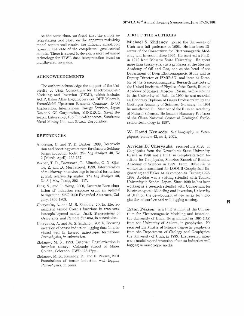
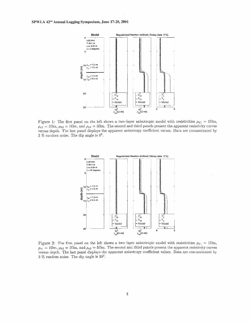
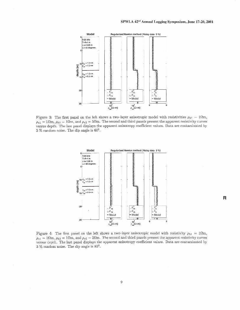
Two-layer model with a dip angle We as­sume tha t tensor ind uct ion logging is conducted by a tool coaxial with a borehole. We calculate the model responses (indu ction tensor components) for th e dif­ferent positions ofthe tool along the bor ehole. Using these responses as th e synthetic data, we compute th e low frequency (O"~ a and O" ~ a) apparent conduc­tivities according to formulae (13) and (16) as an init ial model. Then more accurate est imations of the ap parent conductivit ies, O"ha and £Iva, were com­puted using th e Newton inversion , as described in the previous sect ion. The results were plotted as ap parent resistivity curves, P~a ' P~a ' Pha, and pva, versus depth for a different dip angle a, equal to 0, 30, 60, and 85 degrees, respectively (Figure s 1- 4).

Each of the Figures (1-4) has four panels. The first panel on t he left shows the parameters of the two layer model. The second two panels present the apparent resistivity curves versus depth. The last panel displays th e apparent anisot ropy coefficient values versus depth. The solid lines show th e true parameters of the model. The apparent resist ivit ies

and anisot ropy coefficient, P~a ' P~a , and A~, ob­tained by the low frequency asymptotics, are shown by the dotted lines. The circles represent the in­vert ed apparent resistivit ies and anisotro py coeffi­cient , Pha, Pva, and Aa·

The data were contaminated by 3% random Gaus­sian noise at each observat ion point . One can see th at th e low frequency asymptotics overestimates th e vertical resistivities and t he anisot ropy coeffi­cient for dip angle values below 45 degrees. At a equal to 60 degrees, t he ap parent parameters are surprisingly close to the t rue model. At the larger dip angle (a =85 degrees) the low frequency asymp­toties underest imat e th e vert ical resistivities and th e anisotropy coefficient . At the same t ime, the appar ­ent par ameters inverted by use of th e regulari zed Newton method are very close to th e true parame­ters of the model for any dip angle (the curves shown by circles in Figures 1-4).

Note th at in this model, with the convent ional in­duction tool, we can obtain only one apparent con­ductivi ty, which reflects the integrated effect of both vertical an d horizont al conduct ivit ies.

The boun dary cannot be seen by using only th e apparent resistivity expression for Pha (Figure 1). But the vert ical apparent resistiv ity clearly responds to the position of th e boundary. The Pva curve changes sharp ly when the tool reaches the bound­ary. Thi s model provides a simple illust ration of an important addit ional power of tensor induction well logging in anisot ropic formation in comp arison with the t radit ional induction logging tool.

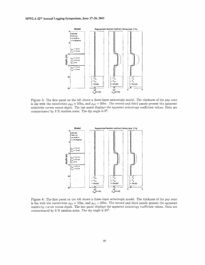
Three-layer model with a dip angle In the next set of numerical simulations, we consider a mode l of a three-layer formation. Figur e 5 shows the model on the left panel. Thi s model is a very good example of a practical situation where conven­t ional induct ion logging can miss a geological struc­ture . The layer th ickness is 5m. There is no hor ­izontal conduct ivity variat ion in t his model, while the vertical conduct ivity of the second layer is dif­ferent from th e top and bottom layers. On the sec­ond panel from the left , representing the horizontal apparent resistivi ties, we cannot see any indication of the second layer. However , it is possible to deter­mine the layer boundari es by using vert ical resistiv­ity informat ion (the third panel from t he left ). The last panel displays the ani sotropy coefficient values versus depth.

The synthet ic data simulated for th is model were contaminated by 3% random Gau ssian noise. The solid lines show the true parameters of the model.

R

5

SPWLA 42nd Annual Logging Symposium, June 17-20,2001

The apparent resistivities and an isotropy coefficient , P~a ' P~a ' and A~ , obtained by low frequency asymp­toties, are shown by th e dotted lines. Th e circles represent t he inverted apparent resist ivities pha, Pva, and anisotropy coefficient , Aa , computed using the regularized Newton meth od . Figu re 5 presents the TIWL data interpretat ion results for a case of a ver­tical well (the dip angle a is equal to 0). Figures 6-8 show similar results for the different dip angles 30, 60, and 85 degrees, respect ively. One can observe th e same regulari ty in th ese plots as in Figu res 1-4. The low frequency asymptot ics overestimates the verti­cal resistivi ties and th e anisotropy coefficient for dip angle values below 45 degrees, and und erestimates these parameters for a dip angle above 60 degrees. T he inversion of TIWL data, based on t he Newton method, provides practically correct reconstruction of the true parameters of th e model within the ent ire range of dip angles (th e curves shown by circles in Figu res 5-8).

Multi-layer models of anisotropic for­mations with a dip angle We considered three multi- layered models of anisotropic forma­t ions , based on the well known benchmark mod­els: And erson and Bar ber (1999) model, "Okla­homa" model, and "Chirp" mode l. The first one is a modified model , considered by Anderson and Barber (1999, p.135, Figure 3). The horizontal re­sisti vity profile of our model is the same as in An­derson and Barber (1999). It is shown by the solid line in the left panel of Figure 9. We int roduced the anisotropic layers in this model with the vertical re­sist ivity shown by th e solid lines in the right pan el of Figure 9. We simulated the synthet ic data for this model using a library of 3- D Green 's tensors in the layered anisotropic formations (Cheryauka and Zhdanov, 200la) . The data were contaminated by 3% ra ndom Gaussian noise. Figure 9 presents th e TIWL data interpretat ion result s for the case of a vertical well (the dip angle a is equal to 0). Fig­ure 10 present s similar resul ts for the dip angle of 30 degrees . The solid lines show the true param­eters of the model. The apparent resistiv it ies and anisot ropy coefficient, P~a ' P~a ' and A~ , obtained by th e low frequ ency asymptotics, are shown by the dotted lines. The circles represent the invert ed ap­parent resistivities Pha , Pva, and anisot ropy coeffi­cient , Aa , computed using the Newton method.

The second multi- layered model is the "Ok­lahoma" model (Bar ber et aI., 1999). In our anisotropic mod el we use the same horizontal resis­tivity as in the original "Oklahoma" model (solid

6

line in th e left panel of Figure 11) but we also add some an isotropy to the model by assigning various vertical resistivities (solid line in the right panel of Figure 11). The comput er simulated data for this model with 3% random noise added were processed using the TIWL interpretation technique out lined above. Th e results of interpretation for t he dip an­gles of 0 and of 30 degrees are presented in Figure 11 and 12. One can see that we can reconstruct well the horizont al resisti vity distribution, while the vertical resistivi ty is mostly underestimated in th is case.

The third model is the "Chirp" model (Fang and Wang, 2000), represented by a solid line in the left panel of Figure 13 (the hor izont al resistivity profile). We modified thi s model, adding a profile of vertical resistivity (right panel in Figure 13). The results of the synthetic TIWL data int erpretation for different dip angles are shown in Figur es 13-14. Once again the ap parent resistivities describe well the horizontal resist ivity, but recover the vertical resistivity much less successfully. These results show t hat, in the case of complicated geoelectri cal mode ls, the simple interpretation tool based on the apparent resistivity mode l cannot well resolve the different anisotropic layers. In this case one should use more advanced technology based on multilayered inversion . Some element s of this development are discussed in the paper by Cheryauka and Zhdanov (2001b) .

CONCLUSIONS

In th is paper we examined the basic principles of tensor induct ion well logging (TIWL) in the devi­ated boreho le in anisot ropic layered formations. We introduced a simp le technique of TIWL data inter­pretat ion based on calcu lat ing the components of the apparent conductivity tensor ("horizontal" and "vertical" apparent conduct ivity ). In th e case of low frequency asymptotics, we can use the analytical ex­pressions for apparent cond uct ivity (or resist ivity) tensor calculat ions. In the higher frequency range, one can use a regularized Newton method to gen­era te the corresponding apparent conductivities (or resistivities) of t he anisotropic media.

We analyzed th e responses of synthetic tensor in­duction logs in the deviated borehole through two-, three-, an d multi-layer anisotropic formations in vertical and deviated wells using numerical simula­tion. Our results demonstrate that the tensor in­strument is sensitive to ani sotropic parameters of geological formations . These cannot be detected in a general case by conventional indu ction logging.

SPWLA 42nd Annual Logging Symposium, June 17-20, 2001

At the same t ime, we found that the simple in­te rpretation too l based on the apparent resistivi ty model cannot well resolve th e different anisotropic layers in the case of th e compl icated geoelectrical mode ls. There is a need to develop a more advanced technology for TIWL dat a int erpretation based on multi layered inversion.

ACKNOWLEDGMENTS

Th e authors acknowledge the support of the Uni­versity of Utah Consortium for Electromagnetic Modeling and Inversion (CEMI) , which includ es AGIP, Baker Atlas Logging Services, BHP Minerals, ExxonMobil Upstream Resear ch Company, INCO Exploration, International Energy Services, J apan Nat ional Oil Corp oration , MINDECO , Naval Re­search Laboratory, Rio Tinto-Kennecot t , Sumitomo Metal Mining Co., and 3JTech Corporation.

REFERENCES

Anderson , B. and T. D. Barb er, 1999, Deconvolu t ion an d boost ing parameters for obsolete Schlum­berger induction tools: The Log A nalyst, 40 , No 2 (March-April), 133-137.

Barb er , T. D. , Broussard, T ., Minerbo, G. N. Sijer­cic, Z. and D. Mur gatroyd, 1999, Interpretation of mult iarray induct ion logs in invaded form ations at high relative dip angles: The Log Analyst , 40, No 3 ( May-June), 202 - 217.

Fang, S., and T. Wang, 2000, Accurate Born simu­lation of indu ction response using an opt imal background: SEG 2000 Expand ed Abstracts, Cal­gary, 1806-1809.

Cheryauka, A. and M. S. Zhdanov, 2001a, Elect ro­magnetic tensor Green's funct ions in transverse isot ropic layered media: IEEE Transa ction s on Geoscience and R emote Sensing, in submission.

Cheryauka , A. and M. S. Zhdanov, 2001b , Focusing inversion of tensor induction logging data in a de­viated well in layered anisotropic formations: Petrophysics, in submiss ion.

Zhdanov, M. S., 1993, Tutorial: Regularizati on in inversion t heory; Colorado School of Mines, Golden , Colorado, CWP-136,47pp.

Zhdanov, M. S., Kennedy, D., and E. Peksen, 2001, Foundations of tensor induct ion well logging: Petrophysics, in press.

ABOUT THE AUTHORS

Michael S. Zhdanov joined th e University of Utah as a full professor in 1993. He has been Di­rector of the Consortium for Electromagnetic Mod­eling and Inversion since 1995. He received a Ph.D. in 1970 from Moscow State University. He spent more than twenty years as a professor at the Moscow Academy of Oil and Gas, and as the head of th e Department of Deep Electromagnet ic Study and as Deputy Director of IZMIRAN, and later as Direc­tor of the Geoelectromagnetic Resear ch Insti tu te of the United Institute of Physics of the Ea rth, Russian Academy of Science, Moscow, Russia, before moving to the Univers ity of Utah. In 1990 he was awarded an Honorary Diploma of Gauss P rofessorship by the Gottingen Academy of Sciences, Germany. In 1991 he was elected Full Member of the Russian Academy of Natural Sciences. He became Honorary P rofessor of the China Natio nal Center of Geological Explo­ration Technology in 1997.

w. David Kennedy See biography in P etro­physics, volume 42, no 2, 2001.

Arvidas B. Cheryauka received his M.Sc. in Geophysics from the Novosibirsk State University, Russia in 1986 and a Ph.D in Geophysics .from In­stitute for Geophysics, Siberian Branch of Russian Academy of Sciences in 1989. From 1995-1998 he worked as a consult ant for LOOCH Geophysical En­gineer ing and Baker Atlas companies. During 1998­1999, Arvidas was a visit ing scientist with Tohoku University in Sendai , J apan. Since 1999 he has been workin g as a research scienti st wit h Consortium for Electromagnet ic Modeling and Inversion, University of Utah on the development of new ar ray technolo­gies for subsurface and well-logging sensing. R Ertan Peksen is a PhD student at the Consor ­t ium for Electromagnetic Modeling and Inversion, the University of Ut ah . He graduated in 1993 (BS) from th e University of Ankara, in geophysics. He received his Master of Science degree in geophysics from the Department of Geology and Geophysics, the University of Utah, in 1999. His research inter­est is modeling and inversion of tensor induction well logging in anisotropic media.

7

SPWLA 42nd Annual Logging Symposium, June 17-20, 2001

Model ° l~-~--­

1:;:20 kHz

T-R=1 m fi z= 0.2 5 m Ct :;: 0 degrees

_10 !phl =1 n-m .§. IPvl :;: 1 O:- m

.s::: Q.

1 il m~ IPh2 ::: ­15 ~V2 =5 n-m

20

25 LI __~_-,

Regularized Newton method ( Noisy data 3 %)

,, ,.

'i 1 "

f '. , : : , ~

! \:

" ~ ~ .. . ,I ~ t I: :

, .' 1 !

A' . P~a . a'Pha o Aao Pha o Pya

- Model- Model - Model

~ 510' la'

Pha(Q- m) pv.(Q- m)

Figure 1: Th e first panel on the left shows a two- layer an isotropic model with resisti vities Ph I = 10 m, Pvl = 10 m, Ph 2 = 10 m, and Pv2 = SOm. The second and third panels present th e app arent resistivity curves versus depth. The last panel displays th e apparent anisotropy coefficient values. Data are contaminated by 3 % random noise. The dip angle is 0°.

Model a

11=20 kHz T. R: ' m 6 z= O.25 m a :;: 30 degreesI

_,:I... t n- rn

g ~" : , ,, -m s:

~ Ipn2 ::: 1Q-m

't:J1S fPv2= s O-m

20

25 LI --~---'

Regularized Newton method ( Noisy data 3 %)

'.

:: : ~ i >;

i

' f \

"

; ;

. Pha

o Pha

- Model

) : , J ~

::j

J - ' ):

It, ~ .( -,

\ : ~ ) ~il ,: ~ }

. P ~a o Pya

- Model

I

; '

4-ci-. ~ . ": t :':.j

j }

• Aa o Aa - Model

" . io" la' a

Ph. (Q- m) p,.(Q- m)

F igure 2: The first panel on the left shows a two- layer anisot ropic model wit h resistivi ties Phl = 10m, Pv l = 10m, Ph2 = 10m, and Pv2 == SOm. The second and third panels present the apparent resist ivity curves versus depth. T he last panel displays the apparent anisotropy coefficient values. Data are contaminat ed by 3 % random noise. The dip angle is 30°.

8

SPWLA 42nd Annual Logging Symposium , June 17-20, 2001

Model O....--~-~,

1=20 kHz T-R=1 m 6 2= 0.25 m (l :;;; 60 degrees

5 "

Regul arized Newton method ( Noisy data 3 %) ~

,I ,It

>~

\ C:1.:;11~ ~ :: j. \'.~" ': 5

'~ >;

"I" r 20 . A. Pya I ·Pha

: a

C Aa(; Pya D Pha

- Model - Model - Model

I . > 25 L.--~----'

'0' '0' Ph. (fl- m) p, . (fl- m)

Figure 3: The first panel on th e left shows a two-layer anisot ropic model with resistivit ies Phl = 10 m, Pvl = 10m, Ph 2 = 10 m, and poz = 50 m. The second and third panels present th e appare nt resistivity curves versus depth. The last panel displays the apparent anisot ropy coefficient values. Dat a are contaminat ed by 3 % random noise. The dip angle is 60°.

Model O....--~--..,I

1;20 kHz

T-R =1 m li.z- O.25 m Q =85 degrees

5 "

~ ,olPh, = 1 n-m ~ Ip" = 1 !l- m

~ !Ph2= 1n - m 1 5 ~V2 = 5 n-m

20

2SL.__~_-JI

Regularized Newton method ( Noisy data 3 %)

>'e

,

~

::\ i:>': ' ~

• Pha

C Pha

- Model ,

,n H I,:

'1 1 :1

i\ t.,.

~ ~ .:'(, >! ~:: I

fpa o Pya - Model

; '

k

T f. I .. . \

: i.

f A

a o Aa

- Model

R

o10' 10' Ph. (fl- m) pv. (fl- m)

F igure 4: The first panel on the left shows a two-layer anisotropic model with resistivity Ph l = 10 m, Pvl = 10 m, Ph2 = 10m, and Pv2 = 50m. The second and third panels present the apparent resistivity curves versus depth. The last panel displays th e appare nt anisotropy coefficient values. Dat a are contamina ted by 3 % random noise. The dip angle is 85°.

9

SPWLA 42nd Annual Logging Symposium, June 17-20,2001

Model Regularized Newton method ( Noisy data 3 'Yo)

P =1 Q- m hl

Pvl ::. 1 Q- m

~10c' -- ­

" i

"

:

' [

,

! i

~

' Pha c Pha

- Model

.:

'I ':

:1 ':':' :

~~ " ,

w'" l ~

'I • Pya

o Pya - Model

'4a )~ Iph,=,n_m a. pv2= sn- m .g h2=5m ,(I , . '

15--­ rrPh'=' n-m ~ Pv3= 1 Q- m

I20 )Y

, a

o "'a - Model

25 LI _ _ ~_---,

10' 10' Pha(Q- m) pva(Q- m)

Figure 5: T he first panel on the left shows a t hree-layer anisot ropic model. Th e thickness of the pay zone is 5m with t he resisti vities Ph2 = 10m, and Pv2 = 50m. T he second an d third panels present the apparent resisti vity curves versus depth. Th e last panel displays the apparent anisotropy coefficient values. Dat a are cont ami nated by 3 % random noise. Th e dip angle is 00

.

Model 0

1=20 kHz

T-R=l m

A z= O.25 m a = 30 degr ees

5

Ph' =1 n-m Pvt =1 Q- m

_1 0

.§. s: [Ph' .ln-m

pv2 = S fi - m 1i. III h2=5 m "0

1 ; Ph3 ;;; 1 Q- m Pv3= t Q- m

)

;

RegUlarized Newton method ( Noisy data 3 'Yo)

I:

i I:

~~ .

:; ~ 'f ~ .

,7"

,'\ . Pya

o Pya - Model

, "

~

'j

[

. ~

f'

lh­-<;1" \

,.i ,:}

i 0'

il' i I, ;

] 1

)Y . a

Phao Pha o "a 1- Mod el - Model

10' 10' Pha(Q-m) pva(Q- m)

F igure 6: T he first panel on the left shows a three-layer anisot ropic model. T he thickness of the pay zone is 5m wit h the resistivi ti es Ph2 = 10m, and Pv2 = 50 m. The second and third panels present the apparent resistivi ty curves versus depth. Th e last panel displays the ap parent anisotropy coefficient values. Dat a are cont aminated by 3 % random noise. Th e dip angle is 300

.

10

Model 0

1=20kHz

T-R=1 m lJ. z= O.25 m a = 60 degrees

;

Ph1= 1Q- m P :::; 1 n-m

v1

1

Ph2 = 1 Q- m

pv: ::: S Q- m

h2 =5m

1 ; PJ13;: 1 Q- m

Pv3 :::1 Q- m

1

2S

~1

.§.

.t: Q.., '0

SPWLA 42nd Annual Logging Symposium, June 17-20, 2001

Regularized Newton method ( Noisy data 3 %)

,

:1

g .~

~ rf ; ~

, ,:­

• Pha o Pha

- Model

'. 10'

Pha(Q-m)

" ,:

;: 1

, D!

:,1 . Pya

o Pya

- Model

I:t.... ~'t-

;>,

~

)!• a

o i'a - Model

10' pv.(Q- m)

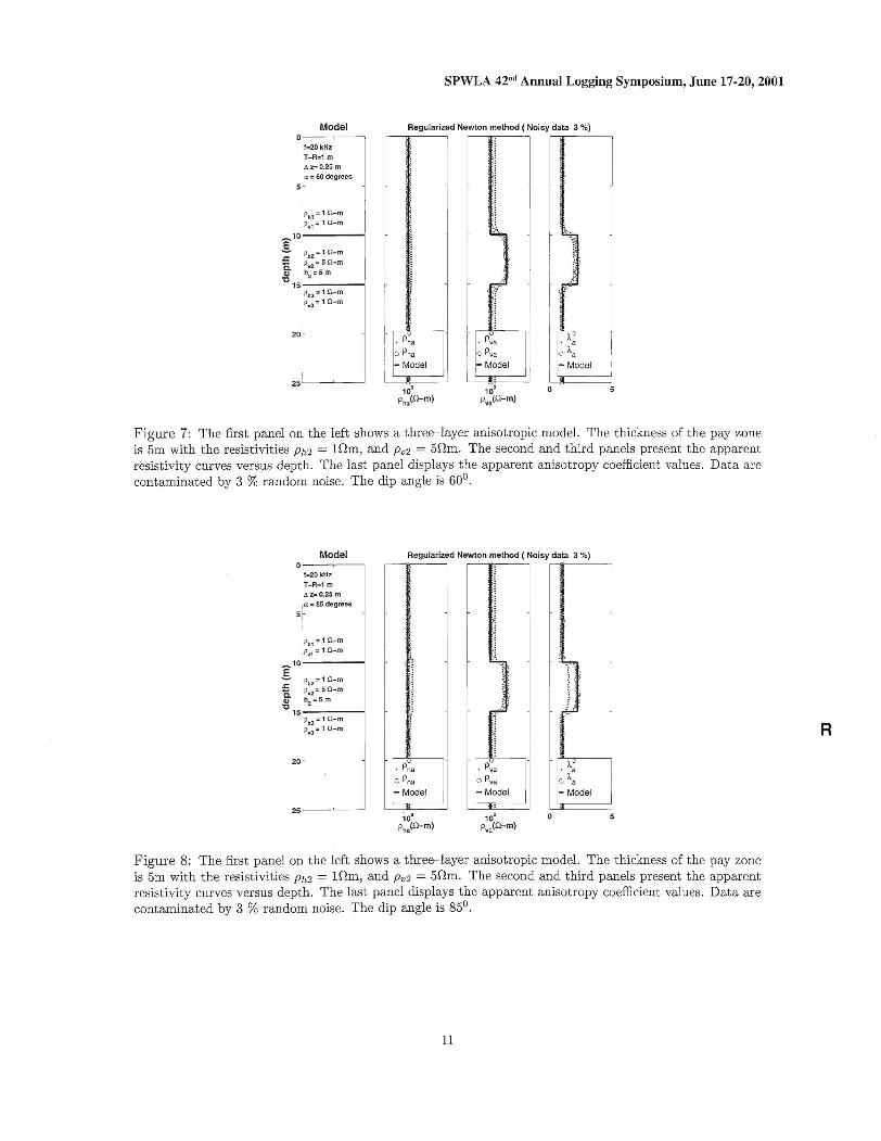
F igure 7: The first panel on the left shows a three-layer anisot ropic model. The thickness of t he pay zone is Sm with the resistivities Ph2 = 1l1m, and Pv2 = SOm. The second and third panels present t he apparent resisti vity curves versus depth. The last panel displays the apparent an isotropy coefficient values. Dat a are contaminated by 3 % random noise. The dip angle is 60°.

Model 0

1=20 kHz

T-R=l m !J.z=0.25 m 0: .: 85 degrees

S

P = 1 Q-mhl Pvl ;: 1 Q- m

1

Ph2 = 1 Q-m Pv2 :::S Q-m

h2=5 m

; Ph3:::1 D:- m Pv3 = 1 Q- m

1

;

~1

.§. s: Q.., '0

1

RegUlarized Newton method ( Noisy data 3 %)

~ .:' ,: ·,1

I ~

r 11

~--~, .....--fOi---­

.

• Pha o Pha

- Model

10' Ph. (Q- m)

i '1 , .'~ \ : .:

'1 . ':. .'

-

1 #.." ~

, : R '1

)!. Pya • a

o Pya C A.a - Model Model

:

10' pv.(Q- m)

Figure 8: The first panel on t he left shows a three-layer anisot ropic model. The thickness of t he pay zone is Sm with the resistiv iti es Ph2 = 10m, and Pv2 = SOm. The second and third panels present t he apparent resistivity curves versus depth. The last panel displays th e appare nt anisot ropy coefficient values. Data are contaminated by 3 % random noise. The dip angle is 8So.

11

SPWLA 42nd Annual Logging Symposium, June 17-20,2001

Regular ized Newton method -

P~a o Pha - Model

I 10

15

:[20

s: Q. <l> 25 "C

30

35

40

45

( <>=0" Noisy data 3 %)

Pva o Pva

Model

o

10~ 110- 1 10° 10' 10' 10° 101 10'

Pha(n- m) pva(n - m)

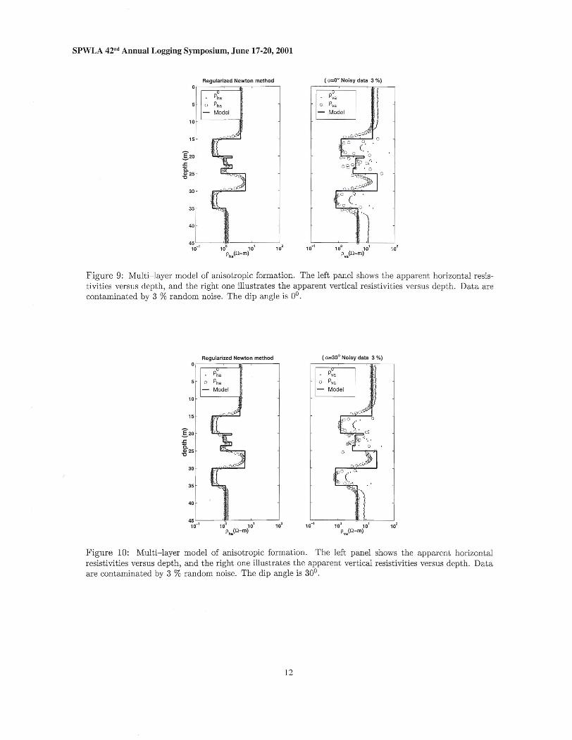
F igure 9: Mult i-layer model of anisotropic format ion. The left panel shows the apparent hor izontal resis­t ivities versus depth, and t he right one illustrates the apparent ver tical resist ivit ies versus depth. Data are contaminated by 3 % random noise. The dip angle is 0°.

Regularized Newton method ( <>=300 Noisy data 3 %)

~

o

;) Pva · I ~. o5 0 Pha Pva

Model r - Model 110 }

",&" "~ 15

:[20

s: Q. <l> 25

"C

30

35

40

45 10-1 10' 10' 10' 10-1

10° 101 10' Pha(n- m) pv.<n- m)

Figure 10: Multi- layer model of anisot ropic formation. The left panel shows the apparent horizontal resistivit ies versus depth, and th e right one illust rates the ap parent vert ical resistivities versus depth. Data are contaminated by 3 % ra ndom noise. The dip angle is 30°.

12

Regular ized Newto n method o --rl "

Pha

o PM 10

20

g J: 30 g. "tl

40

50

60 i!:l 2' -1 1 210-1 lOU 101 10 10' 10 . 10 10 10' Ph.(Q-m) pvo(Q-m)

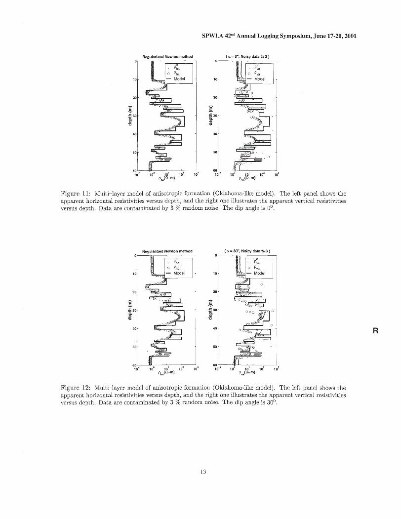
F igure 11: Mult i-layer model of anisotropic formation (Oklahoma-like model). Th e left panel shows t he apparent horizontal resistivities versus depth, and the right one illustrates the apparent vert ical resistiv ities versus depth. Data are contaminated by 3 % rand om noise. The dip angle is 0°.

SPWLA 42nd Annual Logging Symposium, June 17-20, 2001

( (J, = 0", Noisy dala % 3 )

10

20

g J: 30 a. CI> "tl

40

50

60' ' II! I I

o

Regular ized Newton method

60 ' IJII 10-1 10° 10

1 10

2 10' 10-1 to" 101

102 10'

Ph.(Q- m) pv. (Q- m)

F igure 12: Mult i- layer model of anisotropic formation (Oklahoma-like model) . The left panel shows the apparent horizontal resist ivities versus depth , an d the right one illust rates the apparent vert ical resistivities versus depth. Data are contaminated by 3 % random noise. The dip angle is 30°.

( (J, =30°, Noisy dala % 3 )

pv•

o Pya 10

20

g a30

Q)

"tl

40 R

50

60 ' ''I f I

o

10

20

g a30

CI> "tl

40

50

~~-;:::=:::.:;;::::::'====; . Pha

o Pha

- Model

. ~

13

SPWLA 42nd Annual Logging Symposium, June 17-20, 2001

50

100

150

:[ -a 200 Q)

"C

250

300

350

Pha Pha Model

400L--1I 2 310°

Regularized Newton method

I , "

I10' 10 10 10' PhaCQ- m)

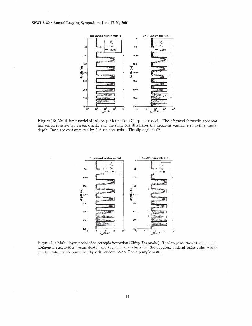
Figure 13: Multi-layer model of aniso tropic form ation (Chirp-like model). The left pa nel shows the apparent horizontal resistivities versus depth, and t he right one illustrat es t he apparent vertical resistivities versus depth. Dat a are contamina ted by 3 % random noise. The dip angle is 00.

50 ,

100 f

150

:[ :5 200 e, Q) "C

250

300

Regularized Newton method

Pha

~ o Pha Model

ill

,.,- ­_. ., ~~

( ex = 0'", Noisy data % 3 )

01 Ib I ' Ii

50

100

150

:[ :a200

Q)

"C

250

300

350

Pva

o Pva

- Mode l

2 310 10

p,.(Q- m)

o

Cex ; 30° • Noisy data % 3 ) 0

p,.

50 0 P,a - Model

100 0

~150i 0

.§..

a200

Q) "C

250

~' ..i

~L350

0:::Uit?: : 1 400 ,~ 1~ 1 ~ 1~ 10' 100 10' 10' 10' 10'

PhaCQ-m) p,.(Q- m)

Figure 14: Multi-layer model of anisotropic forma tion (Chirp-like model) . The left panel shows th e apparent horizontal resistivities versus depth, and the righ t one illustrates the apparent vertical resistivities versus depth. Dat a are contamina ted by 3 % random noise . The dip angle is 300 .

14