Embed Size (px)
Citation preview

[email protected] | Tel: +44 (0)20 32393041 | Fax: +44 (0)20 33573123 | www.engys.eu
Precompiled Applications and Utilities, Running Tutorials,
Running in Parallel,and General Post-Processing
Utilities
Eugene de Villiers13 June 2011
Copyright © 2011 Engys Ltd.
You Will Learn About...
Copyright © 2011 Engys Ltd.
• Pre-compiled applications and utilities in OPENFOAM®
• Running OPENFOAM® tutorials
• OPENFOAM® postprocessing and advanced running options
• Running OPENFOAM® in parallel
You Will Learn About...
Copyright © 2011 Engys Ltd.
• Pre-compiled applications and utilities in OPENFOAM®
• Running OPENFOAM® tutorials
• OPENFOAM® postprocessing and advanced running options
• Running OPENFOAM® in parallel
Getting started
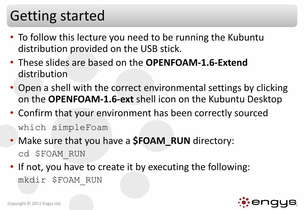
• To follow this lecture you need to be running the Kubuntudistribution provided on the USB stick.
• These slides are based on the OPENFOAM-1.6-Extend distribution
• Open a shell with the correct environmental settings by clicking on the OPENFOAM-1.6-ext shell icon on the Kubuntu Desktop
• Confirm that your environment has been correctly sourced
which simpleFoam
• Make sure that you have a $FOAM_RUN directory:cd $FOAM_RUN
• If not, you have to create it by executing the following:mkdir $FOAM_RUN
Copyright © 2011 Engys Ltd.
OPENFOAM® Applications
Copyright © 2011 Engys Ltd.
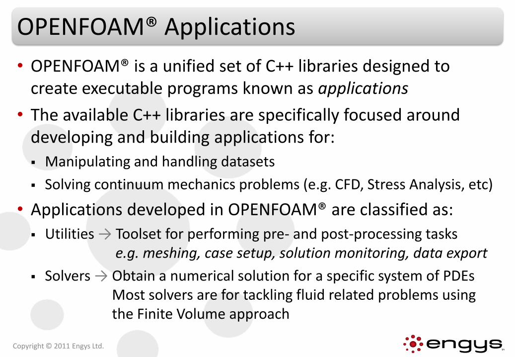
• OPENFOAM® is a unified set of C++ libraries designed to create executable programs known as applications
• The available C++ libraries are specifically focused around developing and building applications for:
Manipulating and handling datasets
Solving continuum mechanics problems (e.g. CFD, Stress Analysis, etc)
• Applications developed in OPENFOAM® are classified as:
Utilities → Toolset for performing pre- and post-processing taskse.g. meshing, case setup, solution monitoring, data export
Solvers → Obtain a numerical solution for a specific system of PDEsMost solvers are for tackling fluid related problems using the Finite Volume approach
Applications | Utilities Overview
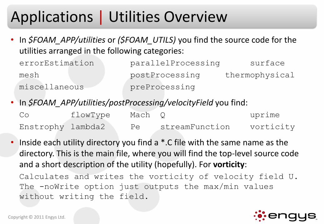
• In $FOAM_APP/utilities or ($FOAM_UTILS) you find the source code for the utilities arranged in the following categories:
errorEstimation parallelProcessing surface
mesh postProcessing thermophysical
miscellaneous preProcessing
• In $FOAM_APP/utilities/postProcessing/velocityField you find:
Co flowType Mach Q uprime
Enstrophy lambda2 Pe streamFunction vorticity
• Inside each utility directory you find a *.C file with the same name as the directory. This is the main file, where you will find the top-level source code and a short description of the utility (hopefully). For vorticity:
Calculates and writes the vorticity of velocity field U.
The -noWrite option just outputs the max/min values
without writing the field.
Copyright © 2011 Engys Ltd.
Applications | Utilities
Copyright © 2011 Engys Ltd.
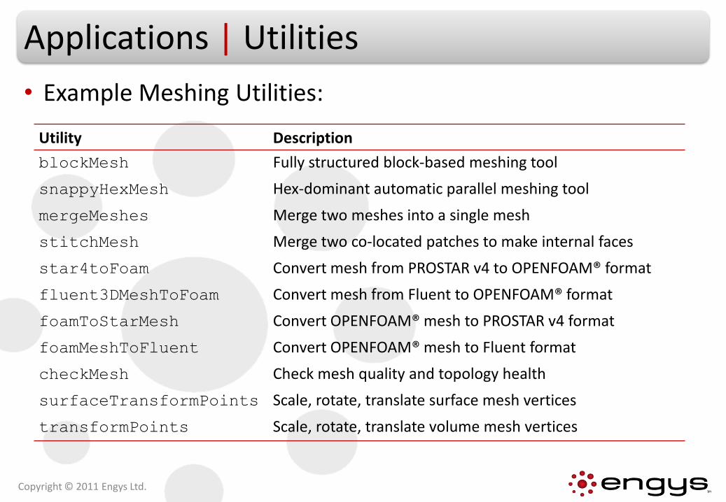
Utility Description
blockMesh Fully structured block-based meshing tool
snappyHexMesh Hex-dominant automatic parallel meshing tool
mergeMeshes Merge two meshes into a single mesh
stitchMesh Merge two co-located patches to make internal faces
star4toFoam Convert mesh from PROSTAR v4 to OPENFOAM® format
fluent3DMeshToFoam Convert mesh from Fluent to OPENFOAM® format
foamToStarMesh Convert OPENFOAM® mesh to PROSTAR v4 format
foamMeshToFluent Convert OPENFOAM® mesh to Fluent format
checkMesh Check mesh quality and topology health
surfaceTransformPoints Scale, rotate, translate surface mesh vertices
transformPoints Scale, rotate, translate volume mesh vertices
• Example Meshing Utilities:
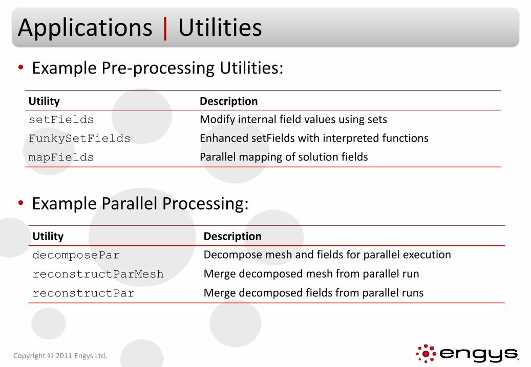
• Example Pre-processing Utilities:
• Example Parallel Processing:
Applications | Utilities
Copyright © 2011 Engys Ltd.
Utility Description
setFields Modify internal field values using sets
FunkySetFields Enhanced setFields with interpreted functions
mapFields Parallel mapping of solution fields
Utility Description
decomposePar Decompose mesh and fields for parallel execution
reconstructParMesh Merge decomposed mesh from parallel run
reconstructPar Merge decomposed fields from parallel runs
Applications | Utilities
Copyright © 2011 Engys Ltd.
Utility Description
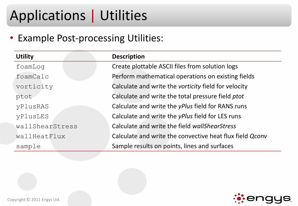
foamLog Create plottable ASCII files from solution logs
foamCalc Perform mathematical operations on existing fields
vorticity Calculate and write the vorticity field for velocity
ptot Calculate and write the total pressure field ptot
yPlusRAS Calculate and write the yPlus field for RANS runs
yPlusLES Calculate and write the yPlus field for LES runs
wallShearStress Calculate and write the field wallShearStress
wallHeatFlux Calculate and write the convective heat flux field Qconv
sample Sample results on points, lines and surfaces
• Example Post-processing Utilities:
Applications | Utilities
Copyright © 2011 Engys Ltd.
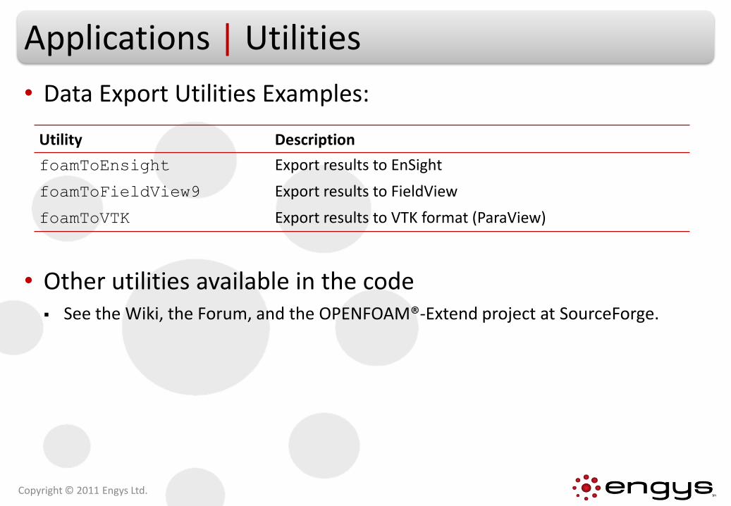
• Data Export Utilities Examples:
• Other utilities available in the code See the Wiki, the Forum, and the OPENFOAM®-Extend project at SourceForge.
Utility Description
foamToEnsight Export results to EnSight
foamToFieldView9 Export results to FieldView
foamToVTK Export results to VTK format (ParaView)
Solvers in OPENFOAM®
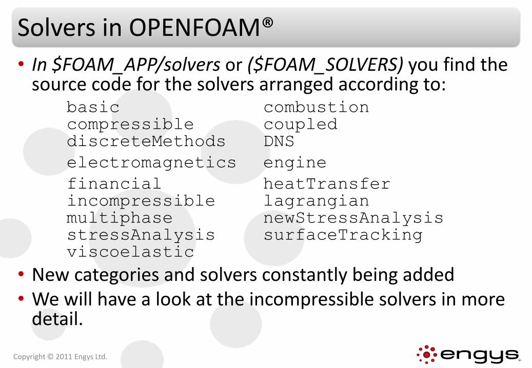
• In $FOAM_APP/solvers or ($FOAM_SOLVERS) you find the source code for the solvers arranged according to:
basic combustioncompressible coupleddiscreteMethods DNS
electromagnetics engine
financial heatTransferincompressible lagrangianmultiphase newStressAnalysisstressAnalysis surfaceTrackingviscoelastic
• New categories and solvers constantly being added• We will have a look at the incompressible solvers in more
detail.
Copyright © 2011 Engys Ltd.
Solvers in OPENFOAM®
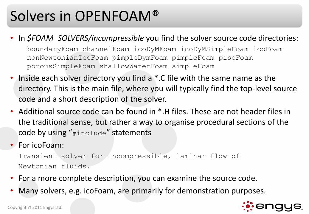
• In $FOAM_SOLVERS/incompressible you find the solver source code directories:boundaryFoam channelFoam icoDyMFoam icoDyMSimpleFoam icoFoam
nonNewtonianIcoFoam pimpleDymFoam pimpleFoam pisoFoam
porousSimpleFoam shallowWaterFoam simpleFoam
• Inside each solver directory you find a *.C file with the same name as the directory. This is the main file, where you will typically find the top-level source code and a short description of the solver.
• Additional source code can be found in *.H files. These are not header files in the traditional sense, but rather a way to organise procedural sections of the code by using “#include” statements
• For icoFoam:Transient solver for incompressible, laminar flow of
Newtonian fluids.
• For a more complete description, you can examine the source code.
• Many solvers, e.g. icoFoam, are primarily for demonstration purposes.
Copyright © 2011 Engys Ltd.
Applications | Solvers
Copyright © 2011 Engys Ltd.
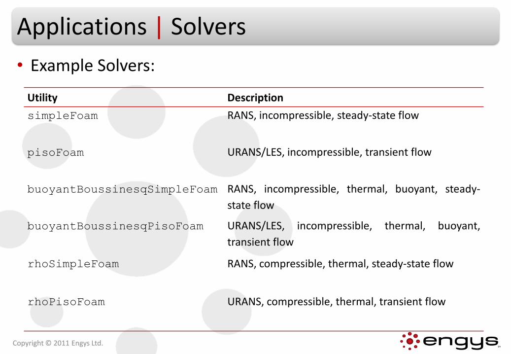
• Example Solvers:
Utility Description
simpleFoam RANS, incompressible, steady-state flow
pisoFoam URANS/LES, incompressible, transient flow
buoyantBoussinesqSimpleFoam RANS, incompressible, thermal, buoyant, steady-
state flow
buoyantBoussinesqPisoFoam URANS/LES, incompressible, thermal, buoyant,
transient flow
rhoSimpleFoam RANS, compressible, thermal, steady-state flow
rhoPisoFoam URANS, compressible, thermal, transient flow
You Will Learn About...
Copyright © 2011 Engys Ltd.
• Pre-compiled applications and utilities in OPENFOAM®
• Running OPENFOAM® tutorials
• OPENFOAM® postprocessing and advanced running options
• Running OPENFOAM® in parallel
Running Tutorials
• A simple tutorial is provided as an introduction to running a CFD simulation using OPENFOAM®.
• A simple external aerodynamics test case is considered.
• Initially a block mesh will be generated which will form a starting mesh for running the OPENFOAM® mesh generator snappyHexMesh.
• The mesh will then be run through OPENFOAM® initialisation routines before being run with a Reynolds Averaged Navier Stokes (RANS) flow solver.
Copyright © 2011 Engys Ltd.
Preparation
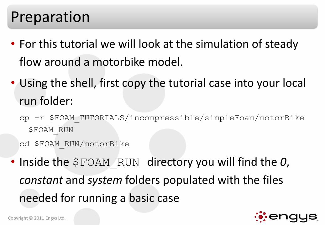
• For this tutorial we will look at the simulation of steady
flow around a motorbike model.
• Using the shell, first copy the tutorial case into your local
run folder:cp -r $FOAM_TUTORIALS/incompressible/simpleFoam/motorBike
$FOAM_RUN
cd $FOAM_RUN/motorBike
• Inside the $FOAM_RUN directory you will find the 0,
constant and system folders populated with the files
needed for running a basic case
Copyright © 2011 Engys Ltd.
Preparation
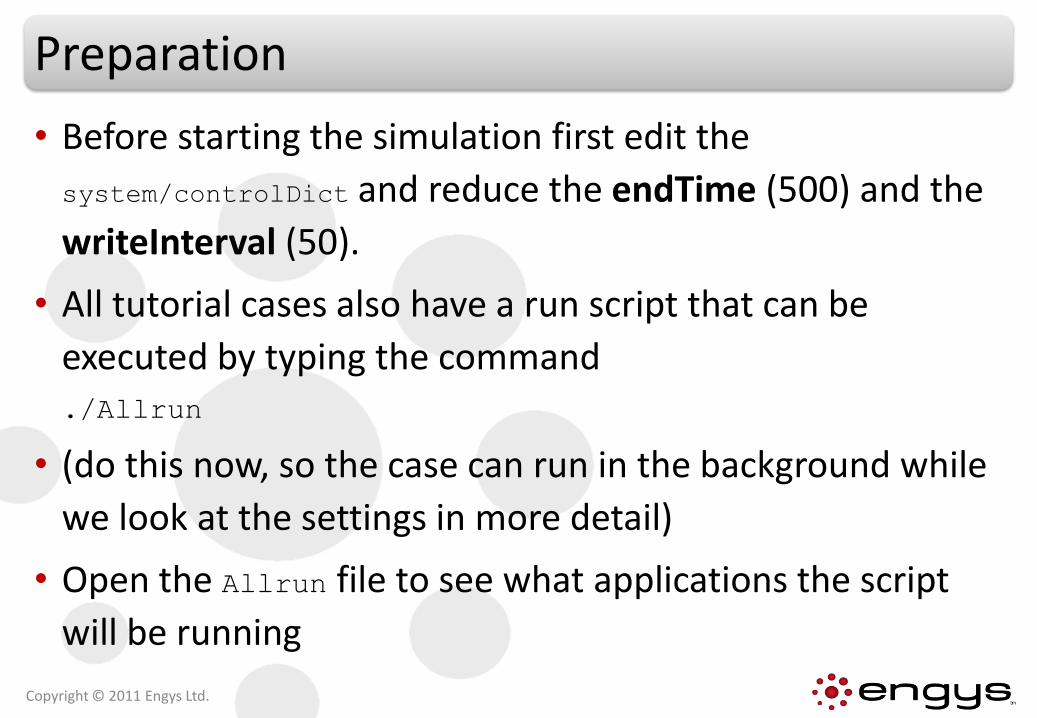
• Before starting the simulation first edit the
system/controlDict and reduce the endTime (500) and the
writeInterval (50).
• All tutorial cases also have a run script that can be
executed by typing the command./Allrun
• (do this now, so the case can run in the background while
we look at the settings in more detail)
• Open the Allrun file to see what applications the script
will be running
Copyright © 2011 Engys Ltd.
Creating a Base Block Mesh
• The application blockMesh is used for creating an initial base mesh which is needed for running the mesh generation application snappyHexMesh.
• The file blockMeshDict is used to control the block mesh generation process.
• By default the blockMesh application looks for this file in the constant/polyMesh folder.
• Alternatively the location of the file can be specified using the –dictoption at run time.
• You need the following files to be able to run blockMesh:
Dictionary file constant/polyMesh/blockMeshDict
Dictionary system/controlDict
Copyright © 2011 Engys Ltd.
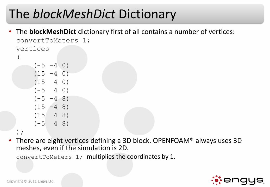
The blockMeshDict Dictionary• The blockMeshDict dictionary first of all contains a number of vertices:convertToMeters 1;
vertices
(
(-5 -4 0)
(15 -4 0)
(15 4 0)
(-5 4 0)
(-5 -4 8)
(15 -4 8)
(15 4 8)
(-5 4 8)
);
• There are eight vertices defining a 3D block. OPENFOAM® always uses 3D meshes, even if the simulation is 2D.convertToMeters 1; multiplies the coordinates by 1.
Copyright © 2011 Engys Ltd.

The blockMeshDict Dictionary• Next, blockMeshDict defines a block and the mesh from the
• vertices:
blocks
(
hex (0 1 2 3 4 5 6 7) (20 8 8) simpleGrading (1 1 1)
);
• hex means that it is a structured hexahedral block.
• (0 1 2 3 4 5 6 7) is the vertices used to define the block. The order of these is important - they should form a right-hand system with closed loops
0 - 1 is the “x” direction for number of cells and grading purposes
1 – 2 is the “y” direction for number of cells and grading purposes
“z” direction is found assuming a right-handed coordinate system
• (20 8 8) is the number of mesh cells in each direction based on the vertex definitions.
• simpleGrading (1 1 1) is the expansion ratio, in this case equidistant. The numbers are the ratios between the end cells along x, y and z edges.
Copyright © 2011 Engys Ltd.
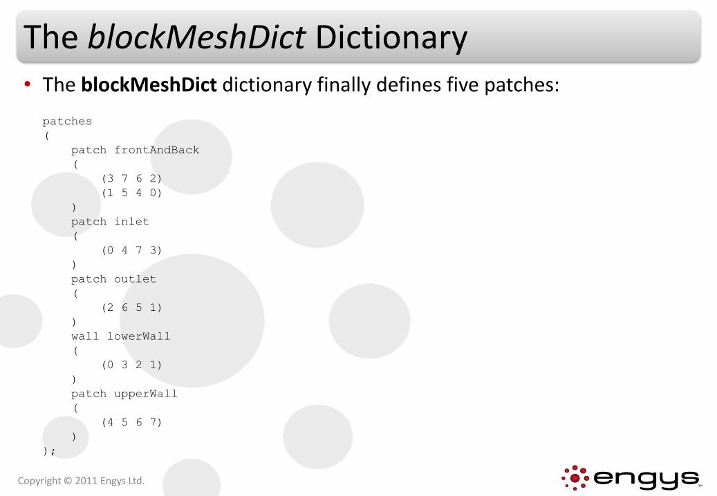
The blockMeshDict Dictionary• The blockMeshDict dictionary finally defines five patches:
patches
(
patch frontAndBack
(
(3 7 6 2)
(1 5 4 0)
)
patch inlet
(
(0 4 7 3)
)
patch outlet
(
(2 6 5 1)
)
wall lowerWall
(
(0 3 2 1)
)
patch upperWall
(
(4 5 6 7)
)
);
Copyright © 2011 Engys Ltd.
The blockMeshDict Dictionary
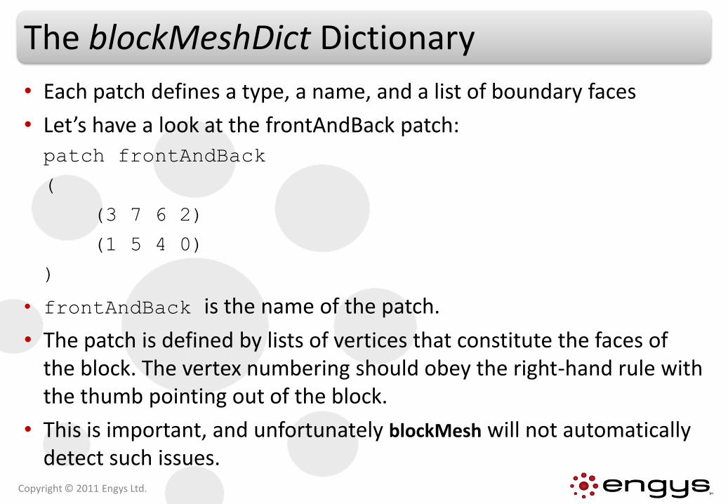
• Each patch defines a type, a name, and a list of boundary faces
• Let’s have a look at the frontAndBack patch:
patch frontAndBack
(
(3 7 6 2)
(1 5 4 0)
)
• frontAndBack is the name of the patch.
• The patch is defined by lists of vertices that constitute the faces of the block. The vertex numbering should obey the right-hand rule with the thumb pointing out of the block.
• This is important, and unfortunately blockMesh will not automatically detect such issues.
Copyright © 2011 Engys Ltd.
The blockMesh Utility
• The utility can be executed by issuing the following command from within the $FOAM_RUN/motorbike directory:
blockMesh
• This will generate a set of mesh files in the constant/polyMesh folder which make up the basic definition of a computational mesh for OPENFOAM®.
• A starting block mesh with a uniform resolution of 1 m everywhere will be produced
Copyright © 2011 Engys Ltd.
Generating a Mesh Using snappyHexMesh
• The block mesh created by blockMesh is used as a starting mesh for the mesh generation application snappyHexMesh.
• The dictionary snappyHexMeshDict inside the systemfolder is used for controlling the mesh generation process.
• Requirements: Dictionary file system/snappyHexMeshDict
Geometry data (stl, nas) in constant/triSurface
blockMesh files
Dictionary file system/decomposeParDict for parallel runs
Base system dictionaries (controlDict, fvSchemes, fvSolutions)
Copyright © 2011 Engys Ltd.
snappyHexMeshDict | Overview
Copyright © 2011 Engys Ltd.
• The snappyHexMeshDict in the example is in a compressed gzipformat. Unzip it with the following command before proceeding:
gunzip system/snappyHexMeshDict.gz
Open the dictionary file, it consists of five main sections:
• The snappyHexMeshDict in the example
• geometry → Prescribe geometry entities for meshing
• castellatedMeshControls → Prescribe feature, surface and volume mesh refinements
• snapControls→ Control mesh surface snapping
• addLayersControls→ Control boundary layer mesh growth
• meshQualityControls → Control mesh quality metrics
snappyHexMeshDict | Basic Controls
• The top level keywords in this dictionary castellatedMesh, snap and addLayers control the three main mesh generation stages refinement, surface recovery (snapping) and layer addition, respectively.
• Generally only the addLayers option tends to be switched on or off, the others are almost always switched oncastellatedMesh true;
snap true;
addLayers true;
Copyright © 2011 Engys Ltd.
snappyHexMeshDict | geometry
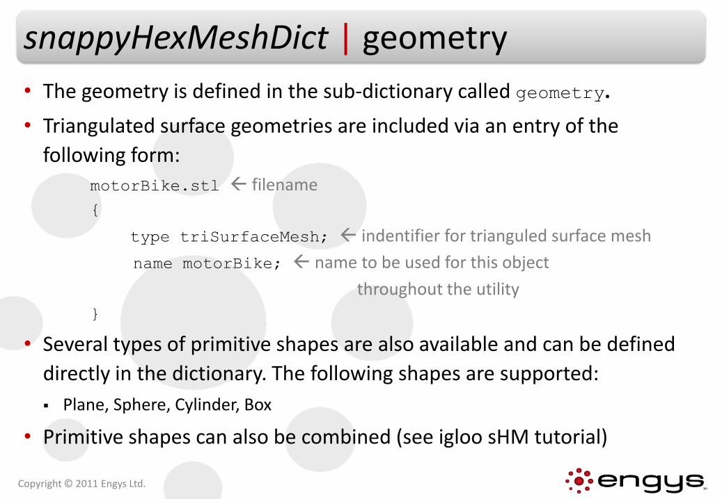
• The geometry is defined in the sub-dictionary called geometry.
• Triangulated surface geometries are included via an entry of the
following form:
motorBike.stl filename
{
type triSurfaceMesh; indentifier for trianguled surface mesh
name motorBike; name to be used for this object
throughout the utility
}
• Several types of primitive shapes are also available and can be defined
directly in the dictionary. The following shapes are supported:
Plane, Sphere, Cylinder, Box
• Primitive shapes can also be combined (see igloo sHM tutorial)
Copyright © 2011 Engys Ltd.
snappyHexMeshDict | geometry
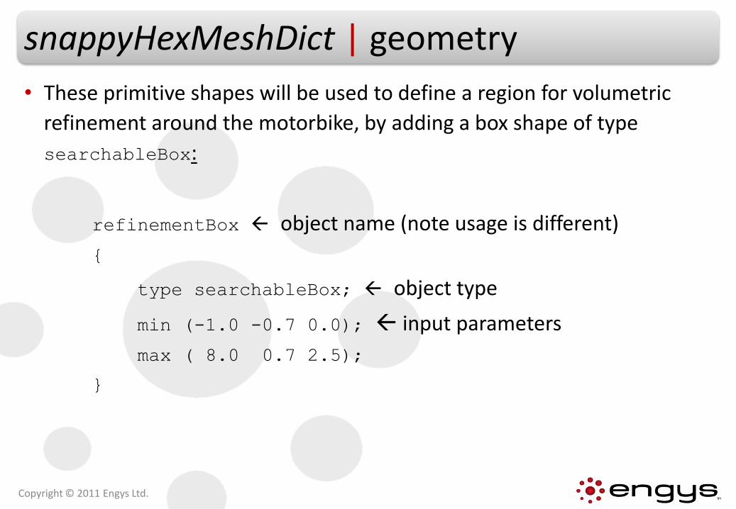
• These primitive shapes will be used to define a region for volumetric
refinement around the motorbike, by adding a box shape of type
searchableBox:
refinementBox object name (note usage is different)
{
type searchableBox; object type
min (-1.0 -0.7 0.0); input parameters
max ( 8.0 0.7 2.5);
}
Copyright © 2011 Engys Ltd.
snappyHexMeshDict | castellatedMesh
• The first stage of meshing is called refinement and is controlled by the castellatedMeshControls sub-dictionary settings. Three types of refinement take place:
Feature line
Surface
Volumetric
• Feature line refinement can be done by means of surface curvature or by specifying an explicit feature line via a FOAM format eMesh file.
Copyright © 2011 Engys Ltd.

snappyHexMeshDict | castellatedMesh
• The feature line and surface refinements are controlled by the settings inside the refinementSurfaces sub dictionary.
• The refinement is controlled by the keyword level which must be set for every surface
• The global level can optionally be overwritten for specific surface patch identifiers by specifying it inside a region{} subsection.
• Tip: you can see the region names in an STL file by executing:
gunzip constant/triSurface/motorBike.stl.gz
grep endsolid constant/triSurface/motorBike.stl
• The setting for level has two integer values:
The first is the minimum refinement level and this is the refinement level that is guaranteed to be generated on the specified surface
The second is the maximum refinement level which will be obtained if a given surface curvature threshold is triggered
Copyright © 2011 Engys Ltd.
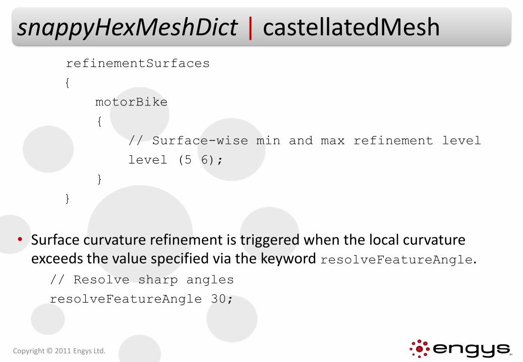
snappyHexMeshDict | castellatedMeshrefinementSurfaces
{
motorBike
{
// Surface-wise min and max refinement level
level (5 6);
}
}
• Surface curvature refinement is triggered when the local curvature exceeds the value specified via the keyword resolveFeatureAngle.
// Resolve sharp angles
resolveFeatureAngle 30;
Copyright © 2011 Engys Ltd.
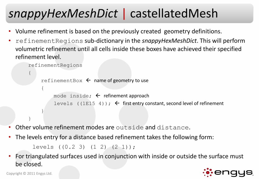
snappyHexMeshDict | castellatedMesh• Volume refinement is based on the previously created geometry definitions.
• refinementRegions sub-dictionary in the snappyHexMeshDict. This will perform volumetric refinement until all cells inside these boxes have achieved their specified refinement level.
refinementRegions
{
refinementBox name of geometry to use
{
mode inside; refinement approach
levels ((1E15 4)); first entry constant, second level of refinement
}
}
• Other volume refinement modes are outside and distance.
• The levels entry for a distance based refinement takes the following form:
levels ((0.2 3) (1 2) (2 1));
• For triangulated surfaces used in conjunction with inside or outside the surface must be closed.
Copyright © 2011 Engys Ltd.
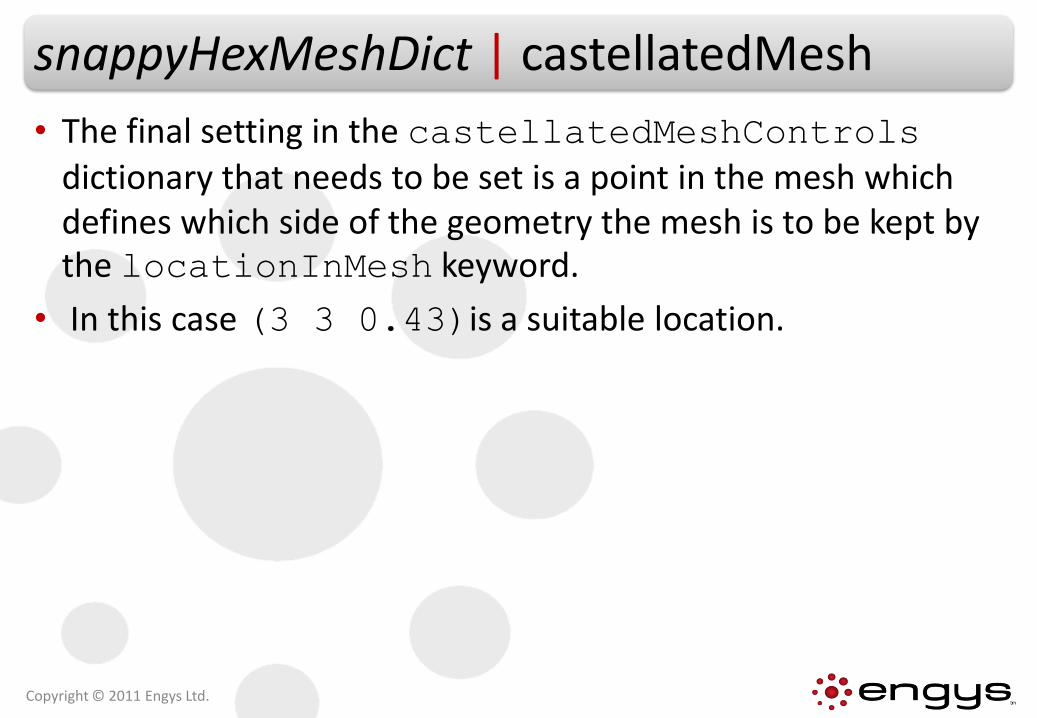
snappyHexMeshDict | castellatedMesh
• The final setting in the castellatedMeshControlsdictionary that needs to be set is a point in the mesh which defines which side of the geometry the mesh is to be kept by the locationInMesh keyword.
• In this case (3 3 0.43)is a suitable location.
Copyright © 2011 Engys Ltd.
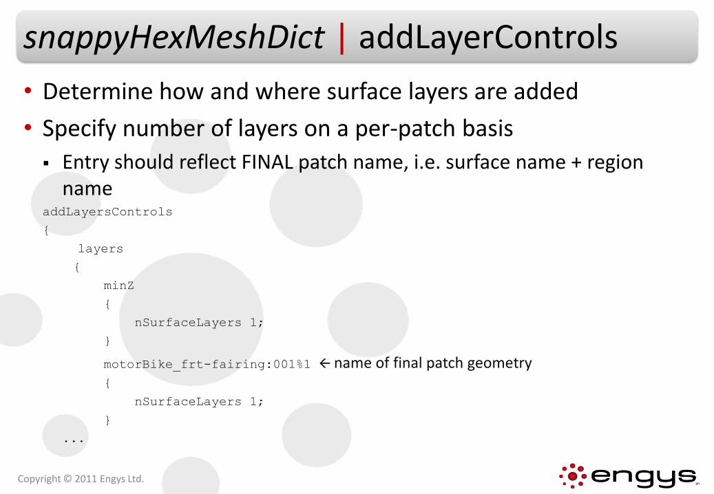
snappyHexMeshDict | addLayerControls
• Determine how and where surface layers are added
• Specify number of layers on a per-patch basis
Entry should reflect FINAL patch name, i.e. surface name + region name
addLayersControls
{
layers
{
minZ
{
nSurfaceLayers 1;
}
motorBike_frt-fairing:001%1 name of final patch geometry{
nSurfaceLayers 1;
}
...
Copyright © 2011 Engys Ltd.
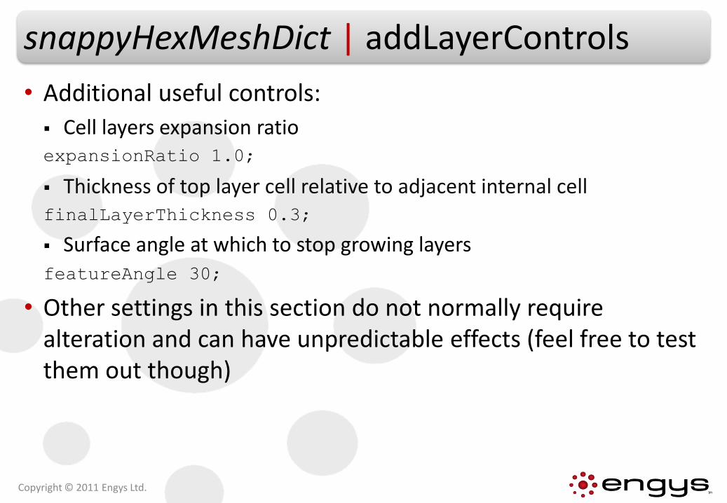
snappyHexMeshDict | addLayerControls
• Additional useful controls:
Cell layers expansion ratioexpansionRatio 1.0;
Thickness of top layer cell relative to adjacent internal cellfinalLayerThickness 0.3;
Surface angle at which to stop growing layersfeatureAngle 30;
• Other settings in this section do not normally require alteration and can have unpredictable effects (feel free to test them out though)
Copyright © 2011 Engys Ltd.
snappyHexMeshDict | Other Controls
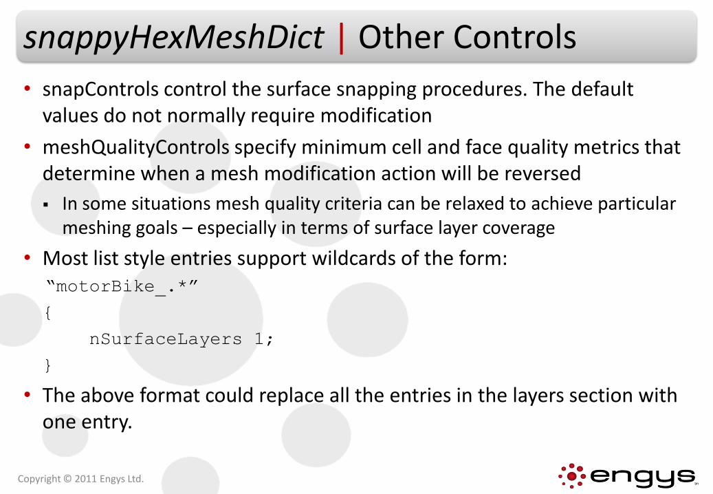
• snapControls control the surface snapping procedures. The default values do not normally require modification
• meshQualityControls specify minimum cell and face quality metrics that determine when a mesh modification action will be reversed
In some situations mesh quality criteria can be relaxed to achieve particular meshing goals – especially in terms of surface layer coverage
• Most list style entries support wildcards of the form:“motorBike_.*”
{
nSurfaceLayers 1;
}
• The above format could replace all the entries in the layers section with one entry.
Copyright © 2011 Engys Ltd.
Running snappyHexMesh and checkMesh
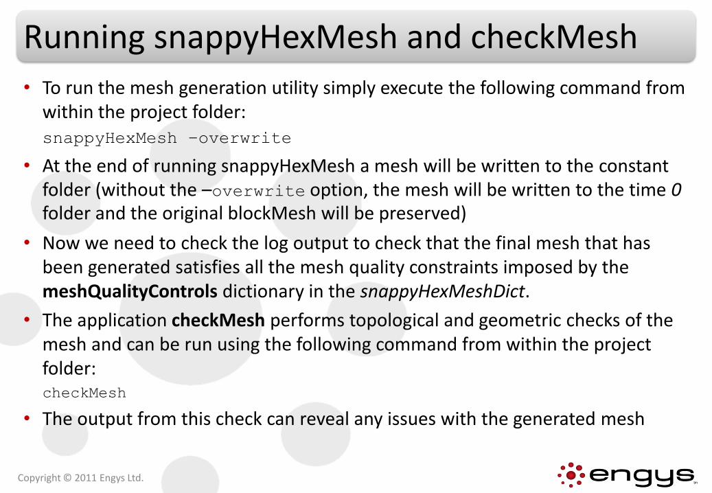
• To run the mesh generation utility simply execute the following command from within the project folder:snappyHexMesh –overwrite
• At the end of running snappyHexMesh a mesh will be written to the constant folder (without the –overwrite option, the mesh will be written to the time 0folder and the original blockMesh will be preserved)
• Now we need to check the log output to check that the final mesh that has been generated satisfies all the mesh quality constraints imposed by the meshQualityControls dictionary in the snappyHexMeshDict.
• The application checkMesh performs topological and geometric checks of the mesh and can be run using the following command from within the project folder:checkMesh
• The output from this check can reveal any issues with the generated mesh
Copyright © 2011 Engys Ltd.
Solver settings | Project Folders
Copyright © 2011 Engys Ltd.
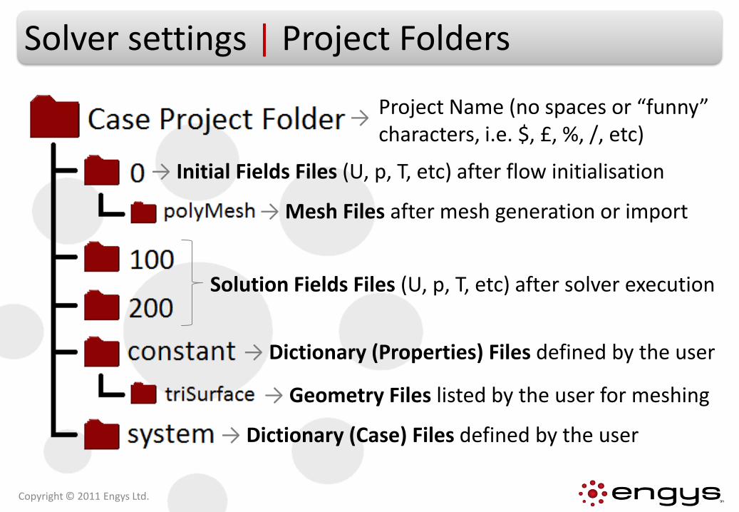
→ Mesh Files after mesh generation or import
→ Dictionary (Properties) Files defined by the user
→ Dictionary (Case) Files defined by the user
→ Geometry Files listed by the user for meshing
→ Initial Fields Files (U, p, T, etc) after flow initialisation
Solution Fields Files (U, p, T, etc) after solver execution
Project Name (no spaces or “funny” characters, i.e. $, £, %, /, etc)
→
Solver settings | system
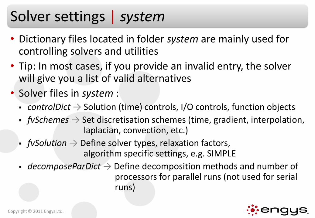
• Dictionary files located in folder system are mainly used for controlling solvers and utilities
• Tip: In most cases, if you provide an invalid entry, the solver will give you a list of valid alternatives
• Solver files in system : controlDict → Solution (time) controls, I/O controls, function objects
fvSchemes → Set discretisation schemes (time, gradient, interpolation, laplacian, convection, etc.)
fvSolution → Define solver types, relaxation factors, algorithm specific settings, e.g. SIMPLE
decomposeParDict → Define decomposition methods and number of processors for parallel runs (not used for serial runs)
Copyright © 2011 Engys Ltd.
Solver settings | system/controlDict
Copyright © 2011 Engys Ltd.
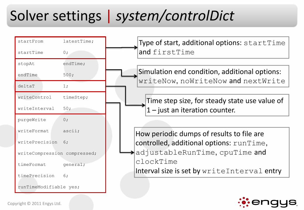
startFrom latestTime;
startTime 0;
stopAt endTime;
endTime 500;
deltaT 1;
writeControl timeStep;
writeInterval 50;
purgeWrite 0;
writeFormat ascii;
writePrecision 6;
writeCompression compressed;
timeFormat general;
timePrecision 6;
runTimeModifiable yes;
Type of start, additional options: startTimeand firstTime
Time step size, for steady state use value of 1 – just an iteration counter.
Simulation end condition, additional options: writeNow, noWriteNow and nextWrite
How periodic dumps of results to file are controlled, additional options: runTime,
adjustableRunTime, cpuTime and clockTime
Interval size is set by writeInterval entry
Solver settings | system/controlDict
Copyright © 2011 Engys Ltd.
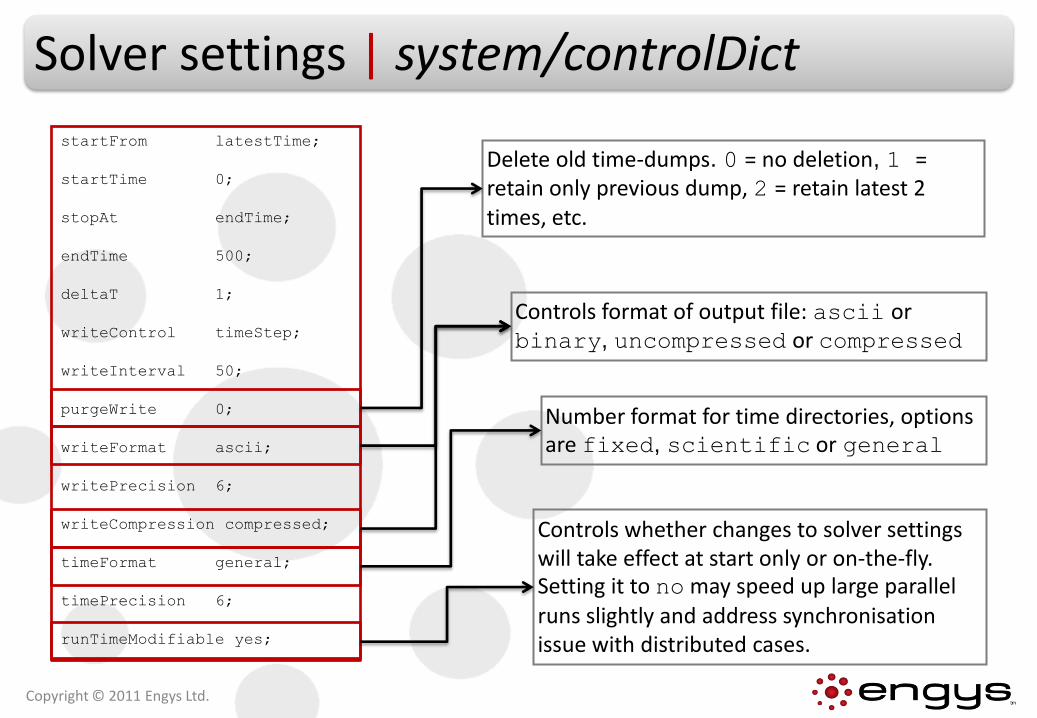
startFrom latestTime;
startTime 0;
stopAt endTime;
endTime 500;
deltaT 1;
writeControl timeStep;
writeInterval 50;
purgeWrite 0;
writeFormat ascii;
writePrecision 6;
writeCompression compressed;
timeFormat general;
timePrecision 6;
runTimeModifiable yes;
Delete old time-dumps. 0 = no deletion, 1 = retain only previous dump, 2 = retain latest 2 times, etc.
Controls whether changes to solver settings will take effect at start only or on-the-fly. Setting it to no may speed up large parallel runs slightly and address synchronisation issue with distributed cases.
Controls format of output file: ascii orbinary, uncompressed or compressed
Number format for time directories, options are fixed, scientific or general
Solver settings | system/fvSchemes
Copyright © 2011 Engys Ltd.
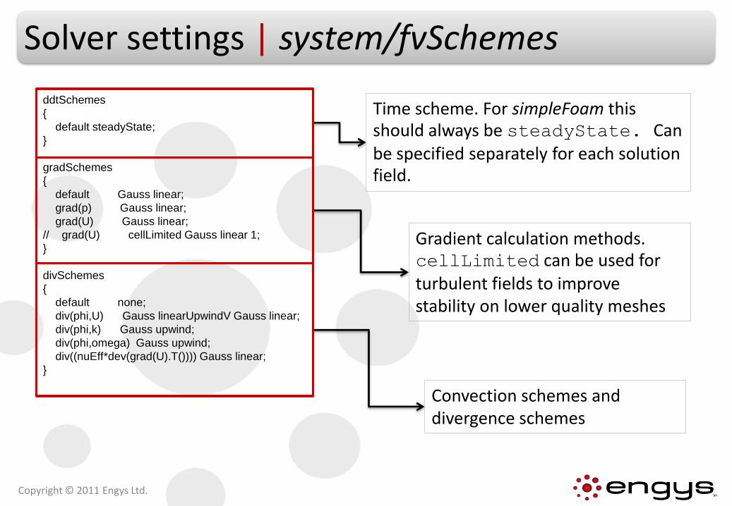
ddtSchemes
{
default steadyState;
}
gradSchemes
{
default Gauss linear;
grad(p) Gauss linear;
grad(U) Gauss linear;
// grad(U) cellLimited Gauss linear 1;
}
divSchemes
{
default none;
div(phi,U) Gauss linearUpwindV Gauss linear;
div(phi,k) Gauss upwind;
div(phi,omega) Gauss upwind;
div((nuEff*dev(grad(U).T()))) Gauss linear;
}
Time scheme. For simpleFoam this should always be steadyState. Can be specified separately for each solution field.
Convection schemes and divergence schemes
Gradient calculation methods. cellLimited can be used for turbulent fields to improve stability on lower quality meshes
Solver settings | system/fvSchemes
Copyright © 2011 Engys Ltd.
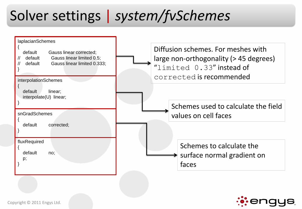
laplacianSchemes
{
default Gauss linear corrected;
// default Gauss linear limited 0.5;
// default Gauss linear limited 0.333;
}
interpolationSchemes
{
default linear;
interpolate(U) linear;
}
snGradSchemes
{
default corrected;
}
fluxRequired
{
default no;
p;
}
Diffusion schemes. For meshes with large non-orthogonality (> 45 degrees) “limited 0.33” instead of corrected is recommended
Schemes to calculate the surface normal gradient on faces
Schemes used to calculate the field values on cell faces
Solver settings | system/fvSolution
Copyright © 2011 Engys Ltd.
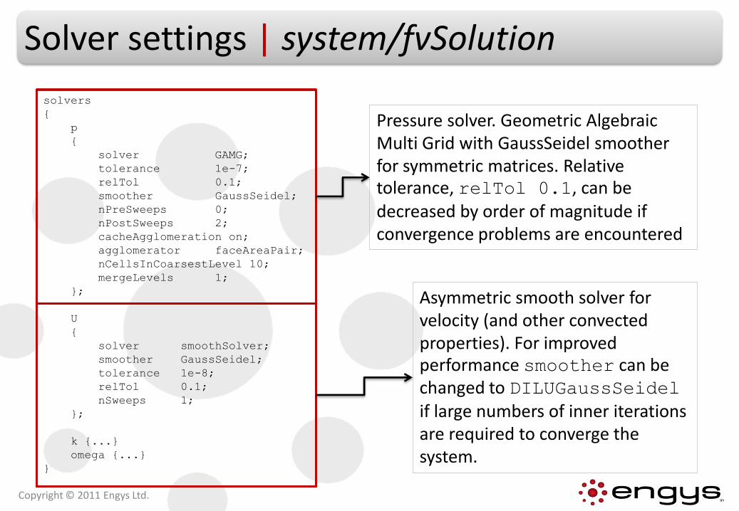
solvers
{
p
{
solver GAMG;
tolerance 1e-7;
relTol 0.1;
smoother GaussSeidel;
nPreSweeps 0;
nPostSweeps 2;
cacheAgglomeration on;
agglomerator faceAreaPair;
nCellsInCoarsestLevel 10;
mergeLevels 1;
};
U
{
solver smoothSolver;
smoother GaussSeidel;
tolerance 1e-8;
relTol 0.1;
nSweeps 1;
};
k {...}
omega {...}
}
Pressure solver. Geometric Algebraic Multi Grid with GaussSeidel smoother for symmetric matrices. Relative tolerance, relTol 0.1, can be decreased by order of magnitude if convergence problems are encountered
Asymmetric smooth solver for velocity (and other convectedproperties). For improved performance smoother can be changed to DILUGaussSeidelif large numbers of inner iterations are required to converge the system.
Solver settings | system/fvSolution
Copyright © 2011 Engys Ltd.
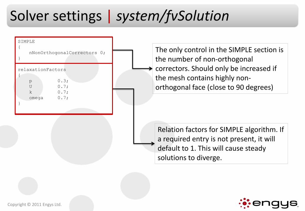
SIMPLE
{
nNonOrthogonalCorrectors 0;
}
relaxationFactors
{
p 0.3;
U 0.7;
k 0.7;
omega 0.7;
}
The only control in the SIMPLE section is the number of non-orthogonal correctors. Should only be increased if the mesh contains highly non-orthogonal face (close to 90 degrees)
Relation factors for SIMPLE algorithm. If a required entry is not present, it will default to 1. This will cause steady solutions to diverge.
Solver settings | constant
• Dictionary files located in the constant folder are mainly used for defining specific models settings and properties
• For the motorbike example:
RASproperties → Define specific RAS turbulence model
transportProperties → Material properties for incompressible flow
Copyright © 2011 Engys Ltd.
Settings | constant/transportProperties
Copyright © 2011 Engys Ltd.
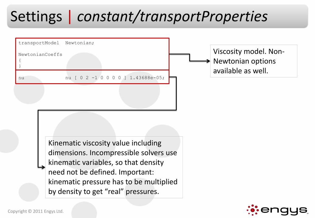
transportModel Newtonian;
NewtonianCoeffs
{
}
nu nu [ 0 2 -1 0 0 0 0 ] 1.43688e-05;
Viscosity model. Non-Newtonian options available as well.
Kinematic viscosity value including dimensions. Incompressible solvers use kinematic variables, so that density need not be defined. Important: kinematic pressure has to be multiplied by density to get “real” pressures.
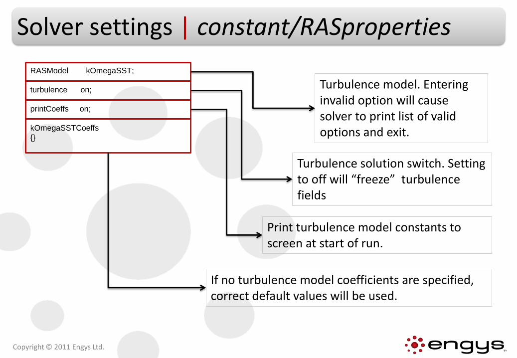
Solver settings | constant/RASproperties
Copyright © 2011 Engys Ltd.
RASModel kOmegaSST;
turbulence on;
printCoeffs on;
kOmegaSSTCoeffs
{}
Turbulence model. Entering invalid option will cause solver to print list of valid options and exit.
Turbulence solution switch. Setting to off will “freeze” turbulence fields
Print turbulence model constants to screen at start of run.
If no turbulence model coefficients are specified, correct default values will be used.
Solver settings | Fields
• Field files contain the following data:
Flow field solution values on each cell and boundary of the mesh
Boundary condition settings and values for each field
• One field file for each flow variable, i.e. U, p, T, k, omega, epsilon, etc
• Field files are saved in the time directories
Time 0 usually refers to the initial fields
Subsequent time dumps are created during the solution based on the user defined I/O settings in system/controlDict
• Field files, like all dictionaries, can include regular expressions and directives like “#include”
(directives start with a # symbol)Copyright © 2011 Engys Ltd.

Fields | Example U @ Time 0
Copyright © 2011 Engys Ltd.
FoamFile
{
version 2.0;
format ascii;
class volVectorField;
location "0";
object U;
}
#include “initialConditions”
dimensions [0 1 -1 0 0 0 0];
internalField uniform $flowVelocity;
boundaryField
{
#include “fixedInlet”
outlet
{
type inletOutlet;
inletValue uniform (0 0 0);
value $internalField;
}
...
}
File header• class → scalar, vector or tensor
Internal field valuesflowVelocity defined in initialConditions file
Boundary conditions → type and values
Dimensions [m/s]
#include directive“pastes” contents of initialConditions file here
Running a RANS Flow Solver
• The run can be started using the provided settings
• The only modification required is to shorten the run time in the controlDict file.
• The incompressible, steady RAS flow solver in OPENFOAM® is called simpleFoam and can be executed with the following command (from within the project folder): simpleFoam
Copyright © 2011 Engys Ltd.
You Will Learn About...
Copyright © 2011 Engys Ltd.
• Pre-compiled applications and utilities in OPENFOAM®
• Running OPENFOAM® tutorials
• OPENFOAM® postprocessing and advanced running options
• Running OPENFOAM® in parallel
paraFoam Post-Processing Tool
• The results of the calculation can be visualised using ParaView
• ParaView is the main post-processing tool provided with OPENFOAM®
• paraFoam is a script that launches ParaView using the reader module supplied with OPENFOAM®. It is executed like any of the OPENFOAM® utilities with the root directory path and the case directory name as arguments:
paraFoam [-case dir]
• OPENFOAM® also includes the foamToVTK utility to convert data from its native format to VTK format, which means that any VTK-based graphics tools can be used to post-process OPENFOAM® cases. This provides an alternative means for using ParaView with OPENFOAM®.
The foamToVTK tool has many command-line options that can be useful in some situations
Copyright © 2011 Engys Ltd.
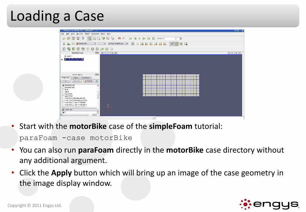
Loading a Case
• Start with the motorBike case of the simpleFoam tutorial:
paraFoam -case motorBike
• You can also run paraFoam directly in the motorBike case directory without any additional argument.
• Click the Apply button which will bring up an image of the case geometry in the image display window.
Copyright © 2011 Engys Ltd.
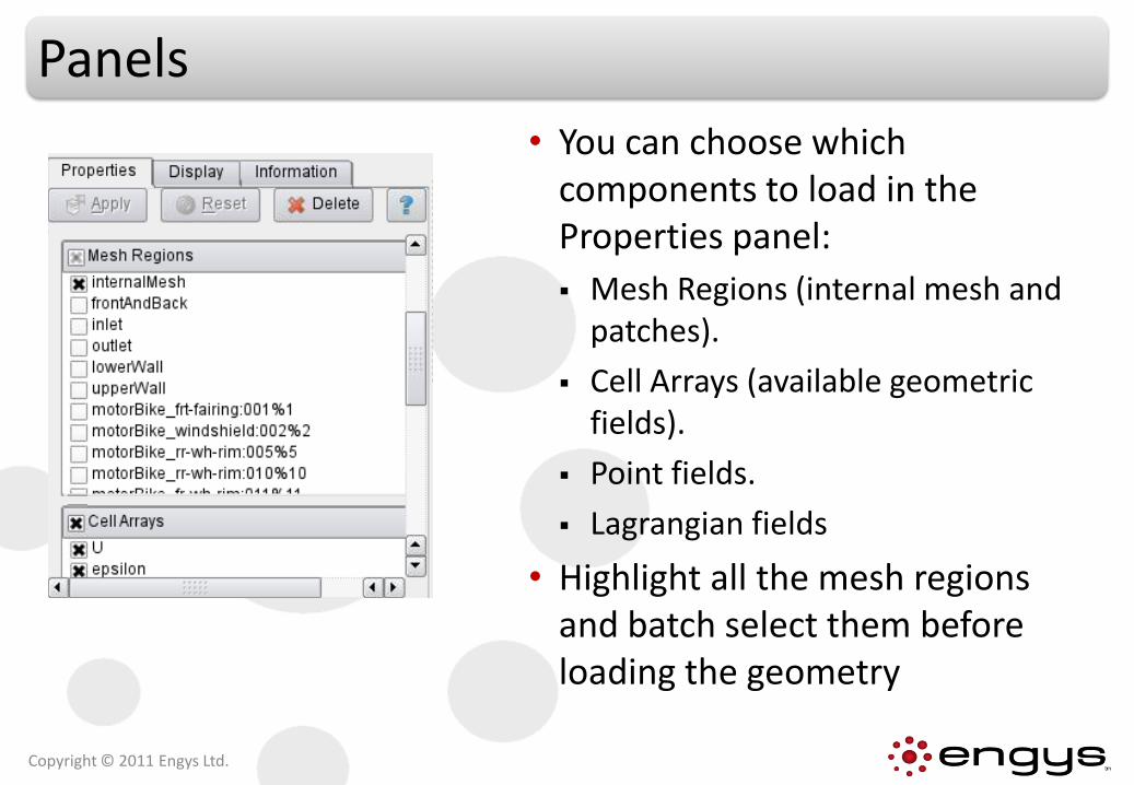
Panels
• You can choose which components to load in the Properties panel:
Mesh Regions (internal mesh and patches).
Cell Arrays (available geometric fields).
Point fields.
Lagrangian fields
• Highlight all the mesh regions and batch select them before loading the geometry
Copyright © 2011 Engys Ltd.
Basic Interfaces
• When paraView is launched, visualization is controlled by:
Pipeline browser: lists the modules opened in ParaView, where the selected modules are highlighted in blue and the graphics for the given module can be enabled/disabled by clicking the eye button alongside
Object inspector consisting in three different panels:
• Properties panel: it contains the input selections for the case, such as times, regions and fields.
• Display panel controls the visual representation of the selected module, e.g. colors.
• Information panel gives case statistics such as mesh geometry and size.
Current time control panel allows to selects the simulation time to be visualized.
• ParaView operates a tree-based structure in which data can be filtered from the top-level case module to create sets of sub-modules.
Copyright © 2011 Engys Ltd.
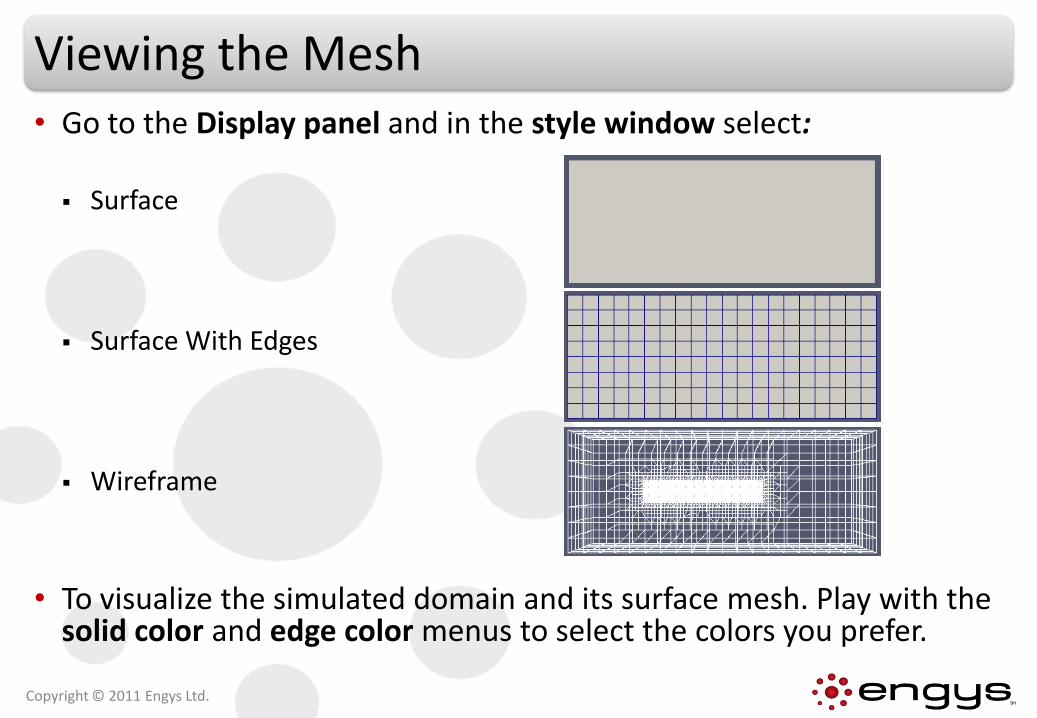
Viewing the Mesh• Go to the Display panel and in the style window select:
Surface
Surface With Edges
Wireframe
• To visualize the simulated domain and its surface mesh. Play with the solid color and edge color menus to select the colors you prefer.
Copyright © 2011 Engys Ltd.

Viewing the Mesh
• You can visualise selected parts of the geometry by using the Extract Block filter. From the menu select:
Filters Alphabetical Extract Block
• Batch select all the motorbike parts and extract the surface of the motorbike.
Copyright © 2011 Engys Ltd.
Viewing Fields: Display Panels
• The Display panel contains the settings for visualizing the data/fields for a given case module. You can choose to color the mesh with a constant solid color or with a colour range representing the field values. The same operation can be done directly in the Active variable controls variable menu located on left-top of the screen.
Activate the legend visibility button to see the field data range.
The magnitude or the single components of a vector field can be visualized.
The Edit color map window makes it possible to choose the color range and appropriate legend font colors and size.
The image can be made translucent by editing the value in Opacity (1 = solid, 0 = invisible).
The activated component can be translated, scaled, rotated with respect to other ones.
• It is possible to select the field that the user wants to plot in the color window.
Copyright © 2011 Engys Ltd.
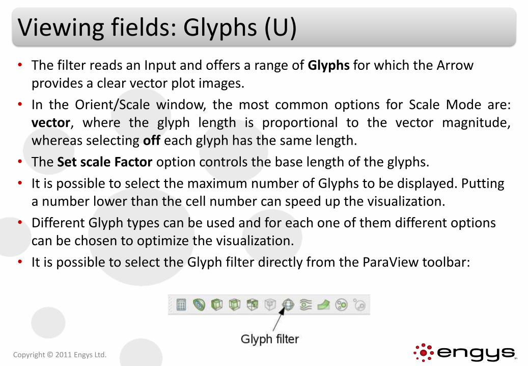
Viewing fields: Glyphs (U)
• The filter reads an Input and offers a range of Glyphs for which the Arrow provides a clear vector plot images.
• In the Orient/Scale window, the most common options for Scale Mode are:vector, where the glyph length is proportional to the vector magnitude,whereas selecting off each glyph has the same length.
• The Set scale Factor option controls the base length of the glyphs.
• It is possible to select the maximum number of Glyphs to be displayed. Putting a number lower than the cell number can speed up the visualization.
• Different Glyph types can be used and for each one of them different options can be chosen to optimize the visualization.
• It is possible to select the Glyph filter directly from the ParaView toolbar:
Copyright © 2011 Engys Ltd.
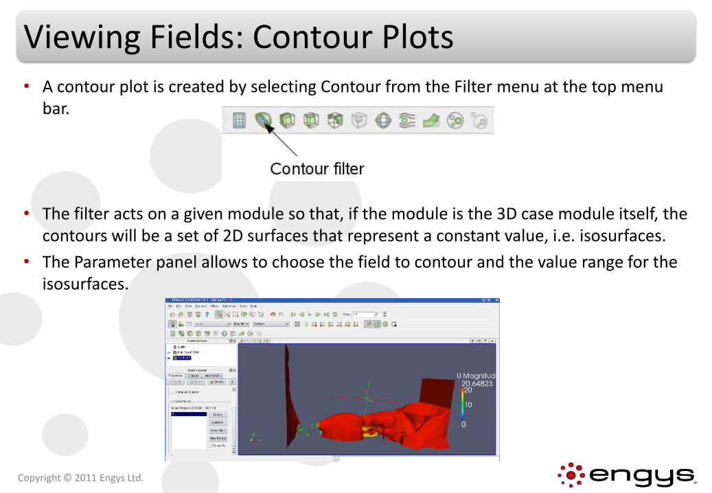
Viewing Fields: Contour Plots• A contour plot is created by selecting Contour from the Filter menu at the top menu
bar.
• The filter acts on a given module so that, if the module is the 3D case module itself, the contours will be a set of 2D surfaces that represent a constant value, i.e. isosurfaces.
• The Parameter panel allows to choose the field to contour and the value range for the isosurfaces.
Copyright © 2011 Engys Ltd.
Viewing Fields: Streamlines
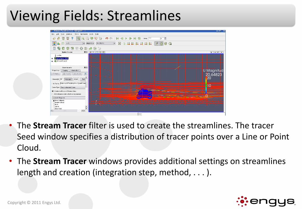
• The Stream Tracer filter is used to create the streamlines. The tracer Seed window specifies a distribution of tracer points over a Line or Point Cloud.
• The Stream Tracer windows provides additional settings on streamlines length and creation (integration step, method, . . . ).
Copyright © 2011 Engys Ltd.
Viewing Fields: Probes
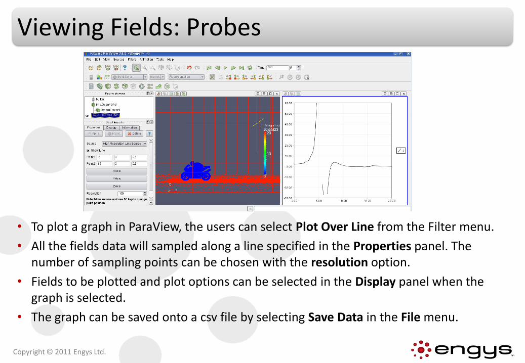
• To plot a graph in ParaView, the users can select Plot Over Line from the Filter menu.
• All the fields data will sampled along a line specified in the Properties panel. The number of sampling points can be chosen with the resolution option.
• Fields to be plotted and plot options can be selected in the Display panel when the graph is selected.
• The graph can be saved onto a csv file by selecting Save Data in the File menu.
Copyright © 2011 Engys Ltd.
Cut Planes
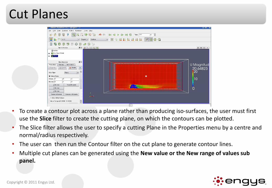
• To create a contour plot across a plane rather than producing iso-surfaces, the user must first use the Slice filter to create the cutting plane, on which the contours can be plotted.
• The Slice filter allows the user to specify a cutting Plane in the Properties menu by a centre and normal/radius respectively.
• The user can then run the Contour filter on the cut plane to generate contour lines.
• Multiple cut planes can be generated using the New value or the New range of values sub panel.
Copyright © 2011 Engys Ltd.
Clip Filter
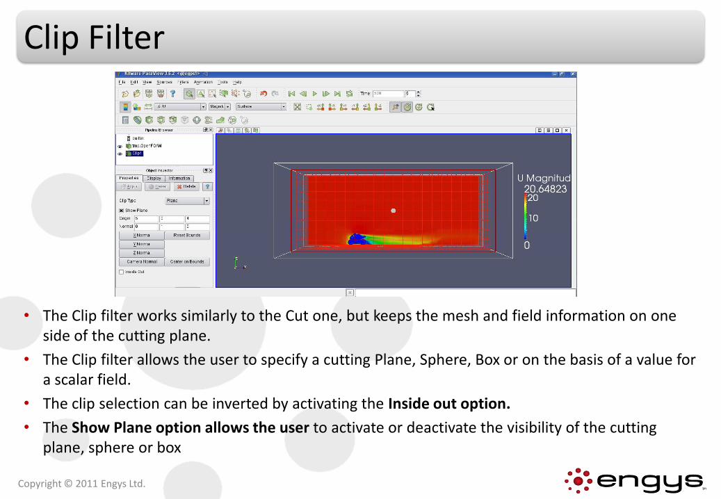
• The Clip filter works similarly to the Cut one, but keeps the mesh and field information on one side of the cutting plane.
• The Clip filter allows the user to specify a cutting Plane, Sphere, Box or on the basis of a value for a scalar field.
• The clip selection can be inverted by activating the Inside out option.
• The Show Plane option allows the user to activate or deactivate the visibility of the cutting plane, sphere or box
Copyright © 2011 Engys Ltd.
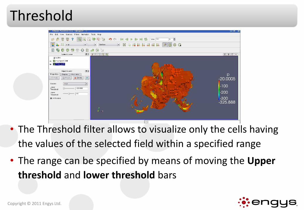
Threshold
• The Threshold filter allows to visualize only the cells having
the values of the selected field within a specified range
• The range can be specified by means of moving the Upper
threshold and lower threshold bars
Copyright © 2011 Engys Ltd.
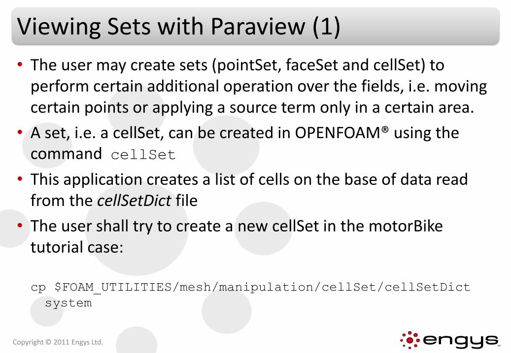
Viewing Sets with Paraview (1)
• The user may create sets (pointSet, faceSet and cellSet) to perform certain additional operation over the fields, i.e. moving certain points or applying a source term only in a certain area.
• A set, i.e. a cellSet, can be created in OPENFOAM® using the command cellSet
• This application creates a list of cells on the base of data read from the cellSetDict file
• The user shall try to create a new cellSet in the motorBiketutorial case:
cp $FOAM_UTILITIES/mesh/manipulation/cellSet/cellSetDict
system
Copyright © 2011 Engys Ltd.
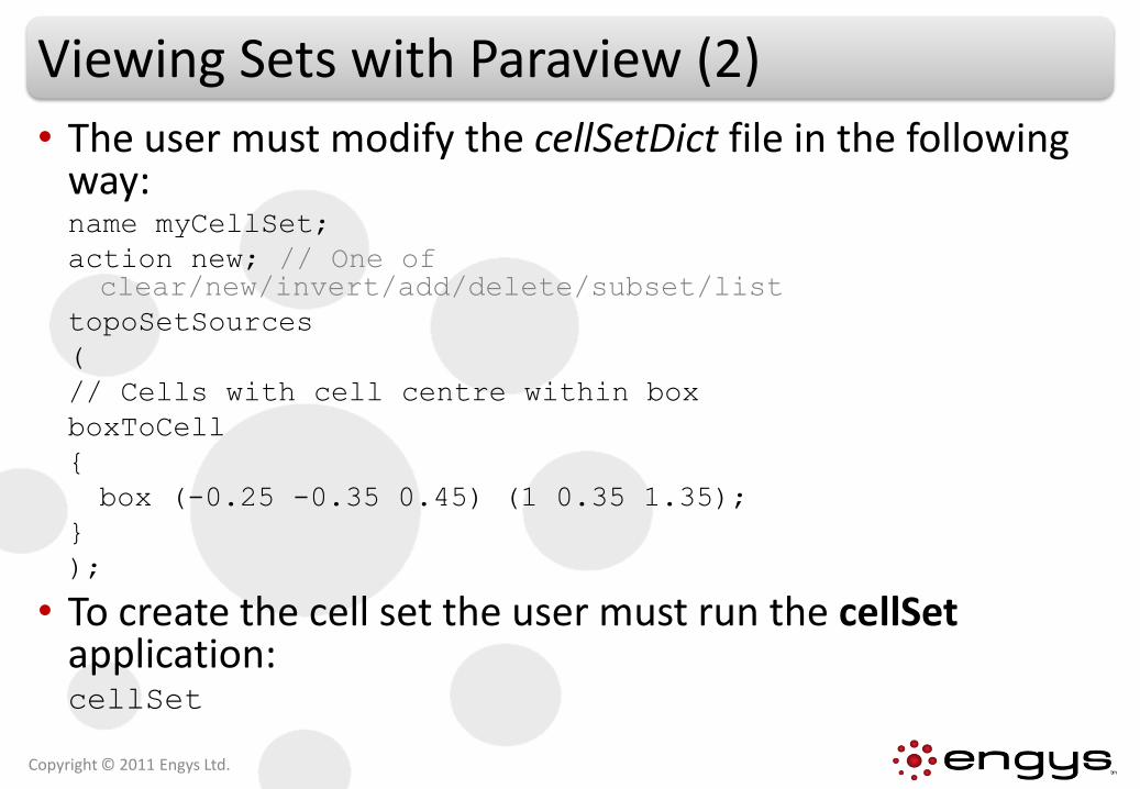
Viewing Sets with Paraview (2)
• The user must modify the cellSetDict file in the following way:name myCellSet;
action new; // One of clear/new/invert/add/delete/subset/list
topoSetSources
(
// Cells with cell centre within box
boxToCell
{
box (-0.25 -0.35 0.45) (1 0.35 1.35);
}
);
• To create the cell set the user must run the cellSetapplication:cellSet
Copyright © 2011 Engys Ltd.
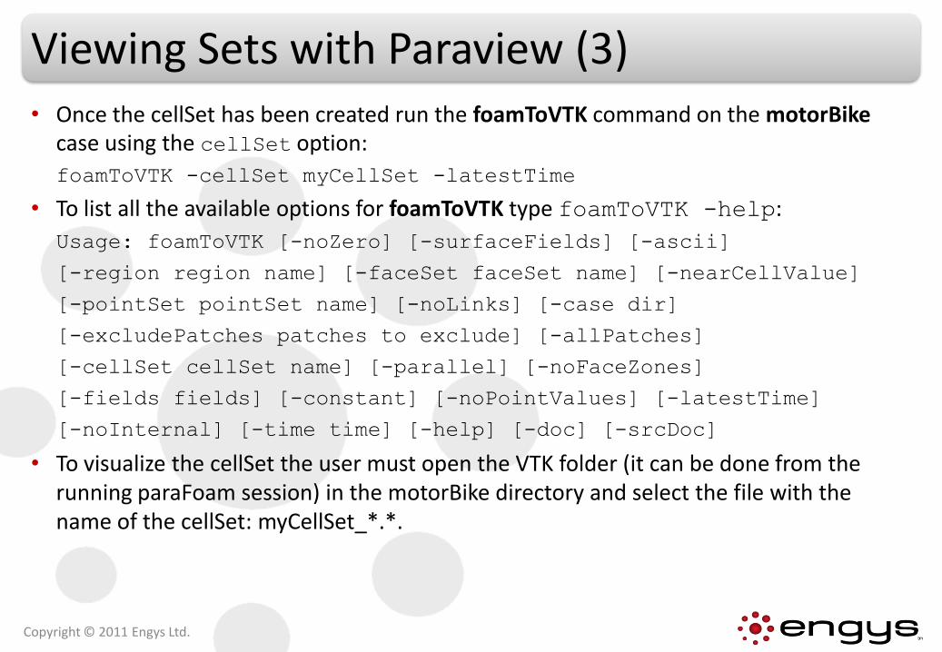
Viewing Sets with Paraview (3)• Once the cellSet has been created run the foamToVTK command on the motorBike
case using the cellSet option:
foamToVTK -cellSet myCellSet -latestTime
• To list all the available options for foamToVTK type foamToVTK -help:
Usage: foamToVTK [-noZero] [-surfaceFields] [-ascii]
[-region region name] [-faceSet faceSet name] [-nearCellValue]
[-pointSet pointSet name] [-noLinks] [-case dir]
[-excludePatches patches to exclude] [-allPatches]
[-cellSet cellSet name] [-parallel] [-noFaceZones]
[-fields fields] [-constant] [-noPointValues] [-latestTime]
[-noInternal] [-time time] [-help] [-doc] [-srcDoc]
• To visualize the cellSet the user must open the VTK folder (it can be done from the running paraFoam session) in the motorBike directory and select the file with the name of the cellSet: myCellSet_*.*.
Copyright © 2011 Engys Ltd.
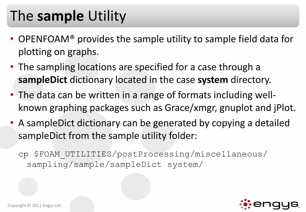
The sample Utility
• OPENFOAM® provides the sample utility to sample field data for plotting on graphs.
• The sampling locations are specified for a case through a sampleDict dictionary located in the case system directory.
• The data can be written in a range of formats including well-known graphing packages such as Grace/xmgr, gnuplot and jPlot.
• A sampleDict dictionary can be generated by copying a detailed sampleDict from the sample utility folder:
cp $FOAM_UTILITIES/postProcessing/miscellaneous/
sampling/sample/sampleDict system/
Copyright © 2011 Engys Ltd.
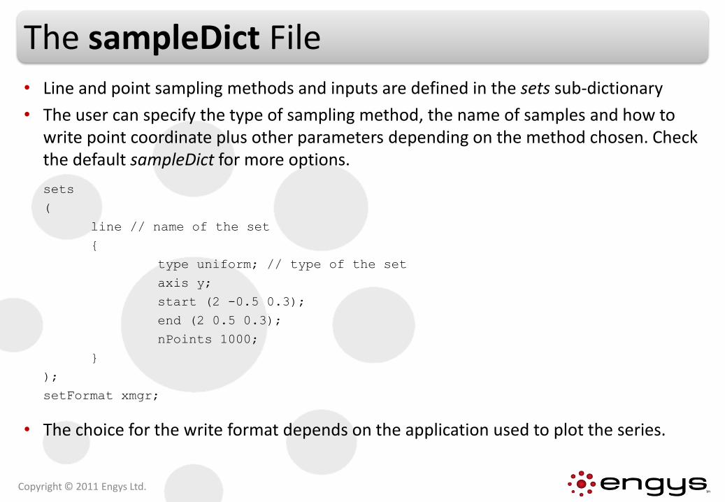
The sampleDict File• Line and point sampling methods and inputs are defined in the sets sub-dictionary
• The user can specify the type of sampling method, the name of samples and how to write point coordinate plus other parameters depending on the method chosen. Check the default sampleDict for more options.
sets
(
line // name of the set
{
type uniform; // type of the set
axis y;
start (2 -0.5 0.3);
end (2 0.5 0.3);
nPoints 1000;
}
);
setFormat xmgr;
• The choice for the write format depends on the application used to plot the series.
Copyright © 2011 Engys Ltd.
The sampleDict File
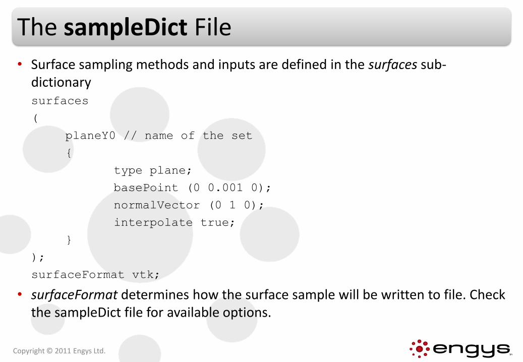
• Surface sampling methods and inputs are defined in the surfaces sub-dictionary surfaces
(
planeY0 // name of the set
{
type plane;
basePoint (0 0.001 0);
normalVector (0 1 0);
interpolate true;
}
);
surfaceFormat vtk;
• surfaceFormat determines how the surface sample will be written to file. Check the sampleDict file for available options.
Copyright © 2011 Engys Ltd.
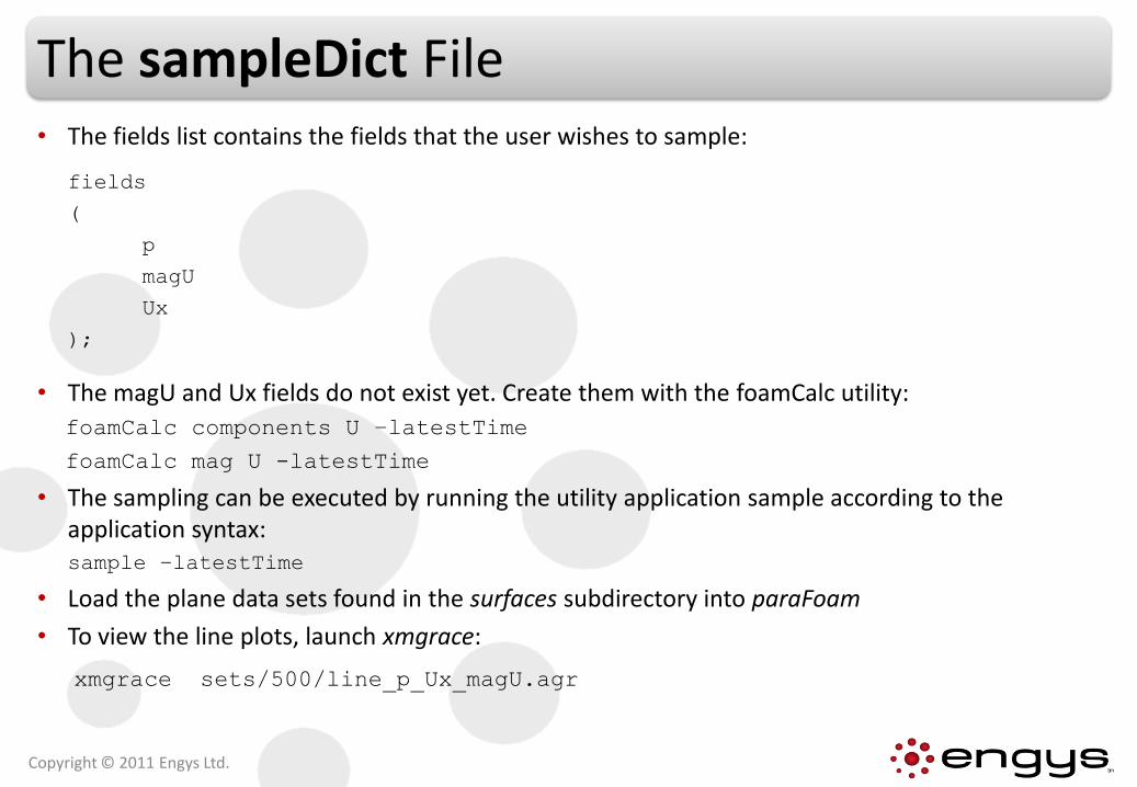
The sampleDict File• The fields list contains the fields that the user wishes to sample:
fields
(
p
magU
Ux
);
• The magU and Ux fields do not exist yet. Create them with the foamCalc utility:
foamCalc components U –latestTime
foamCalc mag U -latestTime
• The sampling can be executed by running the utility application sample according to the application syntax:sample –latestTime
• Load the plane data sets found in the surfaces subdirectory into paraFoam
• To view the line plots, launch xmgrace:
xmgrace sets/500/line_p_Ux_magU.agr
Copyright © 2011 Engys Ltd.
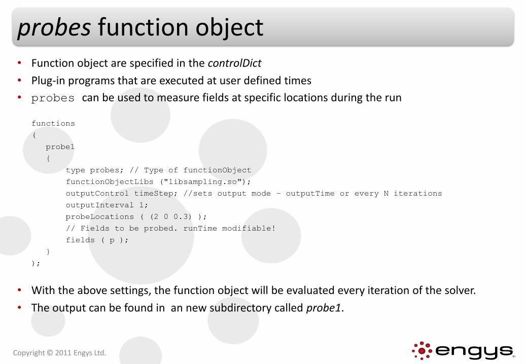
probes function object• Function object are specified in the controlDict
• Plug-in programs that are executed at user defined times
• probes can be used to measure fields at specific locations during the run
functions
(
probe1
{
type probes; // Type of functionObject
functionObjectLibs ("libsampling.so");
outputControl timeStep; //sets output mode – outputTime or every N iterations
outputInterval 1;
probeLocations ( (2 0 0.3) );
// Fields to be probed. runTime modifiable!
fields ( p );
}
);
• With the above settings, the function object will be evaluated every iteration of the solver.
• The output can be found in an new subdirectory called probe1.
Copyright © 2011 Engys Ltd.
You Will Learn About...
Copyright © 2011 Engys Ltd.
• Pre-compiled applications and utilities in OPENFOAM®
• Running OPENFOAM® tutorials
• OPENFOAM® postprocessing and advanced running options
• Running OPENFOAM® in parallel
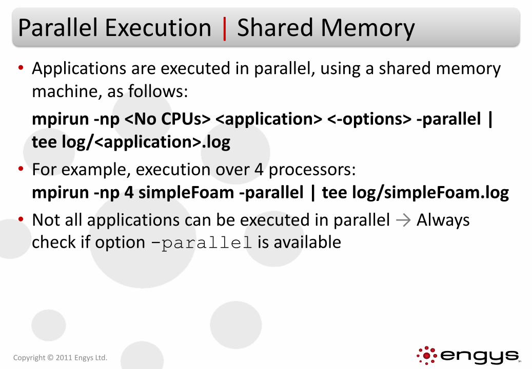
Parallel Execution | Shared Memory
• Applications are executed in parallel, using a shared memory machine, as follows:
mpirun -np <No CPUs> <application> <-options> -parallel | tee log/<application>.log
• For example, execution over 4 processors: mpirun -np 4 simpleFoam -parallel | tee log/simpleFoam.log
• Not all applications can be executed in parallel → Always check if option -parallel is available
Copyright © 2011 Engys Ltd.
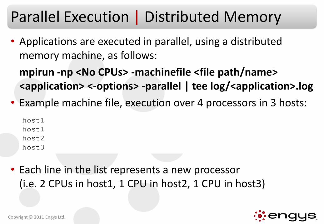
Parallel Execution | Distributed Memory
• Applications are executed in parallel, using a distributed memory machine, as follows:
mpirun -np <No CPUs> -machinefile <file path/name> <application> <-options> -parallel | tee log/<application>.log
• Example machine file, execution over 4 processors in 3 hosts:
• Each line in the list represents a new processor(i.e. 2 CPUs in host1, 1 CPU in host2, 1 CPU in host3)
Copyright © 2011 Engys Ltd.
host1
host1
host2
host3
Parallel Execution
Copyright © 2011 Engys Ltd.
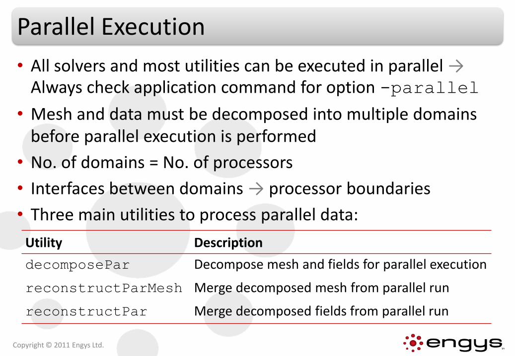
• All solvers and most utilities can be executed in parallel → Always check application command for option -parallel
• Mesh and data must be decomposed into multiple domains before parallel execution is performed
• No. of domains = No. of processors
• Interfaces between domains → processor boundaries
• Three main utilities to process parallel data:
Utility Description
decomposePar Decompose mesh and fields for parallel execution
reconstructParMesh Merge decomposed mesh from parallel run
reconstructPar Merge decomposed fields from parallel run
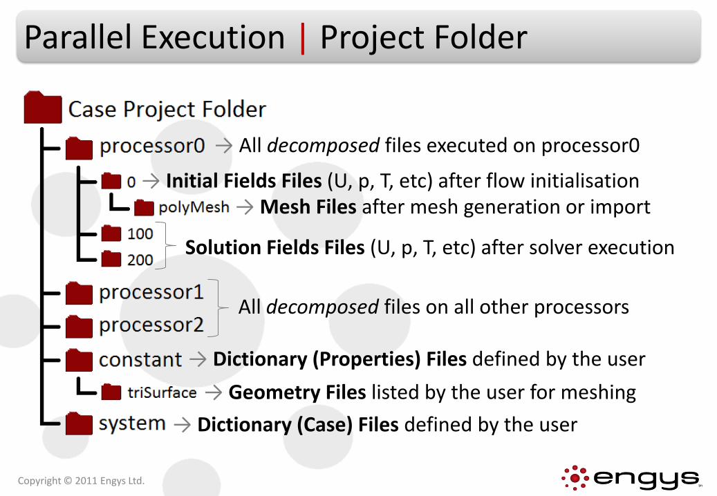
Parallel Execution | Project Folder
Copyright © 2011 Engys Ltd.
→ Mesh Files after mesh generation or import
→ Dictionary (Properties) Files defined by the user
→ Dictionary (Case) Files defined by the user
→ Geometry Files listed by the user for meshing
→ Initial Fields Files (U, p, T, etc) after flow initialisation
Solution Fields Files (U, p, T, etc) after solver execution
→ All decomposed files executed on processor0
All decomposed files on all other processors
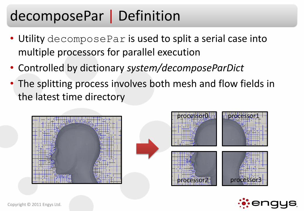
decomposePar | Definition
• Utility decomposePar is used to split a serial case into multiple processors for parallel execution
• Controlled by dictionary system/decomposeParDict
• The splitting process involves both mesh and flow fields in the latest time directory
Copyright © 2011 Engys Ltd.
processor0 processor1
processor2 processor3
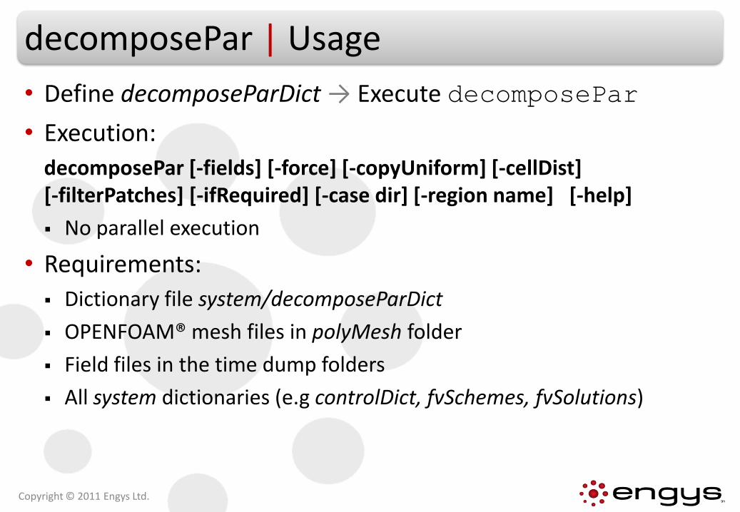
decomposePar | Usage
• Define decomposeParDict → Execute decomposePar
• Execution:
decomposePar [-fields] [-force] [-copyUniform] [-cellDist] [-filterPatches] [-ifRequired] [-case dir] [-region name] [-help]
No parallel execution
• Requirements:
Dictionary file system/decomposeParDict
OPENFOAM® mesh files in polyMesh folder
Field files in the time dump folders
All system dictionaries (e.g controlDict, fvSchemes, fvSolutions)
Copyright © 2011 Engys Ltd.
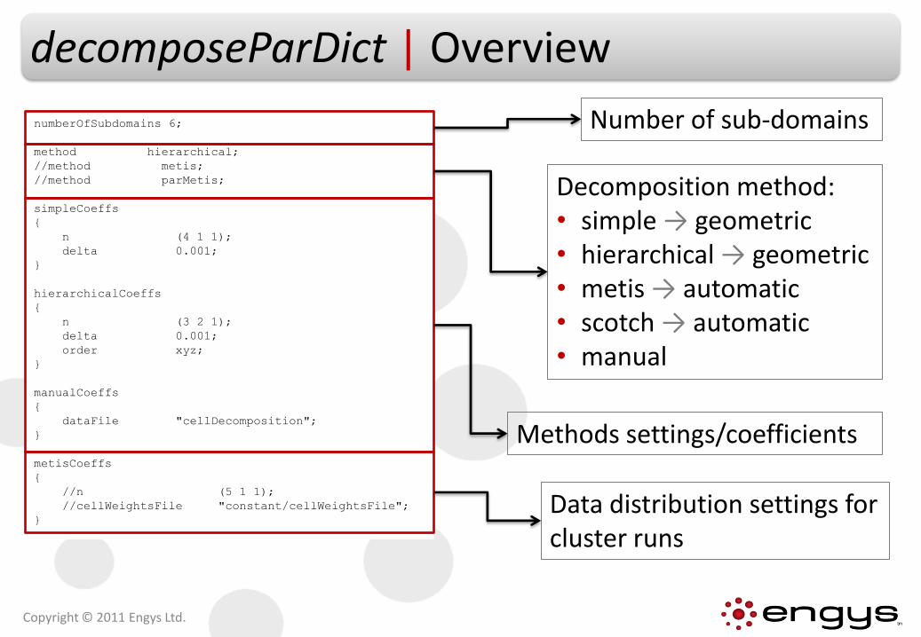
numberOfSubdomains 6;
method hierarchical;
//method metis;
//method parMetis;
simpleCoeffs
{
n (4 1 1);
delta 0.001;
}
hierarchicalCoeffs
{
n (3 2 1);
delta 0.001;
order xyz;
}
manualCoeffs
{
dataFile "cellDecomposition";
}
metisCoeffs
{
//n (5 1 1);
//cellWeightsFile "constant/cellWeightsFile";
}
decomposeParDict | Overview
Copyright © 2011 Engys Ltd.
Number of sub-domains
Decomposition method:• simple → geometric • hierarchical → geometric • metis → automatic• scotch → automatic• manual
Methods settings/coefficients
Data distribution settings for cluster runs
Case Reconstruction
• Decomposed data from parallel runs can be reconstructed into a single domain by executing two utilities: First execute reconstructParMesh → reconstruct mesh only
Second execute reconstructPar → reconstruct solution fields only
• NOTE → the mesh must be reconstructed first before attempting to reconstruct the fields
Copyright © 2011 Engys Ltd.
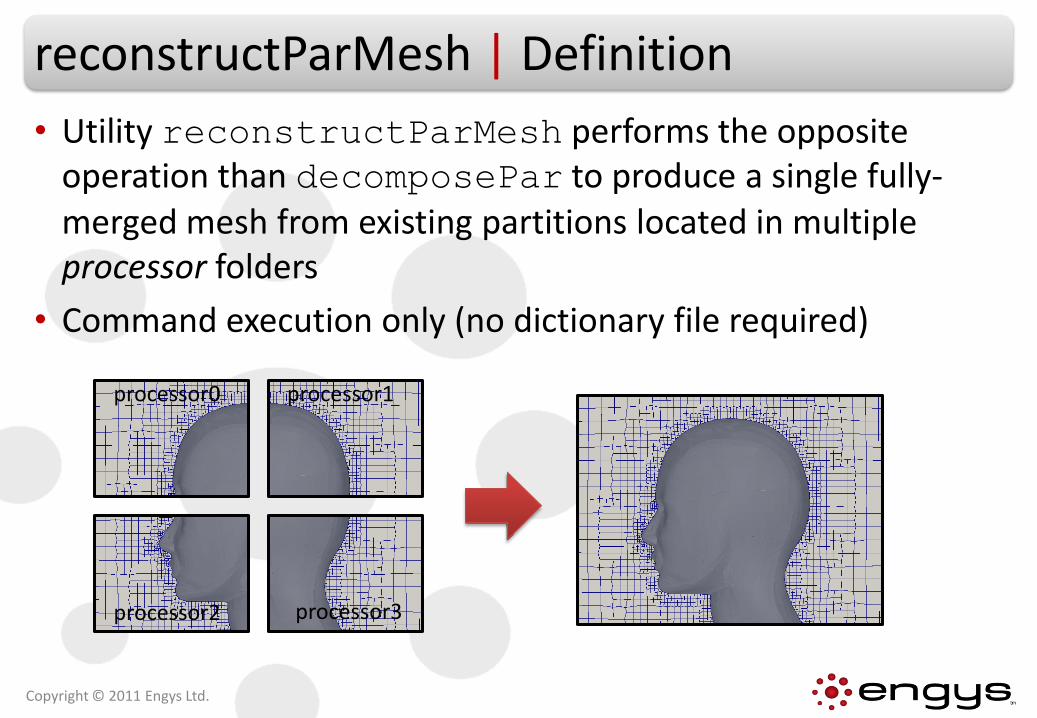
reconstructParMesh | Definition
• Utility reconstructParMesh performs the opposite operation than decomposePar to produce a single fully-merged mesh from existing partitions located in multiple processor folders
• Command execution only (no dictionary file required)
Copyright © 2011 Engys Ltd.
processor0 processor1
processor2 processor3
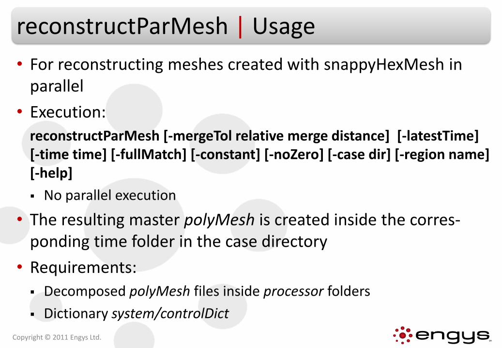
reconstructParMesh | Usage
• For reconstructing meshes created with snappyHexMesh in parallel
• Execution:
reconstructParMesh [-mergeTol relative merge distance] [-latestTime] [-time time] [-fullMatch] [-constant] [-noZero] [-case dir] [-region name] [-help]
No parallel execution
• The resulting master polyMesh is created inside the corres-ponding time folder in the case directory
• Requirements:
Decomposed polyMesh files inside processor folders
Dictionary system/controlDict
Copyright © 2011 Engys Ltd.
reconstructPar | Definition
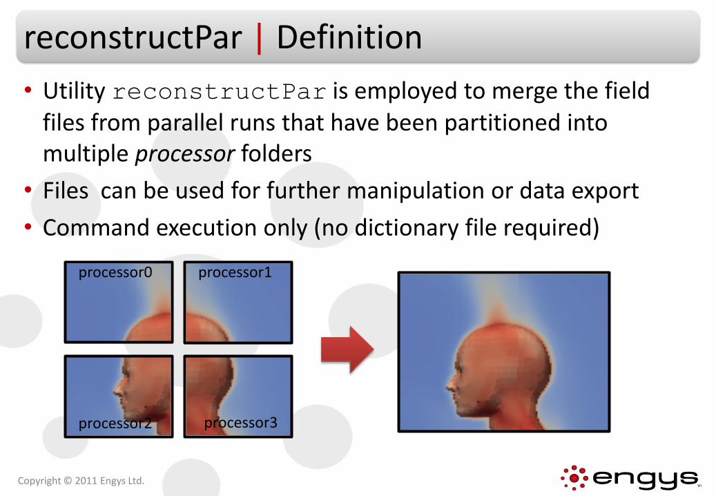
• Utility reconstructPar is employed to merge the field files from parallel runs that have been partitioned into multiple processor folders
• Files can be used for further manipulation or data export
• Command execution only (no dictionary file required)
Copyright © 2011 Engys Ltd.
processor0 processor1
processor2 processor3
You Learned About...
Copyright © 2011 Engys Ltd.
• Pre-compiled applications and utilities in OPENFOAM®
• Running OPENFOAM® tutorials
• OPENFOAM® postprocessing and advanced running options
• Running OPENFOAM® in parallel


![Apha slides tfah sanyal slides[1]](https://img.pdfslide.net/doc/110x75/557c653ad8b42a855d8b46d1/apha-slides-tfah-sanyal-slides1.jpg)


![{Slides} Job+ Presentation Slides [MKS-40]](https://img.pdfslide.net/doc/110x75/58f058861a28ab96248b45f5/slides-job-presentation-slides-mks-40.jpg)