Embed Size (px)
Citation preview

DFA Minimization Algorithms in Map-Reduce
Iraj Hedayati Somarin
A thesis
in
The Department
of
Computer Science and Software Engineering
Presented in Partial Fulfillment of the Requirements
For the Degree of Master of Computer Science
Concordia University
Montreal, Quebec, Canada
January 2016
c⃝ Iraj Hedayati Somarin, 2016
Rajagopalan Jayakumar
Brigitte Jaumard
Hovhannes A. Harutyunyan
Gosta K. Grahne
Sudhir P. Mudur
January 11, 2016
Concordia UniversitySchool of Graduate Studies
This is to certify that the thesis prepared
By: Iraj Hedayati Somarin
Entitled: DFA Minimization Algorithms in Map-Reduce
and submitted in partial fulfillment of the requirements for the degree of
Master of Computer Science
complies with the regulations of this University and meets the accepted standards
with respect to originality and quality.
Signed by the final examining commitee:
Chair
Examiner
Examiner
Examiner
Supervisor
ApprovedChair of Department or Graduate Program Director
Amir Asif, Ph.D., Dean
Faculty of Engineering and Computer Science
Abstract
DFA Minimization Algorithms in Map-Reduce
Iraj Hedayati Somarin
Map-Reduce has been a highly popular parallel-distributed programming model. In
this thesis, we study the problem of minimizing Deterministic Finite State Automata
(DFA). We focus our attention on two well-known (serial) algorithms, namely the
algorithms of Moore (1956) and of Hopcroft (1971). The central cost-parameter
in Map-Reduce is that of communication cost i.e., the amount of data that has to
be communicated between the processes. Using techniques from Communication
Complexity we derive an O(kn log n) lower bound and O(kn3 log n) upper bound for
the problem, where n is the number of states in the DFA to be minimized, and k
is the size of its alphabet. We then develop Map-Reduce versions of both Moore’s
and Hopcroft’s algorithms, and show that their communication cost is O(kn2(log n+
log k)). Both methods have been implemented and tested on large DFA, with 131,072
states. The experiments verify our theoretical analysis, and also reveal that Hopcroft’s
algorithm – considered superior in the sequential framework – is very sensitive to skew
in the topology of the graph of the DFA, whereas Moore’s algorithm handles skew
without major efficiency loss.
iii

Acknowledgments
Above all, the researcher’s honest and sincere appreciation extends to his supervisor,
Prof. Gosta Grahne, for his constant encouragement and creative and comprehensive
guidance until this work came to existence.
On a more personal note, his gratitude goes to love of his life for her boundless support
and patience. The researcher also wishes to give credit to research team members, Mr.
Shahab Harrafi and Mr. Ali Moallemi, for their generous and constructive comments,
suggestions and foresights throughout this process.
iv
Table of Contents
Acknowledgments iv
List of Figures ix
List of Tables xi
List of Algorithms xii
List of Abbreviations xiv
1 Introduction 1
1.1 DFA Minimization . . . . . . . . . . . . . . . . . . . . . . . . . . . . 2
1.2 Big-Data Processing in Map-Reduce Model . . . . . . . . . . . . . . . 3
1.3 Motivation and Contributions . . . . . . . . . . . . . . . . . . . . . . 4
1.4 Thesis Organization . . . . . . . . . . . . . . . . . . . . . . . . . . . . 5
2 Background and Related Work 7
v
TABLE OF CONTENTS
2.1 Finite State Automata and their Minimization . . . . . . . . . . . . . 7
2.1.1 Moore’s Algorithm . . . . . . . . . . . . . . . . . . . . . . . . 13
2.1.2 Hopcroft’s Algorithm . . . . . . . . . . . . . . . . . . . . . . . 17
2.1.2.1 Complexity of Hopcroft’s Algorithm . . . . . . . . . 19
2.1.2.2 Slow Automata . . . . . . . . . . . . . . . . . . . . . 24
2.1.3 Parallel Algorithms . . . . . . . . . . . . . . . . . . . . . . . . 25
2.1.3.1 CRCW-PRAM DFA Minimization Algorithm . . . . 26
2.1.3.2 EREW-PRAM DFA Minimization Algorithm . . . . 28
2.2 Map-Reduce and Hadoop . . . . . . . . . . . . . . . . . . . . . . . . . 30
2.2.1 Map-Reduce . . . . . . . . . . . . . . . . . . . . . . . . . . . . 30
2.2.1.1 Map Function . . . . . . . . . . . . . . . . . . . . . . 31
2.2.1.2 Partitioner Function . . . . . . . . . . . . . . . . . . 33
2.2.1.3 Reducer Function . . . . . . . . . . . . . . . . . . . . 33
2.2.2 Mapping Schema . . . . . . . . . . . . . . . . . . . . . . . . . 34
2.3 Automata Algorithms in Map-Reduce . . . . . . . . . . . . . . . . . . 35
2.3.1 NFA Intersection . . . . . . . . . . . . . . . . . . . . . . . . . 35
2.3.2 DFA Minimization (Moore-MR) . . . . . . . . . . . . . . . . . 37
2.4 Cost Model . . . . . . . . . . . . . . . . . . . . . . . . . . . . . . . . 39
2.4.1 Communication Complexity . . . . . . . . . . . . . . . . . . . 39
2.4.2 The Lower Bound Recipe for Replication Rate . . . . . . . . . 44
vi

TABLE OF CONTENTS
2.4.3 Computational Complexity of Map-Reduce . . . . . . . . . . . 45
3 DFA Minimization Algorithms in Map-Reduce 48
3.1 Moore’s DFA Minimization in Map-Reduce (Moore-MR-PPHF) . . . 49
3.1.1 PPHF in Map-Reduce (PPHF-MR) . . . . . . . . . . . . . . . 54
3.1.2 An Example of Running Moore-MR-PPHF . . . . . . . . . . . 56
3.2 Hopcroft’s DFA Minimization algorithm in Map-Reduce (Hopcroft-MR) 61
3.2.1 Correctness . . . . . . . . . . . . . . . . . . . . . . . . . . . . 68
3.3 Enhanced Hopcroft-MR (Hopcroft-MR-PAR) . . . . . . . . . . . . . . 71
3.3.1 Splitters and QUE . . . . . . . . . . . . . . . . . . . . . . . . . 71
3.3.2 Detection . . . . . . . . . . . . . . . . . . . . . . . . . . . . . 74
3.3.3 Update Blocks . . . . . . . . . . . . . . . . . . . . . . . . . . 75
3.4 Cost Measures for DFA Minimization in Map-Reduce . . . . . . . . . 75
3.4.1 Minimum Communication Cost . . . . . . . . . . . . . . . . . 76
3.4.2 Lower Bound on Replication Rate . . . . . . . . . . . . . . . . 78
3.4.3 Communication Complexity of Moore-MR-PPHF . . . . . . . 79
3.4.3.1 Replication Rate . . . . . . . . . . . . . . . . . . . . 80
3.4.3.2 Communication Cost . . . . . . . . . . . . . . . . . . 80
3.4.4 Communication Complexity of Hopcroft-MR . . . . . . . . . . 82
3.4.4.1 Replication Rate . . . . . . . . . . . . . . . . . . . . 82
3.4.4.2 Communication Cost . . . . . . . . . . . . . . . . . . 83
vii

TABLE OF CONTENTS
3.4.5 Communication Complexity of Hopcroft-MR-PAR . . . . . . . 85
3.4.6 Comparison of Algorithms . . . . . . . . . . . . . . . . . . . . 88
4 Experimental Results 91
4.1 Cluster Configuration . . . . . . . . . . . . . . . . . . . . . . . . . . . 91
4.2 Data Generation Methods . . . . . . . . . . . . . . . . . . . . . . . . 92
4.3 Experiments . . . . . . . . . . . . . . . . . . . . . . . . . . . . . . . . 95
5 Conclusion and Future Work 102
5.1 Conclusion . . . . . . . . . . . . . . . . . . . . . . . . . . . . . . . . . 102
5.2 Future Work . . . . . . . . . . . . . . . . . . . . . . . . . . . . . . . . 103
References 105
viii
List of Figures
1 Forest of DFA minimization families . . . . . . . . . . . . . . . . . . 10
2 Sample DFA . . . . . . . . . . . . . . . . . . . . . . . . . . . . . . . . 15
3 Minimized version of sample DFA (Moore) . . . . . . . . . . . . . . . 15
4 Binary tree for Hopcroft’s algorithm . . . . . . . . . . . . . . . . . . . 21
5 Sample slow automaton . . . . . . . . . . . . . . . . . . . . . . . . . 24
6 Map-Reduce architecture . . . . . . . . . . . . . . . . . . . . . . . . . 32
7 Mapping in Map-Reduce . . . . . . . . . . . . . . . . . . . . . . . . . 33
9 Sample DFA after round 1 (Moore-MR-PPHF) . . . . . . . . . . . . . 59
10 Minimized version of sample DFA (Moore-MR-PPHF) . . . . . . . . 60
11 Processing multiple splitters from QUE . . . . . . . . . . . . . . . . . 73
12 A sample circular DFA . . . . . . . . . . . . . . . . . . . . . . . . . . 93
13 Minimal DFA equivalent to the DFA in Figure 12 . . . . . . . . . . . 93
14 A sample replicated-random DFA . . . . . . . . . . . . . . . . . . . . 94
15 Minimal DFA equivalent to the DFA in Figure 14 . . . . . . . . . . . 94
ix
LIST OF FIGURES
16 Communication Cost of Moore-MR and Moore-MR-PPHF on slow DFA 95
17 Processing time of Moore-MR and Moore-MR-PPHF on slow DFA . . 96
18 Communication Cost of slow DFA for the alphabet size k = 2 . . . . 97
19 Processing time of slow DFA for the alphabet size k = 2 . . . . . . . 97
20 Communication Cost of circular DFA for the alphabet size k = 4 . . . 98
21 Processing time of circular DFA for the alphabet size k = 4 . . . . . . 98
22 Communication Cost of replicated-random DFA for alphabet size k = 4 99
23 Processing time of replicated-random DFA for alphabet size k = 4 . . 100
x

List of Tables
1 A sample partition refinement for Moore’s algorithm . . . . . . . . . 14
2 First round of executing Moore-MR-PPHF . . . . . . . . . . . . . . . 58
3 Data distribution across reducers in PPHF-MR . . . . . . . . . . . . 60
4 Data structures used in Hopcroft-MR . . . . . . . . . . . . . . . . . . 61
5 Comparison of complexity measures for algorithms . . . . . . . . . . . 88
6 Experimental Hadoop cluster configuration . . . . . . . . . . . . . . . 91
7 Number of rounds for each algorithm with different datasets . . . . . 101
xi

List of Algorithms
1 Moore’s DFA minimization algorithm . . . . . . . . . . . . . . . . . . 14
2 Hopcroft’s DFA minimization algorithm . . . . . . . . . . . . . . . . 20
3 CRCW-PRAM algorithm for DFA minimization [33] . . . . . . . . . 27
4 EREW-PRAM algorithm for DFA minimization [28] . . . . . . . . . . 29
5 Moore’s algorithm in Map-Reduce (Moore-MR) . . . . . . . . . . . . 53
6 Hopcroft’s algorithm in Map-Reduce (Hopcroft-MR) . . . . . . . . . 62
7 Pre-Processing Job for Hopcroft-MR . . . . . . . . . . . . . . . . . . 64
8 Partition Detection Job for Hopcroft-MR . . . . . . . . . . . . . . . . 66
9 Block Update for Hopcroft-MR . . . . . . . . . . . . . . . . . . . . . 67
xii
List of Abbreviations
CC Communication Complexity
CRCW Common Read Common Write
CREW Common Read Exclusive Write
DCC Deterministic Communication Complexity
DFA Deterministic Finite Automata
DFS Distributed File System
ERCW Exclusive Read Common Write
EREW Exclusive Read Exclusive Write
FA Finite Automata
HDFS Hadoop Distributed File System
MIMD Multiple Instructions Multiple Data
xiii

LIST OF ALGORITHMS
MISD Multiple Instructions Single Data
NFA Non-deterministic Finite Automata
PHF Perfect Hashing Function
PPHF Parallel Perfect Hashing Function
PRAM Parallel Random Access Machine
SIMD Single Instruction Multiple Data
SISD Single Instruction Single Data
xiv

Chapter 1
Introduction
Finite Automata (FA) are one of the most robust machines for modelling discrete
phenomena with a wide range of applications playing one of the two roles: models
or descriptors [36]. Deterministic Finite Automaton (DFA) is a variant of FA which
plays a significant role in pattern matching, compiler and hardware design, lexical
analysis, protocol verification, and software model testing problems among the others.
Although for any specific language there could be a wide range of accepting DFA,
it is well-known that there is just one unique minimal DFA for this language. As
computing very large DFA is time consuming, a good practice is DFA minimization.
Nowadays, in presence of exponentially growing amount of data and data-models as
well, applying serial algorithms to this matter becomes almost impossible.
In this thesis, we will discuss some of the most efficient minimization methods and
1
1. Introduction
propose parallel- distributed algorithms on Map-Reduce model.
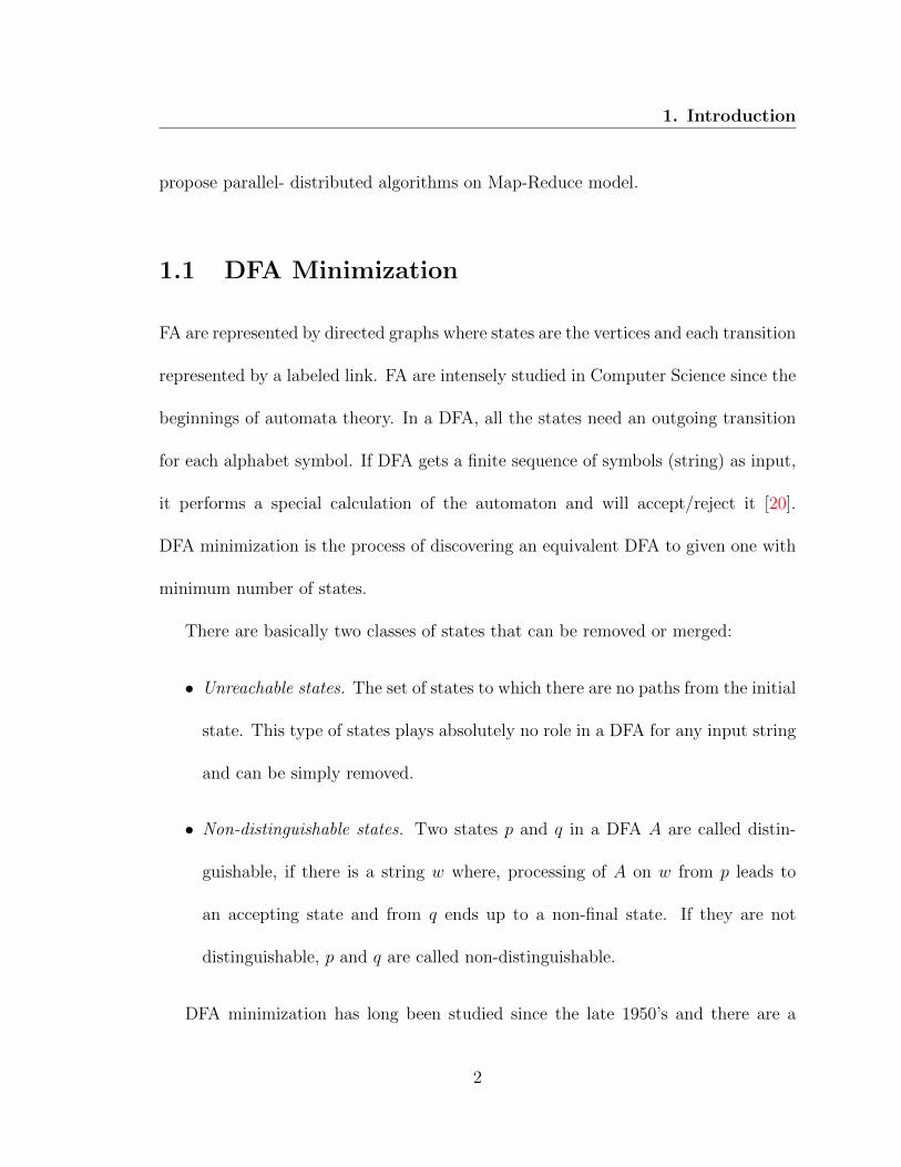
1.1 DFA Minimization
FA are represented by directed graphs where states are the vertices and each transition
represented by a labeled link. FA are intensely studied in Computer Science since the
beginnings of automata theory. In a DFA, all the states need an outgoing transition
for each alphabet symbol. If DFA gets a finite sequence of symbols (string) as input,
it performs a special calculation of the automaton and will accept/reject it [20].
DFA minimization is the process of discovering an equivalent DFA to given one with
minimum number of states.
There are basically two classes of states that can be removed or merged:
• Unreachable states. The set of states to which there are no paths from the initial
state. This type of states plays absolutely no role in a DFA for any input string
and can be simply removed.
• Non-distinguishable states. Two states p and q in a DFA A are called distin-
guishable, if there is a string w where, processing of A on w from p leads to
an accepting state and from q ends up to a non-final state. If they are not
distinguishable, p and q are called non-distinguishable.
DFA minimization has long been studied since the late 1950’s and there are a
2

1. Introduction
variety of algorithms utilizing different approaches [37]. On the other hand, data
is growing and consequently, nowadays, we are dealing with DFA’s with petastates
1 for which DFA minimization process becomes not only time-consuming but also
almost impossible. It is well known that one of the most powerful methods to handle
large size of data is Map-Reduce model where we first send part of data appropri-
ate to a processing unit to one or more machines (Mapping) and do the processing
simultaneously (Reducing) [14].
As mentioned, there are variety of algorithms introduced in field of DFA minimiza-
tion. However, Finite Automata processing is very difficult to parallelize because of
tight dependencies between successive loops making it hard to distribute loops over
processing units and also consequently in each iteration there is a few computations
which are very input-dependent and unpredictable. When it comes to processing
finite automata in Map-Reduce environment, the most important part of algorithm
design is reducing number of rounds as well as replication rate and communication
cost.
1.2 Big-Data Processing in Map-Reduce Model
It is more than trivial that amount of data is unlimited including data from past,
present and what will happen in future as long as could be observed by humankind.
1petastate DFA is a DFA with more than 1015 states
3

1. Introduction
Fortunately, data storage technology is growing exponentially. This leads to increase
in amount of data to be processed as well. It can be observed from amount of data
that individual organizations, in a narrowed field of study, are dealing with. For
instance, the followings are facing to petabyte 2 data:
• Since 20 years ago, NASA ECS project archive [10]
• Since 13 years ago, High Energy Physics [5]
• Around 5 years ago, Astronomy [8].
In order to give the possibility of processing this amount of data, Map-Reduce model
is introduced to organize data in smaller chunks and process each of them separately.
This will be discussed more in details in 2.2.
1.3 Motivation and Contributions
DFA Minimization is a fundamental field of study in computer science because of
the exhibited power for modeling variety of problems. On the other hand, data ex-
plosion happened in computer industry results complexity in running data intensive
programs. The lack of proper work on performing DFA minimization in parallel moti-
vated us to conduct this research to propose algorithms on Map-Reduce model mainly
by using equivalence relation and analyzing the performance of different approaches.
2Petabyte is equal to250 byte
4

1. Introduction
Besides proposing two distinct algorithms, we found that the graph topology of DFA
has a direct effect on the running performance and consuming resources. In addition,
the upper and lower bound on communication cost for minimizing a DFA in parallel
environments is calculated. Also, it has been discovered that there is not a universal
and comprehensive cost model and new measures is suggested in this thesis. These
works are supported by experiments running on DFA with more than 100, 000 states
with different topologies.
1.4 Thesis Organization
The rest of this thesis is organized as follows.
In Chapter 2, we review the background information necessary for this research. DFA
minimization approaches in serial and parallel are represented in Section 2.1. Section
2.2 will briefly introduce the Map-Reduce model and its open source implementation
called Hadoop. We look into contributions in processing FA using Map-Reduce model,
in Section 2.3 and finally the work done in cost model in parallel environment is
investigated in Section 2.4.
In Chapter 3, we study the DFA minimization problem in Map-Reduce model and
its cost measures. We propose an enhancement to the only known implementation
of Moore’s algorithm in Map-Reduce model [18] in Section 3.1. Additionally, a new
algorithm based on Hopcroft’s DFA minimization method [19] is proposed in the
5
1. Introduction
Map-Reduce model in Section 3.2. Section 3.4 is about the cost measures for DFA
minimization in Map-Reduce. The upper and lower bound on communication cost
is derived from Yao’s two parties model [41] in Section 3.4.1. In addition, following
Afrati et al. [2], the lower bound for data replicating over processing units is studied
in Section 3.4.2. The communication cost for the algorithms are presented in Sections
3.4.3 and 3.4.4.
Afterwards, Chapter 4 will demonstrate the performance of each algorithm in
terms of execution time and required space. After reviewing the underlying envi-
ronment in Section 4.1, the methods for generating sample data sets are described
in Section 4.2. In Section 4.3 the results gathered from experiments are shown and
discussed.
Finally, Chapter 5 is assigned for conclusion and future works including the re-
flection of study conducted in this thesis.
6

Chapter 2
Background and Related Work
2.1 Finite State Automata and their Minimization
An FA is a 5-tuple A = (Q,Σ, δ, s, F ), where Q is a finite set of states, Σ is a finite set
of alphabet symbols, δ ⊆ Q×Σ×Q is the transition relation, s ∈ Q is the start state,
and F ⊆ Q is a set of final states. By Σ∗ we denote the set of all finite strings over Σ.
Let w = a1a2 . . . an where ai ∈ Σ, be a string in Σ∗. An accepting computation path
of w in A is a sequence (s, a1, q1), (q1, a2, q2), . . . , (qn−1, an, qf ) of tuples (elements) of
δ, where qf ∈ F . The language accepted by A, denoted L(A), is the set of all strings
in Σ∗ for which there exists an accepting computation path in A. A language L is
regular if and only if there exists an FA A such that L(A) = L.
An FA A = (Q,Σ, δ, s, F ) is said to be deterministic if for all p ∈ Q and a ∈ Σ
7
2. Background and Related Work
there is a q ∈ Q, such that (q, a, p) ∈ δ. Otherwise the FA is non-deterministic.
Deterministic FA’s are called DFA’s, and non-deterministic ones are called NFA’s.
By the well known subset construction, any NFA A can be turned into a DFA AD,
such that L(AD) = L(A). For a DFA A = (Q,Σ, δ, s, F ), we also write δ in the
functional format, i.e. δ(p, a) = q iff (p, a, q) ∈ δ. In this thesis, both notation is used
whenever it is necessary. For a state p ∈ Q, and string w = a1a2 . . . an ∈ Σ∗, we
denote by δ(p, w) the unique state δ(δ(· · · δ(δ(p, a1), a2) · · · , an−1), an).
A DFA A is said to be minimal, if all DFA’s B, such that L(A) = L(B), have
at least as many states as A. For each regular language L, there is a unique (up to
isomorphism of their graph representations) minimal DFA that accepts L.
The DFA minimization problem has been studied since 1950s. A taxonomy of DFA
minimization algorithms was created by B. W. Watson in 1993 [37]. The taxonomy is
illustrated in Figure 1. Most of the algorithms are based on the notion of equivalent
states (to be defined). The sole exception is Brzozowski’s algorithm [42], which is
based on reversal and determinization of automata. Let A = (Q,Σ, δ, s, F ) be a DFA.
Then the reversal of A is the NFA AR = (Q,Σ, δR, F, {s}), where δR = {(p, a, q) :
(q, a, p) ∈ δ}. Brzozowski’s showed in 1962 that if A is a DFA, then (((AR)D)R)D
is a minimal DFA for L(A). This rather surprising result does not however yield a
practical minimization algorithm since there is a potential double exponential blow-up
in the number of states, due to the two determinization steps.
8
2. Background and Related Work
The rest of the algorithms is based on equivalence of states. Let A = (Q,Σ, δ, s, F )
be a DFA, and p, q ∈ Q. The p is equivalent with q, denoted p ≡ q, if for all strings
w ∈ Σ∗, it holds that δ(p, w) ∈ F if and only if δ(q, w) ∈ F . The quotient DFA
A/≡ = (Q/≡,Σ, γ, s/≡, F/≡) where γ(p/≡, a) = δ(p, a)/≡, is then a minimal DFA,
such that L(A/≡) = L(A). Note that Q/≡ is a partition of the state-space Q. An
important observation is that ≡ can be computed iteratively as⋁∞
i=0 ≡i, where p ≡0 q
if p ∈ F ⇔ q ∈ F , and p ≡i+1 q, if p ≡i q and δ(p, a) ∈ F ⇔ δ(q, a) ∈ F , for all
a ∈ Σ. This means that Q/≡ can be computed iteratively, each step refining Q/≡ito
Q/≡i+1.
Here is a brief description of each node under the Equivalence of States tree:
• Equivalence Relation: Find distinguishable states based on the equivalence class
of every state.
– Bottom-up approach. This approach starts out with a partition of n blocks
where n is number of states. Each block contains one and only one state.
Afterwards, the classes are iteratively merged and updated based on dis-
covering more equivalent states. After each iteration, intermediate results
can be used to make a smaller DFA [38].
– Top-down approach. In this classical methodology, we initially divide states
in two class of equivalency called final and non-final. During minimization
process, this partition is refined gradually by finding new distinguishable
9

2. Background and Related Work
DFA Minimization Methods
Equivalenceof States
Pointwise
ImperativeProgram
Memorization
EquivalenceRelation
Bottom-Up Top-Down
Layerwise Unordered
Lists
State pairs
Non-Equivalenceof States
Brzozowski
Figure 1: The forest expressing the family of finite automata minimizationalgorithms and their relations. As it can be seen, Brzozowski algorithmfor minimization is completely unrelated to others and is not connectedto this tree.
10
2. Background and Related Work
states. This approach is similar to the Coarsest Partitioning problem [20].
The input to the Coarsest Partition problem is a set S of n elements and
a partition π over them as well as one or more function fi : S → S. The
problem is to form a new partition π′ where each member of π′ is a subset
of one of the π members and fi(s) = fi(t) whenever s and t belong to
the same block of the new partition. The final partition of minimization
process contains equivalence classes each of which represents one state
in minimized DFA. Under this category we can talk about the following
methods:
∗ Layer-wise: this algorithm is called Layer-Wise as it computes the
equivalency of two states for strings of length i [40] [27] [9] [35].
Moore’s algorithm [27] will be discussed later on in Section 2.1.1.
∗ Un-ordered: this method called Un-Ordered because it does not fol-
low normal orders of processing like Layer-wise. This family of algo-
rithms have a free choice of states at each round to calculate partition
refinement. The best known running time of DFA minimization algo-
rithm [19] utilizes a list of blocks to which others should be compared.
This algorithm is so called Hopcroft’s DFA Minimization Algorithm
that will be discussed later in Section 2.1.2.
∗ State pairs: This algorithm presented in [20] in which every two pairs
11
2. Background and Related Work
will be compared to each other and if there exist an alphabet symbol
they go to different classes with, they are distinguishable.
• Point-wise: this method is mainly introduced in [32] for functional programming
purpose. The main idea is that two states are equivalent unless it is shown
otherwise. This matter can be achieved recursively. To accomplish finding
equivalent states, it mainly requires a data structure. Basically we can employ
global variables. However in real world applications it is almost impossible to
achieve that. Derived methods such as Imperative Program and Memorization
are placed under Point-wise sub-tree.
From above discussion, despite all differences, one may observe that a common
property for all methods under taxonomy tree is being iterative. Each tries to refine
partition of a DFA at each iteration until no more refinement can be applied. We
may call each iteration a round in DFA minimization algorithm or shortly round in
this thesis.
12

2. Background and Related Work
2.1.1 Moore’s Algorithm
The earliest iterative algorithm was proposed by Moore in 1956 [27]. The algorithm
computes the partition Q/≡ by iteratively refining the initial partition π = {F,Q\F}.
In the algorithm, partitions are recorded by a function π : Q→ {0, 1}logn.
Algorithm 1 exhibits Moore’s algorithm. The main data structure employed here
is an array block with size of n = |Q| which keeps equivalence class for every state.
The partitions are labeled by bit strings. The initial partition is π = {F,Q \ F} and
block(p) is 1 if p ∈ F and 0 otherwise(line 1 to 6). At each iteration, we refine the
current partition based on the outgoing transitions of the states for all alphabet (lines
8 to 10). Note that the symbol “·” on line 9 of the algorithm denotes concatenation
(of strings). Based on discovered block, lines 11 to 13 of algorithm are responsible to
refine every block of π using similarity (∼) relation. Two states p and q are similar if
and only if block(p) = block(q). By replacing B by B/∼, it will refine π consequently.
This algorithm will stop whenever new partition is equal to previous one (π′), e.g. no
refinement is happened. The minimal automaton can now be obtained by replacing
each transition (p, a, q) ∈ δ by (block(p), a, block(q)), and then removing duplicate
tuples.
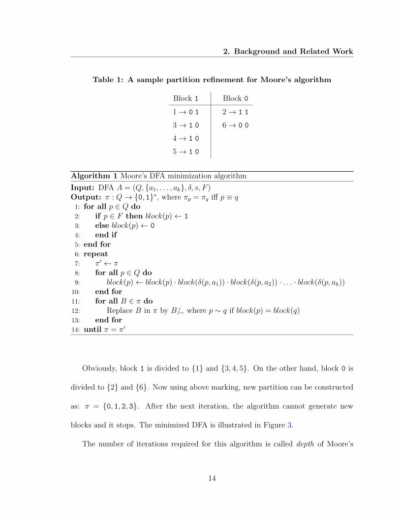
As an example, consider DFA in Figure 2. Initial partition is π = {0, 1}. Running
loop from line 9 yields to the marking shown in Table 1.
13
2. Background and Related Work
Table 1: A sample partition refinement for Moore’s algorithm
Block 1 Block 0
1→ 0 1 2→ 1 1
3→ 1 0 6→ 0 0
4→ 1 0
5→ 1 0
Algorithm 1 Moore’s DFA minimization algorithm
Input: DFA A = (Q, {a1, . . . , ak}, δ, s, F )Output: π : Q→ {0, 1}∗, where πp = πq iff p ≡ q1: for all p ∈ Q do2: if p ∈ F then block(p)← 1
3: else block(p)← 0
4: end if5: end for6: repeat7: π′ ← π8: for all p ∈ Q do9: block(p)← block(p) · block(δ(p, a1)) · block(δ(p, a2)) · . . . · block(δ(p, ak))10: end for11: for all B ∈ π do12: Replace B in π by B/∼ where p ∼ q if block(p) = block(q)13: end for14: until π = π′
Obviously, block 1 is divided to {1} and {3, 4, 5}. On the other hand, block 0 is
divided to {2} and {6}. Now using above marking, new partition can be constructed
as: π = {0, 1, 2, 3}. After the next iteration, the algorithm cannot generate new
blocks and it stops. The minimized DFA is illustrated in Figure 3.
The number of iterations required for this algorithm is called depth of Moore’s
14

2. Background and Related Work
1start
1
2
0
3
1
4
1
5
1
6 0
a
b
a
b
a
b
a
b
a
b
a, b
Figure 2: An example DFA
1start
3
2
0
3, 4, 5
1
6 2a
b
a
b
a
b
a, b
Figure 3: The minimized version of DFA in Figure 2
15

2. Background and Related Work
algorithm [6]. This factor strictly relies on the language recognized by automaton
not topology of DFA. Lines 8 to 10 of Algorithm 1 iterates O(kn) where n is the
number of states and k is size of alphabet. Besides, second loop at lines 11 to 13
can be implemented using Radix Sort having running time of O(kn). Denoting the
number of rounds as r, running time of Moore’s algorithm is O(rkn). Although the
worst case is obtained for r = n− 2 in family of slow automata (described in 2.1.2.2),
a detailed study in [3] [13] shows that there are only a few automata for which r is
greater than log n.
16

2. Background and Related Work
2.1.2 Hopcroft’s Algorithm
As it can be seen in Figure 1, under un-ordered DFA minimization method, there
should be a list to control the next step of the process. In ordered methods such as
Moore’s algorithm, the topology of DFA is not considered. In these algorithms, all
the states are being processed. By doing a pre-processing on DFA, we can avoid these
unnecessary work. The only known method using lists, has been introduced by John
Hopcroft [19].
Hopcroft gave an efficient algorithm in 1971 for minimizing the number of states
in a finite automaton [19]. The running time of his algorithm is O(kn log n) for n
states and k input alphabet symbols. Here, the original algorithm by Hopcroft is
described in more details.
The algorithm computes the partition π generated by ≡. We start with some
definitions. Let A = (Q,Σ, δ, s, F ) be a DFA, P,R ∈ π and a ∈ Σ. Then ⟨P, a⟩ is
called a splitter, and
R÷ ⟨P, a⟩ = {R1, R2}, where
R1 = {q ∈ R : δ(q, a) ∈ P}
R2 = {q ∈ R : δ(q, a) /∈ P}.
If either of R1 or R2 is empty, we set R÷⟨P, a⟩ = R. Otherwise ⟨P, a⟩ is said to split
17

2. Background and Related Work
R. Furthermore, for P ⊂ Q and a ∈ Σ, we define
a(P ) = {p ∈ P : δ(q, a) = p for some q ∈ Q}. (1)
That is, a(P ) consists of those states in P that have an incoming transition labelled
a. As initial partition π, contains a final and a non-final block, labelled as 1 and 2
respectively. Then, for all a in Σ and P ∈ {1, 2}, construct:
a(P ) = {q|q ∈ P ∧ δ−1(q, a) = ∅} (2)
where P ∈ π and δ−1(q, a) is set of states from which there is a transition labelled a
to q.
Now using Equation 2, we can define a set of splitters.
Q = {⟨P, a⟩|a ∈ Σ, P ∈ π = {1, 2}} (3)
where,
P =
⎧⎪⎪⎪⎨⎪⎪⎪⎩1 if |a(1)| ≤ |a(2)|
2 otherwise
The above mentioned steps about initializing required data structure are shown
in line 1 to 7 of Algorithm 2. The algorithm will stop as soon as the list Q becomes
18

2. Background and Related Work
empty. At each round , it picks a pair ⟨P, a⟩ from Q (line 9), and finds the blocks
which has to be partitioned with respect to ⟨P, a⟩. Once partition is refined (lines 11
and 12), it is necessary to apply Equation 2 again in order to update data structures
regarding new π. On the other hand, each time the block R is split, corresponding
splitters have to be added to Q. For every alphabet symbol a, if ⟨R, a⟩ we previously
in Q, it has to be replaced by ⟨R1, a⟩ and ⟨R2, a⟩. Otherwise, we only insert one of
⟨R1, a⟩ or ⟨R2, a⟩, namely the one where the block Ri has fewer incoming transitions
labelled a by extending Equation 3 to Equation 4 (lines 17 to 19).
∀a ∈ Σ,Q =
⎧⎪⎪⎪⎨⎪⎪⎪⎩Q∪ {⟨R1, a⟩} if |a(R1)| ≤ |a(R2)|
Q ∪ {⟨R2, a⟩} otherwise
(4)
The minimal automaton equivalent withA is obtained by choosing a representative
pi for each equivalence class Pi, then replacing each (p, a, q) in δ with (pi, a, qj) where
p ∈ Pi and q ∈ Pj, and finally removing duplicates.
2.1.2.1 Complexity of Hopcroft’s Algorithm
Hopcroft’s work published in 1971 and his proof of complexity is difficult to under-
stand. David Gries gave a better explanation of algorithm complexity in [17] two
years later which we tried to simplify here.
19
2. Background and Related Work
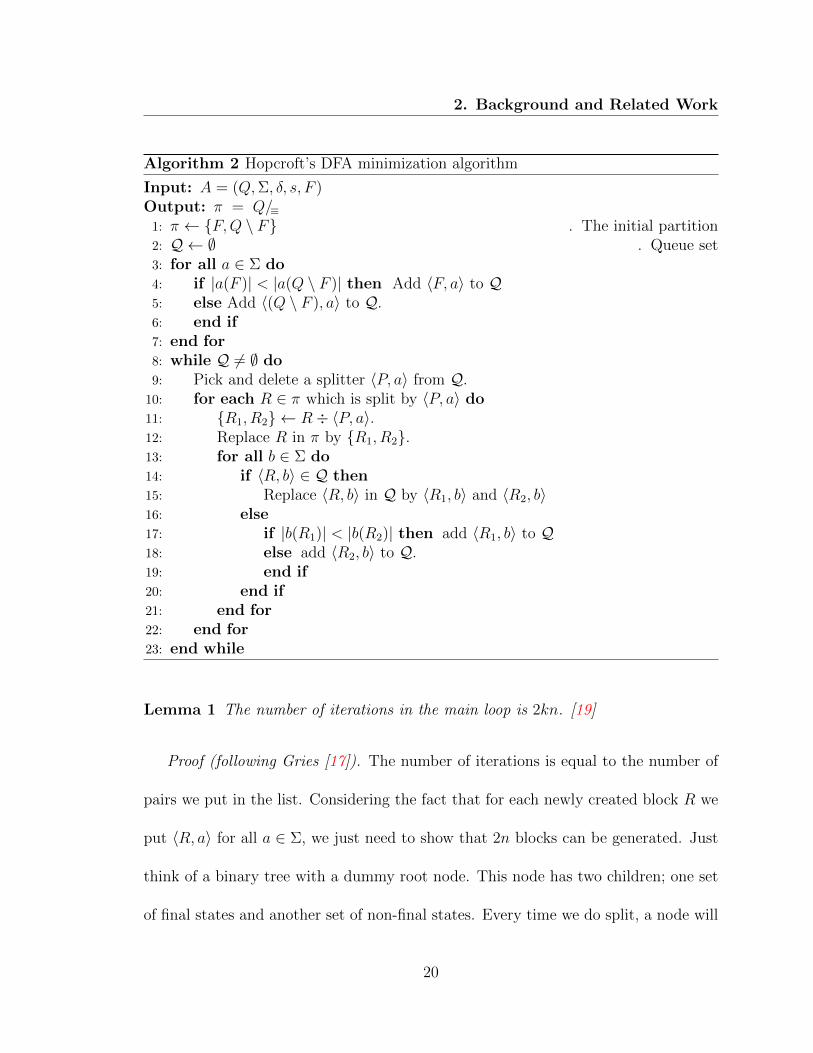
Algorithm 2 Hopcroft’s DFA minimization algorithm
Input: A = (Q,Σ, δ, s, F )Output: π = Q/≡1: π ← {F,Q \ F} ◃ The initial partition2: Q ← ∅ ◃ Queue set3: for all a ∈ Σ do4: if |a(F )| < |a(Q \ F )| then Add ⟨F, a⟩ to Q5: else Add ⟨(Q \ F ), a⟩ to Q.6: end if7: end for8: while Q = ∅ do9: Pick and delete a splitter ⟨P, a⟩ from Q.10: for each R ∈ π which is split by ⟨P, a⟩ do11: {R1, R2} ← R÷ ⟨P, a⟩.12: Replace R in π by {R1, R2}.13: for all b ∈ Σ do14: if ⟨R, b⟩ ∈ Q then15: Replace ⟨R, b⟩ in Q by ⟨R1, b⟩ and ⟨R2, b⟩16: else17: if |b(R1)| < |b(R2)| then add ⟨R1, b⟩ to Q18: else add ⟨R2, b⟩ to Q.19: end if20: end if21: end for22: end for23: end while
Lemma 1 The number of iterations in the main loop is 2kn. [19]
Proof (following Gries [17]). The number of iterations is equal to the number of
pairs we put in the list. Considering the fact that for each newly created block R we
put ⟨R, a⟩ for all a ∈ Σ, we just need to show that 2n blocks can be generated. Just
think of a binary tree with a dummy root node. This node has two children; one set
of final states and another set of non-final states. Every time we do split, a node will
20
2. Background and Related Work
R1 = F
...
p1 p2
...
p3
R2 = Q \ F
...
pn−2
...
pn−1 pn· · ·
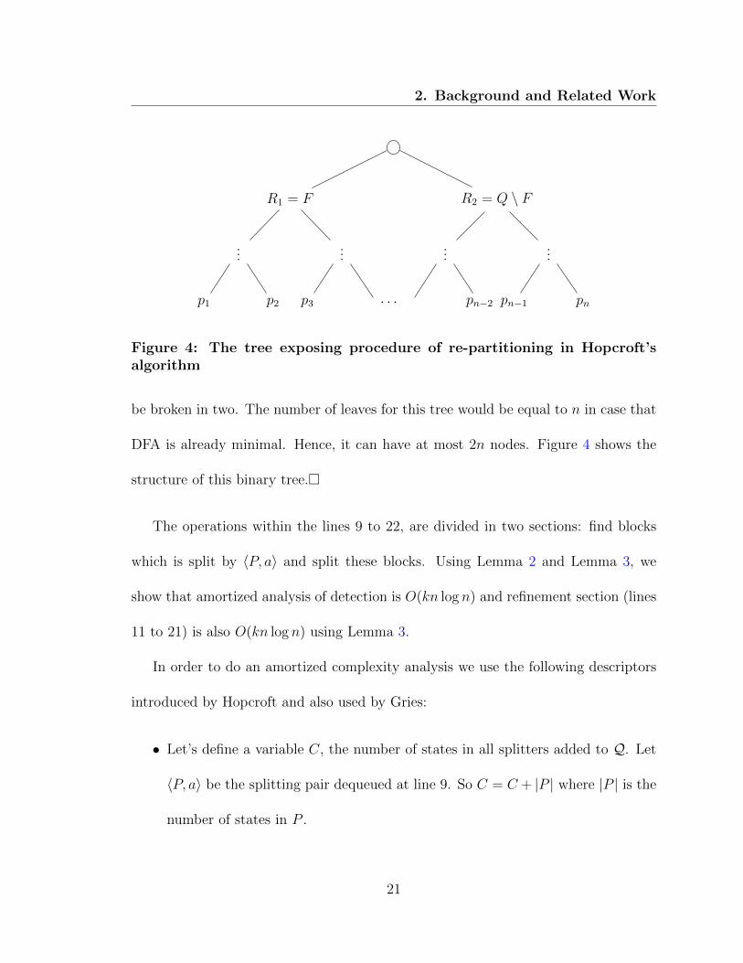
Figure 4: The tree exposing procedure of re-partitioning in Hopcroft’salgorithm
be broken in two. The number of leaves for this tree would be equal to n in case that
DFA is already minimal. Hence, it can have at most 2n nodes. Figure 4 shows the
structure of this binary tree.�
The operations within the lines 9 to 22, are divided in two sections: find blocks
which is split by ⟨P, a⟩ and split these blocks. Using Lemma 2 and Lemma 3, we
show that amortized analysis of detection is O(kn log n) and refinement section (lines
11 to 21) is also O(kn log n) using Lemma 3.
In order to do an amortized complexity analysis we use the following descriptors
introduced by Hopcroft and also used by Gries:
• Let’s define a variable C, the number of states in all splitters added to Q. Let
⟨P, a⟩ be the splitting pair dequeued at line 9. So C = C + |P | where |P | is the
number of states in P .
21
2. Background and Related Work
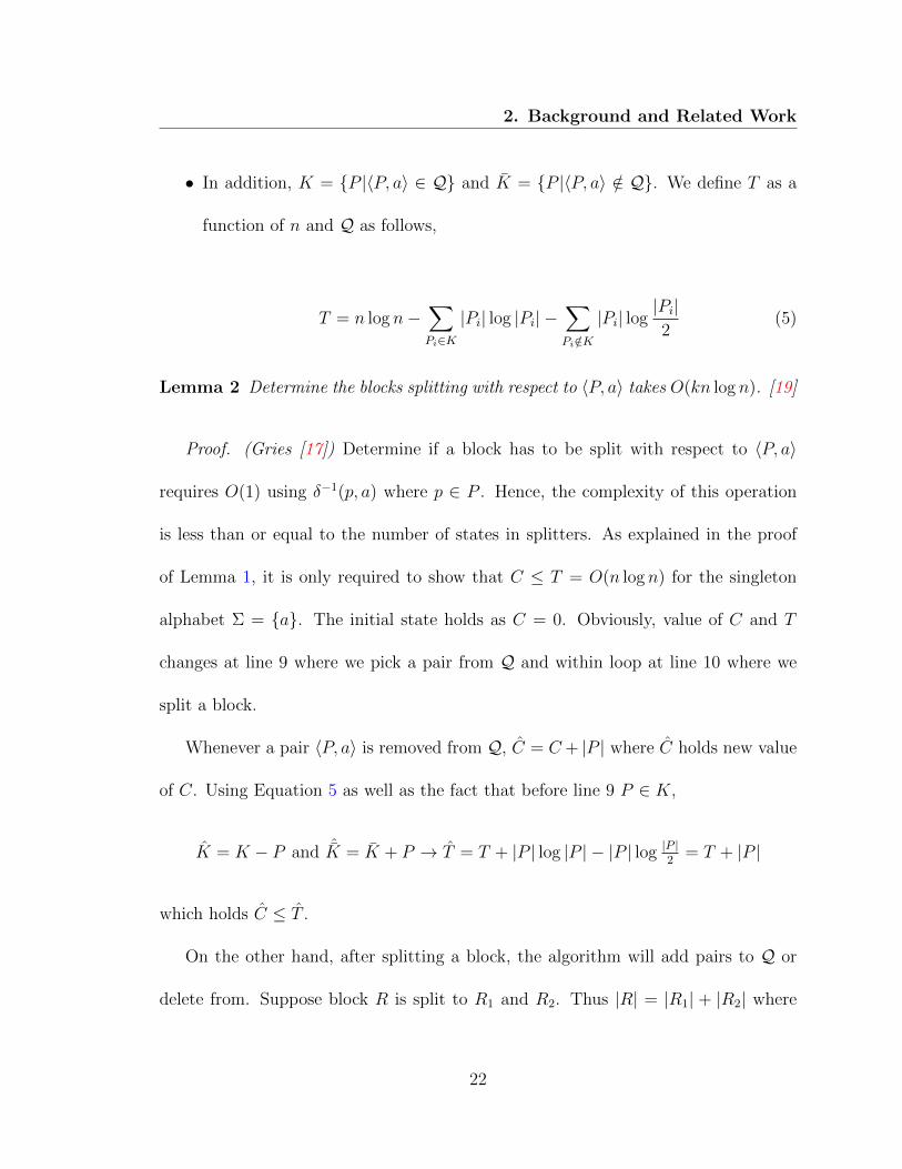
• In addition, K = {P |⟨P, a⟩ ∈ Q} and K = {P |⟨P, a⟩ /∈ Q}. We define T as a
function of n and Q as follows,
T = n log n−∑Pi∈K
|Pi| log |Pi| −∑Pi /∈K
|Pi| log|Pi|2
(5)
Lemma 2 Determine the blocks splitting with respect to ⟨P, a⟩ takes O(kn log n). [19]
Proof. (Gries [17]) Determine if a block has to be split with respect to ⟨P, a⟩
requires O(1) using δ−1(p, a) where p ∈ P . Hence, the complexity of this operation
is less than or equal to the number of states in splitters. As explained in the proof
of Lemma 1, it is only required to show that C ≤ T = O(n log n) for the singleton
alphabet Σ = {a}. The initial state holds as C = 0. Obviously, value of C and T
changes at line 9 where we pick a pair from Q and within loop at line 10 where we
split a block.
Whenever a pair ⟨P, a⟩ is removed from Q, C = C + |P | where C holds new value
of C. Using Equation 5 as well as the fact that before line 9 P ∈ K,
K = K − P and ˆK = K + P → T = T + |P | log |P | − |P | log |P |2
= T + |P |
which holds C ≤ T .
On the other hand, after splitting a block, the algorithm will add pairs to Q or
delete from. Suppose block R is split to R1 and R2. Thus |R| = |R1| + |R2| where
22

2. Background and Related Work
without loss of generality |R1| ≤ |R2|. First consider the situation that ⟨R, a⟩ was in
the list. In this situation, the algorithm removes ⟨R, a⟩ and adds ⟨R1, a⟩ and ⟨R2, a⟩
back to the Q. Then:
• T = T + |R| log |R| − |R1| log |R1| − |R2| log |R2|
• |R1| log |R1|+ |R2| log |R2| ≤ (|R1|+ |R2|) log |R2| = |R| log |R2| < |R| log |R|
∴ T > T
Now suppose that ⟨R, a⟩ ∈ Q, then ⟨R1, a⟩ has to be added into Q. Hence:
T = T + |R| log |R|2− |R1| log |R1| − |R2| log |R2|
2
Which again T > T . Therefore C < T = O(n log n) in either cases.�
The last step is to find number of times a pair ⟨P, a⟩ consisting a specific p ∈ P
can be in Q.
Lemma 3 The total number of states need to move to new block because of split
operation is bounded by O(kn log n) [19]
Proof. (Gries [17]) Suppose p, q ∈ Q, q ∈ P and δ(p, a) = q for some arbitrary
a ∈ Σ. When ⟨P, a⟩ is picked as splitter, p has to be moved to new block. We show
that the next time a splitter ⟨P1, a⟩ where q ∈ P1 is added to Q, |P1| ≤ |P |2. As a
result, the number of times that p has to be moved from one block to another one
23

2. Background and Related Work
because of split is bounded to O(k log n). If ⟨P, a⟩ is picked and if later P itself splits
into P1 and P2, and w.l.g. |P1| ≤ |P |2≤ |P2|, then only ⟨|P1|, a⟩ will be put back into
Q at line 17. In addition, |P | ≤ n/2 together with above mentioned fact exposes that
p can not be moved with respect to transition (p, a, q) more than log n times. There
are n state each of which having k transitions. This concludes that the total number
of states need to move to new block because of split is bounded by O(kn log n) �
Considering Lemma 1, 2 and 3, amortized complexity of running time of Hopcroft’s
algorithm is O(kn log n).
2.1.2.2 Slow Automata
As proved earlier by Lemma 1, the main loop will run at most kn times. This is in
the worst case, and happens when each newly generated block has a constant number
of states and at each iteration only one block can be split. One of the famous slow
automaton demonstrated in Figure 5. These types of automata are slow for most of
the DFA minimization algorithms.
0start 1 2 . . . na a a a
a
Figure 5: An example of slow automata for Hopcroft and Moore’s algo-rithms
24
2. Background and Related Work
2.1.3 Parallel Algorithms
In the presence of massive computations in terms of time and space, parallel com-
puting is a handful tool. The Parallel Random Access Memory (PRAM) is used to
model parallel algorithmic performance such as time and space complexity. When-
ever multiple parties are co-operating to solve a problem beside time and space issues
we face shared data operation conflicts as well as communication. The later will be
discussed in Section 2.4.1. Here we outline the data conflicts briefly.
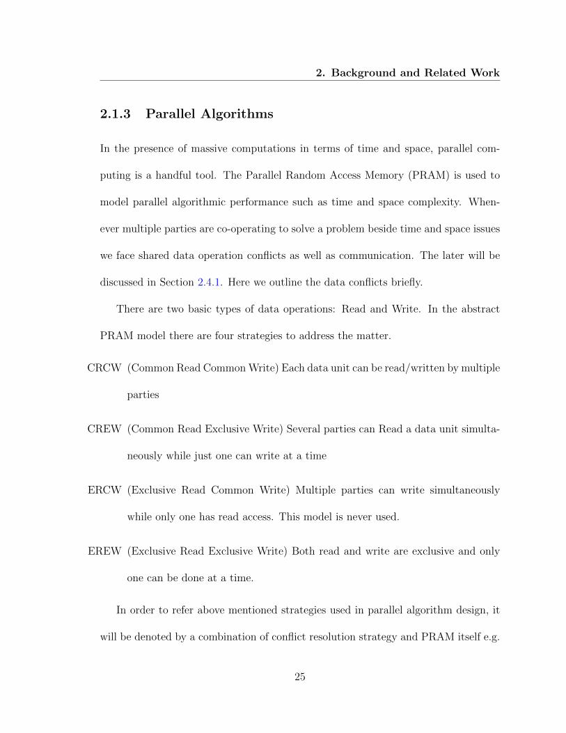
There are two basic types of data operations: Read and Write. In the abstract
PRAM model there are four strategies to address the matter.
CRCW (Common Read CommonWrite) Each data unit can be read/written by multiple
parties
CREW (Common Read Exclusive Write) Several parties can Read a data unit simulta-
neously while just one can write at a time
ERCW (Exclusive Read Common Write) Multiple parties can write simultaneously
while only one has read access. This model is never used.
EREW (Exclusive Read Exclusive Write) Both read and write are exclusive and only
one can be done at a time.
In order to refer above mentioned strategies used in parallel algorithm design, it
will be denoted by a combination of conflict resolution strategy and PRAM itself e.g.
25
2. Background and Related Work
EREW-PRAM. The complexity of parallel algorithms in PRAM model is expressed in
both space and time. Obviously time has a direct relation to the number of processing
units assigned for solving the problem. To compare two different algorithms, work
complexity is defined as O(T (n)·P (n)) where T (n) is required time for each processing
unit in presence of input size n and P (n) is the number of processing units.
Although DFA minimization is inherently an iterative problem and hard to per-
form in parallel environment[12], especially for slow automata, efforts have been done
in this area. DFA minimization has been broadly studied on numerous parallel com-
putation models. An exceptionally straightforward algorithm is suggested by Srikant
[29], while the best cost-effective algorithm is presented by Jaja and Ryu [21] when
the size of alphabet is 1. The algorithm described using CRCW-PRAM has time
complexity of O(log n) requires O(n6) processors. Having one alphabet makes this a
one function coarsest partitioning problem [11] which can be solved by transitive clo-
sure. As focus of this thesis is on general DFA’s without any restrictive assumptions,
these algorithms will not be discussed here.
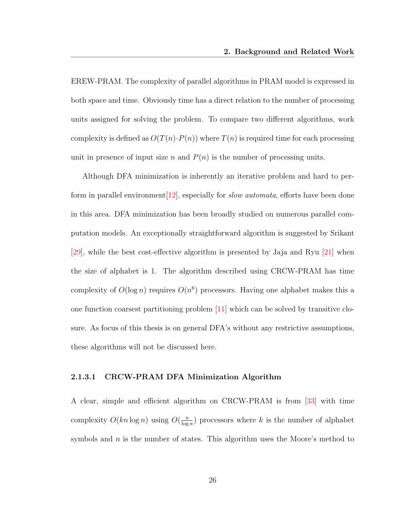
2.1.3.1 CRCW-PRAM DFA Minimization Algorithm
A clear, simple and efficient algorithm on CRCW-PRAM is from [33] with time
complexity O(kn log n) using O( nlogn
) processors where k is the number of alphabet
symbols and n is the number of states. This algorithm uses the Moore’s method to
26

2. Background and Related Work
assign new block numbers in parallel. This is illustrated in Algorithm 3. States and
blocks are represented by a number. The shared data structure in this algorithm is
an array block[0 . . . n], where the block number of state p is stored in block[p].
Algorithm 3 CRCW-PRAM algorithm for DFA minimization [33]
1: Initialize block array2: while Number of blocks is changing do3: for i = 0 to k − 1 do4: for j = 1 to ⌈ n
logn⌉ do ◃ Parallel loop
5: for m = (j − 1) log n to j log n− 1 do6: b1 = block[qm]7: b2 = block[δ(qm, ai)]8: label state qm with (b1, b2)9: end for10: end for11: Refine group numbers using parallel hashing12: end for13: end while
As it can be seen, main loop iterates in parallel until there are no more splits
in partition which as it mentioned in section 2.1.1, is n. Inside the loop, for every
alphabet a, all states will get new labels based on previous blocks they belonged to
and the block with a-transition they go.
Considering the fact that if we represent blocks using consecutive integer num-
bers, values can not exceed n. Thus, block numbers can be stored using log n bits.
However, in line 8, size of these markers is being doubled. If iteration takes i rounds
for minimization, at round i, it is 2i log n. In order to prevent exponential space
requirements for block numbers in line 11 of algorithm, they will be shrink to O(n)
27

2. Background and Related Work
using a Parallel Perfect Hashing Function (PPHF).
The Perfect Hashing Function (PHF) used in above mentioned algorithm comes
from [26] whose function is mapping a number from set of integers S from interval
[1,m] to a set of integers R from interval [1, n] where m >> n but |S| ≤ |R|. First,
it finds values present in S and counts them in parallel. Then the function tries to
compute partial sums. Using later results, it can now map from S to R in parallel.
Despite simplicity and efficiency of this algorithm with work time O(kn2), it has
a section in parallel hashing called partial summation which has to be done in serial
and execution of algorithm is opposed to CRCW-PRAM model.
2.1.3.2 EREW-PRAM DFA Minimization Algorithm
Algorithm 4 describes the EREW-PRAM algorithm by Ravikumar and Xiong in
1996 [28]. The basic assumption of this algorithm is that all states are reachable.
Otherwise, there should be a pre-processing step to remove unreachable states.
As claimed by author, the outer loop cannot be parallelized in this algorithm. This
algorithm fits in the Layer-wise family and uses Moore’s technique for minimization.
Instead of perfect hashing function introduced in CRCW-PRAM algorithm, parallel
sorting is being used here. Additionally, assigning new block number is done in line
8 of Algorithm 4 in serial again.
28

2. Background and Related Work
Algorithm 4 EREW-PRAM algorithm for DFA minimization [28]
Input: DFA A = (Q,Σ, δ, s, F )Output: minimized DFA.
1: procedure ParallelMin(M)2: repeat3: for i = 0 to k − 1 do ◃ Loop over a k-letter alphabet4: for j = 0 to n− 1 do ◃ Do this loop in parallel5: Label qj ∈ Q with BqjBδ(qj ,ai);6: Re-arrange(e.g. by parallel sorting) the states into blocks so that
the states with the same labels are contiguous;7: end for ◃ End parallel for8: Assign a unique number to all states in the same block9: end for10: until no new block produced11: end procedure
The cost of above mentioned algorithm is O(kn2). The main loop iterates at most
n times. The number of iterations for the loop at line 3 is k. Algorithm requires n
processors which leads to total work complexity of O(kn2).
29

2. Background and Related Work
2.2 Map-Reduce and Hadoop
In the past decade, we experienced exponentially growing amount of data which leads
to introducing the “Big-Data” concept into computer science. Big-data is the amount
of information that is stored but not possible to be processed utilizing traditional algo-
rithms and infrastructures [43]. Caused by unavoidable aggregation of data, computer
scientists have put an effort to introduce new processing models to address enterprise
concerns in this regards. One of the most famous models is called Map-Reduce (MR)
which divides data into smaller chunks, does operations and as a result reduces the
amount of data. Underneath this model is situated a robust infrastructure consisting
of a variety of technologies in order to handle data distribution, fault tolerance, and
job management. This enables separating algorithm design from low level technical
details.
2.2.1 Map-Reduce
Due to massive data mining and processing in one of the largest company working
with unimaginable amount of data, Map-Reduce was born in Google as a parallel-
distributed programming model working on a cluster of computers [14]. It has been
called parallel as tasks are done by dedicating multiple processing units in a paral-
lel environment and distributed as data is laid over separate storages. Hadoop [1]
is an open-source implementation of Map-Reduce framework and mainly developed
30
2. Background and Related Work
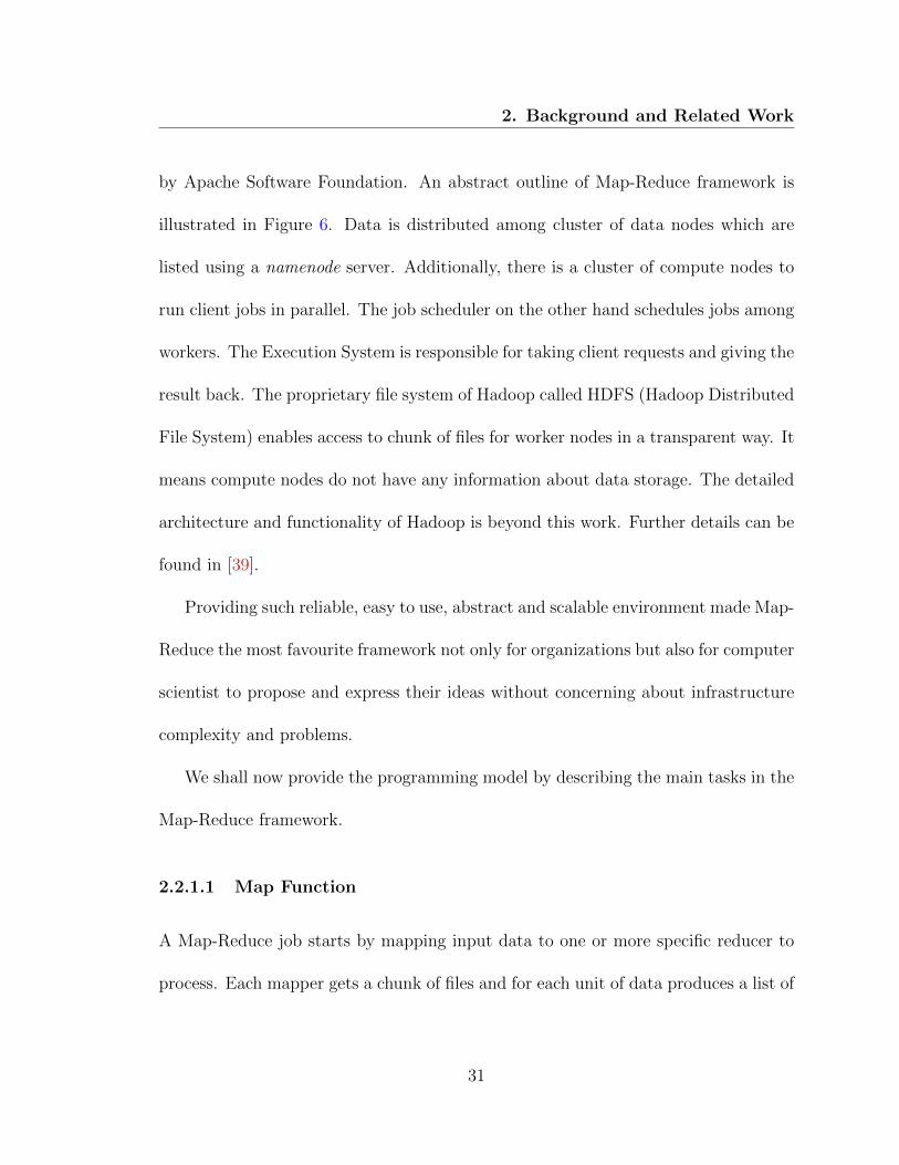
by Apache Software Foundation. An abstract outline of Map-Reduce framework is
illustrated in Figure 6. Data is distributed among cluster of data nodes which are
listed using a namenode server. Additionally, there is a cluster of compute nodes to
run client jobs in parallel. The job scheduler on the other hand schedules jobs among
workers. The Execution System is responsible for taking client requests and giving the
result back. The proprietary file system of Hadoop called HDFS (Hadoop Distributed
File System) enables access to chunk of files for worker nodes in a transparent way. It
means compute nodes do not have any information about data storage. The detailed
architecture and functionality of Hadoop is beyond this work. Further details can be
found in [39].
Providing such reliable, easy to use, abstract and scalable environment made Map-
Reduce the most favourite framework not only for organizations but also for computer
scientist to propose and express their ideas without concerning about infrastructure
complexity and problems.
We shall now provide the programming model by describing the main tasks in the
Map-Reduce framework.
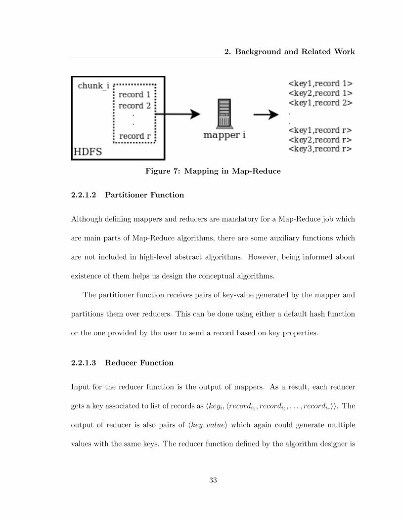
2.2.1.1 Map Function
A Map-Reduce job starts by mapping input data to one or more specific reducer to
process. Each mapper gets a chunk of files and for each unit of data produces a list of
31

2. Background and Related Work
Figure 6: Map-Reduce architecture
⟨key, value⟩ pairs based on a mapping schema (Section 2.2.2). Pairs with same keys
form a list and would be present in the same reducer. The mapping schema is the
most important part of a Map-Reduce algorithm which directly affects correctness,
time and space complexity. Figure 7 shows how the mapping schema works. Note
that a record can be present in different lists and the amount of replication can be
independent from all other input records.
32
2. Background and Related Work
Figure 7: Mapping in Map-Reduce
2.2.1.2 Partitioner Function
Although defining mappers and reducers are mandatory for a Map-Reduce job which
are main parts of Map-Reduce algorithms, there are some auxiliary functions which
are not included in high-level abstract algorithms. However, being informed about
existence of them helps us design the conceptual algorithms.
The partitioner function receives pairs of key-value generated by the mapper and
partitions them over reducers. This can be done using either a default hash function
or the one provided by the user to send a record based on key properties.
2.2.1.3 Reducer Function
Input for the reducer function is the output of mappers. As a result, each reducer
gets a key associated to list of records as ⟨keyi, ⟨recordi1 , recordi2 , . . . , recordir⟩⟩. The
output of reducer is also pairs of ⟨key, value⟩ which again could generate multiple
values with the same keys. The reducer function defined by the algorithm designer is
33

2. Background and Related Work
applied in parallel to the input list of values within each reducer. The output of each
reducer will be written on the Distributed File System (DFS).
2.2.2 Mapping Schema
As we studied, every input element can be mapped to one or more reducers in the
mapping part of Map-Reduce model. Although in most algorithms, we consider
unlimited capacity in terms of memory and computation for reducers, in the real
world the reducer workers have limitations. Let us denote this limit for maximum
input size as ρ. A mapping schema is defined to be an assignment of inputs to every
reducer with respect to ρ. It is also trivial that for every output of the problem at
least one reducer has to cover it. It means that reducers can have overlap output. [2].
Having in mind this definition, the replication rate R for an algorithm is the sum
of all inputs sent to every reducer divided by the actual input size |I|. Furthermore,
let ρi be the size of input sent to reducer i and denote the number of reducers by η.
Hence,
R =
∑ηi=1 ρi|I|
. (6)
34
2. Background and Related Work
2.3 Automata Algorithms in Map-Reduce
Graphs and automata take a large portion of Big-Data nowadays as part of social
networks, web, software models, etc. It is a serious concern for organizations to
process and interpret stored data. In this section, two algorithms for processing FA
using Map-Reduce model are represented.
2.3.1 NFA Intersection
NFA are one of the powerful tools in automata theory having a great benefit in being
closed under concatenation, intersection, difference, and homomorphic images. This
makes NFA interesting in design and study modular approaches such as web service
composition and protocol design.
In [16], authors have studied NFA intersection using Map-Reduce model broadly.
They proposed three algorithms with different mapping schema as well as introducing
the lower bound on replication rate computing NFA intersection using Map-Reduce
data processing model.
Consider automata A1 = (Q1,Σ1, δ1, s1, F1) and A2 = (Q2,Σ2, δ2, s2, F2) as two
NFAs accepting L(A1) and L(A2) languages. Intersection of these two NFA can be
computed as
A1 ⊗ A2 = (Q1 ×Q2,Σ, δ, (s1, s2), F1 × F2)
35

2. Background and Related Work
where L(A) = L(A1) ∩ L(A2). Using associative property of ⊗, we can compute
intersection of m NFA as A1 ⊗ . . .⊗ Am.
The lower bound for replication rate (which will be discussed later in section 2.4.2)
for NFA intersection is:
R ≥ρ× |δ1|×···×|δm|
km−1
(ρ/m)m × (|δ1|+ · · ·+ |δm|)(7)
where ρ is maximum capacity of a reducer and k = |Σ| is number of alphabets.
Mapping based on states
The basic assumption is that there are nm reducers where m denotes number of
NFA and n is maximum transitions in any. In first approach, mappers emit key-value
pairs as ⟨K, (pi, ci, qi)⟩ where (pi, ci, qi) is a transition and key is for all ij ∈ {1, . . . , n}:
⟨i1, . . . , ii−1, h(pi), ii+1, . . . , im⟩.
Note that h is a function as h : Q ↦→ {1, . . . , n}. Replication rate for this method is
R ≤ (nmρ)m−1.
Mapping based on alphabet
As the second approach, it is been assumed that there is one reducer for each
36
2. Background and Related Work
alphabet symbol. So the mappers emit key-value pair for every transition from au-
tomata Ai as:
⟨h(c), (pi, c, qi)⟩.
Every reducer will output transition as ⟨(p1, . . . , pm), c, (q1, . . . , qm)⟩. Replication rate
is R = 1.
Mapping based on both alphabet and state
In this method, we have two hashing function hs : pi ↦→ {1, . . . , bs} and ha :
aj ↦→ {1, . . . , ba}. For all ij ∈ {1, . . . , bs}, we will map each transition to reducers
⟨i1, . . . , ii−1, hs(pi), ii+1, . . . , im, ha(ci)⟩. It has been assumed that total number of
reducers are bm−1s · ba. Replication rate for this method is R ≤ (nml
ρk)m−1 where l is
average number of alphabet symbols received by a reducer.
2.3.2 DFA Minimization (Moore-MR)
To the best of our knowledge, the only algorithm for DFA minimization proposed
on Map-Reduce model is published in [18]. Author used method of Moore’s DFA
minimization for distributing data among reducer and compute minimal DFA.
Algorithm is introduced as a sequence of Map-Reduce jobs which output of one
job is input of next consecutive one. Mappers will emit pair of key-values as:
⟨h(p), (p, a, q, c,∆)⟩
37

2. Background and Related Work
where ∆ ∈ {0, 1} indicates if value is a transition (0) or a reverse transition (1). The
reverse transition for (p, a, q) is defined as (q, a, p). Assume that there are n reducers
(number of reducers is equal to number of states), transitions belonging to each state
will be present in one reducer called h(p). In each reducer, new equivalence class is
computed as
P ipj
= P i−1p P i−1
qj1. . . P i−1
qjk
having k alphabet where P ip denotes block of state p in round i represented as a bit
string. In order to calculate the classes for each state, it is required to have class of
target state q in each transition. This can be achieved if each reverse transition also
be sent to its target (which is actually source of the original transition). In above
mentioned procedure, we just update class of source states in original transitions.
Therefore, we need to send each reverse transition to its source (which in this case
is target of the original transition). This procedure requires replication rate 32if the
input is the union of both transitions and their reverses. The Algorithm will stop
if there is no new block generated within the partition. Decision of convergence is
being made as a parallel voting system where each reducer is responsible for one state
ad votes to continue if number of adjacent blocks is changed. Same as in Moore’s
algorithm, it requires O(n) rounds to generate the minimal DFA.
Beside simplicity of the algorithm, it suffers from exploding amount of data. Con-
sider that algorithm will take r rounds to finish. Size of class identifiers at round i
38
2. Background and Related Work
would be ki. This directly will affect communication cost despite having replication
rate O(1). An improvement for this algorithm will be proposed later in 3.1.
2.4 Cost Model
We now introduce a parameter that helps us modelling the Map-Reduce cost respect-
ing both computation and communications. First, we will discuss a general and basic
method to find the minimum required communication to solve a function in paral-
lel. Then after introducing a lower bound recipe for determining replication rate and
communication cost for Map-Reduce algorithm having one round was first suggested
in [2], a new enhanced version of Map-Reduce cost model from [34] will be discussed.
2.4.1 Communication Complexity
In parallel computing environment multiple parties are engaged to accomplish either
one single or multiple tasks, based on one of the computer architectures in Flynn’s
taxonomy [15]:
SISD Single Instruction Single Data which is a serial computer running single instruc-
tion on one instance of data stream.
SIMD Single Instruction Multiple Data which is an array of processors computing
multiple streams of data. Obviously, data should be naturally parallelized.
39

2. Background and Related Work
MISD Multiple Instructions Single Data which multiple processing units are working
on the same data stream. This model is more about integrity, consistency and
fault tolerance. All parties should be agree about the result.
MIMD Multiple Instructions Multiple Data, In this model, multiple processing units
are working on multiple streams of data at the same time. This model is the
most common one nowadays and Distributed Systems are a generalization of
this model.
Based on the selected model, most of the time it is required that processing units
communicate data to fulfil their tasks. An algorithm designed to run on one of the
parallel or distributed computing models, should be analysed regarding to the amount
of communication done in the system. Considering the fact that in Map-Reduce
model, after mapping data to associated reducers, one pre-defined function will be
applied on each list of key-value pairs, this will be equivalent to SIMD definition of
Flynn’s model which also can extended to MIMD.
Communication Complexity (CC) is an area has been studied for a long time. It
has been used for proving lower bounds in many areas. In this thesis Yao’s two-party
CC model [41] described and extended by Kushilevitz [23] is employed which is best
match to SIMD model. In Yao’s model, there are two parties (Alice and Bob) wishing
to evaluate a Boolean function f : {0, 1}n × {0, 1}n → {0, 1}. Here, x ∈ {0, 1}n is
input in Alice’s hand and Bob just got y ∈ {0, 1}n. The aim of this model is to
40
2. Background and Related Work
determine the amount of communication and so we do not care how parties will do
the computation. Although there are different methods for CC, we use deterministic
one which would gives more robust analysis to this problem.
The communication protocol P is responsible to decide which party is allowed to
which decides about who, when and what is sent. In addition, the protocol decides
whenever communication shall be terminated and when it does, what is the final
result of f . Also, if EP(x, y) = {m1, . . . ,mk} contains messages exchanged between
Alice and Bob during execution of protocol P over input x and y, then we can denote
|EP(x, y)| = Σki=1|mi|. Now we will define Deterministic Communication Complexity
(DCC) of P as
D(P) = max(x,y)∈{0,1}n×{0,1}n
|EP(x, y)| (8)
DCC of a function f can be defined as
D(f) = minP:P computes f
D(P) (9)
The worst case for any function f : {0, 1}n × {0, 1}n → {0, 1} is one party Alice
sends all its input to Bob and Bob will send the result back. Hence,
∀f ,D(f) ≤ n+ 1 (10)
41

2. Background and Related Work
is an upper bound. In order to find the minimum DCC, first we define rectangles.
Definition 1 A rectangle is a subset of {0, 1}n×{0, 1}n of the form A×B, where each
of A and B is a subset of {0, 1}n. A rectangle R = A× B is called f-monochromatic
if for every x ∈ A and y ∈ B the value of f(x, y) is the same. [23]
Here we define CP(f) as the minimum number of f -monochromatic rectangles in
protocol P that partition the space of inputs, {0, 1}n × {0, 1}n.
Lemma 4 For every function f : {0, 1}n × {0, 1}n → {0, 1},
D(f) ≥ log2CP(f) (11)
proof. Every protocol P will partition input space of {0, 1}n×{0, 1}n into f -monochromatic
rectangles. Each message would lead to two new states. Thus, the number of rect-
angles which equals to the number of possible communications (CP(f)) is at most
2D(P). From Equations 8 and Equation 9, we know that D(f) ≤ D(P). Hence,
CP(f) ≤ 2D(f) and it is equivalent to say D(f) ≥ log2CP(f) �
In Lemma 4 we found that in order to calculate DCC, it is required to find CP(f).
In [25], the fooling set method was explicitly used to find lower bound in VLSI
problems.
Definition 2 A set of input pairs S ⊆ X × Y is called a fooling set (of size ℓ) with
42
2. Background and Related Work
respect to f if there exists z ∈ {0, 1} such that
1. ∀(x, y) ∈ S, f(x, y) = z
2. For any two pairs (x1, y2) and (x2, y1) either f(x1, y2) = z or f(x2, y1) = z
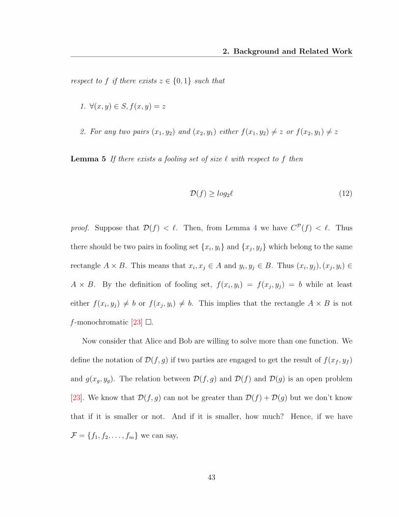
Lemma 5 If there exists a fooling set of size ℓ with respect to f then
D(f) ≥ log2ℓ (12)
proof. Suppose that D(f) < ℓ. Then, from Lemma 4 we have CP(f) < ℓ. Thus
there should be two pairs in fooling set {xi, yi} and {xj, yj} which belong to the same
rectangle A× B. This means that xi, xj ∈ A and yi, yj ∈ B. Thus (xi, yj), (xj, yi) ∈
A × B. By the definition of fooling set, f(xi, yi) = f(xj, yj) = b while at least
either f(xi, yj) = b or f(xj, yi) = b. This implies that the rectangle A × B is not
f -monochromatic [23] �.
Now consider that Alice and Bob are willing to solve more than one function. We
define the notation of D(f, g) if two parties are engaged to get the result of f(xf , yf )
and g(xg, yg). The relation between D(f, g) and D(f) and D(g) is an open problem
[23]. We know that D(f, g) can not be greater than D(f) +D(g) but we don’t know
that if it is smaller or not. And if it is smaller, how much? Hence, if we have
F = {f1, f2, . . . , fm} we can say,
43

2. Background and Related Work
D(F) = m(max∀fi∈F
D(fi)). (13)
The minimum communication complexity for DFA minimization has not been
determined yet. Though we know that it is in NL [11][12]. However, in Section 3.4,
we will propose an analysis for finding minimum compulsory amount of data to be
exchanged between multiple parties for minimizing DFAs using lower bound recipe
and extended Map-Reduce CC model which will be discussed more in this section.
2.4.2 The Lower Bound Recipe for Replication Rate
The replication rate is defined to be the number of key-value pairs generated by all
the mapper functions, divided by the number of inputs [24]. Afrati et al. proposed a
cost model in [2] to discover the lower bound on the replication rate for problems in
map-reduce.
Recall the mapping schema from Section 2.2.2, a mapper is free to send each input
to more than one reducer. This is called replication rate. The replication rate will
directly affect effectiveness of the algorithm. On the other hand, for some problems,
there is a lower bound for replication rate as well. Here, in this section, the recipe
from [2] to find this lower bound is presented.
Regarding the notion that every output shall be produced by at least one reducer,
this particular reducer should receive all required inputs to compute it. Denote g(ρ)
44
2. Background and Related Work
as an upper bound on the number of outputs reducer with capacity of ρ can cover.
Thus, g(ρi) is the number of outputs that reducer i covers. This can be simplified by
a formula as follows:
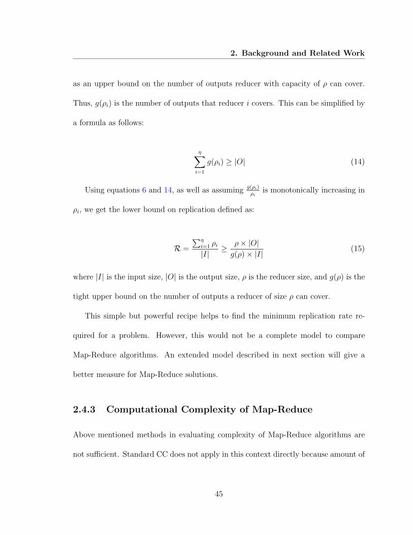
η∑i=1
g(ρi) ≥ |O| (14)
Using equations 6 and 14, as well as assuming g(ρi)ρi
is monotonically increasing in
ρi, we get the lower bound on replication defined as:
R =
∑ηi=1 ρi|I|
≥ ρ× |O|g(ρ)× |I|
(15)
where |I| is the input size, |O| is the output size, ρ is the reducer size, and g(ρ) is the
tight upper bound on the number of outputs a reducer of size ρ can cover.
This simple but powerful recipe helps to find the minimum replication rate re-
quired for a problem. However, this would not be a complete model to compare
Map-Reduce algorithms. An extended model described in next section will give a
better measure for Map-Reduce solutions.
2.4.3 Computational Complexity of Map-Reduce
Above mentioned methods in evaluating complexity of Map-Reduce algorithms are
not sufficient. Standard CC does not apply in this context directly because amount of
45

2. Background and Related Work
communication is more than linear. Additionally, lower bound recipe is just working
on one round algorithms. In order to remedy these issues, Gyorgy Turan in [34] has
proposed a formal definition of Map-Reduce model using Turing Machine to analyse
Map-Reduce algorithms and compare them not only with each other, but also with
other parallel and distributed computing models.
Time-space tradeoffs are studied in [7] by relating TIME(T (n)) and SPACE(S(n)).
TISP (T (n), S(n)) are problems which can be decided by a Turing Machine where
T (n) is time complexity and S(n) is required space in presence of input size n. As
it is been discussed, Map-Reduce algorithms consist two major sections: mapper and
reducer. In above mentioned paper, each of them is a separate run of the same
Turing machine M(m, r, n, ρ) where m is a flag denoting whether run map or reduce
function, r is round number, n is total input size and ρ as machine input size .
Moreover, it requires R rounds of Map-Reduce run to accomplish the task. On the
other hand, let us denote a mapper as α and reducer as β, both polynomial time-space
Turing machines. Then we can model a Map-Reduce run as series of mappers and
reducers α1, β1, α2, β2, . . .. Authors in [34] defined uniform deterministic Map-Reduce
Complexity model (MRC) as described in definition 3.
Definition 3 A language L is said to be in MRC[f(n), g(n)] if there is a constant
0 < c < 1, an O(nc)-space and O(g(n))-time Turing machine M(m, r, n, ρ), and an
R = O(f(n)), such that for all x ∈ {0, 1}n, the following holds,
46
2. Background and Related Work
1. Letting αr = M(1, r, n,−), βr = M(0, r, n,−), the MRC machine MR = (α1, β1,
. . . , αR, βR) accepts x if and only if x ∈ L
2. Each αr outputs O(nc) distinct keys
The first parameter c is related to the replication rate. Recall Equation 6, if c = 1,
R =
∑ηi=0 |I||I|
= η
which means we are sending whole data to all reducers. This is also an upper bound
for replication rate. On the other hand if c = 0 then we have nc = 1 means every
input record would be sent once and R = 1. Number of rounds R = f(n) however has
a serious impact, as initializing a Map-Reduce job in practice requires an initialization
overhead mainly containing huge amount of I/O read and write as well as network
communications. After that, although g(n) as mentioned before, has the least effect on
evaluation of Map-Reduce algorithms, yet shall be counted as a complexity parameter.
Last but not least, is input size ρ to each Turing machine. As it can be combination
of intermediate data, total input and subset of total input.
Later in Chapter 3 and 4, we will use this model to compare our algorithms.
47
Chapter 3
DFA Minimization Algorithms in
Map-Reduce
In this chapter, DFA minimization algorithms in Map-Reduce model are presented.
First we discuss the Moore-MR algorithm introduced in Section 2.3.2 in more detail.
Then after, an algorithm for PPHF in Map-Reduce model (PPHF-MR) will be pro-
posed. Finally, an improved version of Moore-MR, called Moore-MR-PPHF will be
constructed by applying PPHF-MR. Then a new naive algorithm called Hopcroft-MR,
based on Hopcroft’s algorithm, will be proposed. Right after, an enhanced version of
Hopcroft-MR, called Hopcroft-MR-PAR is represented. At the end of this chapter,
communication and computation costs will be analysed.
48

3. DFA Minimization Algorithms in Map-Reduce
3.1 Moore’s DFA Minimization in Map-Reduce
(Moore-MR-PPHF)
Moore’s algorithm (Section 2.1.1) is one of the most simple and straightforward meth-
ods for minimizing DFA and such it can be easily developed in parallel environments.
In this section, the enhanced version of the algorithm described in Section 2.3.2
(Moore-MR) from [18] will be introduced.
The Moore-MR algorithm consists of a pre-processing stage, and one or more
rounds of map and reduce functions. Additionally, each reducer which is associated
to transitions of one state, will check whether the number of equivalence classes has
been changed or not. Based on this parallel voting system, algorithm will decide
about convergence and finish the process. The final minimized DFA can be generated
from output of the last round (Algorithm 5).
Pre-processing: Let the automaton be A = (Q, {a1, . . . , ak}, δ, s, F ). We first build
a set ∆ from δ. This set will consist of annotated transitions of the form (p, a, q, πp, D),
where πp is a bit-string representing the initial block where the state p belongs, D = +
indicates that the tuple represents a transition (an outgoing edge), and D = −
indicates that the tuple is a ”dummy” transition carrying in its fourth position the
information of the initial block of the aforementioned state q (now occuring in the
49

3. DFA Minimization Algorithms in Map-Reduce
first position). More specifically, for each (p, a, q) ∈ δ we insert into ∆
⎧⎪⎪⎪⎪⎪⎪⎪⎪⎪⎪⎨⎪⎪⎪⎪⎪⎪⎪⎪⎪⎪⎩
(p, a, q, 1,+) and (q, a, p, 1,−) when p, q ∈ F
(p, a, q, 1,+) and (q, a, p, 0,−) when p ∈ F, q ∈ Q \ F
(p, a, q, 0,+) and (q, a, p, 1,−) when p ∈ Q \ F, q ∈ F
(p, a, q, 0,+) and (q, a, p, 0,−) when p, q ∈ Q \ F.
Recall that Moore’s algorithm is an iterative refinement of the initial partition
π = {F,Q \ F}. In Moore-MR, each reducer will be responsible for one or more
states p ∈ Q. Since there is no global data structure, we need to annotate each state
p with the block it currently belongs to. This annotation is kept in all transitions
(p, ai, qi), i = 1, . . . , k. Hence tuples (p, ai, qi, πp,+) are in ∆. In order to update
class of equivalency for p, the reducer also needs to know the current block of all the
above states qi, which is why tuples (qi, ai, p, πqi ,−) are in ∆. Furthermore, the new
block of state p will be needed in the next round when updating the block annotation
of states r1, . . . , rm, where (ri, aij , p) are all transitions leading to p. Thus tuples
(p, aij , ri, πp,−) are in ∆. Also we assume that the number of reducers available for
Moore-MR is equal to the number of states (n).
Map function: Let h : Q→ {1, . . . , n} be a hashing function. Each mapper gets a
50

3. DFA Minimization Algorithms in Map-Reduce
chunk of ∆ as input, and for each tuple (p, a, q, πp, D) emits
⎧⎪⎪⎨⎪⎪⎩⟨h(p), (p, a, q, πp, D)⟩ when D = +
⟨h(p), (p, a, q, πp, D)⟩ and ⟨h(q), (p, a, q, πp, D)⟩ when D = −
Reducer function: Each reducer is denoted by an integer number in range of [1, n]
and for all p ∈ Q, reducer h(p) receives the list of outgoing transitions
(p, a1, q1, πp,+), . . . , (p, ak, qk, πp,+)
as well as the dummy for its outgoing transitions
(q1, a1, p, πq1 ,−), . . . , (qk, ak, p, πqk ,−),
and the dummy for its incoming transitions (p, a1j , r1, πp,−), . . . , (p, amj, rm, πp,−)
where r1, . . . , rm are all the states with transitions into p. The reducer computes the
new equivalence class of state p in line 16 to 25 of the algorithm as
πr+1p ← πr
p · πrδ(p,a1)
· . . . πrδ(p,ak)
(16)
and then in line 26 to 29, writes the new value πr+1p in all the above tuples. At the
end, in line 31, it will emit a true record to vote YES for continuing the algorithm if
51

3. DFA Minimization Algorithms in Map-Reduce
there is any new class of equivalency around this state.
The proof of correctness is well described in [18]. But the cost analysis lacks
considering exponentially growing amount of data. The size of equivalence class
labels, starting from 1 bit for original DFA, is:
|π0p| = 1 and |πr
p| = (k + 1) · |πr−1| → |πrp| = (k + 1)r (17)
By denoting a transition as t and number of storage units to store a transition
record as |t|, the communication cost of this algorithm claimed to be 52(2kn|t|)R =
5kn|t|r where R ≤ n is number of rounds. The constant 52comes from the replication
rate 32plus the output of each round which is equal to writing down all the transitions
and dummy transitions once. However, the size of each transition varies at each
iteration. Let’s denote the size of transition at iteration r as |tr|. Then |tr| =
|⟨p, a, q, πrp, D⟩| = log n+ log k + log n+ |πr
p|+ 1 = 2 log n+ log k + |πrp|+ 1. Now we
can rewrite the communication cost as:
CC = 5knR∑
r=1
tr = 5knR∑
r=1
(2 log n+ log k + |πrp|+ 1)
which by Equation 17, it will be:
CC = 5kn(R(2 log n+ log k + 1) +R∑
r=1
(k + 1)r) < 5knkR − 1
k − 1= O(knn) (18)
52

3. DFA Minimization Algorithms in Map-Reduce
Algorithm 5 Moore’s algorithm in Map-Reduce (Moore-MR)
Input: ∆ as union of δ and dummy transitionsOutput: Updated δ exposing the minimal DFA1: repeat
2: function Mapper(∆)3: for all t ∈ ∆ do4: if D = + then5: Emit (⟨h(p), t⟩6: else7: if p = q then8: Emit ⟨h(q), t⟩9: Emit ⟨h(p), t⟩10: end if11: end if12: end for13: end function
14: function Reducer(⟨K, [t1, t2, . . . , tj] ⟩)15: π ← null16: for all ti do17: if D = + then18: if pi = qi then19: π ← π πpi
20: else21: s← find dummy transition of ti from the input list22: π ← π πs.p
23: end if24: end if25: end for26: Update πp in all transitions ti ∈ [t1, t2, . . . , tj] by π27: Emit ⟨K, ti⟩28: Update πq in all dummy transitions ti ∈ [t1, t2, . . . , tj] where q = K by π29: Emit ⟨K, ti⟩30: if the number of equivalence classes around state p = K changes then31: Emit (⟨p, true⟩32: end if33: end function
34: until no new equivalence class produced
53

3. DFA Minimization Algorithms in Map-Reduce
In order to avoid this data explosion, a new job at each iteration is introduced in
next section to change the labels using PPHF.
3.1.1 PPHF in Map-Reduce (PPHF-MR)
Most parallel algorithms, as mentioned in 2.1.3, use PPHF. The function PHF : S →
R where S ⊂ S ′, and |S| = |R| << |S ′| is a one-to-one and total function has the
following property:
∀x1, x2 ∈ S (PHF(x1) = PHF(x2)→ x1 = x2)
In order to apply PPHF in Map-Reduce (PPHF-MR), let S = πr and from Equa-
tion 17, S ′ = {0, 1, . . . , n(k+1)}. On the other hand, let R = n2. Now we can denote
PPHF-MR as,
PPHF-MR : πr → n2
The idea is that the mapper in PPHF job will map transitions based on equivalence
block label, h(πp), and all with the same classes will get a unique number. However,
recall that πp >> n and it will cause transitions from two class of equivalency meet
each other at the same reducer due to nature of hashing function. In order to avoid
54
3. DFA Minimization Algorithms in Map-Reduce
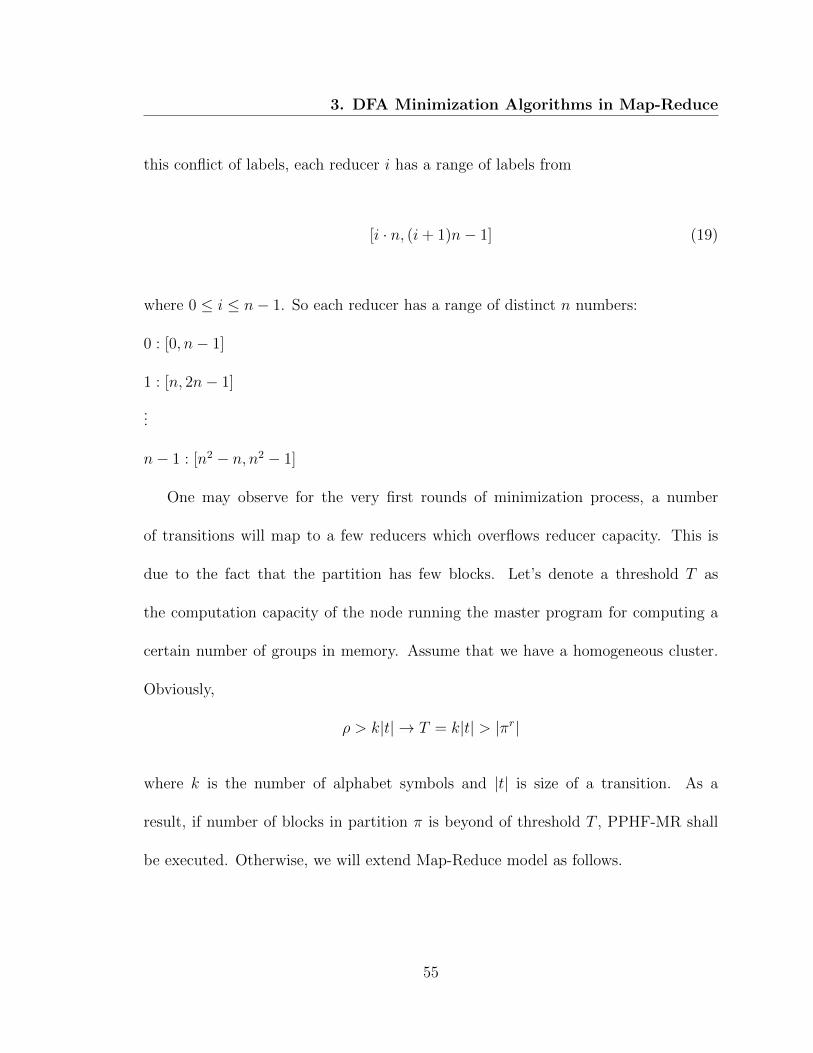
this conflict of labels, each reducer i has a range of labels from
[i · n, (i+ 1)n− 1] (19)
where 0 ≤ i ≤ n− 1. So each reducer has a range of distinct n numbers:
0 : [0, n− 1]
1 : [n, 2n− 1]
...
n− 1 : [n2 − n, n2 − 1]
One may observe for the very first rounds of minimization process, a number
of transitions will map to a few reducers which overflows reducer capacity. This is
due to the fact that the partition has few blocks. Let’s denote a threshold T as
the computation capacity of the node running the master program for computing a
certain number of groups in memory. Assume that we have a homogeneous cluster.
Obviously,
ρ > k|t| → T = k|t| > |πr|
where k is the number of alphabet symbols and |t| is size of a transition. As a
result, if number of blocks in partition π is beyond of threshold T , PPHF-MR shall
be executed. Otherwise, we will extend Map-Reduce model as follows.
55

3. DFA Minimization Algorithms in Map-Reduce
Extending Map-Reduce model. Recall the structure of Map-Reduce illus-
trated in Figure 6. As discussed before, namenode is responsible for keeping index
of files and directories on HDFS. The information about the folders and where the
files are stored can be retrieved using an API call to namenode. Here this property
can be employed to implement in-memory PHF. Suppose that we store transitions
associated to the states within a block in same directory and all the directories in one
upper level directory, called DFA. Now querying list of sub-directories under DFA,
it will get back a list of labels for every block. Despite the order of block labels in
the list, we will associate index of retrieved label as new label name. This method
follows exactly definition of PHF. Adding PPHF-MR at the end of each iteration in
line 33 of Algorithm 5, block labels are mapped into range [0 − n2] and we call this
algorithm Moore-MR-PPHF.
3.1.2 An Example of Running Moore-MR-PPHF
In order to have better understanding of Moore’s algorithm in Map-Reduce and
PPHF-MR, a sample DFA will be minimized.
Consider DFA from Figure 8 whereQ = {1, 2, 3, 4, 5, 6}, Σ = {a, b}, F = {1, 3, 4, 5}
and π0 = {0, 1}. The input contains transitions as well as dummy transitions:
56
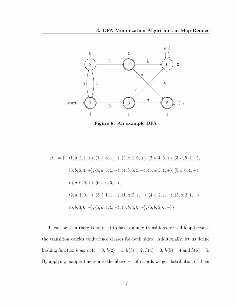
3. DFA Minimization Algorithms in Map-Reduce
1start
1
2
0
3
1
4
1
5
1
6 0
a
b
a
b
a
b
a
b
a
b
a, b
Figure 8: An example DFA
∆ = { ⟨1, a, 2, 1,+⟩, ⟨1, b, 3, 1,+⟩, ⟨2, a, 1, 0,+⟩, ⟨2, b, 4, 0,+⟩, ⟨3, a, 5, 1,+⟩,
⟨3, b, 6, 1,+⟩, ⟨4, a, 5, 1,+⟩, ⟨4, b, 6, 1,+⟩, ⟨5, a, 5, 1,+⟩, ⟨5, b, 6, 1,+⟩,
⟨6, a, 6, 0,+⟩, ⟨6, b, 6, 0,+⟩,
⟨2, a, 1, 0,−⟩, ⟨3, b, 1, 1,−⟩, ⟨1, a, 2, 1,−⟩, ⟨4, b, 2, 1,−⟩, ⟨5, a, 3, 1,−⟩,
⟨6, b, 3, 0,−⟩, ⟨5, a, 4, 1,−⟩, ⟨6, b, 4, 0,−⟩, ⟨6, b, 5, 0,−⟩}
It can be seen there is no need to have dummy transitions for self loop because
the transition carries equivalence classes for both sides. Additionally, let us define
hashing function h as: h(1) = 0, h(2) = 1, h(3) = 2, h(4) = 3, h(5) = 4 and h(6) = 5.
By applying mapper function to the above set of records we get distribution of them
57
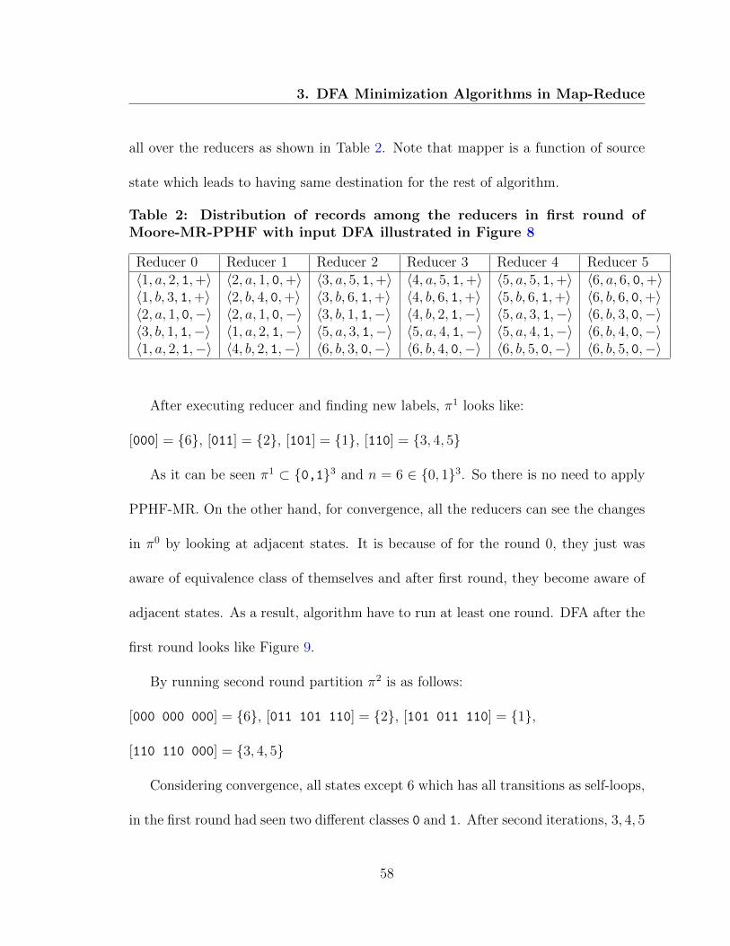
3. DFA Minimization Algorithms in Map-Reduce
all over the reducers as shown in Table 2. Note that mapper is a function of source
state which leads to having same destination for the rest of algorithm.
Table 2: Distribution of records among the reducers in first round ofMoore-MR-PPHF with input DFA illustrated in Figure 8
Reducer 0 Reducer 1 Reducer 2 Reducer 3 Reducer 4 Reducer 5⟨1, a, 2, 1,+⟩ ⟨2, a, 1, 0,+⟩ ⟨3, a, 5, 1,+⟩ ⟨4, a, 5, 1,+⟩ ⟨5, a, 5, 1,+⟩ ⟨6, a, 6, 0,+⟩⟨1, b, 3, 1,+⟩ ⟨2, b, 4, 0,+⟩ ⟨3, b, 6, 1,+⟩ ⟨4, b, 6, 1,+⟩ ⟨5, b, 6, 1,+⟩ ⟨6, b, 6, 0,+⟩⟨2, a, 1, 0,−⟩ ⟨2, a, 1, 0,−⟩ ⟨3, b, 1, 1,−⟩ ⟨4, b, 2, 1,−⟩ ⟨5, a, 3, 1,−⟩ ⟨6, b, 3, 0,−⟩⟨3, b, 1, 1,−⟩ ⟨1, a, 2, 1,−⟩ ⟨5, a, 3, 1,−⟩ ⟨5, a, 4, 1,−⟩ ⟨5, a, 4, 1,−⟩ ⟨6, b, 4, 0,−⟩⟨1, a, 2, 1,−⟩ ⟨4, b, 2, 1,−⟩ ⟨6, b, 3, 0,−⟩ ⟨6, b, 4, 0,−⟩ ⟨6, b, 5, 0,−⟩ ⟨6, b, 5, 0,−⟩
After executing reducer and finding new labels, π1 looks like:
[000] = {6}, [011] = {2}, [101] = {1}, [110] = {3, 4, 5}
As it can be seen π1 ⊂ {0,1}3 and n = 6 ∈ {0, 1}3. So there is no need to apply
PPHF-MR. On the other hand, for convergence, all the reducers can see the changes
in π0 by looking at adjacent states. It is because of for the round 0, they just was
aware of equivalence class of themselves and after first round, they become aware of
adjacent states. As a result, algorithm have to run at least one round. DFA after the
first round looks like Figure 9.
By running second round partition π2 is as follows:
[000 000 000] = {6}, [011 101 110] = {2}, [101 011 110] = {1},
[110 110 000] = {3, 4, 5}
Considering convergence, all states except 6 which has all transitions as self-loops,
in the first round had seen two different classes 0 and 1. After second iterations, 3, 4, 5
58
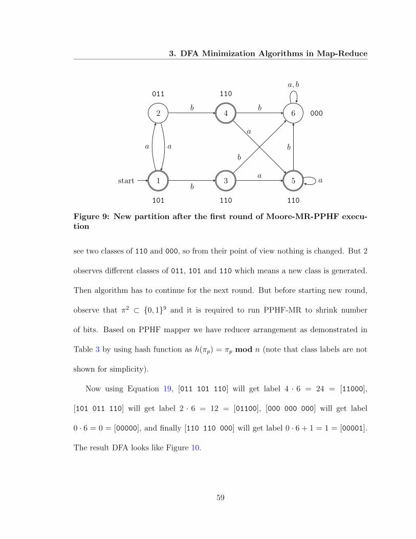
3. DFA Minimization Algorithms in Map-Reduce
1start
101
2
011
3
110
4
110
5
110
6 000
a
b
a
b
a
b
a
b
a
b
a, b
Figure 9: New partition after the first round of Moore-MR-PPHF execu-tion
see two classes of 110 and 000, so from their point of view nothing is changed. But 2
observes different classes of 011, 101 and 110 which means a new class is generated.
Then algorithm has to continue for the next round. But before starting new round,
observe that π2 ⊂ {0, 1}9 and it is required to run PPHF-MR to shrink number
of bits. Based on PPHF mapper we have reducer arrangement as demonstrated in
Table 3 by using hash function as h(πp) = πp mod n (note that class labels are not
shown for simplicity).
Now using Equation 19, [011 101 110] will get label 4 · 6 = 24 = [11000],
[101 011 110] will get label 2 · 6 = 12 = [01100], [000 000 000] will get label
0 · 6 = 0 = [00000], and finally [110 110 000] will get label 0 · 6 + 1 = 1 = [00001].
The result DFA looks like Figure 10.
59
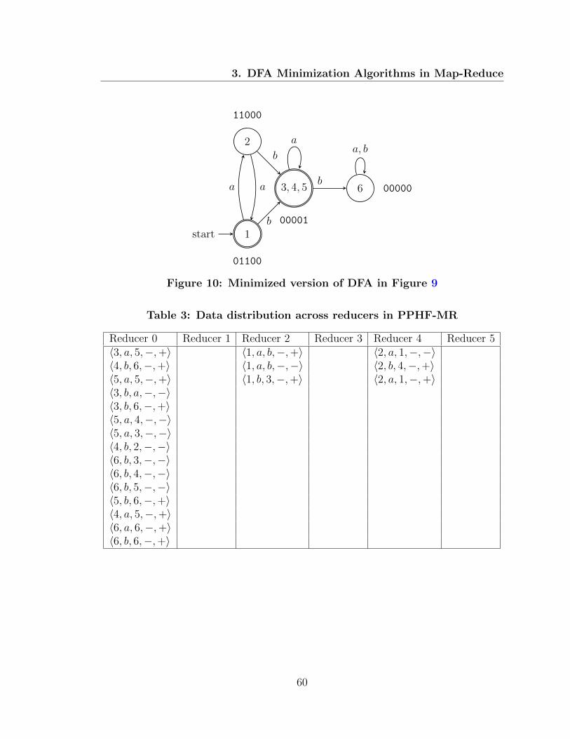
3. DFA Minimization Algorithms in Map-Reduce
1start
01100
2
11000
3, 4, 5
00001
6 00000a
b
a
b
a
b
a, b
Figure 10: Minimized version of DFA in Figure 9
Table 3: Data distribution across reducers in PPHF-MR
Reducer 0 Reducer 1 Reducer 2 Reducer 3 Reducer 4 Reducer 5⟨3, a, 5,−,+⟩ ⟨1, a, b,−,+⟩ ⟨2, a, 1,−,−⟩⟨4, b, 6,−,+⟩ ⟨1, a, b,−,−⟩ ⟨2, b, 4,−,+⟩⟨5, a, 5,−,+⟩ ⟨1, b, 3,−,+⟩ ⟨2, a, 1,−,+⟩⟨3, b, a,−,−⟩⟨3, b, 6,−,+⟩⟨5, a, 4,−,−⟩⟨5, a, 3,−,−⟩⟨4, b, 2,−,−⟩⟨6, b, 3,−,−⟩⟨6, b, 4,−,−⟩⟨6, b, 5,−,−⟩⟨5, b, 6,−,+⟩⟨4, a, 5,−,+⟩⟨6, a, 6,−,+⟩⟨6, b, 6,−,+⟩
60
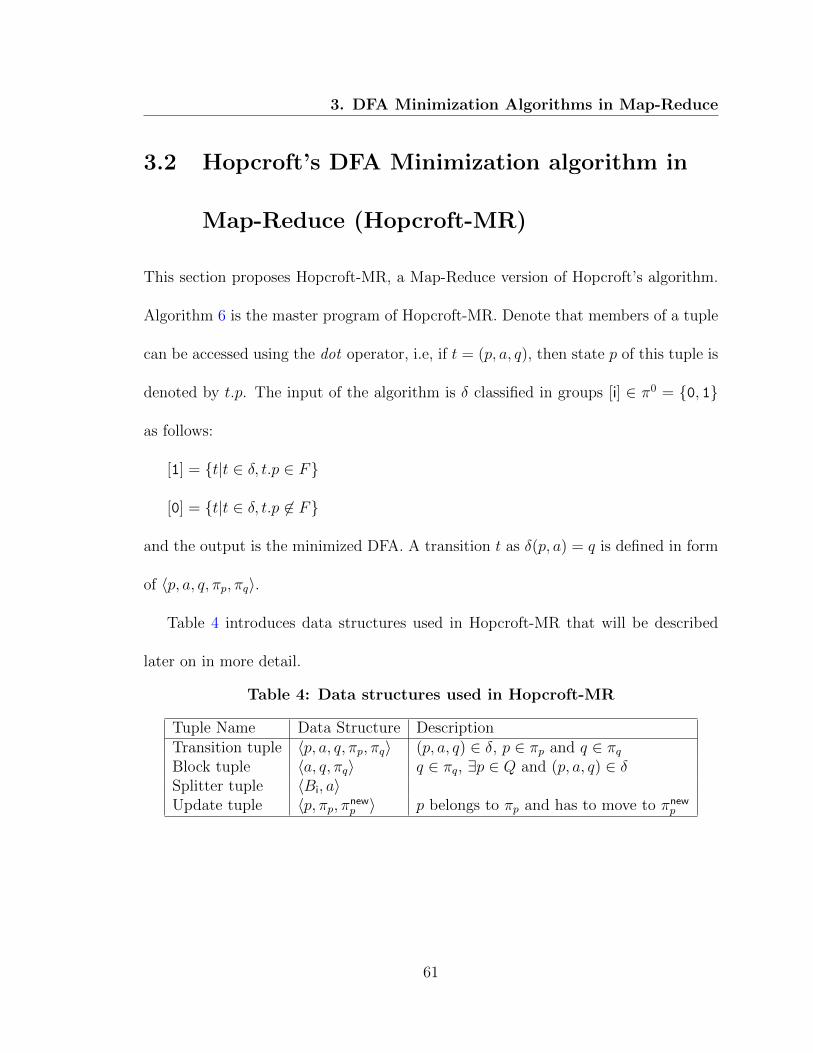
3. DFA Minimization Algorithms in Map-Reduce
3.2 Hopcroft’s DFA Minimization algorithm in
Map-Reduce (Hopcroft-MR)
This section proposes Hopcroft-MR, a Map-Reduce version of Hopcroft’s algorithm.
Algorithm 6 is the master program of Hopcroft-MR. Denote that members of a tuple
can be accessed using the dot operator, i.e, if t = (p, a, q), then state p of this tuple is
denoted by t.p. The input of the algorithm is δ classified in groups [i] ∈ π0 = {0, 1}
as follows:
[1] = {t|t ∈ δ, t.p ∈ F}
[0] = {t|t ∈ δ, t.p ∈ F}
and the output is the minimized DFA. A transition t as δ(p, a) = q is defined in form
of ⟨p, a, q, πp, πq⟩.
Table 4 introduces data structures used in Hopcroft-MR that will be described
later on in more detail.
Table 4: Data structures used in Hopcroft-MR
Tuple Name Data Structure DescriptionTransition tuple ⟨p, a, q, πp, πq⟩ (p, a, q) ∈ δ, p ∈ πp and q ∈ πq
Block tuple ⟨a, q, πq⟩ q ∈ πq, ∃p ∈ Q and (p, a, q) ∈ δSplitter tuple ⟨Bi, a⟩Update tuple ⟨p, πp, π
newp ⟩ p belongs to πp and has to move to πnew
p
61
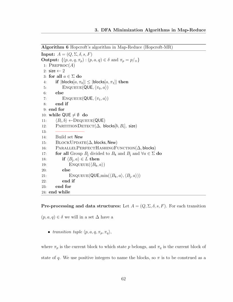
3. DFA Minimization Algorithms in Map-Reduce
Algorithm 6 Hopcroft’s algorithm in Map-Reduce (Hopcroft-MR)
Input: A = (Q,Σ, δ, s, F )Output: {(p, a, q, πp) : (p, a, q) ∈ δ and πp = p/≡}1: Preproc(A)2: size← 23: for all a ∈ Σ do4: if |blocks[a, π0]| ≤ |blocks[a, π1]| then5: Enqueue(QUE, ⟨π0, a⟩)6: else7: Enqueue(QUE, ⟨π1, a⟩)8: end if9: end for10: while QUE = ∅ do11: ⟨Bi, b⟩ ←Dequeue(QUE)12: PartitionDetect(∆, blocks[b, Bi], size)13: ——————–14: Build set New15: BlockUpdate(∆, blocks,New)16: ParallelPerfectHashingFunction(∆, blocks)17: for all Group Bj divided to Bk and Bj and ∀a ∈ Σ do18: if ⟨Bj, a⟩ ∈ L then19: Enqueue(⟨Bk, a⟩)20: else21: Enqueue(QUE,min(⟨Bk, a⟩, ⟨Bj, a⟩))22: end if23: end for24: end while
Pre-processing and data structures: Let A = (Q,Σ, δ, s, F ). For each transition
(p, a, q) ∈ δ we will in a set ∆ have a
• transition tuple ⟨p, a, q, πp, πq⟩,
where πp is the current block to which state p belongs, and πq is the current block of
state of q. We use positive integers to name the blocks, so π is to be construed as a
62

3. DFA Minimization Algorithms in Map-Reduce
mapping from Q to the positive integers. Initially, πp = 1 for p ∈ F , and πp = 0 for
p ∈ Q \F . The set ∆ will initially be chunked over DFS. The file system contains an
array blocks[a, i], where an entry contains, for current block Bi, and alphabet a,
• block tuples ⟨a, q, πq⟩,
where πq = i. A block tuple indicates that state q currently belongs to block Bi,
and that there is a transition labelled a incident upon state q. The file system also
includes
• a global variable size,
initially having the value 2 assigned in line 2 of master program, indicating the number
of blocks in the current partition. The value of size can be queried by extended model
of Map-Reduce described in Section 3.1.1. Finally, the queue of splitters is maintained
by the master node, and it is denoted QUE. As blocks are represented by positive
integers, we denote
• splitter tuples with ⟨Bi, a⟩,
where Bi is the i:th block.
The pre-processing job responsible for initializing block tuples and blocks array, is
presented in Algorithm 7. Each mapper handles a chunk of ∆, and for each tuple
⟨p, a, q, πp, πq⟩ in its chunk, it emits ⟨t.q, t⟩. Within the reducer, δ−1(b) for every
63
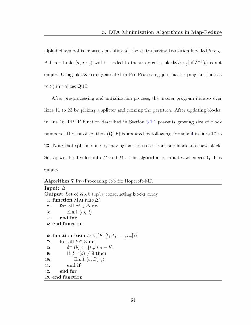
3. DFA Minimization Algorithms in Map-Reduce
alphabet symbol is created consisting all the states having transition labelled b to q.
A block tuple ⟨a, q, πq⟩ will be added to the array entry blocks[a, πq] if δ−1(b) is not
empty. Using blocks array generated in Pre-Processing job, master program (lines 3
to 9) initializes QUE.
After pre-processing and initialization process, the master program iterates over
lines 11 to 23 by picking a splitter and refining the partition. After updating blocks,
in line 16, PPHF function described in Section 3.1.1 prevents growing size of block
numbers. The list of splitters (QUE) is updated by following Formula 4 in lines 17 to
23. Note that split is done by moving part of states from one block to a new block.
So, Bj will be divided into Bj and Bk. The algorithm terminates whenever QUE is
empty.
Algorithm 7 Pre-Processing Job for Hopcroft-MR
Input: ∆Output: Set of block tuples constructing blocks array1: function Mapper(∆)2: for all ∀t ∈ ∆ do3: Emit ⟨t.q, t⟩4: end for5: end function
6: function Reducer(⟨K, [t1, t2, . . . , tm]⟩)7: for all b ∈ Σ do8: δ−1(b)← {t.p|t.a = b}9: if δ−1(b) = ∅ then10: Emit ⟨a,Bq, q⟩11: end if12: end for13: end function
64
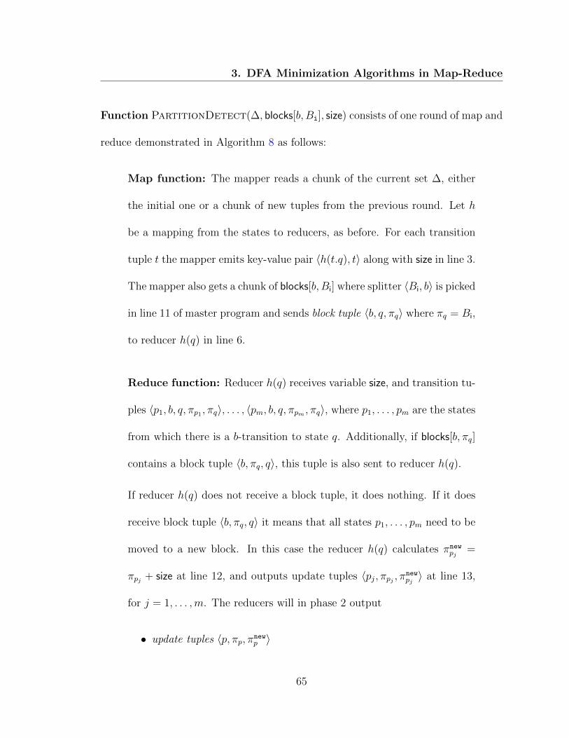
3. DFA Minimization Algorithms in Map-Reduce
Function PartitionDetect(∆, blocks[b, Bi], size) consists of one round of map and
reduce demonstrated in Algorithm 8 as follows:
Map function: The mapper reads a chunk of the current set ∆, either
the initial one or a chunk of new tuples from the previous round. Let h
be a mapping from the states to reducers, as before. For each transition
tuple t the mapper emits key-value pair ⟨h(t.q), t⟩ along with size in line 3.
The mapper also gets a chunk of blocks[b, Bi] where splitter ⟨Bi, b⟩ is picked
in line 11 of master program and sends block tuple ⟨b, q, πq⟩ where πq = Bi,
to reducer h(q) in line 6.
Reduce function: Reducer h(q) receives variable size, and transition tu-
ples ⟨p1, b, q, πp1 , πq⟩, . . . , ⟨pm, b, q, πpm , πq⟩, where p1, . . . , pm are the states
from which there is a b-transition to state q. Additionally, if blocks[b, πq]
contains a block tuple ⟨b, πq, q⟩, this tuple is also sent to reducer h(q).
If reducer h(q) does not receive a block tuple, it does nothing. If it does
receive block tuple ⟨b, πq, q⟩ it means that all states p1, . . . , pm need to be
moved to a new block. In this case the reducer h(q) calculates πnewpj
=
πpj + size at line 12, and outputs update tuples ⟨pj, πpj , πnewpj⟩ at line 13,
for j = 1, . . . ,m. The reducers will in phase 2 output
• update tuples ⟨p, πp, πnewp ⟩
65
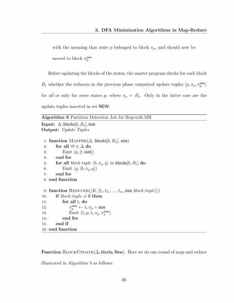
3. DFA Minimization Algorithms in Map-Reduce
with the meaning that state p belonged to block πp, and should now be
moved to block πnewp .
Before updating the blocks of the states, the master program checks for each block
Bi whether the reducers in the previous phase outputted update tuples ⟨p, πp, πnewp ⟩
for all or only for some states p, where πp = Bi. Only in the latter case are the
update tuples inserted in set NEW.
Algorithm 8 Partition Detection Job for Hopcroft-MR
Input: ∆, blocks[b, Bi], sizeOutput: Update Tuples
1: function Mapper(∆, blocks[b, Bi], size)2: for all ∀t ∈ ∆ do3: Emit ⟨q, [t, size]⟩4: end for5: for all block tuple ⟨b, πq, q⟩ in blocks[b, Bi] do6: Emit ⟨q, ⟨b, πq, q⟩⟩7: end for8: end function
9: function Reducer(⟨K, [t1, t2, . . . , tm, size, block tuple]⟩)10: if block tuple = ∅ then11: for all ti do12: πnew
p ← ti.πp + size13: Emit ⟨ti.p, ti.πp, π
newp ⟩
14: end for15: end if16: end function
Function BlockUpdate(∆, blocks,New). Here we do one round of map and reduce
illustrated in Algorithm 9 as follows:
66
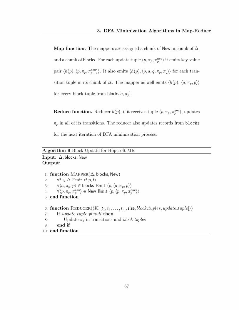
3. DFA Minimization Algorithms in Map-Reduce
Map function. The mappers are assigned a chunk of New, a chunk of ∆,
and a chunk of blocks. For each update tuple ⟨p, πp, πnewp ⟩ it emits key-value
pair ⟨h(p), ⟨p, πp, πnewp ⟩⟩. It also emits ⟨h(p), ⟨p, a, q, πp, πq⟩⟩ for each tran-
sition tuple in its chunk of ∆. The mapper as well emits ⟨h(p), ⟨a, πp, p⟩⟩
for every block tuple from blocks[a, πp].
Reduce function. Reducer h(p), if it receives tuple ⟨p, πp, πnewp ⟩, updates
πp in all of its transitions. The reducer also updates records from blocks
for the next iteration of DFA minimization process.
Algorithm 9 Block Update for Hopcroft-MR
Input: ∆, blocks,NewOutput:
1: function Mapper(∆, blocks,New)2: ∀t ∈ ∆ Emit ⟨t.p, t⟩3: ∀⟨a, πp, p⟩ ∈ blocks Emit ⟨p, ⟨a, πp, p⟩⟩4: ∀⟨p, πp, π
newp ⟩ ∈ New Emit ⟨p, ⟨p, πp, π
newp ⟩⟩
5: end function
6: function Reducer(⟨K, [t1, t2, . . . , tm, size, block tuples, update tuple]⟩)7: if update tuple = null then8: Update πp in transitions and block tuples9: end if10: end function
67
3. DFA Minimization Algorithms in Map-Reduce
3.2.1 Correctness
In this section, we prove the correctness of the Hopcroft-MR.
Theorem 1 (Termination) The algorithm terminates when the queue is empty.
Proof. Initially, a splitter is enqueued either in line 5 or 7 of Algorithm 6 for every
alphabet. During the main loop of master program, first we dequeue a splitter. A
new splitter will be added at line 19 or 21 if there is a split. Considering the fact that
the number of blocks in any partition of DFA can be no bigger than the number of
states, thus the algorithm will terminate eventually �
Theorem 2 When algorithm terminates, p ≡ q if and only if p ∈ πp and q ∈ πq and
πp = πq.
Proof. Suppose p, q ∈ Bi and p ≡ q and there exists a ∈ Σ where p and q are
distinguishable because of δ(p, a) and δ(q, a). As p and q are distinguishable states,
they are in one of two following situations:
1.
δ(p, a) ∈ Bj, δ(q, a) ∈ Bk and j = k (20)
2.
δ(p, a), δ(q, a) ∈ Bl (21)
68
3. DFA Minimization Algorithms in Map-Reduce
First, following Equation 21, there exists w ∈ Σ∗ where δ(p, w) ∈ Bj′ and δ(q, w) ∈
Bk′ where Bj′ = Bk′ . Here, w is the shortest word with this property. In this case
there is a word w′ where w = w′a and δ(p, w′), δ(q, w′) ∈ Bl′ and δ(δ(p, w′), a) ≡
δ(δ(q, w′), a). Replacing δ(p, w′) by p and δ(t, w′) by q gets back to Equation 20.
Consider the point when δ(p, a) and δ(q, a) were partitioned. At this point, with-
out loss of generality, in reducer h(δ(p, aa′)) where a′ can be equal to a itself, we do
have the transition ⟨δ(p, a), a′, δ(p, aa′)⟩, as well as ⟨a′, πδ(q,aa′), δ(p, aa′)⟩. In this case
reducer will decide to emit the partitioning flag and puts δ(p, a) in new generated
block. After the second round, the master program decides to enqueue at least one
of the new blocks. Through one of the further rounds, this block will be dequeued
and the block containing p and q is partitioned and p and q can not be in the same
block. This is a contradiction for p, q ∈ Bi.
Evaluating the other direction of the theorem, the block label of states (transi-
tions) is only updated in the refinement job and in the presence of an update tuple
which says state p is moved to new block. Based on the fact that in the DFA there
is a transition per alphabet, this record can be generated just in one reducer h(q)
where δ(p, a) = q. Reducer h(q) will emit the update tuple if and only if it received
block tuple stating that q belongs to a block Bi where ⟨Bi, a⟩ is splitter pair for this
69

3. DFA Minimization Algorithms in Map-Reduce
iteration. So,
p ∈ B1 ∧ q ∈ B2 ∧B1 = B2 → ∃a ∈ Σ, (δ(p, a) ∈ B′1 ∧ δ(q, a) ∈ B′
2)→ p ≡ q
�
Updating records should keep consistency and integrity of data structure and DFA
records. We proved that updating group numbers respect equivalency class of states.
But to make sure that algorithm is and remains correct, it is necessary to know that
updates do not violate integrity of auxiliary data structure. Specially block tuples
which has a critical role in partition detection job.
Theorem 3 Suppose p ≡r q and ”block tuples” for p and q are in blocks[a,Bi]. If Bi
splits in round r + 1 to Bi and Bj, p ∈ Bi and q ∈ Bj, then ⟨a,Bi, p⟩ ∈ blocks[a,Bi]
and ⟨a,Bj, q⟩ ∈ blocks[a,Bj].
proof. Recall Equation 2 and the format of block tuple records,
(p ∈ Bi ∧ (∃p′ ∈ Q : δ(p′, a) = p))→ ⟨a,Bi, p⟩ ∈ blocks[a,Bi]
This holds initially when the records are generated in pre-processing and the block
tuple record for state p is emitted if δ−1(p, a) = ∅. Suppose after round r, there are
records ⟨a,Bi, p⟩ and ⟨a,Bi, p⟩ in blocks[a,Bi]. Now, if in round r + 1, the detection
70

3. DFA Minimization Algorithms in Map-Reduce
job decided to refine Bi, the update tuple ⟨q, Bi, Bj⟩ is generated and by mapper of
refinement job will be sent to reducer h(q). Then, the block tuple record for q is
updated to ⟨a,Bj, q⟩. However, ⟨a,Bi, p⟩ remains untouched. This means p ∈ a(Bi)
and q ∈ a(Bj) �.
3.3 Enhanced Hopcroft-MR (Hopcroft-MR-PAR)
In previous section we employed a list of splitter as introduced in Hopcroft’s original
algorithm. However, at each iteration we picked one splitter and refined the partition
if there was any split. Then we added more splitters. However, it is possible to process
all the splitters in QUE in parallel. In this section, by applying some changes in the
master program of Hopcroft-MR (Algorithm 6), the detection job (Algorithm 8), and
its refinement job (Algorithm 9), an enhanced version called Hopcroft-MR-PAR will
be proposed.
3.3.1 Splitters and QUE
Recall in line 11 of Algorithm 6, one splitter is picked from the queue at each iteration.
In the enhanced version, we remove this line and put the whole QUE as the input of
PartitionDetect job. Furthermore, in line 18, if block Bi is divided into Bi and
Bj, for every alphabet symbol a, we first check if there is already a splitter ⟨Bi, a⟩
71

3. DFA Minimization Algorithms in Map-Reduce
in QUE or not. But in Hopcroft-MR-PAR, the whole queue is deleted and there is
no need to check it. On the other hand, as there are multiple splitters processing in
detection job, it is highly possible that one block divide into more than two blocks.
To make Hopcroft-MR-PAR consistent with Hopcroft-MR, let us first examine an
example. Consider block 1 in Figure 11 with four states (p1, p2, p3, p4) inside as part
of a DFA with singleton set of alphabet Σ = {a}. In addition, each state has one
and only one incoming transition labelled a. Before processing round r, there are 3
splitters in queue,
QUE = {⟨2, a⟩, ⟨3, a⟩, ⟨4, a⟩}
Lets take ⟨2, a⟩ out. The block 1 will split into {p1, p2} and {p3, p4}. Then let us
put new splitters to another queue QUE′. As splitter ⟨1, a⟩ is not in QUE and size of
both newly generated blocks are the same, we put just ⟨1, a⟩ into QUE′. Then we pick
⟨3, a⟩ out. Again, block 1 will split into {p3} and {p4}. Now we already have ⟨1, a⟩
splitter. So it is required to put ⟨6, a⟩ into QUE′. By picking ⟨4, a⟩ nothing will change
as block 1 only has one member. We need to make sure that by processing all the
splitters in QUE and getting newly generated blocks, QUE for next iteration is same
as QUE’ in this example or at least exhibits the same functionality. Our focus is on
states inside original block 1. After split it into {1, 5, 6}, it is possible to add a splitter
for every blocks except the biggest one. Consequently, QUE = QUE′ = {⟨6, a⟩, ⟨1, a⟩}.
72
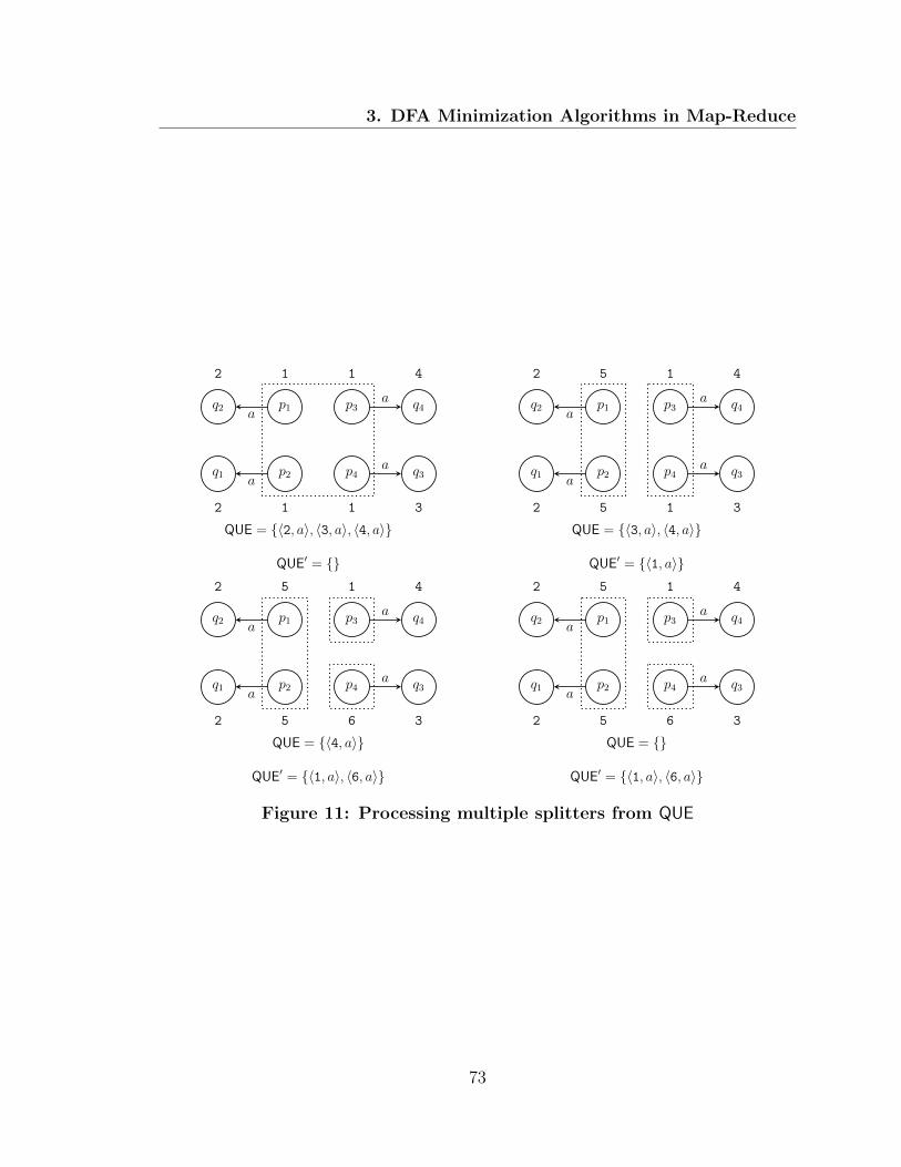
3. DFA Minimization Algorithms in Map-Reduce
q1
2
q2
2
p2
1
p1
1
p4
1
p3
1
q3
3
q4
4
a
a
a
a
QUE = {⟨2, a⟩, ⟨3, a⟩, ⟨4, a⟩}
QUE′ = {}
q1
2
q2
2
p2
5
p1
5
p4
1
p3
1
q3
3
q4
4
a
a
a
a
QUE = {⟨3, a⟩, ⟨4, a⟩}
QUE′ = {⟨1, a⟩}
q1
2
q2
2
p2
5
p1
5
p4
6
p3
1
q3
3
q4
4
a
a
a
a
QUE = {⟨4, a⟩}
QUE′ = {⟨1, a⟩, ⟨6, a⟩}
q1
2
q2
2
p2
5
p1
5
p4
6
p3
1
q3
3
q4
4
a
a
a
a
QUE = {}
QUE′ = {⟨1, a⟩, ⟨6, a⟩}
Figure 11: Processing multiple splitters from QUE
73
3. DFA Minimization Algorithms in Map-Reduce
3.3.2 Detection
The mapper function of detection job remains the same as before. Inside the reducers,
there could be none or multiple block tuples based on the splitters picked from QUE.
We need to change the way of generating the new block number.
Recall from line 12 of Algorithm 8 where πnewp = πp + size and the fact that
the splitters can have different block-alphabet pairs. To reflect these two facts in
new block numbers and distinguish states within a block by splitters, a bit array
denoted as A all elements initialized to 0 is employed. Now suppose a set of splitters
S = {⟨πq, a1⟩, . . . , ⟨πq, am⟩} are present in reducer h(q) where 0 ≤ m ≤ k and state p
has a set of transitions to state q. The value of A for state p is defined as follows:
Ap[i] = 1↔ (⟨πq, ai⟩ ∈ S ∧ (p, ai, q) ∈ δ)
Now line 12 of Algorithm 8 can be replaced by,
πnewp = πp + size · A
Note that, two states p, p′ ∈ Bk can be marked in different reducers and splitters
⟨Bi, ai⟩ and ⟨Bj, ai⟩. In order to differentiate these two changes, we attach Bi and
Bj to the new block numbers.
74

3. DFA Minimization Algorithms in Map-Reduce
3.3.3 Update Blocks
The block update job in Algorithm 9 is designed to apply changes outlined in detection
job. By using an enhanced version of the detection job, it is possible to have different
new block numbers present in reducer h(p). The new block number can be calculated
by applying logical AND on A bit arrays and concatenating Bis attached to the update
records. Although it may generate large bit strings, applying PPHF-MR will map
them to range of [0, n2].
3.4 Cost Measures for DFA Minimization in Map-
Reduce
Taking into account the amount of data that needs to be processed in DFA minimiza-
tion algorithms in Big-Data context, it is crucial to analyse the cost model precisely.
Although computation analysis is very important, the amount of data replicated to
reducers is the most important part of the complexity analysis in Map-Reduce algo-
rithms [34]. On top of that, the number of rounds for iterated Map-Reduce algorithms
is an effective factor on the cost [22]. In this chapter, we try to find the minimum
communication for finding minimal DFA using equivalence class. For this matter, the
communication complexity model described in Section 2.4.1 is utilized. Additionally
we will investigate minimum replication rate for this problem, using the lower-bound
75

3. DFA Minimization Algorithms in Map-Reduce
recipe from Section 2.4.2. At the end, by extending complexity model from 2.4.3, the
cost for all algorithms are examined. It is worth to mention that the analysis is done
in this thesis is about algorithms which are under Top-Down sub-tree in Figure 1.
3.4.1 Minimum Communication Cost
In this section we will find maximum communication cost of minimizing a DFA in
parallel environment as well as the lower bound for communication complexity using
two parties model.
Recall Yao’s two-party model from Section 2.4.1. We need to define a simple
function of equivalency (EQ). Having two inputs x, y ∈ {0, 1}m, z = EQ(x, y) is 1
if x = y and 0 otherwise. The maximum communication needed to evaluate this
function is sending all the m bits of x by Alice to Bob and Bob returns one bit result
of evaluation back to Alice. Thus D ≤ m+ 1. Moreover, the fooling set for EQ is:
S = {(x, x)|x ∈ {0, 1}m}
Counting z = 0, we have |S| = m+ 1. Hence D(EQ(x, y)) ≥ log2 (m+ 1) ≥ log2m.
Lemma 6 Maximum communication cost for p ≡i q is k log n
76

3. DFA Minimization Algorithms in Map-Reduce
Proof. Recall definition of equivalency,
p ≡i q ↔ (πi−1p = πi−1
q ∧ ∀a ∈ Σ (πi−1δ(p,a) = πi−1
δ(q,a)))
Each equivalence class can be represented by maximum m = log n bits. Thus we can
define the following functions:
1. f0 : {0, 1}m × {0, 1}m → {0, 1} for πi−1p = πi−1
q
2. ∀a ∈ Σ, fa : {0, 1}m × {0, 1}m → {0, 1} for πi−1δ(p,a) = πi−1
δ(q,a)
Each above mentioned function is equivalent to EQ. Hence there are k + 1 func-
tions. So, using Equation 10 and 13 :
D(p ≡i q) = (k + 1)(n′ + 1) = (k + 1)(log n+ 1) = O(k log n) (22)
�
Theorem 4 The upper bound for DFA minimization in Map-Reduce model is O(kn3 log n).
Proof. DFA minimization has n rounds in worst case as it is discussed in Section
2.1.2. At every iteration, again in worst case, it is required to check equivalency of all
pairs which is n(n−1)2
= O(n2). Using Lemma 6, each pair requires at most O(k log n)
77
3. DFA Minimization Algorithms in Map-Reduce
bits to evaluate the function. So upper bound for DFA minimization DCC would be
O(kn3 log n).�
From now on we can talk about lower bound on DCC for above mentioned problem
p ≡i q.
Theorem 5 The lower bound on DCC for DFA minimization in Map-Reduce model
is O(kn log n).
Proof. Lemma 3, shows that during splitting process, O(kn log n) states will move
from one block to new one. Now suppose Alice has p and Bob has q. Bob will inform
Alice to move p from its current block to a new one. To carry out this task, Bob has
to send a bit to Alice. So, minimum number of bits required to be communicated is
O(kn log n) �
3.4.2 Lower Bound on Replication Rate
Replication Rate has a direct effect on communication cost for Map-Reduce algo-
rithms. Using lower-bound recipe introduced in Section 2.4.2, we will find minimum
required replication rate. Recall Equation 15,
r ≥ ρ× |O|g(ρ)× |I|
78

3. DFA Minimization Algorithms in Map-Reduce
The input data for DFA minimization algorithm (I) is the transitions of original
DFA. Hence |I| = kn|t| where |t| is size of transition in bits. On the other hand, the
output (O) is updated transitions from input exposing minimal DFA and |O| = kn|t|.
Clearly the size of transitions are different between input and output. This is due
to at the beginning we have two blocks can be represented by one bit. However,
for outputs the number of bits needed to store block numbers is log n2 = 2 log n by
applying PPHF algorithm (Section 3.1.1). We can assume transition size in input is
equal to output. Moreover, if a reducer gets ρ amount of transitions, it can compute
and update at most only those transitions not anymore. So, maximum output from
a reducer is g(ρ) = ρ. Now having these facts, we can compute lower bound in
replication for DFA minimization as follow:
R ≥ ρ× |O|g(ρ)× |I|
=ρ× knτ
ρ× knτ= 1 (23)
3.4.3 Communication Complexity of Moore-MR-PPHF
In this section we examine replication rate and communication cost of Moore-MR-
PPHF.
79

3. DFA Minimization Algorithms in Map-Reduce
3.4.3.1 Replication Rate
Recall Algorithm 5 for computing minimal DFA in Map-Reduce using Moore’s method,
the input data are not only transitions from original DFA, but also dummy ones. We
will emit each transition once at and each dummy transition twice. This makes the
replication rate,
RMoore-MR =3
2
This replication rate is almost equal to the lower bound.
3.4.3.2 Communication Cost
Communication cost as discussed before is amount of data transmitted during Map-
Reduce computations. Input records (transitions) for each round is in form of t =
⟨p, a, q, πp, D⟩ which makes the size of transition |t| = O(log n+ log k). Note that for
first job it is 2 log n+log k+2 due to the size of π equal to two and can be represented
by 1 bit. In addition, note that using PPHF, block labels are in the range of [1, n2]
and we need 2 log n bits for that.
The communication cost is equal to the number of rounds times communications
in each round, which is replication rate times input plus output. Considering the
maximum number of rounds is R = n, we can say
CC = O(R(R|I|+ |O|)) = O(n(R|I|+ |O|)) (24)
80

3. DFA Minimization Algorithms in Map-Reduce
The output of each round is:
• One record per transition
• One record per dummy transition
• One record for convergence voting
Third item is about if one state detects any of other k states it has a transition
to, has moved to a new block. Lemma 3 shows that there could be at most n log n
state moving to new block during DFA minimization procedure each of which can
force at most k states to issue the voting record in size of 1. This will be applied to
CC separately. As a conclusion,
|O| = n(k|t|+ k|t|) = O(kn(log n+ log k))
Now the communication cost of Moor’s algorithm in Map-Reduce can be computed
as follows,
CC = O(n(R|I|+ |O|)) +O(kn log n)
= O(n(3
2kn(log n+ log k) + kn(log n+ log k)) + kn log n)
= O(n(kn(log n+ log k)))
= O(kn2(log n+ log k))
(25)
81
3. DFA Minimization Algorithms in Map-Reduce
Amount of required communication in PPHF is sending all transitions in mapper
and sending all updated transitions back in reducer and it is 2kn|t| which is much
less than CC from Equation 25.
3.4.4 Communication Complexity of Hopcroft-MR
Calculating the cost for Hopcroft-MR algorithm due to auxiliary generated informa-
tion is a little bit complicated than Moore-MR-PPHF. First of all, from Algorithm
6, we know that there are 4 different jobs, one of which is Pre-Processing. This job
will not be included in computation because of (1) replication rate is 1 (2) during
asymptotic analysis, in presence of iterative procedure, the amount of communication
for pre-processing job is much less than the iterative part.
3.4.4.1 Replication Rate
There are 3 different jobs in Hopcroft-MR except PPHF-MR. We saw in previous
section that its replication rate is one.
1. Pre-Processing: The mapper emits every transition record one in line 1 of Al-
gorithm 7 once.
2. Detection: The mapper emits transitions in line 3 once and block tuple once in
line 6 og Algorithm 8.
82

3. DFA Minimization Algorithms in Map-Reduce
3. Block Update: The mapper emits every record once in Algorithm 9.
Above analysis shows that the replication rate for Hopcroft-MR isR = 1. It is exactly
equal to minimum replicate rate we found in section 3.4.2.
3.4.4.2 Communication Cost
The main communication cost is related to three jobs in the loop. We calculate each
of them separately:
• Partition Detection. Using the splitter ⟨P, a⟩, every transition in P is emit-
ting once at round r. Besides, mapper sends every block tuple record in blocks[P, a].
According to Lemma 2 the total number of states in all splitters we may
put in queue is bounded by n log n. So these records can not be more than
C = O(n log n) each of which requires 2 log n + log k bits. On the other hand,
reducers would send a record for every state which has to be moved to new
block. According to Lemma 3, it is O(n log n). Every update tuple is in form of
⟨p, πp, πnewp ⟩ and its size is log n+ 2 · 2 log n = 5 log n. Thus the total communi-
cation cost for detection job is:
CC1 =
O(n log n · (|t|+ log n) + n log n · (log k + log n) + n log n · log n) =
O(n log n(log n+ log k))
83

3. DFA Minimization Algorithms in Map-Reduce
• Update Blocks For the update job, we need to send all the transitions,
block tuples as well as update tuples to the reducers. Number of update tu-
ples is O(n log n) in whole DFA minimization process. Moreover, the number
of block tuples is at most n. According to Lemma 1 the number of iterations in
Hopcroft’s method is equal to R = 2kn. Moreover, we found in Section 3.4.4.1
that replication rate for every job in Hopcroft-MR is equal to R = 1. Now,
using Equation 24, the amount of communication in mapper side is equal to
CCmapper = O(RR|I|). Thus we have,
CCmapper2 = O(RR|I|)
O(kn · (kn · (log k + log n) + n · (log k + log n))) +O(n log n · log n) =
O((kn)2(log n+ log k)) +O(n log n2) =
O((kn)2(log n+ log k))
In reducer side, it will write in output every transitions and update tuples, either
it is updated or not. So, the total communication cost for the reducer task in
update job is CCreducer = O(R|O|)
CCreducer2 =
O(kn · (kn · (log k + log n) + n · (log k + log n))) =
O((kn)2(log n+ log k))
84
3. DFA Minimization Algorithms in Map-Reduce
Thus,
CC2 = CCmapper2 + CCreducer
2 =
O((kn)2(log n+ log k) + (kn)2(log n+ log k)) =
O((kn)2(log n+ log k))
• PPHF As it has been computed in previous section,
CC3 = O(kn2(log n+ log k))
Hence we can conclude communication cost for minimizing DFA using Hopcroft-
MR is:
CC = CC1 + CC2 + CC3 =
O(n log n(log n+ log k) + (kn)2(log n+ log k) + kn2(log n+ log k)) =
O((kn)2(log n+ log k))
(26)
3.4.5 Communication Complexity of Hopcroft-MR-PAR
As shown in Section 3.3, mapping schema of Hopcroft-MR-PAR is same as Hopcroft-
MR, R = 1. Moreover, in Hopcroft-MR-PAR we send the whole QUE in the detection
job though the total number of block tuples, update tuples, and states within splitters
85

3. DFA Minimization Algorithms in Map-Reduce
follow the Lemma 2 and 3. However, number of bits in update tuples is now equal to
log n+2 log n+(k+2 log n+c2 log n). Recall the update tuples in form of ⟨p, πp, πnewp ⟩.
We need log n bits to store p and 2 log n bits to store πp (note that PPHF-MR maps
block labels to range [0 − n2)). The πnewp contains πp along with k-bits A and block
labels for those we have splitter. If c bits of A is set to 1, then we need to attach c
block labels to new block number. As a result the communication cost for detection
job is,
CC1 = O(n log n(log n+ k))
Lemma 7 Number of rounds for Hopcroft-MR-PAR is O(n)
Proof. Using Lemma 1, the maximum number of iterations for Hopcroft’s algorithm
is O(kn) where k is the number of alphabet symbols and n is the number of states.
The worst case is slow automata where at each iteration block R is split into R and
R1 where w.l.g |R1| = 1. In this case, we add k splitters ⟨R1, ai⟩ into QUE where
i = 1, 2, ..., k. In Hopcroft-MR-PAR, we process the whole QUE. As a result, all the
k splitters are taken out and QUE is empty for the next round. So, the number of
iteration of Hopcroft-MR-PAR is equal to R = n.
Update Blocks. Recall communication cost for mapper as CC = O(R(R|I| +
|O|)) from 3.4.4.2. As mentioned before R = 1 and also input size and output size for
Hopcroft-MR-PAR is equal to Hopcroft-MR’s. However, by Lemma 7, the number of
86
3. DFA Minimization Algorithms in Map-Reduce
rounds in worst case for Hopcroft-MR-PAR is equal to
RHopcroft-MR-PAR = O(n) = RHopcroft-MR/k
So,
CC2 = O(RHopcroft-MR-PAR(R|I+|O|)) =O((kn)2(log n+ log k))
k= O(kn2(log n+log k))
The last job is PPHF-MR to shrink block labels. It has the same complexity as
Hopcroft-MR and is equal to:
CC3 = O(kn2(log n+ log k))
Using above mentioned factors, the communication cost for Hopcroft-MR-PAR is:
CC = CC1 + CC2 + CC3 =
O(n log n(log n+ k)) +O(kn2(log n+ log k)) +O(kn2(log n+ log k)) =
O(kn2(log n+ log k))
87

3. DFA Minimization Algorithms in Map-Reduce
Table 5: Comparison of complexity measures for algorithms
Replication
RateCommunication Cost
Sensitive to
Skewness
Lower Bound 1 O(kn log n) −
Moore-MR 2.3.2 [18] 32[18] O(nkn) No
Moore-MR-PPHF 3.1 32
O(kn2(log n+ log k)) No
Hopcroft-MR 3.2 1 O((kn)2(log n+ log k)) Yes
Hopcroft-MR-PAR 3.2 1 O(kn2(log n+ log k)) Yes
3.4.6 Comparison of Algorithms
In this section we will compare the algorithms as illustrated in Table 5. Three mea-
sures is employed here; Replication Rate, Communication Cost, and Sensitivity to
Skewness. All the algorithm are analyzed using MRC[f(n),g(n)] (2.4.3) and all are
in MRC[O(n),O(n)] with c = 0.
Sometimes, the mapping schema can not distribute the input data evenly among
the reducers. This phenomenon can cause flooding some reducers while others are
starving and causes a phenomenon called the curse of last reducer [30] where
99% of the computation finishes quickly, but the remaining
1% takes a disproportionately longer amount of time.
The other drawback of Skewness is that it makes it impossible to run an algorithm
on some special input data. That is the reason why a new measure has been added
to the comparison table to measure if an algorithm is sensitive to skewness or not.
88
3. DFA Minimization Algorithms in Map-Reduce
In section 3.4.2 we found that the lower bound on Replication Rate is 1 which
all the algorithms are almost equal to. On the other hand, as all the algorithms are
under family of Top-Down minimization approach, they are iterative and number of
required rounds is O(n) except for Hopcroft-MR which is O(kn).
The second column shows that the amount of communication in bits required for
each algorithm bounded from bottom to O(kn log n). The basic algorithm from [18]
(Moore-MR), requires O(nkn) bits for computing minimized DFA while by apply-
ing PPHF-MR it becomes O(kn2(log n + log k)) (Moore-MR-PPHF). On the other
hand, the Hopcroft-MR algorithm requires O((kn)2(log n + log k)) bits of communi-
cation. By processing the splitters in QUE in Hopcroft-MR-PAR, we reach to the
same communication complexity as Moore-MR. However, it would require less ac-
tual computations in reducers because not all the reducers are engaged in dividing
partitions.
The last parameter to consider is Sensitivity to Skewness. In Moore-MR and
Moore-MR-PPHF, the mapping schema is based on the source state of a transition.
The number of the records (transitions) associated to each state is determined and
equal to k, the size of the alphabet. Correspondingly, data has been distributed
evenly among the reducers and there is no Skewness. However, in Hopcroft-MR
and Hopcroft-MR-PAR, mapping schema for detection job is based on the reverse
transitions and is not deterministic. This may cause sending amount of transitions
89

3. DFA Minimization Algorithms in Map-Reduce
to a reducer that may not be tolerated in terms of space.
Recall MRC from Section 2.4.3 as a class of computational complexity. Although
both time and space are included in the model along with number of iterations and
replication rate, it may not reflect cover to very important factors affecting algorithms
in Map-Reduce:
• Sensitivity to Skewness
• Horizontal Growth of Data [4]
We already discussed about the skewness. In some algorithms like Moore-MR, in
order to accomplish the task, there is required to put additional data in input records.
However, if this operation repeats over several iterations, the amount of data will go
beyond of space capacity. As the main focus of Map-Reduce model is to address
data intensive problems, these two measures are extremely critical to be reflected in
complexity class of MRC.
90
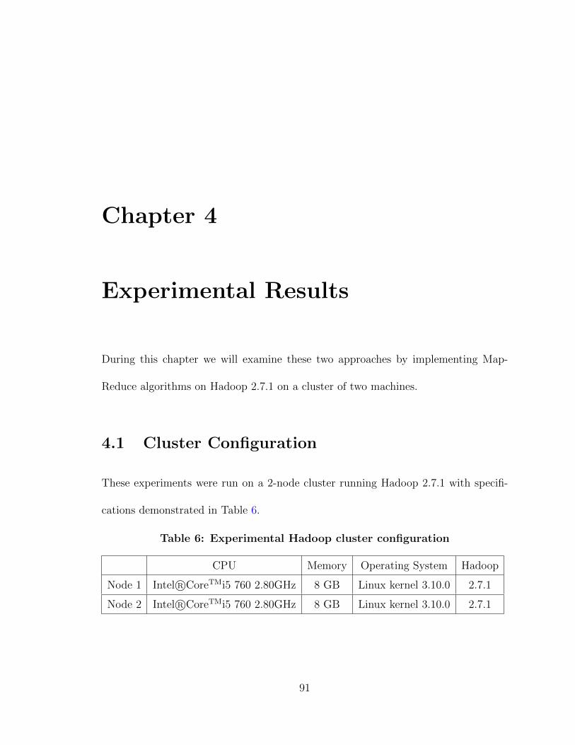
Chapter 4
Experimental Results
During this chapter we will examine these two approaches by implementing Map-
Reduce algorithms on Hadoop 2.7.1 on a cluster of two machines.
4.1 Cluster Configuration
These experiments were run on a 2-node cluster running Hadoop 2.7.1 with specifi-
cations demonstrated in Table 6.
Table 6: Experimental Hadoop cluster configuration
CPU Memory Operating System Hadoop
Node 1 Intel R⃝CoreTMi5 760 2.80GHz 8 GB Linux kernel 3.10.0 2.7.1
Node 2 Intel R⃝CoreTMi5 760 2.80GHz 8 GB Linux kernel 3.10.0 2.7.1
91

4. Experimental Results
4.2 Data Generation Methods
Before exposing the results, we shall briefly discuss about sample data we ran algo-
rithms on. States, alphabets and block labels are all represented by numbers.
For these experiments we have three different types of DFA. First a circular DFA
introduced in original paper of Hopcroft. Having Q = {0, 1, 2, . . . , n − 1} and Σ =
{1, 2, . . . , k}, for all transitions (p, a, q) ∈ δ, we will first compute q as follows:
q =
⎧⎪⎪⎪⎨⎪⎪⎪⎩p+ a, if a ≤ ⌈k
2⌉
p− ⌊a2⌋, otherwise.
Then we will refine it as follows.
q =
⎧⎪⎪⎪⎨⎪⎪⎪⎩q, if q ≥ 0
n+ q. otherwise
Start state is s = 0 and p ∈ F if k|p.
Note that the state index starts from 0 while alphabet index starts from 1. The
minimized DFA has |Σ| = k states. A sample generated DFA with |Q| = 8 and
|Σ| = 4, is illustrated in Figure 12 and its minimal DFA is Figure 13.
92
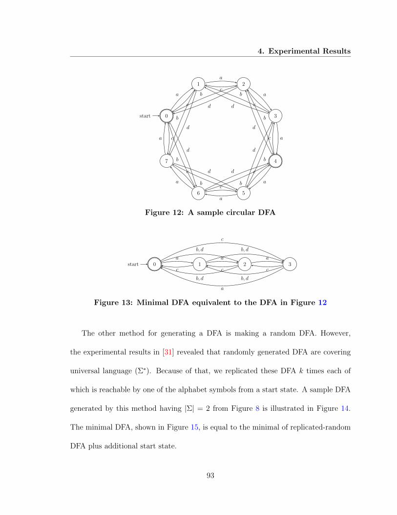
4. Experimental Results
0start
1 2
3
4
56
7
a b
c
d
a
b
c
d
a
b
c
d
a
b
cd
ab
c
d
a
b
c
d
a
b
c
d
a
b
c d
Figure 12: A sample circular DFA
0start 1 2 3a
b, d
c
a
b, d
c
a
b, d
c
a
b, d
c
Figure 13: Minimal DFA equivalent to the DFA in Figure 12
The other method for generating a DFA is making a random DFA. However,
the experimental results in [31] revealed that randomly generated DFA are covering
universal language (Σ∗). Because of that, we replicated these DFA k times each of
which is reachable by one of the alphabet symbols from a start state. A sample DFA
generated by this method having |Σ| = 2 from Figure 8 is illustrated in Figure 14.
The minimal DFA, shown in Figure 15, is equal to the minimal of replicated-random
DFA plus additional start state.
93

4. Experimental Results
1
2
3
4
5
6
7
8
9
10
11
120start
a
b
a
b
a
b
a
b
a
b
a
b
a, b
a
b
a
b
a
b
a
b
a
b
a, b
Figure 14: A sample replicated-random DFA
1, 7
2, 8
3, 4, 5, 9, 10, 11 6, 120starta, b
a
b
a
b
a
b
a, b
Figure 15: Minimal DFA equivalent to the DFA in Figure 14
The last data set is generated from the slow DFA introduced in Section 2.1.2.2.
In this automata, p0 is the start state, F = {pn} is the final state where |Q| = n, and
for 0 ≤ i < n
∀a ∈ Σ, δ(pi, a) = pi+1
The transitions of the final state are all self-loops. This DFA is “already minimal”.
94
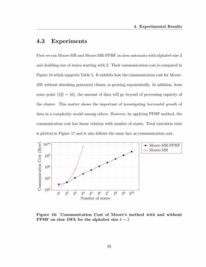
4. Experimental Results
4.3 Experiments
First we ran Moore-MR and Moore-MR-PPHF on slow automata with alphabet size 2
and doubling size of states starting with 2. Their communication cost is compared in
Figure 16 which supports Table 5. It exhibits how the communication cost for Moore-
MR without shrinking generated classes, is growing exponentially. In addition, from
some point (|Q| = 16), the amount of data will go beyond of processing capacity of
the cluster. This matter shows the important of investigating horizontal growth of
data in a complexity model among others. However, by applying PPHF method, the
communication cost has linear relation with number of states. Total execution time
is plotted in Figure 17 and it also follows the same fact as communication cost.
21 22 23 24 25 26 27 28 29 210102
104
106
108
1010
Number of states
Com
municationCost(B
yte)
Moore-MR-PPHFMoore-MR
Figure 16: Communication Cost of Moore’s method with and withoutPPHF on slow DFA for the alphabet size k = 2
95
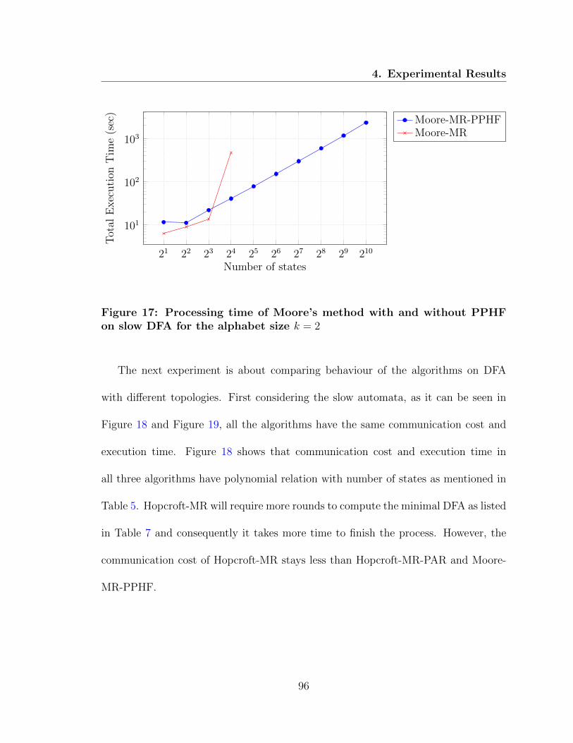
4. Experimental Results
21 22 23 24 25 26 27 28 29 210
101
102
103
Number of states
Total
Execution
Tim
e(sec)
Moore-MR-PPHFMoore-MR
Figure 17: Processing time of Moore’s method with and without PPHFon slow DFA for the alphabet size k = 2
The next experiment is about comparing behaviour of the algorithms on DFA
with different topologies. First considering the slow automata, as it can be seen in
Figure 18 and Figure 19, all the algorithms have the same communication cost and
execution time. Figure 18 shows that communication cost and execution time in
all three algorithms have polynomial relation with number of states as mentioned in
Table 5. Hopcroft-MR will require more rounds to compute the minimal DFA as listed
in Table 7 and consequently it takes more time to finish the process. However, the
communication cost of Hopcroft-MR stays less than Hopcroft-MR-PAR and Moore-
MR-PPHF.
96

4. Experimental Results
21 22 23 24 25
103
104
105
Number of states
Com
municationCost(B
yte)
Moore-MR-PPHFHopcroft-MRHopcroft-MR-PAR
Figure 18: Communication Cost of slow DFA for the alphabet size k = 2
21 22 23 24 25
101
102
Number of states
Total
Execution
Tim
e(sec)
Moore-MR-PPHFHopcroft-MRHopcroft-MR-PAR
Figure 19: Processing time of slow DFA for the alphabet size k = 2
The second data set is Circular DFA. The main feature of this automata is that
each state has k incoming transitions. It makes uniform distribution of transitions in
both mapping schema based on source state and target state. As a result, Figures
97

4. Experimental Results
20 and 21 are exhibiting better performance of Hopcroft’s algorithms in comparison
with Moore-MR-PPHF.
23 25 27 29 211 213 215 217
104
106
108
1010
1012
Number of states
Com
municationCost(B
yte)
Moore-MR-PPHFHopcroft-MRHopcroft-MR-PAR
Figure 20: Communication Cost of circular DFA for the alphabet size k = 4
23 25 27 29 211 213 215 217
104
105
106
107
Number of states
Total
Execution
Tim
e(sec)
Moore-MR-PPHFHopcroft-MRHopcroft-MR-PAR
Figure 21: Processing time of circular DFA for the alphabet size k = 4
The last dataset is Replicated-Random. The number of alphabet is fixed and equal
98

4. Experimental Results
to 4. The replicated-random DFA have 16 + 1 states to 131, 072 + 1. Each DFA is
replicated four times and parts are connected using an auxiliary state. The random-
ness prevents having uniform distribution of incoming transitions among the states.
This fact injects skewness in the mapping schema for Hopcroft’s algorithms. Figure
22 reflects the fact that Hopcroft-MR requires more communication amount than the
others. Although Hopcroft-MR-PAR communicates almost same data as Moore-MR-
PPHF, Figure 23 reveals that it requires more processing time than Moore-MR-PPHF
to calculate the minimized version of DFA. Finally, for DFA with 32+1 = 25+1 states,
Hopcroft’s algorithms had much better performance than Moore-MR-PPHF. This is
due the fact that this DFA does not have any final records. Hopcroft’s algorithms
detect the matter in first round while Moore-MR-PPHF has to run 2 rounds.
23 25 27 29 211 213 215 217
104
106
108
1010
1012
1014
Number of states
Com
municationCost(B
yte)
Moore-MR-PPHFHopcroft-MRHopcroft-MR-PAR
Figure 22: Communication Cost of replicated-random DFA for alphabetsize k = 4
99
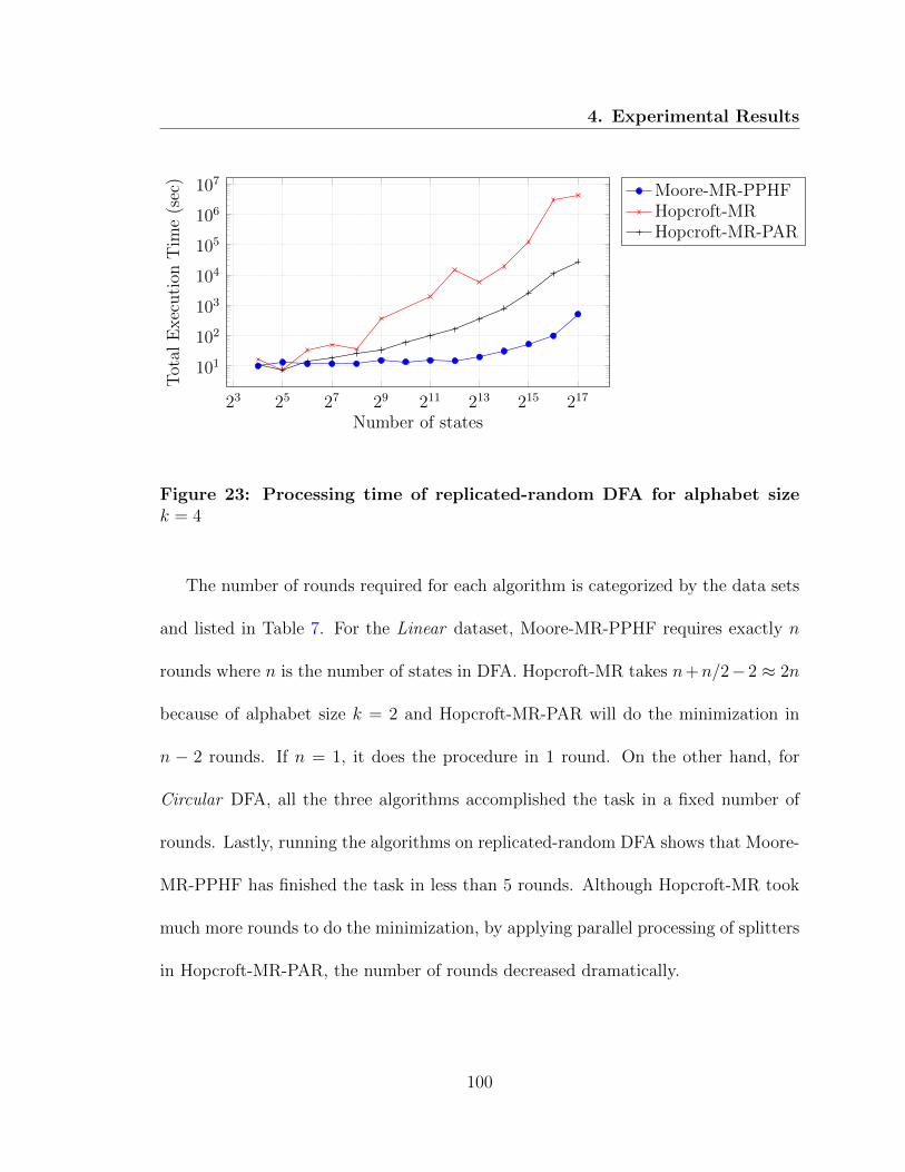
4. Experimental Results
23 25 27 29 211 213 215 217
101
102
103
104
105
106
107
Number of states
Total
Execution
Tim
e(sec)
Moore-MR-PPHFHopcroft-MRHopcroft-MR-PAR
Figure 23: Processing time of replicated-random DFA for alphabet sizek = 4
The number of rounds required for each algorithm is categorized by the data sets
and listed in Table 7. For the Linear dataset, Moore-MR-PPHF requires exactly n
rounds where n is the number of states in DFA. Hopcroft-MR takes n+n/2− 2 ≈ 2n
because of alphabet size k = 2 and Hopcroft-MR-PAR will do the minimization in
n − 2 rounds. If n = 1, it does the procedure in 1 round. On the other hand, for
Circular DFA, all the three algorithms accomplished the task in a fixed number of
rounds. Lastly, running the algorithms on replicated-random DFA shows that Moore-
MR-PPHF has finished the task in less than 5 rounds. Although Hopcroft-MR took
much more rounds to do the minimization, by applying parallel processing of splitters
in Hopcroft-MR-PAR, the number of rounds decreased dramatically.
100
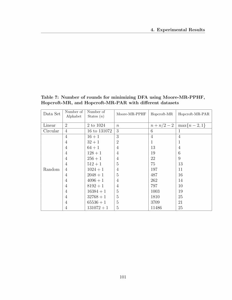
4. Experimental Results
Table 7: Number of rounds for minimizing DFA using Moore-MR-PPHF,Hopcroft-MR, and Hopcroft-MR-PAR with different datasets
Data SetNumber ofAlphabet
Number ofStates (n)
Moore-MR-PPHF Hopcroft-MR Hopcroft-MR-PAR
Linear 2 2 to 1024 n n+ n/2− 2 max{n− 2, 1}Circular 4 16 to 131072 3 6 1
Random
4 16 + 1 3 4 44 32 + 1 2 1 14 64 + 1 4 13 44 128 + 1 4 19 64 256 + 1 4 22 94 512 + 1 5 75 134 1024 + 1 4 197 114 2048 + 1 5 487 164 4096 + 1 4 262 144 8192 + 1 4 797 104 16384 + 1 5 1003 194 32768 + 1 5 1810 254 65536 + 1 5 3709 214 131072 + 1 5 11486 25
101
Chapter 5
Conclusion and Future Work
5.1 Conclusion
In this research we studied methods for computing minimal equivalent automaton for
large scale DFA using equivalence classes in Map-Reduce. Our focus was mainly on
Moore’s and Hopcroft’s methods.
We proposed an algorithm for minimizing DFA in Map-Reduce based on Hopcroft’s
method, along with an enhancement to a previously work employed Moore’s algo-
rithm. Moreover, we showed that adding information to input records will cause
horizontal growth of data [4] and it has to be controlled and measured in complex-
ity models. For this matter, we proposed an efficient new parallel perfect hashing
function in Map-Reduce model for numerical values. Furthermore, we extended the
102
5. Conclusion and Future Work
Map-Reduce model in order to categorizing data on distributed file system for achiev-
ing more efficiency.
Additionally, we studied different measures of algorithms in Map-Reduce model
with a focus on DFA minimization. We found that DFA minimization using equiva-
lence classes are suitable for Map-Reduce model as we proved that the lower bound
on replication of data is one and our algorithms are coincident with. We also found a
lower and an upper bound for DFA minimization problem in parallel environments.
In addition, our analysis on topology of DFA supported by experimental results,
shows that Sensitivity on Skewness is a critical measure for Map-Reduce algorithms.
The experiments done on different DFA showed that both methods have the same
complexity in terms of amount of data has to be communicated in minimization pro-
cess. However, it shows as well that Hopcroft’s method is very sensitive to skewness.
5.2 Future Work
For the future works, the following question are interesting:
1. Reducer capacity vs. Number of reducers trade-off
The capacity of reducer workers will directly affect the number of rounds for
iterative problems such as DFA minimization. The question is that what is the
relation between reducer capacity and number of rounds? How the problem
103

5. Conclusion and Future Work
itself affects the trade-off?
2. Investigating other methods of minimization
How the other methods of minimizing a DFA will behave in Map-Reduce model.
We know that methods relying on equivalence classes are iterative and these
problems show very bad results in Map-Reduce model. Now the question is a
method like Brzozowski which computes the minimal DFA in two rounds, how
can be compared with proposed algorithms in this study?
3. Extending complexity model and class
Currently available complexity models and classes for Map-Reduce do not take
into account data growth during iterations as well as sensitivity to skewness.
We showed that how these to can decrease efficiency of Map-Reduce algorithms.
4. Is it possible to compare Map-Reduce algorithms with others in dif-
ferent models?
The focus of Map-Reduce model is on solving data intensive problems in Big-
Data concept where the others fail to run. To do so, scientists has to concern
more on possibility and least in efficiency. The question is if it is wise to compare
these two or not?
104
References
[1] Apache Hadoop. Available at http://hadoop.apache.org/.
[2] Foto N. Afrati, Anish Das Sarma, Semih Salihoglu, and Jeffrey D. Ullman. Upper
and lower bounds on the cost of a map-reduce computation. PVLDB, 6(4):277–
288, 2013.
[3] Frederique Bassino, Julien David, and Cyril Nicaud. On the average complexity
of Moore’s state minimization algorithm. CoRR, abs/0902.1048, 2009.
[4] Paul Beame, Paraschos Koutris, and Dan Suciu. Communication steps for par-
allel query processing. In Proceedings of the 32Nd Symposium on Principles of
Database Systems, PODS ’13, pages 273–284, New York, NY, USA, 2013. ACM.
[5] Jacek Becla and Daniel L. Wang. Lessons learned from managing a petabyte.
In Proceedings, 2nd Biennial Conference on Innovative Data Systems Research,
Stanford, CA, Jan 2005.
105
REFERENCES
[6] Jean Berstel, Luc Boasson, Olivier Carton, and Isabelle Fagnot. Minimization
of automata. CoRR, abs/1010.5318, 2010.
[7] Ronald V. Book, Christopher B. Wilson, and Xu Mei-Rui. Relativizing time,
space, and time-space. SIAM Journal on Computing, 11(3):571–581, 1982.
[8] Kirk D. Borne. Scientific data mining in astronomy. CoRR, abs/0911.0505, 2009.
[9] Wilfried Brauer. On minimizing finite automata. Bulletin of the EATCS, 35:113–
116, 1988.
[10] Parris M. Caulk. The design of a petabyte archive and distribution system for
the NASA ECS project. In Fourth NASA Goddard Conference on Mass Storage
Systems and Technologies, pages 7–17. NASA, 1995.
[11] Sang Cho and Dung T. Huynh. The parallel complexity of coarsest set partition
problems. Inf. Process. Lett., 42(2):89–94, 1992.
[12] Sang Cho and Dung T. Huynh. The parallel complexity of finite-state automata
problems. Information and Computation, 97(1):1–22, 1992.
[13] Julien David. The average complexity of Moore’s state minimization algorithm
is O(n log log n). In MFCS, pages 318–329. Springer, 2010.
[14] Jeffrey Dean and Sanjay Ghemawat. Mapreduce: simplified data processing on
large clusters. Communications of the ACM, 51(1):107–113, 2008.
106
REFERENCES
[15] Michael J. Flynn. Some computer organizations and their effectiveness. IEEE
Transactions on Computers, 21(9):948–960, 1972.
[16] Gosta Grahne, Shahab Harrafi, Ali Moallemi, and Adrian Onet. Comput-
ing NFA intersections in map-reduce. In Proceedings of the Workshops of the
EDBT/ICDT Joint Conference (EDBT/ICDT), pages 42–45, 2015.
[17] David Gries. Describing an algorithm by Hopcroft. Acta Informatica, 2(2):97–
109, 1973.
[18] Shahab Harrafi Saveh. Finite automata algorithms in map-reduce. Master’s
thesis, Concordia University, April 2015.
[19] John E. Hopcroft. An n log n algorithm for minimizing states in a finite automa-
ton. In Theory of Machines and Computations, pages 189–196. Academic Press,
New York, 1971.
[20] John E. Hopcroft and Jeffrey D. Ullman. Introduction to Automata Theory,
Languages and Computation. Addison-Wesley, 1979.
[21] Joseph F. JaJa and Kwan Woo Ryu. An efficient parallel algorithm for the
single function coarsest partition problem. In Proceedings of the fifth annual
ACM symposium on Parallel algorithms and architectures, pages 230–239. ACM,
1993.
107

REFERENCES
[22] Howard Karloff, Siddharth Suri, and Sergei Vassilvitskii. A model of compu-
tation for mapreduce. In Proceedings of the Twenty-First Annual ACM-SIAM
Symposium on Discrete Algorithms, pages 938–948. Society for Industrial and
Applied Mathematics, 2010.
[23] Eyal Kushilevitz. Communication complexity. Advances in Computers, 44:331–
360, 1997.
[24] Jure Leskovec, Anand Rajaraman, and Jeffrey D. Ullman. Mining of Massive
Datasets. Cambridge University Press, 2014.
[25] Richard J. Lipton and Robert Sedgewick. Lower bounds for VLSI. In Proceedings
of the thirteenth annual ACM symposium on Theory of computing, pages 300–
307. ACM, 1981.
[26] Yossi Matias and Uzi Vishkin. On parallel hashing and integer sorting. Journal
of Algorithms, 12(4):573–606, 1991.
[27] Edward F. Moore. Gedanken-experiments on sequential machines. Automata
studies, 34:129–153, 1956.
[28] Bala Ravikumar and Xuanxing Xiong. A parallel algorithm for minimization of
finite automata. In The 10th International Parallel Processing Symposium, pages
187–191, April 1996.
108

REFERENCES
[29] Y. N. Srikant. A parallel algorithm for the minimization of finite state automata.
International Journal of Computer Mathematics, 32(1-2):1–11, 1990.
[30] Siddharth Suri and Sergei Vassilvitskii. Counting triangles and the curse of the
last reducer. In Proceedings of the 20th international conference on World wide
web, pages 607–614. ACM, 2011.
[31] Deian Tabakov and Moshe Y. Vardi. Experimental evaluation of classical au-
tomata constructions. In Logic for Programming, Artificial Intelligence, and
Reasoning, 12th International Conference, LPAR 2005, Montego Bay, Jamaica,
December 2-6, 2005, Proceedings, pages 396–411, 2005.
[32] H. M. M. ten Eikelder. Some algorithms to decide the equivalence of recursive
types. Technical Report 31, Faculty of Computing Science, Eindhoven University
of Technology, 1991.
[33] Ambuj Tewari, Utkarsh Srivastava, and Phalguni Gupta. A parallel DFA
minimization algorithm. In High Performance ComputingHiPC, pages 34–40.
Springer, 2002.
[34] Gyorgy Turan. On the computational complexity of mapreduce. In Distributed
Computing: 29th International Symposium, volume 9363 of DISC 2015, page 1,
Tokyo, Japan, October 2015. Springer.
109

REFERENCES
[35] Friedrich J. Urbanek. On minimizing finite automata. Bulletin of the EATCS,
39:205–206, 1989.
[36] Moshe Y. Vardi. Nontraditional applications of automata theory. In Theoretical
Aspects of Computer Software, pages 575–597. Springer, 1994.
[37] Bruce W. Watson. A taxonomy of finite automata minimization algorithms.
Computing Science Note 93/44, Eindhoven University of Technology, The
Netherlands, 1993.
[38] Bruce W. Watson and Jan Daciuk. An efficient incremental DFA minimization
algorithm. Natural Language Engineering, 9(01):49–64, 2003.
[39] Tom White. Hadoop: The Definitive Guide. O’Reilly Media, Inc, 3rd edition,
May 2012.
[40] Derick Wood. Theory of Computation. John Wiley, 1987.
[41] Andrew Chi-Chih Yao. Some complexity questions related to distributive com-
puting. In Proceedings of the Eleventh Annual ACM Symposium on Theory of
Computing, STOC ’79, pages 209–213, New York, NY, USA, 1979. ACM.
[42] Michael Yoeli. Canonical representations of chain events. Information and Con-
trol, 8(2):180 – 189, 1965.
110
REFERENCES
[43] Paul C. Zikopoulos, Chris Eaton, Drik deRoos, Thomas Deutsch, and George
Lapis. Understanding Big Data: Analytics for Enterprise Class Hadoop and
Streaming Data. McGraw-Hill Osborne Media, 1st edition, 2011.
111