Embed Size (px)
Citation preview

Differential Equations in RTutorial useR conference 2011
Karline Soetaert amp Thomas Petzoldt
Centre for Estuarine and Marine Ecology (CEME)Netherlands Institute of Ecology (NIOO-KNAW)
POBox 1404400 AC YersekeThe Netherlands
ksoetaertniooknawnl
Technische Universitat DresdenFaculty of Forest- Geo- and Hydrosciences
Institute of Hydrobiology01062 Dresden
Germany
thomaspetzoldttu-dresdende
September 15 2011
Introduction Model Specification Solvers Plotting Forcings + Events Delay Diff Equations Partial Diff Equations Speeding up
Outline
I How to specify a model
I An overview of solver functions
I Plotting scenario comparison
I Forcing functions and events
I Partial differential equations with ReacTran
I Speeding up
Introduction Model Specification Solvers Plotting Forcings + Events Delay Diff Equations Partial Diff Equations Speeding up
Installing
Installing the R Software and packagesDownloading R from the R-project website httpwwwr-projectorg
Packages can be installed from within the R-software
or via commandline
installpackages(deSolve dependencies = TRUE)
Introduction Model Specification Solvers Plotting Forcings + Events Delay Diff Equations Partial Diff Equations Speeding up
Installing
Installing a suitable editorTinn-R is suitable (if you are a Windows adept)
Rstudio is very promising
Introduction Model Specification Solvers Plotting Forcings + Events Delay Diff Equations Partial Diff Equations Speeding up
Installing
Necessary packages
Several packages deal with differential equations
I deSolve main integration package
I rootSolve steady-state solver
I bvpSolve boundary value problem solvers
I ReacTran partial differential equations
I simecol interactive environment for implementing models
All packages have at least one author in commonrarr Consistency in interface
Introduction Model Specification Solvers Plotting Forcings + Events Delay Diff Equations Partial Diff Equations Speeding up
Getting help
Getting help
I deSolve opens the main help fileI Index at bottom of this page opens an index page
I One main manual (or ldquovignetterdquo)I vignette(deSolve)I vignette(rootSolve)I vignette(bvpSolve)I vignette(ReacTran)I vignette(simecol-introduction)
I Several dedicated vignettesI vignette(compiledCode)I vignette(bvpTests)I vignette(PDE)I vignette(simecol-Howto)
Introduction Model Specification Solvers Plotting Forcings + Events Delay Diff Equations Partial Diff Equations Speeding up
One equation
Model specification
Letrsquos begin
Introduction Model Specification Solvers Plotting Forcings + Events Delay Diff Equations Partial Diff Equations Speeding up
One equation
Logistic growth
Differential equation
dN
dt= r middot N middot
(1minus N
K
)
Analytical solution
Nt =KN0ert
K + N0 (ert minus 1)
R implementation
gt logistic lt- function(t r K N0) + K N0 exp(r t) (K + N0 (exp(r t) - 1))+ gt plot(0100 logistic(t = 0100 r = 01 K = 10 N0 = 01))
Introduction Model Specification Solvers Plotting Forcings + Events Delay Diff Equations Partial Diff Equations Speeding up
One equation
Numerical simulation in R
Why numerical solutions
I Not all systems have an analytical solution
I Numerical solutions allow discrete forcings events
Why R
I If standard tool for statistics why x$$$ for dynamic simulations
I Other reasons will show up at this conference (useR2011)
Introduction Model Specification Solvers Plotting Forcings + Events Delay Diff Equations Partial Diff Equations Speeding up
One equation
Numerical solution of the logistic equation
library(deSolve)
model lt- function (time y parms)
with(aslist(c(y parms))
dN lt- r N (1 - N K)
list(dN)
)
y lt- c(N = 01)
parms lt- c(r = 01 K = 10)
times lt- seq(0 100 1)
out lt- ode(y times model parms)
plot(out)
Numerical methods provided by the
deSolve package
httpdesolver-forger-projectorg
Differential equation
bdquosimilar to formula on paper
Introduction Model Specification Solvers Plotting Forcings + Events Delay Diff Equations Partial Diff Equations Speeding up
One equation
Inspecting output
I Print to screengt head(out n = 4)
time N[1] 0 01000000[2] 1 01104022[3] 2 01218708[4] 3 01345160
I Summarygt summary(out)
NMin 01000001st Qu 1096000Median 5999000Mean 53960003rd Qu 9481000Max 9955000N 101000000sd 3902511
Introduction Model Specification Solvers Plotting Forcings + Events Delay Diff Equations Partial Diff Equations Speeding up
One equation
Inspecting output -ctd
I Plottinggt plot(out main = logistic growth lwd = 2)
Introduction Model Specification Solvers Plotting Forcings + Events Delay Diff Equations Partial Diff Equations Speeding up
One equation
Inspecting output -ctdI Diagnostic features of simulation
gt diagnostics(out)
--------------------lsoda return code--------------------
return code (idid) = 2Integration was successful
--------------------INTEGER values--------------------
1 The return code 22 The number of steps taken for the problem so far 1053 The number of function evaluations for the problem so far 2115 The method order last used (successfully) 56 The order of the method to be attempted on the next step 57 If return flag =-4-5 the largest component in error vector 08 The length of the real work array actually required 369 The length of the integer work array actually required 2114 The number of Jacobian evaluations and LU decompositions so far 015 The method indicator for the last succesful step
1=adams (nonstiff) 2= bdf (stiff) 116 The current method indicator to be attempted on the next step
1=adams (nonstiff) 2= bdf (stiff) 1
--------------------RSTATE values--------------------
1 The step size in t last used (successfully) 12 The step size to be attempted on the next step 13 The current value of the independent variable which the solver has reached 10086454 Tolerance scale factor gt 10 computed when requesting too much accuracy 05 The value of t at the time of the last method switch if any 0
Introduction Model Specification Solvers Plotting Forcings + Events Delay Diff Equations Partial Diff Equations Speeding up
Coupled equations
Coupled ODEs the rigidODE problem
Problem [3]
I Euler equations of a rigid body without external forces
I Three dependent variables (y1 y2 y3) the coordinates of therotation vector
I I1 I2 I3 are the principal moments of inertia
Introduction Model Specification Solvers Plotting Forcings + Events Delay Diff Equations Partial Diff Equations Speeding up
Coupled equations
Coupled ODEs the rigidODE equations
Differential equation
y prime1 = (I2 minus I3)I1 middot y2y3
y prime2 = (I3 minus I1)I2 middot y1y3
y prime3 = (I1 minus I2)I3 middot y1y2
Parameters
I1 = 05 I2 = 2 I3 = 3
Initial conditions
y1(0) = 1 y2(0) = 0 y3(0) = 09
Introduction Model Specification Solvers Plotting Forcings + Events Delay Diff Equations Partial Diff Equations Speeding up
Coupled equations
Coupled ODEs the rigidODE problem
R implementation
gt library(deSolve)gt rigidode lt- function(t y parms) + dy1 lt- -2 y[2] y[3]+ dy2 lt- 125 y[1] y[3]+ dy3 lt- -05 y[1] y[2]+ list(c(dy1 dy2 dy3))+ gt yini lt- c(y1 = 1 y2 = 0 y3 = 09)gt times lt- seq(from = 0 to = 20 by = 001)gt out lt- ode (times = times y = yini func = rigidode parms = NULL)
gt head (out n = 3)
time y1 y2 y3[1] 000 10000000 000000000 09000000[2] 001 09998988 001124925 08999719[3] 002 09995951 002249553 08998875
Introduction Model Specification Solvers Plotting Forcings + Events Delay Diff Equations Partial Diff Equations Speeding up
Coupled equations
Coupled ODEs plotting the rigidODE problemgt plot(out)gt library(scatterplot3d)gt par(mar = c(0 0 0 0))gt scatterplot3d(out[-1] xlab = ylab = zlab = labeltickmarks = FALSE)
Introduction Model Specification Solvers Plotting Forcings + Events Delay Diff Equations Partial Diff Equations Speeding up
Exercise
Exercise the Rossler equations
Differential equation [12]
y prime1 = minusy2 minus y3
y prime2 = y1 + a middot y2
y prime3 = b + y3 middot (y1 minus c)
Parameters
a = 02 b = 02 c = 5
Initial Conditions
y1 = 1 y2 = 1 y3 = 1
Introduction Model Specification Solvers Plotting Forcings + Events Delay Diff Equations Partial Diff Equations Speeding up
Exercise
Exercise the Rossler equations - ctd
Tasks
I Solve the ODEs on the interval [0 100]
I Produce a 3-D phase-plane plot
I Use file examplesrigidODERtxt as a template
Introduction Model Specification Solvers Plotting Forcings + Events Delay Diff Equations Partial Diff Equations Speeding up
Solvers
Solver overview stiffness accuracy
Introduction Model Specification Solvers Plotting Forcings + Events Delay Diff Equations Partial Diff Equations Speeding up
Solvers
Integration methods package deSolve [20]
Euler
RungeminusKutta Linear Multistep
Explicit RK Adams Implicit RK BDF
nonminusstiff problems stiff problems
Introduction Model Specification Solvers Plotting Forcings + Events Delay Diff Equations Partial Diff Equations Speeding up
Solvers
Solver overview package deSolve
Function Description
lsoda [9] IVP ODEs full or banded Jacobian automatic choice forstiff or non-stiff method
lsodar [9] same as lsoda includes a root-solving procedure
lsode [5]vode [2]
IVP ODEs full or banded Jacobian user specifies if stiff(bdf) or non-stiff (adams)
lsodes [5] IVP ODEs arbitrary sparse Jacobian stiff
rk4 rk
euler
IVP ODEs Runge-Kutta and Euler methods
radau [4] IVP ODEs+DAEs implicit Runge-Kutta method
daspk [1] IVP ODEs+DAEs bdf and adams method
zvode IVP ODEs like vode but for complex variables
adapted from [19]
Introduction Model Specification Solvers Plotting Forcings + Events Delay Diff Equations Partial Diff Equations Speeding up
Solvers
Solver overview package deSolve
Solver Notes stiff
yrsquo=f(ty)
Myrsquo=f(ty)
F(yrsquoty)=0
Roots
Events
Lags (DDE)
Nesting
lsodalsodar automatic method
selectionauto x x x x
lsode bdf adams hellip user defined x x x x
lsodes sparse Jacobian yes x x x x
vode bdf adams hellip user defined x x x
zvode complex numbers user defined x x x
daspk DAE solver yes x x x x x
radau DAE implicit RK yes x x x x x
rk rk4 euler euler ode23 ode45 hellip
rkMethodno x x x
iteration returns state at t+dt no x x x
- ode odeband ode1D ode2D ode3D top level functions (wrappers)
- red functionality added by us
adaptedfrom [18]
Introduction Model Specification Solvers Plotting Forcings + Events Delay Diff Equations Partial Diff Equations Speeding up
Solvers
Options of solver functions
Top level function
gt ode(y times func parms+ method = c(lsoda lsode lsodes lsodar vode daspk+ euler rk4 ode23 ode45 radau+ bdf bdf_d adams impAdams impAdams_d+ iteration) )
Workhorse function the individual solvergt lsoda(y times func parms rtol = 1e-6 atol = 1e-6+ jacfunc = NULL jactype = fullint rootfunc = NULL+ verbose = FALSE nroot = 0 tcrit = NULL+ hmin = 0 hmax = NULL hini = 0 ynames = TRUE+ maxordn = 12 maxords = 5 bandup = NULL banddown = NULL+ maxsteps = 5000 dllname = NULL initfunc = dllname+ initpar = parms rpar = NULL ipar = NULL nout = 0+ outnames = NULL forcings = NULL initforc = NULL+ fcontrol = NULL events = NULL lags = NULL)
Introduction Model Specification Solvers Plotting Forcings + Events Delay Diff Equations Partial Diff Equations Speeding up
Solvers
Arghhh which solver and which options
Problem type
I ODE use ode
I DDE use dede
I DAE daspk or radau
I PDE ode1D ode2D ode3D
others for specific purposes eg root finding difference equations (euler
iteration) or just to have a comprehensive solver suite (rk4 ode45)
Stiffness
I default solver lsoda selects method automatically
I adams or bdf may speed up a little bit if degree of stiffness is known
I vode or radau may help in difficult situations
Introduction Model Specification Solvers Plotting Forcings + Events Delay Diff Equations Partial Diff Equations Speeding up
Stiffness
Solvers for stiff systems
Stiffness
I Difficult to give a precise definition
asymp system where some components change more rapidly than others
Sometimes difficult to solve
I solution can be numerically unstable
I may require very small time steps (slow)
I deSolve contains solvers that are suitable for stiff systems
But ldquostiff solversrdquo slightly less efficient for ldquowell behavingrdquo systems
I Good news lsoda selects automatically between stiff solver (bdf)and nonstiff method (adams)
Introduction Model Specification Solvers Plotting Forcings + Events Delay Diff Equations Partial Diff Equations Speeding up
Stiffness
Van der Pol equation
Oscillating behavior of electrical circuits containing tubes [22]
2nd order ODE
y primeprime minus micro(1minus y 2)y prime + y = 0
must be transformed into two 1st order equations
y prime1 = y2
y prime2 = micro middot (1minus y12) middot y2 minus y1
I Initial values for state variables at t = 0 y1(t=0)= 2 y2(t=0)
= 0
I One parameter micro = large rarr stiff system micro = small rarr non-stiff
Introduction Model Specification Solvers Plotting Forcings + Events Delay Diff Equations Partial Diff Equations Speeding up
Stiffness
Model implementation
gt library(deSolve)gt vdpol lt- function (t y mu) + list(c(+ y[2]+ mu (1 - y[1]^2) y[2] - y[1]+ ))+
gt yini lt- c(y1 = 2 y2 = 0)
gt stiff lt- ode(y = yini func = vdpol times = 03000 parms = 1000)gt nonstiff lt- ode(y = yini func = vdpol times = seq(0 30 001) parms = 1)
gt head(stiff n = 5)
time y1 y2[1] 0 2000000 00000000000[2] 1 1999333 -00006670373[3] 2 1998666 -00006674088[4] 3 1997998 -00006677807[5] 4 1997330 -00006681535
Introduction Model Specification Solvers Plotting Forcings + Events Delay Diff Equations Partial Diff Equations Speeding up
Stiffness
Interactive exercise
I The following link opens in a web browser It requires a recentversion of Firefox Internet Explorer or Chrome ideal is Firefox 50 infull-screen mode Use Cursor keys for slide transition
I Left cursor guides you through the full presentation
I Mouse and mouse wheel for full-screen panning and zoom
I Pos1 brings you back to the first slide
I examplesvanderpolsvg
I The following opens the code as text file for life demonstrations in RI examplesvanderpolRtxt
Introduction Model Specification Solvers Plotting Forcings + Events Delay Diff Equations Partial Diff Equations Speeding up
Stiffness
Plotting
Stiff solution
gt plot(stiff type = l which = y1+ lwd = 2 ylab = y+ main = IVP ODE stiff)
Nonstiff solutiongt plot(nonstiff type = l which = y1+ lwd = 2 ylab = y+ main = IVP ODE nonstiff)
Default solver lsodagt systemtime(+ stiff lt- ode(yini 03000 vdpol parms = 1000)+ )
user system elapsed059 000 061
gt systemtime(+ nonstiff lt- ode(yini seq(0 30 by = 001) vdpol parms = 1)+ )
user system elapsed067 000 069
Implicit solver bdf
gt systemtime(+ stiff lt- ode(yini 03000 vdpol parms = 1000 method = bdf)+ )
user system elapsed055 000 060
gt systemtime(+ nonstiff lt- ode(yini seq(0 30 by = 001) vdpol parms = 1 method = bdf)+ )
user system elapsed036 000 036
rArr Now use other solvers eg adams ode45 radau
Introduction Model Specification Solvers Plotting Forcings + Events Delay Diff Equations Partial Diff Equations Speeding up
Stiffness
Results
Timing results your computer may be faster
solver non-stiff stiffode23 037 27119lsoda 026 023adams 013 61613bdf 015 022radau 053 072
Comparison of solvers for a stiff and a non-stiff parametrisation of thevan der Pol equation (time in seconds mean values of ten simulations onan AMD AM2 X2 3000 CPU)
Introduction Model Specification Solvers Plotting Forcings + Events Delay Diff Equations Partial Diff Equations Speeding up
Accuracy
Accuracy and stability
I Options atol and rtol specify accuracy
I Stability can be influenced by specifying hmax and maxsteps
Introduction Model Specification Solvers Plotting Forcings + Events Delay Diff Equations Partial Diff Equations Speeding up
Accuracy
Accuracy and stability - ctd
atol (default 10minus6) defines absolute threshold
I select appropriate value depending of the size of yourstate variables
I may be between asymp 10minus300 (or even zero) and asymp 10300
rtol (default 10minus6) defines relative threshold
I It makes no sense to specify values lt 10minus15 becauseof the limited numerical resolution of double precisionarithmetics (asymp 16 digits)
hmax is automatically set to the largest difference in times toavoid that the simulation possibly ignores short-termevents Sometimes it may be set to a smaller value toimprove robustness of a simulation
hmin should normally not be changed
Example Setting rtol and atol examplesPCmod_atol_0Rtxt
Introduction Model Specification Solvers Plotting Forcings + Events Delay Diff Equations Partial Diff Equations Speeding up
Plotting scenario comparison observations
Introduction Model Specification Solvers Plotting Forcings + Events Delay Diff Equations Partial Diff Equations Speeding up
Overview
Plotting and printingMethods for plotting and extracting data in deSolve
I subset extracts specific variables that meet certain constraints
I plot hist create one plot per variable in a number of panels
I image for plotting 1-D 2-D models
I plot1D and matplot1D for plotting 1-D outputs
I plotdeSolve opens the main help file
rootSolve has similar functions
I subset extracts specific variables that meet certain constraints
I plot for 1-D model outputs image for plotting 2-D 3-D modeloutputs
I plotsteady1D opens the main help file
Introduction Model Specification Solvers Plotting Forcings + Events Delay Diff Equations Partial Diff Equations Speeding up
Example Chaos
Chaos
The Lorenz equations
I chaotic dynamic system of ordinary differential equations
I three variables X Y and Z represent idealized behavior of theearthrsquos atmosphere
gt chaos lt- function(t state parameters) + with(aslist(c(state)) ++ dx lt- -83 x + y z+ dy lt- -10 (y - z)+ dz lt- -x y + 28 y - z++ list(c(dx dy dz))+ )+ gt yini lt- c(x = 1 y = 1 z = 1)gt yini2 lt- yini + c(1e-6 0 0)gt times lt- seq(0 100 001)gt out lt- ode(y = yini times = times func = chaos parms = 0)gt out2 lt- ode(y = yini2 times = times func = chaos parms = 0)
Introduction Model Specification Solvers Plotting Forcings + Events Delay Diff Equations Partial Diff Equations Speeding up
Example Chaos
Plotting multiple scenariosI The default for plotting one or more objects is to draw a line plotI We can plot as many objects of class deSolve as we wantI By default different outputs get different colors and line types
gt plot(out out2 xlim = c(0 30) lwd = 2 lty = 1)
Introduction Model Specification Solvers Plotting Forcings + Events Delay Diff Equations Partial Diff Equations Speeding up
Example Chaos
Changing the panel arrangement
DefaultThe number of panels per page is automatically determined up to 3 x 3(par(mfrow = c(3 3)))
Use mfrow() or mfcol() to overrule
gt plot(out out2 xlim = c(030) lwd = 2 lty = 1 mfrow = c(1 3))
Importantupon returning the default mfrow is NOT restored
Introduction Model Specification Solvers Plotting Forcings + Events Delay Diff Equations Partial Diff Equations Speeding up
Example Chaos
Changing the defaults
I We can change the defaults of the dataseries (col lty etc)I will be effective for all figures
I We can change the default of each figure (title labels etc)I vector input can be specified by a list NULL will select the default
gt plot(out out2 col = c(blue orange) main = c(Xvalue Yvalue Zvalue)+ xlim = list(c(20 30) c(25 30) NULL) mfrow = c(1 3))
Introduction Model Specification Solvers Plotting Forcings + Events Delay Diff Equations Partial Diff Equations Speeding up
Example Chaos
Rrsquos default plotI If we select x and y-values Rrsquos default plot will be used
gt plot(out[x] out[y] pch = main = Lorenz butterfly+ xlab = x ylab = y)
Introduction Model Specification Solvers Plotting Forcings + Events Delay Diff Equations Partial Diff Equations Speeding up
Example Chaos
Rrsquos default plotI Use subset to select values that meet certain conditions
gt XY lt- subset(out select = c(x y) subset = y lt 10 amp x lt 40)gt plot(XY main = Lorenz butterfly xlab = x ylab = y pch = )
Introduction Model Specification Solvers Plotting Forcings + Events Delay Diff Equations Partial Diff Equations Speeding up
Multiple scenarios
Plotting multiple scenariosSimple if number of outputs is known
gt derivs lt- function(t y parms)+ with (aslist(parms) list(r y (1-yK)))gt parms lt- c(r = 1 K = 10)gt yini lt- c(y = 2)gt yini2 lt- c(y = 12)gt times lt- seq(from = 0 to = 30 by = 01)gt out lt- ode(y = yini parms = parms func = derivs times = times)gt out2 lt- ode(y = yini2 parms = parms func = derivs times = times)gt plot(out out2 lwd = 2)
Introduction Model Specification Solvers Plotting Forcings + Events Delay Diff Equations Partial Diff Equations Speeding up
Multiple scenarios
Plotting multiple scenariosUse a list if many or unknown number of outputs
gt outlist lt- list()gt plist lt- cbind(r = runif(30 min = 01 max = 5)+ K = runif(30 min = 8 max = 15))gt for (i in 1nrow(plist))+ outlist[[i]] lt- ode(y = yini parms = plist[i] func = derivs times = times)gt plot(out outlist)
Introduction Model Specification Solvers Plotting Forcings + Events Delay Diff Equations Partial Diff Equations Speeding up
Multiple scenarios
Observed data
Arguments obs and obspar are used to add observed data
gt obs2 lt- dataframe(time = c(1 5 10 20 25) y = c(12 10 8 9 10))gt plot(out out2 obs = obs2 obspar = list(col = red pch = 18 cex = 2))
Introduction Model Specification Solvers Plotting Forcings + Events Delay Diff Equations Partial Diff Equations Speeding up
Multiple scenarios
Observed dataA list of observed data is allowedgt obs2 lt- dataframe(time = c(1 5 10 20 25) y = c(12 10 8 9 10))gt obs1 lt- dataframe(time = c(1 5 10 20 25) y = c(1 6 8 9 10))gt plot(out out2 col = c(blue red) lwd = 2+ obs = list(obs1 obs2)+ obspar = list(col = c(blue red) pch = 18 cex = 2))
Introduction Model Specification Solvers Plotting Forcings + Events Delay Diff Equations Partial Diff Equations Speeding up
Under control Forcing functions and events
Introduction Model Specification Solvers Plotting Forcings + Events Delay Diff Equations Partial Diff Equations Speeding up
Discontinuities in dynamic models
Most solvers assume that dynamics is smoothHowever there can be several types of discontinuities
I Non-smooth external variables
I Discontinuities in the derivatives
I Discontinuites in the values of the state variables
A solver does not have large problems with first two types ofdiscontinuities but changing the values of state variables is much moredifficult
Introduction Model Specification Solvers Plotting Forcings + Events Delay Diff Equations Partial Diff Equations Speeding up
External Variables
External variables in dynamic models
also called forcing functions
Why external variables
I Some important phenomena are not explicitly included in adifferential equation model but imposed as a time series (egsunlight important for plant growth is never ldquomodeledrdquo)
I Somehow during the integration the model needs to know thevalue of the external variable at each time step
Introduction Model Specification Solvers Plotting Forcings + Events Delay Diff Equations Partial Diff Equations Speeding up
External Variables
External variables in dynamic models
Implementation in R
I R has an ingenious function that is especially suited for this taskfunction approxfun
I It is used in two stepsI First an interpolating function is constructed that contains the data
This is done before solving the differential equation
afun lt- approxfun(data)
I Within the derivative function this interpolating function is called toprovide the interpolated value at the requested time point (t)
tvalue lt- afun(t)
forcings will open a help file
Introduction Model Specification Solvers Plotting Forcings + Events Delay Diff Equations Partial Diff Equations Speeding up
External Variables
Example Predator-Prey model with time-varying input
This example is from [15]
Create an artificial time-seriesgt times lt- seq(0 100 by = 01)gt signal lt- asdataframe(list(times = times import = rep(0 length(times))))gt signal$import lt- ifelse((trunc(signal$times) 2 == 0) 0 1)
gt signal[812]
times import8 07 09 08 010 09 011 10 112 11 1
Create the interpolating function using approxfun
gt input lt- approxfun(signal rule = 2)
gt input(seq(from = 098 to = 101 by = 0005))
[1] 080 085 090 095 100 100 100
Introduction Model Specification Solvers Plotting Forcings + Events Delay Diff Equations Partial Diff Equations Speeding up
External Variables
A Predator-Prey model with time-varying input
Use interpolation function in ODE function
gt SPCmod lt- function(t x parms) + with(aslist(c(parms x)) ++ import lt- input(t)++ dS lt- import - b S P + g C+ dP lt- c S P - d C P+ dC lt- e P C - f C+ res lt- c(dS dP dC)+ list(res signal = import)+ )+
gt parms lt- c(b = 01 c = 01 d = 01 e = 01 f = 01 g = 0)gt xstart lt- c(S = 1 P = 1 C = 1)gt out lt- ode(y = xstart times = times func = SPCmod parms)
Introduction Model Specification Solvers Plotting Forcings + Events Delay Diff Equations Partial Diff Equations Speeding up
External Variables
Plotting model output
gt plot(out)
Introduction Model Specification Solvers Plotting Forcings + Events Delay Diff Equations Partial Diff Equations Speeding up
Events
Discontinuities in dynamic models Events
What
I An event is when the values of state variables change abruptly
Events in Most Programming Environments
I When an event occurs the simulation needs to be restarted
I Use of loops etc
I Cumbersome messy code
Events in R
I Events are part of a model no restart necessary
I Separate dynamics inbetween events from events themselves
I Very neat and efficient
Introduction Model Specification Solvers Plotting Forcings + Events Delay Diff Equations Partial Diff Equations Speeding up
Events
Discontinuities in dynamic models Events
Two different types of events in R
I Events occur at known timesI Simple changes can be specified in a dataframe with
I name of state variable that is affectedI the time of the eventI the magnitude of the eventI event method (ldquoreplacerdquo ldquoaddrdquo ldquomultiplyrdquo)
I More complex events can be specified in an event function thatreturns the changed values of the state variablesfunction(t y parms )
I Events occur when certain conditions are metI Event is triggered by a root functionI Event is specified in an event function
events will open a help file
Introduction Model Specification Solvers Plotting Forcings + Events Delay Diff Equations Partial Diff Equations Speeding up
Events
A patient injects drugs in the blood
Problem Formulation
I Describe the concentration of the drug in the blood
I Drug injection occurs at known times rarr dataframe
Dynamics inbetween events
I The drug decays with rate b
I Initially the drug concentration = 0
gt pharmaco lt- function(t blood p) + dblood lt- - b blood+ list(dblood)+
gt b lt- 06gt yini lt- c(blood = 0)
Introduction Model Specification Solvers Plotting Forcings + Events Delay Diff Equations Partial Diff Equations Speeding up
Events
A patient injects drugs in the blood
Specifying the event
I Daily doses at same time of day
I Injection makes the concentration in the blood increase by 40 units
I The drug injections are specified in a special event dataframe
gt injectevents lt- dataframe(var = blood+ time = 020+ value = 40+ method = add)
gt head(injectevents)
var time value method1 blood 0 40 add2 blood 1 40 add3 blood 2 40 add4 blood 3 40 add5 blood 4 40 add6 blood 5 40 add
Introduction Model Specification Solvers Plotting Forcings + Events Delay Diff Equations Partial Diff Equations Speeding up
Events
A patient injects drugs in the blood
Solve model
I Pass events to the solver in a list
I All solvers in deSolve can handle events
I Here we use the ldquoimplicit Adamsrdquo method
gt times lt- seq(from = 0 to = 10 by = 124)gt outDrug lt- ode(func = pharmaco times = times y = yini+ parms = NULL method = impAdams+ events = list(data = injectevents))
Introduction Model Specification Solvers Plotting Forcings + Events Delay Diff Equations Partial Diff Equations Speeding up
Events
plotting model output
gt plot(outDrug)
Introduction Model Specification Solvers Plotting Forcings + Events Delay Diff Equations Partial Diff Equations Speeding up
Events
An event triggered by a root A Bouncing Ball
Problem formulation [13]
I A ball is thrown vertically from the ground (y(0) = 0)
I Initial velocity (yrsquo) = 10 m sminus1 acceleration g = 98 m sminus2
I When ball hits the ground it bounces
ODEs describe height of the ball above the ground (y)
Specified as 2nd order ODE
y primeprime = minusgy(0) = 0y prime(0) = 10
Specified as 1st order ODE
y prime1 = y2
y prime2 = minusgy1(0) = 0y2(0) = 10
Introduction Model Specification Solvers Plotting Forcings + Events Delay Diff Equations Partial Diff Equations Speeding up
Events
A Bouncing Ball
Dynamics inbetween events
gt library(deSolve)
gt ball lt- function(t y parms) + dy1 lt- y[2]+ dy2 lt- -98++ list(c(dy1 dy2))+
gt yini lt- c(height = 0 velocity = 10)
Introduction Model Specification Solvers Plotting Forcings + Events Delay Diff Equations Partial Diff Equations Speeding up
Events
The Ball Hits the Ground and Bounces
Root the Ball hits the ground
I The ground is where height = 0
I Root function is 0 when y1 = 0
gt rootfunc lt- function(t y parms) return (y[1])
Event the Ball bounces
I The velocity changes sign (-) and is reduced by 10
I Event function returns changed values of both state variables
gt eventfunc lt- function(t y parms) + y[1] lt- 0+ y[2] lt- -09y[2]+ return(y)+
Introduction Model Specification Solvers Plotting Forcings + Events Delay Diff Equations Partial Diff Equations Speeding up
Events
An event triggered by a root the bouncing ball
Solve model
I Inform solver that event is triggered by root (root = TRUE)
I Pass event function to solver
I Pass root function to solver
gt times lt- seq(from = 0 to = 20 by = 001)gt out lt- ode(times = times y = yini func = ball+ parms = NULL rootfun = rootfunc+ events = list(func = eventfunc root = TRUE))
Get information about the rootgt attributes(out)$troot
[1] 2040816 3877551 5530612 7018367 8357347 9562428 10647001 11623117[9] 12501621 13292274 14003862 14644290 15220675 15739420 16206290 16626472[17] 17004635 17344981 17651291 17926970 18175080 18398378 18599345 18780215[25] 18942998 19089501 19221353 19340019 19446817 19542935 19629441 19707294[33] 19777362 19840421 19897174 19948250 19994217
Introduction Model Specification Solvers Plotting Forcings + Events Delay Diff Equations Partial Diff Equations Speeding up
Events
An event triggered by a root the bouncing ball
gt plot(out select = height)
Introduction Model Specification Solvers Plotting Forcings + Events Delay Diff Equations Partial Diff Equations Speeding up
Events
An event triggered by a root the bouncing ballCreate Movie-like output
for (i in seq(1 2001 10))
plot(out which = height type = l lwd = 1
main = xlab = Time ylab = Height
)
points(t(out[i12]) pch = 21 lwd = 1 col = 1 cex = 2
bg = rainbow(30 v = 06)[20-abs(out[i3])+1])
Syssleep(001)

Introduction Model Specification Solvers Plotting Forcings + Events Delay Diff Equations Partial Diff Equations Speeding up
Outline
I How to specify a model
I An overview of solver functions
I Plotting scenario comparison
I Forcing functions and events
I Partial differential equations with ReacTran
I Speeding up
Introduction Model Specification Solvers Plotting Forcings + Events Delay Diff Equations Partial Diff Equations Speeding up
Installing
Installing the R Software and packagesDownloading R from the R-project website httpwwwr-projectorg
Packages can be installed from within the R-software
or via commandline
installpackages(deSolve dependencies = TRUE)
Introduction Model Specification Solvers Plotting Forcings + Events Delay Diff Equations Partial Diff Equations Speeding up
Installing
Installing a suitable editorTinn-R is suitable (if you are a Windows adept)
Rstudio is very promising
Introduction Model Specification Solvers Plotting Forcings + Events Delay Diff Equations Partial Diff Equations Speeding up
Installing
Necessary packages
Several packages deal with differential equations
I deSolve main integration package
I rootSolve steady-state solver
I bvpSolve boundary value problem solvers
I ReacTran partial differential equations
I simecol interactive environment for implementing models
All packages have at least one author in commonrarr Consistency in interface
Introduction Model Specification Solvers Plotting Forcings + Events Delay Diff Equations Partial Diff Equations Speeding up
Getting help
Getting help
I deSolve opens the main help fileI Index at bottom of this page opens an index page
I One main manual (or ldquovignetterdquo)I vignette(deSolve)I vignette(rootSolve)I vignette(bvpSolve)I vignette(ReacTran)I vignette(simecol-introduction)
I Several dedicated vignettesI vignette(compiledCode)I vignette(bvpTests)I vignette(PDE)I vignette(simecol-Howto)
Introduction Model Specification Solvers Plotting Forcings + Events Delay Diff Equations Partial Diff Equations Speeding up
One equation
Model specification
Letrsquos begin
Introduction Model Specification Solvers Plotting Forcings + Events Delay Diff Equations Partial Diff Equations Speeding up
One equation
Logistic growth
Differential equation
dN
dt= r middot N middot
(1minus N
K
)
Analytical solution
Nt =KN0ert
K + N0 (ert minus 1)
R implementation
gt logistic lt- function(t r K N0) + K N0 exp(r t) (K + N0 (exp(r t) - 1))+ gt plot(0100 logistic(t = 0100 r = 01 K = 10 N0 = 01))
Introduction Model Specification Solvers Plotting Forcings + Events Delay Diff Equations Partial Diff Equations Speeding up
One equation
Numerical simulation in R
Why numerical solutions
I Not all systems have an analytical solution
I Numerical solutions allow discrete forcings events
Why R
I If standard tool for statistics why x$$$ for dynamic simulations
I Other reasons will show up at this conference (useR2011)
Introduction Model Specification Solvers Plotting Forcings + Events Delay Diff Equations Partial Diff Equations Speeding up
One equation
Numerical solution of the logistic equation
library(deSolve)
model lt- function (time y parms)
with(aslist(c(y parms))
dN lt- r N (1 - N K)
list(dN)
)
y lt- c(N = 01)
parms lt- c(r = 01 K = 10)
times lt- seq(0 100 1)
out lt- ode(y times model parms)
plot(out)
Numerical methods provided by the
deSolve package
httpdesolver-forger-projectorg
Differential equation
bdquosimilar to formula on paper
Introduction Model Specification Solvers Plotting Forcings + Events Delay Diff Equations Partial Diff Equations Speeding up
One equation
Inspecting output
I Print to screengt head(out n = 4)
time N[1] 0 01000000[2] 1 01104022[3] 2 01218708[4] 3 01345160
I Summarygt summary(out)
NMin 01000001st Qu 1096000Median 5999000Mean 53960003rd Qu 9481000Max 9955000N 101000000sd 3902511
Introduction Model Specification Solvers Plotting Forcings + Events Delay Diff Equations Partial Diff Equations Speeding up
One equation
Inspecting output -ctd
I Plottinggt plot(out main = logistic growth lwd = 2)
Introduction Model Specification Solvers Plotting Forcings + Events Delay Diff Equations Partial Diff Equations Speeding up
One equation
Inspecting output -ctdI Diagnostic features of simulation
gt diagnostics(out)
--------------------lsoda return code--------------------
return code (idid) = 2Integration was successful
--------------------INTEGER values--------------------
1 The return code 22 The number of steps taken for the problem so far 1053 The number of function evaluations for the problem so far 2115 The method order last used (successfully) 56 The order of the method to be attempted on the next step 57 If return flag =-4-5 the largest component in error vector 08 The length of the real work array actually required 369 The length of the integer work array actually required 2114 The number of Jacobian evaluations and LU decompositions so far 015 The method indicator for the last succesful step
1=adams (nonstiff) 2= bdf (stiff) 116 The current method indicator to be attempted on the next step
1=adams (nonstiff) 2= bdf (stiff) 1
--------------------RSTATE values--------------------
1 The step size in t last used (successfully) 12 The step size to be attempted on the next step 13 The current value of the independent variable which the solver has reached 10086454 Tolerance scale factor gt 10 computed when requesting too much accuracy 05 The value of t at the time of the last method switch if any 0
Introduction Model Specification Solvers Plotting Forcings + Events Delay Diff Equations Partial Diff Equations Speeding up
Coupled equations
Coupled ODEs the rigidODE problem
Problem [3]
I Euler equations of a rigid body without external forces
I Three dependent variables (y1 y2 y3) the coordinates of therotation vector
I I1 I2 I3 are the principal moments of inertia
Introduction Model Specification Solvers Plotting Forcings + Events Delay Diff Equations Partial Diff Equations Speeding up
Coupled equations
Coupled ODEs the rigidODE equations
Differential equation
y prime1 = (I2 minus I3)I1 middot y2y3
y prime2 = (I3 minus I1)I2 middot y1y3
y prime3 = (I1 minus I2)I3 middot y1y2
Parameters
I1 = 05 I2 = 2 I3 = 3
Initial conditions
y1(0) = 1 y2(0) = 0 y3(0) = 09
Introduction Model Specification Solvers Plotting Forcings + Events Delay Diff Equations Partial Diff Equations Speeding up
Coupled equations
Coupled ODEs the rigidODE problem
R implementation
gt library(deSolve)gt rigidode lt- function(t y parms) + dy1 lt- -2 y[2] y[3]+ dy2 lt- 125 y[1] y[3]+ dy3 lt- -05 y[1] y[2]+ list(c(dy1 dy2 dy3))+ gt yini lt- c(y1 = 1 y2 = 0 y3 = 09)gt times lt- seq(from = 0 to = 20 by = 001)gt out lt- ode (times = times y = yini func = rigidode parms = NULL)
gt head (out n = 3)
time y1 y2 y3[1] 000 10000000 000000000 09000000[2] 001 09998988 001124925 08999719[3] 002 09995951 002249553 08998875
Introduction Model Specification Solvers Plotting Forcings + Events Delay Diff Equations Partial Diff Equations Speeding up
Coupled equations
Coupled ODEs plotting the rigidODE problemgt plot(out)gt library(scatterplot3d)gt par(mar = c(0 0 0 0))gt scatterplot3d(out[-1] xlab = ylab = zlab = labeltickmarks = FALSE)
Introduction Model Specification Solvers Plotting Forcings + Events Delay Diff Equations Partial Diff Equations Speeding up
Exercise
Exercise the Rossler equations
Differential equation [12]
y prime1 = minusy2 minus y3
y prime2 = y1 + a middot y2
y prime3 = b + y3 middot (y1 minus c)
Parameters
a = 02 b = 02 c = 5
Initial Conditions
y1 = 1 y2 = 1 y3 = 1
Introduction Model Specification Solvers Plotting Forcings + Events Delay Diff Equations Partial Diff Equations Speeding up
Exercise
Exercise the Rossler equations - ctd
Tasks
I Solve the ODEs on the interval [0 100]
I Produce a 3-D phase-plane plot
I Use file examplesrigidODERtxt as a template
Introduction Model Specification Solvers Plotting Forcings + Events Delay Diff Equations Partial Diff Equations Speeding up
Solvers
Solver overview stiffness accuracy
Introduction Model Specification Solvers Plotting Forcings + Events Delay Diff Equations Partial Diff Equations Speeding up
Solvers
Integration methods package deSolve [20]
Euler
RungeminusKutta Linear Multistep
Explicit RK Adams Implicit RK BDF
nonminusstiff problems stiff problems
Introduction Model Specification Solvers Plotting Forcings + Events Delay Diff Equations Partial Diff Equations Speeding up
Solvers
Solver overview package deSolve
Function Description
lsoda [9] IVP ODEs full or banded Jacobian automatic choice forstiff or non-stiff method
lsodar [9] same as lsoda includes a root-solving procedure
lsode [5]vode [2]
IVP ODEs full or banded Jacobian user specifies if stiff(bdf) or non-stiff (adams)
lsodes [5] IVP ODEs arbitrary sparse Jacobian stiff
rk4 rk
euler
IVP ODEs Runge-Kutta and Euler methods
radau [4] IVP ODEs+DAEs implicit Runge-Kutta method
daspk [1] IVP ODEs+DAEs bdf and adams method
zvode IVP ODEs like vode but for complex variables
adapted from [19]
Introduction Model Specification Solvers Plotting Forcings + Events Delay Diff Equations Partial Diff Equations Speeding up
Solvers
Solver overview package deSolve
Solver Notes stiff
yrsquo=f(ty)
Myrsquo=f(ty)
F(yrsquoty)=0
Roots
Events
Lags (DDE)
Nesting
lsodalsodar automatic method
selectionauto x x x x
lsode bdf adams hellip user defined x x x x
lsodes sparse Jacobian yes x x x x
vode bdf adams hellip user defined x x x
zvode complex numbers user defined x x x
daspk DAE solver yes x x x x x
radau DAE implicit RK yes x x x x x
rk rk4 euler euler ode23 ode45 hellip
rkMethodno x x x
iteration returns state at t+dt no x x x
- ode odeband ode1D ode2D ode3D top level functions (wrappers)
- red functionality added by us
adaptedfrom [18]
Introduction Model Specification Solvers Plotting Forcings + Events Delay Diff Equations Partial Diff Equations Speeding up
Solvers
Options of solver functions
Top level function
gt ode(y times func parms+ method = c(lsoda lsode lsodes lsodar vode daspk+ euler rk4 ode23 ode45 radau+ bdf bdf_d adams impAdams impAdams_d+ iteration) )
Workhorse function the individual solvergt lsoda(y times func parms rtol = 1e-6 atol = 1e-6+ jacfunc = NULL jactype = fullint rootfunc = NULL+ verbose = FALSE nroot = 0 tcrit = NULL+ hmin = 0 hmax = NULL hini = 0 ynames = TRUE+ maxordn = 12 maxords = 5 bandup = NULL banddown = NULL+ maxsteps = 5000 dllname = NULL initfunc = dllname+ initpar = parms rpar = NULL ipar = NULL nout = 0+ outnames = NULL forcings = NULL initforc = NULL+ fcontrol = NULL events = NULL lags = NULL)
Introduction Model Specification Solvers Plotting Forcings + Events Delay Diff Equations Partial Diff Equations Speeding up
Solvers
Arghhh which solver and which options
Problem type
I ODE use ode
I DDE use dede
I DAE daspk or radau
I PDE ode1D ode2D ode3D
others for specific purposes eg root finding difference equations (euler
iteration) or just to have a comprehensive solver suite (rk4 ode45)
Stiffness
I default solver lsoda selects method automatically
I adams or bdf may speed up a little bit if degree of stiffness is known
I vode or radau may help in difficult situations
Introduction Model Specification Solvers Plotting Forcings + Events Delay Diff Equations Partial Diff Equations Speeding up
Stiffness
Solvers for stiff systems
Stiffness
I Difficult to give a precise definition
asymp system where some components change more rapidly than others
Sometimes difficult to solve
I solution can be numerically unstable
I may require very small time steps (slow)
I deSolve contains solvers that are suitable for stiff systems
But ldquostiff solversrdquo slightly less efficient for ldquowell behavingrdquo systems
I Good news lsoda selects automatically between stiff solver (bdf)and nonstiff method (adams)
Introduction Model Specification Solvers Plotting Forcings + Events Delay Diff Equations Partial Diff Equations Speeding up
Stiffness
Van der Pol equation
Oscillating behavior of electrical circuits containing tubes [22]
2nd order ODE
y primeprime minus micro(1minus y 2)y prime + y = 0
must be transformed into two 1st order equations
y prime1 = y2
y prime2 = micro middot (1minus y12) middot y2 minus y1
I Initial values for state variables at t = 0 y1(t=0)= 2 y2(t=0)
= 0
I One parameter micro = large rarr stiff system micro = small rarr non-stiff
Introduction Model Specification Solvers Plotting Forcings + Events Delay Diff Equations Partial Diff Equations Speeding up
Stiffness
Model implementation
gt library(deSolve)gt vdpol lt- function (t y mu) + list(c(+ y[2]+ mu (1 - y[1]^2) y[2] - y[1]+ ))+
gt yini lt- c(y1 = 2 y2 = 0)
gt stiff lt- ode(y = yini func = vdpol times = 03000 parms = 1000)gt nonstiff lt- ode(y = yini func = vdpol times = seq(0 30 001) parms = 1)
gt head(stiff n = 5)
time y1 y2[1] 0 2000000 00000000000[2] 1 1999333 -00006670373[3] 2 1998666 -00006674088[4] 3 1997998 -00006677807[5] 4 1997330 -00006681535
Introduction Model Specification Solvers Plotting Forcings + Events Delay Diff Equations Partial Diff Equations Speeding up
Stiffness
Interactive exercise
I The following link opens in a web browser It requires a recentversion of Firefox Internet Explorer or Chrome ideal is Firefox 50 infull-screen mode Use Cursor keys for slide transition
I Left cursor guides you through the full presentation
I Mouse and mouse wheel for full-screen panning and zoom
I Pos1 brings you back to the first slide
I examplesvanderpolsvg
I The following opens the code as text file for life demonstrations in RI examplesvanderpolRtxt
Introduction Model Specification Solvers Plotting Forcings + Events Delay Diff Equations Partial Diff Equations Speeding up
Stiffness
Plotting
Stiff solution
gt plot(stiff type = l which = y1+ lwd = 2 ylab = y+ main = IVP ODE stiff)
Nonstiff solutiongt plot(nonstiff type = l which = y1+ lwd = 2 ylab = y+ main = IVP ODE nonstiff)
Default solver lsodagt systemtime(+ stiff lt- ode(yini 03000 vdpol parms = 1000)+ )
user system elapsed059 000 061
gt systemtime(+ nonstiff lt- ode(yini seq(0 30 by = 001) vdpol parms = 1)+ )
user system elapsed067 000 069
Implicit solver bdf
gt systemtime(+ stiff lt- ode(yini 03000 vdpol parms = 1000 method = bdf)+ )
user system elapsed055 000 060
gt systemtime(+ nonstiff lt- ode(yini seq(0 30 by = 001) vdpol parms = 1 method = bdf)+ )
user system elapsed036 000 036
rArr Now use other solvers eg adams ode45 radau
Introduction Model Specification Solvers Plotting Forcings + Events Delay Diff Equations Partial Diff Equations Speeding up
Stiffness
Results
Timing results your computer may be faster
solver non-stiff stiffode23 037 27119lsoda 026 023adams 013 61613bdf 015 022radau 053 072
Comparison of solvers for a stiff and a non-stiff parametrisation of thevan der Pol equation (time in seconds mean values of ten simulations onan AMD AM2 X2 3000 CPU)
Introduction Model Specification Solvers Plotting Forcings + Events Delay Diff Equations Partial Diff Equations Speeding up
Accuracy
Accuracy and stability
I Options atol and rtol specify accuracy
I Stability can be influenced by specifying hmax and maxsteps
Introduction Model Specification Solvers Plotting Forcings + Events Delay Diff Equations Partial Diff Equations Speeding up
Accuracy
Accuracy and stability - ctd
atol (default 10minus6) defines absolute threshold
I select appropriate value depending of the size of yourstate variables
I may be between asymp 10minus300 (or even zero) and asymp 10300
rtol (default 10minus6) defines relative threshold
I It makes no sense to specify values lt 10minus15 becauseof the limited numerical resolution of double precisionarithmetics (asymp 16 digits)
hmax is automatically set to the largest difference in times toavoid that the simulation possibly ignores short-termevents Sometimes it may be set to a smaller value toimprove robustness of a simulation
hmin should normally not be changed
Example Setting rtol and atol examplesPCmod_atol_0Rtxt
Introduction Model Specification Solvers Plotting Forcings + Events Delay Diff Equations Partial Diff Equations Speeding up
Plotting scenario comparison observations
Introduction Model Specification Solvers Plotting Forcings + Events Delay Diff Equations Partial Diff Equations Speeding up
Overview
Plotting and printingMethods for plotting and extracting data in deSolve
I subset extracts specific variables that meet certain constraints
I plot hist create one plot per variable in a number of panels
I image for plotting 1-D 2-D models
I plot1D and matplot1D for plotting 1-D outputs
I plotdeSolve opens the main help file
rootSolve has similar functions
I subset extracts specific variables that meet certain constraints
I plot for 1-D model outputs image for plotting 2-D 3-D modeloutputs
I plotsteady1D opens the main help file
Introduction Model Specification Solvers Plotting Forcings + Events Delay Diff Equations Partial Diff Equations Speeding up
Example Chaos
Chaos
The Lorenz equations
I chaotic dynamic system of ordinary differential equations
I three variables X Y and Z represent idealized behavior of theearthrsquos atmosphere
gt chaos lt- function(t state parameters) + with(aslist(c(state)) ++ dx lt- -83 x + y z+ dy lt- -10 (y - z)+ dz lt- -x y + 28 y - z++ list(c(dx dy dz))+ )+ gt yini lt- c(x = 1 y = 1 z = 1)gt yini2 lt- yini + c(1e-6 0 0)gt times lt- seq(0 100 001)gt out lt- ode(y = yini times = times func = chaos parms = 0)gt out2 lt- ode(y = yini2 times = times func = chaos parms = 0)
Introduction Model Specification Solvers Plotting Forcings + Events Delay Diff Equations Partial Diff Equations Speeding up
Example Chaos
Plotting multiple scenariosI The default for plotting one or more objects is to draw a line plotI We can plot as many objects of class deSolve as we wantI By default different outputs get different colors and line types
gt plot(out out2 xlim = c(0 30) lwd = 2 lty = 1)
Introduction Model Specification Solvers Plotting Forcings + Events Delay Diff Equations Partial Diff Equations Speeding up
Example Chaos
Changing the panel arrangement
DefaultThe number of panels per page is automatically determined up to 3 x 3(par(mfrow = c(3 3)))
Use mfrow() or mfcol() to overrule
gt plot(out out2 xlim = c(030) lwd = 2 lty = 1 mfrow = c(1 3))
Importantupon returning the default mfrow is NOT restored
Introduction Model Specification Solvers Plotting Forcings + Events Delay Diff Equations Partial Diff Equations Speeding up
Example Chaos
Changing the defaults
I We can change the defaults of the dataseries (col lty etc)I will be effective for all figures
I We can change the default of each figure (title labels etc)I vector input can be specified by a list NULL will select the default
gt plot(out out2 col = c(blue orange) main = c(Xvalue Yvalue Zvalue)+ xlim = list(c(20 30) c(25 30) NULL) mfrow = c(1 3))
Introduction Model Specification Solvers Plotting Forcings + Events Delay Diff Equations Partial Diff Equations Speeding up
Example Chaos
Rrsquos default plotI If we select x and y-values Rrsquos default plot will be used
gt plot(out[x] out[y] pch = main = Lorenz butterfly+ xlab = x ylab = y)
Introduction Model Specification Solvers Plotting Forcings + Events Delay Diff Equations Partial Diff Equations Speeding up
Example Chaos
Rrsquos default plotI Use subset to select values that meet certain conditions
gt XY lt- subset(out select = c(x y) subset = y lt 10 amp x lt 40)gt plot(XY main = Lorenz butterfly xlab = x ylab = y pch = )
Introduction Model Specification Solvers Plotting Forcings + Events Delay Diff Equations Partial Diff Equations Speeding up
Multiple scenarios
Plotting multiple scenariosSimple if number of outputs is known
gt derivs lt- function(t y parms)+ with (aslist(parms) list(r y (1-yK)))gt parms lt- c(r = 1 K = 10)gt yini lt- c(y = 2)gt yini2 lt- c(y = 12)gt times lt- seq(from = 0 to = 30 by = 01)gt out lt- ode(y = yini parms = parms func = derivs times = times)gt out2 lt- ode(y = yini2 parms = parms func = derivs times = times)gt plot(out out2 lwd = 2)
Introduction Model Specification Solvers Plotting Forcings + Events Delay Diff Equations Partial Diff Equations Speeding up
Multiple scenarios
Plotting multiple scenariosUse a list if many or unknown number of outputs
gt outlist lt- list()gt plist lt- cbind(r = runif(30 min = 01 max = 5)+ K = runif(30 min = 8 max = 15))gt for (i in 1nrow(plist))+ outlist[[i]] lt- ode(y = yini parms = plist[i] func = derivs times = times)gt plot(out outlist)
Introduction Model Specification Solvers Plotting Forcings + Events Delay Diff Equations Partial Diff Equations Speeding up
Multiple scenarios
Observed data
Arguments obs and obspar are used to add observed data
gt obs2 lt- dataframe(time = c(1 5 10 20 25) y = c(12 10 8 9 10))gt plot(out out2 obs = obs2 obspar = list(col = red pch = 18 cex = 2))
Introduction Model Specification Solvers Plotting Forcings + Events Delay Diff Equations Partial Diff Equations Speeding up
Multiple scenarios
Observed dataA list of observed data is allowedgt obs2 lt- dataframe(time = c(1 5 10 20 25) y = c(12 10 8 9 10))gt obs1 lt- dataframe(time = c(1 5 10 20 25) y = c(1 6 8 9 10))gt plot(out out2 col = c(blue red) lwd = 2+ obs = list(obs1 obs2)+ obspar = list(col = c(blue red) pch = 18 cex = 2))
Introduction Model Specification Solvers Plotting Forcings + Events Delay Diff Equations Partial Diff Equations Speeding up
Under control Forcing functions and events
Introduction Model Specification Solvers Plotting Forcings + Events Delay Diff Equations Partial Diff Equations Speeding up
Discontinuities in dynamic models
Most solvers assume that dynamics is smoothHowever there can be several types of discontinuities
I Non-smooth external variables
I Discontinuities in the derivatives
I Discontinuites in the values of the state variables
A solver does not have large problems with first two types ofdiscontinuities but changing the values of state variables is much moredifficult
Introduction Model Specification Solvers Plotting Forcings + Events Delay Diff Equations Partial Diff Equations Speeding up
External Variables
External variables in dynamic models
also called forcing functions
Why external variables
I Some important phenomena are not explicitly included in adifferential equation model but imposed as a time series (egsunlight important for plant growth is never ldquomodeledrdquo)
I Somehow during the integration the model needs to know thevalue of the external variable at each time step
Introduction Model Specification Solvers Plotting Forcings + Events Delay Diff Equations Partial Diff Equations Speeding up
External Variables
External variables in dynamic models
Implementation in R
I R has an ingenious function that is especially suited for this taskfunction approxfun
I It is used in two stepsI First an interpolating function is constructed that contains the data
This is done before solving the differential equation
afun lt- approxfun(data)
I Within the derivative function this interpolating function is called toprovide the interpolated value at the requested time point (t)
tvalue lt- afun(t)
forcings will open a help file
Introduction Model Specification Solvers Plotting Forcings + Events Delay Diff Equations Partial Diff Equations Speeding up
External Variables
Example Predator-Prey model with time-varying input
This example is from [15]
Create an artificial time-seriesgt times lt- seq(0 100 by = 01)gt signal lt- asdataframe(list(times = times import = rep(0 length(times))))gt signal$import lt- ifelse((trunc(signal$times) 2 == 0) 0 1)
gt signal[812]
times import8 07 09 08 010 09 011 10 112 11 1
Create the interpolating function using approxfun
gt input lt- approxfun(signal rule = 2)
gt input(seq(from = 098 to = 101 by = 0005))
[1] 080 085 090 095 100 100 100
Introduction Model Specification Solvers Plotting Forcings + Events Delay Diff Equations Partial Diff Equations Speeding up
External Variables
A Predator-Prey model with time-varying input
Use interpolation function in ODE function
gt SPCmod lt- function(t x parms) + with(aslist(c(parms x)) ++ import lt- input(t)++ dS lt- import - b S P + g C+ dP lt- c S P - d C P+ dC lt- e P C - f C+ res lt- c(dS dP dC)+ list(res signal = import)+ )+
gt parms lt- c(b = 01 c = 01 d = 01 e = 01 f = 01 g = 0)gt xstart lt- c(S = 1 P = 1 C = 1)gt out lt- ode(y = xstart times = times func = SPCmod parms)
Introduction Model Specification Solvers Plotting Forcings + Events Delay Diff Equations Partial Diff Equations Speeding up
External Variables
Plotting model output
gt plot(out)
Introduction Model Specification Solvers Plotting Forcings + Events Delay Diff Equations Partial Diff Equations Speeding up
Events
Discontinuities in dynamic models Events
What
I An event is when the values of state variables change abruptly
Events in Most Programming Environments
I When an event occurs the simulation needs to be restarted
I Use of loops etc
I Cumbersome messy code
Events in R
I Events are part of a model no restart necessary
I Separate dynamics inbetween events from events themselves
I Very neat and efficient
Introduction Model Specification Solvers Plotting Forcings + Events Delay Diff Equations Partial Diff Equations Speeding up
Events
Discontinuities in dynamic models Events
Two different types of events in R
I Events occur at known timesI Simple changes can be specified in a dataframe with
I name of state variable that is affectedI the time of the eventI the magnitude of the eventI event method (ldquoreplacerdquo ldquoaddrdquo ldquomultiplyrdquo)
I More complex events can be specified in an event function thatreturns the changed values of the state variablesfunction(t y parms )
I Events occur when certain conditions are metI Event is triggered by a root functionI Event is specified in an event function
events will open a help file
Introduction Model Specification Solvers Plotting Forcings + Events Delay Diff Equations Partial Diff Equations Speeding up
Events
A patient injects drugs in the blood
Problem Formulation
I Describe the concentration of the drug in the blood
I Drug injection occurs at known times rarr dataframe
Dynamics inbetween events
I The drug decays with rate b
I Initially the drug concentration = 0
gt pharmaco lt- function(t blood p) + dblood lt- - b blood+ list(dblood)+
gt b lt- 06gt yini lt- c(blood = 0)
Introduction Model Specification Solvers Plotting Forcings + Events Delay Diff Equations Partial Diff Equations Speeding up
Events
A patient injects drugs in the blood
Specifying the event
I Daily doses at same time of day
I Injection makes the concentration in the blood increase by 40 units
I The drug injections are specified in a special event dataframe
gt injectevents lt- dataframe(var = blood+ time = 020+ value = 40+ method = add)
gt head(injectevents)
var time value method1 blood 0 40 add2 blood 1 40 add3 blood 2 40 add4 blood 3 40 add5 blood 4 40 add6 blood 5 40 add
Introduction Model Specification Solvers Plotting Forcings + Events Delay Diff Equations Partial Diff Equations Speeding up
Events
A patient injects drugs in the blood
Solve model
I Pass events to the solver in a list
I All solvers in deSolve can handle events
I Here we use the ldquoimplicit Adamsrdquo method
gt times lt- seq(from = 0 to = 10 by = 124)gt outDrug lt- ode(func = pharmaco times = times y = yini+ parms = NULL method = impAdams+ events = list(data = injectevents))
Introduction Model Specification Solvers Plotting Forcings + Events Delay Diff Equations Partial Diff Equations Speeding up
Events
plotting model output
gt plot(outDrug)
Introduction Model Specification Solvers Plotting Forcings + Events Delay Diff Equations Partial Diff Equations Speeding up
Events
An event triggered by a root A Bouncing Ball
Problem formulation [13]
I A ball is thrown vertically from the ground (y(0) = 0)
I Initial velocity (yrsquo) = 10 m sminus1 acceleration g = 98 m sminus2
I When ball hits the ground it bounces
ODEs describe height of the ball above the ground (y)
Specified as 2nd order ODE
y primeprime = minusgy(0) = 0y prime(0) = 10
Specified as 1st order ODE
y prime1 = y2
y prime2 = minusgy1(0) = 0y2(0) = 10
Introduction Model Specification Solvers Plotting Forcings + Events Delay Diff Equations Partial Diff Equations Speeding up
Events
A Bouncing Ball
Dynamics inbetween events
gt library(deSolve)
gt ball lt- function(t y parms) + dy1 lt- y[2]+ dy2 lt- -98++ list(c(dy1 dy2))+
gt yini lt- c(height = 0 velocity = 10)
Introduction Model Specification Solvers Plotting Forcings + Events Delay Diff Equations Partial Diff Equations Speeding up
Events
The Ball Hits the Ground and Bounces
Root the Ball hits the ground
I The ground is where height = 0
I Root function is 0 when y1 = 0
gt rootfunc lt- function(t y parms) return (y[1])
Event the Ball bounces
I The velocity changes sign (-) and is reduced by 10
I Event function returns changed values of both state variables
gt eventfunc lt- function(t y parms) + y[1] lt- 0+ y[2] lt- -09y[2]+ return(y)+
Introduction Model Specification Solvers Plotting Forcings + Events Delay Diff Equations Partial Diff Equations Speeding up
Events
An event triggered by a root the bouncing ball
Solve model
I Inform solver that event is triggered by root (root = TRUE)
I Pass event function to solver
I Pass root function to solver
gt times lt- seq(from = 0 to = 20 by = 001)gt out lt- ode(times = times y = yini func = ball+ parms = NULL rootfun = rootfunc+ events = list(func = eventfunc root = TRUE))
Get information about the rootgt attributes(out)$troot
[1] 2040816 3877551 5530612 7018367 8357347 9562428 10647001 11623117[9] 12501621 13292274 14003862 14644290 15220675 15739420 16206290 16626472[17] 17004635 17344981 17651291 17926970 18175080 18398378 18599345 18780215[25] 18942998 19089501 19221353 19340019 19446817 19542935 19629441 19707294[33] 19777362 19840421 19897174 19948250 19994217
Introduction Model Specification Solvers Plotting Forcings + Events Delay Diff Equations Partial Diff Equations Speeding up
Events
An event triggered by a root the bouncing ball
gt plot(out select = height)
Introduction Model Specification Solvers Plotting Forcings + Events Delay Diff Equations Partial Diff Equations Speeding up
Events
An event triggered by a root the bouncing ballCreate Movie-like output
for (i in seq(1 2001 10))
plot(out which = height type = l lwd = 1
main = xlab = Time ylab = Height
)
points(t(out[i12]) pch = 21 lwd = 1 col = 1 cex = 2
bg = rainbow(30 v = 06)[20-abs(out[i3])+1])
Syssleep(001)

Introduction Model Specification Solvers Plotting Forcings + Events Delay Diff Equations Partial Diff Equations Speeding up
Outline
I How to specify a model
I An overview of solver functions
I Plotting scenario comparison
I Forcing functions and events
I Partial differential equations with ReacTran
I Speeding up
Introduction Model Specification Solvers Plotting Forcings + Events Delay Diff Equations Partial Diff Equations Speeding up
Installing
Installing the R Software and packagesDownloading R from the R-project website httpwwwr-projectorg
Packages can be installed from within the R-software
or via commandline
installpackages(deSolve dependencies = TRUE)
Introduction Model Specification Solvers Plotting Forcings + Events Delay Diff Equations Partial Diff Equations Speeding up
Installing
Installing a suitable editorTinn-R is suitable (if you are a Windows adept)
Rstudio is very promising
Introduction Model Specification Solvers Plotting Forcings + Events Delay Diff Equations Partial Diff Equations Speeding up
Installing
Necessary packages
Several packages deal with differential equations
I deSolve main integration package
I rootSolve steady-state solver
I bvpSolve boundary value problem solvers
I ReacTran partial differential equations
I simecol interactive environment for implementing models
All packages have at least one author in commonrarr Consistency in interface
Introduction Model Specification Solvers Plotting Forcings + Events Delay Diff Equations Partial Diff Equations Speeding up
Getting help
Getting help
I deSolve opens the main help fileI Index at bottom of this page opens an index page
I One main manual (or ldquovignetterdquo)I vignette(deSolve)I vignette(rootSolve)I vignette(bvpSolve)I vignette(ReacTran)I vignette(simecol-introduction)
I Several dedicated vignettesI vignette(compiledCode)I vignette(bvpTests)I vignette(PDE)I vignette(simecol-Howto)
Introduction Model Specification Solvers Plotting Forcings + Events Delay Diff Equations Partial Diff Equations Speeding up
One equation
Model specification
Letrsquos begin
Introduction Model Specification Solvers Plotting Forcings + Events Delay Diff Equations Partial Diff Equations Speeding up
One equation
Logistic growth
Differential equation
dN
dt= r middot N middot
(1minus N
K
)
Analytical solution
Nt =KN0ert
K + N0 (ert minus 1)
R implementation
gt logistic lt- function(t r K N0) + K N0 exp(r t) (K + N0 (exp(r t) - 1))+ gt plot(0100 logistic(t = 0100 r = 01 K = 10 N0 = 01))
Introduction Model Specification Solvers Plotting Forcings + Events Delay Diff Equations Partial Diff Equations Speeding up
One equation
Numerical simulation in R
Why numerical solutions
I Not all systems have an analytical solution
I Numerical solutions allow discrete forcings events
Why R
I If standard tool for statistics why x$$$ for dynamic simulations
I Other reasons will show up at this conference (useR2011)
Introduction Model Specification Solvers Plotting Forcings + Events Delay Diff Equations Partial Diff Equations Speeding up
One equation
Numerical solution of the logistic equation
library(deSolve)
model lt- function (time y parms)
with(aslist(c(y parms))
dN lt- r N (1 - N K)
list(dN)
)
y lt- c(N = 01)
parms lt- c(r = 01 K = 10)
times lt- seq(0 100 1)
out lt- ode(y times model parms)
plot(out)
Numerical methods provided by the
deSolve package
httpdesolver-forger-projectorg
Differential equation
bdquosimilar to formula on paper
Introduction Model Specification Solvers Plotting Forcings + Events Delay Diff Equations Partial Diff Equations Speeding up
One equation
Inspecting output
I Print to screengt head(out n = 4)
time N[1] 0 01000000[2] 1 01104022[3] 2 01218708[4] 3 01345160
I Summarygt summary(out)
NMin 01000001st Qu 1096000Median 5999000Mean 53960003rd Qu 9481000Max 9955000N 101000000sd 3902511
Introduction Model Specification Solvers Plotting Forcings + Events Delay Diff Equations Partial Diff Equations Speeding up
One equation
Inspecting output -ctd
I Plottinggt plot(out main = logistic growth lwd = 2)
Introduction Model Specification Solvers Plotting Forcings + Events Delay Diff Equations Partial Diff Equations Speeding up
One equation
Inspecting output -ctdI Diagnostic features of simulation
gt diagnostics(out)
--------------------lsoda return code--------------------
return code (idid) = 2Integration was successful
--------------------INTEGER values--------------------
1 The return code 22 The number of steps taken for the problem so far 1053 The number of function evaluations for the problem so far 2115 The method order last used (successfully) 56 The order of the method to be attempted on the next step 57 If return flag =-4-5 the largest component in error vector 08 The length of the real work array actually required 369 The length of the integer work array actually required 2114 The number of Jacobian evaluations and LU decompositions so far 015 The method indicator for the last succesful step
1=adams (nonstiff) 2= bdf (stiff) 116 The current method indicator to be attempted on the next step
1=adams (nonstiff) 2= bdf (stiff) 1
--------------------RSTATE values--------------------
1 The step size in t last used (successfully) 12 The step size to be attempted on the next step 13 The current value of the independent variable which the solver has reached 10086454 Tolerance scale factor gt 10 computed when requesting too much accuracy 05 The value of t at the time of the last method switch if any 0
Introduction Model Specification Solvers Plotting Forcings + Events Delay Diff Equations Partial Diff Equations Speeding up
Coupled equations
Coupled ODEs the rigidODE problem
Problem [3]
I Euler equations of a rigid body without external forces
I Three dependent variables (y1 y2 y3) the coordinates of therotation vector
I I1 I2 I3 are the principal moments of inertia
Introduction Model Specification Solvers Plotting Forcings + Events Delay Diff Equations Partial Diff Equations Speeding up
Coupled equations
Coupled ODEs the rigidODE equations
Differential equation
y prime1 = (I2 minus I3)I1 middot y2y3
y prime2 = (I3 minus I1)I2 middot y1y3
y prime3 = (I1 minus I2)I3 middot y1y2
Parameters
I1 = 05 I2 = 2 I3 = 3
Initial conditions
y1(0) = 1 y2(0) = 0 y3(0) = 09
Introduction Model Specification Solvers Plotting Forcings + Events Delay Diff Equations Partial Diff Equations Speeding up
Coupled equations
Coupled ODEs the rigidODE problem
R implementation
gt library(deSolve)gt rigidode lt- function(t y parms) + dy1 lt- -2 y[2] y[3]+ dy2 lt- 125 y[1] y[3]+ dy3 lt- -05 y[1] y[2]+ list(c(dy1 dy2 dy3))+ gt yini lt- c(y1 = 1 y2 = 0 y3 = 09)gt times lt- seq(from = 0 to = 20 by = 001)gt out lt- ode (times = times y = yini func = rigidode parms = NULL)
gt head (out n = 3)
time y1 y2 y3[1] 000 10000000 000000000 09000000[2] 001 09998988 001124925 08999719[3] 002 09995951 002249553 08998875
Introduction Model Specification Solvers Plotting Forcings + Events Delay Diff Equations Partial Diff Equations Speeding up
Coupled equations
Coupled ODEs plotting the rigidODE problemgt plot(out)gt library(scatterplot3d)gt par(mar = c(0 0 0 0))gt scatterplot3d(out[-1] xlab = ylab = zlab = labeltickmarks = FALSE)
Introduction Model Specification Solvers Plotting Forcings + Events Delay Diff Equations Partial Diff Equations Speeding up
Exercise
Exercise the Rossler equations
Differential equation [12]
y prime1 = minusy2 minus y3
y prime2 = y1 + a middot y2
y prime3 = b + y3 middot (y1 minus c)
Parameters
a = 02 b = 02 c = 5
Initial Conditions
y1 = 1 y2 = 1 y3 = 1
Introduction Model Specification Solvers Plotting Forcings + Events Delay Diff Equations Partial Diff Equations Speeding up
Exercise
Exercise the Rossler equations - ctd
Tasks
I Solve the ODEs on the interval [0 100]
I Produce a 3-D phase-plane plot
I Use file examplesrigidODERtxt as a template
Introduction Model Specification Solvers Plotting Forcings + Events Delay Diff Equations Partial Diff Equations Speeding up
Solvers
Solver overview stiffness accuracy
Introduction Model Specification Solvers Plotting Forcings + Events Delay Diff Equations Partial Diff Equations Speeding up
Solvers
Integration methods package deSolve [20]
Euler
RungeminusKutta Linear Multistep
Explicit RK Adams Implicit RK BDF
nonminusstiff problems stiff problems
Introduction Model Specification Solvers Plotting Forcings + Events Delay Diff Equations Partial Diff Equations Speeding up
Solvers
Solver overview package deSolve
Function Description
lsoda [9] IVP ODEs full or banded Jacobian automatic choice forstiff or non-stiff method
lsodar [9] same as lsoda includes a root-solving procedure
lsode [5]vode [2]
IVP ODEs full or banded Jacobian user specifies if stiff(bdf) or non-stiff (adams)
lsodes [5] IVP ODEs arbitrary sparse Jacobian stiff
rk4 rk
euler
IVP ODEs Runge-Kutta and Euler methods
radau [4] IVP ODEs+DAEs implicit Runge-Kutta method
daspk [1] IVP ODEs+DAEs bdf and adams method
zvode IVP ODEs like vode but for complex variables
adapted from [19]
Introduction Model Specification Solvers Plotting Forcings + Events Delay Diff Equations Partial Diff Equations Speeding up
Solvers
Solver overview package deSolve
Solver Notes stiff
yrsquo=f(ty)
Myrsquo=f(ty)
F(yrsquoty)=0
Roots
Events
Lags (DDE)
Nesting
lsodalsodar automatic method
selectionauto x x x x
lsode bdf adams hellip user defined x x x x
lsodes sparse Jacobian yes x x x x
vode bdf adams hellip user defined x x x
zvode complex numbers user defined x x x
daspk DAE solver yes x x x x x
radau DAE implicit RK yes x x x x x
rk rk4 euler euler ode23 ode45 hellip
rkMethodno x x x
iteration returns state at t+dt no x x x
- ode odeband ode1D ode2D ode3D top level functions (wrappers)
- red functionality added by us
adaptedfrom [18]
Introduction Model Specification Solvers Plotting Forcings + Events Delay Diff Equations Partial Diff Equations Speeding up
Solvers
Options of solver functions
Top level function
gt ode(y times func parms+ method = c(lsoda lsode lsodes lsodar vode daspk+ euler rk4 ode23 ode45 radau+ bdf bdf_d adams impAdams impAdams_d+ iteration) )
Workhorse function the individual solvergt lsoda(y times func parms rtol = 1e-6 atol = 1e-6+ jacfunc = NULL jactype = fullint rootfunc = NULL+ verbose = FALSE nroot = 0 tcrit = NULL+ hmin = 0 hmax = NULL hini = 0 ynames = TRUE+ maxordn = 12 maxords = 5 bandup = NULL banddown = NULL+ maxsteps = 5000 dllname = NULL initfunc = dllname+ initpar = parms rpar = NULL ipar = NULL nout = 0+ outnames = NULL forcings = NULL initforc = NULL+ fcontrol = NULL events = NULL lags = NULL)
Introduction Model Specification Solvers Plotting Forcings + Events Delay Diff Equations Partial Diff Equations Speeding up
Solvers
Arghhh which solver and which options
Problem type
I ODE use ode
I DDE use dede
I DAE daspk or radau
I PDE ode1D ode2D ode3D
others for specific purposes eg root finding difference equations (euler
iteration) or just to have a comprehensive solver suite (rk4 ode45)
Stiffness
I default solver lsoda selects method automatically
I adams or bdf may speed up a little bit if degree of stiffness is known
I vode or radau may help in difficult situations
Introduction Model Specification Solvers Plotting Forcings + Events Delay Diff Equations Partial Diff Equations Speeding up
Stiffness
Solvers for stiff systems
Stiffness
I Difficult to give a precise definition
asymp system where some components change more rapidly than others
Sometimes difficult to solve
I solution can be numerically unstable
I may require very small time steps (slow)
I deSolve contains solvers that are suitable for stiff systems
But ldquostiff solversrdquo slightly less efficient for ldquowell behavingrdquo systems
I Good news lsoda selects automatically between stiff solver (bdf)and nonstiff method (adams)
Introduction Model Specification Solvers Plotting Forcings + Events Delay Diff Equations Partial Diff Equations Speeding up
Stiffness
Van der Pol equation
Oscillating behavior of electrical circuits containing tubes [22]
2nd order ODE
y primeprime minus micro(1minus y 2)y prime + y = 0
must be transformed into two 1st order equations
y prime1 = y2
y prime2 = micro middot (1minus y12) middot y2 minus y1
I Initial values for state variables at t = 0 y1(t=0)= 2 y2(t=0)
= 0
I One parameter micro = large rarr stiff system micro = small rarr non-stiff
Introduction Model Specification Solvers Plotting Forcings + Events Delay Diff Equations Partial Diff Equations Speeding up
Stiffness
Model implementation
gt library(deSolve)gt vdpol lt- function (t y mu) + list(c(+ y[2]+ mu (1 - y[1]^2) y[2] - y[1]+ ))+
gt yini lt- c(y1 = 2 y2 = 0)
gt stiff lt- ode(y = yini func = vdpol times = 03000 parms = 1000)gt nonstiff lt- ode(y = yini func = vdpol times = seq(0 30 001) parms = 1)
gt head(stiff n = 5)
time y1 y2[1] 0 2000000 00000000000[2] 1 1999333 -00006670373[3] 2 1998666 -00006674088[4] 3 1997998 -00006677807[5] 4 1997330 -00006681535
Introduction Model Specification Solvers Plotting Forcings + Events Delay Diff Equations Partial Diff Equations Speeding up
Stiffness
Interactive exercise
I The following link opens in a web browser It requires a recentversion of Firefox Internet Explorer or Chrome ideal is Firefox 50 infull-screen mode Use Cursor keys for slide transition
I Left cursor guides you through the full presentation
I Mouse and mouse wheel for full-screen panning and zoom
I Pos1 brings you back to the first slide
I examplesvanderpolsvg
I The following opens the code as text file for life demonstrations in RI examplesvanderpolRtxt
Introduction Model Specification Solvers Plotting Forcings + Events Delay Diff Equations Partial Diff Equations Speeding up
Stiffness
Plotting
Stiff solution
gt plot(stiff type = l which = y1+ lwd = 2 ylab = y+ main = IVP ODE stiff)
Nonstiff solutiongt plot(nonstiff type = l which = y1+ lwd = 2 ylab = y+ main = IVP ODE nonstiff)
Default solver lsodagt systemtime(+ stiff lt- ode(yini 03000 vdpol parms = 1000)+ )
user system elapsed059 000 061
gt systemtime(+ nonstiff lt- ode(yini seq(0 30 by = 001) vdpol parms = 1)+ )
user system elapsed067 000 069
Implicit solver bdf
gt systemtime(+ stiff lt- ode(yini 03000 vdpol parms = 1000 method = bdf)+ )
user system elapsed055 000 060
gt systemtime(+ nonstiff lt- ode(yini seq(0 30 by = 001) vdpol parms = 1 method = bdf)+ )
user system elapsed036 000 036
rArr Now use other solvers eg adams ode45 radau
Introduction Model Specification Solvers Plotting Forcings + Events Delay Diff Equations Partial Diff Equations Speeding up
Stiffness
Results
Timing results your computer may be faster
solver non-stiff stiffode23 037 27119lsoda 026 023adams 013 61613bdf 015 022radau 053 072
Comparison of solvers for a stiff and a non-stiff parametrisation of thevan der Pol equation (time in seconds mean values of ten simulations onan AMD AM2 X2 3000 CPU)
Introduction Model Specification Solvers Plotting Forcings + Events Delay Diff Equations Partial Diff Equations Speeding up
Accuracy
Accuracy and stability
I Options atol and rtol specify accuracy
I Stability can be influenced by specifying hmax and maxsteps
Introduction Model Specification Solvers Plotting Forcings + Events Delay Diff Equations Partial Diff Equations Speeding up
Accuracy
Accuracy and stability - ctd
atol (default 10minus6) defines absolute threshold
I select appropriate value depending of the size of yourstate variables
I may be between asymp 10minus300 (or even zero) and asymp 10300
rtol (default 10minus6) defines relative threshold
I It makes no sense to specify values lt 10minus15 becauseof the limited numerical resolution of double precisionarithmetics (asymp 16 digits)
hmax is automatically set to the largest difference in times toavoid that the simulation possibly ignores short-termevents Sometimes it may be set to a smaller value toimprove robustness of a simulation
hmin should normally not be changed
Example Setting rtol and atol examplesPCmod_atol_0Rtxt
Introduction Model Specification Solvers Plotting Forcings + Events Delay Diff Equations Partial Diff Equations Speeding up
Plotting scenario comparison observations
Introduction Model Specification Solvers Plotting Forcings + Events Delay Diff Equations Partial Diff Equations Speeding up
Overview
Plotting and printingMethods for plotting and extracting data in deSolve
I subset extracts specific variables that meet certain constraints
I plot hist create one plot per variable in a number of panels
I image for plotting 1-D 2-D models
I plot1D and matplot1D for plotting 1-D outputs
I plotdeSolve opens the main help file
rootSolve has similar functions
I subset extracts specific variables that meet certain constraints
I plot for 1-D model outputs image for plotting 2-D 3-D modeloutputs
I plotsteady1D opens the main help file
Introduction Model Specification Solvers Plotting Forcings + Events Delay Diff Equations Partial Diff Equations Speeding up
Example Chaos
Chaos
The Lorenz equations
I chaotic dynamic system of ordinary differential equations
I three variables X Y and Z represent idealized behavior of theearthrsquos atmosphere
gt chaos lt- function(t state parameters) + with(aslist(c(state)) ++ dx lt- -83 x + y z+ dy lt- -10 (y - z)+ dz lt- -x y + 28 y - z++ list(c(dx dy dz))+ )+ gt yini lt- c(x = 1 y = 1 z = 1)gt yini2 lt- yini + c(1e-6 0 0)gt times lt- seq(0 100 001)gt out lt- ode(y = yini times = times func = chaos parms = 0)gt out2 lt- ode(y = yini2 times = times func = chaos parms = 0)
Introduction Model Specification Solvers Plotting Forcings + Events Delay Diff Equations Partial Diff Equations Speeding up
Example Chaos
Plotting multiple scenariosI The default for plotting one or more objects is to draw a line plotI We can plot as many objects of class deSolve as we wantI By default different outputs get different colors and line types
gt plot(out out2 xlim = c(0 30) lwd = 2 lty = 1)
Introduction Model Specification Solvers Plotting Forcings + Events Delay Diff Equations Partial Diff Equations Speeding up
Example Chaos
Changing the panel arrangement
DefaultThe number of panels per page is automatically determined up to 3 x 3(par(mfrow = c(3 3)))
Use mfrow() or mfcol() to overrule
gt plot(out out2 xlim = c(030) lwd = 2 lty = 1 mfrow = c(1 3))
Importantupon returning the default mfrow is NOT restored
Introduction Model Specification Solvers Plotting Forcings + Events Delay Diff Equations Partial Diff Equations Speeding up
Example Chaos
Changing the defaults
I We can change the defaults of the dataseries (col lty etc)I will be effective for all figures
I We can change the default of each figure (title labels etc)I vector input can be specified by a list NULL will select the default
gt plot(out out2 col = c(blue orange) main = c(Xvalue Yvalue Zvalue)+ xlim = list(c(20 30) c(25 30) NULL) mfrow = c(1 3))
Introduction Model Specification Solvers Plotting Forcings + Events Delay Diff Equations Partial Diff Equations Speeding up
Example Chaos
Rrsquos default plotI If we select x and y-values Rrsquos default plot will be used
gt plot(out[x] out[y] pch = main = Lorenz butterfly+ xlab = x ylab = y)
Introduction Model Specification Solvers Plotting Forcings + Events Delay Diff Equations Partial Diff Equations Speeding up
Example Chaos
Rrsquos default plotI Use subset to select values that meet certain conditions
gt XY lt- subset(out select = c(x y) subset = y lt 10 amp x lt 40)gt plot(XY main = Lorenz butterfly xlab = x ylab = y pch = )
Introduction Model Specification Solvers Plotting Forcings + Events Delay Diff Equations Partial Diff Equations Speeding up
Multiple scenarios
Plotting multiple scenariosSimple if number of outputs is known
gt derivs lt- function(t y parms)+ with (aslist(parms) list(r y (1-yK)))gt parms lt- c(r = 1 K = 10)gt yini lt- c(y = 2)gt yini2 lt- c(y = 12)gt times lt- seq(from = 0 to = 30 by = 01)gt out lt- ode(y = yini parms = parms func = derivs times = times)gt out2 lt- ode(y = yini2 parms = parms func = derivs times = times)gt plot(out out2 lwd = 2)
Introduction Model Specification Solvers Plotting Forcings + Events Delay Diff Equations Partial Diff Equations Speeding up
Multiple scenarios
Plotting multiple scenariosUse a list if many or unknown number of outputs
gt outlist lt- list()gt plist lt- cbind(r = runif(30 min = 01 max = 5)+ K = runif(30 min = 8 max = 15))gt for (i in 1nrow(plist))+ outlist[[i]] lt- ode(y = yini parms = plist[i] func = derivs times = times)gt plot(out outlist)
Introduction Model Specification Solvers Plotting Forcings + Events Delay Diff Equations Partial Diff Equations Speeding up
Multiple scenarios
Observed data
Arguments obs and obspar are used to add observed data
gt obs2 lt- dataframe(time = c(1 5 10 20 25) y = c(12 10 8 9 10))gt plot(out out2 obs = obs2 obspar = list(col = red pch = 18 cex = 2))
Introduction Model Specification Solvers Plotting Forcings + Events Delay Diff Equations Partial Diff Equations Speeding up
Multiple scenarios
Observed dataA list of observed data is allowedgt obs2 lt- dataframe(time = c(1 5 10 20 25) y = c(12 10 8 9 10))gt obs1 lt- dataframe(time = c(1 5 10 20 25) y = c(1 6 8 9 10))gt plot(out out2 col = c(blue red) lwd = 2+ obs = list(obs1 obs2)+ obspar = list(col = c(blue red) pch = 18 cex = 2))
Introduction Model Specification Solvers Plotting Forcings + Events Delay Diff Equations Partial Diff Equations Speeding up
Under control Forcing functions and events
Introduction Model Specification Solvers Plotting Forcings + Events Delay Diff Equations Partial Diff Equations Speeding up
Discontinuities in dynamic models
Most solvers assume that dynamics is smoothHowever there can be several types of discontinuities
I Non-smooth external variables
I Discontinuities in the derivatives
I Discontinuites in the values of the state variables
A solver does not have large problems with first two types ofdiscontinuities but changing the values of state variables is much moredifficult
Introduction Model Specification Solvers Plotting Forcings + Events Delay Diff Equations Partial Diff Equations Speeding up
External Variables
External variables in dynamic models
also called forcing functions
Why external variables
I Some important phenomena are not explicitly included in adifferential equation model but imposed as a time series (egsunlight important for plant growth is never ldquomodeledrdquo)
I Somehow during the integration the model needs to know thevalue of the external variable at each time step
Introduction Model Specification Solvers Plotting Forcings + Events Delay Diff Equations Partial Diff Equations Speeding up
External Variables
External variables in dynamic models
Implementation in R
I R has an ingenious function that is especially suited for this taskfunction approxfun
I It is used in two stepsI First an interpolating function is constructed that contains the data
This is done before solving the differential equation
afun lt- approxfun(data)
I Within the derivative function this interpolating function is called toprovide the interpolated value at the requested time point (t)
tvalue lt- afun(t)
forcings will open a help file
Introduction Model Specification Solvers Plotting Forcings + Events Delay Diff Equations Partial Diff Equations Speeding up
External Variables
Example Predator-Prey model with time-varying input
This example is from [15]
Create an artificial time-seriesgt times lt- seq(0 100 by = 01)gt signal lt- asdataframe(list(times = times import = rep(0 length(times))))gt signal$import lt- ifelse((trunc(signal$times) 2 == 0) 0 1)
gt signal[812]
times import8 07 09 08 010 09 011 10 112 11 1
Create the interpolating function using approxfun
gt input lt- approxfun(signal rule = 2)
gt input(seq(from = 098 to = 101 by = 0005))
[1] 080 085 090 095 100 100 100
Introduction Model Specification Solvers Plotting Forcings + Events Delay Diff Equations Partial Diff Equations Speeding up
External Variables
A Predator-Prey model with time-varying input
Use interpolation function in ODE function
gt SPCmod lt- function(t x parms) + with(aslist(c(parms x)) ++ import lt- input(t)++ dS lt- import - b S P + g C+ dP lt- c S P - d C P+ dC lt- e P C - f C+ res lt- c(dS dP dC)+ list(res signal = import)+ )+
gt parms lt- c(b = 01 c = 01 d = 01 e = 01 f = 01 g = 0)gt xstart lt- c(S = 1 P = 1 C = 1)gt out lt- ode(y = xstart times = times func = SPCmod parms)
Introduction Model Specification Solvers Plotting Forcings + Events Delay Diff Equations Partial Diff Equations Speeding up
External Variables
Plotting model output
gt plot(out)
Introduction Model Specification Solvers Plotting Forcings + Events Delay Diff Equations Partial Diff Equations Speeding up
Events
Discontinuities in dynamic models Events
What
I An event is when the values of state variables change abruptly
Events in Most Programming Environments
I When an event occurs the simulation needs to be restarted
I Use of loops etc
I Cumbersome messy code
Events in R
I Events are part of a model no restart necessary
I Separate dynamics inbetween events from events themselves
I Very neat and efficient
Introduction Model Specification Solvers Plotting Forcings + Events Delay Diff Equations Partial Diff Equations Speeding up
Events
Discontinuities in dynamic models Events
Two different types of events in R
I Events occur at known timesI Simple changes can be specified in a dataframe with
I name of state variable that is affectedI the time of the eventI the magnitude of the eventI event method (ldquoreplacerdquo ldquoaddrdquo ldquomultiplyrdquo)
I More complex events can be specified in an event function thatreturns the changed values of the state variablesfunction(t y parms )
I Events occur when certain conditions are metI Event is triggered by a root functionI Event is specified in an event function
events will open a help file
Introduction Model Specification Solvers Plotting Forcings + Events Delay Diff Equations Partial Diff Equations Speeding up
Events
A patient injects drugs in the blood
Problem Formulation
I Describe the concentration of the drug in the blood
I Drug injection occurs at known times rarr dataframe
Dynamics inbetween events
I The drug decays with rate b
I Initially the drug concentration = 0
gt pharmaco lt- function(t blood p) + dblood lt- - b blood+ list(dblood)+
gt b lt- 06gt yini lt- c(blood = 0)
Introduction Model Specification Solvers Plotting Forcings + Events Delay Diff Equations Partial Diff Equations Speeding up
Events
A patient injects drugs in the blood
Specifying the event
I Daily doses at same time of day
I Injection makes the concentration in the blood increase by 40 units
I The drug injections are specified in a special event dataframe
gt injectevents lt- dataframe(var = blood+ time = 020+ value = 40+ method = add)
gt head(injectevents)
var time value method1 blood 0 40 add2 blood 1 40 add3 blood 2 40 add4 blood 3 40 add5 blood 4 40 add6 blood 5 40 add
Introduction Model Specification Solvers Plotting Forcings + Events Delay Diff Equations Partial Diff Equations Speeding up
Events
A patient injects drugs in the blood
Solve model
I Pass events to the solver in a list
I All solvers in deSolve can handle events
I Here we use the ldquoimplicit Adamsrdquo method
gt times lt- seq(from = 0 to = 10 by = 124)gt outDrug lt- ode(func = pharmaco times = times y = yini+ parms = NULL method = impAdams+ events = list(data = injectevents))
Introduction Model Specification Solvers Plotting Forcings + Events Delay Diff Equations Partial Diff Equations Speeding up
Events
plotting model output
gt plot(outDrug)
Introduction Model Specification Solvers Plotting Forcings + Events Delay Diff Equations Partial Diff Equations Speeding up
Events
An event triggered by a root A Bouncing Ball
Problem formulation [13]
I A ball is thrown vertically from the ground (y(0) = 0)
I Initial velocity (yrsquo) = 10 m sminus1 acceleration g = 98 m sminus2
I When ball hits the ground it bounces
ODEs describe height of the ball above the ground (y)
Specified as 2nd order ODE
y primeprime = minusgy(0) = 0y prime(0) = 10
Specified as 1st order ODE
y prime1 = y2
y prime2 = minusgy1(0) = 0y2(0) = 10
Introduction Model Specification Solvers Plotting Forcings + Events Delay Diff Equations Partial Diff Equations Speeding up
Events
A Bouncing Ball
Dynamics inbetween events
gt library(deSolve)
gt ball lt- function(t y parms) + dy1 lt- y[2]+ dy2 lt- -98++ list(c(dy1 dy2))+
gt yini lt- c(height = 0 velocity = 10)
Introduction Model Specification Solvers Plotting Forcings + Events Delay Diff Equations Partial Diff Equations Speeding up
Events
The Ball Hits the Ground and Bounces
Root the Ball hits the ground
I The ground is where height = 0
I Root function is 0 when y1 = 0
gt rootfunc lt- function(t y parms) return (y[1])
Event the Ball bounces
I The velocity changes sign (-) and is reduced by 10
I Event function returns changed values of both state variables
gt eventfunc lt- function(t y parms) + y[1] lt- 0+ y[2] lt- -09y[2]+ return(y)+
Introduction Model Specification Solvers Plotting Forcings + Events Delay Diff Equations Partial Diff Equations Speeding up
Events
An event triggered by a root the bouncing ball
Solve model
I Inform solver that event is triggered by root (root = TRUE)
I Pass event function to solver
I Pass root function to solver
gt times lt- seq(from = 0 to = 20 by = 001)gt out lt- ode(times = times y = yini func = ball+ parms = NULL rootfun = rootfunc+ events = list(func = eventfunc root = TRUE))
Get information about the rootgt attributes(out)$troot
[1] 2040816 3877551 5530612 7018367 8357347 9562428 10647001 11623117[9] 12501621 13292274 14003862 14644290 15220675 15739420 16206290 16626472[17] 17004635 17344981 17651291 17926970 18175080 18398378 18599345 18780215[25] 18942998 19089501 19221353 19340019 19446817 19542935 19629441 19707294[33] 19777362 19840421 19897174 19948250 19994217
Introduction Model Specification Solvers Plotting Forcings + Events Delay Diff Equations Partial Diff Equations Speeding up
Events
An event triggered by a root the bouncing ball
gt plot(out select = height)
Introduction Model Specification Solvers Plotting Forcings + Events Delay Diff Equations Partial Diff Equations Speeding up
Events
An event triggered by a root the bouncing ballCreate Movie-like output
for (i in seq(1 2001 10))
plot(out which = height type = l lwd = 1
main = xlab = Time ylab = Height
)
points(t(out[i12]) pch = 21 lwd = 1 col = 1 cex = 2
bg = rainbow(30 v = 06)[20-abs(out[i3])+1])
Syssleep(001)

Introduction Model Specification Solvers Plotting Forcings + Events Delay Diff Equations Partial Diff Equations Speeding up
Installing
Necessary packages
Several packages deal with differential equations
I deSolve main integration package
I rootSolve steady-state solver
I bvpSolve boundary value problem solvers
I ReacTran partial differential equations
I simecol interactive environment for implementing models
All packages have at least one author in commonrarr Consistency in interface
Introduction Model Specification Solvers Plotting Forcings + Events Delay Diff Equations Partial Diff Equations Speeding up
Getting help
Getting help
I deSolve opens the main help fileI Index at bottom of this page opens an index page
I One main manual (or ldquovignetterdquo)I vignette(deSolve)I vignette(rootSolve)I vignette(bvpSolve)I vignette(ReacTran)I vignette(simecol-introduction)
I Several dedicated vignettesI vignette(compiledCode)I vignette(bvpTests)I vignette(PDE)I vignette(simecol-Howto)
Introduction Model Specification Solvers Plotting Forcings + Events Delay Diff Equations Partial Diff Equations Speeding up
One equation
Model specification
Letrsquos begin
Introduction Model Specification Solvers Plotting Forcings + Events Delay Diff Equations Partial Diff Equations Speeding up
One equation
Logistic growth
Differential equation
dN
dt= r middot N middot
(1minus N
K
)
Analytical solution
Nt =KN0ert
K + N0 (ert minus 1)
R implementation
gt logistic lt- function(t r K N0) + K N0 exp(r t) (K + N0 (exp(r t) - 1))+ gt plot(0100 logistic(t = 0100 r = 01 K = 10 N0 = 01))
Introduction Model Specification Solvers Plotting Forcings + Events Delay Diff Equations Partial Diff Equations Speeding up
One equation
Numerical simulation in R
Why numerical solutions
I Not all systems have an analytical solution
I Numerical solutions allow discrete forcings events
Why R
I If standard tool for statistics why x$$$ for dynamic simulations
I Other reasons will show up at this conference (useR2011)
Introduction Model Specification Solvers Plotting Forcings + Events Delay Diff Equations Partial Diff Equations Speeding up
One equation
Numerical solution of the logistic equation
library(deSolve)
model lt- function (time y parms)
with(aslist(c(y parms))
dN lt- r N (1 - N K)
list(dN)
)
y lt- c(N = 01)
parms lt- c(r = 01 K = 10)
times lt- seq(0 100 1)
out lt- ode(y times model parms)
plot(out)
Numerical methods provided by the
deSolve package
httpdesolver-forger-projectorg
Differential equation
bdquosimilar to formula on paper
Introduction Model Specification Solvers Plotting Forcings + Events Delay Diff Equations Partial Diff Equations Speeding up
One equation
Inspecting output
I Print to screengt head(out n = 4)
time N[1] 0 01000000[2] 1 01104022[3] 2 01218708[4] 3 01345160
I Summarygt summary(out)
NMin 01000001st Qu 1096000Median 5999000Mean 53960003rd Qu 9481000Max 9955000N 101000000sd 3902511
Introduction Model Specification Solvers Plotting Forcings + Events Delay Diff Equations Partial Diff Equations Speeding up
One equation
Inspecting output -ctd
I Plottinggt plot(out main = logistic growth lwd = 2)
Introduction Model Specification Solvers Plotting Forcings + Events Delay Diff Equations Partial Diff Equations Speeding up
One equation
Inspecting output -ctdI Diagnostic features of simulation
gt diagnostics(out)
--------------------lsoda return code--------------------
return code (idid) = 2Integration was successful
--------------------INTEGER values--------------------
1 The return code 22 The number of steps taken for the problem so far 1053 The number of function evaluations for the problem so far 2115 The method order last used (successfully) 56 The order of the method to be attempted on the next step 57 If return flag =-4-5 the largest component in error vector 08 The length of the real work array actually required 369 The length of the integer work array actually required 2114 The number of Jacobian evaluations and LU decompositions so far 015 The method indicator for the last succesful step
1=adams (nonstiff) 2= bdf (stiff) 116 The current method indicator to be attempted on the next step
1=adams (nonstiff) 2= bdf (stiff) 1
--------------------RSTATE values--------------------
1 The step size in t last used (successfully) 12 The step size to be attempted on the next step 13 The current value of the independent variable which the solver has reached 10086454 Tolerance scale factor gt 10 computed when requesting too much accuracy 05 The value of t at the time of the last method switch if any 0
Introduction Model Specification Solvers Plotting Forcings + Events Delay Diff Equations Partial Diff Equations Speeding up
Coupled equations
Coupled ODEs the rigidODE problem
Problem [3]
I Euler equations of a rigid body without external forces
I Three dependent variables (y1 y2 y3) the coordinates of therotation vector
I I1 I2 I3 are the principal moments of inertia
Introduction Model Specification Solvers Plotting Forcings + Events Delay Diff Equations Partial Diff Equations Speeding up
Coupled equations
Coupled ODEs the rigidODE equations
Differential equation
y prime1 = (I2 minus I3)I1 middot y2y3
y prime2 = (I3 minus I1)I2 middot y1y3
y prime3 = (I1 minus I2)I3 middot y1y2
Parameters
I1 = 05 I2 = 2 I3 = 3
Initial conditions
y1(0) = 1 y2(0) = 0 y3(0) = 09
Introduction Model Specification Solvers Plotting Forcings + Events Delay Diff Equations Partial Diff Equations Speeding up
Coupled equations
Coupled ODEs the rigidODE problem
R implementation
gt library(deSolve)gt rigidode lt- function(t y parms) + dy1 lt- -2 y[2] y[3]+ dy2 lt- 125 y[1] y[3]+ dy3 lt- -05 y[1] y[2]+ list(c(dy1 dy2 dy3))+ gt yini lt- c(y1 = 1 y2 = 0 y3 = 09)gt times lt- seq(from = 0 to = 20 by = 001)gt out lt- ode (times = times y = yini func = rigidode parms = NULL)
gt head (out n = 3)
time y1 y2 y3[1] 000 10000000 000000000 09000000[2] 001 09998988 001124925 08999719[3] 002 09995951 002249553 08998875
Introduction Model Specification Solvers Plotting Forcings + Events Delay Diff Equations Partial Diff Equations Speeding up
Coupled equations
Coupled ODEs plotting the rigidODE problemgt plot(out)gt library(scatterplot3d)gt par(mar = c(0 0 0 0))gt scatterplot3d(out[-1] xlab = ylab = zlab = labeltickmarks = FALSE)
Introduction Model Specification Solvers Plotting Forcings + Events Delay Diff Equations Partial Diff Equations Speeding up
Exercise
Exercise the Rossler equations
Differential equation [12]
y prime1 = minusy2 minus y3
y prime2 = y1 + a middot y2
y prime3 = b + y3 middot (y1 minus c)
Parameters
a = 02 b = 02 c = 5
Initial Conditions
y1 = 1 y2 = 1 y3 = 1
Introduction Model Specification Solvers Plotting Forcings + Events Delay Diff Equations Partial Diff Equations Speeding up
Exercise
Exercise the Rossler equations - ctd
Tasks
I Solve the ODEs on the interval [0 100]
I Produce a 3-D phase-plane plot
I Use file examplesrigidODERtxt as a template
Introduction Model Specification Solvers Plotting Forcings + Events Delay Diff Equations Partial Diff Equations Speeding up
Solvers
Solver overview stiffness accuracy
Introduction Model Specification Solvers Plotting Forcings + Events Delay Diff Equations Partial Diff Equations Speeding up
Solvers
Integration methods package deSolve [20]
Euler
RungeminusKutta Linear Multistep
Explicit RK Adams Implicit RK BDF
nonminusstiff problems stiff problems
Introduction Model Specification Solvers Plotting Forcings + Events Delay Diff Equations Partial Diff Equations Speeding up
Solvers
Solver overview package deSolve
Function Description
lsoda [9] IVP ODEs full or banded Jacobian automatic choice forstiff or non-stiff method
lsodar [9] same as lsoda includes a root-solving procedure
lsode [5]vode [2]
IVP ODEs full or banded Jacobian user specifies if stiff(bdf) or non-stiff (adams)
lsodes [5] IVP ODEs arbitrary sparse Jacobian stiff
rk4 rk
euler
IVP ODEs Runge-Kutta and Euler methods
radau [4] IVP ODEs+DAEs implicit Runge-Kutta method
daspk [1] IVP ODEs+DAEs bdf and adams method
zvode IVP ODEs like vode but for complex variables
adapted from [19]
Introduction Model Specification Solvers Plotting Forcings + Events Delay Diff Equations Partial Diff Equations Speeding up
Solvers
Solver overview package deSolve
Solver Notes stiff
yrsquo=f(ty)
Myrsquo=f(ty)
F(yrsquoty)=0
Roots
Events
Lags (DDE)
Nesting
lsodalsodar automatic method
selectionauto x x x x
lsode bdf adams hellip user defined x x x x
lsodes sparse Jacobian yes x x x x
vode bdf adams hellip user defined x x x
zvode complex numbers user defined x x x
daspk DAE solver yes x x x x x
radau DAE implicit RK yes x x x x x
rk rk4 euler euler ode23 ode45 hellip
rkMethodno x x x
iteration returns state at t+dt no x x x
- ode odeband ode1D ode2D ode3D top level functions (wrappers)
- red functionality added by us
adaptedfrom [18]
Introduction Model Specification Solvers Plotting Forcings + Events Delay Diff Equations Partial Diff Equations Speeding up
Solvers
Options of solver functions
Top level function
gt ode(y times func parms+ method = c(lsoda lsode lsodes lsodar vode daspk+ euler rk4 ode23 ode45 radau+ bdf bdf_d adams impAdams impAdams_d+ iteration) )
Workhorse function the individual solvergt lsoda(y times func parms rtol = 1e-6 atol = 1e-6+ jacfunc = NULL jactype = fullint rootfunc = NULL+ verbose = FALSE nroot = 0 tcrit = NULL+ hmin = 0 hmax = NULL hini = 0 ynames = TRUE+ maxordn = 12 maxords = 5 bandup = NULL banddown = NULL+ maxsteps = 5000 dllname = NULL initfunc = dllname+ initpar = parms rpar = NULL ipar = NULL nout = 0+ outnames = NULL forcings = NULL initforc = NULL+ fcontrol = NULL events = NULL lags = NULL)
Introduction Model Specification Solvers Plotting Forcings + Events Delay Diff Equations Partial Diff Equations Speeding up
Solvers
Arghhh which solver and which options
Problem type
I ODE use ode
I DDE use dede
I DAE daspk or radau
I PDE ode1D ode2D ode3D
others for specific purposes eg root finding difference equations (euler
iteration) or just to have a comprehensive solver suite (rk4 ode45)
Stiffness
I default solver lsoda selects method automatically
I adams or bdf may speed up a little bit if degree of stiffness is known
I vode or radau may help in difficult situations
Introduction Model Specification Solvers Plotting Forcings + Events Delay Diff Equations Partial Diff Equations Speeding up
Stiffness
Solvers for stiff systems
Stiffness
I Difficult to give a precise definition
asymp system where some components change more rapidly than others
Sometimes difficult to solve
I solution can be numerically unstable
I may require very small time steps (slow)
I deSolve contains solvers that are suitable for stiff systems
But ldquostiff solversrdquo slightly less efficient for ldquowell behavingrdquo systems
I Good news lsoda selects automatically between stiff solver (bdf)and nonstiff method (adams)
Introduction Model Specification Solvers Plotting Forcings + Events Delay Diff Equations Partial Diff Equations Speeding up
Stiffness
Van der Pol equation
Oscillating behavior of electrical circuits containing tubes [22]
2nd order ODE
y primeprime minus micro(1minus y 2)y prime + y = 0
must be transformed into two 1st order equations
y prime1 = y2
y prime2 = micro middot (1minus y12) middot y2 minus y1
I Initial values for state variables at t = 0 y1(t=0)= 2 y2(t=0)
= 0
I One parameter micro = large rarr stiff system micro = small rarr non-stiff
Introduction Model Specification Solvers Plotting Forcings + Events Delay Diff Equations Partial Diff Equations Speeding up
Stiffness
Model implementation
gt library(deSolve)gt vdpol lt- function (t y mu) + list(c(+ y[2]+ mu (1 - y[1]^2) y[2] - y[1]+ ))+
gt yini lt- c(y1 = 2 y2 = 0)
gt stiff lt- ode(y = yini func = vdpol times = 03000 parms = 1000)gt nonstiff lt- ode(y = yini func = vdpol times = seq(0 30 001) parms = 1)
gt head(stiff n = 5)
time y1 y2[1] 0 2000000 00000000000[2] 1 1999333 -00006670373[3] 2 1998666 -00006674088[4] 3 1997998 -00006677807[5] 4 1997330 -00006681535
Introduction Model Specification Solvers Plotting Forcings + Events Delay Diff Equations Partial Diff Equations Speeding up
Stiffness
Interactive exercise
I The following link opens in a web browser It requires a recentversion of Firefox Internet Explorer or Chrome ideal is Firefox 50 infull-screen mode Use Cursor keys for slide transition
I Left cursor guides you through the full presentation
I Mouse and mouse wheel for full-screen panning and zoom
I Pos1 brings you back to the first slide
I examplesvanderpolsvg
I The following opens the code as text file for life demonstrations in RI examplesvanderpolRtxt
Introduction Model Specification Solvers Plotting Forcings + Events Delay Diff Equations Partial Diff Equations Speeding up
Stiffness
Plotting
Stiff solution
gt plot(stiff type = l which = y1+ lwd = 2 ylab = y+ main = IVP ODE stiff)
Nonstiff solutiongt plot(nonstiff type = l which = y1+ lwd = 2 ylab = y+ main = IVP ODE nonstiff)
Default solver lsodagt systemtime(+ stiff lt- ode(yini 03000 vdpol parms = 1000)+ )
user system elapsed059 000 061
gt systemtime(+ nonstiff lt- ode(yini seq(0 30 by = 001) vdpol parms = 1)+ )
user system elapsed067 000 069
Implicit solver bdf
gt systemtime(+ stiff lt- ode(yini 03000 vdpol parms = 1000 method = bdf)+ )
user system elapsed055 000 060
gt systemtime(+ nonstiff lt- ode(yini seq(0 30 by = 001) vdpol parms = 1 method = bdf)+ )
user system elapsed036 000 036
rArr Now use other solvers eg adams ode45 radau
Introduction Model Specification Solvers Plotting Forcings + Events Delay Diff Equations Partial Diff Equations Speeding up
Stiffness
Results
Timing results your computer may be faster
solver non-stiff stiffode23 037 27119lsoda 026 023adams 013 61613bdf 015 022radau 053 072
Comparison of solvers for a stiff and a non-stiff parametrisation of thevan der Pol equation (time in seconds mean values of ten simulations onan AMD AM2 X2 3000 CPU)
Introduction Model Specification Solvers Plotting Forcings + Events Delay Diff Equations Partial Diff Equations Speeding up
Accuracy
Accuracy and stability
I Options atol and rtol specify accuracy
I Stability can be influenced by specifying hmax and maxsteps
Introduction Model Specification Solvers Plotting Forcings + Events Delay Diff Equations Partial Diff Equations Speeding up
Accuracy
Accuracy and stability - ctd
atol (default 10minus6) defines absolute threshold
I select appropriate value depending of the size of yourstate variables
I may be between asymp 10minus300 (or even zero) and asymp 10300
rtol (default 10minus6) defines relative threshold
I It makes no sense to specify values lt 10minus15 becauseof the limited numerical resolution of double precisionarithmetics (asymp 16 digits)
hmax is automatically set to the largest difference in times toavoid that the simulation possibly ignores short-termevents Sometimes it may be set to a smaller value toimprove robustness of a simulation
hmin should normally not be changed
Example Setting rtol and atol examplesPCmod_atol_0Rtxt
Introduction Model Specification Solvers Plotting Forcings + Events Delay Diff Equations Partial Diff Equations Speeding up
Plotting scenario comparison observations
Introduction Model Specification Solvers Plotting Forcings + Events Delay Diff Equations Partial Diff Equations Speeding up
Overview
Plotting and printingMethods for plotting and extracting data in deSolve
I subset extracts specific variables that meet certain constraints
I plot hist create one plot per variable in a number of panels
I image for plotting 1-D 2-D models
I plot1D and matplot1D for plotting 1-D outputs
I plotdeSolve opens the main help file
rootSolve has similar functions
I subset extracts specific variables that meet certain constraints
I plot for 1-D model outputs image for plotting 2-D 3-D modeloutputs
I plotsteady1D opens the main help file
Introduction Model Specification Solvers Plotting Forcings + Events Delay Diff Equations Partial Diff Equations Speeding up
Example Chaos
Chaos
The Lorenz equations
I chaotic dynamic system of ordinary differential equations
I three variables X Y and Z represent idealized behavior of theearthrsquos atmosphere
gt chaos lt- function(t state parameters) + with(aslist(c(state)) ++ dx lt- -83 x + y z+ dy lt- -10 (y - z)+ dz lt- -x y + 28 y - z++ list(c(dx dy dz))+ )+ gt yini lt- c(x = 1 y = 1 z = 1)gt yini2 lt- yini + c(1e-6 0 0)gt times lt- seq(0 100 001)gt out lt- ode(y = yini times = times func = chaos parms = 0)gt out2 lt- ode(y = yini2 times = times func = chaos parms = 0)
Introduction Model Specification Solvers Plotting Forcings + Events Delay Diff Equations Partial Diff Equations Speeding up
Example Chaos
Plotting multiple scenariosI The default for plotting one or more objects is to draw a line plotI We can plot as many objects of class deSolve as we wantI By default different outputs get different colors and line types
gt plot(out out2 xlim = c(0 30) lwd = 2 lty = 1)
Introduction Model Specification Solvers Plotting Forcings + Events Delay Diff Equations Partial Diff Equations Speeding up
Example Chaos
Changing the panel arrangement
DefaultThe number of panels per page is automatically determined up to 3 x 3(par(mfrow = c(3 3)))
Use mfrow() or mfcol() to overrule
gt plot(out out2 xlim = c(030) lwd = 2 lty = 1 mfrow = c(1 3))
Importantupon returning the default mfrow is NOT restored
Introduction Model Specification Solvers Plotting Forcings + Events Delay Diff Equations Partial Diff Equations Speeding up
Example Chaos
Changing the defaults
I We can change the defaults of the dataseries (col lty etc)I will be effective for all figures
I We can change the default of each figure (title labels etc)I vector input can be specified by a list NULL will select the default
gt plot(out out2 col = c(blue orange) main = c(Xvalue Yvalue Zvalue)+ xlim = list(c(20 30) c(25 30) NULL) mfrow = c(1 3))
Introduction Model Specification Solvers Plotting Forcings + Events Delay Diff Equations Partial Diff Equations Speeding up
Example Chaos
Rrsquos default plotI If we select x and y-values Rrsquos default plot will be used
gt plot(out[x] out[y] pch = main = Lorenz butterfly+ xlab = x ylab = y)
Introduction Model Specification Solvers Plotting Forcings + Events Delay Diff Equations Partial Diff Equations Speeding up
Example Chaos
Rrsquos default plotI Use subset to select values that meet certain conditions
gt XY lt- subset(out select = c(x y) subset = y lt 10 amp x lt 40)gt plot(XY main = Lorenz butterfly xlab = x ylab = y pch = )
Introduction Model Specification Solvers Plotting Forcings + Events Delay Diff Equations Partial Diff Equations Speeding up
Multiple scenarios
Plotting multiple scenariosSimple if number of outputs is known
gt derivs lt- function(t y parms)+ with (aslist(parms) list(r y (1-yK)))gt parms lt- c(r = 1 K = 10)gt yini lt- c(y = 2)gt yini2 lt- c(y = 12)gt times lt- seq(from = 0 to = 30 by = 01)gt out lt- ode(y = yini parms = parms func = derivs times = times)gt out2 lt- ode(y = yini2 parms = parms func = derivs times = times)gt plot(out out2 lwd = 2)
Introduction Model Specification Solvers Plotting Forcings + Events Delay Diff Equations Partial Diff Equations Speeding up
Multiple scenarios
Plotting multiple scenariosUse a list if many or unknown number of outputs
gt outlist lt- list()gt plist lt- cbind(r = runif(30 min = 01 max = 5)+ K = runif(30 min = 8 max = 15))gt for (i in 1nrow(plist))+ outlist[[i]] lt- ode(y = yini parms = plist[i] func = derivs times = times)gt plot(out outlist)
Introduction Model Specification Solvers Plotting Forcings + Events Delay Diff Equations Partial Diff Equations Speeding up
Multiple scenarios
Observed data
Arguments obs and obspar are used to add observed data
gt obs2 lt- dataframe(time = c(1 5 10 20 25) y = c(12 10 8 9 10))gt plot(out out2 obs = obs2 obspar = list(col = red pch = 18 cex = 2))
Introduction Model Specification Solvers Plotting Forcings + Events Delay Diff Equations Partial Diff Equations Speeding up
Multiple scenarios
Observed dataA list of observed data is allowedgt obs2 lt- dataframe(time = c(1 5 10 20 25) y = c(12 10 8 9 10))gt obs1 lt- dataframe(time = c(1 5 10 20 25) y = c(1 6 8 9 10))gt plot(out out2 col = c(blue red) lwd = 2+ obs = list(obs1 obs2)+ obspar = list(col = c(blue red) pch = 18 cex = 2))
Introduction Model Specification Solvers Plotting Forcings + Events Delay Diff Equations Partial Diff Equations Speeding up
Under control Forcing functions and events
Introduction Model Specification Solvers Plotting Forcings + Events Delay Diff Equations Partial Diff Equations Speeding up
Discontinuities in dynamic models
Most solvers assume that dynamics is smoothHowever there can be several types of discontinuities
I Non-smooth external variables
I Discontinuities in the derivatives
I Discontinuites in the values of the state variables
A solver does not have large problems with first two types ofdiscontinuities but changing the values of state variables is much moredifficult
Introduction Model Specification Solvers Plotting Forcings + Events Delay Diff Equations Partial Diff Equations Speeding up
External Variables
External variables in dynamic models
also called forcing functions
Why external variables
I Some important phenomena are not explicitly included in adifferential equation model but imposed as a time series (egsunlight important for plant growth is never ldquomodeledrdquo)
I Somehow during the integration the model needs to know thevalue of the external variable at each time step
Introduction Model Specification Solvers Plotting Forcings + Events Delay Diff Equations Partial Diff Equations Speeding up
External Variables
External variables in dynamic models
Implementation in R
I R has an ingenious function that is especially suited for this taskfunction approxfun
I It is used in two stepsI First an interpolating function is constructed that contains the data
This is done before solving the differential equation
afun lt- approxfun(data)
I Within the derivative function this interpolating function is called toprovide the interpolated value at the requested time point (t)
tvalue lt- afun(t)
forcings will open a help file
Introduction Model Specification Solvers Plotting Forcings + Events Delay Diff Equations Partial Diff Equations Speeding up
External Variables
Example Predator-Prey model with time-varying input
This example is from [15]
Create an artificial time-seriesgt times lt- seq(0 100 by = 01)gt signal lt- asdataframe(list(times = times import = rep(0 length(times))))gt signal$import lt- ifelse((trunc(signal$times) 2 == 0) 0 1)
gt signal[812]
times import8 07 09 08 010 09 011 10 112 11 1
Create the interpolating function using approxfun
gt input lt- approxfun(signal rule = 2)
gt input(seq(from = 098 to = 101 by = 0005))
[1] 080 085 090 095 100 100 100
Introduction Model Specification Solvers Plotting Forcings + Events Delay Diff Equations Partial Diff Equations Speeding up
External Variables
A Predator-Prey model with time-varying input
Use interpolation function in ODE function
gt SPCmod lt- function(t x parms) + with(aslist(c(parms x)) ++ import lt- input(t)++ dS lt- import - b S P + g C+ dP lt- c S P - d C P+ dC lt- e P C - f C+ res lt- c(dS dP dC)+ list(res signal = import)+ )+
gt parms lt- c(b = 01 c = 01 d = 01 e = 01 f = 01 g = 0)gt xstart lt- c(S = 1 P = 1 C = 1)gt out lt- ode(y = xstart times = times func = SPCmod parms)
Introduction Model Specification Solvers Plotting Forcings + Events Delay Diff Equations Partial Diff Equations Speeding up
External Variables
Plotting model output
gt plot(out)
Introduction Model Specification Solvers Plotting Forcings + Events Delay Diff Equations Partial Diff Equations Speeding up
Events
Discontinuities in dynamic models Events
What
I An event is when the values of state variables change abruptly
Events in Most Programming Environments
I When an event occurs the simulation needs to be restarted
I Use of loops etc
I Cumbersome messy code
Events in R
I Events are part of a model no restart necessary
I Separate dynamics inbetween events from events themselves
I Very neat and efficient
Introduction Model Specification Solvers Plotting Forcings + Events Delay Diff Equations Partial Diff Equations Speeding up
Events
Discontinuities in dynamic models Events
Two different types of events in R
I Events occur at known timesI Simple changes can be specified in a dataframe with
I name of state variable that is affectedI the time of the eventI the magnitude of the eventI event method (ldquoreplacerdquo ldquoaddrdquo ldquomultiplyrdquo)
I More complex events can be specified in an event function thatreturns the changed values of the state variablesfunction(t y parms )
I Events occur when certain conditions are metI Event is triggered by a root functionI Event is specified in an event function
events will open a help file
Introduction Model Specification Solvers Plotting Forcings + Events Delay Diff Equations Partial Diff Equations Speeding up
Events
A patient injects drugs in the blood
Problem Formulation
I Describe the concentration of the drug in the blood
I Drug injection occurs at known times rarr dataframe
Dynamics inbetween events
I The drug decays with rate b
I Initially the drug concentration = 0
gt pharmaco lt- function(t blood p) + dblood lt- - b blood+ list(dblood)+
gt b lt- 06gt yini lt- c(blood = 0)
Introduction Model Specification Solvers Plotting Forcings + Events Delay Diff Equations Partial Diff Equations Speeding up
Events
A patient injects drugs in the blood
Specifying the event
I Daily doses at same time of day
I Injection makes the concentration in the blood increase by 40 units
I The drug injections are specified in a special event dataframe
gt injectevents lt- dataframe(var = blood+ time = 020+ value = 40+ method = add)
gt head(injectevents)
var time value method1 blood 0 40 add2 blood 1 40 add3 blood 2 40 add4 blood 3 40 add5 blood 4 40 add6 blood 5 40 add
Introduction Model Specification Solvers Plotting Forcings + Events Delay Diff Equations Partial Diff Equations Speeding up
Events
A patient injects drugs in the blood
Solve model
I Pass events to the solver in a list
I All solvers in deSolve can handle events
I Here we use the ldquoimplicit Adamsrdquo method
gt times lt- seq(from = 0 to = 10 by = 124)gt outDrug lt- ode(func = pharmaco times = times y = yini+ parms = NULL method = impAdams+ events = list(data = injectevents))
Introduction Model Specification Solvers Plotting Forcings + Events Delay Diff Equations Partial Diff Equations Speeding up
Events
plotting model output
gt plot(outDrug)
Introduction Model Specification Solvers Plotting Forcings + Events Delay Diff Equations Partial Diff Equations Speeding up
Events
An event triggered by a root A Bouncing Ball
Problem formulation [13]
I A ball is thrown vertically from the ground (y(0) = 0)
I Initial velocity (yrsquo) = 10 m sminus1 acceleration g = 98 m sminus2
I When ball hits the ground it bounces
ODEs describe height of the ball above the ground (y)
Specified as 2nd order ODE
y primeprime = minusgy(0) = 0y prime(0) = 10
Specified as 1st order ODE
y prime1 = y2
y prime2 = minusgy1(0) = 0y2(0) = 10
Introduction Model Specification Solvers Plotting Forcings + Events Delay Diff Equations Partial Diff Equations Speeding up
Events
A Bouncing Ball
Dynamics inbetween events
gt library(deSolve)
gt ball lt- function(t y parms) + dy1 lt- y[2]+ dy2 lt- -98++ list(c(dy1 dy2))+
gt yini lt- c(height = 0 velocity = 10)
Introduction Model Specification Solvers Plotting Forcings + Events Delay Diff Equations Partial Diff Equations Speeding up
Events
The Ball Hits the Ground and Bounces
Root the Ball hits the ground
I The ground is where height = 0
I Root function is 0 when y1 = 0
gt rootfunc lt- function(t y parms) return (y[1])
Event the Ball bounces
I The velocity changes sign (-) and is reduced by 10
I Event function returns changed values of both state variables
gt eventfunc lt- function(t y parms) + y[1] lt- 0+ y[2] lt- -09y[2]+ return(y)+
Introduction Model Specification Solvers Plotting Forcings + Events Delay Diff Equations Partial Diff Equations Speeding up
Events
An event triggered by a root the bouncing ball
Solve model
I Inform solver that event is triggered by root (root = TRUE)
I Pass event function to solver
I Pass root function to solver
gt times lt- seq(from = 0 to = 20 by = 001)gt out lt- ode(times = times y = yini func = ball+ parms = NULL rootfun = rootfunc+ events = list(func = eventfunc root = TRUE))
Get information about the rootgt attributes(out)$troot
[1] 2040816 3877551 5530612 7018367 8357347 9562428 10647001 11623117[9] 12501621 13292274 14003862 14644290 15220675 15739420 16206290 16626472[17] 17004635 17344981 17651291 17926970 18175080 18398378 18599345 18780215[25] 18942998 19089501 19221353 19340019 19446817 19542935 19629441 19707294[33] 19777362 19840421 19897174 19948250 19994217
Introduction Model Specification Solvers Plotting Forcings + Events Delay Diff Equations Partial Diff Equations Speeding up
Events
An event triggered by a root the bouncing ball
gt plot(out select = height)
Introduction Model Specification Solvers Plotting Forcings + Events Delay Diff Equations Partial Diff Equations Speeding up
Events
An event triggered by a root the bouncing ballCreate Movie-like output
for (i in seq(1 2001 10))
plot(out which = height type = l lwd = 1
main = xlab = Time ylab = Height
)
points(t(out[i12]) pch = 21 lwd = 1 col = 1 cex = 2
bg = rainbow(30 v = 06)[20-abs(out[i3])+1])
Syssleep(001)

Introduction Model Specification Solvers Plotting Forcings + Events Delay Diff Equations Partial Diff Equations Speeding up
Getting help
Getting help
I deSolve opens the main help fileI Index at bottom of this page opens an index page
I One main manual (or ldquovignetterdquo)I vignette(deSolve)I vignette(rootSolve)I vignette(bvpSolve)I vignette(ReacTran)I vignette(simecol-introduction)
I Several dedicated vignettesI vignette(compiledCode)I vignette(bvpTests)I vignette(PDE)I vignette(simecol-Howto)
Introduction Model Specification Solvers Plotting Forcings + Events Delay Diff Equations Partial Diff Equations Speeding up
One equation
Model specification
Letrsquos begin
Introduction Model Specification Solvers Plotting Forcings + Events Delay Diff Equations Partial Diff Equations Speeding up
One equation
Logistic growth
Differential equation
dN
dt= r middot N middot
(1minus N
K
)
Analytical solution
Nt =KN0ert
K + N0 (ert minus 1)
R implementation
gt logistic lt- function(t r K N0) + K N0 exp(r t) (K + N0 (exp(r t) - 1))+ gt plot(0100 logistic(t = 0100 r = 01 K = 10 N0 = 01))
Introduction Model Specification Solvers Plotting Forcings + Events Delay Diff Equations Partial Diff Equations Speeding up
One equation
Numerical simulation in R
Why numerical solutions
I Not all systems have an analytical solution
I Numerical solutions allow discrete forcings events
Why R
I If standard tool for statistics why x$$$ for dynamic simulations
I Other reasons will show up at this conference (useR2011)
Introduction Model Specification Solvers Plotting Forcings + Events Delay Diff Equations Partial Diff Equations Speeding up
One equation
Numerical solution of the logistic equation
library(deSolve)
model lt- function (time y parms)
with(aslist(c(y parms))
dN lt- r N (1 - N K)
list(dN)
)
y lt- c(N = 01)
parms lt- c(r = 01 K = 10)
times lt- seq(0 100 1)
out lt- ode(y times model parms)
plot(out)
Numerical methods provided by the
deSolve package
httpdesolver-forger-projectorg
Differential equation
bdquosimilar to formula on paper
Introduction Model Specification Solvers Plotting Forcings + Events Delay Diff Equations Partial Diff Equations Speeding up
One equation
Inspecting output
I Print to screengt head(out n = 4)
time N[1] 0 01000000[2] 1 01104022[3] 2 01218708[4] 3 01345160
I Summarygt summary(out)
NMin 01000001st Qu 1096000Median 5999000Mean 53960003rd Qu 9481000Max 9955000N 101000000sd 3902511
Introduction Model Specification Solvers Plotting Forcings + Events Delay Diff Equations Partial Diff Equations Speeding up
One equation
Inspecting output -ctd
I Plottinggt plot(out main = logistic growth lwd = 2)
Introduction Model Specification Solvers Plotting Forcings + Events Delay Diff Equations Partial Diff Equations Speeding up
One equation
Inspecting output -ctdI Diagnostic features of simulation
gt diagnostics(out)
--------------------lsoda return code--------------------
return code (idid) = 2Integration was successful
--------------------INTEGER values--------------------
1 The return code 22 The number of steps taken for the problem so far 1053 The number of function evaluations for the problem so far 2115 The method order last used (successfully) 56 The order of the method to be attempted on the next step 57 If return flag =-4-5 the largest component in error vector 08 The length of the real work array actually required 369 The length of the integer work array actually required 2114 The number of Jacobian evaluations and LU decompositions so far 015 The method indicator for the last succesful step
1=adams (nonstiff) 2= bdf (stiff) 116 The current method indicator to be attempted on the next step
1=adams (nonstiff) 2= bdf (stiff) 1
--------------------RSTATE values--------------------
1 The step size in t last used (successfully) 12 The step size to be attempted on the next step 13 The current value of the independent variable which the solver has reached 10086454 Tolerance scale factor gt 10 computed when requesting too much accuracy 05 The value of t at the time of the last method switch if any 0
Introduction Model Specification Solvers Plotting Forcings + Events Delay Diff Equations Partial Diff Equations Speeding up
Coupled equations
Coupled ODEs the rigidODE problem
Problem [3]
I Euler equations of a rigid body without external forces
I Three dependent variables (y1 y2 y3) the coordinates of therotation vector
I I1 I2 I3 are the principal moments of inertia
Introduction Model Specification Solvers Plotting Forcings + Events Delay Diff Equations Partial Diff Equations Speeding up
Coupled equations
Coupled ODEs the rigidODE equations
Differential equation
y prime1 = (I2 minus I3)I1 middot y2y3
y prime2 = (I3 minus I1)I2 middot y1y3
y prime3 = (I1 minus I2)I3 middot y1y2
Parameters
I1 = 05 I2 = 2 I3 = 3
Initial conditions
y1(0) = 1 y2(0) = 0 y3(0) = 09
Introduction Model Specification Solvers Plotting Forcings + Events Delay Diff Equations Partial Diff Equations Speeding up
Coupled equations
Coupled ODEs the rigidODE problem
R implementation
gt library(deSolve)gt rigidode lt- function(t y parms) + dy1 lt- -2 y[2] y[3]+ dy2 lt- 125 y[1] y[3]+ dy3 lt- -05 y[1] y[2]+ list(c(dy1 dy2 dy3))+ gt yini lt- c(y1 = 1 y2 = 0 y3 = 09)gt times lt- seq(from = 0 to = 20 by = 001)gt out lt- ode (times = times y = yini func = rigidode parms = NULL)
gt head (out n = 3)
time y1 y2 y3[1] 000 10000000 000000000 09000000[2] 001 09998988 001124925 08999719[3] 002 09995951 002249553 08998875
Introduction Model Specification Solvers Plotting Forcings + Events Delay Diff Equations Partial Diff Equations Speeding up
Coupled equations
Coupled ODEs plotting the rigidODE problemgt plot(out)gt library(scatterplot3d)gt par(mar = c(0 0 0 0))gt scatterplot3d(out[-1] xlab = ylab = zlab = labeltickmarks = FALSE)
Introduction Model Specification Solvers Plotting Forcings + Events Delay Diff Equations Partial Diff Equations Speeding up
Exercise
Exercise the Rossler equations
Differential equation [12]
y prime1 = minusy2 minus y3
y prime2 = y1 + a middot y2
y prime3 = b + y3 middot (y1 minus c)
Parameters
a = 02 b = 02 c = 5
Initial Conditions
y1 = 1 y2 = 1 y3 = 1
Introduction Model Specification Solvers Plotting Forcings + Events Delay Diff Equations Partial Diff Equations Speeding up
Exercise
Exercise the Rossler equations - ctd
Tasks
I Solve the ODEs on the interval [0 100]
I Produce a 3-D phase-plane plot
I Use file examplesrigidODERtxt as a template
Introduction Model Specification Solvers Plotting Forcings + Events Delay Diff Equations Partial Diff Equations Speeding up
Solvers
Solver overview stiffness accuracy
Introduction Model Specification Solvers Plotting Forcings + Events Delay Diff Equations Partial Diff Equations Speeding up
Solvers
Integration methods package deSolve [20]
Euler
RungeminusKutta Linear Multistep
Explicit RK Adams Implicit RK BDF
nonminusstiff problems stiff problems
Introduction Model Specification Solvers Plotting Forcings + Events Delay Diff Equations Partial Diff Equations Speeding up
Solvers
Solver overview package deSolve
Function Description
lsoda [9] IVP ODEs full or banded Jacobian automatic choice forstiff or non-stiff method
lsodar [9] same as lsoda includes a root-solving procedure
lsode [5]vode [2]
IVP ODEs full or banded Jacobian user specifies if stiff(bdf) or non-stiff (adams)
lsodes [5] IVP ODEs arbitrary sparse Jacobian stiff
rk4 rk
euler
IVP ODEs Runge-Kutta and Euler methods
radau [4] IVP ODEs+DAEs implicit Runge-Kutta method
daspk [1] IVP ODEs+DAEs bdf and adams method
zvode IVP ODEs like vode but for complex variables
adapted from [19]
Introduction Model Specification Solvers Plotting Forcings + Events Delay Diff Equations Partial Diff Equations Speeding up
Solvers
Solver overview package deSolve
Solver Notes stiff
yrsquo=f(ty)
Myrsquo=f(ty)
F(yrsquoty)=0
Roots
Events
Lags (DDE)
Nesting
lsodalsodar automatic method
selectionauto x x x x
lsode bdf adams hellip user defined x x x x
lsodes sparse Jacobian yes x x x x
vode bdf adams hellip user defined x x x
zvode complex numbers user defined x x x
daspk DAE solver yes x x x x x
radau DAE implicit RK yes x x x x x
rk rk4 euler euler ode23 ode45 hellip
rkMethodno x x x
iteration returns state at t+dt no x x x
- ode odeband ode1D ode2D ode3D top level functions (wrappers)
- red functionality added by us
adaptedfrom [18]
Introduction Model Specification Solvers Plotting Forcings + Events Delay Diff Equations Partial Diff Equations Speeding up
Solvers
Options of solver functions
Top level function
gt ode(y times func parms+ method = c(lsoda lsode lsodes lsodar vode daspk+ euler rk4 ode23 ode45 radau+ bdf bdf_d adams impAdams impAdams_d+ iteration) )
Workhorse function the individual solvergt lsoda(y times func parms rtol = 1e-6 atol = 1e-6+ jacfunc = NULL jactype = fullint rootfunc = NULL+ verbose = FALSE nroot = 0 tcrit = NULL+ hmin = 0 hmax = NULL hini = 0 ynames = TRUE+ maxordn = 12 maxords = 5 bandup = NULL banddown = NULL+ maxsteps = 5000 dllname = NULL initfunc = dllname+ initpar = parms rpar = NULL ipar = NULL nout = 0+ outnames = NULL forcings = NULL initforc = NULL+ fcontrol = NULL events = NULL lags = NULL)
Introduction Model Specification Solvers Plotting Forcings + Events Delay Diff Equations Partial Diff Equations Speeding up
Solvers
Arghhh which solver and which options
Problem type
I ODE use ode
I DDE use dede
I DAE daspk or radau
I PDE ode1D ode2D ode3D
others for specific purposes eg root finding difference equations (euler
iteration) or just to have a comprehensive solver suite (rk4 ode45)
Stiffness
I default solver lsoda selects method automatically
I adams or bdf may speed up a little bit if degree of stiffness is known
I vode or radau may help in difficult situations
Introduction Model Specification Solvers Plotting Forcings + Events Delay Diff Equations Partial Diff Equations Speeding up
Stiffness
Solvers for stiff systems
Stiffness
I Difficult to give a precise definition
asymp system where some components change more rapidly than others
Sometimes difficult to solve
I solution can be numerically unstable
I may require very small time steps (slow)
I deSolve contains solvers that are suitable for stiff systems
But ldquostiff solversrdquo slightly less efficient for ldquowell behavingrdquo systems
I Good news lsoda selects automatically between stiff solver (bdf)and nonstiff method (adams)
Introduction Model Specification Solvers Plotting Forcings + Events Delay Diff Equations Partial Diff Equations Speeding up
Stiffness
Van der Pol equation
Oscillating behavior of electrical circuits containing tubes [22]
2nd order ODE
y primeprime minus micro(1minus y 2)y prime + y = 0
must be transformed into two 1st order equations
y prime1 = y2
y prime2 = micro middot (1minus y12) middot y2 minus y1
I Initial values for state variables at t = 0 y1(t=0)= 2 y2(t=0)
= 0
I One parameter micro = large rarr stiff system micro = small rarr non-stiff
Introduction Model Specification Solvers Plotting Forcings + Events Delay Diff Equations Partial Diff Equations Speeding up
Stiffness
Model implementation
gt library(deSolve)gt vdpol lt- function (t y mu) + list(c(+ y[2]+ mu (1 - y[1]^2) y[2] - y[1]+ ))+
gt yini lt- c(y1 = 2 y2 = 0)
gt stiff lt- ode(y = yini func = vdpol times = 03000 parms = 1000)gt nonstiff lt- ode(y = yini func = vdpol times = seq(0 30 001) parms = 1)
gt head(stiff n = 5)
time y1 y2[1] 0 2000000 00000000000[2] 1 1999333 -00006670373[3] 2 1998666 -00006674088[4] 3 1997998 -00006677807[5] 4 1997330 -00006681535
Introduction Model Specification Solvers Plotting Forcings + Events Delay Diff Equations Partial Diff Equations Speeding up
Stiffness
Interactive exercise
I The following link opens in a web browser It requires a recentversion of Firefox Internet Explorer or Chrome ideal is Firefox 50 infull-screen mode Use Cursor keys for slide transition
I Left cursor guides you through the full presentation
I Mouse and mouse wheel for full-screen panning and zoom
I Pos1 brings you back to the first slide
I examplesvanderpolsvg
I The following opens the code as text file for life demonstrations in RI examplesvanderpolRtxt
Introduction Model Specification Solvers Plotting Forcings + Events Delay Diff Equations Partial Diff Equations Speeding up
Stiffness
Plotting
Stiff solution
gt plot(stiff type = l which = y1+ lwd = 2 ylab = y+ main = IVP ODE stiff)
Nonstiff solutiongt plot(nonstiff type = l which = y1+ lwd = 2 ylab = y+ main = IVP ODE nonstiff)
Default solver lsodagt systemtime(+ stiff lt- ode(yini 03000 vdpol parms = 1000)+ )
user system elapsed059 000 061
gt systemtime(+ nonstiff lt- ode(yini seq(0 30 by = 001) vdpol parms = 1)+ )
user system elapsed067 000 069
Implicit solver bdf
gt systemtime(+ stiff lt- ode(yini 03000 vdpol parms = 1000 method = bdf)+ )
user system elapsed055 000 060
gt systemtime(+ nonstiff lt- ode(yini seq(0 30 by = 001) vdpol parms = 1 method = bdf)+ )
user system elapsed036 000 036
rArr Now use other solvers eg adams ode45 radau
Introduction Model Specification Solvers Plotting Forcings + Events Delay Diff Equations Partial Diff Equations Speeding up
Stiffness
Results
Timing results your computer may be faster
solver non-stiff stiffode23 037 27119lsoda 026 023adams 013 61613bdf 015 022radau 053 072
Comparison of solvers for a stiff and a non-stiff parametrisation of thevan der Pol equation (time in seconds mean values of ten simulations onan AMD AM2 X2 3000 CPU)
Introduction Model Specification Solvers Plotting Forcings + Events Delay Diff Equations Partial Diff Equations Speeding up
Accuracy
Accuracy and stability
I Options atol and rtol specify accuracy
I Stability can be influenced by specifying hmax and maxsteps
Introduction Model Specification Solvers Plotting Forcings + Events Delay Diff Equations Partial Diff Equations Speeding up
Accuracy
Accuracy and stability - ctd
atol (default 10minus6) defines absolute threshold
I select appropriate value depending of the size of yourstate variables
I may be between asymp 10minus300 (or even zero) and asymp 10300
rtol (default 10minus6) defines relative threshold
I It makes no sense to specify values lt 10minus15 becauseof the limited numerical resolution of double precisionarithmetics (asymp 16 digits)
hmax is automatically set to the largest difference in times toavoid that the simulation possibly ignores short-termevents Sometimes it may be set to a smaller value toimprove robustness of a simulation
hmin should normally not be changed
Example Setting rtol and atol examplesPCmod_atol_0Rtxt
Introduction Model Specification Solvers Plotting Forcings + Events Delay Diff Equations Partial Diff Equations Speeding up
Plotting scenario comparison observations
Introduction Model Specification Solvers Plotting Forcings + Events Delay Diff Equations Partial Diff Equations Speeding up
Overview
Plotting and printingMethods for plotting and extracting data in deSolve
I subset extracts specific variables that meet certain constraints
I plot hist create one plot per variable in a number of panels
I image for plotting 1-D 2-D models
I plot1D and matplot1D for plotting 1-D outputs
I plotdeSolve opens the main help file
rootSolve has similar functions
I subset extracts specific variables that meet certain constraints
I plot for 1-D model outputs image for plotting 2-D 3-D modeloutputs
I plotsteady1D opens the main help file
Introduction Model Specification Solvers Plotting Forcings + Events Delay Diff Equations Partial Diff Equations Speeding up
Example Chaos
Chaos
The Lorenz equations
I chaotic dynamic system of ordinary differential equations
I three variables X Y and Z represent idealized behavior of theearthrsquos atmosphere
gt chaos lt- function(t state parameters) + with(aslist(c(state)) ++ dx lt- -83 x + y z+ dy lt- -10 (y - z)+ dz lt- -x y + 28 y - z++ list(c(dx dy dz))+ )+ gt yini lt- c(x = 1 y = 1 z = 1)gt yini2 lt- yini + c(1e-6 0 0)gt times lt- seq(0 100 001)gt out lt- ode(y = yini times = times func = chaos parms = 0)gt out2 lt- ode(y = yini2 times = times func = chaos parms = 0)
Introduction Model Specification Solvers Plotting Forcings + Events Delay Diff Equations Partial Diff Equations Speeding up
Example Chaos
Plotting multiple scenariosI The default for plotting one or more objects is to draw a line plotI We can plot as many objects of class deSolve as we wantI By default different outputs get different colors and line types
gt plot(out out2 xlim = c(0 30) lwd = 2 lty = 1)
Introduction Model Specification Solvers Plotting Forcings + Events Delay Diff Equations Partial Diff Equations Speeding up
Example Chaos
Changing the panel arrangement
DefaultThe number of panels per page is automatically determined up to 3 x 3(par(mfrow = c(3 3)))
Use mfrow() or mfcol() to overrule
gt plot(out out2 xlim = c(030) lwd = 2 lty = 1 mfrow = c(1 3))
Importantupon returning the default mfrow is NOT restored
Introduction Model Specification Solvers Plotting Forcings + Events Delay Diff Equations Partial Diff Equations Speeding up
Example Chaos
Changing the defaults
I We can change the defaults of the dataseries (col lty etc)I will be effective for all figures
I We can change the default of each figure (title labels etc)I vector input can be specified by a list NULL will select the default
gt plot(out out2 col = c(blue orange) main = c(Xvalue Yvalue Zvalue)+ xlim = list(c(20 30) c(25 30) NULL) mfrow = c(1 3))
Introduction Model Specification Solvers Plotting Forcings + Events Delay Diff Equations Partial Diff Equations Speeding up
Example Chaos
Rrsquos default plotI If we select x and y-values Rrsquos default plot will be used
gt plot(out[x] out[y] pch = main = Lorenz butterfly+ xlab = x ylab = y)
Introduction Model Specification Solvers Plotting Forcings + Events Delay Diff Equations Partial Diff Equations Speeding up
Example Chaos
Rrsquos default plotI Use subset to select values that meet certain conditions
gt XY lt- subset(out select = c(x y) subset = y lt 10 amp x lt 40)gt plot(XY main = Lorenz butterfly xlab = x ylab = y pch = )
Introduction Model Specification Solvers Plotting Forcings + Events Delay Diff Equations Partial Diff Equations Speeding up
Multiple scenarios
Plotting multiple scenariosSimple if number of outputs is known
gt derivs lt- function(t y parms)+ with (aslist(parms) list(r y (1-yK)))gt parms lt- c(r = 1 K = 10)gt yini lt- c(y = 2)gt yini2 lt- c(y = 12)gt times lt- seq(from = 0 to = 30 by = 01)gt out lt- ode(y = yini parms = parms func = derivs times = times)gt out2 lt- ode(y = yini2 parms = parms func = derivs times = times)gt plot(out out2 lwd = 2)
Introduction Model Specification Solvers Plotting Forcings + Events Delay Diff Equations Partial Diff Equations Speeding up
Multiple scenarios
Plotting multiple scenariosUse a list if many or unknown number of outputs
gt outlist lt- list()gt plist lt- cbind(r = runif(30 min = 01 max = 5)+ K = runif(30 min = 8 max = 15))gt for (i in 1nrow(plist))+ outlist[[i]] lt- ode(y = yini parms = plist[i] func = derivs times = times)gt plot(out outlist)
Introduction Model Specification Solvers Plotting Forcings + Events Delay Diff Equations Partial Diff Equations Speeding up
Multiple scenarios
Observed data
Arguments obs and obspar are used to add observed data
gt obs2 lt- dataframe(time = c(1 5 10 20 25) y = c(12 10 8 9 10))gt plot(out out2 obs = obs2 obspar = list(col = red pch = 18 cex = 2))
Introduction Model Specification Solvers Plotting Forcings + Events Delay Diff Equations Partial Diff Equations Speeding up
Multiple scenarios
Observed dataA list of observed data is allowedgt obs2 lt- dataframe(time = c(1 5 10 20 25) y = c(12 10 8 9 10))gt obs1 lt- dataframe(time = c(1 5 10 20 25) y = c(1 6 8 9 10))gt plot(out out2 col = c(blue red) lwd = 2+ obs = list(obs1 obs2)+ obspar = list(col = c(blue red) pch = 18 cex = 2))
Introduction Model Specification Solvers Plotting Forcings + Events Delay Diff Equations Partial Diff Equations Speeding up
Under control Forcing functions and events
Introduction Model Specification Solvers Plotting Forcings + Events Delay Diff Equations Partial Diff Equations Speeding up
Discontinuities in dynamic models
Most solvers assume that dynamics is smoothHowever there can be several types of discontinuities
I Non-smooth external variables
I Discontinuities in the derivatives
I Discontinuites in the values of the state variables
A solver does not have large problems with first two types ofdiscontinuities but changing the values of state variables is much moredifficult
Introduction Model Specification Solvers Plotting Forcings + Events Delay Diff Equations Partial Diff Equations Speeding up
External Variables
External variables in dynamic models
also called forcing functions
Why external variables
I Some important phenomena are not explicitly included in adifferential equation model but imposed as a time series (egsunlight important for plant growth is never ldquomodeledrdquo)
I Somehow during the integration the model needs to know thevalue of the external variable at each time step
Introduction Model Specification Solvers Plotting Forcings + Events Delay Diff Equations Partial Diff Equations Speeding up
External Variables
External variables in dynamic models
Implementation in R
I R has an ingenious function that is especially suited for this taskfunction approxfun
I It is used in two stepsI First an interpolating function is constructed that contains the data
This is done before solving the differential equation
afun lt- approxfun(data)
I Within the derivative function this interpolating function is called toprovide the interpolated value at the requested time point (t)
tvalue lt- afun(t)
forcings will open a help file
Introduction Model Specification Solvers Plotting Forcings + Events Delay Diff Equations Partial Diff Equations Speeding up
External Variables
Example Predator-Prey model with time-varying input
This example is from [15]
Create an artificial time-seriesgt times lt- seq(0 100 by = 01)gt signal lt- asdataframe(list(times = times import = rep(0 length(times))))gt signal$import lt- ifelse((trunc(signal$times) 2 == 0) 0 1)
gt signal[812]
times import8 07 09 08 010 09 011 10 112 11 1
Create the interpolating function using approxfun
gt input lt- approxfun(signal rule = 2)
gt input(seq(from = 098 to = 101 by = 0005))
[1] 080 085 090 095 100 100 100
Introduction Model Specification Solvers Plotting Forcings + Events Delay Diff Equations Partial Diff Equations Speeding up
External Variables
A Predator-Prey model with time-varying input
Use interpolation function in ODE function
gt SPCmod lt- function(t x parms) + with(aslist(c(parms x)) ++ import lt- input(t)++ dS lt- import - b S P + g C+ dP lt- c S P - d C P+ dC lt- e P C - f C+ res lt- c(dS dP dC)+ list(res signal = import)+ )+
gt parms lt- c(b = 01 c = 01 d = 01 e = 01 f = 01 g = 0)gt xstart lt- c(S = 1 P = 1 C = 1)gt out lt- ode(y = xstart times = times func = SPCmod parms)
Introduction Model Specification Solvers Plotting Forcings + Events Delay Diff Equations Partial Diff Equations Speeding up
External Variables
Plotting model output
gt plot(out)
Introduction Model Specification Solvers Plotting Forcings + Events Delay Diff Equations Partial Diff Equations Speeding up
Events
Discontinuities in dynamic models Events
What
I An event is when the values of state variables change abruptly
Events in Most Programming Environments
I When an event occurs the simulation needs to be restarted
I Use of loops etc
I Cumbersome messy code
Events in R
I Events are part of a model no restart necessary
I Separate dynamics inbetween events from events themselves
I Very neat and efficient
Introduction Model Specification Solvers Plotting Forcings + Events Delay Diff Equations Partial Diff Equations Speeding up
Events
Discontinuities in dynamic models Events
Two different types of events in R
I Events occur at known timesI Simple changes can be specified in a dataframe with
I name of state variable that is affectedI the time of the eventI the magnitude of the eventI event method (ldquoreplacerdquo ldquoaddrdquo ldquomultiplyrdquo)
I More complex events can be specified in an event function thatreturns the changed values of the state variablesfunction(t y parms )
I Events occur when certain conditions are metI Event is triggered by a root functionI Event is specified in an event function
events will open a help file
Introduction Model Specification Solvers Plotting Forcings + Events Delay Diff Equations Partial Diff Equations Speeding up
Events
A patient injects drugs in the blood
Problem Formulation
I Describe the concentration of the drug in the blood
I Drug injection occurs at known times rarr dataframe
Dynamics inbetween events
I The drug decays with rate b
I Initially the drug concentration = 0
gt pharmaco lt- function(t blood p) + dblood lt- - b blood+ list(dblood)+
gt b lt- 06gt yini lt- c(blood = 0)
Introduction Model Specification Solvers Plotting Forcings + Events Delay Diff Equations Partial Diff Equations Speeding up
Events
A patient injects drugs in the blood
Specifying the event
I Daily doses at same time of day
I Injection makes the concentration in the blood increase by 40 units
I The drug injections are specified in a special event dataframe
gt injectevents lt- dataframe(var = blood+ time = 020+ value = 40+ method = add)
gt head(injectevents)
var time value method1 blood 0 40 add2 blood 1 40 add3 blood 2 40 add4 blood 3 40 add5 blood 4 40 add6 blood 5 40 add
Introduction Model Specification Solvers Plotting Forcings + Events Delay Diff Equations Partial Diff Equations Speeding up
Events
A patient injects drugs in the blood
Solve model
I Pass events to the solver in a list
I All solvers in deSolve can handle events
I Here we use the ldquoimplicit Adamsrdquo method
gt times lt- seq(from = 0 to = 10 by = 124)gt outDrug lt- ode(func = pharmaco times = times y = yini+ parms = NULL method = impAdams+ events = list(data = injectevents))
Introduction Model Specification Solvers Plotting Forcings + Events Delay Diff Equations Partial Diff Equations Speeding up
Events
plotting model output
gt plot(outDrug)
Introduction Model Specification Solvers Plotting Forcings + Events Delay Diff Equations Partial Diff Equations Speeding up
Events
An event triggered by a root A Bouncing Ball
Problem formulation [13]
I A ball is thrown vertically from the ground (y(0) = 0)
I Initial velocity (yrsquo) = 10 m sminus1 acceleration g = 98 m sminus2
I When ball hits the ground it bounces
ODEs describe height of the ball above the ground (y)
Specified as 2nd order ODE
y primeprime = minusgy(0) = 0y prime(0) = 10
Specified as 1st order ODE
y prime1 = y2
y prime2 = minusgy1(0) = 0y2(0) = 10
Introduction Model Specification Solvers Plotting Forcings + Events Delay Diff Equations Partial Diff Equations Speeding up
Events
A Bouncing Ball
Dynamics inbetween events
gt library(deSolve)
gt ball lt- function(t y parms) + dy1 lt- y[2]+ dy2 lt- -98++ list(c(dy1 dy2))+
gt yini lt- c(height = 0 velocity = 10)
Introduction Model Specification Solvers Plotting Forcings + Events Delay Diff Equations Partial Diff Equations Speeding up
Events
The Ball Hits the Ground and Bounces
Root the Ball hits the ground
I The ground is where height = 0
I Root function is 0 when y1 = 0
gt rootfunc lt- function(t y parms) return (y[1])
Event the Ball bounces
I The velocity changes sign (-) and is reduced by 10
I Event function returns changed values of both state variables
gt eventfunc lt- function(t y parms) + y[1] lt- 0+ y[2] lt- -09y[2]+ return(y)+
Introduction Model Specification Solvers Plotting Forcings + Events Delay Diff Equations Partial Diff Equations Speeding up
Events
An event triggered by a root the bouncing ball
Solve model
I Inform solver that event is triggered by root (root = TRUE)
I Pass event function to solver
I Pass root function to solver
gt times lt- seq(from = 0 to = 20 by = 001)gt out lt- ode(times = times y = yini func = ball+ parms = NULL rootfun = rootfunc+ events = list(func = eventfunc root = TRUE))
Get information about the rootgt attributes(out)$troot
[1] 2040816 3877551 5530612 7018367 8357347 9562428 10647001 11623117[9] 12501621 13292274 14003862 14644290 15220675 15739420 16206290 16626472[17] 17004635 17344981 17651291 17926970 18175080 18398378 18599345 18780215[25] 18942998 19089501 19221353 19340019 19446817 19542935 19629441 19707294[33] 19777362 19840421 19897174 19948250 19994217
Introduction Model Specification Solvers Plotting Forcings + Events Delay Diff Equations Partial Diff Equations Speeding up
Events
An event triggered by a root the bouncing ball
gt plot(out select = height)
Introduction Model Specification Solvers Plotting Forcings + Events Delay Diff Equations Partial Diff Equations Speeding up
Events
An event triggered by a root the bouncing ballCreate Movie-like output
for (i in seq(1 2001 10))
plot(out which = height type = l lwd = 1
main = xlab = Time ylab = Height
)
points(t(out[i12]) pch = 21 lwd = 1 col = 1 cex = 2
bg = rainbow(30 v = 06)[20-abs(out[i3])+1])
Syssleep(001)

Introduction Model Specification Solvers Plotting Forcings + Events Delay Diff Equations Partial Diff Equations Speeding up
One equation
Inspecting output -ctdI Diagnostic features of simulation
gt diagnostics(out)
--------------------lsoda return code--------------------
return code (idid) = 2Integration was successful
--------------------INTEGER values--------------------
1 The return code 22 The number of steps taken for the problem so far 1053 The number of function evaluations for the problem so far 2115 The method order last used (successfully) 56 The order of the method to be attempted on the next step 57 If return flag =-4-5 the largest component in error vector 08 The length of the real work array actually required 369 The length of the integer work array actually required 2114 The number of Jacobian evaluations and LU decompositions so far 015 The method indicator for the last succesful step
1=adams (nonstiff) 2= bdf (stiff) 116 The current method indicator to be attempted on the next step
1=adams (nonstiff) 2= bdf (stiff) 1
--------------------RSTATE values--------------------
1 The step size in t last used (successfully) 12 The step size to be attempted on the next step 13 The current value of the independent variable which the solver has reached 10086454 Tolerance scale factor gt 10 computed when requesting too much accuracy 05 The value of t at the time of the last method switch if any 0
Introduction Model Specification Solvers Plotting Forcings + Events Delay Diff Equations Partial Diff Equations Speeding up
Coupled equations
Coupled ODEs the rigidODE problem
Problem [3]
I Euler equations of a rigid body without external forces
I Three dependent variables (y1 y2 y3) the coordinates of therotation vector
I I1 I2 I3 are the principal moments of inertia
Introduction Model Specification Solvers Plotting Forcings + Events Delay Diff Equations Partial Diff Equations Speeding up
Coupled equations
Coupled ODEs the rigidODE equations
Differential equation
y prime1 = (I2 minus I3)I1 middot y2y3
y prime2 = (I3 minus I1)I2 middot y1y3
y prime3 = (I1 minus I2)I3 middot y1y2
Parameters
I1 = 05 I2 = 2 I3 = 3
Initial conditions
y1(0) = 1 y2(0) = 0 y3(0) = 09
Introduction Model Specification Solvers Plotting Forcings + Events Delay Diff Equations Partial Diff Equations Speeding up
Coupled equations
Coupled ODEs the rigidODE problem
R implementation
gt library(deSolve)gt rigidode lt- function(t y parms) + dy1 lt- -2 y[2] y[3]+ dy2 lt- 125 y[1] y[3]+ dy3 lt- -05 y[1] y[2]+ list(c(dy1 dy2 dy3))+ gt yini lt- c(y1 = 1 y2 = 0 y3 = 09)gt times lt- seq(from = 0 to = 20 by = 001)gt out lt- ode (times = times y = yini func = rigidode parms = NULL)
gt head (out n = 3)
time y1 y2 y3[1] 000 10000000 000000000 09000000[2] 001 09998988 001124925 08999719[3] 002 09995951 002249553 08998875
Introduction Model Specification Solvers Plotting Forcings + Events Delay Diff Equations Partial Diff Equations Speeding up
Coupled equations
Coupled ODEs plotting the rigidODE problemgt plot(out)gt library(scatterplot3d)gt par(mar = c(0 0 0 0))gt scatterplot3d(out[-1] xlab = ylab = zlab = labeltickmarks = FALSE)
Introduction Model Specification Solvers Plotting Forcings + Events Delay Diff Equations Partial Diff Equations Speeding up
Exercise
Exercise the Rossler equations
Differential equation [12]
y prime1 = minusy2 minus y3
y prime2 = y1 + a middot y2
y prime3 = b + y3 middot (y1 minus c)
Parameters
a = 02 b = 02 c = 5
Initial Conditions
y1 = 1 y2 = 1 y3 = 1
Introduction Model Specification Solvers Plotting Forcings + Events Delay Diff Equations Partial Diff Equations Speeding up
Exercise
Exercise the Rossler equations - ctd
Tasks
I Solve the ODEs on the interval [0 100]
I Produce a 3-D phase-plane plot
I Use file examplesrigidODERtxt as a template
Introduction Model Specification Solvers Plotting Forcings + Events Delay Diff Equations Partial Diff Equations Speeding up
Solvers
Solver overview stiffness accuracy
Introduction Model Specification Solvers Plotting Forcings + Events Delay Diff Equations Partial Diff Equations Speeding up
Solvers
Integration methods package deSolve [20]
Euler
RungeminusKutta Linear Multistep
Explicit RK Adams Implicit RK BDF
nonminusstiff problems stiff problems
Introduction Model Specification Solvers Plotting Forcings + Events Delay Diff Equations Partial Diff Equations Speeding up
Solvers
Solver overview package deSolve
Function Description
lsoda [9] IVP ODEs full or banded Jacobian automatic choice forstiff or non-stiff method
lsodar [9] same as lsoda includes a root-solving procedure
lsode [5]vode [2]
IVP ODEs full or banded Jacobian user specifies if stiff(bdf) or non-stiff (adams)
lsodes [5] IVP ODEs arbitrary sparse Jacobian stiff
rk4 rk
euler
IVP ODEs Runge-Kutta and Euler methods
radau [4] IVP ODEs+DAEs implicit Runge-Kutta method
daspk [1] IVP ODEs+DAEs bdf and adams method
zvode IVP ODEs like vode but for complex variables
adapted from [19]
Introduction Model Specification Solvers Plotting Forcings + Events Delay Diff Equations Partial Diff Equations Speeding up
Solvers
Solver overview package deSolve
Solver Notes stiff
yrsquo=f(ty)
Myrsquo=f(ty)
F(yrsquoty)=0
Roots
Events
Lags (DDE)
Nesting
lsodalsodar automatic method
selectionauto x x x x
lsode bdf adams hellip user defined x x x x
lsodes sparse Jacobian yes x x x x
vode bdf adams hellip user defined x x x
zvode complex numbers user defined x x x
daspk DAE solver yes x x x x x
radau DAE implicit RK yes x x x x x
rk rk4 euler euler ode23 ode45 hellip
rkMethodno x x x
iteration returns state at t+dt no x x x
- ode odeband ode1D ode2D ode3D top level functions (wrappers)
- red functionality added by us
adaptedfrom [18]
Introduction Model Specification Solvers Plotting Forcings + Events Delay Diff Equations Partial Diff Equations Speeding up
Solvers
Options of solver functions
Top level function
gt ode(y times func parms+ method = c(lsoda lsode lsodes lsodar vode daspk+ euler rk4 ode23 ode45 radau+ bdf bdf_d adams impAdams impAdams_d+ iteration) )
Workhorse function the individual solvergt lsoda(y times func parms rtol = 1e-6 atol = 1e-6+ jacfunc = NULL jactype = fullint rootfunc = NULL+ verbose = FALSE nroot = 0 tcrit = NULL+ hmin = 0 hmax = NULL hini = 0 ynames = TRUE+ maxordn = 12 maxords = 5 bandup = NULL banddown = NULL+ maxsteps = 5000 dllname = NULL initfunc = dllname+ initpar = parms rpar = NULL ipar = NULL nout = 0+ outnames = NULL forcings = NULL initforc = NULL+ fcontrol = NULL events = NULL lags = NULL)
Introduction Model Specification Solvers Plotting Forcings + Events Delay Diff Equations Partial Diff Equations Speeding up
Solvers
Arghhh which solver and which options
Problem type
I ODE use ode
I DDE use dede
I DAE daspk or radau
I PDE ode1D ode2D ode3D
others for specific purposes eg root finding difference equations (euler
iteration) or just to have a comprehensive solver suite (rk4 ode45)
Stiffness
I default solver lsoda selects method automatically
I adams or bdf may speed up a little bit if degree of stiffness is known
I vode or radau may help in difficult situations
Introduction Model Specification Solvers Plotting Forcings + Events Delay Diff Equations Partial Diff Equations Speeding up
Stiffness
Solvers for stiff systems
Stiffness
I Difficult to give a precise definition
asymp system where some components change more rapidly than others
Sometimes difficult to solve
I solution can be numerically unstable
I may require very small time steps (slow)
I deSolve contains solvers that are suitable for stiff systems
But ldquostiff solversrdquo slightly less efficient for ldquowell behavingrdquo systems
I Good news lsoda selects automatically between stiff solver (bdf)and nonstiff method (adams)
Introduction Model Specification Solvers Plotting Forcings + Events Delay Diff Equations Partial Diff Equations Speeding up
Stiffness
Van der Pol equation
Oscillating behavior of electrical circuits containing tubes [22]
2nd order ODE
y primeprime minus micro(1minus y 2)y prime + y = 0
must be transformed into two 1st order equations
y prime1 = y2
y prime2 = micro middot (1minus y12) middot y2 minus y1
I Initial values for state variables at t = 0 y1(t=0)= 2 y2(t=0)
= 0
I One parameter micro = large rarr stiff system micro = small rarr non-stiff
Introduction Model Specification Solvers Plotting Forcings + Events Delay Diff Equations Partial Diff Equations Speeding up
Stiffness
Model implementation
gt library(deSolve)gt vdpol lt- function (t y mu) + list(c(+ y[2]+ mu (1 - y[1]^2) y[2] - y[1]+ ))+
gt yini lt- c(y1 = 2 y2 = 0)
gt stiff lt- ode(y = yini func = vdpol times = 03000 parms = 1000)gt nonstiff lt- ode(y = yini func = vdpol times = seq(0 30 001) parms = 1)
gt head(stiff n = 5)
time y1 y2[1] 0 2000000 00000000000[2] 1 1999333 -00006670373[3] 2 1998666 -00006674088[4] 3 1997998 -00006677807[5] 4 1997330 -00006681535
Introduction Model Specification Solvers Plotting Forcings + Events Delay Diff Equations Partial Diff Equations Speeding up
Stiffness
Interactive exercise
I The following link opens in a web browser It requires a recentversion of Firefox Internet Explorer or Chrome ideal is Firefox 50 infull-screen mode Use Cursor keys for slide transition
I Left cursor guides you through the full presentation
I Mouse and mouse wheel for full-screen panning and zoom
I Pos1 brings you back to the first slide
I examplesvanderpolsvg
I The following opens the code as text file for life demonstrations in RI examplesvanderpolRtxt
Introduction Model Specification Solvers Plotting Forcings + Events Delay Diff Equations Partial Diff Equations Speeding up
Stiffness
Plotting
Stiff solution
gt plot(stiff type = l which = y1+ lwd = 2 ylab = y+ main = IVP ODE stiff)
Nonstiff solutiongt plot(nonstiff type = l which = y1+ lwd = 2 ylab = y+ main = IVP ODE nonstiff)
Default solver lsodagt systemtime(+ stiff lt- ode(yini 03000 vdpol parms = 1000)+ )
user system elapsed059 000 061
gt systemtime(+ nonstiff lt- ode(yini seq(0 30 by = 001) vdpol parms = 1)+ )
user system elapsed067 000 069
Implicit solver bdf
gt systemtime(+ stiff lt- ode(yini 03000 vdpol parms = 1000 method = bdf)+ )
user system elapsed055 000 060
gt systemtime(+ nonstiff lt- ode(yini seq(0 30 by = 001) vdpol parms = 1 method = bdf)+ )
user system elapsed036 000 036
rArr Now use other solvers eg adams ode45 radau
Introduction Model Specification Solvers Plotting Forcings + Events Delay Diff Equations Partial Diff Equations Speeding up
Stiffness
Results
Timing results your computer may be faster
solver non-stiff stiffode23 037 27119lsoda 026 023adams 013 61613bdf 015 022radau 053 072
Comparison of solvers for a stiff and a non-stiff parametrisation of thevan der Pol equation (time in seconds mean values of ten simulations onan AMD AM2 X2 3000 CPU)
Introduction Model Specification Solvers Plotting Forcings + Events Delay Diff Equations Partial Diff Equations Speeding up
Accuracy
Accuracy and stability
I Options atol and rtol specify accuracy
I Stability can be influenced by specifying hmax and maxsteps
Introduction Model Specification Solvers Plotting Forcings + Events Delay Diff Equations Partial Diff Equations Speeding up
Accuracy
Accuracy and stability - ctd
atol (default 10minus6) defines absolute threshold
I select appropriate value depending of the size of yourstate variables
I may be between asymp 10minus300 (or even zero) and asymp 10300
rtol (default 10minus6) defines relative threshold
I It makes no sense to specify values lt 10minus15 becauseof the limited numerical resolution of double precisionarithmetics (asymp 16 digits)
hmax is automatically set to the largest difference in times toavoid that the simulation possibly ignores short-termevents Sometimes it may be set to a smaller value toimprove robustness of a simulation
hmin should normally not be changed
Example Setting rtol and atol examplesPCmod_atol_0Rtxt
Introduction Model Specification Solvers Plotting Forcings + Events Delay Diff Equations Partial Diff Equations Speeding up
Plotting scenario comparison observations
Introduction Model Specification Solvers Plotting Forcings + Events Delay Diff Equations Partial Diff Equations Speeding up
Overview
Plotting and printingMethods for plotting and extracting data in deSolve
I subset extracts specific variables that meet certain constraints
I plot hist create one plot per variable in a number of panels
I image for plotting 1-D 2-D models
I plot1D and matplot1D for plotting 1-D outputs
I plotdeSolve opens the main help file
rootSolve has similar functions
I subset extracts specific variables that meet certain constraints
I plot for 1-D model outputs image for plotting 2-D 3-D modeloutputs
I plotsteady1D opens the main help file
Introduction Model Specification Solvers Plotting Forcings + Events Delay Diff Equations Partial Diff Equations Speeding up
Example Chaos
Chaos
The Lorenz equations
I chaotic dynamic system of ordinary differential equations
I three variables X Y and Z represent idealized behavior of theearthrsquos atmosphere
gt chaos lt- function(t state parameters) + with(aslist(c(state)) ++ dx lt- -83 x + y z+ dy lt- -10 (y - z)+ dz lt- -x y + 28 y - z++ list(c(dx dy dz))+ )+ gt yini lt- c(x = 1 y = 1 z = 1)gt yini2 lt- yini + c(1e-6 0 0)gt times lt- seq(0 100 001)gt out lt- ode(y = yini times = times func = chaos parms = 0)gt out2 lt- ode(y = yini2 times = times func = chaos parms = 0)
Introduction Model Specification Solvers Plotting Forcings + Events Delay Diff Equations Partial Diff Equations Speeding up
Example Chaos
Plotting multiple scenariosI The default for plotting one or more objects is to draw a line plotI We can plot as many objects of class deSolve as we wantI By default different outputs get different colors and line types
gt plot(out out2 xlim = c(0 30) lwd = 2 lty = 1)
Introduction Model Specification Solvers Plotting Forcings + Events Delay Diff Equations Partial Diff Equations Speeding up
Example Chaos
Changing the panel arrangement
DefaultThe number of panels per page is automatically determined up to 3 x 3(par(mfrow = c(3 3)))
Use mfrow() or mfcol() to overrule
gt plot(out out2 xlim = c(030) lwd = 2 lty = 1 mfrow = c(1 3))
Importantupon returning the default mfrow is NOT restored
Introduction Model Specification Solvers Plotting Forcings + Events Delay Diff Equations Partial Diff Equations Speeding up
Example Chaos
Changing the defaults
I We can change the defaults of the dataseries (col lty etc)I will be effective for all figures
I We can change the default of each figure (title labels etc)I vector input can be specified by a list NULL will select the default
gt plot(out out2 col = c(blue orange) main = c(Xvalue Yvalue Zvalue)+ xlim = list(c(20 30) c(25 30) NULL) mfrow = c(1 3))
Introduction Model Specification Solvers Plotting Forcings + Events Delay Diff Equations Partial Diff Equations Speeding up
Example Chaos
Rrsquos default plotI If we select x and y-values Rrsquos default plot will be used
gt plot(out[x] out[y] pch = main = Lorenz butterfly+ xlab = x ylab = y)
Introduction Model Specification Solvers Plotting Forcings + Events Delay Diff Equations Partial Diff Equations Speeding up
Example Chaos
Rrsquos default plotI Use subset to select values that meet certain conditions
gt XY lt- subset(out select = c(x y) subset = y lt 10 amp x lt 40)gt plot(XY main = Lorenz butterfly xlab = x ylab = y pch = )
Introduction Model Specification Solvers Plotting Forcings + Events Delay Diff Equations Partial Diff Equations Speeding up
Multiple scenarios
Plotting multiple scenariosSimple if number of outputs is known
gt derivs lt- function(t y parms)+ with (aslist(parms) list(r y (1-yK)))gt parms lt- c(r = 1 K = 10)gt yini lt- c(y = 2)gt yini2 lt- c(y = 12)gt times lt- seq(from = 0 to = 30 by = 01)gt out lt- ode(y = yini parms = parms func = derivs times = times)gt out2 lt- ode(y = yini2 parms = parms func = derivs times = times)gt plot(out out2 lwd = 2)
Introduction Model Specification Solvers Plotting Forcings + Events Delay Diff Equations Partial Diff Equations Speeding up
Multiple scenarios
Plotting multiple scenariosUse a list if many or unknown number of outputs
gt outlist lt- list()gt plist lt- cbind(r = runif(30 min = 01 max = 5)+ K = runif(30 min = 8 max = 15))gt for (i in 1nrow(plist))+ outlist[[i]] lt- ode(y = yini parms = plist[i] func = derivs times = times)gt plot(out outlist)
Introduction Model Specification Solvers Plotting Forcings + Events Delay Diff Equations Partial Diff Equations Speeding up
Multiple scenarios
Observed data
Arguments obs and obspar are used to add observed data
gt obs2 lt- dataframe(time = c(1 5 10 20 25) y = c(12 10 8 9 10))gt plot(out out2 obs = obs2 obspar = list(col = red pch = 18 cex = 2))
Introduction Model Specification Solvers Plotting Forcings + Events Delay Diff Equations Partial Diff Equations Speeding up
Multiple scenarios
Observed dataA list of observed data is allowedgt obs2 lt- dataframe(time = c(1 5 10 20 25) y = c(12 10 8 9 10))gt obs1 lt- dataframe(time = c(1 5 10 20 25) y = c(1 6 8 9 10))gt plot(out out2 col = c(blue red) lwd = 2+ obs = list(obs1 obs2)+ obspar = list(col = c(blue red) pch = 18 cex = 2))
Introduction Model Specification Solvers Plotting Forcings + Events Delay Diff Equations Partial Diff Equations Speeding up
Under control Forcing functions and events
Introduction Model Specification Solvers Plotting Forcings + Events Delay Diff Equations Partial Diff Equations Speeding up
Discontinuities in dynamic models
Most solvers assume that dynamics is smoothHowever there can be several types of discontinuities
I Non-smooth external variables
I Discontinuities in the derivatives
I Discontinuites in the values of the state variables
A solver does not have large problems with first two types ofdiscontinuities but changing the values of state variables is much moredifficult
Introduction Model Specification Solvers Plotting Forcings + Events Delay Diff Equations Partial Diff Equations Speeding up
External Variables
External variables in dynamic models
also called forcing functions
Why external variables
I Some important phenomena are not explicitly included in adifferential equation model but imposed as a time series (egsunlight important for plant growth is never ldquomodeledrdquo)
I Somehow during the integration the model needs to know thevalue of the external variable at each time step
Introduction Model Specification Solvers Plotting Forcings + Events Delay Diff Equations Partial Diff Equations Speeding up
External Variables
External variables in dynamic models
Implementation in R
I R has an ingenious function that is especially suited for this taskfunction approxfun
I It is used in two stepsI First an interpolating function is constructed that contains the data
This is done before solving the differential equation
afun lt- approxfun(data)
I Within the derivative function this interpolating function is called toprovide the interpolated value at the requested time point (t)
tvalue lt- afun(t)
forcings will open a help file
Introduction Model Specification Solvers Plotting Forcings + Events Delay Diff Equations Partial Diff Equations Speeding up
External Variables
Example Predator-Prey model with time-varying input
This example is from [15]
Create an artificial time-seriesgt times lt- seq(0 100 by = 01)gt signal lt- asdataframe(list(times = times import = rep(0 length(times))))gt signal$import lt- ifelse((trunc(signal$times) 2 == 0) 0 1)
gt signal[812]
times import8 07 09 08 010 09 011 10 112 11 1
Create the interpolating function using approxfun
gt input lt- approxfun(signal rule = 2)
gt input(seq(from = 098 to = 101 by = 0005))
[1] 080 085 090 095 100 100 100
Introduction Model Specification Solvers Plotting Forcings + Events Delay Diff Equations Partial Diff Equations Speeding up
External Variables
A Predator-Prey model with time-varying input
Use interpolation function in ODE function
gt SPCmod lt- function(t x parms) + with(aslist(c(parms x)) ++ import lt- input(t)++ dS lt- import - b S P + g C+ dP lt- c S P - d C P+ dC lt- e P C - f C+ res lt- c(dS dP dC)+ list(res signal = import)+ )+
gt parms lt- c(b = 01 c = 01 d = 01 e = 01 f = 01 g = 0)gt xstart lt- c(S = 1 P = 1 C = 1)gt out lt- ode(y = xstart times = times func = SPCmod parms)
Introduction Model Specification Solvers Plotting Forcings + Events Delay Diff Equations Partial Diff Equations Speeding up
External Variables
Plotting model output
gt plot(out)
Introduction Model Specification Solvers Plotting Forcings + Events Delay Diff Equations Partial Diff Equations Speeding up
Events
Discontinuities in dynamic models Events
What
I An event is when the values of state variables change abruptly
Events in Most Programming Environments
I When an event occurs the simulation needs to be restarted
I Use of loops etc
I Cumbersome messy code
Events in R
I Events are part of a model no restart necessary
I Separate dynamics inbetween events from events themselves
I Very neat and efficient
Introduction Model Specification Solvers Plotting Forcings + Events Delay Diff Equations Partial Diff Equations Speeding up
Events
Discontinuities in dynamic models Events
Two different types of events in R
I Events occur at known timesI Simple changes can be specified in a dataframe with
I name of state variable that is affectedI the time of the eventI the magnitude of the eventI event method (ldquoreplacerdquo ldquoaddrdquo ldquomultiplyrdquo)
I More complex events can be specified in an event function thatreturns the changed values of the state variablesfunction(t y parms )
I Events occur when certain conditions are metI Event is triggered by a root functionI Event is specified in an event function
events will open a help file
Introduction Model Specification Solvers Plotting Forcings + Events Delay Diff Equations Partial Diff Equations Speeding up
Events
A patient injects drugs in the blood
Problem Formulation
I Describe the concentration of the drug in the blood
I Drug injection occurs at known times rarr dataframe
Dynamics inbetween events
I The drug decays with rate b
I Initially the drug concentration = 0
gt pharmaco lt- function(t blood p) + dblood lt- - b blood+ list(dblood)+
gt b lt- 06gt yini lt- c(blood = 0)
Introduction Model Specification Solvers Plotting Forcings + Events Delay Diff Equations Partial Diff Equations Speeding up
Events
A patient injects drugs in the blood
Specifying the event
I Daily doses at same time of day
I Injection makes the concentration in the blood increase by 40 units
I The drug injections are specified in a special event dataframe
gt injectevents lt- dataframe(var = blood+ time = 020+ value = 40+ method = add)
gt head(injectevents)
var time value method1 blood 0 40 add2 blood 1 40 add3 blood 2 40 add4 blood 3 40 add5 blood 4 40 add6 blood 5 40 add
Introduction Model Specification Solvers Plotting Forcings + Events Delay Diff Equations Partial Diff Equations Speeding up
Events
A patient injects drugs in the blood
Solve model
I Pass events to the solver in a list
I All solvers in deSolve can handle events
I Here we use the ldquoimplicit Adamsrdquo method
gt times lt- seq(from = 0 to = 10 by = 124)gt outDrug lt- ode(func = pharmaco times = times y = yini+ parms = NULL method = impAdams+ events = list(data = injectevents))
Introduction Model Specification Solvers Plotting Forcings + Events Delay Diff Equations Partial Diff Equations Speeding up
Events
plotting model output
gt plot(outDrug)
Introduction Model Specification Solvers Plotting Forcings + Events Delay Diff Equations Partial Diff Equations Speeding up
Events
An event triggered by a root A Bouncing Ball
Problem formulation [13]
I A ball is thrown vertically from the ground (y(0) = 0)
I Initial velocity (yrsquo) = 10 m sminus1 acceleration g = 98 m sminus2
I When ball hits the ground it bounces
ODEs describe height of the ball above the ground (y)
Specified as 2nd order ODE
y primeprime = minusgy(0) = 0y prime(0) = 10
Specified as 1st order ODE
y prime1 = y2
y prime2 = minusgy1(0) = 0y2(0) = 10
Introduction Model Specification Solvers Plotting Forcings + Events Delay Diff Equations Partial Diff Equations Speeding up
Events
A Bouncing Ball
Dynamics inbetween events
gt library(deSolve)
gt ball lt- function(t y parms) + dy1 lt- y[2]+ dy2 lt- -98++ list(c(dy1 dy2))+
gt yini lt- c(height = 0 velocity = 10)
Introduction Model Specification Solvers Plotting Forcings + Events Delay Diff Equations Partial Diff Equations Speeding up
Events
The Ball Hits the Ground and Bounces
Root the Ball hits the ground
I The ground is where height = 0
I Root function is 0 when y1 = 0
gt rootfunc lt- function(t y parms) return (y[1])
Event the Ball bounces
I The velocity changes sign (-) and is reduced by 10
I Event function returns changed values of both state variables
gt eventfunc lt- function(t y parms) + y[1] lt- 0+ y[2] lt- -09y[2]+ return(y)+
Introduction Model Specification Solvers Plotting Forcings + Events Delay Diff Equations Partial Diff Equations Speeding up
Events
An event triggered by a root the bouncing ball
Solve model
I Inform solver that event is triggered by root (root = TRUE)
I Pass event function to solver
I Pass root function to solver
gt times lt- seq(from = 0 to = 20 by = 001)gt out lt- ode(times = times y = yini func = ball+ parms = NULL rootfun = rootfunc+ events = list(func = eventfunc root = TRUE))
Get information about the rootgt attributes(out)$troot
[1] 2040816 3877551 5530612 7018367 8357347 9562428 10647001 11623117[9] 12501621 13292274 14003862 14644290 15220675 15739420 16206290 16626472[17] 17004635 17344981 17651291 17926970 18175080 18398378 18599345 18780215[25] 18942998 19089501 19221353 19340019 19446817 19542935 19629441 19707294[33] 19777362 19840421 19897174 19948250 19994217
Introduction Model Specification Solvers Plotting Forcings + Events Delay Diff Equations Partial Diff Equations Speeding up
Events
An event triggered by a root the bouncing ball
gt plot(out select = height)
Introduction Model Specification Solvers Plotting Forcings + Events Delay Diff Equations Partial Diff Equations Speeding up
Events
An event triggered by a root the bouncing ballCreate Movie-like output
for (i in seq(1 2001 10))
plot(out which = height type = l lwd = 1
main = xlab = Time ylab = Height
)
points(t(out[i12]) pch = 21 lwd = 1 col = 1 cex = 2
bg = rainbow(30 v = 06)[20-abs(out[i3])+1])
Syssleep(001)

Introduction Model Specification Solvers Plotting Forcings + Events Delay Diff Equations Partial Diff Equations Speeding up
Coupled equations
Coupled ODEs the rigidODE problem
Problem [3]
I Euler equations of a rigid body without external forces
I Three dependent variables (y1 y2 y3) the coordinates of therotation vector
I I1 I2 I3 are the principal moments of inertia
Introduction Model Specification Solvers Plotting Forcings + Events Delay Diff Equations Partial Diff Equations Speeding up
Coupled equations
Coupled ODEs the rigidODE equations
Differential equation
y prime1 = (I2 minus I3)I1 middot y2y3
y prime2 = (I3 minus I1)I2 middot y1y3
y prime3 = (I1 minus I2)I3 middot y1y2
Parameters
I1 = 05 I2 = 2 I3 = 3
Initial conditions
y1(0) = 1 y2(0) = 0 y3(0) = 09
Introduction Model Specification Solvers Plotting Forcings + Events Delay Diff Equations Partial Diff Equations Speeding up
Coupled equations
Coupled ODEs the rigidODE problem
R implementation
gt library(deSolve)gt rigidode lt- function(t y parms) + dy1 lt- -2 y[2] y[3]+ dy2 lt- 125 y[1] y[3]+ dy3 lt- -05 y[1] y[2]+ list(c(dy1 dy2 dy3))+ gt yini lt- c(y1 = 1 y2 = 0 y3 = 09)gt times lt- seq(from = 0 to = 20 by = 001)gt out lt- ode (times = times y = yini func = rigidode parms = NULL)
gt head (out n = 3)
time y1 y2 y3[1] 000 10000000 000000000 09000000[2] 001 09998988 001124925 08999719[3] 002 09995951 002249553 08998875
Introduction Model Specification Solvers Plotting Forcings + Events Delay Diff Equations Partial Diff Equations Speeding up
Coupled equations
Coupled ODEs plotting the rigidODE problemgt plot(out)gt library(scatterplot3d)gt par(mar = c(0 0 0 0))gt scatterplot3d(out[-1] xlab = ylab = zlab = labeltickmarks = FALSE)
Introduction Model Specification Solvers Plotting Forcings + Events Delay Diff Equations Partial Diff Equations Speeding up
Exercise
Exercise the Rossler equations
Differential equation [12]
y prime1 = minusy2 minus y3
y prime2 = y1 + a middot y2
y prime3 = b + y3 middot (y1 minus c)
Parameters
a = 02 b = 02 c = 5
Initial Conditions
y1 = 1 y2 = 1 y3 = 1
Introduction Model Specification Solvers Plotting Forcings + Events Delay Diff Equations Partial Diff Equations Speeding up
Exercise
Exercise the Rossler equations - ctd
Tasks
I Solve the ODEs on the interval [0 100]
I Produce a 3-D phase-plane plot
I Use file examplesrigidODERtxt as a template
Introduction Model Specification Solvers Plotting Forcings + Events Delay Diff Equations Partial Diff Equations Speeding up
Solvers
Solver overview stiffness accuracy
Introduction Model Specification Solvers Plotting Forcings + Events Delay Diff Equations Partial Diff Equations Speeding up
Solvers
Integration methods package deSolve [20]
Euler
RungeminusKutta Linear Multistep
Explicit RK Adams Implicit RK BDF
nonminusstiff problems stiff problems
Introduction Model Specification Solvers Plotting Forcings + Events Delay Diff Equations Partial Diff Equations Speeding up
Solvers
Solver overview package deSolve
Function Description
lsoda [9] IVP ODEs full or banded Jacobian automatic choice forstiff or non-stiff method
lsodar [9] same as lsoda includes a root-solving procedure
lsode [5]vode [2]
IVP ODEs full or banded Jacobian user specifies if stiff(bdf) or non-stiff (adams)
lsodes [5] IVP ODEs arbitrary sparse Jacobian stiff
rk4 rk
euler
IVP ODEs Runge-Kutta and Euler methods
radau [4] IVP ODEs+DAEs implicit Runge-Kutta method
daspk [1] IVP ODEs+DAEs bdf and adams method
zvode IVP ODEs like vode but for complex variables
adapted from [19]
Introduction Model Specification Solvers Plotting Forcings + Events Delay Diff Equations Partial Diff Equations Speeding up
Solvers
Solver overview package deSolve
Solver Notes stiff
yrsquo=f(ty)
Myrsquo=f(ty)
F(yrsquoty)=0
Roots
Events
Lags (DDE)
Nesting
lsodalsodar automatic method
selectionauto x x x x
lsode bdf adams hellip user defined x x x x
lsodes sparse Jacobian yes x x x x
vode bdf adams hellip user defined x x x
zvode complex numbers user defined x x x
daspk DAE solver yes x x x x x
radau DAE implicit RK yes x x x x x
rk rk4 euler euler ode23 ode45 hellip
rkMethodno x x x
iteration returns state at t+dt no x x x
- ode odeband ode1D ode2D ode3D top level functions (wrappers)
- red functionality added by us
adaptedfrom [18]
Introduction Model Specification Solvers Plotting Forcings + Events Delay Diff Equations Partial Diff Equations Speeding up
Solvers
Options of solver functions
Top level function
gt ode(y times func parms+ method = c(lsoda lsode lsodes lsodar vode daspk+ euler rk4 ode23 ode45 radau+ bdf bdf_d adams impAdams impAdams_d+ iteration) )
Workhorse function the individual solvergt lsoda(y times func parms rtol = 1e-6 atol = 1e-6+ jacfunc = NULL jactype = fullint rootfunc = NULL+ verbose = FALSE nroot = 0 tcrit = NULL+ hmin = 0 hmax = NULL hini = 0 ynames = TRUE+ maxordn = 12 maxords = 5 bandup = NULL banddown = NULL+ maxsteps = 5000 dllname = NULL initfunc = dllname+ initpar = parms rpar = NULL ipar = NULL nout = 0+ outnames = NULL forcings = NULL initforc = NULL+ fcontrol = NULL events = NULL lags = NULL)
Introduction Model Specification Solvers Plotting Forcings + Events Delay Diff Equations Partial Diff Equations Speeding up
Solvers
Arghhh which solver and which options
Problem type
I ODE use ode
I DDE use dede
I DAE daspk or radau
I PDE ode1D ode2D ode3D
others for specific purposes eg root finding difference equations (euler
iteration) or just to have a comprehensive solver suite (rk4 ode45)
Stiffness
I default solver lsoda selects method automatically
I adams or bdf may speed up a little bit if degree of stiffness is known
I vode or radau may help in difficult situations
Introduction Model Specification Solvers Plotting Forcings + Events Delay Diff Equations Partial Diff Equations Speeding up
Stiffness
Solvers for stiff systems
Stiffness
I Difficult to give a precise definition
asymp system where some components change more rapidly than others
Sometimes difficult to solve
I solution can be numerically unstable
I may require very small time steps (slow)
I deSolve contains solvers that are suitable for stiff systems
But ldquostiff solversrdquo slightly less efficient for ldquowell behavingrdquo systems
I Good news lsoda selects automatically between stiff solver (bdf)and nonstiff method (adams)
Introduction Model Specification Solvers Plotting Forcings + Events Delay Diff Equations Partial Diff Equations Speeding up
Stiffness
Van der Pol equation
Oscillating behavior of electrical circuits containing tubes [22]
2nd order ODE
y primeprime minus micro(1minus y 2)y prime + y = 0
must be transformed into two 1st order equations
y prime1 = y2
y prime2 = micro middot (1minus y12) middot y2 minus y1
I Initial values for state variables at t = 0 y1(t=0)= 2 y2(t=0)
= 0
I One parameter micro = large rarr stiff system micro = small rarr non-stiff
Introduction Model Specification Solvers Plotting Forcings + Events Delay Diff Equations Partial Diff Equations Speeding up
Stiffness
Model implementation
gt library(deSolve)gt vdpol lt- function (t y mu) + list(c(+ y[2]+ mu (1 - y[1]^2) y[2] - y[1]+ ))+
gt yini lt- c(y1 = 2 y2 = 0)
gt stiff lt- ode(y = yini func = vdpol times = 03000 parms = 1000)gt nonstiff lt- ode(y = yini func = vdpol times = seq(0 30 001) parms = 1)
gt head(stiff n = 5)
time y1 y2[1] 0 2000000 00000000000[2] 1 1999333 -00006670373[3] 2 1998666 -00006674088[4] 3 1997998 -00006677807[5] 4 1997330 -00006681535
Introduction Model Specification Solvers Plotting Forcings + Events Delay Diff Equations Partial Diff Equations Speeding up
Stiffness
Interactive exercise
I The following link opens in a web browser It requires a recentversion of Firefox Internet Explorer or Chrome ideal is Firefox 50 infull-screen mode Use Cursor keys for slide transition
I Left cursor guides you through the full presentation
I Mouse and mouse wheel for full-screen panning and zoom
I Pos1 brings you back to the first slide
I examplesvanderpolsvg
I The following opens the code as text file for life demonstrations in RI examplesvanderpolRtxt
Introduction Model Specification Solvers Plotting Forcings + Events Delay Diff Equations Partial Diff Equations Speeding up
Stiffness
Plotting
Stiff solution
gt plot(stiff type = l which = y1+ lwd = 2 ylab = y+ main = IVP ODE stiff)
Nonstiff solutiongt plot(nonstiff type = l which = y1+ lwd = 2 ylab = y+ main = IVP ODE nonstiff)
Default solver lsodagt systemtime(+ stiff lt- ode(yini 03000 vdpol parms = 1000)+ )
user system elapsed059 000 061
gt systemtime(+ nonstiff lt- ode(yini seq(0 30 by = 001) vdpol parms = 1)+ )
user system elapsed067 000 069
Implicit solver bdf
gt systemtime(+ stiff lt- ode(yini 03000 vdpol parms = 1000 method = bdf)+ )
user system elapsed055 000 060
gt systemtime(+ nonstiff lt- ode(yini seq(0 30 by = 001) vdpol parms = 1 method = bdf)+ )
user system elapsed036 000 036
rArr Now use other solvers eg adams ode45 radau
Introduction Model Specification Solvers Plotting Forcings + Events Delay Diff Equations Partial Diff Equations Speeding up
Stiffness
Results
Timing results your computer may be faster
solver non-stiff stiffode23 037 27119lsoda 026 023adams 013 61613bdf 015 022radau 053 072
Comparison of solvers for a stiff and a non-stiff parametrisation of thevan der Pol equation (time in seconds mean values of ten simulations onan AMD AM2 X2 3000 CPU)
Introduction Model Specification Solvers Plotting Forcings + Events Delay Diff Equations Partial Diff Equations Speeding up
Accuracy
Accuracy and stability
I Options atol and rtol specify accuracy
I Stability can be influenced by specifying hmax and maxsteps
Introduction Model Specification Solvers Plotting Forcings + Events Delay Diff Equations Partial Diff Equations Speeding up
Accuracy
Accuracy and stability - ctd
atol (default 10minus6) defines absolute threshold
I select appropriate value depending of the size of yourstate variables
I may be between asymp 10minus300 (or even zero) and asymp 10300
rtol (default 10minus6) defines relative threshold
I It makes no sense to specify values lt 10minus15 becauseof the limited numerical resolution of double precisionarithmetics (asymp 16 digits)
hmax is automatically set to the largest difference in times toavoid that the simulation possibly ignores short-termevents Sometimes it may be set to a smaller value toimprove robustness of a simulation
hmin should normally not be changed
Example Setting rtol and atol examplesPCmod_atol_0Rtxt
Introduction Model Specification Solvers Plotting Forcings + Events Delay Diff Equations Partial Diff Equations Speeding up
Plotting scenario comparison observations
Introduction Model Specification Solvers Plotting Forcings + Events Delay Diff Equations Partial Diff Equations Speeding up
Overview
Plotting and printingMethods for plotting and extracting data in deSolve
I subset extracts specific variables that meet certain constraints
I plot hist create one plot per variable in a number of panels
I image for plotting 1-D 2-D models
I plot1D and matplot1D for plotting 1-D outputs
I plotdeSolve opens the main help file
rootSolve has similar functions
I subset extracts specific variables that meet certain constraints
I plot for 1-D model outputs image for plotting 2-D 3-D modeloutputs
I plotsteady1D opens the main help file
Introduction Model Specification Solvers Plotting Forcings + Events Delay Diff Equations Partial Diff Equations Speeding up
Example Chaos
Chaos
The Lorenz equations
I chaotic dynamic system of ordinary differential equations
I three variables X Y and Z represent idealized behavior of theearthrsquos atmosphere
gt chaos lt- function(t state parameters) + with(aslist(c(state)) ++ dx lt- -83 x + y z+ dy lt- -10 (y - z)+ dz lt- -x y + 28 y - z++ list(c(dx dy dz))+ )+ gt yini lt- c(x = 1 y = 1 z = 1)gt yini2 lt- yini + c(1e-6 0 0)gt times lt- seq(0 100 001)gt out lt- ode(y = yini times = times func = chaos parms = 0)gt out2 lt- ode(y = yini2 times = times func = chaos parms = 0)
Introduction Model Specification Solvers Plotting Forcings + Events Delay Diff Equations Partial Diff Equations Speeding up
Example Chaos
Plotting multiple scenariosI The default for plotting one or more objects is to draw a line plotI We can plot as many objects of class deSolve as we wantI By default different outputs get different colors and line types
gt plot(out out2 xlim = c(0 30) lwd = 2 lty = 1)
Introduction Model Specification Solvers Plotting Forcings + Events Delay Diff Equations Partial Diff Equations Speeding up
Example Chaos
Changing the panel arrangement
DefaultThe number of panels per page is automatically determined up to 3 x 3(par(mfrow = c(3 3)))
Use mfrow() or mfcol() to overrule
gt plot(out out2 xlim = c(030) lwd = 2 lty = 1 mfrow = c(1 3))
Importantupon returning the default mfrow is NOT restored
Introduction Model Specification Solvers Plotting Forcings + Events Delay Diff Equations Partial Diff Equations Speeding up
Example Chaos
Changing the defaults
I We can change the defaults of the dataseries (col lty etc)I will be effective for all figures
I We can change the default of each figure (title labels etc)I vector input can be specified by a list NULL will select the default
gt plot(out out2 col = c(blue orange) main = c(Xvalue Yvalue Zvalue)+ xlim = list(c(20 30) c(25 30) NULL) mfrow = c(1 3))
Introduction Model Specification Solvers Plotting Forcings + Events Delay Diff Equations Partial Diff Equations Speeding up
Example Chaos
Rrsquos default plotI If we select x and y-values Rrsquos default plot will be used
gt plot(out[x] out[y] pch = main = Lorenz butterfly+ xlab = x ylab = y)
Introduction Model Specification Solvers Plotting Forcings + Events Delay Diff Equations Partial Diff Equations Speeding up
Example Chaos
Rrsquos default plotI Use subset to select values that meet certain conditions
gt XY lt- subset(out select = c(x y) subset = y lt 10 amp x lt 40)gt plot(XY main = Lorenz butterfly xlab = x ylab = y pch = )
Introduction Model Specification Solvers Plotting Forcings + Events Delay Diff Equations Partial Diff Equations Speeding up
Multiple scenarios
Plotting multiple scenariosSimple if number of outputs is known
gt derivs lt- function(t y parms)+ with (aslist(parms) list(r y (1-yK)))gt parms lt- c(r = 1 K = 10)gt yini lt- c(y = 2)gt yini2 lt- c(y = 12)gt times lt- seq(from = 0 to = 30 by = 01)gt out lt- ode(y = yini parms = parms func = derivs times = times)gt out2 lt- ode(y = yini2 parms = parms func = derivs times = times)gt plot(out out2 lwd = 2)
Introduction Model Specification Solvers Plotting Forcings + Events Delay Diff Equations Partial Diff Equations Speeding up
Multiple scenarios
Plotting multiple scenariosUse a list if many or unknown number of outputs
gt outlist lt- list()gt plist lt- cbind(r = runif(30 min = 01 max = 5)+ K = runif(30 min = 8 max = 15))gt for (i in 1nrow(plist))+ outlist[[i]] lt- ode(y = yini parms = plist[i] func = derivs times = times)gt plot(out outlist)
Introduction Model Specification Solvers Plotting Forcings + Events Delay Diff Equations Partial Diff Equations Speeding up
Multiple scenarios
Observed data
Arguments obs and obspar are used to add observed data
gt obs2 lt- dataframe(time = c(1 5 10 20 25) y = c(12 10 8 9 10))gt plot(out out2 obs = obs2 obspar = list(col = red pch = 18 cex = 2))
Introduction Model Specification Solvers Plotting Forcings + Events Delay Diff Equations Partial Diff Equations Speeding up
Multiple scenarios
Observed dataA list of observed data is allowedgt obs2 lt- dataframe(time = c(1 5 10 20 25) y = c(12 10 8 9 10))gt obs1 lt- dataframe(time = c(1 5 10 20 25) y = c(1 6 8 9 10))gt plot(out out2 col = c(blue red) lwd = 2+ obs = list(obs1 obs2)+ obspar = list(col = c(blue red) pch = 18 cex = 2))
Introduction Model Specification Solvers Plotting Forcings + Events Delay Diff Equations Partial Diff Equations Speeding up
Under control Forcing functions and events
Introduction Model Specification Solvers Plotting Forcings + Events Delay Diff Equations Partial Diff Equations Speeding up
Discontinuities in dynamic models
Most solvers assume that dynamics is smoothHowever there can be several types of discontinuities
I Non-smooth external variables
I Discontinuities in the derivatives
I Discontinuites in the values of the state variables
A solver does not have large problems with first two types ofdiscontinuities but changing the values of state variables is much moredifficult
Introduction Model Specification Solvers Plotting Forcings + Events Delay Diff Equations Partial Diff Equations Speeding up
External Variables
External variables in dynamic models
also called forcing functions
Why external variables
I Some important phenomena are not explicitly included in adifferential equation model but imposed as a time series (egsunlight important for plant growth is never ldquomodeledrdquo)
I Somehow during the integration the model needs to know thevalue of the external variable at each time step
Introduction Model Specification Solvers Plotting Forcings + Events Delay Diff Equations Partial Diff Equations Speeding up
External Variables
External variables in dynamic models
Implementation in R
I R has an ingenious function that is especially suited for this taskfunction approxfun
I It is used in two stepsI First an interpolating function is constructed that contains the data
This is done before solving the differential equation
afun lt- approxfun(data)
I Within the derivative function this interpolating function is called toprovide the interpolated value at the requested time point (t)
tvalue lt- afun(t)
forcings will open a help file
Introduction Model Specification Solvers Plotting Forcings + Events Delay Diff Equations Partial Diff Equations Speeding up
External Variables
Example Predator-Prey model with time-varying input
This example is from [15]
Create an artificial time-seriesgt times lt- seq(0 100 by = 01)gt signal lt- asdataframe(list(times = times import = rep(0 length(times))))gt signal$import lt- ifelse((trunc(signal$times) 2 == 0) 0 1)
gt signal[812]
times import8 07 09 08 010 09 011 10 112 11 1
Create the interpolating function using approxfun
gt input lt- approxfun(signal rule = 2)
gt input(seq(from = 098 to = 101 by = 0005))
[1] 080 085 090 095 100 100 100
Introduction Model Specification Solvers Plotting Forcings + Events Delay Diff Equations Partial Diff Equations Speeding up
External Variables
A Predator-Prey model with time-varying input
Use interpolation function in ODE function
gt SPCmod lt- function(t x parms) + with(aslist(c(parms x)) ++ import lt- input(t)++ dS lt- import - b S P + g C+ dP lt- c S P - d C P+ dC lt- e P C - f C+ res lt- c(dS dP dC)+ list(res signal = import)+ )+
gt parms lt- c(b = 01 c = 01 d = 01 e = 01 f = 01 g = 0)gt xstart lt- c(S = 1 P = 1 C = 1)gt out lt- ode(y = xstart times = times func = SPCmod parms)
Introduction Model Specification Solvers Plotting Forcings + Events Delay Diff Equations Partial Diff Equations Speeding up
External Variables
Plotting model output
gt plot(out)
Introduction Model Specification Solvers Plotting Forcings + Events Delay Diff Equations Partial Diff Equations Speeding up
Events
Discontinuities in dynamic models Events
What
I An event is when the values of state variables change abruptly
Events in Most Programming Environments
I When an event occurs the simulation needs to be restarted
I Use of loops etc
I Cumbersome messy code
Events in R
I Events are part of a model no restart necessary
I Separate dynamics inbetween events from events themselves
I Very neat and efficient
Introduction Model Specification Solvers Plotting Forcings + Events Delay Diff Equations Partial Diff Equations Speeding up
Events
Discontinuities in dynamic models Events
Two different types of events in R
I Events occur at known timesI Simple changes can be specified in a dataframe with
I name of state variable that is affectedI the time of the eventI the magnitude of the eventI event method (ldquoreplacerdquo ldquoaddrdquo ldquomultiplyrdquo)
I More complex events can be specified in an event function thatreturns the changed values of the state variablesfunction(t y parms )
I Events occur when certain conditions are metI Event is triggered by a root functionI Event is specified in an event function
events will open a help file
Introduction Model Specification Solvers Plotting Forcings + Events Delay Diff Equations Partial Diff Equations Speeding up
Events
A patient injects drugs in the blood
Problem Formulation
I Describe the concentration of the drug in the blood
I Drug injection occurs at known times rarr dataframe
Dynamics inbetween events
I The drug decays with rate b
I Initially the drug concentration = 0
gt pharmaco lt- function(t blood p) + dblood lt- - b blood+ list(dblood)+
gt b lt- 06gt yini lt- c(blood = 0)
Introduction Model Specification Solvers Plotting Forcings + Events Delay Diff Equations Partial Diff Equations Speeding up
Events
A patient injects drugs in the blood
Specifying the event
I Daily doses at same time of day
I Injection makes the concentration in the blood increase by 40 units
I The drug injections are specified in a special event dataframe
gt injectevents lt- dataframe(var = blood+ time = 020+ value = 40+ method = add)
gt head(injectevents)
var time value method1 blood 0 40 add2 blood 1 40 add3 blood 2 40 add4 blood 3 40 add5 blood 4 40 add6 blood 5 40 add
Introduction Model Specification Solvers Plotting Forcings + Events Delay Diff Equations Partial Diff Equations Speeding up
Events
A patient injects drugs in the blood
Solve model
I Pass events to the solver in a list
I All solvers in deSolve can handle events
I Here we use the ldquoimplicit Adamsrdquo method
gt times lt- seq(from = 0 to = 10 by = 124)gt outDrug lt- ode(func = pharmaco times = times y = yini+ parms = NULL method = impAdams+ events = list(data = injectevents))
Introduction Model Specification Solvers Plotting Forcings + Events Delay Diff Equations Partial Diff Equations Speeding up
Events
plotting model output
gt plot(outDrug)
Introduction Model Specification Solvers Plotting Forcings + Events Delay Diff Equations Partial Diff Equations Speeding up
Events
An event triggered by a root A Bouncing Ball
Problem formulation [13]
I A ball is thrown vertically from the ground (y(0) = 0)
I Initial velocity (yrsquo) = 10 m sminus1 acceleration g = 98 m sminus2
I When ball hits the ground it bounces
ODEs describe height of the ball above the ground (y)
Specified as 2nd order ODE
y primeprime = minusgy(0) = 0y prime(0) = 10
Specified as 1st order ODE
y prime1 = y2
y prime2 = minusgy1(0) = 0y2(0) = 10
Introduction Model Specification Solvers Plotting Forcings + Events Delay Diff Equations Partial Diff Equations Speeding up
Events
A Bouncing Ball
Dynamics inbetween events
gt library(deSolve)
gt ball lt- function(t y parms) + dy1 lt- y[2]+ dy2 lt- -98++ list(c(dy1 dy2))+
gt yini lt- c(height = 0 velocity = 10)
Introduction Model Specification Solvers Plotting Forcings + Events Delay Diff Equations Partial Diff Equations Speeding up
Events
The Ball Hits the Ground and Bounces
Root the Ball hits the ground
I The ground is where height = 0
I Root function is 0 when y1 = 0
gt rootfunc lt- function(t y parms) return (y[1])
Event the Ball bounces
I The velocity changes sign (-) and is reduced by 10
I Event function returns changed values of both state variables
gt eventfunc lt- function(t y parms) + y[1] lt- 0+ y[2] lt- -09y[2]+ return(y)+
Introduction Model Specification Solvers Plotting Forcings + Events Delay Diff Equations Partial Diff Equations Speeding up
Events
An event triggered by a root the bouncing ball
Solve model
I Inform solver that event is triggered by root (root = TRUE)
I Pass event function to solver
I Pass root function to solver
gt times lt- seq(from = 0 to = 20 by = 001)gt out lt- ode(times = times y = yini func = ball+ parms = NULL rootfun = rootfunc+ events = list(func = eventfunc root = TRUE))
Get information about the rootgt attributes(out)$troot
[1] 2040816 3877551 5530612 7018367 8357347 9562428 10647001 11623117[9] 12501621 13292274 14003862 14644290 15220675 15739420 16206290 16626472[17] 17004635 17344981 17651291 17926970 18175080 18398378 18599345 18780215[25] 18942998 19089501 19221353 19340019 19446817 19542935 19629441 19707294[33] 19777362 19840421 19897174 19948250 19994217
Introduction Model Specification Solvers Plotting Forcings + Events Delay Diff Equations Partial Diff Equations Speeding up
Events
An event triggered by a root the bouncing ball
gt plot(out select = height)
Introduction Model Specification Solvers Plotting Forcings + Events Delay Diff Equations Partial Diff Equations Speeding up
Events
An event triggered by a root the bouncing ballCreate Movie-like output
for (i in seq(1 2001 10))
plot(out which = height type = l lwd = 1
main = xlab = Time ylab = Height
)
points(t(out[i12]) pch = 21 lwd = 1 col = 1 cex = 2
bg = rainbow(30 v = 06)[20-abs(out[i3])+1])
Syssleep(001)

Introduction Model Specification Solvers Plotting Forcings + Events Delay Diff Equations Partial Diff Equations Speeding up
Coupled equations
Coupled ODEs plotting the rigidODE problemgt plot(out)gt library(scatterplot3d)gt par(mar = c(0 0 0 0))gt scatterplot3d(out[-1] xlab = ylab = zlab = labeltickmarks = FALSE)
Introduction Model Specification Solvers Plotting Forcings + Events Delay Diff Equations Partial Diff Equations Speeding up
Exercise
Exercise the Rossler equations
Differential equation [12]
y prime1 = minusy2 minus y3
y prime2 = y1 + a middot y2
y prime3 = b + y3 middot (y1 minus c)
Parameters
a = 02 b = 02 c = 5
Initial Conditions
y1 = 1 y2 = 1 y3 = 1
Introduction Model Specification Solvers Plotting Forcings + Events Delay Diff Equations Partial Diff Equations Speeding up
Exercise
Exercise the Rossler equations - ctd
Tasks
I Solve the ODEs on the interval [0 100]
I Produce a 3-D phase-plane plot
I Use file examplesrigidODERtxt as a template
Introduction Model Specification Solvers Plotting Forcings + Events Delay Diff Equations Partial Diff Equations Speeding up
Solvers
Solver overview stiffness accuracy
Introduction Model Specification Solvers Plotting Forcings + Events Delay Diff Equations Partial Diff Equations Speeding up
Solvers
Integration methods package deSolve [20]
Euler
RungeminusKutta Linear Multistep
Explicit RK Adams Implicit RK BDF
nonminusstiff problems stiff problems
Introduction Model Specification Solvers Plotting Forcings + Events Delay Diff Equations Partial Diff Equations Speeding up
Solvers
Solver overview package deSolve
Function Description
lsoda [9] IVP ODEs full or banded Jacobian automatic choice forstiff or non-stiff method
lsodar [9] same as lsoda includes a root-solving procedure
lsode [5]vode [2]
IVP ODEs full or banded Jacobian user specifies if stiff(bdf) or non-stiff (adams)
lsodes [5] IVP ODEs arbitrary sparse Jacobian stiff
rk4 rk
euler
IVP ODEs Runge-Kutta and Euler methods
radau [4] IVP ODEs+DAEs implicit Runge-Kutta method
daspk [1] IVP ODEs+DAEs bdf and adams method
zvode IVP ODEs like vode but for complex variables
adapted from [19]
Introduction Model Specification Solvers Plotting Forcings + Events Delay Diff Equations Partial Diff Equations Speeding up
Solvers
Solver overview package deSolve
Solver Notes stiff
yrsquo=f(ty)
Myrsquo=f(ty)
F(yrsquoty)=0
Roots
Events
Lags (DDE)
Nesting
lsodalsodar automatic method
selectionauto x x x x
lsode bdf adams hellip user defined x x x x
lsodes sparse Jacobian yes x x x x
vode bdf adams hellip user defined x x x
zvode complex numbers user defined x x x
daspk DAE solver yes x x x x x
radau DAE implicit RK yes x x x x x
rk rk4 euler euler ode23 ode45 hellip
rkMethodno x x x
iteration returns state at t+dt no x x x
- ode odeband ode1D ode2D ode3D top level functions (wrappers)
- red functionality added by us
adaptedfrom [18]
Introduction Model Specification Solvers Plotting Forcings + Events Delay Diff Equations Partial Diff Equations Speeding up
Solvers
Options of solver functions
Top level function
gt ode(y times func parms+ method = c(lsoda lsode lsodes lsodar vode daspk+ euler rk4 ode23 ode45 radau+ bdf bdf_d adams impAdams impAdams_d+ iteration) )
Workhorse function the individual solvergt lsoda(y times func parms rtol = 1e-6 atol = 1e-6+ jacfunc = NULL jactype = fullint rootfunc = NULL+ verbose = FALSE nroot = 0 tcrit = NULL+ hmin = 0 hmax = NULL hini = 0 ynames = TRUE+ maxordn = 12 maxords = 5 bandup = NULL banddown = NULL+ maxsteps = 5000 dllname = NULL initfunc = dllname+ initpar = parms rpar = NULL ipar = NULL nout = 0+ outnames = NULL forcings = NULL initforc = NULL+ fcontrol = NULL events = NULL lags = NULL)
Introduction Model Specification Solvers Plotting Forcings + Events Delay Diff Equations Partial Diff Equations Speeding up
Solvers
Arghhh which solver and which options
Problem type
I ODE use ode
I DDE use dede
I DAE daspk or radau
I PDE ode1D ode2D ode3D
others for specific purposes eg root finding difference equations (euler
iteration) or just to have a comprehensive solver suite (rk4 ode45)
Stiffness
I default solver lsoda selects method automatically
I adams or bdf may speed up a little bit if degree of stiffness is known
I vode or radau may help in difficult situations
Introduction Model Specification Solvers Plotting Forcings + Events Delay Diff Equations Partial Diff Equations Speeding up
Stiffness
Solvers for stiff systems
Stiffness
I Difficult to give a precise definition
asymp system where some components change more rapidly than others
Sometimes difficult to solve
I solution can be numerically unstable
I may require very small time steps (slow)
I deSolve contains solvers that are suitable for stiff systems
But ldquostiff solversrdquo slightly less efficient for ldquowell behavingrdquo systems
I Good news lsoda selects automatically between stiff solver (bdf)and nonstiff method (adams)
Introduction Model Specification Solvers Plotting Forcings + Events Delay Diff Equations Partial Diff Equations Speeding up
Stiffness
Van der Pol equation
Oscillating behavior of electrical circuits containing tubes [22]
2nd order ODE
y primeprime minus micro(1minus y 2)y prime + y = 0
must be transformed into two 1st order equations
y prime1 = y2
y prime2 = micro middot (1minus y12) middot y2 minus y1
I Initial values for state variables at t = 0 y1(t=0)= 2 y2(t=0)
= 0
I One parameter micro = large rarr stiff system micro = small rarr non-stiff
Introduction Model Specification Solvers Plotting Forcings + Events Delay Diff Equations Partial Diff Equations Speeding up
Stiffness
Model implementation
gt library(deSolve)gt vdpol lt- function (t y mu) + list(c(+ y[2]+ mu (1 - y[1]^2) y[2] - y[1]+ ))+
gt yini lt- c(y1 = 2 y2 = 0)
gt stiff lt- ode(y = yini func = vdpol times = 03000 parms = 1000)gt nonstiff lt- ode(y = yini func = vdpol times = seq(0 30 001) parms = 1)
gt head(stiff n = 5)
time y1 y2[1] 0 2000000 00000000000[2] 1 1999333 -00006670373[3] 2 1998666 -00006674088[4] 3 1997998 -00006677807[5] 4 1997330 -00006681535
Introduction Model Specification Solvers Plotting Forcings + Events Delay Diff Equations Partial Diff Equations Speeding up
Stiffness
Interactive exercise
I The following link opens in a web browser It requires a recentversion of Firefox Internet Explorer or Chrome ideal is Firefox 50 infull-screen mode Use Cursor keys for slide transition
I Left cursor guides you through the full presentation
I Mouse and mouse wheel for full-screen panning and zoom
I Pos1 brings you back to the first slide
I examplesvanderpolsvg
I The following opens the code as text file for life demonstrations in RI examplesvanderpolRtxt
Introduction Model Specification Solvers Plotting Forcings + Events Delay Diff Equations Partial Diff Equations Speeding up
Stiffness
Plotting
Stiff solution
gt plot(stiff type = l which = y1+ lwd = 2 ylab = y+ main = IVP ODE stiff)
Nonstiff solutiongt plot(nonstiff type = l which = y1+ lwd = 2 ylab = y+ main = IVP ODE nonstiff)
Default solver lsodagt systemtime(+ stiff lt- ode(yini 03000 vdpol parms = 1000)+ )
user system elapsed059 000 061
gt systemtime(+ nonstiff lt- ode(yini seq(0 30 by = 001) vdpol parms = 1)+ )
user system elapsed067 000 069
Implicit solver bdf
gt systemtime(+ stiff lt- ode(yini 03000 vdpol parms = 1000 method = bdf)+ )
user system elapsed055 000 060
gt systemtime(+ nonstiff lt- ode(yini seq(0 30 by = 001) vdpol parms = 1 method = bdf)+ )
user system elapsed036 000 036
rArr Now use other solvers eg adams ode45 radau
Introduction Model Specification Solvers Plotting Forcings + Events Delay Diff Equations Partial Diff Equations Speeding up
Stiffness
Results
Timing results your computer may be faster
solver non-stiff stiffode23 037 27119lsoda 026 023adams 013 61613bdf 015 022radau 053 072
Comparison of solvers for a stiff and a non-stiff parametrisation of thevan der Pol equation (time in seconds mean values of ten simulations onan AMD AM2 X2 3000 CPU)
Introduction Model Specification Solvers Plotting Forcings + Events Delay Diff Equations Partial Diff Equations Speeding up
Accuracy
Accuracy and stability
I Options atol and rtol specify accuracy
I Stability can be influenced by specifying hmax and maxsteps
Introduction Model Specification Solvers Plotting Forcings + Events Delay Diff Equations Partial Diff Equations Speeding up
Accuracy
Accuracy and stability - ctd
atol (default 10minus6) defines absolute threshold
I select appropriate value depending of the size of yourstate variables
I may be between asymp 10minus300 (or even zero) and asymp 10300
rtol (default 10minus6) defines relative threshold
I It makes no sense to specify values lt 10minus15 becauseof the limited numerical resolution of double precisionarithmetics (asymp 16 digits)
hmax is automatically set to the largest difference in times toavoid that the simulation possibly ignores short-termevents Sometimes it may be set to a smaller value toimprove robustness of a simulation
hmin should normally not be changed
Example Setting rtol and atol examplesPCmod_atol_0Rtxt
Introduction Model Specification Solvers Plotting Forcings + Events Delay Diff Equations Partial Diff Equations Speeding up
Plotting scenario comparison observations
Introduction Model Specification Solvers Plotting Forcings + Events Delay Diff Equations Partial Diff Equations Speeding up
Overview
Plotting and printingMethods for plotting and extracting data in deSolve
I subset extracts specific variables that meet certain constraints
I plot hist create one plot per variable in a number of panels
I image for plotting 1-D 2-D models
I plot1D and matplot1D for plotting 1-D outputs
I plotdeSolve opens the main help file
rootSolve has similar functions
I subset extracts specific variables that meet certain constraints
I plot for 1-D model outputs image for plotting 2-D 3-D modeloutputs
I plotsteady1D opens the main help file
Introduction Model Specification Solvers Plotting Forcings + Events Delay Diff Equations Partial Diff Equations Speeding up
Example Chaos
Chaos
The Lorenz equations
I chaotic dynamic system of ordinary differential equations
I three variables X Y and Z represent idealized behavior of theearthrsquos atmosphere
gt chaos lt- function(t state parameters) + with(aslist(c(state)) ++ dx lt- -83 x + y z+ dy lt- -10 (y - z)+ dz lt- -x y + 28 y - z++ list(c(dx dy dz))+ )+ gt yini lt- c(x = 1 y = 1 z = 1)gt yini2 lt- yini + c(1e-6 0 0)gt times lt- seq(0 100 001)gt out lt- ode(y = yini times = times func = chaos parms = 0)gt out2 lt- ode(y = yini2 times = times func = chaos parms = 0)
Introduction Model Specification Solvers Plotting Forcings + Events Delay Diff Equations Partial Diff Equations Speeding up
Example Chaos
Plotting multiple scenariosI The default for plotting one or more objects is to draw a line plotI We can plot as many objects of class deSolve as we wantI By default different outputs get different colors and line types
gt plot(out out2 xlim = c(0 30) lwd = 2 lty = 1)
Introduction Model Specification Solvers Plotting Forcings + Events Delay Diff Equations Partial Diff Equations Speeding up
Example Chaos
Changing the panel arrangement
DefaultThe number of panels per page is automatically determined up to 3 x 3(par(mfrow = c(3 3)))
Use mfrow() or mfcol() to overrule
gt plot(out out2 xlim = c(030) lwd = 2 lty = 1 mfrow = c(1 3))
Importantupon returning the default mfrow is NOT restored
Introduction Model Specification Solvers Plotting Forcings + Events Delay Diff Equations Partial Diff Equations Speeding up
Example Chaos
Changing the defaults
I We can change the defaults of the dataseries (col lty etc)I will be effective for all figures
I We can change the default of each figure (title labels etc)I vector input can be specified by a list NULL will select the default
gt plot(out out2 col = c(blue orange) main = c(Xvalue Yvalue Zvalue)+ xlim = list(c(20 30) c(25 30) NULL) mfrow = c(1 3))
Introduction Model Specification Solvers Plotting Forcings + Events Delay Diff Equations Partial Diff Equations Speeding up
Example Chaos
Rrsquos default plotI If we select x and y-values Rrsquos default plot will be used
gt plot(out[x] out[y] pch = main = Lorenz butterfly+ xlab = x ylab = y)
Introduction Model Specification Solvers Plotting Forcings + Events Delay Diff Equations Partial Diff Equations Speeding up
Example Chaos
Rrsquos default plotI Use subset to select values that meet certain conditions
gt XY lt- subset(out select = c(x y) subset = y lt 10 amp x lt 40)gt plot(XY main = Lorenz butterfly xlab = x ylab = y pch = )
Introduction Model Specification Solvers Plotting Forcings + Events Delay Diff Equations Partial Diff Equations Speeding up
Multiple scenarios
Plotting multiple scenariosSimple if number of outputs is known
gt derivs lt- function(t y parms)+ with (aslist(parms) list(r y (1-yK)))gt parms lt- c(r = 1 K = 10)gt yini lt- c(y = 2)gt yini2 lt- c(y = 12)gt times lt- seq(from = 0 to = 30 by = 01)gt out lt- ode(y = yini parms = parms func = derivs times = times)gt out2 lt- ode(y = yini2 parms = parms func = derivs times = times)gt plot(out out2 lwd = 2)
Introduction Model Specification Solvers Plotting Forcings + Events Delay Diff Equations Partial Diff Equations Speeding up
Multiple scenarios
Plotting multiple scenariosUse a list if many or unknown number of outputs
gt outlist lt- list()gt plist lt- cbind(r = runif(30 min = 01 max = 5)+ K = runif(30 min = 8 max = 15))gt for (i in 1nrow(plist))+ outlist[[i]] lt- ode(y = yini parms = plist[i] func = derivs times = times)gt plot(out outlist)
Introduction Model Specification Solvers Plotting Forcings + Events Delay Diff Equations Partial Diff Equations Speeding up
Multiple scenarios
Observed data
Arguments obs and obspar are used to add observed data
gt obs2 lt- dataframe(time = c(1 5 10 20 25) y = c(12 10 8 9 10))gt plot(out out2 obs = obs2 obspar = list(col = red pch = 18 cex = 2))
Introduction Model Specification Solvers Plotting Forcings + Events Delay Diff Equations Partial Diff Equations Speeding up
Multiple scenarios
Observed dataA list of observed data is allowedgt obs2 lt- dataframe(time = c(1 5 10 20 25) y = c(12 10 8 9 10))gt obs1 lt- dataframe(time = c(1 5 10 20 25) y = c(1 6 8 9 10))gt plot(out out2 col = c(blue red) lwd = 2+ obs = list(obs1 obs2)+ obspar = list(col = c(blue red) pch = 18 cex = 2))
Introduction Model Specification Solvers Plotting Forcings + Events Delay Diff Equations Partial Diff Equations Speeding up
Under control Forcing functions and events
Introduction Model Specification Solvers Plotting Forcings + Events Delay Diff Equations Partial Diff Equations Speeding up
Discontinuities in dynamic models
Most solvers assume that dynamics is smoothHowever there can be several types of discontinuities
I Non-smooth external variables
I Discontinuities in the derivatives
I Discontinuites in the values of the state variables
A solver does not have large problems with first two types ofdiscontinuities but changing the values of state variables is much moredifficult
Introduction Model Specification Solvers Plotting Forcings + Events Delay Diff Equations Partial Diff Equations Speeding up
External Variables
External variables in dynamic models
also called forcing functions
Why external variables
I Some important phenomena are not explicitly included in adifferential equation model but imposed as a time series (egsunlight important for plant growth is never ldquomodeledrdquo)
I Somehow during the integration the model needs to know thevalue of the external variable at each time step
Introduction Model Specification Solvers Plotting Forcings + Events Delay Diff Equations Partial Diff Equations Speeding up
External Variables
External variables in dynamic models
Implementation in R
I R has an ingenious function that is especially suited for this taskfunction approxfun
I It is used in two stepsI First an interpolating function is constructed that contains the data
This is done before solving the differential equation
afun lt- approxfun(data)
I Within the derivative function this interpolating function is called toprovide the interpolated value at the requested time point (t)
tvalue lt- afun(t)
forcings will open a help file
Introduction Model Specification Solvers Plotting Forcings + Events Delay Diff Equations Partial Diff Equations Speeding up
External Variables
Example Predator-Prey model with time-varying input
This example is from [15]
Create an artificial time-seriesgt times lt- seq(0 100 by = 01)gt signal lt- asdataframe(list(times = times import = rep(0 length(times))))gt signal$import lt- ifelse((trunc(signal$times) 2 == 0) 0 1)
gt signal[812]
times import8 07 09 08 010 09 011 10 112 11 1
Create the interpolating function using approxfun
gt input lt- approxfun(signal rule = 2)
gt input(seq(from = 098 to = 101 by = 0005))
[1] 080 085 090 095 100 100 100
Introduction Model Specification Solvers Plotting Forcings + Events Delay Diff Equations Partial Diff Equations Speeding up
External Variables
A Predator-Prey model with time-varying input
Use interpolation function in ODE function
gt SPCmod lt- function(t x parms) + with(aslist(c(parms x)) ++ import lt- input(t)++ dS lt- import - b S P + g C+ dP lt- c S P - d C P+ dC lt- e P C - f C+ res lt- c(dS dP dC)+ list(res signal = import)+ )+
gt parms lt- c(b = 01 c = 01 d = 01 e = 01 f = 01 g = 0)gt xstart lt- c(S = 1 P = 1 C = 1)gt out lt- ode(y = xstart times = times func = SPCmod parms)
Introduction Model Specification Solvers Plotting Forcings + Events Delay Diff Equations Partial Diff Equations Speeding up
External Variables
Plotting model output
gt plot(out)
Introduction Model Specification Solvers Plotting Forcings + Events Delay Diff Equations Partial Diff Equations Speeding up
Events
Discontinuities in dynamic models Events
What
I An event is when the values of state variables change abruptly
Events in Most Programming Environments
I When an event occurs the simulation needs to be restarted
I Use of loops etc
I Cumbersome messy code
Events in R
I Events are part of a model no restart necessary
I Separate dynamics inbetween events from events themselves
I Very neat and efficient
Introduction Model Specification Solvers Plotting Forcings + Events Delay Diff Equations Partial Diff Equations Speeding up
Events
Discontinuities in dynamic models Events
Two different types of events in R
I Events occur at known timesI Simple changes can be specified in a dataframe with
I name of state variable that is affectedI the time of the eventI the magnitude of the eventI event method (ldquoreplacerdquo ldquoaddrdquo ldquomultiplyrdquo)
I More complex events can be specified in an event function thatreturns the changed values of the state variablesfunction(t y parms )
I Events occur when certain conditions are metI Event is triggered by a root functionI Event is specified in an event function
events will open a help file
Introduction Model Specification Solvers Plotting Forcings + Events Delay Diff Equations Partial Diff Equations Speeding up
Events
A patient injects drugs in the blood
Problem Formulation
I Describe the concentration of the drug in the blood
I Drug injection occurs at known times rarr dataframe
Dynamics inbetween events
I The drug decays with rate b
I Initially the drug concentration = 0
gt pharmaco lt- function(t blood p) + dblood lt- - b blood+ list(dblood)+
gt b lt- 06gt yini lt- c(blood = 0)
Introduction Model Specification Solvers Plotting Forcings + Events Delay Diff Equations Partial Diff Equations Speeding up
Events
A patient injects drugs in the blood
Specifying the event
I Daily doses at same time of day
I Injection makes the concentration in the blood increase by 40 units
I The drug injections are specified in a special event dataframe
gt injectevents lt- dataframe(var = blood+ time = 020+ value = 40+ method = add)
gt head(injectevents)
var time value method1 blood 0 40 add2 blood 1 40 add3 blood 2 40 add4 blood 3 40 add5 blood 4 40 add6 blood 5 40 add
Introduction Model Specification Solvers Plotting Forcings + Events Delay Diff Equations Partial Diff Equations Speeding up
Events
A patient injects drugs in the blood
Solve model
I Pass events to the solver in a list
I All solvers in deSolve can handle events
I Here we use the ldquoimplicit Adamsrdquo method
gt times lt- seq(from = 0 to = 10 by = 124)gt outDrug lt- ode(func = pharmaco times = times y = yini+ parms = NULL method = impAdams+ events = list(data = injectevents))
Introduction Model Specification Solvers Plotting Forcings + Events Delay Diff Equations Partial Diff Equations Speeding up
Events
plotting model output
gt plot(outDrug)
Introduction Model Specification Solvers Plotting Forcings + Events Delay Diff Equations Partial Diff Equations Speeding up
Events
An event triggered by a root A Bouncing Ball
Problem formulation [13]
I A ball is thrown vertically from the ground (y(0) = 0)
I Initial velocity (yrsquo) = 10 m sminus1 acceleration g = 98 m sminus2
I When ball hits the ground it bounces
ODEs describe height of the ball above the ground (y)
Specified as 2nd order ODE
y primeprime = minusgy(0) = 0y prime(0) = 10
Specified as 1st order ODE
y prime1 = y2
y prime2 = minusgy1(0) = 0y2(0) = 10
Introduction Model Specification Solvers Plotting Forcings + Events Delay Diff Equations Partial Diff Equations Speeding up
Events
A Bouncing Ball
Dynamics inbetween events
gt library(deSolve)
gt ball lt- function(t y parms) + dy1 lt- y[2]+ dy2 lt- -98++ list(c(dy1 dy2))+
gt yini lt- c(height = 0 velocity = 10)
Introduction Model Specification Solvers Plotting Forcings + Events Delay Diff Equations Partial Diff Equations Speeding up
Events
The Ball Hits the Ground and Bounces
Root the Ball hits the ground
I The ground is where height = 0
I Root function is 0 when y1 = 0
gt rootfunc lt- function(t y parms) return (y[1])
Event the Ball bounces
I The velocity changes sign (-) and is reduced by 10
I Event function returns changed values of both state variables
gt eventfunc lt- function(t y parms) + y[1] lt- 0+ y[2] lt- -09y[2]+ return(y)+
Introduction Model Specification Solvers Plotting Forcings + Events Delay Diff Equations Partial Diff Equations Speeding up
Events
An event triggered by a root the bouncing ball
Solve model
I Inform solver that event is triggered by root (root = TRUE)
I Pass event function to solver
I Pass root function to solver
gt times lt- seq(from = 0 to = 20 by = 001)gt out lt- ode(times = times y = yini func = ball+ parms = NULL rootfun = rootfunc+ events = list(func = eventfunc root = TRUE))
Get information about the rootgt attributes(out)$troot
[1] 2040816 3877551 5530612 7018367 8357347 9562428 10647001 11623117[9] 12501621 13292274 14003862 14644290 15220675 15739420 16206290 16626472[17] 17004635 17344981 17651291 17926970 18175080 18398378 18599345 18780215[25] 18942998 19089501 19221353 19340019 19446817 19542935 19629441 19707294[33] 19777362 19840421 19897174 19948250 19994217
Introduction Model Specification Solvers Plotting Forcings + Events Delay Diff Equations Partial Diff Equations Speeding up
Events
An event triggered by a root the bouncing ball
gt plot(out select = height)
Introduction Model Specification Solvers Plotting Forcings + Events Delay Diff Equations Partial Diff Equations Speeding up
Events
An event triggered by a root the bouncing ballCreate Movie-like output
for (i in seq(1 2001 10))
plot(out which = height type = l lwd = 1
main = xlab = Time ylab = Height
)
points(t(out[i12]) pch = 21 lwd = 1 col = 1 cex = 2
bg = rainbow(30 v = 06)[20-abs(out[i3])+1])
Syssleep(001)

Introduction Model Specification Solvers Plotting Forcings + Events Delay Diff Equations Partial Diff Equations Speeding up
Exercise
Exercise the Rossler equations - ctd
Tasks
I Solve the ODEs on the interval [0 100]
I Produce a 3-D phase-plane plot
I Use file examplesrigidODERtxt as a template
Introduction Model Specification Solvers Plotting Forcings + Events Delay Diff Equations Partial Diff Equations Speeding up
Solvers
Solver overview stiffness accuracy
Introduction Model Specification Solvers Plotting Forcings + Events Delay Diff Equations Partial Diff Equations Speeding up
Solvers
Integration methods package deSolve [20]
Euler
RungeminusKutta Linear Multistep
Explicit RK Adams Implicit RK BDF
nonminusstiff problems stiff problems
Introduction Model Specification Solvers Plotting Forcings + Events Delay Diff Equations Partial Diff Equations Speeding up
Solvers
Solver overview package deSolve
Function Description
lsoda [9] IVP ODEs full or banded Jacobian automatic choice forstiff or non-stiff method
lsodar [9] same as lsoda includes a root-solving procedure
lsode [5]vode [2]
IVP ODEs full or banded Jacobian user specifies if stiff(bdf) or non-stiff (adams)
lsodes [5] IVP ODEs arbitrary sparse Jacobian stiff
rk4 rk
euler
IVP ODEs Runge-Kutta and Euler methods
radau [4] IVP ODEs+DAEs implicit Runge-Kutta method
daspk [1] IVP ODEs+DAEs bdf and adams method
zvode IVP ODEs like vode but for complex variables
adapted from [19]
Introduction Model Specification Solvers Plotting Forcings + Events Delay Diff Equations Partial Diff Equations Speeding up
Solvers
Solver overview package deSolve
Solver Notes stiff
yrsquo=f(ty)
Myrsquo=f(ty)
F(yrsquoty)=0
Roots
Events
Lags (DDE)
Nesting
lsodalsodar automatic method
selectionauto x x x x
lsode bdf adams hellip user defined x x x x
lsodes sparse Jacobian yes x x x x
vode bdf adams hellip user defined x x x
zvode complex numbers user defined x x x
daspk DAE solver yes x x x x x
radau DAE implicit RK yes x x x x x
rk rk4 euler euler ode23 ode45 hellip
rkMethodno x x x
iteration returns state at t+dt no x x x
- ode odeband ode1D ode2D ode3D top level functions (wrappers)
- red functionality added by us
adaptedfrom [18]
Introduction Model Specification Solvers Plotting Forcings + Events Delay Diff Equations Partial Diff Equations Speeding up
Solvers
Options of solver functions
Top level function
gt ode(y times func parms+ method = c(lsoda lsode lsodes lsodar vode daspk+ euler rk4 ode23 ode45 radau+ bdf bdf_d adams impAdams impAdams_d+ iteration) )
Workhorse function the individual solvergt lsoda(y times func parms rtol = 1e-6 atol = 1e-6+ jacfunc = NULL jactype = fullint rootfunc = NULL+ verbose = FALSE nroot = 0 tcrit = NULL+ hmin = 0 hmax = NULL hini = 0 ynames = TRUE+ maxordn = 12 maxords = 5 bandup = NULL banddown = NULL+ maxsteps = 5000 dllname = NULL initfunc = dllname+ initpar = parms rpar = NULL ipar = NULL nout = 0+ outnames = NULL forcings = NULL initforc = NULL+ fcontrol = NULL events = NULL lags = NULL)
Introduction Model Specification Solvers Plotting Forcings + Events Delay Diff Equations Partial Diff Equations Speeding up
Solvers
Arghhh which solver and which options
Problem type
I ODE use ode
I DDE use dede
I DAE daspk or radau
I PDE ode1D ode2D ode3D
others for specific purposes eg root finding difference equations (euler
iteration) or just to have a comprehensive solver suite (rk4 ode45)
Stiffness
I default solver lsoda selects method automatically
I adams or bdf may speed up a little bit if degree of stiffness is known
I vode or radau may help in difficult situations
Introduction Model Specification Solvers Plotting Forcings + Events Delay Diff Equations Partial Diff Equations Speeding up
Stiffness
Solvers for stiff systems
Stiffness
I Difficult to give a precise definition
asymp system where some components change more rapidly than others
Sometimes difficult to solve
I solution can be numerically unstable
I may require very small time steps (slow)
I deSolve contains solvers that are suitable for stiff systems
But ldquostiff solversrdquo slightly less efficient for ldquowell behavingrdquo systems
I Good news lsoda selects automatically between stiff solver (bdf)and nonstiff method (adams)
Introduction Model Specification Solvers Plotting Forcings + Events Delay Diff Equations Partial Diff Equations Speeding up
Stiffness
Van der Pol equation
Oscillating behavior of electrical circuits containing tubes [22]
2nd order ODE
y primeprime minus micro(1minus y 2)y prime + y = 0
must be transformed into two 1st order equations
y prime1 = y2
y prime2 = micro middot (1minus y12) middot y2 minus y1
I Initial values for state variables at t = 0 y1(t=0)= 2 y2(t=0)
= 0
I One parameter micro = large rarr stiff system micro = small rarr non-stiff
Introduction Model Specification Solvers Plotting Forcings + Events Delay Diff Equations Partial Diff Equations Speeding up
Stiffness
Model implementation
gt library(deSolve)gt vdpol lt- function (t y mu) + list(c(+ y[2]+ mu (1 - y[1]^2) y[2] - y[1]+ ))+
gt yini lt- c(y1 = 2 y2 = 0)
gt stiff lt- ode(y = yini func = vdpol times = 03000 parms = 1000)gt nonstiff lt- ode(y = yini func = vdpol times = seq(0 30 001) parms = 1)
gt head(stiff n = 5)
time y1 y2[1] 0 2000000 00000000000[2] 1 1999333 -00006670373[3] 2 1998666 -00006674088[4] 3 1997998 -00006677807[5] 4 1997330 -00006681535
Introduction Model Specification Solvers Plotting Forcings + Events Delay Diff Equations Partial Diff Equations Speeding up
Stiffness
Interactive exercise
I The following link opens in a web browser It requires a recentversion of Firefox Internet Explorer or Chrome ideal is Firefox 50 infull-screen mode Use Cursor keys for slide transition
I Left cursor guides you through the full presentation
I Mouse and mouse wheel for full-screen panning and zoom
I Pos1 brings you back to the first slide
I examplesvanderpolsvg
I The following opens the code as text file for life demonstrations in RI examplesvanderpolRtxt
Introduction Model Specification Solvers Plotting Forcings + Events Delay Diff Equations Partial Diff Equations Speeding up
Stiffness
Plotting
Stiff solution
gt plot(stiff type = l which = y1+ lwd = 2 ylab = y+ main = IVP ODE stiff)
Nonstiff solutiongt plot(nonstiff type = l which = y1+ lwd = 2 ylab = y+ main = IVP ODE nonstiff)
Default solver lsodagt systemtime(+ stiff lt- ode(yini 03000 vdpol parms = 1000)+ )
user system elapsed059 000 061
gt systemtime(+ nonstiff lt- ode(yini seq(0 30 by = 001) vdpol parms = 1)+ )
user system elapsed067 000 069
Implicit solver bdf
gt systemtime(+ stiff lt- ode(yini 03000 vdpol parms = 1000 method = bdf)+ )
user system elapsed055 000 060
gt systemtime(+ nonstiff lt- ode(yini seq(0 30 by = 001) vdpol parms = 1 method = bdf)+ )
user system elapsed036 000 036
rArr Now use other solvers eg adams ode45 radau
Introduction Model Specification Solvers Plotting Forcings + Events Delay Diff Equations Partial Diff Equations Speeding up
Stiffness
Results
Timing results your computer may be faster
solver non-stiff stiffode23 037 27119lsoda 026 023adams 013 61613bdf 015 022radau 053 072
Comparison of solvers for a stiff and a non-stiff parametrisation of thevan der Pol equation (time in seconds mean values of ten simulations onan AMD AM2 X2 3000 CPU)
Introduction Model Specification Solvers Plotting Forcings + Events Delay Diff Equations Partial Diff Equations Speeding up
Accuracy
Accuracy and stability
I Options atol and rtol specify accuracy
I Stability can be influenced by specifying hmax and maxsteps
Introduction Model Specification Solvers Plotting Forcings + Events Delay Diff Equations Partial Diff Equations Speeding up
Accuracy
Accuracy and stability - ctd
atol (default 10minus6) defines absolute threshold
I select appropriate value depending of the size of yourstate variables
I may be between asymp 10minus300 (or even zero) and asymp 10300
rtol (default 10minus6) defines relative threshold
I It makes no sense to specify values lt 10minus15 becauseof the limited numerical resolution of double precisionarithmetics (asymp 16 digits)
hmax is automatically set to the largest difference in times toavoid that the simulation possibly ignores short-termevents Sometimes it may be set to a smaller value toimprove robustness of a simulation
hmin should normally not be changed
Example Setting rtol and atol examplesPCmod_atol_0Rtxt
Introduction Model Specification Solvers Plotting Forcings + Events Delay Diff Equations Partial Diff Equations Speeding up
Plotting scenario comparison observations
Introduction Model Specification Solvers Plotting Forcings + Events Delay Diff Equations Partial Diff Equations Speeding up
Overview
Plotting and printingMethods for plotting and extracting data in deSolve
I subset extracts specific variables that meet certain constraints
I plot hist create one plot per variable in a number of panels
I image for plotting 1-D 2-D models
I plot1D and matplot1D for plotting 1-D outputs
I plotdeSolve opens the main help file
rootSolve has similar functions
I subset extracts specific variables that meet certain constraints
I plot for 1-D model outputs image for plotting 2-D 3-D modeloutputs
I plotsteady1D opens the main help file
Introduction Model Specification Solvers Plotting Forcings + Events Delay Diff Equations Partial Diff Equations Speeding up
Example Chaos
Chaos
The Lorenz equations
I chaotic dynamic system of ordinary differential equations
I three variables X Y and Z represent idealized behavior of theearthrsquos atmosphere
gt chaos lt- function(t state parameters) + with(aslist(c(state)) ++ dx lt- -83 x + y z+ dy lt- -10 (y - z)+ dz lt- -x y + 28 y - z++ list(c(dx dy dz))+ )+ gt yini lt- c(x = 1 y = 1 z = 1)gt yini2 lt- yini + c(1e-6 0 0)gt times lt- seq(0 100 001)gt out lt- ode(y = yini times = times func = chaos parms = 0)gt out2 lt- ode(y = yini2 times = times func = chaos parms = 0)
Introduction Model Specification Solvers Plotting Forcings + Events Delay Diff Equations Partial Diff Equations Speeding up
Example Chaos
Plotting multiple scenariosI The default for plotting one or more objects is to draw a line plotI We can plot as many objects of class deSolve as we wantI By default different outputs get different colors and line types
gt plot(out out2 xlim = c(0 30) lwd = 2 lty = 1)
Introduction Model Specification Solvers Plotting Forcings + Events Delay Diff Equations Partial Diff Equations Speeding up
Example Chaos
Changing the panel arrangement
DefaultThe number of panels per page is automatically determined up to 3 x 3(par(mfrow = c(3 3)))
Use mfrow() or mfcol() to overrule
gt plot(out out2 xlim = c(030) lwd = 2 lty = 1 mfrow = c(1 3))
Importantupon returning the default mfrow is NOT restored
Introduction Model Specification Solvers Plotting Forcings + Events Delay Diff Equations Partial Diff Equations Speeding up
Example Chaos
Changing the defaults
I We can change the defaults of the dataseries (col lty etc)I will be effective for all figures
I We can change the default of each figure (title labels etc)I vector input can be specified by a list NULL will select the default
gt plot(out out2 col = c(blue orange) main = c(Xvalue Yvalue Zvalue)+ xlim = list(c(20 30) c(25 30) NULL) mfrow = c(1 3))
Introduction Model Specification Solvers Plotting Forcings + Events Delay Diff Equations Partial Diff Equations Speeding up
Example Chaos
Rrsquos default plotI If we select x and y-values Rrsquos default plot will be used
gt plot(out[x] out[y] pch = main = Lorenz butterfly+ xlab = x ylab = y)
Introduction Model Specification Solvers Plotting Forcings + Events Delay Diff Equations Partial Diff Equations Speeding up
Example Chaos
Rrsquos default plotI Use subset to select values that meet certain conditions
gt XY lt- subset(out select = c(x y) subset = y lt 10 amp x lt 40)gt plot(XY main = Lorenz butterfly xlab = x ylab = y pch = )
Introduction Model Specification Solvers Plotting Forcings + Events Delay Diff Equations Partial Diff Equations Speeding up
Multiple scenarios
Plotting multiple scenariosSimple if number of outputs is known
gt derivs lt- function(t y parms)+ with (aslist(parms) list(r y (1-yK)))gt parms lt- c(r = 1 K = 10)gt yini lt- c(y = 2)gt yini2 lt- c(y = 12)gt times lt- seq(from = 0 to = 30 by = 01)gt out lt- ode(y = yini parms = parms func = derivs times = times)gt out2 lt- ode(y = yini2 parms = parms func = derivs times = times)gt plot(out out2 lwd = 2)
Introduction Model Specification Solvers Plotting Forcings + Events Delay Diff Equations Partial Diff Equations Speeding up
Multiple scenarios
Plotting multiple scenariosUse a list if many or unknown number of outputs
gt outlist lt- list()gt plist lt- cbind(r = runif(30 min = 01 max = 5)+ K = runif(30 min = 8 max = 15))gt for (i in 1nrow(plist))+ outlist[[i]] lt- ode(y = yini parms = plist[i] func = derivs times = times)gt plot(out outlist)
Introduction Model Specification Solvers Plotting Forcings + Events Delay Diff Equations Partial Diff Equations Speeding up
Multiple scenarios
Observed data
Arguments obs and obspar are used to add observed data
gt obs2 lt- dataframe(time = c(1 5 10 20 25) y = c(12 10 8 9 10))gt plot(out out2 obs = obs2 obspar = list(col = red pch = 18 cex = 2))
Introduction Model Specification Solvers Plotting Forcings + Events Delay Diff Equations Partial Diff Equations Speeding up
Multiple scenarios
Observed dataA list of observed data is allowedgt obs2 lt- dataframe(time = c(1 5 10 20 25) y = c(12 10 8 9 10))gt obs1 lt- dataframe(time = c(1 5 10 20 25) y = c(1 6 8 9 10))gt plot(out out2 col = c(blue red) lwd = 2+ obs = list(obs1 obs2)+ obspar = list(col = c(blue red) pch = 18 cex = 2))
Introduction Model Specification Solvers Plotting Forcings + Events Delay Diff Equations Partial Diff Equations Speeding up
Under control Forcing functions and events
Introduction Model Specification Solvers Plotting Forcings + Events Delay Diff Equations Partial Diff Equations Speeding up
Discontinuities in dynamic models
Most solvers assume that dynamics is smoothHowever there can be several types of discontinuities
I Non-smooth external variables
I Discontinuities in the derivatives
I Discontinuites in the values of the state variables
A solver does not have large problems with first two types ofdiscontinuities but changing the values of state variables is much moredifficult
Introduction Model Specification Solvers Plotting Forcings + Events Delay Diff Equations Partial Diff Equations Speeding up
External Variables
External variables in dynamic models
also called forcing functions
Why external variables
I Some important phenomena are not explicitly included in adifferential equation model but imposed as a time series (egsunlight important for plant growth is never ldquomodeledrdquo)
I Somehow during the integration the model needs to know thevalue of the external variable at each time step
Introduction Model Specification Solvers Plotting Forcings + Events Delay Diff Equations Partial Diff Equations Speeding up
External Variables
External variables in dynamic models
Implementation in R
I R has an ingenious function that is especially suited for this taskfunction approxfun
I It is used in two stepsI First an interpolating function is constructed that contains the data
This is done before solving the differential equation
afun lt- approxfun(data)
I Within the derivative function this interpolating function is called toprovide the interpolated value at the requested time point (t)
tvalue lt- afun(t)
forcings will open a help file
Introduction Model Specification Solvers Plotting Forcings + Events Delay Diff Equations Partial Diff Equations Speeding up
External Variables
Example Predator-Prey model with time-varying input
This example is from [15]
Create an artificial time-seriesgt times lt- seq(0 100 by = 01)gt signal lt- asdataframe(list(times = times import = rep(0 length(times))))gt signal$import lt- ifelse((trunc(signal$times) 2 == 0) 0 1)
gt signal[812]
times import8 07 09 08 010 09 011 10 112 11 1
Create the interpolating function using approxfun
gt input lt- approxfun(signal rule = 2)
gt input(seq(from = 098 to = 101 by = 0005))
[1] 080 085 090 095 100 100 100
Introduction Model Specification Solvers Plotting Forcings + Events Delay Diff Equations Partial Diff Equations Speeding up
External Variables
A Predator-Prey model with time-varying input
Use interpolation function in ODE function
gt SPCmod lt- function(t x parms) + with(aslist(c(parms x)) ++ import lt- input(t)++ dS lt- import - b S P + g C+ dP lt- c S P - d C P+ dC lt- e P C - f C+ res lt- c(dS dP dC)+ list(res signal = import)+ )+
gt parms lt- c(b = 01 c = 01 d = 01 e = 01 f = 01 g = 0)gt xstart lt- c(S = 1 P = 1 C = 1)gt out lt- ode(y = xstart times = times func = SPCmod parms)
Introduction Model Specification Solvers Plotting Forcings + Events Delay Diff Equations Partial Diff Equations Speeding up
External Variables
Plotting model output
gt plot(out)
Introduction Model Specification Solvers Plotting Forcings + Events Delay Diff Equations Partial Diff Equations Speeding up
Events
Discontinuities in dynamic models Events
What
I An event is when the values of state variables change abruptly
Events in Most Programming Environments
I When an event occurs the simulation needs to be restarted
I Use of loops etc
I Cumbersome messy code
Events in R
I Events are part of a model no restart necessary
I Separate dynamics inbetween events from events themselves
I Very neat and efficient
Introduction Model Specification Solvers Plotting Forcings + Events Delay Diff Equations Partial Diff Equations Speeding up
Events
Discontinuities in dynamic models Events
Two different types of events in R
I Events occur at known timesI Simple changes can be specified in a dataframe with
I name of state variable that is affectedI the time of the eventI the magnitude of the eventI event method (ldquoreplacerdquo ldquoaddrdquo ldquomultiplyrdquo)
I More complex events can be specified in an event function thatreturns the changed values of the state variablesfunction(t y parms )
I Events occur when certain conditions are metI Event is triggered by a root functionI Event is specified in an event function
events will open a help file
Introduction Model Specification Solvers Plotting Forcings + Events Delay Diff Equations Partial Diff Equations Speeding up
Events
A patient injects drugs in the blood
Problem Formulation
I Describe the concentration of the drug in the blood
I Drug injection occurs at known times rarr dataframe
Dynamics inbetween events
I The drug decays with rate b
I Initially the drug concentration = 0
gt pharmaco lt- function(t blood p) + dblood lt- - b blood+ list(dblood)+
gt b lt- 06gt yini lt- c(blood = 0)
Introduction Model Specification Solvers Plotting Forcings + Events Delay Diff Equations Partial Diff Equations Speeding up
Events
A patient injects drugs in the blood
Specifying the event
I Daily doses at same time of day
I Injection makes the concentration in the blood increase by 40 units
I The drug injections are specified in a special event dataframe
gt injectevents lt- dataframe(var = blood+ time = 020+ value = 40+ method = add)
gt head(injectevents)
var time value method1 blood 0 40 add2 blood 1 40 add3 blood 2 40 add4 blood 3 40 add5 blood 4 40 add6 blood 5 40 add
Introduction Model Specification Solvers Plotting Forcings + Events Delay Diff Equations Partial Diff Equations Speeding up
Events
A patient injects drugs in the blood
Solve model
I Pass events to the solver in a list
I All solvers in deSolve can handle events
I Here we use the ldquoimplicit Adamsrdquo method
gt times lt- seq(from = 0 to = 10 by = 124)gt outDrug lt- ode(func = pharmaco times = times y = yini+ parms = NULL method = impAdams+ events = list(data = injectevents))
Introduction Model Specification Solvers Plotting Forcings + Events Delay Diff Equations Partial Diff Equations Speeding up
Events
plotting model output
gt plot(outDrug)
Introduction Model Specification Solvers Plotting Forcings + Events Delay Diff Equations Partial Diff Equations Speeding up
Events
An event triggered by a root A Bouncing Ball
Problem formulation [13]
I A ball is thrown vertically from the ground (y(0) = 0)
I Initial velocity (yrsquo) = 10 m sminus1 acceleration g = 98 m sminus2
I When ball hits the ground it bounces
ODEs describe height of the ball above the ground (y)
Specified as 2nd order ODE
y primeprime = minusgy(0) = 0y prime(0) = 10
Specified as 1st order ODE
y prime1 = y2
y prime2 = minusgy1(0) = 0y2(0) = 10
Introduction Model Specification Solvers Plotting Forcings + Events Delay Diff Equations Partial Diff Equations Speeding up
Events
A Bouncing Ball
Dynamics inbetween events
gt library(deSolve)
gt ball lt- function(t y parms) + dy1 lt- y[2]+ dy2 lt- -98++ list(c(dy1 dy2))+
gt yini lt- c(height = 0 velocity = 10)
Introduction Model Specification Solvers Plotting Forcings + Events Delay Diff Equations Partial Diff Equations Speeding up
Events
The Ball Hits the Ground and Bounces
Root the Ball hits the ground
I The ground is where height = 0
I Root function is 0 when y1 = 0
gt rootfunc lt- function(t y parms) return (y[1])
Event the Ball bounces
I The velocity changes sign (-) and is reduced by 10
I Event function returns changed values of both state variables
gt eventfunc lt- function(t y parms) + y[1] lt- 0+ y[2] lt- -09y[2]+ return(y)+
Introduction Model Specification Solvers Plotting Forcings + Events Delay Diff Equations Partial Diff Equations Speeding up
Events
An event triggered by a root the bouncing ball
Solve model
I Inform solver that event is triggered by root (root = TRUE)
I Pass event function to solver
I Pass root function to solver
gt times lt- seq(from = 0 to = 20 by = 001)gt out lt- ode(times = times y = yini func = ball+ parms = NULL rootfun = rootfunc+ events = list(func = eventfunc root = TRUE))
Get information about the rootgt attributes(out)$troot
[1] 2040816 3877551 5530612 7018367 8357347 9562428 10647001 11623117[9] 12501621 13292274 14003862 14644290 15220675 15739420 16206290 16626472[17] 17004635 17344981 17651291 17926970 18175080 18398378 18599345 18780215[25] 18942998 19089501 19221353 19340019 19446817 19542935 19629441 19707294[33] 19777362 19840421 19897174 19948250 19994217
Introduction Model Specification Solvers Plotting Forcings + Events Delay Diff Equations Partial Diff Equations Speeding up
Events
An event triggered by a root the bouncing ball
gt plot(out select = height)
Introduction Model Specification Solvers Plotting Forcings + Events Delay Diff Equations Partial Diff Equations Speeding up
Events
An event triggered by a root the bouncing ballCreate Movie-like output
for (i in seq(1 2001 10))
plot(out which = height type = l lwd = 1
main = xlab = Time ylab = Height
)
points(t(out[i12]) pch = 21 lwd = 1 col = 1 cex = 2
bg = rainbow(30 v = 06)[20-abs(out[i3])+1])
Syssleep(001)

Introduction Model Specification Solvers Plotting Forcings + Events Delay Diff Equations Partial Diff Equations Speeding up
Solvers
Solver overview package deSolve
Solver Notes stiff
yrsquo=f(ty)
Myrsquo=f(ty)
F(yrsquoty)=0
Roots
Events
Lags (DDE)
Nesting
lsodalsodar automatic method
selectionauto x x x x
lsode bdf adams hellip user defined x x x x
lsodes sparse Jacobian yes x x x x
vode bdf adams hellip user defined x x x
zvode complex numbers user defined x x x
daspk DAE solver yes x x x x x
radau DAE implicit RK yes x x x x x
rk rk4 euler euler ode23 ode45 hellip
rkMethodno x x x
iteration returns state at t+dt no x x x
- ode odeband ode1D ode2D ode3D top level functions (wrappers)
- red functionality added by us
adaptedfrom [18]
Introduction Model Specification Solvers Plotting Forcings + Events Delay Diff Equations Partial Diff Equations Speeding up
Solvers
Options of solver functions
Top level function
gt ode(y times func parms+ method = c(lsoda lsode lsodes lsodar vode daspk+ euler rk4 ode23 ode45 radau+ bdf bdf_d adams impAdams impAdams_d+ iteration) )
Workhorse function the individual solvergt lsoda(y times func parms rtol = 1e-6 atol = 1e-6+ jacfunc = NULL jactype = fullint rootfunc = NULL+ verbose = FALSE nroot = 0 tcrit = NULL+ hmin = 0 hmax = NULL hini = 0 ynames = TRUE+ maxordn = 12 maxords = 5 bandup = NULL banddown = NULL+ maxsteps = 5000 dllname = NULL initfunc = dllname+ initpar = parms rpar = NULL ipar = NULL nout = 0+ outnames = NULL forcings = NULL initforc = NULL+ fcontrol = NULL events = NULL lags = NULL)
Introduction Model Specification Solvers Plotting Forcings + Events Delay Diff Equations Partial Diff Equations Speeding up
Solvers
Arghhh which solver and which options
Problem type
I ODE use ode
I DDE use dede
I DAE daspk or radau
I PDE ode1D ode2D ode3D
others for specific purposes eg root finding difference equations (euler
iteration) or just to have a comprehensive solver suite (rk4 ode45)
Stiffness
I default solver lsoda selects method automatically
I adams or bdf may speed up a little bit if degree of stiffness is known
I vode or radau may help in difficult situations
Introduction Model Specification Solvers Plotting Forcings + Events Delay Diff Equations Partial Diff Equations Speeding up
Stiffness
Solvers for stiff systems
Stiffness
I Difficult to give a precise definition
asymp system where some components change more rapidly than others
Sometimes difficult to solve
I solution can be numerically unstable
I may require very small time steps (slow)
I deSolve contains solvers that are suitable for stiff systems
But ldquostiff solversrdquo slightly less efficient for ldquowell behavingrdquo systems
I Good news lsoda selects automatically between stiff solver (bdf)and nonstiff method (adams)
Introduction Model Specification Solvers Plotting Forcings + Events Delay Diff Equations Partial Diff Equations Speeding up
Stiffness
Van der Pol equation
Oscillating behavior of electrical circuits containing tubes [22]
2nd order ODE
y primeprime minus micro(1minus y 2)y prime + y = 0
must be transformed into two 1st order equations
y prime1 = y2
y prime2 = micro middot (1minus y12) middot y2 minus y1
I Initial values for state variables at t = 0 y1(t=0)= 2 y2(t=0)
= 0
I One parameter micro = large rarr stiff system micro = small rarr non-stiff
Introduction Model Specification Solvers Plotting Forcings + Events Delay Diff Equations Partial Diff Equations Speeding up
Stiffness
Model implementation
gt library(deSolve)gt vdpol lt- function (t y mu) + list(c(+ y[2]+ mu (1 - y[1]^2) y[2] - y[1]+ ))+
gt yini lt- c(y1 = 2 y2 = 0)
gt stiff lt- ode(y = yini func = vdpol times = 03000 parms = 1000)gt nonstiff lt- ode(y = yini func = vdpol times = seq(0 30 001) parms = 1)
gt head(stiff n = 5)
time y1 y2[1] 0 2000000 00000000000[2] 1 1999333 -00006670373[3] 2 1998666 -00006674088[4] 3 1997998 -00006677807[5] 4 1997330 -00006681535
Introduction Model Specification Solvers Plotting Forcings + Events Delay Diff Equations Partial Diff Equations Speeding up
Stiffness
Interactive exercise
I The following link opens in a web browser It requires a recentversion of Firefox Internet Explorer or Chrome ideal is Firefox 50 infull-screen mode Use Cursor keys for slide transition
I Left cursor guides you through the full presentation
I Mouse and mouse wheel for full-screen panning and zoom
I Pos1 brings you back to the first slide
I examplesvanderpolsvg
I The following opens the code as text file for life demonstrations in RI examplesvanderpolRtxt
Introduction Model Specification Solvers Plotting Forcings + Events Delay Diff Equations Partial Diff Equations Speeding up
Stiffness
Plotting
Stiff solution
gt plot(stiff type = l which = y1+ lwd = 2 ylab = y+ main = IVP ODE stiff)
Nonstiff solutiongt plot(nonstiff type = l which = y1+ lwd = 2 ylab = y+ main = IVP ODE nonstiff)
Default solver lsodagt systemtime(+ stiff lt- ode(yini 03000 vdpol parms = 1000)+ )
user system elapsed059 000 061
gt systemtime(+ nonstiff lt- ode(yini seq(0 30 by = 001) vdpol parms = 1)+ )
user system elapsed067 000 069
Implicit solver bdf
gt systemtime(+ stiff lt- ode(yini 03000 vdpol parms = 1000 method = bdf)+ )
user system elapsed055 000 060
gt systemtime(+ nonstiff lt- ode(yini seq(0 30 by = 001) vdpol parms = 1 method = bdf)+ )
user system elapsed036 000 036
rArr Now use other solvers eg adams ode45 radau
Introduction Model Specification Solvers Plotting Forcings + Events Delay Diff Equations Partial Diff Equations Speeding up
Stiffness
Results
Timing results your computer may be faster
solver non-stiff stiffode23 037 27119lsoda 026 023adams 013 61613bdf 015 022radau 053 072
Comparison of solvers for a stiff and a non-stiff parametrisation of thevan der Pol equation (time in seconds mean values of ten simulations onan AMD AM2 X2 3000 CPU)
Introduction Model Specification Solvers Plotting Forcings + Events Delay Diff Equations Partial Diff Equations Speeding up
Accuracy
Accuracy and stability
I Options atol and rtol specify accuracy
I Stability can be influenced by specifying hmax and maxsteps
Introduction Model Specification Solvers Plotting Forcings + Events Delay Diff Equations Partial Diff Equations Speeding up
Accuracy
Accuracy and stability - ctd
atol (default 10minus6) defines absolute threshold
I select appropriate value depending of the size of yourstate variables
I may be between asymp 10minus300 (or even zero) and asymp 10300
rtol (default 10minus6) defines relative threshold
I It makes no sense to specify values lt 10minus15 becauseof the limited numerical resolution of double precisionarithmetics (asymp 16 digits)
hmax is automatically set to the largest difference in times toavoid that the simulation possibly ignores short-termevents Sometimes it may be set to a smaller value toimprove robustness of a simulation
hmin should normally not be changed
Example Setting rtol and atol examplesPCmod_atol_0Rtxt
Introduction Model Specification Solvers Plotting Forcings + Events Delay Diff Equations Partial Diff Equations Speeding up
Plotting scenario comparison observations
Introduction Model Specification Solvers Plotting Forcings + Events Delay Diff Equations Partial Diff Equations Speeding up
Overview
Plotting and printingMethods for plotting and extracting data in deSolve
I subset extracts specific variables that meet certain constraints
I plot hist create one plot per variable in a number of panels
I image for plotting 1-D 2-D models
I plot1D and matplot1D for plotting 1-D outputs
I plotdeSolve opens the main help file
rootSolve has similar functions
I subset extracts specific variables that meet certain constraints
I plot for 1-D model outputs image for plotting 2-D 3-D modeloutputs
I plotsteady1D opens the main help file
Introduction Model Specification Solvers Plotting Forcings + Events Delay Diff Equations Partial Diff Equations Speeding up
Example Chaos
Chaos
The Lorenz equations
I chaotic dynamic system of ordinary differential equations
I three variables X Y and Z represent idealized behavior of theearthrsquos atmosphere
gt chaos lt- function(t state parameters) + with(aslist(c(state)) ++ dx lt- -83 x + y z+ dy lt- -10 (y - z)+ dz lt- -x y + 28 y - z++ list(c(dx dy dz))+ )+ gt yini lt- c(x = 1 y = 1 z = 1)gt yini2 lt- yini + c(1e-6 0 0)gt times lt- seq(0 100 001)gt out lt- ode(y = yini times = times func = chaos parms = 0)gt out2 lt- ode(y = yini2 times = times func = chaos parms = 0)
Introduction Model Specification Solvers Plotting Forcings + Events Delay Diff Equations Partial Diff Equations Speeding up
Example Chaos
Plotting multiple scenariosI The default for plotting one or more objects is to draw a line plotI We can plot as many objects of class deSolve as we wantI By default different outputs get different colors and line types
gt plot(out out2 xlim = c(0 30) lwd = 2 lty = 1)
Introduction Model Specification Solvers Plotting Forcings + Events Delay Diff Equations Partial Diff Equations Speeding up
Example Chaos
Changing the panel arrangement
DefaultThe number of panels per page is automatically determined up to 3 x 3(par(mfrow = c(3 3)))
Use mfrow() or mfcol() to overrule
gt plot(out out2 xlim = c(030) lwd = 2 lty = 1 mfrow = c(1 3))
Importantupon returning the default mfrow is NOT restored
Introduction Model Specification Solvers Plotting Forcings + Events Delay Diff Equations Partial Diff Equations Speeding up
Example Chaos
Changing the defaults
I We can change the defaults of the dataseries (col lty etc)I will be effective for all figures
I We can change the default of each figure (title labels etc)I vector input can be specified by a list NULL will select the default
gt plot(out out2 col = c(blue orange) main = c(Xvalue Yvalue Zvalue)+ xlim = list(c(20 30) c(25 30) NULL) mfrow = c(1 3))
Introduction Model Specification Solvers Plotting Forcings + Events Delay Diff Equations Partial Diff Equations Speeding up
Example Chaos
Rrsquos default plotI If we select x and y-values Rrsquos default plot will be used
gt plot(out[x] out[y] pch = main = Lorenz butterfly+ xlab = x ylab = y)
Introduction Model Specification Solvers Plotting Forcings + Events Delay Diff Equations Partial Diff Equations Speeding up
Example Chaos
Rrsquos default plotI Use subset to select values that meet certain conditions
gt XY lt- subset(out select = c(x y) subset = y lt 10 amp x lt 40)gt plot(XY main = Lorenz butterfly xlab = x ylab = y pch = )
Introduction Model Specification Solvers Plotting Forcings + Events Delay Diff Equations Partial Diff Equations Speeding up
Multiple scenarios
Plotting multiple scenariosSimple if number of outputs is known
gt derivs lt- function(t y parms)+ with (aslist(parms) list(r y (1-yK)))gt parms lt- c(r = 1 K = 10)gt yini lt- c(y = 2)gt yini2 lt- c(y = 12)gt times lt- seq(from = 0 to = 30 by = 01)gt out lt- ode(y = yini parms = parms func = derivs times = times)gt out2 lt- ode(y = yini2 parms = parms func = derivs times = times)gt plot(out out2 lwd = 2)
Introduction Model Specification Solvers Plotting Forcings + Events Delay Diff Equations Partial Diff Equations Speeding up
Multiple scenarios
Plotting multiple scenariosUse a list if many or unknown number of outputs
gt outlist lt- list()gt plist lt- cbind(r = runif(30 min = 01 max = 5)+ K = runif(30 min = 8 max = 15))gt for (i in 1nrow(plist))+ outlist[[i]] lt- ode(y = yini parms = plist[i] func = derivs times = times)gt plot(out outlist)
Introduction Model Specification Solvers Plotting Forcings + Events Delay Diff Equations Partial Diff Equations Speeding up
Multiple scenarios
Observed data
Arguments obs and obspar are used to add observed data
gt obs2 lt- dataframe(time = c(1 5 10 20 25) y = c(12 10 8 9 10))gt plot(out out2 obs = obs2 obspar = list(col = red pch = 18 cex = 2))
Introduction Model Specification Solvers Plotting Forcings + Events Delay Diff Equations Partial Diff Equations Speeding up
Multiple scenarios
Observed dataA list of observed data is allowedgt obs2 lt- dataframe(time = c(1 5 10 20 25) y = c(12 10 8 9 10))gt obs1 lt- dataframe(time = c(1 5 10 20 25) y = c(1 6 8 9 10))gt plot(out out2 col = c(blue red) lwd = 2+ obs = list(obs1 obs2)+ obspar = list(col = c(blue red) pch = 18 cex = 2))
Introduction Model Specification Solvers Plotting Forcings + Events Delay Diff Equations Partial Diff Equations Speeding up
Under control Forcing functions and events
Introduction Model Specification Solvers Plotting Forcings + Events Delay Diff Equations Partial Diff Equations Speeding up
Discontinuities in dynamic models
Most solvers assume that dynamics is smoothHowever there can be several types of discontinuities
I Non-smooth external variables
I Discontinuities in the derivatives
I Discontinuites in the values of the state variables
A solver does not have large problems with first two types ofdiscontinuities but changing the values of state variables is much moredifficult
Introduction Model Specification Solvers Plotting Forcings + Events Delay Diff Equations Partial Diff Equations Speeding up
External Variables
External variables in dynamic models
also called forcing functions
Why external variables
I Some important phenomena are not explicitly included in adifferential equation model but imposed as a time series (egsunlight important for plant growth is never ldquomodeledrdquo)
I Somehow during the integration the model needs to know thevalue of the external variable at each time step
Introduction Model Specification Solvers Plotting Forcings + Events Delay Diff Equations Partial Diff Equations Speeding up
External Variables
External variables in dynamic models
Implementation in R
I R has an ingenious function that is especially suited for this taskfunction approxfun
I It is used in two stepsI First an interpolating function is constructed that contains the data
This is done before solving the differential equation
afun lt- approxfun(data)
I Within the derivative function this interpolating function is called toprovide the interpolated value at the requested time point (t)
tvalue lt- afun(t)
forcings will open a help file
Introduction Model Specification Solvers Plotting Forcings + Events Delay Diff Equations Partial Diff Equations Speeding up
External Variables
Example Predator-Prey model with time-varying input
This example is from [15]
Create an artificial time-seriesgt times lt- seq(0 100 by = 01)gt signal lt- asdataframe(list(times = times import = rep(0 length(times))))gt signal$import lt- ifelse((trunc(signal$times) 2 == 0) 0 1)
gt signal[812]
times import8 07 09 08 010 09 011 10 112 11 1
Create the interpolating function using approxfun
gt input lt- approxfun(signal rule = 2)
gt input(seq(from = 098 to = 101 by = 0005))
[1] 080 085 090 095 100 100 100
Introduction Model Specification Solvers Plotting Forcings + Events Delay Diff Equations Partial Diff Equations Speeding up
External Variables
A Predator-Prey model with time-varying input
Use interpolation function in ODE function
gt SPCmod lt- function(t x parms) + with(aslist(c(parms x)) ++ import lt- input(t)++ dS lt- import - b S P + g C+ dP lt- c S P - d C P+ dC lt- e P C - f C+ res lt- c(dS dP dC)+ list(res signal = import)+ )+
gt parms lt- c(b = 01 c = 01 d = 01 e = 01 f = 01 g = 0)gt xstart lt- c(S = 1 P = 1 C = 1)gt out lt- ode(y = xstart times = times func = SPCmod parms)
Introduction Model Specification Solvers Plotting Forcings + Events Delay Diff Equations Partial Diff Equations Speeding up
External Variables
Plotting model output
gt plot(out)
Introduction Model Specification Solvers Plotting Forcings + Events Delay Diff Equations Partial Diff Equations Speeding up
Events
Discontinuities in dynamic models Events
What
I An event is when the values of state variables change abruptly
Events in Most Programming Environments
I When an event occurs the simulation needs to be restarted
I Use of loops etc
I Cumbersome messy code
Events in R
I Events are part of a model no restart necessary
I Separate dynamics inbetween events from events themselves
I Very neat and efficient
Introduction Model Specification Solvers Plotting Forcings + Events Delay Diff Equations Partial Diff Equations Speeding up
Events
Discontinuities in dynamic models Events
Two different types of events in R
I Events occur at known timesI Simple changes can be specified in a dataframe with
I name of state variable that is affectedI the time of the eventI the magnitude of the eventI event method (ldquoreplacerdquo ldquoaddrdquo ldquomultiplyrdquo)
I More complex events can be specified in an event function thatreturns the changed values of the state variablesfunction(t y parms )
I Events occur when certain conditions are metI Event is triggered by a root functionI Event is specified in an event function
events will open a help file
Introduction Model Specification Solvers Plotting Forcings + Events Delay Diff Equations Partial Diff Equations Speeding up
Events
A patient injects drugs in the blood
Problem Formulation
I Describe the concentration of the drug in the blood
I Drug injection occurs at known times rarr dataframe
Dynamics inbetween events
I The drug decays with rate b
I Initially the drug concentration = 0
gt pharmaco lt- function(t blood p) + dblood lt- - b blood+ list(dblood)+
gt b lt- 06gt yini lt- c(blood = 0)
Introduction Model Specification Solvers Plotting Forcings + Events Delay Diff Equations Partial Diff Equations Speeding up
Events
A patient injects drugs in the blood
Specifying the event
I Daily doses at same time of day
I Injection makes the concentration in the blood increase by 40 units
I The drug injections are specified in a special event dataframe
gt injectevents lt- dataframe(var = blood+ time = 020+ value = 40+ method = add)
gt head(injectevents)
var time value method1 blood 0 40 add2 blood 1 40 add3 blood 2 40 add4 blood 3 40 add5 blood 4 40 add6 blood 5 40 add
Introduction Model Specification Solvers Plotting Forcings + Events Delay Diff Equations Partial Diff Equations Speeding up
Events
A patient injects drugs in the blood
Solve model
I Pass events to the solver in a list
I All solvers in deSolve can handle events
I Here we use the ldquoimplicit Adamsrdquo method
gt times lt- seq(from = 0 to = 10 by = 124)gt outDrug lt- ode(func = pharmaco times = times y = yini+ parms = NULL method = impAdams+ events = list(data = injectevents))
Introduction Model Specification Solvers Plotting Forcings + Events Delay Diff Equations Partial Diff Equations Speeding up
Events
plotting model output
gt plot(outDrug)
Introduction Model Specification Solvers Plotting Forcings + Events Delay Diff Equations Partial Diff Equations Speeding up
Events
An event triggered by a root A Bouncing Ball
Problem formulation [13]
I A ball is thrown vertically from the ground (y(0) = 0)
I Initial velocity (yrsquo) = 10 m sminus1 acceleration g = 98 m sminus2
I When ball hits the ground it bounces
ODEs describe height of the ball above the ground (y)
Specified as 2nd order ODE
y primeprime = minusgy(0) = 0y prime(0) = 10
Specified as 1st order ODE
y prime1 = y2
y prime2 = minusgy1(0) = 0y2(0) = 10
Introduction Model Specification Solvers Plotting Forcings + Events Delay Diff Equations Partial Diff Equations Speeding up
Events
A Bouncing Ball
Dynamics inbetween events
gt library(deSolve)
gt ball lt- function(t y parms) + dy1 lt- y[2]+ dy2 lt- -98++ list(c(dy1 dy2))+
gt yini lt- c(height = 0 velocity = 10)
Introduction Model Specification Solvers Plotting Forcings + Events Delay Diff Equations Partial Diff Equations Speeding up
Events
The Ball Hits the Ground and Bounces
Root the Ball hits the ground
I The ground is where height = 0
I Root function is 0 when y1 = 0
gt rootfunc lt- function(t y parms) return (y[1])
Event the Ball bounces
I The velocity changes sign (-) and is reduced by 10
I Event function returns changed values of both state variables
gt eventfunc lt- function(t y parms) + y[1] lt- 0+ y[2] lt- -09y[2]+ return(y)+
Introduction Model Specification Solvers Plotting Forcings + Events Delay Diff Equations Partial Diff Equations Speeding up
Events
An event triggered by a root the bouncing ball
Solve model
I Inform solver that event is triggered by root (root = TRUE)
I Pass event function to solver
I Pass root function to solver
gt times lt- seq(from = 0 to = 20 by = 001)gt out lt- ode(times = times y = yini func = ball+ parms = NULL rootfun = rootfunc+ events = list(func = eventfunc root = TRUE))
Get information about the rootgt attributes(out)$troot
[1] 2040816 3877551 5530612 7018367 8357347 9562428 10647001 11623117[9] 12501621 13292274 14003862 14644290 15220675 15739420 16206290 16626472[17] 17004635 17344981 17651291 17926970 18175080 18398378 18599345 18780215[25] 18942998 19089501 19221353 19340019 19446817 19542935 19629441 19707294[33] 19777362 19840421 19897174 19948250 19994217
Introduction Model Specification Solvers Plotting Forcings + Events Delay Diff Equations Partial Diff Equations Speeding up
Events
An event triggered by a root the bouncing ball
gt plot(out select = height)
Introduction Model Specification Solvers Plotting Forcings + Events Delay Diff Equations Partial Diff Equations Speeding up
Events
An event triggered by a root the bouncing ballCreate Movie-like output
for (i in seq(1 2001 10))
plot(out which = height type = l lwd = 1
main = xlab = Time ylab = Height
)
points(t(out[i12]) pch = 21 lwd = 1 col = 1 cex = 2
bg = rainbow(30 v = 06)[20-abs(out[i3])+1])
Syssleep(001)

Introduction Model Specification Solvers Plotting Forcings + Events Delay Diff Equations Partial Diff Equations Speeding up
Solvers
Arghhh which solver and which options
Problem type
I ODE use ode
I DDE use dede
I DAE daspk or radau
I PDE ode1D ode2D ode3D
others for specific purposes eg root finding difference equations (euler
iteration) or just to have a comprehensive solver suite (rk4 ode45)
Stiffness
I default solver lsoda selects method automatically
I adams or bdf may speed up a little bit if degree of stiffness is known
I vode or radau may help in difficult situations
Introduction Model Specification Solvers Plotting Forcings + Events Delay Diff Equations Partial Diff Equations Speeding up
Stiffness
Solvers for stiff systems
Stiffness
I Difficult to give a precise definition
asymp system where some components change more rapidly than others
Sometimes difficult to solve
I solution can be numerically unstable
I may require very small time steps (slow)
I deSolve contains solvers that are suitable for stiff systems
But ldquostiff solversrdquo slightly less efficient for ldquowell behavingrdquo systems
I Good news lsoda selects automatically between stiff solver (bdf)and nonstiff method (adams)
Introduction Model Specification Solvers Plotting Forcings + Events Delay Diff Equations Partial Diff Equations Speeding up
Stiffness
Van der Pol equation
Oscillating behavior of electrical circuits containing tubes [22]
2nd order ODE
y primeprime minus micro(1minus y 2)y prime + y = 0
must be transformed into two 1st order equations
y prime1 = y2
y prime2 = micro middot (1minus y12) middot y2 minus y1
I Initial values for state variables at t = 0 y1(t=0)= 2 y2(t=0)
= 0
I One parameter micro = large rarr stiff system micro = small rarr non-stiff
Introduction Model Specification Solvers Plotting Forcings + Events Delay Diff Equations Partial Diff Equations Speeding up
Stiffness
Model implementation
gt library(deSolve)gt vdpol lt- function (t y mu) + list(c(+ y[2]+ mu (1 - y[1]^2) y[2] - y[1]+ ))+
gt yini lt- c(y1 = 2 y2 = 0)
gt stiff lt- ode(y = yini func = vdpol times = 03000 parms = 1000)gt nonstiff lt- ode(y = yini func = vdpol times = seq(0 30 001) parms = 1)
gt head(stiff n = 5)
time y1 y2[1] 0 2000000 00000000000[2] 1 1999333 -00006670373[3] 2 1998666 -00006674088[4] 3 1997998 -00006677807[5] 4 1997330 -00006681535
Introduction Model Specification Solvers Plotting Forcings + Events Delay Diff Equations Partial Diff Equations Speeding up
Stiffness
Interactive exercise
I The following link opens in a web browser It requires a recentversion of Firefox Internet Explorer or Chrome ideal is Firefox 50 infull-screen mode Use Cursor keys for slide transition
I Left cursor guides you through the full presentation
I Mouse and mouse wheel for full-screen panning and zoom
I Pos1 brings you back to the first slide
I examplesvanderpolsvg
I The following opens the code as text file for life demonstrations in RI examplesvanderpolRtxt
Introduction Model Specification Solvers Plotting Forcings + Events Delay Diff Equations Partial Diff Equations Speeding up
Stiffness
Plotting
Stiff solution
gt plot(stiff type = l which = y1+ lwd = 2 ylab = y+ main = IVP ODE stiff)
Nonstiff solutiongt plot(nonstiff type = l which = y1+ lwd = 2 ylab = y+ main = IVP ODE nonstiff)
Default solver lsodagt systemtime(+ stiff lt- ode(yini 03000 vdpol parms = 1000)+ )
user system elapsed059 000 061
gt systemtime(+ nonstiff lt- ode(yini seq(0 30 by = 001) vdpol parms = 1)+ )
user system elapsed067 000 069
Implicit solver bdf
gt systemtime(+ stiff lt- ode(yini 03000 vdpol parms = 1000 method = bdf)+ )
user system elapsed055 000 060
gt systemtime(+ nonstiff lt- ode(yini seq(0 30 by = 001) vdpol parms = 1 method = bdf)+ )
user system elapsed036 000 036
rArr Now use other solvers eg adams ode45 radau
Introduction Model Specification Solvers Plotting Forcings + Events Delay Diff Equations Partial Diff Equations Speeding up
Stiffness
Results
Timing results your computer may be faster
solver non-stiff stiffode23 037 27119lsoda 026 023adams 013 61613bdf 015 022radau 053 072
Comparison of solvers for a stiff and a non-stiff parametrisation of thevan der Pol equation (time in seconds mean values of ten simulations onan AMD AM2 X2 3000 CPU)
Introduction Model Specification Solvers Plotting Forcings + Events Delay Diff Equations Partial Diff Equations Speeding up
Accuracy
Accuracy and stability
I Options atol and rtol specify accuracy
I Stability can be influenced by specifying hmax and maxsteps
Introduction Model Specification Solvers Plotting Forcings + Events Delay Diff Equations Partial Diff Equations Speeding up
Accuracy
Accuracy and stability - ctd
atol (default 10minus6) defines absolute threshold
I select appropriate value depending of the size of yourstate variables
I may be between asymp 10minus300 (or even zero) and asymp 10300
rtol (default 10minus6) defines relative threshold
I It makes no sense to specify values lt 10minus15 becauseof the limited numerical resolution of double precisionarithmetics (asymp 16 digits)
hmax is automatically set to the largest difference in times toavoid that the simulation possibly ignores short-termevents Sometimes it may be set to a smaller value toimprove robustness of a simulation
hmin should normally not be changed
Example Setting rtol and atol examplesPCmod_atol_0Rtxt
Introduction Model Specification Solvers Plotting Forcings + Events Delay Diff Equations Partial Diff Equations Speeding up
Plotting scenario comparison observations
Introduction Model Specification Solvers Plotting Forcings + Events Delay Diff Equations Partial Diff Equations Speeding up
Overview
Plotting and printingMethods for plotting and extracting data in deSolve
I subset extracts specific variables that meet certain constraints
I plot hist create one plot per variable in a number of panels
I image for plotting 1-D 2-D models
I plot1D and matplot1D for plotting 1-D outputs
I plotdeSolve opens the main help file
rootSolve has similar functions
I subset extracts specific variables that meet certain constraints
I plot for 1-D model outputs image for plotting 2-D 3-D modeloutputs
I plotsteady1D opens the main help file
Introduction Model Specification Solvers Plotting Forcings + Events Delay Diff Equations Partial Diff Equations Speeding up
Example Chaos
Chaos
The Lorenz equations
I chaotic dynamic system of ordinary differential equations
I three variables X Y and Z represent idealized behavior of theearthrsquos atmosphere
gt chaos lt- function(t state parameters) + with(aslist(c(state)) ++ dx lt- -83 x + y z+ dy lt- -10 (y - z)+ dz lt- -x y + 28 y - z++ list(c(dx dy dz))+ )+ gt yini lt- c(x = 1 y = 1 z = 1)gt yini2 lt- yini + c(1e-6 0 0)gt times lt- seq(0 100 001)gt out lt- ode(y = yini times = times func = chaos parms = 0)gt out2 lt- ode(y = yini2 times = times func = chaos parms = 0)
Introduction Model Specification Solvers Plotting Forcings + Events Delay Diff Equations Partial Diff Equations Speeding up
Example Chaos
Plotting multiple scenariosI The default for plotting one or more objects is to draw a line plotI We can plot as many objects of class deSolve as we wantI By default different outputs get different colors and line types
gt plot(out out2 xlim = c(0 30) lwd = 2 lty = 1)
Introduction Model Specification Solvers Plotting Forcings + Events Delay Diff Equations Partial Diff Equations Speeding up
Example Chaos
Changing the panel arrangement
DefaultThe number of panels per page is automatically determined up to 3 x 3(par(mfrow = c(3 3)))
Use mfrow() or mfcol() to overrule
gt plot(out out2 xlim = c(030) lwd = 2 lty = 1 mfrow = c(1 3))
Importantupon returning the default mfrow is NOT restored
Introduction Model Specification Solvers Plotting Forcings + Events Delay Diff Equations Partial Diff Equations Speeding up
Example Chaos
Changing the defaults
I We can change the defaults of the dataseries (col lty etc)I will be effective for all figures
I We can change the default of each figure (title labels etc)I vector input can be specified by a list NULL will select the default
gt plot(out out2 col = c(blue orange) main = c(Xvalue Yvalue Zvalue)+ xlim = list(c(20 30) c(25 30) NULL) mfrow = c(1 3))
Introduction Model Specification Solvers Plotting Forcings + Events Delay Diff Equations Partial Diff Equations Speeding up
Example Chaos
Rrsquos default plotI If we select x and y-values Rrsquos default plot will be used
gt plot(out[x] out[y] pch = main = Lorenz butterfly+ xlab = x ylab = y)
Introduction Model Specification Solvers Plotting Forcings + Events Delay Diff Equations Partial Diff Equations Speeding up
Example Chaos
Rrsquos default plotI Use subset to select values that meet certain conditions
gt XY lt- subset(out select = c(x y) subset = y lt 10 amp x lt 40)gt plot(XY main = Lorenz butterfly xlab = x ylab = y pch = )
Introduction Model Specification Solvers Plotting Forcings + Events Delay Diff Equations Partial Diff Equations Speeding up
Multiple scenarios
Plotting multiple scenariosSimple if number of outputs is known
gt derivs lt- function(t y parms)+ with (aslist(parms) list(r y (1-yK)))gt parms lt- c(r = 1 K = 10)gt yini lt- c(y = 2)gt yini2 lt- c(y = 12)gt times lt- seq(from = 0 to = 30 by = 01)gt out lt- ode(y = yini parms = parms func = derivs times = times)gt out2 lt- ode(y = yini2 parms = parms func = derivs times = times)gt plot(out out2 lwd = 2)
Introduction Model Specification Solvers Plotting Forcings + Events Delay Diff Equations Partial Diff Equations Speeding up
Multiple scenarios
Plotting multiple scenariosUse a list if many or unknown number of outputs
gt outlist lt- list()gt plist lt- cbind(r = runif(30 min = 01 max = 5)+ K = runif(30 min = 8 max = 15))gt for (i in 1nrow(plist))+ outlist[[i]] lt- ode(y = yini parms = plist[i] func = derivs times = times)gt plot(out outlist)
Introduction Model Specification Solvers Plotting Forcings + Events Delay Diff Equations Partial Diff Equations Speeding up
Multiple scenarios
Observed data
Arguments obs and obspar are used to add observed data
gt obs2 lt- dataframe(time = c(1 5 10 20 25) y = c(12 10 8 9 10))gt plot(out out2 obs = obs2 obspar = list(col = red pch = 18 cex = 2))
Introduction Model Specification Solvers Plotting Forcings + Events Delay Diff Equations Partial Diff Equations Speeding up
Multiple scenarios
Observed dataA list of observed data is allowedgt obs2 lt- dataframe(time = c(1 5 10 20 25) y = c(12 10 8 9 10))gt obs1 lt- dataframe(time = c(1 5 10 20 25) y = c(1 6 8 9 10))gt plot(out out2 col = c(blue red) lwd = 2+ obs = list(obs1 obs2)+ obspar = list(col = c(blue red) pch = 18 cex = 2))
Introduction Model Specification Solvers Plotting Forcings + Events Delay Diff Equations Partial Diff Equations Speeding up
Under control Forcing functions and events
Introduction Model Specification Solvers Plotting Forcings + Events Delay Diff Equations Partial Diff Equations Speeding up
Discontinuities in dynamic models
Most solvers assume that dynamics is smoothHowever there can be several types of discontinuities
I Non-smooth external variables
I Discontinuities in the derivatives
I Discontinuites in the values of the state variables
A solver does not have large problems with first two types ofdiscontinuities but changing the values of state variables is much moredifficult
Introduction Model Specification Solvers Plotting Forcings + Events Delay Diff Equations Partial Diff Equations Speeding up
External Variables
External variables in dynamic models
also called forcing functions
Why external variables
I Some important phenomena are not explicitly included in adifferential equation model but imposed as a time series (egsunlight important for plant growth is never ldquomodeledrdquo)
I Somehow during the integration the model needs to know thevalue of the external variable at each time step
Introduction Model Specification Solvers Plotting Forcings + Events Delay Diff Equations Partial Diff Equations Speeding up
External Variables
External variables in dynamic models
Implementation in R
I R has an ingenious function that is especially suited for this taskfunction approxfun
I It is used in two stepsI First an interpolating function is constructed that contains the data
This is done before solving the differential equation
afun lt- approxfun(data)
I Within the derivative function this interpolating function is called toprovide the interpolated value at the requested time point (t)
tvalue lt- afun(t)
forcings will open a help file
Introduction Model Specification Solvers Plotting Forcings + Events Delay Diff Equations Partial Diff Equations Speeding up
External Variables
Example Predator-Prey model with time-varying input
This example is from [15]
Create an artificial time-seriesgt times lt- seq(0 100 by = 01)gt signal lt- asdataframe(list(times = times import = rep(0 length(times))))gt signal$import lt- ifelse((trunc(signal$times) 2 == 0) 0 1)
gt signal[812]
times import8 07 09 08 010 09 011 10 112 11 1
Create the interpolating function using approxfun
gt input lt- approxfun(signal rule = 2)
gt input(seq(from = 098 to = 101 by = 0005))
[1] 080 085 090 095 100 100 100
Introduction Model Specification Solvers Plotting Forcings + Events Delay Diff Equations Partial Diff Equations Speeding up
External Variables
A Predator-Prey model with time-varying input
Use interpolation function in ODE function
gt SPCmod lt- function(t x parms) + with(aslist(c(parms x)) ++ import lt- input(t)++ dS lt- import - b S P + g C+ dP lt- c S P - d C P+ dC lt- e P C - f C+ res lt- c(dS dP dC)+ list(res signal = import)+ )+
gt parms lt- c(b = 01 c = 01 d = 01 e = 01 f = 01 g = 0)gt xstart lt- c(S = 1 P = 1 C = 1)gt out lt- ode(y = xstart times = times func = SPCmod parms)
Introduction Model Specification Solvers Plotting Forcings + Events Delay Diff Equations Partial Diff Equations Speeding up
External Variables
Plotting model output
gt plot(out)
Introduction Model Specification Solvers Plotting Forcings + Events Delay Diff Equations Partial Diff Equations Speeding up
Events
Discontinuities in dynamic models Events
What
I An event is when the values of state variables change abruptly
Events in Most Programming Environments
I When an event occurs the simulation needs to be restarted
I Use of loops etc
I Cumbersome messy code
Events in R
I Events are part of a model no restart necessary
I Separate dynamics inbetween events from events themselves
I Very neat and efficient
Introduction Model Specification Solvers Plotting Forcings + Events Delay Diff Equations Partial Diff Equations Speeding up
Events
Discontinuities in dynamic models Events
Two different types of events in R
I Events occur at known timesI Simple changes can be specified in a dataframe with
I name of state variable that is affectedI the time of the eventI the magnitude of the eventI event method (ldquoreplacerdquo ldquoaddrdquo ldquomultiplyrdquo)
I More complex events can be specified in an event function thatreturns the changed values of the state variablesfunction(t y parms )
I Events occur when certain conditions are metI Event is triggered by a root functionI Event is specified in an event function
events will open a help file
Introduction Model Specification Solvers Plotting Forcings + Events Delay Diff Equations Partial Diff Equations Speeding up
Events
A patient injects drugs in the blood
Problem Formulation
I Describe the concentration of the drug in the blood
I Drug injection occurs at known times rarr dataframe
Dynamics inbetween events
I The drug decays with rate b
I Initially the drug concentration = 0
gt pharmaco lt- function(t blood p) + dblood lt- - b blood+ list(dblood)+
gt b lt- 06gt yini lt- c(blood = 0)
Introduction Model Specification Solvers Plotting Forcings + Events Delay Diff Equations Partial Diff Equations Speeding up
Events
A patient injects drugs in the blood
Specifying the event
I Daily doses at same time of day
I Injection makes the concentration in the blood increase by 40 units
I The drug injections are specified in a special event dataframe
gt injectevents lt- dataframe(var = blood+ time = 020+ value = 40+ method = add)
gt head(injectevents)
var time value method1 blood 0 40 add2 blood 1 40 add3 blood 2 40 add4 blood 3 40 add5 blood 4 40 add6 blood 5 40 add
Introduction Model Specification Solvers Plotting Forcings + Events Delay Diff Equations Partial Diff Equations Speeding up
Events
A patient injects drugs in the blood
Solve model
I Pass events to the solver in a list
I All solvers in deSolve can handle events
I Here we use the ldquoimplicit Adamsrdquo method
gt times lt- seq(from = 0 to = 10 by = 124)gt outDrug lt- ode(func = pharmaco times = times y = yini+ parms = NULL method = impAdams+ events = list(data = injectevents))
Introduction Model Specification Solvers Plotting Forcings + Events Delay Diff Equations Partial Diff Equations Speeding up
Events
plotting model output
gt plot(outDrug)
Introduction Model Specification Solvers Plotting Forcings + Events Delay Diff Equations Partial Diff Equations Speeding up
Events
An event triggered by a root A Bouncing Ball
Problem formulation [13]
I A ball is thrown vertically from the ground (y(0) = 0)
I Initial velocity (yrsquo) = 10 m sminus1 acceleration g = 98 m sminus2
I When ball hits the ground it bounces
ODEs describe height of the ball above the ground (y)
Specified as 2nd order ODE
y primeprime = minusgy(0) = 0y prime(0) = 10
Specified as 1st order ODE
y prime1 = y2
y prime2 = minusgy1(0) = 0y2(0) = 10
Introduction Model Specification Solvers Plotting Forcings + Events Delay Diff Equations Partial Diff Equations Speeding up
Events
A Bouncing Ball
Dynamics inbetween events
gt library(deSolve)
gt ball lt- function(t y parms) + dy1 lt- y[2]+ dy2 lt- -98++ list(c(dy1 dy2))+
gt yini lt- c(height = 0 velocity = 10)
Introduction Model Specification Solvers Plotting Forcings + Events Delay Diff Equations Partial Diff Equations Speeding up
Events
The Ball Hits the Ground and Bounces
Root the Ball hits the ground
I The ground is where height = 0
I Root function is 0 when y1 = 0
gt rootfunc lt- function(t y parms) return (y[1])
Event the Ball bounces
I The velocity changes sign (-) and is reduced by 10
I Event function returns changed values of both state variables
gt eventfunc lt- function(t y parms) + y[1] lt- 0+ y[2] lt- -09y[2]+ return(y)+
Introduction Model Specification Solvers Plotting Forcings + Events Delay Diff Equations Partial Diff Equations Speeding up
Events
An event triggered by a root the bouncing ball
Solve model
I Inform solver that event is triggered by root (root = TRUE)
I Pass event function to solver
I Pass root function to solver
gt times lt- seq(from = 0 to = 20 by = 001)gt out lt- ode(times = times y = yini func = ball+ parms = NULL rootfun = rootfunc+ events = list(func = eventfunc root = TRUE))
Get information about the rootgt attributes(out)$troot
[1] 2040816 3877551 5530612 7018367 8357347 9562428 10647001 11623117[9] 12501621 13292274 14003862 14644290 15220675 15739420 16206290 16626472[17] 17004635 17344981 17651291 17926970 18175080 18398378 18599345 18780215[25] 18942998 19089501 19221353 19340019 19446817 19542935 19629441 19707294[33] 19777362 19840421 19897174 19948250 19994217
Introduction Model Specification Solvers Plotting Forcings + Events Delay Diff Equations Partial Diff Equations Speeding up
Events
An event triggered by a root the bouncing ball
gt plot(out select = height)
Introduction Model Specification Solvers Plotting Forcings + Events Delay Diff Equations Partial Diff Equations Speeding up
Events
An event triggered by a root the bouncing ballCreate Movie-like output
for (i in seq(1 2001 10))
plot(out which = height type = l lwd = 1
main = xlab = Time ylab = Height
)
points(t(out[i12]) pch = 21 lwd = 1 col = 1 cex = 2
bg = rainbow(30 v = 06)[20-abs(out[i3])+1])
Syssleep(001)

Introduction Model Specification Solvers Plotting Forcings + Events Delay Diff Equations Partial Diff Equations Speeding up
Stiffness
Plotting
Stiff solution
gt plot(stiff type = l which = y1+ lwd = 2 ylab = y+ main = IVP ODE stiff)
Nonstiff solutiongt plot(nonstiff type = l which = y1+ lwd = 2 ylab = y+ main = IVP ODE nonstiff)
Default solver lsodagt systemtime(+ stiff lt- ode(yini 03000 vdpol parms = 1000)+ )
user system elapsed059 000 061
gt systemtime(+ nonstiff lt- ode(yini seq(0 30 by = 001) vdpol parms = 1)+ )
user system elapsed067 000 069
Implicit solver bdf
gt systemtime(+ stiff lt- ode(yini 03000 vdpol parms = 1000 method = bdf)+ )
user system elapsed055 000 060
gt systemtime(+ nonstiff lt- ode(yini seq(0 30 by = 001) vdpol parms = 1 method = bdf)+ )
user system elapsed036 000 036
rArr Now use other solvers eg adams ode45 radau
Introduction Model Specification Solvers Plotting Forcings + Events Delay Diff Equations Partial Diff Equations Speeding up
Stiffness
Results
Timing results your computer may be faster
solver non-stiff stiffode23 037 27119lsoda 026 023adams 013 61613bdf 015 022radau 053 072
Comparison of solvers for a stiff and a non-stiff parametrisation of thevan der Pol equation (time in seconds mean values of ten simulations onan AMD AM2 X2 3000 CPU)
Introduction Model Specification Solvers Plotting Forcings + Events Delay Diff Equations Partial Diff Equations Speeding up
Accuracy
Accuracy and stability
I Options atol and rtol specify accuracy
I Stability can be influenced by specifying hmax and maxsteps
Introduction Model Specification Solvers Plotting Forcings + Events Delay Diff Equations Partial Diff Equations Speeding up
Accuracy
Accuracy and stability - ctd
atol (default 10minus6) defines absolute threshold
I select appropriate value depending of the size of yourstate variables
I may be between asymp 10minus300 (or even zero) and asymp 10300
rtol (default 10minus6) defines relative threshold
I It makes no sense to specify values lt 10minus15 becauseof the limited numerical resolution of double precisionarithmetics (asymp 16 digits)
hmax is automatically set to the largest difference in times toavoid that the simulation possibly ignores short-termevents Sometimes it may be set to a smaller value toimprove robustness of a simulation
hmin should normally not be changed
Example Setting rtol and atol examplesPCmod_atol_0Rtxt
Introduction Model Specification Solvers Plotting Forcings + Events Delay Diff Equations Partial Diff Equations Speeding up
Plotting scenario comparison observations
Introduction Model Specification Solvers Plotting Forcings + Events Delay Diff Equations Partial Diff Equations Speeding up
Overview
Plotting and printingMethods for plotting and extracting data in deSolve
I subset extracts specific variables that meet certain constraints
I plot hist create one plot per variable in a number of panels
I image for plotting 1-D 2-D models
I plot1D and matplot1D for plotting 1-D outputs
I plotdeSolve opens the main help file
rootSolve has similar functions
I subset extracts specific variables that meet certain constraints
I plot for 1-D model outputs image for plotting 2-D 3-D modeloutputs
I plotsteady1D opens the main help file
Introduction Model Specification Solvers Plotting Forcings + Events Delay Diff Equations Partial Diff Equations Speeding up
Example Chaos
Chaos
The Lorenz equations
I chaotic dynamic system of ordinary differential equations
I three variables X Y and Z represent idealized behavior of theearthrsquos atmosphere
gt chaos lt- function(t state parameters) + with(aslist(c(state)) ++ dx lt- -83 x + y z+ dy lt- -10 (y - z)+ dz lt- -x y + 28 y - z++ list(c(dx dy dz))+ )+ gt yini lt- c(x = 1 y = 1 z = 1)gt yini2 lt- yini + c(1e-6 0 0)gt times lt- seq(0 100 001)gt out lt- ode(y = yini times = times func = chaos parms = 0)gt out2 lt- ode(y = yini2 times = times func = chaos parms = 0)
Introduction Model Specification Solvers Plotting Forcings + Events Delay Diff Equations Partial Diff Equations Speeding up
Example Chaos
Plotting multiple scenariosI The default for plotting one or more objects is to draw a line plotI We can plot as many objects of class deSolve as we wantI By default different outputs get different colors and line types
gt plot(out out2 xlim = c(0 30) lwd = 2 lty = 1)
Introduction Model Specification Solvers Plotting Forcings + Events Delay Diff Equations Partial Diff Equations Speeding up
Example Chaos
Changing the panel arrangement
DefaultThe number of panels per page is automatically determined up to 3 x 3(par(mfrow = c(3 3)))
Use mfrow() or mfcol() to overrule
gt plot(out out2 xlim = c(030) lwd = 2 lty = 1 mfrow = c(1 3))
Importantupon returning the default mfrow is NOT restored
Introduction Model Specification Solvers Plotting Forcings + Events Delay Diff Equations Partial Diff Equations Speeding up
Example Chaos
Changing the defaults
I We can change the defaults of the dataseries (col lty etc)I will be effective for all figures
I We can change the default of each figure (title labels etc)I vector input can be specified by a list NULL will select the default
gt plot(out out2 col = c(blue orange) main = c(Xvalue Yvalue Zvalue)+ xlim = list(c(20 30) c(25 30) NULL) mfrow = c(1 3))
Introduction Model Specification Solvers Plotting Forcings + Events Delay Diff Equations Partial Diff Equations Speeding up
Example Chaos
Rrsquos default plotI If we select x and y-values Rrsquos default plot will be used
gt plot(out[x] out[y] pch = main = Lorenz butterfly+ xlab = x ylab = y)
Introduction Model Specification Solvers Plotting Forcings + Events Delay Diff Equations Partial Diff Equations Speeding up
Example Chaos
Rrsquos default plotI Use subset to select values that meet certain conditions
gt XY lt- subset(out select = c(x y) subset = y lt 10 amp x lt 40)gt plot(XY main = Lorenz butterfly xlab = x ylab = y pch = )
Introduction Model Specification Solvers Plotting Forcings + Events Delay Diff Equations Partial Diff Equations Speeding up
Multiple scenarios
Plotting multiple scenariosSimple if number of outputs is known
gt derivs lt- function(t y parms)+ with (aslist(parms) list(r y (1-yK)))gt parms lt- c(r = 1 K = 10)gt yini lt- c(y = 2)gt yini2 lt- c(y = 12)gt times lt- seq(from = 0 to = 30 by = 01)gt out lt- ode(y = yini parms = parms func = derivs times = times)gt out2 lt- ode(y = yini2 parms = parms func = derivs times = times)gt plot(out out2 lwd = 2)
Introduction Model Specification Solvers Plotting Forcings + Events Delay Diff Equations Partial Diff Equations Speeding up
Multiple scenarios
Plotting multiple scenariosUse a list if many or unknown number of outputs
gt outlist lt- list()gt plist lt- cbind(r = runif(30 min = 01 max = 5)+ K = runif(30 min = 8 max = 15))gt for (i in 1nrow(plist))+ outlist[[i]] lt- ode(y = yini parms = plist[i] func = derivs times = times)gt plot(out outlist)
Introduction Model Specification Solvers Plotting Forcings + Events Delay Diff Equations Partial Diff Equations Speeding up
Multiple scenarios
Observed data
Arguments obs and obspar are used to add observed data
gt obs2 lt- dataframe(time = c(1 5 10 20 25) y = c(12 10 8 9 10))gt plot(out out2 obs = obs2 obspar = list(col = red pch = 18 cex = 2))
Introduction Model Specification Solvers Plotting Forcings + Events Delay Diff Equations Partial Diff Equations Speeding up
Multiple scenarios
Observed dataA list of observed data is allowedgt obs2 lt- dataframe(time = c(1 5 10 20 25) y = c(12 10 8 9 10))gt obs1 lt- dataframe(time = c(1 5 10 20 25) y = c(1 6 8 9 10))gt plot(out out2 col = c(blue red) lwd = 2+ obs = list(obs1 obs2)+ obspar = list(col = c(blue red) pch = 18 cex = 2))
Introduction Model Specification Solvers Plotting Forcings + Events Delay Diff Equations Partial Diff Equations Speeding up
Under control Forcing functions and events
Introduction Model Specification Solvers Plotting Forcings + Events Delay Diff Equations Partial Diff Equations Speeding up
Discontinuities in dynamic models
Most solvers assume that dynamics is smoothHowever there can be several types of discontinuities
I Non-smooth external variables
I Discontinuities in the derivatives
I Discontinuites in the values of the state variables
A solver does not have large problems with first two types ofdiscontinuities but changing the values of state variables is much moredifficult
Introduction Model Specification Solvers Plotting Forcings + Events Delay Diff Equations Partial Diff Equations Speeding up
External Variables
External variables in dynamic models
also called forcing functions
Why external variables
I Some important phenomena are not explicitly included in adifferential equation model but imposed as a time series (egsunlight important for plant growth is never ldquomodeledrdquo)
I Somehow during the integration the model needs to know thevalue of the external variable at each time step
Introduction Model Specification Solvers Plotting Forcings + Events Delay Diff Equations Partial Diff Equations Speeding up
External Variables
External variables in dynamic models
Implementation in R
I R has an ingenious function that is especially suited for this taskfunction approxfun
I It is used in two stepsI First an interpolating function is constructed that contains the data
This is done before solving the differential equation
afun lt- approxfun(data)
I Within the derivative function this interpolating function is called toprovide the interpolated value at the requested time point (t)
tvalue lt- afun(t)
forcings will open a help file
Introduction Model Specification Solvers Plotting Forcings + Events Delay Diff Equations Partial Diff Equations Speeding up
External Variables
Example Predator-Prey model with time-varying input
This example is from [15]
Create an artificial time-seriesgt times lt- seq(0 100 by = 01)gt signal lt- asdataframe(list(times = times import = rep(0 length(times))))gt signal$import lt- ifelse((trunc(signal$times) 2 == 0) 0 1)
gt signal[812]
times import8 07 09 08 010 09 011 10 112 11 1
Create the interpolating function using approxfun
gt input lt- approxfun(signal rule = 2)
gt input(seq(from = 098 to = 101 by = 0005))
[1] 080 085 090 095 100 100 100
Introduction Model Specification Solvers Plotting Forcings + Events Delay Diff Equations Partial Diff Equations Speeding up
External Variables
A Predator-Prey model with time-varying input
Use interpolation function in ODE function
gt SPCmod lt- function(t x parms) + with(aslist(c(parms x)) ++ import lt- input(t)++ dS lt- import - b S P + g C+ dP lt- c S P - d C P+ dC lt- e P C - f C+ res lt- c(dS dP dC)+ list(res signal = import)+ )+
gt parms lt- c(b = 01 c = 01 d = 01 e = 01 f = 01 g = 0)gt xstart lt- c(S = 1 P = 1 C = 1)gt out lt- ode(y = xstart times = times func = SPCmod parms)
Introduction Model Specification Solvers Plotting Forcings + Events Delay Diff Equations Partial Diff Equations Speeding up
External Variables
Plotting model output
gt plot(out)
Introduction Model Specification Solvers Plotting Forcings + Events Delay Diff Equations Partial Diff Equations Speeding up
Events
Discontinuities in dynamic models Events
What
I An event is when the values of state variables change abruptly
Events in Most Programming Environments
I When an event occurs the simulation needs to be restarted
I Use of loops etc
I Cumbersome messy code
Events in R
I Events are part of a model no restart necessary
I Separate dynamics inbetween events from events themselves
I Very neat and efficient
Introduction Model Specification Solvers Plotting Forcings + Events Delay Diff Equations Partial Diff Equations Speeding up
Events
Discontinuities in dynamic models Events
Two different types of events in R
I Events occur at known timesI Simple changes can be specified in a dataframe with
I name of state variable that is affectedI the time of the eventI the magnitude of the eventI event method (ldquoreplacerdquo ldquoaddrdquo ldquomultiplyrdquo)
I More complex events can be specified in an event function thatreturns the changed values of the state variablesfunction(t y parms )
I Events occur when certain conditions are metI Event is triggered by a root functionI Event is specified in an event function
events will open a help file
Introduction Model Specification Solvers Plotting Forcings + Events Delay Diff Equations Partial Diff Equations Speeding up
Events
A patient injects drugs in the blood
Problem Formulation
I Describe the concentration of the drug in the blood
I Drug injection occurs at known times rarr dataframe
Dynamics inbetween events
I The drug decays with rate b
I Initially the drug concentration = 0
gt pharmaco lt- function(t blood p) + dblood lt- - b blood+ list(dblood)+
gt b lt- 06gt yini lt- c(blood = 0)
Introduction Model Specification Solvers Plotting Forcings + Events Delay Diff Equations Partial Diff Equations Speeding up
Events
A patient injects drugs in the blood
Specifying the event
I Daily doses at same time of day
I Injection makes the concentration in the blood increase by 40 units
I The drug injections are specified in a special event dataframe
gt injectevents lt- dataframe(var = blood+ time = 020+ value = 40+ method = add)
gt head(injectevents)
var time value method1 blood 0 40 add2 blood 1 40 add3 blood 2 40 add4 blood 3 40 add5 blood 4 40 add6 blood 5 40 add
Introduction Model Specification Solvers Plotting Forcings + Events Delay Diff Equations Partial Diff Equations Speeding up
Events
A patient injects drugs in the blood
Solve model
I Pass events to the solver in a list
I All solvers in deSolve can handle events
I Here we use the ldquoimplicit Adamsrdquo method
gt times lt- seq(from = 0 to = 10 by = 124)gt outDrug lt- ode(func = pharmaco times = times y = yini+ parms = NULL method = impAdams+ events = list(data = injectevents))
Introduction Model Specification Solvers Plotting Forcings + Events Delay Diff Equations Partial Diff Equations Speeding up
Events
plotting model output
gt plot(outDrug)
Introduction Model Specification Solvers Plotting Forcings + Events Delay Diff Equations Partial Diff Equations Speeding up
Events
An event triggered by a root A Bouncing Ball
Problem formulation [13]
I A ball is thrown vertically from the ground (y(0) = 0)
I Initial velocity (yrsquo) = 10 m sminus1 acceleration g = 98 m sminus2
I When ball hits the ground it bounces
ODEs describe height of the ball above the ground (y)
Specified as 2nd order ODE
y primeprime = minusgy(0) = 0y prime(0) = 10
Specified as 1st order ODE
y prime1 = y2
y prime2 = minusgy1(0) = 0y2(0) = 10
Introduction Model Specification Solvers Plotting Forcings + Events Delay Diff Equations Partial Diff Equations Speeding up
Events
A Bouncing Ball
Dynamics inbetween events
gt library(deSolve)
gt ball lt- function(t y parms) + dy1 lt- y[2]+ dy2 lt- -98++ list(c(dy1 dy2))+
gt yini lt- c(height = 0 velocity = 10)
Introduction Model Specification Solvers Plotting Forcings + Events Delay Diff Equations Partial Diff Equations Speeding up
Events
The Ball Hits the Ground and Bounces
Root the Ball hits the ground
I The ground is where height = 0
I Root function is 0 when y1 = 0
gt rootfunc lt- function(t y parms) return (y[1])
Event the Ball bounces
I The velocity changes sign (-) and is reduced by 10
I Event function returns changed values of both state variables
gt eventfunc lt- function(t y parms) + y[1] lt- 0+ y[2] lt- -09y[2]+ return(y)+
Introduction Model Specification Solvers Plotting Forcings + Events Delay Diff Equations Partial Diff Equations Speeding up
Events
An event triggered by a root the bouncing ball
Solve model
I Inform solver that event is triggered by root (root = TRUE)
I Pass event function to solver
I Pass root function to solver
gt times lt- seq(from = 0 to = 20 by = 001)gt out lt- ode(times = times y = yini func = ball+ parms = NULL rootfun = rootfunc+ events = list(func = eventfunc root = TRUE))
Get information about the rootgt attributes(out)$troot
[1] 2040816 3877551 5530612 7018367 8357347 9562428 10647001 11623117[9] 12501621 13292274 14003862 14644290 15220675 15739420 16206290 16626472[17] 17004635 17344981 17651291 17926970 18175080 18398378 18599345 18780215[25] 18942998 19089501 19221353 19340019 19446817 19542935 19629441 19707294[33] 19777362 19840421 19897174 19948250 19994217
Introduction Model Specification Solvers Plotting Forcings + Events Delay Diff Equations Partial Diff Equations Speeding up
Events
An event triggered by a root the bouncing ball
gt plot(out select = height)
Introduction Model Specification Solvers Plotting Forcings + Events Delay Diff Equations Partial Diff Equations Speeding up
Events
An event triggered by a root the bouncing ballCreate Movie-like output
for (i in seq(1 2001 10))
plot(out which = height type = l lwd = 1
main = xlab = Time ylab = Height
)
points(t(out[i12]) pch = 21 lwd = 1 col = 1 cex = 2
bg = rainbow(30 v = 06)[20-abs(out[i3])+1])
Syssleep(001)

Introduction Model Specification Solvers Plotting Forcings + Events Delay Diff Equations Partial Diff Equations Speeding up
Accuracy
Accuracy and stability - ctd
atol (default 10minus6) defines absolute threshold
I select appropriate value depending of the size of yourstate variables
I may be between asymp 10minus300 (or even zero) and asymp 10300
rtol (default 10minus6) defines relative threshold
I It makes no sense to specify values lt 10minus15 becauseof the limited numerical resolution of double precisionarithmetics (asymp 16 digits)
hmax is automatically set to the largest difference in times toavoid that the simulation possibly ignores short-termevents Sometimes it may be set to a smaller value toimprove robustness of a simulation
hmin should normally not be changed
Example Setting rtol and atol examplesPCmod_atol_0Rtxt
Introduction Model Specification Solvers Plotting Forcings + Events Delay Diff Equations Partial Diff Equations Speeding up
Plotting scenario comparison observations
Introduction Model Specification Solvers Plotting Forcings + Events Delay Diff Equations Partial Diff Equations Speeding up
Overview
Plotting and printingMethods for plotting and extracting data in deSolve
I subset extracts specific variables that meet certain constraints
I plot hist create one plot per variable in a number of panels
I image for plotting 1-D 2-D models
I plot1D and matplot1D for plotting 1-D outputs
I plotdeSolve opens the main help file
rootSolve has similar functions
I subset extracts specific variables that meet certain constraints
I plot for 1-D model outputs image for plotting 2-D 3-D modeloutputs
I plotsteady1D opens the main help file
Introduction Model Specification Solvers Plotting Forcings + Events Delay Diff Equations Partial Diff Equations Speeding up
Example Chaos
Chaos
The Lorenz equations
I chaotic dynamic system of ordinary differential equations
I three variables X Y and Z represent idealized behavior of theearthrsquos atmosphere
gt chaos lt- function(t state parameters) + with(aslist(c(state)) ++ dx lt- -83 x + y z+ dy lt- -10 (y - z)+ dz lt- -x y + 28 y - z++ list(c(dx dy dz))+ )+ gt yini lt- c(x = 1 y = 1 z = 1)gt yini2 lt- yini + c(1e-6 0 0)gt times lt- seq(0 100 001)gt out lt- ode(y = yini times = times func = chaos parms = 0)gt out2 lt- ode(y = yini2 times = times func = chaos parms = 0)
Introduction Model Specification Solvers Plotting Forcings + Events Delay Diff Equations Partial Diff Equations Speeding up
Example Chaos
Plotting multiple scenariosI The default for plotting one or more objects is to draw a line plotI We can plot as many objects of class deSolve as we wantI By default different outputs get different colors and line types
gt plot(out out2 xlim = c(0 30) lwd = 2 lty = 1)
Introduction Model Specification Solvers Plotting Forcings + Events Delay Diff Equations Partial Diff Equations Speeding up
Example Chaos
Changing the panel arrangement
DefaultThe number of panels per page is automatically determined up to 3 x 3(par(mfrow = c(3 3)))
Use mfrow() or mfcol() to overrule
gt plot(out out2 xlim = c(030) lwd = 2 lty = 1 mfrow = c(1 3))
Importantupon returning the default mfrow is NOT restored
Introduction Model Specification Solvers Plotting Forcings + Events Delay Diff Equations Partial Diff Equations Speeding up
Example Chaos
Changing the defaults
I We can change the defaults of the dataseries (col lty etc)I will be effective for all figures
I We can change the default of each figure (title labels etc)I vector input can be specified by a list NULL will select the default
gt plot(out out2 col = c(blue orange) main = c(Xvalue Yvalue Zvalue)+ xlim = list(c(20 30) c(25 30) NULL) mfrow = c(1 3))
Introduction Model Specification Solvers Plotting Forcings + Events Delay Diff Equations Partial Diff Equations Speeding up
Example Chaos
Rrsquos default plotI If we select x and y-values Rrsquos default plot will be used
gt plot(out[x] out[y] pch = main = Lorenz butterfly+ xlab = x ylab = y)
Introduction Model Specification Solvers Plotting Forcings + Events Delay Diff Equations Partial Diff Equations Speeding up
Example Chaos
Rrsquos default plotI Use subset to select values that meet certain conditions
gt XY lt- subset(out select = c(x y) subset = y lt 10 amp x lt 40)gt plot(XY main = Lorenz butterfly xlab = x ylab = y pch = )
Introduction Model Specification Solvers Plotting Forcings + Events Delay Diff Equations Partial Diff Equations Speeding up
Multiple scenarios
Plotting multiple scenariosSimple if number of outputs is known
gt derivs lt- function(t y parms)+ with (aslist(parms) list(r y (1-yK)))gt parms lt- c(r = 1 K = 10)gt yini lt- c(y = 2)gt yini2 lt- c(y = 12)gt times lt- seq(from = 0 to = 30 by = 01)gt out lt- ode(y = yini parms = parms func = derivs times = times)gt out2 lt- ode(y = yini2 parms = parms func = derivs times = times)gt plot(out out2 lwd = 2)
Introduction Model Specification Solvers Plotting Forcings + Events Delay Diff Equations Partial Diff Equations Speeding up
Multiple scenarios
Plotting multiple scenariosUse a list if many or unknown number of outputs
gt outlist lt- list()gt plist lt- cbind(r = runif(30 min = 01 max = 5)+ K = runif(30 min = 8 max = 15))gt for (i in 1nrow(plist))+ outlist[[i]] lt- ode(y = yini parms = plist[i] func = derivs times = times)gt plot(out outlist)
Introduction Model Specification Solvers Plotting Forcings + Events Delay Diff Equations Partial Diff Equations Speeding up
Multiple scenarios
Observed data
Arguments obs and obspar are used to add observed data
gt obs2 lt- dataframe(time = c(1 5 10 20 25) y = c(12 10 8 9 10))gt plot(out out2 obs = obs2 obspar = list(col = red pch = 18 cex = 2))
Introduction Model Specification Solvers Plotting Forcings + Events Delay Diff Equations Partial Diff Equations Speeding up
Multiple scenarios
Observed dataA list of observed data is allowedgt obs2 lt- dataframe(time = c(1 5 10 20 25) y = c(12 10 8 9 10))gt obs1 lt- dataframe(time = c(1 5 10 20 25) y = c(1 6 8 9 10))gt plot(out out2 col = c(blue red) lwd = 2+ obs = list(obs1 obs2)+ obspar = list(col = c(blue red) pch = 18 cex = 2))
Introduction Model Specification Solvers Plotting Forcings + Events Delay Diff Equations Partial Diff Equations Speeding up
Under control Forcing functions and events
Introduction Model Specification Solvers Plotting Forcings + Events Delay Diff Equations Partial Diff Equations Speeding up
Discontinuities in dynamic models
Most solvers assume that dynamics is smoothHowever there can be several types of discontinuities
I Non-smooth external variables
I Discontinuities in the derivatives
I Discontinuites in the values of the state variables
A solver does not have large problems with first two types ofdiscontinuities but changing the values of state variables is much moredifficult
Introduction Model Specification Solvers Plotting Forcings + Events Delay Diff Equations Partial Diff Equations Speeding up
External Variables
External variables in dynamic models
also called forcing functions
Why external variables
I Some important phenomena are not explicitly included in adifferential equation model but imposed as a time series (egsunlight important for plant growth is never ldquomodeledrdquo)
I Somehow during the integration the model needs to know thevalue of the external variable at each time step
Introduction Model Specification Solvers Plotting Forcings + Events Delay Diff Equations Partial Diff Equations Speeding up
External Variables
External variables in dynamic models
Implementation in R
I R has an ingenious function that is especially suited for this taskfunction approxfun
I It is used in two stepsI First an interpolating function is constructed that contains the data
This is done before solving the differential equation
afun lt- approxfun(data)
I Within the derivative function this interpolating function is called toprovide the interpolated value at the requested time point (t)
tvalue lt- afun(t)
forcings will open a help file
Introduction Model Specification Solvers Plotting Forcings + Events Delay Diff Equations Partial Diff Equations Speeding up
External Variables
Example Predator-Prey model with time-varying input
This example is from [15]
Create an artificial time-seriesgt times lt- seq(0 100 by = 01)gt signal lt- asdataframe(list(times = times import = rep(0 length(times))))gt signal$import lt- ifelse((trunc(signal$times) 2 == 0) 0 1)
gt signal[812]
times import8 07 09 08 010 09 011 10 112 11 1
Create the interpolating function using approxfun
gt input lt- approxfun(signal rule = 2)
gt input(seq(from = 098 to = 101 by = 0005))
[1] 080 085 090 095 100 100 100
Introduction Model Specification Solvers Plotting Forcings + Events Delay Diff Equations Partial Diff Equations Speeding up
External Variables
A Predator-Prey model with time-varying input
Use interpolation function in ODE function
gt SPCmod lt- function(t x parms) + with(aslist(c(parms x)) ++ import lt- input(t)++ dS lt- import - b S P + g C+ dP lt- c S P - d C P+ dC lt- e P C - f C+ res lt- c(dS dP dC)+ list(res signal = import)+ )+
gt parms lt- c(b = 01 c = 01 d = 01 e = 01 f = 01 g = 0)gt xstart lt- c(S = 1 P = 1 C = 1)gt out lt- ode(y = xstart times = times func = SPCmod parms)
Introduction Model Specification Solvers Plotting Forcings + Events Delay Diff Equations Partial Diff Equations Speeding up
External Variables
Plotting model output
gt plot(out)
Introduction Model Specification Solvers Plotting Forcings + Events Delay Diff Equations Partial Diff Equations Speeding up
Events
Discontinuities in dynamic models Events
What
I An event is when the values of state variables change abruptly
Events in Most Programming Environments
I When an event occurs the simulation needs to be restarted
I Use of loops etc
I Cumbersome messy code
Events in R
I Events are part of a model no restart necessary
I Separate dynamics inbetween events from events themselves
I Very neat and efficient
Introduction Model Specification Solvers Plotting Forcings + Events Delay Diff Equations Partial Diff Equations Speeding up
Events
Discontinuities in dynamic models Events
Two different types of events in R
I Events occur at known timesI Simple changes can be specified in a dataframe with
I name of state variable that is affectedI the time of the eventI the magnitude of the eventI event method (ldquoreplacerdquo ldquoaddrdquo ldquomultiplyrdquo)
I More complex events can be specified in an event function thatreturns the changed values of the state variablesfunction(t y parms )
I Events occur when certain conditions are metI Event is triggered by a root functionI Event is specified in an event function
events will open a help file
Introduction Model Specification Solvers Plotting Forcings + Events Delay Diff Equations Partial Diff Equations Speeding up
Events
A patient injects drugs in the blood
Problem Formulation
I Describe the concentration of the drug in the blood
I Drug injection occurs at known times rarr dataframe
Dynamics inbetween events
I The drug decays with rate b
I Initially the drug concentration = 0
gt pharmaco lt- function(t blood p) + dblood lt- - b blood+ list(dblood)+
gt b lt- 06gt yini lt- c(blood = 0)
Introduction Model Specification Solvers Plotting Forcings + Events Delay Diff Equations Partial Diff Equations Speeding up
Events
A patient injects drugs in the blood
Specifying the event
I Daily doses at same time of day
I Injection makes the concentration in the blood increase by 40 units
I The drug injections are specified in a special event dataframe
gt injectevents lt- dataframe(var = blood+ time = 020+ value = 40+ method = add)
gt head(injectevents)
var time value method1 blood 0 40 add2 blood 1 40 add3 blood 2 40 add4 blood 3 40 add5 blood 4 40 add6 blood 5 40 add
Introduction Model Specification Solvers Plotting Forcings + Events Delay Diff Equations Partial Diff Equations Speeding up
Events
A patient injects drugs in the blood
Solve model
I Pass events to the solver in a list
I All solvers in deSolve can handle events
I Here we use the ldquoimplicit Adamsrdquo method
gt times lt- seq(from = 0 to = 10 by = 124)gt outDrug lt- ode(func = pharmaco times = times y = yini+ parms = NULL method = impAdams+ events = list(data = injectevents))
Introduction Model Specification Solvers Plotting Forcings + Events Delay Diff Equations Partial Diff Equations Speeding up
Events
plotting model output
gt plot(outDrug)
Introduction Model Specification Solvers Plotting Forcings + Events Delay Diff Equations Partial Diff Equations Speeding up
Events
An event triggered by a root A Bouncing Ball
Problem formulation [13]
I A ball is thrown vertically from the ground (y(0) = 0)
I Initial velocity (yrsquo) = 10 m sminus1 acceleration g = 98 m sminus2
I When ball hits the ground it bounces
ODEs describe height of the ball above the ground (y)
Specified as 2nd order ODE
y primeprime = minusgy(0) = 0y prime(0) = 10
Specified as 1st order ODE
y prime1 = y2
y prime2 = minusgy1(0) = 0y2(0) = 10
Introduction Model Specification Solvers Plotting Forcings + Events Delay Diff Equations Partial Diff Equations Speeding up
Events
A Bouncing Ball
Dynamics inbetween events
gt library(deSolve)
gt ball lt- function(t y parms) + dy1 lt- y[2]+ dy2 lt- -98++ list(c(dy1 dy2))+
gt yini lt- c(height = 0 velocity = 10)
Introduction Model Specification Solvers Plotting Forcings + Events Delay Diff Equations Partial Diff Equations Speeding up
Events
The Ball Hits the Ground and Bounces
Root the Ball hits the ground
I The ground is where height = 0
I Root function is 0 when y1 = 0
gt rootfunc lt- function(t y parms) return (y[1])
Event the Ball bounces
I The velocity changes sign (-) and is reduced by 10
I Event function returns changed values of both state variables
gt eventfunc lt- function(t y parms) + y[1] lt- 0+ y[2] lt- -09y[2]+ return(y)+
Introduction Model Specification Solvers Plotting Forcings + Events Delay Diff Equations Partial Diff Equations Speeding up
Events
An event triggered by a root the bouncing ball
Solve model
I Inform solver that event is triggered by root (root = TRUE)
I Pass event function to solver
I Pass root function to solver
gt times lt- seq(from = 0 to = 20 by = 001)gt out lt- ode(times = times y = yini func = ball+ parms = NULL rootfun = rootfunc+ events = list(func = eventfunc root = TRUE))
Get information about the rootgt attributes(out)$troot
[1] 2040816 3877551 5530612 7018367 8357347 9562428 10647001 11623117[9] 12501621 13292274 14003862 14644290 15220675 15739420 16206290 16626472[17] 17004635 17344981 17651291 17926970 18175080 18398378 18599345 18780215[25] 18942998 19089501 19221353 19340019 19446817 19542935 19629441 19707294[33] 19777362 19840421 19897174 19948250 19994217
Introduction Model Specification Solvers Plotting Forcings + Events Delay Diff Equations Partial Diff Equations Speeding up
Events
An event triggered by a root the bouncing ball
gt plot(out select = height)
Introduction Model Specification Solvers Plotting Forcings + Events Delay Diff Equations Partial Diff Equations Speeding up
Events
An event triggered by a root the bouncing ballCreate Movie-like output
for (i in seq(1 2001 10))
plot(out which = height type = l lwd = 1
main = xlab = Time ylab = Height
)
points(t(out[i12]) pch = 21 lwd = 1 col = 1 cex = 2
bg = rainbow(30 v = 06)[20-abs(out[i3])+1])
Syssleep(001)

Introduction Model Specification Solvers Plotting Forcings + Events Delay Diff Equations Partial Diff Equations Speeding up
Example Chaos
Rrsquos default plotI Use subset to select values that meet certain conditions
gt XY lt- subset(out select = c(x y) subset = y lt 10 amp x lt 40)gt plot(XY main = Lorenz butterfly xlab = x ylab = y pch = )
Introduction Model Specification Solvers Plotting Forcings + Events Delay Diff Equations Partial Diff Equations Speeding up
Multiple scenarios
Plotting multiple scenariosSimple if number of outputs is known
gt derivs lt- function(t y parms)+ with (aslist(parms) list(r y (1-yK)))gt parms lt- c(r = 1 K = 10)gt yini lt- c(y = 2)gt yini2 lt- c(y = 12)gt times lt- seq(from = 0 to = 30 by = 01)gt out lt- ode(y = yini parms = parms func = derivs times = times)gt out2 lt- ode(y = yini2 parms = parms func = derivs times = times)gt plot(out out2 lwd = 2)
Introduction Model Specification Solvers Plotting Forcings + Events Delay Diff Equations Partial Diff Equations Speeding up
Multiple scenarios
Plotting multiple scenariosUse a list if many or unknown number of outputs
gt outlist lt- list()gt plist lt- cbind(r = runif(30 min = 01 max = 5)+ K = runif(30 min = 8 max = 15))gt for (i in 1nrow(plist))+ outlist[[i]] lt- ode(y = yini parms = plist[i] func = derivs times = times)gt plot(out outlist)
Introduction Model Specification Solvers Plotting Forcings + Events Delay Diff Equations Partial Diff Equations Speeding up
Multiple scenarios
Observed data
Arguments obs and obspar are used to add observed data
gt obs2 lt- dataframe(time = c(1 5 10 20 25) y = c(12 10 8 9 10))gt plot(out out2 obs = obs2 obspar = list(col = red pch = 18 cex = 2))
Introduction Model Specification Solvers Plotting Forcings + Events Delay Diff Equations Partial Diff Equations Speeding up
Multiple scenarios
Observed dataA list of observed data is allowedgt obs2 lt- dataframe(time = c(1 5 10 20 25) y = c(12 10 8 9 10))gt obs1 lt- dataframe(time = c(1 5 10 20 25) y = c(1 6 8 9 10))gt plot(out out2 col = c(blue red) lwd = 2+ obs = list(obs1 obs2)+ obspar = list(col = c(blue red) pch = 18 cex = 2))
Introduction Model Specification Solvers Plotting Forcings + Events Delay Diff Equations Partial Diff Equations Speeding up
Under control Forcing functions and events
Introduction Model Specification Solvers Plotting Forcings + Events Delay Diff Equations Partial Diff Equations Speeding up
Discontinuities in dynamic models
Most solvers assume that dynamics is smoothHowever there can be several types of discontinuities
I Non-smooth external variables
I Discontinuities in the derivatives
I Discontinuites in the values of the state variables
A solver does not have large problems with first two types ofdiscontinuities but changing the values of state variables is much moredifficult
Introduction Model Specification Solvers Plotting Forcings + Events Delay Diff Equations Partial Diff Equations Speeding up
External Variables
External variables in dynamic models
also called forcing functions
Why external variables
I Some important phenomena are not explicitly included in adifferential equation model but imposed as a time series (egsunlight important for plant growth is never ldquomodeledrdquo)
I Somehow during the integration the model needs to know thevalue of the external variable at each time step
Introduction Model Specification Solvers Plotting Forcings + Events Delay Diff Equations Partial Diff Equations Speeding up
External Variables
External variables in dynamic models
Implementation in R
I R has an ingenious function that is especially suited for this taskfunction approxfun
I It is used in two stepsI First an interpolating function is constructed that contains the data
This is done before solving the differential equation
afun lt- approxfun(data)
I Within the derivative function this interpolating function is called toprovide the interpolated value at the requested time point (t)
tvalue lt- afun(t)
forcings will open a help file
Introduction Model Specification Solvers Plotting Forcings + Events Delay Diff Equations Partial Diff Equations Speeding up
External Variables
Example Predator-Prey model with time-varying input
This example is from [15]
Create an artificial time-seriesgt times lt- seq(0 100 by = 01)gt signal lt- asdataframe(list(times = times import = rep(0 length(times))))gt signal$import lt- ifelse((trunc(signal$times) 2 == 0) 0 1)
gt signal[812]
times import8 07 09 08 010 09 011 10 112 11 1
Create the interpolating function using approxfun
gt input lt- approxfun(signal rule = 2)
gt input(seq(from = 098 to = 101 by = 0005))
[1] 080 085 090 095 100 100 100
Introduction Model Specification Solvers Plotting Forcings + Events Delay Diff Equations Partial Diff Equations Speeding up
External Variables
A Predator-Prey model with time-varying input
Use interpolation function in ODE function
gt SPCmod lt- function(t x parms) + with(aslist(c(parms x)) ++ import lt- input(t)++ dS lt- import - b S P + g C+ dP lt- c S P - d C P+ dC lt- e P C - f C+ res lt- c(dS dP dC)+ list(res signal = import)+ )+
gt parms lt- c(b = 01 c = 01 d = 01 e = 01 f = 01 g = 0)gt xstart lt- c(S = 1 P = 1 C = 1)gt out lt- ode(y = xstart times = times func = SPCmod parms)
Introduction Model Specification Solvers Plotting Forcings + Events Delay Diff Equations Partial Diff Equations Speeding up
External Variables
Plotting model output
gt plot(out)
Introduction Model Specification Solvers Plotting Forcings + Events Delay Diff Equations Partial Diff Equations Speeding up
Events
Discontinuities in dynamic models Events
What
I An event is when the values of state variables change abruptly
Events in Most Programming Environments
I When an event occurs the simulation needs to be restarted
I Use of loops etc
I Cumbersome messy code
Events in R
I Events are part of a model no restart necessary
I Separate dynamics inbetween events from events themselves
I Very neat and efficient
Introduction Model Specification Solvers Plotting Forcings + Events Delay Diff Equations Partial Diff Equations Speeding up
Events
Discontinuities in dynamic models Events
Two different types of events in R
I Events occur at known timesI Simple changes can be specified in a dataframe with
I name of state variable that is affectedI the time of the eventI the magnitude of the eventI event method (ldquoreplacerdquo ldquoaddrdquo ldquomultiplyrdquo)
I More complex events can be specified in an event function thatreturns the changed values of the state variablesfunction(t y parms )
I Events occur when certain conditions are metI Event is triggered by a root functionI Event is specified in an event function
events will open a help file
Introduction Model Specification Solvers Plotting Forcings + Events Delay Diff Equations Partial Diff Equations Speeding up
Events
A patient injects drugs in the blood
Problem Formulation
I Describe the concentration of the drug in the blood
I Drug injection occurs at known times rarr dataframe
Dynamics inbetween events
I The drug decays with rate b
I Initially the drug concentration = 0
gt pharmaco lt- function(t blood p) + dblood lt- - b blood+ list(dblood)+
gt b lt- 06gt yini lt- c(blood = 0)
Introduction Model Specification Solvers Plotting Forcings + Events Delay Diff Equations Partial Diff Equations Speeding up
Events
A patient injects drugs in the blood
Specifying the event
I Daily doses at same time of day
I Injection makes the concentration in the blood increase by 40 units
I The drug injections are specified in a special event dataframe
gt injectevents lt- dataframe(var = blood+ time = 020+ value = 40+ method = add)
gt head(injectevents)
var time value method1 blood 0 40 add2 blood 1 40 add3 blood 2 40 add4 blood 3 40 add5 blood 4 40 add6 blood 5 40 add
Introduction Model Specification Solvers Plotting Forcings + Events Delay Diff Equations Partial Diff Equations Speeding up
Events
A patient injects drugs in the blood
Solve model
I Pass events to the solver in a list
I All solvers in deSolve can handle events
I Here we use the ldquoimplicit Adamsrdquo method
gt times lt- seq(from = 0 to = 10 by = 124)gt outDrug lt- ode(func = pharmaco times = times y = yini+ parms = NULL method = impAdams+ events = list(data = injectevents))
Introduction Model Specification Solvers Plotting Forcings + Events Delay Diff Equations Partial Diff Equations Speeding up
Events
plotting model output
gt plot(outDrug)
Introduction Model Specification Solvers Plotting Forcings + Events Delay Diff Equations Partial Diff Equations Speeding up
Events
An event triggered by a root A Bouncing Ball
Problem formulation [13]
I A ball is thrown vertically from the ground (y(0) = 0)
I Initial velocity (yrsquo) = 10 m sminus1 acceleration g = 98 m sminus2
I When ball hits the ground it bounces
ODEs describe height of the ball above the ground (y)
Specified as 2nd order ODE
y primeprime = minusgy(0) = 0y prime(0) = 10
Specified as 1st order ODE
y prime1 = y2
y prime2 = minusgy1(0) = 0y2(0) = 10
Introduction Model Specification Solvers Plotting Forcings + Events Delay Diff Equations Partial Diff Equations Speeding up
Events
A Bouncing Ball
Dynamics inbetween events
gt library(deSolve)
gt ball lt- function(t y parms) + dy1 lt- y[2]+ dy2 lt- -98++ list(c(dy1 dy2))+
gt yini lt- c(height = 0 velocity = 10)
Introduction Model Specification Solvers Plotting Forcings + Events Delay Diff Equations Partial Diff Equations Speeding up
Events
The Ball Hits the Ground and Bounces
Root the Ball hits the ground
I The ground is where height = 0
I Root function is 0 when y1 = 0
gt rootfunc lt- function(t y parms) return (y[1])
Event the Ball bounces
I The velocity changes sign (-) and is reduced by 10
I Event function returns changed values of both state variables
gt eventfunc lt- function(t y parms) + y[1] lt- 0+ y[2] lt- -09y[2]+ return(y)+
Introduction Model Specification Solvers Plotting Forcings + Events Delay Diff Equations Partial Diff Equations Speeding up
Events
An event triggered by a root the bouncing ball
Solve model
I Inform solver that event is triggered by root (root = TRUE)
I Pass event function to solver
I Pass root function to solver
gt times lt- seq(from = 0 to = 20 by = 001)gt out lt- ode(times = times y = yini func = ball+ parms = NULL rootfun = rootfunc+ events = list(func = eventfunc root = TRUE))
Get information about the rootgt attributes(out)$troot
[1] 2040816 3877551 5530612 7018367 8357347 9562428 10647001 11623117[9] 12501621 13292274 14003862 14644290 15220675 15739420 16206290 16626472[17] 17004635 17344981 17651291 17926970 18175080 18398378 18599345 18780215[25] 18942998 19089501 19221353 19340019 19446817 19542935 19629441 19707294[33] 19777362 19840421 19897174 19948250 19994217
Introduction Model Specification Solvers Plotting Forcings + Events Delay Diff Equations Partial Diff Equations Speeding up
Events
An event triggered by a root the bouncing ball
gt plot(out select = height)
Introduction Model Specification Solvers Plotting Forcings + Events Delay Diff Equations Partial Diff Equations Speeding up
Events
An event triggered by a root the bouncing ballCreate Movie-like output
for (i in seq(1 2001 10))
plot(out which = height type = l lwd = 1
main = xlab = Time ylab = Height
)
points(t(out[i12]) pch = 21 lwd = 1 col = 1 cex = 2
bg = rainbow(30 v = 06)[20-abs(out[i3])+1])
Syssleep(001)

Introduction Model Specification Solvers Plotting Forcings + Events Delay Diff Equations Partial Diff Equations Speeding up
Multiple scenarios
Plotting multiple scenariosSimple if number of outputs is known
gt derivs lt- function(t y parms)+ with (aslist(parms) list(r y (1-yK)))gt parms lt- c(r = 1 K = 10)gt yini lt- c(y = 2)gt yini2 lt- c(y = 12)gt times lt- seq(from = 0 to = 30 by = 01)gt out lt- ode(y = yini parms = parms func = derivs times = times)gt out2 lt- ode(y = yini2 parms = parms func = derivs times = times)gt plot(out out2 lwd = 2)
Introduction Model Specification Solvers Plotting Forcings + Events Delay Diff Equations Partial Diff Equations Speeding up
Multiple scenarios
Plotting multiple scenariosUse a list if many or unknown number of outputs
gt outlist lt- list()gt plist lt- cbind(r = runif(30 min = 01 max = 5)+ K = runif(30 min = 8 max = 15))gt for (i in 1nrow(plist))+ outlist[[i]] lt- ode(y = yini parms = plist[i] func = derivs times = times)gt plot(out outlist)
Introduction Model Specification Solvers Plotting Forcings + Events Delay Diff Equations Partial Diff Equations Speeding up
Multiple scenarios
Observed data
Arguments obs and obspar are used to add observed data
gt obs2 lt- dataframe(time = c(1 5 10 20 25) y = c(12 10 8 9 10))gt plot(out out2 obs = obs2 obspar = list(col = red pch = 18 cex = 2))
Introduction Model Specification Solvers Plotting Forcings + Events Delay Diff Equations Partial Diff Equations Speeding up
Multiple scenarios
Observed dataA list of observed data is allowedgt obs2 lt- dataframe(time = c(1 5 10 20 25) y = c(12 10 8 9 10))gt obs1 lt- dataframe(time = c(1 5 10 20 25) y = c(1 6 8 9 10))gt plot(out out2 col = c(blue red) lwd = 2+ obs = list(obs1 obs2)+ obspar = list(col = c(blue red) pch = 18 cex = 2))
Introduction Model Specification Solvers Plotting Forcings + Events Delay Diff Equations Partial Diff Equations Speeding up
Under control Forcing functions and events
Introduction Model Specification Solvers Plotting Forcings + Events Delay Diff Equations Partial Diff Equations Speeding up
Discontinuities in dynamic models
Most solvers assume that dynamics is smoothHowever there can be several types of discontinuities
I Non-smooth external variables
I Discontinuities in the derivatives
I Discontinuites in the values of the state variables
A solver does not have large problems with first two types ofdiscontinuities but changing the values of state variables is much moredifficult
Introduction Model Specification Solvers Plotting Forcings + Events Delay Diff Equations Partial Diff Equations Speeding up
External Variables
External variables in dynamic models
also called forcing functions
Why external variables
I Some important phenomena are not explicitly included in adifferential equation model but imposed as a time series (egsunlight important for plant growth is never ldquomodeledrdquo)
I Somehow during the integration the model needs to know thevalue of the external variable at each time step
Introduction Model Specification Solvers Plotting Forcings + Events Delay Diff Equations Partial Diff Equations Speeding up
External Variables
External variables in dynamic models
Implementation in R
I R has an ingenious function that is especially suited for this taskfunction approxfun
I It is used in two stepsI First an interpolating function is constructed that contains the data
This is done before solving the differential equation
afun lt- approxfun(data)
I Within the derivative function this interpolating function is called toprovide the interpolated value at the requested time point (t)
tvalue lt- afun(t)
forcings will open a help file
Introduction Model Specification Solvers Plotting Forcings + Events Delay Diff Equations Partial Diff Equations Speeding up
External Variables
Example Predator-Prey model with time-varying input
This example is from [15]
Create an artificial time-seriesgt times lt- seq(0 100 by = 01)gt signal lt- asdataframe(list(times = times import = rep(0 length(times))))gt signal$import lt- ifelse((trunc(signal$times) 2 == 0) 0 1)
gt signal[812]
times import8 07 09 08 010 09 011 10 112 11 1
Create the interpolating function using approxfun
gt input lt- approxfun(signal rule = 2)
gt input(seq(from = 098 to = 101 by = 0005))
[1] 080 085 090 095 100 100 100
Introduction Model Specification Solvers Plotting Forcings + Events Delay Diff Equations Partial Diff Equations Speeding up
External Variables
A Predator-Prey model with time-varying input
Use interpolation function in ODE function
gt SPCmod lt- function(t x parms) + with(aslist(c(parms x)) ++ import lt- input(t)++ dS lt- import - b S P + g C+ dP lt- c S P - d C P+ dC lt- e P C - f C+ res lt- c(dS dP dC)+ list(res signal = import)+ )+
gt parms lt- c(b = 01 c = 01 d = 01 e = 01 f = 01 g = 0)gt xstart lt- c(S = 1 P = 1 C = 1)gt out lt- ode(y = xstart times = times func = SPCmod parms)
Introduction Model Specification Solvers Plotting Forcings + Events Delay Diff Equations Partial Diff Equations Speeding up
External Variables
Plotting model output
gt plot(out)
Introduction Model Specification Solvers Plotting Forcings + Events Delay Diff Equations Partial Diff Equations Speeding up
Events
Discontinuities in dynamic models Events
What
I An event is when the values of state variables change abruptly
Events in Most Programming Environments
I When an event occurs the simulation needs to be restarted
I Use of loops etc
I Cumbersome messy code
Events in R
I Events are part of a model no restart necessary
I Separate dynamics inbetween events from events themselves
I Very neat and efficient
Introduction Model Specification Solvers Plotting Forcings + Events Delay Diff Equations Partial Diff Equations Speeding up
Events
Discontinuities in dynamic models Events
Two different types of events in R
I Events occur at known timesI Simple changes can be specified in a dataframe with
I name of state variable that is affectedI the time of the eventI the magnitude of the eventI event method (ldquoreplacerdquo ldquoaddrdquo ldquomultiplyrdquo)
I More complex events can be specified in an event function thatreturns the changed values of the state variablesfunction(t y parms )
I Events occur when certain conditions are metI Event is triggered by a root functionI Event is specified in an event function
events will open a help file
Introduction Model Specification Solvers Plotting Forcings + Events Delay Diff Equations Partial Diff Equations Speeding up
Events
A patient injects drugs in the blood
Problem Formulation
I Describe the concentration of the drug in the blood
I Drug injection occurs at known times rarr dataframe
Dynamics inbetween events
I The drug decays with rate b
I Initially the drug concentration = 0
gt pharmaco lt- function(t blood p) + dblood lt- - b blood+ list(dblood)+
gt b lt- 06gt yini lt- c(blood = 0)
Introduction Model Specification Solvers Plotting Forcings + Events Delay Diff Equations Partial Diff Equations Speeding up
Events
A patient injects drugs in the blood
Specifying the event
I Daily doses at same time of day
I Injection makes the concentration in the blood increase by 40 units
I The drug injections are specified in a special event dataframe
gt injectevents lt- dataframe(var = blood+ time = 020+ value = 40+ method = add)
gt head(injectevents)
var time value method1 blood 0 40 add2 blood 1 40 add3 blood 2 40 add4 blood 3 40 add5 blood 4 40 add6 blood 5 40 add
Introduction Model Specification Solvers Plotting Forcings + Events Delay Diff Equations Partial Diff Equations Speeding up
Events
A patient injects drugs in the blood
Solve model
I Pass events to the solver in a list
I All solvers in deSolve can handle events
I Here we use the ldquoimplicit Adamsrdquo method
gt times lt- seq(from = 0 to = 10 by = 124)gt outDrug lt- ode(func = pharmaco times = times y = yini+ parms = NULL method = impAdams+ events = list(data = injectevents))
Introduction Model Specification Solvers Plotting Forcings + Events Delay Diff Equations Partial Diff Equations Speeding up
Events
plotting model output
gt plot(outDrug)
Introduction Model Specification Solvers Plotting Forcings + Events Delay Diff Equations Partial Diff Equations Speeding up
Events
An event triggered by a root A Bouncing Ball
Problem formulation [13]
I A ball is thrown vertically from the ground (y(0) = 0)
I Initial velocity (yrsquo) = 10 m sminus1 acceleration g = 98 m sminus2
I When ball hits the ground it bounces
ODEs describe height of the ball above the ground (y)
Specified as 2nd order ODE
y primeprime = minusgy(0) = 0y prime(0) = 10
Specified as 1st order ODE
y prime1 = y2
y prime2 = minusgy1(0) = 0y2(0) = 10
Introduction Model Specification Solvers Plotting Forcings + Events Delay Diff Equations Partial Diff Equations Speeding up
Events
A Bouncing Ball
Dynamics inbetween events
gt library(deSolve)
gt ball lt- function(t y parms) + dy1 lt- y[2]+ dy2 lt- -98++ list(c(dy1 dy2))+
gt yini lt- c(height = 0 velocity = 10)
Introduction Model Specification Solvers Plotting Forcings + Events Delay Diff Equations Partial Diff Equations Speeding up
Events
The Ball Hits the Ground and Bounces
Root the Ball hits the ground
I The ground is where height = 0
I Root function is 0 when y1 = 0
gt rootfunc lt- function(t y parms) return (y[1])
Event the Ball bounces
I The velocity changes sign (-) and is reduced by 10
I Event function returns changed values of both state variables
gt eventfunc lt- function(t y parms) + y[1] lt- 0+ y[2] lt- -09y[2]+ return(y)+
Introduction Model Specification Solvers Plotting Forcings + Events Delay Diff Equations Partial Diff Equations Speeding up
Events
An event triggered by a root the bouncing ball
Solve model
I Inform solver that event is triggered by root (root = TRUE)
I Pass event function to solver
I Pass root function to solver
gt times lt- seq(from = 0 to = 20 by = 001)gt out lt- ode(times = times y = yini func = ball+ parms = NULL rootfun = rootfunc+ events = list(func = eventfunc root = TRUE))
Get information about the rootgt attributes(out)$troot
[1] 2040816 3877551 5530612 7018367 8357347 9562428 10647001 11623117[9] 12501621 13292274 14003862 14644290 15220675 15739420 16206290 16626472[17] 17004635 17344981 17651291 17926970 18175080 18398378 18599345 18780215[25] 18942998 19089501 19221353 19340019 19446817 19542935 19629441 19707294[33] 19777362 19840421 19897174 19948250 19994217
Introduction Model Specification Solvers Plotting Forcings + Events Delay Diff Equations Partial Diff Equations Speeding up
Events
An event triggered by a root the bouncing ball
gt plot(out select = height)
Introduction Model Specification Solvers Plotting Forcings + Events Delay Diff Equations Partial Diff Equations Speeding up
Events
An event triggered by a root the bouncing ballCreate Movie-like output
for (i in seq(1 2001 10))
plot(out which = height type = l lwd = 1
main = xlab = Time ylab = Height
)
points(t(out[i12]) pch = 21 lwd = 1 col = 1 cex = 2
bg = rainbow(30 v = 06)[20-abs(out[i3])+1])
Syssleep(001)
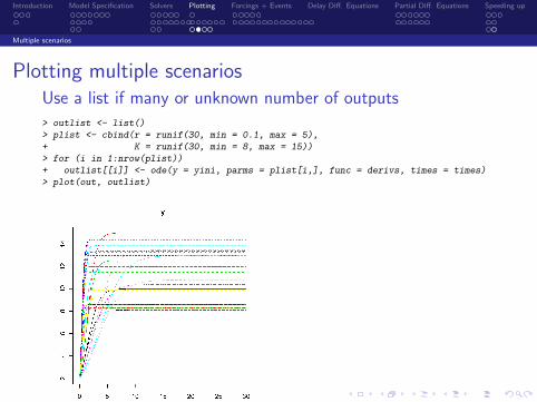
Introduction Model Specification Solvers Plotting Forcings + Events Delay Diff Equations Partial Diff Equations Speeding up
Multiple scenarios
Observed dataA list of observed data is allowedgt obs2 lt- dataframe(time = c(1 5 10 20 25) y = c(12 10 8 9 10))gt obs1 lt- dataframe(time = c(1 5 10 20 25) y = c(1 6 8 9 10))gt plot(out out2 col = c(blue red) lwd = 2+ obs = list(obs1 obs2)+ obspar = list(col = c(blue red) pch = 18 cex = 2))
Introduction Model Specification Solvers Plotting Forcings + Events Delay Diff Equations Partial Diff Equations Speeding up
Under control Forcing functions and events
Introduction Model Specification Solvers Plotting Forcings + Events Delay Diff Equations Partial Diff Equations Speeding up
Discontinuities in dynamic models
Most solvers assume that dynamics is smoothHowever there can be several types of discontinuities
I Non-smooth external variables
I Discontinuities in the derivatives
I Discontinuites in the values of the state variables
A solver does not have large problems with first two types ofdiscontinuities but changing the values of state variables is much moredifficult
Introduction Model Specification Solvers Plotting Forcings + Events Delay Diff Equations Partial Diff Equations Speeding up
External Variables
External variables in dynamic models
also called forcing functions
Why external variables
I Some important phenomena are not explicitly included in adifferential equation model but imposed as a time series (egsunlight important for plant growth is never ldquomodeledrdquo)
I Somehow during the integration the model needs to know thevalue of the external variable at each time step
Introduction Model Specification Solvers Plotting Forcings + Events Delay Diff Equations Partial Diff Equations Speeding up
External Variables
External variables in dynamic models
Implementation in R
I R has an ingenious function that is especially suited for this taskfunction approxfun
I It is used in two stepsI First an interpolating function is constructed that contains the data
This is done before solving the differential equation
afun lt- approxfun(data)
I Within the derivative function this interpolating function is called toprovide the interpolated value at the requested time point (t)
tvalue lt- afun(t)
forcings will open a help file
Introduction Model Specification Solvers Plotting Forcings + Events Delay Diff Equations Partial Diff Equations Speeding up
External Variables
Example Predator-Prey model with time-varying input
This example is from [15]
Create an artificial time-seriesgt times lt- seq(0 100 by = 01)gt signal lt- asdataframe(list(times = times import = rep(0 length(times))))gt signal$import lt- ifelse((trunc(signal$times) 2 == 0) 0 1)
gt signal[812]
times import8 07 09 08 010 09 011 10 112 11 1
Create the interpolating function using approxfun
gt input lt- approxfun(signal rule = 2)
gt input(seq(from = 098 to = 101 by = 0005))
[1] 080 085 090 095 100 100 100
Introduction Model Specification Solvers Plotting Forcings + Events Delay Diff Equations Partial Diff Equations Speeding up
External Variables
A Predator-Prey model with time-varying input
Use interpolation function in ODE function
gt SPCmod lt- function(t x parms) + with(aslist(c(parms x)) ++ import lt- input(t)++ dS lt- import - b S P + g C+ dP lt- c S P - d C P+ dC lt- e P C - f C+ res lt- c(dS dP dC)+ list(res signal = import)+ )+
gt parms lt- c(b = 01 c = 01 d = 01 e = 01 f = 01 g = 0)gt xstart lt- c(S = 1 P = 1 C = 1)gt out lt- ode(y = xstart times = times func = SPCmod parms)
Introduction Model Specification Solvers Plotting Forcings + Events Delay Diff Equations Partial Diff Equations Speeding up
External Variables
Plotting model output
gt plot(out)
Introduction Model Specification Solvers Plotting Forcings + Events Delay Diff Equations Partial Diff Equations Speeding up
Events
Discontinuities in dynamic models Events
What
I An event is when the values of state variables change abruptly
Events in Most Programming Environments
I When an event occurs the simulation needs to be restarted
I Use of loops etc
I Cumbersome messy code
Events in R
I Events are part of a model no restart necessary
I Separate dynamics inbetween events from events themselves
I Very neat and efficient
Introduction Model Specification Solvers Plotting Forcings + Events Delay Diff Equations Partial Diff Equations Speeding up
Events
Discontinuities in dynamic models Events
Two different types of events in R
I Events occur at known timesI Simple changes can be specified in a dataframe with
I name of state variable that is affectedI the time of the eventI the magnitude of the eventI event method (ldquoreplacerdquo ldquoaddrdquo ldquomultiplyrdquo)
I More complex events can be specified in an event function thatreturns the changed values of the state variablesfunction(t y parms )
I Events occur when certain conditions are metI Event is triggered by a root functionI Event is specified in an event function
events will open a help file
Introduction Model Specification Solvers Plotting Forcings + Events Delay Diff Equations Partial Diff Equations Speeding up
Events
A patient injects drugs in the blood
Problem Formulation
I Describe the concentration of the drug in the blood
I Drug injection occurs at known times rarr dataframe
Dynamics inbetween events
I The drug decays with rate b
I Initially the drug concentration = 0
gt pharmaco lt- function(t blood p) + dblood lt- - b blood+ list(dblood)+
gt b lt- 06gt yini lt- c(blood = 0)
Introduction Model Specification Solvers Plotting Forcings + Events Delay Diff Equations Partial Diff Equations Speeding up
Events
A patient injects drugs in the blood
Specifying the event
I Daily doses at same time of day
I Injection makes the concentration in the blood increase by 40 units
I The drug injections are specified in a special event dataframe
gt injectevents lt- dataframe(var = blood+ time = 020+ value = 40+ method = add)
gt head(injectevents)
var time value method1 blood 0 40 add2 blood 1 40 add3 blood 2 40 add4 blood 3 40 add5 blood 4 40 add6 blood 5 40 add
Introduction Model Specification Solvers Plotting Forcings + Events Delay Diff Equations Partial Diff Equations Speeding up
Events
A patient injects drugs in the blood
Solve model
I Pass events to the solver in a list
I All solvers in deSolve can handle events
I Here we use the ldquoimplicit Adamsrdquo method
gt times lt- seq(from = 0 to = 10 by = 124)gt outDrug lt- ode(func = pharmaco times = times y = yini+ parms = NULL method = impAdams+ events = list(data = injectevents))
Introduction Model Specification Solvers Plotting Forcings + Events Delay Diff Equations Partial Diff Equations Speeding up
Events
plotting model output
gt plot(outDrug)
Introduction Model Specification Solvers Plotting Forcings + Events Delay Diff Equations Partial Diff Equations Speeding up
Events
An event triggered by a root A Bouncing Ball
Problem formulation [13]
I A ball is thrown vertically from the ground (y(0) = 0)
I Initial velocity (yrsquo) = 10 m sminus1 acceleration g = 98 m sminus2
I When ball hits the ground it bounces
ODEs describe height of the ball above the ground (y)
Specified as 2nd order ODE
y primeprime = minusgy(0) = 0y prime(0) = 10
Specified as 1st order ODE
y prime1 = y2
y prime2 = minusgy1(0) = 0y2(0) = 10
Introduction Model Specification Solvers Plotting Forcings + Events Delay Diff Equations Partial Diff Equations Speeding up
Events
A Bouncing Ball
Dynamics inbetween events
gt library(deSolve)
gt ball lt- function(t y parms) + dy1 lt- y[2]+ dy2 lt- -98++ list(c(dy1 dy2))+
gt yini lt- c(height = 0 velocity = 10)
Introduction Model Specification Solvers Plotting Forcings + Events Delay Diff Equations Partial Diff Equations Speeding up
Events
The Ball Hits the Ground and Bounces
Root the Ball hits the ground
I The ground is where height = 0
I Root function is 0 when y1 = 0
gt rootfunc lt- function(t y parms) return (y[1])
Event the Ball bounces
I The velocity changes sign (-) and is reduced by 10
I Event function returns changed values of both state variables
gt eventfunc lt- function(t y parms) + y[1] lt- 0+ y[2] lt- -09y[2]+ return(y)+
Introduction Model Specification Solvers Plotting Forcings + Events Delay Diff Equations Partial Diff Equations Speeding up
Events
An event triggered by a root the bouncing ball
Solve model
I Inform solver that event is triggered by root (root = TRUE)
I Pass event function to solver
I Pass root function to solver
gt times lt- seq(from = 0 to = 20 by = 001)gt out lt- ode(times = times y = yini func = ball+ parms = NULL rootfun = rootfunc+ events = list(func = eventfunc root = TRUE))
Get information about the rootgt attributes(out)$troot
[1] 2040816 3877551 5530612 7018367 8357347 9562428 10647001 11623117[9] 12501621 13292274 14003862 14644290 15220675 15739420 16206290 16626472[17] 17004635 17344981 17651291 17926970 18175080 18398378 18599345 18780215[25] 18942998 19089501 19221353 19340019 19446817 19542935 19629441 19707294[33] 19777362 19840421 19897174 19948250 19994217
Introduction Model Specification Solvers Plotting Forcings + Events Delay Diff Equations Partial Diff Equations Speeding up
Events
An event triggered by a root the bouncing ball
gt plot(out select = height)
Introduction Model Specification Solvers Plotting Forcings + Events Delay Diff Equations Partial Diff Equations Speeding up
Events
An event triggered by a root the bouncing ballCreate Movie-like output
for (i in seq(1 2001 10))
plot(out which = height type = l lwd = 1
main = xlab = Time ylab = Height
)
points(t(out[i12]) pch = 21 lwd = 1 col = 1 cex = 2
bg = rainbow(30 v = 06)[20-abs(out[i3])+1])
Syssleep(001)

Introduction Model Specification Solvers Plotting Forcings + Events Delay Diff Equations Partial Diff Equations Speeding up
External Variables
External variables in dynamic models
Implementation in R
I R has an ingenious function that is especially suited for this taskfunction approxfun
I It is used in two stepsI First an interpolating function is constructed that contains the data
This is done before solving the differential equation
afun lt- approxfun(data)
I Within the derivative function this interpolating function is called toprovide the interpolated value at the requested time point (t)
tvalue lt- afun(t)
forcings will open a help file
Introduction Model Specification Solvers Plotting Forcings + Events Delay Diff Equations Partial Diff Equations Speeding up
External Variables
Example Predator-Prey model with time-varying input
This example is from [15]
Create an artificial time-seriesgt times lt- seq(0 100 by = 01)gt signal lt- asdataframe(list(times = times import = rep(0 length(times))))gt signal$import lt- ifelse((trunc(signal$times) 2 == 0) 0 1)
gt signal[812]
times import8 07 09 08 010 09 011 10 112 11 1
Create the interpolating function using approxfun
gt input lt- approxfun(signal rule = 2)
gt input(seq(from = 098 to = 101 by = 0005))
[1] 080 085 090 095 100 100 100
Introduction Model Specification Solvers Plotting Forcings + Events Delay Diff Equations Partial Diff Equations Speeding up
External Variables
A Predator-Prey model with time-varying input
Use interpolation function in ODE function
gt SPCmod lt- function(t x parms) + with(aslist(c(parms x)) ++ import lt- input(t)++ dS lt- import - b S P + g C+ dP lt- c S P - d C P+ dC lt- e P C - f C+ res lt- c(dS dP dC)+ list(res signal = import)+ )+
gt parms lt- c(b = 01 c = 01 d = 01 e = 01 f = 01 g = 0)gt xstart lt- c(S = 1 P = 1 C = 1)gt out lt- ode(y = xstart times = times func = SPCmod parms)
Introduction Model Specification Solvers Plotting Forcings + Events Delay Diff Equations Partial Diff Equations Speeding up
External Variables
Plotting model output
gt plot(out)
Introduction Model Specification Solvers Plotting Forcings + Events Delay Diff Equations Partial Diff Equations Speeding up
Events
Discontinuities in dynamic models Events
What
I An event is when the values of state variables change abruptly
Events in Most Programming Environments
I When an event occurs the simulation needs to be restarted
I Use of loops etc
I Cumbersome messy code
Events in R
I Events are part of a model no restart necessary
I Separate dynamics inbetween events from events themselves
I Very neat and efficient
Introduction Model Specification Solvers Plotting Forcings + Events Delay Diff Equations Partial Diff Equations Speeding up
Events
Discontinuities in dynamic models Events
Two different types of events in R
I Events occur at known timesI Simple changes can be specified in a dataframe with
I name of state variable that is affectedI the time of the eventI the magnitude of the eventI event method (ldquoreplacerdquo ldquoaddrdquo ldquomultiplyrdquo)
I More complex events can be specified in an event function thatreturns the changed values of the state variablesfunction(t y parms )
I Events occur when certain conditions are metI Event is triggered by a root functionI Event is specified in an event function
events will open a help file
Introduction Model Specification Solvers Plotting Forcings + Events Delay Diff Equations Partial Diff Equations Speeding up
Events
A patient injects drugs in the blood
Problem Formulation
I Describe the concentration of the drug in the blood
I Drug injection occurs at known times rarr dataframe
Dynamics inbetween events
I The drug decays with rate b
I Initially the drug concentration = 0
gt pharmaco lt- function(t blood p) + dblood lt- - b blood+ list(dblood)+
gt b lt- 06gt yini lt- c(blood = 0)
Introduction Model Specification Solvers Plotting Forcings + Events Delay Diff Equations Partial Diff Equations Speeding up
Events
A patient injects drugs in the blood
Specifying the event
I Daily doses at same time of day
I Injection makes the concentration in the blood increase by 40 units
I The drug injections are specified in a special event dataframe
gt injectevents lt- dataframe(var = blood+ time = 020+ value = 40+ method = add)
gt head(injectevents)
var time value method1 blood 0 40 add2 blood 1 40 add3 blood 2 40 add4 blood 3 40 add5 blood 4 40 add6 blood 5 40 add
Introduction Model Specification Solvers Plotting Forcings + Events Delay Diff Equations Partial Diff Equations Speeding up
Events
A patient injects drugs in the blood
Solve model
I Pass events to the solver in a list
I All solvers in deSolve can handle events
I Here we use the ldquoimplicit Adamsrdquo method
gt times lt- seq(from = 0 to = 10 by = 124)gt outDrug lt- ode(func = pharmaco times = times y = yini+ parms = NULL method = impAdams+ events = list(data = injectevents))
Introduction Model Specification Solvers Plotting Forcings + Events Delay Diff Equations Partial Diff Equations Speeding up
Events
plotting model output
gt plot(outDrug)
Introduction Model Specification Solvers Plotting Forcings + Events Delay Diff Equations Partial Diff Equations Speeding up
Events
An event triggered by a root A Bouncing Ball
Problem formulation [13]
I A ball is thrown vertically from the ground (y(0) = 0)
I Initial velocity (yrsquo) = 10 m sminus1 acceleration g = 98 m sminus2
I When ball hits the ground it bounces
ODEs describe height of the ball above the ground (y)
Specified as 2nd order ODE
y primeprime = minusgy(0) = 0y prime(0) = 10
Specified as 1st order ODE
y prime1 = y2
y prime2 = minusgy1(0) = 0y2(0) = 10
Introduction Model Specification Solvers Plotting Forcings + Events Delay Diff Equations Partial Diff Equations Speeding up
Events
A Bouncing Ball
Dynamics inbetween events
gt library(deSolve)
gt ball lt- function(t y parms) + dy1 lt- y[2]+ dy2 lt- -98++ list(c(dy1 dy2))+
gt yini lt- c(height = 0 velocity = 10)
Introduction Model Specification Solvers Plotting Forcings + Events Delay Diff Equations Partial Diff Equations Speeding up
Events
The Ball Hits the Ground and Bounces
Root the Ball hits the ground
I The ground is where height = 0
I Root function is 0 when y1 = 0
gt rootfunc lt- function(t y parms) return (y[1])
Event the Ball bounces
I The velocity changes sign (-) and is reduced by 10
I Event function returns changed values of both state variables
gt eventfunc lt- function(t y parms) + y[1] lt- 0+ y[2] lt- -09y[2]+ return(y)+
Introduction Model Specification Solvers Plotting Forcings + Events Delay Diff Equations Partial Diff Equations Speeding up
Events
An event triggered by a root the bouncing ball
Solve model
I Inform solver that event is triggered by root (root = TRUE)
I Pass event function to solver
I Pass root function to solver
gt times lt- seq(from = 0 to = 20 by = 001)gt out lt- ode(times = times y = yini func = ball+ parms = NULL rootfun = rootfunc+ events = list(func = eventfunc root = TRUE))
Get information about the rootgt attributes(out)$troot
[1] 2040816 3877551 5530612 7018367 8357347 9562428 10647001 11623117[9] 12501621 13292274 14003862 14644290 15220675 15739420 16206290 16626472[17] 17004635 17344981 17651291 17926970 18175080 18398378 18599345 18780215[25] 18942998 19089501 19221353 19340019 19446817 19542935 19629441 19707294[33] 19777362 19840421 19897174 19948250 19994217
Introduction Model Specification Solvers Plotting Forcings + Events Delay Diff Equations Partial Diff Equations Speeding up
Events
An event triggered by a root the bouncing ball
gt plot(out select = height)
Introduction Model Specification Solvers Plotting Forcings + Events Delay Diff Equations Partial Diff Equations Speeding up
Events
An event triggered by a root the bouncing ballCreate Movie-like output
for (i in seq(1 2001 10))
plot(out which = height type = l lwd = 1
main = xlab = Time ylab = Height
)
points(t(out[i12]) pch = 21 lwd = 1 col = 1 cex = 2
bg = rainbow(30 v = 06)[20-abs(out[i3])+1])
Syssleep(001)

Introduction Model Specification Solvers Plotting Forcings + Events Delay Diff Equations Partial Diff Equations Speeding up
External Variables
Plotting model output
gt plot(out)
Introduction Model Specification Solvers Plotting Forcings + Events Delay Diff Equations Partial Diff Equations Speeding up
Events
Discontinuities in dynamic models Events
What
I An event is when the values of state variables change abruptly
Events in Most Programming Environments
I When an event occurs the simulation needs to be restarted
I Use of loops etc
I Cumbersome messy code
Events in R
I Events are part of a model no restart necessary
I Separate dynamics inbetween events from events themselves
I Very neat and efficient
Introduction Model Specification Solvers Plotting Forcings + Events Delay Diff Equations Partial Diff Equations Speeding up
Events
Discontinuities in dynamic models Events
Two different types of events in R
I Events occur at known timesI Simple changes can be specified in a dataframe with
I name of state variable that is affectedI the time of the eventI the magnitude of the eventI event method (ldquoreplacerdquo ldquoaddrdquo ldquomultiplyrdquo)
I More complex events can be specified in an event function thatreturns the changed values of the state variablesfunction(t y parms )
I Events occur when certain conditions are metI Event is triggered by a root functionI Event is specified in an event function
events will open a help file
Introduction Model Specification Solvers Plotting Forcings + Events Delay Diff Equations Partial Diff Equations Speeding up
Events
A patient injects drugs in the blood
Problem Formulation
I Describe the concentration of the drug in the blood
I Drug injection occurs at known times rarr dataframe
Dynamics inbetween events
I The drug decays with rate b
I Initially the drug concentration = 0
gt pharmaco lt- function(t blood p) + dblood lt- - b blood+ list(dblood)+
gt b lt- 06gt yini lt- c(blood = 0)
Introduction Model Specification Solvers Plotting Forcings + Events Delay Diff Equations Partial Diff Equations Speeding up
Events
A patient injects drugs in the blood
Specifying the event
I Daily doses at same time of day
I Injection makes the concentration in the blood increase by 40 units
I The drug injections are specified in a special event dataframe
gt injectevents lt- dataframe(var = blood+ time = 020+ value = 40+ method = add)
gt head(injectevents)
var time value method1 blood 0 40 add2 blood 1 40 add3 blood 2 40 add4 blood 3 40 add5 blood 4 40 add6 blood 5 40 add
Introduction Model Specification Solvers Plotting Forcings + Events Delay Diff Equations Partial Diff Equations Speeding up
Events
A patient injects drugs in the blood
Solve model
I Pass events to the solver in a list
I All solvers in deSolve can handle events
I Here we use the ldquoimplicit Adamsrdquo method
gt times lt- seq(from = 0 to = 10 by = 124)gt outDrug lt- ode(func = pharmaco times = times y = yini+ parms = NULL method = impAdams+ events = list(data = injectevents))
Introduction Model Specification Solvers Plotting Forcings + Events Delay Diff Equations Partial Diff Equations Speeding up
Events
plotting model output
gt plot(outDrug)
Introduction Model Specification Solvers Plotting Forcings + Events Delay Diff Equations Partial Diff Equations Speeding up
Events
An event triggered by a root A Bouncing Ball
Problem formulation [13]
I A ball is thrown vertically from the ground (y(0) = 0)
I Initial velocity (yrsquo) = 10 m sminus1 acceleration g = 98 m sminus2
I When ball hits the ground it bounces
ODEs describe height of the ball above the ground (y)
Specified as 2nd order ODE
y primeprime = minusgy(0) = 0y prime(0) = 10
Specified as 1st order ODE
y prime1 = y2
y prime2 = minusgy1(0) = 0y2(0) = 10
Introduction Model Specification Solvers Plotting Forcings + Events Delay Diff Equations Partial Diff Equations Speeding up
Events
A Bouncing Ball
Dynamics inbetween events
gt library(deSolve)
gt ball lt- function(t y parms) + dy1 lt- y[2]+ dy2 lt- -98++ list(c(dy1 dy2))+
gt yini lt- c(height = 0 velocity = 10)
Introduction Model Specification Solvers Plotting Forcings + Events Delay Diff Equations Partial Diff Equations Speeding up
Events
The Ball Hits the Ground and Bounces
Root the Ball hits the ground
I The ground is where height = 0
I Root function is 0 when y1 = 0
gt rootfunc lt- function(t y parms) return (y[1])
Event the Ball bounces
I The velocity changes sign (-) and is reduced by 10
I Event function returns changed values of both state variables
gt eventfunc lt- function(t y parms) + y[1] lt- 0+ y[2] lt- -09y[2]+ return(y)+
Introduction Model Specification Solvers Plotting Forcings + Events Delay Diff Equations Partial Diff Equations Speeding up
Events
An event triggered by a root the bouncing ball
Solve model
I Inform solver that event is triggered by root (root = TRUE)
I Pass event function to solver
I Pass root function to solver
gt times lt- seq(from = 0 to = 20 by = 001)gt out lt- ode(times = times y = yini func = ball+ parms = NULL rootfun = rootfunc+ events = list(func = eventfunc root = TRUE))
Get information about the rootgt attributes(out)$troot
[1] 2040816 3877551 5530612 7018367 8357347 9562428 10647001 11623117[9] 12501621 13292274 14003862 14644290 15220675 15739420 16206290 16626472[17] 17004635 17344981 17651291 17926970 18175080 18398378 18599345 18780215[25] 18942998 19089501 19221353 19340019 19446817 19542935 19629441 19707294[33] 19777362 19840421 19897174 19948250 19994217
Introduction Model Specification Solvers Plotting Forcings + Events Delay Diff Equations Partial Diff Equations Speeding up
Events
An event triggered by a root the bouncing ball
gt plot(out select = height)
Introduction Model Specification Solvers Plotting Forcings + Events Delay Diff Equations Partial Diff Equations Speeding up
Events
An event triggered by a root the bouncing ballCreate Movie-like output
for (i in seq(1 2001 10))
plot(out which = height type = l lwd = 1
main = xlab = Time ylab = Height
)
points(t(out[i12]) pch = 21 lwd = 1 col = 1 cex = 2
bg = rainbow(30 v = 06)[20-abs(out[i3])+1])
Syssleep(001)

Introduction Model Specification Solvers Plotting Forcings + Events Delay Diff Equations Partial Diff Equations Speeding up
Events
Discontinuities in dynamic models Events
Two different types of events in R
I Events occur at known timesI Simple changes can be specified in a dataframe with
I name of state variable that is affectedI the time of the eventI the magnitude of the eventI event method (ldquoreplacerdquo ldquoaddrdquo ldquomultiplyrdquo)
I More complex events can be specified in an event function thatreturns the changed values of the state variablesfunction(t y parms )
I Events occur when certain conditions are metI Event is triggered by a root functionI Event is specified in an event function
events will open a help file
Introduction Model Specification Solvers Plotting Forcings + Events Delay Diff Equations Partial Diff Equations Speeding up
Events
A patient injects drugs in the blood
Problem Formulation
I Describe the concentration of the drug in the blood
I Drug injection occurs at known times rarr dataframe
Dynamics inbetween events
I The drug decays with rate b
I Initially the drug concentration = 0
gt pharmaco lt- function(t blood p) + dblood lt- - b blood+ list(dblood)+
gt b lt- 06gt yini lt- c(blood = 0)
Introduction Model Specification Solvers Plotting Forcings + Events Delay Diff Equations Partial Diff Equations Speeding up
Events
A patient injects drugs in the blood
Specifying the event
I Daily doses at same time of day
I Injection makes the concentration in the blood increase by 40 units
I The drug injections are specified in a special event dataframe
gt injectevents lt- dataframe(var = blood+ time = 020+ value = 40+ method = add)
gt head(injectevents)
var time value method1 blood 0 40 add2 blood 1 40 add3 blood 2 40 add4 blood 3 40 add5 blood 4 40 add6 blood 5 40 add
Introduction Model Specification Solvers Plotting Forcings + Events Delay Diff Equations Partial Diff Equations Speeding up
Events
A patient injects drugs in the blood
Solve model
I Pass events to the solver in a list
I All solvers in deSolve can handle events
I Here we use the ldquoimplicit Adamsrdquo method
gt times lt- seq(from = 0 to = 10 by = 124)gt outDrug lt- ode(func = pharmaco times = times y = yini+ parms = NULL method = impAdams+ events = list(data = injectevents))
Introduction Model Specification Solvers Plotting Forcings + Events Delay Diff Equations Partial Diff Equations Speeding up
Events
plotting model output
gt plot(outDrug)
Introduction Model Specification Solvers Plotting Forcings + Events Delay Diff Equations Partial Diff Equations Speeding up
Events
An event triggered by a root A Bouncing Ball
Problem formulation [13]
I A ball is thrown vertically from the ground (y(0) = 0)
I Initial velocity (yrsquo) = 10 m sminus1 acceleration g = 98 m sminus2
I When ball hits the ground it bounces
ODEs describe height of the ball above the ground (y)
Specified as 2nd order ODE
y primeprime = minusgy(0) = 0y prime(0) = 10
Specified as 1st order ODE
y prime1 = y2
y prime2 = minusgy1(0) = 0y2(0) = 10
Introduction Model Specification Solvers Plotting Forcings + Events Delay Diff Equations Partial Diff Equations Speeding up
Events
A Bouncing Ball
Dynamics inbetween events
gt library(deSolve)
gt ball lt- function(t y parms) + dy1 lt- y[2]+ dy2 lt- -98++ list(c(dy1 dy2))+
gt yini lt- c(height = 0 velocity = 10)
Introduction Model Specification Solvers Plotting Forcings + Events Delay Diff Equations Partial Diff Equations Speeding up
Events
The Ball Hits the Ground and Bounces
Root the Ball hits the ground
I The ground is where height = 0
I Root function is 0 when y1 = 0
gt rootfunc lt- function(t y parms) return (y[1])
Event the Ball bounces
I The velocity changes sign (-) and is reduced by 10
I Event function returns changed values of both state variables
gt eventfunc lt- function(t y parms) + y[1] lt- 0+ y[2] lt- -09y[2]+ return(y)+
Introduction Model Specification Solvers Plotting Forcings + Events Delay Diff Equations Partial Diff Equations Speeding up
Events
An event triggered by a root the bouncing ball
Solve model
I Inform solver that event is triggered by root (root = TRUE)
I Pass event function to solver
I Pass root function to solver
gt times lt- seq(from = 0 to = 20 by = 001)gt out lt- ode(times = times y = yini func = ball+ parms = NULL rootfun = rootfunc+ events = list(func = eventfunc root = TRUE))
Get information about the rootgt attributes(out)$troot
[1] 2040816 3877551 5530612 7018367 8357347 9562428 10647001 11623117[9] 12501621 13292274 14003862 14644290 15220675 15739420 16206290 16626472[17] 17004635 17344981 17651291 17926970 18175080 18398378 18599345 18780215[25] 18942998 19089501 19221353 19340019 19446817 19542935 19629441 19707294[33] 19777362 19840421 19897174 19948250 19994217
Introduction Model Specification Solvers Plotting Forcings + Events Delay Diff Equations Partial Diff Equations Speeding up
Events
An event triggered by a root the bouncing ball
gt plot(out select = height)
Introduction Model Specification Solvers Plotting Forcings + Events Delay Diff Equations Partial Diff Equations Speeding up
Events
An event triggered by a root the bouncing ballCreate Movie-like output
for (i in seq(1 2001 10))
plot(out which = height type = l lwd = 1
main = xlab = Time ylab = Height
)
points(t(out[i12]) pch = 21 lwd = 1 col = 1 cex = 2
bg = rainbow(30 v = 06)[20-abs(out[i3])+1])
Syssleep(001)

Introduction Model Specification Solvers Plotting Forcings + Events Delay Diff Equations Partial Diff Equations Speeding up
Events
A patient injects drugs in the blood
Solve model
I Pass events to the solver in a list
I All solvers in deSolve can handle events
I Here we use the ldquoimplicit Adamsrdquo method
gt times lt- seq(from = 0 to = 10 by = 124)gt outDrug lt- ode(func = pharmaco times = times y = yini+ parms = NULL method = impAdams+ events = list(data = injectevents))
Introduction Model Specification Solvers Plotting Forcings + Events Delay Diff Equations Partial Diff Equations Speeding up
Events
plotting model output
gt plot(outDrug)
Introduction Model Specification Solvers Plotting Forcings + Events Delay Diff Equations Partial Diff Equations Speeding up
Events
An event triggered by a root A Bouncing Ball
Problem formulation [13]
I A ball is thrown vertically from the ground (y(0) = 0)
I Initial velocity (yrsquo) = 10 m sminus1 acceleration g = 98 m sminus2
I When ball hits the ground it bounces
ODEs describe height of the ball above the ground (y)
Specified as 2nd order ODE
y primeprime = minusgy(0) = 0y prime(0) = 10
Specified as 1st order ODE
y prime1 = y2
y prime2 = minusgy1(0) = 0y2(0) = 10
Introduction Model Specification Solvers Plotting Forcings + Events Delay Diff Equations Partial Diff Equations Speeding up
Events
A Bouncing Ball
Dynamics inbetween events
gt library(deSolve)
gt ball lt- function(t y parms) + dy1 lt- y[2]+ dy2 lt- -98++ list(c(dy1 dy2))+
gt yini lt- c(height = 0 velocity = 10)
Introduction Model Specification Solvers Plotting Forcings + Events Delay Diff Equations Partial Diff Equations Speeding up
Events
The Ball Hits the Ground and Bounces
Root the Ball hits the ground
I The ground is where height = 0
I Root function is 0 when y1 = 0
gt rootfunc lt- function(t y parms) return (y[1])
Event the Ball bounces
I The velocity changes sign (-) and is reduced by 10
I Event function returns changed values of both state variables
gt eventfunc lt- function(t y parms) + y[1] lt- 0+ y[2] lt- -09y[2]+ return(y)+
Introduction Model Specification Solvers Plotting Forcings + Events Delay Diff Equations Partial Diff Equations Speeding up
Events
An event triggered by a root the bouncing ball
Solve model
I Inform solver that event is triggered by root (root = TRUE)
I Pass event function to solver
I Pass root function to solver
gt times lt- seq(from = 0 to = 20 by = 001)gt out lt- ode(times = times y = yini func = ball+ parms = NULL rootfun = rootfunc+ events = list(func = eventfunc root = TRUE))
Get information about the rootgt attributes(out)$troot
[1] 2040816 3877551 5530612 7018367 8357347 9562428 10647001 11623117[9] 12501621 13292274 14003862 14644290 15220675 15739420 16206290 16626472[17] 17004635 17344981 17651291 17926970 18175080 18398378 18599345 18780215[25] 18942998 19089501 19221353 19340019 19446817 19542935 19629441 19707294[33] 19777362 19840421 19897174 19948250 19994217
Introduction Model Specification Solvers Plotting Forcings + Events Delay Diff Equations Partial Diff Equations Speeding up
Events
An event triggered by a root the bouncing ball
gt plot(out select = height)
Introduction Model Specification Solvers Plotting Forcings + Events Delay Diff Equations Partial Diff Equations Speeding up
Events
An event triggered by a root the bouncing ballCreate Movie-like output
for (i in seq(1 2001 10))
plot(out which = height type = l lwd = 1
main = xlab = Time ylab = Height
)
points(t(out[i12]) pch = 21 lwd = 1 col = 1 cex = 2
bg = rainbow(30 v = 06)[20-abs(out[i3])+1])
Syssleep(001)

Introduction Model Specification Solvers Plotting Forcings + Events Delay Diff Equations Partial Diff Equations Speeding up
Events
An event triggered by a root the bouncing ball
gt plot(out select = height)
Introduction Model Specification Solvers Plotting Forcings + Events Delay Diff Equations Partial Diff Equations Speeding up
Events
An event triggered by a root the bouncing ballCreate Movie-like output
for (i in seq(1 2001 10))
plot(out which = height type = l lwd = 1
main = xlab = Time ylab = Height
)
points(t(out[i12]) pch = 21 lwd = 1 col = 1 cex = 2
bg = rainbow(30 v = 06)[20-abs(out[i3])+1])
Syssleep(001)
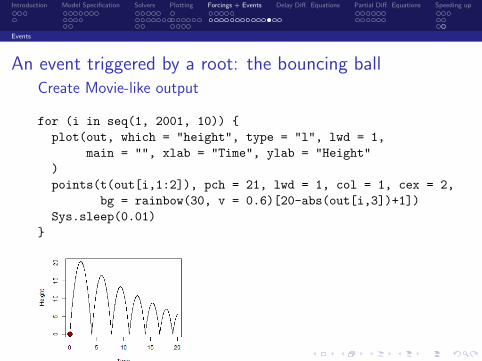
Introduction Model Specification Solvers Plotting Forcings + Events Delay Diff Equations Partial Diff Equations Speeding up
Events
An event triggered by a root the bouncing ballCreate Movie-like output
for (i in seq(1 2001 10))
plot(out which = height type = l lwd = 1
main = xlab = Time ylab = Height
)
points(t(out[i12]) pch = 21 lwd = 1 col = 1 cex = 2
bg = rainbow(30 v = 06)[20-abs(out[i3])+1])
Syssleep(001)
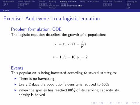
Introduction Model Specification Solvers Plotting Forcings + Events Delay Diff Equations Partial Diff Equations Speeding up
Events
Exercise Add events to a logistic equation
Problem formulation ODEThe logistic equation describes the growth of a population
y prime = r middot y middot (1minus y
K)
r = 1K = 10 y0 = 2
EventsThis population is being harvested according to several strategies
I There is no harvesting
I Every 2 days the populationrsquos density is reduced to 50
I When the species has reached 80 of its carrying capacity itsdensity is halved
Introduction Model Specification Solvers Plotting Forcings + Events Delay Diff Equations Partial Diff Equations Speeding up
Events
Exercise Add events to a logistic equation - ctd
Tasks
I Run the model for 20 days
I Implement first strategy in a dataframe
I Second strategy requires root and event function
I Use file exampleslogisticEventRtxt as a template
Introduction Model Specification Solvers Plotting Forcings + Events Delay Diff Equations Partial Diff Equations Speeding up
Delay Differential Equations
WhatDelay Differential Equations are similar to ODEs except that they involvepast values of variables andor derivatives
DDEs in R R-package deSolve
I dede solves DDEs
I lagvalue provides lagged values of the state variables
I lagderiv provides lagged values of the derivatives
Introduction Model Specification Solvers Plotting Forcings + Events Delay Diff Equations Partial Diff Equations Speeding up
Example Chaotic Production of White Blood Cells
Mackey-Glass Equation [8]
I y current density of white blood cells
I yτ is the density τ time-units in the past
I first term equation is production rate
I b is destruction rate
y prime = ayτ1
1+y cτminus by
yτ = y(t minus τ)yt = 05 for t le 0
(1)
I For τ = 10 the output is periodic
I For τ = 20 cell densities display a chaotic pattern
Introduction Model Specification Solvers Plotting Forcings + Events Delay Diff Equations Partial Diff Equations Speeding up
Solution in R
gt library(deSolve)gt retarded lt- function(t y parms tau) + tlag lt- t - tau+ if (tlag lt= 0)+ ylag lt- 05+ else+ ylag lt- lagvalue(tlag)++ dy lt- 02 ylag 1(1+ylag^10) - 01 y+ list(dy = dy ylag = ylag)+ gt yinit lt- 05gt times lt- seq(from = 0 to = 300 by = 01)gt yout1 lt- dede(y = yinit times = times func = retarded parms = NULL tau = 10)gt yout2 lt- dede(y = yinit times = times func = retarded parms = NULL tau = 20)
Introduction Model Specification Solvers Plotting Forcings + Events Delay Diff Equations Partial Diff Equations Speeding up
Solution in Rgt plot(yout1 lwd = 2 main = tau=10 ylab = y mfrow = c(2 2) which = 1)gt plot(yout1[-1] type = l lwd = 2 xlab = y)gt plot(yout2 lwd = 2 main = tau=20 ylab = y mfrow = NULL which = 1)gt plot(yout2[-1] type = l lwd = 2 xlab = y)
Introduction Model Specification Solvers Plotting Forcings + Events Delay Diff Equations Partial Diff Equations Speeding up
Exercise the Lemming model
A nice variant of the logistic model is the DDE lemming model [14]
y prime = r middot y(1minus y(t minus τ)
K) (2)
Use file examplesddelemmingRtxt as a template to implement thismodel
I initial condition y(t = 0) = 19001
I parameter values r = 35 τ = 074 K = 19
I history y(t) = 19 for t lt 0
I Generate output for t in [0 40]
Introduction Model Specification Solvers Plotting Forcings + Events Delay Diff Equations Partial Diff Equations Speeding up
Diffusion advection and reactionPartial differential equations (PDE) with ReacTran
Introduction Model Specification Solvers Plotting Forcings + Events Delay Diff Equations Partial Diff Equations Speeding up
Partial Differential Equations
PDEs as advection-diffusion problemsMany second-order PDEs can be written as advection-diffusion problems
partC
partt= minusv
partC
partx+ D
part2C
partx2+ f (t x C )
same for 2-D and 3-D
Example wave equation in 1-D
part2u
partt2= c2 part
2u
partx2(3)
can be written asdu
dt= v
partv
partt= c2 part
2u
partx2
(4)
Introduction Model Specification Solvers Plotting Forcings + Events Delay Diff Equations Partial Diff Equations Speeding up
Three packages for solving PDEs in R
ReacTran methods for numerical approximation of PDEs [16]
I tran1D(C Cup Cdown D v )
I tran2D tran3D
deSolve special solvers for time-varying cases [20]
I ode1D(y times func parms nspec dimens method names )
I ode2D ode3D
rootSolve special solvers for time-invariant cases [19]
I steady1D(y time func parms nspec dimens method names )
I steady2D steady3D
Introduction Model Specification Solvers Plotting Forcings + Events Delay Diff Equations Partial Diff Equations Speeding up
1-D PDEs
Numerical solution of the wave equation
library(ReacTran)
wave lt- function (t y parms)
u lt- y[1N]
v lt- y[(N+1)(2N)]
du lt- v
dv lt- tran1D(C = u Cup = 0 Cdown = 0 D = 1
dx = xgrid)$dC
list(c(du dv))
xgrid lt- setupgrid1D(-100 100 dx1 = 02)
x lt- xgrid$xmid
N lt- xgrid$N
uini lt- exp(-02x^2)
vini lt- rep(0 N)
yini lt- c(uini vini)
times lt- seq (from = 0 to = 50 by = 1)
out lt- ode1D(yini times wave parms method = adams
names = c(u v) dimens = N)
image(out grid = x)
Numerical method provided by the
deSolve package
httpdesolver-forger-projectorg
Methods from ReacTran
Introduction Model Specification Solvers Plotting Forcings + Events Delay Diff Equations Partial Diff Equations Speeding up
1-D PDEs
Plotting 1-D PDEs matplot1Dgt outtime lt- seq(from = 0 to = 50 by = 10)gt matplot1D(out which = u subset = time in outtime grid = x+ xlab = x ylab = u type = l lwd = 2 xlim = c(-50 50) col=black)
Introduction Model Specification Solvers Plotting Forcings + Events Delay Diff Equations Partial Diff Equations Speeding up
1-D PDEs
Plotting 1-D PDEs image
gt image(out which = u grid = x)
Introduction Model Specification Solvers Plotting Forcings + Events Delay Diff Equations Partial Diff Equations Speeding up
1-D PDEs
Plotting 1-D PDEs persp plotsgt image(out which = u grid = x method = persp border = NA+ col = lightblue box = FALSE shade = 05 theta = 0 phi = 60)
Introduction Model Specification Solvers Plotting Forcings + Events Delay Diff Equations Partial Diff Equations Speeding up
1-D PDEs
Exercise the Brusselator
Problem formulation [6]The Brusselator is a model for an auto-catalytic chemical reactionbetween two products A and B and producing also C and D in anumber of intermediary steps
Ak1minusrarr X1
B + X1k2minusrarr X2 + C
2X1 + X2k3minusrarr 3X1
X1k4minusrarr D
where the ki are the reaction rates
Introduction Model Specification Solvers Plotting Forcings + Events Delay Diff Equations Partial Diff Equations Speeding up
1-D PDEs
Exercise Implement the Brusselator in 1-D
Equations for X1 and X2
partX1
partt = DX1
part2X1
partx2 + 1 + X 21 X2 minus 4X1
partX2
partt = DX2
part2X2
partx2 + 3X1 minus X 21 X2
Tasks
I The grid x extends from 0 to 1 and consists of 50 cells
I Initial conditions
X1(0) = 1 + sin(2 lowast π lowast x)X2(0) = 3
I Generate output for t = 0 1 10
I Use file implementing the wave equation as a templateexampleswaveRtxt
Introduction Model Specification Solvers Plotting Forcings + Events Delay Diff Equations Partial Diff Equations Speeding up
2-D PDEs
2-D wave equation Sine-Gordon
Problem formulationThe Sine-Gordon equation is a non-linear hyperbolic (wave-like) partialdifferential equation involving the sine of the dependent variable
part2u
partt2= D
part2u
partx2+ D
part2u
party 2minus sin u (5)
Rewritten as two first order differential equations
dudt = vpartvpartt = D part2u
partx2 + D part2uparty2 minus sin u
(6)
Introduction Model Specification Solvers Plotting Forcings + Events Delay Diff Equations Partial Diff Equations Speeding up
2-D PDEs
2-D Sine-Gordon in R
gridgt Nx lt- Ny lt- 100gt xgrid lt- setupgrid1D(-7 7 N = Nx) x lt- xgrid$xmidgt ygrid lt- setupgrid1D(-7 7 N = Ny) y lt- ygrid$xmid
derivative functiongt sinegordon2D lt- function(t C parms) + u lt- matrix(nrow = Nx ncol = Ny data = C[1 (NxNy)])+ v lt- matrix(nrow = Nx ncol = Ny data = C[(NxNy+1) (2NxNy)])+ dv lt- tran2D (C = u Cxup = 0 Cxdown = 0 Cyup = 0 Cydown = 0+ Dx = 1 Dy = 1 dx = xgrid dy = ygrid)$dC - sin(u)+ list(c(v dv))+
initial conditionsgt peak lt- function (x y x0 y0) return(exp(-( (x-x0)^2 + (y-y0)^2)))gt uini lt- outer(x y FUN = function(x y) peak(x y 22) + peak(x y-2-2)+ + peak(x y-22) + peak(x y 2-2))gt vini lt- rep(0 NxNy)
solutiongt out lt- ode2D (y = c(uinivini) times = 03 parms = 0 func = sinegordon2D+ names = c(u v) dimens = c(Nx Ny) method = ode45)
Introduction Model Specification Solvers Plotting Forcings + Events Delay Diff Equations Partial Diff Equations Speeding up
2-D PDEs
Plotting 2-D PDEs image plots
gt image(out which = u grid = list(x y) mfrow = c(22) ask = FALSE)
Introduction Model Specification Solvers Plotting Forcings + Events Delay Diff Equations Partial Diff Equations Speeding up
2-D PDEs
Plotting 2-D PDEs persp plotsgt image(out which = u grid = list(x y) method = persp border = NA+ col = lightblue box = FALSE shade = 05 theta = 0 phi = 60+ mfrow = c(22) ask = FALSE)
Introduction Model Specification Solvers Plotting Forcings + Events Delay Diff Equations Partial Diff Equations Speeding up
2-D PDEs
Movie-like output of 2-D PDEs
out lt- ode2D (y = c(uini vini) times = seq(0 3 by = 01)
parms = NULL func = sinegordon2D
names=c(u v) dimens = c(Nx Ny)
method = ode45)
image(out which = u grid = list(x = x y = y)
method = persp border = NA
theta = 30 phi = 60 box = FALSE ask = FALSE)
Introduction Model Specification Solvers Plotting Forcings + Events Delay Diff Equations Partial Diff Equations Speeding up
2-D PDEs
Exercise Implement the Brusselator in 2-DEquations
partX1
partt = DX1
part2X1
partx2 + DX1
part2X1
party2 + 1 + X 21 X2 minus 4X1
partX2
partt = DX2
part2X1
partx2 + DX2
part2X1
party2 + 3X1 minus X 21 X2
Tasks
I The grids x and y extend from 0 to 1 and consist of 50 cells
I Parameter settings diffusion coefficient
DX1 = 2 DX2 = 8 lowast DX1
I Initial condition for X1 X2 random numbers inbetween 0 and 1
I Generate output for t = 0 1 8
I Use the file implementing the Sine-Gordon equation as a templateexamplessinegordonRtxt
Introduction Model Specification Solvers Plotting Forcings + Events Delay Diff Equations Partial Diff Equations Speeding up
Speeding up Matrices and compiled code
Introduction Model Specification Solvers Plotting Forcings + Events Delay Diff Equations Partial Diff Equations Speeding up
Methods for speeding up
I Use matrices
I Implement essential parts in compiled code (Fortran C)
I Implement the full method in compiled code
Formulating a model with matrices and vectors can lead to a considerablespeed gain ndash and compact code ndash while retaining the full flexibility of RThe use of compiled code saves even more CPU time at the cost of ahigher development effort
Introduction Model Specification Solvers Plotting Forcings + Events Delay Diff Equations Partial Diff Equations Speeding up
Using matrices
Use of matrices
A Lotka-Volterra model with 4 species
gt model lt- function(t n parms) + with(aslist(c(n parms)) + dn1 lt- r1 n1 - a13 n1 n3+ dn2 lt- r2 n2 - a24 n2 n4+ dn3 lt- a13 n1 n3 - r3 n3+ dn4 lt- a24 n2 n4 - r4 n4+ return(list(c(dn1 dn2 dn3 dn4)))+ )+ gt parms lt- c(r1 = 01 r2 = 01 r3 = 01 r4 = 01 a13 = 02 a24 = 01)gt times = seq(from = 0 to = 500 by = 01)gt n0 = c(n1 = 1 n2 = 1 n3 = 2 n4 = 2)
gt systemtime(out lt- ode(n0 times model parms))
user system elapsed302 000 302
Source exampleslv-plain-or-matrixRtxt
Introduction Model Specification Solvers Plotting Forcings + Events Delay Diff Equations Partial Diff Equations Speeding up
Using matrices
Use of matrices
A Lotka-Volterra model with 4 species
gt model lt- function(t n parms) + with(parms + dn lt- r n + n (A n)+ return(list(c(dn)))+ )+ gt parms lt- list(+ r = c(r1 = 01 r2 = 01 r3 = -01 r4 = -01)+ A = matrix(c(00 00 -02 00 prey 1+ 00 00 00 -01 prey 2+ 02 00 00 00 predator 1 eats prey 1+ 00 01 00 00) predator 2 eats prey 2+ nrow = 4 ncol = 4 byrow = TRUE)+ )
gt systemtime(out lt- ode(n0 times model parms))
user system elapsed166 000 170
Source exampleslv-plain-or-matrixRtxt
Introduction Model Specification Solvers Plotting Forcings + Events Delay Diff Equations Partial Diff Equations Speeding up
Using matrices
Results
I plot(out) will show the results
I Note that the ldquoplainrdquo version has only 1 to 1 connections but thematrix model is already full connected (with most connections arezero) The comparison is insofar unfair that the matrix version(despite faster execution) is more powerful
I Exercise Create a fully connected model in the plain version for afair comparison
I A parameter example (eg for weak coupling) can be found onhttp
tolstoynewcastleeduauRe7help09061230html
Introduction Model Specification Solvers Plotting Forcings + Events Delay Diff Equations Partial Diff Equations Speeding up
Compiled code
Using compiled code
All solvers of deSolve
I allow direct communication between solvers and a compiled model
See vignette (compiledCode) [15]
Principle
I Implement core model (and only this) in C or Fortran
I Use data handling storage and plotting facilities of R
examplescompiled_lorenzcompiledcodesvg
Introduction Model Specification Solvers Plotting Forcings + Events Delay Diff Equations Partial Diff Equations Speeding up
Compiled code
The End
Thank you
More Infohttpdesolver-forger-projectorg
Introduction Model Specification Solvers Plotting Forcings + Events Delay Diff Equations Partial Diff Equations Speeding up
Finally
Acknowledgments
CitationA lot of effort went in creating this software please cite it when using it
I to cite deSolve [20] rootSolve [19] ReacTran [16]
I Some complex examples can be found in [18]
I A framework to fit differential equation models to data is FME [17]
I A framework for ecological modelling is simecol [10]
Acknowledgments
I None of this would be possible without the splendid work of the RCore Team [11]
I This presentation was created with Sweave [7]
I Creation of the packages made use of Rforge [21]
Introduction Model Specification Solvers Plotting Forcings + Events Delay Diff Equations Partial Diff Equations Speeding up
Finally
Bibliography I
[1] K E Brenan S L Campbell and L R PetzoldNumerical Solution of Initial-Value Problems in Differential-Algebraic EquationsSIAM Classics in Applied Mathematics 1996
[2] P N Brown G D Byrne and A C HindmarshVode a variable-coefficient ode solverSIAM Journal on Scientific and Statistical Computing 101038ndash1051 1989
[3] E Hairer S P Norsett and G WannerSolving Ordinary Differential Equations I Nonstiff Problems Second Revised EditionSpringer-Verlag Heidelberg 2009
[4] E Hairer and G WannerSolving Ordinary Differential Equations II Stiff and Differential-Algebraic Problems Second Revised EditionSpringer-Verlag Heidelberg 2010
[5] A C HindmarshODEPACK a systematized collection of ODE solversIn R Stepleman editor Scientific Computing Vol 1 of IMACS Transactions on Scientific Computation pages 55ndash64 IMACS North-Holland Amsterdam 1983
[6] R Lefever G Nicolis and I PrigogineOn the occurrence of oscillations around the steady state in systems of chemical reactions far from equilibriumJournal of Chemical Physics 471045ndash1047 1967
[7] Friedrich LeischDynamic generation of statistical reports using literate data analysisIn W Hardle and B Ronz editors COMPSTAT 2002 ndash Proceedings in Computational Statistics pages 575ndash580 Heidelberg 2002Physica-Verlag
[8] M C Mackey and L GlassOscillation and chaos in physiological control systemsScience 197287ndash289 1977
Introduction Model Specification Solvers Plotting Forcings + Events Delay Diff Equations Partial Diff Equations Speeding up
Finally
Bibliography II
[9] Linda R PetzoldAutomatic selection of methods for solving stiff and nonstiff systems of ordinary differential equationsSIAM Journal on Scientific and Statistical Computing 4136ndash148 1983
[10] Thomas Petzoldt and Karsten Rinkesimecol An object-oriented framework for ecological modeling in RJournal of Statistical Software 22(9)1ndash31 2007
[11] R Development Core TeamR A Language and Environment for Statistical ComputingR Foundation for Statistical Computing Vienna Austria 2011ISBN 3-900051-07-0
[12] OE RosslerAn equation for continous chaosPhysics Letters A 57 (5)397ndash398 1976
[13] L F Shampine I Gladwell and S ThompsonSolving ODEs with MATLABCambridge University Press Cambridge 2003
[14] LF Shampine and S ThompsonSolving ddes in matlabApp Numer Math 37441ndash458 2001
[15] K Soetaert T Petzoldt and RW SetzerR-package deSolve Writing Code in Compiled Languages 2009package vignette
[16] Karline Soetaert and Filip MeysmanReactive transport in aquatic ecosystems rapid model prototyping in the open source software REnvironmental modelling and software page in press 2011
Introduction Model Specification Solvers Plotting Forcings + Events Delay Diff Equations Partial Diff Equations Speeding up
Finally
Bibliography III
[17] Karline Soetaert and Thomas PetzoldtInverse modelling sensitivity and monte carlo analysis in R using package FMEJournal of Statistical Software 33(3)1ndash28 2010
[18] Karline Soetaert and Thomas PetzoldtSolving ODEs DAEs DDEs and PDEs in RJournal of Numerical Analysis Industrial and Applied Mathematics in press 2011
[19] Karline Soetaert Thomas Petzoldt and R Woodrow SetzerSolving Differential Equations in RThe R Journal 2(2)5ndash15 December 2010
[20] Karline Soetaert Thomas Petzoldt and R Woodrow SetzerSolving differential equations in R Package deSolveJournal of Statistical Software 33(9)1ndash25 2010
[21] Stefan Theuszligl and Achim ZeileisCollaborative Software Development Using R-ForgeThe R Journal 1(1)9ndash14 May 2009
[22] B van der Pol and J van der MarkFrequency demultiplicationNature 120363ndash364 1927

Introduction Model Specification Solvers Plotting Forcings + Events Delay Diff Equations Partial Diff Equations Speeding up
Example Chaotic Production of White Blood Cells
Mackey-Glass Equation [8]
I y current density of white blood cells
I yτ is the density τ time-units in the past
I first term equation is production rate
I b is destruction rate
y prime = ayτ1
1+y cτminus by
yτ = y(t minus τ)yt = 05 for t le 0
(1)
I For τ = 10 the output is periodic
I For τ = 20 cell densities display a chaotic pattern
Introduction Model Specification Solvers Plotting Forcings + Events Delay Diff Equations Partial Diff Equations Speeding up
Solution in R
gt library(deSolve)gt retarded lt- function(t y parms tau) + tlag lt- t - tau+ if (tlag lt= 0)+ ylag lt- 05+ else+ ylag lt- lagvalue(tlag)++ dy lt- 02 ylag 1(1+ylag^10) - 01 y+ list(dy = dy ylag = ylag)+ gt yinit lt- 05gt times lt- seq(from = 0 to = 300 by = 01)gt yout1 lt- dede(y = yinit times = times func = retarded parms = NULL tau = 10)gt yout2 lt- dede(y = yinit times = times func = retarded parms = NULL tau = 20)
Introduction Model Specification Solvers Plotting Forcings + Events Delay Diff Equations Partial Diff Equations Speeding up
Solution in Rgt plot(yout1 lwd = 2 main = tau=10 ylab = y mfrow = c(2 2) which = 1)gt plot(yout1[-1] type = l lwd = 2 xlab = y)gt plot(yout2 lwd = 2 main = tau=20 ylab = y mfrow = NULL which = 1)gt plot(yout2[-1] type = l lwd = 2 xlab = y)
Introduction Model Specification Solvers Plotting Forcings + Events Delay Diff Equations Partial Diff Equations Speeding up
Exercise the Lemming model
A nice variant of the logistic model is the DDE lemming model [14]
y prime = r middot y(1minus y(t minus τ)
K) (2)
Use file examplesddelemmingRtxt as a template to implement thismodel
I initial condition y(t = 0) = 19001
I parameter values r = 35 τ = 074 K = 19
I history y(t) = 19 for t lt 0
I Generate output for t in [0 40]
Introduction Model Specification Solvers Plotting Forcings + Events Delay Diff Equations Partial Diff Equations Speeding up
Diffusion advection and reactionPartial differential equations (PDE) with ReacTran
Introduction Model Specification Solvers Plotting Forcings + Events Delay Diff Equations Partial Diff Equations Speeding up
Partial Differential Equations
PDEs as advection-diffusion problemsMany second-order PDEs can be written as advection-diffusion problems
partC
partt= minusv
partC
partx+ D
part2C
partx2+ f (t x C )
same for 2-D and 3-D
Example wave equation in 1-D
part2u
partt2= c2 part
2u
partx2(3)
can be written asdu
dt= v
partv
partt= c2 part
2u
partx2
(4)
Introduction Model Specification Solvers Plotting Forcings + Events Delay Diff Equations Partial Diff Equations Speeding up
Three packages for solving PDEs in R
ReacTran methods for numerical approximation of PDEs [16]
I tran1D(C Cup Cdown D v )
I tran2D tran3D
deSolve special solvers for time-varying cases [20]
I ode1D(y times func parms nspec dimens method names )
I ode2D ode3D
rootSolve special solvers for time-invariant cases [19]
I steady1D(y time func parms nspec dimens method names )
I steady2D steady3D
Introduction Model Specification Solvers Plotting Forcings + Events Delay Diff Equations Partial Diff Equations Speeding up
1-D PDEs
Numerical solution of the wave equation
library(ReacTran)
wave lt- function (t y parms)
u lt- y[1N]
v lt- y[(N+1)(2N)]
du lt- v
dv lt- tran1D(C = u Cup = 0 Cdown = 0 D = 1
dx = xgrid)$dC
list(c(du dv))
xgrid lt- setupgrid1D(-100 100 dx1 = 02)
x lt- xgrid$xmid
N lt- xgrid$N
uini lt- exp(-02x^2)
vini lt- rep(0 N)
yini lt- c(uini vini)
times lt- seq (from = 0 to = 50 by = 1)
out lt- ode1D(yini times wave parms method = adams
names = c(u v) dimens = N)
image(out grid = x)
Numerical method provided by the
deSolve package
httpdesolver-forger-projectorg
Methods from ReacTran
Introduction Model Specification Solvers Plotting Forcings + Events Delay Diff Equations Partial Diff Equations Speeding up
1-D PDEs
Plotting 1-D PDEs matplot1Dgt outtime lt- seq(from = 0 to = 50 by = 10)gt matplot1D(out which = u subset = time in outtime grid = x+ xlab = x ylab = u type = l lwd = 2 xlim = c(-50 50) col=black)
Introduction Model Specification Solvers Plotting Forcings + Events Delay Diff Equations Partial Diff Equations Speeding up
1-D PDEs
Plotting 1-D PDEs image
gt image(out which = u grid = x)
Introduction Model Specification Solvers Plotting Forcings + Events Delay Diff Equations Partial Diff Equations Speeding up
1-D PDEs
Plotting 1-D PDEs persp plotsgt image(out which = u grid = x method = persp border = NA+ col = lightblue box = FALSE shade = 05 theta = 0 phi = 60)
Introduction Model Specification Solvers Plotting Forcings + Events Delay Diff Equations Partial Diff Equations Speeding up
1-D PDEs
Exercise the Brusselator
Problem formulation [6]The Brusselator is a model for an auto-catalytic chemical reactionbetween two products A and B and producing also C and D in anumber of intermediary steps
Ak1minusrarr X1
B + X1k2minusrarr X2 + C
2X1 + X2k3minusrarr 3X1
X1k4minusrarr D
where the ki are the reaction rates
Introduction Model Specification Solvers Plotting Forcings + Events Delay Diff Equations Partial Diff Equations Speeding up
1-D PDEs
Exercise Implement the Brusselator in 1-D
Equations for X1 and X2
partX1
partt = DX1
part2X1
partx2 + 1 + X 21 X2 minus 4X1
partX2
partt = DX2
part2X2
partx2 + 3X1 minus X 21 X2
Tasks
I The grid x extends from 0 to 1 and consists of 50 cells
I Initial conditions
X1(0) = 1 + sin(2 lowast π lowast x)X2(0) = 3
I Generate output for t = 0 1 10
I Use file implementing the wave equation as a templateexampleswaveRtxt
Introduction Model Specification Solvers Plotting Forcings + Events Delay Diff Equations Partial Diff Equations Speeding up
2-D PDEs
2-D wave equation Sine-Gordon
Problem formulationThe Sine-Gordon equation is a non-linear hyperbolic (wave-like) partialdifferential equation involving the sine of the dependent variable
part2u
partt2= D
part2u
partx2+ D
part2u
party 2minus sin u (5)
Rewritten as two first order differential equations
dudt = vpartvpartt = D part2u
partx2 + D part2uparty2 minus sin u
(6)
Introduction Model Specification Solvers Plotting Forcings + Events Delay Diff Equations Partial Diff Equations Speeding up
2-D PDEs
2-D Sine-Gordon in R
gridgt Nx lt- Ny lt- 100gt xgrid lt- setupgrid1D(-7 7 N = Nx) x lt- xgrid$xmidgt ygrid lt- setupgrid1D(-7 7 N = Ny) y lt- ygrid$xmid
derivative functiongt sinegordon2D lt- function(t C parms) + u lt- matrix(nrow = Nx ncol = Ny data = C[1 (NxNy)])+ v lt- matrix(nrow = Nx ncol = Ny data = C[(NxNy+1) (2NxNy)])+ dv lt- tran2D (C = u Cxup = 0 Cxdown = 0 Cyup = 0 Cydown = 0+ Dx = 1 Dy = 1 dx = xgrid dy = ygrid)$dC - sin(u)+ list(c(v dv))+
initial conditionsgt peak lt- function (x y x0 y0) return(exp(-( (x-x0)^2 + (y-y0)^2)))gt uini lt- outer(x y FUN = function(x y) peak(x y 22) + peak(x y-2-2)+ + peak(x y-22) + peak(x y 2-2))gt vini lt- rep(0 NxNy)
solutiongt out lt- ode2D (y = c(uinivini) times = 03 parms = 0 func = sinegordon2D+ names = c(u v) dimens = c(Nx Ny) method = ode45)
Introduction Model Specification Solvers Plotting Forcings + Events Delay Diff Equations Partial Diff Equations Speeding up
2-D PDEs
Plotting 2-D PDEs image plots
gt image(out which = u grid = list(x y) mfrow = c(22) ask = FALSE)
Introduction Model Specification Solvers Plotting Forcings + Events Delay Diff Equations Partial Diff Equations Speeding up
2-D PDEs
Plotting 2-D PDEs persp plotsgt image(out which = u grid = list(x y) method = persp border = NA+ col = lightblue box = FALSE shade = 05 theta = 0 phi = 60+ mfrow = c(22) ask = FALSE)
Introduction Model Specification Solvers Plotting Forcings + Events Delay Diff Equations Partial Diff Equations Speeding up
2-D PDEs
Movie-like output of 2-D PDEs
out lt- ode2D (y = c(uini vini) times = seq(0 3 by = 01)
parms = NULL func = sinegordon2D
names=c(u v) dimens = c(Nx Ny)
method = ode45)
image(out which = u grid = list(x = x y = y)
method = persp border = NA
theta = 30 phi = 60 box = FALSE ask = FALSE)
Introduction Model Specification Solvers Plotting Forcings + Events Delay Diff Equations Partial Diff Equations Speeding up
2-D PDEs
Exercise Implement the Brusselator in 2-DEquations
partX1
partt = DX1
part2X1
partx2 + DX1
part2X1
party2 + 1 + X 21 X2 minus 4X1
partX2
partt = DX2
part2X1
partx2 + DX2
part2X1
party2 + 3X1 minus X 21 X2
Tasks
I The grids x and y extend from 0 to 1 and consist of 50 cells
I Parameter settings diffusion coefficient
DX1 = 2 DX2 = 8 lowast DX1
I Initial condition for X1 X2 random numbers inbetween 0 and 1
I Generate output for t = 0 1 8
I Use the file implementing the Sine-Gordon equation as a templateexamplessinegordonRtxt
Introduction Model Specification Solvers Plotting Forcings + Events Delay Diff Equations Partial Diff Equations Speeding up
Speeding up Matrices and compiled code
Introduction Model Specification Solvers Plotting Forcings + Events Delay Diff Equations Partial Diff Equations Speeding up
Methods for speeding up
I Use matrices
I Implement essential parts in compiled code (Fortran C)
I Implement the full method in compiled code
Formulating a model with matrices and vectors can lead to a considerablespeed gain ndash and compact code ndash while retaining the full flexibility of RThe use of compiled code saves even more CPU time at the cost of ahigher development effort
Introduction Model Specification Solvers Plotting Forcings + Events Delay Diff Equations Partial Diff Equations Speeding up
Using matrices
Use of matrices
A Lotka-Volterra model with 4 species
gt model lt- function(t n parms) + with(aslist(c(n parms)) + dn1 lt- r1 n1 - a13 n1 n3+ dn2 lt- r2 n2 - a24 n2 n4+ dn3 lt- a13 n1 n3 - r3 n3+ dn4 lt- a24 n2 n4 - r4 n4+ return(list(c(dn1 dn2 dn3 dn4)))+ )+ gt parms lt- c(r1 = 01 r2 = 01 r3 = 01 r4 = 01 a13 = 02 a24 = 01)gt times = seq(from = 0 to = 500 by = 01)gt n0 = c(n1 = 1 n2 = 1 n3 = 2 n4 = 2)
gt systemtime(out lt- ode(n0 times model parms))
user system elapsed302 000 302
Source exampleslv-plain-or-matrixRtxt
Introduction Model Specification Solvers Plotting Forcings + Events Delay Diff Equations Partial Diff Equations Speeding up
Using matrices
Use of matrices
A Lotka-Volterra model with 4 species
gt model lt- function(t n parms) + with(parms + dn lt- r n + n (A n)+ return(list(c(dn)))+ )+ gt parms lt- list(+ r = c(r1 = 01 r2 = 01 r3 = -01 r4 = -01)+ A = matrix(c(00 00 -02 00 prey 1+ 00 00 00 -01 prey 2+ 02 00 00 00 predator 1 eats prey 1+ 00 01 00 00) predator 2 eats prey 2+ nrow = 4 ncol = 4 byrow = TRUE)+ )
gt systemtime(out lt- ode(n0 times model parms))
user system elapsed166 000 170
Source exampleslv-plain-or-matrixRtxt
Introduction Model Specification Solvers Plotting Forcings + Events Delay Diff Equations Partial Diff Equations Speeding up
Using matrices
Results
I plot(out) will show the results
I Note that the ldquoplainrdquo version has only 1 to 1 connections but thematrix model is already full connected (with most connections arezero) The comparison is insofar unfair that the matrix version(despite faster execution) is more powerful
I Exercise Create a fully connected model in the plain version for afair comparison
I A parameter example (eg for weak coupling) can be found onhttp
tolstoynewcastleeduauRe7help09061230html
Introduction Model Specification Solvers Plotting Forcings + Events Delay Diff Equations Partial Diff Equations Speeding up
Compiled code
Using compiled code
All solvers of deSolve
I allow direct communication between solvers and a compiled model
See vignette (compiledCode) [15]
Principle
I Implement core model (and only this) in C or Fortran
I Use data handling storage and plotting facilities of R
examplescompiled_lorenzcompiledcodesvg
Introduction Model Specification Solvers Plotting Forcings + Events Delay Diff Equations Partial Diff Equations Speeding up
Compiled code
The End
Thank you
More Infohttpdesolver-forger-projectorg
Introduction Model Specification Solvers Plotting Forcings + Events Delay Diff Equations Partial Diff Equations Speeding up
Finally
Acknowledgments
CitationA lot of effort went in creating this software please cite it when using it
I to cite deSolve [20] rootSolve [19] ReacTran [16]
I Some complex examples can be found in [18]
I A framework to fit differential equation models to data is FME [17]
I A framework for ecological modelling is simecol [10]
Acknowledgments
I None of this would be possible without the splendid work of the RCore Team [11]
I This presentation was created with Sweave [7]
I Creation of the packages made use of Rforge [21]
Introduction Model Specification Solvers Plotting Forcings + Events Delay Diff Equations Partial Diff Equations Speeding up
Finally
Bibliography I
[1] K E Brenan S L Campbell and L R PetzoldNumerical Solution of Initial-Value Problems in Differential-Algebraic EquationsSIAM Classics in Applied Mathematics 1996
[2] P N Brown G D Byrne and A C HindmarshVode a variable-coefficient ode solverSIAM Journal on Scientific and Statistical Computing 101038ndash1051 1989
[3] E Hairer S P Norsett and G WannerSolving Ordinary Differential Equations I Nonstiff Problems Second Revised EditionSpringer-Verlag Heidelberg 2009
[4] E Hairer and G WannerSolving Ordinary Differential Equations II Stiff and Differential-Algebraic Problems Second Revised EditionSpringer-Verlag Heidelberg 2010
[5] A C HindmarshODEPACK a systematized collection of ODE solversIn R Stepleman editor Scientific Computing Vol 1 of IMACS Transactions on Scientific Computation pages 55ndash64 IMACS North-Holland Amsterdam 1983
[6] R Lefever G Nicolis and I PrigogineOn the occurrence of oscillations around the steady state in systems of chemical reactions far from equilibriumJournal of Chemical Physics 471045ndash1047 1967
[7] Friedrich LeischDynamic generation of statistical reports using literate data analysisIn W Hardle and B Ronz editors COMPSTAT 2002 ndash Proceedings in Computational Statistics pages 575ndash580 Heidelberg 2002Physica-Verlag
[8] M C Mackey and L GlassOscillation and chaos in physiological control systemsScience 197287ndash289 1977
Introduction Model Specification Solvers Plotting Forcings + Events Delay Diff Equations Partial Diff Equations Speeding up
Finally
Bibliography II
[9] Linda R PetzoldAutomatic selection of methods for solving stiff and nonstiff systems of ordinary differential equationsSIAM Journal on Scientific and Statistical Computing 4136ndash148 1983
[10] Thomas Petzoldt and Karsten Rinkesimecol An object-oriented framework for ecological modeling in RJournal of Statistical Software 22(9)1ndash31 2007
[11] R Development Core TeamR A Language and Environment for Statistical ComputingR Foundation for Statistical Computing Vienna Austria 2011ISBN 3-900051-07-0
[12] OE RosslerAn equation for continous chaosPhysics Letters A 57 (5)397ndash398 1976
[13] L F Shampine I Gladwell and S ThompsonSolving ODEs with MATLABCambridge University Press Cambridge 2003
[14] LF Shampine and S ThompsonSolving ddes in matlabApp Numer Math 37441ndash458 2001
[15] K Soetaert T Petzoldt and RW SetzerR-package deSolve Writing Code in Compiled Languages 2009package vignette
[16] Karline Soetaert and Filip MeysmanReactive transport in aquatic ecosystems rapid model prototyping in the open source software REnvironmental modelling and software page in press 2011
Introduction Model Specification Solvers Plotting Forcings + Events Delay Diff Equations Partial Diff Equations Speeding up
Finally
Bibliography III
[17] Karline Soetaert and Thomas PetzoldtInverse modelling sensitivity and monte carlo analysis in R using package FMEJournal of Statistical Software 33(3)1ndash28 2010
[18] Karline Soetaert and Thomas PetzoldtSolving ODEs DAEs DDEs and PDEs in RJournal of Numerical Analysis Industrial and Applied Mathematics in press 2011
[19] Karline Soetaert Thomas Petzoldt and R Woodrow SetzerSolving Differential Equations in RThe R Journal 2(2)5ndash15 December 2010
[20] Karline Soetaert Thomas Petzoldt and R Woodrow SetzerSolving differential equations in R Package deSolveJournal of Statistical Software 33(9)1ndash25 2010
[21] Stefan Theuszligl and Achim ZeileisCollaborative Software Development Using R-ForgeThe R Journal 1(1)9ndash14 May 2009
[22] B van der Pol and J van der MarkFrequency demultiplicationNature 120363ndash364 1927
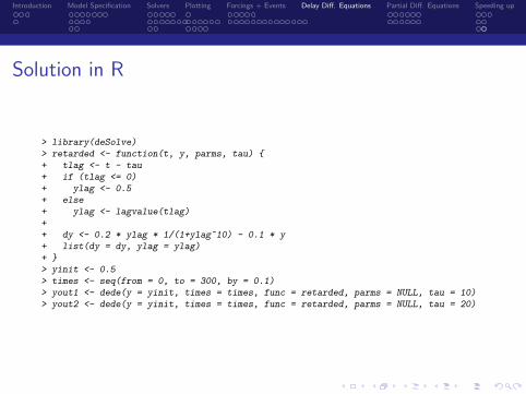
Introduction Model Specification Solvers Plotting Forcings + Events Delay Diff Equations Partial Diff Equations Speeding up
1-D PDEs
Exercise Implement the Brusselator in 1-D
Equations for X1 and X2
partX1
partt = DX1
part2X1
partx2 + 1 + X 21 X2 minus 4X1
partX2
partt = DX2
part2X2
partx2 + 3X1 minus X 21 X2
Tasks
I The grid x extends from 0 to 1 and consists of 50 cells
I Initial conditions
X1(0) = 1 + sin(2 lowast π lowast x)X2(0) = 3
I Generate output for t = 0 1 10
I Use file implementing the wave equation as a templateexampleswaveRtxt
Introduction Model Specification Solvers Plotting Forcings + Events Delay Diff Equations Partial Diff Equations Speeding up
2-D PDEs
2-D wave equation Sine-Gordon
Problem formulationThe Sine-Gordon equation is a non-linear hyperbolic (wave-like) partialdifferential equation involving the sine of the dependent variable
part2u
partt2= D
part2u
partx2+ D
part2u
party 2minus sin u (5)
Rewritten as two first order differential equations
dudt = vpartvpartt = D part2u
partx2 + D part2uparty2 minus sin u
(6)
Introduction Model Specification Solvers Plotting Forcings + Events Delay Diff Equations Partial Diff Equations Speeding up
2-D PDEs
2-D Sine-Gordon in R
gridgt Nx lt- Ny lt- 100gt xgrid lt- setupgrid1D(-7 7 N = Nx) x lt- xgrid$xmidgt ygrid lt- setupgrid1D(-7 7 N = Ny) y lt- ygrid$xmid
derivative functiongt sinegordon2D lt- function(t C parms) + u lt- matrix(nrow = Nx ncol = Ny data = C[1 (NxNy)])+ v lt- matrix(nrow = Nx ncol = Ny data = C[(NxNy+1) (2NxNy)])+ dv lt- tran2D (C = u Cxup = 0 Cxdown = 0 Cyup = 0 Cydown = 0+ Dx = 1 Dy = 1 dx = xgrid dy = ygrid)$dC - sin(u)+ list(c(v dv))+
initial conditionsgt peak lt- function (x y x0 y0) return(exp(-( (x-x0)^2 + (y-y0)^2)))gt uini lt- outer(x y FUN = function(x y) peak(x y 22) + peak(x y-2-2)+ + peak(x y-22) + peak(x y 2-2))gt vini lt- rep(0 NxNy)
solutiongt out lt- ode2D (y = c(uinivini) times = 03 parms = 0 func = sinegordon2D+ names = c(u v) dimens = c(Nx Ny) method = ode45)
Introduction Model Specification Solvers Plotting Forcings + Events Delay Diff Equations Partial Diff Equations Speeding up
2-D PDEs
Plotting 2-D PDEs image plots
gt image(out which = u grid = list(x y) mfrow = c(22) ask = FALSE)
Introduction Model Specification Solvers Plotting Forcings + Events Delay Diff Equations Partial Diff Equations Speeding up
2-D PDEs
Plotting 2-D PDEs persp plotsgt image(out which = u grid = list(x y) method = persp border = NA+ col = lightblue box = FALSE shade = 05 theta = 0 phi = 60+ mfrow = c(22) ask = FALSE)
Introduction Model Specification Solvers Plotting Forcings + Events Delay Diff Equations Partial Diff Equations Speeding up
2-D PDEs
Movie-like output of 2-D PDEs
out lt- ode2D (y = c(uini vini) times = seq(0 3 by = 01)
parms = NULL func = sinegordon2D
names=c(u v) dimens = c(Nx Ny)
method = ode45)
image(out which = u grid = list(x = x y = y)
method = persp border = NA
theta = 30 phi = 60 box = FALSE ask = FALSE)
Introduction Model Specification Solvers Plotting Forcings + Events Delay Diff Equations Partial Diff Equations Speeding up
2-D PDEs
Exercise Implement the Brusselator in 2-DEquations
partX1
partt = DX1
part2X1
partx2 + DX1
part2X1
party2 + 1 + X 21 X2 minus 4X1
partX2
partt = DX2
part2X1
partx2 + DX2
part2X1
party2 + 3X1 minus X 21 X2
Tasks
I The grids x and y extend from 0 to 1 and consist of 50 cells
I Parameter settings diffusion coefficient
DX1 = 2 DX2 = 8 lowast DX1
I Initial condition for X1 X2 random numbers inbetween 0 and 1
I Generate output for t = 0 1 8
I Use the file implementing the Sine-Gordon equation as a templateexamplessinegordonRtxt
Introduction Model Specification Solvers Plotting Forcings + Events Delay Diff Equations Partial Diff Equations Speeding up
Speeding up Matrices and compiled code
Introduction Model Specification Solvers Plotting Forcings + Events Delay Diff Equations Partial Diff Equations Speeding up
Methods for speeding up
I Use matrices
I Implement essential parts in compiled code (Fortran C)
I Implement the full method in compiled code
Formulating a model with matrices and vectors can lead to a considerablespeed gain ndash and compact code ndash while retaining the full flexibility of RThe use of compiled code saves even more CPU time at the cost of ahigher development effort
Introduction Model Specification Solvers Plotting Forcings + Events Delay Diff Equations Partial Diff Equations Speeding up
Using matrices
Use of matrices
A Lotka-Volterra model with 4 species
gt model lt- function(t n parms) + with(aslist(c(n parms)) + dn1 lt- r1 n1 - a13 n1 n3+ dn2 lt- r2 n2 - a24 n2 n4+ dn3 lt- a13 n1 n3 - r3 n3+ dn4 lt- a24 n2 n4 - r4 n4+ return(list(c(dn1 dn2 dn3 dn4)))+ )+ gt parms lt- c(r1 = 01 r2 = 01 r3 = 01 r4 = 01 a13 = 02 a24 = 01)gt times = seq(from = 0 to = 500 by = 01)gt n0 = c(n1 = 1 n2 = 1 n3 = 2 n4 = 2)
gt systemtime(out lt- ode(n0 times model parms))
user system elapsed302 000 302
Source exampleslv-plain-or-matrixRtxt
Introduction Model Specification Solvers Plotting Forcings + Events Delay Diff Equations Partial Diff Equations Speeding up
Using matrices
Use of matrices
A Lotka-Volterra model with 4 species
gt model lt- function(t n parms) + with(parms + dn lt- r n + n (A n)+ return(list(c(dn)))+ )+ gt parms lt- list(+ r = c(r1 = 01 r2 = 01 r3 = -01 r4 = -01)+ A = matrix(c(00 00 -02 00 prey 1+ 00 00 00 -01 prey 2+ 02 00 00 00 predator 1 eats prey 1+ 00 01 00 00) predator 2 eats prey 2+ nrow = 4 ncol = 4 byrow = TRUE)+ )
gt systemtime(out lt- ode(n0 times model parms))
user system elapsed166 000 170
Source exampleslv-plain-or-matrixRtxt
Introduction Model Specification Solvers Plotting Forcings + Events Delay Diff Equations Partial Diff Equations Speeding up
Using matrices
Results
I plot(out) will show the results
I Note that the ldquoplainrdquo version has only 1 to 1 connections but thematrix model is already full connected (with most connections arezero) The comparison is insofar unfair that the matrix version(despite faster execution) is more powerful
I Exercise Create a fully connected model in the plain version for afair comparison
I A parameter example (eg for weak coupling) can be found onhttp
tolstoynewcastleeduauRe7help09061230html
Introduction Model Specification Solvers Plotting Forcings + Events Delay Diff Equations Partial Diff Equations Speeding up
Compiled code
Using compiled code
All solvers of deSolve
I allow direct communication between solvers and a compiled model
See vignette (compiledCode) [15]
Principle
I Implement core model (and only this) in C or Fortran
I Use data handling storage and plotting facilities of R
examplescompiled_lorenzcompiledcodesvg
Introduction Model Specification Solvers Plotting Forcings + Events Delay Diff Equations Partial Diff Equations Speeding up
Compiled code
The End
Thank you
More Infohttpdesolver-forger-projectorg
Introduction Model Specification Solvers Plotting Forcings + Events Delay Diff Equations Partial Diff Equations Speeding up
Finally
Acknowledgments
CitationA lot of effort went in creating this software please cite it when using it
I to cite deSolve [20] rootSolve [19] ReacTran [16]
I Some complex examples can be found in [18]
I A framework to fit differential equation models to data is FME [17]
I A framework for ecological modelling is simecol [10]
Acknowledgments
I None of this would be possible without the splendid work of the RCore Team [11]
I This presentation was created with Sweave [7]
I Creation of the packages made use of Rforge [21]
Introduction Model Specification Solvers Plotting Forcings + Events Delay Diff Equations Partial Diff Equations Speeding up
Finally
Bibliography I
[1] K E Brenan S L Campbell and L R PetzoldNumerical Solution of Initial-Value Problems in Differential-Algebraic EquationsSIAM Classics in Applied Mathematics 1996
[2] P N Brown G D Byrne and A C HindmarshVode a variable-coefficient ode solverSIAM Journal on Scientific and Statistical Computing 101038ndash1051 1989
[3] E Hairer S P Norsett and G WannerSolving Ordinary Differential Equations I Nonstiff Problems Second Revised EditionSpringer-Verlag Heidelberg 2009
[4] E Hairer and G WannerSolving Ordinary Differential Equations II Stiff and Differential-Algebraic Problems Second Revised EditionSpringer-Verlag Heidelberg 2010
[5] A C HindmarshODEPACK a systematized collection of ODE solversIn R Stepleman editor Scientific Computing Vol 1 of IMACS Transactions on Scientific Computation pages 55ndash64 IMACS North-Holland Amsterdam 1983
[6] R Lefever G Nicolis and I PrigogineOn the occurrence of oscillations around the steady state in systems of chemical reactions far from equilibriumJournal of Chemical Physics 471045ndash1047 1967
[7] Friedrich LeischDynamic generation of statistical reports using literate data analysisIn W Hardle and B Ronz editors COMPSTAT 2002 ndash Proceedings in Computational Statistics pages 575ndash580 Heidelberg 2002Physica-Verlag
[8] M C Mackey and L GlassOscillation and chaos in physiological control systemsScience 197287ndash289 1977
Introduction Model Specification Solvers Plotting Forcings + Events Delay Diff Equations Partial Diff Equations Speeding up
Finally
Bibliography II
[9] Linda R PetzoldAutomatic selection of methods for solving stiff and nonstiff systems of ordinary differential equationsSIAM Journal on Scientific and Statistical Computing 4136ndash148 1983
[10] Thomas Petzoldt and Karsten Rinkesimecol An object-oriented framework for ecological modeling in RJournal of Statistical Software 22(9)1ndash31 2007
[11] R Development Core TeamR A Language and Environment for Statistical ComputingR Foundation for Statistical Computing Vienna Austria 2011ISBN 3-900051-07-0
[12] OE RosslerAn equation for continous chaosPhysics Letters A 57 (5)397ndash398 1976
[13] L F Shampine I Gladwell and S ThompsonSolving ODEs with MATLABCambridge University Press Cambridge 2003
[14] LF Shampine and S ThompsonSolving ddes in matlabApp Numer Math 37441ndash458 2001
[15] K Soetaert T Petzoldt and RW SetzerR-package deSolve Writing Code in Compiled Languages 2009package vignette
[16] Karline Soetaert and Filip MeysmanReactive transport in aquatic ecosystems rapid model prototyping in the open source software REnvironmental modelling and software page in press 2011
Introduction Model Specification Solvers Plotting Forcings + Events Delay Diff Equations Partial Diff Equations Speeding up
Finally
Bibliography III
[17] Karline Soetaert and Thomas PetzoldtInverse modelling sensitivity and monte carlo analysis in R using package FMEJournal of Statistical Software 33(3)1ndash28 2010
[18] Karline Soetaert and Thomas PetzoldtSolving ODEs DAEs DDEs and PDEs in RJournal of Numerical Analysis Industrial and Applied Mathematics in press 2011
[19] Karline Soetaert Thomas Petzoldt and R Woodrow SetzerSolving Differential Equations in RThe R Journal 2(2)5ndash15 December 2010
[20] Karline Soetaert Thomas Petzoldt and R Woodrow SetzerSolving differential equations in R Package deSolveJournal of Statistical Software 33(9)1ndash25 2010
[21] Stefan Theuszligl and Achim ZeileisCollaborative Software Development Using R-ForgeThe R Journal 1(1)9ndash14 May 2009
[22] B van der Pol and J van der MarkFrequency demultiplicationNature 120363ndash364 1927

Introduction Model Specification Solvers Plotting Forcings + Events Delay Diff Equations Partial Diff Equations Speeding up
2-D PDEs
Movie-like output of 2-D PDEs
out lt- ode2D (y = c(uini vini) times = seq(0 3 by = 01)
parms = NULL func = sinegordon2D
names=c(u v) dimens = c(Nx Ny)
method = ode45)
image(out which = u grid = list(x = x y = y)
method = persp border = NA
theta = 30 phi = 60 box = FALSE ask = FALSE)
Introduction Model Specification Solvers Plotting Forcings + Events Delay Diff Equations Partial Diff Equations Speeding up
2-D PDEs
Exercise Implement the Brusselator in 2-DEquations
partX1
partt = DX1
part2X1
partx2 + DX1
part2X1
party2 + 1 + X 21 X2 minus 4X1
partX2
partt = DX2
part2X1
partx2 + DX2
part2X1
party2 + 3X1 minus X 21 X2
Tasks
I The grids x and y extend from 0 to 1 and consist of 50 cells
I Parameter settings diffusion coefficient
DX1 = 2 DX2 = 8 lowast DX1
I Initial condition for X1 X2 random numbers inbetween 0 and 1
I Generate output for t = 0 1 8
I Use the file implementing the Sine-Gordon equation as a templateexamplessinegordonRtxt
Introduction Model Specification Solvers Plotting Forcings + Events Delay Diff Equations Partial Diff Equations Speeding up
Speeding up Matrices and compiled code
Introduction Model Specification Solvers Plotting Forcings + Events Delay Diff Equations Partial Diff Equations Speeding up
Methods for speeding up
I Use matrices
I Implement essential parts in compiled code (Fortran C)
I Implement the full method in compiled code
Formulating a model with matrices and vectors can lead to a considerablespeed gain ndash and compact code ndash while retaining the full flexibility of RThe use of compiled code saves even more CPU time at the cost of ahigher development effort
Introduction Model Specification Solvers Plotting Forcings + Events Delay Diff Equations Partial Diff Equations Speeding up
Using matrices
Use of matrices
A Lotka-Volterra model with 4 species
gt model lt- function(t n parms) + with(aslist(c(n parms)) + dn1 lt- r1 n1 - a13 n1 n3+ dn2 lt- r2 n2 - a24 n2 n4+ dn3 lt- a13 n1 n3 - r3 n3+ dn4 lt- a24 n2 n4 - r4 n4+ return(list(c(dn1 dn2 dn3 dn4)))+ )+ gt parms lt- c(r1 = 01 r2 = 01 r3 = 01 r4 = 01 a13 = 02 a24 = 01)gt times = seq(from = 0 to = 500 by = 01)gt n0 = c(n1 = 1 n2 = 1 n3 = 2 n4 = 2)
gt systemtime(out lt- ode(n0 times model parms))
user system elapsed302 000 302
Source exampleslv-plain-or-matrixRtxt
Introduction Model Specification Solvers Plotting Forcings + Events Delay Diff Equations Partial Diff Equations Speeding up
Using matrices
Use of matrices
A Lotka-Volterra model with 4 species
gt model lt- function(t n parms) + with(parms + dn lt- r n + n (A n)+ return(list(c(dn)))+ )+ gt parms lt- list(+ r = c(r1 = 01 r2 = 01 r3 = -01 r4 = -01)+ A = matrix(c(00 00 -02 00 prey 1+ 00 00 00 -01 prey 2+ 02 00 00 00 predator 1 eats prey 1+ 00 01 00 00) predator 2 eats prey 2+ nrow = 4 ncol = 4 byrow = TRUE)+ )
gt systemtime(out lt- ode(n0 times model parms))
user system elapsed166 000 170
Source exampleslv-plain-or-matrixRtxt
Introduction Model Specification Solvers Plotting Forcings + Events Delay Diff Equations Partial Diff Equations Speeding up
Using matrices
Results
I plot(out) will show the results
I Note that the ldquoplainrdquo version has only 1 to 1 connections but thematrix model is already full connected (with most connections arezero) The comparison is insofar unfair that the matrix version(despite faster execution) is more powerful
I Exercise Create a fully connected model in the plain version for afair comparison
I A parameter example (eg for weak coupling) can be found onhttp
tolstoynewcastleeduauRe7help09061230html
Introduction Model Specification Solvers Plotting Forcings + Events Delay Diff Equations Partial Diff Equations Speeding up
Compiled code
Using compiled code
All solvers of deSolve
I allow direct communication between solvers and a compiled model
See vignette (compiledCode) [15]
Principle
I Implement core model (and only this) in C or Fortran
I Use data handling storage and plotting facilities of R
examplescompiled_lorenzcompiledcodesvg
Introduction Model Specification Solvers Plotting Forcings + Events Delay Diff Equations Partial Diff Equations Speeding up
Compiled code
The End
Thank you
More Infohttpdesolver-forger-projectorg
Introduction Model Specification Solvers Plotting Forcings + Events Delay Diff Equations Partial Diff Equations Speeding up
Finally
Acknowledgments
CitationA lot of effort went in creating this software please cite it when using it
I to cite deSolve [20] rootSolve [19] ReacTran [16]
I Some complex examples can be found in [18]
I A framework to fit differential equation models to data is FME [17]
I A framework for ecological modelling is simecol [10]
Acknowledgments
I None of this would be possible without the splendid work of the RCore Team [11]
I This presentation was created with Sweave [7]
I Creation of the packages made use of Rforge [21]
Introduction Model Specification Solvers Plotting Forcings + Events Delay Diff Equations Partial Diff Equations Speeding up
Finally
Bibliography I
[1] K E Brenan S L Campbell and L R PetzoldNumerical Solution of Initial-Value Problems in Differential-Algebraic EquationsSIAM Classics in Applied Mathematics 1996
[2] P N Brown G D Byrne and A C HindmarshVode a variable-coefficient ode solverSIAM Journal on Scientific and Statistical Computing 101038ndash1051 1989
[3] E Hairer S P Norsett and G WannerSolving Ordinary Differential Equations I Nonstiff Problems Second Revised EditionSpringer-Verlag Heidelberg 2009
[4] E Hairer and G WannerSolving Ordinary Differential Equations II Stiff and Differential-Algebraic Problems Second Revised EditionSpringer-Verlag Heidelberg 2010
[5] A C HindmarshODEPACK a systematized collection of ODE solversIn R Stepleman editor Scientific Computing Vol 1 of IMACS Transactions on Scientific Computation pages 55ndash64 IMACS North-Holland Amsterdam 1983
[6] R Lefever G Nicolis and I PrigogineOn the occurrence of oscillations around the steady state in systems of chemical reactions far from equilibriumJournal of Chemical Physics 471045ndash1047 1967
[7] Friedrich LeischDynamic generation of statistical reports using literate data analysisIn W Hardle and B Ronz editors COMPSTAT 2002 ndash Proceedings in Computational Statistics pages 575ndash580 Heidelberg 2002Physica-Verlag
[8] M C Mackey and L GlassOscillation and chaos in physiological control systemsScience 197287ndash289 1977
Introduction Model Specification Solvers Plotting Forcings + Events Delay Diff Equations Partial Diff Equations Speeding up
Finally
Bibliography II
[9] Linda R PetzoldAutomatic selection of methods for solving stiff and nonstiff systems of ordinary differential equationsSIAM Journal on Scientific and Statistical Computing 4136ndash148 1983
[10] Thomas Petzoldt and Karsten Rinkesimecol An object-oriented framework for ecological modeling in RJournal of Statistical Software 22(9)1ndash31 2007
[11] R Development Core TeamR A Language and Environment for Statistical ComputingR Foundation for Statistical Computing Vienna Austria 2011ISBN 3-900051-07-0
[12] OE RosslerAn equation for continous chaosPhysics Letters A 57 (5)397ndash398 1976
[13] L F Shampine I Gladwell and S ThompsonSolving ODEs with MATLABCambridge University Press Cambridge 2003
[14] LF Shampine and S ThompsonSolving ddes in matlabApp Numer Math 37441ndash458 2001
[15] K Soetaert T Petzoldt and RW SetzerR-package deSolve Writing Code in Compiled Languages 2009package vignette
[16] Karline Soetaert and Filip MeysmanReactive transport in aquatic ecosystems rapid model prototyping in the open source software REnvironmental modelling and software page in press 2011
Introduction Model Specification Solvers Plotting Forcings + Events Delay Diff Equations Partial Diff Equations Speeding up
Finally
Bibliography III
[17] Karline Soetaert and Thomas PetzoldtInverse modelling sensitivity and monte carlo analysis in R using package FMEJournal of Statistical Software 33(3)1ndash28 2010
[18] Karline Soetaert and Thomas PetzoldtSolving ODEs DAEs DDEs and PDEs in RJournal of Numerical Analysis Industrial and Applied Mathematics in press 2011
[19] Karline Soetaert Thomas Petzoldt and R Woodrow SetzerSolving Differential Equations in RThe R Journal 2(2)5ndash15 December 2010
[20] Karline Soetaert Thomas Petzoldt and R Woodrow SetzerSolving differential equations in R Package deSolveJournal of Statistical Software 33(9)1ndash25 2010
[21] Stefan Theuszligl and Achim ZeileisCollaborative Software Development Using R-ForgeThe R Journal 1(1)9ndash14 May 2009
[22] B van der Pol and J van der MarkFrequency demultiplicationNature 120363ndash364 1927
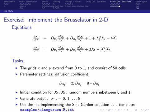
Introduction Model Specification Solvers Plotting Forcings + Events Delay Diff Equations Partial Diff Equations Speeding up
2-D PDEs
Exercise Implement the Brusselator in 2-DEquations
partX1
partt = DX1
part2X1
partx2 + DX1
part2X1
party2 + 1 + X 21 X2 minus 4X1
partX2
partt = DX2
part2X1
partx2 + DX2
part2X1
party2 + 3X1 minus X 21 X2
Tasks
I The grids x and y extend from 0 to 1 and consist of 50 cells
I Parameter settings diffusion coefficient
DX1 = 2 DX2 = 8 lowast DX1
I Initial condition for X1 X2 random numbers inbetween 0 and 1
I Generate output for t = 0 1 8
I Use the file implementing the Sine-Gordon equation as a templateexamplessinegordonRtxt
Introduction Model Specification Solvers Plotting Forcings + Events Delay Diff Equations Partial Diff Equations Speeding up
Speeding up Matrices and compiled code
Introduction Model Specification Solvers Plotting Forcings + Events Delay Diff Equations Partial Diff Equations Speeding up
Methods for speeding up
I Use matrices
I Implement essential parts in compiled code (Fortran C)
I Implement the full method in compiled code
Formulating a model with matrices and vectors can lead to a considerablespeed gain ndash and compact code ndash while retaining the full flexibility of RThe use of compiled code saves even more CPU time at the cost of ahigher development effort
Introduction Model Specification Solvers Plotting Forcings + Events Delay Diff Equations Partial Diff Equations Speeding up
Using matrices
Use of matrices
A Lotka-Volterra model with 4 species
gt model lt- function(t n parms) + with(aslist(c(n parms)) + dn1 lt- r1 n1 - a13 n1 n3+ dn2 lt- r2 n2 - a24 n2 n4+ dn3 lt- a13 n1 n3 - r3 n3+ dn4 lt- a24 n2 n4 - r4 n4+ return(list(c(dn1 dn2 dn3 dn4)))+ )+ gt parms lt- c(r1 = 01 r2 = 01 r3 = 01 r4 = 01 a13 = 02 a24 = 01)gt times = seq(from = 0 to = 500 by = 01)gt n0 = c(n1 = 1 n2 = 1 n3 = 2 n4 = 2)
gt systemtime(out lt- ode(n0 times model parms))
user system elapsed302 000 302
Source exampleslv-plain-or-matrixRtxt
Introduction Model Specification Solvers Plotting Forcings + Events Delay Diff Equations Partial Diff Equations Speeding up
Using matrices
Use of matrices
A Lotka-Volterra model with 4 species
gt model lt- function(t n parms) + with(parms + dn lt- r n + n (A n)+ return(list(c(dn)))+ )+ gt parms lt- list(+ r = c(r1 = 01 r2 = 01 r3 = -01 r4 = -01)+ A = matrix(c(00 00 -02 00 prey 1+ 00 00 00 -01 prey 2+ 02 00 00 00 predator 1 eats prey 1+ 00 01 00 00) predator 2 eats prey 2+ nrow = 4 ncol = 4 byrow = TRUE)+ )
gt systemtime(out lt- ode(n0 times model parms))
user system elapsed166 000 170
Source exampleslv-plain-or-matrixRtxt
Introduction Model Specification Solvers Plotting Forcings + Events Delay Diff Equations Partial Diff Equations Speeding up
Using matrices
Results
I plot(out) will show the results
I Note that the ldquoplainrdquo version has only 1 to 1 connections but thematrix model is already full connected (with most connections arezero) The comparison is insofar unfair that the matrix version(despite faster execution) is more powerful
I Exercise Create a fully connected model in the plain version for afair comparison
I A parameter example (eg for weak coupling) can be found onhttp
tolstoynewcastleeduauRe7help09061230html
Introduction Model Specification Solvers Plotting Forcings + Events Delay Diff Equations Partial Diff Equations Speeding up
Compiled code
Using compiled code
All solvers of deSolve
I allow direct communication between solvers and a compiled model
See vignette (compiledCode) [15]
Principle
I Implement core model (and only this) in C or Fortran
I Use data handling storage and plotting facilities of R
examplescompiled_lorenzcompiledcodesvg
Introduction Model Specification Solvers Plotting Forcings + Events Delay Diff Equations Partial Diff Equations Speeding up
Compiled code
The End
Thank you
More Infohttpdesolver-forger-projectorg
Introduction Model Specification Solvers Plotting Forcings + Events Delay Diff Equations Partial Diff Equations Speeding up
Finally
Acknowledgments
CitationA lot of effort went in creating this software please cite it when using it
I to cite deSolve [20] rootSolve [19] ReacTran [16]
I Some complex examples can be found in [18]
I A framework to fit differential equation models to data is FME [17]
I A framework for ecological modelling is simecol [10]
Acknowledgments
I None of this would be possible without the splendid work of the RCore Team [11]
I This presentation was created with Sweave [7]
I Creation of the packages made use of Rforge [21]
Introduction Model Specification Solvers Plotting Forcings + Events Delay Diff Equations Partial Diff Equations Speeding up
Finally
Bibliography I
[1] K E Brenan S L Campbell and L R PetzoldNumerical Solution of Initial-Value Problems in Differential-Algebraic EquationsSIAM Classics in Applied Mathematics 1996
[2] P N Brown G D Byrne and A C HindmarshVode a variable-coefficient ode solverSIAM Journal on Scientific and Statistical Computing 101038ndash1051 1989
[3] E Hairer S P Norsett and G WannerSolving Ordinary Differential Equations I Nonstiff Problems Second Revised EditionSpringer-Verlag Heidelberg 2009
[4] E Hairer and G WannerSolving Ordinary Differential Equations II Stiff and Differential-Algebraic Problems Second Revised EditionSpringer-Verlag Heidelberg 2010
[5] A C HindmarshODEPACK a systematized collection of ODE solversIn R Stepleman editor Scientific Computing Vol 1 of IMACS Transactions on Scientific Computation pages 55ndash64 IMACS North-Holland Amsterdam 1983
[6] R Lefever G Nicolis and I PrigogineOn the occurrence of oscillations around the steady state in systems of chemical reactions far from equilibriumJournal of Chemical Physics 471045ndash1047 1967
[7] Friedrich LeischDynamic generation of statistical reports using literate data analysisIn W Hardle and B Ronz editors COMPSTAT 2002 ndash Proceedings in Computational Statistics pages 575ndash580 Heidelberg 2002Physica-Verlag
[8] M C Mackey and L GlassOscillation and chaos in physiological control systemsScience 197287ndash289 1977
Introduction Model Specification Solvers Plotting Forcings + Events Delay Diff Equations Partial Diff Equations Speeding up
Finally
Bibliography II
[9] Linda R PetzoldAutomatic selection of methods for solving stiff and nonstiff systems of ordinary differential equationsSIAM Journal on Scientific and Statistical Computing 4136ndash148 1983
[10] Thomas Petzoldt and Karsten Rinkesimecol An object-oriented framework for ecological modeling in RJournal of Statistical Software 22(9)1ndash31 2007
[11] R Development Core TeamR A Language and Environment for Statistical ComputingR Foundation for Statistical Computing Vienna Austria 2011ISBN 3-900051-07-0
[12] OE RosslerAn equation for continous chaosPhysics Letters A 57 (5)397ndash398 1976
[13] L F Shampine I Gladwell and S ThompsonSolving ODEs with MATLABCambridge University Press Cambridge 2003
[14] LF Shampine and S ThompsonSolving ddes in matlabApp Numer Math 37441ndash458 2001
[15] K Soetaert T Petzoldt and RW SetzerR-package deSolve Writing Code in Compiled Languages 2009package vignette
[16] Karline Soetaert and Filip MeysmanReactive transport in aquatic ecosystems rapid model prototyping in the open source software REnvironmental modelling and software page in press 2011
Introduction Model Specification Solvers Plotting Forcings + Events Delay Diff Equations Partial Diff Equations Speeding up
Finally
Bibliography III
[17] Karline Soetaert and Thomas PetzoldtInverse modelling sensitivity and monte carlo analysis in R using package FMEJournal of Statistical Software 33(3)1ndash28 2010
[18] Karline Soetaert and Thomas PetzoldtSolving ODEs DAEs DDEs and PDEs in RJournal of Numerical Analysis Industrial and Applied Mathematics in press 2011
[19] Karline Soetaert Thomas Petzoldt and R Woodrow SetzerSolving Differential Equations in RThe R Journal 2(2)5ndash15 December 2010
[20] Karline Soetaert Thomas Petzoldt and R Woodrow SetzerSolving differential equations in R Package deSolveJournal of Statistical Software 33(9)1ndash25 2010
[21] Stefan Theuszligl and Achim ZeileisCollaborative Software Development Using R-ForgeThe R Journal 1(1)9ndash14 May 2009
[22] B van der Pol and J van der MarkFrequency demultiplicationNature 120363ndash364 1927

Introduction Model Specification Solvers Plotting Forcings + Events Delay Diff Equations Partial Diff Equations Speeding up
Using matrices
Use of matrices
A Lotka-Volterra model with 4 species
gt model lt- function(t n parms) + with(parms + dn lt- r n + n (A n)+ return(list(c(dn)))+ )+ gt parms lt- list(+ r = c(r1 = 01 r2 = 01 r3 = -01 r4 = -01)+ A = matrix(c(00 00 -02 00 prey 1+ 00 00 00 -01 prey 2+ 02 00 00 00 predator 1 eats prey 1+ 00 01 00 00) predator 2 eats prey 2+ nrow = 4 ncol = 4 byrow = TRUE)+ )
gt systemtime(out lt- ode(n0 times model parms))
user system elapsed166 000 170
Source exampleslv-plain-or-matrixRtxt
Introduction Model Specification Solvers Plotting Forcings + Events Delay Diff Equations Partial Diff Equations Speeding up
Using matrices
Results
I plot(out) will show the results
I Note that the ldquoplainrdquo version has only 1 to 1 connections but thematrix model is already full connected (with most connections arezero) The comparison is insofar unfair that the matrix version(despite faster execution) is more powerful
I Exercise Create a fully connected model in the plain version for afair comparison
I A parameter example (eg for weak coupling) can be found onhttp
tolstoynewcastleeduauRe7help09061230html
Introduction Model Specification Solvers Plotting Forcings + Events Delay Diff Equations Partial Diff Equations Speeding up
Compiled code
Using compiled code
All solvers of deSolve
I allow direct communication between solvers and a compiled model
See vignette (compiledCode) [15]
Principle
I Implement core model (and only this) in C or Fortran
I Use data handling storage and plotting facilities of R
examplescompiled_lorenzcompiledcodesvg
Introduction Model Specification Solvers Plotting Forcings + Events Delay Diff Equations Partial Diff Equations Speeding up
Compiled code
The End
Thank you
More Infohttpdesolver-forger-projectorg
Introduction Model Specification Solvers Plotting Forcings + Events Delay Diff Equations Partial Diff Equations Speeding up
Finally
Acknowledgments
CitationA lot of effort went in creating this software please cite it when using it
I to cite deSolve [20] rootSolve [19] ReacTran [16]
I Some complex examples can be found in [18]
I A framework to fit differential equation models to data is FME [17]
I A framework for ecological modelling is simecol [10]
Acknowledgments
I None of this would be possible without the splendid work of the RCore Team [11]
I This presentation was created with Sweave [7]
I Creation of the packages made use of Rforge [21]
Introduction Model Specification Solvers Plotting Forcings + Events Delay Diff Equations Partial Diff Equations Speeding up
Finally
Bibliography I
[1] K E Brenan S L Campbell and L R PetzoldNumerical Solution of Initial-Value Problems in Differential-Algebraic EquationsSIAM Classics in Applied Mathematics 1996
[2] P N Brown G D Byrne and A C HindmarshVode a variable-coefficient ode solverSIAM Journal on Scientific and Statistical Computing 101038ndash1051 1989
[3] E Hairer S P Norsett and G WannerSolving Ordinary Differential Equations I Nonstiff Problems Second Revised EditionSpringer-Verlag Heidelberg 2009
[4] E Hairer and G WannerSolving Ordinary Differential Equations II Stiff and Differential-Algebraic Problems Second Revised EditionSpringer-Verlag Heidelberg 2010
[5] A C HindmarshODEPACK a systematized collection of ODE solversIn R Stepleman editor Scientific Computing Vol 1 of IMACS Transactions on Scientific Computation pages 55ndash64 IMACS North-Holland Amsterdam 1983
[6] R Lefever G Nicolis and I PrigogineOn the occurrence of oscillations around the steady state in systems of chemical reactions far from equilibriumJournal of Chemical Physics 471045ndash1047 1967
[7] Friedrich LeischDynamic generation of statistical reports using literate data analysisIn W Hardle and B Ronz editors COMPSTAT 2002 ndash Proceedings in Computational Statistics pages 575ndash580 Heidelberg 2002Physica-Verlag
[8] M C Mackey and L GlassOscillation and chaos in physiological control systemsScience 197287ndash289 1977
Introduction Model Specification Solvers Plotting Forcings + Events Delay Diff Equations Partial Diff Equations Speeding up
Finally
Bibliography II
[9] Linda R PetzoldAutomatic selection of methods for solving stiff and nonstiff systems of ordinary differential equationsSIAM Journal on Scientific and Statistical Computing 4136ndash148 1983
[10] Thomas Petzoldt and Karsten Rinkesimecol An object-oriented framework for ecological modeling in RJournal of Statistical Software 22(9)1ndash31 2007
[11] R Development Core TeamR A Language and Environment for Statistical ComputingR Foundation for Statistical Computing Vienna Austria 2011ISBN 3-900051-07-0
[12] OE RosslerAn equation for continous chaosPhysics Letters A 57 (5)397ndash398 1976
[13] L F Shampine I Gladwell and S ThompsonSolving ODEs with MATLABCambridge University Press Cambridge 2003
[14] LF Shampine and S ThompsonSolving ddes in matlabApp Numer Math 37441ndash458 2001
[15] K Soetaert T Petzoldt and RW SetzerR-package deSolve Writing Code in Compiled Languages 2009package vignette
[16] Karline Soetaert and Filip MeysmanReactive transport in aquatic ecosystems rapid model prototyping in the open source software REnvironmental modelling and software page in press 2011
Introduction Model Specification Solvers Plotting Forcings + Events Delay Diff Equations Partial Diff Equations Speeding up
Finally
Bibliography III
[17] Karline Soetaert and Thomas PetzoldtInverse modelling sensitivity and monte carlo analysis in R using package FMEJournal of Statistical Software 33(3)1ndash28 2010
[18] Karline Soetaert and Thomas PetzoldtSolving ODEs DAEs DDEs and PDEs in RJournal of Numerical Analysis Industrial and Applied Mathematics in press 2011
[19] Karline Soetaert Thomas Petzoldt and R Woodrow SetzerSolving Differential Equations in RThe R Journal 2(2)5ndash15 December 2010
[20] Karline Soetaert Thomas Petzoldt and R Woodrow SetzerSolving differential equations in R Package deSolveJournal of Statistical Software 33(9)1ndash25 2010
[21] Stefan Theuszligl and Achim ZeileisCollaborative Software Development Using R-ForgeThe R Journal 1(1)9ndash14 May 2009
[22] B van der Pol and J van der MarkFrequency demultiplicationNature 120363ndash364 1927

Introduction Model Specification Solvers Plotting Forcings + Events Delay Diff Equations Partial Diff Equations Speeding up
Using matrices
Results
I plot(out) will show the results
I Note that the ldquoplainrdquo version has only 1 to 1 connections but thematrix model is already full connected (with most connections arezero) The comparison is insofar unfair that the matrix version(despite faster execution) is more powerful
I Exercise Create a fully connected model in the plain version for afair comparison
I A parameter example (eg for weak coupling) can be found onhttp
tolstoynewcastleeduauRe7help09061230html
Introduction Model Specification Solvers Plotting Forcings + Events Delay Diff Equations Partial Diff Equations Speeding up
Compiled code
Using compiled code
All solvers of deSolve
I allow direct communication between solvers and a compiled model
See vignette (compiledCode) [15]
Principle
I Implement core model (and only this) in C or Fortran
I Use data handling storage and plotting facilities of R
examplescompiled_lorenzcompiledcodesvg
Introduction Model Specification Solvers Plotting Forcings + Events Delay Diff Equations Partial Diff Equations Speeding up
Compiled code
The End
Thank you
More Infohttpdesolver-forger-projectorg
Introduction Model Specification Solvers Plotting Forcings + Events Delay Diff Equations Partial Diff Equations Speeding up
Finally
Acknowledgments
CitationA lot of effort went in creating this software please cite it when using it
I to cite deSolve [20] rootSolve [19] ReacTran [16]
I Some complex examples can be found in [18]
I A framework to fit differential equation models to data is FME [17]
I A framework for ecological modelling is simecol [10]
Acknowledgments
I None of this would be possible without the splendid work of the RCore Team [11]
I This presentation was created with Sweave [7]
I Creation of the packages made use of Rforge [21]
Introduction Model Specification Solvers Plotting Forcings + Events Delay Diff Equations Partial Diff Equations Speeding up
Finally
Bibliography I
[1] K E Brenan S L Campbell and L R PetzoldNumerical Solution of Initial-Value Problems in Differential-Algebraic EquationsSIAM Classics in Applied Mathematics 1996
[2] P N Brown G D Byrne and A C HindmarshVode a variable-coefficient ode solverSIAM Journal on Scientific and Statistical Computing 101038ndash1051 1989
[3] E Hairer S P Norsett and G WannerSolving Ordinary Differential Equations I Nonstiff Problems Second Revised EditionSpringer-Verlag Heidelberg 2009
[4] E Hairer and G WannerSolving Ordinary Differential Equations II Stiff and Differential-Algebraic Problems Second Revised EditionSpringer-Verlag Heidelberg 2010
[5] A C HindmarshODEPACK a systematized collection of ODE solversIn R Stepleman editor Scientific Computing Vol 1 of IMACS Transactions on Scientific Computation pages 55ndash64 IMACS North-Holland Amsterdam 1983
[6] R Lefever G Nicolis and I PrigogineOn the occurrence of oscillations around the steady state in systems of chemical reactions far from equilibriumJournal of Chemical Physics 471045ndash1047 1967
[7] Friedrich LeischDynamic generation of statistical reports using literate data analysisIn W Hardle and B Ronz editors COMPSTAT 2002 ndash Proceedings in Computational Statistics pages 575ndash580 Heidelberg 2002Physica-Verlag
[8] M C Mackey and L GlassOscillation and chaos in physiological control systemsScience 197287ndash289 1977
Introduction Model Specification Solvers Plotting Forcings + Events Delay Diff Equations Partial Diff Equations Speeding up
Finally
Bibliography II
[9] Linda R PetzoldAutomatic selection of methods for solving stiff and nonstiff systems of ordinary differential equationsSIAM Journal on Scientific and Statistical Computing 4136ndash148 1983
[10] Thomas Petzoldt and Karsten Rinkesimecol An object-oriented framework for ecological modeling in RJournal of Statistical Software 22(9)1ndash31 2007
[11] R Development Core TeamR A Language and Environment for Statistical ComputingR Foundation for Statistical Computing Vienna Austria 2011ISBN 3-900051-07-0
[12] OE RosslerAn equation for continous chaosPhysics Letters A 57 (5)397ndash398 1976
[13] L F Shampine I Gladwell and S ThompsonSolving ODEs with MATLABCambridge University Press Cambridge 2003
[14] LF Shampine and S ThompsonSolving ddes in matlabApp Numer Math 37441ndash458 2001
[15] K Soetaert T Petzoldt and RW SetzerR-package deSolve Writing Code in Compiled Languages 2009package vignette
[16] Karline Soetaert and Filip MeysmanReactive transport in aquatic ecosystems rapid model prototyping in the open source software REnvironmental modelling and software page in press 2011
Introduction Model Specification Solvers Plotting Forcings + Events Delay Diff Equations Partial Diff Equations Speeding up
Finally
Bibliography III
[17] Karline Soetaert and Thomas PetzoldtInverse modelling sensitivity and monte carlo analysis in R using package FMEJournal of Statistical Software 33(3)1ndash28 2010
[18] Karline Soetaert and Thomas PetzoldtSolving ODEs DAEs DDEs and PDEs in RJournal of Numerical Analysis Industrial and Applied Mathematics in press 2011
[19] Karline Soetaert Thomas Petzoldt and R Woodrow SetzerSolving Differential Equations in RThe R Journal 2(2)5ndash15 December 2010
[20] Karline Soetaert Thomas Petzoldt and R Woodrow SetzerSolving differential equations in R Package deSolveJournal of Statistical Software 33(9)1ndash25 2010
[21] Stefan Theuszligl and Achim ZeileisCollaborative Software Development Using R-ForgeThe R Journal 1(1)9ndash14 May 2009
[22] B van der Pol and J van der MarkFrequency demultiplicationNature 120363ndash364 1927

Introduction Model Specification Solvers Plotting Forcings + Events Delay Diff Equations Partial Diff Equations Speeding up
Compiled code
The End
Thank you
More Infohttpdesolver-forger-projectorg
Introduction Model Specification Solvers Plotting Forcings + Events Delay Diff Equations Partial Diff Equations Speeding up
Finally
Acknowledgments
CitationA lot of effort went in creating this software please cite it when using it
I to cite deSolve [20] rootSolve [19] ReacTran [16]
I Some complex examples can be found in [18]
I A framework to fit differential equation models to data is FME [17]
I A framework for ecological modelling is simecol [10]
Acknowledgments
I None of this would be possible without the splendid work of the RCore Team [11]
I This presentation was created with Sweave [7]
I Creation of the packages made use of Rforge [21]
Introduction Model Specification Solvers Plotting Forcings + Events Delay Diff Equations Partial Diff Equations Speeding up
Finally
Bibliography I
[1] K E Brenan S L Campbell and L R PetzoldNumerical Solution of Initial-Value Problems in Differential-Algebraic EquationsSIAM Classics in Applied Mathematics 1996
[2] P N Brown G D Byrne and A C HindmarshVode a variable-coefficient ode solverSIAM Journal on Scientific and Statistical Computing 101038ndash1051 1989
[3] E Hairer S P Norsett and G WannerSolving Ordinary Differential Equations I Nonstiff Problems Second Revised EditionSpringer-Verlag Heidelberg 2009
[4] E Hairer and G WannerSolving Ordinary Differential Equations II Stiff and Differential-Algebraic Problems Second Revised EditionSpringer-Verlag Heidelberg 2010
[5] A C HindmarshODEPACK a systematized collection of ODE solversIn R Stepleman editor Scientific Computing Vol 1 of IMACS Transactions on Scientific Computation pages 55ndash64 IMACS North-Holland Amsterdam 1983
[6] R Lefever G Nicolis and I PrigogineOn the occurrence of oscillations around the steady state in systems of chemical reactions far from equilibriumJournal of Chemical Physics 471045ndash1047 1967
[7] Friedrich LeischDynamic generation of statistical reports using literate data analysisIn W Hardle and B Ronz editors COMPSTAT 2002 ndash Proceedings in Computational Statistics pages 575ndash580 Heidelberg 2002Physica-Verlag
[8] M C Mackey and L GlassOscillation and chaos in physiological control systemsScience 197287ndash289 1977
Introduction Model Specification Solvers Plotting Forcings + Events Delay Diff Equations Partial Diff Equations Speeding up
Finally
Bibliography II
[9] Linda R PetzoldAutomatic selection of methods for solving stiff and nonstiff systems of ordinary differential equationsSIAM Journal on Scientific and Statistical Computing 4136ndash148 1983
[10] Thomas Petzoldt and Karsten Rinkesimecol An object-oriented framework for ecological modeling in RJournal of Statistical Software 22(9)1ndash31 2007
[11] R Development Core TeamR A Language and Environment for Statistical ComputingR Foundation for Statistical Computing Vienna Austria 2011ISBN 3-900051-07-0
[12] OE RosslerAn equation for continous chaosPhysics Letters A 57 (5)397ndash398 1976
[13] L F Shampine I Gladwell and S ThompsonSolving ODEs with MATLABCambridge University Press Cambridge 2003
[14] LF Shampine and S ThompsonSolving ddes in matlabApp Numer Math 37441ndash458 2001
[15] K Soetaert T Petzoldt and RW SetzerR-package deSolve Writing Code in Compiled Languages 2009package vignette
[16] Karline Soetaert and Filip MeysmanReactive transport in aquatic ecosystems rapid model prototyping in the open source software REnvironmental modelling and software page in press 2011
Introduction Model Specification Solvers Plotting Forcings + Events Delay Diff Equations Partial Diff Equations Speeding up
Finally
Bibliography III
[17] Karline Soetaert and Thomas PetzoldtInverse modelling sensitivity and monte carlo analysis in R using package FMEJournal of Statistical Software 33(3)1ndash28 2010
[18] Karline Soetaert and Thomas PetzoldtSolving ODEs DAEs DDEs and PDEs in RJournal of Numerical Analysis Industrial and Applied Mathematics in press 2011
[19] Karline Soetaert Thomas Petzoldt and R Woodrow SetzerSolving Differential Equations in RThe R Journal 2(2)5ndash15 December 2010
[20] Karline Soetaert Thomas Petzoldt and R Woodrow SetzerSolving differential equations in R Package deSolveJournal of Statistical Software 33(9)1ndash25 2010
[21] Stefan Theuszligl and Achim ZeileisCollaborative Software Development Using R-ForgeThe R Journal 1(1)9ndash14 May 2009
[22] B van der Pol and J van der MarkFrequency demultiplicationNature 120363ndash364 1927

Introduction Model Specification Solvers Plotting Forcings + Events Delay Diff Equations Partial Diff Equations Speeding up
Finally
Acknowledgments
CitationA lot of effort went in creating this software please cite it when using it
I to cite deSolve [20] rootSolve [19] ReacTran [16]
I Some complex examples can be found in [18]
I A framework to fit differential equation models to data is FME [17]
I A framework for ecological modelling is simecol [10]
Acknowledgments
I None of this would be possible without the splendid work of the RCore Team [11]
I This presentation was created with Sweave [7]
I Creation of the packages made use of Rforge [21]
Introduction Model Specification Solvers Plotting Forcings + Events Delay Diff Equations Partial Diff Equations Speeding up
Finally
Bibliography I
[1] K E Brenan S L Campbell and L R PetzoldNumerical Solution of Initial-Value Problems in Differential-Algebraic EquationsSIAM Classics in Applied Mathematics 1996
[2] P N Brown G D Byrne and A C HindmarshVode a variable-coefficient ode solverSIAM Journal on Scientific and Statistical Computing 101038ndash1051 1989
[3] E Hairer S P Norsett and G WannerSolving Ordinary Differential Equations I Nonstiff Problems Second Revised EditionSpringer-Verlag Heidelberg 2009
[4] E Hairer and G WannerSolving Ordinary Differential Equations II Stiff and Differential-Algebraic Problems Second Revised EditionSpringer-Verlag Heidelberg 2010
[5] A C HindmarshODEPACK a systematized collection of ODE solversIn R Stepleman editor Scientific Computing Vol 1 of IMACS Transactions on Scientific Computation pages 55ndash64 IMACS North-Holland Amsterdam 1983
[6] R Lefever G Nicolis and I PrigogineOn the occurrence of oscillations around the steady state in systems of chemical reactions far from equilibriumJournal of Chemical Physics 471045ndash1047 1967
[7] Friedrich LeischDynamic generation of statistical reports using literate data analysisIn W Hardle and B Ronz editors COMPSTAT 2002 ndash Proceedings in Computational Statistics pages 575ndash580 Heidelberg 2002Physica-Verlag
[8] M C Mackey and L GlassOscillation and chaos in physiological control systemsScience 197287ndash289 1977
Introduction Model Specification Solvers Plotting Forcings + Events Delay Diff Equations Partial Diff Equations Speeding up
Finally
Bibliography II
[9] Linda R PetzoldAutomatic selection of methods for solving stiff and nonstiff systems of ordinary differential equationsSIAM Journal on Scientific and Statistical Computing 4136ndash148 1983
[10] Thomas Petzoldt and Karsten Rinkesimecol An object-oriented framework for ecological modeling in RJournal of Statistical Software 22(9)1ndash31 2007
[11] R Development Core TeamR A Language and Environment for Statistical ComputingR Foundation for Statistical Computing Vienna Austria 2011ISBN 3-900051-07-0
[12] OE RosslerAn equation for continous chaosPhysics Letters A 57 (5)397ndash398 1976
[13] L F Shampine I Gladwell and S ThompsonSolving ODEs with MATLABCambridge University Press Cambridge 2003
[14] LF Shampine and S ThompsonSolving ddes in matlabApp Numer Math 37441ndash458 2001
[15] K Soetaert T Petzoldt and RW SetzerR-package deSolve Writing Code in Compiled Languages 2009package vignette
[16] Karline Soetaert and Filip MeysmanReactive transport in aquatic ecosystems rapid model prototyping in the open source software REnvironmental modelling and software page in press 2011
Introduction Model Specification Solvers Plotting Forcings + Events Delay Diff Equations Partial Diff Equations Speeding up
Finally
Bibliography III
[17] Karline Soetaert and Thomas PetzoldtInverse modelling sensitivity and monte carlo analysis in R using package FMEJournal of Statistical Software 33(3)1ndash28 2010
[18] Karline Soetaert and Thomas PetzoldtSolving ODEs DAEs DDEs and PDEs in RJournal of Numerical Analysis Industrial and Applied Mathematics in press 2011
[19] Karline Soetaert Thomas Petzoldt and R Woodrow SetzerSolving Differential Equations in RThe R Journal 2(2)5ndash15 December 2010
[20] Karline Soetaert Thomas Petzoldt and R Woodrow SetzerSolving differential equations in R Package deSolveJournal of Statistical Software 33(9)1ndash25 2010
[21] Stefan Theuszligl and Achim ZeileisCollaborative Software Development Using R-ForgeThe R Journal 1(1)9ndash14 May 2009
[22] B van der Pol and J van der MarkFrequency demultiplicationNature 120363ndash364 1927

Introduction Model Specification Solvers Plotting Forcings + Events Delay Diff Equations Partial Diff Equations Speeding up
Finally
Bibliography III
[17] Karline Soetaert and Thomas PetzoldtInverse modelling sensitivity and monte carlo analysis in R using package FMEJournal of Statistical Software 33(3)1ndash28 2010
[18] Karline Soetaert and Thomas PetzoldtSolving ODEs DAEs DDEs and PDEs in RJournal of Numerical Analysis Industrial and Applied Mathematics in press 2011
[19] Karline Soetaert Thomas Petzoldt and R Woodrow SetzerSolving Differential Equations in RThe R Journal 2(2)5ndash15 December 2010
[20] Karline Soetaert Thomas Petzoldt and R Woodrow SetzerSolving differential equations in R Package deSolveJournal of Statistical Software 33(9)1ndash25 2010
[21] Stefan Theuszligl and Achim ZeileisCollaborative Software Development Using R-ForgeThe R Journal 1(1)9ndash14 May 2009
[22] B van der Pol and J van der MarkFrequency demultiplicationNature 120363ndash364 1927