Embed Size (px)
Citation preview

Differential Equations (Ordinary)
Sebastian J. Schreiber
Department of Evolution and Ecology and the Center for Population Biology
University of California, Davis, California 95616; [email protected]
Since their Newtonian inception, differential equations have been a fundamental tool for mod-
eling the natural world. As the name suggests, these equations involve the derivatives of dependent
variables (e.g. viral load, species densities, genotypic frequencies) with respect to independent vari-
ables (e.g. time, space). When the independent variable is scalar, the differential equation is called
ordinary. Far from ordinary, these equations have provided key insights into catastrophic shifts in
ecosystems, dynamics of disease outbreaks, mechanisms maintaining biodiversity, and stabilizing
forces in food webs.
I. Basic definitions and notation
Before getting caught up in definitions, lets consider two classical ecological examples of or-
dinary differential equations. The Logistic equation describes population growth rate of a species
with density x with respect to time t
dx
dt= r x(1− x/K) (1)
where r is the intrinsic rate of growth of the population and K is its carrying capacity. The left hand
side of this equation is the derivative of x with respect to time t and corresponds to the population
growth rate. The right hand side describes how the population growth rate depends on the current
population density. For this equation, one might be interested in understanding how the species’
density changes in time and how these temporal changes depend on its initial density. Often,
ecological systems involve many “moving parts” with multiple types of interacting individuals in
which case describing their dynamics involves systems of ordinary differential equations. A classical
example of this type is the Lotka-Volterra predator-prey equations that describe the dynamics
between a prey with density x1 and its predator with denisty x2
dx1dt
= r x1 − a x1x2
dx2dt
= c a x1x2 −mx2 (2)
where a, c, and d are the predator’s attack rate, conversion efficiency, and per-capita mortality
rate. For these more complicated equations, one might ask “do these equations have well-defined
dynamical behaviors?” and “how complicated can these behaviors be?” This entry addresses the
answers to these and many more questions.

– 2 –
A system of ordinary differential equations involves a finite number of state variables, say
x1, x2, . . . , xn, possibly representing densities of interacting species, abundances of different age or
size classes, frequencies of behavioral strategies, or availability of abiotic factors such as light, water,
or temperature. These equations assume the state variables vary smoothly in time. If the instanta-
neous rates of change of the state variables are given by functions f1(x1, . . . , xn), . . . , fn(x1, . . . , xn)
of the dependent variables, then one arrives at a system of autonomous, first-order ordinary differ-
ential equations:
dx1dt
= f1(x1, . . . , xn)
dx2dt
= f2(x1, . . . , xn)
... (3)
dxndt
= fn(x1, . . . , xn)
where t denotes time. Here, first-order refers to the fact that only first-order derivatives appear
in the equations. Autonomous refers to the fact that the rates of change f1, , fn do not depend on
t. Equation (3) can account for higher-order time derivatives or time dependence by introducing
extra state variables as discussed later.
A simple example of this type of differential equation is the Logistic equation
Equation (3) can be written more succinctly in vector notation. Let x = (x1, x2, . . . , xn) be the
vector of state variables and f(x) = (f1(x), f2(x), . . . , fn(x)) be the vector of their corresponding
rates of change. Then (3) simplifies to the vector-valued differential equation:
dx
dt= f(x). (4)
II. Existence, uniqueness, and geometry of solutions
After writing down a differential equation model of an ecological system, a modeler wants
to know how do the variables of interest change in time. For instance, how are densities of the
prey and predator changing relative to one another? Moreover, how does this dynamic depend on
the initial densities of both populations? To answer these types of questions, one needs to find
solutions to the differential equation. A solution to (4) is a (vector-valued) function of time x(t)
such that when x(t) is plugged into both sides of the equation, both sides are equal to one another
i.e. x′(t) = f(x(t)) where ′ denotes a derivative with respect to time. If x(t) is a solution and the
initial state of the system is given by x(0) = x0, then x(t) is a solution to the initial value problem:
dx
dt= f(x) x(0) = x0. (5)

– 3 –
0 5 10 15 20 25 30
020
4060
80100
time
extinction
(a)
1000 1400 1800500
1000
2000
3000
year
popu
latio
n si
zedoomsday
(b)
Fig. 1.— Population extinction and blow-up in finite time. In (a), solutions to dx/dt = −√x
that all satisfy x(20) = 0 i.e. there are multiple population trajectories for which the population
is extinct at time 20. In (b), data on human population growth until 1960 (green circles) and the
best fitting (in the sense of least squares) solution of dx/dt = r x1+b which blow up in finite time
in year 2026.
Verifying a function x(t) is a solution is straight-forward: plug x(t) in both parts of the equation
and verify both sides are equal.
Consider, for example, the simplest model of population growth in which the per-capita growth
rate r of the population is constant in time. If x = x is the population density, then
dx
dt= r x x(0) = x0.
The solution of this initial value problem is x(t) = x0ert. Indeed, x′(t) = r x0e
rt = r x(t), and
x(0) = x0. Intuitively, when the per-capita rate r is positive and x0 is positive, the population
exhibits unbounded exponential growth. When r is negative, the population declines exponentially
to extinction. However, extinction is only achieved in the infinite time horizon. When the per-
capita growth rate or the initial population density is zero, the population density remains constant
for all time. This latter type of solution is known as an equilibrium or steady-state solution.
In general, an equilibrium for (4) is a state x = x∗ such that the rates of change are zero
at this state: f(x∗) = 0. The solution corresponding to an equilibrium x = x∗ is the constant
solution x(t) = x∗ for all t. Indeed, plugging x(t) = x∗ into the left and right side of equation (3)
yields x′(t) = 0 and f(x∗) = 0. For example, for the Logistic equation (1) x = 0 is the “no-cats,

– 4 –
no-kittens” equilibrium and x = K is the equilibrium corresponding to the carrying capacity of the
population.
A fundamental question is “when do solutions to the initial value problem (5) exist?” After
all, if there is no solution, there is no point in looking for one. In 1890, the Italian mathematician
Giuseppe Peano proved that solutions to (5) exist whenever f(x) is continuous. This continuity
assumption is met for many models (in particular, the Logistic equation and the Lotka-Volterra
equations), but not all. For example, population models including optimal behavior can exhibit dis-
continuities at population states where multiple behaviors are optimal. When these discontinuities
occur, what constitutes the dynamic of the equations needs to be defined by the modeler.
Given a solution to the initial value problem (5) exists, one has to wonder whether it is unique.
After all, if it is not unique, one may never know if all solutions have been uncovered and which,
if any, are biologically relevant. Provided that f(x) is differentiable, French mathematician Emile
Picard proved that solutions are unique. When f(x) is not differentiable, biologically plausible
things can still happen. For example, if x = x is the density of a declining population whose
growth rate is dxdt = −
√x, then the growth rate is not differentiable at x = 0. This equation
yields an infinite number of solutions in which the population has gone extinct by some specified
time (Fig. 1a). Despite the model being deterministic, knowing the population is extinct now
doesn’t tell you when it went extinct. This biologically realistic feature does not occur in models
where f(x) is differentiable. While f(x) is differentiable for most ecological models, there are
important exceptions such as predator-prey models with a ratio-dependent functional response (e.g.,
a(x1/x2)/(1+ahx1/x2) where x1/x2 is the ratio of prey density to predator density), epidemiological
models with frequency dependent transmission rates, or models incorporating optimal behavior.
Even if solutions to the initial value problem (5) exist and are unique, they might not be
defined for all time. An important example is super-exponential population growth where the rate
of change of the population density x is dxdt = r x1+b where b > 0 and r > 0. This model with
b ≈ 1 was the basis for the 1960s prediction of “Doomsday: Friday, 13 November A.D. 2026.”
Indeed, for b = 1, this equation can be solved by separating variables and integrating which yields
x(t) = 1/(1/x0−r t) where x0 is the initial population density. Amazingly this solution approaches
infinity as t approaches t = 1/(x0r). This phenomena is called blow-up and occurs in models of
combustion and other runaway processes. In this ecological context, the time of blow up t = 1/(x0r)
corresponds to doomsday. In the words of a Pogo cartoon, at this time “everyone gets squeezed to
death” (Fig. 1b).
Provided f(x) is differentiable, solutions to (5) exist for all time if the system is dissipative:
there is a bounded region that all solutions eventually enter and remain in for all time. Since the
world is finite and can only sustain a finite density of individuals, all ecologically realistic models
should be dissipative i.e. there populations densities eventually are bounded by a constant inde-
pendent of initial conditions. Verifying dissipativeness can be challenging, and may be violated
in unexpected ways. For example, in Lotka-Volterra type models of mutualistic interactions, pop-

– 5 –
x(t)
x(t) + f(x(t))
Fig. 2.— A solution x(t) of a differential equation plotted in its state space. At each point along
the solution, it’s tangent vector is given by f(x(t)).
ulation densities can blow up in finite time despite each species being self-limited. In the words
of Robert May, “for mutualisms that are sufficiently strong, these simple models lead to both
populations undergoing unbounded exponential growth, in an orgy of reciprocal benefaction.”
Geometrically, solutions trace out curves in the state space, the set of all possible states. For
example, for models of n interacting species, the state space consists of all vectors x = (x1, . . . , xn)
whose components are non-negative. Alternatively, in metacommunity models where each patch
can be in one of n different states (e.g. a particular community of species is occupying the patch),
the state space consists of all distributions on the n states: non-negative x = (x1, . . . , xn) such that
x1 + · · ·+xn = 1. Solutions x(t) are characterized by being curves whose tangent vectors are given
by the right hand side f(x(t)) of the differential equation (Fig. 2). This geometric interpretation
of solutions is extremely useful for understanding their qualitative behavior as discussed further
below.
III. Linear equations
In the absence of density-dependent or frequency-dependent feedbacks, ecological dynamics can
be described by systems of linear differential equations. These linear models, just like their discrete-

– 6 –
x1
x 2
stable
x1
x 2
stable (oscillatory)
x1
x 2
unstable
x1
x 2
unstable (oscillatory)
x1
x2
stable
x1
x2
stable (oscillatory)
x1
x2
unstable
x1
x2
unstable (oscillatory)
x1
x2
stable
x1
x2
x2
unstable
x
x2
unstable (oscillatory)
x 1
x2
stable
x 1
x2
stable
(osc
illator
y)
x 1
x2
unstable
x 1
x2
unsta
ble (o
scilla
tory)
x1
x2
stable
x1
x2
x2
unstable
x1
x2
unstable (oscillatory)
x1
x2
stable
x1
x2
stable (oscillatory)
x1
unstable
x1
x2
unstable (oscillatory)
x1
x2
stable
x1
x2
x2
unstable
x1
x2
unstable (oscillatory)
x1
x2
stable
x1
x2
x2
unstable
x
x2
unstable (oscillatory)
x1
stable
x
x2
unstable
x1
x2
unstable (oscillatory)
x1
stable
x1
x2
unstable
x1
x2
unstable (oscillatory)
stable
x1 x2
unstable (oscillatory)
x 1
x2
x 1
x
unstable
x2
unstable (oscillatory)
x1
stable
x2
unstable
x1
x2
unstable (oscillatory)
x1
x2
stable
x1
x2
x2
unstable
x2
unstable (oscillatory)
x 1
stable
x 1
x2
stable
(osci
llatory
)
unstable
x
x2
unsta
ble (o
scillat
ory)x1
x2
stable
x1
x2
stable (oscillatory)
x
unstable
x2
unstable (oscillatory)
Fig. 3.— Different dynamical behaviors in the phase plane for two dimensional linear equations.
time Matrix model counterparts, are particularly useful for describing populations structured in
space, size, or age. For these models, the rates of change are linear functions of the state variables:
fi(x) = ai1x1 + ai2x2 + · · ·+ ainxn.
If A is the matrix whose i–j-th entry is aij , then these linear differential equations can be written
more simply asdx
dt= Ax
where Ax denotes matrix multiplication of A and x.
Remarkably, as in the scalar case, the general solution for these equations can be written down
explicitly as x(t) = exp(At)x(0) where exp(A) denotes matrix exponentiation of A and x(0) is the
initial state of the system. As in the case of the exponential function, matrix exponentiation is
given by an infinite power series, exp(A) = I +A+A2/2! +A3/3! + , and can be carried out easily
in most numerical software packages and program languages.
For the “typical” matrix A (i.e. the eigenvalues all have non-zero real part), the behavior
of the matrix equation (4) can be classified into two types (for n = 2 see Fig. 3) . Analogous
to the exponential growth model with a negative per-capita growth rate, all solutions of (4) decay
exponentially to zero if all eigenvalues of A have negative real part. In this case, the origin is stable:
solutions starting near the origin asymptotically approach the origin. For structured populations,
this behavior corresponds to a deterministic asymptotic decline to extinction. Alternatively, all (or
– 7 –
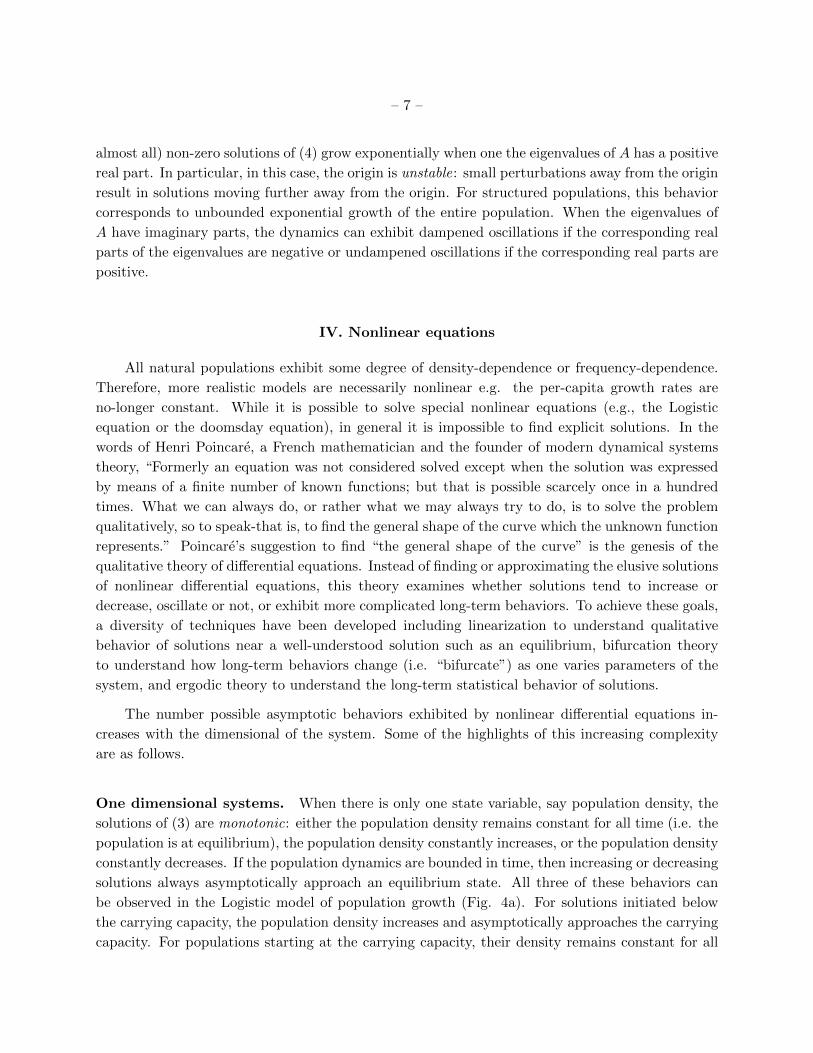
almost all) non-zero solutions of (4) grow exponentially when one the eigenvalues of A has a positive
real part. In particular, in this case, the origin is unstable: small perturbations away from the origin
result in solutions moving further away from the origin. For structured populations, this behavior
corresponds to unbounded exponential growth of the entire population. When the eigenvalues of
A have imaginary parts, the dynamics can exhibit dampened oscillations if the corresponding real
parts of the eigenvalues are negative or undampened oscillations if the corresponding real parts are
positive.
IV. Nonlinear equations
All natural populations exhibit some degree of density-dependence or frequency-dependence.
Therefore, more realistic models are necessarily nonlinear e.g. the per-capita growth rates are
no-longer constant. While it is possible to solve special nonlinear equations (e.g., the Logistic
equation or the doomsday equation), in general it is impossible to find explicit solutions. In the
words of Henri Poincare, a French mathematician and the founder of modern dynamical systems
theory, “Formerly an equation was not considered solved except when the solution was expressed
by means of a finite number of known functions; but that is possible scarcely once in a hundred
times. What we can always do, or rather what we may always try to do, is to solve the problem
qualitatively, so to speak-that is, to find the general shape of the curve which the unknown function
represents.” Poincare’s suggestion to find “the general shape of the curve” is the genesis of the
qualitative theory of differential equations. Instead of finding or approximating the elusive solutions
of nonlinear differential equations, this theory examines whether solutions tend to increase or
decrease, oscillate or not, or exhibit more complicated long-term behaviors. To achieve these goals,
a diversity of techniques have been developed including linearization to understand qualitative
behavior of solutions near a well-understood solution such as an equilibrium, bifurcation theory
to understand how long-term behaviors change (i.e. “bifurcate”) as one varies parameters of the
system, and ergodic theory to understand the long-term statistical behavior of solutions.
The number possible asymptotic behaviors exhibited by nonlinear differential equations in-
creases with the dimensional of the system. Some of the highlights of this increasing complexity
are as follows.
One dimensional systems. When there is only one state variable, say population density, the
solutions of (3) are monotonic: either the population density remains constant for all time (i.e. the
population is at equilibrium), the population density constantly increases, or the population density
constantly decreases. If the population dynamics are bounded in time, then increasing or decreasing
solutions always asymptotically approach an equilibrium state. All three of these behaviors can
be observed in the Logistic model of population growth (Fig. 4a). For solutions initiated below
the carrying capacity, the population density increases and asymptotically approaches the carrying
capacity. For populations starting at the carrying capacity, their density remains constant for all

– 8 –
out[, 1]
out[,
2]
time
density
(a)
prey density
pred
ator
den
sity
(b)
rock frequency
pape
r fre
quen
cy
(c)
sin(!t)
predator
(d)
prey
top
pred
ator
(e)
time
top
pred
ator
den
sity (e)
Fig. 4.— Asymptotic behaviors of nonlinear differential equations. For 1-dimensional equations
such as the Logistic equation (a), solutions plotted against time are monotonic and asymptotically
approach an equilibrium. For 2-dimensional systems, two new asymptotic behaviors are introduced
in the phase-plane: periodic motions as in predator-prey models (b) and heteroclinic cycles as in
rock-paper-scissor population games (c). For 3-dimensional systems, the dynamics become infinitely
enriched. This enrichment includes quasi-periodic motions of periodically forced predator-prey
interactions (d), and chaotic motions (e) and chaotic transients (f) of tritrophic interactions.
time. For population starting above the carrying capacity, overcrowding results in the population
density decreasing to the carrying capacity.

– 9 –
Despite the simplicity of the short-term and long-term behaviors of one-dimensional models,
they can produce surprising predictions due to the appearance and disappearance of equilibria as
parameters vary. For example, consider the Logistic model with constant harvesting at rate h,
dx/dt = rx(1−x/K)−h. For harvesting rates below a critical threshold h = rK/2, the population
can persist at an equilibrium supporting a density greater than half of the carrying capacity K.
For harvesting rates above this threshold, the population goes deterministically extinct in finite
time. Hence, increasing harvesting rates above this critical threshold cause sudden population
disappearances as population crash from densities greater than K/2 to extinction.
Two dimensional systems. Nonlinear feedbacks between two state variables introduces two
new asymptotic behaviors for solutions: periodicity and heteroclinic cycles.
Periodicity occurs when the system supports a periodic solution: there exists a period T > 0
such that x(t + T ) = x(t) for all time t. The classic ecological example of periodic behavior is
Logistic-Holling model of predator-prey interactions. For this model, the prey exhibit Logistic
growth in the absence of the predator and the predator has a saturating functional response. If x1and x2 denote the prey and predator densities, respectively, then their dynamics are given by
dx1dt
= r x1(1− x1/K)− a x11 + a hx1
dx2dt
=c a x1
1 + a hx1−mx2
where and a, h, c, m denote the predator’s searching efficiency, handling time, conversion efficiency,
and per-capita mortality rate. When prey’s carrying capacity is sufficiently large, the equilibrium
supporting the predator and prey becomes unstable and there is a periodic solution supporting
both species (Fig. 4b). For this model, this periodic solution is globally stable (almost all solutions
approach it asymptotically) and unique. However, for other forms of functional responses, there can
be multiple periodic solutions. Determining the multiplicity of periodic solutions is a tricky affair.
Unlike equilibria, there is no simple algebraic procedure to solve for periodic solution. In fact, one
of the most difficult open problems in mathematics, Hilbert’s 16th problem, involves finding upper
bounds to the number of possible periodic solutions to two-dimensional differential equations.
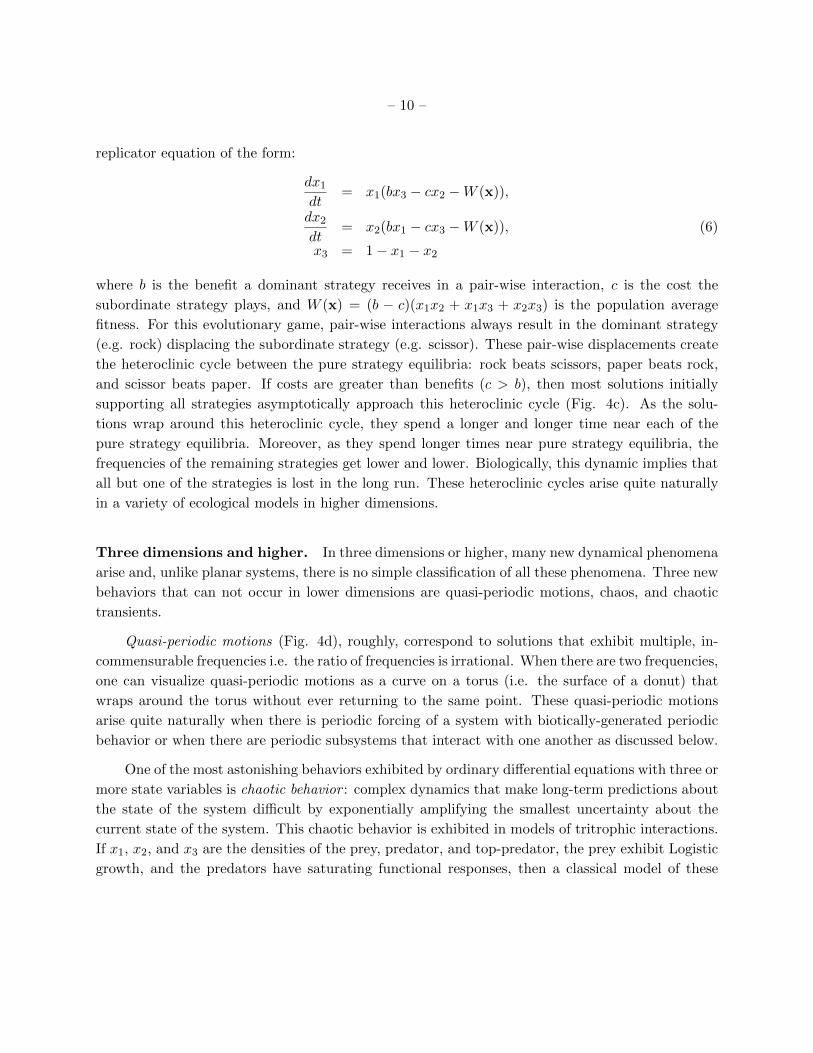
The other new asymptotic behavior introduced by the 2nd dimension corresponds to solutions
approaching a heteroclinic cycle: equilibria connected in a cyclic fashion by other solutions of the
differential equations. A classic example of this behavior occurs for three competing strategies
playing an evolutionary game of rock-paper-scissors (Fig. 4c). If x1,x2,x3 denote the frequencies
of the rock, paper, and scissor strategies, respectively, then this dynamic can be described by a
– 10 –
replicator equation of the form:
dx1dt
= x1(bx3 − cx2 −W (x)),
dx2dt
= x2(bx1 − cx3 −W (x)), (6)
x3 = 1− x1 − x2
where b is the benefit a dominant strategy receives in a pair-wise interaction, c is the cost the
subordinate strategy plays, and W (x) = (b − c)(x1x2 + x1x3 + x2x3) is the population average
fitness. For this evolutionary game, pair-wise interactions always result in the dominant strategy
(e.g. rock) displacing the subordinate strategy (e.g. scissor). These pair-wise displacements create
the heteroclinic cycle between the pure strategy equilibria: rock beats scissors, paper beats rock,
and scissor beats paper. If costs are greater than benefits (c > b), then most solutions initially
supporting all strategies asymptotically approach this heteroclinic cycle (Fig. 4c). As the solu-
tions wrap around this heteroclinic cycle, they spend a longer and longer time near each of the
pure strategy equilibria. Moreover, as they spend longer times near pure strategy equilibria, the
frequencies of the remaining strategies get lower and lower. Biologically, this dynamic implies that
all but one of the strategies is lost in the long run. These heteroclinic cycles arise quite naturally
in a variety of ecological models in higher dimensions.
Three dimensions and higher. In three dimensions or higher, many new dynamical phenomena
arise and, unlike planar systems, there is no simple classification of all these phenomena. Three new
behaviors that can not occur in lower dimensions are quasi-periodic motions, chaos, and chaotic
transients.
Quasi-periodic motions (Fig. 4d), roughly, correspond to solutions that exhibit multiple, in-
commensurable frequencies i.e. the ratio of frequencies is irrational. When there are two frequencies,
one can visualize quasi-periodic motions as a curve on a torus (i.e. the surface of a donut) that
wraps around the torus without ever returning to the same point. These quasi-periodic motions
arise quite naturally when there is periodic forcing of a system with biotically-generated periodic
behavior or when there are periodic subsystems that interact with one another as discussed below.
One of the most astonishing behaviors exhibited by ordinary differential equations with three or
more state variables is chaotic behavior : complex dynamics that make long-term predictions about
the state of the system difficult by exponentially amplifying the smallest uncertainty about the
current state of the system. This chaotic behavior is exhibited in models of tritrophic interactions.
If x1, x2, and x3 are the densities of the prey, predator, and top-predator, the prey exhibit Logistic
growth, and the predators have saturating functional responses, then a classical model of these

– 11 –
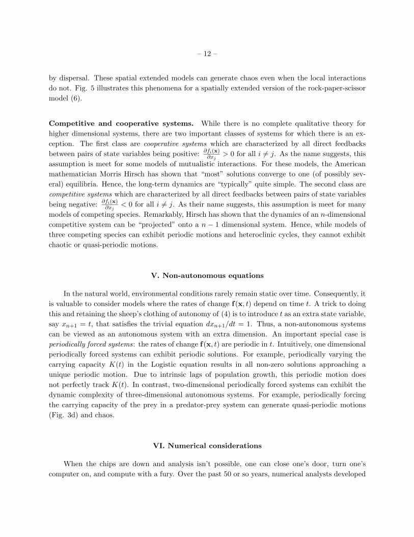
Fig. 5.— Spatial-temporal chaos in a spatial version of the rock-paper-scissor game on a 100 by
100 grid with dispersal to nearest neighbors.
interactions is
dx1dt
= r x1(1− x1/K)− a2 x1x21 + a2 h2 x1
dx2dt
=c2 a2 x1x2
1 + a2 h2 x1−m2 x2 −
a3 x2x31 + a3 h3 x2
(7)
dx3dt
=c3a3 x2x3
1 + a3 h3 x2−m3x3
where ai,hi, ci, mi are searching efficiencies, handling times, conversion efficiencies, and per-capita
mortality rates of the predator and top-predator. Alan Hastings and Thomas Powell showed that
this deceptively simple system exhibits chaotic motions (Fig. 4e) for biologically plausible parameter
values. These chaotic motions trace out a tea-cup in the three dimensional state space: the predator
and prey exhibit oscillatory dynamics that dampen as they wind up the tea cup, a reduction in the
predator’s density causes top-predator’s density to crash down the handle of the tea cup, and the
oscillatory path up the tea cup reinitiates.
Chaotic motions may be unstable i.e. population trajectories initiated near a chaotic motion
ultimately move away from this chaotic motion. However, unstable chaotic motions can “trap”
nearby solutions in their topologically complex maze for exceptionally long-periods of time. When
this occurs, the system exhibits chaotic transients before switching to its final asymptotic behavior.
For example, Kevin McCann and Peter Yodzis showed that the tri-trophic model (7) can exhibit
long-term chaotic transients supporting all three species, but ultimately the top-predator is lost as
the dynamics simplify to a predator-prey oscillation (Fig. 4f). This outcome is somewhat shocking
as it implies that even without any additional disturbances, a population that appears to persisting
heartily today may be deterministically doomed to extinction in the near future.
One startling way to generate chaotic dynamics and quasi-periodic motions is to increase
dimensions by spatially extending models. For ordinary differential equations, this extension can
be achieved by modelling space as a finite number of discrete patches and coupling local interactions
– 12 –
by dispersal. These spatial extended models can generate chaos even when the local interactions
do not. Fig. 5 illustrates this phenomena for a spatially extended version of the rock-paper-scissor
model (6).
Competitive and cooperative systems. While there is no complete qualitative theory for
higher dimensional systems, there are two important classes of systems for which there is an ex-
ception. The first class are cooperative systems which are characterized by all direct feedbacks
between pairs of state variables being positive: ∂fi(x)∂xj
> 0 for all i 6= j. As the name suggests, this
assumption is meet for some models of mutualistic interactions. For these models, the American
mathematician Morris Hirsch has shown that “most” solutions converge to one (of possibly sev-
eral) equilibria. Hence, the long-term dynamics are “typically” quite simple. The second class are
competitive systems which are characterized by all direct feedbacks between pairs of state variables
being negative: ∂fi(x)∂xj
< 0 for all i 6= j. As their name suggests, this assumption is meet for many
models of competing species. Remarkably, Hirsch has shown that the dynamics of an n-dimensional
competitive system can be “projected” onto a n − 1 dimensional system. Hence, while models of
three competing species can exhibit periodic motions and heteroclinic cycles, they cannot exhibit
chaotic or quasi-periodic motions.
V. Non-autonomous equations
In the natural world, environmental conditions rarely remain static over time. Consequently, it
is valuable to consider models where the rates of change f(x, t) depend on time t. A trick to doing
this and retaining the sheep’s clothing of autonomy of (4) is to introduce t as an extra state variable,
say xn+1 = t, that satisfies the trivial equation dxn+1/dt = 1. Thus, a non-autonomous systems
can be viewed as an autonomous system with an extra dimension. An important special case is
periodically forced systems: the rates of change f(x, t) are periodic in t. Intuitively, one dimensional
periodically forced systems can exhibit periodic solutions. For example, periodically varying the
carrying capacity K(t) in the Logistic equation results in all non-zero solutions approaching a
unique periodic motion. Due to intrinsic lags of population growth, this periodic motion does
not perfectly track K(t). In contrast, two-dimensional periodically forced systems can exhibit the
dynamic complexity of three-dimensional autonomous systems. For example, periodically forcing
the carrying capacity of the prey in a predator-prey system can generate quasi-periodic motions
(Fig. 3d) and chaos.
VI. Numerical considerations
When the chips are down and analysis isn’t possible, one can close one’s door, turn one’s
computer on, and compute with a fury. Over the past 50 or so years, numerical analysts developed

– 13 –
0 20 40 60 80 100
0.0
0.2
0.4
0.6
0.8
1.0
time
fract
ion
occu
pied
∞50050
Fig. 6.— Deterministic approximation of metapopulation dynamics. A solution for the Levin’s
metapopulation model dp/dt = cp(1 − p) − ep is plotted in black. Sample trajectories for the
stochastic counterpart of this model with 50 and 500 patches are plotted in red and blue, respec-
tively.
methods to accurately and efficiently approximate solutions of ordinary differential equations. The
simplest method is Euler’s method in which you approximate dx/dt with the difference quotient
(x(t + h) − x(t))/h where h is a “time step.” This approximation yields the difference equation
(see Difference Equations)
x(t + h) = x(t) + h f(x(t))
that can be applied iteratively to approximation solutions to (4). While this method has been
used by many theoreticians due to its simple and intuitive appeal, it is generally inefficient for two
reasons: errors are of order h2, and time steps do not dynamically adjust to the magnitude of f(x)
e.g. one can take larger time steps when f(x) is small. Higher order methods (e.g. fourth-order
Runge-Kutta) with adaptive time steps are available in standard libraries for computing languages
like C or Fortran, and computational software like MatLab, R, Maple, and Mathematica. When
using these advanced libraries, however, it is important to find implementations that preserve basic
structural aspects of the models e.g. preserve non-negativity of population densities.

– 14 –
V. Philosophical considerations.
When is it appropriate to model ecological dynamics with differential equations? This question
can be answered indirectly by examining two defining features of differential equations.
First, and foremost, differential equations are deterministic. In the words of Henri Poincare,
“If we knew exactly the laws of nature and the situation of the universe at the initial moment,
we could predict exactly the situation of the same universe at a succeeding moment.” Differential
equations cannot account for populations being finite collections of interacting individuals and the
associated uncertainty of the individual demography. However, when population abundances are
sufficiently large, the American mathematician Thomas Kurtz showed that differential equations
provide good approximations (over finite time horizons) to individual based stochastic models. For
instance, consider the Levins’ metapopulation model for which the fraction of occupied patches p is
modeled by dp/dt = cp(1−p)−ep with per-capita extinction and colonization rates e and c. Implicit
in Levins’ model formulation is that there are an infinite number of patches. This idealization does
a good job approximating stochastic models with a finite number of patches whenever the number
of patches is sufficiently large (Fig. 6).
A second defining feature of differential equations is that they assume all demographic pro-
cesses occur continuously in time. For autonomous differential equations, this assumption is quite
strong and implies that the populations exhibit overlapping generations. However, by adding time-
dependence into differential equations, one can account for temporally concentrated demographic
events such as synchronized reproductive or migratory events. Classically, populations with these
concentrated demographic events have been modeled by difference equations. For populations ex-
hibiting a combination of discrete and continuous demographic processes, there exist impulsive
differential equations that lie at the crossroads of difference and differential equations. Despite
having a long mathematical history, the impulsive differential equation models have only recently
entered the theoretical ecology literature. Whether these hybrid models will overtake the literature
remains to be seen.
See Also the Following Articles:
Bifurcations
Birth and Death Models
Chaos
Difference Equations
Matrix Models
Non-dimensionalization
Phase-Plane Analysis
Predator-Prey Models
Single-Species Metapopulation Models

– 15 –
Single-Species Population Models
Three-Species Models and Food Web Modules
Two-Species Competition
Glossary
continuous a function f(x) is continuous, roughly, if small changes in x result in small changes
in f(x). Equivalently, the graph of f exhibits no breaks or jumps.
derivative the derivative of a function f(x) is given by its instantaneous rate of change: the value
of (f(x+h)−f(x))/h as h gets infinitesimally small. A function for which this limit is defined
at x is called differentiable at x.
dissipative the state of the system asymptotically entering and remaining in a bounded set.
equilibrium the state of system remaining constant over time. For a differential equation dx/dt =
f(x), equilibria correspond to states x∗ such that f(x∗) = 0.
ergodic theory a branch of mathematics that examines the long-term behavior of dynamical
systems from a statistical or probabilistic viewpoint. This view is particularly useful for
systems exhibiting complex behavior such as quasi-periodic or chaotic motions.
quasi-periodic curves in state space that exhibit multiple, incommensurable frequencies i.e. the
ratio of frequencies is irrational. When there are two frequencies, one can visualize quasi-
periodic motions as a curve on a torus (i.e. the surface of a donut) that wraps around the
torus without ever returning to the same point
periodic a pattern that repeats itself at regular intervals. A function x(t) is periodic if there exists
T > 0 such that x(t + T ) = x(t) for all t.
rate of change the change in a quantity per unit of time. For example, speed is rate of change
corresponding to distance traveled per unit time. For a function x(t) of time t, the rate of
change over an interval of length h is given by (x(t + h)− x(t))/t.
state space a set corresponds to all possible states of the system being modeled. For example,
the state space for models of planetary motion is the position and velocity of all the planets.
Further Reading
Hofbauer, J. and Sigmund, K. 1998. Evolutionary games and population dynamics. Cam-
bridge University Press

– 16 –
Katok, A. and Hasselblatt, B. 1997. Introduction to the modern theory of dynamical systems.
Cambridge University Press.
Kurtz, T.G. 1981. Approximation of population processes. Society for Industrial and Applied
Mathematics.
Perko, L. 2001. Differential equations and dynamical systems. Springer-Verlag.
Smith, H.L. 1995. Monotone dynamical systems: An introduction to the theory of competitive
and cooperative systems. American Mathematical Society
Strogatz, S.H. 1994. Nonlinear dynamics and chaos: With applications to physics, biology,
chemistry, and engineering. Addison-Wesley.