Embed Size (px)
Citation preview

Di it l Si l P iDigital Signal Processing for Speech Recognition
Berlin ChenDepartment of Computer Science & Information Engineering
R f
g gNational Taiwan Normal University
References:1. A. V. Oppenheim and R. W. Schafer, Discrete-time Signal Processing, 19992. X. Huang et. al., Spoken Language Processing, Chapters 5, 63 J R Deller et al Discrete-Time Processing of Speech Signals Chapters 4-63. J. R. Deller et. al., Discrete Time Processing of Speech Signals, Chapters 4 64. J. W. Picone, “Signal modeling techniques in speech recognition,” proceedings of the IEEE,
September 1993, pp. 1215-1247

Digital Signal Processingg g g
• Digital Signalg g– Discrete-time signal with discrete amplitude
[ ]nx
• Digital Signal Processing– Manipulate digital signals in a digital computer
SP- Berlin Chen 2

Two Main Approaches to Digital Signal ProcessingProcessing
• Filteringg
FilterSignal in Signal out
[ ]nx [ ]ny[ ] nx [ ]ny
Amplify or attenuate some frequencycomponents of [ ] nx
• Parameter Extraction
P tSignal in Parameter outParameterExtraction
Signal in Parameter out
[ ] nx11⎥⎤
⎢⎡c 21
⎥⎤
⎢⎡c 1
⎥⎤
⎢⎡ Lc
12
⎥⎥⎥⎥⎥⎥
⎢⎢⎢⎢⎢⎢c
22
⎥⎥⎥⎥⎥⎥
⎢⎢⎢⎢⎢⎢c
2
⎥⎥⎥⎥⎥⎥
⎢⎢⎢⎢⎢⎢
Lce.g.:1. Spectrum Estimation2. Parameters for Recognition
SP- Berlin Chen 3
1⎥⎥
⎦⎢⎢
⎣ mc 2⎥⎦⎢⎣ mc ⎥⎦⎢⎣ Lmc

Sinusoid Signals
: amplitude (振幅)[ ] ( )φω += nAnx cos
A10
frequency normalized:≤≤ f
f
– : amplitude (振幅)– : angular frequency (角頻率), – : phase (相角)
ωφ
A
Tf ππω 22 ==
: phase (相角)φ Period, represented by number of samples
[ ] ⎟⎠⎞
⎜⎝⎛ −=
2cos πωnAnx
⎠⎝
samples 25=T[ ] [ ] )(cos ⎟
⎞⎜⎛ −+=+= NnANnxnx πω
Right-shifted
[ ] [ ]
( ),...2,122
2)(cos
==⇒=⇒
⎟⎠
⎜⎝
+=+=
kN
kkN
NnANnxnx
πωπω
ω
SP- Berlin Chen 4
• E.g., speech signals can be decomposed as sums of sinusoids

Sinusoid Signals (cont.)g ( )
• is periodic with a period of N (samples)[ ]nx is periodic with a period of N (samples)[ ]nx[ ] [ ]nxNnx =+
( ) ( )φφ ANA )(( ) ( )φωφω +=++ nANnA cos)(cos)21( 2 ,...,kkN == πω
π2
• Examples (sinusoid signals)Nπω 2
=
• Examples (sinusoid signals)
– is periodic with period N=8[ ] ( )4/cos1 nnx π=– is periodic with period N=16– is not periodic
[ ] ( )8/3cos2 nnx π=
[ ] ( )nnx cos3 =
SP- Berlin Chen 5

Sinusoid Signals (cont.)g ( )
[ ] ( )4/cos1
⎞⎛⎞⎛⎞⎛
= nnx π
( )integers positive are and 824
44cos)(
4cos
4cos
111
11
⋅=⇒⋅=⇒
⎟⎠
⎞⎜⎝
⎛ +=⎟⎠
⎞⎜⎝
⎛ +=⎟⎠
⎞⎜⎝
⎛=
kNkNkN
NnNnn
ππ
ππππ
84
1 =∴ N
[ ] ( )8/3cos2
⎞⎛⎞⎛⎞⎛
= nnx π
( )
( )numberspositive areand 3
1628
3
83
83cos
83cos
83cos
222
22
=⇒⋅=⋅⇒
⎟⎠⎞
⎜⎝⎛ ⋅+⋅=⎟
⎠⎞
⎜⎝⎛ +=⎟
⎠⎞
⎜⎝⎛ ⋅=
kNkNkN
NnNnn
ππ
ππππ
( )
16
p38
2
222
=∴ N
[ ] ( )cos3 nnx =[ ] ( )( ) ( )( ) ( )
ii id2
cos1cos1cos cos
3
33
3
kNkN
NnNnnnnx
⋅=⇒+=+⋅=⋅=
π
SP- Berlin Chen 6
!exist t doesn' integerspositive are and
3
3
NkN
∴Q

Sinusoid Signals (cont.)g ( )
• Complex Exponential Signalp p g– Use Euler’s relation to express complex numbers
j
( )φφφ sincos
jAAez
jyxzj +==⇒
+=
( )numberrealais A( )
22 yx + 22 yx
x
+22 yx
y
+
ImImaginary part
φφ
sin cos
AyAx
==
SP- Berlin Chen 7Re
φsinAy =
real part

Sinusoid Signals (cont.)g ( )
• A Sinusoid Signalg
[ ] ( )φω nAnx cos +=[ ] ( )( ){ }φω
φωnjAe
nAnxRe
cos=
+=+{ }
{ }φω jnj eAeRe =real part
SP- Berlin Chen 8

Sinusoid Signals (cont.)g ( )
• Sum of two complex exponential signals with p p gsame frequency
( ) ( )φωφω ++ + njnj eAeA 10( ) ( )
( )φφω
φφ
+=
+jjnj
jj
eAeAe
eAeA10
10
10
10
( )φω
φω
+
=nj
jnj
Ae
Aee
– When only the real part is considered
( )φ= jAenumbers real are and , 10 AAA
( ) ( ) ( )φωφωφω +=+++ nAnAnA coscoscos 1100
SP- Berlin Chen 9
– The sum of N sinusoids of the same frequency is another sinusoid of the same frequency

Sinusoid Signals (cont.)g ( )
• Trigonometric IdentitiesTrigonometric Identities
1100
1100coscossinsintan
φφφφ
φAAAA
++
=
( ) ( )( )101010
21
20
2
21100
21100
2
sinsincoscos2
sinsincoscos
φφφφ
φφφφ
+++=
+++=
AAAAA
AAAAA
SP- Berlin Chen 10
( )( )1010
21
20
10101010
cos2 φφ
φφφφ
−++= AAAA

Some Digital Signalsg g
SP- Berlin Chen 11

Some Digital Signalsg g
• Any signal sequence can be represented hif l d
[ ]nxas a sum of shift and scaled unit impulse sequences (signals)
∞[ ] [ ] [ ]knkxnxk
−∑=∞
−∞=δ
scale/weightedTime-shifted unit impulse sequence,...3,2,1,0,1,2..., −−=n scale/weighted impulse sequence
[ ] [ ] [ ] [ ] [ ]
[ ] [ ] [ ] [ ] [ ] [ ] [ ] [ ] [ ] [ ] [ ] [ ]
3
2
−=−= ∑∑−=
∞
−∞=
knkxknkxnxkk
δδ
SP- Berlin Chen 12
[ ] [ ] [ ] [ ] [ ] [ ] [ ] [ ] [ ] [ ] [ ] [ ]( ) [ ] ( ) [ ] ( ) [ ] ( ) [ ] ( ) [ ] ( ) [ ]31211121221
33221101122 −+−−+−+++−++=
−+−+−+++−++−=nnnnnn
nxnxnxnxnxnxδδδδδδ
δδδδδδ

Digital Systemsg y
• A digital system T is a system that, given an input signal x[n], generates an output signal y[n]
[ ] [ ]{ }nxTny =
[ ]nx { }•T [ ]ny[ ]nx { } [ ]ny
SP- Berlin Chen 13

Properties of Digital Systemsg y
• Linear– Linear combination of inputs maps to linear
combination of outputs
[ ] [ ]{ } [ ]{ } [ ]{ }nxbTnxaTnbxnaxT 2121 +=+
• Time-invariant (Time-shift)– A time shift in the input by m samples gives a shift inA time shift in the input by m samples gives a shift in
the output by m samples[ ] [ ]{ } mmnxTmny ∀±=± ,[ ] [ ]{ }y
time sift [ ][ ] lhifl f)(if
samples shift right )0 (if mmmnx ⇒>−
SP- Berlin Chen 14
[ ] samplesshift left )0 (if mmmnx ⇒>+

Properties of Digital Systems (cont.)g y ( )
• Linear time-invariant (LTI)– The system output can be expressed as a
convolution (迴旋積分) of the input x[n] and the i l h[ ]impulse response h[n]
[ ]{ } [ ] [ ] [ ] [ ] [ ] [ ]khknxknhkxnhnxnxT ∑ −=−∑=∗=∞∞
– The system can be characterized by the system’s impulse response h[n], which also is a signal
kk −∞=−∞=
impulse response h[n], which also is a signal sequence
• If the input x[n] is impulse , the output is h[n][ ]nδp [ ] p p [ ]
Digital[ ]nδ [ ]nh
SP- Berlin Chen 15
System

Properties of Digital Systems (cont.)g y ( )
• Linear time-invariant (LTI)Linear time invariant (LTI)– Explanation:
[ ] [ ] [ ]knkxnx −= ∑∞
δ Time-shifted unit impulse sequence[ ] [ ] [ ]
k −∞=
[ ]{ } [ ] [ ]{ }knkxTnxT −=⇒ ∑∞
δ
scaleimpulse sequence
[ ]{ } [ ] [ ]{ }[ ] [ ]{ }knTkx
k
k
−= ∑∞
−∞=
−∞=
δlinear
[ ] [ ][ ] [ ]nhnx
knhkxk
∗=
−= ∑∞
−∞=
Di i l[ ]nδ [ ]nh Time-invariantImpulse response
[ ] [ ]nhnx ∗=
Time invariant
DigitalSystem
[ ]nδ [ ]nh
[ ] [ ]convolution
SP- Berlin Chen 16
[ ] [ ][ ] [ ]knhkn
nhnT
T
−⎯→⎯−
⎯→⎯
δ
δ
Properties of Digital Systems (cont.)g y ( )
• Linear time-invariant (LTI)– Convolution
• Example1
3
Length=M=3
[ ]nδ 0 12
1
-2[ ]nh
[ ]3LTILength=L=3
LTI[ ]nx ?
0 1 2
23
1
3 23
9
Length=L+M-1
[ ]nh⋅3
0
3
0 12
-6
26
[ ]nδ⋅3
3
11
1
Sum up
[ ]ny
[ ]nh3
[ ]12⋅ nh
1
2
1 23
2
-41 1 3
[ ]12 −⋅ nδ 0 1 2
13
-1
4
-2
[ ]12 −⋅ nh
[ ]2nh
SP- Berlin Chen 17
2
1
2 34
1 3
-2
[ ]21 −⋅ nδ[ ]2−nh

Properties of Digital Systems (cont.)g y ( )
• Linear time-invariant (LTI)Linear time invariant (LTI)– Convolution: Generalization
• Reflect h[k] about the origin (→ h[-k])Reflect h[k] about the origin (→ h[ k]) • Slide (h[-k] → h[-k+n] or h[-(k-n)] ), multiply it with
x[k] [ ] [ ] [ ]knhkxny −= ∑∞[ ]
• Sum up [ ]kx
[ ] [ ] [ ]
[ ] ( )[ ]nkhkx
knhkxny
k
k
−−=
=
∑
∑∞
−∞=
−∞=
[ ]kh Reflect Multiply
[ ]kh −slide
Sum up
SP- Berlin Chen 18
n

21
3
[ ]kh
Convolution0 1
-22
31
[ ]kh
[ ]
Reflect [ ] [ ] [ ][ ] [ ]knhkx
nhnxny
=
∗=
∑∞
-21
30 1 2
3
[ ]kx
[ ] 0, =nny
[ ] [ ]knhkxk
−= ∑−∞=
0-1-2
-20
13 11
[ ]kh −
[ ] 1, =nny
10-1
1
-21
13 1
11Sum up
[ ]1+−kh[ ],y
[ ] 2=nny [ ]ny
210
1
-22
13 0
3
1 2
13
-1
4
-2
[ ]2+−kh[ ] 2, =nny
[ ] 3=nny
[ ]ny
321
1
-2 -1
3
3
2
[ ]3+−kh[ ] 3, =nny
[ ] 4, =nny
SP- Berlin Chen 19
432
13
-2 -2
4[ ]4+−kh
[ ] 4, nny

Properties of Digital Systems (cont.)g y ( )
• Linear time-invariant (LTI)Linear time invariant (LTI)– Convolution is commutative and distributive
[ ] [ ] [ ][ ] [ ] [ ]nhnhnx
nhnhnx 21
****
[ ]nh 1 [ ]nh 2 [ ]nh 2 [ ]nh 1
[ ]h
[ ] [ ] [ ]nhnhnx 12 **=
[ ] [ ] [ ]( )nhnhnx 21* +
Commutation
[ ]nh 2
[ ]nh 1
[ ] [ ]nhnh 21 +[ ] [ ] [ ] [ ]nhnxnhnx 21 ** +=
Distribution
[ ] [ ] [ ][ ] [ ]nxnh
nhnxny==
* *
– An impulse response has finite duration» Finite Impulse Response (FIR)
[ ] [ ]
[ ] [ ]knxkh
knhkxk
−=
−=
∑
∑
∞
∞
−∞=
» Finite-Impulse Response (FIR)
– An impulse response has infinite duration» Infinite-Impulse Response (IIR)
SP- Berlin Chen 20
[ ] [ ]k −∞=
p p ( )

Properties of Digital Systems (cont.)g y ( )
• Prove convolution is commutativeProve convolution is commutative
[ ] [ ] [ ]nhnxny *=
[ ] [ ]knhkxk
−∑=∞
−∞=
[ ] [ ] ( )knmhmnxm
mlet −=∑ −=∞
−∞=
[ ] [ ][ ] [ ]
knxkhk
∑ −=∞
−∞=
[ ] [ ]nxnh * =
SP- Berlin Chen 21

Properties of Digital Systems (cont.)g y ( )
• Linear time-varying SystemLinear time varying System– E.g., is an amplitude modulator [ ] [ ] nnxny 0cos ω=
[ ] [ ] [ ] [ ]0?
101 that suppose nnynynnxnx −=⇒−=[ ] [ ] [ ] [ ]
[ ] [ ] [ ] 00011
0101
coscos
pp
nnnxnnxny
yy
−== ωω[ ] [ ] [ ]
[ ] [ ] ( )0000
00011
cosBut nnωnnxnny
y
−−=−[ ] [ ] ( )0000
SP- Berlin Chen 22

Properties of Digital Systems (cont.)g y ( )
• Bounded Input and Bounded Output (BIBO): stablep p ( )
[ ][ ]
nBnx x ∀∞<≤ and
– A LTI system is BIBO if only if h[n] is absolutely summable
[ ] nBny y ∀∞<≤
[ ] ∞≤∑∞
−∞=kkh
SP- Berlin Chen 23

Properties of Digital Systems (cont.)g y ( )
• Causalityy– A system is “casual” if for every choice of n0, the output
sequence value at indexing n=n0 depends on only the input sequence value for n ≤ nsequence value for n ≤ n0
[ ] [ ] [ ]∑ ∑= =
−+−=K
k
M
mkkk mnxknyny
1000 βα
k mk1
1
0β [ ]ny[ ]nx-1
1
z-1
z-1
β
2β
1β
z-1
z-1
z-1
1α
2α
z-1Mβ z 1
Nα
SP- Berlin Chen 24
– Any noncausal FIR can be made causal by adding sufficient long delay

Discrete-Time Fourier Transform (DTFT)( )
• Frequency Response ( )ωjeHq y p– Defined as the discrete-time Fourier Transform of
– is continuous and is periodic with period=
[ ]nh( )
π2( )ωjeH ( )
proportional to twoi f h litimes of the sampling
frequency
j
– is a complex function of ω( )ωjeH
njne nj ωωω sincos +=
Imis a complex function of ω( ) ( ) ( )
( ) ( )ω
ωωω
jH
ji
jr
j ejHeHeH∠
+=
( )
SP- Berlin Chen 25
( ) ( )ωω jeHjj eeH ∠=
magnitudephase Re

Discrete-Time Fourier Transform (cont.)( )
• Representation of Sequences by Fourier Transformp q y
( ) [ ]∑∞
−∞=
−= ωω enheHn
njj DTFT
A ffi i t diti f th i t f F i t f
[ ] ( )∫ −= ππ
ωω ωπ
deeHnh njj 2
1 Inverse DTFT
– A sufficient condition for the existence of Fourier transform
[ ] ∞<∑∞
−∞=nnh de mnj
−−
∫ ωππ
ω
21 )(absolutely summable
∞=n
[ ]( )
emnj
mnj
−= −
−
π
πππ
ω
i)(2
12
)(
( ) [ ]enheH njj = ∑∞ − ωω
:invertible is ansformFourier tr
( )( )
nmmn
mn
⎨⎧ =
−−
=ππ
,1
sin( ) [ ]
[ ] ( ) [ ] deemhdeeHnh nj
m
mjnjj
n
== ∫ ∑∫
∑
−
∞
−∞=
−−
−∞=
ωπ
ωπ
ππ
ωωππ
ωω
21
21
SP- Berlin Chen 26
[ ]mnnm
−=⎩⎨ ≠
=
δ ,0
[ ] [ ] [ ] [ ]nhmnmhdemhm
mnj
m=−== ∑∫∑
∞
−∞=−
−∞
−∞=δω
πππ
ω 21 )(

Discrete-Time Fourier Transform (cont.)( )• Convolution Property
( )∞
( ) [ ]
[ ] [ ] [ ]
ωω
n
njj enheH =
∞
∞
−∞=
−
∑
∑
[ ] [ ] [ ]k
knhkxnhnxny −=∗=−∞=∑][][
knn −='
( ) [ ] [ ] ωω nj
n k
j eknhkxeY −= −∞
−∞=
∞
−∞=∑ ∑ knn
knn−−=−⇒
+=⇒'
'
[ ] [ ]
( ) ( )
ωω nj
nk
kj enhekx ⎟⎠
⎞⎜⎝
⎛= −
∞
−∞=
∞
−∞=
− ∑∑ ' '
'
( ) ( )
( ) ( )
ωω jj eHeX= ( ) ( ) ( )
( ) ( ) ( )ωωω
ωωω
jjj
jjj
eHeXeY
eHeXeY
=⇒
=
SP- Berlin Chen 27
[ ] ( ) ( )ωω jj eHeXnhnx ⇔∗∴ ][( ) ( ) ( )( ) ( ) ( )ωωω jjj eHeXeY
eHeXeY
∠+∠=∠⇒
⇒

Discrete-Time Fourier Transform (cont.)( )
• Parseval’s Theorem 222
*
conjugatecomplex :
zyxzz
jyxz jyxz*
*
=+=⋅⇒
−=⇒+=
[ ] ( )∫∑ −
∞
−∞== π
πω ω
πdeXnx j
n
22 21
power spectrumThe total energy of a signalcan be given in either the time or frequency domain
zyxzz =+=⇒
– Define the autocorrelation of signal −∞= πn 2
[ ]nx[ ] ][][ *R
∞
time or frequency domain.
l +[ ]
( ) ][][][][
][][
* nxnxlnxlx
mxnmxnRm
xx
−∗=−−=
+=
∗∞
−∞=
∑
∑)(
lnnlm
nml−−=−=⇒
+=
( ) ][][][][l −∞=∑
( ) ( ) ( ) ( ) 2* ωωωω XXXS xx ==
⇔
( ) ( ) ( ) ( )xx
[ ] ( ) ( )∫∫ −−==
π
π
ωπ
π
ω ωωπ
ωωπ
deXdeSnR njnjxxxx
2
21
21
SP- Berlin Chen 28
[ ] [ ] [ ] [ ] ( )∑ ∫∑∞
−∞=−
∞
−∞=
===
=
mmxx dXmxmxmxR
nπ
πωω
π22*
210
0Set

Discrete-Time Fourier Transform (DTFT)( )
• A LTI system with impulse responseWh i h f
[ ]nh[ ] [ ] ( )φA– What is the output for [ ]ny [ ] ( )φω += nAnx cos
[ ] ( )[ ] [ ] [ ] ( )φω
φωnjA
njAnx
+
+=+
sin1
[ ] [ ] [ ] ( )
[ ] ( ) [ ]
[ ] ( )( )φω
φω
φω
knj
nj
nj
Aekh
nhAeny
Aenxnxnx
∑=
=
=+=
+−∞
+
+
*0
10
( )[ ]
( ) [ ]
( )
ωφω kj
k
nj
k
ekhAe
Aekh
∑=
∑=
−∞
−∞=
+
−∞=
( )( ) attenuate 1
amplify 1
<
>
ω
ω
j
j
eH
eH
System’s frequency response( ) ( )
( ) ( ) ( )
( ) ( )
ωφω
ωφω
ωeHjjnj
jnj
eeHAe
eHAe
j
j=
=∠+
+
response
( ) ( ) ( )
( ) ( ) ( )( ) ( ) ( ) ( )( )( ) ( )( )
ωωωω
φωω
φωφω
ω
jjjj
eHjnjj
eHneHjAeHneHA
eeHAj
∠+++∠++=
= ∠++
sincos
[ ]ny [ ]ny1
SP- Berlin Chen 29
[ ] ( ) ( ) ( )( )ωω φω jj eHneHAny ∠++=⇒ cos

Discrete-Time Fourier Transform (cont.)( )
SP- Berlin Chen 30

Z-Transform
• z-transform is a generalization of (Discrete-Time) Fourier g ( )transform
[ ] ( )ωjeHnh
[ ] ( )zHnh
[ ]– z-transform of is defined as
( ) [ ]∑∞
∞=
−=n
nznhzH[ ]nh
• Where , a complex-variable• For Fourier transform
−∞=nωjrez = complex planeIm
ωj
( ) ( ) ωω
jezj zHeH
==
Re
ω
ωjez =
SP- Berlin Chen 31
– z-transform evaluated on the unit circle
e
)1( == zez jω unit circle
Re

Z-Transform (cont.)( )
• Fourier transform vs. z-transform– Fourier transform used to plot the frequency response of a filter– z-transform used to analyze more general filter characteristics, e.g.
stability l lIstability complex plan
R2
Im
• ROC (Region of Converge) R1Re
– Is the set of z for which z-transform exists (converges) ?
[ ] ∞<∑∞
− nznh absolutely summable
– In general, ROC is a ring-shaped region and the Fourier transform exists if ROC includes the unit circle ( )
[ ] ∞<∑−∞=n
znh absolutely summable
1=z
SP- Berlin Chen 32
transform exists if ROC includes the unit circle ( )1=z
Z-Transform (cont.)[ ] [ ] [ ]
[ ] [ ][ ] [ ]knhkx
nxnhnhnxny
k−=
==
∑∞
−∞=
* *
( )
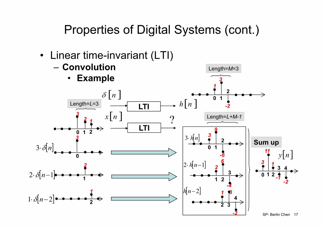
• An LTI system is defined to be causal, if its impulse
[ ] [ ]knxkhk
−= ∑∞
−∞=
y , presponse is a causal signal, i.e.
[ ] 0f0 <h Ri ht id d
– Similarly, anti-causal can be defined as[ ] 0for 0 <= nnh Right-sided sequence
A LTI t i d fi d t b t bl if f
[ ] 0for 0 >= nnh Left-sided sequence
• An LTI system is defined to be stable, if for every bounded input it produces a bounded output– Necessary condition:Necessary condition:
Th t i F i t f i t d th f t f
[ ] ∞<∑∞
−∞=nnh
SP- Berlin Chen 33
• That is Fourier transform exists, and therefore z-transform includes the unit circle in its region of converge
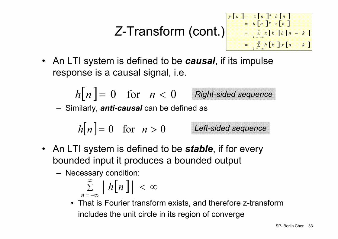
Z-Transform (cont.)( )
• Right-Sided Sequence– E.g., the exponential signal
[ ] [ ] [ ] ⎨⎧ ≥
==0for 1
erewh1 1n
nunuanh n
0
[ ] [ ] [ ]⎩⎨ < 0for 0
ere wh, .1 1 nnunuanh
( ) ( ) 11
11∞ −−∞
=== ∑∑ azzazHnnn
have a pole at az =( ) ( ) 11 1 −−∞=−∞= −aznn
If 11 <−az
p(Pole: z-transform goes to infinity)
azROC >∴ is 1Imth it l Im
[ ] 1ifexistsofansformFourier tr<anh×
the unit cycle
SP- Berlin Chen 34
Rea[ ] 1 ifexists1 <anh×

Z-Transform (cont.)( )
• Left-Sided Sequenceq– E.g.
[ ] [ ] ).,-0,-1,-2,..(n 1 .2 2 ∞=−−−= nuanh n
0
[ ] [ ] )(2
( ) [ ] 12 1 −−
−∞=
−∞
−∞=−=−−−= ∑∑ zaznuazH n
n
nn
n
n If 11 <− za
( ) 11
1
10
1
1 11
11111 −−
−
−
∞
=
−∞
=
−
−=
−−
−=−
−=−=−= ∑∑azza
zaza
zazan
n
n
nn
azROC <∴ is 2
Imthe unit cycle
Im
[ ] [ ]<
nhnha
gowillbecauseexisttdoesn'of ansformFourier tr the,1when
SP- Berlin Chen 35
Rea[ ] [ ]
−∞→nnhnh
aslly exponentia gowill becauseexist,t doesn 22×

Z-Transform (cont.)( )
• Two-Sided Sequenceq– E.g.
[ ] [ ] [ ]121
31 .3 3 −−⎟
⎠⎞
⎜⎝⎛−⎟
⎠⎞
⎜⎝⎛−= nununh
nn0
23 ⎠⎝⎠⎝[ ]
31 ,
311
1 31
1>
+⎯→←⎟
⎠⎞
⎜⎝⎛ −
−z
znu z
n
( )⎟⎞
⎜⎛⎟⎞
⎜⎛
⎟⎠⎞
⎜⎝⎛ −
=+=11
1212
11
11
113
zzzH
[ ]21 ,
211
1 121
1<
−⎯→←−−⎟
⎠⎞
⎜⎝⎛−
−z
znu z
n ⎟⎠⎞
⎜⎝⎛ −⎟⎠⎞
⎜⎝⎛ +−+ −−
21
31
211
311 11 zzzz
Imthe unit cycle 3
1 and 21 is 3 ><∴ zzROC
Im
31
− [ ] existtdoesn'ofansformFourier tr nh
SP- Berlin Chen 36
Re××
21
3 [ ]circleunit theincludet doesn' because
exist,t doesnofansformFourier tr
3
3
ROCnh

Z-Transform (cont.)( )
• Finite-length Sequence– E.g.
[ ]⎩⎨⎧ −≤≤
=th0
10 , .3 4
Nnanh
n
13221 ..... −−−− ++++ NNNN azaazz
0 N-1
[ ]⎩ others ,0
( ) ( ) ( ) azazazzazHNN
N
NN nN nn −
=−
===−− −− − ∑∑ 11
11 114
11( ) ( )azzaz Nnn −− −−==
∑∑ 11004 1
0except plane- entire is4 =∴ zzROC pp4
Imthe unit cycle ( ) 11 ,
2−== ,..,N kaez N
kjk
π
×31
− 4π If N=8
Re
SP- Berlin Chen 37
7 poles at zero A pole and zero at is cancelled az =

Z-Transform (cont.)( )
• Properties of z-transformp1. If is right-sided sequence, i.e. and if ROC
is the exterior of some circle, the all finite for which will be in ROC
[ ]nh [ ] 1 ,0 nnnh ≤=0rz >z
will be in ROC
• If ,ROC will include 01 ≥n ∞=z
A causal sequence is right-sided with ROC is the exterior of circle including
01 ≥n∞=z∴
2 If is left sided sequence i e the ROC is[ ]nh [ ] 0 nnnh ≥=2. If is left-sided sequence, i.e. , the ROC is the interior of some circle,
• If ,ROC will include
[ ]nh [ ] 2 ,0 nnnh ≥=
02 <n 0=z
SP- Berlin Chen 38
3. If is two-sided sequence, the ROC is a ring4. The ROC can’t contain any poles
[ ]nh

Summary of the Fourier and z-transforms
SP- Berlin Chen 39

LTI Systems in the Frequency Domainy y
• Example 1: A complex exponential sequence– System impulse response [ ]nh
[ ] njenx ω=[ ] [ ] [ ]
[ ] [ ][ ] [ ]knhkx
nxnhnhnxny
k−=
==
∑∞
−∞=
* *
[ ] [ ] [ ] [ ] knjekhnhnxny ω=∗= −∞
∞=∑ )(
-k( ) ofansformFo rier trthe:ωjH
[ ] [ ]knxkhk
−= ∑∞
−∞=
[ ]
( )
kjnj ekhe ωω= −∞
∞=∑
-k
( )
responsefrequencysystem theas toreferredoften isIt
response. impulse system the ofansformFourier trthe:ωjeH
– Therefore, a complex exponential input to an LTI systemlt i th l ti l t th t t b t
( ) njj eeH ωω= response.frequency system
results in the same complex exponential at the output, but modified by
• The complex exponential is an eigenfunction of an LTI i l( )
( )jωeH
SP- Berlin Chen 40
system, and is the associated eigenvalue[ ]{ } ( ) [ ]nxeHnxT jω=
( )jωeHscalar

LTI Systems in the Frequency Domain (cont.)y y ( )
• Example 2: A sinusoidal sequence [ ] ( )φ+= nwAnx 0cosp q ( )[ ] ( )
njjnjj AAnAnx cos 0
ωφωφ
φω
−−
+=
( )
θ
θ
θθ
θθj
j
ieie
− −=
+=
1sincos
sincos
– System impulse response
njjnjj eeee 00
22 ωφωφ −−+=
[ ]nh
( )θθθ jj ee −+=⇒21cos
( )ωω
ω
ω
i*
sincos * jj
jejyxzj
j +=⇒+=
[ ] ( ) ( ) 0000 njjjωnjjjω eeAeHeeAeHny += −−− ωφωφ
( )( ) ( )
ωωωω
ωωω
ω
sincos sincos
sincos *
jje
jejyxzj
j
−=−+−=
−=⇒−=−
[ ] ( ) ( )
( ) ( )[ ]0000 )()(
22njjω*njjω eeHeeHA
eeeHeeeHny
+=
+=
+−+ φωφω
( ) ( )( ) ( ) ( )0
00
00
jωeHjjωjω*
jω*jω
eeHeH
eHeH∠−
−
=
=
( ) ( )[ ]
( ) ( ) ( ) ( )[ ]00
000
0 )()(
2
2
njeHjjωnjeHjjω eeeHeeeHA
eeHeeH
jωjω
+=
+
+−∠−+∠ φωφω
SP- Berlin Chen 41
( ) ( )[ ]( ) ( )[ ]00
0cos 2
jωjω eHneHA ∠++= φωmagnitude response phase response

LTI Systems in the Frequency Domain (cont.)y y ( )
• Example 3: A sum of sinusoidal sequencesp q
[ ] ( )∑ +=K
kkk nAnx cos φω=k 1
[ ] ( ) ( )[ ]∑ ∠++=K
jkk
jk
kk eHneHAny cos ωω φωh
– A similar expression is obtained for an input consisting of a sum f l ti l
=k 1 magnitude response phase response
of complex exponentials
SP- Berlin Chen 42

LTI Systems in the Frequency Domain (cont.)y y ( )
• Example 4: Convolution Theorem [ ] [ ] ( ) ( )ωω jj eHeXnhnx ⇔∗
[ ] [ ]∑∞
−∞=−=
kkPnnx δ ( ) ⎥
⎦
⎤⎢⎣
⎡⎟⎠⎞
⎜⎝⎛ −= ∑
∞
kPP
eXk
j πωδπω 22DTFT
[ ] [ ] ( ) ( )
[ ] [ ] 1 , <= ∑∞
−∞=
anuanhk
n⎦⎣ ⎠⎝−∞= PPk
( ) ωω
jj
aeeH −−
=1
1DTFT
( ) ( ) ( )ωωω
πωδπ
jjj
k
eXeHeY∞
⎥⎤
⎢⎡
⎟⎞
⎜⎛
∑
=
221
ω
ω
π
ωδ
j
kj
aeP
kPPae
−
−∞=−
=
⎥⎦
⎢⎣
⎟⎠
⎜⎝
−∑−
=
112
1
has a nonzero jaeP −1 value when
πω2
Pk =
SP- Berlin Chen 43

LTI Systems in the Frequency Domain (cont.)y y ( )
• Example 5: Windowing Theorem [ ] [ ] ( ) ( )ωω jj eXeWnwnx ∗⇔21 ( ) ( )π2
[ ] [ ]∑∞
−∞=−=
kkPnnx δ
[ ]⎪⎩
⎪⎨⎧
−=⎟⎠⎞
⎜⎝⎛
−−=
otherwise 0
1,......,1,0 ,1
2cos46.054.0 NnN
nnw
πHamming window
⎩( ) ( ) ( )
( ) ∑∞
⎟⎠⎞
⎜⎝⎛ −∗=
∗=
j
jjj
keW
eXeWeY
ω
ωωω
πωδππ
22121
( )
( )∑
∑∞
−∞=
−∞=
⎭⎬⎫
⎩⎨⎧
⎟⎠⎞
⎜⎝⎛ −∗=
⎟⎠
⎜⎝
k
j
k
kP
eWP
kPP
eW
ω πωδ
ωδπ
21
2
( )
∑
∑ ∑∞ ⎟
⎠⎞
⎜⎝⎛ −
∞
−∞=
∞=
−∞=
⎟⎞
⎜⎛
⎭⎬⎫
⎩⎨⎧
⎟⎠⎞
⎜⎝⎛ −−=
kj
k
m
m
jm mkP
eWP
πω
πωδ
21
2 1
has a nonzero
SP- Berlin Chen 44
∑−∞=
⎟⎠
⎜⎝
⎟⎟⎠
⎞⎜⎜⎝
⎛=
k
Pj
eWP1 value when
kP
m πω 2−=

Difference Equation Realization for a Digital Filterfor a Digital Filter
• The relation between the output and input of a digital p p gfilter can be expressed by
[ ] [ ] [ ]∑ ∑ −+−=N M
kk knxknyny βα 0β [ ]ny[ ]nx[ ] [ ] [ ]∑ ∑= =
+k k
kk knxknyny1 0
βα
delay property[ ] ( )zXnx →
linearity and delay properties z-1
z-1
2β
1β
z-1
z-11α
2α
( ) ( ) ( ) kN Mk
kk zzXzzYzY −−∑ ∑+= βα
[ ] ( )[ ] ( ) 0
0nzzXnnx −→−
z-1Mβ z-1
Nα
( ) ( ) ( )k k
kk zzXzzYzY= =∑ ∑+
1 0βα
A rational transfer functionCausal:Rightsided, the ROC outside the
( ) ( )( )
∑=
−
== N
M
k
kk z
XzYzH 0
βoutmost poleStable:The ROC includes the unit circleC l d St bl
SP- Berlin Chen 45
( ) ( ) ∑=
−−N
k
kk zzX
11 α Causal and Stable:
all poles must fall inside the unit circle (not including zeros)

Difference Equation Realization for a Digital Filter (cont )for a Digital Filter (cont.)
SP- Berlin Chen 46

Magnitude-Phase Relationshipg
• Minimum phase system:p y– The z-transform of a system impulse response sequence ( a
rational transfer function) has all zeros as well as poles inside the unit cycleunit cycle
– Poles and zeros called “minimum phase components”– Maximum phase: all zeros (or poles) outside the unit cyclep ( p ) y
• All-pass system:– Consist a cascade of factor of the form
1
111
±
− ⎥⎦
⎤⎢⎣
⎡
− azz-a*
– Characterized by a frequency responsewith unit (or flat) magnitude for all frequencies 1
11
1 =− −az
z-a*
SP- Berlin Chen 47
Poles and zeros occur at conjugate reciprocal locations

Magnitude-Phase Relationship (cont.)g ( )
• Any digital filter can be represented by the cascade of a y g p yminimum-phase system and an all-pass system
( ) ( ) ( )zHzHzH apmin=( ) ( ) ( )apmin
( )( )
1)( 1 zero oneonly has that Suppose <aa*zH
( )( ) ( )( ) ( )
( )filter) phase minimum a is ( 1
:asexpressed becan circle.unit theoutside
*1
*1 −= zHzazHzH
zH
( )( ) ( )( )
:where
111 1
*1
1 −−
−−
−=az
zaazzH
( )( )( )1
filter. phase minimum a also is 1
:where
*
11
−−
za
azzH
SP- Berlin Chen 48
( )( ) filter. pass-all a is 11 1−−−
azza

FIR Filters
• FIR (Finite Impulse Response)( p p )– The impulse response of an FIR filter has finite duration– Have no denominator in the rational function
• No feedback in the difference equation ( )zH
[ ] [ ]M [ ]ny[ ]nx[ ] [ ]∑
=−=
M
rr rnxny
0β
z-1
z-1
1β0β
[ ]ny[ ]nx
[ ]⎩⎨⎧ ≤≤
=h i0
0 , Mnnh nβ
z-1Mβ
[ ]⎩⎨ otherwise ,0
( ) ( )( ) ∑ −==
M
k
kk z
XzYzH
0β
– Can be implemented with simple a train of delay, multiple, and add operations
( ) =kzX 0
SP- Berlin Chen 49

First-Order FIR Filters
• A special case of FIR filters p
[ ] [ ] [ ]1−+= nxnxny α ( ) 11 −+= zzH α
( ) jj( ) ωω α jj eeH −+= 1( ) ( )
( ) ( ) ++=++=
−+=
ωααωαωα
ωωαω
cos21sincos1
sincos1
222
22j jeHRe Im
( ) ⎟⎠
⎞⎜⎝
⎛+
−=ωα
ωαθ ωcos1
sinarctanje: pre-emphasis filter0<α
Re
( ) 2( ) 2log10 ωjeH
SP- Berlin Chen 50

Discrete Fourier Transform (DFT)( )
• The Fourier transform of a discrete-time sequence is a continuous function of frequency– We need to sample the Fourier transform finely enough to be
able to recover the sequenceable to recover the sequence– For a sequence of finite length N, sampling yields the new
transform referred to as discrete Fourier transform (DFT)
( ) [ ] 10 , 21
0−≤≤∑=
−−
=NnenxkX
knN
jN
n
π
DFT, Analysis
[ ] ( ) 10 , 1 21
0
−≤≤∑=−
=
NnekXN
nxkn
NjN
nπ
Inverse DFT, Synthesis0=N k
SP- Berlin Chen 51

Discrete Fourier Transform (cont.)( )
10 k
[ ] [ ] ≤≤
−≤≤∀
−−
∑ 10
1021
NnenxkX
Nkkn
NjN π
[ ] [ ]
[ ] [ ] ⎤⎡⎤⎡⎤⎡
−≤≤==∑
00111
10 ,0
Xx
NnenxkX N
n
L( )
[ ][ ]
[ ][ ]
⎥⎥⎥⎤
⎢⎢⎢⎡
=⎥⎥⎥⎤
⎢⎢⎢⎡
⎥⎥⎥⎤
⎢⎢⎢⎡
−⋅−⋅−10
10
1
111112112
XX
xx
eeN
Nj
Nj
MMMMM
Lππ
( ) ( ) ( ) [ ] [ ]⎥⎥
⎦⎢⎢
⎣ −⎥⎥
⎦⎢⎢
⎣ −⎥⎥⎥
⎦⎢⎢⎢
⎣−⋅−−⋅−− 111112112
NXNxeeNN
NjN
Nj
MM
L
MLMMππ
Orthogonal
⎦⎣
SP- Berlin Chen 52

Discrete Fourier Transform (cont.)( )
• Orthogonality of Complex Exponentials g y p p( )
⎩⎨⎧ =
=∑− −
otherwise0 if ,11 1 2 mNk-r
eN
N nrkN
j π
⎩∑= otherwise ,00N n
knjNπ2
11[ ] [ ]
[ ] [ ]( )nrk
Njrn
Nj
knN
j
kX
ekXN
nx
N NN
N
kππ 22
1 11
1
0
1
1
−−
∑ ∑∑⇒
∑=
− −−
−
=
[ ] [ ]
[ ]( )nrk
Nj
ekX
ekXN
enx
NN
n knπ2
11
0 00
1 −
⎥⎥⎤
⎢⎢⎡
∑∑=
∑ ∑=∑⇒
−−
= ==
[ ] [ ][ ]rX
mNrXkX=
+=[ ]
[ ]knj
rX
N
N
nk
π21
00
=
⎥⎦⎢⎣∑∑==
[ ]rX
SP- Berlin Chen 53
[ ] [ ]kn
Nj
enxkXN
n
1
0
−
∑=⇒−
=

Discrete Fourier Transform (DFT)( )
• Parseval’s theorem
[ ] ( )∑∑−−
=1
21
2 1 NN
kXN
nx Energy density[ ] ( )∑∑== 00 kn N
SP- Berlin Chen 54

Analog Signal to Digital Signalg g g g
Analog SignalAnalog Signal
Digital Signal:
[ ] ( ) periodsampling:TT
Discrete-time Signal or Digital SignalDigital Signal:
Discrete-time signal with discrete
amplitude[ ] ( ) periodsampling: , TnTxnx a=nTt =
SP- Berlin Chen 55
rate sampling 1TFs =
sampling period=125μs=>sampling rate=8kHz

Analog Signal to Digital Signal (cont.)g g g g ( )
Impulse TrainSamplingContinuous-Time
SignalDiscrete-Time
SignalContinuous-Time to Discrete-Time Conversion
Impulse TrainTo
Sequence [ ] ( ))( ˆ nTxnx a=
p g
( )∞
s tx
( )tx a
( ) ( ) ( ) ( )
( ) ( ) [ ] ( )∑∑
∑∞∞
∞
−∞=
−=−=
−==
a
naa
nTtnxnTtnTx
nTttxtstx
δδ
δ
( ) ( )∑∞
−= nTtts δ
switch
−∞=−∞= nn
Digital Signal
[ ] nx−∞=n
Periodic Impulse Train ( ) [ ]nxtxs by specifieduniquely becan
Discrete-time signal with discrete
amplitude
( )tx a
amplitude
( ) ( )∞
( )∞
≠∀= 0 ,0 ttδ1
SP- Berlin Chen 56
( ) ( )∑∞
−∞=−=
nnTtts δ ( )∫
∞
∞−
= 1dttδ1
T0 2T 3T 4T 5T 6T 7T 8T-T-2T

Analog Signal to Digital Signal (cont.)g g g g ( )
• A continuous signal sampled at different periodsg p p
( )tx a ( )tx a
TT
1
( )tx ( )
( ) ( ) ( ) ( )∑∞∞
∞
−∞=
−==n
aa
s
nTttxtstx
tx
δ
SP- Berlin Chen 57
( ) ( ) [ ] ( )∑∑∞
−∞=
∞
−∞=
−=−=nn
a nTtnxnTtnTx δδ

Analog Signal to Digital Signal (cont.)g g g g ( )
( )ΩjXa
• Spectra( )ja
2π2NΩ
frequency) (sampling22ss F
Tππ
==Ω( ) ( )∑∞
−∞=Ω−Ω=Ω
ksk
TjS δπ2
⎞⎛ π1
( ) ( ) ( )∞
Ω∗Ω=Ω as jSjXjX
121π ( )
⎩⎨⎧ Ω<Ω
=ΩΩ otherwise 0 2/ sT
jRs
( ) ( ) ( )ΩΩ=Ω Ω jXjRjX pa s
⎟⎠⎞
⎜⎝⎛=Ω<Ω
TsNπ
21( ) ( )( )∑
−∞=
Ω−Ω=Ωk
sas kjXT
jX 1
( )⎬⎫
⎨⎧ Ω>Ω−Ω NNsQ
Low-pass filter
⎟⎠⎞
⎜⎝⎛=Ω>Ω
TsNπ
21
⎭⎬
⎩⎨ Ω>Ω⇒ 2 Ns
high frequency componentsgot superimposed onlow frequency
SP- Berlin Chen 58
⎠⎝ T2
aliasing distortion
( )⎭⎬⎫
⎩⎨⎧
Ω<Ω⇒Ω<Ω−Ω
2 Ns
NNsQ
( ) ( )ΩΩ jXjX pa from recovered bet can'
components

Analog Signal to Digital Signal (cont.)g g g g ( )
• To avoid aliasing (overlapping, fold over)– The sampling frequency should be greater than two times of
frequency of the signal to be sampled →(Nyquist) sampling theorem
Ns Ω>Ω 2– (Nyquist) sampling theorem
• To reconstruct the original continuous signalFil d i h l fil i h b d li i– Filtered with a low pass filter with band limit
• Convolved in time domain sΩ
( ) ( ) ( )∑∞
= nTthnTxtx( ) tth sΩ= sinc
( ) ( ) ( )
( ) ( )∑
∑∞
−∞=
−∞=
−Ω=
−=
nsa
naa
nTtnTx
nTthnTxtx
sinc
SP- Berlin Chen 59


![[k mpjutey nl] [fown l d i] Speech Recognition And Text-to-Speech Systems](https://img.pdfslide.net/doc/110x75/56649e165503460f94b016ad/k-mpjutey-nl-fown-l-d-i-speech-recognition-and-text-to-speech.jpg)