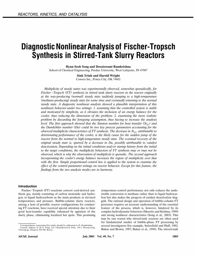
REACTORS, KINETICS, AND CATALYSIS

Diagnostic NonlinearAnalysisof Fischer-TropschSynthesis in Stirred-Tank Slurry Reactors

Hyun-Seob Song and Doraiswami RamkrishnaSchool of Chemical Engineering, Purdue University, West Lafayette, IN 47907

Sinh Trinh and Harold WrightConoco Inc., Ponca City, OK 74602

Multiplicity of steady states was experimentally obser®ed, somewhat sporadically, for( )Fischer �Tropsch FT synthesis in stirred tank slurry reactors in the reactor originally

( )at the wax-producing normal steady state suddenly jumping to a high-temperature( )methane-producing steady state for some time and e®entually returning to the normalsteady state. A diagnostic nonlinear analysis showed a plausible interpretation of thisnonlinear beha®ior under two settings: 1. assuming that the controlled system is stableand moti®ated by simplicity, as it ob®iates the inclusion of an energy balance for thecooler, thus reducing the dimension of the problem; 2. examining the more realisticproblem by discarding the foregoing assumption, thus ha®ing to increase the analysis

( )le®el. The first approach showed that the Stanton number for heat transfer St andH( )the Damkohler number Da could be two key process parameters accounting for the¨

obser®ed multiplicity characteristics of FT synthesis. The decrease in St , attributable toHdeteriorating performance of the cooler, is the likely cause for the sudden jump of thereactor from the normal to high-temperature steady state. The e®entual reco®ery of theoriginal steady state is, spurred by a decrease in Da, possibly attributable to catalystdeacti®ation. Depending on the initial conditions andror startup history from the initialto the target conditions, the multiplicity beha®iors of FT synthesis may or may not beobser®ed, which is why the obser®ation of multiplicity is sporadic. The second approachincorporating the cooler’s energy balance increases the region of multiplicity o®er thatwith the first. Simple proportional control law is applied to the system to examine theeffect of the control parameter settings on reactor beha®ior. Except for this feature, thefindings from the two analysis modes are in harmony.

IntroductionŽ .Fischer�Tropsch FT reactions convert coal-derived syn-

thesis gas, mainly consisting of carbon monoxide and hydro-gen, to liquid hydrocarbons as the main products at elevatedtemperatures and pressure. Bubble-column slurry reactors,among a host of possible reactor configurations for conduct-ing FT reactions, have received special attention due to theirgood heat-transfer capability enhanced by agitation of theslurry phase, eliminating localized hot spots. This promising

Correspondence concerning this article should be addressed to D. Ramkrishna.Current address of H.-S. Song: LG ChemrResearch Park, 104-1 Moonji-dong,

Yuseong-gu, Daejeon 305-380, Korea.

temperature-control performance not only reduces the unde-sirable conversion to methane rather than to liquid hydrocar-bon but also makes the progress of catalyst deactivation slug-gish. The rational design and operation of bubble-column FTprocesses requires an accurate understanding of the essentialfeature of the process, which is, however, hindered by its

Ž .complex hydrodynamic behaviors Maretto and Krishna, 1999Ž .and strong nonlinear characteristics Song et al., 2003 . This

may be one reason why stirred-tank reactors are often usedfor fundamental studies of bubble-phase FT processing by

Žseveral investigators for example, Satterfield and Huff, 1982;.Bukur and Brown, 1987; Bukur et al., 1994 . The stirred-tank

July 2003 Vol. 49, No. 7AIChE Journal 1803

reactor configuration can provide a better environment forthe analysis of FT processes compared to general bubble-col-umn reactors by achieving uniform distributions of tempera-ture, concentration, and catalyst particles within the reactor.

This study is motivated by some strange nonlinear behav-iors experimentally observed in an FT stirred-tank slurry re-actor on laboratory scale. Under normal operation, liquid hy-drocarbons are constantly produced as the main products, andthe product selectivity is in a desirable range. This wax-pro-ducing mode continues until the cobalt catalyst requires re-generation due to serious loss of activity. However, occasion-ally, one encounters multiplicity behaviors that require a de-tailed understanding of the reaction system. The reactiontemperature of the FT process suddenly jumps to a highervalue, and accordingly the conversion of the synthesis gas isalso increased, undesirably switching the process from FTsynthesis mode to methane-producing mode. As a result, theprocess produces methane instead of liquid hydrocarbons atthis high-temperature steady state. Interestingly, the steadystate at higher reaction temperature returns to the previousoperating steady state after a couple of hours. The conver-sion of the recovered state is, however, somewhat lower andthe selectivity of methane is slightly higher than the one atthe starting condition. The objective of this work is to seek arational explanation for the foregoing phenomenon as well asto elucidate the background of its sporadic character. Fur-ther, the analysis will establish the extent to which simplifica-tion of reaction kinetics sacrifices its capacity to representthe nonlinear behavior of the reaction system, at least for thestirred reactor. It may not be unreasonable to expect that thisinvestigation could also be used to assess the admissibility ofthe reaction kinetics to investigate more complex reactorconfigurations with a view toward improving conversion andselectivity as well as identifying their safety limits of opera-tion.

Ž .Shah et al. 1990 have previously made an attempt to ad-dress multiplicity behavior of FT reactors. Rather than basesuch an investigation on the methods of nonlinear analysis,they limited themselves to interpretations based entirely onthe heat generation and dissipation curves identified from the

Ž .data of Bhattacharjee et al. 1986 . Thus, ignition and extinc-tion conditions were calculated as functions of process pa-rameters without recourse to rigorous analysis. For a com-plete elucidation of the multiplicity and stability features ofthe multidimensional FT reaction system, the thermal analy-

Ž .sis of Shah et al. 1990 does not constitute an alternative tothe application of rigorous bifurcation theory.

Nonlinear analysis of continuous stirred-tank reactorsŽ .CSTR has been the subject of intensive investigation by en-gineers and mathematicians, based on the use of catastrophe

Žor singularity theories Golubitsky and Keyfitz, 1980; Balako-.taiah and Luss, 1981, 1983; Farr and Aris, 1986 . However,

the task at hand is rendered considerably more difficult be-Ž .cause of various factors pertinent to FT synthesis: 1 multi-

phase nature of the system, that is, a solid catalyst phase, agas phase of reactants and low molecular-weight products, aliquid phase of higher molecular weight products with a po-

Ž .tential for a second liquid aqueous phase; 2 a wide-rangingŽ .spectrum of gaseous and liquid products; 3 high exother-

Ž .micity of the reactions; 4 strong interaction between trans-Ž .port and chemical reactions; 5 catalyst deactivation; and nu-

merous others. A consequence of the foregoing complexities,in spite of simplifications, is the high dimensionality of themodel system with a large number of variables and parame-ters, which present one with a cumbersome mathematicalproblem.

A comprehensive nonlinear analysis has been conductedbased on singularity theory to investigate the fundamentalreasons for the observed multiplicity behavior. The bifurca-tion behavior of the system by varying process parametershas been investigated using two approaches. The first is con-ducted on a simplified model, which assumes that the con-trolled process is stable and that the dynamics of the con-troller need not be considered. The second undertakes theburden of the full problem with a proportional controller forthe coolant flow rate. In view of the potential for deteriora-tion in the performance of the cooler and activity of the cata-lyst, with the progress of reaction, special focus was placed

Ž .on the effects of the Stanton number for heat transfer StHŽ .and the Damkohler number Da on the bifurcation behav-¨

iors of the process. The sequel to the analyses has shown thatdeterioration of heat removal performance and catalyst deac-tivation with time could reasonably account for the observednonlinear characteristics of FT synthesis reactors. The for-mer effects are reflected into St and the latter into Da inHthe derived dimensionless model equations, as will be estab-lished subsequently. The decrease in St , a consequence ofHthe diminishing heat-transfer coefficient between the coolantand the reaction medium, is shown to cause a sudden jump

Ž .from the normal steady state or wax-producing model toŽthe high-temperature steady state or methane-producing

.mode . Thereafter, decrease in Da, attributable to progress-ing catalyst deactivation, presents a possible explanation forthe restoration of the normal operating steady state, albeitwith a conversion and selectivity lower than before. We alsoestablish that, depending on the initial condition and startuphistory, the steady-state transition between the wax- and themethane-producing mode may or may not happen in FT syn-thesis reactions. Furthermore, we show how this nonlinearbehavior can be sporadic through a global bifurcation dia-gram in the St and Da space. We stress that the accom-Hplishment of this article is a testimonial to the effectivenessof nonlinear analysis in diagnosing the origin of a practicalindustrial problem.

Model FormulationIn most published models the FT process is generally rep-

Žresented by a combination of the main FT synthesis that is,. Ž .the production of hydrocarbons and water�gas shift WGS

reactions, of which the latter is considered to be inactive forcobalt-based catalysts being dealt with here. The net reactionconducted under cobalt-based catalysts can be grossly repre-sented as follows

y� H q y� CO™� C H q� H O 1Ž . Ž . Ž .1 2 2 3 n m 4 2

The stoichiometric coefficients and the average number ofŽ . Ž .carbon n and hydrogen m of the obtained hydrocarbon

products can be expressed in terms of the chain-growth prob-

July 2003 Vol. 49, No. 7 AIChE Journal1804

Ž .ability factor � and the paraffin fraction in the reactionŽ . Ž .products � as shown below Stern et al., 1985

2� sy 2q 1y� q�� 1y� 2Ž . Ž . Ž .1

� sy1 3Ž .2

� s1y� 4Ž .3

� sy� 5Ž .4 2

and

y1ns 1y� 6Ž . Ž .y1ms2 1y� q 1y� q�� 7Ž . Ž . Ž .

Hereafter, the subscripts 1, 2, 3, and 4 denote hydrogen, car-bon monoxide, hydrocarbon, and water, respectively. Amongother available kinetic models of FT synthesis in the litera-ture, the following equation is selected as the most appropri-

Žate form for cobalt catalysts Withers et al., 1990; Kirillov et.al., 1999

� kC2C2 1 2Rs 8Ž .2ž /� q� C C qKC1 2 1 2 4

Instead of considering all the complex reaction mecha-nisms involved in FT synthesis, the simple Anderson�

Ž .Schultz�Flory ASF equation is adopted here to describe theproduct selectivity. The mole fractions of hydrocarbons withthe number of carbons equal to i are given as a function of

Žthe chain-growth probability factor or also called ASF fac-.tor , �

x s 1y� � iy1 9Ž . Ž .i

The determination of the parameter � is of great importancein that it would govern the product distribution as well asaffect the stoichiometric coefficients of the FT reaction to-gether with the parameter � just given. While the value of �

Žhas been fixed as 0.85 that is, 85% paraffin in the hydrocar-.bon products throughout the calculation in this study, we

have tried to consider the functional dependence of � on thereaction conditions as much as possible. For example, thetemperature dependence of � should essentially be incorpo-rated into the model in order to account for the product se-lectivity changes at different states, that is, the FT processmainly forms liquid hydrocarbons under the usual operatingconditions, which would, however, be replaced by methanegas at the high-temperature steady state as described in thebeginning of this article.

Unfortunately, aside from a concentration dependence, agenerally acceptable explicit correlation of � with reaction

Žconditions is not available in the literature. Lox and Fro-Ž .ment 1993a,b proposed � as a function of temperature and

reaction mixture composition for an iron catalyst, but thatcorrelation is not used here because it is shown to be inap-

.propriate for our system based on cobalt catalysts. In an ex-periment over an alumina-supported cobalt catalyst pro-

Ž .moted with zirconium, Yermakova and Anikeev 2000 sug-

gested, after testing several different equations, the followingempirical functional relation between � and the composi-tions of H and CO2

y2�s A qB 10Ž .

y q y1 2

where y indicates the mole fraction of the gas-phase compo-nent. The model parameters A and B are assigned as con-

Žstant values that is, As0.2332�0.0740 and Bs0.6330�.0.0420 because all the variables other than compositions have

been fixed in their experimental work. This equation can beapplied to the limited case where only compositions arechanging. To extend the usage of Yermakova and Anikeev’smodel and, more importantly, to make our model capable ofexplaining the significant changes of the product compositionbetween the two different observed steady states, Eq. 10 isslightly modified by adding temperature dependence as asimple linear function as follows

y2 w x�s A qB 1y0.0039 Ty533 11Ž . Ž .ž /y q y1 2

Equation 11 is immediately reduced to Eq. 10 by setting Ts533 K, the temperature for which Eq. 10 is derived. It shouldbe noted that this equation is only applicable to the range ofthe operating conditions rendering 0F�F1. The slope oftemperature dependence has been fitted to various experi-mental data summarized in Figure 13 of a recent article by

Ž .Van Der Laan and Beenackers 1999 .The principal assumptions in the formulation of this model

are summarized as follows:Ž .1 The mass-transfer resistance between liquid phase and

solid catalysts is neglected, so that we need consider only twophases of gas and slurry in mass balances.Ž .2 The gas and slurry phases are well mixed and the

species concentrations in each phase are constant.Ž .3 The catalyst particles are uniformly distributed in the

reactor.Ž .4 The gas phase obeys the ideal gas law.Ž .5 The heat-transfer resistance between the two phases is

neglected so that the temperature is constant throughout thereactor.Ž .6 The coolant is assumed to be well-mixed in the cooler

so that its temperature can be regarded as constant.Ž .7 There is no input or output of slurry associated with

the reactor.Ž .8 The process parameters involved in modeling such as

gas holdup, heat capacities, and densities, are constant.Under the foregoing assumptions, the steady-state equa-

tions are written in dimensionless form

� yq � ySt � y� s0 js1, . . . , ns 12Ž . Ž .Ž .Gj,0 G G j j G j L j

St � y� q� Da� s0 jy1, . . . , ns 13Ž . Ž .Ž .j G j L j j

ns ns˜� yq Pr� y St � y� s0 14Ž .Ž .Ý ÝGj,0 G j G j L jž /

js1 js1

� � yq � � ySt �y� qDa� Be s0 15Ž .Ž . Ž .G ,0 G ,0 G G H C R

July 2003 Vol. 49, No. 7AIChE Journal 1805

where ns indicates the number of species that is 4 in our˜model, �, � , q, P, St, St , Be , Da, � , and indicate con-H R

centration, temperature, flow rate, pressure, Stanton num-bers for mass and heat transfer, heat of reaction, Damkohler¨number, and activation energy, respectively, and the physicalimplication of the other dimensionless parameters can bereadily inferred from their definitions given below. The sub-

Ž .scripts G, L, 0, j denote gas phase, liquid or slurry phase,inlet condition, and species j, respectively

C C CGj,0 G j L j� s , � s , � sGj,0 G j L jC C CG1,0 G1,0 G1,0

Q T TG G ,0q s , � s , �sG G ,0Q T TG ,0 C ,0 C ,0

CT P G ,0 pG ,0C ˜� s , Ps , � sC G ,0T C RT CC ,0 G1,0 C ,0 L pL

C k aŽ . jG pG L� s , St sG j C He Q rVL pL j G ,0

h a y� H CŽ .C C R G1,0St s , Be sH R C Q rV C TL pL G ,0 L pL C ,0

w 1y� a k T rHeŽ . Ž .G cat C ,0 1Das

Q rVG ,0

21 � �L,1 L ,2� sexp y y1ž / ˜� � � qK�L,1 L ,2 L ,4

E He He1 2˜ s , KsK 16Ž .RT C HeC ,0 G1,0 4

The nominal values for the preceding dimensionless parame-ters are given in Table 1. Equations 12 to 15 are the massbalance of species i in the gas phase, the overall mass bal-ance of the gas phase, the mass balance of species i in theslurry phase, and energy balance, respectively.

Local Multiplicity BehaviorExamination of possible causes

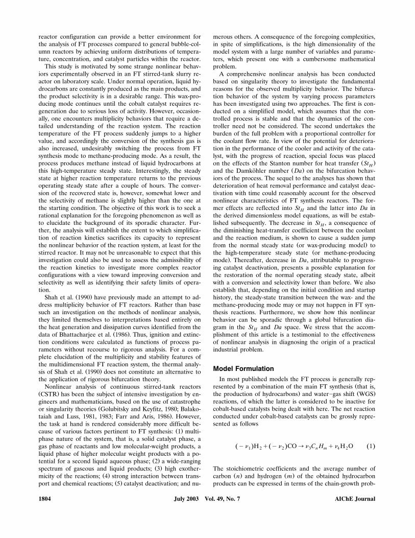
A typical S-shaped temperature profile is obtained by solv-ing the model equations given by Eqs. 12 to 15 based on the

Ž .parameter values of Table 1 Figure 1 . The dotted and thesolid lines in Figure 1 indicate the unstable and the stablesteady-state solutions, respectively. The nominal operatingtemperature of the FT reactor is around 1.1772, as markedby solid circle in Figure 1. This figure shows that careful op-erations are necessary to maintain the process at this unsta-ble intermediate steady state. The process may go astray fromthis unstable state to upper or lower stable steady state whensmall disturbances are introduced unless appropriate controlactions are taken. At this stage, we present two modes ofanalysis in this article. We at first assume that the processcan be stabilized by feedback controllers throughout the op-eration, that is, no unstable steady states exist in our systemin the closed-loop context. This premise is justified in a later

Table 1. Nominal Values for the Model Parameters

Dimensionless Values

Feed conditions � s1, � s0.5, � s0, � s0,G1,0 G 2,0 G 3,0 G 4,0� s0.6928G ,0

Stanton nos. for heat St s0.38, St s5.3423, St s7.5196,H 1 2and mass transfer St s3.8956, St s37.7613 4

Reaction parameters Das0.01225, Be s0.3021, s27.657,R

K̃s0.12067

˜Pressure and temp. Ps1.0392, � s1.1772SET

Others � s0.0097, � s0.0057,G ,0 G� s� s0.000934, s20C ,0 C

section investigating the effects of control-parameter settingson the stability and multiplicity behavior of the same process.Indeed improper tuning of control parameters might be re-sponsible to some extent for the runaway behavior, especiallywhen the process characteristics are significantly changedduring operation. However, in order to examine this issue,we extend the analysis to include an additional energy bal-ance around the cooler, thus increasing by one the alreadysizable set of equations. The simpler approach considered atfirst, however, has the advantage of enlightening us with theproper range of process parameters without having to be bur-dened with the full set of equations.

Another problem in the operation of our FT process foundfrom Figure 1 may be the ignition andror extinction risksaround the two turning points due to the hysteresis charac-teristics of the process. This issue has been theoretically

Ž .treated by Shah et al. 1990 based on the experimental ob-Ž .servation by Bhattacharjee et al. 1986 , where the critical

conditions for ignition and extinction are provided in termsof the various process parameters, such as CO feed concen-tration, gas space velocity, and activation energy. They warnedthat it is essential to avoid the ignition. Once the ignition

Figure 1. Sigmoidal temperature curve obtained withparameters given in Table 1.

July 2003 Vol. 49, No. 7 AIChE Journal1806

occurs, the normal FT synthesis reaction would be switchedto the methane-forming mode, seemingly never to return. Thisis because the catalyst could suffer serious deactivation onexposure to the high temperature resulting from the ignition.However, the evidence, sporadic as it may be, is contrary tothe scenario just suggested. First of all, as identified in Fig-ure 1, the possibility of ignition is very low as the nominaloperating condition of the FT process is far away from theignition temperature. In fact, this situation is more conduciveto extinction than ignition, one that has never arisen in ourreactor facilities. Furthermore, the subsequent return after

Žsome hours to the properly steady state even granting the.lower selective conversion is in sharp contrast to the obser-

Ž .vation by Bhattacharjee et al. 1986 . The foregoing argu-ments provide strong evidence against ignition being the un-derlying mechanism for the steady-state transition of our sys-tem. Also, the actual reactor temperature after the runaway,which had been monitored during operation, was significantly

lower than the one to be realized by the ignition predicted byour model.

From the arguments presented earlier, we have ruled outtwo possibilities in the interpretation of the multiplicity be-havior displayed by our FT reactor. The first, which discountsinstability arising from poor tuning of control parameters, issomewhat arbitrary for the present, but one that is justifiedin a later selection, which discusses the more detailed analy-sis incorporating the cooler and controller dynamics. The sec-ond rules out ignition in accord with the arguments pre-sented in the preceding paragraph. This, however, should im-ply that the normal steady state should prevail, as the reactorparameters would seem to be safely off the limits of asteady-state switch. The conclusion just made is on the pre-sumption that all process parameters must remain invariantwith time. Naturally, an explanation for the disturbance ofstatus quo must take root in the dynamic variation of somekey parameters with time, perhaps on a much slower time

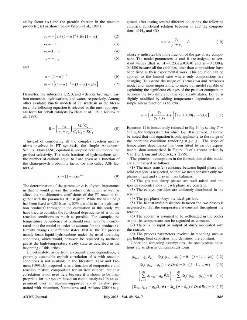
[( ) ( )] [( ) ( )]Figure 2. Effects of the variation St a and b and Da c and d on the shape of temperature curves on theH( ) ( )� -� plane and the multiplicity map on the St -� plane.c H c

July 2003 Vol. 49, No. 7AIChE Journal 1807

scale. The steady-state shift must occur as a consequence of adynamic change in one or more process parameters. Moreprecisely, we envisage, some parameters varying with time ina way such that the process characteristics are altered signifi-cantly. From this consideration, two key process parametersthat are believed to be responsible for our problem are sug-gested here: the heat-transfer coefficient between the coolerand the reactor and activity of the catalyst.

The overall heat-transfer coefficient, h , or, in other words,cthe heat-removal performance of the cooler, would decreasewith time due to fouling of the surface andror increasing vis-cosity of the reaction medium, or possibly other reasons. Theheat-transfer coefficient is contained in St , which is propor-Htional to the ratio of the convective heat transfer to the ther-mal capacity of fluid as defined in Eq. 16. We can directlyregard St as the measure of the heat-removal capability ofHthe cooler because all the parameters except the heat-trans-fer coefficient are assumed to be constant in the definition ofSt . Thus, St is no more than the dimensionless version ofH Hthe heat-transfer coefficient in this article. On the other hand,the catalyst activity, a , appears in Da as defined in Eq. 16.catAt the outset, the activity parameter would be assumed to beunity, that is, no catalyst deactivation. However, it wouldgradually diminish as the concentration of active sites in thecatalyst decreases with the progress of the reaction. The ac-tivity of cobalt catalysts in FT slurry reactors can be de-creased by the high temperature, the accumulation of thelonger hydrocarbons surrounding the catalysts, or any other

Ž .poisoning factors Liu et al., 1997; Gormley et al., 1997 . Theeffects of water on the FT cobalt catalysts were varied, prob-ably depending on the support materials, promoters, cobalt

Ž .precursors, and preparation methods Hilmen et al., 1999 .Da indicates the ratio of reaction rate to the convectivetransport rate, but we can simply interpret Da as the mea-sure of the catalyst’s activity here. Incorporating these tran-sient parameters into our model is not difficult, as one ex-pects that the time scales for both the decreasing St andHthe decreasing Da are quite large compared to the processcharacteristic times for reaction, convection, and diffusion;thus, it can be assumed that the process immediately arrivesat steady state at every instant during the period that thesetwo parameters are varying. This assumption validates thesteady-state model equations, Eqs. 12 to 15, even during thetransient period of a deteriorating performance of the coolerand catalyst activity.

A scenario for experimental obser©ationsIn order to connect the variation of these two parameters

with the observed multiplicity behaviors, local sensitivity testshave been conducted around the nominal operating condi-tions. First, effects of St are shown in Figure 2a, where theHthicker line indicates the standard initial operating curve.These trends of Figure 2a are readily interpreted. For exam-ple, high St means that we have a good cooler with a highHheat-transfer coefficient or with a large heat-transfer area.The shift of the temperature profile to the right with higherSt may be interpreted as the increase of the cooler temper-Hature for keeping the reactor temperature at the target value.A small temperature difference between the reactor and thecooler would be sufficient to control the reaction tempera-

ture for high St . The reverse explanation holds for smallHŽ .St . Thus, it is seen that the increase decrease of St has aH H

Ž .favorable unfavorable effect in regard to multiplicity. HighSt , that is, good heat-removal performance of the cooler,Hsuppresses the possibility of multiple steady state by dimin-ishing the nonlinear heat-generation effects and vice versaŽ .see also Figure 2b .

The effects of Da are quite different from those of St . AsHŽ .shown in Figure 2c, increase or decrease in Da requires a

Ž .lower or higher cooler temperature for keeping the desiredsteady state, which is exactly the opposite effect of St . ThisHbehavior obviously arises from Da multiplying the heat ofreaction term. The decrease of Da has little effect on theshape of the temperature profile, at least around the nominalcondition, although the S-shape will eventually disappear

Ž .when Da approaches zero see Figure 2d .Based on the effects of St and Da on the process behav-H

ior, we suggest a possible scenario for the observed multiplic-ity phenomenon. We expect in reality that both of these twoparameters would decrease with time as the reaction pro-ceeds due to reasons that were deliberated earlier. The timescale of this drifting behavior would require more extendedvigilance on the reactor performance. Consequently, we haverestricted our goal here to elucidating how the experimentalobservations are related to the gradual decrease of St andHDa.

ŽWe suppose for the present that the drift rate of decreas-.ing St is initially dominant compared to that of Da. At theH

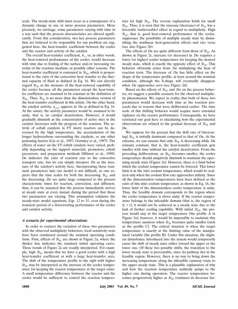
extreme, we can assume that only St is decreasing while DaHremains constant, that is, the heat-transfer coefficient getssmaller with time without the catalyst deactivation. From thepreceding deliberations, as St becomes smaller, the coolerHtemperature should adaptively diminish to maintain the oper-

Ž .ating steady state Figure 3a . However, there is a limit belowwhich the coolant temperature cannot be lowered. This lowerlimit is in the inlet coolant temperature, which would be real-ized only when the coolant flow rate approaches infinity. Sinceall the dimensionless temperatures have been defined as theratio of this inlet coolant temperature as shown in Eq. 16, thelower limit of the dimensionless cooler temperature is unity.Thus, the feasible domain corresponds to the region wherethe cooler temperature is above unity. If the reactor temper-

Žature belongs to the infeasible domain that is, the region of.� �1 , it would not be achieved as a steady state due to thec

lack of further cooling capability. With initial St , the pro-HŽcess would stay at the target temperature the profile A in

.Figure 3a ; however, it would be impossible to maintain thisŽtemperature anymore when St becomes quite smaller suchH

.as the profile C . The critical situation is when the targettemperature is exactly at the limiting value of the manipu-

Ž .lated variable the profile B . Under this situation, the slight-est disturbance introduced into the system would temporarilycause the shift of steady state either toward the upper or thelower one. Of these two possible shifts, the transition to thelower steady state is preventable, since its pathway lies in thefeasible region. However, there is no way to bring down theincreasing temperature along the infeasible runaway route tothe upper steady state. This is a plausible explanation of whyand how the reaction temperature suddenly jumps to thehigher one during operation. The reactor temperature be-comes progressively higher as St continues its decrease fur-H

July 2003 Vol. 49, No. 7 AIChE Journal1808

( )Figure 3. a Steady-state jumping from the normalwax-producing mode to the methane-formind

( )mode with the decrease of St ; b eventualHrecovery of the previous steady state with thedecrease of Da.

ther. At the high reaction temperature, the main product ofFT reactors will switch from the liquid hydrocarbons tomethane gas. As pointed out earlier, this phenomenon shouldbe distinguished from a typical ignition phenomenon. For thelatter to occur, the process should be in operation at the lowersteady-state branch of the sigmoidal temperature curve nearits turning point to the right. At these low reaction tempera-ture conditions, however, the expected conversion is consid-erably below that which is observed at the beginning. It mightbe interesting to see whether or not a Hopf bifurcation formsas St decreases in Figures 2a and 3a. In order to determineHthis, we investigated the existence of a simple pair of purelyimaginary eigenvalues of the Jacobian matrix at every pointalong the temperature curves throughout the calculation, butthey were never found. The definition of the Jacobian matrixwill be given later.

Next, we address the eventual return of the upper steadystate to the normal operating steady state. Once the reactor

temperature is boosted up to a higher value, the rate of cata-lyst deactivation would be enhanced by sintering or other fac-tors. The consequent decrease of Da by the catalyst deactiva-tion would push back the temperature profile to the feasible

Ž .region such as from the profile C toward the profile E asshown in Figure 3b. It should be noted that the critical condi-tion for the desirable intermediate state to be restored is dif-ferent from that of the initial jump. The previous steady stateis not recovered until the left turning point of the sigmoidaltemperature curve passes the limiting line of the cooler tem-

Ž .perature the profile D . This is because the returning path-way to the normal condition is rendered inaccessible by theinfeasible region before the left turning point enters the fea-sible region. The main products at the restored normal con-dition again become the heavy hydrocarbons rather thanmethane gas, although the conversion is decreased somewhatby deactivation of the catalyst. The recovery of the normalwax-producing mode from methane production is clear evi-dence that the runaway behavior observed in our system isnot due to ignition. If the runaway were caused by the igni-tion, the reactor temperature at the new steady state wouldbe high enough to seriously deactivate the catalyst, makingthe recovery to the wax-producing mode virtually impossible.

Global Multiplicity FeaturesFrom the local sensitivity analysis given earlier, we could

provide a reasonable answer to the question of how and whythe normal FT synthesis mode is suddenly switched to thehigher temperature state with the production of mainlymethane, eventually returning again to the original operatingstate with some loss of conversion. However, it remains toelucidate the critical values of St and Da at which the fore-Hgoing transitions occur. Moreover, we also need to throw somelight on the sporadic nature of the transitions. Toward thisend, we seek to analyze the global multiplicity features of thesystem. These questions will be clear from the global multi-plicity portrait over the parameter space of St and Da,Hwhich will be constructed using advanced nonlinear analysistools in the following sections.

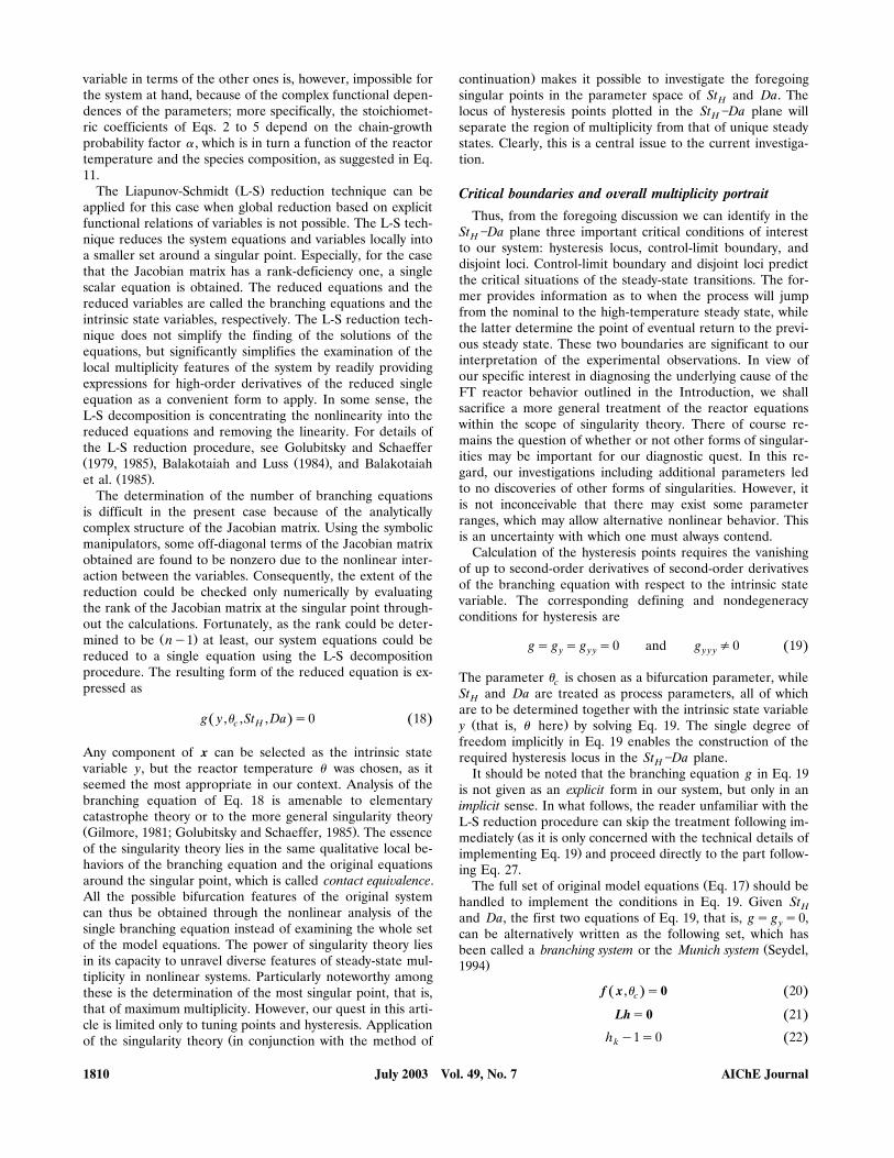
( )Liapuno©-Schmidt L-S Reduction and SingularityTheory

The model equations of our system, Eqs. 12 through 15,can be rewritten in the following general form

f x , p s0 17Ž . Ž .

where the n-dimensional vector x denotes the 10 state vari-ables, that is, 8 species concentrations in the gas and slurryphases, overall gas velocity, and reactor temperature, and them-dimensional vector p indicates the bifurcation and processparameters, that is, � , St , and Da. The mapping f : Rn�c HRm™Rn is assumed to be infinitely differentiable with re-spect to x and p. Comprehensive nonlinear analysis of a setof highly nonlinear equations like Eq. 17 becomes cumber-some when the dimensionality of system equations and thenumber of parameters are large. The difficulties of doing thistask could be substantially relieved if we could reduce thenumber of model equations into one using the analytic rela-tions between the variables. Explicit representation of one

July 2003 Vol. 49, No. 7AIChE Journal 1809

variable in terms of the other ones is, however, impossible forthe system at hand, because of the complex functional depen-dences of the parameters; more specifically, the stoichiomet-ric coefficients of Eqs. 2 to 5 depend on the chain-growthprobability factor � , which is in turn a function of the reactortemperature and the species composition, as suggested in Eq.11.

Ž .The Liapunov-Schmidt L-S reduction technique can beapplied for this case when global reduction based on explicitfunctional relations of variables is not possible. The L-S tech-nique reduces the system equations and variables locally intoa smaller set around a singular point. Especially, for the casethat the Jacobian matrix has a rank-deficiency one, a singlescalar equation is obtained. The reduced equations and thereduced variables are called the branching equations and theintrinsic state variables, respectively. The L-S reduction tech-nique does not simplify the finding of the solutions of theequations, but significantly simplifies the examination of thelocal multiplicity features of the system by readily providingexpressions for high-order derivatives of the reduced singleequation as a convenient form to apply. In some sense, theL-S decomposition is concentrating the nonlinearity into thereduced equations and removing the linearity. For details ofthe L-S reduction procedure, see Golubitsky and SchaefferŽ . Ž .1979, 1985 , Balakotaiah and Luss 1984 , and Balakotaiah

Ž .et al. 1985 .The determination of the number of branching equations

is difficult in the present case because of the analyticallycomplex structure of the Jacobian matrix. Using the symbolicmanipulators, some off-diagonal terms of the Jacobian matrixobtained are found to be nonzero due to the nonlinear inter-action between the variables. Consequently, the extent of thereduction could be checked only numerically by evaluatingthe rank of the Jacobian matrix at the singular point through-out the calculations. Fortunately, as the rank could be deter-

Ž .mined to be ny1 at least, our system equations could bereduced to a single equation using the L-S decompositionprocedure. The resulting form of the reduced equation is ex-pressed as

g y ,� ,St , Da s0 18Ž .Ž .c H

Any component of x can be selected as the intrinsic statevariable y, but the reactor temperature � was chosen, as itseemed the most appropriate in our context. Analysis of thebranching equation of Eq. 18 is amenable to elementarycatastrophe theory or to the more general singularity theoryŽ .Gilmore, 1981; Golubitsky and Schaeffer, 1985 . The essenceof the singularity theory lies in the same qualitative local be-haviors of the branching equation and the original equationsaround the singular point, which is called contact equi®alence.All the possible bifurcation features of the original systemcan thus be obtained through the nonlinear analysis of thesingle branching equation instead of examining the whole setof the model equations. The power of singularity theory liesin its capacity to unravel diverse features of steady-state mul-tiplicity in nonlinear systems. Particularly noteworthy amongthese is the determination of the most singular point, that is,that of maximum multiplicity. However, our quest in this arti-cle is limited only to tuning points and hysteresis. Application

Žof the singularity theory in conjunction with the method of

.continuation makes it possible to investigate the foregoingsingular points in the parameter space of St and Da. TheHlocus of hysteresis points plotted in the St �Da plane willHseparate the region of multiplicity from that of unique steadystates. Clearly, this is a central issue to the current investiga-tion.

Critical boundaries and o©erall multiplicity portraitThus, from the foregoing discussion we can identify in the

St �Da plane three important critical conditions of interestHto our system: hysteresis locus, control-limit boundary, anddisjoint loci. Control-limit boundary and disjoint loci predictthe critical situations of the steady-state transitions. The for-mer provides information as to when the process will jumpfrom the nominal to the high-temperature steady state, whilethe latter determine the point of eventual return to the previ-ous steady state. These two boundaries are significant to ourinterpretation of the experimental observations. In view ofour specific interest in diagnosing the underlying cause of theFT reactor behavior outlined in the Introduction, we shallsacrifice a more general treatment of the reactor equationswithin the scope of singularity theory. There of course re-mains the question of whether or not other forms of singular-ities may be important for our diagnostic quest. In this re-gard, our investigations including additional parameters ledto no discoveries of other forms of singularities. However, itis not inconceivable that there may exist some parameterranges, which may allow alternative nonlinear behavior. Thisis an uncertainty with which one must always contend.

Calculation of the hysteresis points requires the vanishingof up to second-order derivatives of second-order derivativesof the branching equation with respect to the intrinsic statevariable. The corresponding defining and nondegeneracyconditions for hysteresis are

gs g s g s0 and g �0 19Ž .y y y y y y

The parameter � is chosen as a bifurcation parameter, whilecSt and Da are treated as process parameters, all of whichHare to be determined together with the intrinsic state variableŽ .y that is, � here by solving Eq. 19. The single degree of

freedom implicitly in Eq. 19 enables the construction of therequired hysteresis locus in the St �Da plane.H

It should be noted that the branching equation g in Eq. 19is not given as an explicit form in our system, but only in animplicit sense. In what follows, the reader unfamiliar with theL-S reduction procedure can skip the treatment following im-

Žmediately as it is only concerned with the technical details of.implementing Eq. 19 and proceed directly to the part follow-

ing Eq. 27.Ž .The full set of original model equations Eq. 17 should be

handled to implement the conditions in Eq. 19. Given StHand Da, the first two equations of Eq. 19, that is, gs g s0,ycan be alternatively written as the following set, which has

Žbeen called a branching system or the Munich system Seydel,.1994

f x ,� s0 20Ž .Ž .c

Lhs0 21Ž .h y1s0 22Ž .k

July 2003 Vol. 49, No. 7 AIChE Journal1810

Equation 21, in view of Eq. 22, is equivalent to the Jacobian2 Ž w x Žmatrix L the Jacobian matrix, L� � fr� x Is1, 2, . . . , n;i j

.js1, 2, . . . , n being singular. That is, if the linearized systemEq. 21 has a nontrivial solution h �0, then we will have a0rank-deficient Jacobian matrix. Equation 22 is necessary tochoose one solution vector among the infinite candidates forh , where the subscript k therein can be any integer value0

Ž .between 1 and n s10 here . The equations are closed sincewe have 21 unknowns of x, h, � for 21 equations with Stc Hand Da fixed.

The second- and third-order derivatives of the branchingequation in Eq. 19 can be readily calculated by the formulas

Žderived by the L-S procedure Golubitsky and Schaeffer,.1985

² � 2 :g s © ,d f © ,© 23Ž . Ž .y y 0 0 0

² � 3 2 y1 2 :g s © ,d f © ,© ,© y3d f © , L Ed f © ,©Ž . Ž .Ž .y y y 0 0 0 0 0 0 0

24Ž .

² :where the symbol indicates the inner product and E isthe projection operator onto the range of L, ©� and © are0 0n-dimensional vectors satisfying

L© s0 25Ž .0

L�©�s0 26Ž .0

where L� is the adjoint matrix of L. The k th differential ofŽ .the vector function f at x, p can be represented in terms of

the kth partial derivatives of f , for example, if ks3, then

n 3� f3d f u ,©,w s x , p u ® w 27Ž . Ž . Ž . Ž .Ž .x , p Ý i j k� x � x � xi j ki , j ,ks1

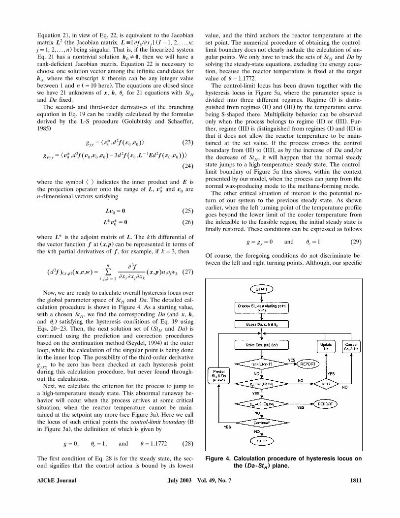
Now, we are ready to calculate overall hysteresis locus overthe global parameter space of St and Da. The detailed cal-Hculation procedure is shown in Figure 4. As a starting value,

Žwith a chosen St , we find the corresponding Da and x, h,H.and � satisfying the hysteresis conditions of Eq. 19 usingc

Ž .Eqs. 20�23. Then, the next solution set of St and Da isHcontinued using the prediction and correction procedures

Ž .based on the continuation method Seydel, 1994 at the outerloop, while the calculation of the singular point is being donein the inner loop. The possibility of the third-order derivativeg to be zero has been checked at each hysteresis pointy y yduring this calculation procedure, but never found through-out the calculations.

Next, we calculate the criterion for the process to jump toa high-temperature steady state. This abnormal runaway be-havior will occur when the process arrives at some criticalsituation, when the reactor temperature cannot be main-

Ž .tained at the setpoint any more see Figure 3a . Here we callŽthe locus of such critical points the control-limit boundary B

.in Figure 3a , the definition of which is given by

gs0, � s1, and �s1.1772 28Ž .c

The first condition of Eq. 28 is for the steady state, the sec-ond signifies that the control action is bound by its lowest

value, and the third anchors the reactor temperature at theset point. The numerical procedure of obtaining the control-limit boundary does not clearly include the calculation of sin-gular points. We only have to track the sets of St and Da byHsolving the steady-state equations, excluding the energy equa-tion, because the reactor temperature is fixed at the targetvalue of �s1.1772.

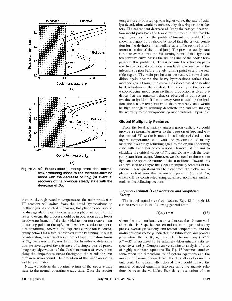
The control-limit locus has been drawn together with thehysteresis locus in Figure 5a, where the parameter space is

Ž .divided into three different regimes. Regime I is distin-Ž . Ž .guished from regimes II and III by the temperature curve

being S-shaped there. Multiplicity behavior can be observedŽ . Ž .only when the process belongs to regime II or III . Fur-

Ž . Ž . Ž .ther, regime III is distinguished from regimes I and II inthat it does not allow the reactor temperature to be main-tained at the set value. If the process crosses the control

Ž . Ž .boundary from II to III , as by the increase of Da androrthe decrease of St , it will happen that the normal steadyHstate jumps to a high-temperature steady state. The control-limit boundary of Figure 5a thus shows, within the contextpresented by our model, when the process can jump from thenormal wax-producing mode to the methane-forming mode.

The other critical situation of interest is the potential re-turn of our system to the previous steady state. As shownearlier, when the left turning point of the temperature profilegoes beyond the lower limit of the cooler temperature fromthe infeasible to the feasible region, the initial steady state isfinally restored. These conditions can be expressed as follows

gs g s0 and � s1 29Ž .y c

Of course, the foregoing conditions do not discriminate be-tween the left and right turning points. Although, our specific

Figure 4. Calculation procedure of hysteresis locus on( )the Da-St plane.H

July 2003 Vol. 49, No. 7AIChE Journal 1811

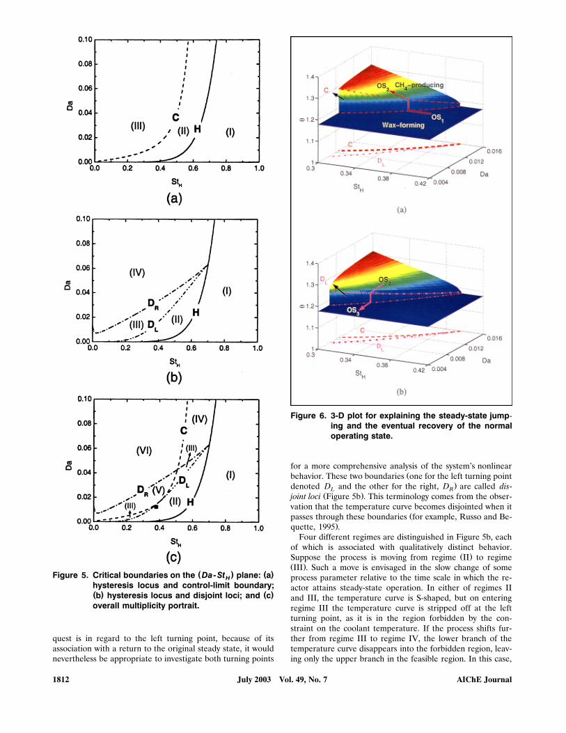
( ) ( )Figure 5. Critical boundaries on the Da- St plane: aHhysteresis locus and control-limit boundary;( ) ( )b hysteresis locus and disjoint loci; and coverall multiplicity portrait.

quest is in regard to the left turning point, because of itsassociation with a return to the original steady state, it wouldnevertheless be appropriate to investigate both turning points

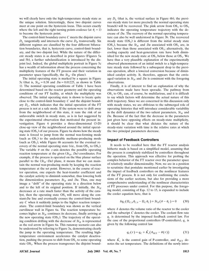
Figure 6. 3-D plot for explaining the steady-state jump-ing and the eventual recovery of the normaloperating state.

for a more comprehensive analysis of the system’s nonlinearŽbehavior. These two boundaries one for the left turning point

.denoted D and the other for the right, D are called dis-L RŽ .joint loci Figure 5b . This terminology comes from the obser-

vation that the temperature curve becomes disjointed when itŽpasses through these boundaries for example, Russo and Be-

.quette, 1995 .Four different regimes are distinguished in Figure 5b, each

of which is associated with qualitatively distinct behavior.Ž .Suppose the process is moving from regime II to regime

Ž .III . Such a move is envisaged in the slow change of someprocess parameter relative to the time scale in which the re-actor attains steady-state operation. In either of regimes IIand III, the temperature curve is S-shaped, but on enteringregime III the temperature curve is stripped off at the leftturning point, as it is in the region forbidden by the con-straint on the coolant temperature. If the process shifts fur-ther from regime III to regime IV, the lower branch of thetemperature curve disappears into the forbidden region, leav-ing only the upper branch in the feasible region. In this case,

July 2003 Vol. 49, No. 7 AIChE Journal1812

we will clearly have only the high-temperature steady state asthe unique solution. Interestingly, these two disjoint curvesmeet at one point on the hysteresis locus. This occurs exactly

Ž .where the left and the right turning points coalesce at � s1cto become the hysteresis point.

The control-limit boundary curve C meets the disjoint curveD tangentially and intersects the curve D transversally. SixL Rdifferent regimes are classified by the four different bifurca-tion boundaries, that is, hysteresis curve, control-limit bound-ary, and the two disjoint loci. While the nature of the differ-

Žent steady states is as described in prior figures Figures 5a.and 5b , a further subclassification is introduced by the dis-

joint loci. Indeed, the global multiplicity portrait in Figure 5chas a wealth of information about the process concerning themultiplicity features of the FT process and their variation in

Ž .parameter space specifically, the St �Da plane .HThe initial operating state is marked by a square in FigureŽ5c that is, St s0.38 and Das0.01225, as shown in TableH

.1 . The nominal operating conditions of Table 1 have beendetermined based on the reactor geometry and the operatingconditions of our FT facility, at which the multiplicity wasobserved. The initial operating state is shown to locate quiteclose to the control-limit boundary C and the disjoint bound-ary D , which indicates that the initial operation of the FTLprocess is not at a safe mode. If the system were to drift awayfrom the neighborhood of this state, it runs the risk of anunfavorable switch in steady state, as is in fact suggested bythe experimental observation that motivated the present in-

Ž .vestigation. Figure 6 provides a three-dimensional 3-Dclose-up view of the neighborhood around the initial operat-

Ž .ing state OS of our process. Figure 6a shows how the steady1state is forced to jump from the normal wax-forming modeŽ .such as OS to the undesirable methane-producing mode1Ž .such as OS , while Figure 6b accounts for the eventual re-2

Ž .covery of the normal operating state viz., from OS to OS .2 3The variable � on the z-axis denotes the possible operating

Ž .reaction temperature at the given St , Da coordinates. ForHexample, if the process is operated on the blue planar surface

Ž .parallel to the St �Da plane, it means that we can main-Htain the normal wax-producing mode by keeping the reactiontemperature at the set point. However, in the course of reac-tor operation, one expects the heat-transfer coefficient andthe catalyst activity to diminish somewhat, thus lowering boththe dimensionless parameters St and Da. Thus, one mayHimage a ‘‘drift’’ of the operating state in a direction belowand to the left of its original position. If initially, the StHdecreases at a rate much faster than the activity of the cata-lyst, then the operating state OS will move along the con-1stant-Da line and eventually crosses the control-limit bound-ary C when it suddenly jumps to the higher reaction temper-ature. The control-limit boundary was shown as the verticalcurvilinear wall in Figure 6a. The reaction temperature be-comes higher as St continues its decrease, finally arriving atH

Ž .the new operating state OS . The trajectory of the operat-2ing condition drifting with the decrease of St is representedHas the red arrow in Figure 6a. This runaway scenario can alsobe understood by referring to Figure 3a, demonstrating clearlythe jump in the operating temperature. The resulting high-temperature environment accelerates the catalyst deactiva-tion, pushing the process to shift from OS to some operating2state OS . When the process transgresses the disjoint bound-3

Ž .ary D that is, the vertical surface in Figure 6b , the previ-LŽous steady state or more precisely the normal operating state

.branch will be recovered. The pink arrow from OS to OS2 3indicates the operating temperature trajectory with the de-crease of Da. The recovery of the normal operating tempera-ture can also be well understood in Figure 3b. The recovered

Ž .steady state OS is different from the initial steady state3Ž .OS , because the St and Da associated with OS are, in1 H 3fact, lower than those associated with OS ; alternatively, the1cooling capacity and heat-generation rate have both dimin-ished for the new steady state at OS below those at OS . We3 1have thus a very plausible explanation of the experimentallyobserved phenomenon of an initial switch to a high-tempera-ture steady state followed by a subsequent drop to the previ-ous operation, albeit a lowered conversion because of dimin-ished catalyst activity. It, therefore, appears that the envis-aged variation in St and Da is consistent with the foregoingHobservations.

Finally, it is of interest to find an explanation of why theobservations made have been sporadic. The pathway fromOS to OS can, of course, be multifarious, and it is difficult1 3to say which factors will determine the actual nature of thisdrift trajectory. Since we are concerned in this discussion onlywith steady states, we are oblivious to the submerged role ofoperating histories that will introduce considerable variabilityin the drift dynamics of the two salient parameters, St andHDa. Because of the fact that the decrease in the parametersjust given have opposing effects on steady-state multiplicity,it should be clear that what dictates the nature of thesteady-state variation with time is the relative rates at whichthe two principal parameters decrease.

Impact of Feedback ControllersIt needs to be recalled here that the FT reactor analysis

hitherto made is based on a simplified model, assuming thatthe process is completely stabilized by controllers throughoutthe operation. This approach was effective for probing thecomplex behavior of the FT reactor over the parameter spaceof relatively smaller dimensionality. Now, we are in a positionto scrutinize that postulate mentioned earlier by investigatingthe impact of feedback controllers on the nonlinear featuresof the FT process. It is not only for confirming the conclu-sions of the earlier sections, but also for providing a morecomprehensive understanding of the nonlinear characteristicsof FT processes under control. For this purpose, the forego-ing model, consisting of Eqs. 12 to 15, is expanded to includethe cooler equation here, that is

q � � y� � qSt �y� s0 30Ž .Ž . Ž .C C ,0 C ,0 C C H C

where denotes the volume ratio of the reactor to the coolerand the subscript C denotes the cooler. The coolant flow rateq is determined by the imposed feedback control law. Forc

Ž .the case of the proportional controllers P-controllers , q iscgiven by the following control law

˜q � sq qK � y� � 31Ž . Ž . Ž .Ž .C C c SET

˜where K is the control gain of P-controller, and � de-c SETnotes the set temperature. The definitions of the newly intro-

July 2003 Vol. 49, No. 7AIChE Journal 1813

duced dimensionless parameters in Eqs. 30 and 31 are shownbelow, and their nominal values are also given in Table 1

C CC ,0 pC ,0 C pC� s , � sC ,0 C C CL pL L pL

V KC˜ s , K s 32Ž .CV Q rTC G ,0 C ,0

For the sake of convenience, we call the models withoutand with the cooler equation the ten-state and ele®en-statemodel, respectively, in the same way that Russo and Be-

Ž .quette 1995 did. In the ten-state model, the coolant temper-ature � is directly regarded as the manipulated variable toccontrol the reaction temperature, and it is also treated as thebifurcation parameter to search bifurcation points in nonlin-ear analysis. In the ele®en-state model, on the other hand, thecoolant flow rate, q , is employed as the manipulated vari-cable and also as the bifurcation parameter, while � subse-cquently becomes a state variable, which is a more realisticsituation.

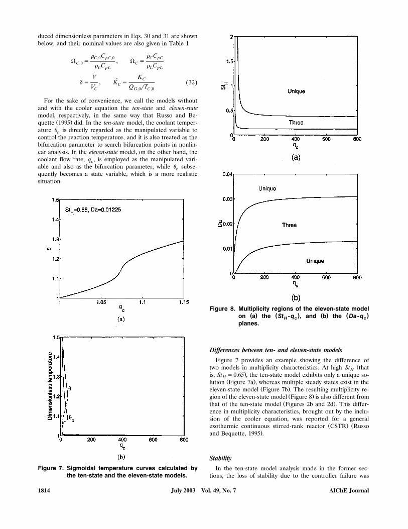
Figure 7. Sigmoidal temperature curves calculated bythe ten-state and the eleven-state models.

Figure 8. Multiplicity regions of the eleven-state model( ) ( ) ( ) ( )on a the St -q , and b the Da-qH c c

planes.

Differences between ten- and ele©en-state modelsFigure 7 provides an example showing the difference of

Žtwo models in multiplicity characteristics. At high St thatH.is, St s0.65 , the ten-state model exhibits only a unique so-H

Ž .lution Figure 7a , whereas multiple steady states exist in theŽ .eleven-state model Figure 7b . The resulting multiplicity re-

Ž .gion of the eleven-state model Figure 8 is also different fromŽ .that of the ten-state model Figures 2b and 2d . This differ-

ence in multiplicity characteristics, brought out by the inclu-sion of the cooler equation, was reported for a general

Ž . Žexothermic continuous stirred-rank reactor CSTR Russo.and Bequette, 1995 .

StabilityIn the ten-state model analysis made in the former sec-

tions, the loss of stability due to the controller failure was

July 2003 Vol. 49, No. 7 AIChE Journal1814

ruled out among possible causes responsible for the observedsteady-state shift. In order to verify the preceding postulate,it seems important to assure the existence of finite values forthe control parameters capable of safely keeping the processstable during operation. More specifically, it is determined

˜here that the controller gain, K , of the P-controller for sta-Cbilizing the process is within the reasonable range for physi-cal implementation. If it is shown that the process is stabi-lized even by P-controllers, we can say that the stability wouldbe much more easily achieved when PI- or PID-controllersare employed.

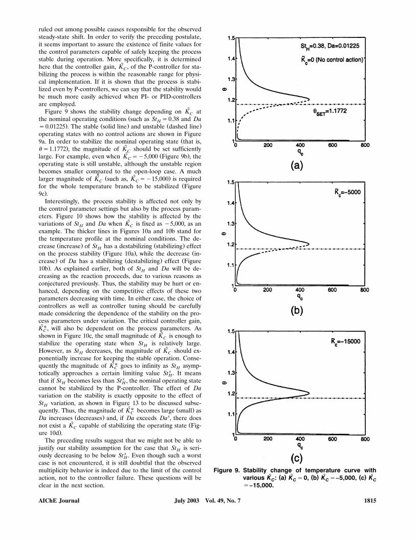
˜Figure 9 shows the stability change depending on K atCŽthe nominal operating conditions such as St s0.38 and DaH

. Ž . Ž .s0.01225 . The stable solid line and unstable dashed lineoperating states with no control actions are shown in Figure

Ž9a. In order to stabilize the nominal operating state that is,˜.�s1.1772 , the magnitude of K should be set sufficientlyC˜ Ž .large. For example, even when K sy5,000 Figure 9b , theC

operating state is still unstable, although the unstable regionbecomes smaller compared to the open-loop case. A much

˜ ˜Ž .larger magnitude of K such as, K sy15,000 is requiredC CŽfor the whole temperature branch to be stabilized Figure

.9c .Interestingly, the process stability is affected not only by

the control parameter settings but also by the process param-eters. Figure 10 shows how the stability is affected by the

˜variations of St and Da when K is fixed as y5,000, as anH Cexample. The thicker lines in Figures 10a and 10b stand forthe temperature profile at the nominal conditions. The de-

Ž . Ž .crease increase of St has a destabilizing stabilizing effectHŽ . Žon the process stability Figure 10a , while the decrease in-

. Ž . Žcrease of Da has a stabilizing destabilizing effect Figure.10b . As explained earlier, both of St and Da will be de-H

creasing as the reaction proceeds, due to various reasons asconjectured previously. Thus, the stability may be hurt or en-hanced, depending on the competitive effects of these twoparameters decreasing with time. In either case, the choice ofcontrollers as well as controller tuning should be carefullymade considering the dependence of the stability on the pro-cess parameters under variation. The critical controller gain,˜�K , will also be dependent on the process parameters. AsC

˜shown in Figure 10c, the small magnitude of K is enough toCstabilize the operating state when St is relatively large.H

˜However, as St decreases, the magnitude of K should ex-H Cponentially increase for keeping the stable operation. Conse-

˜�quently the magnitude of K goes to infinity as St asymp-C Htotically approaches a certain limiting value St s . It meansHthat if St becomes less than St s , the nominal operating stateH Hcannot be stabilized by the P-controller. The effect of Davariation on the stability is exactly opposite to the effect ofSt variation, as shown in Figure 13 to be discussed subse-H

˜� Ž .quently. Thus, the magnitude of K becomes large small asCŽ . sDa increases decreases and, if Da exceeds Da , there does

˜ Žnot exist a K capable of stabilizing the operating state Fig-C.ure 10d .

The preceding results suggest that we might not be able tojustify our stability assumption for the case that St is seri-Hously decreasing to be below St s . Even though such a worstHcase is not encountered, it is still doubtful that the observedmultiplicity behavior is indeed due to the limit of the controlaction, not to the controller failure. These questions will beclear in the next section.

Figure 9. Stability change of temperature curve with˜ ˜ ˜ ˜( ) ( ) ( )various K : a K s0, b K s–5,000, c KC C C C

s–15,000.

July 2003 Vol. 49, No. 7AIChE Journal 1815

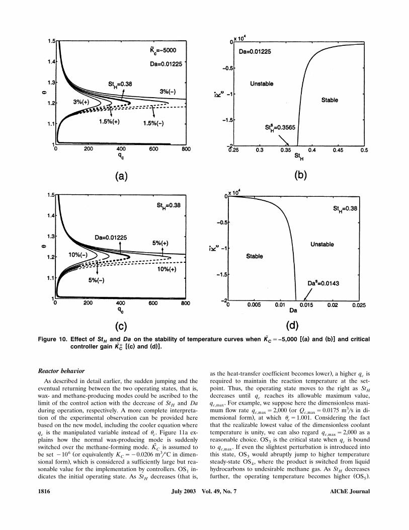
˜ [( ) ( )]Figure 10. Effect of St and Da on the stability of temperature curves when K s–5,000 a and b and criticalH C˜� [( ) ( )]controller gain K c and d .C

Reactor beha©iorAs described in detail earlier, the sudden jumping and the

eventual returning between the two operating states, that is,wax- and methane-producing modes could be ascribed to thelimit of the control action with the decrease of St and DaHduring operation, respectively. A more complete interpreta-tion of the experimental observation can be provided herebased on the new model, including the cooler equation whereq is the manipulated variable instead of � . Figure 11a ex-c cplains how the normal wax-producing mode is suddenly

˜switched over the methane-forming mode. K is assumed toC6 Ž 3be set y10 or equivalently K sy0.0206 mr�C in dimen-C.sional form , which is considered a sufficiently large but rea-

sonable value for the implementation by controllers. OS in-1Ždicates the initial operating state. As St decreases that is,H

.as the heat-transfer coefficient becomes lower , a higher q iscrequired to maintain the reaction temperature at the set-point. Thus, the operating state moves to the right as StHdecreases until q reaches its allowable maximum value,cq . For example, we suppose here the dimensionless maxi-c,max

Ž 3mum flow rate q s2,000 or Q s0.0175 mrs in di-c,max c,max.mensional form , at which � s1.001. Considering the factc

that the realizable lowest value of the dimensionless coolanttemperature is unity, we can also regard q s2,000 as ac,maxreasonable choice. OS is the critical state when q is bound3 cto q . If even the slightest perturbation is introduced intoc,maxthis state, OS would abruptly jump to higher temperature3steady-state OS , where the product is switched from liquid4hydrocarbons to undesirable methane gas. As St decreasesH

Ž .further, the operating temperature becomes higher OS .5

July 2003 Vol. 49, No. 7 AIChE Journal1816

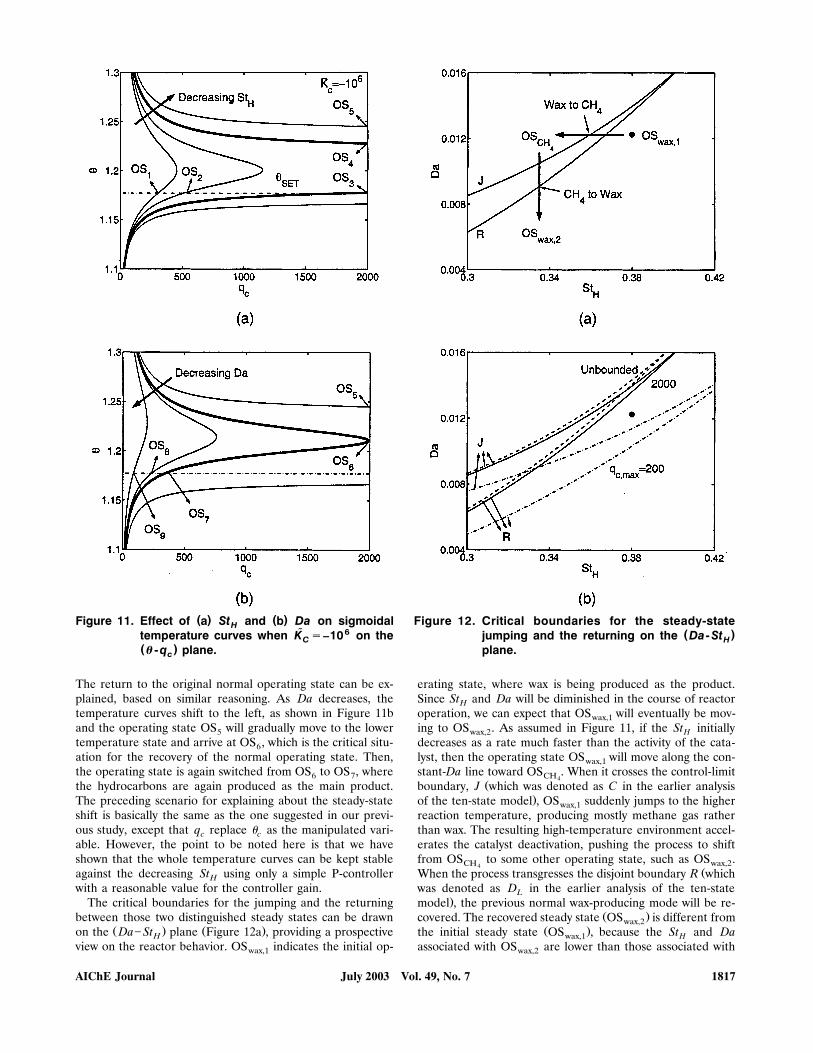
( ) ( )Figure 11. Effect of a St and b Da on sigmoidalH˜ 6temperature curves when K s–10 on theC

( )� -q plane.c

The return to the original normal operating state can be ex-plained, based on similar reasoning. As Da decreases, thetemperature curves shift to the left, as shown in Figure 11band the operating state OS will gradually move to the lower5temperature state and arrive at OS , which is the critical situ-6ation for the recovery of the normal operating state. Then,the operating state is again switched from OS to OS , where6 7the hydrocarbons are again produced as the main product.The preceding scenario for explaining about the steady-stateshift is basically the same as the one suggested in our previ-ous study, except that q replace � as the manipulated vari-c cable. However, the point to be noted here is that we haveshown that the whole temperature curves can be kept stableagainst the decreasing St using only a simple P-controllerHwith a reasonable value for the controller gain.

The critical boundaries for the jumping and the returningbetween those two distinguished steady states can be drawn

Ž . Ž .on the Da� St plane Figure 12a , providing a prospectiveHview on the reactor behavior. OS indicates the initial op-wax,1

Figure 12. Critical boundaries for the steady-state( )jumping and the returning on the Da- StH

plane.

erating state, where wax is being produced as the product.Since St and Da will be diminished in the course of reactorHoperation, we can expect that OS will eventually be mov-wax,1ing to OS . As assumed in Figure 11, if the St initiallywax,2 Hdecreases as a rate much faster than the activity of the cata-lyst, then the operating state OS will move along the con-wax,1stant-Da line toward OS . When it crosses the control-limitCH4

Žboundary, J which was denoted as C in the earlier analysis.of the ten-state model , OS suddenly jumps to the higherwax,1

reaction temperature, producing mostly methane gas ratherthan wax. The resulting high-temperature environment accel-erates the catalyst deactivation, pushing the process to shiftfrom OS to some other operating state, such as OS .CH wax,24

ŽWhen the process transgresses the disjoint boundary R whichwas denoted as D in the earlier analysis of the ten-stateL

.model , the previous normal wax-producing mode will be re-Ž .covered. The recovered steady state OS is different fromwax,2

Ž .the initial steady state OS , because the St and Dawax,1 Hassociated with OS are lower than those associated withwax,2

July 2003 Vol. 49, No. 7AIChE Journal 1817

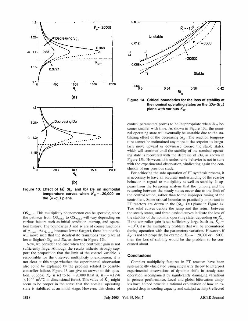
( ) ( )Figure 13. Effect of a St and b Da on sigmoidalH˜temperature curves when K s–20,000 onC

( )the � -q plane.c

OS . This multiplicity phenomenon can be sporadic, sincewax,1the pathway from OS to OS will vary depending onwax,1 wax,2various factors such as initial condition, startup, and opera-tion history. The boundaries J and R are of course functions

Ž .of q . As q becomes lower larger , those boundariesc,max c,maxwill move such that the steady-state transitions take place at

Ž .lower higher St and Da, as shown in Figure 12b.HNow, we consider the case when the controller gain is not

sufficiently large. Although the results hitherto strongly sup-port the proposition that the limit of the control variable isresponsible for the observed multiplicity phenomenon, it isnot clear at this stage whether the experimental observationalso could be explained by the problem related to possiblecontroller failure. Figure 13 can give an answer to this ques-

˜ Žtion. Suppose K is set to be y20,000 that is, K s4.1298C Cy4 3 ˜.�10 mr�C in dimensional form . This value of K mightC

seem to be proper in the sense that the nominal operatingstate is stabilized at an initial stage. However, this choice of

Figure 14. Critical boundaries for the loss of stability at( )the nominal operating states on the Da- StH

˜plane with various K .C

control parameters proves to be inappropriate when St be-Hcomes smaller with time. As shown in Figure 13a, the nomi-nal operating state will eventually be unstable due to the sta-bilizing effect of the decreasing St . The reaction tempera-Hture cannot be maintained any more at the setpoint to irregu-larly move upward or downward toward the stable states,which will continue until the stability of the nominal operat-ing state is recovered with the decrease of Da, as shown inFigure 13b. However, this undesirable behavior is not in tunewith the experimental observation, vindicating again the con-clusion of our previous study.

For achieving the safe operation of FT synthesis process, itis necessary to have an accurate understanding of the reactorbehavior in regard to multiplicity as well as stability. It ap-pears from the foregoing analysis that the jumping and thereturning between the steady states occur due to the limit ofthe control action, rather than to the improper tuning of thecontrollers. Some critical boundaries practically important in

Ž .FT reactors are drawn in the St �Da plane in Figure 14.HTwo solid curves denote the jump and the return betweenthe steady states, and three dashed curves indicate the loss of

˜the stability of the nominal operating state, depending on K .C˜ŽIf the controller gain is set sufficiently large such as, K sC

6.y10 , it is the multiplicity problem that will be encounteredduring operation with the parameters variation. However, if˜ ˜K is not set properly, for example, K sy20,000 or y5000,C Cthen the loss of stability would be the problem to be con-cerned about.

ConclusionsComplex multiplicity features in FT reactors have been

systematically elucidated using singularity theory to interpretexperimental observations of dynamic shifts in steady-stateoperation accompanied by significantly damaging variationsin process performance. Local and global bifurcation analy-ses have helped provide a rational explanation of how an ex-

Žpected drop in cooling capacity and catalyst activity reflected

July 2003 Vol. 49, No. 7 AIChE Journal1818

.in the decrease of the parameters St and Da with timeHcould be the plausible causes for the observed multiplicitybehaviors in our FT system. Variations of these two parame-ters have opposite effects on the multiplicity. The decrease of

ŽSt may cause the initial steady state that is, nominal wax-H.producing mode to be switched over to the high-tempera-

Ž .ture state that is, undesirable methane-producing mode bydecreasing the cooling capacity of the cooler. The eventualrecovery of the earlier steady state is attributed to the de-crease of Da by deactivation of catalysts. From the globalbifurcation diagram constructed based on the L-S reductionand the singularity theory, the sporadic nature of suchsteady-state transitions can be understood. The relative ratesat which the parameters St and the Da decrease would de-Htermine the nature of the steady-state shifts observed in theFT reactor. This relative rate is clearly a function of transienteffects associated with both startup and approach to steadystates during shifts.

The preceding conclusions are corroborated as well whenthe dynamics of the cooler is considered in the bifurcationanalysis of the process. Taking P-controller as an example,we could show that the observed multiplicity behavior is in-deed not due to the loss of stability by poor tuning. It is alsorevealed that the process stability is impaired as St de-Hcreases but enforced as Da decreases, but there exists a rea-sonable range of the controller gain capable of stabilizing theprocess in spite of the deleterious effect on stability of thedecreasing St during operation. In order to guarantee theHsafe operation of FT reactors, therefore, the choice of thecontrollers and control parameter settings should be carefullymade, considering the dependence of the stability on the pro-cess parameter variations during operation.

AcknowledgmentSincere gratitude is expressed to Conoco Inc., which provided fi-

nancial support for this research.

Notationa scatalyst activitycatC sconcentration of species j in gas phaseG j

C sinlet concentration of species j in gas phaseG j,0C sconcentration of species j in slurry phaseL jC sheat capacity of gas phasepG

C sheat capacity of gas at the inlet conditionspG ,0C sheat capacity of slurry phasepLK scontroller gainC

Esactivation energyh a soverall heat transfer coefficient per unit volumeC C

He sHenry’s constant for species jjŽ .y� H sheat of reaction per unit mole of COR

ksreaction rate constant of Eq. 8Ksreaction constant of Eq. 8

Ž .k a smass-transfer coefficient per unit volume for species jL jPspressure of the system

Q svolumetric flow rate of the gas phaseGQ sinlet volumetric flow rate of the gas phaseG ,0

Rschemical reaction rate defined by Eq. 8 or universal gasconstant

Tsreaction temperatureT scoolant temperatureC

T sinlet coolant temperatureC ,0T sinlet gas temperatureG ,0

Vsreactor volume

V scooler volumeCwscatalyst loading in slurry

Greek letters� sgas holdup ratioG� sstoichiometric coefficient for species jj

� sdensity of gas phaseG� sdensity of gas phase at the inlet conditionsG ,0

� sdensity of slurry phaseL

Literature CitedBalakotaiah, V., and D. Luss, ‘‘Analysis of the Multiplicity Patterns

Ž .of a CSTR,’’ Chem. Eng. Commun., 13, 111 1981 .Balakotaiah, V., and D. Luss, ‘‘Multiplicity Features of Reacting Sys-

tems: Dependence of the Steady-States of a CSTR on the Resi-Ž .dence Time,’’ Chem. Eng. Sci., 38, 1709 1983 .

Balakotaiah, V., and D. Luss, ‘‘Global Analysis of the MultiplicityFeatures of Multi-Reaction Lumped-Parameter Systems,’’ Chem.

Ž .Eng. Sci., 39, 865 1984 .Balakotaiah, V., D. Luss, and B. L. Keyfitz, ‘‘Steady State Multiplic-

ity Analysis of Lumped-Parameter Systems Described by a Set ofŽ .Algebraic Equations,’’ Chem. Eng. Commun., 36, 121 1985 .

Bhattacharjee, S., J. W. Tierney, and Y. T. Shah, ‘‘Thermal Behaviorof a Slurry Reactor: Application to Synthesis Gas Conversion,’’ Ind.

Ž .Eng. Chem. Process Des. De®., 25, 117 1986 .Bukur, D. B., and R. F. Brown, ‘‘Fischer-Tropsch Synthesis in a

Stirred Tank Slurry Reactor�Reaction Rates,’’ Can. J. Chem.Ž .Eng., 65, 604 1987 .

Bukur, D. B., L. Nowicki, and X. Lang, ‘‘Fischer-Tropsch SynthesisŽ .in a Stirred Tank Slurry Reactor,’’ Chem. Eng. Sci., 49, 4615 1994 .

Farr, W. W., and R. Aris, ‘‘Yet Who Would Have Thought the OldMan to Have Had so Much Blood in Him?�Reflections on theMultiplicity of Steady States of the Stirred Tank Reactor,’’ Chem.

Ž .Eng. Sci., 41, 1385 1986 .Gilmore, R., Catastrophe Theory for Scientists and Engineers, Dover,

Ž .New York 1981 .Golubitsky, M., and B. L. Keyfitz, ‘‘A Qualitative Study of the

Steady-State Solutions for a Continuous Flow Stirred Tank Chemi-Ž .cal Reactor,’’ SIAM J. Math Anal., 11, 316 1980 .

Golubitsky, M., and D. G. Schaeffer, ‘‘A Theory for Imperfect Bifur-cation via Singularity Theory,’’ Commun. Pure Appl. Math., 32, 21Ž .1979 .

Golubitsky, M., and D. G. Schaeffer, Singularities and Groups in Bi-Ž .furcation Theory, Vol. I, Springer-Verlag, New York 1985 .

Gormley, R. J., M. F. Zarochak, P. W. Deffenbaugh, and K. R. P. M.Rao, ‘‘Effect of Initial Wax Medium on the Fischer-Tropsch Slurry

Ž .Reaction,’’ Appl. Catal. A, 161, 263 1997 .Hilmen, A. M., D. Schanke, K. F. Hanssen, and A. Holmen, ‘‘Study

of the Effect of Water on Alumina Supported Cobalt Fischer-Ž .Tropsch Catalysts,’’ Appl. Catal. A, 186, 169 1999 .

Kirillov, V. A., V. M. Khanaev, V. D. Meshcheryakov, S. I. Fadeev,and R. G. Luk’yanova, ‘‘Numerical Analysis of Fischer-TropschProcesses in Reactors with a Slurried Catalyst Bed,’’ Theor. Found.

Ž .Chem. Eng., 33, 270 1999 .Liu, Z.-T., Y.-W. Li, J.-L. Zhou, Z.-X. Zhang, and B.-J. Zhang,

‘‘Deactivation Model of Fischer-Tropsch Synthesis over an Fe-Cu-Ž .K Commercial Catalyst,’’ Appl. Catal. A, 161, 137 1997 .

Lox, E. S., and G. F. Froment, ‘‘Kinetics of the Fischer-Tropsch Re-action on a Precipitated Promoted Iron Catalyst. 1. Experimental

Ž .Procedure and Results,’’ Ind. Eng. Chem. Res., 32, 61 1993a .Lox, E. S., and G. F. Froment, ‘‘Kinetics of the Fischer-Tropsch Re-

action on a Precipitated Promoted Iron Catalyst. 2. Kinetic Model,’’Ž .Ind. Eng. Chem. Res., 32, 71 1993b .

Maretto, C., and R. Krishna, ‘‘Modelling of a Bubble Column SlurryReactor for Fischer-Tropsch Synthesis,’’ Catal. Today, 52, 279Ž .1999 .

Russo, L. P., and B. W. Bequette, ‘‘Impact of Process Design on theMultiplicity Behavior of a Jacketed Exothermic CSTR,’’ AIChE J.,

Ž .41, 135 1995 .Satterfield, C. N., and G. A. Huff, Jr., ‘‘Mass Transfer and Product

Selectivity in a Mechanically Stirred Fischer-Tropsch Slurry Reac-Ž .tor,’’ ACS Symp., 196, 225 1982 .

July 2003 Vol. 49, No. 7AIChE Journal 1819

Seydel, R., Practical Bifurcation and Stability Analysis: From Equilib-Ž .rium To Chaos, Springer-Verlag, New York 1994 .

Shah, Y. T., C. G. Dassori, and J. W. Tierney, ‘‘Multiple SteadyStates in Non-Isothermal FT Slurry Reactor,’’ Chem. Eng. Com-

Ž .mun., 88, 49 1990 .Song, H.-S., D. Ramkrishna, S. Trinh, R. L. Espinoza, and H. Wright,

‘‘Multiplicity and Sensitivity Analysis of Fischer-Tropsch BubbleColumn Slurry Reactors: Plug-Flow Gas and Well-Mixed Slurry

Ž . Ž .Model,’’ Chem. Eng. Sci., 58, 12 , 2759 2003 .Stern, D., A. T. Bell, and H. Heinemann, ‘‘A Theoretical Model for

the Performance of Bubble-Column Reactors Used for Fischer-Ž .Tropsch Synthesis,’’ Chem. Eng. Sci., 40, 1665 1985 .

Van Der Laan, G. P., and A. A. C. M. Beenackers, ‘‘Kinetics andSelectivity of the Fischer-Tropsch Synthesis: A Literature Review,’’

Ž .Catal. Re®.� Sci. Eng., 41, 255 1999 .Withers, H. P., K. F. Eliezer, and J. W. Mitchell, ‘‘Slurry-Phase Fis-

cher-Tropsch Synthesis and Kinetic Studies over Supported CobaltŽ .Carbonyl Derived Catalysts,’’ Ind. Eng. Chem. Res., 29, 1807 1990 .

Yermakova, A., and V. I. Anikeev, ‘‘Thermodynamic Calculations inthe Modeling of Multiphase Processes and Reactors,’’ Ind. Eng.

Ž .Chem. Res., 39, 1453 2000 .

Manuscript recei®ed June 19, 2002, re®ision recei®ed Jan. 23, 2003, and finalre®ision recei®ed Mar. 17, 2003.

July 2003 Vol. 49, No. 7 AIChE Journal1820