Did Frederick Brodie Discover

the World’s First Environmental Kuznets Curve,

and If So, Why Should Anyone Really Care?

Karen Clay

Carnegie Mellon University

and

Werner Troesken

University of Pittsburgh & NBER

1According to Brazell (1968, p. 102), meteorologists did not construct a standardized

definition of fog “until the development of aviation after the First World War.”

1

0. Introduction

In 1903, at a meeting of the Royal Meteorological Society, a British climatologist named

Frederick J. Brodie presented a deceptively simple paper. Using data from the Brixton weather

station in London, Brodie graphed the number foggy days per year between 1871 and 1903.

His data, reproduced here in figure 1, revealed an inverted U-shaped pattern: the annual

number of foggy days in London rose during the 1870s and 1880s; reversed trend sometime

around 1888 or 1889; and then fell steadily during the 1890s and early 1900s. Brodie attributed

the rise and fall of the London fog to variation in the production of coal smoke. During the

1870s and 80s, Brodie claimed, London businesses and homeowners burned coal with reckless

abandon, filling the atmosphere with soot and giving rise to dense and dark fogs. After 1890,

however, technological, legal, and social changes enabled, or forced, homeowners and

businesses to burn coal more efficiently and cleanly. In particular, the expansion of gas for

heating and cooking, and electricity for lighting curtailed domestic sources of smoke; and the

London Coal Smoke Abatement Society lobbied local authorities to enforce the Public Health

Acts which required manufacturers to adopt low-smoke technologies (Brodie 1905, pp. 15-20).

The criticisms of Brodie’s paper were many. Multiple observers argued that the series

Brodie had assembled was not believable because it focused on a single weather station, and

fog data were based on subjective, non-instrumental observations. Brodie himself did not

define what exactly was meant when a day was recorded as “foggy.”1 Were other weather

2

stations in London revealing the same trend? Were other, more objective measures consistent

with the reported decline in fog? If not, one could not even believe the underlying pattern

Brodie was trying to explain, let alone his contentious interpretation. Other critics argued that

changing wind speeds and directions could account for the rise and fall of the fog, in part

because fog does not usually form in windy environments. H.L. Mill focused on the changing

relationship between rainfall and fogs during the 1880s and on variation in atmospheric

conditions over time. Another discussant wondered how the environs of London could

possibly have been becoming less smokey over time, given the rapid growth in the city’s

population and manufacturing base. J.E. Clark believed one could ascribe at least part of the

pattern observed by Brodie to the eruption of Krakatoa in Java in 1883, which had significant

and lasting meteorological effects all over the globe. Clark seemed to suggest that Krakatoa

might account for the increase in atmospheric haze in the immediate aftermath of the eruption,

and also explain the decline in haze as the effects dissipated (Brodie 1905, pp. 21-27).

In this paper, we reconsider Brodie’s data and his interpretation of those data.

Specifically, we want to ask whether independent sources of evidence indicate smoke-induced

changes in London’s atmosphere over the course of the nineteenth and early twentieth century.

Besides Brixton, do other London weather stations record a similar rise and fall in foggy days

per annum? Do other measures of atmospheric conditions, such as hours of bright sunlight,

also indicate improvement in London after 1890? Similarly, if London’s air were becoming less

polluted with coal smoke after 1890, this would have manifested itself in effects on human

health, particularly deaths from respiratory diseases. To the extent that other sources of

2Ideally, we would like to get data on wind speed and direction, as well as the

occurrence of anticyclones, a condition of extreme stillness that often produced fog,

independent of the level of smoke in the air. Unfortunately, after much search, we have been

unable to find such data. Nevertheless, some of the data and evidence we present below will

provide indirect and qualitative information on the evolution of wind speed and the formation

of fog in London.

3

evidence corroborate Brodie’s basic finding—that the incidence of fog and smoke in London

was rising before 1890 and declining thereafter—we need to turn to Brodie’s interpretation of

that finding and ask why the atmosphere changed over time. Three sorts of evidence will be

considered. First, if smoke abatement efforts really were causing Londoners to burn coal more

efficiently and adopt (relatively) smokeless technologies such as gas and electricity, this should

be observable in data on coal consumption per capita and in data on gas and electricity

production. Second, we will construct a crude panel of cities and ask whether smoke

abatement interventions in those cities also reduced pollution levels as manifested in deaths

from respiratory diseases. Third, we will present a brief history of smoke abatement

technologies and the enforcement of pollution control laws during the Victorian and

Edwardian eras. This history will help establish a circumstantial case, for or against, the

proposition that such actions helped make London a less smoky place.2

The ostensible rise and fall of the London fog should interest economists and economic

historians on at least two levels. First, the debate surrounding Brodie’s paper prefigures

current debates about the Environmental Kuznets Curve (EKC). Indeed, if Brodie’s data and

interpretations prove sound, he identified an archaic EKC. The construction of this early EKC

might suggest pathways for studying the long-term evolution of the environment and

3See, however, List and Gallet (1999) who employ data on sulphur emissions in

American states back to 1929.

4

environmental regulation. Other than a few metrics of water quality (e.g., bacteria counts and

nitrate concentrations), governments before 1950 did not usually measure and report data on

greenhouse gas emissions, air quality, or any of the inorganic environmental pollutants that

interest us today.3 One solution to this problem is to search for data that might serve as a

proxy for environmental pollution. This paper provides, as far as we are aware, the first

systematic attempt to implement and evaluate such proxies, in this case data on fogs and death

rates. Along the same lines, when economists estimate the shape of the EKC, they must rely on

cross-sections or very short time series from the late-twentieth century. While there is a

venerable tradition of inferring the time series from cross-sectional relationships (e.g., Deaton

and Paxson 1994), recent empirical work suggests that such exercises are problematic in the

context of the EKC (e.g., Deacon and Norman 2006; and De Bruyn 1997). A true historical time

series would therefore be desirable. Documenting efforts by Western governments at an early

stage of development to regulate coal smoke, this paper provides the beginnings of such a time

series and helps to resolve some fundamental questions about the meaning of the EKC.

Second, the basic question Brodie raised and attempted to answer is of no small

historical moment: how could there have been a meaningful environmental movement in

Victorian England? It seems a stretch. Smoke abatement technologies strike most of us as a

distinctly late-twentieth century invention. Aside from a wholesale switch from coal to natural

gas (which did not happen), what could be done in 1890 to reduce coal smoke? Whatever the

4This paper spans the Victorian (1837-1901) and Edwardian (1901-1910) eras. As we

show later, however, most of the interesting activity in terms of regulations, climate, and

technology were products of the Victorian period.

5

available technology, surely it must have been much less efficient and more costly than today’s

abatement methods. How could a country that in 1890 was not much more wealthy than

Mexico today, afford such an investment? The politics too seems all wrong. We tend to think

of Victorian Britain as a place where the expedience of cholera and child labor trumped the

expense of clean water and a decent wage, as a place where environmental and social

degradation served as the handmaidens of avarice and economic development. Yet Brodie’s

paper suggests something quite different, as does even a cursory look at the political and

economic history of smoke abatement. How can one reconcile all of this? There is, in short,

much history to write and revise if Brodie turns out to be right, even partially right.4

1. What Was the London Fog?

The immediate causes of the London fog were evocatively described by the renowned

nineteenth-century scientist Rollo Russell. According to Russell, the London fog began early in

the morning around 6 a.m., when the city, or parts of the city, were enveloped by an “ordinary

thick white fog.” Soon after this, the city would awaken by lighting “about a million fires.”

These fires charged the atmosphere with “carbonaceous particles,” which upon cooling,

attached themselves to the spheres of water that constituted the fog. Ordinarily the warmth of

the sun would have quickly dissipated the fog, but the smoke and an oily tar that surrounded

the spheres of water impaired this process. In these conditions, city residents would not have

5This passage quoting Russell is from Hann’s (1903) Handbook of Climatology , p. 78.

6Russell (1891, p. 11) wrote: “The dust always present in the atmosphere offers this free

surface to the gaseous water, and thus induces its condensation. This specific action of dust

varies very considerably, first with regards to its composition, and second with regard to the

size and abundance of the particles present. Sulphur burnt in the air is a most active fog

producer, so is salt.” For a similar statement regarding the origins and persistence of smoke-

laden fogs, see Frankland (1882).

6

sunlight until noon.5 In an article in Nature, W.J. Russell (1891, p. 11) developed a similar line

of thought, arguing that coal and sulphur particles induced the formation of fog by offering

gaseous water a surface on which to condensate.6 Late twentieth century scientists concur. For

example, Brazell (1968, p. 102) writes: “London fogs are particularly obnoxious because the fog

droplets tend to form on minute particles of atmospheric pollution which are usually produced

by the combustion of coal, oil, and petrol.”

While most of us use the word smog to describe the “cocktail of motor exhaust gases

catalysed by sunlight and typically found over Los Angeles,” the word is actually the product

of nineteenth-century thinking about the unholy merger of smoke and fog. The person who

first coined the term, or at least claimed credit for doing so, was H.A. Des Voeux, the Treasurer

of the London Coal Smoke Abatement Society. In a letter to the Times (Dec. 27, 1904, p. 11), Des

Voeux wrote that he wished to call London’s fog problem by the name “smog” to show that it

consisted “more of smoke than of true fog.” Des Voeux believed that ordinary fogs were

caused by the condensation moisture and that nothing could be done to eliminate them. Smog,

on the other hand, was a different matter entirely. “Fog,” Des Voeux wrote, was “incurable

and infrequent” while “smog” was “curable and frequent.” Brodie (1905, p. 20) expressed the

7

same sentiment when he wrote colorfully about the benefits of an atmosphere purged of

smoke: “With cleaner air . . . there is little doubt that fogs would diminish in frequency, and

even when they did arise, the vapour particles would not be impregnated, as they are now, by

the pestilential products arising from an imperfect and wasteful consumption of fuel.”

With or without the coal smoke, though, London would have been subjected to much

ordinary fog. Describing London as “incorrigible” from a “meteorological point of view,”

Brodie argued that the city’s geography and proximity to a large river made it “eminently

favorable to the development of fog and mist.” There were also more direct climatological

factors. Two government reports issued in the early 1900s showed that the formation of fog in

London was correlated with temperature, humidity, and wind-speed. Fogs were much more

likely when the temperature in the city was below 40 degrees (no dense fog was observed

when temperature was above 40), when humidity was high, and when the winds were calm.

London fogs, these reports concluded, were of indigenous origin; they were not blown in from

the countryside or nearby marshes, as many suggested. There was also a surprising inversion

of temperatures during the most intense fogs. An article in Nature (April 9, 1903, p. 549)

explained: “On March 7, during fog, the temperature in the streets of London was nearly 10° F.

below that on the roof of the Meteorological Office, the elevated stations, and the surrounding

country on the southern and western sides.”

Britain’s “latitudinal and continental position” was of special importance, because it left

the whole country in the path of sequences of “migratory depressions” and anticyclones

(Chandler 1965, p. 35). Anticyclones, and the temperature inversions that accompanied them,

8

played a central role in the propagation of a certain kind of London fog. A short article in the

journal Notes and Queries (March 2, 1878, p. 178) provides the clearest contemporary statement

we have found on the significance of anticyclones. We quote it in full:

These fogs are not caused by the rarefaction of the air, or by the

consumption of gas, nor yet by the hills on the north, nor by the river.

The peculiar atmospheric condition termed an anti-cyclone is the real

cause of these annoying visitations; the wind is then blowing round a

well defined circle, in the centre of which the air is tranquil, and

consequently the smoke, condensed vapours, & c., cannot escape as they

do when there is a direct onward movement of the wind. The pressure

of the atmosphere at such times is almost invariably greatly in excess of

the average in the midst of the anti-cyclone, which, by preventing the

rise of the smoke, & c., increases the intensity of the fog. Whenever,

therefore, an anti-cyclone occurs with London at or near the centre, there

must necessarily be a `London fog,’ the density of which will be in

proportion to the smoke evolved at the time. The same phenomenon

may be observed in other places within the anticyclonic circle, but of

course in a less degree of density.

The most extreme and malignant forms of the London fog were those associated with

anticyclones. In section 3, we will describe these fogs more fully and discuss their effects on

human health. An econometric analysis of the excess deaths caused by such fogs will help us

construct a measure of pollution that is independent of Brodie’s fog counts.

2. Do Other Sources of Suggest a Decline in Fog?

In 1910, the Times of London published a short article entitled, “A Purified London

Air.” Although part of the article appears to have been based on Brodie’s original paper, other

parts of the article provide independent corroboration of Brodie’s findings about the incidence

of fogs and their connection to smoke. The opening paragraph, for example, begins with the

reporter’s own assessment of the situation, an assessment he clearly believed was unassailable:

7This was not the first time that the Times argued that London’s atmosphere was

becoming cleaner. In an editorial published a few months before Brodie’s paper, the Times

(Dec. 24, 1904) wrote: “we think no one whose experience of London extends over many years

can entertain the slightest doubt that the fogs of the present day, even the worst of them, are

definitely less filthy and less opaque than those of the early or middle Victorian period. The

change is commonly, and perhaps right, attributed to the extent to which the production of

smoke in the metropolis has been diminished by legislation.” See also, Schlicht (1907, p. 685),

who in an article published in the Journal of the Society of Arts, wrote: “It must be said . . . that in

recent years, thanks to admirable efforts of the Coal Smoke Abatement Society, and the

exploitation of gas as a substitute for coal by the gas companies, the atmosphere of London is

much less offensive than it was twenty-five or thirty years ago.”

9

The decrease in recent years, not only in the frequency but in the

intensity of London fog, is a matter which admits no serious question.

Persons who have reached middle age well remember the time when

dense smoke fogs of the worst possible description were a common

feature of the winter season, and lasted not infrequently for a week or

more at a stretch.

In contrast to these earlier periods, “visitations” of smoke-laden fogs were “rare” by 1910, and

“seldom” continued “without intermission for more than two or three days.” The same article

also presented data on the hours of bright sunshine in London, which presumably would have

been inversely correlated with the incidence of fog. Sunshine, in contrast to fog, was measured

instrumentally using a device known as the “Campbell Stokes Sunshine Recorder.” The

recorder consisted of a clear ball that magnified bright sunlight and gradually burned away a

piece of cardboard. The sunshine data found in the Times are broadly consistent Brodie’s data

on the fog; they suggest that improvements in London’s air began five to ten years earlier,

during the early to mid 1880s as opposed to the early 1890s (Times, Dec. 27, 1910, p. 11).7

In a paper read before an international conference sponsored by the Coal Smoke

Abatement Society in 1912, Rollo Russell presented a paper entitled, “Smoke and Fog.” Russell

8Russell, it should be noted, did not entirely dismiss the possible roles of technological

change and environmental activism, but he did assign them a clearly secondary role. Toward

the end of his paper, he wrote: “Another influence tending to reduce the worst fogs is the

increased use of gas. . . . Further, there are improved grates and kitcheners, and some

extension of radiators and central heating, which reduces the smoke product per head. The

efforts of the Coal Smoke Abatement Society have brought about an improvement in stoking,

which is one of the most important of all factors, and a reduction in the emission of black

smoke (Russell 1912, p. 22).”

9Russell (1912, p. 21) wrote: “The last ten years have been remarkably free from dense

fogs, not only in London but in the south of England generally. Meteorological conditions have

been such that occasions for the development of dense ground fogs have been unusually few.

This is not mere impression, but is derived from an examination of the Greenwich, Kew,

Oxford, and other records. So rare have been the days and nights of calm, great cold, and

dense fog, that we cannot know how the worst kind of London fog of the present would

compare with one of thirty years ago. There can, I think, be little doubt that it would be

somewhat less intense or less dark. It was not a very uncommon thing in the early eighties to

be unable to see across a street.”

10

echoed much of the Times report. Like the Times article, Russell began his paper by observing

that London had become much less foggy in recent years. This was no mere impression; it was,

he argued based on observations from London weather stations. While Russell and the Times

agreed that London was becoming less smoky and foggy, they disagreed as to why. The paper

subscribed to Brodie’s view:

The diminution of smoke which has taken place within recent years may

be attributed in a large measure to a more vigorous enforcement of the

smoke prevention clauses of the Public Health Act, but it has in all

probability been materially aided by the increased use of gas fires for

both heating and cooking purposes, and also by improved methods of

lighting (Times, Dec. 27, 1910, p. 11).

Russell, in contrast, emphasized London’s changing geography and broader weather patterns

that were affecting the entire south of England.8 For Russell, the declining incidence of fog was

not unique to London fog, but common to all cities and towns in the region.9 This claim cuts to

10Lempfert’s argument—that if fogs (or a lack of sunshine) were generated by coal

smoke, they would be more frequent and more severe during the winter months—was

commonly made by climate scientists of the time. We will exploit this logic later in the paper.

11

the heart of Brodie’s argument and we will come back to it as our narrative proceeds.

Presenting a paper at the same conference, R.G.K. Lempfert introduced evidence

inconsistent with the argument that London’s atmosphere was improving solely because of

broader, region-wide weather patterns. Lempfert was an accomplished climate scientist, and

the Superintendent of the Forecast Division of the Royal Meteorological Office. Lempfert

(1912, p. 23) described his paper as an empirical exercise. “It is my object,” he wrote, “to

examine the statistics of bright sunshine for London and other large towns to see whether they

afford evidence of progressive amelioration or the reverse of the smoke nuisance.” Lempfert’s

identification strategy was simple. If London’s atmosphere was becoming more sunny because

of purely meteorological phenomena, those same phenomena would have affected

surrounding rural areas as well. If, however, London’s atmosphere was improving because of

innovations (both regulatory and technological) unique to metropolitan areas, London would

have become increasingly sunny relative to the neighboring control areas. Furthermore,

because far more coal was burnt during the winter months than the summer, if reductions in

coal smoke were driving the improvement in London’s atmosphere, one should observe

greater relative improvement when we restrict the sample to the winter (Lempfert 1912).10

Table 1 reproduces the data from Lempfert’s paper. In first two columns of data, the

table expresses the duration of bright sunshine at two London weather stations (Westminster

and Bunhill Row) as a proportion of the duration at four nearby “country” stations (Oxford;

11The word relative is important. Kew was not entirely immune from the effects of

London smoke and there is a small literature that documents how the gardens were adversely

affected by the city’s production of coal smoke. See, for example, J.W. Bean’s article, “A Note

on Recent Observations of the Smoke Nuisance at Kew Gardens,” presented at Coal Smoke

Abatement Conference in 1912.

12Lempfert (1912, pp. 27-28) offered a caveat regarding instrumental measures of bright

sunlight. The glass-balls employed in the Campbell-Stokes recorders began to yellow and

became less sensitive to sunlight with time. Lempfert argued that this would lead observers to

understate increases in the incidence of bright sunlight in London. Unfortunately, it would

also have had the same effect in the control counties. Lempfert suggested that, whatever the

12

Cambridge; Marlboro; and Geldeston). Notice that for the first five year interval, 1881-85,

London in the winter enjoys only 17 percent of the sunshine enjoyed by the control areas; by

the last five year interval, 1906-10, London’s relative sunshine rate has more than doubled, to

38 percent. There is evidence of improvement during the summer—the relative sunshine rate

grows from 83 to 92 percent—but the improvement is much less pronounced than that

observed during the winter months. The third and forth columns of data perform the same

experiment for the weather station at Kew Gardens as the (placebo) treatment. The Kew

station resided on the western edge of London (today, about ten miles directly east of

Heathrow airport) and was relatively immune from the smoke problems that plagued the rest

of the metropolis.11 Kew shows little relative improvement in the duration of sunshine, in

either winter or summer. The final two columns of data compare sunshine at the city stations

to that observed at the Kew station. As when the country stations were used as controls, there

is evidence that the city stations became increasingly sunny relative to the station at Kew.

Again the improvement is concentrated in the winter months, with the relative sunshine rate

rising from 20 to 46 percent during the winter, and from 84 to 92 percent during the summer.12

bias, these effects would have been small, and that officials took steps to minimize the resulting

measurement errors. Nevertheless, the caution should be noted.

13If the sample is restricted so that it covers only fog during the winter months,

Greenwich does exhibit a downward trend, as do all of the other London stations.

13

The final part of Lempfert’s paper contains data on fogs at the following weather

stations in and around London: Greenwich; Kew; Tottenham; Camden Square; Westminster;

and West Norwood. Figure 2 plots Lempfert’s data from 1904 through 1911. Only one series

(Greenwich) does not exhibit a secular downward trend in the number of foggy days per

year;13 the remaining five series all trend downward. Expanding on Lempfert’s data, figure 3

juxtaposes a fog series for the West Norwood station with Brodie’s original series for Brixton.

The Brixton station was five miles south of the Thames; West Norwood was another ten miles

south. Comparing the Brixton and West Norwood series suggests that Brodie was providing, if

anything, a picture that understated the changes taking place in London’s atmosphere. From

peak to trough, Brixton falls from 80 days of fog per year to around 35; West Norwood falls

from nearly 200 days of fog per year to around 45. Taken together, figures 2 and 3 call into

question the argument that Brodie’s data are unreliable because they were based on only a

single weather station. One might still argue that all fog data are unreliable because they were

based on subjective (non-instrumental) observations. The difficulty with this line of thought is

that the data on bright sunshine (which as explained above, were measured instrumentally) tell

the same basic story.

3. Fog-Related Events: Identification, History, and Health Effects

Imagine London in the late nineteenth century. Although it is noon, the city is as dark

14

as night. People must uses torches just to see a few yards ahead of them. Horse drawn

carriages cannot move; trains crawl at a snail’s pace, and in some instances, cease operating.

The fog is so thick, justice must take a holiday. The courts cancel trials because witnesses

cannot find their way. Thieves, on the other hand, enjoy the protection of a new found night.

The fog even manages to penetrate inside buildings. At theaters, for example, actors and

audiences have difficulty seeing one another and shows have to be cancelled. On the Thames,

boat traffic is brought to a halt because of the darkness. Those who continue to move run into

one another and fall from sidewalks, piers, and railway stops; others are thrown from their

taxis, boats, and barges down to the curb or into the river. On one sad occasion, a young

woman becomes disorientated and falls into the ice-cold Thames. She drowns before anyone

can find her. On another, a railroad worker falls from a train and cracks his skull.

People described the darkness as fog because it was wet and heavy, and because it

almost always occurred during unusually cold and calm conditions when fog was otherwise

common. But it was also more than just fog. The darkness burned the eyes and throat. Deaths

from all causes, but especially bronchitis and other acute respiratory diseases, spiked during

such dense fogs and immediately after they lifted. First hand observes blamed the coal smoke

trapped in the fog: “There was nothing more irritating than the unburnt carbon floating in the

air; it fell on the air tubes of the human system, and formed that dark expectoration which was

so injurious to the constitution; it gathered on the lungs and there accumulated (Times, Feb. 7,

1882, p. 10).” During a cattle show in 1873, the fog was so thick that the Queen’s prize bull

dropped dead, as did several other large animals. If all this were not enough, imagine too that

14This composite is based heavily on a report in the Times, Feb. 6, 1882, p. 7. The

quotation is from a talk by Dr. J.M. Fothergill recorded in the Times, Feb. 7, 1882, p. 10. Other

articles in the Times that corroborate this picture, include: Jan. 21, 1861, p. 9; Nov. 19, 1862, p. 6;

Nov. 26, 1858, p. 10;

15

the fog went on for days at a time, and in some extraordinary cases, weeks. Although a

composite of several of the most famous London fogs, these images convey what it was like to

experience the most dense and persistent ones.14

After a severe fog in early February of 1882, the Times (Feb. 13, 1882, p. 10) published

the results of the coroner’s inquest into several fog-related deaths. The results provide a

window into the physiological mechanisms that made some fogs so deadly. James Smith, aged

60, was a wheelwright. According to his wife Ann, Smith “had been suffering from chest

affection some time past.” Although Ann “begged him” not go out in the fog, he went out

anyway. The air was “highly charged with the fumes from numberless naphtha lamps used by

the market people.” When he returned, he was “very ill” and spent the next day in bed,

coughing and vomiting. He tried to resume working, but died a few days later. The coroner

ruled that “the fog had hastened his death very materially, increasing and developing

bronchitis to an alarming extent.” Alice Wright, aged 66, was married to a copper-plate

printer. She went out when the “fog was the thickest, to fetch her mangling.” Twenty-minutes

later, a passerby found her lying in a passage and ran into the home to search out her daughter.

Finding Wright unconscious, the daughter brought her inside and called for a doctor, “who

found the poor creature dead.” The post-mortem “showed that the fog had brought on effusion

on the brain.” William Henry Pepper, aged three months, was the son of a blacksmith.

16

Although he had been a healthy baby, he took ill after he and his mother had ventured into the

fog. The coroner concluded that “the child’s lungs” were “to weak to resist the poison which

had filtered into them.” “Bronchial pneumonia” set in and “death resulted.”

For convenience, we refer to extreme conditions like those just described as a “fog-

related event.” Fog-related events were an extreme form of smog. The available evidence

indicates that they were associated with anticyclones and temperature inversions (Brodie 1891;

Scott 1896; Times, Dec. 13, 1873, p. 7; Wise 2001, pp. 15-18). London’s most famous fog-related

event occurred in December 1952, and is documented in William Wise’s popular book, Killer

Smog: The World’s Worst Air Pollution Disaster. The fog began on December 5, and did not lift

for five days. Government officials estimated that there were roughly 4,000 excess deaths

because of the fog, mostly due to respiratory complaints such as asthma and bronchitis.

Although we might know this event best, that does not necessarily mean it was the worst.

Earlier fogs lasted longer, and there is evidence that they took a heavier death toll. For

example, the aforementioned cattle-show fog of 1873 lasted a week (Brazell 1968, p. 111). The

December fog of 1879 lasted nearly two weeks, darkening London’s skies from December 3

through December 27 (Brazell 1968, p. 111; Scott 1896). There was also the aptly named

“anticyclonic winter” of 1890-1891, a two month interval of almost uninterrupted fog (Brodie

1891). Estimates presented below suggest that this event generated 7,405 excess deaths, nearly

twice the number of excess deaths observed during the winter of 1952.

As the discussion above suggests, a defining features of a fog-related event is an

unusually large number of deaths, especially from acute respiratory diseases. One the clearest

17

contemporary statements on the spike in death rates that accompanied for-related events

comes from a short article in the British Medical Journal (BMJ). The article described an event

that occurred in February of 1880 (Feb. 14, 1880, p. 254):

If one or two weeks during the cholera epidemic of 1849 and 1854 be

excepted, the recorded mortality in London last week was higher than it

has been at any time during the past forty years of civil registration. No

fewer than 3,376 deaths were registered within the metropolis during the

week ending Saturday, showing an excess of 1,657 upon the average

number in the corresponding week of the last ten years.

Of these deaths, most were attributable to respiratory diseases, particularly bronchitis:

The excess of mortality was mainly referred to diseases of the respiratory

organs, which caused 1,557 deaths last week, against 559 and 757 in the

two preceding two weeks, showing an excess of 1,118 upon the corrected

weekly average. The fatal cases of bronchitis, which had been 531 in the

previous week, rose to 1,223 last week.

The last time the weekly death rate in the metropolis had approached these levels was during

the cattle-show fog of 1873. The BMJ called on scientists to isolate the factors that generated

such unusual and unhealthy fogs:

The terrible slaughter caused by these London fogs, and registered last

week, should suggest a scientific inquiry as to how far the poisonous and

suffocating qualities of these fogs are different from most fogs out of

London—arise from causes which should be, if they are not, within the

control of efficient sanitory authorities.

The article concluded by identifying smoke as the ultimate culprit and asking whether

something could be done to minimize this nuisance: “It is smoke that makes the London fog so

mischievous; and bearing in mind the disaster last week, it is worth inquiring whether

anything cannot be done to mitigate the main cause of this remarkable mortality.”

18

Ideally, we would like to have a complete history of all of the fog-related events in

London during the late-nineteenth and early twentieth century. If we possessed such a history,

and that history was independent of Brodie’s fog observations, we could look at the frequency

and severity of fog-related events before and after 1890. If Brodie’s data were correct, we

would expect to observe increasing frequency and severity in the years leading up to 1890, and

decreasing frequency and severity in the years following. The difficultly, however, is that

there is no formal history of fog-related events in London that claims to be comprehensive in

any sense. The question, then, is how to construct such a history. One approach might be to

return to the records of the Royal Meteorological Office (which Brodie used) and search for

extended periods of dense fog. This approach is problematic because it is not fully

independent of Brodie’s data and because it would replicate much of the evidence already

presented in section 2. More importantly, it would be much too crude: there were periods of

persistent and dense fog in London that were not associated with unusually high mortality and

would not fall under our definition of a fog-related event. As an alternative strategy, one

might scour the Times of London and other contemporary news outlets for articles that described

phenomena consistent with fog-related events. Besides the high search costs and subjectivity

of this approach, one could never be certain that all of the events had been identified.

The BMJ article discussed above suggests an econometric strategy for identifying

events. The article observed that deaths spiked during the weeks associated with fog-related

events, and that these spikes were large and uncommon. Our identification strategy is an

event study in reverse: we use spikes in the data to predict events, as opposed to using events

15This happens only once in the early 1890s. If we re-coded the event and treated it as

generated by a fog, the results and conclusions below would remain unchanged.

19

to predict spikes in the data. To implement this strategy, we proceed as follows. We first

collect weekly data on deaths in London during the late nineteenth and early twentieth

centuries and calculate the weekly crude death rate. Using a simple regression framework—

the weekly crude death rate is regressed against a few control variables—we then estimate a

predicted death rate for the each of the weeks in our sample. From there, it is a simple matter

to calculate a residual death rate for each week. The value of the residual establishes a

necessary, but not a sufficient, condition to qualify as an event week. In particular, to be coded

as an event week, the week must satisfy the following three conditions:

(c.1) The residual death rate for the week must exceed .1. The choice of

.1 as a threshold is not entirely arbitrary. Residuals above .1 are rare—

they are 1.1 percent of the total sample—and as shown below, they are

probably generated by a different set of forces than those below the

threshold.

(c.2) There must be supporting qualitative evidence in the Times

indicating the presence of unusually dense and persistent fog during the

week or sometime in the preceding week.

(c.3) The preponderance of evidence must suggest that the spike of was

not caused by something other than fog, such as an epidemic disease

like cholera or influenza. If the weight of the evidence suggests an

epidemic disease was present and important, the week is coded as a

non-event week.15 The on-line catalogues of the BMJ (at PubMed

Central) and the Times are searched for such evidence.

As reported below, there are 32 weeks out of the sample that satisfy all three of these

requirements and are coded as event weeks.

Before turning to the results of this exercise, a few points of clarification are in order.

16England’s death registration system began in 1836, and included provisions that fined

those who failed to report deaths.

20

The data on deaths per week are gathered from the Weekly Returns of the Registrar General,

which recorded deaths for several of England’s largest cities including London. For years

when the published volumes of the Registrar General are unavailable, the Times is consulted.

After 1888, the Times regularly summarized the weekly returns of the Registrar General.16

Death rates are calculated as deaths per 1,000 persons and are constructed using interpolated

population data from Mitchell (1988, p. 673). Note that we calculate and report a true weekly

death rate, not an annualized death rate. The sample period covers the 55 year interval

extending from 1855 to 1910, yielding a maximum possible sample size of 2,860 (52 × 55). There

are, however, 25 weeks for which data are unavailable. Dropping these from the sample, 2,835

observations remain. Regressing the crude death rate against week and year dummies and an

overall time trend, we estimate the following model:

(1) dkt = " + wk $1 + yt $2 + $3 N + ekt,

where dkt is the overall death rate in London in week k (k = 1, 2, . . . , 52) and year t (t = 1, 2, . . . ,

55); wk is a vector of week dummies; yt is a vector of year dummies; N is an overall time trend

(N = 1, 2, . . ., 2,860); and ekt is a random error term.

The model has an adjusted-R2 of .788. Even after including the week and year

dummies, the time trend is significant at the .001 level. All of our results are identical when the

time trend is excluded from the regression. We include the trend because there exists steep

downward trend in the London death rate over the entire sample period, 1855 to 1910. (See

21

figure 8.) In addition, the results reported below are robust to changes in our criteria that

define event weeks. If, for example, we drop conditions (c.2) and (c.3) the same basic patterns

and substantive conclusions emerge. The results are also unchanged if we lower or raise the

residual threshold by a modest amount. Our main results follow in a table and a series of

figures.

Table 2 identifies the 32 weeks in the 1855-1910 interval that satisfy the conditions

necessary to be designated as an event week. The first two columns indicate the year, and the

week of the year in which the event took place. The final column, labeled documentation,

provides citations to the month, day, and page of the Times corroborating the presence of a fog-

related event. If the event has already been described in the secondary literature on the

London fog, citations to representative secondary sources are provided. The third column,

labeled “known,” indicates whether the secondary literature already describes the weeks as

involving fog-related events. Of the 32 event weeks, 22 are part of a sequence of continuous

weeks. Events 1 and 2 involve the 4th and 5th weeks of 1855; events 3 and 4 involve the 47th and

48th weeks of 1858; and so on. The longest sequences are five weeks (events 22-26), and four

weeks (events 29-32). The last event occurs in the second week of 1900. After that time, fog-

related events cease. There are no fog-related events for the near decade that follows.

It is notable how few of the event weeks we identify have been identified by the extant

literature. For the period between 1855 and 1872, the reverse event study yields ten previously

unknown events. The descriptions of these events found in the Times suggest the procedure is

onto something. Describing events 6 and 7, the Times (Jan. 21, 1861, p. 9) observed:

17On the Dec. 2, 1874, the Times quoted one observer as saying, “the most dense fog I

ever saw in this locality.” An editorial in the Times (Jan. 8, 1875) attributed the large number of

deaths in the metropolis to cold and variable temperatures, but this observation, combined

with the numerous reports of dense fog over a long period suggest an anticyclone.

22

Last Thursday week, when the whole of the metropolis was enveloped in

a dense fog, large numbers of person [sic] were stuck down as if shot.

Dr. Lotheby, in his report to the city . . . says `the quantity of organic

vapour, sulphate of ammonia, and finely divided soot in the atmosphere

was unprecedented.’

The Times (Nov. 19, 1862, p. 6) characterized the fogs associated with event 8 this way: “There

was a dense fog on Tuesday night, and on Thursday afternoon fog prevailed of a density that

has not been equaled for several years.” Of events 3 and 4, the Times (Nov. 26, 1858, p. 10) said,

“it has been several years since we have seen so dense a fog.” Events 12 through 15 are also

missed by the current literature. Occurring one year after the cattle show fog, these events

might have been overshadowed by their immediate predecessor, but newspaper accounts

suggest an anticyclone and a series of dense and persistent fogs extending over weeks.17 Of the

previously unidentified fog of 1882 (event 19), the Times (Feb. 6, 1882, p. 7) wrote:

By general consent the fog which prevailed over a great part of the

metropolis during Saturday and Saturday night was one of the densest

ever experienced. It was attended with all the usual inconvenience and

incidents, intensified to an unprecedented degree. Trains were delayed,

fog signals were heard in rapid succession on the railways, street lamps

were lighted, street traffic was impeded and gradually suspended, many

tramcars ceased to run, and businesses everywhere carried on by

artificial light. In the streets, torches and lamps did not much expedite

locomotion. Market carts failed to reach Covenant garden until many

hours after they were due.

Lastly, it is important to point out that our procedure misses no fog-related event suggested by

18

23

the existing secondary literature.18

Figure 4 plots the residuals for event and non-event weeks. Event week residuals are

given by black triangles; non-event week residuals by small, empty circles. To calculate the

residuals, we estimate equation (1) using only non-event weeks. The difference between the

predicted and observed death rate equals the residual. The triangles are consonant with

Brodie’s data on the incidence of fog. The size of the residuals increase in the years leading up

to 1891, and are more frequent before 1891 than after. There is a large and unusual spike in the

non-event week residuals in the 8th, 9th, 10th, and 11th weeks of 1895. This is the result of an

influenza epidemic (Times, March 9, 1895, p. 5). Note that the non-event residuals fall below

!.100 only twice, when they reach !.111 and !.103. To the extent that we expect symmetry in

the structure of the error term, one might plausibly argue that any residual greater than .1 is

generated by a different process than that which produces the non-event residuals.

One objection to figure 4 is that the crude death in London falls by 50 percent over the

course of the sample period. (See figure 9.) Given such a large reduction in the baseline death

rate, one might argue that it is misleading to look at absolute deviations from trend; relative

deviations could be preferable. Accordingly, figure 5 plots a measure of relative deviation, the

residual death rate divided by the predicted rate. This change does not alter the basic pattern

observed in figure 4: increasing severity before 1891, and more fog-related events before 1891

than after. Figure 5 does, however, provide a clearer picture of the effects of fog-related events

on weekly death rates. The least severe events increased weekly death rates by 25 to 30

24

percent. The most severe events could double death rates, increasing them by 75 to 100

percent. Figure 6 provides a second look at the absolute effects of fog-related events. Plotting

the excess number of deaths associated with event weeks, figure 6 again shows increasing

severity before 1891, and declining severity and frequency thereafter. The excess deaths

associated with the fog-related events of the 1850s and 1860s numbered around 500, but by

1891, these deaths neared 2,000. As in figures 3 and 4, it is significant that fog-related events

cease after 1900.

Taken together, the results in table 2 and in figures 4 through 6 support Brodie’s

contention that London’s atmosphere was worsening before 1890 and improving thereafter.

These results, however, do not help us resolve the debate surrounding his interpretation.

Perhaps fog-related events declined in frequency and severity after 1900 because there was a

decline in anticyclonic activity. Perhaps fog-related events disappeared, or became much less

severe, because of smoke abatement efforts. Without additional evidence, we cannot be sure.

As an indicator of mortality, there is a concern with figures 4 through 6. Demographers

call it “harvesting” and it occurs when adverse events strike heavily among the most

vulnerable parts of the population. In the case of fog-related events, suppose that fogs killed

only the frailest and most sickly individuals, people who would have died within a few days or

weeks of the fog, whether or not the fog had ever occurred. If so, the data above would

overstate the significance of fog-related events. There is anecdotal evidence to support this

hypothesis. Witness, for example, the coroner inquests of James Smith, Alice Wright, and

William Henry Pepper, discussed above.

25

To address this concern, we estimate the following variant of equation (1) using the full

sample of event and non-event weeks:

(2) dkt = " + wk $1 + yt $2 + $3 N + R0 F0 + R1 F1 + R2 F2 + . . . + R12 F12 + ekt,

where, F0 is a dummy variable that assumes a value of one for all event weeks, and zero

otherwise; F1 is a dummy variable that assumes a value of one for the week immediately

following an event week, and zero otherwise; F2 is a dummy variable that assumes a value of

one for two weeks after an event week, and zero otherwise; and so on down to F12, which

assumes a value of one for twelve weeks after an event week, and zero otherwise. All other

variables in equation (2) have the same definitions as in equation (1).

Figure 7 plots the estimated coefficients on F0 through F12. The black diamonds indicate

a statistically significant coefficient at the 1 percent level; the empty circles indicate

insignificant coefficients. The average fog-related event increased the weekly death rate by a

statistically-significant .16 points. In the first and second weeks after the event, the death rate

remained a statistically-significant .02 to .03 points above normal. Except for week four, all

subsequent weeks are indistinguishably different from zero in terms of statistical significance.

As for magnitudes, the point estimates are usually positive and are always very close to zero.

Only weeks 5, 9, and 11 fall below zero, to !.002, !.003, and !.007, respectively. These

patterns are inconsistent with the hypothesis that fog-related events merely rearranged deaths,

only causing people to die a few weeks or days earlier than they otherwise would have.

26

4. A Kuznets Curve Too Far

A simple way to explore Brodie’s hypothesis is to look at the annual death rate from

bronchitis, which as explained above was highly responsive to fog-related events and

presumably to smog in general. To the extent that the air of London was becoming more or

less polluted, one expects that the death rate from bronchitis would have been positively

correlated with such changes. For example, in a paper published in the Journal of the Royal

Sanitary Institute in 1907, Louis Ascher presented fragmentary evidence linking the rise and fall

of bronchitis and acute pulmonary diseases in the United States and Prussia to changes in

exposure to coal smoke. Ascher also collected data for Manchester, England, which showed

that between 1896 and 1905, the number of foggy days fell by 36 percent, while over the same

period, the death rate from acute respiratory diseases fell by 18 percent. Ascher (1907, p. 89)

hypothesized that both reductions might have resulted from smoke control: “From these

statistics we see that the number of fog days has decreased, and we find a corresponding

decrease in mortality from acute pulmonary diseases . . . . This decrease may, perhaps, be due

to coal smoke abatement, which in Manchester is classical.” While Ascher was clearly justified

in his tentativeness, the hypothesis is intriguing, as was his suggestion that broad national

changes in respiratory death rates in the U.S. and Prussia were driven by changes in coal

smoke emissions.

Figure 8 plots the annual death rate from bronchitis in London from 1850 through 1920.

The figure also plots the death rate from three respiratory diseases combined: bronchitis;

pneumonia; and tuberculosis. Of the two series, we believe the bronchitis series is superior

27

because bronchitis is more closely correlated with fog and inorganic pathogens; pneumonia

and tuberculosis, which have bacterial and viral origins, have weaker connections (Lawther

1959; White and Shuey 1914). We include the latter series only because one might question the

ability of nineteenth century physicians to distinguish among the three diseases. The

bronchitis rate trends upward between 1850 and 1880, increasing by 67 percent, from around

150 deaths per 100,000 persons to 250. Notice that in 1880 the bronchitis rate spikes to 300,

double the rate observed at the start of the series. This is the result of a fog-related event in

February of 1880 (events 16 and 17 in table 2). After this event, however, the bronchitis rate

reverses trend, and over the next three decades is more than halved, falling from 250 to 100.

The death rate for respiratory diseases in general does not reveal the same sharp reversal in

trend. Rather, the respiratory-disease death rate is flat between 1850 and 1880, and then begins

a steep downward trend that parallels the trend for bronchitis. These patterns are an uneasy fit

with Brodie’s data. The bronchitis death rate maps out an inverted U-shape that is broadly

consistent with the rise and fall of the London fog, but the inflection point occurs almost a

decade before the inflection point observed in the fog data.

Are there interventions other than coal smoke abatement that might explain the sharp

reversal in trend in the bronchitis death rate? One contentious line of thought attributes the

decline in respiratory diseases (specifically tuberculosis) observed during this period to a rising

standard of living, which resulted in better housing and improved nutrition. It is true that

nutrition and wages were rising during the late nineteenth century, but to explain the break in

trend observed here, they would have had to have been declining up to 1880 and then

28

suddenly have started to improve. We are aware of no evidence to support such a conjecture.

A more plausible hypothesis builds on the idea that bronchitis might have been a

common sequella to some other disease that experienced a highly effective intervention. The

most logical candidate here is water. The Mills-Reincke phenomenon, identified

independently by scientists in Massachusetts and Germany, posited that for every one death

from typhoid fever there were four or more deaths from some other cause (not directly

waterborne) that was the sequella of typhoid (Sedgwick and MacNutt 1910). Hence when

cities began filtering water supplies, they not only reduced deaths from waterborne diseases

like cholera and typhoid, they also reduced deaths from non-waterborne diseases like

pneumonia, tuberculosis, kidney disease, and heart disease. There are two problems with this

line of thought. In an econometric analysis of the Mills-Reincke phenomenon, Ferrie and

Troesken (2008) find no evidence that bronchitis commonly followed typhoid (or enteric fever

as it was called in England). And even if bronchitis had been a common sequella to typhoid,

London began cleaning up its water supply long before 1880 (Tynan 2002).

Another possibility, akin to the sequella hypothesis, is that the rise and fall of bronchitis

was part of a larger mortality transition taking place in London, a transition that saw a broad

swath of diseases rise and fall between 1850 and 1910. This is not consistent with figure 9,

which shows the crude death rate in London declining over the entire period after 1865. Before

that time, the overall death rate is stagnant, except for two large spikes caused by cholera.

The final two hypotheses are the most plausible, but they also raise more questions than

they answer. Consider figure 10, which plots the bronchitis death rate in London relative to

19One plausible hypothesis that we have not fully considered is that there was a

nationwide shift in how physicians in England and Wales diagnosed bronchitis. We searched

multiple online databases for articles in the history of medicine as well as contemporary

journals such as the Lancet and the BMJ for evidence of such a shift, but found none. Moreover,

even when we aggregated respiratory diseases (similar to what was done in figure 7, only for

the whole of England and Wales) we found evidence of a change in trend taking place around

1880. This seems inconsistent with a story about physicians mistaking one respiratory disease

for another.

20Ascher’s data do not agree with ours, though both came from the identical source, The

Annual Reports of the Registrar General. Ascher (1908) suggests bronchitis and pneumonia rates

in England and Wales were rising between 1866 and 1895, and fell thereafter. As already

shown, our data suggest an earlier turning point.

29

the death rates in England and Wales in general. These data suggest that bronchitis rates were

improving in the country as a whole, not just in London. One interpretation of this result is

that there was some intervention other than smoke abatement that was common to all areas of

England and Wales that caused death rates to start falling. The problem here is that we are no

closer to understanding the ultimate cause of the change in trend. What exactly was this

unidentified intervention? All we have done is push the question back to a higher level of

aggregation.19 Another interpretation, for which there is supporting evidence, is that London

was not alone in pursuing efforts to limit smoke emissions. All major cities in the England and

Wales were pursuing these efforts and were subject to many of the same laws as was London

(BMJ, Aug. 20, 1908, p. 615). We are not the first to suggest this possibility. More than one

hundred years ago, Ascher (1907, p. 89) observed that bronchitis and pneumonia rates

throughout England and Wales rose during the mid-1800s and then fell during the later part of

the century. At the time Ascher suggested that “it would be a valuable work to examine

whether” this pattern was the result of “coal smoke abatement.”20 Although we cannot give

21We have examined bronchitis rates in five American cities and one state (Chicago,

Milwaukee, New Orleans, New York, Washington DC, and New Hampshire). Although we do

not report these plots here, we found that in all of these places a sharp change in trend in

bronchitis rates took place around 1890, ten years after the change observed in England and

Wales. Several of these cities enacted smoke control ordinances in the 1890s, but others did

not.

30

the hypothesis full justice in this paper, we can offer some preliminary observations.21

In this preliminary context, we turn to the experiences of Glasgow in particular, and

Scotland in general. Glasgow was much like London. It too was a foggy place that sometimes

experienced unusually dense and persistent fogs, apparently as a result of anticyclones and

temperature inversions. For example, the British Medical Journal reported that during the first

week of January 1875, the death rate in Glasgow rose 150 percent above its normal level for the

week (Jan. 30, 1875, p. 153):

Those who lived in Glasgow during the last three weeks of 1874 will

hardly be surprised at the enormous death rate. There was a fog of no

ordinary character. A fog is bad enough, but this one . . . could not only

be seen, but tasted and smelt. The moisture was evidently impregnated

with soot and chemical fumes in the highest degree.

Nor was this first time Glasgow had been enveloped by such a fog. Quoting a local physician,

the BMJ explained that “every Glasgow citizen” had “of late” found themselves “in the midst

of choking fogs.” The BMJ concluded by observing that during Glasgow fogs, brass and metal

plates on doors or any other exposed surface quickly oxidized. If this is what the fog did to

polished metal, what, the journal wondered, would it do to an individual’s bronchial passages?

It is well known that when the wind blows from the east, it is almost

impossible to keep the handles of doors, door-bells, or any polished

metal from becoming quickly oxidised. And during the late fog it

needed only an hour or two to darken the most brilliantly polished door-

31

plate. The air was evidently impregnated with active chemical gases,

and these, no doubt, acted on delicate bronchial tubes as well as the more

enduring brass.

Describing a much later fog, the Medical Press (Feb. 22, 1899) observed: “On account of

the dense fog in Glasgow a few days ago the death rate made a lead upward to 35 per 1,000 of

the population, placing Glasgow in the unenviable position of having the largest death rate of

any town in the United Kingdom.” The last time death rates rose so high was five years prior,

“when the frost and fog were intense.” “Even then,” however, “the same suffocating and

throttling effect was not experienced as on the present occasion, when several instances of

giddiness and vomiting in the street came under immediate notice.” Offering a more general

characterization, Kirkwood’s Dictionary of Glasgow and Vicinity (1884, p. 60) wrote: “Although

Glasgow fogs do not equal those of London . . . in the depth of winter, when the intensity of the

frost prevents the lifting of smoke which always hangs over the city, the visitor or resident will

doubtless consider them bad enough.” The Dictionary lamented the fact that attempts “to force

the public works to consumer their own smoke had “been in vain,” but offered the following

advice in consolation: “go out-of-doors as little as possible, and . . . keep the mouth as much as

possible closed. Few things can be more hurtful than to take into the lungs and air-passages

the exhalations and half-consumed floating carbon which, together, constitute a Glasgow fog.”

Figure 11 plots bronchitis rates in Glasgow and Scotland from 1855 through 1905. The

patterns are similar to those observed for London and for England and Wales. For Scotland as

a whole, the bronchitis rate rises by a factor of 2.5 between 1855 and 1878, and then initiates a

sharp downward trend, falling back to its original level by 1905. The data for Glasgow are not

22Specifically, Gairdner published two consecutive letters. The first appeared under the

heading, “Chemical Vapours, Fog, and the Death Rate,” and was published on pp. 866-67 of the

Edinburgh Medical Journal, Volume 20, Part 2, January-June 1875. The second appeared under

32

available before 1880, but after that date, they exhibit an even sharper downward trend. The

death rate from bronchitis falls from a high of 400 deaths per 100,000 to just over 100, a

reduction of nearly 75 percent. What distinguishes Glasgow’s experience from London’s,

however, is the strong evidence of relative improvement. In 1880, Glasgow’s death rate was

roughly 60 percent greater than the death for the whole of Scotland; by 1905, the Glasgow

bronchitis penalty vanished, and the city’s death rate equaled that of the rest of the country.

Although we can not treat Glasgow’s smoke abatement movement with the same level

of detail that we will treat London’s (see section 5), two observations can be made here. First,

laws regulating coal smoke in Glasgow were passed in 1866, 1867, and 1892. There is evidence

that the earlier laws were actively enforced by the late 1880s (Thomson 1894-95). Is it possible

that these laws, and variation in there enforcement, could account for the patterns we observe

in bronchitis rates and fogs? Evidence presented below for London suggests this is a

possibility.

Second, there are the short but remarkably perceptive letters written by William

Tennant Gairdner, a prominent and widely-published Glasgow physician. Writing to the

Edinburgh Medical Journal in January of 1875, Gairdner made an eloquent case that the only way

to eliminate Glasgow’s high fog-related mortality was to disperse the population and

manufacturers over a broader area so that their smoke and noxious vapors became less

concentrated.22 After describing a December fog as bringing “Egyptian darkness into our

the heading, “The Death-Rate in Glasgow—The Debate at the Police Board,” and was

published on pp. 867-68. The quotations below (with one brief exception) are from the second

letter.

33

houses at noonday,” Gairdner began his extended plea:

Hence the practical lesson to be derived from the late inordinate rate of

mortality, is the necessity of diminishing the permanent rate; and this, I

apprehend, can only be done by the gradual dispersion of the town over a

larger area, thereby diminishing at once the concentration of noxious

vapours, and the dangerously excessive density of the resident

population [emphasis original].

Later in the same letter, Gairdner made reference to Glasgow’s Improvement Trust, which

during the late nineteenth century destroyed privately-owned tenement housing and replaced

it with municipally-owned housing. These references are notable because they suggest the city

had within its power the ability to use its police powers to force suburbanization, the very

thing Gairdner advocated:

The operations of the Improvement Trust have been very successful in

clearing out some of the most densely peopled spots in the centre of the

city, with great benefit alike to the health and morals of their immediate

neighbourhood, as Bailie Morrison so clearly showed in his paper read at

the Social Science Congress. But the persons displaced by the City

Improvement Act have not in all probability found their way to any

extent into the suburbs—in other words, the Improvement Act, although

greatly improving the spots which it affects, has not to any considerable

extent decentralized Glasgow. And this is what we must aim at

doing—gradually of course—if we are ever to have a purer atmosphere,

a less overcrowded population, and a lower death rate [emphasis

original].

Implicit in Gairdner’s advocacy and analysis are the beginnings of an hypothesis: might

suburbanization, a process that not only redistributed people but also smoke, help explain the

rise and fall in bronchitis throughout the United Kingdom, as well as fogs in London? Data

23To create this series, we splice together three different data series on fog in London.

The longest series is from Mossmann (1897), who gathered non-instrumental readings of

London weather from 1713 through 1896 and then published his results in the Quarterly Journal

of the Royal Meteorological Society. The next series is foggy days at the Brixton weather station,

the series Brodie (1905) used. The third series is foggy days at the West Norwood Station. Part

of this series is found in the discussion following Brodie’s paper, and the other part of the

series is from Lempfert (1912). Although it does not change the picture much, we use simple

regression techniques to make the separate series comparable over time.

34

and evidence presented in section 5 will allow us to explore this possibility.

5. Victorian Environmentalism: Theory, History, and Evidence

Figure 12 plots two data series, one for fog and one for coal. The first series, given by

the small hollow circles, is the number of foggy days in London from 1730 to 1910. A trend line

is also plotted for this series.23 The second series, given by the small black circles, is coal

consumption per capita. We proxy consumption with imports of coal into London. Nearly all

coal imported into London was consumed there (citation, EHR article, old JPE article). Before

1800 and the industrial revolution, the number of foggy days in London is stagnant, hovering

around 12 days per year. Coal consumption per head shows only slight growth during the

same period. After 1800 and the onset of industrialization, both series begin to rise, and after

1850 the growth is exponential. The foggy days measure rises threefold between 1850 and

1890, increasing from around 25 to more than 75 days per annum. Similarly, coal consumption

rises by a factor of about 2.5, from one ton per head in 1850 to 2.5 tons per head in 1890. Things

change abruptly for both series around 1890. Foggy days per annum reverses trend, and

plummets by around 85 percent within a twenty year interval. Although the coal consumption

series does not reverse trend, it stagnates, showing no growth over the next thirty years.

35

Figure 13 plots a measure of total coal consumption over time, the natural log of tons of

coal imported into London. The observed log is plotted by the empty circles. A vertical

reference line is plotted at the year 1890 to indicate the inflection point in the fog series from

figure 12. Figure 13 also includes several trend lines that identify changes in slope over

different historical intervals. The flattest trend line indicates the growth rate in total coal

consumption between 1700 and 1750; the next line indicates the growth rate between 1750 and

1800; the next to steepest line indicates the growth rate between 1800 and 1840; and the steepest

line the growth rate between 1840 and 1880. As in figure 12, these lines show that over time,

the growth rate in coal consumption steadily increases. Not until sometime after 1890 does this

pattern of increasing growth cease. There is clear evidence that after this point, for the next

thirty years, coal consumption is well below trend.

At first blush, the patterns in figures 12 (and 13) seem broadly consistent with Brodie’s

data and interpretation of the rise and fall of the London fog. When coal consumption in

England grew slowly, and in some absolute sense, was not large, London fogs were much less

frequent than they would later prove to be. Because it will be useful later in the analysis, we

formalize this observation by saying that smoke-associated fogs will not emerge as long as the

concentration or density of smoke, Sd, does not exceed some threshold, T. With the onset of

industrialization in 1800, coal consumption continued to increase, and eventually, the

concentration of smoke in London rose above the threshold T. At this point, the environment

began to degrade, manifesting itself in a slow but observable increase in the number of foggy

days per year. When coal consumption exploded after 1850, so too did the number of foggy

36

days. Only when coal consumption stabilized around 1890 did London air begin to improve

and fog begin to decline.

There is a problem here, however. How could stabilization in the per capita

consumption of coal initiate a decline in fog? If increases in coal consumption per capita drove

the increase in fog, the converse—that a decline in coal consumption in per capita drove the

decrease in fog—would also have to be true, would it not? Moreover, to the extent that smoke

density was determined solely by the amount of coal consumed, one should not even bother

looking at coal consumption per head; all that should matter is total consumption of coal. By

this logic, a reduction in smoke required a reduction in the total amount of coal consumed.

Without such a reduction there is no way we (or Brodie) could use smoke abatement to explain

the demise of the London fog. And we know from figure 13 that total coal consumption did

not fall. Its rate of growth slowed, but it did not reverse trend and begin to decline.

We think that this formulation misses three points. The first point builds on Gairdner’s

argument that Glasgow could have made its atmosphere cleaner by dispersing people and

smoke over a larger area, in effect, diluting the smoke. The second point appeals to a weak

version of Porter’s conjecture that in the quest to abate pollution firms might discover new

technologies and operating procedures that make them more productive. The third point is

that not all coals are equal; some create much more smoke than others. To make these points

more clearly, we construct a simple model of smoke density, (Sd) in and around the area known

as London, or more formally, as Greater London. After constructing the model, we engage in a

crude calibration exercise. Using historical observation and some limited data, we give the

37

model a plausible structure. In the context of that structured model, we argue that a policy

change observed in 1891 could account for the patterns Brodie documented. Before turning to

the model, however, we need to more clearly define what is meant by the word “London.”

Today, London proper covers only 1.2 square miles; Greater London covers nearly 660 square

miles. Thus far, all of our references to London have actually been to Greater London. We will

continue this practice, but will also draw the distinction when appropriate. We did not raise

this fine point of urban geography earlier because it was not relevant until now.

Let smoke density in any year t in Greater London be determined by a simple function:

(3) Sd = ((C)/A,

where A is a measure of the geographic area covered by Greater London in year t; C is the

amount of coal consumed or burned in year t; and ( is a scalar, ( 0 (0,1). The scalar ( reflects

the amount of unburnt coal and soot that escapes into the atmosphere during the firing and

stoking process. The product of ( × C is smoke. Today, when we think about smoke

abatement, we typically think about reducing ( through the installation of some sort of

scrubber technology; or we might think about reducing C by switching from coal to some other

fuel such as natural gas, solar, or nuclear power. Most people in the nineteenth and early

twentieth century thought in a similar way. Nevertheless, one could also reduce Sd by

increasing A. We explain these different mechanisms by giving the elements of equation (3)

more structure.

Both A and C are strictly increasing functions of population. As population increases,

the amount of coal consumed rises, which in turn increases the absolute amount of smoke and

38

smoke density. But there is also a countervailing effect. As population increases, so too does

the area of the city. New migrants do not only move to previously settled areas of the city; they

also take up residence in outlying areas that were previously unsettled. This increases in A.

One might even conceive of a world where population density in the central areas of the

metropolis fall as residents of those areas move to less densely populated areas on the edge of

the city, perhaps spurred by other migrants locating there. Redistributing population from a

densely populated core to a less densely populated periphery would also change the

distribution of smoke.

Under the right set of conditions, the redistribution of population and smoke might

generate a reduction in smoke-associated fogs without any reduction in coal consumption,

relative or absolute. In the simplest case, divide London into two parts, an old part that is

densely populated, very smoky, and prone to smoke-associated fogs; and a new part that is

sparsely populated, not smoky at all, and not prone to fog. Smoke density in the old part of the

city is given by So, where So > T. (T recall is the fog threshold). Smoke density in the new part

is given by Sn, where Sn < T. Let Ro = (So - T) and Rn = (T - Sn). Suppose the migration of

households from the old part of the city to the new reduces smoke in the old area by Ro and

increases smoke in the new area by the same amount. As long as Ro # Rn, the reduction in

smoke in the old area would eliminate fogs there, while the associated increase in smoke in the

new area would not be sufficiently large to generate fogs there. Smoke-related fogs would

disappear. To the extent that population increases are associated with expansions in territory,

and a dilution in the density of smoke, it seems appropriate to look at coal consumption per

24Poore (1893), it should be noted, believed that the increase in the area of the city was a

cause of fogs.

39

capita.

Better than coal consumption per capita, though, would be time series data on the

distribution of London’s population between the dense core and the sparse periphery. Figure

14 provides those data, plotting population density in London proper (the core) and the whole

of Greater London from 1811 through 2001. Population density in London proper starts the

series at a remarkable 400 persons per hectare and holds steady there until 1861, when it

implodes. By 1911, population density in London proper falls to 103.6. Population density for

Greater London rises from .6 persons per hectare in 1811 to 1.44 in 1861, after which it begins a

more rapid ascent. By 1911, population density in Greater London rises to 3.5. These data

suggest that one path to solving London’s smoke problem began to emerge three decades

before Brodie’s inflection point around 1890. Poore (1893) indicated that it was not just London

proper that experienced an outflow of people. The combined population of all five of London’s

central districts—Holborn; the Strand; St. Martins; St. Giles; and the city proper—dropped from

a peak of 334,369 in 1861 to 247,140 in 1891.24

By driving people out of the center of the metropolis, the dense, smoky fogs of central

London might have contained the seeds of their own demise. An article published in Science

more than a century ago explained. Asking why the population density of Paris was so much

higher than that of London, the unnamed author of the article wrote (Feb. 19, 1886, pp. 173-74):

The average density of Paris is more than double that of London, and yet

the streets are brighter and cleaner. The question probably turns more

40

upon the prevention of smoke than any thing else. If the fog and gloom

could be removed, and free access provided for the sunlight, there is no

pleasanter [sic] or healthier place to live than the west end of London;

and many who now endure, morning and evening, forty minutes’

journey through choking tunnels, and walk long distances to railway

termini, would stay in town if they could be relieved from the depression

which is the accompaniment of a murky atmosphere.

The idea that central London was, in a relative sense, an unhealthy place to live because of fog

receives support from the available data on death rates. Figure 15 plots the trend in the crude

death rate for London as a whole, and the observed crude death rate for London’s five central

districts. The death rate in London as a whole falls by around 25 percent between 1860 and

1890; the death rate in the central district remains flat.

While the data in figures 14 and 15 bear-out aspects of the suburbanization/smoke

redistribution story, this story can not explain the sudden stagnation in the growth of coal

consumption per capita observed in figure 12. Nor would it seem to do a very good job

accounting for the sudden reversal in trend we observe for foggy days around 1890. The other

components of equation (3), however, do provide a framework for explaining why foggy days

started to trend down at the same time that coal consumption per capita stagnated. Recall the

smoke term, (C. Advocates of smoke control suggested that ( and C were not independent of

one another. On the contrary, as explained below, there was a large literature that claimed to

demonstrate that as firms adopted technologies and operating procedures that mitigated

smoke emissions, they would conserve on coal consumption because dense emissions of coal

smoke contained a large amount of unburnt and unexploited coal. We formalize this idea by

characterizing C as a weakly increasing function of (:

41

(4) C = c(() and C( $ 0.

In a sense, ( is also a function of C. More precisely, firms and households in the

nineteenth century had a choice between two types of coal, soft (bituminous) or hard

(anthracite). The amount of smoke generated by coal depended upon which type was used.

Soft coal, Cs, generated much more smoke than hard coal , Ch. Let h denote the proportion of

coal used in London that was anthracite:

(5) h = (Ch)/(C),

where C = (Cs + Ch). The proportion of burned coal that escaped into the atmosphere was a

negative function of how much of that coal was anthracite. We formalize this idea by

characterizing ( as a strictly decreasing function of h:

(6) ( = g(h) and (h < 0.

Barr (1900, pp. 9-48) provides a clear scientific explanation for this assumption.

This set up give us a framework for understanding what happened in 1891. First we

quickly summarize what we believe happened without providing any evidence; then we offer

a longer historical discussion with evidence. In 1891, the British government passed the Public

Health Act. This law empowered police in metropolitan London to fine manufacturers

throughout the area for dense smoke emissions. Enforcement of this law encouraged firms to

conserve on soft coal, setting in motion processes that drove up h, drove down (, and at least

put downward pressure on Cs. Although the absolute amount of coal (C) in London did not

fall as a result of these processes, the relative amount stabilized as actors worked to economize

on their use of soft coal. Complementing the actions of manufacturers, London homeowners

42

also became more cognizant of ways to conserve on coal, and adopted gas for cooking and

heating or purchased grates and boilers designed to minimize smoke emissions and wasted

fuel. It is important to emphasize that none of this need to have been rational or profit-

maximizing from a given firm’s perspective. Logic suggests it must have cost firms more to

economize on soft coal than the coal was worth, otherwise they would have adopted smoke

abatement technologies and practices without the impetus of the Public Health Act.

Although London had a long history of anti-smoke agitation (see Brimblecombe 1987,

pp. 10-18, and 90-107), the movement began in earnest in 1880 with the creation of the National

Smoke Abatement Institution (NSAI). A private institution located mainly in London but with

ties throughout the United Kingdom, the NSAI organized exhibitions for inventors and

manufacturers to display heating and cooking grates, stoves, steam boilers, smokeless fuels,

and other devices designed to mitigate emissions of coal smoke. The group offered prizes for

inventions deemed especially promising and created venues through which it sought to

instruct manufacturers and homeowners in ways to conserve on coal. (Report of the Smoke

Abatement Committee, 1883, p. 183; and Nature, Feb. 9, 1888, pp. 356-68).

The members of the NSAI, like most participants in the late-nineteenth-century smoke

abatement movement, embraced an early incarnation of the Porter hypothesis, the idea that

environmental regulations and controls might spur productivity advances. The NSAI believed

that the technologies it recognized and helped introduce to the world would not only make

nineteenth-century cities cleaner and less polluted, they would make businesses more efficient

and profitable. Arguing that dense smoke represented imperfect combustion and wasted fuel,

43

the advocates of this early Porterism claimed that proper stoking methods, specially-designed

coal grates, stoking machines, and various types of smoke consumers would enable

manufacturers to conserve on coal (e.g., Report from the Select Committee on Smoke Prevention

1843; Report of the Smoke Abatement Committee, 1883, p. 183; BMJ, Aug. 20, 1908, p. 615).

Whether or not one is convinced by the claim that smoke abatement would make firms

more profitable, participants in the smoke-control movement made a strong case that,

whatever the cost of abatement, it would simultaneously economize on coal and reduce smoke.

In his paper, “Wasteful Power Production: With Special Reference to Waste Due to Smoke,”

John S. Owens (1912, p. 93) explained:

The production of dense smoke means that the burning gases are being

extinguished, form some cause, before combustion is complete. This is

often due to insufficient air supply to the combustion chamber while the

gases are being distilled off and burnt. Insufficient air means not only

smoke but the escape of unconsumed gases, and these are a source of

considerable loss.

According to Owens, the simplest and easiest way to assure adequate air-flow was by stoking

the coals properly:

It is a very curious thing that so little effort is made to ensure a

knowledge of the first principles of their calling in the men whose

business it is to feed the fuel to a furnace. It has been shown that a bad

stoker may burn 15 or 20 percent more fuel than a good one to get the

same effect; and while doing so he usually produces a great deal more

smoke than necessary. If fact, it is well known that smoke production

and wasteful combustion go hand in hand. And although it might not

pay a manufacturer to educate his stokers, or employ more skilled

labour, in order to save the proportion of the fuel which is lost in soot

alone; it would certainly pay him to see that the method of stoking is

such as will give the best economy of fuel and the most perfect

combustion.

44

This logic suggests that proper stoking reduced smoke, Sd, through two mechanism, one direct,

the other indirect. The direct mechanism was that proper stoking itself reduced smoke. The

indirect mechanism is that proper stoking also reduced coal consumption.

The idea that proper stoking prevented smoke and saved coal has a long history and

was widely accepted, even among producers and manufacturers who were otherwise resistant

to smoke abatement. In a paper read before the Royal Sanitary Institute, Caborne (1906)

expressed the identical argument. Twenty year earlier in front of the same venue, Fletcher

(1887-88) claimed to have stated the obvious when he discussed the efficacy of proper stoking.

A survey conducted by the London Coal Smoke Abatement Society in the early 1900s also

supports the idea that factory owners believed Owens’s central message. Surveying 63 London

factories who had not been cited for excessive smoke in the last six months of 1904, the society

elicited 35 useful responses. Of the respondents, just over half (13) ascribed “their success in

preventing the emission of smoke to careful stoking (Rideal 1906, p. 149).” The argument that

proper stoking economized on coal by producing more heat from a given stock of coal lays an

empirical and historical foundation for the assumption, C( $ 0.

Arguably the most important factor driving down ( in the aftermath of the Public

Health Act was the direct effect of having producers switch from soft coal to different varieties

of hard coal. In the context of figure 11, the data on coal consumption per capita are for the

consumption of all kinds of coal not just soft coal. We have found no data source that would

allow us to construct separate times series for hard and soft coal. However, of the 35 firms

responding to the aforementioned survey of the smoke abatement society, all but one used

45

some variety of coke or anthracite. Seventeen firms used Welsh coal, a variety of anthracite

(Rideal 1906). When miners in the south of Wales struck during the late 1890s, London

factories that had been using Welsh coal were forced to use bituminous. Their furnaces ill-

equipped for bituminous coal and unable to stoke their fires properly, the factory owners were

“hauled up before sundry magistrates to show cause why they should not abate the smoke

nuisance they [were] making (Booth 1898, p. 1064).” In the absence of legislation punishing

smoke emissions, it is difficult to imagine that manufacturers would have switched from soft to

hard coal, which all reports indicate was “much dearer” than soft coal (citations).

As manufacturers switched from soft coal to hard, they also indirectly helped reduce

overall coal consumption. Once again, Owens (1912, pp. 93-94) provides a useful explanation

of this mechanism. Because soot was a “very bad conductor of heat,” when boiler plates

became covered in soot, “the rate of heat transfer [was] reduced.” Owens conducted a series of

experiments to measure the amount of heat that might have been lost when factory owners and

operatives allowed soot to build up on boiler plates. He found that a layer of soot 1/20 of an

inch thick, reduced the transfer of heat by 15 percent. One way manufacturers could prevent

the development of coal soot on boiler plate was to use hard coal intermittently or mixed with

the bituminous coal. Because Welsh and anthracite coals generated less soot and tar than

bituminous coal, even their intermittent use delayed the formation of soot on boiler plates and

enabled workers to generate more heat than they otherwise would have when they used

bituminous coal alone. It was not uncommon for manufacturers in turn-of-the-century London

to use a mixtures of smokeless coal and bituminous coal (Rideal 1906). This pathway suggests

46

another justification for the assumption, C( $ 0.

UNFINISHED

6. Governance, the Environment, and the EKC

Consider two countries A and B. Country A is rich and has many environmental

regulations; country B is poor and has few regulations. We infer from this cross-sectional

relationship that environmental regulation is a normal good, and that once country B is

sufficiently rich it will begin to invest in pollution mitigation. The true time series of

environmental regulation might tell a completely different story, however. Perhaps a

environmental regulation is a signal of good governance, that policymakers are not beholden to

a narrow class of special interests who otherwise work to preserve the status quo. In this case,

maybe the wealthy country (A) always had a strong set of environmental laws and regulations.

This is not to say that A grew rich because of those laws; only that A’s early environmental

laws signal some other variable, such as good governance, that does generate growth.

If this story sounds contrived, it should not. López and Mitra (2001) construct a model

demonstrating that rent-seeking behavior can delay the onset of the standard turning point in

the EKC. Three empirical studies—each exploiting a different methodology, data set, and

institutional setting—find evidence that corruption and poor institutional governance

undermine the provision of environmental regulation and control (Culas 2007; Leitão 2006; and

Welsch 2004). UNFINISHED

7. Conclusions UNFINISHED

47

References

INCOMPLETE LIST

Brazell, J.H. 1968. London Weather. London: Her Majesty’s Stationary Office.

Brodie, Frederick J. 1891. “Some Remarkable Features in the Winter of 1890-91,” Quarterly

Journal of the Royal Meteorological Society, 17:155-67.

Brodie, Frederick J. 1905. “Decrease of Fog in London During Recent Years,” Quarterly Journal

of the Royal Meteorological Society, 31:15-28.

Chandler, T.J. 1968. The Climate of London. London: Hutchinson of London.

Culas, Richard J. 2007. “Deforestation and the Environmental Kuznets Curve: An Institutional

Perspective, Ecological Economics, 61:429-37.

Frankland, E. 1882. “Climate in Town and Country,” Nature, Aug. 17, 1882, pp. 380-83.

Hann, Julius. 1903. Handbook of Climatology. Part I. General Climatology. New York: MacMillan

and Co.

Lawther, P.J. 1959. “Chronic Bronchitis and Air Pollution,” Journal of the Royal Society for the

Promotion of Health, 1:4-9.

Leitão, Alexandra. 2006. “Corruption and the Environmental Kuznets Curve: Empirical

Evidence for Sulfur.” Unpublished paper. Universidade Nova de Lisboa, Faculdade de

Economia, Campus de Campolide, PT-1099-032, Portugal.

R.G.K. Lempfert. 1912. “Sunshine Records: A Comparison of Sunshine Statistics for Urban

and Rural Stations,” in Papers Read at the Smoke Abatement Conferences. March 26, 27 & 28, pp.

23-28. Westminster: Coal Smoke Abatement Society.

Mitchell, B.R. 1988. British Historical Statistics. London: Cambridge University Press.

Mossman, R.C. 1897. “The Non-Instrumental Meteorology of London, 1713-1896,” Quarterly

Journal of the Royal Meteorological Society, 23:287-94.

Russell, W.J. 1891. “Town Fogs and Their Effects,” Nature, November 5, 1891, pp. 10-16.

Schlicht, Paul. 1907. “The Production of Coke and Its Application in Domestic Fires,” Journal of

48

the Society of Arts, May 10, pp. 684-98.

Scott, Robert H. 1896. “Notes on Some of the Differences Between Fogs, as Related to the

Weather Systems which Accompany Them,” Quarterly Journal of the Royal Meteorological Society,

22:41-65.

Sedwick, William T., and J. Scott MacNutt. 1910. “On the Mills-Reincke Phenomenon and

Hazen’s Theorem Concerning the Decrease in Mortality from Diseases Other than Typhoid

Fever Following the Purification of Polluted Water Supplies, “ Journal of Infectious Diseases,

12:489-564.

Thomson, Geo. Carruthers. 1894-95. “Smoke Abatement with reference to Steam Boiler

Furnaces,” Proceedings of the Philosophical Society of Glasgow, 26:148-73.

Tyan, Nicola. 2002. “London’s Private Water Supply, 1582-1902,” in Reinventing Water and

Wastewater Systems, pp. 342-359. David Haarmeyer and Paul Seidenstat, editors. London: John

Wiley & Sons.

Welsch, Heinz. 2004. “Corruption, Growth, and the Environment: A Cross-Country Analysis,”

Environment and Development Economics, 9:663-93.

White, William Charles, and Paul Shuey. 1914. “The Influence of Smoke on Acute and Chronic

Lung Infections,” in Papers on the Influence of Smoke on Health, pp. 164-73. Oskar Klotz and Wm.

Charles White, editors. Pittsburgh: Mellon Institute of Industrial Research and School of

Specific Industries.

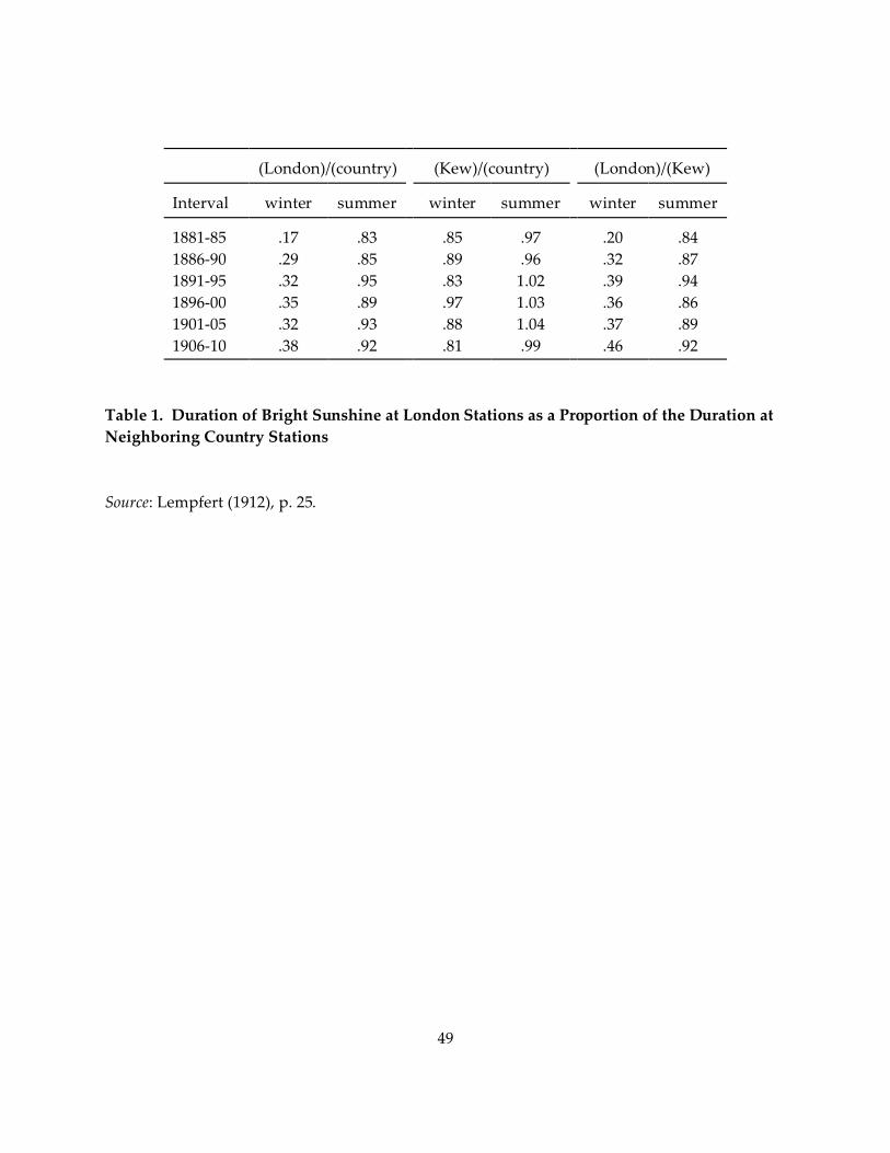
49

(London)/(country) (Kew)/(country) (London)/(Kew)

Interval winter summer winter summer winter summer

1881-85

1886-90

1891-95

1896-00

1901-05

1906-10

.17

.29

.32

.35

.32

.38

.83

.85

.95

.89

.93

.92

.85

.89

.83

.97

.88

.81

.97

.96

1.02

1.03

1.04

.99

.20

.32

.39

.36

.37

.46

.84

.87

.94

.86

.89

.92

Table 1. Duration of Bright Sunshine at London Stations as a Proportion of the Duration at

Neighboring Country Stations

Source: Lempfert (1912), p. 25.

50

Year Week Event # Knowna Documentation (Times unless otherwise indicated)

1855

1855

1858

1858

1859

1861

1861

1862

1864

1871

1873

1874

1874

1874

1875

1879

1880

1880

1882

1890

1890

1892

1892

1892

1892

1892

1893

1894

1899

1899

1900

1900

4

5

47

48

52

3

4

48

3

50

51

48

49

52

1

51

5

6

6

2

3

1

2

3

4

5

49

2

51

52

1

2

1

2

3

4

5

6

7

8

9

10

11

12

13

14

15

16

17

18

19

20

21

22

23

24

25

26

27

28

29

30

31

32

No

No

No

No

No

No

No

No

No

No

Yes

No

No

No

No

Yes

Yes

Yes

No

Yes

Yes

Yes

Yes

Yes

Yes

Yes

No

No

Yes

Yes

Yes

Yes

1/15, p. 10; 2/1, p. 5

2/5, p. 10

11/17, p. 10

11/26, p. 10

12/19, p. 6; 12/20, p. 10; 12/21, p. 12; 12/30, p. 9; 1/8, p. 6

1/11, p. 9; 1/16, p. 10

1/21, p. 10; 1/23, p. 12

11/15, p. 11; 11/17, p. 10; 11/19, p. 6; 12/3, p. 12

1/13, p. 12; 1/22, p.12

11/18, p. 9; 11/19, p. 8; 12/20, p. 6

12/19, p. 10; Brazell (1968), p. 111

11/23, p. 5

12/2, p. 10

12/25, p. 7; 12/28, p. 5

1/1, p. 11; 1/8, p. 9

12/17, p. 8; Scott (1896); Nature, Nov. 5, 1891, p. 13

BMJ, Feb. 14, 1880, p. 254; Nature, Nov. 5, 1891, p. 13

same as above

2/3, p. 6; 2/6, p. 7; 2/7, p. 10; 2/13, p. 10

Nature, Nov. 5, 1891, pp. 14-15

same as above

Brodie (1891); Nature, Nov. 5, 1891, pp. 14-15

same as above

same as above

same as above

same as above

11/23, p. 8; 11/30, p. 8

1/8, p. 6; 1/15, p. 6

12/1, p. 11; 12/2, p. 5; 12/4, p. 13; 12/13, p. 11

12/23, p. 12; 12/28, p. 5

1/3, p. 8; Brazell (1968), p. 111

same as above

Table 2. Fog-Related Events Identified by Reverse Event Study, 1855-1910

Sources: see text and final column of table.

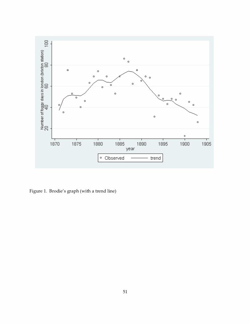
51

Figure 1. Brodie’s graph (with a trend line)

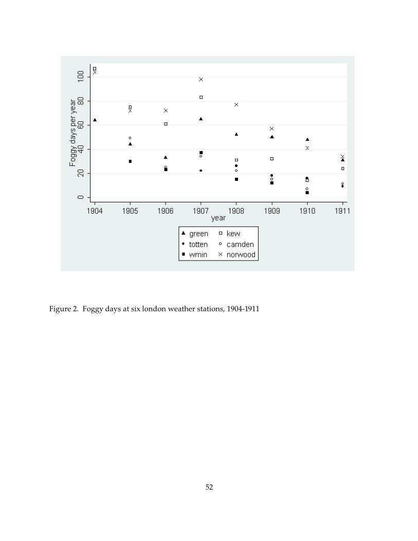
52

Figure 2. Foggy days at six london weather stations, 1904-1911

53

Figure 3. Foggy days in brixton and west norwood

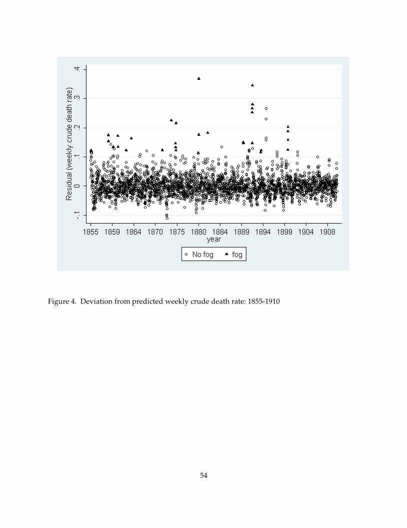
54

Figure 4. Deviation from predicted weekly crude death rate: 1855-1910

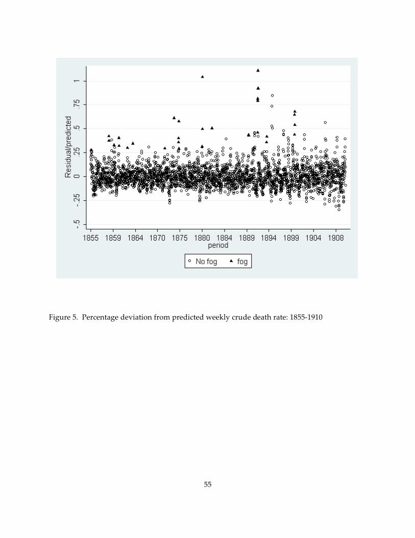
55

Figure 5. Percentage deviation from predicted weekly crude death rate: 1855-1910

56

Figure 6. Excess number of deaths during fog-related events

57

Figure 7. Deviation from predicted death rate in weeks following fog-related events

58

Figure 8. Deaths from respiratory diseases in london: 1850-1920

The category “all respiratory” includes: pneumonia, phthisis (tuberculosis), and bronchitis

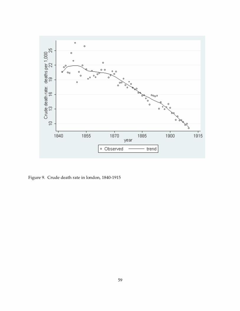
59

Figure 9. Crude death rate in london, 1840-1915

60

Figure 10. Death rate from bronchitis in london and england & wales, 1850-1920

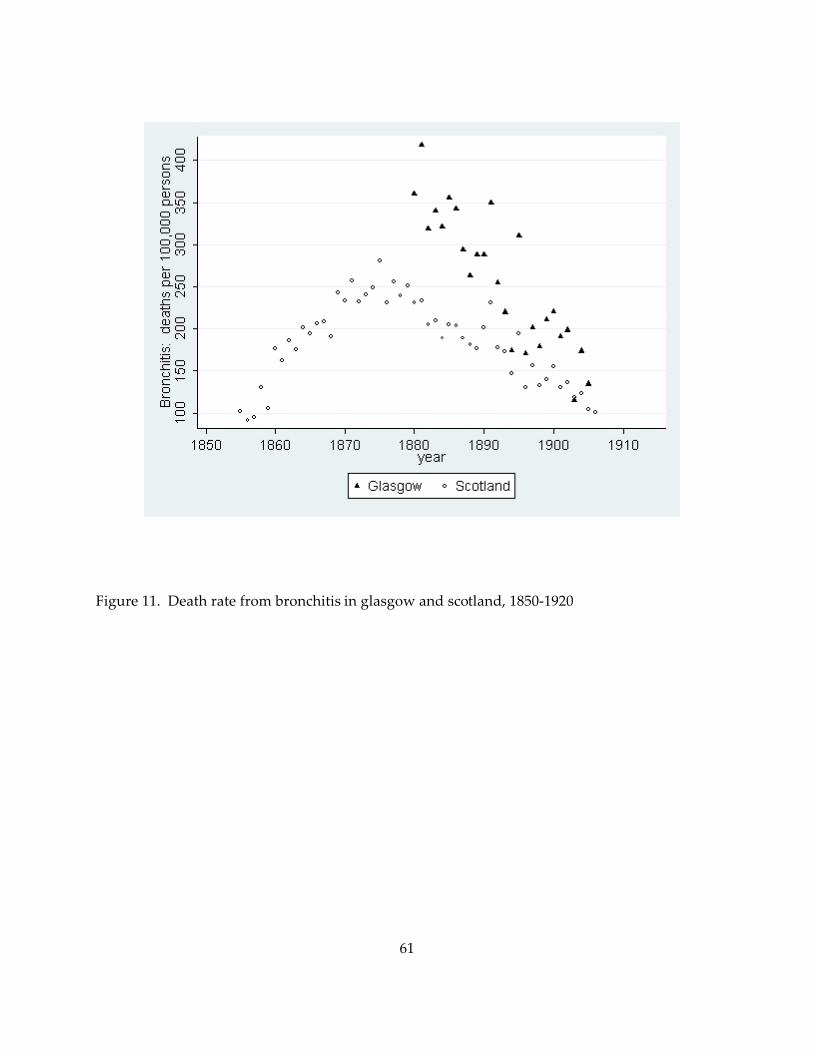
61

Figure 11. Death rate from bronchitis in glasgow and scotland, 1850-1920

62

Figure 12. Coal consumption per capital and foggy days in london, 1700-1925

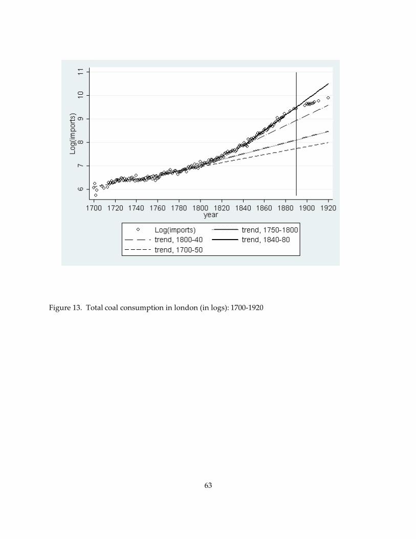
63

Figure 13. Total coal consumption in london (in logs): 1700-1920

64

Figure 14. Population density in london proper and greater london, 1801-2001

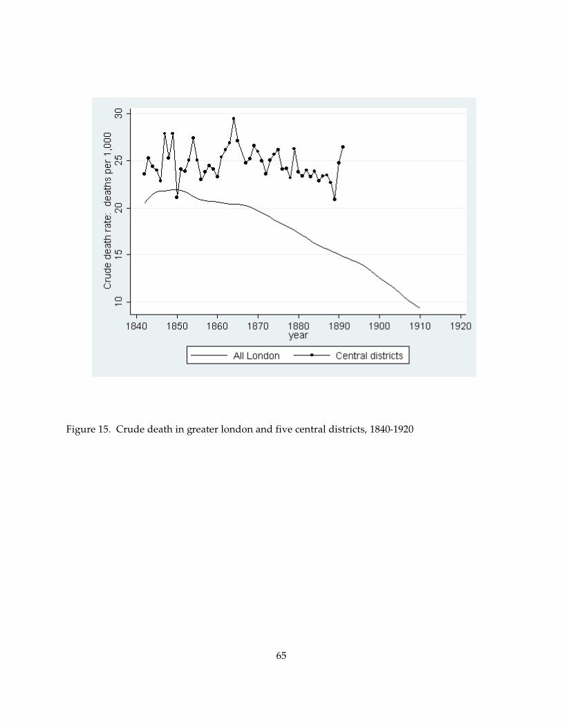
65

Figure 15. Crude death in greater london and five central districts, 1840-1920