DID REALITY TV REALLY CAUSE A DECLINE IN TEENAGE CHILDBEARING? A CAUTIONARY TALE OF EVALUATING IDENTIFYING ASSUMPTIONS

David A. Jaeger Theodore J. Joyce Robert Kaestner

September 2017 © 2017 by David A. Jaeger, Theodore J. Joyce, and Robert Kaestner. All rights reserved. Short sections of text, not to exceed two paragraphs, may be quoted without explicit permission provided that full credit, including © notice, is given to the source.

Did Reality TV Really Cause a Decline in Teenage Childbearing? A Cautionary Tale of Evaluating Identifying Assumptions September 2017 JEL No. J13, L82

ABSTRACT

Evaluating policy changes that occur everywhere at the same time is difficult because of the lack of a clear counterfactual. To address this problem, researchers often proxy for differential exposure using some observed characteristic. In an influential paper, Melissa Kearney and Philip Levine examine the effect of the MTV program 16 and Pregnant on teen birth rates, using the pre-treatment levels of MTV viewership across media markets as an instrument. This is essentially a difference-in-differences approach. We show that controlling for differential time trends in birth rates by a market’s pre-treatment racial/ethnic composition or unemployment rate cause Kearney and Levine’s results to disappear, invalidating the parallel trends assumption necessary for a causal interpretation. Extending the pre-treatment period and estimating placebo tests, we find evidence of an “effect” long before 16 and Pregnant started broadcasting. We also reassess Kearney and Levine’s social media evidence and show that it is fragile and inconsistent, casting substantial doubt on the hypothesized causal mechanism. Our results strongly suggest that the identifying assumptions necessary for a causal interpretation of the effect of 16 and Pregnant on teen birth rates are not met and highlight the difficulty of drawing causal inference from national point-in-time policy changes. Keywords: Social Media, Difference-in-Differences, Teen Pregnancy David A. Jaeger Robert Kaestner Ph.D. Program in Economics Institute of Government and Public Affairs CUNY Graduate Center University of Illinois 365 Fifth Ave 815 West Van Buren Street, Suite 525 New York, NY 10016 Chicago, IL 60607 and University of Cologne and NBER and IZA robert.kaestner@ucr.edu and NBER djaeger@gc.cuny.edu Ted Joyce Baruch College, CUNY Department of Economics and Finance 55 Lexington Ave New York, NY 10010 and NBER theodore.joyce@baruch.cuny.edu

1

Evaluating policy changes that occur nationally at one point in time is particularly

challenging. Cross-country comparisons are unlikely to be convincing because of institutional and

cultural difference and simple before-and-after comparisons within a country will are likely to be

confounded by secular changes over time in the outcome. Finding an appropriate counterfactual

in such cases is daunting and the assumptions necessary for any claim of identifying a causal effect

should be thoroughly scrutinized.

To illustrate the difficulty of meeting the assumptions necessary for identifying a causal

effect when a policy change occurs at the same time in all locations, we reexamine the results of a

recent and influential paper by Kearney and Levine (2015c, henceforth KL) that claimed the MTV

reality shows 16 and Pregnant, Teen Mom, and Teen Mom 2 caused a 4.3 percent drop in teen birth

rates between July 2009 and December 2010. This effect is large and would account for a quarter

of the total reduction in teen childbearing during this period. KL interpret their estimates as causal

and write that “…a social media campaign in the guise of a very popular reality TV show… adds

a new ‘policy mix’” (p. 3598) to current interventions designed to reduce teen pregnancy. Such

proscriptions are only warranted when they have on robust empirical foundations.

The salience of KL’s results is underscored by the fact that, despite recent declines, the

teen birth rate in the U.S. is still substantial higher than in Western European countries.1 It is

widely believed that teen pregnancy has adverse consequences for both mother and child and a

consensus as to the causes of teen childbearing remains elusive. These circumstances likely explain

1 There are a variety of possible explanations for the decline in birth rates (Boonstra 2014), including more effective contraception (Santelli, et al. 2007; Lindberg, Santelli and Desai 2016), welfare reform (Kaestner, Korenman and O’Neill 2003; Lopoo and Delaire 2006), labor market conditions (Dehejia and Llearas-Muney 2004, and Ananat, Gassman-Pines and Gibson-Davis 2013), and income inequality (Kearney and Levine 2014b). None of these explanations appear to be definitive.

2

the immediate and widespread attention in the national media garnered the working paper version

of KL (2014a).2

Trends in teen birth rates also suggest why KL’s identification strategy may be

problematic. KL use the audience share watching MTV from 9 to 10 pm on Tuesdays in a media

market in the year before 16 and Pregnant began broadcasting as an instrument for the 16 and

Pregnant viewership on Tuesdays from 9 to 10 pm in the same media market. The exogeneity of

this instrument lacks face validity, however, as viewing MTV, 16 and Pregnant, or some other

show, from 9 to 10 pm on Tuesdays on a specific cable station is a choice determined by many

factors, including demographics and socioeconomic status, that are likely associated with teen

births. KL’s research design is more appropriately viewed as a difference-in-differences (DD)

approach. Understood in this way, KL’s identification relies on comparing changes in teen birth

rates before and after 16 and Pregnant in media markets with relatively high- and low-MTV

viewership in the year before the show.

The assumption necessary for a causal interpretation of KL’s results is that trends in teen

birth rates in geographic areas with high- and low-MTV viewership would have been the same,

conditional on area and time fixed effect and a limited set of covariates, in the absence of 16 and

Pregnant. How likely is it that this identifying assumption holds? Teen birth rates began falling

precipitously with the onset of the Great Recession in 2008 and there were profound racial and

2 For the initial reaction to the working paper by Kearney and Levine (2014) see: CNN: http://www.cnn.com/2014/01/13/health/16-pregnant-teens-childbirth/; The Washington Post: https://www.washingtonpost.com/news/arts-and-entertainment/wp/2014/04/09/how-mtvs-16-and-pregnant-led-to-declining-teen-birth-rates/; Time: http://time.com/825/does-16-and-pregnant-prevent-or-promote-teen-pregnancy/; Newsweek: http://www.newsweek.com/why-teen-birth-rate-keeps-dropping-333946; and The New York Times: http://www.nytimes.com/2014/01/13/business/media/mtvs-16-and-pregnant-derided-by-some-may-resonate-as-a-cautionary-tale.html (All last accessed 15 January 2016). For the continuing popularity of 16 and Pregnant as an explanation for the decline in teen birth rates, see http://www.nytimes.com/2016/07/19/opinion/winning-the-campaign-to-curb-teen-pregnancy.html (Last accessed 24 August 2016).

3

ethnic differences in the rate of decline. Given the substantial geographic variation in racial/ethnic

composition, trends in birth rates in the media markets used by KL are also likely to vary because

of different trends in birth rates by race/ethnicity. These differences may confound KL’s estimates

and violate the parallel trend assumption necessary for a causal interpretation.

This is precisely what we find. Allowing for differential time trends by the racial/ethnic

composition of a media market eliminates any association between 16 and Pregnant and teen birth

rates, as well as the birth rates of women ages 20 to 24 and 25-29. We obtain the same null findings

when we interact the racial/ethnic composition of an area with the unemployment rate. The

importance of differential time trends in teen birth rates prior to 16 and Pregnant is evident from

KL’s own results. They report no association between 16 and Pregnant and the birth rates of non-

Hispanic black and Hispanic teens when their analyses are stratified by race/ethnicity, despite

national data indicating that black and Hispanic young women watched the show as much, or even

more, than their white counterparts (Kearney and Levine 2014).

To assess whether parallel trends in birth rates between low- and high-MTV viewing areas

held before 16 and Pregnant began broadcasting, we perform a series of placebo tests and find an

“effect” of 16 and Pregnant prior to the advent of the show. Using Kearney and Levine’s “IV

Event Study” methodology, we also show that including even a few additional periods in the

analysis prior to the beginning of 16 and Pregnant leads to a rejection of the hypothesis that pre-

treatment trends were parallel.

To test the causal mechanism that KL hypothesize is driving their results, we also provide

evidence that KL’s analysis of social media is problematic. KL estimate the association between

broadcasts of 16 and Pregnant and Google searches and Twitter tweets for birth control and

abortion. KL present these results as evidence of the causal chain that links 16 and Pregnant to

4

behaviors that lead to lower birth rates. We demonstrate that the social media analyses are

extremely fragile and that that no reliable inferences can be made from them.

Our results illustrate the general difficulty of identifying the causal effect of a “policy”

change that occurred everywhere at single point in time. In the case we examine, the outcome of

interest was also changing rapidly during a period of exceptional economic uncertainty, making

the task of evaluating the validity of the research design in this context particularly important. The

identifying assumptions in such cases deserve substantial added scrutiny before researchers,

policymakers, and the media assign much weight to them. Testing the identifying assumptions

within the sample period and prior to treatment leads to one clear conclusion: claims that 16 and

Pregnant caused a decline in teen birth rates are unjustified.

I. Previous Studies of the Impact of Television on Behavior

There is a robust literature that has examined the impact of the introduction of television

or specific television content on a variety of outcomes, such as voter turnout (Gentzkow 2006),

tests scores (Gentzkow and Shapiro 2008), women’s empowerment (Jensen and Oster 2009),

voting behavior (DellaVigna and Kaplan 2007), and fertility and divorce (La Ferrara, Chong, and

Duryea 2012). In each of these studies, the authors acknowledged the endogeneity of television

viewing and addressed the problem using plausibly exogenous changes across both space and time

in access to television or specific content. Kearney and Levine (2015b) followed a similar approach

in their study of the effect of Sesame Street broadcasts on long-term educational outcomes, using

the distance to a UHF or VHF television tower and temporal and spatial variation in the

introduction of Sesame Street as sources of plausibly exogenous variation in viewership.

5

KL’s analysis of 16 and Pregnant is markedly different from these other media studies.

They address the endogeneity of viewership of 16 and Pregnant through an instrumental variables

approach, where the instrument is average viewership of other programs that aired on MTV in the

same time slot, but a year earlier, interacted with an indicator for the post-16 and Pregnant period.

This measure of MTV viewership is a time-invariant, geographic-specific measure. The instrument

was not justified on theoretical grounds and is clearly not exogenous, as MTV viewership in an

area is a choice largely determined by the same factors that affect 16 and Pregnant viewership.

II. KL’s Empirical Framework

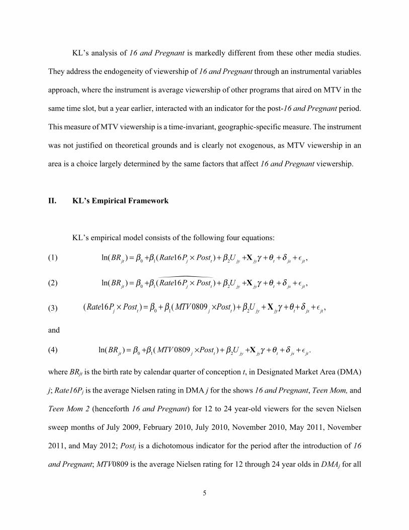
KL’s empirical model consists of the following four equations:

(1)

(2)

(3)

and

(4)

where BRjt is the birth rate by calendar quarter of conception t, in Designated Market Area (DMA)

j; Rate16Pj is the average Nielsen rating in DMA j for the shows 16 and Pregnant, Teen Mom, and

Teen Mom 2 (henceforth 16 and Pregnant) for 12 to 24 year-old viewers for the seven Nielsen

sweep months of July 2009, February 2010, July 2010, November 2010, May 2011, November

2011, and May 2012; Postj is a dichotomous indicator for the period after the introduction of 16

and Pregnant; MTV0809 is the average Nielsen rating for 12 through 24 year olds in DMAj for all

ln(BRjt ) = β0 +β1(Rate16Pj × Postt )+ β2U jy +X jyγ +θt +δ js + ε jt ,

ln(BRjt ) = β0 +β1(Rate16Pj × Postt )! + β2U jy +X jyγ +θt +δ js + ε jt ,

(Rate16Pj × Postt ) = β0 + β1( MTV 0809 j ×Postt )+ β2U jy + X jyγ +θt+δ js + ε jt ,

ln(BRjt ) = β0 +β1( MTV 0809 j ×Postt )+ β2U jy +X jyγ +θt +δ js + ε jt .

6

MTV shows in the sweeps months of July 2008, November 2008, February 2009, and May 2009,

Ujy is the annual unemployment rate in DMA j in year y; Xjy is vector that includes the percent

population in the DMA that is that non-Hispanic black, and the percent that is Hispanic in calendar

year y; �t is a set of quarterly dummy variables; and �js is a full set of DMA ´ season fixed

effects, which implicitly defines DMA fixed effects.3

Equation (1) represents the equation of interest that yields estimates of the association

between 16 and Pregnant viewership and teen birth rates. Equation (3) is the first stage regression

with (MTV0809j ́ Postt) as an instrument. Equation (2) is the second stage regression and identical

to equation (1) except that predicted 16 and Pregnant viewership derived from equation (2) is used

instead of actual 16 and Pregnant viewership. Equation (4) represents the reduced form effect of

MTV viewership on teen birth rates.

KL’s study period includes 24 quarters (2005:QI – 2010:QIV) for 205 DMAs for a total

(potential) sample of 4,920 observations.4 Ratings for 16 and Pregnant are measured during the

time slot from 9:00 to 10:00 pm for 12 to 24 year-old viewers on Tuesdays in the sweep months.5

KL average these Tuesday ratings within each month and then average the four months of ratings

3 We follow KL’s notation, although in actuality the parameters represent different quantities across the different equations, i.e. b1 in equation (3) is not the same quantity as b1 in equation (4). 4 The dependent variable is missing in some DMAs in some quarters because there are no teen births. This occurs more frequently in the analyses stratified by age or race/ethnicity. 5 KL use ratings when a new episode of 16 and Pregnant was broadcast for a broad age range at a single time in the later evening (9:00-10:00 p.m.). Using this as a measure of the total exposure to 16 and Pregnant for teenagers has several problems. Previous episodes are broadcast at various times on the same day as the new episode, which is also rebroadcast at different times during the week. Exposure to the show is therefore uncertain. Nielsen also collects separate ratings for teens aged 12-17 separately from young women 18 to 24 years old. The younger teens are more likely to watch 16 and Pregnant earlier in the day than women 18 to 24. By aggregating ratings across age groups, KL potentially reduce noise in the data, but at the expense of accurately measuring exposure. KL also average Nielsen ratings from seven sweep months drawn from 2009-2012 and assign this average to conceptions from 2009:III to 2010:QIV, leading to another source of mis-measurement of exposure to 16 and Pregnant. Teens who conceived in August of 2009, for example, are assigned a rating that pertains to future broadcasts to which they could not have been exposed. Ratings almost tripled in the first year suggesting important variation by quarter of conception. This measurement error potentially biases KL’s estimates.

7

and assign that value to the six post-16 and Pregnant quarters within each DMA. They follow the

same procedure for the MTV ratings during the period 2008:QIII to 2009:QII by using the average

for the four quarters within each DMA. The ratings that KL use for 16 and Pregnant and MTV

therefore vary only in the cross section (by DMA).

III. The Nature of KL’s Instrument

KL use the interaction between a time-invariant, DMA-specific measure of MTV

viewership and an indicator for the post-16 and Pregnant period as the instrument for the

viewership of 16 and Pregnant. For the instrument to be valid, MTV viewership in the pre-16 and

Pregnant Period must “randomly” assign 16 and Pregnant viewership, conditional on DMA fixed

effects and small number of covariates. Because of the inclusion of DMA fixed effects, this

interaction is necessary to generate time series variation in the instrument, which consists of zeros

in all DMAs and all quarters from 2005:QI to 2009:QII with a discrete jump for each DMA in

2009:QIII. The measure of 16 and Pregnant is also time invariant in the post-treatment period

(and obviously zero in the pre-treatment period), generating a strong (but somewhat mechanical)

first-stage association.

We first explore the validity of this instrument by using two, similarly endogenous

variables in the same way that KL employ MTV viewership as an instrument. We use the percent

of individuals aged 25 to 34 with at least a bachelor’s degree and the percent of individuals aged

25 to 34 in poverty in a media market in the year prior to the start of 16 and Pregnant.6 Each is

6 The Appendix describes the creation of these variables at the DMA level using data from the American Community Survey.

8

then interacted with Postt to form an instrument, although they are almost surely not valid as

instruments for 16 and Pregnant viewership because of their likely correlation with birth rates.

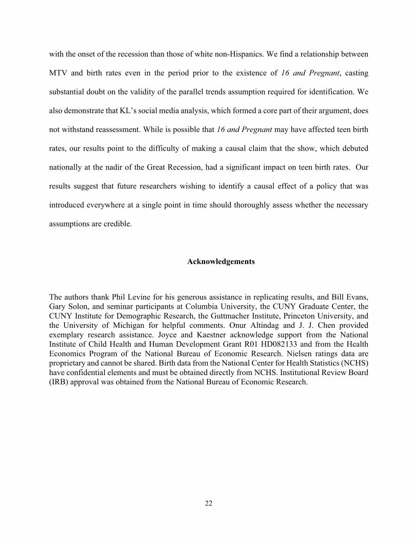
The results of this exercise are presented in Table 1. We begin by replicating KL’s reduced

form and IV estimates in Panel 1 (rows 1 and 2, respectively). Their IV estimate indicates that a

one percentage-point increase in the viewership of 16 and Pregnant lowers teen birth rates by 2.37

percent. To assess the magnitude of this effect, KL multiply the coefficient by the average rating

of 16 and Pregnant in their post period (1.8 percent) and conclude the show can account for a 4.27

(-2.37 ´ 1.8) percentage point reduction in teen birth rate between 2008 and 2010. In actuality, the

Nielsen ratings for 16 and Pregnant were 2.26 percent in 2010, the peak year of the show’s ratings.

Based on this figure, 16 and Pregnant can account for a 5.3 percentage point decline in teen birth

rates between 2008 and 2010.

In panel 2 we estimate the reduced form and IV models using the percent of individuals

aged 25 to 34 with at least a bachelor’s degree as an instrument. As noted, we construct the

instrument in the same manner as KL construct their instrument using MTV viewership, by

interacting this measure of schooling in the year before 16 and Pregnant within each DMA

interacted with Postt, the indicator for the post-16 and Pregnant period. The IV estimate in row 4

has the same sign as KL’s and is statistically significant at the one percent level, indicating that a

one percentage-point increase in the viewership of 16 and Pregnant is associated with a 6.2 percent

decline in teen birth rates when instrumented by schooling. To compare the magnitude of this

estimate to that obtained using MTV at the instrument, we follow KL and multiply the change in

schooling from the year before 16 and Pregnant to 2010 (0.90 percentage points) and calculate

that 16 and Pregnant accounts for a 5.6 (-6.2 ´ 0.90) percent decline in teen birth rates when

instrumented by schooling, a figure impressively close to KL’s. In panel 3 we perform the same

9

exercise using the annual percent of individuals aged 25 to 34 in poverty in the year prior to the

start of 16 and Pregnant interacted with Postt. We find the same results: 16 and Pregnant has a

negative and statistically significantly effect on birth rates.

In the case of both instruments, the reduced form yields plausible estimates, as DMAs with

more bachelor’s degrees are associated with lower teen birth rates while higher poverty rates are

positively related to teen births. The mechanical nature of KL method of constructing the

instruments leads to reasonable first stage results. That we can generate IV estimates that are

similar to KL’s with instruments that are not credible suggests, at a minimum, that MTV

viewership, an endogenous choice, is likely not to meet the exogeneity assumption or the exclusion

restriction necessary to be a valid instrument

IV. Within-Sample Evaluation of KL’s Identifying Assumptions

KL’s reduced form compares teen birth rates before and after the introduction of 16 and

Pregnant, stratified by levels of MTV viewership in the year before the show began. The key

identification assumption is therefore parallel trends: in the absence of 16 and Pregnant, birth

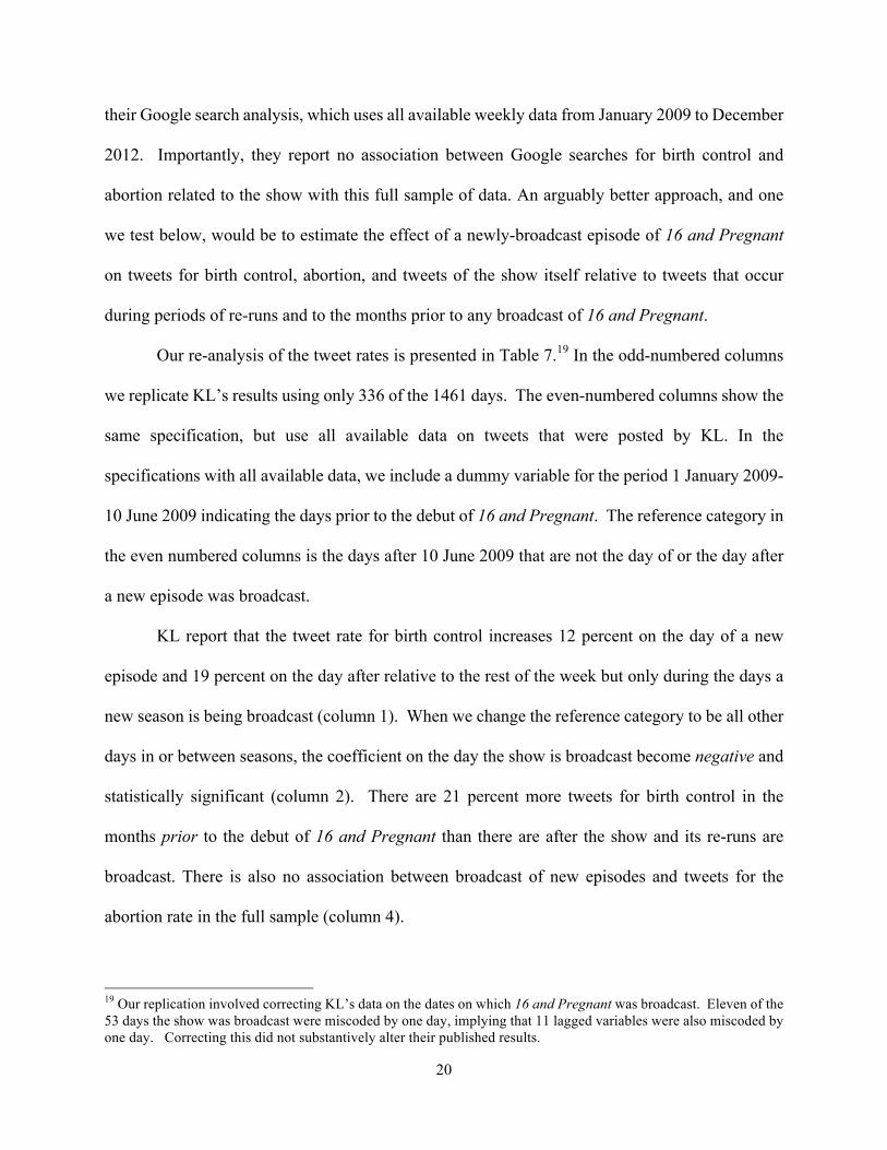
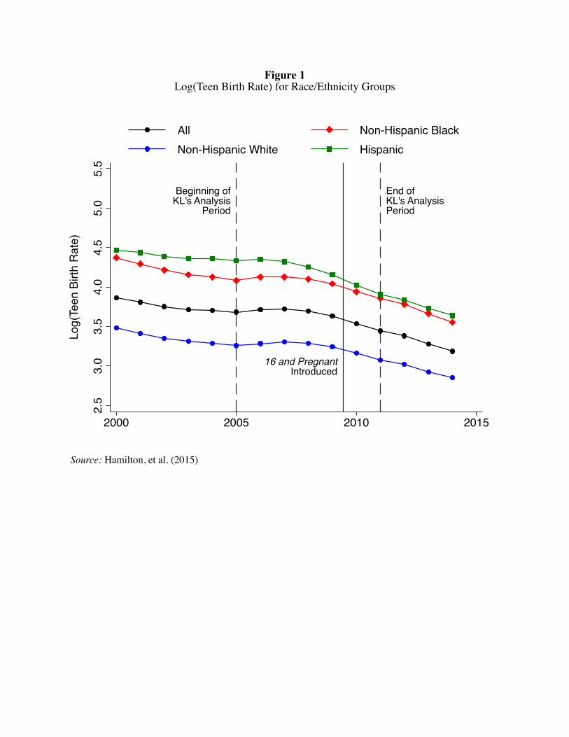
rates should change in the same way in areas with high and low MTV viewership. Figure 1 shows

that overall teen birth rates decline significantly prior to 16 and Pregnant and that the rate of

decline accelerates after 2007 with the onset of the Great Recession. There is substantial variation

in the rate of decline across race/ethnicity groups. The average annual change in teen births

between 2005 and 2010 was -1.9 percent among non-Hispanic whites, -2.9 percent among non-

Hispanic blacks and -6.3 percent among Hispanics.7 If the trends in birth rates vary by racial and

7 Authors’ calculations based on data reported in Hamilton, et al. (2015).

10

ethnic composition of a DMA and if they are related to the timing of 16 and Pregnant, then the

parallel trends assumption is unlikely to hold.

To assess the extent of this potential confounding, we augment KL’s model with time

trends that vary with levels of the exogenous covariates, particularly the pre-16 and Pregnant

racial/ethnic composition. This approach has been used in several recent articles (Hoynes and

Schanzenbach 2009; Hoynes, Schanzenbach, and Almond 2016; and Hjort, Sølvsten, and Wüst, in

press). Large changes in the IV and reduced form coefficients after including these trends would

suggest that KL’s estimates are biased.

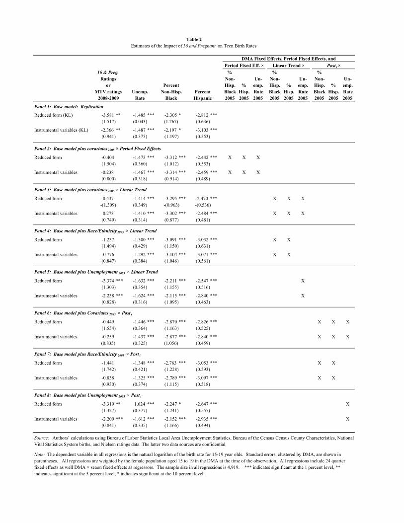
The results are displayed in Table 2. In each panel, we show the reduced form estimates

from equation (4) and the IV estimates from equation (2), which include DMA and period fixed

effects. Panel 1 exactly replicates KL’s reduced form and IV estimates for comparison. In panel

2 we show estimates from a specification in which we interact the values of the covariates, X, in

2005 (well before the start of 16 and Pregnant) with the period fixed effects. Both the reduced

form relationship between MTV and the IV estimate of the impact of 16 and Pregnant are reduced

by a factor of approximately 10 and are no longer statistically significantly different from zero. It

is noteworthy, however, that the coefficients on the three covariates are essentially unchanged.

The results in panel 2 strongly suggest that the parallel trends assumption in KL’s model

does not hold. In panel 3 we reduce the possibility of overfitting by estimating a more

parsimonious specification, adding only interactions of the three covariates with a linear trend to

the base models from equations (4) and (2). These results, again, suggest that the parallel trends

assumption does not hold. In panel 4 we limit the trend interactions to the percent non-Hispanic

black and percent Hispanic in 2005, yielding reduced form and IV coefficients that are still

approximately only 1/3 the size of those in panel 1 and are not statistically significantly different

11

from zero. In contrast, in panel 5 we include only the interaction of a trend with the unemployment

rate in 2005 and obtain results that are quite similar to KL’s in panel 1.

As Figure 1 suggests, the results in panels 4 and 5 lead to the conclusion that the effect of

16 and Pregnant that KL estimate is largely driven by differential trends in birth rates across race

and ethnic groups that are correlated with the timing of the introduction 16 and Pregnant. We

confirm this in panels 6 through 8, where we simplify the trend interactions further and merely

interact the covariate levels in 2005 with Postt.8 The results are essentially the same as in panels

3 through 5. Taken together, the results in Table 1 strongly suggest that the parallel trend

assumption underlying the KL analysis does not hold and that a causal interpretation of KL’s

estimated impact of 16 and Pregnant is unwarranted.

Stratification by Age

In their Table 2, KL present results of the effect of 16 and Pregnant stratified by age and

race/ethnicity. We exactly replicate their estimates for 20-24 year olds (panel 1), 25-29 year olds

(panel 2) and 30-34 year olds (panel 3) in the odd-numbered rows in our Table 3.9 In the even-

numbered rows, we modify those specifications by including, as in panel 3 of Table 2, a linear

time trend interacted with level of the three covariates in 2005.10 As in Table 2, when we include

these interactions, we find no statistically significant associations between 16 and Pregnant and

8 The single interaction of the covariate levels in 2005 with the post-period dummy is nested within the specification that interacts the same covariates with the complete set of time fixed effects. A Wald test indicates that we cannot reject the restrictions implied in panel 6 relative to panel 2. 9 KL’s results for 15-19 year olds are already presented in Table 2. 10 We have also estimated these models using both the full set of period ´ 2005 covariate interactions as well as the 2005 covariates interacted with the Postt dummy. The results are qualitatively similar and available from the authors by request.

12

birth rates by age. For example, KL report that a one ratings point increase in the viewership of

16 and Pregnant lowers birth rates of 20-24 year olds by 2.4 percent (row 3, panel 1). Inclusion

of the additional trend terms reduces the effect to a statistically insignificant reduction (p-value of

0.19) of 0.9 percent (row 4, panel 1). We find the same pattern for 25-29 and 30-34 year olds,

respectively.

The results in Tables 2 and 3 suggest that the estimated association between 16 and

Pregnant and teen birth rates reported by KL is due to differential trends in birth rates across areas

in ways that are associated with MTV viewing. The more challenging task is to explain why. As

Figure 1 shows, the differential rate of decline in teen birth rates by race/ethnicity appears to have

increased with the onset of the Great Recession. Several recent studies demonstrate that the Great

Recession had particularly large effects on the fertility of young women (Sobotka, Skirbekk, and

Philipov, 2011; Cherlin, et al. 2013). Autor, Dorn, and Hanson (2017) show that recent trade

shocks that affect the employment opportunities of less educated men and women decrease both

marriage and birth rates. Kearney and Wilson (2017) have documented that improved economic

conditions from the fracking boom may lead to increased non-marital and marital fertility. Most

relevant for our analysis, Villarreal (2014) finds that areas with relatively large Hispanic

populations may have been more affected by the Great Recession through decreased employment

and flow of immigrants.

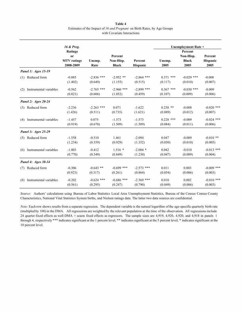
To explore the differential response of birth rates to the Great Recession, in Table 4 we

interact each of the three covariate levels in 2005 with the unemployment rate.11 We find that for

teens, the IV coefficient on 16 and Pregnant falls from -2.37 (Table 2, row 3) to -0.562 (Table 4,

row 2). For this group, the interaction between the share of the DMA that is black in 2005 and the

11 For comparison, the relevant results from KL are shown in Table 1, panel 1 (for Table 4, panel 1); Table 2, panel 1 (for Table 4, panel 2); Table 2, panel 2 (for Table 4, panel 3), and Table 2, panel 3 (for Table 4, panel 4).

13

unemployment rate is negative and statistically significant – consistent with the hypothesis that

worse labor market conditions lowered birth rates differentially for minority populations. We find

similar results for Hispanics in the other age groups. For all age groups, the interaction between

the unemployment rate in 2005 and the contemporaneous unemployment rate are also statistically

significant, suggesting a non-linear relationship between birth rates and labor market conditions.

As in Tables 2 and 3, allowing for the effect of the racial/ethnic composition on birth rates to vary

over time reduces the reduced form and IV coefficients such that they are no longer statistically

significant.

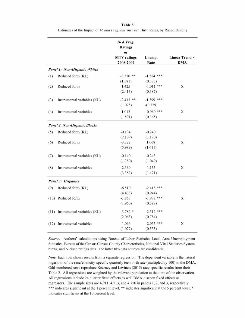
Stratification by Race/Ethnicity

KL stratify by race/ethnicity and find that the effects of 16 and Pregnant are statistically

significant for non-Hispanic whites and marginally so for Hispanics. In the odd-numbered rows

of Table 5 we replicate these results for all three race/ethnicity groups. KL do not include

race/ethnicity variables in these regressions. To test the parallel trends assumption, therefore, we

now include a full set of DMA-specific time trends.12 KL find that an increase in 16 and Pregnant

viewership lowers the birth rates of non-Hispanic whites by 2.4 percent (panel 1, row 3). When

we include DMA-specific trends, this coefficient turns positive and is statistically insignificantly

different from zero (panel 1, row 4). We find no statistically significant reduced form or IV effects

12 The results for the full sample and for different age groups with DMA-specific time trends are available from the authors by request. As with the race-specific results, we do not estimate a statistically significant coefficient in either the reduced form or IV equations, with the exception of the IV effect in the full sample, which is statistically significant at the 10 percent level. We have also run the regressions with more parsimonious specifications that include the time-varying race/ethnicity variables with the unemployment rate well as the interactions of all three covariates with a linear time trend. Our finding of no significant reduced form or IV effect is unaltered. These results are available from the authors by request.

14

for non-Hispanic blacks (panel 2) or Hispanics (panel 3). As with the full sample, we find little

in these results to suggest that 16 and Pregnant affected birth rates in any of the race/ethnicity

groups.

V. Out-of-Sample Evaluation of KL’s Identifying Assumptions

Placebo Tests

As we have noted, MTV ratings should be unrelated to trends in birth rates conditional on

time and DMA fixed effects except through their relationship with 16 and Pregnant ratings. Any

association between MTV ratings and birth rates in the pre-16 and Pregnant period would suggest

a violation of the exclusion restriction (i.e., parallel trends) necessary for identification. In Table

6, we present results from a series of reduced form and IV regressions in which we artificially start

a placebo “show” in sequential quarters. Each regression includes 24 quarters, the same length of

analysis used by KL: 18 prior to the beginning of the placebo show and 6 after, including the

quarter that the “show” starts. We estimate the reduced form equation (4) and IV equation (5) and

use MTV viewing from 2008-2009 interacted with a post-“show” indicator as the instrument.

Each row of Table 6 presents the estimated coefficients and standard errors from the

estimation of the reduced form and instrumental variables models from a different 24 quarter-

period. For example, in row (1) the 24-quarter period begins in 2001:Q1 and ends in 2006:QIV,

with the placebo show beginning in 2005:QIII. Row 12, which is shaded in the table, reproduces

KL’s reduced form and instrumental variables results from their Table 1 columns (4) and (3),

respectively. For the reduced form, we find that 9 of the 11 estimated coefficients in rows (1)

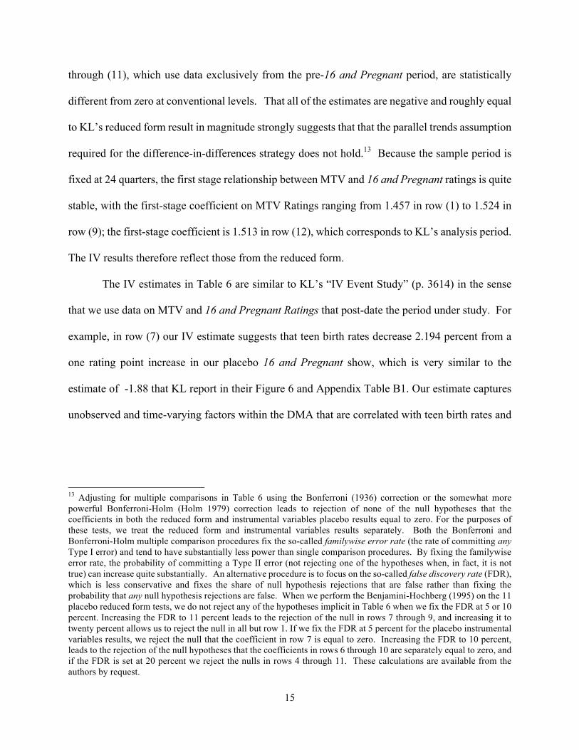
15

through (11), which use data exclusively from the pre-16 and Pregnant period, are statistically

different from zero at conventional levels. That all of the estimates are negative and roughly equal

to KL’s reduced form result in magnitude strongly suggests that that the parallel trends assumption

required for the difference-in-differences strategy does not hold.13 Because the sample period is

fixed at 24 quarters, the first stage relationship between MTV and 16 and Pregnant ratings is quite

stable, with the first-stage coefficient on MTV Ratings ranging from 1.457 in row (1) to 1.524 in

row (9); the first-stage coefficient is 1.513 in row (12), which corresponds to KL’s analysis period.

The IV results therefore reflect those from the reduced form.

The IV estimates in Table 6 are similar to KL’s “IV Event Study” (p. 3614) in the sense

that we use data on MTV and 16 and Pregnant Ratings that post-date the period under study. For

example, in row (7) our IV estimate suggests that teen birth rates decrease 2.194 percent from a

one rating point increase in our placebo 16 and Pregnant show, which is very similar to the

estimate of -1.88 that KL report in their Figure 6 and Appendix Table B1. Our estimate captures

unobserved and time-varying factors within the DMA that are correlated with teen birth rates and

13 Adjusting for multiple comparisons in Table 6 using the Bonferroni (1936) correction or the somewhat more powerful Bonferroni-Holm (Holm 1979) correction leads to rejection of none of the null hypotheses that the coefficients in both the reduced form and instrumental variables placebo results equal to zero. For the purposes of these tests, we treat the reduced form and instrumental variables results separately. Both the Bonferroni and Bonferroni-Holm multiple comparison procedures fix the so-called familywise error rate (the rate of committing any Type I error) and tend to have substantially less power than single comparison procedures. By fixing the familywise error rate, the probability of committing a Type II error (not rejecting one of the hypotheses when, in fact, it is not true) can increase quite substantially. An alternative procedure is to focus on the so-called false discovery rate (FDR), which is less conservative and fixes the share of null hypothesis rejections that are false rather than fixing the probability that any null hypothesis rejections are false. When we perform the Benjamini-Hochberg (1995) on the 11 placebo reduced form tests, we do not reject any of the hypotheses implicit in Table 6 when we fix the FDR at 5 or 10 percent. Increasing the FDR to 11 percent leads to the rejection of the null in rows 7 through 9, and increasing it to twenty percent allows us to reject the null in all but row 1. If we fix the FDR at 5 percent for the placebo instrumental variables results, we reject the null that the coefficient in row 7 is equal to zero. Increasing the FDR to 10 percent, leads to the rejection of the null hypotheses that the coefficients in rows 6 through 10 are separately equal to zero, and if the FDR is set at 20 percent we reject the nulls in rows 4 through 11. These calculations are available from the authors by request.

16

16 and Pregnant viewership. Finding any statistically significant coefficients in a period before

16 and Pregnant began broadcasting strongly suggests that KL’s instrument is invalid.

Although we have presented a series of placebo results in order to keep from “cherry

picking” those that are particularly favorable to our argument, we recognize that the results in

Table 6 are not independent of one another when the “treatment” periods overlap. We have

therefore boxed rows 1 and 7 to illustrate results where the “post” periods are disjoint (and as

indicated above, all placebo “treatment” periods are disjoint from the actual period when 16 and

Pregnant was being broadcast). Focusing only on rows 1, 7, and 12, on the basis of the coefficients

and their statistical significance, it would be virtually impossible to distinguish which of these

results was generated by the actual 16 and Pregnant and which were placebo tests.

“Reduced Form Event Study”

KL present results from an “event study” of the reduced-room relationship between MTV

viewership and teen birth rates (KL Figure 5 and Appendix Table B1). Their primary goal is to

assess the validity of the parallel trends assumption, although they also cite their results as “visual

evidence” in favor of their conclusions.14 They estimate the following regression:

14 KL’s characterization of equation (5) as an event study is something of a misnomer. In common parlance an “event study” design summarize changes before and after an intervention that occurs at different points in time across different units (e.g. Jacobson, LaLonde and Sullivan 1993; Jacobson and Royer 2011; Bailey 2012; Bailey and Goodman-Bacon 2015; Dobkin, Finkelstein, Kluender and Motowidigdo 2016; Jackson, Johnson and Persico 2016). In these studies, setting the reference period to one just before the treatment occurs facilitates comparisons across units for which the calendar date of the intervention varied. This normalization has less justification when the treatment occurs at the same point in calendar time for all units. KL’s “event study” is more accurately characterized as a difference-in-differences analysis with leads and lags.

17

(5)

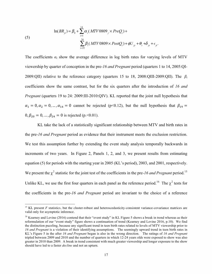
The coefficients αi show the average difference in log birth rates for varying levels of MTV

viewership by quarter of conception in the pre-16 and Pregnant period (quarters 1 to 14, 2005:QI-

2009:QII) relative to the reference category (quarters 15 to 18, 2008:QIII-2009:QII). The βi

coefficients show the same contrast, but for the six quarters after the introduction of 16 and

Pregnant (quarters 19 to 24: 2009:III-2010:QIV). KL reported that the joint null hypothesis that

!" = 0, !& = 0,… , !"( = 0 cannot be rejected (p<0.12), but the null hypothesis that )"* =

0, )&+ = 0,… , )&( = 0 is rejected (p.<0.01).

KL take the lack of a statistically significant relationship between MTV and birth rates in

the pre-16 and Pregnant period as evidence that their instrument meets the exclusion restriction.

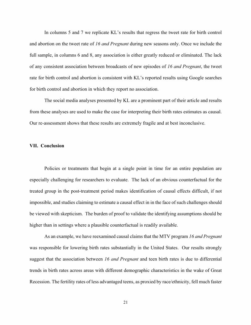
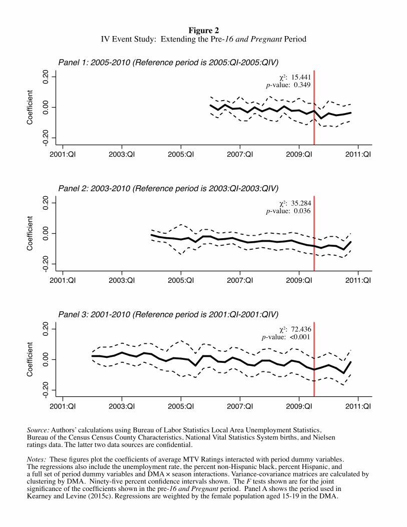
We test this assumption further by extending the event study analysis temporally backwards in

increments of two years. In Figure 2, Panels 1, 2, and 3, we present results from estimating

equation (5) for periods with the starting year in 2005 (KL’s period), 2003, and 2001, respectively.

We present the c2 statistic for the joint test of the coefficients in the pre-16 and Pregnant period.15

Unlike KL, we use the first four quarters in each panel as the reference period.16 The c2 tests for

the coefficients in the pre-16 and Pregnant period are invariant to the choice of a reference

15 KL present F statistics, but the cluster-robust and heteroscedasticity-consistent variance-covariance matrices are valid only for asymptotic inference. 16 Kearney and Levine (2016) contend that their “event study” in KL Figure 5 shows a break in trend whereas as their reformulation of our “event study” figure shows a continuation of trend (Kearney and Levine 2016, p.10). We find the distinction puzzling, because any significant trend in teen birth rates related to levels of MTV viewership prior to 16 and Pregnant is a violation of their identifying assumptions. The seemingly upward trend in teen birth rates in KL’s Figure 5 in the after 16 and Pregnant began is also in the wrong direction. The ratings of 16 and Pregnant tripled between 2009 and 2010 and the number of quarters in which 12-24 years olds were exposed to show was also greater in 2010 than 2009. A break in trend consistent with much greater viewership and longer exposure to the show should have led to a faster decline and not an upturn.

ln(BRjt ) = β0 + α ii=1

14

∑ ( MTV 0809 j × PreQi )+

βii=19

24

∑ ( MTV 0809× PostQi )+φU jy +θt +δ js + ε jt .

18

category (in the pre-treatment period). KL’s choice of using the four quarters prior to the start of

16 and Pregnant as the reference category is arbitrary, obscures existing trends in the birth rates,

and gives the appearance of a discontinuity when, in fact, a break in trend is difficult to discern.

The downward trend in teen birth rates in the years prior to 16 and Pregnant and the lack

of a clear discontinuity at 2009:QIII is quite apparent in all three panels and we strongly reject the

null hypothesis that the pre-16 and Pregnant coefficients are jointly equal to zero in Panels 2 and

3 with p-values of 0.036 and <0.001, respectively. These results are artifacts of greatly extending

the period of analysis. In KL’s period, these coefficients are very close to statistically significant

the 10 percent level and by extending the pre-16 and Pregnant period even by only two years

(Panel A of Table 2) we reject the null that pre-treatment coefficients are jointly equal to zero. The

sensitivity of KL’s results to extending the pre-treatment period by a even small amount suggests

that the assumptions needed to identify a causal effect are unlikely to be met.

VI. Missing Links in the Causal Chain: Evaluating KL’s Evidence from Social Media

KL commendably attempt to establish a connection between the broadcast of 16 and

Pregnant and behaviors that might lead to lower birth rates, like using contraception and having

an abortion. Survey data that would allow them to measure such behaviors directly are unavailable

at the frequency necessary for a fine-grained link to broadcasts of 16 and Pregnant. Instead, KL

use data from Twitter feeds and Google searches focusing on phrases related to birth control and

abortion directly following broadcasts of 16 and Pregnant from January 2009 through December

2012 as in an effort to trace the causal chain linking the show to lower teen birth rates.17

17 KL write, “In all of these approaches using high frequency data, we believe that the results plausibly provide causal estimates of the impact of the show” (p. 3621). In their response to Jaeger, Joyce, and Kaestner (2016), they write,

19

Using data from Google trends, KL regress national search rates for “how to get birth

control,” “how get birth control pill,” and “how get abortion” over the 209 weeks from 2009 to

2012 on an indicator of a week a new episode of 16 and Pregnant was aired. They report no

association between Google searches for birth control and abortion for the weeks in which new

episodes were broadcast or with Google searches for 16 and Pregnant (KL, Tables 3 and 4).18

With Twitter, KL use daily tweet rates that mention abortion or birth control between

January 2009 and December 2012. They only include the 336 days during weeks which a new

episode of 16 and Pregnant was aired in their regressions, out of 1,461 possible days of Twitter

data that they make available. The limited sample of tweets is potentially problematic for several

reasons. First, re-runs of 16 and Pregnant are shown throughout the year and at numerous times

during the day. There is, in other words, constant exposure to the show’s messages during the

entire study period. Second, their full sample of tweet data includes five months prior to any

broadcasts of 16 and Pregnant. KL drop these data, which is surprising because they provide a

useful baseline of “normal” tweeting of birth control and abortion in the months leading up to the

show’s debut. Lastly, including tweets from the full study period would be more comparable with

however, that “[T]he JJK [Jaeger, Joyce, and Kaestner 2016] paper also works to demonstrate the fragility of the social media regressions in the KL paper that illustrate spikes in Google Searches and Tweets containing the terms ‘birth control’ after the show was introduced. That analysis was secondary and suggestive, the data was necessarily limited, and we would not be surprised if the results are sensitive to various weighting schemes.” (Kearney and Levine 2016). Kearney and Levine’s (2016) description of the social media analysis as “secondary and suggestive” is surprising given that fully half of the data analysis in KL is devoted to social media. In Kearney and Levine (2014a), which garnered much attention from the national press, they argued that the analysis of social media and its effect on attitudes was a primary contribution. 18 KL aggregate Google searchers and the tweet rate for birth control and abortion to the state level and regress them on searches or tweets for 16 and Pregnant. Google searches for abortion and birth control are positively associated with Google searches for 16 and Pregnant at the state level. These regression, however, are rudimentary: a pre-post analysis with 12 or 15 states and two board time periods (January 2005-June 2009 is the pre-period and June 2009-December 2012 the post-period). There is no comparison group or control for trends in Google searches during a period of rapid growth in internet use. We have also replicated KL’s Twitter results at the state level and show that they do not remain statistically significant when not weighted by the number of tweets. These results are available from the authors by request. We contend that little can be inferred from these state-level analyses.

20

their Google search analysis, which uses all available weekly data from January 2009 to December

2012. Importantly, they report no association between Google searches for birth control and

abortion related to the show with this full sample of data. An arguably better approach, and one

we test below, would be to estimate the effect of a newly-broadcast episode of 16 and Pregnant

on tweets for birth control, abortion, and tweets of the show itself relative to tweets that occur

during periods of re-runs and to the months prior to any broadcast of 16 and Pregnant.

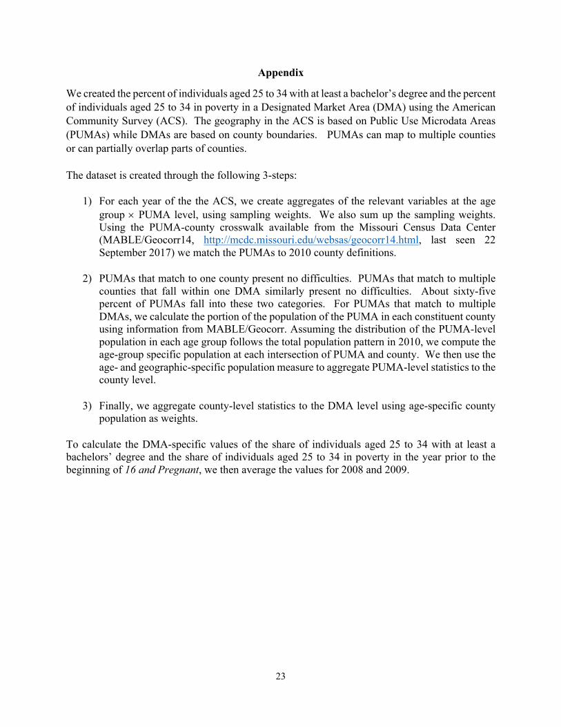
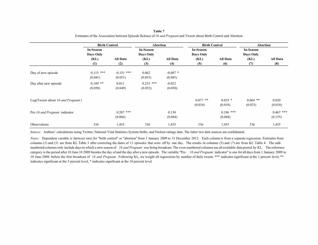
Our re-analysis of the tweet rates is presented in Table 7.19 In the odd-numbered columns

we replicate KL’s results using only 336 of the 1461 days. The even-numbered columns show the

same specification, but use all available data on tweets that were posted by KL. In the

specifications with all available data, we include a dummy variable for the period 1 January 2009-

10 June 2009 indicating the days prior to the debut of 16 and Pregnant. The reference category in

the even numbered columns is the days after 10 June 2009 that are not the day of or the day after

a new episode was broadcast.

KL report that the tweet rate for birth control increases 12 percent on the day of a new

episode and 19 percent on the day after relative to the rest of the week but only during the days a

new season is being broadcast (column 1). When we change the reference category to be all other

days in or between seasons, the coefficient on the day the show is broadcast become negative and

statistically significant (column 2). There are 21 percent more tweets for birth control in the

months prior to the debut of 16 and Pregnant than there are after the show and its re-runs are

broadcast. There is also no association between broadcast of new episodes and tweets for the

abortion rate in the full sample (column 4).

19 Our replication involved correcting KL’s data on the dates on which 16 and Pregnant was broadcast. Eleven of the 53 days the show was broadcast were miscoded by one day, implying that 11 lagged variables were also miscoded by one day. Correcting this did not substantively alter their published results.

21

In columns 5 and 7 we replicate KL’s results that regress the tweet rate for birth control

and abortion on the tweet rate of 16 and Pregnant during new seasons only. Once we include the

full sample, in columns 6 and 8, any association is either greatly reduced or eliminated. The lack

of any consistent association between broadcasts of new episodes of 16 and Pregnant, the tweet

rate for birth control and abortion is consistent with KL’s reported results using Google searches

for birth control and abortion in which they report no association.

The social media analyses presented by KL are a prominent part of their article and results

from these analyses are used to make the case for interpreting their birth rates estimates as causal.

Our re-assessment shows that these results are extremely fragile and at best inconclusive.

VII. Conclusion

Policies or treatments that begin at a single point in time for an entire population are

especially challenging for researchers to evaluate. The lack of an obvious counterfactual for the

treated group in the post-treatment period makes identification of causal effects difficult, if not

impossible, and studies claiming to estimate a causal effect in in the face of such challenges should

be viewed with skepticism. The burden of proof to validate the identifying assumptions should be

higher than in settings where a plausible counterfactual is readily available.

As an example, we have reexamined causal claims that the MTV program 16 and Pregnant

was responsible for lowering birth rates substantially in the United States. Our results strongly

suggest that the association between 16 and Pregnant and teen birth rates is due to differential

trends in birth rates across areas with different demographic characteristics in the wake of Great

Recession. The fertility rates of less advantaged teens, as proxied by race/ethnicity, fell much faster

22

with the onset of the recession than those of white non-Hispanics. We find a relationship between

MTV and birth rates even in the period prior to the existence of 16 and Pregnant, casting

substantial doubt on the validity of the parallel trends assumption required for identification. We

also demonstrate that KL’s social media analysis, which formed a core part of their argument, does

not withstand reassessment. While is possible that 16 and Pregnant may have affected teen birth

rates, our results point to the difficulty of making a causal claim that the show, which debuted

nationally at the nadir of the Great Recession, had a significant impact on teen birth rates. Our

results suggest that future researchers wishing to identify a causal effect of a policy that was

introduced everywhere at a single point in time should thoroughly assess whether the necessary

assumptions are credible.

Acknowledgements

The authors thank Phil Levine for his generous assistance in replicating results, and Bill Evans, Gary Solon, and seminar participants at Columbia University, the CUNY Graduate Center, the CUNY Institute for Demographic Research, the Guttmacher Institute, Princeton University, and the University of Michigan for helpful comments. Onur Altindag and J. J. Chen provided exemplary research assistance. Joyce and Kaestner acknowledge support from the National Institute of Child Health and Human Development Grant R01 HD082133 and from the Health Economics Program of the National Bureau of Economic Research. Nielsen ratings data are proprietary and cannot be shared. Birth data from the National Center for Health Statistics (NCHS) have confidential elements and must be obtained directly from NCHS. Institutional Review Board (IRB) approval was obtained from the National Bureau of Economic Research.

23

Appendix

We created the percent of individuals aged 25 to 34 with at least a bachelor’s degree and the percent of individuals aged 25 to 34 in poverty in a Designated Market Area (DMA) using the American Community Survey (ACS). The geography in the ACS is based on Public Use Microdata Areas (PUMAs) while DMAs are based on county boundaries. PUMAs can map to multiple counties or can partially overlap parts of counties.

The dataset is created through the following 3-steps:

1) For each year of the the ACS, we create aggregates of the relevant variables at the age group ´ PUMA level, using sampling weights. We also sum up the sampling weights. Using the PUMA-county crosswalk available from the Missouri Census Data Center (MABLE/Geocorr14, http://mcdc.missouri.edu/websas/geocorr14.html, last seen 22 September 2017) we match the PUMAs to 2010 county definitions.

2) PUMAs that match to one county present no difficulties. PUMAs that match to multiple counties that fall within one DMA similarly present no difficulties. About sixty-five percent of PUMAs fall into these two categories. For PUMAs that match to multiple DMAs, we calculate the portion of the population of the PUMA in each constituent county using information from MABLE/Geocorr. Assuming the distribution of the PUMA-level population in each age group follows the total population pattern in 2010, we compute the age-group specific population at each intersection of PUMA and county. We then use the age- and geographic-specific population measure to aggregate PUMA-level statistics to the county level.

3) Finally, we aggregate county-level statistics to the DMA level using age-specific county population as weights.

To calculate the DMA-specific values of the share of individuals aged 25 to 34 with at least a bachelors’ degree and the share of individuals aged 25 to 34 in poverty in the year prior to the beginning of 16 and Pregnant, we then average the values for 2008 and 2009.

24

References

Ananat, E. O., A. Gassman-Pines, and C. Gibson-Davis (2013) “Community-Wide Job Loss and Teenage Fertility: Evidence from North Carolina,” Demography 50, 2151–2171.

Autor, D., D. Dorn, and G. Hanson (2017) “When Work Disappears: Manufacturing Decline and the Falling Marriage-Market Value of Men,” Mimeo. MIT Department of Economics. Available at https://economics.mit.edu/files/12736.

Boonstra, H. (2014) “What Is Behind the Declines in Teen Pregnancy Rates?” Guttmacher Policy Review 17, 15–21.

Cherlin, A., E. Cumberworth, S. P. Morgan, and C. Wimer (2013) “The Effects of the Great Recession on Family Structure and Fertility,” Annals of the American Academy of Political and Social Science 650, 214–231.

Dehejia, R., and A. Lleras-Muney (2004) “Booms, Busts, and Babies’ Health,” Quarterly Journal of Economics 119, 1091–1130.

DellaVigna, S., and E. Kaplan (2007) “The Fox News Effect: Media Bias and Voting,” Quarterly Journal of Economics 122, 1187–1234.

Dobkin, C., A. Finkelstein, R. Kluender, and M. J. Notowidigdo (2016) “The Economic Consequences of Hospital Admissions.” NBER Working Paper 22288.

Gentzkow, M. (2006) “Television and Voter Turnout,” Quarterly Journal of Economics 121, 931–972.

Gentzkow, M., and J. M. Shapiro (2008) “Preschool Television Viewing and Adolescent Test Scores: Historical Evidence from the Coleman Study,” Quarterly Journal of Economics 123, 279–323.

Hamilton, B. E, J.A. Martin, M. J. K. Osterman, S. C. Curtin, and T. J. Matthews (2015) Births: Final Data for 2014. National Vital Statistics Reports. Volume 64, Number 12. Hyattsville, MD: National Center for Health Statistics.

Hjort, J., M. Sølvsten, and M. Wüst. (in press) “Universal Investment in Infants and Long-Run Health: Evidence from Denmark's 1937 Home Visiting Program,” American Economic Journal: Applied Economics.

Hoynes, H. W. and D. W. Schanzenbach (2009) “Consumption Responses to In-Kind Transfers: Evidence from the Introduction of the Food Stamp Program,” American Economic Journal: Applied Economics 1 (4): 109–139.

Hoynes, H. W., D. W. Schanzenbach, and Douglas Almond (2016) “Long-Run Impacts of Childhood Access to the Safety Net,” American Economic Review 106 (4): 96-34.

Jaeger, D. A., T. J. Joyce, and R. Kaestner (2016) “Does Reality TV Induce Real Effects? On the Questionable Association Between 16 and Pregnant and Teenage Childbearing,” IZA Discussion Paper 10317. Available at http://ftp.iza.org/dp10317.pdf.

Jensen, R., and E. Oster (2009) “The Power of TV: Cable Television and Women’s Status in India,” Quarterly Journal of Economics 124, 1057–1094.

25

Jackson, C. K., R. C. Johnson, and C. Persico (2015) “The Effects of School Spending on Educational and Economic Outcomes: Evidence from School Finance Reforms,” Quarterly Journal of Economics 131, 157-218.

Kaestner, R., S. Korenman, and J. O’Neill (2003) “Has Welfare Reform Changed Teenage Behaviors?” Journal of Policy Analysis and Management 22, 225–248.

Kearney, M. S., and P. B. Levine (2014a) “Media Influences on Social Outcomes: The Impact of MTV’s 16 and Pregnant on Teen Childbearing,” National Bureau of Economic Research Working Paper 19795. Available at http://www.nber.org/papers/w19795.

_____ (2014b) “Income Inequality and Early Nonmarital Childbearing,” Journal of Human Resources 49, 1–31.

_____ (2015a) “Investigating Recent Trends in the U.S. Teen Birth Rate,” Journal of Health Economics 41 (May): 15–29.

_____ (2015b) “Early Childhood Education by MOOC: Lessons from Sesame Street,” National Bureau of Economic Research Working Paper 21229. Available at http://www.nber.org/papers/w21229.

_____ (2015c) “Media Influences on Social Outcomes: The Impact of MTV’s 16 and Pregnant on Teen Childbearing,” American Economic Review 105, 3597–3632.

_____ (2016) “Does Reality TV Induce Real Effects? A Response to Jaeger, Joyce, and Kaestner (2016),” IZA Discussion Paper 10318. Available at http://ftp.iza.org/dp10318.pdf

Kearney, M. S., and R. Wilson (2017) “Male Earnings, Marriageable Men, and Nonmarital Fertility: Evidence from the Fracking Boom.,” National Bureau of Economic Research Working Paper 23408. Available at http://www.nber.org/papers/w23408.

La Ferrara, E., A. Chong, and S. Duryea (2012) “Soap Operas and Fertility: Evidence from Brazil,” American Economic Journal: Applied Economics 4, 1–31.

Lindberg, L., J.Santelli, and S. Desai (2016) “Understanding the Decline in Adolescent Fertility in the United States, 2007-2012,” Journal of Adolescent Health 59, 577-583.

Lopoo, L. M., and T. DeLeire (2006) “Did Welfare Reform Influence the Fertility of Young Teens?” Journal of Policy Analysis and Management 25, 275–298.

Santelli, J. S., L. D. Lindberg, L. B. Finer, and S. Singh (2007) “Explaining Recent Declines in Adolescent Pregnancy in the United States: The Contribution of Abstinence and Improved Contraceptive Use,” American Journal of Public Health 97, 150–156.

Sobotka, T., V. Skirbekk, and D. Philipov (2011) “Economic Recession and Fertility in the Developed World,” Population and Development Review 37, 267–306.

Villearreal, A. (2014) “Explaining the Decline in Mexico-U.S. Migration: The Effect of the Great Recession,” Demography 51, 2203–2228.

16 and PregnantIntroduced

Beginning ofKL's Analysis

Period

End ofKL's AnalysisPeriod

2.5

3.0

3.5

4.0

4.5

5.0

5.5

Log(

Teen

Birt

h R

ate)

2000 2005 2010 2015

All Non-Hispanic BlackNon-Hispanic White Hispanic

Source: Hamilton, et al. (2015)

Figure 1Log(Teen Birth Rate) for Race/Ethnicity Groups

χ2: 15.441p-value: 0.349

-0.2

00.

000.

20

Coe

ffici

ent

2001:QI 2003:QI 2005:QI 2007:QI 2009:QI 2011:QI

Panel 1: 2005-2010 (Reference period is 2005:QI-2005:QIV)

χ2: 35.284p-value: 0.036

-0.2

00.

000.

20

Coe

ffici

ent

2001:QI 2003:QI 2005:QI 2007:QI 2009:QI 2011:QI

Panel 2: 2003-2010 (Reference period is 2003:QI-2003:QIV)

χ2: 72.436p-value: <0.001

-0.2

00.

000.

20

Coe

ffici

ent

2001:QI 2003:QI 2005:QI 2007:QI 2009:QI 2011:QI

Panel 3: 2001-2010 (Reference period is 2001:QI-2001:QIV)

Source: Authors’ calculations using Bureau of Labor Statistics Local Area Unemployment Statistics, Bureau of the Census Census County Characteristics, National Vital Statistics System births, and Nielsen ratings data. The latter two data sources are confidential. Notes: These figures plot the coefficients of average MTV Ratings interacted with period dummy variables.The regressions also include the unemployment rate, the percent non-Hispanic black, percent Hispanic, and a full set of period dummy variables and DMA × season interactions. Variance-covariance matrices are calculated by clustering by DMA. Ninety-five percent confidence intervals shown. The F tests shown are for the jointsignificance of the coefficients shown in the pre-16 and Pregnant period. Panel A shows the period used inKearney and Levine (2015c). Regressions are weighted by the female population aged 15-19 in the DMA.

Figure 2IV Event Study: Extending the Pre-16 and Pregnant Period

Panel 1: Instrument: MTV × Post t

(1) Reduced form (KL) ** *** * ***

(2) Instrumental variables (KL) ** *** * ***

Panel 2: Instrument: Schooling × Post t

(3) Reduced form *** *** * ***

(4) Instrumental variables ** *** * ***

Panel 3: Poverty × Post t

(5) Reduced form *** *** * ***

(6) Instrumental variables ** *** ***

-2.197(1.197)

-3.103(0.553)

-2.305(1.267) (0.636)

Unemp.Rate

-2.812

PercentNon-Hisp.

BlackPercent

Hispanic

16 & Preg.

or

-2.366(0.941)

MTV ratings2008-2009

-1.487(0.375)

-3.581(1.517)

-1.485(0.043)

-2.172 -2.659

-2.036(1.230)

-3.395(0.619)(2.768)

-1.510(0.423)

-2.335(1.250)

-1.633(0.440)

-0.132(0.043)

Source: Authors’ calculations using Bureau of Labor Statistics Local Area UnemploymentStatistics, Bureau of the Census Census County Characteristics, National Vital Statistics Systembirths, and Nielsen ratings data. The latter two data sources are confidential.

Note: The dependent variable in all regressions is the natural logarithm of the birth rate for 15-19year olds. Standard errors, clustered by DMA, are shown in parentheses. All regressions areweighted by the female population aged 15 to 19 in the DMA at the time of the observation. Allregressions include 24 quarter fixed effects as well DMA × seaon fixed effects as regressors. Panel1 replicates KL's results. Panel 2 uses the percent of the population in the DMA aged 25-34 with atleast a Barchelor's degree in the year before 16 and Pregnant started broadcasting interacted withPost t as the instrument. Panels 3 uses percent the population aged 25-34 in the DMA in poverty inthe year before 16 and Pregnant started broadcasting interacted with Post t as the instrument. Thesample size in all regressions is 4,919. *** indicates significant at the 1 percent level, ** indicates significant at the 5 percent level, * indicates significant at the 10 percent level.

(0.448) (1.303) (0.706)(3.194)

Table 1

Ratings

-7.924 -1.699 -1.963 -3.528

(0.093) (0.407) (1.296) (0.607)

Estimates of the Impact of 16 and Pregnant on Teen Birth Rates using Alternative Instruments

-2.906(0.597)

0.323 -1.487

-6.188

% % %Non- Un- Non- Un- Non- Un-Hisp. % emp. Hisp. % emp. Hisp. % emp.Black Hisp. Rate Black Hisp. Rate Black Hisp. Rate2005 2005 2005 2005 2005 2005 2005 2005 2005

Panel 1: Base model: Replication

Reduced form (KL) ** *** * ***

Instrumental variables (KL) ** *** * ***

Panel 2: Base model plus covariates 2005 × Period Fixed Effects

Reduced form *** *** *** X X X

Instrumental variables *** *** *** X X X

Panel 3: Base model plus covariates 2005 × Linear Trend

Reduced form *** *** *** X X X

Instrumental variables *** *** *** X X X

Panel 4: Base model plus Race/Ethnicity 2005 × Linear Trend

Reduced form *** *** *** X X

Instrumental variables *** *** *** X X

Panel 5: Base model plus Unemployment 2005 × Linear Trend

Reduced form *** *** *** *** X

Instrumental variables *** *** *** *** X

Panel 6: Base model plus Covariates 2005 × Post t

Reduced form *** *** *** X X X

Instrumental variables *** *** *** X X X

Panel 7: Base model plus Race/Ethnicity 2005 × Post t

Reduced form *** *** *** X X

Instrumental variables *** *** *** X X

Panel 8: Base model plus Unemployment 2005 × Post t

Reduced form ** *** * *** X

Instrumental variables *** *** *** *** X

-2.812(0.636)

16 & Preg.

or

-2.197(1.197)

-3.103(0.553)

-2.305(1.267)

PercentNon-Hisp.

BlackPercent

Hispanic

-2.366(0.941)

-1.487(0.375)

-3.581(1.517)

-1.485(0.043)

MTV ratings2008-2009

Unemp.Rate

-0.437-(1.309)

-2.470-(0.536)

-3.312(1.012)

-0.238(0.800)

-1.467(0.318)

-2.442(0.553)

-0.404(1.504)

-1.473(0.360)

-1.414(0.349)

-3.295-(0.963)

-1.410(0.314)

-3.314(0.914)

-2.459(0.489)

-1.237(1.494)

(0.847)-0.776

-1.300(0.429)

-2.211 -2.547

-3.302(0.877)

-2.484(0.481)

0.273(0.749)

(0.354) (1.155) (0.516)

-3.091(1.150)

-3.032(0.631)

-1.292(0.384)

-3.104(1.046)

-3.071(0.561)

Table 2

Ratings

-1.441 -1.348 -2.763 -3.053

-0.259 -1.437 -2.877 -2.840

-0.449 -1.446 -2.870 -2.826(1.554) (0.364) (1.163) (0.525)

-2.238 -1.624 -2.115 -2.840

DMA Fixed Effects, Period Fixed Effects, andPeriod Fixed Eff. ×

Estimates of the Impact of 16 and Pregnant on Teen Birth Rates

(0.835) (0.325) (1.056) (0.459)

-3.319 1.624 -2.247 -2.647

(1.742) (0.421) (1.228) (0.593)

-0.838 -1.325 -2.789 -3.097

(0.316) (1.095) (0.463)

-3.374 -1.632

(0.828)

(1.303)

Post t×Linear Trend ×

Note: The dependent variable in all regressions is the natural logarithm of the birth rate for 15-19 year olds. Standard errors, clustered by DMA, are shown in parentheses. All regressions are weighted by the female population aged 15 to 19 in the DMA at the time of the observation. All regressions include 24 quarter fixed effects as well DMA × seaon fixed effects as regressors. The sample size in all regressions is 4,919. *** indicates significant at the 1 percent level, ** indicates significant at the 5 percent level, * indicates significant at the 10 percent level.

Source: Authors’ calculations using Bureau of Labor Statistics Local Area Unemployment Statistics, Bureau of the Census Census County Characteristics, National Vital Statistics System births, and Nielsen ratings data. The latter two data sources are confidential.

(0.930) (0.374) (1.115) (0.518)

(0.841) (0.335) (1.166) (0.494)-2.209 -1.612 -2.152 -2.935

(1.327) (0.377) (1.241) (0.557)

%Non- Un-Hisp. % emp.Black Hisp. Rate2005 2005 2005

Panel 1: Ages 20-24

(1) Reduced form (KL) *** ***

(2) Reduced form *** X X X

(3) Instrumental variables (KL) ** ***

(4) Instrumental variables *** X X X

Panel 2: Ages 25-29

(5) Reduced form (KL) *** ***

(6) Reduced form *** X X X

(7) Instrumental variables (KL) *** *** *

(8) Instrumental variables *** X X X

Panel 3: Ages 30-34

(9) Reduced form (KL) *** ** ***

(10) Reduced form *** ** *** X X X

(11) Instrumental variables (KL) *** ** ***

(12) Instrumental variables *** ** *** X X X

Source: Authors’ calculations using Bureau of Labor Statistics Local Area Unemployment Statistics, Bureau of theCensus Census County Characteristics, National Vital Statistics System births, and Nielsen ratings data. The lattertwo data sources are confidential.

-0.529 -2.651(0.838) (0.153) (0.246) (0.739)-0.141 -0.730

Note: Each row shows results from a separate regression. The dependent variable is the natural logarithm of the age-specific quarterly birth rate (multipled by 100) in the DMA. Odd-numbered rows reproduce Kearney and Levine's (2015) resultsfrom their Table 2. All regressions are weighted by the relevant population at the time of the observation. All regressionsinclude 24 quarter fixed effects as well DMA × seaon fixed effects as regressors. The sample sizes are 4,920, 4,920, and4,918 in panels 1, 2, and 3, respectively *** indicates significant at the 1 percent level, ** indicates significant at the 5percent level, * indicates significant at the 10 percent level.

-0.504 -2.449(0.689) (0.146) (0.243) (0.781)

-0.091 -0.730 -0.539 -0.652(0.496) (0.139) (0.252) (0.813)

0.538 -2.463(1.016) (0.165) (0.241) (0.843)

-1.136 -0.629 1.406 -1.941(0.700) (0.235) (0.877) (1.199)

Table 3Estimates of the Impact of 16 and Pregnant on Birth Rates, by Age Groups

16 & Preg.Ratings

or PercentMTV ratings Unemp. Non-Hisp. Percent

Linear Trend ×

2008-2009 Rate Black Hispanic

-3.498 -1.726 -0.820 -1.057(1.312) (0.325) (0.791) (1.683)

-2.422 -1.810 -0.923 0.845(0.993) (0.308) (0.706) (1.622)

-1.389 -1.459 0.319 -1.965(1.245) (0.027) (0.788) (1.434)

-0.897 -1.459 0.313 -1.935(0.755) (0.247) (0.717) (1.322)

-2.344 -0.721 1.394 -2.029(1.151) (0.252) (0.904) (1.313)

-1.789 -0.623

-0.455 -0.897

-0.328 -0.910

-1.606 -0.800 1.504 -1.976(0.817) (0.229) (0.825) (1.202)

1.392 -1.962(1.140) (0.256) (0.945) (1.318)

Panel 1: Ages 15-19

(1) Reduced form *** ** *** *** ***

(2) Instrumental variables *** *** *** *** ***

Panel 2: Ages 20-24

(3) Reduced form *** ** ***

(4) Instrumental variables *** ***

Panel 3: Ages 25-29

(5) Reduced form **

(6) Instrumental variables * * ***

Panel 4: Ages 30-34

(7) Reduced form ** *** *** ***

(8) Instrumental variables *** *** *** ***

(0.821) (0.606) (1.052) (0.459)

(1.234) (0.359) (0.929) (1.352)

with Covariate Interactions

-1.457 0.075 -1.573 -1.573(0.919) (0.670) (1.509) (1.509)

-1.558 -0.510 1.461 -2.094

16 & Preg.Ratings

or

(0.923) (0.317) (0.261) (0.864)

-1.003 -0.412 1.516 -2.084(0.770) (0.349) (0.849) (1.230)

-0.306 -0.643 -0.699 -2.573

-0.686 -2.569(0.561) (0.295) (0.247) (0.790)-0.202 -0.624

(0.049)

Source: Authors’ calculations using Bureau of Labor Statistics Local Area Unemployment Statistics, Bureau of the Census Census CountyCharacteristics, National Vital Statistics System births, and Nielsen ratings data. The latter two data sources are confidential.

Note: Each row shows results from a separate regression. The dependent variable is the natural logarithm of the age-specific quarterly birth rate(multipled by 100) in the DMA. All regressions are weighted by the relevant population at the time of the observation. All regressions include24 quarter fixed effects as well DMA × seaon fixed effects as regressors. The sample sizes are 4,919, 4,920, 4,920, and 4,918 in panels 1through 4, respectively *** indicates significant at the 1 percent level, ** indicates significant at the 5 percent level, * indicates significant at the10 percent level.

0.010 0.002 -0.010(0.006) (0.003)

-0.562 -2.765 -2.960 -2.899

Non-Hisp.Unemp. Black

0.371 -0.029

0.367 -0.030

(1.402) (0.649) (1.155) (0.515)

Percent2008-2009 Rate Black Hispanic

PercentMTV ratings Unemp. Non-Hisp.

(0.107) (0.009) (0.006)

-0.008(0.117) (0.010) (0.007)

Hispanic2005 2005 2005

Table 4Estimates of the Impact of 16 and Pregnant on Birth Rates, by Age Groups

(1.621)(0.735)(0.511)(1.426)-1.6220.071-2.263-2.236

-2.864-2.952-2.836-0.885

Unemployment Rate ×Percent

Percent

0.238 -0.008 -0.020(0.089) (0.012) (0.007)

-0.009

0.011 0.003 -0.009(0.054) (0.006) (0.003)

0.042 -0.010 -0.013(0.047) (0.009) (0.004)

(0.050) (0.010) (0.005)0.047 -0.009 -0.010

0.228 -0.009 -0.024(0.084) (0.011) (0.006)

Linear Trend ×DMA

Panel 1: Non-Hispanic Whites

(1) Reduced form (KL) ** ***

(2) Reduced form *** X

(3) Instrumental variables (KL) ** ***

(4) Instrumental variables *** X

Panel 2: Non-Hispanic Blacks

(5) Reduced form (KL)

(6) Reduced form X

(7) Instrumental variables (KL)

(8) Instrumental variables X

Panel 3: Hispanics

(9) Reduced form (KL) ***

(10) Reduced form *** X

(11) Instrumental variables (KL) * ***

(12) Instrumental variables *** X(1.072) (0.535)-1.066 -2.055

Note: Each row shows results from a separate regression. The dependent variable is the natural logarithm of the race/ethnicity-specific quarterly teen birth rate (multipled by 100) in the DMA. Odd-numbered rows reproduce Kearney and Levine's (2015) race-specific results from their Table 2. All regressions are weighted by the relevant population at the time of the observation. All regressions include 24 quarter fixed effects as well DMA × seaon fixed effects as regressors. The sample sizes are 4,911, 4,513, and 4,750 in panels 1, 2, and 3, respectively. *** indicates significant at the 1 percent level, ** indicates significant at the 5 percent level, * indicates significant at the 10 percent level.

Source: Authors’ calculations using Bureau of Labor Statistics Local Area UnemploymentStatistics, Bureau of the Census Census County Characteristics, National Vital Statistics Systembirths, and Nielsen ratings data. The latter two data sources are confidential.

(2.063) (0.784)

-1.857 -1.972(1.960) (0.589)

-3.782 -2.512

Table 5

16 & Preg.Ratings

orMTV ratings Unemp.

Estimates of the Impact of 16 and Pregnant on Teen Birth Rates, by Race/Ethnicity

2008-2009 Rate

-3.370 -1.354(1.581) (0.375)

-2.413 -1.399(1.075) -(0.329)

1.425 -1.011(2.413) (0.387)

(5.989) (1.611)

1.013 -0.960(1.591) (0.365)

-0.194 -0.240

(4.433) (0.944)

(2.109) (1.170)-3.322 1.068

-6.510 -2.418

-2.360 -1.153(3.382) (1.471)

-0.140 -0.243(1.380) (1.049)

Row Begin "Show" Start End Std. Err. Std. Err.

(1) 2001:QI 2005:QIII 2006:QIV -2.437 * 1.324 -1.639 * 0.846(2) 2001:QII 2005:QIV 2007:QI -1.994 1.299 -1.330 0.837(3) 2001:QIII 2006:QI 2007:QII -2.554 * 1.441 -1.693 * 0.948(4) 2001:QIV 2006:QII 2007:QIII -2.929 ** 1.473 -1.936 ** 0.977(5) 2002:QI 2006:QIII 2007:QIV -2.968 * 1.521 -1.958 ** 0.992(6) 2002:QII 2006:QIV 2008:QI -3.144 ** 1.569 -2.068 ** 1.028(7) 2002:QIII 2007:QI 2008:QII -3.341 ** 1.508 -2.194 ** 1.014(8) 2002:QIV 2007:QII 2008:QIII -3.079 ** 1.458 -2.021 ** 0.966(9) 2003:QI 2007:QIII 2008:QIV -2.756 * 1.476 -1.809 * 0.967(10) 2003:QII 2007:QIV 2009:QI -2.543 * 1.485 -1.673 * 0.969(11) 2003:QIII 2008:QI 2009:QII -2.377 1.558 -1.566 1.002(12) 2005:QI 2009:QIII 2010:QIV -3.581 ** 1.517 -2.368 ** 0.942

Notes: Entries in the table are a) in the reduced form, the estimated coefficient on MTV Ratings in 2008:QIII-2009:QIIinteracted with a dummy variable for being in the "post" period and b) for instrumental variables, the estimated coefficient on 16 and Pregnant Ratings interacted with a dummy variable for being in the "post" period where the instrument is theregressor of interest from the reduced form regressions. Standard errors, clustered by DMA, are shown in parentheses. Allregressions are weighted by the female population aged 15-19 in the DMA at the time of the observation. In each regressionthere are 18 pre-"show" quarers and 6 post-"show" quarters. All regressions also include the unemployment rate, the percentof the population that is non-Hispanic black and the percent of the population that is Hispanic, 24 quarter fixed effects aswell DMA × season fixed effects as regressors. The period analyzed by Kearney and Levine's (2015b) is boxed. In theperiods that are lightly shaded, the placebo post period partially includes the actual post -16 and Pregnant period. Samplesize in rows (1) through (17), and (19) through (21 is 4,918, the sample size in row (18) is 4,917, and the sample size inrows (22) through (25) is 4,919. *** indicates significant at the 1 percent level, ** indicates significant at the 5 percentlevel, * indicates significant at the 10 percent level.

Instrumental VariablesCoefficient

Table 6Placebo Tests of Estimated Reduced Form and Instrumental Variables Impact on Teen Birth Rates

Rolling 24 Quarter Periods

Source: Authors’ calculations using Bureau of Labor Statistics Local Area Unemployment Statistics, Bureau of the CensusCensus County Characteristics, National Vital Statistics System births, and Nielsen ratings data. The latter two data sourcesare confidential.

Reduced FormDatesCoefficient

Day of new episode *** *** *

Day after new episode ** ***

Log(Tweets about 16 and Pregnant ) ** * **

Pre-16 and Pregnant indicator *** *** ***

Observations

-0.151(0.051)

0.011(0.049)

(KL)

Birth Control

0.207(0.066)

336 1,455

In-Season

All DataDays Only

0.115(0.041)

0.189(0.050)

(1) (2)

AbortionIn-SeasonDays Only

(KL) All Data(3) (4)

0.062 -0.087(0.053) (0.045)

336 1,455

Birth Control AbortionIn-Season In-SeasonDays Only Days Only

0.233 -0.022(0.052) (0.050)

0.130(0.084)

(KL) All Data (KL) All Data(5) (6) (7) (8)

(0.155)

336 1,455 336 1,455

Table 7Estimates of the Association between Episode Release of 16 and Pregnant and Tweets about Birth Control and Abortion

Source: Authors’ calculations using Twitter, National Vital Statistics System births, and Nielsen ratings data. The latter two data sources are confidential.

Notes: Dependent variable is ln(tweet rate) for "birth control" or "abortion" from 1 January 2009 to 31 December 2012. Each column is from a separate regression. Estimates fromcolumns (1) and (3) are from KL Table 3 after correcting the dates of 11 episodes that were off by one day. The results in columns (5) and (7) are from KL Table 4. The odd-numbered columns only include days in which a new season of 16 and Pregnant was being broadcast. The even-numbered columns use all available data posted by KL. The referencecategory is the period after 10 June 10 2009 besides the day of and the day after a new episode. The variable "Pre- 16 and Pregnant indicator" is one for all days from 1 January 2009 to10 June 2009, before the first broadcast of 16 and Pregnant . Following KL, we weight all regressions by number of daily tweets. *** indicates significant at the 1 percent level, **indicates significant at the 5 percent level, * indicates significant at the 10 percent level.

0.077 0.035 0.064 0.020(0.034) (0.018) (0.025) (0.018)

0.196 0.467(0.068)