1

6/5/2007

Provisional draft

Did the Decline in Social Capital Decrease American Happiness?

A Relational Explanation of the Happiness Paradox

S. Bartolini, University of Siena

E. Bilancini, University of Siena

M. Pugno, University of Cassino

Abstract Most popular explanations of the happiness paradox cannot fully account for the lack of growth in U.S. reported well-being during the last thirty years (Blanchflower and Oswald (2004)). In this paper we test an alternative hypothesis, namely that the decline in U.S. social capital is responsible for what is left unexplained by previous research. We provide three main findings. First, we show that the inclusion of social capital does improve the account of reported happiness. Second, we provide evidence of a decline in social capital indicators for the period 1975-2004, confirming Putnam's claim to a large extent. Finally, we show that failed growth of happiness is mostly due to the decline of social capital and, in particular, to the decline of its relational and intrinsically motivated component.

1. Introduction

This paper provides evidence that the decline of social capital can contribute to explain the

happiness paradox. The latter was formulated by Easterlin (1974), who showed two stylized facts:

that people in industrialized countries are not becoming happier over time despite economic growth,

and that people with a higher income than others, at any given point in time, do report higher levels

of happiness. If more income makes an individual better off, why does an increase in the income of

all not improve everybody’s lot?

Further evidence of the paradox has been provided by subsequent research and it has

attracted interest on the determinants of well-being. The literature introduced by Easterlin has

become a booming industry by now. This literature is fed by the abundance of data on self-reported

well-being, which proved to contain relevant information on the well-being of individuals.

Econometric studies have detected, among others, the importance of income aspirations,

unemployment, inflation and social capital for people’s well-being (Oswald, 1997; Blanchflower

and Oswald, 2004; Easterlin, 1995; Frey and Stutzer, 2000; Di Tella and McCulloch).

2

However, not all these variables, usually omitted from utility functions, can aid in

explaining the happiness paradox. In order to do so, they need to have a trend that can offset the

positive impact exerted by rising income on well-being. For instance, unemployment and inflation

cannot be used to explain the paradox simply because they do not exhibit a rising trend.

Income aspirations have progressively attracted wide consensus due to their potential in

explaining the paradox. In fact, the shift in income aspirations may, in principle, compensate for the

positive impact of rising income on well-being. Two sources of aspirations dynamics have been

pointed out. Aspirations can be linked to one’s past income or to the income of one’s reference

group. The former case has been often referred to as a hedonic adaptation to a consumption

standard, while the latter is linked to the tradition emphasizing the importance of social

comparisons in determining consumption choices (Veblen, 1899; Duesenberry 1949). In both cases,

economic growth tends to raise income aspirations with negative effects on happiness. Growth

triggers a Hedonic Treadmill (people adapt their aspirations to past living standards) and a

Positional Treadmill (people compare their income to that of others and set their aspirations

accordingly), which may partly or completely offset the positive effect exerted on well-being by

rising absolute income.

However, the shift in income aspirations cannot fully account for a decreasing trend in

happiness. Reasonably, it can account for, at most, a stable trend. In fact, aspirations must concern

that which individuals consider relevant per se and not what is regarded as unimportant. In other

words, one can aspire to a greater absolute income only if absolute income is considered relevant. If

only relative income matters, then it is relative income that becomes the object of aspiration and,

hence, adaptation occurs with respect to relative position. Therefore, the total negative effects of the

hedonic and the positional treadmills cannot go beyond the elimination of any benefit accruing from

income growth.1 Summing up, a declining trend in happiness remains partly unexplained at the

current state of the literature.2

As a remarkable example, Blanchflower and Oswald (2004) observe that a negative time-

trend of well-being in the US between 1974 and 1998 persists, even if controlled, for relative 1 The empirical evidence on these issues is controversial: Blanchflower and Oswald (2004) show that the effect of an increase in the income of others does not completely compensate for the increase in one’s own income (also Stutzer (2004), Luttmer (2005)). On the other hand, some research shows that the impact of the income of others is as strong as that of one’s own (see Ferrer-I-Carbonell 2005). 2 Di Tella and McCulloch (2005) further attempt to give an answer to the happiness paradox by adding to the conventional arguments of the utility function other aggregate variables, like unemployment rate, inflation, average divorce rate, life expectancy, pollution, and crime, and by attempting an estimate of their contribution to reported well-being. However, “introducing omitted variables worsens the income-without-happiness paradox” (Di Tella and McCulloch 2005:1, emphasis added), at least for Europe.

3

income, alongside the other usual socio-economic controls. They thus conclude asking for more

research on this point.

Our thesis is that the decline in U.S. social capital can account for what is left unexplained

of the happiness trend. In particular, we test the hypothesis that the decline in the quality and

quantity of intrinsically motivated relations may have played a major role in the evolution of

happiness over the last thirty years. The possible role of social capital in explaining the happiness

paradox is still an open question, currently explored by a few pioneering studies (Helliwell (2003,

2006), Helliwell and Putnam (2005). Bruni and Stanca (2006) focus on the relational dimension of

social capital. These studies show a positive impact of social capital on happiness. However, since

they do not analyze trends of social capital variables, they do not allow drawing any conclusions on

their possible role in explaining happiness trends.3

Social capital trends in the US during the last 5 decades have been the object of a lively

debate raised by Putnam (Putnam (2000), and for a concise survey see Stall and Hooghe (2004)).

His evidence has been criticized by Ladd (1996), and then carefully scrutinized for the variable used

and the period considered by Paxton (1999), Robinson and Jackson (2001), and Costa and Kahn

(2003). On balance, social capital has been confirmed as declining in the US, although not so

dramatically as Putnam claimed.

Summing up, in this paper we test a number of interrelated hypotheses: that the various

proxies for social capital declined during the recent decades; that these proxies play an important

role in an individual’s self-reported well-being over the same period; that absolute and relative

income maintain significant roles.

These aims require a generous data set. For this purpose we use the US General Social

Survey (GSS) since it includes many questions directly linked to social capital, questions on

absolute as well as perceived relative income, and as it extends over 32 years drawing from very

large samples of the US population. The main limitation of the GSS is that it is not a panel.

Consequently, adaptation cannot be properly studied.

Blanchflower and Oswald (2004) have already estimated a happiness equation with a

number of demographic and socio-economic controls using GSS data. In the first part of the paper

we follow their strategy. The present work may also be seen as an extension and an advancement of

Blanchflower and Oswald (2004). We respect to them, we analyze a longer period (up to 2004

3 When the studies concentrate on social capital, the cross-country approach is adopted. This approach not only impedes the analysis over time, but the usual data set employed (the World Value Survey) does not allow the comparison of individuals’ level of absolute income.

4

instead of 1998); we include social capital variables; we refine the controls for relative income; and,

most importantly, we calculate the impact of each of our regressors on the trend of happiness.

The paper proceeds as follows. In Section 2, we define concepts and variables. In Section 3,

we estimate the impact of social capital on happiness. In Section 4, we estimate the trend of social

capital. In Section 5, we estimate the happiness trend predicted by our figures and compare it to the

observed trend. Section 6 draws conclusions and comments on both problems of interpretation and

implications for policy.

2. Theoretical framework: social capital, relations, motivations

Social capital (SC) is a rather vague concept and, often, scholars ascribe different meanings to it. By

SC we mean the stock of non-market relations and beliefs that affect the return of available

resources, either in physical or utility terms. In particular, we call the stock of non-market relations

relational social capital (RSC).

We further distinguish between intrinsically and extrinsically motivated RSC. The concept of

extrinsic motivations refers to the incentives coming from outside an individual. By contrast, major

psychological schools emphasize the intrinsic motives issuing from within an individual. According

to Deci (1971, pg. 105), “one is said to be intrinsically motivated to perform an activity when one

receives no apparent reward except the activity itself”. Notice that Deci’s definition concentrates on

the non-instrumental nature of intrinsically motivated activities which directly enter the utility

functions of individuals. The distinction between intrinsic and extrinsic motivations is a well-

established concept in social sciences. Various empirical studies in psychology have found that

extrinsic motivations can crowd out intrinsic ones. This has arisen a lively debate in psychology

(Sansone and Harackievicz, 2000), but it has also attracted interest among the economists (Frey

1997; Benabou and Tirole 2003; Kreps 1997).

Notice that, according to such a distinction, instrumental relations are not exhausted by

market relations. In fact, also non-market relations can be extrinsically motivated. Moreover, they

may be both extrinsically and intrinsically motivated. Therefore, we adopt the following definitions

which provide a clear and economically meaningful distinction. By intrinsic relational social

capital (or intrinsic RSC) we mean the stock of RSC that enters into people's utility functions. By

purely extrinsic or non-intrinsic relational social capital we mean the stock of RSC that does not

directly enter into people's utility functions, but is instrumental to something else that may be

considered valuable.

As measures of the non-relational component of SC – i.e. the “beliefs” component – we use

several reports of trust in institutions such as organized labor, education, Congress, the military

5

forces, banks and financial institutions, major corporations, the executive branch of government,

etc. This is quite standard (Paxton (2004), Costa and Kahn (2003)). As measures of RSC we use

marital status, social contacts, trust in individuals, membership in various groups and organizations,

watching TV. We recognize that marital status is not always considered a social capital variable.

Nevertheless, it is obviously a relational variable and, hence, we find it reasonable to put it among

RSC variables. Moreover, it is an important source of information on the family, which, according

to Putnam (2000), is considered the main source of social capital. Furthermore, we classify marital

status and social contacts (with neighbors, friends and relatives, at bars and taverns) as indicators of

intrinsic RSC. Besides possible extrinsic motivations, their intrinsic nature should be obvious

enough. In the following, we illustrate why we also consider membership in certain groups,

watching TV and trust in individuals as indicators of intrinsic RSC.

Membership in groups and organizations is widely considered to be a good indicator of

relational activities (also referred to as “weak ties” in the social capital literature (Olson (1982),

Putnam (2000), Costa and Khan (2003), Sabatini (2006)). Given the different nature of the various

groups and organizations, we propose a distinction between intrinsically and extrinsically motivated

group memberships. For this purpose, we sort groups into two main categories which we call,

following the intuition of Knack (2003), Putnam’s groups and Olson’s groups. The distinction

between Olson’s and Putnam’s groups is based on the classic works of Olson (1982) and Putnam

(1993). They provide sharply conflicting perspectives on the impact of private associations on

economic performance and social conflict. Olson (1982) emphasized the propensity of associations

to act as special interest groups that lobby for preferential policies, imposing disproportionate costs

on the rest of society with adverse consequences for economic performance. Labor unions,

professional associations, trade associations and other groups lobby government for tariffs, tax

breaks, subsidies or competition-inhibiting regulation, which benefit them but at a large cost to

society as a whole. Putnam (1993) viewed membership in horizontal associations much more

favorably, as a source of generalized trust and social ties conducive to governmental efficiency,

trust and economic performance. These different views motivated empirical tests aimed at verifying

if different horizontal associations, called Olsonian and Putnamian, have a different impact on

economic growth (Knack (2003), Gleaser et al. (2000)).

In this paper, membership in Putnam’s group is interpreted as intrinsic RSC, while

membership in Olson’s group is interpreted as purely extrinsic RSC. In other words, membership in

Putnam’s groups is supposed to be mostly experienced for the pleasure of being a member (e.g. the

pleasure derived by the idea of acting together with other individuals towards a common aim, the

pleasure of interacting with people having the same tastes, etc.). Conversely, membership in Olson’s

6

groups is supposed to be experienced only for instrumental reasons (e.g. rent-seeking). Among

Putnam’s groups we include service groups, church organizations, sports clubs, art and literature

clubs, national organizations, hobby clubs, fraternal groups and youth associations. Among Olson’s

groups we include fraternity associations, unions, professional organizations and farm

organizations. Three groups were left unclassified and we put them under the label of Other groups.

We do this because it is not clear whether these groups constitute intrinsic RSC or not. Among such

Other groups we put veterans associations, political parties and “other groups” (the latter is the

label used in the GSS for groups that do not fall in any of the types otherwise described).4

We also classify social trust variables – i.e. reports of general perceived trustworthiness,

helpfulness and fairness – as indicators of intrinsic RSC. We interpret them as judgments about the

behavior of others, which stem from the quality of individuals' actual relationships. In other words,

we posit that people judge that others are trustworthy or helpful on the basis of their actual

experiences and that these relationships are more likely to be based on trust and mutual help when

they are intrinsically motivated. This does not exclude extrinsic motivations but requires intrinsic

ones to play an important role.

Finally, we consider the number of hours spent watching TV as a proxy for both the quantity

and the quality of relational activities, namely as a negative indicator of RSC. Apart from the time

constraint – which reasonably supports our interpretation – we also suppose that individuals

spending much time watching TV are, on average, less engaged in relational activities and, in

particular, those that are intrinsically motivated (Bruni and Stanca (2006)). The basic idea is that

watching TV reduces relational activities and that intrinsic relations are more elastic to watching

TV than extrinsic ones.

3. Empirical Strategy, Data and Estimation Results

Our core empirical strategy is the same applied by Blanchflower and Oswald (2004) (BO from now

on). Using GSS data, we estimate several ordered logit equations, each characterized by a different

set of regressors. We introduce a time variable in all these regressions in order to capture the

residual trend in happiness that is left unexplained. By comparing the coefficient of the time

4 Knack (2003) does not refer to intrinsic and extrinsic motivations. Moreover, the types of groups recognized in

the GSS do not coincide with those recognized in the database used by Knack (2003) so our classifications are partly different. However, this is not the only reasons for the minor differences between ours and Knack's classification. We (manca qualcosa) some further changes because of a different interpretation: groups whose main objective is to foster collective actions do not necessarily fall in the Olson category. For instance, we put political parties among Other groups – and not among Olson's group – because we believe that membership in a political party is not necessarily a matter of rent-seeking.

7

variable across regressions, we deduce information about the impact of the different groups of

regressors on the trend of reported happiness.

The equations that we estimate are variations of the following general specification:

h* = h(u(Soc-Demo,Inc,RelInc,SC,Time)) )1)

where Soc-Demo is a set of controls for socio-demographic characteristics, Inc is a set of controls

for absolute income, RelInc is a set of controls for relative income, SC is a set of controls for social

capital and Time is the time variable. Function h() determines “perceived happiness” and is assumed

to be a positive monotone transformation of the function u() which determines “true” utility.

Neither utility u nor perceived happiness h* can be directly observed. However, we do observe

reported happiness h according to the following rule: h = 1 if h* < c1, h = 2 if c1 < h* < c2, h = 3 if

c2 < h*, for some threshold values c1and c2. Our first set of regressions contains, beside the time variable, only demographic and economic

variables. The purpose is twofold. Firstly, we want to establish that which remains to be explained

once we have checked for plausible determinants of happiness that cannot be related to SC (either

relational or non-relational). Secondly, we are interested in checking what the best control for

relative income is. In fact, the one used by Blachflower and Oswald (2004) – the ratio between

household per capita income and regional income – performs rather badly, in our opinion. Since our

aim is to measure to what extent SC can account for the happiness trend, we want to be reasonably

sure that the unexplained residual in the happiness trend is not due to a poor control for relative

income.

Table 1 shows the results for this first group of regressions. Some variables are used as they

occur in the GSS. Other variables are constructed using variables found in the GSS. For example,

our dependent variable is reported happiness, measured in the GSS by the survey question: “Taken

all together, how would you say things are these days? Would you say you are very happy, pretty

happy or not too happy?”, associating the numbers from 1 to 3 to the three answers. We intend a

higher number to mean greater happiness so we associate 3 to “very happy”, 2 to “pretty happy”

and 1 to “not too happy”. Several categorical and ordered variables require more than two values.

We either collapse all categories into just two or construct a dummy for each category. Two

variables come from two other data sets. Details about definition, source and summary statistics of

all variables used in these and subsequent estimations can be found in the appendix. A brief

description is provided in the text whenever the variable meaning is not immediately clear.

8

In Regression 1, we control for demographic characteristics such as age, gender and race, and

for socio-economic factors such as work status, years of education and absolute income. We also

add a dummy for living with both parents at the age of 16 and another dummy for the divorce of

one’s parents at the same age. These are supposed to be controls for important individual past

events which may have affected individuals' preferences and/or future choices. Both variables have

significant coefficients that show the expected signs. This suggests that life events such as the

divorce or death of one’s parents do have permanent negative effects on the reported well-being of

individuals.

We use household income instead of personal income, because the former is available for

most observations while the latter is not. Moreover we are confident that household income is a

better measure of an individual’s overall economic condition. Unfortunately, there is no reliable

income data for 2004, which forces us to restrict our analysis to 2002. The period covered is 1972-

2002. The magnitude and sign of coefficients is in line with other studies in this area and, in

particular, with BO (see also Di Tella and MacCulloch (2005), Di Tella et al (2003), Bruni and

Stanca (2006), Alesina et at. (2004)).5 Net of the income loss, unemployment has a huge negative

impact on happiness. Income buys happiness, but at a very high price. Finally, the coefficient of the

time variable is -.019 and highly significant. This confirms that reported happiness has a residual

negative trend in the period 1972-2004 which is not explained by the controls.

In Regression 2, we follow BO adding a control for relative income and a control for

differentials in life costs across U.S. census regions. The first control is obtained by calculating the

ratio between “per capita” household income (household income divided by household size) and

regional per capita income (source: US Dept. of Commerce, Bureau of Economic Analysis). The

second control is an index (base is the U.S. average), which measures the difference in house values

for single-family detached homes on which at least two mortgages were originated or subsequently

purchased or securitized (source: The Office of Federal Housing Enterprise Oversight’s, Repeat

Sales House Price Index). Our results differ from those provided by BO in two respects. First, the

relative income variable has a negative and insignificant coefficient. Second, the control for life cost

differentials has a negative and highly significant coefficient. This may be due to the fact that we

constructed the latter variable in a way which is different from that followed by BO or to the fact

that the time period that we study is different (1975-2002 instead of 1972-1998). However, the

coefficient of the time variable is about -0.162 and highly significant, results very similar to those

5 The coefficient of household size is positive and significant, while in BO it is negative and significant. Most

probably, this difference is due to the fact that here household size is a proxy for marriage. In fact, when marital status

is added, the coefficient of household size becomes negative and significant (see Table 3).

9

obtained by BO. Overall this suggests to us that the control for relative income may be a rather poor

one.

In Regressions 3 and 4, we add further controls for relative income. In the GSS, subjects are

asked to evaluate the relative standing of their household income. Available answers are “very

below the average”, “below the average”, “average”, “above average” and “very above the

average”. Although this is a subjective evaluation of relative position, we find it much more

informative than the ratio between per capita household income and regional income. Moreover,

what is supposed to be relevant for happiness is the perceived relative standing, which depends on

both objective relative standing and reference group. Clearly, we cannot exclude that a happier

individual tends to perceive a higher relative standing. However, this is true for most variables

contained in the regression – including absolute income – and, therefore, we do not find particular

reasons against the use of a subjective control for relative income.

We add a dummy for each answer, assuming that “average” is the omitted case. As Table 1

shows, results are quite impressive. The coefficients of these dummies have the rights sign and are

both large and significant. Interestingly, being “very below the average” reduces the probability of

reporting a high level of happiness twice as much as being “below the average” and five times as

much as being “above the average” increases such a probability. Moreover, significance decreases

substantially as we move from “below the average” to” above the average”. This suggests that there

is a strong asymmetry in the impact of perceived relative position. Being convinced of lying below

the average life standard hurts people much more than the benefits associated to being convinced of

lying above the average one.6 The coefficient of the time variable increases sensibly, though it

remains negative and highly significant. Most importantly, the time coefficient is almost the same in

Regressions 3 and 4 – which differ solely for the inclusion of the ratio between per capita household

income and regional income. Overall, this suggests that our control for relative income performs

rather better than the one used by BO and, hence, in the subsequent regressions we drop the latter in

favor of the former.

Finally, Regression 5 differs from Regression 4 only for the specification of absolute income

and constitutes our reference point for investigating the impact of social capital variables. We

reintroduce household income and household size in place of per capita household income, because

the latter specification of absolute income seems to us less reasonable as it imposes a very specific

6 Such a result is certainly interesting per se and has important implications. For instance, it suggests that

inequality may have an overall negative effect. However, since in this paper we are interested in the role of social

capital, we leave these issues for future research.

10

relationship between household size and personal income.7 The coefficient of the time variable is

about -.012 and is highly significant. We interpret this result as evidence that demographic and

socio-economic characteristics leave unexplained a substantial part of the trend in reported

happiness.

The next set of regressions explores the impact of SC variables: marital status and children,

social contacts, social trust, watching TV, group membership and confidence in institutions. One

serious problem with these variables is that they are not observed for the entire sample of

individuals. We have observations for every variable for both 1975 and 2004. This gives us the

possibility to look at their variation over a 30-year time span. However, when we consider all these

variables together, we end up with less than six thousands observations out of more than thirty-two

thousands. What is worst, the questions about group membership had not been asked during the

period 1996-2002 (included). This, coupled with the fact that we do not have reliable observations

for household income in 2004, forces us to restrict the time frame to 1975-1994 whenever we place

absolute income and variables related to group membership in the same regression.

In total, we run seven additional regressions. In each regression from 6 to 11, we add a

different group of social capital variables to the regressors used in Regression 5. In Regression 11,

we add all groups of social capital variables. We adopt this strategy for two reasons. First, it allows

us to extend the time period up to 2002 for most regression, which, in turn, gives us the possibility

of investigating whether the results that we obtain for Regression 11 – relative to the period 1975-

1994 – can be reasonably extended to the period 1975-2002. Second, by running separate

regressions for each group of social capital variables, we obtain information about the impact of

each group on the trend of happiness. In fact, we are not only interested in the impact of social

capital as a whole. We also want to understand wherein lays the contribution of relational variables,

with respect to non-relational variables, to the explanation of the happiness trend.

Table 3 shows the results for Regressions 6-12. Although not reported, all controls present in

Regression 5 are maintained here. Regression 6 investigates the impact of marital status and the

number of children. As expected, marital status is very important. In particular, being married

increases the level of reported happiness as much as being unemployed decreases it. This confirms

that marital status has a large impact on an individual’s happiness. Interestingly, people in their

7 Introducing household per capita income seems to increase the coefficient of the time variable by a value

between .005 and .003, while making age and gender not significant. We cannot find an economically meaningful

explanation of these results. However, the comparison between the coefficient of the time variable of Regression 3 and

Regression 5 confirms the poorness of the ratio between per capita household income and regional per capita income as

a control for relative standing.

11

second marriage are not as happy as people in their first marriage, even without considering the

happiness reduction due to a divorce. Separated and divorced people are less happy than unmarried

people. Being divorced is as bad as being widowed. Quite surprisingly, children do not seem to

have an impact on happiness. This is the case even if we substitute the number of children with a

dummy for 1 or 2 children. One reason may be that household size already captures the effect of

children. However, when we control for marital status, the coefficient of household size becomes

negative and significant (as in BO), suggesting that household size is mostly a control for household

expenditures. Another reason may be that the number of children is a too rough variable: what

makes parents happy is not the number of children but the relationship they have with them. In any

case, evidence has been provided that, when controlling for individual fixed effects, having a child

has almost no effect (Clark and Oswald (2002)). Finally, Regression 6 shows that this group of

variables has a considerable impact on the happiness trend. Although the coefficient of the time

variable remains negative and significant at the 1% level, it drops from about -.012 to about -0.04,

suggesting that a consistent part of the decline in happiness in the period 1975-2002 can be

explained with a deterioration of marital relationships.

Regression 7 explores the role of social contacts. We introduce four dummies which are set

equal to one if the respondent declared to spend at least one evening per month with, respectively,

his/her relatives, his/her neighbors, his/her friends (outside the neighborhood) or at a bar, tavern and

the like. The result is twofold. On the one hand, the coefficients of the four dummies are all large

and significant, suggesting that social contacts matter a great deal for reported happiness. In

particular, spending evenings with relatives, neighbors or friends goes with a greater reported

happiness, while spending evenings at a bar goes with a lower one. More precisely, spending at

least one evening with relatives increases happiness twice as much as spending one evening with

friends or neighbors. Spending at least one evening at a bar has a negative effect that is as large as

the positive effect of spending evenings with relatives. We believe that this last result is due to the

fact that spending evenings at a bar is a proxy for poor social relations. In our opinion, this

interpretation especially fits the case of U.S., where going to a bar in search of company – and not

already in company – is a standard practice. On the other hand, however, there is no substantial

change in the coefficient of the time variable with respect to Regression 5. This suggests that

although social contacts are important for reported well-being, they do not contribute much to the

explanation of the happiness trend.

Regression 8 also investigates the role of relational activities but does not distinguish between

types of relations. The result is quite interesting. The coefficient of watching TV is negative and

highly significant. Watching 8 hours of TV per day hurts as much as being below the average

12

standard of life and two-thirds as much as being unemployed. This is definitely a large impact.

However, the coefficient of the time variable only drops from about -.124 to -0.107, remaining

highly significant. Therefore, if our interpretation of TV watching is correct, these numbers do

suggest that a reduction (in terms of quality or quantity) in relational activities involved in TV

watching may contribute to explaining the happiness trend in the period 1975-2002, but only in

small part.

Regression 9 explores the impact of social trust. With respect to Regression 5, we add three

dummies for the respondent considering, respectively, most people to be trustworthy, most people

to be helpful and most people to act unfairly – i.e. taking advantage of others whenever possible.

The coefficients of these three variables are all highly significant and their signs are as one would

expect. Considering people trustworthy or helpful goes with a higher reported happiness, while

considering people unfair goes with a lower reported happiness. The impact of social trust variables

on reported happiness is comparable to that of social contact variables, ranging from about one-

third to one-sixth of the impact of unemployment. In this case, however, the coefficient of the time

variable drops to slightly less than -.008, while remaining significant at the 1% level. This definitely

makes the decline in social trust a good candidate for explaining the happiness trend.

Regression 10 shows the impact of group membership. As anticipated, this regression only

covers the period between 1975 and 1994. We add four dummies for being a member, respectively,

of one, two, three and four or more of Putnam’s groups. Moreover, we add two dummies for being

member of one and two or more of Olson’s groups. We also add one dummy variable for

membership in at least one group which does not fall in any of the two previous group categories.

As anticipated in the previous section, among Putnam’s groups we put service groups, church

organizations, sports clubs, art and literature clubs, national organizations, hobby clubs, fraternal

groups and youth associations. Among Olson’s groups we put fraternity associations, unions,

professional organizations and farm organizations. The unclassified groups are veterans

associations, political parties and “other groups”.

Results for Putnam’s and Olson’s groups differ sharply (being member of other types of

groups seems to have no effect on reported happiness). Membership in Putnamian groups goes with

higher reported happiness, although the increase seems to be decreasing with the number of groups

one belongs to (the difference between being a member of three and being a member of four or

more groups is quite small). The four coefficients are highly significant and also quite large: being a

member of three Putnamian groups has almost the same effect (and, of course, opposite sign) as

being below the average standard of life. On the contrary, being a member of an Olsonian group

goes with, if anything, lower reported happiness. Moreover, only the coefficient of the dummy for

13

being member of two or more groups is significant and it is smaller, in absolute value, than the

coefficient of being member of just one of Putnam’s groups.

Overall, these numbers suggest that group membership is good for reported happiness only if

it involves relational activities that are intrinsically motivated. In contrast, membership in groups

that are fundamentally based on extrinsically motivated relations may even be detrimental to

reported happiness, especially if one is a member of several groups of this type. Finally, the

coefficient of the time variable drops to -.10 and remains significant at the 1% level. One may be

tempted to conclude, as in the case of watching TV, that the evolution of group membership during

the years between 1975 and 2004 may have some role in explaining the happiness trend, but not a

very big one. This conclusion, however, may be substantially incorrect. If membership in Olsonian

groups declined substantially in the period 1975-2004, then the impact of group membership may

be greatly underestimated if one just looks at the change in the coefficient of the time variable. In

fact, the effects of a decline in the participation in Olson’s groups may have been partly offsetting

the effect of a decline in the membership of Putnamian groups. We explore this issue in next

section.

Regression 11 investigates the role of non-relational social capital in the form of confidence

in institutions. We add a dummy for the respondent’s expression of strong confidence in each of the

following “institutions”: banks/financial institutions, major corporations, organized religion,

education, the executive branch of government, organized labor, the press, medicine, TV, the

Supreme Court, the scientific community, Congress, the military forces. As shown in Table 3, the

coefficients for confidence in TV, the Supreme Court, the scientific community and the military

forces are small and not significant. The remaining coefficients are all significant and, with the only

exception of the press, are also strictly positive.8 Moreover, apart from the coefficient of confidence

in major corporations, which is about .22, the positive coefficients are all comprised between .10

and .15. Therefore, being strongly confident in institutions is accompanied, on average, by a

substantially higher level of reported happiness. This definitely makes sense: U.S. citizens who

believe in the correct functioning and usefulness of U.S. institutions are convinced of living in a

better world and, hence, are happier. However, the coefficient of the time variable only drops to

about .011, even less than for watching TV (Regression 8) and group membership (Regression 10).

This suggests that confidence in institutions can explain, at most, only a small part of the happiness

trend.

8 We do not have an intuitive explanation for the result about confidence in the press. It may be that more confidence in the press goes with some personal trait that is against reporting high happiness, but we do not try to guess what such a trait may be.

14

Finally, in Regression 12 we include all social capital variables plus the regressors used in

Regression 5. Despite the notable reduction in the number of observations and the shortening of the

time frame, results are in line with those obtained in the previous six regressions. Marital status

variables maintain similar coefficients, although only married and widowed remain significant. The

only exception is being divorced, which seems to lose much of its importance. The impact of social

contact variables is almost unchanged and the same is true for watching TV. Among the coefficients

of social trust variables, only the variable concerning general trust changes. It maintains the same

sign but becomes much smaller and not significant. Also the coefficients of the variables

concerning group membership are not affected very much by the inclusion of all social capital

variables. The only differences from Regression 10 are that the coefficient of being a member of

one of Putnam’s group becomes very small and insignificant, while and the coefficient of being a

member of at least two of Olson’s groups becomes relatively more important. Finally, the variables

regarding confidence in institutions decrease their relative impact, but only slightly. In particular,

the coefficients of the variables relating to confidence in organized religion, the press, medicine and

Congress become smaller and not significant, while the remaining maintain their size and

significance – and in some cases they slightly increase them.

In conclusion, Regression 12 confirms the findings of Regressions 6-11, suggesting that our

estimates are robust to the inclusion of all social capital variables. In other words, the impact on

reported happiness of each group of social capital variables is not washed away by the inclusion of

all variables, even if this means that the time span drops to from 31 to 20 years. Thus, we can be

reasonably confident that the happiness equation estimated for the period 1975-1994 is not far off

from the one that we would obtain for the period 1975-2004, if we had enough observations.

Furthermore, the coefficient of the time variable jumps to .11 and is significant at the 5% level. This

means that the negative residual in the happiness trend is more than offset by the introduction of

social capital variables. More precisely, it is reverted to a positive trend. These numbers definitely

suggest that the decline in social capital is a candidate explanation of the happiness paradox.

However, they also suggest that we may be missing some important positive contributor to

happiness. This may be an omitted variable with a positive effect on happiness and a negative trend

or one with a negative effect on happiness and a positive trend. Putting it in very simple terms, this

analysis proposes the decline of social capital as the answer to the question “why did happiness not

increase in the last 30 years?” and, at the same time, it poses the new question “why did happiness

not decrease more sharply?”.

Given the importance and novelty of these findings, we believe that a further check of their

robustness is necessary. Moreover, we are interested in establishing the relative importance of each

15

group of SC variables in order to understand which type of social capital -- intrinsic RSC, non-

intrinsic RSC or non-relational SC – has played a major role in the failed growth of happiness. We

try to perform both tasks using the following two-step strategy. First, we calculate the trend of our

social capital variables for the period 1975-2004, checking if and to what extent they actually

declined. Second, we calculate the predicted change in happiness due to the change in these

variables which occurred throughout this 30 years period. Finally, we compare these predicted

changes among themselves, with the predicted change due to demographic and socio-economic

variables and with the actual change in happiness.

4. The trends of social capital

We investigate the trends of SC variables by regressing them on the time variable. Since the GSS

has been carried out with different sampling techniques, we also provide a regression with

demographic controls. Furthermore, in a third regression we include dummies for 10-year cohorts in

order to test Putnam’s hypothesis that the decline in social capital is mainly generational. We use

logit or OLS depending on the nature of the dependent variable. On the whole, our analysis suggests

that both relational and non-relational SC declined between 1974 and 2002. Moreover, the control

for 10-year cohorts suggests that generations played an important role in this decline but that they

cannot fully explain it. Results are reported in Table 4. The first column shows the estimated

coefficient of the time variable in regressions without demographic controls, the second column

shows the coefficient of the time variable in regression with demographic controls and the third

shows the coefficient of the time variable in regressions with both demographic and 10-year-cohorts

controls.

Marriage shows, both in simple and controlled estimates, a decreasing trend, while separation

an increasing one. Widowhood and divorce do not show a significant trend. Unfortunately, the GSS

does not report data on cohabitation, which is certainly on the rise, and which would presumably

have effects on well-being similar to those exerted by marriage. However, the impact of

cohabitation seems to be somewhat more ambiguous and difficult to capture than that of marriage.

The status “living as married” in the happiness equation emerges as not significant in the case of the

UK (Blanchflower and Oswald 2004), although it appears as significant and positively correlated in

the case of a heterogeneous cross-section of countries (Helliwell 2003). Moreover, while in some

cases it is possible to track actual cohabitation, it is rather difficult to obtain data on past ones, and,

therefore, it is hard to control for partnership breakdowns that may have an important negative

effect – especially because cohabitation is found to be more unstable than marriage (Kamp Dush et

al. (2003), Brown (2006)).

16

The fraction of people who report spending more than one evening per month with neighbors

shows a significant declining trend, while the same activity with friends shows a significant

increasing trend. The fraction of people reporting to spend more than one evening with relatives is

stable, while that of people spending at least one evening per month at a bar or a similar place is

slightly declining, although the trend disappears when we control for cohorts. These mixed results

suggest that contacts have mostly changed in type but did not decrease much in number. This is

somewhat in contrast with the evidence obtained from other data sets. For instance, Costa and Kahn

(2003) find a significant declining trend for three variables drawn from different data sets: the

probability of spending time visiting or at parties (Time Use Studies 1965-1985), the probability of

spending time visiting family or friends (NPD Group Time Study 1992-1999), and the probability

of entertaining frequently at home among married people and family eating dinner together (DDB

Life Style Study 1975-1998).

Trusts in individuals have a negative trend. More precisely, general trust and a perception of

helpfulness have a negative trend, while the perception of unfairness has a positive one. The decline

in helpfulness seems a generational phenomenon, while the decline of general trust and the increase

in perceived unfairness seem not to be one. These results confirm the evidence from other studies

using the same data set but different estimation techniques (Brehm and Rahn 1997; Putnam 2000;

Smith 1997; Paxton 1999; Robinson and Jackson 2001).

Daily hours spent watching TV seem to be slightly declining over the last 30 years, although

if cohorts are considered then no clear trend emerges. In this case, as well, there are other studies

that show a different picture, namely that watching television is increasing (Putnam 2000; Costa

and Kahn 2001). Looking at Figure 1, our impression is that watching television has been rising up

to the early 90s and then declining. One explanation may be that, during the 90s, it has been

substituted by other home entertainment options.

The participation in Putnamian groups is significantly declining both in simple and controlled

estimates of the trend, at least when participation is in 1 or 2 groups. The participation in Olsonian

and Other groups is also declining, again in the case of 1 group. The total number of memberships

in groups of any of the three types shows a negative trend. However, once we control for 10-year

cohort these trends disappear (apart from the negative trend of participation in 1 of Putnam's

groups). Overall, this suggests that there has been a sort of polarization, with people participating in

groups getting involved in a greater number of groups, while the fraction of people participating in

some group has decreased. Moreover, this seems to be a generational phenomenon, confirming

Putnam's thesis. Other studies have investigated this issue, but this is the first one using GSS data

up to 2004. Costa and Kahn (2003) show a significant declining trend also for variables drawn from

17

other data sets, i.e. the probability of spending time in organizational activity (Time Use Studies

1965-1985), the proportion of 25 to 54-year olds volunteering in the past year (Current Population

Survey 1974-1989), the volunteer rate (DDB 1975-1998). However, for what concerns the GSS,

they used data only up to 1994 and found that a negative trend is mostly due to the decline in

church-related membership.

Our results about confidences in organizations suggest that these indicators have a

significant negative trend in the period considered, with the interesting exception of confidence in

the military forces, which is significantly positive. The inclusion of cohort controls makes estimates

insignificant in three cases: confidence in major corporations, confidence in the executive branch of

government and confidence in science. Confidence in the Supreme Court does not show a

significant trend. These findings are in line with Paxton (2001), though we consider a longer period.

In conclusion, we interpret these results as evidence that SC has declined in the US over the

last 30 years. In other words, we confirm Putnam’s thesis. However, this decline is not equally

distributed among SC indicators: marriage, group membership, trust in individuals and trust in

institutions seem to be the most negatively affected. Furthermore, our findings suggest that part of

this decline is linked to the disappearance of older generations but that there is also another part that

has to be explained in a different way. In this respect, we can only partly confirm Putnam’s claim.

For instance, trust in individuals and in institutions seems to be declining also (and mostly) for

reasons different than a generational turn-over, while a decline in group membership seems to be

entirely due to latter. Very interestingly, the decline of marriage and the growing number of

separations do not seem to be a generational matter.9

5. Impact of the decline in social capital on the happiness trend. How much?

In Section 3, we have shown that SC affects reported happiness. More precisely, our results suggest

that non-relational SC and intrinsic RSC have a positive effect, while extrinsic RSC has a negative

effect. In Section 4, we have shown that SC has declined, on average, during the period 1975-2004.

In particular, marriage, group membership, trust in individuals and trust in institutions all had a

negative trend. In this section, we try to quantify how much the decline in SC has affected reported

happiness. In other words, we try to find out to what extent the decline in SC can help to explain the

happiness paradox. Our empirical strategy is a rather simple one. We run a regression with the

variables included in Regression 12 but with a linear specification (applying OLS), which allows a

9 Some sociological literature has argued that social capital has not declined in the US, if membership in voluntary organizations and political participation are observed. However, this contrary evidence produced by, e.g., Baumgartner and Walker (1988) and Ladd (1996), has been either contested on methodological grounds (Smith 1990) or it emerges as fragmentary pieces of evidence, as in Ladd (1996).

18

better and simpler calculation of the effects of changes in independent variables.10 We also

calculate the variations of each independent variable in the period 1975-2004. We use these

numbers to predict the variation of happiness implied by the variations of independent variables and

then we compare it to the actual variation of reported happiness. In other words, we calculate the

predicted variation in happiness Δh = α(X2004 - X1975), where α is the vector of coefficients obtained

with OLS and the variables included in Regression 12, X2004 and X1975 are vectors containing

average values of regressors in, respectively, the year 2004 and the year 1975. Finally, we compare

the total effect of the different set of variables to check which had the most prominent role.

Detailed results about the impact of each independent variable are reported in Table 5, while

in Table 6 we report the effects of different groups of variables and the total effect. The actual

variation in average reported happiness between 1975 and 2004 has been about -.0192. This is a

rather small change but nevertheless a relevant one. The main question that we ask of the data is:

“what would this figure have been if social capital had remained at its 1975 level?” The answer is

approximately .0416, a positive and relatively large increase (about 2% happier instead of about 1%

less happy). In our opinion, this definitely confirms that SC can help to explain the lack of growth

in happiness.11

However, we are also interested in understanding what part of SC has played a major role and

what differences there are between intrinsic and extrinsic RSC. If intrinsic RSC remained at its

1975 level, then the predicted variation would have been about .0336 (obtained by subtracting the

total impact of intrinsic RSC from the predicted variation in happiness). Roughly two thirds of the

impact of intrinsic RSC on the happiness trend derives from marital status (-.0322). One third of the

impact is provided by other forms of intrinsic RSC (-.0160). Among the latter, trust in individuals

and membership in Putnam’s groups played a major role, while social contacts seem to have had a

negligible impact. The decline of extrinsic RSC, in the form of membership in Olson’s groups,

slightly counteracted the effect of the decline of intrinsic RSC, raising happiness by about .0031.

Non-relational SC, in the form of trust in institutions, seems to have played a non-negligible role,

depressing reported happiness by about .0025. However, it is definitely marginal with respect to the

impact of intrinsic RSC.

10 This does not pose any particular problem since evidence is very strong that estimations of happiness equations using OLS are equivalent, for all practical purposes, to ordered logit and ordered probit (Ferrer-i-Carbonell and Frijters (2004)). 11 One may think that a few percentage points of change in 30 years are not very relevant. Although this is not much emphasized, most of the literature on happiness finds an extremely low variability in average reported happiness (especially that which uses measures in a 3-step scale). Therefore, even a few percentage points should be considered as non-negligible. Moreover, since reported happiness is not well-being but reported well-being, a few percentage points of change may correspond to large differences in well-being.

19

Our figures also confirm that income matters a great deal. Absolute income is the main

positive contributor to the happiness trend, with a total impact of about .0492. Notice that this is net

of relative income concerns. Moreover, this number certainly is an underestimation because we lack

observations on income for the year 2004 (we have to stop at 2002). Relative income had a negative

impact due to the increase in perceived economic differences. In fact, an increasing number of

people perceived their income to be either above or below the average family income.

Unfortunately, given the nature of our controls for relative income, we cannot quantify how much

the rise in the income of others negatively impacted on happiness. Other socio-economic factors

had a non-negligible negative effect, which is mostly due to the reduction of people staying at home

and keeping house (slightly compensated by the rise of retired individuals). Finally, demographics

had a non-negligible negative impact, which is almost totally due to the dynamics of average age.

Finally, notice that our estimates have a high predictive power of the happiness trend (-.0147

predicted, -.0192 observed), implying a predicted variation of happiness that departs from the actual

value of only .0045. Unfortunately, though we explain much of the variance over time, we are able

to explain only a very small fraction of the cross-sectional variance. Most probably, this is due to

fact that we are unable to control for unobserved individual characteristics. In any case, apart from

major social or cultural changes, we believe that unobserved individual characteristics are unlikely

to exert any large influence on the happiness trend (which can explain our good result concerning

the trend).

Summing up, the trend of SC seems to have mattered a great deal for the happiness trend. In

particular, it seems that this is the case because of the decline of intrinsic RSC. Therefore, our

analysis suggests that there are good reasons to believe that intrinsic RSC is the first responsible for

the US decline in happiness in the last 30 years. Although other relevant variables are likely to be

missing (e.g. adaptation) , the difference between the predicted variation and the actual variation in

happiness is small enough to leave a limited role to other explanations. Of course, this residual may

hide a different story. In particular, it may be underestimated because of biases due to the lack of

controls for cohabitation or because of the underestimation of the impact of income (either because

we lack data for 2004 or because the measure provided by the GSS is too biased).

6. Summary of Conclusions, Problems of Interpretations and Implications for Policy

Summing up, our findings are the following:

1. including social capital indicators in the empirical model developed by Blanchflower and Oswald

(2004) sensibly improves the account of the trend in US reported happiness;

20

2. the intrinsically motivated part of relational social capital goes with a greater reported happiness;

3. the extrinsically motivated part of relational social capital goes with a smaller reported happiness;

4. non-relational social capital, such as trust in institutions, goes with a greater reported happiness;

5. with the only exception of confidence in the military forces, the trend of social capital indicators

that we have studied suggests that social capital declined between 1975 and 2004;

6. the decline of social capital seems to be linked to the disappearance of older generations (Putnam

(2000)), but this does not exhaust the issue; in particular, while group membership seems to have

declined exactly for the former reason, the decline of marriage and trust in individuals seems to

have other causes;

7. if social capital had remained at its 1975 level, our estimates predict that happiness would have

increased and not decreased, as it actually did; this suggests that the so called “happiness paradox”

may find an explanation if social capital is also taken into account;

8. absolute income seems to be the main positive contributor to happiness, even once we control for

perceived relative standing;

9. intrinsic relational social capital seems to be the main negative contributor to happiness; in

particular, the decline of marriage (strong relational ties) roughly counts for two thirds of the

negative impact, while one third comes from the decline in trust in individuals and group

membership (weak relational ties);

10. the predicted positive impact of absolute income is more than offset by the predicted negative

impact of intrinsic relational social capital.

11. the difference between the variation predicted by our figures and the actual variation in

happiness is very small

21

The main problem in the interpretation of the evidence that we provided is about causal

relationships. The underlying assumption of our empirical strategy is that reported happiness is the

result, and not the cause, of the variables that we included in our set of regressors. Of course, we

cannot prove this. Nor we can provide any definitive argument that reported happiness is not

causing any of our supposedly independent variables. In principle, there are many ways in which

being happier affects income, relations, trust in institutions, etc. For instance, it is now common

wisdom among medical scientists that happier people have more efficient immune system or that

they are less likely to suffer from high cholesterol concentration or high blood pressure.

Unfortunately, at this level of analysis, we cannot use other arguments to support our thesis

than the reasonableness of our assumptions. Because of the very subjective nature of reported

happiness, we definitely lack credible instrumental variables for most regressors. Moreover, since

the endogeneity problem may affect any of our regressors, in order to carry out a fourth estimation,

we would require many instruments that, in turn, would require a long list of additional assumptions

about their relationships with both regressors and happiness. We remain skeptical about the

usefulness of such an estimation because it would be subject to a high risk of bias due to false

assumptions about instruments. More defensively, we adopt Blanchflower and Oswald’s pragmatic

approach: “at this point in the history of economic research it is necessary to document patterns and

to be circumspect about causality” (Blanchflower and Oswald (2004), pg. 1380). Being circumspect

means not taking for granted what is suggested by our estimation, but considering it, nevertheless,

as a piece of evidence.

Finally, we want to briefly comment on what the policy implications are, if our findings are to

be taken seriously. The straightforward implication of our results is that the impact on SC of any

public policy should be considered when taking decisions. This applies to a vast array of issues such

as labor market regulations, education, policies for infancy and adolescence, care of the elderly,

health care, urban policies, environmental policies, etc. However, there is one issue which deserves

particular attention by economists. We can summarize it by answering the question posed in the

famous title of Easterlin’s paper “Does economic growth improve the human lot?” (Easterlin

(1974)). In the light of our results, the answer is a conditional yes. In fact, our figures suggest that

absolute income buys happiness and that it does this beyond positional concerns. Therefore, in

principle, income growth is good for well-being. Income growth, however, is desirable as far as it is

not associated with a deterioration of SC. In particular, the positive effects of income growth may

be lost (or even more than offset, as in the US case) if growth is accompanied by the growth of

extrinsic RSC or the impoverishment of intrinsic RSC or other non-relational SC (such as

confidence in institutions). Therefore, in order to judge the desirability of growth, we have to take

22

into account its effects on SC. In conclusion, the happiness paradox may not be the result of the fact

that “money can’t buy happiness”, but may be due to the loss in terms of SC that accompanied

economic growth.

23

Table 1. Ordered Logit Regression, happiness and relative income 1. 1972-2002 2. 1975-2002 3. 1975-2002 4. 1975-2002 5. 1975-2002

Female .0747241*** (3.36)

.0113064 (0.48)

.0294293 (1.23)

.0298298 (1.24)

.0563859** (2.34)

Age -.0189944*** (5.06)

-.0066548* (1.67)

-.0032651 (0.81)

-.0032874 (0.81)

-.0166102*** (4.03)

Age square .0002628*** (6.57)

.0000915* (2.19)

.000067 (1.58)

.000067 (1.58)

.0002371*** (5.41)

Black -.4801454*** (14.53)

-.496009*** (13.92)

-.4644708*** (13.02)

-.4664015*** (13.10)

-.4412243*** (12.32)

Other non-white -.1253531** (2.01)

-.097917 (1.50)

-.0926304 (1.41)

-.0930578 (1.42)

-.110425* (1.68)

Years of education .0226497*** (5.63)

.0354578*** (8.08)

.0292545*** (6.53)

.0290759*** (6.49)

.0246014*** (5.50)

Retired .1274525*** (2.77)

.0893249* (1.79)

.0981127* (1.94)

.0988726** (1.96)

.1208461** (2.39)

Unemployed -.7764868*** (11.33)

-.883336*** (11.98)

-.7508626*** (10.21)

-.7520457*** (10.23)

-.7143622*** (9.65)

Keeping house .1202834*** (3.72)

.1390803*** (3.88)

.1353341*** (3.76)

.1339606*** (3.72)

.119742*** (3.32)

Student .1341999** (2.03)

.0815238 (1.15)

.1016211 (1.43)

.097783 (1.38)

.16085** (2.22)

Other -.4658172*** (4.74)

-.6227398*** (5.96)

-.4611463*** (4.46)

-.4623096*** (4.48)

-.3642011*** (3.56)

Parents divorced or separated

-.1090997*** (2.68)

-.1230674*** (2.83)

-.0985931** (2.26)

-.0991429** (0.023)

-.0941874** (2.15)

Living with own parents at 16

.0943295*** (3.13)

.1167276*** (3.55)

.1118929*** (3.38)

.1119051*** (3.38)

.0923122*** (2.78)

Ln household income/1000

.3478708*** (25.28)

.2210991*** (13.43)

Household Size .0476364*** (6.20)

.066523*** (7.84)

Ln household per capita inc./1000

.2198727*** (10.15)

.0853934*** (3.81)

.0715257*** (4.74)

% Diff. Regional price index

-.271039*** (4.38)

-.3071625*** (4.93)

-.3006151*** (4.86)

-.3540348*** (5.71)

Personal/ regional

-.0139962 (1.19)

-.0107315 (0.87)

Income very below average

-.9955188*** (16.35)

-1.001388*** (16.59)

-.8596578*** (14.27)

Income below average

-.5373882*** (18.25)

-.5387744*** (18.33)

-.4549791*** (15.31)

Income above average

.1900226*** (6.07)

.1845482*** (5.99)

.1095128*** (3.51)

Income very above average

.1609059* (1.83)

.1459914* (1.69)

.071117 (0.83)

Time -.0190505*** (13.81)

-.0162215*** (8.93)

-.0086434*** (4.65)

-.0078757*** (4.89)

-.0123591*** (7.63)

Cut 1 -.8990779 .1278454 -1.190789 -1.300776 -1.323761

Cut 2 1.996996 3.024628 1.759509 1.649367 1.649868

Obs 37910 32349 32153 32153 32153

loglikelihood -34598.372 -29613.504 -29090.98 -29091.407 -28931.034

Wald Chi2 1905.57 1204.49 1831.80 1831.45 2100.99

Prob > Chi2 0.0000 0.0000 0.0000 0.0000 0.0000

Pseudo R2 0.0308 0.0227 0.0341 0.0341 0.0394 Note: Estimation with robust standard errors (in parenthesis)

24

Table 2. Summary statistics of variables Variable Obs Mean Standard Dev. Min Value Max Value Happiness 43317 2.199483 .6337112 1 3

Female 46510 .5606106 .4963181 0 1 Age 46344 45.26474 17.48464 18 89

Black 46510 .1375833 .3444658 0 1 Other non-white 46510 .0350677 .183953 0 1

Years of education 46369 12.60765 3.166813 0 20 Retired 46506 .1271879 .3331869 0 1

Unemployed 46506 .0301466 .1709926 0 1 Keeping house 46506 .1767299 .381444 0 1

Student 46506 .0299101 .1703412 0 1 Other 46506 .0171591 .1298653 0 1

Parents divorced or separated 46485 .1177799 .3223508 0 1 Living with own parents at 16 46485 .7249866 .4465259 0 1

Ln household income/1000 39540 3.636754 1.069562 0 6.083747 Ln household per capita inc./1000 39538 9.684456 1.121593 4.60517 12.9915

Household size 46504 2.730346 1.539986 1 16 Number of Children 46351 1.964316 1.812595 0 8

% Diff. Regional price index 40372 .0116351 .1855122 -.4092308 .8303686 Personal/regional 39538 1.646384 1.625489 .004891 21.69769

Income very below average 43183 .0521502 .2223323 0 1 Income below average 43183 .2355325 .4243361 0 1 Income above average 43183 .184656 .3880227 0 1

Income very above average 43183 .0195679 .1385115 0 1 Married 46502 .555417 .4969248 0 1

2nd+ Marriage 46502 .1054148 .3070905 0 1 Separated 46502 .1161025 .3203513 0 1 Divorced 46502 .0349447 .1836418 0 1 Widowed 46502 .1003398 .3004557 0 1

Monthly with relatives 26923 .5389815 .4984874 0 1 Monthly with neighbors 26892 .364086 .4811819 0 1

Monthly with friends 26905 .4239361 .4941896 0 1 Monthly at bar 26869 .1673304 .3732775 0 1

Others can be trusted 29496 .393172 .4884627 0 1 Others are helpful 29782 .4960043 .4999924 0 1 Others are unfair 29684 .3667969 .4819386 0 1

Member of 1 Putnam's Group 20444 .2765114 .4472836 0 1 Member of 2 Putnem's Groups 20444 .1510468 .3581032 0 1 Member of 3 Putnam's Groups 20444 .0806594 .2723179 0 1

Member of 4+ Putnam's Groups 20444 .0770397 .266661 0 1 Member of 1 Olson's Group 20536 .2539443 .4352767 0 1

Member of 2+ Olson's Groups 20536 .0519088 .2218484 0 1 Member of 1+ other Groups 19985 .1909432 .3930542 0 1 Hours watching tv per day 27820 2.964306 2.29229 0 24 Very confident in banks 29053 .2704712 .4442109 0 1

Very confident in companies 31264 .2564611 .4366863 0 1 Very confident in organized religion 31492 .2966785 .4568008 0 1

Very confident in education 32201 .3117916 .4632324 0 1 Very confident in executive 31711 .1728422 .3781168 0 1

Very confident in organized labor 30766 .1227004 .3280983 0 1 Very confident in press 31961 .1734614 .3786516 0 1

Very confident in medicine 32290 .4822236 .4996916 0 1 Very confident in television 32162 .1416268 .3486723 0 1

Very confident in supreme court 31231 .3290321 .4698692 0 1 Very confident in scientific 30010 .4317894 .4953337 0 1 Very confident in congress 31696 .1373044 .3441738 0 1

Very confident in military forces 31671 .3752329 .4841906 0 1

Table 3. Ordered Logit Regression, Happiness and Social Capital 6. 1975-2002 7. 1975-2002 8. 1975-2002 9. 1976-2002 10. 1975-1994 11. 1975-2002 12. 1975-1994

Married .6746414*** (18.24)

.6959921*** (7.30)

2nd+ Marriage -.0797213** .0818254

25

(2.07) (0.89)

Separated -.1762623*** (3.99)

-.2024829 (1.64)

Divorced -.3792365*** (5.31)

-.0606763 (0.32)

Widowed -.3295549*** (5.67)

-.3965252*** (2.37)

Number of Children .0110415 (1.28)

.02016 (0.89)

Monthly with relatives .2321711*** (8.17)

.1447402** (2.56)

Monthly with neighbors .1262863*** (4.26)

.14161** (2.40)

Monthly with friends .1107262*** (3.71)

.1522999*** (2.61)

Monthly at bar -.2300772***(6.05)

-.200949*** (2.65)

Hours watching TV -.0548215*** (7.99)

-.0742846*** (4.65)

Others can be trusted .1520262*** (4.89)

.0414533 (0.67)

Others are helpful .2801727*** (9.09)

.2140502*** (3.29)

Others are unfair -.2710613*** (8.12)

-.1837664*** (2.58)

Member of 1 P-Group

.1849807*** (4.44)

.0280198 (0.38)

Member of 2 P-Groups

.2650689*** (5.28)

.2112474** (2.54)

Member of 3 P-Groups

.343729*** (5.42)

.2884388*** (2.89)

Member of 4+ P-Groups

.3792164*** (5.59)

.3258464*** (3.11)

Member of 1 O-Group

-.0214333 (0.53)

.0356015 (0.53)

Member of 2+ O-Groups

-.1540064** (2.06)

-.2309979** (2.02)

Member of other Groups

-.0081094 (0.19)

-.0622346 (0.90)

Very confident in banks .1204857*** (3.42)

.2592246*** (3.56)

Very confident in companies

.2235814*** (6.46)

.3040021*** (4.31)

Very confident in organized relig.

.1276652*** (3.77)

.066541 (0.98)

Very confident in education

.1330791*** (3.92)

.2407746*** (3.63)

Very confident in executive

.1467188*** (3.46)

.1953302** (2.31)

Very confident in organized labor

.083708* (1.68)

.1822264* (1.75)

Very confident in press -.1302652*** (3.18)

-.0482809 (0.63)

Very confident in medicine

.1082198*** (3.52)

.0082096 (0.13)

Very confident in television

.0333411 (0.72)

.0744808 (0.85)

Very confident in supreme court

.0466049 (1.40)

-.0032072 (0.05)

26

Very confident in scientific

-.0267325 (0.85)

-.0149271 (0.24)

Very confident in congress

.109209** (2.23)

.0271064 (0.29)

Very confident in military forces

.0515223 (1.58)

.0443092 (0.68)

Time -.0045145*** (2.73)

-.0124251***(6.20)

-.0106861*** (5.62)

-.0079171*** (3.92)

-.0100816*** (3.06)

-.0112245*** (5.51)

.0111213** (2.07)

Cut 1 -1.922611 -1.076352 -1.532347 -1.853618 -1.511124 -1.167868 -2.413583

Cut 2 1.121085 1.978934 1.485625 1.132802 1.422251 1.843665 .8305286

Obs 32083 20794 23050 21107 14362 20741 5532

Loglikelihood -28408.304 -18457.916 -20594.573 -18881.001 -12970.625 -18451.111 -4690.2051

Wald Chi2 2988.72 1391.45 1494.61 1703.08 936.09 1648.00 653.81

Prob > Chi2 0.0000 0.0000 0.0000 0.0000 0.0000 0.0000 0.0000

Pseudo R2 0.0549 0.0409 0.0395 0.0482 0.0393 0.0481 0.0743 Note: Estimation with robust standard errors (in parenthesis)

27

Table 4. Social Capital Trends

Probit(OLS) I. Trends II. Controls III. Controls + cohorts

Variable Time Coefficient

Standard Error

Time Coefficient

Standard Error

Time Coefficient

Standard Error

Time Period

Obs

Married -.0299363*** 30.74 -.0352385*** 33.50 -.0360682*** 9.92 '72-'04 46502

Separated .0377813*** 25.59 .3300767*** 10.83 .015344*** 3.44 '72-'04 46502

Divorced .0029935 1.17 -.0005805 0.22 -.0117655 1.27 '72-'04 46502

At least monthly with relatives

-.0014439 1.05 -.0012393 0.88 .0004335 0.10 '74-'04 26923

At least monthly with neighbors

-.0147846*** 10.21 -.0137078*** 9.27 -.0150468*** 3.19 '74-'04 26892

At least monthly with friends

.0060217*** 4.31 .0092548*** 6.31 .0099264** 2.11 '74-'04 26905

At least monthly at bar

-.0088071*** 4.73 -.0052513*** 2.67 -.0046908 0.74 '74-'04 26869

General trust -.0148809*** 11.76 -.0141656*** 10.84 -.0092464** 2.06 '74-'04 29496

People unfair .009879*** 7.64 .0098812*** 7.29 .0093629** 2.05 '74-'04 29684

People helpful -.005639*** 4.54 -.0052227*** 4.07 -.002344 0.54 '74-'04 29782

Hours watching TV (OLS)

-.0032083* 1.93 -.0036406** 2.23 -.0001183 0.02 '74-'04 27820

Member of 1 Puntnam's Group

-.0077458*** 3.88 -.0091539*** 4.49 -.0119141** 2.03 '74-'04 20444

Member of 2 Puntnam's Groups

-.006101** 2.42 -.0054213** 2.14 -.0055202 0.77 '74-'04 20444

Member of 3 Puntnam's Groups

.0005229 0.16 .0021976 0.68 -.0036234 0.38 '74-'04 20444

Member of 4+ Puntnam's Groups

.0030414 0.89 .0033134 0.97 .0077856 0.78 '74-'94 20444

#Putnam's Groups(OSL)

-.0026733** 2.09 -.0022001* 1.71 -.0030044 0.81 '74-'04 20444

Member of 1 Olson's Group

-.0074154*** 3.62 -.0068865*** 3.28 .0019586 0.32 '74-'04 20444

Member of 2+ Olson's Groups

.0043654 1.13 .0061606 1.59 .0011249 0.10 '74-'04 20444

#Olson's Groups(OSL)

-.0010361** 1.97 -.0006273 1.20 .0005817 0.38 '74-'04 20444

Member of other Groups

-.004136** 1.85 -.0035254 1.55 .0047848 0.71 '74-'04 20444

#other Groups (OSL)

-.0009175** 2.32 -.0008759** 2.20 .0005297 0.45 '74-'04 20444

Very confident in banks

-.0243909*** 14.67 -.0250674*** 14.75 -.0256894*** 5.14 '75-'04 29053

Very confident in companies

-.0060181*** 4.22 -.0058606*** 4.05 -.006238 1.30 '75-'04 31264

Very confident in organized religion

-.0227844*** 16.27 -.0238471*** 16.64 -.024187*** 5.24 '75-'04 31492

Very confident in education

-.0237482*** 17.42 -.0257481*** 18.42 -.0276271*** 6.14 '75-'04 32201

28

Very confident in executive

-.0068542*** 4.10 -.0077339*** 4.56 .0034781 0.63 '75-'04 31711

Very confident in organized labor

-.009248*** 4.58 -.0097953*** 4.72 -.0080532 1.25 '75-'04 30766

Very confident in press

-.0447282*** 25.88 -.0457263*** 25.99 -.047839*** 8.68 '75-'04 31961

Very confident in medicine

-.019897*** 16.11 -.0192119*** 15.33 -.0138134*** 3.35 '75-'04 32290

Very confident in television

-.0300173*** 16.26 -.0317508*** 16.68 -.0316482*** 5.34 '75-'04 32162

Very confident in supreme court

.0002232 0.17 .0006384 0.47 -.001413 0.32 '75-'04 31231

Very confident in in science

-.003356*** 2.61 -.0022105* 1.68 -.0016486 0.38 '75-'04 30010

Very confident in congress

-.0195107*** 10.42 -.0208569*** 10.92 -.0192758*** 3.18 '75-'04 31696

Very confident in military forces

.0159521*** 12.31 .0155258*** 11.78 .0206457*** 4.79 '75-'04 31671

Controls:10-years age cohort, gender, age, age squared, black race,other non-white race, Note:Robust Standard Errors, *significantat10%,**significantat5%,***significantat1%

29

Table 5. Predicted Impacts on Reported Happiness Coefficient Mean 1975 Mean 2004 Var 1975-2004 Var. Happiness

Female 0.0113 0.55 0.54 -0.0055 -0.0001Age -0.0139 44.31 45.96 1.6569 -0.0230

Age square 0.0001 2275.16 2395.01 119.8560 0.0171Black -0.0650 0.11 0.13 0.0247 -0.0016

Other non-white 0.0191 0.00 0.07 0.0688 0.0013-0.0770 0.02 0.00 -0.0195 0.00150.0281 2.95 4.24 1.2831 0.0361

Household size -0.0163 3.17 2.45 -0.7161 0.0116Years of education -0.0007 11.68 13.70 2.0156 -0.0013

Retired 0.0549 0.11 0.14 0.0326 0.0018Unemployed -0.1515 0.04 0.04 -0.0057 0.0009

Keeping house 0.0569 0.27 0.09 -0.1752 -0.0100Student 0.0770 0.03 0.04 0.0080 0.0006Other -0.0498 0.01 0.02 0.0086 -0.0004

Parents divorced or separated -0.0110 0.09 0.17 0.0763 -0.0008Living with own parents at 16 -0.0017 0.77 0.70 -0.0653 0.0001Income very below average -0.1860 0.04 0.05 0.0083 -0.0015

Income below average -0.1124 0.24 0.24 0.0073 -0.0008Income above average 0.0220 0.18 0.21 0.0249 0.0005

Income very above average 0.0259 0.01 0.03 0.0151 0.0004Married 0.1913 0.67 0.53 -0.1465 -0.0280

2nd+ Marriage 0.0271 0.11 0.13 0.0205 0.0006Separated -0.0592 0.06 0.15 0.0912 -0.0054Divorced -0.0195 0.03 0.03 0.0009 0.0000

Number of Children 0.0064 2.11 1.82 -0.2898 -0.0019Widowed -0.1057 0.10 0.07 -0.0241 0.0025

Monthly with relatives 0.0434 0.56 0.58 0.0234 0.0010Monthly with neighbors 0.0404 0.42 0.34 -0.0783 -0.0032

Monthly with friends 0.0402 0.39 0.41 0.0236 0.0010Monthly at bar -0.0590 0.16 0.15 -0.0127 0.0007

Hours watching TV 0.0113 3.05 2.87 -0.1818 -0.0021Others can be trusted 0.0634 0.40 0.36 -0.0363 -0.0023

Others are helpful 0.0109 0.56 0.50 -0.0631 -0.0007Others are unfair -0.0534 0.31 0.40 0.0908 -0.0048

Member of 1 P-Group 0.0637 0.30 0.24 -0.0589 -0.0038Member of 2 P-Groups 0.0858 0.15 0.13 -0.0213 -0.0018Member of 3 P-Groups 0.0974 0.08 0.08 -0.0014 -0.0001Member of 4+ P-Groups 0.0094 0.08 0.08 0.0082 0.0001Member of 1 O-Group -0.0582 0.27 0.21 -0.0561 0.0033

Member of 2+ O-Groups -0.0132 0.04 0.05 0.0118 -0.0002Member of other Groups -0.0198 0.18 0.15 -0.0319 0.0006Very confident in banks 0.0726 0.33 0.28 -0.0472 -0.0034

Very confident in companies 0.0898 0.20 0.17 -0.0340 -0.00310.0170 0.26 0.24 -0.0198 -0.0003

Very confident in education 0.0726 0.31 0.27 -0.0400 -0.0029Very confident in executive 0.0508 0.14 0.21 0.0711 0.0036

0.0474 0.11 0.12 0.0164 0.0008Very confident in press -0.0122 0.25 0.09 -0.1539 0.0019

Very confident in medicine 0.0016 0.51 0.37 -0.1472 -0.0002Very confident in television 0.0157 0.18 0.10 -0.0795 -0.0012

Very confident in supreme court 0.0025 0.32 0.31 -0.0116 0.0000Very confident in scientific -0.0060 0.42 0.42 0.0032 0.0000Very confident in congress 0.0088 0.14 0.13 -0.0039 0.0000

Very confident in military forces 0.0126 0.37 0.57 0.1988 0.0025

% Diff, Regional price index Ln household income/1000

Very confident in organized relig,

Very confident in organized labor

30

Table 6. Predicted Impacts on Reported Happiness by Group of Variables

Happiness 2.1980 2.1788 -0.0192

Total of Impacts of Happiness

1 Demographics -0.00632 Absolute Household Income 0.04923 Socio-economic -0.00924 Relative Income -0.00145 Marital status & Children -0.03226 Social Contacts -0.00057 Watching TV -0.00218 Social Trust -0.00789 P-Group Membership -0.005610 O-Group Membership 0.003111 Other Group 0.000612 Confidence in Institutions -0.0025

SUB-TOTALS

A= 1 + 2 + 3 + 4 0.0324 Impact of Demo-Socio-Economic factorB = 5 + 6 + 7+ 8 + 9 -0.0482 Impact of Intrinsic Relational CapitalC = 10 + 11 0.0037 Impact of Other Relational CapitalD = 12 -0.0025 Impact of Other Social CapitalE = B + C + D -0.0470 Impact of Social CapitalTotal (A + E) -0.0146 Predicted decline in Happiness

31

References Alesina, Alberto, Di Tella, Rafael, MacCulloch, Robert, 2004. "Inequality and happiness: are

Europeans and Americans different?," Journal of Public Economics, Elsevier, vol. 88(9-10), pages 2009-2042.

Baumgartner FR and JL Walker (1988) “Survey Research and Membership in Voluntary Associations”, American Journal of Political Science, Vol. 32, No. 4., pp. 908-928.

D. Blanchower and A. Oswald, 2004 “Well-Being Over Time in Britain and the USA". Journal of Public Economics, (88):1359-1386.

Brehm J and W Rahn (1997) “Individual-level evidence for the causes and consequences of social capital”, American Journal of Political Science, 41, 99-1023

Brown S L (2006) “Links between premarital cohabitation and subsequent marital quality, stability, and divorce: A comparison of covenant versus standard marriages”, Social Science Research, 35(2), 454-470

Bruni, Luigino and Stanca, Luca, 2006 "Watching alone. Happiness, Relational goods and television", Journal of Economic Behavoir and Organization forthcoming

Costa D. L., Kahn M. E., (2003), Understanding the decline in social capital,. 1952-1998, Kyklos, 56, 17-46.

Rafael Di Tella, Robert J. MacCulloch and Andrew J. Oswald, 2003. "The Macroeconomics of Happiness," The Review of Economics and Statistics, MIT Press, vol. 85(4), pages 809-827, 09.

Rafael Di Tella and Robert MacCulloch, 2005. "Gross National Happiness as an Answer to the Easterlin Paradox?," Macroeconomics 0504027, EconWPA.

J. S. Duesenberry. Income, Savings and the Theory of Consumer Behaviour. Harvard University Press, Cambridge, MA, 1949.

Easterlin, R.A. (1974). “Does economic growth improve the human lot? Some empirical evidence”. In David PA. & Melvin, W.R. (eds.) Nations and households in economic growth. Palo Alto, Ca: Stanford University Press. 98-125.

Easterlin, R.A., 1995. “Will raising the incomes of all increase the happiness of all?” Journal of Economic Behavior and Organization 27, 35–47

Ferrer-i-Carbonell, A., and P. Frijters, 2004. How important is methodology for the estimates of the determinants of happiness? The Economic Journal, 114(July): 641-659.

Frey, Bruno S, 1997. "A Constitution for Knaves Crowds Out Civic Virtues," Economic Journal, Royal Economic Society, vol. 107(443), pages 1043-53, July.

Frey, B.S., Stutzer, A., 2000. “Happiness, economy and institutions”. Economic Journal 110, 918– 938.

Glaeser, L.Edwards, Laibson, David I; Scheinkman, Jose A.; Soutter, Christine L. 2000 “Measuring Trust” The Quarterly Journal of Economics, Vol. 115, No. 3., pp. 811-846

Helliwell, J.F. (2003) “How’s life? Combining individual and national variables to explain subjective well-being”. Economic Modelling 20(2), 331-360

Helliwell, John F. and R.D. Putnam (2004) ‘The social context of well-being’ Phil Trans R. Soc Lon. B vol. 359, pp. 1435-46. To be reprinted in F.A. Huppert, B. Kaverne and N. Baylis, eds., The Science of Well-Being. London: Oxford University Press.

John F. Helliwell (2006) “Well-Being, Social Capital and Public Policy: What's New?” The Economic Journal 116 (510), C34–C45.

Kamp Dush C.M., Cohan C.L., Amato P.R. (2003), “The Relationship Between Cohabitation and Marital Quality and Stability: Change Across Cohorts?”, Journal of Marriage and Family, vol.65, Issue 3, Page 539

Knack, Stephen, 2003. “Groups, growth and trust: Cross-country evidence on the Olson and Putnam hypotheses”,, Public Choice 117: 341–355

Ladd, E. (1996) ‘The Data Just Don’t Show Erosion of America’s Social Capital’ , Public Perspective 7: 1-30

32

Olson, M., 1982. The Rise and Decline of Nations: Economic Growth, Stagflation and Social Rigidities. Yale UP: New Haven

Oswald, AJ. (1997), "Happiness and Economic Performance*, Economic Journal, n. 107, pp. 1815-1831.

Paxton, Pamela (Jul., 1999), “Is Social Capital Declining in the United States? A Multiple Indicator Assessment”, The American Journal of Sociology, Vol. 105, No. 1 pp. 88-127

Putnam, R. D. (1993) Making Democracy Work: Civic Traditions in Modern Italy. Princeton NJ: Princeton University Press

Putnam, R.D., 2000. Bowling Alone. The Collapse and Revival of American Community. Simon & Schuster: NY

Robinson RV and EF. Jackson (2001) “Is Trust in Others Declining in America? An Age–Period–Cohort Analysis”, Social Science Research 30, 117–145

Sabatini, Fabio (2006), "Social Capital as Social Networks: a New Framework for Measurement", under revision for resubmission to the Journal of Socio-Economics.

Smith TW (1990) “Trends in Voluntary Group Membership: Comments on Baumgartner and Walker”, American Journal of Political Science, Vol. 34, No. 3., pp. 646-661.

Stolle, D. and Hooghe, M. (2004) "Inaccurate, Exceptional, One-sided or Irrelevant? The Debate About the Alleged Decline of Social Capital and Civic Engagement in Western Societies", British Journal of Political Science 35, 149–167

T. Veblen. The Theory of the Leisure Class. Macmillan, New York, 1899.

Databases DDB Worldwide. 1998. The DDB Life Style Data. http://www.bowlingalone.com/. Juster, FT, P Courant, GJ. Duncan, JP Robinson, and FP. Stafford. 1979. Time Use in Economic and Social Accounts, 1975-1976. ICPSR 7580. Inter-university, Consortium for Political and Social Research. Ann Arbor, MI. The NPD Group, Inc. 1999. The NPD Group Time Study Data. Data available upon permission from The NPD Group.

33

Definition of Variables Happiness: 3 if respondent declares to be “very happy”, 2 if “pretty happy” and 1 if “not too happy” Female: 1 if subject is female Age: number of years since born Age square: age to the power of 2 Black: 1 if respondent defines himself afro-American Other non-white: 1 if respondent neither defines himself as white nor afro-American Years of education: number of years the respondent declared to have attended school Retired: 1 if respondent declares to have retired Unemployed: 1 if respondent declares to be unemployed Keeping house: 1 if respondent declares to be keep house as work status Student: 1 if respondent declares to be a student as work status Other: 1 if respondent declares to be neither working (full or part-time), nor retired, unemployed, keeping house or student Parents divorced or separated: 1 if respondent declares to be not be with own parents at 16 years old because they where divorced or separated Living with own parents at 16: 1 if respondent declares to be living with own parents at 16 years old Ln household income/1000: natural logarithm of reported household income as provided in the GSS (variable name: coninc) divided by 1000 (dollars 2000) Ln household per capita inc./1000: reported household income divided by the number of household component (household size) divided by 1000 (dollars 2000) Household size: number of reported household members Number of Children: reported number of children % Diff. Regional price index: percentage of variation between average national house values for single-family detached homes on which at least two mortgages were originated or subsequently purchased or securitized and average regional values Personal/regional: reported household income divided by the number of household component and by regional per capita income (dollars 2000) Income very below average: 1 if respondent reported to be “very below average household income” Income below average: 1 if respondent reports to be “below average household income” Income above average: 1 if respondent reports to be “above average household income” Income very above average: 1 if respondent reports to be “very above average household income” Married: 1 if respondent reports to be currently married 2nd+ Marriage: 1 if respondent reports to be married but not for the first time Separated: 1 if respondent reports to be currently separated Divorced: 1 if respondent reports to be currently divorced Widowed: 1 if respondent reports to be currently widowed Monthly with relatives: 1 if respondent reports to spend at least one evening per month with relatives Monthly with neighbors: 1 if respondent reports to spend at least one evening per month with neighbors Monthly with friends: 1 if respondent reports to spend at least one evening per month with friends living outside her neighborhood Monthly at bar: 1 if respondent reports to spend at least one evening per month at bar or tavern Others can be trusted: 1 if respondent considers people to be trustworthy (0 is associated with answers “not trustworthy” and “depends”) Others are helpful: 1 if respondent considers people to be helpful (0 is associated with answers “not helpful” and “depends”) Others are unfair: 1 if respondent considers people to be unfair and to take advantage whenever possible (0 is associated with answers “fair” and “depends”) Member of 1 Putnam’s Group: 1 if respondent declares to be member of one, and only one, among service groups, church organizations, sport clubs, art and literature clubs, national organizations, hobby clubs, fraternal groups and youth associations Member of 2 Putnam’s Groups: 1 if respondent declares to be member of 2 Member of 3 Putnam’s Groups: 1 if respondent declares to be member of 3 Member of 4+ Putnam’s Groups: 1 if respondent declares to be member of at least 4 Member of 1 Olson’s Group: 1 if respondent declares to be member of one, and only one, among fraternity associations, unions, professional organizations and farm organizations Member of 2+ Olson’s Groups: 1 if respondent declares to be member of at least 2 Member of 1+ other Groups: 1 if respondent declares to be member of at least one among veteran associations, political party and “other groups” (the latter is a residual category used in the GSS) Hours watching TV per day: average hours per day watching TV reported by the respondent

34

Very confident in banks: 1 if respondent declares to be very confident in banks and financial institutions (0 is associated with answers “confident” and “not very confident”) Very confident in major companies: 1 if respondent declares to be very confident in major companies (0 is associated with answers “confident” and “not very confident”) Very confident in organized religion: 1 if respondent declares to be very confident in organized religion (0 is associated with answers “confident” and “not very confident”) Very confident in education: 1 if respondent declares to be very confident in education (0 is associated with answers “confident” and “not very confident”) Very confident in executive: 1 if respondent declares to be very confident in U.S. executive branch of government (0 is associated with answers “confident” and “not very confident”) Very confident in organized labor: 1 if respondent declares to be very confident in organized labor (0 is associated with answers “confident” and “not very confident”) Very confident in press: 1 if respondent declares to be very confident in press (0 is associated with answers “confident” and “not very confident”) Very confident in medicine: 1 if respondent declares to be very confident in medicine (0 is associated with answers “confident” and “not very confident”) Very confident in television: 1 if respondent declares to be very confident in television (0 is associated with answers “confident” and “not very confident”) Very confident in Supreme Court: 1 if respondent declares to be very confident the U.S. Supreme Court (0 is associated with answers “confident” and “not very confident”) Very confident in scientific community: 1 if respondent declares to be very confident in the scientific community (0 is associated with answers “confident” and “not very confident”) Very confident in Congress: 1 if respondent declares to be very confident in the U.S. Congress (0 is associated with answers “confident” and “not very confident”) Very confident in military forces: 1 if respondent declares to be very confident in U.S: military forces (0 is associated with answers “confident” and “not very confident”)

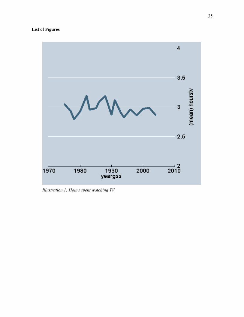
35

List of Figures

Illustration 1: Hours spent watching TV

36

Illustration 2: Trust in individuals

37

Illustration 3: Social contacts

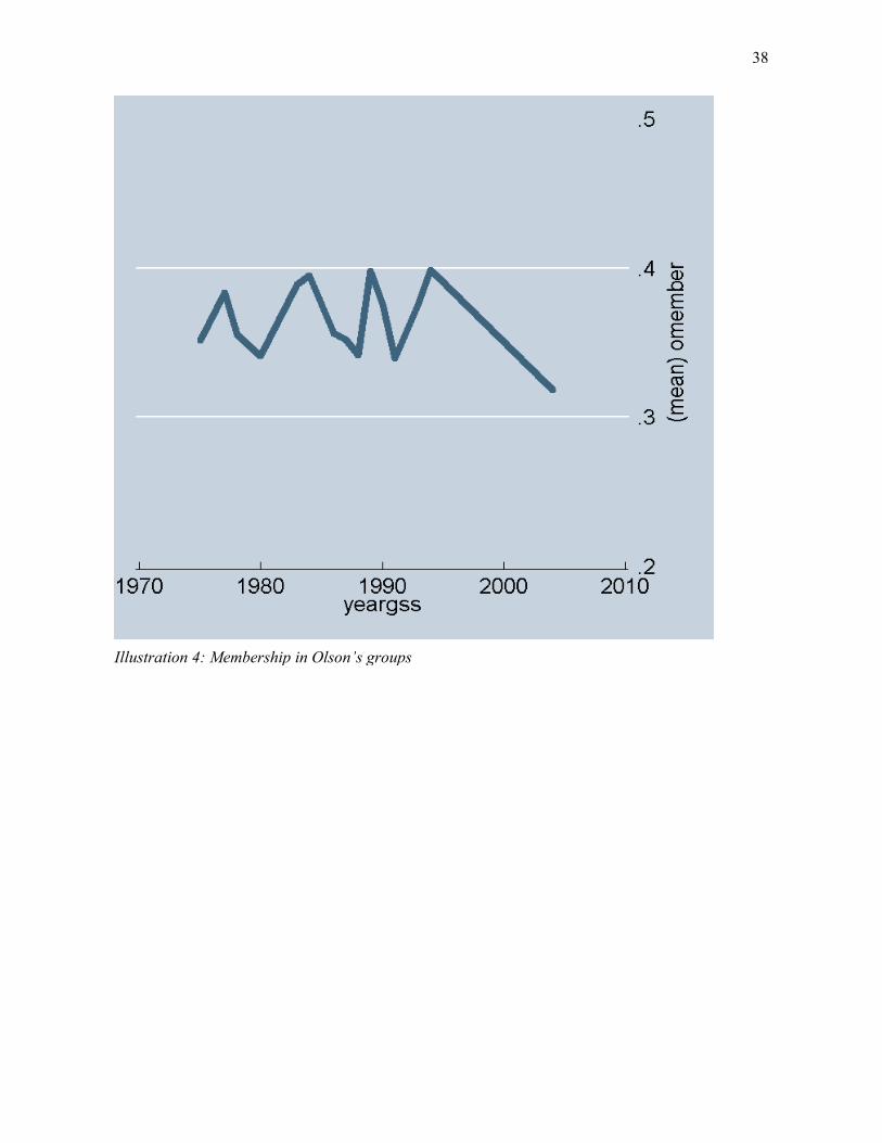
38

Illustration 4: Membership in Olson’s groups

39

Illustration 5: Membership in 1 and 2 or more of Olson’s groups

40

Illustration 6: Membership in Other groups

41

Illustration 7: Membership in 1 or more of Other groups

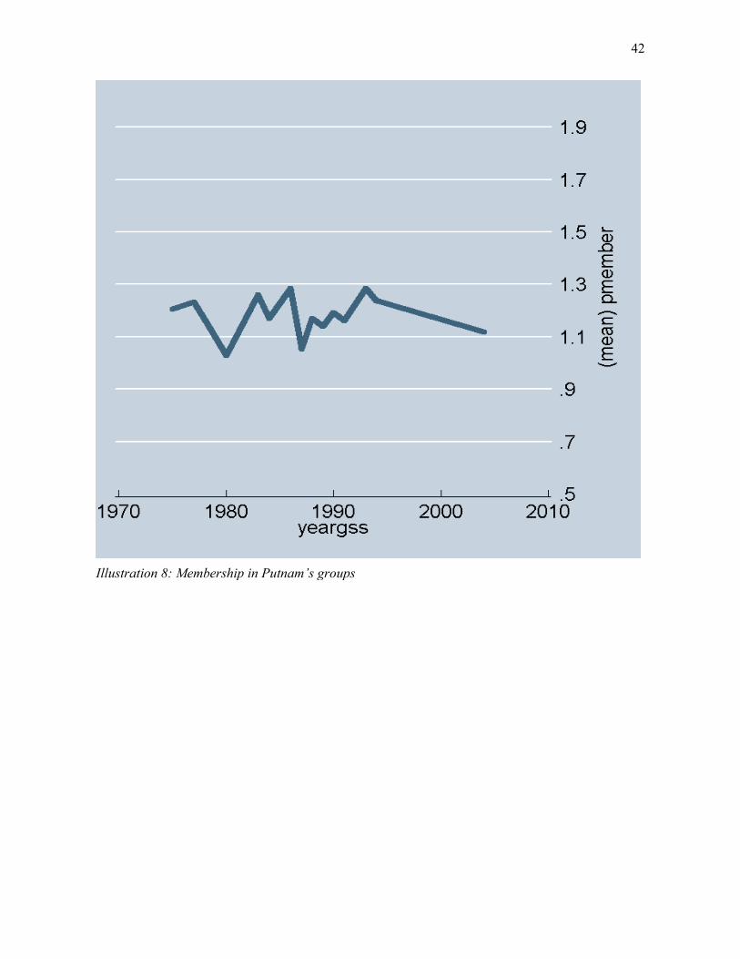
42

Illustration 8: Membership in Putnam’s groups

43

Illustration 9: Membership in 1, 2, 3 and 4 or more of Putnam’s Groups