Dielectric film optical amplifier

Dielectric film optical amplifier

Maurice J. Halmos and Oscar M. Stafsudd

An optical amplifier is described using an active dielectric film. Electromagnetic scattering from this type ofactive film has been studied in the past using infinite plane waves. The use of unbounded fields resulted inscattering coefficients that approached infinity at resonance. In this paper, the active scatterer is viewed asan optical amplifier with finite incident and scattered fields. An analytical description is presented and thensupported by a numerical analysis. Finite gains are calculated. This analysis also predicts spatial filtering ofthe incident field, and experimental results confirm these predictions.

1. Introduction

Electromagnetic scattering from dielectric struc-tures has long been studied. The interaction of planewaves and spheres was first successfully discussed byMie.1 Numerical investigation of the interaction ofthe plane with colloidal particles was made byBlumer.2 More recently, structures with active mediawere studied.3 -5 Extensive numerical analysis of infi-nite cylinders was performed by Kerker.6 These stud-ies predicted sharp resonance scattering when the me-dia are active. Recently, experimental verification ofthese sharp resonances was obtained using active sheetstructures.7 ' 8 It was shown that these resonances oc-curred when the incident beam coupled with the leakymodes of the structure. All the theoretical studiespredict that the scattering cross section of the dielec-tric bodies goes to infinity at resonance. In recentpapers, unbounded scattered fields were also calculat-ed for the resonance condition. However, the actualratio of active to passive scattered fields was found tobe typically a factor of 100 accompanied by a verynarrow angular acceptance.

In the present work, we describe the resonance scat-tering using spatially finite fields. This will result infinite fields being scattered. Since the scatteredwaves are collimated and collinear with the incidentfields, we can view the active scatterer as an opticalamplifier. The spatial effects of this amplifier aretheoretically studied. Two models of the amplifier aredescribed; the first yields analytical insight into the

problem, and the second yields numerical results thatsupport the first model. Finite gains are calculatedusing the numerical model. Experimental results ver-ify the theoretical description where the mode is spa-tially filtered by the structure.

II. Active Leaky Dielectric WaveguideThe case of a thin dielectric slab, where the index of

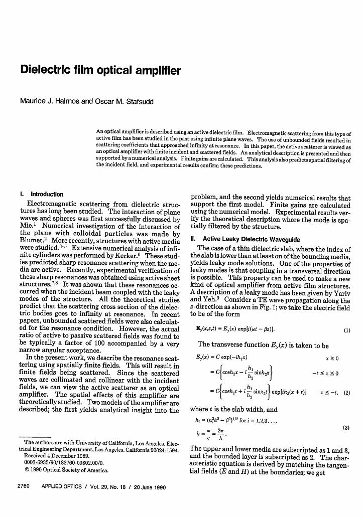
the slab is lower than at least on of the bounding media,yields leaky mode solutions. One of the properties ofleaky modes is that coupling in a transversal directionis possible. This property can be used to make a newkind of optical amplifier from active film structures.A description of a leaky mode has been given by Yarivand Yeh.9 Consider a TE wave propagation along thez-direction as shown in Fig. 1; we take the electric fieldto be of the form

Ey(xzt) = E(x) exp[i(wt - z)]. (1)

The transverse function Ey(x) is taken to be

Ey(x) = C exp(-ihlx)

= C{cosh2 x - i ! sinh2x}

= Ccosh 2t + i I sinx2t} exp[ih3(x + t)I

where t is the slab width, and

hi = (nik 2 2)1/2 for i = 1,2,3...,

x > 0

-t < x <0

x <-t, (2)

The authors are with University of California, Los Angeles, Elec-trical Engineering Department, Los Angeles, California 90024-1594.

Received 4 December 1989.0003-6935/90/182760-09$02.00/0.© 1990 Optical Society of America.

co 2r vu,k =- -=C X

The upper and lower media are subscripted as 1 and 3,and the bounded layer is subscripted as 2. The char-acteristic equation is derived by matching the tangen-tial fields (E and H) at the boundaries; we get

2760 APPLIED OPTICS / Vol. 29, No. 18 / 20 June 1990

10'Scattered Wave (T) n3

n2

zScattered Wave (R)

IncidentWave

Fig. 1. Coupling of an incident wave to a leaky waveguide in which

n2 < nl,3.

h2 (h1 + h 3)tan h 2t h 2+hh 3

This equation can be approximated if we assume 1(loss, which occurs at near grazing angles. Yariv aYeh arrive at the following expression:

+ t2k {(n2 -n2)l (n n2)1}.

Substituting back into Eq. (3) we get

B= r- ia = (n~k2 - h2)

Then one obtains the imaginary part of A3, a, whicorresponds to the loss experienced by the leaky modue to the lack of complete reflection at the interfaiThe approximate solution, using Eq. (5), was coipared with a numerical solution of the dispersion I(4) yielding good agreement up to three significafigures. One can show that in deriving Eq. (5), h2 !

will vanish by choosing a complex value for n2 so th

1(n2)- a0,/[!(n 2)k21.

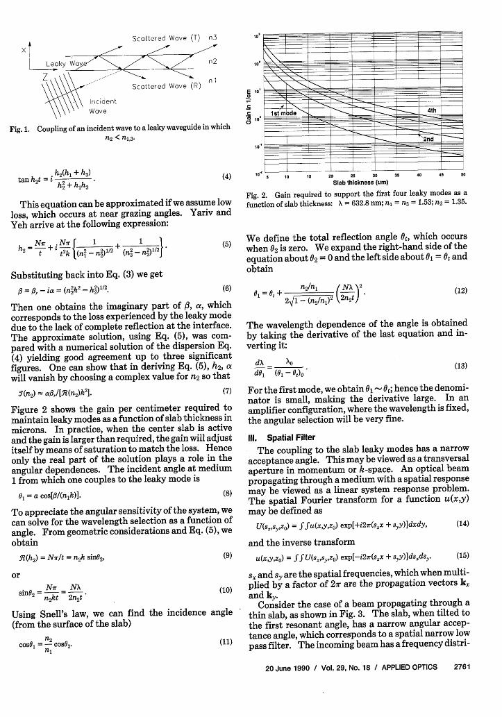
Figure 2 shows the gain per centimeter requiredmaintain leaky modes as a function of slab thicknessmicrons. In practice, when the center slab is actiand the gain is larger than required, the gain will adjiitself by means of saturation to match the loss. Heronly the real part of the solution plays a role in tangular dependences. The incident angle at media1 from which one couples to the leaky mode is

01 = a cos[#/(nlk)].

To appreciate the angular sensitivity of the system,'can solve for the wavelength selection as a functionangle. From geometric considerations and Eq. (5),'obtain

R(h2) = Nrlt = n2k sin62 ,

or

sin62 r NXn2 kt 2n2 t

Using Snell's law, we can find the incidence ani(from the surface of the slab)

n2cos01 = - cos0 2.

10'

n

E

CaO

10

lo'

5 10 15 20 25 30 35 40 45 50

Slab thickness (um)

Fig. 2. Gain required to support the first four leaky modes as a

function of slab thickness: X = 632.8 nm; nj = n3 = 1.53; n2 = 1.35.

We define the total reflection angle Ot, which occurswhen 02 is zero. We expand the right-hand side of theequation about 02 = 0 and the left side about 0i = Ot andobtain

(6) 0 = + n2/n (NX N2

rich 1 21 - (n 2/n)2 k2n2 t)

(12)

The wavelength dependence of the angle is obtainedby taking the derivative of the last equation and in-verting it:

dX = X

d0 ( 0,), (13)

For the first mode, we obtain 01 Ot; hence the denomi-nator is small, making the derivative large. In anamplifier configuration, where the wavelength is fixed,the angular selection will be very fine.

111. Spatial Filter

The coupling to the slab leaky modes has a narrowacceptance angle. This may be viewed as a transversalaperture in momentum or k-space. An optical beampropagating through a medium with a spatial responsemay be viewed as a linear system response problem.The spatial Fourier transform for a function u(x,y)may be defined as

we U(sx~syszo) = ffu(xyzo) exp[+i27r(sxx + syy)Idxdy,

and the inverse transform

(9) u(x,y,z 0 ) = fSfU(sx,sy,zo) exp[-i23r(sxx + sYy)]ds.dsY. (15)

sX and sy are the spatial frequencies, which when multi-10) plied by a factor of 2ir are the propagation vectors k,

and ky.Consider the case of a beam propagating through a

le thin slab, as shown in Fig. 3. The slab, when tilted tothe first resonant angle, has a narrow angular accep-tance angle, which corresponds to a spatial narrow lowpass filter. The incoming beam has a frequency distri-

20 June 1990 / Vol. 29, No. 18 / APPLIED OPTICS 2761

(14)

Incoming Beam

Waist wo

2tx

Apertures

Fig. 3. Dielectric film slab as a spatial filter.

bution that is filtered or convoluted with the slabresponse.

The interaction region, shown in one dimension astx, may be thought of as two apertures, one at theentrance and the other at the exit of an infinite slabfilter. The apertures operate (multiply) the fields inthe x-y space, and the slab multiplies in the k-kyspatial frequency space:

E0.,(xy) = [Ej.(x,y) Tap(xy)] 0 TangI(XY)- Tap(XY). (16)

Using the apertures to define the finite active regionallows the slab to be modeled as infinite. The spatialfrequency response is a -function at k and k equal tozero (paraxial configuration). A -function in the spa-tial frequency domain corresponds to a plane wavepropagating in the z-direction (in this case). Thisplane wave goes through the second aperture yieldingthe output beam.

The active region of the slab is established by thepump beam, which has a Gaussian intensity distribu-tion. The active region aperture may then be modeledas a Gaussian distributed transmission. In the case ofno active medium, the interaction region may be de-fined as a decaying exponential, where the decay con-stant is the leaky mode power decay constant.

Example: A typical configuration is where the in-put beam is much smaller than the active region. Inthis case, the first aperture has little or no effect in Eq.(3). Assume the input beam to be Gaussian:

i(xy) = E expe- in ksae (17)

The Fourier spectrum in k-space is6(Sssy) = 1(6i) = Eio(2r)W exp[_T(s + Sy)W2J. (18)

The slab is a 6-function in the k-space that multipliesEq. (17) at sx = sy=0. The second aperture we assumeto be Gaussian (the active case), which convolves thebeam in k-space. This yields the output beam

,Go(SxSy) = ToEio(2)W02t2 exp [-r(s + l)tfl, (19)

where To is the transmission gain going through theactive slab. Taking the inverse transform, we obtainthe output beam in the x-y space:

EO(xy) = ToEio(W0 /tx)2 exp( +2 Y). (20)

Output

Beam

k 1<

Hollow n1 > n2Slab

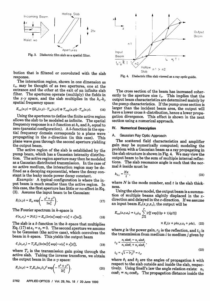
Fig. 4. Dielectric film slab viewed as a ray optic guide.

The cross section of the beam has increased coher-ently to the aperture size t. This implies that theoutput beam characteristics are determined mainly bythe pump characteristics. If the pump cross section islarger than the incident beam area, the output willhave a lower cross k-distribution, hence a lower propa-gation divergence. This effect is shown in the nextsection using a numerical approach.

IV. Numerical Description

A. Gaussian Ray Optic Approach

The scattered field characteristics and amplifiergain may be numerically computed; modeling theproblem with a Gaussian beam as a ray propagating inthe slab structure is shown in Fig. 4. We may view theoutput beam to be the sum of multiple internal reflec-tions. The slab resonance angle is such that the nor-mal k inside must be

k2 1 = N- (21)

where N is the mode number, and t is the slab thick-ness.

Using the above model, the output beam is a summa-tion of multiple beams slightly displaced in the x-direction and delayed in the z-direction. If we assumean input beam E(xy ,z ), the output will be

P

Eout(X1Yzo) = tl2t2 exp[(2p + 1)lg/2Jjp0o

X E(x + pbxsyz + pz), (22)

where g is the power gain, rij is the reflection, and tij isthe transmission from medium i to medium given by

ni sinOi - nj sinO

nisinOi + njsinOj '

tij = 41Irj2 = t,(23)

where 01 and 02 are the angles of propagation k withrespect to the slab outside and inside the slab, respec-tively. Using Snell's law the angle relation exists: njcos0 = n2 cos02. The propagation distance inside the


I

slab between reflections is given by I = t/sinO2, and the

shifts in the x- and z-directions are given by

x = 21 cos(02) sin(01),(24)

bz = 21[n2 /n1 - COS(02 ) COS(01 )].

The expression for the vector form of the fundamen-tal Gaussian beam in a medium with index n1 is givenby

E(x,y,z) = Eo( +ib) exp{ iknl 2(z + ib)] exp(-iknlz)

(25)

where the confocal parameter b and the radius R aregiven by

7VW2b =-,Xni

1 Z

R Z2 +b2

(26)

and wo is the waist of the Gaussian beam.The number of terms used in Eq. (1) are limited by

the effective aperture across the beam (x-direction)Xapp so that P = Xapplkx

B. Numerical Results

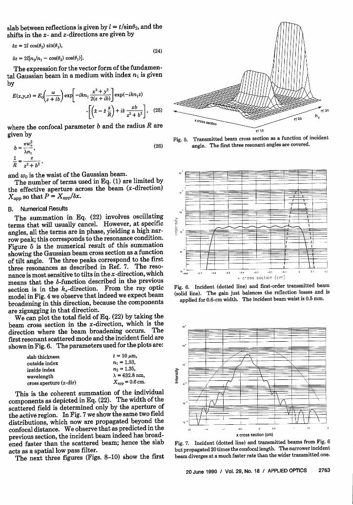
The summation in Eq. (22) involves oscillatingterms that will usually cancel. However, at specificangles, all the terms are in phase, yielding a high nar-row peak; this corresponds to the resonance condition.Figure 5 is the numerical result of this summationshowing the Gaussian beam cross section as a functionof tilt angle. The three peaks correspond to the firstthree resonances as described in Ref. 7. The reso-nance is most sensitive to tilts in the x-direction, whichmeans that the 6-function described in the previoussection is in the kr-direction. From the ray opticmodel in Fig. 4 we observe that indeed we expect beam

broadening in this direction, because the componentsare zigzagging in that direction.

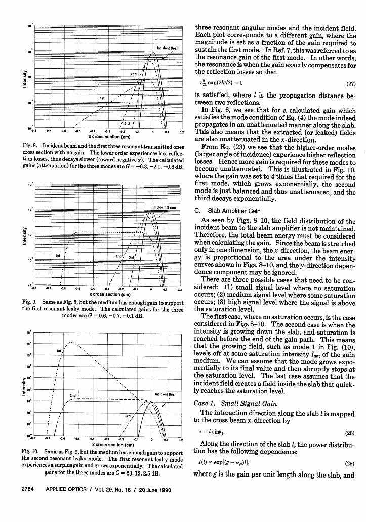
We can plot the total field of Eq. (22) by taking thebeam cross section in the x-direction, which is thedirection where the beam broadening occurs. Thefirst resonant scattered mode and the incident field areshown in Fig. 6. The parameters used for the plots are:

slab thicknessoutside indexinside indexwavelengthcross aperture (x-dir)

t = 10 'm,nl = 1.53,n2= 1.35,X = 632.8 nm,Xapp = 0.6 cm.

This is the coherent summation of the individualcomponents as depicted in Eq. (22). The width of thescattered field is determined only by the aperture of

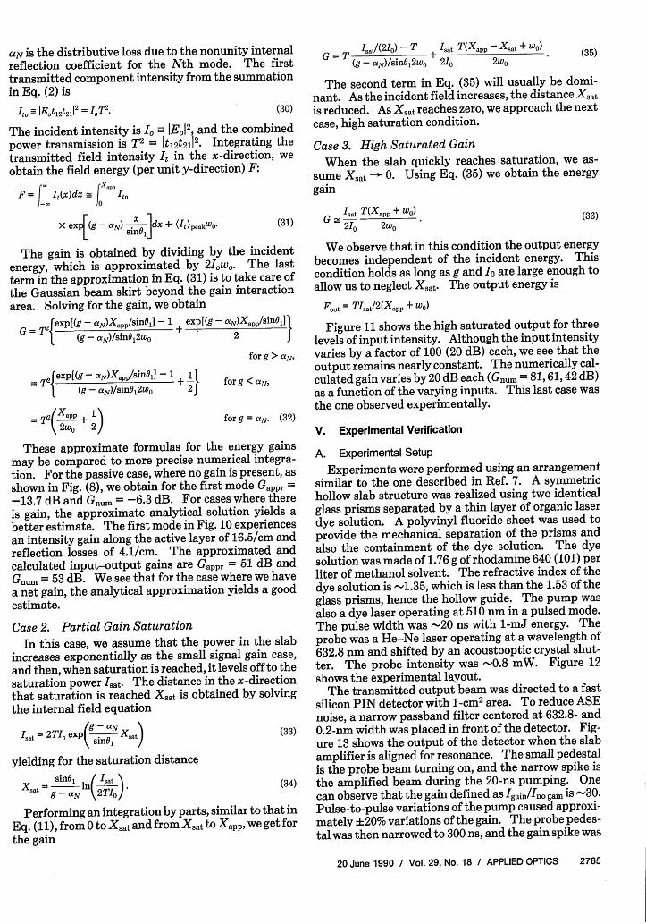
the active region. In Fig. 7 we show the same two field

distributions, which now are propagated beyond theconfocal distance. We observe that as predicted in theprevious section, the incident beam indeed has broad-ened faster than the scattered beam; hence the slabacts as a spatial low pass filter.

The next three figures (Figs. 8-10) show the first

Xf r - 3/t

ff 1/t

Fig. 5. Transmitted beam cross section as a function of incident

angle. The first three resonant angles are covered.

-08 - 7 -0 - 5 -0 * -3 -0.2 - I 0 2

x cross section (cm)

Fig. 6. Incident (dotted line) and first-order transmitted beam

(solid line). The gain just balances the reflection losses and is

applied for 0.6-cm width. The incident beam waist is 0.5 mm.

a.c

-2 -1 5 -1 -0.5 0 05


Fig. 7. Incident (dotted line) and transmitted beams from Fig. 6

but propagated 20 times the confocal length. The narrower incident

beam diverges at a much faster rate than the wider transmitted one.


,0

loo

1(2 - 2 " + i2 X' i]'R) _,2 0

_-- _- -

_ , .' .1 _ . I ~ ~~ ~~I1 nt I

4_-0.8 -0.7

/ 3rd 1 l

-0.6 . -0.4 0.3 -0.2 0.1

x cross section (cm)0 0.1 0.2

Fig. 8. Incident beam and the first three resonant transmitted onescross section with no gain. The lower order experiences less reflec-tion losses, thus decays slower (toward negative x). The calculatedgains (attenuation) for the three modes are G = -6.3, -2.1, -0.8 dB.

_ _ _ _

-0.6 -0.5

I'

O.4 -0.3 -0.2 -0.1

x cross section (cm)Fig. 9. Same as Fig. 8, but the medium has enough gain to supportthe first resonant leaky mode. The calculated gains for the three

modes are G = 0.6, -0.7, -0.1 dB.

1'L

2nd IncldentBeanm

$/'D

-0.8 -0.7 -0.6 -0.5 -0.4 -0.3 -0.2 -0.I 0 0.1 0.2

x cross section (cm)Fig. 10. Same as Fig. 9, but the medium has enough gain to supportthe second resonant leaky mode. The first resonant leaky modeexperiences a surplus gain and grows exponentially. The calculated

gains for the three modes are G = 53, 12, 2.5 dB.

three resonant angular modes and the incident field.Each plot corresponds to a different gain, where themagnitude is set as a fraction of the gain required tosustain the first mode. In Ref. 7, this was referred to asthe resonance gain of the first mode. In other words,the resonance is when the gain exactly compensates forthe reflection losses so that

r21 exp(21g/2) = 1 (27)

is satisfied, where I is the propagation distance be-tween two reflections.

In Fig. 6, we see that for a calculated gain whichsatisfies the mode condition of Eq. (4) the mode indeedpropagates in an unattenuated manner along the slab.This also means that the extracted (or leaked) fieldsare also unattenuated in the x-direction.

From Eq. (23) we see that the higher-order modes(larger angle of incidence) experience higher reflectionlosses. Hence more gain is required for these modes tobecome unattenuated. This is illustrated in Fig. 10,where the gain was set to 4 times that required for thefirst mode, which grows exponentially, the secondmode is just balanced and thus unattenuated, and thethird decays exponentially.

C. Slab Amplifier Gain

As seen by Figs. 8-10, the field distribution of theincident beam to the slab amplifier is not maintained.Therefore, the total beam energy must be consideredwhen calculating the gain. Since the beam is stretchedonly in one dimension, the x-direction, the beam ener-gy is proportional to the area under the intensitycurves shown in Figs. 8-10, and the y-direction depen-dence component may be ignored.

There are three possible cases that need to be con-sidered: (1) small signal level where no saturationoccurs; (2) medium signal level where some saturationoccurs; (3) high signal level where the signal is abovethe saturation level.

The first case, where no saturation occurs, is the caseconsidered in Figs 8-10. The second case is when theintensity is growing down the slab, and saturation isreached before the end of the gain path. This meansthat the growing field, such as mode 1 in Fig. (10),levels off at some saturation intensity Iat of the gainmedium. We can assume that the mode grows expo-nentially to its final value and then abruptly stops atthe saturation level. The last case assumes that theincident field creates a field inside the slab that quick-ly reaches the saturation level.

Case 1. Small Signal GainThe interaction direction along the slab 1 is mapped

to the cross beam x-direction byx = sinG1. (28)

Along the direction of the slab 1, the power distribu-tion has the following dependence:

I(1) exp[(g - aN)1

], (29)

where g is the gain per unit length along the slab, and

2764 APPLIED OPTICS Vol. 29, No. 18 / 20 June 1990

10

10

10

C

10

10

10

10

-PC 100)

10

10

10'

10I

10

10'

p1o4.0

10'

10'

1o'

.- I l S _ _~I_ * ,!\

,, . HU I *11

{_I 11 1 ' 'it

I

z

I.

.7

II

II .1

aN is the distributive loss due to the nonunity internalreflection coefficient for the Nth mode. The firsttransmitted component intensity from the summationin Eq. (2) is

Ito IEJt12t2112 = I72. (30)

The incident intensity is I, -E,12, and the combinedpower transmission is = t12t2 l12. Integrating thetransmitted field intensity It in the x-direction, weobtain the field energy (per unit y-direction) F:

F = J It(x)dx _ pp

X exI{(g - N) ix + (i)peakWo (31)

The gain is obtained by dividing by the incidentenergy, which is approximated by 2I0w0. The lastterm in the approximation in Eq. (31) is to take care ofthe Gaussian beam skirt beyond the gain interactionarea. Solving for the gain, we obtain

exp[(g - aN)Xapp/Sinl~] - 1 exp[(g

= (g - a s)/SinOl2wo

= V |exp[(9 - N)Xapp/sin~j] - 1I+

l 9 (g aN)sinal2w, 2J

= I -P- + 2w: 2 )

2

for g

(35)IsaJ(2Io) - T Isat T(Xapp- Xsat + w0 )

(g - aN)/sinOl2w, 2Io 2wo

The second term in Eq. (35) will usually be domi-nant. As the incident field increases, the distance Xsatis reduced. As Xsat reaches zero, we approach the nextcase, high saturation condition.

Case 3. High Saturated GainWhen the slab quickly reaches saturation, we as-

sume Xsat - 0. Using Eq. (35) we obtain the energygain

Isat T(Xapp + wo)

21o 2wo(36)

We observe that in this condition the output energybecomes independent of the incident energy. Thiscondition holds as long as g and Io are large enough toallow us to neglect Xsat. The output energy is

Fout = TIsat/2 (Xapp + WO)

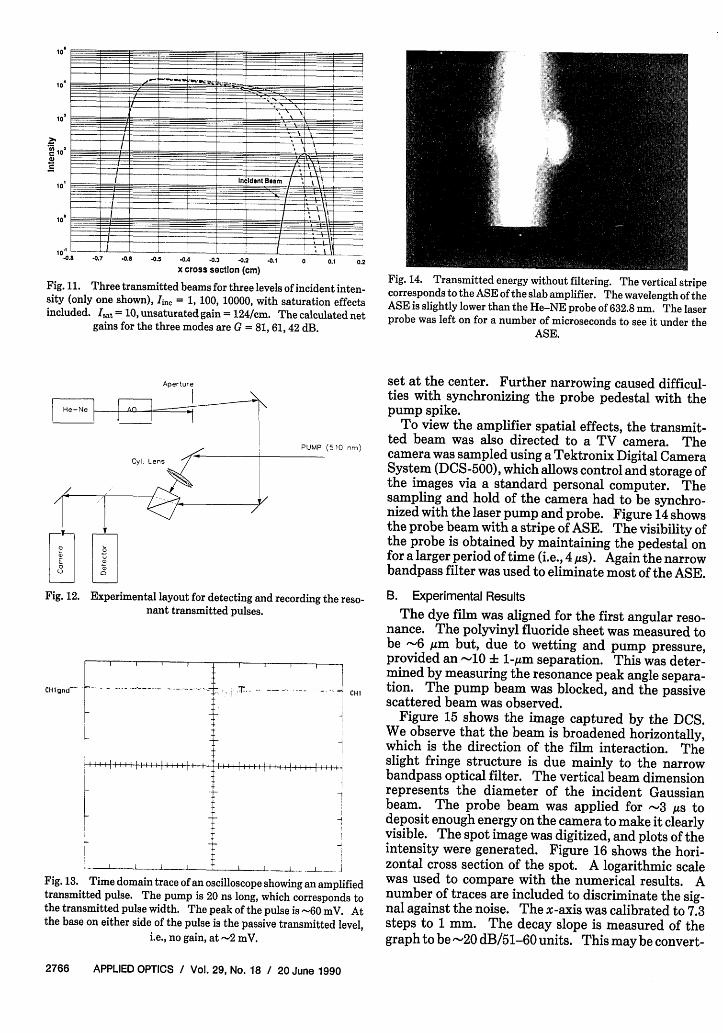
-app/sin0ljI Figure 11 shows the high saturated output for threelevels of input intensity. Although the input intensity

forg > aN, varies by a factor of 100 (20 dB) each, we see that theoutput remains nearly constant. The numerically cal-

< aN, culated gain varies by 20 dB each (Gnum = 81,61,42 dB)as a function of the varying inputs. This last case wasthe one observed experimentally.

for g = a. (32)

These approximate formulas for the energy gainsmay be compared to more precise numerical integra-tion. For the passive case, where no gain is present, asshown in Fig. (8), we obtain for the first mode Gappr =-13.7 dB and Gnum = -6.3 dB. For cases where thereis gain, the approximate analytical solution yields abetter estimate. The first mode in Fig. 10 experiencesan intensity gain along the active layer of 16.5/cm andreflection losses of 4.1/cm. The approximated andcalculated input-output gains are Gappr = 51 dB andGnum = 53 dB. We see that for the case where we havea net gain, the analytical approximation yields a goodestimate.

Case 2. Partial Gain SaturationIn this case, we assume that the power in the slab

increases exponentially as the small signal gain case,and then, when saturation is reached, it levels off to thesaturation power Isat. The distance in the x-directionthat saturation is reached Xsat is obtained by solvingthe internal field equation

Isat = 2 TIs exp(1. s N Xsat) (33)

yielding for the saturation distancesinG1 I sat

Xsat = mi 2I. (34)g-ctN (2T° )

Performing an integration by parts, similar to that inEq. (11), from 0 to Xsat and from Xsat to Xapp, we get forthe gain

V. Experimental Verification

A. Experimental Setup

Experiments were performed using an arrangementsimilar to the one described in Ref. 7. A symmetrichollow slab structure was realized using two identicalglass prisms separated by a thin layer of organic laserdye solution. A polyvinyl fluoride sheet was used toprovide the mechanical separation of the prisms andalso the containment of the dye solution. The dyesolution was made of 1.76 g of rhodamine 640 (101) perliter of methanol solvent. The refractive index of thedye solution is -1.35, which is less than the 1.53 of theglass prisms, hence the hollow guide. The pump wasalso a dye laser operating at 510 nm in a pulsed mode.The pulse width was -20 ns with 1-mJ energy. Theprobe was a He-Ne laser operating at a wavelength of632.8 nm and shifted by an acoustooptic crystal shut-ter. The probe intensity was -0.8 mW. Figure 12shows the experimental layout.

The transmitted output beam was directed to a fastsilicon PIN detector with 1-cm2 area. To reduce ASEnoise, a narrow passband filter centered at 632.8- and0.2-nm width was placed in front of the detector. Fig-ure 13 shows the output of the detector when the slabamplifier is aligned for resonance. The small pedestalis the probe beam turning on, and the narrow spike isthe amplified beam during the 20-ns pumping. Onecan observe that the gain defined as Igain/Ino gain is -30.Pulse-to-pulse variations of the pump caused approxi-mately +20% variations of the gain. The probe pedes-tal was then narrowed to 300 ns, and the gain spike was


10

104

10.

.tC

10

C)

10.

10o

loll -I I I I I _ _I llL,.0.8 -0.7 -0.6 0.5 .0.4 .0.3 .0.2 .0.1 0 0.1 0.2


Fig. 11. Three transmitted beams for three levels of incident inten-sity (only one shown), Ii,, = 1, 100, 10000, with saturation effectsincluded. Isat = 10, unsaturated gain = 124/cm. The calculated net

gains for the three modes are G = 81, 61, 42 dB.

Aperture

Fig. 12. Experimental layout for detecting and recording the reso-nant transmitted pulses.

CHI lQnd4 - CHI

a+I I I I {-HIII1F111111ItI I I I i |IIII

F I I I1

Fig. 13. Time domain trace of an oscilloscope showing an amplifiedtransmitted pulse. The pump is 20 ns long, which corresponds tothe transmitted pulse width. The peak of the pulse is -60 mV. Atthe base on either side of the pulse is the passive transmitted level,

i.e., no gain, at -2 mV.

Fig. 14. Transmitted energy without filtering. The vertical stripecorresponds to the ASE of the slab amplifier. The wavelength of theASE is slightly lower than the He-NE probe of 632.8 nm. The laserprobe was left on for a number of microseconds to see it under the

ASE.

set at the center. Further narrowing caused difficul-ties with synchronizing the probe pedestal with thepump spike.

To view the amplifier spatial effects, the transmit-ted beam was also directed to a TV camera. The

PUMP (510 camera was sampled using a Tektronix Digital CameraSystem (DCS-500), which allows control and storage ofthe images via a standard personal computer. Thesampling and hold of the camera had to be synchro-nized with the laser pump and probe. Figure 14 showsthe probe beam with a stripe of ASE. The visibility ofthe probe is obtained by maintaining the pedestal onfor a larger period of time (i.e., 4 Ms). Again the narrowbandpass filter was used to eliminate most of the ASE.

B. Experimental Results

The dye film was aligned for the first angular reso-nance. The polyvinyl fluoride sheet was measured tobe -6 m but, due to wetting and pump pressure,provided an 10 + 1-,um separation. This was deter-mined by measuring the resonance peak angle separa-tion. The pump beam was blocked, and the passivescattered beam was observed.

Figure 15 shows the image captured by the DCS.We observe that the beam is broadened horizontally,which is the direction of the film interaction. Theslight fringe structure is due mainly to the narrowbandpass optical filter. The vertical beam dimensionrepresents the diameter of the incident Gaussianbeam. The probe beam was applied for 3 s todeposit enough energy on the camera to make it clearlyvisible. The spot image was digitized, and plots of theintensity were generated. Figure 16 shows the hori-zontal cross section of the spot. A logarithmic scalewas used to compare with the numerical results. Anumber of traces are included to discriminate the sig-nal against the noise. The x-axis was calibrated to 7.3steps to 1 mm. The decay slope is measured of thegraph to be -20 dB/51-60 units. This may be convert-


L - -

iI

-i

I

ii

I __ - I -- I

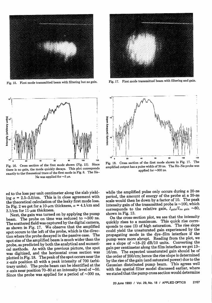
Fig. 15. First mode transmitted beam with filtering but no gain.

10

~~~~~~~~~ me

100 l II I ' ''_ __-

0 20 40 60 80 100 120

Fig. 16. Cross section of the first mode shown (Fig. 15). Since

there is no gain, the mode quickly decays. This plot corresponds

exactly to the theoretical trace of the first mode in Fig. 8. The He-Ne was applied for -3 js.

ed to the loss per unit centimeter along the slab yield-ing a = 2.5-3.0/cm. This is in close agreement withthe theoretical calculation of the leaky first mode loss.In Fig. 2 we get for a 10-Mum thickness, a = 4.1/cm and

3.1/cm for 11-,om thickness.Next, the gain was turned on by applying the pump

beam. The probe on time was reduced to -300 ns.The scattered field was captured by the digital camera,as shown in Fig. 17. We observe that the amplified

spot occurs to the left of the probe, which is the direc-tion where the probe decayed in the passive case. Thespot size of the amplified beam is much wider than theprobe, as predicted by both the analytical and numeri-cal methods. As with the previous picture, the spotwas digitized, and the horizontal cross section wasplotted in Fig. 18. The peak of the spot occurs near thex-axis position 45 with a peak intensity of 700 (arbi-trary units). The probe beam can be identified at thex-axis near position 70-80 at an intensity level of -50.Since the probe was applied for a period of -300 ns,

In10'

.ral10:

C

0 20 40 so 80 100 120

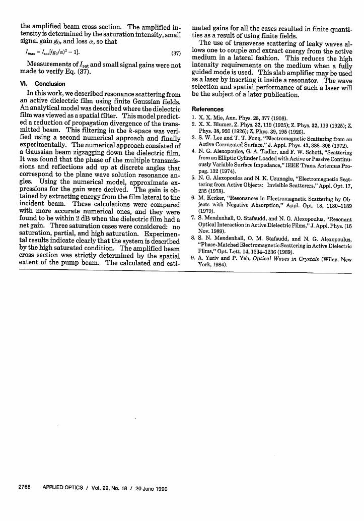
Fig. 18. Cross section of the first mode shown in Fig. 17. The

amplified output has a pulse width of 20 ns. The He-Ne probe was

applied for -300 ns.

while the amplified pulse only occurs during a 20-nsperiod, the amount of energy of the probe at a 20-nsscale would then be down by a factor of 10. The peakintensity gain of the transmitted probe is -100, whichcorresponds to the relative gain, Igain/Ino gain 0shown in Fig. 13.

On the cross-section plot, we see that the intensityquickly rises to a maximum. This quick rise corre-sponds to case (3) of high saturation. The rise slopecould yield the unsaturated gain experienced by thepropagating mode in the dye-film interface if thepump were more abrupt. Reading from the plot, wesee a slope of -18-22 dB/10 units. Converting thegain per centimeter along the film interface we get 13-16/cm. The expected unsaturated gain should be ofthe order of 200/cm; hence the rise slope is determinedby the rise of the gain (and saturated power) due to theGaussian distributed pump beam. This agrees wellwith the spatial filter model discussed earlier, wherewe stated that the pump cross section would determine


Fig. 17. First mode transmitted beam with filtering and gain.

the amplified beam cross section. The amplified in-tensity is determined by the saturation intensity, smallsignal gain go, and loss a, so that

,max = Isat[(go/a)2 _ 1]. (37)

Measurements Of Isat and small signal gains were notmade to verify Eq. (37).

VI. Conclusion

In this work, we described resonance scattering froman active dielectric film using finite Gaussian fields.An analytical model was described where the dielectricfilm was viewed as a spatial filter. This model predict-ed a reduction of propagation divergence of the trans-mitted beam. This filtering in the k-space was veri-fied using a second numerical approach and finallyexperimentally. The numerical approach consisted ofa Gaussian beam zigzagging down the dielectric film.It was found that the phase of the multiple transmis-sions and reflections add up at discrete angles thatcorrespond to the plane wave solution resonance an-gles. Using the numerical model, approximate ex-pressions for the gain were derived. The gain is ob-tained by extracting energy from the film lateral to theincident beam. These calculations were comparedwith more accurate numerical ones, and they werefound to be within 2 dB when the dielectric film had anet gain. Three saturation cases were considered: nosaturation, partial, and high saturation. Experimen-tal results indicate clearly that the system is describedby the high saturated condition. The amplified beamcross section was strictly determined by the spatialextent of the pump beam. The calculated and esti-

mated gains for all the cases resulted in finite quanti-ties as a result of using finite fields.

The use of transverse scattering of leaky waves al-lows one to couple and extract energy from the activemedium in a lateral fashion. This reduces the highintensity requirements on the medium when a fullyguided mode is used. This slab amplifier may be usedas a laser by inserting it inside a resonator. The waveselection and spatial performance of such a laser willbe the subject of a later publication.

References

1. X. X. Mie, Ann. Phys. 25, 377 (1908).2. X. X. Blumer, Z. Phys. 32, 119 (1925); Z. Phys. 32, 119 (1925); Z.

Phys. 38, 920 (1926); Z. Phys. 39, 195 (1926).3. S. W. Lee and T. T. Fong, "Electromagnetic Scattering from an

Active Corrugated Surface," J. Appl. Phys. 43, 388-395 (1972).4. N. G. Alexopoulos, G. A. Tadler, and F. W. Schott, "Scattering

from an Elliptic Cylinder Loaded with Active or Passive Continu-ously Variable Surface Impedance," IEEE Trans. Antennas Pro-pag. 132 (1974).

5. N. G. Alexopoulos and N. K. Uzunoglu, "Electromagnetic Scat-tering from Active Objects: Invisible Scatterers," Appl. Opt. 17,235 (1978).

6. M. Kerker, "Resonances in Electromagnetic Scattering by Ob-jects with Negative Absorption," Appl. Opt. 18, 1180-1189(1979).

7. S. Mendenhall, 0. Stafsudd, and N. G. Alexopoulus, "ResonantOptical Interaction in Active Dielectric Films," J. Appl. Phys. (15Nov. 1989).

8. S. N. Mendenhall, 0. M. Stafsudd, and N. G. Alexopoulus,"Phase-Matched Electromagnetic Scattering in Active DielectricFilms," Opt. Lett. 14, 1234-1236 (1989).

9. A. Yariv and P. Yeh, Optical Waves in Crystals (Wiley, NewYork, 1984).


Documents

Dielectric film optical amplifier