Embed Size (px)
Citation preview
arX
iv:1
512.
0736
4v3
[as
tro-
ph.C
O]
6 J
un 2
016
Prepared for submission to JCAP
Differential cosmic expansion and the
Hubble flow anisotropy
Krzysztof Bolejko,a M. Ahsan Nazerb and David L. Wiltshireb
aSydney Institute for Astronomy, School of Physics, A28, The University of Sydney, NSW2006, Australia
bDepartment of Physics and Astronomy, University of Canterbury, Private Bag 4800, Christchurch8140, New Zealand
E-mail: [email protected], [email protected],[email protected]
Abstract. The Universe on scales 10–100h−1Mpc is dominated by a cosmic web of voids,filaments, sheets and knots of galaxy clusters. These structures participate differently in theglobal expansion of the Universe: from non-expanding clusters to the above average expansionrate of voids. In this paper we characterize Hubble expansion anisotropies in the COMPOS-ITE sample of 4534 galaxies and clusters. We concentrate on the dipole and quadrupolein the rest frame of the Local Group. These both have statistically significant amplitudes.These anisotropies, and their redshift dependence, cannot be explained solely by a boostof the Local Group in the Friedmann-Lemaıtre-Robertson-Walker (FLRW) model which ex-pands isotropically in the rest frame of the cosmic microwave background (CMB) radiation.We simulate the local expansion of the Universe with inhomogeneous Szekeres solutions,which match the standard FLRW model on >∼ 100h−1Mpc scales but exhibit nonkinematicrelativistic differential expansion on small scales. We restrict models to be consistent withobserved CMB temperature anisotropies, while simultaneously fitting the redshift variationof the Hubble expansion dipole. We include features to account for both the Local Void andthe “Great Attractor”. While this naturally accounts for the Hubble expansion and CMBdipoles, the simulated quadrupoles are smaller than observed. Further refinement to incor-porate additional structures may improve this. This would enable a test of the hypothesisthat some large angle CMB anomalies result from failing to treat the relativistic differentialexpansion of the background geometry; a natural feature of solutions to Einstein’s equationsnot included in the current standard model of cosmology.
Keywords: gravity, cosmological simulations, redshift surveys, cosmic web, CMBR theory,CMBR experiments
ArXiv ePrint: 1512.07364
Contents
1 Introduction 1
2 Terminology 3
2.1 Nonkinematic and relativistic differential expansion 3
2.2 Large scale homogeneous isotropic distance–redshift nonlinearity 5
2.3 Small scale nonlinearities: the “nonlinear regime” 5
2.4 Model independent characterization of small scale nonlinear expansion 6
3 The observational data 8
3.1 The anisotropy of the Hubble expansion 8
3.2 Completeness and robustness 10
3.3 Kinematic interpretation of anisotropies 11
4 Light propagation in the non-linear relativistic regime and the origin of
anisotropies 15
4.1 The geometry and Einstein equations 15
4.2 Constructing mock catalogues 19
4.3 Anisotropy of the Hubble expansion generated by cosmic structures modelledby the Szekeres model 20
5 Potential impact on CMB anomalies 23
6 Conclusion 24
1 Introduction
In cosmology deviations from a uniform expansion are most commonly treated as peculiarvelocities relative to a linear Hubble law
vpec = cz −H0r (1.1)
where z is the redshift, c the speed of light, r an appropriate distance measure, and H0≡
H(t0) = 100h km s−1Mpc−1 is the Hubble constant, h being a dimensionless number. Such a
theoretical framework is a natural description if the assumption of homogeneity and isotropyholds at all scales, so that all cosmologically relevant motions can be understood in termsthe background expansion of one single Friedmann–Lemaıtre–Robertson–Walker (FLRW)geometry, with a Hubble parameter, H(t), given by the Friedmann equation, plus localboosts which can be treated by eq. (1.1) for suitably small values of the distance,1 r.
However, on scales of tens of megaparsecs the Universe exhibits strong inhomogeneities,dominated in volume by voids with density contrasts close to the minimum possible δρ/ρ =
1Even within FLRW models, for large values of r one has to take into account that H(t) varies with time,and that the redshift is not additive but rather a multiplicative quantity, so a simple addition as in (1.1) doesnot apply: 1 + z1+2 = (1 + z1)(1 + z2) 6= 1 + z1 + z2.
– 1 –
−1 [1–4]. Galaxies and galaxy clusters are not randomly distributed but are strung in fila-ments that thread and surround the voids to form a complex cosmic web [5–7]. The Uni-verse is only spatially homogeneous is some statistical sense when one averages on scales>∼ 100h−1Mpc. Just how large this scale is, is debated [8–12]. However, based on the frac-tal dimension of the 2–point galaxy correlation function making a gradual transition to thehomogeneous limit D2 → 3 in three spatial dimensions, a scale of statistical homogeneity inthe range 70 <∼ rssh <∼ 120h−1Mpc seems to be observed [10].
Despite the fact that the FLRW geometry can only be observationally justified on>∼ 100h−1Mpc scales, by tradition it is conventionally assumed that such a geometry is stillapplicable at all scales on which space is expanding below rssh∼ 100h−1Mpc, that is, untilone gets to the very small scales of bound clusters of galaxies. However, this assumptionis not justified by the principles of general relativity. In general, in solutions of Einstein’sequations the background space does not expand rigidly to maintain constant spatial curva-ture as it does in the FLRW geometry. General inhomogeneous cosmological models, suchas the Lemaıtre–Tolman (LT) [13–15] and Szekeres [16] models, exhibit differential cosmicexpansion. The Hubble parameter becomes a function of space as well as time, and anyrelation (1.1) can no longer have the physical sense of defining a peculiar velocity field withrespect to a single expansion rate.
In this paper we will present the results of numerical investigations that quantify thenonlinearity associated with differential cosmic expansion in Szekeres solutions chosen tomatch key features of both the Cosmic Microwave Background (CMB) anisotropies, and alsothe Hubble expansion on <∼ 100h−1Mpc scales. The crucial feature in these simulations isthat the dipole induced by local inhomogeneities cannot be directly attributed to a 635 km s−1
local boost of the Local Group (LG) of galaxies, and is thus nonkinematic (as we define moreprecisely in Section 2.1 below).
Despite its naturalness in general relativity, the hypothesis of a nonkinematic originfor a fraction of the CMB dipole goes against the consensus of what has been assumed inobservational cosmology [17, 18] ever since the first bounds were placed on the anisotropyof the CMB in the 1960s [19]. By now it is standard practice to automatically transformredshift data to the CMB rest frame before performing cosmological analyses.
Within the standard peculiar velocities framework, the amplitude of bulk flows, theirconsistency with the standard Lambda Cold Dark Matter (ΛCDM) cosmology and their con-vergence to the CMB frame, are matters of ongoing debate [20–31]. A possible nonkinematicorigin for a fraction of the CMB dipole would impact directly on this debate, as well assuggesting a reexamination of other observational puzzles. Arguably the most important ofthese are the large angle anomalies that have been observed in the CMB anisotropy spectrumfor over a decade [32–41], with a statistical significance that has increased with the releaseof Planck satellite data [42–44].
The hypothesis that a fraction of the local Hubble expansion is nonkinematic shouldbe subject to appropriate observational tests. In recent work [45, 46] we devised such testsand found very strong Bayesian evidence for the nonkinematic hypothesis. In an independentstudy [47], the hypothesis of a purely kinematic origin for the dipole in the cosmic distributionof radio galaxies has been rejected at the 99.5% confidence level.
In order to develop more powerful tests of the nonkinematic differential expansion hy-pothesis, in this paper we will use exact solutions of Einstein’s equations for structures smallerthan the statistical homogeneity scale [10] for the purpose of ray–tracing simulations.
There have been a number of previous studies which have used the LT solution to model
– 2 –
the effects of anisotropic expansion [48–55], including its effects on the CMB. However, thesehave typically considered the effects of voids at large distances from our location, or theeffects of voids much larger than the small scale inhomogeneities we will consider.
To our knowledge this paper contains the first ever study which seeks to use exactsolutions of Einstein’s equations to model structures giving rise to nonlinear expansion onscales comparable to those observed, constrained directly by both ray–tracing of the CMBand by the Hubble expansion field from actual surveys. While the Szekeres solution has beenemployed for a number of cosmological problems [56–65], we believe that this is also thefirst time that it has been used for ray–tracing simulations of local structures. We will seethat although we are not able to match all features of the nonlinear Hubble expansion belowthe statistical homogeneity scale, with the Szekeres solution we can nonetheless match morefeatures of the actual data than with other models, including the standard FLRW cosmologywith a local boost of the Local Group of galaxies.
This paper provides a proof–of–principle demonstration that we hope will encourageeven more sophisticated investigations of relativistic effects beyond the perturbed FLRWmodel. Some potential future investigations are outlined in Sec. 5.
2 Terminology
In this paper we often use terms such as nonlinear and nonkinematic. These terms areambiguous and therefore this Section describes how these terms are defined in this paper.
2.1 Nonkinematic and relativistic differential expansion
The fact that cosmic expansion can vary not only in time but in space leads to a variation inthe redshift of observed astronomical sources, be they galaxies or the CMB. If the redshiftof an observed object can be described solely in terms of a homogeneous expansion and aDoppler effect, then we would call the redshift anisotropy kinematic:
(1 + z)obs = (1 + z)FLRW(1 + z)Doppler . (2.1)
The first redshift term on the right hand side refers to the global homogeneous and isotropicexpansion of the FLRW model, and second term is due to a Doppler effect with respect to theFLRW background that combines the motions of the observer (local boost) and the observedobject (peculiar motion). If the redshift of an observed source (galaxies or CMB) cannot beexplained entirely in terms of the above equation then nonkinematic effects are present, bethey a real physical phenomenon or merely some observational bias2.
The factor (1+z)FLRW
in (2.1) can only be defined with respect to a canonical choice ofour local Lorentz frame. Since the CMB is remarkably isotropic, with a dipole of amplitude1.23×10−3T0 of the mean temperature T0 = 2.725K, the canonical CMB rest frame is definedby matching the 3.37mK temperature dipole to the dipole in the series expansion
T0
γCMB(1− βCMB cos θ)= T
0
[1 + β
CMBcos θ + β2
CMB
(cos2 θ − 1
2
)+ . . .
](2.2)
2We assume all observational biases can be accounted for, although this requires care in actual dataanalysis [46]. We deal only with the case of real physical effects in this paper. Furthermore, while all galaxieswithin larger bound clusters will still be assumed to exhibit peculiar local motions within each cluster, fornonkinematic redshift anisotropies we are only interested in redshifts and distances assigned collectively togravitationally bound structures.
– 3 –
where βCMB cos θ ≡ βCMB · nhel, nhel is the unit vector on the sky in the heliocentric frame,βCMB = vCMB/c is the boost vector of the CMB frame in the heliocentric frame, and γCMB =
(1− β2CMB
)−1/2 is the standard Lorentz gamma factor.
Using measurements of redshifts and distances of galaxy clusters, one can independentlydefine the local average isotropic expansion (AIE) frame as the Lorentz frame at our locationin which the spherically averaged distance–redshift relation in independent radial shells hasminimal variations relative to a linear Hubble law [45, 46]. Since isotropy is only definedby an average then the observed redshift of any individual source will in general display anonkinematic anisotropy differing from (2.1) with a dependence, z(nAIE), on the unit vectoron the sky in the AIE frame, nAIE.
According to (2.1), even a perturbed FLRW model will display nonkinematic effects.However, such effects are small and are not expected to affect the identification of the dipole in(2.2). In this paper, we will study models with nonkinematic effects that we will characterizein terms of the variation of averages of the nearby Hubble expansion. These nonkinematiceffects will turn out to be so large that they are also likely to be distinguishable whencompared to perturbed FLRW models, offering a simple alternative characterization. Inparticular, if we make a boost from the AIE frame to the heliocentric frame of our ownmeasurements then the difference of the CMB temperature dipole and the standard kinematicdipole identified by (2.2) can be observationally significant.
We will therefore define general relativistic nonkinematic differential expansion (or moresuccinctly relativistic differential expansion) to occur when the difference
∆Tnk−hel =TAIE
γAIE(1− βAIE · nhel)− T0
γCMB(1− βCMB · nhel)(2.3)
has a measurably nonzero dipole when expanded in spherical harmonics3, where βAIE =
vAIE
/c is the boost of the AIE frame in the heliocentric frame, γAIE
= (1− β2AIE
)−1/2, and
TAIE(nAIE) =TCMB
1 + zAIE
(nAIE
), (2.4)
is the anisotropic CMB temperature as measured in the AIE frame. Here TCMB = (1+zdec)T0
is the mean intrinsic temperature of the primordial plasma at decoupling, zdec being theconstant isotropic redshift of decoupling in the FLRW model. In practice, “measurablynonzero” here means a contribution to (2.3) of at the least the same level, 10−5T0, as theprimordial spectrum; i.e., one order of magnitude larger than the boost dipole in (2.2).
This an operational model–independent4 definition. Since eq. (2.4) does not separateout the primordial CMB anisotropies, our definition cannot distinguish a primordial CMBdipole from “local” nonkinematic relativistic effects. However, we will construct numericalsolutions constrained by large galaxy surveys, leading to direct predictions for the amplitudeand direction of the nonkinematic dipole in terms of general relativity alone, rather than byappealing to unknown physics in the early Universe.
3By construction (2.3) has zero monopole.4The definition applies not only to exact solutions of Einstein’s equations, but to any cosmological model
with a close to linear Hubble law, including models with backreaction such as the timescape model [67–70].One could further refine this definition to treat the quadrupole and small frequency dependent effects of aboost on the black body spectrum [71]. However, as yet we are unable to distinguish such terms given currentknowledge of the modelling of foregrounds such as galactic dust.
– 4 –
Once one accounts for the known motions of the Sun and Milky Way within the boundsystem that forms the Local Group of galaxies, to explain the observed dipole in (2.2) theLG has to move with a velocity
vo = 635 ± 38 km s−1 (2.5)
in the direction(ℓo, bo) = (276.4, 29.3)± 3.2, (2.6)
in galactic coordinates [66]. The results of [45, 46] show that the CMB and AIE frames arestatistically significantly different, while the LG frame cannot be statistically distinguishedfrom the AIE frame given uncertainties in the data. Thus if we take the LG frame as the AIEframe then (2.3) will involve the subtraction of two milli-Kelvin anisotropies, one of which isnonkinematic, leaving a residual which is likely to be observationally significant.
Our numerical simulations are not yet sophisticated enough that we will apply (2.3)directly to sky maps. For the purpose of our numerical simulations we will assume that theaverage isotropic expansion frame coincides with the LG frame, so that TLG = TAIE andnLG = nAIE as given by (2.4). Furthermore, rather than working in the heliocentric frame,we will work in the LG frame and constrain the CMB dipole and quadrupole of (2.4) directlyby ray tracing.
2.2 Large scale homogeneous isotropic distance–redshift nonlinearity
Independently of the energy momentum tensor, the luminosity distance relation of any FLRWcosmology can be Taylor expanded at low redshifts to give
dL(z) =c
H0
z +
1
2
[1− q0
]z2 − 1
6
[1− q0 − 3q0
2 + j0 +kc2
H02a
02
]z3 +O(z4)
(2.7)
where dL is the luminosity distance to the observed galaxy, q0 the deceleration parameter, j0the jerk parameter, a0 = a(t0) the present cosmic scale factor, and k = −1, 0, 1 the spatialcurvature. The O(z2) and higher order terms represent nonlinear corrections to the linearHubble law.
Even if the Universe is not described by a FLRW model, but by some alternative inwhich a notion of statistical homogeneity applies, then we can still expect a cosmic expansionlaw with a Taylor series in z similar to (2.7). This is the case for the timescape cosmology[67–70], for example. However, in such cases the higher order coefficients will not have theform given in (2.7). In particular, generically averages of inhomogeneous models do notexpand in such a way as to maintain a rigid constant spatial curvature, k.
2.3 Small scale nonlinearities: the “nonlinear regime”
Even if the FLRW model is a good fit on large scales, the Taylor expansion (2.7) is only apriori justified on scales dL >∼ rssh on which a notion of statistical homogeneity applies. Smallscale differences will lead to complex deviations from an average linear Hubble expansion.In the perturbed FLRW model such deviations are induced on small scales when densityperturbations become nonlinear, giving rise to the nonlinear regime of perturbation theory.
In the standard cosmology small scale nonlinear cosmic expansion is investigated withlarge N -body numerical simulations using Newtonian gravity in a uniformly expanding box,with an expansion rate fit to a FLRWmodel. While any form of nonlinear expansion might be
– 5 –
interpreted as “differential expansion”, by construction the N–body simulations can alwaysbe interpreted in terms of small scale flows in which velocities are added with respect tothe assumed FLRW background. Such models do not allow the possibility of a relativisticdifferential expansion as defined by eqs. (2.3), (2.4). The characterization of the differencesbetween N -body simulations and the models of this paper will be left to future work [72].
In the present paper, we are interested in the observational scales which are usuallyinterpreted in the nonlinear regime of perturbed FLRW models, but we make different modelassumptions to interpret the observations. Regardless of the assumed cosmological model,we use the term nonlinear regime to apply to redshift–space distortions due to nonlinearexpansion on scales of tens of megaparsecs that affect all cosmological observations. For moredistant objects the redshift–space distortions at the source will lead to small uncertaintiesas a fraction of the overall distance. However, in our own vicinity on scales dL <∼ rssh theseeffects can be large.
In order to construct any numerical simulation some model is required. In this paper, wewill perform simulations with the Szekeres solution, which does allow for a relativistic nonk-inematic differential expansion. However, we will first discuss the recent model–independentinvestigation of the Hubble expansion in the nonlinear regime, which motivated the presentstudy.
2.4 Model independent characterization of small scale nonlinear expansion
In recent work [45, 46] the problem of characterizing the Hubble expansion below rssh wasapproached with no prior assumptions about the homogeneity of the spatial geometry. Inparticular, given a large data set with good sky coverage, one can simply determine the bestfit average linear Hubble law in radial shells, even in the regime in which the expansionis nonlinear, a technique first used by Li and Schwarz [73]. Another alternative is to takeangular averages, for example, by employing a Gaussian window averaging method pioneeredby McClure and Dyer [74].
Wiltshire et al. [45] applied these techniques to the COMPOSITE sample of 4,534galaxies and clusters compiled from earlier surveys by Watkins et al. [20, 75]. A startlingresult was found — when the best fit spherically averaged Hubble parameter in inner shellswas compared to the asymptotic value on r > 156h−1Mpc scales, it was found that theHubble expansion was more uniform in the rest frame of the Local Group (LG) of galaxiesthan in the standard CMB rest frame, with very strong Bayesian evidence. There is noreason why this should be true in the standard cosmology. It is expected that the CMB restframe should coincide with the local frame in which the Hubble expansion is most uniform,with minimum statistical variations.
It was argued by Wiltshire et al. [45] that an arbitrary boost, v, of the central observerfrom a rest frame in which the Hubble parameter, H, is close to uniform will display asystematic offset of the value H ′ determined by least squares regression in spherical shells
in the boosted frame. In particular, when minimizing the sum χ2s =
∑i
[σ−1i (ri − cz′i/H
′)]2
with respect to H ′, where ri and σi are individual distances and their uncertainties, under aboost of the central observer the original redshifts transform as czi → cz′i = czi + v cosφi forsmall v, where φi is the angle between each data point and the boost direction. Provided thenumber density of objects in a distance catalogue is balanced on opposite sides of the sky,then terms linear in the boost cancel from opposite sides of the sky in a spherical average,
– 6 –
leaving a term proportional to v2. The offset is found to give approximately
H ′ −H ≃ v2
2H0
⟨r2i⟩ , (2.8)
in successive radial shells, where H0 is the asymptotic Hubble constant in the range whereexpansion is linear. McKay and Wiltshire [46] found that such a signature is indeed observedbetween the CMB and LG rest frames in both the COMPOSITE sample [20, 75], and in thelarger Cosmicflows-II (CF2) sample [76].
It was also found by Wiltshire et al. [45] that the largest residual monopole variation inthe Hubble expansion in the LG rest frame occurs in a range 40h−1 – 60h−1Mpc, whereasthe monopole variation in the CMB frame is less than in the LG frame in this range only.Over the same distance range H ′ − H is found to deviate from the relation (2.8) in boththe COMPOSITE and CF2 catalogues5. Angular averages reveal a dipole structure in theHubble expansion, whose amplitude changes markedly over the range 32h−1 – 62h−1Mpc,in different ways in the two rest frames. The conclusion from various analyses [45] is thatthe boost from the LG frame to the CMB frame appears to be compensating for the effecton cosmic expansion of inhomogeneous structures within this distance range. A boost tothe CMB frame has the effect of almost cancelling the monopole and dipole variations; butnot perfectly. Whereas the amplitude of the dipole expansion variation declines to levelsstatistically consistent with zero for r >∼ 65h−1Mpc in the LG frame, in the CMB frame thedipole amplitude drops to a minimum value close to zero at r∼ 44h−1Mpc, but subsequentlyincreases [45].
Finally, using Gaussian window averages, a sky map of angular Hubble expansion varia-tion on r > 15h−1Mpc scales was determined for theCOMPOSITE sample and its correlationcoefficient, C, with the residual CMB dipole in the LG frame was computed. It was foundthat C = −0.92 for an angular smoothing scale σθ = 25, which was almost unchanged asthe smoothing scale was varied in the range 15 < σθ < 40.
The combination of the above results led to the hypothesis of Wiltshire et al. [45] thata significant component of the observed CMB dipole, which is conventionally attributed toa local boost (2.5), (2.6) of the Local Group of galaxies, is nonkinematic in origin. It shouldbe attributed to a differential expansion of space, due to foreground inhomogeneities on<∼ 65h−1Mpc scales which result in a 0.5% anisotropy in the distance–redshift relation belowthese scales.
From the point of view of general relativity, such a hypothesis is not surprising — itis simply a property of general inhomogeneous cosmological models. Indeed, using a simpleNewtonian approximation [52] for LT models [13–15], numerical estimates of the size of theeffect were made by Wiltshire et al. [45]. These were indeed consistent observationally bothin terms of the magnitude of the CMB temperature dipole and quadrupole, and the scale ofthe void relative to that of the actual structures observed in the nearby Universe [77].
5The reported CF2 distances include untreated distribution Malmquist biases [76] which lead to an addi-tional spurious monopole [30, 46] when spherical averages are taken. Despite this bias the signature (2.8) isstill apparent in the CF2 catalogue in the difference H
′ − H , but with a somewhat broader distance range,30 h−1 <
∼ r <∼ 67h−1Mpc, over which (2.8) does not apply, consistent with there being additional systematic
uncertainties in individual distances [46].
– 7 –
3 The observational data
3.1 The anisotropy of the Hubble expansion
At low redshifts the Hubble constant for a spatially flat FLRW universe can be calculatedby rearranging the terms of (2.7) to obtain
H0 =c
dL
[z +
1
2(1− q0)z
2 − 1
6(1− q0 − 3q0
2 + j0)z3
]. (3.1)
Given a large set of data with independently measured values of z and dL one could determineH
0, q
0and j
0for any spatially homogeneous isotropic cosmology using the above formula. In
practice, with current data one is only able to independently determine H0at low redshifts,
and when terms beyond the linear Hubble law are used in (3.1) then fixed values of q0 andj0 must be assumed from other observations. For example, the SH0ES [78] estimate assumesvalues q0 = −0.55 and j0 = 1 consistent with a spatially flat FLRW model with Ωm = 0.3.In the present paper, we use q0 = −0.5275 and j0 = 1, consistent with the best fit valueΩm = 0.315 of Ade et al. [79].
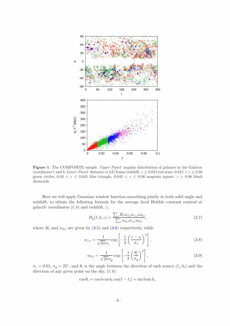
As seen from Fig. 1, except for the Zone of Avoidance region obscured by our Galaxy(|b| <∼ 15), the COMPOSITE sample has good angular coverage6, and thus can be used toevaluate large angle anisotropies of the Hubble expansion (dipole and quadrupole). However,the COMPOSITE sample has large uncertainties associated with the distance measure.
From the point of view of propagation of uncertainty, it is better to work with theformula (2.7) with dL as the independent variable in the numerator. To infer H
0from the
data we therefore minimize the following sum
χ2 =∑
i
(di − cζi/H0
∆di
)2
, (3.2)
where
ζi =
[zi +
1
2(1− q
0)z2i −
1
6(1− q
0− 3q
02 + j
0)z3i
], (3.3)
di and zi are respectively the luminosity distance and redshift of each object in theCOMPOSITEsample, and ∆di is the distance uncertainty. The above is equivalent to calculating the Hub-ble constant as a weighted average,
H0 =
∑iHiwd,i∑iwd,i
, (3.4)
whereHi = cζi/di (3.5)
andwd,i = cζidi/(∆di)
2. (3.6)
Wiltshire et al. [45] evaluated (3.4) for spherical averages in independent radial shells, for thecase of a linear Hubble law with ζi = zi, and separately considered angular averages using aGaussian window function smoothing in solid angle.
6This statement remains true when the data is broken into concentric radial shells in distance, as is seenin Fig. 2 of Wiltshire et al. [45], where only the innermost of 11 radial shells (with dL < 18.75 h−1Mpc) wasfound to have insufficient sky coverage when performing statistical checks.
– 8 –
-90
-60
-30
0
30
60
90
0 60 120 180 240 300 360
b
l
0
50
100
150
200
250
300
350
400
0 0.02 0.04 0.06 0.08 0.1
d L h
-1 [M
pc]
z
Figure 1. The COMPOSITE sample. Upper Panel: angular distribution of galaxies in the Galacticcoordinates ℓ and b; Lower Panel: distance vs LG frame redshift; z ≤ 0.015 red stars, 0.015 < z ≤ 0.03green circles, 0.03 < z ≤ 0.045 blue triangle, 0.045 < z ≤ 0.06 magenta square, z > 0.06 blackdiamonds.
Here we will apply Gaussian window function smoothing jointly in both solid angle andredshift, to obtain the following formula for the average local Hubble constant centred atgalactic coordinates (ℓ, b) and redshift, z,
H0(ℓ, b, z) =
∑iHiwd,iwz,iwθ,i∑iwd,iwz,iwθ,i
, (3.7)
where Hi and wd,i are given by (3.5) and (3.6) respectively, while
wz,i =1√2πσz
exp
[−1
2
(z − ziσz
)2], (3.8)
wθ,i =1√2πσθ
exp
[−1
2
(θiσθ
)2], (3.9)
σz = 0.01, σθ = 25, and θi is the angle between the direction of each source (ℓi, bi) and thedirection of any given point on the sky, (ℓ, b):
cos θi = cos b cos bi cos(ℓ− ℓi) + sin b sin bi.
– 9 –
For wz,i = 1 — i.e., with no redshift smoothing — equations (3.7) and (3.9) reduceto equations (B5) and (B9) derived in Appendix B of ref. [45] using a procedure based onminimizing the scatter in H−1.
Using (3.7) we calculate the regional contributions to our locally measured Hubbleconstant on an angular and redshift grid. For each redshift value on the grid, we constructthe angular maps of the Hubble expansion and express the Hubble flow in terms of itsfluctuations
∆H0
〈H0〉=
H0(ℓ, b, z) − 〈H0〉〈H0〉
, (3.10)
where
〈H0〉 =∫dΩ H0(ℓ, b, z)
4π, (3.11)
is the spherically averaged value of (3.7).
For each redshift, the fluctuations (3.10) are then analysed using the spherical harmonicdecomposition
∆H0
H0
=∑
l,m
almYlm, (3.12)
which allows us to evaluate the angular power spectrum:
Cl =1
2l + 1
∑
m
|alm|2. (3.13)
The power spectrum obtained in this way is subject to several biases and uncertainties[80]
Cl =∑
l′
Mll′B2l′Cl′ +Nl′ (3.14)
where Cl′ is the true underlying power spectrum, Mll′ describes the mode–mode couplingresulting from incomplete sky coverage, Bl is a window function due to the smoothing, andNl is the noise. As seen in Fig. 1 for |b| <∼ 15 data is incomplete in the galactic plane.In this paper, we do not mask these regions. Instead we extrapolate data to these regionsusing Gaussian smoothing of radius σθ = 25, as follows from eq. (3.14). While this canpotentially affect the inferred power spectrum, for the large angular scales (such as dipoleand quadrupole) of interest here the results are not significantly altered [45]. As for the noise,we estimate the level of contamination of the power spectrum due to distance uncertaintiesand number of data in the next section.
3.2 Completeness and robustness
As seen from Fig. 1, and in more detail in Fig. 2 of Wiltshire et al. [45], there is good angularcoverage in the COMPOSITE data. Potential systematic uncertainties from anisotropiesgenerated by insufficient sky cover were investigated in detail by Wiltshire et al. [45], whoperformed 12 million random reshuffles of the data in independent spherical shells, with theconclusion that for a binning scale ∆d = 12.5h−1Mpc (or ∆z ≃ 0.004) results concerningthe dipole anisotropy were robust on scales 0.002 < z < 0.04, with up to 99.999% confidencein some ranges.
In our case, we are also investigating the quadrupole anisotropy and adopt the largerredshift smoothing scale ∆z = 0.01. However, there is still a possibility that the inferred
– 10 –
anisotropy could result from some biases in the data. To minimize any systematic bias andto confirm that the measured anisotropy is not spurious, we performed the following checks:
• We used the fluctuations (3.12) rather than the spherical average (3.4). In the hypothet-ical case of an exactly homogeneous and isotropic universe (and perfect measurements)∆H0 = 0, so even if we have all the data only in one part of the sky and the rest of thesky without any measurement we should not detect any anisotropy.
• We shuffled the data. We tested the robustness of the results on the dipole andquadrupole anisotropies by analyzing the reshuffled data — for each pair of z anddL we randomly reshuffled the angular position. We generated 100,000 reshuffledCOMPOSITE catalogues and calculated the dipole and quadrupole of the Hubbleexpansion. If the measured signal were comparable with the signal obtained fromreshuffled samples that would indicate that the original result is spurious. That wasnot the case, however.
• We used half of the data. An alternative test of robustness was performed by takinghalf of the COMPOSITE sample to calculate the dipole and quadrupole anisotropiesof the Hubble expansion. This was done for 100,000 randomly selected halves of theoriginal COMPOSITE catalogue. If the measured signal was not consistent with theanisotropy obtained from half of the sample that would indicate that the original resultis spurious. Again, this was not the case.
The results of the above analyses are combined in Fig. 2. As seen our analysis passesthese tests at the 2σ level for z <∼ 0.045. This is consistent with the more exhaustive testsof Wiltshire et al. [45], which showed that the dipole is not a systematic effect, to very highconfidence.
3.3 Kinematic interpretation of anisotropies
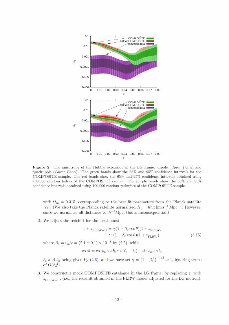
The results presented in Fig. 2 indicate the presence of anisotropy in the Hubble expansionup to z∼ 0.045, as determined from the COMPOSITE sample redshifts transformed to theLG rest frame. The anisotropy is largest for small redshifts z ∼ 0.02, with the amplitude ofthe dipole dropping one order of magnitude from z = 0.02 to z = 0.045, from which pointthe dipole amplitude is consistent with that of the randomly reshuffled data at 2σ.
According to the conventional explanation the anisotropy of the Hubble expansion ob-served in Fig. 2 should have a kinematic origin, due to a boost (2.5), (2.6) from the LG toCMB rest frame. This hypothesis can be directly tested by assuming a spatially homoge-neous universe in the CMB frame, generating mock COMPOSITE samples in that frame,adjusting the redshift by performing a local boost to the LG frame, and then analysing themock data in the manner of Fig. 2. Specifically,
1. We take the COMPOSITE sample. For each galaxy we have its angular position (ℓi, bi),luminosity distance di, uncertainty in distance ∆di and redshift zi. For each of thesedirections (ℓi, bi) we use the FLRWmodel to find the redshift (zFLRW) at which dL = di,by solving
dL = (1 + z)c
H0
zFLRW∫
0
dz1√
Ωm(1 + z)3 + 1− Ωm
,
– 11 –
1e-06
1e-05
0.0001
0.001
0.01
0.1
0 0.01 0.02 0.03 0.04 0.05 0.06 0.07 0.08
C1
z
COMPOSITEhalf of COMPOSITE
reshuffled data
1e-06
1e-05
0.0001
0.001
0.01
0.1
0 0.01 0.02 0.03 0.04 0.05 0.06 0.07 0.08
C2
z
COMPOSITEhalf of COMPOSITE
reshuffled data
Figure 2. The anisotropy of the Hubble expansion in the LG frame: dipole (Upper Panel) andquadrupole (Lower Panel). The green bands show the 65% and 95% confidence intervals for theCOMPOSITE sample. The red bands show the 65% and 95% confidence intervals obtained using100,000 random halves of the COMPOSITE sample. The purple bands show the 65% and 95%confidence intervals obtained using 100,000 random reshuffles of the COMPOSITE sample.
with Ωm = 0.315, corresponding to the best fit parameters from the Planck satellite[79]. (We also take the Planck satellite normalized H0 = 67.3 km s−1Mpc−1. However,since we normalize all distances to h−1Mpc, this is inconsequential.)
2. We adjust the redshift for the local boost
1 + zFLRW−B = γ(1− βo cos θ)(1 + zFLRW)
≃ (1− βo cos θ)(1 + zFLRW), (3.15)
where βo = vo/c = (2.1± 0.1) × 10−3 by (2.5), while
cos θ = cos bo cos bi cos(ℓo − ℓi) + sin bo sin bi,
ℓo and bo being given by (2.6), and we have set γ =(1− βo
2)−1/2 ≃ 1, ignoring terms
of O(βo2).
3. We construct a mock COMPOSITE catalogue in the LG frame, by replacing zi withzFLRW−B, (i.e., the redshift obtained in the FLRW model adjusted for the LG motion).
– 12 –
0.0001
0.001
0.01
0.1
0 0.01 0.02 0.03 0.04 0.05 0.06 0.07 0.08
C1
z
COMPOSITEFLRW + 635 km/s boostFLRW + 350 km/s boost
1e-05
0.0001
0.001
0.01
0.1
0 0.01 0.02 0.03 0.04 0.05 0.06 0.07 0.08
C2
z
COMPOSITEFLRW + 635 km/s boostFLRW + 350 km/s boost
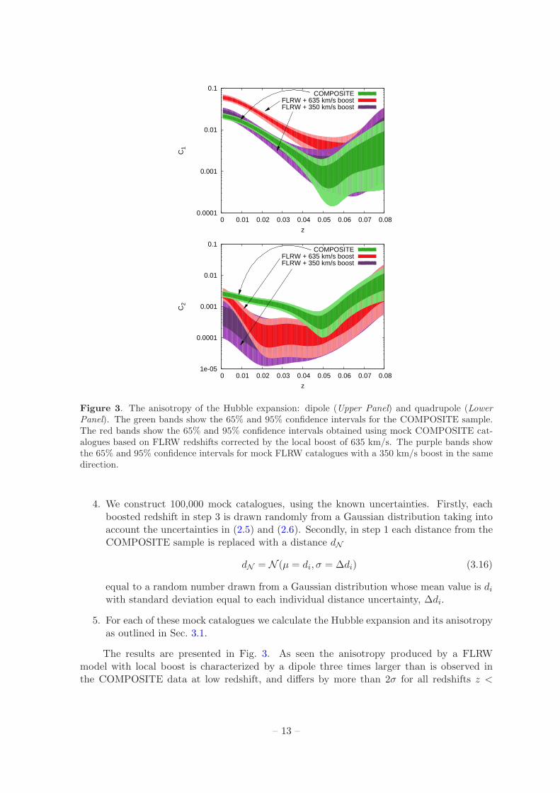
Figure 3. The anisotropy of the Hubble expansion: dipole (Upper Panel) and quadrupole (LowerPanel). The green bands show the 65% and 95% confidence intervals for the COMPOSITE sample.The red bands show the 65% and 95% confidence intervals obtained using mock COMPOSITE cat-alogues based on FLRW redshifts corrected by the local boost of 635 km/s. The purple bands showthe 65% and 95% confidence intervals for mock FLRW catalogues with a 350 km/s boost in the samedirection.
4. We construct 100,000 mock catalogues, using the known uncertainties. Firstly, eachboosted redshift in step 3 is drawn randomly from a Gaussian distribution taking intoaccount the uncertainties in (2.5) and (2.6). Secondly, in step 1 each distance from theCOMPOSITE sample is replaced with a distance dN
dN = N (µ = di, σ = ∆di) (3.16)
equal to a random number drawn from a Gaussian distribution whose mean value is diwith standard deviation equal to each individual distance uncertainty, ∆di.
5. For each of these mock catalogues we calculate the Hubble expansion and its anisotropyas outlined in Sec. 3.1.
The results are presented in Fig. 3. As seen the anisotropy produced by a FLRWmodel with local boost is characterized by a dipole three times larger than is observed inthe COMPOSITE data at low redshift, and differs by more than 2σ for all redshifts z <
– 13 –
0.04. On the other hand the quadrupole generated by the FLRW model with local boostis comparable to that of the COMPOSITE sample as z → 0, but becomes smaller thanthat of the COMPOSITE sample for z >∼ 0.01, being consistent with that of the randomlyreshuffled data in Fig. 2. Thus for z > 0.01 the local boost of 635 km/s cannot account forthe amplitude of the observed quadrupole in the COMPOSITE sample.
We note that the linear cos θ dependence in (3.15) gives rise to a pure dipole anisotropyat fixed values of zFLRW and dL in a linear Hubble relation. However, once (3.15) is substi-tuted in the Taylor series (3.3), a quadrupole and higher order multipoles are also generatedat fixed redshift. The amplitude of the boosted quadrupole in Fig. 3 is larger than wouldbe produced with perfect data, the ratio of the boost quadrupole and dipole contributionsto (3.12) generated by (3.3) and (3.15) being proportional to βo
2 ∼ 4 × 10⁻⁶. The rela-tively large value of the ratio C2/C1 ∼ 0.05 reflects the combination of the effect of angularsmoothing in the Gaussian window average (3.7)–(3.9) with the actual distance uncertaintiesassigned to the mock data, leading to C2∼ 0.004 at low redshift for the randomly reshuffledCOMPOSITE data in Fig. 2.
We have investigated by how much the magnitude of the local boost on the axis of theCMB and LG frames must be reduced in order to match the Hubble expansion dipole of theCOMPOSITE sample. We find that a 350 km/s boost would match the Hubble expansiondipole, giving results which are also shown in Fig. 3. The quadrupole of the COMPOSITEsample is not matched, however. For a 350 km/s boost the quadrupole is consistent with theresidual level of the randomly reshuffled data within 2σ for all redshifts.
The interpretation of the anisotropy within a framework of the FLRW model plus localboosts leads to a conundrum. The mismatch between the 350 km/s amplitude of a LocalGroup boost that would be consistent with the Hubble dipole anisotropy and the 635 km/sboost required to account for the CMB dipole kinematically suggests two possible solutions:(i) the galaxies in the COMPOSITE sample are in a coherent bulk flow with respect to theCMB on scales up to z∼ 0.045; or (ii) the Hubble dipole and other anisotropies contain asubstantial nonkinematic component.
While the bulk flow hypothesis is the one that is widely studied — being based on thestandard FLRW model — it is at odds with the results of [45] that the spherically averaged,or monopole, Hubble expansion variation is very significantly reduced in the LG frame ascompared to the CMB frame on <∼ 70h−1Mpc scales. The spherical average of a coherentbulk flow on such scales does not produce a monopole expansion variation of the characterseen in the COMPOSITE sample [45], and such a result is not seen in N–body Newtoniansimulations7. Moreover, the signature of a systematic boost offset (2.8) from the LG toCMB frame is seen in both the COMPOSITE and Cosmicflows-2 samples [46], providing apotential explanation for the CMB frame monopole variation if the LG rest frame is closerto being the frame in which anisotropies in the Hubble expansion are minimized.
We will now investigate the extent to which a nonkinematic interpretation of theanisotropies is observationally consistent by ray tracing in exact inhomogeneous solutionsof the Einstein equations.
7The effect of a local boost of the central observer is the most significant aspect of our analysis. FLRWmodels with additional inhomogeneities produced by Newtonian N–body simulations do not lead to resultssignificantly different from a pure FLRW model plus local boost shown as shown in Fig. 3. These results willbe reported elsewhere [72].
– 14 –
4 Light propagation in the non-linear relativistic regime and the origin of
anisotropies
Relativistic cosmological models predict the expansion of the Universe, which induces cosmo-logical redshift. Cosmic expansion, however, does depend on the local coupling of matter andcurvature, and only in the FLRW model is expansion spatially homogeneous and isotropic.The general relativistic formula for the redshift is [81]
1
(1 + z)2dz
ds=
1
3Θ + Σabn
anb + ua;bubna, (4.1)
where ua is the matter velocity field, na is the connecting covector field locally orthogonal8 toua, Σab is the shear of the velocity field, and Θ = ua;a is its expansion. In the limit of spatiallyhomogeneous and isotropic models the shear vanishes, Σab → 0, and the expansion of thevelocity field reduces to the Hubble parameter, Θ → 3H(t). However, once cosmic structuresform, the expansion field becomes non-uniform (ranging from Θ = 0 inside virialized clustersof galaxies to Θ > 3H0 within cosmic voids), and so the shear, Σab, and acceleration, ua;bu
b,of the velocity field are nonzero.
Distances are also affected by presence of cosmic structures. The general relativisticframework that allows us to calculate the distance is based on the Sachs equations [82, 83]
d2dAds2
= −(σ2 +
1
2Rabk
akb)dA, (4.2)
where ka is the tangent to null geodesics in a congruence, σ = 12σabσ
ab is the scalar shear ofthe null geodesic bundle, and Rab is the Ricci curvature. The first term on the right handside of (4.2) is often referred to as the Weyl focusing as it involves the Weyl curvature, whilethe second term is known as the Ricci focusing. For the type of inhomogeneities consideredin this paper, the amplitudes of the density contrast and density gradient are such that theWeyl focusing is negligibly small compared to the Ricci focusing [84]. Therefore, in thispaper we work within the Ricci focusing regime9 and we neglect any contribution from σ.The luminosity distance dL is then given by the reciprocity theorem [81, 85]
dL = (1 + z)2dA. (4.3)
Solving (4.2), (4.3) for the areal and luminosity distances, and (4.1) for the redshift, wearrive at a general relativistic distance–redshift relation, which will give rise to an anisotropicHubble expansion generated by the spatial inhomogeneities in the geometric terms on theright hand sides of (4.1) and (4.2). The anisotropies will be most prominent over lengthscales characteristic of the matter inhomogeneities, and will have characteristics which aredistinct from a simple FLRW geometry plus Lorentz boosts.
4.1 The geometry and Einstein equations
In order to solve (4.1), (4.2) for the distance–redshift relation we need to calculate all relevantphysical quantities such as the Ricci curvature, the shear of the null and timelike geodesic
8I.e., uana = 0, nan
a = 1. In the case that the vorticity of the velocity field vanishes — i.e., u[a;b] = 0 —then na is also the normal to a spatial hypersurface with tangent ua. For practical purposes, this is taken tobe the case in cosmological averages.
9See ref. [84] for a detailed discussion on the applicability of Ricci focusing and the contribution of theWeyl curvature on light propagation.
– 15 –
bundles, and the expansion scalar. For this purpose we use the Szekeres solution [16], whichis the most general known exact solution of the Einstein equations for an inhomogeneousdust source. In the limit of a spatially homogeneous matter distribution it reduces to theFLRW model.
The advantage of the Szekeres model over the perturbed FLRW model10 is that we canaccount for possible nonkinematic differential expansion which we find to be associated withactual observed structures in the local Universe. In particular, we will study a quasisphericalSzekeres model generated by a spherical void onto which an additional inhomogeneity withan axial density gradient is superposed. Thus we have both overdense and underdense regionsin the same exact solution of Einstein’s equations.
The Szekeres model reduces to the spherically symmetric LT model in the limit of nosuperposed axial density gradient. In the LT limit the anisotropy in the Hubble expansionis generated solely by the off–centre position of an observer relative to the centre of theinhomogeneity. In the Szekeres model this parameter will still play a role. However, theangle between the observer and the density gradient axis will also give rise to more complexand realistic anisotropies than are possible with the LT model alone. This allows us greaterfreedom to more closely model actual structures in the local Universe. Of course, the Szekeresmodel still has limitations as to what it can describe. (We will return to this issue later on.)
The metric of the quasispherical Szekeres solution [16, 86] is usually represented in thefollowing form
ds2 = c2dt2 −
(R′ −RE ′
E
)2
1− kdr2 − R2
E2(dp2 + dq2), (4.4)
where ′ ≡ ∂/∂r, R = R(t, r), and k = k(r) ≤ 1 is an arbitrary function of r. The function Eis given by
E(r, p, q) = 1
2S(p2 + q2)− P
Sp− Q
Sq +
P 2
2S+
Q2
2S+
S
2, (4.5)
where the functions S = S(r), P = P (r), Q = Q(r), but are otherwise arbitrary. We takethe coordinates r, p, q and the functions P , Q, R, S, E all to have dimensions of length. Wecan also define angular coordinates, (θ,φ), by
p− P = S cotθ
2cosφ, q −Q = S cot
θ
2sinφ. (4.6)
Then E = S/(1− cos θ), and the metric (4.4) takes the form
ds2 = c2dt2 − 1
1− k
[R′ +
R
S
(S′ cos θ +N sin θ
)]2dr2 −
[S′ sin θ +N (1− cos θ)
S
]2R2dr2
−[(∂φN) (1− cos θ)
S
]2R2dr2 +
2 [S′ sin θ +N (1− cos θ)]
SR2dr dθ
− 2(∂φN) sin θ (1− cos θ)
SR2dr dφ− R2(dθ2 + sin2 θ dφ2), (4.7)
where N(r, φ) ≡ (P ′ cosφ+Q′ sinφ).The Einstein equations with cosmological constant, Λ, and dust source of mass density,
ρ,Gab − Λgab = κ2ρ uaub, (4.8)
10We will present a comparison of the distinct differences from N–body simulations in a future paper [72].
– 16 –
where κ2 = 8πG/c4, reduce to the evolution equation and the mass distribution equation.The evolution equation is
R2 = −k(r) +2M(r)
R+
1
3Λc2R2, (4.9)
where ˙≡ ∂/∂t, and M(r) is a function related to the mass density by
κρ =2 (M ′ − 3ME ′/E)R2 (R′ −RE ′/E) . (4.10)
Note thatE ′
E =−1
S
[S′ cos θ +N sin θ
](4.11)
is the only term in (4.10) which gives a departure from spherical symmetry. One is free tospecify the various functions as long as (4.9)–(4.11) are satisfied. Since R(t, r) is the onlyfunction that depends on time, (4.9) can be integrated to give
t− tB(r) =
R∫
0
dR√−k + 2M/R + 1
3Λc2R2
, (4.12)
where tB(r) is one more arbitrary function called the bang time function, which describes thefact that the age of the Universe can be position dependent. If we demand that the age ofthe Universe is everywhere the same for comoving observers — the homogeneous Big Bangcondition — then the above equations link M(r) and k(r). In the generic case M and kcan be arbitrary, which could mean either a non-uniform Big Bang, or some turbulent initialconditions; i.e., conditions that would require a more complicated model than the Szekeresmodel.
The matter distribution in the Szekeres model has a structure of a dipole superposed on amonopole, (cf., upper left panel of Fig. 4). In order to determine the Szekeres model and solveall the equations, we need to specify its five arbitrary functions. These are: M and k whichdescribe the monopole distribution, and S, P , and Q which describe the dipole. If S, P , Q areconstant the dipole vanishes and we recover spherical symmetry; if S′ 6= 0, and P ′ = 0 = Q′
then the model is axially symmetric. These five functions (or any other combination offunctions from which these can be evaluated) are sufficient to solve all the equations thatdescribe the evolution of matter and light propagation in the evolving geometry.
In the FLRW limit when the model becomes spatially homogeneous and isotropic wehave:
R → ra(t) (4.13)
M → M0r3, (4.14)
k → k0r2, (4.15)
where M0 = 12H0
2 Ωm, k0 = H02(Ωm + ΩΛ − 1), and the functions S, P , and Q are constant
(S′ = 0 = P ′ = Q′). Therefore, in the FLRW limit the dependence on r in (4.9) cancels outand after dividing by a2 we recover the well known form of the Friedmann equation
H2 = H02(Ωma−3 +Ωka
−2 +ΩΛ
),
– 17 –
where ΩΛ = Λc2/(3H02), and Ωm +Ωk +ΩΛ = 1.
Let us then model the departure from homogeneity using the following profile of themass function
M = M0r3 [1 + δM (r)] , (4.16)
where
δM (r) =1
2δ0
(1− tanh
r − r02∆r
), (4.17)
with −1 ≤ δ0 < 0, is a localized perturbation which is underdense at the origin. As r → ∞,we have δM → 0 so that the spatial geometry is asymptotically that of the homogeneous andisotropic FLRW model. We normalize this geometry by choosing the spatially flat FLRWmodel which best fits the Planck satellite data, with Ωm = 0.315 andH0 = 67.3 km s−1 Mpc−1
[79].
The function k(r) is then evaluated from (4.12) for each r under the assumptions:(i) the age of the Universe is everywhere the same for comoving observers, tB = 0; and(ii) R(t
0, r) = r for each r, where the age of the Universe, t
0, is equal to that of the asymptotic
background spatially flat FLRW model.
Finally we assume axial symmetry, with dipole described by only the function S, whichwe choose to be:
S = r
(r
1 Mpc
)α−1
,
P = 0,
Q = 0, (4.18)
where α is a free parameter. When α → 0 the model becomes the spherically symmetric LTmodel, as shown in the lower left panel of Fig. 4.
The model has 7 free parameters:
• 4 parameters that specify the Szekeres model α, δ0, r0, ∆r,
• 3 parameters that specify the position of the observer robs, ϕobs, ϑobs.
Since the model considered here is axially symmetric, we can choose the observer to lie inthe plane ϕobs = π/2 without loss of generality. In order to reduce the dimension of theparameter space we also set ∆r = 0.1r0 for simplicity. That leaves us with 5 parameters. Inreality, we expect the perturbations that describe actual cosmic structures to be much morecomplicated than the parameterization adopted here. So while this gives us some flexibility,not all structures can be described using this parameterization. The structures that canbe described using this parameterization consist of a void and an adjacent overdensity, aspresented in the upper left panel of Fig. 4. While not perfect, this parameterization aims tomodel some of the major structures in the local Universe, such as the Local Void and theoverdensity known as the Great Attractor [66].
By varying the five free parameters, we can tune the size of the void and/or overden-sity, the amplitude of the density contrast and the position of the observer relative to thestructures. We run a search through this 5-dimensional parameter space looking for a modelwhich as closely as possible satisfies constraints in the following order of importance:
– 18 –
1. The CMB temperature has a maximum value of T0 + ∆T relative to the mean T0 =2.725K, where
∆T (ℓ = 276.4, b = 29.3) = 5.77 ± 0.36 mK, (4.19)
which corresponds to the CMB temperature dipole amplitude and direction in the LGrest frame.
2. The quadrupole of the CMB anisotropy is lower than the observed value [87]
C2,CMB < 242.2+563.6−140.1 µK2. (4.20)
While the dipole of the CMB is significantly affected by local expansion, the quadrupoleis dominated by the baryonic physics of the early Universe, and the observed valueitself is about 5 times smaller than the expectation based on the standard cosmology.Therefore we implement this constraint to ensure that the quadrupole generated bylocal inhomogeneities is much lower than the quadrupole generated at last scattering.
3. The dipole of the Hubble expansion anisotropy and its redshift dependence must beconsistent with the observed anisotropy of the COMPOSITE sample as presented inFig. 3.
4. The quadrupole of the Hubble expansion anisotropy and its redshift dependence mustbe consistent with the observed anisotropy of the COMPOSITE sample as presentedin Fig. 3.
4.2 Constructing mock catalogues
The algorithm of our analysis can be summarized by the following steps:
1. We first specify the Szekeres model.
2. We apply the HEALPix grid of the sky and propagate light rays in these directions.
3. We then calculate the CMB temperature maps.
4. We use HEALPix routines to calculate the anisotropy of the CMB map.
5. We take the COMPOSITE sample. For each galaxy we have its angular position (ℓi, bi),luminosity distance di, uncertainty in distance ∆di and redshift zi. For each of thesedirections (ℓi, bi) we numerically propagate light rays, using the null geodesic equationsof the Szekeres model, up until d = di. We then write down the redshift evaluatedwithin the Szekeres model z
Sz.
6. We construct the mock COMPOSITE catalogue, by replacing zi with zSz, (i.e., theredshift obtained in the Szekeres model for this direction and this distance).
7. We construct 100,000 mock catalogues, by taking into account the actual uncertainties,∆di, in the distances. As for the boosted FLRW mock catalogues, this is done byreplacing the distance from the COMPOSITE sample by dN according to (3.16).
8. For each of these mock catalogues we calculate the Hubble expansion and its anisotropyas outlined in Sec. 3.1.
– 19 –
0.0001
0.001
0.01
0.1
0 0.01 0.02 0.03 0.04 0.05 0.06 0.07 0.08
C1
z
COMPOSITESzekeres
1e-05
0.0001
0.001
0.01
0.1
0 0.01 0.02 0.03 0.04 0.05 0.06 0.07 0.08
C2
z
COMPOSITESzekeres
1e-05
0.0001
0.001
0.01
0.1
0 0.01 0.02 0.03 0.04 0.05 0.06 0.07 0.08
C2
z
COMPOSITEFLRW + 635 km/s boost
Spherical (LT)
0.0001
0.001
0.01
0.1
0 0.01 0.02 0.03 0.04 0.05 0.06 0.07 0.08
C1
z
COMPOSITEFLRW + 635 km/s boost
Spherical (LT)
-60 -40 -20 0 20 40 60
p h-1 [Mpc]
-60
-40
-20
0
20
40
60
q h-1
[Mpc
]
-1
-0.5
0
0.5
1
1.5
2
+
-60 -40 -20 0 20 40 60
p h-1 [Mpc]
-60
-40
-20
0
20
40
q h-1
[Mpc
]
-1
-0.5
0
0.5
1
1.5
2
+
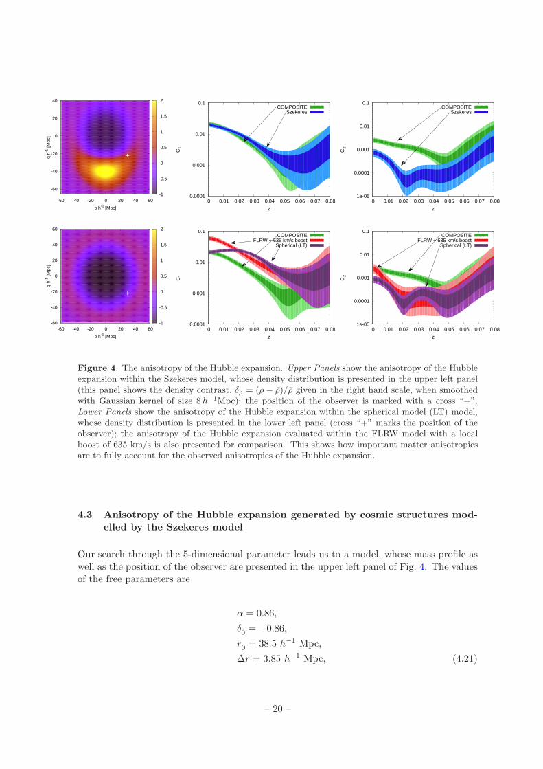
Figure 4. The anisotropy of the Hubble expansion. Upper Panels show the anisotropy of the Hubbleexpansion within the Szekeres model, whose density distribution is presented in the upper left panel(this panel shows the density contrast, δρ = (ρ − ρ)/ρ given in the right hand scale, when smoothedwith Gaussian kernel of size 8 h−1Mpc); the position of the observer is marked with a cross “+”.Lower Panels show the anisotropy of the Hubble expansion within the spherical model (LT) model,whose density distribution is presented in the lower left panel (cross “+” marks the position of theobserver); the anisotropy of the Hubble expansion evaluated within the FLRW model with a localboost of 635 km/s is also presented for comparison. This shows how important matter anisotropiesare to fully account for the observed anisotropies of the Hubble expansion.
4.3 Anisotropy of the Hubble expansion generated by cosmic structures mod-
elled by the Szekeres model
Our search through the 5-dimensional parameter leads us to a model, whose mass profile aswell as the position of the observer are presented in the upper left panel of Fig. 4. The valuesof the free parameters are
α = 0.86,
δ0= −0.86,
r0 = 38.5 h−1 Mpc,
∆r = 3.85 h−1 Mpc, (4.21)
– 20 –
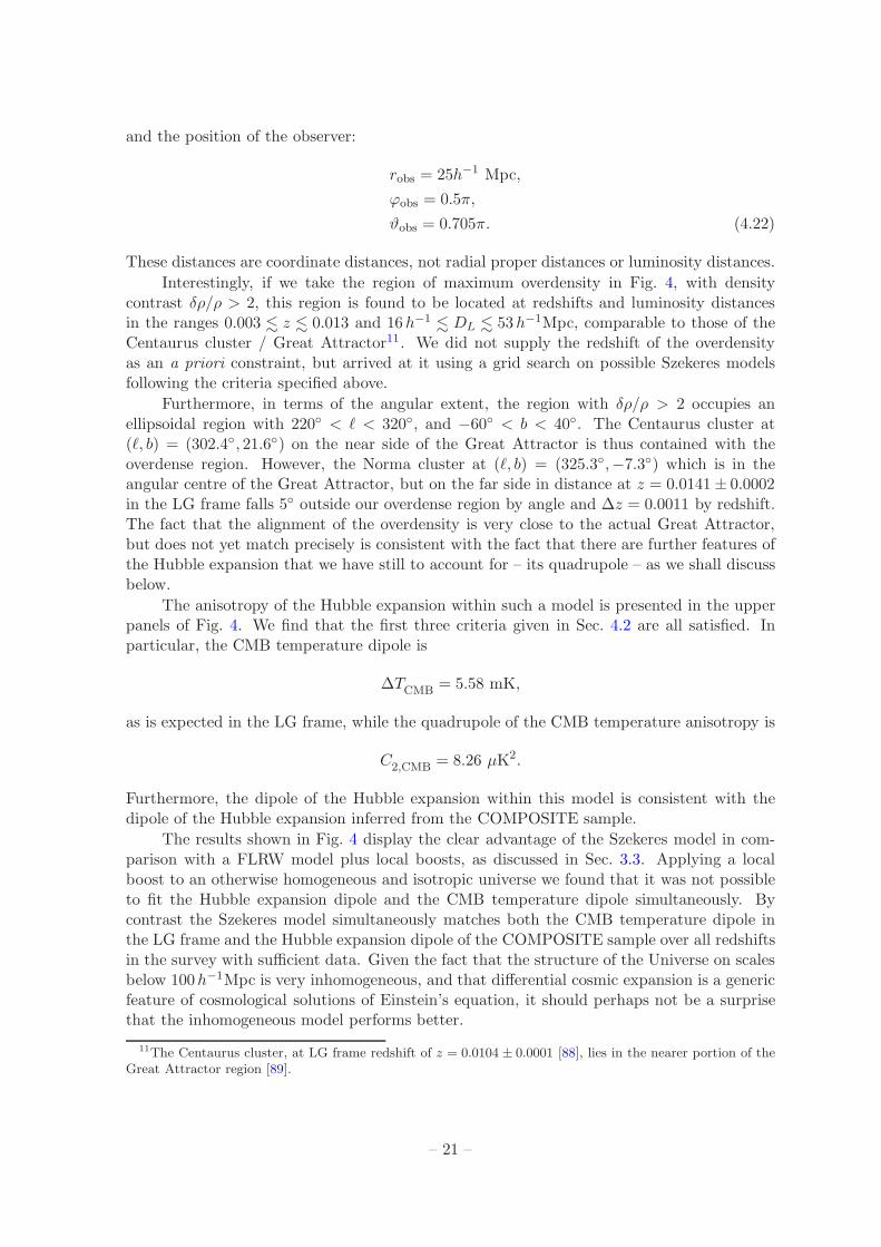
and the position of the observer:
robs = 25h−1 Mpc,
ϕobs = 0.5π,
ϑobs = 0.705π. (4.22)
These distances are coordinate distances, not radial proper distances or luminosity distances.
Interestingly, if we take the region of maximum overdensity in Fig. 4, with densitycontrast δρ/ρ > 2, this region is found to be located at redshifts and luminosity distancesin the ranges 0.003 <∼ z <∼ 0.013 and 16h−1 <∼ DL <∼ 53h−1Mpc, comparable to those of theCentaurus cluster / Great Attractor11. We did not supply the redshift of the overdensityas an a priori constraint, but arrived at it using a grid search on possible Szekeres modelsfollowing the criteria specified above.
Furthermore, in terms of the angular extent, the region with δρ/ρ > 2 occupies anellipsoidal region with 220 < ℓ < 320, and −60 < b < 40. The Centaurus cluster at(ℓ, b) = (302.4, 21.6) on the near side of the Great Attractor is thus contained with theoverdense region. However, the Norma cluster at (ℓ, b) = (325.3,−7.3) which is in theangular centre of the Great Attractor, but on the far side in distance at z = 0.0141± 0.0002in the LG frame falls 5 outside our overdense region by angle and ∆z = 0.0011 by redshift.The fact that the alignment of the overdensity is very close to the actual Great Attractor,but does not yet match precisely is consistent with the fact that there are further features ofthe Hubble expansion that we have still to account for – its quadrupole – as we shall discussbelow.
The anisotropy of the Hubble expansion within such a model is presented in the upperpanels of Fig. 4. We find that the first three criteria given in Sec. 4.2 are all satisfied. Inparticular, the CMB temperature dipole is
∆TCMB
= 5.58 mK,
as is expected in the LG frame, while the quadrupole of the CMB temperature anisotropy is
C2,CMB = 8.26 µK2.
Furthermore, the dipole of the Hubble expansion within this model is consistent with thedipole of the Hubble expansion inferred from the COMPOSITE sample.
The results shown in Fig. 4 display the clear advantage of the Szekeres model in com-parison with a FLRW model plus local boosts, as discussed in Sec. 3.3. Applying a localboost to an otherwise homogeneous and isotropic universe we found that it was not possibleto fit the Hubble expansion dipole and the CMB temperature dipole simultaneously. Bycontrast the Szekeres model simultaneously matches both the CMB temperature dipole inthe LG frame and the Hubble expansion dipole of the COMPOSITE sample over all redshiftsin the survey with sufficient data. Given the fact that the structure of the Universe on scalesbelow 100h−1Mpc is very inhomogeneous, and that differential cosmic expansion is a genericfeature of cosmological solutions of Einstein’s equation, it should perhaps not be a surprisethat the inhomogeneous model performs better.
11The Centaurus cluster, at LG frame redshift of z = 0.0104 ± 0.0001 [88], lies in the nearer portion of theGreat Attractor region [89].
– 21 –
On the other hand, the particular Szekeres model considered here is not able to re-produce the quadrupole of the Hubble expansion seen in the COMPOSITE sample, whichis about three times larger in magnitude than in the simulation. The Hubble expansionquadrupole in the Szekeres model (4.16)–(4.22) in fact has an amplitude consistent with thatof the randomly reshuffled data in Fig. 2, and is not statistically significant.
The fact that we can account for the Hubble expansion dipole, but not the quadrupolemay well be due to the simplicity of the model (4.16)–(4.22), (cf., upper panel of Fig. 4).In particular, the choice (4.18) enforces an axial symmetry on the mass distribution, whichcould be altered to give finer details. This would require a more complex model, and is leftfor future investigations.
As an indication of how the properties of the Hubble expansion variation are inducedby changes in the matter distribution, we have also investigated the anisotropy of the Hubbleexpansion evaluated using a spherical void LT model, which is obtained from the Szekeresmodel in the limit of a vanishing matter dipole, α → 0.
We use the same parameterization and procedure as outline above with α = 0, whichensures spherical symmetry. As in the case of a simple boost (Sec. 3.3) we are not able tosimultaneously fit the CMB temperature variation and the full redshift dependence of theHubble expansion anisotropy. At best, we can only reproduce some of the features.
An example of this investigation is presented in lower panels of Fig. 4. The values ofthe free parameters are
α = 0,
δ0 = −0.95,
r0 = 45.5 h−1 Mpc,
∆r = 4.55 h−1 Mpc (4.23)
and the position of the observer is
robs = 28h−1 Mpc,
ϕobs = 0.5π,
ϑobs = 0.5π. (4.24)
The model matches the correct temperature dipole of the CMB in the LG frame
∆TCMB = 5.63 mK
and the quadrupole of the CMB temperature anisotropy is
C2,CMB = 20.73 µK2.
However, the Hubble expansion dipole anisotropy can only be matched at very low redshifts(see middle panel of Fig. 4). As the redshift is increased the magnitude of the dipole increasesuntil for, z > 0.015, it becomes consistent with that predicted by the FLRW model plus alocal boost of 635 km/s in the LG frame — which was not consistent with the COMPOSITEdata, however.
This illustrates the fact that the amplitudes of the CMB dipole and higher multipolesin LT models can be roughly estimated for off–centre observers by an effective Newtonianapproximation [52] using the velocity appropriate to a boosted observer in the FLRW geom-etry. This limit was discussed by Wiltshire et al. [45], who gave an example of a LT void
– 22 –
with a somewhat different mass profile but with similar parameters, being 18% larger butwith a less sharp density gradient.
An examination of the density profile panels of Fig. 4 illustrates the role that is played bydifferential cosmic expansion. In particular, Lorentz boosts represent a point symmetry in thetangent space of any general observer. In the case of the LT model, the axis which joins thecentre of the void to the position of the off–centre observer defines a direction along which aradial boost can be taken to act from the void centre. Since the differential expansion is purelyradial with respect to the centre, it still somewhat mimics the action of a point symmetry.Thus it is not surprising that the LT dipole becomes equivalent to the FLRW model plusboost on scales larger than r0 + robs. By contrast, the Szekeres model incorporates a massdipole on an axis distinct from that joining r0 to robs. This distributed density gradienttherefore gives rise to a differential cosmic expansion which cannot be mimicked by a boostor any other point symmetry relative to the central point, r0.
The models considered in this Section show how the presence of cosmic structures affectthe anisotropy of the Hubble expansion. The more structures that are present in the model,the better is the consistency with observational data.
5 Potential impact on CMB anomalies
Any model cosmology in which (2.3) is nonzero will demand a different to standard approachto the analysis of large angle CMB anisotropies. The multipole expansion of (2.3) will consistof terms which could be deemed to be “anomalous multipoles” relative to the kinematicexpectation. As the dipoles will not cancel perfectly, to leading order there will generally bean “anomalous dipole” which may demand a reexamination of the observed power asymmetryand related large angle anomalies [42, 43]. This would have a major impact on observationalcosmology, as has already been discussed by Wiltshire et al. [45].
While one should naturally be sceptical of any suggestion that large angle CMB anoma-lies result from a nonkinematic relativistic differential expansion on <∼ 70h−1Mpc scales, avery important implication of the present paper is that ray-traced exact solutions similar tothose described here will provide, for the first time ever, concrete models that can actually betested against Planck satellite data for their effect on large angle anomalies. Such a projectmight even demand subtle changes in the treatment of the galactic foreground in the mapmaking procedures. Thus it is important to first have the best possible model of relativisticdifferential expansion before embarking on such a challenge.
A detailed analysis of the multipoles of (2.3) is therefore left for future work. In par-ticular, we need to first refine the Szekeres model to incorporate additional structures givinga Hubble expansion quadrupole with the observed redshift dependence. Since the CMBquadrupole for the Szekeres model (4.21), (4.22) is 30 times smaller in amplitude than theobserved CMB quadrupole, we should reasonably expect that this can be accommodated. Theredshift dependence of the Hubble expansion dipole and quadrupole seen in theCOMPOSITEsample should also to be confirmed with other data sets12.
In this paper, we have considered LT and Szekeres models in the the LG frame treatedas the average isotropic expansion frame, with a ray-traced CMB treated according to (2.4),as this is computationally simpler. With a refined Szekeres model one should also boost tothe heliocentric frame and constrain the ray traced simulations with the complete sky map
12In the case of the Cosmicflows-2 sample [76], for example, this requires a careful treatment of Malmquistbiases to remove a monopole bias [30, 46].
– 23 –
of the observed heliocentric dipole from Planck satellite data with an appropriate galacticsky mask applied, rather than adopting our simpler procedure (4.19) of just matching theamplitude of the equivalent temperature dipole in the LG frame.
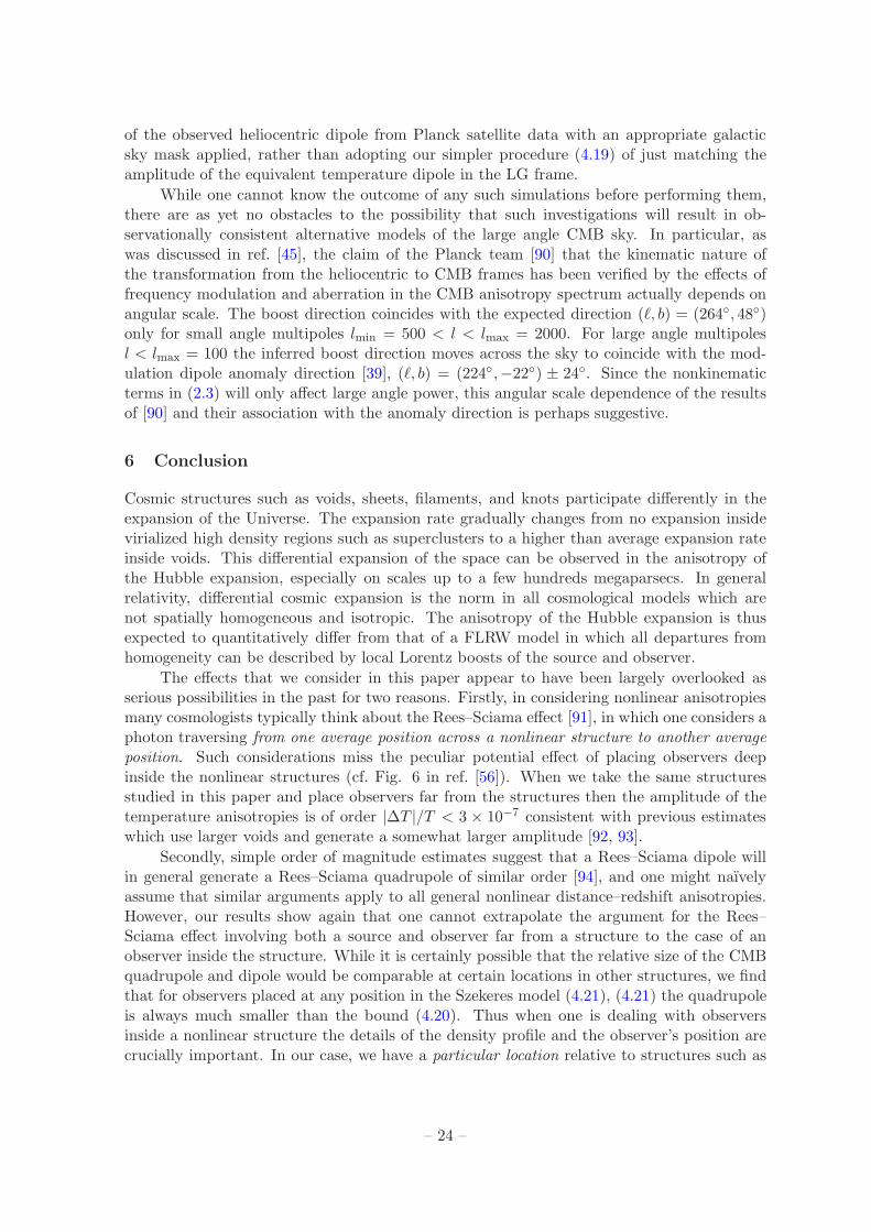
While one cannot know the outcome of any such simulations before performing them,there are as yet no obstacles to the possibility that such investigations will result in ob-servationally consistent alternative models of the large angle CMB sky. In particular, aswas discussed in ref. [45], the claim of the Planck team [90] that the kinematic nature ofthe transformation from the heliocentric to CMB frames has been verified by the effects offrequency modulation and aberration in the CMB anisotropy spectrum actually depends onangular scale. The boost direction coincides with the expected direction (ℓ, b) = (264, 48)only for small angle multipoles lmin = 500 < l < lmax = 2000. For large angle multipolesl < lmax = 100 the inferred boost direction moves across the sky to coincide with the mod-ulation dipole anomaly direction [39], (ℓ, b) = (224,−22) ± 24. Since the nonkinematicterms in (2.3) will only affect large angle power, this angular scale dependence of the resultsof [90] and their association with the anomaly direction is perhaps suggestive.
6 Conclusion
Cosmic structures such as voids, sheets, filaments, and knots participate differently in theexpansion of the Universe. The expansion rate gradually changes from no expansion insidevirialized high density regions such as superclusters to a higher than average expansion rateinside voids. This differential expansion of the space can be observed in the anisotropy ofthe Hubble expansion, especially on scales up to a few hundreds megaparsecs. In generalrelativity, differential cosmic expansion is the norm in all cosmological models which arenot spatially homogeneous and isotropic. The anisotropy of the Hubble expansion is thusexpected to quantitatively differ from that of a FLRW model in which all departures fromhomogeneity can be described by local Lorentz boosts of the source and observer.
The effects that we consider in this paper appear to have been largely overlooked asserious possibilities in the past for two reasons. Firstly, in considering nonlinear anisotropiesmany cosmologists typically think about the Rees–Sciama effect [91], in which one considers aphoton traversing from one average position across a nonlinear structure to another averageposition. Such considerations miss the peculiar potential effect of placing observers deepinside the nonlinear structures (cf. Fig. 6 in ref. [56]). When we take the same structuresstudied in this paper and place observers far from the structures then the amplitude of thetemperature anisotropies is of order |∆T |/T < 3 × 10⁻⁷ consistent with previous estimateswhich use larger voids and generate a somewhat larger amplitude [92, 93].
Secondly, simple order of magnitude estimates suggest that a Rees–Sciama dipole willin general generate a Rees–Sciama quadrupole of similar order [94], and one might naıvelyassume that similar arguments apply to all general nonlinear distance–redshift anisotropies.However, our results show again that one cannot extrapolate the argument for the Rees–Sciama effect involving both a source and observer far from a structure to the case of anobserver inside the structure. While it is certainly possible that the relative size of the CMBquadrupole and dipole would be comparable at certain locations in other structures, we findthat for observers placed at any position in the Szekeres model (4.21), (4.21) the quadrupoleis always much smaller than the bound (4.20). Thus when one is dealing with observersinside a nonlinear structure the details of the density profile and the observer’s position arecrucially important. In our case, we have a particular location relative to structures such as
– 24 –
the Local Void and the “Great Attractor”. Our study is the first to benefit from constrainingray tracing simulations with actual large galaxy surveys outside a framework of the FLRWcosmology plus local boosts.
In this paper we investigated the anisotropy pattern of the Hubble expansion, consider-ing the dipole and quadrupole variations in the LG frame. Most previous studies have eitherfocused on the monopole, i.e., the global (average) value of H0, or on bulk flows. In a waythis is analogous to studies of the CMB in 1970s–1990s. However, with increasing amountof data and precision of measurements, we are slowly arriving at the stage where we canstudy anisotropies of the Hubble expansion, just as we now study the anisotropy of the CMBtemperature fluctuations.
In analogy to CMB temperature fluctuations, we show that the Hubble expansion can bedecomposed using spherical harmonics and expressed in terms of an angular power spectrum.Moreover, by averaging data at various redshifts we can have additional information about theredshift dependence of the multipoles of the Hubble expansion. Irrespective of any theoreticalassumptions about cosmic expansion, this is a novel technique that carries complimentary ifnot additional information to studies of bulk flow that have been extensively carried out inthe past years.
In Sec. 3.1 we developed the formalism used to study the anisotropy of the Hubbleexpansion. When applied to the COMPOSITE sample we identified the presence of dipoleand quadrupole anisotropies in the Hubble expansion. These anisotropies are statisticallysignificant in the data up to z <∼ 0.045. For larger redshifts the amount of data is small andthe signal is no longer distinguishable from noise.
We compared the measured anisotropy with predictions from a FLRW model assumedto be homogeneous and isotropic in the CMB frame, and also particular LT and Szekeresmodels with small scale inhomogeneities in the LG frame. All models were assumed to beidentical to a spatially flat FLRW models on scales >∼ 100h−1Mpc, with parameters fixed tothose of the FLRW model that best fits the Planck satellite data [79]. The FLRW modelwith a local boost from the CMB to LG frame did not fit the observed redshift dependence ofthe dipole of the Hubble expansion of the COMPOSITE sample as seen in the LG frame. Inorder to match the observed features of the dipole of the Hubble expansion, the local boostwould have to be reduced to approximately 350 km/s, which is much smaller than the actual635± 38 km/s that is required if the CMB temperature dipole is purely kinematic.
A quasispherical Szekeres solution that allows for variations of the local geometry gener-ated by the presence of cosmic structures, which effectively model the Local Void and “GreatAttractor”, was found to improve the fit. This analysis shows that the local cosmologicalenvironment does affect the Hubble expansion. Physically, this can be understood in termsof the differential expansion of the space, with the void expanding faster and the overdensityexpanding at a slower than the average expansion rate.
As yet, the numerical model does not have a Hubble quadrupole as large as that seenin the COMPOSITE sample. However, if extra modifications are added — for example, byusing methods to include extra structures [65] — then given the magnitude of the effects thatremain to be explained, it is highly plausible that highly accurate models of the local cosmicexpansion can be developed.
All our models are constrained by a match to the magnitude and direction of the CMBtemperature dipole. Since the models are nonlinear the addition of further structures canaffect the alignment and scale of the structures, and the position of the observer, as comparedto a simpler model. In moving from the simple LT void model to our single void / single
– 25 –
overdensity Szekeres model, for example, the scale of the void was reduced by 40%, whilealso achieving a fit to the Hubble expansion dipole over a range of redshifts.
The effect which remains to be explained – the Hubble expansion quadrupole – is anorder of magnitude smaller than the Hubble expansion dipole. Therefore we should notexpect such large changes of scale as occurred between the LT and Szekeres models alreadystudied. However, we note that the overdensity in our simple Szekeres model overlaps withthe observed Great Attractor in both angle and redshift on the near side but not completelyon the far side. Furthermore, the additional major structures that should still be accountedfor include most notably the Perseus–Pisces concentration, which lies at LG frame redshifts0.0182–0.0194. This is at the upper end of the redshift/distance range of the structuresthat we are considering, with a a likely impacting on the alignment of the far side of theoverdensity which we have identified with the Great Attractor. Whether this can be donewhile also accounting for the Hubble expansion quadrupole is an important question left forfuture work.
As discussed in Sec. 5, our approach may potentially provide a simple physical expla-nation of particular large anomalies in the CMB radiation, in terms of known physics. Butthis is a matter for future investigations.
The main result of this paper is that with just the FLRW geometry plus a local boostof the Local Group of galaxies it is impossible to simultaneously fit both the CMB dipoleand quadrupole anisotropies and the redshift dependence of the dipole anisotropy of thelocal expansion of the Universe, determined by the COMPOSITE sample. To explain theobserved features we need to use models that exhibit differential cosmic expansion. Furtherrefinement of such models may potentially have a major impact on cosmology.
Acknowledgments
We thank Francois Bouchet, Thomas Buchert, Lawrence Dam, Syksy Rasanen, Nezihe Uzunand Jim Zibin for helpful discussions and correspondence. This work was supported by theMarsden Fund of the Royal Society of New Zealand, and by the Australian Research Councilthrough the Future Fellowship FT140101270. Computational resources used in this workwere provided by Intersect Australia Ltd and the University of Sydney Faculty of Science.
References
[1] F. Hoyle and M.S. Vogeley, Voids in the Point Source Catalogue Survey and the UpdatedZwicky Catalog, Astrophys. J. 566 (2002) 641, [astro-ph/0109357]
[2] F. Hoyle and M.S. Vogeley, Voids in the 2dF Galaxy Redshift Survey, Astrophys. J. 607 (2004)751, [astro-ph/0312533]
[3] A.V. Tikhonov and I.D. Karachentsev, Minivoids in the local volume, Astrophys. J. 653 (2006)969, [astro-ph/0609109]
[4] D.C. Pan, M.S. Vogeley, F. Hoyle, Y.Y. Choi and C. Park, Cosmic voids in Sloan Digital SkySurvey Data Release 7, Mon. Not. Roy. Astron. Soc. 421 (2012) 926, [arXiv:1103.4156]
[5] J.E. Forero–Romero, Y. Hoffman, S. Gottlober, A. Klypin and G. Yepes, A dynamicalclassification of the cosmic web, Mon. Not. Roy. Astron. Soc. 396 (2009) 1815,[arXiv:0809.4135]
[6] M. Bilicki, J.A. Peacock, T.H. Jarrett, M.E. Cluver and L. Steward, Mapping the cosmic webwith the largest all-sky surveys, IAU Symp. 308 (2014), arXiv:1408.0799
– 26 –
[7] J. Einasto, Yakov Zeldovich and the Cosmic Web Paradigm, IAU Symp. 308 (2014),arXiv:1410.6932
[8] D.W. Hogg, D.J. Eisenstein, M.R. Blanton, N.A. Bahcall, J. Brinkmann, J.E. Gunn andD.P. Schneider, Cosmic homogeneity demonstrated with luminous red galaxies, Astrophys. J.624 (2005) 54, [astro-ph/0411197]
[9] F. Sylos Labini, N.L. Vasilyev, L. Pietronero and Y.V. Baryshev, Absence of self-averaging andof homogeneity in the large scale galaxy distribution, Europhys. Lett. 86 (2009) 49001,[arXiv:0805.1132]
[10] M. Scrimgeour, T. Davis, C. Blake, et al., The WiggleZ Dark Energy Survey: the transition tolarge-scale cosmic homogeneity, Mon. Not. Roy. Astron. Soc. 425 (2012) 116,[arXiv:1205.6812]
[11] R.G. Clowes, K.A. Harris, S. Raghunathan, L.E. Campusano, I.K. Soechting and M.J. Graham,A structure in the early universe at z∼ 1.3 that exceeds the homogeneity scale of the R-Wconcordance cosmology, Mon. Not. Roy. Astron. Soc. 429 (2013) 2910, [arXiv:1211.6256]
[12] B.F. Roukema, T. Buchert, J.J. Ostrowski and M.J. France, Can an inhomogeneous metric bedetected with the baryonic acoustic oscillation peak?, Mon. Not. Roy. Astron. Soc. 448 (2015)1660, [arXiv:1410.1687]
[13] G. Lemaıtre, l’Univers en expansion, Ann. Soc. Sci. Bruxelles A 53 (1933) 51 The expandinguniverse, [English translation: Gen. Rel. Grav. 29 (1997) 641]
[14] R.C. Tolman, Effect of inhomogeneity on cosmological models, Proc. Nat. Acad. Sci. 20 (1934)169
[15] H. Bondi, Spherically symmetrical models in general relativity, Mon. Not. Roy. Astron. Soc.107 (1947) 410
[16] P. Szekeres, A class of inhomogeneous cosmological models, Commun. Math. Phys. 41 (1975) 55
[17] J.M. Stewart and D.W. Sciama, Peculiar velocity of the sun and its relation to the cosmicmicrowave background, Nature 216 (1967) 748
[18] P.J.E. Peebles and D.T. Wilkinson, Comment on the anisotropy of the primeval fireball, Phys.Rev. 174 (1968) 2168
[19] R.B. Partridge and D.T. Wilkinson, Isotropy and homogeneity of the universe frommeasurements of the cosmic microwave background, Phys. Rev. Lett. 18 (1967) 557
[20] R. Watkins, H.A. Feldman and M.J. Hudson, Consistently large cosmic flows on scales of100h−1 Mpc: A challenge for the standard ΛCDM cosmology, Mon. Not. Roy. Astron. Soc.392 (2009) 743, [arXiv:0809.4041]
[21] G. Lavaux, R.B. Tully, R. Mohayaee and S. Colombi, Cosmic flow from 2MASS redshift survey:The origin of CMB dipole and implications for ΛCDM cosmology, Astrophys. J. 709 (2010)483, [arXiv:0810.3658]
[22] A. Kashlinsky, F. Atrio–Barandela, H. Ebeling, A. Edge and D. Kocevski, A new measurementof the bulk flow of X-ray luminous clusters of galaxies, Astrophys. J. 712 (2010) L81,[arXiv:0910.4958]
[23] J. Colin, R. Mohayaee, S. Sarkar and A. Shafieloo, Probing the anisotropic local universe andbeyond with SNe Ia data, Mon. Not. Roy. Astron. Soc. 414 (2011) 264, [arXiv:1011.6292]
[24] A. Nusser and M. Davis, The cosmological bulk flow: consistency with ΛCDM and z ≈ 0constraints on σ8 and γ, Astrophys. J. 736 (2011) 93, [arXiv:1101.1650]
[25] S.J. Turnbull, M.J. Hudson, H.A. Feldman, M. Hicken, R.P. Kirshner and R. Watkins, Cosmicflows in the nearby universe from Type Ia Supernovae, Mon. Not. Roy. Astron. Soc. 420 (2012)447, [arXiv:1111.0631]
– 27 –
[26] G. Lavaux, N. Afshordi, M.J. Hudson, First measurement of the bulk flow of nearby galaxiesusing the cosmic microwave background, Mon. Not. Roy. Astron. Soc. 430 (2013) 1617,[arXiv:1207.1721]
[27] Y.Z. Ma and D. Scott, Cosmic bulk flows on 50 h−1Mpc scales: A Bayesian hyper-parametermethod and multi-shells likelihood analysis, Mon. Not. Roy. Astron. Soc. 428 (2013) 2017,[arXiv:1208.2028]
[28] F. Atrio–Barandela, On the statistical significance of the bulk flow measured by the Plancksatellite, Astron. Astrophys. 557 (2013) A116, [arXiv:1303.6614]
[29] Planck Collaboration, P.A.R. Ade, N. Aghanim, M. Arnaud, et al., Planck intermediate results.XIII. Constraints on peculiar velocities, Astron. Astrophys. 561 (2014) A97, [arXiv:1303.5090]
[30] Y. Hoffman, H.M. Courtois and R.B. Tully, Cosmic bulk flow and the local motion fromCosmicflows-2, Mon. Not. Roy. Astron. Soc. 449 (2015) 4494, [arXiv:1503.05422]
[31] J. Carrick, S.J. Turnbull, G. Lavaux and M.J. Hudson, Cosmological parameters from thecomparison of peculiar velocities with predictions from the 2M++ density field, Mon. Not. Roy.Astron. Soc. 450 (2015) 317, [arXiv:1504.04627]
[32] M. Tegmark, A. de Oliveira–Costa and A.J.S. Hamilton, A high resolution foreground cleanedCMB map from WMAP, Phys. Rev. D 68 (2003) 123523, [astro-ph/0302496]
[33] H.K. Eriksen, F.K. Hansen, A.J. Banday, K.M. Gorski and P.B. Lilje, Asymmetries in theCMB anisotropy field, Astrophys. J. 605 (2004) 14 [Erratum ibid 609 (2004) 1198],[astro-ph/0307507]
[34] A. de Oliveira-Costa, M. Tegmark, M. Zaldarriaga and A. Hamilton, The significance of thelargest scale CMB fluctuations in WMAP, Phys. Rev. D 69 (2004) 063516,[astro-ph/0307282]
[35] D.J. Schwarz, G.D. Starkman, D. Huterer and C.J. Copi, Is the low-l microwave backgroundcosmic?, Phys. Rev. Lett. 93 (2004) 221301, [astro-ph/0403353]
[36] K. Land and J. Magueijo, The axis of evil, Phys. Rev. Lett. 95 (2005) 071301,[astro-ph/0502237]
[37] C.J. Copi, D. Huterer, D.J. Schwarz and G.D. Starkman, On the large-angle anomalies of themicrowave sky, Mon. Not. Roy. Astron. Soc. 367 (2006) 79, [astro-ph/0508047]
[38] H.K. Eriksen, A.J. Banday, K.M. Gorski, F.K. Hansen and P.B. Lilje, Hemispherical powerasymmetry in the three-year Wilkinson Microwave Anisotropy Probe sky maps, Astrophys. J.660 (2007) L81, [astro-ph/0701089]
[39] J. Hoftuft, H.K. Eriksen, A.J. Banday, K.M. Gorski, F.K. Hansen and P.B. Lilje, Increasingevidence for hemispherical power asymmetry in the five-year WMAP data, Astrophys. J. 699(2009) 985, [arXiv:0903.1229]
[40] J. Kim and P. Naselsky, Anomalous parity asymmetry of the Wilkinson Microwave AnisotropyProbe power spectrum data at low multipoles, Astrophys. J. 714 (2010) L265,[arXiv:1001.4613]
[41] Y. Akrami, Y. Fantaye, A. Shafieloo, H.K. Eriksen, F.K. Hansen, A.J. Banday andK.M. Gorski, Power asymmetry in WMAP and Planck temperature sky maps as measured by alocal variance estimator, Astrophys. J. 784 (2014) L42, [arXiv:1402.0870]
[42] Planck Collaboration, P.A.R. Ade, N. Aghanim, C. Armitage-Caplan, et al., Planck 2013results. XXIII. Isotropy and statistics of the CMB, Astron. Astrophys. 571 (2014) A23,[arXiv:1303.5083]
[43] Planck Collaboration, P.A.R. Ade, N. Aghanim, Y. Akrami, et al., Planck 2015 results. XVI.Isotropy and statistics of the CMB, (2015), arXiv:1506.07135
– 28 –
[44] D.J. Schwarz, C.J. Copi, D. Huterer and G.D. Starkman, CMB anomalies after Planck, (2015),arXiv:1510.07929
[45] D.L. Wiltshire, P.R. Smale, T. Mattsson and R. Watkins, Hubble flow variance and the cosmicrest frame, Phys. Rev. D 88 (2013) 083529, [arXiv:1201.5371]
[46] J.H. McKay and D.L. Wiltshire, Defining the frame of minimum nonlinear Hubble expansionvariation, Mon. Not. Roy. Astron. Soc. 457 (2016) 3285, [arXiv:1503.04192]
[47] M. Rubart and D.J. Schwarz, Cosmic radio dipole from NVSS and WENSS, Astron. Astrophys.555, A117 (2013), [arXiv:1301.5559]
[48] J.V. Arnau, M.J. Fullana, L. Monreal and D. Saez, On the microwave anisotropies produced bya nonlinear voids, Astrophys. J. 402 (1993) 359
[49] J.V. Arnau, M.J. Fullana and D. Saez, Great Attractor-like structures and large-scaleanisotropy, Mon. Not. Roy. Astron. Soc. 268 (1994) L17
[50] N.P. Humphreys, R. Maartens and D.R. Matravers, Anisotropic observations in universes withnonlinear inhomogeneity, Astrophys. J. 477 (1997) 47, [astro-ph/9602033].,
[51] K. Tomita, Bulk flows and cosmic microwave background dipole anisotropy in cosmological voidmodels, Astrophys. J. 529 (2000) 26, [astro-ph/9905278]
[52] H. Alnes and M. Amarzguioui, CMB anisotropies seen by an off-center observer in a sphericallysymmetric inhomogeneous universe, Phys. Rev. D 74 (2006) 103520, [astro-ph/0607334]
[53] K. Bolejko and C. Hellaby, The Great Attractor and the Shapley Concentration, Gen. Rel.Grav. 40 (2008) 1771, [astro-ph/0604402]
[54] K. Bolejko, C. Clarkson, R. Maartens, D. Bacon, N. Meures and E. Beynon, Antilensing: Thebright side of voids, Phys. Rev. Lett. 110 (2013) 021302, [arXiv:1209.3142]
[55] D.J. Bacon, S. Andrianomena, C. Clarkson, Bolejko, K. and R. Maartens, Cosmology withDoppler lensing, Mon. Not. Roy. Astron. Soc. 443 (2014) 1900, [arXiv:1401.3694]
[56] K. Bolejko, The Szekeres Swiss Cheese model and the CMB observations, Gen. Rel. Grav. 41(2009) 1737, [arXiv:0804.1846]
[57] K. Bolejko and M.N. Celerier, Szekeres Swiss-cheese model and supernova observations, Phys.Rev. D 82 (2010) 103510, [arXiv:1005.2584]
[58] A. Nwankwo, M. Ishak and J. Thompson, Luminosity distance and redshift in the Szekeresinhomogeneous cosmological models, JCAP 05 (2011) 028, [arXiv:1005.2989]
[59] M. Ishak and A. Peel, The growth of structure in the Szekeres inhomogeneous cosmologicalmodels and the matter-dominated era, Phys. Rev. D 85 (2012) 083502, [arXiv:1104.2590]
[60] K. Bolejko and R.A. Sussman, Cosmic spherical void via coarse-graining and averagingnon-spherical structures, Phys. Lett. B 697 (2011) 265
[61] R.G. Buckley and E.M. Schlegel, CMB dipoles and other low-order multipoles in thequasispherical Szekeres model, Phys. Rev. D 87 (2013) 023524
[62] S.M. Koksbang and S. Hannestad, Methods for studying the accuracy of light propagation inN-body simulations, Phys. Rev. D 91 (2015) 043508, [arXiv:1501.01413]
[63] S.M. Koksbang and S. Hannestad, Studying the precision of ray tracing techniques with Szekeresmodels, Phys. Rev. D 92 (2015) 023532; err. ibid. 92 (2015) 069904, [arXiv:1506.09127]
[64] R.A. Sussman, I.D. Gaspar and J.C. Hidalgo, Coarse-grained description of cosmic structurefrom Szekeres models, JCAP 03 (2016) 012, [arXiv:1507.02306]
[65] R.A. Sussman and I.D. Gaspar, Multiple non-spherical structures from the extrema of Szekeresscalars, Phys. Rev. D 92 (2015) 083533, [arXiv:1508.03127]
– 29 –
[66] B.R. Tully, J.E. Shaya, D.I. Karachentsev, M.H. Courtois, D.D. Kocevski, L. Rizzi and A. Peel,Our peculiar motion away from the Local Void, Astrophys. J. 676 (2008) 184,[arXiv:0705.4139]
[67] D.L. Wiltshire, Cosmic clocks, cosmic variance and cosmic averages, New J. Phys. 9 (2007) 377[gr-qc/0702082]
[68] D.L. Wiltshire, Exact solution to the averaging problem in cosmology, Phys. Rev. Lett. 99(2007) 251101, [arXiv:0709.0732]
[69] D.L. Wiltshire, Average observational quantities in the timescape cosmology, Phys. Rev. D 80
(2009) 123512, [arXiv:0909.0749]
[70] J.A.G. Duley, M.A. Nazer and D.L. Wiltshire, Timescape cosmology with radiation fluid, Class.Quant. Grav. 30 (2013) 175006, [arXiv:1306.3208]
[71] M. Kamionkowski and L. Knox, Aspects of the cosmic microwave background dipole, Phys. Rev.D 67 (2003) 063001, [astro-ph/0210165]
[72] K. Bolejko, et al., in preparation
[73] N. Li and D.J. Schwarz, Scale dependence of cosmological backreaction, Phys. Rev. D 78 (2008)083531, [arXiv:0710.5073]
[74] M.L. McClure and C.C. Dyer, Anisotropy in the Hubble constant as observed in the HSTextragalactic distance scale Key Project results, New Astron. 12 (2007) 533,[astro-ph/0703556]
[75] H.A. Feldman, R. Watkins and M.J. Hudson, Cosmic flows on 100 Mpc/h scales: Standardizedminimum variance bulk flow, shear and octupole moments, Mon. Not. Roy. Astron. Soc. 407(2010) 2328, [arXiv:0911.5516]
[76] R.B. Tully, H.M. Courtois, A.E. Dophin, et al., Cosmicflows-2: The Data, Astron. J. 146(2013) 86, [arXiv:1307.7213]
[77] P. Erdogdu, O. Lahav, J.P. Huchra, et al., Reconstructed density and velocity fields from the2MASS redshift survey, Mon. Not. Roy. Astron. Soc. 373 (2006) 45, [astro-ph/0610005]
[78] A.G. Riess, L. Macri, S. Casertano, et al., A 3Space Telescope and Wide Field Camera 3,Astrophys. J. 730, 119; (E) 732, 129, [arXiv:1103.2976]
[79] Planck Collaboration, P.A.R. Ade, N. Aghanim, C. Armitage-Caplan, et al., Planck 2013results. XVI. Cosmological parameters, Astron. Astrophys. 571 (2014) A16, [arXiv:1303.5083]
[80] E. Hivon, K.M. Gorski, C.B. Netterfield, B.P. Crill, S. Prunet and F. Hansen, Master of thecosmic microwave background anisotropy power spectrum: a fast method for statistical analysisof large and complex cosmic microwave background data sets, Astrophys. J. 567 (2002) 2,[astro-ph/0105302]
[81] G.F.R. Ellis, in Proceedings of the International School of Physics ‘Enrico Fermi’ (1971)Course 47: General Relativity and Cosmology, ed. R.K. Sachs (Academic Press, New York andLondon), pp. 104–182; reprinted, with historical comments, in Gen. Rel. Grav. 41 (2009) 581
[82] R. Sachs, Gravitational waves in general relativity. VI. The outgoing radiation condition, Proc.Roy. Soc. Lond. A 264 (1961) 309
[83] P.J.E. Peebles, Principles of Physical Cosmology, (Princeton University Press, 1993)
[84] K. Bolejko and P.G. Ferreira, Ricci focusing, shearing, and the expansion rate in an almosthomogeneous Universe, JCAP 05 (2012) 003, [arXiv:1204.0909]
[85] I.M.H. Etherington, Phil. Mag. 15 (1933) 761; reprinted, with historical comments, in Gen.Rel. Grav. 39 (2007) 1055
[86] P. Szekeres, Quasispherical gravitational collapse, Phys. Rev. D 12 (1975) 2941
– 30 –
[87] Planck Legacy Archive COM PowerSpect CMB R2.01.fits (2013)http://www.cosmos.esa.int/web/planck/pla
[88] M.F. Struble and H.J. Rood, A compilation of redshifts and velocity dispersions for ACOclusters, Astrophys. J. Suppl. 125 (1999) 35
[89] H.M. Courtois, D. Pomarede, R.B. Tully, Y. Hoffman, D. Courtois, Cosmography of the LocalUniverse, Astron. J. 146 (2013) 69, [arXiv:1306.0091]
[90] Planck Collaboration, N. Aghanim, C. Armitage-Caplan, M. Arnaud, et al., Planck 2013results. XXVII. Doppler boosting of the CMB: Eppur si muove, Astron. Astrophys. 571 (2014)A27, [arXiv:1303.5087]
[91] M.J. Rees and D.W. Sciama, Large-scale density inhomogeneities in the universe, Nature 217
(1968) 511
[92] A. Rakic, S. Rasanen and D.J. Schwarz, Microwave sky and the local Rees-Sciama effect, Mon.Not. Roy. Astron. Soc. 369 (2006) L27, [arXiv:, [astro-ph/0601445]
[93] K.T. Inoue and J. Silk, Local voids as the origin of large-angle cosmic microwave backgroundanomalies, Astrophys. J. 648 (2006) 23, [astro-ph/0602478]
[94] A. Meszaros and Z. Molnar, On the alternative origin of the dipole anisotropy of microwavebackground due to the Rees-Sciama effect, Astrophys. J. 470 (1996) 49
– 31 –


![arXiv:1907.05922v1 [astro-ph.CO] 12 Jul 2019 · The Carnegie-Chicago Hubble Program 3 The temperature and polarization anisotropy spectra for thePlanck Collabora-tion et al.(2018)](https://img.pdfslide.net/doc/110x75/5e70bf3d4f73967c46124af7/arxiv190705922v1-astro-phco-12-jul-2019-the-carnegie-chicago-hubble-program.jpg)