Embed Size (px)
Citation preview
Differential Protection of Transformers
Author:Søren Slumstrup
Supervisor:Filipe Faria da Silva
January 18th 2018

Aalborg University
Title: Differential Protection of TransformersSemester: 7thSemester theme: N/AProject period: 09.11.17 to 18.01.18ECTS: 15Supervisor: Filipe Faria da SilvaProject group: EE7-722
Søren Slumstrup
SYNOPSIS:
This report was formed as a follow upproject to the authors internship report,which dealt with wiring and designinga 60/20 kV substation. The projectinvolves the technical aspect of configuringdifferential protection for a transformer.In order to successfully create a workingdifferential protection, various transformerspecific events are investigated. A practicalexample of parametrizing a transformer,simulating the inrushes in the transformerand then setting up differential relays tocope with the inrush is carried out. Theproject was semi successful, as workingsettings for the inrush were achieved,however due to technical constraints, a fulldifferential protection for the transformerwas not achieved.
Pages, total: 51Appendix: 5Supplements: 3
By accepting the request from the fellow student who uploads the studygroup’s project report in Digital Exam System, you confirm that all groupmembers have participated in the project work, and thereby all membersare collectively liable for the contents of the report. Furthermore, all groupmembers confirm that the report does not include plagiarism.
i

Summary (Danish)
Dette projekt tager udgangspunkt i forfatterens praktikprojekt. Her arbejdede forfatterenmed elektrisk design og konstruktion af højspændings understationer. Ud fra dette blevdet besluttet at arbejde videre med et stykke arbejde udført på et transformer felt.Snitfladen for det tidligere projekt sluttede ved klemmerne på relæerne og de enkeltebeskyttelseskomponenter.
For at fortsætte dette arbejde blev de tekniske aspekter af differentiale beskyttelseundersøgt. Det blev fundet at moderne differentiale beskyttelse er udført ved hjælp afdigitale relæer. Der blev fundet forskellige styrker og svagheder ved transformer differentielbeskyttelse. En af styrkerne er at det er ekstremt hurtigt. En fejlramt transformer kantages ud af drift på under en halv cyklus (10 ms). Udover dette er det en meget selektivform for beskyttelse, da beskyttelsesområdet er fysisk afgrænset af strømtransformere.
Dog er systemet ikke perfekt, da det også har nogle ret markante svagheder. Ideelt burdestrømmene kunne sammenlignes 1:1, og enhver afvigelse burde resultere i en udkobling.I virkeligheden er der dog adskillelige fejlkilder. Disse kommer fra transformerensegetforbrug, fejlmålinger i strømtransformerne grundet deres unøjagtighed, og fejlmålingerfra når strømtransformerne går i mætning. Udover disse, vil det også være nødvendigtat skalere strømmene på grund af det beskyttede objekt. Dettes gøres fra sag til sag,da det skifter med objektet. For en transformer betyder det at strømmene der blivermålt på hver side skal skaleres. Dette skal de da strømmene på sekundærsiden erinvers proportionale med viklingsforholdet. Derudover skal der tages højde for vektorgrupperingen af transformeren, da denne vil resultere i at sekundærsiden enten har positiveller negativ faseforskydning. Bruges transformeren også til at skabe galvanisk isolation erdet derudover vigtigt at man eliminerer den nul sekvens strøm der kan løbe i jordledereni et jordet stjernepunkt, da denne ikke transformeres over til trekants viklingen.
Når en effekt transformer skal kobles ind på nettet sker dette ved først at koble primærsidenind. Derefter kobler man sekundær siden med belastningen ind. Når primærsidenkobles ind opstår der en magnetisk transient, som gør at der løber en meget stormagnetiseringsstrøm. Denne startstrøm kan være så stor at den kan skade udstyr ogvære årsag til at spændingen falder lokalt, grundet spændingsfaldet igennem nettetsmodstand. Størrelsen af denne strøm bestemmes primært af kortslutningseffekten af detnet som transformeren tilsluttes, samt størrelsen af transformeren. I rapporten evalueresflere metoder, som kan bruges til at reducere størrelsen af strømmen. Eftersom atstartstrømmen opstår selvom sekundærsiden ikke er tilkoblet, ses den som en fejlstrømaf relæerne. Det fastslås dog at startstrømmen kan blive identificeret af relæerne vedat udføre FFT analyse på den. Dette er muligt da startstrømmen har et meget stortharmonisk indhold, da den store størrelse på den skyldes at transformeren går i mætningog derfor ikke opfører sig lineært. Særligt er den andenharmoniske strøm stor, og dennebruges derfor til at blokere for relæets udkoblingssystem.
iii

EE7-722
For at verificere det arbejde der er udført i teoriafsnittet, er der udført laboratorie arbejde.I laboratoriet blev en transformer parametriseret, hvilket dannede grundlaget for en rækkesimuleringer. Igennem simuleringerne blev det påvist at der opstod startstrømme der varcirka 20 gange så store som normalstrømmen i transformeren. Dette påviste at strømmeneselv ved mindre transformere kan skabe problemer. For at teste de indstillinger derblev diskuteret i teoridelen blev to Siemens 7sd610 relæer programmeret. Herefter blevstartstrøms simuleringerne testet på relæerne ved hjælp af en OMICRON CMC 256-6. Udfra dette kunne det ses at startstrømmene blev detekteret og at udkoblingsmekanismerneblokeret i relæet.
iv
Preface
This project is made as a follow up project to the internship report compiled by the author.The topic of the internship report was the physical aspects of differential protection of adistribution transformer. It involved designing and drawing schematics for the differentialrelay and auxiliary systems of the transformer bay. This project involves the theoreticalaspects and programming of the relay.
Reading Guide
The report is written with the presumption that the reader has a general knowledge ofelectrical theory and basic electrical components. Therefore, some components and termswill be mentioned without further explanation.
The literature and sources are cited using the Harvard method, and appear in brackets,containing: the authors last name, firm or website, and the year of publication. If thesource is used as a knowledge base, it will be referred to in the introduction to the chapteror section. If anything is taken directly from the source, it will be cited right after the use.All the sources are gathered in the bibliography where the URL for web pages is givenalong with the date of use.
Tables, figures and equations are numbered in the order of appearance, where the firstnumbers are the chapter and subsection numbers, and the last number is the object number.An example of this could be Figure 2.3 meaning the third Figure in Chapter 2. Equationsare given in parentheses but are numbered the same way as Figures. Abbreviations usedin the report are presented in a bracket after the full word or sentence for which theyabbreviate.
The reports layout is designed for two-sided color print, and is meant to be setup as abook either by stitching or glued book binding.
v
Contents
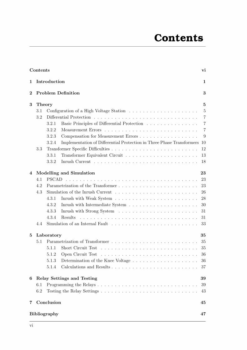
Contents vi
1 Introduction 1
2 Problem Definition 3
3 Theory 53.1 Configuration of a High Voltage Station . . . . . . . . . . . . . . . . . . . . 53.2 Differential Protection . . . . . . . . . . . . . . . . . . . . . . . . . . . . . . 7
3.2.1 Basic Principles of Differential Protection . . . . . . . . . . . . . . . 73.2.2 Measurement Errors . . . . . . . . . . . . . . . . . . . . . . . . . . . 73.2.3 Compensation for Measurement Errors . . . . . . . . . . . . . . . . . 93.2.4 Implementation of Differential Protection in Three Phase Transformers 10
3.3 Transformer Specific Difficulties . . . . . . . . . . . . . . . . . . . . . . . . . 123.3.1 Transformer Equivalent Circuit . . . . . . . . . . . . . . . . . . . . . 133.3.2 Inrush Current . . . . . . . . . . . . . . . . . . . . . . . . . . . . . . 18
4 Modelling and Simulation 234.1 PSCAD . . . . . . . . . . . . . . . . . . . . . . . . . . . . . . . . . . . . . . 234.2 Parametrization of the Transformer . . . . . . . . . . . . . . . . . . . . . . . 234.3 Simulation of the Inrush Current . . . . . . . . . . . . . . . . . . . . . . . . 26
4.3.1 Inrush with Weak System . . . . . . . . . . . . . . . . . . . . . . . . 284.3.2 Inrush with Intermediate System . . . . . . . . . . . . . . . . . . . . 304.3.3 Inrush with Strong System . . . . . . . . . . . . . . . . . . . . . . . 314.3.4 Results . . . . . . . . . . . . . . . . . . . . . . . . . . . . . . . . . . 31
4.4 Simulation of an Internal Fault . . . . . . . . . . . . . . . . . . . . . . . . . 33
5 Laboratory 355.1 Parametrization of Transformer . . . . . . . . . . . . . . . . . . . . . . . . . 35
5.1.1 Short Circuit Test . . . . . . . . . . . . . . . . . . . . . . . . . . . . 355.1.2 Open Circuit Test . . . . . . . . . . . . . . . . . . . . . . . . . . . . 365.1.3 Determination of the Knee Voltage . . . . . . . . . . . . . . . . . . . 365.1.4 Calculations and Results . . . . . . . . . . . . . . . . . . . . . . . . . 37
6 Relay Settings and Testing 396.1 Programming the Relays . . . . . . . . . . . . . . . . . . . . . . . . . . . . . 396.2 Testing the Relay Settings . . . . . . . . . . . . . . . . . . . . . . . . . . . . 43
7 Conclusion 45
Bibliography 47
vi

Contents Aalborg University
A Open and Short Circuit Data 49
B Knee Voltage Data and Calculations 51
C Open and Short Circuit Calculations 55
vii

Introduction 1Transmission and distribution networks have moved from being a local entity to becominga continent spanning machine, which consist of power plants, wind turbine farms, country-spanning transmission lines, etc. The joints connecting all these elements are thetransformers. The transformers scale the voltages to connect the lower level distributionnetworks to the highway of electricity: the transmission network.
Typically, transformers are the piece of equipment in the chain that malfunctions first, ifsubjected to maloperation. At a household level, this is not an issue as the transformersused are cheap and replacements are stocked. In the distribution and transmissionnetwork however, transformers are expensive pieces of equipment with long delivery times.This necessitates protection systems for the transformers. In the transmission networkthree groups of electrical protection systems are typically used. The first is overcurrentprotection. This is a simple form of protection, which is rather slow and does not providemuch selectivity. It simply protects against large currents. It is typically added as asecondary form of protection, to provide backup protection if the main protection fails.The next type is distance protection. Distance protection works by measuring the voltageand currents, and using these to calculate the impedance of the surrounding network. Bymeasuring the impedance on a line for example, the distance to a fault can be estimated.Furthermore, by dividing the surrounding network into zones, it provides selectivity andrelatively fast protection. In the first zone as fast as 20-40 ms, and 300-400 ms in thesecond zone. Furthermore it can act as backup protection by reaching into the busbarsand transformers the lines are connected to. [Ziegler, 2011] However, as the transformer isquickly damaged during a fault, faster and more selective protection is required. For thispurpose, differential protection is utilized. By defining its zones with current transformers,it provides 100% selectivity, and tripping times can be under one cycle (20 ms at 50 Hz).[Ziegler, 2012] This is done by comparing the currents flowing into the transformer. Anyinternal error will show up as a differential current, and cause a trip. In the ideal system,this is very simple to do. In practice however, several sources can contribute to erroneousoperation, which will require compensation. This is the subject of this report, in whichthe phenomena surrounding the differential protection will be investigated.
1

Problem Definition 2In order to narrow the scope of this report, the problems to be researched must be defined.The objectives and limitations of the scope are defined. Differential protection can beapplied to a great number of systems. As the title of the report implies, this reportdeals with only the protection of transformers. Additionally, differential protection can beapplied to transformers with more than two windings, so in order to narrow the scope, onlytwo winding transformers are evaluated. The scope of the report does not include in-depthwork with tap changer transformers. As a note to these transformer limitations, sometheory used is generalizable and could be applied to systems including these topologies,but this will not be elaborated on further.
The objectives and research questions of this project are presented in bullet form below.
• How does differential protection work?• How does the differential protection deal with vector grouping, winding ratios and
other transformer related scaling?• How does the differential protection distinguish between fault and inrush currents?• What is the cause of the inrush current, and how can it be mitigated?• How are differential protection systems built in real life using numerical relays, and
how are they programmed?• How is the differential protection system tested?
3

Theory 3In this chapter the necessary theory will be investigated. This is done in order to createa knowledge base to refer to when evaluating models and simulations. The objective isto cover all relevant fields, in order to centralize the knowledge required to carry out thedifferential protection of a transformer.
The knowledge in section 3.2 is, unless explicitly stated, compiled from Gerhard Ziegler’sNumerical Differential Protection [Ziegler, 2012]
3.1 Configuration of a High Voltage Station
In order to provide some context to the project, the locations of various objects related tothe subject are specified in this review of a typical substation. Everything in a high voltagestation is constructed in a manner that ensures the maximum level of redundancy. In atypical substation such as a 150/60 kV station, there are typically two or more incoming150 kV lines. The lines connect the substation with the neighbouring substations, and arepart of the transmission network. The incoming lines are connected to a busbar, whichcan be designed in different manners to ensure redundancy.
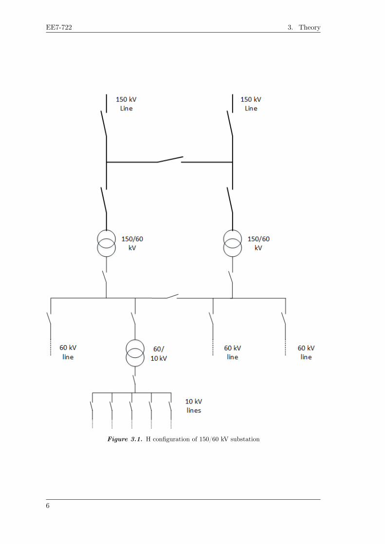
The substation can be equipped with one or more 150/60 kV transformers. If the substationonly has one 150/60 kV transformer, the need for redundancy in the connections is limited,as the substation will not be operational if the transformer malfunctions. However, if thereare two or more transformers, the substation can remain at least partially operational ifa proper busbar design is utilized. One method is to have twin busbars, and then installswitchgear to enable switching between one or the other. This is a very flexible, albeitcostly solution. Another method is to design the busbar in an H configuration. An exampleof an H configuration is shown in Figure 3.1. If a line is taken out of operation, the twotransformers can be powered by the single line remaining. If part of the busbar is faulty,that part can be switched off at the connection in the middle of the H. By doing this,one 150/60 kV transformer remains operational, without the need to duplicate the entirebusbar.
On the low voltage side of the transformers are another set of busbars, onto which the60 kV distribution grid is connected. Some substations also have lower voltage levels, whichmeans that there is another transformer connected to the 60 kV busbar, transforming thevoltage down to the lower distribution level of 10 kV. This introduces yet another busbar,onto which several incoming and outgoing connections can be made. The same principleapplies as from the higher voltage levels, as the busbars can be connected and disconnectedto bypass a faulty transformer or similar. This is also shown in Figure 3.1, as any given
5
EE7-722 3. Theory
Figure 3.1. H configuration of 150/60 kV substation
6
3.2. Differential Protection Aalborg University
component can fail, and the remaining system can still be powered, albeit not with the fullpower available. The switches shown are for illustration purposes only, as in reality eachswitching area can contain circuit breaker, disconnector and an earth switch. The circuitbreaker is the load switching component, which can break the high currents during eventssuch as short circuits. Besides the circuit breaker, each connection is also equipped with adisconnector, which is not designed for de-energizing the system but is there for the safetyof personnel servicing the disconnected part. Each piece of cable and line is also equippedwith an earthswitch, which can ground the system as another safety precaution.
3.2 Differential Protection
Differential protection is, as the name implies, a form of protection that utilizesmeasurements to detect differences. This is done by bounding an area by two measurementsand evaluating the difference between the measurements.
3.2.1 Basic Principles of Differential Protection
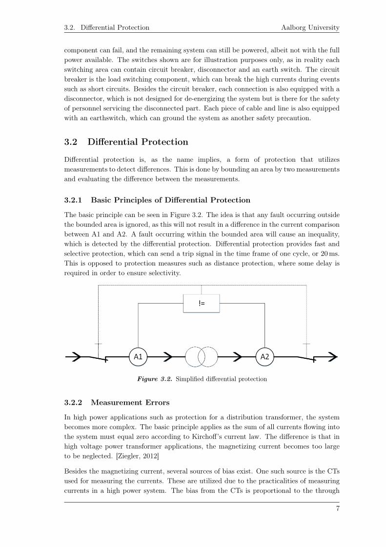
The basic principle can be seen in Figure 3.2. The idea is that any fault occurring outsidethe bounded area is ignored, as this will not result in a difference in the current comparisonbetween A1 and A2. A fault occurring within the bounded area will cause an inequality,which is detected by the differential protection. Differential protection provides fast andselective protection, which can send a trip signal in the time frame of one cycle, or 20 ms.This is opposed to protection measures such as distance protection, where some delay isrequired in order to ensure selectivity.
Figure 3.2. Simplified differential protection
3.2.2 Measurement Errors
In high power applications such as protection for a distribution transformer, the systembecomes more complex. The basic principle applies as the sum of all currents flowing intothe system must equal zero according to Kirchoff’s current law. The difference is that inhigh voltage power transformer applications, the magnetizing current becomes too largeto be neglected. [Ziegler, 2012]
Besides the magnetizing current, several sources of bias exist. One such source is the CTsused for measuring the currents. These are utilized due to the practicalities of measuringcurrents in a high power system. The bias from the CTs is proportional to the through
7
EE7-722 3. Theory
current while the CTs are operating in the linear range. How large the error is depends onthe type of CT. The typical classification of a CT follows IEC norm 60044-1.
The norm dictates that the CTs are marked in a specific way. The marking is as follows:xPy z. The x is the accuracy limit factor (ALF), which indicates how accurate the CT isat the accuracy limit current (ALC). The ALF is given in percentage of deviation fromthe true current. The P simply indicates that this CT is for protection purposes. The y isthe ALC, which is defined by multiples of the nominal current. Thus, if the transformerhas a nominal current of 5 A in the secondary, the CT will have an accuracy equal to theALF at a secondary current of y · 5 A. The z indicates the maximum burden that canbe connected to the secondary of the CT, and is usually given in VA. The burden comesfrom the resistance of the wires connecting the relay and the CT, and any resistance ofthe terminal, as a voltage will be induced in these by the current from the CT. If thespecified burden is exceeded, the transformer will saturate prematurely, and the accuracywill decrease dramatically. All the variables are interconnected so the x value is only validif the burden of the transformer does not exceed the z value while operating the CT atthe y value. However, if the burden of the connected relay is lower than the z value whileoperating it at the y value, a new y’ can be calculated, meaning that the CT can operatewith a higher secondary current than indicated by y. Similarly, it can be calculated to belower than the original value, if the burden is higher than specified.
If the fault occurs outside of the bounded area, it is not desirable to disconnect thetransformer. If the fault current is large enough, it can send the CTs into saturation,which causes the false current to rise rapidly.
Another source of bias is the tap changer of the power transformer. As the current ismeasured on both sides, the ratio of the power transformer is utilized in this calculation.During operation of the tap changer, this ratio changes, which is a reason for themeasurement errors.
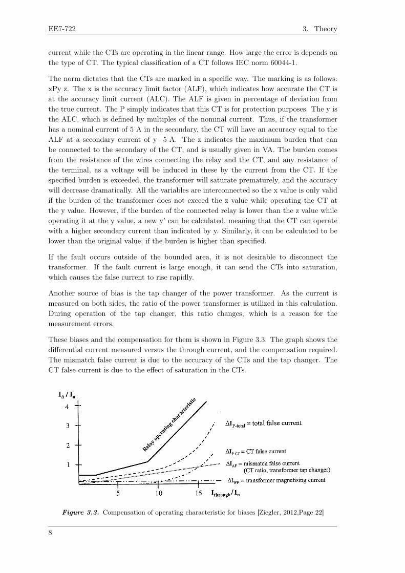
These biases and the compensation for them is shown in Figure 3.3. The graph shows thedifferential current measured versus the through current, and the compensation required.The mismatch false current is due to the accuracy of the CTs and the tap changer. TheCT false current is due to the effect of saturation in the CTs.
Figure 3.3. Compensation of operating characteristic for biases [Ziegler, 2012,Page 22]
8
3.2. Differential Protection Aalborg University
Besides the previously mentioned phenomena, the localization of the differential protectionalso plays a role. The use of pilot wires can introduce measurement errors, but it isgenerally only a problem on distances greater than 25 km. Since this project is aboutprotecting a transformer, both ends of the differential protection will always be relativelyclose compared to that, and thus not be a problem.
3.2.3 Compensation for Measurement Errors
As made clear from section 3.2.2, some criterion for when the differential protection shouldact is needed. This criterion is defined by the operating boundary. The operating boundaryis the boundary between when something is considered an error in measurement or a fault.In other words, if the ratio between through current and differential current becomes toolarge, the differential protection needs to pick up on this and send a trip signal.
In order to define the operating boundary, two new currents, IOp and IRes, are introduced.The sign convention used is: currents entering the transformer are positive and currentsexiting are negative.
The operating current IOp is a current that triggers an operation such as tripping. Theoperating current is defined by equation (3.1), where the subscript of the measured currentsdenotes the associated CT.
The restraint current IRes, acts as a stabilizer for the operation of the relay, preventingunwanted operations. The restraint current is defined in equation (3.2).
IOp = |I1 + I2| (3.1)
IRes = |I1|+ |I2| (3.2)
Traditionally, the relay characteristic, which is the boundary between the operation andrestraint areas, was defined by an offset linear function. Today, with the use of numericalrelays, the operating current is defined by a piecewise linear function. This is done in orderto fit the growth of the total false current as a function of through current, as shown inFigure 3.3.
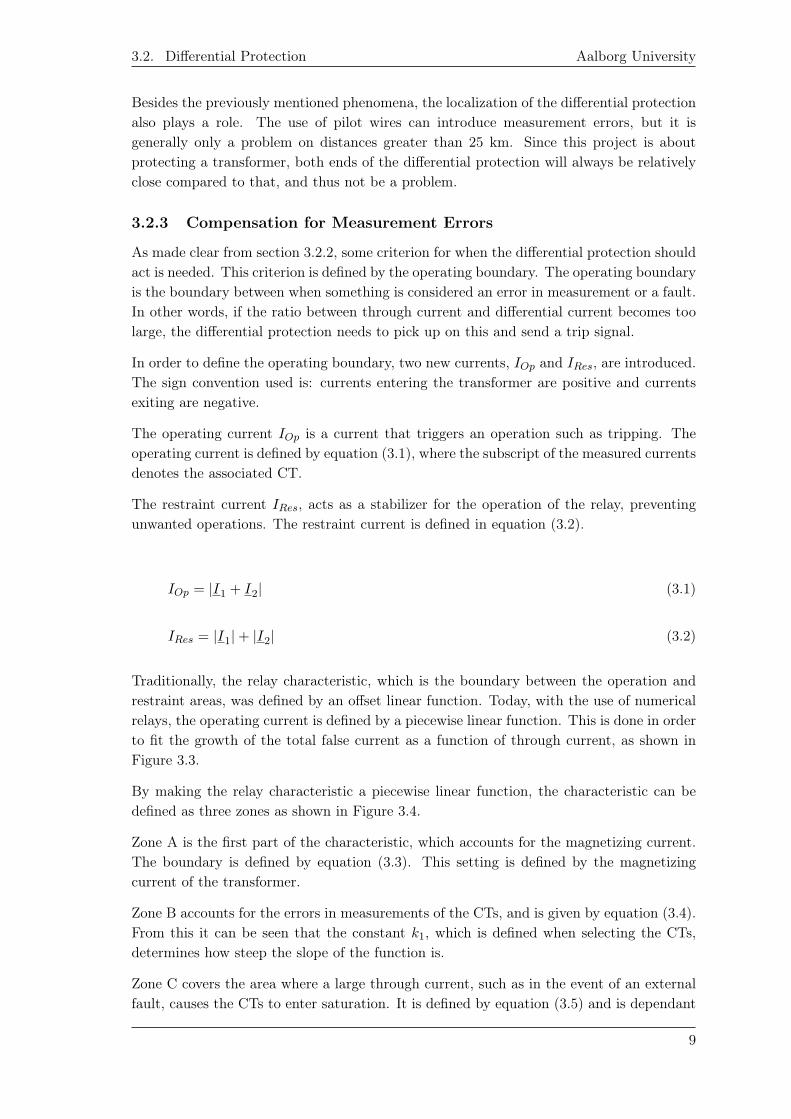
By making the relay characteristic a piecewise linear function, the characteristic can bedefined as three zones as shown in Figure 3.4.
Zone A is the first part of the characteristic, which accounts for the magnetizing current.The boundary is defined by equation (3.3). This setting is defined by the magnetizingcurrent of the transformer.
Zone B accounts for the errors in measurements of the CTs, and is given by equation (3.4).From this it can be seen that the constant k1, which is defined when selecting the CTs,determines how steep the slope of the function is.
Zone C covers the area where a large through current, such as in the event of an externalfault, causes the CTs to enter saturation. It is defined by equation (3.5) and is dependant
9
EE7-722 3. Theory
on k2, which is a constant determined in the same manner as k1, and IR0 which is thecrossing with the x axis of this particular linear function.
Zone A: IOp > IB (3.3)
Zone B: IOp > k1 · IRes (3.4)
Zone C: IOp > k2 · (IRes − IR0) (3.5)
Figure 3.4. Zones for differential operation [Ziegler, 2012,Page 31]
The result of all this is, that the higher the through current (restraint current), the higherthe differential current (operating current) must be in order to trigger an event (trip).The boundary is defined by the components used and is a piecewise linear function,whose slope increases depending on the through current (restraint current). As allthe previously discussed theory is per phase, a translation to a three-phase system isrequired. As discussed, the distances for transformer differential protection are small,making communication trivial compared to a line differential protection. Due to this, aper phase comparison of the currents is appropriate.
3.2.4 Implementation of Differential Protection in Three PhaseTransformers
The implementation of the differential protection is done on a case-by-case basis, as theimplementation varies with type of transformer. This is due to the fact that transformerscome in several different configurations. The vector group of the transformer matters, asthe various configurations of star/star star/delta etc. introduce various degrees of lag andvoltage differences with the same amount of windings, which must be compensated when
10
3.2. Differential Protection Aalborg University
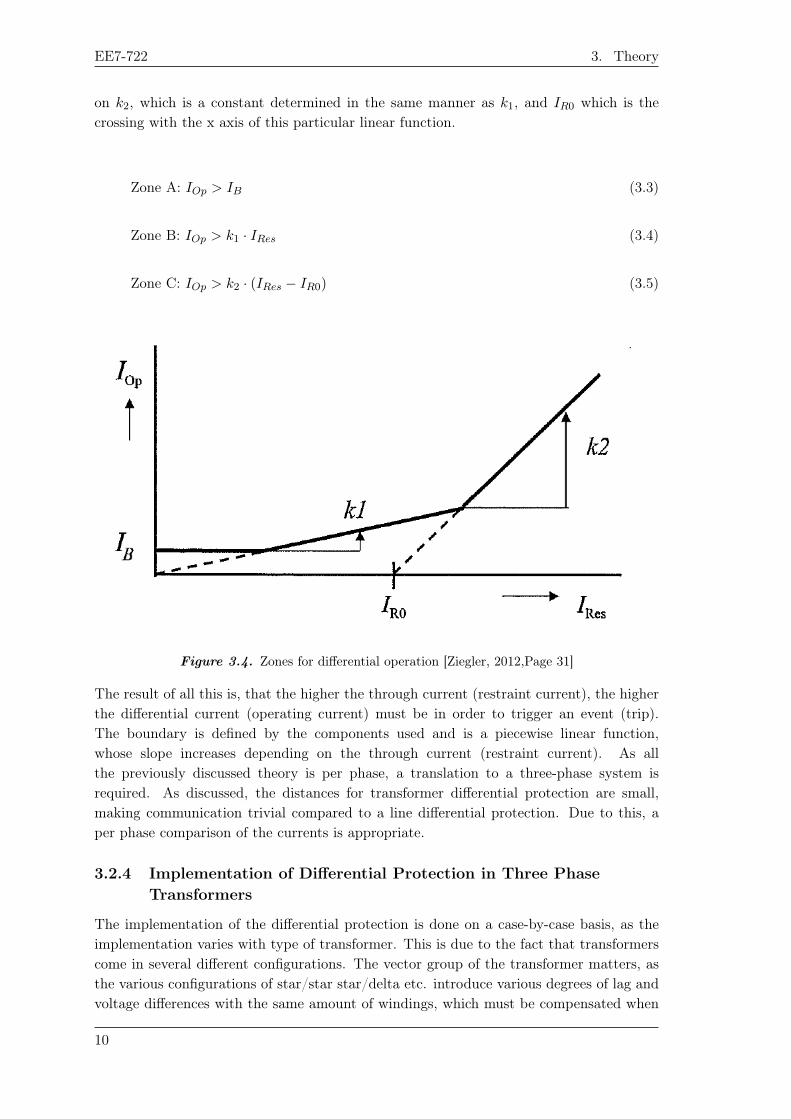
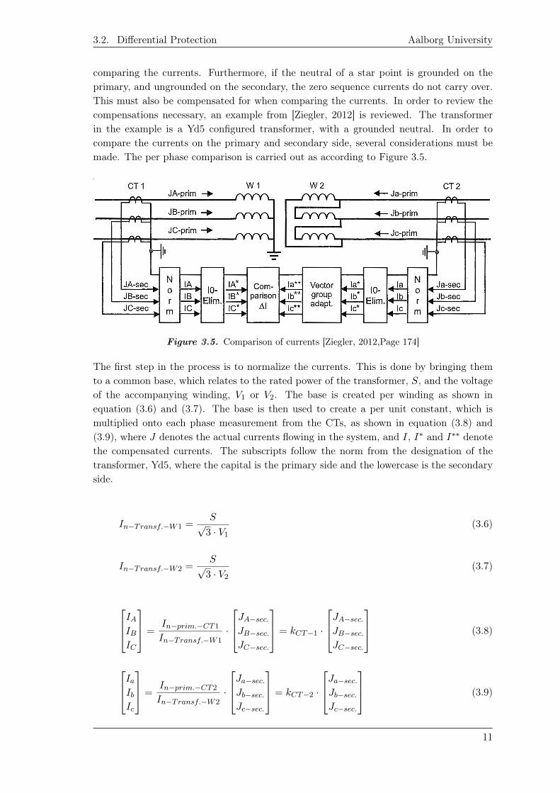
comparing the currents. Furthermore, if the neutral of a star point is grounded on theprimary, and ungrounded on the secondary, the zero sequence currents do not carry over.This must also be compensated for when comparing the currents. In order to review thecompensations necessary, an example from [Ziegler, 2012] is reviewed. The transformerin the example is a Yd5 configured transformer, with a grounded neutral. In order tocompare the currents on the primary and secondary side, several considerations must bemade. The per phase comparison is carried out as according to Figure 3.5.
Figure 3.5. Comparison of currents [Ziegler, 2012,Page 174]
The first step in the process is to normalize the currents. This is done by bringing themto a common base, which relates to the rated power of the transformer, S, and the voltageof the accompanying winding, V1 or V2. The base is created per winding as shown inequation (3.6) and (3.7). The base is then used to create a per unit constant, which ismultiplied onto each phase measurement from the CTs, as shown in equation (3.8) and(3.9), where J denotes the actual currents flowing in the system, and I, I∗ and I∗∗ denotethe compensated currents. The subscripts follow the norm from the designation of thetransformer, Yd5, where the capital is the primary side and the lowercase is the secondaryside.
In−Transf.−W1 =S√
3 · V1
(3.6)
In−Transf.−W2 =S√
3 · V2
(3.7)
IAIBIC
=In−prim.−CT1
In−Transf.−W1·
JA−sec.JB−sec.JC−sec.
= kCT−1 ·
JA−sec.JB−sec.JC−sec.
(3.8)
IaIbIc
=In−prim.−CT2
In−Transf.−W2·
Ja−sec.Jb−sec.Jc−sec.
= kCT−2 ·
Ja−sec.Jb−sec.Jc−sec.
(3.9)
11
EE7-722 3. Theory
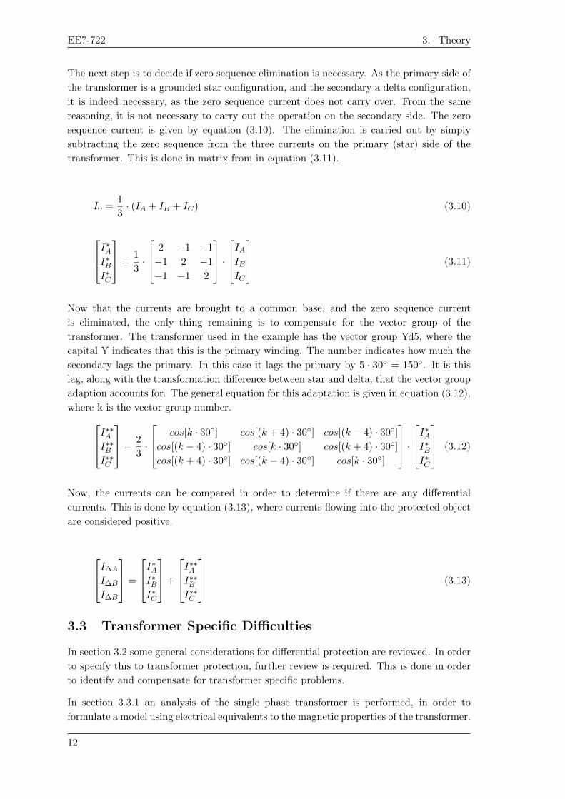
The next step is to decide if zero sequence elimination is necessary. As the primary side ofthe transformer is a grounded star configuration, and the secondary a delta configuration,it is indeed necessary, as the zero sequence current does not carry over. From the samereasoning, it is not necessary to carry out the operation on the secondary side. The zerosequence current is given by equation (3.10). The elimination is carried out by simplysubtracting the zero sequence from the three currents on the primary (star) side of thetransformer. This is done in matrix from in equation (3.11).
I0 =1
3· (IA + IB + IC) (3.10)
I∗AI∗BI∗C
=1
3·
2 −1 −1
−1 2 −1
−1 −1 2
·IAIBIC
(3.11)
Now that the currents are brought to a common base, and the zero sequence currentis eliminated, the only thing remaining is to compensate for the vector group of thetransformer. The transformer used in the example has the vector group Yd5, where thecapital Y indicates that this is the primary winding. The number indicates how much thesecondary lags the primary. In this case it lags the primary by 5 · 30 = 150. It is thislag, along with the transformation difference between star and delta, that the vector groupadaption accounts for. The general equation for this adaptation is given in equation (3.12),where k is the vector group number.I∗∗AI∗∗B
I∗∗C
=2
3·
cos[k · 30] cos[(k + 4) · 30] cos[(k − 4) · 30]
cos[(k − 4) · 30] cos[k · 30] cos[(k + 4) · 30]
cos[(k + 4) · 30] cos[(k − 4) · 30] cos[k · 30]
·I∗AI∗BI∗C
(3.12)
Now, the currents can be compared in order to determine if there are any differentialcurrents. This is done by equation (3.13), where currents flowing into the protected objectare considered positive.
I∆A
I∆B
I∆B
=
I∗AI∗BI∗C
+
I∗∗AI∗∗BI∗∗C
(3.13)
3.3 Transformer Specific Difficulties
In section 3.2 some general considerations for differential protection are reviewed. In orderto specify this to transformer protection, further review is required. This is done in orderto identify and compensate for transformer specific problems.
In section 3.3.1 an analysis of the single phase transformer is performed, in order toformulate a model using electrical equivalents to the magnetic properties of the transformer.
12
3.3. Transformer Specific Difficulties Aalborg University
This is done to gain a better understanding of the transformer. The method used to derivethe equivalent circuit and all formulas are sourced from [Umans, 2014].
In section 3.3.2 an analysis of the inrush phenomena is performed. This is done in orderto evaluate the scale of the problem, mitigation methods, and how the relay knows it isinrush happening and not an internal fault. The knowledge in this section is compiledfrom [C4.307, 2013] and [Ziegler, 2012]
3.3.1 Transformer Equivalent Circuit
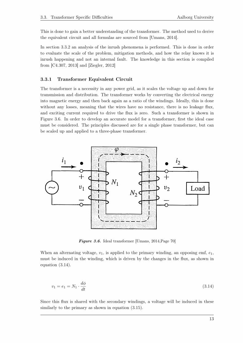
The transformer is a necessity in any power grid, as it scales the voltage up and down fortransmission and distribution. The transformer works by converting the electrical energyinto magnetic energy and then back again as a ratio of the windings. Ideally, this is donewithout any losses, meaning that the wires have no resistance, there is no leakage flux,and exciting current required to drive the flux is zero. Such a transformer is shown inFigure 3.6. In order to develop an accurate model for a transformer, first the ideal casemust be considered. The principles discussed are for a single phase transformer, but canbe scaled up and applied to a three-phase transformer.
Figure 3.6. Ideal transformer [Umans, 2014,Page 70]
When an alternating voltage, v1, is applied to the primary winding, an opposing emf, e1,must be induced in the winding, which is driven by the changes in the flux, as shown inequation (3.14).
v1 = e1 = N1 ·dφ
dt(3.14)
Since this flux is shared with the secondary windings, a voltage will be induced in thesesimilarly to the primary as shown in equation (3.15).
13
EE7-722 3. Theory
v2 = e2 = N2 ·dφ
dt(3.15)
From equations (3.14) and (3.15) it can be derived that the ratio between the voltages isthe same as the ratio of the windings as shown in equation (3.16).
v1
v2=N1
N2(3.16)
By connecting a load to the transformers secondary windings a load current, i2, is drawn.This load current produces a magnetomotive force (mmf), N2 ·i2, in the secondary winding.The mmf is the driving force of the magnetic flux and is equivalent to the emf driving theelectrical current. Since the ideal transformer’s flux does not change due to the load,and the fact that it is lossless, the mmf must be balanced by a counteracting mmf in theprimary winding as shown in equation (3.17).
N1 · i1 = N2 · i2 (3.17)
From this it can be shown that the currents flowing in the primary and secondary areinversely proportional to the ratio of the windings as shown in equation (3.18).
i1i2
=N2
N1(3.18)
Since the transformer is ideal, there are no losses. This means that the power going intothe system must equal the power leaving the system as shown in equation (3.19).
v1 · i1 = v2 · i2 (3.19)
Even though a real transformer approximates the theory discussed in this section, somelosses and limitations apply. In order to approximate a real transformer, an electricalequivalent to the magnetic properties of the transformer is desired. In order to representthe complex numbers throughout this derivation, phasor representations of the voltagesand currents will be used.
The first step is to recognize that the windings have resistance, which can be modelled as aresistor in series. This changes the voltage balance as described in equation (3.14), as theinduced emf is now lower than the input voltage, due to the voltage drop in the resistor.This is shown in equation (3.20).
V 1 = R1 · I1 + E1 (3.20)
14
3.3. Transformer Specific Difficulties Aalborg University
In the ideal transformer, all flux is contained within the core. This is not the case with areal transformer. There will always be some leakage to the air, which can be modelled bya leakage inductance, Ll1. This leakage induces a voltage in the primary winding, whichvaries linearly with the primary current. For ease of calculation, the leakage inductance isconverted to a reactance as shown in equation (3.21).
Xl1 = 2 · π · f · Ll1 (3.21)
This adds a contribution to the voltage balance, which now changes to equation (3.22).
V 1 = R1 · I1 + j ·Xl1 · I1 + E1 (3.22)
In the ideal transformer, besides containing all the flux in the core, it required no energy todrive this flux. In a real transformer, this is not the case. The primary and the secondarywindings are linked by their mutual flux, which requires a certain mmf. This mmf mustbe supplied by the primary current, and is called the exciting current, Iϕ. Furthermore,the secondary current will counteract the primary, as it will try to demagnetize the ironcore. This mmf must also be supplied by the primary current.
This changes the mmf balance from equation (3.17), as the resultant mmf from theinput and output is no longer equal to zero, but results in the mutual mmf as shownin equation (3.23).
N1 · Iϕ = N1 · I1 −N2 · I2 (3.23)
Since the primary current I1 is composed of the exciting current Iϕ and the load current,which is the load on the secondary transformed to the primary as per equation (3.18), itcan be written as the sum of these, which changes equation (3.23) to equation (3.24)
N1 · Iϕ = N1 · (Iϕ + I ′2)−N2 · I2 (3.24)
The exciting current can be considered as a sinusoidal current consisting of two currents.One current Ic is there to account for the core losses, and is in phase with E1. The otherlags it by 90 and is the magnetizing component Im. These currents can be introduced tothe equivalent circuit by adding a shunt branch, which consists of a resistor in parallel withan inductor. The inductor is represented by the reactance Xm in equation (3.25) whereLm is the mutual inductance and f is the frequency of the system.
Xm = 2 · π · f · Lm (3.25)
15
EE7-722 3. Theory
Figure 3.7. Primary side of non ideal transformer model [Umans, 2014,Page 75]
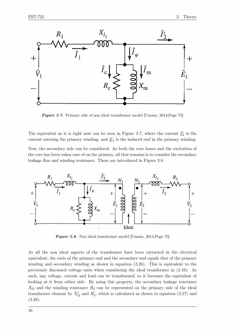
The equivalent as it is right now can be seen in Figure 3.7, where the current I ′2 is thecurrent entering the primary winding, and E1 is the induced emf in the primary winding.
Now, the secondary side can be considered. As both the core losses and the excitation ofthe core has been taken care of on the primary, all that remains is to consider the secondaryleakage flux and winding resistance. These are introduced in Figure 3.8.
Figure 3.8. Non ideal transformer model [Umans, 2014,Page 75]
As all the non ideal aspects of the transformer have been extracted in the electricalequivalent, the ratio of the primary emf and the secondary emf equals that of the primarywinding and secondary winding as shown in equation (3.26). This is equivalent to thepreviously discussed voltage ratio when considering the ideal transformer in (3.16). Assuch, any voltage, current and load can be transformed, so it becomes the equivalent oflooking at it from either side. By using this property, the secondary leakage reactanceXl2 and the winding resistance R2 can be represented on the primary side of the idealtransformer element by X ′l2 and R′2, which is calculated as shown in equation (3.27) and(3.28).
16
3.3. Transformer Specific Difficulties Aalborg University
E1
E2
=N1
N2(3.26)
X ′l2 =
(N1
N2
)2
·Xl2 (3.27)
R′2 =
(N1
N2
)2
·R2 (3.28)
All that remains within the transformer is to transform the secondary voltage to theprimary voltage base. This is done as shown in equation (3.29)
V ′2 =N1
N2· V2 (3.29)
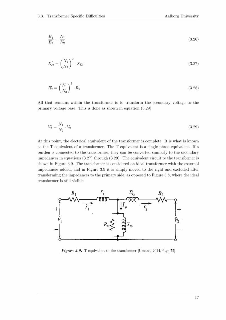
At this point, the electrical equivalent of the transformer is complete. It is what is knownas the T equivalent of a transformer. The T equivalent is a single phase equivalent. If aburden is connected to the transformer, they can be converted similarly to the secondaryimpedances in equations (3.27) through (3.29). The equivalent circuit to the transformer isshown in Figure 3.9. The transformer is considered an ideal transformer with the externalimpedances added, and in Figure 3.9 it is simply moved to the right and excluded aftertransforming the impedances to the primary side, as opposed to Figure 3.8, where the idealtransformer is still visible.
Figure 3.9. T equivalent to the transformer [Umans, 2014,Page 75]
17
EE7-722 3. Theory
3.3.2 Inrush Current
Inrush current is a phenomena that takes place in a transformer when the magnetic fieldin to the transformer is subjected to abrupt change. As the inrush current is a transientevent caused by the magnetization of the transformer, it only flows into the transformerand not out the other side. Due to this, it causes a differential current, which is capableof tripping the differential protection. In order to narrow the scope of this report, onlyinrush of a single transformer due to initial energization will be investigated. This excludesseries and parallel sympathetic inrush, where the inrush current is partially drawn throughand from other transformers. It also excludes pseudo inrush, where the inrush is causeddue to a fault being cleared, where the voltage returns to normal. The reason for thisspecification is due to the inrush being detected in the same manner, and acted upon inthe same manner.
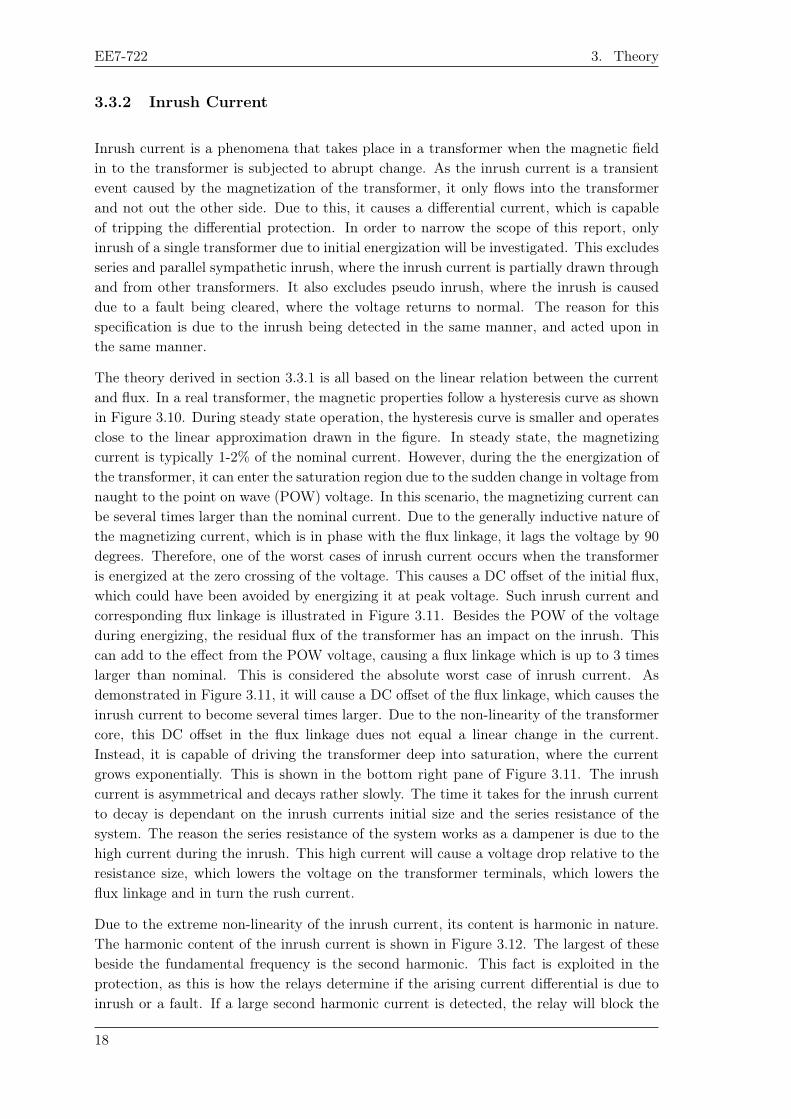
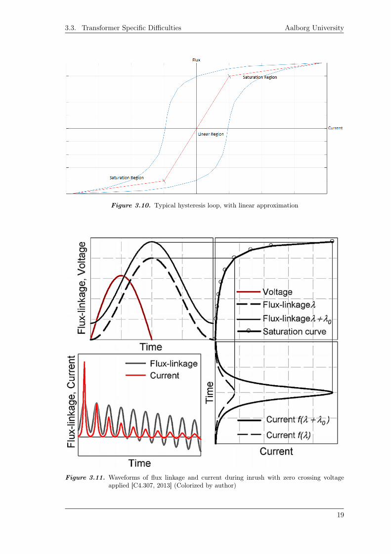
The theory derived in section 3.3.1 is all based on the linear relation between the currentand flux. In a real transformer, the magnetic properties follow a hysteresis curve as shownin Figure 3.10. During steady state operation, the hysteresis curve is smaller and operatesclose to the linear approximation drawn in the figure. In steady state, the magnetizingcurrent is typically 1-2% of the nominal current. However, during the the energization ofthe transformer, it can enter the saturation region due to the sudden change in voltage fromnaught to the point on wave (POW) voltage. In this scenario, the magnetizing current canbe several times larger than the nominal current. Due to the generally inductive nature ofthe magnetizing current, which is in phase with the flux linkage, it lags the voltage by 90degrees. Therefore, one of the worst cases of inrush current occurs when the transformeris energized at the zero crossing of the voltage. This causes a DC offset of the initial flux,which could have been avoided by energizing it at peak voltage. Such inrush current andcorresponding flux linkage is illustrated in Figure 3.11. Besides the POW of the voltageduring energizing, the residual flux of the transformer has an impact on the inrush. Thiscan add to the effect from the POW voltage, causing a flux linkage which is up to 3 timeslarger than nominal. This is considered the absolute worst case of inrush current. Asdemonstrated in Figure 3.11, it will cause a DC offset of the flux linkage, which causes theinrush current to become several times larger. Due to the non-linearity of the transformercore, this DC offset in the flux linkage dues not equal a linear change in the current.Instead, it is capable of driving the transformer deep into saturation, where the currentgrows exponentially. This is shown in the bottom right pane of Figure 3.11. The inrushcurrent is asymmetrical and decays rather slowly. The time it takes for the inrush currentto decay is dependant on the inrush currents initial size and the series resistance of thesystem. The reason the series resistance of the system works as a dampener is due to thehigh current during the inrush. This high current will cause a voltage drop relative to theresistance size, which lowers the voltage on the transformer terminals, which lowers theflux linkage and in turn the rush current.
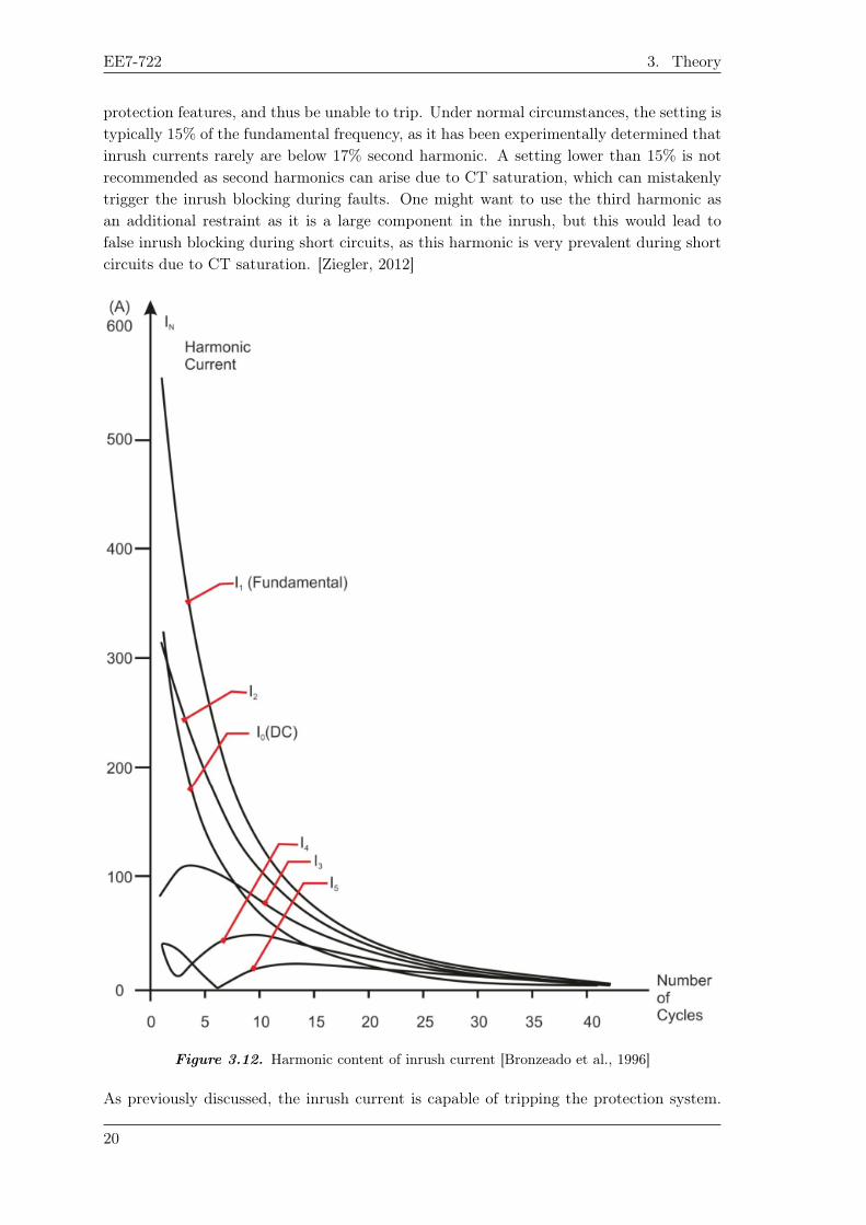
Due to the extreme non-linearity of the inrush current, its content is harmonic in nature.The harmonic content of the inrush current is shown in Figure 3.12. The largest of thesebeside the fundamental frequency is the second harmonic. This fact is exploited in theprotection, as this is how the relays determine if the arising current differential is due toinrush or a fault. If a large second harmonic current is detected, the relay will block the
18
3.3. Transformer Specific Difficulties Aalborg University
Figure 3.10. Typical hysteresis loop, with linear approximation
Figure 3.11. Waveforms of flux linkage and current during inrush with zero crossing voltageapplied [C4.307, 2013] (Colorized by author)
19
EE7-722 3. Theory
protection features, and thus be unable to trip. Under normal circumstances, the setting istypically 15% of the fundamental frequency, as it has been experimentally determined thatinrush currents rarely are below 17% second harmonic. A setting lower than 15% is notrecommended as second harmonics can arise due to CT saturation, which can mistakenlytrigger the inrush blocking during faults. One might want to use the third harmonic asan additional restraint as it is a large component in the inrush, but this would lead tofalse inrush blocking during short circuits, as this harmonic is very prevalent during shortcircuits due to CT saturation. [Ziegler, 2012]
Figure 3.12. Harmonic content of inrush current [Bronzeado et al., 1996]
As previously discussed, the inrush current is capable of tripping the protection system.
20
3.3. Transformer Specific Difficulties Aalborg University
This is mitigated by blocking the protection systems during the inrush by comparing thefundamental frequency with the second harmonic. However, the tripping of the protectionsystems is not the only effect of the inrush current, as the rush currents can be so largethat they can damage the insulation of the windings. Therefore, it can be desireable tonot just mitigate the false tripping of the protection, but also reduce the magnitude ofthe rush currents. The magnitude of the inrush current is primarily dependant on thefollowing parameters.
• Design of the transformer, such as the type of magnetic steel used for the core, andthe dimensions of it and operation point.
• Initial conditions, such as POW voltage and remanence flux.
• Dampening effects from the connected network, such as series resistance.
As for mitigation on an existing transformer, one option is to deflux the transformerbefore energizing it. This is however impractical, and not an option being used typically.Defluxing the transformer is connected to the initial conditions, as it means bringing downthe remanence flux.
Another initial condition that can be manipulated is the POW voltage applied to thetransformer. This is done by controlling the switching times of the circuit breaker, in orderto ensure that the POW voltage is at its peak, and therefore the magnetizing current drawnbeing at its lowest. This relation between peak voltage and the smallest inrush currentis only valid if there is no remanence in the core. Furthermore, energizing at the peakof the voltage curve can introduce overvoltage problems, which must be considered whendesigning such a mitigation method. It is very dependant on having repeatable closingtimes, as the delay in closing must be accounted for, in order to ensure connection at thedesired POW. Furthermore, they must be able to close the different phases at differenttimes as they are lagging each other by 120 degrees, and thus if all three were closed atthe same time, even though phase one might be at the correct POW, phase two and threewill be 120 and 240 degrees offset. Another improvement on this is to know the remanenceflux of the transformer by controlling the de-energization as well. By doing this, the exactPOW current can be matched, ensuring the lowest inrush possible. This is however notvalid during a fault, as the breaker will disconnect all three phases at the same time.However, since this method is generally only applied on very high voltage systems (400kVand above), and as such systems rarely experience faults, this is not an issue.
As mentioned, the dampening of the inrush is controlled by the series resistance of thesystem. Therefore, it makes sense to simply connect a higher resistance during theenergization of the transformer. In practice however, it is very involved and requiresmore circuit breakers or other expensive equipment.
Similar for all the mitigation techniques is that they add cost to the system. The morefeatures the circuit breaker has, the costly it generally is. Due to this, an investigation of theinrush currents might be a better and more cost effective option, as they do not necessarilydamage the transformer. Naturally, this depends on the transformer in question. Theinrush current can be estimated by analytic calculations, but in practice it is better tosimulate it with numerical software, as solutions for this are abundant. However, in orderto explain the transient events, a simple method for modelling the inrush is reviewed
21
EE7-722 3. Theory
As previously mentioned, the phenomena of inrush current is a highly non-linear event.Therefore, the model derived in section 3.3.1 is not going to work without modification.The model is derived based on an assumption of steady state, which means that thetransformer is operating in the linear part of the hysteresis loop shown in Figure 3.10.The slope of this linear region is defined by the inductance of the magnetizing branch inFigure 3.9. In order to model the transient events during inrush, this part of the hysteresisloop is not sufficient, as the transformer saturates and operates outside of the linear region.
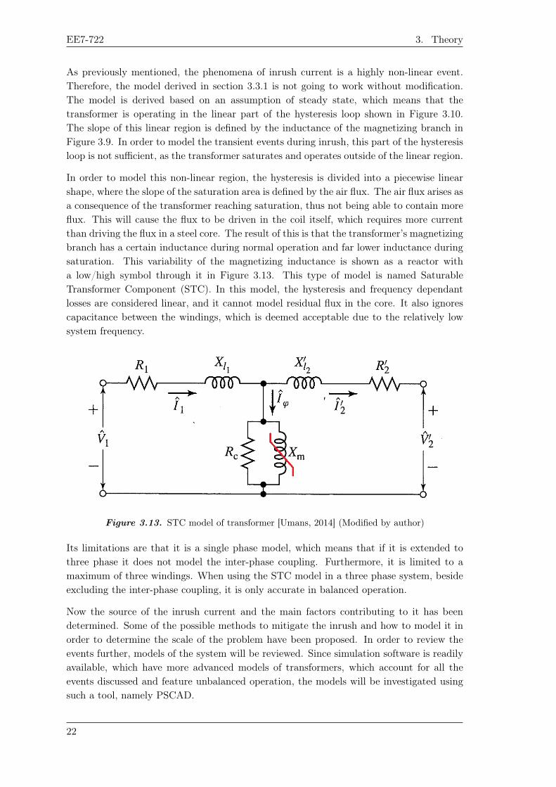
In order to model this non-linear region, the hysteresis is divided into a piecewise linearshape, where the slope of the saturation area is defined by the air flux. The air flux arises asa consequence of the transformer reaching saturation, thus not being able to contain moreflux. This will cause the flux to be driven in the coil itself, which requires more currentthan driving the flux in a steel core. The result of this is that the transformer’s magnetizingbranch has a certain inductance during normal operation and far lower inductance duringsaturation. This variability of the magnetizing inductance is shown as a reactor witha low/high symbol through it in Figure 3.13. This type of model is named SaturableTransformer Component (STC). In this model, the hysteresis and frequency dependantlosses are considered linear, and it cannot model residual flux in the core. It also ignorescapacitance between the windings, which is deemed acceptable due to the relatively lowsystem frequency.
Figure 3.13. STC model of transformer [Umans, 2014] (Modified by author)
Its limitations are that it is a single phase model, which means that if it is extended tothree phase it does not model the inter-phase coupling. Furthermore, it is limited to amaximum of three windings. When using the STC model in a three phase system, besideexcluding the inter-phase coupling, it is only accurate in balanced operation.
Now the source of the inrush current and the main factors contributing to it has beendetermined. Some of the possible methods to mitigate the inrush and how to model it inorder to determine the scale of the problem have been proposed. In order to review theevents further, models of the system will be reviewed. Since simulation software is readilyavailable, which have more advanced models of transformers, which account for all theevents discussed and feature unbalanced operation, the models will be investigated usingsuch a tool, namely PSCAD.
22
Modelling and Simulation 4In this chapter, the theory compiled in chapter 3 will be utilized in order to makepredictions of the problem in order to make a strategy for mitigating the problem. Themodel is reviewed in the simulation software PSCAD, which is described in section 4.1. Inorder to evaluate the transformer in question, the parameters for the PSCAD model areinvestigated in section 4.2.
In section 4.3 various scenarios are simulated, in order to determine how various systemsaffect the magnitude and decay of the inrush current, along with a fault scenario insection 4.4. This data is then to be used when setting up the differential relays.
4.1 PSCAD
PSCAD is the simulation software of choice in this report. One of the main advantages forthis software is the interconnectivity with OMICRON, which allows for exports of scenariosdirectly from PSCAD to OMICRON. The OMICRON can then simulate the scenario to therelay, in order to check if the parameters of the relays are correctly set. PSCAD can modeltransformers using two different methods. One is the classic transformer equivalent, whichis similar to the STC previously discussed. The other is the Unified Magnetic EquivalentCircuit (UMEC). By using the UMEC model, linkage between phases are accounted for,and it is capable of accurately modelling three phase transformers. However, due to itssimpler methodology, the classic model is used in this project.
4.2 Parametrization of the Transformer
Similar for both the simplified STC model evaluated in section 3.3.2 and for models inPSCAD is that they require parameters which directly relate to the transformer in question.The parameters are determined by the impedance of the windings and the core of thetransformer. These parameters must be determined in order to simulate the transientevents in the transformer. The parameters are determined either by the data sheet of thetransformer, or by carrying out short circuit and open circuit tests of the transformer. Theparameters to be determined are the ones shown in Figure 3.13. Typically, all parametersare calculated in per unit (P.U.). Per unit is a unit system which works by referring allvariables such as impedances, voltages and currents to a common base, in order to avoidconfusion when working with transformers.
In the short circuit test the information is typically the voltage in percentage of the ratedvoltage, Vsc%, and the active power Psc per winding pair. From this data, the windingimpedance is calculated by using equation (4.2) and from the copper losses in PSCAD.
23
EE7-722 4. Modelling and Simulation
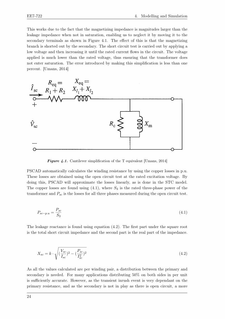
This works due to the fact that the magnetizing impedance is magnitudes larger than theleakage impedance when not in saturation, enabling us to neglect it by moving it to thesecondary terminals as shown in Figure 4.1. The effect of this is that the magnetizingbranch is shorted out by the secondary. The short circuit test is carried out by applying alow voltage and then increasing it until the rated current flows in the circuit. The voltageapplied is much lower than the rated voltage, thus ensuring that the transformer doesnot enter saturation. The error introduced by making this simplification is less than onepercent. [Umans, 2014]
Figure 4.1. Cantilever simplification of the T equivalent [Umans, 2014]
PSCAD automatically calculates the winding resistance by using the copper losses in p.u.These losses are obtained using the open circuit test at the rated excitation voltage. Bydoing this, PSCAD will approximate the losses linearly, as is done in the STC model.The copper losses are found using (4.1), where S3 is the rated three-phase power of thetransformer and Psc is the losses for all three phases measured during the open circuit test.
Psc−p.u =Psc
S3(4.1)
The leakage reactance is found using equation (4.2). The first part under the square rootis the total short circuit impedance and the second part is the real part of the impedance.
Xsc = k ·
√(VscIsc
)2 − (Psc
I2sc
)2 (4.2)
As all the values calculated are per winding pair, a distribution between the primary andsecondary is needed. For many applications distributing 50% on both sides in per unitis sufficiently accurate. However, as the transient inrush event is very dependant on theprimary resistance, and as the secondary is not in play as there is open circuit, a more
24
4.2. Parametrization of the Transformer Aalborg University
accurate distribution is wanted. One way to distribute it with higher accuracy is to measurethe DC resistance on both sides of the transformer and then distributing the resistanceas a ratio of these. This is done in equations (4.3) and (4.4). The distribution of Xsc ishowever not as easily done. In PSCAD the distribution is handled automatically. Theonly input needed is the total leakage reactance in p.u. and the copper losses in p.u.
RACHV = Rsc ·RDCHV
RDCHV +RDCLV(4.3)
RACLV = Rsc ·RDCLV
RDCHV +RDCLV(4.4)
Now that the parameters for the windings are taken care of, it is time to consider the coreof the transformer, or in the electrical equivalent, the magnetizing branch. The values areobtained from the no load test as, theoretically, the only current that should be flowing inthis test is the magnetizing current. When one side is open, the impedance at the terminalsinclude the leakage impedance, but as this is so small compared to the magnetizing branch,it can be neglected. The test is conducted from the secondary, as this is more practical andsafe due to the lower voltage required. The parameters to be determined for the model inPSCAD are the air core reactance in p.u., the magnetizing current in p.u. and the kneevoltage in p.u.
The air core reactance is the reactance of a winding when the steel core of the transformeris fully saturated. When this happens, the only available reactance is that of the coilitself, with a core of air. It determines the flux to current ratio during the saturation.This reactance is based on the number of turns and the dimensions of the winding. It istypically printed on the nameplate of the transformer, as it requires knowledge that at bestcan only be estimated without dismantling the transformer. If the air core reactance is notknown, it can be estimated to be approximately twice the leakage reactance. [HVDC.ca]
The magnetizing current is the current flowing in the magnetizing branch of the equivalentcircuit. It is calculated by first calculating the iron losses by using equation (4.5), where Poc
is the resistive losses in watts, k is either 1 or 3 depending on Wye or Delta configurationand Vp.u. is the excitation voltage. Then the no load current is calculated by equation (4.6),which is the total current entering the transformer. Here Ioc is the total current measuredduring the open circuit test, k is either 1 or 3 depending on Wye or Delta configuration.The magnetizing current can now be calculated, due to the fact that it lags the resistivecurrent by 90 degrees. This is done in equation (4.7).
Iloss =Poc
k · Voc(4.5)
Ino−load =Iock
(4.6)
25
EE7-722 4. Modelling and Simulation
Im =√I2no−load − I2
loss (4.7)
The knee voltage is either found in the data sheet or by experiment. Experimentally, itis found by sweeping the voltage supplied to the transformer. Usually this is done on thelow voltage side, leaving the high voltage side open. The knee point is the point where thetransformer enters saturation, and thus the linear relation between flux and current breaksdown and becomes non linear. As the flux is proportional to the voltage, this breakdowncan be found by comparing the voltage and current, and then finding the point where theyare no longer linear. The knee voltage is defined by when an increase in the voltage appliedto a transformers secondary by 10% corresponds in a current increase of 50%.
The data for the parametrization can be found in section 5.1, where the tests described inthis section are carried out. This data is the data used for the simulation carried out insection 4.3.
4.3 Simulation of the Inrush Current
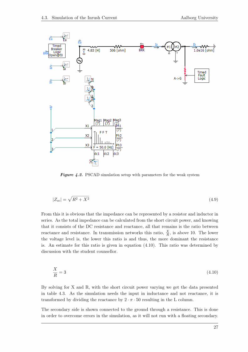
Now that the software for the simulation has been reviewed, and the parameters for themodel have been acquired, the system can be simulated. This is done in order to estimatethe magnitude of the inrush current and to review its harmonic content. The secondharmonic content of the inrush current should be very large and can therefore be usedas a constraint against tripping. The simulation can then be exported and used in theOMICRON, in order to simulate the inrush scenario for the relay. This is done in chapter 6.The setup used in the simulation is shown in Figure 4.2. The values of the inductor andresistor change depending on whether it is the weak or strong system.
The parameters for the transformer are as described in table 5.1.4. The transformer issetup to be a delta/wye transformer with a line-to-line voltage ratio of 400/230 V. Thesimulations are run with a step time of 25 microseconds. The voltage source is an idealsource set to 400 V line-to-line, and a frequency of 50 hz. As the inrush current will varydepending on the connected system, three cases are investigated. A very weak system, anintermediate system based on the lab, and a very strong system. The very weak systemhas a short circuit power of 0.1 kVA. The intermediate system is based on knowledge aboutthe isolating transformer used in the lab, which is 30 kVA. The very strong system has ashort circuit power of 200 MVA. The short circuit power can be represented by a shortcircuit impedance in series with the source. The stronger the system is, the smaller theimpedance and vise versa. The impedance is given by equation (4.8), where Ssc is theshort circuit power in VA, V is the line-to-line voltage.
Zsc =V 2
Ssc(4.8)
Recalling that the impedance can be defined by the dc resistance and the reactance, it canbe found using equation (4.9), where R is the DC resistance of the connected system, andX is the reactance of the system.
26
4.3. Simulation of the Inrush Current Aalborg University
Figure 4.2. PSCAD simulation setup with parameters for the weak system
|Zsc| =√R2 +X2 (4.9)
From this it is obvious that the impedance can be represented by a resistor and inductor inseries. As the total impedance can be calculated from the short circuit power, and knowingthat it consists of the DC resistance and reactance, all that remains is the ratio betweenreactance and resistance. In transmission networks this ratio, X
R , is above 10. The lowerthe voltage level is, the lower this ratio is and thus, the more dominant the resistanceis. An estimate for this ratio is given in equation (4.10). This ratio was determined bydiscussion with the student counsellor.
X
R= 3 (4.10)
By solving for X and R, with the short circuit power varying we get the data presentedin table 4.3. As the simulation needs the input in inductance and not reactance, it istransformed by dividing the reactance by 2 · π · 50 resulting in the L column.
The secondary side is shown connected to the ground through a resistance. This is donein order to overcome errors in the simulation, as it will not run with a floating secondary.
27
EE7-722 4. Modelling and Simulation
Ssc [VA] X [Ω] L [H] R [Ω]1.00e2 1.52e3 4.83e0 5.06e23.00e4 5.06e0 1.61e-2 1.69e02.00e8 7.59e-4 2.42e-6 2.53e-4
Table 4.1. X, L, and R values for varying short circuit power
The resistance is set to 1e16. It limits the current flowing in the secondary to under 1e-12ampere in the simulation, which can therefore be neglected. In order to control the POWvoltage, a breaker is introduced. The fault component is disabled for the inrush tests.
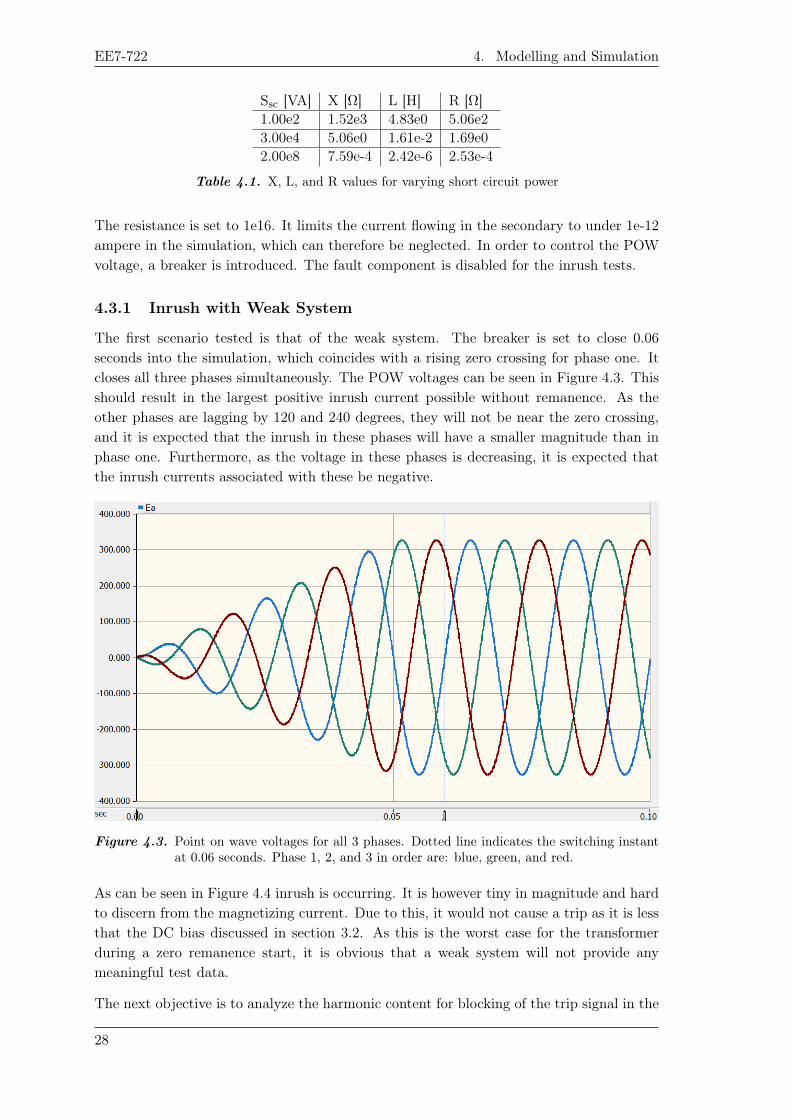
4.3.1 Inrush with Weak System
The first scenario tested is that of the weak system. The breaker is set to close 0.06seconds into the simulation, which coincides with a rising zero crossing for phase one. Itcloses all three phases simultaneously. The POW voltages can be seen in Figure 4.3. Thisshould result in the largest positive inrush current possible without remanence. As theother phases are lagging by 120 and 240 degrees, they will not be near the zero crossing,and it is expected that the inrush in these phases will have a smaller magnitude than inphase one. Furthermore, as the voltage in these phases is decreasing, it is expected thatthe inrush currents associated with these be negative.
Figure 4.3. Point on wave voltages for all 3 phases. Dotted line indicates the switching instantat 0.06 seconds. Phase 1, 2, and 3 in order are: blue, green, and red.
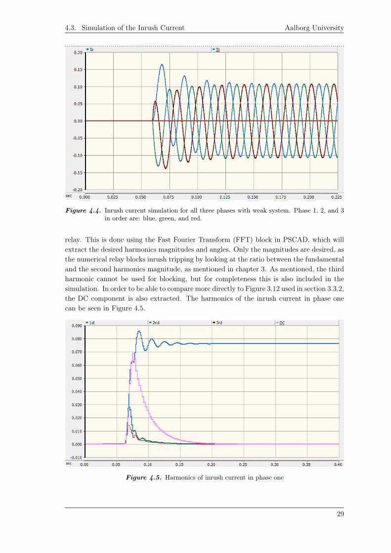
As can be seen in Figure 4.4 inrush is occurring. It is however tiny in magnitude and hardto discern from the magnetizing current. Due to this, it would not cause a trip as it is lessthat the DC bias discussed in section 3.2. As this is the worst case for the transformerduring a zero remanence start, it is obvious that a weak system will not provide anymeaningful test data.
The next objective is to analyze the harmonic content for blocking of the trip signal in the
28
4.3. Simulation of the Inrush Current Aalborg University
Figure 4.4. Inrush current simulation for all three phases with weak system. Phase 1, 2, and 3in order are: blue, green, and red.
relay. This is done using the Fast Fourier Transform (FFT) block in PSCAD, which willextract the desired harmonics magnitudes and angles. Only the magnitudes are desired, asthe numerical relay blocks inrush tripping by looking at the ratio between the fundamentaland the second harmonics magnitude, as mentioned in chapter 3. As mentioned, the thirdharmonic cannot be used for blocking, but for completeness this is also included in thesimulation. In order to be able to compare more directly to Figure 3.12 used in section 3.3.2,the DC component is also extracted. The harmonics of the inrush current in phase onecan be seen in Figure 4.5.
Figure 4.5. Harmonics of inrush current in phase one
29
EE7-722 4. Modelling and Simulation
From the figure it can be seen that the DC component is almost as large as the fundamentalfrequency during the inrush. Furthermore, the second harmonic is clearly very large inpresence, with values of over 33% of the first harmonic. This means that the default relationused in Siemens numerical relays shown in equation (4.11), where I1 is the fundamentalfrequency component and I2 is the second harmonic component, will accurately detectthe inrush, and has potential to be tuned higher. By studying the harmonics, it can beseen more clearly just how fast the inrush decays with the weak network. This is mostlikely due to the very high resistance of 500 Ω, as this dampens the inrush as discussed insection 3.3.2.
I2
I1> 0.15 (4.11)
4.3.2 Inrush with Intermediate System
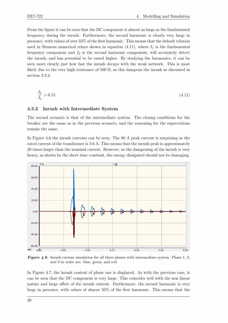
The second scenario is that of the intermediate system. The closing conditions for thebreaker are the same as in the previous scenario, and the reasoning for the expectationsremain the same.
In Figure 4.6 the inrush currents can be seen. The 80 A peak current is surprising as therated current of the transformer is 3.6 A. This means that the inrush peak is approximately20 times larger than the nominal current. However, as the dampening of the inrush is veryheavy, as shown by the short time constant, the energy dissipated should not be damaging.
Figure 4.6. Inrush current simulation for all three phases with intermediate system. Phase 1, 2,and 3 in order are: blue, green, and red.
In Figure 4.7, the inrush content of phase one is displayed. As with the previous case, itcan be seen that the DC component is very large. This coincides well with the non linearnature and large offset of the inrush current. Furthermore, the second harmonic is verylarge in presence, with values of almost 50% of the first harmonic. This means that the
30

4.3. Simulation of the Inrush Current Aalborg University
relation described in equation (4.11) should accurately detect the inrush and block thetripping action. As the second harmonic is so large, the blocking criterion could be tunedto be higher than the default 15%.
Figure 4.7. Harmonics of inrush current in phase one
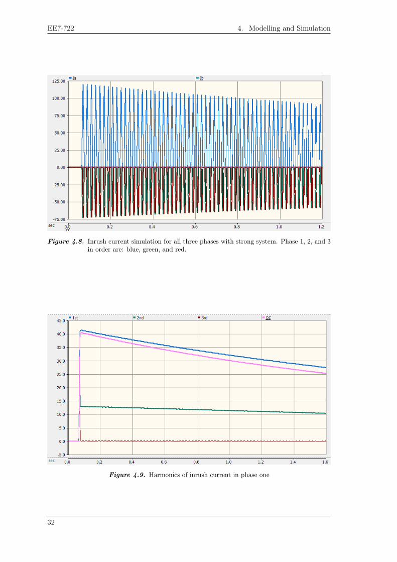
4.3.3 Inrush with Strong System
The last case in this report is the case of inrush currents in a very strong system. Thesystem is unrealistically strong for this voltage level, but it should demonstrate the absolutemaximum amount of inrush that could occur using this transformer. In Figure 4.8 theinrush current of the transformer can be seen. As expected, it is larger in magnitude andthe dampening is minuscule when comparing with the previous cases. It is important tonote the difference in timescale. This inrush current is not even down to 80 A after 1.2seconds, whereas with the intermediate system, it was almost completely gone after 0.3seconds.
In Figure 4.9 the harmonics of the inrush current can be seen. What is interesting whenlooking at this at a long timescale like this, is that it enters a quasi-steadystate. The thirdharmonic is almost instantly gone after the switching occurs, but the ratio between thesecond and first harmonic remain what appears to be constant. This ratio could potentiallybe used to set the inrush blocking ratio.
4.3.4 Results
From this section, it is clear that the system the transformer is connected to is just asimportant as the transformer itself, as it can make the inrush vary by several orders ofmagnitude. As the intermediate system is the one which emulates the lab conditions theclosest, this is the scenario which will be used for further analysis. The data acquired inthis section can now be used in setting the parameters of the relay. More specifically, itcan be used to adjust the inrush blocking, and adjust the expectations of peak currents.Furthermore, the scenario simulated can be exported using the analog data export block
31
EE7-722 4. Modelling and Simulation
Figure 4.8. Inrush current simulation for all three phases with strong system. Phase 1, 2, and 3in order are: blue, green, and red.
Figure 4.9. Harmonics of inrush current in phase one
32
4.4. Simulation of an Internal Fault Aalborg University
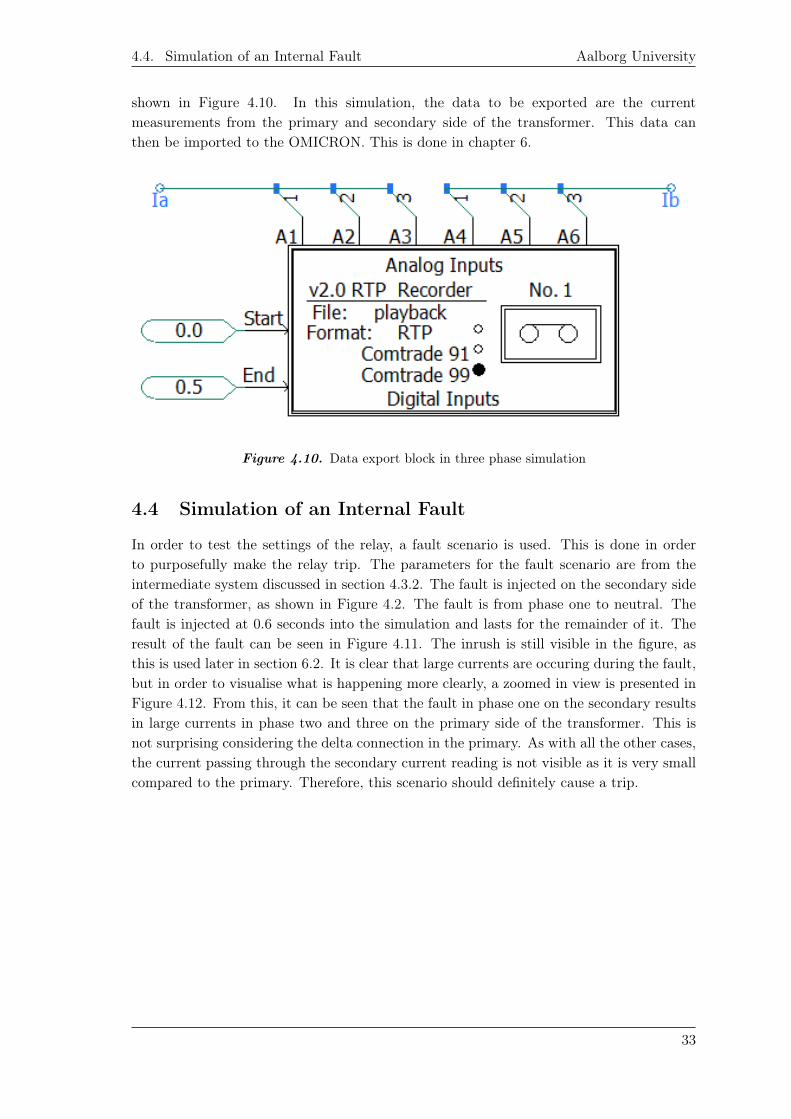
shown in Figure 4.10. In this simulation, the data to be exported are the currentmeasurements from the primary and secondary side of the transformer. This data canthen be imported to the OMICRON. This is done in chapter 6.
Figure 4.10. Data export block in three phase simulation
4.4 Simulation of an Internal Fault
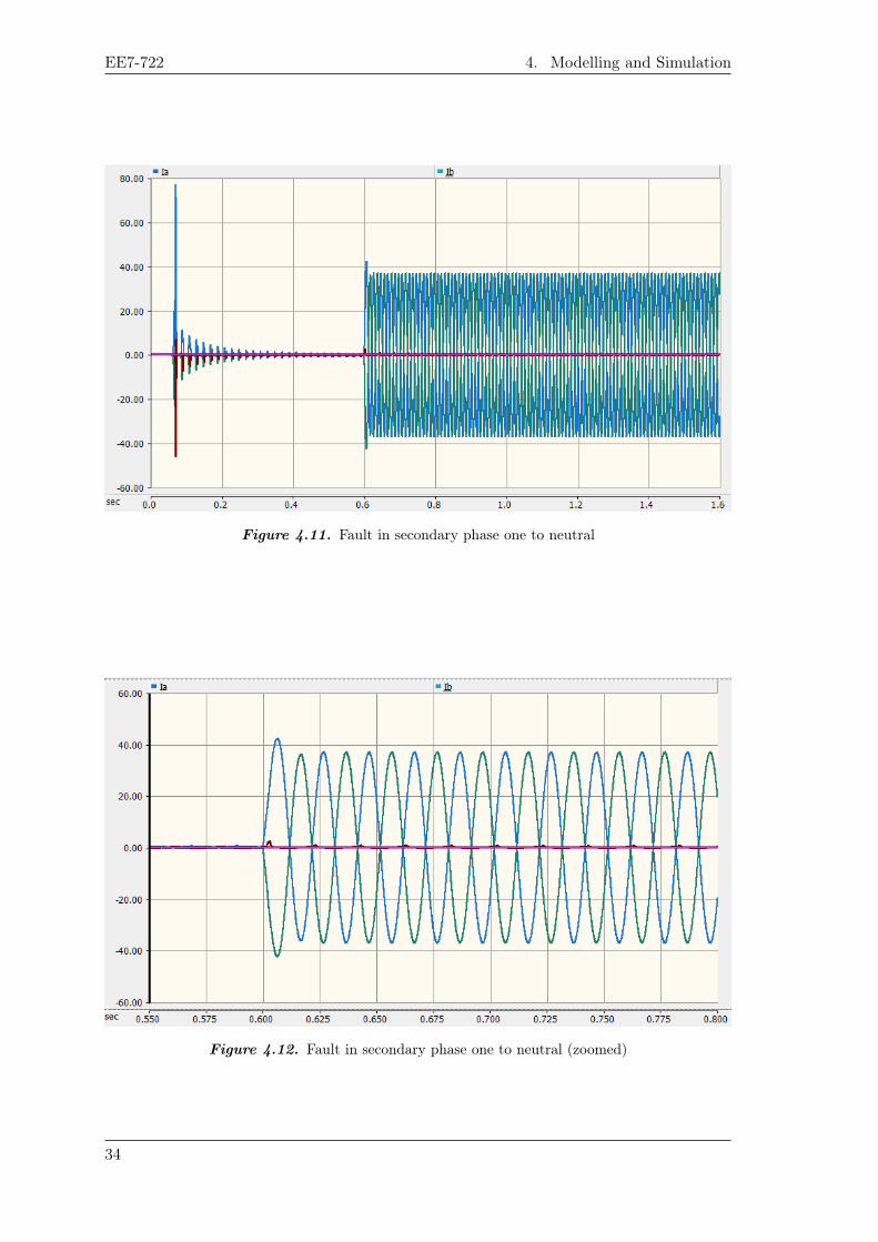
In order to test the settings of the relay, a fault scenario is used. This is done in orderto purposefully make the relay trip. The parameters for the fault scenario are from theintermediate system discussed in section 4.3.2. The fault is injected on the secondary sideof the transformer, as shown in Figure 4.2. The fault is from phase one to neutral. Thefault is injected at 0.6 seconds into the simulation and lasts for the remainder of it. Theresult of the fault can be seen in Figure 4.11. The inrush is still visible in the figure, asthis is used later in section 6.2. It is clear that large currents are occuring during the fault,but in order to visualise what is happening more clearly, a zoomed in view is presented inFigure 4.12. From this, it can be seen that the fault in phase one on the secondary resultsin large currents in phase two and three on the primary side of the transformer. This isnot surprising considering the delta connection in the primary. As with all the other cases,the current passing through the secondary current reading is not visible as it is very smallcompared to the primary. Therefore, this scenario should definitely cause a trip.
33
EE7-722 4. Modelling and Simulation
Figure 4.11. Fault in secondary phase one to neutral
Figure 4.12. Fault in secondary phase one to neutral (zoomed)
34
Laboratory 5In order to continue with the modelling of the transformer, some lab work is required. Thelab work is done in order to create simulations, which are as close to reality as possible.This is done by taking a real transformer and then using the theory previously discussedin order to parametrize it. These parameters are then used in the simulations.
5.1 Parametrization of Transformer
In order to continue working with simulations, the parameters of the transformer must bedetermined. These parameters are discussed in detail in section 4.2. In order to determinethe parameters three tests types are conducted. The transformer in question is a 400/230DYn11 with a rated power of Sn = 2.5 KVa and a rated frequency of fs = 50 Hz. Thetransformer is rated for a line current of 3.6 A. The DYn11 designation means that it isa Delta/Wye transformer with vector group 11. The vector group indicates the lag of thelow voltage (LV) in respect to the high voltage (HV). Vector group 11 equals a lag of 330degrees, or vice versa that the LV leads the HV by 30 degrees. The equipment used insections 5.1.1, 5.1.2 and 5.1.3 is listed in table 5.1.
Equipment Name Model AAU NumberThree phase power analyzer Voltech PM300 93642Autotransformer 400/400 V 10 A Lübcke RV31002-20 89119DYn11 400/230 2.5 kVA transformer Dantrafo DT 18784-1 N/A
Table 5.1. Equipment used in parametrization of the transformer
5.1.1 Short Circuit Test
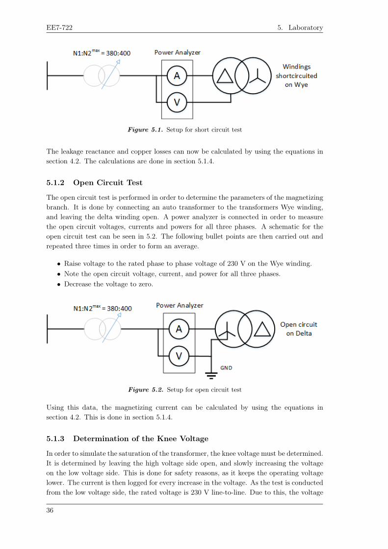
The short circuit test is performed in order to determine the conductor losses, leakagereactance, and air core reactance. It is done by shorting out the Wye winding, connectingthe power analyzer and then connecting the delta winding to an auto transformer. Theauto transformer is connected to the laboratory mains. A schematic for the short circuittest can be seen in Figure 5.1. The reason for the delta winding being used for the shortcircuit test is to keep the currents as low as possible. The power analyzer measures thevoltage, current and power for all three phases. The following bullet points are then carriedout and repeated three times in order to form an average.
• Raise voltage till the rated current of 3.6 A flows into the transformer per phase.• Note the short circuit voltage, current, and power for all three phases.• Decrease the voltage to zero.
35
EE7-722 5. Laboratory
Figure 5.1. Setup for short circuit test
The leakage reactance and copper losses can now be calculated by using the equations insection 4.2. The calculations are done in section 5.1.4.
5.1.2 Open Circuit Test
The open circuit test is performed in order to determine the parameters of the magnetizingbranch. It is done by connecting an auto transformer to the transformers Wye winding,and leaving the delta winding open. A power analyzer is connected in order to measurethe open circuit voltages, currents and powers for all three phases. A schematic for theopen circuit test can be seen in 5.2. The following bullet points are then carried out andrepeated three times in order to form an average.
• Raise voltage to the rated phase to phase voltage of 230 V on the Wye winding.• Note the open circuit voltage, current, and power for all three phases.• Decrease the voltage to zero.
Figure 5.2. Setup for open circuit test
Using this data, the magnetizing current can be calculated by using the equations insection 4.2. This is done in section 5.1.4.
5.1.3 Determination of the Knee Voltage
In order to simulate the saturation of the transformer, the knee voltage must be determined.It is determined by leaving the high voltage side open, and slowly increasing the voltageon the low voltage side. This is done for safety reasons, as it keeps the operating voltagelower. The current is then logged for every increase in the voltage. As the test is conductedfrom the low voltage side, the rated voltage is 230 V line-to-line. Due to this, the voltage
36
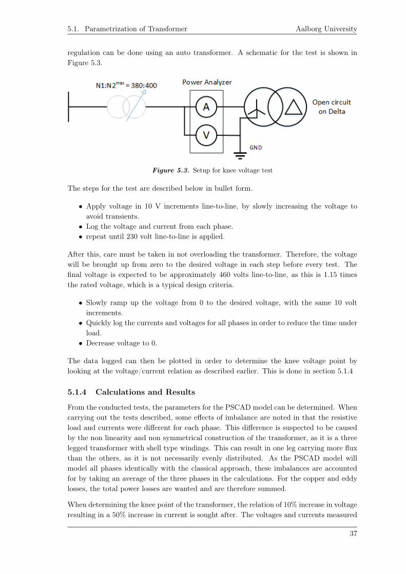
5.1. Parametrization of Transformer Aalborg University
regulation can be done using an auto transformer. A schematic for the test is shown inFigure 5.3.
Figure 5.3. Setup for knee voltage test
The steps for the test are described below in bullet form.
• Apply voltage in 10 V increments line-to-line, by slowly increasing the voltage toavoid transients.
• Log the voltage and current from each phase.• repeat until 230 volt line-to-line is applied.
After this, care must be taken in not overloading the transformer. Therefore, the voltagewill be brought up from zero to the desired voltage in each step before every test. Thefinal voltage is expected to be approximately 460 volts line-to-line, as this is 1.15 timesthe rated voltage, which is a typical design criteria.
• Slowly ramp up the voltage from 0 to the desired voltage, with the same 10 voltincrements.
• Quickly log the currents and voltages for all phases in order to reduce the time underload.
• Decrease voltage to 0.
The data logged can then be plotted in order to determine the knee voltage point bylooking at the voltage/current relation as described earlier. This is done in section 5.1.4
5.1.4 Calculations and Results
From the conducted tests, the parameters for the PSCAD model can be determined. Whencarrying out the tests described, some effects of imbalance are noted in that the resistiveload and currents were different for each phase. This difference is suspected to be causedby the non linearity and non symmetrical construction of the transformer, as it is a threelegged transformer with shell type windings. This can result in one leg carrying more fluxthan the others, as it is not necessarily evenly distributed. As the PSCAD model willmodel all phases identically with the classical approach, these imbalances are accountedfor by taking an average of the three phases in the calculations. For the copper and eddylosses, the total power losses are wanted and are therefore summed.
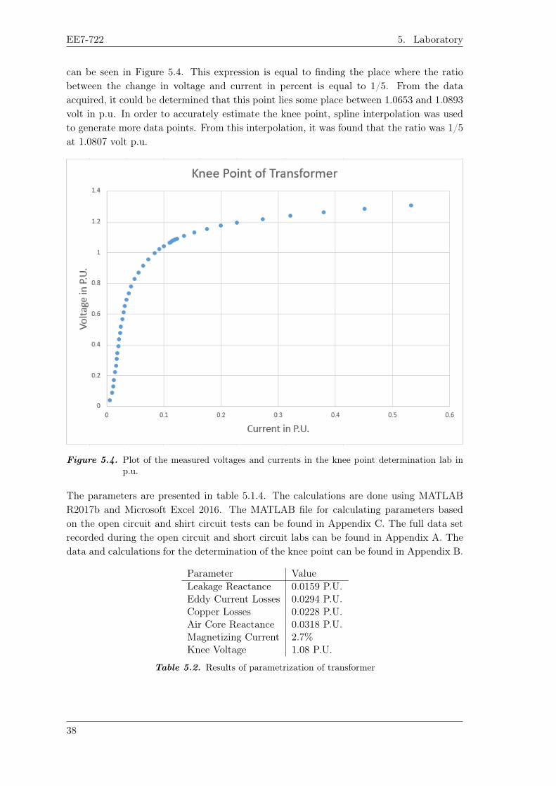
When determining the knee point of the transformer, the relation of 10% increase in voltageresulting in a 50% increase in current is sought after. The voltages and currents measured
37
EE7-722 5. Laboratory
can be seen in Figure 5.4. This expression is equal to finding the place where the ratiobetween the change in voltage and current in percent is equal to 1/5. From the dataacquired, it could be determined that this point lies some place between 1.0653 and 1.0893volt in p.u. In order to accurately estimate the knee point, spline interpolation was usedto generate more data points. From this interpolation, it was found that the ratio was 1/5at 1.0807 volt p.u.
Figure 5.4. Plot of the measured voltages and currents in the knee point determination lab inp.u.
The parameters are presented in table 5.1.4. The calculations are done using MATLABR2017b and Microsoft Excel 2016. The MATLAB file for calculating parameters basedon the open circuit and shirt circuit tests can be found in Appendix C. The full data setrecorded during the open circuit and short circuit labs can be found in Appendix A. Thedata and calculations for the determination of the knee point can be found in Appendix B.
Parameter ValueLeakage Reactance 0.0159 P.U.Eddy Current Losses 0.0294 P.U.Copper Losses 0.0228 P.U.Air Core Reactance 0.0318 P.U.Magnetizing Current 2.7%Knee Voltage 1.08 P.U.
Table 5.2. Results of parametrization of transformer
38
Relay Settings and Testing 6In section 3.2, the fundamentals of differential protection are described. In the section, itis described that current measurements on both sides of a transformer are taken, whichthen undergo various operations in order to scale them based on the vector group ofthe transformer, the winding ratio, and varying CT ratios. In real life applications, thestate of the art is to use numerical relays. This relay terminology is a remnant, as theyare not just relays anymore. They are often mentioned as IED or Intelligent ElectronicDevice, as they essentially are computers with various binary and analogue inputs andoutputs. The relays used in this project are Siemens Siprotec 7SD61, and are differentialrelays. They are capable of providing differential protection not only for transformers,but also transmission and distribution systems such as overhead lines and cables. As thisproject scope only includes transformers, some settings are omitted and disabled in therelays. Because the relays are multipurpose, not only in that they can be used for differentsystems, but also allow a great degree of customization in the usage of CTs etc. someprogramming is necessary. In section 6.1, the specifics about programming the relays willbe elaborated. In section 6.2 the settings will be tested with simulated scenarios.
6.1 Programming the Relays
When programming relays, it is important to note that there are two relays to program.In this section, one is named Local or relay 1 interchangeably, and the other is namedRemote or relay 2 interchangeably. In this section the various parameters for the relay willbe investigated and set in correspondence to the information gathered in section 3.2. Theprimary source for programming the relays is the manual for the relay [Siemens, 2016].
The relay is programmed using Siemens DIGSI software. DIGSI is a graphical user interfacesoftware in which various parameters on the relays can be set. Furthermore, it can beused to create special functions, should the user need it. It is programmed by accessing"addresses" and toggling them or inputting a value.
The first settings to change are the device configuration settings. In this menu, settingsrelating to the function of the relay can be changed. For the scope of this report, onlythe differential protection is enabled at address 112. The 7SD61 can be ordered with anoption to include a power transformer in its protection zone, but the particular relay usedhere is not built with that option. The address of this setting is 143. As this optionis missing, it is impossible to test the transformer fault scenario, as it cannot accountfor the vector grouping or winding ratio of the transformer, and thus will see the phaseshift and transformation ratio as errors. For the sake of completion, the missing settingswill be evaluated and elaborated, but not actually programmed. Since the purpose of
39
EE7-722 6. Relay Settings and Testing
the inrush test is to test if the relay properly picks up the second harmonic content andblocks for tripping, it can still be tested, as any tripping due to vector grouping or windingratio should be blocked. This means that when testing the inrush scenario, it should stayonline. However, as soon as the second harmonic content drops to below the specifiedlevel, it should send a trip signal due to the previously mentioned reasons.
The next group of settings is labelled Power System Data 1. This group relates tothe system the relays are used to protect. The first subgroup of settings is called"Transformers" and relates to the connection of the CTs. Here, the star point of theCTs can be defined as being towards the line or the busbar. This is done on address 201,and is left at the default towards line, as this does not really matter in this case as noCTs are used in the lab. The next two options on address 205 and 206 are the primaryand secondary currents of the CT, which are set to 100 and 1, as this is the ratio usedin the OMICRON when simulating the scenarios. This means that the currents measuredby the relay are scaled up by a factor of 100 when displaying them on the LCD. As thetransformer has an earthed star connection on the secondary side, it is necessary to havesome earth fault protection. This can be done by a separate earth fault relay, or it can behandled by an optional purchase in the differential relay. The way it works is by having aseparate CT measure the current flowing in the earth connection, which is then comparedto the current flowing in the phases. By doing this selectivity is obtained as it only protectswithin the boundary created by the four CTs. If this is desired it is important to enablethe I4 CT in address 220. Furthermore, the ratio of the earth CT and the phase CTs mustbe defined in 221. This is necessary as the earth fault transformer can be much smaller,as there normally should not be a current present in it, thus it does not need to be ableto handle the full load of the transformer.
The next subgroup is labelled "Power System". Here, information regarding the systembeing protected are defined. First, the earthing of the system is defined. This is donein address 207 and options are: Solid Earthed, Peterson Coil, and Isolated. For thesimulations, a solid earth is used and therefore this is the setting defined here. Furthermore,the frequency of the system is defined in address 230, which is set to 50 Hz. The nextsubgroup is "Breaker", which contains only one setting, namely dead time for CB test-autore-closure. This is the time it takes for the breaker connected to this particular relay tore-close after breaking a fault. As no physical breakers are present in this report, it is leftat the default 0.10 seconds. The last subgroup is labelled "CT Data" and relates to thespecific CTs used in the system. Recall that there are three regions of operating the systemas seen in Figure 3.4 defined by equations (3.3) to (3.5). First is at low currents whereCT error does not matter and only the transformer magnetizing current is compensatedfor. The second region is where CT error starts to compound and requires a slope k basedon the CTs in question. The last region is the saturation region, where the CTs start tosaturate. The first setting in the relay, at address 251, is the ratio between the actualALF (ALF’) and the nominal ALF of the CTs. This is given by equation (6.1), where n′
is the operational ALF, n is the rated ALF from the specs, PN is the rated burden of theCT, Pi is the internal burden of the CT, and P ′ is the burden connected to the CT. P ′ isfound by measuring the DC resistance of the connected wiring and then using the relationthat P ′ ≈ Rwire · I, where I is the rated secondary current. Pi is typically available in thetest report from the factory, but can be calculated similarly to P ′, by measuring the DC
40
6.1. Programming the Relays Aalborg University
resistance of the CT. Siemens recommend that this ratio is kept below 1.5, and if this isnot possible with the selected CTs, considerations should be made to select other CTs.
n′
n=PN + Pi
P ′ + Pi(6.1)
The next setting is called "CT error in % at ALF’/ALF" and is at address 253. This is thetransformation error specified in the datasheet for the CT plus a safety margin. Siemensrecommends for a 5P, where it could be 1% at rated current, to add a safety margin of 2%adding up to a total of 3% in this setting. The next setting is called "CT error in % atALF and is at address 254. This is the number before the P plus a safety margin. For a 5Psiemens recommends adding a safety margin of 5% adding up to 10%. These CT settingsaddress the issue of transformation error and defines a slope similarly to equation (3.4).They do however not address the issue of CT saturation defined in the last region. Thisis instead done by "High-speed charge comparison", where the relay calculates the chargeand compares it to the previous charge. The charge is calculated by equation (6.2), wherethe integration time is 1
4 of a period, or 5ms at 50 Hz. The relays then compare the chargemeasured at both ends of the system and will provide high speed tripping if they are notequal. These settings for the CTs are all bounded by the fact that the CTs must be selectedvia three criteria. The first criterion is that the ratio between the maximum fault currentand the nominal primary current must not be larger than the operational ALF. The secondcriterion is that the operational ALF must be at least 30 (Calculated by solving for n′ inequation (6.1)), or the CTs must be guaranteed to not saturate in under 1
4 of a period. Thethird criterion is that the ratio between the primary currents at both ends of the systemmust be below 8, thus a transformer must have a winding ratio of maximum 8.
Q =
∫ t2
t1i(t)dt (6.2)
For the testing of the inrush scenario, all of these values can be set very low, as there arein fact no CT’s connected and thus no error imposed by them. Therefore, the settings areselected to follow those of a 5p CT. This means that address 251 = 1.00, 253 = 3.0% and254 = 10%.
That concludes the power system data 1 settings. The next settings group is called powersystems data 2, which contains information about the system. First, there is informationabout the current level of the system. This setting is located at address 1104, and is thebasis for the systems calculations. Ideally this would be set to 3.6 A, as this is the currentrating of the transformers primary side, but it does not go lower than 10, so it will beset to that. It is important to set the current levels corresponding to which winding therelay is connected to. When working with a transformer differential, different options areavailable. It can include settings such as full scale voltage, power, line angle, etc. In address1103 the full scale voltage can be set. This is the rated voltage of the end of the systembeing observed. It is important that this is set correctly, with respect to what side of thetransformer the relay is at, as it is used in the per unit calculations. It is furthermore
41
EE7-722 6. Relay Settings and Testing
all the relay needs to know about the winding ratio, as the vector group is dealt withelsewhere. In address 1106 the operation power can be set. It is the highest apparentpower the transformer can transfer for any winding pair. Thus, in the case of this report,that value would be set to 2.5 kVA. Had the differential relay has the transformer optionsenabled, the vector group could be set. This is important as previously mentioned it willcause a phase shift. This is set in address 1161 and 1162. The methodology is that thevector group is set for each relay, such that the relay for a winding has the correspondingvector group. In the case of this report, the transformer has the vector group Dyn11, sofor the local relay the vector group should be set to 0 as it is the reference. For the remoterelay, the vector group should be set to 11. In address 1163 the zero sequence eliminationmentioned in section 3.2 is enabled or disabled. As the transformer in question has agrounded star point on the secondary side, this should be enabled in the remote relay. Thenext subgroup is Line Status, which defines parameters for when it is allowed to reset thetrip signal and other overheard line specifics. As automatic re-closure of a transformer isnot permitted after a trip, these settings are left at default settings.
The next settings group is named Differential Protection. The first option is at address1201, and enables or disables the differential protection. Naturally, this should be enabledin our case. The next option is at address 1210 and is the I-DIFF > Pickup value. This isthe DC offset described in section 3.2, by equation (3.3). Siemens recommends taking themagnetizing current and then doubling the value for this bias. The magnetizing currentof the transformer in question has been calculated to be 2.7% of the full load current insection 5.1.4, which is 2.7% of 3.6 A. The minimum allowed value in the relay is 10 A,which is the setting used. The next option is I-Diff during switch on. Recall that an inrushoccurs when switching the transformer on. Siemens recommend a setting of 4 times thecharging or magnetizing current, which equals to 4 · 0.027 · 3.6 A, thus lower than the 10A minimum setting. Please note that the inrush can be much larger than this. Therefore,it is mitigated by other means than a simple added restraint current. The next parameteris I-DIFF» at address 1233, which is the "Pickup value charge comparison stage". Thisis the stage that reacts to very large short circuit currents, and is therefore very fast. Itmust be set to exclude the inrush current, as it is not supposed to pick this up. From thesimulations we know that the largest expectable rush current is approximately 80 A, whichis coincidentally the smallest value allowable in the relay. The next parameter is I-DIFF»at address 1235, which is switch on of the charge comparison. Depending on the objectprotected, stray fluxes can cause the charges to differ on the secondary and primary sideduring switch on, which can cause a faulty trip. Siemens recommend setting this value totwo to three times the I-DIFF» value if the protected object is a bushing transformer. Asthis is not the case, it is set to the same as I-DIFF.
The next settings group relates to inrush currents. For the scope of this project, it is oneof the most important settings. It is enabled by toggling address 2301. At address 2302the amount of second harmonic in percent of the fundamental which must be present forthe inrush blocking to be enabled is defined. By default this is set to 15%. This value is agood starting point, as it is lower than what should be expected from a transformer, thussuccessfully blocking the relay from tripping during inrush. The next setting is called CrossBlock and is located at address 2303. By enabling cross block, inrush in one phase willblock tripping action for all phases. Please recall from section 3.3.2 that one phase can be
42

6.2. Testing the Relay Settings Aalborg University
without inrush if it is switched at the right time, while the others are experiencing heavyinrush. This means that a potential error on that phase can be observed and the relaywill then trip, if cross blocking is not enabled. As this relay is not meant for transformers,if a phase was without blocking a trip would occur. Therefore, cross blocking is enabled,which allows for the inrush scenario to be tested without tripping. The next parameter isat address 2305, and is the maximum inrush peak value. As the name implies, this is tobe set to the highest inrush expected. It supersedes the inrush blocking, and thus if thispeak is exceeded then the relay will trip, even if the second harmonic content is greaterthan the previously defined value. The highest expected value is 80 A, as shown earlierin section 4.3. The minimum value the relay allows is however 110 A, which is the valueset. The last parameter available to tune here is the time for cross block, at address 2310.By default it is set to zero, but for some tests in section 6.2 it will be changed to a highervalue. This concludes the differential protection settings.
Although the differential protection on both sides of the transformer should detect thesame errors, extra trip commands should not be necessary. However, in address 1301 sucha command can be enabled. The action for receiving the command from the opposing relaycan be defined in address 1302, where it can be set to an alarm or a trip. In address 1303a delay for the tripping command can be introduced and in 1304 the trip length can bedefined. In order to communicate with the remote relay, different techniques can be used.It can communicate via a network, via copper wires or fibreoptics. In the lab the relaysare connected by fibreoptics. This is defined in the settings, along with settings pertainingto the maximum delay in communication before an alarm is raised. In address 4701 and4702 the relays are labelled with an identifying number. Default setting is naming them1 and 2, and this is fine for the scope of this project. In a larger system a more complexnaming scheme might be used. Furthermore, in address 4710 it is defined which relay isthe local relay. In this case it is relay 1.
6.2 Testing the Relay Settings
In order to verify the settings made in section 6.1 tests must be carried out. The waythis is done is by simulating the desired scenarios for the relays, and then monitoring theactions taken by the relay. By doing this, the relay settings can be tested without everbeing connected to the transformer they are meant to protect. This makes testing easier,as it is all done via computer, instead of having to deal with the practicalities of testingin real life.
The desired scenarios are simulated in appropriate software, such as PSCAD, where thedesired variables, such as the current measurements, are exported into an external file.This file is then imported into software which controls an OMICRON CMC 256 (referredto as OMICRON). The OMICRON is, as previously mentioned, a signal generator withbuilt in amplifiers. It can generate the waveforms desired from the simulation scenario.Naturally, it is impractical to generate the real currents which the scenario calls for, incase of the inrush upwards of 80 A. Therefore, the signals are scaled down, as with aCT. This essentially means that the currents the OMICRON outputs can be seen as thesecondary currents of the CTs, which allows it to be connected directly to the currentmeasuring circuits of the relays. A schematic showing the connections and process is
43
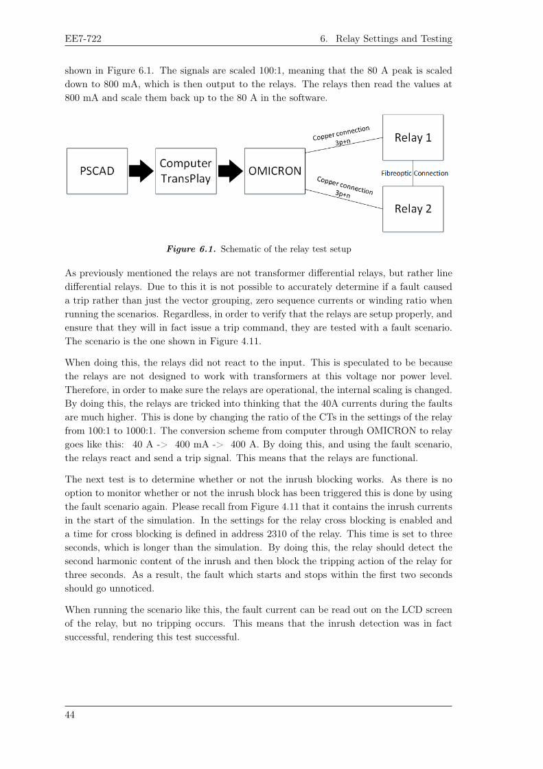
EE7-722 6. Relay Settings and Testing
shown in Figure 6.1. The signals are scaled 100:1, meaning that the 80 A peak is scaleddown to 800 mA, which is then output to the relays. The relays then read the values at800 mA and scale them back up to the 80 A in the software.
Figure 6.1. Schematic of the relay test setup
As previously mentioned the relays are not transformer differential relays, but rather linedifferential relays. Due to this it is not possible to accurately determine if a fault causeda trip rather than just the vector grouping, zero sequence currents or winding ratio whenrunning the scenarios. Regardless, in order to verify that the relays are setup properly, andensure that they will in fact issue a trip command, they are tested with a fault scenario.The scenario is the one shown in Figure 4.11.
When doing this, the relays did not react to the input. This is speculated to be becausethe relays are not designed to work with transformers at this voltage nor power level.Therefore, in order to make sure the relays are operational, the internal scaling is changed.By doing this, the relays are tricked into thinking that the 40A currents during the faultsare much higher. This is done by changing the ratio of the CTs in the settings of the relayfrom 100:1 to 1000:1. The conversion scheme from computer through OMICRON to relaygoes like this: 40 A -> 400 mA -> 400 A. By doing this, and using the fault scenario,the relays react and send a trip signal. This means that the relays are functional.
The next test is to determine whether or not the inrush blocking works. As there is nooption to monitor whether or not the inrush block has been triggered this is done by usingthe fault scenario again. Please recall from Figure 4.11 that it contains the inrush currentsin the start of the simulation. In the settings for the relay cross blocking is enabled anda time for cross blocking is defined in address 2310 of the relay. This time is set to threeseconds, which is longer than the simulation. By doing this, the relay should detect thesecond harmonic content of the inrush and then block the tripping action of the relay forthree seconds. As a result, the fault which starts and stops within the first two secondsshould go unnoticed.
When running the scenario like this, the fault current can be read out on the LCD screenof the relay, but no tripping occurs. This means that the inrush detection was in factsuccessful, rendering this test successful.
44
Conclusion 7The author began the work by identifying that there is a trend towards decentralizationof the energy production taking place. One of the engineering challenges this will pose, isthat it shifts the scope of fault on the distribution transformer from being an outage forconsumers to also shutting down production from these decentralized units. During theinternship the author acquired skills in designing the protection for the transformer, andlearned a great deal about the safety equipment associated with transformer protection.
In this work a systematic study of differential protection of a small transformer wascarried out. It was determined that the inrush currents associated with the magnetizationtransients not only were large enough to cause a false differential current, but could in factbe large enough to destroy the equipment. Simulations were conducted using parametersfitted from a real transformer. It was found that even if the current was not large enoughto cause damage, it could still cause a false positive in the protection. The inrush currentwas found to be of considerable harmonic character, caused by the non-linear nature ofthe transformer during saturation. By performing FFT on the current waveform a ratio ofthe fundamental frequency and the second harmonic was computed as a possible blockingcriterion for the protection system. In the lab two Siemens 7SD610’s were programmed topick up the inrush current. An inrush scenario corresponding to the simulation conditionswas performed using an OMICRON CMC 256-6. The calculated blocking ratio successfullyprevented tripping action, demonstrating quantitative agreement between simulation andexperiment.
Even though the project has been concluded, and the most important aspects have beeninvestigated and tested, it has potential for further work. As it has been determined thatthe ratio for blocking inrush tripping could be tuned, it would be of interest to see exactlyhow much. Additionally, by acquiring a larger transformer plus relays with more options,through-fault scenarios could be tested using the OMICRON CMC 256-6 and verifiedexperimentally. With the current setup, the inrush current simulated in section 4.3.2could be verified experimentally.
45

Bibliography
Bronzeado et al., 1996. H.S. Bronzeado, P.B. Brogan and R. Yacamini. Harmonicanalysis of transient currents during sympathetic interactions. IEEE Transactions onPower Systems, pages 2051–2056, 1996.
C4.307, 2013. WG C4.307. Transformer Energization in Power Systems: A StudyGuide, 2013.
HVDC.ca. HVDC.ca. The Classical Approach. https://hvdc.ca/webhelp/EMTDC/Transformers/The_Classical_Approach/the_classical_approach.htm#More.Accessed: 2017-17-12.
Siemens, 2016. Siemens. Siprotec Differential Protection 7sd610 v4.70 Manual, 2016.Accessed: 2018-09-01.
Umans, 2014. Stephen D. Umans. Fitzgerald and Kingsley’s Electric Machinery.McGraw-Hill Education, 2014. ISBN 978-1-259-25466-6.
Ziegler, 2012. Gerhard Ziegler. Numerical Differential Protection. Publicis Publishing,2012. ISBN 978-3-89578-351-7.
Ziegler, 2011. Gerhard Ziegler. Numerical Distance Protection. Publicis Publishing,2011. ISBN 978-3-89578-381-4.
47


Open and Short CircuitData A
49
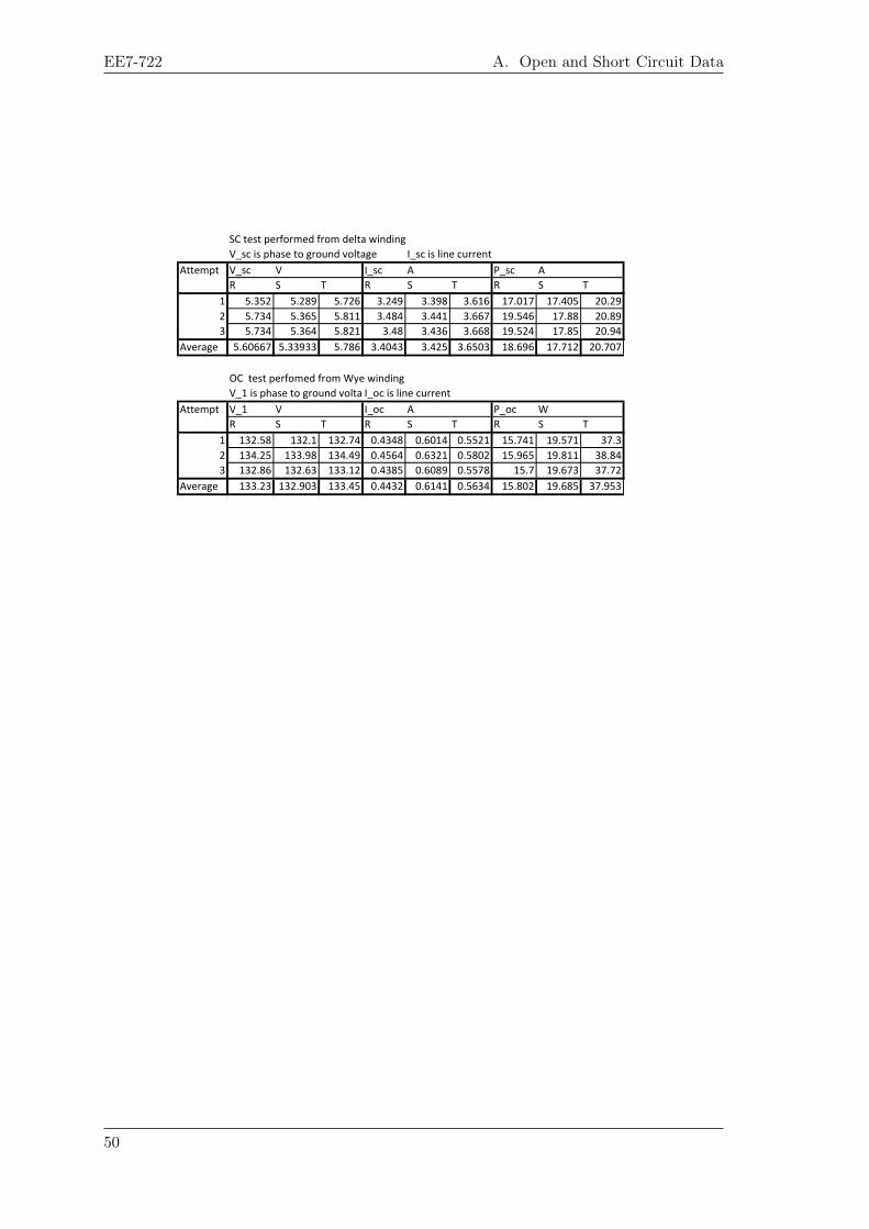
SC test performed from delta winding
V_sc is phase to ground voltage I_sc is line current
Attempt V_sc V I_sc A P_sc A
R S T R S T R S T
1 5.352 5.289 5.726 3.249 3.398 3.616 17.017 17.405 20.29
2 5.734 5.365 5.811 3.484 3.441 3.667 19.546 17.88 20.89
3 5.734 5.364 5.821 3.48 3.436 3.668 19.524 17.85 20.94
Average 5.60667 5.33933 5.786 3.4043 3.425 3.6503 18.696 17.712 20.707
OC test perfomed from Wye winding
V_1 is phase to ground voltageI_oc is line current
Attempt V_1 V I_oc A P_oc W
R S T R S T R S T
1 132.58 132.1 132.74 0.4348 0.6014 0.5521 15.741 19.571 37.3
2 134.25 133.98 134.49 0.4564 0.6321 0.5802 15.965 19.811 38.84
3 132.86 132.63 133.12 0.4385 0.6089 0.5578 15.7 19.673 37.72
Average 133.23 132.903 133.45 0.4432 0.6141 0.5634 15.802 19.685 37.953
EE7-722 A. Open and Short Circuit Data
50

Knee Voltage Data andCalculations B
51
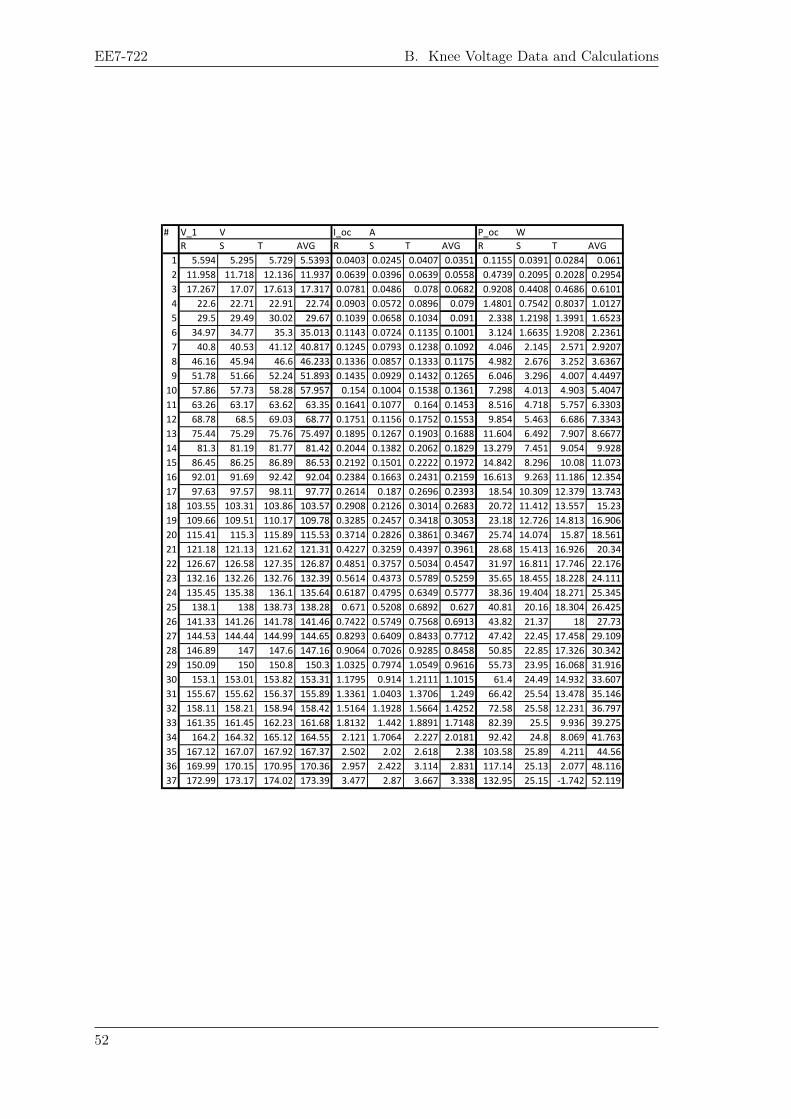
# V_1 V I_oc A P_oc W
R S T AVG R S T AVG R S T AVG
1 5.594 5.295 5.729 5.5393 0.0403 0.0245 0.0407 0.0351 0.1155 0.0391 0.0284 0.061
2 11.958 11.718 12.136 11.937 0.0639 0.0396 0.0639 0.0558 0.4739 0.2095 0.2028 0.2954
3 17.267 17.07 17.613 17.317 0.0781 0.0486 0.078 0.0682 0.9208 0.4408 0.4686 0.6101
4 22.6 22.71 22.91 22.74 0.0903 0.0572 0.0896 0.079 1.4801 0.7542 0.8037 1.0127
5 29.5 29.49 30.02 29.67 0.1039 0.0658 0.1034 0.091 2.338 1.2198 1.3991 1.6523
6 34.97 34.77 35.3 35.013 0.1143 0.0724 0.1135 0.1001 3.124 1.6635 1.9208 2.2361
7 40.8 40.53 41.12 40.817 0.1245 0.0793 0.1238 0.1092 4.046 2.145 2.571 2.9207
8 46.16 45.94 46.6 46.233 0.1336 0.0857 0.1333 0.1175 4.982 2.676 3.252 3.6367
9 51.78 51.66 52.24 51.893 0.1435 0.0929 0.1432 0.1265 6.046 3.296 4.007 4.4497
10 57.86 57.73 58.28 57.957 0.154 0.1004 0.1538 0.1361 7.298 4.013 4.903 5.4047
11 63.26 63.17 63.62 63.35 0.1641 0.1077 0.164 0.1453 8.516 4.718 5.757 6.3303
12 68.78 68.5 69.03 68.77 0.1751 0.1156 0.1752 0.1553 9.854 5.463 6.686 7.3343
13 75.44 75.29 75.76 75.497 0.1895 0.1267 0.1903 0.1688 11.604 6.492 7.907 8.6677
14 81.3 81.19 81.77 81.42 0.2044 0.1382 0.2062 0.1829 13.279 7.451 9.054 9.928
15 86.45 86.25 86.89 86.53 0.2192 0.1501 0.2222 0.1972 14.842 8.296 10.08 11.073
16 92.01 91.69 92.42 92.04 0.2384 0.1663 0.2431 0.2159 16.613 9.263 11.186 12.354
17 97.63 97.57 98.11 97.77 0.2614 0.187 0.2696 0.2393 18.54 10.309 12.379 13.743
18 103.55 103.31 103.86 103.57 0.2908 0.2126 0.3014 0.2683 20.72 11.412 13.557 15.23
19 109.66 109.51 110.17 109.78 0.3285 0.2457 0.3418 0.3053 23.18 12.726 14.813 16.906
20 115.41 115.3 115.89 115.53 0.3714 0.2826 0.3861 0.3467 25.74 14.074 15.87 18.561
21 121.18 121.13 121.62 121.31 0.4227 0.3259 0.4397 0.3961 28.68 15.413 16.926 20.34
22 126.67 126.58 127.35 126.87 0.4851 0.3757 0.5034 0.4547 31.97 16.811 17.746 22.176
23 132.16 132.26 132.76 132.39 0.5614 0.4373 0.5789 0.5259 35.65 18.455 18.228 24.111
24 135.45 135.38 136.1 135.64 0.6187 0.4795 0.6349 0.5777 38.36 19.404 18.271 25.345
25 138.1 138 138.73 138.28 0.671 0.5208 0.6892 0.627 40.81 20.16 18.304 26.425
26 141.33 141.26 141.78 141.46 0.7422 0.5749 0.7568 0.6913 43.82 21.37 18 27.73
27 144.53 144.44 144.99 144.65 0.8293 0.6409 0.8433 0.7712 47.42 22.45 17.458 29.109
28 146.89 147 147.6 147.16 0.9064 0.7026 0.9285 0.8458 50.85 22.85 17.326 30.342
29 150.09 150 150.8 150.3 1.0325 0.7974 1.0549 0.9616 55.73 23.95 16.068 31.916
30 153.1 153.01 153.82 153.31 1.1795 0.914 1.2111 1.1015 61.4 24.49 14.932 33.607
31 155.67 155.62 156.37 155.89 1.3361 1.0403 1.3706 1.249 66.42 25.54 13.478 35.146
32 158.11 158.21 158.94 158.42 1.5164 1.1928 1.5664 1.4252 72.58 25.58 12.231 36.797
33 161.35 161.45 162.23 161.68 1.8132 1.442 1.8891 1.7148 82.39 25.5 9.936 39.275
34 164.2 164.32 165.12 164.55 2.121 1.7064 2.227 2.0181 92.42 24.8 8.069 41.763
35 167.12 167.07 167.92 167.37 2.502 2.02 2.618 2.38 103.58 25.89 4.211 44.56
36 169.99 170.15 170.95 170.36 2.957 2.422 3.114 2.831 117.14 25.13 2.077 48.116
37 172.99 173.17 174.02 173.39 3.477 2.87 3.667 3.338 132.95 25.15 -1.742 52.119
EE7-722 B. Knee Voltage Data and Calculations
52
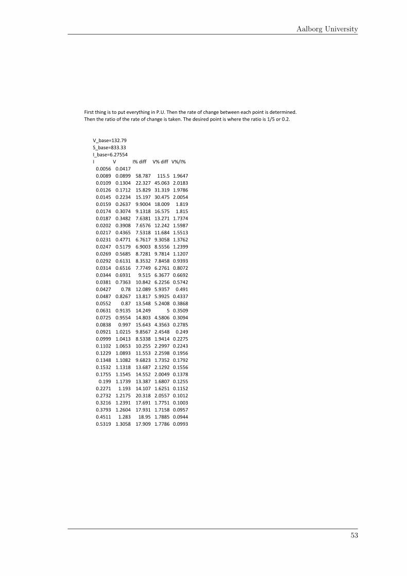
First thing is to put everything in P.U. Then the rate of change between each point is determined.
Then the ratio of the rate of change is taken. The desired point is where the ratio is 1/5 or 0.2.
V_base=132.79
S_base=833.33
I_base=6.27554
I V I% diff V% diff V%/I%
0.0056 0.0417
0.0089 0.0899 58.787 115.5 1.9647
0.0109 0.1304 22.327 45.063 2.0183
0.0126 0.1712 15.829 31.319 1.9786
0.0145 0.2234 15.197 30.475 2.0054
0.0159 0.2637 9.9004 18.009 1.819
0.0174 0.3074 9.1318 16.575 1.815
0.0187 0.3482 7.6381 13.271 1.7374
0.0202 0.3908 7.6576 12.242 1.5987
0.0217 0.4365 7.5318 11.684 1.5513
0.0231 0.4771 6.7617 9.3058 1.3762
0.0247 0.5179 6.9003 8.5556 1.2399
0.0269 0.5685 8.7281 9.7814 1.1207
0.0292 0.6131 8.3532 7.8458 0.9393
0.0314 0.6516 7.7749 6.2761 0.8072
0.0344 0.6931 9.515 6.3677 0.6692
0.0381 0.7363 10.842 6.2256 0.5742
0.0427 0.78 12.089 5.9357 0.491
0.0487 0.8267 13.817 5.9925 0.4337
0.0552 0.87 13.548 5.2408 0.3868
0.0631 0.9135 14.249 5 0.3509
0.0725 0.9554 14.803 4.5806 0.3094
0.0838 0.997 15.643 4.3563 0.2785
0.0921 1.0215 9.8567 2.4548 0.249
0.0999 1.0413 8.5338 1.9414 0.2275
0.1102 1.0653 10.255 2.2997 0.2243
0.1229 1.0893 11.553 2.2598 0.1956
0.1348 1.1082 9.6823 1.7352 0.1792
0.1532 1.1318 13.687 2.1292 0.1556
0.1755 1.1545 14.552 2.0049 0.1378
0.199 1.1739 13.387 1.6807 0.1255
0.2271 1.193 14.107 1.6251 0.1152
0.2732 1.2175 20.318 2.0557 0.1012
0.3216 1.2391 17.691 1.7751 0.1003
0.3793 1.2604 17.931 1.7158 0.0957
0.4511 1.283 18.95 1.7885 0.0944
0.5319 1.3058 17.909 1.7786 0.0993
Aalborg University
53
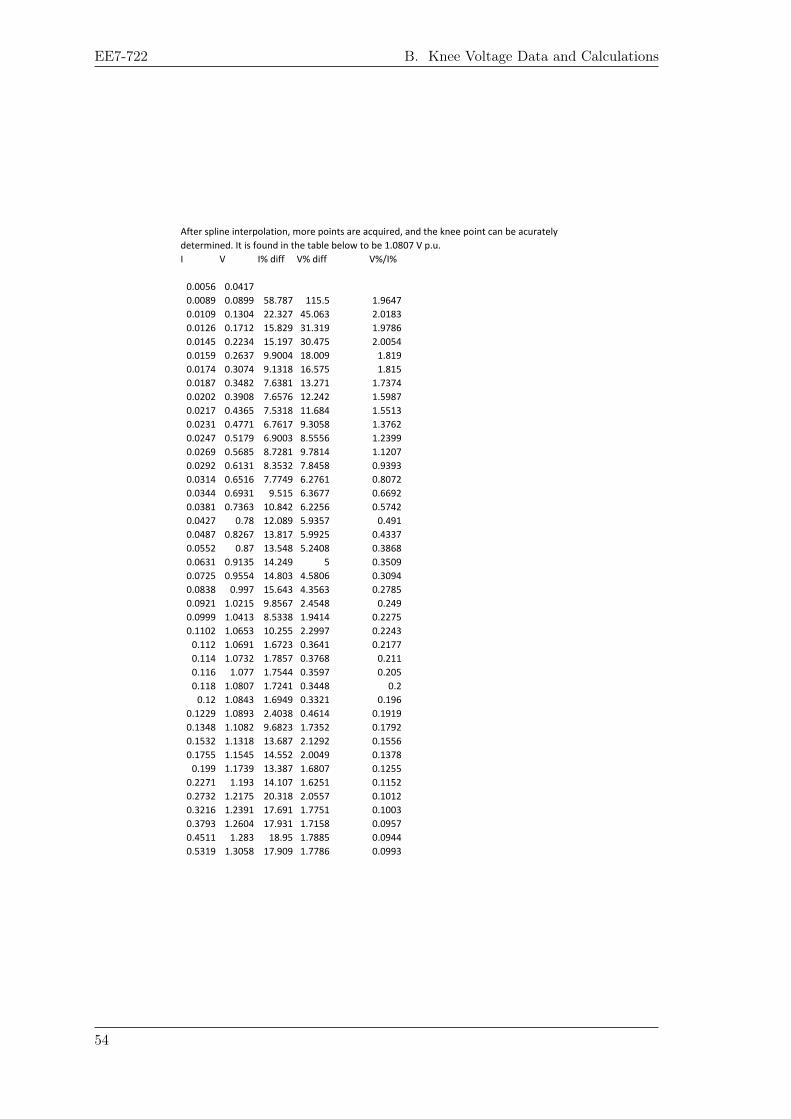
After spline interpolation, more points are acquired, and the knee point can be acurately
determined. It is found in the table below to be 1.0807 V p.u.
I V I% diff V% diff V%/I%
0.0056 0.0417
0.0089 0.0899 58.787 115.5 1.9647
0.0109 0.1304 22.327 45.063 2.0183
0.0126 0.1712 15.829 31.319 1.9786
0.0145 0.2234 15.197 30.475 2.0054
0.0159 0.2637 9.9004 18.009 1.819
0.0174 0.3074 9.1318 16.575 1.815
0.0187 0.3482 7.6381 13.271 1.7374
0.0202 0.3908 7.6576 12.242 1.5987
0.0217 0.4365 7.5318 11.684 1.5513
0.0231 0.4771 6.7617 9.3058 1.3762
0.0247 0.5179 6.9003 8.5556 1.2399
0.0269 0.5685 8.7281 9.7814 1.1207
0.0292 0.6131 8.3532 7.8458 0.9393
0.0314 0.6516 7.7749 6.2761 0.8072
0.0344 0.6931 9.515 6.3677 0.6692
0.0381 0.7363 10.842 6.2256 0.5742
0.0427 0.78 12.089 5.9357 0.491
0.0487 0.8267 13.817 5.9925 0.4337
0.0552 0.87 13.548 5.2408 0.3868
0.0631 0.9135 14.249 5 0.3509
0.0725 0.9554 14.803 4.5806 0.3094
0.0838 0.997 15.643 4.3563 0.2785
0.0921 1.0215 9.8567 2.4548 0.249
0.0999 1.0413 8.5338 1.9414 0.2275
0.1102 1.0653 10.255 2.2997 0.2243
0.112 1.0691 1.6723 0.3641 0.2177
0.114 1.0732 1.7857 0.3768 0.211
0.116 1.077 1.7544 0.3597 0.205
0.118 1.0807 1.7241 0.3448 0.2
0.12 1.0843 1.6949 0.3321 0.196
0.1229 1.0893 2.4038 0.4614 0.1919
0.1348 1.1082 9.6823 1.7352 0.1792
0.1532 1.1318 13.687 2.1292 0.1556
0.1755 1.1545 14.552 2.0049 0.1378
0.199 1.1739 13.387 1.6807 0.1255
0.2271 1.193 14.107 1.6251 0.1152
0.2732 1.2175 20.318 2.0557 0.1012
0.3216 1.2391 17.691 1.7751 0.1003
0.3793 1.2604 17.931 1.7158 0.0957
0.4511 1.283 18.95 1.7885 0.0944
0.5319 1.3058 17.909 1.7786 0.0993
EE7-722 B. Knee Voltage Data and Calculations
54

Open and Short CircuitCalculations C
55
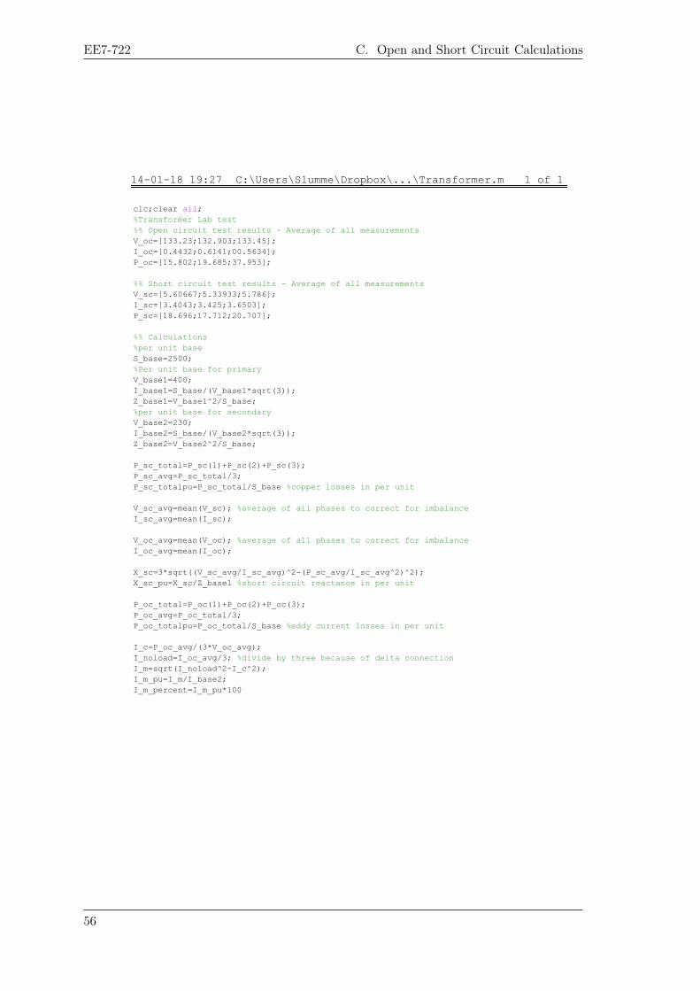
14-01-18 19:27 C:\Users\Slumme\Dropbox\...\Transformer.m 1 of 1
clc;clear all;
%Transformer Lab test
%% Open circuit test results - Average of all measurements
V_oc=[133.23;132.903;133.45];
I_oc=[0.4432;0.6141;00.5634];
P_oc=[15.802;19.685;37.953];
%% Short circuit test results - Average of all measurements
V_sc=[5.60667;5.33933;5.786];
I_sc=[3.4043;3.425;3.6503];
P_sc=[18.696;17.712;20.707];
%% Calculations
%per unit base
S_base=2500;
%Per unit base for primary
V_base1=400;
I_base1=S_base/(V_base1*sqrt(3));
Z_base1=V_base1^2/S_base;
%per unit base for secondary
V_base2=230;
I_base2=S_base/(V_base2*sqrt(3));
Z_base2=V_base2^2/S_base;
P_sc_total=P_sc(1)+P_sc(2)+P_sc(3);
P_sc_avg=P_sc_total/3;
P_sc_totalpu=P_sc_total/S_base %copper losses in per unit
V_sc_avg=mean(V_sc); %average of all phases to correct for imbalance
I_sc_avg=mean(I_sc);
V_oc_avg=mean(V_oc); %average of all phases to correct for imbalance
I_oc_avg=mean(I_oc);
X_sc=3*sqrt((V_sc_avg/I_sc_avg)^2-(P_sc_avg/I_sc_avg^2)^2);
X_sc_pu=X_sc/Z_base1 %short circuit reactance in per unit
P_oc_total=P_oc(1)+P_oc(2)+P_oc(3);
P_oc_avg=P_oc_total/3;
P_oc_totalpu=P_oc_total/S_base %eddy current losses in per unit
I_c=P_oc_avg/(3*V_oc_avg);
I_noload=I_oc_avg/3; %divide by three because of delta connection
I_m=sqrt(I_noload^2-I_c^2);
I_m_pu=I_m/I_base2;
I_m_percent=I_m_pu*100
EE7-722 C. Open and Short Circuit Calculations
56