Embed Size (px)
Citation preview
Different Shades of Risk: Mortality Trends Impliedby Term Insurance Prices⇤
Qiheng Guo†
Department of Risk Management and Insurance. Georgia State University
35 Broad Street. Atlanta, GA 30303. USA
Daniel Bauer‡
Department of Risk Management and Insurance. Georgia State University
35 Broad Street. Atlanta, GA 30303. USA
December 2016
Abstract
To infer forward-looking, market-based mortality trends, we estimate a flex-ible affine stochastic mortality model based on a set of US term life insuranceprices using a generalized method of moments approach. We find that neithermortality shocks nor stochasticity in the aggregate trend seem to affect the prices.In contrast, allowing for heterogeneity in the mortality rates across carriers is cru-cial. We conclude that for life insurance, rather than aggregate mortality risk, thekey risks emanate from the composition of the portfolio of policyholders. Thesefindings have consequences for mortality risk management and emphasize impor-tant directions of mortality-related actuarial research.
Keywords: Mortality Catastrophe. Affine Stochastic Mortality Model. GMMEstimation. Basis Risk. Mortality Heterogeneity.
⇤A previous version was presented at the Twelfth International Longevity Risk and Capital Markets SolutionsConference (Longevity 12) under the title “Mortality Trends Implied by Term Insurance Prices”, and parts aretaken from the earlier working paper “The Risk in Catastrophe Mortality Securitization Transactions” by thesecond author. The authors are grateful for helpful comments from the Longevity 12 conference participants andfor financial support under a Society of Actuaries CAE grant.
†Corresponding author. Phone: +1-(678)-999-6385. Fax: +1-(404)-413-7499. E-mail: [email protected].‡E-mail address: [email protected].
1
DIFFERENT SHADES OF RISK: MORTALITY TRENDS IMPLIED BY TERM INSURANCE PRICES 2
1 Introduction
Term life insurance policies are typically considered to be fairly homogeneous products. Aside
from conversion options and financial strength ratings—the relevance of which is mitigated to
some extent by guaranty funds protection—the ensuing cash flows are typically relative con-
generous across issuers. The key risk factors are investment/interest and mortality risks, where
in view of the former investment opportunities and strategies again do not vary much across
companies. Thus, given competitive forces in this large and undifferentiated market, it seems
proximate to infer forward-looking, market-based estimates of future mortality dynamics from
insurance prices (Mullin and Philipson, 1997).
Building on this logic, we estimate the stochastic mortality model from Bauer and Kramer
(2016) to a set of US (term) life insurance prices using a generalized method of moments
(GMM) approach, where we allow for selection/underwriting effects, surrenders, pertinent
expenses, etc. The model includes a catastrophe component to pick up mortality shocks asso-
ciated with pandemics or natural disasters, a fairly flexible mortality trend component, and a
diffusion term to capture stochastic variations in the mortality trend. Our results are striking:
Neither the catastrophe component nor the diffusion term are significant, and a model com-
parison favors a simple deterministic mortality model. In contrast, allowing for heterogeneity
among the carriers is of utmost importance: A model that does not incorporate differences in
mortality trends between the different companies is strongly rejected. The company effects
are large in magnitude and point towards three possible sub-markets.
Our interpretation is that for pricing and managing term life insurance products—potentially
in contrast to annuity and pension products—the key risks emanate from the composition of
the pool of policyholders, rather than the uncertainty in aggregate mortality trends. Differ-
ences in underwriting criteria, primary distribution channels and distribution area, and other
factors jointly determine the composition of the insurer’s portfolio of policies in each rating
class. The relevant mortality rates for a given company will be based on the demographic
DIFFERENT SHADES OF RISK: MORTALITY TRENDS IMPLIED BY TERM INSURANCE PRICES 3
evolution of this subgroup, and their behavior with regards to lapsing their contracts. Given
heterogeneity in mortality trends for different population subgroups and different causes of
death, the cross-sectional risk dimension dwarfs uncertainties in the aggregate trend. In other
words, basis risk, i.e. the deviation of the experience in the particular pool relative to the
aggregate population, seems to dominate systematic mortality risk, i.e. uncertainties in the ag-
gregate trend component. And, indeed, an active management of the composition of the pool,
by accepting certain risks and rejecting others, may be a way to compete in the marketplace.
Our findings have consequences for mortality risk management and for the corresponding
actuarial literature. On the one side, they do not support assertions that aggregate mortal-
ity risks are important for life insurance products. For instance, papers presenting “natural
hedging” between life insurance and annuity lines as an internal way to manage a company’s
mortality exposure implicitly assume that the corresponding populations of policyholders are
subject to the same variations. Thus, our results cast doubt on the effectiveness of such strate-
gies, pointing to the necessity of market-based solutions for managing longevity. On the other
side, our conclusion that mortality trends for different partitions of the population and differ-
ent conditions determine the mortality profile of the relevant portfolio of policyholders, and
that it may be possible to actively manage this profile, emphasizes the importance of studying
mortality at a more granular level.
Related Literature and Organization of the Paper
A closely related paper to ours is Mullin and Philipson (1997), who argue that under the
assumption that insurance companies are close to risk-neutral with respect to their mortality
exposure, it is possible to derive market-based estimates from zero expected profit (moment)
conditions. In contrast to Mullin and Philipson, however, we include additional institutional
factors affecting life insurance prices such as expenses, selection/underwriting effects, and
policy surrenders/lapses. Furthermore, we consider variations in mortality in the time and
DIFFERENT SHADES OF RISK: MORTALITY TRENDS IMPLIED BY TERM INSURANCE PRICES 4
the cross-sectional (across companies) direction. The latter aspect, in particular, allows us to
draw our primary conclusions. Several papers in the actuarial literature also rely on prices of
insurance products to obtain parameters in mortality models. In particular, Lin and Cox (2005)
and Bauer et al. (2010) use annuity quotes to estimate risk premiums for longevity risk.
In the estimation process, we use the stochastic mortality model from Bauer and Kramer
(2016). As discussed in their paper, the model is flexible enough to fit a relatively long time
series of US mortality data, it includes a mortality catastrophe component, and it is tractable.
The latter property originates from it falling in the class of affine mortality models (Biffis,
2005; Dahl and Møller, 2006). In particular, this allows for an efficient computation of sur-
vival probabilities and, thus, basic life insurance prices, which is essential for our estimation
approach.
Our results relate to recent results in the economic and medical literature on the het-
erogeneity of mortality trends across different subpopulations that show that there are large
disparities in life expectancy between different racial, regional, and socio-economic groups
(Chetty et al., 2016; Case and Deaton, 2015). Furthermore, they relate and endorse analyses
of cause-specific mortality rates, and how these in aggregate affect the mortality of a certain
population (Arnold et al., 2016; Arnold and Sherris, 2016, and references therein). An in-
surer’s underwriting process, together with its regional presence, its advertising strategy, etc.,
determines the composition of the portfolio of policyholders, and it is the mortality dynamics
of that group that is relevant for the insurer’s future cash flows.
As indicated, our findings are relevant for so-called “natural hedging” approaches to man-
aging longevity risk by trading off annuity and life insurance exposures (Cox and Lin, 2007;
Li and Haberman, 2015, and references therein). In particular, our results suggest that beyond
difficulties with natural hedging within the same population (Zhu and Bauer, 2015), basis risk
may inhibit the effectiveness of such strategies.
The remainder of the paper is structured as follows: Section 2 introduces the affine mor-
DIFFERENT SHADES OF RISK: MORTALITY TRENDS IMPLIED BY TERM INSURANCE PRICES 5
tality model from Bauer and Kramer (2016) with some extensions to suit our setting. Section
3 introduces our GMM estimation method, presents results, and their discussion. Finally,
Section 4 concludes.
2 Model
In what follows, we introduce the mortality model from Bauer and Kramer (2016), which
we rely on in the remainder of the text. As discussed in their paper, the model consists of
three parts: 1) a catastrophe component, 2) an age-dependent affine mortality component,
and 3) a temporary component. In contrast to their analysis, we use the third part to include
selection/underwriting effects, rather than a temporary deterministic trend. Furthermore, we
subsequently augment the model by company, risk class, and calendar year effects that account
for heterogeneity in mortality trends.
As in Bauer and Kramer (2016), we introduce the stochastic force of mortality by relying
on conventional concepts from credit risk modeling (Lando, 1998). More precisely, it given
a stochastic process X = (Xt
)0tT
and positive, continuous function µ(·, ·), we define an
individual’s time of death as the first jump time of a Cox-process with intensity µ(x0 + t,Xt
):
⌧x0 = inf
⇢t :
Zt
0
µ(x0 + s,Xs
) ds � E
�, (1)
where E is a Exp(1)-distributed random variable and independent among individuals.
Considering only one single insured for now, let the filtrations G = (Gt
)0tT
⇤ and
H = (Ht
)0tT
⇤ be given as the augmentations of the filtrations generated by (Xt
)0tT
⇤
and�1{⌧
x0t}�0tT
⇤ , respectively, and set Ft
= Gt
_ Ht
. From Equation (1), we can then
derive the (T � t)-year survival probability at time t for an xt
= x0 + t year old individual as
T�t
px
t
(t) := E⇥
1{⌧x0>T}
��Gt
, ⌧x0 > t
⇤= E
exp
⇢�Z
T
t
µ (x0 + s,Xs
) ds
�����Gt
, ⌧x0 > t
�,

DIFFERENT SHADES OF RISK: MORTALITY TRENDS IMPLIED BY TERM INSURANCE PRICES 6
(2)
and, from results of Lando (1998),
E⇥
1{⌧x0>T}
��Ft
⇤= 1{⌧
x0>t} T�t
px0+t
(t)
Following Bauer and Kramer (2016), we use the following model for the baseline stochas-
tic force of mortality:
µt
(x0) = µ(x0 + t, Yt
,�t
) = eb (x0+t) Yt
+ �
t
+Dt
(x0), �0, Y0 > 0. (3)
The catastrophe component follows the dynamics:
d�t
= ��t
dt+ dJt
, �0 � 0,
where (Jt
) is a compound Poisson process with intensity � and Exp(⇠)-distributed jumps.
And the baseline component follows the dynamics:
dYt
= ↵
�Y0 � �(2)
�| {z }
�
(3)
e��
(1)t
+ �(2) � Yt
!dt+ �
pYt
dWt
, Y0 > 0,
where (Wt
)0tT
⇤ is a one-dimensional Brownian motion and ↵, �(1), �(2), and � are positive
constants with ↵ 6= �(1). �(2)+ �(3) describes the trend level at time 0. We refer to their paper
for the motivation of the model in the context of demographic research.
We use the temporary component Dt
(x0) to introduce selection effects acting to temporary
reduce mortality. Here the selection effect does not refer to the potential impact of adverse se-

DIFFERENT SHADES OF RISK: MORTALITY TRENDS IMPLIED BY TERM INSURANCE PRICES 7
lection on life insurance prices but the impact of underwriting during the early policy years.1 In
particular, this is important for the evaluation of life insurance prices as here mandatory health
examinations lead to significant selection effects. Within our model, this can be captured via
the temporary component D by a roughly proportional structure akin to a proportional hazards
model:
Dt
(x0) = c� �c+ eb(x0+t) ⌧
�⇥ �¯T⇥ (
¯T � t)+.
Note that the component is still deterministic and it is only roughly proportional since we
use an approximation of the relevant force of mortality based on the initial values. Moreover,
this specification of D only relies on the four additional parameters (c, ⌧ , �, ¯T ) minding the
complexity of the estimation process. We obtain:
¯Dt,T
(x0) =
ZT
t
Ds
(x0) ds
= c (T � t)� c�¯T
h�(
¯T � t)+�2 � �
(
¯T � T )+�2i
�⌧ �¯Tb
⇥(
¯T � T )+ exp
�b(x0 +min{T, ¯T )} � (
¯T � t)+ exp
�b(x0 +min{t, ¯T )} ⇤
� ⌧ �¯Tb2
⇥exp
�b(x0 +min{T, ¯T}) � exp
�b(x0 +min{t, ¯T}) ⇤ .
The (exponential-)affine structure enables us to write down an analytical representation of the
survival function (cf. Prop. 1 in Duffie et al. (2000)):
T�t
px0+t
(t) = exp
⇢u(T � t) + v(T � t)Y
t
� �
t
�1� e�(T�t)
�� �(T � t)
⇣+ 1
�
⇥ exp
⇢�⇣
⇣+ 1
log
1 +
1
⇣
�1� e�(T�t)
��� ¯Dt,T
(x0)
�, (4)
1In insurance practice, actuaries rely on so-called “select-and-ultimate” tables to account for this type ofselection, where the “select” tables used in early policy years display lower mortality due to underwriting exam-inations.

DIFFERENT SHADES OF RISK: MORTALITY TRENDS IMPLIED BY TERM INSURANCE PRICES 8
where u and v satisfy the following Riccatti ODEs:
v0(s) = �eb(x0+T�s) � ↵ v(s) +1
2
�2 v2(s), v(0) = 0,
u0(s) = v(s)↵
⇣e��
(1) (T�s) Y0 + (1� e��
(1) (T�s)) �(2)
⌘, u(0) = 0. (5)
Here, µt
(x0) andT�t
px0+t
(t) represent the baseline force of mortality and survival function,
respectively.
We introduce heterogeneity in mortality trends by assuming that the aggregate force of
mortality in each company’s portfolio is proportional to the baseline. Thus, the force of mor-
tality for company i can be written as:
µi
t
(x0) = µt
(x0)(1 + Eco
i
),X
i
Eco
i
= 0, i = 1, 2, ..., I
where Eco
i
is the company effect. We can further add the risk class effect Erc
j
and calendar
year effect Eyear
h
to the model to account for variation within a company and across different
calendar year:
µ(i,j,h)t
(x0) = µt
(x0)(1 + Eco
i
+ Erc
j
+ Eyear
h
),
X
i
Eco
i
=
X
j
Erc
j
=
X
h
Eyear
h
= 0, Eco
i
+ Erc
j
+ Eyear
h
> �1 8i, j, h
with risk class j ranges from 1 (highest mortality risk, e.g. regular class) to J (lowest
mortality risk, e.g. preferred plus class) and year h spans all calendar years of insurance
prices. The three effect components do not relate to the industry baseline force of mortality.
Therefore, the survival function for company i, risk class j in calendar year h is:
T�t
p(i,j,h)x0+t
(t) =T�t
px0+t
(t)(1+E
co
i
+E
rc
j
+E
year
h
)
Given risk class, calendar year, and company effect parameters, it remains to calculate the sur-
DIFFERENT SHADES OF RISK: MORTALITY TRENDS IMPLIED BY TERM INSURANCE PRICES 9
vival function (4) and actuarial present values by simply solving the ODEs from Equation (5).
The full analytical representation of the survival function facilitates the estimation process.
3 Estimation to Insurance Price Data
3.1 Insurance Price GMM Estimator
We are given annual term-insurance premiums P(i,j,h)x,n
for age x, term n, risk class j 21, 2, ..., J , calendar year h 2 1, 2, ..., H and a fixed benefit B payable upon death at the end
of the year of from I companies, i.e. i 2 {1, 2, . . . , I}, which we take to be i.i.d. Denote by Cthe collection of all available age-term combinations (x, n) and we have N
x,n
such combina-
tion. As is common in actuarial modeling and in contrast to Mullin and Philipson (1997), we
consider various types of expenses to be reflected in our insurance price data. In particular, we
include initial expenses both as a percentage of the first premium c(1)IP
and as a fixed amount
depending on the death benefit c(2)IP
, as well as a fixed maintenance expense cM
(Society of
Actuaries, 2004).
We assume policyholders surrender at a fixed proportion q(l)u
in policy year u, u � 1,
immediately before premiums become due. Thus, policies remain in force for k years with a
probability of
k
p(⌧)x0(0) =
k
p(i,j,h)x0
(0)
Y
1uk
(1� q(l)u
)
| {z }k
p
(l)x0
, k � 1.
Upon surrendering at time k, policyholders may be entitled to so-called cash surrender values
(CSVs)k
C(i,j,h)x,n
, which are to be calculated according to the National Association of Insur-
ance Commissioners’ (NAIC) Standard Nonforfeiture Law for Life Insurance. This regulation
essentially entails the calculation of guaranteed reserve levels according to given interest rates,
a given mortality table, and given expense levels. For the simplicity of model, we assume the
DIFFERENT SHADES OF RISK: MORTALITY TRENDS IMPLIED BY TERM INSURANCE PRICES 10
cost and surrender probabilities are the same across all companies.2
We start by writing down the an insurance company’s loss function, or the negative profit
function:
f(✓, P (i,j,h)x,n
) =P
n�1k=0 p(0, k + 1)
hk
p(l)x
⇣k
p(i,j,h)x
(0)�k+1p
(i,j,h)x
(0)⌘B +
k+1p(i,j,h)x
q(l)k+1 k+1Cx,n
i
+c(2)IP
+ cM
Pn�1k=0 p(0, k) kp
(⌧)x0 (0)� P
(i,j,h)x,n
⇣Pn�1k=0 p(0, k) kp
(⌧)x0 (0)� c
(1)IP
⌘,
(6)
where p(t, ⌧) denotes the time t price of a zero coupon bond with maturity t + ⌧ . Of course,
equation (6) depends on the (risk-neutral) parameters of the mortality model as well as on the
parameters governing expenses, selection, and surrenders, which we stack in the parameter
vector ✓. The key assumption is now that the so-called equivalence principle holds, i.e. that
the expected present value of future benefits (including expenses) equals the expected present
value of future premiums for all of the company’s policies for one mortality profile, that is, for
one risk class in one calendar year. Thus, the equivalence principle must hold for each i, j,
and h combination. That is to say, for each company every risk class in one calendar year, the
expected profit (loss) from selling insurance contracts is zero. Therefore, we can write down
our moment conditions for GMM estimation as follows:
Ex,n
⇥f(✓, P (i,j,h)
x,n
)
⇤= 0, (x, n) 2 C.
The efficient GMM estimator can be obtained using so-called “two-step feasible GMM”
method, which yields efficient and consistent estimators. First, choose a weighting matrix W ,
where W is a I ⇥ J ⇥ H dimensional square matrix. W can be any such matrix in the first2This assumption, again, is motivated by competitive pressures in the market. Large differences in costs
should be competed away unless they are linked to aspects relating to underlying heterogeneity.
DIFFERENT SHADES OF RISK: MORTALITY TRENDS IMPLIED BY TERM INSURANCE PRICES 11
step. We choose W such that
W�1= diag
��2x,n
, (x, n) 2 C ,
where �2x,n
= Var [Px,n
] with corresponding sample version �2x,n
. We obtain a GMM estimate
ˆ✓1 by minimizing the following function of ✓:
ˆ✓1 = argmin
✓
"1
Nx,n
N
x,nX
x,n
f(✓, P (i,j,h)x,n
)
#0
(i,j,h)
W
"1
Nx,n
N
x,nX
x,n
f(✓, P (i,j,h)x,n
)
#
(i,j,h)
, (7)
Then, we update the weighting matrix using ˆ✓1:
ˆW (
ˆ✓1)�1
= diag
(1
Nx,n
N
x,nX
j=1
⇣f(ˆ✓1, P
(i,j,h)x,n
)
⌘2
, (i, j, h)
)(8)
and minimize function (7) using W =
ˆW (
ˆ✓1) to obtain our estimate ˆ✓. We carry out both
minimization numerically.
3.2 Data and Estimation
We use quotes for annual life insurance premiums from the CompuLife price quotation system
(historical data) for April 2012, 2013, 2014 and 2015. More precisely, we focus on contracts
with a face amount of $500,000 for male non-smokers under two underwriting categories:
regular (Rg, residual standard), and preferred plus (Pf+, super preferred). From 31 companies,
we retrieved data for 33 age-term combinations, with terms of 10, 15, 20, and 30 years, and
ages from 25 to 75, where for numerical convenience we use ages of multiple of five only.
We only allow for a single quote per company per age/term-combination. Since the records
include several instances of multiple quotes from the same company for different states—
though prices usually coincide—we averaging over these quotes. All in all, we rely on 7,688
DIFFERENT SHADES OF RISK: MORTALITY TRENDS IMPLIED BY TERM INSURANCE PRICES 12
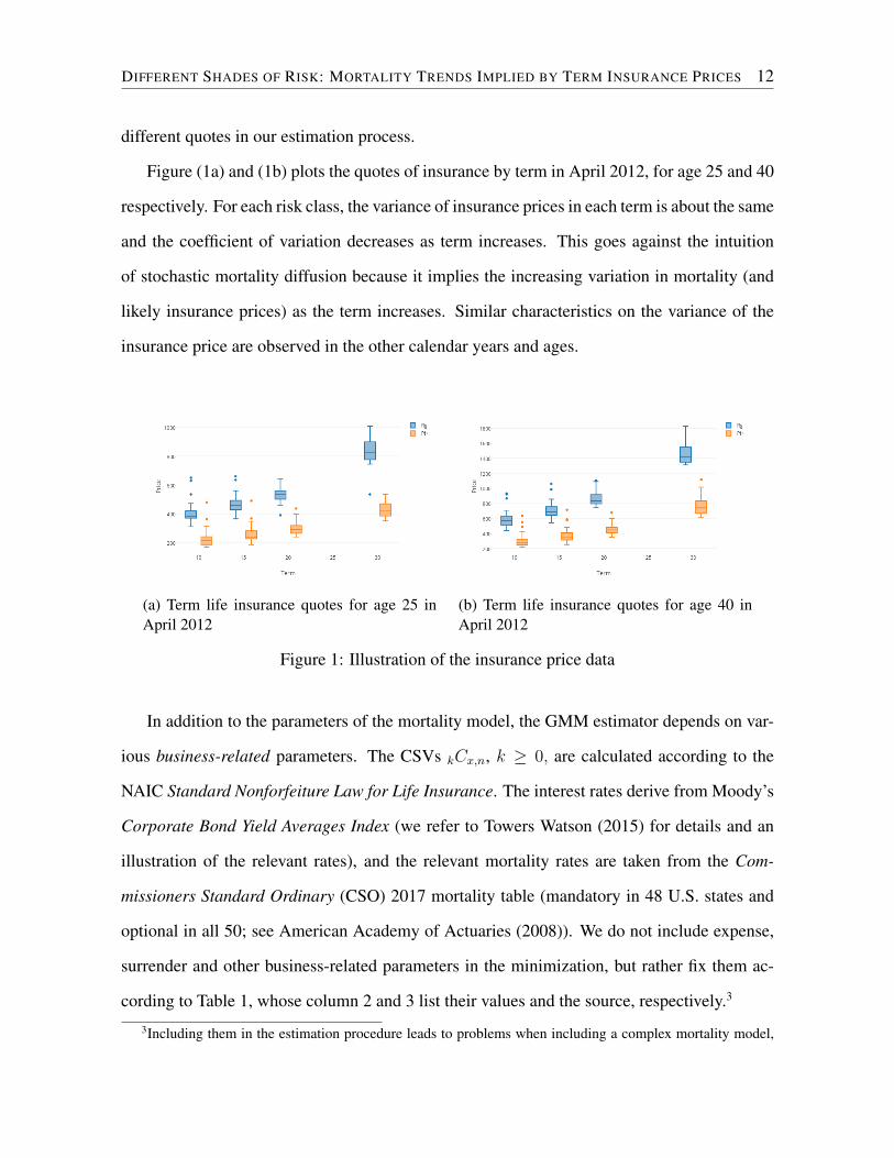
different quotes in our estimation process.
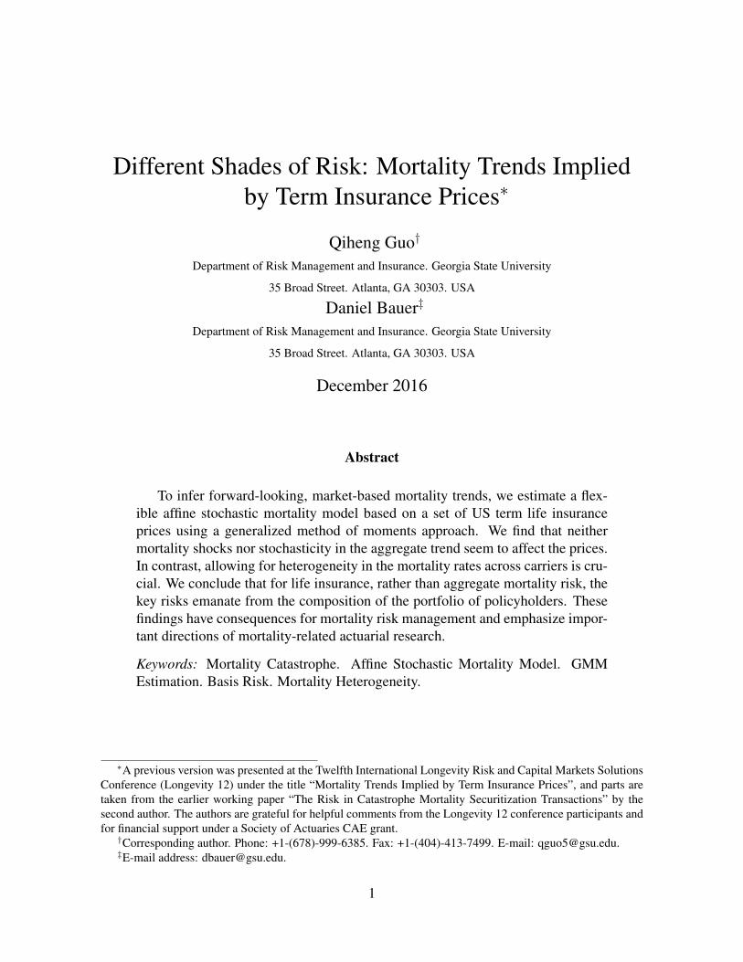
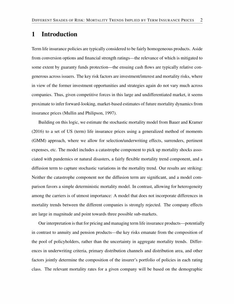
Figure (1a) and (1b) plots the quotes of insurance by term in April 2012, for age 25 and 40
respectively. For each risk class, the variance of insurance prices in each term is about the same
and the coefficient of variation decreases as term increases. This goes against the intuition
of stochastic mortality diffusion because it implies the increasing variation in mortality (and
likely insurance prices) as the term increases. Similar characteristics on the variance of the
insurance price are observed in the other calendar years and ages.
(a) Term life insurance quotes for age 25 inApril 2012
(b) Term life insurance quotes for age 40 inApril 2012
Figure 1: Illustration of the insurance price data
In addition to the parameters of the mortality model, the GMM estimator depends on var-
ious business-related parameters. The CSVsk
Cx,n
, k � 0, are calculated according to the
NAIC Standard Nonforfeiture Law for Life Insurance. The interest rates derive from Moody’s
Corporate Bond Yield Averages Index (we refer to Towers Watson (2015) for details and an
illustration of the relevant rates), and the relevant mortality rates are taken from the Com-
missioners Standard Ordinary (CSO) 2017 mortality table (mandatory in 48 U.S. states and
optional in all 50; see American Academy of Actuaries (2008)). We do not include expense,
surrender and other business-related parameters in the minimization, but rather fix them ac-
cording to Table 1, whose column 2 and 3 list their values and the source, respectively.3
3Including them in the estimation procedure leads to problems when including a complex mortality model,
DIFFERENT SHADES OF RISK: MORTALITY TRENDS IMPLIED BY TERM INSURANCE PRICES 13
Parameter Value Source
c(1)IP
60% Avg. values from the 2005c(2)IP
$882.5 “Generally Recognized Expense Table”cM
$45 (see e.g. Society of Actuaries (2004))
¯T 18 years Avg. value from Society of Actuaries (2007)� 60% Value matched to CSO 2017 mort. table
qi
15%, i 3, Roughly matches pattern (non-renewable)5%, i > 3 according to LIMRA and SOA (2005)
Table 1: Parameters relevant to the insurance contracts.
For the numerical optimization in (7), we rely on Julia language and apply the COBYLA
(constrained optimization by linear approximation) algorithm, suitable for a minimization task
with a large number of equality and inequality constraints of the parameters. For the numer-
ical solution of the ordinary differential equations arising in each time step, we rely on an
implementation of a Runge-Kutta method with a variable time step as available within Julia
(ode45).
We estimate five versions of the model. The first model version (Full model) includes
catastrophe component parameters (, � and ⇣). In the second version (w/o CAT), we exclude
the catastrophe component. In the third model (w/o Sigma), we assume that the stochastic dif-
fusion parameter � is zero. In the fourth model (w/o Trend), we set the trend parameters �1 and
�3 to zero so that Yt
is fixed at �2. The fifth model (w/o Co. effect) takes away company effect
from the w/o CAT model. We record the estimates, standard errors and also a likelihood-like
J-statistics, which is the basis for testing the overall specification and parametric restrictions
since the impact on insurance prices is similar to those originating from certain components. We obtain reason-able magnitudes not too different from the set values in the context of simple mortality models.
DIFFERENT SHADES OF RISK: MORTALITY TRENDS IMPLIED BY TERM INSURANCE PRICES 14
as in Sargan (1958) and Hansen (1982). It is calculated as follows:
J = Nx,n
"1
Nx,n
N
x,nX
x,n
f(ˆ✓, P (i,j,h)x,n
)
#0
(i,j,h)
W (
ˆ✓)
"1
Nx,n
N
x,nX
x,n
f(ˆ✓, P (i,j,h)x,n
)
#
(i,j,h)
J , a Wald statistic, converges in distribution to �2(L�K) under the null hypothesis that the
model is valid, or well specified, where L is the number of moment equations and K is the
number of parameters. In terms of testing parametric restrictions, according to Newey and
West (1987), the difference of two J-statistics, the GMM counterpart to the likelihood ratio
test statistic, converges in distribution to �2(K1 � K2), where K1 � K2 is the number of
restricted parameters in model 2 compared to model 1. This “Likelihood-ratio-like” statistic
can be used to test the parameter restrictions and offer guidance to model comparison, which
is highlighted in the next part.
3.3 Results and Discussion
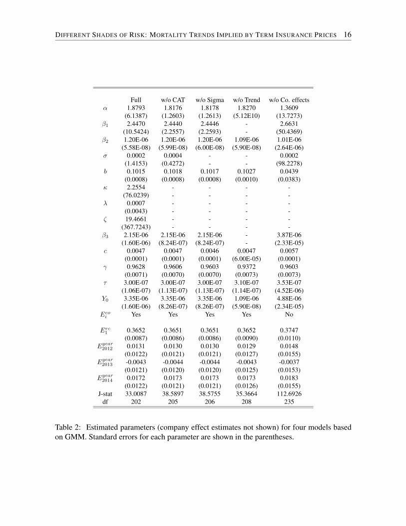
Table 2 provides the parameter estimates for all five model versions, with the first four hav-
ing the company effect parameters. In the Full model, the catastrophe parameter estimates
(, �, ⇣) have large standard errors and are not significant, so do the trend parameter �1 and
diffusion parameter �. In contrast, the trend parameter �2 and Gompertz parameter b are
significant, pointing to a simple deterministic mortality model. Parameters related to selec-
tion/underwriting effect (c, ⌧ , �) are significant in the first four model estimations, highlighting
such effect in life insurance underwriting.
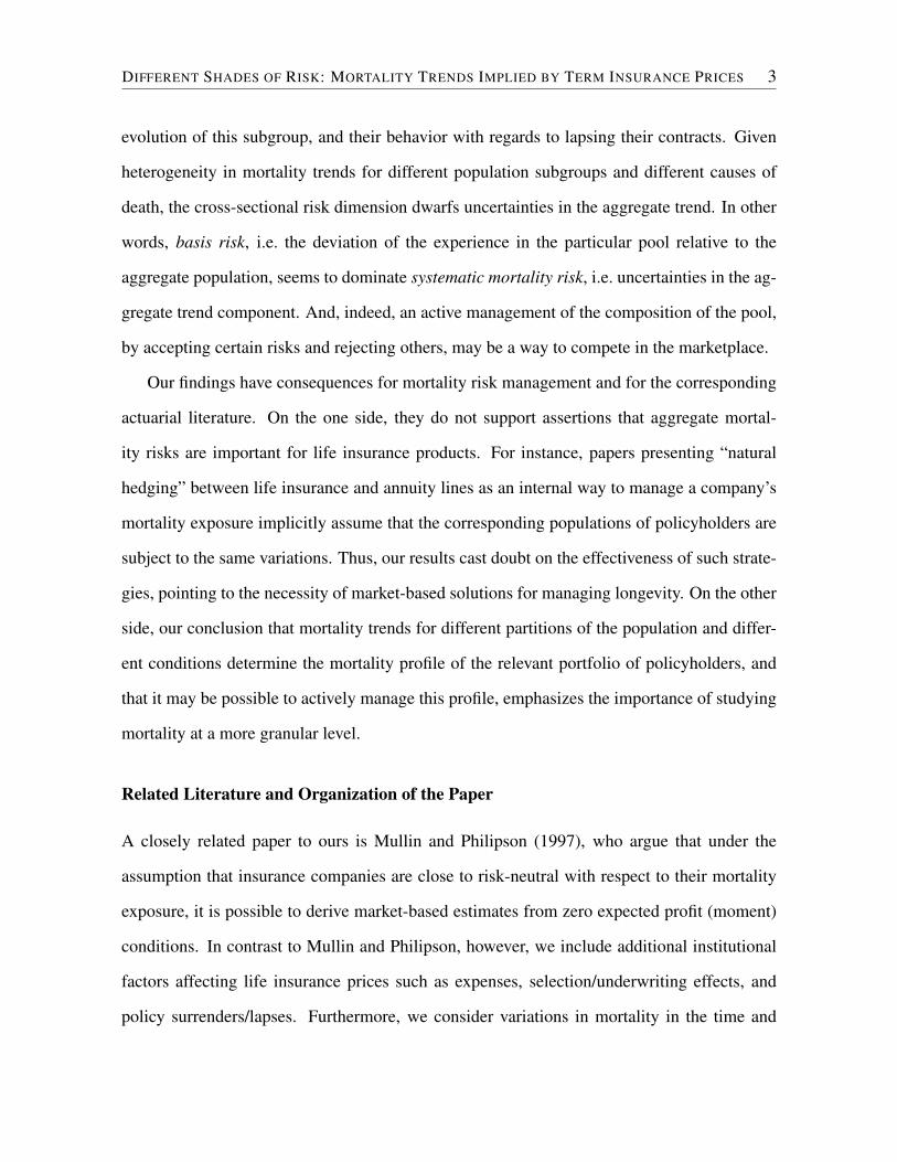
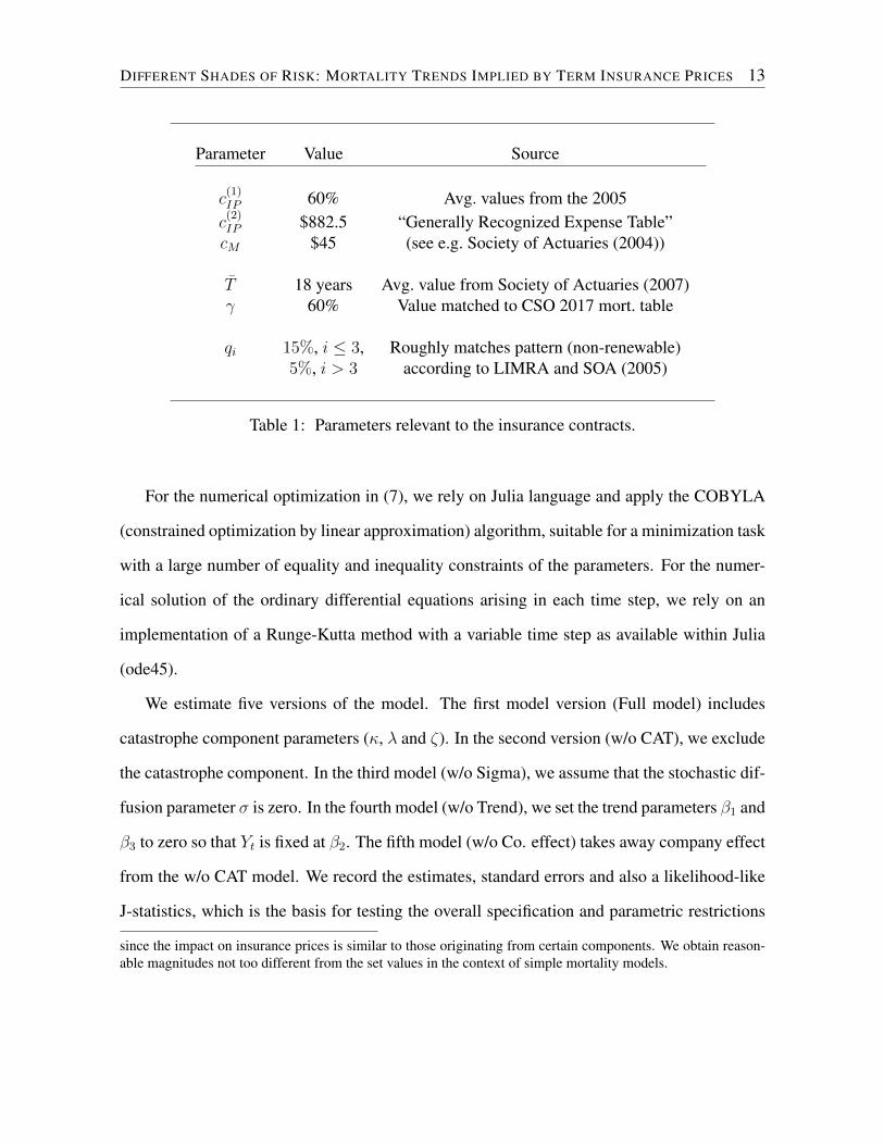
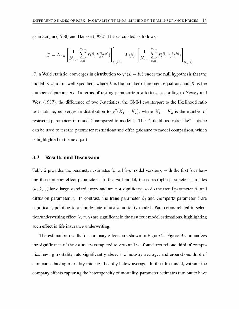
The estimation results for company effects are shown in Figure 2. Figure 3 summarizes
the significance of the estimates compared to zero and we found around one third of compa-
nies having mortality rate significantly above the industry average, and around one third of
companies having mortality rate significantly below average. In the fifth model, without the
company effects capturing the heterogeneity of mortality, parameter estimates turn out to have
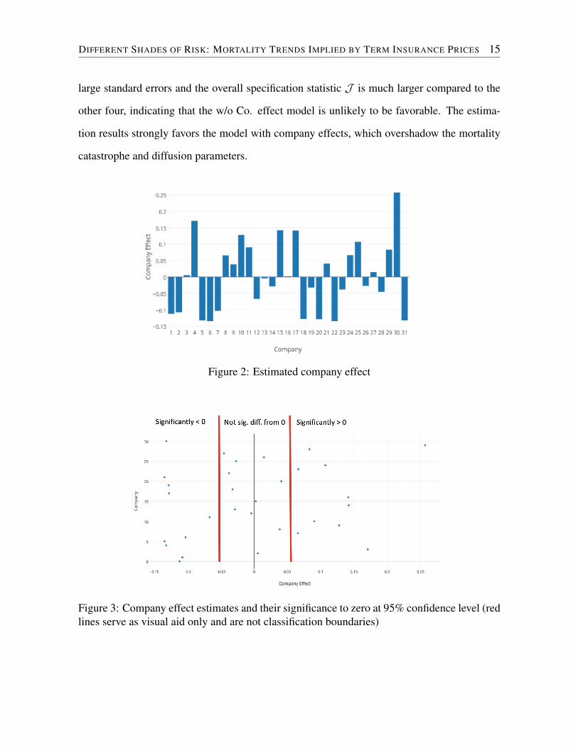
DIFFERENT SHADES OF RISK: MORTALITY TRENDS IMPLIED BY TERM INSURANCE PRICES 15
large standard errors and the overall specification statistic J is much larger compared to the
other four, indicating that the w/o Co. effect model is unlikely to be favorable. The estima-
tion results strongly favors the model with company effects, which overshadow the mortality
catastrophe and diffusion parameters.
Figure 2: Estimated company effect
Figure 3: Company effect estimates and their significance to zero at 95% confidence level (redlines serve as visual aid only and are not classification boundaries)
DIFFERENT SHADES OF RISK: MORTALITY TRENDS IMPLIED BY TERM INSURANCE PRICES 16
Full w/o CAT w/o Sigma w/o Trend w/o Co. effects↵ 1.8793 1.8176 1.8178 1.8270 1.3609
(6.1387) (1.2603) (1.2613) (5.12E10) (13.7273)�1 2.4470 2.4440 2.4446 - 2.6631
(10.5424) (2.2557) (2.2593) - (50.4369)�2 1.20E-06 1.20E-06 1.20E-06 1.09E-06 1.01E-06
(5.58E-08) (5.99E-08) (6.00E-08) (5.90E-08) (2.64E-06)� 0.0002 0.0004 - - 0.0002
(1.4153) (0.4272) - - (98.2278)b 0.1015 0.1018 0.1017 0.1027 0.0439
(0.0008) (0.0008) (0.0008) (0.0010) (0.0383) 2.2554 - - - -
(76.0239) - - - -� 0.0007 - - - -
(0.0043) - - - -⇣ 19.4661 - - - -
(367.7243) - - - -�3 2.15E-06 2.15E-06 2.15E-06 - 3.87E-06
(1.60E-06) (8.24E-07) (8.24E-07) - (2.33E-05)c 0.0047 0.0047 0.0046 0.0047 0.0057
(0.0001) (0.0001) (0.0001) (6.00E-05) (0.0001)� 0.9628 0.9606 0.9603 0.9372 0.9603
(0.0071) (0.0070) (0.0070) (0.0073) (0.0073)⌧ 3.00E-07 3.00E-07 3.00E-07 3.10E-07 3.53E-07
(1.06E-07) (1.13E-07) (1.13E-07) (1.14E-07) (4.52E-06)Y0 3.35E-06 3.35E-06 3.35E-06 1.09E-06 4.88E-06
(1.60E-06) (8.26E-07) (8.26E-07) (5.90E-08) (2.34E-05)Eco
i
Yes Yes Yes Yes No
Erc
1 0.3652 0.3651 0.3651 0.3652 0.3747(0.0087) (0.0086) (0.0086) (0.0090) (0.0110)
Eyear
2012 0.0131 0.0130 0.0130 0.0129 0.0148(0.0122) (0.0121) (0.0121) (0.0127) (0.0155)
Eyear
2013 -0.0043 -0.0044 -0.0044 -0.0043 -0.0037(0.0121) (0.0120) (0.0120) (0.0125) (0.0153)
Eyear
2014 0.0172 0.0173 0.0173 0.0173 0.0183(0.0122) (0.0121) (0.0121) (0.0126) (0.0155)
J-stat 33.0087 38.5897 38.5755 35.3664 112.6926df 202 205 206 208 235
Table 2: Estimated parameters (company effect estimates not shown) for four models basedon GMM. Standard errors for each parameter are shown in the parentheses.
DIFFERENT SHADES OF RISK: MORTALITY TRENDS IMPLIED BY TERM INSURANCE PRICES 17
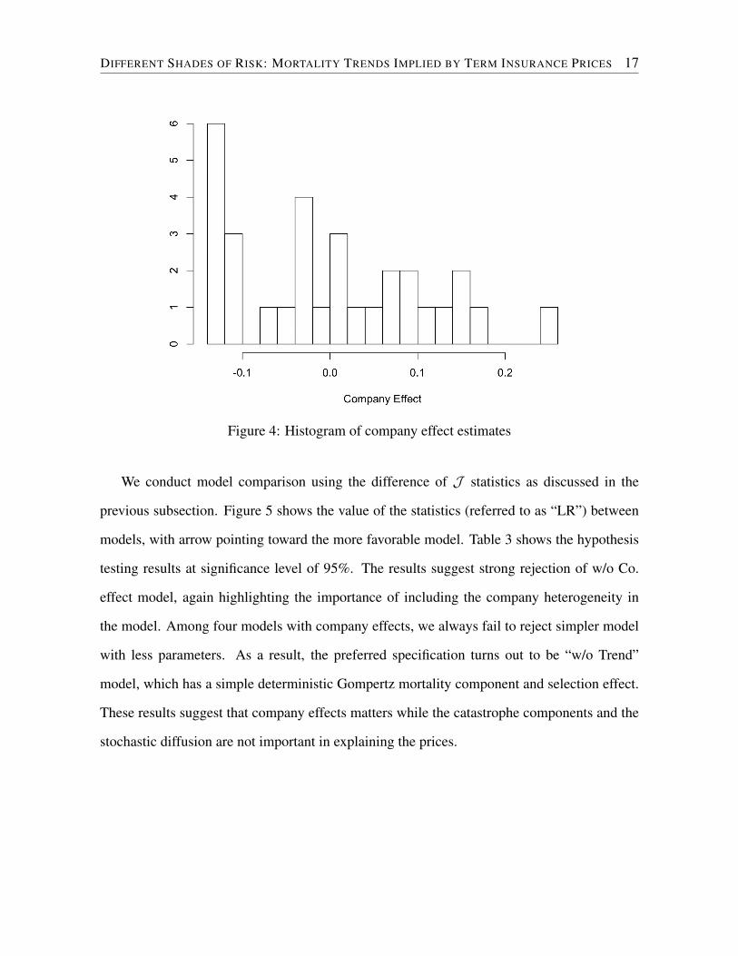
Figure 4: Histogram of company effect estimates
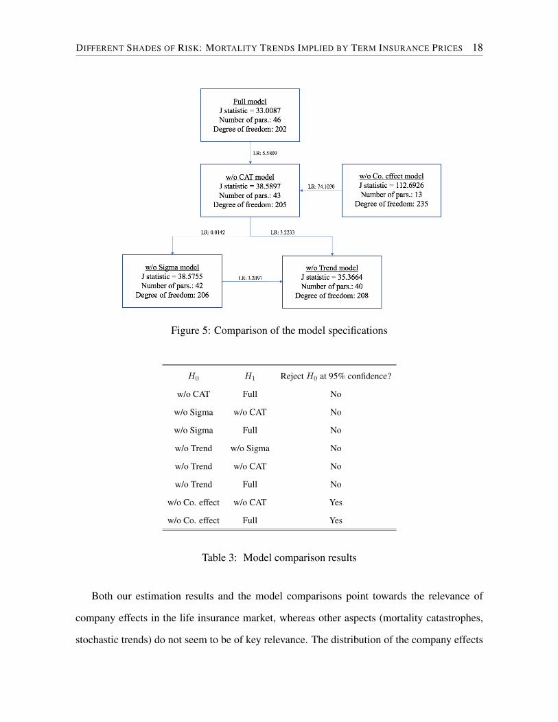
We conduct model comparison using the difference of J statistics as discussed in the
previous subsection. Figure 5 shows the value of the statistics (referred to as “LR”) between
models, with arrow pointing toward the more favorable model. Table 3 shows the hypothesis
testing results at significance level of 95%. The results suggest strong rejection of w/o Co.
effect model, again highlighting the importance of including the company heterogeneity in
the model. Among four models with company effects, we always fail to reject simpler model
with less parameters. As a result, the preferred specification turns out to be “w/o Trend”
model, which has a simple deterministic Gompertz mortality component and selection effect.
These results suggest that company effects matters while the catastrophe components and the
stochastic diffusion are not important in explaining the prices.
DIFFERENT SHADES OF RISK: MORTALITY TRENDS IMPLIED BY TERM INSURANCE PRICES 18
Figure 5: Comparison of the model specifications
H0 H1 Reject H0 at 95% confidence?
w/o CAT Full No
w/o Sigma w/o CAT No
w/o Sigma Full No
w/o Trend w/o Sigma No
w/o Trend w/o CAT No
w/o Trend Full No
w/o Co. effect w/o CAT Yes
w/o Co. effect Full Yes
Table 3: Model comparison results
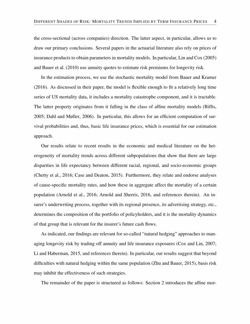
Both our estimation results and the model comparisons point towards the relevance of
company effects in the life insurance market, whereas other aspects (mortality catastrophes,
stochastic trends) do not seem to be of key relevance. The distribution of the company effects
DIFFERENT SHADES OF RISK: MORTALITY TRENDS IMPLIED BY TERM INSURANCE PRICES 19
takes a roughly tri-modal shape as shown in Figure 4, with several company bunching at
positive effects (worse mortality experience) around 0.1, some companies bunching around
0 (average mortality experience), and some companies bunching with negative effect (better
mortality experience) around -0.1, also seen in Figure 3. The results suggests that there are
roughly three segments in the market.
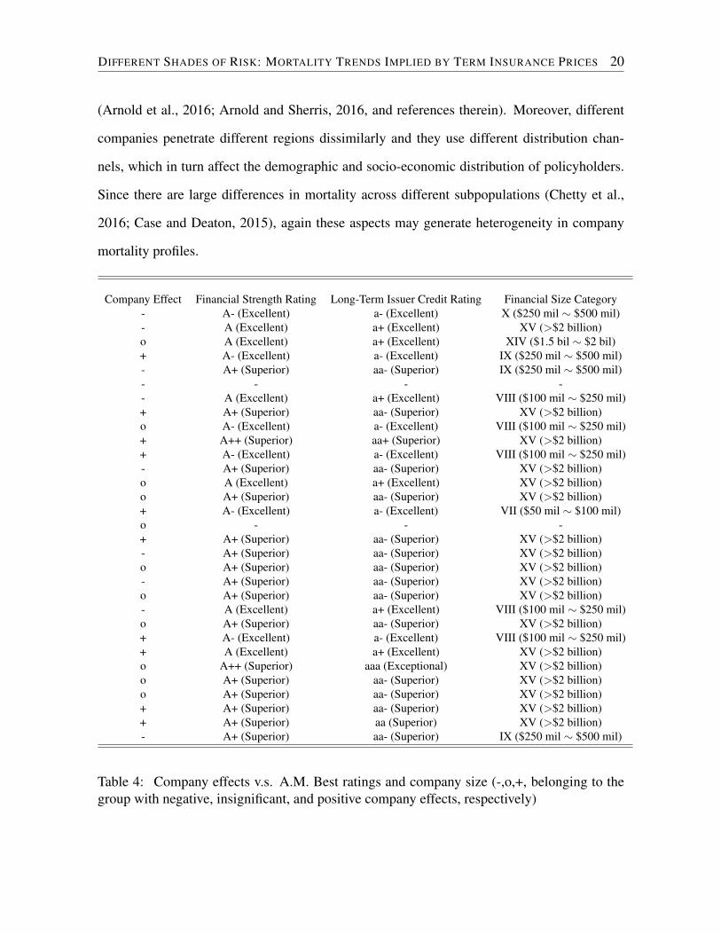
We retrieved information from A.M. Best to check whether these groups can be explained
by company characteristics. More precisely, from A.M. Best Rating/Information Services,
we obtain company ratings and company size (two companies’ information are not available).
Here, financial strength rating means A.M. Best’s independent opinion of “an insurer’s finan-
cial strength and ability to meet its ongoing insurance policy and contract obligations” and
issuer credit rating refers to A.M. Best’s independent opinion of “an entity’s ability to meet its
ongoing financial obligations”. Table 4 provides the information together with the company
effects from our estimation. In addition to including the effect, we code the companies ac-
cording to the three segments, -,o,+, belonging to the group with negative, insignificant, and
positive company effects, respectively.
There are no obvious relationships to company size or company ratings. There are very
highly rated companies and very large companies in each segment, and there are smaller and
relatively low-rated companies in each segment. In other words, company characteristics do
not seem to explain the market segmentation—or, more generally, the significant heterogeneity
in prices. Thus, it appears that differences in the pools of policyholders between companies
must lead to the segmentation.
These differences in the mortality profile of each company’s risk profile may arise from
different channels. First, underwriting criteria, and particularly the categorization of individ-
uals with a certain health history to rating classes, differ among carriers. Since in the end the
mortality experience is driven by morbidity rates and cause-specific mortality rates, and since
these in aggregate shape the mortality profile of the relevant pool, heterogeneity may arise
DIFFERENT SHADES OF RISK: MORTALITY TRENDS IMPLIED BY TERM INSURANCE PRICES 20
(Arnold et al., 2016; Arnold and Sherris, 2016, and references therein). Moreover, different
companies penetrate different regions dissimilarly and they use different distribution chan-
nels, which in turn affect the demographic and socio-economic distribution of policyholders.
Since there are large differences in mortality across different subpopulations (Chetty et al.,
2016; Case and Deaton, 2015), again these aspects may generate heterogeneity in company
mortality profiles.
Company Effect Financial Strength Rating Long-Term Issuer Credit Rating Financial Size Category- A- (Excellent) a- (Excellent) X ($250 mil ⇠ $500 mil)- A (Excellent) a+ (Excellent) XV (>$2 billion)o A (Excellent) a+ (Excellent) XIV ($1.5 bil ⇠ $2 bil)+ A- (Excellent) a- (Excellent) IX ($250 mil ⇠ $500 mil)- A+ (Superior) aa- (Superior) IX ($250 mil ⇠ $500 mil)- - - -- A (Excellent) a+ (Excellent) VIII ($100 mil ⇠ $250 mil)+ A+ (Superior) aa- (Superior) XV (>$2 billion)o A- (Excellent) a- (Excellent) VIII ($100 mil ⇠ $250 mil)+ A++ (Superior) aa+ (Superior) XV (>$2 billion)+ A- (Excellent) a- (Excellent) VIII ($100 mil ⇠ $250 mil)- A+ (Superior) aa- (Superior) XV (>$2 billion)o A (Excellent) a+ (Excellent) XV (>$2 billion)o A+ (Superior) aa- (Superior) XV (>$2 billion)+ A- (Excellent) a- (Excellent) VII ($50 mil ⇠ $100 mil)o - - -+ A+ (Superior) aa- (Superior) XV (>$2 billion)- A+ (Superior) aa- (Superior) XV (>$2 billion)o A+ (Superior) aa- (Superior) XV (>$2 billion)- A+ (Superior) aa- (Superior) XV (>$2 billion)o A+ (Superior) aa- (Superior) XV (>$2 billion)- A (Excellent) a+ (Excellent) VIII ($100 mil ⇠ $250 mil)o A+ (Superior) aa- (Superior) XV (>$2 billion)+ A- (Excellent) a- (Excellent) VIII ($100 mil ⇠ $250 mil)+ A (Excellent) a+ (Excellent) XV (>$2 billion)o A++ (Superior) aaa (Exceptional) XV (>$2 billion)o A+ (Superior) aa- (Superior) XV (>$2 billion)o A+ (Superior) aa- (Superior) XV (>$2 billion)+ A+ (Superior) aa- (Superior) XV (>$2 billion)+ A+ (Superior) aa (Superior) XV (>$2 billion)- A+ (Superior) aa- (Superior) IX ($250 mil ⇠ $500 mil)
Table 4: Company effects v.s. A.M. Best ratings and company size (-,o,+, belonging to thegroup with negative, insignificant, and positive company effects, respectively)
DIFFERENT SHADES OF RISK: MORTALITY TRENDS IMPLIED BY TERM INSURANCE PRICES 21
4 Conclusion
Our study of term life insurance prices goes against the common perception that life insurance
is fairly homogeneous and that aggregate mortality trends are highly relevant in this market-
place. Our estimates do not reflect significance of mortality catastrophe or stochastic mortality
trends. The model comparison strongly rejects the model without company specific mortality
effects, however, pointing to a significant heterogeneity in the mortality profiles among dif-
ferent life insurance companies. Thus, “basis risk” dominates systematic mortality risk in life
insurance. This questions the efficiency of so-called “natural hedging” of longevity risk us-
ing life insurance exposure. Furthermore, it points to the relevance of understanding granular
mortality trends.
References
American Academy of Actuaries. 2008. Life and Health Valuation Law Manual. 14th Edition,
American Academy of Actuaries, Washington D.C.
Arnold, S., Boumezoued, A., Hardy, H. L., and El Karoui, N. 2016. Cause-of-Death Mor-
tality: What Can Be Learned From Population Dynamics?. Forthcoming in Insurance:
Mathematics and Economics.
Arnold, S., and Sherris, M. 2016 International Cause-Specific Mortality Rates: New Insights
From A Cointegration Analysis. ASTIN Bulletin 46: 9-38.
Bauer, D., Borger, M., and Ruß, J. 2010. On the Pricing of Longevity-Linked Securities.
Insurance: Mathematics and Economics 46: 139-149.
Bauer, D., and Kramer, F. 2016. The Risk of a Mortality Catastrophe. Journal of Business
and Economic Statistics.
DIFFERENT SHADES OF RISK: MORTALITY TRENDS IMPLIED BY TERM INSURANCE PRICES 22
Biffis, E. 2005. Affine processes for dynamic mortality and actuarial valuations. Insurance:
Mathematics and Economics 37: 443-468.
Case, A., and Deaton, A. 2015. Rising morbidity and mortality in midlife among white non-
Hispanic Americans in the 21st century. Proceedings of the National Academy of Sciences
112(49): 15078–15083
Chetty, R., Stepner, M., Abraham, S., et al. 2016. The association between income and life
expectancy in the United States, 2001-2014. JAMA 315(16): 1750–1766
Cox, S. H., and Lin, Y. 2007. Natural hedging of life and annuity mortality risks. North
American Actuarial Journal 11: 1-15.
Cummins, J.D. 1988. Risk-Based Premiums for Insurance Guaranty Funds. Journal of Fi-
nance 43: 823–839.
Dahl, M., and Møller, T. 2006. Valuation and hedging of life insurance liabilities with system-
atic mortality risk. Insurance: Mathematics and Economics 39: 193-217.
Duffie, D., J. Pan, and K. Singleton. 2000. Transform analysis and asset pricing for affine
jump-diffusions. Econometrica 68: 1343–1376.
Hansen, L. P. 1982. Large sample properties of generalized method of moments estimators.
Econometrica: Journal of the Econometric Society 1029–1054.
Lando, D. 1998. On Cox processes and credit risky securities. Review of Derivatives Research
2: 99–120.
Lee, S.-J., D. Mayers, and C.W. Smith Jr. 1992. Guaranty funds and risk-taking evidence from
the insurance industry. Journal of Financial Economics 44: 3–24.
Li, J., and Haberman, S. 2015. On the effectiveness of natural hedging for insurance compa-
nies and pension plans. Insurance: Mathematics and Economics 61: 286-297.
DIFFERENT SHADES OF RISK: MORTALITY TRENDS IMPLIED BY TERM INSURANCE PRICES 23
Life Insurance Management Research Association (LIMRA) and the Society of Actuaries
(SOA), 2005. U.S. Individual Life Persistency Update. Joint report available at: http:
//www.soa.org.
Lin, Y., and Cox, S. H. 2005. Securitization of mortality risks in life annuities. Journal of Risk
and Insurance 72: 227-252.
Mullin, C. and T. Philipson. 1997. The Future of Old-Age Longevity: Competitive Pricing of
Mortality Contingent Claims. NBER Working Paper No. W6042.
Newey, W.K. and West, K.D. 1987. Hypothesis testing with efficient method of moments
estimation. International Economic Review 777–787.
Sargan, J. D. 1958. The estimation of economic relationships using instrumental variables.
Econometrica: Journal of the Econometric Society 393–415.
Society of Actuaries. 2004. The 2005 Version of the Generally Recognized Expense Table
(GRET). By L.L. Langlitz, Small Talk Newsletter, November 2004 (23).
Society of Actuaries. 2007. Report of the Society of Actuaries Mortality Table Con-
struction Survey Subcommittee. Available at: http://www.soa.org/files/pdf/
mort-table-report.pdf.
Towers Watson. 2015. Prescribed U.S. Statutory and Tax Interest Rates for the Valuation of
Life Insurance and Annuity Products. Available at: http://www.towerswatson.
com/,
Zhu, N. and Bauer, D. 2015. A cautionary note on natural hedging of longevity risk. North
American Actuarial Journal 18(1): 393–415.