Differentiable Optimization-Based Modelingfor Machine Learning

Brandon Amos

CMU-CS-19-109

May 2019

Computer Science DepartmentSchool of Computer ScienceCarnegie Mellon University

Pittsburgh, PA 15213

Thesis CommitteeJ. Zico Kolter, Chair Carnegie Mellon University

Barnabás Póczos Carnegie Mellon UniversityJeff Schneider Carnegie Mellon University

Vladlen Koltun Intel Labs

Submitted in partial fulfillment of the requirementsfor the degree of Doctor of Philosophy.

Copyright © 2019 Brandon Amos

This research was sponsored by the Air Force Research Laboratory under award number FA87501720152, by the NationalScience Foundation under award IIs1065336, by the National Science Foundation under award CCF-1522054, by the NationalScience Foundation under award 1518865, by the National Science Foundation under award DGE0750271, by the UnitedStates Air Force, Defense Advanced Research Projects Agency under a cooperative agreement with the National RuralElectric Cooperative Association under award FA8750-16-2-0207, by Robert Bosch, LLC under award A021950, by an awardfrom Intel ISTC-CC by the Intel Corporation, by a gift from Vodafone Group, and by a gift from Google LLC. The viewsand conclusions contained in this document are those of the author and should not be interpreted as representing the officialpolicies, either expressed or implied, of any sponsoring institution, the U.S. government or any other entity.

Keywords: machine learning, statistical modeling, convex optimization, deep learning,control, reinforcement learning

To all of the people that light up my life. ♡

AbstractDomain-specific modeling priors and specialized components are becoming

increasingly important to the machine learning field. These components inte-grate specialized knowledge that we have as humans into model. We argue inthis thesis that optimization methods provide an expressive set of operationsthat should be part of the machine learning practitioner’s modeling toolbox.

We present two foundational approaches for optimization-based modeling:1) the OptNet architecture that integrates optimization problems as individuallayers in larger end-to-end trainable deep networks, and 2) the input-convexneural network (ICNN) architecture that helps make inference and learning indeep energy-based models and structured prediction more tractable.

We then show how to use the OptNet approach 1) as a way of combiningmodel-free and model-based reinforcement learning and 2) for top-k learningproblems. We conclude by showing how to differentiate cone programs and turnthe cvxpy domain specific language into a differentiable optimization layer thatenables rapid prototyping of the approaches in this thesis.

The source code for this thesis document is available in open source form at:https://github.com/bamos/thesis

AcknowledgmentsI have been incredibly fortunate and privileged throughout my entire life to

have been given many opportunities that have led me to pursue this thesis re-search. Thanks to the thousands of people in the universe throughout the pastfew millennia who have provided me with the foundation, environment, safety,health, support, service, financial well-being, love, joy, knowledge, kindness,calmness, and happiness to produce this work.

This thesis would not have been possible without the close collaborationI have had with my advisor J. Zico Kolter over the past few years. Zico’screativity and passion have profoundly shaped the way I think about academicproblems and pursue research directions, and more broadly I have learned muchmore from him along the way. I am incredibly grateful for the immense amountof time and energy Zico has put into shaping the direction of this work and formolding me into who I am.

Thanks to all of my close collaborators who have contributed to projectsappearing in this thesis, including Byron Boots, Ivan Jimenez, Vladlen Koltun,Jacob Sacks, and Lei Xu, and more recently Akshay Agrawal, Shane Barratt,Stephen Boyd, Steven Diamond, and Brendan O’Donoghue.

This thesis was also made possible by the great research environment thatCMU has provided me during my studies here. CMU’s collaborative, thriv-ing, and understanding environment gave me the true capabilities to pursuemy passions throughout my time here. I spent my first two years honing mysystems skills working on wearable cognitive assistance applications with Ma-hadev (Satya) Satyanarayanan and am indebted to him for kindly giving methe freedom to pursue my interests in machine learning while part of his sys-tems group. I hope that someday I will be able to pay this kindness forward.Thanks also to all of the administrative staff that have kept everything atCMU running smoothly, including Deb Cavlovich and Ann Stetser. I am alsovery thankful to Gaurav Manek for a well-engineered cluster setup that hasmade running and managing experiments effortless for the rest of us. Andthanks to everybody else at CMU who have made graduate school incrediblyenjoyable. These wonderful memories will stay with me for life. This includesMaruan Al-Shedivat, Alnur Ali, Filipe de Avila Belbute-Peres, Shaojie Bai,Sol Boucher, Noam Brown, Volkan Cirik, Dominic Chen, Zhuo Chen, MichaelCoblenz, Jeremy Cohen, Jonathan Dinu, Priya Donti, Gabriele Farina, Ben-jamin Gilbert, Kiryong Ha, Jan Harkes, Wenlu Hu, Roger Iyengar, ChristianKroer, Jonathan Laurent, Jay-Yoon Lee, Lisa Lee, Chun Kai Ling, StefanMuller, Vaishnavh Nagarajan, Vittorio Perera, Padmanabhan (Babu) Pillai,George Philipp, Aurick Qiao, Leslie Rice, Wolf Richter, Mel Roderick, PetarStojanov, Dougal Sutherland, Junjue Wang, Phillip Wang, Po-Wei Wang, JoshWilliams, Ezra Winston, Eric Wong, Han Zhao, and Xiao Zhang.

My Ph.D. would have been severely lacking without my internships at Deep-Mind in 2017 and Intel Labs in 2018. I learned how to craft large-scale rein-

forcement learning systems from Nando de Freitas and Misha Denil at Deep-Mind and about cutting-edge vision research from Vladlen Koltun at IntelLabs. Thank you all for hosting me. I am also grateful for all of the con-versations and collaborations with the other interns and researchers in theindustry as well, including Yannis Assael, David Budden, Serkan Cabi, KrisCao, Chen Chen, Qifeng Chen, Yutian Chen, Mike Chrzanowski, Sergio GomezColmenarejo, Tim Cooijmans, Soham De, Laurent Dinh, Vincent Dumoulin,Tom Erez, Michael Figurnov, Jakob Foerster, Marco Fraccaro, Yaroslav Ganin,Katelyn Gao, Yang Gao, Caglar Gulcehre, Karol Hausman, Matthew W. Hoff-man, Drew Jaegle, David Lindell, Hanxiao Liu, Simon Kohl, Alistair Muldal,Alexander Novikov, Tom Le Paine, Ben Poole, Rene Ranftl, Scott Reed, Ger-man Ros, Evan Shelhamer, Sainbayar Sukhbaatar, Casper Kaae Sønderby,Brendan Shillingford, Yuval Tassa, Jonathan Uesato, Ziyu Wang, Abhay Ya-dav, Xuaner Zhang, and Yuke Zhu.

I am grateful to the broader machine learning research community that hasbeen thriving throughout my studies and has supported the direction of thiswork. This includes the Caffe, PyTorch, and TensorFlow communities I haveinteracted with over the years. These ecosystems have made the implementa-tion and engineering side of this thesis easy and enjoyable. Thanks especiallyto Soumith Chintala, Adam Paszke, and the rest of the (Py)Torch communityfor helping me debug many strange errors and eventually contribute back. Andthanks to everybody in the broader machine learning community who has givenme deeper insights into problems or has graciously helped me with their code,including David Belanger, Alfredo Canziani, Alex Terenin, and Rowan Zellers.

Thanks to all of the other communities that have provided me with the tool-ing and infrastructure necessary that allows me to work comfortably. Thesecommunities deserve more credit for the impacts that they have and the im-mense amount of development effort behind them and include the emacs [Sta81],git [TH+05], hammerspoon, homebrew, LATEX[Lam94], Linux, mjolnir, mu4e,mutt, tmux, vim, xmonad [SS07], and zsh projects, as well as the many pieces ofthe Python ecosystem [VD95; Oli07], especially Jupyter [Klu+16], Matplotlib[Hun07], seaborn, numpy [VCV11], pandas [McK12], and SciPy [JOP14].

Looking back, my teachers and mentors earlier in my life ignited my in-terests in mathematics and computer science and opened my eyes. My highschool teachers Suzanne Nicewonder, Susheela Shanta, and Janet Washingtongave me a solid foundation in engineering and mathematics. Mack McGhee atSunapsys hosted me for an internship that introduced to the wonderful worldof Linux. Moving into my undergrad, Layne T. Watson and David Easterlingintroduced me to the beautiful fields of optimization, numerical methods, andhigh-performance computing, and taught me how to write extremely optimizedand robust Fortran code. I apologize for going to the dark side and writingANTODL (another thesis on deep learning). Jules White and Hamilton Turnertaught me how to hack Android internals and architect awesome Scala code.Binoy Ravindran, Alastair Murray, and Rob Lyerly taught me how to hack on

compilers and the Linux kernel.On the personal side, I would like to thank all of my other friends, family

members, and partners that have provided me with an immense amount of love,support, and encouragement throughout the years, especially Alice, Emma, andNil-Jana. Thanks to my parents Sandy and David; brothers Chad and Chase;grandparents Candyth, Marshall, and Geneva; and the rest of my extendedfamily for raising me in a wonderful environment and encouraging me at everystep along the way. Thanks to my uncle Dan Dunlap for inspiring me andraving about AI, CS, philosophy, and music all of these years. And thanks toeverybody else I have met in the arts, board games, climbing, cycling, dance,lifting, meditation, music, nature, poetry, theatre, and yoga communities inPittsburgh, San Francisco, and London for providing a near-infinite amount ofdistractions from this thesis.

x

Contents

1 Introduction 11.1 Summary of research contributions . . . . . . . . . . . . . . . . . . . . . . 21.2 Summary of open source contributions . . . . . . . . . . . . . . . . . . . . 41.3 Summary of publications . . . . . . . . . . . . . . . . . . . . . . . . . . . . 5

2 Preliminaries and Background 72.1 Preliminaries . . . . . . . . . . . . . . . . . . . . . . . . . . . . . . . . . . 72.2 Energy-based Learning . . . . . . . . . . . . . . . . . . . . . . . . . . . . . 7

2.2.1 Energy-based Models Subsume Feedforward Models . . . . . . . . . 82.2.2 Structured Prediction Energy Networks . . . . . . . . . . . . . . . 9

2.3 Modeling with Domain-Specific Knowledge . . . . . . . . . . . . . . . . . . 92.4 Optimization-based Modeling . . . . . . . . . . . . . . . . . . . . . . . . . 10

2.4.1 Explicit Differentiation . . . . . . . . . . . . . . . . . . . . . . . . . 102.4.2 Unrolled Differentiation . . . . . . . . . . . . . . . . . . . . . . . . 102.4.3 Implicit argmin differentiation . . . . . . . . . . . . . . . . . . . . . 112.4.4 An optimization view of the ReLU, sigmoid, and softmax . . . . . . 12

2.5 Reinforcement Learning and Control . . . . . . . . . . . . . . . . . . . . . 14

I Foundations 17

3 OptNet: Differentiable Optimization as a Layer in Deep Learning 193.1 Introduction . . . . . . . . . . . . . . . . . . . . . . . . . . . . . . . . . . . 193.2 Connections to related work . . . . . . . . . . . . . . . . . . . . . . . . . . 203.3 Solving optimization within a neural network . . . . . . . . . . . . . . . . 21

3.3.1 An efficient batched QP solver . . . . . . . . . . . . . . . . . . . . 233.3.2 Properties and representational power . . . . . . . . . . . . . . . . 253.3.3 Limitations of the method . . . . . . . . . . . . . . . . . . . . . . . 28

3.4 Experimental results . . . . . . . . . . . . . . . . . . . . . . . . . . . . . . 293.4.1 Batch QP solver performance . . . . . . . . . . . . . . . . . . . . . 303.4.2 Total variation denoising . . . . . . . . . . . . . . . . . . . . . . . . 313.4.3 MNIST . . . . . . . . . . . . . . . . . . . . . . . . . . . . . . . . . 333.4.4 Sudoku . . . . . . . . . . . . . . . . . . . . . . . . . . . . . . . . . 34

3.5 Conclusion . . . . . . . . . . . . . . . . . . . . . . . . . . . . . . . . . . . . 35

xi

4 Input-Convex Neural Networks 374.1 Introduction . . . . . . . . . . . . . . . . . . . . . . . . . . . . . . . . . . . 374.2 Connections to related work . . . . . . . . . . . . . . . . . . . . . . . . . . 394.3 Convex neural network architectures . . . . . . . . . . . . . . . . . . . . . 40

4.3.1 Fully input convex neural networks . . . . . . . . . . . . . . . . . . 404.3.2 Convolutional input-convex architectures . . . . . . . . . . . . . . . 414.3.3 Partially input convex architectures . . . . . . . . . . . . . . . . . . 41

4.4 Inference in ICNNs . . . . . . . . . . . . . . . . . . . . . . . . . . . . . . . 434.4.1 Exact inference in ICNNs . . . . . . . . . . . . . . . . . . . . . . . 434.4.2 Approximate inference in ICNNs . . . . . . . . . . . . . . . . . . . 444.4.3 Approximate inference via the bundle method . . . . . . . . . . . . 444.4.4 Approximate inference via the bundle entropy method . . . . . . . 45

4.5 Learning in ICNNs . . . . . . . . . . . . . . . . . . . . . . . . . . . . . . . 474.5.1 Max-margin structured prediction . . . . . . . . . . . . . . . . . . . 484.5.2 Argmin differentiation . . . . . . . . . . . . . . . . . . . . . . . . . 49

4.6 Experiments . . . . . . . . . . . . . . . . . . . . . . . . . . . . . . . . . . . 524.6.1 Synthetic 2D example . . . . . . . . . . . . . . . . . . . . . . . . . 524.6.2 Multi-Label Classification . . . . . . . . . . . . . . . . . . . . . . . 534.6.3 Image completion on the Olivetti faces . . . . . . . . . . . . . . . . 544.6.4 Continuous Action Reinforcement Learning . . . . . . . . . . . . . 55

4.7 Conclusion and future work . . . . . . . . . . . . . . . . . . . . . . . . . . 57

II Extensions and Applications 59

5 Differentiable MPC for End-to-end Planning and Control 615.1 Introduction . . . . . . . . . . . . . . . . . . . . . . . . . . . . . . . . . . . 615.2 Connections to related work . . . . . . . . . . . . . . . . . . . . . . . . . . 635.3 Differentiable LQR . . . . . . . . . . . . . . . . . . . . . . . . . . . . . . . 635.4 Differentiable MPC . . . . . . . . . . . . . . . . . . . . . . . . . . . . . . . 65

5.4.1 Differentiating Box-Constrained QPs . . . . . . . . . . . . . . . . . 675.4.2 Differentiating MPC with Box Constraints . . . . . . . . . . . . . . 695.4.3 Drawbacks of Our Approach . . . . . . . . . . . . . . . . . . . . . . 69

5.5 Experimental Results . . . . . . . . . . . . . . . . . . . . . . . . . . . . . . 705.5.1 MPC Solver Performance . . . . . . . . . . . . . . . . . . . . . . . 705.5.2 Imitation Learning: Linear-Dynamics Quadratic-Cost (LQR) . . . . 715.5.3 Imitation Learning: Non-Convex Continuous Control . . . . . . . . 715.5.4 Imitation Learning: SysId with a non-realizable expert . . . . . . . 73

5.6 Conclusion . . . . . . . . . . . . . . . . . . . . . . . . . . . . . . . . . . . . 74

6 The Limited Multi-Label Projection Layer 756.1 Introduction . . . . . . . . . . . . . . . . . . . . . . . . . . . . . . . . . . . 756.2 Background and Related Work . . . . . . . . . . . . . . . . . . . . . . . . 76

6.2.1 Cardinality Potentials and Modeling . . . . . . . . . . . . . . . . . 76

xii

6.2.2 Top-k and Ranking-Based Loss Functions . . . . . . . . . . . . . . 766.2.3 Scene Graph Generation . . . . . . . . . . . . . . . . . . . . . . . . 78

6.3 The Limited Multi-Label Projection Layer . . . . . . . . . . . . . . . . . . 796.3.1 Efficiently computing the LML projection . . . . . . . . . . . . . . 806.3.2 Backpropagating through the LML layer . . . . . . . . . . . . . . . 81

6.4 Maximizing Top-k Recall via Maximum Likelihood with The LML layer . . 826.4.1 Top-k Image Classification . . . . . . . . . . . . . . . . . . . . . . . 856.4.2 Scene Graph Generation . . . . . . . . . . . . . . . . . . . . . . . . 85

6.5 Experimental Results . . . . . . . . . . . . . . . . . . . . . . . . . . . . . . 866.5.1 Performance Comparisons . . . . . . . . . . . . . . . . . . . . . . . 866.5.2 Top-k Image Classification on CIFAR-100 . . . . . . . . . . . . . . 876.5.3 Scene Graph Generation . . . . . . . . . . . . . . . . . . . . . . . . 88

6.6 Conclusions . . . . . . . . . . . . . . . . . . . . . . . . . . . . . . . . . . . 90

7 Differentiable cvxpy Optimization Layers 917.1 Introduction . . . . . . . . . . . . . . . . . . . . . . . . . . . . . . . . . . . 917.2 Background . . . . . . . . . . . . . . . . . . . . . . . . . . . . . . . . . . . 92

7.2.1 The cvxpy modeling language . . . . . . . . . . . . . . . . . . . . . 927.2.2 Cone Preliminaries . . . . . . . . . . . . . . . . . . . . . . . . . . . 927.2.3 Cone Programming . . . . . . . . . . . . . . . . . . . . . . . . . . . 92

7.3 Differentiating cvxpy and Cone Programs . . . . . . . . . . . . . . . . . . 947.3.1 Differentiating Cone Programs . . . . . . . . . . . . . . . . . . . . 95

7.4 Implementation . . . . . . . . . . . . . . . . . . . . . . . . . . . . . . . . . 967.4.1 Forward Pass: Efficiently solving batches of cone programs with SCS

and PyTorch . . . . . . . . . . . . . . . . . . . . . . . . . . . . . . 967.4.2 Backward pass: Efficiently solving the linear system . . . . . . . . . 97

7.5 Examples . . . . . . . . . . . . . . . . . . . . . . . . . . . . . . . . . . . . 987.5.1 The ReLU, sigmoid, and softmax . . . . . . . . . . . . . . . . . . . 987.5.2 The OptNet QP . . . . . . . . . . . . . . . . . . . . . . . . . . . . 1007.5.3 Learning Polyhedral Constraints . . . . . . . . . . . . . . . . . . . 1017.5.4 Learning Ellipsoidal Constraints . . . . . . . . . . . . . . . . . . . . 102

7.6 Evaluation . . . . . . . . . . . . . . . . . . . . . . . . . . . . . . . . . . . . 1037.6.1 Forward pass profiling . . . . . . . . . . . . . . . . . . . . . . . . . 1047.6.2 Backward pass profiling . . . . . . . . . . . . . . . . . . . . . . . . 107

7.7 Conclusion . . . . . . . . . . . . . . . . . . . . . . . . . . . . . . . . . . . . 110

III Conclusions and Future Directions 111

8 Conclusions and Future Directions 113

Bibliography 117

xiii

xiv

List of Figures

3.1 Creases for a three-term pointwise maximum (left), and a ReLU network(right). . . . . . . . . . . . . . . . . . . . . . . . . . . . . . . . . . . . . . . 28

3.2 Performance of a linear layer and a QP layer. (Batch size 128) . . . . . . . 303.3 Performance of Gurobi and our QP solver. . . . . . . . . . . . . . . . . . . 303.4 Error of the fully connected network for denoising . . . . . . . . . . . . . . 323.5 Initial and learned difference operators for denoising. . . . . . . . . . . . . 323.6 Error rate from fine-tuning the TV solution for denoising . . . . . . . . . . 333.7 Training performance on MNIST; top: fully connected network; bottom:

OptNet as final layer.) . . . . . . . . . . . . . . . . . . . . . . . . . . . . . 333.8 Example mini-Sudoku initial problem and solution. . . . . . . . . . . . . . 343.9 Sudoku training plots. . . . . . . . . . . . . . . . . . . . . . . . . . . . . . 35

4.1 A fully input convex neural network (FICNN). . . . . . . . . . . . . . . . . 404.2 A partially input convex neural network (PICNN). . . . . . . . . . . . . . 424.3 FICNN (top) and PICNN (bottom) classification of synthetic non-convex

decision boundaries. Best viewed in color. . . . . . . . . . . . . . . . . . . 524.4 Training (blue) and test (red) macro-F1 score of a feedforward network (left)

and PICNN (right) on the BibTeX multi-label classification dataset. Thefinal test F1 scores are 0.396 and 0.415, respectively. (Higher is better.) . 53

4.5 Example Olivetti test set image completions of the bundle entropy ICNN. . 54

5.1 Illustration of our contribution: A learnable MPC module that canbe integrated into a larger end-to-end reinforcement learning pipeline. Ourmethod allows the controller to be updated with gradient information di-rectly from the task loss. . . . . . . . . . . . . . . . . . . . . . . . . . . . 62

5.2 Runtime comparison of fixed point differentiation (FP) to unrolling theiLQR solver (Unroll), averaged over 10 trials. . . . . . . . . . . . . . . . . 70

5.3 Model and imitation losses for the LQR imitation learning experiments. . 705.4 Learning results on the (simple) pendulum and cartpole environments. We

select the best validation loss observed during the training run and reportthe corresponding train and test loss. Every datapoint is averaged over fourtrials. . . . . . . . . . . . . . . . . . . . . . . . . . . . . . . . . . . . . . . 72

5.5 Learning results on the (simple) pendulum and cartpole environments. Weselect the best validation loss observed during the training run and reportthe best test loss. . . . . . . . . . . . . . . . . . . . . . . . . . . . . . . . 73

xv

5.6 Convergence results in the non-realizable Pendulum task. . . . . . . . . . 74

6.1 The LML polytope Ln,k is the set of points in the unit n-hypercube withcoordinates that sum to k. Ln,1 is the (n− 1)-simplex. The L3,1 and L3,2

polytopes (triangles) are on the left in blue. The L4,2 polytope (an octahe-dron) is on the right. . . . . . . . . . . . . . . . . . . . . . . . . . . . . . 76

6.2 Example of finding the optimal dual variable ν with x ∈ R6 and k = 2by solving the root-finding problem g(ν) = 0 in Equation (6.10), which isshown on the left. The right shows the decomposition of the individuallogistic functions that contribute to g(ν). We show the initial lower andupper bounds described in Section 6.3.1. . . . . . . . . . . . . . . . . . . 80

6.3 Timing performance results. Each point is from 50 trials on an unloadedsystem. . . . . . . . . . . . . . . . . . . . . . . . . . . . . . . . . . . . . . 87

6.4 Testing performance on CIFAR-100 with label noise. . . . . . . . . . . . . 876.5 (Constrained) Scene graph generation on the Visual Genome: Training and

validation progress comparing the vanilla Neural Motif model to the Enttrand LML versions. . . . . . . . . . . . . . . . . . . . . . . . . . . . . . . . 88

6.6 (Unconstrained) Scene graph generation on the Visual Genome: Trainingand validation progress comparing the vanilla Neural Motif model to theEnttr and LML versions. . . . . . . . . . . . . . . . . . . . . . . . . . . . 89

7.1 Summary of our differentiable cvxpy layer that allows users to easily turnmost convex optimization problems into layers for end-to-end machine learn-ing. . . . . . . . . . . . . . . . . . . . . . . . . . . . . . . . . . . . . . . . 95

7.2 Learning polyhedrally constrained problems. . . . . . . . . . . . . . . . . 1017.3 Learning ellipsoidally constrained problems. . . . . . . . . . . . . . . . . . 1027.4 Forward pass execution times. For each task we run ten trials on an un-

loaded system and normalize the runtimes to the CPU execution time ofthe specialized solver. The bars show the 95% confidence interval. For ourmethod, we show the best performing mode. . . . . . . . . . . . . . . . . 104

7.5 Forward pass execution time speedups of our best performing method incomparison to the specialized solver’s execution time. For each task werun ten trials on an unloaded system. The bars show the 95% confidenceinterval. . . . . . . . . . . . . . . . . . . . . . . . . . . . . . . . . . . . . . 105

7.6 Full data for the forward pass execution times. For each task we run tentrials on an unloaded system. The bars show the 95% confidence interval. 106

7.7 Sample linear system coefficients for the backward pass system in Equa-tion (7.15) on smaller versions of the tasks we consider. The tasks weconsider are approximately five times larger than these systems. . . . . . 107

7.8 LSQR convergence for the backward pass systems. The shaded areas showthe 95% confidence interval across ten problem instances. . . . . . . . . . 108

7.9 Backward pass execution times. For each task we run ten trials on anunloaded system. The bars show the 95% confidence interval. . . . . . . . 109

xvi

List of Tables

3.1 Denoising task error rates. . . . . . . . . . . . . . . . . . . . . . . . . . . . 33

4.1 Comparison of approaches on BibTeX multi-label classification task. (Higheris better.) . . . . . . . . . . . . . . . . . . . . . . . . . . . . . . . . . . . . 53

4.2 Olivetti image completion test reconstruction errors. . . . . . . . . . . . . 554.3 State and action space sizes in the OpenAI gym MuJoCo benchmarks. . . 554.4 Maximum test reward for ICNN algorithm versus alternatives on several

OpenAI Gym tasks. (All tasks are v1.) . . . . . . . . . . . . . . . . . . . . 56

6.1 Scene graph generation on the Visual Genome: Test Dataset Results. . . 886.2 Scene graph generation on the Visual Genome: Best Validation Recall

Scores . . . . . . . . . . . . . . . . . . . . . . . . . . . . . . . . . . . . . . 90

xvii

xviii

List of Algorithms

1 A typical bundle method to optimize f : Rm×n → R over Rn for K iterationswith a fixed x and initial starting point y1. . . . . . . . . . . . . . . . . . . 45

2 Our bundle entropy method to optimize f : Rm × [0, 1]n → R over [0, 1]n

for K iterations with a fixed x and initial starting point y1. . . . . . . . . 473 Deep Q-learning with ICNNs. Opt-Alg is a convex minimization algorithm

such as gradient descent or the bundle entropy method. Qθ is the objectivethe optimization algorithm solves. In gradient descent, Qθ(s, a) = Q(s, a|θ)and with the bundle entropy method, Qθ(s, a) = Q(s, a|θ) +H(a). . . . . 56

4 LQRT (xinit;C, c, F, f) Solves Equation (5.2) as described in [Lev17b] . 641 Differentiable LQR (The LQR algorithm is defined in Algorithm 4) . . . . 655 MPCT,u,u(xinit, uinit;C, f) Solves Equation (5.10) as described in [TMT14] 682 Differentiable MPC (The MPC algorithm is defined in Algorithm 5) . . . 693 The Limited Multi-Label Projection Layer . . . . . . . . . . . . . . . . . . 796 Bracketing method to find g(ν) = 0 . . . . . . . . . . . . . . . . . . . . . . 817 Maximizing top-k recall via maximum likelihood with the LML layer. . . . 82

xix

xx

Chapter 1Introduction

The field of machine learning has grown rapidly over the past few years and has a growingset of well-defined and well-understood operations and paradigms that allow a practitionerto inject domain knowledge into the modeling procedure. These operations include lin-ear maps, convolutions, activation functions, random sampling, and simple projections(e.g. onto the simplex or Birkhoff polytope). In addition to these layers, the practitionercan also inject domain knowledge at a higher-level of how modeling components interact.Paradigms are becoming well-established for modeling images, videos, audio, sequences,permutations, and graphs, among others. This thesis proposes a new set of primitive opera-tions and paradigms based on optimization that allow the practitioner to inject specializeddomain knowledge into the modeling procedure.

Optimization plays a large role in machine learning for parameter optimization or ar-chitecture search. In this thesis, we argue that optimization should have a third role inmachine learning separate from these two, that it can be used as a modeling tool inside ofthe inference procedure. Optimization is a powerful modeling tool and as we show in Sec-tion 2.4.4, many of the standard operations such as the ReLU, sigmoid, and softmax can allbe interpreted as explicit closed-form solutions to constrained convex optimization prob-lems. We also highlight in Section 2.2.1 that the standard feedforward supervised learningsetup can be captured by an energy-based optimization problem. Thus these techniquesare captured as special cases of the general optimization-based modeling methods we studyin this thesis that don’t necessarily have explicit closed-form solutions. This generalizationadds new modeling capabilities that were not possible before and enables new ways thatpractitioners can inject domain knowledge into the models.

From an optimization viewpoint, the techniques we propose in this thesis can be usedfor partial modeling of optimization problems. Traditionally a modeler needs to have acomplete analytic view of their system if they want to use optimization to solve theirproblem, such as in many control, planning, and scheduling tasks. The techniques inthis thesis lets the practitioner leave latent parts in their optimization-based modelingprocedure that can then be learned from data.

1

1.1 Summary of research contributionsThe first portion of this thesis presents foundational modeling techniques that use optimization-based modeling:

• Chapter 3 presents the OptNet architecture that shows how to use constrained convexoptimization as a layer in an end-to-end architecture.

Section 3.3 presents the formulation of these architectures and shows how back-propagation can be done in them by implicitly differentiating the KKT condi-tions.Section 3.3.2 studies the representational power of these architectures and proveshow they can represent any piecewise linear function including the ReLU.Section 3.3.1 presents our efficient QP solver for these layers and Section 3.3.1shows how we can compute the backwards pass with almost no computationaloverhead.Section 3.4 shows empirical results that uses OptNet for a synthetic denoisingtask and to learn the rules of the Sudoku game.

• Chapter 4 presents the input-convex neural network architecture.Section 4.4 discusses efficient inference techniques for these architectures. Wepropose a new inference technique called the Bundle-Entropy method in Sec-tion 4.4.4.Section 4.5 discusses efficient learning techniques for these architecture.Section 4.6 shows empirical results applying ICNNs to structured prediction,data imputation, and continuous-action Q learning.

The remaining portions discuss applications and extensions of OptNet.• Chapter 5 presents our differentiable model predictive control (MPC) work as a step

towards leveraging MPC as a differentiable policy class for reinforcement learning incontinuous state-action spaces.

Section 5.3 shows how to efficiently differentiate through the Linear QuadraticRegulator (LQR) by solving another LQR problem. This result comes fromimplicitly differentiating the KKT conditions of LQR and interpreting the re-sulting system as solving another LQR problem.Section 5.4 shows how to differentiate through non-convex MPC problems bydifferentiating through the fixed point obtained when solving the MPC problemwith sequential quadratic programming (SQP).Section 5.5 shows our empirical results using imitation learning in the pendulumand cartpole environments. Notably, we show why doing end-to-end learningwith a controller is important in tasks when the expert is non-realizable.

2

• Chapter 6 presents the Limited Multi-Layer Projection (LML) layer for top-k learningproblems.

Section 6.3 introduces the LML projection problem that we study.Section 6.3.1 shows how to efficiently solve the LML projection problem bysolving the dual with a parallel bracketed root-finding method.Section 6.4 presents how to maximize the top-k recall with the LML layer.Section 6.5 shows our empirical results on top-k image classification and scenegraph generation.

• Chapter 7 shows how to make differentiable cvxpy optimization layers by differen-tiating through the internal transformations and internal cone program solver. Thisenables rapid prototyping of all of the convex optimization-based modeling methodswe consider in this thesis.

Section 7.3 shows how to differentiate cone programs (including non-polyhedralcone programs) by implicitly differentiating the residual map of Minty’s param-eterization of the homogeneous self-dual embedding.Section 7.5 shows examples of using our package to implement optimization lay-ers for the ReLU, sigmoid, softmax; projections onto polyhedral and ellipsoidalsets; and the OptNet QP.

3

1.2 Summary of open source contributionsThe code and experiments developed for this thesis are free and open-source:

• https://github.com/locuslab/icnn: TensorFlow experiments for the input-convexneural networks work presented in Chapter 4.

• https://locuslab.github.io/qpth/ and https://github.com/locuslab/qpth: Astand-alone PyTorch library for the OptNet QP layers presented in Chapter 3.

• https://github.com/locuslab/optnet: PyTorch experiments for the OptNet workpresented in Chapter 3.

• https://locuslab.github.io/mpc.pytorch and https://github.com/locuslab/mpc.pytorch: A stand-alone PyTorch library for the differentiable model predictivecontrol approach presented in Chapter 5.

• https://github.com/locuslab/differentiable-mpc: PyTorch experiments for thedifferentiable MPC work presented in Chapter 5.

I have also created the following open source projects during my Ph.D.:• https://github.com/bamos/block: An intelligent block matrix library for numpy,

PyTorch, and beyond.• https://github.com/bamos/dcgan-completion.tensorflow: Image Completion

with Deep Learning in TensorFlow.• https://github.com/cmusatyalab/openface: Face recognition with deep neural

networks.• https://github.com/bamos/densenet.pytorch: A PyTorch implementation of DenseNet.

4

1.3 Summary of publications

The content of Chapter 3 appears in:

[AK17] Brandon Amos and J. Zico Kolter. “OptNet: Differentiable Opti-mization as a Layer in Neural Networks”. In: Proceedings of the InternationalConference on Machine Learning. 2017

The content of Chapter 4 appears in:

[AXK17] Brandon Amos, Lei Xu, and J. Zico Kolter. “Input Convex NeuralNetworks”. In: Proceedings of the International Conference on MachineLearning. 2017

The content of Chapter 5 appears in:

[Amo+18b] Brandon Amos, Ivan Jimenez, Jacob Sacks, Byron Boots, andJ. Zico Kolter. “Differentiable MPC for End-to-end Planning and Control”.In: Advances in Neural Information Processing Systems. 2018, pp. 8299–8310

Non-thesis research: I have also pursued the following research directions during myPh.D. studies. These are excluded from the remainder of this thesis.

[Amo+18a] Brandon Amos, Laurent Dinh, Serkan Cabi, Thomas Rothörl,Sergio Gómez Colmenarejo, Alistair Muldal, Tom Erez, Yuval Tassa,Nando de Freitas, and Misha Denil. “Learning Awareness Models”. In:International Conference on Learning Representations. 2018

[ALS16] Brandon Amos, Bartosz Ludwiczuk, and Mahadev Satyanarayanan.OpenFace: A general-purpose face recognition library with mobile appli-cations. Tech. rep. Technical Report CMU-CS-16-118, CMU School ofComputer Science, 2016Available online at: https://cmusatyalab.github.io/openface

I have also contributed to the following publications as a non-primary author.

Priya L Donti, Brandon Amos, and J. Zico Kolter. “Task-based End-to-endModel Learning”. In: NIPS. 2017

Han Zhao, Tameem Adel, Geoff Gordon, and Brandon Amos. “CollapsedVariational Inference for Sum-Product Networks”. In: ICML. 2016

5

Zhuo Chen et al. “An Empirical Study of Latency in an Emerging Class ofEdge Computing Applications for Wearable Cognitive Assistance”. In: Pro-ceedings of the Second ACM/IEEE Symposium on Edge Computing. ACM.2017, p. 12

Zhuo Chen, Lu Jiang, Wenlu Hu, Kiryong Ha, Brandon Amos, Padman-abhan Pillai, Alex Hauptmann, and Mahadev Satyanarayanan. “Early Im-plementation Experience with Wearable Cognitive Assistance Applications”.In: WearSys. 2015

Nigel Andrew Justin Davies, Nina Taft, Mahadev Satyanarayanan, SarahClinch, and Brandon Amos. “Privacy mediators: helping IoT cross thechasm”. In: HotMobile. 2016

Junjue Wang, Brandon Amos, Anupam Das, Padmanabhan Pillai, NormanSadeh, and Mahadev Satyanarayanan. “A Scalable and Privacy-Aware IoTService for Live Video Analytics”. In: Proceedings of the 8th ACM on Mul-timedia Systems Conference. ACM. 2017, pp. 38–49

Wenlu Hu, Brandon Amos, Zhuo Chen, Kiryong Ha, Wolfgang Richter,Padmanabhan Pillai, Benjamin Gilbert, Jan Harkes, and Mahadev Satya-narayanan. “The Case for Offload Shaping”. In: HotMobile. 2015

Mahadev Satyanarayanan, Pieter Simoens, Yu Xiao, Padmanabhan Pillai,Zhuo Chen, Kiryong Ha, Wenlu Hu, and Brandon Amos. “Edge Analytics inthe Internet of Things”. In: IEEE Pervasive Computing 2 (2015), pp. 24–31

Ying Gao, Wenlu Hu, Kiryong Ha, Brandon Amos, Padmanabhan Pillai,and Mahadev Satyanarayanan. Are Cloudlets Necessary? Tech. rep. Tech-nical Report CMU-CS-15-139, CMU School of Computer Science, 2015

Kiryong Ha, Yoshihisa Abe, Thomas Eiszler, Zhuo Chen, Wenlu Hu, Bran-don Amos, Rohit Upadhyaya, Padmanabhan Pillai, and Mahadev Satya-narayanan. “You can teach elephants to dance: agile VM handoff for edgecomputing”. In: Proceedings of the Second ACM/IEEE Symposium on EdgeComputing. ACM. 2017, p. 12

Wenlu Hu, Ying Gao, Kiryong Ha, Junjue Wang, Brandon Amos, ZhuoChen, Padmanabhan Pillai, and Mahadev Satyanarayanan. “Quantifyingthe impact of edge computing on mobile applications”. In: Proceedings ofthe 7th ACM SIGOPS Asia-Pacific Workshop on Systems. ACM. 2016, p. 5

6

Chapter 2Preliminaries and Background

This section provides a broad overview of foundational ideas and background materialrelevant to this thesis. In most chapters of this thesis, we include a deeper discussion ofthe related literature relevant to that material.

2.1 PreliminariesThe content in this thesis builds on the following topics. We assume preliminary knowledgeof these topics and give a limited set of key references here. The reader should have anunderstanding of statistical and machine learning modeling paradigms as described inWasserman [Was13], Bishop [Bis07], and Friedman, Hastie, and Tibshirani [FHT01]. Ourcontributions mostly focus on end-to-end modeling with deep architectures as describedin Schmidhuber [Sch15] and Goodfellow, Bengio, Courville, and Bengio [Goo+16] withapplications in computer vision as described in Forsyth and Ponce [FP03], Bishop [Bis07],and Szeliski [Sze10]. Our contributions also involve optimization theory and applicationsas described in Bertsekas [Ber99], Boyd and Vandenberghe [BV04], Bonnans and Shapiro[BS13], Griewank and Walther [GW08], Nocedal and Wright [NW06], Sra, Nowozin, andWright [SNW12], and Wright [Wri97]. One application area of this thesis work focuses oncontrol and reinforcement learning. Control is one kind of optimization-based modelingand is further described in Bertsekas, Bertsekas, Bertsekas, and Bertsekas [Ber+05], Sastryand Bodson [SB11], and Levine [Lev17b]. Reinforcement learning methods are summarizedin Sutton, Barto, et al. [SB+98] and Levine [Lev17a].

2.2 Energy-based LearningEnergy-based learning is a machine learning method typically used in supervised settingsthat explicitly adds relationships and dependencies to the model’s output space. This is incontrast to purely feed-forward models that typically cannot explicitly capture dependen-cies in the output space. At the core of energy-based learning methods is a scalar-valuedenergy function Eθ(x, y) : X × Y → R parameterized by θ that measures the fit between

7

some input x and output y. Inference in energy-based models is done by solving theoptimization problem

y = argminy

Eθ(x, y). (2.1)

We note that this is a powerful formulation for modeling and learning and subsumes therepresentational capacity of standard deep feedforward models, which we show how to doin Section 2.2.1. The energy function can also be interpreted from a probabilistic lens asthe negated unnormalized joint distribution over the input and output spaces.

Energy-based methods have been in use for over a decade and the tutorial LeCun,Chopra, Hadsell, Ranzato, and Huang [LeC+06] overviews many of the foundational meth-ods and challenges in energy-based learning. The two main challenges for energy-basedlearning are 1) learning the parameters θ of the energy function Eθ and 2) efficiently solv-ing the inference procedure in Equation (2.1). These challenges have historically beentamed by using simpler energy functions consisting of hand-engineered feature extractorsfor the inputs x and linear functions of y. This captures models such as Markov randomfields [Li94] and conditional random fields [LMP01; SM+12]. Standard gradient-basedmethods are difficult to use for parameter learning because y depends on θ through theargmin operator, which is not always differentiable. Historically, a common approach todoing parameter learning in energy-based models has been to directly shape the energyfunction with a max-margin approach Taskar, Guestrin, and Koller [TGK04] and Taskar,Chatalbashev, Koller, and Guestrin [Tas+05].

More recently, there has been a strong push to further incorporate structured predic-tion methods like conditional random fields as the “last layer” of a deep network architec-ture [PBX09; Zhe+15; Che+15a] as well as in deeper energy-based architectures [BM16;BYM17; Bel17; WFU16]. We further discuss Structured Prediction Energy Networks(SPENs) in Section 2.2.2.

An ongoing discussion in the community argues whether adding the dependencies ex-plicitly in an energy-based is useful or not. Feedforward models have a remarkable rep-resentational capacity that can implicitly learn the dependencies and relationships fromdata without needing to impose additional structure or modeling assumptions and withoutmaking the model more computationally expensive with an optimization-based inferenceprocedure. One argument against this viewpoint that supports energy-based modeling isthat explicitly including modeling information improves the data efficiency and requiresless samples to learn because some structure and knowledge is already present in the modeland does not have to be learned from scratch.

2.2.1 Energy-based Models Subsume Feedforward ModelsWe highlight the power of energy-based modeling for supervised learning by noting howthey subsume deep feedforward models. Let y = fθ(x) be a deep feedforward model.The energy-based representation of this model is E(x, y) = ||y − fθ(x)||22 and inferencebecomes the convex optimization problem y = argminy E(x, y), which has the exact solu-tion y = fθ(x). An energy function that has more structure over the output space addsrepresentational capacity that a feedforward model wouldn’t be able to capture explicitly.

8

2.2.2 Structured Prediction Energy NetworksStructured Prediction Energy Networks (SPENs) [BM16; BYM17; Bel17] are a way ofbridging the gap between modern deep learning methods and classical energy-based learn-ing methods. SPENs provide a deep structure over input and output spaces by representingthe energy function Eθ(x, y) with a standard feed-forward neural network. This expressiveformulation comes at the cost of making the inference procedure in Equation (2.1) difficultand non-convex. SPENs typically use an approximate inference procedure by taking afixed-number of gradient descent steps for inference. For learning, SPENs typically replacethe inference with an unrolled gradient-based optimizer that starts with some prediction y0and takes a fixed number of gradient steps to minimize the energy function

yi+1 = yi − α∇yEθ(x, yi).

The final iterate as then taken as the prediction y ≜ yN . Gradient-based parameterlearning can be done by differentiating the prediction y with respect to θ by unrollingthe inference procedure. Unrolling the inference procedure can be done in most autodiffframeworks such as PyTorch [Pas+17b] or TensorFlow [Aba+16]. activation functions withsmooth first derivatives such as the sigmoid or softplus [GBB11] should be used to avoiddiscontinuities because unrolling the inference procedure involves computing∇θ∇yEθ(x, y).

2.3 Modeling with Domain-Specific KnowledgeThe role of domain-specific knowledge in the machine learning and computer vision fieldshas been an active discussion topic over the past decade and beyond. Historically, domainknowledge such as fixed hand-crafted feature and edge detectors were rigidly part of thecomputer vision pipeline and have been overtaken by learnable convolutional models Le-Cun, Cortes, and Burges [LCB98] and Krizhevsky, Sutskever, and Hinton [KSH12]. Tohighlight the power of convolutional architectures, they provide a reasonable prior for vi-sion tasks even without learning [UVL18]. Machine learning models extend far beyond thereach of vision tasks and the community has a growing interest on domain-specific priorsrather than just using fully-connected architectures. These priors ideally can be integratedas end-to-end learnable modules into a larger system that are learned as a whole withgradient-based information. In contrast to pure fully-connected architectures, specializedsubmodules ideally improve the data efficiency of the model, add interpretability, andenable grey-box verification.

Recent work has gone far beyond the classic examples of adding modeling priors byusing convolutional or sequential models. A full discussion of all of the recent improvementsis beyond the scope of this thesis, and here we highlight a few key recent developments.

• Differentiable beam search [Goy+18] and differentiable dynamic programming [MB18]• Differentiable protein simulator [Ing+18]• Differentiable particle filters [JRB18]• Neural ordinary differential equations [Che+18] and applications to reversible gen-

erative models [Gra+18]

9

• Relational reasoning on sets, graphs, and trees [Bat+18; Zah+17; KW16; Gil+17;San+17; HYL17; Bat+16; Xu+18; Far+17; She+18]

• Geometry-based priors [Bro+17; Gul+18; Mon+17; TT18; Li+18a]• Memory [SWF+15; GWD14; Gra+16; XMS16; Hil+15; PS17]• Attention [BCB14; Vas+17; Wan+18]• Capsule networks [SFH17; HSF18; XC18]• Program synthesis [RD15; NLS15; Bal+16; Dev+17; Par+16]

2.4 Optimization-based ModelingOptimization can be used for modeling in machine learning. Among many other applica-tions, these architectures are well-studied for generic classification and structured predic-tion tasks [Goo+13; SRE11; BSS13; LeC+06; BM16; BYM17]; in vision for tasks such asdenoising [Tap+07; SR14] or edge-aware smoothing [BP16]. Diamond, Sitzmann, Heide,and Wetzstein [Dia+17] presents unrolled optimization with deep priors. Metz, Poole,Pfau, and Sohl-Dickstein [Met+16] uses unrolled optimization within a network to stabi-lize the convergence of generative adversarial networks [Goo+14]. Indeed, the general ideaof solving restricted classes of optimization problem using neural networks goes back manydecades [KC88; Lil+93], but has seen a number of advances in recent years. These modelsare often trained by one of the following four methods.

2.4.1 Explicit DifferentiationIf an analytic solution to the argmin can be found, such as in an unconstrained quadraticminimization, the gradients can often also be computed analytically. This is done inTappen, Liu, Adelson, and Freeman [Tap+07] and Schmidt and Roth [SR14]. We cannotuse these methods for the constrained optimization problems we consider in this thesisbecause there are no known analytic solutions.

2.4.2 Unrolled DifferentiationThe argmin operation over an unconstrained objective can be approximated by a first-ordergradient-based method and unrolled. These architectures typically introduce an optimiza-tion procedure such as gradient descent into the inference procedure. This is done in Domke[Dom12], Belanger, Yang, and McCallum [BYM17], Metz, Poole, Pfau, and Sohl-Dickstein[Met+16], Goodfellow, Mirza, Courville, and Bengio [Goo+13], Stoyanov, Ropson, and Eis-ner [SRE11], Brakel, Stroobandt, and Schrauwen [BSS13], and Finn, Abbeel, and Levine[FAL17]. The optimization procedure is unrolled automatically or manually [Dom12] toobtain derivatives during training that incorporate the effects of these in-the-loop opti-mization procedures.

10

Given an unconstrained optimization problem with a parameterized objective

argminx

fθ(x),

gradient descent starts at an initial value x0 and takes steps

xi+1 = xi − α∇xfθ(x).

For learning, the final iterate of this procedure xN can be taken as the output and ∂xN/∂θcan be computed with automatic differentiation.

In all of these cases, the optimization problem is unconstrained and unrolling gradientdescent is often easy to do. When constraints are added to the optimization problem,iterative algorithms often use a projection operator that may be difficult to unroll throughand storing all of the intermediate iterates may become infeasible.

2.4.3 Implicit argmin differentiationMost closely related to this thesis work, there have been several applications of the implicitfunction theorem to differentiating through constrained convex argmin operations. Thesemethods typically parameterize an optimization problem’s objective or constraints andthen applies the implicit function theorem (Theorem 1) to optimality conditions of the op-timization problem that implicitly define the solution, such as the KKT conditions [BV04,Section 5.5.3]. We will first review the implicit function theorem and KKT conditions andthen discuss related work in this space.

Implicit function analysis [DR09] typically focuses on solving an equation f(p, x) =0 for x as a function s of p, i.e. x = s(p). Implicit differentiation considers how todifferentiate the solution mapping with respect to the parameters, i.e. ∇ps(p). The implicitfunction theorem used in standard calculus textbooks can be traced back to the lecturenotes from 1877-1878 of Dini [Din77] and is presented in Dontchev and Rockafellar [DR09,Theorem 1.B.1] as follows.Theorem 1 (Implicit function theorem). Let f : Rd × Rn → Rn be continuously differen-tiable in a neighborhood of (p, x) and such that f(p, x) = 0, and let the partial Jacobianof f with respect to x at (p, x), namely ∇xf(p, x), be nonsingular. Then the solutionmapping S(p) =

{x ∈ Rn

∣∣ f(p, x) = 0}

has a single-valued localization s around p forx which is continuously differentiable in a neighborhood Q of p with Jacobian satisfying∇s(p) = −∇xf(p, s(p))

−1∇pf(p, s(p)) for every p ∈ Q.In addition to the content in this thesis, several other papers apply the implicit function

theorem to differentiate through the argmin operators. This approach frequently comesup in bilevel optimization [Gou+16; KP13] and sensitivity analysis [Ber99; FI90; BB08;BS13]. [Bar18] is a note on applying the implicit function theorem to the KKT conditions ofconvex optimization problems and highlights assumptions behind the derivative being well-defined. Gould, Fernando, Cherian, Anderson, Santa Cruz, and Guo [Gou+16] describesgeneral techniques for differentiation through optimization problems, but only describethe case of exact equality constraints rather than both equality and inequality constraints

11

(they add inequality constraints via a barrier function). Johnson, Duvenaud, Wiltschko,Adams, and Datta [Joh+16] performs implicit differentiation on (multi-)convex objectiveswith coordinate subspace constraints. The older work of Mairal, Bach, and Ponce [MBP12]considers argmin differentiation for a LASSO problem, derives specific rules for this case,and presents an efficient algorithm based upon our ability to solve the LASSO problemefficiently. Jordan-Squire [Jor15] studies convex optimization over probability measuresand implicit differentiation in this context. Bell and Burke [BB08] adapts automatic dif-ferentiation to obtain derivatives of implicitly defined functions.

2.4.4 An optimization view of the ReLU, sigmoid, and softmaxIn this section we note how the commonly used ReLU, sigmoid, and softmax functions canbe interpreted as explicit closed-form solutions to constrained convex optimization (argmin)problems. Bibi, Ghanem, Koltun, and Ranftl [Bib+18] presents another view that inter-prets other layers as proximal operators and stochastic solvers. We use these as examplesto further highlight the power of optimization-based inference, not to provide a new anal-ysis of these layers. The main focus of this thesis is not on learning and re-discoveringexisting activation functions. In this thesis, we rather propose new optimization-based in-ference layers that do not have explicit closed-form solutions like these examples and showthat they can still be efficiently turned into differentiable building blocks for end-to-endarchitectures.Theorem 2. The ReLU, defined by f(x) = max{0, x}, can be interpreted as projecting apoint x ∈ Rn onto the non-negative orthant as

f(x) = argminy

1

2||x− y||22 s. t. y ≥ 0. (2.2)

Proof. The usual solution can be obtained by looking at the KKT conditions of Equa-tion (2.2). Introducing a dual variable λ ≥ 0 for the inequality constraint, the Lagrangianof Equation (2.2) is

L(y, λ) =1

2||x− y||22 − λ⊤y. (2.3)

The stationarity condition ∇yL(y⋆, λ⋆) = 0 gives a way of expressing the primal optimal

variable y⋆ in terms of the dual optimal variable λ⋆ as y⋆ = x + λ⋆. Complementaryslackness λ⋆

i (xi + λ⋆i ) = 0 shows that λ⋆

i ∈ {0,−xi}. Consider two cases:• Case 1: xi ≥ 0. Then λ⋆

i must be 0 since we require λ⋆ ≥ 0. Thus y⋆i = xi+λ⋆i = xi.

• Case 2: xi < 0. Then λ⋆i must be −xi since we require y ≥ 0. Thus y⋆i = xi+λ⋆

i = 0.Combining these cases gives the usual solution of y⋆ = max{0, x}.

12

Theorem 3. The sigmoid or logistic function, defined by f(x) = (1 + e−x)−1, can beinterpreted as projecting a point x ∈ Rn onto the interior of the unit hypercube as

f(x) = argmin0<y<1

−x⊤y −Hb(y), (2.4)

where Hb(y) = − (∑

i yi log yi + (1− yi) log(1− yi)) is the binary entropy function.

Proof. The usual solution can be obtained by looking at the first-order optimality conditionof Equation (2.4). The domain of the binary entropy function Hb restricts us to 0 < y < 1without needing to explicitly represent this as a constraint in the optimization problem. Letg(y;x) = −x⊤y−Hb(y) be the objective. The first-order optimality condition ∇yg(y

⋆;x) =0 gives us −xi + log y⋆i − log(1− y⋆i ) = 0 and thus y⋆ = (1 + e−x)−1.

Theorem 4. The softmax, defined by f(x)j = exj/∑

i exi, can be interpreted as projecting

a point x ∈ Rn onto the interior of the (n− 1)-simplex

∆n−1 = {p ∈ Rn | 1⊤p = 1 and p ≥ 0}

asf(x) = argmin

0<y<1−x⊤y −H(y) s. t. 1⊤y = 1 (2.5)

where H(y) = −∑

i yi log yi is the entropy function.

Proof. The usual solution can be obtained by looking at the KKT conditions of Equa-tion (2.5). Introducing a scalar-valued dual variable ν for the equality constraint, theLagrangian is

L(y, ν) = −x⊤y −H(y) + ν(1⊤y − 1) (2.6)The stationarity condition ∇yL(y

⋆, ν⋆) = 0 gives a way of expressing the primal optimalvariable y⋆ in terms of the dual optimal variable ν⋆ as

y⋆j = exp{xj − 1− ν⋆}. (2.7)

Putting this back into the equality constraint 1⊤y⋆ = 1 gives us∑

i exp{xi − 1− ν⋆} = 1and thus ν⋆ = log

∑i exp{xi − 1}. Substituting this back into Equation (2.7) gives us the

usual definition of yj = exj/∑

i exi .

Corollary 1. A temperature-scaled softmax scales the entropy term in the objective andthe sparsemax [MA16] replaces the objective’s entropy penalty with a ridge section.

13

2.5 Reinforcement Learning and ControlThe fields of reinforcement learning (RL) and optimal control typically involve creatingagents that act optimally in an environment. These environments can typically be rep-resented as a Markov decision process (MDP) with a continuous or discrete state spaceand a continuous or discrete action space. The environment often has some oracle-givenreward associated with each state and the goal of RL and control is to find a policy thatmaximizes the cumulative reward achieved.

Using the notation from [Lev17a], policy search methods learn a policy πθ(ut|xt) pa-rameterized by θ that predicts a distribution over next action to take given the currentstate xt. The goal of policy search is to find a policy that maximizes the expected return

argmaxθ

Eτ∼pθ(τ)

[∑t

γtr(xt, ut)

], (2.8)

where pθ(τ) = p(x1)∏

πθ(ut|xt)p(xt+1|xt, ut) is the distribution over trajectories, γ ∈ (0, 1]is a discount factor, r(xt, ut) is the state-action reward at time t, and p(xt+1|xt, ut) is thestate-transition probability. In many scenarios, the reward r is assumed to be a black-box function that derivative information cannot be obtained from. Model-free techniquesfor policy search typically do not attempt to model the state-transition probability whilemodel-based and control approaches do.

Control approaches typically provide a policy by planning based on known state transi-tions. For example, in continuous state-action spaces with deterministic state transitions,the finite-horizon model predictive control problem is

argminx1:T∈X ,u1:T∈U

T∑t=1

Ct(xt, ut) subject to xt+1 = f(xt, ut), x1 = xinit, (2.9)

where xinit is the current system state, the cost Ct is typically hand-engineered and differ-entiable, and xt+1 = f(xt, ut) is the deterministic next-state transition, i.e. the point-massgiven by p(xt+1|xt, ut). While this thesis focuses on the continuous and deterministic set-ting, control approaches can also be applied in discrete and stochastic settings.

Pure model-free techniques for policy search have demonstrated promising re-sults in many domains by learning reactive polices which directly map observations toactions [Mni+13; Oh+16; Gu+16b; Lil+15; Sch+15; Sch+16; Gu+16a]. Despite their suc-cess, model-free methods have many drawbacks and limitations, including a lack of inter-pretability, poor generalization, and a high sample complexity. Model-based methodsare known to be more sample-efficient than their model-free counterparts. These methodsgenerally rely on learning a dynamics model directly from interactions with the real sys-tem and then integrate the learned model into the control policy [Sch97; AQN06; DR11;Hee+15; Boe+14]. More recent approaches use a deep network to learn low-dimensionallatent state representations and associated dynamics models in this learned representation.They then apply standard trajectory optimization methods on these learned embeddings[LKS15; Wat+15; Lev+16]. However, these methods still require a manually specified and

14

hand-tuned cost function, which can become even more difficult in a latent representation.Moreover, there is no guarantee that the learned dynamics model can accurately captureportions of the state space relevant for the task at hand.

To leverage the benefits of both approaches, there has been significant interest in com-bining the model-based and model-free paradigms. In particular, much attentionhas been dedicated to utilizing model-based priors to accelerate the model-free learningprocess. For instance, synthetic training data can be generated by model-based controlalgorithms to guide the policy search or prime a model-free policy [Sut90; TBS10; LA14;Gu+16b; Ven+16; Lev+16; Che+17a; Nag+17; Sun+17]. [Ban+17] learns a controller andthen distills it to a neural network policy which is then fine-tuned with model-free policylearning. However, this line of work usually keeps the model separate from the learnedpolicy.

Alternatively, the policy can include an explicit planning module which leverageslearned models of the system or environment, both of which are learned through model-free techniques. For example, the classic Dyna-Q algorithm [Sut90] simultaneously learnsa model of the environment and uses it to plan. More recent work has explored incorporat-ing such structure into deep networks and learning the policies in an end-to-end fashion.Tamar, Wu, Thomas, Levine, and Abbeel [Tam+16] uses a recurrent network to predict thevalue function by approximating the value iteration algorithm with convolutional layers.Karkus, Hsu, and Lee [KHL17] connects a dynamics model to a planning algorithm andformulates the policy as a structured recurrent network. Silver, Hasselt, Hessel, Schaul,Guez, Harley, Dulac-Arnold, Reichert, Rabinowitz, Barreto, et al. [Sil+16] and Oh, Singh,and Lee [OSL17] perform multiple rollouts using an abstract dynamics model to predictthe value function. A similar approach is taken by Weber, Racanière, Reichert, Buesing,Guez, Rezende, Badia, Vinyals, Heess, Li, et al. [Web+17] but directly predicts the nextaction and reward from rollouts of an explicit environment model. Farquhar, Rocktäschel,Igl, and Whiteson [Far+17] extends model-free approaches, such as DQN [Mni+15] andA3C [Mni+16], by planning with a tree-structured neural network to predict the cost-to-go.While these approaches have demonstrated impressive results in discrete state and actionspaces, they are not applicable to continuous control problems.

To tackle continuous state and action spaces, Pascanu, Li, Vinyals, Heess, Buesing,Racanière, Reichert, Weber, Wierstra, and Battaglia [Pas+17a] propose a neural archi-tecture which uses an abstract environmental model to plan and is trained directly froman external task loss. Pong, Gu, Dalal, and Levine [Pon+18] learn goal-conditioned valuefunctions and use them to plan single or multiple steps of actions in an MPC fashion. Sim-ilarly, Pathak, Mahmoudieh, Luo, Agrawal, Chen, Shentu, Shelhamer, Malik, Efros, andDarrell [Pat+18] train a goal-conditioned policy to perform rollouts in an abstract featurespace but ground the policy with a loss term which corresponds to true dynamics data. Theaforementioned approaches can be interpreted as a distilled optimal controller which doesnot separate components for the cost and dynamics. Taking this analogy further, anotherstrategy is to differentiate through an optimal control algorithm itself. Okada, Rigazio,and Aoshima [ORA17] and Pereira, Fan, An, and Theodorou [Per+18] present a way todifferentiate through path integral optimal control [Wil+16; WAT17] and learn a planningpolicy end-to-end. Srinivas, Jabri, Abbeel, Levine, and Finn [Sri+18] shows how to embed

15

differentiable planning (unrolled gradient descent over actions) within a goal-directed pol-icy. In a similar vein, Tamar, Thomas, Zhang, Levine, and Abbeel [Tam+17] differentiatesthrough an iterative LQR (iLQR) solver [LT04; XLH17; TMT14] to learn a cost-shapingterm offline. This shaping term enables a shorter horizon controller to approximate thebehavior of a solver with a longer horizon to save computation during runtime.

16

Part I

Foundations

17

Chapter 3OptNet: Differentiable Optimization as aLayer in Deep Learning

This chapter describes OptNet, a network architecture that integrates optimization prob-lems (here, specifically in the form of quadratic programs) as individual layers in largerend-to-end trainable deep networks. These layers encode constraints and complex depen-dencies between the hidden states that traditional convolutional and fully-connected layersoften cannot capture. We explore the foundations for such an architecture: we show howtechniques from sensitivity analysis, bilevel optimization, and implicit differentiation canbe used to exactly differentiate through these layers and with respect to layer parameters;we develop a highly efficient solver for these layers that exploits fast GPU-based batchsolves within a primal-dual interior point method, and which provides backpropagationgradients with virtually no additional cost on top of the solve; and we highlight the ap-plication of these approaches in several problems. In one notable example, we show thatthe method is capable of learning to play mini-Sudoku (4x4) given just input and outputgames, with no a priori information about the rules of the game; this highlights the abilityof our architecture to learn hard constraints better than other neural architectures.

The contents of this chapter have been previously published at ICML 2017 in Amosand Kolter [AK17].

3.1 IntroductionIn this chapter, we consider how to treat exact, constrained optimization as an individuallayer within a deep learning architecture. Unlike traditional feedforward networks, wherethe output of each layer is a relatively simple (though non-linear) function of the previ-ous layer, our optimization framework allows for individual layers to capture much richerbehavior, expressing complex operations that in total can reduce the overall depth of thenetwork while preserving richness of representation. Specifically, we build a frameworkwhere the output of the i + 1th layer in a network is the solution to a constrained op-timization problem based upon previous layers. This framework naturally encompasses

19

a wide variety of inference problems expressed within a neural network, allowing for thepotential of much richer end-to-end training for complex tasks that require such inferenceprocedures.

Concretely, in this chapter we specifically consider the task of solving small quadraticprograms as individual layers. These optimization problems are well-suited to capturinginteresting behavior and can be efficiently solved with GPUs. Specifically, we considerlayers of the form

zi+1 = argminz

1

2zTQ(zi)z + q(zi)

T z

subject to A(zi)z = b(zi)

G(zi)z ≤ h(zi)

(3.1)

where z is the optimization variable, Q(zi), q(zi), A(zi), b(zi), G(zi), and h(zi) are param-eters of the optimization problem. As the notation suggests, these parameters can dependin any differentiable way on the previous layer zi, and which can eventually be optimizedjust like any other weights in a neural network. These layers can be learned by takingthe gradients of some loss function with respect to the parameters. In this chapter, wederive the gradients of (3.1) by taking matrix differentials of the KKT conditions of theoptimization problem at its solution.

In order to the make the approach practical for larger networks, we develop a customsolver which can simultaneously solve multiple small QPs in batch form. We do so bydeveloping a custom primal-dual interior point method tailored specifically to dense batchoperations on a GPU. In total, the solver can solve batches of quadratic programs over100 times faster than existing highly tuned quadratic programming solvers such as Gurobiand CPLEX. One crucial algorithmic insight in the solver is that by using a specific fac-torization of the primal-dual interior point update, we can obtain a backward pass overthe optimization layer virtually “for free” (i.e., requiring no additional factorization oncethe optimization problem itself has been solved). Together, these innovations enable pa-rameterized optimization problems to be inserted within the architecture of existing deepnetworks.

We begin by highlighting background and related work, and then present our optimiza-tion layer itself. Using matrix differentials we derive rules for computing all the necessarybackpropagation updates. We then detail our specific solver for these quadratic programs,based upon a state-of-the-art primal-dual interior point method, and highlight the novelelements as they apply to our formulation, such as the aforementioned fact that we cancompute backpropagation at very little additional cost. We then provide experimentalresults that demonstrate the capabilities of the architecture, highlighting potential tasksthat these architectures can solve, and illustrating improvements upon existing approaches.

3.2 Connections to related workOptimization plays a key role in modeling complex phenomena and providing concretedecision making processes in sophisticated environments. A full treatment of optimiza-

20

tion applications is beyond our scope [BV04] but these methods have bound applicabilityin control frameworks [ML99; SB11]; numerous statistical and mathematical formalisms[SNW12], and physical simulation problems like rigid body dynamics [Löt84].

We contrast the OptNet approach to the related differentiable optimization-based in-ference methods in Section 2.4. We do not use analytical differentiation or unrolling,as the optimization problem we consider is constrained and does not have an explicitclosed-form solution. The argmin differentiation work we discuss in Section 2.4.3 is themost closely related to this chapter. Johnson, Duvenaud, Wiltschko, Adams, and Datta[Joh+16] performs implicit differentiation on (multi-)convex objectives with coordinatesubspace constraints, but don’t consider inequality constraints and don’t consider in de-tail general linear equality constraints. Their optimization problem is only in the finallayer of a variational inference network while we propose to insert optimization problemsanywhere in the network. Therefore a special case of OptNet layers (with no inequalityconstraints) has a natural interpretation in terms of Gaussian inference, and so Gaussiangraphical models (or CRF ideas more generally) provide tools for making the computationmore efficient and interpreting or constraining its structure. Similarly, the older work ofMairal, Bach, and Ponce [MBP12] considered argmin differentiation for a LASSO problem,deriving specific rules for this case, and presenting an efficient algorithm based upon ourability to solve the LASSO problem efficiently.

In this chapter, we use implicit differentiation [DR09; GW08] and techniques frommatrix differential calculus [MN88] to derive the gradients from the KKT matrix of theproblem we are interested in. A notable difference from other work within ML that weare aware of, is that we analytically differentiate through inequality as well as just equal-ity constraints, but differentiating the complementarity conditions; this differs from e.g.,Gould, Fernando, Cherian, Anderson, Santa Cruz, and Guo [Gou+16] where they insteadapproximately convert the problem to an unconstrained one via a barrier method. We havealso developed methods to make this approach practical and reasonably scalable withinthe context of deep architectures.

3.3 Solving optimization within a neural networkAlthough in the most general form, an OptNet layer can be any optimization problem, inthis chapter we will study OptNet layers defined by a quadratic program

minimizez

1

2zTQz + qT z

subject to Az = b, Gz ≤ h(3.2)

where z ∈ Rn is our optimization variable Q ∈ Rn×n ⪰ 0 (a positive semidefinite matrix),q ∈ Rn, A ∈ Rm×n, b ∈ Rm, G ∈ Rp×n and h ∈ Rp are problem data, and leaving out thedependence on the previous layer zi as we showed in (3.1) for notational convenience. As iswell-known, these problems can be solved in polynomial time using a variety of methods;if one desires exact (to numerical precision) solutions to these problems, then primal-dualinterior point methods, as we will use in a later section, are the current state of the art in

21

solution methods. In the neural network setting, the optimal solution (or more generally,a subset of the optimal solution) of this optimization problems becomes the output of ourlayer, denoted zi+1, and any of the problem data Q, q, A, b,G, h can depend on the valueof the previous layer zi. The forward pass in our OptNet architecture thus involves simplysetting up and finding the solution to this optimization problem.

Training deep architectures, however, requires that we not just have a forward passin our network but also a backward pass. This requires that we compute the derivativeof the solution to the QP with respect to its input parameters, a general topic we topicwe discussed previously. To obtain these derivatives, we differentiate the KKT conditions(sufficient and necessary conditions for optimality) of (3.2) at a solution to the problem us-ing techniques from matrix differential calculus [MN88]. Our analysis here can be extendedto more general convex optimization problems.

The Lagrangian of (3.2) is given by

L(z, ν, λ) =1

2zTQz + qT z + νT (Az − b) + λT (Gz − h) (3.3)

where ν are the dual variables on the equality constraints and λ ≥ 0 are the dual variableson the inequality constraints. The KKT conditions for stationarity, primal feasibility, andcomplementary slackness are

Qz⋆ + q + ATν⋆ +GTλ⋆ = 0

Az⋆ − b = 0

D(λ⋆)(Gz⋆ − h) = 0,

(3.4)

where D(·) creates a diagonal matrix from a vector and z⋆, ν⋆ and λ⋆ are the optimalprimal and dual variables. Taking the differentials of these conditions gives the equations

dQz⋆ +Qdz + dq + dATν⋆+

ATdν + dGTλ⋆ +GTdλ = 0

dAz⋆ + Adz − db = 0

D(Gz⋆ − h)dλ+D(λ⋆)(dGz⋆ +Gdz − dh) = 0

(3.5)

or written more compactly in matrix form Q GT AT

D(λ⋆)G D(Gz⋆ − h) 0A 0 0

dzdλdν

=

−dQz⋆ − dq − dGTλ⋆ − dATν⋆

−D(λ⋆)dGz⋆ +D(λ⋆)dh−dAz⋆ + db

. (3.6)

Using these equations, we can form the Jacobians of z⋆ (or λ⋆ and ν⋆, though we don’tconsider this case here), with respect to any of the data parameters. For example, if wewished to compute the Jacobian ∂z⋆

∂b∈ Rn×m, we would simply substitute db = I (and

set all other differential terms in the right hand side to zero), solve the equation, and theresulting value of dz would be the desired Jacobian.

In the backpropagation algorithm, however, we never want to explicitly form the actualJacobian matrices, but rather want to form the left matrix-vector product with some

22

previous backward pass vector ∂ℓ∂z⋆∈ Rn, i.e., ∂ℓ

∂z⋆∂z⋆

∂b. We can do this efficiently by noting

the solution for the (dz, dλ, dν) involves multiplying the inverse of the left-hand-side matrixin (3.6) by some right hand side. Thus, if we multiply the backward pass vector by thetranspose of the differential matrixdzdλ

dν

= −

Q GTD(λ⋆) AT

G D(Gz⋆ − h) 0A 0 0

−1 ∇z⋆ℓ00

(3.7)

then the relevant gradients with respect to all the QP parameters can be given by

∇Qℓ =1

2(dzz

T + zdTz ) ∇qℓ = dz

∇Aℓ = dνzT + νdTz ∇bℓ = −dν

∇Gℓ = D(λ⋆)(dλzT + λdTz ) ∇hℓ = −D(λ⋆)dλ

(3.8)

where as in standard backpropagation, all these terms are at most the size of the parametermatrices. We note that some of these parameters should depend on the previous layer ziand the gradients with respect to the previous layer can be obtained through the chainrule. As we will see in the next section, the solution to an interior point method in factalready provides a factorization we can use to compute these gradient efficiently.

3.3.1 An efficient batched QP solverDeep networks are typically trained in mini-batches to take advantage of efficient data-parallel GPU operations. Without mini-batching on the GPU, many modern deep learningarchitectures become intractable for all practical purposes. However, today’s state-of-the-art QP solvers like Gurobi and CPLEX do not have the capability of solving multipleoptimization problems on the GPU in parallel across the entire minibatch. This makeslarger OptNet layers become quickly intractable compared to a fully-connected layer withthe same number of parameters.

To overcome this performance bottleneck in our quadratic program layers, we haveimplemented a GPU-based primal-dual interior point method (PDIPM) based on Mat-tingley and Boyd [MB12] that solves a batch of quadratic programs, and which providesthe necessary gradients needed to train these in an end-to-end fashion. Our performanceexperiments in Section 3.4.1 shows that our solver is significantly faster than the standardnon-batch solvers Gurobi and CPLEX.

Following the method of Mattingley and Boyd [MB12], our solver introduces slackvariables on the inequality constraints and iteratively minimizes the residuals from theKKT conditions over the primal variable z ∈ Rn, slack variable s ∈ Rp, and dual variablesν ∈ Rm associated with the equality constraints and λ ∈ Rp associated with the inequalityconstraints. Each iteration computes the affine scaling directions by solving

K

∆zaff

∆saff

∆λaff

∆νaff

=

−(ATν +GTλ+Qz + q)

−Sλ−(Gz + s− h)−(Az − b)

(3.9)

23

where

K =

Q 0 GT AT

0 D(λ) D(s) 0G I 0 0A 0 0 0

,

then centering-plus-corrector directions by solving

K

∆zcc

∆scc

∆λcc

∆νcc

=

0

σµ1−D(∆saff)∆λaff

00

, (3.10)

where µ = sTλ/p is the duality gap and σ is defined in Mattingley and Boyd [MB12].Each variable v is updated with ∆v = ∆vaff + ∆vcc using an appropriate step size. Weactually solve a symmetrized version of the KKT conditions, obtained by scaling the secondrow block by D(1/s). We analytically decompose these systems into smaller symmetricsystems and pre-factorize portions of them that don’t change (i.e. that don’t involveD(λ/s) between iterations). We have implemented a batched version of this method withthe PyTorch library [Pas+17b] and have released it as an open source library at https://github.com/locuslab/qpth. It uses a custom CUBLAS extension that provides aninterface to solve multiple matrix factorizations and solves in parallel, and which providesthe necessary backpropagation gradients for their use in an end-to-end learning system.

Efficiently computing gradients

A key point of the particular form of primal-dual interior point method that we employis that it is possible to compute the backward pass gradients “for free” after solving theoriginal QP, without an additional matrix factorization or solve. Specifically, at eachiteration in the primal-dual interior point, we are computing an LU decomposition of thematrix Ksym.1 This matrix is essentially a symmetrized version of the matrix needed forcomputing the backpropagated gradients, and we can similarly compute the dz,λ,ν termsby solving the linear system

Ksym

dzdsdλdν

=

∇zi+1

ℓ000

, (3.11)

where dλ = D(λ⋆)dλ for dλ as defined in (3.7). Thus, all the backward pass gradients can becomputed using the factored KKT matrix at the solution. Crucially, because the bottleneck

1We actually perform an LU decomposition of a certain subset of the matrix formed by eliminatingvariables to create only a p×p matrix (the number of inequality constraints) that needs to be factor duringeach iteration of the primal-dual algorithm, and one m×m and one n× n matrix once at the start of theprimal-dual algorithm, though we omit the detail here. We also use an LU decomposition as this routineis provided in batch form by CUBLAS, but could potentially use a (faster) Cholesky factorization if andwhen the appropriate functionality is added to CUBLAS).

24

of solving this linear system is computing the factorization of the KKT matrix (cubic timeas opposed to the quadratic time for solving via backsubstitution once the factorizationis computed), the additional time requirements for computing all the necessary gradientsin the backward pass is virtually nonexistent compared with the time of computing thesolution. To the best of our knowledge, this is the first time that this fact has been exploitedin the context of learning end-to-end systems.

3.3.2 Properties and representational powerIn this section we briefly highlight some of the mathematical properties of OptNet layers.The proofs here are straightforward and are mostly based upon well-known results in convexanalysis. The first result simply highlights that (because the solution of strictly convexQPs is continuous), that OptNet layers are subdifferentiable everywhere, and differentiableat all but a measure-zero set of points.Theorem 5. Let z⋆(θ) be the output of an OptNet layer, where θ = {Q, p,A, b,G, h}.Assuming Q ≻ 0 and that A has full row rank, then z⋆(θ) is subdifferentiable everywhere:∂z⋆(θ) = ∅, where ∂z⋆(θ) denotes the Clarke generalized subdifferential [Cla75] (an ex-tension of the subgradient to non-convex functions), and has a single unique element (theJacobian) for all but a measure zero set of points θ.

Proof. The fact that an OptNet layer is subdifferentiable from strictly convex QPs (Q ≻ 0)follows directly from the well-known result that the solution of a strictly convex QP iscontinuous (though not everywhere differentiable). Our proof essentially just boils downto showing this fact, though we do so by explicitly showing that there is a unique solutionto the Jacobian equations (3.6) that we presented earlier, except on a measure zero set.This measure zero set consists of QPs with degenerate solutions, points where inequalityconstraints can hold with equality yet also have zero-valued dual variables. For simplicitywe assume that A has full row rank, but this can be relaxed.

From the complementarity condition, we have that at a primal dual solution (z⋆, λ⋆, ν⋆)

(Gz⋆ − h)i < 0→ λ⋆i = 0

λ⋆i > 0→ (Gz⋆ − h)i = 0

(3.12)

(i.e., we cannot have both these terms non-zero).First we consider the (typical) case where exactly one of (Gz⋆ − h)i and λ⋆

i is zero.Then the KKT differential matrix Q GT AT

D(λ⋆)G D(Gz⋆ − h) 0A 0 0

(3.13)

(the left hand side of (3.6)) is non-singular. To see this, note that if we let I be the setwhere λ⋆

i > 0, then the matrix Q GTI AT

D(λ⋆)GI D(Gz⋆ − h)I 0A 0 0

=

Q GTI AT

D(λ⋆)GI 0 0A 0 0

(3.14)

25

is non-singular (scaling the second block by D(λ⋆)−1 gives a standard KKT system [BV04,Section 10.4], which is nonsingular for invertible Q and [GT

I AT ] with full column rank,which must hold due to our condition on A and the fact that there must be less than ntotal tight constraints at the solution. Also note that for any i ∈ I, only the D(Gz⋆− h)iiterm is non-zero for the entire row in the second block of the matrix. Thus, if we want tosolve the system Q GT

I AT

D(λ⋆)GI D(Gz⋆ − h)I 0A 0 0

zλν

=

abc

(3.15)

we simply first set λi = bi/(Gz⋆ − h)i for i ∈ I and then solve the nonsingular system Q GTI AT

D(λ⋆)GI 0 0A 0 0

zλIν

=

a−GTIλI

bIc.

(3.16)

Alternatively, suppose that we have both λ⋆i = 0 and (Gz⋆ − h)i = 0. Then although

the KKT matrix is now singular (any row for which λ⋆i = 0 and (Gz⋆ − h)i = 0 will be all

zero), there still exists a solution to the system (3.6), because the right hand side is alwaysin the range of D(λ⋆) and so will also be zero for these rows. In this case there will nolonger be a unique solution, corresponding to the subdifferentiable but not differentiablecase.

The next two results show the representational power of the OptNet layer, specificallyhow an OptNet layer compares to the common linear layer followed by a ReLU activation.The first theorem shows that an OptNet layer can approximate arbitrary elementwisepiecewise-linear functions, and so among other things can represent a ReLU layer.Theorem 6. Let f : Rn → Rn be an elementwise piecewise linear function with k linearregions. Then the function can be represented as an OptNet layer using O(nk) parameters.Additionally, the layer zi+1 = max{Wzi + b, 0} for W ∈ Rn×m, b ∈ Rn can be representedby an OptNet layer with O(mn) parameters.

Proof. The proof that an OptNet layer can represent any piecewise linear univariate func-tion relies on the fact that we can represent any such function in “sum-of-max” form

f(x) =k∑

i=1

wi max{aix+ b, 0} (3.17)

where wi ∈ {−1, 1}, ai, bi ∈ R (to do so, simply proceed left to right along the breakpointsof the function adding a properly scaled linear term to fit the next piecewise section). TheOptNet layer simply represents this function directly.

That is, we encode the optimization problem

minimizez∈R,t∈Rk

∥t∥22 + (z − wT t)2

subject to aix+ bi ≤ ti, i = 1, . . . , k(3.18)

26

Clearly, the objective here is minimized when z = wT t, and t is as small as possible,meaning each t must either be at its bound aix + b ≤ ti or, if aix + b < 0, then ti = 0will be the optimal solution due to the objective function. To obtain a multivariate butelementwise function, we simply apply this function to each coordinate of the input x.

To see the specific case of a ReLU network, note that the layer

z = max{Wx+ b, 0} (3.19)

is simply equivalent to the OptNet problem

minimizez

∥z −Wx− b∥22subject to z ≥ 0.

(3.20)

Finally, we show that the converse does not hold: that there are function representableby an OptNet layer which cannot be represented exactly by a two-layer ReLU layer, whichtake exponentially many units to approximate (known to be a universal function approxi-mator). A simple example of such a layer (and one which we use in the proof) is just themax over three linear functions f(z) = max{aT1 x, aT2 x, aT3 x}.Theorem 7. Let f(z) : Rn → R be a scalar-valued function specified by an OptNet layerwith p parameters. Conversely, let f ′(z) =

∑mi=1wi max{aTi z+bi, 0} be the output of a two-

layer ReLU network. Then there exist functions that the ReLU network cannot representexactly over all of R, and which require O(cp) parameters to approximate over a finiteregion.

Proof. The final theorem simply states that a two-layer ReLU network (more specifically,a ReLU followed by a linear layer, which is sufficient to achieve a universal function ap-proximator), can often require exponentially many more units to approximate a functionspecified by an OptNet layer. That is, we consider a single-output ReLU network, muchlike in the previous section, but defined for multi-variate inputs.

f(x) =m∑i=1

wi max{aTi x+ b, 0} (3.21)

Although there are many functions that such a network cannot represent, for illustrationwe consider a simple case of a maximum of three linear functions

f ′(x) = max{aT1 x, aT2 x, aT3 x} (3.22)

To see why a ReLU is not capable of representing this function exactly, even for x ∈ R2,note that any sum-of-max function, due to the nature of the term max{aTi x + bi, 0} asstated above must have “creases” (breakpoints in the piecewise linear function), than spanthe entire input space; this is in contrast to the max terms, which can have creases thatonly partially span the space. This is illustrated in Figure 3.1. It is apparent, therefore,that the two-layer ReLU cannot exactly approximate the three maximum term (any ReLU

27

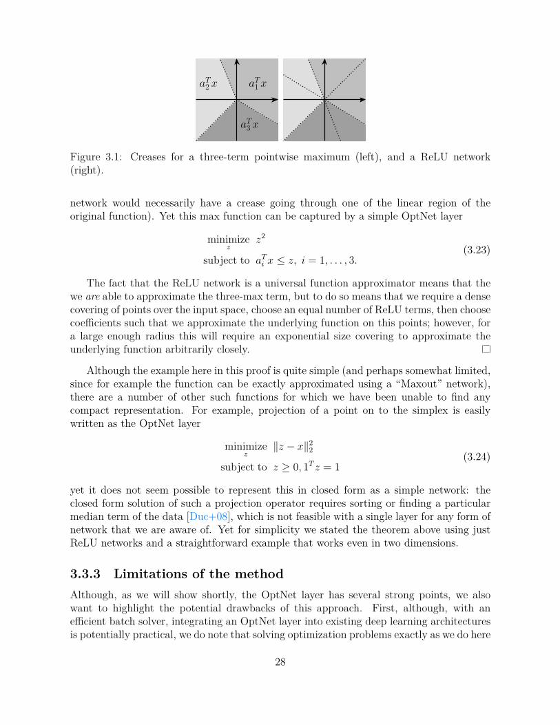
aT1 xaT2 x

aT3 x

Figure 3.1: Creases for a three-term pointwise maximum (left), and a ReLU network(right).

network would necessarily have a crease going through one of the linear region of theoriginal function). Yet this max function can be captured by a simple OptNet layer

minimizez

z2

subject to aTi x ≤ z, i = 1, . . . , 3.(3.23)

The fact that the ReLU network is a universal function approximator means that thewe are able to approximate the three-max term, but to do so means that we require a densecovering of points over the input space, choose an equal number of ReLU terms, then choosecoefficients such that we approximate the underlying function on this points; however, fora large enough radius this will require an exponential size covering to approximate theunderlying function arbitrarily closely.

Although the example here in this proof is quite simple (and perhaps somewhat limited,since for example the function can be exactly approximated using a “Maxout” network),there are a number of other such functions for which we have been unable to find anycompact representation. For example, projection of a point on to the simplex is easilywritten as the OptNet layer

minimizez

∥z − x∥22subject to z ≥ 0, 1T z = 1

(3.24)

yet it does not seem possible to represent this in closed form as a simple network: theclosed form solution of such a projection operator requires sorting or finding a particularmedian term of the data [Duc+08], which is not feasible with a single layer for any form ofnetwork that we are aware of. Yet for simplicity we stated the theorem above using justReLU networks and a straightforward example that works even in two dimensions.

3.3.3 Limitations of the methodAlthough, as we will show shortly, the OptNet layer has several strong points, we alsowant to highlight the potential drawbacks of this approach. First, although, with anefficient batch solver, integrating an OptNet layer into existing deep learning architecturesis potentially practical, we do note that solving optimization problems exactly as we do here

28

has has cubic complexity in the number of variables and/or constraints. This contrastswith the quadratic complexity of standard feedforward layers. This means that we areultimately limited to settings where the number of hidden variables in an OptNet layer isnot too large (less than 1000 dimensions seems to be the limits of what we currently find tothe be practical, and substantially less if one wants real-time results for an architecture).

Secondly, there are many improvements to the OptNet layers that are still possible.Our QP solver, for instance, uses fully dense matrix operations, which makes the solvesvery efficient for GPU solutions, and which also makes sense for our general setting wherethe coefficients of the quadratic problem can be learned. However, for setting many real-world optimization problems (and hence for architectures that wish to more closely mimicsome real-world optimization problem), there is often substantial structure (e.g., sparsity),in the data matrices that can be exploited for efficiency. There is of course no prohibitionof incorporating sparse matrix methods into the fast custom solver, but doing so wouldrequire substantial added complexity, especially regarding efforts like finding minimum fillorderings for different sparsity patterns of the KKT systems. In our open source solverqpth, we have started experimenting with cuSOLVER’s batched sparse QR factorizationsand solves.

Lastly, we note that while the OptNet layers can be trained just as any neural networklayer, since they are a new creation and since they have manifolds in the parameter spacewhich have no effect on the resulting solution (e.g., scaling the rows of a constraint matrixand its right hand side does not change the optimization problem), there is admittedlymore tuning required to get these to work. This situation is common when developingnew neural network architectures and has also been reported in the similar architectureof Schmidt and Roth [SR14]. Our hope is that techniques for overcoming some of thechallenges in learning these layers will continue to be developed in future work.

3.4 Experimental results

In this section, we present several experimental results that highlight the capabilities of theQP OptNet layer. Specifically we look at 1) computational efficiency over exiting solvers;2) the ability to improve upon existing convex problems such as those used in signaldenoising; 3) integrating the architecture into an generic deep learning architectures; and4) performance of our approach on a problem that is challenging for current approaches.In particular, we want to emphasize the results of our system on learning the game of(4x4) mini-Sudoku, a well-known logical puzzle; our layer is able to directly learn thenecessary constraints using just gradient information and no a priori knowledge of therules of Sudoku. The code and data for our experiments are open sourced in the icml2017branch of https://github.com/locuslab/optnet and our batched QP solver is availableas a library at https://github.com/locuslab/qpth.

29

10 50 100 500Number of Variables (and Inequality Constraints)

10-5

10-4

10-3

10-2

10-1

100

101

Runti

me (

s)Linear Forward

QP Forward

Linear Backward

QP Backward

Figure 3.2: Performance of a linear layerand a QP layer. (Batch size 128)

1 64 128

Batch Size

10-2

10-1

100

101

Runti

me (

s)

Gurobi

Ours Serial

Ours Batched

Figure 3.3: Performance of Gurobi andour QP solver.

3.4.1 Batch QP solver performance

All of the OptNet performance results in this section are run on an unloaded Titan XGPU. Gurobi is run on an unloaded quad-core Intel Core i7-5960X CPU @ 3.00GHz.

Our OptNet layers are much more computationally expensive than a linear or convo-lutional layer and a natural question is to ask what the performance difference is. We setup an experiment comparing a linear layer to a QP OptNet layer with a mini-batch sizeof 128 on CUDA with randomly generated input vectors sized 10, 50, 100, and 500. Eachlayer maps this input to an output of the same dimension; the linear layer does this with abatched matrix-vector multiplication and the OptNet layer does this by taking the argminof a random QP that has the same number of inequality constraints as the dimensionalityof the problem. Figure 3.2 shows the profiling results (averaged over 10 trials) of the for-ward and backward passes. The OptNet layer is significantly slower than the linear layeras expected, yet still tractable in many practical contexts.

Our next experiment illustrates why standard baseline QP solvers like CPLEX andGurobi without batch support are too computationally expensive for QP OptNet layersto be tractable. We set up random QP of the form (3.1) that have 100 variables and 100inequality constraints in Gurobi and in the serialized and batched versions of our solverqpth and vary the batch size.2

Figure 3.3 shows the means and standard deviations of running each trial 10 times,showing that our batched solver outperforms Gurobi, itself a highly tuned solver for rea-sonable batch sizes. For the minibatch size of 128, we solve all problems in an averageof 0.18 seconds, whereas Gurobi tasks an average of 4.7 seconds. In the context of train-ing a deep architecture this type of speed difference for a single minibatch can make thedifference between a practical and a completely unusable solution.

2Experimental details: we sample entries of a matrix U from a random uniform distribution and setQ = UTU + 10−3I, sample G with random normal entries, and set h by selecting generating some z0random normal and s0 random uniform and setting h = Gz0 + s0 (we didn’t include equality constraintsjust for simplicity, and since the number of inequality constraints in the primary driver of complexity forthe iterations in a primal-dual interior point method). The choice of h guarantees the problem is feasible.

30

3.4.2 Total variation denoisingOur next experiment studies how we can use the OptNet architecture to improve uponsignal processing techniques that currently use convex optimization as a basis. Specifically,our goal in this case is to denoise a noisy 1D signal given training data consistency of noisyand clean signals generated from the same distribution. Such problems are often addressedby convex optimization procedures, and (1D) total variation denoising is a particularlycommon and simple approach. Specifically, the total variation denoising approach attemptsto smooth some noisy observed signal y by solving the optimization problem

argminz

1

2||y − z||+ λ||Dz||1 (3.25)

where D is the first-order differencing operation, which can be expressed in matrix form bya matrix with rows Di = ei−ei+1 Penalizing the ℓ1 norm of the signal difference encouragesthis difference to be sparse, i.e., the number of changepoints of the signal is small, and weend up approximating y by a (roughly) piecewise constant function.

To test this approach and competing ones on a denoising task, we generate piecewiseconstant signals (which are the desired outputs of the learning algorithm) and corruptthem with independent Gaussian noise (which form the inputs to the learning algorithm).Table 3.1 shows the error rate of these four approaches.

Baseline: Total variation denoising

To establish a baseline for denoising performance with total variation, we run the aboveoptimization problem varying values of λ between 0 and 100. The procedure performs bestwith a choice of λ ≈ 13, and achieves a minimum test MSE on our task of about 16.5 (theunits here are unimportant, the only relevant quantity is the relative performances of thedifferent algorithms).

Baseline: Learning with a fully-connected neural network

An alternative approach to denoising is by learning from data. A function fθ(x) param-eterized by θ can be used to predict the original signal. The optimal θ can be learnedby using the mean squared error between the true and predicted signals. Denoising istypically a difficult function to learn and Table 3.1 shows that a fully-connected neuralnetwork perform substantially worse on this denoising task than the convex optimizationproblem. Figure 3.4 shows the error of the fully connected network on the denoising task.

Learning the differencing operator with OptNet

Between the feedforward neural network approach and the convex total variation opti-mization, we could instead use a generic OptNet layers that effectively allowed us to solve(3.25) using any denoising matrix, which we randomly initialize. While the accuracy hereis substantially lower than even the fully connected case, this is largely the result of learn-ing an over-regularized solution to D. This is indeed a point that should be addressed in

31

0 50 100 150 200

Epoch

15

20

25

30

35

40

45

50

Error

TrainTest

Figure 3.4: Error of the fully connected network for denoising

Figure 3.5: Initial and learned difference operators for denoising.

future work (we refer back to our comments in the previous section on the potential chal-lenges of training these layers), but the point we want to highlight here is that the OptNetlayer seems to be learning something very interpretable and understandable. Specifically,Figure 3.5 shows the D matrix of our solution before and after learning (we permute therows to make them ordered by the magnitude of where the large-absolute-value entriesoccurs). What is interesting in this picture is that the learned D matrix typically capturesexactly the same intuition as the D matrix used by total variation denoising: a mainlysparse matrix with a few entries of alternating sign next to each other. This implies thatfor the data set we have, total variation denoising is indeed the “right” way to think aboutdenoising the resulting signal, but if some other noise process were to generate the data,then we can learn that process instead. We can then attain lower actual error for themethod (in this case similar though slightly higher than the TV solution), by fixing thelearned sparsity of the D matrix and then fine tuning.

Fine-tuning and improving the total variation solution

To finally highlight the ability of the OptNet methods to improve upon the results of aconvex program, specifically tailoring to the data. Here, we use the same OptNet archi-tecture as in the previous subsection, but initialize D to be the differencing matrix as inthe total variation solution. As shown in Table 3.1, the procedure is able to improve boththe training and testing MSE over the TV solution, specifically improving upon test MSEby 12%. Figure 3.6 shows the convergence of the OptNet fine-tuned TV solution.

32

Method Train MSE Test MSEFC Net 18.5 29.8Pure OptNet 52.9 53.3Total Variation 16.3 16.5OptNet Tuned TV 13.8 14.4

Table 3.1: Denoising task error rates.

0 10 20 30 40 50

Epoch

10

11

12

13

14

15

16

17

18

Error

TrainTest

Figure 3.6: Error rate from fine-tuning the TV solution for denoising

3.4.3 MNISTIn this section we consider the integration of QP OptNet layers into a traditional fullyconnected network for the MNIST problem. The results here show only very marginalimprovement if any over a fully connected layer (MNIST, after all, is very fairly well-solved by a fully connected network, let alone a convolution network). But our main pointof this comparison is simply to illustrate that we can include these layers within existingnetwork architectures and efficiently propagate the gradients through the layer.

Specifically we use a FC600-FC10-FC10-SoftMax fully connected network and compareit to a FC600-FC10-Optnet10-SoftMax network, where the numbers after each layer indi-cate the layer size. The OptNet layer in this case includes only inequality constraints andthe previous layer is only used in the linear objective term p(zi) = zi. To keep Q ≻ 0, weuse a Cholesky factorization Q = LLT + ϵI and directly learn L (without any informationfrom the previous layer). We also directly learn A and G, and to ensure a feasible solutionalways exists, we select some learnable z0 and s0 and set b = Az0 and h = Gz0 + s0.

Figure 3.7 shows that the results are similar for both networks with slightly lower errorand less variance in the OptNet network.

0 50 100 150 200

Epoch

0.0

0.5

1.0

1.5

2.0

2.5

3.0

3.5

4.0

Error

TrainTest

0 50 100 150 200

Epoch

0.0

0.5

1.0

1.5

2.0

2.5

3.0

3.5

4.0

Error

TrainTest

Figure 3.7: Training performance on MNIST; top: fully connected network; bottom: Opt-Net as final layer.)

33

31

44 1

2 4 1 31 3 2 43 1 4 24 2 3 1

Figure 3.8: Example mini-Sudoku initial problem and solution.

3.4.4 Sudoku

Finally, we present the main illustrative example of the representational power of ourapproach, the task of learning the game of Sudoku. Sudoku is a popular logical puzzle,where a (typically 9x9) grid of points must be arranged given some initial point, so thateach row, each column, and each 3x3 grid of points must contain one of each number 1through 9. We consider the simpler case of 4x4 Sudoku puzzles, with numbers 1 through4, as shown in Section 3.4.3.

Sudoku is fundamentally a constraint satisfaction problem, and is trivial for computersto solve when told the rules of the game. However, if we do not know the rules of the game,but are only presented with examples of unsolved and the corresponding solved puzzle, thisis a challenging task. We consider this to be an interesting benchmark task for algorithmsthat seek to capture complex strict relationships between all input and output variables.The input to the algorithm consists of a 4x4 grid (really a 4x4x4 tensor with a one-hotencoding for known entries an all zeros for unknown entries), and the desired output is a4x4x4 tensor of the one-hot encoding of the solution.

This is a problem where traditional neural networks have difficulties learning the nec-essary hard constraints. As a baseline inspired by the models at https://github.com/Kyubyong/sudoku, we implemented a multilayer feedforward network to attempt to solveSudoku problems. Specifically, we report results for a network that has 10 convolutionallayers with 512 3x3 filters each, and tried other architectures as well. The OptNet layerwe use on this task is a completely generic QP in “standard form” with only positivity in-equality constraints but an arbitrary constraint matrix Ax = b, a small Q = 0.1I to makesure the problem is strictly feasible, and with the linear term q simply being the inputone-hot encoding of the Sudoku problem. We know that Sudoku can be approximated wellwith a linear program (indeed, integer programming is a typical solution method for suchproblems), but the model here is told nothing about the rules of Sudoku.

We trained these models using ADAM [KB14] to minimize the MSE (which we refer toas “loss”) on a dataset we created consisting of 9000 training puzzles, and we then testedthe models on 1000 different held-out puzzles. The error rate is the percentage of puzzlessolved correctly if the cells are assigned to whichever index is largest in the prediction.Figure 3.9 shows that the convolutional is able to learn all of the necessary logic for thetask and ends up over-fitting to the training data. We contrast this with the performanceof the OptNet network, which learns most of the correct hard constraints within the firstthree epochs and is able to generalize much better to unseen examples.

34

0 2 4 6 8 10 12 14 16 18

Epoch

10-3

10-2

10-1

Loss

Conv Train Conv Test OptNet Train OptNet Test

0 2 4 6 8 10 12 14 16 18

Epoch

10-3

10-2

10-1Loss

0 2 4 6 8 10 12 14 16 18

Epoch

10-3

10-2

10-1

100

Error

Figure 3.9: Sudoku training plots.

3.5 ConclusionWe have presented OptNet, a neural network architecture where we use optimization prob-lems as a single layer in the network. We have derived the algorithmic formulation fordifferentiating through these layers, allowing for backpropagating in end-to-end architec-tures. We have also developed an efficient batch solver for these optimizations based upona primal-dual interior point method, and developed a method for attaining the necessarygradient information “for free” from this approach. Our experiments highlight the potentialpower of these networks, showing that they can solve problems where existing networksare very poorly suited, such as learning Sudoku problems purely from data. There aremany future directions of research for these approaches, but we feel that they add anotherimportant primitive to the toolbox of neural network practitioners.

35

36

Chapter 4Input-Convex Neural Networks

This chapter describes the input-convex neural network (ICNN) architecture that helpsmake inference and learning in deep energy-based models and structured prediction moretractable. These are scalar-valued (potentially deep) neural networks with constraints onthe network parameters such that the output of the network is a convex function of (someof) the inputs. The networks allow for efficient inference via optimization over some inputsto the network given others, and can be applied to settings including structured prediction,data imputation, reinforcement learning, and others. In this chapter we lay the basicgroundwork for these models, proposing methods for inference, optimization and learning,and analyze their representational power. We show that many existing neural networkarchitectures can be made input-convex with a minor modification, and develop specializedoptimization algorithms tailored to this setting. Finally, we highlight the performanceof the methods on multi-label prediction, image completion, and reinforcement learningproblems, where we show improvement over the existing state of the art in many cases.

The contents of this chapter have been previously published at ICML 2017 in Amos,Xu, and Kolter [AXK17].

4.1 IntroductionInput-convex neural networks (ICNNs) are scalar-valued (potentially deep) neural net-works with constraints on the network parameters such that the output of the network isa convex function of (some of) the inputs. The networks allow for efficient inference viaoptimization over some inputs to the network given others, and can be applied to settingsincluding structured prediction, data imputation, reinforcement learning, and others. Inthis chapter we lay the basic groundwork for these models, proposing methods for infer-ence, optimization and learning, and analyze their representational power. We show thatmany existing neural network architectures can be made input-convex with a minor mod-ification, and develop specialized optimization algorithms tailored to this setting. Finally,we highlight the performance of the methods on multi-label prediction, image completion,and reinforcement learning problems, where we show improvement over the existing state

37

of the art in many cases.More specifically, input-convex neural networks are scalar-valued neural networks f(x, y; θ)

where x and y denotes inputs to the function and θ denotes the parameters, built in sucha way that the network is convex in (a subset of) inputs y.1 The fundamental benefit tothese ICNNs is that we can optimize over the convex inputs to the network given somefixed value for other inputs. That is, given some fixed x (and possibly some fixed elementsof y) we can globally and efficiently (because the problem is convex) solve the optimizationproblem

argminy

f(x, y; θ). (4.1)

Fundamentally, this formalism lets us perform inference in the network via optimization.That is, instead of making predictions in a neural network via a purely feedforward process,we can make predictions by optimizing a scalar function (which effectively plays the roleof an energy function) over some inputs to the function given others. There are a numberof potential use cases for these networks.

Structured prediction As is perhaps apparent from our notation above, a key applica-tion of this work is in structured prediction. Given (typically high-dimensional) structuredinput and output spaces X ×Y , we can build a network over (x, y) pairs that encodes theenergy function for this pair, following typical energy-based learning formalisms [LeC+06].Prediction involves finding the y ∈ Y that minimizes the energy for a given x, which isexactly the argmin problem in Equation (4.1). In our setting, assuming that Y is a con-vex space (a common assumption in structured prediction), this optimization problem isconvex. This is similar in nature to the structured prediction energy networks (SPENs)[BM16], which also use deep networks over the input and output spaces, with the differencebeing that in our setting f is convex in y, so the optimization can be performed globally.

Data imputation Similar to structured prediction but slightly more generic, if weare given some space Y we can learn a network f(y; θ) (removing the additional x inputs,though these can be added as well) that, given an example with some subset I missing,imputes the likely values of these variables by solving the optimization problem as aboveyI = argminyI

f(yI , yI ; θ) This could be used e.g., in image inpainting where the goal is tofill in some arbitrary set of missing pixels given observed ones.

Continuous action reinforcement learning Given a reinforcement learning problemwith potentially continuous state and action spaces S ×A, we can model the (negative) Qfunction, −Q(s, a; θ) as an input convex neural network. In this case the action selectionprocedure can be formulated as a convex optimization problem a⋆(s) = argmina−Q(s, a; θ).

1 We emphasize the term “input convex” since convexity in machine learning typically refers to convexity(of the loss minimization learning problem) in the parameters, which is not the case here. Note that in ournotation, f needs only be a convex function in y, and may still be non-convex in the remaining inputs x.Training these neural networks remains a nonconvex problem, and the convexity is only being exploitedat inference time.

38

4.2 Connections to related workEnergy-based learning The interplay between inference, optimization, and structuredprediction has a long history in neural networks. Several early incarnations of neural net-works were explicitly trained to produce structured sequences (e.g. Simard and LeCun[SL91]), and there was an early appreciation that structured models like hidden Markovmodels could be combined with the outputs of neural networks [BLH94]. Much of thisearlier work is surveyed and synthesized by LeCun, Chopra, Hadsell, Ranzato, and Huang[LeC+06], who give a tutorial on these energy based learning methods. In recent years,there has been a strong push to further incorporate structured prediction methods like con-ditional random fields as the “last layer” of a deep network architecture [PBX09; Zhe+15;Che+15a]. Several methods have proposed to build general neural networks over jointinput and output spaces, and perform inference over outputs using generic optimizationtechniques such as Generative Adversarial Networks (GANs) [Goo+14] and Structured Pre-diction Energy Networks (SPENs) [BM16]. SPENs provide a deep structure over input andoutput spaces that performs the inference in Equation (4.1) as a non-convex optimizationproblem.

The current work is highly related to the past approaches but also differs in a particularway. Each of these structured prediction methods based upon energy-based models oper-ates in one of two ways, either: 1) the architecture is built in a very particular way suchthat optimization over the output is guaranteed to be “easy” (e.g. convex, or the result ofrunning some inference procedure), usually by introducing a structured linear objective atthe last layer of the network; or 2) no attempt is made to make the architecture “easy” torun inference over, and instead a general model is built over the output space. In contrast,our approach lies somewhere in between: by ensuring convexity of the resulting decisionspace, we are constraining the inference problem to be easy in some respect, but we specifyvery little about the architecture other than the constraints required to make it convex.In particular, as we will show, the network architecture over the variables to be optimizedover can be deep and involve multiple non-linearities. The goal of the proposed work isto allow for complex functions over the output without needing to specify them manually(exactly analogous to how current deep neural networks treat their input space).

Structured prediction and MAP inference Our work also draws some connectionto MAP-inference-based learning and approximate inference. There are two broad classesof learning approaches in structured prediction: method that use probabilistic inferencetechniques (typically exploiting the fact that the gradient of log likelihood is given by theactual feature expectations minus their expectation under the learned model [KF09, Ch20]), and methods that rely solely upon MAP inference (such as max-margin structuredprediction [Tas+05; Tso+05]). MAP inference in particular also has close connections tooptimization, as various convex relaxations of the general MAP inference problem oftenperform well in theory and practice.

The proposed methods can be viewed as an extreme case of these methods whereinference is based solely upon a convex optimization problem that may not have anyprobabilistic semantics at all. Finally, although it is more abstract, we feel there is aphilosophical similarity between our proposed approach and sum-product networks [PD11];

39

Figure 4.1: A fully input convex neural network (FICNN).

both settings define networks where inference is accomplished “easily” either by a sum-product message passing algorithm (by construction) or via convex optimization.

Fitting convex functions Finally, the proposed work relates to a topic less consideredin the machine learning literature, that of fitting convex functions to data [BV04, pg. 338].Indeed our learning problem can be viewed as parameter estimation under a model thatis guaranteed to be convex by its construction. The most similar work of which we areaware specifically fits sums of rectified half-planes to data [MB09], which is similar to onelayer of our rectified linear units. However, the actual training scheme is much different,and our deep network architecture allows for a much richer class of representations, whilestill maintaining convexity.

4.3 Convex neural network architecturesHere we more formally present different ICNN architectures and prove their convexityproperties given certain constraints on the parameter space. Our chief claim is that theclass of (full and partial) input convex models is rich and lets us capture complex jointmodels over the input to a network.

4.3.1 Fully input convex neural networksTo begin, we consider a fully convex, k-layer, fully connected ICNN that we call a FICNNand is shown in Figure 4.1. This model defines a neural network over the input y (i.e.,omitting any x term in this function) using the architecture for i = 0, . . . , k − 1

zi+1 = gi

(W

(z)i zi +W

(y)i y + bi

), f(y; θ) = zk (4.2)

where zi denotes the layer activations (with z0,W(z)0 ≡ 0), θ = {W (y)

0:k−1,W(z)1:k−1, b0:k−1} are

the parameters, and gi are non-linear activation functions. The central result on convexityof the network is the following:Proposition 1. The function f is convex in y provided that all W (z)

1:k−1 are non-negative,and all functions gi are convex and non-decreasing.

The proof is simple and follows from the fact that non-negative sums of convex functionsare also convex and that the composition of a convex and convex non-decreasing functionis also convex (see e.g. Boyd and Vandenberghe [BV04, p. 3.2.4]). The constraint that thegi be convex non-decreasing is not particularly restrictive, as current non-linear activation

40

units like the rectified linear unit or max-pooling unit already satisfy this constraint. Theconstraint that the W (z) terms be non-negative is somewhat restrictive, but because thebias terms and W (y) terms can be negative, the network still has substantial representationpower, as we will shortly demonstrate empirically.

One notable addition in the ICNN are the “passthrough” layers that directly connectthe input y to hidden units in deeper layers. Such layers are unnecessary in traditionalfeedforward networks because previous hidden units can always be mapped to subsequenthidden units with the identity mapping; however, for ICNNs, the non-negativity constraintsubsequent W (z) weights restricts the allowable use of hidden units that mirror the identitymapping, and so we explicitly include this additional passthrough. Some passthroughlayers have been recently explored in the deep residual networks [He+15] and denselyconnected convolutional networks [HLW16], though these differ from those of an ICNN asthey pass through hidden layers deeper in the network, whereas to maintain convexity ourpassthrough layers can only apply to the input directly.

Other linear operators like convolutions can be included in ICNNs without changing theconvexity properties. Indeed, modern feedforward architectures such as AlexNet [KSH12],VGG [SZ14], and GoogLeNet [Sze+15] with ReLUs [NH10] can be made input convexwith Proposition 1. In the experiments that follow, we will explore ICNNs with both fullyconnected and convolutional layers.

4.3.2 Convolutional input-convex architecturesConvolutional architectures are important for many vision tasks and can easily be madeinput-convex because the convolution is a linear operator. The construction of convo-lutional layers in ICNNs depends on the type of input and output space. If the inputand output space are similarly structured (e.g. both spatial), the jth feature map of aconvolutional PICNN layer i can be defined by

zji+1 = gi

(zi ∗W (z)

i,j + (Sx) ∗W (x)i,j + (Sy) ∗W (y)

i,j + bi,j

)(4.3)

where the convolution kernels W are the same size and S scales the input and output tobe the same size as the previous feature map, and were we omit some of the Hadamardproduct terms that can appear above for simplicity of presentation.

If the input space is spatial, but the output space has another structure (e.g. the sim-plex), the convolution over the output space can be replaced by a matrix-vector operation,such as

zji+1 = gi

(zi ∗W (z)

i,j + (Sx) ∗W (x)i,j +B

(y)i,j y + bi,j

)(4.4)

where the product B(y)i,j y is a scalar.

4.3.3 Partially input convex architecturesThe FICNN provides joint convexity over the entire input to the function, which indeedmay be a restriction on the allowable class of models. Furthermore, this full joint convexity

41

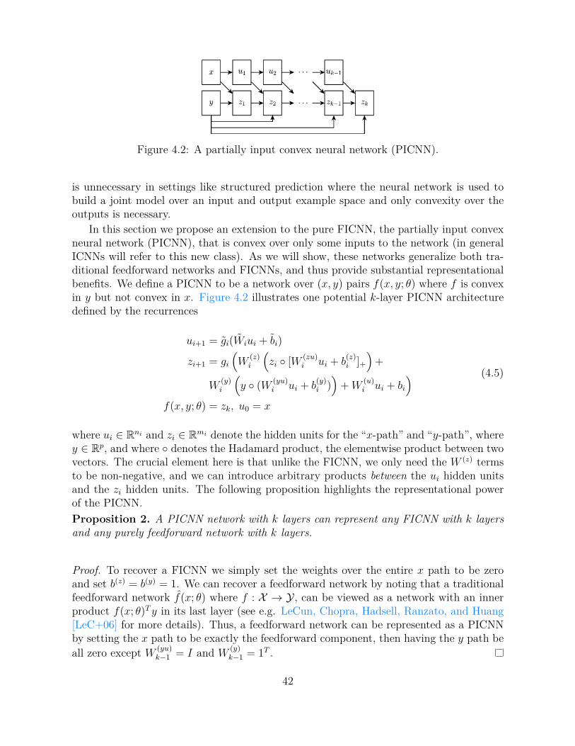
Figure 4.2: A partially input convex neural network (PICNN).

is unnecessary in settings like structured prediction where the neural network is used tobuild a joint model over an input and output example space and only convexity over theoutputs is necessary.

In this section we propose an extension to the pure FICNN, the partially input convexneural network (PICNN), that is convex over only some inputs to the network (in generalICNNs will refer to this new class). As we will show, these networks generalize both tra-ditional feedforward networks and FICNNs, and thus provide substantial representationalbenefits. We define a PICNN to be a network over (x, y) pairs f(x, y; θ) where f is convexin y but not convex in x. Figure 4.2 illustrates one potential k-layer PICNN architecturedefined by the recurrences

ui+1 = gi(Wiui + bi)

zi+1 = gi

(W

(z)i

(zi ◦ [W (zu)

i ui + b(z)i ]+

)+

W(y)i

(y ◦ (W (yu)

i ui + b(y)i ))+W

(u)i ui + bi

)f(x, y; θ) = zk, u0 = x

(4.5)

where ui ∈ Rni and zi ∈ Rmi denote the hidden units for the “x-path” and “y-path”, wherey ∈ Rp, and where ◦ denotes the Hadamard product, the elementwise product between twovectors. The crucial element here is that unlike the FICNN, we only need the W (z) termsto be non-negative, and we can introduce arbitrary products between the ui hidden unitsand the zi hidden units. The following proposition highlights the representational powerof the PICNN.Proposition 2. A PICNN network with k layers can represent any FICNN with k layersand any purely feedforward network with k layers.

Proof. To recover a FICNN we simply set the weights over the entire x path to be zeroand set b(z) = b(y) = 1. We can recover a feedforward network by noting that a traditionalfeedforward network f(x; θ) where f : X → Y , can be viewed as a network with an innerproduct f(x; θ)Ty in its last layer (see e.g. LeCun, Chopra, Hadsell, Ranzato, and Huang[LeC+06] for more details). Thus, a feedforward network can be represented as a PICNNby setting the x path to be exactly the feedforward component, then having the y path beall zero except W

(yu)k−1 = I and W

(y)k−1 = 1T .

42

4.4 Inference in ICNNsPrediction in ICNNs (which we also refer to as inference), requires solving the convexoptimization problem

minimizey∈Y

f(x, y; θ) (4.6)

While the resulting tasks are convex optimization problems (and thus “easy” to solvein some sense), in practice this still involves the solution of a potentially very complexoptimization problem. We discuss here several approaches for approximately solving theseoptimization problems. We can usually obtain reasonably accurate solutions in manysettings using a procedure that only involves a small number of forward and backwardpasses through the network, and which thus has a complexity that is at most a constantfactor worse than that for feedforward networks. The same consideration will apply totraining such networks, which we will discuss in Section 4.5.

4.4.1 Exact inference in ICNNsAlthough it is not a practical approach for solving the optimization tasks, we first highlightthe fact that the inference problem for the networks presented above (where the non-linearare either ReLU or linear units) can be posed as as linear program. Specifically, consideringthe FICNN network in (4.2) can be written as the optimization problem

minimizey,z1,...,zk

zk

subject to zi+1 ≥ W(z)i zi +W

(y)i y + bi, i = 0, . . . , k − 1

zi ≥ 0, i = 1, . . . , k − 1.

(4.7)

This problem exactly replicates the equations of the FICNN, with the exception that wehave replaced ReLU and the equality constraint between layers with a positivity constrainton the zi terms and an inequality. However, because we are minimizing the final zk term,and because each inequality constraint is convex, at the solution one of these constraintsmust be tight, i.e., (zi)j = (W

(z)i zi + W

(y)i y + bi)j or (zi)j = 0, which recovers the ReLU

non-linearity exactly. The exact same procedure can be used to write to create an exactinference procedure for the PICNN.

Although the LP formulation is appealing in its simplicity, in practice these optimiza-tion problems will have a number of variables equal to the total number of activationsin the entire network. Furthermore, most LP solution methods to solve such problemsrequire that we form and invert structured matrices with blocks such as W T

i Wi — thecase for most interior-point methods [Wri97] or even approximate algorithms such as thealternating direction method of multipliers [Boy+11] — which are large dense matrices orhave structured forms such as non-cyclic convolutions that are expensive to invert. Evenincremental approaches like the Simplex method require that we form inverses of subsetsof columns of these matrices, which are additionally different for structured operations likeconvolutions, and which overall still involve substantially more computation than a sin-gle forward pass. Furthermore, such solvers typically do not exploit the substantial effort

43

that has gone in to accelerating the forward and backward computation passes for neuralnetworks using hardware such as GPUs. Thus, as a whole, these do not present a viableoption for optimizing the networks.

4.4.2 Approximate inference in ICNNsBecause of the impracticality of exact inference, we focus on approximate approaches tooptimizing over the inputs to these networks, but ideally ones that still exploit the convexityof the resulting problem. We specifically focus on gradient-based approaches, which usethe fact that we can easily compute the gradient of an ICNN with respect to its inputs,∇yf(x, y; θ), using backpropagation.

Gradient descent. The simplest gradient-based methods for solving Equation (4.6) isjust (projected sub-) gradient descent, or modifications such as those that use a momentumterm [Pol64; RHW88], or spectral step size modifications [BB88; BMR00]. That is, we startwith some initial y and repeat the update

y ← PY (y − α∇yf(x, y; θ)) (4.8)

This method is appealing in its simplicity, but suffers from the typical problems of gradientdescent on non-smooth objectives: we need to pick a step size and possibly use a sequenceof decreasing step sizes, and don’t have an obvious method to assess how accurate of acurrent solution we have obtained (since an ICNN with ReLUs is piecewise linear, it willnot have zero gradient at the solution). The method is also more challenging to integratewith some learning procedures, as we often need to differentiate through an entire chain ofthe gradient descent algorithm [Dom12]. Thus, while the method can sometimes work inpractice, we have found that other approaches typically far outperform this method, andwe will focus on alternative approximate approaches for the remainder of this section.

4.4.3 Approximate inference via the bundle methodWe here review the basic bundle method [SVL08] that we build upon in our bundle entropymethod. The bundle method takes advantage of the fact that for a convex objective, thefirst-order approximation at any point is a global under-estimator of the function; thislets us maintain a piecewise linear lower bound on the function by adding cutting planesformed by this first order approximation, and then repeatedly optimizing this lower bound.Specifically, the process follows the procedure shown in Algorithm 1. Denoting the iteratesof the algorithm as yk, at each iteration of the algorithm, we compute the first orderapproximation to the function

f(x, yk; θ) +∇yf(x, yk; θ)T (y − yk) (4.9)

and update the next iteration by solving the optimization problem

yk+1 := argminy∈Y

max1≤i≤k

{f(x, yi; θ) +∇yf(x, yi; θ)T (y − yi)}. (4.10)

44

A bit more concretely, the optimization problem can be written via a set of linear inequalityconstraints

yk+1, tk+1 := argminy∈Y,t

{t | Gy + h ≤ t1} (4.11)

where G ∈ Rk×n has rows equal to

gTi = ∇yf(x, yi; θ)T (4.12)

and h ∈ Rk has entries equal to

hi = f(x, yi; θ)−∇yf(x, yi; θ)Tyi. (4.13)

Algorithm 1 A typical bundle method to optimize f : Rm×n → R over Rn for K iterationswith a fixed x and initial starting point y1.

function BundleMethod(f , x, y1, K)G ← 0 ∈ RK×n

h ← 0 ∈ RK

for k = 1, K doGT

k ← ∇yf(x, yk; θ)T ▷ kth row of G

hk ← f(x, yk; θ)−∇yf(x, yk; θ)Tyk

yk+1, tk+1 ← argminy∈Y,t {t | G1:ky + h1:k ≤ t1}end forreturn yK+1

end function

4.4.4 Approximate inference via the bundle entropy methodAn alternative approach to gradient descent is the bundle method [SVL08], also known asthe epigraph cutting plane approach, which iteratively optimizes a piecewise lower boundon the function given by the maximum over a set of first-order approximations. However,as, the traditional bundle method is not well suited to our setting (we need to evaluate anumber of gradients equal to the dimension of x, and solve a complex optimization problemat each step) we have developed a new optimization algorithm for this domain that weterm the bundle entropy method. This algorithm specifically applies to the (common) casewhere Y is bounded, which we assume to be Y = [0, 1]n (other upper or lower bounds canbe attained through scaling). The method is also easily extensible to the setting whereelements of Y belong to a higher-dimensional probability simplex as well.

For this approach, we consider adding an additional “barrier” function to the optimiza-tion in the form of the negative entropy −H(y), where

H(y) = −n∑

i=1

(yi log yi + (1− yi) log(1− yi)). (4.14)

45

In other words, we instead want to solve the optimization problem argminy f(x, y; θ) −H(y) (with a possible additional scaling term). The negative entropy is a convex function,with the limits of limy→0H(y) = limy→1H(y) = 0, and negative values in the interior ofthis range. The function acts as a barrier because, although it does not approach infinity asit reaches the barrier of the feasible set, its gradient does approach infinity as it reaches thebarrier, and thus the optimal solution will always lie in the interior of the unit hypercubeY .

An appealing feature of the entropy regularization comes from its close connectionwith sigmoid units in typical neural networks. It follows easily from first-order optimalityconditions that the optimization problem

minimizey

cTy −H(y) (4.15)

is given by y⋆ = 1/(1 + exp(c)). Thus if we consider the “trivial” PICNN mentioned inSection 4.3.3, which simply consists of the function f(x, y; θ) = yT f(x; θ) for some purelyfeedforward network f(x; θ), then the entropy-regularized minimization problem gives asolution that is equivalent to simply taking the sigmoid of the neural network outputs.Thus, the move to ICNNs can be interpreted as providing a more structured joint energyfunctional over the linear function implicitly used by sigmoid layers.

At each iteration of the bundle entropy method, we solve the optimization problem

yk+1, tk+1 := argminy,t

{t−H(y) | Gy + h ≤ t1} (4.16)

where G ∈ Rk×n has rows equal to

gTi = ∇yf(x, yi; θ)T (4.17)

and h ∈ Rk has entries equal to

hi = f(x, yi; θ)−∇yf(x, yi; θ)Tyi. (4.18)

The Lagrangian of the optimization problem is

L(y, t, λ) = t−H(y) + λT (Gy + h− t1) (4.19)

and differentiating with respect to y and t gives the optimality conditions

∇yL(y, t, λ) = 0 =⇒ y =1

1 + exp(GTλ)

∇tL(y, t, λ) = 0 =⇒ 1Tλ = 1

(4.20)

which in turn leads to the dual problem

maximizeλ

(G1 + h)Tλ− 1T log(1 + exp(GTλ))

subject to λ ≥ 0, 1Tλ = 1.(4.21)

46

This is a smooth optimization problem over the unit simplex, and can be solved usinga method like the Projected Newton method of [Ber82, pg. 241, eq. 97]. A completedescription of the bundle entropy method is given in Algorithm 2. For lower dimensionalproblems, the bundle entropy method often attains an exact solution after a relativelysmall number of iterations. And even for larger problems, we find that the approximatesolutions generated by a very small number of iterations (we typically use 5 iterations),still substantially outperform gradient descent approaches. Further, because we maintainan explicit lower bound on the function, we can compute an optimality gap of our solution,though in practice just using a fixed number of iterations performs well.

Algorithm 2 Our bundle entropy method to optimize f : Rm × [0, 1]n → R over [0, 1]n

for K iterations with a fixed x and initial starting point y1.function BundleEntropyMethod(f , x, y1, K)

Gℓ ← [ ]hℓ ← [ ]for k = 1, K do

Append(Gℓ, ∇yf(x, yk; θ)T )

Append(hℓ, f(x, yk; θ)−∇yf(x, yk; θ)Tyk)

ak ← Length(Gℓ) ▷ The number of active constraints.Gk ← Concat(Gℓ)∈ Rak×n

hk ← Concat(hℓ)∈ Rak

if ak = 1 thenλk ← 1

elseλk ← ProjNewtonLogistic(Gk, hk)

end ifyk+1 ← (1 + exp(GT

k λk))−1

Delete(Gℓ[i] and hℓ[i] where λi ≤ 0) ▷ Prune inactive constraints.end forreturn yK+1

end function

4.5 Learning in ICNNsGenerally speaking, ICNN learning shapes the objective’s energy function to produce thedesired values when optimizing over the relevant inputs. That is, for a given input outputpair (x, y⋆), our goal is to find ICNN parameters θ such that

y⋆ ≈ argminy

f(x, y; θ) (4.22)

where for the entirely of this section, we use the notation f to denote the combination ofthe neural network function plus the regularization term such as −H(y), if it is included,

47

i.e.f(x, y; θ) = f(x, y; θ)−H(y). (4.23)

Although we only discuss the entropy regularization in this work, we emphasize that otherregularizers are also possible. Depending on the setting, there are several different ap-proaches we can use to ensure that the ICNN achieves the desired targets, and we considerthree approaches below: direct functional fitting, max-margin structured prediction, andargmin differentiation.

Direct functional fitting. We first note that in some domains, we do not needa specialized procedure for fitting ICNNs, but can use existing approaches that directlyfit the ICNN. An example of this is the Q-learning setting. Given some observed tuple(s, a, r, s′), Q learning updates the parameters θ with the gradient(

Q(s, a)− r − γmaxa′

Q(s′, a′))∇θQ(s, a), (4.24)

where the maximization step is carried out with gradient descent or the bundle entropymethod. These updates can be applied to ICNNs with the only additional requirementthat we project the weights onto their feasible sets after this update (i.e., clip or projectany W terms that are required to be positive). Algorithm 3 gives a complete descriptionof deep Q-learning with ICNNs.

4.5.1 Max-margin structured predictionIn the more traditional structured prediction setting, where we do not aim to fit the energyfunction directly but fit the predictions made by the system to some target outputs, thereare different possibilities for learning the ICNN parameters. One such method is basedupon the max-margin structured prediction framework [Tso+05; Tas+05]. Given sometraining example (x, y⋆), we would like to require that this example has a joint energy thatis lower than all other possible values for y. That is, we want the function f to satisfy theconstraint

f(x, y⋆; θ) ≤ miny

f(x, y; θ) (4.25)

Unfortunately, these conditions can be trivially fit by choosing a constant f (although theentropy term alleviates this problem slightly, we can still choose an approximately constantfunction), so instead the max-margin approach adds a margin-scaling term that requiresthis gap to be larger for y further from y⋆, as measured by some loss function ∆(y, y⋆).Additionally adding slack variables to allow for potential violation of these constraints, wearrive at the typical max-margin structured prediction optimization problem

minimizeθ,ξ≥0

λ

2∥θ∥22 +

m∑i=1

ξi

subject to f(xi, yi; θ) ≤ miny∈Y

(f(xi, y; θ)−∆(yi, y)

)− ξi

(4.26)

As a simple example, for multiclass classification tasks where y⋆ denotes a “one-hot” en-coding of examples, we can use a multi-variate entropy term and let ∆(y, y⋆) = y⋆T (1− y).

48

Training requires solving this “loss-augmented” inference problem, which is convex forsuitable choices of the margin scaling term.

The optimization problem (4.26) is naturally still not convex in θ, but can be solvedvia the subgradient method for structured prediction [RBZ07]. This algorithm iterativelyselects a training example xi, yi, then 1) solves the optimization problem

y⋆ = argminy∈Y

f(xi, y; θ)−∆(yi, y) (4.27)

and 2) if the margin is violated, updates the network’s parameters according to the sub-gradient

θ := P+ [θ − α (λθ +∇θf(xi, yi, θ)−∇θf(xi, y⋆; θ))] (4.28)

where P+ denotes the projection of W (z)1:k−1 onto the non-negative orthant. This method can

be easily adapted to use mini-batches instead of a single example per subgradient step, andalso adapted to alternative optimization methods like AdaGrad [DHS11] or ADAM [KB14].Further, a fast approximate solution to y⋆ can be used instead of the exact solution.

4.5.2 Argmin differentiationIn our final proposed approach, that of argmin differentiation, we propose to directlyminimize a loss function between true outputs and the outputs predicted by our model,where these predictions themselves are the result of an optimization problem. We explicitlyconsider the case where the approximate solution to the inference problem is attained viathe previously-described bundle entropy method, typically run for some fixed (usuallysmall) number of iterations. To simplify notation, in the following we will let

y(x; θ) = argminy

mint{t−H(y) | Gy + h ≤ t1}

≈ argminy

f(x, y; θ)(4.29)

refer to the approximate minimization over y that results from running the bundle entropymethod, specifically at the last iteration of the method.

Given some example (x, y⋆), our goal is to compute the gradient, with respect to theICNN parameters, of the loss between y⋆ and y(x; θ): ℓ(y(x; θ), y⋆). This is in some sensethe most direct analogue to traditional neural network learning, since we typically optimizenetworks by minimizing some loss between the network’s (feedforward) predictions andthe true desired labels. Doing this in the predictions-via-optimization setting requires thatwe differentiate “through” the argmin operator, which can be accomplished via implicitdifferentiation of the KKT optimality conditions. Although the derivation is somewhatinvolved, the final result is fairly compact, and is given by the following proposition (forsimplicity, we will write y below instead of y(x; θ) when the notation should be clear):Proposition 3. The gradient of the neural network loss for predictions generated through

49

the minimization process is

∇θℓ(y(x; θ), y⋆) =

k∑i=1

(cλi∇θf(x, yi; θ) +∇θ

(∇yf(x, y

i; θ)T(λic

y + cλi(y(x; θ)− yi

))))

(4.30)where yi denotes the solution returned by the ith iteration of the entropy bundle method, λdenotes the dual variable solution of the entropy bundle method, and where the c variablesare determined by the solution to the linear system H GT 0

G 0 −10 −1T 0

cy

cλ

ct

=

−∇yℓ(y, y⋆)

00

. (4.31)

where H = diag(

1y+ 1

1−y

).

Proof (of Proposition 3). We have by the chain rule that

∂ℓ

∂θ=

∂ℓ

∂y

(∂y

∂G

∂G

∂θ+

∂y

∂h

∂h

∂θ

). (4.32)

The challenging terms to compute in this equation are the ∂y∂G

and ∂y∂h

terms. These canbe computed (although we will ultimately not compute them explicitly, but just computethe product of these matrices and other terms in the Jacobian), by implicit differentiationof the KKT conditions. Specifically, the KKT conditions of the bundle entropy method(considering only the active constraints at the solution) are given by

1 + log y − log(1− y) +GTλ = 0

Gy + h− t1 = 0

1Tλ = 1.

(4.33)

For simplicity of presentation, we consider first the Jacobian with respect to h. Takingdifferentials of these equations with respect to h gives

diag

(1

y+

1

1− y

)dy +GTdλ = 0

Gdy + dh− dt1 = 0

1Tdλ = 0

(4.34)

or in matrix form diag(

1y+ 1

1−y

)GT 0

G 0 −10 −1T 0

dy

dλdt

=

0−dh0

. (4.35)

To compute the Jacobian ∂y∂h

we can solve the system above with the right hand side givenby dh = I, and the resulting dy term will be the corresponding Jacobian. However, in our

50

ultimate objective we always left-multiply the proper terms in the above equation by ∂ℓ∂y

.Thus, we instead define

cy

cλ

ct

=

diag(1y + 1

1−y

)GT 0

G 0 −10 −1T 0

−1 −( ∂ℓ∂y )T0

0

(4.36)

and we have the the simple formula for the Jacobian product

∂ℓ

∂y

∂y

∂h= (cλ)T . (4.37)

A similar set of operations taking differentials with respect to G leads to the matrixequations diag

(1y + 1

1−y

)GT 0

G 0 −10 −1T 0

dy

dλdt

=

−dGTλ−dGy

0

(4.38)

and the corresponding Jacobian products / gradients are given by

∂ℓ

∂y

∂y

∂G= cyλT + y(cλ)T . (4.39)

Finally, using the definitions that

gTi = ∇yf(x, yi; θ)T , hi = f(x, yk; θ)−∇yf(x, y

i; θ)Tyi (4.40)

we recover the formula presented in the proposition.

The complexity of computing this gradient will be linear in k, which is the number ofactive constraints at the solution of the bundle entropy method. The inverse of this matrixcan also be computed efficiently by just inverting the k× k matrix GH−1GT via a variableelimination procedure, instead of by inverting the full matrix. The gradients ∇θf(x, yi; θ)are standard neural network gradients, and further, can be computed in the same for-ward/backward pass as we use to compute the gradients for the bundle entropy method.The main challenge of the method is to compute the terms of the form ∇θ(∇yf(x, yi; θ)

Tv)for some vector v. This quantity can be computed by most autodifferentiation tools (thegradient inner product ∇yf(x, yi; θ)

Tv itself just becomes a graph computation than canbe differentiated itself), or it can be computed by a finite difference approximation. Thecomplexity of computing this entire gradient is a small constant multiple of computing kgradients with respect to θ.

Given this ability to compute gradients with respect to an arbitrary loss function, wecan fit the parameter using traditional stochastic gradient methods examples. Specifically,given an example (or a minibatch of examples) xi, yi, we compute gradients∇θℓ(y(xi; θ), yi)and update the parameters using e.g. the ADAM optimizer [KB14].

51

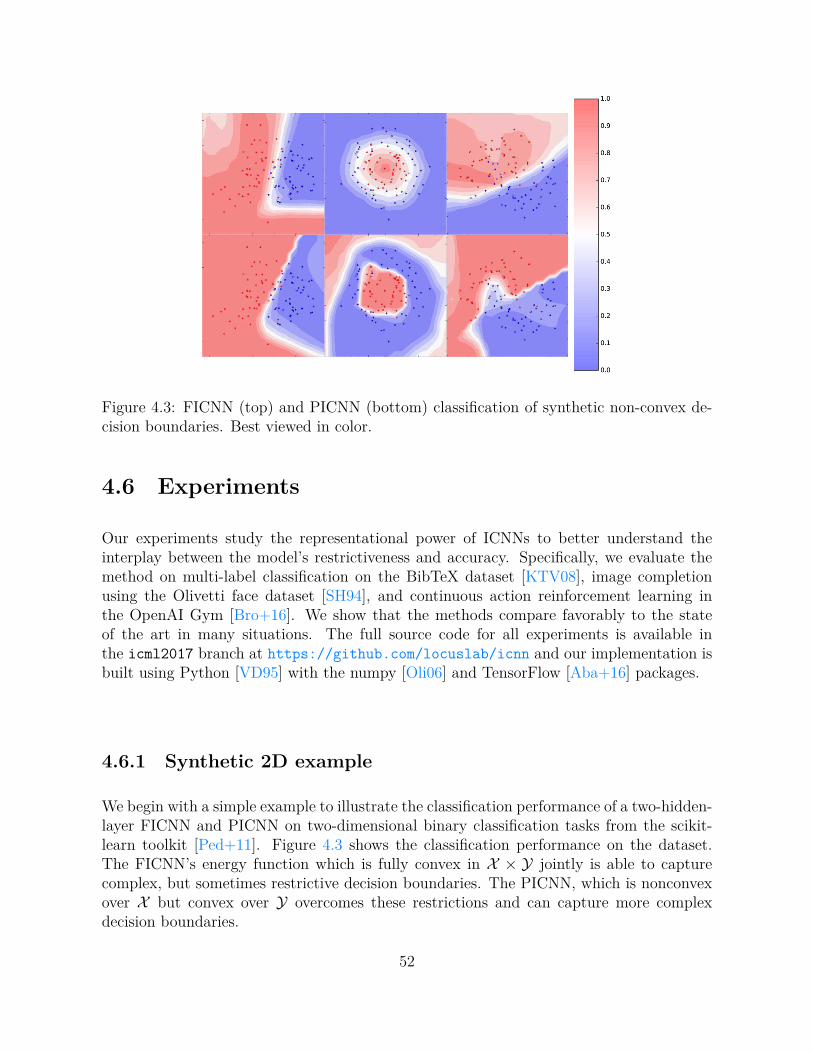
Figure 4.3: FICNN (top) and PICNN (bottom) classification of synthetic non-convex de-cision boundaries. Best viewed in color.

4.6 Experiments

Our experiments study the representational power of ICNNs to better understand theinterplay between the model’s restrictiveness and accuracy. Specifically, we evaluate themethod on multi-label classification on the BibTeX dataset [KTV08], image completionusing the Olivetti face dataset [SH94], and continuous action reinforcement learning inthe OpenAI Gym [Bro+16]. We show that the methods compare favorably to the stateof the art in many situations. The full source code for all experiments is available inthe icml2017 branch at https://github.com/locuslab/icnn and our implementation isbuilt using Python [VD95] with the numpy [Oli06] and TensorFlow [Aba+16] packages.

4.6.1 Synthetic 2D example

We begin with a simple example to illustrate the classification performance of a two-hidden-layer FICNN and PICNN on two-dimensional binary classification tasks from the scikit-learn toolkit [Ped+11]. Figure 4.3 shows the classification performance on the dataset.The FICNN’s energy function which is fully convex in X × Y jointly is able to capturecomplex, but sometimes restrictive decision boundaries. The PICNN, which is nonconvexover X but convex over Y overcomes these restrictions and can capture more complexdecision boundaries.

52

Method Test Macro-F1Feedforward net 0.396ICNN 0.415SPEN [BM16] 0.422

Table 4.1: Comparison of approaches on BibTeX multi-label classification task. (Higher isbetter.)

4.6.2 Multi-Label ClassificationWe first study how ICNNs perform on multi-label classification with the BibTeX datasetand benchmark presented in Katakis, Tsoumakas, and Vlahavas [KTV08]. This bench-mark maps text classification from an input space X of 1836 bag-of-works indicator (bi-nary) features to an output space Y of 159 binary labels. We use the train/test split of4880/2515 from [KTV08] and evaluate with the macro-F1 score (higher is better). Weuse the ARFF version of this dataset from Mulan [Tso+11]. Our PICNN architecture formulti-label classification uses fully-connected layers with ReLU activation functions andbatch normalization [IS15] along the input path. As a baseline, we use a fully-connectedneural network with batch normalization and ReLU activation functions. Both architec-tures have the same structure (600 fully connected, 159 (#labels) fully connected). Weoptimize our PICNN with 30 iterations of gradient descent with a learning rate of 0.1 anda momentum of 0.3.

Table 4.1 compares several different methods for this problem. Our PICNN’s finalmacro-F1 score of 0.415 outperforms our baseline feedforward network’s score of 0.396,which indicates PICNNs have the power to learn a robust structure over the output space.SPENs obtain a macro-F1 score of 0.422 on this task [BM16] and pose an interestingcomparison point to ICNNs as they have a similar (but not identical) deep structure that isnon-convex over the input space. The difference of 0.007 between ICNNs and SPENs couldbe due to differences in our experimental setups, architectures, and random experimentalnoise. Figure 4.4 shows the training progress of the feed-forward and PICNN models.

Figure 4.4: Training (blue) and test (red) macro-F1 score of a feedforward network (left)and PICNN (right) on the BibTeX multi-label classification dataset. The final test F1scores are 0.396 and 0.415, respectively. (Higher is better.)

53

Figure 4.5: Example Olivetti test set image completions of the bundle entropy ICNN.

4.6.3 Image completion on the Olivetti faces

As a test of the system on a structured prediction task over a much more complex out-put space Y , we apply a convolutional PICNN to face completion on the sklearn version[Ped+11] of the Olivetti data set [SH94], which contains 400 64x64 grayscale images. IC-NNs for face completion should be invariant to translations and other transformations inthe input space. To achieve this invariance, our PICNN is inspired by the DQN architec-ture in Mnih, Kavukcuoglu, Silver, Rusu, Veness, Bellemare, Graves, Riedmiller, Fidjeland,Ostrovski, et al. [Mni+15], which preserves this invariance in the different context of rein-forcement learning. Specifically, our network is over (x, y) pairs where x (32x64) is the lefthalf and y (32x64) is the right half of the image. The input and output paths are: 32x8x8conv (stride 4x2), 64x4x4 conv (stride 2x2), 64x3x3 conv, 512 fully connected.

This experiment uses the same training/test splits and minimizes the mean squarederror (MSE) as in Poon and Domingos [PD11]. We report the sum-product network resultsfrom Poon and Domingos [PD11] and have also implemented dilated CNN [YK15] and fullyconvolutional network (FCN) [LSD15] baselines. We also explore the tradeoffs between thebundle entropy method and gradient descent and compare to the non-convex variant tobetter understand the impacts of convexity. We use a learning rate of 0.01 and momentumof 0.9 with gradient descent for the inner optimization in the ICNN.

Table 4.2 shows the test MSEs for the different approaches and example image com-pletions are shown in Figure 4.5. We note that as future work, an ICNN variant of thebaseline dilated CNN and FCN architectures could be made in addition to the DQN archi-tecture the ICNN in this experiment uses. For ICNNs, these results show that the bundleentropy method can leverage more information from these five iterations than gradientdescent, even when the convexity constraint is relaxed. The PICNN trained with back-optimization with the relaxed convexity constraint slightly outperforms the network withthe convexity constraint, but not the network trained with the bundle-entropy method.This shows that for image completion with PICNNs, convexity does not seem to inhibitthe representational power. Furthermore, this experiment suggests that a small number ofinner optimization iterations (five in this case) is sufficient for good performance.

54

Method MSESum-Product Network Baseline [PD11] 942.0Dilated CNN Baseline [YK15] 800.0FCN Baseline [LSD15] 795.4ICNN - Bundle Entropy 833.0ICNN - Gradient Decent 872.0ICNN - Nonconvex 850.9

Table 4.2: Olivetti image completion test reconstruction errors.

4.6.4 Continuous Action Reinforcement Learning

Finally, we present standard benchmarks in continuous action reinforcement learning fromthe OpenAI Gym [Bro+16] that use the MuJoCo physics simulator [TET12]. We considerthe environments shown in Table 4.3. We model the (negative) Q function, −Q(s, a; θ) as anICNN and select actions with the convex optimization problem a⋆(s) = argmina−Q(s, a; θ).We use Q-learning to optimize the ICNN as described in Section 4.5 and Algorithm 3. Attest time, the policy is selected by optimizing Q(s, a; θ). All of our experiments use aPICNN with two fully-connected layers that each have 200 hidden units. We compare toDeep Deterministic Policy Gradient (DDPG) [Lil+15] and Normalized Advantage Func-tions (NAF) [Gu+16b] as state-of-the-art off-policy learning baselines.2

Environment # State # ActionInvertedPendulum-v1 4 1

InvertedDoublePendulum-v1 11 1Reacher-v1 11 2

HalfCheetah-v1 17 6Swimmer-v1 8 2

Hopper-v1 11 3Walker2d-v1 17 6

Ant-v1 111 8Humanoid-v1 376 17

HumanoidStandup-v1 376 17

Table 4.3: State and action space sizes in the OpenAI gym MuJoCo benchmarks.

2Because there are not official DDPG or NAF implementations or results on the OpenAI gym tasks, weuse the Simon Ramstedt’s DDPG implementation from https://github.com/SimonRamstedt/ddpg andhave re-implemented NAF.

55

Task DDPG NAF ICNNAnt 1000.00 999.03 1056.29HalfCheetah 2909.77 2575.16 3822.99Hopper 1501.33 1100.43 831.00Humanoid 524.09 5000.68 433.38HumanoidStandup 134265.96 116399.05 141217.38InvDoubPend 9358.81 9359.59 9359.41InvPend 1000.00 1000.00 1000.00Reacher -6.10 -6.31 -5.08Swimmer 49.79 69.71 64.89Walker2d 1604.18 1007.25 298.21

Table 4.4: Maximum test reward for ICNN algorithm versus alternatives on several OpenAIGym tasks. (All tasks are v1.)

Algorithm 3 Deep Q-learning with ICNNs. Opt-Alg is a convex minimization algorithmsuch as gradient descent or the bundle entropy method. Qθ is the objective the optimizationalgorithm solves. In gradient descent, Qθ(s, a) = Q(s, a|θ) and with the bundle entropymethod, Qθ(s, a) = Q(s, a|θ) +H(a).

Select a discount factor γ ∈ (0, 1) and moving average factor τ ∈ (0, 1)Initialize the ICNN −Q(s, a|θ) with target network parameters θ′ ← θ and a replaybuffer R← ∅for each episode e = 1, E do

Initialize a random process N for action explorationReceive initial observation state s1for i = 1, I do

ai ← Opt-Alg(−Qθ, si, ai,0)+Ni ▷ For some initial action ai,0Execute ai and observe ri+1 and si+1

Insert(R, (si, ai, si+1, ri+1))Sample a random minibatch from the replay buffer: RM ⊆ Rfor (sm, am, s

+m, r

+m) ∈ RM do

a+m ← Opt-Alg(−Qθ′ ,s+m,a+m,0) ▷ Uses the target parameters θ′

ym ← r+m + γQ(s+m, a+m|θ′)

end forUpdate θ with a gradient step to minimize L = 1

|RM |∑

m

(Q(sm, am|θ)− ym

)2θ′ ← τθ + (1− τ)θ′ ▷ Update the target network.

end forend for

Table 4.4 shows the maximum test reward achieved on these tasks and, shows theICNNs can be used as a drop-in replacement for a function approximator in Q-learning.Comparing the performance of the algorithms does not give a clear winner, as no algorithmstrictly outperforms the others and there are non-deterministic and high-variance issues in

56

evaluating deep RL agents [Hen+18].NAF poses a particularly interesting comparison point to ICNNs. In particular, NAF

decomposes the Q function in terms of the value function an an advantage functionQ(s, a) = V (s)+A(s, a) where the advantage function is restricted to be concave quadraticin the actions, and thus always has a closed-form solution. In a sense, this closely mirrorsthe setup of the PICNN architecture: like NAF, we have a separate non-convex path forthe s variables, and an overall function that is convex in a; however, the distinction is thatwhile NAF requires that the convex portion be quadratic, the ICNN architecture allowsany convex functional form.

4.7 Conclusion and future workThis chapter laid the groundwork for the input convex neural network model. By incor-porating relatively simple constraints into existing network architectures, we can fit verygeneral convex functions and the apply optimization as an inference procedure. Sincemany existing models already fit into this overall framework (e.g., CRF models perform anoptimization over an output space where parameters are given by the output of a neuralnetwork), the proposed method presents an extension where the entire inference procedureis “learned” along with the network itself, without the need for explicitly building typicalstructured prediction architectures. This work explored only a small subset of the possi-ble applications of these network, and the networks offer promising directions for manyadditional domains.

57

58

Part II

Extensions and Applications

59

Chapter 5Differentiable MPC for End-to-end Planningand Control

We present foundations for using Model Predictive Control (MPC) as a differentiable policyclass for reinforcement learning in continuous state and action spaces. This provides oneway of leveraging and combining the advantages of model-free and model-based approaches.Specifically, we differentiate through MPC by using the KKT conditions of the convexapproximation at a fixed point of the controller. Using this strategy, we are able to learnthe cost and dynamics of a controller via end-to-end learning. Our experiments focus onimitation learning in the pendulum and cartpole domains, where we learn the cost anddynamics terms of an MPC policy class. We show that our MPC policies are significantlymore data-efficient than a generic neural network and that our method is superior totraditional system identification in a setting where the expert is unrealizable.

The contents of this chapter have been previously published at NeurIPS 2018 in Amos,Jimenez, Sacks, Boots, and Kolter [Amo+18b].

5.1 IntroductionModel-free reinforcement learning has achieved state-of-the-art results in many challengingdomains. However, these methods learn black-box control policies and typically suffer frompoor sample complexity and generalization. Alternatively, model-based approaches seekto model the environment the agent is interacting in. Many model-based approaches uti-lize Model Predictive Control (MPC) to perform complex control tasks [Gon+11; LKS15;LDM14; Kam+15; ETT12; Ale+11; BAT12; Neu+16]. MPC leverages a predictive modelof the controlled system and solves an optimization problem online in a receding horizonfashion to produce a sequence of control actions. Usually the first control action is appliedto the system, after which the optimization problem is solved again for the next time step.

Formally, MPC requires that at each time step we solve the optimization problem:

argminx1:T∈X ,u1:T∈U

T∑t=1

Ct(xt, ut) subject to xt+1 = f(xt, ut), x1 = xinit, (5.1)

61

… …

States Policy Actions Loss

Learnable MPC ModuleSubmodules: Cost and Dynamics

Backprop

Figure 5.1: Illustration of our contribution: A learnable MPC module that can beintegrated into a larger end-to-end reinforcement learning pipeline. Our method allows thecontroller to be updated with gradient information directly from the task loss.

where xt, ut are the state and control at time t, X and U are constraints on valid states andcontrols, Ct : X ×U → R is a (potentially time-varying) cost function, f : X ×U → X is adynamics model, and xinit is the initial state of the system. The optimization problem inEquation (5.1) can be efficiently solved in many ways, for example with the finite-horizoniterative Linear Quadratic Regulator (iLQR) algorithm [LT04]. Although these techniquesare widely used in control domains, much work in deep reinforcement learning or imitationlearning opts instead to use a much simpler policy class such as a linear function or neuralnetwork. The advantages of these policy classes is that they are differentiable and the losscan be directly optimized with respect to them while it is typically not possible to do fullend-to-end learning with model-based approaches.

In this chapter, we consider the task of learning MPC-based policies in an end-to-endfashion, illustrated in Figure 5.1. That is, we treat MPC as a generic policy class u =π(xinit;C, f) parameterized by some representations of the cost C and dynamics model f .By differentiating through the optimization problem, we can learn the costs and dynamicsmodel to perform a desired task. This is in contrast to regressing on collected dynamicsor trajectory rollout data and learning each component in isolation, and comes with thetypical advantages of end-to-end learning (the ability to train directly based upon the taskloss of interest, the ability to “specialize” parameter for a given task, etc).

Still, efficiently differentiating through a complex policy class like MPC is challenging.Previous work with similar aims has either simply unrolled and differentiated through asimple optimization procedure [Tam+17] or has considered generic optimization solversthat do not scale to the size of MPC problems [AK17]. This chapter makes the followingtwo contributions to this space. First, we provide an efficient method for analyticallydifferentiating through an iterative non-convex optimization procedure based upon a box-constrained iterative LQR solver [TMT14]; in particular, we show that the analyticalderivative can be computed using one additional backward pass of a modified iterativeLQR solver. Second, we empirically show that in imitation learning scenarios we canrecover the cost and dynamics from an MPC expert with a loss based only on the actions(and not states). In one notable experiment, we show that directly optimizing the imitationloss results in better performance than vanilla system identification.

62

5.2 Connections to related workAll of the methods discussed in Section 2.5 require differentiating through planning proce-dures by explicitly “unrolling” the optimization algorithm itself. While this is a reasonablestrategy, it is both memory- and computationally-expensive and challenging when un-rolling through many iterations because the time- and space-complexity of the backwardpass grows linearly with the forward pass. In contrast, we address this issue by show-ing how to analytically differentiate through the fixed point of a nonlinear MPC solver.Specifically, we compute the derivatives of an iLQR solver with a single LQR step in thebackward pass. This makes the learning process more computationally tractable while stillallowing us to plan in continuous state and action spaces. Unlike model-free approaches,explicit cost and dynamics components can be extracted and analyzed on their own. More-over, in contrast to pure model-based approaches, the dynamics model and cost functioncan be learned entirely end-to-end.

5.3 Differentiable LQRDiscrete-time finite-horizon LQR is a well-studied control method that optimizes a convexquadratic objective function with respect to affine state-transition dynamics from an initialsystem state xinit. Specifically, LQR finds the optimal nominal trajectory τ ⋆1:T = {xt, ut}1:Tby solving the optimization problem

τ ⋆1:T = argminτ1:T

∑t

1

2τ⊤t Ctτt + c⊤t τt subject to x1 = xinit, xt+1 = Ftτt + ft. (5.2)

From a policy learning perspective, this can be interpreted as a module with unknownparameters θ = {C, c, F, f}, which can be integrated into a larger end-to-end learningsystem. The learning process involves taking derivatives of some loss function ℓ, which arethen used to update the parameters. Instead of directly computing each of the individualgradients, we present an efficient way of computing the derivatives of the loss function withrespect to the parameters

∂ℓ

∂θ=

∂ℓ

∂τ ⋆1:T

∂τ ⋆1:T∂θ

. (5.3)

By interpreting LQR from an optimization perspective [Boy08], we associate dual variablesλ1:T with the state constraints. The Lagrangian of the optimization problem is then givenby

L(τ, λ) =∑t

1

2τ⊤t Ctτt + c⊤t τt +

T−1∑t=0

λ⊤t (Ftτt + ft − xt+1), (5.4)

where the initial constraint x1 = xinit is represented by setting F0 = 0 and f0 = xinit.Differentiating Equation (5.4) with respect to τ ⋆t yields

∇τtL(τ ⋆, λ⋆) = Ctτ⋆t + ct + F⊤

t λ⋆t −

[λ⋆t−1

0

]= 0, (5.5)

63

Algorithm 4 LQRT (xinit;C, c, F, f) Solves Equation (5.2) as described in [Lev17b]The state space is n-dimensional and the control space is m-dimensional.T ∈ Z+ is the horizon length, the number of nominal timesteps to optimize for in the future.xinit ∈ Rn is the initial stateC ∈ RT×n+m×n+m and c ∈ RT×n+m are the quadratic cost terms. Every Ct must be PSD.F ∈ RT×n×n+m f ∈ RT×n are the affine cost terms.▷ Backward RecursionVT = vT = 0for t = T to 1 do

Qt = Ct + F⊤t Vt+1Ft

qt = ct + F⊤t Vt+1ft + F⊤

t vt+1

Kt = −Q−1t,uuQt,ux

kt = −Q−1t,uuqt,u

Vt = Qt,xx +Qt,xuKt +K⊤t Qt,ux +K⊤

t Qt,uuKt

vt = qt,x +Qt,xukt +K⊤t qt,u +K⊤

t Qt,uuktend for

▷ Forward Recursionx1 = xinit

for t = 1 to T dout = Ktxt + kt

xt+1 = Ft

[xt

ut

]+ ft

end for

return x1:T , u1:T

Thus, the normal approach to solving LQR problems with dynamic Riccati recursioncan be viewed as an efficient way of solving the KKT system

K︷ ︸︸ ︷τt λt τt+1 λt+1

. . .Ct F⊤

t

Ft [−I 0][−I0

]Ct+1 F⊤

t+1

Ft+1

. . .

...τ ⋆tλ⋆t

τ ⋆t+1

λ⋆t+1...

= −

...ctftct+1

ft+1...

. (5.6)

Given an optimal nominal trajectory τ ⋆1:T , Equation (5.5) shows how to compute theoptimal dual variables λ with the backward recursion

λ⋆T = CT,xτ

⋆T + cT,x λ⋆

t = F⊤t,xλ

⋆t+1 + Ct,xτ

⋆t + ct,x, (5.7)

where Ct,x, ct,x, and Ft,x are the first block-rows of Ct, ct, and Ft, respectively. Now thatwe have the optimal trajectory and dual variables, we can compute the gradients of the loss

64

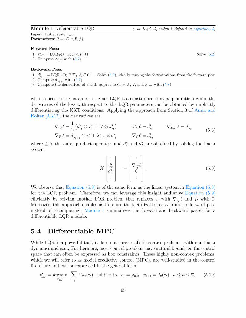
Module 1 Differentiable LQR (The LQR algorithm is defined in Algorithm 4)Input: Initial state xinit

Parameters: θ = {C, c, F, f}

Forward Pass:1: τ⋆1:T = LQRT (xinit;C, c, F, f) ▷ Solve (5.2)2: Compute λ⋆

1:T with (5.7)

Backward Pass:1: d⋆τ1:T = LQRT (0;C,∇τ⋆ℓ, F, 0) ▷ Solve (5.9), ideally reusing the factorizations from the forward pass2: Compute d⋆λ1:T

with (5.7)3: Compute the derivatives of ℓ with respect to C, c, F , f , and xinit with (5.8)

with respect to the parameters. Since LQR is a constrained convex quadratic argmin, thederivatives of the loss with respect to the LQR parameters can be obtained by implicitlydifferentiating the KKT conditions. Applying the approach from Section 3 of Amos andKolter [AK17], the derivatives are

∇Ctℓ =1

2

(d⋆τt ⊗ τ ⋆t + τ ⋆t ⊗ d⋆τt

)∇ctℓ = d⋆τt ∇xinit

ℓ = d⋆λ0

∇Ftℓ = d⋆λt+1⊗ τ ⋆t + λ⋆

t+1 ⊗ d⋆τt ∇ftℓ = d⋆λt

(5.8)

where ⊗ is the outer product operator, and d⋆τ and d⋆λ are obtained by solving the linearsystem

K

...d⋆τtd⋆λt...

= −

...∇τ⋆t

ℓ0...

. (5.9)

We observe that Equation (5.9) is of the same form as the linear system in Equation (5.6)for the LQR problem. Therefore, we can leverage this insight and solve Equation (5.9)efficiently by solving another LQR problem that replaces ct with ∇τ⋆t

ℓ and ft with 0.Moreover, this approach enables us to re-use the factorization of K from the forward passinstead of recomputing. Module 1 summarizes the forward and backward passes for adifferentiable LQR module.

5.4 Differentiable MPCWhile LQR is a powerful tool, it does not cover realistic control problems with non-lineardynamics and cost. Furthermore, most control problems have natural bounds on the controlspace that can often be expressed as box constraints. These highly non-convex problems,which we will refer to as model predictive control (MPC), are well-studied in the controlliterature and can be expressed in the general form

τ ⋆1:T = argminτ1:T

∑t

Cθ,t(τt) subject to x1 = xinit, xt+1 = fθ(τt), u ≤ u ≤ u, (5.10)

65

where the non-convex cost function Cθ and non-convex dynamics function fθ are (po-tentially) parameterized by some θ. We note that more generic constraints on the controland state space can be represented as penalties and barriers in the cost function. Thestandard way of solving the control problem Equation (5.10) is by iteratively forming andoptimizing a convex approximation

τ i1:T = argminτ1:T

∑t

Ciθ,t(τt) subject to x1 = xinit, xt+1 = f i

θ(τt), u ≤ u ≤ u, (5.11)

where we have defined the second-order Taylor approximation of the cost around τ i as

Ciθ,t = Cθ,t(τ

it ) + (pit)

⊤(τt − τ it ) +1

2(τt − τ it )

⊤H it(τt − τ it ) (5.12)

with pit = ∇τ itCθ,t and H i

t = ∇2τ itCθ,t. We also have a first-order Taylor approximation of

the dynamics around τ i as

f iθ,t(τt) = fθ,t(τ

it ) + F i

t (τt − τ it ) (5.13)

with F it = ∇τ it

fθ,t. In practice, a fixed point of Equation (5.11) is often reached, especiallywhen the dynamics are smooth. As such, differentiating the non-convex problem Equa-tion (5.10) can be done exactly by using the final convex approximation. Without thebox constraints, the fixed point in Equation (5.11) could be differentiated with LQR aswe show in Section 5.3. In the next section, we will show how to extend this to the casewhere we have box constraints on the controls as well.

66

5.4.1 Differentiating Box-Constrained QPs

First, we consider how to differentiate a more generic box-constrained convex QP of theform

x⋆ = argminx

1

2x⊤Qx+ p⊤x subject to Ax = b, x ≤ x ≤ x. (5.14)

Given active inequality constraints at the solution in the form Gx = h, this problem turnsinto an equality-constrained optimization problem with the solution given by the linearsystem

Q A⊤ G⊤

A 0 0

G 0 0

x⋆

λ⋆

ν⋆

= −

pbh

(5.15)

With some loss function ℓ that depends on x⋆, we can use the approach in Amos and Kolter[AK17] to obtain the derivatives of ℓ with respect to Q, p, A, and b as

∇Qℓ =1

2(d⋆x⊗x⋆+x⋆⊗d⋆x) ∇pℓ = d⋆x ∇Aℓ = d⋆λ⊗x⋆+λ⋆⊗d⋆x ∇bℓ = −d⋆λ (5.16)

where d⋆x and d⋆λ are obtained by solving the linear system

Q A⊤ G⊤

A 0 0

G 0 0

d⋆xd⋆λd⋆ν

= −

∇x⋆ℓ00

(5.17)

The constraint Gd⋆x = 0 is equivalent to the constraint d⋆xi= 0 if x⋆

i ∈ {xi, xi}. Thussolving the system in Equation (5.17) is equivalent to solving the optimization problem

d⋆x = argmindx

1

2d⊤xQdx + (∇x⋆ℓ)⊤dx subject to Adx = 0, dxi

= 0 if x⋆i ∈ {xi, xi} (5.18)

67

Algorithm 5 MPCT,u,u(xinit, uinit;C, f) Solves Equation (5.10) as described in [TMT14]The state space is n-dimensional and the control space is m-dimensional.T ∈ Z+ is the horizon length, the number of nominal timesteps to optimize for in the future.u, u ∈ Rm are respectively the control lower- and upper-bounds.xinit ∈ Rn, uinit ∈ RT×m are respectively the initial state and nominal control sequenceC : Rn×m → R is the non-convex and twice-differentiable cost function.F : Rn×m → Rn is the non-convex and once-differentiable dynamics function.x11 = xinit

for t = 1 to T-1 dox1t+1 = f(xt, uinit,t)

end forτ1 = [x1, uinit]

for i = 1 to [converged] dofor t = 1 to T do

▷ Form the second-order Taylor expansion of the cost as in Equation (5.12)Ci

t = ∇2τ itC(τ it )

cit = ∇τ itC(τ it )− (Ci

t)⊤τ it

▷ Form the first-order Taylor expansion of the dynamics as in Equation (5.13)F it = ∇τ i

tf(τ it )

f it = f(τ it )− F i

t τit

end forτ i+11:T = MPCstepT,u,u(xinit, C, f, τ

i1:T , C

i, ci, F i, f i)end for

function MPCstepT,u,u( xinit, C, f, τ1:T , C, c, F, f)▷ C, f are the true cost and dynamics functions. τ1:T is the current trajectory iterate.▷ C, c, F, f are the approximate cost and dynamics terms around the current trajectory.

▷ Backward Recursion: Over the linearized trajectory.VT = vT = 0for t = T to 1 do

Qt = Ct + F⊤t Vt+1Ft

qt = ct + F⊤t Vt+1ft + F⊤

t vt+1

kt = argminδu12δu

⊤Qt,uuδu+Q⊤x δu s.t. u ≤ u+ δu ≤ u

▷ Can be solved with a Projected-Newton method as described in [TMT14].▷ Let f, c respectively index the free and clamped dimensions of this optimization problem.

Kt,f = −Q−1t,uu,fQt,ux

Kt,c = 0

Vt = Qt,xx +Qt,xuKt +K⊤t Qt,ux +K⊤

t Qt,uuKt

vt = qt,x +Qt,xukt +K⊤t qt,u +K⊤

t Qt,uuktend for

▷ Forward Recursion and Line Search: Over the true cost and dynamics.repeat

x1 = τx1

for t = 1 to T dout = τut

+ αkt +Kt(xt − τxt)

xt+1 = f(xt, ut)end forα = γα

until∑

t C([xt, ut]) ≤∑

t C(τt)

return x1:T , u1:T

end function

68

Module 2 Differentiable MPC (The MPC algorithm is defined in Algorithm 5)Given: Initial state xinit and initial control sequence uinit

Parameters: θ of the objective Cθ(τ) and dynamics fθ(τ)

Forward Pass:1: τ⋆1:T = MPCT,u,u(xinit, uinit;Cθ, Fθ) ▷ Solve Equation (5.10)2: The solver should reach the fixed point in (5.11) with approximations to the cost Hn

θ and dynamics Fnθ

3: Compute λ⋆1:T with (5.7)

Backward Pass:1: Fn

θ is Fnθ with the rows corresponding to the tight control constraints zeroed

2: d⋆τ1:T = LQRT (0;Hnθ ,∇τ⋆ℓ, Fn

θ , 0) ▷ Solve (5.19), ideally reusing factorizations from the forward pass3: Compute d⋆λ1:T

with (5.7)4: Differentiate ℓ with respect to the approximations Hn

θ and Fnθ with (5.8)

5: Differentiate these approximations with respect to θ and use the chain rule to obtain ∂ℓ/∂θ

5.4.2 Differentiating MPC with Box ConstraintsAt a fixed point, we can use Equation (5.16) to compute the derivatives of the MPCproblem, where d⋆τ and d⋆λ are found by solving the linear system in Equation (5.9) withthe additional constraint that dut,i

= 0 if u⋆t,i ∈ {ut,i, ut,i}. Solving this system can be

equivalently written as a zero-constrained LQR problem of the form

d⋆τ1:T = argmindτ1:T

∑t

1

2d⊤τtH

nt dτt + (∇τ⋆t

ℓ)⊤dτt

subject to dx1 = 0, dxt+1 = F nt dτt , dut,i

= 0 if u⋆i ∈ {ut,i, ut,i}

(5.19)

where n is the iteration that Equation (5.11) reaches a fixed point, and Hn and F n arethe corresponding approximations to the objective and dynamics defined earlier. Mod-ule 2 summarizes the proposed differentiable MPC module. To solve the MPC problem inEquation (5.10) and reach the fixed point in Equation (5.11), we use the box-DDP heuris-tic [TMT14]. For the zero-constrained LQR problem in Equation (5.19) to compute thederivatives, we use an LQR solver that zeros the appropriate controls.

5.4.3 Drawbacks of Our ApproachSometimes the controller does not run for long enough to reach a fixed point of Equa-tion (5.11), or a fixed point doesn’t exist, which often happens when using neural net-works to approximate the dynamics. When this happens, Equation (5.19) cannot be usedto differentiate through the controller, because it assumes a fixed point. Differentiatingthrough the final iLQR iterate that’s not a fixed point will usually give the wrong gradients.Treating the iLQR procedure as a compute graph and differentiating through the unrolledoperations is a reasonable alternative in this scenario that obtains surrogate gradients tothe control problem. However, as we empirically show in Section 5.5.1, the backward passof this method scales linearly with the number of iLQR iterations used in the forward.Instead, fixed-point differentiation is constant time and only requires a single iLQR solve.

69

1 32 64 128Number of LQR Steps

10-3

10-2

10-1

100

101

Runt

ime

(s)

FP ForwardFP Backward

Unroll ForwardUnroll Backward

Figure 5.2: Runtime comparison of fixedpoint differentiation (FP) to unrolling theiLQR solver (Unroll), averaged over 10 tri-als.

0 200 400 600 800 1000Iteration

0.0

0.2

0.4

0.6

0.8

1.0

1.2

Imita

tion

Loss

0 200 400 600 800 1000Iteration

0.0

0.5

1.0

1.5

2.0

2.5

3.0

Mod

el L

oss

Figure 5.3: Model and imitation losses forthe LQR imitation learning experiments.

5.5 Experimental ResultsIn this section, we present several results that highlight the performance and capabilities ofdifferentiable MPC in comparison to neural network policies and vanilla system identifica-tion (SysId). We show 1) superior runtime performance compared to an unrolled solver, 2)the ability of our method to recover the cost and dynamics of a controller with imitation,and 3) the benefit of directly optimizing the task loss over vanilla SysId.

We have released our differentiable MPC solver as a standalone open source pack-age that is available at https://github.com/locuslab/mpc.pytorch and our experi-mental code for this chapter is also openly available at https://github.com/locuslab/differentiable-mpc. Our experiments are implemented with PyTorch [Pas+17b].

5.5.1 MPC Solver PerformanceFigure 5.2 highlights the performance of our differentiable MPC solver. We compare to analternative version where each box-constrained iLQR iteration is individually unrolled, andgradients are computed by differentiating through the entire unrolled chain. As illustratedin the figure, these unrolled operations incur a substantial extra cost. Our differentiableMPC solver 1) is slightly more computationally efficient even in the forward pass, as it doesnot need to create and maintain the backward pass variables; 2) is more memory efficientin the forward pass for this same reason (by a factor of the number of iLQR iterations);and 3) is significantly more efficient in the backward pass, especially when a large numberof iLQR iterations are needed. The backward pass is essentially free, as it can reuse all the

70

factorizations for the forward pass and does not require multiple iterations.

5.5.2 Imitation Learning: Linear-Dynamics Quadratic-Cost (LQR)In this section, we show results to validate the MPC solver and gradient-based learningapproach for an imitation learning problem. The expert and learner are LQR controllersthat share all information except for the linear system dynamics f(xt, ut) = Axt+But. Thecontrollers have the same quadratic cost (the identity), control bounds [−1, 1], horizon (5timesteps), and 3-dimensional state and control spaces. Though the dynamics can also berecovered by fitting next-state transitions, we show that we can alternatively use imitationlearning to recover the dynamics using only controls.

Given an initial state x, we can obtain nominal actions from the controllers as u1:T (x; θ),where θ = {A,B}. We randomly initialize the learner’s dynamics with θ and minimize theimitation loss

L = Ex

[||τ1:T (x; θ)− τ1:T (x; θ)||22

], .

We do learning by differentiating L with respect to θ (using mini-batches with 32 examples)and taking gradient steps with RMSprop [TH12]. Figure 5.3 shows the model and imitationloss of eight randomly sampled initial dynamics, where the model loss is MSE(θ, θ).The model converges to the true parameters in half of the trials and achieves a perfectimitation loss. The other trials get stuck in a local minimum of the imitation loss andcauses the approximate model to significantly diverge from the true model. These faultytrials highlight that despite the LQR problem being convex, the optimization problem ofsome loss function w.r.t. the controller’s parameters is a (potentially difficult) non-convexoptimization problem that typically does not have convergence guarantees.

5.5.3 Imitation Learning: Non-Convex Continuous ControlWe next demonstrate the ability of our method to do imitation learning in the pendulumand cartpole benchmark domains. Despite being simple tasks, they are relatively challeng-ing for a generic policy to learn quickly in the imitation learning setting. In our experimentswe use MPC experts and learners that produce a nominal action sequence u1:T (x; θ) whereθ parameterizes the model that’s being optimized. The goal of these experiments is to op-timize the imitation loss L = Ex

[||u1:T (x; θ)− u1:T (x; θ)||22

], again which we can uniquely

do using only observed controls and no observations. We consider the following methods:Baselines: nn is an LSTM that takes the state x as input and predicts the nominal

action sequence. In this setting we optimize the imitation loss directly. sysid assumesthe cost of the controller is known and approximates the parameters of the dynamics byoptimizing the next-state transitions.

Our Methods: mpc.dx assumes the cost of the controller is known and approximatesthe parameters of the dynamics by directly optimizing the imitation loss. mpc.cost assumesthe dynamics of the controller is known and approximates the cost by directly optimizingthe imitation loss. mpc.cost.dx approximates both the cost and parameters of the dynamicsof the controller by directly optimizing the imitation loss.

71

In all settings that involve learning the dynamics (sysid, mpc.dx, and mpc.cost.dx) weuse a parameterized version of the true dynamics. In the pendulum domain, the parametersare the mass, length, and gravity; and in the cartpole domain, the parameters are the cart’smass, pole’s mass, gravity, and length. For cost learning in mpc.cost and mpc.cost.dx weparameterize the cost of the controller as the weighted distance to a goal state C(τ) =||wg ◦ (τ − τg)||22. We have found that simultaneously learning the weights wg and goalstate τg is instable and in our experiments we alternate learning of wg and τg independentlyevery 10 epochs. We collected a dataset of trajectories from an expert controller and varythe number of trajectories our models are trained on. A single trial of our experimentstakes 1-2 hours on a modern CPU. We optimize the nn setting with Adam [KB14] witha learning rate of 10−4 and all other settings are optimized with RMSprop [TH12] with alearning rate of 10−2 and a decay term of 0.5.

Figure 5.5 shows that in nearly every case we are able to directly optimize the imitationloss with respect to the controller and we significantly outperform a general neural networkpolicy trained on the same information. In many cases we are able to recover the truecost function and dynamics of the expert. We show the training and validation losses inFigure 5.4. The comparison between our approach mpc.dx and SysId is notable, as we areable to recover equivalent performance to SysId with our models using only the controlinformation and without using state information.

nn sysid mpc.dxmpc.cost

mpc.cost.dx

10-9

10-7

10-5

10-3

10-1

101

Imita

tion

Loss

Pendulum (#Train: 10)

nn sysid mpc.dxmpc.cost

mpc.cost.dx

10-9

10-7

10-5

10-3

10-1

101Pendulum (#Train: 50)

nn sysid mpc.dxmpc.cost

mpc.cost.dx

10-9

10-7

10-5

10-3

10-1

101Pendulum (#Train: 100)

nn sysid mpc.dxmpc.cost

mpc.cost.dx

10-4

10-3

10-2

10-1

100

101

102

Imita

tion

Loss

Cartpole (#Train: 10)

nn sysid mpc.dxmpc.cost

mpc.cost.dx

10-4

10-3

10-2

10-1

100

101

102 Cartpole (#Train: 50)

nn sysid mpc.dxmpc.cost

mpc.cost.dx

10-4

10-3

10-2

10-1

100

101

102 Cartpole (#Train: 100)

Train Val Test

Figure 5.4: Learning results on the (simple) pendulum and cartpole environments. Weselect the best validation loss observed during the training run and report the correspondingtrain and test loss. Every datapoint is averaged over four trials.

Again, while we emphasize that these are simple tasks, there are stark differencesbetween the approaches. Unlike the generic network-based imitation learning, the MPCpolicy can exploit its inherent structure. Specifically, because the network contains a

72

nn sysid mpc.dxmpc.cost

mpc.cost.dx

10-9

10-7

10-5

10-3

10-1

101

Imita

tion

Loss

Baselines OursPendulum

nn sysid mpc.dxmpc.cost

mpc.cost.dx

10-4

10-3

10-2

10-1

100

101

Imita

tion

Loss

Baselines OursCartpole

#Train: 10 #Train: 50 #Train: 100

Figure 5.5: Learning results on the (simple) pendulum and cartpole environments. Weselect the best validation loss observed during the training run and report the best testloss.

well-defined notion of the dynamics and cost, it is able to learn with much lower samplecomplexity that a typical network. But unlike pure system identification (which would bereasonable only for the case where the physical parameters are unknown but all other costsare known), the differentiable MPC policy can naturally be adapted to objectives besidessimple state prediction, such as incorporating the additional cost learning portion.

5.5.4 Imitation Learning: SysId with a non-realizable expertAll of our previous experiments that involve SysId and learning the dynamics are in theunrealistic case when the expert’s dynamics are in the model class being learned. In thisexperiment we study a case where the expert’s dynamics are outside of the model classbeing learned. In this setting we will do imitation learning for the parameters of a dynamicsfunction with vanilla SysId and by directly optimizing the imitation loss (sysid and thempc.dx in the previous section, respectively).

SysId often fits observations from a noisy environment to a simpler model. In oursetting, we collect optimal trajectories from an expert in the pendulum environment thathas an additional damping term and also has another force acting on the point-massat the end (which can be interpreted as a “wind” force). We do learning with dynamicsmodels that do not have these additional terms and therefore we cannot recover the expert’sparameters. Figure 5.6 shows that even though vanilla SysId is slightly better at optimizingthe next-state transitions, it finds an inferior model for imitation compared to our approachthat directly optimizes the imitation loss.

We argue that the goal of doing SysId is rarely in isolation and always serves the purposeof performing a more sophisticated task such as imitation or policy learning. TypicallySysId is merely a surrogate for optimizing the task and we claim that the task’s loss signalprovides useful information to guide the dynamics learning. Our method provides one wayof doing this by allowing the task’s loss function to be directly differentiated with respectto the dynamics function being learned.

73

0 50 100 150 200 250Epoch

0.000

0.005

0.010SysID Loss

0 50 100 150 200 250Epoch

0.0

0.1

0.2

0.3Imitation Loss

Vanilla SysId Baseline (Ours) Directly optimizing the Imitation Loss

Figure 5.6: Convergence results in the non-realizable Pendulum task.5.6 ConclusionThis chapter lays the foundations for differentiating and learning MPC-based controllerswithin reinforcement learning and imitation learning. Our approach, in contrast to themore traditional strategy of “unrolling” a policy, has the benefit that it is much less com-putationally and memory intensive, with a backward pass that is essentially free giventhe number of iterations required for a the iLQR optimizer to converge to a fixed point.We have demonstrated our approach in the context of imitation learning, and have high-lighted the potential advantages that the approach brings over generic imitation learningand system identification.

We also emphasize that one of the primary contributions of this chapter is to defineand set up the framework for differentiating through MPC in general. Given the recentprominence of attempting to incorporate planning and control methods into the loop ofdeep network architectures, the techniques here offer a method for efficiently integratingMPC policies into such situations, allowing these architectures to make use of a very pow-erful function class that has proven extremely effective in practice. The future applicationsof our differentiable MPC method include tuning model parameters to task-specific goalsand incorporating joint model-based and policy-based loss functions; and our method canalso be extended for stochastic control.

74

Chapter 6The Limited Multi-Label Projection Layer

We present the Limited Multi-Label (LML) projection layer as a new primitive operationfor end-to-end learning systems. The LML layer provides a probabilistic way of modelingmulti-label predictions limited to having exactly k labels. We derive efficient forwardand backward passes for this layer and show how the layer can be used to optimize thetop-k recall for multi-label tasks with incomplete label information. We evaluate LMLlayers on top-k CIFAR-100 classification and scene graph generation. We show that LMLlayers add a negligible amount of computational overhead, strictly improve the model’srepresentational capacity, and improve accuracy.

The content of this chapter is joint work with J. Zico Kolter and Vladlen Koltun.

6.1 IntroductionMulti-label prediction tasks show up frequently in computer vision and language processing.Multi-label predictions can arise from a task being truly multi-label, as in language andgraph generation tasks, or by turning a single-label prediction task into a multi-labelprediction task that predicts a set of top-k labels, for example. In high-dimensional cases,such as scene graph generation, annotating multi-label data is difficult and often resultsin datasets that have an incomplete labeling. In these cases, models are typically limitedto predicting k labels and are evaluated on the recall, the proportion of known labels thatare present in the model’s predicted set. As we will show later, the standard approachesof using a softmax or sigmoid functions are not ideal here as they have no way of allowingthe model to capture labels that are unobserved.

In this chapter, we present the LML layer as a new way of modeling in multi-labelsettings where the model needs to make a prediction of exactly k labels. We derive howto efficiently implement and differentiate through LML layers in Section 6.3. The LMLlayer has a probabilistic interpretation and can be trained with a standard maximum-likelihood approach that we show in Section 6.4, where we also highlight applications totop-k image classification and scene graph generation. We show experiments in Section 6.5on CIFAR-100 classification and scene graph generation.

75

k=1

k=2

000

101

010 110

011

100

111

001

01010110

10101001

1100

0011

Figure 6.1: The LML polytope Ln,k is the set of points in the unit n-hypercube withcoordinates that sum to k. Ln,1 is the (n− 1)-simplex. The L3,1 and L3,2 polytopes(triangles) are on the left in blue. The L4,2 polytope (an octahedron) is on the right.

6.2 Background and Related WorkOur work is motivated by the ubiquity of projections onto polytopes in machine learning.We showed in Section 2.4.4 how the ReLU, sigmoid, and softmax layers can be interpretedas explicit closed-form solutions to a projection optimization problem. Similar projectionsare also done onto more complex polytopes such as the marginal polytope for structuredinference [Nic+18] or the Birkhoff polytope for permutations [AZ11; San+18; Men+18].

The remainder of this section reviews related work on cardinality modeling, top-koptimization, ranking-based loss functions, and scene graph generation.

6.2.1 Cardinality Potentials and ModelingCardinality potentials and modeling are a closely related line of work typically found in thestructured prediction and constraint programming literature. Régin [Rég96] shows how toadd constraints to models for worker scheduling. Tarlow, Swersky, Zemel, Adams, andFrey [Tar+12] and Globerson, Lazic, Chakrabarti, Subramanya, Ringaard, and Pereira[Glo+16] propose ways of performing structured prediction with cardinality potentials,and Brukhim and Globerson [BG18] propose a soft projection operation that integratecardinality modeling into deep structured prediction architectures like SPENs [BM15].In contrast to all of these methods, our projection and constraint is exact and can beintegrated in the standard forward pass of a deep model outside of structured prediction.None of our experiments use structured prediction techniques and we instead do standardsupervised learning of vanilla feedforward models that use our LML layer. In contrast toBrukhim and Globerson [BG18], we show that the backward pass of our soft projectioncan be exactly computed instead of unrolled as part of a structured prediction procedure.

6.2.2 Top-k and Ranking-Based Loss FunctionsThere has been a significant amount of work on creating specialized loss functions foroptimizing the model’s top-k prediction error [GBW14; LJZ14; Liu+15; LHS15; Liu+15;LHS16; BZK18] and ranking error [Aga11; Rud09; Boy+12; Rak12].

76

Most relevant to our contributions are the smooth top-k loss functions discussed inLapin, Hein, and Schiele [LHS16] and the Smooth SVM [BZK18]. Among other loss func-tions, Lapin, Hein, and Schiele [LHS16] propose the truncated top-k entropy loss, which wereview in Section 6.2.2 and extend to cases when multiple ground-truth labels are presentin Section 6.2.2.

In contrast to all of these methods, our approach does not hand-craft a loss functionand instead puts the top-k knowledge into the modeling part of the pipeline, which isthen optimized as a likelihood maximization problem. We show in Section 6.5.2 that LMLlayers are competitive in the top-k prediction task from Berrada, Zisserman, and Kumar[BZK18].

Truncated Top-k Entropy Derivation

This section reviews the truncated top-k entropy derivation from Section 2.5 of Lapin,Hein, and Schiele [LHS16]. We start with the standard likelihood

P (y | x) = exp{fy(x)}∑j exp{fj(x)}

(6.1)

and then consider the negative log-likelihood

− logP (y | x) = − logexp{fy(x)}∑j exp{fj(x)}

= log

∑j exp{fj(x)}exp{fy(x)}

= log

(1 +

∑j =y

exp{fj(x)− fy(x)}

) (6.2)

Truncating the index set of the last sum gives the truncated top-k entropy loss

log

1 +∑j∈Jy

exp{fj(x)− fy(x)}

(6.3)

where Jy are the indices of the m−k smallest components of (fj(x))j =y. This loss is smallwhenever the top-k error is zero.

Multi-Label Truncated Top-k Entropy Derivation

The truncated top-k entropy loss from Lapin, Hein, and Schiele [LHS16] is a competitiveand simple loss function for optimizing the model’s top-k predictions in single-label clas-sification tasks. In this section, we show how it can be extended to optimizing the top-kpredictions in multi-label classification tasks, such as scene graph generation.

77

We start by making an independence assumption between the observed labels anddecomposing the likelihood as

P (Y | x) =∏i

P (Yi|x). (6.4)

Then, we can assume the likelihood of each label is obtained with a softmax as

P (Yi | x) =exp{fyi(x)}∑j exp{fj(x)}

. (6.5)

We note that in general, maximum-likelihood estimation of the form Equation (6.5) willnever achieve perfect likelihood as the softmax restricts the likelihoods over all of the labels.However following the approach from Lapin, Hein, and Schiele [LHS16], we can rearrangethe terms of the negative log-likelihood and truncate parts of to obtain a reasonable lossfunction.

− logP (Y | x) = −∑i

logexp{fyi(x)}∑j exp{fj(x)}

=∑i

log

∑j exp{fj(x)}exp{fyi(x)}

=∑i

log

(1 +

∑j =yi

exp{fj(x)− fyi(x)}

) (6.6)

Truncating the index set of the last sum gives the multi-label truncated top-k entropy loss

∑i

log

1 +∑j∈Jy

exp{fj(x)− fyi(x)}

(6.7)

where Jy are the indices of the m− k smallest components of (fj(x))j ∈y. This loss is smallwhenever the top-k recall is zero.

6.2.3 Scene Graph GenerationScene graph generation is the task of generating a set of objects and relationships betweenthem from an input image and has been extensively studied recently [Joh+15; Yan+17;Plu+17; LLX17; Rap+17; ND17; Xu+17; Li+18b; Her+18; Zel+18; Woo+18]. Mostrelevant to our work are the methods that score all of the possible relationships betweenobjects and select the top-scoring relationships [Xu+17; Li+18b; Her+18; Woo+18]. Thesemethods include the near-state-of-the-art Neural Motifs model [Zel+18] that generates ascene graph by creating object- and edge-level contexts.

We propose a way of improving the relationship prediction portion of methods thatfully enumerate all of the possible relationships, and we empirically demonstrate that thisimproves the representational capacity of Neural Motifs.

78

Module 3 The Limited Multi-Label Projection LayerInput: x ∈ Rn

Forward Pass (Described in Section 6.3.1)1: Compute ν⋆ with Algorithm 62: return y⋆ = σ(x+ ν⋆)

Backward Pass (Described in Section 6.3.2)1: h = (y⋆)−1 + (1− y⋆)−1

2: dν = (1⊤h−1)−1h−⊤ (∇y⋆ℓ)3: dy = h−1 ◦ (dν −∇y⋆ℓ)4: return ∇xℓ = −dy

6.3 The Limited Multi-Label Projection LayerWe propose the Limited Multi-Label projection layer as a way of projecting onto the set ofpoints in the unit n-hypercube with coordinates that sum to exactly k. This space can berepresented as a polytope, which we define as the (n,k)-Limited Multi-Label polytope

Ln,k = {p ∈ Rn | 0 ≤ p ≤ 1 and 1⊤p = k}.

When k = 1, the LML polytope is the (n− 1)-simplex. Notationally, if n is implied by thecontext we will leave it out and write Lk. Figure 6.1 shows three low-dimensional examplesof this polytope.

We consider projections onto the interior of the LML polytope of the form

ΠLk(x) = argmin

0<y<1−x⊤y −Hb(y) s. t. 1⊤y = k (6.8)

where Hb(y) = −∑

i yi log yi + (1 − yi) log(1 − yi) is the binary entropy function. Theentropy-based regularizer in the objective helps prevent sparsity in the gradients of thisprojection, which is important for learning and the same reason it is useful in the softmax.We note that other projections could be done by changing the regularizer or by scaling theentropy term with a temperature parameter. The following is one useful property of theLML projection when x is the output of a function such as a neural network.Proposition 4. ΠLk

(x) preserves the (magnitude-based) order of the coordinates of x.The intuition is that ΠLk

(x) can be decomposed to applying a monotonic transformationto each element of x, which we show in Equation (6.9). Thus, this preserves the (magnitude-based) ordering of x.

The LML projection layer does not have an explicit closed-form solution like the layersdiscussed in Section 2.4.4, despite the similarity to the softmax layer. We show how toefficiently solve the optimization problem for the forward pass in Section 6.3.1 and how tobackpropagate through the LML projection in Section 6.3.2 by implicitly differentiatingthe KKT conditions. Module 3 summarizes the implementation of the layer.

79

6.3.1 Efficiently computing the LML projectionThe LML projection in Equation (6.8) is a convex and constrained optimization problem.In this section we propose an efficient way of solving it that is GPU-amenable.

�10.0 �7.5 �5.0 �2.5 0.0 2.5 5.0 7.5 10.0

⌫

�2

�1

0

1

2

3

4

g(⌫) =P

i �(xi + ⌫) � k

�10.0 �7.5 �5.0 �2.5 0.0 2.5 5.0 7.5 10.0

⌫

0.0

0.2

0.4

0.6

0.8

1.0

�(xi + ⌫)

π(x)1:kπ(x)k+1

π(x)k+2:n

Figure 6.2: Example of finding the optimal dual variable ν with x ∈ R6 and k = 2 bysolving the root-finding problem g(ν) = 0 in Equation (6.10), which is shown on the left.The right shows the decomposition of the individual logistic functions that contribute tog(ν). We show the initial lower and upper bounds described in Section 6.3.1.

Introducing a dual variable ν ∈ R for the constraint k − 1⊤y = 01, the Lagrangian ofEquation (6.8) is

L(y, ν) = −x⊤y −Hb(y) + ν(k − 1⊤y).

Differentiating this gives

∇yL(y, ν) = −x+ logy

1− y− ν

and the first-order optimality condition ∇yL(y⋆, ν⋆) = 0 gives

y⋆ = σ(x+ ν⋆) (6.9)

where σ is the logistic function. To find the optimal dual variable ν⋆, we can substituteEquation (6.9) into the constraint

g(ν) ≜ 1⊤σ(x+ ν)− k = 0. (6.10)

Thus the LML projection can be computed by solving g(ν) = 0 for the optimal dualvariable and then using Equation (6.9) for the projection.

Solving g(ν) = 0

g(ν) = 0 is a scalar-valued root-finding problem of a differentiable, continuous, non-convexfunction that is monotonically increasing. Despite the differentiability, we advocate forsolving g(ν) = 0 with a bracketing method that maintains an interval of lower and upperbounds around the solution ν⋆ and is amenable to parallelization, instead of a Newton

1 We unconventionally negate the equality constraint to make analyzing g(ν) easier.

80

Algorithm 6 Bracketing method to find g(ν) = 0

Input: x ∈ Rn

Parameters: d: the number of per-iteration samples∆: the saturation offset

1: Initialize νℓ = −π(x)k −∆ and νu = −π(x)k+1 +∆2: while |νℓ − νu| > ϵ do3: Sample ν1:d linearly from the interval [νℓ, νu]4: g1:d = (g(νi))

di=1 ▷ Ideally parallelized

5: ▷ Return the corresponding νi early if any gi = 06: iℓ = max{i | gi < 0} and iu = iℓ + 17: νℓ = νiℓ and νu = νiu8: end while9: return (νℓ + νu)/2

method that would use the derivative information but is not as amenable to parallelization.Our method generalizes the bisection bracketing method by sampling g(ν) for d values ofν per iteration instead of a single point. On the GPU by default, we sample d = 100points in parallel for each iteration, which usually reaches machine epsilon in less than 10iterations, and on the CPU we sample d = 10 points. We present our bracketing methodin Algorithm 6 and show an example of g(ν) and the component functions in Figure 6.2.

The initial lower bound νℓ and upper bound νu on the root can be obtained by observingthat g(ν) takes a sum of logistic functions that are offset by the entries of x ∈ Rn asσ(xj + ν). With high probability, we can use the saturated areas of the logistic functionsto construct the initial bounds.

Let π(x) sort x ∈ Rn in descending order so that

π(x)1 ≥ π(x)2 ≥ . . . ≥ π(x)n

and ∆ be a sufficiently large offset that causes the sigmoid units to saturate. We use ∆ = 7in all of our experiments.

Use νℓ = −π(x)k − ∆ for the initial lower bound. This makes σ(xj + νℓ) ≈ 0 forxj ∈ π(x)k,...,n and 0 < σ(xj + νℓ) < 1 for xj ∈ π(x)1,...,k−1, and thus g(νℓ) ≤ −1 ≤ 0.

Use νu = −π(x)k+1 +∆ for the initial upper bound. This makes σ(xj + νu) ≈ 1 forevery xj ∈ π(x)1,...,k+1 and thus g(νu) ≥ 1 ≥ 0.

6.3.2 Backpropagating through the LML layerLet y⋆ = ΠLk

(x) be outputs of the LML layer from Equation (6.8). Integrating this layerinto a gradient-based end-to-end learning system requires that we compute the derivative

∂ℓ

∂x=

∂ℓ

∂y⋆∂y⋆

∂x,

where ℓ is a loss function. The LML projection ΠLk(x) does not have an explicit closed-

form solution and we therefore cannot use an autodiff framework to compute the gradient

81

Algorithm 7 Maximizing top-k recall via maximum likelihood with the LML layer.Model: fθ : X → Rn

Model Predictions: Yi = {j | fθ(xi)j ≥ π (fθ(xi))k}Training Procedure:

1: while unconverged do2: Sample (xi, Yi) ∼ D3: p = ΠLk

(fθ(xi))4: Update θ with a gradient step ∇θℓ(Yi, p) where

ℓ(Yi, p) = −∑j∈Yi

log pj

5: end while

∂y⋆/∂x. We note that even though the solution can be represented as y⋆ = σ(x + ν⋆),differentiating this form is still difficult because ν⋆ is also a function of x. We instead im-plicitly differentiate the KKT conditions of Equation (6.8). Using the approach described,e.g., in OptNet [AK17], we can solve the linear system[

H −1−1⊤ 0

] [dydν

]= −

[∇y⋆ℓ0

](6.11)

where H = ∇2yL(y, ν) is defined by H = diag(h) and

h =1

y⋆+

1

1− y⋆. (6.12)

The system in Equation (6.11) can be solved analytically with

dν =1

1⊤h−1h−⊤ (∇y⋆ℓ) and dy = h−1 ◦ (dν −∇y⋆ℓ) (6.13)

where ◦ is the elementwise product and h−1 is the elementwise inverse. Finally, we havethat ∇xℓ = −dy.

6.4 Maximizing Top-k Recall via Maximum Likelihoodwith The LML layer

In this section, we highlight one application of the LML layer for maximizing the top-krecall. We consider a multi-label classification setting where the data has an incomplete(strict) subset of the true labels and we want to model the task by predicting a set ofexactly k labels. This setting comes up in practice for predicting the top-k labels in imageclassification and in predicting a set of k relationships in a graph for scene graph generation,which we discuss in Sections 6.4.1 and 6.4.2, respectively.

82

Formally, we have samples (xi, Yi) ∼ D from some data generating process D withfeatures xi ∈ Xi and labels Yi ⊆ Y ⋆

i ⊆ Y ≜ {1, . . . , n}, where Y ⋆i are the ground-truth

labels and Yi are the observed labels. There is typically some k ≪ n such that |Y ⋆i | ≤ k

for all i. We will model this by predicting exactly k labels Yi ⊆ {1, . . . n} where |Yi| = k.The model’s predictions should have high recall on the observed data, which for a single

sample is defined byrecall(Y, Y ) =

1

|Y |∑j∈Y

Jyj ∈ Y K,where the Iverson bracket JP K is 1 if P is true and 0 otherwise. We note that the 0-1 error,defined as

error(Y, Y ) = JY = Y K,or smooth variants thereof, are not a reasonable proxy for the recall as it incorrectlypenalizes the model when it makes a correct prediction Y that is in the ground truthlabels Y ⋆ but not in the observation Y .

We will next use a probabilistic approach to motivate the use of LML layers for max-imum recall. Given access to the ground-truth data in addition to the observation andassuming label independence, we could maximize the likelihood of a parametric modelwith

P (Y, Y ⋆ | x) =∏j∈Y

P (j ∈ Y ⋆ | x). (6.14)

We can decompose P (Y, Y ⋆ | x) as

P (Y, Y ⋆ | x) =∏j∈Y ⋆

P (j ∈ Y ⋆ | x)∏

j∈Y−Y ⋆

P (j ∈ Y ⋆ | x).

︷ ︸︸ ︷∏j∈Y

P (j ∈ Y ⋆ | x)∏

j∈Y ⋆−Y

P (j ∈ Y ⋆ | x)

The difficulty in modeling this problem given only the observed labels Y comes from notknowing which of the unobserved labels should be active or inactive. In the case when all|Y ⋆| = k, then the ground-truth labels can be interpreted as vertices of the LML polytopethat have a value of 1 if the label is present and 0 otherwise. Thus, we can use a modelthat makes a prediction on the LML polytope fθ : X → Lk. The outputs of this modelp = fθ(x) are then the likelihoods pj ≜ P (j ∈ Y ⋆ | x). For example, fθ can be modeledwith a standard deep feed-forward network with an LML layer at the end. The set ofpredicted labels can be obtained with

Y (x) = {j | fθ(x)j ≥ π (fθ(x))k},

breaking ties if necessary in the unlikely case that multiple fθ(x)j = π (fθ(x))k. We nextstate assumptions under which we can reason about maximum-likelihood solutions.

Assumptions. For the following, we assume that 1) in the infinite data setting, theground-truth labels are able to be reconstructed from the observed labels (e.g. for a fixedfeature, the observed labels are sampled from the ground-truth labels with a non-zero

83

weight on each label), 2) there is no noise in the data generating process, 3) the truemodel is realizable and therefore maximizing the likelihoods can be done exactly, and 4)all |Y ⋆

i | = k. We claim that all of these assumptions can be reasonably relaxed and weempirically show that LML layers are effective in settings where these don’t hold.Proposition 5. Maximizing the likelihood of fθ(xi) : X → Lk on only the observed data

maxθ

E

[∏j∈Yi

(fθ(xi))j

]≜ E

[∏j∈Yi

P (j ∈ Y ⋆i | xi)

]

implicitly maximizes E [P (Y ⋆i | xi)]. All expectations are done over samples from the data

generating process (xi, Yi) ∼ D.This can be proven by observing that the model’s LML output space will allow the

unobserved positive labels to have high likelihood∏j∈Y ⋆−Y

P (j ∈ Y ⋆ | x)

while forcing all the true negative data to have low likelihood∏j∈Y−Y ⋆

P (j ∈ Y ⋆ | x).

We note that Proposition 5 does not hold for a standard multi-label prediction modelthat makes predictions onto the unit hypercube fθ : X → [0, 1]n where

pj = fθ(xi) ≜ P (j ∈ Y ⋆ | x)

as only maximizing ∏j∈Yi

P (j ∈ Y ⋆ | x)

will result in a collapsed model that predicts pj = 1 for every label j ∈ Y .Corollary 2. Maximizing the likelihood of fθ : X → Lk on the observed data E [P (Yi | xi)]

maximizes the recall of the observed data E[recall(Y, Y )

].

The ground-truth data are vertices of the LML polytope and fθ approaches the ground-truth likelihoods. Thus the model’s prediction Y (x) is the ground-truth and the recall ofthe observed data is maximized. We again note that the model’s 0-1 error on the observeddata error(Y, Y ) is in general not minimized, but that the error on the ground-truth dataerror(Y ⋆, Y ) is minimized, as the observed data may not have all of the labels that arepresent in the ground-truth data.

We propose a gradient-based approach of solving this maximum likelihood problem inAlgorithm 7 that we use for all of our experiments.

84

6.4.1 Top-k Image ClassificationIn top-k image classification, the dataset consists of images xi with single labels yi andthe task is to predict a set of k labels Y that maximizes recall({yi}, Y ). We show inSection 6.5.2 that LML models are competitive with the state-of-the-art methods for top-k image classification on the noisy variant of CIFAR-100 from Berrada, Zisserman, andKumar [BZK18].

6.4.2 Scene Graph GenerationAs briefly introduced in Section 6.2.3, scene graph generation methods take an image asinput and output a graph of the objects in the image (the nodes of the graph) and therelationships between them (the edges of the graph). One of the recent state-of-the-artmethods that is characteristic of many of the other methods is Neural Motifs [Zel+18].Neural Motifs and related models such as Xu, Zhu, Choy, and Fei-Fei [Xu+17] make anassumption that the relationships on separate edges are independent from each other. Inthis section, we show how we can use the maximum recall training with an LML layerto make a minor modification to the training procedure of these models that allows us torelax this assumption with negligible computational overhead.

Specifically, the Neural Motifs architecture decomposes the scene graph generation taskas

P (G | I) = P (B | I) P (O | B, I)P (R | B,O, I)

where G is the scene graph, I is the input image, B is a set of region proposals, and Ois a set of object proposals. The relationship generation process P (R | B,O, I) makes anindependence assumption that, given a latent variable z that is present at each edge as zij,the relationships on each edge are independent. That is,

P ([xi→j]ij | z, B,O, I) =∏i,j

P (xi→j | zij, B,O, I),

where the set of relationships between all of the nodes is R = [xi→j]ij.Neural Motifs models these probabilities with

P (xi→j | B,O, I) = pij ≜ softmax(zij) ∈ ∆n, (6.15)

where n is the number of relationships for the task. The predictions are made in the n-simplex instead of the (n−1)-simplex because an additional class is added to indicate thatno relationship is present on the edge. For inference, graphs are generated by selectingthe relationships that have the highest probability by concatenating all pij and selectingthe top k. Typical values of k are 20, 50, and 100. The method is then evaluated on thetop-k recall of the scene graphs; i.e. the number of ground-truth relationships that are inthe model’s top-k relationship predictions.

Two drawbacks of the vanilla Neural Motif model of treating the edge relationshipsas independent softmax functions are that 1) edges with multiple relationships will neverachieve perfect likelihood because the softmax function is being used to make a prediction

85

at each edge. If multiple relationships are present on a single edge, the training code forNeural Motifs randomly samples a single one to use for the update in that iteration. Forinference, multiple relationships on a node can be predicted if their individual probabilitiesare within the top-k threshold, although they are still subject to the simplex constraintsand therefore may be unreasonably low; and 2) the evaluation metric of generating a graphwith k relationships is not part of the training procedure that just treats each edge as aclassification problem that maximizes the likelihood of the observed relationships.

Using an LML layer to predict all of the relationship probabilities jointly overcomesthese drawbacks. We model the joint probability with

P ([xi→j]ij | z, B,O, I) = ΠLk(cat([zij]ij)) (6.16)

where cat is the concatenation function. This is now a top-k recall problem that we train bymaximizing the likelihood of the observed relationships with Algorithm 7. We have addedthe LML training procedure to the official Neural Motifs codebase in ≈20 lines of code toproject [zij]ij onto the LML polytope instead of projecting each zij onto the simplex, andto optimize the likelihood of the data jointly instead of independently.

The LML approach for scene graph generation overcomes both of the drawbacks of thevanilla approach by 1) allowing the ground-truth data to achieve near-perfect likelihoodas multiple relationships are allowed to be present between the edges, and 2) introducingthe knowledge predicting k nodes into the training procedure. One downside of the LMLapproach for scene graph generation is that the training procedure now depends on kwhile the vanilla training procedure does not. We empirically show that it is typicallycompetitive to train with a fixed k and evaluate for others.

6.5 Experimental ResultsIn this section we study the computational efficiency of the LML layer and show that itperforms competitively with other methods for top-k image classification. When added tothe Neural Motifs model for scene graph generation, LML layers significantly improve themodeling capability with almost no computational overhead.

6.5.1 Performance ComparisonsThe LML layer presented in Module 3 has a non-trivial forward and backward pass thatmay be computationally expensive if not implemented efficiently. To better understand thecomputational costs of the LML layer, we have measured the timing performance of ourlayer in comparison to the Smooth SVM loss from [BZK18] and the truncated top-k entropyEnttr from [LHS16], which we review in Section 6.2.2. The Summation Algorithm (SA) andDivide-and-Conquer (DC) algorithms for the Smooth SVM loss are further described inBerrada, Zisserman, and Kumar [BZK18]. We use the official Smooth SVM implementationand have re-implemented the truncated top-k entropy in PyTorch for our experiments. Thetruncated top-k entropy loss function is only bottlenecked by a sorting operation, whichwe implemented using PyTorch’s sort function.

86

10-4

10-3

10-2

10-1

100

101

Tim

e (s

)

k=5 k=50 k=100 k=5 k=50 k=1001000 Classes 10000 Classes

Forward Time

10-4

10-3

10-2

10-1

100

Tim

e (s

)

k=5 k=50 k=100 k=5 k=50 k=1001000 Classes 10000 Classes

Backward Time

Smooth SVM ( SA DC Backward) Enttr LML

Figure 6.3: Timing performance results. Each point is from 50 trials on an unloadedsystem.

0.0 0.2 0.4 0.6 0.8 1.0Noise

0

20

40

60

80

100

Accu

racy

@1

0.0 0.2 0.4 0.6 0.8 1.0Noise

70

80

90

100

Accu

racy

@k

Cross-Entropy Smooth SVM Enttr LML

Figure 6.4: Testing performance on CIFAR-100 with label noise.

We use the experimental setup from Berrada, Zisserman, and Kumar [BZK18] to mea-sure the performance, which uses a minibatch size of 256 and runs 50 trials for each datapoint. We ran all of the experiments on an unloaded NVIDIA GeForce GTX 1080 Ti GPU.

Figure 6.3 shows the performance results on problems with a minibatch size of 256 andhighlights the minimal overhead of the LML layer. In nearly all instances, the LML layeroutperforms the Smooth SVM forward and backward passes. Notably, the LML backwardpass is significantly faster in all cases. The forward pass of the smooth SVM becomescomputationally expensive as k grows while the LML layer’s performance remains con-stant. The top-k entropy loss is only bottlenecked by a sorting operation and significantlyoutperforms both the Smooth SVM and LML layers.

6.5.2 Top-k Image Classification on CIFAR-100We next evaluate the LML layer on the noisy top-5 CIFAR-100 task from Berrada, Zis-serman, and Kumar [BZK18] that uses the DenseNet 40-40 architecture [Hua+17]. TheCIFAR-100 labels are organized into 20 “coarse” classes, each consisting of 5 “fine” labels.With probability p, noise is added to the labels by resampling from the set of “fine” labels.

Figure 6.4 shows that the LML model is competitive with the other baseline methods forthis task: standard cross-entropy training, the Smooth SVM models, and the truncatedentropy loss. We used the experimental setup and code from Berrada, Zisserman, and

87

0 5 10 15 20 25 30Epoch

0.60

0.65

0.70

0.75

Reca

ll

Train Recall (Constrained)

0 5 10 15 20 25 30Epoch

0.60

0.62

0.64

0.66

0.68

Reca

ll

Val Recall (Constrained)

[Zel+18] R@( 20 50 100) +Enttr R@( 20 50 100) +LML R@( 20 50 100)

Figure 6.5: (Constrained) Scene graph generation on the Visual Genome: Training andvalidation progress comparing the vanilla Neural Motif model to the Enttr and LML ver-sions.

Predicate Classification (Constrained) Predicate Classification (Unconstrained)

Model R@20 R@50 R@100 R@20 R@50 R@100

[Zel+18] 58.5 65.2 67.1 66.6 81.1 88.2

+Enttr 59.4 66.1 67.8 60.8 70.7 75.6+LML 58.5 66.0 67.9 64.2 79.4 87.6

Table 6.1: Scene graph generation on the Visual Genome: Test Dataset Results.

Kumar [BZK18] and added the LML experiments with a few lines of code. Notably, wealso re-implemented the truncated entropy loss from Lapin, Hein, and Schiele [LHS16] asanother reasonable baseline for this task. Following the method of Berrada, Zisserman,and Kumar [BZK18], we ran four seeds for the truncated entropy and LML models andreport the average test performance. For reference, a model making random predictionswould obtain 1% top-1 accuracy and 5% top-5 accuracy.

The results show that relative to the cross-entropy, the smooth SVM, truncated entropy,and LML losses perform similarly. Relative to each other the best method is not clear,which is consistent with the experimental results on other tasks in Lapin, Hein, and Schiele[LHS16]. We interpret these results as showing that all of the methods evaluated for top-k optimization provide nearly identical gradient information to the model and only havesmall differences.

6.5.3 Scene Graph GenerationFor our scene graph generation experiments we use the MotifNet-LeftRight model,experimental setup, and official code from Zellers, Yatskar, Thomson, and Choi [Zel+18].We added the LML variant with ≈20 lines of code. This experiment uses the VisualGenome dataset [Kri+17], using the the publicly released preprocessed data and splitsfrom Xu, Zhu, Choy, and Fei-Fei [Xu+17]. In this chapter, we focus solely on the PredicateClassification evaluation mode PredCls which uses a pre-trained detector and classifierand only measures improvements to the relationship predicate model P (R | B,O, I). Our

88

0 5 10 15 20 25 30Epoch

0.70

0.75

0.80

0.85

0.90

0.95

Reca

ll

Train Recall (Unconstrained)

0 5 10 15 20 25 30Epoch

0.70

0.75

0.80

0.85

0.90

Reca

ll

Val Recall (Unconstrained)

[Zel+18] R@( 20 50 100) +Enttr R@( 20 50 100) +LML R@( 20 50 100)

Figure 6.6: (Unconstrained) Scene graph generation on the Visual Genome: Trainingand validation progress comparing the vanilla Neural Motif model to the Enttr and LMLversions.

methods can also be extended to the other evaluation modes that jointly learn modelsfor the detection and object classification portions P (G | I) and we believe that ourimprovements on the PredCls mode upper-bound the improvements an LML layer wouldadd to the other evaluation modes. Constrained graph generation constrains the graphsto have at most a single relationship present at each edge, and is more common in theliterature.

We also consider using a modified version of the truncated top-k entropy loss that wederive in Section 6.2.2. We do not consider modifications of the Smooth SVM becausethe performance results in Section 6.5.1 show that the approach is nearly computationallyinfeasible when scaling to the size necessary for scene-graph generation. An image with20 objects and 50 possible relationships generates 20(19)(50) = 19000 possible relationshipcandidates.

All of the LML and truncated top-k entropy (Enttr) models we evaluate in this sectionare trained on predicting graphs with 20 relationships, which perform competitively onthe validation dataset. Figure 6.6 shows the training progress for unconstrained graphgeneration. Table 6.2 shows the validation performance for the truncated top-k entropy andLML layers when trained for k ∈ {20, 50, 100}. Figure 6.5 shows that the truncated top-kentropy and LML approach both add significant representational capacity and improvethe training recall by 5-10% for all evaluation modes for constrained graph generation.This behavior is also present for unconstrained graph generation in Figure 6.6. Theseimprovements are not as significant on the validation dataset, or on the test dataset inTable 6.1. In the unconstrained evaluation mode, the LML layers outperform the truncatedtop-k entropy and almost reach the performance of the baseline. This performance gap islikely because the Visual Genome dataset has a lot of noise from the human-generated scenegraph annotations, and the LML model fits to more noise in the training dataset that doesnot generalize to the noise present in the validation or test datasets. Surprisingly, the LMLmodel improves the constrained graph generation test performance but slightly decreasesthe unconstrained graph generation performance. We theorize this is again because ofnoise that the model starts to overfit to and that constraining the model to only make asingle prediction at each edge is a reasonable heuristic.

89

Predicate Classification (Constrained) Predicate Classification (Unconstrained)

Model R@20 R@50 R@100 R@20 R@50 R@100

[Zel+18] 61.5 66.7 68.2 70.1 82.6 89.2

+LML-20 62.6 67.9 69.2 71.9 84.3 90.7+LML-50 62.5 67.8 69.1 71.6 84.1 90.5+LML-100 61.2 66.3 67.7 70.4 83.3 90.7

+Enttr-20 62.1 67.1 68.6 71.5 83.9 90.1+Enttr-50 61.7 66.9 68.4 71.1 84.0 90.3+Enttr-100 60.7 66.3 67.8 69.7 83.5 90.1

Table 6.2: Scene graph generation on the Visual Genome: Best Validation Recall Scores

6.6 ConclusionsWe have presented the LML layer for top-k multi-label learning. The LML layer hasa forward pass that can be efficiently computed with a parallel bracketing method anda backward pass that can be efficiently computed by perturbing the KKT conditions ofthe optimization problem. We have empirically demonstrated that the LML layer addssignificant representational capacity for top-k optimization and in many cases can be addedto existing code with ≈20 additional lines of code. As a compelling future research directionfor these layers, these layers can also enable deep structured prediction models to be usedfor top-k prediction.

90

Chapter 7Differentiable cvxpy Optimization Layers

In this chapter, we show how to turn the cvxpy modeling language [DB16] into a differen-tiable optimization layer and implement our method in PyTorch [Pas+17b]. This allowsusers to express convex optimization layers in the intuitive cvxpy modeling language with-out needing to manually implement the backward pass.

7.1 IntroductionThis thesis has presented differentiable optimization layers as a powerful class of operationsfor end-to-end learning that allow more specialized domain knowledge to be integratedinto the modeling pipeline in a differentiable way. Convex optimization layers can berepresented as

zi+1 = argminz

fθ(z, zi) s.t. z ∈ Cθ(zi) (7.1)

where zi is the previous layer, f is a convex objective function parameterized by θ, and C isa convex constraint set. From the perspective of end-to-end learning, convex optimizationlayers can be seen as a module that outputs zi+1 and has parameters θ that can be learnedwith gradient descent. We note that the convex case captures many of the applicationsabove, and can be used as a building block for differentiable non-convex optimizationproblems.

Implementing optimization layers can be non-trivial as explicit closed-form solutionstypically do not exist. The forward pass needs to call into an optimization problem solverand the backward pass typically cannot leverage automatic differentiation. The backwardspass is usually implemented by implicitly differentiating the KKT conditions of the op-timization problem as done in bilevel optimization [Gou+16; KP13], sensitivity analysis[Ber99; FI90; BS13], and in our OptNet approach Chapter 3. Thus to implement an opti-mization layer, users have to manually implement the backwards pass, which is cumbersomeand error-prone, or use an existing optimization problem layer such as the differentiableQP layer from Chapter 3, which is not capable of exploiting problem-specific structures,uses dense operations, and requires the user to manually transform their problem into astandard form.

91

We make cvxpy differentiable with respect to the Parameter objects provided to theoptimization problem by making internal cvxpy components differentiable. This involvesdifferentiating the reduction from the cvxpy language to the problem data of a cone pro-gram in standard form and then differentiating through the cone program. We show howto differentiate through cone programs by implicitly differentiating the residual map fromBusseti, Moursi, and Boyd [BMB18], which is of standalone interest as this shows how todifferentiate through optimization problems with non-polytope constraints.

7.2 Background

7.2.1 The cvxpy modeling languagecvxpy [DB16] is a domain-specific modeling language based on disciplined convex pro-gramming [GBY06] that allows users to express optimization problems in a more naturalway than the standard form required my most optimization problem solvers. cvxpy worksby transforming the optimization problem from their domain-specific language to a stan-dard (or canonical) form that is passed into a solver. This inner canonicalized problemis then solved and the results are returned to the user. In this chapter, we focus on thecanonicalization to a cone program, which is one of the most commonly used modes asmost convex optimization problems can be expressed as a cone program, although we notethat our method can be applied to other cvxpy solvers. Figure 7.1 overviews the relevantcvxpy components.

7.2.2 Cone PreliminariesA set K is a cone if for all x ∈ K and t > 0, tx ∈ K. The dual cone of a cone K is

K∗ ={y∣∣ infx∈K

y⊤x ≥ 0}.

Commonly used cones include the nonnegative orthant{x∣∣ x ≥ 0

}, second-order cone{

(x, t) ∈ Rn+

∣∣ t ≥ ||x||2}, positive semidefinite cone {X = X⊤ ⪰ 0}, and exponential cone{(x, y, z)

∣∣ y > 0, yex/y ≤ z}∪{(x, 0, z)

∣∣ x ≤ 0, z ≥ 0}

(7.2)

We can also create a cone from the Cartesian products of simpler cones as K = K1×. . .×Kp.

7.2.3 Cone ProgrammingMost convex optimization problems can be represented and efficiently solved as a coneprogram that uses the nonnegative orthant, second-order cone, positive semidefinite cone,and exponential cones. This applicability makes them a commonly used internal solver forcvxpy, which implements many of the well-known transformations from problems to theirconic form. In the following we state properties of cone programs and useful definitions

92

for this chapter. More details about cone programming can be found in Boyd and Van-denberghe [BV04], Ben-Tal and Nemirovski [BN01], Busseti, Moursi, and Boyd [BMB18],O’Donoghue, Chu, Parikh, and Boyd [ODo+16], Lobo, Vandenberghe, Boyd, and Lebret[Lob+98], and Alizadeh and Goldfarb [AG03].

In their primal (P) and dual (D) forms, cone programs can be represented as

(P) x⋆, s⋆ = argminx,s c⊤xsubject to Ax+ s = b

s ∈ K

(D) y⋆ = argmaxy b⊤ysubject to A⊤y + c = 0

y ∈ K∗(7.3)

where x ∈ Rn is the primal variable, s ∈ Rm is the primal slack variable, y ∈ Rm is thedual variable. and K is a nonempty, closed, convex cone with dual cone K∗.

The KKT optimality conditions. The Karush–Kuhn–Tucker (KKT) conditionsfor the cone program in Equation (7.3) provide necessary and sufficient conditions foroptimality and are defined by

Ax+ s = b, A⊤y + c = 0, s ∈ K, y ∈ K∗, s⊤y = 0. (7.4)

The complimentary slackness condition s⊤y = 0 can alternatively be captured with acondition that makes the duality gap zero c⊤x+ b⊤y = 0.

The homogenous self-dual embedding. Ye, Todd, and Mizuno [YTM94] convertsthe primal and cone dual programs in Equation (7.3) into a single feasibility problem calledthe homogenous self-dual embedding, which is defined by

Qu = v, u ∈ K, v ∈ K∗, um+n+1 + vm+n+1 > 0, (7.5)

whereK = Rn ×K∗ × R+, K∗ = {0}n ×K × R+,

and Q is the skew-symmetric matrix

Q =

0 A⊤ c−A 0 b−c⊤ −b⊤ 0

.

A solution to this embedding problem (u⋆, v⋆) can be used to determine the solution of aconic problem, or to certify the infeasibilty of the problem if a solution doesn’t exist. If asolution exists, then u⋆ = (x⋆/τ, y⋆/τ, τ) and v⋆ = (0, s⋆/τ, 0).

The conic complementarity set. The conic complementarity set is defined by

C ={(u, v) ∈ K×K∗ ∣∣ u⊤v = 0

}. (7.6)

We denote the Euclidean projection onto K with Π and the Euclidean projection onto −K∗

with Π∗. Moreau [Mor61] shows that Π∗ = I − Π.Minty’s parameterization of the complementarity set. Minty’s parameterization

M : Rm+n+1 → C of C is defined by M(z) = (Πz,−Π∗z). This parameterization is invert-ible with M−1(u, v) = u− v. See Rockafellar [Roc70, Corollary 31.5.1] and Bauschke and

93

Combettes [BC17, Remark 23.23(i)] for more details. The homogeneous self-dual embed-ding can be expressed using Minty’s parameterization as −Π∗z = QΠz where zm+n+1 = 0.

The residual map of Minty’s parameterization. Busseti, Moursi, and Boyd[BMB18] defines the residual map of Minty’s parameterization R : Rm+n+1 → Rm+n+1 as

R(z) = QΠz +Π∗z = ((Q− I)Π + I)z. (7.7)

and shows how to compute the derivative of it when Π is differentiable at z as

DzR(z) = (Q− I)DzΠ(z) + I, (7.8)

where z ∈ Rm+n+1. The cone projection differentiation DzΠ(z) can be computed as de-scribed in Ali, Wong, and Kolter [AWK17].

The Splitting Conic Solver (SCS). SCS [ODo+16] is an efficient way of solvinggeneral cone programs by using the alternating direction method of multipliers (ADMM)[Boy+11] and is a commonly used solver with cvxpy. In the simplified form, each iterationof SCS consists of the following three steps:

uk+1 = (I +Q)−1(uk + vk)

uk+1 = Π(uk+1 − vk

)vk+1 = vk − uk+1 + uk+1.

(7.9)

The first step projects onto an affine subspace, the second projects onto the cone andthe last updates the dual variable. In this paper we will mostly focus on solving the affinesubspace projection step. O’Donoghue, Chu, Parikh, and Boyd [ODo+16, Section 4.1]shows that the affine subspace projection can be reduced to solving linear systems of theform [

I −A⊤

−A −I

] [zx−zy

]=

[wx

wy

], (7.10)

which can be re-written as

zx = (I + A⊤A)−1(wx − A⊤wy), zy = wy + Azx. (7.11)

7.3 Differentiating cvxpy and Cone ProgramsWe have created a differentiable cvxpy layer by making the relevant components differ-entiable, which we visually show in Figure 7.1. We make the transformation from theproblem data in the original form to the problem data of the canonicalized cone prob-lem differentiable by replacing the numpy operations for this component with PyTorch[Pas+17b] operations. We then pass this data into a differentiable cone program solver,which we show how to create in Section 7.3.1 by implicitly differentiating the residual mapof Minty’s parameterization for the backward pass. The solution of this cone program canthen be mapped back up to the original problem space in a differentiable way and returned.

94

…Inputs Losscvxpy optimization layer

!"#$ = argmin,

-.(!, !")s.t. ! ∈ ∁.(!")

Backprop

…

Parameters

Variables

Constants

CanonicalizedCone Program

argmin7

89:s.t. ;: ≼= >

Problem

ObjectiveConstraints

Cone ProgramSolution

Original ProblemSolution

Figure 7.1: Summary of our differentiable cvxpy layer that allows users to easily turn mostconvex optimization problems into layers for end-to-end machine learning.

7.3.1 Differentiating Cone ProgramsWe consider the argmin of the primal cone program in Equation (7.3) as a function thatmaps from the problem data θ = {c, A, b} to the solution x⋆. The approach from Chap-ter 3 that differentiates through convex quadratic programs by implicitly differentiatingthe KKT conditions is difficult to use for cone programs. This is because the cone con-straints in the KKT conditions in Equation (7.4) make it difficult to form a set of implicitfunctions. Instead of implicitly differentiating the KKT conditions, we show how to simi-larly apply implicit differentiation to the residual map of Minty’s parameterization shownin Busseti, Moursi, and Boyd [BMB18] to compute the derivative ∂x⋆/∂θ. Furthermorefor backpropagation, the full Jacobian is expensive and unnecessary to form and we showhow to efficiently compute ∂ℓ/∂θ given ∂ℓ/∂x⋆.

Implicit differentiation of the residual map

We assume that we have solved the forward pass of the cone program in Equation (7.3)and have a solution x⋆, s⋆, y⋆. We now show how to compute ∂x⋆/∂θ. This derivationwas concurrently considered and done by Agrawal, Barratt, Boyd, Busseti, and Moursi[Agr+19].

We construct u⋆ = (x⋆, y⋆, 1), and v⋆ = (0, s⋆, 0), and z⋆ = u⋆ − v⋆. The residualmap of Minty’s parameterization is zero, R(z⋆) = 0, and forms a set of implicit equationsthat describe the solution mapping. Implicit differentiation can be done as described inDontchev and Rockafellar [DR09] with

Dθz⋆ = − (DzR(z⋆))−1DθR(z⋆). (7.12)

(DzR(z⋆))−1 can be computed as described in [BMB18] and DθR(z⋆) can be analyticallycomputed. We consider the scaling factor τ = zm+n+1 = 1 to be a constant because asolution to the cone program exists. Finally, applying the chain rule to u⋆ = Πz⋆ gives

Dθu⋆ = (DzΠz)Dθz

⋆. (7.13)

95

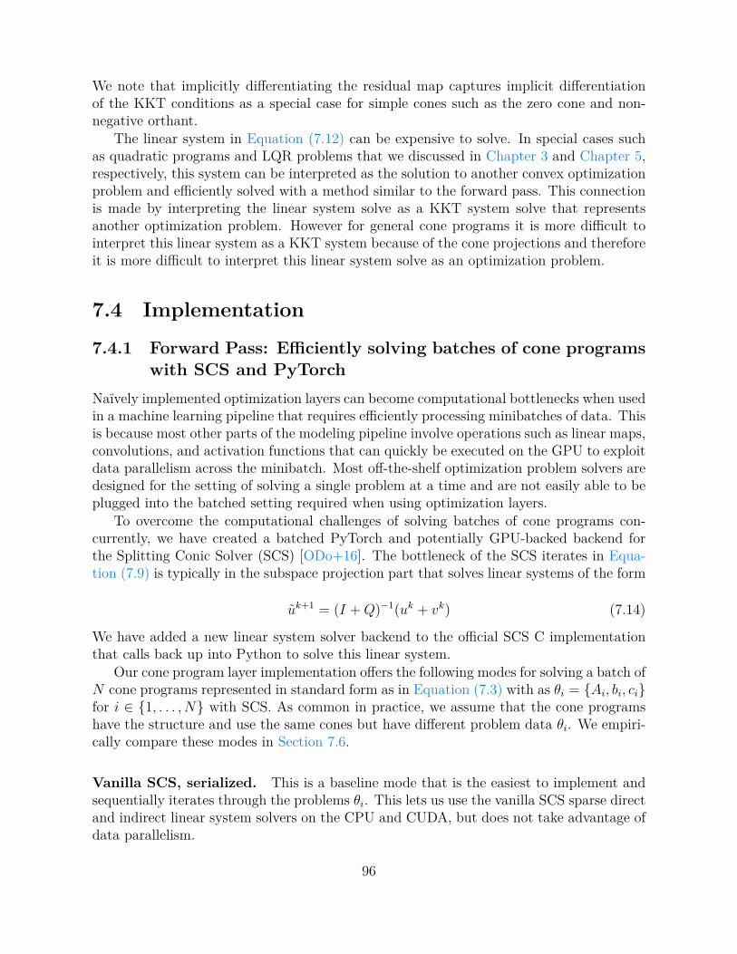
We note that implicitly differentiating the residual map captures implicit differentiationof the KKT conditions as a special case for simple cones such as the zero cone and non-negative orthant.

The linear system in Equation (7.12) can be expensive to solve. In special cases suchas quadratic programs and LQR problems that we discussed in Chapter 3 and Chapter 5,respectively, this system can be interpreted as the solution to another convex optimizationproblem and efficiently solved with a method similar to the forward pass. This connectionis made by interpreting the linear system solve as a KKT system solve that representsanother optimization problem. However for general cone programs it is more difficult tointerpret this linear system as a KKT system because of the cone projections and thereforeit is more difficult to interpret this linear system solve as an optimization problem.

7.4 Implementation

7.4.1 Forward Pass: Efficiently solving batches of cone programswith SCS and PyTorch

Naïvely implemented optimization layers can become computational bottlenecks when usedin a machine learning pipeline that requires efficiently processing minibatches of data. Thisis because most other parts of the modeling pipeline involve operations such as linear maps,convolutions, and activation functions that can quickly be executed on the GPU to exploitdata parallelism across the minibatch. Most off-the-shelf optimization problem solvers aredesigned for the setting of solving a single problem at a time and are not easily able to beplugged into the batched setting required when using optimization layers.

To overcome the computational challenges of solving batches of cone programs con-currently, we have created a batched PyTorch and potentially GPU-backed backend forthe Splitting Conic Solver (SCS) [ODo+16]. The bottleneck of the SCS iterates in Equa-tion (7.9) is typically in the subspace projection part that solves linear systems of the form

uk+1 = (I +Q)−1(uk + vk) (7.14)

We have added a new linear system solver backend to the official SCS C implementationthat calls back up into Python to solve this linear system.

Our cone program layer implementation offers the following modes for solving a batch ofN cone programs represented in standard form as in Equation (7.3) with as θi = {Ai, bi, ci}for i ∈ {1, . . . , N} with SCS. As common in practice, we assume that the cone programshave the structure and use the same cones but have different problem data θi. We empiri-cally compare these modes in Section 7.6.

Vanilla SCS, serialized. This is a baseline mode that is the easiest to implement andsequentially iterates through the problems θi. This lets us use the vanilla SCS sparse directand indirect linear system solvers on the CPU and CUDA, but does not take advantage ofdata parallelism.

96

Vanilla SCS, batched. This is another baseline mode that comes from observing thata batch of cone programs can be represented as a single cone program in standard formas in Equation (7.3) with variables x = [x⊤

1 , . . . , x⊤N ]

⊤ and data A = diag(A1, . . . , AN),b = [b⊤1 , . . . , b

⊤N ]

⊤, and c = [c⊤1 , . . . , c⊤N ]

⊤. This exploits the knowledge that all of the coneprograms can be solved concurrently. The bottleneck of this mode is still typically in thelinear system solve portion of SCS, which happens using sparse operations on the CPU orGPU.

SCS+PyTorch, batched. In this mode we represent the batch of cone programs asa single batched cone program use SCS will callbacks up into Python so that we canuse PyTorch to efficiently solve the linear system. This allows us to keep the A datain PyTorch and potentially on the GPU without converting/transferring it and passingit into the SCS. Specifically we use dense operations and have implemented direct andindirect methods to solve Equation (7.11) in PyTorch and then pass the result back downinto SCS for the rest of the operations. Our direct method uses PyTorch’s batched LUfactorizations and solves and our indirect method uses a batched conjugate gradient (CG)implementation. These custom linear system solvers are able to explicitly take advantageof the independence present in the linear systems that the sparse linear system solvers maynot recognize automatically, and the dense solvers are also useful for dense cone programs,which come up in the context of differentiable optimization layers when large portions ofthe constraints are being learned.

7.4.2 Backward pass: Efficiently solving the linear systemWhen using cone programs as layers in end-to-end learning systems with some scalar-valued loss function ℓ, the full Jacobian Dθx

⋆ is expensive and unnecessary to form andrequires solving |θ| linear systems. The Jacobian is only used when applying the chainrule to obtain Dθℓ = (Dx⋆ℓ)Dθx

⋆. We can directly compute Dθℓ without computing theintermediate Jacobian by solving a single linear system. Following the method of Chapter 3,we set up the system

DzR(z⋆)

dz1dz20

= −

∇x⋆ℓ00

. (7.15)

Applying the chain rule to u⋆ = Πz⋆ gives dx = dz1 and dy = (DzΠz)dz2 . We then computethe relevant backpropagation derivatives as

∇cℓ = dx ∇Aℓ = dy ⊗ x⋆ + y⋆ ⊗ dx ∇bℓ = −dy (7.16)Solving Equation (7.15) is still challenging to implement in practice as DzR(z⋆) can

be large and sparse and doesn’t have obviously exploitable properties such as symmetryor anti-symmetry. In addition to directly solving this linear system, we also explore theuse of LSQR [PS82] as an iterative indirect method of solving this system in Section 7.6.2.Our LSQR implementation uses the implementation from Ali, Wong, and Kolter [AWK17]to compute DzΠ(z) in the form of an abstract linear operator so the full matrix does notneed to be explicitly formed.

97

7.5 ExamplesThis section provides example use cases of our cvxpy optimization layer. All of these usethe preamble

1 import cvxpy as cp2 from cvxpyth import CvxpyLayer

7.5.1 The ReLU, sigmoid, and softmaxWe will start with basic examples and revisit the optimization views of the ReLU, sigmoid,and softmax from Section 2.4.4. These can be implemented with our cvxpy layer in a fewlines of code.

The ReLU. Recall from Equation (2.2) that the optimization view is

f(x) = argminy

1

2||x− y||22 s. t. y ≥ 0.

We can implement this layer with:1 x = cp.Parameter(n)2 y = cp.Variable(n)3 obj = cp.Minimize(cp.sum_squares(y-x))4 cons = [y >= 0]5 prob = cp.Problem(obj, cons)6 layer = CvxpyLayer(prob, params=[x], out_vars=[y])

This layer can be used and differentiated through just as any other PyTorch layer.Here is the output and derivative for a single dimension, illustrating that this is indeedperforming the same operation as the ReLU.

98

The sigmoid. Recall from Equation (2.4) that the optimization view is

f(x) = argmin0<y<1

−x⊤y −Hb(y).

We can implement this layer with:1 x = cp.Parameter(n)2 y = cp.Variable(n)3 obj = cp.Minimize(-x.T*y - cp.sum(cp.entr(y) + cp.entr(1.-y)))4 prob = cp.Problem(obj)5 layer = CvxpyLayer(prob, params=[x], out_vars=[y])

We can also check that the output and derivative matches what we expect from the usualsigmoid function:

The softmax. Lastly recall from Equation (2.5) that the optimization view is

f(x) = argmin0<y<1

−x⊤y −H(y) s. t. 1⊤y = 1

We can implement this layer with:1 x = cp.Parameter(d)2 y = cp.Variable(d)3 obj = cp.Minimize(-x.T*y - cp.sum(cp.entr(y)))4 cons = [sum(y) == 1.]5 prob = cp.Problem(obj, cons)6 layer = CvxpyLayer(prob, params=[x], out_vars=[y])

99

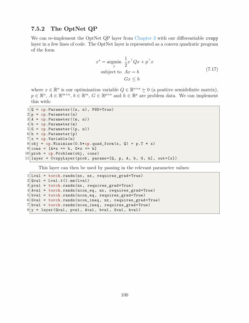
7.5.2 The OptNet QPWe can re-implement the OptNet QP layer from Chapter 3 with our differentiable cvxpylayer in a few lines of code. The OptNet layer is represented as a convex quadratic programof the form

x⋆ = argminx

1

2x⊤Qx+ p⊤x

subject to Ax = b

Gx ≤ h

(7.17)

where x ∈ Rn is our optimization variable Q ∈ Rn×n ⪰ 0 (a positive semidefinite matrix),p ∈ Rn, A ∈ Rm×n, b ∈ Rm, G ∈ Rp×n and h ∈ Rp are problem data. We can implementthis with:

1 Q = cp.Parameter((n, n), PSD=True)2 p = cp.Parameter(n)3 A = cp.Parameter((m, n))4 b = cp.Parameter(m)5 G = cp.Parameter((p, n))6 h = cp.Parameter(p)7 x = cp.Variable(n)8 obj = cp.Minimize(0.5*cp.quad_form(x, Q) + p.T * x)9 cons = [A*x == b, G*x <= h]

10 prob = cp.Problem(obj, cons)11 layer = CvxpyLayer(prob, params=[Q, p, A, b, G, h], out=[x])

This layer can then be used by passing in the relevant parameter values:1 Lval = torch.randn(nx, nx, requires_grad=True)2 Qval = Lval.t().mm(Lval)3 pval = torch.randn(nx, requires_grad=True)4 Aval = torch.randn(ncon_eq, nx, requires_grad=True)5 bval = torch.randn(ncon_eq, requires_grad=True)6 Gval = torch.randn(ncon_ineq , nx, requires_grad=True)7 hval = torch.randn(ncon_ineq , requires_grad=True)8 y = layer(Qval, pval, Aval, bval, Gval, hval)

100

True Polytope Approximate Polytope

Figure 7.2: Learning polyhedrally constrained problems.

7.5.3 Learning Polyhedral ConstraintsWe demonstrate how gradient-based learning can be done with a cvxpy layer in this syn-thetic example. Consider the polyhedrally constrained projection problem

y = argminy

1

2||p− y||22

s.t. Gy ≤ h

Suppose we don’t know the polytope’s parameters θ = {G, h} and want to learn them fromdata. Then using the MSE for ℓ, we can randomly initialize ellipsoids θ and learn themwith gradient steps ∇θℓ. We note that this problem is meant for illustrative purposes andcould be solved by taking the convex hull of the input data points. However our approachwould still work if this was over a latent and unobserved part of the model, of if you wantto take an approximate convex hull that limits the number of polytope edges.

We can implement this layer with the following code. Figure 7.2 shows the resultsof learning on two examples. Each problem has a true known polytope that we show inblue and the model’s approximation is in red. Learning starts on the left with randomlyinitialized polytopes that are updated with gradient steps, which are shown in the imagesprogressing to the right.

1 G = cp.Parameter((m, n))2 h = cp.Parameter(m)3 p = cp.Parameter(n)4 y = cp.Variable(n)5 obj = cp.Minimize(0.5*cp.sum_squares(y-p))6 cons = [G*y <= h]7 prob = cp.Problem(obj, cons)8 layer = CvxpyLayer(prob, params=[p, G, h], out=[y])

101

True Ellipsoid Approximate Ellipsoid

Figure 7.3: Learning ellipsoidally constrained problems.

7.5.4 Learning Ellipsoidal ConstraintsIn addition to learning polyhedral constraints, we can easily learn any parameterized convexconstraint set. Suppose instead that we want to learn an ellipsoidal projection of the form

y = argminy

1

2||p− y||22

s.t.1

2(y − z)⊤A(y − z) ≤ 1

with ellipsoid parameters θ = {A, z} This is an interesting optimization problem to considerbecause it is an example of doing learning with a non-polytope cone program (a SOCP),which prior approaches such as OptNet could not easily handle.

We can implement this layer with the following code. Figure 7.3 visualizes the learningprocess on two examples. As before, each problem has a true known ellipsoid that we showin blue and the model’s approximation is in red. Learning starts on the left with randomlyinitialized ellipsoids that are updated with gradient steps, which are shown in the imagesprogressing to the right.

1 A = cp.Parameter((n, n), PSD=True)2 z = cp.Parameter(n)3 p = cp.Parameter(n)4 y = cp.Variable(n)5 obj = cp.Minimize(0.5*cp.sum_squares(y-p))6 cons = [0.5*cp.quad_form(y-z, A) <= 1]7 prob = cp.Problem(obj, cons)8 layer = CvxpyLayer(prob, params=[p, A, z], out=[y])

102

7.6 EvaluationIn this section we analyze the runtime of our layer’s forward and backward passes comparedto hand-written implementations for commonly used optimization layers. We will focus onthree tasks:

Task 1: Dense QP. We consider a QP layer of the form Equation (7.17) with a densequadratic objective and dense inequality constraints. Our default experiment uses a QPwith 100 latent variables, 100 inequality constraints, and a minibatch size of 128 examples.We chose this task to understand how the performance of our cvxpy layer compares to theqpth implementation from Chapter 3, which we use as a comparison point. The problemsize we consider here is comparable to the QP problem sizes considered in Chapter 3. Thebackwards pass of qpth is optimized to use a single batched, pre-factorized linear systemsolve.

Task 2: Box QP. We consider a QP layer of the form Equation (7.17) with a densequadratic objective constrained to the box [−1, 1]n. Our default experiment uses a QPwith 100 latent variables and a minibatch size of 128 examples. We chose this task tostudy the impacts of sparsity on the runtime. We again use qpth as the comparison pointfor these experiments.

Task 3: Linear Quadratic Regulator (LQR). We consider a continuous-state-action,discrete-time, finite-horizon LQR problem of the form

τ ⋆1:T = argminτ1:T

∑t

1

2τ⊤t Ctτt + c⊤t τt subject to x1 = xinit, xt+1 = Ftτt + ft. (7.18)

where τ1:T = {xt, ut}1:T is the nominal trajectory, T is the horizon, xt, ut are the state andcontrol at time t, {Ct, ct} parameterize a convex quadratic cost, and {Ft, ft} parameterizean affine system transition dynamics. We consider a control problem with 10 states, 2actions, and a horizon of 5. We compare to the differentiable model predictive control(MPC) solver from [Amo+18b], which uses batched PyTorch operations to solve a batchof LQR problems with the Riccati equations, and then implements the backward pass withanother, simpler, LQR solve with the Riccati equations.

For each of these tasks we have measured the forward and backward pass executiontimes for our layer in comparison to the specialized solvers. We have run these experimentson an unloaded system with an NVIDIA GeForce GTX 1080 Ti GPU and a four-core2.60GHz Intel Xeon E5-2623 CPUs hyper-threaded to eight cores. We set the number ofOpenMP threads to 8 for our experiments. For numerical stability, we use 64-bits for all ofour implementations and baselines. For qpth and our implementation, we use an iterationstopping condition of ϵ = 10−3.

103

0.0

0.5

1.0

1.5

2.0

Norm

alize

d Ru

ntim

e

15.98

CPU CUDA CPU CUDA CPU CUDADense QP Box QP LQR

Forward Pass Times

Specialized Solver PyTorch Block Direct SCS Serial Direct

Figure 7.4: Forward pass execution times. For each task we run ten trials on an unloadedsystem and normalize the runtimes to the CPU execution time of the specialized solver.The bars show the 95% confidence interval. For our method, we show the best performingmode.

7.6.1 Forward pass profilingFigure 7.4 summarizes our main forward pass execution times. Figure 7.6 shows the run-times of all of the modes and batch sizes, and Figure 7.5 illustrates the speedup of ourbest mode compared to the specialized solvers. We have implemented and run every modefrom Section 7.4.1 and our summary presents the best-performing mode, which in everycase on the GPU is our block direct solver. On the CPU, serializing SCS calls is compet-itive for problems with more sparsity. For dense and sparse QPs on the CPU and GPU,our batched SCS+PyTorch direct cone solver is faster than the qpth solver, which likelycomes from the acceleration, convergence, and normalization tricks in SCS that are notpresent in qpth. The LQR task presents a sparse problem that illustrates the challenges tousing a general cone program formulation. Our specialized solver that solves the Riccatiequations in batched form exploits the sparsity pattern of the problem that is extremelydifficult for the general cone program formulation we consider here to take advantage of. Ifthe correct mappings to the cone program exist, our layer could be modified to accept anoptimized user-provided solver for the forward pass so that users can still take advantageof our backward pass implementation.

104

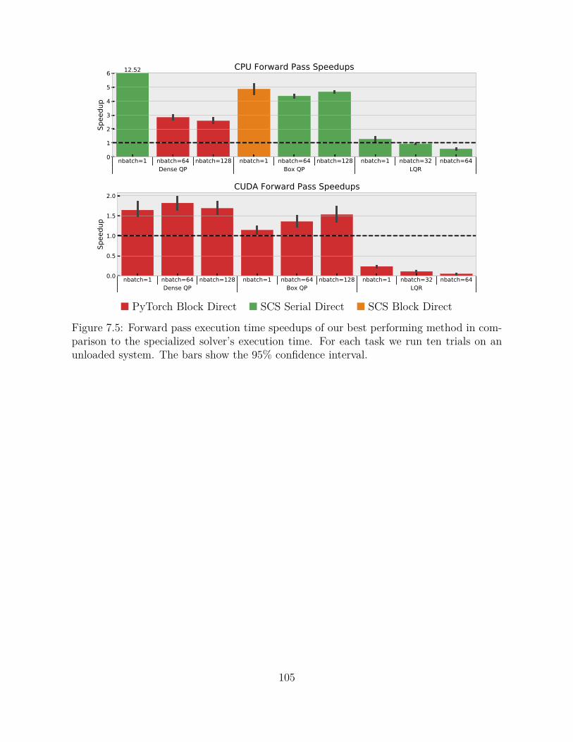
0

1

2

3

4

5

6

Spee

dup

nbatch=1 nbatch=64 nbatch=128 nbatch=1 nbatch=64 nbatch=128 nbatch=1 nbatch=32 nbatch=64Dense QP Box QP LQR

12.52 CPU Forward Pass Speedups

0.0

0.5

1.0

1.5

2.0

Spee

dup

nbatch=1 nbatch=64 nbatch=128 nbatch=1 nbatch=64 nbatch=128 nbatch=1 nbatch=32 nbatch=64Dense QP Box QP LQR

CUDA Forward Pass Speedups

PyTorch Block Direct SCS Serial Direct SCS Block Direct

Figure 7.5: Forward pass execution time speedups of our best performing method in com-parison to the specialized solver’s execution time. For each task we run ten trials on anunloaded system. The bars show the 95% confidence interval.

105

nbatch=1 nbatch=64nbatch=128

10-3

10-2

10-1

100

101

102

Tim

e (s

)

CPU Forward

nbatch=1 nbatch=64nbatch=128

10-3

10-2

10-1

100

101

102

Tim

e (s

)

CUDA ForwardDense QP

nbatch=1 nbatch=64nbatch=128

10-3

10-2

10-1

100

101

102

Tim

e (s

)

CPU Forward

nbatch=1 nbatch=64nbatch=128

10-3

10-2

10-1

100

101

102

Tim

e (s

)

CUDA ForwardBox QP

nbatch=1 nbatch=32nbatch=64

10-3

10-2

10-1

100

101

102

Tim

e (s

)

CPU Forward

nbatch=1 nbatch=32nbatch=64

10-3

10-2

10-1

100

101

102

Tim

e (s

)

CUDA ForwardLQR

Specialized Solver PyTorch Block Direct PyTorch Block IndirectSCS Serial Direct SCS Serial Indirect SCS Block Direct SCS Block Indirect

Figure 7.6: Full data for the forward pass execution times. For each task we run ten trialson an unloaded system. The bars show the 95% confidence interval.

106

0 10 20 30 40 50 60

0

10

20

30

40

50

60

Dense QP

0 10 20 30 40 50 60 70 80

0

10

20

30

40

50

60

70

80

Box QP

0 10 20 30 40 50 60

0

10

20

30

40

50

60

LQR

1.00

0.75

0.50

0.25

0.00

0.25

0.50

0.75

1.00

Figure 7.7: Sample linear system coefficients for the backward pass system in Equa-tion (7.15) on smaller versions of the tasks we consider. The tasks we consider are ap-proximately five times larger than these systems.

7.6.2 Backward pass profilingIn this section we compare the backward pass times of our layer in comparison to thespecialized solvers on the same three tasks as before: the dense QP, the box QP, and LQR.We show that differentiating through our conic solver is competitive in comparison to thespecialized solver. As a comparison point, the qpth solver exploits the property that thelinear system for the backward pass is the same as the linear system in the forward passand can therefore do the backward pass with a single pre-factorized solve. The LQR solverexploits the property that the backward pass for LQR can be interpreted as another LQRproblem that can efficiently be solved with the Riccati recursion.

These comparisons are important because the linear system for differentiating coneprograms in Equation (7.15) is a more general form and cannot leverage the same exploitsas the specialized solvers. To get an intuition of what these linear systems look like on ourtasks, we plot sample maps on smaller problems of the coefficient matrix in Figure 7.7.This illustrates the sparsity that is typically present in the linear system that needs to besolved, but also illustrates that beyond sparsity, there is no other common property thatcan be exploited between the tasks.

To understand how many LSQR iterations are necessary to solve our task, we comparethe approximate derivatives computed by LSQR to the derivatives obtained by directlysolving the linear system in Figure 7.8. This shows that typically 500-1000 LSQR iterationsare necessary for the tasks that we consider. In some cases such as ∂x⋆/∂A for LQR, theapproximate gradient computed by LSQR does never converges exactly to the true gradient.

107

0 250 500 750 1000 1250 1500 1750 2000LSQR Iterations

0.0

0.2

0.4

0.6

0.8

1.0

1.2

MSE

0 250 500 750 1000 1250 1500 1750 2000LSQR Iterations

0

5

10

15

20

25

Max

imum

Abs

olut

e Er

ror

Dense QP

0 100 200 300 400 500LSQR Iterations

0

1

2

3

4

5

6

7

8

MSE

0 100 200 300 400 500LSQR Iterations

0

10

20

30

40

50

60

Max

imum

Abs

olut

e Er

ror

Box QP

0 250 500 750 1000 1250 1500 1750 2000LSQR Iterations

0

2

4

6

8

10

MSE

0 250 500 750 1000 1250 1500 1750 2000LSQR Iterations

0

10

20

30

40

50

60

Max

imum

Abs

olut

e Er

ror

MPC

∂x⋆/∂A ∂x⋆/∂b ∂x⋆/∂c

Figure 7.8: LSQR convergence for the backward pass systems. The shaded areas show the95% confidence interval across ten problem instances.

108

nbatch=1 nbatch=64nbatch=128

10-3

10-2

10-1

100

101

102

Tim

e (s

)

CPU Backward

nbatch=1 nbatch=64nbatch=128

10-3

10-2

10-1

100

101

102

Tim

e (s

)

CUDA BackwardDense QP

nbatch=1 nbatch=64nbatch=128

10-3

10-2

10-1

100

101

102

Tim

e (s

)

CPU Backward

nbatch=1 nbatch=64nbatch=128

10-3

10-2

10-1

100

101

102

Tim

e (s

)

CUDA BackwardBox QP

nbatch=1 nbatch=32nbatch=64

10-3

10-2

10-1

100

101

102

Tim

e (s

)

CPU Backward

nbatch=1 nbatch=32nbatch=64

10-3

10-2

10-1

100

101

102

Tim

e (s

)

CUDA BackwardLQR

Specialized Solver Direct (Dense) LSQR ( 100 500 1000) Iterations

Figure 7.9: Backward pass execution times. For each task we run ten trials on an unloadedsystem. The bars show the 95% confidence interval.

109

Figure 7.9 compares our backward pass times to the specialized solvers for the QP andLQR tasks. This shows that there is a slight computational overhead in comparison tothe specialized solvers, but that solving the linear system is still tractable for these tasks.The LSQR runtime is serialized across the batch, and is currently only implemented on theCPU. We emphasize that if the backward pass time becomes a bottleneck, the runtime canbe further improved by further exploiting the sparsity by investigating other direct andindirect solvers for the systems, or by exploiting the property that we mentioned earlier inSection 7.3.1 that for simple cones like the free and non-negative cones, parts of the systembecome the same as parts of the KKT system.

7.7 ConclusionThis section has presented a way of differentiating through cone programs that enabled usto create a powerful prototyping tool for differentiable convex optimization layers. Prac-titioners can use this library in place of hand-implementing a solver and implicitly dif-ferentiating the KKT conditions. The speed of our tool is competitive with the speed ofspecialized solvers, even in the batched setting required for machine learning.

110

Part III

Conclusions and Future Directions

111

Chapter 8Conclusions and Future Directions

In this thesis we have introduced new building blocks and fundamental components formachine learning that enable optimization-based domain knowledge to be injected into themodeling pipeline. We have presented the OptNet architecture as a foundation for convexoptimization layers and the input-convex neural network architecture as a foundation fordeep convex energy-based learning. We have shown how the OptNet approach can beapplied to differentiable model-predictive control and top-k learning. To enable rapidprototyping in this space, we have shown how cvxpy can be turned into a differentiablelayer. Differentiable optimization provides an expressive set of operations and have apromising set of future directions. In the following we provide a brief outlook of howoptimization-based modeling benefits seven application areas, and we highlight a few keyreferences in this space.

1. Game theory. The game theory literature typically focuses on finding optimalstrategies of playing games with known rules. While the rules of a lot of gamesare known explicitly, scenarios could come up where it’s useful to learn the rulesof a game and to have a “game theory” equilibrium-finding layer. For example inreinforcement learning, an agent can have an arbitrary differentiable “game theory”layer that is able of representing complex tasks, state spaces, and problems as anequilibrium-finding problem in a game where the rules are automatically extracted.This is explored in Ling, Fang, and Kolter [LFK18].

2. Stochastic optimization and end-to-end learning. Typically probabilistic mod-els are used in the context of larger systems. When these systems have an objectivethat is being optimized, it is usually ideal to incorporate the knowledge of this objec-tive into the probabilistic modeling component. If the downstream systems involvesolving stochastic optimization problems, as in power-systems, creating an end-to-enddifferentiable architecture is more difficult and can be done by using differentiableoptimization as in Donti, Amos, and Kolter [DAK17].

113

3. Reinforcement learning and control.• Safety. RL agents may be deployed in scenarios when the agent should avoid

parts of the state space, e.g. in safety-critical environments. Differentiable op-timization layers can be used to help constrain the policy class so that these re-gions are avoided. This is explored in Dalal, Dvijotham, Vecerik, Hester, Padu-raru, and Tassa [Dal+18] and Pham, De Magistris, and Tachibana [PDT18].

• Differentiable control and planning. The differentiable MPC approach wepresented in Chapter 5 is just one step towards a significantly broader vision ofintegrating control and learning for doing imitation or policy learning.

• Physics-based modeling. When RL environments involve physical systems,it may be useful to have a physics-based modeling. This can be done with a dif-ferentiable physics engines as in Avila Belbute-Peres, Smith, Allen, Tenenbaum,and Kolter [Avi+18].

• Inverse cost and reward learning. Given observed trajectories in an imita-tion learning setup, modeling agents as controllers that are optimizing an ob-jective is a powerful paradigm [NR+00; FLA16]. Differentiable controllers areuseful when trying to reconstruct an optimization problem that other agents aresolving. This is done in the context of cost shaping in Tamar, Thomas, Zhang,Levine, and Abbeel [Tam+17].

• Multi-agent environments. In multi-agent environments, other agents canbe modeled as entities that are solving control optimization or other learningproblems. This knowledge can be integrated into the learning procedure as inFoerster, Chen, Al-Shedivat, Whiteson, Abbeel, and Mordatch [Foe+18].

• Control in high-dimensional state spaces. Control in high-dimensionalstate spaces such as visual spaces is challenging and it is typically useful toextract a lower-dimensional latent space from the original feature space. This istypically done by either hand-engineering a feature extractor, or by learning anembedding with an unsupervised learning method as in Watter, Springenberg,Boedecker, and Riedmiller [Wat+15] and Kurutach, Tamar, Yang, Russell, andAbbeel [Kur+18]. Viewing controllers as differentiable entities is reasonable forembedding states because the cost function of the controller can be parameter-ized to learn a cost associated with the latent representation.

4. Discrete, combinatorial, and submodular optimization. The space of discrete,combinatorial, and mixed optimization problems captures an even more expressiveset of operations than the continuous and convex optimization problems we haveconsidered in this thesis. Similar optimization components can be made for some ofthese types of problems and is explored in Djolonga and Krause [DK17], Tschiatschek,Sahin, and Krause [TSK18], Mensch and Blondel [MB18], Niculae, Martins, Blondel,and Cardie [Nic+18], and Niculae and Blondel [NB17].

114

5. Meta-learning. Some meta-learning formulations such as Finn, Abbeel, and Levine[FAL17] and Ravi and Larochelle [RL16] involve learning through an unrolled opti-mizer that typically solve an unconstrained, continuous, and non-convex optimizationproblem. In some cases, unrolling through a solver with many iterations may requireinefficient amounts of compute or memory. Meta-learning methods can be improvedby using differentiable closed-form solvers, as done in MetaOptNet [Lee+19] with adifferentiable SVM layer and in Bertinetto, Henriques, Torr, and Vedaldi [Ber+18]with differentiable ridge and logistic regression.

6. Optimization viewpoints of standard components. A motivation behind thisthesis work has been the optimization viewpoints of standard layers we discussedin Section 2.4.4. Many other directions can be taken with the viewpoints, such asthe proximal operator viewpoint in Bibi, Ghanem, Koltun, and Ranftl [Bib+18] thatinterprets deep layers as stochastic solvers.

7. Hyper-parameter and generalization optimization. The learning procedurefor many linear machine learning models can be interpreted as the solution to aconvex optimization problem over the loss function. This convex learning process cantherefore also be made differentiable and used for optimizing the hyper-parametersof these algorithms. This is done in Barratt and Sharma [BS18] to optimize thecross-validation risk of convex formulations, including logistic regression, SVMs, andelastic net regression; for least squares in Barratt and Boyd [BB19]; and SVMs inLee, Maji, Ravichandran, and Soatto [Lee+19].

115

116

BibliographyThis bibliography contains 279 references.

[Aba+16] Martın Abadi, Paul Barham, Jianmin Chen, Zhifeng Chen, Andy Davis, Jef-frey Dean, Matthieu Devin, Sanjay Ghemawat, Geoffrey Irving, Michael Is-ard, et al. “Tensorflow: a system for large-scale machine learning.” In: OSDI.Vol. 16. 2016, pp. 265–283.

[AG03] Farid Alizadeh and Donald Goldfarb. “Second-order cone programming”. In:Mathematical programming 95.1 (2003), pp. 3–51.

[Aga11] Shivani Agarwal. “The infinite push: A new support vector ranking algorithmthat directly optimizes accuracy at the absolute top of the list”. In: Proceed-ings of the 2011 SIAM International Conference on Data Mining. SIAM.2011, pp. 839–850.

[Agr+19] Akshay Agrawal, Shane Barratt, Stephen Boyd, Enzo Busseti, and WalaaM. Moursi. “Differentiating Through a Conic Program”. In: arXiv e-prints,arXiv:1904.09043 (Apr. 2019), arXiv:1904.09043. arXiv: 1904.09043 [math.OC].

[AK17] Brandon Amos and J. Zico Kolter. “OptNet: Differentiable Optimization asa Layer in Neural Networks”. In: Proceedings of the International Conferenceon Machine Learning. 2017.

[Ale+11] Kostas Alexis, Christos Papachristos, George Nikolakopoulos, and AnthonyTzes. “Model predictive quadrotor indoor position control”. In: Control &Automation (MED), 2011 19th Mediterranean Conference on. IEEE. 2011,pp. 1247–1252.

[ALS16] Brandon Amos, Bartosz Ludwiczuk, and Mahadev Satyanarayanan. Open-Face: A general-purpose face recognition library with mobile applications.Tech. rep. Technical Report CMU-CS-16-118, CMU School of Computer Sci-ence, 2016.

[Amo+18a] Brandon Amos, Laurent Dinh, Serkan Cabi, Thomas Rothörl, Sergio GómezColmenarejo, Alistair Muldal, Tom Erez, Yuval Tassa, Nando de Freitas, andMisha Denil. “Learning Awareness Models”. In: International Conference onLearning Representations. 2018.

[Amo+18b] Brandon Amos, Ivan Jimenez, Jacob Sacks, Byron Boots, and J. Zico Kolter.“Differentiable MPC for End-to-end Planning and Control”. In: Advances inNeural Information Processing Systems. 2018, pp. 8299–8310.

117

[AQN06] Pieter Abbeel, Morgan Quigley, and Andrew Y Ng. “Using inaccurate modelsin reinforcement learning”. In: Proceedings of the 23rd international confer-ence on Machine learning. ACM. 2006, pp. 1–8.

[Avi+18] Filipe de Avila Belbute-Peres, Kevin Smith, Kelsey Allen, Josh Tenenbaum,and J. Zico Kolter. “End-to-end differentiable physics for learning and con-trol”. In: Advances in Neural Information Processing Systems. 2018, pp. 7178–7189.

[AWK17] Alnur Ali, Eric Wong, and J. Zico Kolter. “A semismooth Newton method forfast, generic convex programming”. In: Proceedings of the 34th InternationalConference on Machine Learning-Volume 70. JMLR. org. 2017, pp. 70–79.

[AXK17] Brandon Amos, Lei Xu, and J. Zico Kolter. “Input Convex Neural Networks”.In: Proceedings of the International Conference on Machine Learning. 2017.

[AZ11] Ryan Prescott Adams and Richard S Zemel. “Ranking via Sinkhorn Propa-gation”. In: arXiv preprint arXiv:1106.1925 (2011).

[Bal+16] Matej Balog, Alexander L Gaunt, Marc Brockschmidt, Sebastian Nowozin,and Daniel Tarlow. “Deepcoder: Learning to write programs”. In: arXiv preprintarXiv:1611.01989 (2016).

[Ban+17] Somil Bansal, Roberto Calandra, Sergey Levine, and Claire Tomlin. “MBMF:Model-Based Priors for Model-Free Reinforcement Learning”. In: arXiv preprintarXiv:1709.03153 (2017).

[Bar18] Shane Barratt. “On the differentiability of the solution to convex optimiza-tion problems”. In: arXiv preprint arXiv:1804.05098 (2018).

[Bat+16] Peter Battaglia, Razvan Pascanu, Matthew Lai, Danilo Jimenez Rezende, etal. “Interaction networks for learning about objects, relations and physics”.In: Advances in neural information processing systems. 2016, pp. 4502–4510.

[Bat+18] Peter W Battaglia, Jessica B Hamrick, Victor Bapst, Alvaro Sanchez-Gonzalez,Vinicius Zambaldi, Mateusz Malinowski, Andrea Tacchetti, David Raposo,Adam Santoro, Ryan Faulkner, et al. “Relational inductive biases, deep learn-ing, and graph networks”. In: arXiv preprint arXiv:1806.01261 (2018).

[BAT12] P. Bouffard, A. Aswani, and C. Tomlin. “Learning-based model predictivecontrol on a quadrotor: Onboard implementation and experimental results”.In: IEEE International Conference on Robotics and Automation. 2012.

[BB08] Bradley M Bell and James V Burke. “Algorithmic differentiation of implicitfunctions and optimal values”. In: Advances in Automatic Differentiation.Springer, 2008, pp. 67–77.

[BB19] Shane Barratt and Stephen Boyd. “Least Squares Auto-Tuning”. In: arXivpreprint arXiv:1904.05460 (2019).

[BB88] Jonathan Barzilai and Jonathan M Borwein. “Two-point step size gradientmethods”. In: IMA Journal of Numerical Analysis 8.1 (1988), pp. 141–148.

[BC17] Heinz H Bauschke and Patrick L Combettes. “Convex Analysis and MonotoneOperator Theory in Hilbert Spaces, second edition”. In: (2017).

118

[BCB14] Dzmitry Bahdanau, Kyunghyun Cho, and Yoshua Bengio. “Neural machinetranslation by jointly learning to align and translate”. In: arXiv preprintarXiv:1409.0473 (2014).

[Bel17] David Belanger. “Deep Energy-Based Models for Structured Prediction”.PhD thesis. University of Massachusetts Amherst, 2017.

[Ber+05] Dimitri P Bertsekas, Dimitri P Bertsekas, Dimitri P Bertsekas, and DimitriP Bertsekas. Dynamic programming and optimal control. Vol. 1. 3. Athenascientific Belmont, MA, 2005.

[Ber+18] Luca Bertinetto, João F Henriques, Philip HS Torr, and Andrea Vedaldi.“Meta-learning with differentiable closed-form solvers”. In: arXiv preprintarXiv:1805.08136 (2018).

[Ber82] Dimitri P Bertsekas. “Projected Newton methods for optimization problemswith simple constraints”. In: SIAM Journal on control and Optimization 20.2(1982), pp. 221–246.

[Ber99] Dimitri P Bertsekas. Nonlinear programming. Athena scientific Belmont,1999.

[BG18] Nataly Brukhim and Amir Globerson. “Predict and Constrain: Modeling Car-dinality in Deep Structured Prediction”. In: arXiv preprint arXiv:1802.04721(2018).

[Bib+18] Adel Bibi, Bernard Ghanem, Vladlen Koltun, and René Ranftl. “Deep Layersas Stochastic Solvers”. In: (2018).

[Bis07] Christopher Bishop. Pattern Recognition and Machine Learning (InformationScience and Statistics), 1st edn. 2006. corr. 2nd printing edn. Springer, NewYork, 2007.

[BLH94] Yoshua Bengio, Yann LeCun, and Donnie Henderson. “Globally trained hand-written word recognizer using spatial representation, convolutional neuralnetworks, and hidden Markov models”. In: Advances in neural informationprocessing systems (1994), pp. 937–937.

[BM15] David Belanger and Andrew McCallum. “Structured Prediction Energy Net-works”. In: arXiv:1511.06350 (2015).

[BM16] David Belanger and Andrew McCallum. “Structured prediction energy net-works”. In: Proceedings of the International Conference on Machine Learning.2016.

[BMB18] Enzo Busseti, W Moursi, and Stephen Boyd. “Solution Refinement at RegularPoints of Conic Problems”. In: arXiv preprint arXiv:1811.02157 (2018).

[BMR00] Ernesto G Birgin, José Mario Martınez, and Marcos Raydan. “Nonmonotonespectral projected gradient methods on convex sets”. In: SIAM Journal onOptimization 10.4 (2000), pp. 1196–1211.

[BN01] Ahron Ben-Tal and Arkadi Nemirovski. Lectures on modern convex optimiza-tion: analysis, algorithms, and engineering applications. Vol. 2. Siam, 2001.

[Boe+14] Joschika Boedecker, Jost Tobias Springenberg, Jan Wulfing, and MartinRiedmiller. “Approximate Real-Time Optimal Control Based on Sparse Gaus-

119

sian Process Models”. In: IEEE Symposium on Adaptive Dynamic Program-ming and Reinforcement Learning (ADPRL). 2014.

[Boy+11] Stephen Boyd, Neal Parikh, Eric Chu, Borja Peleato, and Jonathan Eck-stein. “Distributed optimization and statistical learning via the alternatingdirection method of multipliers”. In: Foundations and Trends® in MachineLearning 3.1 (2011), pp. 1–122.

[Boy+12] Stephen Boyd, Corinna Cortes, Mehryar Mohri, and Ana Radovanovic. “Ac-curacy at the top”. In: Advances in neural information processing systems.2012, pp. 953–961.

[Boy08] Stephen Boyd. LQR via Lagrange multipliers. Stanford EE 363: Linear Dy-namical Systems. 2008.

[BP16] Jonathan T Barron and Ben Poole. “The fast bilateral solver”. In: EuropeanConference on Computer Vision. Springer. 2016, pp. 617–632.

[Bro+16] Greg Brockman, Vicki Cheung, Ludwig Pettersson, Jonas Schneider, JohnSchulman, Jie Tang, and Wojciech Zaremba. “OpenAI Gym”. In: arXiv preprintarXiv:1606.01540 (2016).

[Bro+17] Michael M Bronstein, Joan Bruna, Yann LeCun, Arthur Szlam, and PierreVandergheynst. “Geometric deep learning: going beyond euclidean data”. In:IEEE Signal Processing Magazine 34.4 (2017), pp. 18–42.

[BS13] J Frédéric Bonnans and Alexander Shapiro. Perturbation analysis of opti-mization problems. Springer Science & Business Media, 2013.

[BS18] Shane Barratt and Rishi Sharma. “Optimizing for Generalization in MachineLearning with Cross-Validation Gradients”. In: arXiv preprint arXiv:1805.07072(2018).

[BSS13] Philémon Brakel, Dirk Stroobandt, and Benjamin Schrauwen. “Training energy-based models for time-series imputation.” In: Journal of Machine LearningResearch 14.1 (2013), pp. 2771–2797.

[BV04] Stephen Boyd and Lieven Vandenberghe. Convex optimization. Cambridgeuniversity press, 2004.

[BYM17] David Belanger, Bishan Yang, and Andrew McCallum. “End-to-End Learn-ing for Structured Prediction Energy Networks”. In: Proceedings of the In-ternational Conference on Machine Learning. 2017.

[BZK18] Leonard Berrada, Andrew Zisserman, and M Pawan Kumar. “Smooth LossFunctions for Deep Top-k Classification”. In: Proceedings of the InternationalConference on Learning Representations. 2018.

[Che+15a] Liang-Chieh Chen, Alexander G Schwing, Alan L Yuille, and Raquel Urta-sun. “Learning deep structured models”. In: Proceedings of the InternationalConference on Machine Learning. 2015.

[Che+15b] Zhuo Chen, Lu Jiang, Wenlu Hu, Kiryong Ha, Brandon Amos, Padmanab-han Pillai, Alex Hauptmann, and Mahadev Satyanarayanan. “Early Imple-mentation Experience with Wearable Cognitive Assistance Applications”. In:WearSys. 2015.

120

[Che+17a] Yevgen Chebotar, Karol Hausman, Marvin Zhang, Gaurav Sukhatme, Ste-fan Schaal, and Sergey Levine. “Combining Model-Based and Model-FreeUpdates for Trajectory-Centric Reinforcement Learning”. In: arXiv preprintarXiv:1703.03078 (2017).

[Che+17b] Zhuo Chen et al. “An Empirical Study of Latency in an Emerging Class ofEdge Computing Applications for Wearable Cognitive Assistance”. In: Pro-ceedings of the Second ACM/IEEE Symposium on Edge Computing. ACM.2017, p. 12.

[Che+18] Tian Qi Chen, Yulia Rubanova, Jesse Bettencourt, and David K Duvenaud.“Neural ordinary differential equations”. In: Advances in Neural InformationProcessing Systems. 2018, pp. 6572–6583.

[Cla75] Frank H Clarke. “Generalized gradients and applications”. In: Transactionsof the American Mathematical Society 205 (1975), pp. 247–262.

[DAK17] Priya L Donti, Brandon Amos, and J. Zico Kolter. “Task-based End-to-endModel Learning”. In: NIPS. 2017.

[Dal+18] Gal Dalal, Krishnamurthy Dvijotham, Matej Vecerik, Todd Hester, CosminPaduraru, and Yuval Tassa. “Safe exploration in continuous action spaces”.In: arXiv preprint arXiv:1801.08757 (2018).

[Dav+16] Nigel Andrew Justin Davies, Nina Taft, Mahadev Satyanarayanan, SarahClinch, and Brandon Amos. “Privacy mediators: helping IoT cross the chasm”.In: HotMobile. 2016.

[DB16] Steven Diamond and Stephen Boyd. “CVXPY: A Python-embedded model-ing language for convex optimization”. In: The Journal of Machine LearningResearch 17.1 (2016), pp. 2909–2913.

[Dev+17] Jacob Devlin, Jonathan Uesato, Surya Bhupatiraju, Rishabh Singh, Abdel-rahman Mohamed, and Pushmeet Kohli. “Robustfill: Neural program learn-ing under noisy I/O”. In: Proceedings of the 34th International Conferenceon Machine Learning-Volume 70. JMLR. org. 2017, pp. 990–998.

[DHS11] John Duchi, Elad Hazan, and Yoram Singer. “Adaptive subgradient methodsfor online learning and stochastic optimization”. In: The Journal of MachineLearning Research 12 (2011), pp. 2121–2159.

[Dia+17] Steven Diamond, Vincent Sitzmann, Felix Heide, and Gordon Wetzstein.“Unrolled optimization with deep priors”. In: arXiv preprint arXiv:1705.08041(2017).

[Din77] U Dini. “Analisi infinitesimale, Lezioni dettate nella R”. In: Universitá diPisa (1877/78) (1877).

[DK17] Josip Djolonga and Andreas Krause. “Differentiable learning of submodu-lar models”. In: Advances in Neural Information Processing Systems. 2017,pp. 1013–1023.

[Dom12] Justin Domke. “Generic Methods for Optimization-Based Modeling.” In: AIS-TATS. Vol. 22. 2012, pp. 318–326.

[DR09] Asen L Dontchev and R Tyrrell Rockafellar. “Implicit functions and solutionmappings”. In: Springer Monogr. Math. (2009).

121

[DR11] Marc Deisenroth and Carl E Rasmussen. “PILCO: A model-based and data-efficient approach to policy search”. In: Proceedings of the 28th InternationalConference on machine learning (ICML-11). 2011, pp. 465–472.

[Duc+08] John Duchi, Shai Shalev-Shwartz, Yoram Singer, and Tushar Chandra. “Ef-ficient projections onto the l 1-ball for learning in high dimensions”. In: Pro-ceedings of the 25th international conference on Machine learning. 2008,pp. 272–279.

[ETT12] T. Erez, Y. Tassa, and E. Todorov. “Synthesis and stabilization of complexbehaviors through online trajectory optimization”. In: International Confer-ence on Intelligent Robots and Systems. 2012.

[FAL17] Chelsea Finn, Pieter Abbeel, and Sergey Levine. “Model-agnostic meta-learningfor fast adaptation of deep networks”. In: Proceedings of the 34th Inter-national Conference on Machine Learning-Volume 70. JMLR. org. 2017,pp. 1126–1135.

[Far+17] Gregory Farquhar, Tim Rocktäschel, Maximilian Igl, and Shimon Whiteson.“TreeQN and ATreeC: Differentiable Tree Planning for Deep ReinforcementLearning”. In: arXiv preprint arXiv:1710.11417 (2017).

[FHT01] Jerome Friedman, Trevor Hastie, and Robert Tibshirani. The elements ofstatistical learning. Vol. 1. 10. Springer series in statistics New York, NY,USA: 2001.

[FI90] Anthony V Fiacco and Yo Ishizuka. “Sensitivity and stability analysis fornonlinear programming”. In: Annals of Operations Research 27.1 (1990),pp. 215–235.

[FLA16] Chelsea Finn, Sergey Levine, and Pieter Abbeel. “Guided cost learning: Deepinverse optimal control via policy optimization”. In: International Conferenceon Machine Learning. 2016, pp. 49–58.

[Foe+18] Jakob Foerster, Richard Y Chen, Maruan Al-Shedivat, Shimon Whiteson,Pieter Abbeel, and Igor Mordatch. “Learning with opponent-learning aware-ness”. In: Proceedings of the 17th International Conference on AutonomousAgents and MultiAgent Systems. International Foundation for AutonomousAgents and Multiagent Systems. 2018, pp. 122–130.

[FP03] David A Forsyth and Jean Ponce. “A modern approach”. In: Computer vision:a modern approach (2003), pp. 88–101.

[Gao+15] Ying Gao, Wenlu Hu, Kiryong Ha, Brandon Amos, Padmanabhan Pillai, andMahadev Satyanarayanan. Are Cloudlets Necessary? Tech. rep. TechnicalReport CMU-CS-15-139, CMU School of Computer Science, 2015.

[GBB11] Xavier Glorot, Antoine Bordes, and Yoshua Bengio. “Deep sparse rectifierneural networks”. In: Proceedings of the fourteenth international conferenceon artificial intelligence and statistics. 2011, pp. 315–323.

[GBW14] Maya R Gupta, Samy Bengio, and Jason Weston. “Training highly multi-class classifiers”. In: The Journal of Machine Learning Research 15.1 (2014),pp. 1461–1492.

122

[GBY06] Michael Grant, Stephen Boyd, and Yinyu Ye. “Disciplined convex program-ming”. In: Global optimization. Springer, 2006, pp. 155–210.

[Gil+17] Justin Gilmer, Samuel S Schoenholz, Patrick F Riley, Oriol Vinyals, andGeorge E Dahl. “Neural message passing for quantum chemistry”. In: arXivpreprint arXiv:1704.01212 (2017).

[Glo+16] Amir Globerson, Nevena Lazic, Soumen Chakrabarti, Amarnag Subramanya,Michael Ringaard, and Fernando Pereira. “Collective entity resolution withmulti-focal attention”. In: Proceedings of the 54th Annual Meeting of theAssociation for Computational Linguistics (Volume 1: Long Papers). Vol. 1.2016, pp. 621–631.

[Gon+11] Ramón González, Mirko Fiacchini, José Luis Guzmán, Teodoro Álamo, andFrancisco Rodrıguez. “Robust tube-based predictive control for mobile robotsin off-road conditions”. In: Robotics and Autonomous Systems 59.10 (2011),pp. 711–726.

[Goo+13] Ian Goodfellow, Mehdi Mirza, Aaron Courville, and Yoshua Bengio. “Multi-prediction deep Boltzmann machines”. In: Advances in Neural InformationProcessing Systems. 2013, pp. 548–556.

[Goo+14] Ian Goodfellow, Jean Pouget-Abadie, Mehdi Mirza, Bing Xu, David Warde-Farley, Sherjil Ozair, Aaron Courville, and Yoshua Bengio. “Generative ad-versarial nets”. In: Advances in Neural Information Processing Systems. 2014,pp. 2672–2680.

[Goo+16] Ian Goodfellow, Yoshua Bengio, Aaron Courville, and Yoshua Bengio. Deeplearning. Vol. 1. MIT press Cambridge, 2016.

[Gou+16] Stephen Gould, Basura Fernando, Anoop Cherian, Peter Anderson, RodrigoSanta Cruz, and Edison Guo. “On Differentiating Parameterized Argminand Argmax Problems with Application to Bi-level Optimization”. In: arXivpreprint arXiv:1607.05447 (2016).

[Goy+18] Kartik Goyal, Graham Neubig, Chris Dyer, and Taylor Berg-Kirkpatrick.“A continuous relaxation of beam search for end-to-end training of neuralsequence models”. In: Thirty-Second AAAI Conference on Artificial Intelli-gence. 2018.

[Gra+16] Alex Graves, Greg Wayne, Malcolm Reynolds, Tim Harley, Ivo Danihelka,Agnieszka Grabska-Barwińska, Sergio Gómez Colmenarejo, Edward Grefen-stette, Tiago Ramalho, John Agapiou, et al. “Hybrid computing using aneural network with dynamic external memory”. In: Nature 538.7626 (2016),p. 471.

[Gra+18] Will Grathwohl, Ricky TQ Chen, Jesse Betterncourt, Ilya Sutskever, andDavid Duvenaud. “Ffjord: Free-form continuous dynamics for scalable re-versible generative models”. In: arXiv preprint arXiv:1810.01367 (2018).

[Gu+16a] Shixiang Gu, Timothy Lillicrap, Zoubin Ghahramani, Richard E Turner, andSergey Levine. “Q-prop: Sample-efficient policy gradient with an off-policycritic”. In: arXiv preprint arXiv:1611.02247 (2016).

123

[Gu+16b] Shixiang Gu, Timothy Lillicrap, Ilya Sutskever, and Sergey Levine. “Con-tinuous Deep Q-Learning with Model-based Acceleration”. In: Proceedings ofthe International Conference on Machine Learning. 2016.

[Gul+18] Caglar Gulcehre, Misha Denil, Mateusz Malinowski, Ali Razavi, Razvan Pas-canu, Karl Moritz Hermann, Peter Battaglia, Victor Bapst, David Raposo,Adam Santoro, et al. “Hyperbolic attention networks”. In: arXiv preprintarXiv:1805.09786 (2018).

[GW08] Andreas Griewank and Andrea Walther. Evaluating derivatives: principlesand techniques of algorithmic differentiation. SIAM, 2008.

[GWD14] Alex Graves, Greg Wayne, and Ivo Danihelka. “Neural turing machines”. In:arXiv preprint arXiv:1410.5401 (2014).

[Ha+17] Kiryong Ha, Yoshihisa Abe, Thomas Eiszler, Zhuo Chen, Wenlu Hu, Bran-don Amos, Rohit Upadhyaya, Padmanabhan Pillai, and Mahadev Satya-narayanan. “You can teach elephants to dance: agile VM handoff for edgecomputing”. In: Proceedings of the Second ACM/IEEE Symposium on EdgeComputing. ACM. 2017, p. 12.

[He+15] Kaiming He, Xiangyu Zhang, Shaoqing Ren, and Jian Sun. “Deep ResidualLearning for Image Recognition”. In: arXiv preprint arXiv:1512.03385 (2015).

[Hee+15] Nicolas Heess, Gregory Wayne, David Silver, Tim Lillicrap, Tom Erez, andYuval Tassa. “Learning continuous control policies by stochastic value gradi-ents”. In: Advances in Neural Information Processing Systems. 2015, pp. 2944–2952.

[Hen+18] Peter Henderson, Riashat Islam, Philip Bachman, Joelle Pineau, Doina Pre-cup, and David Meger. “Deep reinforcement learning that matters”. In: Thirty-Second AAAI Conference on Artificial Intelligence. 2018.

[Her+18] Roei Herzig, Moshiko Raboh, Gal Chechik, Jonathan Berant, and AmirGloberson. “Mapping Images to Scene Graphs with Permutation-InvariantStructured Prediction”. In: arXiv preprint arXiv:1802.05451 (2018).

[Hil+15] Felix Hill, Antoine Bordes, Sumit Chopra, and Jason Weston. “The goldilocksprinciple: Reading children’s books with explicit memory representations”. In:arXiv preprint arXiv:1511.02301 (2015).

[HLW16] Gao Huang, Zhuang Liu, and Kilian Q Weinberger. “Densely Connected Con-volutional Networks”. In: arXiv preprint arXiv:1608.06993 (2016).

[HSF18] Geoffrey E Hinton, Sara Sabour, and Nicholas Frosst. “Matrix capsules withEM routing”. In: (2018).

[Hu+15] Wenlu Hu, Brandon Amos, Zhuo Chen, Kiryong Ha, Wolfgang Richter, Pad-manabhan Pillai, Benjamin Gilbert, Jan Harkes, and Mahadev Satyanarayanan.“The Case for Offload Shaping”. In: HotMobile. 2015.

[Hu+16] Wenlu Hu, Ying Gao, Kiryong Ha, Junjue Wang, Brandon Amos, Zhuo Chen,Padmanabhan Pillai, and Mahadev Satyanarayanan. “Quantifying the im-pact of edge computing on mobile applications”. In: Proceedings of the 7thACM SIGOPS Asia-Pacific Workshop on Systems. ACM. 2016, p. 5.

124

[Hua+17] Gao Huang, Zhuang Liu, Laurens Van Der Maaten, and Kilian Q Weinberger.“Densely connected convolutional networks”. In: 2017 IEEE Conference onComputer Vision and Pattern Recognition (CVPR). IEEE. 2017, pp. 2261–2269.

[Hun07] John D Hunter. “Matplotlib: A 2D graphics environment”. In: Computing inscience & engineering 9.3 (2007), p. 90.

[HYL17] Will Hamilton, Zhitao Ying, and Jure Leskovec. “Inductive representationlearning on large graphs”. In: Advances in Neural Information ProcessingSystems. 2017, pp. 1024–1034.

[Ing+18] John Ingraham, Adam Riesselman, Chris Sander, and Debora Marks. “Learn-ing Protein Structure with a Differentiable Simulator”. In: (2018).

[IS15] Sergey Ioffe and Christian Szegedy. “Batch Normalization: Accelerating DeepNetwork Training by Reducing Internal Covariate Shift”. In: Proceedings ofThe 32nd International Conference on Machine Learning. 2015, pp. 448–456.

[Joh+15] Justin Johnson, Ranjay Krishna, Michael Stark, Li-Jia Li, David Shamma,Michael Bernstein, and Li Fei-Fei. “Image retrieval using scene graphs”. In:Proceedings of the IEEE conference on computer vision and pattern recogni-tion. 2015, pp. 3668–3678.

[Joh+16] Matthew Johnson, David K Duvenaud, Alex Wiltschko, Ryan P Adams, andSandeep R Datta. “Composing graphical models with neural networks forstructured representations and fast inference”. In: Advances in Neural Infor-mation Processing Systems. 2016, pp. 2946–2954.

[JOP14] Eric Jones, Travis Oliphant, and Pearu Peterson. “{SciPy}: Open sourcescientific tools for {Python}”. In: (2014).

[Jor15] Christopher Jordan-Squire. “Convex Optimization over Probability Measures”.PhD thesis. 2015.

[JRB18] Rico Jonschkowski, Divyam Rastogi, and Oliver Brock. “Differentiable par-ticle filters: End-to-end learning with algorithmic priors”. In: arXiv preprintarXiv:1805.11122 (2018).

[Kam+15] Mina Kamel, Kostas Alexis, Markus Achtelik, and Roland Siegwart. “Fastnonlinear model predictive control for multicopter attitude tracking on SO(3)”. In: Control Applications (CCA), 2015 IEEE Conference on. IEEE. 2015,pp. 1160–1166.

[KB14] Diederik Kingma and Jimmy Ba. “Adam: A method for stochastic optimiza-tion”. In: arXiv preprint arXiv:1412.6980 (2014).

[KC88] Michael Peter Kennedy and Leon O Chua. “Neural networks for nonlinearprogramming”. In: IEEE Transactions on Circuits and Systems 35.5 (1988),pp. 554–562.

[KF09] Daphne Koller and Nir Friedman. Probabilistic graphical models: principlesand techniques. MIT press, 2009.

[KHL17] Peter Karkus, David Hsu, and Wee Sun Lee. “Qmdp-net: Deep learning forplanning under partial observability”. In: Advances in Neural InformationProcessing Systems. 2017, pp. 4697–4707.

125

[Klu+16] Thomas Kluyver, Benjamin Ragan-Kelley, Fernando Pérez, Brian E Granger,Matthias Bussonnier, Jonathan Frederic, Kyle Kelley, Jessica B Hamrick,Jason Grout, Sylvain Corlay, et al. “Jupyter Notebooks-a publishing formatfor reproducible computational workflows.” In: ELPUB. 2016, pp. 87–90.

[KP13] Karl Kunisch and Thomas Pock. “A bilevel optimization approach for param-eter learning in variational models”. In: SIAM Journal on Imaging Sciences6.2 (2013), pp. 938–983.

[Kri+17] Ranjay Krishna, Yuke Zhu, Oliver Groth, Justin Johnson, Kenji Hata, JoshuaKravitz, Stephanie Chen, Yannis Kalantidis, Li-Jia Li, David A Shamma,et al. “Visual genome: Connecting language and vision using crowdsourceddense image annotations”. In: International Journal of Computer Vision 123.1(2017), pp. 32–73.

[KSH12] Alex Krizhevsky, Ilya Sutskever, and Geoffrey E Hinton. “Imagenet classi-fication with deep convolutional neural networks”. In: Advances in neuralinformation processing systems. 2012, pp. 1097–1105.

[KTV08] Ioannis Katakis, Grigorios Tsoumakas, and Ioannis Vlahavas. “Multilabeltext classification for automated tag suggestion”. In: ECML PKDD discoverychallenge 75 (2008).

[Kur+18] Thanard Kurutach, Aviv Tamar, Ge Yang, Stuart J Russell, and PieterAbbeel. “Learning plannable representations with causal infogan”. In: Ad-vances in Neural Information Processing Systems. 2018, pp. 8733–8744.

[KW16] Thomas N Kipf and Max Welling. “Semi-supervised classification with graphconvolutional networks”. In: arXiv preprint arXiv:1609.02907 (2016).

[LA14] Sergey Levine and Pieter Abbeel. “Learning neural network policies withguided policy search under unknown dynamics”. In: Advances in Neural In-formation Processing Systems. 2014, pp. 1071–1079.

[Lam94] Leslie Lamport. LATEX: a document preparation system: user’s guide andreference manual. Addison-wesley, 1994.

[LCB98] Yann LeCun, Corinna Cortes, and Christopher JC Burges. The MNISTdatabase of handwritten digits. 1998.

[LDM14] Alexander Liniger, Alexander Domahidi, and Manfred Morari. “Optimization-based autonomous racing of 1:43 scale RC cars”. In: Optimal Control Appli-cations and Methods. 2014, pp. 628–647.

[LeC+06] Yann LeCun, Sumit Chopra, Raia Hadsell, M Ranzato, and F Huang. “Atutorial on energy-based learning”. In: Predicting structured data 1 (2006).

[Lee+19] Kwonjoon Lee, Subhransu Maji, Avinash Ravichandran, and Stefano Soatto.“Meta-Learning with Differentiable Convex Optimization”. In: arXiv preprintarXiv:1904.03758 (2019).

[Lev+16] Sergey Levine, Chelsea Finn, Trevor Darrell, and Pieter Abbeel. “End-to-endtraining of deep visuomotor policies”. In: The Journal of Machine LearningResearch 17.1 (2016), pp. 1334–1373.

[Lev17a] Sergey Levine. Introduction to Reinforcement Learning. Berkeley CS 294-112:Deep Reinforcement Learning. 2017.

126

[Lev17b] Sergey Levine. Optimal Control and Planning. Berkeley CS 294-112: DeepReinforcement Learning. 2017.

[LFK18] Chun Kai Ling, Fei Fang, and J. Zico Kolter. “What game are we playing?end-to-end learning in normal and extensive form games”. In: arXiv preprintarXiv:1805.02777 (2018).

[LHS15] Maksim Lapin, Matthias Hein, and Bernt Schiele. “Top-k multiclass SVM”.In: Advances in Neural Information Processing Systems. 2015, pp. 325–333.

[LHS16] Maksim Lapin, Matthias Hein, and Bernt Schiele. “Loss functions for top-k error: Analysis and insights”. In: Proceedings of the IEEE Conference onComputer Vision and Pattern Recognition. 2016, pp. 1468–1477.

[Li+18a] Xiang Li, Luke Vilnis, Dongxu Zhang, Michael Boratko, and Andrew Mc-Callum. “Smoothing the Geometry of Probabilistic Box Embeddings”. In:(2018).

[Li+18b] Yikang Li, Wanli Ouyang, Bolei Zhou, Jianping Shi, Chao Zhang, and Xi-aogang Wang. “Factorizable net: an efficient subgraph-based framework forscene graph generation”. In: European Conference on Computer Vision. Springer.2018, pp. 346–363.

[Li94] Stan Z Li. “Markov random field models in computer vision”. In: Europeanconference on computer vision. Springer. 1994, pp. 361–370.

[Lil+15] Timothy P Lillicrap, Jonathan J Hunt, Alexander Pritzel, Nicolas Heess,Tom Erez, Yuval Tassa, David Silver, and Daan Wierstra. “Continuous con-trol with deep reinforcement learning”. In: arXiv preprint arXiv:1509.02971(2015).

[Lil+93] Walter E Lillo, Mei Heng Loh, Stefen Hui, and Stanislaw H Zak. “On solvingconstrained optimization problems with neural networks: A penalty methodapproach”. In: IEEE Transactions on neural networks 4.6 (1993), pp. 931–940.

[Liu+15] Li-Ping Liu, Thomas G Dietterich, Nan Li, and Zhi-Hua Zhou. “Transductiveoptimization of top k precision”. In: arXiv preprint arXiv:1510.05976 (2015).

[LJZ14] Nan Li, Rong Jin, and Zhi-Hua Zhou. “Top rank optimization in linear time”.In: Advances in neural information processing systems. 2014, pp. 1502–1510.

[LKS15] Ian Lenz, Ross A Knepper, and Ashutosh Saxena. “DeepMPC: LearningDeep Latent Features for Model Predictive Control.” In: Robotics: Scienceand Systems. 2015.

[LLX17] Xiaodan Liang, Lisa Lee, and Eric P Xing. “Deep variation-structured rein-forcement learning for visual relationship and attribute detection”. In: Com-puter Vision and Pattern Recognition (CVPR), 2017 IEEE Conference on.IEEE. 2017, pp. 4408–4417.

[LMP01] John Lafferty, Andrew McCallum, and Fernando CN Pereira. “Conditionalrandom fields: Probabilistic models for segmenting and labeling sequencedata”. In: (2001).

127

[Lob+98] Miguel Sousa Lobo, Lieven Vandenberghe, Stephen Boyd, and Hervé Lebret.“Applications of second-order cone programming”. In: Linear algebra and itsapplications 284.1-3 (1998), pp. 193–228.

[Löt84] Per Lötstedt. “Numerical simulation of time-dependent contact and frictionproblems in rigid body mechanics”. In: SIAM journal on scientific and sta-tistical computing 5.2 (1984), pp. 370–393.

[LSD15] Jonathan Long, Evan Shelhamer, and Trevor Darrell. “Fully convolutionalnetworks for semantic segmentation”. In: Proceedings of the IEEE conferenceon computer vision and pattern recognition. 2015, pp. 3431–3440.

[LT04] Weiwei Li and Emanuel Todorov. “Iterative Linear Quadratic Regulator De-sign for Nonlinear Biological Movement Systems”. In: 2004.

[MA16] Andre Martins and Ramon Astudillo. “From softmax to sparsemax: A sparsemodel of attention and multi-label classification”. In: International Confer-ence on Machine Learning. 2016, pp. 1614–1623.

[MB09] Alessandro Magnani and Stephen P Boyd. “Convex piecewise-linear fitting”.In: Optimization and Engineering 10.1 (2009), pp. 1–17.

[MB12] Jacob Mattingley and Stephen Boyd. “CVXGEN: A code generator for em-bedded convex optimization”. In: Optimization and Engineering 13.1 (2012),pp. 1–27.

[MB18] Arthur Mensch and Mathieu Blondel. “Differentiable dynamic programmingfor structured prediction and attention”. In: arXiv preprint arXiv:1802.03676(2018).

[MBP12] Julien Mairal, Francis Bach, and Jean Ponce. “Task-driven dictionary learn-ing”. In: IEEE Transactions on Pattern Analysis and Machine Intelligence34.4 (2012), pp. 791–804.

[McK12] Wes McKinney. Python for data analysis: Data wrangling with Pandas,NumPy, and IPython. ” O’Reilly Media, Inc.”, 2012.

[Men+18] Gonzalo Mena, David Belanger, Scott Linderman, and Jasper Snoek. “Learn-ing Latent Permutations with Gumbel-Sinkhorn Networks”. In: arXiv preprintarXiv:1802.08665 (2018).

[Met+16] Luke Metz, Ben Poole, David Pfau, and Jascha Sohl-Dickstein. “UnrolledGenerative Adversarial Networks”. In: arXiv preprint arXiv:1611.02163 (2016).

[ML99] Manfred Morari and Jay H Lee. “Model predictive control: past, present andfuture”. In: Computers & Chemical Engineering 23.4 (1999), pp. 667–682.

[MN88] X Magnus and Heinz Neudecker. “Matrix differential calculus”. In: New York(1988).

[Mni+13] Volodymyr Mnih, Koray Kavukcuoglu, David Silver, Alex Graves, IoannisAntonoglou, Daan Wierstra, and Martin Riedmiller. “Playing atari with deepreinforcement learning”. In: arXiv preprint arXiv:1312.5602 (2013).

[Mni+15] Volodymyr Mnih, Koray Kavukcuoglu, David Silver, Andrei A Rusu, JoelVeness, Marc G Bellemare, Alex Graves, Martin Riedmiller, Andreas K Fid-

128

jeland, Georg Ostrovski, et al. “Human-level control through deep reinforce-ment learning”. In: Nature 518.7540 (2015), pp. 529–533.

[Mni+16] Volodymyr Mnih, Adria Puigdomenech Badia, Mehdi Mirza, Alex Graves,Timothy Lillicrap, Tim Harley, David Silver, and Koray Kavukcuoglu. “Asyn-chronous methods for deep reinforcement learning”. In: International Con-ference on Machine Learning. 2016, pp. 1928–1937.

[Mon+17] Federico Monti, Davide Boscaini, Jonathan Masci, Emanuele Rodola, JanSvoboda, and Michael M Bronstein. “Geometric deep learning on graphs andmanifolds using mixture model cnns”. In: Proceedings of the IEEE Conferenceon Computer Vision and Pattern Recognition. 2017, pp. 5115–5124.

[Mor61] Jean Jacques Moreau. “Décomposition orthogonale d’un espace hilbertienselon deux cônes mutuellement polaires”. In: Comptes rendus hebdomadairesdes séances de l’Académie des sciences 255 (1961), pp. 238–240.

[Nag+17] Anusha Nagabandi, Gregory Kahn, Ronald S. Fearing, and Sergey Levine.“Neural Network Dynamics for Model-Based Deep Reinforcement Learningwith Model-Free Fine-Tuning”. In: arXiv preprint arXiv:1708.02596. 2017.

[NB17] Vlad Niculae and Mathieu Blondel. “A regularized framework for sparse andstructured neural attention”. In: Advances in Neural Information ProcessingSystems. 2017, pp. 3338–3348.

[ND17] Alejandro Newell and Jia Deng. “Pixels to graphs by associative embedding”.In: Advances in neural information processing systems. 2017, pp. 2171–2180.

[Neu+16] Michael Neunert, Cedric de Crousaz, Fardi Furrer, Mina Kamel, FarbodFarshidian, Roland Siegwart, and Jonas Buchli. “Fast Nonlinear Model Pre-dictive Control for Unified Trajectory Optimization and Tracking”. In: ICRA.2016.

[NH10] Vinod Nair and Geoffrey E Hinton. “Rectified linear units improve restrictedboltzmann machines”. In: Proceedings of the 27th International Conferenceon Machine Learning (ICML-10). 2010, pp. 807–814.

[Nic+18] Vlad Niculae, André FT Martins, Mathieu Blondel, and Claire Cardie. “SparseMAP:Differentiable sparse structured inference”. In: arXiv preprint arXiv:1802.04223(2018).

[NLS15] Arvind Neelakantan, Quoc V Le, and Ilya Sutskever. “Neural programmer:Inducing latent programs with gradient descent”. In: arXiv preprint arXiv:1511.04834(2015).

[NR+00] Andrew Y Ng, Stuart J Russell, et al. “Algorithms for inverse reinforcementlearning.” In: Icml. Vol. 1. 2000, p. 2.

[NW06] Jorge Nocedal and Stephen J Wright. Sequential quadratic programming.Springer, 2006.

[ODo+16] Brendan O’Donoghue, Eric Chu, Neal Parikh, and Stephen Boyd. “Conicoptimization via operator splitting and homogeneous self-dual embedding”.In: Journal of Optimization Theory and Applications 169.3 (2016), pp. 1042–1068.

129

[Oh+16] Junhyuk Oh, Valliappa Chockalingam, Satinder Singh, and Honglak Lee.“Control of Memory, Active Perception, and Action in Minecraft”. In: Pro-ceedings of the 33rd International Conference on Machine Learning (ICML)(2016).

[Oli06] Travis E Oliphant. A guide to NumPy. Vol. 1. Trelgol Publishing USA, 2006.[Oli07] Travis E Oliphant. “Python for scientific computing”. In: Computing in Sci-

ence & Engineering 9.3 (2007), pp. 10–20.[ORA17] Masashi Okada, Luca Rigazio, and Takenobu Aoshima. “Path Integral Net-

works: End-to-End Differentiable Optimal Control”. In: arXiv preprint arXiv:1706.09597(2017).

[OSL17] Junhyuk Oh, Satinder Singh, and Honglak Lee. “Value prediction network”.In: Advances in Neural Information Processing Systems. 2017, pp. 6120–6130.

[Par+16] Emilio Parisotto, Abdel-rahman Mohamed, Rishabh Singh, Lihong Li, Dengy-ong Zhou, and Pushmeet Kohli. “Neuro-symbolic program synthesis”. In:arXiv preprint arXiv:1611.01855 (2016).

[Pas+17a] Razvan Pascanu, Yujia Li, Oriol Vinyals, Nicolas Heess, Lars Buesing, Se-bastien Racanière, David Reichert, Théophane Weber, Daan Wierstra, andPeter Battaglia. “Learning model-based planning from scratch”. In: arXivpreprint arXiv:1707.06170 (2017).

[Pas+17b] Adam Paszke, Sam Gross, Soumith Chintala, Gregory Chanan, Edward Yang,Zachary DeVito, Zeming Lin, Alban Desmaison, Luca Antiga, and AdamLerer. “Automatic differentiation in PyTorch”. In: NIPS Autodiff Workshop(2017).

[Pat+18] Deepak Pathak, Parsa Mahmoudieh, Guanghao Luo, Pulkit Agrawal, DianChen, Yide Shentu, Evan Shelhamer, Jitendra Malik, Alexei A Efros, andTrevor Darrell. “Zero-shot visual imitation”. In: arXiv preprint arXiv:1804.08606(2018).

[PBX09] Jian Peng, Liefeng Bo, and Jinbo Xu. “Conditional neural fields”. In: Ad-vances in neural information processing systems. 2009, pp. 1419–1427.

[PD11] Hoifung Poon and Pedro Domingos. “Sum-product networks: A new deeparchitecture”. In: UAI 2011, Proceedings of the Twenty-Seventh Conferenceon Uncertainty in Artificial Intelligence, Barcelona, Spain, July 14-17, 2011.2011, pp. 337–346.

[PDT18] Tu-Hoa Pham, Giovanni De Magistris, and Ryuki Tachibana. “Optlayer-practical constrained optimization for deep reinforcement learning in the realworld”. In: 2018 IEEE International Conference on Robotics and Automation(ICRA). IEEE. 2018, pp. 6236–6243.

[Ped+11] Fabian Pedregosa, Gaël Varoquaux, Alexandre Gramfort, Vincent Michel,Bertrand Thirion, Olivier Grisel, Mathieu Blondel, Peter Prettenhofer, RonWeiss, Vincent Dubourg, et al. “Scikit-learn: Machine learning in Python”.In: The Journal of Machine Learning Research 12 (2011), pp. 2825–2830.

130

[Per+18] Marcus Pereira, David D. Fan, Gabriel Nakajima An, and Evangelos Theodorou.“MPC-Inspired Neural Network Policies for Sequential Decision Making”. In:arXiv preprint arXiv:1802.05803 (2018).

[Plu+17] Bryan A Plummer, Arun Mallya, Christopher M Cervantes, Julia Hocken-maier, and Svetlana Lazebnik. “Phrase localization and visual relationshipdetection with comprehensive image-language cues”. In: Proc. ICCV. 2017.

[Pol64] Boris T Polyak. “Some methods of speeding up the convergence of iterationmethods”. In: USSR Computational Mathematics and Mathematical Physics4.5 (1964), pp. 1–17.

[Pon+18] Vitchyr Pong, Shixiang Gu, Murtaza Dalal, and Sergey Levine. “TemporalDifference Models: Model-Free Deep RL for Model-Based Control”. In: arXivpreprint arXiv:1802.09081 (2018).

[PS17] Emilio Parisotto and Ruslan Salakhutdinov. “Neural map: Structured mem-ory for deep reinforcement learning”. In: arXiv preprint arXiv:1702.08360(2017).

[PS82] Christopher C Paige and Michael A Saunders. “LSQR: An algorithm forsparse linear equations and sparse least squares”. In: ACM Transactions onMathematical Software (TOMS) 8.1 (1982), pp. 43–71.

[Rak12] Alain Rakotomamonjy. “Sparse support vector infinite push”. In: arXiv preprintarXiv:1206.6432 (2012).

[Rap+17] David Raposo, Adam Santoro, David Barrett, Razvan Pascanu, TimothyLillicrap, and Peter Battaglia. “Discovering objects and their relations fromentangled scene representations”. In: arXiv preprint arXiv:1702.05068 (2017).

[RBZ07] Nathan D Ratliff, J Andrew Bagnell, and Martin Zinkevich. “(Approximate)Subgradient Methods for Structured Prediction”. In: International Confer-ence on Artificial Intelligence and Statistics. 2007, pp. 380–387.

[RD15] Scott Reed and Nando De Freitas. “Neural programmer-interpreters”. In:arXiv preprint arXiv:1511.06279 (2015).

[Rég96] Jean-Charles Régin. “Generalized arc consistency for global cardinality con-straint”. In: Proceedings of the thirteenth national conference on Artificialintelligence-Volume 1. AAAI Press. 1996, pp. 209–215.

[RHW88] David E Rumelhart, Geoffrey E Hinton, and Ronald J Williams. “Learn-ing representations by back-propagating errors”. In: Cognitive modeling 5.3(1988), p. 1.

[RL16] Sachin Ravi and Hugo Larochelle. “Optimization as a model for few-shotlearning”. In: (2016).

[Roc70] R Tyrrell Rockafellar. “Convex Analysis Princeton University Press”. In:Princeton, NJ (1970).

[Rud09] Cynthia Rudin. “The p-norm push: A simple convex ranking algorithm thatconcentrates at the top of the list”. In: Journal of Machine Learning Research10.Oct (2009), pp. 2233–2271.

131

[San+17] Adam Santoro, David Raposo, David GT Barrett, Mateusz Malinowski, Raz-van Pascanu, Peter Battaglia, and Timothy Lillicrap. “A simple neural net-work module for relational reasoning”. In: arXiv preprint arXiv:1706.01427(2017).

[San+18] Rodrigo Santa Cruz, Basura Fernando, Anoop Cherian, and Stephen Gould.“Visual permutation learning”. In: IEEE transactions on pattern analysis andmachine intelligence (2018).

[Sat+15] Mahadev Satyanarayanan, Pieter Simoens, Yu Xiao, Padmanabhan Pillai,Zhuo Chen, Kiryong Ha, Wenlu Hu, and Brandon Amos. “Edge Analytics inthe Internet of Things”. In: IEEE Pervasive Computing 2 (2015), pp. 24–31.

[SB+98] Richard S Sutton, Andrew G Barto, et al. Reinforcement learning: An intro-duction. MIT press, 1998.

[SB11] Shankar Sastry and Marc Bodson. Adaptive control: stability, convergenceand robustness. Courier Corporation, 2011.

[Sch+15] John Schulman, Sergey Levine, Pieter Abbeel, Michael Jordan, and PhilippMoritz. “Trust region policy optimization”. In: Proceedings of the 32nd In-ternational Conference on Machine Learning (ICML-15). 2015, pp. 1889–1897.

[Sch+16] John Schulman, Philpp Moritz, Sergey Levine, Michael I. Jordan, and PieterAbbeel. “High-Dimensional Continuous Control Using Generalized Advan-tage Estimation”. In: International Conference on Learning Representations(2016).

[Sch15] Jürgen Schmidhuber. “Deep learning in neural networks: An overview”. In:Neural networks 61 (2015), pp. 85–117.

[Sch97] Jeff G Schneider. “Exploiting model uncertainty estimates for safe dynamiccontrol learning”. In: Advances in neural information processing systems.1997, pp. 1047–1053.

[SFH17] Sara Sabour, Nicholas Frosst, and Geoffrey E Hinton. “Dynamic routing be-tween capsules”. In: Advances in neural information processing systems. 2017,pp. 3856–3866.

[SH94] Ferdinando S Samaria and Andy C Harter. “Parameterisation of a stochasticmodel for human face identification”. In: Applications of Computer Vision,1994., Proceedings of the Second IEEE Workshop on. IEEE. 1994, pp. 138–142.

[She+18] Yikang Shen, Shawn Tan, Alessandro Sordoni, and Aaron Courville. “Or-dered Neurons: Integrating Tree Structures into Recurrent Neural Networks”.In: arXiv preprint arXiv:1810.09536 (2018).

[Sil+16] David Silver, Hado van Hasselt, Matteo Hessel, Tom Schaul, Arthur Guez,Tim Harley, Gabriel Dulac-Arnold, David Reichert, Neil Rabinowitz, AndreBarreto, et al. “The predictron: End-to-end learning and planning”. In: arXivpreprint arXiv:1612.08810 (2016).

132

[SL91] Patrice Simard and Yann LeCun. “Reverse TDNN: an architecture for tra-jectory generation”. In: Advances in Neural Information Processing Systems.Citeseer. 1991, pp. 579–588.

[SM+12] Charles Sutton, Andrew McCallum, et al. “An introduction to conditionalrandom fields”. In: Foundations and Trends® in Machine Learning 4.4 (2012),pp. 267–373.

[SNW12] Suvrit Sra, Sebastian Nowozin, and Stephen J Wright. Optimization for ma-chine learning. Mit Press, 2012.

[SR14] Uwe Schmidt and Stefan Roth. “Shrinkage fields for effective image restora-tion”. In: Proceedings of the IEEE Conference on Computer Vision and Pat-tern Recognition. 2014, pp. 2774–2781.

[SRE11] Veselin Stoyanov, Alexander Ropson, and Jason Eisner. “Empirical Risk Min-imization of Graphical Model Parameters Given Approximate Inference, De-coding, and Model Structure.” In: AISTATS. 2011, pp. 725–733.

[Sri+18] Aravind Srinivas, Allan Jabri, Pieter Abbeel, Sergey Levine, and ChelseaFinn. “Universal Planning Networks”. In: arXiv preprint arXiv:1804.00645(2018).

[SS07] Don Stewart and Spencer Sjanssen. “Xmonad”. In: Proceedings of the ACMSIGPLAN workshop on Haskell workshop. ACM. 2007, pp. 119–119.

[Sta81] Richard M Stallman. EMACS the extensible, customizable self-documentingdisplay editor. Vol. 16. 6. ACM, 1981.

[Sun+17] Liting Sun, Cheng Peng, Wei Zhan, and Masayoshi Tomizuka. “A Fast Inte-grated Planning and Control Framework for Autonomous Driving via Imita-tion Learning”. In: arXiv preprint arXiv:1707.02515. 2017.

[Sut90] Richard S Sutton. “Integrated architectures for learning, planning, and re-acting based on approximating dynamic programming”. In: Proceedings ofthe seventh international conference on machine learning. 1990, pp. 216–224.

[SVL08] Alex J. Smola, S.v.n. Vishwanathan, and Quoc V. Le. “Bundle Methods forMachine Learning”. In: Advances in Neural Information Processing Systems20. Ed. by J. C. Platt, D. Koller, Y. Singer, and S. T. Roweis. Curran Asso-ciates, Inc., 2008, pp. 1377–1384.

[SWF+15] Sainbayar Sukhbaatar, Jason Weston, Rob Fergus, et al. “End-to-end mem-ory networks”. In: Advances in neural information processing systems. 2015,pp. 2440–2448.

[SZ14] Karen Simonyan and Andrew Zisserman. “Very deep convolutional networksfor large-scale image recognition”. In: arXiv preprint arXiv:1409.1556 (2014).

[Sze+15] Christian Szegedy, Wei Liu, Yangqing Jia, Pierre Sermanet, Scott Reed,Dragomir Anguelov, Dumitru Erhan, Vincent Vanhoucke, and Andrew Ra-binovich. “Going deeper with convolutions”. In: Proceedings of the IEEEConference on Computer Vision and Pattern Recognition. 2015, pp. 1–9.

[Sze10] Richard Szeliski. Computer vision: algorithms and applications. Springer Sci-ence & Business Media, 2010.

133

[Tam+16] Aviv Tamar, Yi Wu, Garrett Thomas, Sergey Levine, and Pieter Abbeel.“Value iteration networks”. In: Advances in Neural Information ProcessingSystems. 2016, pp. 2154–2162.

[Tam+17] Aviv Tamar, Garrett Thomas, Tianhao Zhang, Sergey Levine, and PieterAbbeel. “Learning from the hindsight plan—Episodic MPC improvement”.In: Robotics and Automation (ICRA), 2017 IEEE International Conferenceon. IEEE. 2017, pp. 336–343.

[Tap+07] Marshall F Tappen, Ce Liu, Edward H Adelson, and William T Freeman.“Learning gaussian conditional random fields for low-level vision”. In: Com-puter Vision and Pattern Recognition, 2007. CVPR’07. IEEE Conference on.IEEE. 2007, pp. 1–8.

[Tar+12] Daniel Tarlow, Kevin Swersky, Richard S Zemel, Ryan Prescott Adams, andBrendan J Frey. “Fast exact inference for recursive cardinality models”. In:arXiv preprint arXiv:1210.4899 (2012).

[Tas+05] Ben Taskar, Vassil Chatalbashev, Daphne Koller, and Carlos Guestrin. “Learn-ing structured prediction models: A large margin approach”. In: Proceedingsof the 22nd International Conference on Machine Learning. ACM. 2005,pp. 896–903.

[TBS10] Evangelos Theodorou, Jonas Buchli, and Stefan Schaal. “A generalized pathintegral control approach to reinforcement learning”. In: Journal of MachineLearning Research 11.Nov (2010), pp. 3137–3181.

[TET12] Emanuel Todorov, Tom Erez, and Yuval Tassa. “MuJoCo: A physics enginefor model-based control”. In: 2012 IEEE/RSJ International Conference onIntelligent Robots and Systems. IEEE. 2012, pp. 5026–5033.

[TGK04] Ben Taskar, Carlos Guestrin, and Daphne Koller. “Max-margin Markov net-works”. In: Advances in neural information processing systems. 2004, pp. 25–32.

[TH+05] Linus Torvalds, J Hamano, et al. “Git”. In: http://git-scm.com (2005).[TH12] Tijmen Tieleman and Geoffrey Hinton. “Lecture 6.5-rmsprop: Divide the

gradient by a running average of its recent magnitude”. In: COURSERA:Neural networks for machine learning 4.2 (2012), pp. 26–31.

[TMT14] Yuval Tassa, Nicolas Mansard, and Emo Todorov. “Control-limited differ-ential dynamic programming”. In: Robotics and Automation (ICRA), 2014IEEE International Conference on. IEEE. 2014, pp. 1168–1175.

[TSK18] Sebastian Tschiatschek, Aytunc Sahin, and Andreas Krause. “Differentiablesubmodular maximization”. In: arXiv preprint arXiv:1803.01785 (2018).

[Tso+05] Ioannis Tsochantaridis, Thorsten Joachims, Thomas Hofmann, and YaseminAltun. “Large margin methods for structured and interdependent outputvariables”. In: Journal of Machine Learning Research 6 (2005), pp. 1453–1484.

[Tso+11] Grigorios Tsoumakas, Eleftherios Spyromitros-Xioufis, Jozef Vilcek, and Ioan-nis Vlahavas. “Mulan: A java library for multi-label learning”. In: Journal ofMachine Learning Research 12.Jul (2011), pp. 2411–2414.

134

[TT18] Chengzhou Tang and Ping Tan. “Ba-net: Dense bundle adjustment network”.In: arXiv preprint arXiv:1806.04807 (2018).

[UVL18] Dmitry Ulyanov, Andrea Vedaldi, and Victor Lempitsky. “Deep image prior”.In: Proceedings of the IEEE Conference on Computer Vision and PatternRecognition. 2018, pp. 9446–9454.

[Vas+17] Ashish Vaswani, Noam Shazeer, Niki Parmar, Jakob Uszkoreit, Llion Jones,Aidan N Gomez, Łukasz Kaiser, and Illia Polosukhin. “Attention is all youneed”. In: Advances in Neural Information Processing Systems. 2017, pp. 5998–6008.

[VCV11] Stefan Van Der Walt, S Chris Colbert, and Gael Varoquaux. “The NumPyarray: a structure for efficient numerical computation”. In: Computing inScience & Engineering 13.2 (2011), p. 22.

[VD95] Guido Van Rossum and Fred L Drake Jr. Python reference manual. Centrumvoor Wiskunde en Informatica Amsterdam, 1995.

[Ven+16] Arun Venkatraman, Roberto Capobianco, Lerrel Pinto, Martial Hebert, DanieleNardi, and J Andrew Bagnell. “Improved learning of dynamics models forcontrol”. In: International Symposium on Experimental Robotics. Springer.2016, pp. 703–713.

[Wan+17] Junjue Wang, Brandon Amos, Anupam Das, Padmanabhan Pillai, NormanSadeh, and Mahadev Satyanarayanan. “A Scalable and Privacy-Aware IoTService for Live Video Analytics”. In: Proceedings of the 8th ACM on Multi-media Systems Conference. ACM. 2017, pp. 38–49.

[Wan+18] Xiaolong Wang, Ross Girshick, Abhinav Gupta, and Kaiming He. “Non-local neural networks”. In: Proceedings of the IEEE Conference on ComputerVision and Pattern Recognition. 2018, pp. 7794–7803.

[Was13] Larry Wasserman. All of statistics: a concise course in statistical inference.Springer Science & Business Media, 2013.

[Wat+15] Manuel Watter, Jost Springenberg, Joschka Boedecker, and Martin Ried-miller. “Embed to control: A locally linear latent dynamics model for controlfrom raw images”. In: Advances in neural information processing systems.2015, pp. 2746–2754.

[WAT17] Grady Williams, Andrew Aldrich, and Evangelos A Theodorou. “Model pre-dictive path integral control: From theory to parallel computation”. In: Jour-nal of Guidance, Control, and Dynamics 40.2 (2017), pp. 344–357.

[Web+17] Théophane Weber, Sébastien Racanière, David P Reichert, Lars Buesing,Arthur Guez, Danilo Jimenez Rezende, Adria Puigdomènech Badia, OriolVinyals, Nicolas Heess, Yujia Li, et al. “Imagination-Augmented Agents forDeep Reinforcement Learning”. In: arXiv preprint arXiv:1707.06203 (2017).

[WFU16] Shenlong Wang, Sanja Fidler, and Raquel Urtasun. “Proximal deep struc-tured models”. In: Advances in Neural Information Processing Systems. 2016,pp. 865–873.

[Wil+16] Grady Williams, Paul Drews, Brian Goldfain, James M Rehg, and Evange-los A Theodorou. “Aggressive driving with model predictive path integral

135

control”. In: Robotics and Automation (ICRA), 2016 IEEE InternationalConference on. IEEE. 2016, pp. 1433–1440.

[Woo+18] Sanghyun Woo, Dahun Kim, Donghyeon Cho, and In So Kweon. “LinkNet:Relational Embedding for Scene Graph”. In: Advances in Neural InformationProcessing Systems. 2018, pp. 558–568.

[Wri97] Stephen J Wright. Primal-dual interior-point methods. Siam, 1997.[XC18] Zhang Xinyi and Lihui Chen. “Capsule Graph Neural Network”. In: (2018).[XLH17] Zhaoming Xie, C. Karen Liu, and Kris Hauser. “Differential Dynamic Pro-

gramming with Nonlinear Constraints”. In: International Conference on Roboticsand Automation (ICRA). 2017.

[XMS16] Caiming Xiong, Stephen Merity, and Richard Socher. “Dynamic memory net-works for visual and textual question answering”. In: International conferenceon machine learning. 2016, pp. 2397–2406.

[Xu+17] Danfei Xu, Yuke Zhu, Christopher B Choy, and Li Fei-Fei. “Scene graph gen-eration by iterative message passing”. In: Proceedings of the IEEE Conferenceon Computer Vision and Pattern Recognition. Vol. 2. 2017.

[Xu+18] Keyulu Xu, Weihua Hu, Jure Leskovec, and Stefanie Jegelka. “How Powerfulare Graph Neural Networks?” In: arXiv preprint arXiv:1810.00826 (2018).

[Yan+17] Michael Ying Yang, Wentong Liao, Hanno Ackermann, and Bodo Rosen-hahn. “On support relations and semantic scene graphs”. In: ISPRS journalof photogrammetry and remote sensing 131 (2017), pp. 15–25.

[YK15] Fisher Yu and Vladlen Koltun. “Multi-scale context aggregation by dilatedconvolutions”. In: arXiv preprint arXiv:1511.07122 (2015).

[YTM94] Yinyu Ye, Michael J Todd, and Shinji Mizuno. “An O(√nL)-iteration ho-

mogeneous and self-dual linear programming algorithm”. In: Mathematics ofOperations Research 19.1 (1994), pp. 53–67.

[Zah+17] Manzil Zaheer, Satwik Kottur, Siamak Ravanbakhsh, Barnabas Poczos, Rus-lan R Salakhutdinov, and Alexander J Smola. “Deep sets”. In: Advances inneural information processing systems. 2017, pp. 3391–3401.

[Zel+18] Rowan Zellers, Mark Yatskar, Sam Thomson, and Yejin Choi. “Neural Motifs:Scene Graph Parsing with Global Context”. In: Proceedings of the IEEEConference on Computer Vision and Pattern Recognition. 2018, pp. 5831–5840.

[Zha+16] Han Zhao, Tameem Adel, Geoff Gordon, and Brandon Amos. “CollapsedVariational Inference for Sum-Product Networks”. In: ICML. 2016.

[Zhe+15] Shuai Zheng, Sadeep Jayasumana, Bernardino Romera-Paredes, Vibhav Vi-neet, Zhizhong Su, Dalong Du, Chang Huang, and Philip HS Torr. “Con-ditional random fields as recurrent neural networks”. In: Proceedings of theIEEE International Conference on Computer Vision. 2015, pp. 1529–1537.

136