Differential column measurements using compact solar ... · we directly observe the mass loading of the atmosphere due ... 8480 J. Chen et al.: Differential column measurements using

Atmos. Chem. Phys., 16, 8479–8498, 2016www.atmos-chem-phys.net/16/8479/2016/doi:10.5194/acp-16-8479-2016© Author(s) 2016. CC Attribution 3.0 License.

Differential column measurements using compactsolar-tracking spectrometersJia Chen1,a, Camille Viatte2, Jacob K. Hedelius2, Taylor Jones1, Jonathan E. Franklin1, Harrison Parker3, ElaineW. Gottlieb1, Paul O. Wennberg2, Manvendra K. Dubey3, and Steven C. Wofsy1

1School of Engineering and Applied Sciences and Department of Earth and Planetary Sciences, Harvard University,Cambridge, MA 02138, USA2Division of Geological and Planetary Sciences, California Institute of Technology, Pasadena, CA 91125, USA3Earth and Environmental Sciences, Los Alamos National Laboratory, Los Alamos, NM 87545, USAanow at: Electrical and Computer Engineering, Technische Universität München, Munich, 80333, Germany

Correspondence to: Jia Chen ([email protected])

Received: 29 December 2015 – Published in Atmos. Chem. Phys. Discuss.: 17 February 2016Revised: 6 June 2016 – Accepted: 8 June 2016 – Published: 12 July 2016

Abstract. We demonstrate the use of compact solar-trackingFourier transform spectrometers (Bruker EM27/SUN) fordifferential measurements of the column-averaged dry-airmole fractions of CH4 and CO2 within urban areas. UsingAllan variance analysis, we show that the differential columnmeasurement has a precision of 0.01 % for XCO2 and XCH4

with an optimum integration time of 10 min, correspondingto Allan deviations of 0.04 ppm and 0.2 ppb, respectively.The sensor system is very stable over time and after relo-cation across the continent. We report tests of the differentialcolumn measurement, and its sensitivity to emission sources,by measuring the downwind-minus-upwind column differ-ence 1XCH4 across dairy farms in the Chino area, Califor-nia, and using the data to verify emissions reported in the lit-erature. Ratios of spatial column differences1XCH4/1XCO2

were observed across Pasadena within the Los Angeles basin,indicating values consistent with regional emission ratiosfrom the literature. Our precise, rapid measurements allow usto determine significant short-term variations (5–10 min) ofXCO2 and XCH4 and to show that they represent atmosphericphenomena.

Overall, this study helps establish a range of new applica-tions for compact solar-viewing Fourier transform spectrom-eters. By accurately measuring the small differences in in-tegrated column amounts across local and regional sources,we directly observe the mass loading of the atmosphere dueto the influence of emissions in the intervening locale. Theinference of the source strength is much more direct than in-

version modeling using only surface concentrations and lesssubject to errors associated with small-scale transport phe-nomena.

1 Introduction

Cities and their surrounding urban regions occupy less than3 % of the global land surface (Grimm et al., 2008) but arehome to 54 % of the world population (WHO, 2014) and ac-count for more than 70 % of global fossil-fuel CO2 emissions(Gurney et al., 2015). Hence, accurate methods for measur-ing urban- and regional-scale carbon fluxes are required inorder to design and implement policies for emission reduc-tion initiatives.

It is challenging to use in situ measurements of CO2 andCH4 to derive emission fluxes in urban regions. Surface con-centrations typically have high variance due to the influ-ence of nearby sources, and they are strongly modulated bymesoscale transport phenomena that are difficult to simu-late in atmospheric models. These include the variation ofthe depth of the planetary boundary layer (PBL), sea breeze,topographic flows, etc. (McKain et al., 2012; Bréon et al.,2015).

The mass loading of the atmosphere can be directly de-termined by measuring the column-integrated amount of atracer through the whole atmosphere. Column measurementsare insensitive to vertical redistribution of tracer mass, e.g.,

Published by Copernicus Publications on behalf of the European Geosciences Union.

8480 J. Chen et al.: Differential column measurements using compact solar-tracking spectrometers

due to growth of the PBL, and are also less influenced bynearby point sources whose emissions are concentrated in athin layer near the surface. Column observations are morecompatible with the scale of atmospheric models and henceprovide stronger constraints for inverse modeling (Linden-maier et al., 2014).

One potential drawback, however, is that column obser-vations are sensitive to surface emissions over a very widerange of spatial scales, spanning nearby emissions and allthose upwind in the urban, continental, and hemispheric do-mains. In this paper we demonstrate how to use simultaneousmeasurements of the column-averaged dry-air mole fractions(DMFs) of CH4 and CO2 (denoted by XCH4 and XCO2 , re-spectively) at upwind and downwind sites to mitigate thislimitation. The horizontal gradients within a region are rel-atively insensitive to surface fluxes upwind of the domain,providing favorable input for regional flux inversions.

We use three matched, compact Fourier transform spec-trometers (FTSs) to measure the small (0.1 %) differences ofXCH4 andXCO2 , and we demonstrate sufficient precision andspeed to determine emission rates at the urban scale. By di-rectly measuring spatial and temporal gradients of the massloading, we reduce the sensitivity of inverse model results toatmospheric fine structure, such as may arise from verticalredistribution of trace gases, and that often complicates theinterpretation of surface in situ data (Chang et al., 2014).

Our ground-based network of spectrometers measuringgradients of column amounts could enable new approachesto validate the urban–rural gradients of satellite observationssuch as OCO-2 (Crisp et al., 2008; Frankenberg et al., 2015)and TROPOMI (Veefkind et al., 2012). In contrast to thelarge, high-spectral-resolution instruments of the Total Car-bon Column Observing Network (TCCON), which are noteasily relocated, the compact spectrometers can be deployeddirectly under satellite tracks that pass near major cities toassess potential artifacts in satellite-derived tracer gradientsthat might arise from urban-rural differences in aerosol bur-den, land surface properties, etc.

Several recent papers have studied column-averaged con-centrations of trace gases to derive source fluxes. Wunchet al. (2009) observed diurnal patterns for XCO2 , XCH4 , andXCO over Los Angeles, similar to the model simulations ofMcKain et al. (2012) for Salt Lake City. Kort et al. (2012)used GOSAT satellite data to measure the difference betweenCO2 columns inside and outside Los Angeles and to derive atop-down inventory for CO2. Papers by Stremme et al. (2009,2013) and Té et al. (2012) used total column measurementsfrom a ground-based FTS to estimate and monitor CO emis-sion in Mexico City and Paris, respectively. Mellqvist et al.(2010) studied plumes from industrial complexes, and Lin-denmaier et al. (2014) examined plumes from two powerplants and discriminated them. Kort et al. (2014) quantifiedlarge methane sources missing in inventories at Four Corners,New Mexico. However, these studies did not have simulta-

neous upwind and downwind column data, one of the novelelements of the present paper.

Frey et al. (2015) and Hase et al. (2015) reported de-ployments of multiple FTSs of the same type as employedhere, deriving calibration and stability characteristics in afield setting. We extend this analysis by determining the Al-lan variances of column concentration differences betweenspectrometer pairs deployed side-by-side, providing a rigor-ous assessment of the precision of the differential columnmeasurements.

Here we study local-scale gradients in XCO2 and XCH4 intwo applications. First, we deployed our spectrometers up-wind and downwind of the dairy farms in Chino, Califor-nia (about 50 km2 area), and use the data to compare withemissions reported in the literature. A second applicationuses the observed ratio of differences in XCO2 and XCH4 ,i.e.,1XCH4/1XCO2 , to characterize emission ratios for thesegases within the Los Angeles basin.

In another application of the compact spectrometers, weco-located spectrometers to demonstrate measurement ofshort-term (5–10 min) variations of column-averaged DMFsin the atmosphere. The high-precision measurements withrapid scan rates are an advantage of the compact spectrome-ters compared to larger, higher-spectral-resolution spectrom-eters that have scan durations in the minute range. We showthat high-frequency observations can be used to quantify theinfluence of sporadic events, such as plumes, transient peaks,or instabilities across the top of the mixed layer (ML), onmeasurements in urban areas.

2 Differential column network

2.1 Column measurement and existing FTS network

Solar-tracking FTSs can be used to measure the gas col-umn number densities, i.e., the number of gas moleculesper unit area in the atmospheric column (columnG, unit:molec. m−2). The sun is used as light source and the FTS islocated on the ground for measuring the solar radiation trans-mitted through the atmosphere. The recorded sun radiationspectrum is broadband and covers the absorption fingerprintsof diverse gas species including CO2, CH4, H2O, and O2.The attenuation of the solar intensity at specific frequenciesprovides a measure for the column number density of variousgases. For further details of modeling the atmospheric trans-mittance spectrum, please see Wunch et al. (2011) and Haseet al. (2004); for the working principles of FTS please referto Davis et al. (2001) and Griffiths and De Haseth (2007).

The existing FTS networks include NDACC (Network forthe Detection of Atmospheric Composition Change; Hanni-gan, 2011) and TCCON (Toon et al., 2009; Wunch et al.,2010, 2011). NDACC measures at mid-infrared wavelengthsand detects atmospheric O3, HNO3, HCl, HF, CO, N2O,CH4, HCN, C2H6, and ClONO2, chosen to help understand

Atmos. Chem. Phys., 16, 8479–8498, 2016 www.atmos-chem-phys.net/16/8479/2016/

J. Chen et al.: Differential column measurements using compact solar-tracking spectrometers 8481

the physical and chemical state of the upper troposphere andthe stratosphere. The TCCON network focuses on columnmeasurements of greenhouse gases, mainly CO2, CH4, N2O,and CO, at near-infrared wavelengths. It uses the Bruker IFS125HR spectrometer that is large in dimension (containersize) and heavyweight (> 500 kg; Bruker, 2006). The spectrain the TCCON network are recorded with a spectral resolu-tion of approx. 0.02 cm−1 and require about 170 s for oneforward/backward scan pair (Hedelius et al., 2016).

2.2 Differential column measurement with compactFTS

Our differential column network uses at least two spectrom-eters to make simultaneous measurements of column num-ber densities of CO2, CH4, and O2. We then compute thecolumn-averaged DMFs (Wunch et al., 2011) for each gasG, i.e.,

XG =columnG

columnO2

· 0.2095, (1)

and differences, i.e.,

1XG =XdG−X

uG, (2)

where XdG and Xu

G stand for column-averaged DMFs atdownwind and upwind sites.

Our sensors are two EM27/SUN FTS units owned byHarvard University and one owned by Los Alamos Na-tional Laboratory: nos. 45, 46, and 34 Bruker Optics (des-ignated ha, hb, and pl, respectively). They are compact(62.5 cm× 35.6 cm× 47.3 cm) and lightweight (22.8 kg in-cluding the sun tracker), with a spectral resolution of0.5 cm−1 and a scan time of 5.8 s (forward or backwardscan). The EM27/SUN tracks the sun precisely (1σ : 11 arc-sec) using a camera for fine alignment of the tracking mirrors(Gisi et al., 2011). It is mechanically very robust, with excel-lent precision in retrieving XCO2 and XCH4 (Gisi et al., 2012;Klappenbach et al., 2015; Hedelius et al., 2016), comparableto Bruker IFS 125HR used in the TCCON network (Wunchet al., 2011).

We carried out extensive side-by-side measurements of haand hb in Cambridge, Massachusetts and Pasadena, Califor-nia, over many months, thoroughly examining precision androbustness, and also compared these spectrometers to theTCCON spectrometer in Pasadena (Hedelius et al., 2016).We confirm that these spectrometers are stable (Frey et al.,2015). We show that comparing pairs of them cancels outmost of the systematic error and bias from diverse sources,e.g., spectroscopic and retrieval errors, instrument bias, anderrors in pressure and temperature, enabling us to determine0.1 % differences in column-averaged DMFs across the net-work.

3 System characterization

3.1 Allan analysis for system precision

Known standards cannot be exchanged for the ambient airin a total column measurement; hence it is difficult to as-sess the precision of atmospheric measurements end to end.Two commonly used literature methods for precision esti-mates are as follows.

– The first method is based on measurements of the stan-dard deviation of the DMF time series, with the trend re-moved subtracting a moving average (Gisi et al., 2012).This approach is confounded by real variations in theatmosphere that occur on short timescales (vide infra).

– The second method is based on the residual of thespectral fit. The estimate obtained by this method doesnot separate systematic errors, e.g., errors in spectro-scopic database and modeling of instrument line shape(ILS), from the measurement noise, and therefore thisapproach may overestimate the true random uncertaintyof the measurement (cf. Fu et al., 2014).

In this paper we use the Allan variance method (Allan,1966; Werle et al., 1993) to estimate the measurement preci-sion. Figure 1 shows the Allan deviations of the differencesin column-averaged DMFs measured simultaneously by haand hb at the same location, i.e, 1XG(t)=X

hbG (t)−X

haG (t).

The Allan variance of 1XG is denoted by σ 2allan,1XG

, whichis the expectation value 〈〉 of the difference between adjacentsamples averaged over the time period τ :

σ 2allan,1XG

(τ )=12

⟨(1XG,n+1−1XG,n)

2⟩, (3)

with

1XG,n =1τ

tn+τ∫tn

1XG(t)dt.

Practically, 1XG,n is the mean of all 1XG measurementswithin the time interval [tn, tn+ τ).

According to the Allan deviation plots (Fig. 1), we madethe following findings.

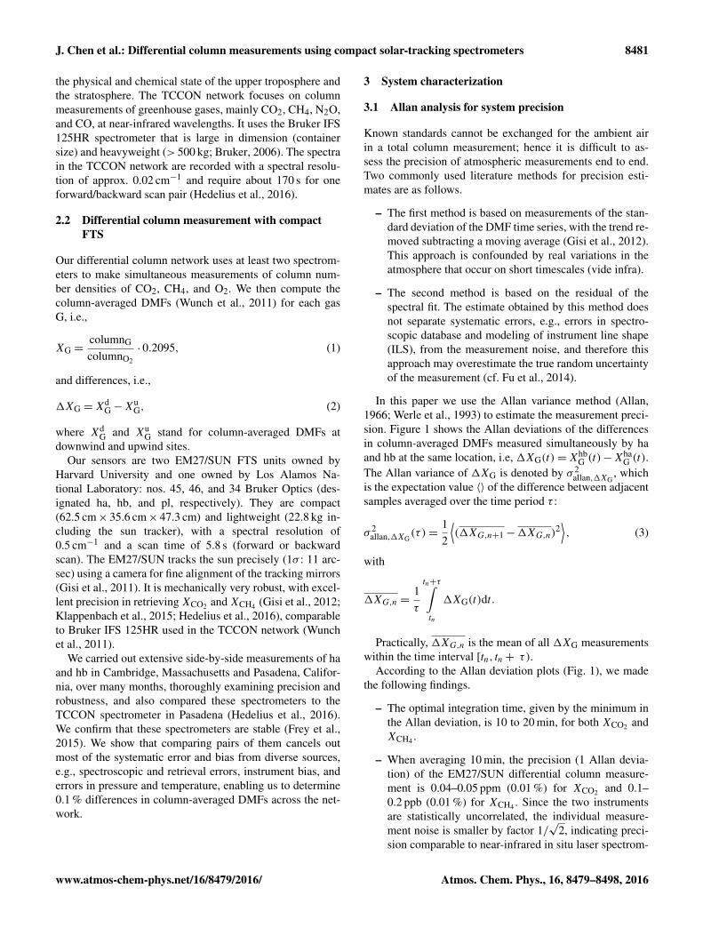
– The optimal integration time, given by the minimum inthe Allan deviation, is 10 to 20 min, for both XCO2 andXCH4 .

– When averaging 10 min, the precision (1 Allan devia-tion) of the EM27/SUN differential column measure-ment is 0.04–0.05 ppm (0.01 %) for XCO2 and 0.1–0.2 ppb (0.01 %) for XCH4 . Since the two instrumentsare statistically uncorrelated, the individual measure-ment noise is smaller by factor 1/

√2, indicating preci-

sion comparable to near-infrared in situ laser spectrom-

www.atmos-chem-phys.net/16/8479/2016/ Atmos. Chem. Phys., 16, 8479–8498, 2016


-1/2 f 0

1/2f -2

-1/2 f 0

Figure 1. Allan deviations σallan,1XCO2 and σallan,1XCH4 as a function of the integrating time τ . The black dashed lines represent a slopeof −1/2 and a slope of 1/2, which correspond to power spectral densities S(f )= f 0 (white noise) and S(f )= f−2 (Brownian noise),respectively. The Allan deviation follows a slope of −1/2 up to an integration time of 10 to 20 min, then stays constant (S(f )= f−1), andsubsequently turns over to a slope of 1/2, which describes a drift.

eters with commensurate optical path length and inte-gration time (Picarro, 2015a, b). Note that these pre-cision estimates represent the full end-to-end process-ing of the observations, including deriving the spectrumfrom the interferogram, retrieving the column num-ber densities in the atmosphere, and normalizing withthe O2 column amount to obtain the column-averagedDMFs.

– When integrating less than 10 min, the Allan deviationfollows a slope of−1/2 in the double logarithmic scale,indicating white noise (τ−1/2

→ f 0) that has a constantpower spectral density over the frequency f . As the av-eraging time τ increases beyond 10 min, the Allan devi-ation rises a little, showing a small color noise compo-nent (τ 1/2

→ f−2), which arises from instrument drift,in part due to temperature differences inside of the spec-trometers. There is also a small divergence between themeasurements of ha and hb at high solar zenith an-gles, traceable to their slightly different ILSs. The mea-sured ILS parameters are given in Appendix A. Mi-croscale eddies have durations of 10 s to 10 min andlength scales from tens to hundreds of meters (Stull,1988, Fig. 2.2). Therefore atmospheric turbulence prob-ably does not play a major role in the Allan plot becausethere is little color noise within timescale ≤ 10 min fortwo spectrometers looking along atmospheric paths sep-arated by roughly one meter.

We use a shorter integration time (5 min) for measuringemissions from local- and regional-scale sources (Sects. 4.1and 4.2), in order to retain high-frequency atmospheric sig-nals, giving us precision of 0.05–0.06 ppm for 1XCO2 and0.2–0.3 ppb for 1XCH4 (see Fig. 1). To study the short-termvariations due to pollution plumes or turbulent eddies we use2 min integration time (Sect. 4.3).

3.2 System stability

Differential column observations by two spectrometers willinevitably have bias in addition to fluctuations and drift. Forthe EM27/SUN, small differences in the alignments of theinterferometers result in minute, but observable and system-atic, deviations in the retrieval results. We examined the bi-ases between ha and hb over a long period of time to de-termine whether these errors can be effectively corrected byapplying a constant calibration factor to the retrieval of oneinstrument to match the performance of the other. The cali-bration factors are determined assuming a linear model, i.e.,Xhb

G =XhaG ·RG, and for each gas individually.

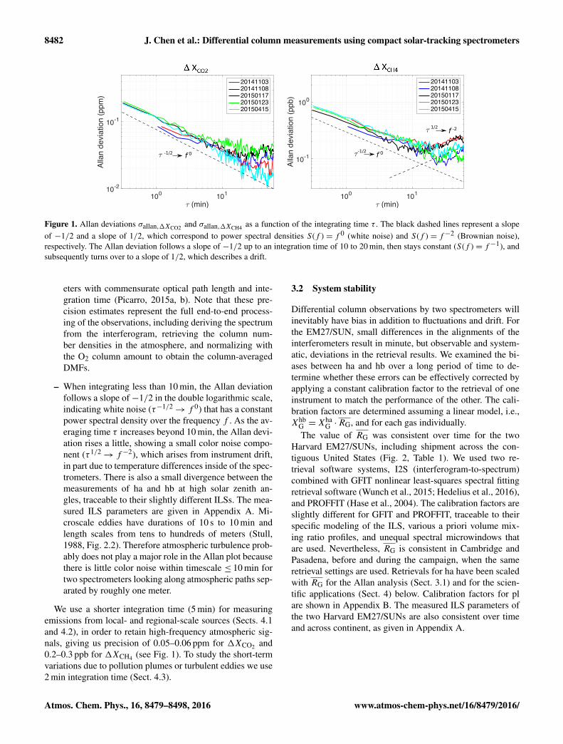
The value of RG was consistent over time for the twoHarvard EM27/SUNs, including shipment across the con-tiguous United States (Fig. 2, Table 1). We used two re-trieval software systems, I2S (interferogram-to-spectrum)combined with GFIT nonlinear least-squares spectral fittingretrieval software (Wunch et al., 2015; Hedelius et al., 2016),and PROFFIT (Hase et al., 2004). The calibration factors areslightly different for GFIT and PROFFIT, traceable to theirspecific modeling of the ILS, various a priori volume mix-ing ratio profiles, and unequal spectral microwindows thatare used. Nevertheless, RG is consistent in Cambridge andPasadena, before and during the campaign, when the sameretrieval settings are used. Retrievals for ha have been scaledwith RG for the Allan analysis (Sect. 3.1) and for the scien-tific applications (Sect. 4) below. Calibration factors for plare shown in Appendix B. The measured ILS parameters ofthe two Harvard EM27/SUNs are also consistent over timeand across continent, as given in Appendix A.



390 395 400 405ha X

CO2 (ppm)

390

395

400

405

hb

XC

O2 (

pp

m)

Slope: 0.99880r2: 0.98802

2014082020141103201411082015011420150117201501192015012120150123

1.82 1.84 1.86 1.88 1.9ha X

CH4 (ppm)

1.82

1.83

1.84

1.85

1.86

1.87

1.88

1.89

1.9

hb

XC

H4 (

pp

m)

Slope: 0.99578r2: 0.98263

2014082020141103201411082015011420150117201501192015012120150123

390 395 400 405ha X

CO2 (ppm)

390

395

400

405

hb

XC

O2 (

pp

m)

Slope: 0.99835r2: 0.99155

2014082020141103201411082015011420150117201501192015012120150123

1.76 1.78 1.8 1.82 1.84ha X

CH4 (ppm)

1.76

1.77

1.78

1.79

1.8

1.81

1.82

1.83

1.84

hb

XC

H4 (

pp

m)

Slope: 0.99810r2: 0.98972

2014082020141103201411082015011420150117201501192015012120150123

Figure 2. Scatter plots with the slopes representing RG for different days using I2S/GFIT retrieval (top panels) and PROFFIT retrieval(bottom panels). January measurements are carried out in Pasadena, others in Cambridge. The first 4 days are before the field study; othersare during the campaign.

Table 1. Calibration factors RG for XCH4 and XCO2 before andduring the field campaign, determined by forcing a linear regressionline to go through the origin. RG for XCH4 and XCO2 , determinedusing all data, are provided in the last row and used for the fieldstudy.

RCH4 RCO2

GFIT PROFFIT GFIT PROFFIT

Before 0.99574 0.99813 0.99877 0.99838During 0.99580 0.99809 0.99881 0.99834Both 0.99578 0.99810 0.99880 0.99835

4 Scientific applications

4.1 Emission of an area source

We measured the column-averaged dry-air mole fractionsXCO2 and XCH4 simultaneously at locations upwind anddownwind of the dairy farms in Chino, California, for sev-eral days in January 2015. Field results for ha, hb, and pl areshown in Fig. 4.

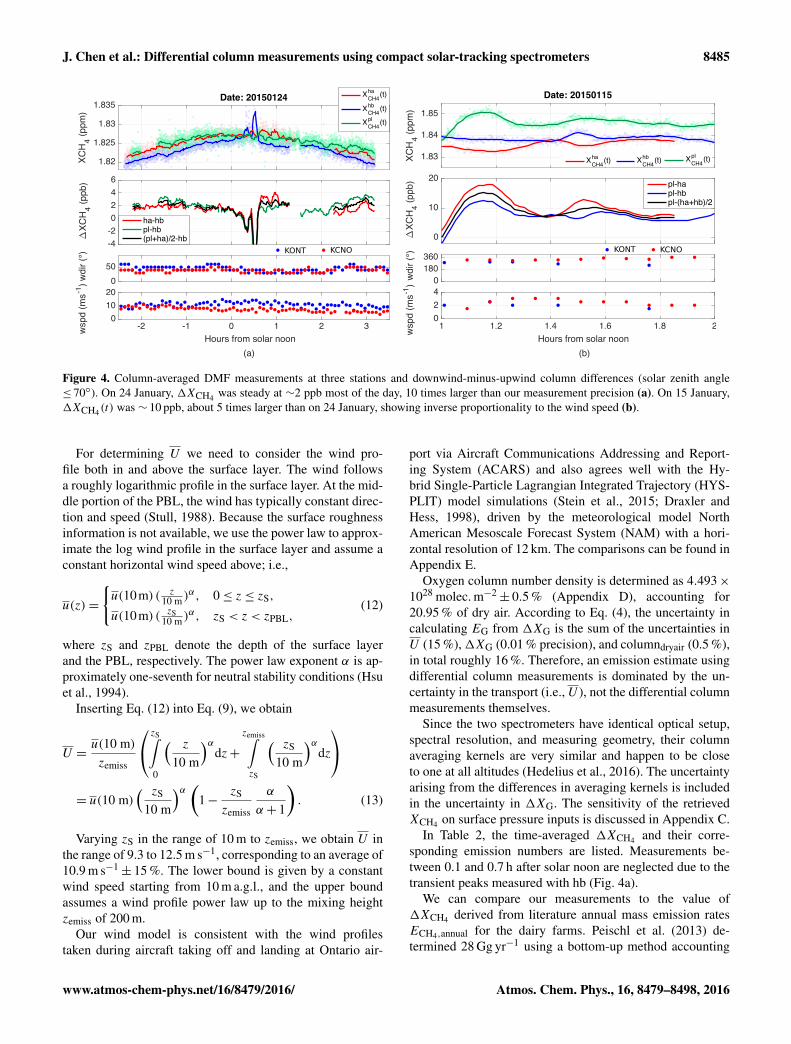
Meteorological conditions were particularly favorable on24 January 2015, with consistent wind directions and wind

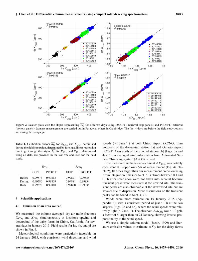
speeds (∼ 10 m s−1) at both Chino airport (KCNO; 1 kmnortheast of the downwind station ha) and Ontario airport(KONT; 3 km north of the upwind station hb) (Figs. 3a and4a); 5 min averaged wind information from Automated Sur-face Observing System (ASOS) is used.

The measured methane enhancement 1XCH4 was notablyconsistent at ∼2 ppb over 5 h of measurement (Fig. 4a, Ta-ble 2), 10 times larger than our measurement precision using5 min integration time (see Sect. 3.1). Times between 0.1 and0.7 h after solar noon were not taken into account becausetransient peaks were measured at the upwind site. The tran-sient peaks are also observable at the downwind site but areweaker due to dispersion. More discussions on the transientpeaks can be found in Sect. 4.3.2.

Winds were more variable on 15 January 2015 (Ap-pendix F), with a consistent period of just ∼ 1 h at the twoairports (Figs. 3b and 4b), where the wind speeds were rela-tively light (∼ 2 m s−1). The observed1XCH4 was ∼ 10 ppb,a factor of 5 larger than on 24 January, showing inverse pro-portionality to the wind speed.

We use a simple column model (Jacob, 1999) and liter-ature emission values to estimate 1XG for the dairy farms



Figure 3. Locations of FTS stations and mean wind directions on24 January 2015 (a) and 15 January 2015 (b). Map provided byGoogle Earth, Image Landsat, Data SIO, NOAA, US Navy, NGA,and GEBCO.

(area source) and to verify our measurements:

1XG =XdG−X

uG =

D

U×

EG

columndryair, (4)

where EG is the mean emission flux (unit: molec. m−2 s−1)along the line traversing the area source, and D is the lengthof the transect. columndryair denotes the mean column num-ber density of dry air. The frame of reference is the air col-umn, which picks up the emissions of gas G from the dairiesas the air traverses the farms. The longer the air column trav-els in the emission field, the larger the difference between thecolumn number densities of the downwind and upwind siteswill become. 1XG is therefore proportional to the residencetimeD/U of the air column and inversely proportional to thewind speed U . This simple column model is applicable whenthe wind direction and speed are consistent across the area,and fluxes are uniform at plume scale.

Our model assumes that air parcels within the air columnare transported with a mean velocity U in the horizontal di-rection, which can be estimated using real-time data for thewind speed at the surface. Using Reynolds’ decomposition,the time series of horizontal (u) and vertical (w) wind speedare split into a mean part and a turbulent part, i.e.,

u(t)= u+ uturb(t), w(t)= w+wturb(t), (5)

σu =

√< u2

turb >, σw =

√<w2

turb >. (6)

σu and σw are the standard deviations of the turbulent com-ponents. We assume that the turbulence is horizontally ho-mogeneous (σu is independent of location) and isotropic(σw = σu) and that the mean vertical wind speed w iszero. Strictly speaking, U denotes the “mass-enhancement-weighted” wind velocity, i.e., u(z) weighted with the vertical

distribution of the CH4 molecules emitted from the dairies,denoted as PDF1CH4(z):

U =

∞∫0

u(z)PDF1CH4(z)dz. (7)

Note if u(z)= const.; we have U = u(z)= const., i.e., U isindependent of the vertical distribution of the CH4 moleculesbeing added in the column. However, since the wind speedgenerally increases with altitude, PDF1CH4(z) needs to beconsidered for the estimate of U .

We assume 1CH4 is uniformly distributed up to a mixingheight zemiss and negligible above:

PDF1CH4(z)=

{1

zemiss, 0≤ z ≤ zemiss,

0, z > zemiss,(8)

U =1

zemiss

zemiss∫0

u(z)dz. (9)

We use a 2-D random-walk model (McCrea and Whipple,1940) to estimate zemiss, the height to which CH4 emissionsare transported vertically by turbulent flow. The number ofthe random-walk steps n is given by the ratio between theaverage transit time of the emission τtransit and the decorrela-tion time of the turbulent velocity fluctuations τeddy, i.e.,

n=τtransit

τeddy=Dσw

2uλ. (10)

Assuming homogeneous emission, τtransit is approxi-mately D/2u, with u representing the mean speed at the sur-face. This also corresponds to the transit time of a particleemitted at the center of the field. τeddy is given by λ/σw,where λ denotes the average eddy scale.

On 24 January, the mean horizontal wind speed overthe entire measurement time is 11.35 m s−1 at KONT and7.29 m s−1 at KCNO with a standard deviation (1σ ) of1.75 m s−1 and 1.59 m s−1, respectively. The wind direc-tions are likewise very consistent over time, with a stan-dard deviation of 8.9◦ (KONT) and 6.5◦ (KCNO). Thewind speed at 10 m a.g.l. (above ground level) is assumedto be the average at the two airports over time, whichgives u(10 m)= 9.3 m s−1 with fluctuations σu(10 m)=σw(10 m)= 1.7 m s−1. Assuming an average eddy scale of100 m, the expected value of the height to which CH4 emis-sions rise is therefore

zemiss =λ√n

√2=

12

√Dσw(10 m)λu(10 m)

=12

√DI λ≈ 200m. (11)

According to Taylor’s hypothesis (Taylor, 1938), the tur-bulence intensity I = σu/u should be constant, which indi-cates zemiss depends not on u but rather only on the eddyscale λ and the turbulence intensity.



KCNOKONT KCNOKONT

Hours from solar noon Hours from solar noon

(b)(a)

Figure 4. Column-averaged DMF measurements at three stations and downwind-minus-upwind column differences (solar zenith angle≤ 70◦). On 24 January, 1XCH4 was steady at ∼2 ppb most of the day, 10 times larger than our measurement precision (a). On 15 January,1XCH4(t) was ∼ 10 ppb, about 5 times larger than on 24 January, showing inverse proportionality to the wind speed (b).

For determining U we need to consider the wind pro-file both in and above the surface layer. The wind followsa roughly logarithmic profile in the surface layer. At the mid-dle portion of the PBL, the wind has typically constant direc-tion and speed (Stull, 1988). Because the surface roughnessinformation is not available, we use the power law to approx-imate the log wind profile in the surface layer and assume aconstant horizontal wind speed above; i.e.,

u(z)=

{u(10m) ( z

10 m )α, 0≤ z ≤ zS,

u(10m) ( zS10 m )

α, zS < z < zPBL,(12)

where zS and zPBL denote the depth of the surface layerand the PBL, respectively. The power law exponent α is ap-proximately one-seventh for neutral stability conditions (Hsuet al., 1994).

Inserting Eq. (12) into Eq. (9), we obtain

U =u(10 m)zemiss

zS∫0

( z

10 m

)αdz+

zemiss∫zS

( zS

10 m

)αdz

= u(10 m)

( zS

10 m

)α (1−

zS

zemiss

α

α+ 1

). (13)

Varying zS in the range of 10 m to zemiss, we obtain U inthe range of 9.3 to 12.5 m s−1, corresponding to an average of10.9 m s−1

± 15 %. The lower bound is given by a constantwind speed starting from 10 m a.g.l., and the upper boundassumes a wind profile power law up to the mixing heightzemiss of 200 m.

Our wind model is consistent with the wind profilestaken during aircraft taking off and landing at Ontario air-

port via Aircraft Communications Addressing and Report-ing System (ACARS) and also agrees well with the Hy-brid Single-Particle Lagrangian Integrated Trajectory (HYS-PLIT) model simulations (Stein et al., 2015; Draxler andHess, 1998), driven by the meteorological model NorthAmerican Mesoscale Forecast System (NAM) with a hori-zontal resolution of 12 km. The comparisons can be found inAppendix E.

Oxygen column number density is determined as 4.493×1028 molec. m−2

± 0.5 % (Appendix D), accounting for20.95 % of dry air. According to Eq. (4), the uncertainty incalculating EG from 1XG is the sum of the uncertainties inU (15 %),1XG (0.01 % precision), and columndryair (0.5 %),in total roughly 16 %. Therefore, an emission estimate usingdifferential column measurements is dominated by the un-certainty in the transport (i.e., U ), not the differential columnmeasurements themselves.

Since the two spectrometers have identical optical setup,spectral resolution, and measuring geometry, their columnaveraging kernels are very similar and happen to be closeto one at all altitudes (Hedelius et al., 2016). The uncertaintyarising from the differences in averaging kernels is includedin the uncertainty in 1XG. The sensitivity of the retrievedXCH4 on surface pressure inputs is discussed in Appendix C.

In Table 2, the time-averaged 1XCH4 and their corre-sponding emission numbers are listed. Measurements be-tween 0.1 and 0.7 h after solar noon are neglected due to thetransient peaks measured with hb (Fig. 4a).

We can compare our measurements to the value of1XCH4 derived from literature annual mass emission ratesECH4,annual for the dairy farms. Peischl et al. (2013) de-termined 28 Gg yr−1 using a bottom-up method accounting



Table 2. Time-averaged 1XCH4 , using ha or pl, or ha and pl as downwind stations on 24 January 2015, and their corresponding emissionnumbers calculated using Eq. (4).1XCH4 is rounded to one decimal place in the table, whereas for the calculation of ECH4 and ECH4,annualall available digits are used. The uncertainty of 16 % is given by the uncertainties in U , columndryair, and 1XG. Uncertainty in ECH4,annualis 16 % added with 10 % uncertainty in the emission area. This table also displays the annual emission rates estimated by Peischl et al. (2013)using bottom-up and top-down methods. The corresponding column differences 1XCH4 and their uncertainties, as derived in Eq. 14, aresummarized in the second column.

Configuration 1XCH4 ECH4 ECH4,annual(ppb) (molec. m−2 s−1) (Gg yr−1)

ha – hb 1.8 5.38×1017(±16%) 22.5 (±26%)pl – hb 2.1 6.15×1017(±16%) 25.8 (±26%)(pl+ha)/2 – hb 2.1 6.09×1017(±16%) 25.5 (±26%)

Peischl’s bottom-up 2.3 (±0.6) 28.0Peischl’s top-down (4.0± 1.0) (± 50 %) 49.0 (±50 %)

for enteric fermentation and dry manure management and49(±50 %) Gg yr−1 using a top-down method with aircraft-based mass balance approach during the CalNex field study.We assume a dairy area (areaemiss) of 50 km2

± 10 % and aconstant emission rate across the farm throughout day andnight to convert ECH4,annual (unit: Gg yr−1) to ECH4 (unit:molec. m−2 s−1). The transect lengthD is approximated with8 km, which is the diameter of a circle with 50 km2 area.

For 24 January 2015,

1XCH4,expected (14)

=D

U×

ECH4,annual(Peischl’s number)mCH4 · areaemiss ·Ns year−1 · columndryair

=

{2.3± 0.6 ppb, for 28Ggyr−1(bottom-up),(4.0± 1.0)(±50%) ppb, for 49(±50%)Ggyr−1 (top-down),

where mCH4 denotes the molecular mass of methane (unit:g molec.−1) and Ns year−1 represents the number of secondsper year.

The observed 1XCH4 , ∼ 2 ppb (Fig. 4a, Table 2), falls inthe lower half of the range from Peischl. Our results and Peis-chl’s top-down estimates both represent just a few days ofdata. The difference with Peischl’s results using the aircraft-based mass balance approach could be due to seasonal fac-tors, activity levels at the farms, uncertainties in U as well asin background concentrations and in boundary layer depthfor the aircraft measurements (Cambaliza et al., 2014), ormodel errors. Longer deployments with more ancillary data,such as wind profiles, would be needed to refine the result.Further studies using a Weather Research and Forecasting(WRF) model in large-eddy simulation (LES) mode will bepresented in Viatte et al. (2016). The differential columnmeasurement using compact FTSs has shown the capabilityto determine the emission flux when deployed across an areasource such as Chino farms.

4.2 Source characterization using ratios of columndifferences

Pasadena is a city within the South Coast Air Basin (SCAB)with heterogeneous CO2 and CH4 emissions, from differentsource types such as transportation, electricity generation, in-dustry, landfills, and gas leaks in the natural gas delivery sys-tem. The ratio of column differences can be used to charac-terize regional emissions. For example, Wunch et al. (2009)measured diurnal changes of XCH4 ,XCO2 , and XCO (tempo-ral difference) and used the CO2 emission inventories fromthe California Air Resources Board (CARB) and EDGAR(Emission Database for Global Atmospheric Research) to es-timate emissions of CH4 and CO in the SCAB.

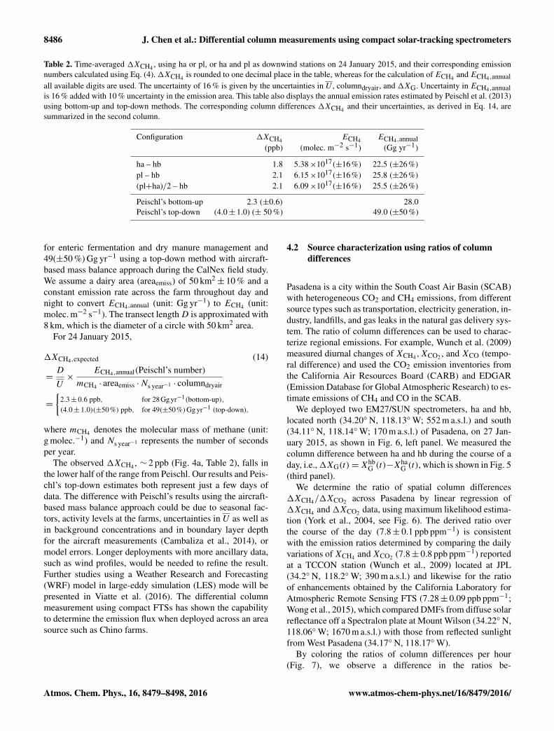
We deployed two EM27/SUN spectrometers, ha and hb,located north (34.20◦ N, 118.13◦W; 552 m a.s.l.) and south(34.11◦ N, 118.14◦W; 170 m a.s.l.) of Pasadena, on 27 Jan-uary 2015, as shown in Fig. 6, left panel. We measured thecolumn difference between ha and hb during the course of aday, i.e.,1XG(t)=X

hbG (t)−X

haG (t), which is shown in Fig. 5

(third panel).We determine the ratio of spatial column differences

1XCH4/1XCO2 across Pasadena by linear regression of1XCH4 and1XCO2 data, using maximum likelihood estima-tion (York et al., 2004, see Fig. 6). The derived ratio overthe course of the day (7.8± 0.1 ppb ppm−1) is consistentwith the emission ratios determined by comparing the dailyvariations ofXCH4 andXCO2 (7.8± 0.8 ppb ppm−1) reportedat a TCCON station (Wunch et al., 2009) located at JPL(34.2◦ N, 118.2◦W; 390 m a.s.l.) and likewise for the ratioof enhancements obtained by the California Laboratory forAtmospheric Remote Sensing FTS (7.28± 0.09 ppb ppm−1;Wong et al., 2015), which compared DMFs from diffuse solarreflectance off a Spectralon plate at Mount Wilson (34.22◦ N,118.06◦W; 1670 m a.s.l.) with those from reflected sunlightfrom West Pasadena (34.17◦ N, 118.17◦W).

By coloring the ratios of column differences per hour(Fig. 7), we observe a difference in the ratios be-



Figure 5. First and second panels: measuredXCO2 andXCH4 north(ha) and south (hb) of Pasadena on 27 January with 5 min averagingtime. Third panel: 1XCO2 and 1XCH4 are temporally correlatedand their ratio is determined as 7.8 ppb ppm−1, shown in Fig. 6.

+

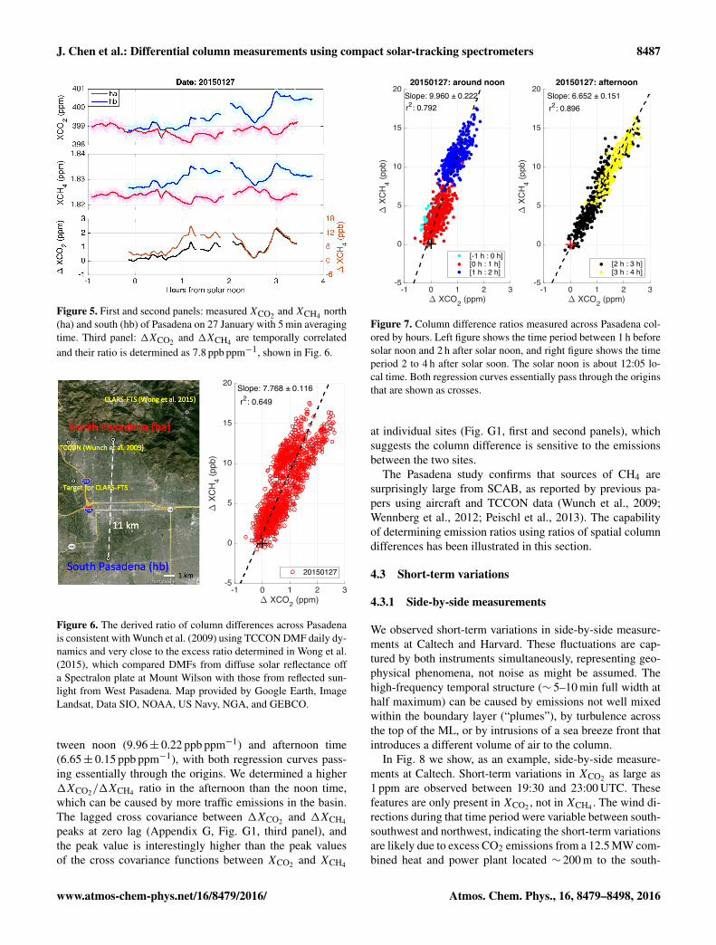
Figure 6. The derived ratio of column differences across Pasadenais consistent with Wunch et al. (2009) using TCCON DMF daily dy-namics and very close to the excess ratio determined in Wong et al.(2015), which compared DMFs from diffuse solar reflectance offa Spectralon plate at Mount Wilson with those from reflected sun-light from West Pasadena. Map provided by Google Earth, ImageLandsat, Data SIO, NOAA, US Navy, NGA, and GEBCO.

tween noon (9.96± 0.22 ppb ppm−1) and afternoon time(6.65± 0.15 ppb ppm−1), with both regression curves pass-ing essentially through the origins. We determined a higher1XCO2/1XCH4 ratio in the afternoon than the noon time,which can be caused by more traffic emissions in the basin.The lagged cross covariance between 1XCO2 and 1XCH4

peaks at zero lag (Appendix G, Fig. G1, third panel), andthe peak value is interestingly higher than the peak valuesof the cross covariance functions between XCO2 and XCH4

+ +

Figure 7. Column difference ratios measured across Pasadena col-ored by hours. Left figure shows the time period between 1 h beforesolar noon and 2 h after solar noon, and right figure shows the timeperiod 2 to 4 h after solar soon. The solar noon is about 12:05 lo-cal time. Both regression curves essentially pass through the originsthat are shown as crosses.

at individual sites (Fig. G1, first and second panels), whichsuggests the column difference is sensitive to the emissionsbetween the two sites.

The Pasadena study confirms that sources of CH4 aresurprisingly large from SCAB, as reported by previous pa-pers using aircraft and TCCON data (Wunch et al., 2009;Wennberg et al., 2012; Peischl et al., 2013). The capabilityof determining emission ratios using ratios of spatial columndifferences has been illustrated in this section.

4.3 Short-term variations

4.3.1 Side-by-side measurements

We observed short-term variations in side-by-side measure-ments at Caltech and Harvard. These fluctuations are cap-tured by both instruments simultaneously, representing geo-physical phenomena, not noise as might be assumed. Thehigh-frequency temporal structure (∼ 5–10 min full width athalf maximum) can be caused by emissions not well mixedwithin the boundary layer (“plumes”), by turbulence acrossthe top of the ML, or by intrusions of a sea breeze front thatintroduces a different volume of air to the column.

In Fig. 8 we show, as an example, side-by-side measure-ments at Caltech. Short-term variations in XCO2 as large as1 ppm are observed between 19:30 and 23:00 UTC. Thesefeatures are only present in XCO2 , not in XCH4 . The wind di-rections during that time period were variable between south-southwest and northwest, indicating the short-term variationsare likely due to excess CO2 emissions from a 12.5 MW com-bined heat and power plant located ∼ 200 m to the south-



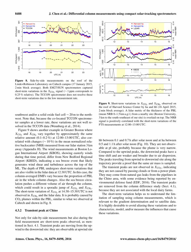
Figure 8. Side-by-side measurements on the roof of theLinde+Robinson Laboratory on Caltech campus (17 January 2015,2 min block average). Both EM27/SUN spectrometers capturedshort-term variations in the XCO2 signal (∼ 1 ppm corresponds to0.25 % relative). The TCCON spectrometer does not resolve theseshort-term variations due to the low measurement rate.

southwest and/or a solid oxide fuel cell ∼ 20 m to the north-west. Note that, because the co-located TCCON spectrome-ter samples at a lower rate, these variations are not well re-solved in the TCCON data (Wennberg et al., 2014).

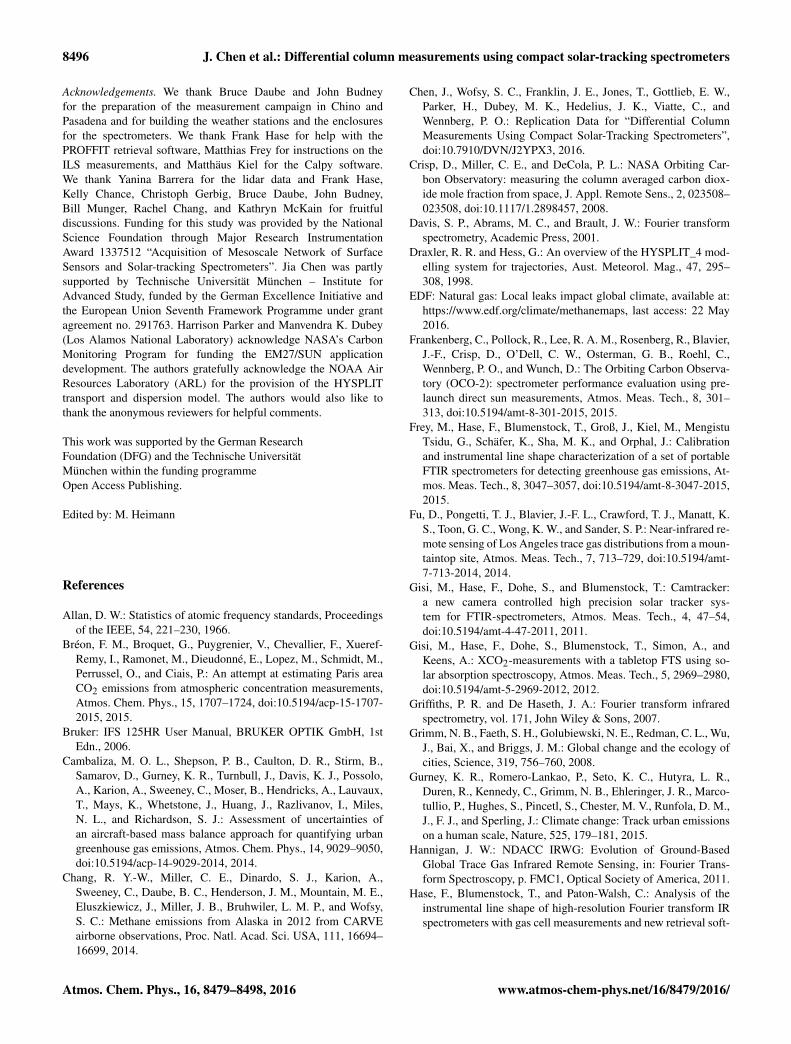
Figure 9 shows another example in Greater Boston whereXCO2 and XCH4 vary together by approximately the samerelative amount (0.1–0.2 %) at 12:00–13:00 UTC, also cor-related with changes (∼ 10 %) in the mean normalized rela-tive backscatter (NRB) measured from our lidar station 3 kmaway (Appendix H). The wind measurements at Boston Lo-gan International Airport (KBOS), showing easterly windsduring that time period, differ from New Bedford RegionalAirport (KBED), indicating a sea breeze event that likelygenerates wind shear and turbulence across the top of theML. The depth of PBL undergoes short-term variations thatare also visible in the lidar data at 12:30 UTC. In this case, thecolumn-averaged DMFs vary because the proportion of PBLair in the whole column changes. Also the sea breeze circu-lation pushes a different volume of air through the column,which could result in a sporadic jump of XCO2 and XCH4 .The short-term variation of XCO2 at 14:30–15:30 UTC is notobserved in XCH4 and the lidar data. It is probably caused byCO2 plumes within the PBL, similar to what we observed atCaltech and shown in Fig. 8.

4.3.2 Transient peak at Chino

Not only for side-by-side measurements but also during thefield measurement are short-term peaks observed, as men-tioned in Sect. 4.1. Transient peaks are moving from the up-wind to the downwind site: they are observable at upwind site

Figure 9. Short-term variations in XCO2 and XCH4 observed onthe roof of Harvard Science Center by ha and hb (16 April 2015,2 min block average). A lidar metric of the thickness of the PBL(mean NRB 0–1.5 km a.g.l.) from a nearby site (Boston University,3 km to the south-southeast of our site) is overlaid on top. The NRBsignal is positively correlated with the short-term variations of theFTS measurements at 12:00–13:00 UTC.

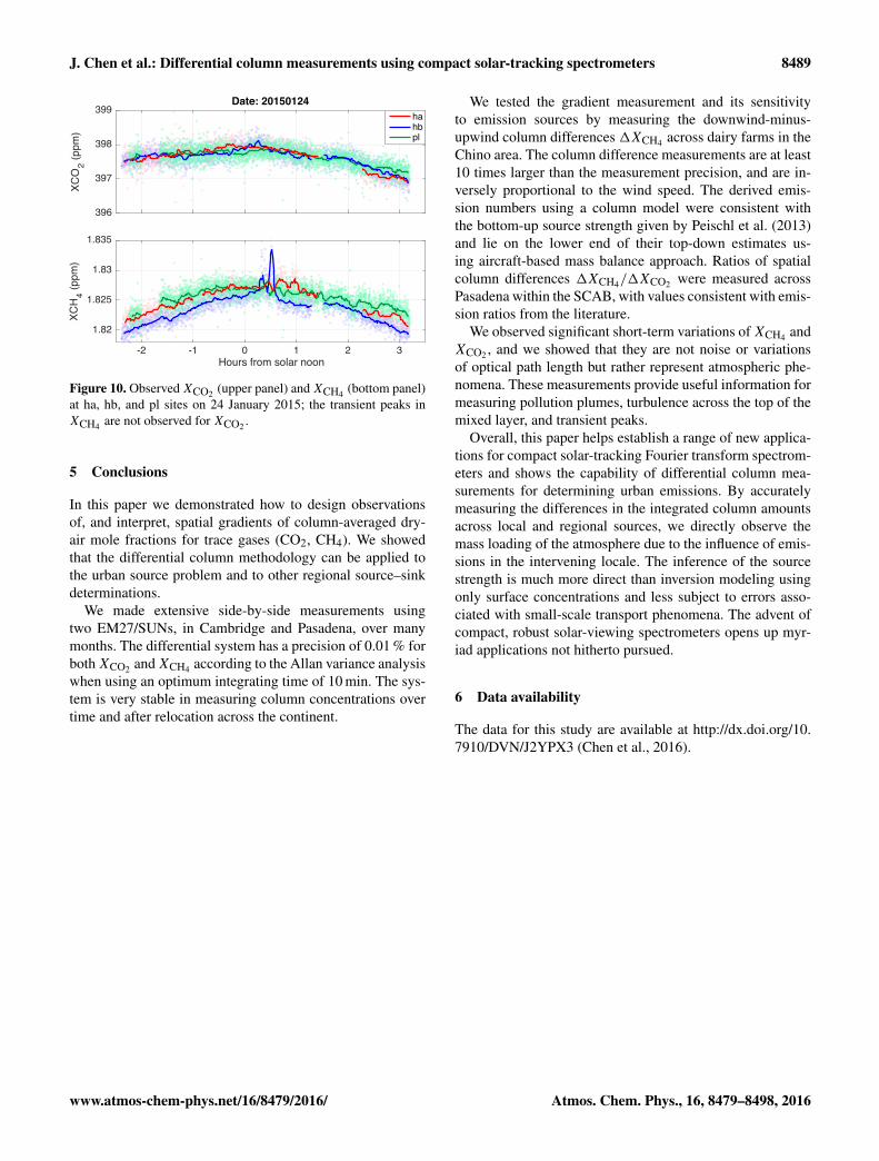
hb between 0.1 and 0.7 h after solar noon and at ha between0.5 and 1.1 h after solar noon (Fig. 10). They are not observ-able at pl site, probably because the plume is very narrow.Compared to the upwind peaks, the downwind peaks have atime shift and are weaker and broader due to air dispersion.The peaks traveling from upwind to downwind site along thetrajectory provide a proof that the same air mass is sampled.

The transient peaks are not observed in XCO2 , indicatingthey are not caused by passing clouds or from a power plant.They may come from natural gas leaks from the pipelines inthe Chino area, with some evidence being reported by en-vironmental defense fund (EDF, 2016). The transient peaksare removed from the column difference study (Sect. 4.1),because they are not associated with the local dairy farms.

The short-term variation helps us to understand the lim-itation of sampling using column measurements, which isrelevant to the gradient determination and to satellite data.It is highly desirable to avoid aliasing these variations and tocharacterize, model, and/or measure the influences that causethese variations.



396

397

398

399

XC

O2 (

pp

m)

Date: 20150124

hahbpl

-2 -1 0 1 2 3Hours from solar noon

1.82

1.825

1.83

1.835

XC

H4 (

pp

m)

Figure 10. ObservedXCO2 (upper panel) andXCH4 (bottom panel)at ha, hb, and pl sites on 24 January 2015; the transient peaks inXCH4 are not observed for XCO2 .

5 Conclusions

In this paper we demonstrated how to design observationsof, and interpret, spatial gradients of column-averaged dry-air mole fractions for trace gases (CO2, CH4). We showedthat the differential column methodology can be applied tothe urban source problem and to other regional source–sinkdeterminations.

We made extensive side-by-side measurements usingtwo EM27/SUNs, in Cambridge and Pasadena, over manymonths. The differential system has a precision of 0.01 % forbothXCO2 andXCH4 according to the Allan variance analysiswhen using an optimum integrating time of 10 min. The sys-tem is very stable in measuring column concentrations overtime and after relocation across the continent.

We tested the gradient measurement and its sensitivityto emission sources by measuring the downwind-minus-upwind column differences 1XCH4 across dairy farms in theChino area. The column difference measurements are at least10 times larger than the measurement precision, and are in-versely proportional to the wind speed. The derived emis-sion numbers using a column model were consistent withthe bottom-up source strength given by Peischl et al. (2013)and lie on the lower end of their top-down estimates us-ing aircraft-based mass balance approach. Ratios of spatialcolumn differences 1XCH4/1XCO2 were measured acrossPasadena within the SCAB, with values consistent with emis-sion ratios from the literature.

We observed significant short-term variations ofXCH4 andXCO2 , and we showed that they are not noise or variationsof optical path length but rather represent atmospheric phe-nomena. These measurements provide useful information formeasuring pollution plumes, turbulence across the top of themixed layer, and transient peaks.

Overall, this paper helps establish a range of new applica-tions for compact solar-tracking Fourier transform spectrom-eters and shows the capability of differential column mea-surements for determining urban emissions. By accuratelymeasuring the differences in the integrated column amountsacross local and regional sources, we directly observe themass loading of the atmosphere due to the influence of emis-sions in the intervening locale. The inference of the sourcestrength is much more direct than inversion modeling usingonly surface concentrations and less subject to errors asso-ciated with small-scale transport phenomena. The advent ofcompact, robust solar-viewing spectrometers opens up myr-iad applications not hitherto pursued.

6 Data availability

The data for this study are available at http://dx.doi.org/10.7910/DVN/J2YPX3 (Chen et al., 2016).


http://dx.doi.org/10.7910/DVN/J2YPX3



Appendix A: Instrument line shape function parameters

The measured spectrum is a convolution between the atmo-spheric spectrum and instrument line shape in the frequencydomain ILS(ν). In the ideal case, ILS(ν) is a delta function,which corresponds to a constant modulation efficiency forall optical path differences (OPDs). However, in practice,ILS(ν) is broader than a delta impulse, caused by the spec-trometer’s finite OPD, finite aperture size, and also misalign-ment of the interferometer. The ILS in the interferogram do-main can be approximated using a simple model that assumesa linear decay of the modulation efficiency with increasingOPD and a constant phase error (Hase et al., 1999).

We estimated the ILS parameters of both spectrometerswith an experimental setup, similar to that described in Freyet al. (2015), and determined the modulation efficiency atmaximum OPD (OPDmax) and phase error using the simplemodel implemented in the LINEFIT software (Hase et al.,1999). Matlab scripts for automation purposes have been de-veloped and can be obtained from the corresponding author.

Even though the measured ILS parameters are different forthe two spectrometers due to the different internal alignment,the ILS of each single instrument is consistent over time andafter relocation of the instrument across the contiguous USA(see Table A1).

Table A1. Modulation efficiency and phase error determined forEM27/SUN ha and hb in Cambridge and Pasadena.

Cambridge

Instrument Modulation efficiency Phase errorat OPDmax (rad)

ha 0.975 −3× 10−3

hb 0.988 5× 10−3

Pasadena

Instrument Modulation efficiency Phase errorat OPDmax (rad)

ha 0.973 −2× 10−3

hb 0.991 4× 10−3

Appendix B: Calibration factors for ha and pl

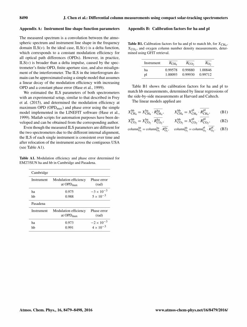
Table B1. Calibration factors for ha and pl to match hb, for XCH4 ,XCO2 , and oxygen column number density measurements, deter-mined using GFIT retrieval.

Instrument RCH4 RCO2 RO2

ha 0.99578 0.99880 1.00846pl 1.00093 0.99930 0.99712

Table B1 shows the calibration factors for ha and pl tomatch hb measurements, determined by linear regressions ofthe side-by-side measurements at Harvard and Caltech.

The linear models applied are

XhbCH4=Xha

CH4·Rha

CH4, Xhb

CH4=X

plCH4·R

plCH4

, (B1)

XhbCO2=Xha

CO2·Rha

CO2, Xhb

CO2=X

plCO2·R

plCO2

, (B2)

columnhbO2= columnha

O2·Rha

O2, columnhb

O2= columnpl

O2·R

plO2. (B3)



1.815

1.82

1.825

1.83

1.835

XC

H4 (

pp

m)

Date: 20150124 pl (ha met + 1.652 hPa)pl (KCNO met + 5.2 hPa)hb (hb met)hb (ha met - 7.788 hPa)ha (ha met)

-2 -1 0 1 2 3Hours from solar noon (h)

985

990

995

1000

Pre

ssu

re(h

Pa

)

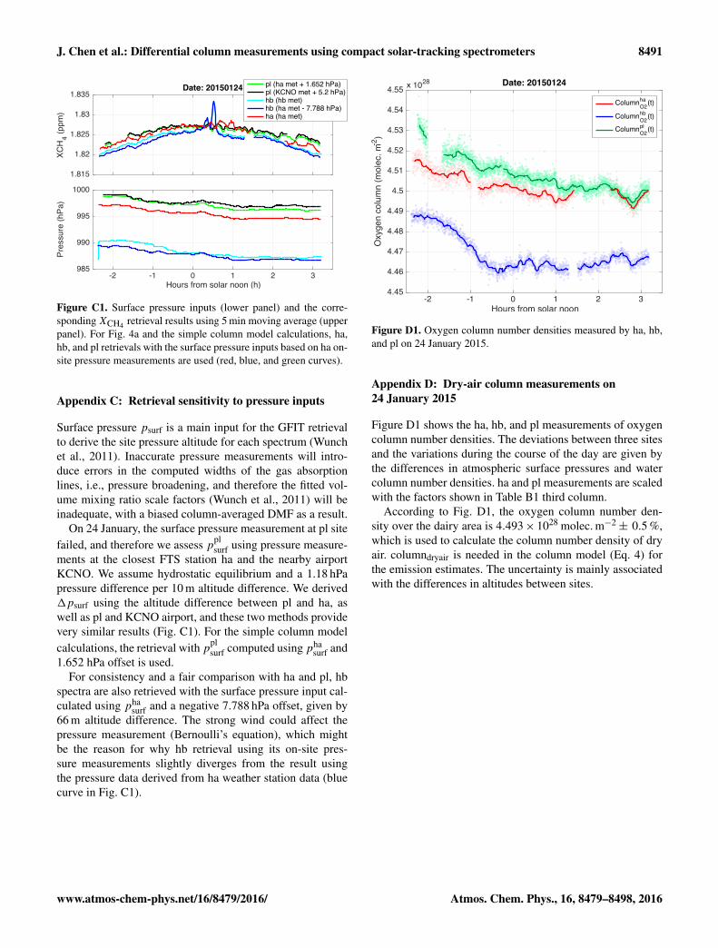
Figure C1. Surface pressure inputs (lower panel) and the corre-spondingXCH4 retrieval results using 5 min moving average (upperpanel). For Fig. 4a and the simple column model calculations, ha,hb, and pl retrievals with the surface pressure inputs based on ha on-site pressure measurements are used (red, blue, and green curves).

Appendix C: Retrieval sensitivity to pressure inputs

Surface pressure psurf is a main input for the GFIT retrievalto derive the site pressure altitude for each spectrum (Wunchet al., 2011). Inaccurate pressure measurements will intro-duce errors in the computed widths of the gas absorptionlines, i.e., pressure broadening, and therefore the fitted vol-ume mixing ratio scale factors (Wunch et al., 2011) will beinadequate, with a biased column-averaged DMF as a result.

On 24 January, the surface pressure measurement at pl sitefailed, and therefore we assess ppl

surf using pressure measure-ments at the closest FTS station ha and the nearby airportKCNO. We assume hydrostatic equilibrium and a 1.18 hPapressure difference per 10 m altitude difference. We derived1psurf using the altitude difference between pl and ha, aswell as pl and KCNO airport, and these two methods providevery similar results (Fig. C1). For the simple column modelcalculations, the retrieval with ppl

surf computed using phasurf and

1.652 hPa offset is used.For consistency and a fair comparison with ha and pl, hb

spectra are also retrieved with the surface pressure input cal-culated using pha

surf and a negative 7.788 hPa offset, given by66 m altitude difference. The strong wind could affect thepressure measurement (Bernoulli’s equation), which mightbe the reason for why hb retrieval using its on-site pres-sure measurements slightly diverges from the result usingthe pressure data derived from ha weather station data (bluecurve in Fig. C1).

-2 -1 0 1 2 3Hours from solar noon

4.45

4.46

4.47

4.48

4.49

4.5

4.51

4.52

4.53

4.54

4.55

Oxyg

en

co

lum

n (

mo

lec. m

-2)

1028 Date: 20150124

Columnha

O2(t)

Columnhb

O2(t)

Columnpl

O2(t)

x

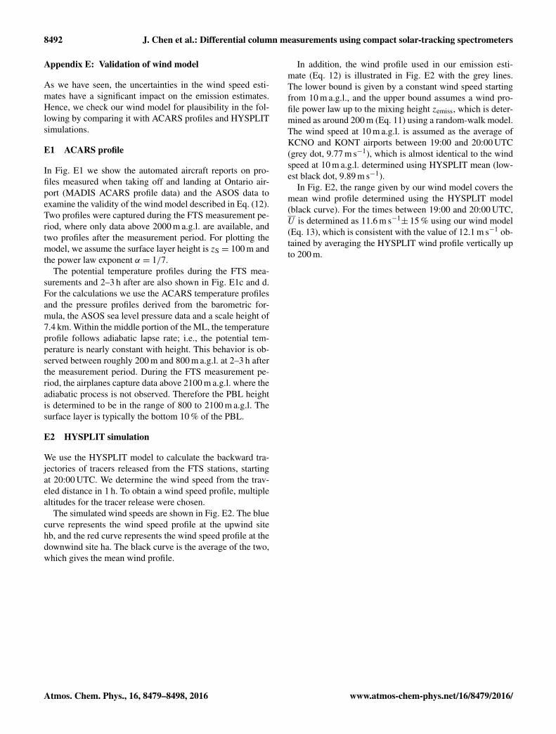
Figure D1. Oxygen column number densities measured by ha, hb,and pl on 24 January 2015.

Appendix D: Dry-air column measurements on24 January 2015

Figure D1 shows the ha, hb, and pl measurements of oxygencolumn number densities. The deviations between three sitesand the variations during the course of the day are given bythe differences in atmospheric surface pressures and watercolumn number densities. ha and pl measurements are scaledwith the factors shown in Table B1 third column.

According to Fig. D1, the oxygen column number den-sity over the dairy area is 4.493× 1028 molec. m−2

± 0.5 %,which is used to calculate the column number density of dryair. columndryair is needed in the column model (Eq. 4) forthe emission estimates. The uncertainty is mainly associatedwith the differences in altitudes between sites.



Appendix E: Validation of wind model

As we have seen, the uncertainties in the wind speed esti-mates have a significant impact on the emission estimates.Hence, we check our wind model for plausibility in the fol-lowing by comparing it with ACARS profiles and HYSPLITsimulations.

E1 ACARS profile

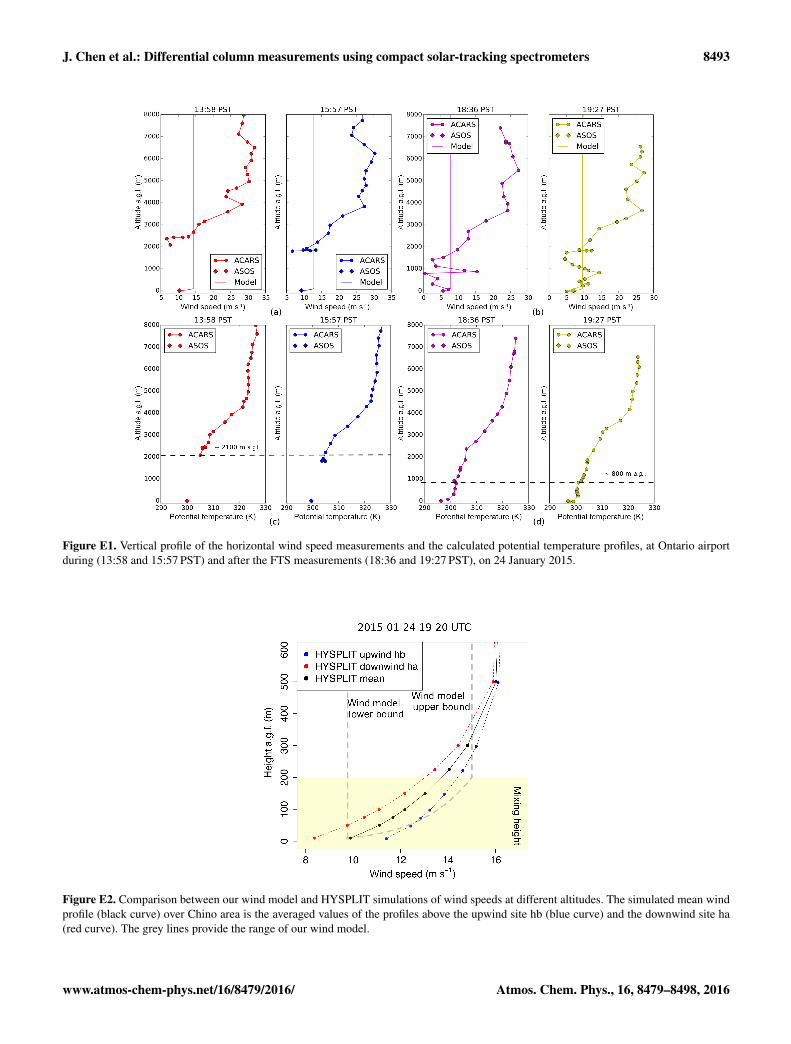
In Fig. E1 we show the automated aircraft reports on pro-files measured when taking off and landing at Ontario air-port (MADIS ACARS profile data) and the ASOS data toexamine the validity of the wind model described in Eq. (12).Two profiles were captured during the FTS measurement pe-riod, where only data above 2000 m a.g.l. are available, andtwo profiles after the measurement period. For plotting themodel, we assume the surface layer height is zS = 100 m andthe power law exponent α = 1/7.

The potential temperature profiles during the FTS mea-surements and 2–3 h after are also shown in Fig. E1c and d.For the calculations we use the ACARS temperature profilesand the pressure profiles derived from the barometric for-mula, the ASOS sea level pressure data and a scale height of7.4 km. Within the middle portion of the ML, the temperatureprofile follows adiabatic lapse rate; i.e., the potential tem-perature is nearly constant with height. This behavior is ob-served between roughly 200 m and 800 m a.g.l. at 2–3 h afterthe measurement period. During the FTS measurement pe-riod, the airplanes capture data above 2100 m a.g.l. where theadiabatic process is not observed. Therefore the PBL heightis determined to be in the range of 800 to 2100 m a.g.l. Thesurface layer is typically the bottom 10 % of the PBL.

E2 HYSPLIT simulation

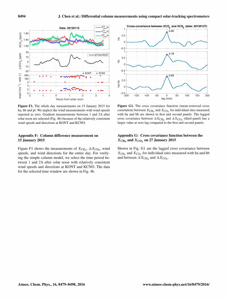
We use the HYSPLIT model to calculate the backward tra-jectories of tracers released from the FTS stations, startingat 20:00 UTC. We determine the wind speed from the trav-eled distance in 1 h. To obtain a wind speed profile, multiplealtitudes for the tracer release were chosen.

The simulated wind speeds are shown in Fig. E2. The bluecurve represents the wind speed profile at the upwind sitehb, and the red curve represents the wind speed profile at thedownwind site ha. The black curve is the average of the two,which gives the mean wind profile.

In addition, the wind profile used in our emission esti-mate (Eq. 12) is illustrated in Fig. E2 with the grey lines.The lower bound is given by a constant wind speed startingfrom 10 m a.g.l., and the upper bound assumes a wind pro-file power law up to the mixing height zemiss, which is deter-mined as around 200 m (Eq. 11) using a random-walk model.The wind speed at 10 m a.g.l. is assumed as the average ofKCNO and KONT airports between 19:00 and 20:00 UTC(grey dot, 9.77 m s−1), which is almost identical to the windspeed at 10 m a.g.l. determined using HYSPLIT mean (low-est black dot, 9.89 m s−1).

In Fig. E2, the range given by our wind model covers themean wind profile determined using the HYSPLIT model(black curve). For the times between 19:00 and 20:00 UTC,U is determined as 11.6 m s−1

± 15 % using our wind model(Eq. 13), which is consistent with the value of 12.1 m s−1 ob-tained by averaging the HYSPLIT wind profile vertically upto 200 m.



Figure E1. Vertical profile of the horizontal wind speed measurements and the calculated potential temperature profiles, at Ontario airportduring (13:58 and 15:57 PST) and after the FTS measurements (18:36 and 19:27 PST), on 24 January 2015.

Figure E2. Comparison between our wind model and HYSPLIT simulations of wind speeds at different altitudes. The simulated mean windprofile (black curve) over Chino area is the averaged values of the profiles above the upwind site hb (blue curve) and the downwind site ha(red curve). The grey lines provide the range of our wind model.



KCNOKONT

Hours from solar noon

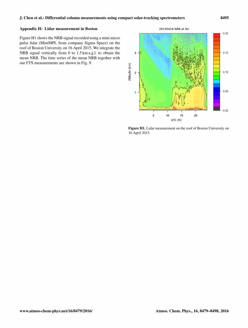
Figure F1. The whole day measurements on 15 January 2015 forha, hb and pl. We neglect the wind measurements with wind speedsreported as zero. Gradient measurements between 1 and 2 h aftersolar noon are selected (Fig. 4b) because of the relatively consistentwind speeds and directions at KONT and KCNO.

Appendix F: Column difference measurement on15 January 2015

Figure F1 shows the measurements of XCH4 , 1XCH4 , windspeeds, and wind directions for the entire day. For verify-ing the simple column model, we select the time period be-tween 1 and 2 h after solar noon with relatively consistentwind speeds and directions at KONT and KCNO. The datafor the selected time window are shown in Fig. 4b.

-0.5

0

0.5

1

ha

Cross-covariance between XCO and XCH (date: 20150127)2 4

0.80

-0.5

0

0.5

1

hb

0.78

-200 -150 -100 -50 0 50 100 150 200lag (min)

-0.5

0

0.5

1

ha

-hb

0.83

Figure G1. The cross covariance function (mean-removed crosscorrelation) between XCH4 and XCO2 for individual sites measuredwith ha and hb are shown in first and second panels. The laggedcross covariance between 1XCH4 and 1XCO2 (third panel) has alarger value at zero lag compared to the first and second panels.

Appendix G: Cross covariance function between theXCH4 and XCO2 on 27 January 2015

Shown in Fig. G1 are the lagged cross covariance betweenXCH4 and XCO2 for individual sites measured with ha and hband between 1XCH4 and 1XCO2 .



Appendix H: Lidar measurement in Boston

Figure H1 shows the NRB signal recorded using a mini micropulse lidar (MiniMPL from company Sigma Space) on theroof of Boston University on 16 April 2015. We integrate theNRB signal vertically from 0 to 1.5 km a.g.l. to obtain themean NRB. The time series of the mean NRB together withour FTS measurements are shown in Fig. 9.

Figure H1. Lidar measurement on the roof of Boston University on16 April 2015.



Acknowledgements. We thank Bruce Daube and John Budneyfor the preparation of the measurement campaign in Chino andPasadena and for building the weather stations and the enclosuresfor the spectrometers. We thank Frank Hase for help with thePROFFIT retrieval software, Matthias Frey for instructions on theILS measurements, and Matthäus Kiel for the Calpy software.We thank Yanina Barrera for the lidar data and Frank Hase,Kelly Chance, Christoph Gerbig, Bruce Daube, John Budney,Bill Munger, Rachel Chang, and Kathryn McKain for fruitfuldiscussions. Funding for this study was provided by the NationalScience Foundation through Major Research InstrumentationAward 1337512 “Acquisition of Mesoscale Network of SurfaceSensors and Solar-tracking Spectrometers”. Jia Chen was partlysupported by Technische Universität München – Institute forAdvanced Study, funded by the German Excellence Initiative andthe European Union Seventh Framework Programme under grantagreement no. 291763. Harrison Parker and Manvendra K. Dubey(Los Alamos National Laboratory) acknowledge NASA’s CarbonMonitoring Program for funding the EM27/SUN applicationdevelopment. The authors gratefully acknowledge the NOAA AirResources Laboratory (ARL) for the provision of the HYSPLITtransport and dispersion model. The authors would also like tothank the anonymous reviewers for helpful comments.

This work was supported by the German ResearchFoundation (DFG) and the Technische UniversitätMünchen within the funding programmeOpen Access Publishing.

Edited by: M. Heimann

References

Allan, D. W.: Statistics of atomic frequency standards, Proceedingsof the IEEE, 54, 221–230, 1966.

Bréon, F. M., Broquet, G., Puygrenier, V., Chevallier, F., Xueref-Remy, I., Ramonet, M., Dieudonné, E., Lopez, M., Schmidt, M.,Perrussel, O., and Ciais, P.: An attempt at estimating Paris areaCO2 emissions from atmospheric concentration measurements,Atmos. Chem. Phys., 15, 1707–1724, doi:10.5194/acp-15-1707-2015, 2015.

Bruker: IFS 125HR User Manual, BRUKER OPTIK GmbH, 1stEdn., 2006.

Cambaliza, M. O. L., Shepson, P. B., Caulton, D. R., Stirm, B.,Samarov, D., Gurney, K. R., Turnbull, J., Davis, K. J., Possolo,A., Karion, A., Sweeney, C., Moser, B., Hendricks, A., Lauvaux,T., Mays, K., Whetstone, J., Huang, J., Razlivanov, I., Miles,N. L., and Richardson, S. J.: Assessment of uncertainties ofan aircraft-based mass balance approach for quantifying urbangreenhouse gas emissions, Atmos. Chem. Phys., 14, 9029–9050,doi:10.5194/acp-14-9029-2014, 2014.

Chang, R. Y.-W., Miller, C. E., Dinardo, S. J., Karion, A.,Sweeney, C., Daube, B. C., Henderson, J. M., Mountain, M. E.,Eluszkiewicz, J., Miller, J. B., Bruhwiler, L. M. P., and Wofsy,S. C.: Methane emissions from Alaska in 2012 from CARVEairborne observations, Proc. Natl. Acad. Sci. USA, 111, 16694–16699, 2014.

Chen, J., Wofsy, S. C., Franklin, J. E., Jones, T., Gottlieb, E. W.,Parker, H., Dubey, M. K., Hedelius, J. K., Viatte, C., andWennberg, P. O.: Replication Data for “Differential ColumnMeasurements Using Compact Solar-Tracking Spectrometers”,doi:10.7910/DVN/J2YPX3, 2016.

Crisp, D., Miller, C. E., and DeCola, P. L.: NASA Orbiting Car-bon Observatory: measuring the column averaged carbon diox-ide mole fraction from space, J. Appl. Remote Sens., 2, 023508–023508, doi:10.1117/1.2898457, 2008.

Davis, S. P., Abrams, M. C., and Brault, J. W.: Fourier transformspectrometry, Academic Press, 2001.

Draxler, R. R. and Hess, G.: An overview of the HYSPLIT_4 mod-elling system for trajectories, Aust. Meteorol. Mag., 47, 295–308, 1998.

EDF: Natural gas: Local leaks impact global climate, available at:https://www.edf.org/climate/methanemaps, last access: 22 May2016.

Frankenberg, C., Pollock, R., Lee, R. A. M., Rosenberg, R., Blavier,J.-F., Crisp, D., O’Dell, C. W., Osterman, G. B., Roehl, C.,Wennberg, P. O., and Wunch, D.: The Orbiting Carbon Observa-tory (OCO-2): spectrometer performance evaluation using pre-launch direct sun measurements, Atmos. Meas. Tech., 8, 301–313, doi:10.5194/amt-8-301-2015, 2015.

Frey, M., Hase, F., Blumenstock, T., Groß, J., Kiel, M., MengistuTsidu, G., Schäfer, K., Sha, M. K., and Orphal, J.: Calibrationand instrumental line shape characterization of a set of portableFTIR spectrometers for detecting greenhouse gas emissions, At-mos. Meas. Tech., 8, 3047–3057, doi:10.5194/amt-8-3047-2015,2015.

Fu, D., Pongetti, T. J., Blavier, J.-F. L., Crawford, T. J., Manatt, K.S., Toon, G. C., Wong, K. W., and Sander, S. P.: Near-infrared re-mote sensing of Los Angeles trace gas distributions from a moun-taintop site, Atmos. Meas. Tech., 7, 713–729, doi:10.5194/amt-7-713-2014, 2014.

Gisi, M., Hase, F., Dohe, S., and Blumenstock, T.: Camtracker:a new camera controlled high precision solar tracker sys-tem for FTIR-spectrometers, Atmos. Meas. Tech., 4, 47–54,doi:10.5194/amt-4-47-2011, 2011.

Gisi, M., Hase, F., Dohe, S., Blumenstock, T., Simon, A., andKeens, A.: XCO2-measurements with a tabletop FTS using so-lar absorption spectroscopy, Atmos. Meas. Tech., 5, 2969–2980,doi:10.5194/amt-5-2969-2012, 2012.

Griffiths, P. R. and De Haseth, J. A.: Fourier transform infraredspectrometry, vol. 171, John Wiley & Sons, 2007.

Grimm, N. B., Faeth, S. H., Golubiewski, N. E., Redman, C. L., Wu,J., Bai, X., and Briggs, J. M.: Global change and the ecology ofcities, Science, 319, 756–760, 2008.

Gurney, K. R., Romero-Lankao, P., Seto, K. C., Hutyra, L. R.,Duren, R., Kennedy, C., Grimm, N. B., Ehleringer, J. R., Marco-tullio, P., Hughes, S., Pincetl, S., Chester, M. V., Runfola, D. M.,J., F. J., and Sperling, J.: Climate change: Track urban emissionson a human scale, Nature, 525, 179–181, 2015.

Hannigan, J. W.: NDACC IRWG: Evolution of Ground-BasedGlobal Trace Gas Infrared Remote Sensing, in: Fourier Trans-form Spectroscopy, p. FMC1, Optical Society of America, 2011.

Hase, F., Blumenstock, T., and Paton-Walsh, C.: Analysis of theinstrumental line shape of high-resolution Fourier transform IRspectrometers with gas cell measurements and new retrieval soft-


http://dx.doi.org/10.5194/acp-15-1707-2015




http://dx.doi.org/10.1117/1.2898457

https://www.edf.org/climate/methanemaps

http://dx.doi.org/10.5194/amt-8-301-2015







ware, Appl. Optics, 38, 3417–3422, doi:10.1364/AO.38.003417,1999.

Hase, F., Hannigan, J., Coffey, M., Goldman, A., Höpfner, M.,Jones, N., Rinsland, C., and Wood, S.: Intercomparison of re-trieval codes used for the analysis of high-resolution, ground-based FTIR measurements, J. Quant. Spectrosc. Ra., 87, 25–52,2004.

Hase, F., Frey, M., Blumenstock, T., Groß, J., Kiel, M., Kohlhepp,R., Mengistu Tsidu, G., Schäfer, K., Sha, M. K., and Orphal, J.:Application of portable FTIR spectrometers for detecting green-house gas emissions of the major city Berlin, Atmos. Meas.Tech., 8, 3059–3068, doi:10.5194/amt-8-3059-2015, 2015.

Hedelius, J. K., Viatte, C., Wunch, D., Roehl, C., Toon, G. C., Chen,J., Jones, T., Wofsy, S. C., Franklin, J. E., Parker, H., Dubey, M.K., and Wennberg, P. O.: Assessment of errors and biases in re-trievals of XCO2, XCH4, XCO, and XN2O from a 0.5 cm−1 reso-lution solar viewing spectrometer, Atmos. Meas. Tech. Discuss.,doi:10.5194/amt-2016-39, in review, 2016.

Hsu, S., Meindl, E. A., and Gilhousen, D. B.: Determining thepower-law wind-profile exponent under near-neutral stabilityconditions at sea, J. Appl. Meteorol., 33, 757–765, 1994.

Jacob, D.: Introduction to atmospheric chemistry, Princeton Univer-sity Press, 1999.

Klappenbach, F., Bertleff, M., Kostinek, J., Hase, F., Blumenstock,T., Agusti-Panareda, A., Razinger, M., and Butz, A.: Accuratemobile remote sensing of XCO2 and XCH4 latitudinal transectsfrom aboard a research vessel, Atmos. Meas. Tech., 8, 5023–5038, doi:10.5194/amt-8-5023-2015, 2015.

Kort, E. A., Frankenberg, C., Miller, C. E., and Oda, T.: Space-basedobservations of megacity carbon dioxide, Geophys. Res. Lett.,39, L17806, doi:10.1029/2012GL052738, 2012.

Kort, E. A., Frankenberg, C., Costigan, K. R., Lindenmaier, R.,Dubey, M. K., and Wunch, D.: Four corners: The largest USmethane anomaly viewed from space, Geophys. Res. Lett., 41,6898–6903, 2014.

Lindenmaier, R., Dubey, M. K., Henderson, B. G., Butterfield, Z. T.,Herman, J. R., Rahn, T., and Lee, S.-H.: Multiscale observationsof CO2, 13CO2, and pollutants at Four Corners for emission ver-ification and attribution, Proc. Natl. Acad. Sci., 111, 8386–8391,2014.

McCrea, W. and Whipple, F.: Random Paths in Two and Three Di-mensions, Proc. R. Soc. Edin., 60, 281–298, 1940.

McKain, K., Wofsy, S. C., Nehrkorn, T., Eluszkiewicz, J.,Ehleringer, J. R., and Stephens, B. B.: Assessment of ground-based atmospheric observations for verification of greenhousegas emissions from an urban region, Proc. Natl. Acad. Sci., 109,8423–8428, 2012.

Mellqvist, J., Samuelsson, J., Johansson, J., Rivera, C., Lefer, B.,Alvarez, S., and Jolly, J.: Measurements of industrial emissionsof alkenes in Texas using the solar occultation flux method, J.Geophys. Res., 115, D00F17, doi:10.1029/2008JD011682, 2010.

Peischl, J., Ryerson, T. B., Brioude, J., Aikin, K. C., Andrews, A. E.,Atlas, E., Blake, D., Daube, B. C., de Gouw, J. A., Dlugokencky,E., Frost, G. J., Gentner, D. R., Gilman, J. B., Goldstein, A. H.,Harley, R. A., Holloway, J. S., Kofler, J., Kuster, W. C., Lang,P. M., Novelli, P. C., Santoni, G. W., Trainer, M., Wofsy, S. C.,and Parrish, D. D.: Quantifying sources of methane using lightalkanes in the Los Angeles basin, California, J. Geophys. Res.-Atmos., 118, 4974–4990, 2013.

Picarro G2301 CRDS Analyzer for CO2 CH4 H2O Measure-ments in Air, available at: https://picarro.box.com/shared/static/dzibhjqlmbw81pfpa838fbs8kck6it9q.pdf (last access: 2 July2016) 2015a.

Picarro G2401 CO2 + CO + CH4 + H2O CRDS Ana-lyzer, available at: https://picarro.box.com/shared/static/vfh80atc42tnq04t4a996t8sestqov9x.pdf (last access: 2 July2016) 2015b.

Stein, A., Draxler, R., Rolph, G., Stunder, B., Cohen, M., andNgan, F.: NOAA’s HYSPLIT atmospheric transport and disper-sion modeling system, B. Ame. Meteorol. Soc., 96, 2059–2077,2015.

Stremme, W., Ortega, I., and Grutter, M.: Using ground-based solarand lunar infrared spectroscopy to study the diurnal trend of car-bon monoxide in the Mexico City boundary layer, Atmos. Chem.Phys., 9, 8061–8078, doi:10.5194/acp-9-8061-2009, 2009.

Stremme, W., Grutter, M., Rivera, C., Bezanilla, A., Garcia, A. R.,Ortega, I., George, M., Clerbaux, C., Coheur, P.-F., Hurtmans,D., Hannigan, J. W., and Coffey, M. T.: Top-down estimationof carbon monoxide emissions from the Mexico Megacity basedon FTIR measurements from ground and space, Atmos. Chem.Phys., 13, 1357–1376, doi:10.5194/acp-13-1357-2013, 2013.

Stull, R. B.: An introduction to boundary layer meteorology, vol. 13,Springer Science & Business Media, 1988.

Taylor, G. I.: The spectrum of turbulence, in: Proceedings of theRoyal Society of London A: Mathematical, Physical and Engi-neering Sciences, 164, 476–490, The Royal Society, 1938.

Té, Y., Dieudonné, E., Jeseck, P., Hase, F., Hadji-Lazaro, J., Cler-baux, C., Ravetta, F., Payan, S., Pépin, I., Hurtmans, D., Pelon,J., and Camy-Peyret, C.: Carbon monoxide urban emission moni-toring: A ground-based FTIR case study, J. Atmos. Ocean. Tech.,29, 911–921, 2012.

Toon, G., Blavier, J.-F., Washenfelder, R., Wunch, D., Keppel-Aleks, G., Wennberg, P., Connor, B., Sherlock, V., Griffith, D.,Deutscher, N., and Notholt, J.: Total column carbon observ-ing network (TCCON), in: Fourier Transform Spectroscopy, p.JMA3, Optical Society of America, 2009.

Veefkind, J., Aben, I., McMullan, K., Förster, H., de Vries, J., Ot-ter, G., Claas, J., Eskes, H., de Haan, J., Kleipool, Q., van Weele,M., Hasekamp, O., Hoogeveen, R., Landgraf, J., Snel, R., Tol,P., Ingmann, P., Voors, R., Kruizinga, B., Vink, R., Visser, H.,and Levelt, P. : TROPOMI on the ESA Sentinel-5 Precursor: AGMES mission for global observations of the atmospheric com-position for climate, air quality and ozone layer applications, Re-mote Sens. Environ., 120, 70–83, 2012.

Viatte, C., Lauvaux, T., Hedelius, J. K., Parker, H., Chen, J.,Jones, T., Franklin, J. E., Deng, A. J., Gaudet, B., Verhulst, K.,Duren, R., Wunch, D., Roehl, C., Dubey, M. K., Wofsy, S., andWennberg, P. O.: Methane emissions from dairies in the LosAngeles Basin, Atmos. Chem. Phys. Discuss., doi:10.5194/acp-2016-281, in review, 2016.

Wennberg, P. O., Mui, W., Wunch, D., Kort, E. A., Blake, D. R.,Atlas, E. L., Santoni, G. W., Wofsy, S. C., Diskin, G. S., Jeong, S.,and Fischer, M. L.: On the sources of methane to the Los Angelesatmosphere, Environ. Sci. Technol., 46, 9282–9289, 2012.

Wennberg, P. O., Wunch, D., Roehl, C., Blavier, J.-F., Toon, G. C.,and Allen, N.: TCCON data from California Institute of Technol-ogy, Pasadena, California, USA, Release GGG2014R1, TCCONdata archive, hosted by the Carbon Dioxide Information Analysis


http://dx.doi.org/10.1364/AO.38.003417


http://dx.doi.org/10.5194/amt-2016-39


http://dx.doi.org/10.1029/2012GL052738

http://dx.doi.org/10.1029/2008JD011682

https://picarro.box.com/shared/static/dzibhjqlmbw81pfpa838fbs8kck6it9q.pdf

https://picarro.box.com/shared/static/dzibhjqlmbw81pfpa838fbs8kck6it9q.pdf

https://picarro.box.com/shared/static/vfh80atc42tnq04t4a996t8sestqov9x.pdf

https://picarro.box.com/shared/static/vfh80atc42tnq04t4a996t8sestqov9x.pdf



http://dx.doi.org/10.5194/acp-2016-281

http://dx.doi.org/10.5194/acp-2016-281


Center, Oak Ridge National Laboratory, Oak Ridge, Tennessee,USA, doi:10.14291/tccon.ggg2014.pasadena01.R1/1182415,2014.

Werle, P., Mücke, R., and Slemr, F.: The limits of signal averag-ing in atmospheric trace-gas monitoring by tunable diode-laserabsorption spectroscopy (TDLAS), Appl. Phys. B, 57, 131–139,1993.

WHO: available at: http://www.who.int/gho/urban_health/situation_trends/urban_population_growth_text (last access:28 October 2015), 2014.

Wong, K. W., Fu, D., Pongetti, T. J., Newman, S., Kort, E. A.,Duren, R., Hsu, Y.-K., Miller, C. E., Yung, Y. L., and Sander,S. P.: Mapping CH4 : CO2 ratios in Los Angeles with CLARS-FTS from Mount Wilson, California, Atmos. Chem. Phys., 15,241–252, doi:10.5194/acp-15-241-2015, 2015.

Wunch, D., Wennberg, P. O., Toon, G. C., Keppel-Aleks, G.,and Yavin, Y. G.: Emissions of greenhouse gases from aNorth American megacity, Geophys. Res. Lett., 36, L15810,doi:10.1029/2009GL039825, 2009.

Wunch, D., Toon, G. C., Wennberg, P. O., Wofsy, S. C., Stephens,B. B., Fischer, M. L., Uchino, O., Abshire, J. B., Bernath, P., Bi-raud, S. C., Blavier, J.-F. L., Boone, C., Bowman, K. P., Browell,E. V., Campos, T., Connor, B. J., Daube, B. C., Deutscher, N.M., Diao, M., Elkins, J. W., Gerbig, C., Gottlieb, E., Griffith, D.W. T., Hurst, D. F., Jiménez, R., Keppel-Aleks, G., Kort, E. A.,Macatangay, R., Machida, T., Matsueda, H., Moore, F., Morino,I., Park, S., Robinson, J., Roehl, C. M., Sawa, Y., Sherlock, V.,Sweeney, C., Tanaka, T., and Zondlo, M. A.: Calibration of theTotal Carbon Column Observing Network using aircraft pro-file data, Atmos. Meas. Tech., 3, 1351–1362, doi:10.5194/amt-3-1351-2010, 2010.

Wunch, D., Toon, G. C., Blavier, J. F., Washenfelder, R. A., Notholt,J., Connor, B. J., Griffith, D. W., Sherlock, V., and Wennberg,P. O.: The total carbon column observing network, Philos. Trans.A Math. Phys. Eng. Sci., 369, 2087–112, 2011.

Wunch, D., Toon, G. C., Sherlock, V., Deutscher, N. M.,Liu, X., Feist, D. G., and Wennberg, P. O.: The To-tal Carbon Column Observing Network’s GGG2014 DataVersion, Carbon Dioxide Information Analysis Center, OakRidge National Laboratory, Oak Ridge, Tennessee, USA, 10,doi:10.14291/tccon.ggg2014.documentation.R0/1221662, 2015.

York, D., Evensen, N. M., Martınez, M. L., and Delgado, J. D. B.:Unified equations for the slope, intercept, and standard errors ofthe best straight line, Am. J. Phys., 72, 367–375, 2004.


http://dx.doi.org/10.14291/tccon.ggg2014.pasadena01.R1/1182415

http://www.who.int/gho/urban_health/situation_trends/urban_population_growth_text

http://www.who.int/gho/urban_health/situation_trends/urban_population_growth_text


http://dx.doi.org/10.1029/2009GL039825



http://dx.doi.org/10.14291/tccon.ggg2014.documentation.R0/1221662

Documents

Differential column measurements using compact solar ... · we directly observe the mass loading of the atmosphere due ... 8480 J. Chen et al.: Differential column measurements using