ii

ii

ii

ii

BULETINUL INSTITUTULUI POLITEHNIC DIN IASIPublicat de

Universitatea Tehnica ,,Gheorghe Asachi” din IasiTomul LV (LIX), Fasc. 2, 2009

SectiaCONSTRUCTII. ARHITECTURA

DIFFERENTIAL EQUATION OF A VISCO-ELASTIC BEAMSUBJECTED TO BENDING

BY

M. VRABIE, IONUT-OVIDIU TOMA∗ and ST. JERCA

Abstract. Generally, building materials exhibit a rheological behaviour as a directconsequence of their fundamental material properties such as elasticity, viscosity andplasticity. Based on the Kelvin–Voight model, governing the behaviour of the visco-elastic materials such as concrete, the present paper proposes the differential equationcorresponding to the middle line of a visco-elastic beam subjected to bending. The derivedequation is then used in the finite element analysis of the beam, also known as the Galerkinmethod. Following the solving procedure, a system of first order differential equations(expressed in terms of deformations and deformation velocities) is obtained, written inmatrix form. The solution of such a system of equations could be obtained by means ofthe finite differences method.

Key Words: Kelvin-Voight model; Galerkin method; finite differences method.

1. Introduction

The constitutive law of the mechanical behaviour of construction materialscould be expressed by the following rheologic eq.

(1) f (σ , σ , . . . ,ε, ε, . . . , t,T ) = 0,

that is a function of stresses, strains, their derivatives with respect to the time, t,time and temperature. Furthermore there are also coefficients in eq. (1), calledphenomenologic parameters that can be either constant or variable in time. It can,therefore, be said that eq. (1) is a highly empirical equation.

In a three dimensional space having σ , ε , t as coordinates, eq. (1) defines asurface called characteristic surface. Based on the variation of each parameter,the following three cases could be distinguished:

a) for t = const., the constitutive law defined by the eq.

(2) f1 (σ ,ε) = 0.

∗Corresponding author: e-mail address: e-mail: iotoma@ce.tuiasi.ro

ii

ii

ii

ii

22 M. Vrabie, Ionut-Ovidiu Toma and St. Jerca

b) for ε = constant, the constitutive law defined by the eq.

(3) f2 (σ , t) = 0.

c) for σ = const., the constitutive law defined by the eq.

(4) f3 (ε, t) = 0.

Generally, equation (1) expresses mathematically the combination of the threefundamental mechanical properties of materials, in different percentages, such as

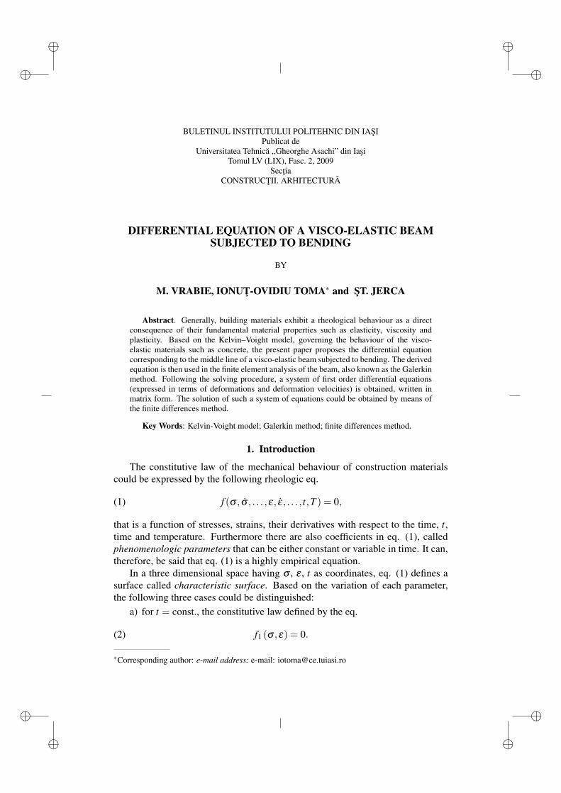
a) Linear elasticity (Hooke behaviour) – the elastic deformation goes back tothe initial unloaded state (zero deformation) after the load has been removed. Suchbehaviour could be graphically represented by means of the spring equivalence.Its characteristic curve is shown in Fig. 1a,

b) Viscosity – characterizes the property of materials to partly recover fromtheir deformed state but with a complete recovery of the deformation speed. Suchbehaviour is idealized by a dash-pot or damper being characterized by the curveshown in Fig. 1b, where η is the viscosity coefficient,

c) Plasticity – the material property that defines a continuous deformationeven under constant load. It is also characterized by a residual deformation afterthe load has been removed. Such behaviour could be graphically represented bythe rigid-plastic Saint–Venant model, in the form of a sliding mechanism, shownin Fig. 1c.

2

behaviour is idealized by a dash-pot or damper being characterized by the curve shown in Fig. 1b, where η is the viscosity coefficient.

c) Plasticity – the material property that defines a continuous deformation even under constant load. It is also characterized by a residual deformation after the load has been removed. Such behaviour could be graphically represented by the rigid-plastic Saint-Venant model, in the form of a sliding mechanism, shown in Fig. 1c.

Fig. 1. Mechanical behaviour models of construction materials

As it is known, construction materials have a diverse behaviour due to the fact that the three properties presented above are mixed in different percentages. As a consequence, complex behaviour material models have been developed such as: Prandtl elasto-plastic model (Fig. 2a) and Kelvin-Voigt visco-elastic model (Fig. 2b).

tgE

Eσ ε

α==

α ε

σ

0 α

ε

σ

0 ε

σ

0

tgσ η εη α==

i

σc

, for cσ σ ε= ∀

σ σ E

Elastic spring (Hooke) Damper (Newton)

σ σ η

σ σ

Slide (Rigid plastic)

ε

σ

0

σc

σ E σ

E

σ

η

11

.

22

εσεησ

E== σ

Visco-elastic

SV

H N

ELASTO- VISCO- PLASTIC El

asto

-pla

stic

Vis

co-p

last

ic

a b c

Fig. 1. – Mechanical behaviour models of construction materials.

As it is known, construction materials have a diverse behaviour due to thefact that the three properties presented above are mixed in different percentages.As a consequence, complex behaviour material models have been developed such

ii

ii

ii

ii

Bul. Inst. Polit. Iasi, t. LV (LIX), f. 2, 2009 23

2

behaviour is idealized by a dash-pot or damper being characterized by the curve shown in Fig. 1b, where η is the viscosity coefficient.

c) Plasticity – the material property that defines a continuous deformation even under constant load. It is also characterized by a residual deformation after the load has been removed. Such behaviour could be graphically represented by the rigid-plastic Saint-Venant model, in the form of a sliding mechanism, shown in Fig. 1c.

Fig. 1. Mechanical behaviour models of construction materials

As it is known, construction materials have a diverse behaviour due to the fact that the three properties presented above are mixed in different percentages. As a consequence, complex behaviour material models have been developed such as: Prandtl elasto-plastic model (Fig. 2a) and Kelvin-Voigt visco-elastic model (Fig. 2b).

( )αεσ

tgEE

==

α ε

σ

0 α

ε

σ

0 ε

σ

0

( )αηεησ

tg==

.

σc

εσσ ∀= forc ,

σ σ E

Elastic spring (Hooke) Damper (Newton)

σ σ η

σ σ

Slide (Rigid plastic)

a) b) c)

ε

σ

0

σc

σ E σ

E

σ

η

11

.

22

εσεησ

E== σ

Visco-elastic

SV

H N

ELASTO- VISCO- PLASTIC El

asto

-pla

stic

Vis

co-p

last

ic

a c b

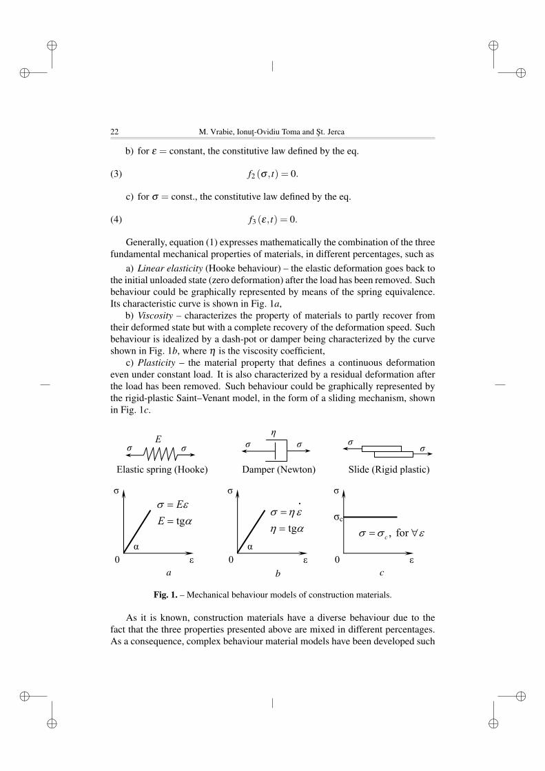
Fig. 2. – Rheological behaviour triangle and complex behaviour material models.

as: Prandtl elasto-plastic model (Fig. 2a) and Kelvin–Voigt visco-elastic model(Fig. 2b).

The triangle of rheological behaviour gives the possibility to visualize the as-sociation and combination of the three fundamental material properties (Fig. 2c).The vertexes of an equilateral triangle are represented by each fundamentalmaterial property, individually (Hooke, Newton and Saint–Venant). The sidejoining two vertexes characterizes the materials that have the two propertiesfrom the nodes mixed in different percentages. For example, the side joiningthe vertexes representing the Hooke and Newton models, denoted by H and N,respectively, characterizes the visco-elastic materials. Consequently, the sidejoining the vertexes representing the Newton and Saint–Venant models, denotedby SV, characterizes the materials with a visco–plastic behaviour. The third sideof the triangle, H – SV defines the materials with elasto-plastic behaviour. All thepoints inside the rim of the triangle represent materials with elasto-visco-plasticbehaviour [5].

2. Kelvin–Voigt (K–V) Mechanical Model

The rheologic behaviour of visco-elastic materials can be mathematicallyexpressed by means of differential eqs. having the general form

(5) f (σ , σ , . . . ,ε, ε, . . .) = 0,

in which the above mentioned phenomenological coefficients are taken intoaccount as constants. The values of these coefficients are considered based onequivalent mechanical models that consist in one or more springs and dash-potsconnected in series or parallel. The analytical formulation of the behaviour ofthe system is based on the following two conditions: static equilibrium and

ii

ii

ii

ii

24 M. Vrabie, Ionut-Ovidiu Toma and St. Jerca

compatibility of the deformations. The K–V model, defining the solid bodies,is obtained by linking together, in parallel, a spring (Hooke) and a dash-pot(Newton) as shown in Fig. 2b.

The equilibrium of the body can be expressed as

(6) σ1 +σ2 = σ ,

and the compatibility equation takes the form

(7) ε1 = ε2 = ε.

The stresses in the spring and in the dash-pot (damper) are written as

(8) σ1 = Eε1,σ2 = ηε2,

and by substituting eqs. (7) and (8) in the expression (6) it follows

(9) Eε1 +ηε2 = Eε +ηε = σ .

Eq. (9) can also be written in differential form

(10)(

E +ηddt

)ε = σ , Q(ε) = P(σ),

where Q and P are the following differential operators:

(11) Q = E +ηddt

= E +ηs, P = 1.

Taking into account the notation sn = dn/dtn, it follows that the Q and Poperators become polynomials in terms of s.

3. Differential Equation of the Beam Made From Visco-Elastic Material

The static equivalence relationship between the efforts and the stresses on across-section is

(12) M =∫A

yσdA.

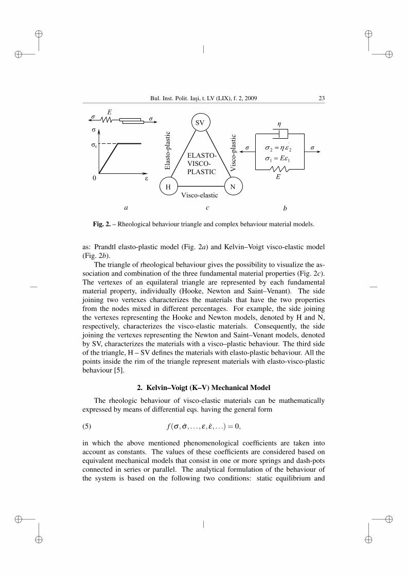
According to Bernoulli’s postulate, the linear strain of a fibre located at adistance, y, from the neutral axis is ε = χy, where χ = 1/ρ is the curvature of theneutral axis. From the similarity of the ”curved” triangles in Fig. 3a, it follows:

(13)yρ

=εxdxdx

χy = εx.

ii

ii

ii

ii

Bul. Inst. Polit. Iasi, t. LV (LIX), f. 2, 2009 25

The differential operator with respect to time, P, is applied to eq. (12), leadingto

(14) P(M) =∫A

yP(σ)dA.

Furthermore, the rheologic eq. (10) can be re-written as

(15) P(s)(σ) = Q(s)(ε) = Q(s)(yχ) = yQ(s)(χ),

and substituting the above expression in eq. (14), it leads to

(16) P(M) =∫A

yyQ(s)χdA = IzQ(s)χ,

where Iz =∫

y2dA is the moment of inertia (or the second moment of area) with

respect to the z-axis of the cross-section.

5

Furthermore, the rheologic equation (10) can be re-written as: )yQ(s)( = )Q(s)(y = )Q(s)( = )P(s)( χχεσ (15) and substituting the above expression in equation (14), it leads to: χχ∫ Q(s)I = dAy.yQ(s) = P(M) z

A

(16)

where ∫= dAyI z2 is the moment of inertia (or the second moment of area) with

respect to the z axis of the cross-section.

Fig. 3. Differential element of a beam (a) and the sign convention of the curvature (b)

For small deformations the substitution χ = - v" can be made, the sign convention from Fig. 3b being taken into account. If χ were substituted in equation (16):

Q(s)I

P(s).M- = vvQ(s)I- = Q(s)I- = P(M)z

zz ′′⇒′′χ (17)

and taking the second order derivative with respect to x: IV

z nQ(s) = P(s)pvI (18) which represents the fourth order differential equation of the deformed shape of the

a b

Fig. 3. – Differential element of a beam (a) and the sign convention of the curvature (b).

For small deformations the substitution χ = −v′′ can be made, the signconvention from Fig. 3b being taken into account. If χ were substituted in eq.(16) it results

(17) P(M) =−IzQ(s)χ =−IzQ(s)v′′ ⇒ v′′ =−P(s)MIzQ(s)

and taking the second order derivative with respect to x,

(18) IzQ(s)vIV = P(s)pn,

ii

ii

ii

ii

26 M. Vrabie, Ionut-Ovidiu Toma and St. Jerca

which represents the fourth order differential eq. of the deformed shape of theneutral axis of a beam made of a visco-elastic material. Following the sameprocedure, the corresponding eq. for an elastic beam is

(19) EIzvIV = P(s)pn.

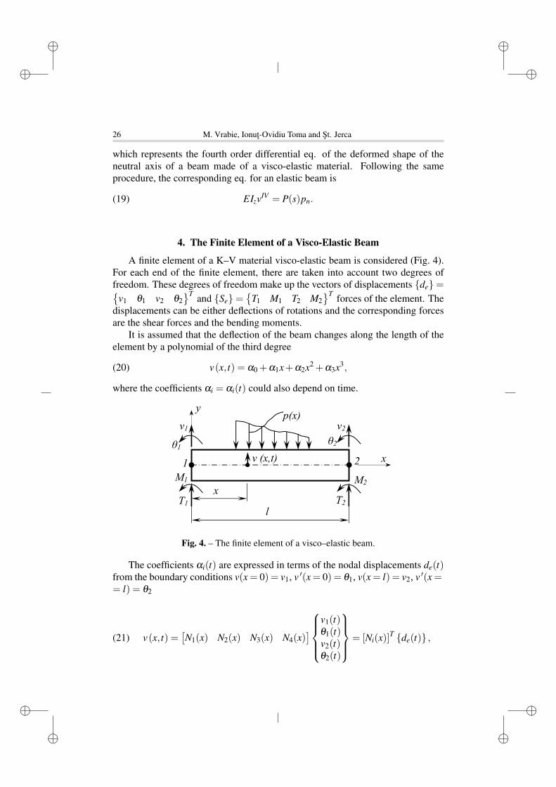
4. The Finite Element of a Visco-Elastic Beam

A finite element of a K–V material visco-elastic beam is considered (Fig. 4).For each end of the finite element, there are taken into account two degrees offreedom. These degrees of freedom make up the vectors of displacements {de}={

v1 θ1 v2 θ2}T and {Se}=

{T1 M1 T2 M2

}T forces of the element. Thedisplacements can be either deflections of rotations and the corresponding forcesare the shear forces and the bending moments.

It is assumed that the deflection of the beam changes along the length of theelement by a polynomial of the third degree

(20) v(x, t) = α0 +α1x+α2x2 +α3x3,

where the coefficients αi = αi(t) could also depend on time.

Key words: Kelvin-Voight model, Galerkin method, finite differences method

v (x,t)

x

l

v1 v2

θ1 θ2

T2

M2 M1

T1

1 2 x

y p(x)

Fig. 4. – The finite element of a visco–elastic beam.

The coefficients αi(t) are expressed in terms of the nodal displacements de(t)from the boundary conditions v(x = 0) = v1, v ′(x = 0) = θ1, v(x = l) = v2, v ′(x == l) = θ2

(21) v(x, t) =[N1(x) N2(x) N3(x) N4(x)

]v1(t)θ1(t)v2(t)θ2(t)

= [Ni(x)]T {de(t)} ,

ii

ii

ii

ii

Bul. Inst. Polit. Iasi, t. LV (LIX), f. 2, 2009 27

where Ni(x) are the shape functions of Hermite type [1].The residue can be obtained based on eq. (18) namely

(22) ε(x, t) = IQ(s)vIV (x, t)−P(s)p = 0,

and the Galerkin function should be minimized on the finite element

(23)

Πe =l∫

0

Ni(x)ε(x, t)dx =l∫

0

Ni(x)[IQ(s)vIV (x, t)−P(s)p

]dx =

= IQ(s)l∫

0

Ni(x)vIV (x, t)dx−P(s)l∫

0

Ni(x)p(x)dx = 0

For simplicity, starting from eq. (22), the notations Iz = I and pn = p havebeen used.

After integrating twice the first member of the sum with respect to x

(24)

I1 = IQ(s)Ni(x)v′′′(x, t)∣∣l0− IQ(s)

l∫0

N′i (x)v

′′′(x, t)dx =

= IQ(s)

Ni(x)v′′′(x, t)∣∣l0− N′

i (x)v′′(x, t)

∣∣l0 +

l∫0

N′′i (x)v′′(x, t)dx

.

The expressions (17) and (18) are taken into account when writing eq. (24)and I1 is also substituted in the expression of Πe in order to obtain the relationship

(25)

Πe = −Ni(x)P(s)T (x, t)|l0 + N′i (x)P(s)M(x, t)

∣∣l0 +

+IQ(s)

l∫0

N′′i (x)N′′

i (x)dx

{de(t)}−P(s)l∫

0

Ni(x)pdx = 0.

Applying the sign convention from the FEM and after performing all thecalculations, a simpler form of the above eq. is obtained

(26) P(s)({Se}−{Re}) = IQ(s)[ke]{de},

where: [ke] is the stiffness matrix of the finite element with the 4×4 size; {R−e}– the vector of the support reactions in a double fixed beam (as a result of thedistributed loads over the length of the element). The entries of the stiffness matrixand of the reaction vector are computed using the following relation:

(27) ki j =l∫

0

N′′i (x)N′′

j (x)dx, Ri =l∫

0

p(x)Ni(x)dx, (i, j = 1, . . . ,4).

ii

ii

ii

ii

28 M. Vrabie, Ionut-Ovidiu Toma and St. Jerca

The terms ki j and Ri are computed in the same manner as in the elastic case butRi could still be time dependent provided that p = p(x, t). Equation (26) representsthe physical eq. of the finite element of a visco-elastic beam.

In case of the K–V model, P(s) = 1 and Q(s) = E + ηd/dt. Therefore, eq.(26) becomes

(28)(

E +ηddt

)I[ke]{de}= {Se}−{Re},

or, after performing further simplifying mathematical operations

(29) EI[ke]{de}+ηI[ke] ˙{de}= {Se}−{Re}= {Fe}

where {Fe} denotes the vector of nodal forces of the finite element.In order to be able to assembly all the obtained vectors based on eq. (29), for

each finite element, to get the vector of nodal displacements of the entire structure,the expansion procedure has to be applied namely

(30) EI[kexpe ]{Ds}+ηI[kexp

e ] ˙{Ds}= {Fexpe }.

The summation of all the terms obtained by means of eq. (29) leads to theconstitutive eq. of the entire structure

(31) EI[Ks]{Ds}+ηI[Ks] ˙{Ds}= {Ps}−{Rs}= {Fs},

where: {Ps} is the vector of the applied forces at the nodes of the structure and[Ks] and {Rs} are computed for the entire structure by means of direct summation

(32) [Ks] =m

∑e=1

[kexpe ] ; {Rs}=

m

∑e=1

{Rexpe } .

From the boundary conditions, eq. (32) becomes

(33) EI[K]{D}+ηI[K] ˙{D}= {P}−{R}= {F},

where: {D} is the vector of the free nodal displacements (different from 0) of theentire structure; {P} – the vector of the active nodal forces. Equation (33) definesa system of first order differential eqs. with respect to the time, t. Such a systemof eqs. can be solved by means of numerical methods such as the finite differencesmethod. For this purpose, the time interval from 0 to t is divided into smaller timesteps, ∆t. The division points of the time interval are denoted by i−1, i, i+1 (Fig.5). The following expression is obtained by using the central differences method:

(34) Di =Di+1−Di−1

2∆t,

ii

ii

ii

ii

Bul. Inst. Polit. Iasi, t. LV (LIX), f. 2, 2009 29

and by substituting it in the system of eqs. defined by eq. (33) written in finitedifferences for the time step t = i∆t, the following expression is obtained

(35) EI[K]{Di}+ηI[K]{Di+1}−{Di−1}

2∆t= {Fi}.

9

[ ]{ } [ ]{ } { } { } { }EI K D + I K D = P - R = Fη & (33) where {D} is the vector of the free nodal displacements (different from 0) of the entire structure and {P} is the vector of the active nodal forces.

Equation (33) defines a system of first order differential equations with respect to the time t. Such a system of equations can be solved by means of numerical methods such as the finite differences method. For this purpose, the time interval from 0 to t is divided into smaller time steps Δt. The division points of the time interval are denoted by i-1, i, i+1 (fig. 5). The following expression is obtained by using the central differences method:

t2D-D = D 1-i1+i

i Δ& (34)

Fig. 5 Graphical representation of the interval nodes

and by substituting it in the system of equations defined by equation (33) written in finite differences for the time step t = iΔt, the following is obtained:

1 1{ } { }} [ ] { }[ ]{ i+ i-ii

-D D+ I K =EI K D F2 tη

Δ (35)

After further mathematical calculations the equations transforms into:

1 1[ ] [ ]{ } { } { } }[ ]{i+ i i- i

I K I K= + - EI K DD F D2 t 2 tη η

Δ Δ (36)

which, in fact, represents a recurrence formula that determines the displacements at the time step i+1 if the corresponding displacements at time steps i-1 and i were known.

The computational algorithm based on the above mentioned relationship starts for the time step t = 0 for which the vector of initial displacements, {D0}, is known.

Fig. 5. – Graphical representation of the interval nodes.

After further mathematical calculations the eqs. transforms into

(36)ηI[K]2∆t

{Di+1}= {Fi}+ηI[K]2∆t

{Di−1}−EI[K]{Di},

which, in fact, represents a recurrence formula that determines the displacementsat the time step i + 1 if the corresponding displacements at time steps i− 1 and iwere known.

The computational algorithm based on the above mentioned relationship startsfor the time step t = 0 for which the vector of initial displacements, {D0}, isknown. Furthermore, the displacement vector prior to the initial 0 conditions,{D−1}, is not known and therefore applying eq. (36) it leads to

(37)ηI[K]2∆t

D1 = {F0}+ηI[K]2∆t

{D−1}−EI[K]{D0}.

From eq. (34) it follows that

(38) {Di+1}= {Di−1}+2∆t ˙{Di},

and when written for the time step t = 0, it leads to

(39) {D1}= {D−1}+2∆t ˙{D0}= {D1}−2∆t ˙{D0}.

Substituting it in the relation (37) and after making the necessary calculations,one reaches the following expression:

(40) {D0}=1

EI

({F0}[K−1]−ηI ˙{D0}

),

ii

ii

ii

ii

30 M. Vrabie, Ionut-Ovidiu Toma and St. Jerca

where {F0} and {D0} are known from the initial given conditions. Equation (40)shows that the displacement of the beam at the initial stage can be expressed asfunctions of the deformation velocity and vice-versa. The recurrence formula (36)can be re-written as

(41) {Di+1}= {Di−1}−2∆tEη{Di}+

2∆tηI

[K−1]{Fi}

in order to allow for the calculation of the displacements for the visco-elastic beamat the time t = (i+1)∆t as a function of the displacements from the preceding timesteps i−1 and i. For the case when the forces {Fi} are constant in time, thereforeequal to {F0}, but the displacements (deflections) of the beam increase with time,it is considered to be the case of slow yielding (also known as creep).

5. Conclusions

The behaviour of materials and structural elements depends on a large numberof parameters. In order to simplify the calculus, the equivalent mechanical modelstake into account only a reduced number of such parameters, namely the onesthat are considered to be critical to describing, as accurate as possible, the realbehaviour.

The Kelvin-Voigt mechanical model takes into account, besides the propertyof linear elasticity, the property of material viscosity, which is an importantparameter in a heterogeneous material such as concrete.

Equation (18) describing the deformed shape of a beam made of a visco-elastic material is a generalized expression of the relationship characteristic toan elastic beam.

The finite element method (FEM) allows the consideration of the rheologicalbehaviour by means of the shape functions describing the displacement field alongthe finite element.

The general mathematical model of an entire structure for the visco-elasticKelvin-Voigt material, derived by means of the FEM, is a system of differentialeqs. of the 1st order, coupled with respect to time. Such a system can be solved byvarious integration methods (in the paper the finite differences method is presents)

The computation algorithm to find the displacements of the visco-elasticbeam, at various time steps, can be very efficiently applied in a computerprogramme.

Received, April 23, 2009 ,,Gheorghe Asachi” Technical University, Jassy,Department of Structural Mechanics.

ii

ii

ii

ii

Bul. Inst. Polit. Iasi, t. LV (LIX), f. 2, 2009 31

REFERENCES

1. Jerca St., Ungureanu N., Diaconu D., Metode numerice ın proiectarea constructiilor.”Gheorghe Asachi” Techn. Univ., Iasi, 1997.

2. Massonnet Ch., Deprez G., Maquoi R. et al., Calculul structurilor la calculatoareelectronice (transl. from French). Edit.Tehnica, Bucuresti, 1974.

3. Nowacki W., Dinamica sistemelor elastice (transl. from Pol.). Edit. Tehnica,Bucuresti, 1969.

4. Teodorescu P.P., Ille V., Teoria elasticitatii si introducere ın mecanica solidelordeformabile. Edit. Dacia, Cluj-Napoca, 1976.

5. Tudose R.Z., Reologia compusilor macromoleculari. Edit. Tehnica, Bucuresti, 1982.6. Vaicum A., Studiul reologic al corpurilor solide. Edit. Academiei, Bucuresti, 1978.

ECUATIA DIFERENTIALA A UNEI BARE VASCOELASTICESOLICITATE LA INCOVOIERE

(Rezumat)

Materialele de constructii prezinta, ın general, o comportare reologica diversa caurmare a asocierii, ın diverse proportii, a proprietatilor fundamentale de elasticitate,vascozitate si plasticitate. Pe baza modelului mecanic Kelvin-Voigt, specific materi-alelor vascoelastice (printre care se numara si betonul), ın lucrare se stabileste ecuatiadiferentiala a fibrei medii deformate a unei grinzi vascoelastice ıncovoiate, ecuatie careeste utilizata apoi ın analiza grinzii prin metoda elementelor finite, procedeul Galerkin. Seajunge la o ecuatie matriceala, care reprezinta un sistem de ecuatii diferentiale de ordinul1 (ın viteze de deformare si deplasari), cuplate ın raport cu timpul, sistem ce se poateintegra, de exemplu, prin metoda diferentelor finite.

ii

ii

ii

ii