Differential Differential Equations Equations

BrannanCopyright © 2010 by John Wiley & Sons,

Inc. All rights reserved.

Chapter 08: Series Solutions of SecondOrder Linear Equations

Chapter 8 Chapter 8 Series Solutions of Second Order Linear EquationsThe general solution of a linear second order

equation P(x)y'' + Q(x)y' + R(x)y = 0 is y = c1y1(x) + c2y2(x), where y1 and y2 are a fundamental set of solutions of the differential equation.

To deal with equations that have general nonconstant coefficients, we need alternative solution techniques. For some applications we may find that approximations using an initial value problem solver are satisfactory for our needs. However there are some variable coefficient equations that frequently recur in applications where infinite series representation of solutions useful.

Chapter 8 - Chapter 8 - Series Solutions of Second Order Linear Equations8.1 Review of Power Series8.2 Series Solutions Near an Ordinary Point,

Part I8.3 Series Solutions Near an Ordinary Point,

Part II8.4 Regular Singular Points8.5 Series Solutions Near a Regular Singular

Point, Part I8.6 Series Solutions Near a Regular Singular

Point, Part II8.7 Bessel’s Equation

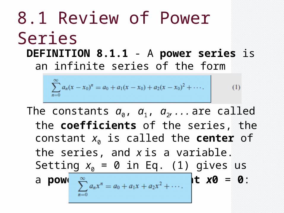
8.1 Review of Power SeriesDEFINITION 8.1.1 - A power series is an

infinite series of the form

The constants a0, a1, a2, . . . are called the coefficients of the series, the constant x0 is called the center of the series, and x is a variable. Setting x0 = 0 in Eq. (1) gives us a power series centered at x0 = 0:

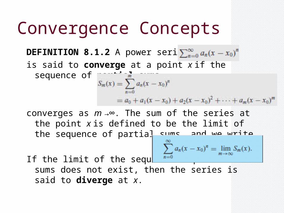
Convergence ConceptsDEFINITION 8.1.2 A power series

is said to converge at a point x if the sequence of partial sums

converges as m →∞. The sum of the series at the point x is defined to be the limit of the sequence of partial sums, and we write

If the limit of the sequence of partial sums does not exist, then the series is said to diverge at x.

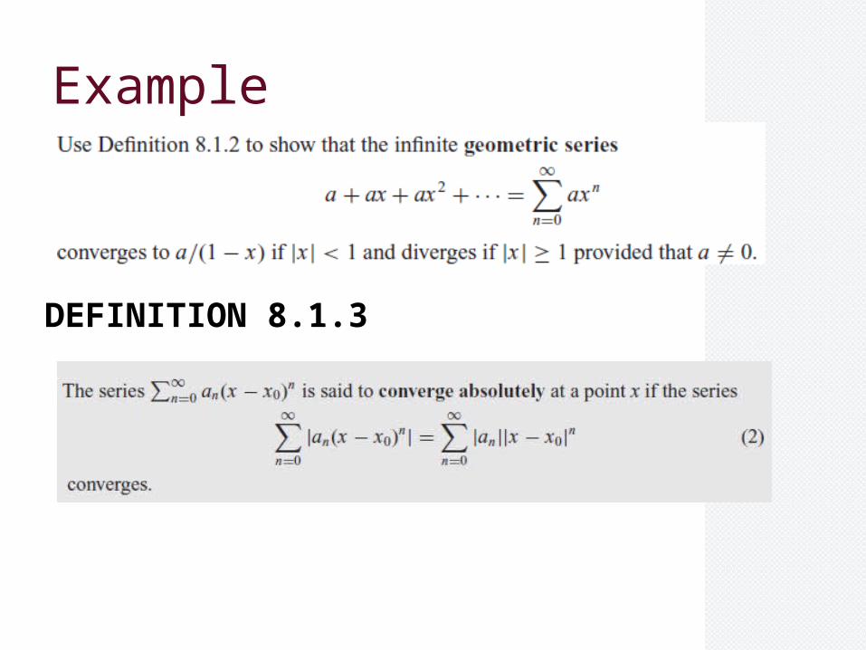
Example

DEFINITION 8.1.3

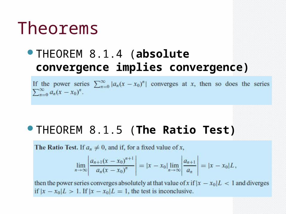
TheoremsTHEOREM 8.1.4 (absolute convergence

implies convergence)

THEOREM 8.1.5 (The Ratio Test)

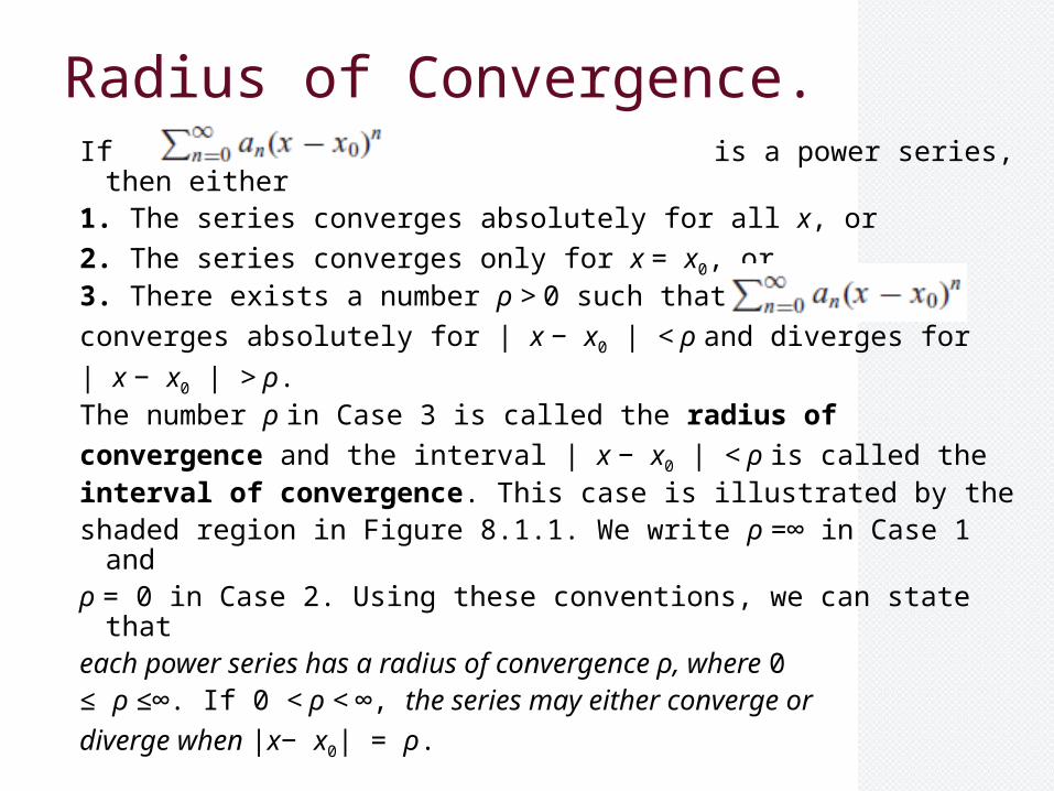
Radius of Convergence.If is a power series, then either1. The series converges absolutely for all x, or

2. The series converges only for x = x0, or3. There exists a number ρ > 0 such that

converges absolutely for | x − x0 | < ρ and diverges for

| x − x0 | > ρ.The number ρ in Case 3 is called the radius of

convergence and the interval | x − x0 | < ρ is called theinterval of convergence. This case is illustrated by theshaded region in Figure 8.1.1. We write ρ =∞ in Case 1 andρ = 0 in Case 2. Using these conventions, we can state thateach power series has a radius of convergence ρ, where 0≤ ρ ≤∞. If 0 < ρ < ∞, the series may either converge or

diverge when |x− x0| = ρ.

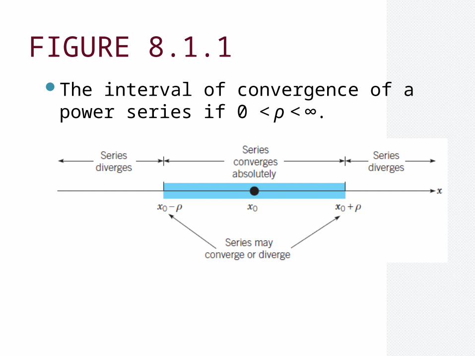
FIGURE 8.1.1The interval of convergence of a power

series if 0 < ρ < ∞.

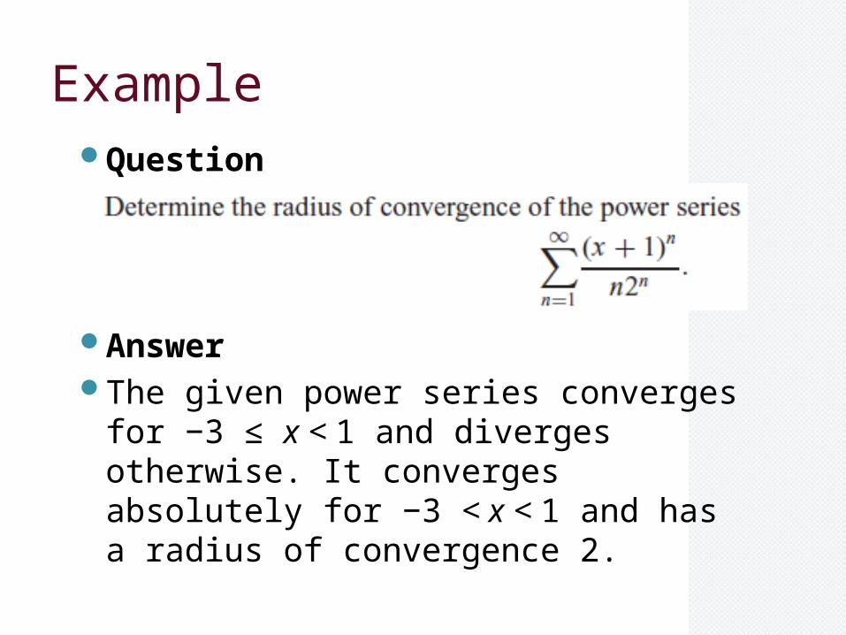
ExampleQuestion

AnswerThe given power series converges for −3 ≤

x < 1 and diverges otherwise. It converges absolutely for −3 < x < 1 and has a radius of convergence 2.

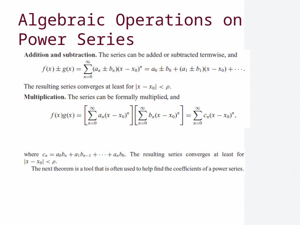
Algebraic Operations on Power Series

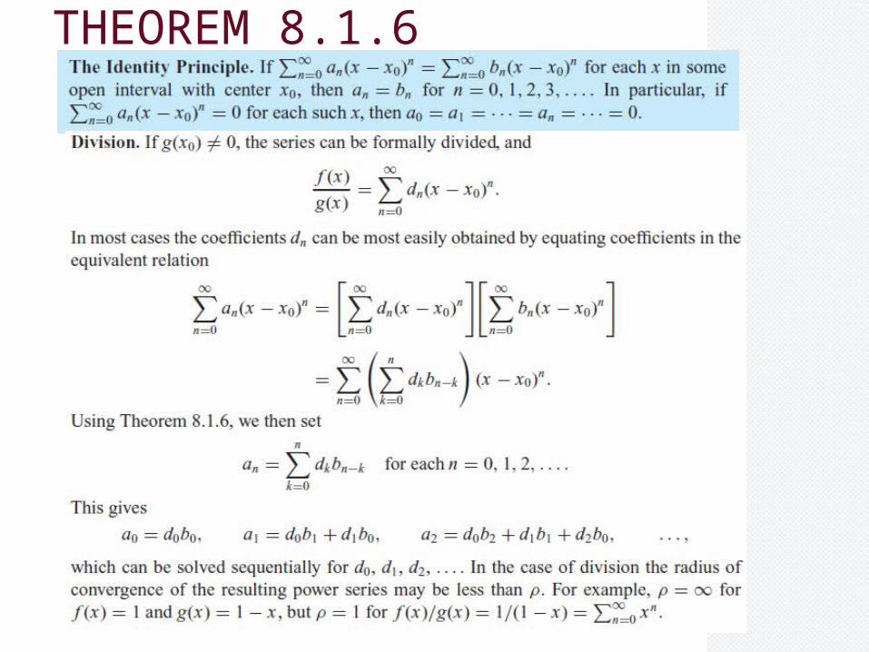
THEOREM 8.1.6

Taylor Series and Analytic Functions

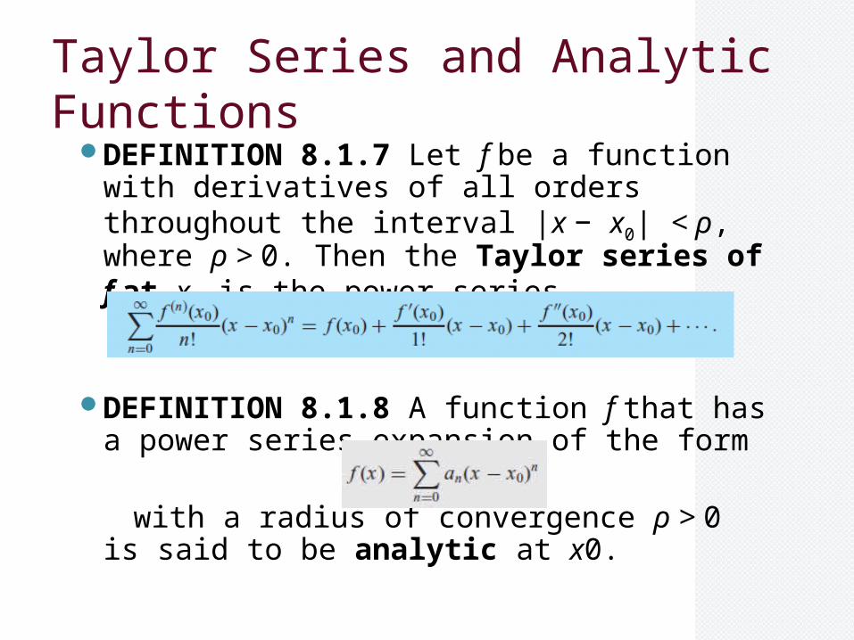
DEFINITION 8.1.7 Let f be a function with derivatives of all orders throughout the interval |x − x0| < ρ, where ρ > 0. Then the Taylor series of f at x0 is the power series

DEFINITION 8.1.8 A function f that has a power series expansion of the form

with a radius of convergence ρ > 0 is said to

be analytic at x0.

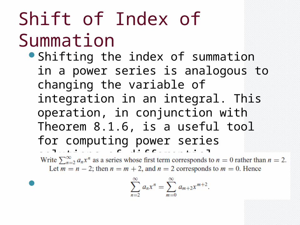
Shift of Index of SummationShifting the index of summation in a power

series is analogous to changing the variable of integration in an integral. This operation, in conjunction with Theorem 8.1.6, is a useful tool for computing power series solutions of differential equations.

EXAMPLE

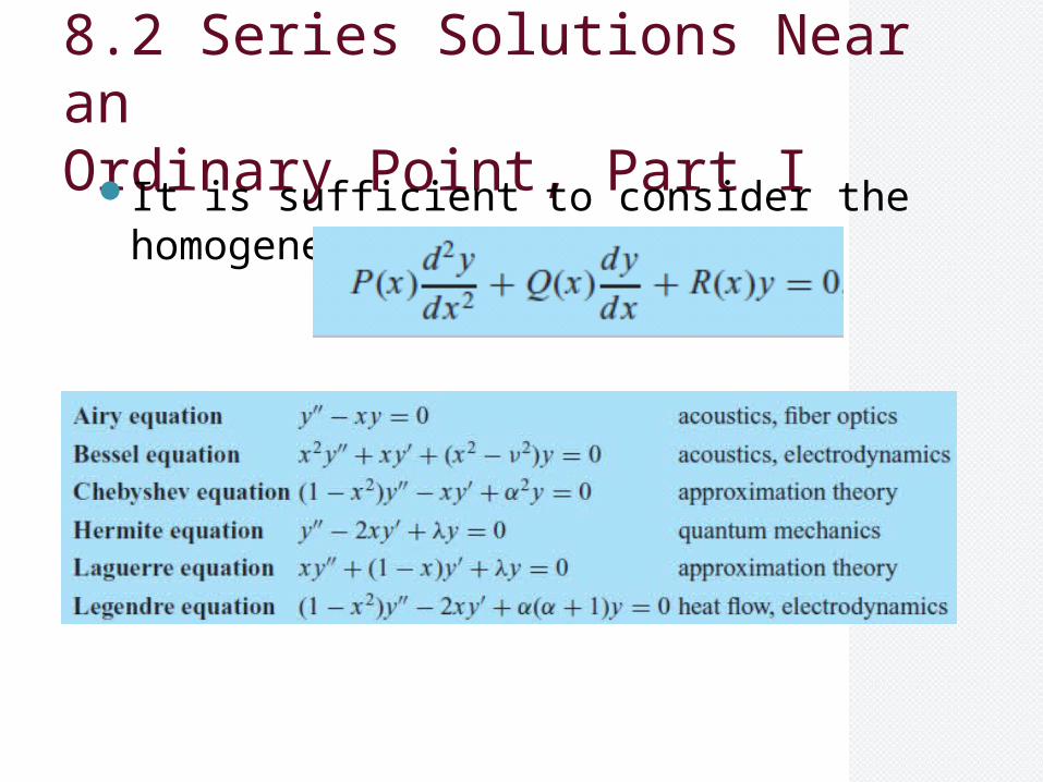
8.2 Series Solutions Near anOrdinary Point, Part I

It is sufficient to consider the homogeneous equation

(1)Examples

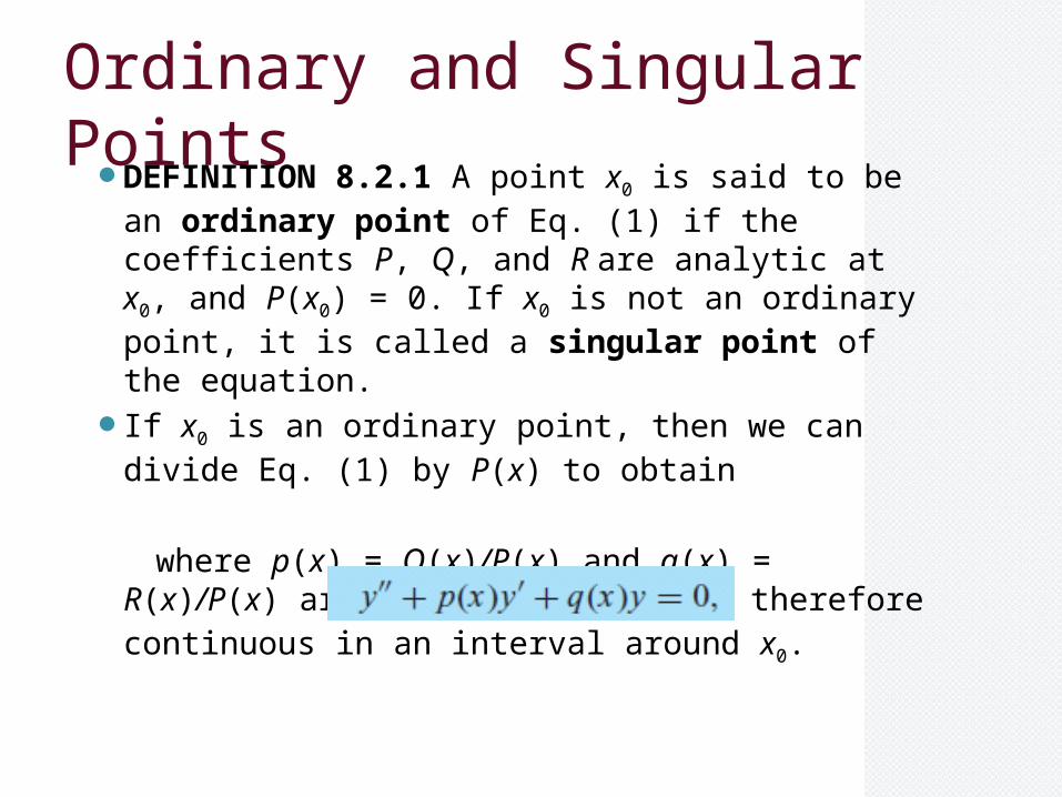
Ordinary and Singular PointsDEFINITION 8.2.1 A point x0 is said to be an

ordinary point of Eq. (1) if the coefficients P, Q, and R are analytic at x0, and P(x0) = 0. If x0 is not an ordinary point, it is called a singular point of the equation.

If x0 is an ordinary point, then we can divide Eq. (1) by P(x) to obtain

where p(x) = Q(x)/P(x) and q(x) = R(x)/P(x) are analytic at x0, and therefore continuous in an interval around x0.

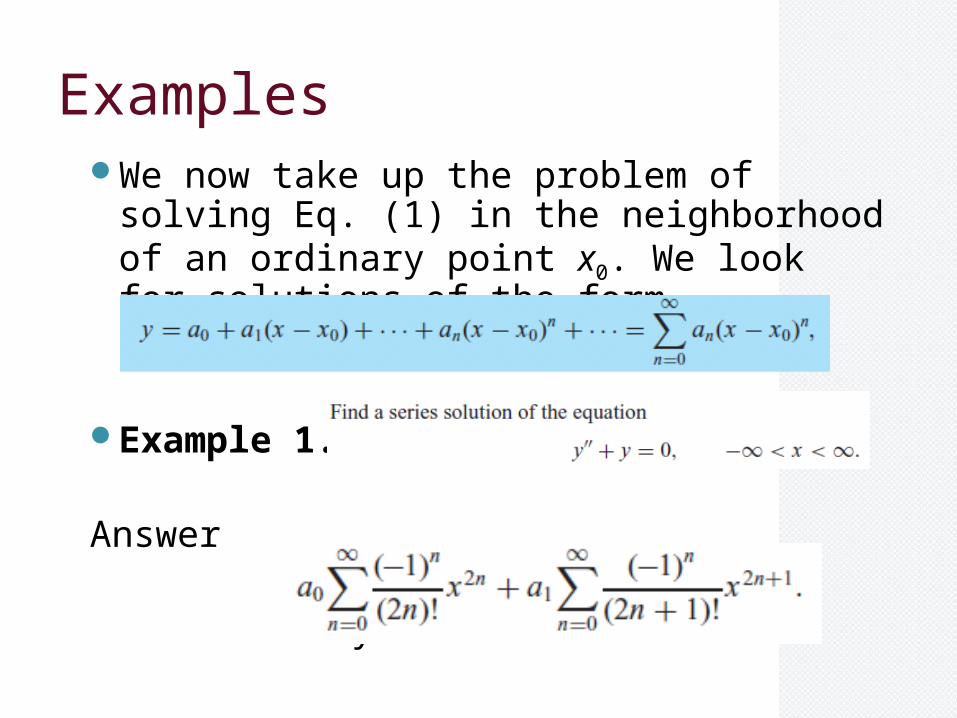
ExamplesWe now take up the problem of solving Eq. (1)

in the neighborhood of an ordinary point x0. We look for solutions of the form

Example 1.

Answer

y =

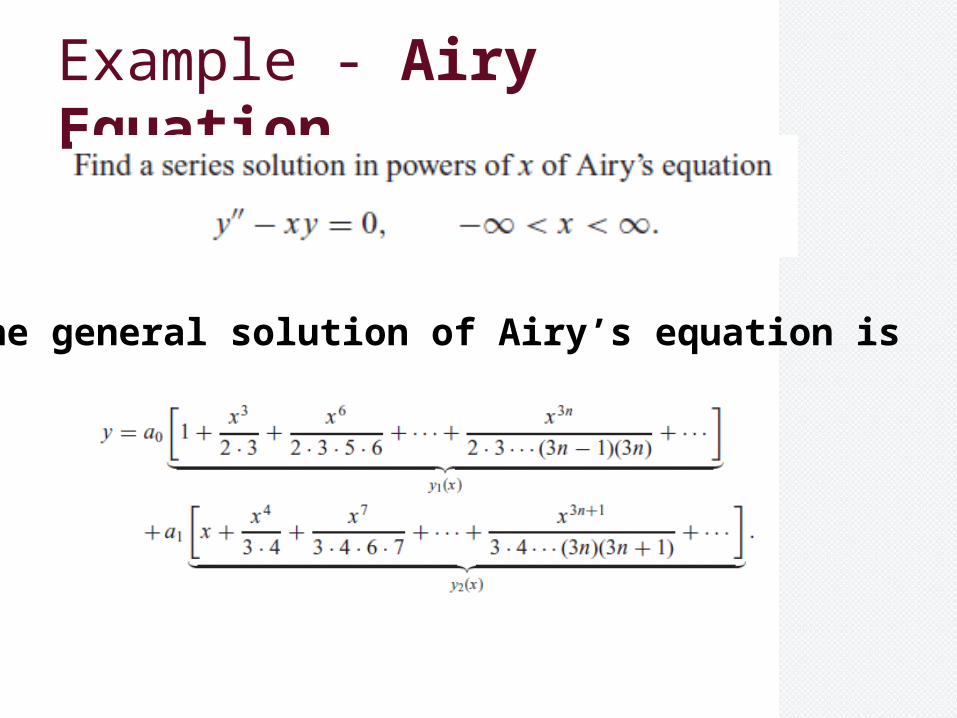
Example - Airy Equation.

The general solution of Airy’s equation is

The Airy Functions Ai(x) and Bi(x)

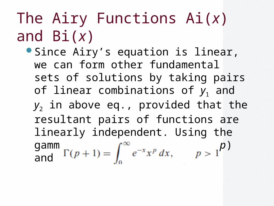
Since Airy’s equation is linear, we can form other fundamental sets of solutions by taking pairs of linear combinations of y1 and y2 in above eq., provided that the resultant pairs of functions are linearly independent. Using the gamma function, denoted by Γ(p) and defined by the integral

The Airy Functions Ai(x) and Bi(x)

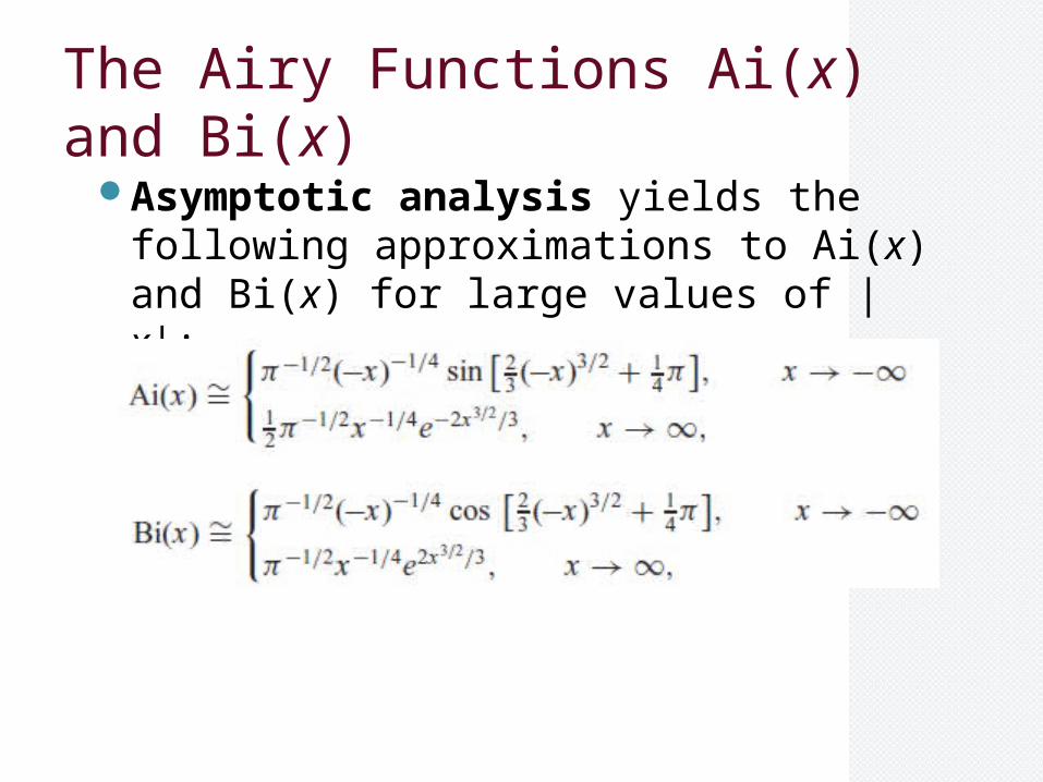
Asymptotic analysis yields the following approximations to Ai(x) and Bi(x) for large values of |x|:

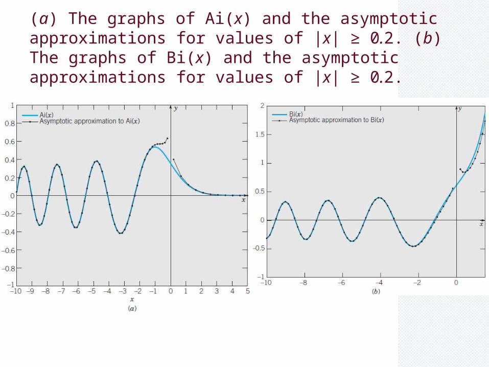
(a) The graphs of Ai(x) and the asymptotic approximations for values of |x| ≥ 0.2. (b) The graphs of Bi(x) and the asymptotic approximations for values of |x| ≥ 0.2.

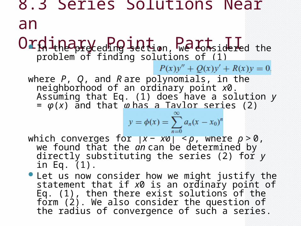
8.3 Series Solutions Near anOrdinary Point, Part II

In the preceding section, we considered the problem of finding solutions of (1)

where P, Q, and R are polynomials, in the neighborhood of an ordinary point x0. Assuming that Eq. (1) does have a solution y = φ(x) and that φ has a Taylor series (2)

which converges for |x − x0| < ρ, where ρ > 0, we found that the an can be determined by directly substituting the series (2) for y in Eq. (1).

Let us now consider how we might justify the statement that if x0 is an ordinary point of Eq. (1), then there exist solutions of the form (2). We also consider the question of the radius of convergence of such a series.

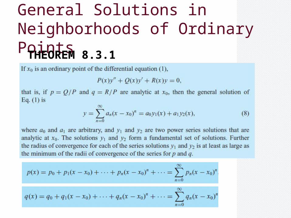
General Solutions in Neighborhoods of Ordinary Points

THEOREM 8.3.1

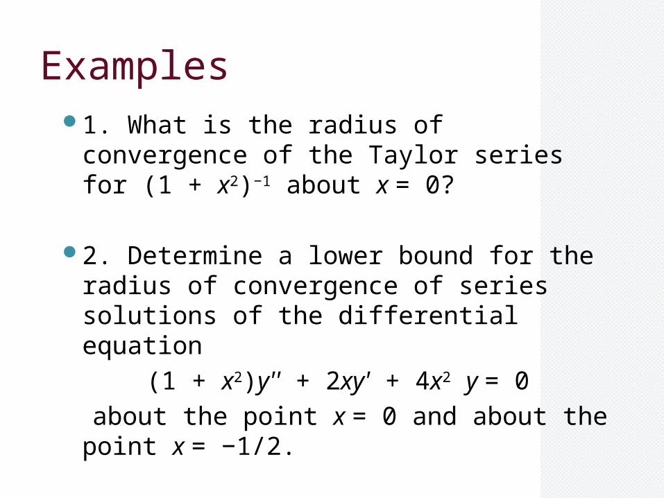
Examples1. What is the radius of convergence of the

Taylor series for (1 + x2)−1 about x = 0?

2. Determine a lower bound for the radius of convergence of series solutions of the differential equation

(1 + x2)y'' + 2xy' + 4x2 y = 0

about the point x = 0 and about the point x = −1/2.

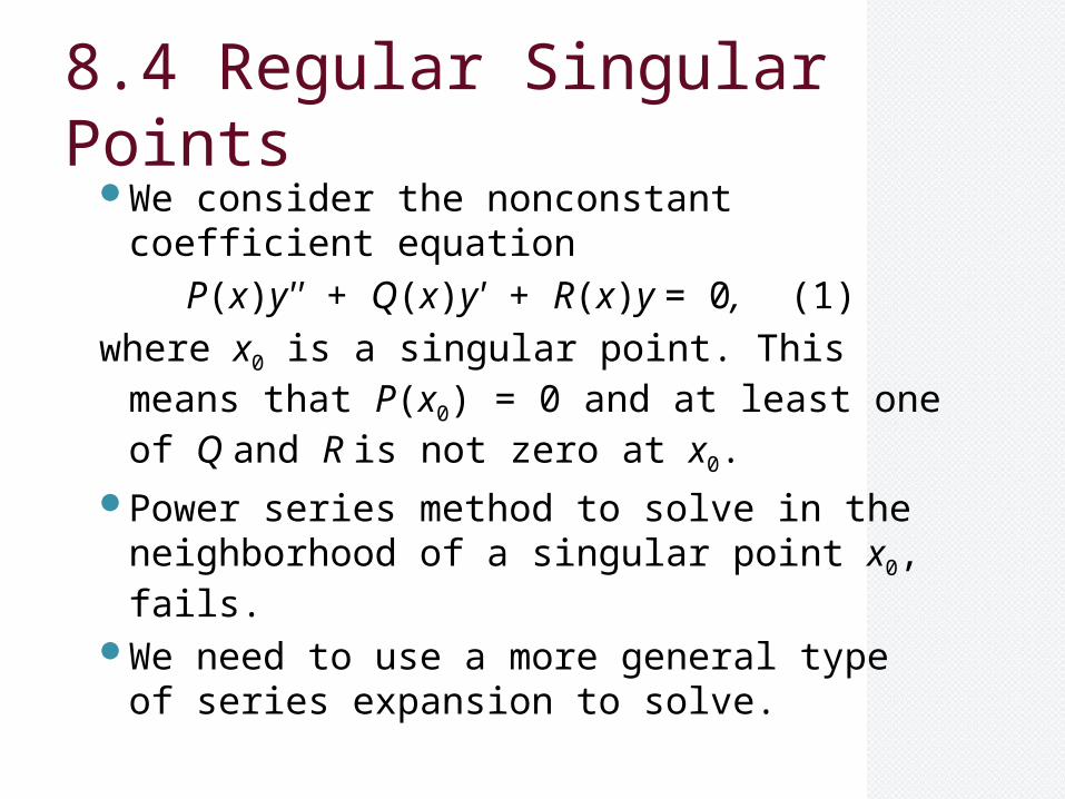
8.4 Regular Singular PointsWe consider the nonconstant coefficient

equation

P(x)y'' + Q(x)y' + R(x)y = 0, (1)

where x0 is a singular point. This means that P(x0) = 0 and at least one of Q and R is not zero at x0.

Power series method to solve in the neighborhood of a singular point x0, fails.

We need to use a more general type of series expansion to solve.

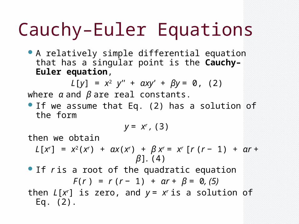
Cauchy–Euler EquationsA relatively simple differential equation that has a

singular point is the Cauchy–Euler equation,L[y] = x2 y'' + αxy' + βy = 0, (2)

where α and β are real constants. If we assume that Eq. (2) has a solution of the form

y = xr , (3)then we obtainL[xr] = x2(xr) + αx(xr) + β xr = xr [r (r − 1) + αr + β]. (4)

If r is a root of the quadratic equation F(r ) = r (r − 1) + αr + β = 0, (5)

then L[xr] is zero, and y = xr is a solution of Eq. (2).

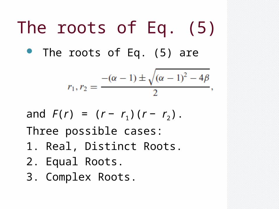
The roots of Eq. (5) The roots of Eq. (5) are

and F(r) = (r − r1)(r − r2).

Three possible cases:

1. Real, Distinct Roots.

2. Equal Roots.

3. Complex Roots.

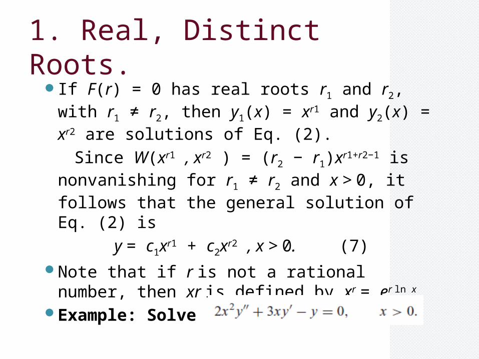
1. Real, Distinct Roots.If F(r) = 0 has real roots r1 and r2, with r1 ≠ r2,

then y1(x) = xr1 and y2(x) = xr2 are solutions of Eq. (2).

Since W(xr1 , xr2 ) = (r2 − r1)xr1+r2−1 is nonvanishing for r1 ≠ r2 and x > 0, it follows that the general solution of Eq. (2) is

y = c1xr1 + c2xr2 , x > 0. (7)Note that if r is not a rational number, then xr

is defined by xr = er ln x.Example: Solve

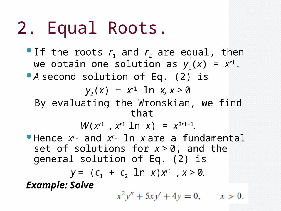
2. Equal Roots.If the roots r1 and r2 are equal, then we

obtain one solution as y1(x) = xr1.A second solution of Eq. (2) is

y2(x) = xr1 ln x, x > 0 By evaluating the Wronskian, we find that

W(xr1 , xr1 ln x) = x2r1−1.Hence xr1 and xr1 ln x are a fundamental set

of solutions for x > 0, and the general solution of Eq. (2) is

y = (c1 + c2 ln x)xr1 , x > 0.Example: Solve

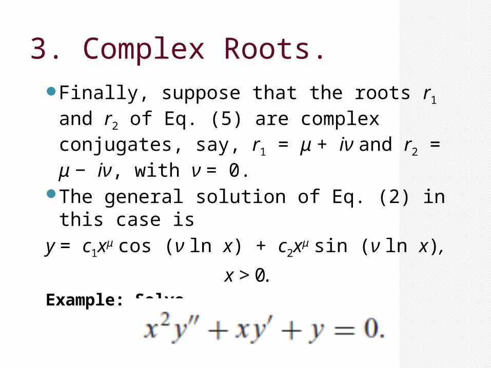
3. Complex Roots.Finally, suppose that the roots r1 and r2

of Eq. (5) are complex conjugates, say, r1 = μ + iν and r2 = μ − iν, with ν = 0.

The general solution of Eq. (2) in this case isy = c1xμ cos (ν ln x) + c2xμ sin (ν ln x),

x > 0.Example: Solve

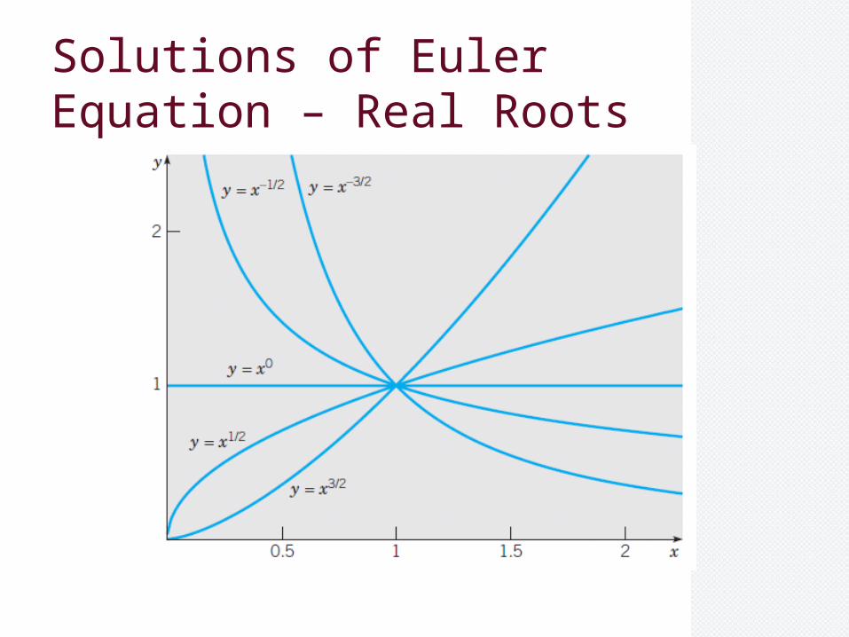
Solutions of Euler Equation – Real Roots

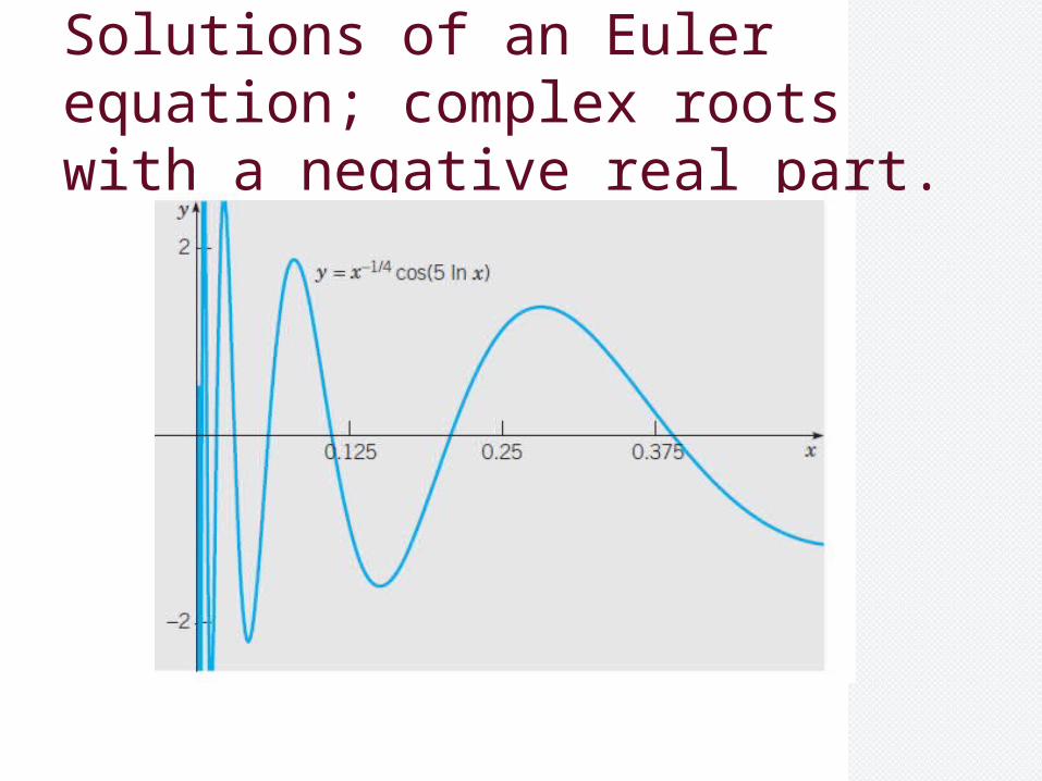
Solutions of an Euler equation; complex roots with a negative real part.

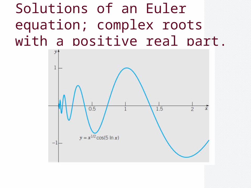
Solutions of an Euler equation; complex roots with a positive real part.

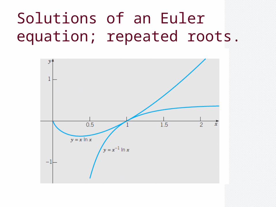
Solutions of an Euler equation; repeated roots.

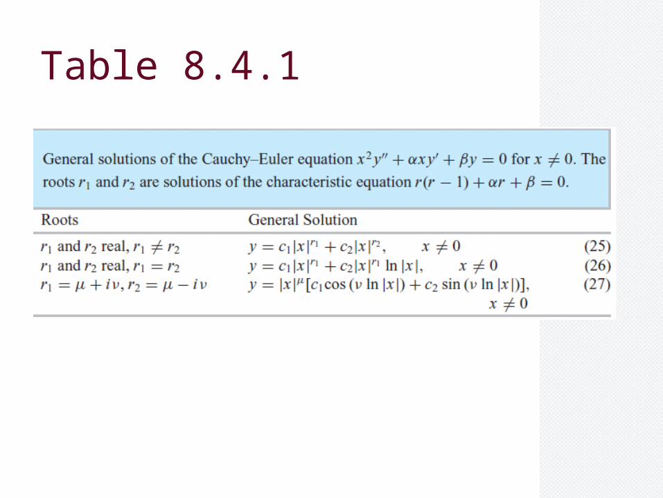
Table 8.4.1

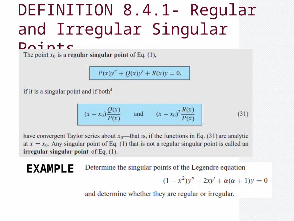
DEFINITION 8.4.1- Regular and Irregular Singular Points

EXAMPLE