Differential Evolution: Foundations, Perspectives, and

Differential Evolution: Foundations, Perspectives, and

Applications

By

Swagatam Das1 and P. N. Suganthan2

1Dept of Electronics and Telecommunication Engg., Jadavpur University

Kolkata 700032, India

2School of Electrical and Electronic Engineering, Nanyang Technological University,

Singapore 639798, Singapore

SSCI 2011

Topics to be Covered

Part – I (By Dr. S. Das)

• Metaheuristics, multi-agent search, and DE

• Steps of the basic DE family of algorithms – a first look

• Control parameters of DE

• Some Significant Single-objective DE-variants for real-parameter

optimization

• A stochastic mathematical model of DE-population and convergence

analysis

Part – II (By Dr. P. N. Suganthan)

• Ensemble Strategies in DE (EPSDE)

• Constraint Handling in DE and ECHT-DE

• DE for Multi-objective Optimization

• DE for Large Scale Optimization

• DE for Multi-modal Optimization

Meta-heuristics

A metaheuristic is a heuristic method for solving a very general class of

computational problems by combining user-given black-box procedures —usually heuristics themselves — in

the hope of obtaining a more efficient ormore robust procedure. The name combines

the Greek prefix "meta" ("beyond", here in the sense of "higher level") and "heuristic"

(from ευρισκειν, heuriskein, "to find").

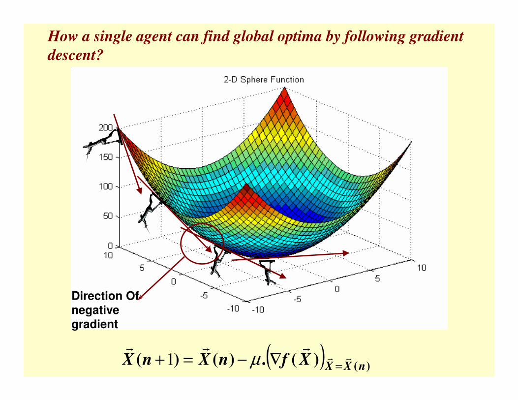
Direction Of negative gradient

How a single agent can find global optima by following gradient

descent?

( ) )()(.)()( nXXXfnXnX ��

��

=∇−=+ µ1

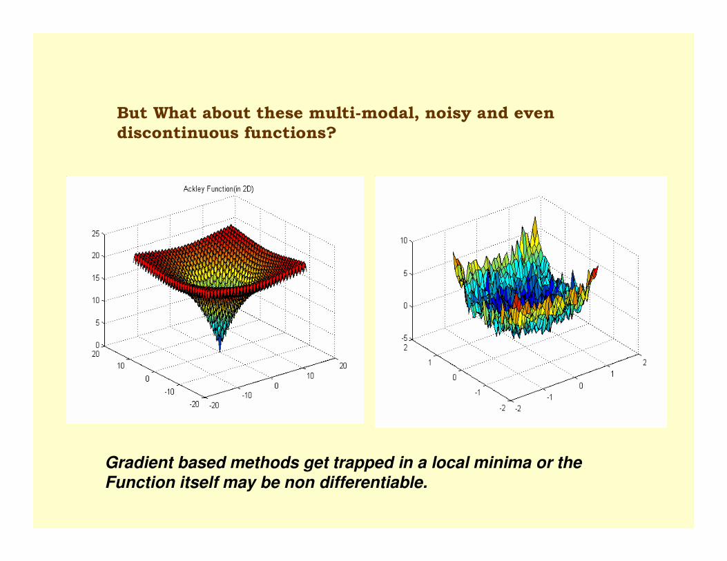
But What about these multi-modal, noisy and even

discontinuous functions?

Gradient based methods get trapped in a local minima or the Function itself may be non differentiable.

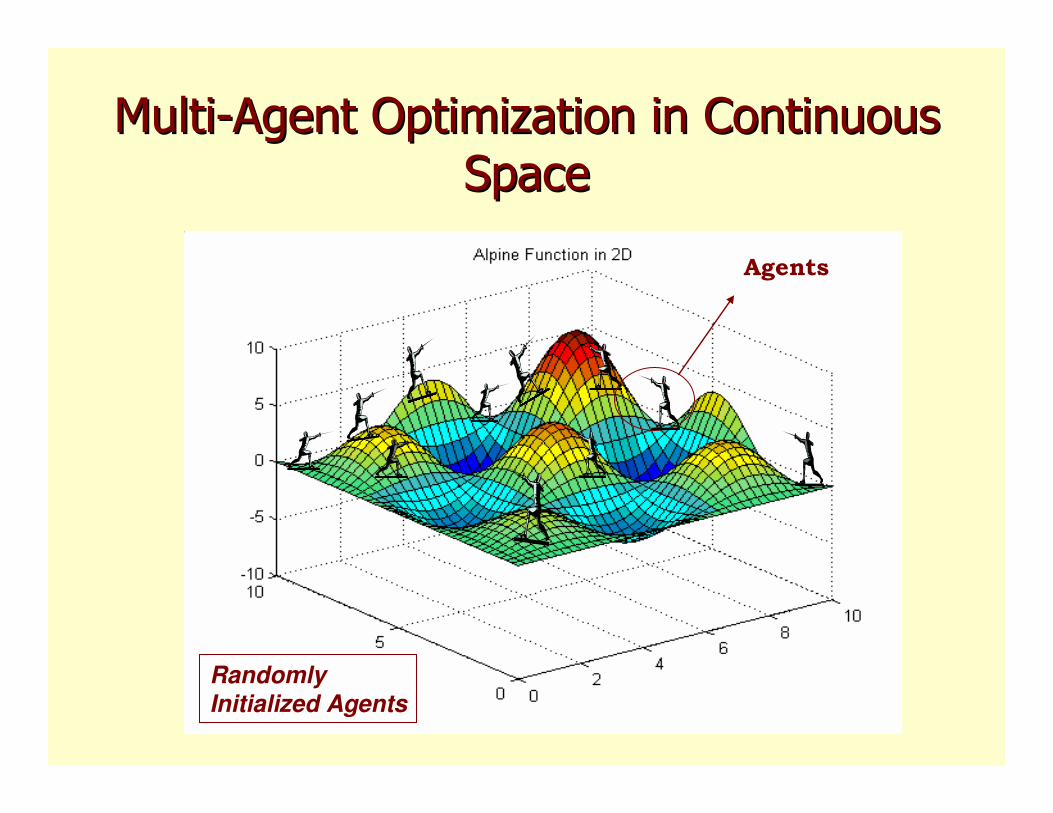
MultiMulti--Agent Optimization in Continuous Agent Optimization in Continuous

SpaceSpace

RandomlyInitialized Agents

Agents

Most Agents are nearGlobal Optima

After Convergence

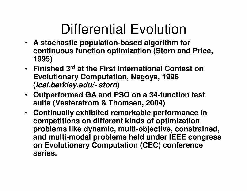
Differential Evolution• A stochastic population-based algorithm for

continuous function optimization (Storn and Price, 1995)

• Finished 3rd at the First International Contest on Evolutionary Computation, Nagoya, 1996 (icsi.berkley.edu/~storn)

• Outperformed GA and PSO on a 34-function test suite (Vesterstrom & Thomsen, 2004)

• Continually exhibited remarkable performance in competitions on different kinds of optimization problems like dynamic, multi-objective, constrained, and multi-modal problems held under IEEE congress on Evolutionary Computation (CEC) conference series.

DE is an Evolutionary Algorithm

This Class also includes GA, Evolutionary Programming and Evolutionary Strategies

Initialization Mutation Recombination Selection

Basic steps of an Evolutionary Algorithm

Representation

Min

Max

May wish to constrain the values taken in each domain

above and below.

x1 x2 x D-1 xD

Solutions are represented as vectors of size D with each

value taken from some domain.

X�

Maintain Population - NP

x1,1 x2,1 x D-1,1 xD,1

x1,2 x2,2 xD-1,2 xD,2

x1,NP x2,NP x D-1,NP xD, NP

We will maintain a population of size NP

1X�

2X�

NPX�

Different values are instantiated for each i and j.

Min

Max

x2,i,0 x D-1,i,0 xD,i,0x1,i,0

, ,0 ,min , ,max ,min[0,1] ( )j i j i j j jx x rand x x= + ⋅ −

0.42 0.22 0.78 0.83


, [0,1]i jrand

iX�


�For each vector select three other parameter vectors randomly.

�Add the weighted difference of two of the parameter vectors to the third to form a donor vector (most commonly seen form of DE-mutation):

�The scaling factor F is a constant from (0, 2)

).(,,,,

321 GrGrGrGi iii XXFXV��

−⋅+=

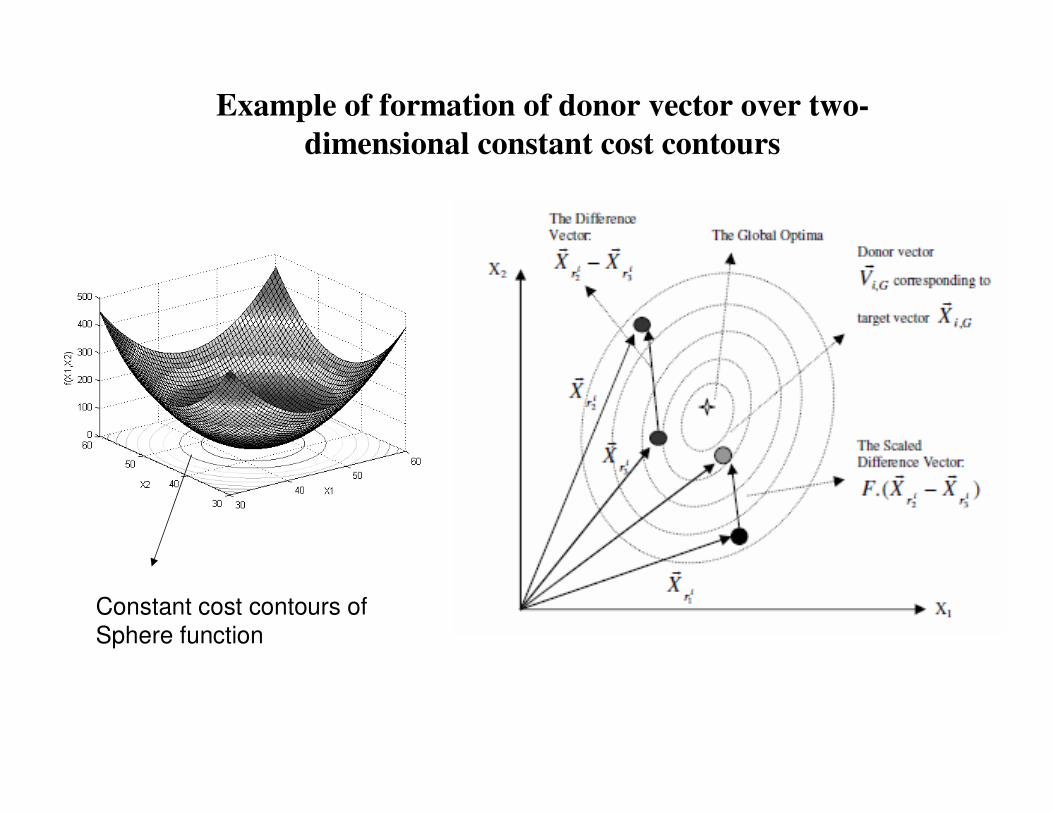
Example of formation of donor vector over two-

dimensional constant cost contours

Constant cost contours of

Sphere function


Components of the donor vector enter into the trial offspring vector in the following way:

Let jrand be a randomly chosen integer between 1,...,D.

Binomial (Uniform) Crossover:

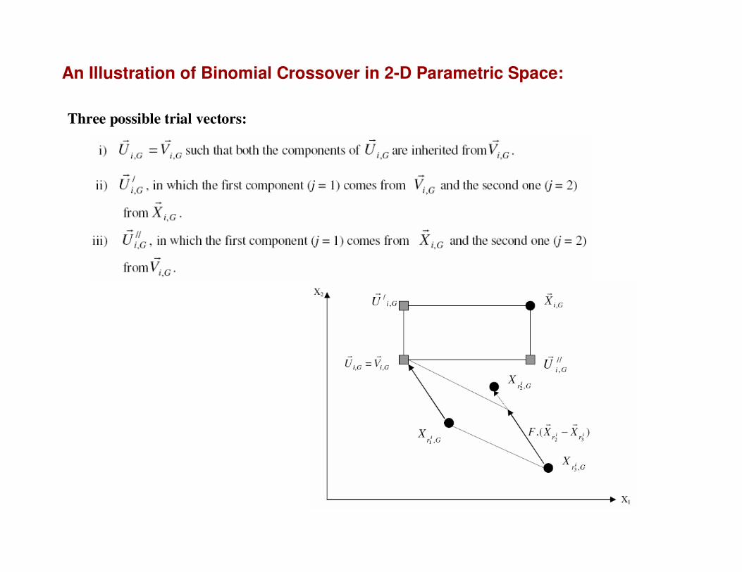
An Illustration of Binomial Crossover in 2-D Parametric Space:

Three possible trial vectors:

Exponential (two-point modulo) Crossover:

Pseudo-code for choosing L:

where the angular brackets Ddenote a modulo function with modulus D.

First choose integers n (as starting point) and L (number of components thedonor actually contributes to the offspring) from the interval [1,D]

Example: Let us consider the following pair of donor and target vectors

,

3.82

4.78

9.34

5.36

3.77

i GX

= − −

�

,

8 .12

10

10

3 .22

1 .12

i GV

= −

− −

�

Suppose n = 3 and L= 3 for this specific example. Then the exponential crossover process can be shown as:


�“Survival of the fittest” principle in selection: The trial offspring vector is compared with the target vector and that on with a better fitness is admitted to the next generation.

1, +GiX�

,,GiU�

= )()( ,, GiGi XfUf��

≤if

,,GiX�

= if )()( ,, GiGi XfUf��

>

An Example of Optimization by DE

Consider the following two-dimensional function

f (x, y) = x2+y2 The minima is at (0, 0)

Let’s start with a population of 5 candidate solutions randomly initiated in the

range (-10, 10)

X1,0 = [2, -1] X2,0 = [6, 1] X3,0 = [-3, 5] X4,0 = [-2, 6] X5,0= [6,-7]

For the first vector X1, randomly select three other vectors say X2, X4 and X5

Now form the donor vector as, V1,0 = X2,0+F. (X4,0 – X5,0)

1,0

6 2 6 0.40.8

1 6 7 10.4V

− − = + × − = −

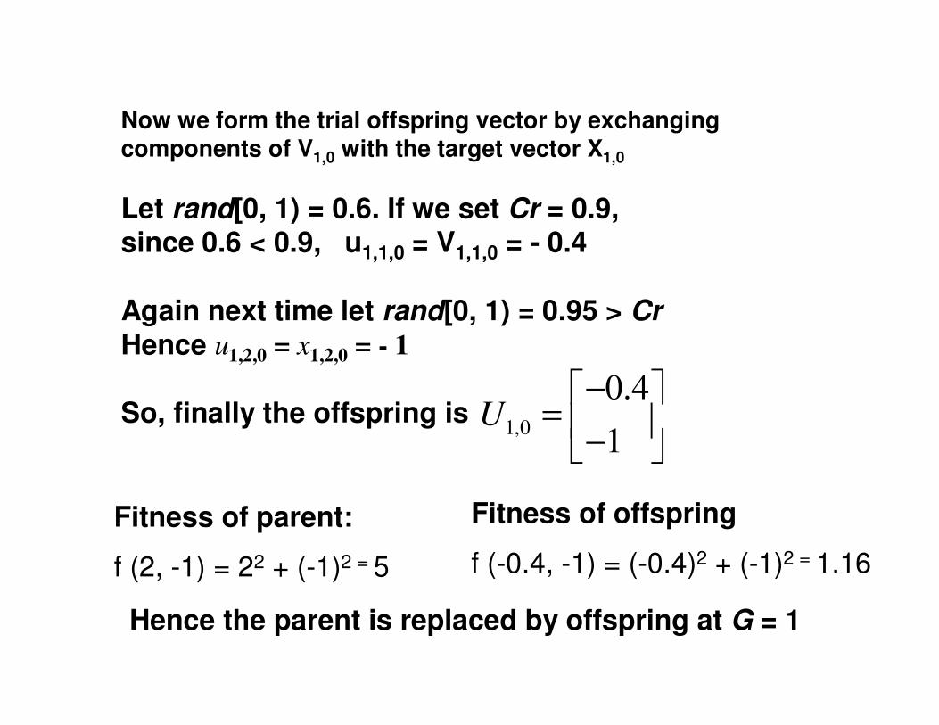
Now we form the trial offspring vector by exchanging components of V1,0 with the target vector X1,0

Let rand[0, 1) = 0.6. If we set Cr = 0.9,since 0.6 < 0.9, u1,1,0 = V1,1,0 = - 0.4

Again next time let rand[0, 1) = 0.95 > Cr

Hence u1,2,0 = x1,2,0 = - 1

So, finally the offspring is 1,0

0.4

1U

− = −

Fitness of parent:

f (2, -1) = 22 + (-1)2 = 5

Fitness of offspring

f (-0.4, -1) = (-0.4)2 + (-1)2 = 1.16

Hence the parent is replaced by offspring at G = 1

Population

at G = 0

Fitness

at G = 0

Donor vector

at G = 0

Offspring

Vector at G = 0

Fitness of

offspring at

G = 1

Evolved

population at

G = 1

X1,0 =

[2,-1]

5 V1,0

=[-0.4,10.4]

U1,0

=[-0.4,-1]

1.16 X1,1

=[-0.4,-1]

X2,0=

[6, 1]

37 V2,0

=[1.2, -0.2]

U2,0

=[1.2, 1]

2.44 X2,1

=[1.2, 1]

X3,0

=

[-3, 5]

34 V3,0

=[-4.4, -0.2]

U3,0

=[-4.4, -0.2]

19.4 X3,1

=[-4.4, -0.2]

X4,0

=

[-2, 6]

40 V4,0

=[9.2, -4.2 ]

U4,0

=[9.2, 6 ]

120.64 X4,1

=[-2, 6 ]

X5,0

=

[6, 7]

85 V5,0

=[5.2, 0.2]

U5,0

=[6, 0.2]

36.04 X5,1

=[6, 0.2]

Locus of the fittest solution: DE working on 2D Sphere Function

Locus of the fittest solution: DE working on 2D Rosenbrock Function

“DE/rand/1”: )).()(()()(321

tXtXFtXtV iii rrri

��

−⋅+=

“DE/best/1”:

“DE/target-to-best/1”:

“DE/best/2”:

“DE/rand/2”:

)).()(.()()(21

tXtXFtXtV iirrbesti

��

−+=

)),()(.())()(.()()(21

tXtXFtXtXFtXtV ii rribestii

��

−+−+=

)).()(.())()(.()()(4321

tXtXFtXtXFtXtV iiii rrrrbesti

��

−+−+=

)).()(.())()(.()()(54321

21 tXtXFtXtXFtXtV iiiii rrrrri

��

−+−+=

Five most frequently used DE mutation schemes

The general convention used for naming the various mutation strategies is DE/x/y/z, where DE stands for Differential Evolution, x represents a string denoting the vector to be perturbed, y is the number of difference vectors considered for perturbation of x, and z stands for the type of crossover being used (exp: exponential; bin: binomial)

Basic Control Parameters of DE:

The Scale Factor F:

1) DE is much more sensitive to the choice of F than it is to the choice of Cr

2) The upper limit of the scale factor F is empirically taken as 1. Although it does not necessarily

mean that a solution is not possible with F > 1, however, until date, no benchmark function that was

successfully optimized with DE required F > 1 .

3) Zaharie derived a lower limit of F and the study revealed that if F is sufficiently small, the

population can converge even in the absence of selection pressure.

22

, ,0

2.( ) 2. . 1 . ( )

G

Cr Crx G Cr x

p pVar P F p Var P

NP NP

= − + +

Zaharie’s Formula for evolution of population-variance in absence of selection:

Critical Value of F:

NP

p

F

Cr

crit

−

=2

1

The population variance decreases when F < Fcrit and increases if F > Fcrit.

Selection and Tuning of F in DE: Some Early Approaches

1) Typically 0.4 < F < 0.95 with F = 0.9 can serve as a good first choice

2) Randomizing F may yield good results over a variety of functions: Price et al. coined the following

terms in this context:

Dither: scales the length of vector differentials because the same factor, Fi, is applied to all components of

a difference vector. (in 2005, Das et al. demonstrated the use of Dither in improving DE’s

performance. They varied F uniformly randomly between 0.5 and 1for each vector.

Jitter: Generates a new value of F for every parameter in every vector is called jitter.

3) Das et al. also proposed a DE with time-varying scale factor where the value of F is linearly decreased from

1 to 0.5 with a view of promoting exploration of diverse regions of the search volume during earlier stagesof search while favoring exploitation during the final stages.

4) A fitness-based adaptation of F was proposed by Ali et al. as:

−

<

−

=

otherwise, 1,max

1 if 1,max

max

minmin

min

max

min

maxmin

f

fl

f

f

f

fl

F

4.0min =l is the lower bound of F.

S. Das, A. Konar, U. K. Chakraborty, “ Two improved differential evolution schemes for faster global search”, appeared in the

ACM-SIGEVO Proceedings of GECCO, Washington D.C., June 2005.

M. M. Ali and A. Törn, “Population set based global optimization algorithms: some modifications and numerical studies,”

Computers and Operations Research, Elsevier, no. 31, pp. 1703–1725, 2004

K. Price, R. Storn, and J. Lampinen, Differential Evolution - A Practical Approach to Global Optimization, Springer, Berlin,

2005.

The Crossover Rate Cr:

1) The parameter Cr controls how many parameters in expectation, are changed in a population member.

2) Low value of Cr, a small number of parameters are changed in each generation and the stepwise movement tends to be orthogonal to the current coordinate axes.

3) High values of Cr (near 1) cause most of the directions of the mutant vector to be inherited prohibiting the

generation of axis orthogonal steps.

Empirical distribution of trial vectors for three different values of Cr has been shown. The plots were obtained by obtained by running DE on a single starting population of 10 vectors for 200 generations with

selection disabled.

(a) Cr = 0(b) Cr = 0.5 (c) Cr = 1.0

For schemes like DE/rand/1/bin the performance is rotationally invariant only when Cr = 1.

At that setting, crossover is a vector-level operation that makes the trial vector a pure mutant i.e.

).(,,,,

321 GrGrGrGi iii XXFXU��

−⋅+=

The Crossover Rate Cr (Contd.):

A low Cr value (e.g. 0 or 0.1) results in a search that changes each direction (or a small subset of

directions) separately.

This is an effective strategy for functions that are separable or decomposable i.e. )()(1

i

D

i

i xfXf ∑=

=�

A Fitness-based adaptation scheme for Cr: Recently Ghosh et al. suggested the following scheme for

fitness-based adaptation of Cr. The basic idea is: if the fitness of the donor vector gets worse,value of Cr should be higher and vice-versa.

Define:_ ( ) ( )donor i i bestf f V f X∆ = −

� �

If ( ) ( ),i bestf V f X≤� �

,i const

Cr Cr= Else max minmin

_

( )

1i

donor i

Cr CrCr Cr

f

−= +

+ ∆

Parametric setup max min0.8, 0.1Cr Cr= =

yielded fairly robust performance over a wide variety of benchmarks.

A. Ghosh, S. Das, A. Chowdhury, and R. Giri, “Differential evolution with a fitness-based adaptation of

control parameters”, Information Sciences, Elsevier Science, Netherlands, (Accepted, 2011).

The population size NP

1) The influence of NP on the performance of DE is yet to be extensively studied and

fully understood.

2) Storn and Price have indicated that a reasonable value for NP could be chosen between

5D and 10D (D being the dimensionality of the problem).

3) Brest and Maučec presented a method for gradually reducing population size of DE. The method improves the efficiency and robustness of the algorithm and can be applied to any variant of a DE

algorithm.

4) Mallipeddi and Suganthan proposed a DE algorithm with an ensemble of parallel populations, where the number of Function Evaluations (FEs) allocated to each population is self-adapted by

learning from their previous experiences in generating superior solutions. Consequently, a more

suitable population size along with its parameter settings can be determined adaptively to match

different search / evolution phases.

•J. Brest and M. S. Maučec, “Population size reduction for the differential evolution algorithm”, Applied Intelligence, Vol. 29, No. 3, pp. 228-247, Dec. 2008.

J. Brest and M. S. Maučec, “Population size reduction for the differential evolution algorithm”,

Applied Intelligence, Vol. 29, No. 3, pp. 228-247, Dec. 2008.

R. Mallipeddi, P. N. Suganthan, “Empirical study on the effect of population size on Differential

evolution Algorithm”, IEEE Congress on Evolutionary Computation, pp. 3663-3670, Hong Kong, 1-6

June, 2008.

•J. Brest and M. S. Maučec, “Population size reduction for the differential evolution algorithm”, Applied Intelligence, Vol. 29, No. 3, pp. 228-247, Dec. 2008.

A Few Significant and Improved Variants of DE for

Continuous Single Objective Optimization

DE with Arithmetic Crossover1) In continuous or arithmetic recombination, the individual components of the trial vector are expressed as a

linear combination of the components from mutant/donor vector and the target vector.

General form: ).( ,,,, 211 GrGriGrGi XXkXW��

−+=

2) ‘DE/current-to-rand/1’ replaces the binomial crossover operator with the rotationally invariant arithmetic

line recombination operator to generate the trial vector by a linear arithmetic recombination of target anddonor vectors:

).( ,,,, GiGiiGiGi XVkXU��

−+=

which further simplifies to: )'.().( ,,,,,, 321 GrGrGiGriGiGi XXFXXkXU��

−+−+=

Change of the trial vectors generated through the discrete

and random intermediate recombination due to rotation of the coordinate system.

/

,

R

GiU�

and //

,

R

GiU�

indicate the new trial vectors due to discrete

recombination in rotated coordinate system.

The ‘jDE’ Algorithm (Brest et al., 2006)

• Control parameters F and Cr into the individual and adjusted them by introducing two new parameters τ1 and τ2

• The new control parameters for the next generation are

computed as follows:

ul FrandF *1+=+1,GiF 12 τ<randif

1, +GiCr3rand=

GiCr ,= else,

1.021 == ττ 0.1,lF =

The new F takes a value from [0.1, 0.9] while the new Cr takes a value from [0, 1].

GiF ,= else.24 τ<randif

J. Brest, S. Greiner, B. Bošković, M. Mernik, and V. Žumer, “Self-adapting Control parametersin differential evolution: a comparative study on numerical benchmark problems,” IEEE Trans. on Evolutionary Computation, Vol. 10, Issue 6, pp. 646 – 657, 2006

Self-Adaptive DE (SaDE) (Qin et al., 2009)

• Includes both control parameter adaptation and strategy adaptation

Strategy Adaptation:

Four effective trial vector generation strategies: DE/rand/1/bin, DE/rand-to-best/2/bin, DE/rand/2/bin and DE/current-to-rand/1 are chosen to constitute a strategy candidate pool.

For each target vector in the current population, one trial vector generation strategyis selected from the candidate pool according to the probability learned from itssuccess rate in generating improved solutions (that can survive to the next generation) within a certain number of previous generations, called the Learning Period (LP).

SaDE (Contd..)

Control Parameter Adaptation:

1) NP is left as a user defined parameter.2) A set of F values are randomly sampled from normal distribution

N(0.5, 0.3) and applied to each target vector in the current population.

3) Cr obeys a normal distribution with mean value Crm and standard deviation Std =0.1, denoted by N (Crm,Std) where Crm is initialized as 0.5.

4) SaDE gradually adjusts the range of Cr values for a given problem according to previous Cr values that have generated trial vectors successfully entering the next generation.

A. K. Qin, V. L. Huang, and P. N. Suganthan, Differential evolution algorithm with strategy adaptation for global numerical optimization", IEEE Trans. on Evolutionary Computation, 13(2):398-417, April, 2009.

Opposition-based DE (Rahnamayan et

al., 2008)

• Three stage modification to original DE framework based on the concept of Opposite Numbers :

Let x be a real number defined in the closed interval [a, b]. Then

the opposite number of x may be defined as:

xbax −+=∪

ODE Steps:

1) Opposition based Population Initialization: Fittest NP individuals are chosen

as the starting population from a combination of NP randomly generated population

members and their opposite members.

2) Opposition Based Generation Jumping: In this stage, after each iteration,

instead of generating new population by evolutionary process, the opposite

population is calculated with a predetermined probability Jr () and the NP fittest

individuals may be selected from the current population and the corresponding

opposite population.

ODE (Contd.)

3) Opposition Based Best Individual Jumping: In this phase, at first a

difference-offspring of the best individual in the current population is created

as:

where r1 and r2 are mutually different random integer indices selected from

{1, 2, ..., NP} and F’ is a real constant. Next the opposite of offspring is

generated as . Finally the current best member is replaced

by the fittest member of the set

)'.( ,,,,_ 21 GrGrGbestGbestnew XXFXX��

−+=

newbestGoppX _

�

{ }GnewbestoppGbestnewGbest XXX ,_,_, ,,��

Rahnamayan, H. R. Tizhoosh, and M. M. A. Salama, “Opposition-based differential evolution”, IEEE Trans. on Evolutionary Computation, Vol. 12, Issue 1, pp. 64-79, Feb. 2008.

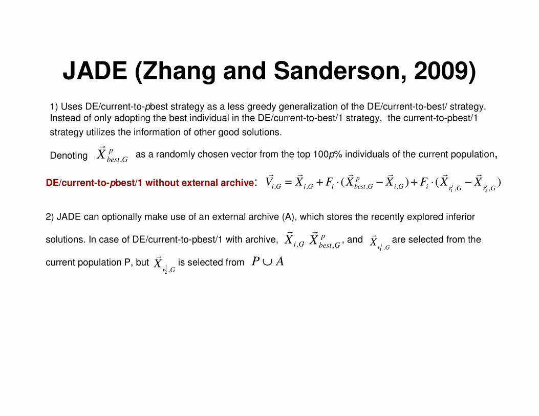
JADE (Zhang and Sanderson, 2009)1) Uses DE/current-to-pbest strategy as a less greedy generalization of the DE/current-to-best/ strategy.

Instead of only adopting the best individual in the DE/current-to-best/1 strategy, the current-to-pbest/1

strategy utilizes the information of other good solutions.

Denoting p

GbestX ,

�

as a randomly chosen vector from the top 100p% individuals of the current population,

DE/current-to-pbest/1 without external archive:1 2

, , , , , ,( ) ( )i i

p

i G i G i best G i G i r G r GV X F X X F X X= + ⋅ − + ⋅ −� � � � � �

2) JADE can optionally make use of an external archive (A), which stores the recently explored inferior

solutions. In case of DE/current-to-pbest/1 with archive, , , and are selected from the

current population P, but is selected from

GiX ,

�

p

GbestX ,

�

Gr iX,1

�

2 ,i

r GX�

AP ∪

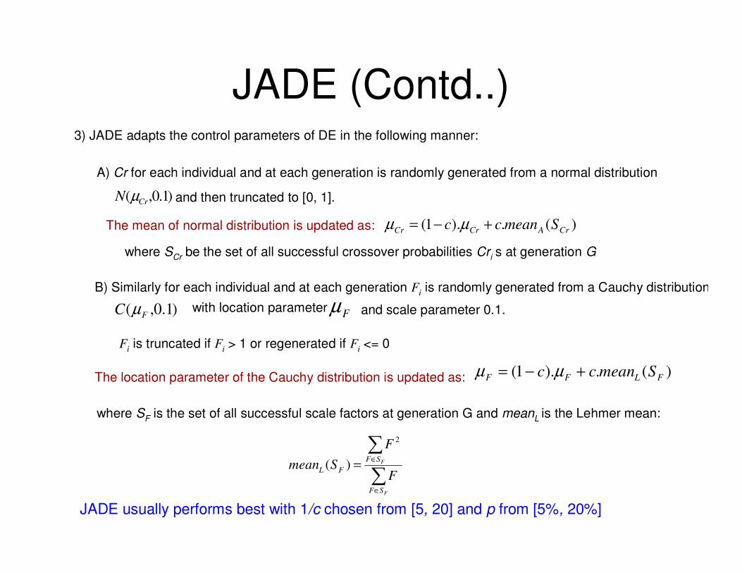
JADE (Contd..)3) JADE adapts the control parameters of DE in the following manner:

A) Cr for each individual and at each generation is randomly generated from a normal distribution

)1.0,( CrN µ and then truncated to [0, 1].

The mean of normal distribution is updated as: )(.).1( CrACrCr Smeancc +−= µµ

where SCr be the set of all successful crossover probabilities Cri s at generation G

B) Similarly for each individual and at each generation Fi is randomly generated from a Cauchy distribution

)1.0,( FC µ with location parameterFµ and scale parameter 0.1.

The location parameter of the Cauchy distribution is updated as:

Fi is truncated if Fi > 1 or regenerated if Fi <= 0

)(.).1( FLFF Smeancc +−= µµ

where SF is the set of all successful scale factors at generation G and meanL is the Lehmer mean:

∑

∑

∈

∈=

F

F

SF

SF

FLF

F

Smean

2

)(

JADE usually performs best with 1/c chosen from [5, 20] and p from [5%, 20%]

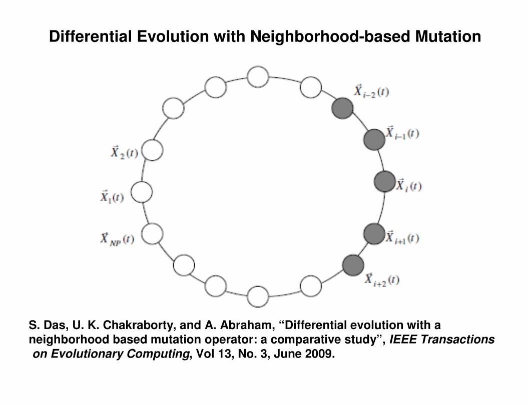
Differential Evolution with Neighborhood-based Mutation

S. Das, U. K. Chakraborty, and A. Abraham, “Differential evolution with a neighborhood based mutation operator: a comparative study”, IEEE Transactionson Evolutionary Computing, Vol 13, No. 3, June 2009.

Local Mutation Model:

))()(())()(()()( _ tXtXtXtXtXtL qpibestnii i

��

−⋅+−⋅+= βα

Global Mutation Model:

))()(())()(()()(21_ tXtXtXtXtXtg rribestgii

��

�

−⋅+−⋅+= βα

Combined Model for Donor Vector generation:

)().1()(.)( tLwtgwtV iii

�

�

�

−+=

The weight factor w may be adjusted during the run or self-adapted through the evolutional learning process.

On Timing Complexity of DEGL

Running of Gmax no. of generations,complexity of DE/rand/1/bin :

)( maxGDNPO ⋅⋅

Runtime complexity of DE/target-to-best/1/bin :

)()),(max( maxmaxmax GDNPOGDNPGNPO ⋅⋅=⋅⋅⋅

Worst case timing complexity of DEGL: )),(max( maxmax GDNPGkNPO ⋅⋅⋅⋅

where k is neighborhood radius.

Asymptotic order of complexity remains )( maxGDNPO ⋅⋅

if k < D, which is usually the case for high-dimensional functions.

DEGL does not impose any serious burden on the runtime complexityof the existing DE variants

A Special Issue on DEjust appeared in:

Feb. 2011

Guest Editors: Swagatam Das, Jadavpur University, IndiaP. N. Suganthan, Nanyang Technological University,Singapore.Carlos A. Coello Coello, Col. San Pedro Zacatenco, México.

This tutorial is partly based on the survey article published in this special issue:

S. Das and P. N. Suganthan, “Differential evolution – a survey of the state-of-the-art”,

IEEE TEVC, Vol. 15, No. 1, feb. 2011.

Introduction to a few DE-variants from the special issue of IEEE TEVC:

1) cDE (Mininno et al., “Compact differential evolution”, IEEE TEVC, Vol 15, No. 1):

- An interesting Estimation of Distribution Algorithm (EDA) which,

analogously to other compact Evolutionary Algorithms (cEAs), does not

store and process the entire population and all of its individuals, but adopts

instead a static representation of the population to perform the optimization

process.

- However, unlike other cEAs, cDE encodes the actual survivor selection

mechanism of the original DE algorithm, as well as its original search logic

(i.e., its crossover and mutation operators).

- cDE uses a fairly limited amount of memory, which makes it appropriate for

hardware implementations.

CoDE (Wang et al., “Differential evolution with composite trial vector generation

strategies and control parameters”, IEEE TEVC, Vol. 15, No. 1):

-adopts three different trial vector generation strategies (rand/1/bin,

rand/2/bin, and current-to-rand/1) and three mechanisms to control DE’s

parameter settings. The parametric choices were:

1) F = 1.0, Cr = 0.1 - meant for dealing with separable problems.

2) F = 1.0, Cr = 0.9 – meant for maintaining population diversity.

3) F = 0.8, Cr = 0.2 – meant for exploiting the search space and

achieving better convergence characteristics.

-Such strategies offer different advantages and, somehow, complement

one another.

DE with Proximity-based Mutation Operators (Epitropakis et al., “Enhancing differential

evolution with proximity-based mutation operators”, IEEE TEVC, Vol. 15, No. 1):

-is based on framework that incorporates information of neighboring individuals

to guide the search towards the global optimum in a more efficient manner.

-The main idea is to adopt a stochastic selection mechanism in which the

probability of selecting an individual to become a parent is inversely proportional

to its distance from the individual undergoing mutation.

-This will favor the search in the vicinity of the mutated individual, which should

promote a proper exploitation of such a neighborhood, without sacrificing the

exploration capabilities of the mutation operator.

-The authors incorporate the proposed framework to several DE variants,

finding that in most cases its use significantly improves the performance of the

algorithm (when there is no improvement, there is no significant degradation in

performance either).

Stochastic Analysis of the DE

• DE has been modeled as a stochastic process with a time-varying PDF.

• The mutation, crossover and selection steps have been analyzed to produce a recurrence relation relating the PDF at time n+1 with the present PDF for time n.

• Investigation of the relation shows the existence of a Lyapunov functional (dependent on the PDF) which proves asymptotic stability of the DE system.

S. Ghosh, S. Das, and A. V. Vasilakos, Convergence Analysis of DifferentialEvolution over a Class of Continuous Functions with Unique Global Optimum, Accepted in IEEE Trans. on SMC Part B, 2011.

( )g x�

1 2 1 2... ( , ,... ). . ...D Dg x x x dx dx dx∫ ∫ ∫

( ).D

g x dx

ℜ

∫� �

The high-dimensional integral of a scalar function like over several components of a vector i.e.

is expressed through a single integration over a vector space like

.

Assumptions on the Objective Function:

Towards a recursive relation of the population PDFs

In binomial crossover, we assume a component is inherited from donor vector with probability

CP And from the corresponding target vector with a probability 1C

P−

mθ

dm,θ mθ

2=m 3D =

For the m-th crossover combination, we define a D-dimensional string Such that a ‘1’ in

(the d-th bit position of ) indicates that the d-th dimension is taken from the donor, and

is represented by ‘001’.

a ‘0’ indicates that thed-th dimension is taken from the parent. For example, and

We define the following sets: }1 and1:{ =≤≤= m,am Daa θα and

}0 and1:{ =≤≤= m,bm Dbb θβ

The probability of the m-th combination appearing in the crossover: ννν

−−= D

CC

D

m PPCP )1(.

ν = Cardinality of setmα

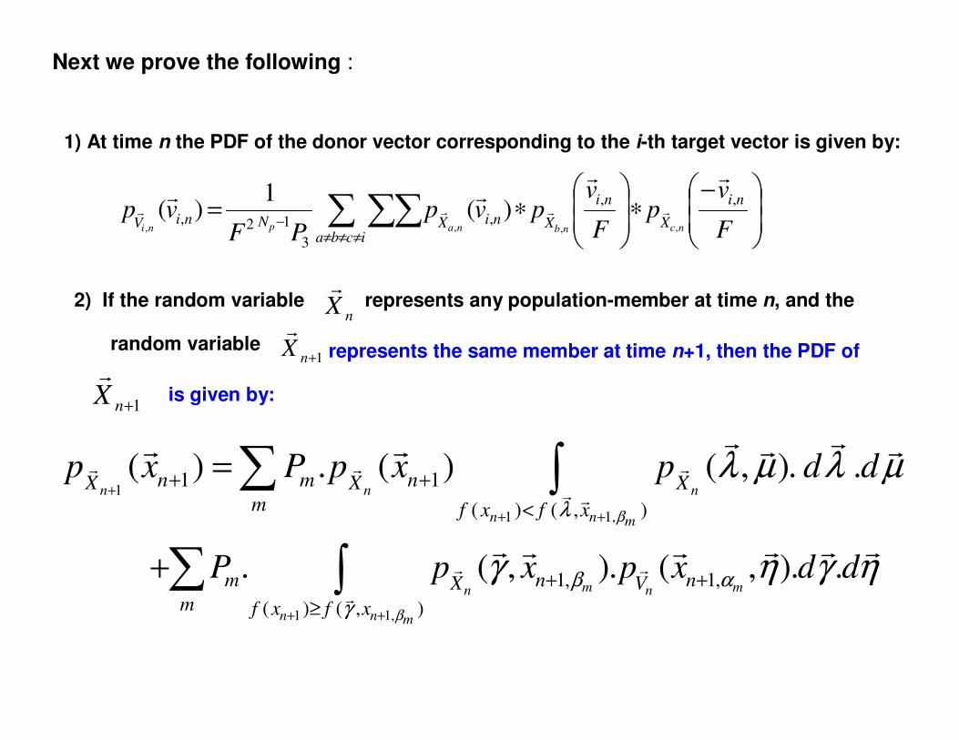
Next we prove the following :

1) At time n the PDF of the donor vector corresponding to the i-th target vector is given by:

−∗

∗= ∑ ∑∑

≠≠≠− F

vp

F

vpvp

PFvp

ni

X

ni

Xicba

niXNniV ncnbnapni

,,

,

3

12,,,,,

)(1

)(

��

��

��

nX�

1+nX�

1+nX�

2) If the random variable represents any population-member at time n, and the

represents the same member at time n+1, then the PDF of

is given by:

random variable

1

1 1,

1 1

( ) ( , )

( ) . ( ) ( , ). .n n n

n n m

n m nX X Xm f x f x

p x P p x p d d

βλ

λ µ λ µ+

+ +

+ +

<

=∑ ∫� � �

�

�

� �

� � � �

1 1,

1, 1,

( ) ( , )

. ( , ). ( , ). .m mn n

n n m

m n nX Vm f x f x

P p x p x d d

β

β α

γ

γ η γ η+ +

+ +

≥

+∑ ∫ � �

�

� � � ��

nXp �

Terms in the relation:

and are PDFs of the population vectors

at times n and n+1 respectively. We have shown that the PDFs for all vectors in the population are identical, so we do not refer to any vector in particular.

is the PDF of the donor vectors at time n. Here also we do not refer to any vector in particular.

Our objective is to express in terms of

and for the point

1nXp

+

�

nVp �

11( )

nnX

p x+

+�

�

1nXp

+

�

nVp �

1nx +

�

What does it mean ?

• The recurrence relation portrays the heuristics in the DE algorithm.

• Failure of the population PDF at time n to find good solutions may contribute to selection of the donor PDF.

• Similarly, failure of the donor PDF to find good solutions may contribute to selection of the original population PDF.

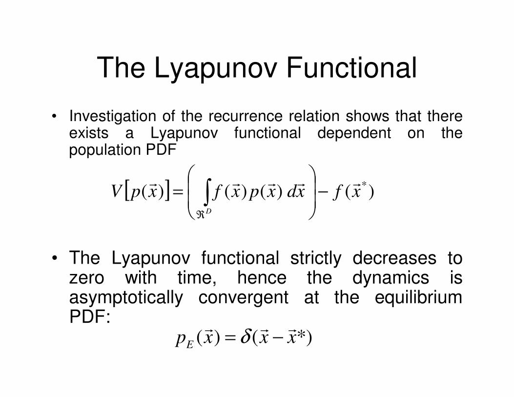
The Lyapunov Functional

• Investigation of the recurrence relation shows that there exists a Lyapunov functional dependent on the population PDF

• The Lyapunov functional strictly decreases to zero with time, hence the dynamics is asymptotically convergent at the equilibrium PDF:

( ) ( *)E

p x x xδ= −� � �

[ ] )()()()( *xfxdxpxfxpVD

��

−

= ∫

ℜ

We prove the following things about the Lyapunov Functional:

1) The functional is positive definite

w.r.t the equilibrium PDF ( ) ( *)Ep x x xδ= −� � �

2) The functional 1

[ ( )] [ ( )]n nX X

V p x V p x+

−� �

defined on the set of all PDFs

( )p x�

is negative semi-definite w.r.t the equilibrium PDF ( ) ( *)Ep x x xδ= −� � �

.

3) For the functional dynamics arising from the transition equation,

1[ ( )] [ ( )]

n nX XV p x V p x+

−� �

does not identically vanish along any trajectory

( )n

nXp x�

�

for all 0≥n

.

taken by the PDF

Dynamics given by the PDF transition equation is asymptotically stable at the equilibrium PDF ( ) ( *)Ep x x xδ= −

� � �

[ ] )()()()( *xfxdxpxfxpVD

��

−

= ∫

ℜ

How correct is the model?

• To check the correctness of our model, we test the actual DE, with DE/1/rand/bin mutation and a large population size (1000), and apply it to some standard one-dimensional benchmarks.

• The estimated PDFs obtained through the experiment are found to be pretty close to the PDFs predicted through the recurrent stochastic model.

• The estimated Lyapunov functional also reduces to zero and is very close to the predicted Lyapunov functional.

The Sphere Function

PDFs predicted for different time instants through the recurrent stochastic model

PDFs estimated by running the DE algorithm

Griewank’s Function

PDFs predicted for different time instants through the stochastic model


Shifted Rastrigin’s Function

PDFs predicted for different time instants through the stochastic model


Conclusions

• The stochastic model accurately predicts the behavior of

the DE algorithm for a large population size.

• The model is also successful in showing that the

population vectors converge at the global optimum point,

provided it exists uniquely.

• Further research can be undertaken to predict the

algorithm’s behavior for a finite number of vectors.

Documents

Differential Evolution: Foundations, Perspectives, and