Embed Size (px)
Citation preview
EPA/600/R-13/352 | October 2013
www.epa.gov/ord
United StatesEnvironmental ProtectionAgency
O�ce of Research and DevelopmentNational Health and Environmental E�ects Research Laboratory, Atlantic Ecology Division
Di�erentiating Impacts of Watershed Development from Superfund Sites on Stream Macroinvertebrates

EPA/600/R-13/352 | October 2013
Differentiating Impacts of Watershed Development from Superfund
Sites on Stream Macroinvertebrates
Naomi E Detenbeck
U.S. Environmental Protection Agency Atlantic Ecology Division
Narragansett, RI
Cornell Rosiu1 U.S. Environmental Protection Agency
Region 1 Boston, MA
Laura Hayes USGS New England Water Science Center
New Hampshire-Vermont Office Pembroke, NH
Jeffrey Legros2
University of Massachusetts-Amherst Amherst, MA
1 Current address is: First Coast Guard District Incident Management Branch, 408 Atlantic Avenue, Boston, MA 02110 2 Formerly student services contractor with the U.S. EPA Atlantic Ecology Division, Narragansett, RI.
ii | Differentiating Impacts of Watershed Development
ABSTRACT Urbanization effect models were developed to differentiate between effects on aquatic macroinvertebrates within a watershed from non-point source urbanization and known local contaminated sediments. Using U.S. Environmental Protection Agency (US EPA) Environmental Monitoring and Assessment Program (EMAP) data from the New England Wadeable Stream Survey (NEWS) and datasets from States of Maine (ME) and Connecticut (CT), we derived macroinvertebrate community response curves for watersheds with different levels of urban development (n = 731). We applied boosted regression trees (BRT) to develop models, allowing us to simultaneously differentiate interactions among variables and quantitatively identify biological effect thresholds with known confidence intervals. Best predictors of watershed development impacts were percent Impervious Area (%IA) at the watershed- or local- scale and percent high density residential area (i.e., with 80–100% impervious cover) in the stream buffer. When these indicators operated at both watershed and local scales, they tended to have synergistic (more than additive) effects. For the first time, we were able to demonstrate the effects of road density and road-stream crossings independent of impervious area effects. We also demonstrated declines in community metrics at very low levels of urbanization (<1–2% IA), once effects of moderating variables had been factored out. Percent forested buffer was a significant moderating influence on impacts, with sensitivity modified by watershed area, slope class, Ecological Unit (Maxwell et al. 1995), and low flow class. BRTs were powerful enough to discriminate local impacts (Superfund contaminated sediment sites) from upstream development with 95% confidence, once toxic stressor-specific indicators were incorporated.
This is the first published case demonstrating the cumulative effects of Superfund sites on stream macroinvertebrate community composition at the whole watershed scale, and distinguishing these effects from those of urban development in the watershed. Application of these urbanization effects models offers potential as diagnostic tools for assessment of in-stream biological condition differentially sensitive to point source and nonpoint source pollution. These models can be used to identify streams where biological impacts are greater than predicted for the level of watershed development (identify potential site point sources) or assess the effectiveness of site remediation or restoration, or watershed best management practices.
Keywords: urbanization indices, streams, boosted regression trees, Superfund, contaminated sediment sites.

Table of Contents | iii
TABLE OF CONTENTS
Abstract ........................................................................................................................................... ii List of Figures ................................................................................................................................ iv
List of Tables .................................................................................................................................. v
Acronyms ....................................................................................................................................... vi Acknowledgements ...................................................................................................................... viii INTRODUCTION .......................................................................................................................... 1
METHODS ..................................................................................................................................... 3
Study area, data sources, and site selection ................................................................................ 3
Calculation of macroinvertebrate response metrics .................................................................... 3
Response metric selection for effects models ............................................................................. 6
Superfund Sites and Other Point Source Data ............................................................................ 6
Hydrologic framework ................................................................................................................ 7
Watershed attributes.................................................................................................................... 7
Classification schemes ................................................................................................................ 7
Variable filtering with ECODIST ............................................................................................... 8
Boosted regression tree model development .............................................................................. 9
RESULTS ..................................................................................................................................... 10
Flow regime class derivation .................................................................................................... 10
O/E model development ........................................................................................................... 10
Response metric selection ......................................................................................................... 10
ECODIST model screening results ........................................................................................... 12
Boosted regression tree models ................................................................................................ 13
DISCUSSION ............................................................................................................................... 21
Urbanization indicators, model sensitivities and spatial scale .................................................. 21
Relative sensitivity of response metrics .................................................................................... 21
Response thresholds and interactions ....................................................................................... 21
Discriminating local contamination effects from watershed development ............................... 23
Moderating factors (watershed area, flow regime, slope class) ................................................ 23
Potential effects of study design and sampling methods on detection of urbanization and Superfund site effects ................................................................................................................ 24
CONCLUSION ............................................................................................................................. 25
LITERATURE CITED ................................................................................................................. 26
iv | Differentiating Impacts of Watershed Development
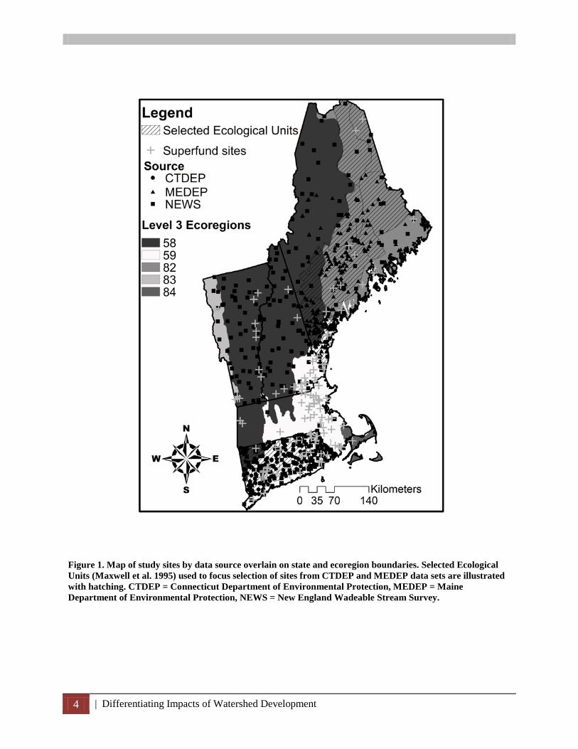
LIST OF FIGURES Figure 1. Map of study sites by data source overlain on state and ecoregion boundaries. Selected Ecological Units (Maxwell et al. 1995) used to focus selection of sites from CTDEP and MEDEP data sets are illustrated with hatching. CTDEP = Connecticut Department of Environmental Protection, MEDEP = Maine Department of Environmental Protection, NEWS = New England Wadeable Stream Survey. .......................................................................................................................................................... 4
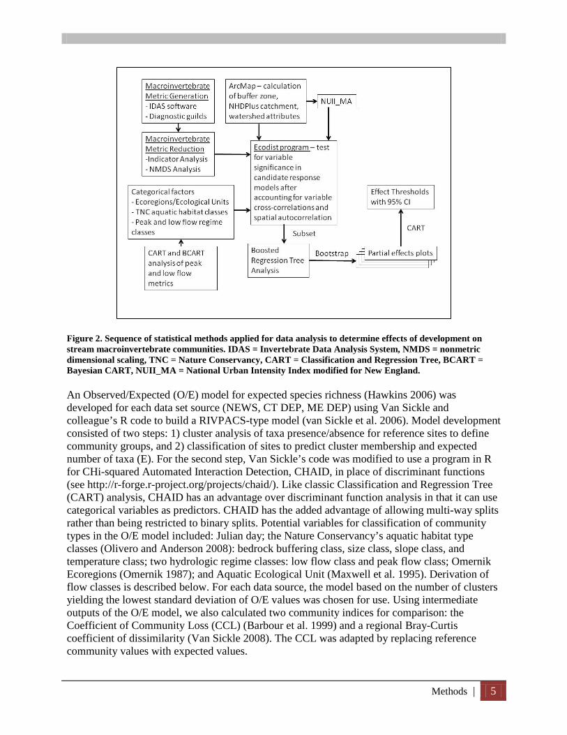
Figure 2. Sequence of statistical methods applied for data analysis to determine effects of development on stream macroinvertebrate communities. IDAS = Invertebrate Data Analysis System, NMDS = nonmetric dimensional scaling, TNC = Nature Conservancy, CART = Classification and Regression Tree, BCART = Bayesian CART, NUII_MA = National Urban Intensity Index modified for New England. ................... 5
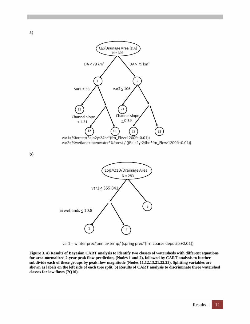
Figure 3. a) Results of Bayesian CART analysis to identify two classes of watersheds with different equations for area-normalized 2-year peak flow prediction, (Nodes 1 and 2), followed by CART analysis to further subdivide each of these groups by peak flow magnitude (Nodes 11,12,13,21,22,23). Splitting variables are shown as labels on the left side of each tree split. b) Results of CART analysis to discriminate three watershed classes for low flows (7Q10). ....................................................................... 11
Figure 4. For the CT DEP data set, partial effects plots of a) Ephemeroptera + Plecoptera + Trichoptera richness (EPTr) __ Ephemeroptera richness (EPr) _ _ Plecoptera richness (PLr) … and b) fraction (relative abundance) Ephemeroptera (fEP) __ fraction Plecoptera (fPL) z _ _ fraction Trichoptera (fTR) … as a function of % imperviousness/watershed. All variables have been normalized and are expressed as z-scores. Thresholds associated with these plots are listed in Appendix 5. Hash marks on upper horizontal axis represent quantiles of the distribution of predictor variables (e.g., 10th percentile – 90th percentile). . 16
Figure 5. For the ME DEP data set, partial effects plots of, Ephemeroptera richness (EPr) _ _ Ephemeroptera + Plecoptera + Trichoptera richness (EPTr) …, and fraction Amphipoda (fAM) _ . as a function of road-stream crossing density/km stream in flowline catchment . All variables have been normalized and are expressed as z-scores. Thresholds associated with these plots are listed in Appendix 5. .................................................................................................................................................................... 17
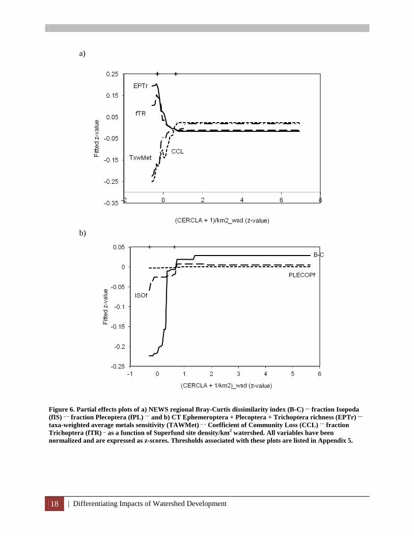
Figure 6. Partial effects plots of a) NEWS regional Bray-Curtis dissimilarity index (B-C) __ fraction Isopoda (fIS) _ _ fraction Plecoptera (fPL) … and b) CT Ephemeroptera + Plecoptera + Trichoptera richness (EPTr) __ taxa-weighted average metals sensitivity (TAWMet) _ _ Coefficient of Community Loss (CCL) … fraction Trichoptera (fTR) _ as a function of Superfund site density/km2 watershed. All variables have been normalized and are expressed as z-scores. Thresholds associated with these plots are listed in Appendix 5. ................................................................................................................................................. 18
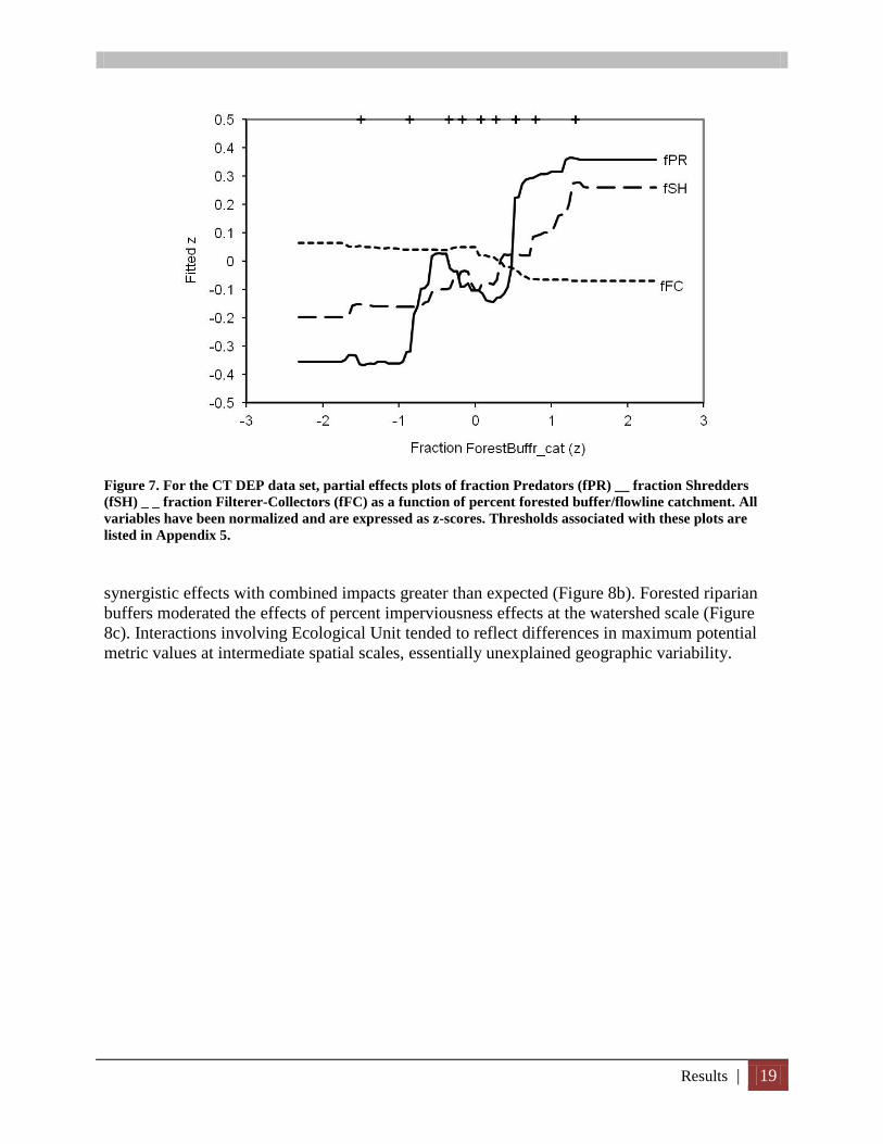
Figure 7. For the CT DEP data set, partial effects plots of fraction Predators (fPR) __ fraction Shredders (fSH) _ _ fraction Filterer-Collectors (fFC) as a function of percent forested buffer/flowline catchment. All variables have been normalized and are expressed as z-scores. Thresholds associated with these plots are listed in Appendix 5. ............................................................................................................................. 19
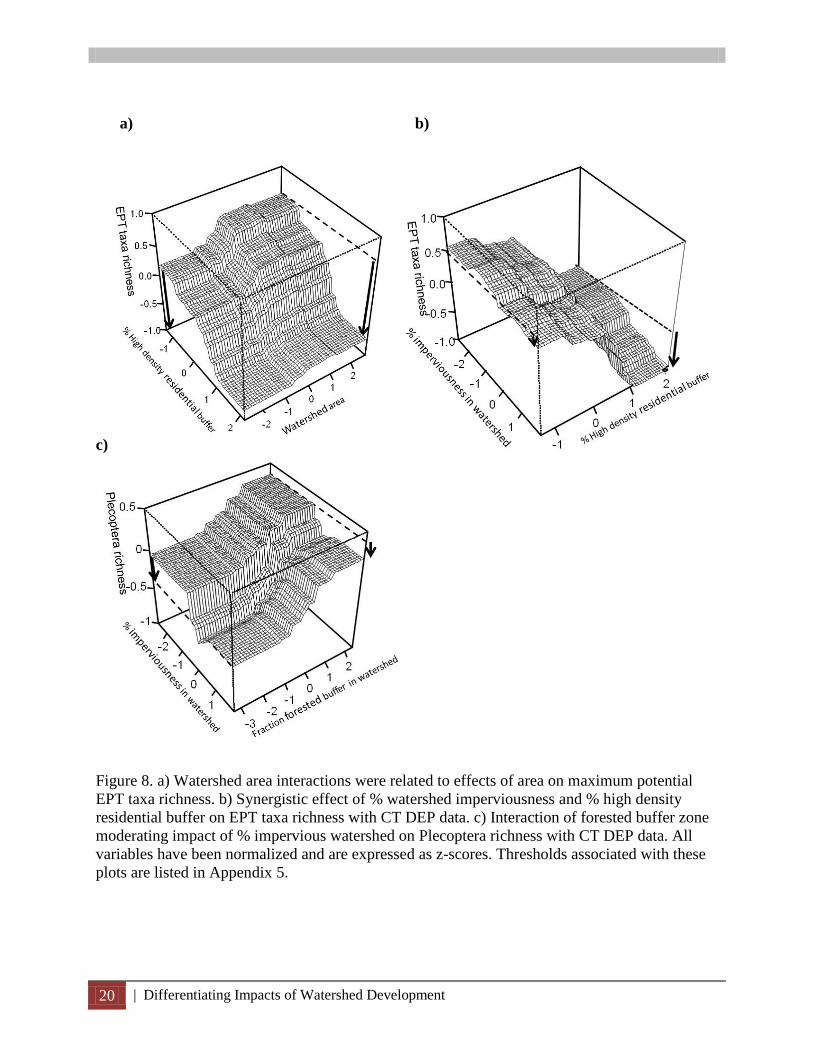
Figure 8. a) Watershed area interactions were related to effects of area on maximum potential EPT taxa richness. b) Synergistic effect of % watershed imperviousness and % high density residential buffer on EPT taxa richness with CT DEP data. c) Interaction of forested buffer zone moderating impact of % impervious watershed on Plecoptera richness with CT DEP data. All variables have been normalized and are expressed as z-scores. Thresholds associated with these plots are listed in Appendix 5. ..................... 20

List of Tables | v
LIST OF TABLES Table 1. Watershed attributes used for flow regime classification. .............................................................. 8
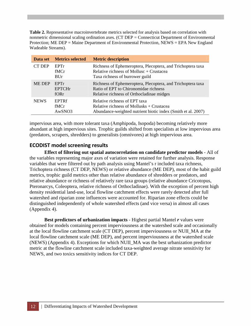
Table 2. Representative macroinvertebrate metrics selected for analysis based on correlation with nonmetric dimensional scaling ordination axes. (CT DEP = Connecticut Department of Environmental Protection; ME DEP = Maine Department of Environmental Protection, NEWS = EPA New England Wadeable Streams). ............................................................................... 12
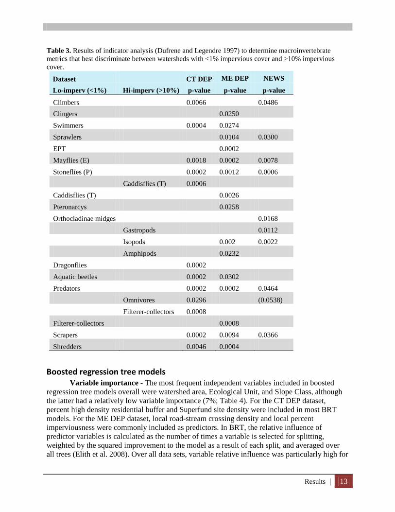
Table 3. Results of indicator analysis (Dufrene and Legendre 1997) to determine macroinvertebrate metrics that best discriminate between watersheds with <1% ............................................................. 13
List of Appendices Appendix 1. Sampling designs, collection procedures and processing methods (US EPA 2004). Appendix 2. Superfund sites in New England. Appendix 3. Data sources Appendix 4. Results of partial Mantel tests. Appendix 5. Thresholds from this study Appendix 6. Variable interactions in boosted regression trees Appendix 7. Thresholds from the literature
vi | Differentiating Impacts of Watershed Development
ACRONYMS 7Q10/Area: 7-day-10-year low flow normalized to watershed area A: Average variable importance AwMET: Abundance-weighted average metals sensitivity AwPAH: Abundance-weighted average PAH sensitivity AwSNO3: Abundance-weighted nutrient biotic index BACI: Before-After-Control-Impact B-C: Bray-Curtis dissimilarity index BCART: Bayesian Classification and Regression Tree BMP: Best management practice BRT: Boosted regression trees BUr: Taxa richness of burrower guild CART: Classification and Regression Tree CCL: Coefficient of community loss CERCLA: Compensation and Liability Act of 1980 (Superfund Program) CERCLAden: Density of Superfund sites CI: Confidence interval CT DEP: Connecticut Department of Environmental Protection CT: Connecticut damden: Dam density (National Dams Inventory) DDT: dichloro diphenyl trichloroethane DDE: dichlorodiphenyldichloroethylene E: Exhaustion threshold ecoreg: Ecoregion (Omernik) ecounit: Maxwell Ecological Unit (Maxwell et al. 1995) EIC: Effective impervious cover EMAP: Environmental Monitoring and Assessment Program EPr: Ephemeroptera richness EPT: Ephemeroptera + Plecoptera + Trichoptera EPTCHr: Ratio of EPT to Chironomidae richness EPTr: Ephemeroptera + Plecoptera + Trichoptera richness EPTRf: Relative richness of EPT taxa F: frequency of inclusion fAM: fraction (relative abundance) Amphipoda fCB: fraction Climbers fCN: fraction Clingers fCO: fraction Coleoptera fCR: fraction Cricotopus fEP: fraction (relative abundance) Ephemeroptera fFC: fraction Filterer-Collectors fForBfr_cat: fraction forested buffer at NHDPlus catchment scale fForBfr_wsd: fraction forested buffer at watershed scale fIS: fraction (relative abundance) Isopoda fGA: fraction Gastropoda fMCr: Relative richness of Mollusc + Crustacea fOM: fraction Omnivores fORr: fraction Orthocladinae midge richness fSP: fraction Sprawlers fSW: fraction Swimmers
Acronyms | vii
Acronyms (cont’d) fPL: fraction (relative abundance) Plecoptera fPR: fraction Predators fPT: fraction Pteronarcys fSH: fraction Shredders fTR: fraction (relative abundance) Trichoptera ft_orgtol: fraction taxa organic-tolerant ft_toxtol: fraction taxa toxics-tolerant GIS: Geographic Information System IA: Impervious Area IBIs: Indices of Biotic Integrity IDAS: Invertebrate Data Analysis System km: kilometer L7Q10node: node (class) of watersheds defined by 7Q10 value LOCEL: Lowest observed community effect levels m 2 : square meter ME DEP: Maine Department of Environmental Protection ME: Maine NAWQA: National Water Quality Assessment program NEGEOCL: New England geology class (TNC habitat scheme) NESLPCL: New England slope class (TNC habitat scheme) NETEMPCL: New England stream temperature class (TNC habitat scheme) NEWS: New England Wadeable Stream Survey NHD: National Hydrography Dataset NHDPlus: National Hydrography Dataset Plus NLCD: National Landcover Dataset NMDA: N-nitrosodimethylamine NMDS: nonmetric multi-dimensional scaling NUII_MA: National Urban Intensity Index Modified for New England NUII_MA_wsd PCBs: polychorinated biphenyls PCE: tetrachloroethene PCP: pentachlorophenol PL: Plecoptera PAH: Polycyclic aromatic hydrocarbon PLr: Plecoptera richness PRISM: Parameter-elevation Regressions on Independent Slopes Model PRP: Potentially responsible party ptagr_cat: percent agriculture at NHDPlus catchment scale ptagr_wsd: pecent agriculture at watershed scale ptHDRBfr_cat: percent high density residential buffer zone at NHDPlus catchment scale ptHDRBfr_wsd: percent high density residential buffer zone at watershed scale ptIMPV_cat: percent impervious area at NHDPlus catchment scale ptIMPV_wsd: percent impervious area at watershed scale ptWtld_cat: percent wetlands at NHDPlus catchment scale ptWtld_wsd: percent wetlands at watershed scale : Q2/Area: Two-year peak flow normalized to watershed area Q2node: watershed class defined by common Q2 values R*: Resistance threshold
viii | Differentiating Impacts of Watershed Development
Acronyms (cont’d) R: Statistical programming language RdStXing_kmcat: Road-stream crossing density per km stream at NHDPlus catchment scale RdStXing_kmwsd: Road-stream crossing density per km stream at watershed scale RI: relative influence SF_Type: Superfund site type (based on distance category) SPARROW: SPAtially Referenced Regressions On Watershed Attributes SVOCs: semi-volatile organic compounds SYSTAT: SYSTAT software TwSNO3: taxa-weighted average nitrate sensitivity TwMet: taxa-weighted average metals sensitivity TwPAH: taxa-weighted average PAH sensitivity TCE: trichloroethene THF: tetrahydrofuran TITAN: Threshold Indicator Taxa ANalysis TNC: The Nature Conservancy TR: Trichoptera TRI: Toxics Release Inventory UII_MA: Urban Intensity Index for Metropolitan Areas USACE: United States Army Corps of Engineers US EPA: United States Environmental Protection Agency USFS: United States Forest Service USFWS: United States Fish and Wildlife Service USGS: United States Geological Survey VOCs: volatile organic compounds wsd: watershed Wdarea: watershed area
ACKNOWLEDGEMENTS The information in this document has been funded by the U.S. Environmental Protection Agency (EPA), in part by EPA’s Regional and Applied Research Efforts (RARE) program. It has been subject to the Agency's peer and administrative review, and it has been approved for publication. Mention of trade names or commercial products does not constitute endorsement or recommendation for use. We thank the US EPA Region 1 (NEWS dataset, Hillary Snook), CT DEP (Chris Bellucci), and ME DEP (Tom Danielson, Leo Tsimedes) for providing the historical monitoring data that were analyzed in this study. We acknowledge technical support on GIS analyses from Donald Parsley and Alexander Sherman, programming support on bootstrap analysis from Harry Buffum, and intellectual input from James Coles (USGS) and Marilyn ten Brink on the original study objectives. We thank the following reviewers for their helpful comments on an earlier version of this report: Brenda Rashleigh, Britta Bierwagen, and Ian Waite, as well as two anonymous reviewers. Mention of trade names or commercial products does not constitute endorsement or recommendation for use.

Introduction | 1
INTRODUCTION Sediment contamination is a pervasive global problem (Spadaro 2011). One reason is that sediment by nature acts as an environmental sink for many persistent chemical pollutants (MacDonald and Ingersoll 2002). Pollutants may originate in the water column but because many have affinities for sediment particles, they can ultimately settle out as contaminated particles and accumulate into contaminated sediment deposits over time. In the United States, the Comprehensive Environmental Response, Compensation and Liability Act (CERCLA) of 1980 (“Superfund” Program) identifies sites from which hazardous substances, pollutants or contaminants have been released and pose a potential threat to human health or the environment (USEPA 2005). Contaminated sediment sites comprise a number of Superfund cleanups across the U.S. which are either carried out directly by the US EPA or supervised as being performed by potentially responsible parties (PRPs).
Contaminated sediment within a watershed comes from many sources, differing geographically and over time (USEPA 2007). Therefore, unless a chemical contaminant is unique and can be attributed to a site-specific source, or the magnitude of its presence alone in sediment or with co-contaminants coincides indelibly with the site (MacDonald and Ingersoll 2002), attributing sediment contamination to one or another source and not just the watershed as a whole can be a problem. Moreover, the problem of attribution becomes even more difficult when non-specific effects on benthic macroinvertebrate confound the determination of whether site impacts on the aquatic ecosystem are occurring or not (MacDonald and Ingersoll 2002; Rosiu and Coles 2005). The objective of this study was to parse out the effects on in-stream macroinvertebrate communities from Superfund sites vs. non-point sources of pollution and the generalized stressor effects of urbanization in the watershed.
Effects of urbanization on freshwater lotic aquatic ecosystems (the “urban stream syndrome”) have been well-documented and reviewed (Malmquist and Rundle 2002; Walsh et al. 2005b; Brown et al. 2009; Wenger et al. 2009). In general, urbanization is associated with increased stream flashiness, reduced baseflow (Chadwick et al. 2006; Kennen et al. 2010), increased loadings of nutrients, dissolved solids, and contaminants (Hatt et al. 2004; Kaushal et al. 2005; Bryant and Goodbred 2009; Daley et al. 2009; Wenger et al. 2009), retention of contaminated sediments (Brydon et al. 2009; Marshall et al. 2010), habitat degradation (Fitzpatrick and Peppler 2010), change in rates of ecosystem processes (Imberger et al. 2008) and loss of ecosystem diversity (Brown et al. 2009; Cuffney et al. 2010, 2011).
Various techniques have been applied to develop predictive urbanization–effects models, including Before-After-Control-Impact (BACI) or paired watershed designs (Roy et al. 2005; Thurston et al. 2008), urban gradient studies with sites chosen to minimize background variation (Brown et al. 2009, Davies et al. 2009), and regional empirical analyses with pre-existing datasets (Purcell et al. 2009). BACI designs allow the greatest control of extraneous variation but by their nature are constrained to small areas, making it difficult to extrapolate results to broad geographic regions. Urban gradient studies have yielded fairly high correlations of response variables to urbanization metrics after background sources of variation (e.g., watershed area, slope, geology, climate) are controlled for, but again, results have been difficult to extrapolate to larger geographic regions (Brown et al. 2009). Empirical analyses of large regional datasets for urbanization effects often yield wedge-shaped plots more amenable to quantile regression

2 | Differentiating Impacts of Watershed Development
analyses of the upper (or lower) envelope of response, based on the assumption that responses of the upper 90th percentile represent the limiting effects of urbanization on condition, with points falling below the line being limited by other factors than urbanization (Purcell et al. 2009). Recently, the power of empirical analyses to differentiate urbanization effects and thresholds has improved through the use of newer statistical techniques and data-mining approaches (Carlisle and Meador 2007). Analysis of responses for individual taxa through Threshold Indicator Taxa ANalysis (TITAN) has demonstrated early responses of sensitive taxa to urbanization (Baker and King 2010; King and Baker 2011). TITAN combines indicator and changepoint analysis to identify the region along a univariate gradient at which individual taxa change most rapidly in frequency and relative abundance, with taxa separated into increasing (tolerant) or decreasing (sensitive) categories before aggregating scores.
Effective restoration of urban ecosystems and use of best management practices (BMPs) requires that managers be able to discriminate among the effects of multiple stressors and predict responses to management actions that may ameliorate some stressors but not others. Improved model development requires refinement of both the predictor and response variables, methods to differentiate effects of other stressors and moderating factors, and discrimination of effects from different types of management actions. Thus, response variables must be chosen not only for their sensitivity to urbanization and associated activities, but also for their ability to detect the effects of ecosystem restoration.
Our goal in the current study was to develop urbanization — response models using available data from existing monitoring programs to allow agencies to discriminate between the local effects of Superfund contaminated sediment sites and the effects of upstream development in the watershed, as a means of determining if impacts on biological condition are occurring and to monitor the effectiveness of site remediation and restoration (Rosiu and Coles 2005). As such, our objectives included regional calibration of the US Geological Survey (USGS) Urban Intensity Index for New England metropolitan areas (UII_MA, Coles et al. 2004; Cuffney and Falcone 2009) and comparison of development intensity metrics (e.g., % urban, % high-density residential development in stream buffers, % impervious cover, road crossing density, and point source densities) as well as selection of appropriate biotic response variables.
Methods | 3
METHODS
Study area, data sources, and site selection Analyses were conducted using data from existing monitoring programs in New England. The study area is geographically and ecologically diverse (Griffith et al. 2009), including five level III ecoregions: Northeastern Highlands (58), Northeastern Coastal Zone (59), Acadian Plains and Hills (82), Eastern Great Lakes Lowlands (83), and Atlantic Coastal Pine Barrens (84) and numerous Ecological Units embedded within these (Maxwell et al. 1995). (Although Ecological Units were delineated much earlier than Omernik’s level IV ecoregions (Griffith et al. 2009), with one minor exception their boundaries coincide.)
Urbanization effects on biological condition were analyzed separately using existing stream macroinvertebrate monitoring data from each of three sources: the U.S. EPA Region 1 New England Wadeable Stream Survey (NEWS) (Snook et al. 2007), the Connecticut Department of Environmental Protection (CT DEP) (Bellucci et al. 2008), and the Maine Department of Environmental Protection (ME DEP) (Davies et al. 1995). Sampling designs, collection procedures and processing methods are detailed and compared by Jessup and Gerritsen (2006) and are summarized in Appendix 1.
All of the NEWS sample sites, but only a subset of CT DEP and ME DEP sites, were included in the study. Stations with extremely large watersheds (Strahler stream order > 4) or watersheds that extended outside of the United States (i.e., with incomplete watershed attribute data) or outside of New England were excluded. Reference condition of biotic communities often varies by ecoregion and sensitivity of macroinvertebrates to development could also vary by ecoregion, so remaining sites were chosen by identifying Ecological Units (Maxwell et al. 1995) that incorporated a gradient of urbanization, and including all stations within each selected Ecological Unit. This excluded near coastal regions of CT and ME, as well as (largely undeveloped) northwestern Maine from the analysis. A total of 731 sites were selected (NEWS = 285, CT DEP = 180, ME DEP =266) (Figure 1).
Calculation of macroinvertebrate response metrics Figure 2 illustrates the sequence of statistical analysis applied to the raw data to create development-response curves. First, to ensure consistency in taxonomic authorities, macroinvertebrate taxa were matched to valid Taxonomic Serial Numbers from the International Taxonomic Information System ( www.itis.gov) before incorporation into the project database. The Invertebrate Data Analysis System (IDAS) was used for preprocessing macroinvertebrate data in order to: 1) enforce the use of unambiguous taxa names, 2) standardize the level of taxonomic resolution used within a given study, and 3) standardize calculation of common macroinvertebrate metrics (Cuffney et al. 2007). To standardize taxonomic resolution, we aggregated taxa to the most common level of resolution for a given group within each data set. We updated ambiguous taxonomic references using Option 4 in the IDAS software. Macroinvertebrate attribute tables in IDAS were updated for New England based on Vieira et al. (2006).
4 | Differentiating Impacts of Watershed Development
Figure 1. Map of study sites by data source overlain on state and ecoregion boundaries. Selected Ecological Units (Maxwell et al. 1995) used to focus selection of sites from CTDEP and MEDEP data sets are illustrated with hatching. CTDEP = Connecticut Department of Environmental Protection, MEDEP = Maine Department of Environmental Protection, NEWS = New England Wadeable Stream Survey.
Methods | 5
Figure 2. Sequence of statistical methods applied for data analysis to determine effects of development on stream macroinvertebrate communities. IDAS = Invertebrate Data Analysis System, NMDS = nonmetric dimensional scaling, TNC = Nature Conservancy, CART = Classification and Regression Tree, BCART = Bayesian CART, NUII_MA = National Urban Intensity Index modified for New England. An Observed/Expected (O/E) model for expected species richness (Hawkins 2006) was developed for each data set source (NEWS, CT DEP, ME DEP) using Van Sickle and colleague’s R code to build a RIVPACS-type model (van Sickle et al. 2006). Model development consisted of two steps: 1) cluster analysis of taxa presence/absence for reference sites to define community groups, and 2) classification of sites to predict cluster membership and expected number of taxa (E). For the second step, Van Sickle’s code was modified to use a program in R for CHi-squared Automated Interaction Detection, CHAID, in place of discriminant functions (see http://r-forge.r-project.org/projects/chaid/). Like classic Classification and Regression Tree (CART) analysis, CHAID has an advantage over discriminant function analysis in that it can use categorical variables as predictors. CHAID has the added advantage of allowing multi-way splits rather than being restricted to binary splits. Potential variables for classification of community types in the O/E model included: Julian day; the Nature Conservancy’s aquatic habitat type classes (Olivero and Anderson 2008): bedrock buffering class, size class, slope class, and temperature class; two hydrologic regime classes: low flow class and peak flow class; Omernik Ecoregions (Omernik 1987); and Aquatic Ecological Unit (Maxwell et al. 1995). Derivation of flow classes is described below. For each data source, the model based on the number of clusters yielding the lowest standard deviation of O/E values was chosen for use. Using intermediate outputs of the O/E model, we also calculated two community indices for comparison: the Coefficient of Community Loss (CCL) (Barbour et al. 1999) and a regional Bray-Curtis coefficient of dissimilarity (Van Sickle 2008). The CCL was adapted by replacing reference community values with expected values.

6 | Differentiating Impacts of Watershed Development
Finally, we chose not to rely on indicators of general tolerance to pollutants that are used in Rapid Bioassessment Protocols (Barbour et al. 1999) because of concerns about their lack of specificity and accuracy (Yuan 2006). We substituted stressor-specific tolerance values for ionic concentration, nutrient concentration, dissolved oxygen/water temperature, suspended sediment concentration and percent fines (Carlisle et al. 2007; Smith et al. 2007). Based on previous work by Yoder and Rankin (1994) and Wogram and Liess (2001), we calculated several additional macroinvertebrate metrics as measures of sensitivity to toxins: percent Cricotopus abundance , percent toxic-tolerant taxa (Cricotopus sp., Dicrotendipes simpsoni, Glyptotendipes barbipes, and Polypedilum (Tripodura) scalaenum group), and taxa-weighted and abundance-weighted indices of sensitivity to polycyclic aromatic hydrocarbons (PAHs) or to heavy metals.
Response metric selection for effects models Analyses were conducted separately for each data source. To reduce the incidence of spurious correlations in our results, we applied two different approaches in PC-ORD software to reduce the number of metrics used as potential response variables: non-metric dimensional scaling (NMDS) of a subset of IDAS metrics including taxa richness, relative abundance and richness for taxonomic groups, trophic guilds, and habit guilds (McCune et al. 2002), and indicator analysis (Dufrene and Legendre 1997). NMDS was applied to identify macroinvertebrate metrics that were associated with the major axes of variation in “species space” for each dataset, regardless of sensitivity to urbanization. NMDS was applied to macroinvertebrate counts after arcsin-square root transformation, with standardization by column maximum, and varimax rotation in three dimensions. Representative metrics that were highly correlated with each of the first three NMDS axes (but not with one another) were selected as response variables for subsequent boosted regression tree models. NMDS scores were not used as dependent variables in subsequent analyses. Unlike community metrics, NMDS scores are specific to a given data set and are not readily interpretable or transferable by managers to new monitoring datasets. Indicator analysis was originally developed for application to individual taxa, for datasets which often have many zeros associated with rare taxa, and takes into account both frequency and abundance. Calculation of relative abundance metrics or guild proportions aggregates species counts just as calculation of relative abundance at genera or family level does, and therefore can produce datasets with similar properties. Indicator analysis was conducted to determine which metrics best discriminated between watersheds with <1% impervious area versus >10% impervious area; these metrics were also analyzed using boosted regression tree analysis (see below).
Superfund Sites and Other Point Source Data New England states contain 102 Superfund sites on the National Priorities List, with another 4 proposed for inclusion. Superfund locations in New England range from 1 to over 3800 hectares in size, occupy the sites of former landfills, industries, military complexes, and abandoned mines, and often contain complex mixtures of toxic organics and heavy metal contaminants (Appendix 2). The density of contaminated sediment (Superfund) sites and other pollutant point sources at the local flowline catchment and watershed scales were calculated using coordinates obtained from EPA Superfund, Permit Compliance System, and Toxics Release Inventory permit databases available online (Appendix 3). Distance from sampling points upstream to Superfund sites were used to classify points by relative distance (< 0.25 km, 0.25-0.5 km, >0.5 km);
Methods | 7
uncertainties in actual location and extent of contaminated sediments and groundwater plumes associated with each site precluded us from using actual distances.
Hydrologic framework The National Hydrography Dataset Plus (NHDPlus version 1; 1:100,000-scale; www.epa.gov/waters/) was chosen as the framework for the Geographic Information Systems (GIS) calculations and analysis. The basic unit of the NHDPlus linear surface-water network is called a flowline, which has an associated flowline catchment, defining the land area that drains directly to that segment of the stream (rather than the full upstream watershed as the term is used elsewhere). NHDPlus flowline catchments are typically much smaller (median = 1.2 km2) than the full watersheds analyzed in this study (median = 36.3 km2) and their attributes were calculated to evaluate local effects. Drainage-area boundaries (or watersheds) were delineated using a combination of a beta version of the NHDPlus Basin Delineator Tool (http://www.horizon-systems.com/NHDPlus/NHDPlusV1_tools.php) and ArcHydro tools for ArcMap 9.3(http://resources.arcgis.com/en/communities/hydro/01vn00000010000000.htm).
Watershed attributes In addition to the drainage area, stream order, climate (mean annual precipitation and temperature), and 1992 land cover attributes that are included with the NHDPlus v.1 release, watersheds were also characterized for main channel length and slope, surficial geology, road density, road-stream crossings, point sources, dams, population density, housing density, updated land cover (2001), impervious surface, tree canopy, and estimated nitrogen and phosphorus yields (Appendix 3). Following the methods of Cuffney and Falcone (2009), a New England metropolitan area version of the National Urban Intensity Index (NUII_MA) was calculated using the variables housing-unit density, percentage of basin area in developed land, and road density.
To characterize the hydrologic environs of each station, calculations were done at multiple scales: the station’s local flowline catchment upstream from the station, the station’s entire watershed, a local flowline riparian corridor, and 240-meter width riparian corridor for the entire watershed. Attributes were calculated for individual flowline catchments and full watersheds using standard vector and grid-based GIS methods in ArcMap 9.3 (ESRI, Redlands, CA), a beta version of the NHDPlus Tool CA3T (http://www.horizon-systems.com/NHDPlus/NHDPlusV1_tools.php), and ArcHydro Tools for ArcMap 9.3.
Classification schemes Three types of classification schemes were included as potential predictor variables in effects model development to explain potential differences in reference condition as well as sensitivity to urbanization: Ecoregion and Ecological Unit classifications (Omernik 1987; Maxwell et al. 1995), watershed-scale flow-regime classifications, and reach-scale aquatic habitat classifications (Olivero and Anderson 2008). Flow-regime classifications were developed separately using each of two response metrics: 2-year peak flow normalized to watershed area (Q2/Area) and 7-day 10-year low flow normalized to watershed area (7Q10/Area). Flow regime response metrics for predictive models were compiled from the most recent USGS flood prediction (n=393) and low flow prediction reports (n=283) for New England states (Wandle 1983; Ries and Friesz 2000; Olson 2002, 2009; Flynn 2003; Ahearn 2004, 2008; Dudley 2004; Wandle and Randall 2007). Watershed attributes used to predict flow classes are listed in
8 | Differentiating Impacts of Watershed Development
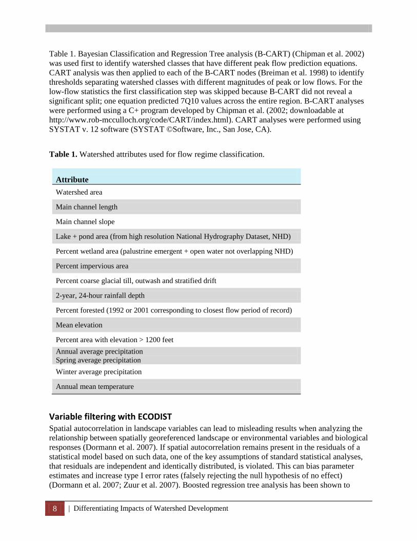
Table 1. Bayesian Classification and Regression Tree analysis (B-CART) (Chipman et al. 2002) was used first to identify watershed classes that have different peak flow prediction equations. CART analysis was then applied to each of the B-CART nodes (Breiman et al. 1998) to identify thresholds separating watershed classes with different magnitudes of peak or low flows. For the low-flow statistics the first classification step was skipped because B-CART did not reveal a significant split; one equation predicted 7Q10 values across the entire region. B-CART analyses were performed using a C+ program developed by Chipman et al. (2002; downloadable at http://www.rob-mcculloch.org/code/CART/index.html). CART analyses were performed using SYSTAT v. 12 software (SYSTAT ©Software, Inc., San Jose, CA).
Table 1. Watershed attributes used for flow regime classification.
Attribute Watershed area
Main channel length
Main channel slope
Lake + pond area (from high resolution National Hydrography Dataset, NHD)
Percent wetland area (palustrine emergent + open water not overlapping NHD)
Percent impervious area
Percent coarse glacial till, outwash and stratified drift
2-year, 24-hour rainfall depth
Percent forested (1992 or 2001 corresponding to closest flow period of record)
Mean elevation
Percent area with elevation > 1200 feet Annual average precipitation Spring average precipitation Winter average precipitation
Annual mean temperature
Variable filtering with ECODIST Spatial autocorrelation in landscape variables can lead to misleading results when analyzing the relationship between spatially georeferenced landscape or environmental variables and biological responses (Dormann et al. 2007). If spatial autocorrelation remains present in the residuals of a statistical model based on such data, one of the key assumptions of standard statistical analyses, that residuals are independent and identically distributed, is violated. This can bias parameter estimates and increase type I error rates (falsely rejecting the null hypothesis of no effect) (Dormann et al. 2007; Zuur et al. 2007). Boosted regression tree analysis has been shown to
Methods | 9
correct for some, but not all, spatial autocorrelation in spatial data sets (Valavanis et al. 2008; Abeare 2009; Crase et al. 2012).
Partial Mantel tests provide a relatively simple approach to test for and factor out the effects of spatial autocorrelation in relationships (King et al. 2005; Goslee and Urban 2007). Models to predict effects of urbanization on macroinvertebrate communities were developed for the subset of metrics identified through NMDS and indicator analysis. To differentiate the effect of land-use/land-cover variables operating at different scales and to factor out the effects of spatial autocorrelation, the R program ecodist was applied to screen potential models (King et al. 2005; Goslee and Urban 2007). Analyses were first run to evaluate partial effects, i.e., to determine if significant relationships could be found for each watershed-scale variable (factoring out watershed-scale effects of other variables) and for each flowline catchment-scale variable (factoring out other flowline catchment-scale effects). Partial effects were also evaluated for watershed- and flowline catchment-scale riparian buffer effects, after factoring out local flowline catchment-scale effects. Bonferroni-corrected p-values were used to determine if at least one predictor variable had significant partial effects at each scale (King et al. 2005). The appropriate scale (watershed or flowline catchment) and best predictor of urbanization effects (NUII_MA, %IA, or percent high density residential development) was chosen using models with lowest p-values. Depending on whether riparian buffer zone effects could be detected, final models with watershed- or flowline catchment-scale effects were run with or without the moderating effects of riparian buffer zones included.
Boosted regression tree model development Models that had been successfully pre-screened using partial Mantel tests were then evaluated with boosted regression tree analysis (De’Ath and Fabricius 2000; De’Ath 2002, 2007 using the gbmplus package (De’Ath 2002) in R. Predictor and response variables were first normalized to facilitate comparisons on a common scale. The number of trees was optimized based on the minimum holdout deviance. The number of predictor variables was reduced by choosing the minimum value (maximum negative value) for the change in predictive deviance as variables were removed (De’Ath 2002). When interaction terms were significant, bivariate response surfaces were examined.
Resistance thresholds (Lowest observed community effect levels (LOCEL)) and exhaustion thresholds (beyond which no more effects were observed; Cuffney et al. 2010) were calculated using BRT partial effects plots. Partial effects plots demonstrate the independent effect of each retained predictor variable while the influence of all other predictor variables is held constant (De’Ath 2002). We analyzed each set of BRT output points for partial effects using CART analysis in SYSTAT software, constrained to identify a maximum of two “Cut Values” for each predictor, with bootstrapping (n=250–300) to yield median thresholds with confidence intervals (5th to 95th percentiles).
10 | Differentiating Impacts of Watershed Development
RESULTS
Flow regime class derivation Bayesian CART analysis identified two classes of watersheds with different equations for 2-year peak flow prediction, distinguished by drainage area (Figure 3a, top). CART analysis subdivided each of these groups into three classes based on a combination of main channel slope and composite indices which incorporated effects of forest cover, 2-year 24 hour rain events, and fraction of elevation over 1200 feet and, for the high drainage area group, also percent wetlands and open water storage (Figure 3a, bottom). Bayesian CART analysis did not effect a separation of watersheds into classes based on differences in predictive equations for low flow (7Q10), but CART analysis did discriminate three watershed classes based on percent wetlands and a combined index comprised of winter: spring precipitation ratio, annual average temperature, and potential infiltration (percent coarse-grained substrate; Figure 3b).
O/E model development The best O/E models for each dataset, based on minimization of the standard deviation of O/E values, were based on 4 reference community types (clusters) for CT, 10 clusters for ME , and 7 clusters for NEWS . CT DEP community types were best predicted by a combination of low flow regime and Ecological Unit, with Cluster 3 dominating in low flow 7Q10 Node 1 and Cluster 2 dominating in Ecological Unit M212CC (Berkshire-Vermont Upland). The standard deviation for this O/E model was relatively poor, at a value of 0.22 (close to 0.1 is optimal, and over 0.2 is considered poor (van Sickle et al. 2006)). ME DEP community types were best predicted by lotic system size, geological buffering, and sample date (Julian Day; streams, rivers). Again, model performance was poor, with an O/E standard deviation of 0.31. The O/E model for NEWS was more complex, depending on size class, sample date (Julian Day), ecoregion, geological buffering, and thermal class for predicting community types. Performance of the NEWS O/E model was only slightly better, with an O/E standard deviation of 0.19.
Response metric selection Ordinations - For each data set, representative macroinvertebrate metrics were chosen
from each of the three ordination axes based on a display of biplots to focus on in subsequent predictive model development. While there was some overlap in variables (Ephemeroptera –Plecoptera-Trichoptera (EPT) taxa richness, fraction Mollusc + Crustacean richness) explaining the majority of variation among sites across the three data sets, the subsets chosen were not identical (Table 2). The abundance-weighted nitrate tolerance indicator was highly correlated with one axis of variation for NEWS but not for the other datasets. The burrower richness axis was unique to CT DEP, and fraction Orthoclad richness axis was unique to ME DEP.
Indicator analysis - With one exception, indicator analysis yielded similar results across the three datasets (Table 3). Trichoptera (and the related filterer-collector guild) were associated with low impervious area in Maine but with high impervious area in Connecticut. Habit guilds other than burrowers tended to be associated with low impervious area. Sensitive taxa groups (Ephemeroptera, Plecoptera, Odonata, Orthocladinae midges) tended to be associated with low
Results | 11
a)
b)
Figure 3. a) Results of Bayesian CART analysis to identify two classes of watersheds with different equations for area-normalized 2-year peak flow prediction, (Nodes 1 and 2), followed by CART analysis to further subdivide each of these groups by peak flow magnitude (Nodes 11,12,13,21,22,23). Splitting variables are shown as labels on the left side of each tree split. b) Results of CART analysis to discriminate three watershed classes for low flows (7Q10).
12 | Differentiating Impacts of Watershed Development
Table 2. Representative macroinvertebrate metrics selected for analysis based on correlation with nonmetric dimensional scaling ordination axes. (CT DEP = Connecticut Department of Environmental Protection; ME DEP = Maine Department of Environmental Protection, NEWS = EPA New England Wadeable Streams).
Data set Metrics selected Metric description CT DEP EPTr
fMCr BUr
Richness of Ephemeroptera, Plecoptera, and Trichoptera taxa Relative richness of Mollusc + Crustacea Taxa richness of burrower guild
ME DEP EPTr EPTCHr fORr
Richness of Ephemeroptera, Plecoptera, and Trichoptera taxa Ratio of EPT to Chironomidae richness Relative richness of Orthocladinae midges
NEWS EPTRf fMCr AwSNO3
Relative richness of EPT taxa Relative richness of Mollusks + Crustacea Abundance-weighted nutrient biotic index (Smith et al. 2007)
impervious area, with more tolerant taxa (Amphipoda, Isopoda) becoming relatively more abundant at high impervious sites. Trophic guilds shifted from specialists at low impervious area (predators, scrapers, shredders) to generalists (omnivores) at high impervious area.
ECODIST model screening results Effect of filtering out spatial autocorrelation on candidate predictor models - All of
the variables representing major axes of variation were retained for further analysis. Response variables that were filtered out by path analysis using Mantel’s r included taxa richness, Trichoptera richness (CT DEP, NEWS) or relative abundance (ME DEP), most of the habit guild metrics, trophic guild metrics other than relative abundance of shredders or predators, and relative abundance or richness of relatively rare taxa groups (relative abundance Cricotopus, Pteronarcys, Coleoptera, relative richness of Orthocladinae). With the exception of percent high density residential land-use, local flowline catchment effects were rarely detected after full watershed and riparian zone influences were accounted for. Riparian zone effects could be distinguished independently of whole watershed effects (and vice versa) in almost all cases (Appendix 4).
Best predictors of urbanization impacts - Highest partial Mantel r values were obtained for models containing percent imperviousness at the watershed scale and occasionally at the local flowline catchment scale (CT DEP), percent imperviousness or NUII_MA at the local flowline catchment scale (ME DEP), and percent imperviousness at the watershed scale (NEWS) (Appendix 4). Exceptions for which NUII_MA was the best urbanization predictor metric at the flowline catchment scale included taxa-weighted average nitrate sensitivity for NEWS, and two toxics sensitivity indices for CT DEP.
Results | 13
Table 3. Results of indicator analysis (Dufrene and Legendre 1997) to determine macroinvertebrate metrics that best discriminate between watersheds with <1% impervious cover and >10% impervious cover.
Dataset CT DEP ME DEP NEWS Lo-imperv (<1%) Hi-imperv (>10%) p-value p-value p-value Climbers 0.0066 0.0486 Clingers 0.0250 Swimmers 0.0004 0.0274 Sprawlers 0.0104 0.0300 EPT 0.0002 Mayflies (E) 0.0018 0.0002 0.0078 Stoneflies (P) 0.0002 0.0012 0.0006 Caddisflies (T) 0.0006 Caddisflies (T) 0.0026 Pteronarcys 0.0258 Orthocladinae midges 0.0168 Gastropods 0.0112 Isopods 0.002 0.0022 Amphipods 0.0232 Dragonflies 0.0002 Aquatic beetles 0.0002 0.0302 Predators 0.0002 0.0002 0.0464 Omnivores 0.0296 (0.0538) Filterer-collectors 0.0008 Filterer-collectors 0.0008 Scrapers 0.0002 0.0094 0.0366 Shredders 0.0046 0.0004
Boosted regression tree models Variable importance - The most frequent independent variables included in boosted
regression tree models overall were watershed area, Ecological Unit, and Slope Class, although the latter had a relatively low variable importance (7%; Table 4). For the CT DEP dataset, percent high density residential buffer and Superfund site density were included in most BRT models. For the ME DEP dataset, local road-stream crossing density and local percent imperviousness were commonly included as predictors. In BRT, the relative influence of predictor variables is calculated as the number of times a variable is selected for splitting, weighted by the squared improvement to the model as a result of each split, and averaged over all trees (Elith et al. 2008). Over all data sets, variable relative influence was particularly high for
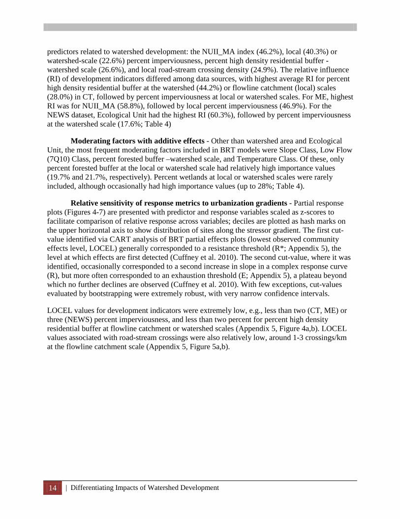
14 | Differentiating Impacts of Watershed Development
predictors related to watershed development: the NUII_MA index (46.2%), local (40.3%) or watershed-scale (22.6%) percent imperviousness, percent high density residential buffer - watershed scale (26.6%), and local road-stream crossing density (24.9%). The relative influence (RI) of development indicators differed among data sources, with highest average RI for percent high density residential buffer at the watershed (44.2%) or flowline catchment (local) scales (28.0%) in CT, followed by percent imperviousness at local or watershed scales. For ME, highest RI was for NUII_MA (58.8%), followed by local percent imperviousness (46.9%). For the NEWS dataset, Ecological Unit had the highest RI (60.3%), followed by percent imperviousness at the watershed scale (17.6%; Table 4)
Moderating factors with additive effects - Other than watershed area and Ecological Unit, the most frequent moderating factors included in BRT models were Slope Class, Low Flow (7Q10) Class, percent forested buffer –watershed scale, and Temperature Class. Of these, only percent forested buffer at the local or watershed scale had relatively high importance values (19.7% and 21.7%, respectively). Percent wetlands at local or watershed scales were rarely included, although occasionally had high importance values (up to 28%; Table 4).
Relative sensitivity of response metrics to urbanization gradients - Partial response plots (Figures 4-7) are presented with predictor and response variables scaled as z-scores to facilitate comparison of relative response across variables; deciles are plotted as hash marks on the upper horizontal axis to show distribution of sites along the stressor gradient. The first cut-value identified via CART analysis of BRT partial effects plots (lowest observed community effects level, LOCEL) generally corresponded to a resistance threshold (R*; Appendix 5), the level at which effects are first detected (Cuffney et al. 2010). The second cut-value, where it was identified, occasionally corresponded to a second increase in slope in a complex response curve (R), but more often corresponded to an exhaustion threshold (E; Appendix 5), a plateau beyond which no further declines are observed (Cuffney et al. 2010). With few exceptions, cut-values evaluated by bootstrapping were extremely robust, with very narrow confidence intervals.
LOCEL values for development indicators were extremely low, e.g., less than two (CT, ME) or three (NEWS) percent imperviousness, and less than two percent for percent high density residential buffer at flowline catchment or watershed scales (Appendix 5, Figure 4a,b). LOCEL values associated with road-stream crossings were also relatively low, around 1-3 crossings/km at the flowline catchment scale (Appendix 5, Figure 5a,b).
Results | 15
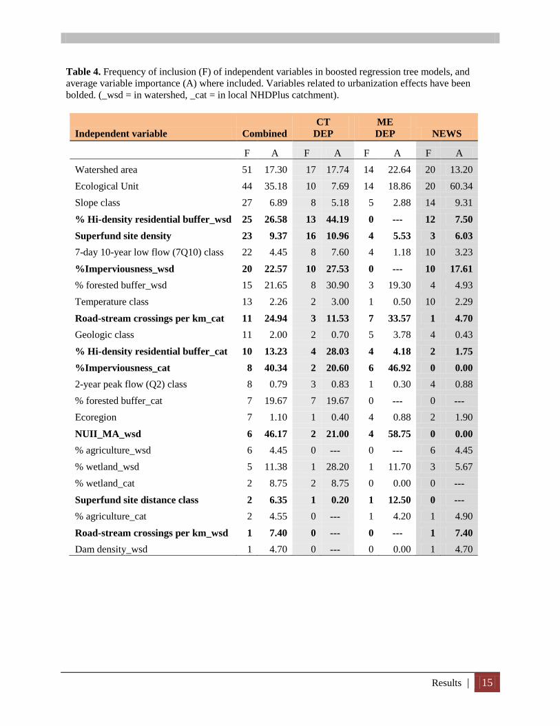
Table 4. Frequency of inclusion (F) of independent variables in boosted regression tree models, and average variable importance (A) where included. Variables related to urbanization effects have been bolded. (_wsd = in watershed, _cat = in local NHDPlus catchment).
CT ME NEWS Independent variable Combined DEP DEP
F A F A
F A
F A Watershed area Ecological Unit Slope class % Hi-density residential buffer_wsd Superfund site density 7-day 10-year low flow (7Q10) class %Imperviousness_wsd % forested buffer_wsd Temperature class Road-stream crossings per km_cat Geologic class % Hi-density residential buffer_cat %Imperviousness_cat 2-year peak flow (Q2) class % forested buffer_cat Ecoregion NUII_MA_wsd % agriculture_wsd % wetland_wsd % wetland_cat Superfund site distance class % agriculture_cat Road-stream crossings per km_wsd Dam density_wsd
51 44 27 25 23 22 20 15 13 11 11 10
8 8 7 7 6 6 5 2 2 2 1 1
17.30 35.18 6.89
26.58 9.37 4.45
22.57 21.65 2.26
24.94 2.00
13.23 40.34 0.79
19.67 1.10
46.17 4.45
11.38 8.75 6.35 4.55 7.40 4.70
17 10 8
13 16 8
10 8 2 3 2 4 2 3 7 1 2 0 1 2 1 0 0 0
17.747.695.18
44.1910.967.60
27.5330.90 3.00
11.53 0.70
28.03 20.60 0.83
19.67 0.40
21.00 ---
28.20 8.75 0.20 --- --- ---
14 14 5 0 4 4 0 3 1 7 5 4 6 1 0 4 4 0 1 0 1 1 0 0
22.6418.862.88
--- 5.531.18
--- 19.30 0.50
33.57 3.78 4.18
46.92 0.30 --- 0.88
58.75 ---
11.70 0.00
12.50 4.20 --- 0.00
20 20 14 12 3
10 10 4
10 1 4 2 0 4 0 2 0 6 3 0 0 1 1 1
13.20 60.34 9.31 7.50 6.03 3.23
17.61 4.93 2.29 4.70 0.43 1.75 0.00 0.88 --- 1.90 0.00 4.45 5.67 --- --- 4.90 7.40 4.70
16 | Differentiating Impacts of Watershed Development
a)
b)
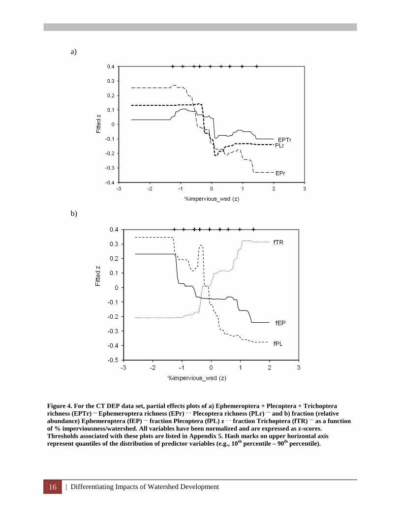
Figure 4. For the CT DEP data set, partial effects plots of a) Ephemeroptera + Plecoptera + Trichoptera richness (EPTr) __ Ephemeroptera richness (EPr) _ _ Plecoptera richness (PLr) … and b) fraction (relative abundance) Ephemeroptera (fEP) __ fraction Plecoptera (fPL) z _ _ fraction Trichoptera (fTR) … as a function of % imperviousness/watershed. All variables have been normalized and are expressed as z-scores. Thresholds associated with these plots are listed in Appendix 5. Hash marks on upper horizontal axis represent quantiles of the distribution of predictor variables (e.g., 10th percentile – 90th percentile).
Results | 17
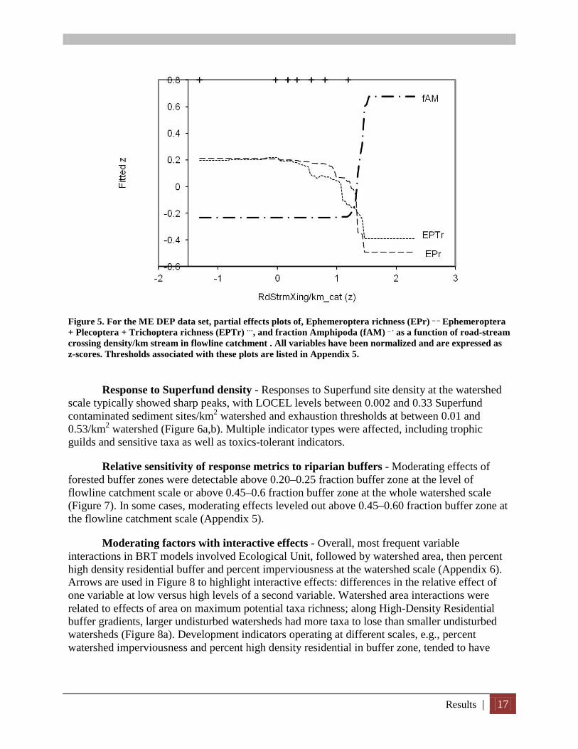
Figure 5. For the ME DEP data set, partial effects plots of, Ephemeroptera richness (EPr) _ _ Ephemeroptera + Plecoptera + Trichoptera richness (EPTr) …, and fraction Amphipoda (fAM) _ . as a function of road-stream crossing density/km stream in flowline catchment . All variables have been normalized and are expressed as z-scores. Thresholds associated with these plots are listed in Appendix 5.
Response to Superfund density - Responses to Superfund site density at the watershed scale typically showed sharp peaks, with LOCEL levels between 0.002 and 0.33 Superfund contaminated sediment sites/km2 watershed and exhaustion thresholds at between 0.01 and 0.53/km2 watershed (Figure 6a,b). Multiple indicator types were affected, including trophic guilds and sensitive taxa as well as toxics-tolerant indicators.
Relative sensitivity of response metrics to riparian buffers - Moderating effects of forested buffer zones were detectable above 0.20–0.25 fraction buffer zone at the level of flowline catchment scale or above 0.45–0.6 fraction buffer zone at the whole watershed scale (Figure 7). In some cases, moderating effects leveled out above 0.45–0.60 fraction buffer zone at the flowline catchment scale (Appendix 5).
Moderating factors with interactive effects - Overall, most frequent variable interactions in BRT models involved Ecological Unit, followed by watershed area, then percent high density residential buffer and percent imperviousness at the watershed scale (Appendix 6). Arrows are used in Figure 8 to highlight interactive effects: differences in the relative effect of one variable at low versus high levels of a second variable. Watershed area interactions were related to effects of area on maximum potential taxa richness; along High-Density Residential buffer gradients, larger undisturbed watersheds had more taxa to lose than smaller undisturbed watersheds (Figure 8a). Development indicators operating at different scales, e.g., percent watershed imperviousness and percent high density residential in buffer zone, tended to have
18 | Differentiating Impacts of Watershed Development
a)
b)
Figure 6. Partial effects plots of a) NEWS regional Bray-Curtis dissimilarity index (B-C) __ fraction Isopoda (fIS) _ _ fraction Plecoptera (fPL) … and b) CT Ephemeroptera + Plecoptera + Trichoptera richness (EPTr) __ taxa-weighted average metals sensitivity (TAWMet) _ _ Coefficient of Community Loss (CCL) … fraction Trichoptera (fTR) _ as a function of Superfund site density/km2 watershed. All variables have been normalized and are expressed as z-scores. Thresholds associated with these plots are listed in Appendix 5.
Results | 19
Figure 7. For the CT DEP data set, partial effects plots of fraction Predators (fPR) __ fraction Shredders (fSH) _ _ fraction Filterer-Collectors (fFC) as a function of percent forested buffer/flowline catchment. All variables have been normalized and are expressed as z-scores. Thresholds associated with these plots are listed in Appendix 5. synergistic effects with combined impacts greater than expected (Figure 8b). Forested riparian buffers moderated the effects of percent imperviousness effects at the watershed scale (Figure 8c). Interactions involving Ecological Unit tended to reflect differences in maximum potential metric values at intermediate spatial scales, essentially unexplained geographic variability.
20 | Differentiating Impacts of Watershed Development
a) b)
c)
Figure 8. a) Watershed area interactions were related to effects of area on maximum potential EPT taxa richness. b) Synergistic effect of % watershed imperviousness and % high density residential buffer on EPT taxa richness with CT DEP data. c) Interaction of forested buffer zone moderating impact of % impervious watershed on Plecoptera richness with CT DEP data. All variables have been normalized and are expressed as z-scores. Thresholds associated with these plots are listed in Appendix 5.
Discussion | 21
DISCUSSION
Urbanization indicators, model sensitivities and spatial scale Our study is the first to simultaneously compare alternative urbanization metrics in response models, distinguish the independent effects of urbanization operating at different scales (e.g., road crossings versus high intensity residential development in buffer zones versus full watershed IA), and discriminate the cumulative effects of upstream Superfund site density from that of watershed development. Most previous studies have been unable to distinguish between effects of urban development in the stream buffer zone versus total IA in the whole watershed because of high spatial autocorrelation (Carlisle and Meador 2007), which we factored out using pre-screening models via the methods of King et al. (2005). The inclusion of high-density residential development in the buffer zone as a predictor in our best models, with effects independent of spatial autocorrelation and % total IA in the watershed, is consistent with the findings of other studies showing a localized zone of influence of tens of meters (King et al. 2005; Urban et al. 2006; van Sickle and Johnson 2008). The low thresholds of impact observed for percent high-density residential buffer in our models might signal the initiation of effects from creation of stormwater drainage networks within watersheds (Walsh 2004; Walsh et al. 2005a). Alternatively, high density residential development in buffer zones could interfere with upstream migration of adult winged insects and recovery from the effects of more frequent spates in urban settings (Smith et al. 2009).
Our urbanization-response models probably could be improved through calculation of effective impervious cover (EIC) rather than total IA (Walsh 2004; Walsh et al. 2005a,b; Han and Burian 2009; Roy and Shuster 2009). However, accurate estimation of EIC would require regional mapping of stormwater drains and networks, data that are currently not available across New England.
Relative sensitivity of response metrics The failure of other studies to account for moderating factors could mask detection of early threshold responses at coarse taxonomic levels. Unlike King and Baker (2011), we were able to detect relatively early declines in aggregate response variables such as Ephemeroptera or Plecoptera richness, starting at as low as 1% total impervious area. King and Baker (2011) argue that low response thresholds (0.5–2% IA) for individual declining taxa measured through TITAN analyses were missed by earlier investigators because of the common practice of creating aggregate metrics at coarser levels of taxonomic resolution across taxa with a range of sensitivities. King and Baker (2011) and other investigators (Appendix 7) typically apply models with a single predictor, without accounting for modifying influences of watershed area, slope or flow regime class, or moderating factors such as forested riparian buffer zones.
Response thresholds and interactions Urbanization - Cuffney et al. (2010) distinguish between three types of response patterns: a) linear response, b) an initial linear response with a breakpoint (shift to lesser slope) at some intermediate level of urbanization, and c) an initial delay in response followed by a linear response after a resistance threshold is reached, followed by a second change to a lesser or zero slope after an exhaustion threshold is reached. All three response types have been noted in the
22 | Differentiating Impacts of Watershed Development
literature (Appendix 6), although in many cases rigorous testing for threshold existence, location, and uncertainty bounds is lacking (Qian and Cuffney 2012).
We were able to demonstrate significant declines even in aggregate community metrics at very low levels of urbanization (<1–2% IA), once effects of moderating variables had been factored out (see also Smucker et al. 2013). These thresholds are comparable to or lower than reported resistance thresholds for individual sensitive taxa (5–15% IA in Boston area streams (King 2011), 1.2–10.3% IA in MD Coastal Plain streams (Utz et al. 2009) and 0.9–35.7% IA in MD Piedmont streams (Utz et al. 2009). Aggregate community metrics that don’t distinguish between sensitive and non-sensitive taxa have typically showed larger resistance thresholds: NUII_MA = 13–19 (Cuffney et al. 2010, King and Baker 2011), and 2.5–5% IA for total richness or EPT-richness (Goetz and Fiske 2008; Hilderbrand et al. 2010) when effects of moderating factors are not accounted for.
Exhaustion thresholds are typically associated with richness metrics, where all sensitive taxa within a Class or Order drop out, leaving only a few tolerant taxa remaining (Morse et al. 2003; Coles et al. 2004; Deacon et al. 2005). Our partial response plots for richness-related metrics in the present study also showed exhaustion thresholds at low to moderate levels of imperviousness for sensitive metrics in all three data sets: CT DEP: 4–7% IA, ME DEP and NEWS: 2–3% IA. Examples of continuous linear declines in EPT-richness (Coles et al. 2004) are probably the result of site selection biases which favored sites with intact riparian zones which moderate urbanization impacts.
Forested riparian buffers - The effect of forested riparian zones in moderating the impacts of urbanization is currently in dispute ( Moore and Palmer 2005; Roy et al. 2005; Walsh et al. 2007). Effects of forested riparian buffers on water quality at the watershed scale can be more pronounced during baseflow conditions (Stewart et al. 2006) than during storm events, when stormwater runoff is routed through stormwater pipes, which expand effective IA from a narrow riparian zone to the entire stormwater network (Walsh and Kunapoo 2009).
More recent literature has highlighted the importance of forested riparian zones in maintaining aquatic insect populations even in the absence of instream habitat degradation because of their facilitation of terrestrial dispersal of adult winged stages (Smith et al. 2009). Spatial autocorrelation in aquatic community composition and abundance after correction for correlation of environmental variables provides evidence of dispersal-limited populations (Urban et al. 2006; Bonada et al. 2012). Spatial autocorrelation of macroinvertebrate taxa declines linearly with an index of dispersal ability that takes into account media (aquatic vs. aerial) and energetics (passive vs. active) of dispersal; Bonada et al. 2012). Urban-sensitive taxa such as Ephemeroptera and Plecoptera have intermediate dispersal abilities. Loss of dispersal corridors is expected to have an even greater impact in streams within high % IA watersheds and frequent hydrological disturbance, leading to an interaction between riparian buffer effectiveness and % IA impacts. Watershed recovery can be facilitated by proximity and quality of surrounding immigrant pools (Patrick and Swan 2011).
Superfund site density - The cumulative effect of Superfund site density within a watershed on downstream biotic condition that we detected has not been reported previously, although urban gradient studies have documented an increase in PAHs, pesticides, herbicides, and heavy metals in surface water (Gregory and Calhoun 2007) and stream sediments (Marshall

Discussion | 23
et al. 2010). Marshall et al. (2010) determined that biotic indices in their urban streams were generally more highly correlated with percent industrial/commercial land-use and a heavy metal quotient than with percent effective impervious area. They confirmed the influence of sediment-based contaminants through bioassays in which sediment from urban sites significantly altered macroinvertebrate communities in microcosms populated with native taxa.
Discriminating local contamination effects from watershed development Few studies have attempted to link urbanization effects to toxicity (Bryant and Goodbred 2009; Marshall et al. 2010), and none previously have attempted to discriminate effects from diffuse nonpoint sources upstream as compared to local contaminated sediments or point-source inputs (e.g., Superfund sites; permit compliance system; toxics release inventory permits). Many of the richness indicators most sensitive to urbanization effects exhibit exhaustion thresholds and thus are relatively insensitive at moderate to high levels of % IA to additional stressors associated with Superfund sites. Community metrics traditionally used in construction of IBIs tend to be sensitive to low dissolved oxygen and fine sediments but do not necessarily coincide with taxa sensitivity rankings for PAHs and heavy metals (Wogram and Liess 2001). However, we found that metrics specifically diagnostic of toxicity can be used to discriminate effects of Superfund activity upstream in the watershed from effects of upstream development and could serve as potential measures of improvement in biological condition in response to site remediation and restoration activities.
Moderating factors (watershed area, flow regime, slope class) Stream theory suggests that macroinvertebrate diversity should increase with stream size as habitat complexity increases, peaking in medium-size rivers (Minshall et al. 1985). The species-area relationship, in combination with the existence of exhaustion thresholds for sensitive EPT-taxa, produces an interactive effect between watershed area and urbanization effects, with greater losses in large watersheds.
Few studies have evaluated the influence of different slope or flow regime classes on sensitivity of macroinvertebrate communities to urbanization (Utz et al. 2009; Cuffney et al. 2011). Cuffney et al. (2011) explained variation in sensitivity of response across nine metropolitan areas as a function of antecedent land-use and regional differences in precipitation and temperature. Utz et al. (2009, 2011) have found differences in sensitivity of macroinvertebrate communities, hydrology, and thermal regime between Piedmont and Coastal Plain regions of Maryland, with differences in thermal sensitivity (but not hydrology) being consistent with differences in biological sensitivity. Utz and Hilderbrand (2011) further investigated differences in geomorphological sensitivity and found greater changes in sediment deposition and size of mobile particles with urbanization in Piedmont streams. They concluded that geomorphic degradation is greater in Piedmont streams and organisms in Coastal Plain streams may be adapted to benthic instability.
With one exception, most slope class effects in our response models were simple or interacted with Ecological Unit rather than urbanization. We did observe an interaction between slope class and percent imperviousness for ME DEP Ephemeroptera richness, with higher values in low gradient systems at low percent imperviousness. Maine abundance-weighted and NEWS taxa-weighted metal sensitivity tended to be lower in low-gradient streams (<0.1% slope). In the NEWS dataset, relative EPT richness, relative abundance Orthocladinae midges, relative
24 | Differentiating Impacts of Watershed Development
abundance Plecoptera, relative Plecoptera richness, and percent shredders were higher and percent omnivores lower in high gradient streams but the difference varied across Ecological Units and did not interact with urbanization effects. However, the NEWS Bray-Curtis coefficient of community dissimilarity did show a greater response to percent watershed imperviousness in low gradient systems. Likewise, we did observe a few interactions of stream temperature or low-flow class with urbanization effects.
Potential effects of study design and sampling methods on detection of urbanization and Superfund site effects Management agencies tend to apply either probabilistic survey designs or targeted designs, rarely combining features of both approaches; this was the case for the three sets of monitoring program results analyzed here. Spatially-balanced probabilistic frameworks are designed to maximize the information content of each monitoring site (avoiding the selection of spatially correlated sites based on Euclidean distance) and to produce unbiased estimates of regional condition with known confidence intervals. Targeted designs are used by agencies in conjunction with upstream-downstream sampling to minimize background variation and yield paired comparisons (e.g., with and without a point source), to stratify by predominant land-use, and/or to evaluate trends at fixed sites over time to evaluate the effects of management practices. However, neither of these survey approaches is designed to optimize the distribution of sites along a gradient of interest. The first stage of a spatially-balanced design is essentially hexagon-based. Grid-based designs (even with a subsequent probabilistic element) tend to under sample relatively rare clustered entities such as urban land-use because these are not randomly distributed (Worner et al. 2009). Conversely, targeted designs, particularly those focused on point sources, could under sample the lower or middle portion of the urbanization gradient. Gaps in the distribution of sites along an urbanization gradient could produce apparent threshold responses as an artifact of sampling. Bootstrapping would yield very wide confidence intervals for artificial thresholds generated near the boundary of a gap. This was not the case for our analyses. Ideally, survey frameworks applied in the future to evaluate responses along urban gradients will incorporate either random-stratified designs or designs with unequal probability weighting for sites associated with different levels of development in the upstream watershed. Survey designs based on simulation models also offer potential for optimizing future sampling designs to reduce areas of uncertainty (Urban 2000).
Variation in relative importance of development indicators in urbanization-response models, sensitivity of response variables, and detection of thresholds could have been influenced by differences in field sampling and laboratory protocols across the three monitoring programs (see Appendix 1). The Maine DEP monitoring program is more likely to detect urbanization effects associated with water quality as compared to habitat because indirect effects related to physical habitat degradation are minimized by the provision of artificial substrates (rock baskets). The NEWS sampling protocols yield higher taxa diversity overall than CT DEP protocols (Jessup and Gerritsen 2006), and thus are less likely to exhibit exhaustion thresholds. NEWS protocols have the potential to evaluate impacts across a wider variety of habitats, but pooling of samples across habitat types could reduce the power of detecting effects specific to riffles. A paired comparison of methods across CT DEP (800–900 micron mesh) and NEWS (600 mesh) has shown a greater proportion of midges in samples processed with NEWS as compared to CT DEP protocols. Other comparisons (keeping mesh size constant) have also shown differences in percent Ephemerop-tera, percent chironomids, and percent Plecoptera and Trichoptera (Hydropsychidae excluded)
Conclusions | 25
between single and multiple habitat protocols (Blocksom et al. 2008). Macroinvertebrate metrics were significantly correlated for samples processed with the NEWS versus CT DEP protocols (Jessup and Gerritsen 2006), although less so for Hydropsychidae and midges. It is possible that the CT DEP monitoring program is less likely to detect differences in smaller-sized indicator taxa.
CONCLUSIONS The sensitivity of urban effects models to predict responses to watershed development at low levels of imperviousness was enhanced by conducting separate analyses by data source, focusing on a suite of independent indicators that explain the maximum amount of variation in each data set and/or are strongly associated with gradients (% IA) of interest, and including the effects of spatial autocorrelation, ancillary effects such as watershed area, Ecological Unit, low flow regime class, slope class, and moderating effects of forested riparian buffers. With the exception of the Maine dataset, % IA and percent high density residential area in the stream buffer at the watershed scale were the best predictors of watershed development effects. For some variables, the independent effects of road-stream crossings also could be detected. Where both watershed- and local-scale development indicators were significant in models, they tended to have synergistic (more than additive) effects.
Resistance thresholds for aggregate community metrics were apparent at very low levels of percent imperviousness at the watershed scale (<1–3%) and of percent high density residential area in stream buffers (<1%). This contradicts earlier suggestions that low thresholds for impairment have been masked in analyses by the practice of lumping taxa of different sensitivities, and suggests that factoring out effects of ancillary variables is equally important. Exhaustion thresholds were also apparent in partial effects plots, particularly for richness-related metrics, as sensitive species were lost. Although exhaustion thresholds limited our ability to detect the effects of upstream Superfund site density for some sensitive metrics, we were able to detect Superfund site effects using specific indicators diagnostic of toxic effects, and to distinguish these from the effects of watershed development.
We were able to demonstrate the effect of forested riparian buffers in moderating approximately one-third to one-half of the level of urbanization impacts. Thresholds for forested riparian zones were not as pronounced as those associated with watershed development, but levels of 40-60% forested riparian area represented zones of greatest effectiveness (steepest slopes in partial effects plots). Although many have argued that forested buffers have limited benefits for urban streams because they are bypassed by urban stormwater infrastructure, forested buffers can still have important functions in urban settings, including temperature moderation, stabilization of stream banks, and provision of migration/recolonization corridors and oviposition sites for adult winged insects.
26 | Differentiating Impacts of Watershed Development
LITERATURE CITED Abeare, S. M. 2009. Comparisons of boosted regression tree, GLM, and GAM performance in
the standardization of yellowfin tuna catch-rate data from the Gulf of Mexico online fishery. Master’s thesis (Louisiana State University, Baton Rouge, LA).
Ahearn, E. A. 2004. Regression equations for estimating flood flows for the 2-, 10-, 25-, 50-,
100-, and 500-year recurrence intervals in Connecticut, Scientific Investigations Report 2004-5160. U.S. Geological Survey, Reston, VA, USA.
Ahearn, E. A. 2008. Flow durations, low-flow frequencies, and monthly median flows for
selected streams in Connecticut through 2005. U.S. Geological Survey Scientific Investigations Report 2007-5270. U.S. Geological Survey, Reston, VA, USA.
Baker, M. E. and R. S. King. 2010. A new method for detecting and interpreting biodiversity and
ecological community thresholds. Methods in Ecology & Evolution 1:25–37. Barbour, M. T., J. Gerritsen, B. D. Snyder, and J. B. Stribling. 1999. Rapid bioassessment
protocols for use in streams and wadeable rivers: Periphyton, benthic macroinvertebrates and fish. EPA 841-B-99-002. U.S. Environmental Protection Agency, Office of Water, Washington, D. C., USA.
Bellucci, C., M. Beauchene, and M. Becker. 2008. Physical, chemical, and biological attributes
of moderately developed watersheds within Connecticut. Accessed online http://www.neiwpcc.org/npsconference/08-presentations/Bellucci.pdf
Bonada, N., S. Dolédec, and B. Statzner. 2012. Spatial autocorrelation patterns of stream
invertebrates: exogenous and endogenous factors. Journal of Biogeography 39:56–68. Breiman, L., J. Friedman, C. J. Stone, and R. A. Olshen. 1998. Classification and Regression
Trees. CRC Press, Boca Raton, FL, USA. Brown, L. R., T. F. Cuffney, J. F. Coles, F. Fitzpatrick, G. McMahon, J. J. Steuer, A. H. Bell,
and J. T. May. 2009. Urban streams across the USA:lessons learned from studies in 9 metropolitan areas. Journal of the North American Benthological Society 28:1051–1069.
Bryant, W. L. and S.L. Goodbred. 2009. The response of hydrophobic organics and potential
toxicity in streams to urbanization of watersheds in six metropolitan areas of the United States. Environmental Monitoring and Assessment 157:419–447.
Brydon, J., I. Oh, J. Wilson, K. Hall, and H. Schreier. 2009. Evaluation of mitigation methods to
manage contaminant transfer in urban watersheds. Water Quality Research Journal of Canada 44:1–15.
Literature Cited | 27
Carlisle, D. M. and M. R. Meador. 2007. A biological assessment of streams in the Eastern United States using a predictive model for macroinvertebrate assemblages. Journal of the American Water Resources Association 43:1194–1207.
Carlisle, D. M., M. R. Meador, S. R. Moulton II, and P. M. Ruhl. 2007. Estimation and
application of indicator values for common macroinvertebrate genera and families of the United States. Ecological Indicators 7:22–33.
Chadwick, M. A., D. R. Dobberfuhl, A. C. Benke, A. D. Huryn, K. Suberkropp, and J. E. Thiele.
2006. Urbanization affects stream ecosystem function by altering hydrology, chemistry, and biotic richness. Ecological Applications 16:1796–1807.
Chipman, H. A., E. I. George, and R. E. McCulloch. 2002. Bayesian treed models. Machine
Learning 48:299–320. Coles, J. F., T. F. Cuffney, G. McMahon, and K. M. Beaulieu. 2004. The effects of urbanization
on the biological, physical, and chemical characteristics of coastal New England streams. Professional Paper 1695, U.S. Geological Survey, Reston, VA, USA.
Crase, B., A. C. Liedloff, and B.A. Wintle. 2012. A new method for dealing with residual spatial
autocorrelation in species distribution models. Ecography. 35: 879–88. Cuffney, T. F., M. D. Bilger, and A. M. Haigler. 2007. Ambiguous taxa:effects on the
characterization and interpretation of invertebrate assemblages. Journal of the North American Benthological Society 26:286–307.
Cuffney, T. F., and J. A. Falcone. 2009. Derivation of nationally consistent indices representing
urban intensity within and across nine metropolitan areas of the conterminous United States. U.S. Geological Survey Scientific Investigations Report 2008-5095, U.S. Geological Survey, Reston, VA, USA.
Cuffney, T. F., R. A. Brightbill, J. T. May, and I. R. Waite. 2010. Responses of benthic
macroinvertebrates to environmental changes associated with urbanization in nine metropolitan area. Ecological Applications 20:1384–1401.
Cuffney, T. F., R. Kashuba, S. S. Qian, I. Alameddine,YoonKyung Cha, B. Lee, J. F. Coles, and
G. McMahon. 2011. Multilevel regression models describing regional patterns of invertebrate and algal responses to urbanization across the USA. Journal of the North American Benthological Society 30:797–819.
Daley, M. L., J. D. Potter, and W. H. McDowell. 2009. Salinization of urbanizing New
Hampshire streams and groundwater:effects of road salt and hydrologic variability. Journal of the North American Benthological Society 28:929–940.

28 | Differentiating Impacts of Watershed Development
Davies, P.J., I.A. Wright, S. J. Findlay, O. J. Jonasson, and S. Burgin. 2010. Impact of urban development on aquatic macroinvertebrates in south eastern Australia: degradation of in-stream habitats and comparison with non-urban streams. Aquatic Ecology 44:685–700.
Davies, S. P., L. Tsomides, D. Courtemanch, and F. Drummond. 1995. Maine Biological
Monitoring and Biocriteria Development Program. Report DEP-LW108. Maine Department of Environmental Protection, Augusta, ME, USA.
De’Ath, G. 2002. Multivariate regression trees:a new technique for modeling species-
environment relationships. Ecology 83:1105–1117. De’Ath, G. 2007. Boosted trees for ecological modeling and prediction. Ecology 88(1):243-251. De’Ath, G. and K. E. Fabricius. 2000. Classification and regression trees:A powerful yet simple
technique for ecological data analysis. Ecology 81:3178–3192. Deacon, J. R., S. A. Soule, and T. E. Smith. 2005. Effects of urbanization on stream quality at
selected sites in the Seacoast region in New Hampshire, 2001–03. U.S. Geological Survey Scientific Investigations Report 2005-5103, U.S. Geological Survey, Reston, VA, USA.
Dormann, C.F., J. M. McPherson, M. B. Araujo, R. Bivand, J. Bolliger, G. Carl, R. G. Davies, A.
Hirzel, W. Jetz, W. D. Kissling, I. Kuhn, R. Ohlemüller, P. R. Peres-Neto, B. Reineking, B. Schröder, F. M. Schurr and R. Wilson. 2007. Methods to account for spatial autocorrelation in the analysis of species distributional data: a review. Ecography 30: 60–628.
Dudley, R. W. 2004. Estimating monthly, annual, and low 7-Day, 10-year streamflows for
ungaged rivers in Maine, Scientific Investigations Report 2004-5026, U.S. Geological Survey, Reston, VA, USA.
Dufrene, M. and P. Legendre. 1997. Species assemblages and indicator species: The need for a
flexible asymmetrical approach. Ecological Monographs 67:345–366. Elith, J., J. R. Leathwick, and T. Hastie. 2008. A working guide to boosted regression trees.
Journal of Animal Ecology 77:802–13. Fitzpatrick, F. A. and M. C. Peppler. 2010. Relation of urbanization to stream habitat and
geomorphic characteristics in nine metropolitan areas of the United States. U.S. Geological Survey Scientific Investigations Report 2010-5056, U.S. Geological Survey, Reston, VA, USA.
Flynn, R. H. 2003. Development of regression equations to estimate flow durations and low-
flow-frequency statistics in New Hampshire streams. Water-Resources Investigations Report 02-4298, U.S. Geological Survey, Reston, VA, USA.
Goetz, S. and G. Fiske. 2008. Linking the diversity and abundance of stream biota to landscapes
in the mid-Atlantic USA. Remote Sensing of Environment 112:4075–4085.
Literature Cited | 29
Goslee, S. C. and D. L. Urban. 2007. The ecodist package for dissimilarity-based analysis of ecological data. Journal of Statistical Software 22:1–19.
Gregory, M. B. and D. L. Calhoun. 2007. Physical, chemical, and biological responses of
streams to increasing watershed urbanization in the Piedmont Ecoregion of Georgia and Alabama. U.S. Geological Survey Scientific Investigations Report 2006-5101-B. U.S. Geological Survey, Reston, VA, USA.
Griffith, G. E., J. M. Omernik, S. A. Bryce, J. Royte, W. D. Hoar, J. Homer, D. Keirstead, K. J.
Metzler, and G. Hellyer. 2009. Ecoregions of New England (color poster with map, descriptive text, summary tables, and photographs), U.S. Geological Survey (map scale 1:1,325,000). U.S. Geological Survey, Reston, VA, USA.
Han, W. S. and S. J. Burian. 2009. Determining effective impervious area for urban hydrologic
modeling. Journal of Hydrologic Engineering 14:111–120. Hatt, B.E., T.D. Fletcher, C.J. Walsh, and S.L. Taylor. 2004. The influence of urban density and
drainage infrastructure on the concentrations and loads of pollutants in small streams. Environmental Management 34: 112–134.
Hawkins, C. P. 2006. Quantifying biological integrity by taxonomic completeness:Its utility in
regional and global assessments. Ecological Applications 16(4):1277–1294. Hilderbrand, R. H., R. M. Utz, S. A. Stranko, and R. L. Raesly. 2010. Applying thresholds to
forecast potential biodiversity loss from human development. Journal of the North American Benthological Society 29:1009–1016.
Imberger, S.J., C.J. Walsh, and M.R. Grace. 2008. More microbial activity, not abrasive flow or
shredder abundance, accelerates breakdown of labile leaf litter in urban streams. Journal of the North American Benthological Society 27:549–561.
Jessup, B. and J. Gerritsen. 2006. Data and Assessment Comparability Among Stream
Bioassessment Methods: EPA-NEWS Methods and New England State Methods. TetraTech, Inc., Montpelier, VT.
Kaushal, S. S., P. M. Groffman, G. E. Likens, K. T. Belt, W. P. Stack, V. R. Kelly, L. E. Band,
and G. T. Fisher. 2005. Increased salinization of fresh water in the northeastern United States. Proceedings of the Academy of Natural Sciences 102:13517-13520.
Kennen, J. G., K. Riva-Murray, and K. M. Beaulieu. 2010. Determining hydrologic factors that
influence stream macroinvertebrate assemblages in the northeastern US. Ecohydrology 33:88–106.
King, R. S., M. E. Baker, D. F. Whigham, D. E. Weller, T. E. Jordan, P. F. Kazyak, and M. K.
Hurd. 2005. Spatial considerations for linking watershed land cover to ecological indicators in streams. Ecological Applications 15:137–153.
30 | Differentiating Impacts of Watershed Development
King, R. S. and M. E. Baker. 2011. How novel is too novel? Stream community thresholds at exceptionally low levels of catchment urbanization. Ecological Applications 21:1659–1678.
Malmquist, B. and S. Rundle. 2002. Threats to the running water ecosystems of the world.
Environmental Conservation 29:134–153. Marshall, S., V. Pettigrove, M. Carewa, and A. Hoffmann. 2010. Isolating the impact of
sediment toxicity in urban streams. Environmental Pollution 158:1716–1725. Maxwell, J. R., C. J. Edwards, C. J. Edwards, M. E. Jensen, S. J. Paustian, H. Parrott, and D. M.
Hill. 1995. A hierarchical framework of aquatic ecological units in North America (Nearctic Zone). General Technical Report NC-176:72. USDA Forest Service, North Central Forest Experiment Station, St Paul, MN, USA.
McCune, B., J. B. Grace, and D. L. Urban. 2002. Analysis of Ecological Communities, MjM
Software Design, Gleneden Beach, OR, USA. MacDonald, D.D. and C.G. Ingersoll. 2002. A Guidance Manual to Support the Assessment of
Contaminated Sediments in Freshwater Ecosystems, Vols I-III. U.S. Environmental Protection Agency, Great Lakes Program Office, Chicago, IL. EPA-905-B02-001-A/B/C.
Minshall, G. W., K. W. Cummins, R. C. Petersen, C. E. Cushing, D. A. Bruns, J. R. Sedell and
R. L. Vannote. 1985. Developments in stream ecosystem theory. Canadian Journal of Fisheries and Aquatic Sciences 42:1045–1055.
Moore, A. A. and M. A. Palmer. 2005. Invertebrate biodiversity in agricultural and urban
headwater streams:Implications for conservation and management Ecological Applications 15:1169–1177.
Morse, C. C., A. D. Huryn, and C. Cronan. 2003. Impervious surface area as a predictor of the
effects of urbanization on stream insect communities in Maine, U.S.A. U.S.A. Environmental Monitoring and Assessment 89:95–127.
Olivero, A. P. and M. G. Anderson. 2008. Northeast aquatic habitat classification system.
Boston, MA, The Nature Conservancy Eastern Regional Office, Boston, MA, USA. Olson, S. A. 2002. Flow-frequency characteristics of Vermont streams. U.S. Geological Survey
Water-Resources Investigations Report 02-4238, U.S. Geological Survey, Reston, VA, USA.
Olson, S. A. 2009. Estimation of flood discharges at selected recurrence intervals for streams in
New Hampshire, U.S. Geological Survey Scientific Investigations Report 2008-5206, U.S. Geological Survey, Reston, VA, USA.
Omernik, J. M. 1987. Ecoregions of the Conterminous United States, U.S. Environmental
Protection Agency, Corvallis Environmental Research Lab., OR, USA.
Literature Cited | 31
Patrick, C. J. and C. M. Swan. 2011. Reconstructing the assembly of a stream-insect metacommunity. Journal of the North American Benthological Society 30:259–272.
Purcell, A. H., D.W. Bressler, M. J. Paul, M. T. Barbour, E. T. Rankin, J. L. Carter, and V. H.
Resh. 2009. Assessment tools for urban catchments:developing biological indicators based on benthic macroinvertebrates. Journal of the American Water Resources Association 45:306–319.
Qian, S. S. and T. F. Cuffney. 2012. To threshold or not to threshold? That’s the question.
Ecological Indicators 15:1–9. Ries, K. G., III and P. J. Friesz. 2000. Methods for estimating low-flow statistics for
Massachusetts streams. Water-Resources Investigations Report 00-4135 , U.S. Geological Survey, Reston, VA, USA.
Rosiu, C. and J. Coles. 2005. Standardizing sediment risk characterization on the basis of urban
intensity of the watershed. EPA Science Forum, Collaborative Science for Environmental Solutions, U.S. Environmental Protection Agency, Washington, D.C., USA.
Roy, A. H., C. L. Faust, M. C. Freeman, and J. L. Meyer 2005. Reach-scale effects of riparian
forest cover on urban stream ecosystems. Canadian Journal. of Fisheries and Aquatic Sciences 62:2312–2329.
Roy, A. H. and W. D. Shuster. 2009. Assessing impervious surface connectivity and applications
for watershed management. Journal of the American Water Resources Association 45:198–209.
Smith, A. J., R. W. Bode, and G. S. Kleppel. 2007. A nutrient biotic index (NBI) for use with
benthic macroinvertebrate communities. Ecological Indicators 7:371–386. Smith, R. F., L. C. Alexander, and W. O. Lamp. 2009. Dispersal by terrestrial stages of stream
insects in urban watersheds:A synthesis of current knowledge. Journal of the North American Benthological Society 28:1022–1037.
Smucker, N. J., N. E. Detenbeck, and A. C. Morrison. 2013. Diatom indicators of urban
development:impervious cover thresholds and moderating effects of riparian green infrastructure. Freshwater Science 32:230–249.
Snook, H., S. P. Davies, J. Gerritsen, B. K. Jessup, R. Langdon, D. Neils, E. Pizutto. 2007. The
New England Wadeable Stream Survey (NEWS):development of common assessments in the framework of the Biological Condition Gradient. Washington, D.C., U.S. Environmental Protection Agency, Office of Science and Technology and Office of Watersheds, Oceans, and Wetlands, Washington, D.C., USA.
Spadaro, P.A. 2011. Remediation of contaminated sediment: a worldwide status survey of
regulation and technology. Terra et Aqua 123: 14–23.
32 | Differentiating Impacts of Watershed Development
State of Connecticut (1999) Ambient monitoring strategy for rivers and streams rotating basin approach. Hartford, CT, USA.
Stewart, S., E. Gemmill, and N. Pentz. 2006. An evaluation of the functions and effectiveness of
urban riparian forest buffers. Water Environment Research Foundation, Alexandria, VA, USA.
Thurston, H. W., A. H. Roy, W. D. Shuster, M. A. Morrison, M. A. Taylor, and H. Cabezas.
2008. Using economic incentives to manage stormwater runoff in the Shepherd Creek watershed, Part I. U.S. Environmental Protection Agency, Cincinnati, OH, USA.
Urban, D.L. 2000. Using model analysis to design monitoring programs for landscape
management and impact assessment. Ecological Applications 10: 1820-32. Urban, M. C., D. K. Skelly, D. Burchsted, W. Price, and S. Lowry. 2006. Stream communities
across a rural–urban landscape gradient. Diversity and Distributions 12:337–350. USEPA. 2005. Contaminated Sediment Remediation Guidance for Hazardous Waste Sites.
United States Environmental Protection Agency, Office of Solid Waste and Emergency Response, Washington, D.C. EPA-540-R-05-012.
U.S. EPA. 2007. Integrating Water and Waste Programs to Restore Watersheds, A Guide for
Federal and State Project Managers., Office of Water and Office of Solid Waste and Emergency Response, United States Environmental Protection Agency, Washington, DC. 179 pp., EPA 540K07001.
Utz, R. M., R. H. Hilderbrand, and D. M. Boward. 2009. Identifying regional differences in
threshold responses of aquatic invertebrates to land cover gradients. Ecological Indicators 9:556–567.
Utz, R. M. and R. H. Hilderbrand. 2011. Interregional variation in urbanization-induced
geomorphic change and macroinvertebrate habitat colonization in headwater streams. Journal of the North American Benthological Society 30:25–37.
Valavanis, V. D., G. J. Pierce, A. F. Zuur, A. Palialexis, A. Saveliev, I. Katara, and J. Wang.
2008. Modelling of essential fish habitat based on remote sensing, spatial analysis, and GIS. Hydrobiologia 612:5–20.
Van Sickle, J. 2008. An index of compositional dissimilarity between observed and expected
assemblages. Journal of North American Benthological Society 27:227–235. Van Sickle, J., D. D. Huff, and C. P. Hawkins. 2006. Selecting discriminant function models for
predicting the expected richness of aquatic macroinvertebrates. Freshwater Biology 51:359–372.
Literature Cited | 33
Van Sickle, J. and C. B. Johnson. 2008. Parametric distance weighting of landscape influence on streams. Landscape Ecology 23:427–438.
Vieira, N. K. M., N. L. Poff, D. M. Carlisle, S. R. Moulton II, M. L. Koski, and B. C.
Kondratieff. 2006. A database of lotic invertebrate traits for North America. U.S. Geological Survey Data Series 187. U.S. Geological Survey, Reston, VA, USA.
Walsh, C. J. 2004. Protection of in-stream biota from urban impacts:minimise catchment
imperviousness or improve drainage design? Marine and Freshwater Research 55:317–326. Walsh, C. J., and J. Kunapo. 2009. The importance of upland flow paths in determining urban
effects on stream ecosystems. Journal of the North American Benthological Society 28:977–990.
Walsh, C. J., T. D. Fletcher, and A. R. Ladson. 2005a. Stream restoration in urban catchments
through redesigning stormwater systems:looking to the catchment to save the stream. Journal of the North American Benthological Society 24:690–705.
Walsh, C. J., A. H. Roy, J. W. Feminella, P. D. Cottingham, P. M. Groffman, and R. P. Morgan
II. 2005b. The urban stream syndrome:current knowledge and the search for a cure. Journal of the North American Benthological Society 24:706–723.
Walsh, C. J., K. A. Waller, J. Gehling and R. MacNally. 2007. Riverine invertebrate assemblages
are degraded more by catchment urbanisation than by riparian deforestation. Freshwater Biology 52:574–587.
Wandle, S. W. 1983. Estimating peak discharges of small, rural streams in Massachusetts,
Water-Supply Paper 2214, U.S. Geological Survey, Reston, VA, USA. Wandle, W. S., Jr. and A. D. Randall. 2007. Effects of surficial geology, lakes and swamps, and
annual water availability on annual low flows of streams in Central New England, and their use in low flow estimation, Water Resources Investigations Report 93-4092, U.S. Geological Survey, Reston, VA, USA.
Wenger, S. J. et al. 2009. Twenty-six key research questions in urban stream ecology:an
assessment of the state of the science. Journal of the North American Benthological Society 28:1080–1098.
Wilks, D.S. and R. P. Cember. 1993. Atlas of precipitation extremes for the Northeastern United
States and Southeastern Canada. Northeast Regional Climate Center Publication No. RR 93-5. Cornell University, Ithaca, NY, USA.
Wogram, J. and M. Liess. 2001. Rank ordering of macroinvertebrate species sensitivity to toxic
compounds by comparison with that of Daphnia magna. Bulletin of Environmental. Contaminants and Toxicology. 67:360–367.
34 | Differentiating Impacts of Watershed Development
Worner, S.P., R. Shah, and R.B. Chapman. 1999. Systematic versus simple random sampling in plant protection. Proc. 52nd N.Z. Plant Protection Conf. 1999: 32–35.
Wrona, F.J., J.M. Culp and R.W. Davies, 1982. Macroinvertebrate subsampling: a simplified
apparatus and approach. Can. J. Fish. Aq. Sci. 39: 1051–1054. Yoder, C. O. and E. T. Rankin. 1994. Biological response signatures and the area of degradation
value:new tools for interpreting multimetric data. Pages 263–286 in W.S. Davis and T.P. Simon, Editors, Biological Assessment and Criteria:Tools for Water Resource Planning and Decision Making. Lewis Publishers, Boca Raton, LA, USA.
Yuan, Y. L. 2006. Estimation and application of macroinvertebrate tolerance values. EPA/600/P-
04/116F. U.S. EPA National Center for Environmental Assessment., Washington, D.C., USA.
Zuur, A. F., Ieno, E. N., and Smith, G. M., 2007: Analyzing Ecological Data. Springer-Verlag,
New York, 672 pp.
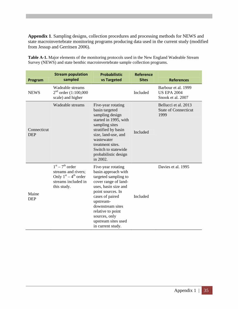
Appendix 1 | 35
Appendix 1. Sampling designs, collection procedures and processing methods for NEWS and state macroinvertebrate monitoring programs producing data used in the current study (modified from Jessup and Gerritsen 2006). Table A-1. Major elements of the monitoring protocols used in the New England Wadeable Stream Survey (NEWS) and state benthic macroinvertebrate sample collection programs.
Program Stream population
sampled Probabilistic vs Targeted
Reference Sites
References
NEWS Wadeable streams 2nd order (1:100,000 scale) and higher
Included Barbour et al. 1999 US EPA 2004 Snook et al. 2007
Connecticut DEP
Wadeable streams Five-year rotating basin targeted sampling design started in 1995, with sampling sites stratified by basin size, land-use, and wastewater treatment sites. Switch to statewide probabilistic design in 2002.
Included
Bellucci et al. 2013 State of Connecticut 1999
Maine DEP
1st – 7th order streams and rivers; Only 1st – 4th order streams included in this study.
Five-year rotating basin approach with targeted sampling to cover range of land-uses, basin size and point sources. In cases of paired upstream-downstream sites relative to point sources, only upstream sites used in current study.
Included
Davies et al. 1995
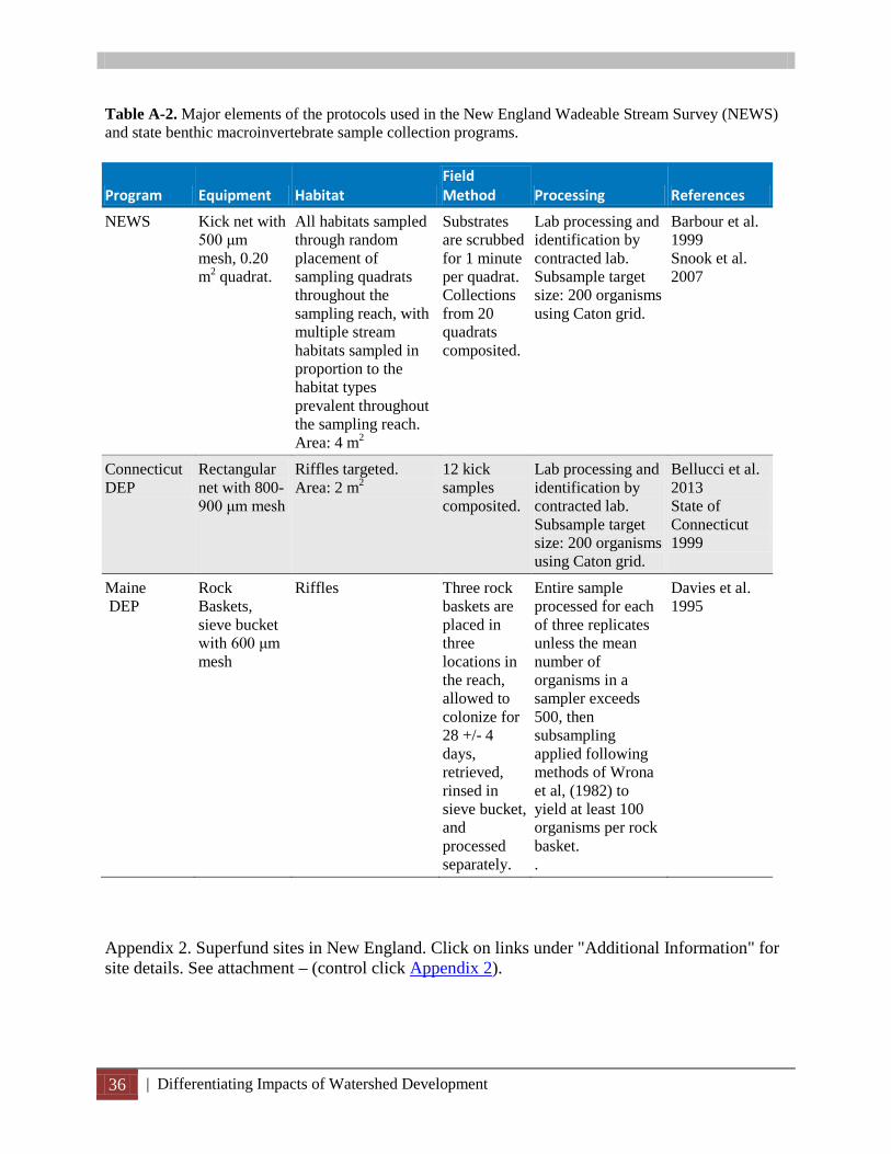
36 | Differentiating Impacts of Watershed Development
Table A-2. Major elements of the protocols used in the New England Wadeable Stream Survey (NEWS) and state benthic macroinvertebrate sample collection programs.
Program Equipment Habitat Field Method Processing References
NEWS Kick net with 500 μm mesh, 0.20 m2 quadrat.
All habitats sampled through random placement of sampling quadrats throughout the sampling reach, with multiple stream habitats sampled in proportion to the habitat types prevalent throughout the sampling reach. Area: 4 m2
Substrates are scrubbed for 1 minute per quadrat. Collections from 20 quadrats composited.
Lab processing and identification by contracted lab. Subsample target size: 200 organisms using Caton grid.
Barbour et al. 1999 Snook et al. 2007
Connecticut DEP
Rectangular net with 800-900 μm mesh
Riffles targeted. Area: 2 m2
12 kick samples composited.
Lab processing and identification by contracted lab. Subsample target size: 200 organisms using Caton grid.
Bellucci et al. 2013 State of Connecticut 1999
Maine DEP
Rock Baskets, sieve bucket with 600 μm mesh
Riffles Three rock baskets are placed in three locations in the reach, allowed to colonize for 28 +/- 4 days, retrieved, rinsed in sieve bucket, and processed separately.
Entire sample processed for each of three replicates unless the mean number of organisms in a sampler exceeds 500, then subsampling applied following methods of Wrona et al, (1982) to yield at least 100 organisms per rock basket. .
Davies et al. 1995
Appendix 2. Superfund sites in New England. Click on links under "Additional Information" for site details. See attachment – (control click Appendix 2).
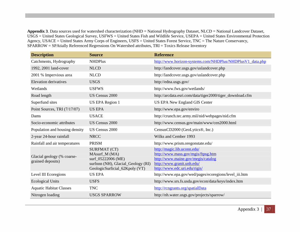
Appendix 3 | 37
Appendix 3. Data sources used for watershed characterization (NHD = National Hydrography Dataset, NLCD = National Landcover Dataset, USGS = United States Geological Survey, USFWS = United States Fish and Wildlife Service, USEPA = United States Environmental Protection Agency, USACE = United States Army Corps of Engineers, USFS = United States Forest Service, TNC = The Nature Conservancy, SPARROW = SPAtially Referenced Regressions On Watershed attributes, TRI = Toxics Release Inventory
Description Source Reference Catchments, Hydrography 1992, 2001 land-cover 2001 % Impervious area Elevation derivatives Wetlands Road length Superfund sites Point Sources, TRI (7/17/07) Dams Socio-economic attributes Population and housing density 2-year 24-hour rainfall Rainfall and air temperatures
Glacial geology (% coarse-grained deposits)
Level III Ecoregions Ecological Units Aquatic Habitat Classes Nitrogen loading
NHDPlus NLCD NLCD USGS USFWS US Census 2000 US EPA Region 1 US EPA USACE US Census 2000 US Census 2000 NRCC PRISM SURFMAT (CT) MAsurf_M (MA) surf_05222006 (ME) surfnnn (NH), Glacial_Geology (RI) GeologicSurficial_62Kpoly (VT) US EPA USFS TNC USGS SPARROW
http://www.horizon-systems.com/NHDPlus/NHDPlusV1_data.php http://landcover.usgs.gov/uslandcover.php http://landcover.usgs.gov/uslandcover.php http://edna.usgs.gov/ http://www.fws.gov/wetlands/ http://arcdata.esri.com/data/tiger2000/tiger_download.cfm US EPA New England GIS Center http://www.epa.gov/enviro http://crunch.tec.army.mil/nid/webpages/nid.cfm http://www.census.gov/main/www/cen2000.html CensusCD2000 (GeoLytics®, Inc.) Wilks and Cember 1993 http://www.prism.oregonstate.edu/ http://magic.lib.uconn.edu/ http://www.mass.gov/mgis/ftpsg.htm http://www.maine.gov/megis/catalog http://www.granit.unh.edu/ http://www.edc.uri.edu/rigis/
http://www.epa.gov/wed/pages/ecoregions/level_iii.htm http://www.srs.fs.usda.gov/econ/data/keys/index.htm http://rcngrants.org/spatialData http://nh.water.usgs.gov/projects/sparrow/
38 | Differentiating Impacts of Watershed Development
Appendix 4. Results of partial Mantel tests.
(control click hyperlink for tables.)
App4_EcodistResultSummary
ECODIST was used to evaluate effects of watershed, catchment, and buffer variables after accounting for spatial autocorrelation and cross-correlations among variables following the methods of King (King et al. 2005). For each potential model, ECODIST was applied to test for 1) the significance of each watershed-scale effect after accounting for all other watershed-scale effects, 2) the significance of each NHDPlus catchment-scale effect after accounting for all other catchment-scale effects, 3) watershed buffer-scale effects after accounting for all other watershed-scale effects, and 4) catchment buffer-scale effects after accounting for all other catchment-scale effects. Mantel’s r values (and probability levels) are shown for final models after spatial autocorrelation is factored out, first without accounting for correlations between watershed and buffer-scale effects, and second, after factoring out buffer-scale effects from watershed-scale effects.
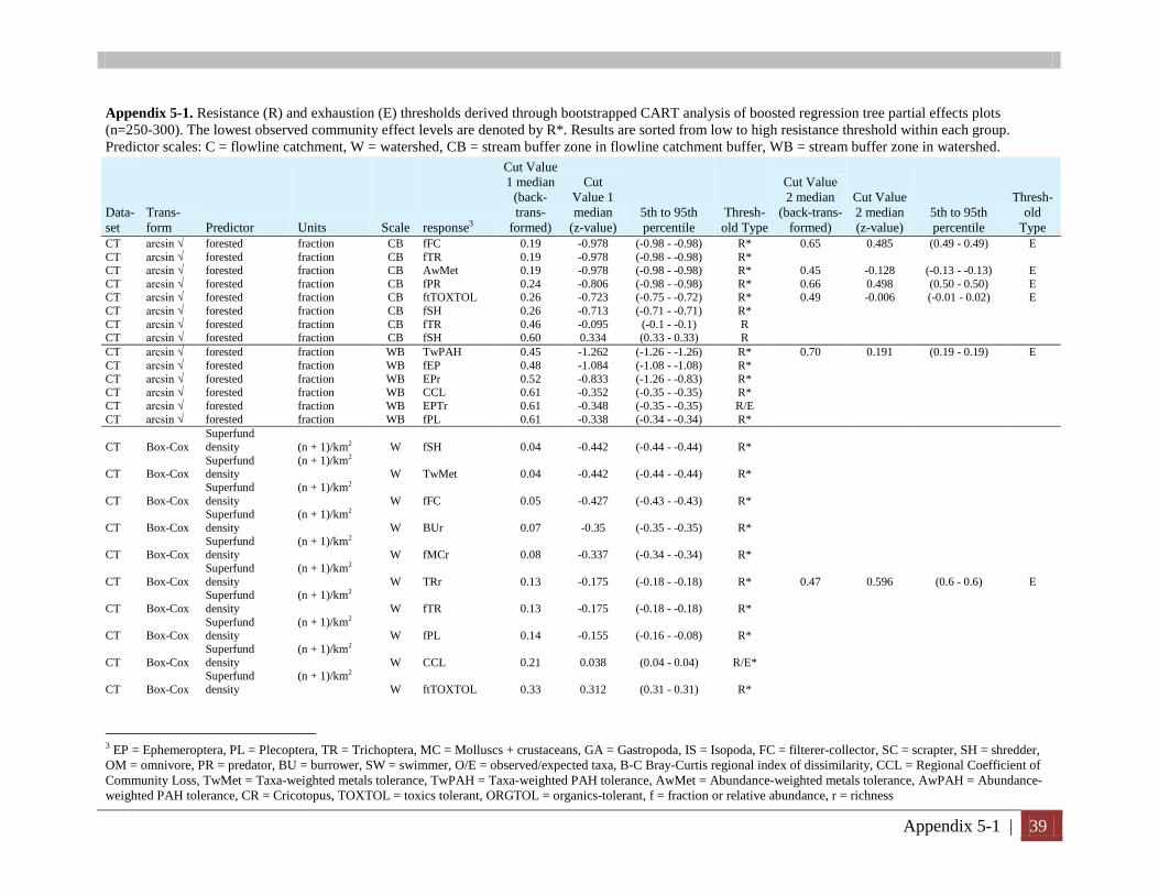
Appendix 5-1 | 39
Appendix 5-1. Resistance (R) and exhaustion (E) thresholds derived through bootstrapped CART analysis of boosted regression tree partial effects plots (n=250-300). The lowest observed community effect levels are denoted by R*. Results are sorted from low to high resistance threshold within each group. Predictor scales: C = flowline catchment, W = watershed, CB = stream buffer zone in flowline catchment buffer, WB = stream buffer zone in watershed.
Data-set
Trans-form Predictor Units Scale response3
Cut Value 1 median
(back-trans-
formed)
Cut Value 1 median
(z-value) 5th to 95th percentile
Thresh- old Type
Cut Value 2 median
(back-trans-formed)
Cut Value 2 median (z-value)
5th to 95th percentile
Thresh- old
Type CT arcsin √ forested fraction CB fFC 0.19 -0.978 (-0.98 - -0.98) R* 0.65 0.485 (0.49 - 0.49) E CT arcsin √ forested fraction CB fTR 0.19 -0.978 (-0.98 - -0.98) R* CT arcsin √ forested fraction CB AwMet 0.19 -0.978 (-0.98 - -0.98) R* 0.45 -0.128 (-0.13 - -0.13) E CT arcsin √ forested fraction CB fPR 0.24 -0.806 (-0.98 - -0.98) R* 0.66 0.498 (0.50 - 0.50) E CT arcsin √ forested fraction CB ftTOXTOL 0.26 -0.723 (-0.75 - -0.72) R* 0.49 -0.006 (-0.01 - 0.02) E CT arcsin √ forested fraction CB fSH 0.26 -0.713 (-0.71 - -0.71) R* CT arcsin √ forested fraction CB fTR 0.46 -0.095 (-0.1 - -0.1) R CT arcsin √ forested fraction CB fSH 0.60 0.334 (0.33 - 0.33) R CT arcsin √ forested fraction WB TwPAH 0.45 -1.262 (-1.26 - -1.26) R* 0.70 0.191 (0.19 - 0.19) E CT arcsin √ forested fraction WB fEP 0.48 -1.084 (-1.08 - -1.08) R* CT arcsin √ forested fraction WB EPr 0.52 -0.833 (-1.26 - -0.83) R* CT arcsin √ forested fraction WB CCL 0.61 -0.352 (-0.35 - -0.35) R* CT arcsin √ forested fraction WB EPTr 0.61 -0.348 (-0.35 - -0.35) R/E CT arcsin √ forested fraction WB fPL 0.61 -0.338 (-0.34 - -0.34) R*
CT Box-Cox Superfund density (n + 1)/km2 W fSH 0.04 -0.442 (-0.44 - -0.44) R*
CT Box-Cox Superfund density
(n + 1)/km2 W TwMet 0.04 -0.442 (-0.44 - -0.44) R*
CT Box-Cox Superfund density
(n + 1)/km2 W fFC 0.05 -0.427 (-0.43 - -0.43) R*
CT Box-Cox Superfund density
(n + 1)/km2 W BUr 0.07 -0.35 (-0.35 - -0.35) R*
CT Box-Cox Superfund density
(n + 1)/km2 W fMCr 0.08 -0.337 (-0.34 - -0.34) R*
CT Box-Cox Superfund density
(n + 1)/km2 W TRr 0.13 -0.175 (-0.18 - -0.18) R* 0.47 0.596 (0.6 - 0.6) E
CT Box-Cox Superfund density
(n + 1)/km2 W fTR 0.13 -0.175 (-0.18 - -0.18) R*
CT Box-Cox Superfund density
(n + 1)/km2 W fPL 0.14 -0.155 (-0.16 - -0.08) R*
CT Box-Cox Superfund density
(n + 1)/km2 W CCL 0.21 0.038 (0.04 - 0.04) R/E*
CT Box-Cox Superfund density
(n + 1)/km2 W ftTOXTOL 0.33 0.312 (0.31 - 0.31) R*
3 EP = Ephemeroptera, PL = Plecoptera, TR = Trichoptera, MC = Molluscs + crustaceans, GA = Gastropoda, IS = Isopoda, FC = filterer-collector, SC = scrapter, SH = shredder, OM = omnivore, PR = predator, BU = burrower, SW = swimmer, O/E = observed/expected taxa, B-C Bray-Curtis regional index of dissimilarity, CCL = Regional Coefficient of Community Loss, TwMet = Taxa-weighted metals tolerance, TwPAH = Taxa-weighted PAH tolerance, AwMet = Abundance-weighted metals tolerance, AwPAH = Abundance-weighted PAH tolerance, CR = Cricotopus, TOXTOL = toxics tolerant, ORGTOL = organics-tolerant, f = fraction or relative abundance, r = richness
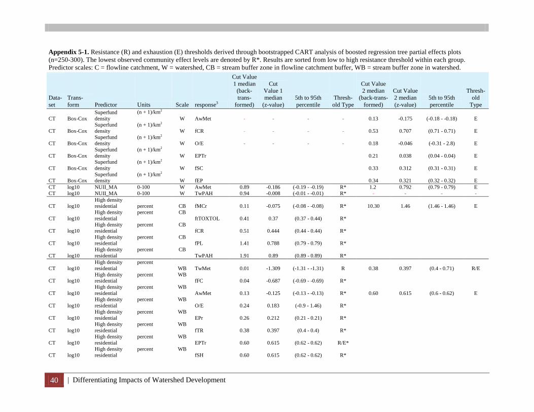
40 | Differentiating Impacts of Watershed Development
Appendix 5-1. Resistance (R) and exhaustion (E) thresholds derived through bootstrapped CART analysis of boosted regression tree partial effects plots (n=250-300). The lowest observed community effect levels are denoted by R*. Results are sorted from low to high resistance threshold within each group. Predictor scales: C = flowline catchment, W = watershed, CB = stream buffer zone in flowline catchment buffer, WB = stream buffer zone in watershed.
Data-set
Trans-form Predictor Units Scale response3
Cut Value 1 median
(back-trans-
formed)
Cut Value 1 median
(z-value) 5th to 95th percentile
Thresh- old Type
Cut Value 2 median
(back-trans-formed)
Cut Value 2 median (z-value)
5th to 95th percentile
Thresh- old
Type
CT Box-Cox Superfund density
(n + 1)/km2 W AwMet 0.13 -0.175 (-0.18 - -0.18) E
CT Box-Cox Superfund density
(n + 1)/km2 W fCR 0.53 0.707 (0.71 - 0.71) E
CT Box-Cox Superfund density
(n + 1)/km2 W O/E 0.18 -0.046 (-0.31 - 2.8) E
CT Box-Cox Superfund density
(n + 1)/km2 W EPTr 0.21 0.038 (0.04 - 0.04) E
CT Box-Cox Superfund density
(n + 1)/km2 W fSC 0.33 0.312 (0.31 - 0.31) E
CT Box-Cox Superfund density
(n + 1)/km2 W fEP 0.34 0.321 (0.32 - 0.32) E
CT log10 NUII_MA 0-100 W AwMet 0.89 -0.186 (-0.19 - -0.19) R* 1.2 0.792 (0.79 - 0.79) E CT log10 NUII_MA 0-100 W TwPAH 0.94 -0.008 (-0.01 - -0.01) R*
CT log10 High density residential percent CB fMCr 0.11 -0.075 (-0.08 - -0.08) R* 10.30 1.46 (1.46 - 1.46) E
CT log10 High density residential
percent CB ftTOXTOL 0.41 0.37 (0.37 - 0.44) R*
CT log10 High density residential
percent CB fCR 0.51 0.444 (0.44 - 0.44) R*
CT log10 High density residential
percent CB fPL 1.41 0.788 (0.79 - 0.79) R*
CT log10 High density residential
percent CB TwPAH 1.91 0.89 (0.89 - 0.89) R*
CT log10 High density residential
percent WB TwMet 0.01 -1.309 (-1.31 - -1.31) R 0.38 0.397 (0.4 - 0.71) R/E
CT log10 High density residential
percent WB fFC 0.04 -0.687 (-0.69 - -0.69) R*
CT log10 High density residential
percent WB AwMet 0.13 -0.125 (-0.13 - -0.13) R* 0.60 0.615 (0.6 - 0.62) E
CT log10 High density residential
percent WB O/E 0.24 0.183 (-0.9 - 1.46) R*
CT log10 High density residential
percent WB EPr 0.26 0.212 (0.21 - 0.21) R*
CT log10 High density residential
percent WB fTR 0.38 0.397 (0.4 - 0.4) R*
CT log10 High density residential
percent WB EPTr 0.60 0.615 (0.62 - 0.62) R/E*
CT log10 High density residential
percent WB fSH 0.60 0.615 (0.62 - 0.62) R*
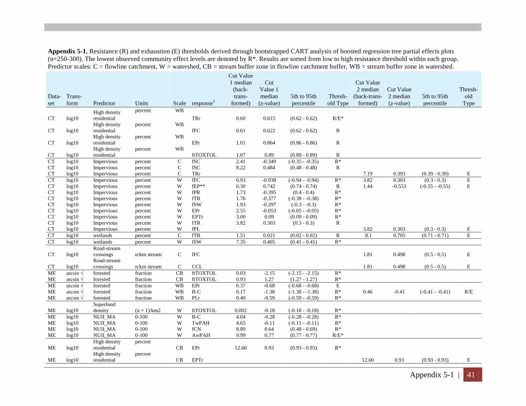
Appendix 5-1 | 41
Appendix 5-1. Resistance (R) and exhaustion (E) thresholds derived through bootstrapped CART analysis of boosted regression tree partial effects plots (n=250-300). The lowest observed community effect levels are denoted by R*. Results are sorted from low to high resistance threshold within each group. Predictor scales: C = flowline catchment, W = watershed, CB = stream buffer zone in flowline catchment buffer, WB = stream buffer zone in watershed.
Data-set
Trans-form Predictor Units Scale response3
Cut Value 1 median
(back-trans-
formed)
Cut Value 1 median
(z-value) 5th to 95th percentile
Thresh- old Type
Cut Value 2 median
(back-trans-formed)
Cut Value 2 median (z-value)
5th to 95th percentile
Thresh- old
Type
CT log10 High density residential
percent WB TRr 0.60 0.615 (0.62 - 0.62) R/E*
CT log10 High density residential
percent WB fFC 0.61 0.622 (0.62 - 0.62) R
CT log10 High density residential
percent WB EPr 1.01 0.864 (0.86 - 0.86) R
CT log10 High density residential
percent WB ftTOXTOL 1.07 0.89 (0.89 - 0.89) R
CT log10 Impervious percent C fSC 2.41 -0.349 (-0.35 - -0.35) R* CT log10 Impervious percent C fSC 8.22 0.484 (0.48 - 0.48) R CT log10 Impervious percent C TRr 7.19 0.393 (0.39 - 0.39) E CT log10 Impervious percent W fFC 0.93 -0.938 (-0.94 - -0.94) R* 3.82 0.303 (0.3 - 0.3) E CT log10 Impervious percent W fEP** 6.30 0.742 (0.74 - 0.74) R 1.44 -0.553 (-0.55 - -0.55) E CT log10 Impervious percent W fPR 1.73 -0.395 (0.4 - 0.4) R* CT log10 Impervious percent W fTR 1.76 -0.377 (-0.38 - -0.38) R* CT log10 Impervious percent W fSW 1.93 -0.297 (-0.3 - -0.3) R* CT log10 Impervious percent W EPr 2.55 -0.053 (-0.05 - -0.05) R* CT log10 Impervious percent W EPTr 3.00 0.09 (0.09 - 0.09) R* CT log10 Impervious percent W fTR 3.82 0.303 (0.3 - 0.3) R CT log10 Impervious percent W fPL 3.82 0.303 (0.3 - 0.3) E CT log10 wetlands percent C fTR 1.51 0.021 (0.02 - 0.02) R 8.1 0.705 (0.71 - 0.71) E CT log10 wetlands percent W fSW 7.35 0.405 (0.41 - 0.41) R*
CT log10 Road-stream crossings n/km stream C fFC 1.81 0.498 (0.5 - 0.5) E
CT log10 Road-stream crossings n/km stream C CCL 1.81 0.498 (0.5 - 0.5) E
ME arcsin √ forested fraction CB ftTOXTOL 0.03 -2.15 (-2.15 - -2.15) R* ME arcsin √ forested fraction CB ftTOXTOL 0.93 1.27 (1.27 - 1.27) R* ME arcsin √ forested fraction WB EPr 0.37 -0.68 (-0.68 - -0.68) E ME arcsin √ forested fraction WB B-C 0.17 -1.38 (-1.38 - -1.38) R* 0.46 -0.41 (-0.41 - -0.41) R/E ME arcsin √ forested fraction WB PLr 0.40 -0.59 (-0.59 - -0.59) R*
ME log10 Superfund density (n + 1)/km2 W ftTOXTOL 0.002 -0.18 (-0.18 - -0.18) R*
ME log10 NUII_MA 0-100 W B-C 4.04 -0.28 (-0.28 - -0.28) R* ME log10 NUII_MA 0-100 W TwPAH 4.65 -0.11 (-0.11 - -0.11) R* ME log10 NUII_MA 0-100 W fCN 8.89 0.64 (0.48 - 0.69) R* ME log10 NUII_MA 0-100 W AwPAH 9.99 0.77 (0.77 - 0.77) R/E*
ME log10 High density residential
percent CB EPr 12.60 0.93 (0.93 - 0.93) R*
ME log10 High density residential
percent CB EPTr 12.60 0.93 (0.93 - 0.93) E
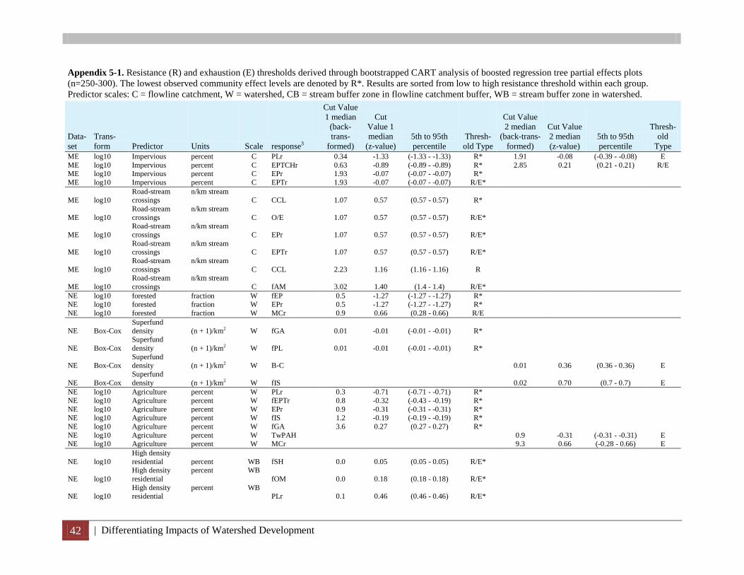
42 | Differentiating Impacts of Watershed Development
Appendix 5-1. Resistance (R) and exhaustion (E) thresholds derived through bootstrapped CART analysis of boosted regression tree partial effects plots (n=250-300). The lowest observed community effect levels are denoted by R*. Results are sorted from low to high resistance threshold within each group. Predictor scales: C = flowline catchment, W = watershed, CB = stream buffer zone in flowline catchment buffer, WB = stream buffer zone in watershed.
Data-set
Trans-form Predictor Units Scale response3
Cut Value 1 median
(back-trans-
formed)
Cut Value 1 median
(z-value) 5th to 95th percentile
Thresh- old Type
Cut Value 2 median
(back-trans-formed)
Cut Value 2 median (z-value)
5th to 95th percentile
Thresh- old
Type ME log10 Impervious percent C PLr 0.34 -1.33 (-1.33 - -1.33) R* 1.91 -0.08 (-0.39 - -0.08) E ME log10 Impervious percent C EPTCHr 0.63 -0.89 (-0.89 - -0.89) R* 2.85 0.21 (0.21 - 0.21) R/E ME log10 Impervious percent C EPr 1.93 -0.07 (-0.07 - -0.07) R* ME log10 Impervious percent C EPTr 1.93 -0.07 (-0.07 - -0.07) R/E*
ME log10 Road-stream crossings
n/km stream C CCL 1.07 0.57 (0.57 - 0.57) R*
ME log10 Road-stream crossings
n/km stream C O/E 1.07 0.57 (0.57 - 0.57) R/E*
ME log10 Road-stream crossings
n/km stream C EPr 1.07 0.57 (0.57 - 0.57) R/E*
ME log10 Road-stream crossings
n/km stream C EPTr 1.07 0.57 (0.57 - 0.57) R/E*
ME log10 Road-stream crossings
n/km stream C CCL 2.23 1.16 (1.16 - 1.16) R
ME log10 Road-stream crossings
n/km stream C fAM 3.02 1.40 (1.4 - 1.4) R/E*
NE log10 forested fraction W fEP 0.5 -1.27 (-1.27 - -1.27) R* NE log10 forested fraction W EPr 0.5 -1.27 (-1.27 - -1.27) R* NE log10 forested fraction W MCr 0.9 0.66 (0.28 - 0.66) R/E
NE Box-Cox Superfund density (n + 1)/km2 W fGA 0.01 -0.01 (-0.01 - -0.01) R*
NE Box-Cox Superfund density (n + 1)/km2 W fPL 0.01 -0.01 (-0.01 - -0.01) R*
NE Box-Cox Superfund density (n + 1)/km2 W B-C 0.01 0.36 (0.36 - 0.36) E
NE Box-Cox Superfund density (n + 1)/km2 W fIS 0.02 0.70 (0.7 - 0.7) E
NE log10 Agriculture percent W PLr 0.3 -0.71 (-0.71 - -0.71) R* NE log10 Agriculture percent W fEPTr 0.8 -0.32 (-0.43 - -0.19) R* NE log10 Agriculture percent W EPr 0.9 -0.31 (-0.31 - -0.31) R* NE log10 Agriculture percent W fIS 1.2 -0.19 (-0.19 - -0.19) R* NE log10 Agriculture percent W fGA 3.6 0.27 (0.27 - 0.27) R* NE log10 Agriculture percent W TwPAH 0.9 -0.31 (-0.31 - -0.31) E NE log10 Agriculture percent W MCr 9.3 0.66 (-0.28 - 0.66) E
NE log10 High density residential percent WB fSH 0.0 0.05 (0.05 - 0.05) R/E*
NE log10 High density residential
percent WB fOM 0.0 0.18 (0.18 - 0.18) R/E*
NE log10 High density residential
percent WB PLr 0.1 0.46 (0.46 - 0.46) R/E*
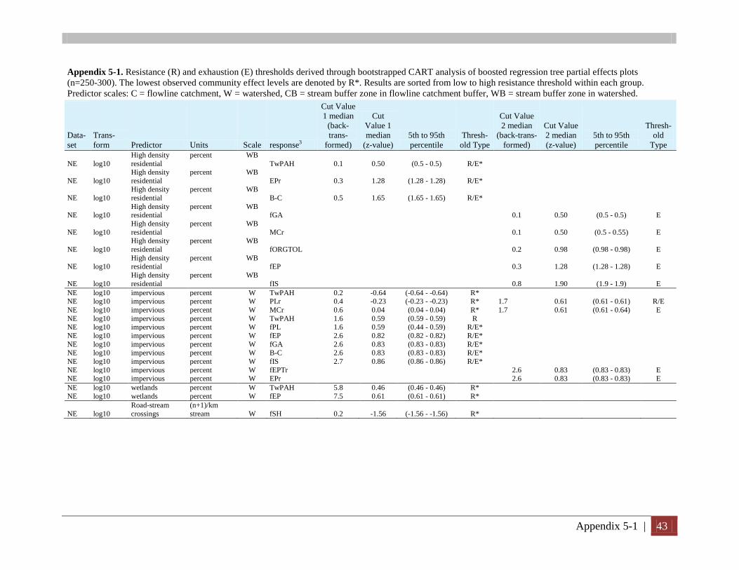
Appendix 5-1 | 43
Appendix 5-1. Resistance (R) and exhaustion (E) thresholds derived through bootstrapped CART analysis of boosted regression tree partial effects plots (n=250-300). The lowest observed community effect levels are denoted by R*. Results are sorted from low to high resistance threshold within each group. Predictor scales: C = flowline catchment, W = watershed, CB = stream buffer zone in flowline catchment buffer, WB = stream buffer zone in watershed.
Data-set
Trans-form Predictor Units Scale response3
Cut Value 1 median
(back-trans-
formed)
Cut Value 1 median
(z-value) 5th to 95th percentile
Thresh- old Type
Cut Value 2 median
(back-trans-formed)
Cut Value 2 median (z-value)
5th to 95th percentile
Thresh- old
Type
NE log10 High density residential
percent WB TwPAH 0.1 0.50 (0.5 - 0.5) R/E*
NE log10 High density residential
percent WB EPr 0.3 1.28 (1.28 - 1.28) R/E*
NE log10 High density residential
percent WB B-C 0.5 1.65 (1.65 - 1.65) R/E*
NE log10 High density residential
percent WB fGA 0.1 0.50 (0.5 - 0.5) E
NE log10 High density residential
percent WB MCr 0.1 0.50 (0.5 - 0.55) E
NE log10 High density residential
percent WB fORGTOL 0.2 0.98 (0.98 - 0.98) E
NE log10 High density residential
percent WB fEP 0.3 1.28 (1.28 - 1.28) E
NE log10 High density residential
percent WB fIS 0.8 1.90 (1.9 - 1.9) E
NE log10 impervious percent W TwPAH 0.2 -0.64 (-0.64 - -0.64) R* NE log10 impervious percent W PLr 0.4 -0.23 (-0.23 - -0.23) R* 1.7 0.61 (0.61 - 0.61) R/E NE log10 impervious percent W MCr 0.6 0.04 (0.04 - 0.04) R* 1.7 0.61 (0.61 - 0.64) E NE log10 impervious percent W TwPAH 1.6 0.59 (0.59 - 0.59) R NE log10 impervious percent W fPL 1.6 0.59 (0.44 - 0.59) R/E* NE log10 impervious percent W fEP 2.6 0.82 (0.82 - 0.82) R/E* NE log10 impervious percent W fGA 2.6 0.83 (0.83 - 0.83) R/E* NE log10 impervious percent W B-C 2.6 0.83 (0.83 - 0.83) R/E* NE log10 impervious percent W fIS 2.7 0.86 (0.86 - 0.86) R/E* NE log10 impervious percent W fEPTr 2.6 0.83 (0.83 - 0.83) E NE log10 impervious percent W EPr 2.6 0.83 (0.83 - 0.83) E NE log10 wetlands percent W TwPAH 5.8 0.46 (0.46 - 0.46) R* NE log10 wetlands percent W fEP 7.5 0.61 (0.61 - 0.61) R*
NE log10 Road-stream crossings
(n+1)/km stream W fSH 0.2 -1.56 (-1.56 - -1.56) R*
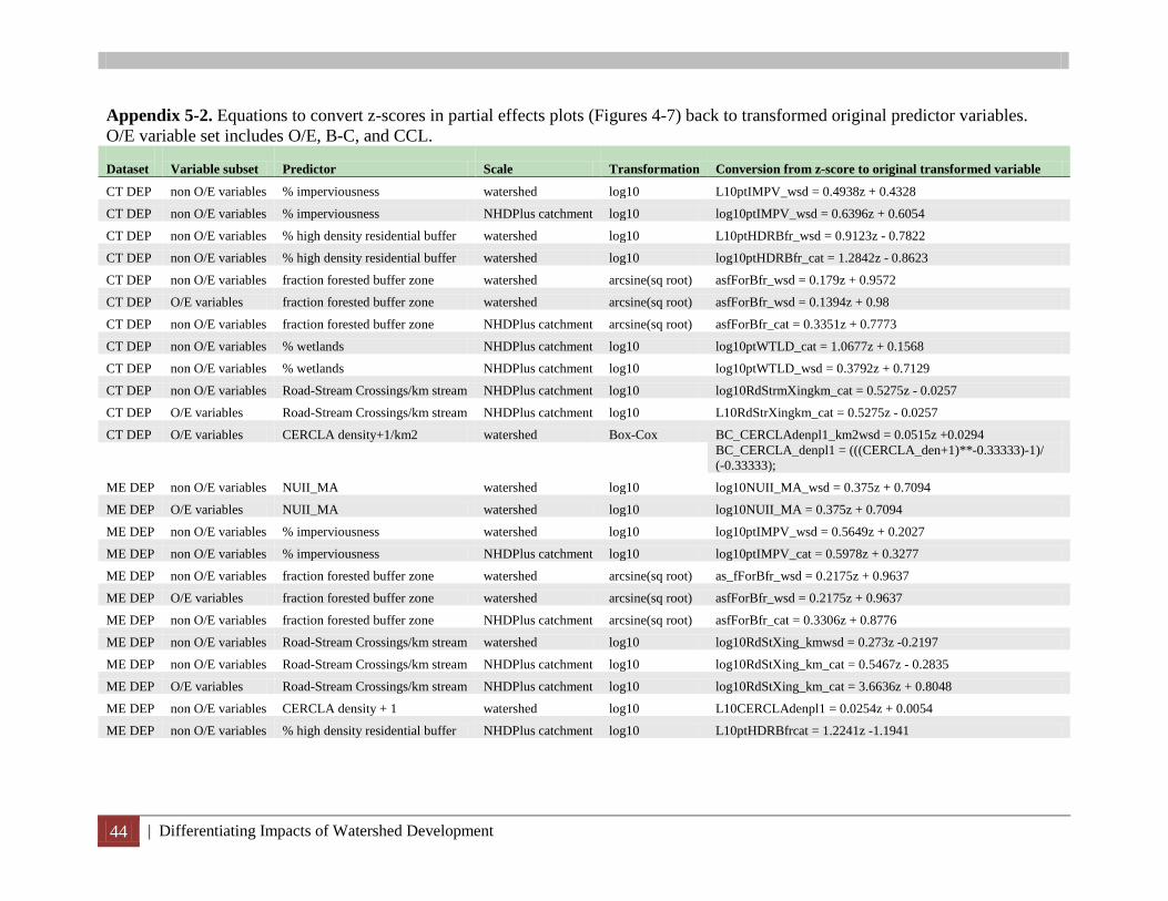
44 | Differentiating Impacts of Watershed Development
Appendix 5-2. Equations to convert z-scores in partial effects plots (Figures 4-7) back to transformed original predictor variables. O/E variable set includes O/E, B-C, and CCL. Dataset Variable subset Predictor Scale Transformation Conversion from z-score to original transformed variable
CT DEP non O/E variables % imperviousness watershed log10 L10ptIMPV_wsd = 0.4938z + 0.4328
CT DEP non O/E variables % imperviousness NHDPlus catchment log10 log10ptIMPV_wsd = 0.6396z + 0.6054
CT DEP non O/E variables % high density residential buffer watershed log10 L10ptHDRBfr_wsd = 0.9123z - 0.7822
CT DEP non O/E variables % high density residential buffer watershed log10 log10ptHDRBfr_cat = 1.2842z - 0.8623
CT DEP non O/E variables fraction forested buffer zone watershed arcsine(sq root) asfForBfr_wsd = 0.179z + 0.9572
CT DEP O/E variables fraction forested buffer zone watershed arcsine(sq root) asfForBfr_wsd = 0.1394z + 0.98
CT DEP non O/E variables fraction forested buffer zone NHDPlus catchment arcsine(sq root) asfForBfr_cat = 0.3351z + 0.7773
CT DEP non O/E variables % wetlands NHDPlus catchment log10 log10ptWTLD_cat = 1.0677z + 0.1568
CT DEP non O/E variables % wetlands NHDPlus catchment log10 log10ptWTLD_wsd = 0.3792z + 0.7129
CT DEP non O/E variables Road-Stream Crossings/km stream NHDPlus catchment log10 log10RdStrmXingkm_cat = 0.5275z - 0.0257
CT DEP O/E variables Road-Stream Crossings/km stream NHDPlus catchment log10 L10RdStrXingkm_cat = 0.5275z - 0.0257
CT DEP O/E variables CERCLA density+1/km2 watershed Box-Cox BC_CERCLAdenpl1_km2wsd = 0.0515z +0.0294
BC_CERCLA_denpl1 = (((CERCLA_den+1)**-0.33333)-1)/ (-0.33333);
ME DEP non O/E variables NUII_MA watershed log10 log10NUII_MA_wsd = 0.375z + 0.7094
ME DEP O/E variables NUII_MA watershed log10 log10NUII_MA = 0.375z + 0.7094
ME DEP non O/E variables % imperviousness watershed log10 log10ptIMPV_wsd = 0.5649z + 0.2027
ME DEP non O/E variables % imperviousness NHDPlus catchment log10 log10ptIMPV_cat = 0.5978z + 0.3277
ME DEP non O/E variables fraction forested buffer zone watershed arcsine(sq root) as_fForBfr_wsd = 0.2175z + 0.9637
ME DEP O/E variables fraction forested buffer zone watershed arcsine(sq root) asfForBfr_wsd = 0.2175z + 0.9637
ME DEP non O/E variables fraction forested buffer zone NHDPlus catchment arcsine(sq root) asfForBfr_cat = 0.3306z + 0.8776
ME DEP non O/E variables Road-Stream Crossings/km stream watershed log10 log10RdStXing_kmwsd = 0.273z -0.2197
ME DEP non O/E variables Road-Stream Crossings/km stream NHDPlus catchment log10 log10RdStXing_km_cat = 0.5467z - 0.2835
ME DEP O/E variables Road-Stream Crossings/km stream NHDPlus catchment log10 log10RdStXing_km_cat = 3.6636z + 0.8048
ME DEP non O/E variables CERCLA density + 1 watershed log10 L10CERCLAdenpl1 = 0.0254z + 0.0054
ME DEP non O/E variables % high density residential buffer NHDPlus catchment log10 L10ptHDRBfrcat = 1.2241z -1.1941
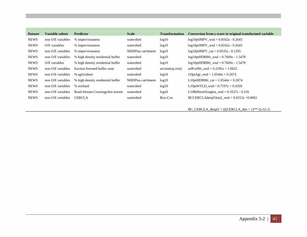
Appendix 5-2 | 45
Dataset Variable subset Predictor Scale Transformation Conversion from z-score to original transformed variable NEWS non O/E variables % imperviousness watershed log10 log10ptIMPV_wsd = 0.8162z - 0.2643
NEWS O/E variables % imperviousness watershed log10 log10ptIMPV_wsd = 0.8162z - 0.2643
NEWS non O/E variables % imperviousness NHDPlus catchment log10 log10ptIMPV_cat = 0.9535z - 0.1295
NEWS non O/E variables % high density residential buffer watershed log10 log10ptHDRBfr_wsd = 0.7669z - 1.5478
NEWS O/E variables % high density residential buffer watershed log10 log10ptHDRBfr_wsd = 0.7669z - 1.5478
NEWS non O/E variables fraction forested buffer zone watershed arcsine(sq root) asfForBfr_wsd = 0.2185z + 1.0622
NEWS non O/E variables % agriculture watershed log10 l10ptAgr_wsd = 1.0544z + 0.2674
NEWS non O/E variables % high density residential buffer NHDPlus catchment log10 L10ptHDRBfr_cat = 1.0544z + 0.2674
NEWS non O/E variables % wetland watershed log10 L10ptWTLD_wsd = 0.7197z + 0.4359
NEWS non O/E variables Road-Stream Crossings/km stream watershed log10 L10RdStrmXingkm_wsd = 0.3527z - 0.216
NEWS non O/E variables CERCLA watershed Box-Cox BCCERCLAdenpl1km2_wsd = 0.0213z +0.0063
BC_CERCLA_denpl1 = (((CERCLA_den + 1)**-2)-1)/-2;
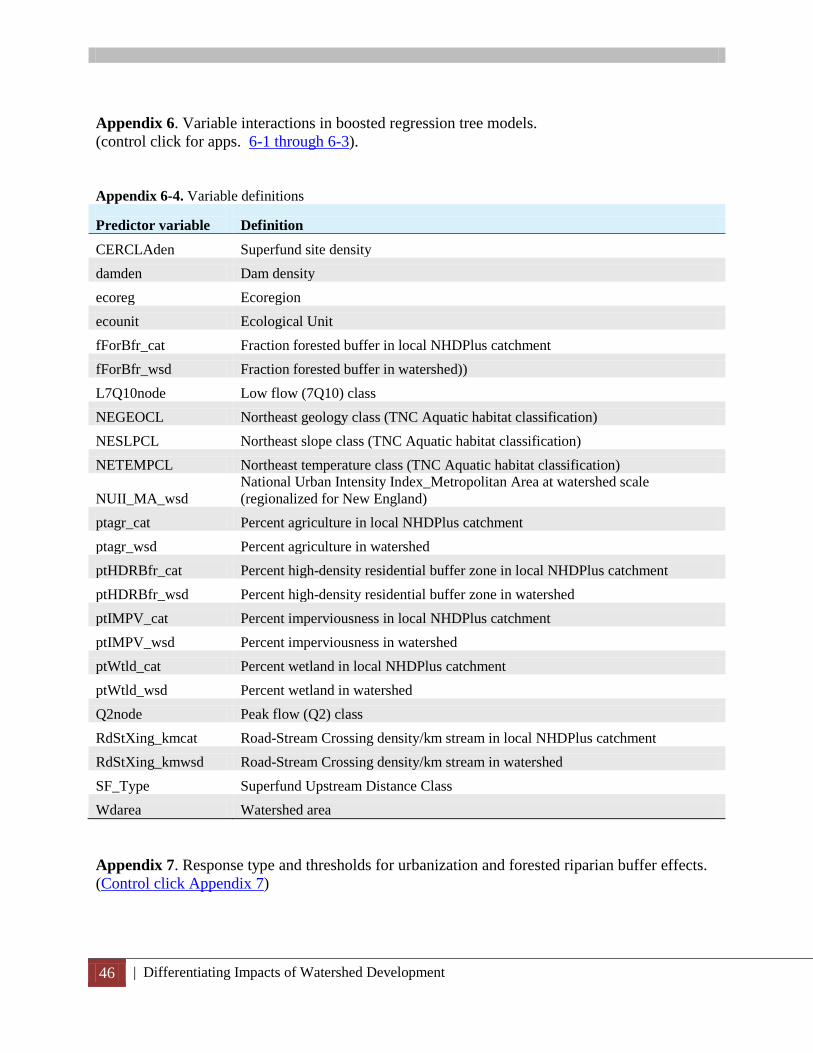
46 | Differentiating Impacts of Watershed Development
Appendix 6. Variable interactions in boosted regression tree models. (control click for apps. 6-1 through 6-3). Appendix 6-4. Variable definitions Predictor variable Definition CERCLAden Superfund site density damden Dam density ecoreg Ecoregion ecounit Ecological Unit fForBfr_cat Fraction forested buffer in local NHDPlus catchment fForBfr_wsd Fraction forested buffer in watershed)) L7Q10node Low flow (7Q10) class NEGEOCL Northeast geology class (TNC Aquatic habitat classification) NESLPCL Northeast slope class (TNC Aquatic habitat classification) NETEMPCL Northeast temperature class (TNC Aquatic habitat classification)
National Urban Intensity Index_Metropolitan Area at watershed scale NUII_MA_wsd (regionalized for New England) ptagr_cat Percent agriculture in local NHDPlus catchment ptagr_wsd Percent agriculture in watershed ptHDRBfr_cat Percent high-density residential buffer zone in local NHDPlus catchment ptHDRBfr_wsd Percent high-density residential buffer zone in watershed ptIMPV_cat Percent imperviousness in local NHDPlus catchment ptIMPV_wsd Percent imperviousness in watershed ptWtld_cat Percent wetland in local NHDPlus catchment ptWtld_wsd Percent wetland in watershed Q2node Peak flow (Q2) class RdStXing_kmcat Road-Stream Crossing density/km stream in local NHDPlus catchment RdStXing_kmwsd Road-Stream Crossing density/km stream in watershed SF_Type Superfund Upstream Distance Class Wdarea Watershed area Appendix 7. Response type and thresholds for urbanization and forested riparian buffer effects. (Control click Appendix 7)

United StatesEnvironmental ProtectionAgency
O�ce of Research and DevelopmentNational Health and Environmental E�ects Research LaboratoryAtlantic Ecology DivisionNarragansett, RI 02882
O�cial BusinessPenalty for Private use$300
EPA/600/R-13/163 | October 2013
www.epa.gov/ord