Diffractive Optical Element Design with Memory-Matrix-Based Identification Methodology

$Page 1: Diffractive Optical Element Design with Memory-Matrix-Based Identification Methodology$
oc

a

Diffractive optical element design withmemory-matrix-based identification methodology

Dhawat E. Pansatiankul and Alexander A. Sawchuk

We present a new technique for the design of diffractive optical elements ~DOE’s! that is based onprevious nonlinear least squares ~NLS! and phase-shifting quantization methods @Appl. Opt. 36, 7297–7306 ~1997!#. The technique uses a memory-matrix-based identification ~MMBI! optimization proce-dure. We compare results from the MMBI method with those from iterative Fourier transform and NLSmethods. In comparison, the MMBI DOE designs produce better-quality reconstructions for DOE’s witheight or more fabrication phase levels and generally have a higher signal-to-noise ratio and betteruniformity. © 2000 Optical Society of America

OCIS codes: 050.1970, 070.4560, 100.5090, 200.2610, 200.4650.

~
1. Introduction
Diffractive optical elements ~DOE’s! became increas-ingly important in many optical applications duringthe last two decades and are now widely used, forexample, as spot-array generators in smart-pixeloptical systems1 and for optical interconnections inptoelectronic single-instruction multiple-data ma-hines.2 DOE’s are used to alter the distribution of

incident light so that a diffraction pattern with adesired distribution can be reconstructed.3 VariousDOE design algorithms have been proposed and stud-ied to obtain a good-quality reconstructed intensitypattern. DOE design procedures commonly usemodifications of either simulated annealing4 or iter-tive Fourier transform5 ~IFT! methods. The former

method can ideally reach a global optimum by use ofa statistical searching procedure with an appropriateannealing schedule, independent of the startingpoint. However, for a large number of discretephase levels, the computation cost of this methodmay be extremely high. In contrast, the lattermethod has a low computation cost, but it is sensitiveto the initial starting point and is also prone to stag-nate in a local optimum.

Recently Chen and Sawchuk introduced nonlinear

The authors are with the Signal and Image Processing Institute,University of Southern California, Los Angeles, California 90089-2564. D. Pansatiankul’s e-mail address is [email protected].

Received 21 December 1999; revised manuscript received Au-gust 7, 2000.

0003-6935y00y325921-08$15.00y0© 2000 Optical Society of America

1

least squares ~NLS! and phase-shifting quantizationPSQ! methods6 for a DOE design that produce a

better-quality reconstruction in terms of signal-to-noise ratio ~SNR! compared with the modifiedIFT method proposed by Wyrowski.7 In this pa-per we present a new DOE design method calledthe memory-matrix-based identification ~MMBI!method, which is based on the NLS and PSQ meth-ods. It results in an improvement of the overall re-construction quality, especially in the uniformity andSNR, and still has an acceptable computation cost.

The mathematical model of DOE design that weuse in this paper is briefly explained in Section 2. InSection 3 we describe the algorithm of the MMBImethod and the way in which it is applied to the DOEdesign. The actual implementation of the MMBImethod and simulation results that include the per-formance comparisons among the MMBI, NLS, andIFT methods are shown in Section 4 for three differ-ent desired intensity patterns. The conclusion ispresented in Section 5.

2. Mathematical Model of Diffractive Optical Elements

In our discussion we assume that the diffractingstructures are large compared with the wavelength oflight being used for illumination; i.e., our DOE’smodel is based on a scalar paraxial approximation.We also assume that multilevel photolithography isused during the fabrication process. We model aDOE design that uses the notation of Wyrowski7 andChen and Sawchuk.6

Let Id be the real, nonnegative M 3 N matrix con-taining the desired intensity pattern. Our optimal

0 November 2000 y Vol. 39, No. 32 y APPLIED OPTICS 5921

w

tsscs

c

s

w

ige

v

t

w

c

5

goal is to find the M 3 N phase-only DOE matrix, G 5exp~iQ!, that satisfies

Id 5 uFT21$G% 3 Wu2 5 uFT21$exp~iQ!% 3 Wu2, (1)

where Q is an M 3 N phase matrix whose elementshave values between 2p and p, W is an M 3 Nmatrix whose elements, W~m, n! 5 sinc~myM!sinc~nyN!, represent the effect of finite feature size of thefabrication process, and FT21$. . .% denotes the in-verse discrete Fourier transform operator.

For general desired intensity patterns, it may notbe possible to obtain an exact solution for the abovenonlinear equation. The DOE design problem,therefore, is to find the best estimate G, or, equiva-lently, Q, that results in a good approximation of Idunder some performance evaluation criteria. Inother words, we want to find the reconstructed inten-sity pattern

I 5 uFT21$G% 3 Wu2 5 uFT21$exp~iQ!% 3 Wu2, (2)

hich can best represent Id in Eq. ~1! under somedesired criteria.

3. Memory-Matrix-Based Identification Method

The MMBI method was first introduced by Udwadiaand Proskurowski to identify the properties of struc-tural and mechanical systems.8 Instead of itera-ively solving the design problem by use of a singletarting point, called an initial guess or Q~0!, anduccessively updating this single point, as in otherommonly used methods, the MMBI algorithm useseveral training initial guesses @for example, Q1

~0!,Q2

~0!, Q3~0!, . . . , etc.# simultaneously as starting points

to build the association between these initial pointsand their corresponding reconstructed intensity pat-terns @for example, I1

~0!, I2~0!, I3

~0!, . . . , etc.#. The algo-rithm then successively updates this association andthe estimated phase matrix by use of a genetic-likeiterative algorithm.

The algorithm of the MMBI method that wepresent in this paper is divided into two parts: ini-tialization and iteration.

~i! Initialization~a! Start with a set of initial guesses ~initial train-

ing vectors! F~0! 5 @u1~0! u2

~0! . . . uL0

~0!#, where we re-write the initial phase matrix Qj

~0! as an ~MN!olumn vector uj

~0!, i.e., a column vector with MNelements, whose elements are taken columnwisefrom matrix Qj

~0!. Then generate a set of corre-ponding reconstructed intensity patterns P~0! 5 @IO1

~0!

IO2~0! . . . IOL0

~0!#, and again rewrite the intensity matrixIj

~0! as a column vector IOj~0!, whose elements are also

taken columnwise from matrix Ij~0!, by use of the re-

lation in Eq. ~2!. Here L0 is the number of initialtraining vectors.

~b! Compute the initial associative memory matrixA~0!, which is defined as8,9

A~0! 5 F~0!P~0!T@P~0!P~0!T 1 aE#21. (3)

922 APPLIED OPTICS y Vol. 39, No. 32 y 10 November 2000

Here E represents an MN 3 MN identity matrix, a isa regularization parameter,8 and $. . .%T is the trans-pose operator.

~c! Use the desired intensity pattern IOd in column-vector form to determine an initial estimate of thephase column vector as u~0! 5 A~0!IOd.

~d! Compute the initial estimate of the recon-structed intensity column vector I~0! by use of Eq. ~2!

ith u~0!.~e! Compute the perturbation factor b1, which will

be used later, as

b1 5 iDIO~0!iyiIOdi 5 i~IOd 2 I~0!!iyiIOdi. (4)

~ii! IterationRepeat this part for k 5 1, 2, 3, . . . , until either

DIO~k!i is less than the predefined tolerance, t, or k isreater than the predefined maximum number of it-rations.~a! Using a single estimate of the phase column

ector u~k21!, we generate the mutations ~the candi-date training vectors! by use of the following steps.

~1! Randomly perturb each element of the esti-mated phase vector u~k21! by a small amount, i.e.,

ui, j~k! 5 ~1 1 mi, jbk!ui

~k21!

for i 5 1, 2, . . . , MN and j 5 1, 2, . . . . (5)

Here ui, j~k! denotes the ith element of ~MN! column

vector uj~k!, mi, j represents a random number uniformly

distributed in ~20.5, 0.5!, and bk is a perturbationfactor.

~2! Compute the corresponding reconstructed in-ensity patterns IOj

~k! from uj~k!, with Eq. ~2!.

~3! Accept L vectors uj~k! that satisfy the criterion

i~IOd 2 IOj~k!!i , diDIO~k21!i, (6)

here d is a constant number and L is the number oftraining vectors in each iteration.

~b! From the previous step, form a set of trainingvectors F~k! 5 @u1

~k! u2~k! . . . uL

~k!# and obtain the corre-sponding reconstructed intensity patterns P~k! 5 @IO1

~k!

IO2~k! . . . IOL

~k!# via Eq. ~2!.~c! Compute the associative memory matrix A~k! by

A~k! 5 F~k!P~k!T@P~k!P~k!T 1 aE#21. (7)

~d! Determine the updated estimate of the phaseolumn vector from

u~k! 5 A~k!IOd. (8)

~e! Calculate the estimate of the reconstructed in-tensity pattern I~k! by use of Eq. ~2! with u~k!.

~f ! Compute the residual as

DIO~k! 5 ~IOd 2 I~k!! (9)

and the perturbation factor as

bk11 5 iDIO~k!iyiIOdi. (10)

zpcinr

Tat

S

f

mwrp

Note that, in the MMBI algorithm shown above, weneed to obtain the appropriate initial training vectorsin the initialization step. We also have to considerthe value of the regularization parameter a. Thevalue of a should be a positive number very close toero if one emphasizes an accurate result at the ex-ense of possible numerical ill-conditioning of theomputed associative memory matrix A. However,f one emphasizes numerical conditioning, i.e., theumerical stability of A at the expense of accurateesults, a should be a large positive number.8 More-

over, the number of training vectors, either L0 or L,may affect the accuracy of the solution and the com-putation cost.

Most of the computation cost in this algorithmarises from computing the reconstructed intensitypatterns of the candidate training vectors in part ~ii!.

ypically, this is done with the fast Fourier transformlgorithm, whose computation cost per iteration is ofhe order of ~MN!log2~MN!. Moreover, the value of d

in relation ~6! should not be either too large, whichreduces the quality of the training vectors, or toosmall, which leads to an excessive computation cost offinding the proper training vectors. In general, ifthe initial set of training vectors is good enough, theMMBI algorithm should converge to the final esti-mate very fast without any difficulty.

4. Diffractive Optical Element Design Simulation

In this section we first define reconstruction qualitycriteria,6 then we describe our actual implementationof the MMBI method and its computational complex-ity. Finally, we compare the numerical results ofthree desired intensity patterns that use three designmethods: MMBI, NLS, and IFT.

A. Criteria for Performance Evaluation

It is clear that we need some criteria to evaluate thequality of the reconstructed intensity pattern. Sincethe MMBI method presented in this paper is mainlybased on the NLS method proposed by Chen andSawchuk, we followed their criteria to have a faircomparison between these two methods.

For any desired intensity pattern Id, we generate aphase-only DOE, which gives the reconstructed in-tensity pattern Ir. This reconstructed intensity pat-tern consists of two parts: Sr and Nr. The matrix

r represents only the signal diffraction orders,whereas the matrix Nr represents only the noise dif-raction orders; i.e., Ir 5 Sr 1 Nr. The diffraction

orders that make up the desired intensity pattern arecalled the signal diffraction orders. Otherwise, theyare called noise diffraction orders.

Assume that the total incident power on the DOE isone. Let Smax be the maximum value among theelements of matrix Sr, Smin be the minimum value~not equal to zero! among the elements of matrix Sr,and Nmax be the maximum value among the elementsof matrix Nr. Following Ref. 6, we define the follow-ing.

1

~a! Nonuniformity ~%! as

NU 5 @~Smax 2 Smin!y~Smax 1 Smin!# 3 100. (11)

~b! Window efficiency ~%! as

hw 5 HF(@m,n

Sr~m, n!GYF(@m,n

Ir~m, n!GJ 3 100. (12)

~c! Grating efficiency ~%! as

hg 5 F(@m,n

Sr~m, n!G 3 100. (13)

~d! SNR ~dB! as

SNR 5 10 log10~SminyNmax!. (14)

~e! Overall quality factor as

QF 5 w1~100 2 NU! 1 w2~hw! 1 w3~hg! 1 w4~SNR!,

(15)

where ~w1 1 w2 1 w3 1 w4! 5 1.With the above linear combination of nonunifor-ity, window efficiency, grating efficiency, and SNR,e are able to evaluate the overall performance of the

econstructed intensity pattern during the iterativerocess. We also note that Sr~m, n! and Ir~m, n!

represent the elements of matrix Sr and matrix Ir,respectively.

In all of our experiments in this paper, we set w1 5~5y7!, w2 5 0, w3 5 ~1y7!, and w4 5 ~1y7!. We usethese particular weights for direct comparison withChen and Sawchuk’s work.6 Moreover, we believethat this particular quality factor is useful for ourapplications of DOE’s. For other applications, thequality factor and its weights may need to be ad-justed. By experience, we have found that even withadjustments of the weights in the quality factor, therelative rankings of alternative techniques comparedwith the MMBI method do not change appreciably.

B. Implementation of the Memory-Matrix-BasedIdentification Method

Before we use the MMBI algorithm we must generategood initial training vectors. In our implementationwe chose the NLS method to generate those initialtraining vectors because of its efficient, simple imple-mentation with the routine LEASTSQ10 in the MATLAB

optimization toolbox11 and its improvement in SNRwith acceptable computation cost.6

Starting from only one initial guess, the NLSmethod theoretically gives one optimal solution com-pared with the desired intensity pattern, in the senseof minimizing mean-squared error. Unfortunately,commonly used NLS algorithms do not give a globaloptimum when they deal with a large number of pa-rameters, i.e., a large number of phase elements inDOE design. The difficulty arises mainly from thefact that there may be many local minima so thatconvergence to the optimal one is possible only if theinitial guess is not too far from it.

In this case, we apply the MMBI method to find a


u

smrmatdriidotoMsssSttmr

ielpTpnngsm

5

more accurate solution. As mentioned in Section 3,the MMBI algorithm uses a set of initial trainingvectors and successively updates these vectors withthe genetic-like iterative procedure to reach an opti-mal solution. To generate L0 initial training vectorsfor the MMBI method, we include small perturba-tions ~within approximately 10% of their original val-

es! in each element of the suboptimal vectorobtained from the NLS method and repeat this pro-cess L0 times.

In every iteration of the MMBI method we computethe associative memory matrix and the estimate ofthe phase matrix. To update this estimate of thephase matrix, we need to specify the desired intensitypattern @Eq. ~8!#. Ideally, we should use exactly theame desired intensity pattern as used by the NLSethod at the beginning. On the basis of our expe-

ience from many simulations and the fact that ainimum mean-squared-error solution may not havemaximum quality factor, we allow constraints on

he original desired intensity pattern to be modifieduring the design process. We have noticed that theesulting reconstruction can have better overall qual-ty with this procedure. The modification procedures to set the signal diffraction orders of the modifiedesired intensity pattern equal to the average valuef those of the reconstructed intensity pattern fromhe NLS method while keeping the noise diffractionrders the same. Following this modification, theMBI method, which theoretically gives the optimal

olution compared with the modified desired inten-ity pattern, should result in a reconstructed inten-ity pattern with lower nonuniformity and higherNR than one from the NLS method. Nevertheless,he above modification can be adjusted, depending onhe desired intensity pattern and the desired perfor-ance criteria, to improve the overall quality of the

econstructed intensity pattern.The MMBI algorithm described in Section 3 results

n an optimal continuous phase distribution; how-ver, based on our assumption of a multilevel photo-ithographic fabrication process, those continuoushase elements need to be quantized in practice.he customary and easiest way to quantize the com-uted continuous phase is to shift its value to theearest predefined discrete phase levels. Unfortu-ately, this traditional method does not necessarilyive the best outcome. Chen and Sawchuk de-cribed a PSQ method to quantize DOE’s phase ele-ents.6 The PSQ method relies on the fact that the

diffraction intensity pattern depends only on the rel-ative phase values among the DOE’s phase elementsrather than their absolute values. Hence it is pos-sible to find a better reconstructed intensity patternunder some specified criteria, by shifting phases ofDOE by a constant phase amount. We then decidedto use the PSQ method as the quantization step of ourimplementation for further optimizing.

In all experiments described in this paper, we usedthe following parameters: L0 5 10, L 5 50, a 510211, and d 5 1.5. The termination condition dur-ing the iteration process was always set so that k, the


number of iterations, is greater than 10 or iDIO~k!i , t,where t 5 1026.

C. Computational Complexity

As mentioned in Section 3, the computation cost periteration of the MMBI algorithm is of the order of~MN!log2~MN!. However, the implementation com-plexity of the complete procedure is now dominatedby the cost of the NLS algorithm used during theinitialization process of the MMBI method. TheNLS algorithm has complexity of the order of~MN!2log2~MN! per iteration or the order of ~MN!2

with further reduction.6 Nonetheless, the estima-tion of the total computation time for a given problemis difficult owing to the fact that it depends on start-ing points and on the particular desired intensitypattern.

D. Simulation Results

In this subsection we show the numerical results ofthree different methods, MMBI, NLS, and IFT, forthree different desired intensity patterns: a 3 3 3uniform spot-array pattern, a reduced cellular hyper-cube interconnection pattern, and an off-axis letter Xpattern.

Figure 1 is a flow diagram of our hybrid procedurethat uses the NLS method to generate an initial set of

Fig. 1. Flow diagram of the MMBI method.

Metho

training vectors, the MMBI algorithm to find the op-timal solution, and the PSQ method to optimize theoutput during the quantization process. In the flowdiagram we first specify the objective efficiency ho ofthe desired intensity pattern as

ho 5 F (m,n[R

Id~m, n!GYF(@m,n

Id~m, n!G , (16)

where R is the region of the signal diffraction ordersand Id~m, n! are the elements of matrix Id. Ideally,

Fig. 2. Diagram of the 3 3 3 uniform spot-array pattern.

Table 1. Simulation Results of Different

MethodPhaseLevels

Nonuniformity~%!

WindowEfficiency

~%!

MMBI 4 1.86 81.148 0.75 91.68

16 0.57 93.9032 0.28 94.3564 0.15 94.53CPa 0.04 94.61

IFT 4 1.85 82.108 1.00 91.80

16 0.74 94.0532 0.25 94.5464 0.42 94.65CP 0.43 94.70

NLS 4 4.71 81.158 2.11 91.80

16 1.07 93.8932 0.51 94.4464 0.33 94.60CP 0.18 94.66

aCP indicates continuous phase.

1

ho should be equal to one; however, we know fromRef. 6 that for the NLS method we should reduce theobjective efficiency to obtain a higher SNR.

As mentioned in Subsection 4.B, we apply the NLSmethod, whose procedure and flow diagram areshown in Ref. 6, to generate an initial set of trainingvectors. We then modify the desired intensity pat-tern as also explained earlier and use the MMBIalgorithm, together with the PSQ method, for 30 it-erations to find the best reconstructed intensity pat-tern under our criteria. We repeat this process 20times and select the best result. This procedure im-plies that the total number of initial sets of trainingvectors for MMBI method is 600.

For all simulations in this paper, we compare thenumerical results of the MMBI reconstructed inten-sity patterns with two other methods. One is theNLS method that uses the PSQ procedure during thequantization step, proposed by Chen and Sawchuk.6The other is the modified two-stage IFT combinedwith the stepwise quantization, proposed by Wy-rowski.7 Flow diagrams of these two methods arefound in the references. We note here that the num-ber of initial vectors for the NLS method is 20, and, tohave a fair comparison, we use the same initialguesses as in the initialization step of the MMBImethod. For the IFT method, we repeat the algo-rithm for the total of 600 initial guesses.

It is clear that the mean-squared error between theoriginal desired intensity pattern and the recon-structed intensity pattern obtained from the MMBImethod may or may not be less than that obtainedfrom the NLS method, although the errors are ap-proximately the same order. This results from thefact that we modify the desired intensity pattern dur-

ds for 3 3 3 Uniform Spot-Array Pattern

tingiency%!

SNR~dB!

QualityFactor

Numberof InitialGuesses

ObjectiveEfficiency

~%!

.18 10.50 82.48 600 100

.01 15.30 85.65 600 100

.12 17.34 86.52 600 97

.87 17.90 86.91 600 97

.14 17.68 87.01 600 97

.25 18.00 87.15 600 97

.31 9.16 82.46 600 100

.42 15.09 85.50 600 100

.84 15.66 86.26 600 100

.64 15.45 86.69 600 100

.83 15.52 86.61 600 100

.92 15.58 86.62 600 100

.46 10.93 80.55 20 100

.39 14.26 84.58 20 100

.13 17.36 86.16 20 97

.08 17.66 86.74 20 97

.27 17.87 86.93 20 97

.32 17.98 87.05 20 97

GraEffic

~

768891919292

778891929292

768891929292


p

ods f

5

ing the MMBI method. Nevertheless, we attain themain goal of better overall performance under thespecified criterion.

1. Three-by-Three Uniform Spot-Array PatternThis spot-array pattern is widely used in smart-pixeloptical systems as a spot-array generator, which il-luminates an array of optical modulators. One ex-ample of these systems is TRANslucent Smart PixelARray network.12 Figure 2 shows the diagram ofthe 3 3 3 uniform spot-array pattern in a 20 3 20phase-element DOE. Note that the black spots rep-

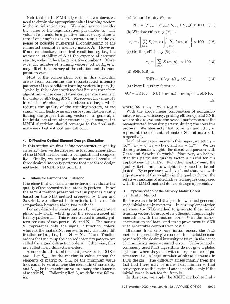
Fig. 3. Diagram of the @4, 8# reduced cellular hypercube pattern.

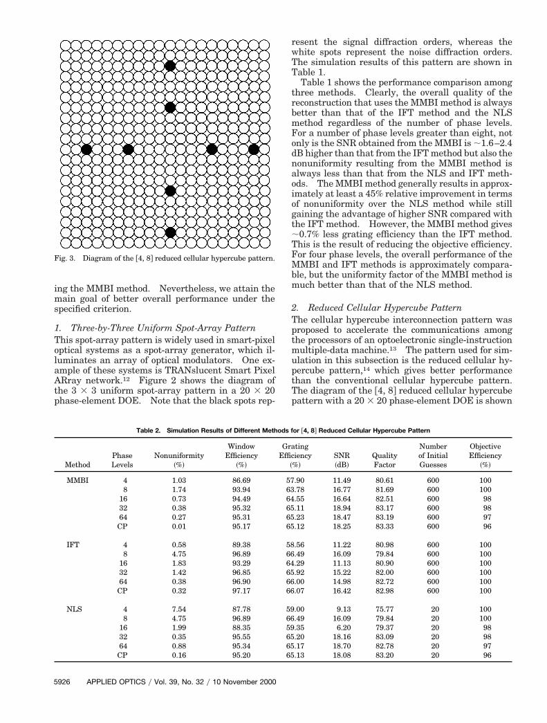
Table 2. Simulation Results of Different Meth

MethodPhaseLevels

Nonuniformity~%!

WindowEfficiency

~%!

MMBI 4 1.03 86.698 1.74 93.94

16 0.73 94.4932 0.38 95.3264 0.27 95.31CP 0.01 95.17

IFT 4 0.58 89.388 4.75 96.89

16 1.83 93.2932 1.42 96.8564 0.38 96.90CP 0.32 97.17

NLS 4 7.54 87.788 4.75 96.89

16 1.99 88.3532 0.35 95.5564 0.88 95.34CP 0.16 95.20


resent the signal diffraction orders, whereas thewhite spots represent the noise diffraction orders.The simulation results of this pattern are shown inTable 1.

Table 1 shows the performance comparison amongthree methods. Clearly, the overall quality of thereconstruction that uses the MMBI method is alwaysbetter than that of the IFT method and the NLSmethod regardless of the number of phase levels.For a number of phase levels greater than eight, notonly is the SNR obtained from the MMBI is ;1.6–2.4dB higher than that from the IFT method but also thenonuniformity resulting from the MMBI method isalways less than that from the NLS and IFT meth-ods. The MMBI method generally results in approx-imately at least a 45% relative improvement in termsof nonuniformity over the NLS method while stillgaining the advantage of higher SNR compared withthe IFT method. However, the MMBI method gives;0.7% less grating efficiency than the IFT method.This is the result of reducing the objective efficiency.For four phase levels, the overall performance of theMMBI and IFT methods is approximately compara-ble, but the uniformity factor of the MMBI method ismuch better than that of the NLS method.

2. Reduced Cellular Hypercube PatternThe cellular hypercube interconnection pattern wasproposed to accelerate the communications amongthe processors of an optoelectronic single-instructionmultiple-data machine.13 The pattern used for sim-ulation in this subsection is the reduced cellular hy-percube pattern,14 which gives better performancethan the conventional cellular hypercube pattern.The diagram of the @4, 8# reduced cellular hypercube

attern with a 20 3 20 phase-element DOE is shown

or @4, 8# Reduced Cellular Hypercube Pattern

tingiency%!

SNR~dB!

QualityFactor


ObjectiveEfficiency

~%!

.90 11.49 80.61 600 100

.78 16.77 81.69 600 100

.55 16.64 82.51 600 98

.11 18.94 83.17 600 98

.23 18.47 83.19 600 97

.12 18.25 83.33 600 96

.56 11.22 80.98 600 100

.49 16.09 79.84 600 100

.29 11.13 80.90 600 100

.92 15.22 82.00 600 100

.00 14.98 82.72 600 100

.07 16.42 82.98 600 100

.00 9.13 75.77 20 100

.49 16.09 79.84 20 100

.35 6.20 79.37 20 98

.20 18.16 83.09 20 98

.17 18.70 82.78 20 97

.13 18.08 83.20 20 96

GraEffic

~

576364656565

586664656666

596659656565

pftonoofMmt~

ent M

in Figure 3, with the signal and noise diffractionorders in black and white, respectively.

Table 2 shows the simulation results of this desiredintensity pattern. For 8 or more phase levels, theMMBI method gives a better overall quality factorcompared with the other two methods. Comparedwith the IFT method, the quality improvement for 16or more phase levels comes from a 1.8–5.5-dB in-crease in SNR and the relative improvement of uni-formity, which is at least 60% better, except for thecase of 64 phase levels, which is ;30% better. Com-pared with the NLS method, for most of the cases, at

Fig. 4. Diagram of the off-axis letter X pattern.

Table 3. Simulation Results of Differ

MethodPhaseLevels

Nonuniformity~%!

WindowEfficiency

~%!

MMBI 4 5.68 77.218 1.12 87.71

16 0.78 89.8932 0.50 91.3164 0.31 91.44CP 0.14 91.41

IFT 4 5.14 78.858 1.48 88.05

16 1.23 90.7232 1.36 91.2364 1.60 90.96CP 1.67 92.04

NLS 4 5.63 73.288 2.41 88.77

16 3.20 91.2532 0.82 91.5964 0.93 91.95CP 1.86 91.81

1

least 60% relative improvement in terms of nonuni-formity results in better overall quality ~except at 32

hase levels at which the improvement arises onlyrom the SNR!. Note that for 8 phase levels, al-hough the IFT and the NLS methods give the sameutcome, the MMBI method can further improve theonuniformity and the overall quality at the expensef the grating efficiency. For 4 phase levels, theverall quality of the reconstructed pattern obtainedrom the IFT method is better than that from the

MBI and the NLS methods; however, the MMBIethod still outperforms the NLS method. Again,

he lower grating efficiency from the MMBI method;0.5–2% less than the IFT method! comes from the

decreasing of objective efficiency in order to gain theadvantage of higher SNR.

3. Off-Axis Letter X PatternThe diagram of this pattern is shown in Fig. 4. Sim-ilar to the previous two patterns, the black spotsrepresent the signal diffraction orders, whereas thewhite spots represent the noise diffraction orders.The purpose of simulating this pattern is to show thatthe MMBI method also works effectively with an off-axis pattern. In Table 3, for 8 or more phase levels,the MMBI method again results in better overall per-formance, especially in terms of nonuniformity andoverall quality factor compared with the IFT and theNLS methods. The MMBI method generally gives aSNR of ;1.5–2.2 dB higher and, relatively, 35–90%better nonuniformity than those from the IFTmethod ~except at 8 phase levels, at which the im-provement comes only from the nonuniformity!.Compared with the NLS method, the MMBI methodgains ;40–90% relative improvement in terms ofnonuniformity while keeping approximately the

ethods for Off-Axis Letter X Pattern

tingiency%!

SNR~dB!

QualityFactor


ObjectiveEfficiency

~%!

.17 10.35 76.45 600 100

.29 11.85 81.22 600 99

.81 13.60 81.93 600 100

.34 13.31 82.31 600 99

.30 14.20 82.56 600 98

.19 14.89 82.77 600 97

.95 10.90 77.02 600 100

.39 12.81 81.12 600 100

.00 11.94 81.54 600 100

.58 11.13 81.41 600 100

.18 12.10 81.32 600 100

.64 13.41 81.53 600 100

.69 9.30 75.83 20 100

.42 12.78 80.45 20 99

.35 12.95 80.33 20 100

.58 13.19 82.10 20 99

.84 12.82 82.00 20 98

.50 14.55 81.53 20 97

GraEffic

~

536263656565

536265656565

496265656565


1

5

same SNR. For 4 phase levels, the IFT method givesbetter DOE performance. Yet the MMBI methodresults in better overall quality than the NLSmethod. For this desired intensity pattern, the grat-ing efficiency obtained from the MMBI method is atmost 1.2% less than that from the IFT method. Notethat, with the off-axis pattern, the MMBI method stillperforms effectively when the number of phase levelsis greater than or equal to 8.

5. Conclusion

We have presented a new DOE design method thatuses the MMBI algorithm with the PSQ method that,in general, results in better overall quality of thereconstructed intensity pattern if the number of DOEfabrication phase levels is greater than or equal to 8.The improvement, compared with the IFT method,mainly comes from lower nonuniformity and higherSNR at the expense of the computation cost. Ourproposed method also produces better uniformitythan the NLS method while still maintaining aboutthe same SNR. In fact, we expect that the MMBImethod should always outperform the NLS methodbecause we use the NLS algorithm to generate theinitial set of training vectors for the MMBI algorithm.The IFT method, however, might be preferable forDOE’s with a small number of phase levels. In thispaper we do not show any simulation results for bi-nary phase levels because all the design methodsdiscussed here usually give poor results. Generally,the simulated annealing method produces acceptableperformance for the case of two-phase levels.

Although we have presented the numerical resultsof only three desired intensity patterns, we expectsimilar results with other desired intensity patterns.Moreover, we believe that the MMBI method is ro-bust enough to produce a high-quality DOE underdifferent evaluation criteria.

This study was supported by the Joint ServicesElectronics Program through the U. S. Air Force Of-fice of Scientific Research under contract F49620-97-10238, by the National Center for IntegratedPhotonic Technology program funded by the DefenseAdvanced Research Projects Agency under contractMDA972-94-1-0001, and by the Integrated MediaSystems Center, a National Science Foundation En-gineering Research Center, with additional support


from the Annenberg Center for Communication atthe University of Southern California and the Cali-fornia Trade and Commerce Agency. We alsogreatly thank Wlodek Proskurowski, who is with theDepartment of Mathematics, University of SouthernCalifornia, for his contributions in this paper and thefruitful discussions with him.

References and Notes1. J. Jahns and S. H. Lee, Optical Computing Hardware ~Aca-

demic, San Diego, Calif., 1994!.2. B. Hoanca and A. A. Sawchuk, “Cellular interconnects optimi-

zation algorithm for optoelectronic single-instruction multiple-data,” Appl. Opt. 37, 871–883 ~1998!.

3. J. W. Goodman, Introduction to Fourier Optics, 2nd ed.~McGraw-Hill, New York, 1996!.

4. M. S. Kim and C. C. Guest, “Simulated annealing algorithm forbinary phase only filters in pattern classification,” Appl. Opt.29, 1203–1208 ~1990!.

5. R. W. Gerchberg and W. O. Saxton, “A practical algorithm forthe determination of phase from image and diffraction planepictures,” Optik 35, 237–246 ~1972!.

6. C.-H. Chen and A. A. Sawchuk, “Nonlinear least-squares andphase-shifting quantization methods for diffractive optical el-ement design,” Appl. Opt. 36, 7297–7306 ~1997!.

7. F. Wyrowski, “Diffractive optical elements: iterative calcula-tion of quantized, blazed phase structures,” J. Opt. Soc. Am. A7, 961–969 ~1990!.

8. F. E. Udwadia and W. Proskurowski, “A memory-matrix-basedidentification methodology for structural and mechanical sys-tem,” Earthquake Eng. Struct. Dyn. 27, 1465–1481 ~1998!.

9. R. Kalaba and F. Udwadia, “An associative memory approachto the rapid identification of nonlinear structural and mechan-ical systems,” J. Optim. Theory Appl. 76, 207–223 ~1993!.

10. Routine LEASTSQ has been replaced with LSQNONLIN. Al-though LEASTSQ currently works, it will be removed from thetoolbox in the future.

1. MATLAB software ~Math Works, Inc., Natick, Mass., 1994!.12. C.-H. Chen, B. Hoanca, C. B. Kuznia, A. A. Sawchuk, and J.-M.

Wu, “TRANslucent smart pixel array ~TRANSPAR! chips forhigh throughput networks and SIMD signal processing,” IEEEJ. Sel. Top. Quantum Electron. 5, 316–329 ~1999!.

13. C. B. Kuznia, “Cellular hypercube interconnections for opto-electronic smart pixel cellular arrays,” Ph.D. dissertation ~Uni-versity of Southern California, Los Angeles, Calif., 1994!.

14. J.-F. Lin and A. A. Sawchuk, “Optoelectronic communicationspeedup on mesh processors using reduced cellular hypercubeinterconnections,” in Optical Computing, Vol. 10 of 1995 OSATechnical Dig Series ~Optical Society of America, Washington,D.C., 1995!, pp. 269–271.

Documents

Diffractive Optical Element Design with Memory-Matrix-Based Identification Methodology