Diffusivity of Light Hydrocarbon Gases in Bitumen

University of Calgary

PRISM: University of Calgary's Digital Repository

Graduate Studies The Vault: Electronic Theses and Dissertations

2017

Diffusivity of Light Hydrocarbon Gases in Bitumen

Richardson, William Daniel Loty

Richardson, W. D. (2017). Diffusivity of Light Hydrocarbon Gases in Bitumen (Unpublished

doctoral thesis). University of Calgary, Calgary, AB. doi:10.11575/PRISM/25712

http://hdl.handle.net/11023/3742

doctoral thesis

University of Calgary graduate students retain copyright ownership and moral rights for their

thesis. You may use this material in any way that is permitted by the Copyright Act or through

licensing that has been assigned to the document. For uses that are not allowable under

copyright legislation or licensing, you are required to seek permission.

Downloaded from PRISM: https://prism.ucalgary.ca

UNIVERSITY OF CALGARY

Diffusivity of Light Hydrocarbon Gases in Bitumen

by

William Daniel Loty Richardson

A THESIS

SUBMITTED TO THE FACULTY OF GRADUATE STUDIES

IN PARTIAL FULFILMENT OF THE REQUIREMENTS FOR THE

DEGREE OF DOCTOR OF PHILOSOPHY

GRADUATE PROGRAM IN CHEMICAL AND PETROLEUM ENGINEERING

CALGARY, ALBERTA

FEBRUARY, 2017

© William Daniel Loty Richardson 2017

ii

ABSTRACT

Most of the world’s heavy oil and bitumen reserves are too viscous to be produced without

heating or dilution. Thermal recovery methods, which decrease the oil viscosity through heating,

are widely applied in Western Canada using steam as a source of heat. Recovery processes using

solvent addition to reduce viscosity are of current industrial interest because these processes have

the potential to reduce water and energy requirements and could be applied to reservoirs

unsuitable for thermal methods. In many solvent based processes, the solvent are gaseous

hydrocarbons, and the rate of oil production is partly dependent on diffusive mass transfer of the

solvent into the oil. The objective of this thesis is both to collect data and to provide a

mathematical model for the diffusion of light hydrocarbons into bitumen.

There is little available diffusivity data at temperatures above room temperature. To supplement

the available literature data, diffusivities and solubilities of light hydrocarbon gases in a Western

Canadian bitumen were measured from 40 to 90oC and pressures from 300 to 2300 kPa, using a

pressure decay method. The gas solubility is a key input into the diffusion model and additional

solubility data were collected using constant composition expansion. The solubility data were fit

with a modified Henry’s Law expression, which was incorporated into the diffusion model.

Existing correlations for solvent diffusivity in heavy oil have a limited range of application and

do not account for the compositional dependence of the diffusivity in a physically meaningful

manner. In this study, a one dimensional model of the diffusion process based on Fick’s Law was

developed and fit to the pressure decay data. This model accounted for the swelling of the

mixture caused by both mass transfer and the decreasing density of the solvent-oil mixture. The

model also accounted for the change in viscosity with mass transfer and could be applied with

any diffusivity correlation. A constant and several concentration dependant diffusivity models

were assessed. The most suitable concentration dependant model was determined to be a power

law relationship between the diffusivity and the viscosity of the mixture. Correlations were

developed to predict both the concentration dependant and constant diffusivities with average

errors of 23 and 12%, respectively, over the full range of conditions investigated.

iii

ACKNOWLEDGEMENTS

My supervisor, Harvey Yarranton, deserves more thanks than I can possibly give. His support

and guidance was invaluable in every stage of this project. Credit also goes to my co-supervisor,

Brij Maini, who pushed me in the right direction from the start.

Our team has two incredible lab managers, Florian and Elaine, who are more knowledgeable and

skilled in the lab than I could ever dream of being. Without Florian’s help and insight I would

have spent the better part of my degree, spinning my wheels, trying to commission my

equipment. I owe him a huge debt.

The AER/HOPP team has been blessed with wonderful students over the years. My former and

current colleagues each deserve individual thanks, as they have all contributed in some way to

my success. However, for the sake of space, I’d like to specifically acknowledge Fatemeh,

Hamed and Francisco (who fit the density and viscosity models that I was so reliant on) and

Catalina Sanchez, whose dedication, intelligence and friendship pushed me to be a better student.

I’d also like to wish Franklin the best of luck as he looks to expand our diffusivity methods and

models to liquid-liquid systems.

My thanks extend to our group’s frequent collaborators Shawn Taylor and Orlando Castellanos

who showed their true worth by always asking insightful questions that helped guide my

research.

This list wouldn’t be complete without including the late Marco Satyro, one of the best teachers

that I’ve ever had and a major influence on my decision to attend graduate school. His constant

enthusiasm, humour, love for life, and brilliance has touched everyone he’s worked with. His

sudden death left a hole in our team that will be difficult to fill.

Thanks to the NSERC Industrial Research Chair in Heavy Oil Properties and Processing,

Shell Canada, Schlumberger, Suncor, Petrobras, Nexen, and Virtual Materials Group for

funding this project.

iv

Special thanks to Apostolos Kantzas, Franck Diedro and John Bryan for providing the CT data

used to test my mathematical model. Thanks also to John Shaw for his help in developing the

concentration dependent diffusivity correlation.

Finally, I need to thank my friend and family for putting up with me over the course of my

degree. My parents Barbara and Bill and my brother, Mike, have always been supportive and,

much like my friends, have been exceedingly patient these past few months while I’ve avoided

any sort of personal interaction for the sake of finishing this thesis.

Also: Kim,

v

ABSTRACT ii

ACKNOWLEDGEMENTS iii

TABLE OF CONTENTS v

LIST OF TABLES ix

LIST OF FIGURES xiv

LIST OF SYMBOLS xxi

CHAPTER ONE: INTRODUCTION 1

1.1 Objectives 3

1.2 Thesis Structure 4

CHAPTER TWO: LITERATURE REVIEW 6

2.1 Mathematical Framework for Diffusion Processes 6

2.1.1 Continuity Equation 6

2.1.2 Diffusion with a Chemical Potential Gradient 7

2.1.3 Solving the Continuity Equation 8

2.2 Models for Diffusivity 10

2.2.1 Theoretical Models 10

2.2.2 Practical Diffusivity Models 14

2.3 Methods to Measure Diffusivity 16

2.3.1 Direct Methods 16

2.3.2 Indirect Methods 17

2.4 Gas Diffusivity in Bitumen 19

2.4.1 Available Data 19

2.4.2 Modeling Diffusion Processes 20

2.5 Solubility and Saturation Pressure of Gas/Bitumen Systems 24

2.5.1 Saturation Pressure Measurements 24

2.5.2 Solubility Data for Gas/Bitumen Systems 25

2.5.3 Gas Solubility Models 26

vi

CHAPTER THREE: EXPERIMENTAL METHODS 31

3.1 Materials 31

3.2 Solubility (Saturation Pressure) Measurement 33

3.3 Diffusivity 38

3.3.1 Diffusivity Apparatus 38

3.3.2 Procedure for Diffusivity Experiments 39

3.3.3 Processing of Pressure Decay Data 40

3.3.4 Validation of the Pressure Decay Measurements 45

CHAPTER FOUR: MODELING PRESSURE DECAY EXPERIMENTS 48

4.1 Description of Problem 48

4.2 Simplifying Assumptions 49

4.3 Initial and Boundary Conditions 52

4.3.1 Initial Condition 52

4.3.2 Boundary Conditions 53

4.4 Solutions at Dilute Conditions 55

4.4.1 Infinite Acting Solution 55

4.4.2 Finite Acting Solution 56

4.5 Modelling Diffusion at Non-Dilute Conditions 57

4.5.1 Model Description 57

4.5.2 Discretization of the Continuity Equation 58

4.5.3 Determination of Layer Thickness and Mass Diffused 59

4.5.4 Models for Diffusivity 61

4.5.5 Prediction of Mixture Density 65

4.5.6 Prediction of Mixture Viscosity 67

4.5.7 Determination of Step Size 70

4.5.8 Algorithm for Fitting Experimental Data 72

CHAPTER FIVE: SOLUBILITY RESULTS AND DISCUSSION 74

5.1 Data Collected 74

5.1.1 Methane 74

vii

5.1.2 Ethane 76

5.1.3 Propane 77

5.2 Modeling Solubility Data 78

5.2.1 Henry’s Law 78

5.2.2 Margules Activity Coefficient Model 80

5.3 Results 83

5.3.1 Saturation Pressure and Solubility of Methane in Bitumen 83

5.3.2 Saturation Pressure of Ethane in Bitumen 86

5.3.3 Saturation Pressure of Propane in Bitumen 92

5.4 Recommendation 96

CHAPTER SIX: DIFFUSIVITY RESULTS AND DISCUSSION 97

6.1 Constant Diffusivity Data from Pressure Decay Measurements 97

6.2 Validation with Data from Computer Assisted Tomography 100

6.3 Comparison with Available Literature Data 104

6.3.1 Methane Data 104

6.3.2 Ethane Data 108

6.3.3 Propane Data 111

6.3.4 Butane Data 116

6.4 Correlations for Constant Diffusivity 117

6.4.1 Correlation with Hayduk-Cheng Equation 119

6.4.2 Correlation with Modified Hayduk-Cheng Equation 120

6.4.3 Correlation with Solubility Corrected Hayduk-Cheng Equation 122

6.5 Concentration Dependent Diffusivity 128

6.5.1 Diffusivity at Infinite Dilution of Bitumen in Solvent (Independently

Determined) 132

6.5.2 Diffusivity at Infinite Dilution of Solvent in Bitumen (Fitted to Mass

Transfer Data) 134

6.5.3 Correlating the Infinite Dilution Diffusivity of Solvent in Bitumen 139

6.5.4 Generalizing the Infinite Dilution Diffusivities of Solvents in Bitumen 146

6.5.5 Generalized Correlation for Concentration Dependent Diffusivity 148

6.6 Testing the Proposed Diffusivity Correlations 151

viii

6.6.1 Preliminary Evaluation of Butane Diffusivity in Bitumen 151

6.6.2 Effect of Oil Composition 153

6.6.3 Constant Diffusivity Correlation Tested on Literature Data 155

6.6.4 Towards an Improved Correlation 160

6.7 Summary of Correlations 164

6.7.1 Correlations for Constant Diffusivity 164

6.7.2 Correlations for Concentration Dependant Diffusivity 165

CHAPTER SEVEN: CONCLUSIONS AND RECOMMENDATIONS 166

7.1 Contributions and Conclusions 166

7.1.1. Diffusivity Measurements 166

7.1.2. Solubility Measurements 167

7.1.3. Constant Diffusivity Correlation 167

7.1.4. Concentration Dependent Diffusivity Determination 168

7.1.5. Concentration Dependent Diffusivity Correlation 169

7.2 Recommendations 169

REFERENCES 171

APPENDIX A 186

ix

LIST OF TABLES

Table 2.1. Data available from the literature for gas diffusivity in bitumen. 19

Table 2.2. Data available from the literature for gas solubility in bitumen. 25

Table 3.1. Selected properties of WC-B-B2 and WC-B-B3 bitumen (Motahhari, 2013) 32

Table 3.2. Spinning band distillation assay of WC-B-B2 bitumen (Agrawal, 2012).. 32

Table 3.3. Vapour pressure of n-pentane measured in the blind cells and calculated from

Green and Perry (2008). 38

Table 3.4. Solubility of methane in n-decane. 46

Table 3.5. Diffusivity of methane in n-decane. 46

Table 3.6. Solubility in methane in n-dodecane. 47

Table 3.7. Diffusivity of methane in n-dodecane. 47

Table 4.1. Parameters for the effective liquid density correlation (Saryazdi et al. 2013). 66

Table 4.2 Expanded Fluid model fluid specific parameters for selected fluids. 68

Table 4.3 Parameters for calculation of dilute gas viscosity 69

Table 5.1 Solubility of methane in WC-B-B3 bitumen measured in the diffusivity

apparatus (*denotes oil that was degassed at 176oC). 75

Table 5.2. Solubility of methane in Athabasca bitumen from Mehrotra and Svrcek(1982). 75

Table 5.3. Solubility of ethane in WC-B-B3 measured in the diffusivity apparatus

(**denotes results from an experiment where the diffusivity was rejected) 76

Table 5.4. Solubility of ethane in WC-B-B3 bitumen measured in the blind PVT cells 76

Table 5.5. Solubility of propane in WC-B-B3 measured in the diffusivity apparatus

(** denotes results from an experiment where the diffusivity was rejected,

$

denotes results from CT data provided by Diedro et al., (2014)) 77

Table 5.6. Solubility of propane in WC-B-B3 from the blind PVT cells 78

Table 5.7. Summary of the parameters for the Green and Perry vapour pressure correlation

(Equation 5.5); temperature in K, and pressure in Pa. 80

Table 5.8. Summary of the parameters for the hypothetical vapour pressure above the

critical point (Equation 5.6). Tmax is maximum temperature at which saturation

pressure was measured in the dataset used in this thesis. 82

x

Table 5.9. Summary of Henry constant parameters for methane, ethane, and propane

in WC-B-B3 bitumen (R=8.314 LkPa/molK). ARD is the average relative

deviation.*Denotes the fit exclusively to methane solubility data from

Svrcek and Mehrotra (1982). 84

Table 5.10. Summary of the Margules parameters for methane, ethane, and propane

in WC-B-B3 bitumen. 84

Table 6.1. Diffusivity of methane in WC-B-B3 bitumen. 98

Table 6.2. Diffusivity of methane in WC-B-B3 bitumen degassed at 176oC. 98

Table 6.3. Diffusivity of methane in WC-B-B3 maltenes. 98

Table 6.4. Diffusivity of ethane in WC-B-B3 bitumen. 99

Table 6.5. Diffusivity of ethane in WC-B-B3 bitumen with non-zero initial solvent

content. 99

Table 6.6. Diffusivity of propane in WC-B-B3 bitumen. 99

Table 6.7. Diffusivity of propane in WC-B-B3 bitumen with non-zero initial solvent

content. 100

Table 6.8. Diffusivity of butane in WC-B-B3 bitumen. 100

Table 6.9. Diffusivity of propane in WC-B-B3 bitumen measured with computer

tomography by Deidro et al. (2014). 104

Table 6.10. Diffusivity of propane in WC-B-B3 at 81oC, modelled with and without

accounting for the swelling of the oil phase. 109

Table 6.11. Parameters of the Hayduk and Cheng (1971) equation fit to pressure

decay results independently for each solvent. Units are m²/s for diffusivity and

mPa.s for viscosity. 119

Table 6.12. Parameters of the Hayduk and Cheng (1971) equation fit to pressure

decay results with the same exponent for all solvents. Units are m²/s for

diffusivity and mPa.s for viscosity. 120

Table 6.13. Parameters of the modified Hayduk and Cheng equation. Units are

m²/s for diffusivity and mPa.s for viscosity. 121

Table 6.14. Parameters of the modified Hayduk and Cheng equation fit with a single

exponent. Units are m²/s for diffusivity and mPa.s for viscosity. 121

Table 6.15. Parameters for the solubility corrected modified Hayduk and Cheng

equation. Units are m²/s for diffusivity and mPa.s for viscosity. 123


equation fit with a single exponent. Units are m²/s for diffusivity and mPa.s

for viscosity. 123

xi



for viscosity. 123

Table 6.18. Parameters for the pressure corrected modified Hayduk and Cheng

equation. Units are m²/s for diffusivity and mPa.s for viscosity. 125



for viscosity. 125


equation fit with a single exponent. Units are m²/s for diffusivity and mPa.s for

viscosity. 125

Table 6.21. Relative deviation of the correlated diffusivities from the experimental data

for each solvent. 127

Table 6.22. Constant diffusivity of ethane and propane in WC-B-B3 bitumen with and

without solvent initially dissolved in oil. 129

Table 6.23. Infinite dilution diffusivity of methane in bitumen fit to the experimental

data with the modified Hayduk-Cheng and Vignes equations using the infinite

dilution diffusivity as the constraint. 135

Table 6.24. Infinite dilution diffusivity of ethane in bitumen, fit to the experimental

data with the modified Hayduk-Cheng and Vignes equations using the infinite

dilution diffusivity as the constraint. 136

Table 6.25. Infinite dilution diffusivity of ethane in bitumen fit to the experimental data

with the modified Hayduk-Cheng and Vignes equations using the infinite

dilution diffusivity as the constraint. Data from experiments with non-zero initial

ethane concentration in bitumen (wso). 136

Table 6.26. Infinite dilution diffusivity of propane in bitumen fit to the experimental

data with the modified Hayduk-Cheng Equation and the self-diffusivity of

propane as the constraint. 137


data with the modified Hayduk-Cheng equation and the self-diffusivity of

propane as the constraint. Data from experiments with non-zero initial

propane concentration in bitumen (wso). 137


data with the modified Hayduk-Cheng, Bearman, and Vignes equations using the

infinite dilution diffusivity as the constraint. 138

xii


data with the modified Hayduk-Cheng, Bearman, and Vignes equations using

the infinite dilution diffusivity as the constraint. Data from experiments with

non-zero initial propane concentration in bitumen (wso). 138

Table 6.30. Infinite dilution diffusivity of butane in bitumen fit to the experimental data

with the modified Hayduk-Cheng Equation using the infinite dilution diffusivity

as the constraint. 138

Table 6.31. Parameters of the infinite propane dilution diffusivity correlation fit to

values determined by fitting propane diffusion data with the modified

Hayduk-Cheng equation with the self-diffusion and infinite dilution of

bitumen endpoints. Units are m²/s for diffusivity and mPa.s for viscosity. 140

Table 6.32. Parameters of the infinite solvent dilution diffusivity correlation fit to

values determined by fitting solvent diffusion data with the modified

Hayduk-Cheng equation. Units are m²/s for diffusivity and mPa.s for viscosity. 141

Table 6.33. Parameters of the infinite solvent dilution diffusivity correlation fit to

values determined by fitting solvent diffusion data with the modified

Hayduk-Cheng equation. The correlation exponent was fixed at m = 0.403.

Units are m²/s for diffusivity and mPa.s for viscosity. 142

Table 6.34. Parameters of the infinite solvent dilution diffusivity correlation fit to values

determined by fitting solvent diffusion data with the modified Bearman equation.

Units are m²/s for diffusivity and mPa.s for viscosity. 143


determined by fitting solvent diffusion data with the Vignes equation. Units are

m²/s for diffusivity and mPa.s for viscosity. 144


determined by fitting solvent diffusion data with the Vignes equation. The

correlation exponent was fixed at m = 0.418. Units are m²/s for diffusivity and

mPa.s for viscosity. 145

Table 6.37. Normal boiling point of methane, ethane, propane, and their liquid density

and molar volume at the boiling point. 147

Table 6.38. Correlated parameters to the infinite dilution diffusivity model of solvents in

heavy oil. Units are m²/s for diffusivity and mPa.s for viscosity. 147

Table 6.39. Average and maximum deviation of the constant diffusivity correlation when

predicting the diffusivity of methane in maltenes and bitumen degassed at 176oC 154


predicting the diffusivity of methane in maltenes and bitumen degassed at 176oC.

155

xiii


predicting the diffusivity of methane in maltenes and Athabasca bitumen (data

from Upreti and Mehrotra, 2002). 156

Table A.1. The infinite dilution diffusivity of bitumen in liquid methane, *predicted

with the Hayduk-Minhas Equation 186

Table A.2. The infinite dilution diffusivity of bitumen in liquid ethane, *predicted


Table A.3. The infinite dilution diffusivity of bitumen in liquid ethane, *predicted

with the Hayduk-Minhas Equation. Data in this table was used in the analysis of

diffusion experiments with an initial ethane concentration in the bitumen. 187

Table A.4. Self-diffusivity of propane and the infinite dilution diffusivity of bitumen

in liquid propane, *predicted with the Hayduk-Minhas Equation 187

Table A.5. Self-diffusivity of propane and the infinite dilution diffusivity of bitumen

in liquid propane, *predicted with the Hayduk-Minhas Equation. Data in this

table used in the analysis of diffusion experiments with an initial propane

concentration in the bitumen. 187

Table A.6. The infinite dilution diffusivity of bitumen in liquid butane, *predicted


xiv

LIST OF FIGURES

Figure 3.1. Schematic of the blind cell apparatus. 35

Figure 3.2. Step-wise isothermal expansion of 11.4% propane in bitumen at 180°C. 36

Figure 3.3. Vapour pressure of n-Pentane measured using the blind cells compared

to the correlation in Green and Perry (2008). 37

Figure 3.4. Saturation pressure of propane diluted bitumen (this thesis) measured in

blind cells. 37

Figure 3.5. Schematic of the diffusivity apparatus 39

Figure 3.6. Mass of propane diffused onto bitumen at 80.7oC and 720 kPa before and

after correction for a small leak. 43

Figure 3.7. Correction for error in initial mass of gas for diffusion of propane into

bitumen at 62.3°C and 1080 kPa. 44

Figure 3.8. Cumulative mass of methane diffused into n-decane at 124oC and 3950 kPa. 45

Figure 4.1. Side view of the diffusion cell. 48

Figure 4.2. Cumulative mass of methane diffused into n-decane against square root of

time at 123°C and 3950 kPa with infinite and finite acting fits to the data. 56

Figure 4.3. Numerical diffusion model for pressure decay experiments 58

Figure 4.4. Sensitivity of calculated mass transfer to time step size with a constant initial

layer thickness of 0.011cm for propane diffusion into bitumen at 80oC and 740

kPa. 71

Figure 4.5. Sensitivity of calculated mass transfer to initial layer thickness with a time

step of 0.1 minute for propane diffusion into bitumen at 80oC and 740 kPa. 71

Figure 4.6. Algorithm for the diffusion model. 72

Figure 4.7. Measured and modeled mass of propane diffused into bitumen versus square

root of time at 80oC and 740kPa 73

Figure 5.1. Saturation pressure of propane against more fraction of propane in

WC-B-B3 bitumen from CCE experiments fit with Henrys Law using:

a) temperature dependent constant; b) temperature and pressure dependent

constant. 79

Figure 5.2. Vapour pressure of ethane predicted using the correlation from Green and

Perry (2008) and the extrapolation fit along with the Margules (1895) activity

coefficient model. 81

xv

Figure 5.3. Saturation pressure versus mole fraction of mixtures of methane and bitumen

fitted with: a) modified Henry’s law model; b) Margules activity coefficient

model. 83

Figure 5.4. Predicted versus measured solubility of methane in Athabasca bitumen

(Svrcek and Mehrotra (1982) and WC-B-B3 bitumen (this work): a) modified

Henry’s law model; b) Margules activity coefficient model. 85

Figure 5.5. Predicted versus measured saturation pressure of methane in Athabasca

bitumen Svrcek and Mehrotra (1982) and WC-B-B3 bitumen (this work):

a) modified Henryls law model; b) Margules activity coefficient model. 85

Figure 5.6. Saturation pressure versus mole fraction of ethane bitumen mixtures fitted

with modified Henry’s law model: a) diffusion cell data; b) blind cell CCE data. 87

Figure 5.7. Saturation pressure versus mole fraction of ethane bitumen mixtures fitted

with modified Margules activity coefficient model: a) diffusion cell data; b) blind

cell CCE data. 87

Figure 5.8. Predicted versus measured solubility of ethane in WC-B-B3 bitumen:

a) modified Henry’s law model; b) Margules activity coefficient model. 88

Figure 5.9. Predicted versus measured saturation pressure of ethane in WC-B-B3:


Figure 5.10. Saturation pressure versus mass percent ethane for Cold Lake bitumen

(Mehrotra and Svrcek, 1988b) compared with models fitted to WC-B-B3/ethane

data: a) modified Henry’s law model; b) Margules activity coefficient model.

Circle indicates liquid-liquid region. 89

Figure 5.11. Saturation pressure versus mass percent ethane for Peace River bitumen

(Mehrotra and Svrcek, 1985b) compared with models fitted to WC-B-B3/ethane

data: a) modified Henry’s law model; b) Margules activity coefficient model.

Circle indicates liquid-liquid region. 90

Figure 5.12. Margules activity coefficient model extended to full composition range for:

a) Cold Lake bitumen/ethane data from Mehrotra and Svrcek (1988b);

b) WC-B-B3 bitumen/ethane data collected for this thesis. The circled region

indicates the data is near or above the critical temperature of ethane that is the

most severely under-predicted. 91

Figure 5.13. Modified Henry’s law model extended to full composition range for:

a) Cold bitumen/ethane data from Mehrotra and Svrcek (1985b); b) WC-B-B3

bitumen/ethane data collected for this thesis. The circled point cannot be fit with

the modified Henry’s law model. 91

xvi

Figure 5.14. Saturation pressure versus mole fraction of mixtures of propane and bitumen

fitted with: a) modified Henry’s Law model; b) Margules activity coefficient

model. Only data in range of diffusion cell experiment are shown. 92

Figure 5.15. Saturation pressure versus mole fraction of mixtures of propane and bitumen

fitted with: a) modified Henry’s Law model; b) Margules activity coefficient

model. Only data in range of diffusion cell experiment are shown. 93

Figure 5.16. Saturation pressure versus mass percent ethane for Athabasca bitumen

(Badamchi-Zadeh et al., 2009) compared with models fitted to WC-B-B3

bitumen/propane data: a) modified Henry’s law model; b) Margules activity

coefficient model. Note, solid symbols were measured using a stepwise CCE

method and hollow symbols were measured using a continuous CCE method. 94

Figure 5.17. Predicted versus measured solubility of propane in WC-B-B3 bitumen:


Figure 5.18. Predicted versus measured saturation pressure of propane in WC-B-B3

bitumen: a) modified Henry’s law model; b) Margules activity coefficient model. 95

Figure 5.19. Predicted versus measured saturation pressure of propane in Athabasca

bitumen and WC-B-B3: a) modified Henry’s law model; b) Margules activity

coefficient model. Note: the three data points at pressures above 4000 kPa were

excluded from these plots to focus on the low pressure data. 96

Figure 6.1. Diagram of diffusion cell used by Deidro et al. (2014) to measure the

diffusivity of propane in bitumen. 100

Figure 6.2. Diffusivity data for propane in bitumen measured using the swelling data

from computer tomography at 40oC and 690 kPa: a) fit of numerical model to

experimental data; b) comparison of the concentration profiles of propane

determined from swelling with the independently measured concentration

profiles. 102

Figure 6.3. Concentration profile of propane in bitumen at 40oC and 690 kPa after 8624

minutes. The plateau indicating the solubility is circled and the interface is

indicated by the arrow. 103

Figure 6.4. Diffusivity of methane in Athabasca bitumen from Upreti and Mehtrotra

(2002) and reanalyzed by Sheikha et al. (2005, 2006) compared with diffusivities

measured in this thesis. 105

Figure 6.5. Diffusivity of methane in Lloydminster heavy oil from Yang (2005)

compared with values measured in this thesis. 106

Figure 6.6. Diffusivity of methane in several different oils (Jalialahmadi et al. (2006);

Zhang et al. 2000; Tharanivasan et al. 2004, 2006) compared to values measured

in this thesis. 107

xvii

Figure 6.7. Diffusivity of ethane in Athabasca bitumen from Upreti and Mehtrotra

(2002) and reanalyzed by Sheikha et al. (2005, 2006) compared with diffusivities

measured in this thesis. 109

Figure 6.8. Diffusivity of ethane in Lloydminster heavy oil from Yang (2005) compared

with values measured in this thesis. 110

Figure 6.9. Diffusivity of propane in Cactus Lake oil from Marrufuzzaman and Henni

(1982) compared with values measured in this thesis. 112

Figure 6.10. Correlations for propane diffusivity in Peace River bitumen from Das and

Butler (1996) compared with propane diffusivity from thesis. 114

Figure 6.11. Diffusivity of propane in Lloydminster heavy oil from Yang and Gu (2007)

and in McKay River bitumen from Etminan et al. (2014b) compared with

diffusivities from this thesis. 114

Figure 6.12. Diffusivity of propane in Peace River and Grosmont bitumens from Diedro

et al. (2015) compared with diffusivities from this thesis. 116

Figure 6.13. Diffusivity of butane in Athabasca bitumen from James (2009) and

recalculated in this thesis compared with diffusivities from this thesis. 117

Figure 6.14. Relationship between constant diffusivity and initial oil viscosity:

a) diffusivity versus initial oil viscosity; b) diffusivity/temperature versus initial

oil viscosity. * Denotes experiments performed with an initial solvent

concentration in the oil and ** denotes the results of the CT experiments. 118

Figure 6.15. Dispersion of modeled (Hayduk-Cheng correlation) versus measured

constant diffusivity: a) fit independently for each component; b) fit with a

constant exponent. * denotes experiments with solvent initially dissolved in the

oil. 120

Figure 6.16. Dispersion of modeled (modified Hayduk-Cheng correlation) versus

measured constant diffusivity: a) fit independently for each component; b) fit with

a constant exponent. * denotes experiments with solvent initially dissolved in the

oil. 122

Figure 6.17. Cross plots of modelled versus measures constant diffusivity using the

solubility corrected modified Hayduk-Cheng correlation a) fit independently for

each component b) fit with a constant power. *denotes experiments with solvent

initially dissolved in the oil. 124

xviii

Figure 6.18. Dispersion of modeled (pressure corrected modified Hayduk-Cheng

correlation) versus measured constant diffusivity: a) fit independently for each

component; b) fit with a constant exponent. c) fit with a constant exponent and

parameter BP. * denotes experiments with solvent initially dissolved in the oil. 126

Figure 6.19. Parameter AP for each solvent fit with a constant power and BP parameter

plotted against molecular weight of the solvent. 127

Figure 6.20. Dispersion of diffusivities correlated with the pressure corrected

Hayduk-Cheng correlation. * denotes experiments with solvent initially dissolved

in the oil. 128

Figure 6.21. Modeling propane diffusion into bitumen at 60°C and 600 kPa using the

three different sets of parameters for the modified Hayduk and Cheng (HC) and

the Vignes equations. The three different sets of parameters fitted for the Hayduk

and Cheng equation are: n=0.3, A=3.40*10-12

(HC1); n=0.6, A=4.68*10-12

(HC2);

n=0.4, A=5.91*10-12

(HC3). 131

Figure 6.22. Concentration profiles predicted from modeling propane diffusion into

bitumen at 60°C and 600 kPa using the two different sets of parameters for the

modified Hayduk and Cheng and the Vignes equations. The sets of parameters

fitted for the Hayduk and Cheng equation are: n=0.6, A=4.68*10-12

(HC2); n=0.4,

A=5.91*10-12

(HC3). 131

Figure 6.23. Self-diffusivity/temperature of propane and infinite dilution

diffusivity/temperature of bitumen in liquid propane calculated at the

experimental conditions. 133

Figure 6.24. Infinite dilution diffusivity of propane in bitumen determined from the

modified Hayduk-Cheng equation constraining the equation with propane

self-diffusivity endpoint constraint. 139

Figure 6.25. Infinite dilution of solvent diffusivity determined by fitting mass transfer

data with the modified Hayduk-Cheng equation (symbols) and correlation to

initial oil viscosity (lines): a) ratio of diffusivity to temperature versus viscosity;

b) dispersion of error of predicted versus measured diffusivity. 141


data with the modified Hayduk-Cheng equation (symbols) and correlation to

initial oil viscosity (lines): a) ratio of diffusivity to temperature versus viscosity;

b) dispersion of error of predicted versus measured diffusivity. Data for all

solvents fit with the same exponent in the power law model. 142

Figure 6.27. Infinite dilution diffusivity of propane in bitumen determined from the

modified Bearman equation equation (symbols). Line is power law fit to the data. 143

xix


data with the Vignes equation (symbols) and correlation to initial oil viscosity

(lines): a) ratio of diffusivity to temperature versus viscosity; b) dispersion of error

of predicted versus measured diffusivity. 144


data with the Vignes equation (symbols) and correlation to initial oil viscosity

(lines): a) ratio of diffusivity to temperature versus viscosity; b) dispersion of

error of predicted versus measured diffusivity. Data for all solvents fit with the

same exponent in the power law model. 145

Figure 6.30. Experimentally determined and fitted A* parameter for each solvent versus

the solvent molar volume at its normal boiling point. 147

Figure 6.31. Infinite dilution of solvent diffusivity fit with the correlated infinite dilution

diffusivity model: a) ratio of diffusivity to temperature versus viscosity;


Figure 6.32. Correlated diffusivity as a function of concentration for a) 86oC and 2300kPa

(A=4.36*10-13

, n=0.329) and b) 74oC and 520kPa (A=3.24*10

-13, n=0.331). 150

Figure 6.33. Comparison of total mass diffused from the correlation with experimental

data at these conditions. For a) 81oC and 720 kPa with a Dsb

∞ error of

5.4% and

b) 60oC and 600kPa, with a Dsb

∞ error of 37%. 150

Figure 6.34. Dispersion of diffusivities correlated with the pressure corrected

Hayduk-Cheng correlation (* denotes experiments with solvent initially dissolved

in the oil). 151


diffusivity model: a) ratio of diffusivity to temperature versus viscosity;


Figure 6.36. Methane diffusivity in the original bitumen, maltenes, and the bitumen

degassed at 176oC* versus initial oil viscosity. The degassed viscosity was

unknown and its diffusivities are plotted versus the original viscosity. 154

Figure 6.37. Methane diffusivity in the original bitumen, maltenes and the bitumen

degassed a 176oC. * is plotted against the initial oil viscosity, as the degassed

viscosity was unknown. 155

Figure 6.38. Constant diffusivity of a) methane and b) ethane in Athabasca bitumen. 156

Figure 6.39. Constant diffusivity of propane in an Iranian Crude oil (0.35 mPa.s at 25°C).

Data from Jalialahmadi et al. (2006). 157

xx

Figure 6.40. Constant diffusivity of a) methane, b) ethane, c) propane in heavy oil

compared to the predictions from the constant diffusivity correlation. Data

measured by Yang and Gu (2006), Yang and Gu (2007), Etminan et al. (2014b),

and Upreti and Mehrotra (2002) 159

Figure 6.41. Constant diffusivity of propane in Cactus Lake oil (742 mPa.s at 26°C).

Data from Marufuzzaman and Henni (2014). 160

Figure 6.42. Normalized experimental diffusivity from this thesis and literature plotted

against normalized pressure for a) methane, b) ethane, c) propane, and d) all

components. 162

Figure 6.43. Diffusivity pressure function versus normalized pressure normalized by

solvent constant As and including preliminary correlation. 163

xxi

LIST OF SYMBOLS

Upper Case Symbols

𝐴 :Proportionality constant in Equation 2.26

:Proportionality constant in Equation 2.27




:Constant of integration in Equation 5.7

𝐴∞ :Proportionality constant in Equation 6.2

𝐴0 :Fitting parameter for dilute gas viscosity equation (equation 4.54) [mPa.s]

:Constant in Equation 6.6

𝐴𝑐 :Cross sectional area [m2]

𝐴𝐴𝐵 :Constant in Margules Equation (2.43)

𝐴𝑁 :Solvent specific parameter in equation 6.29

𝐴𝑝 :Constant in Equation 6.9

𝐴𝑆 :Constant in Equation 6.8

𝐴𝑇 :Constant in Equation 6.7

𝐵∗ :Parameter in effective density correlation [kg/m3MPa]

𝐵0 :Fitting parameter for dilute gas viscosity equation (equation 4.54) [mPa.s/K]

𝐵𝑝 :Constant in Equation 6.9

𝐵𝑆 :Constant in Equation 6.8

𝐶0 :Fitting parameter for dilute gas viscosity equation (equation 4.54) [mPa.s/K2]

𝐶1 :Parameter in vapour pressure correlation (equation 5.5)





𝐶𝑠 :Concentration of solvent in numerical model [g/cm3]

𝐶1∗ :Parameter in extrapolated vapour pressure equation (equation 5.6)


xxii


𝐷 :Diffusivity in numerical model [cm2/s]

𝐷𝐴𝐵 :Diffusivity of species A in B [m2/s]

�̅�𝐴𝐵 :Maxwell-Stefan diffusivity [m2/s]

𝐷𝐴𝐵0 :Infinite dilution diffusivity of species A in B

𝐷𝑠𝑏∞ :Infinite dilution diffusivity of solvent in bitumen

𝐷𝑠𝑏∗ :Infinite dilution diffusivity of bitumen in solvent

𝐷𝐴∗ :Self-diffusivity of species A[m

2/s]

𝐻 :Henry’s constant

𝐻𝑏𝑉𝑎𝑝

:Heat of vaporization of bitumen [J/mol]

𝐾 :Constant in equation 2.12

𝐾1 :Constant in equation 2.13



𝐾𝐴 :K-Value of species A

𝐿 :Stability limit in numerical model

MA :Molecular weight of species A

𝑁 :Avogadro’s number

P :Pressure [kPa]

𝑃𝑐 :Critical Pressure [kPa]

𝑃𝑣,𝐴 :Vapour pressure[kPa]

𝑃𝑖∗ :Hypothetical vapour pressure [Pa]

𝑃𝑁 :Normalized pressure

R :Ideal gas constant [J/kmol.K]

𝑅𝐴 :Radius of diffusing particle[m]

S :Slope

𝑆𝐺 :Specific gravity

T :Temperature [K]

𝑇𝑏 :Normal boiling point [K]

𝑇𝑐 :Critical temperature [K]

xxiii

𝑇𝑟 :Reduced temperature

𝑉 :Volume [cm3]

𝑉𝐴 :Standard liquid molar volume of species A [cm3/mol]

𝑉𝑚𝑖𝑥 :Volume of the oil-solvent mixture[cm3]

𝑍 :Compressibility factor

𝑍𝑗 Compressibility factor of phase j

Lower Case Symbols

𝑎 :Number of nearest neighbours

:Fluid specific parameter in Peng-Robinson equation (2.46)

:Parameter in Henry’s constant

𝑎1∗ :Fluid specific parameter in effective density correlation [kg/m

3]

𝑎2∗ :Fluid specific parameter in effective density correlation [kg/m

3K]

𝑎𝐴 :Activity of component A

𝑏 :Number of nearest neighbours in the same layer

:Fluid specific parameter in Peng-Robinson equation (2.46)

:Parameter in Henry’s constant

𝑏1 :Fluid specific parameter in equation 2.52




𝑏1∗ :Fluid specific parameter in effective density correlation [kg/m

3MPa]

𝑏2∗ :Fluid specific parameter in effective density correlation[kg/m

3MPa.K]

𝑐 :Parameter in pressure dependant Henry’s constant

𝑐2 :Fluid specific parameter in Expanded Fluid viscosity model

𝑐3 :Fluid specific parameter in Expanded Fluid viscosity model

𝑐𝐴 :mass concentration of component A [kg/m3]

cA ,Pi :Solubility of component A at initial system pressure [kg/m3]

𝑐𝐴∗ :Molar concentration of component A [kmol/m

3]

𝑐𝑠 :Solvent concentration[kg/m3]

𝑐𝑠 𝑒𝑞 :Concentration of solvent in saturated oil [kg/m3]

xxiv

𝑐𝑠−𝑖𝑛𝑡 :Concentration immediately above the interface [kg/m3]

𝑐𝑠0 :Initial solvent concentration [kg/m3]

𝑓𝑖𝑗 :Fugacity of species i and phase j [kPa]

∆h :Element thickness in numerical model [cm]

ℎ :Height [m]

ℎ𝑜𝑖𝑙 :Height of oil column [cm]

𝑗𝐴⃑⃑ ⃑ :Mass flux of component A [kg/m2s]

𝑗𝐴∗⃑⃑⃑⃑ ⃑ :Molar flux of component A [kmol/m

2s]

k :Boltzmann constant [m2kg/s

2K]

:Mass transfer coefficient [m/s]

𝑚 :mass diffused [kg]

:Constant in equation 2.36



𝑚𝑏 :mass of bitumen in element [g]

𝑚𝑜𝑖𝑙 :Mass of oil[g]

𝑚𝑠(𝑡) :Mass of solvent dissolved at a given time [g]

𝑚𝑠,𝑐𝑜𝑟𝑟 :Corrected solvent mass diffused [g]

𝑚𝑠,𝑠ℎ𝑖𝑓𝑡𝑒𝑑: Mass of solvent diffused corrected through the origin [g]

n :Constant specific to the diffusing species

𝑛0 :Constant in Equation 6.6

𝑛𝐴 :Number of molecules of species A

𝑛𝑇 :Constant in Equation 6.7

𝑛𝑆 :Constant in Equation 6.8

𝑛𝑝 :Constant in Equation 6.9

𝑟𝐴 :Rate of mass of A added by reaction per unit volume [kg/m³s]

𝑟𝐴∗ :Rate of moles of A added by reaction per unit volume [kmol/m³s]

𝑟𝑙𝑒𝑎𝑘 :Leak rate from diffusion apparatus [g/min]

𝑡 :Time [s]

𝑣 :Mass averaged velocity [m/s]

xxv

𝑣∗⃑⃑⃑⃑ :Molar averaged velocity [m/s]

𝑣𝐴 :Molar volume of species A[m3/mol]

𝑤𝐴 :Mass fraction (weight fraction)

𝑤𝑠𝑜𝑙 :Solubility in mass fraction

𝑤𝑠,𝑎𝑣𝑒 :Average mass fraction of solvent

𝑥𝐴 :Mole fraction of A in liquid phase

𝑦𝐴 :Mole fraction of A in vapour phase

𝑦 :Dependant variable

𝑧 :Position [m]

𝑧0 :Position of interface [m]

𝑧𝑓 :Constant in equation 2.12

Greek Symbols

𝛼 :Thermodynamic correction factor

:fluid specific parameter in Peng-Robinson equation

𝛽𝑠𝑏 :Binary interaction parameter between solvent and bitumen in density equation

𝛽𝑠𝑏298 :Binary interaction parameter between solvent and bitumen at 298 Kelvin

𝛽 :Parameter in Expanded Fluid viscosity model

𝛿𝑖𝑗 :Parameter in mixing rule for dilute gas viscosity

𝜉𝐴𝐵 :Coefficient of friction between components A and B

𝛾𝐴 :Activity coeffiecient of species A.

𝜇 :Viscosity [Pa.s]

𝜇𝑏 :Bitumen viscosity

µB :Viscosity of component B [Pa.s]

𝜇𝐷 :Dilute gas viscosity [mPa.s]

𝜇𝑚𝑖𝑥 :Viscosity of mixture [mPa.s]

𝜇𝑠 :Effective viscosity of solvent [mPa.s]

𝜂𝐴 :Chemical potential of species A [J/kmol]

𝜂𝐴0 :Reference chemical potential of species A [J/kmol]

Φ :Association factor

xxvi

𝜙𝐴 :Volume fraction of species A

𝜑𝐴𝑗 :Fugacity coefficient of species A in phase j

𝜓𝐴𝐵 :Friction coefficient between components A and B

𝜃𝑠𝑏 :Binary interaction parameter between solvent and bitumen in EF viscosity model

𝜌 :Mass density [kg/m3]

𝜌∗ :Molar density [kmol/m3]

𝜌𝑏 :Density of bitumen[g/cm3]

𝜌𝑒 :Effective density [kg/m3]

𝜌𝑒0 :Parameter in effective density correlation [kg/m3]

𝜌𝑠 :Effective density of solvent [g/cm3]

𝜌𝑠0 :Compressed state density [kg/m

3]

𝜌𝑠∗ :Parameter in Expanded Fluid viscosity model [kg/m

3]

𝜌𝑚𝑖𝑥 :Density of element in numerical model [g/cm3]

𝜌𝑚𝑖𝑥,𝑎𝑣𝑒:Average density of the solvent oil mixture [g/cm3]

𝜔 : Acentric factor

Superscripts

j :An arbitrary phase

:Time coordinate index in numerical models

298 :AT 298 Kelvin

* :Infinite dilution of bitumen in solvent

∞ :Infinite dilution of solvent in bitumen

Subscripts

𝐴 :An arbitrary component

𝐵 :An arbitrary component

b :Bitumen

diff :In the diffusion cell

l :Liquid phase

mix :Of a mixture

n :Position coordinate index in numerical models

xxvii

s: Solvent

v :Vapour phase

supply :In the supply cylinder

0 :At the initial state

Abbreviations

CSS : Cyclic Steam Stimulation

SADG : Steam Assisted Gravity Drainage

VAPEX: Vapour Extraction

ES-SAGD: Expanded Solvent Steam Assisted Gravity Drainage

LASER: Liquid Addition to Steam for Enhanced Recovery

SAS : Steam Alternating Solvent Process

SAP : Solvent Assisted Process

NMR : Nuclear Magnetic Resonance

PVT : Pressure Volume Temperature

GC : Gas Chromatograph

CT : Computer Tomography

CCE : Constant Composition Expansion

DPDVA: Dynamic Pendant Drop Volume Analysis

1

CHAPTER ONE: INTRODUCTION

Heavy oils and bitumens are defined as oils with a specific gravity below 20 and 10 °API,

respectively (Dusseault, 2001) and they account for up to 70% of the Earth’s oil reserves

(Alazard and Montadert, 1993). Canadian oil sands and heavy oil deposits are estimated to be

over 290 billion cubic meters. Over 95% of these reserves are in Alberta and the remaining,

currently recoverable, mineable oil sands and in situ heavy oil reserves as of 2014 are estimated

to be 26.4 billion cubic meters, placing Alberta third only to Venezuela and Saudi Arabia in

established reserves (ERCB, 2015).

Heavy oils and bitumens are substantially more viscous than their conventional counterparts. The

viscosity of conventional oils is rarely above 10 mPa.s while the viscosity of bitumen can be

over 1 million mPa.s at room temperature. High viscosity heavy oils and bitumens are essentially

immobile at reservoir conditions and therefore cannot be produced by conventional methods.

Instead, commercial in situ recovery processes employ steam injection to reduce the oil viscosity

so that it can be produced. Commercially proven thermal methods include cyclic steam

stimulation (CSS), steam flooding, and steam assisted gravity drainage (SAGD) (Butler, 1997).

Although these processes can achieve high oil recovery, they are energy and water intensive.

As an alternative, solvent injection processes have been proposed where the viscosity is reduced

by dilution with the solvent including the vapor extraction process (VAPEX) and the NSolv

process. Solvent based methods are of interest because they do not require water and they can

decrease the energy consumed to as little as 3% of SAGD for the same production rate (Upreti et

al., 2007). VAPEX is the solvent vapor analog to the thermal SAGD method and was first

proposed by Butler and Morkys (1989). It has not yet been implemented successfully in the field.

The N-Solv process is similar to VAPEX but involves injecting a heated solvent vapor that

condenses at the solvent/bitumen interface. The oil viscosity is reduced by the combined thermal

effect of from the condensing solvents and dilution effect of dissolving solvent in oil (Nenniger,

2012).

2

Another alternative is to combine solvent and thermal methods to reduce the oil viscosity by both

heat and dilution. These processes also can reduce the water and energy requirements to recover

the oil. Several solvent-assisted steam based processes have been proposed including Expanded

Solvent SAGD (ES-SAGD) (Nasr and Ayodele, 2006), Liquid Addition to Steam for Enhanced

Recovery (LASER) (Leute, 2002), the Steam Alternating Solvent Process (SAS) (Zhao, 2004),

and the Solvent Aided Process (SAP) (Gupta et al., 2002, 2003).

A key parameter in the design of each of the solvent based and solvent assisted process is the

diffusivity of the solvent in the heavy oil or bitumen. The diffusivity of solvent s in heavy oil or

bitumen b is defined via Fick’s First Law of Diffusion (Bird et al., 1987) given by:

𝑗𝑠⃑⃑ = −𝜌𝐷𝑠𝑏

𝑑𝑤𝑠

𝑑𝑧

(1.1)

where Dsb is the diffusivity (the proportionality constant between the mass flux of the diffusing

solvent, js, and the concentration gradient of the diffusing solvent, ρdws/dz), is density, w is

mass fraction, and z is distance. Equation 1.1 is applied in reservoir simulations to predict the

rate at which solvent dissolves into heavy oil or bitumen. The diffusivity is modified for

diffusion in porous media to account for dispersion effects (Boustani and Maini, 2001) but the

starting point is the diffusivity of the solvent vapor (or liquid) in the oil.

Diffusivity of solvent gases in heavy oil has been studied using many different experimental

techniques and modelling approaches. Although the basis for most diffusion experiments is

simple, the measurement of diffusivity is often time consuming because of the rates at which

diffusion processes occur. As a result, few large datasets that have been collected and fewer

attempts have been made to correlate the results.

Several theoretical models have been developed to describe diffusion but these models are only

valid under specific conditions and are unsuitable for solvent-heavy oil applications. Most

theoretical models show that the diffusivity is inversely proportional to the viscosity of the

mixture, although the exact relationship is not known. This relationship is the basis of most

3

correlations for diffusivity. However, many of the available correlations such as the Wilke and

Chang (1955) and Hayduk and Minhas (1982) equations were developed for infinite dilution

diffusivity. These correlations are unsuitable for solvent/oil systems where solvent

concentrations are relatively high.

An alternative to the viscosity based correlations is the Vignes (1966) equation which is

commonly used to model concentration dependent diffusivity. The Vignes equation is a mixing

rule of the infinite dilution diffusivities of the two components in each other as liquids. Neither

of these infinite dilution diffusivities have been widely measured or correlated for solvent-heavy

oil systems.

Despite studying a limited range of conditions, a relationship between diffusivity and viscosity of

the solvent-bitumen mixture was developed by Das and Butler (1996) to model the concentration

dependent diffusivity of propane in Peace River bitumen. Upreti and Mehrotra (2002) measured

the concentration dependence of diffusivity in several solvents (including methane and ethane) in

Athabasca bitumen and developed a relationship that modeled the temperature dependence of the

average diffusivity.

Much of the available literature studying the diffusivity in solvent-bitumen systems is focused on

the development of experimental methods and the mathematical models used to fit the

diffusivities. Therefore, there is a need for data sets large enough to develop a predictive

correlation.

1.1 Objectives

The overall objectives of this thesis are to measure diffusivities of light n-alkanes in a Western

Canadian bitumen and to develop a model that describes the diffusion of hydrocarbon gases into

heavy oil and bitumen. This model is to include the swelling of the oil, a predictive correlation

for diffusivity, the solutions to the continuity equation for systems with simple geometry, and

methods of predicting the required physical properties and parameters required for a fully

defined model. The specific objectives are as follows:

4

1. Build a pressure decay based diffusion apparatus and commission the experiment by

comparing the diffusivity results for binary mixtures with literature data

2. Measure mass transfer rates of methane, ethane, and propane in bitumen at temperatures

from 40 to 180°C.

3. Measure the solubility and saturation pressure of these gases in bitumen over the same

temperature range using the diffusion apparatus and validate these results against

independently measured saturation pressures from constant composition expansion

experiments. Develop solubility correlations that can be used to predict the solubility for

use in the diffusion model.

4. Develop a mass transfer model that can be used to predict the swelling of the oil and the

solvent concentration profiles in the oil without a direct measurement. The model will be

tested against swelling and concentration profiles of solvent oil mixtures measured using

computer tomography.

5. Analyze the measured diffusion data with several models for the concentration

dependence of the diffusivity. Develop correlations for the parameters of these models

for each solvent gas and generalize these parameters for all the gases studied

1.2 Thesis Structure

This thesis is divided into seven chapters including this introduction. The content of the

subsequent chapters is outlined below.

Chapter 2 reviews the current theoretical approaches to predict diffusivity in binary liquid

mixtures. As none of these approaches are capable of describing liquid diffusion, commonly

used correlations are discussed. Methods of modeling solubility are also presented. Published

diffusivities and solubilities of hydrocarbon gases in heavy oils are summarized.

Chapter 3 describes in-house diffusivity apparatus and the blind PVT cells used to measure

saturation pressure and solubility. The chemicals and materials required and the oil pretreatment

procedure are described. The processing of the experimental mass transfer data into a simply

modeled form is discussed. The tests used to commission the diffusivity apparatus are presented.

5

Chapter 4 summarizes the techniques used to model the diffusion experiments and determine the

diffusivity of solvent gases in bitumen. Both analytical and numerical approaches are discussed.

Calculation methods for density and viscosity required to model oil swelling and the

concentration dependence of the diffusivity are also presented.

Chapter 5 presents the results from saturation pressure and solubility experiments. The

approaches to modeling saturation pressure are developed and the models are fitted to the

experimental data.

Chapter 6 presents the results from the diffusivity experiments. Results for both constant and

concentration dependent diffusivities are discussed and correlations for both diffusivity models

are developed.

Chapter 7 summarizes the major results and conclusions from this thesis and provides

recommendations for future work in this area.

6

CHAPTER TWO: LITERATURE REVIEW

In this chapter, a brief summary of diffusion theory is provided including the mathematical

framework for modeling mass transfer and the estimation of diffusivity through liquids.

Common methods for measuring the diffusion of dissolved gases in liquids, particularly gaseous

hydrocarbons in oils, are presented. The measurement and modeling of solubility and bubble

point pressure are also discussed.

2.1 Mathematical Framework for Diffusion Processes

There is no established theoretical approach to predict the diffusivity of liquids. However, a

framework can be created to model diffusion processes based on continuity equations and semi-

empirical relationships for diffusivity. This section briefly reviews the basic equations of

diffusion, the concept of a chemical potential driving force, and the approaches to solving the

diffusion equations.

2.1.1 Continuity Equation

The continuity equation is a mass balance that accounts for mass transferred in and out of a

control volume through, flow, diffusion, and reaction. It is given by (Bird et al., 2007):

𝜕𝑐𝐴𝜕𝑡

= −∇(𝑐𝐴𝑣 ) − ∇(𝑗𝐴⃑⃑ ⃑) + 𝑟𝐴

(2.1)

where cA is the concentration in kg/m³ of the diffusing component A, t is time in s, 𝑣 is the mass

averaged velocity in m/s, rA is the rate of mass addition per unit volume due to reaction in

kg/m³s, 𝑗𝐴⃑⃑ ⃑ is the mass flux in kg/m²s, and ∇ is the gradient operartor with respect to position.

The mass flux is defined by Fick’s first law given previously in Equation 1.1. For a constant

density, Equation 1.1 reduces to the following:

𝑗𝐴⃑⃑ ⃑ = −𝐷𝐴𝐵∇(𝑐𝐴) (2.2)

where DAB is the mutual diffusion coefficient or diffusivity in m2/s. Equations 2.1 and 2.2 can be

rewritten on a molar basis as follows:

7

𝜕𝑐𝐴∗

𝜕𝑡= −∇(𝑐𝐴

∗𝑣∗⃑⃑⃑⃑ ) − ∇(𝑗𝐴∗⃑⃑⃑⃑ ⃑) + 𝑟𝐴∗

(2.3)

𝑗𝐴∗⃑⃑⃑⃑ ⃑ = −𝐷𝐴𝐵∇(𝑐𝐴∗) (2.4)

where cA* is the molar concentration in kmol/m³, 𝑣∗⃑⃑⃑⃑ is the molar average velocity in m/s, 𝑗𝐴∗⃑⃑⃑⃑ ⃑ is

the molar flux in kmol/m²s and 𝑟𝐴∗is the rate of moles of A added by reaction per unit volume in

kmol/m3s. In systems without reactions or bulk flow and where the mass flow from diffusion is

limited to one dimension, Equation 2.1 simplifies to:

𝜕

𝜕𝑧(𝐷𝐴𝐵

𝜕𝑐𝐴𝜕𝑧

) =𝜕𝑐𝐴𝜕𝑡

(2.5)

where z is position in m. If the diffusivity is constant, Equation 2.5 simplifies to Fick’s second

law, given by:

𝐷𝐴𝐵

𝜕2𝑐𝐴𝜕𝑧2

=𝜕𝑐𝐴𝜕𝑡

(2.6)

2.1.2 Diffusion with a Chemical Potential Gradient

Strictly speaking the driving force for diffusion is not the concentration gradient used in

Equation 2.4 but rather the chemical potential gradient which is related to the molar flux as

follows (Koojiman and Taylor, 1991; Bird et al., 2007; Ghai et al. 1973):

𝑗𝐴∗⃑⃑⃑⃑ ⃑ = −

𝜌∗�̅�𝐴𝐵𝑥𝐴

𝑅𝑇∇𝑇,𝑃𝜂𝐴

(2.7)

where 𝜌∗ is the total molar density in kmol/m³, T is the temperature in K, R is the gas constant in

J/kmol.K, xA is the mole fraction of the diffusing species, ηA is the chemical potential of

component A in J/kmol, and �̅�𝐴𝐵 is referred to as the Maxwell-Stefan diffusivity (Koojiman and

Taylor, 1991) or simply the corrected diffusivity (Ghai et al., 1973 in m2/s). The chemical

potential is often defined in terms of a reference potential as follows:

8

𝜂𝐴 = 𝜂𝐴0 + 𝑅𝑇 ln(𝑎𝐴) (2.8)

where ηA0 is the chemical potential at a reference state in J/kmol and aA is the activity of

component A. Equation 2.8 is substituted into Equation 2.7 to obtain the following equation for

molar flux:

𝑗𝐴∗⃑⃑⃑⃑ ⃑ = −�̅�𝐴𝐵 (

𝑑 ln 𝑎𝐴

𝑑 ln 𝑥𝐴) ∇(𝑐𝐴

∗)

(2.9)

Equations 2.9 and 2.4 can be combined to obtain the following relationship relating the mutual

diffusivity to the Maxwell Stephen Diffusivity:

𝐷𝐴𝐵 = �̅�𝐴𝐵 (

𝑑 ln 𝑎𝐴

𝑑 ln 𝑥𝐴) = �̅�𝐴𝐵𝛼

(2.10)

where α is referred to as the thermodynamic correction factor and is equal to unity for a pure

component. This correction factor can become significant in systems with large variations in

composition and is often included in models for the diffusivity in systems at high concentration.

2.1.3 Solving the Continuity Equation

Solutions to the continuity equation can vary substantially depending on the type of system,

geometry, and initial conditions. Nonetheless, all solutions to the continuity equation require one

initial condition and two boundary conditions for each spatial dimension modeled. The initial

condition used to model most of the systems of interest in this thesis is zero initial concentration

of the diffusing gas; that is:

𝑐𝐴(𝑧, 𝑡 = 0) = 0 (2.11)

For gas-liquid systems, it is common to apply boundary conditions at the gas-liquid interface and

at the surfaces of the container, as these are areas where there the most information about the

system is known. The three main categories of boundary conditions are the Dirichlet, Neumann,

9

and Robin (or Cauchy) conditions. The Dirichlet condition directly specifies the value of the

variable at the boundary and is expressed as follows:

𝑐𝐴(𝑧 = 𝑧0, 𝑡) = 𝐾 (2.12)

where z is the spatial variable and t is time. The constants 𝑧0 and K are the values of z and 𝑐𝐴 at

the boundary. The coordinate system used to model the diffusion process in this thesis is defined

such that 𝑧0 = 0 at the interface. The Neumann boundary condition specifies the value of the

variable’s derivative at the boundary and generally has the form:

𝑑𝑐𝐴𝑑𝑧 𝑧=𝑧0

= 𝐾1

(2.13)

where K1 is a constant. The Robin boundary condition is a linear combination of the Neumann

and Dirichlet conditions defined as follows:

𝑑𝑐𝐴𝑑𝑧 𝑧=𝑧0

+ 𝐾2𝑐𝐴(𝑧 = 𝑧0, 𝑡) = 𝐾3

(2.14)

where K2 and K3 are constants.

With a fully defined mathematical model, solutions to the continuity equation can be obtained

and matched to experimental data. The direct solution of the model is a series of concentration

profiles that are a function of position and time. However, few experiments provide a direct

measurement of the concentration profile. For example, in this thesis, the mass that diffuses over

time through a fixed cross-sectional area is measured. This mass rate is calculated from the

concentration profiles using Fick’s Law as follows:

𝑑𝑚

𝑑𝑡= −𝐴𝑐𝐷𝐴𝐵 (

𝜕𝑐𝐴𝜕𝑧

)𝑧=0

(2.15)

10

where m is the total mass diffused in kg and Ac is the cross-sectional area of the diffusion cell in

m2. The mass diffused at a given time is determined by integrating this equation to the desired

time:

𝑚(𝑡) = −𝐴𝑐𝐷𝐴𝐵 ∫(𝜕𝑐𝐴𝜕𝑧

)𝑧=0

𝑑𝑡

𝑡

0

(2.16)

This result is equivalent to integrating the concentration profiles with respect to position for each

time as follows:

𝑚(𝑡) = 𝐴𝑐 ∫ 𝑐𝐴𝑑𝑧 − 𝐴𝑐 ∫ 𝑐𝐴0𝑑𝑧

ℎ0

0

ℎ

0

(2.17)

Where ℎ0 is the initial height of the liquid in m and 𝑐𝐴0 is the initial concentration profile of A.

One method may prove superior to the other depending on the nature of the solution of the

continuity equation. For simpler equations and boundary conditions, analytical solutions can be

obtained. As the equation or boundary conditions become more complicated, it is likely that a

numerical solution will be required to match the data. Some analytical and numerical solutions

for the systems considered in this thesis are presented in Chapter 4.

2.2 Models for Diffusivity

2.2.1 Theoretical Models

A review of the four major theoretical approaches to liquid diffusion was presented by Ghai et

al. (1973). These approaches are: the Stokes-Einstein relation, the Darken and Hartley-Crank

approach, Erying’s theory, the friction coefficient approaches of Lamm, Bearman and Kirkwood,

and kinetic theory. These theories can be applied to predict liquid diffusivity for ideal solutions

but become invalid as the solution becomes less ideal.

Stokes-Einstein Equation

The Stokes-Einstein relationship is given by the following equation Einstein (1956):

𝐷𝐴𝐵 =

𝑘𝑇

4𝜋𝑅𝐴𝜇𝐵

11

(2.18)

where k is the Boltzmann Constant in m2kg/s

2K, RA is the radius of the diffusing particle in m,

and µB is the viscosity of the continuous phase in Pa.s. This model is only applicable to spherical

molecules diffusing through liquids of much smaller molecules.

Darken and Hartley-Crank Equations

The Darken (1948) equation was originally developed for diffusion in molten metals and relates

the diffusivity of the mixture to the self-diffusivity of the two components mixed linearly by

mole fraction.

𝐷𝐴𝐵 = (𝐷𝐴

∗𝑥𝐵 + 𝐷𝐵∗𝑥𝐴) (

𝑑 ln 𝑎𝐴

𝑑 ln 𝑥𝐴)

(2.19)

where 𝐷𝑖∗ is the self-diffusivity of species i. Following a similar approach to Darken, Hartley

and Crank (1949) developed the following expression that predicts the mutual diffusion

coefficient with a volume weighted average of the self-diffusivity.

𝐷𝐴𝐵 = (𝐷𝐴

∗𝜙𝐵 + 𝐷𝐵∗𝜙𝐴) (

𝑑 ln 𝑎𝐴

𝑑 ln 𝑥𝐴)

(2.20)

where 𝜙𝑖 is the volume fraction of component i. Self-diffusion data are rarely available so

Equation 2.19 is commonly written in terms of the infinite dilution diffusivity (Reid et al., 1987)

as follows:

𝐷𝐴𝐵 = (𝐷𝐴𝐵

0 𝑥𝐵 + 𝐷𝐵𝐴0 𝑥𝐴) (

𝑑 ln 𝑎𝐴

𝑑 ln 𝑥𝐴)

(2.21)

where 𝐷𝑖𝑗0 is the infinite dilution diffusivity of component i in j.

Carman and Stein (1956) developed an alternative to Equation 2.21 that includes the viscosity of

the components and the mixture.

12

𝐷𝐴𝐵 =

(𝐷𝐴𝐵0 𝑥𝐵𝜇𝐵 + 𝐷𝐵𝐴

0 𝑥𝐴𝜇𝐴)

𝜇𝑚𝑖𝑥(𝑑 ln 𝑎𝐴

𝑑 ln 𝑥𝐴)

(2.22)

Predictions of diffusivity from these models work well for ideal systems but cannot accurately

predict the diffusivities of binary systems where the molecules are of substantially different size

or shape.

Eyring Theory

Eyring’s theory models the diffusion process as an activated rate process. The theory is best

applied in dilute or ideal solutions with a uniform concentration. Li and Chang (1955) applied

this theory to a fluid with simple cubic packing to achieve the following expression for the

infinite dilution diffusivity:

𝐷𝐴𝐵 =

𝑘𝑇

𝜇𝐵(𝑎 − 𝑏

2𝑎) (

𝑁

𝑣𝐴)1/3

(2.23)

where a is the number of nearest neighbors in total, b is the number of nearest neighbors in the

same layer, N is Avogadro’s Number and vA is the molar volume of A. For a simple cubic

molecular arrangement (a=6, b=4), this equation is simplified to

𝐷𝐴𝐵 =

𝑘𝑇

6𝜇𝐵(𝑁

𝑣𝐴)1/3

(2.24)

Equation 2.24 can be shown to be 6/2 of the value from the Einstein-Stokes equation.

Lamm-Dullien Theory

This theory, originally proposed by Lamm (1943, 1944), assumes that diffusion is governed by

the friction between molecules (Ghai et al., 1973). The original approach was to relate the

chemical potential gradient to the relative velocity of the diffusing component with a friction

coefficient as the constant of proportionality. The resulting equation for diffusivity is given by

Dullien (1963):

13

𝐷𝐴𝐵 =

𝑅𝑇

𝜓𝐴𝐵 + 𝜓𝐵𝐴(𝑑 ln 𝑎𝐴

𝑑 ln 𝑥𝐴)

(2.25)

where 𝜓𝑖𝑗 is the friction coefficients between molecules i and j per mole of i. The friction

coefficients in this model are not measurable or related to a measurable quantity and cannot

easily be applied to binary systems.

Statistical-Mechanical Approach

Statistical mechanics has been applied to model diffusivities in gases by Chapman and Cowling

(1970). Bearman (1960, 1961) substantially advanced this approach and developed the following

expression for the diffusivity:

𝐷𝐴𝐵 =

𝑘𝑇𝑉𝑚𝜉𝐴𝐵

(𝑑 ln 𝑎𝐴

𝑑 ln 𝑥𝐴)

(2.26)

where 𝜉𝐴𝐵is the coefficient of friction between A and B. Bearman (1960) showed that this was

equivalent to Lamm’s Equation (Equation 2.25), and subject to the same limitations. With some

simplifying assumptions to the form of the friction coefficients, Bearman (1961) was able to

derive the Darken Equation (Equation 2.19).

Kinetic Theory

Arnold (1930) applied the kinetic theory of gases to model liquid diffusion, assuming that the

only resistance to diffusion arises from the collision of molecule pairs. The diffusivity predicted

with this approach has the following form:

𝐷𝐴𝐵 =

𝐴

𝜇1/2

(2.26)

where A is a proportionality constant. Although this model is not commonly applied directly,

some empirical correlations have a similar form.

14

2.2.2 Practical Diffusivity Models

Since no current theory adequately captures the nature of diffusion, empirical and semi-empirical

correlations are often used to predicted liquid diffusivity.

Dilute Systems

In many circumstances, particularly in dilute systems, a constant diffusivity is sufficient to model

diffusion. In dilute systems, the constant diffusivity is taken as the infinite dilution diffusivity.

Correlations for the infinite diffusivity are often based on the work of Hayduk and Cheng (1971)

who correlated diffusivity to the viscosity of the continuous phase as follows:

𝐷𝐴𝐵

0 =𝐴

𝜇𝑛

(2.27)

where 𝐷𝐴𝐵0 is the infinite dilution diffusivity in m

2/s, and µ is the viscosity of the continuous

phase in mPa.s, and A and n are dependent only on the properties of the diffusing component.

Two commonly used correlations for liquids of low viscosity (Reid et al., 1987) are the Wilke

and Chang (1955) equation, given by:

𝐷𝐴𝐵

0 =7.4 ∗ 10−8√ϕM𝐵𝑇

𝜇𝐵𝑉𝐴0.6

(2.28)

and the Hayduk and Minhas (1982) equation, given by:

𝐷𝐴𝐵0 =

13.3 ∗ 10−8𝑇1.47𝜇𝐵

(10.2𝑉𝐴

⁄ −0.791)

𝑉𝐴0.71

(2.29)

where MB is the molar mass of the continuous phase in g/mol, VA is the standard liquid molar

volume of the diffusing species in cm3/mol, 𝜙 is a dimensionless association factor equal to unity

for non-associating systems and 𝐷𝐴𝐵0 is the infinite dilution diffusivity in cm

2/s. Values for

associating systems are listed in Reid et al. (1987).

15

Non-Dilute Systems

To accurately model diffusion in non-dilute systems, the diffusivity cannot be considered a

constant that is invariant with composition (Reid et al., 1987). Many theories and models have

been adapted and developed to try and model the compositional dependence of diffusivity. In

many cases, the departure from the infinite dilution diffusivity is assumed to be proportional to

the thermodynamic correction factor described in Equation 2.10 (Bird et al. 1987). For example,

the Bearman equation (Bird et al.,1987; Bearman 1961) was adapted from a simplified model to

predict concentration dependent diffusivities of ideal regular solutions, and is given by:

𝐷𝐴𝐵𝜇𝑚𝑖𝑥

(𝐷𝐴𝐵𝜇𝑚𝑖𝑥)𝑥𝐴→0= [1 + 𝑥𝐴 (

𝑉𝐴

𝑉𝐵− 1)] (

𝑑 ln 𝑎𝐴

𝑑 ln 𝑥𝐴)

(2.30)

Vignes (1966) proposed the following model:

𝐷𝐴𝐵 = (𝐷𝐴𝐵

0 )𝑥𝐵(𝐷𝐵𝐴0 )𝑥𝐴 (

𝑑 ln 𝑎𝐴

𝑑 ln 𝑥𝐴)

(2.31)

The Vignes equation was shown to work very well for ideal systems, but should be used

cautiously for non-ideal systems, particularly when there is molecular association (Ghai et

al.,1973; Dullien, 1971). One limiting factor of the concentration dependent models listed above

is that they all require the thermodynamic correction factor as an input. This derivative can be

difficult to obtain for systems where there is limited or no available thermodynamic data.

Upreti and Mehrotra (2002) investigated the concentration dependence of the diffusivity of gas

into oil. The authors correlated the average measured diffusivity with temperature using the

following equation:

ln𝐷𝐴𝐵 = 𝑑0 + 𝑑1(𝑇) (2.32)

where 𝐷𝐴𝐵 is the average diffusivity of the diffusing gas in m2/s, T is temperature in K, and do

and d1 are parameters dependent on the diffusing gas and the pressure.

16

2.3 Methods to Measure Diffusivity

Unlike many other physical properties, there are no standard methods for determining the

diffusivity of one substance in another. In general, diffusion measurement methods fall into two

major categories: direct methods and indirect methods (Sheikha et al.,2005). Direct methods

measure the concentration profile of solvent in the oil and this profile is used to determine the

diffusivity. In general, direct methods are relatively expensive and are often intrusive (Etminan

et al.,2010).As a result many indirect methods have been developed to measure the diffusivity.

Indirect methods measure another parameter, such as a pressure drop or the volume change of

the oil, and do not require a measured concentration profile to determine the diffusivity. Some

indirect methods have been adapted or specifically designed to measure the diffusivity of a gas in

a liquid. The indirect and non-intrusive direct methods that have been applied to solvent-heavy

oil systems are discussed below.

2.3.1 Non-Intrusive Direct Methods

Nuclear Magnetic Resonance

Proton nuclear magnetic resonance (NMR) is a technique that measures the response of

hydrogen nuclei to a magnetic field. Because the concentration and orientation of the hydrogen

nuclei in the oil and solvent are different, it is expected that these two materials have a different

response to the NMR. Hence, the concentration at any location can be calibrated to the

concentration of the solvent. To apply this method, an oil sample is placed in a container and a

solvent gas is injected above the oil. The NMR response of the liquid phase is measured at a

series of depths. The solvent concentration profile is determined from the calibrated NMR

response at each depth at a known value of elapsed time after the start of diffusion. Then, the

diffusivity is calculated by fitting a diffusion model to the profile. NMR techniques for

determining diffusivity have been successfully implemented by several researchers (Wen et

al.,2005a; Wen et al., 2005b; Afashi and Kantzas, 2007)

X-Ray Tomography

The attenuation of x-rays is related to the density of the medium and x-ray tomography is a

method to measure density profiles within a medium. To use this technique to obtain diffusivity,

an experiment is set up in a similar fashion to the NMR method. X-ray images are taken at a

17

series of depths over time and the density profiles are determined from a calibration. The density

profile is converted into a concentration profile based on the known relationship between the

solvent concentration and the oil phase density. X-ray tomography has been successfully applied

to measure diffusivity by several authors (Guerrero-Aconcha and Kantzas, 2009; Guerrero-

Aconcha et al., 2008; Luo et al., 2007; Luo and Kantzas, 2011, Song et al., 2010a; Song et al.,

2010a; Diedro et al. 2015).

Light Absorption

Concentration profiles of solvent in heavy oil can be obtained by measuring the light absorption

of the oil column. To implement this method, a thin glass cell is placed between a light source

and the light detector. The cell is charged with a heavy oil sample and solvent is injected above

the oil. The light absorption of the mixture changes as the solvent diffuses into the oil. After

calibration with prepared solutions, the light absorption gradient is converted into a

concentration profile. This method has been used for liquid-liquid diffusion (toluene in bitumen)

by Oballa and Butler (1989). The method could be adapted for gaseous solvents if the changes in

light absorption with increasing solvent concentration are large enough that an absorption

gradient can be measured.

2.3.2 Indirect Methods

Pressure Decay Method

Pressure decay methods measure the amount of gaseous solvent that diffuses into the oil based

on the pressure drop in the gas phase. The diffusivity is obtained by fitting the data with a

suitable diffusion model. The original pressure decay method was developed by Lundberg et al.

(1963) for methane in polystyrene and was first applied to hydrocarbon systems by Riazi (1996).

The method has also been modified to simplify the analysis by maintaining a constant pressure

above the oil. Gas is injected into the sample cell to compensate for the solvent which diffuses

into the oil (Etminan et al., 2010). The mass of the injected gas is measured over time to

determine the amount of diffused gas.

18

Volume Change Method

Volume change methods determine the diffusivity by measuring the oil swelling that occurs

when a solvent dissolves into oil. The volume change measurement is usually achieved by

tracking the gas-liquid interface in a system constrained to move in one direction. Do and

Pinczewski (1991) and Jamialahmadi et al. (2006) have implemented this type of experiment.

Saturated Solvent Method

James et al. (2012) and James (2009) developed a method for determining the diffusion and

solubility of hydrocarbon gases in heavy oil. In their experiment, a diffusion cell is charged with

bitumen and connected to a cylinder of liquid hydrocarbons at its saturation pressure. As the

hydrocarbon vapour diffuses into the oil, the liquid hydrocarbon reservoir will evaporate to

maintain its vapour pressure. The decrease in the height of the hydrocarbon reservoir and the

height of the swelling oil phase are both tracked and can be related to the total mass dissolved

into the oil similarly to the pressure decay and volume change methods. This experiment is

limited to the diffusion of gases near their saturation pressure.

Dynamic Pendant Drop Volume Analysis (DPDVA)

In DPDVA experiments (Yang and Gu, 2006, Yang and Gu, 2007), a droplet of heavy oil is

injected into a pressurized vessel containing the gaseous solvent. The dimensions of the oil

droplet change as the solvent diffuses into the oil. Sequential photograph are taken of the oil

droplet over the course of the experiment and the pressure change is recorded. The diffusivity of

the solvent in the oil can be determined by analyzing the changing shape of the droplet and the

pressure drop with time.

Balance Methods

Marufuzzaman and Henni (2014) use a microbalance to measure the diffusivity of propane in

bitumen. The experiment is set up by filling a small sample vessel with a small amount of

bitumen on the microbalance. The system is filled with gas and the pressure is maintained over

the course of the experiment. As gas dissolves into the oil, the total mass in of the sample vessel

will increase giving a direct measurement of the mass diffused with time. The diffusivity is

determined by fitting the mass diffusion data as described for the pressure decay method.

19

Hele-Shaw Cell

Das and Butler (1996) measured the diffusivity propane in Peace River bitumen using a Hele-

Shaw cell. The cell consists of two parallel glass plates open only to one side in an isothermal

pressure vessel as described in Das and Butler (1994). The space between the plates is filled with

the oil sample and the pressure vessel is filled with gas to the desired pressure. As the gas

dissolves into the oil it flows out the open side of the plates and the movement of the gas-

bitumen interface is monitored with a camera. These data can be used to calculate the oil

production rate. The diffusivity can be calculated from this production rate using a VAPEX

model.

2.4 Gas Diffusivity in Bitumen

2.4.1 Available Data

Table 2.1 outlines all the available data to date. The gases considered include carbon dioxide,

nitrogen, methane, ethane, and propane. Most of the data were collected at temperatures between

20 and 100°C and pressures below 10 MPa. There are relatively few data points at high pressures

and temperatures or for propane and butane.

Table 2.1. Data available from the literature for gas diffusivity in bitumen

Author Solvent Oil T (oC) P (MPa) Method Swelling

Conc.

Dependent

Upreti and

Mehrotra, 2002

CO2

Athabasca

Bitumen 25-90 4-8

Pressure

Decay Yes Yes

CH4

C2H6

N2

Sheikha et al.,

2005, 2006

CO2

Athabasca

Bitumen 25-90 8

Pressure

Decay No No

CH4

C2H6

N2

Etminan et al.,

2010 CO2

Athabasca

Bitumen 50-75 3.2-3.8

Constant

Pressure No No

Etminan et al.,

2014b C3H8

McKay

River 24 0.4-0.8

Constant

Pressure Yes No

Yang and Gu,

2006

CO2 Lloydminster

Heavy Oil

24 2-6

DPDVA Yes No CH4 24 6-14

C2H6 24 1.5-3.5

Yang and Gu,

2007 C3H8

Lloydminster

Heavy Oil 24 0.4-0.9 DPDVA Yes No

Das and Butler, C3H8 Peace River 21-35 0.82-1.16 Hele- Yes Yes

20

1996 C4H10 Bitumen 35 0.31 Shaw

Schmidt et al.,

1982 CO2

Athabasca

Bitumen 20-200 5 - - -

Schmidt et al.,

1986

CO2 Athabasca

Bitumen

20-200 5 - - -

CH4 50 5 - - -

C2H6 20-75 5 - - -

Fisher et al.,

2000 C3H8

Athabasca

Bitumen 17 - NMR No No

Jamialahmadi

et al.. 2006 CH4 Iranian Crude 25,50 3-25

Volume

Change Yes No

Zhang et al.,

2000

CO2 Heavy Oil

(5 Pa s) 21 3.5

Pressure

Decay No No

CH4

Tharanivasan et

al., 2006

CO2 Lloydminster

Heavy Oil

24 3.5 Pressure

Decay No No CH4 24 4.9

C3H8 24 0.5

Zainal et al.,

2011

CH4 Heavy Oil

(10.4 Pa s) 60

5.5-7.1

Pressure

Decay No No

CH4 Heavy Oil

(4730 mPa s) 90 6.6-8.9

James et al.,

2012 C4H10

Athabasca

Bitumen 22-26 0.2-0.25 James Yes Yes

Marufuzzaman

and Henni,

2014

C3H8

Cactus Lake

Oil (1816

mPa s)

and it’s

SARA

fractions

15-30 0.4-0.6 Balance

Method No No

Diedro et al.,

2015 C3H8

Peace River

Bitumen 22 0.6 CT Yes Yes

Grosmont

Bitumen

2.4.2 Modeling Diffusion Processes

Dilute Conditions

Modeling at dilute conditions is relatively straight forward because the diffusivity is

approximately independent of concentration and there is negligible swelling of the liquid phase.

Therefore, analytical solutions to the mass transfer can usually be found. The analytical solutions

for pressure decay experiments of dilute systems used in this thesis are provided in Chapter 4.

In the pressure decay method of interest for this thesis, research has mainly focused on dilute

conditions and the concentration dependence of diffusivity and the effect of swelling have been

neglected; for example, the diffusion of methane, carbon dioxide, and nitrogen into oil (Etminan

21

et al., 2010; Civan and Rasmussen, 2009; Tharanivasan et al., 2006; Tharanivasan et al., 2004;

Sheikha et al., 2005; Sheikha et al., 2006; Zhang et al., 2000; Ghaderi et al., 2011; Yang and Gu,

2006). Neglecting swelling has little impact at dilute conditions but may have significant impact

for solvents with high solubility in the liquid such as propane in bitumen. Nontheless, several

invertigators have chosen to model systems at non-dilute conditions assuming no swelling

(Marufuzzaman and Henni,2014; Sheikha et al., 2005; Sheikha et al., 2006 Tharanivasan et al.,

2006). In some cases, this assumption was made to maintain a consistent modeling approact to a

series of diffusion experiments using different gases. To limit the complexity of the diffusion

model, systems of ethane and propane diffusion into oil are often modeled with a constant

diffusivity as well (Marufuzzaman and Henni,2014; Sheikha et al., 2005; Sheikha et al., 2006

Tharanivasan et al., 2006; Yang and Gu, 2007 Fisher et al., 2000).

Non-Dilute Conditions

Modeling non-dilute system has proved more challenging because there is the possibility of

substantial swelling in the system and at higher concentrations of dissolved gas, the diffusivity is

concentration dependent. In general, a numerical solution to the model of the experiment is

required to determine the diffusivity.

Swelling and Density

As hydrocarbon gas dissolves into oil, the volume of the oil increases (swells) from the added

mass but also because the density of the liquid phase decreases (Saryazdi et al. 2013). The mass

transfer in a system with swelling is a moving boundary problem because the domain of the mass

transfer (for example a liquid column) is changing with time.

Although the density of oil-solvent mixtures is important in developing an accurate model of the

system (Luo et al. 2007), gas-oil mixtures are often treated as ideal and any excess volume due

to mixing is neglected (James et al. 2012; Das and Butler, 1996; Wen and Kantzas, 2005; Salama

and Kantzas, 2005; Zhang and Shaw 2007, Yang and Gu, 2005; Yang and Gu, 2005). In this

case, the swelling (for example, the movement of the gas-liquid interface) is attributed entirely to

the mass of gas entering the liquid. Some researchers have accounted for non-ideal behavior by

directly measuring the density at different concentrations and including this data in their models

22

(Guerrero-Aconcha, 2008; Jamialahmadi et al., 2006; Upreti and Mehrotra, 2002) others have

included excess volume term in their liquid density model (Luo et al. 2007).

Concentration Dependence

As was shown in Section 2.2, the diffusivity at non-dilute conditions is expected to depend on

the composition of the mixture. Treating the diffusivity as a variable can dramatically increase

the complexity of the model because it changes the continuity equation from a linear to a non-

linear partial differential equation. For a system where the gas solubility in the liquid is low, such

as methane in oil, the concentration dependence is often omitted because there is too little

composition change to significantly alter the diffusivity.

Das and Butler (1996) measured the diffusivity of propane and butane in Peace River bitumen

using a Hele-Shaw cell. They matched their VAPEX model to the produced oil data by adjusting

the diffusivity. They assumed diffusivity fit the Hayduk-Cheng Equation (Equation 2.29) and

proposed the following correlations.

𝐷𝐶3𝐵 = 1.309 ∗ 10−9𝜇−0.46 (2.33)

𝐷𝐶4𝐵 = 4.13 ∗ 10−9𝜇−0.46 (2.34)

where 𝐷𝐶3𝐵 is the diffusivity of propane in bitumen in m²/s, 𝐷𝐶4𝐵 is the diffusivity of butane in

bitumen in m²/s, and 𝜇 is the mixture viscosity in Pa.s. These correlations were created under a

narrow range of temperatures (21-35oC) and relatively high solvent concentrations (8-23 wt%

propane). Only one experiment was performed using butane, and the exponent was assumed to

be equal to that of propane.

Upreti and Mehrotra (2002) used the pressure decay method to determine the concentration

dependent diffusivity of nitrogen, carbon dioxide, methane and ethane in Athabasca bitumen.

They solved the continuity equation with a pressure dependent boundary condition. They

iteratively solved the continuity equation by adjusting the diffusivity value at each solvent

concentration to minimize the error in the fitted concentration profiles. The fitted diffusivity

23

versus concentration for each solvent was not easily fit to any established model for the

diffusivity and a simple correlation for the average diffusivity was presented.

Guerrero-Aconcha (2008) used the Vignes Equation (Equation 2.23) to model the diffusivity of

liquid n-alkanes in heavy oil based on concentration profiles obtained using computer assisted

tomography. Since the thermodynamic correction factor was not known, the authors used it as a

piecewise fitting parameter.

James et al. (2012) measured mass transfer of butane in bitumen using the constant saturation

method. They fit three diffusivity models to their experimental data, the Vignes equation

(Equation 2.23), a constant diffusivity, and a mass based linear mixing of infinite dilution

diffusivities similar to the Darken and Hartley-Crank equations given by:

𝐷𝐴𝐵 = (𝐷𝐴𝐵0 𝑤𝐵 + 𝐷𝐵𝐴

0 𝑤𝐴) (2.35)

Comparing the results of these three models, they concluded that they could not determine the

functional form of the concentration dependence with their experimental procedure because all

of their models gave very similar matches to the data.

Ghaderi et al. (2011) applied the following concentration dependent models for diffusivity in

pressure decay experiments.

𝐷𝐴𝐵 = 𝐷𝐴𝐵0 𝑒𝑚(𝑐𝐴 𝑐𝐴,𝑃𝑖)⁄ (2.36)

𝐷𝐴𝐵 = 𝐷𝐴𝐵0 (𝑐𝐴 𝑐𝐴,𝑃𝑖)⁄ 𝑚

(2.37)

where cA ,Pi is the solubility of the diffusing component A at the initial system pressure in kg/m3

and m is a constant. The model was able to satisfactorily fit synthetic data but the concentration

dependent models were not tested on real pressure decay data.

24

2.5 Solubility and Saturation Pressure of Gas/Bitumen Systems

The solubility of a gas is the limiting amount of gas that can dissolve in a liquid at a given

temperature and pressure (saturation pressure) in the two-phase region. The solubility of gases

in oil is an important parameter in modeling the diffusion process. It is frequently applied in the

boundary conditions used to solve the continuity equation, either directly as an equilibrium

condition (Equation 2.12) or as a limiting case of a Robin type equation (Equation 2.14).

2.5.1 Saturation Pressure Measurements

The methods used to measure the saturation pressures of gases in heavy oils include the constant

composition expansion, pressure decay, balance, and gas release methods. Each method is

outlined below.

Constant Composition Expansion (CCE)

A mixture of gas and bitumen of a known composition is prepared in a PVT cell. The mixture is

compressed until it is well above its saturation pressure. Then, the fluid is slowly expanded while

both the pressure and volume change are measured. This process can either be performed in

small volume steps where the fluid is allowed to equilibrate before the pressure is measured, or

as a very slow continuous process. The bubble point is determined from the change in slope of

the pressure volume isotherm (Badamchi-Zadeh et al., 2009).

Pressure Decay

The pressure decay apparatus developed by Lundberg et al. (1963) can measure both the

diffusivity and the solubility of the mixture. As noted previously, this method measures the

amount of gas that diffuses into a fluid with time. If an experiment is allowed to run until the gas

and liquid phases are in equilibrium, the solubility at the final pressure can be calculated from

the total mass diffused.

Balance Method

Marufuzzaman and Henni (2014, 2015) used a microbalance to measure the diffusivity and the

solubility of propane in heavy oil. This method directly measures the amount of mass dissolving

25

into the oil with time at a constant pressure. If an experiment is allowed to run until the gas and

liquid phases are in equilibrium, the solubility can be calculated from the initial and final mass.

Gas Release Method

This method is based on the concept that the gas dissolved in oil will come out of solution if the

pressure on the system is decreased or the temperature is increased Svrcek and Mehrotra (1982).

The oil is saturated with a gas at the measurement pressure, expanded to atmospheric pressure,

and the volume of gas is measured. The gas that evolves is captured and weighed. The solubility

at the initial conditions is calculated from the initial mass and the mass of evolved gas.

2.5.2 Solubility Data for Gas/Bitumen Systems

Many researchers have investigated the solubility of hydrocarbon gases in heavy oil. Mehrotra

and Svrcek (1982a, 1982b, 1984, 1985a, 1985b. 1985c, 1988) measured the solubility and other

physical properties of gas-oil mixtures for methane, ethane, carbon dioxide and nitrogen in five

different Canadian oils. Other authors have measured the solubility propane and butane in

Athabasca bitumen and other heavy oils. There are considerable data at ambient temperatures but

very little data available at temperatures above 100°C, Table 2.2.

Table 2.2. Data available from the literature for gas solubility in bitumen

Author Solvent Oil T (oC) P (MPa) Method

Badamchi-Zadeh et

al., 2009 C3H8

Athabasca

Bitumen 10-50 0-1.6 CCE

Mehrotra and Svrcek,

1988a, 1988b

CH4

Cold Lake

Bitumen

25-103 2.5-10

Gas

Release

C2H6 25-102 1-10

CO2 15-98 2.3-11

N2 30-100 2.5-10.5


1985a

CO Athabasca

Bitumen 25-120 0-10

Gas

Release C2H6


1985b

CH4

Peace River

22-114 2.5-7.6

Gas

Release

C2H6 23-107 1.4-4.3

CO2 22-107 1.6-6.2

N2 23-100 3-9


1985c

CH4

Wabasca 20-110 0-10 Gas

Release

C2H6

CO2

CO

26

N2


1984 CO2 Marguerite Lake 23-103 0-6.7

Gas

Release


1982; Svrcek and

Mehrotra, 1982

CH4 Athabasca

Bitumen

26-100 1 -10 Gas

Release CO2 25-97 1.7-5.5

N2 32-100 2.8-9

Marufuzzaman and

Henni, 2015

C2H6 Cactus Lake Oil

And it’s SARA

Fractions

15-30 0.2-2 Balance

Method CO2

Marufuzzaman and

Henni, 2014 C3H8

Cactus Lake Oil

And it’s SARA

Fractions

15-30 0.05-0.6 Balance

Method

Varet et al. 2013

CH4 Athabasca

Bitumen 20-80

2.9-16

CCE CO2 3-12

CH4 Venezuelan

Heavy Oil

3.1-17

CO2 1.6-11.8

2.5.3 Gas Solubility Models

Saturation pressures are achieved when the system is at equilibrium and can be modeled using

the equality of the chemical potential of each component between the gas and liquid phases.

Chemical potential is not a convenient variable to work with, so the equality of fugacity is often

used instead (Elliott and Lira, 1999).

𝑓𝐴𝑣 = 𝑓𝐴

𝑙 (2.38)

where fA is the fugacity of component A and the superscripts v and l refer to the vapour and liquid

phase respectively. The fugacities can be defined as functions of pressure and composition to

obtain the following equality (Elliott and Lira, 1999):

𝑦𝐴𝜑𝐴𝑣𝑃 = 𝑥𝐴𝛾𝐴𝑃𝑣,𝐴 (2.39)

where yA and xA are the mole fractions of component A in the gas and liquid phases, respectively,

P is the system pressure in kPa, 𝑃𝑣,𝐴is the vapour pressure of component in kPa, 𝜑𝐴𝑣 is the

fugacity coefficient of component A in the vapour phase, and 𝛾𝐴 is the activity coefficient of

component A in the liquid phase. The fugacity coefficient can be obtained from an equation of

state and the activity coefficients from an appropriate activity coefficient model.

27

For a pure gas phase (as applicable for this thesis), Equation 2.39 simplifies to:

𝑃 = 𝑥𝐴𝛾𝐴𝑃𝑣,𝐴 (2.40)

For an ideal solution, the activity coefficient is unity and Equation 2.40 simplifies to the

following:

𝑃 = 𝑥𝐴𝑃𝑣,𝐴 (2.41)

Equation 2.41 is usually only applicable at dilute conditions (xA approaches zero). An alternative

for concentrated conditions (xi approaches unity) is given by (Reid et al., 1987):

𝑃 = 𝑥𝐴𝐻 (2.42)

where H is Henry’s constant and has the same units as the pressure, P.

For intermediate mole fractions, an activity coefficient model is required. There are many

activity coefficient models (Reid et al., 1987). One simple yet flexible example is the Margules

(1895) equation for binary mixtures, given by:

ln 𝛾𝐴 = [𝐴𝐴𝐵 + 2(𝐴𝐵𝐴 − 𝐴𝐴𝐵)𝑥𝐴]𝑥𝐵2 (2.43)

where 𝐴𝐴𝐵 and 𝐴𝐵𝐴are constant for each binary pair.

Alternatively, an equation of state can be used to determine the fugacities and calculate the

saturation pressure. In this case, the equilibrium is defined as follows:

𝑦𝐴𝜑𝐴𝑣𝑃 = 𝑥𝐴𝜑𝐴

𝑙 𝑃𝑣,𝐴 (2.44)

where 𝜑𝐴𝑙 is the fugacity coefficient of component i in the liquid phase. The following expression

can be used to calculate the fugacity coefficients (Reid et al., 1987).

28

RTln𝜑𝐴𝑗= ∫ [(

𝜕𝑃

𝜕𝑛𝐴)𝑇,𝑉,𝑛𝐵

−𝑅𝑇

𝑣𝐴]

∞

𝑣𝑗

𝑑𝑣𝐴 − 𝑅𝑇 ln 𝑍𝑗

(2.45)

where nA is the moles of component A, 𝑣𝑗 is the molar volume of phase j and Zj is the

compressibility factor in phase j. The pressure, P is calculated from an equation of state, such as

the Peng-Robinson (Peng and Robinson, 1976) equation of state, which for a pure component is

given as:

𝑃 =

𝑅𝑇

𝑣𝐴 − 𝑏−

𝑎𝛼

𝑣𝐴2 + 2𝑏𝑣𝐴 − 𝑏2

(2.46)

𝑎 =

0.45724𝑅2𝑇𝑐2

𝑃𝑐

(2.47)

𝑏 =

0.07780𝑅𝑇𝐶

𝑃𝑐

(2.48)

𝛼 = (1 + (0.37464 + 1.54226𝜔 − 0.26992𝜔2)(1 − 𝑇𝑟0.5))

2 (2.49)

𝑇𝑟 =

𝑇

𝑇𝑐

(2.50)

where Tc is the critical temperature, Pc is the critical pressure, and ω is the acentric factor.

Mixing rules are used to determine the values of the equation of state parameters, a and b, (Peng

and Robinson, 1976)

A simpler method to model gas-liquid phase behavior is the K-value approach which is based on

of the following definition (Reid et al., 1987):

𝐾𝐴 =

𝑦𝐴

𝑥𝐴=

𝜑𝐴𝑙

𝜑𝐴𝑣

(2.51)

where KA is the K-value. Values of KA for various gases and liquids have been tabulated

(Whitson et al., 2000) and are very useful for quick calculations or reservoir simulations where

the computation cost of phase calculations is kept low to minimize run time. This method has

29

limited usefulness, as the tabulated K-values are only valid for narrow ranges of conditions

Agrawal et al. (2012).

Solubility Models Applied to Gas/Bitumen Systems

Mehrotra and Svrcek (1982) noticed the following empirical trend of solubility with pressure

carbon dioxide, methane, and nitrogen in bitumen:

𝑤𝑠𝑜𝑙 = 𝑏1 + 𝑏2𝑃 + 𝑏3

𝑃

𝑇+ 𝑏4 (

𝑃

𝑇)2

(2.52)

where wsol is the solubility in wt%, P is the pressure in MPa, T is the temperature in K, and the b

coefficients are fitting parameters. This approach was used by Quail et al. (1988) to model

methane and carbon dioxide solubility in Saskatchewan heavy oils.

Badamchi-Zadeh et al. (2009) modeled the bubble point pressure of mixtures of propane in

Athabasca bitumen using Equation 2.40 with a constant activity coefficient of 1.158.

Marufuzzaman and Henni (2014, 2015) successfully applied Henry’s Law (Equation 2.42) to

model the solubility of carbon dioxide, ethane and propane in heavy oils. Varet et al. (2013) used

the following form of Henry’s constant to fit their solubility data for methane and carbon

dioxide.

𝐻 = 𝑎 −

𝑏

𝑇

(2.53)

where a and b are fitting parameters.

Fu et al. (1986) predicted gas solubility data for carbon dioxide and methane in three different

bitumens with the Peng-Robison equation of state. When modelling , they used a modified Black

and Twu (1983) correlationto predict the pseudo critical properties for the each bitumen as a

whole. They matched the experimental data (from Mehrotra and Svrcek (1985b), Robinson and

Sim (1980), Fu et al. (1984) and Fu and Puntagana (1985) by varying the binary interaction

parameters between the solvent and the whole bitumen pseudo component. Mehrotra and Svrcek

(1988c) also used the Peng-Robinson equation of state (PR EoS) to model their solubility data

30

for carbon dioxide, nitrogen, methane, and ethane data (Mehrotra and Svrcek, 1982; Svrcek and

Mehrotra, 1982). They divided the oil phase into three pseudo-components: the asphaltenes, the

distillable maltenes and the non-distillable maltenes. The interaction parameter between the

solvent gas and each pseudo-component was adjusted to fit the data. Kokal and Sayegh (1993)

modeled the solubility of carbon dioxide in Lone Rock heavy oil using the PR EoS and a similar

three pseudo-component oil characterization. The model was fit to their experimental data by

adjusting the binary interaction parameters between the carbon dioxide and the two maltene

pseudo-components. Yazdani et al. (2010) modeled the solubility of butane in Frog Lake heavy

oil also with the PR EoS but dividing the oil into only two pseudo-components.

Agrawal et al. (2012) used the Advanced Peng-Robinson equation of state (Virtual Materials

Group, 2010) and 16 pseudo-components to model the solubility of carbon dioxide, methane,

ethane and propane in bitumen as well as the onset of asphaltene precipitation. The fit was

obtained by varying the exponent in a critical temperature based correlation for the interaction

parameter between each of the solvent gases (carbon dioxide, methane, ethane and propane) and

each bitumen pseudo-component.

Zhang et al. (2012) used a cubic plus association equation of state (Kontogeorgis et al., 1996) to

model data for asphaltene precipitation and the saturation pressure of live oils collected by

Fotland (1997), Jamaluddin (2002), and Yonebayashi, 2009. The live oil was split into 8 pseudo-

components and 10 known components. The physical properties of the pseudo-components were

estimated using the Kesler and Lee (1976) and Riazi et al. (1980, 1996) correlations. The binary

interaction parameters between all the components were adjusted to match vapour liquid

equilibrium and the association terms for the resin-asphaletene and asphaltene-asphaltene

interaction were fit to asphaltene precipitation data.

Ma et al. (2016) used a simplified Perturbed-Chain Statistical Associating Fluid Theory (PC-

SAFT) to model the solubility of methane, ethane and carbon dioxide in Athabasca bitumen. PC-

SAFT (von Solms et al., 2003) is a version of the SAFT equation of state developed by Chapman

et al. (1989). The oil was split into 8 pseudo-components, one for the asphaltenes and 7 for the

maltene components. The model was fit to the data by varying the interaction parameters

between the gas and the bitumen pseudo-components.

31

CHAPTER THREE: EXPERIMENTAL METHODS

This chapter outlines the materials and experimental methods used to collect data in this thesis.

The procedures to prepare the oil samples are provided. The constant composition expansion

method used to measure the saturation pressure of mixtures of gas and bitumen is presented. The

pressure decay methods used to measure diffusivity are described in detail.

3.1 Materials

The Western Canadian bitumen sample (WC-B-B3) used in this thesis was provided by Shell

Canada. The oil was dewatered by sonication in an ultrasonic bath at 40oC for 4 hours. The

mixture was then allowed to settle in a separator heated to no more than 70oC before the water

phase was drained from the bottom of the separator. The specific gravity, viscosity, and C5-

asphaltene content of the WC-B-B3 bitumen are listed in Table 3.1. A SARA and a spinning

band distillation assay for a similar sample from the same field (WC-B-B2, also provided by

Shell Canada) are given in Tables 3.1 and 3.2, respectively (Agrawal, 2012). The properties of

the WC-B-B2 sample (Motahhari, 2013) are compared with those of the WC-B-B3 sample in

Table 3.1.

The following hydrocarbon gases were purchased from Praxair and used for the diffusivity and

saturation pressure measurements: methane (99.97 wt% purity), ethane (99.0 wt% purity),

propane (99.5 wt% purity), and butane (99.5 wt% purity). n-Decane (99.4 wt% purity) and n-

dodecane (99 wt% purity) purchased from Fisher Scientific and Acros Organics, respectively,

were used to commission the diffusivity apparatus. The 98% n-Pentane (98 wt% purity)

purchased from VWR was used to precipitate asphaltenes from the bitumen.

32

Table 3.1. Selected properties of WC-B-B2 and WC-B-B3 bitumen (Motahhari, 2013).

Property WC-B-B2 WC-B-B3 WC-B-B2 Maltenes

Specific Gravity 1.015 1.020 0.984

Viscosity at 20°C and 1 atm,

mPa.s

89200 118000 145

Saturates, wt% 17 - -

Aromatics, wt% 46.9 - -

Resins, wt% 16.7 - -

C5-asphaltenes, wt% 19.4 19.2 0

Table 3.2. Spinning band distillation assay of WC-B-B2 bitumen (Agrawal, 2012).

Volume % Distilled

Normal Boiling Point,

°C

1.68 218.0

3.36 237.4

5.04 252.4

6.72 267.9

8.40 278.6

10.08 289.4

11.76 301.7

13.44 313.5

15.13 324.0

18.49 339.8

20.17 349.6

21.85 358.0

23.53 367.3

25.21 375.2

26.89 380.0

28.57 382.5

30.25 384.0

31.93 385.0

33

Maltenes (required for some diffusion experiments) were obtained by deasphalting the bitumen

using a method described in Alboudwarej et al. (2003). n-Pentane (C5) was added to the bitumen

in a 40:1 ratio of n-pentane to bitumen by volume. The mixture was sonicated for 45 minutes in

an ultrasonic bath at 40oC and left to equilibrate overnight. The precipitated asphaltenes settled

to the bottom of the beaker. The pentane-rich supernatant was decanted and filtered using VWR

413 filter paper (particle retention of 5µm) to remove any asphaltenes present. The pentane was

evaporated off in a roto-evaporator at 70oC until the mass of the liquid sample remained

constant. The maltenes recovered using n-pentane are termed maltenes in this thesis. The pentane

content in the maltenes is expected to be less than 3.5% (Sanchez-Lemus, 2015). The specific

gravity and viscosity of the C5-maltenes from the WC-B-B2 bitumen are listed in Table 3.1.

Note, a GC assay of the the WC-B-B2 maltenenes perfoemed by Motahhari (2013) indicate a

solvent concentration of 0.41 and 3.83 wt% n-pentane and toluene respectively. No toluene was

used in the extraction of the maltenes in this thesis; therefore, the toluene concentration in the

maltenes is expected to be negligible.

Several diffusion experiments were also performed with bitumen that was degassed at 176oC. To

degas the sample, it was placed in the diffusion cell at atmospheric pressure, heated to 176oC,

and vacuumed to 15 kPa for two minutes. The system was then cooled to the temperature of the

diffusion experiment. The procedure was found to remove a maximum of 5 wt% of the bitumen

based on the pressure increase in the cell while heating and a molecular weight of 550 g/mol for

the oil in the gas phase.

3.2 Solubility (Saturation Pressure) Measurement

The solubility (and saturation pressure) of hydrocarbon gases in bitumen was determined with

two methods: 1) from the diffusion experiments described later, and; 2) using the constant

composition expansion method described below. The volume expansions in this thesis were

performed in a PVT apparatus with no sight glass or method to determine phase volume. This

PVT apparatus referred to at the blind cell apparatus in this thesis.

The in-house built blind cell apparatus, Figure 3.1, can simultaneously measure the saturation

pressure of up to five solvent/bitumen mixtures. This apparatus contains five 100 mL blind cells

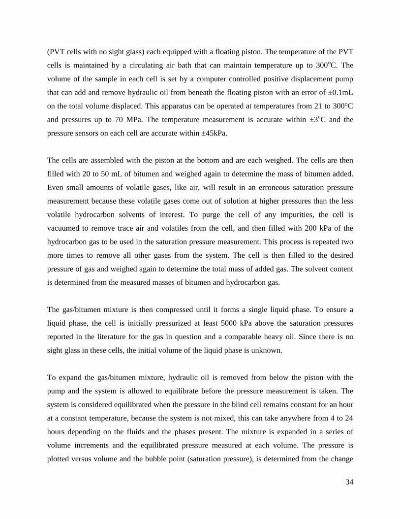
34

(PVT cells with no sight glass) each equipped with a floating piston. The temperature of the PVT

cells is maintained by a circulating air bath that can maintain temperature up to 300oC. The

volume of the sample in each cell is set by a computer controlled positive displacement pump

that can add and remove hydraulic oil from beneath the floating piston with an error of ±0.1mL

on the total volume displaced. This apparatus can be operated at temperatures from 21 to 300°C

and pressures up to 70 MPa. The temperature measurement is accurate within ±3oC and the

pressure sensors on each cell are accurate within ±45kPa.

The cells are assembled with the piston at the bottom and are each weighed. The cells are then

filled with 20 to 50 mL of bitumen and weighed again to determine the mass of bitumen added.

Even small amounts of volatile gases, like air, will result in an erroneous saturation pressure

measurement because these volatile gases come out of solution at higher pressures than the less

volatile hydrocarbon solvents of interest. To purge the cell of any impurities, the cell is

vacuumed to remove trace air and volatiles from the cell, and then filled with 200 kPa of the

hydrocarbon gas to be used in the saturation pressure measurement. This process is repeated two

more times to remove all other gases from the system. The cell is then filled to the desired

pressure of gas and weighed again to determine the total mass of added gas. The solvent content

is determined from the measured masses of bitumen and hydrocarbon gas.

The gas/bitumen mixture is then compressed until it forms a single liquid phase. To ensure a

liquid phase, the cell is initially pressurized at least 5000 kPa above the saturation pressures

reported in the literature for the gas in question and a comparable heavy oil. Since there is no

sight glass in these cells, the initial volume of the liquid phase is unknown.

To expand the gas/bitumen mixture, hydraulic oil is removed from below the piston with the

pump and the system is allowed to equilibrate before the pressure measurement is taken. The

system is considered equilibrated when the pressure in the blind cell remains constant for an hour

at a constant temperature, because the system is not mixed, this can take anywhere from 4 to 24

hours depending on the fluids and the phases present. The mixture is expanded in a series of

volume increments and the equilibrated pressure measured at each volume. The pressure is

plotted versus volume and the bubble point (saturation pressure), is determined from the change

35

in slope as shown in Figure 3.2. Note that, since the initial volume of fluid in the cell is not

known, its density cannot be determined.

Figure 3.1. Schematic of the blind cell apparatus.

The methodology was validated with n-pentane and the measured data are compared with the

vapour pressure predicted from the correlations provided in Perry’s Chemical Engineers’

Handbook (Green and Perry, 2008) in Figure 3.3. The deviations are reported in Table 3.3. The

data are within 4% of the correlation above approximately 450 kPa but deviate significantly at

lower pressures. The deviation below 450 kPa is larger than the expected error from the pressure

measurement indicating that there are other contributing factors to the error.

One source of error is the fluctuation in room temperature. Despite insulating the hydraulic oil

lines outside of the oven, the variation in the room temperature over the course of a day can

cause a variation of ±50 kPa. However, this variation is compensated for by averaging the

pressure data and is smaller than the observed deviation. The main source of error at low

pressure is caused by a small amount of air trapped in the lines to the pressure gauge. This air

dissolves in the hydraulic oil at higher pressure but evolves when the pressure drops below

approximately 500 kPa (depending on the temperature). Hence, the apparatus detects a saturation

36

pressure in the hydraulic oil at this pressure. Once the hydraulic oil drops below its saturation

pressure, the pressure of the system no longer changes and the true saturation pressure of the

sample cannot be detected. Figure 3.4 shows that the same deviation occurs in the propane

diluted bitumen saturation pressure data collected for this thesis. Therefore, only data above the

air/hydraulic oil saturation pressure were considered in this thesis. Note, once the source of the

error was identified, a procedure was developed to remove most of the trapped air and, in future,

saturation pressure measurements at lower pressure can be made.

As will be presented in Chapter 5, the solubilities from the blind cell experiments were within an

average of 8% of the models fit to solubility data collected in this thesis. The solubility model fit

to the data from this thesis was shown to predict literature data for different heavy oils with an

average deviation of 11%. Hence, the solubilities are considered to be validated with an

uncertainty of ±8%

.

Figure 3.2. Step-wise isothermal expansion of 11.4% propane in bitumen at 180°C.

6000

7000

8000

9000

10000

11000

12000

0 1 2 3 4

Pre

ssu

re, kP

a

Volume, cm³

37

Figure 3.3. Vapour pressure of n-Pentane measured using the blind cells compared to the

correlation in Green and Perry (2008).

Figure 3.4. Saturation pressure of propane diluted bitumen (this thesis) measured in blind cells.

0

500

1000

1500

2000

2500

3000

0 50 100 150 200

Vap

ou

r P

ressu

re, kP

a

Temperature, oC

CCE

Green and Perry

0

1000

2000

3000

0 0.2 0.4 0.6 0.8

Pre

ss

ure

(k

Pa

)

Mole Fraction Propane

50 C, CCE

75 C, CCE

90 C, CCE

Henry's Law

90oC

75oC

50oC

38

Table 3.3. Vapour pressure of n-pentane measured in the blind cells and calculated from Green

and Perry (2008)

T oC

Measured

Saturation Pressure

kPa

Correlation

Saturation Pressure

kPa

Absolute

Error

kPa

Relative

Error

%

47.7 340 158 182 116

74.7 439 321 118 37

89.4 474 464 10 2

134 1154 1193 -39 -3

180 2501 2615 -114 -4

3.3 Diffusivity

3.3.1 Diffusivity Apparatus

The diffusivity of gas in bitumen was measured using both the pressure decay method and

constant pressure gas delivery methods, using two apparatus with a common design. The

apparatus is based on the design by Etminan et al. (2010) which, in turn, is based on the pressure

decay apparatus developed originally by Riazi (1996). The apparatus consists of a cylindrical

diffusion cell connected to a gas supply cylinder all in a heated oil bath, Figure 3.5. The cells are

connected by a block valve, V2, and a pressure regulator, R1. The temperature of the bath is

measured with a thermocouple with an accuracy of ±2oC and the pressures of the gas supply and

diffusion cell are measured with pressure transducers with an accuracy of ±21 kPa,

The apparatus was designed for two experimental methods, which each require a different

procedure: 1) conventional pressure decay where gas supply and diffusion cell are left open to

one another, by opening valve V2 and the whole system pressure decreases as gas diffuses into

the oil; 2) constant pressure method where the pressure in the diffusion cell pressure is held

constant through the pressure regulator, R1, and pressure decreases only in the gas supply. For

both types of experiments, the temperature and both the diffusion cell and gas supply pressures

are measured with time and used in the analysis.

39

Diffusion

CellGas Supply

To Vacuum

PT2PT1

T

Heated Oil Bath

Gas

Cylinder

R2

R1

V2

V1

V3

V4

Figure 3.5. Schematic of the diffusivity apparatus

3.3.2 Procedure for Diffusivity Experiments

Start Up:

To start an experiment, 10-50 mL of bitumen is placed in a clean, dry diffusion cell of known

mass. The filled diffusion cell is weighed to determine the mass of bitumen added. The diffusion

cell is then connected to the gas supply line and placed into the oil bath. The whole system is

then vacuumed and purged with the solvent gas three times.

Procedure for Conventional Pressure Decay Mode:

The regulator is bypassed, the diffusion cell is isolated under vacuum by closing valve V2 and

the gas supply is filled with gas. The temperature in the bath is then set to the desired

temperature and the system is allowed to equilibrate overnight. To run an experiment, Valve V2

is opened slowly to connect the diffusion cell to the gas supply. The gas supply and diffusion cell

remain in pressure communication throughout the experiment. As time progresses, gas diffuses

40

into the oil and the system pressure decreases. The pressure is monitored with both pressure

gauges which are used to calculate the change in mass on their respective side of the apparatus.

Data collection begins as the system is being heated using a slow sample rate (one measurement

every 15 minute). The system is monitored until the temperature and both pressure

measurements are constant for at least 2 hours. Once the measurements are stable the time step

is decreased to fast sample rate of one measurement every 1-30 seconds while the diffusion cell

is filled and the initial data is collected. After two hours, and the initial data has been collected.

And the sample rate is decreased to one measurement every 5-15 minutes for the remainder of

the experiment.

Procedure for Constant Pressure Mode:

Valve 2 is bypassed, the diffusion cell is isolated under vacuum by closing the regulator, and the

gas supply is filled with gas. The temperature in the bath is then set to the desired temperature

and the system is allowed to equilibrate overnight. To run an experiment, the regulator, R1, is

slowly opened to the desired operating pressure. The regulator maintains a pressure in the

diffusion cell constant to ±70, kPa. Hence, the pressure drop occurs only in the gas supply

although some variation in the diffusion cell pressure occurs particularly when the regulator is

first opened. Both the pressure of the gas supply and of the diffusion cell are monitored as

described above.

3.3.3 Processing of Pressure Decay Data

Determination of Mass Transfer

The total mass diffused is calculated from the change in mass in each side of the cell as follows:

𝑚𝑠(𝑡) = ∆𝑚𝑑𝑖𝑓𝑓 + ∆𝑚𝑠𝑢𝑝𝑝𝑙𝑦 (3.1)

where 𝑚𝑠(𝑡) is the total mass of solvent diffused with time in g , ∆𝑚𝑑𝑖𝑓𝑓 is the mass change in

the gas phase of the diffusion cell in g, ∆𝑚𝑠𝑢𝑝𝑝𝑙𝑦 is the change of mass in the sample gas in g.

The mass change in each side of the diffusion cell is determined from the real gas law as follows:

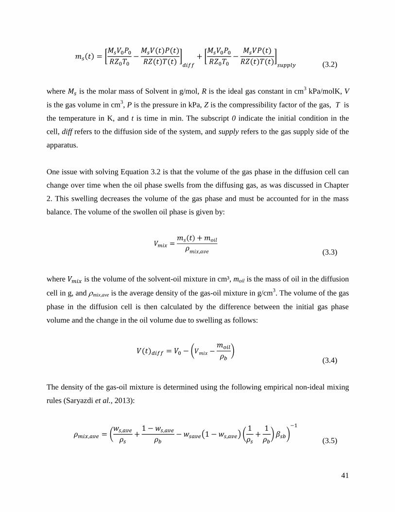
41

𝑚𝑠(𝑡) = [

𝑀𝑠𝑉0𝑃0

𝑅𝑍0𝑇0−

𝑀𝑠𝑉(𝑡)𝑃(𝑡)

𝑅𝑍(𝑡)𝑇(𝑡)]𝑑𝑖𝑓𝑓

+ [𝑀𝑠𝑉0𝑃0

𝑅𝑍0𝑇0−

𝑀𝑠𝑉𝑃(𝑡)

𝑅𝑍(𝑡)𝑇(𝑡)]𝑠𝑢𝑝𝑝𝑙𝑦

(3.2)

where 𝑀𝑠 is the molar mass of Solvent in g/mol, R is the ideal gas constant in cm3 kPa/molK, V

is the gas volume in cm3, P is the pressure in kPa, Z is the compressibility factor of the gas, T is

the temperature in K, and t is time in min. The subscript 0 indicate the initial condition in the

cell, diff refers to the diffusion side of the system, and supply refers to the gas supply side of the

apparatus.

One issue with solving Equation 3.2 is that the volume of the gas phase in the diffusion cell can

change over time when the oil phase swells from the diffusing gas, as was discussed in Chapter

2. This swelling decreases the volume of the gas phase and must be accounted for in the mass

balance. The volume of the swollen oil phase is given by:

𝑉𝑚𝑖𝑥 =

𝑚𝑠(𝑡) + 𝑚𝑜𝑖𝑙

𝜌𝑚𝑖𝑥,𝑎𝑣𝑒

(3.3)

where 𝑉𝑚𝑖𝑥 is the volume of the solvent-oil mixture in cm³, moil is the mass of oil in the diffusion

cell in g, and mix,ave is the average density of the gas-oil mixture in g/cm3. The volume of the gas

phase in the diffusion cell is then calculated by the difference between the initial gas phase

volume and the change in the oil volume due to swelling as follows:

𝑉(𝑡)𝑑𝑖𝑓𝑓 = 𝑉0 − (𝑉𝑚𝑖𝑥 −𝑚𝑜𝑖𝑙

𝜌𝑏)

(3.4)

The density of the gas-oil mixture is determined using the following empirical non-ideal mixing

rules (Saryazdi et al., 2013):

𝜌𝑚𝑖𝑥,𝑎𝑣𝑒 = (

𝑤𝑠,𝑎𝑣𝑒

𝜌𝑠+

1 − 𝑤𝑠,𝑎𝑣𝑒

𝜌𝑏− 𝑤𝑠𝑎𝑣𝑒(1 − 𝑤𝑠,𝑎𝑣𝑒) (

1

𝜌𝑠+

1

𝜌𝑏) 𝛽𝑠𝑏)

−1

(3.5)

42

where 𝑤𝑠,𝑎𝑣𝑒 the solvent concentration in the oil phase in wt%, 𝜌𝑠 is the effective density of the

solvent in g/cm3, 𝜌𝑏 is the density of the oil in g/cm

3, and 𝛽𝑠𝑏 is a binary interaction parameter

between the solvent and the oil. The component densities and binary interaction parameter

determination are described in Chapter 4. The average solvent concentration in the system is

calculated from the mass diffused and the total mass of bitumen in the system

𝑤𝑠,𝑎𝑣𝑒 =

𝑚𝑠(𝑡)

𝑚𝑠(𝑡) + 𝑚𝑜𝑖𝑙

(3.6)

If required, the height of the oil is given by:

ℎ𝑜𝑖𝑙 =

𝑉𝑚𝑖𝑥

𝐴𝑐

(3.7)

where hoil is the height of the swollen oil column and Ac is the cross sectional area of the

diffusion cell.

Treatment of Leaks

The constant pressure and pressure decay methods described in this chapter are susceptible to

leaks in the apparatus. Experiments with large leaks are rejected because mass lost from the leak

masks the mass transferred in the diffusion process. For small leaks, the effect of the leak can be

corrected for to determine the mass transfer from diffusion. Small leaks from the system

manifest themselves as a linear increase in mass diffused over time and become apparent when

the oil becomes saturated with gas. Instead of reaching a plateau, a linear increase is mass

diffused is observed. The slope of this linear increase is measured and the mass transfer data are

corrected by taking the difference between the calculated mass diffused and the amount of gas

leaked as follows:

𝑚𝑠,𝑐𝑜𝑟𝑟 = 𝑚𝑠(𝑡) − 𝑟𝑙𝑒𝑎𝑘 ∗ 𝑡 (3.8)

43

where ms,corr is the corrected mass diffused in g, rleak is the leak rate in g/min, and t is the time in

minutes. Figure 3.6 shows the mass transfer data for a propane bitumen system with a small leak

before and after the correction.

Figure 3.6. Mass of propane diffused onto bitumen at 80.7oC and 720 kPa before and after

correction for a small leak.

Treatment of Start Up

Several diffusion experiments with propane in bitumen did not follow the expected mass balance

at early times. Recall that the mass transfer at early times is linearly related to the square root of

time and must pass through the origin. Figure 3.7 shows that, in some cases, the data follow the

expected linear trend but do not pass through the origin. This discrepancy is attributed to errors

in the volume measurements, errors in the pressure measurements, and condensation of propane

in the apparatus. When the discrepancy was small and a clear linear trend was observed, the data

were corrected by shifting the calculated diffusion curve to pass through the origin as follows:

𝑚𝑠,𝑠ℎ𝑖𝑓𝑡𝑒𝑑 = 𝑚𝑠(𝑡) − 𝑖𝑛𝑡𝑒𝑟𝑐𝑒𝑝𝑡 (3.9)

0

0.05

0.1

0.15

0.2

0.25

0.3

0.35

0.4

0.45

0 5000 10000

Ma

ss D

iffu

sed

(g)

Time (min)

Original Data

Corrected Data

44

where ms,shifted is the mass of solvent diffused corrected through the origin in g and intercept is

the deviation from the origin of the initially calculated mass. In effect, the correction adjusts for

an error in the calculated initial mass of gas in the system.

Figure 3.7. Correction for error in initial mass of gas for diffusion of propane into bitumen at

62.3°C and 1080 kPa.

As seen in Figure 3.7, there can be a lag period before the expected linear trend begins. The lag

could result from an initial temperature disequilibrium between the two sides of the diffusion

system or from a disturbance of the interface when the gas is introduced to the cell. As the gas is

introduced to the diffusion cell, it expands and cools causing a temporary drop in temperature. In

addition, the initial large volume stream of solvent vapour may disturb the interface of the oil

causing a short period of convection. Both effects can account for some instability in the mass

diffusion curves at early times.

Use of Processed Data

Figure 3.8 shows the mass of methane diffused into decane over time from a commissioning

experiment. In this case, no corrections to the mass diffused were required. The solubility is

determined from the plateau and the diffusivity is calculated by modeling the change in mass

-0.5

0

0.5

1

1.5

2

0 50 100

Ma

ss

Dif

fuse

d (

g)

Square Root Time (min0.5)

Original Data

Shifted Data

45

over time. Analytical and numerical approaches to modeling the mass transfer are discussed in

Chapter 4.

Figure 3.8. Cumulative mass of methane diffused into n-decane at 124oC and 3950 kPa.

3.3.4 Validation of the Pressure Decay Measurements

First, the repeatability of the method was assessed based on four pressure decay experiments

performed with methane in bitumen at 100oC and approximately 4200 kPa, shown in Table 6.1.

The measured solubilities had a 90% confidence interval of 0.031wt%, coresponsing to a 6.3%

deviation from the mean. The measured diffusivites had a 90% confidence interval of 1.6E-10

m2/s coresponding to a 15% deviation from the mean.

The diffusion apparatus was further tested by measuring the diffusion of methane into n-decane

and n-dodecane and comparing the results with literature data. The solubility was determined

from the plateau in mass transferred at the end of the experiment. The diffusivity was determined

analytically with both the infinite acting and finite acting solutions presented in Chapter 4. The

solutions provided nearly identical diffusivities and the average values of the two methods were

used here.

46

Methane into n-Decane

Table 3.4 compares the methane solubilities in n-decane measured from the constant pressure

diffusion experiments with data collected by Srivastan et al.(1992) using constant coposition

expansion. The solubility data from this study are comparable with the literature data, with a

maximum deviation of 10%. Table 3.5 compares the diffusivities calculated from the pressure

decay apparatus data with data collected by Reamer et al. (1956) using a constant pressure gas

injection method. The diffusivities are up to 25% lower than the literature data.

Table 3.4. Solubility of methane in n-decane

T

(oC)

P

(kPa)

Solubility

Srivastan et al., 1992

(mol%)

Solubility

This Work

(mol%)

Deviation

(%)

86 3165 0.12 0.115 -5

124 3955 0.14 0.125 -10

Table 3.5. Diffusivity of methane in n-decane

T

(oC)

P

(kPa)

Diffusivity

Reamer et al., 1956

(x109

m/s²)

Diffusivity

This Work

(x109

m/s²)

Deviation

(%)

86 3165 11 8.6 -25

124 3955 16 12.5 -20

Methane into n-Dodecane

The methane solubilities and diffusivities in n-dodecane measured from the constant pressure

diffusion experiments are compared with pressure decay (constant pressure boundary condition)

data from Etminan at al. (2010) and conventional pressure decay data from Jamialahmadi et al.

(2006). The comparisons for solubility and diffusivity data are provided in Tables 3.6 and 3.7,

respectively. The solubility data from this study are comparable with the literature data, with a

maximum deviation of 7%. In this case, the diffusivities fall within the range of the literature

values (+9 and -48% deviation).

47

Table 3.6. Solubility in methane in n-dodecane

T

(oC)

P

(kPa)

Solubility

Etminan et al. 2010

(wt%)

Solubility

Jamialahmadi et al. 2006

(wt%)

Solubility

This Work

(wt%)

Deviation

(%)

45 3440 1.6 1.7 1.5 -3, -7

Table 3.7. Diffusivity of methane in n-dodecane

T

(oC)

P

(kPa)

Diffusivity

Etminan at al. 2010

(x109

m/s2)

Diffusivity

Jamialahmadi et al. 2006

(x109

m/s2)

Diffusivity

This Work

(x109

m/s2)

Deviation

(%)

45 3440 4.3 9.0 5.0 +9, -48

Overall, the solubilities determined with the new apparatus are consistently lower but still within

10% of the literature values for pure components. As will be presented in Chapter 5, the

solubilities from the diffusion experiments were within an average of 11% of the models fit to

diffusivity and blind cell experiments. The fit for solubility was shown to predict literature data

with an average deviation of 11%. These deviations are larger than the repeatability error of

6.3% and, therefore, the solubilities are considered to be have an uncertainty of 11%.

There is more deviation in the diffusivities which is not surprising considering the notable

variation between the results reported in the literature, even for two similar methods. The

commissioning data collected in this thesis lies within 50% of the literature values. However, the

diffusivity for the methane/n-dodecane system lies between the two results from the literature

and is in very good agreement with the diffusion data collected using an analogous constant

pressure method by Etminan et al. (2010). As will be shown in Chapter 6, the diffusivities of

solvents in bitumen measured in this thesis follow the expected trend with viscosity and can be

correlated within an average error of 12% with a small pressure correction. This deviation is

similar to the repeatability error of 15% and, therefore, the diffusivities are considered to be

validated with an uncertainty of ±15%.

48

CHAPTER FOUR: MODELING PRESSURE DECAY EXPERIMENTS

This chapter presents the mathematical models used to fit the pressure decay data collected in

this thesis. The key assumptions and relevant boundary conditions are discussed and simple

analytical solutions to Fick’s law are provided. A numerical model for mass transfer, accounting

for swelling and a concentration dependent diffusivity, is developed. The diffusivity, density, and

viscosity models required to implement the mass transfer model are presented.

4.1 Description of Problem

The pressure decay experiments to be modeled were described in Chapter 3 and involve a gas

diffusing into a column of oil, Figure 4.1. The gas enters at the gas-oil interface, z=0, and

reaches a second boundary at the bottom of the oil column, z = h(t). At dilute conditions, the

total height is constant. At high dissolved gas concentrations, the oil phase is expected to swell

and increase the height of the bitumen column. In this case, the gas-liquid interface will remain

set at the origin of the domain and the change in height will be accounted for in the domain

length, h(t).

Figure 4.1. Side view of the diffusion cell.

As was discussed in Chapter 2, the mass transfer is determined from the general mass continuity

equation given by:

𝜕𝑐𝐴𝜕𝑡

= −∇(𝑐𝐴 ∗ 𝑣 ) − ∇(𝑗𝐴⃑⃑ ⃑) + 𝑟𝐴 (2.1)

𝑗𝐴⃑⃑ ⃑ = −𝐷𝐴𝐵∇(𝑐𝐴) (2.2)

49

where cA is the mass concentration in kg/m³, 𝑣 is the mass average velocity in m/s, and 𝑗𝐴⃑⃑ ⃑ is the

molar flux in kg/m²s, t is the time in s, and DAB is the diffusivity in m2/s. The first step in solving

the continuity equation is to simplify the problem as is appropriate for the geometry and

conditions of the experiment. Then, the initial and boundary conditions are set and the simplified

continuity equation is solved at these conditions to determine the concentration profiles of the

diffusing gas and the total mass of solvent diffused into the oil with time. The mass diffused

curve is compared with the experimental data and the value of the diffusivity or the coefficients

of the model for the concentration dependent diffusivity are varied until the model fits the

experimental data.

4.2 Simplifying Assumptions

The assumptions used to simplify the continuity equation and develop the mass transfer models

used in this thesis are listed below.

Isothermal System

Assuming that the system is isothermal gives a significant simplification to model because there

is no longer a need to solve the coupled heat and mass transfer equations. The diffusion cell is

metal and is placed in a heated oil bath with a relatively large thermal mass. The bath

temperature was monitored was stable within 1oC. The heat of dissolution at any time is expected

to be small compared with the rate of heat transfer. As the diffusion cell is filled with gas, there

is a small temperature change in the gas phase, which lasts less than two minutes. Therefore, the

system was considered to be isothermal.

One Dimensional Diffusion

The assumption of one dimensional diffusion dramatically simplifies the continuity equation.

The diffusion cell is a cylinder set up such that the majority of the diffusion is expected to occur

perpendicular to the circular cross-section. Any radial diffusion that might occur from wall

effects is ignored, as in previous works in pressure decay.

50

No Chemical Reactions

This assumption also simplifies the continuity equation. The gaseous solvents used in these

experiments are constituents of the live oil and therefore the dead oil and solvent are not

expected to react. It is possible that at higher temperatures, a thermal cracking reaction could

occur which would change the nature of the oil. Cracking reactions are not expected to become

significant until a temperature of at least 250oC (Gray, 2015), which is much higher than the

pressure decay experiments performed in this thesis. Gray (2015) noted that thermal processing

bitumen at as low as 250oC produces hydrogen sulfide, a common indicator of bitumen cracking.

No Second Liquid Phase

Second liquid phases can form from mixtures of solvent and bitumen including light liquid

phases and asphaltene-rich phases. Droplets of a light liquid phase or precipitated asphaltene

particles would dramatically change the nature of the liquid phase. The dispersed material would

cause discontinuities in the fluid and this situation would require a different modeling approach.

In addition, the settling of dense asphaltene particles could cause natural convection.

The solvents considered in this study are methane, ethane, and propane. Asphaltene precipitation

is not anticipated with methane or ethane (Agrawal et al., 2012) but a light liquid phase can form

at ethane contents above 7.2 wt% (Agrawal et al., 2012; Mehrotra and Svrcek, 1985b).

Therefore, all diffusion experiments with ethane were conducted at solubilities below this value.

Agrawal et al. (2012) performed asphaltene onset experiments with propane in a bitumen from

the same field as the sample studied in this thesis. They measured an asphaltene onset

concentration using a using a high pressure microscope and found the onset point to be between

13 and 15 wt% propane at 50oC. From experiments performed with n-pentane in bitumen in the

same paper, it was observed that asphaltene onset solvent content increases with increasing

temperature. Therefore, the diffusion experiments were performed at solubilities below the onset

condition at 50°C (the lowest anticipated onset condition).

51

No Natural Convection

The existence of natural convection in the system would dramatically increase the rate of mass

transfer. However, mixtures of hydrocarbon solvents in bitumen are less dense than the oil alone.

Hence, there would be no density driven convection in the system because an upper layer would

always be less dense than a lower layer. Asphaltene precipitation could cause the density

gradient required to promote convection. The concentrations of the experiments are kept below

this threshold.

Oil is Non Volatile

Having a non-volatile oil ensures that diffusion only occurs in the liquid phase, and no oil

diffuses though the gas phase. The bitumen used in this thesis was heated to 70°C to remove

water before the diffusion experiments. When the diffusion experiment is begun, the bath was

heated and the pressure was monitored in the diffusion cell and gas supply. While heating the

system to 90oC, the pressure in the diffusion cell did not increase more than that of the sample

cylinder, indicating that little gas was evaporating

Pseudo-Binary System

Although oil is composed of a large number of different molecules, modelling the diffusion

process is dramatically simplified by assuming the oil is a single pseudo-component. If the oil is

non-volatile, there is no diffusion at all across the upper boundary. However, while the final

conditions is a homogeneous mixture, the lighter bitumen components may diffuse from lower

bitumen-rich layers to upper solvent-rich layers more rapidly than heavier component. There was

no way to test for this effect and it was neglected.

Negligible Density Gradient

The diffusivity experiments modeled in this thesis are generally at low solubility, with only three

experiments above 7 wt%. Therefore, at low solubility the density gradients will be small in the

oil phase. This assumption allows the combine the density and weight fraction and density into

the derivative in Fick’s First Law.

52

Negligible Velocity Contribution

The only velocity in the system is caused by swelling as the solvent dissolves into the bitumen.

Then initial velocity was estimated near the interface, where it is expected to be highest. The

contribution of convection to the calculated mass diffused was less than 0.1% of the mass

diffused from diffusion. The velocity contribution is therefore neglected in the mathematical

model.

After applying the above assumptions, the mass balance equation simplifies to the following

form, as was discussed in Chapter 2:

𝜕

𝜕𝑧(𝐷𝑠𝑏

𝜕𝑐𝑠

𝜕𝑧) =

𝜕𝑐𝑠

𝜕𝑡 (4.1)

Where Dsb is the diffusivity of solvent in bitumen in m2/s and cs is the concentration of solvent in

oil in kg/m3.

4.3 Initial and Boundary Conditions

Diffusion in the cylindrical geometry described in Figure 1 can be modelled using a one

dimensional diffusion model that requires one initial and two boundary conditions to solve.

4.3.1 Initial Condition

Two initial conditions are used in modelling the systems of interest in this thesis. For the

majority of experiments in this thesis the oil is dead and there is no initial solvent concentration

as indicated by the following boundary condition:

𝑐𝑠(𝑧, 𝑡 = 0) = 0 (4.2)

where cs is the concentration, z is the position in the oil column, and t is the time. A small

number of experiments were conducting with the oil phase containing an evenly distributed

initial concentration of the solvent gas. To model these systems, the following boundary

condition is used.

53

𝑐𝑠(𝑧, 𝑡 = 0) = 𝑐𝑠0 (4.3)

where cs0 is the initial concentration of solvent gas.

4.3.2 Boundary Conditions

The two boundary conditions required to solve the continuity equation are usually taken at the

gas-oil interface and at the bottom of the oil column as was shown in Figure 1. These are the

locations in the system where the most information regarding the diffusing gas is available.

At the Gas-Oil Interface

Tharanivasan et al., (2004) compared three different gas-oil boundary conditions used to model

pressure decay experiments. For systems of methane diffusing into oil, the following Dirichlet

equilibrium boundary conditions was found to best fit the data:

𝑐𝑠(𝑧 = 0, 𝑡) = 𝑐𝑠 𝑒𝑞 (4.4)

where cseq is the equilibrium composition of the diffusion cell in kg/m3. For pressure decay

experiments, cseq is defined at the equilibrium pressure at the end of the experiment. For a

constant pressure boundary condition experiment, cseq is defined at the operating pressure of the

experiment.

Etminan et al. (2012) developed a time dependent Robin boundary condition for both methane

and carbon dioxide diffusion into bitumen (Etminan et al., 2014a) that accounts for the

possibility of mass transfer resistance at the interface, given by:

−𝐷𝑠𝑏

𝑑𝑐𝑠

𝑑𝑧 𝑧=0= 𝑘(𝑐𝑠−𝑖𝑛𝑡(𝑡) − 𝑐𝑠(𝑧 = 0, 𝑡))

(4.5)

where Dsb is the diffusivity of the solvent (s) through the bitumen (b) in m²/s, k is the mass

transfer coefficient in m/s, cA-int is the concentration immediately above the interface in kg/m³,

and cA(z=0, t) is the concentration immediately below the interface kg/m³. The sensitivity of the

54

pressure drop to each of these variables was measured. The results were very consistent to those

found with a Dirichlet boundary condition Tharanivasan et al, (2004) and; therefore, it was

concluded that a Dirichlet condition is sufficient to model pressure decay data of methane in

heavy oil. Therefore, in this thesis, Equation 4.4 will be used to model the pressure decay and

constant pressure delivery experiments.

At the Bottom of the Oil Column

There are two common boundary conditions taken at the bottom of the oil column. The first is an

infinite acting boundary condition where it is assumed that the oil column is infinitely deep and

the initial condition of the system is maintained at infinite depth. This boundary condition

applies when the diffusing solvent has not yet reached the bottom of the bitumen column. The

systems in this thesis where this condition is applied have no initial concentration of dissolved

gas and therefore the boundary condition is given by:

𝑐𝑠(𝑧 → ∞, 𝑡) = 0 (4.6)

The second common boundary condition is the finite acting condition and it is applied before and

after the solvent reaches the bottom of the bitumen column. Since the bottom of the oil column is

in contact with the metal diffusion cylinder, there will be no gas diffusion though this position.

Hence, the concentration gradient is zero at this point and the boundary condition is given by:

𝑑𝑐𝑠

𝑑𝑧 𝑧=ℎ= 0

(4.7)

where h is the height of the oil column. Equations 4.6 and 4.7 give identical solutions to the

continuity equation until the diffusing gas reaches the bottom of the oil column.

In this thesis, the entire range of data collected from pressure decay experiments is analyzed and;

therefore, Equation 4.7 is used. Equation 4.6 was used to analyze early time data for some

experiments and the results were compared with those obtained with Equation 4.7 in order to

validate that the method was implemented correctly.

55

4.4 Solutions at Dilute Conditions

Analytical solutions to Fick’s Law can be obtained when the diffusivity is a constant and there is

no swelling; that is, at dilute conditions. The solutions with the infinite and finite acting

boundary conditions are provided below.

4.4.1 Infinite Acting Solution

The solution to Fick’s Law with the infinite acting boundary condition (Equation 4.6), the

equilibrium gas-oil interface equation (Equation 4.3), and no initial solvent content (Equation

4.1) is given by:

𝑐𝑠

𝑐𝑠 𝑒𝑞= 1 − 𝑒𝑟𝑓 (

𝑧

√4𝐷𝑠𝑏𝑡)

(4.8)

where erf is the error function.

As was discussed in Chapter 2, the mass diffused at a given time is determined from the

following integral:

𝑚𝑠(𝑡) = 𝐴𝑐 ∫ 𝑐𝑠𝑑𝑧

ℎ

0

(4.9)

Equation 4.8 is substituted into Equation 4.9 to obtain the following expression:

𝑚𝑠(𝑡) = 2𝐴𝑐𝑐𝑠 𝑒𝑞√𝐷𝑠𝑏𝑡

𝜋

(4.10)

Since the infinite acting boundary condition does not account for the finite nature of the oil

column, valid comparisons with experimental data can only be made until the diffusing gas

reaches the bottom of the diffusion cell. The experiment is usually run until the oil is saturated

with the gas in order to determine cs eq.

As an example, the infinite acting analysis was applied to the pressure decay data for methane

diffusing into n-decane. The data are plotted against the square root of time to show the linear

infinite acting region, Figure 4.2. The solubility, cAeq, is determined from the asymptote in the

56

cumulative mass diffused. The slope of the infinite acting linear region is determined and the

diffusivity is calculated by rearranging Equation 4.10 as follows:

𝐷𝑠𝑏 = (

𝑆

2𝐴𝑐𝑠 𝑒𝑞)

2

𝜋

(4.11)

where S is the slope if the linear region.

Figure 4.2. Cumulative mass of methane diffused into n-decane against square root of time at

123°C and 3950 kPa with infinite and finite acting fits to the data.

4.4.2 Finite Acting Solution

The solution to Fick’s Law with the finite acting boundary condition (Equation 4.6), the

equilibrium gas-oil interface equation (Equation 4.4), and no initial solvent content (Equation

4.1) is given by:

𝑐𝑠

𝑐𝑠 𝑒𝑞= 1 −

4

𝜋∑

1

(2𝑛 − 1)sin ( (

2𝑛 − 1

2)𝜋

ℎ𝑥)

∞

𝑛=1

𝑒𝑥𝑝(−((2𝑛 − 1

2)𝜋

ℎ)

2

𝐷𝑠𝑏𝑡)

(4.12)

0

0.5

1

1.5

2

0 20 40 60 80

Cu

mu

lati

ve M

ass (

g)

Square Root of Time (min0.5)

Experimental

Infinite Acting

Finite Acting

57

Equation 4.12 is substituted into Equation 4.9 to obtain the following expression relating the total

mass diffused to time:

𝑚𝑠(𝑡) =8𝐴𝑐𝑐𝑠 𝑒𝑞ℎ

𝜋2∑

1

(2𝑛 − 1)2(1 − 𝑒𝑥𝑝 (−((

2𝑛 − 1

2)𝜋

ℎ)

2

𝐷𝑠𝑏𝑡))

∞

𝑛=1

(4.13)

This model is fit to the data by varying both the solubility and the diffusivity to minimize the

error. The finite acting solution for the methane diffusion example discussed previously is also

presented in Figure 2. Both the finite and infinite acting solutions are identical until the diffusing

solvent reaches the bottom on the oil column. Only the finite acting solution can describe the

diffusion from this point until the entire fluid column is saturated with methane. The infinite

series of equations 4.12 and 4.13 are truncated at n=500 where the modeled mass diffused at all

times was within 1% of the predicted mass using a truncation of 1000.

4.5 Modelling Diffusion at Non-Dilute Conditions

At non-dilute conditions, the solvent content is high enough to cause significant swelling of the

oil column and therefore the upper boundary is no longer in a fixed position. In addition, the

diffusivity may be a function of composition and this dependence may become significant at

higher solvent contents. Hence, the analytical solutions presented in Section 4.3 are no longer

valid. A numerical model was developed to include both swelling and compositionally

dependent diffusivities.

4.5.1 Model Description

To set up the model of the pressure decay experiments, the oil phase is divided into layers of

equal thickness and the gas phase is assumed to be homogeneous (Figure 4.3). The initial solvent

concentration in each oil layer is set to a uniform initial value, usually zero. The solvent

concentration at the gas-oil interface is set to the solvent solubility limit and the finite acting

boundary condition is applied to the bottom of the column.

At each time step, solvent diffusion from the gas to the oil from each layer to the next is

determined from the continuity equation using either a fixed diffusivity or a compositionally

58

dependent diffusivity. The mass of bitumen in each cell is held constant and only the mass of

solvent changes. The density of each cell is updated and the height of the cell recalculated. The

mass diffused is the sum of the solvent masses in each cell. The height of the gas-oil interface is

the sum of the height of all of the layers. Each step in the calculations is described below.

Figure 4.3. Numerical diffusion model for pressure decay experiments.

4.5.2 Discretization of the Continuity Equation

The continuity equation, Equation 4.1, does not include a convective term but does allow the

diffusivity to vary with composition. The equation is discretized using a Forward Time Centered

Space (FTCS) scheme (Fletcher, 1991). In particular, the two point forward difference method is

used to discretize the time derivative and the three point central difference method is used to

discretize the spatial derivative as follows:

𝐶𝑠𝑛𝑗+1 − 𝐶𝑠𝑛

𝑗

𝑡𝑗+1 − 𝑡𝑗=

𝐷𝑛𝑗

(∆h𝑛𝑗)2 (𝐶𝑠𝑛−1

𝑗 + 𝐶𝑠𝑛+1𝑗 − 2𝐶𝑠𝑛

𝑗 )

+(𝐷𝑛+1

𝑗− 𝐷𝑛−1

𝑗)

4(∆h𝑛𝑗)2 (𝐶𝑠𝑛+1

𝑗 −𝐶𝑠𝑛−1𝑗 )

(4.14)

59

where Cs is the solvent concentration in g/cm³, t is time in minutes, D is diffusivity in cm²/min,

∆h𝑛𝑗 is the height of the layer in cm, n and j are the indexes for vertical position and time.

Equation 4.14 is rearranged to solve for the concentration at the subsequent time step as follows:

𝐶𝑠𝑛

𝑗+1= 𝐶𝑠𝑛

𝑗+

(𝑡𝑗+1 − 𝑡𝑗)

(∆h𝑛𝑗)2 (𝐷𝑛

𝑗(𝐶𝑠𝑛−1

𝑗+ 𝐶𝑠𝑛+1

𝑗− 2𝐶𝑠𝑛

𝑗) +

1

4(𝐷

𝑛+1𝑗

− 𝐷𝑛−1𝑗

)(𝐶𝑠𝑛+1𝑗

−𝐶𝑠𝑛−1𝑗

))

(4.15)

Equation 4.15 gives the concentration at each position and time except at the domain boundaries

and at the initial time. In the case of a constant diffusivity this equation can be simplified to:

𝐶𝑠𝑛

𝑗+1= 𝐶𝑠𝑛

𝑗+

(𝑡𝑗+1 − 𝑡𝑗)

(∆h𝑛𝑗)2 𝐷(𝐶𝑠𝑛−1

𝑗+ 𝐶𝑠𝑛+1

𝑗− 2𝐶𝑠𝑛

𝑗)

(4.16)

To specify the concentration at these conditions, the boundary conditions and initial conditions

must be applied. Using the same method, the finite acting boundary condition, the equilibrium

boundary condition at the gas-oil interface, and the initial condition can be discretized to the

following:

𝐶𝑠𝑛𝑚𝑎𝑥

𝑗 = 𝐶𝑠𝑛𝑚𝑎𝑥𝑗−1 +

𝐷𝑛𝑚𝑎𝑥𝑗−1

∗ (𝐶𝑠𝑛𝑚𝑎𝑥−1𝑗−1 −𝐶𝑠𝑛𝑚𝑎𝑥

𝑗−1 )(𝑡𝑗+1 − 𝑡𝑗)

∆h𝑛𝑚𝑎𝑥𝑗−1

(4.17)

𝐶𝑠0𝑗 = 𝑐𝑠 𝑒𝑞 (4.18)

𝐶𝑠𝑛0 = 𝑐𝑠0 (4.19)

where nmax is the bottom layer and 𝑐𝑠0 is the initial concentration of solvent in the oil. The

determination of the diffusivity terms is discussed in Section 4.5.4.

4.5.3 Determination of Layer Thickness and Mass Diffused

The initial thickness of each layer is given by:

∆ℎ𝑛0 =

𝑚𝑜𝑖𝑙

𝜌𝑏 ∗ 𝐴𝑐 ∗ 𝑛𝑚𝑎𝑥

(4.20)

60

where ∆ℎ𝑛0 is the initial thickness of each layer in cm, 𝑚𝑜𝑖𝑙 is the initial mass of oil in g, 𝜌𝑏 is the

density of the oil in g/cm³, and 𝐴𝑐 is the cross sectional area of the diffusion cylinder in cm2.

To calculate the layer thickness at each time step, the volume of fluid in each layer must be

determined at each time step. The height is then the volume divided by the fixed cross sectional

area. The volume is determined from the known mass of bitumen, the mass fraction of solvent in

each layer at the given time step, and the density of the mixture. The mass fraction of solvent in

each layer is calculated from the concentration of solvent in the layer as follows:

𝑤𝑠𝑛

𝑗 =𝐴𝑐 ∗ ∆h𝑛

𝑗−1∗ 𝐶𝑠𝑛

𝑗

𝑚𝑏𝑛𝑗 + 𝐴𝑐 ∗ ∆h𝑛

𝑗−1∗ 𝐶𝑠𝑛

𝑗

(4.21)

where 𝑤𝑠𝑛𝑗 is the mass fraction of solvent in the layer and 𝑚𝑏𝑛

𝑗 is the fixed mass of bitumen in

each layer in g. The density of the mixture is obtained from the mixing rules from Saryazdi et al.

(2013) given by:

𝜌𝑚𝑖𝑥𝑛

𝑗 = (𝑤𝑠𝑛

𝑗

𝜌𝑠+

1 − 𝑤𝑠𝑛𝑗

𝜌𝑏− 𝑤𝑠𝑛

𝑗 ∗ (1 − 𝑤𝑠𝑛𝑗 ) (

1

𝜌𝑠+

1

𝜌𝑏)𝛽𝑠𝑏)

−1

(4.22)

where 𝜌𝑚𝑖𝑥𝑛𝑗 is the density of the mixture in the layer in g/cm³, 𝜌𝑠 is the effective liquid density

of the solvent in g/cm³, 𝜌𝑏 is the density of the bitumen in g/cm³ and sb is the binary interaction

parameter between the solvent and the oil. The density model is discussed in more detail in

Section 4.5.5.

The thickness of each layer is then given by:

∆h𝑛

𝑗=

𝐴𝑐 ∗ ∆h𝑛𝑗−1

∗ 𝐶𝑠𝑛𝑗 + 𝑚𝑏𝑛

𝑗

𝜌𝑚𝑖𝑥𝑛𝑗 ∗ 𝐴𝑐

(4.23)

The total height of the oil can be calculated by adding all of the layer thicknesses

61

ℎ = ∑ ∆h𝑛

𝑗

𝑛𝑚𝑎𝑥

𝑛=1

(4.24)

The total amount of solvent diffused is determined by summing the total mass of solvent in each

of the grid layers.

𝑚𝑠

𝑗 = ∑ 𝐴𝑐 ∗ ∆h𝑛

𝑗

𝑛𝑚𝑎𝑥

𝑛=1

∗ 𝐶𝑠𝑛𝑗

(4.25)

where 𝑚𝑠𝑗 is the total mass of solvent diffused into the oil at time step j.

4.5.4 Models for Diffusivity

In this thesis, five models for the diffusivity were studied:

1) constant diffusivity

𝐷𝑠𝑏 = 𝐶𝑜𝑛𝑠𝑡𝑎𝑛𝑡 (4.26)

2) the Hayduk and Cheng (1971) equation

𝐷𝑠𝑏 =

𝐴

𝜇𝑚𝑖𝑥𝑛

(4.27)

3) the modified Hayduk and Cheng equation

𝐷𝑠𝑏 =

𝐴𝑇


(4.28)

4) a modified Bearman (1961) equation

𝐷𝑠𝑏 =

𝐴

𝜇𝑚𝑖𝑥𝑛[1 + 𝑥𝑠 (

𝑉𝑠𝑉𝑏

− 1)] (𝑑 ln 𝑎𝑠

𝑑 ln 𝑥𝑠)

(4.29)

62

5) the Vignes (1966) equation

𝐷𝑠𝑏 = (𝐷𝑠𝑏

0 )𝑥𝑏(𝐷𝑏𝑠0 )𝑥𝑠 (

𝑑 ln 𝑎𝑠

𝑑 ln 𝑥𝑠)

(4.30)

where 𝐷𝑠𝑏 is the diffusivity of solvent in bitumen, 𝜇𝑚𝑖𝑥 is the mixture viscosity, x is the mole

fraction, V is the molar volume, a is the activity, A and n are parameters specific to the fluid

mixture, the subscripts s and b refer to the solvent and bitumen respectively, and 𝐷𝑠𝑏0 and 𝐷𝑏𝑠

0

are the infinite dilution diffusivities of solvent in bitumen and bitumen is solvent respectively

The models for diffusivity are substituted into the discretized continuity equation (Equation 4.15)

and each diffusivity models is adjusted to best fit the data. When using Equation 4.26, the model

is fit to experimental data by adjusting the value of D. The models using Equations 4.27 to 4.29

are fit to experimental data by adjusting the parameters A and n. The models using Equation 4.30

are fit to experimental data by adjusting the two infinite dilution diffusivities 𝐷𝑠𝑏0 and 𝐷𝑏𝑎

0 .

When modelling with a constant diffusivity, no additions need to be made to the modelling

methodology described earlier in this chapter. However, when applying the concentration

dependent diffusivity models, other inputs may be required including the mixture viscosity, the

mole fraction of the components, the molar volumes of the components, and the thermodynamic

correction of the solvent in the oil. Each of these parameters are evaluated after the concentration

profiles and heights of the layers have been calculated.

Mole Fraction and Molar Volume

The mole fraction of solvent in the layer can be calculated from the weight fraction of solvent

(from Equation 4.21) as follows:

𝑥𝑠𝑛𝑗 =

𝑤𝑠𝑛𝑗

𝑀𝑠

𝑤𝑠𝑛𝑗

𝑀𝑠+


𝑀𝑏

(4.31)

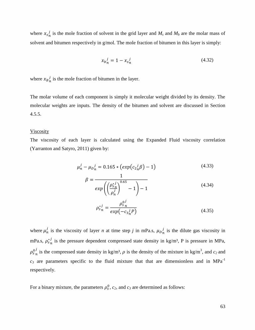
63

where 𝑥𝑠𝑛𝑗 is the mole fraction of solvent in the grid layer and Ms and Mb are the molar mass of

solvent and bitumen respectively in g/mol. The mole fraction of bitumen in this layer is simply:

𝑥𝑏𝑛𝑗 = 1 − 𝑥𝑠𝑛

𝑗 (4.32)

where 𝑥𝐵𝑛𝑗 is the mole fraction of bitumen in the layer.

The molar volume of each component is simply it molecular weight divided by its density. The

molecular weights are inputs. The density of the bitumen and solvent are discussed in Section

4.5.5.

Viscosity

The viscosity of each layer is calculated using the Expanded Fluid viscosity correlation

(Yarranton and Satyro, 2011) given by:

𝜇𝑛𝑗− 𝜇𝐷𝑛

𝑗 = 0.165 ∗ (𝑒𝑥𝑝(𝑐2𝑛𝑗𝛽) − 1) (4.33)

𝛽 =

1

𝑒𝑥𝑝((𝜌𝑠

∗𝑛𝑗

𝜌𝑛𝑗 )

0.65

− 1) − 1

(4.34)

𝜌𝑠

∗𝑛𝑗 =

𝜌𝑠0𝑛

𝑗

𝑒𝑥𝑝(−𝑐3𝑛𝑗𝑃)

(4.35)

where 𝜇𝑛𝑗 is the viscosity of layer n at time step j in mPa.s, 𝜇𝐷𝑛

𝑗 is the dilute gas viscosity in

mPa.s, 𝜌𝑠∗𝑛𝑗 is the pressure dependent compressed state density in kg/m³, P is pressure in MPa,

𝜌𝑠0𝑛

𝑗 is the compressed state density in kg/m³, 𝜌 is the density of the mixture in kg/m

3, and c2 and

c3 are parameters specific to the fluid mixture that that are dimensionless and in MPa-1

respectively.

For a binary mixture, the parameters 𝜌𝑠0, c2, and c3 are determined as follows:

64

𝜌𝑠

0𝑛

𝑗= [

𝑤𝑠𝑛𝑗

𝜌𝑠,𝑠0 +


𝜌𝑠,𝑏0 − 𝑤𝑠𝑛

𝑗 ∗ (1 − 𝑤𝑠𝑛𝑗 ) ∗ (

1

𝜌𝑠,𝑠0 +

1

𝜌𝑠,𝑏0 )𝜃𝑠𝑏]

−1

(4.36)

𝑐2,𝑚𝑖𝑥

𝜌𝑠0𝑛

𝑗=

𝑐2,𝑠𝑤𝑠𝑛𝑗

𝜌𝑠,𝑠0 +

𝑐2,𝑏(1 − 𝑤𝑠𝑛𝑗 )

𝜌𝑠,𝑏0 − 𝑤𝑠𝑛

𝑗 ∗ (1 − 𝑤𝑠𝑛𝑗 ) ∗ (

𝑐2,𝑠

𝜌𝑠,𝑠0 +

𝑐2,𝑏

𝜌𝑠,𝑏0 )𝜃𝑠𝑏

(4.37)

𝑐3𝑛𝑗 = [

𝑤𝑠𝑛𝑗

𝑐3,𝑠+

(1 − 𝑤𝑠𝑛𝑗 )

𝑐3,𝑏]

−1

(4.38)

where θsb is a binary interaction parameter and subscripts s and b denote the solvent and the

bitumen, respectively. A more detailed description of the Expanded Fluid viscosity model and

the determination of its parameters is provided in Section 4.5.6.

Thermodynamic Correction Factor

As described in Chapter 2, the thermodynamic correction factor is defined as follows:

𝛼 =

𝑑 ln 𝑎𝑠

𝑑 ln 𝑥𝑠

(4.39)

where 𝛼 is the thermodynamic correction factor. In this thesis the activity was calculated with an

activity coefficient such that (Elliot and Lira, 1991):

𝑎𝑠 = 𝛾𝑠𝑥𝑠 (4.40)

where 𝛾𝑠is the activity coefficient. The activity coefficient was determined from the Margules

(1895) equation given by:

ln 𝛾𝑠 = [𝐴𝑠𝑏 + 2(𝐴𝑏𝑠 − 𝐴𝑠𝑏)𝑥𝑠](1 − 𝑥𝑠)2 (4.41)

where 𝐴𝑠𝑏 and 𝐴𝑏𝑠are parameters specific to a given mixture. Equation 4.40 is substituted into

Equation 4.39 to obtain the following expression:

65

𝛼 =

𝑑 ln(𝛾𝑠𝑥𝑠)

𝑑 ln 𝑥𝑠=

𝑑 ln 𝛾𝑠

𝑑 ln 𝑥𝑠+ 1 = 𝑥𝑠

𝑑 ln 𝛾𝑠

𝑑𝑥𝑠+ 1

(4.42)

Equations 4.41 is then substituted into Equation 4.42 to obtain the thermodynamic correction

factor for each layer in terms of the Margules coefficients and the mole fraction of solvent in the

layer.

𝛼𝑛𝑗= 1 + 𝑥𝑠𝑛

𝑗 [−2(𝑥𝑠𝑛𝑗 − 1) ∗ (𝐴𝑠𝑏(3𝑥𝑠𝑛

𝑗 − 2) − 3𝐴𝑏𝑠 + 𝐴𝑏𝑠)] (4.43)

The coefficients of the Margules equation were fitted to the solvent oil saturation pressure data

measured for this thesis, as will be discussed in Chapter 5.

4.5.5 Prediction of Mixture Density

The density of mixtures of oil and solvent are required to determine the volume of each layer in

the numerical diffusion model. It is also a key input parameter for the viscosity model used to

determine compositionally dependent diffusivities. The viscosity model is quite sensitive to the

accuracy of the input density. Hence, an accurate density prediction is required.

Saryazdi et al. (2013) demonstrated that a combination of effective solvent densities and non-

ideal mixing rules could fit density data for mixtures of oil and solvent to within the accuracy of

the measurements. They proposed the following form of mixing rule:

𝜌𝑚𝑖𝑥 = [∑∑𝑤𝑖𝑤𝑗

2(1

𝜌𝑖+

1

𝜌𝑗) (1 − 𝛽𝑖𝑗)

𝑗𝑖

]

−1

(4.44)

where ρmix is the mixture density in kg/m³, w is the weight fraction of each component, and ρ is

the density or effective density of the pure components, and βij is the binary interaction

parameter between components i and j. For binary mixtures or pseudo-binaries such as solvent

and bitumen, Equation 4.44 simplifies to the following expression:

66

𝜌𝑚𝑖𝑥 = (

𝑤𝐴

𝜌𝐴

+1 − 𝑤𝐴

𝜌𝐵

− 𝑤𝐴 ∗ (1 − 𝑤𝐴) ∗ (1

𝜌𝐴

+1

𝜌𝐵

)𝛽𝐴𝐵

)

−1

(4.45)

For gases dissolved in liquids, the solvent liquid density is taken as the effective liquid density;

that is, the hypothetical density of that gas when it is part of a liquid mixture. Effective densities

were determined for some common gases by Saryazdi et al. (2013) and fitted with the following

equations.

𝜌𝑒 = 𝜌𝑒0 + 𝐵∗ ∗ 𝑃 (4.46)

𝜌𝑒0 = 𝑎1∗ + 𝑎2

∗𝑇 (4.47)

𝐵∗ = 𝑏1∗ + 𝑏2

∗𝑇 (4.48)

where ρe is the effective density of a gas in liquid in kg/m3, P is the pressure in MPa, T is

temperature in K, and 𝑎1∗, 𝑎2

∗ , 𝑏1∗, and 𝑏2

∗ are fluid specific parameters. The parameters for the

effective liquid density correlations for the hydrocarbons relevant for this thesis are provided in

Table 4.1.

Table 4.1. Parameters for the effective liquid density correlation (Saryazdi et al. 2013).

Component 𝒂𝟏∗

kg/m³

𝒂𝟐∗

kg/(m³·K)

𝒃𝟏∗

kg/(m³·MPa)

𝒃𝟐∗

kg/(m³·MPa·K)

Methane 532.157 -0.69737 0.42606 0.001143

Ethane 704.900 -0.82749 0.21442 0.002012

Propane 793.847 -0.85489 0.05309 0.002440

Butane 846.443 -0.85024 -0.05448 0.002648

In this thesis the bitumen density was determined by interpolating with pressure and temperature,

between experimentally determined bitumen densities measured between 20 and 180oC and

between 0.1 and 10 MPA by Saryazdi et al. (2013).

If regular solution behavior is assumed (binary interaction parameters set to zero), the use of

effective densities in the mixing rules gives density predictions with an average deviation of

0.7% of the measured values for most hydrocarbon/crude oil mixtures. If the binary interaction

parameter is fitted to the data, the average deviation is 0.4%. When no data are available, the

67

following correlation can be used to determine the binary interaction parameter (Saryazdi et al.

2013):

𝛽𝐴𝐵 = 𝛽𝐴𝐵298 + 8.74 ∗ 10−5(𝑇 − 298) (4.49)

𝛽𝐴𝐵

298 = −0.092 |0.435 − 2(|𝑣𝐴

298 − 𝑣𝐵298|

(𝑣𝐴298 + 𝑣𝐵

298))| + 0.022

(4.50)

where 𝛽𝐴𝐵298is the binary interaction parameter between components i and j and 298 K and 𝑣𝑖

298is

the specific volume of component i at 298 K in. The mixing rules with the correlated binary

interaction parameter fit mixture data for oils and solvents with an average deviation of 0.6%. In

this thesis, the correlated binary interaction parameters were used in the numerical modeling.

4.5.6 Prediction of Mixture Viscosity

The viscosity of mixtures of bitumen and solvent are required to account for the compositional

dependence of the diffusivity in several the diffusion models. The viscosity of these mixtures are

determined with the Expanded Fluid Viscosity Model (Yarranton and Satyro, 2009; Motahhari et

al., 2013a-c). This model determines the fluid viscosity as a departure from a dilute gas viscosity

where the departure is a function of density, as follows:

𝜇 − 𝜇𝐷 = 0.165 ∗ (𝑒𝑥𝑝(𝑐2𝛽) − 1) (4.51)

where µD is the dilute gas viscosity in mPa.s, c2 is a fluid specific parameter and the correlating

parameter β is given by:

𝛽 =

1

𝑒𝑥𝑝 ((𝜌𝑠

∗

𝜌 )0.65

− 1) − 1

(4.52)

where ρs*

is the pressure dependent compressed state density in kg/m³ given by:

𝜌𝑠

∗ =𝜌𝑠

0

𝑒𝑥𝑝(−𝑐3𝑃)

(4.53)

68

where P is pressure in MPa, ρso is the compressed state density in kg/m³, and c3 is a fluid specific

parameter in MPa-1

. The fluid specific parameters c2, ρso and c3 for the pure components relevant

for this thesis are listed in Table 4.2. A more extensive set of pure component parameters is

available in Motahhari et al. (2013b).

The three fluid specific parameters 𝑐2, 𝑐3, and 𝜌𝑠0 for the bitumen were fitted to measured

viscosities (Motahhari et al. 2013b). Since there is a sizable variation in the magnitude of the

viscosity with temperature, fitting the data by minimizing the square error would likely skew the

fit towards the point with the highest viscosity. To avoid this problem, the logarithmic error was

minimized.

Table 4.2. Expanded Fluid model fluid specific parameters for selected fluids.

Component ρs0

kg/m³

c2 c3

x 10³ MPa

-1

Methane 540 0.1 0.1

Ethane 724 0.156 0.1

Propane 778 0.174 0.1

Butane 813 0.190 0.15

WC-B-B3 1076.6 0.2025 0.31

The dilute gas viscosity at 1 atm is correlated in Yaws’ Handbook (1999) as follows:

𝜇𝐷 = 𝐴0 + 𝐵0𝑇 + 𝐶0𝑇2 (4.54)

where A0, B0 and C0 are fitting parameters and T is the temperature in K, Table 4.3. If no

parameters are listed the Chung et al. (1988) method can be used to estimate the dilute gas

viscosity (Motahhari et al, 2013b).

69

Table 4.3. Parameters for calculation of dilute gas viscosity

Component A0 x104 (mPa.s) B0 x10

4 (mPa.s K

-1) C0 x10

8(mPa.s K

-2)

Methane 3.8435 0.4011 -1.4303

Ethane 0.5142 0.3345 -0.7107

Propane -5.4615 0.3272 -1.0672

Butane -4.9462 0.29 -0.6967

WC-B-B3 2.8626 0.0638 0.03729

For mixtures, Equations 4.51 to 4.54 are applied with fluid specific parameters calculated for the

mixture. The following mixing rules are used for each fluid specific parameter (Motahari et al.,

2011):

𝜌𝑠,𝑚𝑖𝑥0 = [∑∑

𝑤𝑖𝑤𝑗

2(

1

𝜌𝑠,𝑖0 +

1

𝜌𝑠,𝑗0 ) (1 − 𝜃𝑖𝑗)

𝑛𝑐

𝑗=1

𝑛𝑐

𝑖=1

]

−1

(4.55)

𝑐2,𝑚𝑖𝑥

𝜌𝑠,𝑚𝑖𝑥0 = ∑∑

𝑤𝑖𝑤𝑗

2

𝑛𝑐

𝑗−1

𝑛𝑐

𝑖=1

(𝑐2,𝑖

𝜌𝑠,𝑖0 +

𝑐2,𝑗

𝜌𝑠,𝑗0 ) (1 − 𝜃𝑖𝑗)

(4.56)

𝑐3,𝑚𝑖𝑥 = [∑𝑤𝑖

𝑐3,𝑖

𝑛𝑐

𝑖=1

]

−1

(4.57)

where nc is the number of components in the system and θij is a binary interaction parameter that

can be used to tune the model to experimental data. If no data are available, θij is taken as zero.

The dilute gas viscosity for a mixture can be calculates using the Wilke (1950) method as

outlined by Motahari et al. (2013).

𝜇𝐷,𝑚𝑖𝑥 = ∑𝑥𝑖𝜇0,𝑖

∑ 𝑥𝑗𝛿𝑖𝑗𝑗𝑖

(4.58)

𝛿𝑖𝑗 =[1 + (𝜇0,𝑖 𝜇0,𝑗⁄ )

0.5(𝑀𝑗 𝑀𝑖⁄ )

0.25]2

[8(1 + 𝑀𝑖 𝑀𝑗⁄ )]0.5

(4.59)

If θij is set to zero, the average errors in the predicted viscosities of mixtures of crude oil and

solvent are each generally less than 50% (Motahari et al., 2011; Ramos-Pallares et al., 2016). If

70

the binary interaction parameter is fitted to the data, the average errors in the fitted viscosities are

less than 15%, almost within the experimental error of ±10 %. In this thesis, the binary

interaction parameters were determined by fitting experimental data for the relevant

solvent/bitumen mixtures (Ramos-Pallares et al., 2016).

4.5.7 Determination of Step Size

When setting up the numerical model, the size of the time step and the initial layer thickness

(through the number of layers, nmax) must be defined. Generally speaking, the smaller the steps,

the more accurate the numerical solution will be. However, if the numerical step size is too small

compared to that of the time, the solution will become unstable. The following inequality can be

used to determine the appropriate ratio of time step to layer thickness:

(𝑡𝑗+1 − 𝑡𝑗)

(∆h𝑛𝑗)2 < 𝐿

(4.60)

where L is the maximum value of the ratio before the solution becomes unstable and will be

different for each experiment. After running the model for several different experiments, the

limiting value of L was found to be 2100 min/cm2.

Sensitivity analyses were also performed on the effect of step size and initial layer size on the

predicted mass diffused. Figure 4.4 shows that, within the limits set by Equation 4.60, there was

no appreciable sensitivity to the time step at a fixed initial layer thickness. Figure 4.5 shows that

there is very little change in the model results at a fixed time step once the initial layer thickness

is 0.022 cm or less. To ensure the initial layer thickness is below this threshold in each of the

experiments, the oil column was divided into 50 layers (nmax = 50). To ensure that the limiting

value of L=2100 was not exceeded, a time step of 0.1 minute was used in all cases.

71

Figure 4.4. Sensitivity of calculated mass transfer to time step size with a constant initial layer

thickness of 0.011cm for propane diffusion into bitumen at 80oC and 740 kPa.

Figure 4.5. Sensitivity of calculated mass transfer to initial layer thickness with a time step of

0.1 minute for propane diffusion into bitumen at 80oC and 740 kPa.

72

4.5.8 Algorithm for Fitting Experimental Data

The experimental data to be fitted is the mass diffused over time. The algorithm shown in Figure

4.6 is used to fit the data. The model in initialised with the total mass of bitumen, the cross

sectional area, the density of the solvent and the oil, the binary interaction parameter for the

density mixing rules, the solubility limit of the solvent in the oil, and an initial guess of the

diffusivity. At each time step, the concentration of solvent in each layer, the height of each layer,

the total mass diffused, and the total height of the oil column are calculated. The calculated mass

diffused versus the square root of time is visually compared to the experimental data. If the

calculated mass diffused does not match the experimental data, a new diffusivity is guessed and

the process is repeated. An example of a fitted model is provided in Figure 4.7.

Figure 4.6. Algorithm for the diffusion model.

73

Figure 4.7. Measured and modeled mass of propane diffused into bitumen versus square root of

time at 80oC and 740kPa

74

CHAPTER FIVE: SOLUBILITY RESULTS AND DISCUSSION

This chapter presents the solubility data for methane, ethane, and propane in bitumen collected

from both the blind cells and the diffusion experiments. Analytical models for saturation pressure

are fit to the experimental data to facilitate error analysis and for use in the numerical diffusion

model.

5.1 Data Collected

The solubilities of methane, ethane, and propane in WC-B-B3 bitumen from 50 to 180°C were

measured using the diffusivity apparatus. The saturation pressures (and therefore solubilities) of

ethane and propane in WC-B-B3 bitumen were measured over the same temperature range in the

blind cells. Additional solubility data for methane in Athabasca bitumen was obtained from

Svrcek and Mehrotra (1982). The solubility data used in this thesis are provided below for each

solvent. Modeling, comparisons, and error analysis are discussed later.

Note that some of the diffusion experiments had large fluctuations in the early time data and

could not be interpreted to determine diffusivities. However, a number of these experiments

reached a stable plateau which could be used to determine a solubility. Therefore, there are more

solubility data points than diffusivity data points.

5.1.1 Methane

Table 5.1 lists solubility data for methane in WC-B-B3 bitumen measured in the diffusivity

apparatus. Table 5.2 lists methane solubilities in Athabasca bitumen collected by Mehrotra and

Svrcek (1982).

75

Table 5.1 Solubility of methane in WC-B-B3 bitumen measured in the diffusivity apparatus

(*denotes oil that was degassed at 176oC).

Temperature oC

Pressure

kPa

Solubility

wt%

Solubility

mol%

50 3451 0.42 12

76 4161 0.55 15

100 4226 0.53 15

100 4169 0.48 14

100 4340 0.51 14

101 4119 0.49 14

50* 3513 0.35 10

160* 3332 0.33 10

176* 3615 0.39 11

Table 5.2. Solubility of methane in Athabasca bitumen from Mehrotra and Svrcek (1982).

Temperature oC

Pressure

kPa

Solubility

wt%

Solubility

mol%

27 9770 1.3 31

27 8250 1.1 27

27 7040 1.0 26

27 5790 0.8 22

27 4460 0.6 18

27 3320 0.5 13

27 2320 0.3 10

27 1590 0.2 7

45 9630 1.1 28

45 8180 1.0 25

45 6390 0.8 21

45 5090 0.6 18

45 4280 0.5 14

45 3180 0.4 12

45 2150 0.2 5

45 1080 0.1 4

68 9650 1.0 26

68 8600 0.9 24

68 7470 0.8 23

68 6290 0.7 20

68 5100 0.6 16

68 3640 0.4 11

68 2450 0.2 7

68 880 0.1 3

100 9440 0.9 25

100 7820 0.8 22

100 5790 0.7 19

100 3820 0.3 10

100 950 0.1 2

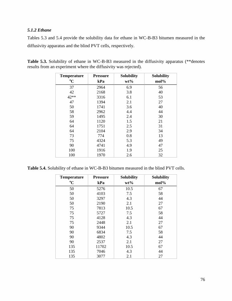
76

5.1.2 Ethane

Tables 5.3 and 5.4 provide the solubility data for ethane in WC-B-B3 bitumen measured in the

diffusivity apparatus and the blind PVT cells, respectively.

Table 5.3. Solubility of ethane in WC-B-B3 measured in the diffusivity apparatus (**denotes

results from an experiment where the diffusivity was rejected).

Temperature oC

Pressure

kPa

Solubility

wt%

Solubility

mol%

37 2964 6.9 56

42 2168 3.8 40

42** 3316 6.1 53

47 1394 2.1 27

50 1741 3.6 40

58 2962 4.4 44

59 1495 2.4 30

64 1120 1.5 21

64 1751 2.5 31

64 2104 2.9 34

73 774 0.8 13

75 4324 5.3 49

90 4741 4.9 47

100 1916 1.9 25

100 1970 2.6 32

Table 5.4. Solubility of ethane in WC-B-B3 bitumen measured in the blind PVT cells.

Temperature oC

Pressure

kPa

Solubility

wt%

Solubility

mol%

50 5276 10.5 67

50 4103 7.5 58

50 3297 4.3 44

50 2190 2.1 27

75 7813 10.5 67

75 5727 7.5 58

75 4128 4.3 44

75 2448 2.1 27

90 9344 10.5 67

90 6834 7.5 58

90 4802 4.3 44

90 2537 2.1 27

135 11702 10.5 67

135 7046 4.3 44

135 3077 2.1 27

77

5.1.3 Propane

Tables 5.5 and 5.6 list the solubility data for ethane in WC-B-B3 bitumen measured in the

diffusivity apparatus and the blind PVT cells, respectively. Solubility data from two diffusion

experiments conducted by Diedro et al. (2014) are included in Table 5.5. These two experiments

were performed using computer tomography and will be discussed in more detail in Chapter 6.

The data were provided courtesy of Dr. Kantzas at the University of Calgary.

Table 5.5. Solubility of propane in WC-B-B3 measured in the diffusivity apparatus (** denotes

results from an experiment where the diffusivity was rejected, $

denotes results from CT data

provided by Deidro et al., (2016)).

Temperature oC

Pressure

kPa

Solubility

wt%

Solubility

mol%

22$ 620 9.5 55

40$ 689 5.1 43

43** 633 6.3 44

50 327 2.6 24

50 724 4.6 36

53 982 6.6 45

59 824 3 27

60 602 3.5 30

62 1080 6.8 46

62 1635 12.9 64

64** 1265 8.9 54

64** 1890 8.6 53

70** 824 3.2 28

70 1077 4.5 36

74 523 2.1 21

74 1006 4.5 36

74** 1132 5.9 42

80 607 2.5 23

80 1507 8 51

81 720 2.4 23

81 1367 7.2 48

85 702 2.5 23

86 1374 5.4 40

86 2303 11.4 60

78

Table 5.6: Solubility of propane in WC-B-B3 from the blind PVT cells.

Temperature oC

Pressure

kPa

Solubility

wt%

Solubility

mol%

50 1114 11.0 60

50 820 5.6 41

50 625 2.8 26

75 1883 11.4 60

75 1191 5.6 41

75 682 2.8 26

89 2360 11.4 60

89 1501 5.6 41

89 843 2.8 26

134 4512 11.4 60

134 2725 5.6 41

134 1551 2.8 26

180 7588 11.4 60

180 4591 5.6 41

180 2877 2.8 26

180 1694 1.1 12

5.2 Modeling Solubility Data

Two analytical approaches for modeling the saturation pressure were considered: Henry’s law

and an activity coefficient model with the Margules equations. Henry’s law, as original

formulated is only valid for small concentrations of dissolved gas but is convenient for data

fitting with minor modifications. The Margules equation is valid for all compositions in the

vapour-liquid region.

5.2.1 Henry’s Law

Henry’s law is discussed in Chapter 2, but is restated here for convenience (Reid et al., 1987).

𝑃 = 𝑥𝑠𝐻 (5.1)

where 𝑃 is the pressure of the system, 𝑥𝑠 is the mole fraction of the dissolved solvent, and H is

Henry’s constant in the same units as the pressure, P. Henry’s constant is expected to be a

function of temperature but to be independent of pressure. The following form of Henry’s

constant was found sufficient to fit the temperature dependence of the data:

79

ln 𝐻 = 𝑎 +

𝑏

𝑇

(5.2)

where a and b are fitting parameters, and T is the temperature in K. Figure 5.1a shows that the

temperature dependent constant provides an adequate fit to the solubility data for propane in

bitumen but fails to capture the upward curvature of the data at higher solubilities. Equation 5.2

was modified to include a pressure term to better fit the data as follows:

ln 𝐻 = 𝑎 +

𝑏

𝑇+

𝑐 ∗ 𝑃

𝑅𝑇

(5.3)

where R is the is the gas constant and c is a fitting parameter. The parameters a, b and c are fit to

the data by minimizing the square error between the modeled and experimental solubility. Figure

5.1b shows the improvement to the fit that is possible with such a modification.

Figure 5.1. Saturation pressure of propane against more fraction of propane in WC-B-B3

bitumen from CCE experiments fit with Henrys Law using: a) temperature dependent constant;

b) temperature and pressure dependent constant.

0

1000

2000

3000

4000

5000

6000

7000

8000

0 0.2 0.4 0.6 0.8

Satu

rati

on

Pre

ss

ure

, k

Pa

Propane Mole Fraction

CCE 50°C

CCE 75°C

CCE 89°C

CCE 135°C

CCE 180°C

Henry's Law

0

1000

2000

3000

4000

5000

6000

7000

8000

0 0.2 0.4 0.6 0.8

Satu

rati

on

Pre

ssu

re, kP

a

Propane Mole Fraction

CCE 50°C

CCE 75°C

CCE 89°C

CCE 135°C

CCE 180°C

Henry's Law

b)

80

5.2.2 Margules Activity Coefficient Model

The Henry model is a simple empirical fit to the data but strictly speaking only applies to dilute

solutions (low solvent contents). As was discussed in Chapter 2, an activity coefficient model is

valid for the entire composition range as long as only a liquid and vapour phase are present. For

pseudo-binary systems of solvent in oil, the equilibrium pressure can be expressed as follows:

𝑃 = 𝑥𝑠𝛾𝑠𝑃𝑣 𝑠 + 𝑥𝑏𝛾𝑏𝑃𝑣 𝑏 (5.4)

where 𝛾𝑖is the activity coefficient of species i (given by Equation 2.43), 𝑃𝑣 𝑖 is the vapour

pressure of component i, and subscripts s and b refer to the solvent and bitumen phase. Equation

5.4 also takes into account the vapour pressure of the oil.

The saturation pressure for the solvent can be calculated using correlations listed in Green and

Perry (2008).

ln 𝑃𝑣 𝑖 = 𝐶1 +

𝐶2

𝑇+ 𝐶3 ln 𝑇 + 𝐶4𝑇

𝐶5 (5.5)

where C1 to C5 are fluid specific parameters, T is the temperature in K, and 𝑃𝑣 𝑖 is the vapor

pressure in Pa. Vapour pressure data only exist up to the critical point and therefore Equation 5.5

is only valid below the critical point. The constants for methane, ethane, and propane are

provided in Table 5.7.

Table 5.7. Summary of the parameters for the Green and Perry vapour pressure correlation (Equation

5.5); temperature in K, and pressure in Pa.

Component C1 C2 C3 C4 C5 Tc (K)

Methane 39.205 -1324.4 -3.4366 3.1019x10-5

2 190.6

Ethane 51.857 -2598.7 -5.1283 1.4913x10-5

2 305.3

Propane 59.078 -3492.6 -6.0669 1.0919x10-5

2 369.5

To model the saturation pressure of a mixture at a temperature above the solvent’s critical point,

a hypothetical vapour pressure of the solvent is required. The following correlation was used to

estimate the hypothetical vapour pressure of a solvent above its critical temperature:

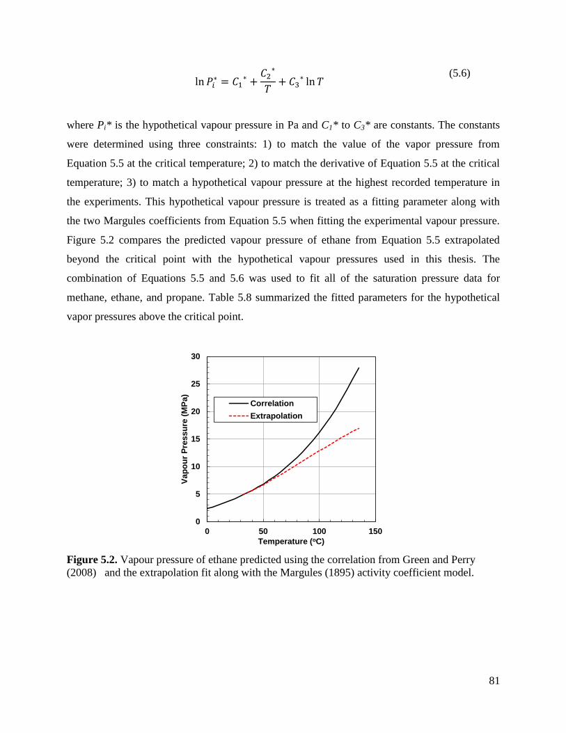
81

ln 𝑃𝑖

∗ = 𝐶1∗ +

𝐶2∗

𝑇+ 𝐶3

∗ ln 𝑇 (5.6)

where Pi* is the hypothetical vapour pressure in Pa and C1* to C3* are constants. The constants

were determined using three constraints: 1) to match the value of the vapor pressure from

Equation 5.5 at the critical temperature; 2) to match the derivative of Equation 5.5 at the critical

temperature; 3) to match a hypothetical vapour pressure at the highest recorded temperature in

the experiments. This hypothetical vapour pressure is treated as a fitting parameter along with

the two Margules coefficients from Equation 5.5 when fitting the experimental vapour pressure.

Figure 5.2 compares the predicted vapour pressure of ethane from Equation 5.5 extrapolated

beyond the critical point with the hypothetical vapour pressures used in this thesis. The

combination of Equations 5.5 and 5.6 was used to fit all of the saturation pressure data for

methane, ethane, and propane. Table 5.8 summarized the fitted parameters for the hypothetical

vapor pressures above the critical point.

Figure 5.2. Vapour pressure of ethane predicted using the correlation from Green and Perry

(2008) and the extrapolation fit along with the Margules (1895) activity coefficient model.

0

5

10

15

20

25

30

0 50 100 150

Vap

ou

r P

res

su

re (

MP

a)

Temperature (oC)

Correlation

Extrapolation

82

Table 5.8. Summary of the parameters for the hypothetical vapour pressure above the critical

point (Equation 5.6). Tmax is maximum temperature at which saturation pressure was measured in

the dataset used in this thesis.

Component C1* C2* C3* Tmax

(oC)

Fitted Pressure

at Tmax

(MPa)

Methane 52.679 -2061.5 -5.0518 100 30.6

Ethane (all) 80.372 -4553.8 -8.7501 135 16.9

Ethane (screened) 80.423 -4556.1 -8.7576 135 16.4

Propane 67.518 -4808.99 -6.6397 180 11.9

The vapour pressure of WC-B-B3 bitumen was measured in the blind cell at 180oC and found to

be 500 kPa (Johnston, 2016). Since the bitumen has been dewatered at 60°C and dewatering

removes the volatile components, the vapour pressure at 60oC was taken as 101 kPa. The vapour

pressures were then fit with the Clausius-Clapeyron equation given by:

ln 𝑃𝑣 𝑏 = 𝐴 −

𝐻𝑏𝑉𝑎𝑝

𝑅𝑇

(5.7)

where 𝑃𝑣 𝑏 is the vapour pressure of the bitumen in kPa, 𝐻𝑏𝑉𝑎𝑝

is the heat of vaporization of

bitumen in J/mol, R is the gas constant in J/molK, and T is temperature in K, and A is a

dimensionless constant of integration. The values of the fitted constants are 𝐴=10.685 and

𝐻𝑏𝑉𝑎𝑝/𝑅=2061 K. The vapour pressure of Athabasca bitumen, required for modeling the

saturation pressure of methane in oil, was assumed to be the same as that of the WC-B-B3

bitumen.

Note, in most cases, the contribution from the bitumen to the saturation pressure is small. For

both methane and ethane, the modeled contribution from the bitumen is never more than 5% of

the total saturation pressure. For propane, the average contribution from the bitumen is less than

7%. The contribution is largest at low temperatures and low propane solubility where the

combined effects of the low propane vapour pressure and low propane mole fraction lead to a

low propane activity.

83

5.3 Results

5.3.1 Saturation Pressure and Solubility of Methane in Bitumen

Figure 5.3 shows the measured saturation pressure and solubility of methane in bitumen and the

fitted modified Henry’s law and the Margules activity coefficient models. As expected, the

saturation pressure increases with increasing gas content and increasing temperature. The data

from this thesis could not be compared directly to the data from Svrcek and Mehrotra (1982)

because they were measured at different conditions. Instead, the literature data were fit with the

modified Henry’s law model (Equation 5.3) and the data from this thesis were compared with the

fitted model at the same conditions. The fitted parameters are provided in Table 5.9. The average

deviation of the solubility and saturation pressure data from this thesis from the fitted model

were 0.95 mol% (8.4%) and 360 kPa (9.5%), respectively. Note, to avoid implicit solutions, the

modified Henry’s Law model was fitted to the mole fractions with saturation pressure as the

input. The deviations in the saturation pressure were determined using the iterative method with

the same fitted parameters and mole fraction inputs. The Margules activity coefficient model was

fitted to the saturation pressures with mole fractions as the input. The deviations in mole

fractions from the Margules equation were calculated using an iterative method and the

experimental saturation pressures as inputs.

Figure 5.3. Saturation pressure versus mole fraction of mixtures of methane and bitumen fitted

with: a) modified Henry’s law model; b) Margules activity coefficient model.

0

2000

4000

6000

8000

10000

0 0.05 0.1 0.15 0.2 0.25 0.3 0.35

Sa

tura

tio

n P

res

su

re, k

Pa

Mole Fraction Methane

27 C, Lit.

45 C, Lit.

68 C, Lit.

100 C, Lit.

50 C. Diff Cell

76 C, Diff. Cell

90 C, Diff. Cell

Henry's Law

a)

0

2000

4000

6000

8000

10000

0 0.05 0.1 0.15 0.2 0.25 0.3 0.35

Sa

tura

tio

n P

res

su

re, k

Pa

Mole Fraction Methane

27 C, Lit.

45 C, Lit.

68 C, Lit.

100 C, Lit.

50 C. Diff Cell

76 C, Diff. Cell

90 C, Diff. Cell

Margules

b)

84

To model the methane solubilities, the measurements collected in this thesis and those obtained

from Mehrotra and Svrcek were fit simultaneously, as shown in Figure 5.3. The two models

provide similar fits to the data although the Margules activity coefficient model is more linear at

high concentration compared to the modified Henry’s law model. Table 5.9 gives the fitted

parameters for the Henry’s constant used to fit the solubility data. Table 5.10 gives the fitted

parameters for the Margules activity coefficient model. Recall that the hypothetical vapour

pressure for methane at the maximum experimental temperature was also fitted and was provided

in Table 5.8. Figures 5.4 and 5.5 are cross plots of the fitted versus measured solubilities and

saturation pressures, respectively. Both models fit the saturation pressure and solubility data with

nearly identical errors (less than 7% average relative deviation) and the cross plots are nearly

indistinguishable.

Table 5.9. Summary of Henry constant parameters for methane, ethane, and propane in WC-B-

B3 bitumen (R=8.314 LkPa/molK). ARD is the average relative deviation.*Denotes the fit

exclusively to methane solubility data from Svrcek and Mehrotra (1982).

Solvent A B

K

C

L/mol

ARD Solubility

%

ARD Psat

%

Methane* 11.57 -475.2 0.093 6.6 8.3

Methane 11.27 -375.9 0.093 6.6 7.8

Ethane (all) 11.39 -925.1 0.225 9.2 11.6

Ethane (screened) 11.59 -992.2 0.220 7.3 9.5

Propane 12.87 -1713 0.241 7.7 8.8

Table 5.10. Summary of the Margules parameters for methane, ethane, and propane in WC-B-

B3 bitumen.

Solvent Asb Abs ARD Solubility

%

ARD Psat

%

Methane -0.247 0.939 5.3 6.2

Ethane (all) -1.832 0.055 9.1 13.4

Ethane (screened) -1.705 0.085 6.8 9.8

Propane -0.646 -0.101 8.7 9.4

85

Figure 5.4. Predicted versus measured solubility of methane in Athabasca bitumen (Svrcek and

Mehrotra (1982) and WC-B-B3 bitumen (this work): a) modified Henryls law model; b)

Margules activity coefficient model.

Figure 5.5. Predicted versus measured saturation pressure of methane in Athabasca bitumen

Svrcek and Mehrotra (1982) and WC-B-B3 bitumen (this work): a) modified Henryls law model;

b) Margules activity coefficient model.

0

0.05

0.1

0.15

0.2

0.25

0.3

0.35

0 0.05 0.1 0.15 0.2 0.25 0.3 0.35

Pre

dic

ted

Mo

le F

racti

on

Measured Mole Fraction

Literature

Diffusion Cell

a)

0

0.05

0.1

0.15

0.2

0.25

0.3

0.35

0 0.05 0.1 0.15 0.2 0.25 0.3 0.35

Pre

dic

ted

Mo

le F

rac

tio

n


Literature

Diffusion Cell

b)

0

1000

2000

3000

4000

5000

6000

7000

8000

9000

10000

0 2000 4000 6000 8000 10000

Mo

de

led

Sa

tura

tio

n P

res

su

re (

kP

a)

Measured Saturation Pressure (kPa)

Literature

Diffusion Cell

a)

0

1000

2000

3000

4000

5000

6000

7000

8000

9000

10000

0 2000 4000 6000 8000 10000

Mo

de

led

Sa

tura

tio

n P

res

su

re (

kP

a)


Literature

Diffusion Cell

b)

86

5.3.2 Saturation Pressure of Ethane in Bitumen

The saturation pressure (solubility) data collected for mixtures of ethane and WC-B-B3 bitumen

from the diffusion apparatus and the blind cells are shown in Figure 5.6. The combined data set

was fit with the modified Henry’s law model also shown in Figure 5.6. The model fit the mole

fraction data from each experimental method with similar accuracy (AARD of 12% for the

diffusion data and 7.5% for the blend cell CCE data) demonstrating that the results from both

methods are consistent with each other. The combined AARD was 9.7%. The combined dataset

was also fit with the Margules activity coefficient model with an AARD of 14%, Figure 5.7. The

dispersion plots are provided in Figure 5.8. Note, as with the methane/bitumen system, the

modified Henry’s law model was fitted to the mole fractions with saturation pressure as the

input. The deviations in the saturation pressure were determined using the iterative method with

the same fitted parameters and mole fraction inputs. The Margules activity coefficient model was

fitted to the saturation pressures with mole fractions as the input. The deviations in mole

fractions from the Margules equation were calculated using an iterative method and the

experimental saturation pressures as inputs.

The following outliers were identified based on an averaged deviation from both of the fitted

models exceeding 25%:

diffusion method, 100°C, 31.7 mol% (2.6 wt%), 1929 kPa

diffusion method, 50°C, 39.6 mol% (3.65 wt%), 1740 kPa

CCE method, 50°C, 27.3 mol% (2.13 wt%), 2190 kPa

These outliers were removed from the dataset and the models were then refit to the screened

data. The modified Henry’s Law and Margules activity coefficient model parameters before and

after screening were provided in Tables 5.9 and 5.10.

87

Figure 5.6. Saturation pressure versus mole fraction of ethane bitumen mixtures fitted with

modified Henry’s law model: a) diffusion cell data; b) blind cell CCE data.

Figure 5.7. Saturation pressure versus mole fraction of ethane bitumen mixtures fitted with

modified Margules activity coefficient model: a) diffusion cell data; b) blind cell CCE data.

0

1000

2000

3000

4000

5000

6000

0 0.2 0.4 0.6

Pre

ssu

re (

kP

a)

Mole Fraction

Henry's Law

100°C

90°C

73°C

64°C

58°C

49°C

41°C

100oC

80oC

60oC

40oC

(a)0

2000

4000

6000

8000

10000

12000

0 0.2 0.4 0.6 0.8

Pre

ssu

re (

kP

a)

Mole Fraction

Henry's Law

135°C, CCE

90°C, CCE

75°C, CCE

50°C, CCE

90oC

75oC

50oC

135oC

(b)

0

1000

2000

3000

4000

5000

6000

0 0.2 0.4 0.6

Pre

ssu

re (

kP

a)

Mole Fraction

Margules

100°C

90°C

73°C

64°C

58°C

49°C

41°C

100oC

80oC

60oC

40oC

(a)

0

2000

4000

6000

8000

10000

12000

0 0.2 0.4 0.6 0.8

Pre

ssu

re (

kP

a)

Mole Fraction

Margules

135°C, CCE

90°C, CCE

75°C, CCE

50°C, CCE

90oC

75oC

50oC

135oC

(b)

88

Figure 5.8. Predicted versus measured solubility of ethane in WC-B-B3 bitumen: a) modified

Henry’s law model; b) Margules activity coefficient model.

Figure 5.9. Predicted versus measured saturation pressure of ethane in WC-B-B3: a) modified


0

0.2

0.4

0.6

0.8

0 0.2 0.4 0.6 0.8

Mo

dele

d M

ole

Fra

cti

on


CCE

Diffusion Cell

a)

0

0.2

0.4

0.6

0.8

0 0.2 0.4 0.6 0.8

Mo

dele

d M

ole

Fra

cti

on


CCE

Diffusion Cell

b)

0

2000

4000

6000

8000

10000

12000

0 2000 4000 6000 8000 10000 12000

Mo

de

led

Sa

tura

tio

n P

res

su

re (

kP

a)


CCE

Diffusion Cell

a)

0

2000

4000

6000

8000

10000

12000

0 2000 4000 6000 8000 10000 12000

Mo

de

led

Sa

tura

tio

n P

res

su

re (

kP

a)


CCE

Diffusion Cell

b)

89

As a further test of the quality of the data, the fitted model was compared with data collected by

Mehrotra and Svrcek (1985b) for mixtures of ethane with Cold Lake bitumen Mehrotra and

Svrcek, 1988b) and Peace River bitumen Mehrotra and Svrcek, 1985b), Figures 5.10 and 5.11,

respectively. Note that a liquid-liquid region was observed at 24°C in both cases, indicated by a

circle in the figures. This region forms at temperatures below the critical temperature and

pressure of ethane (32°C and 4900 kPa). The measured saturation pressures become nearly

constant in the liquid-liquid region and the values above the onset of the second liquid phase

were excluded from the comparison with the model. Figure 5.10 shows that the modified

Henry’s law and Margules activity coefficient models fitted to the data from this study match the

data for the Cold Lake bitumen with AARD of 9.7 and 14%, respectively. In other words, the

models match the new data with the same accuracy as the original dataset even for a different

source bitumen. Figure 5.11 compares the same two models with the data for the Peace River

bitumen and the AARD were 6.6 and 12%, respectively. The relatively low errors are misleading

because the match above 24°C is excellent while the match at 24°C is poor. It is not obvious if

the mismatch at 24°C is an issue with the data or the models. Nonetheless, the agreement

between the models and the independent datasets is generally within the scatter of the data even

though different bitumen samples were considered.

Figure 5.10. Saturation pressure versus mass percent ethane for Cold Lake bitumen (Mehrotra

and Svrcek, 1988b) compared with models fitted to WC-B-B3/ethane data: a) modified Henry’s

law model; b) Margules activity coefficient model. Circle indicates liquid-liquid region.

0

2000

4000

6000

8000

10000

12000

0 0.2 0.4 0.6 0.8 1

Pre

ss

ure

(k

Pa

)

Mole Fraction

Henry's Law

101°C

76°C

50°C

25°C

101oC 76oC

52oC

24oC

(a)

0

2000

4000

6000

8000

10000

12000

0 0.2 0.4 0.6 0.8 1

Pre

ssu

re (

kP

a)

Mole Fraction

Margules

101°C

76°C

50°C

25°C

101oC

76oC

52oC

24oC

(b)

90

Figure 5.11. Saturation pressure versus mass percent ethane for Peace River bitumen (Mehrotra

and Svrcek, 1985b) compared with models fitted to WC-B-B3/ethane data: a) modified Henry’s

law model; b) Margules activity coefficient model. Circle indicates liquid-liquid region.

Overall, the modified Henry’s law model provides a better fit to the data than the Margules

activity coefficient model but there are limitations to both models. The Margules activity

coefficient model is constrained to match the ethane vapour pressure when the mole fraction of

ethane approaches unity. However, a second liquid phase, shown in Figures 5.10 and 5.11, forms

not at a pressure near the vapour pressure of ethane but at a mole fraction far below unity. As a

result, the model tends to under-predict the saturation pressures, as illustrated in Figure 5.12a.

The under-prediction persists at conditions above the critical temperature of ethane (32°C),

where the model is constrained to match the extrapolated vapor pressure of ethane when the

mixture approaches pure ethane. The same type of deviation is just evident with the fitting of the

data from this thesis, which was collected at lower solvent contents, Figure 5.12b. In contrast, the

modified Henry’s law model fits the entire range of collected data. However, it should not be

used for extrapolation because it will predict a non-physical reversal in the saturation pressure

curve at high pressures as shown in Figure 5.13. Also note that the data point (CCE method,

135°C, 67.0 mol% = 10.5 wt%, 11700 kPa) cannot be matched with the modified Henry’s law

model and is likely an outlier.

0

1000

2000

3000

4000

5000

6000

0 0.2 0.4 0.6 0.8

Pre

ss

ure

(k

Pa

)

Mole Fraction

Henry's Law

101°C

76°C

50°C

25°C

105oC 79oC

45oC

24oC

(a)

0

1000

2000

3000

4000

5000

6000

0 0.2 0.4 0.6 0.8

Pre

ssu

re (

kP

a)

Mole Fraction

Margules

101°C

76°C

50°C

25°C

105oC 79oC

45oC

24oC

(b)

91

Figure 5.12. Margules activity coefficient model extended to full composition range for: a) Cold

Lake bitumen/ethane data from Mehrotra and Svrcek (1988b); b) WC-B-B3 bitumen/ethane data

collected for this thesis. The circled region indicates the data is near or above the critical

temperature of ethane that is the most severely under-predicted.

Figure 5.13. Modified Henry’s law model extended to full composition range for: a) Cold

bitumen/ethane data from Mehrotra and Svrcek (1985b); b) WC-B-B3 bitumen/ethane data

collected for this thesis. The circled point cannot be fit with the modified Henry’s law model.

0

2000

4000

6000

8000

10000

12000

14000

0 0.2 0.4 0.6 0.8 1

Pre

ssu

re (

kP

a)

Mole Fraction

Margules

101°C

76°C

50°C

25°C

101oC

76oC

52oC

24oC

(b)

0

2000

4000

6000

8000

10000

12000

14000

16000

18000

0 0.2 0.4 0.6 0.8 1

Pre

ssu

re (

kP

a)

Mole Fraction

Margules

135°C, CCE

90°C, CCE

75°C, CCE

50°C, CCE 90oC

75oC

50oC

135oC

(b)

0

2000

4000

6000

8000

10000

12000

14000

16000

18000

0 0.2 0.4 0.6 0.8 1

Pre

ssu

re (

kP

a)

Mole Fraction

Henry's Law

25°C

50°C

76°C

101°C

101oC 76oC 52oC

24oC

(a)

0

2000

4000

6000

8000

10000

12000

14000

16000

18000

0 0.2 0.4 0.6 0.8 1

Pre

ssu

re (

kP

a)

Mole Fraction

Henry's Law

135°C, CCE

90°C, CCE

75°C, CCE

50°C, CCE

90oC

75oC50oC

135oC

(b)

92

5.3.3 Saturation Pressure of Propane in Bitumen

Figures 5.14 and 15 compare the saturation pressure (solubility) data collected from the diffusion

apparatus and the blind cells at comparable temperatures. Figure 5.14 shows the full range of

data collected while Figure 5.15 expands the scale to focus on the results at the conditions of the

diffusion experiments. There are no obvious outliers and the data follows the expected trend.

However, there is a large amount of scatter in the data measured using the diffusion cell to the

point that some of the measurements at 60oC are intercepting the trends in the CCE data at 90

oC.

Note, as with the methane/bitumen and ethane/bitumen systems, the modified Henry’s law model

was fitted to the mole fractions with saturation pressure as the input. The deviations in the

saturation pressure were determined using the iterative method with the same fitted parameters

and mole fraction inputs. The Margules activity coefficient model was fitted to the saturation

pressures with mole fractions as the input. The deviations in mole fractions from the Margules

equation were calculated using an iterative method and the experimental saturation pressures as

inputs.

Figure 5.14. Saturation pressure versus mole fraction of mixtures of propane and bitumen fitted

with: a) modified Henry’s Law model; b) Margules activity coefficient model. Only data in

range of diffusion cell experiment are shown.

0

2000

4000

6000

8000

10000

0 0.2 0.4 0.6 0.8

Pre

ss

ure

(k

Pa

)


50 C, CCE75 C, CCE90 C, CCE135 C, CCE180 C, CCE40 C, Diff. Cell50 C, Diff. Cell60 C, Diff. Cell80 C, Diff. CellHenry's Law

a)180oC

135oC

90oC

75oC

50oC

0

2000

4000

6000

8000

10000

0 0.2 0.4 0.6 0.8

Pre

ssu

re (

kP

a)


50 C, CCE75 C, CCE90 C, CCE135 C, CCE180 C, CCE40 C, Diff. Cell50 C, Diff. Cell60 C, Diff. Cell80 C, Diff. CellMargules

b)180oC

135oC

90oC

75oC

50oC

93

Figure 5.15. Saturation pressure versus mole fraction of mixtures of propane and bitumen fitted

with: a) modified Henry’s Law model; b) Margules activity coefficient model. Only data in

range of diffusion cell experiment are shown.

Figure 5.16 compares the solubility models developed in this thesis to data for mixtures of

propane and Athabasca bitumen collected by Badamchi-Zadeh et al. (2009). The Henry’s Law

predicts both the solubility and saturation pressure with an average error of 11% even though the

bitumen was from a different source reservoir. Solubility and Saturation pressure predictions for

the Margules Equation have an average error of 13%.

All of the propane solubility and saturation pressure data could be fit using either model. The

modeling issues observed with the ethane/bitumen dataset do not arise with the propane/bitumen

dataset because a second liquid phase does not form at the range of conditions considered. While

all of the data were below the critical temperature and pressure of propane (97°C and 4250 kPa),

the saturations were not high enough to form a second phase. Note that extrapolating the models

for propane solubility to high pressure and propane concentration result in very similar curves to

those of ethane and the same modeling issues would arise.

0

1000

2000

3000

0 0.2 0.4 0.6 0.8

Pre

ssu

re (

kP

a)


50 C, CCE

75 C, CCE

90 C, CCE

40 C, Diff. Cell

50 C, Diff. Cell

60 C, Diff. Cell

80 C, Diff. Cell

Henry's Law

a)

90oC

75oC

50oC

0

1000

2000

3000

0 0.2 0.4 0.6 0.8

Pre

ss

ure

(k

Pa

)


50 C, CCE

75 C, CCE

90 C, CCE

40 C, Diff. Cell

50 C, Diff. Cell

60 C, Diff. Cell

80 C, Diff. Cell

Margules

90oC

75oC

50oC

b)

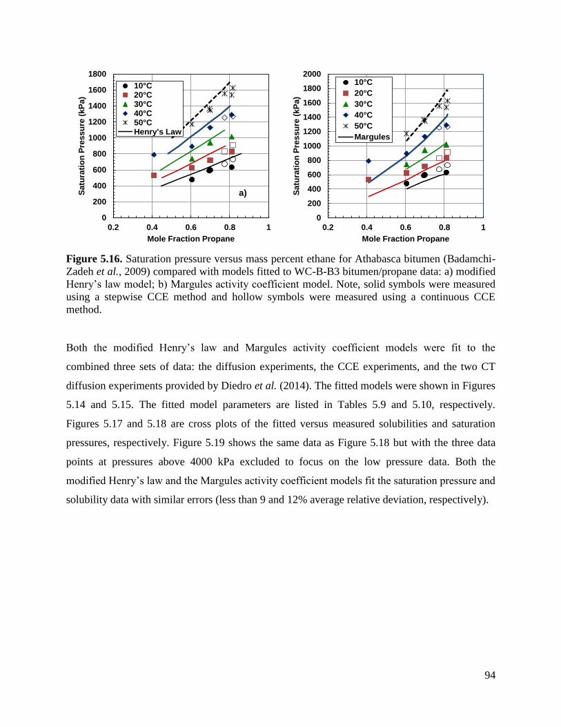
94

Figure 5.16. Saturation pressure versus mass percent ethane for Athabasca bitumen (Badamchi-

Zadeh et al., 2009) compared with models fitted to WC-B-B3 bitumen/propane data: a) modified

Henry’s law model; b) Margules activity coefficient model. Note, solid symbols were measured

using a stepwise CCE method and hollow symbols were measured using a continuous CCE

method.

Both the modified Henry’s law and Margules activity coefficient models were fit to the

combined three sets of data: the diffusion experiments, the CCE experiments, and the two CT

diffusion experiments provided by Diedro et al. (2014). The fitted models were shown in Figures

5.14 and 5.15. The fitted model parameters are listed in Tables 5.9 and 5.10, respectively.

Figures 5.17 and 5.18 are cross plots of the fitted versus measured solubilities and saturation

pressures, respectively. Figure 5.19 shows the same data as Figure 5.18 but with the three data

points at pressures above 4000 kPa excluded to focus on the low pressure data. Both the

modified Henry’s law and the Margules activity coefficient models fit the saturation pressure and

solubility data with similar errors (less than 9 and 12% average relative deviation, respectively).

0

200

400

600

800

1000

1200

1400

1600

1800

0.2 0.4 0.6 0.8 1

Sa

tura

tio

n P

res

su

re (

kP

a)


10°C20°C30°C40°C50°CHenry's Law

a)

0

200

400

600

800

1000

1200

1400

1600

1800

2000

0.2 0.4 0.6 0.8 1

Sa

tura

tio

n P

res

su

re (

kP

a)


10°C

20°C

30°C

40°C

50°C

Margules

95

Figure 5.17. Predicted versus measured solubility of propane in WC-B-B3 bitumen: a) modified


Figure 5.18. Predicted versus measured saturation pressure of propane in WC-B-B3 bitumen: a)

modified Henry’s law model; b) Margules activity coefficient model.

0

0.2

0.4

0.6

0.8

0 0.2 0.4 0.6 0.8

Mo

dele

d P

rop

an

e M

ol F

racti

on

Measured Propane Mol Fraction

CCE

Diffusion Cell

CT

a)

0

0.2

0.4

0.6

0.8

0 0.2 0.4 0.6 0.8

Mo

dele

d P

rop

an

e M

ol F

racti

on

Measured Propane Mol Fraction

CCE

Diffusion Cell

CT

b)

0

2000

4000

6000

8000

10000

0 2000 4000 6000 8000 10000

Mo

dele

d S

atu

rati

on

Pre

ssu

re (

kP

a

Measured Saturaion Pressure (kPa)

CCE

Diffusion Cell

CT

a)

0

2000

4000

6000

8000

10000

0 2000 4000 6000 8000 10000

Mo

dele

d S

atu

rati

on

Pre

ssu

re (

kP

a)


CCE

Diffusion Cell

CT

b)

96

Figure 5.19. Predicted versus measured saturation pressure of propane in Athabasca bitumen and

WC-B-B3: a) modified Henry’s law model; b) Margules activity coefficient model. Note: the

three data points at pressures above 4000 kPa were excluded from these plots to focus on the low

pressure data.

5.4 Recommendation

Both the modified Henry’s law model and the Margules activity coefficient model fit the

experimental data with similar deviations. However, the Margules model tended to under-predict

saturation pressures for ethane at higher mole fractions. The modified Henry’s law model was

able to fit all of the data with the exception of one data point for ethane at 135oC and 67 mol %

ethane. This data point is likely an outlier. Therefore, the modified Henry’s law model was

selected to predict the solubility of methane, ethane and propane in WC-B-B3 if no experimental

data was available. Note, the modified Henry’s law model should not be extrapolated to

pressures above the range of the data used to fit the model because it will predict a non-physical

reversal in ethane solubility at high pressures.

0

1000

2000

3000

4000

0 1000 2000 3000 4000

Mo

de

led

Sa

tura

tio

n P

ress

ure

(k

Pa

)


CCE

Diffusion Cell

CT

a)

0

1000

2000

3000

4000

0 1000 2000 3000 4000

Mo

dele

d S

atu

rati

on

Pre

ssu

re (

kP

a


CCE

Diffusion Cell

CT

b)

97

CHAPTER SIX: DIFFUSIVITY RESULTS AND DISCUSSION

This chapter presents the diffusivity data collected in this thesis for methane, ethane, propane,

and butane in bitumen and bitumen maltenes using the pressure decay method described in

Chapter 3. The diffusivity of the solvent in the medium is determined using the numerical model

developed in Chapter 4 where the diffusivity is the fitting parameter. The data from each

experiment with methane, ethane and propane are fit with a constant diffusivity and with several

expressions for a concentration dependent diffusivity. The fitted constant diffusivities are

correlated to viscosity with a power law equation based on the Hayduk-Cheng (1971) equation.

A correlation for the concentration dependent diffusivity is also developed with endpoints set at

the infinite dilution diffusivities of the bitumen in solvent and the solvent in bitumen. The

correlations are then tested on: data collected for butane with the same bitumen, data collected

for methane with different oil phases (a degassed sample and a maltene cut from the same

bitumen, and literature data for other bitumens and solvents).

6.1 Constant Diffusivity Data from Pressure Decay Measurements

Pressure decay data were collected for methane, ethane, propane, and butane in the original oil as

well as for methane in a bitumen degassed at 180°C and maltenes separated from the bitumen

with pentane. The diffusivities presented in this section are the constant diffusivities fit to these

datasets using the numerical model developed in Chapter 4. In reality, the diffusivity changes

during the course of the experiment as more solvent diffuses into the medium reducing its

viscosity and increasing the diffusivity. The constant diffusivity is an average diffusivity from

the initial to the final conditions of the experiment. The constant diffusivities for each solvent in

each medium are presented below.

Tables 6.1 to 6.3 provide the constant diffusivities for methane in WC-B-B3 bitumen, WC-B-B3

bitumen degassed at 180oC, and WC-B-B3 maltenes, respectively. Table 6.4 lists constant

diffusivities for ethane in WC-B-B3 bitumen. Table 6.5 presents results from ethane diffusivity

experiments where the initial solvent concentration in the oil phase is non zero. Table 6.6 lists

constant diffusivities for propane in WC-B-B3 bitumen. Table 6.7 presents results from propane

diffusivity experiments where the initial solvent concentration in the oil phase is non zero. Table

98

6.8 lists diffusivities for butane in WC-B-B3. Note that, since only a few preliminary

measurements were made for the mixtures with butane, these results are discussed separately

later on.

Table 6.1. Diffusivity of methane in WC-B-B3 bitumen.

Temperature oC

Pressure

kPa

Solubility

wt%

Viscosity

mPa.s

Diffusivity

10-10

m2/s

50 3450 0.42 2040 3.0

76 4160 0.55 390 6.0

100 4230 0.53 120 12

100 4170 0.48 120 9.5

100 4340 0.51 120 11

101 4120 0.49 110 10

Table 6.2. Diffusivity of methane in WC-B-B3 bitumen degassed at 176oC.

Temperature oC

Pressure

kPa

Solubility

wt%

Viscosity

mPa.s

Diffusivity

10-10

m2/s

50 3510 0.35 1990 4.0

160 3330 0.33 15 34

176 3620 0.39 10 41

Table 6.3. Diffusivity of methane in WC-B-B3 maltenes.

Temperature oC

Pressure

kPa

Solubility

wt%

Viscosity

mPa.s

Diffusivity

10-10

m2/s

56 3500 0.61 115 6.0

68 4020 0.70 63 18

81 4250 0.73 36 25

99

Table 6.4. Diffusivity of ethane in WC-B-B3 bitumen.

Temperature oC

Pressure

kPa

Solubility

wt%

Viscosity

mPa.s

Diffusivity

10-10

m2/s

37 2960 6.9 7160 3.3

42 2170 3.8 3930 2.3

47 1390 2.1 2410 2.0

50 1740 3.7 1880 2.5

58 2960 4.4 1140 3.5

59 1500 2.4 994 3.5

64 1750 2.6 740 2.9

64 1120 1.5 712 2.7

73 774 0.84 429 3.0

75 4320 5.3 422 6.8

90 4740 4.9 189 9.5

100 1920 1.9 116 7.3

100 1970 2.6 114 5.0

Table 6.5. Diffusivity of ethane in WC-B-B3 bitumen with non-zero initial solvent content.

Temperature oC

Pressure

kPa

Initial Solvent

wt%

Solubility

wt%

Initial Viscosity

mPa.s

Diffusivity

10-10

m2/s

42 3320 3.6 6.1 80 5.5

64 2100 1.5 2.9 110 4.7

Table 6.6. Diffusivity of propane in WC-B-B3 bitumen.

Temperature oC

Pressure

kPa

Solubility

wt%

Viscosity

mPa.s

Diffusivity

10-10

m2/s

50 327 2.6 2120 1.5

50 724 4.6 2090 1.8

59 824 3.0 999 2.8

60 602 3.5 945 2.2

62 1080 6.8 801 3.5

70 1080 4.5 547 4.8

74 523 2.2 452 3.3

74 1010 4.5 445 4.0

80 1510 8.0 290 5.6

81 720 2.4 282 3.8

81 1370 7.2 272 6.0

85 702 2.5 229 3.5

86 1370 5.4 210 5.8

100

Table 6.7. Diffusivity of propane in WC-B-B3 bitumen with non-zero initial solvent content.

Temperature oC

Pressure

kPa

Initial Solvent

wt%

Solubility

wt%

Viscosity

mPa.s

Diffusivity

10-10

m2/s

64 1890 4.1 8.6 132 8.0

86 2300 5.4 11.4 43 11.5

Table 6.8. Diffusivity of butane in WC-B-B3 bitumen.

Temperature oC

Pressure

kPa

Solubility

wt%

Viscosity

mPa.s

Diffusivity

1010

m2/s

69 284 3.0 589 4.3

90 738 7.9 182 8.0

90 874 10.1 183 13

6.2 Validation with Data from Computer Assisted Tomography

One disadvantage with the pressure decay approach is that concentration profiles are not

measured. Therefore, the concentration profiles predicted by the numerical model could not be

validated against these measurements. Instead, concentration profiles for propane in WC-B-B3

bitumen measured using computer tomography (Deidro et al., 2014) were examined. Deidro et

al. placed bitumen in a horizontal cylinder and propane gas was injected above the bitumen. The

density and height of the bitumen along the centerline of a horizontal cylinder (outlined area in

Figure 6.1) were measured at time intervals with x-ray scans. Details of the method and

calibrations for density are provided elsewhere (Diedro et al., 2014).

Figure 6.1. Diagram of diffusion cell used by Deidro et al. (2014) to measure the diffusivity of

propane in bitumen.

propane

101

Two experiments were performed, one at 22°C and 640 kPa and the other at 40°C and 690 kPa.

The total mass diffused over time in these experiments was calculated from the volume of the

diluted oil given by:

𝑉𝑚𝑖𝑥 =

𝑚𝑠 + 𝑚𝑏

𝜌𝑚𝑖𝑥

(6.1)

where 𝑉𝑚𝑖𝑥 is the oil volume at a given time in cm3, 𝑚𝑠 is the total mass of solvent diffused at a

given time in g, 𝑚𝑏 is the fixed mass of bitumen in the system, and 𝜌𝑚𝑖𝑥 is the average density

of the mixture. The density of the mixture was determined from a mixing rule (Eq. 4.22;

Saryazdi et al., 2013). Eq. 4.22 is substituted into Eq. 6.1 to obtain the following expression:

𝑚𝑠2

𝜌𝑠+ 𝑚𝑠 (

𝑚𝑏

𝜌𝑠+

𝑚𝑏

𝜌𝑏− 𝑚𝑏 (

1

𝜌𝑠+

1

𝜌𝑏) 𝛽 − 𝑉𝑚𝑖𝑥) + (𝑚𝑏𝑉𝑚𝑖𝑥 +

𝑚𝑏2

𝜌𝑏) = 0

(6.2)

where s and b are the density of the solvent and bitumen, respectively, and sb is the binary

interaction parameter between the bitumen and solvent. Eq. 6.2 is solved to obtain the mass

transferred. Figure 6.2a shows that the mass diffused follows the expected linear trend versus

root time.

The concentration profiles were calculated from the mixture density by rearranging Eq. 4.22 into

a polynomial in terms of solvent mass fraction as follows:

𝑤𝑠

2 (1

𝜌𝑠+

1

𝜌𝑏) 𝛽𝑠𝑏 + 𝑤𝑠 (

1

𝜌𝑠−

1

𝜌𝑏(1

𝜌𝑠+

1

𝜌𝑏)𝛽𝑠𝑏) +

1

𝜌𝑏−

1

𝜌𝑚𝑖𝑥= 0

(6.3)

where 𝑤𝑠 is the solvent mass fraction at each density, 𝜌𝑠 is the effective density of the solvent in

g/cm³, 𝜌𝑏 is the density of bitumen in g/cm³, 𝜌𝑚𝑖𝑥 is the measured density of the mixture in

g/cm³, and 𝛽𝑠𝑏 is the binary interaction parameter. The mass concentration of the solvent in the

mixture, cs, is given by:

𝑐𝑠=𝑤𝑠𝜌𝑚𝑖𝑥 (6.4)

The concentration profiles at 40°C and 690 kPa are shown in Figure 6.2b.

102

Figure 6.2. Diffusivity data for propane in bitumen measured using the swelling data from

computer tomography at 40oC and 690 kPa: a) fit of numerical model to experimental data; b)

comparison of the concentration profiles of propane determined from swelling with the

independently measured concentration profiles. Note: In Figures 2b and 3, the position of zero

corresponds to the horizontal centerline of the cylinder and positive values are towards to oil

phase. The initial gas-oil interface is below the centerline at approximately 0.08 cm. Swelling

shifts the interface towards the centerline (zero).

The solubility used in the model was determined from the concentration profile at the highest

experimental time (8624 minutes) shown in Figure 6.3. The solubility was found to be 0.051

g/mL corresponding to the value of the plateau at a position of approximately 0.1 cm. This

solubility is very close to that estimated from the Henry’s Law model developed in Chapter 5,

which had a value of 0.50 g/mL.

Figure 6.3 and Figure 6.2b also show propane concentrations above the solubility limit near the

gas-oil interface. These are artifacts related to the resolution of the measurements. The apparent

concentrations based on the gas phase density above the exact interface and the liquid density

below the interface are averaged. Therefore, the exact position of the interface is challenging to

define from the concentration measurements. Here, it is defined as the point where the

concentration exceeds the solubility limit; there is often a change in slope at this point.

0

0.1

0.2

0.3

0.4

0.5

0.6

0.7

0.8

0 20 40 60

Ma

ss

Dif

fuse

d (

g)


Fit with Numerical Model

Mass Diffused

a)

0

0.01

0.02

0.03

0.04

0.05

0.06

0.07

0.08

0 0.2 0.4 0.6 0.8 1

Co

nc

en

tra

tio

n (

g/m

L)

Position (cm)

484 min

1567 min

3035 min

Fit to mass diffused

b)

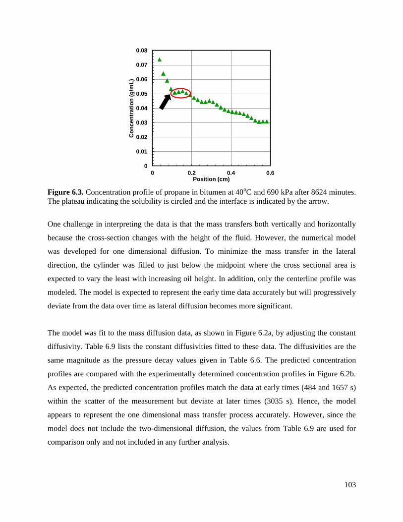
103

Figure 6.3. Concentration profile of propane in bitumen at 40oC and 690 kPa after 8624 minutes.

The plateau indicating the solubility is circled and the interface is indicated by the arrow.

One challenge in interpreting the data is that the mass transfers both vertically and horizontally

because the cross-section changes with the height of the fluid. However, the numerical model

was developed for one dimensional diffusion. To minimize the mass transfer in the lateral

direction, the cylinder was filled to just below the midpoint where the cross sectional area is

expected to vary the least with increasing oil height. In addition, only the centerline profile was

modeled. The model is expected to represent the early time data accurately but will progressively

deviate from the data over time as lateral diffusion becomes more significant.

The model was fit to the mass diffusion data, as shown in Figure 6.2a, by adjusting the constant

diffusivity. Table 6.9 lists the constant diffusivities fitted to these data. The diffusivities are the

same magnitude as the pressure decay values given in Table 6.6. The predicted concentration

profiles are compared with the experimentally determined concentration profiles in Figure 6.2b.

As expected, the predicted concentration profiles match the data at early times (484 and 1657 s)

within the scatter of the measurement but deviate at later times (3035 s). Hence, the model

appears to represent the one dimensional mass transfer process accurately. However, since the

model does not include the two-dimensional diffusion, the values from Table 6.9 are used for

comparison only and not included in any further analysis.

0

0.01

0.02

0.03

0.04

0.05

0.06

0.07

0.08

0 0.2 0.4 0.6

Co

nc

en

tra

tio

n (

g/m

L)

Position (cm)

104

Table 6.9. Diffusivity of propane in WC-B-B3 bitumen measured with computer tomography by

Deidro et al. (2014).

Temperature oC

Pressure

kPa

Solubility*

wt%

Viscosity

mPa.s

Diffusivity

10-10

m2/s

22 621 7.8 53700 2.2

40 689 5.3 7200 1.3

* Solubilities were predicted with Henry’s law (Chapter 5).

6.3 Comparison with Available Literature Data

This section compares the diffusivity measured in this thesis to the data available in the

literature. As noted in Chapter 2, diffusivity is expected to correlate to viscosity and therefore the

data are compared on plots of diffusivity versus the initial oil viscosity. The datasets are screened

for any obvious inconsistencies and those that pass the screening will be used to test the

diffusivity correlations developed later in this chapter. Unless otherwise stated, the reported

dataset will be included in the tests.

6.3.1 Methane Data

Upreti and Mehrotra (2002)

Upreti and Mehrotra (2002) determined the diffusivity of methane and ethane in Athabasca

bitumen (821000 mPa.s at 25oC) using the pressure decay method. Experiments were performed

at 4 and 8 MPa and temperatures from 25 to 90oC. Their one-dimensional diffusion model,

which included a pressure dependent saturation boundary condition at the gas-liquid interface,

swelling of the oil phase, and a concentration dependent diffusivity, was fit to the pressure decay

data by adjusting the diffusivity and the solubility. They also reported their results as a constant

diffusivity equal to an average over the range of concentrations measured. The average

diffusivities are shown in Figure 6.4. Sheikha et al. (2005, 2006) reanalyzed several of these

pressure decay experiments with four graphical methods and determined slightly higher

diffusivities, Figure 6.4.

Figure 6.4 shows that the results of Upreti and Mehrotra (2002) follow a very similar trend with

viscosity as those measured in this thesis. Interestingly, the original results by Upreti and

Mehrotra (2002) show a decreasing trend in diffusivity with pressure, contrary to what is

105

observed in this thesis and in other research in hydrocarbon diffusivity in oils (Jamialahmadi et

al. (2006), Marrafuzaman and Henni (2014), Yang and Gu (2007)).

Figure 6.4. Diffusivity of methane in Athabasca bitumen from Upreti and Mehtrotra (2002) and

reanalyzed by Sheikha et al. (2005, 2006) compared with diffusivities measured in this thesis.

Yang and Gu (2006)

Yang and Gu (2006) and Yang (2005) used Dynamic Pendant Drop Volume Analysis to

determine the constant diffusivity of methane in Lloydminster Heavy oil (23000 mPa.s at 24oC)

at pressures from 6 to 14 MPa. The experiment was modeled using a radial form of the

continuity equation. This model was used to calculate the swelling of an oil droplet suspended in

a gas with time using a constant equilibrium boundary condition. The model was fit to

experimental; swelling data by adjusting the diffusivity and the oil swelling factor. Their data

for methane diffusivity shows a modest increase with increasing pressure. The results are

compared with the diffusivity data measured in this thesis in Figure 6.5. The diffusivities

reported by Yang (2005) are on a consistent trend with the data measured in this thesis even

though their data were collected at much higher pressures.

1E-11

1E-10

1E-09

1E-08

1 100 10000 1000000

Dif

fusiv

ity o

f M

eth

an

e (

m2/s

)

Initial Viscosity (cP)

This thesisUpreti and Mehrotra, 4 MPaUpreti and Mehrotra, 8 MPaSheika et al. (2005), 1, 4 MpaSheika et al. (2005), 2, 4 MpaSheika et al. (2006), A, 8MPaSheika et al. (2006), B, 8 Mpa

106

Figure 6.5. Diffusivity of methane in Lloydminster heavy oil from Yang (2005) compared with

values measured in this thesis.

Tharanivasan et al. (2006)

Tharanivasan et al. (2006) measured the diffusivity of methane and propane in heavy oil (20300

mPa.s at 24oC) using the pressure decay method. The pressure decayed from 5030 to 4900 kPa

during the experiment They developed three infinite series one-dimensional diffusion models for

the concentration profiles based on a constant diffusivity and three different boundary

conditions. Similar to this thesis, these profiles were integrated along the oil column to determine

the total moles of gas diffused, which was then used to calculate the pressure decay. This

pressure decay model was fit to the experimental data by adjusting the diffusivity, the solubility,

and in some cases, the interfacial mass transfer coefficient. The result for methane, modeled with

a constant boundary condition similar to this thesis, is shown in Figure 6.6 and falls on the same

trend versus viscosity as the data collected in this thesis.

Jamialahmadi et al. (2006)

Jamialahmadi et al. (2006) measured the diffusivity of methane in a light crude oil (extrapolated

to 0.35 mPa.s at 25oC and atmospheric pressure) using a moving boundary method. Their one-

dimensional diffusion model calculated the average concentration in the liquid with time and

used experimentally determined densities of the mixture to calculate the swelling. The model

was fit to the experimental swelling data by adjusting a constant or a concentration dependent

1E-11

1E-10

1E-09

1E-08

10 100 1000 10000 100000

Dif

fusiv

ity o

f M

eth

an

e (

m2/s

)


This thesis

Yang and Gu (2006)

107

diffusivity. They measured the constant diffusivity at 25 and 50oC and pressures ranging from 3

to 28 MPa as shown in Figure 6.6. The diffusivity data appears as a column with respect to the

oil viscosity because the pressure dependence of the oil viscosity was not known and the data

was plotted against the atmospheric viscosity. Their data are consistent with the trend in the data

from the thesis even though the oil viscosity is approximately two orders of magnitude lower.

Figure 6.6. Diffusivity of methane in several different oils (Jalialahmadi et al. (2006); Zhang et

al. 2000; Tharanivasan et al. 2004, 2006) compared to values measured in this thesis.

Zhang et al. (2000)

Zhang et al. (2000) used the pressure decay method to determine the diffusivity of 8.6 10-9

m2/s

for methane in a heavy oil (5000 mPa.s) at 23.9oC and 3510 kPa. They developed an infinite

series diffusion model for the concentration profiles in the oil phase that did not account for

swelling and employed a constant diffusivity. A marterial balance on the gaseous solvent was

used to calculate the pressure drop of the gas phase by evaluating the rate of mass transfer from

the gas to the liquid. This infinite series was truncated to the first term to develop a graphical

model easily fit to the experimental data at large times. The pressure decay data from this

experiment was reanalyzed by Tharanivasan et al. (2004). They developed three infinite series

models for the concentration profiles based off of a constant diffusivity and three different

boundary conditions. Similar to this thesis, these profiles were integrated along the oil column to

determine the total moles of gas diffused, which was used to calculate the modeled pressure

1.E-10

1.E-09

1.E-08

1.E-07

1.E-06

0.1 10 1000 100000

Dif

fusiv

ity o

f M

eth

an

e (

m2/s

)


This thesisJalialahmadi et al. (2006), 25CJalialahmadi et al. (2006), 50CZhang et al. (2000)Tharanivasan et al. (2004)Tharanivasan et al. (2006)

108

drop. This pressure drop model was fit to the experimental data by adjusting the diffusivity, the

solubility and in some cases the interfacial mass transfer coefficient. Their model with a constant

equilibrium boundary condition obtain a diffusivity of 1.6 10-8

m2/s. Zhang et al. (2000) showed

that their model is sensitive to the final equilibrium pressure and the associated solubility, where

a lower solubility results in a higher calculated diffusivity. The accuracy of the solubility is

important most diffusion models as it has a large influence on the modelled boundary conditions;

when matching experimental data an inaccurate solubility could lead to misinterpretation of the

data. The pressure decay experiment in this study was not run until the equilibrium pressure

was achieved; rather, a non-linear model with the equilibrium pressure as a parameter was fit to

the experimental data. The authors noted that their calculated solubility was much lower than the

solubility measured by Svrcek and Mehrotra (1985) in a similar oil. This discrepancy could give

too high a diffusivity.

Figure 6.6 shows that the diffusivities from Zhang et al. are an order of magnitude higher than

the data from this thesis and of similar magnitude to the diffusivities in the much less viscous

light crude oil from Jamialahmadi et al. (2006). In fact, their diffusivity is comparable to that of

methane in dodecane (approximately 1 10-8

m²/s, Section 3.3.3). Therefore, the Zhang et al. data

were not used to test the proposed diffusivity correlations.

6.3.2 Ethane Data

Diffusion coefficients for ethane in Athabasca Bitumen (821000 mPa.s at 25oC) were determined

by Upreti and Mehrotra (2002) and reanalyzed by Sheikha et al. (2006) as noted in Section 6.3.1.

The results for both analyses are plotted in Figure 6.7 against the original oil viscosity. The

diffusion coefficients reported by Upreti and Mehrotra (2002) increase with increasing pressure,

as expected, and the reported diffusivities for ethane are also slightly lower than those of

methane. The data also follows a similar trend to the diffusivity measured in this thesis.

The models of Sheikha et al. (2006) substantially decreases the measured value of the diffusivity

compared to Upreti and Mehrotra (2002). Sheikha et al. (2006) suggest that the deviation occurs

because their model not including the swelling in the oil phase. To corroborate this hypothesis,

two pressure decay experiments from this thesis were analyzed without accounting for swelling

109

(propane in WC-B-B3 at 81oC, 1370 kPa and 81

oC, 720 kPa). Table 6.10 shows that failing to

account for swelling reduced the calculated diffusivity by approximately 20%. As noted by

Sheikha et al. (2006), this difference is expected to increase with increasing swelling, and would

be more substantial at higher pressures and with solvents of higher solubility. Because Swelling

was not included in the models from Sheikha et al. (2006) only the original results from Upreti

and Mehrotra (2002) will be used to test the correlation.

Figure 6.7. Diffusivity of ethane in Athabasca bitumen from Upreti and Mehtrotra (2002) and

reanalyzed by Sheikha et al. (2005, 2006) compared with diffusivities measured in this thesis.

Table 6.10. Diffusivity of propane in WC-B-B3 at 81oC, modelled with and without accounting

for the swelling of the oil phase.

Pressure

kPa

Diffusivity with

Swelling

10-10

m2/s

Diffusivity without

Swelling

10-10

m2/s

Difference

%

720 3.8 2.9 -24

1370 6.0 4.8 -20

1E-11

1E-10

1E-09

1E-08

1 100 10000 1000000

Dif

fusiv

ity o

f E

than

e (

m2/s

)


This thesis

Upreti and Mehrotra, 4 MPa


Sheika et al. (2006), A, 8MPa

Sheika et al. (2006), B, 8 Mpa

110

Yang and Gu (2006)

Yang and Gu (2006)Yang (2005) used the Dynamic Pendant Drop Volume Analysis method to

determine the diffusivity of ethane in Lloydminster heavy oil (23000 mPa.s at 24oC) at pressures

from 1.5 to 3.5 MPa using the methods described is Section 6.3.1. Their results are compared to

those measured in this thesis in Figure 6.8. The low pressure diffusivities are consistent with the

data from this thesis but their diffusivities increase dramatically with increasing pressure. This

increase is far above what was observed in this thesis over a larger range of pressures.

Figure 6.8. Diffusivity of ethane in Lloydminster heavy oil from Yang (2005) compared with

values measured in this thesis.

A possible explanation for the relatively high diffusivities is convection. With Yang’s method, a

pendant bitumen drop is suspended in the ethane gas. As gas diffuses into the oil, the density at

the surface will decrease, causing a density gradient between the surface layer and the untouched

bitumen at the center of the drop. This density gradient could cause convection, particularly at

higher pressures where the gas is more soluble in the bitumen.

The issue of convection was addressed by Yang (2005) based on a critical Rayleigh number

value of 1100 at which convection will begin (Tan and Thorpe, 1992,1999). The Rayleigh

number increases with increasing interfacial concentration, increasing density difference between

the oil and the oil-solvent mixture, and with decreasing viscosity of the mixture. Hence, it will

1E-10

1E-09

1E-08

10 100 1000 10000 100000

Dif

fus

ivit

y o

f E

tha

ne

(m

2/s

)


This thesis

Yang and Gu (2006)

111

increase during the course of the experiment and will be more significant at higher solubilities

(pressures). Yang (2005) calculated the Rayleigh number for a propane diffusion experiment at

500 kPa as a function of position in the drop and time (up to 150 seconds) and found that the

calculated Raleigh number never surpassed a value of 300. The Rayleigh number could surpass

the threshold at higher times since the experiment in question lasted 3600 seconds. Note, this

analysis was performed for propane which, as a more soluble gas than ethane, would be the most

likely to cause the gradients needed to allow convection. However, the oil swelling factor

measured for all but one of the ethane diffusion experiments was equal or greater than that used

in their stability analysis. Hence, at the high pressures used in the ethane diffusion experiments,

there is a substantial decrease in the density of the oil phase which could be enough to cause

convection. Although there is a risk that convection affected the measurement, this dataset was

included in the correlation tests.

6.3.3 Propane Data

Marrafuzaman and Henni (2014)

Marrafuzaman and Henni (2014) determined the diffusivity of propane in Cactus Lake oil (724

mPa.s at 26oC) using a microbalance. At each temperature investigated, the first experiment was

performed by filling the cell to the desired pressure and allowing the system to reach

equilibrium. Subsequent experiments were performed by increasing the pressure in the system,

without removing any solvent from the oil or depressurizing the system. Therefore the initial

solvent content of the oil at a higher pressure should be equal to the saturation concentration at

the lower pressure. Viscosity data were given at two of the four temperatures studied.

They modeled the changing average mass fraction of the diffusing propane using an infinite

series expression developed by Yokozeki (2002). This model is based on a constant diffusivity

and a constant equilibrium boundary condition. It does not account for swelling but can be used

to model systems where the liquid contains an initial concentration of the diffusing species. The

mass diffused was fit by adjusting diffusivity and the initial concentration (when non-zero).

112

The viscosity of the mixture at the beginning of each experiment is required to compare their

data with others. The initial viscosity of the solvent oil mixture at the beginning of each

experiment was estimated using the following double log mixing rule:

ln ln(𝜇𝑚𝑖𝑥 + 1) = 𝑤𝑠 ln ln(𝜇𝑠 + 1) + 𝑤𝑏 ln ln(𝜇𝑏 + 1)

(6.5)

where 𝜇𝑚𝑖𝑥 is the mixture viscosity, 𝜇𝑠 is the solvent viscosity, 𝜇𝑏 is the bitumen viscosity, 𝑤𝑠 is

the solvent weight fraction, and 𝑤𝑏 is the bitumen weight fraction. The effective viscosity of the

solvent was calculated with the Hayduk-Minhas (1982) equation as described in Section 6.5.1.

Figure 6.9 shows that, when plotted versus the initial mixture viscosity, the diffusivities

determined by Marrafuzaman and Henni (2014) are in the order of magnitude of those measured

in this thesis. Their diffusivity data show a greater temperature dependence that the data from

this thesis.

Figure 6.9. Diffusivity of propane in Cactus Lake oil from Marrufuzzaman and Henni (1982)

compared with values measured in this thesis.

1E-10

1E-09

1E-08

10 100 1000 10000

Dif

fusiv

ity o

f P

rop

an

e (

m2/s

)


This thesis

Marufuzzaman and Henni, 15 C

Marufuzzaman and Henni, 26 C

113

Das and Butler (1996)

Das and Butler (1996) measured the concentration dependent diffusion coefficients of propane in

Peace River Bitumen (67000 mPa.s at 25oC) using a Hele-Shaw cell at temperatures from 21 to

35oC and pressures from 870 to 1230 kPa. They developed a model that predicts the production

rate from the Hele-Shaw Cell. This model uses a concentration dependent diffusivity, a constant

equilibrium boundary condition, and does not account for swelling. They adjusted the

coefficients on the Hayduk and Cheng Equation used to model the diffusivity to match the

production rates from ten experiments simultaneously. Figure 6.10 shows that the correlation

presented by Das and Butler (1996) is approximately 10 times higher than the diffusivities

measured in this thesis.

The high value of the diffusivity reported by Das and Butler (1996) could be explained by the

formation of a second asphaltene rich phase, which would decrease the viscosity of the oil rich

phase and could possibly cause convection. In 6 of the 10 experiments the predicted solubility

was over 15 wt%, the threshold concentration for the onset of asphaltene precipitation (Agrawal

et al., 2012) and four were over the 18% limit shown by Mancilla-Polanco (2017). Note, the

solubilities of propane in the bitumen were predicted by Das and Butler (1996) using HYSIM

and critical properties by Mehrotra et al. (1985b) and are within 7% of the Henry’s law

correlation developed for propane in Chapter 5. Given the high probability of asphaltene

precipitation, these data were not used to test the diffusivity correlations.

Yang and Gu (2007)

Yang and Gu (2007) measured the diffusivity of propane in Lloydminster heavy oil (23000

mPa.s at 24oC) at pressures from 400 to 900 kPa using the Dynamic Pendant Drop Volume

method discussed in Section 6.3.2. Figure 6.11 shows that as with their ethane data, the

diffusivity increases with pressure much more than the data collected in this thesis. The propane

solubilities in these experiments are below the expected onset of asphaltene precipitation and

therefore the data are not affected by asphaltene settling. Although there is a risk that convection

affected the measurements, this dataset was included in the correlation tests.

114

Figure 6.10. Correlations for propane diffusivity in Peace River bitumen from Das and Butler

(1996) compared with propane diffusivity from thesis.

Figure 6.11. Diffusivity of propane in Lloydminster heavy oil from Yang and Gu (2007) and in

McKay River bitumen from Etminan et al. (2014b) compared with diffusivities from this thesis.


As discussed previously, Tharanivasan et al. (2006) measured the diffusivity of methane and

propane in heavy oil (20300 mPa.s at 24oC) using the pressure decay method. The pressure

decayed from 765 to 380 kPa during the experiment. Note, the diffusion coefficients measured

1E-11

1E-10

1E-09

1E-08

100 1000 10000

Dif

fusiv

ity o

f P

rop

an

e (

m2/s

)


This thesis

Das and Butler

1E-11

1E-10

1E-09

1E-08

100 1000 10000 100000 1000000

Dif

fusiv

ity o

f P

rop

an

e (

m2/s

)


This thesis

Yang and Gu (2007)

Etminan (2014)


115

by Tharanivasan et al. (2006) were 2.1 10-10

m2/s for methane and 17.6 10

-10 m

2/s for propane in

heavy oil. The increase in diffusivity from methane to propane is contrary to the expectation that

diffusivity decreases with increasing molecular weight of the gaseous solvent. This result is 3-20

times larger than that reported by Yang and Gu (2007) at comparable pressures, shown in Figure

6.11. Tharanivasan et al. (2006) also suspect that at the initial pressure there is a possibility of

asphaltene precipitation, which could account for the high measured diffusivity. Because of

these uncertainties and the high value of the reported diffusivity, this experiment will not be used

to test the correlation.

Etminan et al. (2014b)

Etminan et al. (2014b) measured the diffusivity of propane in bitumen from the McKay River

reservoir (128000 mPa.s, 1002.7 kg/m³ at 24oC) at 413 and 827 kPa using the pressure decay

method. Their one-dimensional diffusion model included the swelling of the oil phase with time,

a constant equilibrium boundary condition, and a constant diffusivity. The diffusivity was

adjusted to match the total mass diffused in the pressure decay experiments. Figure 6.11 shows

that their diffusivity at 413 kPa is consistent with the data from this thesis but the diffusivity at

827 kPa is considerably higher. The solubility reported for the 827 kPa experiment is 0.159

g/cm³. Based on a calculated effective density of propane of 540 kg/m³ at these conditions, the

propane solubility is approximately 18 wt%. It is possible that an asphaltene-rich phase formed

during this experiment.

Diedro et al. (2015)

Diedro et al. (2015) measured the diffusivity of propane in Peace River bitumen (the same

bitumen used in this thesis) and a Grosmont bitumen (1.2 107 mPa.s at 22

oC) using a Computer

Tomography method (CT). The CT determined concentration profiles were calculated from the

experimental densities assuming ideal mixing between the solvent and the bitumen. They

calculated the diffusion coefficient and a function of solvent content using the slopes and

intercepts method (Sarafianos, 1986; Guerrero-Aconcha et al. 2008) and determined that the

gaseous solvent diffusivities were approximately constant on a log scale over the concentration

ranges observed. After averaging the diffusivity, they calculated concentration profiles using a

simple solution to Ficks Second Law with a constant equilibrium boundary condition and no

116

swelling. The predicted concentration profiles were then manually adjusted to match the moving

boundary of the oil phase. This simple model could accurately represent the solvent penetration

into the oil. The same Peace River bitumen experiment was analyzed in Section 6.2 to obtain a

diffusivity of 2.2 10-10

m2/s which is twice the value reported using CT (1.1*10

-10 m

2/s). Figure

6.12 shows that both values are above the trend versus viscosity of the data from this thesis. Note

that the viscosity of the Grosmont bitumen may be too high to measure accurately; that is,

without viscous heating or non-Newtonian effects. The uncertainties in the CT method analysis

are significant as discussed in Section 6.2 and therefore these data were not included in the

correlation testing.

Figure 6.12. Diffusivity of propane in Peace River and Grosmont bitumens from Diedro et al.

(2015) compared with diffusivities from this thesis.

6.3.4 Butane Data

James et al. (2012) and James (2009) determined diffusivities of butane in Athabasca Bitumen

twice (238441 mPa.s at 26oC) and 242 kPa by measuring the swelling of the oil phase with time.

They a developed a one-dimensional diffusion model used to describe the swelling of the oil

phase with a constant equilibrium boundary condition, the convective term in the continuity

equation, and several concentration dependent diffusivity models. James et al. (2012) fit their

model to experimental swelling data by adjusting the parameters in the diffusivity model. The

diffusivity was recalculated here using the constant diffusivity model from Chapter 4 fit to the

1E-11

1E-10

1E-09

1 100 10000 1000000 100000000

Dif

fusiv

ity o

f P

rop

an

e (

m2/s

)


This thesisPeace River: Thesis modelPeace River: Diedro et al.Grosmont: Diedro et al.

117

mass of diffused butane determined from the changing height of the experimental butane

column. The diffusivity reported by James et al. (2012) was 4.35 10-10

m2/s and the recalculated

value was 4.5 10-10

m2/s, showing a very good agreement between the two mathematical models.

Figure 6.13 shows that the diffusivities from James (2009) are very high compared to those of

propane and butane measured in this thesis. This high value is likely due to the formation of a

second liquid phase in this experiment. The butane solubility predicted by James et al. (2012)

was between 40 and 60 wt%. According to Agrawal et al. (2012), a second phase asphaltene rich

phase would form at approximately 15 wt% for propane and 45 wt% for pentane in a similar

bitumen at the same pressure and temperature. Therefore, at 40 wt% butane content, there would

almost certainly be a second asphaltene phase. Therefore, these data were not used to test the

diffusivity correlations.

Figure 6.13. Diffusivity of butane in Athabasca bitumen from James (2009) and recalculated in

this thesis compared with diffusivities from this thesis.

6.4 Correlations for Constant Diffusivity

As noted in Chapter 2, diffusivity is expected to correlate to viscosity. However, the constant

diffusivity is an average over the concentration (and viscosity) range of the experiment rather

than at a fixed concentration (or viscosity). Ideally, this average diffusivity should be correlated

to an average viscosity but there is no simple way of determining such a value. Therefore, the

1E-10

1E-09

1E-08

100 1000 10000 100000 1000000

Dif

fusiv

ity (m

2/s

)


This thesis: Propane

This thesis: Data from James (2009)

James (2009)

This thesis: Butane

118

correlations presented in this section will be developed using the initial viscosity of the oil phase.

Concentration dependent diffusivity will be considered later. Note, only data from this thesis was

used to develop the correlations.

Figure 6.14a shows the constant diffusivities listed in Section 6.1 versus the initial oil viscosity.

Since many correlations use diffusivity/temperature (D/T), the D/T values are shown in Figure

6.14b. Not surprisingly, there is considerable scatter in the data when the viscosity changes in the

medium are ignored. Nonetheless, both diffusivity and D/T tend to increase as the original oil

viscosity decreases. Also as expected, the smallest molecule, methane, tends to have the highest

diffusivity. There appears to be two outliers at low temperature (high viscosity) one for ethane

and one from the CT experiments. However, as will be shown later, the outliers are a result of

assuming a constant diffusivity. The ethane outlier disappeared when modeled with a

concentration dependent diffusivity; the CT experiment outlier was not analyzed further as

discussed previously. Note, only a few data points were collected for butane. These data were not

used to develop diffusivity correlations but will be used as a test case later.

Figure 6.14. Relationship between constant diffusivity and initial oil viscosity: a) diffusivity

versus initial oil viscosity; b) diffusivity/temperature versus initial oil viscosity. * Denotes

experiments performed with an initial solvent concentration in the oil and ** denotes the results

of the CT experiments.

1.E-10

1.E-09

1.E-08

10 100 1000 10000 100000

Dif

fusiv

ity (

m2/s

)


Methane Propane

Ethane Propane*

Ethane* Propane**

Butane

a)

1.E-13

1.E-12

1.E-11

10 100 1000 10000 100000

Dif

fusiv

ity/T

em

pera

ture

(m

2/s

K)


Methane Propane

Ethane Propane*

Ethane* Propane**

Butane

b)

119

6.4.1 Correlation with Hayduk-Cheng Equation

The data were first modelled using the Hayduk and Cheng (1971) equation given by:

𝐷𝑠𝑏 =

𝐴𝑜

𝜇𝑜𝑛𝑜

(6.6)

where 𝐷𝑠𝑏 is the diffusivity of solvent in bitumen in m2/s, o is the initial viscosity of the oil

phase in mPa.s, and Ao and no are fitting parameters. This equation was initially developed for

dilute conditions, but the viscous dependency is similar to other diffusivity models for

concentrated conditions.

The constant diffusivity data for each solvent were fitted independently and the fitted parameters

are provided in Table 6.11. Then, for ease of correlation, the data were refitted with a common

exponent to obtain the parameters listed in Table 6.12. The errors from either method are

comparable as shown in the dispersion plots, Figure 6.15. In each case, the average error is

within 32% but the maximum error for the ethane is over 100%. Interestingly, the points with the

highest errors are different for each model although similar in magnitude. After the exponent was

fixed using the combined data, the parameter A trends monotonically from methane to propane

indicting that a more general correlation can be constructed. However, this form of the

correlation is not recommended because the errors are too high even with the direct fit to the

data.

Table 6.11. Parameters of the Hayduk and Cheng (1971) equation fit to pressure decay results

independently for each solvent. Units are m²/s for diffusivity and mPa.s for viscosity.

Solvent Ao (x 108) no AARD

%

MARD

%

Methane 0.760 0.425 6.4 21

Ethane 0.121 0.180 27 101

Propane 1.043 0.534 16 39

120

Table 6.12. Parameters of the Hayduk and Cheng (1971) equation fit to pressure decay results

with the same exponent for all solvents. Units are m²/s for diffusivity and mPa.s for viscosity.

Solvent Ao (x 108) no AARD

%

MARD

%

Methane 0.806 0.433 6.4 18

Ethane 0.736 0.433 32 105

Propane 0.581 0.433 17 37

Figure 6.15. Dispersion of modeled (Hayduk-Cheng correlation) versus measured constant

diffusivity: a) fit independently for each component; b) fit with a constant exponent. * denotes

experiments with solvent initially dissolved in the oil.

6.4.2 Correlation with Modified Hayduk-Cheng Equation

As noted in Chapter 2, several correlations of diffusivity to viscosity, such as the Stokes-Einstein

equation and the Wilke and Chang (1955), correlation include a proportionality to temperature.

Therefore, the Hayduk and Cheng (1971) equation was modified to include a temperature

proportionality as follows:

𝐷𝑠𝑏 =𝐴𝑇𝑇

𝜇𝑜𝑛𝑇

(6.7)

where T is the temperature in K, o is the initial viscosity of the oil phase in mPa.s, and 𝐴𝑇 and

nT are fitting parameters in consistent units.

0

5E-10

1E-09

1.5E-09

0 5E-10 1E-09 1.5E-09

Mo

dele

d C

on

sta

nt

D (

m2/s

)

Measured Constant D (m2/s)

Propane

Propane*

Ethane

Ethane*

Methane

a)

0

5E-10

1E-09

1.5E-09

0 5E-10 1E-09 1.5E-09

Mo

dele

d C

on

sta

nt

D (

m2/s

)


Propane

Propane*

Ethane

Ethane*

Methane

b)

121

The fitted parameters for constant diffusivity data fitted independently for each solvent were are

provided in Table 6.13. The parameters refitted with a common exponent are listed in Table

6.14. The error from either method are comparable, Figure 6.16, except that the maximum error

for ethane is higher when the common exponent is used. In each case, the average error is within

31% but the maximum error for the ethane still exceeds 100%. After the exponent was fixed, the

parameter A still trends monotonically from methane to propane. This form of the correlation is

still not recommended because the errors are too high.

Table 6.13. Parameters of the modified Hayduk and Cheng equation. Units are m²/s for

diffusivity and mPa.s for viscosity.

Solvent AT*1011

nT Average error

%

Maximum error

%

Methane 1.603 0.374 6.2 20

Ethane 0.418 0.199 25 78

Propane 1.666 0.438 16 37

Table 6.14. Parameters of the modified Hayduk and Cheng equation fit with a single exponent.

Units are m²/s for diffusivity and mPa.s for viscosity.

Solvent AT *1011

nT Average error

%

Maximum error

%

Methane 1.598 0.373 6.4 19

Ethane 1.379 0.373 31 108

Propane 1.174 0.373 19 37

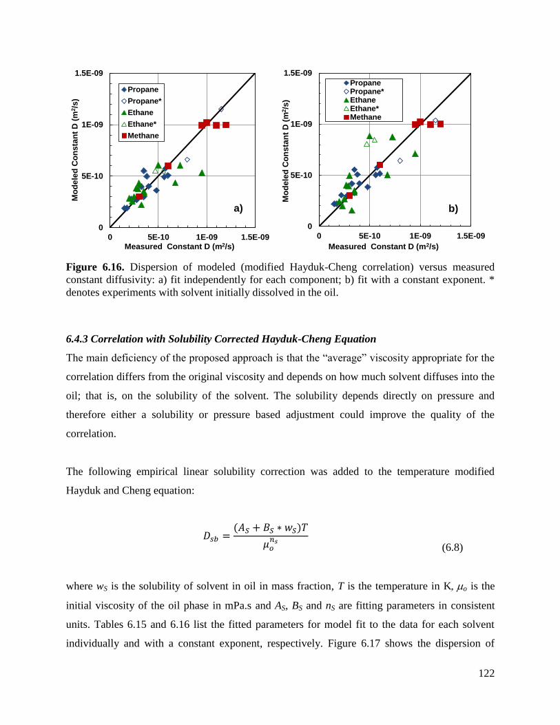
122

Figure 6.16. Dispersion of modeled (modified Hayduk-Cheng correlation) versus measured

constant diffusivity: a) fit independently for each component; b) fit with a constant exponent. *

denotes experiments with solvent initially dissolved in the oil.

6.4.3 Correlation with Solubility Corrected Hayduk-Cheng Equation

The main deficiency of the proposed approach is that the “average” viscosity appropriate for the

correlation differs from the original viscosity and depends on how much solvent diffuses into the

oil; that is, on the solubility of the solvent. The solubility depends directly on pressure and

therefore either a solubility or pressure based adjustment could improve the quality of the

correlation.

The following empirical linear solubility correction was added to the temperature modified

Hayduk and Cheng equation:

𝐷𝑠𝑏 =

(𝐴𝑆 + 𝐵𝑆 ∗ 𝑤𝑆)𝑇

𝜇𝑜𝑛𝑠

(6.8)

where wS is the solubility of solvent in oil in mass fraction, T is the temperature in Ko is the

initial viscosity of the oil phase in mPa.s and AS, BS and nS are fitting parameters in consistent

units. Tables 6.15 and 6.16 list the fitted parameters for model fit to the data for each solvent

individually and with a constant exponent, respectively. Figure 6.17 shows the dispersion of

0

5E-10

1E-09

1.5E-09

0 5E-10 1E-09 1.5E-09

Mo

de

led

Co

ns

tan

t D

(m

2/s

)


Propane

Propane*

Ethane

Ethane*

Methane

a)

0

5E-10

1E-09

1.5E-09

0 5E-10 1E-09 1.5E-09

Mo

dele

d C

on

sta

nt

D (

m2/s

)


PropanePropane*EthaneEthane*Methane

b)

123

error for the two methods. The addition of the solubility correction substantially improves the

quality of the fit to the data. The maximum deviation is less than 60% even when a single

common exponent is used. However, neither AS nor BS follow a consistent trend from methane to

propane when a single exponent is used for all solvents. As an alternative, the parameter BS was

also fixed, but even then, there was no consistent trend in the AS parameter with the different

solvents, as shown in Table 6.17.

Table 6.15. Parameters for the solubility corrected modified Hayduk and Cheng equation. Units

are m²/s for diffusivity and mPa.s for viscosity.

Solvent AS (x 1012

) BS (x 1010

) nS AARD

%

MARD

%

Methane 13.84 2.605 0.366 6.3 22

Ethane 5.295 1.950 0.345 16 54

Propane 7.282 1.015 0.391 10 39

Table 6.16. Parameters for the solubility corrected modified Hayduk and Cheng equation fit with

a single exponent. Units are m²/s for diffusivity and mPa.s for viscosity.

Solvent AS (x 1012

) BS (x 1010

) nS AARD

%

MARD

%

Methane 15.18 1.067 0.370 6.2 20

Ethane 6.277 2.289 0.370 16 56

Propane 6.472 0.916 0.370 10 36

Table 6.17. Parameters for the solubility corrected modified Hayduk and Cheng equation fit with

a single exponent and single Bs. Units are m²/s for diffusivity and mPa.s for viscosity.

Solvent AS (x 1012

) BS (x 1012

) nS AARD

%

MARD

%

Methane 11.45 6.081 0.308 20 48

Ethane 8.655 6.081 0.308 26 77

Propane 9.458 6.081 0.308 25 49

124

Figure 6.17. Cross plots of modelled versus measures constant diffusivity using the solubility

corrected modified Hayduk-Cheng correlation a) fit independently for each component b) fit

with a constant power. *denotes experiments with solvent initially dissolved in the oil.

Since pressure is more readily available, the following alternative pressure correction to the

temperature modified Hayduk and Cheng equation was also tested:

𝐷𝑠𝑏 =

(𝐴𝑃 + 𝐵𝑃 ∗ 𝑃)𝑇

𝜇𝑜𝑛𝑃

(6.9)

where P is the pressure in kPa, T is the temperature in Ko is the initial viscosity of the oil

phase in mPa.s and AP, BP, and nP are fitting parameters in consistent units. Tables 6.18 to 6.20

list the fitted parameters for model fit to the data for each solvent individually, with a constant

exponent, and with both a constant exponent and a constant parameter BP, respectively. Figure

6.18 shows the dispersion of error for the three methods. The addition of the pressure correction

provides a better fit to the data than the solubility correction with a maximum deviation less than

42% even when a single common exponent and a single parameter BP are used. The AP

parameter increases monotonically from methane to propane but, unless it is fixed, the BP

constant still does not follow a consistent trend. When fitting with a constant exponent and constant

BP, the parameter AP had a linear relationship with the molecular weight of the solvent, as shown

in Figure 6.19.

0

5E-10

1E-09

1.5E-09

2E-09

0 5E-10 1E-09 1.5E-09 2E-09

Mo

dele

d C

on

sta

nt

D (

m2/s

)


PropanePropane*EthaneEthane*Methane

a)

0

5E-10

1E-09

1.5E-09

2E-09

0 5E-10 1E-09 1.5E-09 2E-09

Mo

de

led

Co

ns

tan

t D

(m

2/s

)


Propane

Propane*

Ethane

Ethane*

Methane

b)

125

Table 6.18. Parameters for the pressure corrected modified Hayduk and Cheng equation. Units

are m²/s for diffusivity and mPa.s for viscosity.

Solvent AP (x 1012

) BP (x 1015

) nP AARD

%

MARD

%

Methane 9.978 0.985 0.350 6.1 22

Ethane 2.312 1.366 0.239 13 38

Propane 2.367 3.250 0.261 6.8 24

Table 6.19. Parameters for the pressure corrected modified Hayduk and Cheng equation fit with


Solvent AP (x 1012

) BP (x 1015

) nP AARD

%

MARD

%

Methane 0.092 2.037 0.244 10 19

Ethane 2.424 1.398 0.244 13 39

Propane 2.005 3.075 0.244 6.9 22

Table 6.20. Parameters for the pressure corrected modified Hayduk and Cheng equation fit with


Solvent AP (x 1012

) BP (x 1015

) nP AARD

%

MARD

%

Methane 0.633 2.393 0.289 7.5 19

Ethane 2.655 2.393 0.289 16 42

Propane 4.201 2.393 0.289 9.7 28

126

Figure 6.18. Dispersion of modeled (pressure corrected modified Hayduk-Cheng correlation)

versus measured constant diffusivity: a) fit independently for each component; b) fit with a

constant exponent. c) fit with a constant exponent and parameter BP. * denotes experiments

with solvent initially dissolved in the oil.

0

5E-10

1E-09

1.5E-09

0 5E-10 1E-09 1.5E-09

Mo

dele

d C

on

sta

nt

D (

m2/s

)

Measured Constant D (m2/s/)

Propane

Propane*

Ethane

Ethane*

Methane

a)

0

5E-10

1E-09

1.5E-09

0 5E-10 1E-09 1.5E-09

Mo

dele

d C

on

sta

nt

D (

m2/s

)


Propane

Propane*

Ethane

Ethane*

Methane

b)

0

5E-10

1E-09

1.5E-09

0 5E-10 1E-09 1.5E-09

Mo

de

lle

d C

on

sta

nt

D (

m2/s

)


Propane

Propane*

Ethane

Ethane*

Methane

c)

127

Figure 6.19. Parameter AP for each solvent fit with a constant power and BP parameter plotted

against the molecular weight of the solvent.

The Ap parameter was correlated to the solvent molecular weight and the constant diffusivity data

were fit a final time with a constant power, constant BP and the parameter AP to obtain the

following correlation:

𝐷𝑠𝑏 =

(1.104 ∗ 10−13𝑀𝑆 − 7.869 ∗ 10−13 + 2.224 ∗ 10−15𝑃)𝑇

𝜇𝑜0.280

(6.10)

where MS is the molecular weight of the solvent. P is the pressure in kPa, T is the temperature in

Ko is the initial viscosity of the oil phase in mPa.s and 𝐷𝑠𝑏 is the constant diffusivity of

solvent in bitumen in m2/s. The deviation from the measured diffusivities is no more than 40%,

Table 6.21. Figure 6.20 shows the dispersion of error.

Table 6.21. Relative deviation of the correlated diffusivities from the experimental data for each

solvent.

Solvent AARD

%

MARD

%

Methane 8.3 19

Ethane 16 40

Propane 10 27

0

1E-12

2E-12

3E-12

4E-12

0 20 40 60

AP

Solvent Molecular Weight (g/mol)

128

Figure 6.20. Dispersion of diffusivities correlated with the pressure corrected Hayduk-Cheng

correlation. * denotes experiments with solvent initially dissolved in the oil

6.5 Concentration Dependent Diffusivity

As previously discussed, diffusivity is known to depend on viscosity. Since viscosity depends on

the concentration of the solvent in the medium, then diffusivity must also depend on

concentration. To test this hypothesis, four two-stage pressure decay experiments were

performed with zero initial solvent concentration and then with a non-zero initial solvent

concentration in the oil. The first stage was performed at a lower pressure. At the end of the first

stage the oil was saturated with the solvent at the relatively low solubility corresponding to the

relatively low pressure. In the second stage, the pressure was increased to achieve a new higher

solubility end point and a second pressure decay was performed. Table 6.22 shows that in all

cases, the diffusivity was higher in the second stage than in the first. In other words, the higher

solvent content led to a higher diffusivity, confirming the concentration dependence of

diffusivity.

0

5E-10

1E-09

1.5E-09

0 5E-10 1E-09 1.5E-09

Mo

dele

d c

on

sta

nt

D (

m2/s

)

Measured constant D (m2/s/K)

Propane

Propane*

Ethane

Ethane*

Methane

129

Table 6.22. Constant diffusivity of ethane and propane in WC-B-B3 bitumen with and without

solvent initially dissolved in oil.

Solvent T oC

P

kPa

Initial Solvent

wt%

Solubility

wt%

Viscosity

mPa.s

Diffusivity

10-10

m2/s

Ethane 42 2168 0 3.8 3900 2.3

Ethane 42 3316 3.6 6.1 80 5.5

Ethane 64 1120 0 1.5 710 2.7

Ethane 64 2104 1.5 2.9 110 4.7

Propane 64 1290 0 4.1 750 -

Propane 64 1890 4.1 8.6 130 8.0

Propane 86 1374 0 5.4 210 5.8

Propane 86 2303 5.4 11.4 43 11.5

The implication of this concentration dependence is that diffusivity will change throughout the

mass transfer process as the solvent concentration changes. Therefore, the mass transfer is best

modeled with a diffusivity that is calculated at each point in space and time as a function of

concentration (or viscosity). In this case, viscosity was selected over concentration because the

relationship between diffusivity and viscosity is well established. The diffusivity of solvent in

bitumen was assessed using each of the following three equations:

1) a modified Hayduk and Cheng (1971) equation

𝐷𝑠𝑏 =

𝐴𝑇


(6.11)

2) a modified Bearman (1961) equation

𝐷𝑠𝑏 =

𝐴𝑇

𝜇𝑚𝑖𝑥𝑛[1 + 𝑥𝑠 (

𝑉𝑠𝑉𝑏

− 1)] (𝑑 ln 𝑎𝑠

𝑑 ln 𝑥𝑠)

(6.12)

130

3) the Vignes (1966) equation

𝐷𝑠𝑏 = (𝐷𝑠𝑏

0 )𝑥𝐵(𝐷𝑏𝑠0 )𝑥𝐴 (

𝑑 ln 𝑎𝑠

𝑑 ln 𝑥𝑠)

(6.13)

Where applicable, the mixture viscosity was used instead of the initial bitumen viscosity. Note

that temperature dependence was added to the original Hayduk and Cheng (1971) equation. An

exponent was added to the mixture viscosity term in the original Bearman equation because the

original formulation over-emphasized the viscous effect for the systems modeled in this thesis.

The temperature dependence was added for consistency with the modified Hayduk and Cheng

equation. The Vignes equation was not modified. The viscosity dependent diffusivities were

implemented in the numerical model as described in Chapter 4.

A major challenge in implementing the concentration dependent viscosity is that the

concentration dependent diffusivity correlations each have two fitting parameters and equally

good fits to the experimental data can be obtained from multiple sets of parameters. Figure 6.21

shows that three unique sets of parameters for the modified Hayduk and Cheng equation and the

Vignes equation give nearly indistinguishable fits to the mass transfer data. This observation is

consistent with James et al. (2012), who concluded that various models for concentration

dependent diffusivity of butane in bitumen give equally good fits to total mass diffused data.

The concentration profiles predicted from each of these fits are also very similar, as shown in

Figure 6.22. The profiles predicted from the three sets of parameters from the Hayduk and Cheng

equation are indistinguishable; note that one set was removed to avoid clutter. There are slight

differences between the profiles predicted form the Hayduk and Cheng equation and the Vignes

model. As they predict the same total mass diffused, the area under the each profile is the same at

a given time. The Vignes model and Hayduk-Cheng determined profiles cross over one another

at lower times but are nearly identical at 2500 minutes. Despite the slight differences between

models, the concentration profiles have similar shapes. Even with concentration profile data, it

would be difficult to determine the appropriate model given the scatter in experimentally

determined concentration profiles shown in shown in Figure 6.2 (Section 6.2).

131

Figure 6.21. Modeling propane diffusion into bitumen at 60°C and 600 kPa using the three

different sets of parameters for the modified Hayduk and Cheng (HC) and the Vignes equations.

The three different sets of parameters fitted for the Hayduk and Cheng equation are: n=0.3,

A=3.40*10-12

(HC1); n=0.6, A=4.68*10-12

(HC2); n=0.4, A=5.91*10-12

(HC3).

Figure 6.22. Concentration profiles predicted from modeling propane diffusion into bitumen at

60°C and 600 kPa using the two different sets of parameters for the modified Hayduk and Cheng

and the Vignes equations. The sets of parameters fitted for the Hayduk and Cheng equation are:

n=0.6, A=4.68*10-12

(HC2); n=0.4, A=5.91*10-12

(HC3).

To determine a unique fit to the experimental data, either one parameter must be calculated or a

relationship between the two parameters must be obtained. For the modified Hayduk and Cheng

0

0.2

0.4

0.6

0.8

0 50 100

Mass D

iffu

sed

(g

)


Experimental DataHC1HC2HC3Vignes

0

0.01

0.02

0.03

0.04

0.05

0 0.2 0.4 0.6 0.8 1

Co

nc

en

tra

tio

n (

g/m

L)

Depth (cm)

HC2

HC3

Vignes

500 min

1000 min

2500 min

132

equation, the end point diffusivities provide a means to constrain the solution. At infinite dilution

(of solvent), the diffusivity is given by:

𝐷𝑠𝑏

∞ =𝐴𝑇

𝜇𝑏𝑛

(6.14)

where 𝐷𝑠𝑏∞ is the infinite dilution diffusivity of solvent in bitumen and b is the viscosity of the

bitumen. At infinite dilution of bitumen (almost pure solvent), the diffusivity is given by:

𝐷𝑏𝑠

∗ =𝐴𝑇

𝜇𝑠𝑛

(6.15)

where 𝐷𝑠𝑏∗ the diffusivity of the solvent in a solvent medium infinitely dilute in bitumen and s is

the viscosity of the liquid solvent. Once the endpoints are determined, the parameters A and n

can be determined as follows:

𝑛 =

log𝐷𝑏𝑠

∗

𝐷𝑠𝑏∞

log𝜇𝑠

𝜇𝑏

(6.16)

𝐴 =

𝐷𝑠𝑏∞

𝑇𝜇𝑏

𝑛

(6.17)

Hence, if either the infinite dilution or maximum concentration diffusivities can be determined

independently, the other endpoint can be determined by fitting the diffusivity data. The same

approach was applied to the Bearman and the Vignes equations except that, in the latter case, the

two end point diffusivities are input directly in the equation.

6.5.1 Diffusivity at Infinite Dilution of Bitumen in Solvent (Independently Determined)

The diffusivity at infinite dilution of bitumen was selected as the endpoint to be determined

independently because it is a more suitably described by the existing infinite dilution correlations

(designed for large species diffusing though a low molecular weight liquid). If diffusion at this

condition is simply controlled by solvent molecules moving through solvent, then the appropriate

end point is the self-diffusion coefficient of the solvent. However, the mass transfer process

involves both solvent moving through bitumen and bitumen moving through solvent (swelling

must involve the movement of bitumen). Hence, the diffusivity represents mutual diffusion. In

133

this case, the appropriate endpoint is the infinite dilution diffusivity of bitumen in solvent. Both

types of endpoint are evaluated below.

Self-Diffusion Coefficient End Point

Self-diffusion coefficients for saturated liquid propane were measured by Greiner-Schmid et al.

(1991). Their data was fit with the modified Hayduk-Chang equation as follows:

𝐷𝑠

∗ = 5.1 ∗ 10−12𝑇

𝜇𝑠0.951

(6.18)

where 𝐷𝑠∗ is the propane self-diffusivity in m

2/s and 𝜇𝑠 is the viscosity of liquid propane in

mPa.s. The liquid propane viscosity was calculated using the Expanded Fluid model with the

effective density of propane as the input. This approach could only be applied to propane self-

diffusion as there was little self-diffusion data available for methane and ethane in the

appropriate range of temperatures and pressures. The calculated self-diffusion coefficients are

shown in Figure 6.23.

Figure 6.23. Self-diffusivity/temperature of propane and infinite dilution diffusivity/temperature

of bitumen in liquid propane calculated at the experimental conditions.

5E-12

5E-11

0.05 0.5

Dif

fus

ivit

y/T

em

pe

rau

tre

(m

2/s

K)

Propane Viscosity (cP)

Self Diffusion

Wilke-Chang

Hayduk-Minhas

134

Infinite Dilution of Bitumen End Point

This infinite dilution diffusivity was calculated using the Wilke-Chang Equation (1955) and the

Hayduk-Minhas (1982) equation. Both equations are described in Section 2.2.2 and require the

molecular weight and viscosity of the medium and the molar volume of the diffusing species at

its normal boiling point. In this case, the solvent in the medium and bitumen is the diffusing

species. The liquid solvent viscosity was calculated using the Expanded Fluid model with the

effective density of the solvent as the input. A hypothetical average normal boiling point of the

bitumen was estimated using the Soreide Correlation (Riazi 2005)

𝑇𝑏 = 1071.28 − 9.417 ∗ 104

∗ exp[−4.922 ∗ 10−3𝑀𝑏 − 4.7685 ∗ 𝑆𝐺 + 3.462 ∗ 10−3 ∗ 𝑀𝑏

∗ 𝑆𝐺] ∗ 𝑀𝑏−0.03522 ∗ 𝑆𝐺3.266

(6.19)

where Tb is the normal boiling point in K, Mb is the molecular weight (520 g/mol), and SG is the

specific gravity (1.017). The calculated normal boiling point and molar volume of the WC-B-B3

bitumen were 496oC and 770cm

3/mol, respectively. The infinite dilution of bitumen endpoints

for propane are compared in Figure 6.23. They are both approximately an order of magnitude

lower than the self-diffusion coefficients. The infinite dilution diffusivity predicted from the

Hayduk-Minhas and Wilke-Chang equations are very similar and were found to give nearly

identical parameters when fitting the propane mass transfer data. The infinite dilution

diffusivities of bitumen from the Haydak-Minhus equation were used in this thesis because it

was developed from a larger dataset. Tabulated values are provided in Appendix A.

6.5.2 Diffusivity at Infinite Dilution of Solvent in Bitumen (Fitted to Mass Transfer Data)

Once the infinite dilution of bitumen end point was determined, the diffusivity at infinite dilution

of solvent endpoint was calculated by fitting the mass transfer data. Each of three infinite

dilution of solvent end points are evaluated below. Self-diffusion data at the conditions of

interest in this thesis were only found for propane and therefore the self-diffusivity constraint

was only used in the analysis of propane data. As will be discussed later, the modified Bearman

equation resulted in large scatter in the infinite dilution diffusivity for propane in bitumen and

therefore was not tested on the other solvents.

135

Tables 6.23 and 6.24 list the infinite dilution diffusivity of methane and ethane, respectively, in

bitumen determined from the Modified Hayduk-Cheng equation and the Vignes model. Table

6.25 lists the infinite dilution diffusivity of ethane in bitumen calculated from experiments with a

non-zero initial solvent content in the bitumen. Table 6.26 lists the infinite dilution diffusivity of

propane in bitumen determined from the Modified Hayduk-Cheng equation, where the

parameters were constrained using the self-diffusivity of propane. Table 6.27 list the infinite

dilution diffusivity of propane in bitumen calculated form experiments with an initial solvent

content in bitumen using the same constraint. Table 6.28 lists the infinite dilution diffusivity of

propane in bitumen determined from the Modified Hayduk-Cheng, Bearman, and Vignes

equations, where the parameters were constrained using the infinite dilution diffusivity of

bitumen in propane. Table 6.29 lists the infinite dilution diffusivity of propane in bitumen

calculated form experiments with an initial solvent content in the bitumen using the same

constraints. Table 6.30 lists the infinite dilution diffusivity of propane in bitumen determined

from the Modified Hayduk-Cheng equation where the parameters were constrained using the

infinite dilution diffusivity of bitumen in butane.

Table 6.23. Infinite dilution diffusivity of methane in bitumen fit to the experimental data with

the modified Hayduk-Cheng and Vignes equations using the infinite dilution diffusivity as the

constraint.

T oC

P

kPa

ws*

wt%

mPa.s

Dsb∞

Hayduk-Cheng

10-10

m2/s

Dsb∞

Vignes

10-10

m2/s

50 3450 0.42 2040 2.74 2.00

76 4160 0.55 393 5.50 4.00

100 4230 0.53 120 10.72 8.00

100 4170 0.48 122 8.65 6.50

100 4340 0.51 121 9.94 7.50

101 4120 0.49 114 9.72 7.25

136

Table 6.24. Infinite dilution diffusivity of ethane in bitumen, fit to the experimental data with

the modified Hayduk-Cheng and Vignes equations using the infinite dilution diffusivity as the

constraint.

T oC

P

kPa

ws*

wt%

mPa.s

Dsb∞

Hayduk-Cheng

10-10

m2/s

Dsb∞

Vignes

10-10

m2/s

37 2964 6.9 7163 0.83 0.19

42 2168 3.8 3933 1.22 0.39

47 1394 2.1 2408 1.30 0.60

50 1741 3.7 1880 1.18 0.38

58 2962 4.4 1144 1.72 0.50

59 1495 2.4 994 2.45 1.05

64 1751 2.6 740 2.00 0.85

64 1120 1.5 712 2.05 1.05

73 774 0.84 429 2.50 1.70

75 4324 5.3 422 3.21 0.95

90 4741 4.9 189 5.84 1.90

100 1916 1.9 116 5.69 2.80

100 1970 2.6 114 3.42 1.35

Table 6.25. Infinite dilution diffusivity of ethane in bitumen fit to the experimental data with the

modified Hayduk-Cheng and Vignes equations using the infinite dilution diffusivity as the

constraint. Data from experiments with non-zero initial ethane concentration in bitumen (wso).

T oC

P

kPa

wso

wt%

ws*

wt%

mPa.s

Dsb∞

Hayduk-Cheng

10-10

m2/s

Dsb∞

Vignes

10-10

m2/s

42 3316 3.6 6.1 4122 2.06 0.45

64 2104 1.5 2.9 638 2.92 0.98

137

Table 6.26. Infinite dilution diffusivity of propane in bitumen fit to the experimental data with

the modified Hayduk-Cheng Equation and the self-diffusivity of propane as the constraint.

T oC

P

kPa

ws*

wt%

mPa.s

Dsb∞

10-10

m2/s

50 327 2.6 2116 0.83

50 724 4.6 2087 1.28

59 824 3.0 999 2.02

60 602 3.5 945 1.05

62 1080 6.8 801 1.11

70 1077 4.5 547 2.60

74 523 2.2 452 2.79

74 1006 4.5 445 2.09

80 1507 8.0 290 1.88

81 720 2.4 282 2.54

81 1367 7.23 272 2.21

85 702 2.5 229 2.38

86 1374 5.4 210 3.29


the modified Hayduk-Cheng equation and the self-diffusivity of propane as the constraint. Data

from experiments with non-zero initial propane concentration in bitumen (wso).

T oC

P

kPa

wso

wt%

ws*

wt%

mPa.s

Dsb∞

10-10

m2/s

64 1890 4.1 8.6 753 2.06

86 2303 5.4 11.4 210 2.81

138


the modified Hayduk-Cheng, Bearman, and Vignes equations using the infinite dilution

diffusivity as the constraint.

T oC

P

kPa

ws*

wt%

mPa.s

Dsb∞

Hayduk-Cheng

10-10

m2/s

Dsb∞

Bearman

10-10

m2/s

Dsb∞

Vignes

10-10

m2/s

50 327 2.6 2116 1.51 1.37 0.88

50 724 4.6 2087 1.13 1.13 0.45

59 824 3.0 999 2.45 2.34 1.30

60 602 3.5 945 1.33 1.33 0.63

62 1080 6.8 801 1.63 1.95 0.53

70 1077 4.5 547 3.42 3.56 1.50

74 523 2.2 452 3.13 2.88 1.98

74 1006 4.5 445 2.66 2.66 1.15

80 1507 8.0 290 2.94 3.74 0.95

81 720 2.4 282 2.98 2.75 1.65

81 1367 7.2 272 3.40 4.50 1.20

85 702 2.5 229 2.81 2.60 1.30

86 1374 5.4 210 4.29 4.29 1.70


the modified Hayduk-Cheng, Bearman, and Vignes equations using the infinite dilution

diffusivity as the constraint. Data from experiments with non-zero initial propane concentration

in bitumen (wso).

T oC

P

kPa

ws*

wt%

mPa.s

Dsb∞

Hayduk-Cheng

10-10

m2/s

Dsb∞

Bearman

10-10

m2/s

Dsb∞

Vignes

10-10

m2/s

64 1890 8.6 753 3.56 5.55 1.23

86 2303 11.4 210 5.82 11.7 1.70

Table 6.30. Infinite dilution diffusivity of butane in bitumen fit to the experimental data with the

modified Hayduk-Cheng Equation using the infinite dilution diffusivity as the constraint.

T oC

P

kPa

ws*

wt%

mPa.s

Dsb∞

10-10

m2/s

69 284.3 3.0 589 2.74

90 738.2 7.9 182 9.94

90 874.3 10.1 183 9.72

139

6.5.3 Correlating the Infinite Dilution Diffusivity of Solvent in Bitumen

In the previous section, the infinite dilution of solvent diffusivity endpoint was determined from

three different forms of the concentration dependent diffusivity (Hayduk-Cheng, Bearman, and

Vignes) with two different endpoint constraints (self-diffusion and infinite dilution of bitumen

from Hayduk-Minhas). As shown in Figure 6.24, the endpoint diffusivity/temperature (D/T)

appears to correlate to the original oil viscosity. Therefore, the following correlation was fit to

the infinite dilution diffusivity data for each solvent with each diffusivity model and endpoint

constraint:

𝐷𝑠𝑏

∞ =𝐴∞𝑇

𝜇𝑏𝑚

(6.20)

where 𝐴∞ and m are fitting parameters. Note: these constant are not the same as those used to fit

the pressure decay data but are are specific to fitting the infinite dilution diffusivity. The

combinations of diffusivity model and endpoint constraint are examined below to determine the

best correlation to the original oil viscosity.

Figure 6.24. Infinite dilution diffusivity of propane in bitumen determined from the modified

Hayduk-Cheng equation constraining the equation with propane self-diffusivity endpoint

constraint.

1E-13

1E-12

1E-11

100 1000 10000

Inf

Dil

uti

on

Pro

ap

ne D

/T (

m2/s

)K

Original Oil Viscosity (mpa.s)

From Self-Diffusivity

From Infinite Dilution Diffusivity

140

Comparison of Endpoint Constraints

Figure 6.24 compares the infinite dilution diffusivity of propane in bitumen calculated from the

self-diffusivity of propane and the infinite dilution diffusivity of propane in bitumen as the value

of the propane self-diffusivity is higher that the infinite dilution diffusivity of bitumen in

propane, it is reasonable that the resulting infinite dilution diffusivity from the self-diffusion

constraint is slightly lower than the infinite dilution constraint. Both of the relationships for the

infinite dilution diffusivity of propane in bitumen have similar exponents and the average errors

are very similar with the self-diffusivity constraint having slightly less maximum error, Table

6.31.

Since using the solvent self-diffusivity gives less error and it is based on the extrapolation of

experimental data, it would normally be the best choice to constrain the concentration dependent

diffusivity model. However, due to the limited availability of self-diffusivity data for the gases of

interest in this thesis, the Hayduk-Minhas equation was used to constrain the diffusivity equation

and develop the correlations later in this chapter.

Table 6.31. Parameters of the infinite propane dilution diffusivity correlation fit to values

determined by fitting propane diffusion data with the modified Hayduk-Cheng equation with the

self-diffusion and infinite dilution of bitumen endpoints. Units are m²/s for diffusivity and mPa.s

for viscosity.

Endpoint 𝑨∞ (x 1012

) m AARD

%

MARD

%

Self-diffusion 5.32 0.362 21 39

Infinite dilution of bitumen 8.60 0.380 22 53

Comparison of Concentration Dependent Diffusion Equations

Modified Hayduk and Cheng Equation: The infinite dilution D/T of solvent in bitumen from

the modified Hayduk-Chang equation (constraining the equation with the infinite dilution

diffusivity of bitumen in the solvents) is shown versus the initial oil viscosity in Figure 6.25. The

fitted parameters for the infinite dilution of solvent diffusivity are provided in Table 6.32. As

expected, the infinite dilution diffusivity for each solvent increases with decreasing viscosity and

the smaller solvents generally have higher diffusivity. The infinite dilution diffusivity of methane

141

is larger than that of the other two solvents. The difference between ethane, propane, and butane

diffusivities is within the scatter of the data.

Figure 6.25. Infinite dilution of solvent diffusivity determined by fitting mass transfer data with

the modified Hayduk-Cheng equation (symbols) and correlation to initial oil viscosity (lines): a)

ratio of diffusivity to temperature versus viscosity; b) dispersion of error of predicted versus

measured diffusivity.


determined by fitting solvent diffusion data with the modified Hayduk-Cheng equation. Units are

m²/s for diffusivity and mPa.s for viscosity.

Solvent 𝑨∞ (x 1012

) m AARD

%

MARD

%

Methane 16.33 0.388 4.8 13

Ethane 9.72 0.390 20 72

Propane 8.60 0.380 22 53

The exponents, m, of the infinite dilution models for the three solvents are all similar. Therefore,

the infinite dilution diffusivity data were refit with a fixed exponent of 0.403. The refitted D/T

are shown in Figure 6.26 and the refitted parameters are listed in Table 6.33. There was

negligible change in the deviations with this simplified correlation and; therefore, it is the

recommended option.

1E-13

1E-12

1E-11

100 1000 10000

Infi

Dilu

tio

n D

/T o

f S

olv

en

t in

Oi (m

2/s

/K)


Propane

Ethane

Methane

Model

a)

0

4E-10

8E-10

1.2E-09

0 4E-10 8E-10 1.2E-09

Mo

dele

d In

f D

ilu

tio

n D

(m

2/s

)Measured Inf Dilution D (m2/s)

Propane

Ethane

Methane

b)

142


the modified Hayduk-Cheng equation (symbols) and correlation to initial oil viscosity (lines): a)

ratio of diffusivity to temperature versus viscosity; b) dispersion of error of predicted versus

measured diffusivity. Data for all solvents fit with the same exponent in the power law model.


determined by fitting solvent diffusion data with the modified Hayduk-Cheng equation. The

correlation exponent was fixed at m = 0.403. Units are m²/s for diffusivity and mPa.s for

viscosity.

Solvent A∞ (x 10

12) AARD

%

MARD

%

Methane 17.53 5.0 11

Ethane 10.34 20 68

Propane 9.20 23 66

Modified Bearman Equation: The infinite dilution D/T of solvent in bitumen from the

modified Bearman equation (constraining the equation with the infinite dilution diffusivity of

bitumen in the solvents) is shown versus the initial oil viscosity in Figure 6.27. The fitted

parameters for the infinite dilution of solvent diffusivity are provided in Table 6.34. The

predicted diffusivity from this model does not correlate well with viscosity; the scatter in the data

is large, with a maximum relative error of 158%. There are two obvious outliers from the trend,

but data from these two experiments are much closer to trend for the other models investigated in

this thesis. Hence, the Bearman model was not investigated further.

1E-13

1E-12

1E-11

100 1000 10000

Inf

Dilu

tio

n D

/T o

f S

olv

en

t in

Oil (

m2/s

/K)


Propane

Ethane

Methane

Model

a)

0

4E-10

8E-10

1.2E-09

0 4E-10 8E-10 1.2E-09

Mo

dele

d In

f D

ilu

tio

n D

(m

2/s

)

Measured Inf Dilution D (m2/s)

Propane

Ethane

Methane

b)

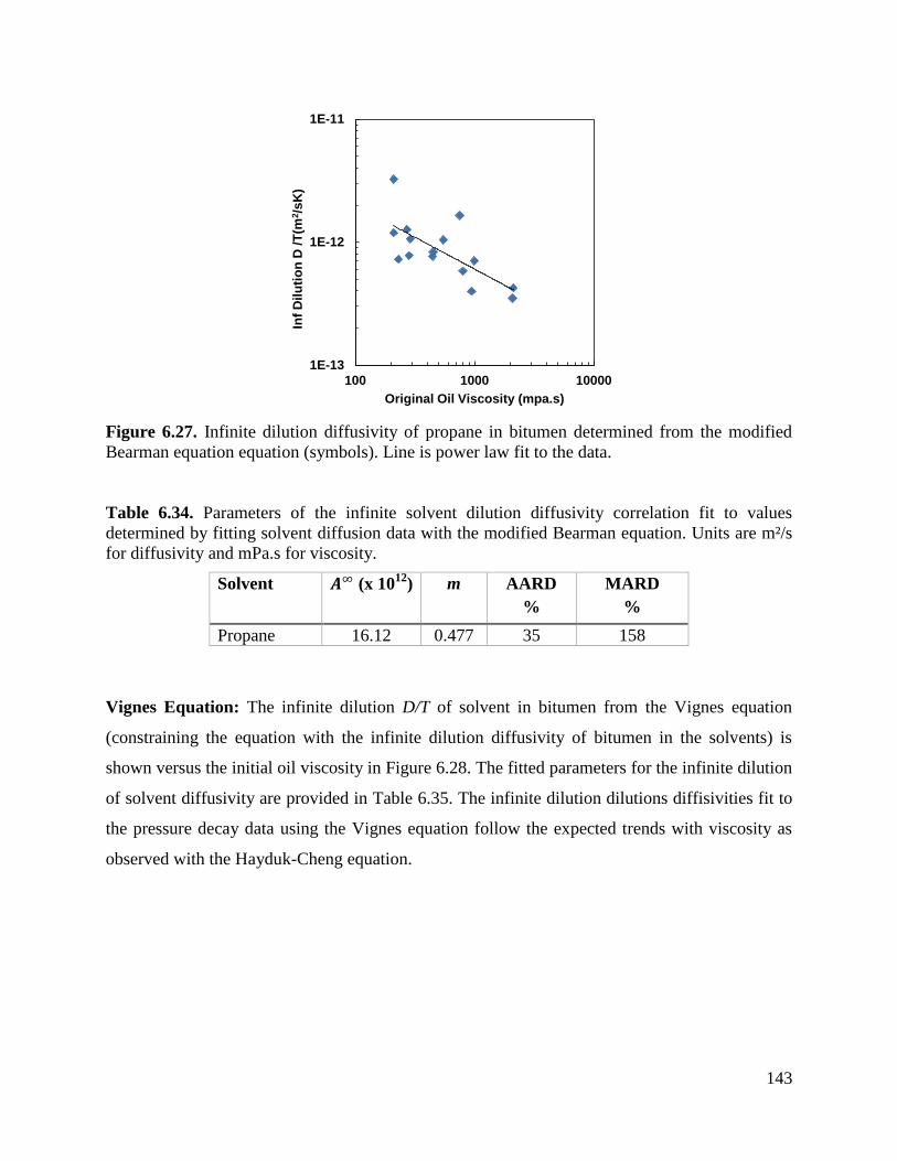
143

Figure 6.27. Infinite dilution diffusivity of propane in bitumen determined from the modified

Bearman equation equation (symbols). Line is power law fit to the data.


determined by fitting solvent diffusion data with the modified Bearman equation. Units are m²/s

for diffusivity and mPa.s for viscosity.


) m AARD

%

MARD

%

Propane 16.12 0.477 35 158

Vignes Equation: The infinite dilution D/T of solvent in bitumen from the Vignes equation

(constraining the equation with the infinite dilution diffusivity of bitumen in the solvents) is

shown versus the initial oil viscosity in Figure 6.28. The fitted parameters for the infinite dilution

of solvent diffusivity are provided in Table 6.35. The infinite dilution dilutions diffisivities fit to

the pressure decay data using the Vignes equation follow the expected trends with viscosity as

observed with the Hayduk-Cheng equation.

1E-13

1E-12

1E-11

100 1000 10000

Inf

Dil

uti

on

D /

T(m

2/s

K)


144


the Vignes equation (symbols) and correlation to initial oil viscosity (lines): a) ratio of diffusivity

to temperature versus viscosity; b) dispersion of error of predicted versus measured diffusivity.


determined by fitting solvent diffusion data with the Vignes equation. Units are m²/s for

diffusivity and mPa.s for viscosity.


) m AARD

%

MARD

%

Methane 12.7 0.396 5.1 13

Ethane 5.30 0.434 22 47

Propane 1.71 0.240 23 54

The exponents of this model are dissimilar and do not follow a clear trend. Nonetheless, the

infinite dilution diffusivity data were refit with a fixed average exponent of 0.418. The refitted

D/T are shown in Figure 6.29 and the refitted parameters are listed in Table 6.36. The deviations

from the data increases with this simplified correlation particularly for methane. The predicted

diffusivity of propane is also slightly higher than that predicted for ethane, which seems unlikely

for a larger, chemically similar molecule. This counter-intuitive trends may arise from the

thermodynamic correction factor used in the Vignes model used to match the data. The

compositional derivative of the activity coefficient was obtained from the Margules Equation fit

only to the saturation pressure of the solvent-oil mixture. For methane, the saturation pressure

1E-14

1E-13

1E-12

1E-11

100 1000 10000

Inf

Dilu

tio

n D

/T o

f so

lven

t in

Oil

(m2/s

/K)

Original Oil Viscosity

Propane

Ethane

Methane

Vignes a)

0

2E-10

4E-10

6E-10

8E-10

0 2E-10 4E-10 6E-10 8E-10

Mo

dele

d In

f D

ilu

tio

n D

(m

2/s

)

Measured Inf Dilution D (m 2/s)

Propane

Ethane

Methane

b)

145

data was supplemented from literature and differences between the oil samples could contribute

to the error.


the Vignes equation (symbols) and correlation to initial oil viscosity (lines): a) ratio of diffusivity

to temperature versus viscosity; b) dispersion of error of predicted versus measured diffusivity.

Data for all solvents fit with the same exponent in the power law model.


determined by fitting solvent diffusion data with the Vignes equation. The correlation exponent

was fixed at m = 0.418. Units are m²/s for diffusivity and mPa.s for viscosity.

Solvent A∞ (x 10

12) AARD

%

MARD

%

Methane 14.92 37 56

Ethane 4.67 21 44

Propane 4.92 28 49

Conclusion: Both the modified Hayduk-Cheng and the Vignes approach lead to similar quality

correlations for the infinite dilution diffusivity of solvent. However, the Vignes approach

requires the determination of the activity coefficient derivative and lack of data limits the

applicability of this approach. The Hayduk-Cheng approach is simpler and provides a good basis

for a correlation of the infinite dilution diffusivity of solvent to the initial oil viscosity.

1E-14

1E-13

1E-12

1E-11

100 1000 10000

Inf

Dil

uti

on

D/T

of

so

lve

nt

in O

il

(m2/s

/K)

Original Oil Viscosity

Propane

Ethane

Methane

Vignes a)

0

2E-10

4E-10

6E-10

8E-10

0.E+00 2.E-10 4.E-10 6.E-10 8.E-10M

od

ele

d In

f D

ilu

tio

n D

(m

2/s

)


Propane

Ethane

Methane

b)

146

6.5.4 Generalizing the Infinite Dilution Diffusivities of Solvents in Bitumen

In the previous section, it was established that the approach that provided the best correlation for

the infinite dilution of solvent diffusivity to the initial oil viscosity is the modified Hayduk-

Cheng equation with the Hayduk-Minhas infinite dilution of bitumen diffusivity endpoint.

However, up to now, the data for each solvent were fitted separately. To generalize the

correlation, the values of A∞ and m determined with this approach must be related to the solvent

type. The exponent was fixed at a constant value of m = 0.403 and therefore only a correlation

for the A∞ parameter is required.

Recall that the Wilke and Chang (1955) and Hayduk and Minhas (1982) equations for infinite

dilution diffusivity are a function of the molar volume of the diffusing species (in this case the

solvent) at its normal boiling point. Therefore, the A∞ parameter was correlated to the solvent

molar volume. Table 6.37 lists the molar volume of the solvents used in the thesis at their normal

boiling points (NIST, 2016). The A∞ parameters were correlated to the molar volumes with the

following relationship:

𝐴∞ =

5.18 ∗ 10−10

𝑉𝑠0.946

(6.21)

where Vs is the liquid molar volume of the solvent at its normal boiling point in cm3/mol. The

correlation fit the values with an average absolute relative deviation of 7.7%, Figure 6.30.

Figure 6.31 shows the correlated infinite dilution diffusivities versus the initial oil viscosity.

Table 6.38 lists the correlated parameters for this model and the average and maximum errors of

the infinite dilution diffusivity prediction. The correlation of A∞

does not dramatically affect the

quality of the fit to the infinite dilution data.

147

Table 6.37. Normal boiling point of methane, ethane, propane, and their liquid density and molar

volume at the boiling point.

Solvent Normal Boiling

Point oC

Liquid Molar

Density

mol/m3

Liquid Molar

Volume

cm3/mol

Methane -161.5 26327 37.98

Ethane -88.6 18090 55.28

Propane -42.1 13174 75.91

Figure 6.30. Experimentally determined and fitted A∞

parameter for each solvent versus the

solvent molar volume at its normal boiling point.

Table 6.38. Correlated parameters to the infinite dilution diffusivity model of solvents in heavy

oil. Units are m²/s for diffusivity and mPa.s for viscosity.

Solvent Correlated

A∞(x 10

12)

m AARD

%

MARD

%

Methane 16.61 0.403 8.2 16

Ethane 11.64 0.403 28 89

Propane 8.63 0.403 25 92

6E-12

8E-12

1E-11

1.2E-11

1.4E-11

1.6E-11

1.8E-11

2E-11

20 40 60 80

A∞

Solvent liquid molar volume at normal boinling point (cm3/mol)

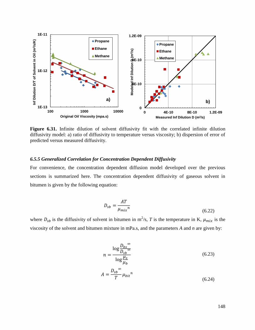
148


diffusivity model: a) ratio of diffusivity to temperature versus viscosity; b) dispersion of error of

predicted versus measured diffusivity.

6.5.5 Generalized Correlation for Concentration Dependent Diffusivity

For convenience, the concentration dependent diffusion model developed over the previous

sections is summarized here. The concentration dependent diffusivity of gaseous solvent in

bitumen is given by the following equation:

𝐷𝑠𝑏 =

𝐴𝑇


(6.22)

where 𝐷𝑠𝑏 is the diffusivity of solvent in bitumen in m2/s, T is the temperature in K, 𝜇𝑚𝑖𝑥 is the

viscosity of the solvent and bitumen mixture in mPa.s, and the parameters A and n are given by:

𝑛 =

log𝐷𝑏𝑠

∞

𝐷𝑠𝑏∞

log𝜇𝑠

𝜇𝑏

(6.23)

𝐴 =

𝐷𝑠𝑏∞

𝑇𝜇𝑏𝑖𝑡

𝑛

(6.24)

1E-13

1E-12

1E-11

100 1000 10000

Inf

Dilu

tio

n D

/T o

f S

olv

en

t in

Oil (

m2/s

/K)


Propane

Ethane

Methane

a)

0

4E-10

8E-10

1.2E-09

0 4E-10 8E-10 1.2E-09

Mo

dele

d In

f D

ilu

tio

n D

(m

2/s

)


Propane

Ethane

Methane

b)

149

where 𝜇𝑠 is the predicted viscosity of the liquid solvent in mPa.s, 𝜇𝑏 is the viscosity of the

bitumen, 𝐷𝑏𝑠∞ is the infinite dilution diffusivity of bitumen in solvent in m

2/s, and 𝐷𝑠𝑏

∞ is the

infinite dilution diffusivity of solvent in bitumen. The former is given by the Hayduk-Minhas

equation:

𝐷𝑏𝑠∞ =

13.3 ∗ 10−12𝑇1.47𝜇𝑠(10.2

𝑉𝑏⁄ −0.791)

𝑉𝑏0.71

(2.25)

where Vb is the liquid molar volume of bitumen at its normal boiling point in cm3/mol. The latter

is given by:

𝐷𝑠𝑏

∞ =5.18 ∗ 10−10𝑇

𝑉𝑠0.946𝜇𝑏

0.403

(6.26)

where Vs is the liquid molar volume of solvent at its normal boiling point in cm3/mol.

The values of n predicted using this correlation are fairly constant for each solvent: 0.224 to

0.240 for methane, 0.306 to 0.321 for ethane, and 0.323 to 0.327 for propane. Das and Butler

(1996) fit propane diffusion data to the Hayduk Cheng Equation with a power of 0.46, although

their model did not include a temperature term, which could account for the difference. As

shown in Section 6.4, the best fit exponents to the Hayduk-Cheng equation (Table 12) were

higher than those for the modified equation which included the temperature (Table 14).

The form of the concentration dependence of diffusivity is illustrated in Figure 6.32 at two

conditions. At low concentrations of either the solvent or the bitumen, the concentration

dependence of the diffusivity is linear, consistent with the findings from James et al. (2012) who

found the best fit to their mass diffusion data was achieved with a diffusivity linearly dependent

on concentration.

To illustrate the performance of the correlation, the predicted mass transfer for two experiments

(a good match and a poor match) are compared with the measured data in Figure 6.33. In the

former case, the error in the infinite dilution of solvent diffusivity prediction error was 5.4% and

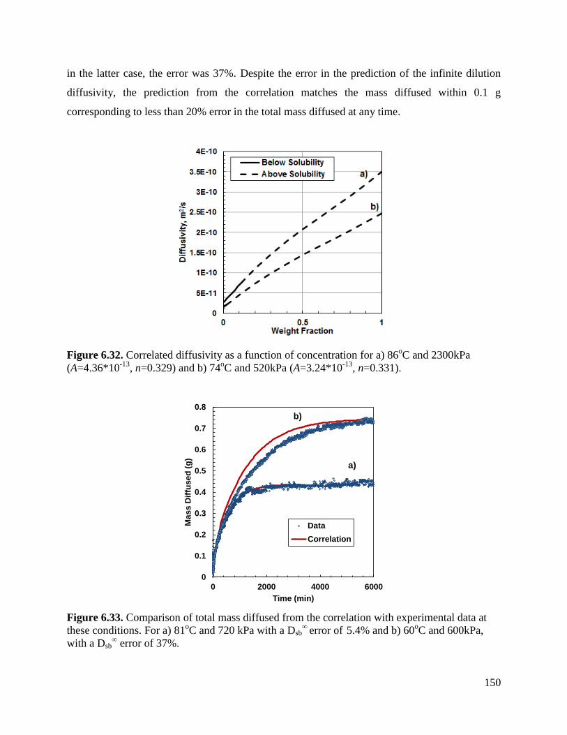
150

in the latter case, the error was 37%. Despite the error in the prediction of the infinite dilution

diffusivity, the prediction from the correlation matches the mass diffused within 0.1 g

corresponding to less than 20% error in the total mass diffused at any time.

Figure 6.32. Correlated diffusivity as a function of concentration for a) 86oC and 2300kPa

(A=4.36*10-13

, n=0.329) and b) 74oC and 520kPa (A=3.24*10

-13, n=0.331).

Figure 6.33. Comparison of total mass diffused from the correlation with experimental data at

these conditions. For a) 81oC and 720 kPa with a Dsb

∞ error of

5.4% and b) 60

oC and 600kPa,

with a Dsb∞ error of 37%.

0

0.1

0.2

0.3

0.4

0.5

0.6

0.7

0.8

0 2000 4000 6000

Mass D

iffu

sed

(g

)

Time (min)

Data

Correlation

b)

a)

151

6.6 Testing the Proposed Diffusivity Correlations

The correlation was tested against the results from additional pressure decay experiments of

three mixtures not included in the correlation: 1) butane in the whole bitumen, 2) methane in the

bitumen degassed at 176oC and 3) methane in bitumen maltenes. The constant diffusivity

correlation was also tested against diffusivity measurements from the literature. The

concentration dependent correlation could not be tested against literature data because the

required pressure decay data were not available.

6.6.1 Preliminary Evaluation of Butane Diffusivity in Bitumen

Constant Diffusivity Correlation

Figure 6.34 shows the cross plot of the modeled versus measured diffusivity of solvent in

bitumen, including butane. The butane diffusivity was not included in the fitting of the

correlation and was predicted to within 38%. The high average error in the butane may arise

from the relatively high solubility of butane which violates the assumption of constant diffusivity

more severely than the other solvents and therefore is harder to correct for.

Figure 6.34. Dispersion of diffusivities correlated with the pressure corrected Hayduk-Cheng

correlation (* denotes experiments with solvent initially dissolved in the oil).

0

5E-10

1E-09

1.5E-09

0 5E-10 1E-09 1.5E-09

Mo

dele

d c

on

sta

nt

D (

m2/s

)

Measured constant D (m2/s/K)

Propane

Propane*

Ethane

Ethane*

Methane

Butane

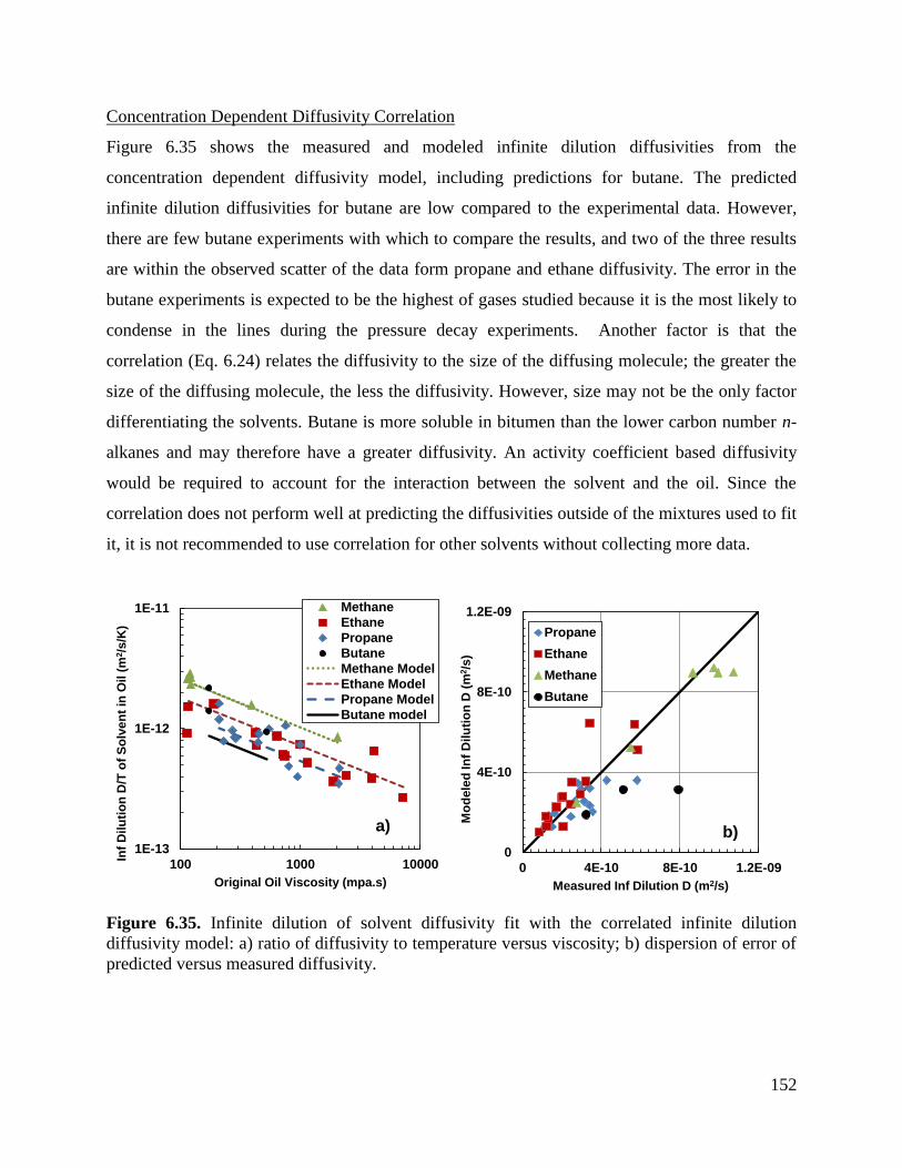
152

Concentration Dependent Diffusivity Correlation

Figure 6.35 shows the measured and modeled infinite dilution diffusivities from the

concentration dependent diffusivity model, including predictions for butane. The predicted

infinite dilution diffusivities for butane are low compared to the experimental data. However,

there are few butane experiments with which to compare the results, and two of the three results

are within the observed scatter of the data form propane and ethane diffusivity. The error in the

butane experiments is expected to be the highest of gases studied because it is the most likely to

condense in the lines during the pressure decay experiments. Another factor is that the

correlation (Eq. 6.24) relates the diffusivity to the size of the diffusing molecule; the greater the

size of the diffusing molecule, the less the diffusivity. However, size may not be the only factor

differentiating the solvents. Butane is more soluble in bitumen than the lower carbon number n-

alkanes and may therefore have a greater diffusivity. An activity coefficient based diffusivity

would be required to account for the interaction between the solvent and the oil. Since the

correlation does not perform well at predicting the diffusivities outside of the mixtures used to fit

it, it is not recommended to use correlation for other solvents without collecting more data.


diffusivity model: a) ratio of diffusivity to temperature versus viscosity; b) dispersion of error of

predicted versus measured diffusivity.

1E-13

1E-12

1E-11

100 1000 10000

Inf

Dilu

tio

n D

/T o

f S

olv

en

t in

Oil (

m2/s

/K)


Methane

Ethane

Propane

Butane

Methane Model

Ethane Model

Propane Model

Butane model

a)

0

4E-10

8E-10

1.2E-09

0 4E-10 8E-10 1.2E-09

Mo

dele

d In

f D

ilu

tio

n D

(m

2/s

)


Propane

Ethane

Methane

Butane

b)

153

6.6.2 Effect of Oil Composition

To assess the effects of oil composition on the diffusivity beyond simply the viscosity, pressure

decay experiments were performed with methane in maltenes and the bitumen degassed at

176oC.

Constant Diffusivity Correlation

The constant diffusivities fit to the pressure decay data for methane in the original bitumen,

degassed bitumen and maltenes are plotted against viscosity in Figure 6.36. In all cases, the

correlation qualitatively captures the trend in diffusivity versus initial oil viscosity. The average

and maximum deviations of the constant diffusivity correlation are listed in Table 6.39.

The maltene data are scattered around the expected trend and it is possible that the deviations

relate to the data rather than the correlation. First, the viscosities were measured for maltenes

from a different oil sample from the same source reservoir and may not be identical to the

viscosity for the sample used in the diffusivity measurements. Second, two batches of maltenes

were recovered for the diffusivity measurements and the batches could have different residual

solvent contents. However, as will be shown later, the concentration dependent diffusivity

correlation results in far less scatter. Therefore, the deviations likely reflect the limitations of this

simple correlation.

The correlation under-predicts the diffusivity of the degassed oil. The viscosity of the degassed

oil was unknown, but the expected viscosity would be higher than that of the original oil.

Therefore, the deviation would be even greater if the correct viscosity were used. The poor

match indicates that the constant diffusivity correlation based on oil viscosity and pressure is not

sufficient to capture the effects of different oil composition.

154

Figure 6.36. Methane diffusivity in the original bitumen, maltenes, and the bitumen degassed at

176oC* versus initial oil viscosity. The degassed viscosity was unknown and its diffusivities are

plotted versus the original viscosity.


predicting the diffusivity of methane in maltenes and bitumen degassed at 176oC

Oil Solvent AARD,

%

MARD

%

Degassed bitumen Methane 70 100

Bitumen maltenes Methane 56 81

Concentration Dependent Diffusivity Correlation

The infinite dilution diffusivity from the concentration dependent diffusivity model are plotted

against viscosity in Figure 6.37 and are compared to the values predicted from the infinite

dilution correlation. The deviations from the constant diffusivity correlation are listed in table

6.40. The infinite dilution correlation systematically over-predicted the methane diffusivity in

maltenes but was within 35% of the experimental values. The correlation systematically under-

predicted the infinite dilution diffusivity of methane in degassed bitumen but was within 45% of

the data. The systematic deviations suggest that a simple correction could be introduced to

account for oil fractions or different oils. More data on a variety of oils and fractions are required

before such a correction can be developed.

1E-11

1E-10

1E-09

1E-08

1 10 100 1000 10000

Co

nsta

nt

Dif

fusiv

ity o

f M

eth

an

e (

m2/s

)


Degassed at 176 C*

Original

Maltenes

Correlation, Degassed

Correlation, Original

Correlation, Maltenes

155

Figure 6.37. Methane diffusivity in the original bitumen, maltenes and the bitumen degassed a

176oC. * is plotted against the initial oil viscosity, as the degassed viscosity was unknown.


predicting the diffusivity of methane in maltenes and bitumen degassed at 176oC.

Solvent AARD,

%

MARD

%

Degassed Bitumen 40 45

Maltenes 28 34

6.6.3 Constant Diffusivity Correlation Tested on Literature Data

The constant diffusivity correlation was also tested against the screened literature data presented

in Section 6.3. The ethane and methane diffusivity data collected by Upreti and Mehrotra (2002)

and by Tharanivasan et al. (2006) are compared with the correlation in Figure 6.38 and the

average and maximum deviations are listen in Table 6.41. The correlation predicts the correct

qualitative trend of diffusivity versus initial oil viscosity and pressure but over-predicts the

pressure effect for both solvents.

The largest deviation of 227% is in the dataset from Upreti and Mehrotra (2002) and is attributed

to an outlier data point which is off-trend from all of the other data. If this data point is excluded

the maximum deviation is 68% (for high pressure methane). Possible explanations for the

deviation are: 1) the correlation does not apply well to viscosities 100 times higher than those

1E-11

1E-10

1E-09

1E-08

1 10 100 1000 10000

Infi

nit

e D

ilu

tio

n D

iffu

siv

ity o

f M

eth

an

e

(m2/s

)


Degassed at 176 C*

Original

Maltenes

Correlation, Degassed

Correlation, Original

Correlation, Maltenes

156

used in its development, possibly because the solubilities differ from the solubility effect

indirectly accounted for within the correlation; 2) experimental issues such as ethane

condensation in the system. The experiment was performed at 25oC and 4MPa near the critical

point of ethane of 32oC and 4.9 MPa (Green and Perry, 2008).

Figure 6.38. Constant diffusivity of a) methane and b) ethane in Athabasca bitumen


predicting the diffusivity of methane in maltenes and Athabasca bitumen (data from Upreti and

Mehrotra, 2002).

Oil Solvent AARD,

%

MARD

%

Upreti and Mehrotra (2002), 4 MPa Methane 14 23

Upreti and Mehrotra (2002), 8 MPa Methane 58 68

Upreti and Mehrotra (2002), 4 MPa Ethane 82 227

Upreti and Mehrotra (2002), 8 MPa Ethane 28 29

Tharanivasan et al. (2004), 4.9MPa Methane - 4.4

The correlation was next tested on Jalialahmadi et al.’s (2006) diffusivities of methane in a light

oil (0.26 mPa.s at 25oC), as shown in Figure 6.39. Although this oil has a viscosity three orders

of magnitude lower than the data used to develop the correlation, the correlation predicts the

diffusivity to within 18% at pressures below 15 MPa but the error increases to over 115% at

1E-11

1E-10

1E-09

1000 10000 100000 1000000

Dif

fusiv

ity o

f M

eth

an

e (

m2/s

)


Correlation, 4 MPaCorrelation, 4.9 MPaCorrelation, 8 MPaUpreti and Mehrotra, 4 MPaUpreti and Mehrotra, 8 MPaTharanivasan et al., 4.9 Mpa

a)

1E-11

1E-10

1E-09

1000 10000 100000 1000000

Dif

fus

ivit

y o

f E

tha

ne

(m

2/s

)


Correlation, 4 MPa

Correlation, 8 MPa



b)

157

pressures of 28 MPa. A possibly explanation for the deviation is that the correlation does not

correctly account for solubility effects at higher pressures.

Figure 6.39. Constant diffusivity of propane in an Iranian Crude oil (0.35 mPa.s at 25°C). Data

from Jalialahmadi et al. (2006).

The effect of pressure on the constant diffusivities of methane, ethane and propane in

Lloydminster heavy oil was investigated by Yang (2005) and Yang and Gu (2006, 2007) at

23.9oC. Similar data were obtained by Etminan et al. (2014b) for propane diffusivity in heavy oil

at 23.9°C. Note, the solubility in Etminan’s higher pressure experiment may have caused

asphaltene precipitation, as discussed in Section 6.3.3. Figure 6.40 compares the predicted and

measured diffusivities versus pressure. The correlation over-predicted the methane diffusivity at

all conditions and the deviations increased slightly with pressure (maximum error of 67%). In

contrast, the correlation under-predicted the diffusivities of ethane and propane at all conditions

and the deviations increased significantly with pressure (10% error at low pressure increasing to

over 500% at high pressure). Here, low pressure indicates a pressure that is low relative to the

solvent vapor pressure).

As noted in Section 6.3, the magnitude of the change in diffusivity with pressure reported by

Yang and Gu (2006, 2007) for ethane and propane is much higher than that observed in this

thesis and by Upreti and Mehrotra (2002). Ethane diffusivity measured by Upreti and Mehrotra

0

5E-09

1E-08

1.5E-08

2E-08

2.5E-08

3E-08

3.5E-08

0 10000 20000 30000

Dif

fusiv

ity o

f M

eth

an

e (

m2/s

)

Pressure (kPa)

Jalialahmadi et al. (2006), 25C

Jalialahmadi et al. (2006), 50C

Correlation 25 C

Correlation 50 C

158

(2002) is plotted in Figure 6.40b) to illustrate the pressure effect on their reported diffusivities.

Note, the magnitude of the diffusivities from each oil differ because the oil viscosities are

different. It is not obvious why the pressure trends differ. The Yang and Gu and Etminan data

were collected at 24°C, 13oC lower than any of the data from this thesis or Upreti and Mehrotra.

It is possible that at low temperature, particularly at higher pressures, the solubility of the solvent

increases more significantly that is indirectly accounted for in the proposed correlation. If the

correlation under-“predicted” the solubility, it would predict too low a diffusivity.

Marufuzzaman and Henni (2014) also reported propane diffusivities at temperatures of 15 and

26°C. The correlation is compared with their data in Figure 6.41. Note, the experiments at 500

and 600 kPa had an initial solvent concentration equal to the solubility at the previous pressure.

The viscosities at these conditions were estimated using a double log mixing rule and the

effective viscosity of propane. The change in viscosity with solubility (pressure) was greater at

15°C than at 26°C and, as a result, the predicted diffusivity curves crossed at 500 kPa.

The correlation predicted the diffusivities at 15°C with a maximum error of 50% but under-

predicted the diffusivity at 26oC with a maximum error of 140%. As noted in Section 6.3.3 the

diffusivity increase between 15 and 26oC is much more than would be expected by the viscous

changes alone. The reason for this discrepancy is not clear because the experimental procedure

was not fully described. Interestingly, the correlation was able to predict the magnitude of the

change in the diffusivity with pressure. It is possible that the correlation is least accurate when

both the temperature is low and the pressure is high; that is, when solvent solubilities in the oil

are highest.

159

Figure 6.40. Constant diffusivity of a) methane, b) ethane, c) propane in heavy oil compared to

the predictions from the constant diffusivity correlation. Data measured by Yang and Gu (2006),

Yang and Gu (2007), Etminan et al. (2014b), and Upreti and Mehrotra (2002)

0

1E-10

2E-10

3E-10

4E-10

5E-10

6E-10

7E-10

8E-10

9E-10

5000 7000 9000 11000 13000 15000

Dif

fusiv

ity o

f M

eth

an

e (

m2/s

)

Pressure (kPa)

Yang (2005)

Prediction for Y

a)

0

1E-10

2E-10

3E-10

4E-10

5E-10

6E-10

7E-10

8E-10

9E-10

0 5000 10000

Dif

fusiv

ity o

f E

than

e (

m2/s

)

Pressure (kPa)

Yang and Gu (2007)Prediction for YUpreti and Mehrotra, 75 CUpreti and Mehrotra, 90 C

b)

0

1E-10

2E-10

3E-10

4E-10

5E-10

6E-10

7E-10

8E-10

9E-10

200 400 600 800 1000

Dif

fusiv

ity o

f P

rop

an

e (

m2/s

)

Pressure (kPa)

Yang and Gu (2007)Prediction for Y&GEtminan (2014)Prediction for E

c)

160

Figure 6.41. Constant diffusivity of propane in Cactus Lake oil (742 mPa.s at 26°C). Data from

Marufuzzaman and Henni (2014).

6.6.4 Towards an Improved Correlation

Overall, the constant diffusivity correlation developed in this thesis over-predicts methane

diffusivity in heavy oils at higher pressures. The correlation uses pressure as a proxy for the

solubility of the solvent in the oil. The pressure effect was assumed to be the same for each

solvent and is an average of all the data collected. Since more data were collected for ethane and

propane, the average trend is less accurate for methane.

For ethane and propane, the correlation matched trends with pressure for some datasets (Upreti

and Mehrotra, 2002; Tharanivasan et al., 2006; Marufuzzaman and Henni, 2014) but not others

(Yang and Gu, 2006, 2007; Etminan et al., 2014b). It is not clear if the deviations are data issues

or a flaw with the correlation. The deviations were highest when both temperature was low

(<30°C) and pressure was high relative to the solvent vapor pressure. This trend suggests that the

linear pressure proxy is not adequate to account for the changes in solubility.

An alternative to correlating the constant diffusivity to pressure is to correlate to a normalized

pressure given by the ratio of the pressure to the solvent vapor pressure. The vapor pressures

were determined from the vapor pressure correlation developed in Section 5 (extrapolated when

above the critical temperature). The revised correlation has the following form:

0

1E-10

2E-10

3E-10

4E-10

5E-10

6E-10

7E-10

8E-10

200 400 600 800

Dif

fusiv

ity o

f P

rop

an

e (

m2/s

)

Pressure (kPa)

15 C26 CCorrelation, 15 CCorrelation, 26 C

161

𝐷𝑠𝑏 =

𝑇𝑓(𝑃𝑁)

𝜇0𝑛

(6.27)

where f(PN) is a function of the normalized pressure, PN, 𝑇 in the temperature in K, n is a fitting

parameter, and 𝜇0 is the viscosity of the initial fluid in mPa.s.

To determine the form of f(PN), Eq. 2.24 was rearranged to calculate experimental values of the

function as follows and as a preliminary estimate the value of n was assumed to be 0.28 (the

value of the constant diffusivity correlation):

𝑓(𝑃𝑁) =

𝐷𝑠𝑏,𝑒𝑥𝑝

𝑇𝜇0

0.28

(6.28)

where 𝐷𝑠𝑏,𝑒𝑥𝑝 is the experimental diffusivity in m2/s. The experimental f(PN) are plotted versus

the normalized pressures in Figures 6.42a, 6.42b, and 6.42c for methane, ethane, and propane,

and for all three n-alkanes respectively. Most of the data follow a similar trend except for the

methane diffusivities of the low viscosity Iranian oil (Jalialahmadi et al., 2006)). These data were

excluded from any further fit to the data. For each solvent, the function tends to a constant

(infinite dilution) diffusivity far from the vapor pressure (PN goes to zero). The infinite dilution

value is slightly different for each solvent. The function appears to increase exponentially as PN

goes to unity, although the data are highly scattered at PN above approximately 0.65. Note, most

of the data in this thesis were collected at PN below 0.65 and therefore the trend at high

normalized pressure was not detected and supports why a linear pressure dependence was

sufficient to fit the thesis data.

162

Figure 6.42. Normalized experimental diffusivity from this thesis and literature plotted against

normalized pressure for a) methane, b) ethane, c) propane, and d) all components.

The following preliminary correlation is proposed that accounts for the different diffusivity for

each solvent as PN goes to zero and the apparent sharp increase in diffusivity as PN goes to unity:

𝐷𝑠𝑏 = 𝐴𝑁

𝑇(1 + 9.79𝑃𝑁3.69)

𝜇00.312

(6.29)

where

𝐴𝑁 = (14.5316 − 0.2023𝑀𝑠) ∙ 10−12

(6.30)

0

1E-11

2E-11

3E-11

4E-11

5E-11

6E-11

0 0.2 0.4 0.6 0.8 1

f(P

N)

Normalized pressure, PN

Methane: This thesis

Methane: Yang and Gu (2005)

Methane: Upreti and Mehrotra (2002)

Methane: Jalialahmadi et al. (2006)

a)

0

1E-11

2E-11

3E-11

4E-11

5E-11

0 0.2 0.4 0.6 0.8 1

f(P

N)


Ethane: This thesis

Ethane: Yang and Gu (2006)

Ethane: Upreti and Mehrotra (2002)

b)

0

1E-11

2E-11

3E-11

4E-11

0 0.2 0.4 0.6 0.8 1

f(P

N)


Propane: This thesis

Propane: Yang and Gu (2007)

Propane: Etminan (2014)

Propane: Marufuzzaman andHenni (2014)

c)

0

1E-11

2E-11

3E-11

4E-11

5E-11

0 0.2 0.4 0.6 0.8 1

f(P

N)

Normalized Pressure, PN

C1: This thesisC1: Upreti and Mehrotra (2002)C1: Yang and Gu (2005)C1: Jalialahmadi et al. (2006)C2: This thesisC2: Yang and Gu (2006)C2: Upreti and Mehrotra (2002)C3: This thesisC3: Yang and Gu (2007)C3: Etminan (2014)C3: Marufuzzaman and Henni (2014)

d)

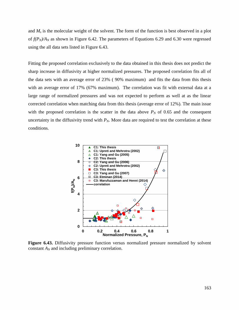
163

and Ms is the molecular weight of the solvent. The form of the function is best observed in a plot

of f(PN)/AN as shown in Figure 6.42. The parameters of Equations 6.29 and 6.30 were regressed

using the all data sets listed in Figure 6.43.

Fitting the proposed correlation exclusively to the data obtained in this thesis does not predict the

sharp increase in diffusivity at higher normalized pressures. The proposed correlation fits all of

the data sets with an average error of 23% ( 90% maximum) and fits the data from this thesis

with an average error of 17% (67% maximum). The correlation was fit with external data at a

large range of normalized pressures and was not expected to perform as well at as the linear

corrected correlation when matching data from this thesis (average error of 12%). The main issue

with the proposed correlation is the scatter in the data above PN of 0.65 and the consequent

uncertainty in the diffusivity trend with PN. More data are required to test the correlation at these

conditions.

Figure 6.43. Diffusivity pressure function versus normalized pressure normalized by solvent

constant AN and including preliminary correlation.

0

2

4

6

8

10

0 0.2 0.4 0.6 0.8 1

f(P

N)/

AN

Normalized Pressure, PN

C1: This thesisC1: Upreti and Mehrotra (2002)

C1: Yang and Gu (2005)C2: This thesis

C2: Yang and Gu (2006)C2: Upreti and Mehrotra (2002)

C3: This thesisC3: Yang and Gu (2007)

C3: Etminan (2014)C3: Marufuzzaman and Henni (2014)

correlation

164

6.7 Summary of Correlations

In this thesis, correlations were developed for both the constant diffusivity and the concentration

dependent diffusivity of solvents in heavy oil. These correlations are summarized below.

6.7.1. Correlations for Constant Diffusivity

The constant diffusivity data collected in this thesis was fit to the following power law function

of the initial viscosity of the oil phase:

𝐷𝑠𝑏 =

(1.104 ∗ 10−13𝑀𝑆 − 7.869 ∗ 10−13 + 2.224 ∗ 10−15𝑃)𝑇

𝜇𝑜0.280

(6.10)

where MS is the molecular weight of the solvent, P is the pressure in kPa, T is the temperature in

Ko is the initial viscosity of the oil phase in mPa.s and 𝐷𝑠𝑏 is the constant diffusivity of

solvent in bitumen in m2/s. Although it fit the data from this thesis with an average error of 12%,

it was unable to predict much of the literature data at low temperature and high pressure, outside

the ranges studied in this thesis. The following modified correlation was fit to the data collected

for this thesis as well as the literature data discussed in Section 6.6.

𝐷𝑠𝑏 = 𝐴𝑁

𝑇(1 + 9.79𝑃𝑁3.69)

𝜇00.312

(6.29)

where

𝐴𝑁 = (14.5316 − 0.2023𝑀𝑠) ∙ 10−12

(6.30)

and Ms is the molecular weight of the solvent, PN is ratio of the system pressure to the vapour

pressure of the gas at the system temperature, T is the temperature in Ko is the initial viscosity

of the oil phase in cP and 𝐷𝑠𝑏 is the constant diffusivity of solvent in bitumen in m2/s.

165

6.7.2. Correlations for Concentration Dependent Diffusivity

The concentration dependent diffusivity data collected in this thesis was fit to a power law

function of the viscosity of the solvent-oil mixture as follows:

𝐷𝑠𝑏 =

𝐴𝑇


(6.22)

where 𝐷𝑠𝑏 is the diffusivity of solvent in bitumen in m2/s, T is the temperature in K, 𝜇𝑚𝑖𝑥 is the

viscosity of the solvent and bitumen mixture in mPa.s, and the parameters A and n are given by:

𝑛 =

log𝐷𝑏𝑠

∞

𝐷𝑠𝑏∞

log𝜇𝑠

𝜇𝑏

(6.23)

𝐴 =

𝐷𝑠𝑏∞

𝑇𝜇𝑏𝑖𝑡

𝑛

(6.24)

where 𝜇𝑠 is the predicted viscosity of the liquid solvent in mPa.s, 𝜇𝑏 is the viscosity of the

bitumen, 𝐷𝑏𝑠∞ is the infinite dilution diffusivity of bitumen in solvent in m

2/s, and 𝐷𝑠𝑏

∞ is the

infinite dilution diffusivity of solvent in bitumen. The former is given by the Hayduk-Minhas

equation:

𝐷𝑏𝑠∞ =

13.3 ∗ 10−12𝑇1.47𝜇𝑠(10.2

𝑉𝑏⁄ −0.791)

𝑉𝑏0.71

(2.25)

where Vb is the liquid molar volume of bitumen at its normal boiling point in cm3/mol. The latter

is given by:

𝐷𝑠𝑏

∞ =5.18 ∗ 10−10𝑇

𝑉𝑠0.946𝜇𝑏

0.403

(6.26)

where Vs is the liquid molar volume of solvent at its normal boiling point in cm3/mol.

166

CHAPTER SEVEN: CONCLUSIONS AND RECOMENDATIONS

The purpose of this thesis was to experimentally determine the diffusivity of light hydrocarbon

gases in bitumen from pressure decay experiments and to develop a model for this mass transfer

process. This model was to include swelling, a predictive correlation for the diffusivity, and

methods to predict the physical properties required to fully define the model, such as the gas

solubility in the oil and the viscosity of the mixture. This chapter lists the major contributions of

this thesis in achieving this end and recommendations for future work to improve the quality and

reliability of diffusion models.

7.1 Contributions and Conclusions

The major contributions from this thesis are:

1. the measurement of constant and concentration dependent diffusivity for methane,

ethane, and propane gases (using several diffusivity models) over a range of temperatures

and pressures,

2. the measurement of gas solubilities in bitumen and their correlation using easily applied

models,

3. the development of a correlation for the constant diffusivity as a function of the initial

liquid viscosity and the pressure of the system,

4. the development of a procedure to calculate the concentration dependence of diffusivity

from pressure decay experiments,

5. the development of a correlation to predict the concentration dependent diffusivity.

Each contribution and the major conclusions related to that contribution are discussed below.

7.1.1. Diffusivity Measurements

The available literature data for the diffusivity of hydrocarbon gases in heavy oil has largely

been measured at or near room temperature. At these conditions, the diffusivity of methane,

ethane, and propane have all been investigated, but with the exception of Upreti and Mehrotra

(2002), no two solvents have been investigated with the same method over a wide range of

conditions. This thesis contributes to the data available in literature by measuring the diffusivity

167

of methane, ethane, and propane in heavy oil at temperatures from 40 to 90oC and pressures from

300 to 2100 kPa using a consistent method and model.

7.1.2. Solubility Measurements

The solubilities and saturation pressures of methane, ethane, and propane in heavy oil were

measured from the pressure decay experiments and in blind PVT cells using a constant

composition expansion method. The data were shown to be consistent with solubility data

available in literature for similar oils. Two models were fit to the experimental solubilities: 1)

Henry’s law, which was modified with a pressure dependent Henry’s constant, and; 2) the

Margules activity coefficient model, which required an extrapolation of the vapour pressure

curve of the solvents to accommodate mixtures above the critical temperature of the solvent.

Henry’s law fit the solubility data within and average error of 8 % and the Margules equation fit

the data with an average error of 9 %. Within the measured pressures, the Henry’s law is the

superior of the two models because it successfully predicts the increasing saturation pressure at

higher solvent solubilities. However, at pressures above the range of available data, the Henry’s

law model predicts a non-physical reversal in solubilities, caused by the added pressure

dependence. Therefore, the equation should not be extrapolated to temperatures and pressures

outside the range studied in this thesis.

7.1.3. Constant Diffusivity Correlation

The constant diffusivities measured in this thesis are, in essence, an average diffusivity over the

concentration ranges studied. However, diffusivity correlates strongly to the viscosity of the

mixture and therefore changes dramatically over the course of a pressure decay experiment. For

example, the constant diffusivity did not correlate strongly to the initial viscosity of the oil as

would be expected from the Hayduk and Cheng (1971) equation. More compellingly, the

diffusivity with a non-zero initial solvent content in the bitumen was significantly higher than the

diffusivity with zero initial solvent content.

To account for this change in viscosity with increasing concentration, several corrections to the

initial correlation were investigated. It was found that a linear pressure correction could decrease

the average error of the correlated diffusivity from 22% to 12% from the original fit with

168

Hayduk-Cheng equation. The pressure corrected correlation was tested on the available data

from literature and was shown to adequately predict many of the diffusivities measured at similar

conditions to those studied in this thesis. The correlation was shown to under-predict the

documented pressure effect on diffusivity at low temperature and over-predict the pressure

effects at high pressure. After considering data from the literature, a preliminary modification to

the correlation was developed that accounts for the pressure effect on the diffusivity through the

ratio of the system pressure to the vapour pressure of the diffusing gas. This new correlation was

fit to all of the tested literature data as well as the data from this thesis with an average error of

23% (17% error for the data from this thesis).

7.1.4. Concentration Dependent Diffusivity Determination

It was shown in this thesis and previously by James et al. (2012) that it is impossible to

determine the form of the concentration dependence of diffusivity from pressure decay data

alone (or other methods that measure the total mass of solvent diffused). Furthermore,

indistinguishable fits to the experimental data can be achieved with multiple sets of parameters

for the same diffusivity model. To determine a unique set of parameters when matching the

experimental data, the concentration dependent diffusivity models were constrained to pass

through a hypothetical infinite dilution diffusivity of oil in solvent. In this thesis, the Hayduk and

Minhas (1982) equation was chosen to predict the infinite dilution diffusivity of oil in solvent.

The pressure decay experiments were analysed using three concentration dependent diffusivity

models: 1) the Vignes (1966) equation; 2) a modified Bearman (1961) equation, and; 3) a

modified Hayduk and Cheng (1971) equation. For the Vignes (1966) equation, the above

constraint directly provides one of the model parameters and in the case of the modified

Bearman (1961) or the modified Hayduk and Cheng (1971), it gives an equation relating the two

parameters. In all cases this constraint reduced the number of independent fitting parameters to

one and the model could be uniquely fit to the pressure decay experiments. The single parameter

for each model is sufficient to calculate the diffusivity at any concentration at the given

experimental condition.

169

7.1.5. Concentration Dependent Diffusivity Correlation

The concentration dependent correlation was formulated so that the diffusivity at any

concentration could be determined from the end points; that is, the infinite dilution diffusivity of

bitumen in solvent and the infinite dilution diffusivity of solvent in bitumen. As noted above, the

infinite dilution diffusivity of bitumen in solvent was determined with the Hayduk and Minhas

(1982) equation. The experimental derived infinite dilution diffusivity of solvent in bitumen for

each model was correlated to the viscosity of the original oil. The best results were obtained with

the modified Hayduk and Cheng (1971) equation with an average error of 23%. The correlation

followed the expected trend with viscosity and molecular weight of the solvent and is a simpler

model than the other equations tested. Therefore, it was selected as the model for the infinite

dilution diffusivity of solvent in heavy oil. With the infinite dilution diffusivity end points of the

correlation established; at a given temperature and pressure there is sufficient information to

calculate the parameters of the modified Hayduk and Cheng equation. The proposed correlation

is valid for all solvent contents and could therefore be expanded to predict the diffusivities in

liquid-liquid systems.

7.2 Recommendations

Recommendations for future studies are as follows:

1) Develop a two or three dimensional diffusion model to more accurately represent the

horizontal cylindrical geometry of the Computer Tomography experiments. Solving the

continuity equation in higher dimensions can be computationally expensive and more

sophisticated algorithms than those presented in this thesis may be required to shorten the

run rime.

2) Update the material balance equation to be in terms of weight fraction instead of

concentration in g/mL. This updated model will be more applicable to systems of higher

solubility such as in liquid-liquid mixtures.

3) Investigate the effect of the medium properties (other than viscosity) on the concentration

dependence of the diffusivity by measuring the diffusivity of solvents in different oil

fractions and in more oils.

170

4) Further investigate the effects of pressure on constant diffusivity of gaseous solvents in

oil. In particular, measure the diffusivity at high P/Pv ratios at different temperatures to

confirm the strong pressure dependence seen in literature.

5) Expand the existing correlations to include the diffusivity of liquid solvents in bitumen.

This expansion would require measuring the diffusivity of liquid solvents in bitumen to

supplement the small amount of data available in literature. In the preliminary constant

diffusivity correlation, the normalized pressure dependence based on vapour pressure

would have to be reassessed.

6) Re-analyse the pressure decay data with the Vignes (1966) equation using different

models for the thermodynamic correction factor (from an equation of state or a more

comprehensive activity coefficient model). There is sufficient data collected for propane-

bitumen mixtures to fit such a model, Mancilla-Polanco (2017); however, supplementary

PVT data would need to be collected for ethane/bitumen and methane/bitumen.

171

REFERENCES

Afashi, B. and Kantzas, A. 2007. Advances in Diffusivity Measurement of Solvents in Oil

Sands. Journal of Canadian Petroleum Technology, 46(11), 56-61.

Agrawal P. 2012. Measuremetn and Modeling of the Phase Behaviour of Solvent Diluted

Bitumen. master’s thesis, M.Sc. Dissertation.

Agrawal. P., Schoeggl, F.F., Satyro, M.A., Taylor, S.D. and Yarranton, H.W. 2012.

Measurement and Modeling of the phase behaviour of solvent diluted bitumens. Fluid Phase

Equilibrium, 334, 51-64.

Alazard, N. and L. Montadert, L. 1993. Oil resources for the 21st century: Constraints and

outlook. Revue de l'Institute Francais du Petrol, 48, 69-82.

Alboudwarej, H. 2003. Asphaltene Deposition in Flowing Systems. Ph.D. Dissertation,

University of Calgary.

Arnold. J. H. 1930. Studies in Diffusion II: A Kinetic Theory of Diffusion in Liquid Systems.

Journal of the American Chemical Society, 52. 3937-3955.

Badamchi-Zadeh, A., Yarranton, H.W., Svrcek, W.Y. and Maini, B. B. 2009. Phase Behaviour

and Physical Property Measuremetns for Vapex Solvents: Part I. Propane and Athabasca

Bitumen. JCPT, 48, pp. 54-61.

Bearman, R.J. 1960. Statistical Mechanical Theory of the Diffusion Coefficients in Liquid

Solutions. Journal of Chemical Physics, 32(5), 1308-1313.

Bearman, R.J. 1961. On the Molecular Basis of some Current Theories of Diffusion. Journal of

Chemical Physics, 28, 1961-1968.

Bird, B.B, Stewart, W. E. and Lightfoot, E. N. 2007. Transport Phenomenon, 2nd Ed., John

Wiley & Sons: New York.

172

Black, C. and Twu, C.H. 1983. Correlations and Prediction of Thermodynamic Properties for

Heavy Petroleum Shale Oils, Tar Sands, and Coal Liquid. AIChE Spring National Meeting,

Houston, USA.

Boustani, A and Maini, B.B. 2001. The Role of Diffusion and Convective Dispersion in Vapour

Extractions Process. JCPT, 40(4), 68-77.

Butler, R.M. 1997. GravDrain’s Blackbook: Thermal recovery of oil and bitumen, GravDrain

Inc: Calgary, Alberta.

Butler, R.M. and Mokrys, I.J. 1991. A New Process (VAPEX) for Recovering Heavy Oils Using

Hot Water Hydrocarbon Vapour. Journal of Canadian Peyroleum Technology, 30, 97-106.

Carman, P.C. and Stein, L.H. 1956. Self Diffusion in Mixtures. Part 1: Theory and its

Application to a Nearly Ideal Binary Liquid Mixture. Transactions of the Faraday Society, 52,

619-627.

Chapman, S. and Cowling, T.G. 1970. The Mathematical Theory of Non-uniform Gases,

Cambridge University Press: London.

Chapman, W.G., Gubbins, K.E., Jackson, G. and Radosz, M. 1989. SAFT: Equation-of-State

Solution Model for Associating Fluids. Fluid Phase Equilibrium, 52, 31-38.

Chung, T.H., Ajlan, M., Lee, L.L. and Starling, K.E. 1988. Generalized multiparameter

correlation for nonpolar and polar fluid transport properties. Ind. Eng. Chem. Res., 27, 671-679.

Civan, F. and Rasmussen, M. L. 2009. Rapid simultaneous evaluation of four parameters of

single-component gases in nonvolatile liquids from a single data set. Chemical Engineering

Science, 64, 5084-5092.

Darken, L.S. 1948. Diffusion, Mobility and Their Interrelation Through Free Energy in Binary

Metalic Systems. Transactions of the American Institute of Mining and Metallurgical Engineers,

175, 184-201.

173

Das, S.K. and Butler, R.M. 1994. Effect og Asphaltene Deposition on the Vapex Process: a

Preliminary Investigation Using a Hele-Shaw Cell. The Journal of Canadian Petroleum

Technology, 33, 39-45.

Das, S.K. and Butler, R.M. 1996. Diffusion Coefficients of Propane and Butane in Peace River

Bitumen. The Canadian Journal of Chemical Engineering, 74, 985-992.

Diedro, F., Bryant, J and Kantzas, A. 2014. Personal Communication.

Diedro, F., Bryant, J., Kryuchkov, S. and Kantzas, A. 2015. Evaluation of diffusion of light

hydrocarbon solvents in bitumen. Paper SPE-174424 presented at the SPE Canada Heavy Oil

Technical Conference, 9-11 June 2015, Calgary, Canada.

Do, H.D. and Pinczewski, W.V. 1991. Diffusion-controlled swelling of reservoir oil by indirect

contact with injection gas. Chemical Engineering Science, 46, 1259-1270.

Dullien, F.A.L. 1963. New Relationship Between Viscosity and the Diffusion Coefficients Based

on Lamms Theory. Transactions of the Faraday Society, 59, 856-868.

Dullien, F.A.L. 1971. Statistical Test of Vignes Correlation of Liquid-Phase Diffusion

Coefficietns. Ind Eng Chem Fundam, 10(1),41-49.

Dusseault, M. B. 2001. Comparing Venezuelan and Canadian Heavy Oil and Tar Sands

Presented at the Petroleum Society of Canada, Canadian International Petroleum Conference,

Calgary, Alberta, 12-14 June 2001.

Einstein, A. 1956. Investigation on the Theory of Brownian Mouvement, 1st English Edition

Dover: New York.

ERCB (Energy Resources Conservation Board). 2015. Alberta Energy Reserves 2014 and

Supply/Demand Outlook for 2015-2024, ST98-2015, Calgary.

Elliott, J. and Lira, C. 1999. Introductory Chemical Engineering Thermodynamics,1st Ed.,.

Prentice Hall: Upper Saddle River, New Jersey.

174

Etminan, S.R. 2014. Improved Experimental and Mathemacial Techniques for Measurement of

Solvent Gas Diffusivity in Heavy Oils. Ph.D.Dissertation, University Of Calgary.

Etminan, S.R.,. Maini, B.B, Chen, Z. and Hassanzadeh, H. 2010. Constant-Pressure Technique

for Gas Diffusivity and Solubility Measurements in Heavy Oil and Bitumen. Energy & Fuels,

24, 533-549

Etminan, S.R, Maini, B.B and Chen, Z. 2014a. Determination of Mass Transfer Parameters in

Solvent-Based Oil Recovery Techniques using a Non-Equilibrium Boundary Condition at the

Interface. Fuel, 120, 218-323.

Etminan, S.R., Maini, B.B. and Chen, Z. 2014b. Modeling the Diffusion Controlled Swelling

and Determination of Molecular Diffusion Coefficient in Propane-Bitumen System Using a

Front Tracking Moving Boundary Technique. Paper SPE-170182 presented at the SPE heavy oil

conference Alberta, Canada, 10-12 June 2014. doi:10.2118/170182-MS.

Etminan, S.R, Pooladi-Darvish, M., Maini, B.B and Chen, Z. 2013. Modeling the Interface

Resistance in Low Soluble Gaseous Solvents-Heavy Oil Systems. Fuel, 105, 672-687.

Fisher, D.B., Singhal, A.K., Das, S.K., Goldman, J. and Jackson, C. 2000. Use of Magnetic

Resonance Imaging and Advanced Image Analysis as a Tool to Extract Mass Transfer

Information from a 2D Physical Model of the Vapex Process. Paper SPE- 59330 presetned at the

SPE/DOE Improved Oil Recovery Symposium, Tulsa, 3-5 April 2000. doi:10.2118/59330-MS.

Fletcher, C.A.J. 1991. Computational Techniques in Fluid Dynamics: Volume 1, 2nd

Ed.,

Springer-Verlag: Berlin, Germany.

Fotland, P., Anifsen, H., Foerdal, H. and Hjermstad, H. P. 1997. The phase diagrams of

asphaltenes: Experimental technique, results and modelling on some North Sea crude oils.

Presented at the Proceedings of the Symposium on the Chemistry of the Asphaltene and Related

Substances, Cancun, Mexico, 11−15 November 1997.

Fu, C., Putaganna, V.R. and Vilcsak, G. 1984. VLE Properties for CO2-Athabasca bitumen and

N2-Athabasca Bitumen. presented at Pac Chem, 1984, Hawaii, USA.

175

Fu, C. and Putaganna, V. R. 1985. Binary Interaction Coefficients of the Modified Redlich-

Kwonq-Soave Equation of State for Bitumen-Containing Systems at In-Situ Conditions.

Presented at the 6th Annual Technical Meeting of the Petroleum Society of the Canadian

Institute of Mining, Edmonton, Alberta, Canada, 1985.

Fu, C., Puttagunta, R., Baumber, L. and Hso, C. 1986. Pseudo-Critical Properties of Heavy Oils

and Bitumens. Fluid Phase Equilibrium, 30, 281-295.

Ghaderi, S.M., Tabatabaie, S.H., Hassanzadeh, H. and Pooladi-Darvish, M. 2011. Estimation of

concentration-dependant diffusion coefficient in pressure decay experimentsof heavy oils and

bitumens. Fluid Phase Equilibria, 305, 132-144.

Ghai, R.K., Erlt, H. and Dullien, F.A.L. 1973. Liquid Diffusion in Nonelectrolytes. AIChE

Journal, 5, 881-900.

Green, D.W. and Perry, R.H. 2008. Perry’s Chemical Engineer’s Handbook, 8th

ed. McGraw-

Hill: New York.

Greiner‐Schmid, A., Wappmann, S., Has, M. and Lüdemann, H.D. 1991. Self-diffusion in the

compressed fluid lower alkanes: Methane, ethane, and propane. Journal of Chemical Physics, 94,

5643-5649.

Grey, M.R. 2015. Upgrading Oilsands Bitumen and Heavy Oil, 1st Ed., University of Alberta

Press: Edmonton.

Guerrero-Aconcha, U. and Kantzas, A. 2009. Diffusion of Hydrocarbon Gases in Heavy Oil and

Bitumen. Paper SPE- 122783 Presented at the SPE Latin American and Caribean Petroleum

Engineering Conference Cartagena, Colombia, 31 May -3 June 2009. doi:10.2118/122783-MS

Guerrero-Aconcha, U., Salama, D. and Kantzas, A. 2008. Diffusion Coefficient of n-Alkanes in

Heavy Oil. Paper SPE-115346 presented at the SPE Annual Technical Conference and

Exhibition, Denver, 21-24 September 2008. doi:10.2118/115346-MS

176

Gupta, S., Gittins, S. and Picherack, P. 2002. Field Implementation of Solvent Aided Process.

Paper 2002-299 presented at the 53rd

Canadian International Petroleum Conference, Calgary,

Alberta, 11-13 June 2002.

Gupta, S., Gittins, S. and Picherack, P. 2003. Insights into some key issues with Solvent Aided

Process. J Can Pet Tech, 42, 54-61.

Hartley, G.S. and Crank,J. 1949. Some Fundamental Definitions and Concepts in Diffusion

Processes. Transactions of the Faraday Society, 45, 801.

Hayduk, W. and Cheng, S.C. 1971. Review of Relation Between Diffusion and Solvent

Viscosity in Dilute Liquid solutions. Chemical Engineering Science, 26, 635.

Hayduk, W. and Minhas, B.S. 1982 Correlation for Prediction of Molecular Diffusivities in

Liquids. Canadian Journal of Chemical Engineering, 60, 295-299.

James, L.A. 2009. Mass Transfer Mechanisms during the Solvent Recovery of Heavy Oil. Ph.D.

Dissertation, Univerisity of Waterloo.

James, L.A., Ioannidis, M.A. and Chatzis, I. 2012. Experimentally Validated Model for the

Determination of Concentration-Dependant Diffusion of a Light Hydrocrabon in Bitumen.

Energy and Fuel, 26, 6200-6209.

Jamialahmadi, M., Emandi, M. and Muller-Steinhagen, H. 2006. Diffusion Coefficients of

Methane in Liquid Hydrocarbons at High Pressure and Temperature. Journal of Petroleum

Science and Engineering, 53, 47-60.

Jamaluddin, A.K.M., Joshi, N., Iwere, F. and Gurpinar, O. 2002. An investigation of asphaltene

instability under nitrogen injection. Paper SPE-74393 presented at the Proceedings of the

Society of Petroleum Engineers (SPE) International Petroleum Conference and Exhibition in

Mexico, Villahermosa, Mexico, 10−12 February 2002.

Johnston, K. 2016. Personal Communication.

177

Kesler, M.G. and. Lee, I.K. 1976. Improve Prediction of Enthalpy of Fractions. Hydrocarbon

Processing, 55, 153-158.

Kokal, S. and Sayegh, S.G. 1993. Phase behavior and Physical Properties of CO2-Saturated

Heavy Oil and its Constitutive Fractions: Experimental Data and Correlation. Journal of

Petroleum Science and Engineering, 9, 289-302.

Kontogeorgis, G.M., Voustas, E.C., Yakoumis, I.V. and Tassios, D. P. 1996. An Equation of

State for Associating Fluids. Industrial & Engineering Chemistry Research, 35, 4310-4318.

Kooijman,H. and Taylor, R. 1991. Estimation of Diffusion Coefficients in Multicomponent

Liquids. Industrial & Engineering Chemistry Research, 30, 1217-1222.

Lamm, O. 1943. Die Theorie der Diffusion biniirer Mischungen und die Interpretierung von

Diffusionsmessungen. Arkiv Kemi, Min. Geol., 17(A).

Lamm, O. 1944. Theorie der Diffusion ternarer Losunger. ibid., 18(A).

Li, J.C.M. and Chang, P. 1955. Self-Diffusion Coefficient and Voscosity in Liquids. Journal of

Chemical Physics, 23, 518-520.

Leaute, R. P. 2002. Liquid addition to steam for enhancing oil recovery of bitumen with CSS:

evolution of technology from research concept to a field pilot at cold lake. Paper SPE- 79011

presented at the SPE International Thermal Operations and Heavy Oil Symposium and

International Horizontal Well Technology Conference, Calgary, Alberta, 4-7 November 2002.

doi:10.2118/79011-MS

Lundberg, J. L., Wilk, M.B., and Huyett, M.J. 1963. Sorption Studies Using Automation and

Computation. Industrial and Engineering Chemistry Fundamentals, 2 (1), 37-43.

Luo H. and Kantzas, A. 2011. Study of Diffusivity of Hydrocarbon Solvent in Heavy Oil

Saturated Sands Using X-Ray Compuer Assiusted Tomography. Journal of Canadian Petroleum

Technology, 50, 24-34.

178

Luo, H., Salama, D., Kryuchov, S. and Kantzas, A. 2007. The Effect of Volume Changes Due

to Mixing on Diffusion Coefficient Determination in Heavy Oil and Hydrocarbon Solvent

Systems. Paper SPE- 110522 Presented at the SPE Annual Technical Conference and Exhibition,

Anaheim, 11-14 November 2007. doi:10.2118/110522-MS

Ma, M., Chen, S. and Abedi, J. 2016. Modeling the density, solubility and viscosity of

bitumen/solvent systems using PC-SAFT. Journal of Petroleum Science and Engineering, 139,

1-12.

Mancilla-Polanco, A., Schoeggl, F.F., Johnston, K., Richardson, W.D., Yarranton, H.W. and

Taylor, S.D. 2017. The Phase Behavior of Heavy Oil and Propane Mixtures. Paper SPE-

presented at the SPE Canada Heavy Oil Technical Conference held in Calgary, Alberta, Canada,

15—16 February 2017.

Margules, M. 1895. Über die Zusammensetzung der gesättigten Dämpfe von Misschungen.

Sitzungsberichte der Kaiserliche Akadamie der Wissenschaften Wien Mathematisch-

Naturwissenschaftliche Klasse, 2, 1243-1278.

Marufuzzaman M. and Henni, A. 2015. Solubility of CO2 and C2H6 in Heavy Oil and it’s

SARA Fractions. Canadian Journal of Chemical Engineering, 93, 553-564.

Marufuzzaman M. and Henni, A. 2014. Solubility and Diffusivity of Propane in Heavy Oil and

it’s SARA Fractions. Canadian Journal of Chemical Engineering, 92, 1421-1431.

Mehrotra, A.K. and Svrcek, W.Y. 1982. Correlations for Properties of Bitumen saturated with

CO2, CH4 and N2, and experiments with Combustion Gas Mixtures. Journal of Canadian

Petroleum Technology, 21, 95-104.

Mehrotra, A.K. and Svrcek, W.Y. 1984. Correlation and Measurement of Viscosity, Density

and Gas Solubility of Marguerite Lake Bitumen saturated with Carbon Dioxide. AOSTRA

Journal of Research, 1, 51-62.

Mehrotra, A.K. and Svrcek, W.Y. 1985a. Viscosity, Density and Gas Solubility Data for Oil

Sand Bitumens. Part I: Athabasca Bitumen Saturated with CO and C2H6. AOSTRA Journal of

Research, 1, 263-268.

179

Mehrotra, A.K. and Svrcek, W.Y. 1985b. Viscosity, Density and Gas Solubility Data for Oil

Sand Bitumens. Part II: Peace River Bitumen Saturated with N2, CO, CH4, CO2, C2H6. AOSTRA


Mehrotra, A.K. and Svrcek, W.Y. 1985c. Viscosity, Density and Gas Solubility Data for Oil

Sand Bitumens. Part III: Wabasca Bitumen Saturated with N2, CO, CH4, CO2, C2H6. AOSTRA


Mehrotra, A.K. and Svrcek, W.Y. 1988a. Properties of Cold Lake Bitumen Saturated with Pure

Gases and Gas Mixtures. Canadian Journal of Chemical Engineering, 66, 656-665.

Mehrotra, A.K. and Svrcek, W.Y. 1988b. Correlation and Prediction of Gas Solubility in Cold

Lake Bitumen. Canadian Journal of Chemical Engineering, 66, 666-670.

Mehrotra, A.K. and Svrcek, W.Y. 1988c. Characterization of Athabasca Bitumen For Gas

Solubility Calculations. Canadian Journal of Chemical Engineering, 27, 107-110.

Motahhari, H. 2013. Development of Viscosity Model for Petroleum Industry Applications.

Ph.D.Dissertation, University Of Calgary.

Motahari, H., Satyro, M.A., Taylor, S.D. and Yarranton, H.W. 2013a. Extension of the

Expanded Fluid Viscosity Model to Characterized Oils. Energy & Fuels,27, , 1881-1898.

Motahhari, H., Schoeggl, F.F., Satyro, M.A. and Yarranton, H.W. 2013b. The Effect of Solvents

on the Viscosity of an Alberta Bitumen at In Situ Thermal Process Conditions,” Paper SPE-

165548 prestented at the SPE Heavy Oil Conference Canada, Calgary, Alberta, Canada, 11-13

June 2013. doi:10.2118/165548-MS

Motahhari, H., Schoeggl, F.F., Satyro, M.A. and Yarranton, H.W. 2013c. Viscosity Prediction

for Solvent-DilutedLive Bitumen and Heavy Oil at Temperatures up to 175oC. Journal of

Canadian Petroleum Technology, 52, 376-390.

Nasr, T. N. and Ayodele, O.R. 2006. New Hybrid Steam-Solvent Processes for the Recovery of

Heavy oil and Bitumen. Paper SPE-101717 presented at the 12th Abu Dhabi International

180

Petroleum Exhibition and Conference, ADIPEC, Abu Dhabi, UAE, 5-8, November 2006.

doi:10.2118/101717-MS.

Nenninger, J. and N-Solv Corporation. 2012. Method and apparatus for stimulating heavy oil

production. Canadian Patent 2633061, 25 Sept 2012.

NIST. 2016. NIST Standard Reference Database 69: NIST Chemistry WebBook. Online:

http://webbook.nist.gov/chemistry/fluid/

Oballa, V. and Butler, R.M. 1989. An Experimental Study of Diffusion in the Bitumen-Toluene

System. The Journal Of Canadian Petroleum Technology, 28(2), 63-69.

Peng, D.Y. and Robinson, D.B. 1976. A New Two-Constant Equation of State. Industrial and

Engineering Chemistry, 15, 59-64.

Quail, B., Hill.G.A. and Jha, K.N. 1988. Correlations of Viscosity, Gas Solubility, and Density

for Saskatchewan Heavy Oils. Industrial Engineering Chemistry Research, 27, 519–523.

Reamer, H., Opfell, J. and Sage, B. 1956. Diffusion Coefficients in Hydrocarbon Systems:

Methane-Decane-Methane in Liquid Phase. Industrial and Engineering Chemistry, 48, pp. 275-

282.

Reid, R.C., Prausnitz, J. M. and Poling, B.E. 1987. The Properties of Gases and Liquids, 4th

Ed.,

McGraw Hill: New York.

Riazi, M.R. 1996. A New Method for experimetnal Measurment of Diffusivity Coefficients in

Reservoir Fluids. Journal of Petroleum Science and Engineering, 14, 235-250.

Riazi, M.R. 2005. Characterization and Properties of Petroleum Fractions, 1st Ed., ASTM

International:Conshohocken, USA:

Riazi, M.R. and Al-Sahhaf, T.A. 1996. Physical properties of heavy petroleum fractions and

crude oils. Fluid Phase Equilibria, 117, 217-224.

Riazi, M.R. and Daubert, T.E. 1980. Simplify Property Predictions. Hydrocarbon Processing,

59, 115-116.

181

Robinson, D.B. and Sim, S.K. 1980. Behaviour of Bitumen-Water-Gas System. Report, D. B.

Robinson & Associates, Edmonton, Alberta, Canada.

Salama, D. and Kantzas, A. 2005. Monitoring of Diffusion of Heav Oil with Hydrocarbonb

Solvents in the presence of sand. Paper SPE-97855 presented at the SPE internationsl Thermal

Operatins and Heavy Oil Symposium, Calgary Canada, 1-3 November 2005. doi:10.2118/97855-

MS.

Sanchez-Lemus, M.C. 2015. Extended Distillation Property Correlations for Heavy Oil. Ph.D.

dissertation, University of Calgary.

Sarafianos, N.J. 1986. An analytical method of calculating variable diffusion coefficients.

Journal of Materials Science, 21(7), 2283-2288.

Saryazdi, F., Motahhari, H., Schoeggl, F.F., Taylor, S.D. and Yarranton, H.W. 2013. Density of

Hydrocarbon Mixtures and Bitumen Diluted With Solvents and Dissolved Gasses. Energy &

Fuel. 27. 3666-3678.

Schmidt, T., Jossy, E. and Puttagunta, T.R. 1986. Mass Transfer Studies, Final Report of

Project 188, Alberta Research Council, Edmonton, AB, 1986

Schmidt, T., Leshchyshyn, T.H. and Puttagunta, V.R.1982, June. Diffusivity of CO2 into

reservoir fluids. Presented at the 33rd Annual technical meeting of the petroleum society of CIM,

Calgary, Canada, 6-9.

Sheikha, H., Mehrotra, A.K. and Pooladi-Darvish, M. 2006. An inverse solution methodology

for estimating the difusion coefficients of gases in Athabasca bitumen from pressure decay data.

Journal of Petroleum Science & Engineering, 53, 189-201.

Sheikha, H., Pooladi-Darvish, M. and Mehrotra, A.K. 2005. Development of graphical methods

for estimating the diffusivity coefficients of gases in bitumen from pressure-decay data. Energy

& Fuels, 19, 2041-2049.

182

Signhal, K., Das, S.K., Leggitt, S.M., Kasraie, M. and Ito, Y. Screening of reservoirs for

exploitation by application of Steam Assisted Gravity Drainage/Vapex processes. Paper SPE-

37144 presented at the 2nd International Conference on Horizontal Well Technology,

18 November.

Song, L., Kantzas, A. and Bryan, J. 2010a. Experimetnal Measurement of diffusion Coefficient

of CO2 in Heavy Oil using X-Ray Computer Tmography Under Reservoir Conditions. Paper

SPE- 137545 Presented at the Canadian Unconventional Resources and Internaltional Petroleum

Conference, Calgary, Alberta, 19-21 October 2010. doi:10.2118/137545-MS

Song, L., Kantzas, A. and Bryan, J. 2010b. Investigation of Co2 Diffusivity in Heavy Oil Using

X-Ray Computer-Assisted Tomography Under Reservoir Conditions. Paper SPE- 138205

Presented at SPE International Conference on CO2 Capture, Storage, and Utilization, New

Orleans, 10-12 November 2010. doi:10.2118/138205-MS

Srivastan, S., Darwish, N., Gasem, K. and Robinson, R. 1992. Solubility of Methane in

Hexane, Decane and Dodecane at Temperatures from 311 to 423 K and Pressures to 10.4 MPa.

Journal of Chemical and Engineering Data, 37, 516-520.

Svrcek, W.Y. and Mehrotra, A.K. 1982. Gas Solubility, Viscosity and Density Measurements

for Athabasca Bitumen. Journal of Canadian Petroleum Technology, 21, 31-38

Tan, K.K. and Thorpe, R.B. 1992. Gas diffusion into viscous and non-Newtonian liquids.

Chemical Engineering Sciecne, 47(13-14), 3565-3572

Tan, K.K. and Thorpe, R.B. 1999. The onset of convection induced by buoyancy during gas

diffusion in deep fluids. Chemical Engineering Sciecne, 54(19), 4179-3572

Tharanivasan, A.K., Yang, C. and Gu, Y. 2004. Comparison of Three different Mass Transfer

Models Used in the Experimental Measurement of Solvent Diffusivity in Heavy Oil. Journal of

Petroleum Science and Engineering, 44, 269-282.

Tharanivasan, A.K., Yang, C. and Gu, Y. 2006. Measurements of Molecular Diffusion

Coefficients of Carbon Dioxide, Methane, and Propane under Reservoir Conditions. Energy &

Fuels, 20, 2509-2517.

183

Upreti, S.R., Lohi, A., Kapadia, R.A. and El-Haj, R. 2007. Vapor extraction of heavy oil and

bitumen: A review. Energy & Fuels, 21, 1562-1574.

Upreti, S.R. and Mehrotra, A.K. 2002. Diffusivity of CO2, CH4, C2H6 and N2 in Athabasca

Bitumen. The Canadian Journal of Petroleum Engineering, 80, 116-125.

Varet, G., Montel, F, Marsi, D. and Daridon, J. 2013. Gas Solubility Measurement in Heavy Oil

and Extra Heavy Oil at Vapour Extraction (VAPEX) Conditions. Energy & Fuels, 27, pp. 2528-

2535.

Vignes, A. 1966. Diffusion in Binary Solutions: Variation of Diffusion Coefficient with

Composition. Industrial and Engineering Chemistry Fundamentals, 5(2), 189-199.

Virtual Materials Group, Inc. 2010. VMG Sim 6.0 User’s Manual, Calgary, Alberta, Canada.

von Solms, N., Michelsen, M.L. and Kontogeorgis, G.M. 2003. Computational and Physical

Performance of a Modified PC-SAFT Equation of State for Highly Asymmetric and Associating

Mixtures. Industrial and Engineering Chemistry Research, 42, 1098–1105.

Wen, Y.W. and Kantzas, A. 2005a. Monitoring Bitumen-Solvent Interactions with Low-Field

Nuclear Magnetic Resonance and X-ray Computer-Assisted Tomography. Energy & Fuels, 19,

1319-1326.

Wen, Y.W., Bryan, J. and Kantzas, A. 2005b. Estimation of Diffusion Coefficients in Bitumen

Solvent Mixtures as Derived from Low Field NMR Spectra. The Journal of Canadian Petroleum

Technology, 44(4), 29-34.

Whitson, C.H. and Brule, M.R. 2000 Phase Behaviour: SPE Monographs Volume 20, Society of

Pertoleum Engineers.

Wilke, C.R. 1950. A Viscosity Equation for Gas Mixtures. Journal of Chemical Physics, 18,

517-519.

Wilke, C.R. and Chang, P. 1955. Correlation of Diffusion Coefficients in Dilute Solutions,”

Chemical Engineering Progress. 48, 2645-270.

http://pubs.acs.org/author/von+Solms%2C+Nicolas

http://pubs.acs.org/author/Michelsen%2C+Michael+L

http://pubs.acs.org/author/Kontogeorgis%2C+Georgios+M

184

Yang, C. 2005. A New Method For Measuring Solvent Diffusion Coefficietns and Oil Swelling

Factors of Heavy Oil-Solvent System. Ph.D. Dissertation, University of Regina.

Yang, C. and Gu, Y. 2005. A New Method for Measuring Solvent Diffusivity in Heavy Oil by

Dynamic Pendant Drop Shape Analysis. SPE Journal, 11, 48-57.

Yang, C. and Gu, Y. 2006. Diffusion Coefficients and oil swelling factors of carbon dioxide,

methane, ethane, propane, and their mixtures in heavy oil. Fluid Phase Equilibria,. 243, 64-73.

Yang, C. and Gu, Y. 2007. A Novel Experimental Technique for studying Solvent Mass

Transfer and Oil-Swelling Effect in the Vapour Extration (VAPEX) Process. The Journal or

Canadian Petroleum Technology, 46, 44-48.

Yarranton, H.W and Satyro M.A. 2011. Expanded Fluid-Based Viscosity Correlation for

Hydrocarbons. Industrial and Engineering Chemistry Research, 48, 3640-3648.

Yaws, C.L. 1999. Yaws’ Handbook of Thermodynamic and Physical Properties of Chemical

Compounds, McGraw-Hill: New York.

Yazdani, A. and Maini, B.B. 2010. Measurements and modelling of phase behaviour and

viscosity of a heavy oil/butane system. Journal of Canadian Petroleum Technology, 49, 9-14.

Yokozeki. A. 2002. Time-dependent behavior of gas absorption in lubricant oil. International

Journal of Refrigeration, 25(6), 695-704

Yonebayashi, H., Masuzawa, T., Dabbouk, C. and Urasaki, D. 2009. Ready for gas injection:

Asphaltene risk evaluation by mathematical modeling of asphaltene precipitation envelope

(APE) with integration of all laboratory deliverables. Paper SPE-125643 presented at the

Proceedings of the Society of Petroleum Engineers (SPE)/European Association of Geoscientists

and Engineers (EAGE) Reservoir Characterization and Simulation Conference; Abu Dhabi,

United Arab Emirates, 19−21, October 2009.

Zainal, S., Yee, H.V. and Saaid, I.M. 2011. Gas Diffusivity Measuremetn In Reservoir Fluid at

Elevated Pressures Systems for Transient Shut-in Modeling. Paper SPE-139004 presented at the

185

SPE Offshore Europe Oil and Gas Conference and Exhibition, Aberdeen, UK, 6-8 September

2011. doi:10.2118/139004-MS

Zhang, Y.P., Hyndman, C.L. and Maini, B.B. 2000. Measurement of Gas Diffusivity in Heavy

Oils. Journal of Petroleum Science and Engineering, 25, 37-47.

Zhang, X., Pedrosa, N. and Moorwood, T. 2012. Modelling Asphaltene Phase behavior:

Comparison of methods for flow assurance studies. Energy & Fuels, 26, 2611-2620.

Zhang, X. and Shaw, J.M. 2007. Liquid Phase mutual Diffusion Coefficients for heavy oil

+Light Hydrocarbon Mixtures. Petroleum Science and Technology, 25(6), 2007.

Zhao, L. L. 2004. Steam Alternating Solvent Process. Paper SPE-86957 presented at the SPE

International Thermal Operations and Heavy Oil Symposium and Western Regional Meeting,

Bakersfield California, USA, 16-18 March 2004

186

APPENDIX A

The following six tables list the values of the solvent viscosity and the corresponding infinite

dilution diffusivity or self-diffusivity of bitumen in solvent. These values are used as constraints

for the concentration dependent diffusivity models.

Table A.1. The infinite dilution diffusivity of bitumen in liquid methane, *predicted with the

Hayduk-Minhas Equation

Temperature oC

Pressure

kPa

Effective Methane

Viscosity

mPa.s

Infinite Dilution

Diffusivity*

10-9

m2/s

50 3451 0.163 2.40

76 4161 0.122 3.39

100 4226 0.097 4.46

100 4169 0.097 4.47

100 4340 0.097 4.45

101 4119 0.096 4.51

Table A.2. The infinite dilution diffusivity of bitumen in liquid ethane, *predicted with the


Temperature oC

Pressure

kPa

Effective Ethane

Viscosity

mPa.s

Infinite Dilution

Diffusivity*

10-9

m2/s

37 2964 0.081 3.90

42 2168 0.078 4.10

47 1394 0.076 4.29

50 1741 0.075 4.39

58 2962 0.073 4.65

59 1495 0.072 4.74

64 1751 0.070 4.92

64 1120 0.070 4.95

73 774 0.067 5.30

75 4324 0.068 5.31

90 4741 0.063 5.96

100 1916 0.060 6.47

100 1970 0.060 6.49

187

Table A.3. The infinite dilution diffusivity of bitumen in liquid ethane, *predicted with the

Hayduk-Minhas Equation. Data in this table was used in the analysis of diffusion experiments

with an initial ethane concentration in the bitumen.

Temperature oC

Pressure

kPa

Effective Propane

Viscosity

mPa.s

Infinite Dilution

Diffusivity*

10-9

m2/s

42 3316 0.079 4.08

64 2104 0.070 4.93

Table A.4. Self-diffusivity of propane and the infinite dilution diffusivity of bitumen in liquid

propane, *predicted with the Hayduk-Minhas Equation

Temperatue oC

Pressure

kPa

Effective Propane

Viscosity

mPa.s

Self-

Diffusivity

of Propane

10-9

m2/s

Infinite

Dilution

Diffusivity*

10-9

m2/s

50 327 0.114 13.0 3.18

50 724 0.114 13.0 3.18

59 824 0.108 14.1 3.46

60 602 0.107 14.2 3.49

62 1080 0.106 14.4 3.54

70 1077 0.102 15.4 3.78

74 523 0.099 15.9 3.92

74 1006 0.100 15.9 3.91

80 607 0.096 16.8 4.15

80 1507 0.096 16.7 4.14

81 720 0.096 16.8 4.16

81 1367 0.096 16.8 4.17

85 702 0.093 17.4 4.31

86 1374 0.093 17.5 4.34

Table A.5. Self-diffusivity of propane and the infinite dilution diffusivity of bitumen in liquid

propane, *predicted with the Hayduk-Minhas Equation. Data in this table used in the analysis of

diffusion experiments with an initial propane concentration in the bitumen.

Temperatue oC

Pressure

kPa

Effective Propane

Viscosity

mPa.s

Self-

Diffusivity

of Propane

10-9

m2/s

Infinite

Dilution

Diffusivity*

10-9

m2/s

64 1890 0.106 14.5 3.6

86 2303 0.094 17.4 4.3

188

Table A.6. The infinite dilution diffusivity of bitumen in liquid butane, *predicted with the


Temperature oC

Pressure

kPa

Effective Butane

Viscosity

mPa.s

Infinite Dilution

Diffusivity*

10-9

m2/s

69 284.3 0.163 2.40

90 738.2 0.097 4.45

90 874.3 0.096 4.51

Documents

Diffusivity of Light Hydrocarbon Gases in Bitumen