1

Digging Deeper—Evidence on the Effects of Macroprudential Policies

from a New Database

Zohair Alam, Adrian Alter, Jesse Eiseman, Gaston Gelos, Heedon Kang, Machiko Narita, Erlend Nier, and Naixi Wang1

December 2019

Abstract

This paper introduces a new comprehensive database of macroprudential policies, which combines information from various sources and covers 134 countries from January 1990 to December 2016. Using these data, we first confirm that loan-targeted instruments have a significant impact on household credit, and a milder, dampening effect on consumption. Next, we exploit novel numerical information on loan-to-value (LTV) limits using a propensity-score-based method to address endogeneity concerns. The results point to economically significant and nonlinear effects, with a declining impact for larger tightening measures. Moreover, the initial LTV level appears to matter; when LTV limits are already tight, the effects of additional tightening on credit is dampened while those on consumption are strengthened.

JEL Classification Numbers: E58, G28 Keywords: Macroprudential policy, loan-to-value ratios, propensity score

Author’s E-Mail Addresses: zohair.alam18@rotman.utoronto.ca, AAlter@imf.org, jesse.eiseman@gmail.com, GGelos@imf.org, HKang@imf.org, MNarita@imf.org, ENier@imf.org, and naixi.wang.mba2016@said.oxford.edu.

1 The authors would like to thank Tobias Adrian, Chikako Baba, Luis Brandao Marques, Lucy Gornicka, Thomas Harjes, Dong He, Luis Jácome, Waesh Khodabocus, Ivo Krznar, David Lipton, Srobona Mitra, Futoshi Narita, Tjoervi Olafsson, Steven Phillips, Tigran Poghosyan, Ratna Sahay, Ilhyock Shim, Egon Zakrajsek, and seminar participants at the BIS, the BoE, the ECB, the ESM, and the IMF for useful comments. We are grateful to Wenyue Yang for her excellent research assistance. The views expressed in this paper are those of the authors and do not necessarily represent the views of the IMF, its Executive Board, or IMF management.

2

I. INTRODUCTION

Despite considerable progress over the past years in assessing the effectiveness of macroprudential policies, many questions remain open.2 In particular, the literature has so far not fully succeeded in rigorously quantifying the effects of various macroprudential measures. This is due in part to a reliance on incomplete datasets in terms of the coverage of countries and measures. Moreover, previous research has mostly used dummy-type policy action indices, which do not allow for an estimation of quantitative effects of policies, a key issue for policymakers. In addition, endogeneity problems often hamper a proper assessment of macroprudential effects: macroprudential measures are usually taken in response to developments in credit and asset prices. If not properly addressed econometrically, this will tend to result in biased estimates (typically understating the effectiveness of macroprudential measures).3 In this paper, we aim to address some of these shortcomings by making progress on four fronts. First, we construct a new comprehensive database of macroprudential policies, combining information from various sources. Second, making use of the unique features of this database, we quantify the impact of a one-percentage-point change in LTV limits on household credit and house prices. Third, we address the endogeneity problem using propensity-score based methods to identify causal effects. Fourth, we make progress toward assessing side effects of macroprudential policies, by investigating their impact on private consumption. Assessing the effects on consumption is a first step toward a more comprehensive assessment of costs and benefits, which is outside of the scope of this paper.4 Our new database, the integrated Macroprudential Policy (iMaPP) database, has three advantages over other databases. First, it provides a comprehensive coverage in terms of instruments, countries, and time periods. It combines information from five existing databases, as well as the IMF’s new Annual Macroprudential Policy Survey, and various additional sources, such as authorities’ official announcements and IMF country documents. Second, the iMaPP database provides the average LTV limit prevailing in a given country at any given point in time, while most other databases only provide dummy-type policy action

2 For a recent survey, see Galati and Moessner (2018). 3 Studies trying to address this problem include Richter et al. (2019) and some studies using micro data, such as Basten and Koch (2015) and Epure et al. (2018). 4 See Alpanda and Zubairy (2017), Svensson (2017), and Brandao et al. (forthcoming) for a cost-benefit assessment of macroprudential policy as well as other policies.

3

indicators.5 Third, the iMaPP database will be updated annually using information from the IMF’s annual survey.6 Using the iMaPP database, we first broadly confirm results from the literature using standard methods and dummy-type indicators. In this analysis, we use panel regressions with data for 34 advanced and 29 emerging market economies for the period 1990: Q1–2016: Q4, and rely on a simple timing assumption to address endogeneity, as is common in the literature. Our results are in line with those in earlier studies: we find significant impacts of loan-targeted instruments on real credit to households, while the effects on house prices are weaker.7 In addition, we document a mild dampening effect on real household consumption. Next, we exploit the new feature of our database—namely numerical information on the calibration of LTV limits—to quantify more precisely the impact of changes in these limits. To better identify the causal effects of LTV changes, we use a propensity-score-based method, which penalizes observations that are likely affected by reverse causality. Rich numerical information of the LTV limits also allows us to investigate nonlinear effects. We find strong and nonlinear effects of LTV changes on household credit, and modest side effects on consumption. For the most common magnitude of LTV action in our sample—a tightening of less than 10 percentage points (ppts)—a one-ppt LTV tightening cumulatively reduces household credit growth by about 0.7 ppts after four quarters. For larger actions—a tightening of between 10 ppts and 25 ppts—the cumulative decline in household credit growth per one-ppt tightening is found to be smaller at 0.4 ppts. The side effects on consumption are less significant and of lesser magnitude, at about 0.1 ppts in both cases. The smaller per-unit effects on household credit of a larger LTV tightening could be driven by policy leakages, because a strong tightening could incentivize credit from abroad or from nonbank lenders, to which LTV limits may not apply. We also find that the initial LTV level appears to matter: when LTV limits are already tight, the effects of a further tightening on credit are milder, but the side effects on consumption stronger. This suggests that countries with tight LTV limits might be better off considering other macroprudential tools to complement existing measures. The rest of the paper is structured as follows. Section II compares features of the iMaPP database to other available databases and explains the construction of the average LTV limit 5 See Appendix I Table 4. Although a few databases provide intensity-adjusted policy action indicators (Vandenbussche et al. 2015 and Richter et al. 2019), they do not provide the level information of the LTV limits, which the iMaPP database does. 6 For a description of this survey see IMF (2018a). 7 Many empirical studies provide the estimated effects per policy action, typically on credit growth and house prices (e.g., Igan and Kang 2011, Elliott et al. 2013, Krznar and Morsink 2014, Kuttner and Shim 2016, Akinci and Olmstead-Rumsey 2018, Cerutti et al. 2017a, IMF 2017, and Poghosyan 2018).

4

data. Section III revisits the standard regression analysis from the literature. Section IV quantifies the effects and the side-effects of a one ppt change in the LTV limits. Section V concludes.

II. INTEGRATED MACROPRUDENTIAL POLICY DATABASE

A. Key Features of the Database

This paper introduces a new macroprudential policy instrument database, the integrated Macroprudential Policy Database (iMaPP).8 It integrates information from five major existing databases and enriches this with information from the IMF’s new Annual Macroprudential Policy Survey and authorities’ official announcements (Appendix I).9 The iMaPP database will be updated regularly with the IMF’s annual survey.10 The iMaPP database provides the most comprehensive picture of the use of macroprudential instruments to date.11 It covers all instruments discussed in IMF (2014), classifying them into 17 categories, and providing information on measures for 134 countries at a monthly frequency from January 1990 to December 2016. For selected instruments (e.g., capital requirements), it also provides the subcategories of general, household-sector, and corporate-sector measures to allow researchers to examine the effects of instruments that target sector-specific exposures. For each category, it provides dummy-type policy action indicators and descriptions of nearly 1,600 policy actions. It is important to note that the iMaPP database includes policy instruments (such as reserves requirements) that can be macroprudential in nature but also serve other purposes, as macroprudential policy instruments can overlap with those of other policies, such as monetary policy and capital flow management measures (IMF 2012, 2017). In addition, the iMaPP database provides a novel quantitative measure of the regulatory limit on LTV ratios—one of the most widely used macroprudential instrument—for 66 countries from January 2000 to December 2016. As many countries have multiple LTV limits for different mortgage loan categories (e.g., loans for the primary residence, and those for buy-to-let properties) we compute the simple average of the regulatory LTV limits of all existing

8 Our definition of macroprudential policy is the use of primarily prudential tools to limit systemic risk, following IMF (2013), and IMF-FSB-BIS (2016). 9 The five existing databases are Lim et al. (2011, 2013), the Global Macroprudential Policy Instrument (GMPI) survey conducted by the IMF in 2013, Shim et al. (2013), and the database by the European Systemic Risk Board (ESRB). See Appendix I for more information. 10 The iMaPP database is available at: https://www.elibrary-areaer.imf.org/Macroprudential/Pages/Home.aspx along with the IMF Annual Survey, or at https://www.imf.org/~/media/Files/Publications/WP/2019/datasets/wp1966.ashx. 11 See Appendix I Table 4 for a comparison of the coverages for existing databases and the iMaPP database.

5

categories in each country for each period, and track the evolution through time of the average LTV limit for each country.12

The average LTV limit series is new. While most existing policy action indices only indicate the direction of a policy change, or at most the intensity of the policy change (Vandenbussche et al. 2015, and Richter et al. 2019), our average LTV limit series informs about the level of regulatory LTV limits as well as the magnitude of policy changes. Since the series tracks the prevailing limits on the LTV ratios, it allows us to quantify in greater detail the effects of changes in regulatory limits. In addition, because it contains the level information, it enables further examination of possible nonlinear effects of changes in regulatory limits (see Section IV).

However, there are also a few caveats. First, the iMaPP database does not cover every initial implementation, especially if instruments were introduced before the sample period. Second, the database only includes policy actions that have been verified and cross-checked with official documents. In some cases, data availability was constrained by language barriers and reporting differences. Third, the average LTV limit series may overstate the importance of LTV limits that only apply to a small group of loans. This is because the simple average gives equal weights to all categories, while regulatory changes affecting a large subset of loans could be considered more important than those applied to a smaller subset.13

B. How has Macroprudential Policy Been Used?

The iMaPP database reveals a growing prevalence of macroprudential policy worldwide. The number of economies that have used any macroprudential policy tool has increased steadily since 1990, before reaching a plateau around 2012 (Figure 1). By that time, over 90 percent of economies in the sample had used at least one such tool. Interestingly, even before the global financial crisis, many had already implemented at least one macroprudential instrument—23 out of 36 advanced economies (AEs) and 61 out of 98 emerging market and developing economies (EMDEs) as of December 2006. Various instruments have been used both in AEs and EMDEs, while the most used instruments differ across these groups of countries (Figure 2). LTV limits emerge as the most popular tool among AEs, while limits on foreign exchange (FX) position are the tools most widely used among EMDEs. This would likely reflect differences in key risks—while many AEs have been facing housing sector vulnerabilities, EMDEs have been more exposed to

12 While some countries maintain such limits also for other types of loans (e.g., for car loans), we focus on those for real estate mortgage loans. Please see Appendix I for more information. 13 One possible refinement could be to construct a weighted average of regulatory LTV limits, based on market shares of loan categories. However, such a weighted average requires time series of loan shares, which are not readily available in many countries.

6

vulnerabilities from external shocks, including volatile capital flows and exchange rates (Cerutti et al., 2017a).

Figure 1. Number of Economies that Have Used Macroprudential Policy

Sources: The iMaPP database (see Appendix I for the original sources) and authors’ calculations. Note: The figure shows the number of economies that have used any macroprudential policy instrument (except for reserve requirements) at least once during the sample period. There are total 134 economies (36 AEs and 98 EMDEs) in the iMaPP database. AE = advanced economies; and EMDE = emerging market and developing economies.

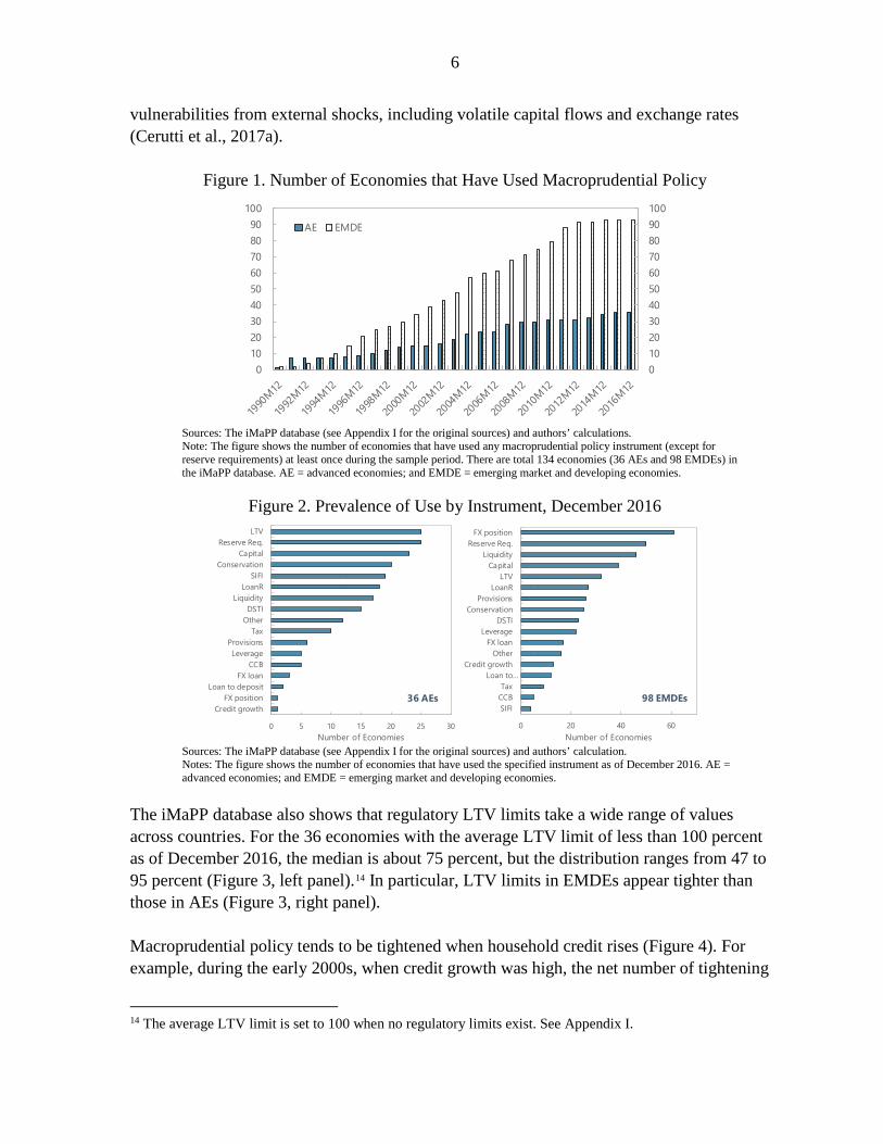
Figure 2. Prevalence of Use by Instrument, December 2016

Sources: The iMaPP database (see Appendix I for the original sources) and authors’ calculation. Notes: The figure shows the number of economies that have used the specified instrument as of December 2016. AE = advanced economies; and EMDE = emerging market and developing economies.

The iMaPP database also shows that regulatory LTV limits take a wide range of values across countries. For the 36 economies with the average LTV limit of less than 100 percent as of December 2016, the median is about 75 percent, but the distribution ranges from 47 to 95 percent (Figure 3, left panel).14 In particular, LTV limits in EMDEs appear tighter than those in AEs (Figure 3, right panel). Macroprudential policy tends to be tightened when household credit rises (Figure 4). For example, during the early 2000s, when credit growth was high, the net number of tightening

14 The average LTV limit is set to 100 when no regulatory limits exist. See Appendix I.

0102030405060708090100

0102030405060708090

100

AE EMDE

0 5 10 15 20 25 30

Credit growthFX position

Loan to depositFX loan

CCBLeverage

ProvisionsTax

OtherDSTI

LiquidityLoanR

SIFIConservation

CapitalReserve Req.

LTV

Number of Economies

36 AEs

0 20 40 60

SIFICCBTax

Loan to…Credit growth

OtherFX loan

LeverageDSTI

ConservationProvisions

LoanRLTV

CapitalLiquidity

Reserve Req.FX position

Number of Economies

98 EMDEs

7

actions across macroprudential instruments rose for both AEs and EMDEs. This suggests that macroprudential authorities actively take actions in response to credit developments, underscoring the importance of the reverse causality problem for empirical analysis.

Figure 3. Distribution of the Average LTV Limit, December 2016

Sources: The iMaPP database (see Appendix I for the original sources) and authors’ calculations. Notes: The left panel shows the histogram of the average LTV limit of less than 100 percent, together with its kernel density estimate. The right panel shows the distributions for AEs and EMDEs. The box represents the inter-quartile interval, the inner line represents the median, and the outer lines represent the minimum and the maximum values. The dots represent outliers. AE = advanced economies; and EMDE = emerging market and developing economies.

Figure 4. Usage of Macroprudential Policies Over Time

Sources: The iMaPP database, Bloomberg, BIS, OECD, others (see Appendix III), and the authors’ calculations. Notes: This figure is based on the 63 countries for which quarterly data of household credit are available. The bars indicate the cumulative sum of the net number of tightening actions of any macroprudential policy instrument over the current and past three quarters and the lines indicate the average household credit growth. AE = advanced economies; and EMDE = emerging market and developing economies.

02

46

Freq

uenc

y

50 60 70 80 90 100average LTV limit

5060

7080

9010

0av

erag

e LT

V lim

it

AEs EMDEs

-20

-10

0

10

20

30

40

-40

-20

0

20

40

60

80

100

Dec-

90

Dec-

91

Dec-

92

Dec-

93

Dec-

94

Dec-

95

Dec-

96

Dec-

97

Dec-

98

Dec-

99

Dec-

00

Dec-

01

Dec-

02

Dec-

03

Dec-

04

Dec-

05

Dec-

06

Dec-

07

Dec-

08

Dec-

09

Dec-

10

Dec-

11

Dec-

12

Dec-

13

Dec-

14

Dec-

15

Dec-

16

Macroprudential policies (AE sum) Macroprudential Policies (EMDE sum)Household Credit (AE avg, rhs) Household Credit (EMDE avg, rhs)

8

III. REVISITING STANDARD REGRESSION ANALYSES

In this section, we estimate panel regressions with fixed effects to assess the effects “per policy action”, which has been the standard approach in the literature. In these regressions both the macroprudential policy indicator and the dependent variable enter with a (one quarter) lag, so that identification of the causal effect of macroprudential policy relies on a timing assumption—macroprudential policies do not affect the dependent variable within the same quarter.15 Building on previous literature, we estimate the following panel regressions:

∆4Ci,t = ρ ∆4C𝑖𝑖,𝑡𝑡−1 + β MaPP𝑖𝑖,𝑡𝑡−1 + γ 𝑿𝑿𝑖𝑖,𝑡𝑡−1 + α𝑖𝑖 + µ𝑡𝑡 + ϵ𝑖𝑖,𝑡𝑡, (1)

where i is country and t is time (quarter). The dependent variable, ∆4𝐶𝐶𝑖𝑖,𝑡𝑡, refers to the year-on-year growth rate of real household credit and private consumption. The lagged dependent variable (∆4Ci,t−1) is included as a regressor to account for persistence. A vector 𝑿𝑿𝑖𝑖,𝑡𝑡−1 includes lagged macro control variables, such as real GDP growth and domestic real interest rates. Time fixed effects (µt) capture time-varying common factors such as global risk aversion, while country fixed effects (αi) capture time-invariant country-specific factors such as institutional characteristics. The main independent variable, MaPPi,t-1, is the policy change indicator for the instrument or the instrument group. This indicator records tightening actions (+), loosening actions (-), and no changes (0), and it is cumulated over the past 4 quarters to account for potential lagged effects. We consider indices for instrument groups such as all, loan-targeted, demand, and supply measures, which are further subdivided into three categories, including general-, capital-, and loan-supply tools (Appendix III).

Using our comprehensive data of macroprudential measures for the sample of 63 countries for which credit variables are available at a quarterly frequency, we first confirm that loan-targeted policy actions have significant effects on household credit growth (Appendix VI Table 1, columns 1-3). A tightening of any macroprudential measure (captured by the overall MaPP index) is, on average, associated with a decline in household credit growth of 0.8 percentage points (ppts). 16 Looking at sub-indices, loan-targeted tools (including both demand-side tools, such as LTV and DSTI and supply-side tools, such as limits on certain types of credit) are found to robustly affect household credit growth across all country groups and their effect is larger than that of the average macroprudential tool. Regarding the

15 These estimates cover 63 countries (34 AEs and 29 EMDEs), where quarterly data are available between 1991: Q1 and 2016: Q4.

16 The unconditional household credit growth averages about 8 ppts per year when all countries are considered. In EMDEs, it averages 11.6 ppts, while in AEs household credit increases yearly by 5.6 percent. See Appendix III Table 3. To assess the validity of these findings, further robustness checks, including those addressing a potential so-called Nickell bias (Nickell 1981) using system GMM panel estimates (Arellano and Bover 1995, Blundell and Bond 1998, Roodman 2009), are presented in Alam et al. (2019).

9

demand-side tools specifically, the tightening of both LTV and DSTI limits are negatively associated with household credit, and the estimated ppt impacts are greater in EMDEs, where one tightening (loosening) action moderates (raises) household credit by about 6 percent for these tools. These results corroborate the findings of Cerutti et al. (2017a) and Kuttner and Shim (2016) who also find significant effects for demand-side tools.17 Turning to the side-effects, our goal is to quantify the consequences of macroprudential policies on macroeconomic outcomes such as a slowdown in private consumption and real GDP growth (Appendix VI Table 2). These consequences are referred to as “side effects,” since they would not typically be the policy objective of macroprudential action (IMF 2012, Richter et al., 2019). In general, we find limited evidence of side effects on consumption. However, loan-targeted policy actions, especially those targeting the supply of bank loans, are negatively associated with private consumption growth. Changes in LTV limits specifically are found to reduce private consumption growth cumulatively by roughly 0.8 ppts after one year for the average action.18 IV. QUANTIFYING THE EFFECTS OF PERCENTAGE-POINT CHANGES IN THE LTV LIMITS

A. Propensity-Score Based Approach

We now move beyond the analysis typically presented in the literature in three ways. First, we quantify the effects of a one-percentage-point change in the LTV limit using our new indicator, the average LTV limit. Second, we examine whether the effects are non-linear—that is, whether the effects of a one-percentage-point tightening differ depending on the size of the overall amount of tightening and the starting level of the LTV limits. We also undertake additional efforts to identify causal effects, by employing a propensity-score based approach. Reverse causality is likely to be a problem in our context because the LTV limits are more likely to be tightened during periods of high credit growth (Figure 4). To address this reverse causality, previous studies—and the approach just presented in the previous section—typically rely on a timing assumption: macroprudential policy does not affect macro-financial variables (e.g., credit growth) within the same quarter. However, this is a rather strong assumption, and the estimated effects would likely be subject to an attenuation bias—biased towards zero—if the timing assumption did not hold (Appendix II).

17 Other studies, using different data and methods, also show that tighter LTV and DSTI limits reduce household credit growth (e.g., Lim et al. 2011; Arregui et al. 2013; Crowe et al. 2013; Krznar and Morsink 2014; and Jácome and Mitra 2015). The effects of macroprudential policies on house prices are mostly weaker (Appendix Table 1, columns 4–6), in line with most existing studies. 18 When considering real GDP growth, the estimated side effects are weaker and generally not statistically significant (Appendix VI Table 2, columns 4–6), except for the limits on credit growth in AEs, which reduce real GDP growth by 0.8 ppts.

10

To more fully address reverse causality, we here employ an inverse propensity-score weighting (IPW) estimator specifically designed for our purposes. The use of propensity score methods is relatively new in the macroeconomics literature,19 but has long been common in biostatistics. The IPW estimator identifies the causal effects of macroprudential policy by penalizing those observations that are likely to be affected by reverse causality. While there are many variants of IPW estimators, we use the Augmented IPW (AIPW) estimator, which achieves the smallest asymptotic variance in the class of the “doubly-robust” estimators.20 Specifically, the AIPW estimation of the effects of changes in LTV limits is conducted in three stages. In the first stage, an ordered logit model—the “treatment model”—is estimated to obtain the propensity score—the probability of changing the LTV limit. The dependent variable is an ordered policy action indicator taking on the values {-20, -10, 0, 10, 20}, which represents the buckets in which the change in the LTV limit (ΔLTV) is grouped into (Table 1), and the regressors are macro variables that may influence policy actions (see Appendix IV for details). In the second stage, outcomes (e.g., credit growth) for each bucket of ΔLTV are predicted using macroeconomic variables to correct for unobserved outcomes—the “outcome model.” Then, in the third stage, the average treatment effect (ATE) on the outcome (e.g., credit growth) is estimated for each bucket of ΔLTV, using (1) the estimated inverse propensity-scores to put more (less) weights on the observations that are less (more) likely to be affected by reverse causality; and (2) the predicted outcomes in lieu of unobserved outcomes in the unrealized states.21 To obtain the estimated ATE of a one-percentage-change in the LTV limit, the estimated ATE is rescaled by the average ΔLTV for each bucket. The AIPW estimation is conducted with panel data of 58 countries over the period 2000: Q1 to 2016: Q4.

19 Jordà and Taylor (2016), Angrist et al. (2016), and Richter et al. (2019) apply propensity-score based methods to estimate the effects of fiscal austerity, monetary policy, and macroprudential policy. 20 It is the class of the estimators of the average treatment effect (ATE) that involves estimating both a treatment model and an outcome model; and that has a “doubly-robust” property—consistency of the estimated ATE only requires either the treatment model or the outcome model to be correctly specified. See, for example, Robins et al. (1994) and Lunceford and Davidian (2004). 21 Please note that actual outcomes are only observed in a realized state—e.g., for countries that tighten their LTV limits, we cannot observe their outcome (e.g., credit growth) in the hypothetical scenario where they did not tighten (i.e., the unrealized state).

11

Table 1. Summary Statistics of the Change in the Average LTV Limit by Group

Sources: The iMaPP database (see Appendix I for the original sources) and the authors’ calculation. Notes: The table shows the summary statistics of the change in the average LTV limit for the four treatment groups and for the control group. Observations with ΔLTV less than or equal to -25 ppts are excluded for the estimation to mitigate the influence of outliers. AE = advanced economies; and EMDE = emerging market and developing economies. For comparison, we also estimate the effect of a one-percent-point LTV tightening using standard panel regression methods, based on the timing identification assumption (Appendix V). When we examine whether results differ across subsamples, such as advanced- versus emerging market economies, we revert to the panel regression methods, since the AIPW estimation, which is already based on a bucketing approach, requires a relatively large number of observations.

B. The Effects of a One-Percentage-Point Change in LTV Limits

The AIPW estimation results indicate strong and nonlinear effects of a one-ppt LTV tightening on household credit—we report ATEs only for tightening groups with relatively more observations. For a tightening of less than 10 ppts—the most common change in our sample—the cumulative decline in real household credit growth after four quarters is estimated at 0.65 ppts per one-ppt LTV tightening—which is a sizable effect—, while it is estimated to be smaller, at -0.36 ppts for a larger tightening in the range between 10 ppts and 25 ppts (Panel 1of Figure 5).22 Interestingly, therefore, the estimated effects per one-ppt tightening are diminishing with respect to the size of the LTV adjustment. The relatively smaller effects of larger tightening could be due to policy leakage (e.g., regulatory arbitrage) effects. For example, if the LTV limits only cover domestic bank loans, a strong tightening could incentivize arbitrage and thus increase non-bank credit or credit from abroad when these loans are not covered by the

22 The average effect on household credit growth of tightening measures is estimated at -0.31 ppts (compared to -0.16 ppts in the FE regression), based on the AIPW estimation with three buckets (i.e., the tightening, loosening, and control groups). However, considering the observed nonlinearity, these linear models would likely be misspecified. The linear model estimates are broadly comparable with the estimates by Richter et al. (2019), although caution is needed when comparing the results because the definition of LTV limits differs—their LTV indicator includes loan prohibitions while ours do not. Their estimated effect on household credit growth ranges from -0.58 to -0.18 ppts—the per-action estimate of -4.1 ppts divided by the average LTV change per tightening of 7.1 ppts (with scope adjustments) or 22.5 ppts (without scope adjustments).

ALL AE EMDE

Tightening by More than or Equal to 10 ppts and Less than 25 ppts -20 -14.2 4.4 22 10 12

Tightening by Less than 10 ppts -10 -3.8 2.3 46 32 14 No Change (Control Group) 0 0.0 0.0 3,905 2,278 1,627 Easing by Less than 10 ppts 10 4 2 23 15 8 Easing by 10+ ppts 20 17.4 7.9 8 4 4

Ordered Policy Action

Indicator

Mean (ALL)

Standard Deviation

(ALL)

Number of Observations

12

limit, offsetting the policy effects on domestic bank credit (see also IMF-FSB-BIS, 2016). The magnitude of the estimated effects depends on the choices of thresholds for tightening groups, partly due to the nonlinearity but for large LTV changes also due to the relatively limited number of observations and the influence of outliers.

Figure 5. Causal Effects of One Percentage Point Tightening in LTV limits 1. Real Household Credit Growth 2. Real Consumption Growth

Sources: The iMaPP database, Bloomberg, BIS, OECD, others (see Appendix III), and the authors’ estimation. Notes: The figure reports the cumulative effects of a one-ppt LTV tightening after four quarters, obtained by the augmented inverse propensity-score weighting (“AIPW”) estimation and the fixed effects estimation with the timing assumption (“FE regression”), which are explained in detail in Appendices VI and VII, respectively. The FE regression uses the interaction terms of ΔLTV with the dummy variables for each bucket (i.e., a tightening by less than 10 ppts and a tightening by more than or equal to 10 ppts and less than 25 ppts). To mitigate the influence of outliers, observations with ΔLTV less than or equal to -25 ppts are excluded for the estimation. Confidence levels: *** p<0.01, ** p<0.05, * p<0.1. Standard errors are clustered by country. Baseline results of the fixed effects regressions are presented in Appendix VI Table 3.

The fixed effect (FE) estimation based on the timing assumption also finds nonlinear effects on household credit, but the estimates are not significant and smaller than the AIPW estimates (Panel 1 of Figure 5).23 This result supports the idea that the typical regression estimates based on the timing assumption suffer from an attenuation bias (Appendix II) and that the AIPW better addresses the endogeneity issue. Across methods, the estimated side effects are found to be smaller and less robust. The AIPW estimates of the consumption growth decline are around 0.1 ppts, and without a clear nonlinear pattern (Panel 2 of Figure 5). Taking this together with the nonlinear effects on credit, a tightening by less than 10 ppts appears to be more efficient in the sense that it has larger effects on credit but smaller side effects on consumption, although a formal welfare analysis is beyond the scope of this paper.

23 Jácome and Mitra (2015) also use the timing assumption and report an effect on mortgage credit of 0.07 ppts in four quarters, based on data of five economies.

-0.65***

-0.36***-0.43

-0.10

-0.8

-0.6

-0.4

-0.2

0.0

0.2

Tightening byLess than 10 ppts

Tighteningby 10- 25 ppts

AIPWFE regression

-0.15* -0.11***

0.110.00

-0.8

-0.6

-0.4

-0.2

0.0

0.2

Tightening byLess than 10 ppts

Tighteningby 10- 25 ppts

AIPWFE regression

13

Further Analysis of Changes in the LTV Limits We conduct some further analysis to examine whether the effects differ with country-characteristics. Looking first at the effect on household credit, our main focus is the sum of the ΔLTV coefficients, which encompasses the cumulative effects of the previous 4 lags (Appendix VI Table 4). We find relatively stronger and more significant impacts for EMDEs, especially when the credit gap is positive, and in countries with a high indebtedness level of low-income borrowers. The magnitude of a one ppt tightening of LTV limit on real household credit varies from about 0.07 ppts to 0.37 ppts, based on the timing assumption,,

and is comparable with those by Richter et al. (2019). 24

Turning to the control variables, higher short-term interest rates are found to negatively impact future household credit growth, as expected. These interest rate effects are found slightly stronger in EMDEs than in AEs. Second, the state of the business cycle, proxied by the past output growth, is found to be positively associated with credit growth, even if the effects are less significant. Finally, the positive and close-to-unity estimates of the lagged credit growth suggest a high degree of persistence in yearly credit growth. We also assess the impact of ΔLTV on real private consumption (see Appendix VI Table 5). The effects are significant when all countries are considered, as well as for the EMDE group, for countries with highly indebted low-income borrowers, and when EMDEs experience a credit boom. The magnitude of one ppt tightening of LTV limit on real private consumption vary from about 0.08 ppts to 0.18 ppts.

C. Do Initial LTV Levels Matter?

It is conceivable that a given change in the LTV limits could have differential impacts on macro-financial outcomes depending on whether the starting level of the LTV ratio cap is still relatively loose, or already tight. To examine this hypothesis, we estimate the effects conditioning on the level of LTV limits. The threshold levels sorting loose and tight initial levels are set to 100 percent in AEs and 90 percent in EMs, which corresponds to the median LTV level for each of these two groups. We then define the LTV limits to be “tight” for all observations below these thresholds (i.e., for lower maximum LTV). The use of different cut-off levels yields broadly similar results. We use the panel regression with the timing assumption for the results distinguishing AEs and EMDEs, while we also conduct the AIPW estimation for the whole sample. The results suggest that the initial LTV level matters, especially for household consumption, with the effect of an additional tightening on consumption larger when LTV limits are already tight. In general, a tightening of the LTV limits by one percentage point is only

24 These results are also robust to controlling for other macroprudential policies and to the use of the Arellano-Bover-Blundell-Bond system GMM estimator (see Alam et al. 2019, Appendix VIII Tables 11–14).

14

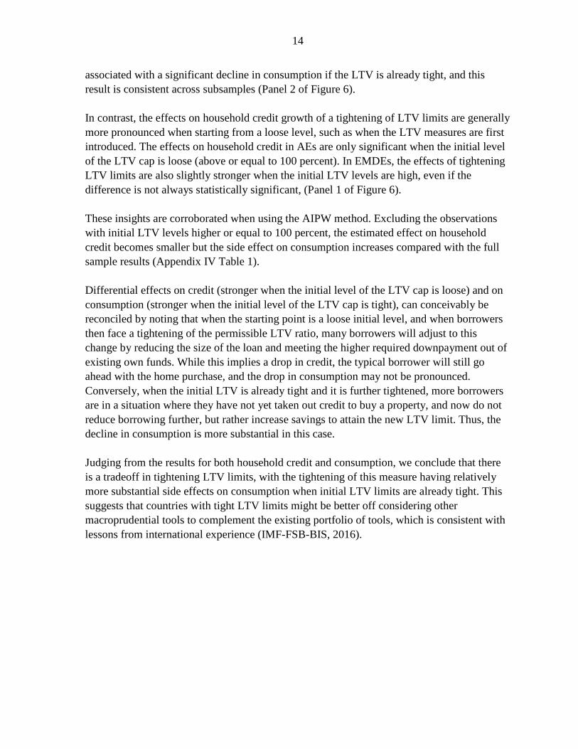
associated with a significant decline in consumption if the LTV is already tight, and this result is consistent across subsamples (Panel 2 of Figure 6). In contrast, the effects on household credit growth of a tightening of LTV limits are generally more pronounced when starting from a loose level, such as when the LTV measures are first introduced. The effects on household credit in AEs are only significant when the initial level of the LTV cap is loose (above or equal to 100 percent). In EMDEs, the effects of tightening LTV limits are also slightly stronger when the initial LTV levels are high, even if the difference is not always statistically significant, (Panel 1 of Figure 6). These insights are corroborated when using the AIPW method. Excluding the observations with initial LTV levels higher or equal to 100 percent, the estimated effect on household credit becomes smaller but the side effect on consumption increases compared with the full sample results (Appendix IV Table 1). Differential effects on credit (stronger when the initial level of the LTV cap is loose) and on consumption (stronger when the initial level of the LTV cap is tight), can conceivably be reconciled by noting that when the starting point is a loose initial level, and when borrowers then face a tightening of the permissible LTV ratio, many borrowers will adjust to this change by reducing the size of the loan and meeting the higher required downpayment out of existing own funds. While this implies a drop in credit, the typical borrower will still go ahead with the home purchase, and the drop in consumption may not be pronounced. Conversely, when the initial LTV is already tight and it is further tightened, more borrowers are in a situation where they have not yet taken out credit to buy a property, and now do not reduce borrowing further, but rather increase savings to attain the new LTV limit. Thus, the decline in consumption is more substantial in this case. Judging from the results for both household credit and consumption, we conclude that there is a tradeoff in tightening LTV limits, with the tightening of this measure having relatively more substantial side effects on consumption when initial LTV limits are already tight. This suggests that countries with tight LTV limits might be better off considering other macroprudential tools to complement the existing portfolio of tools, which is consistent with lessons from international experience (IMF-FSB-BIS, 2016).

15

Figure 6. The Effects of One Percentage Point Tightening in LTV Limits on Household Credit and Private Consumption Growth

1. Real Household Credit Growth

2. Real Consumption Growth

Sources: The iMaPP database, Bloomberg, BIS, OECD, others (see Appendix III), and the authors’ estimation. Note: The figure shows the cumulative effects of one-ppt LTV tightening after four quarters, conditioning on the initial LTV level, estimated by the fixed effects estimation with the timing assumption. Specifically, the bars show the cumulative sum of the ΔLTV coefficients in the previous four quarters is presented for each country group. The “high LTV level” in AEs and EMDEs refers to the LTV limits greater or equal to 100 percent and 90 percent, respectively (i.e., looser limits), and the “low LTV level” refers those levels below the aforementioned thresholds (i.e., tighter limits). For more details see Appendix VI Table 6.

V. CONCLUSIONS

In this paper, we presented a new comprehensive database of macroprudential policies (iMaPP) that combines information from various sources. Exploiting the unique features of this database and using a method that aims to better address endogeneity problems, we found strong and nonlinear effects of LTV changes on household credit. The effects per one percentage point (ppt) LTV tightening are diminishing with the size of the LTV adjustment, likely due to policy leakage effects. The largest per-unit impact is found for the most popular action in our sample—a tightening of less than 10 ppts—and it indicates that a one ppt LTV tightening cumulatively reduces household credit growth by up to 0.65 ppts after one year. This result highlights the importance of considering nonlinearity in estimating policy effects, as well as reverse causality. We also made progress toward assessing side effects of macroprudential policies, by investigating their impact on private consumption. These effects are statistically significant, but more moderate in size relative to effects on household credit. We further establish a nonlinearity in the effects of tightening of LTV limits on consumption, with the effect of an additional tightening larger when LTV limits are already tight. The new iMaPP database will be updated annually with data from the IMF’s new Annual Survey on Macroprudential Policies, offering many opportunities for further research. Among the issues that deserve further exploration are the quantification of the effects of other macroprudential policies and a more comprehensive cost-benefit analysis of macroprudential policies.25 25 See Brandao et al. (forthcoming) for further progress in this regard.

-0.3

-0.2

-0.1

0.0

ALL AE EMDE

Tight LTV levelLoose LTV level

-0.3

-0.2

-0.1

0.0

ALL AE EMDE

Tight LTV levelLoose LTV level

16

APPENDIX I. THE IMAPP DATABASE

The iMaPP database integrates several other available databases of macroprudential measures. Appendix I Figure 1 visualizes how each of these data sources contributes to the iMaPP database. Data availability differs across time and countries, reflecting both countries not having taken measures, and measures not being captured by existing databases. Going forward, the iMaPP database will be updated annually with the IMF’s Annual Macroprudential Policy Survey.

Appendix I Figure 1. Sources and Coverages of the iMaPP Database

Source: Authors. Appendix I Table 1 provides a list of the 134 countries covered in the iMaPP database and Appendix I Table 2 lists the 66 economies where the average LTV limit is available. Appendix I Table 3 lists all the categories of macroprudential instruments available in the iMaPP database, and their definitions. Appendix I Table 4 shows how the iMaPP database compares with other existing databases of macroprudential policy.

IMF’s Annual Macroprudential Policy

Survey

IMF’s Global Macroprudential Policy Instrument Survey (2013)

National and Other Official Sources

Shim et al. (2013)

European Systemic Risk Board’s Dataset

Country Coverage

Time

Lim et al. (2011)

Lim et al. (2013)

134

Coun

trie

s

December 2016 January 1990

17

Appendix I Table 1. Countries Covered in the iMaPP Database

Advanced economies (AEs; 36) Australia, Austria, Belgium, Canada, Cyprus, Czech Republic, Denmark, Estonia, Finland, France, Germany, Greece, Hong Kong SAR, Iceland, Ireland, Israel, Italy, Japan, Korea, Latvia, Lithuania, Luxembourg, Malta, Netherlands, New Zealand, Norway, Portugal, Singapore, Slovak Republic, Slovenia, Spain, Sweden, Switzerland, Taiwan Province of China, United Kingdom, United States. Emerging market and developing economies (EMDEs; 98)2 Albania, Algeria, Angola, Argentina, Armenia, Azerbaijan, The Bahamas, Bahrain, Bangladesh, Belarus, Benin, Bhutan, Bosnia and Herzegovina, Botswana, Brazil, Brunei Darussalam, Bulgaria, Burkina Faso, Burundi, Cambodia, Cabo Verde, Chile, China, Colombia, Congo Democratic Republic, Costa Rica, Croatia, Cote d’Ivoire, Dominican Republic, Ecuador, El Salvador, Ethiopia, Fiji, Gambia, Georgia, Ghana, Guinea Bissau, Haiti, Honduras, Hungary, India, Indonesia, Jamaica, Jordan, Kazakhstan, Kenya, Kosovo, Kyrgyz Republic, Kuwait, Lebanon, Laos, Lesotho, Macedonia, Malaysia, Mali, Mauritania, Mauritius, Mexico, Moldova, Mongolia, Montenegro, Morocco, Mozambique, Nepal, Niger, Nigeria, Oman, Pakistan, Paraguay, Peru, Philippines, Poland, Romania, Russia, Saudi Arabia, Serbia, South Africa, Sri Lanka, St. Kitts and Nevis, Senegal, Solomon Islands, Sudan, Tajikistan, Tanzania, Timor Leste, Thailand, Togo, Tonga, Trinidad and Tobago, Tunisia, Turkey, Uganda, Ukraine, United Arab Emirates, Uruguay, Vietnam, Yemen, and Zambia.

Source: World Economic Outlook (IMF, 2018b). Notes: The 65 economies with relatively more observations are listed in bold letters. They are 35 AEs and 30 EMDEs.

Appendix I Table 2. Countries with the Average LTV Limit in the iMaPP Database

Economies with the average LTV limit (66 economies) Argentina, Australia, Austria, Belgium, Brazil, Bulgaria, Canada, Chile, China, Colombia, Croatia, Cyprus, Czech Republic, Denmark, Estonia, Finland, France, Germany, Greece, Hong Kong SAR. Hungary, Iceland, India, Indonesia, Ireland, Israel, Italy, Japan, Korea, Kuwait, Latvia, Lebanon, Lithuania, Luxembourg, Malaysia, Malta, Mexico, Mongolia, Netherlands, New Zealand, Nigeria, Norway, Peru, Philippines, Poland, Portugal, Romania, Russia, Saudi Arabia, Serbia, Singapore, Slovak Republic, Slovenia, South Africa, Spain, Sweden, Switzerland, Taiwan Province of China, Thailand, Turkey, Ukraine, United Arab Emirates, United Kingdom, United States, Uruguay, and Vietnam.

Source: Authors.

18

Appendix I Table 3. Definitions of Macroprudential Policy Instruments

Source: Authors. Note: * indicates that subcategories are available.

Definition1 Countercyclical

Buffers (CCB)A requirement for banks to maintain a countercyclical capital buffer. Implementations at 0% are not considered as a tightening in dummy-type indicators.

2 Conservation Requirements for banks to maintain a capital conservation buffer, including the one established under Basel III.

3 Capital Requirements*

Capital requirements for banks, which include risk weights, systemic risk buffers, and minimum capital requirements. Countercyclical capital buffers and capital conservation buffers are captured in their sheets respectively and thus not included here. Subcategories of capital measures are also provided, classifying them into household sector targeted (HH), corporate sector targeted (Corp), broad-based (Gen), and FX-loan targeted (FX) measures.

4 Leverage Limits (LVR)

A limit on leverage of banks, calculated by dividing a measure of capital by the bank’s non-risk-weighted exposures (e.g., Basel III leverage ratio).

5 Loan Loss Provisions (LLP)

Loan loss provision requirements for macroprudential purposes, which include dynamic provisioning and sectoral provisions (e.g. housing loans).

6 Limits on Credit Growth (LCG)*

Limits on growth or the volume of aggregate credit, the household-sector credit, or the corporate-sector credit by banks, and penalties for high credit growth. Subcategories of limits to credit growth are also provided, classifying them into household sector targeted (HH), corporate sector targeted (Corp), and broad-based (Gen) measures.

7 Loan Restrictions (LoanR)*

Loan restrictions, that are more tailored than those captured in "LCG". They include loan limits and prohibitions, which may be conditioned on loan characteristics (e.g., the maturity, the size, the LTV ratio and the type of interest rate of loans), bank characteristics (e.g., mortgage banks), and other factors. Subcategories of loan restrictions are also provided, classifying them into household sector targeted (HH), and corporate sector targeted (Corp) measures. Restrictions on foreign currency lending are captured in "LFC".

8 Limits on Foreign Currency (LFC)

Limits on foreign currency (FC) lending, and rules or recommendations on FC loans.

9 Limits on the Loan-to-Value Ratio (LTV)

Limits to the loan-to-value ratios, including those mostly targeted at housing loans, but also includes those targeted at automobile loans, and commercial real estate loans.

10 Limits on the Debt-Service-to-Income Ratio (DSTI)

Limits to the debt-service-to-income ratio and the loan-to-income ratio, which restrict the size of debt services or debt relative to income. They include those targeted at housing loans, consumer loans, and commercial real estate loans.

11 Tax Measures Taxes and levies applied to specified transactions, assets, or liabilities, which include stamp duties, and capital gain taxes.

12 Liquidity Requirements

Measures taken to mitigate systemic liquidity and funding risks, including minimum requirements for liquidity coverage ratios, liquid asset ratios, net stable funding ratios, core funding ratios and external debt restrictions that do not distinguish currencies.

13 Limits on the Loan-to-Deposit Ratio (LTD)

Limits to the loan-to-deposit (LTD) ratio and penalties for high LTD ratios.

14 Limits on Foreign Exchange Positions (LFX)

Limits on net or gross open foreign exchange (FX) positions, limits on FX exposures and FX funding, and currency mismatch regulations.

15 Reserve Requirements (RR)*

Reserve requirements (domestic or foreign currency) for macroprudential purposes. Please note that this category may currently include those for monetary policy as distinguishing those for macroprudential or monetary policy purposes is often not clear-cut. A subcategory of reserve requirements is provided for those differentiated by currency (FCD), as they are typically used for macroprudential purposes.

16 SIFI Measures taken to mitigate risks from global and domestic systemically important financial institutions (SIFIs), which includes capital and liquidity surcharges.

17 Other Macroprudential measures not captured in the above categories—e.g., stress testing, restrictions on profit distribution, and structural measures (e.g., limits on exposures between financial institutions).

19

Appendix I Table 4. The iMaPP Database and Other Existing Databases

Source: Authors. Notes: 1/ The classification of instruments differs across databases. The column "Instruments" shows the number of categories, including subcategories, available in each dataset, without standardizing classification. 2/ "T/L indexes" is the dummy-type indexes for tightening and loosening actions of macroprudential policy measures.

Sources Sample Period

Country Coverage

Instru-ments1/

Frequ-ency

Text Info MaPP Indexes2/

The iMaPP database Databases 1-6 below, national sources, IMF official documents, and websites of the BIS and the FSB. 1990M1-

2016M12 134 27 M Yes

- Average LTV limit- T/L indexes by instrument

Databases Integrated in the iMaPP Database1 Lim et al. (2011) IMF Financial Stability and

Macroprudential Policy Survey, 20101990-2011 49 10 As

reported Yes -

2 Lim et al. (2013) National sources 2000M1-2013M7 39 12 M Yes - Institutional

arrangement indexes3 Global Macroprudential

Policy Instrument (GMPI, 2013)

IMF survey to authorities 2013 and history 133 17 As

reported Yes -

4 Shim et al. (2013) National sources, and data from published papers when they are verified at national sources.

1990M1 - 2012M6 60 8 M Yes

- T/L indexes by instrument

5 ESRB database Country authorities 2013M1-latest

28 (Europe) 18 M Yes -

6 IMF’s Annual Macroprudential Policy Survey

Country authorities 2016 and some history

141 73 As reported Yes -

Other Databases7 Crowe, Dell'Ariccia, Igan,

and Rabanal (2013)The IMF survey of central bankers and bank regulators. 2010 and

history 36 3 A Yes -

8 Vandenbussche et al (2015)

National sources, IMF papers, and academic papers late '90 -

201016

(Europe) 29 Q Yes

- Intensity-adjusted T/L indexes by instrument

9 Dimova, Kongsamut, and Vandenbussche (2016)

Vandenbussche et al. (2015) and national sources.

2002Q1-2012Q4

4 (Europe) 6 Q Yes -

10 Kuttner and Shim (2016) Extended Shim et al. (2013) for 1980M1-1989M12 and added housing taxes and subsidies

1980Q1-2012Q2 60 9 M Yes

- T/L indexes by by instrument

11 Zhang and Zoli (2016) Lim et al. (2013), and national sources 2000Q1-2013Q4 46 - Q No

- Aggregate T/L index

12 Bruno, Shim, and Shin (2017)

Shim et al. (2013) and national sources 2004Q1-2013Q4 12 - Q No

- Aggregate T/L indexes

13 Cerutti et al. (2017a) The GMPI and official documents, cross-checking with Kuttner and Shim (2016), Crowe et al. (2011), and other surveys

2000-2013 119 12 A No

- Number of instruments in place- Indicator of the use by instr.

14 Cerutti et al. (2017b) The GMPI and national sources 2000Q1-2014Q4 64 9 Q Yes - T/L indexes by

by instrument15 Akinci and Olmstead-

Rumsey (2018)Lim et al. (2011), supplemented with Shim et al. (2013), national sources, the GMPI (2013), and Ceruttie et al. (2017a,b)

2000Q1-2013Q4 57 7 Q No

- T/L indexes by instrument

16 Budnik and Kleibl (2018) Country authorities 1995-2014

28 EU member states

64 M Yes- NA, while tightening/loosening tags are available

17 Richter, Schularick, and Shim (2018)

Extended Shim et al. (2013), adding an intensity-adjusted LTV index 1990Q1-

2012Q2 56 7 Q Yes

- Intensity-adjusted LTV change index - T/L indexes by instrument

20

The iMaPP database provides two types of indicators, in addition to descriptions of policy actions: (1) the dummy-type policy action indicators and (2) the average LTV limits. These indicators are recorded based on their effective dates because the announcement dates are often not available. When available, the announcement dates are provided in the description. The dummy-type policy action indicators are available for all instrument categories and for 134 countries from January 1990 to December 2016. They take the value of 1 for tightening actions, -1 for loosening actions, and zero for no change. The dummy-type indices help characterize the use of macroprudential policy instruments and can be used to estimate their effects per policy action, as in previous studies. However, these dummy-type indices only indicate the direction of a policy change, and lack information on the intensity of the change. For this reason, it is important to note that frequent changes in these indices do not necessarily indicate large changes in the policy instruments.

The average LTV limits series is available for 66 countries from January 2000 to December 2016. As the time-series of the simple average of all regulatory limits on LTV ratios in each country, it provides information on the level of the average LTV limit and its changes.

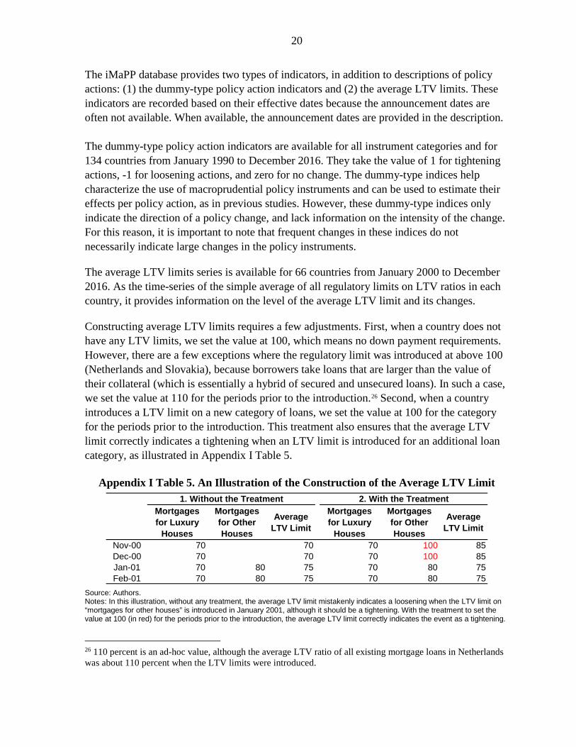
Constructing average LTV limits requires a few adjustments. First, when a country does not have any LTV limits, we set the value at 100, which means no down payment requirements. However, there are a few exceptions where the regulatory limit was introduced at above 100 (Netherlands and Slovakia), because borrowers take loans that are larger than the value of their collateral (which is essentially a hybrid of secured and unsecured loans). In such a case, we set the value at 110 for the periods prior to the introduction.26 Second, when a country introduces a LTV limit on a new category of loans, we set the value at 100 for the category for the periods prior to the introduction. This treatment also ensures that the average LTV limit correctly indicates a tightening when an LTV limit is introduced for an additional loan category, as illustrated in Appendix I Table 5.

Appendix I Table 5. An Illustration of the Construction of the Average LTV Limit

Source: Authors. Notes: In this illustration, without any treatment, the average LTV limit mistakenly indicates a loosening when the LTV limit on “mortgages for other houses” is introduced in January 2001, although it should be a tightening. With the treatment to set the value at 100 (in red) for the periods prior to the introduction, the average LTV limit correctly indicates the event as a tightening.

26 110 percent is an ad-hoc value, although the average LTV ratio of all existing mortgage loans in Netherlands was about 110 percent when the LTV limits were introduced.

Mortgages for Luxury

Houses

Mortgages for Other Houses

Average LTV Limit

Mortgages for Luxury

Houses

Mortgages for Other Houses

Average LTV Limit

Nov-00 70 70 70 100 85Dec-00 70 70 70 100 85Jan-01 70 80 75 70 80 75Feb-01 70 80 75 70 80 75

1. Without the Treatment 2. With the Treatment

21

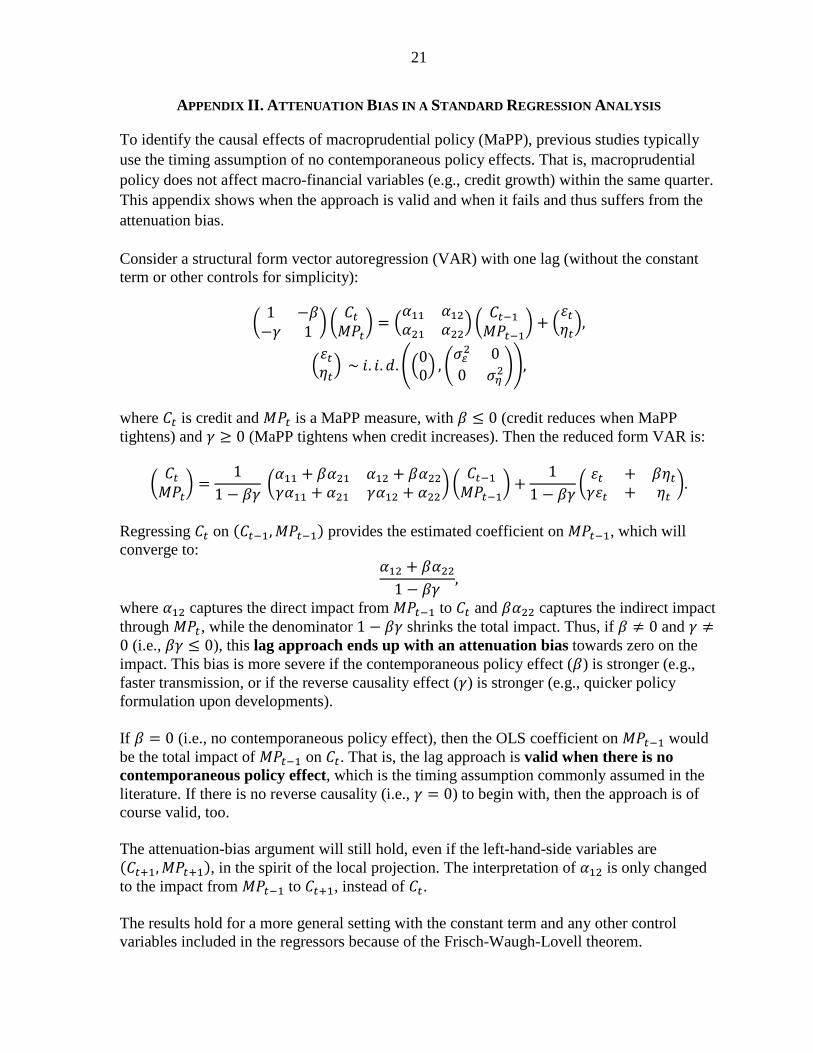
APPENDIX II. ATTENUATION BIAS IN A STANDARD REGRESSION ANALYSIS

To identify the causal effects of macroprudential policy (MaPP), previous studies typically use the timing assumption of no contemporaneous policy effects. That is, macroprudential policy does not affect macro-financial variables (e.g., credit growth) within the same quarter. This appendix shows when the approach is valid and when it fails and thus suffers from the attenuation bias. Consider a structural form vector autoregression (VAR) with one lag (without the constant term or other controls for simplicity):

� 1 −𝛽𝛽−𝛾𝛾 1 � � 𝐶𝐶𝑡𝑡𝑀𝑀𝑀𝑀𝑡𝑡

� = �𝛼𝛼11 𝛼𝛼12𝛼𝛼21 𝛼𝛼22� �

𝐶𝐶𝑡𝑡−1𝑀𝑀𝑀𝑀𝑡𝑡−1

� + �𝜀𝜀𝑡𝑡𝜂𝜂𝑡𝑡�,

�𝜀𝜀𝑡𝑡𝜂𝜂𝑡𝑡� ~ 𝑖𝑖. 𝑖𝑖.𝑑𝑑.��0

0� , �𝜎𝜎𝜀𝜀2 00 𝜎𝜎𝜂𝜂2

��,

where 𝐶𝐶𝑡𝑡 is credit and 𝑀𝑀𝑀𝑀𝑡𝑡 is a MaPP measure, with 𝛽𝛽 ≤ 0 (credit reduces when MaPP tightens) and 𝛾𝛾 ≥ 0 (MaPP tightens when credit increases). Then the reduced form VAR is:

� 𝐶𝐶𝑡𝑡𝑀𝑀𝑀𝑀𝑡𝑡� =

11 − 𝛽𝛽𝛾𝛾

�𝛼𝛼11 + 𝛽𝛽𝛼𝛼21 𝛼𝛼12 + 𝛽𝛽𝛼𝛼22𝛾𝛾𝛼𝛼11 + 𝛼𝛼21 𝛾𝛾𝛼𝛼12 + 𝛼𝛼22

� � 𝐶𝐶𝑡𝑡−1𝑀𝑀𝑀𝑀𝑡𝑡−1� +

11 − 𝛽𝛽𝛾𝛾

� 𝜀𝜀𝑡𝑡 + 𝛽𝛽𝜂𝜂𝑡𝑡𝛾𝛾𝜀𝜀𝑡𝑡 + 𝜂𝜂𝑡𝑡

�.

Regressing 𝐶𝐶𝑡𝑡 on (𝐶𝐶𝑡𝑡−1,𝑀𝑀𝑀𝑀𝑡𝑡−1) provides the estimated coefficient on 𝑀𝑀𝑀𝑀𝑡𝑡−1, which will converge to:

𝛼𝛼12 + 𝛽𝛽𝛼𝛼221 − 𝛽𝛽𝛾𝛾

,

where 𝛼𝛼12 captures the direct impact from 𝑀𝑀𝑀𝑀𝑡𝑡−1 to 𝐶𝐶𝑡𝑡 and 𝛽𝛽𝛼𝛼22 captures the indirect impact through 𝑀𝑀𝑀𝑀𝑡𝑡, while the denominator 1 − 𝛽𝛽𝛾𝛾 shrinks the total impact. Thus, if 𝛽𝛽 ≠ 0 and 𝛾𝛾 ≠0 (i.e., 𝛽𝛽𝛾𝛾 ≤ 0), this lag approach ends up with an attenuation bias towards zero on the impact. This bias is more severe if the contemporaneous policy effect (𝛽𝛽) is stronger (e.g., faster transmission, or if the reverse causality effect (𝛾𝛾) is stronger (e.g., quicker policy formulation upon developments). If 𝛽𝛽 = 0 (i.e., no contemporaneous policy effect), then the OLS coefficient on 𝑀𝑀𝑀𝑀𝑡𝑡−1 would be the total impact of 𝑀𝑀𝑀𝑀𝑡𝑡−1 on 𝐶𝐶𝑡𝑡. That is, the lag approach is valid when there is no contemporaneous policy effect, which is the timing assumption commonly assumed in the literature. If there is no reverse causality (i.e., 𝛾𝛾 = 0) to begin with, then the approach is of course valid, too. The attenuation-bias argument will still hold, even if the left-hand-side variables are (𝐶𝐶𝑡𝑡+1,𝑀𝑀𝑀𝑀𝑡𝑡+1), in the spirit of the local projection. The interpretation of 𝛼𝛼12 is only changed to the impact from 𝑀𝑀𝑀𝑀𝑡𝑡−1 to 𝐶𝐶𝑡𝑡+1, instead of 𝐶𝐶𝑡𝑡. The results hold for a more general setting with the constant term and any other control variables included in the regressors because of the Frisch-Waugh-Lovell theorem.

22

APPENDIX III. DATA FOR THE PANEL REGRESSION ANALYSIS WITH DUMMY-TYPE INDICATORS

Appendix III Table 1 provides the definitions and sources of the variables used in the regression analysis in Sections III and IV. Appendix III Table 2 provides the list of sample economies used in the panel regression analysis in Section III. Appendix III Table 3 provides the summary statistics of the variables used in estimation. The variables capturing changes in macroprudential measures used in Section III are the average of the net number of policy tightening over the current and past three quarters. This accounts for potentially delayed effects. Indicators are constructed both for individual instruments and for groups of instruments. The “Loan-targeted” group consists of the “Demand” and the “Supply-loans” instruments. “Demand” instruments are the limits on the loan-to-value ratio (LTV) and the limits on the debt-service-to-income (DSTI) ratio. “Supply-loans” measures are limits to credit growth (LCG), loan loss provisions (LLP), loan restrictions (LoanR), limits to the loan to deposit ratio, and limits to foreign currency loans. “Supply-general” instruments are reserve requirements, liquidity requirements, and limits to FX positions. “Supply-capital” instruments are leverage limits (LVR), countercyclical buffers (CCB), conservation buffers, and capital requirements. “MaPP index” is the sum of the dummies for all of 17 categories (see also Appendix I Table 3). The distinction between demand-side and supply-side tools is whether the tool is on the borrowers (i.e., credit demand) or on the financial institutions (i.e., credit supply). This is in line with the classification in Kuttner and Shim (2016).

Appendix III Table 1. Variable Descriptions and Sources

Sources: Authors. Notes: BIS = Bank for International Settlements; CEIC = CEIC Data Co., Ltd.; HPDD = Historical Public Debt Database; IFS

= IMF, International Financial Statistics Database; JST = Jordà-Schularick-Taylor Macrohistory Database; OECD = Organisation for Economic Co-operation and Development; WEO = World Economic Outlook Database.

Variables Description SourceMacro-level VariablesHousehold Debt Credit to households and NPISHs from all sectors, in billions,

national currency.BIS; JST; CEIC; ECRI; Haver Analytics; STA-SRF; Central Banks.

Real GDP Gross domestic product, constant prices in national currency WEO.Consumer Price Index Consumer price index, all items. IFS.Interest Rate Three-month treasury bill rate; money market rate; interbank

market rate (percent).IFS; Thomson Reuters Datastream; Bloomberg Finance L.P.

Real House Price Index House price index deflated by CPI. OECD, Global Property Guide, and IMF staff calculations; JST.

Institutional VariablesFinancial Development Index Overall financial development index. Svirydzenka (2016).Exchange Rate Regime Foreign exchange regime. IMF, Ilzetzki, Reinhart and Rogoff

(2017).

Debt-to-income Ratio Debt-to-income of lower-income borrowers (bottom 40 percent of the income distribution).

Alter, Feng, and Valckx (2018).

Capital Openness Index (Chinn-Ito Index)

An index measuring a country's degree of capital account openness.

Chinn, Menzie D. and Hiro Ito (2008).

23

Appendix III Table 2. Sample Economies for the Panel Regression Analysis

Source: Authors.

Advanced Economies (AEs)1 Australia 1 Argentina2 Austria 2 Brazil3 Belgium 3 Bulgaria4 Canada 4 Chile5 Cyprus 5 China6 Czech Republic 6 Colombia7 Denmark 7 Costa Rica8 Estonia 8 Croatia9 Finland 9 Georgia

10 France 10 Hungary11 Germany 11 India12 Greece 12 Indonesia13 Hong Kong 13 Kazakhstan14 Iceland 14 Macedonia15 Ireland 15 Malaysia16 Israel 16 Mexico17 Italy 17 Mongolia18 Japan 18 Morocco19 Latvia 19 Paraguay20 Lithuania 20 Philippines21 Luxembourg 21 Poland22 Netherlands 22 Romania23 New Zealand 23 Russia24 Norway 24 Saudi Arabia25 Portugal 25 South Africa26 Singapore 26 Thailand27 Slovak Republic 27 Turkey28 Slovenia 28 Ukraine29 South Korea 29 Uruguay30 Spain31 Sweden32 Switzerland33 United Kingdom34 United States

Emerging Market and Developing Economies (EMDEs)

24

Appendix III Table 3. Summary Statistics

Sources: The iMaPP database, Bloomberg, BIS, OECD, others (see Appendix IV), and the authors’ estimation. Notes: Individual macroprudential variables and aggregated MaPP indices are presented as the year-on-year average (yoy mean). The MaPP index consists of all 17 individual macroprudential measures. All Loan-related consists of Demand-related and Supply Loan measures. Demand-related includes debt-service-to-income (DSTI) and loan-to-value (LTV) limits. Supply All measures are divided into General, Capital, and Loan. Supply General consists of reserve requirements (RR), liquidity requirements (LR), and limits on foreign exchange positions (LFX). Supply Capital consists of capital requirements (CAPITAL), conservation buffers (CONSERVATION B), the leverage ratio (LVR), capital surcharges for systemically important financial institutions (SIFI), and countercyclical capital buffers (CCB). Supply Loan consists of limits on credit growth (LCG), loan loss provisions (LLP), loan restrictions (LOANR), and limits on foreign currency loans (LFC). For further details, see Appendix I Table 3. Summary statistics are presented for the set of 63 countries used in the regression analysis. AE = advanced economies; EMDE = emerging market and developing economies.

mean sd mean sd mean sdMacro-financial variables

Household Debt (yoy, real, %change) 7.806 13.519 5.613 9.470 11.641 17.961Private Consumption (yoy, real, %change -0.800 5.848 0.090 4.091 -2.511 7.958House Prices (yoy, real, %change) 1.728 8.667 1.746 8.406 1.686 9.289Real GDP (yoy, real, %change) 2.859 3.239 2.355 2.950 3.740 3.522Short-term Interest Rates (level) 9.705 9.969 6.480 3.884 15.346 14.032

Aggregated MaPP Indices

Mapp index (all measures, yoy mean) 0.081 0.368 0.051 0.265 0.132 0.496All Loan-related (yoy mean) 0.033 0.177 0.030 0.156 0.039 0.209Demand (yoy mean) 0.019 0.119 0.018 0.119 0.020 0.119Supply All (yoy mean) 0.044 0.285 0.016 0.180 0.092 0.403Supply Loan (yoy mean) 0.014 0.102 0.011 0.074 0.019 0.138Supply General (yoy mean) 0.005 0.225 -0.015 0.121 0.039 0.335Supply Capital (yoy mean) 0.029 0.116 0.021 0.096 0.043 0.143

Individual MaPP Indices

1 CCB (yoy mean) 0.001 0.024 0.002 0.023 0.000 0.0252 CONSERVATION B. (yoy mean) 0.007 0.044 0.006 0.043 0.009 0.0473 CAPITAL (yoy mean) 0.018 0.095 0.012 0.075 0.029 0.1234 LVR (yoy mean) 0.003 0.026 0.002 0.020 0.005 0.0345 LLP (yoy mean) 0.004 0.046 0.002 0.034 0.006 0.0636 LCG (yoy mean) 0.000 0.035 0.000 0.019 0.000 0.0537 LOANR (yoy mean) 0.007 0.061 0.005 0.051 0.011 0.0748 LFC (yoy mean) 0.003 0.033 0.003 0.030 0.002 0.0389 LTV (yoy mean) 0.012 0.089 0.012 0.087 0.013 0.09410 DSTI (yoy mean) 0.007 0.054 0.006 0.054 0.007 0.05211 TAX (yoy mean) 0.006 0.049 0.005 0.044 0.006 0.05712 Liquidity (yoy mean) 0.006 0.063 0.005 0.049 0.009 0.08213 LTD (yoy mean) 0.000 0.019 0.001 0.013 0.000 0.02714 LFX (yoy mean) 0.002 0.037 0.001 0.017 0.005 0.05715 RR (yoy mean) -0.004 0.218 -0.021 0.109 0.025 0.32816 SIFI (yoy mean) 0.004 0.029 0.005 0.034 0.001 0.01717 OT (yoy mean) 0.005 0.035 0.005 0.036 0.004 0.035

Average LTV Limit (change, percentage po -0.197 2.392 -0.154 1.900 -0.271 3.049

EMDEALL AE

25

APPENDIX IV. AIPW ESTIMATION

Baseline AIPW Estimation In Section IV, we use a propensity-score based approach, combined with a local projection method to estimate the policy effects for different horizons (Angrist et al. 2016, Jordà and Taylor 2016, and Richter et al. 2019). Among many variants of propensity-score based estimators, we use the Augmented Inverse-Propensity-Score Weighting (AIPW) estimator, which is the most efficient estimator in the class of “doubly-robust” estimators.27 The AIPW estimator of the average treatment effect (ATE) is given as follows:

𝐴𝐴𝐴𝐴𝐴𝐴�𝑗𝑗ℎ =

1𝑁𝑁𝐴𝐴

�𝐴𝐴𝐴𝐴�𝑗𝑗,𝑖𝑖𝑡𝑡ℎ

𝑡𝑡,𝑛𝑛

,

where

𝐴𝐴𝐴𝐴�𝑗𝑗,𝑖𝑖𝑡𝑡ℎ = ��

𝐷𝐷𝑗𝑗,𝑖𝑖𝑡𝑡

�̂�𝑝𝑗𝑗,𝑖𝑖𝑡𝑡� �∆ℎ𝑦𝑦𝑖𝑖𝑡𝑡 − 𝑚𝑚�𝑗𝑗,𝑖𝑖𝑡𝑡

ℎ � + 𝑚𝑚�𝑗𝑗,𝑖𝑖𝑡𝑡ℎ � − ��

𝐷𝐷0,𝑖𝑖𝑡𝑡

�̂�𝑝0,𝑖𝑖𝑡𝑡� �∆ℎ𝑦𝑦𝑖𝑖𝑡𝑡 − 𝑚𝑚�0,𝑖𝑖𝑡𝑡

ℎ � + 𝑚𝑚�0,𝑖𝑖𝑡𝑡ℎ �,

(A.IV.1)

h refers the horizon, j refers the treatment (with j = 0 indicating the control group—i.e., no change in the average LTV limit), i refers the country, and t refers the time. ∆ℎ𝑦𝑦𝑖𝑖𝑡𝑡 refers to the h-horizon change in the outcome variable (e.g., log of real household credit), 𝐷𝐷𝑗𝑗,𝑛𝑛𝑡𝑡 is the dummy variable of each treatment, �̂�𝑝𝑗𝑗,𝑖𝑖𝑡𝑡 is the estimated propensity score, and 𝑚𝑚�𝑗𝑗,𝑖𝑖𝑡𝑡

ℎ is the predicted h-horizon change in the outcome variable. The AIPW estimation involves (1) a treatment model to obtain the propensity scores and (2) outcome models to obtain the predicted changes in the outcome variable. Treatment Model: To obtain the propensity scores (�̂�𝑝𝑗𝑗,𝑖𝑖𝑡𝑡), we estimate the following ordered logit model:

𝑧𝑧𝑖𝑖𝑡𝑡∗ = 𝑿𝑿𝒊𝒊𝒊𝒊𝑻𝑻 𝜷𝜷𝑻𝑻 + 𝑒𝑒𝑖𝑖𝑡𝑡𝑇𝑇 , (A.IV.2) where 𝑧𝑧𝑖𝑖𝑡𝑡∗ is the latent variable behind the ordered policy action indicator (𝑧𝑧𝑖𝑖𝑡𝑡), and 𝑿𝑿𝒊𝒊𝒊𝒊𝑻𝑻 includes the lag of real household credit growth, the lag of real GDP growth, the lag of the interest rate, time dummies, and country dummies. 𝑒𝑒𝑖𝑖𝑡𝑡𝑇𝑇 is the error term. Each value of 𝑧𝑧𝑖𝑖𝑡𝑡 ∈{−20,−10, 0, 10, 20} represents one of the following groups: a tightening of more than or equal to 10 ppts and less than 25 ppts (-20); a tightening of less than 10 ppts (-10); no change (0—the control group); an easing of less than 10 ppts (10); and an easing of more than or equal to 10 ppts (20). Estimation with country- or time-dummies may generate inconsistent estimates due to the incidental parameters problem under a fixed T or N. However, the bias would be small when T (or N) is large, as in our case.28 Nevertheless, we consider alternative specifications (such 27 See Lunceford and Davidian (2004) and Jordà and Taylor (2016), for example. 28 See, e.g., Wooldridge (2010, p 612), Dickerson et al. (2011).

26

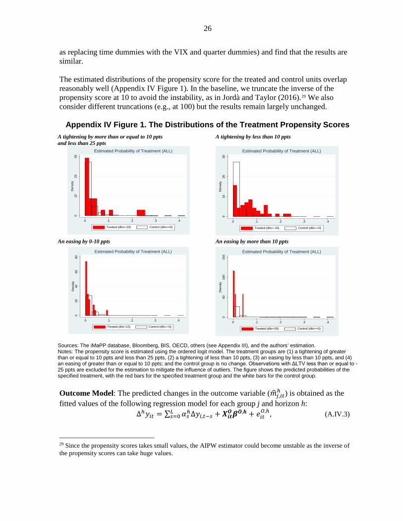
as replacing time dummies with the VIX and quarter dummies) and find that the results are similar. The estimated distributions of the propensity score for the treated and control units overlap reasonably well (Appendix IV Figure 1). In the baseline, we truncate the inverse of the propensity score at 10 to avoid the instability, as in Jordà and Taylor (2016).29 We also consider different truncations (e.g., at 100) but the results remain largely unchanged.

Appendix IV Figure 1. The Distributions of the Treatment Propensity Scores

A tightening by more than or equal to 10 ppts and less than 25 ppts

A tightening by less than 10 ppts

An easing by 0-10 ppts An easing by more than 10 ppts

Sources: The iMaPP database, Bloomberg, BIS, OECD, others (see Appendix III), and the authors’ estimation. Notes: The propensity score is estimated using the ordered logit model. The treatment groups are (1) a tightening of greater than or equal to 10 ppts and less than 25 ppts, (2) a tightening of less than 10 ppts, (3) an easing by less than 10 ppts, and (4) an easing of greater than or equal to 10 ppts; and the control group is no change. Observations with ΔLTV less than or equal to -25 ppts are excluded for the estimation to mitigate the influence of outliers. The figure shows the predicted probabilities of the specified treatment, with the red bars for the specified treatment group and the white bars for the control group. Outcome Model: The predicted changes in the outcome variable (𝑚𝑚�𝑗𝑗,𝑖𝑖𝑡𝑡

ℎ ) is obtained as the fitted values of the following regression model for each group j and horizon h:

∆ℎ𝑦𝑦𝑖𝑖𝑡𝑡 = ∑ 𝛼𝛼𝑠𝑠ℎ∆𝑦𝑦𝑖𝑖,𝑡𝑡−𝑠𝑠𝐿𝐿𝑠𝑠=0 + 𝑿𝑿𝒊𝒊𝒊𝒊𝑶𝑶𝜷𝜷𝑶𝑶,𝒉𝒉 + 𝑒𝑒𝑖𝑖𝑡𝑡

𝑂𝑂,ℎ, (A.IV.3)

29 Since the propensity scores takes small values, the AIPW estimator could become unstable as the inverse of the propensity scores can take huge values.

010

2030

Den

sity

0 .1 .2 .3 .4

Treated (dltv=-20) Control (dltv==0)

Estimated Probability of Treatment (ALL)

010

2030

Den

sity

0 .1 .2 .3 .4

Treated (dltv=-10) Control (dltv==0)

Estimated Probability of Treatment (ALL)

020

4060

80D

ensi

ty

0 .1 .2 .3 .4

Treated (dltv=10) Control (dltv==0)

Estimated Probability of Treatment (ALL)

050

100

150

Den

sity

0 .1 .2 .3 .4

Treated (dltv=20) Control (dltv==0)

Estimated Probability of Treatment (ALL)

27

where ∆ℎ𝑦𝑦𝑡𝑡 = 𝑦𝑦𝑡𝑡+ℎ − 𝑦𝑦𝑡𝑡, ∆𝑦𝑦𝑡𝑡 = 𝑦𝑦𝑡𝑡 − 𝑦𝑦𝑡𝑡−1, and 𝑿𝑿𝒊𝒊𝒊𝒊𝑶𝑶 includes real GDP growth (q-on-q), real short-term interest rate, and VIX, as well as their one-quarter lags, the dummies for AE, EMDE, and quarters.30 The lag length (𝐿𝐿) is set at one and 𝑒𝑒𝑖𝑖𝑡𝑡

𝑂𝑂,ℎ is the error term. We also consider different specifications and find that household credit and house price results are broadly robust while private consumption results are less robust. Average Treatment Effect (ATE): With the predicted propensity scores (�̂�𝑝𝑗𝑗,𝑖𝑖𝑡𝑡) and changes in the outcome variable (𝑚𝑚�𝑗𝑗,𝑖𝑖𝑡𝑡

ℎ ), the AIPW estimate of the ATE is obtained using equation (A.IV.1) for each treatment j and for each horizon h. Specifically, we compute 𝐴𝐴𝐴𝐴�𝑗𝑗,𝑖𝑖𝑡𝑡

ℎ and regress it on a constant term to get 𝐴𝐴𝐴𝐴𝐴𝐴�𝑗𝑗

ℎ and its standard error clustered by country, as in Jordà and Taylor (2016). Please note that these standard errors would miss the uncertainty in the treatment- and outcome- model estimation when either model is misspecified, and thus may be smaller—i.e., statistical significance may be overstated. A one-step estimation or a bootstrap method would be needed to obtain correct standard errors. AIPW Estimation – the Effects of Initial LTV levels To examine whether the LTV effects differ across initial LTV levels (Section IV.C.), we estimate the ATE excluding the observations with high initial LTV levels (i.e.,𝐿𝐿𝐴𝐴𝑉𝑉𝑡𝑡−1 ≥100) and compare it with the baseline results. The AIPW results echo the same insights from the regression results—the initial LTV levels appear to matter for the tradeoff. For the group of a tightening by less than 10 ppts, when excluding the observations with high initial LTV levels, the estimated effect on credit gets smaller but the side effect on consumption gets larger (Appendix IV Table 1). It is not feasible to provide the AIPW estimates for AEs and EMDEs, separately, due to the limited observation of LTV changes.

Appendix IV Table 1: AIPW Results—Effects of Initial LTV Levels

Sources: The iMaPP database, Bloomberg, BIS, OECD, others (see Appendix III), and the authors’ estimation. Notes: The table reports the AIPW estimation results for the group of tightening less than 10 ppts, using the five-bucket model explained in this Appendix. Observations with ΔLTV less than or equal to -25 ppts are excluded for the estimation to mitigate the influence of outliers. 1/ Observations with “LTVt-1≥100” are not used for estimation. The Confidence levels: *** p<0.01, ** p<0.05, * p<0.1.

30 Country and time fixed effect dummies cannot be used due to limited numbers of observations in some treatment groups. Instead, AE and EMDE dummies are used to control some country fixed effects, and quarter dummies and VIX are used to control some time fixed effects.

Houshold Credit Consumption

Number of Observations

(dLTV)Baseline -0.65*** -0.15* 46

w/o High Initial Levels1/ -0.28* 0.34*** 37

28

APPENDIX V: QUANTIFYING THE EFFECTS OF LTV CHANGES (Identification based on the Timing Assumption)

Empirical Design In Section IV, in addition to the AIPW estimation, we also conduct panel regressions with various controls to quantify the effects of a one-percentage-point change in the LTV limit on real household credit growth and real private consumption. Specifically, we estimate the following equation:

𝛥𝛥4𝐶𝐶𝑖𝑖,𝑡𝑡 = ρ ∆4C𝑖𝑖,𝑡𝑡−1 + ∑ 𝛽𝛽𝑠𝑠𝛥𝛥𝐿𝐿𝐴𝐴𝑉𝑉𝑖𝑖,𝑡𝑡−𝑠𝑠4𝑠𝑠=1 + ∑ 𝜸𝜸𝒍𝒍 𝑿𝑿𝑖𝑖,𝑡𝑡−𝑙𝑙𝐿𝐿

𝑙𝑙=1 + 𝛼𝛼𝑖𝑖 + 𝜇𝜇𝑡𝑡 + 𝜖𝜖𝑖𝑖,𝑡𝑡, (A.V.1)

where i is country, t is the time (quarter). The dependent variable, ∆4𝐶𝐶𝑖𝑖,𝑡𝑡 , refers to year-on-year growth rate of real household credit. 𝛥𝛥𝐿𝐿𝐴𝐴𝑉𝑉𝑖𝑖,𝑡𝑡 is the percentage point change in the average LTV limit in country i and quarter t. The lags of 𝛥𝛥𝐿𝐿𝐴𝐴𝑉𝑉𝑖𝑖,𝑡𝑡 are included to capture prolonged effects of policy changes on credit growth. When examining nonlinear effects, we replace 𝛥𝛥𝐿𝐿𝐴𝐴𝑉𝑉𝑖𝑖,𝑡𝑡 with the interaction term 𝛥𝛥𝐿𝐿𝐴𝐴𝑉𝑉𝑖𝑖,𝑡𝑡 ⋅ 𝑍𝑍𝑖𝑖,𝑡𝑡, where 𝑍𝑍𝑖𝑖,𝑡𝑡 is the dummy variable that takes one if 𝛥𝛥𝐿𝐿𝐴𝐴𝑉𝑉𝑖𝑖,𝑡𝑡 is in a specified range (e.g., 𝛥𝛥𝐿𝐿𝐴𝐴𝑉𝑉𝑖𝑖,𝑡𝑡∈(-10,0)) for Section IV.B.; and the initial LTV level for Section IV.C. The lag of ∆4𝐶𝐶𝑖𝑖,𝑡𝑡 is also included as a regressor to capture any autonomous dynamics in real credit growth, and a vector 𝑿𝑿𝑖𝑖,𝑡𝑡 includes other control variables, such as real GDP growth, domestic real interest rates and other macroprudential policies. Time (µt) and country (αi) fixed effects capture time-varying common factors such as global risk aversion and time-invariant country-specific factors such as location or institutional characteristics.

The dependent variable refers to total private credit to household sector (in real terms), which includes both mortgage and consumer credit from all sources.31 When considering the side effects, we replace the dependent variable with real private consumption growth.

To examine whether these effects differ across country characteristics, we estimate equation (A.V.1) with country group subsamples, for instance, EMDE/AE; regions such as Asia, Europe, and Americas; countries with high exchange rate flexibility, high capital openness, high financial development; countries with high debt-to-income ratios among low-income borrowers, or conditioning on a positive credit gap.32

31 This choice is justified given that mortgage data are scarcer across countries and time than total household credit data.

32 Using micro-level household surveys, countries are split into high/low indebtedness of low-income borrowers if the average debt-to-income ratio of the bottom 40 percent households by income is above/below the median.

29

APPENDIX VI. TABLES—REGRESSION ANALYSIS

Appendix VI Table 1. Summary: The Effects of Macroprudential Policies on Household Credit and House Prices

Sources: The iMaPP database, Bloomberg, BIS, OECD, others (see Appendix III), and authors’ estimation. Notes: The table reports the cumulative effects of the specified macroprudential tightening after four quarters, obtained by the fixed effects (FE) estimation. Each MaPP index/policy is considered individually. “dsti”= limits to the debt-service-to-income ratio, “ltv”= limits to the loan-to-value ratio, “tax”= tax measures, “lcg”= limits to credit growth, “llp”= loan loss provisions, “loanr”=loan restrictions, and “capital”=capital requirements. “MaPP index” is the sum of dummies for all of 17 categories. “Loan-targeted” group consists of the “Demand” and the “Supply-loans” instruments. “Demand”: LTV and DSTI. “Supply-loans”: lcg, llp, loanr, limits to the loan to deposit ratio, and limits to foreign currency loans. “Supply-general”: reserve requirements, liquidity requirements, and limits to FX positions. “Supply-capital”: leverage, countercyclical buffers, conservation buffers, and capital requirements. See Appendix I Table 3 for the definitions of instruments. For each country group, R-squared is computed as the average of the individual regressions. AE = advanced economies; and EMDE = emerging market and developing economies.

(1) (2) (3) (4) (5) (6)

Dependent Variable:

Group: ALL AE EMDE ALL AE EMED

MaPP index (all tools) -0.842*** -0.257 -1.388*** -0.0877 -0.898** 0.0619Loan-Targeted -1.883*** -1.043** -2.925*** -1.066** -1.667** -0.615

Demand -1.994*** -0.607 -4.926*** -1.406** -2.049** -0.213Supply-All -0.824* 0.395 -1.511*** 0.253 0.0116 0.00789

Supply- Loans -2.931*** -3.028** -3.005** -1.191 -1.970 -1.191Supply- General -0.602 0.958 -1.354* 0.485 0.0313 0.175Supply- Capital -1.009 0.221 -1.959* 0.270 0.0689 0.459

dsti -2.648*** -1.231 -6.173** -1.455 -3.167 2.537ltv -2.557** -0.654 -5.797*** -1.952*** -2.627*** -1.020tax -0.988 -1.514 -0.860 -0.597 -5.159** 3.235***lcg -4.620 -2.142 -6.562* -1.965 -0.0586 -2.436llp -5.865*** -4.161 -6.656*** -2.987** -1.510 -4.529**loanr -3.489** -4.592** -2.885 -1.385 -4.164* -0.262capital -1.091 0.0547 -1.803 0.304 -0.157 0.582

Observations 4,492 2,858 1,634 4,111 2,780 1,331N (countries) 63 34 29 55 34 21R-squared (avg) 0.884 0.873 0.903 0.812 0.846 0.786

Real Household Credit (yoy growth) Real House Prices (yoy growth)

30

Appendix VI Table 2. Summary: The Side-Effects of Macroprudential Policies on Private Consumption and GDP Growth

Sources: The iMaPP database, Bloomberg, BIS, OECD, others (see Appendix III), and the authors’ estimation. Notes: The table reports the cumulative effects of the specified macroprudential tightening after four quarters, obtained by the fixed effects (FE) estimation with the timing assumption. Each MaPP index/policy is considered individually. “dsti”= limits to the debt-service-to-income ratio, “ltv”= limits to the loan-to-value ratio, “tax”= tax measures, “lcg”= limits to credit growth, “llp”= loan loss provisions, “loanr”=loan restrictions, and “capital”=capital requirements. “MaPP index” is the sum of dummies for all of 17 categories. “Loan-targeted” group consists of the “Demand” and the “Supply-loans” instruments. “Demand”: LTV and DSTI. “Supply-loans”: lcg, llp, loanr, limits to the loan to deposit ratio, and limits to foreign currency loans. “Supply-general”: reserve requirements, liquidity requirements, and limits to FX positions. “Supply-capital”: leverage, countercyclical buffers, conservation buffers, and capital requirements. For each country group, R-squared is computed as the average of the individual regressions. For more details see Appendix Tables 9 and 11. AE = advanced economies; and EMDE = emerging market and developing economies.

(1) (2) (3) (4) (5) (6)

Dependent Variable:

Group: ALL AE EMDE ALL AE EMDE

MaPP index (all tools) -0.150 -0.170 -0.197 0.0466 -0.0414 0.0427Loan-Targeted -0.999*** -0.888** -0.914 -0.0729 -0.119 -0.0582

Demand -0.649* -0.527* -0.607 -0.112 -0.131 -0.138Supply-All 0.0964 0.476 -0.176 0.0885 -0.0131 0.0737

Supply- Loans -2.006** -2.707** -1.370 -0.0633 -0.179 -0.0301Supply- General 0.359 0.998* 0.0276 0.164 -0.0314 0.163Supply- Capital -0.137 -0.0225 -0.453 -0.118 0.103 -0.360

dsti -1.054 -1.066 -1.569 -0.191 -0.207 -0.134ltv -0.778* -0.573 -0.378 -0.127 -0.163 -0.176tax -1.446 -1.685 -1.394** -0.0490 -0.315 0.146lcg 0.638 0.513 0.377 0.197 -0.800** 0.513llp -2.153 -2.193* -2.176 -0.482 -0.614 -0.482loanr -3.841*** -4.267** -2.486 0.00843 -0.0258 -0.0511capital -0.0605 0.175 -0.318 0.0150 0.162 -0.147

Observations 4,639 2,863 1,776 5,416 3,125 2,291N (countries) 55 31 24 64 34 30R-squared (avg) 0.775 0.771 0.792 0.912 0.931 0.900

Real Consumption (yoy growth) Real GDP (yoy growth)

31

Appendix VI Table 3. The Effects and Side-Effects of LTV tightening on Household Credit and Private Consumption Growth

Sources: The iMaPP database, Bloomberg, BIS, OECD, others (see Appendix III), and the authors’ estimation. Notes: The table reports the cumulative effects of the specified macroprudential tightening after four quarters, obtained by the fixed effects (FE) estimation with the timing assumption. Each MaPP index/policy is considered individually. “dsti”= limits to the debt-service-to-income ratio, “ltv”= limits to the loan-to-value ratio, “tax”= tax measures, “lcg”= limits to credit growth, “llp”= loan loss provisions, “loanr”=loan restrictions, and “capital”=capital requirements. “MaPP index” is the sum of dummies for all of 17 categories. “Loan-targeted” group consists of the “Demand” and the “Supply-loans” instruments. “Demand”: LTV and DSTI. “Supply-loans”: lcg, llp, loanr, limits to the loan to deposit ratio, and limits to foreign currency loans. “Supply-general”: reserve requirements, liquidity requirements, and limits to FX positions. “Supply-capital”: leverage, countercyclical buffers, conservation buffers, and capital requirements. For each country group, R-squared is computed as the average of the individual regressions. For more details see Appendix Tables 9 and 11. AE = advanced economies; and EMDE = emerging market and developing economies.

(1) (2) (3) (4) (5) (6)Dependent Variable:

Group: ALL AE EMDE ALL AE EMDE

Household credit 0.890*** 0.884*** 0.891*** (% change, yoy, real, lag=1q) (0.0179) (0.0442) (0.0132)Private consumption 0.831*** 0.842*** 0.805*** (% change, yoy, real, lag=1q) (0.0214) (0.0223) (0.0323)Short-term interest rate (lag=1q) -0.0902*** -0.0977 -0.103*** -0.0843*** -0.0827** -0.0962***

(0.0202) (0.0792) (0.0281) (0.0246) (0.0382) (0.0307)GDP growth (real, lag=1q) 0.156*** 0.148** 0.169 -0.0400 -0.0617 -0.00648

(0.0543) (0.0666) (0.101) (0.0277) (0.0405) (0.0481)

ΔLTV level (lag = 1q, 0> ΔLTV > -10) 0.230 -0.0640 0.995* 0.0181 0.00371 -0.108(0.233) (0.0527) (0.546) (0.0434) (0.0384) (0.204)

ΔLTV level (lag = 2q, 0> ΔLTV > -10) 0.119* 0.0181 0.307** 0.00632 -0.00147 -0.238(0.0655) (0.0418) (0.125) (0.0650) (0.0622) (0.153)

ΔLTV level (lag = 3q, 0> ΔLTV > -10) 0.0871** 0.0604* 0.172 0.00385 -0.0257 -0.0807(0.0366) (0.0314) (0.110) (0.103) (0.122) (0.121)

ΔLTV level (lag = 4q, 0> ΔLTV > -10) -0.00877 -0.0123 -0.134 -0.136* -0.120 -0.343***(0.0564) (0.0389) (0.180) (0.0702) (0.0829) (0.103)

ΔLTV level (lag = 1q, -10≥ ΔLTV >-25) 0.0377 0.0531 0.0407 -0.0153 0.0610 -0.0569(0.0424) (0.0653) (0.0571) (0.0568) (0.125) (0.0489)

ΔLTV level (lag = 2q, -10≥ ΔLTV >-25) 0.0547 0.0478 0.0755 0.0473** 0.0621 0.0217(0.0472) (0.0638) (0.0576) (0.0229) (0.0447) (0.0291)

ΔLTV level (lag = 3q, -10≥ ΔLTV >-25) 0.0422 0.0754 0.0363 -0.0144 0.0422 -0.0754**(0.0518) (0.0703) (0.0715) (0.0339) (0.0489) (0.0349)

ΔLTV level (lag = 4q, -10≥ ΔLTV >-25) -0.0337 -0.0254 0.00681 -0.0129 -0.0443 -0.0119(0.0623) (0.0335) (0.109) (0.0245) (0.0378) (0.0321)

Constant -1.451 1.240 -9.306 0.109 0.0338 0.339(1.898) (1.061) (6.819) (0.474) (0.460) (1.011)

Sum coeff ΔLTV (0> ΔLTV > -10) 0.43 0.00 1.34** -0.11 -0.14 -0.77(0.19) (0.98) (0.04) (0.55) (0.48) (0.13)

Sum coeff ΔLTV (-10≥ ΔLTV >-25) 0.10 0.15 0.16 0.00 0.12 -0.12*(0.56) (0.47) (0.54) (0.96) (0.58) (0.08)

Observations 3,236 2,018 1,218 3,187 1,953 1,234R-squared 0.918 0.912 0.925 0.824 0.815 0.835Country no 58 34 24 52 31 21

Household Credit (% change, yoy, real)

Private Consumption (% change, yoy, real)

32

Appendix VI Table 4. The Effects of ΔLTV Limits on Real Household Credit Growth

Sources: The iMaPP database, Bloomberg, BIS, OECD, others (see Appendix III), and the authors’ estimation. Notes: The table reports the effects of a one-ppt LTV tightening, obtained by the fixed effects estimation with the timing assumption. The row labeled as “Sum coeff LTV level” shows the cumulative effects after four quarters. All specifications include country and time fixed effects. Period sample: 2000Q1 – 2016Q4. The p-value of the F-test regarding the sum of the LTV level changes for the four lags being zero is reported. AE = advanced economies; EMDE = emerging market and developing economies; Hi FX regime flexibility = countries with (de facto) exchange rate regime flexibility, on average, above the median of our sample; Hi capital openness = countries with capital account openness (proxied by Chin-Ito index) above the median of our sample; Hi DTI low-income borrowers = countries with debt-to-income ratio of low-income borrowers (bottom two quintiles) above the median of our sample. Standard errors clustered at the country level are reported in parentheses. Confidence levels: *** p<0.01, ** p<0.05, * p<0.1.

(1) (2) (3) (4) (5) (6) (7) (8) (9) (10) (11) (12)

Group ALL AE EMDE ASIA EUROPE AMERICAS

Hi FX Regime

FlexibilityHi Capital Openness

Hi Financial Development

Hi DTI Low-Income

BorrowersPositive

Credit Gap

Positive Credit Gap & EMDE only

Household credit (% change, yoy, real, lag=1q) 0.890*** 0.885*** 0.895*** 0.836*** 0.910*** 0.820*** 0.886*** 0.907*** 0.835*** 0.967*** 0.842*** 0.855***(0.0179) (0.0444) (0.0134) (0.0342) (0.0210) (0.0199) (0.0230) (0.0355) (0.0421) (0.0101) (0.0337) (0.0263)

Short-term interest rate (lag=1q) -0.0917*** -0.0992 -0.110*** -0.371 -0.101*** -0.0577* -0.0902*** -0.0471*** -0.137 -0.101** -0.148** -0.145**(0.0207) (0.0783) (0.0314) (0.317) (0.0155) (0.0264) (0.0225) (0.0149) (0.107) (0.0302) (0.0587) (0.0652)

GDP growth (real, lag=1q) 0.153*** 0.147** 0.181** 0.0614 0.0825 0.339** 0.146* 0.0817 0.150* 0.0118 0.144* -0.0982(0.0529) (0.0675) (0.0824) (0.115) (0.0658) (0.0995) (0.0738) (0.0619) (0.0723) (0.0306) (0.0861) (0.119)

LTV level (change, lag=1q) 0.0204 0.0347 0.0406 0.0695* -0.0342 0.158** 0.00833 0.0292 0.0592 0.0464 -0.0529 -0.0570 (-/+ = tightening/loosening) (0.0336) (0.0309) (0.0612) (0.0369) (0.0543) (0.0471) (0.0435) (0.0193) (0.0364) (0.0393) (0.0472) (0.0717)LTV level (change, lag=2q) 0.0392 -0.0180 0.133*** 0.0792** 0.0453 0.0346 0.0456 0.0148 0.0330 0.0720* 0.0468 0.108***

(0.0444) (0.0621) (0.0401) (0.0342) (0.0652) (0.151) (0.0630) (0.0200) (0.0355) (0.0351) (0.0481) (0.0356)LTV level (change, lag=3q) 0.0522 0.0398 0.106** 0.0881*** 0.0508 0.153 0.0649 0.0319 0.0419 0.0786 0.0682 0.121*

(0.0347) (0.0335) (0.0430) (0.0268) (0.0582) (0.0888) (0.0505) (0.0240) (0.0345) (0.0680) (0.0625) (0.0619)LTV level (change, lag=4q) 0.0352 0.0133 0.0940*** 0.0631* 0.0239 0.109 0.0537 0.00418 0.0343 0.131** 0.0569 0.117***

(0.0247) (0.0216) (0.0277) (0.0340) (0.0313) (0.164) (0.0406) (0.0266) (0.0309) (0.0482) (0.0354) (0.0288)Constant -1.413 1.249 -8.069 3.212 -0.830 -5.999 -2.835 0.995 0.799 0.249 -6.147 -20.05*

(1.898) (1.055) (6.149) (2.474) (2.510) (6.956) (3.090) (0.736) (0.815) (0.388) (4.273) (11.10)

Observations 3,236 2,018 1,262 674 1,883 479 1,799 1,790 1,302 435 1,513 526R-squared 0.918 0.912 0.934 0.877 0.945 0.893 0.907 0.933 0.854 0.986 0.902 0.940Sum coeff LTV level 0.15 0.07 0.37 0.30 0.09 0.45 0.17 0.08 0.17 0.33 0.12 0.29F-test p-value 0.19 0.58 0.01*** 0.03** 0.60 0.32 0.28 0.25 0.21 0.03** 0.43 0.07*Country no 58 34 24 13 32 8 31 31 22 7 57 24

Dependent Variable: Household Credit (% change, yoy, real)

33

Appendix VI Table 5. The Effects of ΔLTV Limits on Real Private Consumption Growth

Sources: The iMaPP database, Bloomberg, BIS, OECD, others (see Appendix III), and the authors’ estimation. Notes: The table reports the effects of a one-ppt LTV tightening, obtained by the fixed effects estimation with the timing assumption. The row labeled as “Sum coeff LTV level” shows the cumulative effects after four quarters. All specifications include country and time fixed effects. Period sample: 2000Q1 – 2016Q4. The p-value of the F-test regarding the sum of the LTV level changes for the four lags being zero is reported. AE = advanced economies; EMDE = emerging market and developing economies; Hi FX regime flexibility = countries with (de facto) exchange rate regime flexibility, on average, above the median of our sample; Hi capital openness = countries with capital account openness (proxied by Chin-Ito index) above the median of our sample; Hi DTI low-income borrowers = countries with debt-to-income ratio of low-income borrowers (bottom two quintiles) above the median of our sample. Standard errors clustered at the country level are reported in parentheses. Confidence levels: *** p<0.01, ** p<0.05, * p<0.1.

(1) (2) (3) (4) (5) (6) (7) (8) (9) (10) (11) (12)

Group ALL AE EMDE ASIA EUROPE AMERICAS

Hi FX Regime

FlexibilityHi Capital Openness

Hi Financial Development

Hi DTI Low-Income

BorrowersPositive

Credit Gap

Positive Credit Gap & EMDE only

Private consumption (% change, yoy, real, lag=1q) 0.830*** 0.842*** 0.827*** 0.687*** 0.846*** 0.822*** 0.839*** 0.843*** 0.758*** 0.833*** 0.822*** 0.785***(0.0217) (0.0239) (0.0279) (0.0499) (0.0251) (0.0521) (0.0258) (0.0304) (0.0355) (0.0207) (0.0251) (0.0270)

Short-term interest rate (lag=1q) -0.0856*** -0.0825** -0.0843*** -0.211** -0.0596*** -0.119 -0.0864*** -0.0714** -0.0176 -0.0953 -0.112*** -0.133***(0.0245) (0.0359) (0.0269) (0.0732) (0.0134) (0.102) (0.0284) (0.0295) (0.0294) (0.0558) (0.0204) (0.0261)

GDP growth (real, lag=1q) -0.0370 -0.0623 -0.0268 -0.0616 -0.0346 -0.0578 -0.108*** -0.0310 -0.0430 0.00525 -0.141*** -0.158*(0.0277) (0.0405) (0.0417) (0.0559) (0.0323) (0.0659) (0.0332) (0.0377) (0.0366) (0.0272) (0.0463) (0.0856)

LTV level (change, lag=1q) -0.000850 0.0157 0.00237 0.0112 -0.0145 0.0147 -0.00105 0.0151 0.0169 0.0683 -0.0208 0.0142 (-/+ = tightening/loosening) (0.0178) (0.0251) (0.0261) (0.0304) (0.0244) (0.100) (0.0255) (0.0222) (0.0215) (0.0964) (0.0277) (0.0362)LTV level (change, lag=2q) 0.0219 0.00790 0.0311 -0.0158 0.0104 0.0181 0.0188 0.0346 -0.0179 0.0403 0.0520* 0.0773*

(0.0193) (0.0148) (0.0321) (0.0165) (0.0318) (0.0766) (0.0186) (0.0346) (0.0168) (0.0643) (0.0307) (0.0395)LTV level (change, lag=3q) 0.0130 0.0179 0.00427 0.00823 0.0174 0.158 0.0311** 0.00600 0.0190 -0.00263 0.00369 0.00988

(0.0139) (0.0159) (0.0214) (0.0204) (0.0221) (0.105) (0.0125) (0.0187) (0.0177) (0.0335) (0.0194) (0.0283)LTV level (change, lag=4q) 0.0422* -0.00592 0.0767** 0.0396 0.0398 -0.0294 0.0259 0.0312 -0.00845 0.271 0.0500 0.0766*

(0.0236) (0.0174) (0.0360) (0.0222) (0.0350) (0.0477) (0.0250) (0.0395) (0.0257) (0.187) (0.0325) (0.0414)Constant 0.111 0.0345 0.171 2.096* -0.447 1.487 0.546 -0.0593 -0.0153 0.105 0.408 1.025

(0.473) (0.440) (0.891) (1.057) (0.533) (2.057) (0.579) (0.326) (0.410) (0.725) (0.777) (1.549)

Observations 3,187 1,953 1,360 693 1,817 468 1,854 1,764 1,197 441 1,400 545R-squared 0.824 0.814 0.841 0.724 0.837 0.874 0.851 0.808 0.778 0.840 0.833 0.858Sum coeff LTV level 0.08 0.04 0.11 0.04 0.05 0.16 0.07 0.09 0.01 0.38 0.08 0.18F-test p-value 0.08* 0.48 0.09* 0.57 0.43 0.40 0.16 0.27 0.89 0.17 0.21 0.06*Country no 54 31 23 11 29 8 30 29 19 7 51 23

Dependent Variable: Private Consumption (% change, yoy, real)

34

Appendix VI Table 6. The Effects of ΔLTV Limits, Conditional on LTV Levels

Sources: The iMaPP database, Bloomberg, BIS, OECD, others (see Appendix III), and the authors’ estimation. Notes: The table reports the effects of a one-ppt LTV tightening after four quarters with interaction terms with the dummies for high and low initial LTV levels, obtained by the fixed effects estimation with the timing assumption. The rows labeled as “Sum coefficients” show the cumulative effects after four quarters for each group. All specifications include country and time fixed effects. Period sample: 2000Q1 – 2016Q4. AE = advanced economies; and EMDE = emerging market and developing economies. Standard errors clustered at the country level are reported in parentheses. Confidence levels: *** p<0.01, ** p<0.05, * p<0.1.

(1) (2) (3) (4) (5) (6)Dependent Variable:

Group: ALL AE EMDE ALL AE EMDE

Household credit (% change, yoy, real, lag=1q) 0.889*** 0.884*** 0.890***(0.0181) (0.0440) (0.0142)

Private consumption (% change, yoy, real, lag=1q) 0.830*** 0.842*** 0.805***(0.0217) (0.0238) (0.0319)

Short-term interest rate (lag=1q) -0.0927*** -0.102 -0.106*** -0.0852*** -0.0818** -0.0955***(0.0215) (0.0782) (0.0301) (0.0242) (0.0364) (0.0297)

GDP growth (real, lag=1q) 0.153*** 0.146** 0.160 -0.0365 -0.0633 -0.00201(0.0536) (0.0678) (0.0937) (0.0279) (0.0416) (0.0489)

LTV level (high, dummy) 0.306 0.256 0.250 -0.0728 0.125 -0.460(0.375) (0.444) (0.573) (0.171) (0.201) (0.341)

ΔLTV level (lag = 1q) 0.0204 0.0295 0.0120 0.000974 0.0142 -0.00167(0.0424) (0.0313) (0.0679) (0.0177) (0.0250) (0.0283)

LTV level (high) * ΔLTV level (lag = 1q) -0.0563 0.0435 -0.00549 -0.00914 -0.0199 0.0265(0.0825) (0.0469) (0.138) (0.0375) (0.0401) (0.0519)

ΔLTV level (lag = 2q) 0.0319 -0.0232 0.0794 0.0220 0.00622 0.0319(0.0403) (0.0664) (0.0509) (0.0207) (0.0164) (0.0368)

LTV level (high) * ΔLTV level (lag = 2q) 0.0200 0.0580 -0.0127 0.0201 -0.0153 0.0226(0.118) (0.0932) (0.0907) (0.0409) (0.0410) (0.0685)

ΔLTV level (lag = 3q) 0.0432* 0.0356 0.0495 0.0145 0.0168 0.00904(0.0245) (0.0349) (0.0370) (0.0155) (0.0174) (0.0282)

LTV level (high) * ΔLTV level (lag = 3q) 0.0410 -0.00131 0.0246 -0.00641 -0.0479 -0.0342(0.246) (0.0545) (0.221) (0.101) (0.0342) (0.110)

ΔLTV level (lag = 4q) 0.0262 0.00882 0.0562 0.0458* -0.00853 0.0958**(0.0255) (0.0242) (0.0422) (0.0251) (0.0182) (0.0388)

LTV level (high) * ΔLTV level (lag = 4q) 0.0427 0.0421 0.0145 -0.0441 0.0523 -0.114**(0.0745) (0.0308) (0.0979) (0.0352) (0.0725) (0.0492)

Sum coefficients (LTV level low) 0.120 0.053 0.196 0.082 0.036 0.133Sum coefficients (LTV level high) 0.173 0.196 0.224 0.062 0.028 0.041

Observations 3,236 2,018 1,218 3,187 1,953 1,234R-squared 0.918 0.912 0.925 0.824 0.815 0.836

Household Credit (% change, yoy, real)

Private Consumption (% change, yoy, real)

35

References

Akinci, Ozge, and Jane Olmstead-Rumsey, 2018, “How Effective are Macroprudential Policies? An Empirical Investigation,” Journal of Financial Intermediation, Vol. 33, pp. 33–57. Alam, Zohair, Adrian Alter, Jesse Eiseman, Gaston Gelos, Heedon Kang, Machiko Narita, Erlend Nier, Naixi Wang, 2019, “Digging Deeper – Evidence on the Effects of Macroprudential Policies from a New Database,” IMF Working Paper WP/19/66. Alter, Adrian, Alan Xiaochen Feng, and Nico Valckx. 2018, “Understanding the Macro-Financial Effects of Household Debt: A Global Perspective,” IMF Working Paper, WP/18/76 (Washington: International Monetary Fund). Alpanda, Sami, and Sarah Zubairy, 2017, “Addressing Household Indebtedness: Monetary, Fiscal or Macrorprudential Policy?” European Economic Review Vol. 92: pp. 47–73. Angrist, Joshua D., Òscar Jordà, and Guido M. Kuersteiner, 2016, “Semiparametric Estimates of Monetary Policy Effects: String Theory Revisited.” Journal of Business and Economic Statistics, Vol. 36, pp. 371–387. Arellano, Manuel, and Olympia Bover, 1995, “Another Look at the Instrumental Variable Estimation of Error-Components Models,” Journal of Econometrics Vol. 68 (1): 29–51. Arregui, Nicolas, Jaromír Beneš, Ivo Krznar, and Srobona Mitra, S., 2013, “Evaluating the Net Benefits of Macroprudential Policy: A Cookbook.” IMF Working Paper, WP/13/167 (Washington: International Monetary Fund). Basten, Christoph, and Catherine Koch, 2015, “Higher Bank Capital Requirements and Mortgage Pricing: Evidence from the Countercyclical Capital Buffer (CCB),” BIS Working Paper No. 511. Blundell, Richard, and Stephen Bond, 1998, “Initial Conditions and Moment Restrictions in Dynamic Panel Data Models,” Journal of Econometrics, Vol. 87, pp. 115–43. Brandao, Luis, Gaston Gelos, Machiko Narita, and Erlend Nier, (forthcoming), “Leaning Against the Wind: An Empirical Cost-Benefit Analysis.” Bruno, Valentina, Ilhyock Shim, Hyun Song Shin, 2017, “Comparative Assessment of Macroprudential Policies,” Journal of Financial Stability, Vol. 28, pp. 183–202. Budnik, Katarzyna, and Johannes Kleibl, 2018, “Macroprudential Regulation in the European Union in 1995-2014: Introducing a New Data Set on Policy Actions of a Macroprudential Nature,” ECB Working Paper No. 2123. Cerutti, Eugenio, Stijn Claessens, and Luc Laeven, 2017a, “The Use and Effectiveness of Macroprudential Policies: New Evidence,” Journal of Financial Stability, Vol. 28, pp. 203–224. Cerrutti, Eugenio, Ricardo Correa, Elisabetta Fiorentino, and Esther Segalla, 2017b, “Changes in Prudential Policy Instruments—A New Cross-Country Database,” International Journal of Central Banking.

36

Chinn, Menzie D. and Hiro Ito (2008), "A New Measure of Financial Openness," Journal of Comparative Policy Analysis, Vol. 10 (3): 309–22 (September). Crowe, Christopher, Giovanni Dell’Ariccia, Deniz Igan, and Pau Rabanal, 2013, “How to Deal with Real Estate Booms: Lessons from Country Experiences,” Journal of Financial Stability, Vol. 9(3), pp. 300–319. Darbar, Salim M., and Xiaoyong Wu, 2016, “Experiences with Macroprudential Policy—Five Case Studies,” Journal of International Commerce, Economics and Policy, Vol. 07, No. 03, 1650014. Dickerson, Andy, Arne Risa Hole, and Luke Munford, 2011, “A Review of Estimators for the Fixed-Effects Ordered Logit Model,” Slides for United Kingdom Stata Users’ Group Meetings, Stata Users Group. Available at: http://repec.org/usug2011/UK11_Hole.pdf. Dimova, Dilyana, Piyabha Kongsamut, and Jerome Vandenbussche, 2016, “Macroprudential Policies in Southeastern Europe,” IMF Working Paper, WP/16/29 13 (Washington: International Monetary Fund). Elliott, Douglas J., Greg Feldberg, and Andreas Lehnert, 2013, “The History of Cyclical Macroprudential Policy in the United States,” Federal Reserve Board Finance and Economics Discussion Series 2013–29. Epure, Mircea, Irina Mihai, Camelia Minoiu, and Jose-Luis Peydro, 2018, “Household Credit, Global Financial Cycle, and Macroprudential Policies: Credit Register Evidence from an Emerging Country,” IMF Working Paper, WP/18/13 (Washington: International Monetary Fund). Galati, Gabriele, and Richhild Moessner, 2018, “What Do We Know About the Effects of Macroprudential Policy?” Economica, Vol. 85: pp. 735–70. Igan, Deniz, and Heedon Kang, 2011, “Do Loan-to-Value and Debt-to-Income Limits Work? Evidence from Korea,” IMF Working Paper, WP/11/297 (Washington: International Monetary Fund). Ilzetzki, Ethan, Carmen M. Reinhart, and Kenneth S. Rogoff, 2017, “Exchange Arrangements Entering the 21st Century: Which Anchor Will Hold?” NBER Working Paper No. 23134, National Bureau of Economic Research, Cambridge, MA. International Monetary Fund, 2012, “The Interaction of Monetary and Macroprudential Policies,” IMF Policy Paper, International Monetary Fund, Washington. ________, 2013, “Key Aspects of Macroprudential Policy,” IMF Policy Paper (Washington: International Monetary Fund). ________, 2014, “Staff Guidance Note on Macroprudential Policy,” IMF Policy Paper (Washington: International Monetary Fund).

37

________, 2017, “Increasing Resilience to Large and Volatile Capital Flows—The Role of Macroprudential Policies,” IMF Policy Paper (Washington: International Monetary Fund). ________, 2018a, “The IMF’s Annual Macroprudential Policy Survey—Objectives, Design and Policy Responses,” IMF Policy Paper and Note to G20, April, (Washington: International Monetary Fund). ________, 2018b, Statistical Appendix of the April 2018 World Economic Outlook, (Washington: International Monetary Fund). ________, 2018c, “Macroprudential Policies and House Prices in Europe: An Overview of Recent Experiences,” Chapter 2 of November 2018 Regional Economic Outlook, (Washington: International Monetary Fund). International Monetary Fund, Financial Stability Board, and Bank for International Settlements, 2016, “Elements of Effective Macroprudential Policies.” Available at: https://www.imf.org/external/np/g20/pdf/2016/083116.pdf Jácome, Luis I., and Srobona Mitra, 2015, “LTV and DTI Limits—Going Granular,” IMF Working Paper, WP/15/154 (Washington: International Monetary Fund). Jordà, Òscar, and Alan M. Taylor, 2016, “The Time for Austerity: Estimating the Average Treatment Effect of Fiscal Policy,” The Economic Journal, 126(590), pp. 219–255. Koenker, Roger, and Kevin F. Hallock, 2001, “Quantile Regression, “Journal of Economic Perspectives, Vol. 15, 143–15, http://dx.doi.org/10.1257/jep.15.4.143 Krznar, Ivo, and James Morsink, 2014, “With Great Power Comes Great Responsibility: Macroprudential Tools at Work in Canada,” IMF Working Paper, WP/14/83 (Washington: International Monetary Fund). Kuttner, Kenneth N., and Ilhyock Shim, 2016, “Can Non-Interest Rate Policies Stabilize Housing Markets? Evidence from a Panel of 57 Economies,” Journal of Financial Stability, 26, pp.31–44. Lim, Cheng H., Francesco Columba, Alejo Costa, Piyabha Kongsamut, Akira Otani, Mustafa Saiyid, Torsten Wezel, Xiaoyong Wu, 2011, “Macroprudential Policy: What Instruments and How Are They Used? Lessons from Country Experiences,” IMF Working Paper 11/238 (Washington: International Monetary Fund). Lim, Cheng Hoon, Ivo Krznar, Fabian Lipinsky, Akira Otani, and Xiaoyong Wu, 2013, “The Macroprudential Framework: Policy Responsiveness and Institutional Arrangements,” IMF Working Paper, WP/13/166 (Washington: International Monetary Fund). Lunceford, Jared K., and Marie Davidian, 2004, “Stratification and Weighting via the Propensity Score in Estimation of Causal Treatment Effects: A Comparative Study,” Statistics in Medicine, Vol. 23: 2937–2960.

38

Nickell, Stephen, 1981, “Biases in Dynamic Models with Fixed Effects,” Econometrica, 49, 1417–1426. Poghosyan, Tigran, 2019, “How Effective is Macroprudential Policy? Evidence from Lending Restriction Measures in EU Countries,” IMF Working Paper, forthcoming (Washington: International Monetary Fund). Powell, David. 2015, “Quantile Regression with Nonadditive Fixed Effects,” RAND Labor and Population Working Paper. ______, 2016, “Quantile Treatment Effects in the Presence of Covariates,” RAND Labor and Population Working Paper. Richter, Bjorn, Moritz Schularick, and Ilhyock Shim, 2019, “The Costs of Macroprudential Policy,” Journal of International Economics, Vol. 118, pp. 263-282. Robins, M. James, Andrea Rotnitzky, and Lue Ping Zhao, 1994, “Estimation of Regression Coefficients When Some Regressors are not Always Observed,” Journal of the American Statistical Association, Vol. 89(427), pp. 846–66. Roodman, David, 2009, “How to Do Xtabond2: An Introduction to Difference and System GMM in Stata.” Stata Journal, Vol. 9, pp. 86–136. Shim, Ilhyock, Bilyana Bogdanova, Jimmy Shek, and Agne Subelyte, 2013, “Database for Policy Actions on Housing Markets,” BIS Quarterly Review, September 2013. Svensson, Lars, 2017, “Cost-Benefit Analysis of Leaning Against the Wind,” Journal of Monetary Economics, Vol. 90, pp. 193–213. Svirydzenka, Katsiaryna, 2016, “Introducing a New Broad-Based Index of Financial Development,” IMF Working Paper, WP/16/5 (Washington: International Monetary Fund). Vandenbussche, Jerome, Ursula Vogel, and Enrica Detragiache, E., 2015, “Macroprudential Policies and Housing Prices: A New Database and Empirical Evidence for Central, Eastern, and Southeastern Europe,” Journal of Money, Credit and Banking, Supplement to Vol. 47, No. 1, pp. 343–377. Wooldridge, Jeffrey M., 2010, “Econometric Analysis of Cross Section and Panel Data. 2nd ed.” (Massachusetts: MIT Press).