CS 3570

Chapter 5. Digital Audio Processing

Part II

Sec. 5.4-5.7

CS 3570

Digital Audio Filter

• A digital audio filter is a linear system that changesthe amplitude or phase of one or more frequencycomponents of an audio signal.

• Types of digital audio filter

• FIR (finite-impulse response) filter

• IIR (infinite-impulse response) filter

2

CS 3570

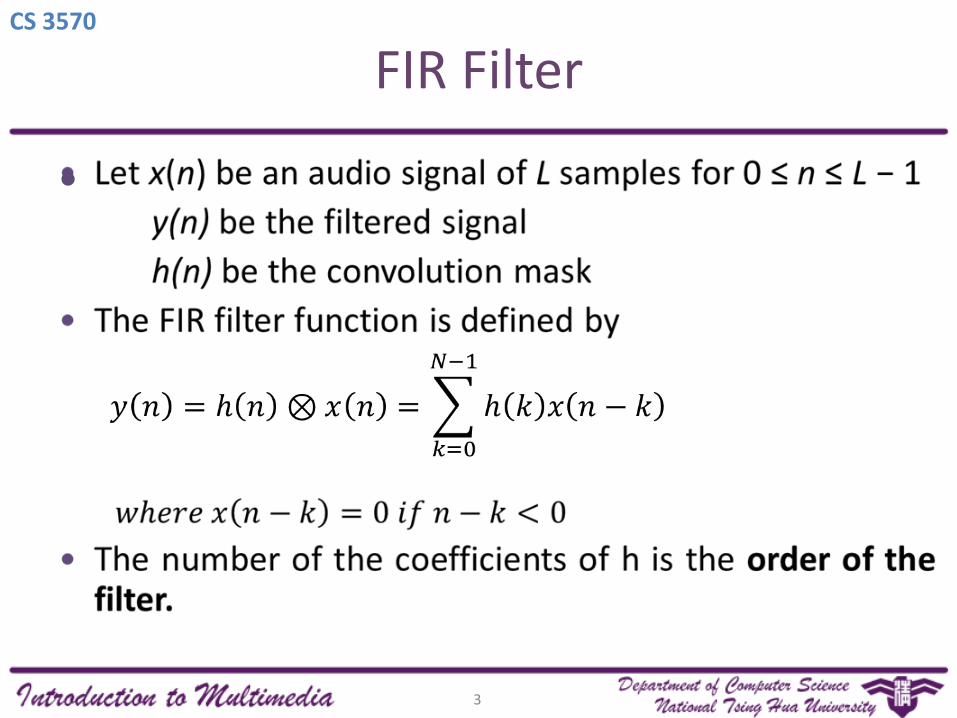
FIR Filter

•

3

CS 3570

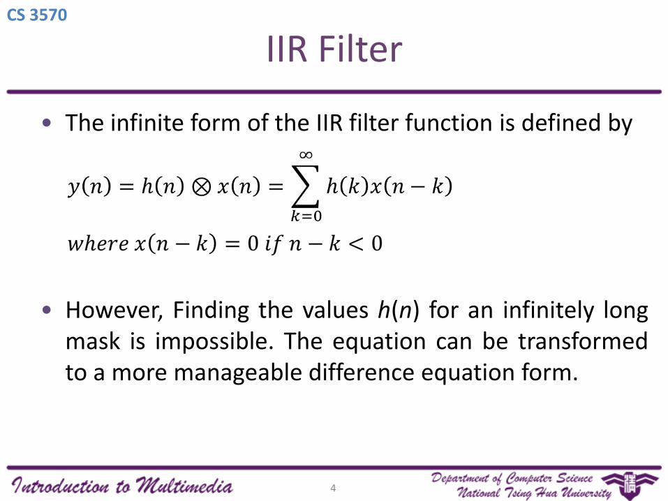
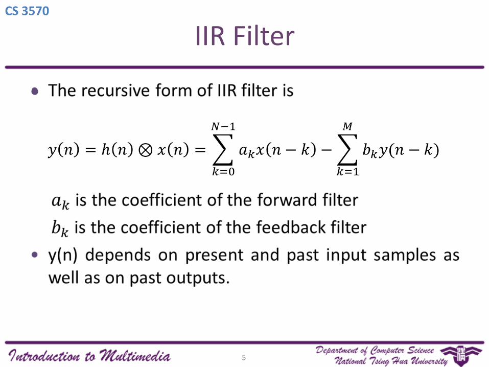
IIR Filter

• The infinite form of the IIR filter function is defined by

• However, Finding the values h(n) for an infinitely longmask is impossible. The equation can be transformedto a more manageable difference equation form.

4

CS 3570

IIR Filter

•

5

CS 3570

Impulse and Frequency Response

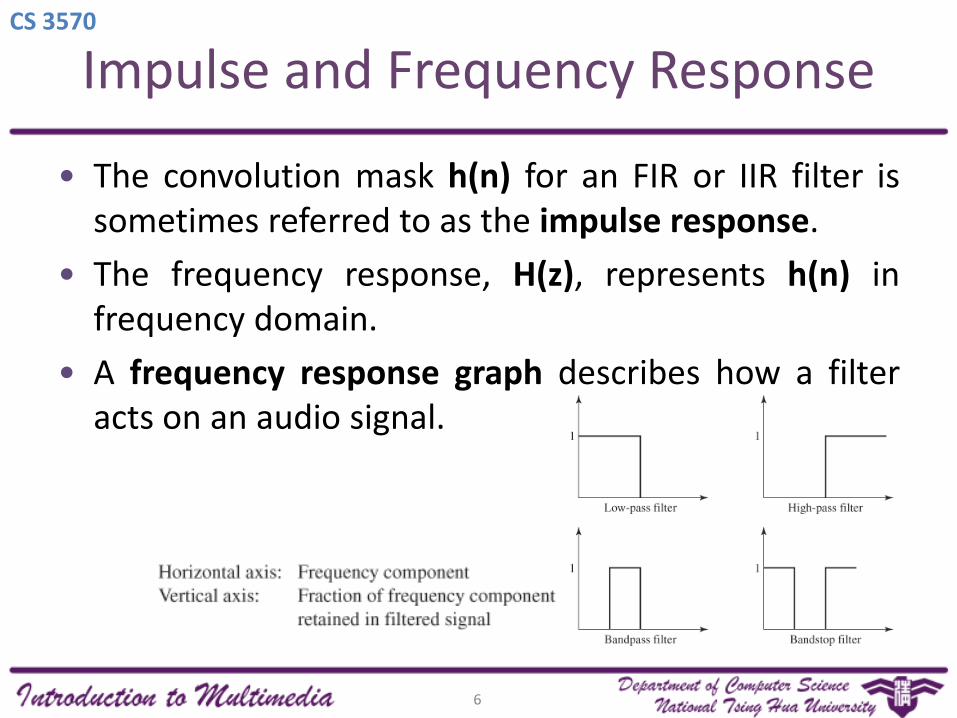
• The convolution mask h(n) for an FIR or IIR filter issometimes referred to as the impulse response.

• The frequency response, H(z), represents h(n) infrequency domain.

• A frequency response graph describes how a filteracts on an audio signal.

6

CS 3570 Filters and Related Tools in Audio Processing Software

• band filters• low-pass filter—retains only frequencies below a given level.

• high-pass filter—retains only frequencies above a given level.

• bandpass filter—retains only frequencies within a given band.

• bandstop filter—eliminates all frequencies within a given band.

• convolution filters— FIR filters that can be used to addan acoustical environment to a sound file—for example,mimicking the reverberations of a concert hall.

7

CS 3570 Filters and Related Tools in Audio Processing Software

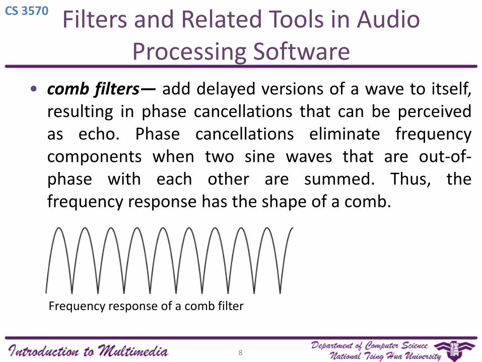
• comb filters— add delayed versions of a wave to itself,resulting in phase cancellations that can be perceivedas echo. Phase cancellations eliminate frequencycomponents when two sine waves that are out-of-phase with each other are summed. Thus, thefrequency response has the shape of a comb.

Frequency response of a comb filter

8

CS 3570 Filters and Related Tools in Audio Processing Software

• graphic equalizer—gives a graphical view that allowsyou to adjust the gain of frequencies within an array ofbands.

• parametric equalizer—similar to a graphic equalizerbut with control over the width of frequency bandsrelative to their location.

9

CS 3570

Equalization

• Equalization (EQ) is the process of selectivelyboosting or cutting certain frequency components inan audio signal.

• EQ tools

• Shelving filter

• Graphic equalizer

• Parametric EQ

10

CS 3570

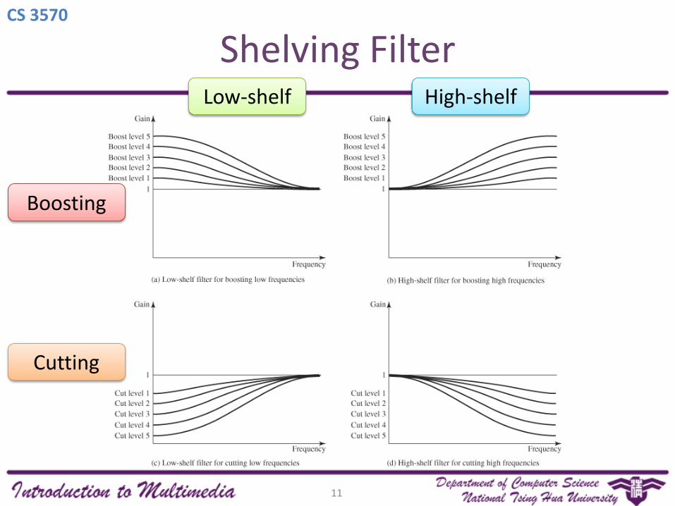
Shelving FilterLow-shelf High-shelf

Boosting

Cutting

11

CS 3570

Graphic Equalizer

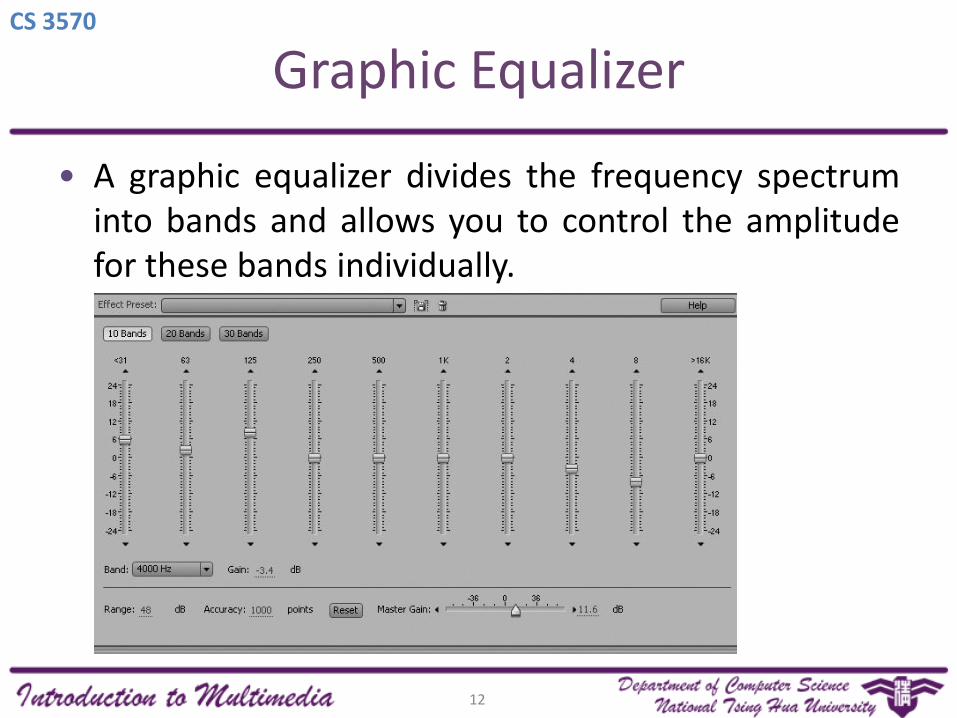
• A graphic equalizer divides the frequency spectruminto bands and allows you to control the amplitudefor these bands individually.

12

CS 3570

Parametric EQ

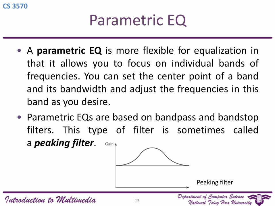
• A parametric EQ is more flexible for equalization inthat it allows you to focus on individual bands offrequencies. You can set the center point of a bandand its bandwidth and adjust the frequencies in thisband as you desire.

• Parametric EQs are based on bandpass and bandstopfilters. This type of filter is sometimes calleda peaking filter.

Peaking filter

13

CS 3570

Parametric EQ

• Q-factor(quality factor): determines how steep andwide the peaking curve is.

• The higher the Q, the steeper the peak of the band.

14

CS 3570Relationship Between Convolution and Fourier Transform

•

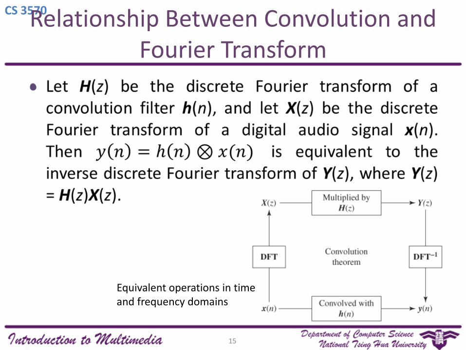
Equivalent operations in time and frequency domains

15

CS 3570

FIR Filter Design

• The following section introduces a simplemethod to design your own filters.

16

CS 3570

FIR Filter Design – Terms

• The convolution mask h(n) is also called the impulseresponse, representing a filter in the time domain.

• Its counterpart in the frequency domain,the frequency response H(z), is also sometimesreferred to as the transfer function.

• A frequency response graph can be used to showthe desired frequency response of a filter you aredesigning.

17

CS 3570

FIR Filter Design – Ideal Filter

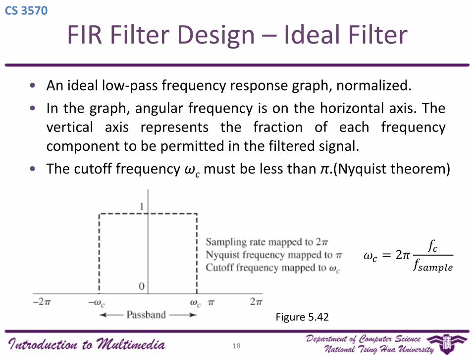
• An ideal low-pass frequency response graph, normalized.

• In the graph, angular frequency is on the horizontal axis. Thevertical axis represents the fraction of each frequencycomponent to be permitted in the filtered signal.

• The cutoff frequency ωc must be less than π.(Nyquist theorem)

Figure 5.42

18

CS 3570

FIR Filter Design – Ideal Filter

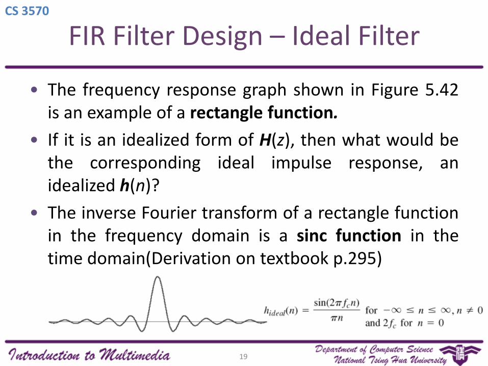
• The frequency response graph shown in Figure 5.42is an example of a rectangle function.

• If it is an idealized form of H(z), then what would bethe corresponding ideal impulse response, anidealized h(n)?

• The inverse Fourier transform of a rectangle functionin the frequency domain is a sinc function in thetime domain(Derivation on textbook p.295)

19

CS 3570

FIR Filter Design – Ideal Filter

20

CS 3570

FIR Filter Design – Ideal to Real

• A sinc function goes on infinitely in the positive andnegative directions … how can we implement an FIRfilter?

• One way is to multiply the ideal impulse response bya windowing function. The purpose of thewindowing function is to make the impulse responsefinite.

• However, making the impulse response finite resultsin a frequency response that is less than ideal,containing “ripples”.

21

CS 3570

FIR Filter Design - Realistic

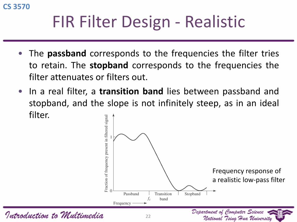
• The passband corresponds to the frequencies the filter triesto retain. The stopband corresponds to the frequencies thefilter attenuates or filters out.

• In a real filter, a transition band lies between passband andstopband, and the slope is not infinitely steep, as in an idealfilter.

Frequency response of a realistic low-pass filter

22

CS 3570

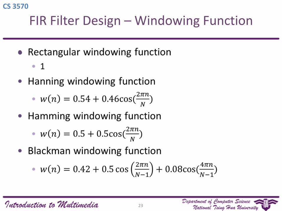
FIR Filter Design – Windowing Function

•

23

CS 3570

FIR Filter Design - Algorithm

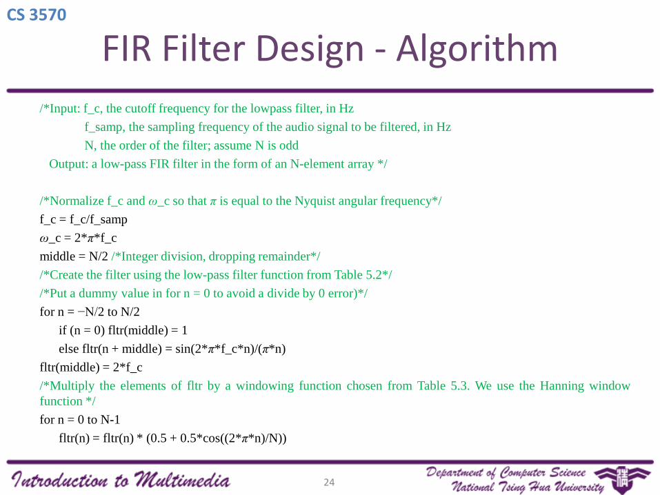
/*Input: f_c, the cutoff frequency for the lowpass filter, in Hz

f_samp, the sampling frequency of the audio signal to be filtered, in Hz

N, the order of the filter; assume N is odd

Output: a low-pass FIR filter in the form of an N-element array */

/*Normalize f_c and ω_c so that π is equal to the Nyquist angular frequency*/

f_c = f_c/f_samp

ω_c = 2*π*f_c

middle = N/2 /*Integer division, dropping remainder*/

/*Create the filter using the low-pass filter function from Table 5.2*/

/*Put a dummy value in for n = 0 to avoid a divide by 0 error)*/

for n = −N/2 to N/2

if (n = 0) fltr(middle) = 1

else fltr(n + middle) = sin(2*π*f_c*n)/(π*n)

fltr(middle) = 2*f_c

/*Multiply the elements of fltr by a windowing function chosen from Table 5.3. We use the Hanning window

function */

for n = 0 to N-1

fltr(n) = fltr(n) * (0.5 + 0.5*cos((2*π*n)/N))

24

CS 3570

Digital Audio Compression

• Time-Based Compression Methods

• No need to transform the data into frequency domain.

• A-law encoding, μ-law encoding(Ch4) … etc.

• These methods are often considered conversiontechniques rather than compression methods.

• The most effective audio compression methodsrequire some information about the frequencyspectrum of the audio signal. These compressionmethods are based on psychoacoustical modelingand perceptual encoding.

25

CS 3570

Psychoacoustics

• Psychoacoustics (心理聲學)

• The study of subjective human perception of sounds.

• The study of all the psychological interactions between humansand the world of sound.

• Psychoacoustical tests have shown that there is a greatdeal of nonlinearity in human sound perception.

• The octave from middle C (called C4) to C5 ranges from261.63 Hz to 523.25 Hz, while C5 to C6 ranges from523.25 to 1046.50 Hz. But the distance from C4 to C5subjectively sounds the same as the distance from C5 toC6.

26

CS 3570

Psychoacoustics

• Humans hear best in the 1000 to 5000 Hz range, thefrequency range of human speech.

• For a 100Hz and 1000Hz tone, the 100Hz tone needlarger amplitude to sound equally loud as the 1000Hz.

• Similarly, For a 10000Hz and 1000Hz tone, the 10000Hztone need larger amplitude to sound equally loud asthe 1000Hz.

27

CS 3570

Psychoacoustics

• At low frequencies, we can distinguish between soundwaves that are only a few Hz apart. At high frequencies,the frequencies must be a hundred or more Hz apartfor us to hear the difference. The reason is that the earis divided into frequency bands called critical bands.

• Human ear perceive different frequencies by theresponse of different critical bands.

• Critical bands are narrower for low- than for high-frequency sounds. Between 1 and 500 Hz, bands areabout 100 Hz in width. The critical band at the highestaudible frequency is over 4000 Hz wide.

28

CS 3570

Psychoacoustics

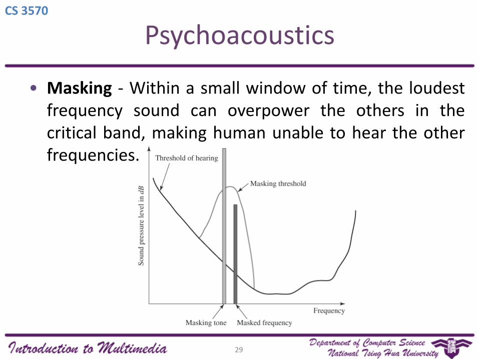
• Masking - Within a small window of time, the loudestfrequency sound can overpower the others in thecritical band, making human unable to hear the otherfrequencies.

29

CS 3570

A Sketch of Compression

• A small window of time called a frame is movedacross a sound file.

• In each frame, use different filters to divide theframe into bands of different frequencies.

• Calculate the masking curve for each band.

• Requantize the samples using fewer bits such thatthe quantization error is below the masking curve.That is, make sure the noise is inaudible.

30

CS 3570

Overview of MPEG

• Acronym for the Motion Picture Experts Group, afamily of compression algorithms for both digitalaudio and video.

• MPEG has been developed in a number of phases:MPEG-1, MPEG-2, MPEG-4, MPEG-7. Each is targetedat a different aspect of multimedia communication.

• MPEG-1 covers CD quality and audio suitable forvideo games.

31

CS 3570

Overview of MPEG

• MPEG audio is also divided into three layers: AudioLayers I, II, and III.

• Each higher layer is more computationally complex,and generally more efficient at lower bitrates thanthe previous.

• The well-known MP3 audio file format isactually MPEG-1 Audio Layer III.

32

CS 3570

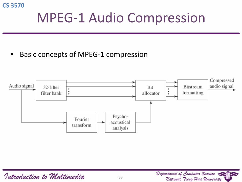
MPEG-1 Audio Compression

• Basic concepts of MPEG-1 compression

33

CS 3570

MPEG-1 Audio Compression - Step 1

• Divide the audio file into frames and analyze thepsychoacoustical properties of each frameindividually.

• To analyze the masking phenomenon, we must look at asmall piece of time because it happens when differentfrequencies are played at close to the same time.

• Frames can contain 384, 576, or 1152 samples, dependingon the MPEG phase and layer.

• For the remainder of these steps, it is assumed that we’reoperating on an individual frame.

34

CS 3570

MPEG-1 Audio Compression - Step 2

• By applying a bank of filters, separate the signal intofrequency bands.

• The samples are divided into frequency bands forpsychoacoustical analysis. Each filter removes allfrequencies except for those in its designated band.

• The use of filter banks is called subband coding. In MPEG-1,the number of filters is 32.

• In MPEG-1 Layers I and II, the frequency bands created bythe filter banks are uniform in size, which doesn’t matchthe width of the critical bands in human hearing. Layer IIImodels critical bands more closely than layer I and II.

35

CS 3570

MPEG-1 Audio Compression - Step 3

• Perform a Fourier transform on the samples in eachband in order to analyze the band’s frequencyspectrum.

• After the Fourier transform, we can know exactly howmuch of each frequency component occurs in each band.

• From the frequency spectrum, a masking curve can beproduced for each band.

36

CS 3570

MPEG-1 Audio Compression - Step 4

• Analyze the influence of tonal and nontonal elementsin each band. (Tonal elements are simple sinusoidalcomponents, such as frequencies related to melodicand harmonic music. Nontonal elements are transientslike the strike of a drum or the clapping of hands.)

• If the frame size is small, then the time resolution is poor.This in turn can mean that transient signals may not beproperly identified. Therefore we’d better identify thetransient first.

37

CS 3570

MPEG-1 Audio Compression - Step 5

• Determine how much each band’s influence is likely tospread to neighboring frequency bands.

• It isn’t sufficient to deal with bands entirely in isolation fromeach other, since there can be a masking effect betweenbands.

38

CS 3570

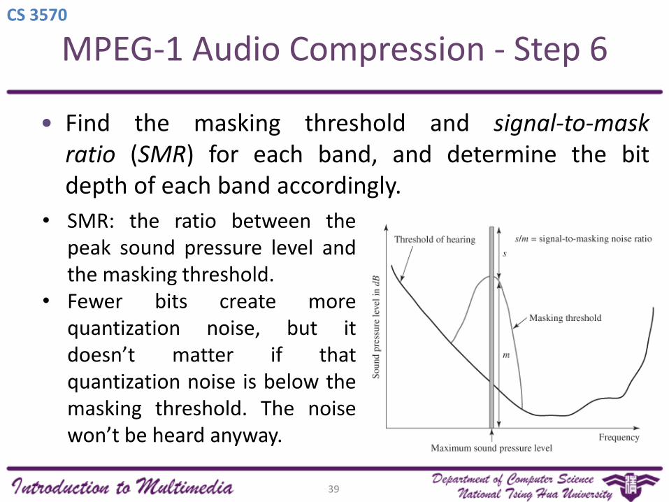
MPEG-1 Audio Compression - Step 6

• Find the masking threshold and signal-to-maskratio (SMR) for each band, and determine the bitdepth of each band accordingly.

• SMR: the ratio between thepeak sound pressure level andthe masking threshold.

• Fewer bits create morequantization noise, but itdoesn’t matter if thatquantization noise is below themasking threshold. The noisewon’t be heard anyway.

39

CS 3570

MPEG-1 Audio Compression - Step 7

• Quantize the samples for the band with theappropriate number of bits, possibly following thiswith Huffman encoding.

• MPEG-1 Layers 1 and 2 use linear quantization, while MP3uses nonlinear.

40