Embed Size (px)
Citation preview
Digital Communication
Lecture-1, Prof. Dr. Habibullah
Jamal
Under Graduate, Spring 2008
Text: Digital Communications: Fundamentals and Applications, By “Bernard Sklar”,
Prentice Hall, 2nd ed, 2001. Probability and Random Signals for Electrical Engineers, Neon Garcia
References: Digital Communications, Fourth Edition, J.G. Proakis, McGraw Hill, 2000.
Course Books
Course Outline Review of Probability
Signal and Spectra (Chapter 1)
Formatting and Base band Modulation (Chapter 2)
Base band Demodulation/Detection (Chapter 3)
Channel Coding (Chapter 6, 7 and 8)
Band pass Modulation and Demod./Detect.
(Chapter 4)
Spread Spectrum Techniques (Chapter 12)
Synchronization (Chapter 10)
Source Coding (Chapter 13)
Fading Channels (Chapter 15)
Today’s Goal
Review of Basic Probability
Digital Communication Basic

Communication
Main purpose of communication is to transfer information
from a source to a recipient via a channel or medium.
Basic block diagram of a communication system:
Source Transmitter Receiver
Recipient
Channel
Brief Description
Source: analog or digital
Transmitter: transducer, amplifier, modulator, oscillator, power
amp., antenna
Channel: e.g. cable, optical fibre, free space
Receiver: antenna, amplifier, demodulator, oscillator, power
amplifier, transducer
Recipient: e.g. person, (loud) speaker, computer
Types of information
Voice, data, video, music, email etc.
Types of communication systems
Public Switched Telephone Network (voice,fax,modem)
Satellite systems
Radio,TV broadcasting
Cellular phones
Computer networks (LANs, WANs, WLANs)
Information Representation
Communication system converts information into electrical electromagnetic/optical signals appropriate for the transmission medium.
Analog systems convert analog message into signals that can propagate through the channel.
Digital systems convert bits(digits, symbols) into signals
Computers naturally generate information as characters/bits
Most information can be converted into bits
Analog signals converted to bits by sampling and quantizing (A/D conversion)
Why digital?
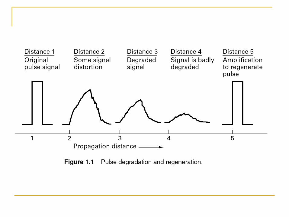
Digital techniques need to distinguish between discrete symbols allowing regeneration versus amplification
Good processing techniques are available for digital signals, such as medium.
Data compression (or source coding)
Error Correction (or channel coding)(A/D conversion)
Equalization
Security
Easy to mix signals and data using digital techniques
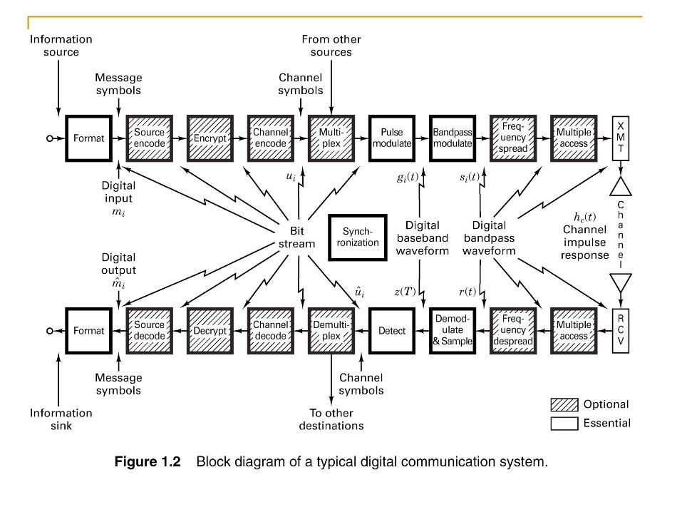
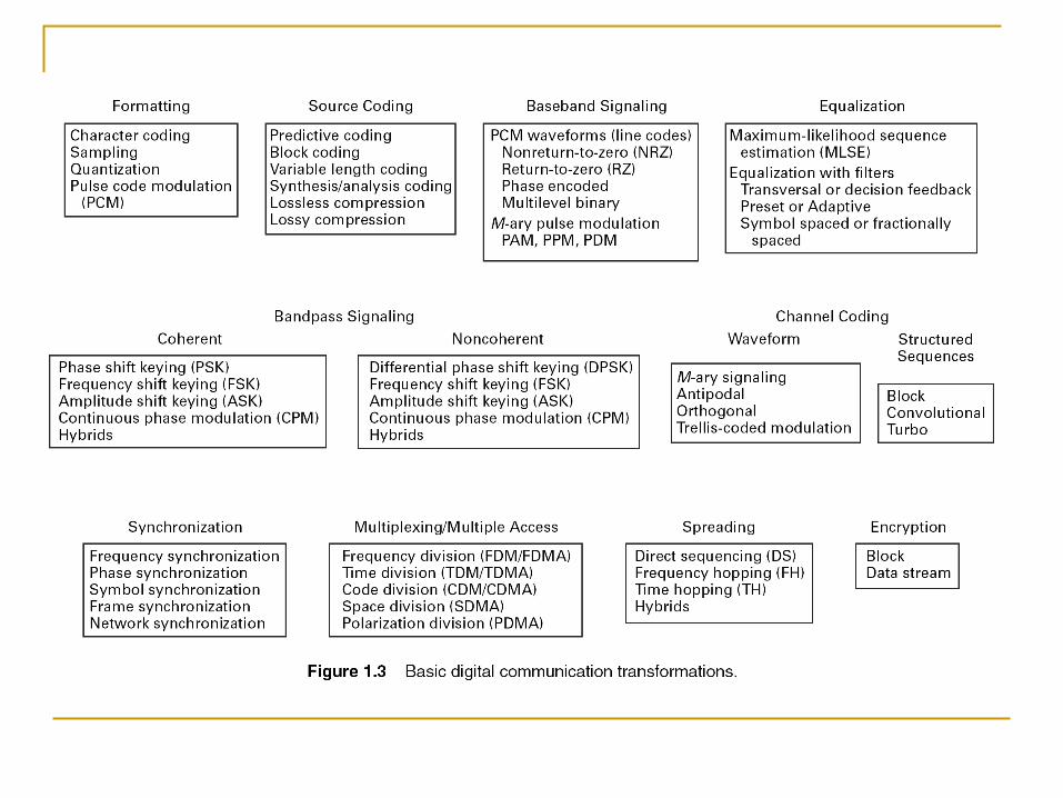
Basic Digital Communication Transformations Formatting/Source Coding
Transforms source info into digital symbols (digitization)
Selects compatible waveforms (matching function)
Introduces redundancy which facilitates accurate decoding despite errors
It is essential for reliable communication Modulation/Demodulation
Modulation is the process of modifying the info signal to facilitate transmission
Demodulation reverses the process of modulation. It involves the detection and retrieval of the info signal
Types
Coherent: Requires a reference info for detection
Noncoherent: Does not require reference phase information
Basic Digital Communication Transformations
Coding/Decoding
Translating info bits to transmitter data symbols
Techniques used to enhance info signal so that they are less vulnerable to channel impairment (e.g. noise, fading, jamming, interference) Two Categories
Waveform Coding
Produces new waveforms with better performance Structured Sequences
Involves the use of redundant bits to determine the occurrence of error (and sometimes correct it) Multiplexing/Multiple Access Is synonymous with resource
sharing with other users
Frequency Division Multiplexing/Multiple Access (FDM/FDMA
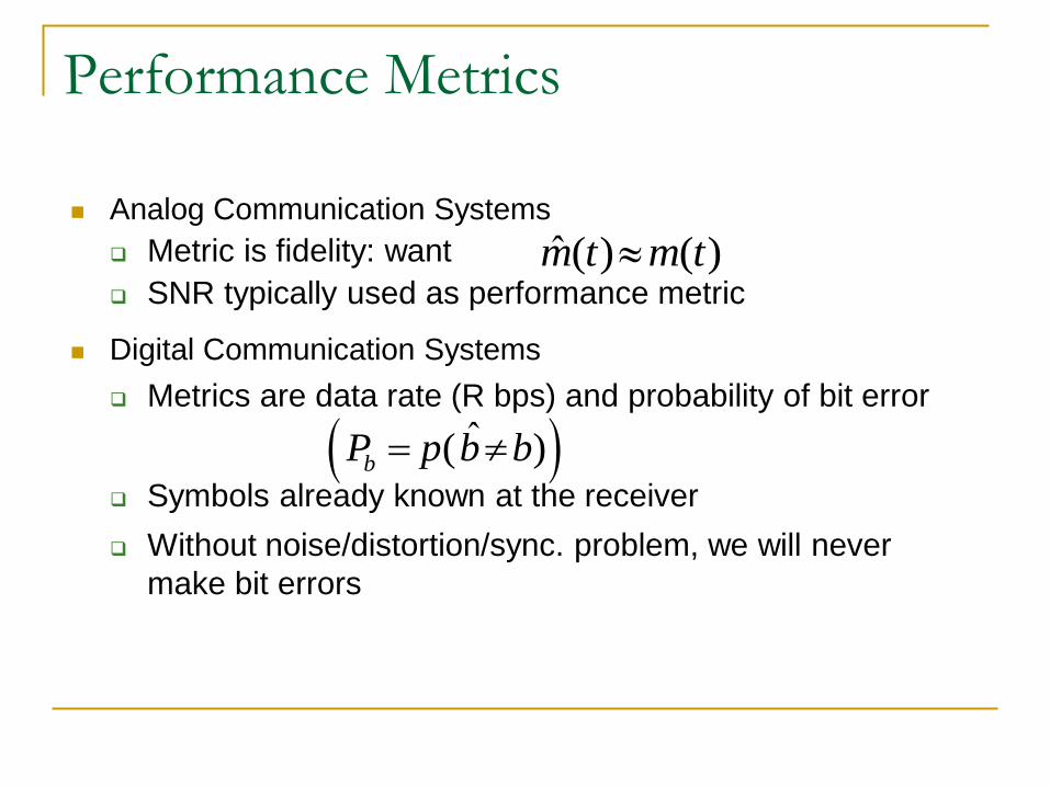
Performance Metrics
Analog Communication Systems
Metric is fidelity: want
SNR typically used as performance metric
Digital Communication Systems
Metrics are data rate (R bps) and probability of bit error
Symbols already known at the receiver
Without noise/distortion/sync. problem, we will never
make bit errors
ˆ ( ) ( )m t m t
ˆ( )bP p b b

Main Points
Transmitters modulate analog messages or bits in case of a DCS
for transmission over a channel.
Receivers recreate signals or bits from received signal (mitigate
channel effects)
Performance metric for analog systems is fidelity, for digital it is
the bit rate and error probability.
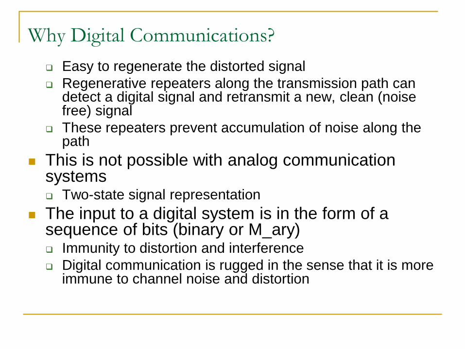
Why Digital Communications? Easy to regenerate the distorted signal
Regenerative repeaters along the transmission path can detect a digital signal and retransmit a new, clean (noise free) signal
These repeaters prevent accumulation of noise along the path
This is not possible with analog communication systems Two-state signal representation
The input to a digital system is in the form of a sequence of bits (binary or M_ary) Immunity to distortion and interference
Digital communication is rugged in the sense that it is more immune to channel noise and distortion
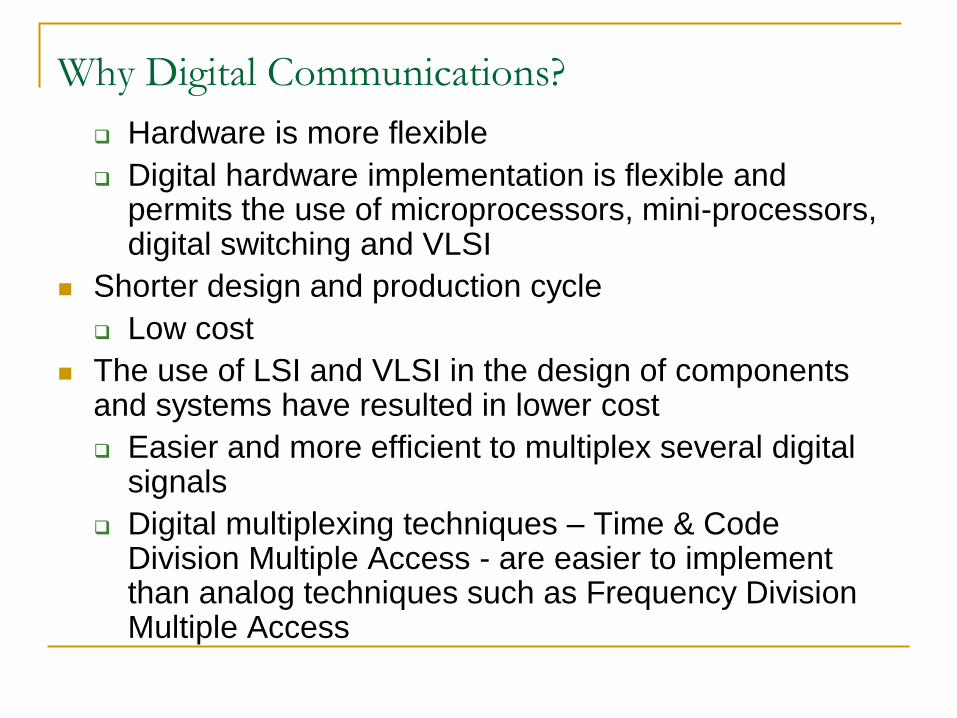
Why Digital Communications? Hardware is more flexible
Digital hardware implementation is flexible and permits the use of microprocessors, mini-processors, digital switching and VLSI
Shorter design and production cycle
Low cost
The use of LSI and VLSI in the design of components and systems have resulted in lower cost
Easier and more efficient to multiplex several digital signals
Digital multiplexing techniques – Time & Code Division Multiple Access - are easier to implement than analog techniques such as Frequency Division Multiple Access
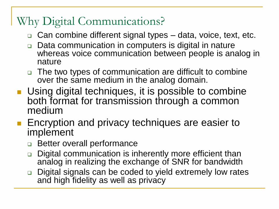
Why Digital Communications? Can combine different signal types – data, voice, text, etc.
Data communication in computers is digital in nature whereas voice communication between people is analog in nature
The two types of communication are difficult to combine over the same medium in the analog domain.
Using digital techniques, it is possible to combine both format for transmission through a common medium
Encryption and privacy techniques are easier to implement Better overall performance
Digital communication is inherently more efficient than analog in realizing the exchange of SNR for bandwidth
Digital signals can be coded to yield extremely low rates and high fidelity as well as privacy
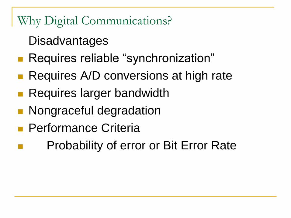
Why Digital Communications?
Disadvantages
Requires reliable ―synchronization‖
Requires A/D conversions at high rate
Requires larger bandwidth
Nongraceful degradation
Performance Criteria
Probability of error or Bit Error Rate
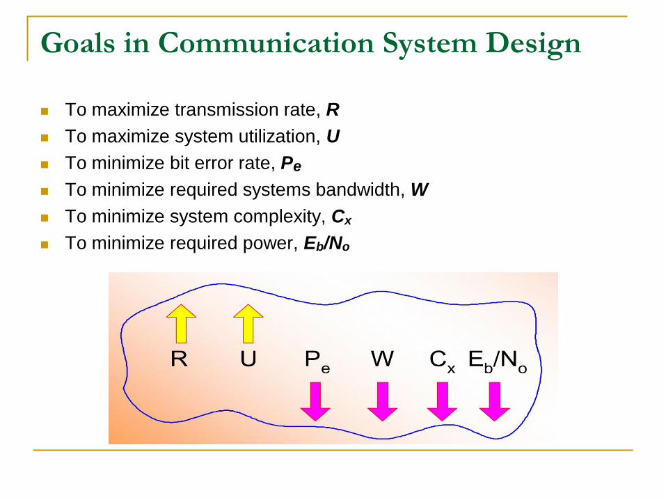
Goals in Communication System Design
To maximize transmission rate, R
To maximize system utilization, U
To minimize bit error rate, Pe
To minimize required systems bandwidth, W
To minimize system complexity, Cx
To minimize required power, Eb/No
Comparative Analysis of Analog and
Digital Communication
Digital Signal Nomenclature
Information Source
Discrete output values e.g. Keyboard
Analog signal source e.g. output of a microphone
Character
Member of an alphanumeric/symbol (A to Z, 0 to 9)
Characters can be mapped into a sequence of binary digits
using one of the standardized codes such as
ASCII: American Standard Code for Information Interchange
EBCDIC: Extended Binary Coded Decimal Interchange Code
Digital Signal Nomenclature
Digital Message
Messages constructed from a finite number of symbols; e.g., printed
language consists of 26 letters, 10 numbers, ―space‖ and several
punctuation marks. Hence a text is a digital message constructed from
about 50 symbols
Morse-coded telegraph message is a digital message constructed from
two symbols ―Mark‖ and ―Space‖
M - ary
A digital message constructed with M symbols
Digital Waveform
Current or voltage waveform that represents a digital symbol
Bit Rate
Actual rate at which information is transmitted per second
Digital Signal Nomenclature
Baud Rate
Refers to the rate at which the signaling elements are
transmitted, i.e. number of signaling elements per
second.
Bit Error Rate
The probability that one of the bits is in error or simply
the probability of error

1.2 Classification Of Signals
1. Deterministic and Random Signals
A signal is deterministic means that there is no uncertainty with
respect to its value at any time.
Deterministic waveforms are modeled by explicit mathematical
expressions, example:
A signal is random means that there is some degree of
uncertainty before the signal actually occurs.
Random waveforms/ Random processes when examined over a
long period may exhibit certain regularities that can be described
in terms of probabilities and statistical averages.
x(t) = 5Cos(10t)
2. Periodic and Non-periodic Signals
A signal x(t) is called periodic in time if there exists a constant
T0 > 0 such that
(1.2)
t denotes time
T0 is the period of x(t).
0x(t) = x(t + T ) for - < t <
3. Analog and Discrete Signals
An analog signal x(t) is a continuous function of time; that is, x(t)
is uniquely defined for all t
A discrete signal x(kT) is one that exists only at discrete times; it
is characterized by a sequence of numbers defined for each time,
kT, where
k is an integer
T is a fixed time interval.
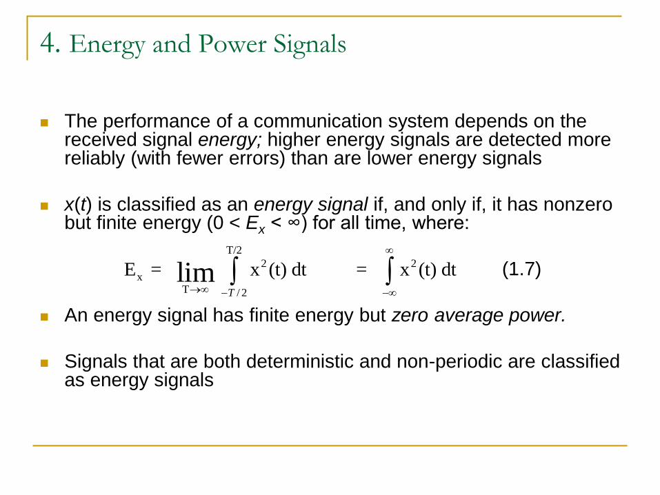
4. Energy and Power Signals
The performance of a communication system depends on the received signal energy; higher energy signals are detected more reliably (with fewer errors) than are lower energy signals
x(t) is classified as an energy signal if, and only if, it has nonzero but finite energy (0 < Ex < ∞) for all time, where:
(1.7)
An energy signal has finite energy but zero average power.
Signals that are both deterministic and non-periodic are classified as energy signals
T/2
2 2
xT / 2
E = x (t) dt = x (t) dtlimT
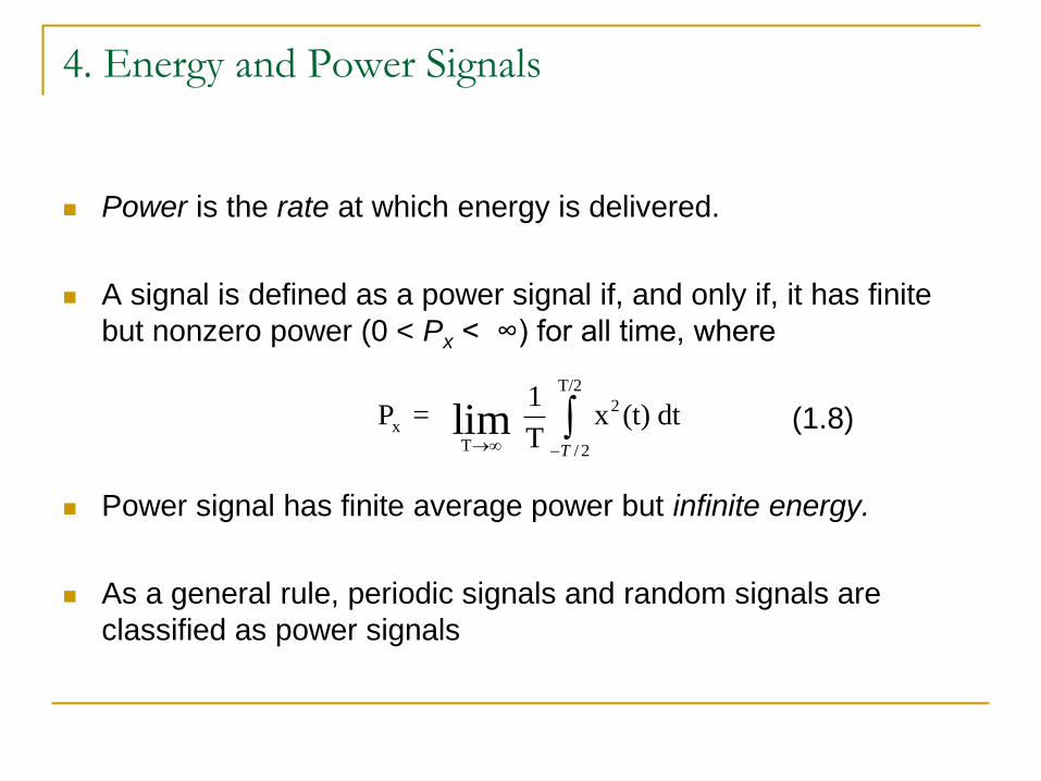
Power is the rate at which energy is delivered.
A signal is defined as a power signal if, and only if, it has finite
but nonzero power (0 < Px < ∞) for all time, where
(1.8)
Power signal has finite average power but infinite energy.
As a general rule, periodic signals and random signals are
classified as power signals
4. Energy and Power Signals
T/2
2
xT / 2
1P = x (t) dt
Tlim
T
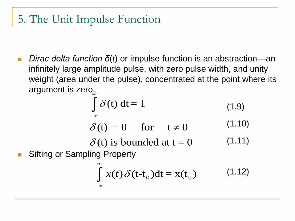
Dirac delta function δ(t) or impulse function is an abstraction—an
infinitely large amplitude pulse, with zero pulse width, and unity
weight (area under the pulse), concentrated at the point where its
argument is zero.
(1.9)
(1.10)
(1.11)
Sifting or Sampling Property
(1.12)
5. The Unit Impulse Function
(t) dt = 1
(t) = 0 for t 0
(t) is bounded at t 0
0 0( ) (t-t )dt = x(t ) x t
1.3 Spectral Density
The spectral density of a signal characterizes the distribution of
the signal’s energy or power in the frequency domain.
This concept is particularly important when considering filtering in
communication systems while evaluating the signal and noise at
the filter output.
The energy spectral density (ESD) or the power spectral density
(PSD) is used in the evaluation.
1. Energy Spectral Density (ESD)
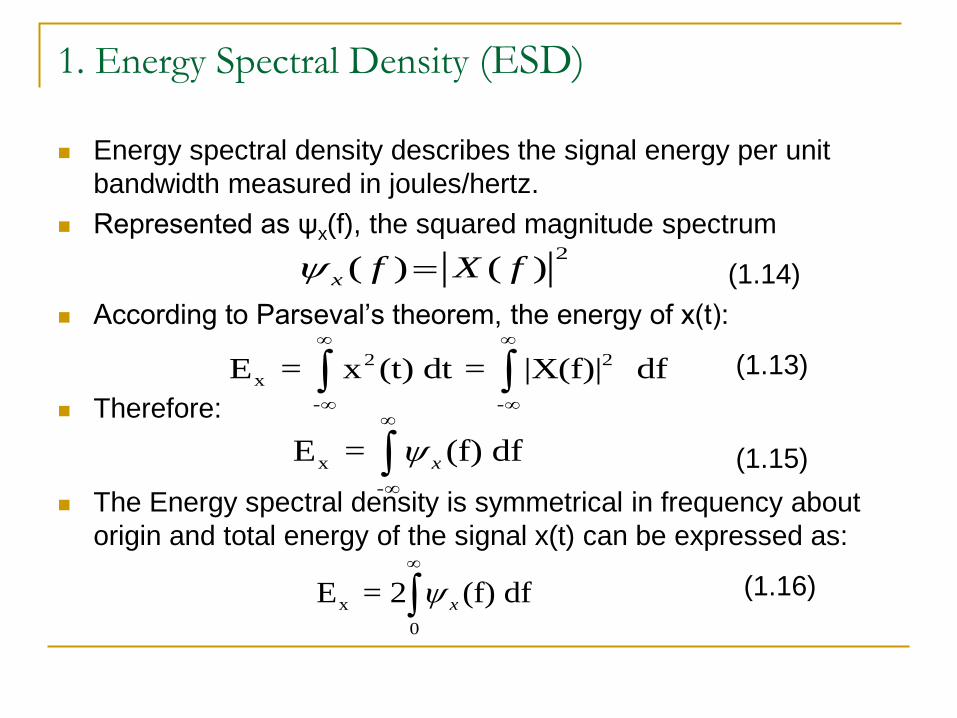
Energy spectral density describes the signal energy per unit
bandwidth measured in joules/hertz.
Represented as ψx(f), the squared magnitude spectrum
(1.14)
According to Parseval’s theorem, the energy of x(t):
(1.13)
Therefore:
(1.15)
The Energy spectral density is symmetrical in frequency about
origin and total energy of the signal x(t) can be expressed as:
(1.16)
2( ) ( )x f X f
2 2
x
- -
E = x (t) dt = |X(f)| df
x
-
E = (f) dfx
x
0
E = 2 (f) dfx

2. Power Spectral Density (PSD)
The power spectral density (PSD) function Gx(f ) of the periodic
signal x(t) is a real, even, and nonnegative function of frequency
that gives the distribution of the power of x(t) in the frequency
domain.
PSD is represented as:
(1.18)
Whereas the average power of a periodic signal x(t) is
represented as:
(1.17)
Using PSD, the average normalized power of a real-valued
signal is represented as:
(1.19)
2
x n 0
n=-
G (f ) = |C | ( ) f nf
0
0
/2
2 2
x n
n=-0 / 2
1P x (t)dt |C |
T
TT
x x x
0
P G (f)df 2 G (f)df
1.4 Autocorrelation
1. Autocorrelation of an Energy Signal
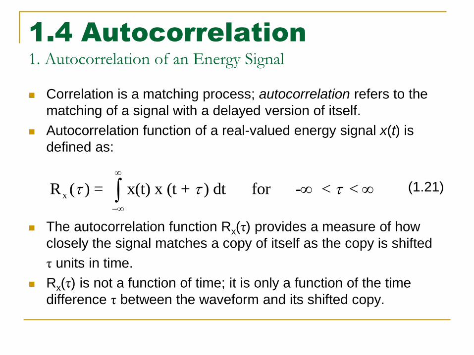
Correlation is a matching process; autocorrelation refers to the
matching of a signal with a delayed version of itself.
Autocorrelation function of a real-valued energy signal x(t) is
defined as:
(1.21)
The autocorrelation function Rx(τ) provides a measure of how
closely the signal matches a copy of itself as the copy is shifted
τ units in time.
Rx(τ) is not a function of time; it is only a function of the time
difference τ between the waveform and its shifted copy.
xR ( ) = x(t) x (t + ) dt for - < <
1. Autocorrelation of an Energy Signal
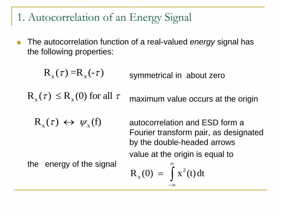
The autocorrelation function of a real-valued energy signal has
the following properties:
symmetrical in about zero
maximum value occurs at the origin
autocorrelation and ESD form a
Fourier transform pair, as designated
by the double-headed arrows
value at the origin is equal to
the energy of the signal
x xR ( ) =R (- )
x xR ( ) R (0) for all
x xR ( ) (f)
2
xR (0) x (t)dt
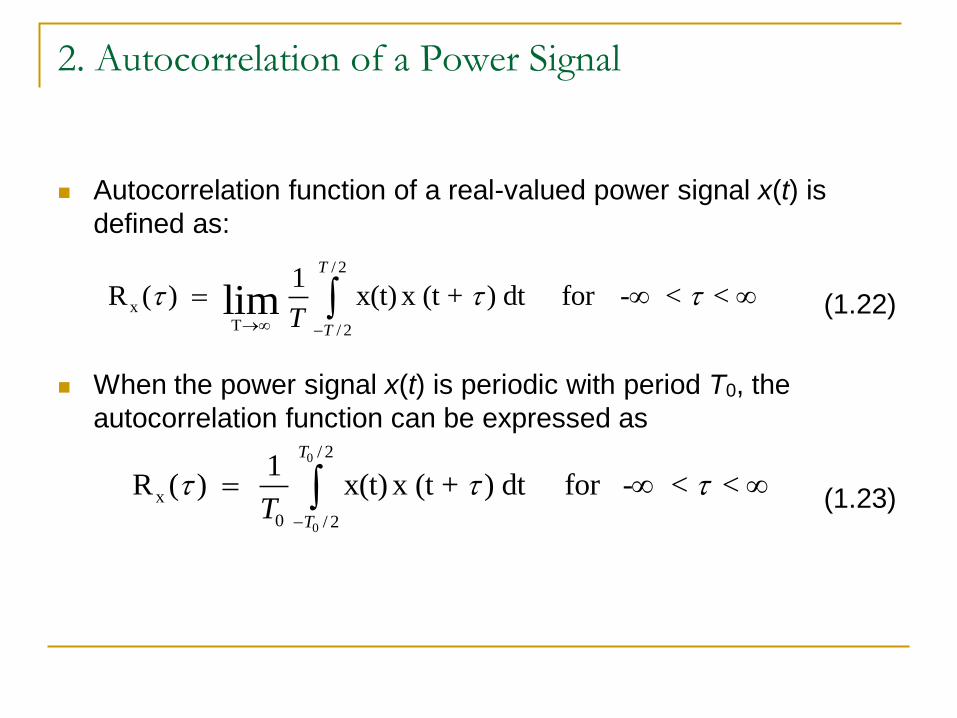
2. Autocorrelation of a Power Signal
Autocorrelation function of a real-valued power signal x(t) is
defined as:
(1.22)
When the power signal x(t) is periodic with period T0, the
autocorrelation function can be expressed as
(1.23)
/ 2
xT / 2
1R ( ) x(t) x (t + ) dt for - < < lim
T
TT
0
0
/ 2
x
0 / 2
1R ( ) x(t) x (t + ) dt for - < <
T
TT
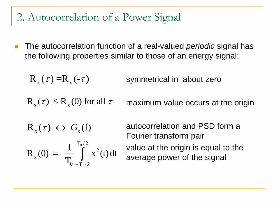
2. Autocorrelation of a Power Signal
The autocorrelation function of a real-valued periodic signal has
the following properties similar to those of an energy signal:
symmetrical in about zero
maximum value occurs at the origin
autocorrelation and PSD form a
Fourier transform pair
value at the origin is equal to the
average power of the signal
x xR ( ) =R (- )
x xR ( ) R (0) for all
x xR ( ) (f)G
0
0
T / 2
2
x
0 T / 2
1R (0) x (t)dt
T
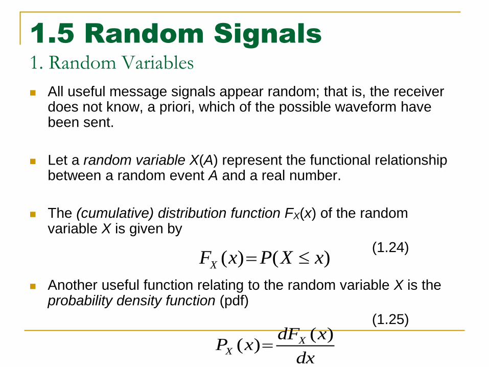
1.5 Random Signals
1. Random Variables
All useful message signals appear random; that is, the receiver does not know, a priori, which of the possible waveform have been sent.
Let a random variable X(A) represent the functional relationship between a random event A and a real number.
The (cumulative) distribution function FX(x) of the random variable X is given by
(1.24)
Another useful function relating to the random variable X is the probability density function (pdf)
(1.25)
( ) ( )XF x P X x
( )( ) X
X
dF xP x
dx
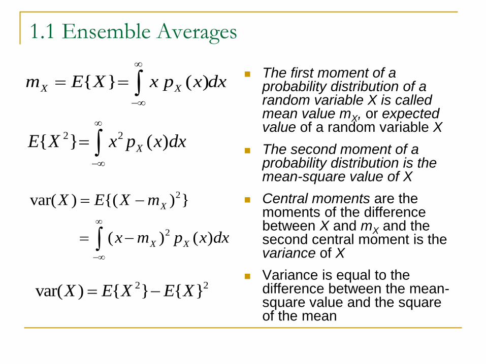
1.1 Ensemble Averages
The first moment of a probability distribution of a random variable X is called mean value mX, or expected value of a random variable X
The second moment of a probability distribution is the mean-square value of X
Central moments are the moments of the difference between X and mX and the second central moment is the variance of X
Variance is equal to the difference between the mean-square value and the square of the mean
{ } ( )X Xm E X x p x dx
2 2{ } ( )XE X x p x dx
2
2
var( ) {( ) }
( ) ( )
X
X X
X E X m
x m p x dx
2 2var( ) { } { }X E X E X
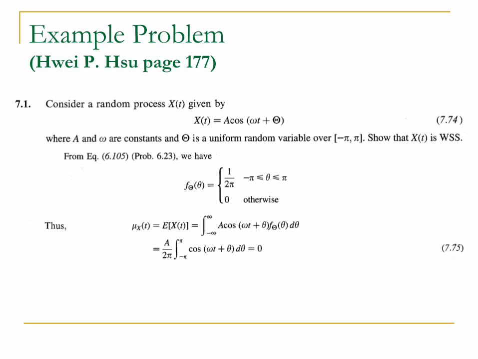
Example Problem (Hwei P. Hsu page 177)
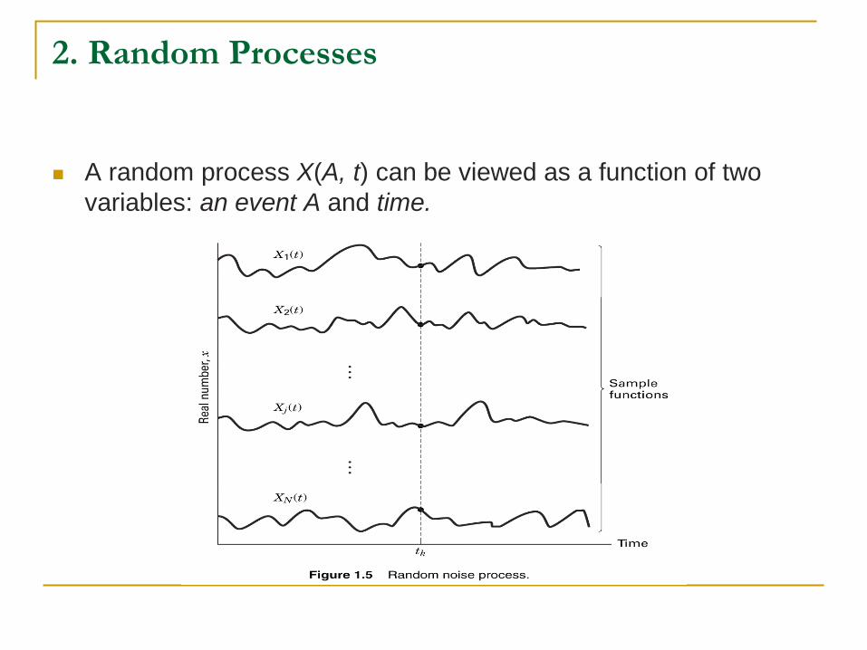
2. Random Processes
A random process X(A, t) can be viewed as a function of two
variables: an event A and time.
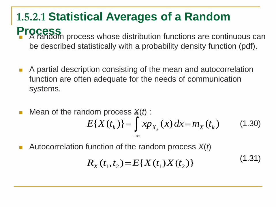
1.5.2.1 Statistical Averages of a Random
Process
A random process whose distribution functions are continuous can
be described statistically with a probability density function (pdf).
A partial description consisting of the mean and autocorrelation
function are often adequate for the needs of communication
systems.
Mean of the random process X(t) :
(1.30)
Autocorrelation function of the random process X(t)
(1.31)
{ ( )} ( ) ( )kk X X kE X t xp x dx m t
1 2 1 2( , ) { ( ) ( )}XR t t E X t X t
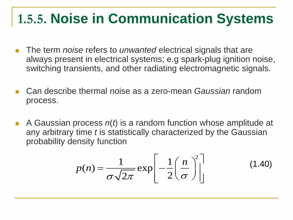
1.5.5. Noise in Communication Systems
The term noise refers to unwanted electrical signals that are
always present in electrical systems; e.g spark-plug ignition noise, switching transients, and other radiating electromagnetic signals.
Can describe thermal noise as a zero-mean Gaussian random process.
A Gaussian process n(t) is a random function whose amplitude at any arbitrary time t is statistically characterized by the Gaussian probability density function
(1.40)
21 1
( ) exp22
np n
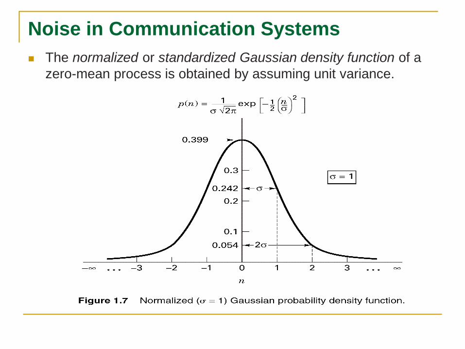
Noise in Communication Systems
The normalized or standardized Gaussian density function of a
zero-mean process is obtained by assuming unit variance.
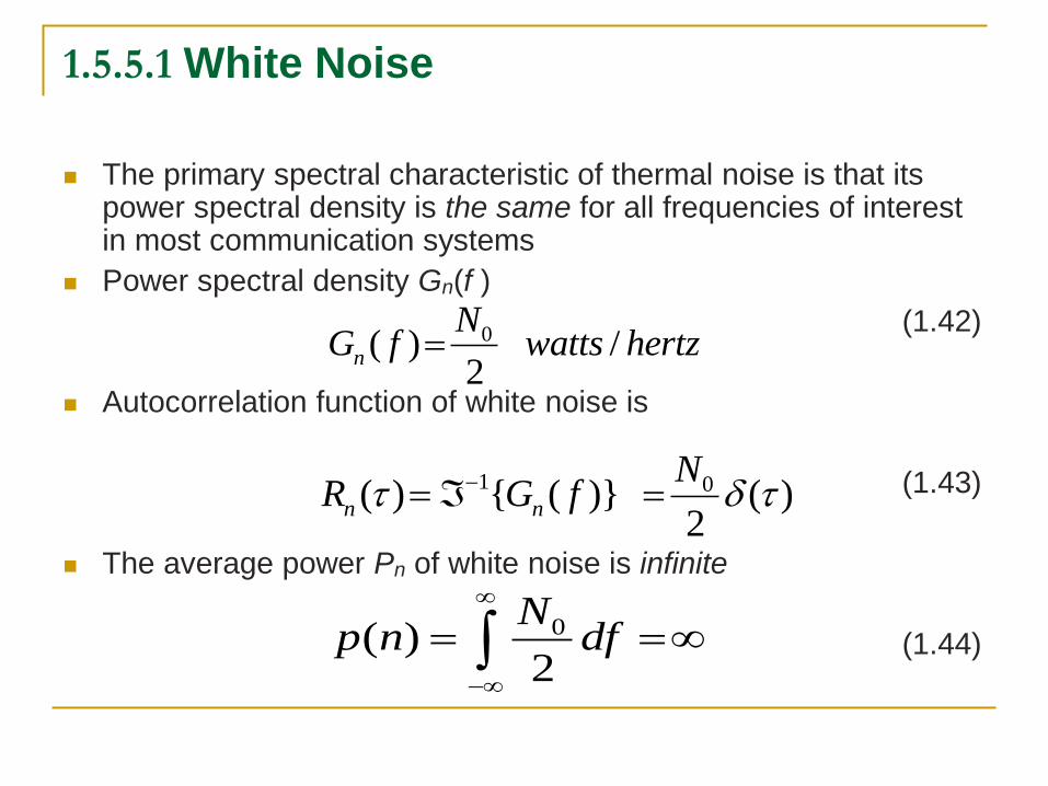
1.5.5.1 White Noise
The primary spectral characteristic of thermal noise is that its power spectral density is the same for all frequencies of interest in most communication systems
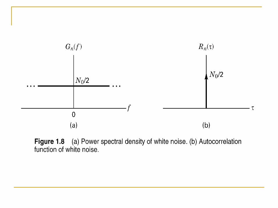
Power spectral density Gn(f )
(1.42)
Autocorrelation function of white noise is
(1.43)
The average power Pn of white noise is infinite
(1.44)
0( ) /2
n
NG f watts hertz
1 0( ) { ( )} ( )2
n n
NR G f
0( )2
Np n df
The effect on the detection process of a channel with additive
white Gaussian noise (AWGN) is that the noise affects each
transmitted symbol independently.
Such a channel is called a memoryless channel.
The term ―additive‖ means that the noise is simply superimposed
or added to the signal
1.6 Signal Transmission through
Linear Systems
A system can be characterized equally well in the time domain
or the frequency domain, techniques will be developed in both
domains
The system is assumed to be linear and time invariant.
It is also assumed that there is no stored energy in the system
at the time the input is applied
1.6.1. Impulse Response
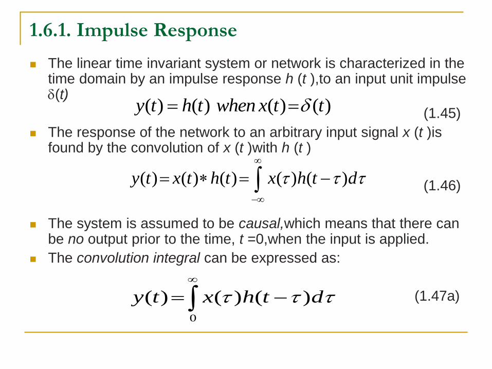
The linear time invariant system or network is characterized in the time domain by an impulse response h (t ),to an input unit impulse (t)
(1.45)
The response of the network to an arbitrary input signal x (t )is found by the convolution of x (t )with h (t )
(1.46)
The system is assumed to be causal,which means that there can be no output prior to the time, t =0,when the input is applied.
The convolution integral can be expressed as:
(1.47a)
( ) ( ) ( ) ( )y t h t when x t t
( ) ( ) ( ) ( ) ( )y t x t h t x h t d
0
( ) ( ) ( )y t x h t d
1.6.2. Frequency Transfer Function
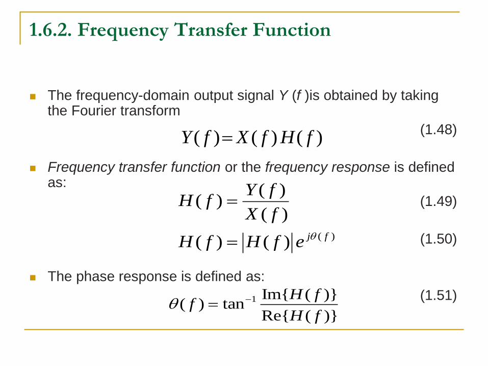
The frequency-domain output signal Y (f )is obtained by taking the Fourier transform
(1.48)
Frequency transfer function or the frequency response is defined as:
(1.49)
(1.50)
The phase response is defined as:
(1.51)
( ) ( ) ( )Y f X f H f
( )
( )( )
( )
( ) ( ) j f
Y fH f
X f
H f H f e
1 Im{ ( )}( ) tan
Re{ ( )}
H ff
H f
1.6.2.1. Random Processes and Linear Systems
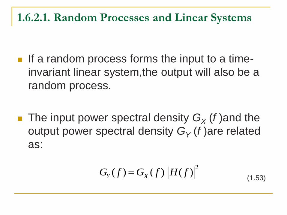
If a random process forms the input to a time-
invariant linear system,the output will also be a
random process.
The input power spectral density GX (f )and the
output power spectral density GY (f )are related
as:
(1.53)
2( ) ( ) ( )Y XG f G f H f
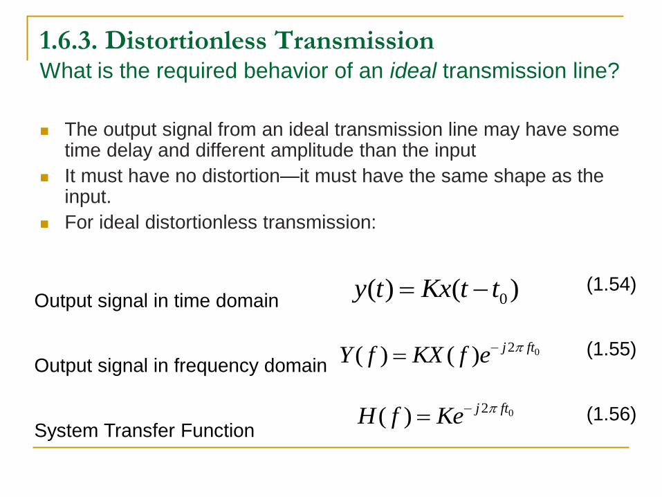
1.6.3. Distortionless Transmission What is the required behavior of an ideal transmission line?
The output signal from an ideal transmission line may have some
time delay and different amplitude than the input
It must have no distortion—it must have the same shape as the input.
For ideal distortionless transmission:
(1.54)
(1.55)
(1.56)
Output signal in time domain
Output signal in frequency domain
System Transfer Function
0( ) ( )y t Kx t t
02( ) ( )
j ftY f KX f e
02( )
j ftH f Ke
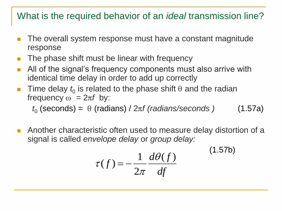
What is the required behavior of an ideal transmission line?
The overall system response must have a constant magnitude
response
The phase shift must be linear with frequency
All of the signal’s frequency components must also arrive with identical time delay in order to add up correctly
Time delay t0 is related to the phase shift and the radian frequency = 2f by:
t0 (seconds) = (radians) / 2f (radians/seconds ) (1.57a)
Another characteristic often used to measure delay distortion of a signal is called envelope delay or group delay:
(1.57b) 1 ( )
( )2
d ff
df
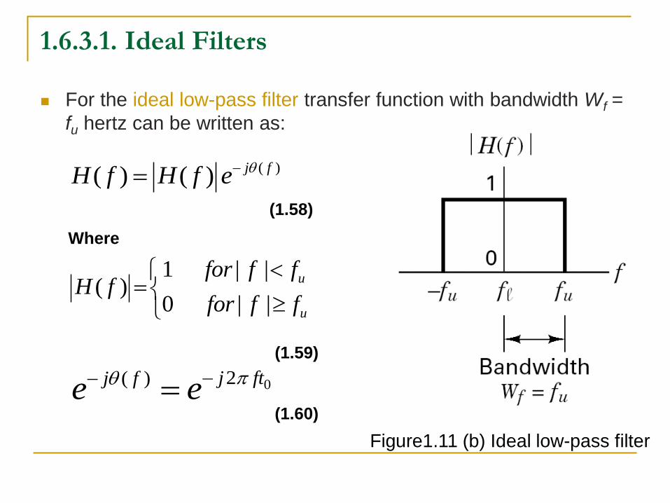
1.6.3.1. Ideal Filters
For the ideal low-pass filter transfer function with bandwidth Wf =
fu hertz can be written as:
Figure1.11 (b) Ideal low-pass filter
(1.58)
Where
(1.59)
(1.60)
( )( ) ( ) j fH f H f e
1 | |( )
0 | |
u
u
for f fH f
for f f
02( ) j ftj fe e
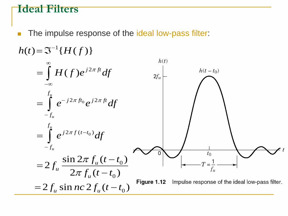
Ideal Filters
The impulse response of the ideal low-pass filter:
0
0
1
2
2 2
2 ( )
0
0
0
( ) { ( )}
( )
sin 2 ( )2
2 ( )
2 sin 2 ( )
u
u
u
u
j ft
f
j ft j ft
f
f
j f t t
f
uu
u
u u
h t H f
H f e df
e e df
e df
f t tf
f t t
f nc f t t
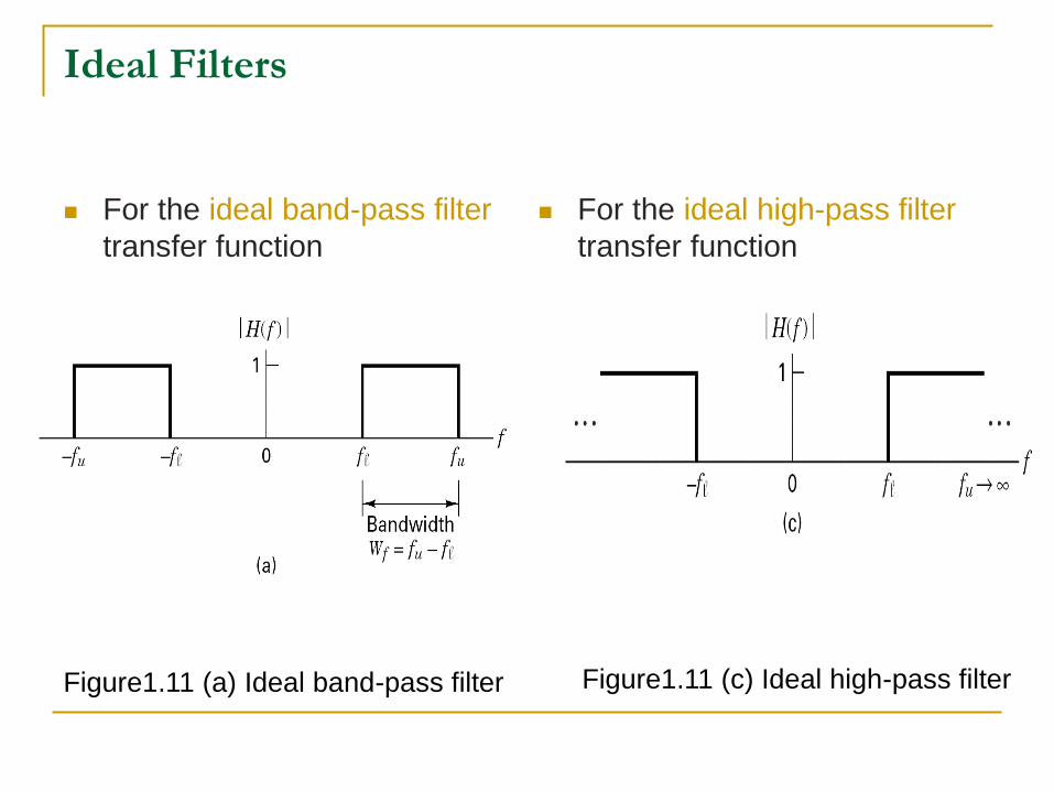
Ideal Filters
For the ideal band-pass filter
transfer function
For the ideal high-pass filter
transfer function
Figure1.11 (a) Ideal band-pass filter Figure1.11 (c) Ideal high-pass filter
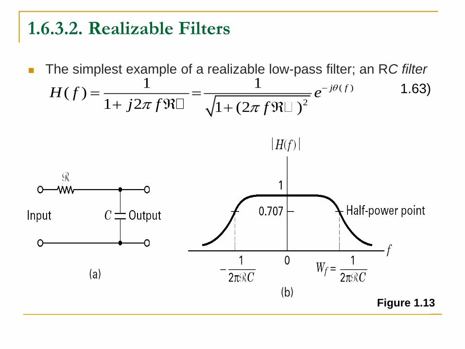
1.6.3.2. Realizable Filters
The simplest example of a realizable low-pass filter; an RC filter
1.63)
Figure 1.13
( )
2
1 1( )
1 2 1 (2 )
j fH f ej f f
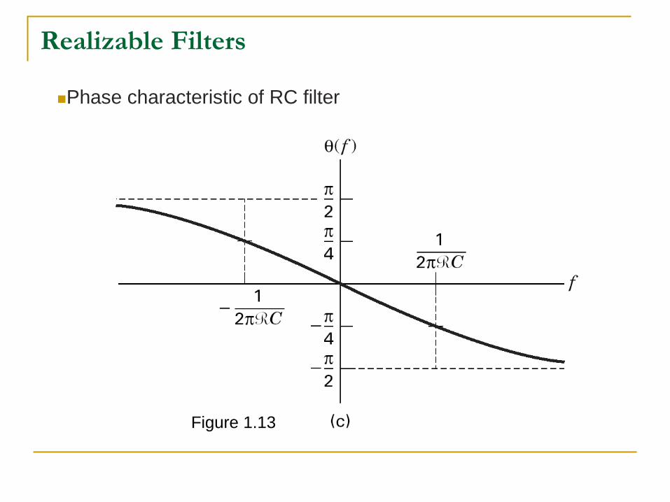
Realizable Filters
Phase characteristic of RC filter
Figure 1.13
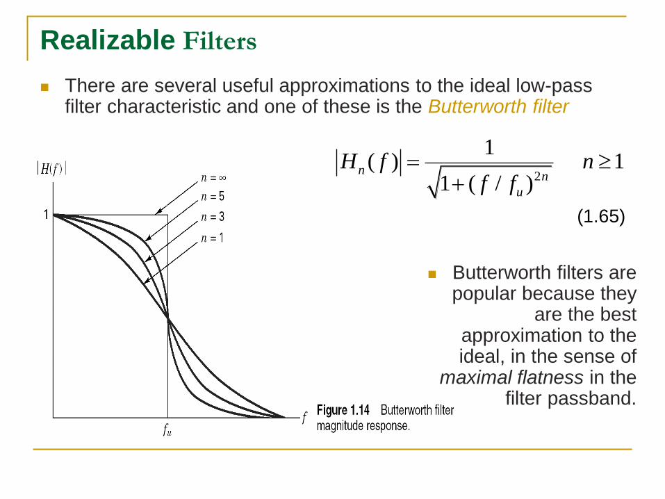
Realizable Filters
There are several useful approximations to the ideal low-pass filter characteristic and one of these is the Butterworth filter
(1.65)
Butterworth filters are popular because they
are the best approximation to the ideal, in the sense of
maximal flatness in the filter passband.
2
1( ) 1
1 ( / )n
n
u
H f nf f
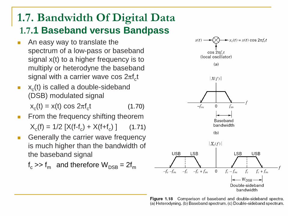
An easy way to translate the
spectrum of a low-pass or baseband
signal x(t) to a higher frequency is to
multiply or heterodyne the baseband
signal with a carrier wave cos 2fct
xc(t) is called a double-sideband
(DSB) modulated signal
xc(t) = x(t) cos 2fct (1.70)
From the frequency shifting theorem
Xc(f) = 1/2 [X(f-fc) + X(f+fc) ] (1.71)
Generally the carrier wave frequency
is much higher than the bandwidth of
the baseband signal
fc >> fm and therefore WDSB = 2fm
1.7. Bandwidth Of Digital Data 1.7.1 Baseband versus Bandpass
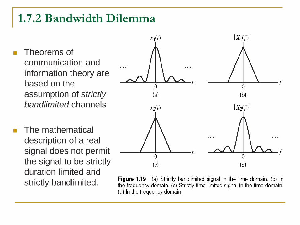
Theorems of
communication and
information theory are
based on the
assumption of strictly
bandlimited channels
The mathematical
description of a real
signal does not permit
the signal to be strictly
duration limited and
strictly bandlimited.
1.7.2 Bandwidth Dilemma
1.7.2 Bandwidth Dilemma
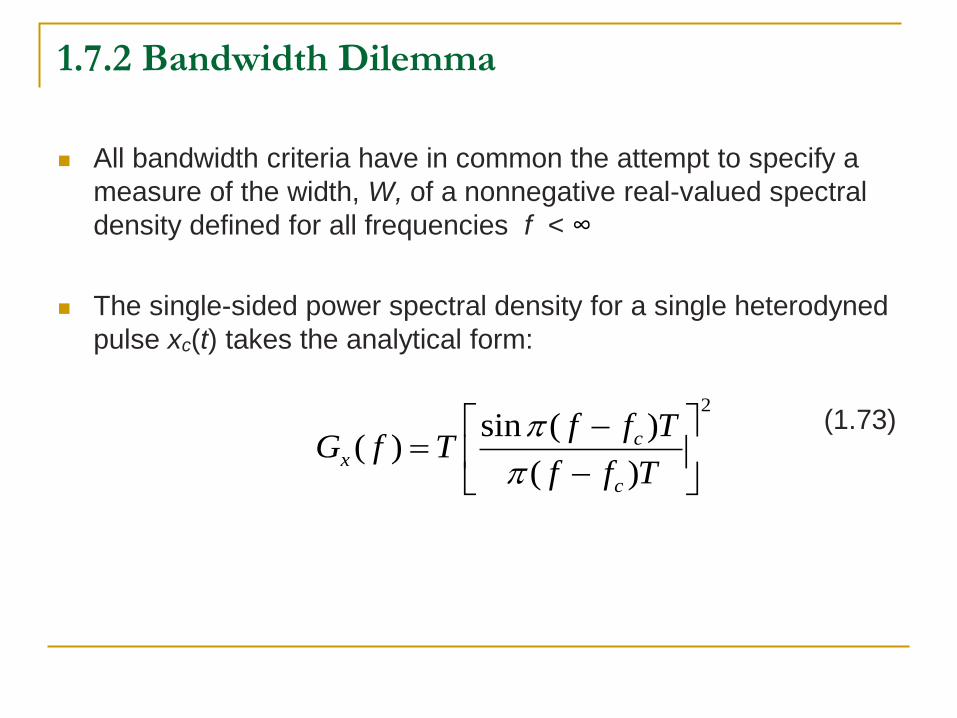
All bandwidth criteria have in common the attempt to specify a
measure of the width, W, of a nonnegative real-valued spectral
density defined for all frequencies f < ∞
The single-sided power spectral density for a single heterodyned
pulse xc(t) takes the analytical form:
(1.73)
2
sin ( )( )
( )
cx
c
f f TG f T
f f T
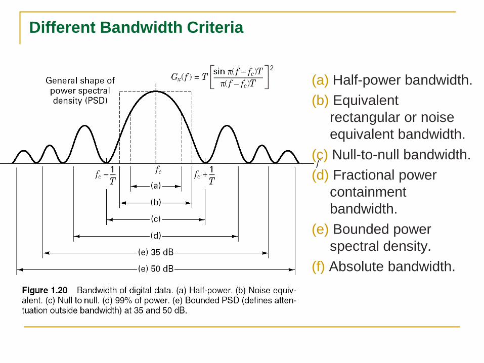
Different Bandwidth Criteria
(a) Half-power bandwidth.
(b) Equivalent
rectangular or noise
equivalent bandwidth.
(c) Null-to-null bandwidth.
(d) Fractional power
containment
bandwidth.
(e) Bounded power
spectral density.
(f) Absolute bandwidth.