Digital Hardware-/Softwaresystems Specification

Seminar Architecture & Design Methods for Embedded Systems

Summer Term 2006

University of Stuttgart

Faculty of Computer Science, Electrical Engineering and Information Technology

Author: Timo Blon

2176039

Advisor: Prof. Dr. Martin Radetzki

Institut für Technische Informatik

Contents

Contents

Contents ............................................................................................................................................................................ 1

1 Introduction .................................................................................................................................................................... 2

1.1 Design of Embedded Systems ............................................................................................................................... 2

1.2 Y-Chart ................................................................................................................................................................... 2

1.2.1 Abstraction hierarchy ....................................................................................................................................... 3

1.2.2 Specification domains and design flow ............................................................................................................ 4

2 System Synthesis ............................................................................................................................................................ 5

2.1 Synthesis .................................................................................................................................................................. 5

2.2 System specification ............................................................................................................................................... 6

2.2.1 Problem specification - Problem graph ............................................................................................................ 7

2.2.2 Specification of target architecture - Architecture graph ................................................................................. 8

2.2.3 Specification of mappings - Specification graph .............................................................................................. 9

2.3 Implementation ...................................................................................................................................................... 9

2.3.1 Allocation and binding ..................................................................................................................................... 9

2.3.2 Scheduling ...................................................................................................................................................... 11

2.3.3 Valid implementation ..................................................................................................................................... 12

2.4 System optimization ............................................................................................................................................. 13

2.4.1 Cost functions ................................................................................................................................................. 13

2.4.2 Refinement of cost model ............................................................................................................................... 14

3 Summary ....................................................................................................................................................................... 16

Figures ............................................................................................................................................................................ 17

References ...................................................................................................................................................................... 18

T.Blon 1

Introduction

1 Introduction

1.1 Design of Embedded Systems

The fast increasing performance of VLSI-Technology (Very Large Scale Integration) and

increasing customer requirements lead to highly complex real-time embedded systems. To handle

this complexity for being successful in a price led global market the use and development of

intelligent computer-aided design (CAD) tools gets more and more important. „Only efficient

tools and reuse can bring design productivity up to the expected level“ [2] to overcome the tight

time-to-market constraints. Another important issue is the verification of such highly complex

distributed systems during the complete development process.

To meet these challenges system-level designs are necessary to raise the level of abstraction.

Based on an abstract system specification CAD tools are used for step-wise refinement until the

final implementation of the system.

1.2 Y-Chart

To give an overview about the different levels of abstraction and to illustrate their interrelation to

the different specification domains, the Y-Chart proposed by Gajeski is commonly used. The

specification domains (behavioural, structural and physical) are diagrammed as three axes and the

different levels of abstraction are represented through the distance to the centre of the chart. With

increasing distance from the origin, the abstraction level, indicated as concentric circles, increases

from the circuit level, over logic level, register transfer (RT) level and the arithmetic level up to

the system level [2] [4].

T.Blon 2

Introduction

1.2.1 Abstraction hierarchy

A behavioural specification at system level has a granularity of interacting tasks and processes, as

well as corresponding design constraints. The structural description at system level defines the

system architecture with its hard- and software parts represented through processors, application

specific integrated circuits (ASIC), communication channels and memories which are finally mapped

to specific hardware devices in physical domain, e.g. processors, chips and boards.

The algorithmic description at the next level is given by a specific instruction set and data formats,

e.g. VHDL-description. The structure at the arithmetic level is represented as a controller, divided

into a control part and a data path which is physically represented in a floor plan.

The behaviour at register-transfer (RT) level is normally specified through states and transitions

between these states. Common notations are flow-tables or hardware description languages. The

structural domain is represented as a sequence chart with decoders and multiplexers which are

implemented as macro cells in physical domain.

As the name logic level already says, this level is characterized by boolean functions like boolean

equations or Karnaugh-diagrams that lead to combinational circuits.

The lowest level of abstraction specifies switching functions which are transferred to circuits that

are finally implemented as a transistor layout. This level is also called transistor level [3].

T.Blon 3

Figure 1: Y-Chart [2]

Introduction

1.2.2 Specification domains and design flow

The Y-Chart also allows illustrating the relation between different design activities as paths on the

chart as illustrated in Figure 1. A complete system design normally starts with describing the

functionality at system level and ends after stepwise refinement and mapping onto structural and

physical domain with the implementation on circuit level.

The synthesis, as transformation of a specification in behavioural domain to a representation in the

structural domain (at the same level of abstraction), is represented as an arc in the Y-chart. Where

the behavioural specification emphasis on input-output functionality without favouring a particular

way of implementation, the resulting structural description already represents an interconnection

of abstract components. These components are separately analysed and used to specify the

functionality at the next lower abstraction level. Based on these functional descriptions the next

synthesis step can be performed [4].

The final step of this classical top-down synthesis approach is the generation of the physical layout

out of the structural specification. This specification focuses on the physical characteristics and

the placement in space without considering further functional aspects.

To reach the required performance, optimization is necessary during the complete development

process. It can be represented at any point in the chart as an arrow that points back to its starting

point. This representation describes that this task results in improved specifications and does not

generate completely new specifications.

T.Blon 4

Figure 2: Y-Chart and design activities

System Synthesis

2 System Synthesis

2.1 Synthesis

After the overview of different abstraction levels we will take a closer look at system-level

synthesis. As already mentioned systems developers try to focus on that high abstraction level to

handle the complexity and reduce development times.

In contrast to high-level synthesis, “which deals with the implementation of algorithms in

application-specific hardware (ASIC design), system-level design focuses on the problem of

mapping an abstract specification model of an entire system onto a target architecture. As

mentioned earlier, a typical target architecture consists of a set of processor cores, memories,

peripheral units, and custom hardware blocks. These system components are interconnected by on-

chip busses whose implementation is part of system-level design as well.“ [4, p.20]

There are several tasks that have to be performed in order to come from a system specification to

the final implementation. At first the decision of which system components should be used has to

be made (allocation). The next important issue is the assignment of functionalities to the selected

components (binding). Depending on various constraints like performance and costs, this step

especially includes the decomposition into hardware and software components (HW/SW co

design). Therefore the system specification describing the functionality and behaviour of a system

should be independent of the implementation without favouring a hardware or a software

realization. Further details about advantages of each realization will be discussed later. After this

partitioning of the system into hardware and software parts, the scheduling has to be worked out.

This addresses the real-time requirements for the system under different optimization criteria (e.g.

costs or power consumption).

It is obvious that there is a large set of possible solution at this synthesis level. Therefore methods

for early cost and performance estimation are very important to find the best fitting design. At one

side there is the possibility to use libraries with optimized latency and known resource

consumption for estimation and composition of the architecture. This approach is mainly used for

data flow oriented systems. It allows the reuse of pre-designed, well-tested components to shorten

development time. This important issue is often referred to as Intellectual Property (IP). For

control flow dominated systems rapid prototyping methods and stepwise improvement are very

important for estimation and performance evaluation [1, p.368].

T.Blon 5

System Synthesis

Functional validation should also be done at this high abstraction level through formal verification

or simulation. This allows finding errors very early in the development process to avoid much

rework and thus leads to high productivity.

After determination of the system architecture and the decomposition into hardware and software

components the communication synthesis must be performed. “This includes the selection of

communication protocols for the selected buses, hardware interface synthesis and software driver

generation.” [4, p.29] To get to the final implementation the components are separately

synthesized.

2.2 System specification

The specification of a system synthesis problem can be divided into three parts:

– Description of functional elements and possible system architectures with directed graphs

(problem and architecture graph)

– The possible mapping of a functional element (behaviour/tasks) to various architecture

components is described with a specification graph. This includes assessment of additional

constraints and attributes related to all kind of assignments.

– Finally the implementation has to be performed. Based on the given requirements, this

includes selection of the final architecture and mapping the functionality to the allocated

system components (allocation, binding, scheduling).

T.Blon 6

Figure 3: System Synthesis [2]

System Synthesis

2.2.1 Problem specification - Problem graph

A problem graph as described by J. Teich is derived from a data flow graph by adding

communication nodes between the functional nodes. Thus a problem graph GP V P , E P is a set

of functional and communication nodes V P connected through directed edges E P which

represent the data dependencies. The functional nodes e.g represent tasks, processes or procedures

[1]. This is the reason why this kind of problem specification is also named task graph as described

in [5]. Figure 4 illustrates a data flow graph and the derived problem graph with additional

communication nodes 6, 7, 8, 9. Modelling the communication nodes allows taking into account

that there are different requirements for the interconnection between the functional nodes (e.g.

latency, throughput).

Although many systems are described in the programming language C, this type of system

specification is often used as input for system-level synthesis tools. There are attempts to develop

automatic task graph generation tools because the manual transformation of the system

specification from C to task graphs is very time consuming and error-prone. One example is the

task graph extraction tool presented in [5].

Figure 4 could for example represent a rough concept of an adaptive cruise control system (ACC).

An ACC system is an advanced type of speed control system in automotive industries. It allows

setting a target vehicle speed and in addition a distance to a vehicle ahead. If the vehicle in front of

the ACC controlled vehicle is slower, the distance is controlled by reducing engine torque or if

necessary by braking. If no vehicle is detected ahead vehicle speed is kept at the desired target

value. To detect objects in front of the car mostly radar sensors are used. The nodes of the problem

graph could correspond to the following functionality:

1. Evaluation of radar sensor input; e.g. analog digital conversion (ADC)

T.Blon 7

Figure 4: Data flow graph and derived problem graph with communication nodes

System Synthesis

2. Processing of radar sensor information to detect objects and determine distance and

differential speed; processing this information requires the use of math intensive signal

processing algorithms within real-time (e.g. fast Fourier transformation (FFT))

3. Evaluation of current vehicle speed out of wheel rotational sensors; the vehicle speed

signal could e.g. be provided as a pulse signal

4. Controller to keep the distance and speed at desired values; calculation and coordination of

control variables for vehicle speed adjustment; also consider possible shut off conditions to

avoid malfunction (if vehicle speed sensor is defect there is no secure operation possible)

5. Output the resulting variables e.g. send information to brake and engine control unit (ECU)

for torque adjustment

2.2.2 Specification of target architecture - Architecture graph

The architecture model consisting of the allocateable resources and their interrelation is

represented in an architecture graph GAV A , E A . The set of nodes V A is given by the

allocateable resources, i.e. functional components like arithmetic units, general purpose

processors, FPGAs or ASICs and communication resources like shared buses or point-to-point

connections. The set of edges E A is defined as directed connections between these resources [1].

The basic idea is to show the set of available resources that could be used for implementing the

system. The target architecture illustrated in Figure 5 consists of three functional resources (RISC,

hardware module HWM and a digital signal processor DSP) and two bus resources (shared bus,

point-to-point bus). The derived architecture graph shows that the point-to-point connection

v BR 2 just allows sending data from v HWM to v DSP . On the other hand, the shared bus is

modelled as a bidirectional connection v BR 1 between the bus subscribers v RISC , v HWM and

v DSP .

T.Blon 8

Figure 5: Target architecture and derived architecture graph

System Synthesis

As a higher abstraction level a chip graph GC V C , EC could be defined to show the assignment

of hardware modules to chips. This is especially important when considering constraints like

power consumption or required space for implementation of the hardware module [1].

2.2.3 Specification of mappings - Specification graph

In order to find an implementation, we need to set up a correlation between the problem graph and

the specified architecture graph. Therefore we map the functional nodes of the problem graph to

the functional resources of the architecture graph and likewise the communication nodes to the

corresponding bus resources. The resulting specification graph can formally be defined as a graph

GS V S , E S , consisting of D graphs Gi V i , E i for i jD and an additional set of

mapping edges EM with V S= ∪i=1

D

V i , ES= ∪i=1

D

E i ∪ EM and EM= ∪i=1

D�1

EMi ,

Emi⊆V i×V i1 ∀ 1iD [1].

Figure 6 illustrates the concept of a specification graph: The nodes of the problem graph GP are

mapped ( EM1 ) to the nodes of the architecture graph GA and the edges EM2 represent the

mapping of the architecture nodes to the corresponding nodes of the chip graph GC .

This graph includes the information about all possible combinations for mapping the

functionalities to corresponding system components. Selection of one concrete mapping by

activating nodes and edges of the specification graph, leads to a possible implementation.

2.3 Implementation

2.3.1 Allocation and binding

The described activation is formally defined as a function a :V S∪E S{0,1} , that assigns every

edge e∈ES and every node v∈V S the value activated 1 or not activated 0 [1].

With this definition of activation the major steps allocation and binding can be defined as follows:

An allocation α is the subset of all activated nodes and edges of the specification graph:

α=αV∪αE

αV={v∈V S ∣a v =1}

αE= ∪i=1

D

{e∈E i ∣ ae=1}

And a binding β is defined as the subset of all activated mappings:

T.Blon 9

System Synthesis

β={e∈E m∣ a e=1}

A binding β is valid if each activated mapping e∈β binds an activated node (e.g from

problem graph) to exactly one allocated node (e.g. of the architecture graph). Furthermore the

communication between the functional nodes has to be ensured by appropriate mapping of the

communication nodes. If there exits at least one valid binding for an allocation α , this allocation

is also defined as valid.

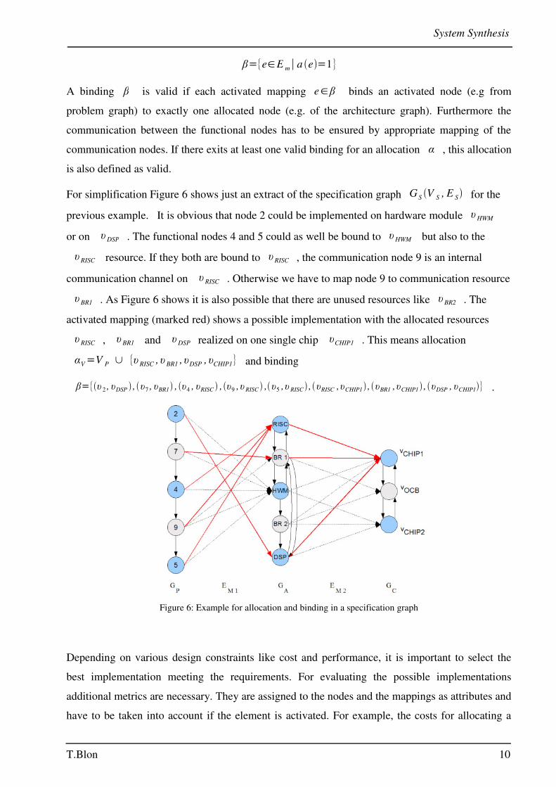
For simplification Figure 6 shows just an extract of the specification graph GS V S , E S for the

previous example. It is obvious that node 2 could be implemented on hardware module υHWM

or on υDSP . The functional nodes 4 and 5 could as well be bound to υHWM but also to the

υRISC resource. If they both are bound to υRISC , the communication node 9 is an internal

communication channel on υRISC . Otherwise we have to map node 9 to communication resource

υBR1 . As Figure 6 shows it is also possible that there are unused resources like υBR2 . The

activated mapping (marked red) shows a possible implementation with the allocated resources

υRISC , υBR1 and υDSP realized on one single chip υCHIP1 . This means allocation

αV=V P ∪ {υRISC ,υBR1 ,υDSP ,υCHIP1} and binding

β={υ 2 , υDSP ,υ7 , υBR1 , υ4 , υRISC ,υ9 ,υRISC ,υ5 ,υRISC ,υRISC ,υCHIP1 ,υBR1 ,υCHIP1 ,υDSP , υCHIP1} .

Depending on various design constraints like cost and performance, it is important to select the

best implementation meeting the requirements. For evaluating the possible implementations

additional metrics are necessary. They are assigned to the nodes and the mappings as attributes and

have to be taken into account if the element is activated. For example, the costs for allocating a

T.Blon 10

Figure 6: Example for allocation and binding in a specification graph

System Synthesis

specific functional component in general (attribute of node) or the costs occurring if binding a

functionality to that functional component (attribute of edge) can be expressed. Further measures

could be the required space, the latency or the memory usage if implementing a functionality on a

particular component. These optimization issues will be addressed later.

2.3.2 Scheduling

Based on the selected architecture, the scheduling has to be determined. Therefore the execution

time of a task υ is specified as an attribute delay υ , β ∈ ℤ in the specification graph.

The execution time is in general dependent on the binding e.g. a hardware implementation on an

ASIC has a higher performance than the equivalent, more flexible software solution. Looking at

the communication nodes, the execution time is interpreted as the transmission latency.

A scheduling is formally defined as a function τ : V Pℤ0

that fulfils for every edge

e=υi ,υ j the following condition:

τ υ j τ υidelayυ j , β

Thereby τ υi can be considered as the activation time of node υi∈V P and an edge

e=υi ,υ j can be considered as the directed edge from node υi to node υ j . It is assumed

that a specification GS , that contains a problem graph GP , a valid binding β and a function

delay υ , β , is given [1]. The important point is that now the data dependency, specified in the

data flow graph, is taken into account again. The above condition expresses that a task υ j that is

somehow dependent from another task υi can first be executed if this task υi has been

activated and finished. Beside this definition there are often additional constraints like deadlines or

resource constraints which have to be considered.

Based on the information given in Figure 7, the scheduling can be determined. For example, the

execution time of υ4 on the RISC processor is delay υ4 ,υ4 ,υRISC =14 . Binding the same

task to the hardware module the execution time could be reduced to delay υ4 ,υ4 ,υHWM =8 .

The internal communication on a functional component is assumed to not generate any latency e.g.

delay υ9 , υ9 ,υRISC =0 .

T.Blon 11

System Synthesis

2.3.3 Valid implementation

Based on a given specification G S a valid implementation is defined as a triple α , β , τ ,

with a valid allocation α , a valid binding β and a scheduling τ [1, p.378].

The implementation from Figure 7 can also be illustrated with the Gantt-Chart in Figure 8. At first

υ2 is executed on υDSP . After transmitting data over υBR1 the tasks υ4 and υ5 are

executed on the RISC processor υRISC . Because of using different resources, it is obvious that

pipelining could be introduced for this example. For continuous computation and reduction of idle

times, task υ2 could be immediately reactivated after finishing the previous calculation.

Likewise the other tasks could be scheduled.

T.Blon 12

Figure 7: Example of a valid implementation (allocation - binding - scheduling)

Figure 8: Allocation, binding and scheduling for discussed implementation

System Synthesis

This very simple example should be sufficient to explain the principles of the concept. In more

complex implementations there could also be concurrent tasks and many data dependencies which

have to be addressed.

2.4 System optimization

The introduced specification model establishes a basis for system synthesis. As already discussed

there are many alternative implementations and a lot of additional constraints which have to be

considered. Even if these additional constraints make the system design difficult, they are very

helpful during the selection process because of reducing the number of feasible solutions [1].

2.4.1 Cost functions

The feasible solutions are defined as a set A of valid implementations α , β , τ . Selecting the

optimal solution can be expressed by minimizing the value of a cost function:

ƒα , β , τ : Aℝ with g i α , β , τ 0 , ∀ i∈{1,... , q}

The functions g i α , β , τ as part of the optimization problem represent additional constraints

to restrict the search space A .

Minimizing the latency of a system as specified above could for example be described with the

cost function (also called objective function) ƒα , β , τ =max {τ υ delay υ , β ∣ υ∈V P} .

An additional cost limit c is given by the constraint g1α , β , τ =c�∑υ∈α

c υ where c υ

represents the costs for realization of an allocated component [1].

This example refers to a very important point: the task of HW/SW partitioning is always to trade

off an inexpensive and flexible software solution versus a high performance hardware

implementation. The optimal solution of a cost functions always depends on the optimization

criteria. Taking the quantity for mass production into account, a hardware solution could also lead

to lower overall costs because the development costs are negligible. If just the HW/SW

partitioning problem is important, a simplified model with just one hardware component and one

software node (processor) connected via a shared bus resource is necessary. Then every functional

component of the problem graph can theoretically be mapped to these two resources. The specified

execution times, resource constraints and costs can be evaluated more easily, because there is just

the decision between a hardware or a software realization.

T.Blon 13

System Synthesis

The previous example points at the idea of cost functions. A more general approach for taking

different metrics into account (e.g. costs c , latency L , power consumption P or things

like chip area, memory usage and testability) is to define a cost function:

ƒ=c1⋅hc ,cc2⋅h L ,Lc3⋅hP , P...

The coefficients c i are used to assess the different criteria specified by functions h . Because

the criteria are referring to limit values (e.g. c or L ) the optimal value of a function h is 0

and exactly meeting the limit value results in h=1 .

Figure 9 illustrates the application of a cost function with three different implementations. At the

left-hand side the three possible implementations are evaluated under the criteria latency, costs,

power consumption and testability. The Kiviat-graph shows that implementation 1 fulfils all

criteria while implementation 2 exceeds the costs and implementation 3 exceeds the limit values

for the costs and the power consumption. The results of the complete cost function are shown in

the right diagram. If the most important optimization criteria are latency L and power

consumption P , implementation 2 is the first choice. If the costs are the main optimization

criterion, implementation 1 is the only feasible solution.

2.4.2 Refinement of cost model

We have already addressed a simple model for cost evaluation. This model leads to rather

pessimistic estimations because the costs were only dependent on the binding of each functional

module itself. It does not take into consideration that the binding of other functionalities could

influence the implementation cost of a functional module. Probably there could be shared

resources or other synergy effects that reduce the total costs.

T.Blon 14

Figure 9: Cost function - evaluating implementations with different optimization criteria

System Synthesis

[1] introduces a more detailed model that also takes the chip area and memory allocation into

account. Therefore the costs are divided into basic costs and additional costs:

The basic costs cb υ originating from allocation of a resource υ∈V A are specified by a

function cb:V Aℤ0

.

If further nodes υ∈V P are bound to an allocated resource υ∈V A additional costs

ca : EM ℤ0

must be considered. These additional costs originate from the memory or chip

area needed by the node, so they are dependent on the mapping e=υ , υ ∈ EM .

For mapping similar functionalities to the same resource υ∈V A the defined additional costs

could be too high because some parts of the resource can be reused (e.g. memory or an arithmetic

unit of a hardware module). The additional costs ca are replaced by type specific additional

costs c t . Therefore the nodes υ∈V P are classified into functional types T i∈T . The

additional costs for binding several nodes of the same functional type T i to one resource

υ∈V A are defined as: c tT i , υ=max {cae ∣ e=υ , υ∈ β ∧ υ∈T i} [1]

Based on these definitions more accurate cost modelling for an implementation is possible. The

overall costs are summed up to: c α , β = ∑υ∈α∩V

A

ch υ , β

The cost for an allocated resource υ are defined as : ch υ , β =cb υ ∑T

i∈T :υ , υ∈β∧ υ∈T

i

ct T i , υ

T.Blon 15

Summary

3 Summary

In this paper I have described the necessity of high abstraction levels to handle the complexity of

todays embedded systems and to overcome the tough market constraints. I outlined the different

levels of abstraction and the tasks during the development process with the Y-Chart. After that, the

system level synthesis was described in detail. Therefor an formal model for system specification

based on directed graphs was presented. Beginning with the problem specification modelled with a

problem graph and defining the target architecture with an architecture graph and a chip graph, the

resulting specification graph was depicted. This formal model allows reducing design time and

enables the use of synthesis techniques to enlarge the space of feasible solutions to a given

problem.

The main activities during the synthesis process were described in detail. The allocation of system

components and the binding of the tasks to these resources were formally defined according to [1].

The scheduling aspects were described with a small example and some basics of HW/SW

partitioning were given. Finally the system optimization was addressed. As a major aspect, cost

functions were introduced because this concept is applicable for nearly every optimization criteria.

Some examples for evaluating possible implementations like execution time, resource usage and

costs were pointed out. I think this is the important part of the system-level synthesis based on

formal models because they allow assessing the system from different perspectives and also

optimizing it under different criteria. Thus it makes early estimations in the design process

possible.

I think the system synthesis approach is the right way to meet future requirements. Nevertheless I

think that there is still a lot of work to do because there is no standardized format for system

specification and the market of CAD tools supporting system-level synthesis is somewhat

intransparent.

T.Blon 16

Figures

Figures

Figure 1: Y-Chart [2]..........................................................................................................................3

Figure 2: Y-Chart and design activities..............................................................................................4

Figure 3: System Synthesis [2]...........................................................................................................6

Figure 4: Data flow graph and derived problem graph with communication nodes..........................7

Figure 5: Target architecture and derived architecture graph.............................................................8

Figure 6: Example for allocation and binding in a specification graph............................................10

Figure 7: Example of a valid implementation (allocation - binding - scheduling)...........................12

Figure 8: Allocation, binding and scheduling for discussed implementation..................................12

Figure 9: Cost function - evaluating implementations with different optimization criteria.............14

T.Blon 17

References

References

[1] J. Teich: Digitale Hardware/Software-Systeme. Berlin - Heidelberg: Springer-

Verlag 1997. ISBN 3-540-62433-3. pp. 367-389

[2] P. Eles, Z. Peng: System Synthesis of Digital Systems. Lecture Notes. University of

Linköping 2000. http://www.ida.liu.se/~petel/SysSyn/ (05/2006)

[3] U. G. Baitinger: Hardware/Software Co-Design. Lecture Notes. Stuttgart University

2001. http://www.infotech.uni-stuttgart.de/pdf/L_HSCD.pdf (05/2006)

[4] R. Dömer: System-level Modelling and Design with the SpecC Language.

Dissertation. University of Dortmund 2000

[5] K. S. Vallerio, N. K. Jha: Task Graph Extraction for Embedded System Synthesis.

Proc. 16th International Conference on VLSI Design 2003

T.Blon 18