Embed Size (px)
Citation preview

Digital Image ProcessingChapter 3: Intensity Transformations and
Spatial Filtering
(3.1 – 3.3.2)

3. Intensity Transformations and Spatial Filtering
Image enhancement
1) Spatial domain methods
2) Frequency domain methods - Fourier transform
3.1 Background
Input imageoutput
T is an operator on f
𝑓(𝑥, 𝑦) ∶ the input image𝑔(𝑥, 𝑦) : the processed imageT[•] : an operator on f , defined over some neighborhood of (𝑥, 𝑦)


S=T(r)Intensity of f
intensity of g밝기변환 함수
3.1 Background

Image negatives
3.2 Some Basic Gray Level Transformations

Intensity of fintensity of g
The negative of an image with intensity levels in the rage [0 , 𝐿 − 1] is obtained by using the negative transformation shown in Fig.3.3, which is given by the expression
𝑠 = 𝐿 − 1 − 𝑟
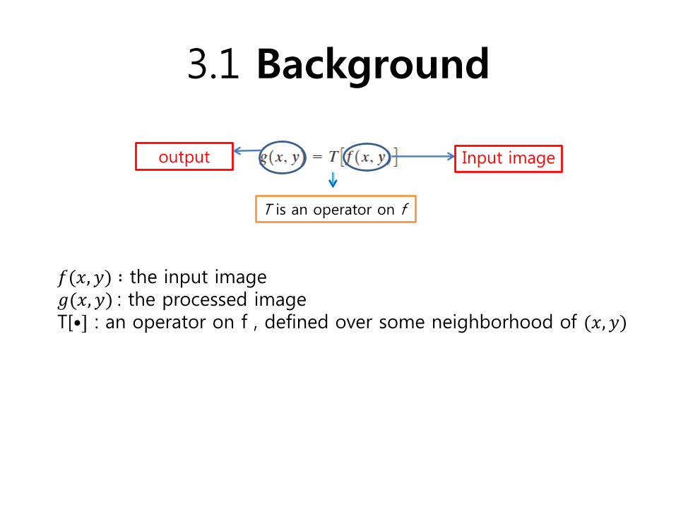
3.2.2 Log Transformations
The general form of the log transformation in Fig.3.3 is𝑠 = 𝑐𝑙𝑜𝑔(1 + 𝑟)
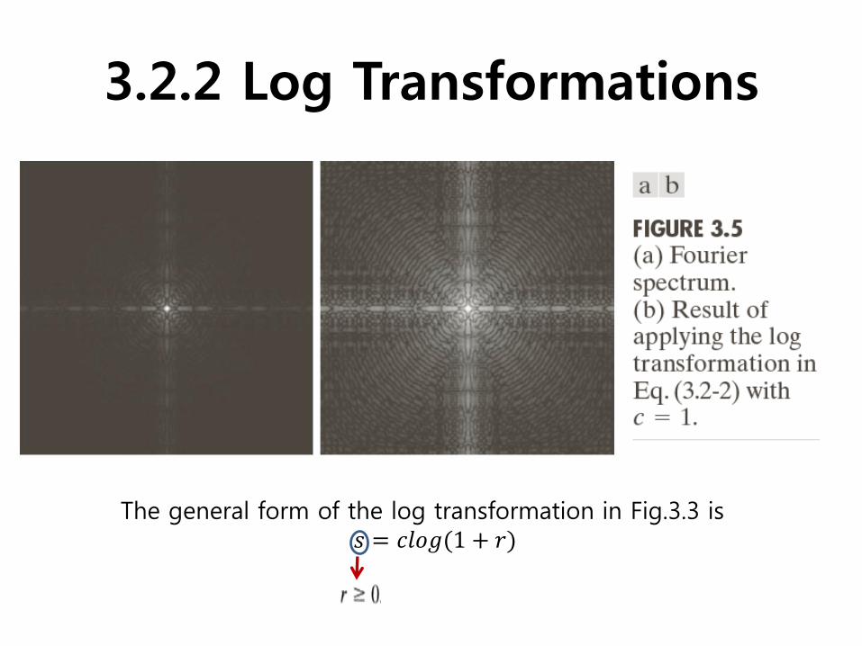
3.2.3 Power-Law Transformations
crs
𝛾 > 1𝛾 = 1𝛾 < 1
: identity transformation
(𝑐 와 𝛾는 양의 상수)

Gamma correction

Gamma correction
r=0.6
r=0.4 r=0.3

Gamma correction
r=3.0
r=5.0r=4.0

3.2.4 Piecewise-Linear Transformation Functions
Contrast stretching
(d) thresholding
(a) transformation function (b) low-contrast image
(c) contrast stretching의 결과
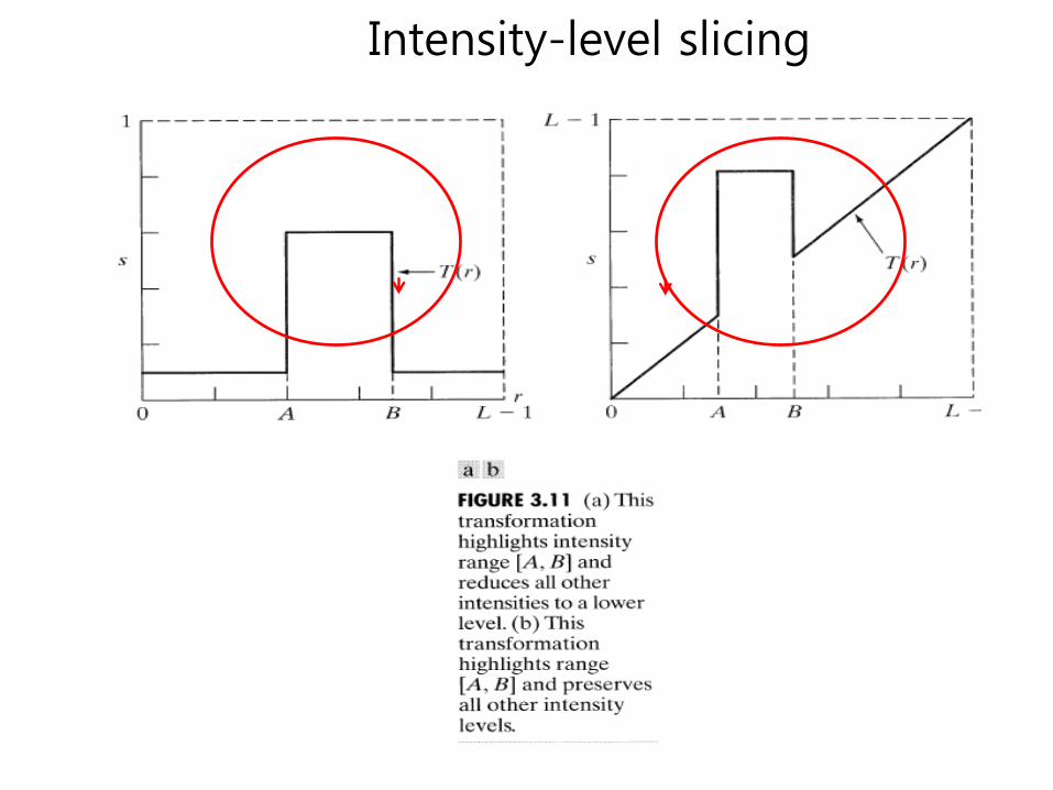
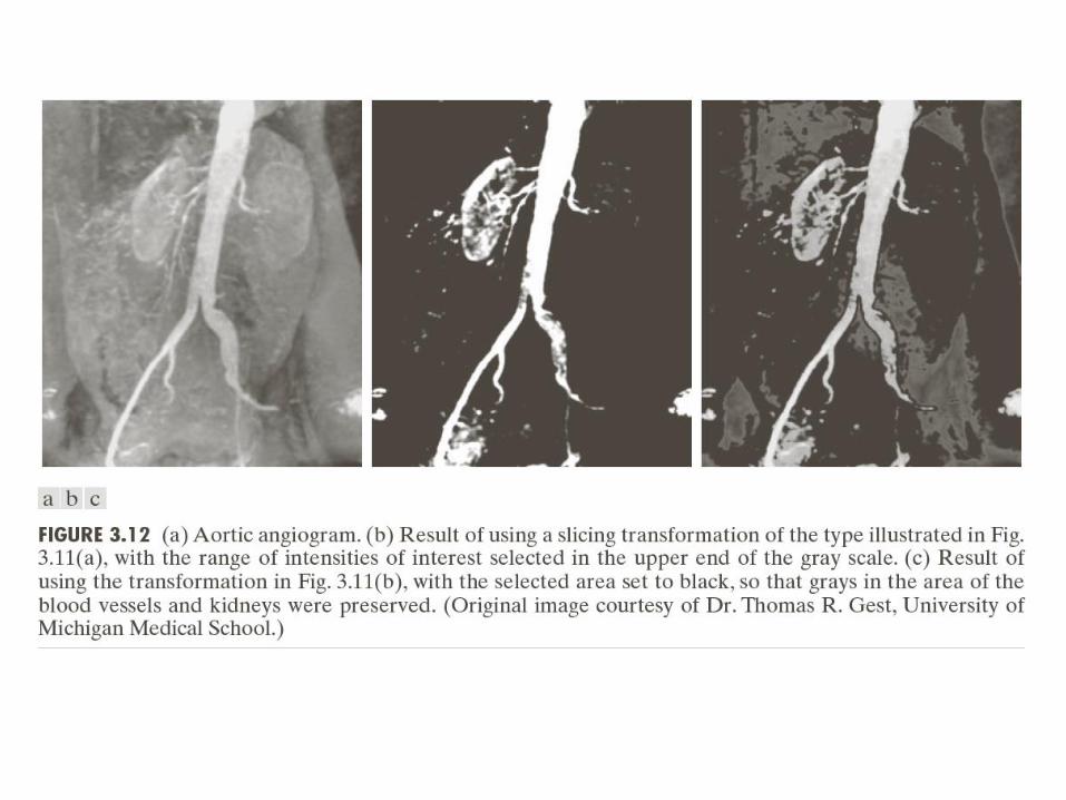
Intensity-level slicing

Bit-plane slicing
픽셀값은 00000000(0)~11111111(255)까지의 값을 가질 수 있다.8개의 bit중에서 최상위 비트를 MSB(Most Significant Bit), 최하위 비트를 LSB(Least Significant Bit)라고 한다.상위 비트로 갈수록 값이 커진다는 것이 핵심이다.최상위 비트는 가장 큰 값이므로 가장 중요하다 (Most Significant)최하위 비트는 가장 작은 값이므로 가장 중요하지 않다 (Least Significant)가 된다.
Figure 3.13

Bit-plane slicing

Bit-plane slicing
저장 공간이 50% 절약된다.
Bit 8,7 Bit 8,7,6 Bit 8,7,6,5
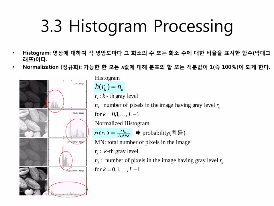
3.3 Histogram Processing
• Histogram: 영상에 대하여 각 명암도마다 그 화소의 수 또는 화소 수에 대한 비율을 표시한 함수(막대그래프)이다.
• Normalization (정규화): 가능한 한 모든 x값에 대해 분포의 합 또는 적분값이 1(즉 100%)이 되게 한다.
1,,1,0for
levelgray having image in the pixels ofnumber :
levelgray th - :
Histogram
Lk
rn
kr
nrh
kk
k
kk
Normalized Histogram
MN: total number of pixels in the image
: -th gray level
: number of pixels in the image having gray level
for 0,1, , 1
k k
k
k k
p r n n
r k
n r
k L
( ) kk
np r
MN
kk nrh )(
probability(확률)
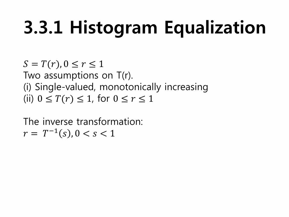
3.3.1 Histogram Equalization
𝑆 = 𝑇(𝑟), 0 ≤ 𝑟 ≤ 1Two assumptions on T(r).(i) Single-valued, monotonically increasing(ii) 0 ≤ 𝑇(𝑟) ≤ 1, for 0 ≤ 𝑟 ≤ 1
The inverse transformation:𝑟 = 𝑇−1 𝑠 , 0 < 𝑠 < 1


영상의 명암도는 [0,L-1] 사이의 범위에서 랜덤 함수로 간주할 수 있다.Pr(r)과 Ps(s)는 랜덤 변수 r과 s의 확률 밀도 함수(Probability Density
Function) 이면, 기초 확률 이론으로부터
)33.3(||)()( ds
drrPsP rs
변환 변수 s의 PDF는 입력 영상의 PDF와 선택된 변환 함수에 의하여 결정된다.
변환 함수(Transformation Function)만약, 변환 함수(Transformation Function)가 우변에서 처럼 랜덤 변수 r의 누적 분포함수 (Cumulative Distribution Function)이면
3.3.1 Histogram Equalization
이변화에 의해 히스토그램의인접픽셀 값은 빈도에 크기의변환이 바뀌지 않음을 의미한다.

r
r dwwprTs0
)()(
r
rr rpdwwpdr
d
dr
rdT
dr
ds
0)(])([
)(
1|)(
1|)(||)()(
rprp
ds
drrpsp
r
rrs
1 s 0
Ps(s)는 Pr(r)에 무관한 균일한 확률밀도함수이다.
Output
변화량
Input
)43.3()()1()(0
r
r dwwpLrTs

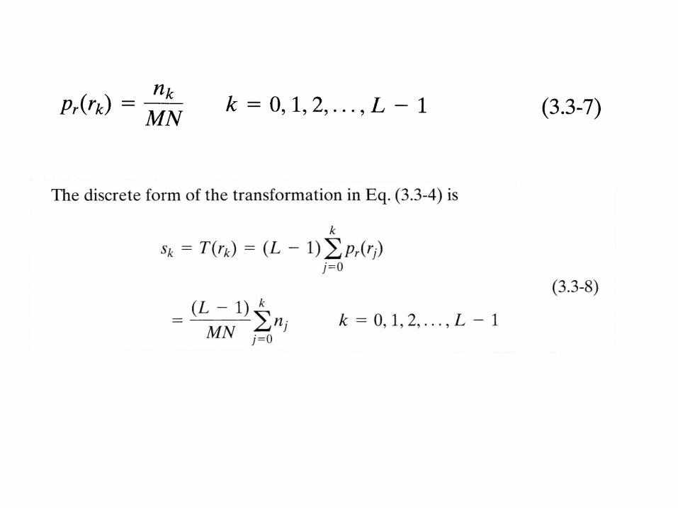
• 이산 값에 대하여,디지털 영상에서 밝기레벨 rk가 나타날 확률은
( ) kr k
np r
n k = 0, 1, 2, . . . . ., L-1
여기서 n은 영상 내의 총 화소수, nk는 rk를 갖는 화소수, L은 영상에서 가능한 명암도의 총수.
k
j
k
j
j
jrkkn
nrprTs
0 0
)()( k = 0, 1, 2, . . . . ., L-1
( )r kp r
3.3.1 Histogram Equalization
)(1
kk sTr 10 ks
S에서 r 로의 역변환:

Histogram Equalization
𝑑𝑠
𝑑𝑟=
𝑑𝑇(𝑟)
𝑑𝑟
= 𝐿 − 1𝑑
𝑑𝑟 0𝑟𝑝𝑟 𝑤 𝑑𝑤
= (𝐿 − 1)𝑝𝑟(𝑟)Substituting this result for dr/ds in Eq.(3.3-3), and keeping in mind that all probability values are positive, yields
𝑝𝑠(𝑠) = 𝑝𝑟(𝑟)𝑑𝑟
𝑑𝑠
= 𝑝𝑟 𝑟1
𝐿−1 𝑝𝑟 𝑟
= 1
𝐿−10 ≤ 𝑠 ≤ 𝐿 − 1

Sr
r
r dwwprTs0
)()(Out put
Input

Histogram Equalization
Continuous form

Before continuing, it will be helpful to work through a simple example. Suppose that a 3-bit image(L = 8) of size 64 X 64 pixels (MN = 4096) has the intensity distribution shown in Table 3.1, where the intensity levels are integers in the range [0, L-1] = [0,7].
The histogram of our hypothetical image is sketched in Fig.3.19(a). Values of the histogram equalization transformation function are obtained using Eq.(3.3-8).For instance,
𝑠1 = 𝑇 𝑟1 = 7
𝑗=0
0
𝑝𝑟(𝑟𝑗) = 7𝑝𝑟 𝑟0 = 1.33
Similarly,𝑠1 = 𝑇 𝑟1 = 7 𝑗=0
1 𝑝𝑟(𝑟𝑗) = 7𝑝𝑟 𝑟0 + 7𝑝𝑟 𝑟1 = 3.08
And 𝑠2 = 4.55, 𝑠3 = 5.67, 𝑠4 = 6.23, 𝑠5 = 6.65, 𝑠6 = 6.86, 𝑠7 = 7.00. This transformation function has the staircase shape shown in Fig.3.19(b).
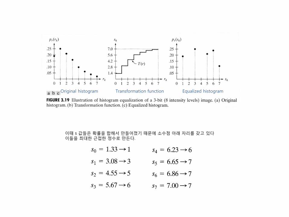
Original histogram Transformation function Equalized histogram
이때 s 값들은 확률을 합해서 만들어졌기 때문에 소수점 아래 자리를 갖고 있다이들을 최대한 근접한 정수로 만든다.

3.3.1 Histogram Equalization


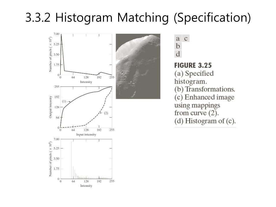
3.3.2 Histogram Matching (Specification)
Pr(r)과 Pz(z)는 랜덤 변수 r과 z의 연속 확률 밀도 함수라 하자.
입력 영상으로부터 Pr(r)을 구할 수 있고 Pz(z)는 출력 영상이 가지기를 원하는확률 밀도 함수이다
• pr(r): continuous PDF for input image• pz(z): specified (desired) cont. PDF for output imageLet s be a random variable where

z(출력 영상)는 다음의 관계식을 만족하여야 한다.
1. T(r)은 입력 영상으로부터 Pr(r)로부터 계산한다.
2. G(z)은 입력 영상으로부터 Pz(z)로부터 계산한다.
3. G-1을 계산한다.
4. 입력 영상의 모든 화소에 대하여 위 관계식으로부터 출력 영상을 얻는다.


Histogram Equalization

3.3.2 Histogram Matching (Specification)

3.3.2 Histogram Matching (Specification)